Embed Size (px)
Citation preview

www.openeering.com
powered by
MODELING IN XCOS USING MODELICA
In this tutorial we show how to model a physical system described by ODE using the Modelica extensions of the Xcos environment. The same model has been solved also with Scilab and Xcos in two previous tutorials.
Level
This work is licensed under a Creative Commons Attribution-NonCommercial-NoDerivs 3.0 Unported License.
Tutorial Xcos + Modelica www.openeering.com page 2/19
Step 1: The purpose of this tutorial
Scilab provides three different approaches (see figure) for modeling a
physical system described by Ordinary Differential Equations (ODE).
For showing all these capabilities we selected a common physical
system, the LHY model for drug abuse. This model is used in our
tutorials as a common problem to show the main features for each
strategy. We are going to recurrently refer to this problem to allow the
reader to better focus on the Scilab approach rather than on mathematical
details.
In this third tutorial we show, step by step, how the LHY model problem
can be implemented in the Xcos + Modelica environment. The sample
code can be downloaded from the Openeering web site.
1 Standard Scilab Programming
2 Xcos Programming
3 Xcos + Modelica
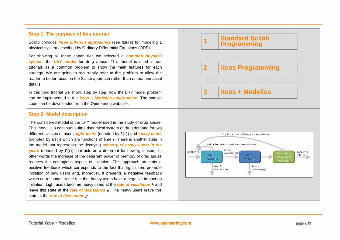
Step 2: Model description
The considered model is the LHY model used in the study of drug abuse.
This model is a continuous-time dynamical system of drug demand for two
different classes of users: light users (denoted by ) and heavy users
(denoted by ) which are functions of time . There is another state in
the model that represents the decaying memory of heavy users in the
years (denoted by ) that acts as a deterrent for new light users. In
other words the increase of the deterrent power of memory of drug abuse
reduces the contagious aspect of initiation. This approach presents a
positive feedback which corresponds to the fact that light users promote
initiation of new users and, moreover, it presents a negative feedback
which corresponds to the fact that heavy users have a negative impact on
initiation. Light users become heavy users at the rate of escalation and
leave this state at the rate of desistance . The heavy users leave this
state at the rate of desistance .
Tutorial Xcos + Modelica www.openeering.com page 3/19
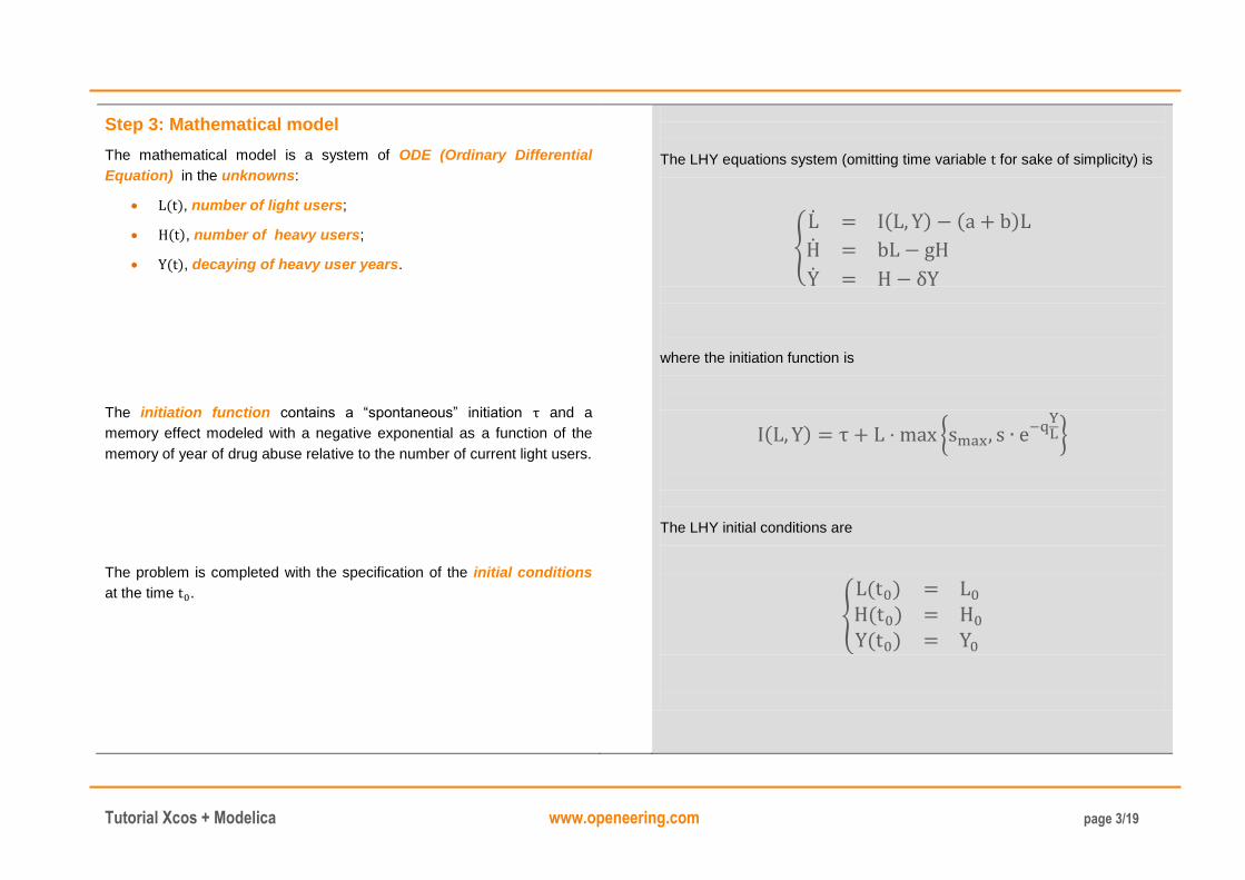
Step 3: Mathematical model
The mathematical model is a system of ODE (Ordinary Differential
Equation) in the unknowns:
, number of light users;
, number of heavy users;
, decaying of heavy user years.
The initiation function contains a “spontaneous” initiation and a
memory effect modeled with a negative exponential as a function of the
memory of year of drug abuse relative to the number of current light users.
The problem is completed with the specification of the initial conditions
at the time .
The LHY equations system (omitting time variable for sake of simplicity) is
{
where the initiation function is
{ }
The LHY initial conditions are
{
Tutorial Xcos + Modelica www.openeering.com page 4/19
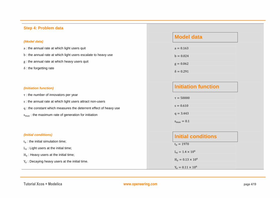
Step 4: Problem data
(Model data)
: the annual rate at which light users quit
: the annual rate at which light users escalate to heavy use
: the annual rate at which heavy users quit
: the forgetting rate
(Initiation function)
: the number of innovators per year
: the annual rate at which light users attract non-users
: the constant which measures the deterrent effect of heavy use
: the maximum rate of generation for initiation
(Initial conditions)
: the initial simulation time;
: Light users at the initial time;
: Heavy users at the initial time;
: Decaying heavy users at the initial time.
Model data
Initiation function
Initial conditions
Tutorial Xcos + Modelica www.openeering.com page 5/19
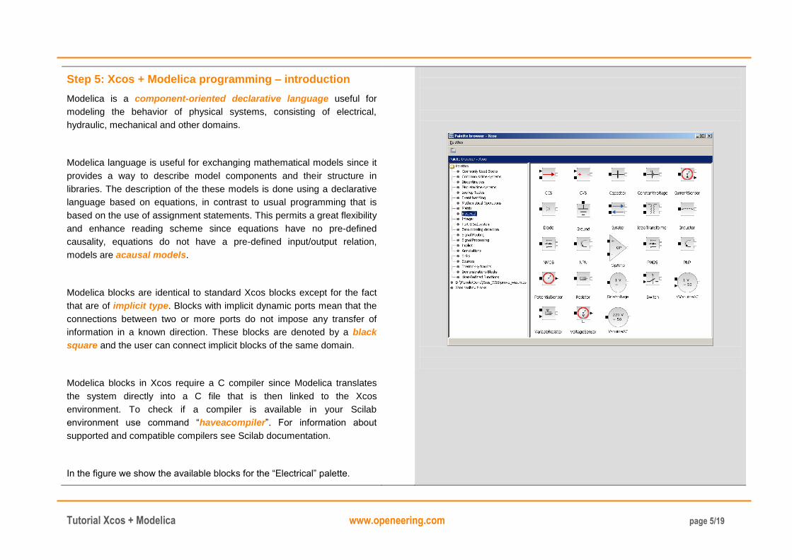
Step 5: Xcos + Modelica programming – introduction
Modelica is a component-oriented declarative language useful for
modeling the behavior of physical systems, consisting of electrical,
hydraulic, mechanical and other domains.
Modelica language is useful for exchanging mathematical models since it
provides a way to describe model components and their structure in
libraries. The description of the these models is done using a declarative
language based on equations, in contrast to usual programming that is
based on the use of assignment statements. This permits a great flexibility
and enhance reading scheme since equations have no pre-defined
causality, equations do not have a pre-defined input/output relation,
models are acausal models.
Modelica blocks are identical to standard Xcos blocks except for the fact
that are of implicit type. Blocks with implicit dynamic ports mean that the
connections between two or more ports do not impose any transfer of
information in a known direction. These blocks are denoted by a black
square and the user can connect implicit blocks of the same domain.
Modelica blocks in Xcos require a C compiler since Modelica translates
the system directly into a C file that is then linked to the Xcos
environment. To check if a compiler is available in your Scilab
environment use command “haveacompiler”. For information about
supported and compatible compilers see Scilab documentation.
In the figure we show the available blocks for the “Electrical” palette.
Tutorial Xcos + Modelica www.openeering.com page 6/19
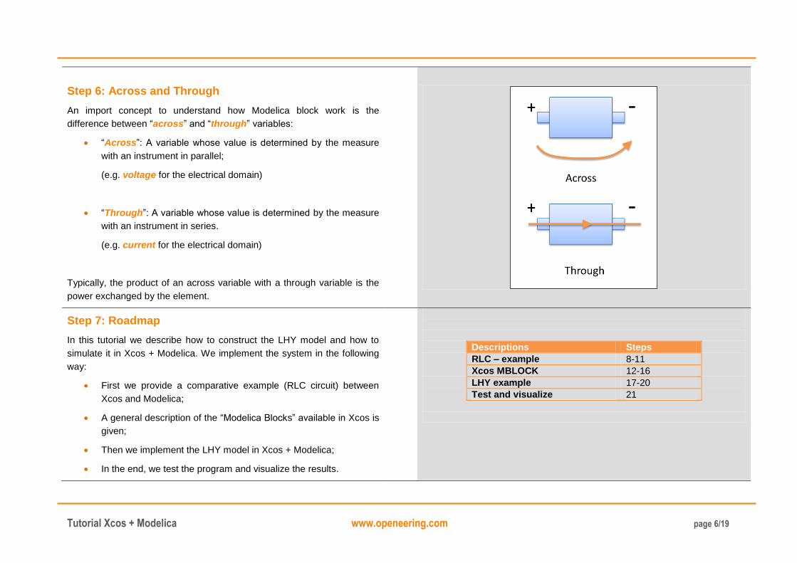
Step 6: Across and Through
An import concept to understand how Modelica block work is the
difference between “across” and “through” variables:
“Across”: A variable whose value is determined by the measure
with an instrument in parallel;
(e.g. voltage for the electrical domain)
“Through”: A variable whose value is determined by the measure
with an instrument in series.
(e.g. current for the electrical domain)
Typically, the product of an across variable with a through variable is the
power exchanged by the element.
Step 7: Roadmap
In this tutorial we describe how to construct the LHY model and how to
simulate it in Xcos + Modelica. We implement the system in the following
way:
First we provide a comparative example (RLC circuit) between
Xcos and Modelica;
A general description of the “Modelica Blocks” available in Xcos is
given;
Then we implement the LHY model in Xcos + Modelica;
In the end, we test the program and visualize the results.
Descriptions Steps
RLC – example 8-11
Xcos MBLOCK 12-16
LHY example 17-20
Test and visualize 21
Tutorial Xcos + Modelica www.openeering.com page 7/19
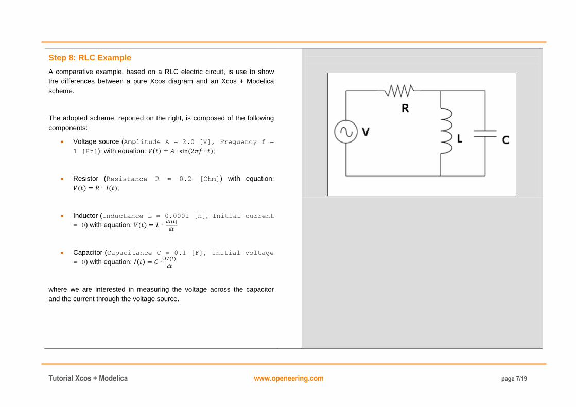
Step 8: RLC Example
A comparative example, based on a RLC electric circuit, is use to show
the differences between a pure Xcos diagram and an Xcos + Modelica
scheme.
The adopted scheme, reported on the right, is composed of the following
components:
Voltage source (Amplitude A = 2.0 [V], Frequency f =
1 [Hz]); with equation: ;
Resistor (Resistance R = 0.2 [Ohm]) with equation:
;
Inductor (Inductance L = 0.0001 [H], Initial current
= 0) with equation:
Capacitor (Capacitance C = 0.1 [F], Initial voltage
= 0) with equation:
where we are interested in measuring the voltage across the capacitor
and the current through the voltage source.
Tutorial Xcos + Modelica www.openeering.com page 8/19
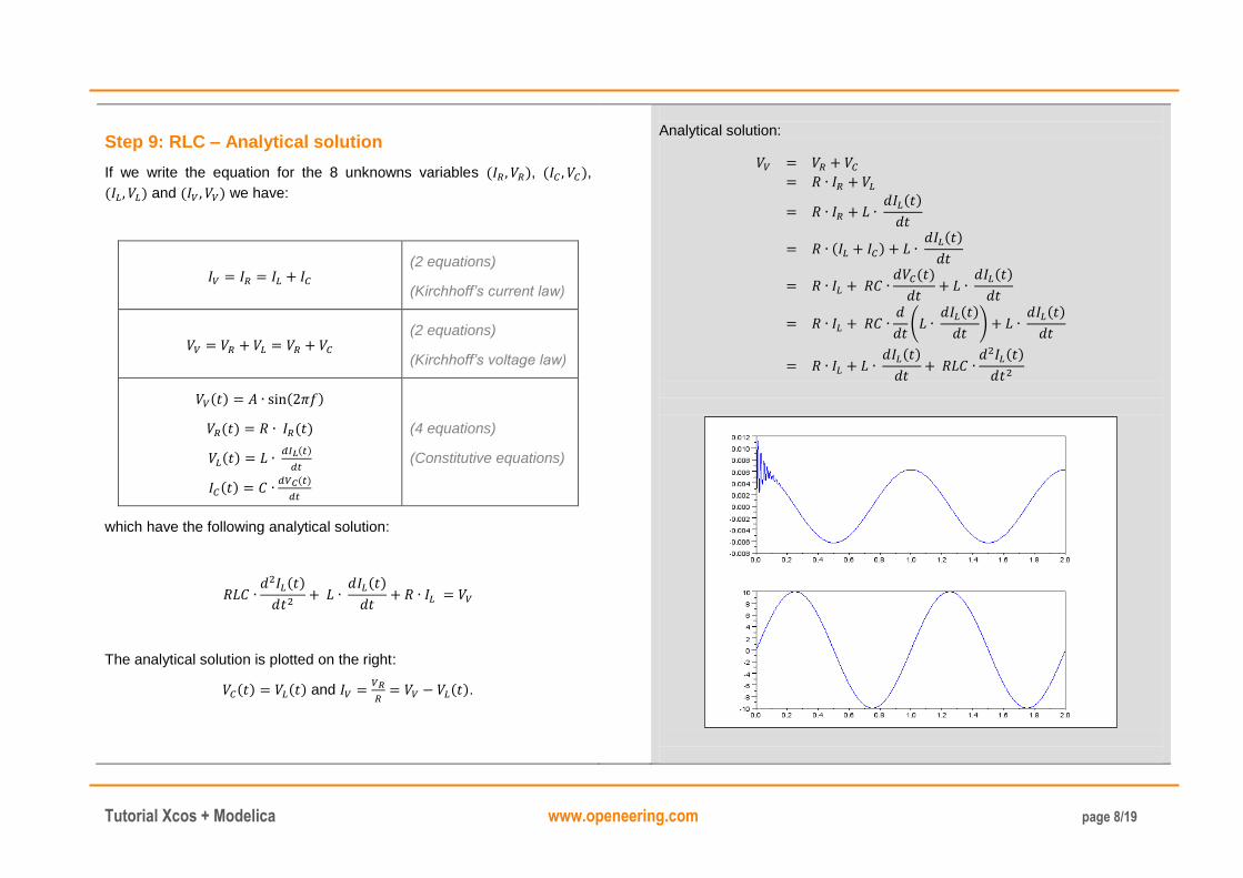
Step 9: RLC – Analytical solution
If we write the equation for the 8 unknowns variables , ,
and we have:
(2 equations)
(Kirchhoff’s current law)
(2 equations)
(Kirchhoff’s voltage law)
(4 equations)
(Constitutive equations)
which have the following analytical solution:
The analytical solution is plotted on the right:
and
.
Analytical solution:
(
)
Tutorial Xcos + Modelica www.openeering.com page 9/19
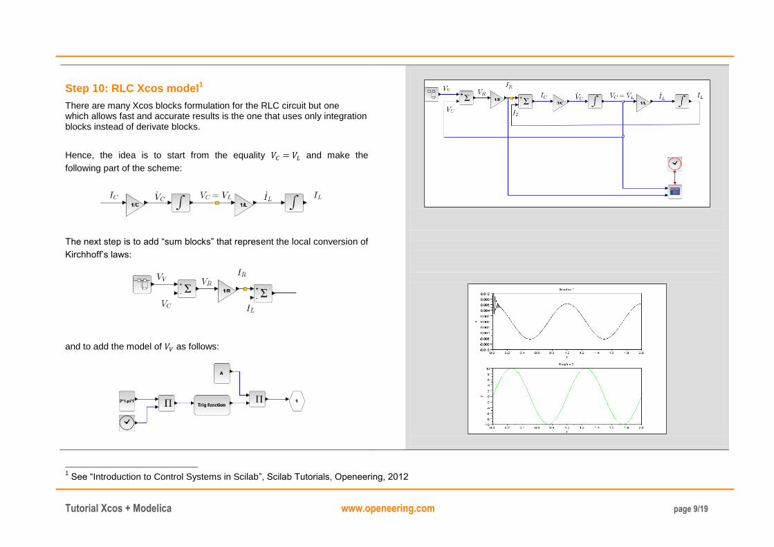
Step 10: RLC Xcos model1
There are many Xcos blocks formulation for the RLC circuit but one which allows fast and accurate results is the one that uses only integration blocks instead of derivate blocks.
Hence, the idea is to start from the equality and make the
following part of the scheme:
The next step is to add “sum blocks” that represent the local conversion of
Kirchhoff’s laws:
and to add the model of as follows:
1 See “Introduction to Control Systems in Scilab”, Scilab Tutorials, Openeering, 2012
Tutorial Xcos + Modelica www.openeering.com page 10/19
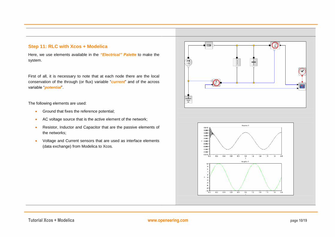
Step 11: RLC with Xcos + Modelica
Here, we use elements available in the “Electrical” Palette to make the
system.
First of all, it is necessary to note that at each node there are the local
conservation of the through (or flux) variable “current” and of the across
variable “potential”.
The following elements are used:
Ground that fixes the reference potential;
AC voltage source that is the active element of the network;
Resistor, Inductor and Capacitor that are the passive elements of
the networks;
Voltage and Current sensors that are used as interface elements
(data exchange) from Modelica to Xcos.
Tutorial Xcos + Modelica www.openeering.com page 11/19
Step 12: Basic Modelica blocks – The MBLOCK
Palette: User defined functions / MBLOCK
Purpose: This block provides an easy way for creating an Xcos interface
for Modelica without creating any interfacing functions.
The Modelica generic block
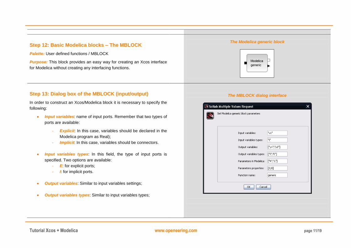
Step 13: Dialog box of the MBLOCK (input/output)
In order to construct an Xcos/Modelica block it is necessary to specify the
following:
Input variables: name of input ports. Remember that two types of
ports are available:
- Explicit: In this case, variables should be declared in the
Modelica program as Real);
- Implicit: In this case, variables should be connectors.
Input variables types: In this field, the type of input ports is
specified. Two options are available:
- E: for explicit ports;
- I: for implicit ports.
Output variables: Similar to input variables settings;
Output variables types: Similar to input variables types;
The MBLOCK dialog interface
Tutorial Xcos + Modelica www.openeering.com page 12/19
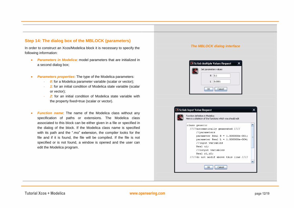
Step 14: The dialog box of the MBLOCK (parameters)
In order to construct an Xcos/Modelica block it is necessary to specify the
following information:
Parameters in Modelica: model parameters that are initialized in
a second dialog box;
Parameters properties: The type of the Modelica parameters:
- 0: for a Modelica parameter variable (scalar or vector);
- 1: for an initial condition of Modelica state variable (scalar
or vector);
- 2: for an initial condition of Modelica state variable with
the property fixed=true (scalar or vector).
Function name: The name of the Modelica class without any
specification of paths or extensions. The Modelica class
associated to this block can be either given in a file or specified in
the dialog of the block. If the Modelica class name is specified
with its path and the “.mo” extension, the compiler looks for the
file and if it is found, the file will be compiled. If the file is not
specified or is not found, a window is opened and the user can
edit the Modelica program.
The MBLOCK dialog interface
Tutorial Xcos + Modelica www.openeering.com page 13/19
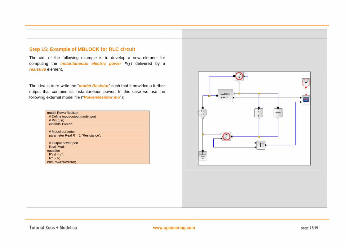
Step 15: Example of MBLOCK for RLC circuit
The aim of the following example is to develop a new element for
computing the instantaneous electric power delivered by a
resistive element.
The idea is to re-write the “model Resistor” such that it provides a further
output that contains its instantaneous power. In this case we use the
following external model file (“PowerResistor.mo”):
model PowerResistor // Define input/output model port // Pin p, n; extends TwoPin; // Model paramter parameter Real R = 1 "Resistance"; // Output power port Real PVal; equation PVal = v*i; R*i = v; end PowerResistor;
Tutorial Xcos + Modelica www.openeering.com page 14/19
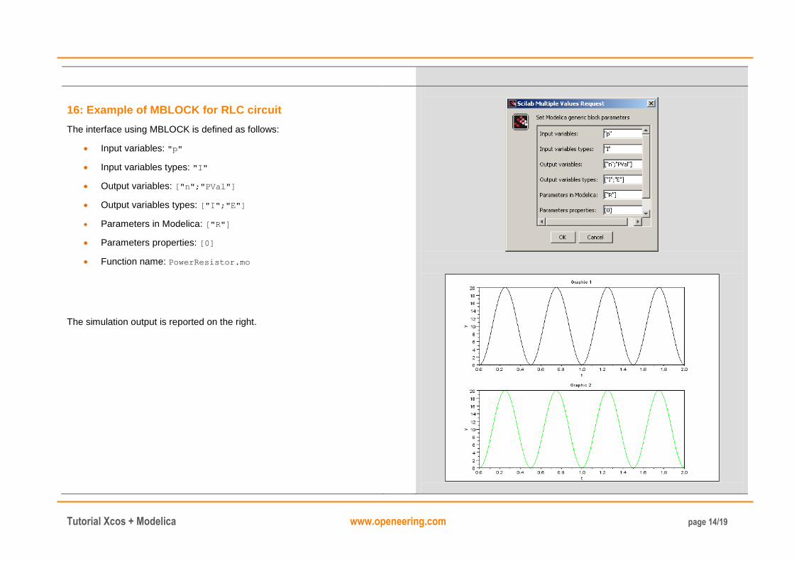
16: Example of MBLOCK for RLC circuit
The interface using MBLOCK is defined as follows:
Input variables: "p"
Input variables types: "I"
Output variables: ["n";"PVal"]
Output variables types: ["I";"E"]
Parameters in Modelica: ["R"]
Parameters properties: [0]
Function name: PowerResistor.mo
The simulation output is reported on the right.
Tutorial Xcos + Modelica www.openeering.com page 15/19
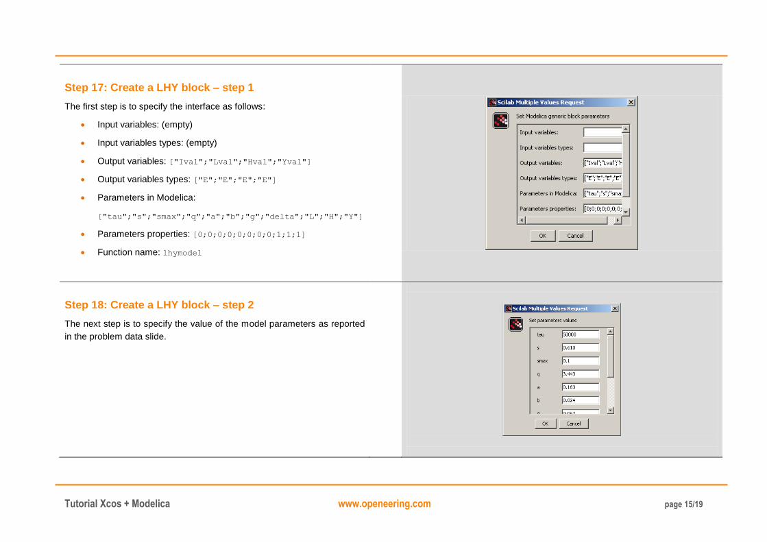
Step 17: Create a LHY block – step 1
The first step is to specify the interface as follows:
Input variables: (empty)
Input variables types: (empty)
Output variables: ["Ival";"Lval";"Hval";"Yval"]
Output variables types: ["E";"E";"E";"E"]
Parameters in Modelica:
["tau";"s";"smax";"q";"a";"b";"g";"delta";"L";"H";"Y"]
Parameters properties: [0;0;0;0;0;0;0;0;1;1;1]
Function name: lhymodel
Step 18: Create a LHY block – step 2
The next step is to specify the value of the model parameters as reported
in the problem data slide.
Tutorial Xcos + Modelica www.openeering.com page 16/19
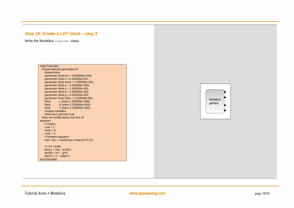
Step 19: Create a LHY block – step 3
Write the Modelica lhymodel class.
class lhymodel ////automatically generated //// //parameters parameter Real tau = 5.000000e+004; parameter Real s = 6.100000e-001; parameter Real smax = 1.000000e-001; parameter Real q = 3.443000e+000; parameter Real a = 1.630000e-001; parameter Real b = 2.400000e-002; parameter Real g = 6.200000e-002; parameter Real delta = 2.910000e-001; Real L (start=1.400000e+006); Real H (start=1.300000e+005); Real Y (start=1.100000e+005); //output variables Real Ival,Lval,Hval,Yval; ////do not modify above this line //// equation // Output Lval = L; Hval = H; Yval = Y; // Initiation equation Ival = tau + max(smax,s*exp(-q*Y/L))*L; // LHY model der(L) = Ival - (a+b)*L; der(H) = b*L - g*H; der(Y) = H - delta*Y; end lhymodel;
Tutorial Xcos + Modelica www.openeering.com page 17/19
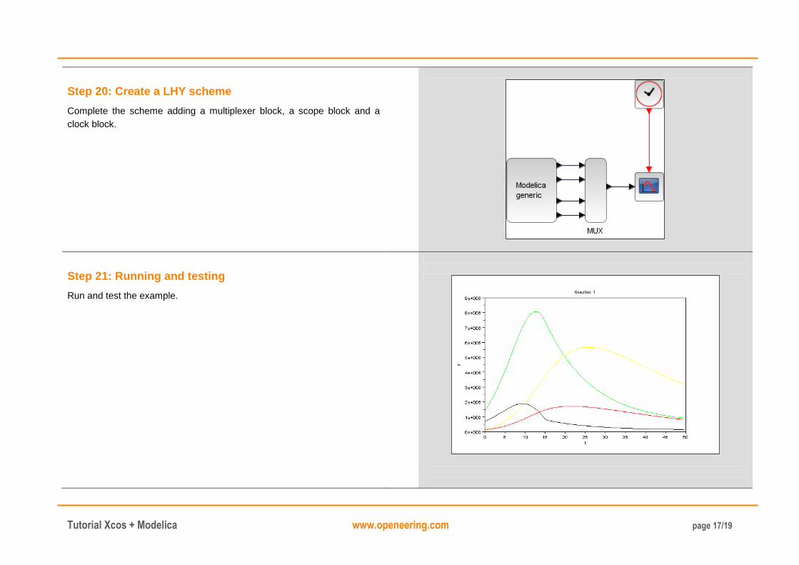
Step 20: Create a LHY scheme
Complete the scheme adding a multiplexer block, a scope block and a
clock block.
Step 21: Running and testing
Run and test the example.
Tutorial Xcos + Modelica www.openeering.com page 18/19
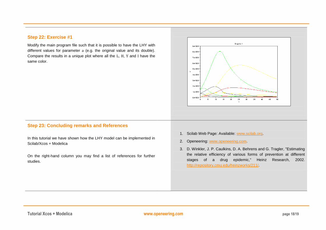
Step 22: Exercise #1
Modify the main program file such that it is possible to have the LHY with
different values for parameter (e.g. the original value and its double).
Compare the results in a unique plot where all the , , and have the
same color.
Step 23: Concluding remarks and References
In this tutorial we have shown how the LHY model can be implemented in
Scilab/Xcos + Modelica
On the right-hand column you may find a list of references for further
studies.
1. Scilab Web Page: Available: www.scilab.org.
2. Openeering: www.openeering.com.
3. D. Winkler, J. P. Caulkins, D. A. Behrens and G. Tragler, "Estimating
the relative efficiency of various forms of prevention at different
stages of a drug epidemic," Heinz Research, 2002.
http://repository.cmu.edu/heinzworks/211/.
Tutorial Xcos + Modelica www.openeering.com page 19/19
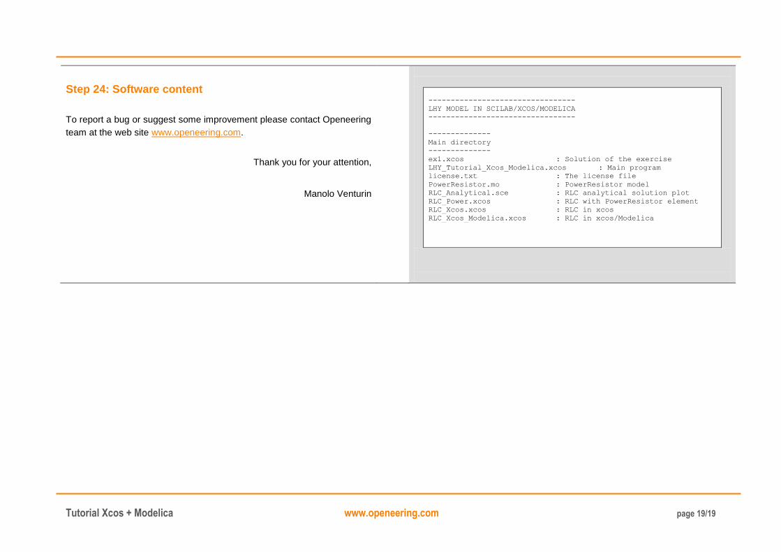
Step 24: Software content
To report a bug or suggest some improvement please contact Openeering
team at the web site www.openeering.com.
Thank you for your attention,
Manolo Venturin
---------------------------------
LHY MODEL IN SCILAB/XCOS/MODELICA
---------------------------------
--------------
Main directory
--------------
ex1.xcos : Solution of the exercise
LHY_Tutorial_Xcos_Modelica.xcos : Main program
license.txt : The license file
PowerResistor.mo : PowerResistor model
RLC_Analytical.sce : RLC analytical solution plot
RLC_Power.xcos : RLC with PowerResistor element
RLC_Xcos.xcos : RLC in xcos
RLC_Xcos_Modelica.xcos : RLC in xcos/Modelica