Embed Size (px)
Citation preview
Lex E. Renner
Linear Algebraic Monoids
SPIN
– Monograph –
January 12, 2005
Springer
Berlin Heidelberg NewYorkHongKong LondonMilan Paris Tokyo

To my parents, Roy and Jo.

Preface
The object of this monograph is to document what is most interesting aboutlinear monoids. We show how these results fit together into a coherent blendof semigroup theory, groups with BN-pair, representation theory, convex ge-ometry and algebraic group theory. The intended reader is one who is familiarwith some of these topics, and is willing to learn about the others.
The intention of the author is to convince the reader that reductivemonoids are among the darlings of algebra. We do this by systematicallyassembling many of the major known results with many proofs, examples andexplanations. To further entice the reader, we have included many exercises.
The theory of linear algebraic monoids is quite recent, originating around1980. Both Mohan Putcha and the author began the systematic study inde-pendently. But this development would not have been possible without thepioneering work of Chevalley, Borel and Tits on algebraic groups. Also, thereis the related, but more general theory of spherical embeddings, developedlargely by Brion, Luna and Vust. These theories were developed somewhatindependently, but it is always a good idea to interpret monoid results in thecombinatorial apparatus of spherical embeddings.
Each chapter of this monograph is focussed on one or more of the majorthemes of the subject. These are: classification, orbits, geometry, representa-tions, universal constructions and combinatorics. There is an inherent diver-sity and richness in the subject that usually rewards a stalwart investigation.
I would like to acknowledge some of those whose efforts or participationhave made this monograph possible. The late Roy R. Douglas, my Ph. D.supervisor, whose boundless, open-minded enthusiasm got me started on thestudy of algebraic monoids. Mohan S. Putcha, for often taking the next stepwhen I was stuck. My former students Wenxue Huang, Zhuo Li and ZhenhengLi, for suggesting improvements and helping me not to forget how mathemat-ical ideas move from one generation to the next. Lou Solomon, for findingthe fundamental links with combinatorics and Hecke-Iwahori algebra. KarlHofmann and Ernest Vinberg, for giving me the opportunity to assess and
VIII Preface
present my ideas in the broader context of Positivity in Lie Theory. VladimirPopov, who invited me into this exciting EMS project with Springer-Verlag.
London, Canada, Lex E. RennerJuly, 2004
Contents
1 Introduction . . . . . . . . . . . . . . . . . . . . . . . . . . . . . . . . . . . . . . . . . . . . . . . 1
2 Background . . . . . . . . . . . . . . . . . . . . . . . . . . . . . . . . . . . . . . . . . . . . . . . 52.1 Algebraic Geometry . . . . . . . . . . . . . . . . . . . . . . . . . . . . . . . . . . . . . 5
2.1.1 Affine Varieties . . . . . . . . . . . . . . . . . . . . . . . . . . . . . . . . . . . 52.1.2 Dimension Theory . . . . . . . . . . . . . . . . . . . . . . . . . . . . . . . . . 72.1.3 Divisor Class Groups . . . . . . . . . . . . . . . . . . . . . . . . . . . . . . 82.1.4 Morphisms . . . . . . . . . . . . . . . . . . . . . . . . . . . . . . . . . . . . . . . 10
2.2 Algebraic Groups . . . . . . . . . . . . . . . . . . . . . . . . . . . . . . . . . . . . . . . . 122.2.1 Algebraic Groups . . . . . . . . . . . . . . . . . . . . . . . . . . . . . . . . . . 122.2.2 Root Systems, Weyl Groups and Dynkin Diagrams . . . . 152.2.3 Tits System and Bruhat Decomposition . . . . . . . . . . . . . . 182.2.4 Representations . . . . . . . . . . . . . . . . . . . . . . . . . . . . . . . . . . . 192.2.5 The Class Group of a Reductive Group . . . . . . . . . . . . . . 212.2.6 Actions, Orbits, Invariants and Quotients . . . . . . . . . . . . . 232.2.7 Cellular Decompositions of Algebraic Varieties . . . . . . . . 25
2.3 Semigroups . . . . . . . . . . . . . . . . . . . . . . . . . . . . . . . . . . . . . . . . . . . . . 262.3.1 Basic Semigroup Theory . . . . . . . . . . . . . . . . . . . . . . . . . . . 262.3.2 Strongly π-regular Semigroups . . . . . . . . . . . . . . . . . . . . . . 272.3.3 Special Types of Semigroups . . . . . . . . . . . . . . . . . . . . . . . . 30
2.4 Exercises . . . . . . . . . . . . . . . . . . . . . . . . . . . . . . . . . . . . . . . . . . . . . . . 312.4.1 Abstract Semigroups . . . . . . . . . . . . . . . . . . . . . . . . . . . . . . . 31
3 Algebraic Monoids . . . . . . . . . . . . . . . . . . . . . . . . . . . . . . . . . . . . . . . . . 333.1 Linear Algebraic Monoids . . . . . . . . . . . . . . . . . . . . . . . . . . . . . . . . 333.2 Normal Monoids . . . . . . . . . . . . . . . . . . . . . . . . . . . . . . . . . . . . . . . . 373.3 D-monoids . . . . . . . . . . . . . . . . . . . . . . . . . . . . . . . . . . . . . . . . . . . . . 383.4 Solvable Monoids . . . . . . . . . . . . . . . . . . . . . . . . . . . . . . . . . . . . . . . . 403.5 Excercises . . . . . . . . . . . . . . . . . . . . . . . . . . . . . . . . . . . . . . . . . . . . . . 40
3.5.1 Linear Algebraic Groups . . . . . . . . . . . . . . . . . . . . . . . . . . . 403.5.2 Linear Algebraic Semigroups . . . . . . . . . . . . . . . . . . . . . . . . 41
X Contents
3.5.3 Irreducible Algebraic Semigroups . . . . . . . . . . . . . . . . . . . . 42
4 Regularity Conditions . . . . . . . . . . . . . . . . . . . . . . . . . . . . . . . . . . . . . 454.1 Reductive Monoids . . . . . . . . . . . . . . . . . . . . . . . . . . . . . . . . . . . . . . 454.2 Semigroup Structure of Reductive Monoids . . . . . . . . . . . . . . . . . 47
4.2.1 The Type Map . . . . . . . . . . . . . . . . . . . . . . . . . . . . . . . . . . . . 474.3 Solvable Regular Monoids . . . . . . . . . . . . . . . . . . . . . . . . . . . . . . . . 484.4 Regular Algebraic Monoids . . . . . . . . . . . . . . . . . . . . . . . . . . . . . . . 504.5 Regularity in Codimension One . . . . . . . . . . . . . . . . . . . . . . . . . . . 524.6 Exercises . . . . . . . . . . . . . . . . . . . . . . . . . . . . . . . . . . . . . . . . . . . . . . . 54
4.6.1 D-monoids . . . . . . . . . . . . . . . . . . . . . . . . . . . . . . . . . . . . . . . 544.6.2 Regular and Reductive monoids . . . . . . . . . . . . . . . . . . . . . 544.6.3 Regularity in Codimension One . . . . . . . . . . . . . . . . . . . . . 55
5 Classification of Reductive Monoids . . . . . . . . . . . . . . . . . . . . . . . 575.1 The Extension Principle . . . . . . . . . . . . . . . . . . . . . . . . . . . . . . . . . . 575.2 Vinberg’s Approach . . . . . . . . . . . . . . . . . . . . . . . . . . . . . . . . . . . . . . 615.3 Algebraic Monoids as Spherical Varieties . . . . . . . . . . . . . . . . . . . 64
5.3.1 Spherical Varieties . . . . . . . . . . . . . . . . . . . . . . . . . . . . . . . . . 645.3.2 Rittatore’s Approach . . . . . . . . . . . . . . . . . . . . . . . . . . . . . . 665.3.3 Type Maps and Colors . . . . . . . . . . . . . . . . . . . . . . . . . . . . . 68
6 Universal Constructions . . . . . . . . . . . . . . . . . . . . . . . . . . . . . . . . . . . 736.1 Quotients . . . . . . . . . . . . . . . . . . . . . . . . . . . . . . . . . . . . . . . . . . . . . . 736.2 Class Groups of Reductive Monoids . . . . . . . . . . . . . . . . . . . . . . . . 756.3 Flat Monoids . . . . . . . . . . . . . . . . . . . . . . . . . . . . . . . . . . . . . . . . . . . 786.4 Multilined Closure . . . . . . . . . . . . . . . . . . . . . . . . . . . . . . . . . . . . . . . 866.5 Normalization and Representations . . . . . . . . . . . . . . . . . . . . . . . . 896.6 Exercises . . . . . . . . . . . . . . . . . . . . . . . . . . . . . . . . . . . . . . . . . . . . . . . 90
6.6.1 Flat Monoids . . . . . . . . . . . . . . . . . . . . . . . . . . . . . . . . . . . . . 90
7 Orbit Structure of Reductive Monoids . . . . . . . . . . . . . . . . . . . . . 917.1 The System of Idempotents and the Type Map . . . . . . . . . . . . . . 917.2 The Cross Section Lattice and the Weyl Chamber . . . . . . . . . . . 937.3 J-irreducible Monoids . . . . . . . . . . . . . . . . . . . . . . . . . . . . . . . . . . . . 967.4 Explicit Calculations of the Type Map . . . . . . . . . . . . . . . . . . . . . 99
7.4.1 The Type Map for the Adjoint Representations . . . . . . . 997.4.2 Further Examples of the Type Map . . . . . . . . . . . . . . . . . . 104
7.5 2-reducible Reductive Monoids . . . . . . . . . . . . . . . . . . . . . . . . . . . . 1077.5.1 Reductive Monoids and Type Maps . . . . . . . . . . . . . . . . . . 1077.5.2 The Type Map of a 2-reducible Monoid . . . . . . . . . . . . . . 1107.5.3 Calculating the Type Map Geometrically . . . . . . . . . . . . . 1147.5.4 Monoids with I+ = ∆\α and I− = ∆\β . . . . . . . . . . 1177.5.5 Monoids with I+ = φ and I− = φ . . . . . . . . . . . . . . . . . . . . 1197.5.6 (J,σ)-irreducible Monoids Revisited . . . . . . . . . . . . . . . . . . 119
Contents XI
7.6 Type Maps in General . . . . . . . . . . . . . . . . . . . . . . . . . . . . . . . . . . . 1227.7 Exercises . . . . . . . . . . . . . . . . . . . . . . . . . . . . . . . . . . . . . . . . . . . . . . . 124
7.7.1 The Cross Section Lattice . . . . . . . . . . . . . . . . . . . . . . . . . . 1247.7.2 Idempotents . . . . . . . . . . . . . . . . . . . . . . . . . . . . . . . . . . . . . . 125
8 The Analogue of the Bruhat Decomposition . . . . . . . . . . . . . . . 1278.1 The Renner Monoid R . . . . . . . . . . . . . . . . . . . . . . . . . . . . . . . . . . . 1278.2 The Analogue of the Tits System . . . . . . . . . . . . . . . . . . . . . . . . . . 1298.3 Row Reduced Echelon Form . . . . . . . . . . . . . . . . . . . . . . . . . . . . . . 1328.4 The Length Function on R . . . . . . . . . . . . . . . . . . . . . . . . . . . . . . . 1358.5 Order-Preserving Elements of R . . . . . . . . . . . . . . . . . . . . . . . . . . . 1378.6 The Adherence Order on R . . . . . . . . . . . . . . . . . . . . . . . . . . . . . . . 1408.7 The j-order, R+ and Pennell’s Theorem . . . . . . . . . . . . . . . . . . . . 1438.8 The Adherence Order on Mn(K) . . . . . . . . . . . . . . . . . . . . . . . . . . 1478.9 Exercises . . . . . . . . . . . . . . . . . . . . . . . . . . . . . . . . . . . . . . . . . . . . . . . 150
9 Representations and Blocks of Algebraic Monoids . . . . . . . . . 1539.1 Conjugacy Classes and Adjoint Quotient . . . . . . . . . . . . . . . . . . . 1539.2 Rep(M) according to Doty . . . . . . . . . . . . . . . . . . . . . . . . . . . . . . . . 1569.3 The Blocks of Mn(K) when char(K) = p > 0 . . . . . . . . . . . . . . . 1599.4 The Blocks of Solvable Algebraic Monoids . . . . . . . . . . . . . . . . . . 160
10 Monoids of Lie Type . . . . . . . . . . . . . . . . . . . . . . . . . . . . . . . . . . . . . . . 16710.1 Finite Groups of Lie Type . . . . . . . . . . . . . . . . . . . . . . . . . . . . . . . . 167
10.1.1 σ Preserves Root Length . . . . . . . . . . . . . . . . . . . . . . . . . . . 16710.1.2 σ Exchanges Root Length . . . . . . . . . . . . . . . . . . . . . . . . . . 168
10.2 Endomorphisms of Linear Algebraic Monoids . . . . . . . . . . . . . . . 16810.3 A Detailed Example . . . . . . . . . . . . . . . . . . . . . . . . . . . . . . . . . . . . . 16910.4 Abstract Monoids of Lie Type . . . . . . . . . . . . . . . . . . . . . . . . . . . . 17210.5 Modular Representations of Finite Reductive Monoids . . . . . . . 17510.6 Exercises . . . . . . . . . . . . . . . . . . . . . . . . . . . . . . . . . . . . . . . . . . . . . . . 184
10.6.1 Weil Zeta Functions . . . . . . . . . . . . . . . . . . . . . . . . . . . . . . . 18410.6.2 Counting Modular Representations . . . . . . . . . . . . . . . . . . 185
11 Cellular Decomposition of Algebraic Monoids . . . . . . . . . . . . . . 18711.1 Monoid Cells . . . . . . . . . . . . . . . . . . . . . . . . . . . . . . . . . . . . . . . . . . . 18811.2 Exercises . . . . . . . . . . . . . . . . . . . . . . . . . . . . . . . . . . . . . . . . . . . . . . . 192
12 Conjugacy Classes . . . . . . . . . . . . . . . . . . . . . . . . . . . . . . . . . . . . . . . . . 19512.1 The Basic Conjugacy Theorem . . . . . . . . . . . . . . . . . . . . . . . . . . . . 19512.2 Some Refinements . . . . . . . . . . . . . . . . . . . . . . . . . . . . . . . . . . . . . . . 19712.3 Putcha’s Decomposition and the Nilpotent Variety . . . . . . . . . . . 199
XII Contents
13 The Centralizer of a Semisimple Element . . . . . . . . . . . . . . . . . . 20513.1 Introduction . . . . . . . . . . . . . . . . . . . . . . . . . . . . . . . . . . . . . . . . . . . . 20513.2 Main Results . . . . . . . . . . . . . . . . . . . . . . . . . . . . . . . . . . . . . . . . . . . 20613.3 The Structure of Rs and Ms . . . . . . . . . . . . . . . . . . . . . . . . . . . . . . 20813.4 Examples . . . . . . . . . . . . . . . . . . . . . . . . . . . . . . . . . . . . . . . . . . . . . . . 209
14 Combinatorics Related to Algebraic Monoids . . . . . . . . . . . . . . 21314.1 The Adherence Order on WeW . . . . . . . . . . . . . . . . . . . . . . . . . . . 21314.2 Shellability and Stanley-Reisner Rings . . . . . . . . . . . . . . . . . . . . . 21714.3 Distribution of Products in Finite Monoids . . . . . . . . . . . . . . . . . 217
14.3.1 Properties of h(a) . . . . . . . . . . . . . . . . . . . . . . . . . . . . . . . . . 21814.3.2 Example . . . . . . . . . . . . . . . . . . . . . . . . . . . . . . . . . . . . . . . . . 223
14.4 Exercises . . . . . . . . . . . . . . . . . . . . . . . . . . . . . . . . . . . . . . . . . . . . . . . 226
15 Survey of Related Developments . . . . . . . . . . . . . . . . . . . . . . . . . . . 22715.1 Complex Representation of Finite Reductive Monoids . . . . . . . . 22715.2 Finite Semigroups and Highest Weight Categories . . . . . . . . . . . 22815.3 Singularities of G-embeddings . . . . . . . . . . . . . . . . . . . . . . . . . . . . . 23015.4 Cohomology of G-embeddings . . . . . . . . . . . . . . . . . . . . . . . . . . . . . 23115.5 Horospherical Varieties . . . . . . . . . . . . . . . . . . . . . . . . . . . . . . . . . . . 23215.6 Monoids associated with Kac-Moody Groups . . . . . . . . . . . . . . . . 232
References . . . . . . . . . . . . . . . . . . . . . . . . . . . . . . . . . . . . . . . . . . . . . . . . . . . . . 235
Index . . . . . . . . . . . . . . . . . . . . . . . . . . . . . . . . . . . . . . . . . . . . . . . . . . . . . . . . . . 243
1
Introduction
The theory of linear algebraic monoids has been developed significantly onlyover the last twenty-five years, due largely to the efforts of Putcha and theauthor. It culminates a natural blend of algebraic groups, torus embeddingsand semigroups. Unfortunately, this work had not been made as accessibleas it might have been. Many of the fundamental developments were obtainedafter Putcha published his basic monograph “Linear algebraic monoids” in1988. Solomon’s 1995 survey “An introduction to reductive monoids” providesan engaging introduction to the theory of reductive monoids for a readerwith an interest in algebra and combinatorics, but without requiring a lot ofbackground from semigroups and algebraic group theory.
The purpose of this monograph is to update the literature with a detailedsurvey of the latest developments, along with many proofs, examples andexplanations. At the same time, we hope to make the discussion reasonably selfcontained, even though the prerequisites are quite high. Our hope is that wecan make this subject, and its methods, more accessible to a larger audience.
The systematic development of the theory of algebraic monoids beganaround 1978. Both Putcha and the author independently saw the potentialin these monoids for a rich, and highly structured blend of group theory,combinatorics and torus embeddings. Putcha began his investigation around1978 by experimenting with some of the main ideas of semigroup theory:Green’s relations, regularity, semilattices, and so on. His efforts yielded a lotof technically useful information. In particular, he established control of theidempotent set of an irreducible monoid.
About the same time I started writing my Ph.D. thesis armed with someencouraging success in applications to rational homotopy theory. These appli-cations inspired the hope that reductive monoids could be properly understoodas a geometric blend of the Zariski closure of a maximal, split torus, and theunit group.
The first major result came around 1982. Reductive monoids are regular.At this point we knew for certain that we were onto something special. Anyregular monoid is inevitably (somehow) determined by its unit group and its
2 1 Introduction
idempotent set. A major developmental theme from this point on was the roleof the idempotent set of any irreducible monoid. From there, Putcha foundhis cross section lattice Λ, the most useful way to control the G × G-orbitsof M . Armed with Λ, and Grosshans’ codimension 2 condition, it was thenpossible for me to develop the classification theory of reductive monoids ina way that allowed a description of the set of morphisms from any reductivenormal monoid. About that time I started my investigation of the analogueof the Bruhat decomposition for reductive monoids.
Around 1986, Putcha observed that each reductive monoid M has a typemap, λ : Λ→ 2S . This is truly the monoid analogue of the Dynkin diagram: itdetermines M up to a kind of central extension, it determines Nambooripad’sbiordered set of idempotents, and it determines the set of B×B-orbits of M .This is just what Putcha needed to develop his abstract theory of Monoids ofLie type, the monoid analogue of the theory of groups with BN pair. But it isno soft excercise in generalization theory (see Chapter 10). In any case, thetype map is the exact, minimal, discrete entity that can be used to determinethe salient structure of a Monoid of Lie type.
In a joint effort, around 1988, we determined explicitly a large class of typemaps. These are the type maps of J-irreducible monoids. A reductive monoidM is J-irreducible if it has exactly one, non zero, minimal G×G-orbit. Thisleads to some speculation about what is possible in general. On the one hand,it is impossible to list all type maps but, on the other hand, there are stillsome interesting questions here. We have recently determined the type mapsof reductive monoids with exactly two minimal, non zero G×G-orbits.
In another joint effort, arround 1990, we investigated the irreducible, mod-ular representations of a finite monoid of Lie type. By combining the results ofsemigroup representations (Munn-Ponizovskii) with the results of Chevalleygroup representations (Curtis-Richen) we obtained the surprising result thatirreducible modular representations of the monoid restrict to irreducible rep-resentations of the unit group. It is as if the finite group is somehow “dense” inthe monoid, as in the geometric case. This led me, around 1998, to a completeclassification of irreducible, modular representations of finite monoids of Lietype; along with an enumerative theory, relating these representations to theWeil zeta function of the adjoint quotient.
We mention here some related developments. Around 1990 Solomon begana study of the monoid Hecke-Iwahori algebra, initially for Mn(Fq). Thesealgebras are semisimple, and they have very recently appeared (with Halversonet al.) in a solution of the Schur-Weyl duality theorem for quantum gln(q).
Around 1990, S. Doty proved that the coordinate algebra of a reductivenormal monoid M in characteristic p > 0 is a direct limit of generalized Schuralgebras in the sense of Donkin. In particular, Rep(M) is a highest weightcategory in the sense of Cline, Parshall and Scott.
In 1994, E.B. Vinberg introduced some new ideas into the theory of alge-braic monoids: abelianization, flat deformation, Env(G0) and the asymptotic
1 Introduction 3
semigroup As(G0). He also gave a new approach to the classification of re-ductive monoids.
Also around 1994, Rittatore in his Grenoble thesis systematically identifiedthe entire theory of algebraic monoids as a part of the theory of sphericalembeddings. He also extended much of Vinberg’s work to characteristic p >0, and later proved that any reductive, normal, algebraic monoid is Cohen-Macaulay.
In writing this survey I have tried to assess every contribution that im-pacts significantly on the theory of algebraic monoids. Hopefully, I have notimproperly stated the work of any author. There is some difficulty on thispoint because there is a natural hierarchy of theories:
i) affine torus embeddingsii) reductive algebraic monoidsiii) symmetric varietiesiv) spherical embeddings.
Indeed, this is obvious from the definitions (and a theorem of Vust, to get fromiii) to iv)). One should also mention horospherical varieties along with thislist. Each of these topics is a legitimate, well established discipline in its ownright, with its own methods and techniques. Furthermore, many results aboutreductive monoids can be identified as the special case of some more generalresults about symmetric varieties or spherical embeddings. As we have alreadypointed out, this observation has led to some important work of Rittatore. Hesystematically identifies the theory of algebraic monoids as a special casewithin the theory of spherical embeddings. We describe his approach in § 5.3.We also identify the key ideas of embedding theory as they pertain to reductivemonoids.
On the other hand, there are several features about algebraic monoids thathave yet to be worked out for general spherical varieties:
i) The possible G×G-orbits that could occur for some reductive monoid areeasy to construct in explicit detail. See § 5.3.3 for some detail here. Onecan calculate the B × B-orbits, and the adherence ordering on the set Rof these orbits, in terms of the lattice of G × G-orbits and the Bruhatordering on the associated Weyl group, and certain of its subgroups.
ii) There is an abstract theory, due to Putcha, known as monoids of Lie typein the spirit of Tits’ theory of BN -pairs.
These monoid constructions should ultimately work for more generalspherical vartieties, when more is known about the “global” structure of spher-ical homogeneous spaces. It appears to be one of the wide open challenges todescribe explicitly (in terms of the dense orbit) the possible spherical homo-geneous spaces that could occur on the boundary of a given spherical variety.
Some of our results in Chapter 11, on the cell decomposition of the “won-derful” compactification X , have been obtained using other methods. Indeed,
4 1 Introduction
Brion has obtained a cell decomposition of X using the method of Birula-Bialynicki.
This survey is organized as follows. Each of the next thirteen chapters isdevoted to some particular theme directly related to algebraic monoids. Chap-ter 7, for example, is devoted to the problem of determining the orbit structureof reductive monoids. There is also a fifteenth chapter where we discuss sev-eral results that are directly related to the theory of algebraic monoids, butwhich require techniques beyond the scope of this survey.
There is no need to summarize every chapter in this introduction. We havealready discussed the main results of the theory above. The reader shouldconsult the table of contents for a description of each chapter and a guide tohow the material is organized.
2
Background
In this chapter we assemble some of the major ideas and results from algebraicgeometry, algebraic group theory and semigroup theory. This is intended toset the tone for the reader. It is intended also to provide some convenientreferences for the ensuing development. The theory of algebraic monoids is arich blend of these three influences.
2.1 Algebraic Geometry
Algebraic monoids are affine, algebraic varieties with other structures attachedto them. In this section, we introduce some basic concepts, such as varieties,morphisms, dimension and divisors. We assume in this section that K is analgebraically closed field.
2.1.1 Affine Varieties
We define affine n-space over K to be Kn, the set of all n-tuples of elementsof K. An element P ∈ Kn is called a point and, if P = (a1, . . . , an), then aiwill be called the coordinates of P . Let A = K[X1, . . . , Xn] be the polynomialring in n variables over K. We think of the elements of A as functions onKn as follows: if f(X1, . . . , Xn) ∈ A, then we define f : Kn → K by therule f(P ) = f(a1, . . . , an). Thus we can talk about the zeros of f , namelyZ(f) = P ∈ Kn|f(P ) = 0 . If E is any subset of A, we define
Z(E) = P ∈ Kn|f(P ) = 0 for all f ∈ E.
Definition 2.1. A subset X of Kn is called an algebraic set if X = Z(E) forsome subset E of A.
Notice that, if X = Z(E) is an algebraic set, then X = Z(E0) forsome finite subset E0 of E. Indeed, A is a Noetherian ring, and thus
6 2 Background
Z(E) = Z((E)), where (E) denotes the ideal generated by E. But then(E) = (f1, . . . , fn) is finitely generated by the Noetherian condition and thusZ((E)) = Z(f1, . . . , fm).
Proposition 2.2. The union of two algebraic sets is algebraic. The intersec-tion of any collection of algebraic sets is algebraic. The empty set is algebraic.The whole space is algebraic.
Proof. If X = Z(E) and Y = Z(F ), then X ∪ Y = Z(EF ), where EF =fg |f ∈ E and g ∈ F. If Xα = Z(Eα), then ∩Xα = Z(∪Eα). φ = Z(1) andKn = Z(0).
Definition 2.3. The Zariski topology on Kn is the topology on Kn definedby taking as open sets the complements of algebraic sets. By Proposition 2.2this is a topology on Kn.
Example 2.4. Consider the Zariski topology on K. In this case, A = K[X ],and it is well known that every ideal of A is principal. Thus every algebraicset Z is the zero locus of a single polynomial f ∈ A. Furthermore, sinceK is algebraically closed, f factors as f(X) = c(X − a1) . . . (X − an) withc, a1, . . . , an ∈ K. Hence Z = a1, . . . , an. Thus the Zariski topology on K isthe cofinite topology.
Definition 2.5. A nonempty subset of a topological space X is called irre-ducible if it cannot be expressed as the union X = X1∪X2 of two, nonempty,proper closed subsets of X.
Example 2.6. K is irreducible because any proper closed subset of K is finite,while K is algebraically closed, and therefore infinite.
Theorem 2.7. (Hilbert’s Vanishing Theorem) Let K be an algebraicallyclosed field, let a be an ideal of A = K[X1, . . . , Xn], and let f ∈ A be apolynomial which vanishes at all points of Z(a). Then f r ∈ a for some integerr > 0.
Proof. See Atiyah-Macdonald [2] page 85.
Thus, there is an inclusion-reversing correspondence between algebraic sets inKn and radical ideals of A = K[X1, . . . , Xn]. It is easy to check that, underthis correspondence, prime ideals correspond to irreducible closed subsets.
Example 2.8. Kn is irreducible, since it corresponds to the zero ideal in A.
Example 2.9. If f is an irreducible polynomial in A = K[X1, . . . , Xn], thenZ(f) is an irreducible, algebraic subset of Kn of codimension one. Z(f) iscalled a hypersurface.
If Y ⊆ Kn we define the ideal of Y by
I(Y ) = f ∈ A|f(P ) = 0 for all P ∈ Y .
2.1 Algebraic Geometry 7
Definition 2.10. If Y is an affine, algebraic set, the affine coordinate ring ofY is K[Y ] = A/I(Y ).
We now study the Zariski topology on affine varieties.
Definition 2.11. A topological space X is called noetherian if it satisfies thedescending chain condition on closed sets: for any sequence Y1 ⊇ Y2 ⊇ . . . ofclosed sets, there exists an integer r > 0 such that Yr = Yr+1 = . . . .
It is easily checked that any affine algebraic set Y is a noetherian topolog-ical space. Indeed, this follows directly from the fact that K[X1, . . . , Xn] is anoetherian ring which, by definition, is a ring which satisfies the ascend-ing chain condition on ideals. Any descending chain of closed subsets of Ydetermines an ascending chain of ideals of K[Y ].
Noetherian topological spaces behave differently from Hausdorff topologi-cal spaces.
Proposition 2.12. Let X be a noetherian topological space and let Y ⊆ X bea closed subset of X. Then Y can be expressed as a finite union Y = Y1∪· · ·∪Yrof irreducible subsets. If we insist that Yi 6⊆ Yj for i 6= j, then the Yi areuniquely determined.
The Yi are called the irreducible components of Y .
Proof. To prove existence of such a decomposition of Y one uses Zorn’s lemma.Let S be the set of nonempty closed subsets of X which cannot be writtenas a finite union of irreducible, closed subsets. If S is nonempty, it must havea minimal element, since X is a noetherian topological space. Let Y be sucha minimal element. Then Y must be reducible, and therefore we can writeY = U ∪ V where U and V are proper closed subsets of Y . By minimalityof Y , each of U and V can be written as a finite union of irreducible closedsubsets, and hence Y also: a contradiction. This establishes the first part ofthe claim. We leave the rest of the proof to the reader.
Corollary 2.13. Any algebraic set in Kn can be expressed uniquely as a unionof irreducible closed subsets, no one containing the other.
2.1.2 Dimension Theory
We begin with a definition.
Definition 2.14. a) Let X be a topological space. The dimension of X is thesupremum of all integers n such that there exists a chain Z0 ⊆ Z1 ⊆ · · · ⊆Zn of distinct, irreducible closed subsets of X. We define the dimensionof an affine variety to be its dimension in this sense.
b) In a commutative ring A, the height of a prime ideal p is the supremum ofall integers n such that there is a chain p0 ⊂ p1 ⊂ · · · ⊂ pn = p of distinctprime ideals. The dimension or Krull dimension of A is the supremum ofthe heights of all prime ideals of A.
8 2 Background
Proposition 2.15. If X is an affine algebraic set, then the dimension of Xis equal to the dimension of its affine coordinate ring K[X ].
Proof. There is a one-to-one inclusion-reversing correspondence between theprime ideals of K[X ] and the irreducible closed subsets of X .
Remark 2.16. a) It follows from Chapter 11 of [2] that the dimension ofK[X ]is equal to the transcendence degree of the fraction field K(X) of K[X ]over K.
b) It follows from a) above that the dimension of Kn is n.c) If A is a noetherian ring and f ∈ A is a regular element, then dim(A/(f))
= dim(A) − 1. See page 122 of [2].
2.1.3 Divisor Class Groups
The class group ultimately contains a subtle mixture of local and global infor-mation about a normal, algebraic variety. In general, it is not easy to calculatethese class groups. But on the other hand, it is often possible to compute theclass group of a variety which can be expressed as the union of well-behavedsubvarieties.
Our general reference for this section is Fossum’s monograph [29]. Also,Section 6 of Chapter II of [38] is a good introduction from a more geometricpoint of view.
A commutative ring A is called an integral domain if, for any x, y ∈A\0, xy 6= 0. It is easy to check that A is an integral domain if and only if thezero ideal of A is a prime ideal. Let A be a noetherian integral domain. We saythat A is normal if it is integrally closed in its field K(A) of fractions. We callan irreducible, algebraic variety X normal if its coordinate ring A = K[X ] isa normal integral domain. A minimal, nonzero prime ideal p of A is called aheight one prime ideal. If X is an algebraic variety over K then the heightone primes of A are in one-to-one correspondence with the closed irreduciblesubvarieties Y of X of codimension one. We call these subvarieties primedivisors. It follows from Theorem 38, page 124 of [57], that
A =⋂
ht(p)=1
Ap.
Furthermore, each Ap is a discrete valuation ring of A. We denote by
νY : K(A)∗ → Z
the discrete valuation on K(A) determined by p and Y = Spec(A/p). If f ∈K(A), it is easy to check that
νY (f) = 0
for all but a finite number of prime divisors Y of X .
2.1 Algebraic Geometry 9
Definition 2.17. If X is a normal, algebraic variety, let Div(X) be the freeabelian group with basis Y | Y is a prime divisor of X. If f ∈ K(X) wedefine the divisor of f , denoted div(f), by
div(f) =∑
νY (f)Y,
where the sum is taken over all prime divisors of X. We refer to div(f) as aprincipal divisor, and denote by Prin(X) ⊆ Div(X) the subgroup of principaldivisors. Finally, we define the divisor class group of X:
Cl(X) = Div(X)/Prin(X).
Notice that we have an exact sequence of abelian groups:
0→ K∗ → K(X)∗ → Prin(X)→ Div(X)→ Cl(X)→ 0.
Example 2.18. Let X be a normal, irreducible, algebraic variety. Then thefollowing are equivalent:
a) Cl(X) = 0.b) Every height one prime p of K[X ] is principal.c) K[X ] is a unique factorization domain.
In particular, Kn has trivial divisor class group.
Proposition 2.19. Let X be irreducible and normal, and let Z be a proper,closed subvariety of X. Let U = X\Z.
a) There is a surjective morphism Cl(X)→ Cl(U) defined by Y → Y ∩U ifY ∩ U is nonempty, and zero otherwise.
b) If codimX(Z) ≥ 2, then Cl(X)→ Cl(U) is an isomorphism.c) If Z = ∪iZi is a union of prime divisors, then there is an exact sequence
⊕iZ→ Cl(X)→ Cl(U)→ 0
where the first map is defined by (a1, . . . , an) →∑aiZi. In particular, if
Cl(U) is trivial, then Cl(X) is generated by Zi.
Proof. For a) notice that every prime divisor of U is the restriction of itsclosure inX . The result in b) follows since Prin(U) = Prin(X) andDiv(U) =Div(X). For c), notice that the kernel of Div(X)→ Div(U) is generated byZi.
Example 2.20. If X = Pn, then Cl(X) = Z. Indeed, let H ⊆ X be a linearhypersurface. Then by c) above, Cl(X) is generated by the class of H , sinceX\H = Kn. On the other hand, each divisor Y of X has a well defined degreedetermined by the degree of its defining equation. But any rational functionon X has degree zero, being the the quotient of two homogeneous polynomialsof the same degree. Hence degree : Cl(X)→ Z is an isomorphism.
10 2 Background
2.1.4 Morphisms
In this section we acquaint the reader with some of the basic facts about mor-phisms of algebraic varieties. Our discussion is mainly concerned with affinevarieties and affine morphisms. This simplifies the discussion significantly.
Definition 2.21. a) Let X be an affine variety with coordinate ring K[X ].A function f : X → K is regular at a point P ∈ X if there is an opensubset U ⊆ X with P ∈ U , and g, h ∈ K[X ] such that f = g/h on U .
b) We say that f is regular on X if it is regular at every point of X.
Definition 2.22. Let X and Y be irreducible affine varieties. A morphismψ : X → Y is a continuous function such that, for every open subset U ⊆ Yand every regular function f : U → K, f ψ : ψ−1(U) → K is a regularfunction.
Proposition 2.23. Let X and Y be affine algebraic varieties with coordinaterings K[X ] and K[Y ] respectively. Define
γ : Hom(X,Y )→ Hom(K[Y ],K[X ])
by γ(f) = f∗, where f∗(h) = h f . Then γ is an bijection. Here Hom on theleft means morphisms of varieties, and Hom on the right means morphismsof K-algebras.
Proof. We give a sketch. See page 19 of [38] for more details. The map γ is welldefined since K[X ] is canonically identified with the ring of regular functionson X . Furthermore, γ is clearly one-to-one.
Conversely, given a homomorphism ψ : K[Y ] → K[X ] of K-algebras,define ψ∗ : X → Y as follows. For x ∈ X , define εx by εx(g) = g(x). Thendefine ψ∗(x) = εx ψ. One then checks that ψ∗ is a morphism, and thatγ(ψ∗) = ψ.
A version of the above result is true even if X is not affine. In that case,let O(X) be the ring of regular functions on X . Then
γ : Hom(X,Y )→ Hom(K[Y ],O(X))
is a bijection. See Proposition 3.5 of Chapter I of [38] for more details.We now distinguish certain classes of morphisms that will be important in
our later discussions.
Definition 2.24. a) A morphism f : X → Y is finite if f∗ : K[Y ] → K[X ]makes K[X ] into a finitely generated module over K[Y ].
b) A morphism f : X → Y is dominant if f(X) ⊆ Y is a dense subset. Noticethat this is equivalent to saying that f∗ : K[Y ]→ K[X ] is injective.
c) A dominant morphism f : X → Y , between irreducible varieties, is bi-rational if f induces an isomorphism f∗ : K(Y ) → K(X) of functionfields.
2.1 Algebraic Geometry 11
d) A morphism f : X → Y is flat if the functor F (M) = M ⊗K[Y ] K[X ],from K[X ]-modules to K[Y ]-modules, is exact.
Remark 2.25. a) A finite morphism has finite fibres.b) A finite dominant morphism f : X → Y induces a K-algebra homomor-
phism f∗ : K(Y )→ K(X) of function fields. The typical fibre has s pointsin it, where s is the separable degree of f .
c) If f : X → Y is a birational morphism, then there are open subsets U ofX and V of Y such that f |U : U → V is an isomorphism.
d) Let X and Y be affine varieties with graded coordinate algebras K[X ] =∑n≥0An and K[Y ] =
∑n≥0Bn, respectively. Assume also that A0 =
B0 = K. Then each of X and Y has a cone point 0X ∈ X and 0Y ∈ Y . Letf : X → Y be a morphism of varieties such that f∗ is a homomorphism ofgraded K-algebras. Then f is a finite morphism if and only if f−1(0Y ) =0X .
e) A flat surjective morphism is open, and has equidimensional fibres.
Given a normal, irreducible, affine variety X , it is sometimes possible to con-struct a morphism f : U → Y from some open subset U of X to the affinevariety Y . On the other hand, we would then like to know whether f extendsto a morphism f : X → Y , without actually constructing this extension. Thefollowing codimension two condition gives us a very useful criterion.
Theorem 2.26. Let X be a normal, irreducible, affine variety, and assumethat U ⊆ X is an open subset such that codimX(X\U) ≥ 2. If f : U → Y isa morphism to the affine variety Y , then f extends uniquely to a morphismf : X → Y .
Proof. Our assumptions give us a K-algebra homomorphism f∗ : K[Y ] →O(U). However, by a previous remark in this section
A =⋂
ht(p)=1
Ap,
where A = K[X ]. But O(U) =⋂ht(p)=1Ap, since codimX(X\U) ≥ 2. Thus
K[X ] = O(U).
Example 2.27. Let Z = K2, and let U = Z\0. Then it is easy to check thatO(U) = K[X,Y,X−1] ∩K[X,Y, Y −1] = K[X,Y ] = O(Z).
The codimension 2 condition has been used very effectively by Grosshans [34]in his work on invariant theory.
It is useful in characteristic p > 0 to keep track of the separable degree ofa morphism. Our definition of separable is not the most general one, but it isgood enough for our purposes.
12 2 Background
Definition 2.28. Let f : X → Y be a dominant morphism of irreducible,algebraic varieties. Assume that f is generically finite. This means that f∗ :K(Y )→ K(X) is a finite extension of fields. We say that f is separable if f∗
is a separable extension of fields.
It turns out that, if f : X → Y is generically finite, then there is an opensubset U of Y such that |f−1(y)| is constant for y ∈ U . If further f is separablethen the degree of K(X) over K(Y ) is this common value.
Notice in particular that, if f is injective, dominant and separable, then itis birational. Also notice that any generically finite morphism is separable incharacteristic zero.
Theorem 2.29. (Zariski’s Main Theorem) Let f : X → Y be a birationalmorphism between irreducible varieties. Assume that f is finite-to-one andthat Y is normal. Then f is an open embedding. In particular, if f is alsosurjective, then it is an isomorphism of varieties.
For a development of this Theorem see Corollary 11.4, Chapter III of [38].
2.2 Algebraic Groups
In this section we (re)acquaint the reader with the fundamentals of algebraicgroup theory. The reader who is unfamiliar with algebraic groups and theirfinite dimensional representations should consult [7, 40, 69, 134]. Algebraicgroup theory is the “generic point” of any theory of algebraic monoids.
Obviously, we cannot state or prove everything we need here. So we tryto assemble the main constructions and results that are particularly relevantto the development of the theory of algebraic monoids. Notice, in particular,that we are interested only in affine algebraic groups.
As usual we assume that our algebraic varieties are defined over the alge-braically closed field K.
2.2.1 Algebraic Groups
Definition 2.30. Let G be an algebraic variety. Assume that we have mor-phisms of algebraic varieties m : G ×G → G, m(x, y) = xy, and i : G → G,i(x) = x−1, such that G is a group with m as multiplication and i as inverse.Then (G,m, i) is called an algebraic group.
Remark 2.31. Let G be an algebraic group.
a) There are obvious notions of morphism and isomorphism of algebraicgroups.
b) Any algebraic group is a smooth variety.c) The direct product of algebraic groups is an algebraic group.
2.2 Algebraic Groups 13
d) Any closed subgroupH ofG is an algebraic group with the group structureit inherits from G.
e) If ρ : G→ H is a morphism of algebraic groups, then the kernelK and im-age N of ρ are algebraic groups. Furthermore, dim(G)=dim(K)+dim(N).
f) If N is a closed, normal subgroup ofG, then G/N has the unique structureof an algebraic group such that the canonical morphism π : G→ G/N isa morphism of algebraic groups.
g) The irreducible components of G are in fact the connected components.So there is a unique, connected component of the identity, denoted G0.G0 is normal in G and has finite index in G.
Example 2.32. a) K∗, the multiplicative group of nonzero elements of K.b) (K,+), the additive group.c) Tn(K), the group of upper-triangular invertible n× n matrices.d) Dn(K), the group of diagonal invertible n× n matrices.e) Un(K), the group of unipotent upper-triangular n× n matrices.f) Gln(K), the group of n× n invertible matrices.
Any algebraic group has certain distinguished subgroups associated with it,suggested already by the above examples. We first define these different typesof groups.
Definition 2.33. Let G be a connected, algebraic group.
a) G is solvable if it is solvable as a group.b) G is a D-group or a torus if its coordinate algebra is generated by char-
acters. A character is a morphism χ : G→ K∗.c) G is nilpotent if it is nilpotent as a group.d) G is unipotent if, for any morphism ρ : G→ Gln(K), there is a nonzero
vector v ∈ Kn such that ρ(g)(v) = v for any g ∈ G. Any unipotentalgebraic group is nilpotent.
Tn(K) is solvable. By the Lie-Kolchin Theorem [40], any connected, solv-able group is isomorphic to a closed subgoup of Tn(K) for some n.
Dn(K) is a D-group. Any D-group is isomorphic to a closed subgroup ofDn(K) for some n.
Un(K) is unipotent. Any unipotent algebraic group is isomorphic to aclosed subgroup of Un(K) for some n.
Each of the groups mentioned above is a maximal subgroup, of the giventype, of Gln(K).
Definition 2.34. (The Radical) Let G be a connected algebraic group. Ghas a maximal, connected, unipotent, normal subgroup, denoted Ru(G). Ru(G)is called the unipotent radical of G. G has a maximal, connected, solvablenormal subgroup, denoted R(G). R(G) is called the radical of G.
14 2 Background
In each case, factoring out the radical yields a group with trivial radical of thattype. A group G is called reductive if the unipotent radical is trivial, andsemisimple if the radical is trivial. Reductive groups are the most importantclass of algebraic groups.
Any algebraic group has maximal, connected, solvable (or unipotent ordiagonalizable) subgroups. This would be a minor issue if there was no wayto compare any two of these maximal subgroups. However, we have the fol-lowing extremely useful conjugacy thereom. This allows one to associate witheach algebraic group, exactly one set of structure constants for each type ofsubgroup. This, ultimately leads to a classification of semisimple algebraicgroups.
Theorem 2.35. (Conjugacy Theorems) Let G be a connected algebraicgroup, and let H and K be two maximal, connected, solvable (or diagonal-izable, or unipotent) subgroups of G. Then there exists g ∈ G such thatgHg−1 = K. Each maximal, connected, solvable subgroup B is the semidi-rect product of its unipotent radical and any of its maximal tori. The maximaltori of B continue to be maximal tori of G. The unipotent radical of B is amaximal, unipotent subgroup of G.
Proof. See Theorem 21.3 and Corollary 21.3A of [40] .
The maximal solvable connected subgroups are called Borel subgroups.Any solvable, connected group G is isomorphic to the semidirect productG = TU of its unipotent radical U and any of its maximal tori T .
One method of proof of the conjugacy of Borel subgroups is the BorelFixed Point Theorem.
Theorem 2.36. (Borel Fixed Point Theorem). Let G be a solvable, con-nected algebraic group acting on the complete variety X. Then G has a fixedpoint.
Proof. Let H = (G,G). Since G is solvable, dim(H)<dim(G). Hence by in-duction on the dimension of G, H has a fixed point on X . If we let Y be theset of fixed points of H on X , then the commutative algebraic group G/Hacts on the nonempty complete variety Y . We are thereby reduced to the caseof a commutative group A = G/H . But now the action of A on Y has orbitsof minimal dimension, which are closed and irreducible. On the other hand,these orbits are affine. But any irreducible, complete, affine variety is a point.
Corollary 2.37. Let B and B′ be two Borel subgroups of the algebraic groupG. Then there exists g ∈ G such that gBg−1 = B′.
Proof. Let B′ be a Borel subgroup of G of maximal dimension, and let Bbe any other Borel subgroup of G. Consider the action B′ × G/B → G/Bdefined by (b, gB)→ bgG. By the Borel Fixed Point Theorem, B′ has a fixedpoint gB on G/B, since G/B is a projective variety. So B′gB = gB, and thusB′gBg−1 = gBg−1. Hence, B′ ⊆ gBg−1 giving B′ = gBg−1.
2.2 Algebraic Groups 15
2.2.2 Root Systems, Weyl Groups and Dynkin Diagrams
There is a much-studied classification of semisimple groups that depends ondiscrete data obtained from the maximal torus and how it acts on the maxi-mal unipotent subgroup of its ambient Borel subgroup. This classification in-evitably involves root sytems, Weyl groups and Dynkin diagrams. The readeris advised to acquire familiarity with at least one of the many textbooks onthis much celebrated theory. Reference [69] contains many specific facts thatare useful in classification problems related to algebraic monoids, and [40]develops the theory in detail from a modest background in linear algebra andalgebraic geometry. Our summary here is brief, and is intended only for con-venient, quick reference. In particular, very little is said about Lie algebras.For more details the reader should consult [7, 40, 69].
The list of simple, algebraic groups is amazingly short, and does not dependon the (algebraically closed) field K. In fact, each group can be defined overZ in such a way that it will specialize to yield the correct (split) group overany ring. There are four infinite families of simple groups, and five exceptionalgroups. Each group has a diagram associated with it, known as its Dynkindiagram. The Dynkin diagram efficiently codes the structural informationneeded to construct the group.
Let G be a semisimple, algebraic group. Let B be a Borel subgroup withmaximal torus T ⊆ B and unipotent radical U . T acts on U by inner auto-morphisms, u → tut−1. This action induces an action of T on the tangentspace u of U . Since T is a D-group, u decomposes into weight spaces indexedby certain characters Φ+ ⊆ X(T ), known as (positive) roots:
u = ⊕α∈Φ+gα
We let Φ = Φ+ ∪ −Φ+.
Theorem 2.38. a) dim(gα)=1, for each α ∈ Φ+.b) There is a unique, closed T -stable subgroup Uα of U whose tangent space
at the identity of U is gα.c) There is a unique, Borel subgroup B−, called the Borel subgroup opposite
to B (relative to T ), such that T ⊆ B− and B ∩B− = T .d) If U− is the unipotent radical of B−, the set of weights of T on u− is−Φ+.
e) G is generated as a group by the groups Uα, α ∈ Φ and T .e) Φ generates a subgroup of finite index in X(T ).
Example 2.39. Let G = Sln(K), and let B = Tn(K) ∩ G, U = Un(K) andT = Dn(K) ∩ G. Then B− = LTn(K) ∩ G, where LTn(K) is the group ofinvertible lower-triangular matrices. One checks easily that Φ+ = αi,j |i > jand Φ− = αi,j |i < j. Here, αi,j(t1, . . . , tn) = tit
−1j and Ui,j = In+aEi,j |a ∈
K, where Ei,j is the elementary matrix with one non zero entry in the (i, j)-position.
16 2 Background
The above theorem ultimately leads to the following definition of a rootsystem. For convenience, these objects are usually defined over R.
Definition 2.40. A root system is a real vector space E together with a finitesubset Φ, called roots, satisfying:
a) Φ spans E, and does not contain zero.b) If α ∈ Φ, the only other multiple of α in Φ is −α.c) If α ∈ Φ, there is a reflection σα : E → E such that σα(α) = −α, and σα
leaves Φ stable.d) If α, β ∈ Φ, then σα(β) − β is an integral multiple of α.
Remark 2.41. a) The group W generated by σα|α ∈ Φ is called the Weylgroup.
b) A subset ∆ = α1, . . . , αr is called a base if ∆ is a basis of E, and eachα ∈ Φ has a unique expression of the form α =
∑ciαi, where the ci are
integers, either all nonnegative or all nonpositive. Bases exist, every rootis in at least one base, and W permutes them simply transitively.
c) The elements of ∆ are called simple roots, and the corresponding reflec-tioons are called simple reflections.
d) W is already generated by σα|α ∈ ∆, and as such it is a Coxetergroup.
e) There is an inner product (α, β) on E relative to which W is a group oforthogonal transformations. For σα we obtain σα(β) = β− < β, α > α,where < β, α >= 2(β, α)/(α, α).
f) If G is a semisimple group with maximal torus T , let E = X(T )⊗R. Then(E,Φ), as in the above theorem, is a root system. The Weyl group of thisroot system is canonically isomorphic to NG(T )/T . G is generated, as agroup, by B and NG(T ).
g) Φ is called irreducible if it cannot be partitioned into a union of two,mutually orthogonal, proper subsets.
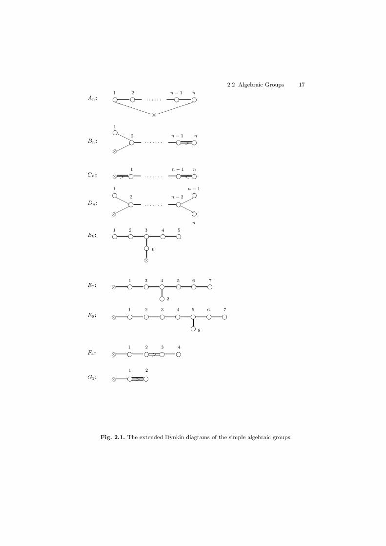
Up to isomorphism, the irreducible root systems correspond to the Dynkindiagrams, which are depicted in Figure 2.1. Each irreducible root system cor-responds to a simple algebraic group.
The numbered nodes (circles) in each diagram correspond to the simpleroots. Nodes corresponding to α and β are joined by < α, β >< β, α > bonds.There is an arrow pointing to the shorter of the two roots, if indeed the rootsare of different length. Notice that α and β can be joined by 0, 1, 2, or 3bonds, according to whether the order of σασβ ∈ W is 2, 3, 4, or 6.
For convenience and completeness, we have depicted the extended Dynkindiagrams. The extra node (circle with a “×”) corresponds to the highest root,which is also the highest weight of the adjoint representation.
It is easy to see that the information embodied in the Dynkin diagram isequivalent to the information embodied in the Cartan matrix:
< α, β >; α, β ∈ ∆.
2.2 Algebraic Groups 17
An: f f f f1 2 n− 1 n
⊗
. . . . . .
PPPPPP
Bn:
f
f f f
1
2 n− 1 n
⊗
HH
. . . . . . . >
Cn: ⊗ > f . . . . . . . f < f1 n− 1 n
Dn:
f
⊗
f f
f
f
1
2 n− 2
n − 1
n
HH . . . . . . .
HH
E6: f f f f f
f
⊗
1 2 3 4 5
6
E7: ⊗ f f f f f f
f
1 3 4 5 6 7
2
E8: ⊗ f f f f f f f
f
1 2 3 4 5 6 7
8
F4: ⊗ f f> f f1 2 3 4
G2: ⊗ f> f
1 2
Fig. 2.1. The extended Dynkin diagrams of the simple algebraic groups.
18 2 Background
The set of fundamental dominant weights λ1, . . . , λr is defined so that< λi, αj >= δi,j (Kronecker delta). The dominant weights are the Z-linearcombinations λ =
∑ciλi with each ci ≥ 0. Each weight is conjugate under W
to exactly one dominant weight. X(T ) has finite index in the set of weights.The Cartan matrix is the coefficient matrix for expressing the fundamentaldominant weights in terms of the simple roots. It can also be used to define apresentation of g via generators and relators.
2.2.3 Tits System and Bruhat Decomposition
Inspired by work of Chevalley [14], Tits [140] devised an efficient set of axiomsto describe the structure of the simple Chevalley groups and other simplealgebraic groups. The resulting theory, known as Tits systems or BN -pairs,is extremely efficient and far-reaching. It is essential in the development ofPutcha’s theory of monoids of Lie type.
Definition 2.42. (Tits System) Let G be a group generated by two sub-groups B and N , where T = B∩N is a normal subgroup of N . Let W = N/T ,and assume that S ⊆W is a set of elements of order two of W . By standardabuse of language, we write wB for w ∈ W . This is allowed since two repre-sentatives of w in N differ by an element of T , which is contained in B. Wesay that (G,B,N, S) is a Tits system if
a) for s ∈ S and w ∈W , sBw ⊂ BwB ∪BswB;b) for s ∈ S, sBs 6= B.
W is the Weyl group of the system, and |S| is the rank. A subgroup of Gconjugate to B is called a Borel subgroup of G.
Example 2.43. Let G be a reductive group, and B a Borel subgroup of Gcontaining the maximal torus T . Let N = NG(T ) and let S be the set ofsimple reflections corresponding to the base ∆ determined by T and B. Then(G,B,N, S) is a Tits system.
Theorem 2.44. Let (G,B,N, S) be a Tits system with Weyl group W . ForI ⊆ S let WI be the subgroup of W generated by I, and let PI = BWIB.
a) PI is a subgroup of G. In particular, PS = G.b) For v, w ∈ W , BvB = BwB if and only if v = w. In particular, sBw ⊂BswB if and only if sBw ∩BwB = φ.
The subgroups PI are called parabolic subgroups of G.
Definition 2.45. For w ∈ W , define the length of w relative to S as l(w) =mink|w = s1 . . . sk, si ∈ S.
Theorem 2.46. a) The only subgroups of G containing B are the PI .c) If PI is conjugate to PJ , then I = J .
2.2 Algebraic Groups 19
c) The following are equivalent.i) I = J .
ii) WI = WJ .iii) PI = PJ .
d) NG(P ) = P .
2.2.4 Representations
In this section, we describe the set of irreducible, rational representations ofa semisimple group G. The case of a reductive group is only slightly morecomplicated. As usual, we let T be a maximal torus of G and B = TU a Borelsubgoup of G containing T . Let B− = TU− be the opposite Borel subgroupcontaining T , and ∆ the the base of Φ determined by B. Let
ρ : G→ Gl(V )
be a rational representation of G. The weights of ρ are the characters of Tassociated with the eigenspaces of the action of T on V . Then V = ⊕Vλ,where Vλ = v ∈ V |ρ(t)(v) = λ(t)v, t ∈ T . By the Lie-Kolchin theorem,there is a one-dimensional subspace L of V such that ρ(B)(L) = L. Then Lis pointwise fixed by the unipotent radical of B. A nonzero vector v in L iscalled a highest weight vector.
Proposition 2.47. Let V be a nonzero, rational G-module, and let v be ahighest weight vector. Let V ′ be the submodule of V generated by v. Then theweights of V ′ are of the form λ −
∑cαα where α ∈ ∆ and the cα are non-
negative integers. Furthermore, dim(V ′λ)=1, and V ′ has a unique, maximal,
proper submodule M . Consequently, V ′/M is an irreducible G-module.
Proof. Since ρ(U)(v) = v, V ′ is spanned by ρ(U−)(v). But U− is a productof Uα’s with α ∈ −Φ+, and so applying U− to a vector of weight λ results in avector of the form v+u. But the components of u have weight λ−
∑cαα 6= λ,
where α ∈ −Φ+ and the cα are non negative. In particular, dim(V ′λ)=1.
Any proper submodule of V ′λ cannot contain v, and consequently it cannot
contain any vectors of weight λ. So take M to be the sum of all propersubmodules of V ′.
The weight λ is called the highest weight of V ′, and V ′ is called ahighest weight module. The above proposition shows that if we order theweights of V ′ as follows:
λ > µ
whenever λ − µ is a sum of positive roots, then λ is greater than all otherweights of V ′ for this partial ordering. It turns out that this weight λ isactually a dominant weight.
20 2 Background
Theorem 2.48. a) Let V be an irreducible, rational G-module. There is aunique B-stable one-dimensional subspace spanned by a highest weightvector v with dominant weight λ. All other weights of V are of the formλ− γ, where γ is a sum of positive roots.
b) If V ′ is another irreducible rational G-module with highest weight λ′, thenV and V ′ are isomorphic if and only if λ = λ′.
c) Let λ ∈ X(T ) be a dominant weight. Then there exists an irreducibleG-module Vλ of highest weight λ.
Proof. For a), we already have everything but the uniquness. But there cannotbe two different, highest weights. For b), if V and V ′ are two irreducible G-modules with highest weight λ, let v ∈ V and v′ ∈ V ′ be the respectivehighest weight vectors. It is easy to construct a highest weight module V ′′
inside V ⊕V ′ that projects onto both V and V ′. But it has a unique maximalsubmodule, M ⊂ V ′′. Then both V and V ′ are isomorphic to V ′′/M .
To prove c), define
H0(λ) = f ∈ K[G]|f(xy) = λ(x)f(y) for x ∈ B−, y ∈ G.
One checks that H0(λ) is a subspace of K[G] stable under right translation.It is possible to find a function f ∈ H0(λ) such that f(xy) = λ(y)f(x) for allx ∈ G and y ∈ B. Here, we may think of λ as a character on B by declaringλ(u) = 1 for u ∈ U . It turns out that the submodule of H0(λ) generatedby this f is the sought after irreducible representation. In characteristic zero,H0(λ) is actually irreducible.
Remark 2.49. (Borel-Weil-Bott Theory) The entity H0(λ) in the proof ofpart c) above can be interpreted geometrically. If λ is interpreted as above, asa character λ : B → K∗, we can define a line bundle on G/B as follows. LetB act on G ×K∗ by the rule b ∗ (g, t) = (gb−1, λ(b)t). Let L(λ) = [g, t]|g ∈G, t ∈ T be the quotient space of this action. We then have a canonicalprojection π : L(λ) → G/B defined by setting π([g, t]) = gB. Then π is aprincipal Gm-bundle over G/B. We let L(λ) be the sheaf on G/B associatedwith π. Notice that λ is not required to be dominant for this construction.The Borel-Weil Theorem states that:
a) H0(λ) is the space of sheaf-theoretic global sections of L(λ).b) H0(λ) is nonzero if and only if λ is dominant; and irreducible if char(K)=0.c) The correspondence λ → L(λ) determines a one-to-one homomophismBW : X(T )→ Pic(G/B). The image has finite index, equal to the orderof the fundamental group of G.
In characteristic zero, a refinement of the above results leads to a decompo-sition of K[G] as a sum of G×G-modules. Indeed, the action (G×G)×G→ G,defined by ((g, h), x) → gxh−1, defines a rational action of G × G on K[G].The resulting decomposition of K[G] into isotypic components leads to thefollowing description of K[G]:
2.2 Algebraic Groups 21
K[G] =⊕
λ∈X(T )+
H0(λ∗)⊗H0(λ).
The summands H0(λ∗)⊗H0(λ) are the blocks of K[G] in the sense of Green[33]. Notice also that K[G] has simple G×G-spectrum. This is in fact oneof the ways to define an affine spherical variety. See [76].
2.2.5 The Class Group of a Reductive Group
Let G be a connected, reductive group with coordinate algebra K[G]. In thissection we calculate the class group of G in terms of certain extremal functionson G (using Proposition 2.19 and the Bruhat-Tits decomposition of G). Manyof our results are contained explicitly or implicitly in [42], [75] and [137].
Let B and B− ⊆ G be opposite Borel subgroups of G. Let
T = B ∩B−.
Then there is a big cell
BB− ⊆ G.
BB− is open and dense in G, and is isomorphic to Km × (K∗)n as varieties.In particular, Cl(BB−) = 0. On the other hand,
G\BB− = ∪α∈∆BsαB−,
where ∆ is the set of simple roots of T relative to B. Write
Dα = BsαB−.
We sometimes write Dα(G) if there is possibility of confusion. By part c) ofProposition 2.19, Cl(G) is generated by Dα | α ∈ ∆ . If f ∈ K[G] and
Z(f) ⊆ ∪α∈∆Dα,
it follows easily that
BfB− = K∗f.
Definition 2.50. Let L(G) = f ∈ K[G] | V (f) ⊆ ∪Dα, f(1) = 1 .
We refer to L(G) as the augmented cone of G (although, strictly speak-ing, L(G) is the set of lattice points of such a cone).
Define
c : L(G)→ Div(G)
by
22 2 Background
c(f) =∑
α∈∆
να(f)Dα
where να is the valuation on K[G] associated with the prime divisor Dα ⊆ Gof G. Notice that c will not be injective unless G is a semisimple group.
Let
Div0(G) = ⊕α∈∆ZDα ⊆ Div(G).
Proposition 2.51. Cl(G) = Div0(G)/ < c(L(G) >, where < c(L(G)) > isthe subgroup of Div0(G) generated by c(L(G)). In particular, Cl(G) = 0 ifand only if the ideal of each Dα is principal.
Proof. By part c) of Proposition 2.19, Cl(G) is generated by Dα, while theprincipal divisors in Div0(G) are exactly the ones comming from L(G).
Proposition 2.52. There is a canonical one-to-one correspondence betweenL(G) and the set X(T )+ of dominant weights of irreducible representationsof G.
Proof. By Theorem 31.4 of [40], if λ ∈ X(T )+ there is a function cλ ∈ L(G)such that the right G-submodule Vλ of
H0(λ) = f ∈ K[G] | f(xy) = λ(x)f(y) for all x ∈ B−, y ∈ G
generated by cλ, is irreducible. It then follows from part b) of Theorem 2.48that this Vλ is unique.
Conversely, any c ∈ L(G) yields an irreducible representation V of G byconsidering the submodule ofK[G] generated by this c under right translation.By part a) of Theorem 2.48, V = Vλ for some λ ∈ X(T )+.
The coefficients να(f) in the formula c(f) =∑
α∈∆ να(f)Dα have thefollowing interpretation for a semisimple group G. Let
α∨ =2α
(α, α)
be the coroot associated with α ∈ ∆. Then, by Theorem 5.3 of [42],
να(f) = (α∨, λ) =< α, λ >
where λ corresponds to f via Proposition 2.52. In particular, if λ = λα isfundamental and dominant, then να(λβ) equals one if α = β and zero ifα 6= β.
Proposition 2.53. Let G be connected and reductive, and let G′ = (G,G).Then
2.2 Algebraic Groups 23
a) Cl(G) = Cl(G′)b) In particular, the following are equivalent:
i) Cl(G) = 0.ii) Cl(G′) = 0.
Proof. Let Z be the connected center of G. The multiplication morphismm : G′ × Z → G is a central isogeny, as in §2 of [42]. Hence, by Proposition2.6 of [42], there is an exact sequence
0→ X(G)→ X(G′ × Z)→ X(ker(m))→ Cl(G)→ Cl(G′ × Z)→ 0.
But X(G) = X(G/G′) = X(Z/(Z ∩G′)) and X(G′ × Z) = X(Z). HenceX(G′ × Z)→ X(ker(m)) is surjective, since ker(m) = Z ∩G′.
Proposition 2.54. Let G be a connected reductive group. Then there existsa connected reductive group G1, with Cl(G1) = 0, and a finite dominantmorphism π : G1 → G with central kernel.
Proof. By Proposition 1 of [75] (reproved in Corollary 3.3 of [42]), this is true
for G′ = (G,G), which is semisimple. Say f : G′ → G′ is the universal coverof G′. Let Z be the connected center of G. Then the desired morphism isg : G′ × Z → G, defined by g(x, z) = f(x)z.
Now let L ⊆ G be a Levi factor of G. Then there exist opposite parabolicsubgroups P, P− of G such that L = P ∩ P−. However,
PP− ∼= U × L× U−,
where U = Ru(P ) and U− = Ru(P−). Since U and U− are affine spaces,
Cl(L) = Cl(PP−).We conclude this section with the following corollary.
Corollary 2.55. There exists a surjective morphism Cl(G)→ Cl(L). In par-ticular, if Cl(G) = 0 then Cl(L) = 0
Proof. PP− is open in G. Hence Cl(G) → Cl(PP−) is surjective from parta) of Proposition 2.19.
2.2.6 Actions, Orbits, Invariants and Quotients
Let G be a reductive group, and let X be an irreducible variety. We assumethat X is affine unless otherwise stated. An action
µ : G×X → X
of G on X is a morphism of algebraic varieties such that:
24 2 Background
a) for all g, h ∈ G and x ∈ X , µ(g, µ(h, x)) = µ(gh, x),b) for all x ∈ X , µ(1, x) = x.
We denote µ(g, x) by gx. The orbit of x ∈ X is Gx = y ∈ X | y =gx for some g ∈ G, x ∈ X. The isotropy subgroup of x ∈ X is Gx =g ∈ G | gx = x. An orbit Gx ∈ X is dense if it is a dense subset of X inthe Zariski topology. Any dense orbit is actually an open subset. The theoryof algebraic monoids provides us with many important examples where someaction G×X → X has a dense orbit.
An orbit Gx ∈ X is closed if it is a closed subset of X in the Zariskitopology. Any orbit of minimal dimension is closed.
The action µ induces a linear action ρ of G on K[X ] as follows. For g ∈ Gand f ∈ K[X ] define ρg(f) ∈ K[X ] by ρg(f)(x) = f(g−1x) for all x ∈ X .ρ is rational in the sense that K[X ] is the union of its finite dimensional,G-stable subspaces. The ring of invariants K[X ]G of µ (or ρ) is defined asfollows:
K[X ]G = f ∈ K[X ] | ρg(f) = f for all g ∈ G.
The following result summarizes some of the fundamental theorems ofGeometric Invariant Theory. The reader should consult [62, 65, 134] foran appreciation of the scope and significance of this theory.
Theorem 2.56. Let µ : G × X → X be an action of the reductive group Gon the affine variety X.
a) K[X ]G is a finitely generated K-algebra.b) If we define the quotient X/G to be the affine variety defined by K[X ]G,
then the canonical morphism π : X → X/G identifies X/G with the set ofclosed orbits of G on X. In fact, the closure of any orbit Gx in X containsexactly one closed G-orbit.
Notice that this notion of quotient is not usually an orbit space in the usualsense. But it has some categorical properties that are normally expected ofany orbit space.
Example 2.57. Let PGln(K)×Mn(K)→Mn(K) be the action defined by
(g,A)→ gAg−1.
Then the quotient of this action can be identified as follows:ForA ∈Mn(K), let det(tI−A) = tn−σ1(A)tn−1+· · ·+σn−1(A)t+(−1)nσn(A)be the characteristic polynomial of A. Then define
Ad : Mn(K)→ Kn
by Ad(A) = (σ1(A), . . . , σn(A)). This is our quotient in the sense of the abovetheorem. It is well known that the closure of the conjugacy class of A containsthe semisimple part As of A. Furthermore, two semisimple endomorphismsare conjugate if and only if they have the same characteristic polynomial.
2.2 Algebraic Groups 25
The following result is originally due to V. L. Popov [74].
Proposition 2.58. Let X be a normal, irreducible, affine variety with trivialdivisor class group. Assume the connected, semisimple, algebraic group G actson X. Let X/G be the geometric invariant theory quotient of this action (as inTheorem 2.56). Then X/G is also a normal variety with trivial divisor classgroup.
Proof. We let A = K[X ], so that K[X/G] = K[X ]G. We denote the action ofG on elements a ∈ A by g(a). Let a ∈ AG be a non-unit. Then a ∈ A is alsoa non-unit. Write a = p1p2 . . . pm, where pi ∈ A is prime. Now for g ∈ G weobtain g(a) = g(p1) . . . g(pm). Since G is connected, the action stabilizes eachirreducible component of Z(a). Thus for each i, g(pi) = αi(g)pi, for someunit αi : G → K∗ with αi(1) = 1. But αi must be constant since the unitgroup of K[G] is K∗. Thus pi ⊆ AG. These pi are easily seen to be primein AG. Thus AG is a unique factorization domain.
2.2.7 Cellular Decompositions of Algebraic Varieties
Some of the well established ways to study the “topology” of an algebraicvariety is the use of comparison theorems or base change theorems, alongwith results that tell us how to proceed when a variety can be broken upinto manageable peices. Roughly speaking, a comparison theorem states thatif an algebraic variety X is considered as a topological space Xtop then thecohomology of X can be understood or calculated in terms of a more conve-nient cohomology theory. One of the most well known comparison theoremsof this type states that, if H∗(X,Ql) is the l-adic cohomology of the smooth,projective variety X , then
H∗(X,Ql)⊗QlC ∼= H∗(X,C).
A base change theorem usually concerns the situation when a variety Xis subjected to some convenient base extension X → X. A lot of informationabout l-adic cohomology of X can be calculated in terms of the Weil zetafunction ofX. This method of counting the points of the appropriate reductionmod p is particularly interesting in the theory of algebraic monoids. We areoften interested in counting the elements of certain finite monoidsM(Fqn) overthe finite field Fqn . Letting n→∞ yields an interesting enumerative theory, aswell as useful topological information about certain related algebraic varieties.
There is another method that applies to varieties that can be broken upinto well-behaved peices, or cells. The most commonly studied cellular decom-positions in algebraic geometry are those of Bialynicki-Birula [4]. If S = K∗
acts on a smooth complete variety X with finite fixed point set F ⊆ X , thenX =
⊔α∈F Xα where Xα = x ∈ X | lim
t→0tx = α. Furthermore, Xα is iso-
morphic to an affine space. We refer to Xα as a BB-cell. If further, a reductivegroup G acts on X extending the action of S, we may assume (replacing S if
26 2 Background
necessary) that each Xα is stable under the action of some Borel subgroup Bof G with S ⊆ B. In case X is a complete homogeneous space for G, each cellXα turns out to consist of exactly one B-orbit.
But there are yet other types of cellular decompositions that do not arisefrom the method of [4] (as we shall see in Theorem 10.15), and these can alsowork out well homologically. In particular, let X be an irreducible algebraicvariety, and assume that X is a disjoint union
X =⊔
i
Ci
of cells, where each cell Ci is isomorphic to the affine space Kni . Assumefurther that ∪ni≤mCi is closed in X for each m > 0.
Theorem 2.59. The natural map
cX : A∗(X)→ H∗(X,Z)
from the Chow ring of X to cellular homology, is an isomorphism. Further-more, Ci | ni = m is a Z-basis for Am(X).
Proof. See Fulton [30] Example 1.9.1 and Example 19.1.11.
2.3 Semigroups
The purpose of this section is to assemble some of the basic ideas from semi-group theory that are particularly relevant to the theory of algebraic monoids.In each situation, we try to illustrate the material with relevant examples fromlinear algebra.
2.3.1 Basic Semigroup Theory
A set S together with an associative operation m : S × S → S is calleda semigroup. If S has an element 1 ∈ S such that 1s = s1 = s for alls ∈ S, then S is called a monoid. If S is a semigroup, we define S1 = Sif S is a monoid, and S1 = S ∪ 1 with the obvious multiplication, if Sis not a monoid. In either case S1 is a monoid. If X ⊆ S then E(X) =e ∈ X |e2 = e is the set of idempotents of X . If S, T are semigroups,then a map ψ : S → T is a homomorphism if ψ(xy) = ψ(x)ψ(y) for allx, y ∈ S. The equivalence relation on S induced by a homomorphism is calleda congruence. A subsemigroup of S which is a group is called a subgroup ofS. Notice that the identity element of a subgroup of S could be any idempotentof S. If e ∈ S is an idempotent, then the unit group of eSe is a maximalsubgroup of S. All maximal subgroups of S are obtained this way. An idealof S is a nonempty subset J of S such that if x ∈ J then S1xS1 ⊆ J . There
2.3 Semigroups 27
is also the notion of one-sided ideal. If S has a minimum ideal K, it is calledthe kernel of S. Any finite semigroup has a kernel.
An element a ∈ S is regular if axa = a for some x ∈ S. S is regular ifeach of its elements is regular. Let M be a monoid with unit group G. Wesay that M is unit regular if, for each a ∈ M , there is a unit g ∈ G suchthat a = aga. Equivalently, M = GE(M) = E(M)G. The monoid Mn(K) ofn×n matrices is unit regular, and the semigroup S of singular n×n matricesis regular.
Let S be a semigroup, and let M = S1. It is useful to introduceGreen′s relations [32].
Definition 2.60. Let a, b ∈M .
a) aRb if aM = bM .b) aLb if Ma = Mb.c) aJb if MaM = MbM .d) aHb if aRb and aLb.e) aDb if aRc and cLb for some c ∈M .
We denote by Hx (or H if no confusion is possible) the H-class of x: andsimilarily for R, L and J.
Example 2.61. Let M = Mn(K). aLb if and only a and b are row equiva-lent. aRb if and only if a and b are column equivalent. aJb if and only ifrank(a)=rank(b). In this example J = D.
Remark 2.62. Let S be a semigroup.
a) If a ∈ S then a lies in a subgroup of S if and only if aHe for someidempotent e ∈ S.
b) If a ∈ S, e ∈ E(S), aRe and H is the H-class of e, then Ha is the H-classof a.
c) For e, f ∈ E(S), eRf if and only if ef = f and fe = e.d) Let a ∈ S be a regular element. Then a = axa for some x ∈ S. Thene = ax, f = xa ∈ E(S), and eRaLf . Thus a is regular if and only if eRafor some e ∈ E(S) if and only if aLf for some f ∈ E(S).
2.3.2 Strongly π-regular Semigroups
We begin this section with a definition.
Definition 2.63. Let S be a semigroup. We say that S is strongly π-regular(sπr) if for any x ∈ S, xn ∈ He for some e ∈ E(S) and some n > 0.
Remark 2.64. a) sπr is the main notion that best captures the semigrouptheoretic essence of many linear semigroups. Indeed, if S = Mn(K), thenany x ∈ S can be written uniquely as x = r + n, where n is nilpotent,rank(xm)=rank(x) for any m > 0, and rn = nr = 0 (Fitting decompo-sition). Then xm ∈ He where e is the unique idempotent of S with thesame rank as r, such that er = re = r.
28 2 Background
b) More generally, let S be an sπr subsemigroup of the semigroup T (forexample T = Mn(K)) with a ∈ S and e ∈ E(T ). If aHe in T , then e ∈ Sand aHe in S.
c) Any finite semigroup is sπr.
The following elementary result is taken from [82]. We include the prooffor convenience. This should indicate the usefulness of the sπr condition.
Theorem 2.65. Let S be an sπr semigroup, a, b, c ∈ S. Then
a) aJab implies aRab, and aJba implies aLba.b) abJbJbc implies bJabc.c) If e ∈ E(S), J is the J-class of e and H is the H-class of e, then J∩eSe =H.
d) J = D on S.e) If aJa2 then the H-class of a is a group.f) aJabJb if and only if aLeRb for some e ∈ E(S).g) Any regular subsemigroup of S is an sπr semigroup.
Proof. For a) suppose that aJab. Then xaby = a for some x, y ∈ S1. Thenxia(by)j = a, for all i, j > 0. But there exists j > 0 such that (by)jHe forsome e ∈ E(S). Then a = ae ∈ a(by)jS ⊆ abS. Hence aRab. For b) wefirst get abLb from a). Then abcLbcJb. For c) let a ∈ eSe ∩ J . Then by a),eRea = a = eaLe. Then eHa. For d), let a, b ∈ S be such that aJb. Thenthere exist x, y ∈ S such that xay = b. So aJxaJxay = b. Then again by a),aLxaRb. Thus xDy. For e), let H denote the H-class of a. From a), we seethat aHa2. Then a2x = a for some x ∈ S1. Then ai+1xi = a for all i > 0.Thus aiRa for all i > 0. By a) again, ai ∈ H for all i > 0. But there existj > 0 and e ∈ E(S) such that ajHe. But then e ∈ H and so H is a group.For f), suppose that aJabJb. Then by a), aRabLb. Hence there exist x, y ∈ S1
such that abx = a and yab = b. Then ya = yabx = bx. Hence aya = a andbxb = b. Thus ya ∈ E(S) and aLya = bxRb. Conversely, assume that thereexists e ∈ E(S) such that aLeRb. Thus xa = by = e for some x, y ∈ S.Hence ab|xaby = e|a|ab. Thus aJab. For g), Let a ∈ S′. There exists i > 0and e ∈ E(S) such that b = aiHe in S. But there exists x ∈ S′ such thatb2xb2 = b2. Then bxb = e, and so e ∈ E(S′) and bHe in S′.
Definition 2.66. Let S be an sπr semigroup. A J-class J of S is regular ifE(J) 6= 0. Equivalently, every element of J is regular. Let U(S) denote thepartially ordered set of all regular J-classes of S. Let J ∈ U(S), and defineJ0 = J ∪ 0, with multiplication
xy =
0 , if x = 0, y = 0 or xy /∈ Jxy , if xy ∈ J .
Definition 2.67. a) A completely simple semigroup is an sπr semigroupwith no ideals other than S.
2.3 Semigroups 29
b) A completely 0-simple semigroup is an sπr semigroup with no ideals otherthan 0 and S.
Remark 2.68. a) Definition 2.67 is not the standard definition of simple andcompletely simple semigroups. However, by a theorem of Munn [63], ourdefinitions are equivalent to the standard ones.
b) Let S be an sπr semigroup, J ∈ U(S). If a, b ∈ J , then there exist s, t, x ∈S1 such that sat = b and axa = a. Then b = (sax)a(xat) ∈ JaJ . Thus J0
is completely 0-simple semigroup.c) Let S be sπr, J ∈ U(S). If E(J)2 ⊆ J , then by Theorem 2.65b) J2 = J ,
and hence J is completely simple.d) A completely 0-simple semigroup has two J-classes, while a completely
simple semigroup has one J-class.
It turns out that there is a very satisfying structure theorem for completelysimple and completely 0-simple semigroups.
Definition 2.69. Let G be a group and let Γ,Λ be non-empty sets.
a) Let P : Λ × Γ → G be any map of sets. Define S = Γ × G × Λ, withmultiplication
(i, g, j)(k, h, l) = (i, gP (j, k)h, l).
One checks that S is a completely simple semigroup.b) Let P : Λ × Γ → G ∪ 0 be any map of sets such that for all i ∈ Γ
there exists j ∈ Λ with P (j, i) 6= 0. Define S = (Γ × G × Λ) ∪ 0 withmultiplication
(i, g, j)(k, h, l) =
0 , if P (j, k) = 0(i, gP (j, k)h, l) , if P (j, k) 6= 0 .
One checks that S is a completely 0-simple semigroup.
In case a), S is called a Rees matrix semigroup without zero over G withsandwich matrix P . In case b) S is called a Rees matrix semigroup with zeroover G with sandwich matrix P .
The following theorem is due to D. Rees [15].
Theorem 2.70. a) Any completely simple semigroup is isomorphic to a Reesmatrix semigroup without zero.
b) Any completely 0-simple semigroup is isomorphic to a Rees matrix semi-group with zero.
Proof. We sketch the proof of b). Part a) follows from this, since we can con-struct a completely 0-simple semigroup from a completely simple semigroupby adjoining a superfluous zero element.
So let S be completely 0-simple semigroup. Thus S = J∪0, where J ⊆ Sis a regular J-class of S. Choose e ∈ E(S), and let H,L,R be the H-class,L-class, R-class of e, respectively. Define
30 2 Background
Γ = L/R = L/H, Λ = R/L = R/H.
For λ ∈ Λ choose rλ ∈ λ, and for γ ∈ Γ choose lγ ∈ γ. Define P : Λ × Γ → Sby
P (λ, γ) = rλlγ .
By part a) of Theorem 2.65 we see that, if rλlγ 6= 0, then rλlγ ∈ H . Thuswe have a map P : Λ × Γ → H ∪ 0. One can check, as in Theorem 1.9of [82], that P is a sandwich matrix, and that S is isomorphic to the Reesmatrix semigroup S′ = (Γ ×H × Λ) ∪ 0 with sandwich matrix P . In fact,an isomorphism
ψ : S′ → S
is given by ψ(0) = 0 and ψ(γ, h, λ) = rλhlγ . One must check that ψ is welldefined and bijective.
2.3.3 Special Types of Semigroups
In this section we introduce some of the different types of semigroups thatshow up in the theory of algebraic semigroups. Certainly we are not intendingto be encyclopedic on this point.
Definition 2.71. A semilattice is a commutative semigroup consisting ofidempotents.
Definition 2.72. a) Let S be a semigroup, and assume that S = tα∈ΩSα ispartitioned into a disjoint union of subsemigroups. Then we say that S isa semilattice of the Sα if, for all α, β ∈ Ω, there exists δ ∈ Ω such thatSαSβ ∪ SβSα ⊆ Sδ.
b) A semigroup S is completely regular if it is the union of its subgroups.c) A semigroup S is a semilattice of groups if, in addition to being completely
regular, each of its J-classes is in fact an H-class.
It turns out that the semigroup S is completely regular if and only if it is asemilattice of completely simple semigroups.
Example 2.73. a) Let S be the set of diagonal n × n matrices. Then S is asemilattice of groups.
b) Let S be the set of upper-triangular n × n matrices A = (ai,j), of rankn− 1, such that an,n = 0. Then S is completely simple.
Let S be a semigroup and a, b ∈ S. Recall that a divides b, written a|b, ifxay = b for some x, y ∈ S1.
Definition 2.74. A semigroup S is archimedean if, for all a, b ∈ S, a|bi forsome i > 0.
2.4 Exercises 31
Remark 2.75. a) A semigroup S is a semilattice of archimedean semigroupsif and only if, for all a, b ∈ S, a|b implies a2|bi for some i > 0. For sucha semigroup, define x ∼ y in S if x|yi for some i > 0 and y|xj for somej > 0. Then ∼ is the desired semilattice decomposition. See Theorem 1.15of [82] for more details.
b) Tn(K), the monoid of upper-triangular matrices, is a semilattice of archimedeansemigroups. The corresponding semilattice in this case is canonically iso-morphic to the semilattice of diagonal idempotents of Tn(K).
c) Any commutative semigroup is a semilattice of archimedean semigroups.
Definition 2.76. A semigroup S is called an inverse semigroup if for eachx ∈ S there exists a unique x∗ ∈ S such that
xx∗x = x, and x∗xx∗ = x∗
Example 2.77. Let N be the set of n× n matrices with at most one nonzeroentry in each row or column. Then N is an inverse semigroup.
Certain finite inverse semigroups will play the role of the Weyl group inthe theory of algebraic monoids. See Proposition 8.1 and Theorem 8.8.
2.4 Exercises
2.4.1 Abstract Semigroups
1. Check that the definitions of S in 2.69 in fact yield completely (0-)simplesemigroups.
2. Let S = Γ × G × Λ be a completeley simple semigroup with sandwichmatrix P : Λ×Γ → G. Identify the Green’s relations R,L and H on S interms of P .
3. Prove that Tn(K) is a semilattice of archimedean semigroups.4. Prove that Mn(K) is sπr.5. Prove that S = x ∈ Mn(K) | rank(x) ≤ 1 is a completely 0-simple
semigroup.

3
Algebraic Monoids
The theory of algebraic monoids is built on the theory of algebraic groups, thetheory of torus embeddings, and related semigroup constructions. Indeed, ifM is an irreducible, algebraic monoid, then M = G where G is the algebraicgroup of units of M . So we hope the reader can acquire some familiarity withalgebraic groups, Lie algebras, Tits buildings and torus embeddings [7, 40,140, 31]. A brief summary of some of this essential background was assembledin the previous chapter.
In this chapter we acquaint the reader with some of the basic results aboutirreducible monoids. A significant number of these results amount to marryingthe semigroup concepts with the geometric concepts. Where appropriate, wesketch some proofs. Nearly everything in this section is discussed in moredetail in Putcha’s monograph [82]. We reproduce some of Putcha’s results forthe convenience of the reader.
The reader might wish to begin with a more concrete and combinato-rial approach, with many useful examples. In that case, he should consultSolomon’s survey [128]. On the other hand, he might wish to start from thepoint of view of linear semigroups, in which case he should consult Okninski’sbook [66].
3.1 Linear Algebraic Monoids
Definition 3.1. Let K be an algebraically closed field.
a) An linear algebraic monoid M is an affine, algebraic variety together withan associative morphism µ : M ×M →M and an identity element 1 ∈Mfor µ.
b) M is irreducible if it cannot be expressed as the union of two, proper,closed, non-empty subsets.
c) The irreducible components of M are the maximal, irreducible subsets ofM .
34 3 Algebraic Monoids
We often write “algebraic monoid” when we mean “linear algebraic monoid”.This abuse of language should not cause problems, since we are here concernedonly with linear monoids, and it is easily seen that these are all affine. Theproblem of characterizing affine algebraic monoids among algebraic monoidshas been discussed in [101, 121].
If M is an algebraic monoid, there is a unique, irreducible componentM0 ⊆ M such that 1 ∈ M0. Indeed, M0 = G0 where G0 is the identitycomponent of the unit group G of M . G is an algebraic group, open in M .Notice also that the monoid structure on an irreducible algebraic monoidis uniquely determined by the group structure of its unit group. This is sobecause the group is open and dense in the monoid. See Proposition 3.12below.
An algebraic monoid M may be identified by its bialgebra A = K[M ].
Definition 3.2. A bialgebra is a K-algebra A together with a coassociativemorphism 5 : A −→ A⊗K A and counit ε : A→ K.
One obtains an algebraic monoid M = M(A) from the bialgebra A asfollows. Define
M = HomK−alg(A,K).
The multiplication ∗ on M is defined via 5:
f ∗ g = (f ⊗K g) 5.
For example consider the bialgebra A = K[Tij | 1 ≤ i, j ≤ n] with
5 : A −→ A⊗K A defined by
5 (Tij) =∑
h
Tih ⊗ Thj , and
ε : A −→ K defined by
ε(Tij) =
1 , i = j0 , i 6= j
.
One easily checks that A is the coordinate ring ofMn(K) = HomK−alg(A,K).The bialgebra approach is useful technically in decomposing the coordinate
algebra into blocks. See § 9.4.
Definition 3.3. A morphism ϕ of algebraic monoids M and N is a morphismϕ : M → N of algebraic varieties such that ϕ(xy) = ϕ(x)ϕ(y) for x, y ∈ M ,and ϕ(1) = 1.
For an interesting example, consider ϕ : M2(K) −→M3(K) defined by
ϕ
(a bc d
)=
a2 ab b2
2ac ad+ bc 2bdc2 cd d2
.
3.1 Linear Algebraic Monoids 35
Definition 3.4. Let M be an algebraic monoid.
a) E(M) = e ∈M | e2 = e is the set of idempotents of M .b) M is regular if for each a ∈M there exists x ∈M such that axa = a.c) M is unit regular if M = GE(M).d) U(M) is the set of subsets of M of the form GeG, where e ∈ E(M). These
subsets are known as regular J-classes. This is not the usual definition,but is equivalent for irreducible algebraic monoids.
It turns out that any regular, irreducible monoid is unit regular. See [82].
Example 3.5. Let M = Mn(K). This is one of the motivating examples formuch of the important structure theory of reductive monoids. Notice thatMn(K) is regular.
Example 3.6. (Finite monoids) Let M be a finite monoid, and let A =Hom(M,K). Define 5 : A −→ A ⊗ A = Hom(M × M,K) by the rule5(f)(s, t) = f(st). It is easy to check that (A,5) is a bialgebra and that theassociated algebraic monoid is canonically isomorphic to M .
Example 3.7. (Semidirect products) Let M and N be algebraic monoidsand suppose that we have a morphism γ : M ×N −→ N of algebraic varietiessuch that
γ(s, t1t2) = γ(s, t1)γ(s, t2) for s ∈M, t1, t2 ∈ N
and
γ(s1s2, t) = γ(s1, t)γ(s2, t) for s1, s2 ∈M, t ∈ N .
Write ts for γ(s, t). Then M ×N is an algebraic monoid with (s1, t1)(s2, t2) =(s1s2, t
s21 t2).
Any algebraic monoidM is strongly π-regular, as in § 2.3.2. Precisely, if x ∈M then xn ∈ He, the unit group of eMe, for some e ∈ E(M). Furthermore,e ∈ xn | n > 0 . The integer n can be chosen independently of x ∈M . In anycase, there is always an abundance of idempotents. For example, if E(M) =1, then M = G. One can easily check this condition for M = Mn(K). Ingeneral, one can use the following theorem.
Theorem 3.8. Let M be an algebraic monoid. Then for some n > 0, thereexists a morphism ρ : M −→ Mn(K), of algebraic monoids, such that ρ is aclosed embedding of algebraic varieties.
The basic idea behind Theorem 3.8 is right translation of functions.Define
γ : M −→ End(K[M ])
by the rule γs(f)(t) = f(ts), where s, t ∈ M , and f ∈ K[M ]. Then γ isa morphism of monoids. To obtain the morphism ρ, one chooses a finite-dimensional subspace V ⊆ K[M ] such that
36 3 Algebraic Monoids
a) γs(V ) ⊆ V for all s ∈M .b) V generates K[M ] as a K-algebra.
It then turns out that ρ : M −→ End(V ), ρ(s)(v) = γs(v), satisfies theconclusion of Theorem 3.8.
Corollary 3.9. Let ϕ : M → N be a morphism of algebraic monoids. Ife ∈ E(N) ∩ ϕ(M), then there exists f ∈ E(M) such that ϕ(f) = e.
Proof. By Theorem 3.8 we can think of M as a submonoid of some End(V ).But then ϕ−1(e) is a closed subsemigroup of End(V ). By the comment justpreceding Theorem 3.8, any such semigroup has idempotents.
Let M be an algebraic monoid. Recall that an ideal I ⊆M is a nonemptysubset such that MIM ⊆ I.
Theorem 3.10. Let M be an irreducible monoid. If P ⊆ M is a prime ideal(so that M\P is multiplicatively closed) then P is closed in M . Furthermore,there exists a morphism χ : M → K of algebraic monoids such that P =χ−1(0).
Theorem 3.10 is proved in [101]. The strategy there is to first show that theresult is true for irreducible monoids Z with unit group a torus. The generalcase then follows once it is shown that P is determined by P ∩T . See Exercises8, 9, 10 and 11 of § 3.5.3 for an outline of this proof.
It follows from Theorem 3.10 that any quasi-affine, irreducible monoid isactually affine.
One should notice that the unit groups of irreducible algebraic monoidsare “big”. The next result records how this observation is reflected in Green’srelations (Definition 2.60).
Proposition 3.11. Let M be an irreducible algebraic monoid. Let a, b ∈ M ,e, f ∈ E(M) and G = G(M).
a) aRb if and only if aG = bG.b) aLb if and only if Ga = Gb.c) aJb if and only if GaG = GbG.
The main point behind the proofs of a), b) and c) is the following basicfact from algebraic group theory: if G×X → X is a regular action then anyorbit is open in its closure.
If M is an algebraic monoid, then J = D. Indeed, by Theorem 1.4 of [82],this is true for any sπr monoid.
Proposition 3.12. Let M be an algebraic monoid and let e ∈ E(M). ThenHe, the unit group of eMe, is an algebraic group, open in eMe.
Proof. This follows from Theorem 3.8 applied to eMe. Indeed, ρ(M) ∩G`n(K) = ρ(G(M)), which is closed in G`n(K) and open in ρ(M).
3.2 Normal Monoids 37
We end this section with a statement of the fundamental results aboutidempotents. See Corollary 6.4 and Corollary 6.8 of [82] for proofs.
Proposition 3.13. Let M be an irreducible algebraic monoid, and let e ∈E(M). Then
a) e ∈ T for some maximal torus T ⊆ G. So E(M) =⋃
g∈G
gE(T )g−1.
b) eJf if and only if g−1eg = f for some g ∈ G.c) eRf if and only if g−1eg = f = eg for some g ∈ G.d) eLf if and only if geg−1 = f = ge for some g ∈ G.
It is possible to characterize which irreducible algebraic groupsG can occurnon trivially as the unit group of some algebraic monoid.
Theorem 3.14. Let G be an irreducible algebraic group. Then the followingare equivalent.
a) There exists an irreducible, algebraic monoid M with unit group G suchthat G 6= M .
b) X(G) 6= 1.
See Execise 6 of 3.5.1 for an outline of the proof.
3.2 Normal Monoids
Unlike the case of algebraic groups, not every irreducible algebraic monoid isnormal as an algebraic variety. This is mainly a technical nuisance, since anyalgebraic monoid has a lot in commom with its normalization. On the otherhand, there are important advantages to normal monoids. This will becomeapparent in the classification problem. See Theorem 5.2.
Let X be an irreducible, algebraic variety. Recall that the normalizationη : X ′ → X of X is the unique finite, birational morphism η from an irre-ducible normal variety X ′ to X . If X is affine, the coordinate algebra of K[X ′]is the integral closure of K[X ] in its field of fractions.
Luckily we have the following result for the normalization of an algebraicmonoid. This was first recorded in [100].
Proposition 3.15. Let M be an irreducible, algebraic monoid with unit groupG. Let η : M ′ → M be the normalization of M . Then M ′ has the uniquestructure of an algebraic monoid such that η is a finite, birational morphismof algebraic monoids.
Proof. One must check that the multiplication morphism m : M ×M → Mextends to a morphismm′ : M ′×M ′ →M ′. This extension is possible becauseof the universal property of normalization.
38 3 Algebraic Monoids
Remark 3.16. If M is an irreducible, algebraic monoid with unit group G,and π : G′ → G is a finite dominant morphism, define M ′ so that K[M ′] isthe integral closure of K[M ] in K[G′]. Then M ′ is an irreducible algebraicmonoid with unit group G′. Furthermore, there is a unique (finite) morphismθ : M ′ →M such that θ|G′ = π.
Example 3.17. LetM = (x, y) | x2 = y3. ThenM is an irreducible, algebraicmonoid with unit group isomorphic to K∗, and pointwise multiplication. Here
K[M ] = K[X,Y ]/(X2 − Y 3),
which is not normal. The normalization of M is
η : K →M,
defined by η(t) = (t3, t2).
3.3 D-monoids
The closure of a maximal torus plays a special role in the theory of algebraicmonoids. For example, from Proposition 3.13, we see that any idempotent isin the closure of a maximal torus. This is good news because such monoidshave been much studied as torus embeddings. In this section we give ashort description of this class of monoids.
Example 3.18. Let H be a closed, connected subgroup of Dn(K)∗ ∼= K∗ ×· · · ×K∗. Let M = H, the Zariski closure of H in Dn(K), the set of diagonalmatrices. Then M is a semilattice of groups in the sense of Definition 2.72 c).Such monoids are called D-monoids. Furthermore, U(M) = [x] ∈ H | [x] =[y] if there exists g ∈ H such that y = gx. This is just another way of talkingabout affine torus embeddings. U(M) is isomorphic to the face lattice of arational polytope [31].
D-monoids are described axiomatically as follows.
Definition 3.19. A D-monoid is an irreducible, algebraic monoid M suchthat K[M ] is spanned over K by X(M) = χ ∈ K[M ] | 5 (χ) = χ ⊗ χ.X(M) is called the character monoid of M . Notice that we may regard X(M)as a subset of X(G).
It is easy to see that M is a D-monoid if and only if M is isomorphicto a closed submonoid of Dn(K) for some n > 0. Indeed, choose charactersχ1, . . . , χn ∈ X(M) that generate K[M ] as an algebra, and define
ψ : M → Dn(K)
by ψ(z) = (χ1(z), . . . , χn(z)).If G is a D-group and ρ : G → Dn(K) ⊆ Mn(K) is a rational represen-
tation of G, the set of weights of ρ is the set Φ = χ ∈ X(G) | ρ(g)(v) =χ(g)v for all g ∈ G and some nonzero v ∈ Kn.
3.3 D-monoids 39
Proposition 3.20. Let M be a D-monoid with unit group G. Let
ρ : G→ Dn(K)
be a representation of G with weights Φ ⊆ X(G). Then ρ extends to a repre-sentation ρ : M → Dn(K) if and only if Φ ⊆ X(M).
Proof. It is easy to check that ρ∗(K[Dn(K)]) ⊆ K[G] is the subalgebra gen-erated by Φ.
Remark 3.21. As we have already mentioned, if Z is a D-monoid with unitgroup T , then the set of T -orbits on Z is naturally the face lattice of a rationalpolytope P(Z). But each T -orbit H of Z contains exactly one idempotente = e(H). So the face lattice of P(Z) is in one-to-one correspondence withE(Z), the set of idempotents of Z. The order relation “e ≤ f , if ef = fe = e”on E(Z) corresponds to the lattice ordering on the face lattice of P(Z).
One can also identify the face lattice of P(Z) as the semilattice ofarchimedean components of the commutative monoid X(Z). See Remark 2.75c).
Many useful properties of rational polytopes transfer over to the semilat-tice E(Z). Recall that a ranked poset is a poset P with a rank functionr : P → N such that, if x covers y, then r(x) = r(y) + 1. This is anotherway of saying that all the maximal chains of P have the same length. Someauthors refer to a ranked poset as a graded poset.
Proposition 3.22. Let Z be a D-monoid of dimension n.
a) E(Z) is a ranked poset. The rank function here is r(e) = dim(Te).b) If f ∈ E(Z), let E1(f) = e ∈ E(Z) | r(e) = n− 1. Then
f = Πe∈E1(f)e.
Proof. The proof amounts to a translation of well known properties of poly-topes to the language of D-monoids.
It is of interest to know when a D-monoid Z is normal. Also it is of interestto identify the coordinate ring of the normalization (Proposition 3.15) of Z.
Proposition 3.23. Let Z be an irreducible D-monoid with unit group G andcoordinate ring the monoid algebra K[X(Z)]. Observe that X(Z) ⊆ X(G).The following are equivalent.
a) Z is normal.b) If χ ∈ X(G) and χm ∈ X(Z) for some m > 0, then χ ∈ X(Z).
Let S = χ ∈ X(G) | χm ∈ X(Z) for some m > 0. Then, if η : Z ′ → Z isthe normalization of Z, the coordinate ring of Z ′ is the semigroup algebra ofS.
We leave the proof to the reader.See Example 3.17 for a simple example. Notice that the normalization
morphism induces a bijection on idempotents.
40 3 Algebraic Monoids
3.4 Solvable Monoids
Definition 3.24. An irreducible monoid M is solvable if G(M) is a solvable,algebraic group.
Remark 3.25. By Theorem 17.6 of [40] and Theorem 3.8 above, any solvablemonoid M is isomorphic to a closed submonoid of Tn(K), the upper trian-gular monoid, for some n > 0. Using this fact one can construct a universalmorphism π : M → Z, to a D-monoid, such that π|T : T → Z is an isomor-phism for any maximal torus T ⊆ G = G(S). If M is irreducible and B ⊆ Gis a Borel subgroup, then B ⊆M is solvable. Furthermore BB ⊆ B. Thus by
a Theorem of Steinberg [134] M = GB. Similarly, M =⋃
g∈G
gBg−1.
The following result is due to Putcha; Corollary 6.32 of [82].
Theorem 3.26. Let M be an irreducible monoid with zero and unit group G.Then the following are equivalent:
a) G is solvable.b) M is a semilattice of archimedean semigroups.
We refer the reader to [82] for the proof. Notice however that, from Re-mark 3.25 above, it suffices to prove that Tn(K) is a semilattice of archimedeansemigroups. See Excercise 3 of 2.4.1. Putcha obtains other interesting char-acterizations of solvable monoids. See Theorem 6.35 of [82] for example.
3.5 Excercises
3.5.1 Linear Algebraic Groups
1. Let G be an algebraic group acting on a variety X . Suppose that Y ⊆ Xis closed and gY ⊆ Y for some g ∈ G. Prove that gY = Y . Hint: Y ⊇gY ⊇ g2Y . . . , yet each gsY is closed in Y .
2. Let U ⊆ G be a closed subsemigroup, where G is an algebraic group.a) Prove that 1 ∈ U .b) Prove that U is a subgroup of G.
3. Let G be a linear algebraic group and let x ∈ G. Write x = su = us,where u is unipotent and s is semisimple. Using Exercise 2 above, provethata) u, s ∈ xn|n ≥ 1b) For any x ∈Mn(k) there exists an idempotent in xn|n ≥ 1.
4. Let M be an irreducible, algebraic monoid with unit groupG, and supposethat ρ : G′ → G is a finite dominant morphism of algebraic groups. Provethat there exists an irreducible algebraic monoid M ′ with unit group G′,and a finite dominant morphism ψ : M ′ →M , such that ψ|G′ = ρ.
3.5 Excercises 41
5. Let G be a connected algebraic group with X(G) = 1. Suppose that Mis an irreducible, algebraic monoid with unit group G. Prove that M = G.
6. Let G be a connected algebraic group with X(G) 6= 1.a) Let T ⊆ G be a maximal torus and let 1 6= χ ∈ X(G) ⊆ X(T ) (by
restriction). For a finite subset S ⊆ X(T ), let < S >⊆ X(T ) denotethe submonoid generated by S. Prove that there exists n > 0 suchthat C =< S + nχ >⊆ X(T ) satisfies C ∩ −C = 0.
b) If ρ : G → Gl(V ) is a representation, show that ρ(T ) has a zeroelement (of its own) if and only if C =< φT (V ) >⊆ X(T ) satisfiesC ∩ −C = 0. Here, φT (V ) is the set of weights of T on V via ρ.
c) Using a), show that there exists a representation ρ : G→ Gl(V ) withfinite kernel such that the condition of b) is satisfied.
d) Using c) and Exercise 4 above, show that there exists an irreduciblealgebraic monoid M with 0 and unit group G.
7. Let M be irreducible and suppose that x, y ∈ T . Suppose that there existsg ∈ G(M) such that gxg−1 = y. Prove that there exists h ∈ NG(T ) suchthat hxh−1 = y
8. Suppose that G ⊆ Gl(V ) is a closed connected subgroup such that V isan irreducible module for G. Prove thata) G is reductive.b) dimZ(G) ≤ 1.
9. Let ρ : G → G′ be a finite dominant morphism of reductive alge-braic groups. Prove that ρ : U → U is bijective. Here, U = g ∈G | g is unipotent .
3.5.2 Linear Algebraic Semigroups
1. Let S be an algebraic semigroup and let I ⊆ S be a two-sided ideal suchthat S\I is multiplicatively closed. Prove that I is Zariski closed.
2. Let A be a positively graded, finitely generated k-algebra with A0 = k. LetM = End(A), the monoid of degree-preserving k-algebra endomorphisms.a) Prove that M is an algebraic monoid with 0.b) For e, f ∈ E(M), define e ∼ f if Image(e) ∼= Image(f) as graded
k-algebras. Prove that E(S)/ ∼ is a finite set.3. Let A be a k-algebra, and assume that we have a rational action ρ : k∗ →Aut(A). Prove that the following are equivalent.a) ρ extends to a rational action ρ : k→ End(A).b) A = ⊕n≥0An, where ρ(f)(t) = tnf , for all f ∈ An.
4. Let ψ : S → T be a morphism of algebraic semigroups, and suppose thate ∈ E(T ) ∩ ψ(S). Prove that ψ−1(e) contains an idempotent.
5. Let M be an algebraic monoid and let x ∈M . Suppose that x has a rightinverse y ∈M such that xy = 1. Prove that y is also a left inverse of x.
6. Let M be an irreducible algebraic monoid, and let ρ : M → End(V ) bean irreducible representation. Let e ∈ E(M). Prove that e(V ) ⊆ V is anirreducible representation of eMe.
42 3 Algebraic Monoids
7. Let k be a field, and let E ⊆ Mn(k) be an infinite set of idempotents ofrank r. Prove there exists e, f ∈ E, e 6= f , such that rank(ef)=rank(fe).
8. With E as in Exercise 7 above, but Zariski closed, let X = f ∈E|rk(fe) < r or rk(ef) < r. Prove that X is a closed, proper subsetof X .
9. Suppose that S ⊆ Mn(k) is a closed subsemigroup, and let e, f ∈ Mn(k)be such that rk(ef)=rk(fe)=rk(e)=rk(f). Show that eJf in S.
10. Let ∼ be the equivalence relation on E(S) generated by e ∼ f ifrk(ef)=rk(fe)=rk(e)=rk(f). Suppose that V ⊆ E(S) is an irreduciblecomponent, and S ⊆ Mn(k) as in Exercise 9. Prove that e ∼ f for alle, f ∈ V .
11. Using Exercies 7-10 prove that any connected component of E(S) consistsof J-related idempotents. See [111] for more details and some applicationsto rational homotopy theory. See also [99, 27] for some related applications.
3.5.3 Irreducible Algebraic Semigroups
1. Let S be an irreducible algebraic semigroup, and suppose that E(S) = S.Prove that S is a rectangular band (see [15]).
2. Let M be an irreducible algebraic monoid and let x ∈ M . Prove thatB ∈ B|x ∈ B is closed in B. Here, B is the projective variety of Borelsubgroups of G.
3. Let M be an irreducible monoid with solvable unit group G, and 0 ∈M .Prove that N = x ∈ M |xn = 0 for some n > 0 is a two-sided ideal ofM .
4. Let M be irreducible. For x ∈M , prove that the following are equivalent:a) x ∈ He, the H-class of some idempotent, and x is a semisimple element
in He.b) For any representation ρ : M → End(V ), ρ(x) is diagonalizable.
5. let M be an algebraic monoid with 0. Prove that the following are equiv-alent.a) M is connected in the Zariski topology.b) There exists a chain of idempotents 1 = e0 > e1 > · · · > en = 0 such
that ei ∈ Hei−1 , for each i = 1, 2, . . . , n.See [106].
6. Let M be an algebraic monoid with M = G. Prove that E(M) ⊆ G0.7. Let M be an irreducible algebraic monoid with 0, such that rk(G)=1.
In particular, G is solvable. Prove that every irreducible component ofN = x ∈M |xn = 0, for some n > 0 has codimension one in M .
8. Let M be an irreducible monoid with solvable unit group G, and letX(M) = Hom(M,k) be the monoid of characters of M . Let T ⊆ Gbe a maximal torus, and let Z = T . Prove that j∗ : X(M)→ X(Z) is anisomorphism, where j : Z → M is the inclusion. Conclude that, for anysuch M , there exists a D-monoid Z and a morphism π : M → Z such
3.5 Excercises 43
that π|T : T → Z is an isomorphism. Furthermore, π is universal for mapsfrom M to D-monoids. (See [101].)
9. Let M be solvable and irreducible with π : M → Z as in Exercise 8 above.An ideal of M is a subset I ⊆M such that MIM ⊆ I. We write I < M .a) Prove that the following are equivalent for I < M :
i) If xn ∈ I for some n > 0, then x ∈ I.ii) I = π−1(π(I)).Such ideals are called radical. Notice that any radical ideal of M isclosed.
b) Prove that there is one-to-one correspondence between radical idealsof M and ideals of Z. Notice that any ideal of Z is radical.
10. Let M be irreducible and suppose that I < M . Let X = B ⊆ M , whereB ⊆ G is a Borel subgroup. Let I(B) = I ∩ M . Suppose that I(B) isradical. Prove that I is closed in M . Conclude that any prime ideal of Mis closed. (An ideal I < M is prime if M\I is multiplicatively closed.)
11. Let M be irreducible, and suppose that P,Q < M are prime ideals suchthat P ∩ T = Q ∩ T . Prove that P = Q. Hint: use exercise 9 above.
12. Let M be an irreducible algebraic monoid, and suppose B ⊆ M is theclosure of a Borel subgroup of G. Suppose x ∈ B is the zero element ofB. Prove that x is the zero element of M .
13. Let M be an irreducible monoid and let η : M ′ →M be the normalizationof M . Prove that M has the unique structure of an algebraic monoid sothat η is a morphism of algebraic monoids.
14. Let M be irreducible. Suppose that V ⊆ M\G is closed, and has codi-mension one in M . Prove that V < M .
15. Let M be reductive, and let e ∈ M . Let P = g ∈ G|ge = ege. Provethat Ru(P )e = e (See [95]).
16. a) Let G be a connected, commutative algebraic group in characteristiczero. Prove that, for all n > 0, ψn : G→ G, ψn(x) = xn, is a surjectivemorphism of algebraic groups.
b) Let M be an irreducible, commutative monoid in characteristic zero.i) Prove that E(M) is finite.ii) Prove that
⋃e∈E(M)He is a submonoid of M .

4
Regularity Conditions
The major question underlying much of the structure theory of algebraicmonoids is the role of idempotents. Namely, “How is a monoid put togetherfrom its unit group and its set of idempotents?”
To identify monoids with interesting structural properties, one needs toassume some kind of regularity condition either directly or indirectly. A reg-ularity condition is some structural assumption that allows the idempotentsto play a decisive role.
4.1 Reductive Monoids
Definition 4.1. Let M be an irreducible algebraic monoid.
a) M is reductive if G(M) = g ∈M | g−1 ∈M is a reductive group.b) M is regular if M = G(M)E(M) = E(M)G(M)
The next result is due to Putcha and the author. We sketch the proof fromTheorems 7.3 of [82].
Theorem 4.2. Let M be an irreducible monoid with unit group G and zeroelement 0 ∈M . The following are equivalent.
a) G is reductive.b) M is regular.c) M has no non-zero nilpotent ideals.
Proof. Assume a), and let S ⊆M be an irreducible component of M\G. Onethen checks that S = MeM for some e ∈ E(S). But GeMeG is closed inM since B1eMeB2 = eMe for appropriate Borel subgroups B1 and B2 of G.On the other hand, GeMeG is dense in S = MeM . Thus S = GeMeG. Butinductively, eMe is regular, since G(eMe) is an image of the reductive groupCG(e). Thus, S consists of regular elements, and so M is regular.
46 4 Regularity Conditions
If M is regular and a ∈ M then, by definition, ag = e = e2 for somee ∈ E(M) and g ∈ G. So there can be no non-zero nilpotent ideals.
Assume that G is not reductive, and find a representation M ⊆ End(V )of M as a closed submonoid. Assume that V1 ⊆ V2 ⊆ · · · ⊆ Vi ⊆ · · · ⊆ Vn = Vis an M -stable filtration such that each Vi/Vi−1 is irreducible over M . Let
M ′ ⊆
n∏
i=1
End (Vi/Vi−1) be the semisimplification of M (as in [102]) and
notice that we have an induced map
θ : M −→M ′ .
Now ker(θ|G) = Ru(G), and so θ−1(0′) is a nilpotent ideal of M of dimensiongreater than or equal to dim(Ru(G)).
But what happens ifM does not have a zero element? The following answeris due to Putcha (see Theorem 7.4 of [82]). For e ∈ E(M), let
Ge = g ∈ G | ge = eg = e .
Recall that a monoid M is completely regular if M =⊔e∈E(M)He. For
example, any commutative, regular monoid is completely regular.
Theorem 4.3. Suppose that M is irreducible with unit group G and minimalidempotent e ∈ E(M). Then the following are equivalent.
a) M is regular.b) R(G) is completely regular.c) Ge := g ∈ G | ge = eg = e0 is reductive.
Proof. If M is regular and a ∈ R(G) then axa = a for some x ∈ M . ButM = ∪B where B is a Borel subgroup of G. Hence x ∈ B for some B. Butalso, a ∈ R(G) ⊆ B. Thus a ∈ B is a regular element of B. But then aHe forsome e ∈ E(B) by 3.19 and 4.12 of [82]. Consequently e ∈ R(G) by an easycalculation.
If R(G) is completely regular, first notice that e ∈ R(G), since all minimalidempotents are conjugate. One then checks that R(Ge) ⊆ R(G)e, while thelatter group is a torus. Thus Ge is reductive.
If Ge is reductive then, by Theorem 4.2, Me := Ge is regular. But from6.13 of [82] M = GMeG, since e ∈ K = ker(M), the minimal, (regular)J-class of M .
Further results have been obtained by Huang in [39]. In particular, heobtains the following characterization of reductive monoids.
Theorem 4.4. Let M be an irreducible algebraic monoid. Then the followingare equivalent.
a) M is reductive.b) M is regular and the semigroup kernel of M is a reductive group.
A similar result was obtained by Rittatore in [121].
4.2 Semigroup Structure of Reductive Monoids 47
4.2 Semigroup Structure of Reductive Monoids
Reductive monoids enjoy the richest and most interesting structural proper-ties. Let M be reductive with unit group G and Borel subgroup B ⊆ G withmaximal torus T ⊆ B. Let E = E(M), and let P , Q denote parabolic sub-groups of G. ClG(e) is the conjugacy class of e in M . The following result wasfirst observed by Putcha in [85].
Theorem 4.5. Let M be an irreducible algebraic monoid with reductive unitgroup G.
a) P (e) = x ∈ G | xe = exe and P−(e) = x ∈ G | ex = exe are oppositeparabolic subgroups such that eRu(P
−) = Ru(P )e = e.b) If e, f ∈ E with eM = fM or Me = Mf , then x−1ex = f for some
x ∈ G.c) Λ := e ∈ E(T ) | Be = eBe ∼= G\M/G. In particular,
M =⊔
e∈Λ
GeG
d) ClG(e) ∼= (P,Q) | P and Q are opposite and there exists x ∈ G suchthat x−1Px = P (e).
4.2.1 The Type Map
Definition 4.6. a) Λ is the cross section lattice of M relative to T and B.b) The type map λ : Λ → 2S is defined as follows: λ(e) ⊆ S is the unique
subset such that P (e) = Pλ(e).
The type map is the most important single combinatorial invariant inthe structure theory of reductive monoids. It is in some sense, the monoidanalogue of the Coxeter-Dynkin graph. It also shows us which G × G-orbitsare involved in the monoid, as well as how the monoid structure is built upfrom these orbits [85, 86]. See § 10.4 for more discussion on how this is done.
Example 4.7. The type map of Mn+1(K). Let S = s1, . . . , sn be the simpleinvolutions of Sln(K) ordered in the usual way. Let
ei =
1. . .
10
. . .
0
i = 1, . . . , n+ 1 ;
Then Λ = 0, e1, . . . , en+1 and, for i ≥ 2,
λ(ei) = s1, . . . , si−1 ∪ si+1, . . . , sn
48 4 Regularity Conditions
See Chapter 7 for more sample calculations of the type map along withthe corresponding lattice diagrams.
Putcha has used Theorem 4.5 as a basis for the “abstract” theory. Indeed,let G be a group with BN pair and finite Weyl group. He then defines amonoid of Lie type to be an abstract monoidM with unit groupG satisfyinga) and b) above, as well as being generated by G and E(M). Properties c)and d) then follow automatically. Such monoids are classified up to centralextension by the type map λ : Λ→ P, λ(e) = P (e) where P = P < G | B ⊆P ∼= 2S . See Chapter 10 for the main details of this surprising development.For example, to see how one constructs a monoid of Lie type from a type mapλ : Λ→ 2S .
In § 5.3.3 the type map is described in terms of the standard classificationmechanism of spherical embeddings.
Theorem 4.8. Let M be an reductive algebraic monoid with unit group G,and cross section lattice Λ. Let e ∈ Λ.
a) DefineeMe = x ∈M | x = exe.
Then eMe is a reductive algebraic monoid with unit group He = eCG(e).A cross section lattice of eMe is eΛ = f ∈ Λ | fe = f.
b) DefineMe = x ∈ G | ex = xe = e0.
Then Me is a reductive monoid with zero e ∈ M and unit group x ∈G | ex = xe = e0. A cross section lattice for Me is Λe = f ∈ Λ | fe =e.
The reader is refered to [82] for the proof.
4.3 Solvable Regular Monoids
Let M be an irreducible normal monid with solvable unit group G. The as-sumption that M is regular imposes decisive restrictions on the structure ofM . The results of this section were first recorded in [108]. Write
G = TU = UT,
where U is the unipotent radical of G, and T ∈ G is a maximal torus of G.Consider X(T ) ⊆ X(T ), the set of characters of T . As indicated, X(T ) canbe thought of as the set of characters of T that extend over T . Let e ∈ E(T )be the minimal idempotent. We assume, with little loss of generality, that eis the zero element of T . Let
U+ = u ∈ U | eu = e
U0 = u ∈ U | eu = ue
U− = u ∈ U | ue = e.
4.3 Solvable Regular Monoids 49
Theorem 4.9. a) m : U+ × U0 × U− −→ U is an isomorphism.b) U0 = CU (T )c) T × U+ −→ U+, (t, u) 7−→ tut−1 extends to an action of T on U+.d) T × U− −→ U−, (t, u) 7−→ t−1ut extends to an action of T on U−.e) m : U+ ×M0 × U− −→ M is an isomorphism of varieties, where M0 =
TU0∼= T × U0.
f) ΦT (U) = α ∈ X(T ) | L(U)α 6= 0 is contained in X(T ) ∪ −X(T ).
A special case of this was first considered on page 182 of [47], and some ofthose embeddings were observed to be algebraic monoids.
The multiplication law on M can be defined in terms of the coordinatesof Theorem 4.9 e). First let
U = U+U0U−∼= U+ × U0 × U− .
Then U−U+ ⊆ U defines
ζ+ : U− × U+ −→ U+
ζ0 : U− × U+ −→ U0
ζ− : U− × U+ −→ U−
so that for u ∈ U− and v ∈ U+
uv = ζ+(u, v)ζ0(u, v)ζ−(u, v) .
Now recall from Theorem 4.9 c) and d) above, the actions
a+ : T × U+ −→ U+
a− : T × U− −→ U−
extending the action of T by inner automorphisms. Denote
a+(x, u) by ux
and
a−(y, u) by uy.
From formula (4) of [108], we obtain the following multiplication table.
Proposition 4.10. The morphism of 4.9 e) is an isomorphism of algebraicmonoids if we define the product on U+ ×M0 × U− by
(u, x, v)(a, y, b) = (uζ+(v, a)x, xζ0(v, a)y, ζ−(v, a)yb) .
There are converses to Theorem 4.9 and Proposition 4.10.
Proposition 4.11. Let U be a connected, unipotent algebraic group and sup-pose we are given the following data.
50 4 Regularity Conditions
a) A torus action ρ : T −→ Aut(U) by algebraic group automorphisms.b) A normal torus embedding T ⊆ T such that 0 ∈ T and ΦT (U) ⊆ X(T ) ∪−X(T ).
Then there exists a unique structure of a regular algebraic monoid on M =U+ × T × CU (T )× U− extending the group law on U+ × T × CU (T )× U− =G = UT .
Proof. Since ΦT (U) ⊆ X(T ) ∪ −X(T ), the actions T × U+ −→ U+ and T ×U− −→ U− both extend over T . Thus we can define a monoid structure onM using the formula
(u, x, v)(a, y, b) = (uζ+(v, a)x, xζ0(v, a)y, ζ−(v, a)yb) .
of 4.10.
4.4 Regular Algebraic Monoids
In this section we deal with the general case: the structure of any normal,regular algebraic monoid M with arbitrary (connected) unit group G. Theseresults were first recorded in [117]. As in [117], we proceed in two steps. Thismakes things easier to understand.
So let M be a normal, regular monoid with unit group G. By Theorem4.3, Ge is reductive for any minimal idempotent e of M .Step 1: Assume that Ge is a Levi factor of G. Thus G is the semidirectproduct
G = Ge n U
of Ge and U , where U = Ru(G) C G is the unipotent radical of G.
Theorem 4.12. Let T ⊆ G be a maximal torus and let T ⊆M be the Zariskiclosure of T in M . Let ΦT (U) ⊆ X(T ) be the weights of the action Ad : T −→Aut(L(U)) on the Lie algebra of U . Then ΦT (U) ⊆ X(T ) ∪−X(T ).
Conversely, suppose that we are given an algebraic group G of the formG = G0 n U , where G0 ⊆ G is a Levi factor, along with a normal algebraicmonoid M0 with zero and unit group G0 and maximal D-submonoid T ⊆M0.Consider the action Ad : T −→ Aut(L(U)) and assume that ΦT (U) ⊆ X(T ).Then there exists a unique, normal, algebraic monoid M with unit group Gand maximal D-submonoid T ⊆M .
Proof. Let N = TU ⊆ M and let e ∈ E(T ) be a minimal idempotent of M .Since Ge is a Levi factorof G, any maximal torus of CG(e) is in Ge. Then e,being the zero element of Ge, is the zero element of T . This is precisely thepoint of the assumption in “Step 1”.
Then (TU)e ∩ U ⊆ Ge ∩ U = 1. Hence (TU)e is a connected solvablegroup with no unipotent elements other than 1. So (TU)e is a torus, and thus,by 4.3, N is regular. Hence, by Theorem 4.9 f), ΦT (U) ⊆ X(T ) ∪ −X(T ).
4.4 Regular Algebraic Monoids 51
Conversely, assume that we have ρ : G0 −→ Aut(U) such that ΦT (U) ⊆X(T ) ∪ −X(T ). Then we can write
U = U+U0U−
where
L(U+) =⊕
α∈X(T )
L(U)α
L(U0) = CL(U)(T )
and
L(U−) =⊕
−α∈x(T)
L(U)α.
One checks that U+, U0 and U− are normalized by G0 since we can definethem (as above) using a central one parameter subgroup of G0. Thereforedefine M by
M = U+ ×M0 × U0 × U− .
Now the action ρ : G0 −→ Aut(U+) extends to ρ : M0 −→ End(U+) andρ−1 : G0 −→ Aut(U−) extends to ρ−1 : M0 −→ End(U−) (using the oppositemonoid Mop
0 in the latter case).Hence we can define the multiplication on M using the formula of Propo-
sition 4.10.
Step 2: Now let M be any normal, irreducible, regular algebraic monoid withunit group G. Let e ∈ E(M) be a minimal idempotent. Let
H = GeRu(G) < G ,
and defineN = H ⊆M .
Theorem 4.13. a) N is a regular monoid of the type considered in Theorem4.12. Furthermore, gNg−1 = N for all g ∈ G.
b) Define N×HG = [x, g] | x ∈ N, g ∈ G where [x, g] = [y, b] if there existsk ∈ H such that y = xk−1 and h = kg. Then N×HG is a regular algebraicmonoid with multiplication [x, g][y, h] = [xgyg−1, gh]. Furthermore,
ϕ : N ×H G −→M
ϕ([x, g]) = xg
is an isomorphism of algebraic monoids.
52 4 Regularity Conditions
Proof. Let g ∈ G. Then gGeg−1 = Ggeg−1 . But geg−1 = heh−1 for some
h ∈ GeRu(G) by Theorem 6.30 of [82]. Thus gGeg−1 = hGeh
−1 and sogGeRu(G)g−1 = GeRu(G). Hence gNg−1 = N . To see that N is regular,notice that GeRu(G))e = Ge and so by Theorem 4.3 N is regular.
Now Ge ×Ru(G) −→ GeRu(G) is bijective, and its kernel is Ge ∩Ru(G),which is an infinitesimal unipotent group scheme. One checks, as in Lemma4.1 of [117], that Ge ∩Ru(G) is actually central in Ge, yet Z(Ge) is a diago-nalizable group scheme. Thus, N is a regular monoid of the type consideredin Theorem 4.12.
For b) one checks that ϕ is surjective and birational while M is normal.Thus, ϕ is an isomorphism.
4.5 Regularity in Codimension One
It follows from Theorem 4.2 above that any normal, reductive monoid M isdetermined by the diagram
T ⊇ T ⊆ G .
Hence, if we know the closure of a maximal torus in M , we can identify M towithin isomorphism. Furthermore, any T ⊇ T ⊆ G, as above, for which
a) the Weyl group action on T extends over T ,b) T is a normal affine variety,
occurs for some M .The main reason for this rigidity in the classification is the Extension
Principle (§ 5.1) enjoyed by all normal reductive monoids and which we nowstate.
Any morphism α : G −→ N of algebraic monoids which extends over Tvia
T
⋂T N
-α|T
can be extended to a unique morphism β : M −→ N of algebraic monoids.This extension property (EP ) results largely from the fact that reductivemonoids are regular. In fact, M =
⋃e∈ΛGeG, a condition that should make
one suspect that M has the EP .So what about nonreductive monoids? It is easy to see from simple exam-
ples that
(1) Not every M is regular.(2) Not every M satisfies EP .
4.5 Regularity in Codimension One 53
(3) There exist morphisms (unlike the case of reductive monoids) of nonre-ductive monoids ϕ : M ′ −→M such that
ϕ : T′−→∼=
T ,
ϕ : G′ −→∼=
G and
ϕ is not a finite-to-one morphism.
To illustrate (3), define
M ′ = (s, t, u) | s, t, u ∈ k
with(s, t, u)(k, `, v) = (sk, t`, `u+ sv)
andM = (s, t, u) | s, t, u ∈ k
with(s, t, u)(k, `, v) = (sk, t`, k`u+ s2v).
Finally, define ϕ : M ′ −→M by
ϕ(s, t, u) = (s, t, su) .
So there are some very significant differences. However, there are some verycompelling open questions here, and they are all related.
Problem 4.14. Given an irreducible monoid M1, does there exist an irre-ducible monoid M and a morphism ϕ : M −→M1 such thata) ϕ : G −→
∼=G1,
b) ϕ : T −→∼=
T 1 and
c) M satisfies EP relative to T ⊇ T ⊆ G?
Problem 4.15. Given T ⊇ T ⊆ G so that the W action on T extends overT , does there exist an M realizing these data?
Problem 4.16. Are the following equivalent for M normal?a)M has the EP relative to T ⊇ T ⊆ G.b)M is regular in codimension one.
We say an irreducible monoid M is regular in codimension one if thereexists a closed two-sided ideal I ⊆M such that
(i) dim(I) ≤ dim(M)− 2(ii) M\I ⊆
⋃e∈E(M)GeG.
Problem 4.17. If M has the EP , is M regular in codimension one?
Remark 4.18. Notice that it is not always possible to find a regular monoidwith given T ⊇ T ⊆ G. (See [103] for the precise restrictions when G issolvable.) For example, no regular monoid shares Dn(k) ⊇ Dn(k)
∗ ⊆ Tn(k)∗
with Tn(k). It is hoped that regularity in codimension one is the exact generalcondition that allows us to extend known results about reductive monoids tothe general case.
54 4 Regularity Conditions
4.6 Exercises
4.6.1 D-monoids
1. Assume that M is reductive and let x ∈ M . Prove that dim(ClG(x))≤dimM - dimT .
2. Let Z = (a, b, c, d) ∈ K4|ab = cd. Find the lattice of idempotents of Z.What is the polytope involved?
3. Let M be irreducible and consider X(M) ⊆ K[M ], the monoid of charac-ters of M . Prove that X(M) is a linearly independent subset of K[M ].
4. Let Z be a D-monoid with zero, and assume that σ : Z → Z is anautomorphism of Z such that σ(e) = e for any e ∈ E(Z). Prove that σ isthe identity automorphism. Conclude that Aut(Z) is a finite group.
5. Let Z be a D-monoid with zero, and let E1(Z) = e ∈ E(Z)|1 covers e.a) Show that Ge = K∗.b) Prove that, for each e ∈ E1(Z), there exists an unique injective mor-
phism αe : K → Z such that α(K∗) = Ge and α(0) = e.c) Consider the morphism ψ : K×· · ·×K → Z defined by ψ(t1, . . . , ts) =
αe1(t1) . . . αes(ts), where E1(Z) = e1, . . . , es. Prove that ψ is sur-jective, and that ψ induces a bijection on E1.
d) Using c), prove that the following are equivalent:i) ψ is a finite morphism.ii) E(Z) is a Boolean lattice.iii) For any e, f ∈ E1(Z), e 6= f , ef ∈ E2(Z).
6. Let Z be a one-dimensional, normal D-monoid with zero. Prove that Z ∼=K.
7. Let Z be a normal D-monoid with zero. For e ∈ E1(Z) define χe : Z →eZ ∼= K by χe(z) = ez. Define ψ : Z → Km, m = |E1(Z)|, by ψ(z) =(χe(z))e∈E1(Z). Prove that ψ is a finite morphism.
8. Let M be reductive and let x ∈ M . Assume that x ∈ T . Prove thatClG(x) ⊆M is closed.
9. Let Z be a three dimensional D-monoid with zero. Prove that |E1(Z)| =|E1(Z)|. Prove that any n ≥ 3 can occur as |E1(Z)|.
10. Let Z be a D-monoid and let e ∈ E(Z). Prove that Ze = x ∈ Z|exHe isthe unique open submonoid of Z with e as minimal idempotent. Prove thatthere exists a morphism χ : Z → K such that Ze = z ∈ Z | χ(z) 6= 0.
4.6.2 Regular and Reductive monoids
1. Let M be regular, and assume that I ⊆ M is a two-sided ideal of M .Prove that I = I.
2. Let ρ : M → N be a morphism of algebraic monoids such thata) ρ|T is bijective,b) ρ(G(M)) = G(N),c) N is regular.
4.6 Exercises 55
Prove that ρ(M) = N .3. Prove that for any irreducible monoid M there exists an irreducible
monoid N and a morphism ρ : M → N satisfting the three conditionsof Exercise 2 above.
4. Let M be reductive with zero. Suppose that σ : M → M is an automor-phim such that σ(x)Jx for any x ∈M . Prove that σ(x) = gxg−1 for someg ∈ G.
5. Let M be reductive with zero and dimZ(G)=1. Assume also that (G,G)is simple. Prove that there exist morphisms ρi : M → Mi, i = 1, . . . , s,such thata) Each ρi : G→ Gi is an isomorphism.b) Each Mi has a unique, nonzero, minimal J-class.c) ρ : M →M1× · · ·×Ms, ρ(x) = (ρ1(x), . . . , ρs(x)), induces a bijection
on minimal nonzero J-classes.6. Let M be reductive and let x ∈ M . Prove there exists a maximal torusT , an idempotent e ∈ E(T ), and σ ∈ NG(T ) such that xHeσ.
7. Let M be irreducible and reductive. Prove there exists a unique, minimalidempotent of M which is central.
8. Let M be irreducible and normal. Prove that T is also normal.
4.6.3 Regularity in Codimension One
1. Let A be a finite-dimensional K-algebra. Prove that the following areequivalent.a) A is regular in codimension one, as an algebraic monoid.b) For any primitive idempotent e ∈ E(A), dim(eAe)=1.
2. Let M be reductive, and let P be a parabolic subgroup of G(M). Provethat P is regular in codimension one.

5
Classification of Reductive Monoids
Associated with any reductive monoid M , are the unit group G of M , andthe maximal D-submonoid Z = T ⊆ M of M . Here, T ⊆ G is a maximaltorus of G. The classification of reductive groups follows the well-establishedidentification in terms of Dynkin diagrams and root systems [7]. On the otherhand Z is an affine torus embedding of T and, as such, it is classified by itsintegral polyhedral cone X(Z) ⊆ X(T ). X(Z) is just the set of charactersof Z, as defined in the previous chapter. Integral polyhedral cones were firstdiscussed in [104], in the classification problem. G and Z are tied together bythe Weyl group W = NG(T )/T . The natural action of W on T extends to anaction of W on Z.
Our approach to the classification of these monoids is straightforward.Assume that M is normal and reductive. As above, we have the diagram,
Z ⊇ T ⊆ G
where Z is a normal T -embedding with W -action extending the natural W -action on T . We explain in this chapter how M is uniquely determined by thisdiagram.
Conversely, given such a diagram we show how to construct the monoidM so that the Zariski closure T ⊆ M of T in M is T -isomorphic to Z. Themain ideas behind § 5.1 are taken from [104].
5.1 The Extension Principle
Let M be a normal, reductive monoid with unit group G and Borel subgroupB ⊆ G. Let T ⊆ B be a maximal torus. Recall from Definition 4.6 that
Λ = e ∈ E(T ) | Be = eBe ,
the cross-section lattice of M associated with B and T . For example, letM = Mn(K), B = Tn(K), T = Dn(K). Then Λ = eo, e1, . . . , en where ei isthe rank = i matrix
58 5 Classification of Reductive Monoids
1. . . 0
10 0
. . .
0
.
The following result provides an analogue of the big cell for algebraicmonoids.
Lemma 5.1. Let B− ⊆ G be the Borel subgroup opposite of B relative to T .Let e ∈ Λ be such that dim(eT ) = dim(T )− 1. Let
Ze = x ∈ T | ex ∈ eT
= T ∪ eT .
Define m : U− × Ze × U −→ M by m(x, y, z) = xyz. Then m is an openembedding.
Proof. Notice first from Corollary 4.3 of [104] that U− −→ U−e, u 7→ ue, isbijective; and similarly for U −→ eU , v 7→ ev.
Now suppose that u1x1v1 = u2x2v2, where ui ∈ U−, vi ∈ U and xi ∈ Ze.
Then u−12 u1x1 = x2v2v
−11 . But u−1
2 u1x1 ∈ B− while x2v2v−11 ∈ B. However,
B ∩ B− = T , using Proposition 27.2 of [40], since in any representation ρof G we can put ρ(B+) and ρ(B−) in the upper and lower triangular form,respectively, by choosing a suitable basis of weight vectors. Thus u−1
2 u1x1 =x2v2v
−11 ∈ T . It then follows easily that u−1
2 u1 = 1 and v2v−11 = 1, and so
x1 = x2 as well. This proves that
m : U− × Ze × U −→M
is injective. But from Proposition 28.5 of [40] we know thatm is also birational.Hence, by Theorem 2.29, it is actually an open embedding since M is normal.
The following extension principle was first recorded in Corollary 4.5 of [104].
Theorem 5.2. (Extension Principle) Let M be normal and reductive,and suppose M ′ is any algebraic monoid. Suppose that α : G −→ M ′ andβ : T →M ′ are morphisms of algebraic monoids with α|T = β|T . Then thereexists a unique morphism ϕ : M →M ′ such that ϕ|G = α and ϕ|T = β.
Proof. By the codimension two condition Theorem 2.26, it suffices to extendα to a morphism γ : U → M ′ where U ⊆ M is any Zariski open set withcodimM (M\U) ≥ 2.
Therefore we let V be an irreducible component of M\G. By Thereom 4.5,there exists e ∈ Λ ∩ V such that dim(eT ) = dim(T ) − 1. But then fromLemma 5.1, Ue ∼= U−×Ze×U is an open subset of M such that Ue ∩V 6= φ.
5.1 The Extension Principle 59
Thus, define U =
(⋃
e∈Λ1
Ue
)∪ G. Here, Λ1 ⊆ Λ is the subset of maximal
idempotents of Λ\1. It suffices to define ϕe : Ue −→M ′ by
ϕe(u, x, v) = α(u)β(x)α(v) .
Clearly the ϕe’s patch together to yield the desired morphism γ : U →M ′.
Remark 5.3. Theorem 5.2 has an appealing interpretation in terms of weights.Let M be a normal, reductive monoid with diagram T ⊇ T ⊆ G. Supposethat ρ : G −→ G`(V ) is a rational representation of G. Then the followingare equivalent.
a) ρ extends over M to a representation ρ : M −→ End(V ).b) The set of weights of ρ|T , say ΦT (ρ), is contained in X(T ).
As a simple example, consider the classical adjoint, ρ : G`n(K) −→G`n(K), defined by ρ(A) = Adj(A). Now G`n(K) is the unit group of Mn(K).If T ⊆ G`n(K) is the maximal torus of diagonal matrices, then T = Dn(K) ⊆Mn(K). Thus X(T ) = 〈χ1, . . . , χn〉, where χi(t1, . . . , tn) = ti (the i-th projec-tion). By the above criterion, ρ extends to ρ : Mn(K) −→Mn(K) since
ΦT (ρ) = χ1 · · · · · χi · · · · · χn | i = 1, . . . , n ⊆ X(T ) = 〈χ1, . . . , χn〉.
Of course, the perceptive reader already knows that the adjoint can be defineddirectly on all of Mn(K) without appealing to weights.
Returning now to our classification problem, we state our main theorem.
Theorem 5.4. a) Let G be a reductive group with maximal torus i : T ⊆ Gand let j : T ⊆ Z be a normal affine torus embedding such that the Weylgroup action on T extends over Z. Then there exists a normal monoid Msuch that T ⊆M is isomorphic to Z.
b) Let M be any normal reductive monoid with unit group G and maximalD-submonoid Z = T ⊆M . Then Z is normal.
c) If M1 and M2 are such that Z1 ⊇ T1 ⊆ G1 and Z2 ⊇ T2 ⊆ G2 areisomorphic as diagrams of the algebraic monoids. Then this isomorphismextends to an isomorphism M1
∼= M2.
Proof. a) j∗ : X(Z)→ X(T ) identifies X(Z) with a “convex” subset of X(T ).By this, we mean that X(Z) is the intersection of a convex subset of X(T )⊗Rwith X(T ). For each dominant λ ∈ X(Z) there exists an irreducible repre-sentation (ρλ, V ) of G such that λ is the highest weight of ρλ. It follows fromProposition 3.5 of [104] that the weights of ρλ, say Φ(ρλ), are contained inX(Z) (proof: Φ(ρλ) ⊆ Conv(W · λ), since λ is the highest weight. But X(Z)is convex). Thus, ρλ : G −→ G`(Vλ) has the property that ρλ|T extends toρλ : Z −→ End(Vλ). Thus we choose (ρλi , Vλi)
si=1, as above, such that
60 5 Classification of Reductive Monoids
s⋃
i=1
W ·λi ⊆ X(Z) generates this monoid. Define M1 = ρ(G) ⊆ End(V ) where
ρ = ⊕si=1ρλi and V = ⊕si=1Vλi . It follows easily that M1 is a reductive monoidwith unit group G, such that T ⊆ T is T -isomorphic to T ⊆ Z. However, M1
may not be normal. Hence let M = M1, the normalization of M1.b) Let M be normal, and consider Z ⊃ T ⊂ G where Z is the closure of
T in M . The issue here is the normality of Z. Hence let α : Z → Z be thenormalization. But then Z ⊇ T ⊆ G is as in a). Thus there exists a normal
monoid M with this Z ⊃ T ⊂ G. But now we have a morphism of diagrams
Z ⊇ T ⊆ G
α
y δ
yyβ
Z ⊇ T ⊆ G
where δ = idT , β = idG.But by Theorem 5.2 we obtain a unique morphism ϕ : M →M such that
ϕ|Z = α and ϕ|G = β. One checks that ϕ is finite and birational. But M isnormal, and so ϕ is an isomorphism by Zariski’s main theorem. In particular,α : Z → Z is an isomorphism, and so Z is normal.
c) follows directly from Theorem 5.2.
Theorem 5.2 has many interesting and useful consequenses. In Chapter 9 itis used to obtain a concise understanding of the finite dimensional representa-tions of reductive normal algebraic monoid. In [104] we obtained the followingtheorem.
Theorem 5.5. Let M be a reductive algebraic monoid with one-dimensionalcenter and zero element 0 ∈M . If M is smooth as an algebraic variety, thenM ∼= Mn(K) as algebraic monoids.
Proof. We sketch the basic idea of the proof. We refer the reader to [104] forthe details. Let T ⊆ G(M) be a maximal torus of G(M). By Theorem 5.2above, one is essentially reduced to showing that G(M) ∼= Gln(K) in such away that T is isomorphic to Dn(K).
First notice that Z = T = x ∈ M | xt = tx for all t ∈ T . For supposethat x ∈ x ∈ M | xt = tx for all t ∈ T . Then x is a semisimple elementof M , in the sense that its G-conjugacy class is closed in M . Also, x is inthe closure of some Borel subgroup B of G. The set of these subgroups canbe regarded as a closed subset of G/B. By the Borel Bixed Point Theorem(Theorem 2.36), we may assume that T ⊆ B since T is solvable. From linearalgebra and the Lie-Kolchin theorem we may assume that B ⊆ Tn(K) (upper-triangular monoid) for some n, and that x∪T ⊆ Dn(K) (diagonal monoid).The composite
x ∪ T ⊆ Dn(K) ⊆ Tn(K)→ Dn(K)
5.2 Vinberg’s Approach 61
is injective, where Tn(K)→ Dn(K) is the projection to the diagonal. But theimage of B and the image of T are the same in Dn(K). Thus x ∈ T .
Hence Z is the centralizer of T acting on the smooth variety M . By wellknown results (see for example [42]) Z is a smooth variety. But Z is an affinetorus embedding with zero. It follows easily that Z ∼= Kn. Now Aut(Kn) ∼=Sn, and so the Weyl group W of T , is a subgroup of Sn. However, it mustbe generated by reflections, and these are easily identified. In fact, if K[Z] =K[χ1, . . . , χn], then the reflections of W are among those of Sn. Each of theseis of the form σi,j , which interchanges χi and χj and fixes all the other χk. Aninteresting exercise then shows that W must be all of Sn, since otherwise ZW
would be too large. The last step here involves identifying the roots. But thesemust be of the form χi/χj since we know the reflections. But the Weyl groupacts transitively on the set χi/χj, and so Φ = χi/χj | i 6= j . The endresult here is that the triple (X(T ), Φ,X(Z)) is what you get from Mn(K). Itfollows easily from this (using 5.2) that M ∼= Mn(K).
Remark 5.6. A reductive monoid M is called semisimple if it is normal, hasa one dimensional center and a zero element. Such a monoid is classified in[104] by its polyhedral root system
M (X(T ), Φ,X(Z))
where T is a maximal torus of G with roots Φ ⊆ X(T ), and Zariski closureZ ⊆ M . It follows from Theorem 5.4, that all reductive, normal monoids areclassified by such triples.
Remark 5.7. One can characterize all smooth reductive algebraic monoids inthe spirit of Theorem 5.5. We refer the interested reader to the work of Tima-shev [138].
5.2 Vinberg’s Approach
In this section we describe another approach, due to Vinberg [142], to theclassification of reductive monoids. In this approach, we assume that K is analgebraically closed field of characteristic zero. This has some obvious advan-tages which we exploit (following [142]). On the other hand, Rittatore [123]has since proved that this assumption on K is not really necessary for manyof Vinberg’s results. For simplicity, we stick to Vinberg’s approach.
Let M be a reductive, normal monoid with unit group G. We obtain
K[M ] ⊆ K[G] .
Now, it is well known that
K[G] =⊕
λ∈X+
K[G]λ
62 5 Classification of Reductive Monoids
where X+ is the set of dominant characters of T with respect to B. Here, eachK[G]λ is an irreducible G×G-module with highest weight λ⊗ λ and G×Gacts on G via ((g, h), x) 7→ gxh−1. This “multiplicity ≤ 1” condition impliesthat any G × G-stable subspace of K[G] is a sum of some of the K[G]λ. Inparticular,
K[M ] =⊕
λ∈L(M)
K[G]λ
where L(M) ⊆ X+. We refer to L(M) as the augmented cone of M . It isclear that distinguishing M from the other reductive monoids with unit groupG amounts to identifying L(M). Notice also that L(M) is not a cone in theusual sense, rather it is the set of lattice points of such a cone.
Definition 5.8. a) For λ, µ ∈ X+ define X(λ, µ) as the set of highest weightsof the irreducible components of K[G]λK[G]µ. Thus,
K[G]λK[G]µ =⊕
ν∈X(λ,µ)
K[G]ν .
It is known that λ+ µ ∈ X(λ, µ) and also that, if ν ∈ X(λ, µ), then
ν = λ+ µ−∑
kiαi
where ki ≥ 0.b) An additive submonoid L ⊆ X+ is called perfect if
λ, µ ∈ L implies X(λ, µ) ⊆ L .
Theorem 5.9. A submonoid L ⊆ X+ defines an algebraic monoid with unitgroup G if and only if it is perfect, finitely generated, and it generates X(T )as a group.
Proof. By definition, any subspace of K[G] of the form K[G]L =⊕
λ∈L
K[G]λ,
for L ⊆ X+ perfect, is a subalgebra of K[G]. On the other hand, one checksthat 5(K[G]λ) ⊆ K[G]λ ⊗ K[G]λ for any λ ∈ X+. Hence K[G]L defines amonoid M . Now K[G]L is finitely generated by results of [76] and so M isalgebraic. To show that K[G]L = K[M ] and K[G] have the same quotientfield one needs to know that the representations ρλ : G −→ G`(Vλ), λ ∈ L,separates the points of G (and conversely). See [142] for the details.
Vinberg goes on to characterize those monoids, as above, with unit groupG which are normal. This makes use of a result, due to Popov in [76], that
implies K[M ] is normal if and only if K[M ]U−×U is normal. This allows
a decisive characterization in terms of rational polyhedral cones related toX(T ) ⊗ Q and its dual. We describe here Vinberg’s classification of normalreductive monoids.
5.2 Vinberg’s Approach 63
Theorem 5.10. A subset L ⊆ X+ defines a normal algebraic monoid M(L)with G as unit group if and only if L = X+ ∩K, where K ⊆ X(T )⊗ Q is aclosed convex polyhedral cone such that
a) −∆ = −α1, . . . ,−αn ⊆ K.b) K ∩ C generates X(T )⊗Q, where C is the Weyl chamber of T .
The reader is refered to Theorem 2 of [142] for many details. Rather thanreproducing those proofs here, we show how the invariant K can be obtainedfrom the results of § 5.1. Conversely, we also indicate how Theorem 5.4 of§ 5.1 can be deduced from Theorem 5.10.
Notice that any cone L as in Theorem 5.10, automatically defines a re-ductive monoid M = M(L) (using Theorem 5.9) since, if ν ∈ X(λ, µ), weobtain
ν = λ+ µ−∑
kiαi
where ki ≥ 0, for all i. Furthermore M(L) has a zero element if and only
a) K ∩X(T/T0) is a pointed cone, andb) K ∩ C0 = 0, where C0 is the Weyl chamber of G0.
There is a unique largest such K with C ∩ K = L. Notice however, thatVinberg works over Q.
Given the augmented cone L = L(M), with M normal and reductive, onecan view L(M) ⊆ X(T ) as a fundamental domain for the Weyl group actionon X(T ). Since X(T ) is an integral polyhedral cone, we obtain
X(T ) = ∩ν∈V 1X(T )ν
where
a) V 1 = νe : X(T )→ Z | νe is induced from λe : K∗ ⊆ T . Here λe : K∗ ⊆T is the unique 1− PSG that converges to the idempotent e ∈ E1(T );
b) X(T )ν = χ ∈ X(T ) | ν(χ) ≥ 0.
Now for each f ∈ E1(T ), there is a unique e ∈ Λ1 = Λ ∩ E1(T ) such thate = wfw−1 for some w ∈W . One observes that
e νe
identifies Λ1 with
N1 = ν ∈ V 1 | ν(−α) ≥ 0 for all α ∈ ∆.
Hence the set of integral points of the maximal K (for this L) is
K(Z) =⋂
e∈Λ1
X(T )νe .
We can now assess how the classification of normal monoids in [142] is relatedto the classification theory of § 5.1. Let K(Q) denote Vinberg’s K.
64 5 Classification of Reductive Monoids
Corollary 5.11. Let M be normal. Let K(Q) and X(T ) be as above. Then
a) X(T ) = (∩w∈Ww(K)) ∩X(T );b) K(Q) = ∩e∈Λ1 (X(T )⊗Q)νe .
5.3 Algebraic Monoids as Spherical Varieties
The theory of reductive algebraic monoids can be thought of as a significantspecial case within the theory of spherical embeddings [121]. Indeed, the action
µ : G×G×G −→ G
µ((g, h), x) = gxh−1
proves that G is isomorphic to (G×G)/∆G, which is homogeneous for G×G.Furthermore, the Borel subgroup B × B− ⊆ G × G has a dense orbit on G.This is the key assumption that makes the theory of spherical varieties work.Thus any algebraic monoid M with unit group G is a spherical embedding for(G×G)/∆G.
5.3.1 Spherical Varieties
Spherical embeddings are classified using a numerical set-up known as thecoloured cone. This theory was founded by Luna and Vust in their seminalpaper [56]. Rittatore [121] has identified how reductive monoids fit into thismore general general set-up, as we shall see in the next section.
We summarize briefly this beautiful theory. The reader who wants to pur-sue this more general point of view in detail should consult [10, 11, 48, 56, 55,139, 144].
Let G be reductive and let G/H be a spherical homogenous space forG. Then by definition, a Borel subgroup B of G has a dense orbit on G/H .Let G/H ⊆ X be a simple embedding of G/H . Then by definition, G actson X , X has a unique closed G-orbit Y ⊆ X , and X is normal.
Now let
Ω =
χ ∈ X(B)
g · f = χ(g)f for all g ∈ B andsome f ∈ K(G/H) with f 6= 0
.
The key point here is that, if f1, f2 are two nonzero rational functions onG/H of weight χ ∈ Ω, then f1/f2 ∈ K(G/H)B = K. Therefore any discretevaluation ν over K has the property ν(f1) = ν(f2). Hence
ν(χ) ∈ Q is well defined for χ ∈ Ω .
In particular, we may think of G-invariant, discrete valuations on K(G/H) aselements of
5.3 Algebraic Monoids as Spherical Varieties 65
Q(G/H) = Hom(Ω,Q) .
Let ρν be the element of Q(G/H) associated with the G-invariant valuationν of K[G/H ]. It is a fundamental theorem of Brion and Vinberg [9, 141] thatB has only a finite number of orbits on any spherical embedding. The originalproof of this theorem applied only in characteristic zero as it relied heavilyon the results of Popov in [76]. However, Grosshans [35] has since extendedmany of the results of [76] to arbitrary characteristic. Thus, the general proofof this fundamental finiteness result in positive characteristic is similar toPopov’s original proof.
Definition 5.12. Let G and G/H be as above, and let X be simple embeddingof G/H with unique closed orbit Y .
a) Denote by V(G/H) the set of G-invariant discrete valuations of K[G/H ].b) Denote by D(G/H) the (finite) set of B-stable prime divisors of G/H.c) Let F(X) = D ∈ D | Y ⊆ D.d) B(X) = D ⊆ X | D is an irreducible G-stable divisor of X ⊆ Q(G/H).
The inclusion is obtained by first identifying D ∈ B with its G-invariant,discrete, normalized valuation on K[G/H ], and then applying the aboveremarks.
F(X) is called the set of colors of X.
Remark 5.13. a) The map ν → ρν is injective.b) Each D ∈ D(G/H) determines a valuation ρD of K[G/H ]. The map D →ρD may be noninjective in general. However, it is injective for reductivemonoids. See part b) of Proposition 5.15 below.
The basic theorem here ([48]) is as follows.
Theorem 5.14. Let G/H ⊆ X be a simple embedding with closed orbit Y ⊆X. Let F(X) and B(X) be as above. Let C(X) be the rational cone in Q(G/H)generated by B(X) ∪ ρ(F(X)). Then the correspondence
X 7−→ (C(X),F(X))
uniquely determines the simple normal G-embedding X of G/H to within G-isomorphism.
The complete and correct formulation of Theorem 5.14 requires the defi-nition of a colored cone [48]. That way one can characterize axiomaticallyexactly which pairs (C,F) can arise from some spherical embedding X ofG/H . However, it is not our mission here to write the book on spherical em-beddings. Theorem 5.14 implies, in particular, thatX is determinied to withinisomorphism by
(B(X),F(X)).
This is sufficient for our purposes since, in the case of reductive normalmonoids, the exact classification has been made precise in Theorem 5.4. Seealso Theorem 5.16 below.
66 5 Classification of Reductive Monoids
5.3.2 Rittatore’s Approach
Let G be a reductive group. We regard G as the homogeneous space for G×Gdefined by the action
µ : G×G×G→ G
µ((g, h), x) = gxh−1. As already mentioned, the Bruhat decomposition showsus that G is spherical for G × G. Indeed, the Borel subgroup B × B− ofG × G has a finite number of orbits on G. Hence exactly one of them mustbe dense in G. For convenience, we simply write G for (G×G)/∆(G), where∆(G) = (g, h) ∈ G | g = h. Let B ⊂ G be a Borel subgroup of G, and letB− be the Borel subgroup of G opposite to B relative to the maximal torusT of G. For convenience, we use the Borel subgroup B ×B− of G×G as theprefered Borel subgroup.
In order to describe Rittatore’s work on reductive monoids, it will benecessary to identify the salient ingredients. These are:
a) the colors of G,b) Q(G), andc) V(G).
Let X(T ) be the set of characters of T , and let S be the set of simple reflec-tions (of the Weyl group W ) relative to T and B. Denote by sα the simplereflection associated with the simple root α. Let C(G) be the Weyl chamberof G associated with T and B.
Proposition 5.15. a) Q(G) ∼= X(T )∗ ⊗Q, the dual of X(T )⊗Q.b) The colors of G are the B ×B−-invariant divisors Dα = BsαB− as α
ranges over the simple roots. The valuation ρD (associated with D = Dα ∈D) is determined in Q = X(T )∗ ⊗Q, by the rule ρD = α∨ ∈ X(T0)
∗ ⊗Q.c) V(G) = −C(G) ⊆ Q(G)
Proof. The set of weights Ω of K(G)(B×B−) is canonically isomorphic toX(T ). Hence
HomZ(Ω,Z) ∼= X(T )∗.
It is well known that the codimension one orbits of the Bruhat decompositionare as stated. See Proposition 9 of [121] for the calculation of ρD.
The proof of c) is more complicated, and consequently we refer the readerto [121] (especially Proposition 8 of [121]) for most of the details. However,the basic idea is easy to describe, and we do that here. Associated with eachnormalized G×G-valuation ν ∈ V(G) is an elementary embedding U of G (asa G × G-variety). Choose a 1 − PSG λ ∈ X(T )∗ such that limt→0λ(t) = xexists and belongs to U\G. We can assume that λ ∈ −C(G), by conjugatingλ if necessary. It then follows that BxB− is open in U\G. It follows from this
5.3 Algebraic Monoids as Spherical Varieties 67
that ν is equivalent to the valuation νλ defined as follows.
K∗ acts on G via λ through G × G. Denote the induced action on K[G] byt · f = λ(t)∗(f). This determines a decomposition K[G] = ⊕n∈ZK[G]n, where
K[G]n = f ∈ K[G] | t · f = tnf.
For f ∈ K[G], we can write f =∑fn, so we define νλ(f) = infn | fn 6= 0.
It is easy to check that νλ extends to a valuation of K(G). One needs to checkthat ν is G×G-invariant. For those details we refer the reader to [121].
We now let M be a normal monoid with reductive unit group G. Assumefor simplicity that M has a zero element (The general case is only superficiallymore complex.). Then
F(M) = D(G)
the set of all B × B−-stable, irreducible divisors of G. Thus, all colors of Gare involved in M , and so not surprisingly they do not play much of a rolein the classification of reductive monoids with zero. Thus, we see that M isdetermined by C(M), or what amounts to the same thing, B(M).
We can now paraphrase Rittatore’s identification (Theorem 4 of [121]) ofthe theory of reductive monoids within the theory of spherical embeddings.
Theorem 5.16. Let G be a reductive group. The irreducible, normal algebraicmonoids M with unit group G are in bijective correspondence with the strictlyconvex polyhedral cones in Q(G) generated by all of D(G) and a finite set ofelements of V(G).
The following proposition (essentially a special case of Proposition 13 of[121]) indicates how Rittatore’s cone is the dual of Vinberg’s cone.
If the solvable group B acts rationally on the K-algebra A, we denote byA(B), the subset of B-eigenvectors of the action.
Proposition 5.17. Let M be normal with group G, and zero element 0 ∈M .Then
K[M ](B×B−) = f ∈ K(G)(B×B−) | χf ∈ C(M)∨ .
Thus if char(K) = 0 then
K[M ] =⊕
λ∈C(M)∨
K[G]λ.
HenceC(M)∨ = L(M)
where L(M) is the augmented cone used in § 5.2 by Vinberg.
68 5 Classification of Reductive Monoids
Proof. The first equality follows from Theorem 3.5 of [48]. Everthing else herecan be deduced from this. On the other hand, by part b) of Corollary 5.11,K = ∩e∈Λ1(X(T )⊗ Q)νe , while X(T )+ = χ ∈ X(T ) | να(χ) ≥ 0 for all α ∈∆, and so L(M) = K(Z) ∩X(T )+. But K(Z) ∩X(T )+ = C∨.
The results of Proposition 5.17 hold in arbitrary characteristic, since anynormal monoid has a good G×G-filtration. See Definition 9.7.
5.3.3 Type Maps and Colors
Let Y = GyG be a G×G-orbit of the reductive monoid M . Let
X = x ∈M | Y ⊆ GxG.
A description of (B(X),F(X)) can be obtained directly from the theory ofspherical embeddings. However, there is also a monoid approach.
In this subsection, we take the following point of view in the study of theorbit structure of a reductive monoid. On the one hand, as in the previoussubsection, we obtain,
a) D(G) = F(M), the colors of M , andb) B(M), the set of G × G-invariant valuations of G associated with M
(identified with the appropriate 1-PSGs of G).
On the other hand, we obtain the type map, (see Definition 4.6).
λ : Λ→ 2S
which is the combinatorial invariant of M analagous to the Dynkin diagram.Λ = e ∈ E(T ) | eB = eBe, the cross-section lattice (relative to B−), is a setof idempotent representatives for the set of G×G-orbits of M . The type mapsays a lot about how the G×G-orbits of M fit together to make the monoidstructure of M possible.
In this subsection, we continue our comparison of the two viewpoints, andfurther assess how the type map approach can be described in terms of the“divisors, colors, and cones” approach.
Let M be a reductive monoid with 0, and recall that
Λ1 = e ∈ Λ\1 | e is maximal.
Λ1 is the algebraic monoid notion equivalent to B. Indeed, for each e ∈Λ1 ⊆ E(T ), there is an essentially unique 1-PSG ν : K∗ → T such thatlimt→0ν(t) = e. So we can make the identification of
B(M) ∼= Λ1
where it is understood that Λ1 includes the set of 1-PSGs involved.Notice that, for e ∈ Λ,
5.3 Algebraic Monoids as Spherical Varieties 69
λ(e) = λ∗(e) t λ∗(e),
where λ∗(e) = s ∈ S | se = es 6= e and λ∗(e) = s ∈ S | se = es = e. SeeDefinition 7.11.
Theorem 5.18. Let e ∈ Λ and let s ∈ S. Then s ∈ λ∗(e) if and only ifGeG ⊆ BsB−.
Proof. Now BeB− is dense in GeG (since BB− ⊆ G is dense), and so GeG ⊆BsB− if and only if BeB− ⊆ BsB−, and this happens if and only if e ∈BsB−. Equivalently, e ∈ eBsB−e. But eBsB−e = eBeseB−e. But He isa reductive group with opposite Borel subgroups eBe and eB−e, and Weylgroup W ∗(e) = eCW (e)e. Furthermore, eBeB−e is the dense eBe × eB−e-orbit of He. Thus, e ∈ eBeseB−e is equivalent to saying that e = ese. This isequivalent to es = se = e for, if e and s do not commute, ese must be strictlyless than e in the J-order.
For an algebraic monoid M we make the following definition.
Definition 5.19. For e ∈ Λ define
λ1(e) = f ∈ Λ1 | fe = ef = e.
The following result helps to illustrate how the Luna-Vust approach tospherical varieties applies to the case of reductive monoids. We give an alge-braic monoid style proof.
Proposition 5.20. Let M be reductive, and let e ∈ Λ. Then e is uniquelydetermined by
(λ1(e), λ∗(e)) ∈ 2Λ1
× 2S .
Furthermore, e ≤ f if and only if λ∗(e) ⊆ λ∗(f) and λ1(e) ⊆ λ1(f).
Proof. Consider e as an element of E(T ), and let A = f ∈ E1(T ) | fe =ef = e, where E1(T ) is the set of maximal idempotents of E(T )\1. Then
e = Πf∈Af.
But it is easy to see that
f ∈ E1(T ) | fe = ef = e = wfw−1 | f ∈ λ1(e) and w ∈ W∗(e).
Thus e is determined by (λ1(e), λ∗(e)) since W∗(e) is the Coxeter group gen-erated by λ∗(e). The claim is clear from this.
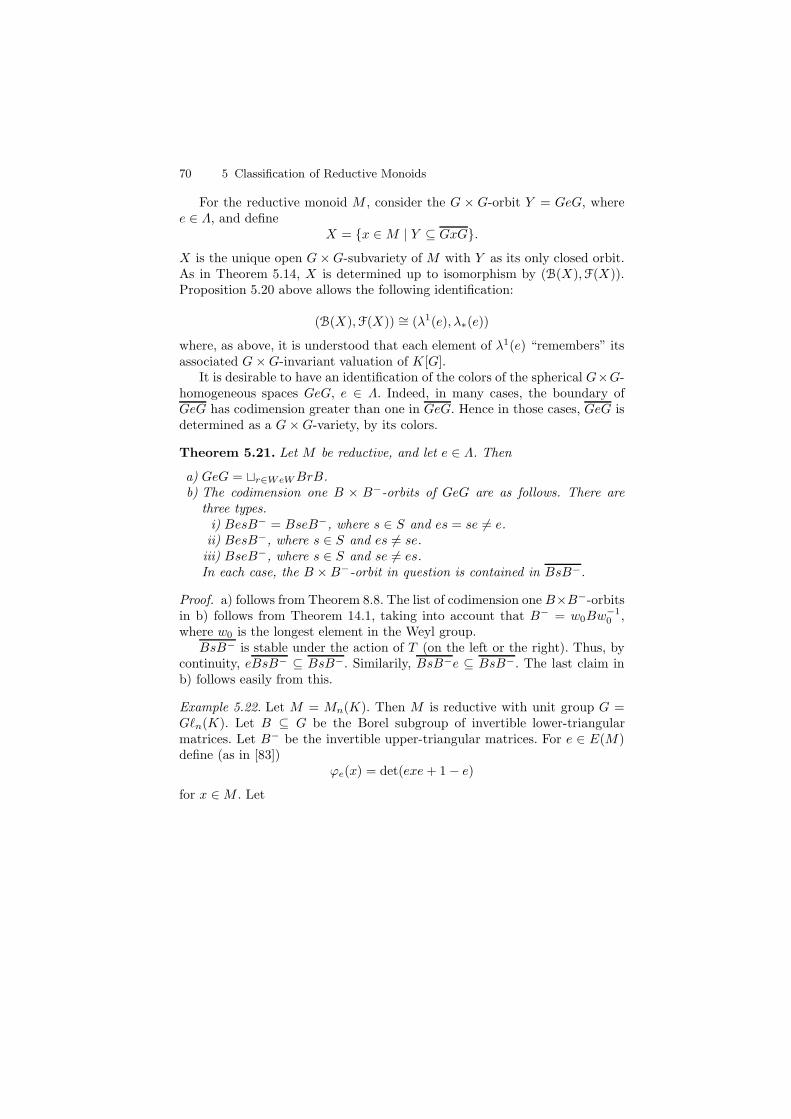
70 5 Classification of Reductive Monoids
For the reductive monoid M , consider the G × G-orbit Y = GeG, wheree ∈ Λ, and define
X = x ∈M | Y ⊆ GxG.
X is the unique open G×G-subvariety of M with Y as its only closed orbit.As in Theorem 5.14, X is determined up to isomorphism by (B(X),F(X)).Proposition 5.20 above allows the following identification:
(B(X),F(X)) ∼= (λ1(e), λ∗(e))
where, as above, it is understood that each element of λ1(e) “remembers” itsassociated G×G-invariant valuation of K[G].
It is desirable to have an identification of the colors of the spherical G×G-homogeneous spaces GeG, e ∈ Λ. Indeed, in many cases, the boundary ofGeG has codimension greater than one in GeG. Hence in those cases, GeG isdetermined as a G×G-variety, by its colors.
Theorem 5.21. Let M be reductive, and let e ∈ Λ. Then
a) GeG = tr∈WeWBrB.b) The codimension one B × B−-orbits of GeG are as follows. There are
three types.i) BesB− = BseB−, where s ∈ S and es = se 6= e.
ii) BesB−, where s ∈ S and es 6= se.iii) BseB−, where s ∈ S and se 6= es.In each case, the B ×B−-orbit in question is contained in BsB−.
Proof. a) follows from Theorem 8.8. The list of codimension one B×B−-orbitsin b) follows from Theorem 14.1, taking into account that B− = w0Bw
−10 ,
where w0 is the longest element in the Weyl group.BsB− is stable under the action of T (on the left or the right). Thus, by
continuity, eBsB− ⊆ BsB−. Similarily, BsB−e ⊆ BsB−. The last claim inb) follows easily from this.
Example 5.22. Let M = Mn(K). Then M is reductive with unit group G =G`n(K). Let B ⊆ G be the Borel subgroup of invertible lower-triangularmatrices. Let B− be the invertible upper-triangular matrices. For e ∈ E(M)define (as in [83])
ϕe(x) = det(exe+ 1− e)
for x ∈M . Let
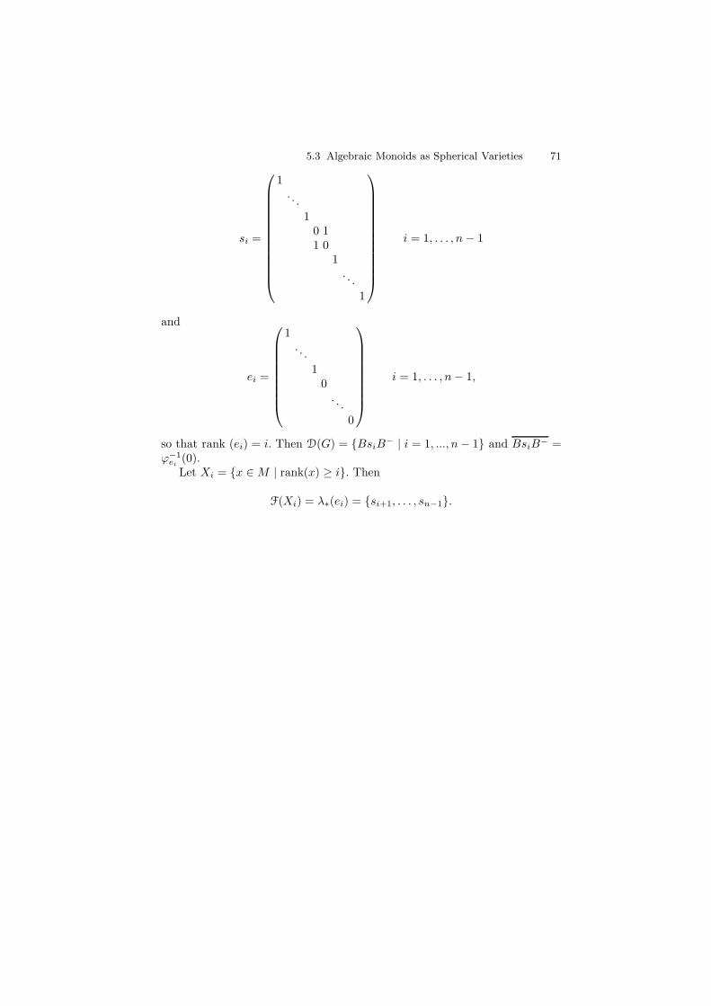
5.3 Algebraic Monoids as Spherical Varieties 71
si =
1. . .
10 11 0
1. . .
1
i = 1, . . . , n− 1
and
ei =
1. . .
10
. . .
0
i = 1, . . . , n− 1,
so that rank (ei) = i. Then D(G) = BsiB− | i = 1, ..., n− 1 and BsiB− =
ϕ−1ei
(0).Let Xi = x ∈M | rank(x) ≥ i. Then
F(Xi) = λ∗(ei) = si+1, . . . , sn−1.

6
Universal Constructions
Every branch of algebra has universal constructions of interest. If reductivemonoids are involved, there are some pleasant surprises.
6.1 Quotients
Theorem 6.1. Let M be an irreducible, algebraic monoid with unit group G,and let Ru(G) ⊆ G be the unipotent radical of G. Then there exists a uniquealgebraic monoid N , and a surjective morphism π : M → N such that
a) the unit group of N is G/Ru(G);b) π|G is the usual quotient morphism from G to G/Ru(G);c) π is universal for morphisms from M with kernel containing Ru(G).
Furthermore, if Z ⊆ M is a maximal D-submonoid of G, then Z ′ = π(Z) isa maximal D-submonoid of N , and π : Z → Z ′ is an isomorphism.
Proof. By Theorem 3.8 we can assume that M ⊆ End(V ) is a closed sub-monoid. There exists a filtration
0 = V1 ⊆ V2 ⊆ · · · ⊆ Vn
of M -modules such that Vi/Vi−1 is a simple M -module. Hence there is acanonical (induced) morphism
ϕ : M → Πni=2End(Vi/Vi−1).
Let N1 = ϕ(M). Then N1 is an irreducible algebraic monoid with unit groupG(N) abstractly isomorphic to G/Ru(G). Furthermore, ϕ induces an isomor-phism ϕ : Z → Z ′ on maximal D-submonoids, since we are just passing tothe associated graded object. By part c) of Theorem 4.5, N1 = G(N)Z ′G(N),and so ϕ : M → N1 is surjective. However, N1 may not be quite right. Sodefine
74 6 Universal Constructions
N = M/U = the normalization of N1 along G/Ru(G)→ G(N1).
Corollary 6.2. Let M be an irreducible, algebraic monoid with solvable unitgroup G = TU . Then the coordinate ring O[M/U ] ⊆ O[M ] of M/U isK[X(M)], the semigroup algebra of the set of characters of M .
Proof. In this case, N = M/U is a D-monoid. Hence π : Z → N is anisomorphism by Theorem 6.1, and O(M/U) = K[X(M)], the monoid algebra,since M/U is a D-monoid.
In group theory, the abelization is already available abstractly. There-fore the corresponding results for algebraic groups are not so surprising. Formonoids, the situation is somewhat different. The following result is mostlydue to Vinberg [142].
Theorem 6.3. Let M be a normal reductive algebraic monoid with unit groupG. Let G0 be the semisimple part of the unit group of G. Let A be the geometricinvariant theory quotient of M by the action (g, h, x)→ gxh−1 of G0×G0 onM . Let π : M → A be the quotient morphism. Then
a) the coordinate algebra of A is K[X(M)], the monoid algebra of the char-acter monoid of M ;
b) if Z is the connected center of G, then π : Z → A is the finite dominantquotient morphism obtained from the action of Z ∩ Z(G0) on Z;
c) the G0 ×G0-orbit G0xG0 ⊆M is closed if and only if it intersects Z.
Proof. Assume that M has a zero element. The general case is only su-perficially more complicated. Now the semisimple part G0 of any reductivemonoid is closed in M (proof: G0 = ∩χ∈X(M)ker(χ)). Thus, for any e ∈ E(Z)eG0 ⊆ eM is closed, since eG0 is the semisimple part of the reductive monoideM . But eG0 = G0eG0 = G0e. Hence by the basic theorem of geometricinvariant theory,
π|Z : Z → A
separates the idempotents of Z. Let Z0 = Z∩Z(G0). It follows that π(Z) ⊆ Ais open and G(A)-invariant. Since M has a zero element, so too does A, andπ(0M ) = 0A. Thus, π(Z) = A. In any case,
Z/Z0 → A
is finite, dominant and birational. Hence by Zariski’s main thereom (Theo-rem 2.29), Z/Z0 → A is an isomorphism. But then Z must meet every closedG0 ×G0-orbit.
6.2 Class Groups of Reductive Monoids 75
6.2 Class Groups of Reductive Monoids
Definition 6.4. Let M be reductive. We say that M is locally simply con-nected (lsc) if H(e) has trivial divisor class group for each e ∈ Λ.
We are here using the word “locally” in the sense of semigroup theory,rather than in the sense of geometry. The property P of a semigroup S is calleda local property if, for any idempotent e ∈ S, P holds for the semigroup eSe.Notice also that, strictly speaking, any simply connected group is semisimple.
Remark 6.5. The following results are discussed in detail in § 2.2.5. We statethem here for convenience. Let G be a connected reductive group with com-mutator subgroup G′.
a) A connected, semisimple group G is simply connected if and only ifCl(G) = 0.
b) Suppose that G is a connected, reductive group whose commutator sub-group G′ = (G,G) has trivial divisor class group. Then the same propertyholds for any Levi subgroup L of G. (This also follows from Remark 2.13and Lemma 2.17 of [137].)
c) For any connected reductive group G, there exists a connected reductivegroup G1 with Cl(G1) = 0, and a finite dominant morphism ζ : G1 → G.
d) If G is connected and reductive, then Cl(G) = 0 if and only if Cl(G′) = 0.
Definition 6.6. M is J-coirreducible if Λ1 is a singleton.
Recall that Λ1 ⊆ Λ is the subset of Λ that represents the codimension oneG×G-orbits of M . See part a) of Definition 4.6 and §5.3.3.
Theorem 6.7. Let M be reductive.
(a) If Cl(M) = (0) then M is locally simply connected.(b) If M is J-coirreducible then there exits M ′ → M , finite and dominant,
such that Cl(M ′) = (0). Furthermore, Cl(M) is finite.(c) For any such M there exists π : M ′ → M such that
(i) Cl(M ′) = (0) and(ii) π induces a bijection of U1(M ′)→ U1(M), where U1(M) denotes the
set of maximal J-classes of M\G.
Proof. Notice first that, given X such that Cl(X) = (0), then Cl(U) = (0) forany open set U ⊆ X . Thus, to prove (a) it suffices to show that Cl(eMe) = (0)for any e ∈ E(M). We apply Theorem 10.6 of [29]. This theorem says thatif the K-algebra A = ⊕i≥0Ai is a graded, noetherian, and factorial then A0
is also factorial. To do this we must show that A = K[M ] = ⊕n≥0An withA0 = K[eMe]. But we know from Corollary 6.10(ii) of [82] that there existsa one parameter subgroup λ : K∗ → G such that lim
t→0λ(t) = e. Consider the
action µ : K∗ ×M → M given by µ(t, x) = λ(t)xλ(t). µ induces a rational
76 6 Universal Constructions
action ρ : K∗ → Aut(K[M ]). If we let An = f ∈ K[M ]|ρ(t)(f) = tnf thenK[M ] = ⊕n≥0An is the desired ⊕-decomposition.
To prove (b) we may assume without loss of generality that 0 ∈M . Noticethat this implies that dim Z(G) = 1. Now M\G is irreducible of codimen-sion one in M . So it determines a divisor class D ∈ Cl(M). Since M\G isirreducible, we have by part c) of Proposition 2.19 an exact sequence
0→ Z ·D → Cl(M)→ Cl(G)→ 0. (1)
By Theorem 3.4 of [101], there exists χ : M → k such that χ−1(0) = M\G.Hence, in Cl(M), D has finite order. We conclude that Cl(M) is finite since,from Corollary 2.8 of [42], Cl(G) is finite. To find M ′ we first assume thatCl(G) = (0). For if Cl(G) 6= 0, we first consider ζ : G1 → G, a finite dominantmorphism with Cl(G1) = (0). We then apply Lemma 7.1.1 of [104] to obtaina reductive monoid M1 with unit group G1 and a finite dominant morphismM1 → M extending ζ. With another application of Lemma 7.1.1 of [104] wemay assume that G = G0×K
∗ where G0 is semisimple and simply connected.From the exact sequence in (1) we obtain Cl(M) = Z · D, a finite cyclicgroup. Before we construct M ′ we need to determine exactly what controlsthe order of D in Cl(M). Let e ∈ Λ\1 be the unique maximal element, andlet Te = T ∪ eT = T . Then Te ⊆ T is an open submonoid. Furthermore, byLemma 5.1 there exist opposite Borel subgroups B, B− containing T suchthat m : B−
u × Te × Bu → M , m(x, y, z) = xyz, is an open embedding.Letting R = K[M ] and S = K[B−
u × Te × Bu], we obtain R ⊆ S. SinceTe ∼= (K∗)r−1 × K as varieties, we see from Corollary 7.2 and Theorem 8.1of [29] that S is a UFD. Let µ = f ∈ R|f |M\G = 0. Clearly |Cl(M)| =infn|µ(n)) is a principal ideal where µ(n) denotes the nth symbolic power ofthe ideal µ ([29]). So write µ(n) = (χ) where n = |Cl(M)|. We may assume thatχ : M → K is a morphism of algebraic monoids, adjusting the initial χ with anon-zero scalar if necessary. Consider χ m ∈ S. From our remarks above wesee that (χm) = pn where p = µ·S. Using the isomorphism Te ∼= (K∗)r−1×Kand the fact that χm factors through p2 : B−
u ×Te×Bn → Te, (x, y, z) y,we obtain the following diagram:
K →jTe →
iB−u × Te ×Bu −→χm
K.
j is the unique inclusion with the property j(0) = e. It follows that n =degree (χ m i j). Now let (X,φ,C) be the polyhedral root system of M(Definition 3.6 of [104]) and let v : C → N be the “valuation” determinedby j (notice that v−1(0) ⊆ C is the facet of C determined by e). Let χ ∈ Cdenote the restriction of χ to T . We can construct a new polyhedral rootsystem (X ′, φ′, C′) as follows:
Since G = G0 × K∗, X = X0 ⊕ Z. Furthermore, C ⊆ X0 ⊕ N and χ =
(0, 1) ∈ C. We define
6.2 Class Groups of Reductive Monoids 77
X ′ = X0 ⊕1
nZ
φ′ = φ
C′ = ζ ∈ X ′|mζ ∈ C for some m > 0.
It is easily checked that (X ′, φ′, C′) is the polyhedral root system of thereductive monoid M ′ obtained via Lemma 7.1.1 of [104] from the mapζ : G → G ⊆ M given by ζ(g, α) = (g, αn). Furthermore, v : C → N extendsuniquely to v′ : C′ → N via v′(a, b/n) = v(a, 0) + b = v(a, 0) + (1/n)v(0, b).Notice that if χ′ = (0, 1/n) then v′(χ′) = 1. But from our above calculationapplied to M ′, |Cl(M ′)| = v′(χ′). Hence Cl(M ′) = (0).
For (c) we may assume M has a zero element. The general case is notessentially different. Let e ∈ Λ1 be a maximal idempotent of Λ\1. As above,there exists v : C → N which extends to v : X → Z. Let
H = χ ∈ X |v(χ) ≥ 0
and let
Ce = ∩w∈Ww∗(H) ⊆ X.
It is easily checked that (X,φ,Ce) is a polyhedral root system with j :(X,φ,C) → (X,φ,Ce). Let Mα be the associated reductive monoid, whereα = GeG ∈ U1(M). By construction Mα is J-coirreducible. Now from Theo-rem 8.l(a) of [104] there exists a birational morphism ζα : Mα →M inducingj above. Applying part (b) above we can modify Mα slightly, if necessary, andassume that Cl(Mα) = (0). The unique maximal J-class of Mα gets mappedto α. After ordering U1(M), define
ζ :∏
α∈U1(Mα)
Mα →M
by ζ(x1, . . . , xm) = ζα1(x1) · · · · · ζαm(xm). Consider the action of H = G0 ×· · ·
(m−1)×G0 on N =
∏Mα given by
(g1, . . . , gm−1)(x1, . . . , xm) = (x1g−11 , g1x2g
−12 , . . . , gm−2xm−1g
−1m−1, gm−1xm).
Define M ′ = N/H , the geometric invariant theory quotient of N by H , andlet q : N →M ′ be the canonical quotient morphism.
By standard results of geometric invariant theory (Theorem 1.10 of [62])there exists a unique morphism π : M ′ → M such that π q = m, wherem : N →M is the multiplication morphism. Based on Proposition 3.3 of [109]we see that M ′ is a reductive algebraic monoid with unit groupG0×K
∗×· · ·(m)×
K∗. Furthermore, by Proposition 2.58, Cl(M) = (0) since Cl(N) = (0) andG0×· · ·×G0 is a semisimple group. To complete the proof we must show thatπ identifies the maximal J-classes of M ′ with those of M . But π is surjective
78 6 Universal Constructions
by construction, and so for each α ∈ U1(M) there exists J ∈ U1(M ′) suchthat π(J) = Jα. But also, Cl(M ′) = (0), and so |U1(M ′)| ≤ dim(Z(G′)) = m.Thus U1(M ′)→ U1(M) is bijective.
Remark 6.8. The above theorem was first recorded in [114]. Part c) leads di-rectly to the construction of a “total coordinate ring” or “Cox ring” for thereductive monoid M . This generalizes some of the main results of [17]. See[28] for a general approach to this problem.
6.3 Flat Monoids
Vinberg [142] discovered a universal construction involving reductive monoidsthat has some remarkable properties. Let K be an algebraically closed fieldof characteristic zero. Associated with each semisimple group G0 is a certainreductive monoid Env(G0) which is the universal flat deformation of G0.
Recall from § 5.2, the augmented cone L(M) of a reductive monoid M .Let Z ⊆M be the closure in M of the connected center Z of G. It is easy tocheck that there is a natural partial order on L(M) defined as follows.
λ1 ≥ λ2 if λ1 = χλ2
for some χ ∈ X(Z). Notice that this makes sense even though X(Z) 6⊆ L(M).Indeed, X(Z) ⊗ Q+ = X(M) ⊗ Q+ ⊆ L(M) ⊗ Q+. Notice also that theremay be a decomposition in L(M) of the form λ1 = χλ2, with χ ∈ X(Z) butχ 6∈ X(M). The point here is that T ∼= T0 ×Z0 Z, where Z0 = Z ∩ T0. ThusX(T ) = (λ, χ) ∈ X(T0)×X(Z) | λ|Z0 = χ|Z0. We let
M ⊆ L(M)
denote the set of minimal elements of L(M) with respect to the above partialorder.
Before stating the main result, we need one more notion. As before, we letX(T0)+ denote the monoid of dominant weights of T0. If λ ∈ X(T0)+, we canwrite
λ =∑
α∈∆
cαλα,
where λα is the set of fundamental dominant weights of G0. Define
c : X(T0)+ → Cl(M)
by c(λ) =∑
α∈∆ cα[BsαB−]. As in § 2.2.5, we write Dα = BsαB−. The mainideas behind the theorem below are due to Vinberg [142]. Our approach is alittle different, in that we emphasise the role of the Dα.
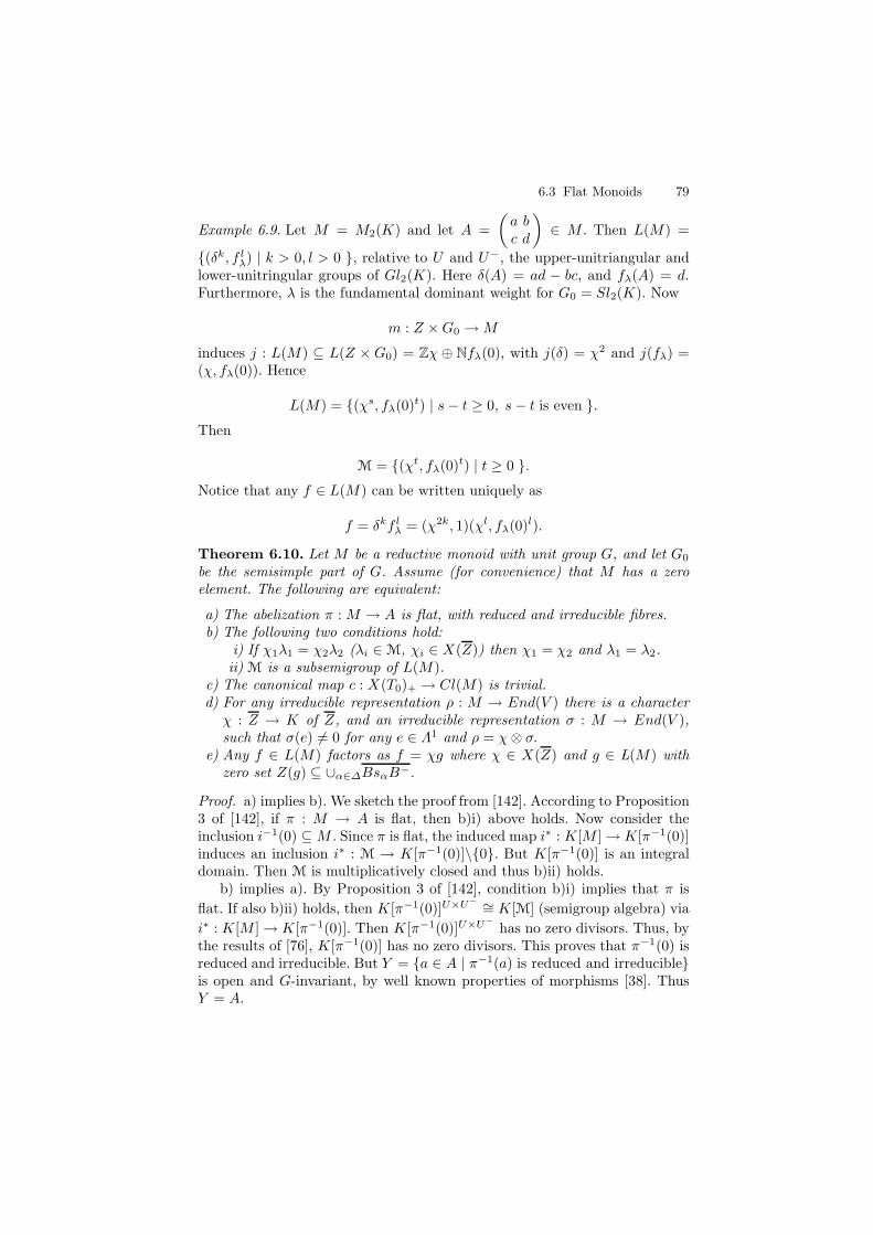
6.3 Flat Monoids 79
Example 6.9. Let M = M2(K) and let A =
(a bc d
)∈ M . Then L(M) =
(δk, f lλ) | k > 0, l > 0 , relative to U and U−, the upper-unitriangular andlower-unitringular groups of Gl2(K). Here δ(A) = ad − bc, and fλ(A) = d.Furthermore, λ is the fundamental dominant weight for G0 = Sl2(K). Now
m : Z ×G0 →M
induces j : L(M) ⊆ L(Z × G0) = Zχ ⊕ Nfλ(0), with j(δ) = χ2 and j(fλ) =(χ, fλ(0)). Hence
L(M) = (χs, fλ(0)t) | s− t ≥ 0, s− t is even .
Then
M = (χt, fλ(0)t) | t ≥ 0 .
Notice that any f ∈ L(M) can be written uniquely as
f = δkf lλ = (χ2k, 1)(χl, fλ(0)l).
Theorem 6.10. Let M be a reductive monoid with unit group G, and let G0
be the semisimple part of G. Assume (for convenience) that M has a zeroelement. The following are equivalent:
a) The abelization π : M → A is flat, with reduced and irreducible fibres.b) The following two conditions hold:
i) If χ1λ1 = χ2λ2 (λi ∈M, χi ∈ X(Z)) then χ1 = χ2 and λ1 = λ2.ii) M is a subsemigroup of L(M).
c) The canonical map c : X(T0)+ → Cl(M) is trivial.d) For any irreducible representation ρ : M → End(V ) there is a characterχ : Z → K of Z, and an irreducible representation σ : M → End(V ),such that σ(e) 6= 0 for any e ∈ Λ1 and ρ = χ⊗ σ.
e) Any f ∈ L(M) factors as f = χg where χ ∈ X(Z) and g ∈ L(M) withzero set Z(g) ⊆ ∪α∈∆BsαB−.
Proof. a) implies b). We sketch the proof from [142]. According to Proposition3 of [142], if π : M → A is flat, then b)i) above holds. Now consider theinclusion i−1(0) ⊆M . Since π is flat, the induced map i∗ : K[M ]→ K[π−1(0)]induces an inclusion i∗ : M → K[π−1(0)]\0. But K[π−1(0)] is an integraldomain. Then M is multiplicatively closed and thus b)ii) holds.
b) implies a). By Proposition 3 of [142], condition b)i) implies that π is
flat. If also b)ii) holds, then K[π−1(0)]U×U− ∼= K[M] (semigroup algebra) via
i∗ : K[M ]→ K[π−1(0)]. Then K[π−1(0)]U×U−
has no zero divisors. Thus, bythe results of [76], K[π−1(0)] has no zero divisors. This proves that π−1(0) isreduced and irreducible. But Y = a ∈ A | π−1(a) is reduced and irreducibleis open and G-invariant, by well known properties of morphisms [38]. ThusY = A.
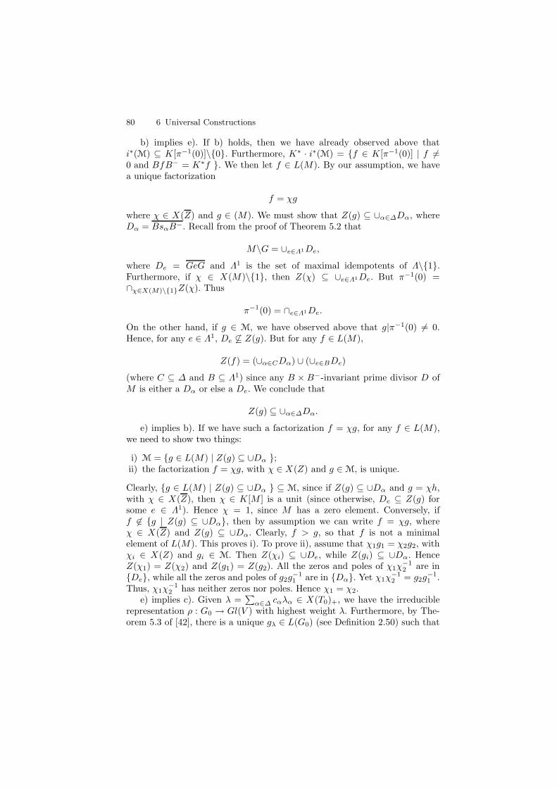
80 6 Universal Constructions
b) implies e). If b) holds, then we have already observed above thati∗(M) ⊆ K[π−1(0)]\0. Furthermore, K∗ · i∗(M) = f ∈ K[π−1(0)] | f 6=0 and BfB− = K∗f . We then let f ∈ L(M). By our assumption, we havea unique factorization
f = χg
where χ ∈ X(Z) and g ∈ (M). We must show that Z(g) ⊆ ∪α∈∆Dα, whereDα = BsαB−. Recall from the proof of Theorem 5.2 that
M\G = ∪e∈Λ1De,
where De = GeG and Λ1 is the set of maximal idempotents of Λ\1.Furthermore, if χ ∈ X(M)\1, then Z(χ) ⊆ ∪e∈Λ1De. But π−1(0) =∩χ∈X(M)\1Z(χ). Thus
π−1(0) = ∩e∈Λ1De.
On the other hand, if g ∈ M, we have observed above that g|π−1(0) 6= 0.Hence, for any e ∈ Λ1, De 6⊆ Z(g). But for any f ∈ L(M),
Z(f) = (∪α∈CDα) ∪ (∪e∈BDe)
(where C ⊆ ∆ and B ⊆ Λ1) since any B × B−-invariant prime divisor D ofM is either a Dα or else a De. We conclude that
Z(g) ⊆ ∪α∈∆Dα.
e) implies b). If we have such a factorization f = χg, for any f ∈ L(M),we need to show two things:
i) M = g ∈ L(M) | Z(g) ⊆ ∪Dα ;ii) the factorization f = χg, with χ ∈ X(Z) and g ∈M, is unique.
Clearly, g ∈ L(M) | Z(g) ⊆ ∪Dα ⊆ M, since if Z(g) ⊆ ∪Dα and g = χh,with χ ∈ X(Z), then χ ∈ K[M ] is a unit (since otherwise, De ⊆ Z(g) forsome e ∈ Λ1). Hence χ = 1, since M has a zero element. Conversely, iff 6∈ g | Z(g) ⊆ ∪Dα, then by assumption we can write f = χg, whereχ ∈ X(Z) and Z(g) ⊆ ∪Dα. Clearly, f > g, so that f is not a minimalelement of L(M). This proves i). To prove ii), assume that χ1g1 = χ2g2, withχi ∈ X(Z) and gi ∈ M. Then Z(χi) ⊆ ∪De, while Z(gi) ⊆ ∪Dα. HenceZ(χ1) = Z(χ2) and Z(g1) = Z(g2). All the zeros and poles of χ1χ
−12 are in
De, while all the zeros and poles of g2g−11 are in Dα. Yet χ1χ
−12 = g2g
−11 .
Thus, χ1χ−12 has neither zeros nor poles. Hence χ1 = χ2.
e) implies c). Given λ =∑α∈∆ cαλα ∈ X(T0)+, we have the irreducible
representation ρ : G0 → Gl(V ) with highest weight λ. Furthermore, by The-orem 5.3 of [42], there is a unique gλ ∈ L(G0) (see Definition 2.50) such that
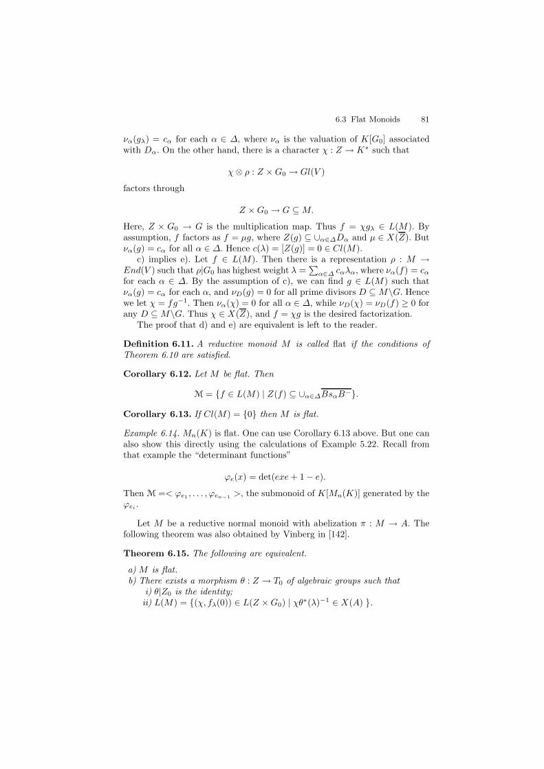
6.3 Flat Monoids 81
να(gλ) = cα for each α ∈ ∆, where να is the valuation of K[G0] associatedwith Dα. On the other hand, there is a character χ : Z → K∗ such that
χ⊗ ρ : Z ×G0 → Gl(V )
factors through
Z ×G0 → G ⊆M.
Here, Z × G0 → G is the multiplication map. Thus f = χgλ ∈ L(M). Byassumption, f factors as f = µg, where Z(g) ⊆ ∪α∈∆Dα and µ ∈ X(Z). Butνα(g) = cα for all α ∈ ∆. Hence c(λ) = [Z(g)] = 0 ∈ Cl(M).
c) implies e). Let f ∈ L(M). Then there is a representation ρ : M →End(V ) such that ρ|G0 has highest weight λ =
∑α∈∆ cαλα, where να(f) = cα
for each α ∈ ∆. By the assumption of c), we can find g ∈ L(M) such thatνα(g) = cα for each α, and νD(g) = 0 for all prime divisors D ⊆M\G. Hencewe let χ = fg−1. Then να(χ) = 0 for all α ∈ ∆, while νD(χ) = νD(f) ≥ 0 forany D ⊆M\G. Thus χ ∈ X(Z), and f = χg is the desired factorization.
The proof that d) and e) are equivalent is left to the reader.
Definition 6.11. A reductive monoid M is called flat if the conditions ofTheorem 6.10 are satisfied.
Corollary 6.12. Let M be flat. Then
M = f ∈ L(M) | Z(f) ⊆ ∪α∈∆BsαB−.
Corollary 6.13. If Cl(M) = 0 then M is flat.
Example 6.14. Mn(K) is flat. One can use Corollary 6.13 above. But one canalso show this directly using the calculations of Example 5.22. Recall fromthat example the “determinant functions”
ϕe(x) = det(exe+ 1− e).
Then M =< ϕe1 , . . . , ϕen−1 >, the submonoid of K[Mn(K)] generated by theϕei .
Let M be a reductive normal monoid with abelization π : M → A. Thefollowing theorem was also obtained by Vinberg in [142].
Theorem 6.15. The following are equivalent.
a) M is flat.b) There exists a morphism θ : Z → T0 of algebraic groups such that
i) θ|Z0 is the identity;ii) L(M) = (χ, fλ(0)) ∈ L(Z ×G0) | χθ
∗(λ)−1 ∈ X(A) .
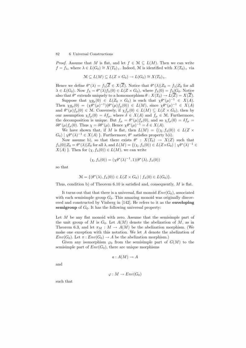
82 6 Universal Constructions
Proof. Assume that M is flat, and let f ∈ M ⊆ L(M). Then we can writef = fλ, where λ ∈ L(G0) ∼= X(T0)+. Indeed, M is identified with X(T0)+ via
M ⊆ L(M) ⊆ L(Z ×G0)→ L(G0) ∼= X(T0)+.
Hence we define θ∗(λ) = fλ|Z ∈ X(Z). Notice that θ∗(λ)|Z0 = fλ|Z0 for allλ ∈ L(G0). Now fλ = θ∗(λ)fλ(0) ∈ L(Z ×G0), where fλ(0) = fλ|G0. Noticealso that θ∗ extends uniquely to a homomorphism θ : X(T0)→ L(Z) = X(Z).
Suppose that χgµ(0) ∈ L(Z0 × G0) is such that χθ∗(µ)−1 ∈ X(A).Then χgµ(0) = (χθ∗(µ)−1)(θ∗(µ)fµ(0)) ∈ L(M), since χθ∗(µ)−1 ∈ X(A)and θ∗(µ)fµ(0) ∈ M. Conversely, if χfµ(0) ∈ L(M) ⊆ L(Z × G0), then byour assumption χfµ(0) = δfµ, where δ ∈ X(A) and fµ ∈ M. Furthermore,the decomposition is unique. But fµ = θ∗(µ)fµ(0), and so χfµ(0) = δfµ =δθ∗(µ)fµ(0). Thus χ = δθ∗(µ). Hence χθ∗(µ)−1 = δ ∈ X(A).
We have shown that, if M is flat, then L(M) = (χ, fλ(0)) ∈ L(Z ×G0) | χθ
∗(λ)−1 ∈ X(A) . Furthermore, θ∗ satisfies property b)i).Now assume b), so that there exists θ∗ : X(T0) → X(Z) such that
fλ(0)|Z0 = θ∗(λ)|Z0 for all λ, and L(M) = (χ, fλ(0)) ∈ L(Z×G0) | χθ∗(λ)−1 ∈
X(A) . Then for (χ, fλ(0)) ∈ L(M), we can write
(χ, fλ(0)) = (χθ∗(λ)−1, 1)(θ∗(λ), fλ(0))
so that
M = (θ∗(λ), fλ(0)) ∈ L(Z ×G0) | fλ(0) ∈ L(G0).
Thus, condition b) of Theorem 6.10 is satisfied and, consequently, M is flat.
It turns out that that there is a universal, flat monoid Env(G0), associatedwith each semisimple group G0. This amazing monoid was originally discov-ered and constructed by Vinberg in [142]. He refers to it as the envelopingsemigroup of G0. It has the following universal property:
Let M be any flat monoid with zero. Assume that the semisimple part ofthe unit group of M is G0. Let A(M) denote the abelization of M , as inTheorem 6.3, and let πM : M → A(M) be the abelization morphism. (Wemake one exception with this notation. We let A denote the abelization ofEnv(G0). Let π : Env(G0)→ A be the abelization morphism.)
Given any isomorphism ϕ0 from the semisimple part of G(M) to thesemisimple part of Env(G0), there are unique morphisms
a : A(M)→ A
and
ϕ : M → Env(G0)
such that
6.3 Flat Monoids 83
i) ϕ|G0 = ϕ0;ii) a πM = π ϕ;iii) φ : M ∼= E(a, π), via φ(x) = (πM (x), ϕ(x)), where E(a, π) = (x, y) ∈
A(M) × Env(G0) | a(x) = π(y), is the fibred product of A(M) andEnv(G0) over A.
There are several ways to construct this monoid Env(G0), and there are al-ready hints in Theorem 6.10. However, we use the construction in Theorem17 of Rittatore’s thesis [120]. The reader should also see Vinberg’s construc-tion in [142]. Notice that we are using multiplicative notation. In particular,X(T0/Z0)+ is the the subgroup of X(T0) generated by the positive roots.
Theorem 6.16. Let G0 be a semisimple group and let
L(G0) = (χ, λ) ∈ L(T0 ×G0) | χλ−1 ∈ X(T0/Z0)+.
Define
K[Env(G0)] =⊕
(χ,λ)∈L(G0)
(Vλ ⊗ V∗λ )⊗ χ ⊆ K[G0 × T0].
Then K[Env(G0)] is the coordinate algebra of the normal, reductive algebraicmonoid Env(G0) with the above-mentioned universal property. In particular,L(Env(G0)) = L(G0).
Proof. It follows from Vinberg’s criterion in Theorem 5.10 that K[Env(G0)]is the coordinate algebra of a normal, reductive monoid. Indeed, this followsdirectly from the defining conditions of L(G0), taking into account the factthat, for all λ, µ ∈ X+, any ν ∈ X(λ, µ) has the form
ν = λ+ µ−∑
kiαi
where ki ≥ 0. Also,
G(A) ∼= T0/Z0
via K[A] =⊕
(χ,fλ)∈X(A) Vλ ⊗ V∗λ ⊗ χ, where
X(A) = (χ, fλ)|dim(Vλ) = 1 ∼= X(T0/Z0)+.
Env(G0) is flat by the criterion of Theorem 6.15. Indeed, if (χ, fλ) ∈L(Env(G0)), we can write
(χ, fλ) = (χλ−1, 1)(λ, fλ)
with (χλ−1, 1) ∈ X(A) ⊆ L(M), and (λ, fλ) ∈ L(M). Hence
M = (λ, fλ) | λ ∈ X(T0) = X(Z.
84 6 Universal Constructions
With these identifications, θ∗ : X(T0)+ → X(Z) = X(T0) is just the inclusion.In particular, θ∗ extends to an isomorphism θ∗ : X(T0)→ X(Z).
Now let M be any flat reductive monoid with semisimple part G0 and zeroelement 0 ∈M . We assume that the semisimple part G0 of the unit group ofM has been identified with G0 ⊆ Env(G0).
So L(M) = (χ, fλ(0)) ∈ L(Z × G0) | χθ∗M (λ)−1 ∈ X(A) , where θ∗M :
X(T0)→ X(Z). Define a∗ : X(Z(Env(G0)))→ X(Z(M)) by
a∗(χ) = θ∗M (γ(χ)),
where γ is the inverse of θ∗, and define ϕ∗ : L(Env(G0))→ L(Z ×G0) by
ϕ∗(χ, fλ(0)) = (θ∗M (γ(χ)), fλ(0)).
It can be checked, as in the proof of Theorem 5 of [142], that ϕ∗(L(Env(G0)) ⊆L(M) ⊆ L(Z × G0), and consequently ϕ : G → Env(G0) extends toa morphism ϕ : M → Env(G0). It then follows from the definition ofL(M), along with a diagram chase, that L(M) is the result of a pushout ofa∗ : X(A)→ X(A(M)) and π∗ : X(A)→ L(Env(G0)). This kind of pushoutturns into a tensor product over K[A] on the level of coordinate algebras.Thus,
K[M ] ∼= K[A(M)]⊗K[A] K[Env(G0)],
which is the coordinate ring of the sought-after fibred product. The morphismsϕ and a are unique because Z ·G0 is dense in M .
Example 6.17. Let M = (x, y, z) ∈M2(K)×K2 | det(x) = yz. In this case,G0 = Sl2(K), and so Env(G0) = M2(K). Also A(M) = (d, y, z) ∈ K3 | d =yz ∼= K2. Thus,
M ∼= E(a, π)
where π : M2(K) → K is the determinant, and a : A(M) → K is given bya(d, y, z) = d = yz
It is useful to know the type map of Env(G0) (see Definition 4.6). Recallthat this is essentially a description of the G × G-orbits of Env(G0), alongwith enough information to build the monoid from these orbits. The latticeof orbits was calculated by Vinberg in [142]. We describe his results in a waythat allows us to relate Env(G0) to certain other monoids associated with G0.Our proof here is somewhat sketchy. See [142] for more details.
Theorem 6.18. Let Λ denote the cross section lattice of Env(G0). Then Λ =eI,X | I,X ⊆ S, and no component of X is contained in S\I. Λ is orderedas follows:
eI,X ≥ eJ,Y if and only if I ⊆ J and X ⊆ Y.
Furthermore, the type map of Env(G0) is given as follows:
6.3 Flat Monoids 85
λ∗(eI,X) = s ∈ S\I | sx = xs for all x ∈ X,λ∗(eI,X) = X.
Furthermore, λ1(eI,X) = eα | α ∈ I, where eα is short for eα,φ.
Proof. Notice that Cl(Env(G0)) is a finite group. Then for each e ∈ Λ1 thereis a χ ∈ X(A) such that χ−1(0) = MeM . Thus, Λ1 = eα | α ∈ S, since A isa simplicial, affine torus embedding with zero element. Then each convergent1 − PSG, λ : K∗ → A, has limit f = fI = limt→0λ(t) ∈ E(A). Also I ⊆ Sequals α ∈ S | π(eα) ≥ f. Now C = λ(K) ⊆ A is one-dimensional, so theinverse image
MI = λ−1(C)
is a semisimple flat monoid. Thus, MI\G(MI) is an irreducible, algebraicvariety (such monoids are called J-coirreducible since |Λ1| = 1). It is known[97] that the cross section lattice of MI is
ΛI = X ⊆ S | no component of X is contained in S\I t 1.
Furthermore, for eX ∈ ΛI , λ∗(eX) = X . Hence λ∗(eX) = s ∈ S\I | sx =xs for all x ∈ X.
If we denote eX ∈ ΛI by eI,X , we see that
Λ = 1 tI∈S Λ′I
where Λ′I = ΛI\1. Putting these all together yields the desired results.
A peculiar yet intriguing by-product of Env(G0) is the irreducible alge-braic semigroup, π−1(0) ⊆ Env(G0). Vinberg [143] calls it the asymptoticsemigroup of G0 since, like the asymptotic cone of a hyperboloid, it canon-ically reflects the behaviour of G0 at infinity. He denotes this semigroup byAs(G0). His construction also depicts G0 as a flat deformation of As(G0).
See Theorem 10.19 for more information about J-irreducible monoids.From the proof of Theorem 6.18 we see that As(G0) = MS\G(MS), where
MS is any J-coirreducible monoid of type S. This means that if Λ1 = eφ,then λ∗(eφ) = φ = S\S. Thus if eφ ∈ T , then eφT is a simplicial affinetorus embedding with zero. Furthermore, the distinct idempotents of eφT arecontained in distinct G×G-orbits of As(G0). Hence there are exactly 2r suchorbits, where r is the semisimple rank of G. The cross section lattice of anyMS is
Λ = 1 t eI | I ⊆ S.
The type map λ of MS is determined by λ∗. Furthermore
λ∗(eI) = I.
It is likely that all the results of this section could be extended to the case ofpositive characteristics. Rittatore has already made an important contributionin this direction in [123].
86 6 Universal Constructions
6.4 Multilined Closure
LetM be a reductive monoid with zero. Associated with each minimal nonzeroJ-class J ∈ U(M), there is an irreducible representation ρ : M → End(V ) suchthat ρ(e) 6= 0 for any e ∈ E(J). So let J1, . . . , Jm be the minimal nonzeroJ-classes of M , and let ρi, i = 1, . . . ,m, be the corresponding irreduciblereresentations of M such that ρi(Ji) 6= 0. Assume that Mj = ρj(M) is a J-irreducible monoid of type Ij . By this we mean that Mj is J-irreducibleand, for any minimal nonzero idempotent e of Mj , Pλ(e) is a parabolic sub-group of G(Mj) of type Ij . See § 7.3 for a detailed discussion of J-irreduciblemonoids. In particular, notice that the cross section lattice of a J-irreduciblemonoid may be identified with a subset of P(S), the set of subsets of the set ofsimple roots. In fact, the cross section lattice ΛI of the J-irreducible monoidMI of type I is
ΛI = eA | A ⊆ S, and no component of A is contained in I ∪ 0.
Then if e ∈ ΛI , we have either e = eA for some A ⊆ S, or else e = e0 = 0.But the “zero” here is not a subset of S. Let
ρ = (ρ1, . . . , ρm) : M → ΠEnd(Vi).
Definition 6.19. We define a multilined closure of type I=(I1, . . . , Im) tobe the closure M(I1, . . . , Im) of ρ(M)(K∗ × .... × K∗) in ΠEnd(Vi). ThenM(I1, . . . , Im) is called the multilined closure associated with M .
The multilined closure was first discussed in [52]. The following structuretheorem was obtained.
Theorem 6.20. Let Λi (respectively, λi) be the cross section lattice (respec-tively, type map) of Mi. Define the following subset of Λ1 × · · · × Λm:
ΛI = (eY1 , . . . , eYm)|Yi ⊆ λj(eYj ), whenever Yi 6= 0.
DefineλI(eY1 , . . . , eYm) = ∩mi=1λi(eYi).
If Λ is the cross section lattice of M(I) and λ is its type map, then
Λ = ΛI, andλ = λI.
The natural map M →M(I) induces a bijection on minimal nonzero J-classes.In particular, it is a finite morphism.
6.4 Multilined Closure 87
Proof. By the results of § 7.3, Λ ⊆ Λ1 × · · · × Λm. Let (e1, . . . , em) ∈ Λ,ei = eYi , i = 1, . . . ,m. We claim that e ∈ ΛI. Otherwise, for some nonemptysets Yiand Yj , we would obtain Yi 6⊆ Yj . Then for some simple root α ∈ ∆,s = sα ∈ Yi while s 6∈ λj(Yj). Let P = P (e) and P− = P−(e). Then the rootsubgroup of α,
Uα ⊆ Ru(PYj ) ⊆ Ru(P ),
since P ⊆ PYj . Hence Uαe = e. Since s ∈ CW (ei), Uα ⊆ CG(ei). Let
H = g ∈ G | gei = eig = ei ⊆ CG(ei).
Since H ⊆ CG(ei) is a normal subgroup with Xα ⊆ H , s ∈ W (H), the Weylgroup of H . Now Q = CB(ei)H is a parabolic subgroup of CG(ei), and thusQ = CB(ei)WKCB(ei). Since H is normal in CG(ei), the component A ⊆ Sof s in Yi is contained in K. Let fi be the set of minimal elements of Λi.Then ei ≥ fi, and
Qfi ⊆ HBfi = HfiBfi = fiBfi.
Hence Q ⊆ P (fi) = PIi , and so A ⊆ Ii, a contradiction. Hence e ∈ ΛI. Clearly,λ(e) = λI(e).
We now prove the converse, namely that λI(e) ⊆ λ. For Y ⊆ S, let
eY = (eY1 , . . . , eYm)
where Yi is the union of the components of Y not contained in Ii. Then forall i, j,
Yi ⊆ Y ⊆ λj(ej).
Hence eY ∈ ΛI. Clearly, eY eZ = eY ∩Z , for all Y, Z ⊆ S. Let
Y = (eZ1 , . . . , eZm) | Zi = 0 or Yi.
We claim that
ΛI = ∪Y⊆SY .
Let 0 6= e = (e1, . . . , em) ∈ ΛI, Y = λ(e). If ei = eZ 6= 0, then
Z ⊆ Y ⊆ λi(ei).
Hence, Yi = Z, and so e ∈ Y . This proves the claim.To finish the proof, we need to show that ΛI ⊆ Λ, and we do this by
induction on m. If m = 1, this is just the J-irreducible case. So assume thatm > 1. By the above discussion, if (e1, . . . , em) ∈ Λ and ei = 1, then
88 6 Universal Constructions
ej = 1 or 0 for all j = 1, . . . ,m. (∗)
Let P be a standard maximal parabolic subgroup ofG. Let P− be its opposite,and let L = P ∩ P−. Let T0 be the identity component of the center of L.Then dim(T0)=1. For i = 1, . . . ,m, let
E(αρi(t) | t ∈ T0) = 1, ei, fi, 0
with P (ei) = P−(fi) = P . By the above discussion (concerning Y ), itsuffices to show that (e1, . . . , em) ∈ Λ. But, by the induction hypothesis,(e1, . . . , em−1, 0) ∈ E(T1), where
T1 = (α1ρ1(t), . . . , αmρm(t)) | αi ∈ K∗, i = 1, . . . ,m
Clearly,
E(T1) ⊆ ⊕mi=11, ei, fi, 0.
By (∗), 1 = (1, . . . , 1) covers (1, . . . , 1, 0), and (1, . . . , 1, 0) covers (e1, . . . , em−1, 0)in E(T1). But E(T1) is a relatively complemented lattice. Hence there existse ∈ E(T1) such that e 6= (1, 1, . . . , 1, 0), and such that
(e1, . . . , em−1, 0) < e < 1
So again by (∗), either e = (e1, . . . , em−1, em), or else e = (e1, . . . , em−1, fm).However, P (e1, . . . , em−1, fm) is not parabolic. Hence e = (e1, . . . , em−1, em),completing the proof.
Remark 6.21. This multilined closure construction behaves as if it is, in somesense, dual to the construction in Theorem 6.7. In the construction of M ′
in Theorem 6.7 the maximal idempotents have a special property, while inthe multilined closure construction the minimal idempotents have a specialproperty.
Example 6.22. Let G0 = Sl3(K) so that S = s1, s2. Let ρ1 = id : G0 −→Gl3(K), and let ρ2 : Sl3(K) −→ Gl3(K) be defined by ρ2(x) = (x−1)t. DefineM1 = K∗ρ1(G0), and M2 = K∗ρ2(G0). Thus
M1 is of type J1 = s1,
M2 is of type J2 = s2.
By Theorem 6.20, M(J1, J2) has cross section lattice as depicted in the dia-gram below.
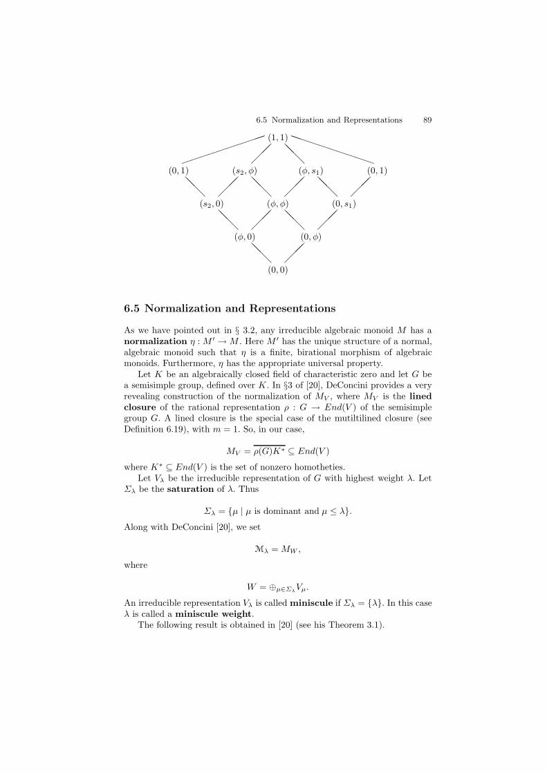
6.5 Normalization and Representations 89
(0, 0)
(0, φ)(φ, 0)
(φ, φ) (0, s1)(s2, 0)
(φ, s1) (0, 1)(s2, φ)(0, 1)
(1, 1)
@@@
@@@
@@@
@@@
@@@
@@@
@@@
PPPPPPPPPP
6.5 Normalization and Representations
As we have pointed out in § 3.2, any irreducible algebraic monoid M has anormalization η : M ′ →M . Here M ′ has the unique structure of a normal,algebraic monoid such that η is a finite, birational morphism of algebraicmonoids. Furthermore, η has the appropriate universal property.
Let K be an algebraically closed field of characteristic zero and let G bea semisimple group, defined over K. In §3 of [20], DeConcini provides a veryrevealing construction of the normalization of MV , where MV is the linedclosure of the rational representation ρ : G → End(V ) of the semisimplegroup G. A lined closure is the special case of the mutiltilined closure (seeDefinition 6.19), with m = 1. So, in our case,
MV = ρ(G)K∗ ⊆ End(V )
where K∗ ⊆ End(V ) is the set of nonzero homotheties.Let Vλ be the irreducible representation of G with highest weight λ. Let
Σλ be the saturation of λ. Thus
Σλ = µ | µ is dominant and µ ≤ λ.
Along with DeConcini [20], we set
Mλ = MW ,
where
W = ⊕µ∈ΣλVµ.
An irreducible representation Vλ is called miniscule if Σλ = λ. In this caseλ is called a miniscule weight.
The following result is obtained in [20] (see his Theorem 3.1).
90 6 Universal Constructions
Theorem 6.23. 1. Mλ is a normal variety with rational singularities.2. Mλ is the normalization of Mλ.3. Mλ and Mλ are equal if and only if λ is a miniscule weight.
His proof requires an application of the results of [21]. The proof alsorequires the result [45] of Kannan on the projective normality of the wonderfulcompactification.
Miniscule weights are the role models for the standard monomial theory. Ifλ is miniscule, the calculation of Vnλ = H0(G/P,Lnλ) involves a striking blendof combinatorics and intersection theory. Hodge worked this out for Sln(K),and then Seshadri extended Hodge’s work to the case of any miniscule weight.See [37] for a good introduction.
6.6 Exercises
6.6.1 Flat Monoids
1. Let f ∈ L(M). Prove that Z(f) ⊆ (∪α∈∆Dα) ∪ (∪e∈Λ1De).2. Let M be reductive. Show that L(M) is a commutative, totally cancella-
tive semigroup that embeds in a free abelian group of rank less than orequal to |∆|+ |Λ1|.
3. Prove the equivalence of d) and e) in Theorem 6.10.
7
Orbit Structure of Reductive Monoids
Let M be a reductive monoid with unit group G. We assume that M hasa zero element 0 ∈ M . The general case is not interestingly different (seeProposition 8 of [121]). From Theorem 4.2, M is regular, so that
M = GE(M) = E(M)G .
But we can do much better than this. Indeed, from Theorem 4.5,
M =⊔
e∈Λ
GeG
where Λ = e ∈ E(T ) | Be ⊆ eB.In this chapter we want to explain how M is “stuck together” using G, Λ
and P (e) = g ∈ G | ge = ege. Since P (e) is a parabolic subgroup containingB, the reader should take note of the key objective here: to obtain control ofthe structure of M in terms of something easily described in terms of theCoxeter-Dynkin complex of G, and the set of standard parabolic subgroupsof G.
Our second objective here is to identify and record a large number ofexamples where we can determine Λ and Λ −→ P, e P (e), explicitly.Notice that there is a canonical identification P = 2S , where S is the set ofsimple reflections. See Theorem 2.46. Thus we usually write the type map asλ : Λ −→ 2S
7.1 The System of Idempotents and the Type Map
In this section we describe the orbit structure of a reductive monoid, assumingthere is only one minimal, nonzero orbit. The results of this section are takenfrom [95].
Let M be reductive with unit group G, Borel subgroup B ⊆ G and max-imal torus T ⊆ B. W = NG(T )/T . From Definition 4.6 we obtain the typemap
92 7 Orbit Structure of Reductive Monoids
λ : Λ −→ 2S .
Recall that λ(e) = s ∈ S | se = es, where S ⊆ W is the set of simplereflections of W relative to B, and Λ is the cross section lattice of M relativeto B and T .
Notice that λ(e) determines P (e) = g ∈ G | ge = ege since P (e) isgenerated by B and λ(e). Note also that P (e) and P−(e) = g ∈ G | eg = egeare opposite parabolic subgroups.
Definition 7.1. Let
E(λ) =
(J, P,Q)
J ∈ G\M/G, P and Q are opposite parabolics,P = gP (e)g−1 for some g ∈ G, where J ∩Λ = e
.
A quasi-ordering on a set E is a relation ≤ on E that is transitive andreflexive.
Theorem 7.2. Both E(M) and E(λ) have canonically defined quasi-orderings≤` and ≤r. Define
ψ : E(M) −→ E(λ)
by ψ(e) = (GeG, P (e), P−(e)). Then ψ is an isomorphism of biordered sets.≤r and ≤` are defined as follows.
On E(M) definee ≤r f if fe = e.e ≤` f if ef = e.e ≤ f if ef = fe = e.
On E(λ) define
(J1, P,Q)R(J2, P′, Q′) if J1 = J2 and P = P ′.
(J1, P,Q)L(J2, P′, Q′) if J1 = J2 and Q = Q′.
(J1, P,Q) ≤ (J2, P′, Q′) if J1 ≤ J2 and there exist opposite Borel sub-
groups B and B−, such that B ⊆ P ∩ P ′ and B− ⊆ Q ∩Q′.
Then define on E(λ)
≤r = R ≤
and
≤` = L ≤ .
Proof. Assume that GeG = GfG. Then one checks, as in Lemma 3.4 of [95],that
~
eM = fM if and only if P (e) = P (f) andMe = Mf if and only if P−(e) = P−(f) .
Next we check that ψ is bijective. Let (J, P,Q) ∈ E(λ). Then P = P (e)for some e ∈ E(J). Further, by the results of [83], P is opposite to P−(e).
7.2 The Cross Section Lattice and the Weyl Chamber 93
So by standard results there exists g ∈ P such that g−1P−(e)g = Q. Thus,(J, P,Q) = ψ(g−1eg). Conversely, if ψ(e) = ψ(f), then by ~ above thateM = fM and Me = Mf . But then e = f , by an elementary semigroupcalculation.
For the remainder of the proof we refer the reader to Theorem 3.5 of [95].Notice that, in view of ~ above, all that remains here is to check that e ≤ fif and only if ψ(e) ≤ ψ(f).
The moral of the story is that, once we know λ, we obtain E automati-cally. If we also know G, then we can reconstruct M up to a kind of “centralextension” abstractly. It can be seen direcly that E(M) is a biordered setin the sense of Nambooripad [64].
7.2 The Cross Section Lattice and the Weyl Chamber
Let M be a reductive algebraic monoid. For the results of this section, itis not necessary to impose any other restrictions. We need to show how thecross-section lattice Λ can be described in terms relating X(T ) and the set ofdominant weights
X(T )+ = χ ∈ X(T ) | ∆α(χ) ≥ 0 for all α ∈ ∆
where ∆α : X(T ) −→ Z is defined by the equation
χ− sα(χ) = ∆α(χ)α.
Let e ∈ E(T ). Then eT is also a D-monoid with unit group eT . So letX(eT ) denote the monoid of characters of eT . Consider
µe =
χ ∈ X(eT ) ⊆ X(T )
∣∣∣∣χ 6= 0 andχeT\eT = 0
where X(eT ) ⊆ X(T ) via the map T → eT , z → ez. One can easily checkthat
X(T )\0 =⊔
e∈E(T )
µe .
Let ∆ be the set of simple roots of G relative to B and T . For α ∈ ∆ letUα be the one dimensional, unipotent subgroup of B, normalized by T withweight α.
Lemma 7.3. Let α ∈ ∆ and e ∈ E(T ). The following are equivalent:
a) Uαe = eUαe;b) either Uαe = eUα, or else Uαf = f for all f ∈ E1(eT ).
94 7 Orbit Structure of Reductive Monoids
Proof. In case eUα 6= e and Uαe 6= e, one obtains that Uαe = eUαe. Otherwise,if Uαf = f for all f ∈ E1(eT ) yet Uαe 6= eUαe (i.e. Uαe 6= eUα and Uαe 6= e),then eUα = e 6= Uαe is the only other possibility. Hence σαeσα 6= e and thus,σαfσα 6= f for some f ∈ E1(eT ). But then fUα = feUα = fe = f . HenceUαf 6= f , since fσα 6= σαf . Contradiction.
Lemma 7.4. a) The following are equivalent:i) Uαe = eUα (equivalently, sαe = esα);
ii) ∆α(χ) = 0 for some χ ∈ µe.b ) The following are equivalent (assuming Uαe 6= eUα).
i) Uαf = f for all f ∈ E1(eT );ii) ∆α(χ) > 0 for some χ ∈ µe.
Proof. For a), first note that, for χ ∈ µe, ∆α(χ) = 0 iff sα(χ) = χ. Butsα(µe) = µe′ where e′ = sαesα. Hence sα(µe) ∩ µe 6= φ iff sαesα = e. Ac-cordingly, if χ ∈ µe and sα(χ) = χ, then χ ∈ sα(µe) ∩ µe. Conversely, ifχ1 ∈ sα(µe) ∩ µe 6= φ, then χ1sα(χ1) ∈ µe and ∆α(χ) = 0.
For b), assume first that Uαf = f for all f ∈ E1(eT ). Now fT ∼= K asalgebraic varieties. Hence there is a unique character χf ∈ X(T ) such thatO(fT ) = K[χf ]. But from Lemma 3.6 of [109], ∆α(χf ) ≥ 0. Now
K[eT ] = K[χ | χn ∈ 〈χf1 , . . . , χf2〉 for some n > 0] (∗)
where fisi=1 = E1(eT ). Now if ∆α(χf ) = 0 for all f ∈ E1(eT ), then
sα(χf ) = χf for all f ∈ E1(eT ). Hence by (∗), sα(K[eT ]) = K[eT ] andso sαe = esα. Thus Uαe = eUα, a contradiction. Thus ∆α(χf ) > 0 for somef ∈ E1(eT ). Hence ∆α(χ) > 0 for all χ ∈ µe. Conversely, suppose that∆α(χf ) > 0 for some f ∈ E1(eT ). Consider
χ = χNf χf2 · . . . · χfs ∈ µe
where N > 0 and E1(eT ) = f, f2, . . . , fs. Then ∆α(χ) < 0 if N >> 0. Thisis a contradiction.
Theorem 7.5. The following are equivalent for e ∈ E(T )\0.
a) e ∈ Λ\0;b) there exists χ ∈ µe such that ∆α(χ) ≥ 0 for all α ∈ ∆.
Proof. Now e ∈ Λ′ := Λ\0 if and only if for all α ∈ ∆ either Uαe = eUαor else Uαe 6= eUα and Uαf = f for all f ∈ E1(eT ). By Lemma 7.4 this isequivalent to:
For each α ∈ ∆, either
∆α(χ) = 0 for some χ ∈ µe
or else∆α(χ) > 0 for all χ ∈ µe .
Thus, e ∈ Λ\0 if and only if for all α ∈ ∆ either
7.2 The Cross Section Lattice and the Weyl Chamber 95
i) ∆α(χ) = 0 for some χ ∈ µe, or elseii) ∆α(χ) > 0 for all χ ∈ µe.
Hence b) implies a).Conversely, if e ∈ Λ\0 then ∆ = ∆1 t∆2, where
∆1 = α ∈ ∆ | sαe = esα
and
∆2 = α ∈ ∆ | sαe 6= esα.
Let χ0 ∈ µe and define
χ =∏
w∈W∆1
w(χ0) ∈ µe .
Then ∆α(χ) = 0 for all α ∈ ∆. But ∆α(χ) > 0 for all α ∈ ∆2.
Theorem 7.5 has a very appealing geometric interpretation.One can identify E(T ) with the face lattice F of the rational polyhedral
coneX(T )⊗Q+ ⊆ X(T )⊗Q. Furthermore,X(T )⊗Q+ isW -invariant. We canthink of µe⊗Q+ as the topological interior of X(eT )⊗Q+ ∈ F. Theorem 7.5says that
Λ =
e ∈ E(T )
the interior of X(eT )⊗Q+ meetsX(T )+ ⊗Q+
.
Clearly, |ClW (e) ∩ Λ| = 1 for all e ∈ E(T ).Recall that a reductive monoid M is semisimple if the center of G is
one-dimensional and M has a zero element. In this case the zero elementof M is in the closure Z of Z the one-dimensional connected center of M .As Z is contained in any maximal torus T of G, we have in particular thatZ ⊆ T . Thus we obtain the induced (dual) map on the corresponding charactermonoids:
γ : X(T )→ X(Z) ∼= N.
This γ determines, on the associated rational polyhedral cones, a homomor-phism
ζ : X(T )⊗Q+ → X(Z)⊗Q+ ∼= Q+,
by setting ζ = γ ⊗ 1. For M semisimple we make the following definition.
Definition 7.6. LetP = ζ−1(1).
P is the polytope of M .
96 7 Orbit Structure of Reductive Monoids
From the above results, P is W -invariant, and the face lattice F of P is canon-ically identified with E(T ). Furthermore, we can identify Λ as a subset of F
using Theorem 7.5.
Example 7.7. Let M = Mn(K), the semisimple monoid of n×n matrices overK. In this case Z = αIn | α ∈ K
∗ , where In is the identity n×n matrix. IfT is the D-group of invertible diagonal matrices then T is the set of diagonalmatrices and ζ : X(T )⊗Q+ → X(Z)⊗Q+ is easily identified with the map
ρ : (Q+)n → Q+
defined by ρ(s1, ..., sn) =∑i si. The polytope here is
P = (s1, ..., sn) ∈ (Q+)n |∑
i
si = 1 .
The face lattice of P is easily identified with E(T )\0. Notice that charactersare written additively in this setup.
7.3 J-irreducible Monoids
We start with a simple lemma to focus our discussion.
Lemma 7.8. Let M be a reductive monoid with zero 0 ∈ M . Let Λ ⊆ E(T )be a cross section lattice. The following are equivalent.
a) Λ\0 has a unique minimal element e0 (so that e0f = e0 for all f ∈ Λ\0);b) there exists a rational representation ρ : M −→ End(V ) such that
i) V is irreducible over M .ii) ρ is a finite morphism.
Proof. Assume that ρ : M −→ End(V ) is as in b). Suppose that e1, e2 ∈ Λ\0are minimal elements yet e1 6= e2. Then e1Me2 = 0. But ρ(Me1)V andρ(Me2)V are M -submodules of V . Thus, ρ(Me1)V = ρ(Me2)V = V . Butthen ρ(e1)V = ρ(e1)ρ(Me2)V = ρ(e1Me2)V = 0, so that ρ(e1) = 0. But thisis impossible since ρ is a finite morphism.
Now assume that Λ\0 has a unique minimal element e. Let ρ : M −→End(W ) be a finite morphism of algebraic monoids [82]. If we replace W by
W =
n⊕
i=1
Wi/Wi−1, where W0 ⊆ W1 ⊆ · · · ⊆ Wn = W is a composition
series of W , then gr(ρ) : M −→ End(W ) is also a finite morphism since, by
regularity of M , gr(ρ)−1(0) = 0. So assume that W =
n⊕
i=1
Vi where each Vi
is irreducible. Now ρ(e) 6= 0, since ρ is finite. Say ρ(e)(V1) 6= 0. Thus we letρ1 = ρ|V1. Then ρ : M −→ End(V1) is the desired irreducible representation.
7.3 J-irreducible Monoids 97
Definition 7.9. Let M be as in Lemma 7.8. We say that M is J-irreducible.
The major purpose of this chapter is to determine the cross section latticesand the type maps of J-irreducible reductive moniods. But first, let us noticewhat determines the cross section lattice Λ and the type map λ : Λ→ 2S .
Given M as in Lemma 7.8, we observe several discrete invariants.
i) the type of the representation ρ : M −→ End(V )ii) λ(e0) = J0 = s ∈ S | se0 = e0s ⊆ Siii) g ∈ G | ge0 = ege0 = P (e0) < G.
To define the type of ρ, let B ⊆ G be a Borel subgroup and let L ⊆ V be theline such that ρ(B)L = L. Then the type of ρ is the parabolic subgroup
P = g ∈ G | ρ(g)L = L .
These invariants all amount to the same thing. Indeed, P = P (e0) =⊔
w∈WJ0
BwB and L = e0(V ). So our mission here is as follows.
Determine the type map λ : Λ→ 2S in terms of λ(e0) = J0 ⊆ S wheree0 ∈ Λ\0 is the minimal element.
For the remainder of this section we assume that M is a J-irreducible monoid.
Lemma 7.10. Let e, f ∈ E(M) be nonzero idempotents. Then P (e) = P (f)if and only if eRf .
Proof. If eRf , then f = eg for some g ∈ G. Hence fe = e. If x ∈ R(e),then xe = exe and so xf = xeg = exeg = fexeg = fexf . Hence f(xf) =f(fexf) = fexf = xf . Thus, P (e) ⊆ P (f). By symmetry, P (f) ⊆ P (e).
Conversely, assume that P (e) = P (f). Assume that e ∈ T ⊆ P (e). Nowthere exists g ∈ P (f) such that f ′ = gfg−1 ∈ T . Then fRf ′ and P (f) =P (f ′). So without loss of generality, f = f ′. Now let h ∈ E1(T ) be such thathe = eh = h. Then there exists a cross section lattice Λ such that e, h ∈ Λ.Then
B = g ∈ G | gh = hgh for all h ∈ Λ
⊆ P (e)
since e ∈ Λ. But B ⊆ P (e) = P (f). Hence by definition,
f ∈ h ∈ E(T ) | gh = hgh for all g ∈ B = Λ .
Since h ∈ Λ is the unique, nonzero, minimal element of Λ, we have fh = h.But this is true for any h ∈ E1(eT ) = h1, . . . , hs, the set of minimal, nonzeroidempotents of eT . Thus f = e since e = h1 ∨ · · · ∨ hs. Similarly, f = fe. Soe = f .
98 7 Orbit Structure of Reductive Monoids
Lemma 7.10 is the crux of the matter. Indeed, let
λ : Λ\0 −→ 2S ,
where λ(e) = s ∈ S | se = es, be the type map. Then P (e) = Pλ(e). Henceby Lemma 7.10, λ is injective. Thus it remains to find λ(Λ\0) ⊆ 2S and torecover the J-ordering on Λ from this image.
Definition 7.11. For e ∈ Λ define
λ∗(e) = s ∈ S | se = es 6= e
λ∗(e) = s ∈ S | se = es = e.
It is easy to check that e ≥ f implies that both λ∗(f) ⊆ λ∗(e) and λ∗(e) ⊆λ∗(f). In particular, λ∗(e) ⊆ λ∗(e0) = J0. But we can do much more here. Itturns out that we can characterize I ∈ 2S | I = λ∗(e) for some e ∈ Λ\0 andthat λ∗(e) determines λ∗(e) ⊆ J0.
First recall the graph structure on S:
s and t are joined by an edge if st 6= ts.
Therefore we can talk about the connected components of any subset ofS. The following theorem is the main result of [95].
Theorem 7.12. a) The following are equivalent for I ⊆ S.i) I = λ∗(e) for some e ∈ Λ\0.
ii) No connected component of I lies entirely in J0.Furthermore, if e ≥ f then λ∗(e) ⊇ λ∗(f)
b) For any e ∈ Λ\0, λ∗(e) = s ∈ J0\λ∗(e) | st = ts for all t ∈ λ∗(e).
Proof. For b) we refer the reader to the straightforward calculation of Lemma4.10 of [95]. For a), first notice that e 7→ λ∗(e) is an injection Λ\0 −→ 2S
since λ is injective and it is determined by λ∗. Furthermore, if e ≥ f theneMe ⊇ fMf , while λ∗(e) is canonically identified with the simple reflectionsof eMe (and similarly for f). Hence λ∗(e) ⊇ λ∗(f).
To see why i) and ii) are equivalent, we start with e0 and notice thatλ∗(e0) = φ; and then work our way “up”. The key step is Theorem 4.13 of[95].
For e ∈ Λ\0 there is a canonical bijection between f ∈ Λ\0 | f coverse and
s ∈ S | se 6= es. (∗)
Hence f corresponds to the unique s with λ∗(f) = λ∗(e) ∪ s.To find f given s, consider WI where I = λ∗(e) ∪ s. Then it is eas-
ily checked that there is a minimal element e′ ∈ ΛWI = e ∈ Λ | we =ew for all w ∈ WI such that e′e = ee′ = e and e′ 6= e. This gives us “a foot
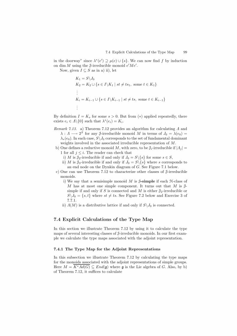
7.4 Explicit Calculations of the Type Map 99
in the doorway” since λ∗(e′) ⊇ µ(e) ∪ s. We can now find f by inductionon dimM using the J-irreducible monoid e′Me′.
Now, given I ⊆ S as in a) ii), let
K1 = S\J0
K2 = K2 ∪ s ∈ I\K1 | st 6= ts1, some t ∈ K1
...
Ki = Ki−1 ∪ s ∈ I\Ki−1 | st 6= ts, some t ∈ Ki−1
...
By definition I = Ks for some s > 0. But from (∗) applied repeatedly, thereexists ei ∈ Λ\0 such that λ∗(ei) = Ki.
Remark 7.13. a) Theorem 7.12 provides an algorithm for calculating Λ andλ : Λ −→ 2S for any J-irreducible monoid M in terms of J0 = λ(e0) =λ∗(e0). In each case, S\J0 corresponds to the set of fundamental dominantweights involved in the associated irreducible representation of M .
b) One defines a reductive monoidM , with zero, to be Ji-irreducible if |Λj | =1 for all j ≤ i. The reader can check that
i) M is J2-irreducible if and only if J0 = S\s for some s ∈ S,ii) M is J3-irreducible if and only if J0 = S\s where s corresponds to
an end node on the Dynkin diagram of G. See Figure 7.1 below.c) One can use Theorem 7.12 to characterize other classes of J-irreducible
monoids.i) We say that a semisimple monoid M is J-simple if each H-class ofM has at most one simple component. It turns out that M is J-simple if and only if S is connected and M is either J2-irreducible orS\J0 = s, t where st 6= ts. See Figure 7.2 below and Exercise 3 of7.7.1.
ii) Λ(M) is a distributive lattice if and only if S\J0 is connected.
7.4 Explicit Calculations of the Type Map
In this section we illustrate Theorem 7.12 by using it to calculate the typemaps of several interesting classes of J-irreducible monoids. In our first exam-ple we calculate the type maps associated with the adjoint representation.
7.4.1 The Type Map for the Adjoint Representations
In this subsection we illustrate Theorem 7.12 by calculating the type mapsfor the monoids associated with the adjoint representations of simple groups.Here M = K∗Ad(G) ⊆ End(g) where g is the Lie algebra of G. Also, by b)of Theorem 7.12, it suffices to calculate
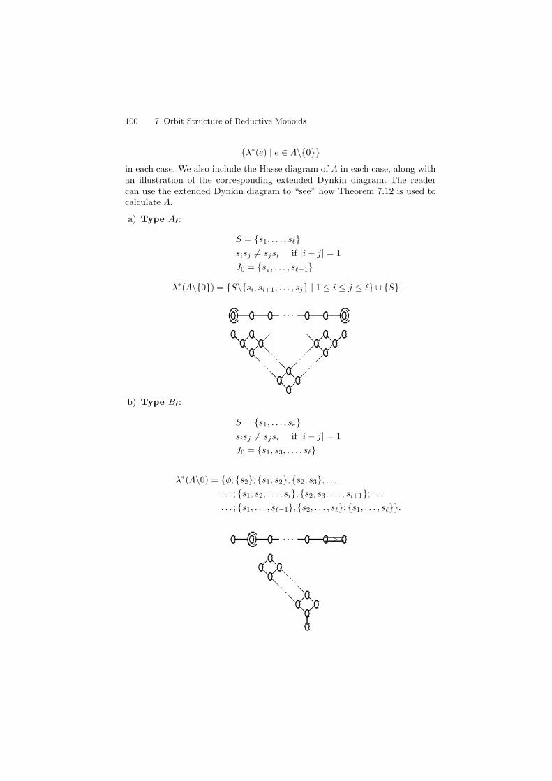
100 7 Orbit Structure of Reductive Monoids
λ∗(e) | e ∈ Λ\0
in each case. We also include the Hasse diagram of Λ in each case, along withan illustration of the corresponding extended Dynkin diagram. The readercan use the extended Dynkin diagram to “see” how Theorem 7.12 is used tocalculate Λ.
a) Type A`:
S = s1, . . . , s`
sisj 6= sjsi if |i− j| = 1
J0 = s2, . . . , s`−1
λ∗(Λ\0) = S\si, si+1, . . . , sj | 1 ≤ i ≤ j ≤ ` ∪ S .
· · ·
??? ??? ???
??? ??
???
?
???
???
??? ???
???
???
???
······
······
b) Type B`:
S = s1, . . . , se
sisj 6= sjsi if |i− j| = 1
J0 = s1, s3, . . . , s`
λ∗(Λ\0) = φ; s2; s1, s2, s2, s3; . . .
. . . ; s1, s2, . . . , si, s2, s3, . . . , si+1; . . .
. . . ; s1, . . . , s`−1, s2, . . . , s`; s1, . . . , s`.
· · · >
???
??? ??
???
?
???
???
???
???
······
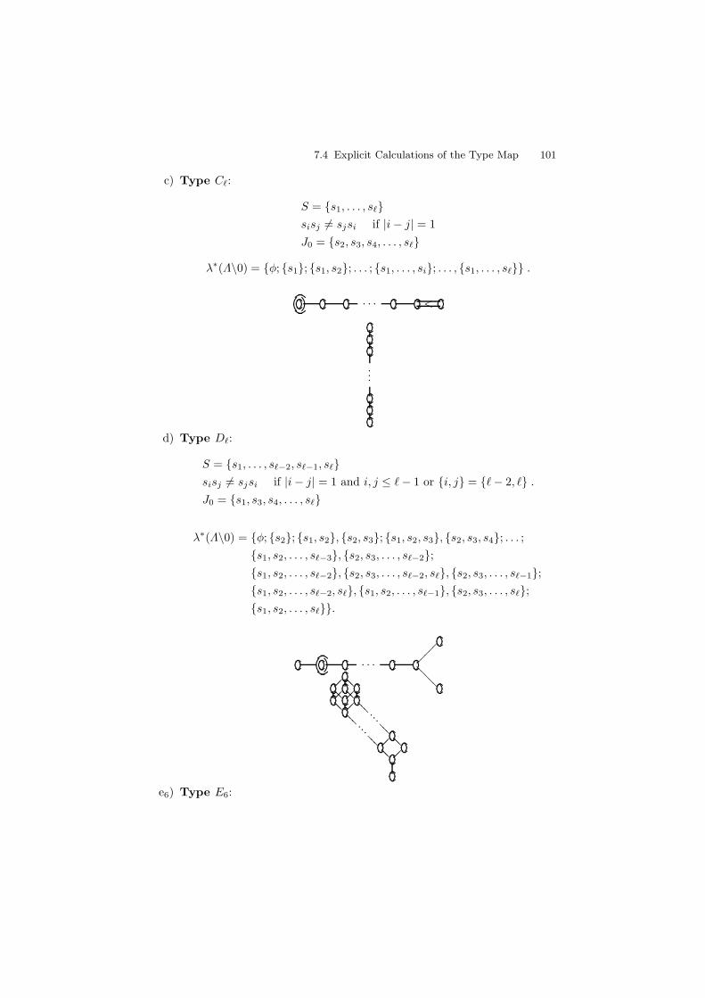
7.4 Explicit Calculations of the Type Map 101
c) Type C`:
S = s1, . . . , s`
sisj 6= sjsi if |i− j| = 1
J0 = s2, s3, s4, . . . , s`
λ∗(Λ\0) = φ; s1; s1, s2; . . . ; s1, . . . , si; . . . , s1, . . . , s` .
· · · <
...
d) Type D`:
S = s1, . . . , s`−2, s`−1, s`
sisj 6= sjsi if |i− j| = 1 and i, j ≤ `− 1 or i, j = `− 2, ` .
J0 = s1, s3, s4, . . . , s`
λ∗(Λ\0) = φ; s2; s1, s2, s2, s3; s1, s2, s3, s2, s3, s4; . . . ;
s1, s2, . . . , s`−3, s2, s3, . . . , s`−2;
s1, s2, . . . , s`−2, s2, s3, . . . , s`−2, s`, s2, s3, . . . , s`−1;
s1, s2, . . . , s`−2, s`, s1, s2, . . . , s`−1, s2, s3, . . . , s`;
s1, s2, . . . , s`.
· · ·
??
???
???
???
???
??? ??
???
?
???
???
???
???
······
e6) Type E6:
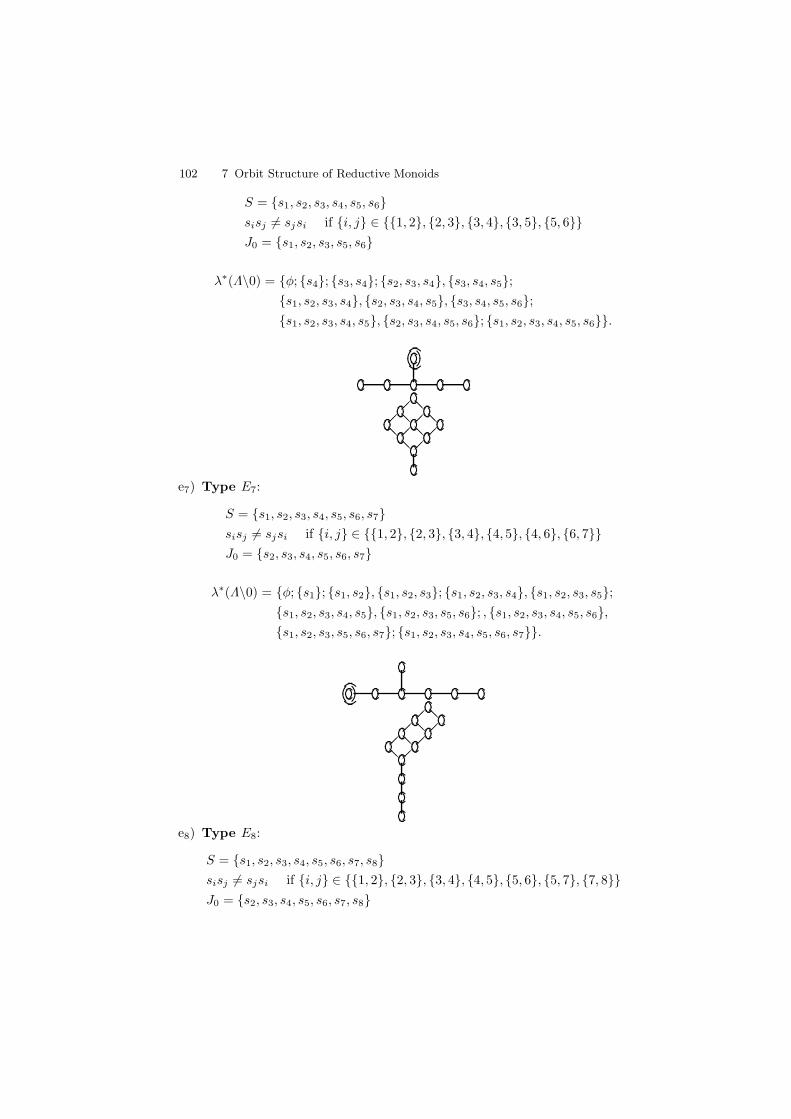
102 7 Orbit Structure of Reductive Monoids
S = s1, s2, s3, s4, s5, s6
sisj 6= sjsi if i, j ∈ 1, 2, 2, 3, 3, 4, 3, 5, 5, 6
J0 = s1, s2, s3, s5, s6
λ∗(Λ\0) = φ; s4; s3, s4; s2, s3, s4, s3, s4, s5;
s1, s2, s3, s4, s2, s3, s4, s5, s3, s4, s5, s6;
s1, s2, s3, s4, s5, s2, s3, s4, s5, s6; s1, s2, s3, s4, s5, s6.
???
??? ???
??? ??? ???
e7) Type E7:
S = s1, s2, s3, s4, s5, s6, s7
sisj 6= sjsi if i, j ∈ 1, 2, 2, 3, 3, 4, 4, 5, 4, 6, 6, 7
J0 = s2, s3, s4, s5, s6, s7
λ∗(Λ\0) = φ; s1; s1, s2, s1, s2, s3; s1, s2, s3, s4, s1, s2, s3, s5;
s1, s2, s3, s4, s5, s1, s2, s3, s5, s6; , s1, s2, s3, s4, s5, s6,
s1, s2, s3, s5, s6, s7; s1, s2, s3, s4, s5, s6, s7.
???
??? ??? ???
e8) Type E8:
S = s1, s2, s3, s4, s5, s6, s7, s8
sisj 6= sjsi if i, j ∈ 1, 2, 2, 3, 3, 4, 4, 5, 5, 6, 5, 7, 7, 8
J0 = s2, s3, s4, s5, s6, s7, s8
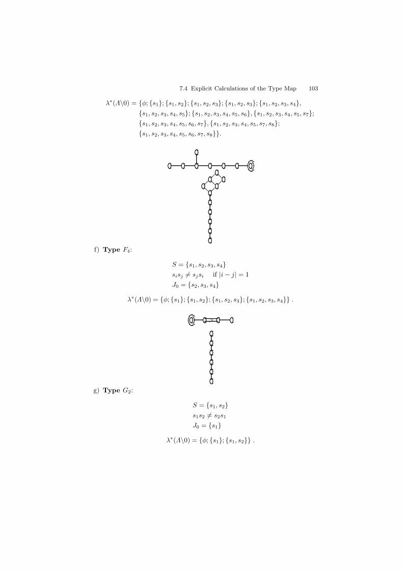
7.4 Explicit Calculations of the Type Map 103
λ∗(Λ\0) = φ; s1; s1, s2; s1, s2, s3; s1, s2, s3; s1, s2, s3, s4,
s1, s2, s3, s4, s5; s1, s2, s3, s4, s5, s6, s1, s2, s3, s4, s5, s7;
s1, s2, s3, s4, s5, s6, s7, s1, s2, s3, s4, s5, s7, s8;
s1, s2, s3, s4, s5, s6, s7, s8.
???
??? ???
f) Type F4:
S = s1, s2, s3, s4
sisj 6= sjsi if |i− j| = 1
J0 = s2, s3, s4
λ∗(Λ\0) = φ; s1; s1, s2; s1, s2, s3; s1, s2, s3, s4 .
>
g) Type G2:
S = s1, s2
s1s2 6= s2s1
J0 = s1
λ∗(Λ\0) = φ; s1; s1, s2 .
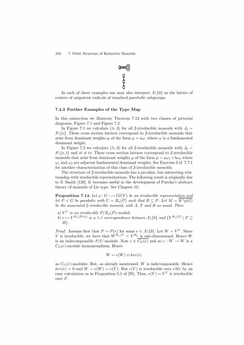
104 7 Orbit Structure of Reductive Monoids
<
In each of these examples one may also interpret Λ\0 as the lattice ofcenters of unipotent radicals of standard parabolic subgroups.
7.4.2 Further Examples of the Type Map
In this subsection we illustrate Theorem 7.12 with two classes of pictorialdiagrams, Figure 7.1 and Figure 7.2.
In Figure 7.1 we calculate (λ,Λ) for all J-irreducible monoids with J0 =S\s. These cross section lattices correspond to J-irreducible monoids thatarise from dominant weights µ of the form µ = aω, where ω is a fundamentaldominant weight.
In Figure 7.2 we calculate (λ,Λ) for all J-irreducible monoids with J0 =S\s, t and st 6= ts. These cross section lattices correspond to J-irreduciblemonoids that arise from dominant weights µ of the form µ = aω1 + bω2 whereω1 and ω2 are adjacent fundamental dominant weights. See Exercise 3 of 7.7.1for another characterization of this class of J-irreducible monoids.
The structure of J-irreducible monoids has a peculiar, but interesting rela-tionship with irreducible representations. The following result is originally dueto S. Smith [126]. It becomes useful in the development of Putcha’s abstracttheory of monoids of Lie type. See Chapter 10.
Proposition 7.14. Let ρ : G −→ G`(V ) be an irreducible representation andlet P < G be parabolic with U = Ru(P ) such that B ⊆ P . Let M = K∗ρ(G)be the associated J-irreducible monoid, with Λ, T and B as usual. Then
a) V U is an irreducible P/Ru(P )-moduleb) e 7→ V Ru(P (e)) is a 1-1 correspondence between Λ\0 and V Ru(P ) | P ⊇B.
Proof. Assume first that P = P (e) for some e ∈ Λ\0. Let W = V U . SinceV is irreducible, we have that WBu/U = V Bu is one-dimensional. Hence Wis an indecomposable P/U -module. Now e ∈ CG(e) and so e : W → W is aCG(e)-module homomorphism. Hence
W = e(W )⊕ ker(e)
as CG(e)-modules. But, as already mentioned, W is indecomposable. Henceker(e) = 0 and W = e(W ) = e(V ). But e(V ) is irreducible over eMe by aneasy calculation as in Proposition 5.1 of [95]. Thus, e(V ) = V U is irreducibleover P .
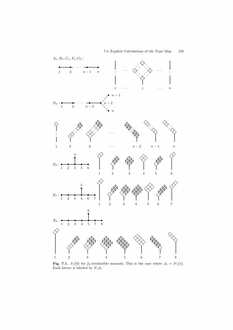
7.4 Explicit Calculations of the Type Map 105
An, Bn, Cn, F4, G2 :
• • • •.. .
1 2 n − 1 n
1
.
.
.
...
.
.
.
n
.
.
.
...
.
.
.
???
??
?
??? ???
??????
???
???
j
..
....
.
..
....
..
....
..
..
....
.
............
... . . .
.... . . .
Dn :
????
??• • • •
•
•
.. .
1 2 n − 3n − 2
n − 1
n
1 2 3 n − 2 n − 1 n···
···
??
??.. ........
??
??
..
??..
??..
??
..
??..
??..
??
.. ..
... ...
...
...
...
..
???...
???..
.???...
???...
???..
.???...
???...
???.
.
????
...??
????
??
...??
??
????
...??
????
??
...??
??
.
... .
... .
...
.
... .
... .
...
.
????
...??
????
??
...??
??
.. .. ..
.. .. ..
.
.
????
...??
????
??
...??
??
.. .. ..
.. .. ..
.
.
E6 : • • • • •
•
1 2 3 5 6
4
1 2 3 4 5 6
..
.??
.
.??..
??
.
.
.
..
??..
??..
??..
??..
??..
??..
??
.
..
???...
???...
???..
.??
?...
???...
???.
.
..
???...
???...
???.
.
.
..
??..
??..
??..
??..
??..
??..
??
.
..
.??
.
.??..
??
.
.
.
E7 : • • • • • •
•
1 2 3 4 6 7
5
1 2 3 4 5 6 7
..
.??
.
.??..
??
.
.
.
.
..
??..
??..
??..
??..
??..
??..
??..
??
.
..
???...
???...
???..
.??
?...
???...
???...
???.
.
..
???...
???...
???...
???.
..
???...
???...
???...
???.
.
..
???..
..
???..
..
???..
..
???..
.
.
..
??..
??..
??..
??
..
??..
??..
??..
??..
??
.
.
.
.??
.
.??..
??..
??
.
.
.
E8 : • • • • • • •
•
1 2 3 4 5 7 8
6
1 2 3 4 5 6 7 8
..
.??
.
.??..
??
.
.
.
.
.
..
??..
??..
??..
??..
??..
??..
??..
??..
??
.
..
???...
???...
???..
.??
?...
???...
???...
???...
???.
.
.
.??
??..
.
.??
??..
.
.??
??..
.
.??
??..
.
.??
??..
.
.??
??..
.
.??
??..
.
????
????????????
????????????
????????
..
. ..
. ..
. ..
. ..
.
..
. ..
. ..
. ..
. ..
.
.
????
??
????
??
????
??
..
..
..
..
..
..
..
..
..
..
.
.
????
??
????
????
????
??
????
????
.. .. .. .. ..
.. .. .. .. .. ..
.
.
.??
????
.
.??????
. .
. .. ..
.
.
.
Fig. 7.1. Λ\0 for J2-irreducible monoids. This is the case where J0 = S\s.Each lattice is labeled by S\J0.
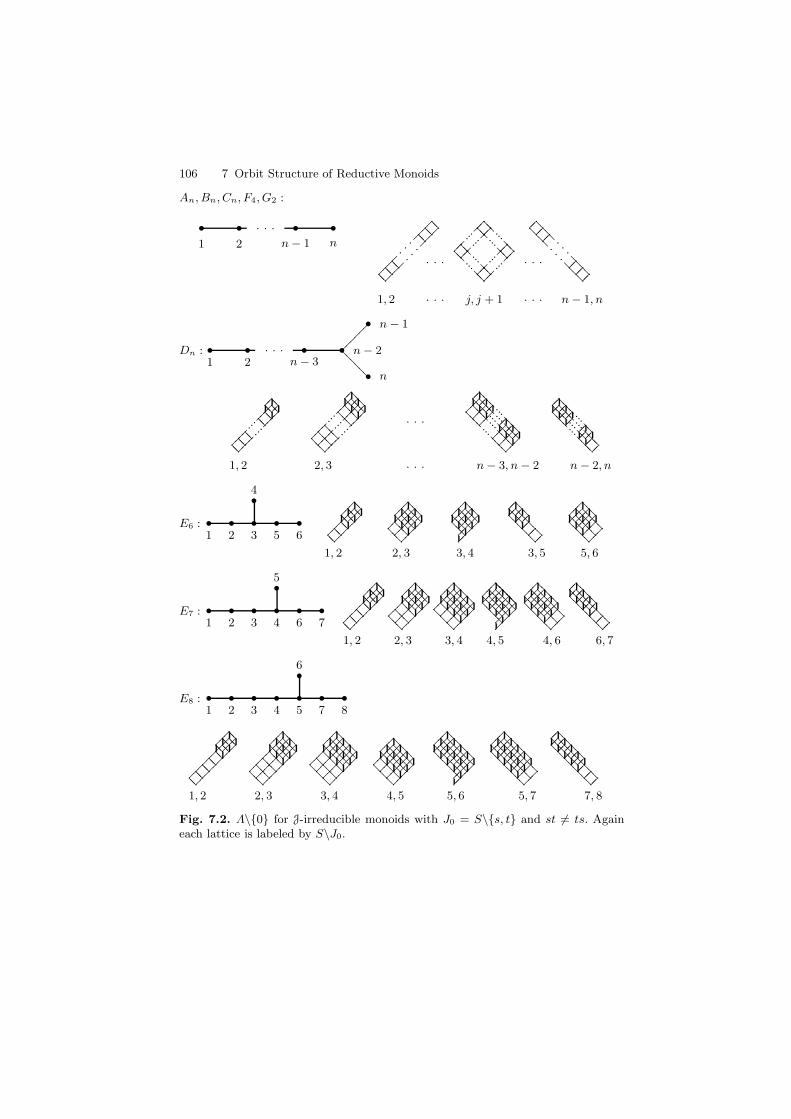
106 7 Orbit Structure of Reductive Monoids
An, Bn, Cn, F4, G2 :
• • • •.. .
1 2 n − 1 n
1, 2 j, j + 1 n − 1, n.. .
.. .
.. .
.. .
...
...
..
??..
??..
??
..
??..
??..
??
???
??
?
??? ???
??????
???
???
..
....
.
..
....
..
....
..
..
....
.
............
????
. . .
????
????
. . .
????
.. .. ..
.. .. ..
Dn :
????
??• • • •
•
•
.. .
1 2 n − 3n − 2
n − 1
n
1, 2 2, 3 n − 3, n − 2 n − 2, n···
···
...
...
..
??..
??..
??..
??..
??
..
??..
??..
??
...
...
...
..
???...
???..
.???...
???...
???..
.???...
???...
???.
....
. ....
. ....
. .
.
..
. ....
. ....
.
.??
??
...??
??
.??
??
...??
??
.??
??
...??
??
.??
??
...??
??
.??
??
...??
??
.... .... .... .... ....
.??
??
...??
.??
??
...??
.??
??
...??
.??
??
...?? .
??
.??
E6 : • • • • •
•
1 2 3 5 6
4
1, 2 2, 3 3, 4 3, 5 5, 6
..
??..
??..
??..
??..
??..
??..
??..
??
..
???...
???...
???..
.??
?...
???...
???...
???.
..
???...
???...
???..
.??
?...
???...
???...
???
????
?????
????
??
.. .. ..
.. .. .. .. ..
???
????
???
?
????
???
?
????
?
..
. ..
. ..
..
.. ..
. ..
. ..
.
E7 : • • • • • •
•
1 2 3 4 6 7
5
1, 2 2, 3 3, 4 4, 5 4, 6 6, 7
..
??..
??..
??..
??..
??..
??..
??..
??..
??
..
???...
???...
???..
.??
?...
???...
???...
???...
???.
.
.??
??..
.
.??
??..
.
.??
??..
.
.??
??..
.
.??
??..
.
.??
??..
.
.??
??..
????
??????????
??????????
??????
..
..
.
..
.
..
.
..
.
..
.
..
????
?
.
.
.
.
...
????
???????
????
???????
????
???????
..
..
.
..
.
..
.
..
.
..
.
..
.
..
.
. .
..
????
?
????
????
????
?
????
????
.. .. .. ..
.. .. .. .. .. ..
E8 : • • • • • • •
•
1 2 3 4 5 7 8
6
1, 2 2, 3 3, 4 4, 5 5, 6 5, 7 7, 8
..
??..
??..
??..
??..
??..
??..
??..
??..
??..
??
..
???...
???...
???..
.??
?...
???...
???...
???...
???...
???.
.
.??
??..
.
.??
??..
.
.??
??..
.
.??
??..
.
.??
??..
.
.??
??..
.
.??
??..
.
.??
??..
.
.??
??..
.
.??
??..
.
.??
??..
.
.??
??..
.
.??
??..
.
.??
??..
.
.??
??..
????
????????????
????????????
????????
..
. ..
. ..
. ..
. ..
.
..
. ..
. ..
. ..
. ..
...
????
??
????
????
????
??
????
????
????
??
????
????
..
. ..
. ..
. ..
. ..
.
..
. ..
. ..
. ..
. ..
. ..
.
????
??
????
????
?
????
??
????
????
?
.. .. .. .. ..
.. .. .. .. .. .. ..
Fig. 7.2. Λ\0 for J-irreducible monoids with J0 = S\s, t and st 6= ts. Againeach lattice is labeled by S\J0.
7.5 2-reducible Reductive Monoids 107
Now assume that P < G is any standard parabolic subgroup. We can thenfind e ∈ Λ\0 such that eCG(e) = eCP (e) and P ⊆ P (e). Indeed, let P = PI ,and write I = λ∗ t λ∗ where λ∗ ⊆ J0 consists of all connected componentsof I lying in J0. Then e ∈ Λ\0 is the unique idempotent with λ∗(e) = λ∗.Hence
e(V ) = V Ru(P (e)) ⊇ V Ru(P ) .
But Ru(P )e = e and so e(V ) ⊆ V Ru(P ) also. This completes the proof.
It turns out that any subspace of V , of the form V U (where U is theunipotent radical of some standard parabolic subgroup Q = PI), is alreadyof the form V U = e(V ) where e ∈ Λ\0. In fact, e ∈ Λ\0 is the uniqueminimal element of e ∈ Λ\0|se = es for all s ∈ I. For more detail, seeCorollary 5.4 of [95].
7.5 2-reducible Reductive Monoids
In this section we study the orbit structure of semisimple algebraic monoidswith exactly two nonzero minimal orbits. These results were first obtained ina joint paper with Putcha [98].
The case of one minimal orbit was diccussed in the previous section. Thepresent situation is more complicated, but our results are still very precise andrevealing. We associate with each 2-reducible monoid M , certain invariants(I+, I−) and (∆+, ∆−). These invariants are not entirely independent, butshould be regarded as the minimal information needed to determine the muchsought after type map of M . We end the discussion with two carefully chosenexamples. The first one illustrates how the Cartan matrix is used in calculating(∆+, ∆−) from (I+, I−) and the polytope of M .
Vinberg obtained a similar description of the G×G-orbits of his universal,flat deformation monoid Env(G0) of the semisimple group G0. See § 6.3 fora summary of these results.
A reductive monoid M is 2-reducible if M\0 has exactly two minimalG × G-orbits. Given a 2-reducible monoid M , we obtain certain invariants(I+, I−) and (∆+, ∆−). From these, we calculate the cross section lattice Λ,and the type map of M . But (I−, I+) and (∆+, ∆−) are not entirely inde-pendent; and it appears that the final answer depends on the “shape” of theinverse of the Cartan matrix; and not just the shape of the Dynkin diagram.
7.5.1 Reductive Monoids and Type Maps
Let M be reductive with unit group G, and let Λ be the cross-section latticeof M , relative to T and B. Then
Λ = e ∈ E(T ) | Be = eBe.
108 7 Orbit Structure of Reductive Monoids
We let
Λ′ = Λ\0,
so that by Theorem 4.5 c)
M =⊔
e∈Λ
GeG.
Since Λ is a lattice, it has two operations, the meet ∧, and the join ∨. Themeet of e, f ∈ Λ is just there product ef in M . The join of e and f is thesmallest idempotent h ∈ Λ with he = e and hf = f .
In this section, we regard the type map
λ : Λ→ 2∆
as taking values in the set of subsets of ∆, the set of simple roots. This slightchange of notation should not cause difficulties.
Lemma 7.15. Let W (e) = Wλ(e) = w ∈ W | we = ew, the associatedparabolic subgroup of W . Let W∗(e) = w ∈ W | we = ew = e, and W ∗(e) =w ∈ W | we = ew 6= e. Then
a) λ∗(e) =⋂f≤e λ(f) and W∗(e) =
⋂f≤eW (f);
b) λ∗(e) =⋂f≥e λ(f) and W ∗(e) =
⋂f≥eW (f).
It follows from Lemma 7.15 that
i) for e ∈ Λ, λ(e) = λ∗(e) t λ∗(e);ii) for e, f ∈ Λ, λ(e) ∩ λ(f) ⊆ λ(e ∨ f) ∩ λ(e ∧ f);iii) for e ∈ Λ, W (e) = W ∗(e)×W∗(e);iv) if e ≥ f then λ∗(e) ⊆ λ∗(f) and λ∗(f) ⊆ λ∗(e). Furthermore, λ∗ restricted
to eMe is the λ∗ of eMe, and λ∗ restricted to Me is the λ∗ of Me.
Here, eMe is the reductive monoid with unit group eCG(e), and Me = Ge,where Ge = g ∈ G | ge = eg = e0; Me is also a reductive monoid.
Definition 7.16. Let M,Λ and λ be as above. Let Λ1 ⊆ Λ be the subset ofnonzero minimal elements.
a) The core C of Λ is
C = e ∈ Λ | e = e1 ∨ · · · ∨ ek, for some ei ∈ Λ1.
b) Define θ : Λ′ → C by
θ(e) = ∨f ∈ Λ1 | f ≤ e
so that, if e1 ≤ e2, then θ(e1) ≤ θ(e2).c) Write Λ′ =
⊔h∈C Λh, where Λh = θ−1(h)
7.5 2-reducible Reductive Monoids 109
Recall that a reductive monoidM with zero is semisimple if dim(Z(G)) =1. For any semisimple monoid M , there is a special relationship between Λ′
and S ⊆ X(T ). If α ∈ ∆ then by Theorem 10.20 of [82] there exists eα ∈ Λ′
such that P (eα) = P∆\α. Morover, eα is unique. See Lemma 7.22 below.
Definition 7.17. Let C ⊆ Λ′ be the core.
a) Define π : ∆→ C by π(α) = θ(eα).b) Write ∆ = th∈C∆h, where ∆h = π−1(h).
Proposition 7.18. a) If e ∈ Λh then
λ∗(e) = α ∈ λ∗(h) | sαsβ = sβsα for all β ∈ λ∗(e).
b) If e ∈ Λh and f ∈ Λk then
e ≤ f if and only if h ≤ k and λ∗(e) ⊆ λ∗(f).
Proof. Consider a). Since e ≥ h, λ∗(e) ⊆ λ∗(h). Let α ∈ λ∗. Then sinceW (e) = W ∗(e)×W∗(e), sαsβ = sβsα for all β ∈ λ∗(e).
So it remains to prove the reverse inclusion. Now E(eT ) is the face latticeof a polytope (see Section 4). Therefore e is the join of the nonzero minimalidempotents of E(eT ). Hence
e = ∨xe′x−1 | e′ ∈ Λ1, e ≥ e′, x ∈ W ∗(e).
Let α ∈ λ∗(h) be such that sαsβ = sβsα for all β ∈ λ∗(e). Then sαx = xsαfor all x ∈ W ∗(e). Let e′ ∈ Λ1 be such that e ≥ e′. Since e ∈ Λh, h ≥ e′. Letx ∈W ∗(e). However, α ∈ λ∗(h). Hence
sαxe′x−1 = xsαe
′x−1 = xe′x−1 = xe′sαx−1 = xe′x−1sα.
By the above join formula for e, and Proposition 7.5 of [82], sαx = xsα. Thus,sα ∈ W (e). Now sα commutes with all the nonzero minimal idempotents inE(eT ), and thus, esα has the same property. Thus, esα commutes with allidempotents of of eT . Since eW (e) acts faithfully on E(eT ), it follows fromChapter 10 of [82] that esα = e. Hence sα ∈ W∗(e) and α ∈ λ∗(e).
For b), let h ≤ k and λ∗(e) ⊆ λ∗(f). Let e′ ∈ Λ1 be such that e ≥ e′. Thene′ ≤ h ≤ k ≤ f . Let x ∈ W ∗(e) ⊆W ∗(f). Then,
fxe′x−1 = xfe′x−1 = xe′x−1.
Hence xe′x−1 ≤ f . Therefore by the above join formula for e, e ≤ f . Theconverse is clear.
110 7 Orbit Structure of Reductive Monoids
7.5.2 The Type Map of a 2-reducible Monoid
Let M be a 2-reducible, semisimple monoid. Our terminology is well chosenbecause of the following proposition.
Proposition 7.19. Let M be a semisimple monoid. The following are equiv-alent.
a) M is 2-reducible;b) i) there is a rational representation ρ : M → End(V ⊕W ) so that ρ is
finite as a morphism, and V and W are irreducible M -summands;ii) M is not J-irreducible.
Proof. If M is 2-reducible, let Λ1 = e, f. There exist irreducible represen-tations ρ1 : M → End(V ) and ρ2 : M → End(W ) such that ρ1(e) 6= 0 andρ2(f) 6= 0. It is easy to check that ρ = ρ1 ⊕ ρ2 does the job. Conversely, ifthe conditions of b) are satisfied, let Λ1 = e1, . . . , er, where r ≥ 2. We canassume that e1(V ) 6= 0. But then e1(V ) generates V as an M -module, andso e2(V ) = 0 since e1Ge2 = 0. Thus e2(W ) 6= 0. But now for any i > 2,ei(V ⊕W ) = 0. Thus r = 2.
In this section, we determine Λ and λ : Λ → 2∆ in terms of certaininvariants (I+, I−) and (∆+, ∆−).
WriteΛ1 = e+, e−.
ThenC = e+, e−, e0,
where e0 = e+ ∨ e−. Let
I+ = λ∗(e+), I− = λ∗(e−) and I0 = λ∗(e0).
ThenI0 = I+ ∩ I−.
By 7.16 c),Λ′ = Λ+ t Λ− t Λ0
and by 7.17 b)∆ = ∆+ t∆− t∆0
where ∆+ = π−1(e+), ∆− = π−1(e−), and ∆0 = π−1(e0). Hence
i) α ∈ ∆+ if eα ≥ e+ and eα 6≥ e−;ii) α ∈ ∆− if eα ≥ e− and eα 6≥ e+;iii) α ∈ ∆0 if eα ≥ e+ and eα ≥ e−.
See the paragraph preceding Definition 7.17 the definition of eα. By Proposi-tion 7.18, our problem is reduced to determining λ∗(Λ+), λ∗(Λ−) and λ∗(Λ0).
7.5 2-reducible Reductive Monoids 111
Remark 7.20. If M is 2-reducible but not semisimple, then dim(Z(G)) = 2.One can then show that, in this situation,
a) λ∗(Λ+) = X ⊆ ∆| no component of X is in I+b) λ∗(Λ−) = X ⊆ ∆| no component of X is in I−c) λ∗(Λ0) = X ⊆ ∆| no component of X is in I0.
In this case, M is a special case of the multilined closure with n = 2. Here nis the number of minimal G × G orbits of M\0. The multilined closure isan appealing situation where the lattice of orbits and the type map can bewritten down directly in terms of the types of the minimal orbits. This hasbeen described in generality in Chapter 6. See also Remark 7.21 below for thecase n = 1. In any case, the semisimple case is more complicated. It is alsomore interesting.
Remark 7.21. We shall freely use the results from § 7.3 about J-irreduciblemonoids in the proof of Theorem 7.23 below. Notice that Proposition 7.18includes Theorem 7.12 as a special case.
We now return to the 2-reducible case.
Lemma 7.22. ∆+ 6= φ and ∆− 6= φ.
Proof. Choose a maximal e ∈ Λ+. Then e is covered by some f ∈ Λ0. Fur-thermore, f is unique, since if e is also covered by h ∈ Λ0, and f 6= h, thene = fh ≥ e0, a contradiction. Thus, both fMf and Mf are J-irreducible,and hence semisimple. Hence λ(e) = ∆\α for some α ∈ ∆. This e ∈ Λ isactually unique with λ(e) = ∆\α. (The connnected center Z of CG(e) istwo dimensional. So Z has exactly four idempotents e, f, 0, 1. P (f) is theopposite parabolic of P (e). But then B 6⊆ P (f), so that f 6∈ Λ.) In any case,α ∈ ∆+. Similarly, ∆− 6= φ.
As we already mentioned, we want to determine λ : Λ → 2∆ in termsof I+, I−, ∆+ and ∆−. By Proposition 2.5, it suffices to determine the setsλ∗(Λ+), λ∗(Λ−) and λ∗(Λ0). Let
A+ = X ⊆ ∆ | no component of X is contained in I+, ∆+ 6⊆ XA− = X ⊆ ∆ | no component of X is contained in I−, ∆− 6⊆ XA0 = X ⊆ ∆ | no component of X is contained in I0, and either ∆+ 6⊆X and ∆− 6⊆ X or else ∆+ ∪∆− ⊆ X.
Theorem 7.23.a) λ∗(Λ+) = A+;b) λ∗(Λ−) = A−;c) λ∗(Λ0) = A0.
In all cases, λ∗ is injective.
112 7 Orbit Structure of Reductive Monoids
Proof. Suppose first thatX ∈ A+. Then α 6∈ X for some α 6∈ ∆+. By Theorem10.20 of [82], there exists e ∈ Λ+ such that λ(e) = ∆\α. Hence X ⊆ λ(e).By Proposition 7.18 a), X ⊆ λ∗(e). Now eMe is a J-irreducible monoid oftype I+ ∩ λ
∗(e). Since no component of X is contained in I+, there existsf < e such that λ∗(f) = X . Clearly, f ∈ Λ+.
Conversely, let f ∈ Λ+. Let e ∈ Λ+ be maximal such that f ≤ e. Bythe proof of Lemma 7.22, |λ(e)| = |∆| − 1. Hence λ(e) = ∆\α for someα ∈ ∆+. Also, λ∗(f) ⊆ λ∗(e) ⊆ ∆\α by iv) following Definition 7.16. Henceλ∗(f) ∈ A+, by Proposition 7.18 a).
Similarly, λ∗(Λ−) = A−.To prove c), we proceed by induction on dim(M). Let f ∈ Λ0. Then f ≤ e
for some maximal e 6= 1. So eMe is a 2-reducible monoid. First, suppose thateMe is not semisimple. Then by Remark 7.20, λ(e) = λ∗(e) = ∆\α1, α2.By Proposition 7.18, α1, α2 6∈ ∆0. Suppose that α1, α2 ∈ S+. Then there existe1, e2 ∈ Λ+ such that λ(e1) = ∆\α1 and λ(e2) = ∆\α2. By Remark 7.20,there exists h ∈ Λ+ such that e covers h and λ(h) ⊆ ∆\α1, α2. By Proposi-tion 7.18 b), h < e1 and f < e2. But 1, e2, h is a maximal chain in E(Th).So dim(Th) = 2, while 1, e1, e2, e, h ⊆ E(T h). This is a contradiction since|E(T h)| = 4 for such D-monoids. Similarly, α1, α2 ∈ ∆− leads to a contradic-tion. So assume that α1 ∈ ∆+ and α2 ∈ ∆−. Then by Proposition 7.18 b),λ∗(f) ⊆ λ∗(e) = ∆\α1, α2. Hence λ∗(f) ∈ A0.
Next assume that eMe is semisimple. Then λ(e) = λ∗(e) = ∆\β forsome β ∈ ∆0. Correspondingly, in eMe, let
∆\β = ∆′+ t∆
′0 t∆
′−.
Let λ1 denote λ in eMe. We claim that ∆+ = ∆′+. Let α ∈ ∆+. Since eMe
is a semisimple monoid, there exists e1 < e such that λ1(e1) = ∆\α, β. Ifλ(e1) = ∆\α, then e1 ∈ Λ+, and hence α ∈ ∆′
+. So assume that λ(e1) =∆\α, β. Now λ(e2) = ∆\α for some e2 ∈ Λ+. However,
β 6∈ λ∗(e2) =⇒ λ∗(e2) ⊆ ∆\β =⇒ e2 ≤ e.
Bute2 ≤ e =⇒ λ1(e2) = ∆\α, β =⇒ e1 = e2 =⇒ α ∈ ∆′
+
Therefore let β ∈ λ∗(e2). Since e2 ∈ Λ+, e2Me2 is J-irreducible, and hencesemisimple. Let λ2 denote λ for e2Me2. There exists e3 < e2 such thatλ2(e3) = λ2(e2)\β. hence
∆\α, β = λ∗(e2) ∪ (λ∗(e2)\β) ⊆ λ2(e3) ∪ λ∗(e2) ⊆ λ(e3).
If λ(e3) = ∆\β, then e3 = e ∈ Λ0, a contradiction. Hence λ(e3) = ∆\α, β.By Proposition 7.18 b), e3 < e and so α ∈ ∆′
+. Thus, ∆+ ⊆ ∆′+. Similarly,
∆− ⊆ ∆′−.
Suppose that α ∈ ∆′+, α 6∈ ∆+. Then α 6∈ ∆− since ∆− ⊆ ∆′
−. Henceα ∈ ∆0. There exists e1 ∈ Λ+ with e1 < e such that λ1(e1) = ∆\α, β. Since
7.5 2-reducible Reductive Monoids 113
α 6∈ ∆+, λ(e1) 6= ∆\α. Hence λ(e1) = ∆\α, β. Now λ(e2) = ∆\α forsome e2 ∈ Λ0, since α ∈ ∆0. By Proposition 7.18 b), e1 < e2. Hence e1 < ee2.By ii) of § 7.5.1
∆\α, β = (∆\α) ∩ (∆\β) ⊆ λ(ee2).
By Proposition 7.18 b), λ(ee2) 6= ∆\α or ∆\β. Hence λ(ee2) = ∆\α, β.Hence λ1(e1) = λ1(ee2) = ∆\α, β. Since eMe is semisimple, e1 = ee2 ∈ Λ0,a contradiction. Hence ∆′
+ ⊆ ∆+ and so ∆′+ = ∆+. Similarly, ∆′
− = ∆−. Bythe induction hypothesis, λ∗(f) ∈ A0. Thus, λ∗(Λ0) ⊆ A0.
Conversely, let X ∈ A0. Suppose first that ∆+ ∪∆− ⊆ X,X 6= ∆. ThenX ⊆ ∆\β for some β ∈ ∆0. There exists f ∈ Λ0 such that λ(f) = ∆\β.If fMf is semisimple, then ∆′
+ = ∆+ and ∆′− = ∆− as above; and by the
induction hypothesis, λ∗(f ′) = X for some f ′ ∈ Λ0, f′ ≤ f . If fMf is not
semisimple, then the same is true by Remark 7.21.Suppose next that ∆+ 6⊆ X and ∆− 6⊆ X . Let α ∈ ∆+, β ∈ ∆− be
such that X ⊆ ∆\α, β. We first show that there exists f ∈ Λ0 such thatλ(f) = ∆\α, β. Now there exists e ∈ Λ+ such that λ(e) = ∆\α. ThenMe and eMe are both semisimple. Suppose that β ∈ λ∗(e). Then there existsf > e such that λ1(f) = λ∗(e)\β, where λ1 is λ for Me. So in M (using iv)following Lemma 7.15),
∆\α, β = (λ∗(e)\β) ∪ λ∗(e) ⊆ λ(f).
Since f > e ≥ e+, f 6∈ Λ−. Hence, λ(f) 6= ∆\β and so λ(f) = ∆\α, β.So e is central in fMf , and thus fMf is not J-irreducible. Hence, f 6∈ Λ+.Thus f ∈ Λ0.
Assume next that β ∈ λ∗(e). Then there exists e1 < e such that λ1(e1) =λ∗(e)\β, where λ1 is λ for eMe. So by iv) just following Lemma 7.15,
∆\α, β = (λ∗(e)\β) ∪ λ∗(e) ⊆ λ(e1).
Since e1 < e, e1 6∈ Λ−. Hence λ(e1) 6= ∆\β and so λ(e1) = ∆\α, β. Hencee is central in Me1 . Thus Me1 has at least four central idempotents. So let f bea central idempotent of Me1 such that f 6∈ 1, e, e1. Then ∆\α, β ⊆ λ(f)by iv) again. Since f > e1, f 6∈ Λ− and so λ(f) 6= ∆\β. Since f 6= e,λ(f) 6= ∆\α. Thus λ(f) = ∆\α, β. If f ∈ Λ+, then fMf is J-irreducible,and e1 is a central idempotent: a contradiction. Hence f ∈ Λ0.
There exists f ∈ Λ0 such that λ(f) = ∆\α, β. Hence either Mf is notsemisimple, or fMf is not semisimple. Suppose that Mf is not semisimple.There exists f ′ > f , f 6= 1, such that f ′ is central in Mf . By iv) just afterLemma 7.15, ∆\α, β ⊆ λ(f ′). Since f ′ ∈ Λ0, α ∈ ∆+, β ∈ ∆−, λ(f ′) 6=∆\α and λ(f ′) 6= ∆\β. Hence λ(f ′) = ∆\α, β. Thus by iv) again, andProposition 7.18 b), f = f ′: a contradiction. Consequently Mf is semisimple.But then fMf is not semisimple. Since X ⊆ ∆\α, β, X ⊆ λ∗(f). ByRemark 7.21, λ∗(f ′) = X for some f ′ ∈ Λ0, f
′ ≤ f . Thus A ⊆ λ∗(Λ0). Thisconcludes the proof.
114 7 Orbit Structure of Reductive Monoids
Corollary 7.24. The partial order on Λ is determined as follows. Let e, f ∈Λ. Then the following are equivalent:
a) e ≤ f ;b) i) λ∗(e) ⊆ λ∗(f), and
ii) e, f ∈ Λ+; e, f ∈ Λ−; e, f ∈ Λ0; e ∈ Λ+, f ∈ Λ0; or e ∈ Λ−, f ∈ Λ0.
Proof. This is straightforward using Proposition 7.18 and Theorem 7.23.
7.5.3 Calculating the Type Map Geometrically
In the previous section we found the exact description of the type map
λ : Λ→ 2∆
of a 2-reducible monoid by first identifying the necessary combinatorial invari-ants (I+, I−) and (∆+, ∆−, ∆0). In this section we determine some geometricrefinements of that situation by calculating the decomposition
∆ = ∆+ t∆− t∆0
in terms of the coordinates of Λ1 = e+, e−, thought of as vertices of thepolytope P of M . The problem here is to determine which decompositions of∆ are possible for a 2-reducible monoid M of type (I+, I−). This is no longera purely combinatorial problem.
Let M be a 2-reducible, semisimple monoid, and let T , T , Λ, etc. have theusual meanings. As above, let P be the polytope of M . By Theorem 7.5, wehave a canonical bijection
ι : Λ1 → x, y.
We write ι(e+) = x and ι(e−) = y where x, y is the set of vertices of P thatare contained in X(T )+⊗Q+. Let Bd(P) be the boundry of P. For α ∈ ∆ let
i) Hα = SpanQ(∆\α)ii) H+
α = ConeQ+(∆\α).
For α ∈ ∆, let ωα ∈ X(T )+ ⊗ Q+ be the fundamental dominant weight thatis orthogonal to Hα.
Lemma 7.25. For any α ∈ ∆ there is a unique zα ∈ Q+ωα such that
(zα +Hα) ∩ P = (zα +Hα) ∩Bd(P) 6= φ.
Furthermore,
i) zα ∈ Bd(P)ii) (zα +Hα) ∩ P is the face F of P corresponding to eα.
7.5 2-reducible Reductive Monoids 115
Proof. Let e = eα be the unique idempotent such that λ(eα) = ∆\α (seeLemma 7.22). Let F ∈ F be the face of P corresponding to e ∈ Λ. Then
Q+ωα ⊆ µe,
and thus Q+ωα ∩ F = zα (since F is a subset of zα + Hα, it must beorthogonal to Qωα). Clearly, F ⊆ Bd(P).
Let I = ∆\α. Then F is WI -invariant. Thus F −zα is also WI -invariant.But Qωα ∩ (F − zα) = 0, and so (F − zα)WI = 0. Thus F − zα ⊆ Hα.Hence F ⊆ Hα + zα.
The author would like to thank Hugh Thomas for the proof of the followingLemma.
Lemma 7.26. The following are equivalent:
a) x ∈ zα +Hα
b) x ∈ zα +H+α
c) e+ ≤ eα.
The corresponding result holds with x replaced by y and e+ replaced by e−.
Proof. For α ∈ ∆, let C1 = Cone(ωα) and C2 = Cone((∆\α) ∪ ωα).We claim that C1 ⊆ C2. It suffices to show that ωβ ∈ C2 for any β ∈ ∆\α.Now
X(T )⊗Q = Hα ⊕Qωα,
an orthogonal decomposition. So let
ωβ = x+ cωα.
It suffice to show that
i) c ≥ 0, andii) x ∈ Cone(∆\α).
To get i), we use the inner product. Since ωβ = x+ cωα, we obtain
< ωβ, ωα >=< x, ωα > +c < ωα, ωα > .
But < x, ωα >= 0, so that
c =< ωβ, ωα > / < ωα, ωα >,
and it is well known that this is non-negative.To get ii), first notice that
< β, x >=< β, ωβ − cωα >=< β, ωβ >= 1.
But if γ 6= β, α, we obtain
116 7 Orbit Structure of Reductive Monoids
< γ, x >=< γ, ωβ − cωα >= 0.
So x is the dual of β in the root system (Hα, ∆\α). But it is well knownthat, for any root system, the cone generated by the fundamental weights iscontained in the cone generated by the positive roots, since the inverse of theCartan matrix has positive entries. This proves the claim.
Now let C = Cone(ωα|α ∈ ∆). We claim now that
(zα +Hα) ∩ C) = (zα +H+α ) ∩ C.
From our first claim,
C =⋃
r≥0
(rzα +H+α ) ∩ C = C =
⋃
r≥0
(rzα +Hα) ∩ C.
But (rzα +Hα) ∩ (szα +Hα) = φ if r 6= s. Hence
(zα +Hα) ∩ C) ⊆ (zα +H+α ) ∩ C,
and this establishes the second claim.Now assume that x ∈ zα + Hα. Then since x ∈ P ∩ C, we get from the
claim that x ∈ zα + H+α . So clearly, a) and b) are equivalent. Also a) and
c) are equivalent since, from Lemma 7.25, (zα + Hα) ∩ P is the face of P
corresponding to eα ∈ Λ; while x ∈ P is the vertex of P corresponding to e+.This completes the proof.
Corollary 7.27. For each α ∈ ∆, either x ∈ zα +Hα, or else y ∈ zα +Hα.
Proof. eα, e+, e− ⊆ Λ′, while Λ1 = e+, e−. Thus eα ≥ e+ or else eα ≥ e−.
Theorem 7.28. Write x− y =∑α∈∆ rαα, where rα ∈ Q.
a) The following are equivalent:i) rα > 0
ii) eα ∈ Λ+
iii) x ∈ zα +H+α , y 6∈ zα +H+
α .b) The following are equivalent:
i) rα < 0ii) eα ∈ Λ−
iii) y ∈ zα +H+α , x 6∈ zα +H+
α .c) The following are equivalent:
i) rα = 0ii) eα ∈ Λ0
iii) x ∈ zα +H+α , y ∈ zα +H+
α .
Proof. In each case, it suffices to show that i) and ii) are equivalent since, byLemma 7.26, ii) and iii) are equivalent. By Corollary 7.27, exactly one of a)iii), b) iii) or c) iii) occurs.
7.5 2-reducible Reductive Monoids 117
In case a), x ∈ zα +H+α and y 6∈ zα +H+
α . Then
x = zα +∑
β 6=α
aββ
andy = zα +
∑
β∈∆
bββ.
But bα < 0, since y lies in the bounded part of C\(zα+Hα), and thus “below”the hyperplane zα +Hα. Hence
x− y =∑
β 6=α
aββ −∑
β∈∆
bββ =∑
β 6=α
(aβ − bβ)β − bαα.
Hence rα = −bα > 0 here. Case b) is similar to case a).In case c) we can write
x = zα +∑
β 6=α
aββ
andx = zα +
∑
β 6=α
bββ.
Hencex− y =
∑
β 6=α
(aβ − bβ)β
and thus, rα = 0 in this case.
7.5.4 Monoids with I+ = ∆\α and I−
= ∆\β
In this section we exhibit some explicit calculations of the type maps of 2-reducible monoids. We restrict our attention to certain monoids with groupG = Gln+1(K). The general problem here is to determine all possible(+,−, 0)-decompositions of ∆ that can actually occur for the given I+ and I−.We do not yet have a general solution to this intriguing problem. However,our calculations indicate that it has something to do with linear programmingproblems involving the inverse of the Cartan matrix.
So let G = Gln+1(K), and let us consider 2-reducible, semisimple monoidsM with unit group G. Let ∆ = α1, . . . , αn be the set of simple roots of G,and ω1, . . . , ωn the set of fumdamental, dominant weights. Then it is wellknown that, for i = 0, . . . , n− 1,
(n+1)ωi+1 = (n− i)α1 +2(n− i)α2 + · · ·+(i+1)(n− i)αi+1 + · · ·+(i+1)αn.
For convenience, we let
118 7 Orbit Structure of Reductive Monoids
xi+1 = (n+ 1)ωi+1.
Let M be a 2-reducible, semisimple monoid with unit group G and assumethat I+ = ∆\α1, I− = ∆\αi+1. The polytope P of M is the convex hullof the W -orbit of x, y ⊆ X(T0) ⊗ Q+. Hence x is a rational multiple ofx1, and y is a rational multiple of xi+1. Without loss of generality, x = x1
and y = rxi+1 for some r > 0. By the results of Theorem 7.28, we need tocalculate
x− y =
n∑
i=1
riαi.
But that is elementary, and we obtain
i) rj = n− j + 1− j(r(n − i)) if j ≤ iii) rj = (1 − (i+ 1)r)(n− j + 1) if j > i.
By Corollary 7.27, we must have
i) n− r(n − i) > 0, andii) (1− (i+ 1)r) < 0.
Hence1/(i+ 1) < r < n/(n− i).
For certain special values of r, rj can be zero. These values are
r = (n− j)/(j + 1)(n− i).
In any case, it is an elementary calculation. We summarize our results asfollows.
Theorem 7.29. Let M be a 2-reducible, semisimple monoid with unit groupGln+1(K), and assume that I+ = ∆\α1, I− = ∆\αi+1. Write x = x1,y = rxi+1 as above. Then
a) 1/(i+ 1) < r < l/(l− i);b) if 1 ≤ j ≤ i− 1 and r = (n− j)/(j + 1)(n− i) then
∆+ = α1, . . . , αj∆− = αj+2, . . . , αn;
c) if 0 ≤ j ≤ i− 1 and (n− j − 1)/(j+ 2)(n− i) < r < (n− j)/(j − i)(n− i)then
∆+ = α1, . . . , αj+1∆− = αj+2, . . . , αn.
It is now possible to calculate Λ and λ in each case using Theorem 7.23. Thedetails are left to the reader.
7.5 2-reducible Reductive Monoids 119
7.5.5 Monoids with I+ = φ and I−
= φ
It is easy to characterize the pairs (I+, I−) that can actually occur as(λ∗(e+), λ∗(e−)) for some 2-reducible semisimple monoid M with Λ1 =e+, e−. Indeed, let A,B ⊆ ∆ be any two proper subsets. Then (A,B) =(I+, I−) for some semisimple, 2-reducible monoid M if and only if either
i) A 6= B, or elseii) A = B and |∆\A| ≥ 2.
In particular, I+ = I− = φ is possible; in fact generic. Notice that this isequivalent to x, y being a subset of C0, the interior of C.
Theorem 7.30. The following are equivalent:
a) there exists a 2-reducible, semisimple monoid M with I+ = I− = φ and(∆+, ∆−) = (U, V );
b) U 6= φ, V 6= φ and U ∩ V = φ.
Proof. Obviously, a) implies b). So assume that U, V ⊆ ∆ satisfy b). Define
δ =∑
α∈U
α−∑
β∈V
β.
It is then easy to find x, y ∈ C0 so that x− y = δ. Then apply Theorem 7.28.
7.5.6 (J,σ)-irreducible Monoids Revisited
In this section we use the results of Theorems 7.23 and 7.28 to study theorbit structure of certain reductive monoids M with involution σ : M →M .
Definition 7.31. Let M be an reductive monoid with zero, and suppose thatσ : M →M is a bijective morphism of algebraic monoids. We say that (M,σ)is (J,σ)-irreducible if the map induced by σ is transitive on the set of minimalG×G-orbits of M\0.
(J,σ)-irreducible monoids were studied systematically by Z. Li and theother authors of [51, 52, 53]. In all cases, except those that contain D4 as acomponent, σ2 induces the identity morphism on the set of G×G-orbits of M .In such cases, M is a 2-reducible monoid precisely when M\0 has exactlytwo minimal G × G-orbits and σ exchanges these orbits. In this section, wediscuss several examples where M is 2-reducible and semisimple, and σ isactually an automorphism of M of order two. The purpose of Theorems 7.23and 7.28 is to identify the minimal information (i.e. ∆+ and ∆−) needed toget the type map of M .
120 7 Orbit Structure of Reductive Monoids
Example 7.32. Let M be a 2-reducible, semisimple monoid with unit groupGl6(K). Assume that there is an automorphism σ : M →M such that σ2 = idand σ|Gl6(K) is transpose-inverse.
Let F = λ1, . . . , λ5 be the set of fundamental dominant weights ofSl6(K). Then σ induces the following involution σ∗ on F :
σ∗(λi) = λ6−i.
From Table 2 on page 295 of [69] we obtain
λ1 − λ5 =1
6(4α1 + 2α2 − 2α4 − 4α5),
and
λ2 − λ4 =1
6(2α1 + 4α2 − 4α4 − 2α5).
Now any 2-reducible, semisimple monoid M has a representaion ρ : M →End(V ⊕W ), as in Proposition 7.19. If V is the irreducible M -module withhighest weight λ ∈ X(T )+, then W is the irreducible M -module with highestweight σ∗(λ) 6= λ. Write
λ = a1λ1 + a2λ2 + a3λ3 + a4λ4 + a5λ5
where ai ≥ 0, and either a1 6= a5 or else a2 6= a4 (so that σ∗(λ) 6= λ). In anycase,
λ− σ∗(λ) =1
6([4(a1 − a5) + 2(a2 − a4)]α1 + [2(a1 − a5) + 4(a2 − a4)]α2)
−1
6([2(a1 − a5) + 4(a2 − a4)]α4 + [4(a1 − a5) + 2(a2 − a4)]α5).
Now
I+ = αi | ai 6= 0
I− = αi | a6−i 6= 0.
Notice that in all cases ∆− = α6−i | αi ∈ ∆+, while α3 6∈ ∆+ t∆−. So itsuffices to calculate the possibilities for ∆+ in terms of λ.
1. ∆+ = α1, α2 if 2(a1−a5)+(a2−a4) > 0 and (a1−a5)+2(a2−a4) > 0.2. ∆+ = α1, α4 if 2(a1−a5)+(a2−a4) > 0 and (a1−a5)+2(a2−a4) < 0.3. ∆+ = α1 if 2(a1 − a5) + (a2 − a4) > 0 and (a1 − a5) + 2(a2 − a4) = 0.4. ∆+ = α2 if 2(a1 − a5) + (a2 − a4) = 0 and (a1 − a5) + 2(a2 − a4) > 0.
All other feasible data are obtained by reversing the roles of λ and σ∗(λ).But we obtain no new monoids. The potential cases with ∆+ = α1, α5 orα2, α4 are not possible. Also, any situation where |∆+| ≥ 3 is not possible.
We see from Theorems 7.23 and 7.28 that the type map of M is nowdetermined in each case.
7.5 2-reducible Reductive Monoids 121
Example 7.33. Let M be a 2-reducible, semisimple monoid with unit groupK∗SO2n(K) ⊆ Gl2n(K). Assume that there is an automorphism σ : M →Msuch that σ2 = id and σ|SO2n(K) is transpose-inverse.
Let F = λ1, . . . , λn−2, λn−1, λn be the set of fundamental dominantweights of SO2n(K). Then σ induces the following involution σ∗ on F :
σ∗(λi) = λi if i ≤ n− 2,
andσ∗(λn−1) = λn, σ
∗(λn) = λn−1.
From Table 2 on page 296 of [69] we obtain
λm − λn−1 =1
2(−αn−1 + αn).
As in the previous example, any 2-reducible, semisimple monoid M has arepresentaion ρ : M → End(V ⊕W ), according to Proposition 7.19. If V isthe irreducible M -module with highest weight λ ∈ X(T )+, then W is theirreducible M -module with highest weight σ∗(λ) 6= λ. Write
λ = a1λ1 + a2λ2 + · · ·+ an−2λn−2 + an−1λn−1 + anλn
where an 6= an−1, (so that σ∗(λ) 6= λ). Then
λ− σ∗(λ) =an − an−1
2(−αn−1 + αn).
Now
I+ = αi | ai 6= 0
I− = αi | ai 6= 0.
where an = an−1, an−1 = an, and ai = ai if i < n−1. Notice again that, in allcases, ∆− = α | α ∈ ∆+, and so we only need to consider the possibilitiesfor ∆+ in terms of λ. There are just two cases:
1. ∆+ = αn−1 if an−1 ≥ an;2. ∆+ = αn if an ≥ an−1.
Again we see from Theorems 7.23 and 7.28 how the type map of M iscompletely determined in each case. The details are left to the reader. Noticethat the two cases yield the same monoid M , since σ∗ exchanges αn−1 andαn.
122 7 Orbit Structure of Reductive Monoids
7.6 Type Maps in General
It is certain that the combinatorial classification of type maps of all semisimplemonoids M is a “dead end” problem. Indeed, it appears to include the com-binatorial classification of all rational polytopes as a proper subproblem. Butthere are still some interesting questions here. It is clear that the type map isthe combinatorial glue that makes the monoid structure possible. But it mayalso be (as it is for the case of two 0-minimal J-classes in Theorem 7.28) animportant combinatorial manifestation of the classification data of reductivemonoids.
In this section, we speculate on the likelihood that the set of isomorphismclasses of reductive monoids may have the structure of a union of rationalpolyhedral cones, similar to the data one obtains from a non affine torus em-bedding. Each face appears to represent the set of isomorphism classes ofmonoids with the same (fixed) type map. The order relation between thesefaces should represent a particular combinatorial degeneracy of that type map.This speculation leads us to a number of interesting results about the geo-metric underpinnings of type maps.
Let G be a semisimple algebraic group with maximal torus T . Let X(T )be the set of characters of T and let ∆ ⊆ X(T ) be the set of simple roots. Asusual, let
C = x ∈ X(T )⊗Q | < α, x >≥ 0 for all α ∈ ∆
be the Weyl chamber of E = X(T )⊗Q associated with ∆.
Definition 7.34. If x1, . . . , xn ∈ C, we say that x1, . . . , xn is stable if, foreach i 6= j,
xi − xj =∑
α∈∆
rαα
has the property that rα < 0 for some α ∈ ∆, and rβ > 0 for some β ∈ ∆.
Conjecture 7.35. The following are equivalent for x1, . . . , xn ⊆ C:
a) x1, . . . , xn is stable,b) Each xi is an extreme point of the convex hull of w(xi) | w ∈ W, i =
1, . . . , n .
Question 7.36. Write Λ1 = x1, . . . , xn ⊆ C. Define, for α ∈ ∆,
rα : Λ1 × Λ1 → Q
by the rule
x− y =∑
α∈∆
rα(x, y)α.
Then
7.6 Type Maps in General 123
a) rα(x, y) + rα(y, z) = rα(x, z);b) rα(x, y) = −rα(y, x);c) if x 6= y then there exists α, β ∈ ∆ such that rα(x, y) > 0 and rβ(x, y) < 0.
Does any collection rα : Λ1 × Λ1 → Q satisfyting a), b) and c) comefrom a subset Λ1 ⊆ C? If not, is there an interpretation?
Given Λ1, Λ′1 ⊆ C as in Definition 7.34 we say that Λ1 and Λ′
1 have thesame shape if there is a bijection ρ : Λ1 → Λ′
1 such that
a) Wx = Wρ(x) for each x ∈ Λ1
b) rα(x, y) = 0 if and only if rα(ρ(x), ρ(y)) = 0c) rα(x, y) > 0 if and only if rα(ρ(x), ρ(y)) > 0.
We do not claim here that, if Λ1 and Λ′1 have the same shape, then they
come from monoids with the same type map. This does not seem to be true,although we do not yet have any revealing examples.
Proposition 7.37. Assuming the above conjecture is true, the bijection ρ :Λ1 → Λ′
1 is unique if it exists.
Proof. Suppose that there there are two, say ρ : Λ1 → Λ′1 and σ : Λ1 → Λ′
1.Then let ψ = ρ−1 σ : Λ1 → Λ1. Notice that ψ satisfies a), b) and c) above.By Conjecture 7.35, there exists α ∈ ∆ such that
rα(x, ψ(x) > 0.
Thus,rα(ψ(x), ψ2(x)) > 0,
...
rα(ψn−1(x), ψn(x)).
Also, where we assume that ψn(x) = x. In any case,
n∑
i=1
rα(ψi−1(x), ψi(x)) > 0.
However,
0 = (x − ψ(x)) + (ψ(x) − ψ2(x)) + · · ·+ (ψn−1(x) − ψn(x))
=∑
α∈∆
rα(x, ψ(x))α + · · ·+∑
α∈∆
rα(ψn−1(x), ψn(x))α
=∑
α∈∆
(n∑
i=1
rα(ψi−1(x), ψi(x)))α.
Thus,∑n
i=1 rα(ψi−1(x), ψi(x)) = 0, since ∆ ⊆ E is a Q-basis. This contradic-tion finishes the proof.
124 7 Orbit Structure of Reductive Monoids
We conclude that, if Λ1 and Λ′1 have the same shape, then we can add
them as follows.Let ρ : Λ1 → Λ′
1 be the unique bijection that evidences Λ1 and Λ′1 of the same
shape. Then define the sum of Λ1 and Λ′1 as
Λ′′1 = x+ ρ(x) | x ∈ Λ1.
Proposition 7.38. Λ′′1 has the same shape as Λ1.
Proof. Define ψ : Λ1 → Λ′′1 by ψ(x) = x+ ρ(x). Now for x ∈ Λ1,
x, ρ(x) ∈ (EWx ∩ C)0,
which is closed under addition. Hence x+ρ(x) ∈ (EWx ∩C)0 as well, and thusWx = Wx+ρ(x), since
(EWx ∩ C)0 = y ∈ C |Wy = Wx.
To finish the proof, notice that
x+ ρ(x)− (y + ρ(y)) =∑
α∈∆
(rα(x, y) + rα(ρ(x), ρ(y))α.
Hence rα(x, y) = 0 implies that rα(ρ(x), ρ(y)) = 0, which implies that rα(x+ρ(x), y + ρ(y)) = 0. Similarly for > and <. Thus Λ1 and Λ′′
1 have the sameshape.
One can pose the dual problem using Λ1 and λ∗. One can determine thetype map in terms of colors (λ∗) and divisors (λ1) (see § 5.3.3). One mightthen be able to define the addition of polytopes and cross section lattices (inthat setup) in terms of the associated valuations comming from Λ1.
7.7 Exercises
7.7.1 The Cross Section Lattice
1. Let M be reductive, and let Λ ⊆ E(T ) be a cross section lattice. Provethat the number of maximal chains in E(T ) is equal to the number ofmaximal chains of Λ times the order of the Weyl group.
2. One defines a reductive monoidM , with zero, to be Ji-irreducible if |Λj | =1 for all j ≤ i. Prove thati) M is J2-irreducible if and only if J0 = S\s for some s ∈ Sii) M is J3-irreducible if and only if J0 = S\s where s corresponds to
an end node on the Dynkin diagram of G.3. One can use Theorem 7.12 also to characterize other classes of J-irreducible
monoids.
7.7 Exercises 125
i) M is J-simple if and only if S is connected and M is either J2-irreducible or S\J0 = s, t where st 6= ts. Here, we say a J-irreduciblemonoid is J-simple if λ∗(e) is a connected subset of the Dynkin dia-gram for each e ∈ Λ.
ii) Λ(M) is a distributive lattice if and only if S\J0 is connected.4. Let M be reductive, and let Λ be a cross section lattice of M . Prove that
there is a one-to-one correspondence between the set of two-sided idealsof M and the set of poset ideals of Λ.
7.7.2 Idempotents
1. Let ψ : M → N be a finite dominant morphism of irreducible algebraicmonoids.a) Prove that U(ψ) : U(M)→ U(N) is bijective.b) Prove that E(ψ) : E(M)→ E(N) is bijective.
2. Let M be irreducible with unit group G and maximal torus T . Let B bea Borel subgroup containing T . Let α be a positive root, and considerUα ⊆ B, e ∈ E(T ).a) Prove the following are equivalent:
i) eUα = Uαe,ii) sαe = esα.
b) Prove the following are equivalent:i) eUα = Uαe 6= e,ii) sαe = esα 6= e.
3. Let M be reductive with e ≤ f ≤ g. Assume that e, f, g ∈ E(T ). Asusual, let S = sα ∈ W | α ∈ ∆, and identify S with the set of nodeson the Dynkin diagram. Prove that each connected component of λ∗(f)is contained in either λ∗(e) or λ∗(g).

8
The Analogue of the Bruhat Decomposition
Recall from § 2.2.3 that any reductive group G has a Bruhat decomposition:
G =⊔
w∈W
BwB
where W = NG(T )/T . In this chapter we extend this result to reductivemonoids. Instead of W we use
R = NG(T )/T
where NG(T ) ⊆ M is the Zariski closure of NG(T ) in M . Since xT = Tx foreach x ∈ NG(T ), R is a monoid, but much more is true. It turns out that thefollowing are true (and will be explained in this chapter).
a) R is a finite inverse semigroup with unit group W .
b) M =⊔
x∈R
BxB, a disjoint union.
c) sBx ⊆ BxB ∪BsxB if s is a simple involution and x ∈ R (Tits’ axiom).d) There is a canonical length function ` : R→ N.e) If we define x ≤ y to mean BxB ⊆ ByB, we can determine (R,≤) in
terms of (W,≤) and the cross section lattice.f) If x ≤ y and `(x) = `(y)− 1, then either x ∈ R+yR+ or else y is obtained
from x by an elementary “interchange” exactly as in the case of a Coxetergroup (Pennell’s Theorem).
vii) There is a combinatorial description of (R,≤) in the case of M = Mn(K).
8.1 The Renner Monoid R
A monoid S is called inverse if for each x ∈ S there exists a unique x∗ ∈ Ssuch that
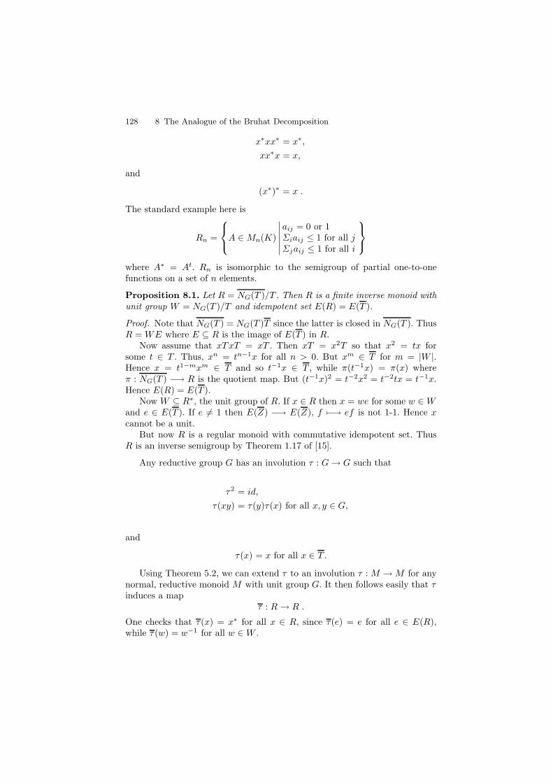
128 8 The Analogue of the Bruhat Decomposition
x∗xx∗ = x∗,
xx∗x = x,
and
(x∗)∗ = x .
The standard example here is
Rn =
A ∈Mn(K)
∣∣∣∣∣∣
aij = 0 or 1Σiaij ≤ 1 for all jΣjaij ≤ 1 for all i
where A∗ = At. Rn is isomorphic to the semigroup of partial one-to-onefunctions on a set of n elements.
Proposition 8.1. Let R = NG(T )/T . Then R is a finite inverse monoid withunit group W = NG(T )/T and idempotent set E(R) = E(T ).
Proof. Note that NG(T ) = NG(T )T since the latter is closed in NG(T ). ThusR = WE where E ⊆ R is the image of E(T ) in R.
Now assume that xTxT = xT . Then xT = x2T so that x2 = tx forsome t ∈ T . Thus, xn = tn−1x for all n > 0. But xm ∈ T for m = |W |.Hence x = t1−mxm ∈ T and so t−1x ∈ T , while π(t−1x) = π(x) whereπ : NG(T ) −→ R is the quotient map. But (t−1x)2 = t−2x2 = t−2tx = t−1x.Hence E(R) = E(T ).
Now W ⊆ R∗, the unit group of R. If x ∈ R then x = we for some w ∈ Wand e ∈ E(T ). If e 6= 1 then E(Z) −→ E(Z), f 7−→ ef is not 1-1. Hence xcannot be a unit.
But now R is a regular monoid with commutative idempotent set. ThusR is an inverse semigroup by Theorem 1.17 of [15].
Any reductive group G has an involution τ : G→ G such that
τ2 = id,
τ(xy) = τ(y)τ(x) for all x, y ∈ G,
and
τ(x) = x for all x ∈ T .
Using Theorem 5.2, we can extend τ to an involution τ : M →M for anynormal, reductive monoid M with unit group G. It then follows easily that τinduces a map
τ : R→ R .
One checks that τ(x) = x∗ for all x ∈ R, since τ(e) = e for all e ∈ E(R),while τ (w) = w−1 for all w ∈W .
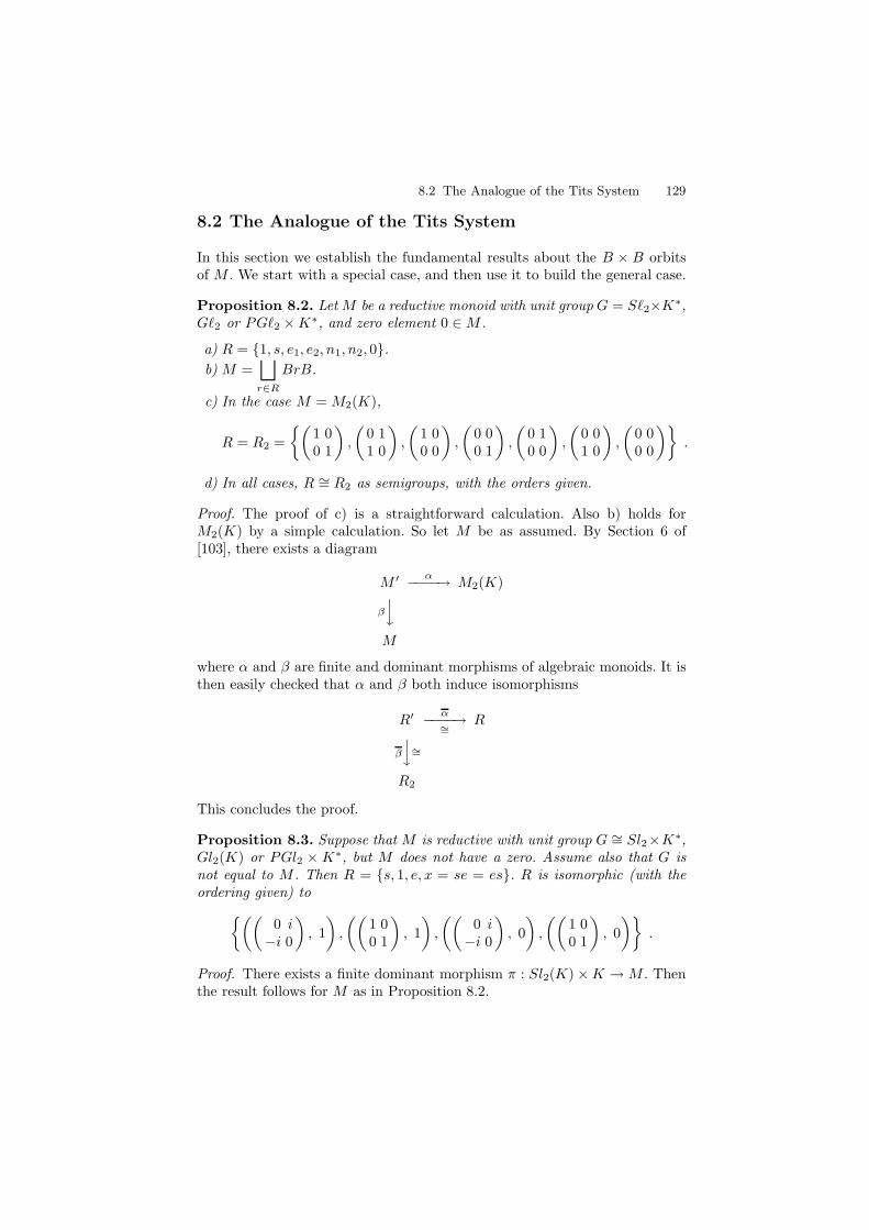
8.2 The Analogue of the Tits System 129
8.2 The Analogue of the Tits System
In this section we establish the fundamental results about the B × B orbitsof M . We start with a special case, and then use it to build the general case.
Proposition 8.2. Let M be a reductive monoid with unit group G = S`2×K∗,
G`2 or PG`2 ×K∗, and zero element 0 ∈M .
a) R = 1, s, e1, e2, n1, n2, 0.
b) M =⊔
r∈R
BrB.
c) In the case M = M2(K),
R = R2 =
(1 00 1
),
(0 11 0
),
(1 00 0
),
(0 00 1
),
(0 10 0
),
(0 01 0
),
(0 00 0
).
d) In all cases, R ∼= R2 as semigroups, with the orders given.
Proof. The proof of c) is a straightforward calculation. Also b) holds forM2(K) by a simple calculation. So let M be as assumed. By Section 6 of[103], there exists a diagram
M ′ α−−−−→ M2(K)
β
y
M
where α and β are finite and dominant morphisms of algebraic monoids. It isthen easily checked that α and β both induce isomorphisms
R′ α−−−−→
∼=R
β
y∼=
R2
This concludes the proof.
Proposition 8.3. Suppose that M is reductive with unit group G ∼= Sl2×K∗,
Gl2(K) or PGl2 × K∗, but M does not have a zero. Assume also that G is
not equal to M . Then R = s, 1, e, x = se = es. R is isomorphic (with theordering given) to
((0 i−i 0
), 1
),
((1 00 1
), 1
),
((0 i−i 0
), 0
),
((1 00 1
), 0
).
Proof. There exists a finite dominant morphism π : Sl2(K)×K →M . Thenthe result follows for M as in Proposition 8.2.
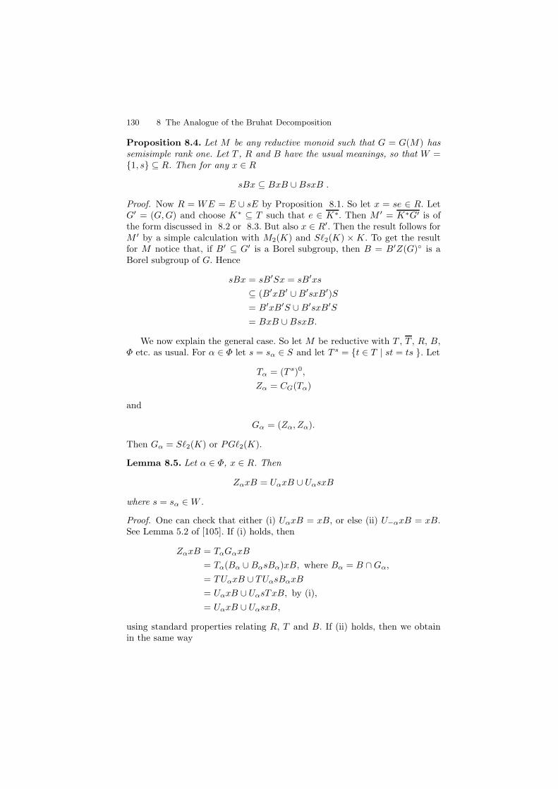
130 8 The Analogue of the Bruhat Decomposition
Proposition 8.4. Let M be any reductive monoid such that G = G(M) hassemisimple rank one. Let T , R and B have the usual meanings, so that W =1, s ⊆ R. Then for any x ∈ R
sBx ⊆ BxB ∪BsxB .
Proof. Now R = WE = E ∪ sE by Proposition 8.1. So let x = se ∈ R. LetG′ = (G,G) and choose K∗ ⊆ T such that e ∈ K∗. Then M ′ = K∗G′ is ofthe form discussed in 8.2 or 8.3. But also x ∈ R′. Then the result follows forM ′ by a simple calculation with M2(K) and S`2(K) ×K. To get the resultfor M notice that, if B′ ⊆ G′ is a Borel subgroup, then B = B′Z(G) is aBorel subgroup of G. Hence
sBx = sB′Sx = sB′xs
⊆ (B′xB′ ∪B′sxB′)S
= B′xB′S ∪B′sxB′S
= BxB ∪BsxB.
We now explain the general case. So let M be reductive with T , T , R, B,Φ etc. as usual. For α ∈ Φ let s = sα ∈ S and let T s = t ∈ T | st = ts . Let
Tα = (T s)0,
Zα = CG(Tα)
and
Gα = (Zα, Zα).
Then Gα = S`2(K) or PG`2(K).
Lemma 8.5. Let α ∈ Φ, x ∈ R. Then
ZαxB = UαxB ∪ UαsxB
where s = sα ∈ W .
Proof. One can check that either (i) UαxB = xB, or else (ii) U−αxB = xB.See Lemma 5.2 of [105]. If (i) holds, then
ZαxB = TαGαxB
= Tα(Bα ∪BαsBα)xB, where Bα = B ∩Gα,
= TUαxB ∪ TUαsBαxB
= UαxB ∪ UαsTxB, by (i),
= UαxB ∪ UαsxB,
using standard properties relating R, T and B. If (ii) holds, then we obtainin the same way
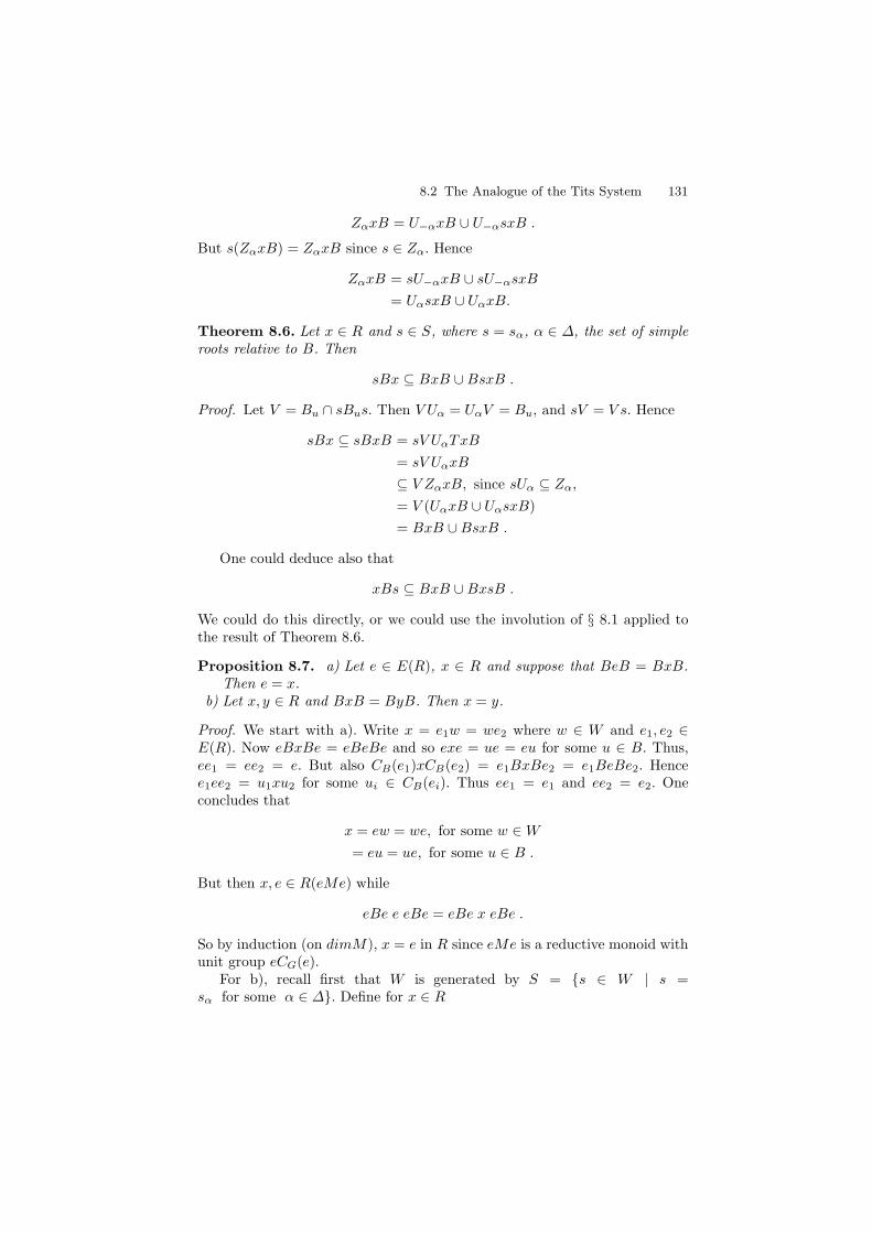
8.2 The Analogue of the Tits System 131
ZαxB = U−αxB ∪ U−αsxB .
But s(ZαxB) = ZαxB since s ∈ Zα. Hence
ZαxB = sU−αxB ∪ sU−αsxB
= UαsxB ∪ UαxB.
Theorem 8.6. Let x ∈ R and s ∈ S, where s = sα, α ∈ ∆, the set of simpleroots relative to B. Then
sBx ⊆ BxB ∪BsxB .
Proof. Let V = Bu ∩ sBus. Then V Uα = UαV = Bu, and sV = V s. Hence
sBx ⊆ sBxB = sV UαTxB
= sV UαxB
⊆ V ZαxB, since sUα ⊆ Zα,
= V (UαxB ∪ UαsxB)
= BxB ∪BsxB .
One could deduce also that
xBs ⊆ BxB ∪BxsB .
We could do this directly, or we could use the involution of § 8.1 applied tothe result of Theorem 8.6.
Proposition 8.7. a) Let e ∈ E(R), x ∈ R and suppose that BeB = BxB.Then e = x.
b) Let x, y ∈ R and BxB = ByB. Then x = y.
Proof. We start with a). Write x = e1w = we2 where w ∈ W and e1, e2 ∈E(R). Now eBxBe = eBeBe and so exe = ue = eu for some u ∈ B. Thus,ee1 = ee2 = e. But also CB(e1)xCB(e2) = e1BxBe2 = e1BeBe2. Hencee1ee2 = u1xu2 for some ui ∈ CB(ei). Thus ee1 = e1 and ee2 = e2. Oneconcludes that
x = ew = we, for some w ∈W
= eu = ue, for some u ∈ B .
But then x, e ∈ R(eMe) while
eBe e eBe = eBe x eBe .
So by induction (on dimM), x = e in R since eMe is a reductive monoid withunit group eCG(e).
For b), recall first that W is generated by S = s ∈ W | s =sα for some α ∈ ∆. Define for x ∈ R
132 8 The Analogue of the Bruhat Decomposition
`(x) = min` | x = ρ1 · · · · · ρ`e, for some e ∈ ER, si ∈ S .
This is not the usual length function on R (as in Definition 8.17 below), but itis useful in this situation. Our proof, imitating Theorem 29.2 of [40], proceedsby induction on m = `(x) ≤ `(y); the case m = 0 being part (a) above. Soassume that 1 ≤ `(x) ≤ `(y) and BxB = ByB. Write x = sx∗, s ∈ S and`(x∗) = `(x)− 1. Then
xB = sx∗B ⊆ ByB .
But thenx∗B ⊆ sByB ⊆ ByB ∪BsyB by 8.6.
Hence, either x∗B ⊆ ByB or else x∗B ⊆ BsyB.The former case is not possible by the induction hypothesis since `(x∗) <
`(x) ≤ `(y). But in the latter case, we must have x∗ = sy, again by induction.But then x = sx∗ = s2y = y.
Theorem 8.8. M =⊔
x∈R
BxB a disjont union.
Proof. We know that the union is disjoint from Proposition 8.7. Let L =⊔
x∈R
BxB. We show that GLG = L. Now G =⊔
w∈W
BwB, and so it suffices
to show that BwBL ⊆ L, for each w ∈ W . Write w = vs where s ∈ S and`(w) = `(v) + 1. `(·) is the usual length function on W . Now
BwBL = BwB(tBxB)
= BvB(tsBxB)
⊆ BvB(t(BxB ∪BsxB)), by Theorem 8.6,
= BvBL
⊆ L by induction on length.
Similarly, LG = L by the comment following Theorem 8.6. But GE(R)G = Mand so L = M .
8.3 Row Reduced Echelon Form
The most important technique in linear algebra is the Gauss-Jordan algo-rithm: given any m× n matrix A we obtain a matrix GJ(A), in row reducedechelon form, by a procedure known as row-reduction. In the case m = n, theprocedure solves the orbit classification problem for the action
G`n(K)×Mn(K) −→Mn(K) ,
(g,A) 7−→ gA .
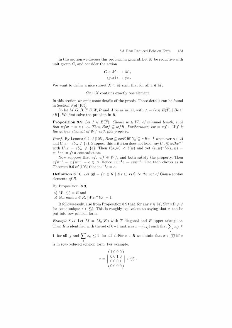
8.3 Row Reduced Echelon Form 133
In this section we discuss this problem in general. Let M be reductive withunit group G, and consider the action
G×M −→ M ,
(g, x) 7−→ gx .
We want to define a nice subset X ⊆M such that for all x ∈M ,
Gx ∩X contains exactly one element.
In this section we omit some details of the proofs. Those details can be foundin Section 9 of [105].
So let M,G,B, T, S,W,R and Λ be as usual, with Λ = e ∈ E(T ) | Be ⊆eB. We first solve the problem in R.
Proposition 8.9. Let f ∈ E(T ). Choose w ∈ W , of minimal length, suchthat wfw−1 = e ∈ Λ. Then Bwf ⊆ wfB. Furthermore, ew = wf ∈ Wf isthe unique element of Wf with this property.
Proof. By Lemma 9.2 of [105], Bew ⊆ ewB iff Uα ⊆ wBw−1 whenever α ∈ ∆
and Uαe = eUα 6= e. Suppose this criterion does not hold: say Uα * wBw−1
with Uαe = eUα 6= e. Then `(sαw) < `(w) and yet (sαw)−1e(sαw) =w−1ew = f : a contradiction.
Now suppose that vf, wf ∈ Wf , and both satisfy the property. Thenvfv−1 = wfw−1 = e ∈ Λ. Hence vw−1e = evw−1. One then checks as inTheorem 9.6 of [105] that vw−1e = e.
Definition 8.10. Let GJ = x ∈ R | Bx ⊆ xB be the set of Gauss-Jordanelements of R.
By Proposition 8.9,
a) W · GJ = R andb) For each x ∈ R, |Wx ∩ GJ| = 1.
It follows easily, also from Proposition 8.9 that, for any x ∈M ,Gx∩rB 6= φfor some unique r ∈ GJ. This is roughly equivalent to saying that x can beput into row echelon form.
Example 8.11. Let M = Mn(K) with T diagonal and B upper triangular.
Then R is identified with the set of 0−1 matrices x = (xij) such that∑
i
xij ≤
1 for all j and∑
j
xij ≤ 1 for all i. For x ∈ R we obtain that x ∈ GJ iff x
is in row-reduced echelon form. For example,
x =
1 0 0 00 0 1 00 0 0 10 0 0 0
∈ GJ .
134 8 The Analogue of the Bruhat Decomposition
We can identify GJ with E(T ) using Proposition 8.9.Given f ∈ E(T ) there is a unique r ∈ Wf ∩ GJ. In the above example, x
corresponds to
1 0 0 00 0 0 00 0 1 00 0 0 1
∈ E(D4) .
We return to our task.
Definition 8.12. Let M be reductive with B, T,R as usual. An element x ∈M is in reduced form if
(a) x ∈ rB for some r ∈ B;(b) xr∗ ∈ Λ where r∗ ∈ R is the inverse of r.
Said differently, if r = wf ∈ GJ and x = wfu with u ∈ Bu, then fuf = f .In the classical situation, (a) says that x is in row echelon form and (b)
says (roughly) that it is reduced.
Theorem 8.13. Let x ∈ M . Then Gx ∩ rB 6= φ for some unique r ∈ GJ.Furthermore, there is a unique T -orbit in Gx ∩ rB consisting of elements inreduced form.
Proof. (Sketch) The first part has already been proved. So assume that x ∈rB. Then we can write
x = wfy, where r = wf , and y ∈ U .
But we can writeU = U1U2
where
U1 =∏
α∈A
Uα, A = α ∈ Φ+ | Uαe = eUα 6= e
U2 =∏
α∈B
Uα, B = α ∈ Φ+ | eUαe = e.
Hence
x = wfy
= wfuv, where u ∈ U1, v ∈ U2,
= uwfv .
One checks that uw ∈ U and also that wfv = (uw)−1x is reduced.To show uniqueness of wfv up to T -orbit, assume that x1, x2 ∈ rB are
both in reduced form with gx1 = x2. One then shows that gx1 = bx1 = x2 forsome b = tu ∈ B = TU . It then follows that ux1 = x1. Hence x2 = tx1. SeeLemma 9.9 of [105].
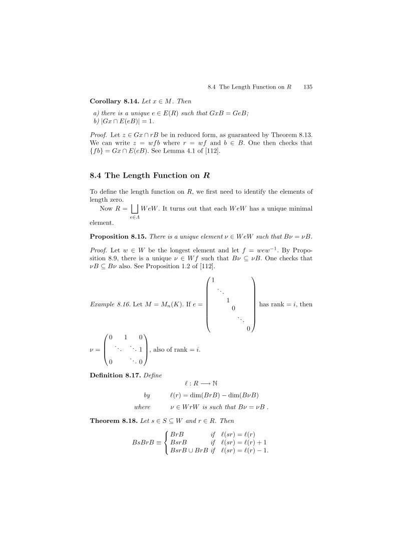
8.4 The Length Function on R 135
Corollary 8.14. Let x ∈M . Then
a) there is a unique e ∈ E(R) such that GxB = GeB;b) |Gx ∩ E(eB)| = 1.
Proof. Let z ∈ Gx ∩ rB be in reduced form, as guaranteed by Theorem 8.13.We can write z = wfb where r = wf and b ∈ B. One then checks thatfb = Gx ∩ E(eB). See Lemma 4.1 of [112].
8.4 The Length Function on R
To define the length function on R, we first need to identify the elements oflength zero.
Now R =⊔
e∈Λ
WeW . It turns out that each WeW has a unique minimal
element.
Proposition 8.15. There is a unique element ν ∈ WeW such that Bν = νB.
Proof. Let w ∈ W be the longest element and let f = wew−1. By Propo-sition 8.9, there is a unique ν ∈ Wf such that Bν ⊆ νB. One checks thatνB ⊆ Bν also. See Proposition 1.2 of [112].
Example 8.16. Let M = Mn(K). If e =
1. . .
10
. . .
0
has rank = i, then
ν =
0 1 0. . .
. . . 1
0. . . 0
, also of rank = i.
Definition 8.17. Define` : R −→ N
by `(r) = dim(BrB) − dim(BνB)
where ν ∈WrW is such that Bν = νB .
Theorem 8.18. Let s ∈ S ⊆W and r ∈ R. Then
BsBrB ≡
BrB if `(sr) = `(r)BsrB if `(sr) = `(r) + 1BsrB ∪BrB if `(sr) = `(r)− 1.
136 8 The Analogue of the Bruhat Decomposition
Proof. By Theorem 8.6 there are the three possibilities. If BsBrB = BrBthen, by Proposition 8.7, sr = r. Thus `(sr) = `(r).
Suppose BsBrB = BsrB. So sBrB ⊆ BsrB and thus `(sr) ≥ `(r).But BsBrB = UαsBrB for some unique α ∈ ∆. Thus `(sr) ≤ `(r) + 1. If`(sr) = `(r) then we obtain sBrB = BsrB, and so sr = r. If BsBrB = BsrBand sr 6= r then we obtain `(sr) = `(r) + 1.
Suppose that BsBνB = BrB∪BsrB and sr 6= r. Then BsBrB = (BsB∪B)rB = PαrB. One then gets that
BrB = Bs(B\V )rB
where V = Ru(Pα). Hence V ⊆ B is the unique closed, normal unipotentsubgroup of B such that sV = V s and V Uα = UαV = B. Hence BsrB ⊆ BrBand thus `(sr) < `(r). One then gets `(sr) = `(r) − 1. See Theorem 1.4 [112]for more details.
Example 8.19. Let M = Mn(K), where K is a finite field. Then M =⊔
x∈Rn
BxB where Rn is the standard example of § 8.1. In [127], Solomon proves
8.15 and 8.18 for this M . He also defines a length function that agrees withthe one in Definition 8.17. He then defines the analogue of Iwahori’s Heckealgebra as follows:
H(M,B) =⊕
x∈Rn
Z · Tx
with multiplication defined by
TsTx =
qTx , `(sx) = `(x)Tsx , `(sx) = `(x) + 1qTsx + (q − 1)Tx , `(sx) = `(x) − 1
TxTs =
qTx , `(xs) = `(x)Txs , `(xs) = `(x) + 1qTxs + (q − 1)Tx , `(xs) = `(x) − 1
TνTx = q`(x)−`(νx)Tνx
TxTν = q`(x)−`(xν)Txν
where
ν =
0 1 0. . .
. . .
0. . .
. . . 10
.
8.5 Order-Preserving Elements of R 137
He then proves in Theorem 4.12 of [127] that H(M,B) is a ring, with thisdefinition. The delicate part here is obtaining integral structure constants.One suspects that his approach works in general. Putcha approached thisproblem systematically in [87].
In [129], Solomon has revisited the representation theory of Rn bringingout a rich blend of combinatorics and algebra.
8.5 Order-Preserving Elements of R
In this section we assess the relationship of elements of R to B, and obtainthe subset of order preserving elements. The standard example here is M =Mn(K), where R is identified with the set of 01 matrices with at most onenonzero entry in each row or column. An element r ∈ R is order preservingif the matrix obtained from r by deleting all the zero rows and all the zerocolumns is an identity matrix. The general definition is as follows.
Definition 8.20. Let O ⊆ R be the subset of elements r ∈ R with the property
rBr∗ ⊂ Brr∗
where r∗ ∈ R is the unique element satisfying rr∗r = r and r∗rr∗ = r∗. Anyelement with this property is called order preserving.
Lemma 8.21. a) If r, s ∈ O then rs ∈ O.b) W ∩O = 1.c) E(R) ⊆ O.d) If r ∈ O then rBr∗ ⊆ rr∗Brr∗.
Proof. a) Suppose that rBr∗ ⊆ Brr∗ and sBs∗ ⊆ Bss∗. Consider ss∗r∗ ∈R. Write ss∗ = e and r∗ = fσ−1. Then ss∗r∗ = efσ−1 = feσ−1 =fσ−1σeσ−1 = r∗(ss∗)σ. Now compute:
rsB(rs)∗ = rsBs∗r∗ ⊆ rBss∗r∗
= rBr∗(ss∗)σ ⊆ Brr∗(ss∗)σ
= Brss∗r∗ = B(rs)(rs)∗ .
b) Suppose that r ∈ W ∩ O. Then r∗ = r−1, and rBr∗ ⊆ Brr∗ impliesrBr−1 = B.
c) If e ∈ E(R) then, by Theorems 6.16 and 6.30 of [82], eBe∗ = eBe =eCB(e)e ⊆ Be = Bee∗.
d) Write r = eσ so that r∗ = σ−1e and rr∗ = e. Then rBr∗ ⊆ eM ∩Be. Butif be ∈ eM ∩Be then be = ex, and so ebe = ex = be. Hence be ∈ eBe. Weconclude finally that rBr∗ ⊆ eM ∩Be ⊆ eBe = rr∗Brr∗.
Corollary 8.22. The following are equivalent.
138 8 The Analogue of the Bruhat Decomposition
a) rBr∗ ⊆ Brr∗.b) rBr∗ ⊆ rr∗B.c) rBr∗ ⊆ rr∗Brr∗.
Proof. rr∗Brr∗ ⊆ Brr∗ ∩ rr∗B.
Recall now the involution τ : M →M . It has the following properties:
τ |T = id,
τ(B) = B−,
τ2 = id,
τ(xy) = τ(y)τ(x),
and
τ(r) = r∗, for all r ∈ R.
Recall also w ∈ W , the longest element. It satisfies wBw−1 = B−.
Proposition 8.23. Let O− = r ∈ R|rB−r∗ ⊆ B−rr∗ and let Ow =wrw−1 ∈ R|r ∈ O. Then O = O− = Ow.
Proof. Let r ∈ R. Then r ∈ O iff rBr∗ ⊆ Brr∗ iff τ(rBr∗) ⊂τ(Brr∗) iff rB−r∗ ⊆ rr∗B− iff rB−r∗ ⊆ B−rr∗ (by Corollary 8.22)iff r ∈ O−. Hence O = O−.
Again if r ∈ R, r ∈ Ow iff wrwB(wrw)∗ ⊆ Bwrw(wrw)∗ iff wrB−r∗w ⊆Bwrr∗w iff rB−r∗ ⊆ B−rr∗ iff r ∈ O−. Hence Ow = O−.
Proposition 8.24. Let O∗ = r∗|r ∈ O. Then O = O∗. In particular, O isan inverse monoid.
Proof. r ∈ O iff rBr∗ = rr∗Brr∗ iff r∗rBr∗r = r∗rr∗Brr∗r = r∗Br iff r ∈O∗. Hence O = O∗.
Lemma 8.25. Let eσ ∈ R. Then there exists c ∈ CW (e) such that ceσ ∈ O.In particular, ceσHeσ.
Proof. eBσe and eBe are Borel subgroups of He containing eT . Thus, thereexists c ∈ CW (e) such that c(eBσe)c−1 = eBe. But c(eBσe)c−1 = eBcσe andso ceσ = ecσ ∈ O.
Proposition 8.26. Let e, f ∈ E(R), eJf . Choose σ ∈ W of minimal lengthsuch that σ−1eσ = f , and let r = eσ. Then r ∈ O.
Proof. We proceed by induction on this minimal length l. If l = 0 then e = fand the result follows from Lemma 8.21(c). So assume that l = n+1. We canwrite eσ = eτρ where l(τ) = n = l(σ)−1. Now eτ ∈ O since, if ζ−1eζ = τ−1eτwith l(ζ) < l(τ), then (ζρ)−1e(ζρ) = σ−1eσ with l(ζρ) < l(σ), a contradiction.
8.5 Order-Preserving Elements of R 139
Also τ−1eτρ 6= ρτ−1eτ since otherwise τ−1eτ = σ−1eσ which contradicts theminimality of l(σ). So we show that τ−1eτ · ρ ∈ O. Then by Lemma 8.21(a)eτ · τ−1eτρ = eσ ∈ O. Hence let f = τ−1eτ . Then we have fρ 6= ρf . Nowρ = σα for some unique α ∈ 4 and there exists a closed subgroup V ⊆ B suchthat B = V Uα = UαV and Bρ = V U−α = U−αV . By Lemma 5.1 of [105] wehave that either fUα = f and U−αf = f or Uαf = f and fU−α = f.In either case fBf = fV f = fBρf . Hence fρ ∈ O.
Theorem 8.27. Suppose that r, s ∈ R, rHs, and r, s ∈ O. Then r = s.
Proof. Let r = eσ and s = ceσ where ce = ec. Then eBσe = eBe = eBcσe =c(eBσe)c−1. But then ce ∈ NHe(eT ) ∩ eBσe and hence ce = e.
There are other ways to characterize the elements of O.
Proposition 8.28. Let r = eσ = σf ∈ R. The following are equivalent:
a) r ∈ O,b) Br ∩ rB = eBr,c) Br ∩ rB = rBf ,d) eBr = rBf .
Proof. r ∈ O iff eBr ⊆ rB iff eBr ⊆ rB ∩ Br (since alwayseBr ⊆Br) iff eBr = rB ∩ Br (by an easy calculation). Similarily, (a) iff (c). ButBr ∩ rB = eBr ∩ rBf for any r ∈ R. Hence (b) iff (c).
Corollary 8.29. Let r ∈ O. Then l(r) = dim(Br) + dim(rB) − 2 dim(eBr).
Proof. Recall that l(r) = dim(BrB)−dim(BνB). But dim(BrB) = dim(Br)+dim(rB) − dim(Br ∩ rB) while, by Proposition 8.28, dim(Br ∩ rB) =dim(BνB).
Remark 8.30. Write r = eσ = σf ∈ R. Then
Br ∩ rB = eBr ∩ rBf
= eBeσ ∩ σfBf
= (eBe ∩ eBσe)σ.
This pictures the elements of O as those for which dim(Br ∩ rB) is maximal.
As usual we fix B ⊆ G a Borel subgroup and T ⊆ B a maximal torus.Recall from Proposition 8.15 that for each W ×W orbit J of R there exists aunique ν ∈ J such that Bν = νB. We now study the Green’s relations on Rand O. Let r, s ∈ R.
Theorem 8.31. Let r ∈ R. Then there exist unique elements r+, r−, r0 ∈ Rsuch that
a) r = r+r0r−
140 8 The Analogue of the Bruhat Decomposition
b) r0Hν, where νJr and Bν = νBc) r+Rr and r−Lrd) r+, r− ∈ O.
Proof. First suppose that, for r ∈ R, we have r = r+r0r− satisfying a)-(d). Ifalso r = s+s0s− then a), b) and c) imply that r+Hs+ and r−Hs−. But then,by Theorem 8.27, r+ = s+ and r− = s−. Hence r+ and r− are unique. Butthen r0 = r∗+rr
∗− and so r0 is also unique.
To establish existence, we count. Let ν = e0σ = σf0 ∈ J = WrW and let
A = x ∈ O|xLe0,
B = x ∈ O|xRf0
andC = x ∈ R|xHν.
By the above, the product map
A× C ×B →WrW = WνW
is injective.By Proposition 8.26 and Theorem 8.27 |A| = |E(J)| and |B| = |E(J)|,
while |C| = |Hν |, where Hν = C is the H-class of ν. Thus |A × C × B| =|E(J)|2|Hν |. To count up J we consider the map
ζ : WνW → E(J)× E(J)
ζ(σντ−1) = (σe0σ−1, τf0τ
−1). It is easy to check that ζ is well defined andsurjective, and all fibres have the same cardinality. But ζ−1(e0, f0) = Hν .Thus, |J | = |E(J)|2|Hν |.
8.6 The Adherence Order on R
Definition 8.32. Let x, y ∈ R. We say that x ≥ y if BxB ⊇ ByB. Clearly,(R,≤) is a poset.
This is the obvious generalization of the Bruhat-Chevalley order fromgroup theory to the case of reductive monoids. The main result of this sectionis the description of (R,≤) in terms of (Λ,≤) and (W,≤). Here,
e ≤ f in Λ if ef = fe = e,
andx ≤ y in W if BxB ⊆ ByB .
In section § 8.8 we go on to obtain a precise description of (R,≤) for M =Mn(K).
8.6 The Adherence Order on R 141
So, back to work: for e ∈ Λ, let
W (e) = CW (e)
W∗(e) = x ∈W (e) | xe = e CW (e)
D(e) = x ∈W | x has minimal length in xW (e)
D∗(e) ≡ x ∈W | x has minimal length in xWe.
Now if v ∈ R we can write
v = xey−1
where x, y ∈W . But we can also assume that y ∈ D(e). (by writing y = y0w,where w ∈W (e) and y0 ∈ D(e), so that v = xey−1 = xe(y0w)−1 = xwey−1
0 .)The following result is recorded in detail, in [73]. We indicate here the
main points of the proof.
Theorem 8.33. Let e, f ∈ Λ, x, s ∈ W , y ∈ D(e) and t ∈ D(f). Then thefollowing are equivalent.
a) xey−1 ≤ sft−1.b) ef = e and there exist w ∈ W (f)W∗(e) and z ∈ W∗(e) such that tw ≤ y
and x ≤ swz.
Proof. Assume that b) holds with w and z as indicated. Now twey ∈ B by(7) of [73]. Hence sfwey−1 = sft−1twey−1 ∈ sft−1B. Thus sfwey−1 ≤sft−1. By assumption w = w1w2 with w1 ∈ W (f) and w2 ∈ W∗(e).Hence sfwey−1 = sfw1w2ey
−1 = sfw1ey−1 = sw1fey
−1 = sw1ey−1 =
sw1w2ey−1 = swey−1. But from (6) of [73], xey−1 ≤ swzey−1. Hence
xey−1 ≤ swzey−1 = swey−1 = sfwey−1 ≤ sft−1 .
Conversely, assume that xey−1 ≤ sft−1. Clearly e ≤ f , and xey−1 ∈Bsft−1B. Hence e ∈ x−1Bsft−1By. Now there exists a unique w ∈ W suchthat
Aw = B−wB ∩ x−1Bs ⊆ x−1Bs
is open and dense. Thus,e ∈ Awft−1By .
From here we can get wfw−1e = e, and finally
w = w1w2 where w1 ∈W∗(e) and w2 ∈W (f) .
But we are not not quite there. There exists a unique u ∈ W such that
Cu = B−uB ∩ w2t−1By ⊆ w2t
−1By
is open and dense.
142 8 The Analogue of the Bruhat Decomposition
It turns out that condition b) is satisfied with
w = w−12 u ∈ W (f)W∗(e) ,
andz = u−1w−1
1 ∈ W∗(e) .
We can simplify the statement in the above theorem by using the followingdefinition.
Definition 8.34. Let a ∈ R. Then
a = xey−1
where e ∈ Λ, x ∈ D∗(e) and y ∈ D(e). We call this the normal form of a.
It easy easy to check that this expression for a is unique. For example, letM = M3(K). Then
Λ =
11
1
,
11
0
,
10
0
,
00
0
= e3, e2, e1, e0
andW = S3 .
Let
a =
0 1 00 0 01 0 0
.
Thena = (132)e2(1).
This is the normal form since
D∗(e2) = W and D(e2) = 1, (23), (123) .
Corollary 8.35. Let a = xey−1 and b = sft−1 be in normal form. Then thefollowing are equivalent:
a) a ≤ bb) e ≤ f and there exists w ∈W (f)W∗(e) such that x ≤ sw and tw ≤ y.
Proof. If b) is satisfied then so too is Theorem 8.33 b) with z = 1. Conversely,given Theorem 8.33 b), we have w ∈ W (f)W∗(e) and z ∈ We with tw ≤ yand x ≤ swz. But if x0 ∈ xW∗(e) is the element of minimal length then
x0 ≤ swγ for all γ ∈W∗(e). (1)
8.7 The j-order, R+ and Pennell’s Theorem 143
On the other hand,W (f) = W ∗(f)×W∗(f) whereW ∗(f) = 〈s ∈ S | sf = fs〉,while W∗(f) ⊆ W∗(e). Hence w ∈ W (f)W∗(e) implies that w = uv whereu ∈ W ∗(f) and v ∈ W∗(e). Let s0 ∈ xW∗(f) be the element of minimallength. Then
sw = s0µw , for some µ ∈W∗(f)= s0µuv= s0uµv , since Wf ⊆ CW (W ∗(f)) .
Hence sw ∈ s0wW∗(e) since µv ∈ W∗(e). Thus from (1) x0 ≤ s0w. Thus, b)is satisfied since x0ey
−1 (respectively, s0ft−1) is the normal form for xey−1
(resp. sft−1).
A special case of Corollary 8.35 has been obtained by Brion [12], Kato [46]and Springer [130], for the canonical monoid.
8.7 The j-order, R+ and Pennell’s Theorem
In this section we describe Pennell’s theorem. This is a decomposition the-orem for the adherence order on R. Unlike the situation of the Weyl group,we now have a principle of two types. The basic idea is easily described:we start with x, y ∈ R and assume x ≤ y. We then see that there existsx0, x2, . . . , xn ∈ R such that x = x0 < x2 <, . . . , < xn = y and `(y)−`(x) = n.Then `(xi+1) = `(xi) + 1. (That part is easy.) Pennell’s idea is to establishthe following dichotomy.
For each xi < xi+1 we have either
a) xi ∈ Bxi+1B, or elseb) xi+1 is obtained from xi via a “Bruhat interchange” (see Definition 8.41.
The key here is that, for each i, only one of a) and b) is true. The exactdefinition of b) will be given below. For Mn(K) it implies that xi and xi+1
have the same nonzero rows and columns. It is the natural generalization ofthe situation encountered in the Bruhat-Chevalley order on a Coxeter group[41]. The order relation of a) has no analogue in group theory. It was firststudied by Pennell [72].
Definition 8.36. a) Let x, y ∈ R. We write x ≤j y if BxB ⊆ ByB. Werefer to ≤j as the j-order on R.
b) DefineR+ = x ∈ R | BxB ⊆ B
= x ∈ R | x ≤ 1 .
Lemma 8.37. Let r = xey−1 ∈ R be in normal form. Then r ∈ R+ if andonly if x ≤ y.
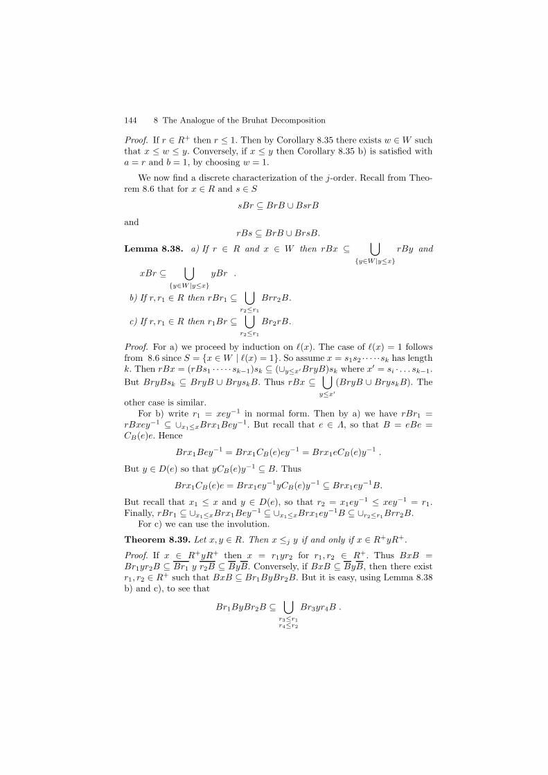
144 8 The Analogue of the Bruhat Decomposition
Proof. If r ∈ R+ then r ≤ 1. Then by Corollary 8.35 there exists w ∈W suchthat x ≤ w ≤ y. Conversely, if x ≤ y then Corollary 8.35 b) is satisfied witha = r and b = 1, by choosing w = 1.
We now find a discrete characterization of the j-order. Recall from Theo-rem 8.6 that for x ∈ R and s ∈ S
sBr ⊆ BrB ∪BsrB
andrBs ⊆ BrB ∪BrsB.
Lemma 8.38. a) If r ∈ R and x ∈ W then rBx ⊆⋃
y∈W |y≤x
rBy and
xBr ⊆⋃
y∈W |y≤x
yBr .
b) If r, r1 ∈ R then rBr1 ⊆⋃
r2≤r1
Brr2B.
c) If r, r1 ∈ R then r1Br ⊆⋃
r2≤r1
Br2rB.
Proof. For a) we proceed by induction on `(x). The case of `(x) = 1 followsfrom 8.6 since S = x ∈ W | `(x) = 1. So assume x = s1s2 · · · · ·sk has lengthk. Then rBx = (rBs1 · · · · · sk−1)sk ⊆ (∪y≤x′BryB)sk where x′ = si · . . . sk−1.
But BryBsk ⊆ BryB ∪ BryskB. Thus rBx ⊆⋃
y≤x′
(BryB ∪ BryskB). The
other case is similar.For b) write r1 = xey−1 in normal form. Then by a) we have rBr1 =
rBxey−1 ⊆ ∪x1≤xBrx1Bey−1. But recall that e ∈ Λ, so that B = eBe =
CB(e)e. Hence
Brx1Bey−1 = Brx1CB(e)ey−1 = Brx1eCB(e)y−1 .
But y ∈ D(e) so that yCB(e)y−1 ⊆ B. Thus
Brx1CB(e)e = Brx1ey−1yCB(e)y−1 ⊆ Brx1ey
−1B.
But recall that x1 ≤ x and y ∈ D(e), so that r2 = x1ey−1 ≤ xey−1 = r1.
Finally, rBr1 ⊆ ∪x1≤xBrx1Bey−1 ⊆ ∪x1≤xBrx1ey
−1B ⊆ ∪r2≤r1Brr2B.For c) we can use the involution.
Theorem 8.39. Let x, y ∈ R. Then x ≤j y if and only if x ∈ R+yR+.
Proof. If x ∈ R+yR+ then x = r1yr2 for r1, r2 ∈ R+. Thus BxB =Br1yr2B ⊆ Br1 y r2B ⊆ ByB. Conversely, if BxB ⊆ ByB, then there existr1, r2 ∈ R
+ such that BxB ⊆ Br1ByBr2B. But it is easy, using Lemma 8.38b) and c), to see that
Br1ByBr2B ⊆⋃
r3≤r1r4≤r2
Br3yr4B .
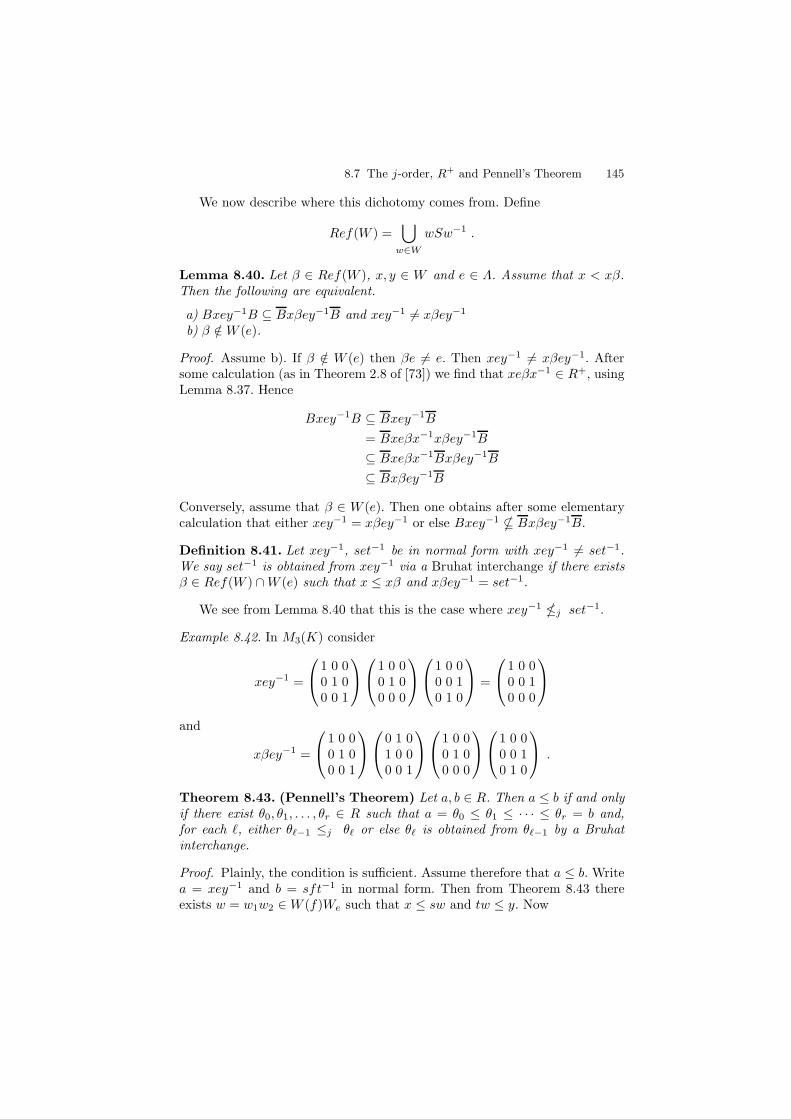
8.7 The j-order, R+ and Pennell’s Theorem 145
We now describe where this dichotomy comes from. Define
Ref(W ) =⋃
w∈W
wSw−1 .
Lemma 8.40. Let β ∈ Ref(W ), x, y ∈ W and e ∈ Λ. Assume that x < xβ.Then the following are equivalent.
a) Bxey−1B ⊆ Bxβey−1B and xey−1 6= xβey−1
b) β /∈W (e).
Proof. Assume b). If β /∈ W (e) then βe 6= e. Then xey−1 6= xβey−1. Aftersome calculation (as in Theorem 2.8 of [73]) we find that xeβx−1 ∈ R+, usingLemma 8.37. Hence
Bxey−1B ⊆ Bxey−1B
= Bxeβx−1xβey−1B
⊆ Bxeβx−1Bxβey−1B
⊆ Bxβey−1B
Conversely, assume that β ∈ W (e). Then one obtains after some elementarycalculation that either xey−1 = xβey−1 or else Bxey−1 * Bxβey−1B.
Definition 8.41. Let xey−1, set−1 be in normal form with xey−1 6= set−1.We say set−1 is obtained from xey−1 via a Bruhat interchange if there existsβ ∈ Ref(W ) ∩W (e) such that x ≤ xβ and xβey−1 = set−1.
We see from Lemma 8.40 that this is the case where xey−1 j set−1.
Example 8.42. In M3(K) consider
xey−1 =
1 0 00 1 00 0 1
1 0 00 1 00 0 0
1 0 00 0 10 1 0
=
1 0 00 0 10 0 0
and
xβey−1 =
1 0 00 1 00 0 1
0 1 01 0 00 0 1
1 0 00 1 00 0 0
1 0 00 0 10 1 0
.
Theorem 8.43. (Pennell’s Theorem) Let a, b ∈ R. Then a ≤ b if and onlyif there exist θ0, θ1, . . . , θr ∈ R such that a = θ0 ≤ θ1 ≤ · · · ≤ θr = b and,for each `, either θ`−1 ≤j θ` or else θ` is obtained from θ`−1 by a Bruhatinterchange.
Proof. Plainly, the condition is sufficient. Assume therefore that a ≤ b. Writea = xey−1 and b = sft−1 in normal form. Then from Theorem 8.43 thereexists w = w1w2 ∈W (f)We such that x ≤ sw and tw ≤ y. Now
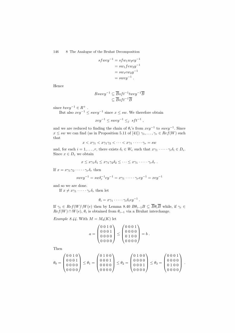
146 8 The Analogue of the Bruhat Decomposition
sfwey−1 = sfw1w2ey−1
= sw1few2y−1
= sw1ew2y−1
= swey−1 .
Hence
Bswey−1 ⊆ Bsft−1twey−1B
⊆ Bsft−1B
since twey−1 ∈ R+ .But also xey−1 ≤ swey−1 since x ≤ sw. We therefore obtain
xey−1 ≤ swey−1 ≤j sft−1 ,
and we are reduced to finding the chain of θi’s from xey−1 to swey−1. Sincex ≤ sw we can find (as in Proposition 5.11 of [41]) γ1, . . . , γr ∈ Ref(W ) suchthat
x < xγ1 < xγ1γ2 < · · · < xγ1 · · · · · γr = sw
and, for each i = 1, . . . , r, there exists δi ∈ We such that xγ1 · · · · · γiδi ∈ De.Since x ∈ De we obtain
x ≤ xγ1δ1 ≤ xγ1γ2δ2 ≤ · · · ≤ xγ1 · · · · · γrδr .
If x = xγ1γ2 · · · · · γrδr then
swey−1 = swδ−1r ey−1 = xγ1 · · · · · γrey
−1 = xey−1
and so we are done.If x 6= xγ1 · · · · · γrδr then let
θi = xγ1 · · · · · γiδiey−1 .
If γi ∈ Ref(W )\W (e) then by Lemma 8.40 Bθi−1B ⊆ BθiB while, if γi ∈Ref(W ) ∩W (e), θi is obtained from θi−1 via a Bruhat interchange.
Example 8.44. With M = M4(K) let
a =
0 0 1 00 0 0 10 0 0 00 0 0 0
≤
0 0 0 10 0 0 00 1 0 00 0 0 0
= b .
Then
θ0 =
0 0 1 00 0 0 10 0 0 00 0 0 0
≤ θ1 =
0 1 0 00 0 0 10 0 0 00 0 0 0
≤ θ2 =
0 1 0 00 0 0 00 0 0 10 0 0 0
≤ θ3 =
0 0 0 10 0 0 00 1 0 00 0 0 0
.
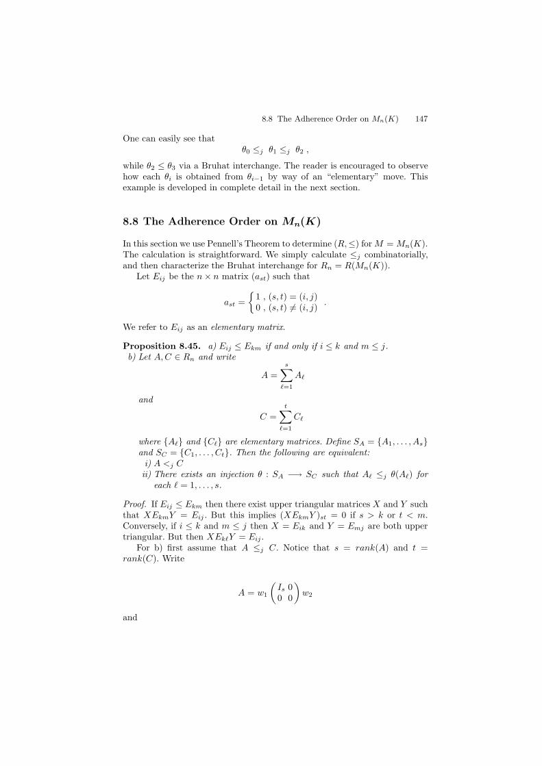
8.8 The Adherence Order on Mn(K) 147
One can easily see thatθ0 ≤j θ1 ≤j θ2 ,
while θ2 ≤ θ3 via a Bruhat interchange. The reader is encouraged to observehow each θi is obtained from θi−1 by way of an “elementary” move. Thisexample is developed in complete detail in the next section.
8.8 The Adherence Order on Mn(K)
In this section we use Pennell’s Theorem to determine (R,≤) forM = Mn(K).The calculation is straightforward. We simply calculate ≤j combinatorially,and then characterize the Bruhat interchange for Rn = R(Mn(K)).
Let Eij be the n× n matrix (ast) such that
ast =
1 , (s, t) = (i, j)0 , (s, t) 6= (i, j)
.
We refer to Eij as an elementary matrix.
Proposition 8.45. a) Eij ≤ Ekm if and only if i ≤ k and m ≤ j.b) Let A,C ∈ Rn and write
A =
s∑
`=1
A`
and
C =
t∑
`=1
C`
where A` and C` are elementary matrices. Define SA = A1, . . . , Asand SC = C1, . . . , Ct. Then the following are equivalent:
i) A <j Cii) There exists an injection θ : SA −→ SC such that A` ≤j θ(A`) for
each ` = 1, . . . , s.
Proof. If Eij ≤ Ekm then there exist upper triangular matrices X and Y suchthat XEkmY = Eij . But this implies (XEkmY )st = 0 if s > k or t < m.Conversely, if i ≤ k and m ≤ j then X = Eik and Y = Emj are both uppertriangular. But then XEk`Y = Eij .
For b) first assume that A ≤j C. Notice that s = rank(A) and t =rank(C). Write
A = w1
(Is 00 0
)w2
and
148 8 The Analogue of the Bruhat Decomposition
C = w3
(It 00 0
)w4 ,
where w1, w2, w3, w4 ∈ Sn, the unit group of Rn. Let x = w1w−13 and Y =
w−14
(Is 00 0
)w2. Then XCY = A, and one checks that, for each k = 1, . . . , t,
XCkY ≤j Ck
andXCkY ∈ SA ∪ 0.
Then define θ(A`) = Ck such that XCkY = A`.Conversely, given an injection θ : SA −→ SC such that A` ≤j θ(A`) for
i = 1, . . . , S, then from a) there exist elementary upper triangular matrices
X` and Y` such that X`θ(A`)Y` = A`. Let X =
s∑
`=1
A` and Y =
s∑
`=1
Y`. Then
XCY = A.
Proposition 8.46. Let A = Ei1j1 + · · ·+ Eisjs ∈ Rn and suppose
C = Ei1j1 + · · ·+ Eih−1ih−1+ Ei`j` + Eih+1jh+1
+ · · ·+ Ei`−1j`−1
+Eihjh + Ei`+1j`+1+ · · ·+ Eisjs
so that C is obtained from A by interchanging two nonzero rows. Relabel thetwo altered positions of A by Eij and Ek`. Then A < C if and only if i < kand j < ` or i > k and j > `.
Proof. First assume that s = 2. Then
A = (`−1 i)· · · ··(12)(k−1 h)· · · · ·(34)(23)E(23) . . . (`−1 `)(12)· · · ··(j−1 j) .
This is the normal form for A. One checks that
C = [(i− 1 i) · · · · · (12)(k − 1 h) · · · · · (34)(23)(12)]
. . . E(23) · · · · · (`− 1 `)(12) · · · · · (j − 1 j) .
But (i − 1 i) · · · · · (23) < (i − 1 i) · · · · · (23)(12) and so A < C. Conversely,if i < k and j > ` or i > k and j < ` then the same argument shows thatC < A.
The proof of the general case (s > 2) is similar.
Proposition 8.46 describes the situation of a Bruhat interchange forMn(K). It says that A < C via a Bruhat interchange if and only if
a) C is obtained from A by interchanging two non-zero rows of A.
b) In the process of a), a 2× 2 submatrix
(1 00 1
)of A ends up as
(0 11 0
).
8.8 The Adherence Order on Mn(K) 149
Theorem 8.47. Let x, y ∈ Rn and assume that x ≤ y with `(x) = `(y) − 1.Then one of the following holds.
a) x is obtained from y by setting some nonzero entry of y to zero.b) x is obtained from y by moving a nonzero entry either upward or to the
right.c) y is obtained from x via a Bruhat interchange.
Proof. Assume that c) is not the case and rank(x) < rank(y). Then by The-orem 8.43 and Proposition 8.45 there is an injection θ : Sx −→ Sy such thatxi ≤ θ(xi) for each xi ∈ Sx. So define θ(x) ∈ Rn by Sθ(x) = θ(Sx). Thenx ≤ θ(x) < y. Thus x = θ(x), and so a) holds.
Now assume that c) is not the case, and rank(x) = rank(y). By Pennell’sTheorem x ≤j y, and so there exist a, b ∈ R+ such that x = ayb. Thenx = ayb ≤ yb ≤ b. Hence, either x = yb or else yb = b. In the first case x = yb,and in the second case x = ay. Assume without loss of generality that x = yb(x and y have the same nonzero rows). An elementary argument shows thatx is obtained from y by moving some nonzero entry of y to the right. Thus b)holds.
Theorem 8.47 allows us to give a combinatorial description of the adher-ence order on Rn. First we represent the elements of Rn by sequences of non-negative integers. Given x ∈ Rn we associate with x a sequence (ε1, ε2, . . . , εn)where for each i, 1 ≤ i ≤ n,
εi =
0 if x has all zeros in the ith columnj if xji = 1 .
For example,
0 0 0 00 0 0 11 0 0 00 0 1 0
corresponds to (3042). Notice that a sequence
(ε1, ε2, . . . , εn) occurs this way for some x ∈ Rn if and only if 0 ≤ εi ≤ nfor each i; and whenever εi = εj , either i = j or else εi = εj = 0.
Theorem 8.48. Let x = (δ1, . . . , δn), y = (ε1, . . . , εn) ∈ Rn. Then ≤ is thesmallest partial order on Rn generated by declaring x < y if either
a) δj = εj for j 6= i and δi < εi, orb) i) δk = εk if k 6∈ i, j
ii) i < jiii) δi = εj, δj = εi and εi > εj.
From Theorem 8.47 we have three possibilities. We indicate how each onefits into the different possibilities of Theorem 8.48.
Proof. Theorem 8.47 a) falls under part a), since we can take δi = 0.
150 8 The Analogue of the Bruhat Decomposition
Theorem 8.47 b) falls under part b) if x and y have the same nonzero rows;and under part a) if they have the same nonzero columns.
Theorem 8.47 c) is the special case of part b) where both εi and εj arenonzero.
Example 8.49. Let x = (21403) and y = (35201) in R5. Then x < y since
(21403) < (31402) , by 8.48b)
< (34102) , by 8.48b)
< (35102) , by 8.48a)
< (35201) , by 8.48b) .
8.9 Exercises
1. Give an explicit description, for Mn(K), of each of the following objects:Λ,R,E(T ), Φ,B, T, PI .
2. Let M be reductive with zero, and let x ∈ M,x 6= 0. Prove there existe, f ∈ E1(T ) such that exf 6= 0.
3. Let M be reductive. Prove that
M =⊔
e∈E(T )
GeB.
4. For the inverse semigroup S recall the natural order ≤ on S: we say thatx ≤ y if there exist e, f ∈ E(S) such that ey = yf = x. Let M bereductive, and let N = NG(T ). Prove that x ≤ y in N , for the naturalorder, if and only if x ∈ yT .
5. Let R+ be the image of B ∩NG(T ) in R. Prove that R+ is J-trivial. i.e.for x, y ∈ R+, xJy if and only if x = y.
6. Assume that M is reductive, and let λ : K∗ →M be a morphism. Definew : M → Aut(M) by w(t)(x) = txt−1. Let M0 = x ∈ M |w(t)(x) = xand letM+ = x ∈M | limt→0w(t)(x) exists in M.a) Find an example where M0 is not irreducible.b) Prove that M+ contains a Borel subgroup of M .c) Prove that M0 and M+ are submonoids of M .d) Prove that ψ : M+ → M0, ψ(x) = limt→0w(t)(x) is a surjective
morphism of algebraic monoids.e) Let B0 ⊆ CG(λ) be a Borel subgroup. Prove that B0\M0/B0 is finite.
Can you identify the orbits?7. Let M be semisimple, and let H ⊆ G be a torus. Let Z ⊆ G be the
connected center of G. Let M∗ = x ∈ M | xH ⊆ Zx . Notice that M∗
is closed in M .
8.9 Exercises 151
a) Let e ∈ E(M∗) = E(M) ∩M∗. Prove that there exists f ∈ E(M∗),fLe, such that sf = fs for all s ∈ H . Hint: H ⊆ ClG(e).
b) Let Λ ⊆ E(T ) ⊆ CG(H) be a cross section lattice. Prove that M∗ =⋃f∈Λ∗ GfCG(H), where Λ∗ = Λ ∩M∗. Hint: use Exercise 6 above.
8. Let M be a reductive monoid with zero and assume that M has theproperty that
Λ(B, T ) =: e ∈ E(T ) | Be ⊆ eB = f ∈ E(T ) | f ≥ e0 ∪ 0
for some e0 ∈ E1(T ). Prove that R has the following property: for anyx ∈ R, either x2 = 0 or else xHe for some idempotent e ∈ E(R).
9. Let M be reductive, and let x ∈M be an element of some minimal J-classof M . Prove that, for some maximal torus T of M , xT = Tx.
10. Let M be reductive, and let x ∈ M be such that xT = Tx for somemaximal torus T of M . Prove that x ∈ NG(T ).
11. Let M = Mn(K). Prove that R has the following property: if e ≤ f < 1are idempotents of R, then there exists r ∈ R such that rs = e for somes > 0, and r is R-related to f .
12. Let G be a connected, solvable group acting on an irreducible, affine va-riety X . Suppose that there are a finite number of orbits. Let O be theset of G-orbits on X . Define x ≤ y, if x ⊆ y. Prove that O is a rankedposet; i.e. any two maximal chains from x to y have the same length. Thisapplies, in particular, to the Bruhat decomposition of a reductive monoid.
13. Let e ∈ E(T ), T ∈ B. Prove that BeB ∩He = CB(e)e, where He is theH-class of e in M .
14. Let M be irreducible with unit group G, e ∈ E(T ), T ∈ B. Let U be theunipotent radical of CB(e). Define U1 = < Uα | eUα = Uαe 6= e >and U2 = < Uα | eUα = Uαe = e >. Define ψ : U1 × U2 → U , byψ(a, b) = ab. Prove that ψ is an isomorphism of groups.
15. Let M be reductive, and let B ⊆ G be a Borel subgroup of G. Let J be aregular J-class of B. Define J∗ = a ∈ M | aHx for some x ∈ J . Provethat J∗ = BHeB, where He is the H-class of e in M .
16. Let M be reductive and let e ∈ E(T ). Prove that
dim(GeG) = |Φ| − |α ∈ Φ | sαe = esα = e |+ dim(eT ).
Hint: BeB− ⊆ GeG is open for appropriate, opposite Borel subgroupscontaining T . So compute dim(BeB−).
17. Let M be reductive with zero. Define rank(x)=dim(xT ) for xT ∈ R. Fore ∈ E1(T ), define χe : T → eT ∼= K by χe(z) = ez. Assume that M has aunique minimal nonzero J-class. Define a bijection between the rank-oneelements of R and s(χe)− χe | e ∈ E1(T ), s ∈W\0.

9
Representations and Blocks of AlgebraicMonoids
The ultimate mathematical dictionary might define the theory of algebraicmonoids as a branch of algebra that determines the content of mathematicalproblems relating convexity and positivity to representation theory. We canregard this imaginary definition as the major theme of this chapter. What Iwant to do here is provide the reader with a self-contained overview of whatis known about algebraic monoids and their finite dimensional representa-tions. In the first section we discuss normal, reductive monoids. Here we findthat there is a perfect analogue of many results about reductive groups. Inparticular, we obtain the desired relationship between the set of irreduciblerepresentations of M and the adjoint quotient of M .
In the next section we focus on the special properties of a normal, reductivemonoid M in characteristic p > 0. The results here are largely due to S.Doty. We find that K[M ] has a good filtration in the sense of Donkin [24].Furthermore, the category of rational M -monoids is a highest weight categoryin the sense of Cline, Parshall and Scott [16].
In the last two sections we study the blocks of an algebraic monoid. Blocksare often better behaved for monoids than they are for groups. We discuss theblocks of monoids in two contrasting situations; solvable monoids with zero,and M = Mn(K) when char(K) = p > 0. The blocks of a solvable monoidwere studied by the author in [113]. The blocks of Mn(K) were calculated byS. Donkin in [25].
9.1 Conjugacy Classes and Adjoint Quotient
Semisimple elements play an important role in the representation theory ofreductive groups. The most fundamental results relate the conjugacy classesof semisimple elements to the characters of irreducible representations, via thering of class functions on the adjoint quotient. In this section we discuss theanalgous results for normal reductive monoids.
154 9 Representations and Blocks of Algebraic Monoids
Let M be an irreducible normal, algebraic monoid. An element x ∈ M issemisimple if ρ(x) ∈ Mn(K) is diagonalizable for any rational representationρ : M −→Mn(K) of M .
Proposition 9.1. Let M be irreducible. The following are equivalent.
a) x ∈M is semisimple.b) x ∈ T for some maximal torus T ⊆ G.
Proof. b) clearly implies a). So assume a). Assume that M ⊆ Mn(K) as aclosed submonoid. Then x ∈ Mn(K) is diagonalizable, and it follows easilythat x ∈ He, the unit group of eMe, for some idempotent e ∈ M . But x issemisimple in this reductive group and so x ∈ S where S ⊆ He is a maximaltorus. However, any maximal torus S of He is of the form S = eT for somemaximal torus T ⊆ CG(e). But eT ⊆ T . Then x ∈ S = eT ⊆ T .
Theorem 9.2. Suppose that M is reductive and x ∈ M . Then the followingare equivalent.
a) x is semisimple.b) x ∈ T for some maximal torus T of G.c) C`(x), the conjugacy class of x, is closed in M .
Proof. Suppose x ∈ T . Then txt−1 = x for t ∈ T . Thus, by 2.13, Corollary 1of [134], C`(x) ⊆M is closed.
Conversely, assume that C`(x) ⊆ M is closed. We assume also that Mhas a zero element. The general case follows easily from this. By [62] thecategorical quotient π : M −→ X of M by G ×M −→ M , (g, x) 7−→ gxg−1,exists and induces a one-to-one correspondence between the closed orbits ofM and the points of X . Consider
π | T : T −→ X .
If π(z) = π(y) then gyg−1 = z for some g. But g−1Tg and T are bothcontained in CG(y)0. Hence there exists h ∈ CG(y)0 such that hg−1Tgh−1 =T . But then hg−1 ∈ NG(T ) while (hg−1)−1g hg−1 = gyg−1 = z. Thus π|Tinduces an injective map
θ : T/W −→ X
where W = NG(T )/T . On the other hand θ is known to be birational byCorollary 2 of [134]. Hence θ is an open embedding, topologically. Since M hasa zero, T/W and X are cones. It follows that θ is a finite bijective morphism.If M is normal then so is X , and thus θ is an isomorphism by Theorem 2.29.
Recall now the element x ∈ M with C`(x) ⊆ M closed. By the above,π(x) = π(y) for some y ∈ T . But π separates closed orbits and so C`(x) =C`(y).
9.1 Conjugacy Classes and Adjoint Quotient 155
Corollary 9.3. Suppose that M is reductive and let T ⊆ G be a maximaltorus. Then
CM (T ) = x ∈M | xt = tx for all t ∈ T
= T .
Proof. If x ∈ CM (T ) then C`(x) ⊆ M is closed and so, by Theorem 9.2, xis semisimple. It is then possible to find a Borel subgroup B ⊆ G such thatT ∪ x ⊆ B. From there we embed B in Tn(K) as a closed submonoid. Itfollows from Proposition 15.4 [40] that T ∪ x is contained in a maximaltorus of Tn(K). Hence T ∪ x ⊆ Tn(K) −→
πDn(K) is injective, where π is
the projection to the diagonal. But from Theorem 6.1, π|B factors throughthe universal morphism of B to a D-monoid θ : B −→ T and thus x ∈ T .
Corollary 9.4. Let π : M −→ X be the categorical quotient induced by con-jugation of G on M . Then in the following diagram θ is an isomorphism:
T → Myyπ
T/W −→θ
X .
Proof. This is included in the proof of Theorem 9.2.
Example 9.5. Let M be a normal monoid with 0 and unit groups G`2(K). By[103], M ∼= Mr, r ∈ Q+, where Mr is the unique semisimple monoid with
X(T ) ∼= (a, b) ∈ Z2
∣∣∣∣∣∣∣∣b− a
b+ a
∣∣∣∣ ≤ r ∪ (0, 0) .
Assume further that r = 1/n with (2, n) = 1. Then
K[T ] ∼= K[x, u, v]/(xn − uv)
and the non-trivial element σ of the Weyl group W = 1, σ acts by
σ(x) = x,
σ(u) = v
and
σ(v) = u.
Hence, the ring of invariants is
K[X ] ∼= K[x, u, v]W = K[x, u+ v] .
Thusπ : Mr −→ X ∼= K2
is a flat morphism.
156 9 Representations and Blocks of Algebraic Monoids
The irreducible representations of a normal monoid can be calculated usingTheorem 9.2. Let M be normal and reductive. We obtain
X(T ) ⊆ X(T ), the set of characters of T ,
and
X(T )+ ⊆ X(T ), the set of dominant weights of T .
X(T )+ is obtained by intersecting the set X(T )+ of dominant weights ofX(T )with X(T ). As expected, X(T )+ is a fundamental domain for the action ofW on X(T ).
Theorem 9.6. Let M be reductive and normal. Then there is a canonicalone-to-one correspondence between X(T )+ and the set of irreducible repre-sentations of M .
Proof. Assume that ρ : M −→ End(V ) is irreducible. Then ρ|G is irreduciblesince G ⊆M is dense. Thus ρ|G is identified by its highest weight λ ∈ X(T )+.But ρ|G came from ρ, and so λ ∈ X(T ). Hence λ ∈ X(T )+. Conversely,given λ ∈ X(T )+ we start with ρλ : G −→ G`(Vλ), the unique irreduciblerepresentation with highest weight λ. But all the other weights of ρλ are inthe convex hull of W ·λ, which is contained in X(T ). Hence ρλ|T extends overT . Thus, by Theorem 5.2, ρλ extends to ρλ : M −→ End(Vλ).
The reader who wants more detailed information about rational represen-tations should consult [26, 107].
9.2 Rep(M) according to Doty
In this section we discuss some results of S. Doty [26] concerning the structureof K[M ] as a G × G-module. This is not much of an issue if char(K) = 0since, in that case, K[M ] =
⊕λ∈L(M)K[M ]λ, and each K[M ]λ is G × G-
irreducible. Furthermore, L(M) is canonically identified with the set of highweights of G that come from representations of M . If M is normal, we seethat L(M) = X(T )+, as in Theorem 9.6.
On the other hand, if char(K) = p > 0, then the situation is more complex.First of all, it is no longer sufficient to consider just the simple G×G-modules.This leads us naturally to the theory of highest weight categories. From therewe can better understand K[M ] in terms of filtrations.
Let λ : B −→ K∗ be a character of the Borel subgroup B of G. Define
H0(λ) = indGB(Kλ) =
f ∈ K[G]
f(bg) = λ(b)f(g) for allb ∈ B, y ∈ G
.
H0(λ) is naturally a G-module via g · f(x) = f(xg) for x, g ∈ G. It is wellknown, from Borel-Weil theory (see Remark 2.49), that H0(λ) is nonzero
9.2 Rep(M) according to Doty 157
if and only if λ is dominant. In this case, the unique, maximal completelyreducible submodule of H0(λ) is
Vλ ⊆ H0(λ),
the irreducible G-module with highest weight λ. Vλ is the socle of H0(λ).Now let M be normal and reductive. Define
indMB
(Kλ) =
f ∈ K[M ]
f(xy) = λ(x)f(y) for allx ∈ B, y ∈M
.
It follows from Theorem 9.6 that indMB (Kλ) 6= (0) if and only if λ ∈ X(T )+,
the set of dominant weights of X(T ).
Definition 9.7. a) A good filtration (0) = V0 ⊆ V1 ⊆ V2 ⊆ . . . of therational G-module V =
⋃i≥0 Vi is one for which Vi+1/Vi ∼= H0(λi) for
each i, where λi is a dominant weight.b) Let X(T )+ be the set of dominant weights of T . If π ⊆ X(T )+ and V is
a rational G-module, we say V belongs to π if any G-module Vλ of theJordan-Holder series of V has λ ∈ π. In any case we let
Oπ(V ) ⊆ V
be the maximal submodule of V belonging to π.
Proposition 9.8. Let π = X(T )+.
a) OπH0(λ) =
H0(λ) if λ ∈ π(0) if λ /∈ π .
b) Let I(λ) (resp. Q(λ)) be the injective hull of Vλ in the category of rationalG-modules (resp. M -modules). Then
Oπ(I(λ)) =
Q(λ) , λ ∈ π(0) , λ /∈ π .
Furthermore, Q(λ) has a good filtration with all factors Vµ having µ ≥ λ.c) OπK[G] = K[M ]. Furthermore, K[M ] has a good filtration as a left G-
module. Each H0(µ), µ ∈ π, occurs exactly dim H0(µ) times.
Proof. For a), notice that any submodule of H0(λ) contains Vλ, and so, ifλ /∈ π, then OπH
0(λ) = (0). Now suppose that λ ∈ π. Then H0(λ) lifts (byTheorem 5.2) to become an M -module. Hence OπH
0(λ) = H0(λ).For b), first notice that Oπ(−) takes injectives to injectives by (1.1d) of
[24]. Then the formula for Oπ(I(λ)) follows, and Q(λ) has a good filtrationby Theorem 8 of [24].
c) is proved by “Frobenius” reciprocity. See Theorem 4.4 of [26].
Corollary 9.9. K[M ] as an M ×M -module has a good filtration with com-position factors of the form H0(λ)⊗H0(λ∗).
158 9 Representations and Blocks of Algebraic Monoids
Proof. This follows from c) using (2.2a) of [24].
We now explain the key features of the category Rep(M) of rational M -modules.
a) X(T )+ = X(T )+ ∩X(T ) the poset of dominant weights of M .b) Vλ | λ ∈ X(T )+ the simple objects of Rep(M).c) H0(λ) | λ ∈ X(T )+ the standard objects of Rep(M).
The following theorem is recorded in [26].
Theorem 9.10. a) The socle of (H0(λ)) is Vλ and the composition series ofH0(λ)/Vλ has only factors of the form Vµ with µ < λ.
b) Each Vλ has an injective hull Vλ ⊆ Q(λ) so that Q(λ) has a good filtration(0) = Q(λ)0 ⊆ Q(λ)1 ⊆ . . . with Q(λ)1 = H0(λ) and Q(λ)i+1/Q(λ)i =H0(µi) with µi > λ for i > 0.
Proof. a) is well known, and b) follows from Proposition 9.8.
We have thus identified a key result about reductive normal monoids.Rep(M) is a highest weight category in the sense of Cline, Parshall and Scott[16]. We cannot pursue all the important consequences of this result, butwe shall give one striking illustration. Let M be reductive and normal, andsuppose M has a zero element. Then we can write uniquely
K[M ] =⊕
χ∈Y
K[M ]χ
where Y = X(ZG0), and each K[M ]χ is the subcoalgebra of K[M ] definedby
K[M ]χ =
f ∈ K[M ]
f(gx) = χ(g)f(x) forg ∈ ZG, and x ∈M
.
It follows that each K[M ]χ is finite dimensional. Thus, for each χ ∈ Y ,
S(M)χ = HomK(K[M ]χ,K)
is a finite dimensional K-algebra. It follows from Theorem 9.10 that
S(M)χ is quasihereditary.
One could also prove this using Donkin’s work since, in Donkin’s notation,S(M)χ is the generalized Schur algebra S(πχ) where
πχ = i∗−1(χ) ∩X(T )+
and i : Z(G) −→ T is the inclusion. Notice that πχ ⊆ X(T )+ is a saturatedsubset of X(T ) with the given ordering.
9.3 The Blocks of Mn(K) when char(K) = p > 0 159
9.3 The Blocks of Mn(K) when char(K) = p > 0
A block can be thought of as an equivalence class of irreducible representa-tions. The equivalence relation in this setup is generated by declaring irre-ducible representations (ρ, U) and (ϕ,W ) to be in the same block if thereexists an indecomposable representation (ψ, V ) such that (ρ, U) and (ϕ,W )occur as factors in a composition series of (ψ, V ). In this section we describeDonkin’s calculation [25] of the blocks of Mn(K). We end this section with arelated, general conjecture about the blocks of irreducible, reductive monoidsin characteristic p > 0.
Let M = Mn(K), and let T ⊆ G`n(K) be the maximal torus of diagonalmatrices. Then
X(T ) = Zn = (λ1, . . . , λn) | λi ∈ Z,
X(T ) = (λ1, . . . , λn) | λi ≥ 0
and
X(T )+ = (λ1, . . . , λn) | λ1 ≥ λ2 ≥ · · · ≥ λn .
ThusX(T )+ = (λ1, . . . , λn) | λ1 ≥ λ2 ≥ · · · ≥ λn ≥ 0,
and from Theorem 9.6 we can identify the set of irreducible representationsof M with X(T )+ via the usual identification using highest weights (V, ρ) =(Vλ, ρλ). So let λ = (λ1, . . . , λn) ∈ X(T )+. Define
n∑
i=1
λi = r, the degree of λ,
and
d(λ) = max
d ≥ 0
λi − λi+1 ≡ −1 mod(pd) forall i = 1, 2, . . . n− 1
.
Assume that char(K) = p > 0.
Theorem 9.11 (Donkin’s Theorem). Let (ρλ, Vλ) and (ρµ, Vµ) be irre-ducible representations of Mn(K), where λ = (λ1, . . . , λn) and µ = (µ1, . . . , µn).Then the following are equivalent.
a) λ and µ are in the same block.b) i) λ and µ have the same degree.
ii) d(λ) = d(µ).iii) There exists π ∈ Sn such that λi−i ≡ µπ(i)−π(i)mod(pd+1) for all i =
1, . . . , n.
160 9 Representations and Blocks of Algebraic Monoids
The basic idea of the proof parallels that used earlier by Donkin in [23]for his classification of blocks of a semisimple algebraic group. Indeed, thefirst step is to reduce the problem to finding the blocks of the Schur algebraS(n, r). The blocks of S(n, r) are then just what one might suspect fromknowing the blocks of GLn(K). But the latter may involve arbitrary r, andit is a delicate matter to compare the two situations.
There is a more conceptual way to state Donkin’s Theorem that leads toan interesting conjecture. Let λ and µ be as above. By the results of [23], λand µ are in the same block for Gln(K) if and only if the three conditions ofTheorem 9.11 b) above are satisfied. Furthermore, the blocks of any reductivegroup can be determined in the spirit of the above result for Gln(K) usingTheorem 5.8 of [23].
Let M be a reductive, normal monoid and let λ, µ ∈ X(T )+ representirreducible representations of M (as in Theorem 9.6). Let
BlG(λ) = ν ∈ X(T )+ | λ and ν are in the same G-block
and let
BlM (λ) = ν ∈ X(T )+ | λ and ν are in the same M -block.
Conjecture 9.12. BlM (λ) = BlG(λ)⋂X(T )+. In particular, λ and µ are in
the same M -block if and only if they are in the same G-block.
9.4 The Blocks of Solvable Algebraic Monoids
It turns out that there is a striking description of the blocks of certain solv-able algebraic monoids. While this is a special case, our basic idea here isexpected to yield some decisive results for a large class of (nonsolvable) alge-braic monoids in characteristic zero.
Let M be an irreducible, algebraic monoid with unit group G and zeroelement 0 ∈M .
Definition 9.13. a) M is solvable if G is a solvable algebraic group (seeDefinition 2.33).
b) M is polarizable if 0 ∈ Z(G).c) M is polarized if we are given θ : K∗ −→ Z(G) such that θ extends toθ : K −→M with θ(0) = 0. Then θ is called the polarization, and (M, θ)is a polarized monoid.
It is easy to check thatM is polarizable if and only if there exists a polarizationθ : K∗ −→ Z(G).
Let (M, θ) be polarized and solvable. Then K∗ ×M −→ M , (α, x) 7−→θ(α)x, induces a direct sum decomposition
9.4 The Blocks of Solvable Algebraic Monoids 161
O(M) =∞⊕
n=0
On(M)
where
On(M) =
f ∈ O(M)
f(θ(α)x) = αnf(x) for allα ∈ K∗, x ∈M
.
It follows easily that
∆(On(M)) ⊆ On(M)⊗ On(M)
where ∆ is the coalgebra structure on O(M).Let (M, θ) and (N,φ) be polarized monoids. A θ-morphism between (M, θ)
and (N,φ) is a morphism ϕ : M −→ N of algebraic monoids such thatϕ(0) = 0 and ϕ( Image (θ)) ⊆ Image (φ). The θ-degree of ϕ is the degree ofϕ|image(θ). Then ϕ(θ(α)) = φ(αn) if ϕ is of θ-degree n.
Let A be a finite-dimensional associative K-algebra. The blocks of A arethe obvious summands in the decomposition
A =⊕
e∈Z
eAe
where Z is the set of primitive, central idempotents of A. We denote the blocksof A by B`(A) and identify them with Z.
If (M, θ) is a polarized monoid we define the blocks of M to be
B`(M) =⊔
n≥0
B`(Sn(M))
where Sn(M) := HomK(On(M),K) has the algebra structure induced fromthe canonical coalgebra structure of On(M).
It is easy to check that this definition agrees with the one given by Greenin 1.6b) of [33]. Indeed, he proves that any coalgebra (R,∆) has a uniqueexpression R =
⊕ρ∈B
Rρ such that
i) ∆(Rρ) ⊆ Rρ ⊗Rρ for all ρ ∈ B,ii) for any other direct sum decomposition R =
⊕γ∈ΛAγ with ∆(Aγ) ⊆
Aγ ⊗ Aγ , each Aγ is a sum of some Rρ’s.
Proposition 9.14. Let (M, θ) and (N,φ) be polarized monoids and let ϕ :M −→ N be a dominant θ-morphism. Then ϕ induces a map of sets B`(ϕ) :B`(N) −→ B`(M). This is a contravariant functor.
Proof. If ϕ has θ-degree k then the induced morphism ϕ∗ : On(N) −→Okn(M) dualizes to obtain a surjective morphism of K-algebras
ϕn : Skn(M) −→ Sn(N) .
For each primitive, central idempotent e of Sn(N) there is a unique prim-itive, central idempotent f ∈ Skn(M) such that ϕn(f)e = e. Hence defineB`(ϕ)(e) = f .
162 9 Representations and Blocks of Algebraic Monoids
We now describe B`(M) for a polarized monoid (M, θ) with solvable unitgroup. As it turns out, there is a straightforward description ofB`(M) in termsof weight spaces. As above we have Sn(M) = HomK(On(M),K). Define
ρn : M −→ Sn(M)
by ρn(x)(f) = f(x). Then ρn is the universal θ-morphism of θ-degree n to aK-algebra. It follows easily that ρn(M) ⊆ Sn(M) spans, and Sn(M) is a solvableK-algebra. If T ⊆ G is a maximal torus one checks that Dn = span(ρn(T ))is a maximal toral subalgebra of Sn(M).
Proposition 9.15. Let T ⊆ G be a maximal torus and define µn : T × T ×Sn(M) −→ Sn(M) by µn(s, t, x) = ρn(s)xρn(t). Then there is a bijectivecorrespondence between the nonzero weight spaces
αSβn = x ∈ Sn(M) | ρn(s)xρn(t) = α(s)β(t)x for all s, t ∈ T
and the pairs of primitive idempotents (e, f) ∈ E(Dn)×E(Dn) with eSn(M)f 6=(0). Also, (e, f) corresponds to the unique αSβn with eSn(M)f = αSβn .
Proof. We leave the details to the reader. The proof hinges on identifying theset of primitive idempotents of Dn with characters of T . See Proposition 2.3of [113].
Thus we define
S =(α, β) ∈ X(T )×X(T ) | αSβn 6= 0 for some n ≥ 0
∆(T ) =(α, β) ∈ X(T )×X(T ) | α = β
.
One checks that∆(T ) ⊆ S ⊆ X(T )×X(T ) .
We use S to define an equivalence relation on X(T ). For α, β ∈ X(T ) wedefine
α −→ β if (α, β) ∈ S, andα←− β if (β, α) ∈ S .
Lemma 9.16. a) The equivalence relation on X(T ) generated by −→ is thesame as the equivalence relation generated by ←−. It can be described asfollows:
α ∼ β if there exist γ1, . . . , γ2m−1 ∈ X(T )
such that
α = γ1 −→ γ2 ←− . . .←− γ2m−1 = β.
b) Suppose that α ∼ β and λ ∼ δ. Then αλ ∼ βδ.
9.4 The Blocks of Solvable Algebraic Monoids 163
Proof. a) is a straightforward calculation. For b) one uses the fact that S isa semigroup, together with the fact that the “m” for α ∼ β can be chosenequal to the “m” for λ ∼ δ.
Theorem 9.17. (X(T )/ ∼ ) ∼= B`(M) via α 7−→ [α]. Then X(T ) −→ B`(M)is a surjective morphism of monoids.
Proof. B`(M) =⊔n≥0B`(Sn(M)). Hence letDn = Span(ρn(T )) be the max-
imal toral subalgebra as discussed above. Using standard facts about associa-tive algebras we see that
B`(Sn(M)) = E1(Dn)/ ∼
where ∼ is the equivalence relation on E1(Dn) generated by declaring
e ∼ f if eSn(M)f 6= 0 or fSn(M)e 6= 0 .
But E1(Dn) is identified, via Proposition 9.15, with Sn = (α, β) ∈ S |αSn(M)β 6= 0. Thus the two equivalence relations correspond. We conclude
that X(T )/ ∼ ∼=(⊔
n≥0E1(Dn))/ ∼.
Now X(T ) −→ X(T )/ ∼ determines a subscheme Y ⊆ T via
Y = Spec(K[X(T )/ ∼]) (monoid algebra)
and one obtains, from 3.2 of [113], that Y ⊆ Z(M), the center of M . Fur-thermore, the surjection, K[M ] −→ K[Y ], identifies Sn(Y ) with the maximaltoral subalgebra of Z(Sn(M)). In particular,
Y =⋂
g∈G
gTg−1 .
From these comments, and a little more calculation (3.5 of [113]), we obtainthe following theorem.
Theorem 9.18. There is a canonical bijection
Bln(M, θ) ∼= Xn(Y )
where Xn(Y ) = χ : Y −→ K | χ has θ-degree n.
We conclude the chapter with three examples and a conjecture.
Example 9.19. We define polarizable, solvable monoids M and M ′ as follows:
M = (u, (r, s)) | u, r, s ∈ K
with multiplication
164 9 Representations and Blocks of Algebraic Monoids
(u, (r, s))(v, (k, `)) = (k`u+ r2v, (rk, s`)),
andM ′ = (u, (r, s) | u, r, s ∈ K
with multiplication
(u, (r, s))(v, (k, `)) = (`u+ rv, (rk, s`)).
Define ϕ : M ′ −→ M by ϕ(u, (r, s)) = (ru, (r, s)). One checks that ϕ is abirational θ-morphism of degree one. Furthermore, ϕ induces an isomorphism
ϕ : T′−→∼=
T .
We now compute the center of each monoid. Clearly,
Z(M) = (0, (r, r))|r ∈ K
since M is the algebra of 2×2 upper triangular matrices. As for M ′, one needsa little more calculation, and we obtain
Z(M ′) = (0, (r, r)) | r ∈ K ∪ (0, (0, s)) | s ∈ K .
In particular, the inclusion Z(M) ⊂ Z(M ′) is proper, so that M and M ′ havedifferent block structure even though ϕ : M ′ −→M is a birational equivalence
with T′−→∼=
T .
Example 9.20. Define a polarizable solvable monoid N as follows:
N = (u, (r, s)) | u, r, s ∈ K
with multiplication
(u, (r, s))(v, (k, `)) = (k2`u+ r3v, (rk, s`)).
One checks that T = (0, (α, β))|α, β ∈ K is the closure in N of the maximaltorus T = (0, (α, β)) | αβ 6= 0. Hence assume (0, (r, s)) ∈ T is central. Thenwe must have
(0, (r, s))(v, (k, `)) = (v, (k, `))(0, (r, s)) for all v, k, ` .
Thus r3v = sr2v for all v and so r3 = sr2. By the comment preceding Theo-rem 9.18
K[Y ] = K[U,R, S]/(U,R3 − SR2)
∼= K[R,S]/(R3 − SR2) .
Let x = R, y = S ∈ K[y]. Then f = x(x − y) 6= 0, and yet
9.4 The Blocks of Solvable Algebraic Monoids 165
f2 = x2(x− y)2 = (x3 − x2y)(x− y) = 0 .
Thus K[Y ] is not reduced. We can also calculate the number of blocks of Nof each θ-degree, using this presentation of K[Y ]. In fact,
|B`0(N)| = 1
|B`1(N)| = 2
|B`n(N)| = 3 if n ≥ 2 .
It appears that there may be an important structural relationship betweenthe blocks of solvable monoids, and the blocks of arbitrary irreducible monoids(at least in characteristic zero).
Example 9.21. We start with M = G, a semisimple, simply connected alge-braic group of rank r in characteristic zero. Here we find that
Bl(G) = IR(G),
and this is a monoid under the “Cartan product”. Let T ⊂ B ⊂ G be amaximal torus of the Borel subgroup B of G. Let ρ1, . . . , ρr be the set offundamental, dominant representations of G, so that ρi : G −→ Gl(Vi). LetLi ⊂ Vi be the unique, one-dimensional subspace stabilized by B. Let Dn(K)be the monoid of diagonal n× n matrices. Define
ϕ : T −→ Dn(K)
by ϕ(t) = (ρ1(t)|L1, . . . , ρr(t)|Lr). Then ϕ is the restriction of a U × U−-equivariant morphism ψ : G −→ Dr(K), which is defined on UTU− byψ(utv) = ϕ(t). Somehow, the U × U−-morphism ψ might be thought of as akind of “basic monoid” associated with G. In particular,
a) Dr(K) is solvable,b) Bl(G) ∼= Bl(Dr(K)),c) G and Dn(K) are (somehow) Morita equivalent via ψ.
Notice that even though G is a group, this “basic” object Dn(K) is amonoid.
The above example leads us to an interesting conjecture about the blocks ofalgebraic monoids.
Conjecture 9.22. Let M be an irreducible, algebraic monoid. There exists anirreducible, algebraic monoid B(M), and a certain dominant morphism ψ :M −→ B(M) of algebraic varieties, such that
a) B(M) is solvable,b) M and B(M) are (somehow) Morita equivalent via ψc) in particular, Bl(M) ∼= Bl(B(M)).
166 9 Representations and Blocks of Algebraic Monoids
The reader might wonder what it means for algebraic monoids M and Nto be Morita equivalent. Unfortunately, this has yet to be formulated precisely.Obviously, it will involve a bijection between Bl(M) and Bl(N), as well asa diagram of Morita equivalences between the corresponding (block) algebrasone obtains from the “coordinate coalgebras” of M and N . In any case, thereshould be enough clues in the above example to find the “correct” definition,at least in the case of polarized monoids.
10
Monoids of Lie Type
Algebraic monoids are rich in structure, mainly because they are algebraicvarieties with much symmetry. In this chapter we focus on those propertiesthat allow us to identify what makes the theory “tick” from an abstract semi-group point of view. The reader should think of this development as a naturalextension of Tits’ viewpoint (in [140]) to the case of monoids. One might evenhope that the theory of spherical embeddings is the undisputed clue thatwill someday lead us to the ultimate formulation of abstract, combinatorialdiagram geometry.
10.1 Finite Groups of Lie Type
The classification of reductive, normal monoids is independent of the (al-gebraically closed) ground field (see Theorem 5.4). Thus it can be applieduniformly to the algebraic closure of finite fields. This allows us to define aclass of finite monoids in the spirit of Steinberg’s theory of Chevalley groupsand their twisted analogues [133]. Such finite monoids are useful in countingproblems related to the Weil zeta function.
Let G be a simple, algebraic group defined over a field of characteristicp > 0. Chevalley classified all endomorphisms σ : G −→ G with the propertythat
Gσ := x ∈ G | σ(x) = x
is a finite group. There are essentially two types.
10.1.1 σ Preserves Root Length
Then σ induces an automorphism ρ of the root system of G so that σ(t) =Frq(ρ(t)), where Frq(t) = tq for all t ∈ T , an appropriately chosen maximaltorus of G. The root systems with automorphisms are An, Dn and E6. Itturns out that Aut(An) = Z/2Z, Aut(Dn) = Z/2Z (n > 4), Aut(D4) = S3
and Aut(E6) = Z/2Z.
168 10 Monoids of Lie Type
10.1.2 σ Exchanges Root Length
Then G is of the type C2, F4 or G2, and char(K) = 2 or 3. See Chapter II of[133] for more details.
Chevalley (ρ = id) and Steinberg (ρ 6= id) studied the groups of type10.1.1, and Suzuki (C2) and Ree (F4, G2) studied the groups of type 10.1.2.Later Tits [140] found the method (BN pairs) that accommodates the struc-ture theory of all sixteen families.
Altogether, there are sixteen different families. In addition to those familieswhere ρ is the identity, there are seven other families:
ρ as in 10.1.1: A2n, D
2n, D
34 , E
26 ;
ρ as in 10.1.2: C22 , F
24 , G
22.
These sixteen families, together with the prime cyclic groups and the alter-nating groups for n ≥ 5, account for all but twenty six of the finite simplegroups.
We are interested in identifying the endomorphisms that yield finite fixedpoint monoids with good behaviour. The following result does the job.
Let G be a connected algebraic group, and let σ be an algebraic groupendomorphism of G. Denote by 1 − σ : G → G, the morphism of varieties1− σ(g) = gσ(g)−1. As above, let
Gσ := x ∈ G | σ(x) = x.
Theorem 10.1. (Lang’s Theorem) Let G and σ be as above, and assumethat σ is surjective. If Gσ is finite then (1 − σ)(G) = G. If G is semisimple,then Gσ is finite if and only if the differential dσ of σ is nilpotent.
See Theorems 10.1 and 10.5 of [133].
10.2 Endomorphisms of Linear Algebraic Monoids
Theorem 10.2. Let σ : M −→ M be an endomorphism of the reductivemonoid M . The following are equivalent:
a) σ is a finite morphism and Gσ = x ∈ G | σ(x) = x is a finite group;b) The morphism 1 − σ : G −→ G, (1 − σ)(x) = xσ(x)−1, is surjective, and
there exists a maximal torus T ⊆ G so that σ(T ) = T .
The keys to Theorem 10.2 are Lang’s Theorem ( 10.1 above), to get 1− σsurjective when Gσ is finite; and Theorem 4.2, to get σ finite when σ(T ) = T .
The importance of Theorem 10.2 will become apparent in Theorem 10.4.We define, for σ and M as in 10.2,
Mσ = x ∈M | σ(x) = x .
10.3 A Detailed Example 169
To obtain the structure of Mσ we need to know a little more about the ho-mogeneity properties of this σ-process. The following result is due to Springerand Steinberg (Section E of [131]).
Proposition 10.3. Let G×X → X be a homogeneous space for the connectedgroup G. Assume that σ : G → G is such that Gσ is finite. Suppose that τ :X → X is a morphism compatible with σ : G→ G (so that τ(gx) = σ(g)τ(x)).Then Xτ = x ∈ X | τ(x) = x 6= φ. If Gx is connected for x ∈ X, thenGσ ×Xτ → Xτ is transitive.
The proof of Proposition 10.3 is a straightforward application of Lang’sTheorem.
Applying Proposition 10.3 to the appropriate orbits of G or G×G on thereductive monoid M yields the following result. See Theorem 4.3 of [96] forthe details.
Theorem 10.4. Let M be reductive with σ : M −→M as in Theorem 10.2.
a) Mσ is finite.b) Mσ is unit regular; Mσ = E(Mσ)Gσ.
c) If T ⊆ B satisfies σ(T ) = T and σ(B) = B, then Mσ =⋃
e∈Λσ
GσeGσ
where Λσ = e ∈ E(T ) | Be = eBe and σ(e) = e. Such T and B exist bythe results of [133].
d) If e ∈ Eσ then Pσ(e) and P−σ (e) are opposite parabolic subgroups of Gσ.
e) If e, f ∈ Eσ and eMσ = fMσ or Mσe = Mσf , then there exists g ∈ Gσsuch that geg−1 = f .
f) If e ∈ Λσ and U C Pσ(e) is the unipotent radical, then Ue = e. Similarlyfor U− C P−
σ (e), eU− = e.
Putcha calls such monoids, satisfying a) - f), monoids of Lie type. He usesthis as the starting point for his theory of “monoids on groups with BNpairs”. See § 10.4 for the details of this surprising development, including aclassification theory based on type maps.
10.3 A Detailed Example
The purpose of this example is to illustrate the two significant features whilecomparing M and Mσ.
a) The BN pair structure of G and Gσ can be different, i.e. G and Gσ canbe associated with different Dynkin diagrams.
b) It can happen that Λσ $ Λ.
170 10 Monoids of Lie Type
Actually a) and b) are equivalent for semisimple monoids.Let K = Fq and let G = S`4(K)×K∗. Define σ : G −→ G by
σ(x, α) = (Frq(w T (x−1)w), αq)
where Frq((xij)) = (xqij) and w =
0 0 0 10 0 1 00 1 0 01 0 0 0
, and T is the transpose opera-
tor.The group Gσ here is a central extension of a unitary group over Fq. See
[135] for those details. The diagonal maximal torus T of G has character groupX(T ) with presentation
X(T ) = 〈x1, x2, x3, x4, δ | x1 + x2 + x3 + x4 = 0〉
where χi ((α1, α2, α3, α4, α)) = αi and δ(α1, α2, α3, α3, α4, α) = α. One checksthat σ∗ : X(T ) −→ X(T ) is given by
σ∗(χ1) = −qχ4
σ∗(χ2) = −qχ3
σ∗(χ3) = −qχ2
σ∗(χ4) = −qχ1
σ∗(δ) = qδ .
Hence
σ∗(χ1 − χ2) = q(χ3 − χ4)
σ∗(χ2 − χ3) = q(χ2 − χ3)
σ∗(χ3 − χ4) = q(χ1 − χ2) .
In the notation of 7.1, ρ∗ is given on the base ∆ = χ1−χ2, χ2−χ3, χ3−χ4via
ρ(χ1 − χ2) = χ3 − χ4
ρ(χ2 − χ3) = χ2 − χ3
ρ(χ3 − χ4) = χ1 − χ2 ,
and σ = Frq ρ. Hence σ is of type A23.
We now construct an interesting reductive monoid M with unit group Gso that σ : G −→ G extends to an endomorphism σ : M −→M that satisfiesthe conditions of Theorem 10.2. To construct M we use Theorem 5.4. Thenit suffices to find a finitely generated submonoid C ⊆ X(T ) such that
i) C generates X(T ) as a groupii) C is invariant under the Weyl group
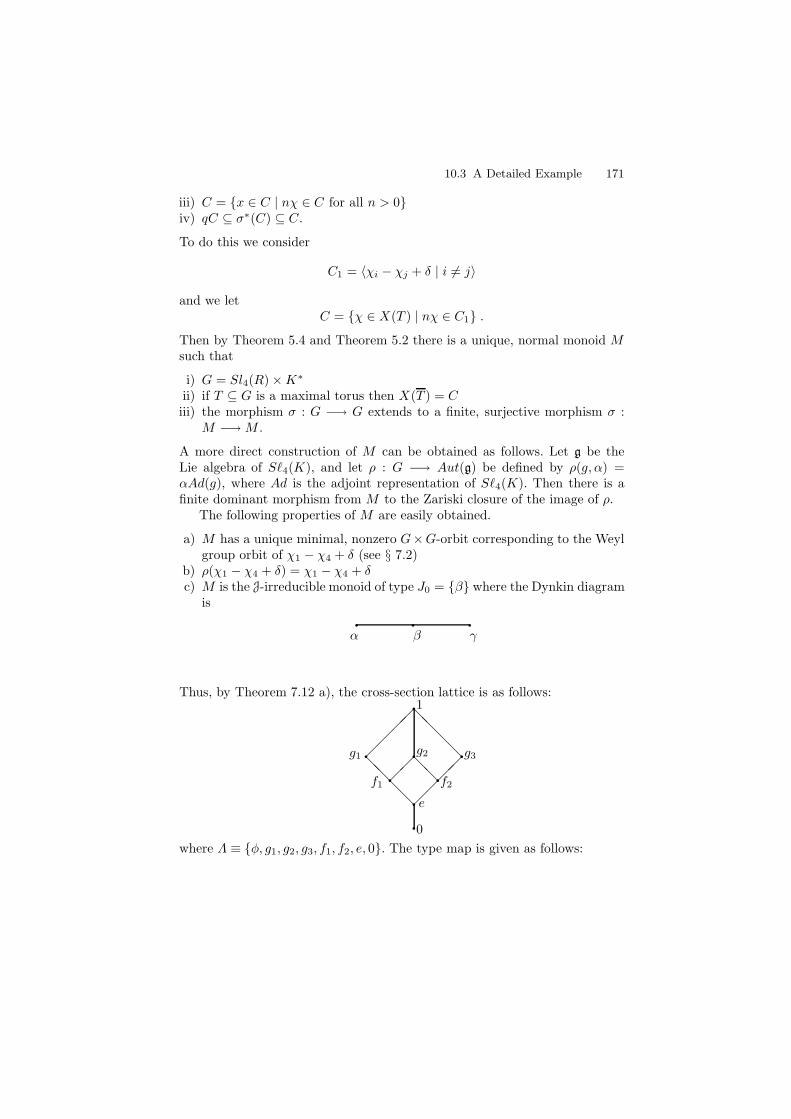
10.3 A Detailed Example 171
iii) C = x ∈ C | nχ ∈ C for all n > 0iv) qC ⊆ σ∗(C) ⊆ C.
To do this we consider
C1 = 〈χi − χj + δ | i 6= j〉
and we letC = χ ∈ X(T ) | nχ ∈ C1 .
Then by Theorem 5.4 and Theorem 5.2 there is a unique, normal monoid Msuch that
i) G = Sl4(R)×K∗
ii) if T ⊆ G is a maximal torus then X(T ) = Ciii) the morphism σ : G −→ G extends to a finite, surjective morphism σ :
M −→M .
A more direct construction of M can be obtained as follows. Let g be theLie algebra of S`4(K), and let ρ : G −→ Aut(g) be defined by ρ(g, α) =αAd(g), where Ad is the adjoint representation of S`4(K). Then there is afinite dominant morphism from M to the Zariski closure of the image of ρ.
The following properties of M are easily obtained.
a) M has a unique minimal, nonzero G×G-orbit corresponding to the Weylgroup orbit of χ1 − χ4 + δ (see § 7.2)
b) ρ(χ1 − χ4 + δ) = χ1 − χ4 + δc) M is the J-irreducible monoid of type J0 = β where the Dynkin diagram
is
q q q
α β γ
Thus, by Theorem 7.12 a), the cross-section lattice is as follows:
q0
q1
q e
q qf2
q
f1
g1 qg2 qg3
@@
@@
@@
@@
@@
where Λ ≡ φ, g1, g2, g3, f1, f2, e, 0. The type map is given as follows:
172 10 Monoids of Lie Type
λ(0) = α, β, γ
λ(e) = β
λ(f1) = α
λ(f2) = γ
λ(g1) = α, β
λ(g2) = α, γ
λ(g3) = β, γ
λ(1) = α, β, γ = S .
Also, from the above calculation of σ∗ we obtain σ(e) = e, σ(f1) = f2, σ(f2) =
f1, σ(g1) = g3, σ(g3) = g1 and σ(g2) = g2. By 10.4,Mσ =⊔
f∈Λσ
GσfGσ, where
Λσ = 0, e, g2, 1 .
The group Gσ is a finite group with BN -pair associated with the diagram
q q
η ζ
obtained by “folding” the diagram
q q qα β γ
at β, thereby identifying α and γ. The type map of Mσ is given by
λ(e) = ζ ←→ β
λ(g2) = ζ ←→ α, γ .
10.4 Abstract Monoids of Lie Type
In this section, we describe Putcha’s theory of abstract monoids of Lie type.This was developed by Putcha in [85, 86] as the method of understandingmany of the purely semigroup theoretic aspects of the theory of algebraicmonoids. The reader might consider this development as the natural monoidanalogue of Tits’ theory of groups with BN-pair.
In this section, we refer the reader to [85, 86, 97] for many of the proofs.
Definition 10.5. Let M be a regular monoid with unit group G and idempo-tent set E(M). Assume that G is a group with BN-pair (B,N, S,W ). We saythat M is a monoid of Lie type on G if
10.4 Abstract Monoids of Lie Type 173
a) M is generated by G and E(M)b) If e ∈ E(M), then P (e) = g ∈ G | ge = ege and P−(e) = g ∈ G | eg =ege are opposite parabolic subgroups of G, and eRu(P
−(e)) = e =Ru(P (e))e
c) If e, f ∈ E(M), and eRf or eLf , then there exists g ∈ G such thatgeg−1 = f .
It follows easily that if ef = fe = f then Ru(P (e)) ⊆ P (f), and soP (e, f) = P (e)∩P (f) is a parabolic subgroup of G. Furthermore, P (e, f) andP−(e, f) are opposite parabolic subgroups.
The following basic result is obtained in [85]. Let B be a Borel subgroupof G. We say that P and P− are standard opposite parabolic subgroups ifB ⊆ P .
Theorem 10.6. Let M be a monoid of Lie type on G. Then
a) M = E(M)G = E(M)Gb) the partially ordered set U of J-classes of M is a latticec) for each J ∈ U there is a unique eJ ∈ E(J) such that P (e) and P−(e) are
standard opposite Borel subgroupsd) if J1, J2 ⊆ U then eJ1eJ2 = eJ1∧J2 , and hence Λ = eJ | J ∈ U ∼= U as
lattices.
Just as in the case of reductive monoids, we refer to Λ as the cross-sectionlattice of M . Furthermore, we have the type map
λ : Λ→ 2S
defined by setting λ(eJ ) = CS(eJ) = s ∈ S | seJ = eJs.
Remark 10.7. There is a purely combinatorial characterization of the typemaps of monoids of Lie type. We refer the reader to [85].
It is useful to know how one constructs a monoid of Lie type directly froma type map of the form mentioned in Remark 10.7 above. In the followingexample, we describe how this is done for a canonical monoid. The details ofthis construction are recorded in [66, 96].
Example 10.8. LetG be a group of Lie type withBN -pair structure (G,B,N, S).If I ⊆ S let PI be the standard parabolic subgroup of G of type I, and letP−I be the parabolic subgroup opposite to P relative to T = N ∩B. It is well
known that
P−I PI
∼= U−I × LI × UI .
where PI ∩ P−I = LI is the Levi factor common to PI and P−
I . Thus we havea natural projection map
θI : P−I PI → LI .
174 10 Monoids of Lie Type
Restricted to PI or P−I , θI is a homomorphism.
For each I ⊆ S, define an idempotent eI so that
Λ = eI | I ⊆ S ∪ 0
and eI ∧ eK = eI∩K if I ∩K 6= φ, and zero otherwise. For eI ∈ Λ, define
JI = GeIG/ ∼
where xeIy ∼ ueIv if u−1x ∈ PI , vy−1 ∈ P−
I and θ(u−1x) = θ(vy−1). Finally,define
M =⊔
I⊆S
JI t 0.
We now define the multiplicative structure on M . Let a = xeIy and b =seKt. Then
ab =
0 , if ys /∈ P−
I PKxleI∩Kmt , if ys ∈ U
−I lmUK , l ∈ LI , m ∈ LK .
It turns out that M is a monoid of Lie type with type map
λ : Λ→ 2S
defined by λ(eI) = I, λ(0) = S. Hence M is a canonical monoid.
The next problem is to quantify the extent to which a monoid of Lie typeis determined by its unit group G, and its type map λ : Λ → 2S . There is avery satisfying answer ([85]), which we now describe.
Let M be a monoid of Lie type, and let J ∈ U. Define
KJ = g ∈ G | geJ = eJg = eJ.
Then KJ is a normal subgroup of LJ = P (e) ∩ P−(e). Let
K = (J,KJ) | J ∈ U.
Let M1 and M2 be monoids of Lie type with unit group G, and the same typemap λ. If K1 = K(M1) and K2 = K(M2), we say that
K1 ≥ K2
if for all J ∈ U, (K1)J ⊆ (K2)J .
Theorem 10.9. Let M be a monoid of Lie type with unit group G and typemap λ : Λ→ 2S.
a) M is completely determinied by (λ,K(M)).
10.5 Modular Representations of Finite Reductive Monoids 175
b) Let M1 and M2 be monoids of Lie type with the same unit group G and thesame type map λ. There is a morphism of monoids M1 →M2, extendingthe identity map on Λ ∪G, if and only if K1 ≥ K2.
c) There is a largest monoid M+(λ) of type λ with KG = 1. K(M+(λ)) =K+
J | J ∈ U, where K+J is the subgroup of LJ generated by all UH and
U−H , where H ∈ U and H ≥ J . In particular, there is a unique morphism
M+(λ)→M , extending the identity on Λ∪G, for any monoid of Lie typeM with group G and type λ.
d) There is a smallest monoid M = M−(λ) of type λ with KG = 1.K(M−(λ)) = K−
J | J ∈ U where
K−J =
⋂
g∈LJ ,J≥H
g(LH ∩ LJ)g−1.
In particular, there is a unique morphism M → M−(λ), extending theidentity on Λ ∪ G, for any monoid of Lie type M with group G and typeλ.
Parts a), b) and d) of Theorem 10.9 are proved in [85], and part c) isproved in [86]. The reader should think of the type map here as determiningM to within a kind of “central extension of monoids”. In the geometric case,it is entirely likely that the isomorphism classes of monoids of fixed type couldbe organized into families of commutative semigroups.
A more refined description of K+J and K−
J has since been given in Theorem1.1 of [97]. In particular, both K+
J and K−J have been identified in terms of
certain Levi subgroups of standard parabolics.Let M be a finite monoid of Lie type. Let G be the group of units of
M , and let Λ be a cross-section lattice of M . Recall from § 2.3.1, the notionof congruence on M . A congruence on M arising from a congruence on Λ iscalled a discrete congruence. At the other extreme, a congruence on M thatarises from an idempotent separating homomorphism is called an idempotentseparating congruence. It is shown in [3] that any congruence on M , which isthe identity on G, factors as a discrete congruence followed by an idempotentseparating congruence.
10.5 Modular Representations of Finite ReductiveMonoids
In this section we consider reductive algebraic monoids M defined over a finitefield k = Fq. We readily obtain finite reductive monoids Mr, r ≥ 1, as follows.
Let Mr = M(Fqr ) be the finite monoid of Fqr -rational points of M . Bystandard facts about finite fields and Galois groups (Chapter II, Section 4 of[61]) there exists an Fq-automorphism σ : M −→ M of algebraic monoidssuch that
176 10 Monoids of Lie Type
Mr = x ∈M | σr(x) = x .
Thus, Mr is a monoid of Lie type in the sense of § 10.4. Such monoids enjoymany special properties.
In this section we describe a useful formula for the number |IR(Mr)| ofirreducible, modular representations of Mr. The basic problem here is to con-sider the fomulas of the form
|IR(Mr)| = (qr − 1)
n∑
i=1
aiqri
where ai ∈ Z and is independent of r. Whenever this can be done, it isparticularly interesting to interpret the ai.
We now state the main result of [96]. This is the main reason we are ableto obtain so much information about irreducible modular representations offinite monoids of Lie type. Let M be a finite monoid of Lie type with unitgroup G of characteristic p.
Theorem 10.10. Suppose that ρ : M → End(V ) is an irreducible represen-tation of M over Fp. Then ρ|G is irreducible.
Proof. First we consider the special case M = M(G), where M(G) is thecanonical monoid of Example 10.17 below. It is then possible to construct
∑
I⊆S
2|S\I|αI
inequivalent, irreducible M(G)-modules, each of which restricts to an irre-ducible representation of G. Here, αI = |Hom(LI ,Fp)|, where LI is a Levifactor of PI . On the other hand, the number of irreducible representations ofM(G) is
∑
I⊆S
∑
K⊆I
αK .
Since the two numbers above are equal, the theorem is true for M(G).To get the result for any finite monoid M of Lie type we start with an
irreducible representation ρ : M −→ End(V ) over Fp. It is then possibleto construct an irreducible representation, as in Corollary 2.7 of [96], ρ :M(G) −→ End(V ) such that ρ|G = ρ|G. Thus, the theorem is proved for M .
The reader is reminded here that there is rarely such a direct and appealingrelationship between the irreducible representations of a monoid and those ofits unit group.
Let M be a finite monoid of Lie type with unit group G. Let S be theCoxeter-Dynkin diagram of G. Let U = U(M) be the set of regular J-classesof M . It turns out that U is the set of two-sided G-orbits of M . Define GaG ≥GbG if b ∈ MaM . In this way, U becomes a lattice. There is a cross-section
10.5 Modular Representations of Finite Reductive Monoids 177
of idempotents Λ = eJ |J ∈ U ⊆ E(M), such that J = GeJG and, for allJ1, J2 ∈ U, eJ1eJ2 = eJ2eJ1 = eJ1∧J2 . Then Λ is called a cross section lattice.Furthermore, E(J) = geJg
−1|g ∈ G.Recall from Definition 4.6 b), the type map:
λ : Λ→ 2S.
It is defined so that for all J ∈ U
P (eJ) = Pλ(J).
P (e) = CrG(e) =: g ∈ G|ge = ege, and PI ⊆ G denotes the parabolicsubgroup of type I as in Theorem 2.44.
Let M be a finite monoid of Lie type of characteristic p, and let ρ : M →End(V ) be an irreducible representation of M defined over Fp. By the theoryof Munn and Ponizovskii [15], ρ determines an apex, Apex(ρ) ∈ U(M). Bydefinition Apex(ρ) is the unique smallest J-class J of M such that ρ(J) 6= 0.But on the other hand, ρ|G is irreducible by Theorem 10.10 above, and so bythe theory of Richen [18] ρ|G is determined by its weight (I(ρ), χ(ρ)). In anycase, ρ : M → End(V ) determines the following data:
(i) J = Apex(ρ) ∈ U(M)(ii) I = I(ρ) ∈ 2S
(iii) χ = χ(ρ) : PI → F∗
p.
We consider the following two questions.
(a) Is ρ uniquely determined up to equivalence of representations by (J, I, χ)?
(b) What are the conditions on a triple (J, I, χ) with χ : PI → F∗
p and J ∈U(M), so that there exists an irreducible representation ρ of M with(i) ρ|G of type (I, χ)(ii) Apex(ρ) = J?
To answer these two questions we need some further notions about monoidsof Lie type. The reader should consult [84] for a detailed account of this theory(notice however that in [84] monoids of Lie type are referred to as regular splitmonoids). Also, the reader needs some familiarity with the representationtheory of finite semigroups. For this, the reader is referred to [15] or [119].
We now introduce some notation. This is mainly for convenience, and toreassert the distinction between an idempotent and the J-class it represents.Let Λ be a cross-section lattice and let e ∈ Λ. Then e = Λ∩J and CrG(e) =Pλ(J), where λ(J) ⊆ S. If B ⊆ CrG(e) is a Borel subgroup and H = g ∈G|ge = e then BH is a parabolic subgroup containing B.
Definition 10.11.ν(J) ∈ 2S via BH = Pν(J).
178 10 Monoids of Lie Type
Notice that ν(J) = λ∗(e), where λ∗(e) is as defined in Definition 7.11. Noticealso that, if we let KJ = g ∈ G|ge = eg = e, then Pν(J) = BKJ . Wecan now state the main theorem (in particular, answering questions a) and b)above).
Theorem 10.12. Let I ∈ 2S and J ∈ U(M). Assume that ν(J) ⊆ I ⊆ λ(J).Define
αI,J = χ : LI → F∗
q |χ(g) = χ(h) if eJg = eJh.
Then there is a one-to-one correspondence between the irreducible representa-tions of M and the set ⊔
I∈2S,J∈U(M)ν(J)⊆I⊆λ(J)
αI,J .
Under this correspondence χ ∈ αI,J corresponds to the unique irreduciblerepresentation ρ : M → End(M) such that
(i) Apex(ρ) = J(ii) there is a line Y ⊆ V such that g ∈ G|ρ(g)Y = Y = PI
(iii) if g ∈ PI and y ∈ Y then ρ(g)(y) = χ(g)y.
Proof. Let ρ : M → End(V ) be irreducible with apex J ∈ U(M). Let J0 =J ∪ 0, with multiplication defined by
xy =
0 , if x = 0, y = 0 or xy /∈ Jxy , if xy ∈ J .
J0 is a completely 0-simple semigroup (see Definition 2.67) So by Munn-Ponizovskii [15], V is also an irreducible J0-module; and by Theorem 10.10above, for e ∈ E(J), e(V ) is an irreducible H(e)-module, where H(e) is theunit group of eMe. But H(e) = eCG(e), and so e(V ) is also an irreducibleCG(e)-module. Now CG(e) ⊆ G is the Levi factor of Pλ(J) = CrG(e), and so itis also a finite group of Lie type. Hence Richen’s theory applies to the CG(e)-module e(V ). Thus, for any Borel subgroup B0 ⊆ CG(e) there exists a uniqueline Y ⊆ e(V ) such that ρ(B0)Y = Y .
Let H = g ∈ G|ρ(g)Y = Y . One checks, as in [114], that H ⊆ CrG(e)and H contains a Borel subgroup of G.
Observe that KJ ⊆ H , and so Pν(J) = BKJ ⊆ H ⊆ Pλ(J). So we can nowsummarize the relevant properties of an irreducible representation ρ : M →End(V ) with apex J ∈ U(M).
(a) Let H = g ∈ G|ρ(g)Y = Y . Then H = PI is parabolic and ν(J) ⊆ I ⊆λ(J).
(b) If g ∈ KJ then ρ(g)y = y for all y ∈ Y .(c) ρ|G is the irreducible representation of type (I, χ), where χ is defined via
ρ(g)(y) = χ(g)y for g ∈ LI .
10.5 Modular Representations of Finite Reductive Monoids 179
On the other hand, suppose that ρ′ : M → End(V ′) is an irreducible rep-resentation with apex J and parabolic subgroup H ′ = PI with character χ.Then by Richen’s results, (ρ′|CG(e), ρ′(e)(V )) ∼= (ρ|CG(e), ρ(e)(V )) since theyhave the same (I, χ). But then by Munn-Ponizovskii, ρ and ρ′ are equivalentbecause they come from the same irreducible representation of eMe. Thus,the correspondence
ρ (I, J, χ)
is injective. To complete the proof, it remains only to be shown that all possibleinvariants (I, J, χ) actually arise from irreducible representations of M . Butthis is now a counting problem. It is easy to check, using Richen’s results,that the number of irreducible representations of H(e) is
∑
ν(J)⊆I⊆λ(J)
|αI,J |.
Thus, by Munn-Ponizovskii, there are exactly∑
J∈U(M)
∑
ν(J)⊆I⊆λ(J)
|αI,J |
irreducible representations of M . Hence the above correspondence must besurjective. This concludes the proof.
Let x ∈Mr. We say that x is semisimple if
i) x is a unit in the monoid eMre for some idempotent e of Mr
ii) xk = e for some k with (k, q) = 1.
Let M ssr = x ∈ M ss
r | x is semisimple and let M ssr / ∼ denote the set of
conjugacy classes of semisimple elements of Mr.
Lemma 10.13. |IR(Mr)| = |Mssr / ∼ |.
Proof. By the theory of Munn and Ponizovskii [15],
|IR(Mr)| =∑
e∈Λ
|IR(H(e))|,
where Hr(e) is the unit group of eMre. But from Theorem 42 of [124],|IR(Hr(e))| = Hr(e)
ss/ ∼. Hence it suffices to see that two elements of Hr(e)are Hr(e)-conjugate if and only if they are Gr-conjugate. But this is straight-forward.
Let π : M → X be the adjoint quotient, as in Corollary 9.4. We need somefurther assumptions to relate M ss
r / ∼ with X(Fqr).Recall that a reductive monoid M is locally simply connected if, for
each e ∈ E(M), He has trivial divisor class group. See Definition 6.4.We say that M is split over Fq if its unit group G is split over Fq in the
usual sense [133]. Recall that any M , defined over Fq, is split over Fqr forsome r > 0.
180 10 Monoids of Lie Type
Proposition 10.14. Let M be a lsc, reductive monoid defined over Fq.
a) The canonical map M ssr / ∼−→ X(Fqr) is bijective for each r > 0.
b) |IR(Mr)| =∑e∈λ q
r(e)|H(e)ab(Fqr )| where r(e) is the semisimple rank ofH(e) and H(e)ab is the abelianization of H(e).
c) If M is split over Fq then |H(e)ab(Fqr )| = (qr − 1)a for some a ≥ 0.
Proof. From Corollary 9.4, X parametrizes G-conjugacy classes of semisim-ple elements of M . But now we can apply Theorem 10.3 of [136]. This saysthat, for each e ∈ Λ, (Hss(Fq)/ ∼) −→ X(Fq) is bijective. Combined withTheorem 10.10 we obtain our result.
To prove b) one needs a careful calculation combining a) above, Richen’stheory [18], Munn-Ponizovskii theory [15], and some basic results from [131].See Theorem 4.2 of [114] for more details.
For c), first notice that |H(e)ab(Fqr)| is a factor of det(σ∗−1) using 6.1(d)of [110]. But M is split so that det(σ∗ − 1) = (qr − 1)m, where m is the rankof G.
We can now obtain very precise information relating IR(Mr) and X ,for lsc monoids.
First, we recall a key definition (see Definition 7.9).A reductive monoid M is J-irreducible if U(M) contains exactly one, min-
imal, nonzero J-class.
Theorem 10.15. Let M be lsc and split over Fq with adjoint quotient π :M −→ X. Then
a) |IR(Mr)| = 1 = (qr − 1)∑i≥0 biq
ri for some integers bi independent ofr > 0;
b) if M is J-irreducible then
|IR(Mr)| − 1 = (qr − 1)∑
i≥0
ai(qr − 1)ri
where
ai =
∣∣∣∣
(I, e) ∈ 2S × Λν(e) ⊆ I ⊆ λ(e)|λ(e)\I| = i
∣∣∣∣ ;
c) If M is J-irreducible then P(X) := (X\0)/K∗ =⊔e∈Λ\0 Ce where Ce ∼=
Kbi . In particular, bi is the 2i-th Betti number of P(X).
Proof. For a) use Proposition 10.14 b) and c). For b) one needs Theorem 3.1 of[114] which calculates |IR(M)| in terms of (I, e) ∈ 2s×Λ | ν(e) ⊆ I ⊆ λ(e).For c) notice that X =
⊔e∈ΛH
ss(e)/ ∼. But from Theorem 1.6 of [110],
(Hss(e)/ ∼) = Kbe ×K∗. Now apply Theorem 2.59.
Notice that the cell decomposition in c) above can not be obtained by themethod of Birula-Bialynicki [4] and so one must use Theorem 2.59 to obtainthese Betti numbers.
10.5 Modular Representations of Finite Reductive Monoids 181
Example 10.16. Let M = Mn(K) where K = Fq. So Mr = Mn(Fqr ). Then,by Munn-Ponizovskii [15],
|IR(Mr)| =
n∑
m=0
|IR(G`m(Fqr ))|
while, by Richen [18],
|IR(G`m(Fqr ))| = (qr − 1)qr(m−1) .
Thus
|IR(Mr)| = (qr − 1)
n−1∑
i=0
qri .
Hence
bi =
1 , i = 0, . . . , n− 10 , otherwise .
Plainly, bi is the 2i-th Betti number of P(X) = Pn−1.But we can also write
|IR(G`m(Fqr ))| =
m−1∑
i=0
(m− 1
i
)(qr − 1)i+1 .
Hence
|IR(Mr)| − 1 =
n∑
m=1
|IR(G`m(Fqr ))|
=
n∑
i=0
(n
i+ 1
)(qr − 1)i+1 .
By 6.4b) we obtain the curious combinatorial formula
(n
i+ 1
)=
∣∣∣∣
(I, e) ∈ 2S × Λν(e) ⊆ I ⊆ λ(e)|λ(e)\I| = i
∣∣∣∣ .
Example 10.17. In [96] the author and M. Putcha construct, for each group Gof Lie type, a certain canonical monoid M(G) having the following properties.
(a) G is the unit group of M(G).(b) The type map λ : U(M(G))→ 2S of M(G) satisfies
(i) λ : U(M(G))\0 → 2S is bijective(ii) λ(Je ∧ Jf ) = λ(Je) ∩ λ(Jf ), where U(M(G)) has been identified with
a cross-section lattice Λ of M(G).(c) For each e ∈ Λ, g ∈ G|ge = eg = e = 1.
182 10 Monoids of Lie Type
By the results of [84], M(G) is determined up to isomorphism by these prop-erties. This monoid also enjoys a number of other useful properties that wereimportant in the proof of Theorem 10.10. In any case, if J ∈ U(M(G)) then
by (c), ν(J) = φ. Furthermore, αI,J = Hom(LI ,F∗
q) for any I ⊆ λ(J). SoαI,J is independent of J if it is non-empty.
Define, for any finite monoid M of Lie type,
IR(M) = ρ : M → End(V )|ρ is irreducible/ ∼
where “∼” denotes equivalence of representations. Thus, by Theorem 10.10,
|IR(M(G))| =∑
I⊆λ(J)
|αI,J |
=∑
I⊆S
∑
J∈U(S)
|αI,J |
=∑
I⊆S
2|S\I|αI
where αI is the common value of |αI,J | for I ⊆ λ(J). This agrees with theformula (1) in the proof of Theorem 2.2 of [96].
If G = S`n+1(Fq) then |S| = n and, for |I| = i, α(I) = (q − 1)n−i. Thus
|IR(M(G))| =∑
I⊆S
2|S\I|α(I)
=
n∑
i=0
(ni
)2n−i(q − 1)n−i
=n∑
i=0
(ni
)(2q − 2)n−i
= (2q − 1)n.
Notice that this corrects the calculation error of Example 2.3 of [96].
The reader might wonder if, for any reductive monoid M , there is a finite,dominant morphism
ϕ : M ′ →M
of reductive monoids with M ′ a lsc monoid. In general this seems to be adelicate problem. However, we do have some positive results.
If M is reductive and normal we denote by Cl(M) the divisor class groupof M . See § 2.1.3 for a summary of some of the main properties relevant toour discussion.
Recall the following results from Theorem 6.7.
10.5 Modular Representations of Finite Reductive Monoids 183
Theorem 10.18. Let M be reductive and normal.
a) If Cl(M) = (0) then M is lsc.b) If M\G is irreducible then Cl(M) is finite and there exists π : M ′ −→M ,
finite and dominant, such that Cl(M ′) = (0).
If M is a J-coirreducible monoid then the lattice of J-classes Λ ∼= U(M),and the type map λ : Λ → 2S are both determined by λ(J) where J ∈U(M)\1 is the unique maximal element. Indeed, if λ(J) = I, then
Λ =
X ∈ 2S
no component of X iscontained in I
∪ 1
where Λ\1 is ordered by reverse inclusion and 1 ∈ Λ is the largest element.Here, X corresponds to eX ∈ Λ. Furthermore, λ : Λ→ 2S is defined by
λ(X) = X tCI(X)
if X 6= φ or 1, and λ(φ) = I and λ(1) = S. Here, CI(X) = α ∈ I|σασβ =σβσα for all β ∈ X. It follows from Definition 7.11 and Lemma 7.15 thatλ∗(eX) = X and λ∗(eX) = CI(X).
Theorem 10.19. Suppose that M is J-coirreducible of type I, split over Fqand with Cl(M) = 0. Then
|IR(M)| =∑
X∈Λ
q|CI(X)|(q − 1)|S\λ(X)| + q|S|(q − 1).
Proof. First notice that |S\X |−|CI(X)| = |S\λ(X)| since λ(X) = X∪CI(X)is a disjoint union whenever no component of X lies in I. But then for eachX ∈ Λ, IR(H(ex)) = q|CI(X)|(q − 1)|S\λ(X)| since H(ex) has rank |S\X | andsemisimple rank |CI(X)|.
Theorem 10.20. Suppose that M is reductive, split over Fq and locally simplyconnected. Then
|IR(M)| =
|S|+1∑
i=0
ai(q − 1)i
where ai = |(I, J) ∈ 2S × U(M)|rank(J) − |I|+ |v(J)| = i|.
Proof. Recalling Theorem 10.12 it suffices to prove that, given our assump-tions on M, |αI,J | = (q− 1)i where i = rank(J)− |I|+ |ν(J)|. But αI,J is thecharacter group of LI\ν(J)(H(e)), the Levi subgroup of He of type I\ν(J).This has rank equal to rank(J) and semisimple rank |I| − |ν(J)|. This yieldsthe formula for ai.
184 10 Monoids of Lie Type
10.6 Exercises
10.6.1 Weil Zeta Functions
Let X be a variety defined over the finite field Fq, and let
Z(X) = exp(∑
r≥1
Nrrtr)
be its Weil zeta function.
1. Suppose there exist complex numbers α1, . . . , αs and β1, . . . , βt such that,for all m ≥ 1,
Nm =
s∑
i=1
αmi −
t∑
j=1
βmj .
Show that
exp(∑
r≥1
Nmm
tm) =Πtj=1(1− βjt)
Πsi=1(1− αit)
.
2. Show that if Z(X) = Πj≥0(1 − qjt)bj , then Z(X × Kn) = Πj≥0(1 −qj+nt)bj .
3. Show that
Z(X ×K∗) =Z(X ×K)
Z(X).
4. Letting Z(X) = Z(t), show that
Z(X × (K∗)n) = Πns=0Z(qst)(−1)n−s(n
s).
5. Recall that, if M is reductive and split over k = Fq, then M = tr∈RBrBin such a way that, if BrB ∼= (K∗)r × K l, then (BrB)(k) ∼= (k∗)r × kl,over k = Fq. Show that
Z(M) = Πmk=0(1− q
kt)bk
where m = dim(M)− rank(M), and
bk =
N∑
r=0
k∑
l=k−r
(−1)r−k+l(
r
k − l
)νr,l
withνr,l = |r ∈ R | BrB ∼= (k∗)r × kl|.
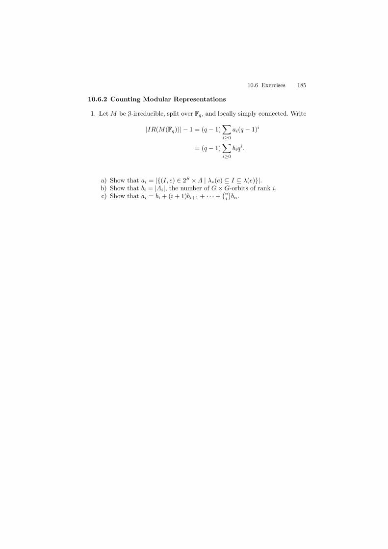
10.6 Exercises 185
10.6.2 Counting Modular Representations
1. Let M be J-irreducible, split over Fq, and locally simply connected. Write
|IR(M(Fq))| − 1 = (q − 1)∑
i≥0
ai(q − 1)i
= (q − 1)∑
i≥0
biqi.
a) Show that ai = |(I, e) ∈ 2S × Λ | λ∗(e) ⊆ I ⊆ λ(e)|.b) Show that bi = |Λi|, the number of G×G-orbits of rank i.c) Show that ai = bi + (i+ 1)bi+1 + · · ·+
(ni
)bn.

11
Cellular Decomposition of Algebraic Monoids
The most commonly studied cell decompositions in algebraic geometry arethose of Bialynicki-Birula [4]. If S = K∗ acts on a smooth complete variety
X with finite fixed point set F ⊆ X , then X =⊔
α∈F
Xα where Xα = x ∈
X | limt→0
tx = α. Furthermore, Xα is isomorphic to an affine space. We refer
to Xα as a BB-cell. If, further, a reductive group G acts on X extending theaction of S, we may assume (replacing S if necessary) that each Xα is stableunder the action of some Borel subgroup B of G with S ⊆ B. In case X isa complete homogeneous space for G, each cell Xα turns out to consist ofexactly one B-orbit.
Let M be a semisimple monoid. That is, M is reductive, normal with zeroelement and with one-dimensional center. Define
X = (M\0)/K∗ .
Then X is projective and G×G acts on X by the rule (g, h) · [x] = [gxh−1].Furthermore, any generic one-parameter subgroup S = K∗ ⊆ G × G has afinite number of fixed points on X .
Each BB-cell on X is made up of a finite number of B × B-orbits. Butthere is often no explicit algorithm for deciding how each BB-cell is made upfrom the B ×B-orbits. On the other hand, we have explicitly identified theseB × B-orbits on M (or X) in Chapter 8. So what we need here is a moredirect definition, guided by the BB-procedure, that simply tells us how eachcell is made up from B ×B-orbits.
In this chapter, we define a notion that yields a decomposition of M\0into a disjoint union of “monoids cells”. These cells are defined directly interms of Λ, B and R. We then explain how to use these monoid cells to obtainan explicit decomposition of the “wonderful compactification” into a disjointunion of affine space.
In the case where X is the wonderful compactification of the adjoint,semisimple group G, this “BB-procedure” has been carried out in [21]. In
188 11 Cellular Decomposition of Algebraic Monoids
fact, they obtain results for a more general class of wonderful compactifica-tions. Let G be a semisimple algebraic group, and suppose that σ : G −→ Gis an involution (so that σ σ = idG) with H = x ∈ G | σ(x) = x. Thewonderful compactification of G/H (according to [21]) is the unique normalG-equivariant compactification X of G/H obtained by considering an irre-ducible representation ρ : G −→ G`(V ) of G with dim(V H) = 1 and withhighest weight in general position. Then let h ∈ V H be nonzero and define
X = ρ(G)[h] ⊆ P(V ),
the Zariski closure of the orbit of [h]. (See Section 2 of [21] for details.) In thischapter we restrict our attention to the special case where the group is G×Gand σ : G×G −→ G×G is given by σ(g, h) = (h, g). It is easy to see that, inthis case, the G×G-variety (G×G)/H can be canonically identified with Gwith its two-sided G-action.
Much important work has been accomplished since [21] appeared. In par-ticular, Brion [12] obtains much information about the structure of X . Among
other things, he finds a BB-decomposition X =⊔
x∈F
Cx from which he then
obtains a basis of the Chow ring of X of the form By(x)Bx∈F . He alsoidentifies explicitly how each cell Cx is made up from B × B-orbits. Sincethen, Springer [130] and Kato [46] have uncovered more geometry related tothis problem.
It appears that my cell decomposition agrees with the one of [12] (al-though we have not actually verified this). The interested reader should con-sult Brion’s paper, as well as those of Kato and Springer, for more informationon the B ×B-orbit closures and the Chow ring for X .
11.1 Monoid Cells
In this section we assume that M is a J-irreducible, reductive monoid as in§ 7.3. Let B ⊆ G be a Borel subgroup with maximal torus T ⊆ B. Define
R1 = x ∈ R | xT = Tx is one-dimensional,
the set of rank one elements of the Renner monoid. Our cells are canonicallyindexed by R1.
Let r ∈ R1. Then there exist unique rank one idempotents e, f ∈ E1(T )such that
r = erf.
We define the monoid cell Cr as follows:
Cr = y ∈M | eBy = eBey ⊆ rB.
The following results are easily obtained.
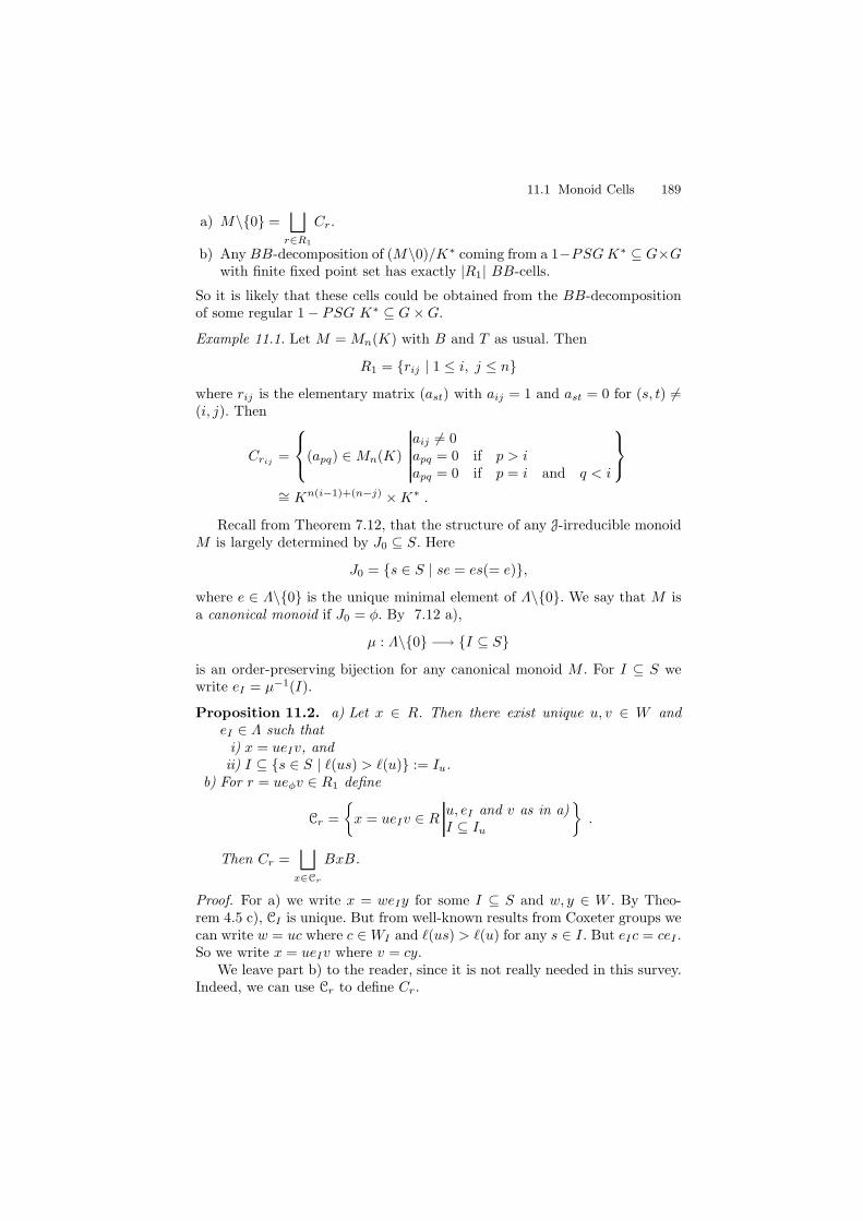
11.1 Monoid Cells 189
a) M\0 =⊔
r∈R1
Cr.
b) Any BB-decomposition of (M\0)/K∗ coming from a 1−PSGK∗ ⊆ G×Gwith finite fixed point set has exactly |R1| BB-cells.
So it is likely that these cells could be obtained from the BB-decompositionof some regular 1− PSG K∗ ⊆ G×G.
Example 11.1. Let M = Mn(K) with B and T as usual. Then
R1 = rij | 1 ≤ i, j ≤ n
where rij is the elementary matrix (ast) with aij = 1 and ast = 0 for (s, t) 6=(i, j). Then
Crij =
(apq) ∈Mn(K)
aij 6= 0apq = 0 if p > iapq = 0 if p = i and q < i
∼= Kn(i−1)+(n−j) ×K∗ .
Recall from Theorem 7.12, that the structure of any J-irreducible monoidM is largely determined by J0 ⊆ S. Here
J0 = s ∈ S | se = es(= e),
where e ∈ Λ\0 is the unique minimal element of Λ\0. We say that M isa canonical monoid if J0 = φ. By 7.12 a),
µ : Λ\0 −→ I ⊆ S
is an order-preserving bijection for any canonical monoid M . For I ⊆ S wewrite eI = µ−1(I).
Proposition 11.2. a) Let x ∈ R. Then there exist unique u, v ∈ W andeI ∈ Λ such that
i) x = ueIv, andii) I ⊆ s ∈ S | `(us) > `(u) := Iu.
b) For r = ueφv ∈ R1 define
Cr =
x = ueIv ∈ R
u, eI and v as in a)I ⊆ Iu
.
Then Cr =⊔
x∈Cr
BxB.
Proof. For a) we write x = weIy for some I ⊆ S and w, y ∈ W . By Theo-rem 4.5 c), CI is unique. But from well-known results from Coxeter groups wecan write w = uc where c ∈ WI and `(us) > `(u) for any s ∈ I. But eIc = ceI .So we write x = ueIv where v = cy.
We leave part b) to the reader, since it is not really needed in this survey.Indeed, we can use Cr to define Cr.
190 11 Cellular Decomposition of Algebraic Monoids
We refer to x = ueIv as the normal form for x.We now determine the structure of each Cr. But first we determine how
the B ×B-orbits fit together.
Proposition 11.3. Let x ∈ R and write x = ueIv in normal form. Then
BxB = (Uu ∩ uU)(eIT )(vU ∩ U−v)∼= (Uu ∩ uU)× eIT × (vU ∩ U−u)
Proof. Let e = eI . Since eB j Be we get eB = CB(e). Also we have vBv−1 =(vBv−1 ∩B)(vBv−1 ∩ U−) (direct product). Then
evBv−1 = e(vBv−1 ∩B)(vBv−1 ∩ U−)
= V e(vBv−1 ∩ U−)
where V ⊆ (Cb(e) is some connected subgroup with T ⊆ V . Then we get
evB = V e(vB ∩ U−v). (∗)
We now look at Bue. Recall first that `(us) < `(u) for any s ∈ I. This isthe same as saying that CB(e) ⊆ u−1Bu ∩B. Thus
u−1Bue = (u−1Bu ∩B)e
since (u−1Bu ∩ U−)e = e. Thus
Bue = (Bu ∩ uB)e (∗∗)
Combining (*) and (**) we obtain that
u−1BuevB = (u−1Bu ∩B)e(V vB ∩ U−v)
= (u−1Bu ∩B)e(vB ∩ U−v)
since V ⊆ CB(e) ⊆ u−1Bu ∩B. Thus
BuevB = (Uu ∩ uU)(eT )(vU ∩ U−v) .
A calculation similar to the proof of Lemma 5.1 shows that this product isdirect. In characteristic p > 0, the product morphism is seen to be separableby a local analysis of the torus action at the fixed point.
Proposition 11.3 tells us exactly why we have found the “correct” definitonof cells.
Proposition 11.4. Let r = ueφv ∈ R1.
a) Cr ∼= (Uu ∩ uU)× Zu × (vU ∩ U−v) where Zu =⊔
J⊆Iu
eIT .
11.1 Monoid Cells 191
b) Zu/K∗ ∼= Ki(u) where i(u) = |Iu|.
Proof. For b) we may assume that u = 1, since any other Zu is a T -orbit
closure in Z1 =⊔
I⊆S
eIT . But one checks, as in Proposition 3.4 of [118], that
O(Z1/K∗) = K[α−1
1 , . . . , α−1s ] where S = α1, . . . , αs.
For a), we have by definition
Cr =⊔
ueIv∈Cr
(Uu ∩ uU)(eIT )(vU ∩ U−v)
= (Uu ∩ uU)
(⊔
ueIv∈Cr
eIT
)(vU ∩ U−v) .
Theorem 11.5. Let r = ueφv ∈ R1. Then there is a bijective morphism
m : Knr −→ Cr/K∗
where nr = `(w0)− `(u) + i(u) + `(σ). Here, w0 ∈ W is the longest element,so that `(w0) = |Φ+|.
Proof. From 11.4 a), dim Cr = dim(Uu∩ uU) + dim(Zu) + dim(vU ∩U−v).One checks that dim(Uu∩uU) = `(w0)−`(u) and that dim(vU∩U−v) = `(v).From 11.4 b) dim(Zu) = i(u) + 1.
We can also consider the cell decomposition for each orbit closure. LetI ⊆ S and define
XI = (GeIG\0)/K∗ .
By [21] XI is a smooth spherical G × G-subvariety of X . We find a cell de-composition of XI as follows.
Given r ∈ R1 and I ⊆ S define
CI,r = Cr ∩XI .
Clearly XI =⊔
r∈R1
CI,r. But we can say more.
Theorem 11.6. Let r = ueφv ∈ R1. Then there is an isomorphism
m : KnI,r −→ CI,r
where nI,r = `(w0)− `(u) + |I ∩ Iu|+ `(v).
Proof. By inspection CI,r =⊔
j⊆I∩Iu
BueJvB, and so
CI,r = (Uu ∩ uU)(ZI,u)(vU ∩ U−v)
where ZI,u =⊔
J⊆I∩In
eJT . Then the proof proceeds as in 11.4 and 11.5.
192 11 Cellular Decomposition of Algebraic Monoids
If Y is a smooth projective algebraic variety with cell decomposition wecan calculate the Betti numbers of Y :
β2i(Y ) = the number of cells of (complex) dimension i.
LetP (X, t) =
∑
i≥0
β2i(X)t2i
be the Poincare polynomial of X .
Theorem 11.7.
P (XI , t) =
(∑
u∈W
t2(`(w0)−`(u)+|Iu∩I|)
)(∑
v∈W
t2`(v)
).
This result is also obtained by DeConcini and Procesi in [21].It appears that Springer has obtained the same cell decomposition in [130],
in his detailed study of the geometry of the B ×B-orbit closures of X .Further results about X have been obtained by Kato [46]. In particular,
he obtains a kind of Borel-Weil theorem for X .Since the appearance of [21], these same authors have continued the study
of these interesting spaces. In [22] they have described the rational cohomologyof X , as well the cohomology of many other spaces closely related to X . In [5](along with Bifet), they describe the rational cohomology ring of any completesymmetric variety by generators and relators. See § 15.4 for a brief descriptionof these developments.
11.2 Exercises
Let W be a Weyl group with generating set S ⊆W , the set of simple involu-tions, and let ∆ ⊆ Φ be the set of positive, simple roots.
1. For x ∈ W , define Ix = α ∈ ∆ | l(sαx) = l(x) − 1 and Jx = α ∈∆ | l(xsα) = l(x)− 1. Show that, for all x ∈ W , Ix = Jx−1 .
2. For a subset θ ⊆ S let w(θ) be the longest element of Coxeter group Wθ.If x ∈ W , let wx = w(Ix). Show that, for all x ∈ W , x = wxx−, wherel(x) = l(wx) + l(x−).
3. For s ∈ S, y ∈ W , define
s ∗ y =
y , if l(sy) < l(y)sy , if l(sy) > l(y) .
Show that ∗ defines on W the structure of a monoid with the followingproperties:a) w(θ) ∗ x = x if and only if θ ⊆ Ix
11.2 Exercises 193
b) x ∗ v = v if and only if x ∗ wv = wv ∗ x = wv.4. Let x ∈ W and s ∈ S. Prove the following:
a) If l(xs) = l(x) + 1 then Ixs = Ix ∪ (xsx−1 ∩ S).b) If l(xs) = l(x)− 1 then Ix = Ixs ∪ (xsx−1 ∩ S).c) Ixs = Ix if and only if xsx−1 6∈ S.
5. Let x ∈ W . Prove that
|x ∈ W | Ix = I| =∑
I⊆J
(−1)|J\I||W |
|WJ |.
6. Show that, for I ⊆ S,
∑
x∈W, Ix=I
tl(x) =∑
I⊆J
(−1)|J\I|tdim(G/PJ )P (J, t)
where P (J, t) =∑j≥0 dim(H2j(G/PJ ))tj is the Poincare polynomial of
G/PJ .

12
Conjugacy Classes
In this chapter we describe Putcha’s theory of conjugacy classes in a reductivemonoid. We can not do justice here to this truly remarkable development. Sowe shall refer the reader to Putcha’s work [88, 89, 90] for the details of manyproofs. Our purpose here is to explain Putcha’s main results while describingsome of the key ideas of his proofs.
The basic idea here is to define, for each (e, σ) ∈ E(T ) × W , a subsetMe,σ ⊆M such that
a) any x ∈M is conjugate to some y ∈Me,σ for some (e, σ) ∈ E(T )×Wb) there is an explicit equivalence relation ∼ on Me,σ such that for a, b ∈
Me,σ, a ∼ b if and only if b = gag−1 for some g ∈ G.
On this basis we discuss some further refinement, especially the issue of
finding a minimal collection A = (e, σ) so that M =⋃
(e,σ)∈A
gMe,σg−1. The
key results here can be described using some finer structure theory of theRenner monoid.
12.1 The Basic Conjugacy Theorem
LetM be a reductive monoid with zero element 0 ∈M and unit groupG ⊆M .Let e ∈ E(T ) and σ ∈ W . For θ ∈W write
eθ = θ−1eθ ∈ E(T ) .
DefineMe,σ = eCG(eθ | θ ∈ 〈σ〉)σ .
Theorem 12.1. Let a ∈ M . Then a is conjugate to an element of Me,σ forsome e, σ.
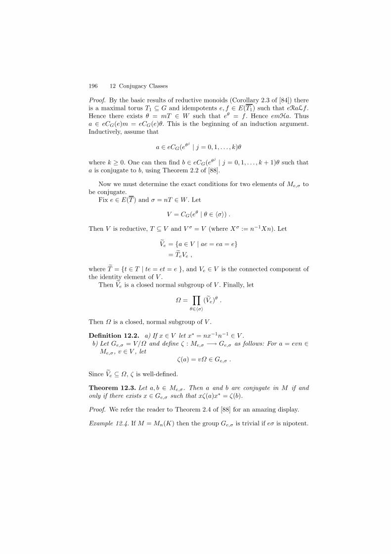
196 12 Conjugacy Classes
Proof. By the basic results of reductive monoids (Corollary 2.3 of [84]) thereis a maximal torus T1 ⊆ G and idempotents e, f ∈ E(T1) such that eRaLf .Hence there exists θ = mT ∈ W such that eθ = f . Hence emHa. Thusa ∈ eCG(e)m = eCG(e)θ. This is the beginning of an induction argument.Inductively, assume that
a ∈ eCG(eθj
| j = 0, 1, . . . , k)θ
where k ≥ 0. One can then find b ∈ eCG(eθj
| j = 0, 1, . . . , k + 1)θ such thata is conjugate to b, using Theorem 2.2 of [88].
Now we must determine the exact conditions for two elements of Me,σ tobe conjugate.
Fix e ∈ E(T ) and σ = nT ∈ W . Let
V = CG(eθ | θ ∈ 〈σ〉) .
Then V is reductive, T ⊆ V and V σ = V (where Xσ := n−1Xn). Let
Ve = a ∈ V | ae = ea = e
= TeVe ,
where T = t ∈ T | te = et = e , and Ve ∈ V is the connected component ofthe identity element of V .
Then Ve is a closed normal subgroup of V . Finally, let
Ω =∏
θ∈〈σ〉
(Ve)θ .
Then Ω is a closed, normal subgroup of V .
Definition 12.2. a) If x ∈ V let x∗ = nx−1n−1 ∈ V .b) Let Ge,σ = V/Ω and define ζ : Me,σ −→ Ge,σ as follows: For a = evn ∈Me,σ, v ∈ V , let
ζ(a) = vΩ ∈ Ge,σ .
Since Ve ⊆ Ω, ζ is well-defined.
Theorem 12.3. Let a, b ∈ Me,σ. Then a and b are conjugate in M if andonly if there exists x ∈ Ge,σ such that xζ(a)x∗ = ζ(b).
Proof. We refer the reader to Theorem 2.4 of [88] for an amazing display.
Example 12.4. If M = Mn(K) then the group Ge,σ is trivial if eσ is nipotent.
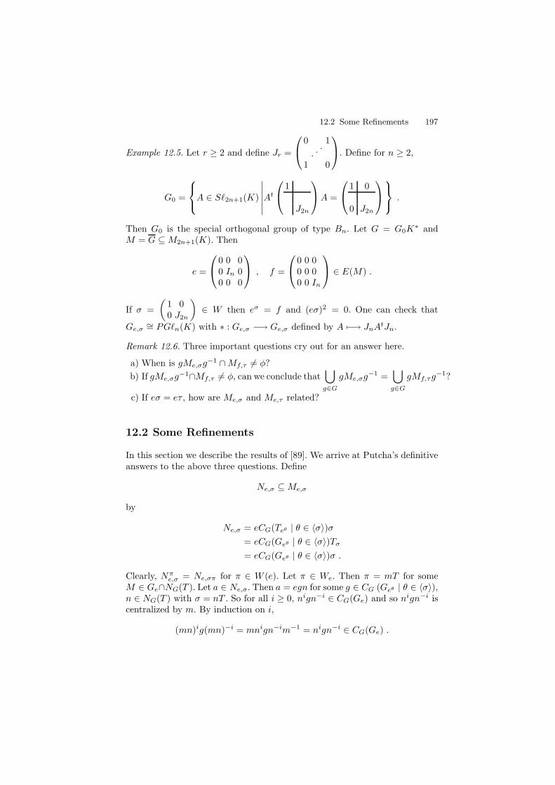
12.2 Some Refinements 197
Example 12.5. Let r ≥ 2 and define Jr =
0 1
· ··
1 0
. Define for n ≥ 2,
G0 =
A ∈ S`2n+1(K)
∣∣∣∣∣∣At
1
J2n
A =
1 0
0 J2n
.
Then G0 is the special orthogonal group of type Bn. Let G = G0K∗ and
M = G ⊆M2n+1(K). Then
e =
0 0 00 In 00 0 0
, f =
0 0 00 0 00 0 In
∈ E(M) .
If σ =
(1 00 J2n
)∈ W then eσ = f and (eσ)2 = 0. One can check that
Ge,σ ∼= PG`n(K) with ∗ : Ge,σ −→ Ge,σ defined by A 7−→ JnAtJn.
Remark 12.6. Three important questions cry out for an answer here.
a) When is gMe,σg−1 ∩Mf,τ 6= φ?
b) If gMe,σg−1∩Mf,τ 6= φ, can we conclude that
⋃
g∈G
gMe,σg−1 =
⋃
g∈G
gMf,τg−1?
c) If eσ = eτ , how are Me,σ and Me,τ related?
12.2 Some Refinements
In this section we describe the results of [89]. We arrive at Putcha’s definitiveanswers to the above three questions. Define
Ne,σ ⊆Me,σ
by
Ne,σ = eCG(Teθ | θ ∈ 〈σ〉)σ
= eCG(Geθ | θ ∈ 〈σ〉)Tσ
= eCG(Geθ | θ ∈ 〈σ〉)σ .
Clearly, Nπe,σ = Ne,σπ for π ∈ W (e). Let π ∈ We. Then π = mT for some
M ∈ Ge∩NG(T ). Let a ∈ Ne,σ. Then a = egn for some g ∈ CG (Geθ | θ ∈ 〈σ〉),n ∈ NG(T ) with σ = nT . So for all i ≥ 0, nign−i ∈ CG(Ge) and so nign−i iscentralized by m. By induction on i,
(mn)ig(mn)−i = mnign−im−1 = nign−i ∈ CG(Ge) .
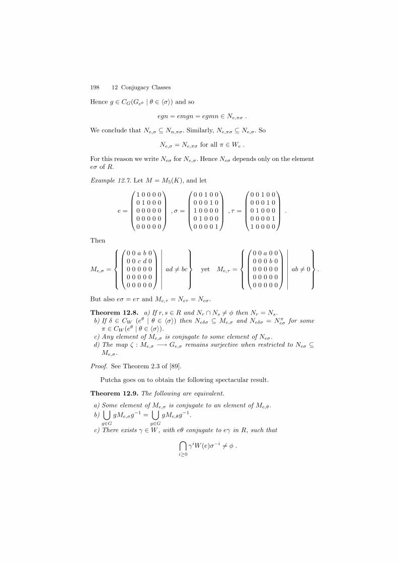
198 12 Conjugacy Classes
Hence g ∈ CG(Geθ | θ ∈ 〈σ〉) and so
egn = emgn = egmn ∈ Ne,πσ .
We conclude that Ne,σ ⊆ Nn,πσ. Similarly, Ne,πσ ⊆ Ne,σ. So
Ne,σ = Ne,πσ for all π ∈We .
For this reason we write Neσ for Ne,σ. Hence Neσ depends only on the elementeσ of R.
Example 12.7. Let M = M5(K), and let
e =
1 0 0 0 00 1 0 0 00 0 0 0 00 0 0 0 00 0 0 0 0
, σ =
0 0 1 0 00 0 0 1 01 0 0 0 00 1 0 0 00 0 0 0 1
, τ =
0 0 1 0 00 0 0 1 00 1 0 0 00 0 0 0 11 0 0 0 0
.
Then
Me,σ =
0 0 a b 00 0 c d 00 0 0 0 00 0 0 0 00 0 0 0 0
∣∣∣∣∣∣∣∣∣∣
ad 6= bc
yet Me,τ =
0 0 a 0 00 0 0 b 00 0 0 0 00 0 0 0 00 0 0 0 0
∣∣∣∣∣∣∣∣∣∣
ab 6= 0
.
But also eσ = eτ and Me,τ = Neτ = Neσ.
Theorem 12.8. a) If r, s ∈ R and Nr ∩Ns 6= φ then Nr = Ns.b) If δ ∈ CW (eθ | θ ∈ 〈σ〉) then Neδσ ⊆ Me,σ and Neδσ = Nπ
eσ for someπ ∈ CW (eθ | θ ∈ 〈σ〉).
c) Any element of Me,σ is conjugate to some element of Neσ.d) The map ζ : Me,σ −→ Ge,σ remains surjective when restricted to Neσ ⊆Me,σ.
Proof. See Theorem 2.3 of [89].
Putcha goes on to obtain the following spectacular result.
Theorem 12.9. The following are equivalent.
a) Some element of Me,σ is conjugate to an element of Me,θ.
b)⋃
g∈G
gMe,σg−1 =
⋃
g∈G
gMe,θg−1.
c) There exists γ ∈W , with eθ conjugate to eγ in R, such that
⋂
i≥0
γiW (e)σ−i 6= φ .
12.3 Putcha’s Decomposition and the Nilpotent Variety 199
d) Nπeσ = Neθ for some π ∈ W (e).
This is nearly complete. The only thing remaining is to isolate the “best”representative in each set
eτ ∈ R |
⋃
g∈G
gMe,σg−1 =
⋃
g∈G
gMe,τg−1
.
This will be the main focus of the next section.
12.3 Putcha’s Decomposition and the Nilpotent Variety
In this section we determine a subset P ⊆ R such that
M =⊔
r∈P
X(r) (∗)
where X(r) =⋃
g∈G
gMe,σg−1 for r = eσ ∈ R. We shall refer to (*) as the
Putcha decomposition of M . We also describe the order relation on P thatcorresponds to the condition X(r) ⊆ X(s). This stunning development hasno analogue in group theory.
Recall now the Weyl group W and its set of Coxeter group generatorsS ⊆W . For I ⊆ S define
DI = g ∈ W | `(gw) = `(g) + `(w) for all w ∈WI
D−1I = g ∈ W | `(wg) = `(w) + `(g) for all w ∈WI .
Definition 12.10. Let x, y ∈ W . We say that x ≡I y if⋂
i≥0
xiWIy−1 6= φ.
Notice that ≡I is an equivalence relation on W . Also notice that
x ≡I wxs−1 if w ∈WI ,
and
x ≡I ux if u ∈⋂
i≥0
xiWIx−i .
Proposition 12.11. Let x ∈ W . Then x ≡I y for some unique y ∈ D−1I .
Furthermore, `(y) ≤ `(x).
Proof. Let
200 12 Conjugacy Classes
x1 = x = w1y1 , w1 ∈ WI , y1 ∈ D−1I
x2 = y1w1 = w2y2 , w2 ∈ WI , y2 ∈ D−1I
...
Now xj+1 = yjwj = w−1j (wjyi)wj = w−1
j xjwj . Hence by comments following12.10, x1 ≡I x2 ≡I x3 ≡I . . . . Also,
`(xj+1) = `(yjwj) ≤ `(yj) + `(wj) = `(wjyj) = `(xj) .
Hence, for some N , `(xN ) = `(xN+1) = . . . . Since yj ∈ D−1I , we see by the
exchange condition that for, j ≥ N ,
yj+1 = yjuj, uj ∈WI
`(yj+1) = `(yj) + `(uj) .
In particular, `(yN ) ≤ `(yN+1) ≤ . . . . Hence, there exists k ≥ N such that
yk = yk+1 = . . . .
Letting y = yk we obtain, after some scrutiny,
y ≡I x
and`(y) ≤ `(x) .
One then checks that this y is unique. See Proposition 1.1 of [90].
We now apply this to our situation. Let I ⊆ S. Then for any J ⊆ S
D−1I ⊆ (D−1
I ∩DJ )WJ .
Thus, for any y ∈ D−1I , we obtain from standard results that
WI ∩ yWJy−1 is a standard parabolic subgroup of (W,S).
HenceWI ∩ yWIy
−1 = WI , , I1 ⊆ IWI ∩ yWI1y
−1 = WI2 , I2 ⊆ I1WI ∩ yWI2y
−1 = WI3 , I3 ⊆ I2...
Then let K = K0 C I, so that K is a union of some connected components ofI. Then, as above,
WI ∩ yWK0y−1 = WK1 , K1 C I1
WI ∩ yWK1y−1 = WK2 , K2 C I2
WI ∩ yWK2y−1 = WK3 , K3 C I3
...
We arrive at our key definition.
12.3 Putcha’s Decomposition and the Nilpotent Variety 201
Definition 12.12. Suppose that I ⊆ S and K C I. Define
D∗I (K) = y ∈ D−1
I | y ∈ DKj for all j ≥ 0 .
Notice that D∗I (φ) = D−1
I and D∗I (I) = DI ∩D
−1I .
The following corollary follows from Proposition 12.11. See Corollary 1.2of [90].
Corollary 12.13. Let y ∈ D∗I (K), z ∈WK and suppose that yz ≡I y
′ ∈ D−1I .
Then `(y′) ≥ `(y). If further `(y′) = `(y), then y = y′.
We now return to conjugacy classes in M . Let e ∈ Λ, the cross-sectionlattice. Then
W (e) = WI for I = λ(e) ⊆ S
W∗(e) = x ∈ W | xe = ex = e = WK for some K C I .
Define
D(e) = DI ,
D∗(e) = D∗I (K)
De = DK .
Notice that
D∗(e) = D(e) ∩D(e)−1 if e ∈ Λ\0 is minimal
and
D∗(e) = D(e)−1 if e ∈ Λ\1 is maximal .
Let y ∈ D(e)−1, e ∈ Λ. Define, as before,
H = CG(zez−1 | z ∈ 〈y〉),
and let Me,y = eHy. Let
X(ey) =⋃
g∈G
gMe,σg−1 .
Theorem 12.14. Let e ∈ Λ.
a) If y ∈ D(e)−1 then
X(ey) =⋃
g∈G
gBeyBg−1 .
b) GeG =⊔
y∈D∗(e)
X(ey).
202 12 Conjugacy Classes
Proof. For a) we refer the reader to Lemma 2.1 and Theorem 2.2 of [90]. For b)let I = λ(e). If x ∈W then, by Proposition 12.11, x ≡I y for some y ∈ D(e)−1
with `(y) ≤ `(x). Thus, by Theorem 12.3 and Theorem 12.9, every element ofGeG is conjugate to an element of Me,σ for some y ∈ D(e)−1. Furthermore,if y1, y2 ∈ D(e)−1 then X(ey1) = X(ey2) if and only if for some x ∈ Wey1 ∼ ex in R and x ≡I y2. We write y1 ≈ y2 in this case. If y1 6≈ y2 thenby Theorem 12.9 X(ey1) ∩X(ey2) = φ. Assume that y is chosen so that `(y)is minimal in the ≈ class of y. It turns out that y ∈ D∗(e). One then checksthat such a y is unique. This proves b).
Definition 12.15. Let P = ey | e ∈ Λ, y ∈ D∗(e). Since P ⊂ R we definea transitive relation 4 on R: 4 is generated by
a) r1 4 r2 if r1 ≤ r2 in the adherence order (see Definition 8.32)b) if y ∈ D(e)−1 and x ∈W then eyx 4 xey.
It follows from Theorem 12.16 a) below that (P,4) is a partially orderedset. We refer to (P,4) as the Putcha poset of M .
Theorem 12.16. a) (P,4) is a poset.
b) M =⊔
r∈P
X(r).
c) If r1, r2 ∈ P then X(r1) ⊆ X(r2) iff r1 4 r2.
d) If r ∈ P then X(r) =⊔
s4r
X(s).
Proof. b) follows from Theorem 12.14 b). For c) and d), let r ∈ R and define
Y (r) =⋃
g∈G
gBrBg−1 .
It turns out that Y (r) = X(r) for any r ∈ P . Now G acts on Y (r) byconjugation, while B stabilizes BrB under this action. Thus,
Y (r) =⋃
g∈G
gBrBg−1 =⋃
r′≤r
Y (r′)
since G/B is a complete variety.From here one checks that b) and c) hold. For a) it remains to show that
if r1 4 r2 4 r1 then r1 = r2. But if r1 4 r2 4 r1 then X(r1) = X(r2) by c)above. Hence X(r1) ∩X(r2) 6= φ. Thus, by 12.14 r1 = r2.
Very little is known about the set
Mnil = x ∈M | xn = 0 for some n,
of “nullforms” of M , except perhaps that Mn ⊆ M is a closed subvariety ofM , invariant under the action of conjugation by G. However, by the resultsabove,
12.3 Putcha’s Decomposition and the Nilpotent Variety 203
Mnil =⊔
r∈Pn
X(r),
where Pnil = r ∈ P | rn = 0 for some n > 0. Furthermore, the irreduciblecomponents of Mnil are in one-to-one correspondence with the maximal ele-ments of (Pnil,4).
Example 12.17. Let M be a J-irreducible monoid of type φ ⊆ S. Then byTheorem 7.12,
λ : Λ\0 −→ 2S
is a bijection. Such monoids are called canonical monoids [96]. In any case,we write
Λ = eX | X ⊆ S ∪ 0 .
The set of maximal elements of Λ1 of Λ\1 are indexed by S. Indeed,
Λ1 = fs | s ∈ S
where λ(fs) = S\s. If eXy ∈ Pn then y = s1 · · · · · s` where si ∈ S ands1 /∈ X . Hence eXy ≤ fs1s1 and thus eXy 4 fs1s1. So we see that the set ofmaximal elements of Pn is
fss | s ∈ s .
Thus the irreducible components of Mnil are
X(fss) =⋃
g∈G
gMfs,sg−1 .
Example 12.18. Let M = Mn(K). In this example we calculate the Putchadecomposition and the Putcha poset for M. Now
M =⊔
r∈P
X(r)
as in Theorem 12.16. One checks that for r ∈ P
X(r) = a ∈M | rank (ai) = rank (ri) for all i > 0 .
Furthermore, the following are equivalent for r, s ∈ P :
i) r 4 sii) X(r) ⊆ X(s)iii) rank (ri) ≤ rank (si) for all i ≥ 0.
For r ∈ P we can write
r =
Ir
Nr
where Ir is an identity matrix and Nr is nilpotent. Thus,
204 12 Conjugacy Classes
P ∼=⊔
m≤n
Πm
where Πm is the set of partitions of m. Here, Πm corresponds to r ∈ P |m = n− rank(Ir) ⊆ P .
The order relation on P can be described as follows.Let
α = (α1 ≥ α2 ≥ . . . ) in Πm
β = (β1 ≥ β2 ≥ . . . ) in Π` .
Then α 4 β ifn−m ≥ n− `
n−m+ α1 ≥ n− `+ β1
n−m+ α1 + α2 ≥ n− `+ β1 + β2
...
Each of these inequalities is a direct translation of the corresponding conditionfrom iii) above.
13
The Centralizer of a Semisimple Element
13.1 Introduction
Let G be a simply connected algebraic group and let s ∈ G be a semisimpleelement. It is well known that CG(s) = g ∈ G | gs = sg is a connectedsubgroup of G which is uniquely determined up to conjugacy by a certainsubset of the extended Dynkin diagram of G.
If M is a reductive monoid with unit group G, the situation is more com-plicated. Is CM (s) = Ms always irreducible? If not, can we still obtain somenumerical/combinatorial identification of these monoids? What sort of struc-ture does the monoid Ms have?
The purpose of this chapter is to answer the above questions in detail, andto supply some illustrative examples. The three main results are as follows.
Let B ⊆ G be a Borel subgroup with maximal torus T ⊆ B. Suppose thats ∈ T and M is a reductive algebraic monoid with unit group G. Let
Gs = g ∈ G | gs = sg
Bs = g ∈ B | gs = sg
Ns = x ∈ NG(T ) | xs = sx
and defineRs = Ns/T = xT = Tx | x ∈ Ns .
In this chapter we obtain the following results.
a) Ms =⊔x∈Rs
BsxBs.b) Ms is a regular monoid.c) Rs is a finite inverse monoid.d) The following are equivalent:
i) Ms is irreducibleii) Rs is unit regular.
206 13 The Centralizer of a Semisimple Element
13.2 Main Results
Let M be a reductive monoid with unit group G. We assume throughout thatG is simply connected. This ensures that, for any semisimple element s of G,CG(s) = g ∈ G | sg = gs is connected. So let B ⊆ G be a Borel subgroupwith maximal torus T ⊆ B. We may assume that s ∈ T .
We now establish our notation and recall the relevant background results.Let
N ′ = x ∈M | xT = Tx.
Then N ′ = N = NG(T ) ⊆ M (Zariski closure) and R = xT = Tx | x ∈ Nis a finite inverse monoid with unit group W = NG(T )/T , the Weyl group. Ifx, y ∈ N and x ≡ y in R then BxB = ByB. Hence BxB ⊆M is well-definedfor x ∈ R.
Recall from Theorem 8.8 that
M =⊔
x∈R
BxB.
Our purpose here is to find an analogue of this result for
Ms = x ∈M | xs = sx .
So we let
Gs = x ∈M | xs = sx = CG(s)
Bs = CB(s)
Ns = CN (s)
Rs = xT = Tx ∈ R | xT ∩Ns 6= φ .
Notice that if xT ∩ Ns 6= φ then sxt = xts for t ∈ T . It follows easily thatxT ⊆ Ns. Indeed,
Rs = xT ∈ R | xT ⊆ Ns .
Lemma 13.1. Let r ∈ R. Then BrB ∼= rT ×Ka for some a ≥ 0.
Proof. Let V = u ∈ U | urB ⊆ rB where U ⊆ B is the unipotent part of B.Then it follows easily that V = u ∈ U | urB = rB = u ∈ U | urB = rB,that V ⊆ U is closed, and that T ⊆ NG(V ). By Proposition 28.1 of [40],
V =∏
Uα⊆V
Uα, where Uα ⊆ U is a root subgroup, α ∈ Φ+. Let X =∏
Uα⊆U
Uα.
ThenX × V −→ U
(u, v) 7−→ xv
is an isomorphism Proposition 28.1 of [40] Thus,
13.2 Main Results 207
BrB = UTrB
= UrTB
= UrB
= XV rB
= XrB .
Thus ϕ : X × rB −→ BrB is surjective. But ϕ is also injective. Indeed,suppose that xrb1 = yrb2. Then rb1 = x−1yrb2 and we obtain rB = x−1yrB.Hence x−1y ∈ V , and so x−1y = v ∈ V . Thus xV = yV , and so x = y sincex× V ∼= U . Hence BrB ∼= X × rB.
Now let Z = u ∈ U | rTu = rT . As for V , Z =∏
Uα⊆Z
Uα. Then let
Y =∏
Uα*Z
Uα. As above, it follows that
rB = rTY ∼= rT × Y .
We conclude thatBrB ∼= X × rB ∼= X × rT × Y .
But X × Y ∼= ka for some a ≥ 0.
Lemma 13.2. There is a unique morphism of algebraic varietiesψ : BrB → rT such that i is the inclusion, α is defined by α(x) = sxs−1, βis induced from α and the following diagram commutes.
rTi
−−−−→ BrBψ
−−−−→ rT
α
y α
y β
y
rTi
−−−−→ BrBψ
−−−−→ rT
Furthermore, ψ i is an isomorphism.
Proof. Since BrB = X × rT × Y , define ψ(x, rt, y) = rt. Then ψ is uniquesince it is the quotient morphism for the action U × U × BrB → BrB,(u, v, x) 7→ uxv−1. The diagram commutes as long as β exists. But, for anyt ∈ T , s(UrtU)s−1 = UrtU .
Corollary 13.3. (BrB)s = b1rb2 ∈ BrB | sb1rb2s−1 = b1rb2. Then
(BrB)s 6= φ⇔ (rT )s 6= φ .
Proof. Assume that (BrB)s 6= φ. Then ψ((BrB)s) 6= φ. But then (rT )s 6= φsince ψ i is an int(s)-equivariant isomorphism. Conversely, if (rT )s 6= φ then(rT )s ⊆ (BrB)s, and so (BrB)s 6= φ.
208 13 The Centralizer of a Semisimple Element
Proposition 13.4.
(BrB)s =
φ if r /∈ RsBsrBs if r ∈ Rs.
Proof. If r /∈ Rs then (rT )s = φ by definition, and so (BrB)s = φ byCorollary 13.3. Then let r ∈ Rs. We must show that (BrB)s = BsrBs.Clearly, BsrBs ⊆ (BrB)s. In the proof of Lemma 13.1 we showed thatBrB = X × rT × Y . Then
(BrB)s = (X × rT × Y )s
= Xs × rT × Ys, since sXs−1 = X and sY s−1 = Y
⊆ BsrBs.
Theorem 13.5. Ms =⊔
r∈Rs
BsrBs, a disjoint union.
Proof.
Ms = (⊔
r∈R
BrB)s, by 8.8 ,
=⊔
r∈Rs
(BrB)s
=⊔
r∈Rs
BsrBs, by 13.4.
13.3 The Structure of Rs and Ms
In this section we examine in more detail Rs and Ms. But first we recall threedefinitions from § 2.3. A semigroup S is regular if for any x ∈ S there existsa ∈ S such that xax = x. Also S is unit regular if for any x ∈ S there existsa unit a ∈ S such that xax = x. A semigroup S is inverse if for any x ∈ Sthere is a unique x∗ ∈ S such that xx∗x = x and x∗xx∗ = x∗.
Proposition 13.6. Rs is a finite inverse monoid.
Proof. Rs ⊆ R, which is finite. Hence Rs is finite. Also, it is easily verifiedthat Rs is a semigroup of R. Therefore let x ∈ R0 and let r∗ ∈ R be theunique inverse (in R) of r. Now srts−1 = rt for some t ∈ T . Thus st−1r∗s−1 =(srts−1)∗ = (rt)∗ = t−1r∗, and so (r∗T )s = (Tr∗)s 6= φ, proving that r∗ ∈ Rs.
Proposition 13.7. Ms is a regular, algebraic monoid.
Proof. By Theorem 13.5 we have Ms =⊔
r∈Rs
BsrBs. Clearly, Ms is a closed
submonoid of M . Now let x = b1rb2 ∈ Ms, where b1, b2 ∈ Bs and Rs. Definea = b−1
2 r∗b−11 ∈ Ms where r∗ ∈ Rs is the unique inverse of r. A simple
calculation proves that xax = x and axa = a. Thus, Ms is regular.
13.4 Examples 209
Theorem 13.8. The following are equivalent:
(a) Ms is irreducible;(b) Rs is unit regular.
Proof. Recall that Ns = x ∈ NG(T ) | xs = sx. A simple calculation verifiesthat Rs is unit regular iff Ns is unit regular.
Assume that Ms is irreducible. Then Ms = CG(s) (Zariski closure). Nowlet r ∈ Rs, so that rs = sr and rT = Tr. But also we have r ∈ Ms. Hencer ∈ NCG(s)(T ) and so Rs = NCG(s)(T ). The latter is unit regular by Theorem13 of [81] and Theorem 7.3 of [82].
Conversely, assume that Ns is unit regular. Then if r ∈ Rs there existσ ∈ NCG(s)(T ) and e ∈ I(T ) = f ∈ T | f2 = f such that r = eσ. Now letx ∈ Ms. Then x = b1rb2, for some r ∈ Ns and b1, b2 ∈ Bs. But r = eσ asabove, so that x = b1eσb2 ∈ BsTNCG(s)(T )Bs ⊆ CG(s). Thus Ms = CG(s).
13.4 Examples
Example 13.9. Let M = Mn(k) and let s ∈ M be semisimple. Then s isconjugate to a matrix of the form
λ1In1 0
. . .
0 λsIns
where λi 6= λj if i 6= j, n1 ≥ · · · ≥ ns, and
m∑
j=1
nj = n. Then
Ms∼=
m∏
i=1
Mni(k)
and
Rs ∼=
An1 0
. . .
0 Anm
∣∣∣∣∣∣∣
Ani is an ni × ni 0-1 matrix withat most one nonzero entry in eachrow or column.
.
For this M , any choice of s yields an irreducible Ms.
Example 13.10. Let ρ : S`2 × S`2 → G`6 be defined by
ρ(A,B) =
(A⊗ tB−1 0
0 B
).
Let G1 = ρ(S`2 × S`2) and let G = tg | t ∈ ZG`6, g ∈ G1. Then
210 13 The Centralizer of a Semisimple Element
M = G ⊆M6(k)
is a reductive algebraic monoid with unit group G and maximal torus closure
T =
wz = xy = rsdiag(w, x, y, z, r, s) r2 = xz
s2 = wy
.
We can calculate E(T ) to obtain
E(T ) = 0, 1 ∪ ei | i = 1, . . . , 8
where
e1 = (1, 0, 0, 0, 0, 0) e5 = (1, 1, 0, 0, 0, 0)
e2 = (0, 1, 0, 0, 0, 0 e6 = (0, 0, 1, 1, 0, 0)
e3 = (0, 0, 1, 0, 0, 0) e7 = (1, 0, 1, 0, 0, 1)
e4 = (0, 0, 0, 1, 0, 0) e8 = (0, 1, 0, 1, 1, 0).
It follows from Theorem 10.7 of [82] that the partially ordered set GxG | x ∈G is 0, J1, J2, J3, G, where
J1 = Ge1G, J2 = Ge5G and J3 = Ge7G .
Furthermore, J3 > J1 and J2 > J1.The Weyl group of G is W = w1, w2, w3, w4 where
w1 =
11
1 01
0 11
= ρ
((1 0
0 1
),
(1 0
0 1
))
w2 =
0 1−1 0
0
0 1−1 0
00 1−1 0
= ρ
((1 0
0 1
),
(0 1
−1 0
))
w3 =
0 1−1
−1 00
1
0 0 1−1 0
= ρ
((0 1
−1 0
),
(0 1
−1 0
))
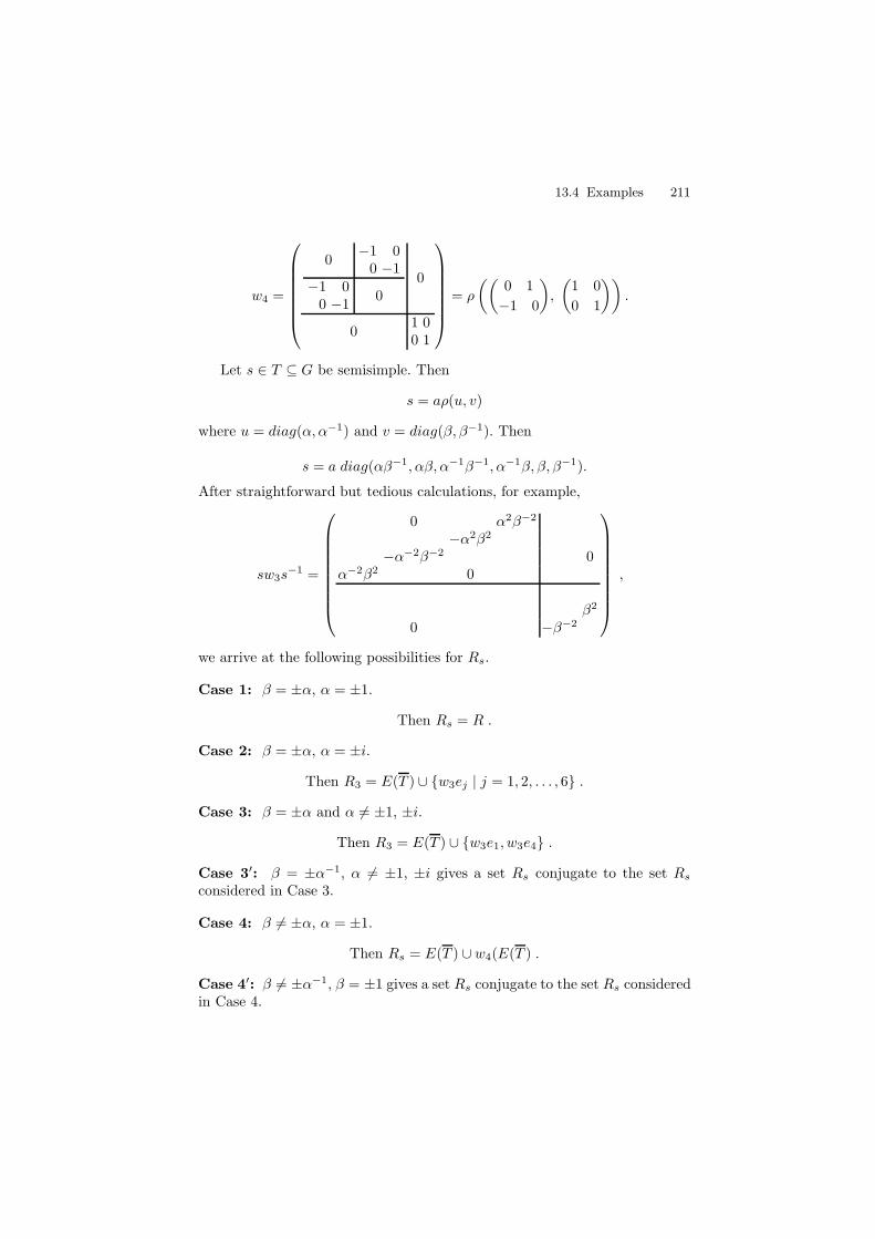
13.4 Examples 211
w4 =
0−1 0
0 −1−1 0
0 −10
0
01 00 1
= ρ
((0 1
−1 0
),
(1 0
0 1
)).
Let s ∈ T ⊆ G be semisimple. Then
s = aρ(u, v)
where u = diag(α, α−1) and v = diag(β, β−1). Then
s = a diag(αβ−1, αβ, α−1β−1, α−1β, β, β−1).
After straightforward but tedious calculations, for example,
sw3s−1 =
0 α2β−2
−α2β2
−α−2β−2 0α−2β2 0
β2
0 −β−2
,
we arrive at the following possibilities for Rs.
Case 1: β = ±α, α = ±1.
Then Rs = R .
Case 2: β = ±α, α = ±i.
Then R3 = E(T ) ∪ w3ej | j = 1, 2, . . . , 6 .
Case 3: β = ±α and α 6= ±1, ±i.
Then R3 = E(T ) ∪ w3e1, w3e4 .
Case 3′: β = ±α−1, α 6= ±1, ±i gives a set Rs conjugate to the set Rsconsidered in Case 3.
Case 4: β 6= ±α, α = ±1.
Then Rs = E(T ) ∪w4(E(T ) .
Case 4′: β 6= ±α−1, β = ±1 gives a set Rs conjugate to the set Rs consideredin Case 4.
212 13 The Centralizer of a Semisimple Element
Case 5: β 6= ±α, β 6= ±α−1, α 6= ±1, β 6= ±1.
Then Rs = E(T ) .
In Case 1, Ms = M .In Case 4 or Case 4′, Ms is irreducible with unit group k∗S`2.In Case 5, Ms = T .In Case 2, Case 3 and Case 3′, Ms is reducible.
Remark 13.11. The monoid Ms is not necessarily of the type discussed in[85, 86] or § 10.4, unless of course it is irreducible. This leads to a number ofbasic questions about Ms.
a) Which spherical varieties (for CG(s)×CG(s)) can occur as an irreduciblecomponent of Ms? Are there any “new” ones?
b) Does the inverse monoid Rs satisfy some analogue of Tits’ axiom “sBx ⊆BxB ∪BsxB if s ∈ S, x ∈ R”?
c) Is there an analogue of the type map λ : Λ→ 2S for Ms?
14
Combinatorics Related to Algebraic Monoids
In this section, we discuss some of the more striking combinatorial problemsthat arise naturally in the study of reductive, algebraic monoids.
14.1 The Adherence Order on WeW
From Corollary 8.35 we have a combinatorial description of the adherenceordering on R:
x ≤ y if BxB ⊆ ByB.
In this section we describe a refinement of those results when we restrict ourattention to the smaller poset (WeW,≤) for e ∈ Λ. The results of this sectionare due to Putcha [92, 93, 94].
The monoid R has a presentation given by:
xe = ex, x ∈W (e)xe = e = ex, x ∈W∗(e).
These relations are of course in addition to those for W and E(T ).If σ ∈ R, then σ has a unique expression:
σ = xwey, e ∈ Λ, x ∈ D(e), w ∈ W ∗(e), y ∈ D(e)−1.
This is the normal form (Definition 8.34) of σ. The length l(σ) can be defined(see [73], [105], [127]) as
l(σ) = l(x) + l(w) + l(e)− l(y)
where l(e) is the length of the longest element in D(e). This notion of lengthagrees with the earlier Definition 8.17. If v0 and w0 are respectively thelongest elements in W (e) and W , then w0e and ev0w0 are respectively the
214 14 Combinatorics Related to Algebraic Monoids
maximum and minimum elements of WeW . Moreover the length function onWeW agrees with the rank function on the graded poset WeW . Also by [73],the length function is subadditive:
l(σθ) ≤ l(σ) + l(θ) for all σ, θ ∈ R.
Let σ = xwey, σ′ = x′w′e′y′ ∈ R be in standard form. Then by [73],
σ ≤ σ′ ⇔ e ≤ e′, xw ≤ x′w′u, u−1y′ ≤ y for some u ∈W (e ′)W∗(e).
This description of the order on R is somewhat unwieldly. A much moreuseful description has been obtained by the Putcha in [92, 93], which we nowdescribe.
We begin with a description of the order on WeW , where e ∈ Λ. LetI = λ(e) and K = λ∗(e). For w ∈ WI , let w = v0wv0, where v0 is the longestelement of WI . Let
WI,K = DI ×WI\K ×D−1I .
Let σ = (x,w, y), σ′ = (x′, w′, y′, ) ∈ WI,K . Define σ ≤ σ′ if w = w1w2w3
with l(w) = l(w1) + l(w2) + l(w3) such that
xw1 ≤ x′, w2 ≤ w
′, w3y ≤ y′.
Let W∗I,K =WI,K as sets but with the above order changed to
xw1 ≤ x′, w2 ≤ w
′, w3y ≤ y′.
Note the subtle difference between these two orderings. The following resultis proved in [92].
Theorem 14.1. WeW is isomorphic to WI,K and the dual of WeW is iso-morphic to W∗
I,K .
We notice that, in many cases, the poset WeW is isomorphic to its dual.This is however not true in general. For instance this is not true of the posetof 4 × 4 rank 3 partial permutation matrices. In general WeW is isomorphicto its dual if no component of W ∗(e) is of type Al(l > 1), Dl(l odd) or E6.
The problem next is to extend the description of the order on the W ×W -orbits to all of R. Let e, f ∈ Λ, e ≤ f . Let ze denote the longest element inW∗(e). Let σ = xwey ∈WeW in standard form. Let
zey = uy1, u ∈W (f), y1 ∈ D(f)−1.
Define the projection,ρe,f (σ) = x′fy1
wherex′ = minxwu′|u′ ≤ u.
Thus we have projection maps ρe,f : WeW →WfW , whenever e ≤ f .
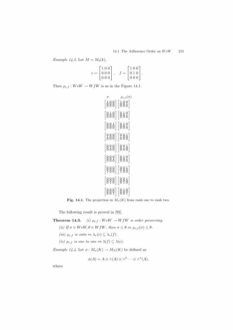
14.1 The Adherence Order on WeW 215
Example 14.2. Let M = M3(k),
e =
1 0 00 0 00 0 0
, f =
1 0 00 1 00 0 0
.
Then ρe,f : WeW →WfW is as in the Figure 14.1.
σ ρe,f (σ)[1 0 00 0 00 0 0
] [1 0 00 0 10 0 0
]
[0 1 00 0 00 0 0
] [0 1 00 0 10 0 0
]
[0 0 10 0 00 0 0
] [0 1 00 0 10 0 0
]
[0 0 01 0 00 0 0
] [0 0 11 0 00 0 0
]
[0 0 00 1 00 0 0
] [0 0 10 1 00 0 0
]
[0 0 00 0 10 0 0
] [0 1 00 0 10 0 0
]
[0 0 00 0 01 0 0
] [0 0 10 0 01 0 0
]
[0 0 00 0 00 1 0
] [0 0 10 0 00 1 0
]
[0 0 00 0 00 0 1
] [0 1 00 0 00 0 1
]
Fig. 14.1. The projection in Mn(K) from rank one to rank two.
The following result is proved in [92].
Theorem 14.3. (i) ρe,f : WeW →WfW is order preserving.
(ii) If σ ∈WeW, θ ∈WfW , then σ ≤ θ ⇔ ρe,f (σ) ≤ θ.
(iii) ρe,f is onto ⇔ λ∗(e) ⊆ λ∗(f).
(iv) ρe,f is one to one ⇔ λ(f) ⊆ λ(e).
Example 14.4. Let φ : Mn(K)→MN (K) be defined as
φ(A) = A⊗ ∧(A)⊗ ∧2 · · · ⊗ ∧n(A),
where
216 14 Combinatorics Related to Algebraic Monoids
N = Πnr=1
(n
r
).
Let M denote the Zariski closure of φ(Mn(K)) in MN(K). In this case, W isthe symmetric group on n letters with S = (12), (23), . . . , (n− 1n). Then
Λ = eI | I ⊆ S ∪ 0
with
eK ≤ eI if and only if K ⊆ I
and
λ(eI) = λ∗(eI) = I, λ∗(eI) = φ
for all I ⊆ S. Then by Theorem 14.3, ρeK ,eI is onto for K ⊆ I.
Example 14.5. Let φ : Mn(K)→MN (K) be defined as
φ(A) = A⊕ ∧(A) ⊕ ∧2 · · · ⊕ ∧n(A)
where N = 2n− 1. Let M denote the Zariski closure of φ(Mn(K) in MN(K).Again W is the symmetric group on n letters with S = (12), (23), . . . , (n −1n). Then
Λ = eI | I ⊆ S ∪ 1
with
eK ≤ eI if and only if K ⊆ I
and
λ(eI) = λ∗(eI) = I, λ∗(eI) = φ
for all I ⊆ S. Again by Theorem 14.3, ρeK ,eI is one to one for K ⊆ I.
If M is a canonical monoid as in Example 10.17, then Theorem 14.3 canbe used to show that R∗ = R\0 is an Eulerian poset. This means thatthe Mobius function µ on R∗ is given by
µ(x, y) = (−1)rkx+rky, forx ≤ y
Here rk is the rank function on the graded poset R∗. The problem of deter-mining the Mobius function on R in general, remains open.
14.3 Distribution of Products in Finite Monoids 217
14.2 Shellability and Stanley-Reisner Rings
Let P be a finite graded partially ordered set with a maximum element 1and a minimum element 0. This means that all maximal chains in P have thesame length. Let ∆ denote the order complex of P . Thus ∆ is the simplicialcomplex whose faces are chains in P . Then ∆ (or P ) is said to be shellableif the maximal faces can be ordered F1, · · · , Fs such that, for i < j, there is amaximal face Fk, k < j, such that Fi∩Fj ⊆ Fk∩Fj = Fj\v for some v ∈ P .This is a topological condition implying that ∆ then has the homotopy typeof a wedge of spheres. Let A denote the commutative algebra (over a field)generated by xα(α ∈ P ). For A = a1, · · · , am ⊆ P , let xA = xa1 · · ·xam . LetI denote the ideal generated by xA, where A is not a face. Then F = A/I iscalled the Stanley-Reisner ring of ∆ (or P ). Note that F is spanned by thefaces of∆. It is well known that, if ∆ is shellable, then F is a Cohen-MacAulayring, cf. [132].
A very useful method for checking the shellability of P has been developedby Bjorner and Wachs [6]. For a, b ∈ P , write a→ b if a covers b (i.e. a > b andthere is no c such that a > c > b). The concept of lexicographic shellability,introduced in [6], can be briefly described as follows. The edges of P are labeledrecursively starting from the top, whereby for a→ b the label depends on thechoice of a maximal chain from 1 to a. Fix a > b and a maximal chain from 1to a. The labeling must be such that there exists a unique maximal chain froma to b with increasing labels and so that this chain is lexicographically lessthan any other maximal chain from a to b. It is shown in [6] that lexicographicshellability implies shellability.
Proctor [80] and Bjorner and Wachs [6] have shown that the Weyl groupW , with respect to the Bruhat-Chevalley order, is lexicographically shellable.It is also shown in [6] that DI is lexicographically shellable for any I ⊆ S.
The following result is due to Putcha [93, 94].
Theorem 14.6. Each W ×W -orbit WeW is lexicographically shellable, andhence its Stanley-Reisner ring is Cohen-Macaulay. A maximal W ×W -orbitis also Eulerian and hence its Stanley-Reisner ring is Gorenstein.
The problem of whether the Stanley-Reisner ring of R is always Cohen-Macaulay, remains open.
14.3 Distribution of Products in Finite Monoids
In this section we consider the problem of distribution of products in a finitemonoid S. In our discussion we naturally arrive at formulas that are familiarin enumerative combinatorics. This problem becomes particularly interestingif S is a finite monoid of Lie type. We obtain explicit formulas for the monoidMn(Fq).
218 14 Combinatorics Related to Algebraic Monoids
Let S be a finite monoid and let a ∈ S. Consider,
Hn(a) = (x1, . . . , xn) ∈ Sn | x1 · ... · xn = a
for n > 0, and definehn(a) = |Hn(a)| .
What can we say about the sequence hn(a) | n > 0? What special propertiesdoes the power series
h(a) =∑
n≥1
hn(a)tn−1
possess? If a = bx, how are h(a) and h(b) related?In this section we treat the above questions (and some others) systemati-
cally from a combinatorial viewpoint.
14.3.1 Properties of h(a)
Let S be a finite monoid and let a ∈ S. As above, we let
hn(a) =∣∣(x1, . . . , xn) ∈ S
n | x1 · ... · xn = a∣∣ .
For a, b ∈ S we write b ≥ a if a = bx for some x ∈ S. We define
R(b/a) = x ∈ S | a = bx
and
r(b/a) = |R(b/a)| .
Proposition 14.7. (i) h1(a) = 1 for any a ∈ S.
(ii) hn+1(a) =∑
b≥a
r(b/a)hn(b) for any n > 1.
Proof. (i) is obvious.For (ii) consider
(x1, . . . , xn, xn+1 ∈ Sn+1
∣∣ x1 · ... · xn+1 = a
=⊔
b∈S
(x1, . . . , xn, xn+1) ∈ s
n+1 x1 · ... · xn+1 = ax1 · ... · xn = b
∼=⊔
b≥a
((x1, . . . , xn) ∈ Sn
∣∣ x1 · ... · xn = b×R(b/a)
).
Hence Hn+1(a) =⊔
b≥a
Hn(b)×R(b/a), and thus
hn+1(a) =∣∣Hn+1(a)
∣∣ =∑
b≥a
∣∣Hn(b)∣∣ ∣∣r(b/a)
∣∣ =∑
b≥a
hn(b)r(b/a) .
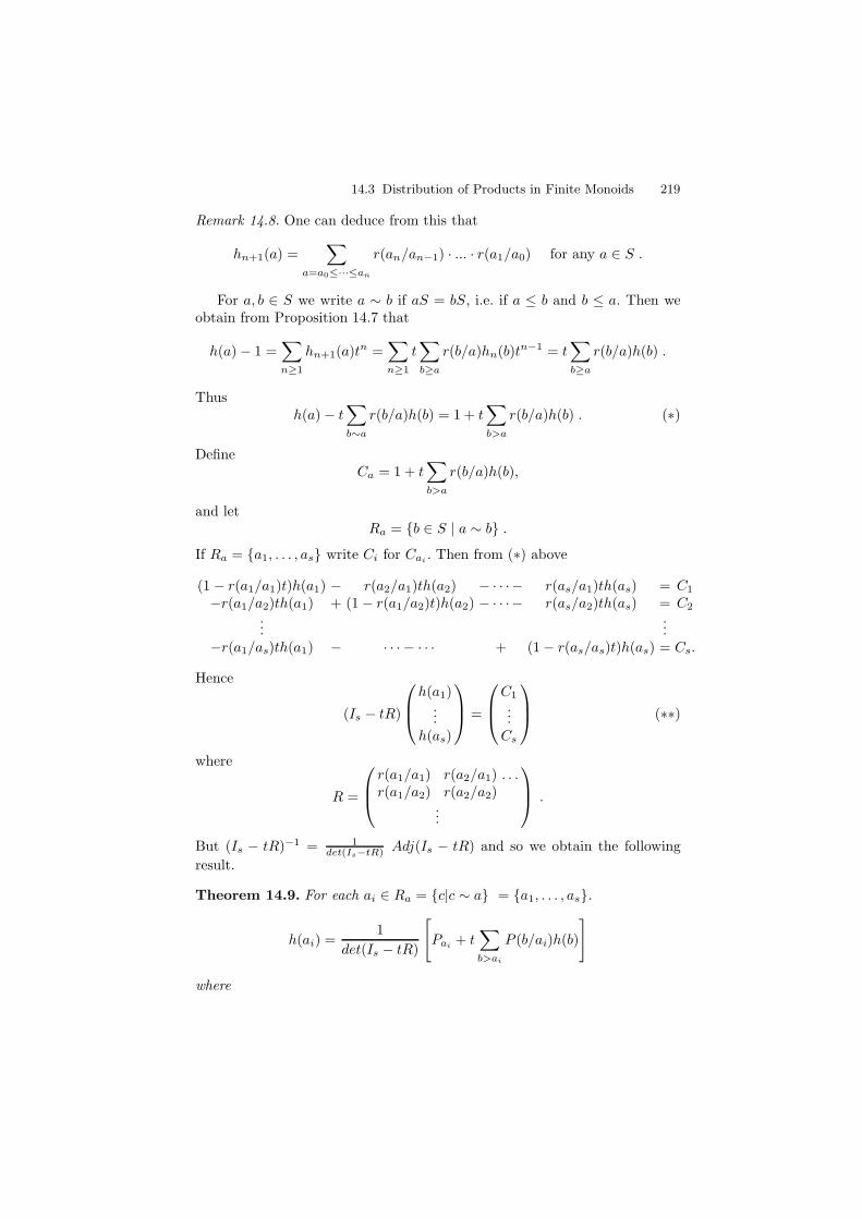
14.3 Distribution of Products in Finite Monoids 219
Remark 14.8. One can deduce from this that
hn+1(a) =∑
a=a0≤···≤an
r(an/an−1) · ... · r(a1/a0) for any a ∈ S .
For a, b ∈ S we write a ∼ b if aS = bS, i.e. if a ≤ b and b ≤ a. Then weobtain from Proposition 14.7 that
h(a)− 1 =∑
n≥1
hn+1(a)tn =
∑
n≥1
t∑
b≥a
r(b/a)hn(b)tn−1 = t
∑
b≥a
r(b/a)h(b) .
Thush(a)− t
∑
b∼a
r(b/a)h(b) = 1 + t∑
b>a
r(b/a)h(b) . (∗)
DefineCa = 1 + t
∑
b>a
r(b/a)h(b),
and letRa = b ∈ S | a ∼ b .
If Ra = a1, . . . , as write Ci for Cai . Then from (∗) above
(1 − r(a1/a1)t)h(a1) − r(a2/a1)th(a2) − · · ·− r(as/a1)th(as) = C1
−r(a1/a2)th(a1) + (1− r(a1/a2)t)h(a2) − · · ·− r(as/a2)th(as) = C2
......
−r(a1/as)th(a1) − · · · − · · · + (1− r(as/as)t)h(as) = Cs.
Hence
(Is − tR)
h(a1)
...h(as)
=
C1
...Cs
(∗∗)
where
R =
r(a1/a1) r(a2/a1) . . .r(a1/a2) r(a2/a2)
...
.
But (Is − tR)−1 = 1det(Is−tR) Adj(Is − tR) and so we obtain the following
result.
Theorem 14.9. For each ai ∈ Ra = c|c ∼ a = a1, . . . , as.
h(ai) =1
det(Is − tR)
[Pai + t
∑
b>ai
P (b/ai)h(b)
]
where
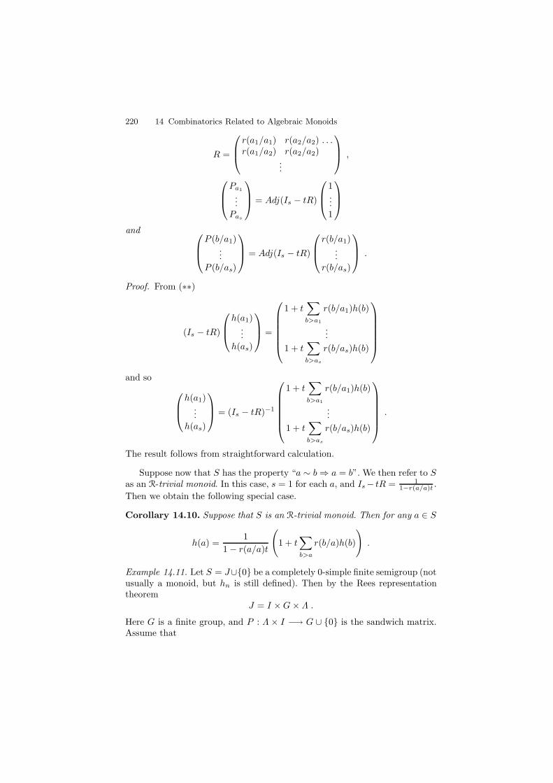
220 14 Combinatorics Related to Algebraic Monoids
R =
r(a1/a1) r(a2/a2) . . .r(a1/a2) r(a2/a2)
...
,
Pa1
...Pas
= Adj(Is − tR)
1...1
and P (b/a1)
...P (b/as)
= Adj(Is − tR)
r(b/a1)
...r(b/as)
.
Proof. From (∗∗)
(Is − tR)
h(a1)
...h(as)
=
1 + t∑
b>a1
r(b/a1)h(b)
...
1 + t∑
b>as
r(b/as)h(b)
and so
h(a1)
...h(as)
= (Is − tR)−1
1 + t∑
b>a1
r(b/a1)h(b)
...
1 + t∑
b>as
r(b/as)h(b)
.
The result follows from straightforward calculation.
Suppose now that S has the property “a ∼ b⇒ a = b”. We then refer to Sas an R-trivial monoid. In this case, s = 1 for each a, and Is− tR = 1
1−r(a/a)t .
Then we obtain the following special case.
Corollary 14.10. Suppose that S is an R-trivial monoid. Then for any a ∈ S
h(a) =1
1− r(a/a)t
(1 + t
∑
b>a
r(b/a)h(b)
).
Example 14.11. Let S = J∪0 be a completely 0-simple finite semigroup (notusually a monoid, but hn is still defined). Then by the Rees representationtheorem
J = I ×G× Λ .
Here G is a finite group, and P : Λ × I −→ G ∪ 0 is the sandwich matrix.Assume that
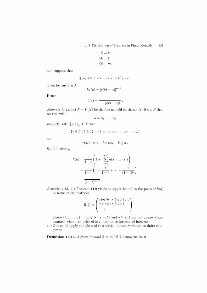
14.3 Distribution of Products in Finite Monoids 221
|I| = k
|Λ| = `
|G| = m.
and suppose that
|(λ, i) ∈ Λ× I | p(λ, i) = 0| = α .
Then for any a ∈ Jhn(a) = [g(k`− α)]n−1 .
Hence
h(a) =1
1− g(k`− α)t.
Example 14.12. Let F = F (X) be the free monoid on the set X . If a ∈ F thenwe can write
a = x1 · ... · xn
uniquely, with xi ⊆ X . Hence
b ∈ F | b ≥ a = 1, x1, x1x2, . . . , xi · ... · xn
andr(b/a) = 1 for any b ≥ a .
So, inductively,
h(a) =1
1− t
(1 + t
n−1∑
i=0
h(xi · ... · xi)
)
=1
1− t
(1 +
t
1− t+ · · ·+
t
(1− t)n
)
=1
(1− t)n+1.
Remark 14.13. (i) Theorem 14.9 yields an upper bound to the poles of h(a)in terms of the matrices
R(b) =
r(b1/b1 r(b2/b1) . . .r(b1/b2) r(b2/b2)
...
where b1, . . . , bs = x ∈ S | x ∼ b and b ≥ a. I am not aware of anyexample where the poles of h(a) are not reciprocals of integers.
(ii) One could apply the ideas of this section almost verbatim to finite cate-gories.
Definition 14.14. A finite monoid S is called R-homogeneous if
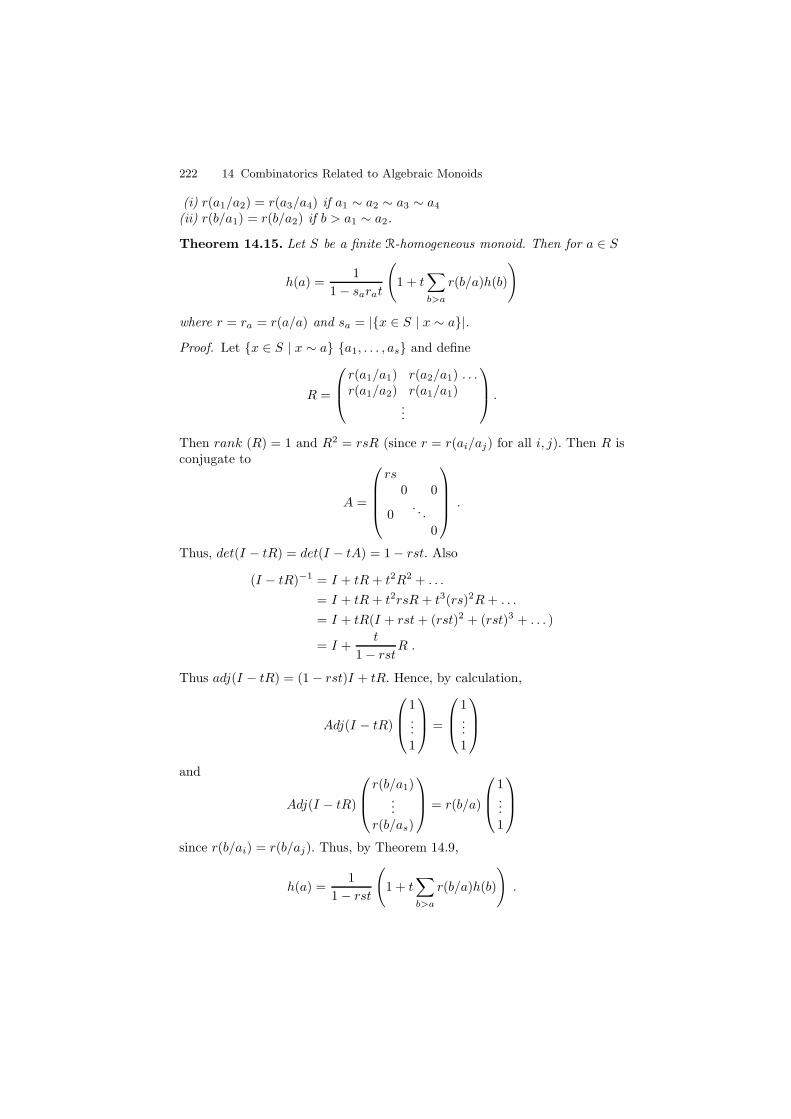
222 14 Combinatorics Related to Algebraic Monoids
(i) r(a1/a2) = r(a3/a4) if a1 ∼ a2 ∼ a3 ∼ a4
(ii) r(b/a1) = r(b/a2) if b > a1 ∼ a2.
Theorem 14.15. Let S be a finite R-homogeneous monoid. Then for a ∈ S
h(a) =1
1− sarat
(1 + t
∑
b>a
r(b/a)h(b)
)
where r = ra = r(a/a) and sa = |x ∈ S | x ∼ a|.
Proof. Let x ∈ S | x ∼ a a1, . . . , as and define
R =
r(a1/a1) r(a2/a1) . . .r(a1/a2) r(a1/a1)
...
.
Then rank (R) = 1 and R2 = rsR (since r = r(ai/aj) for all i, j). Then R isconjugate to
A =
rs0 0
0. . .
0
.
Thus, det(I − tR) = det(I − tA) = 1− rst. Also
(I − tR)−1 = I + tR + t2R2 + . . .
= I + tR + t2rsR + t3(rs)2R+ . . .
= I + tR(I + rst+ (rst)2 + (rst)3 + . . . )
= I +t
1− rstR .
Thus adj(I − tR) = (1− rst)I + tR. Hence, by calculation,
Adj(I − tR)
1...1
=
1...1
and
Adj(I − tR)
r(b/a1)
...r(b/as)
= r(b/a)
1...1
since r(b/ai) = r(b/aj). Thus, by Theorem 14.9,
h(a) =1
1− rst
(1 + t
∑
b>a
r(b/a)h(b)
).
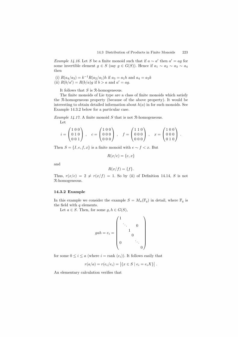
14.3 Distribution of Products in Finite Monoids 223
Example 14.16. Let S be a finite monoid such that if a ∼ a′ then a′ = ag forsome invertible element g ∈ S (say g ∈ G(S)). Hence if a1 ∼ a2 ∼ a3 ∼ a4
then
(i) R(a4/a3) = k−1R(a2/a1)h if a3 = a1h and a4 = a2k(ii) R(b/a′) = R(b/a)g if b > a and a′ = ag.
It follows that S is R-homogeneous.The finite monoids of Lie type are a class of finite monoids which satisfy
the R-homogeneous property (because of the above property). It would beinteresting to obtain detailed information about h(a) in for such monoids. SeeExample 14.3.2 below for a particular case.
Example 14.17. A finite monoid S that is not R-homogeneous.Let
i =
1 0 00 1 00 0 1
, c =
1 0 00 0 00 0 0
, f =
1 1 00 0 00 0 0
, x =
1 0 00 0 00 1 0
.
Then S = I, e, f, x is a finite monoid with e ∼ f < x. But
R(x/e) = e, x
andR(x/f) = f.
Thus, r(x/e) = 2 6= r(x/f) = 1. So by (ii) of Definition 14.14, S is notR-homogeneous.
14.3.2 Example
In this example we consider the example S = Mn(Fq) in detail, where Fq isthe field with q elements.
Let a ∈ S. Then, for some g, h ∈ G(S),
gah = ei =
1. . . 0
10
0. . .
0
for some 0 ≤ i ≤ a (where i = rank (ei)). It follows easily that
r(a/a) = r(ei/ei) =∣∣x ∈ S | ei = eiX
∣∣ .
An elementary calculation verifies that
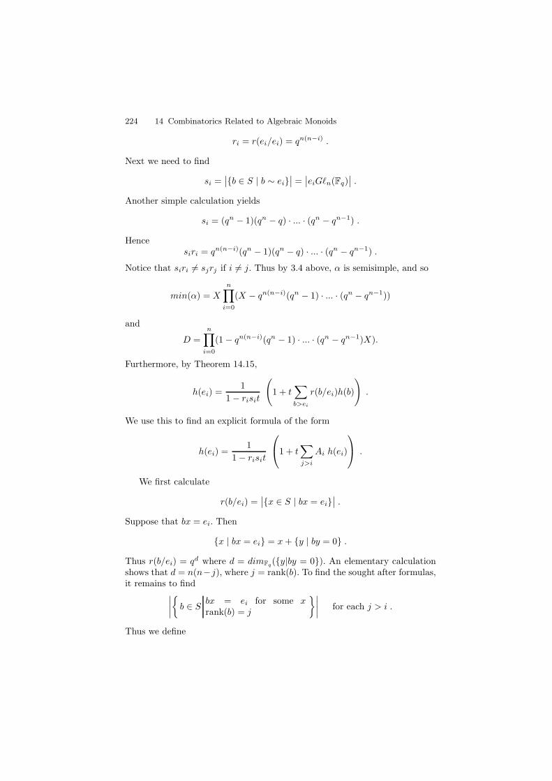
224 14 Combinatorics Related to Algebraic Monoids
ri = r(ei/ei) = qn(n−i) .
Next we need to find
si =∣∣b ∈ S | b ∼ ei
∣∣ =∣∣eiG`n(Fq)
∣∣ .
Another simple calculation yields
si = (qn − 1)(qn − q) · ... · (qn − qn−1) .
Hencesiri = qn(n−i)(qn − 1)(qn − q) · ... · (qn − qn−1) .
Notice that siri 6= sjrj if i 6= j. Thus by 3.4 above, α is semisimple, and so
min(α) = X
n∏
i=0
(X − qn(n−i)(qn − 1) · ... · (qn − qn−1))
and
D =
n∏
i=0
(1− qn(n−i)(qn − 1) · ... · (qn − qn−1)X).
Furthermore, by Theorem 14.15,
h(ei) =1
1− risit
(1 + t
∑
b>ei
r(b/ei)h(b)
).
We use this to find an explicit formula of the form
h(ei) =1
1− risit
1 + t
∑
j>i
Ai h(ei)
.
We first calculate
r(b/ei) =∣∣x ∈ S | bx = ei
∣∣ .
Suppose that bx = ei. Then
x | bx = ei = x+ y | by = 0 .
Thus r(b/ei) = qd where d = dimFq(y|by = 0). An elementary calculationshows that d = n(n−j), where j = rank(b). To find the sought after formulas,it remains to find
∣∣∣∣b ∈ S
bx = ei for some xrank(b) = j
∣∣∣∣ for each j > i .
Thus we define
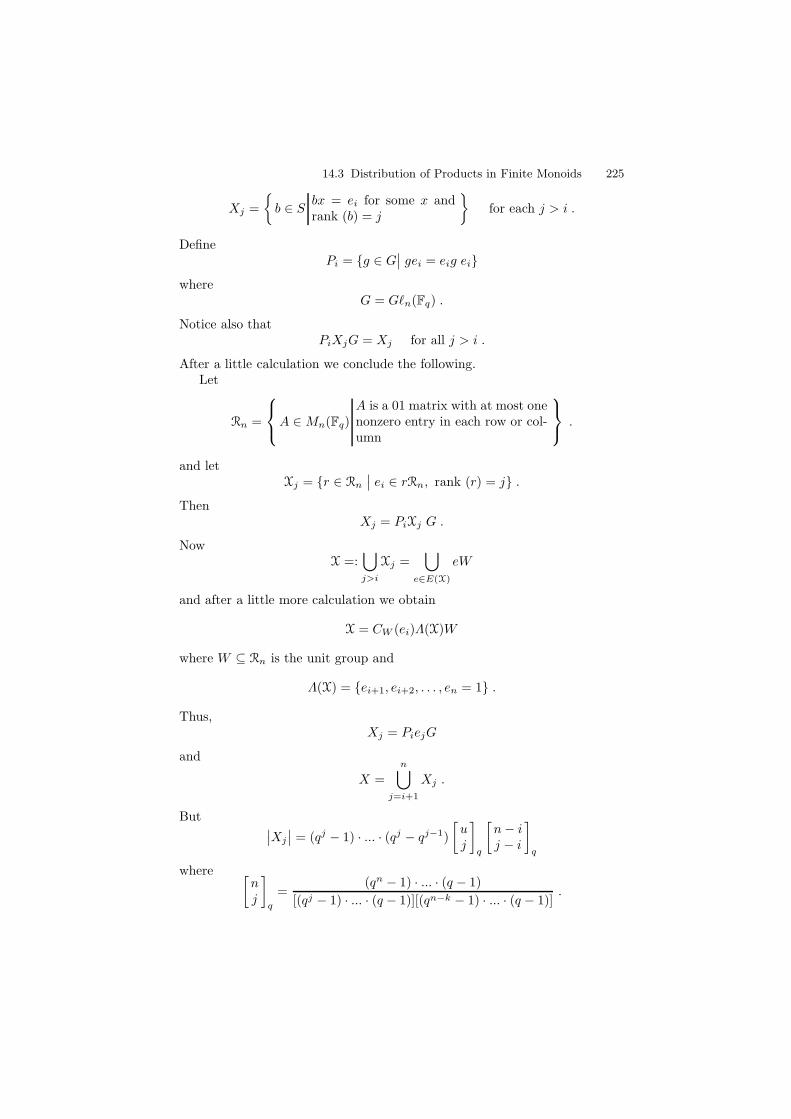
14.3 Distribution of Products in Finite Monoids 225
Xj =
b ∈ S
bx = ei for some x andrank (b) = j
for each j > i .
DefinePi = g ∈ G
∣∣ gei = eig ei
whereG = G`n(Fq) .
Notice also thatPiXjG = Xj for all j > i .
After a little calculation we conclude the following.Let
Rn =
A ∈Mn(Fq)
A is a 01 matrix with at most onenonzero entry in each row or col-umn
.
and letXj = r ∈ Rn
∣∣ ei ∈ rRn, rank (r) = j .
ThenXj = PiXj G .
NowX =:
⋃
j>i
Xj =⋃
e∈E(X)
eW
and after a little more calculation we obtain
X = CW (ei)Λ(X)W
where W ⊆ Rn is the unit group and
Λ(X) = ei+1, ei+2, . . . , en = 1 .
Thus,Xj = PiejG
and
X =
n⋃
j=i+1
Xj .
But ∣∣Xj
∣∣ = (qj − 1) · ... · (qj − qj−1)
[uj
]
q
[n− ij − i
]
q
where [nj
]
q
=(qn − 1) · ... · (q − 1)
[(qj − 1) · ... · (q − 1)][(qn−k − 1) · ... · (q − 1)].
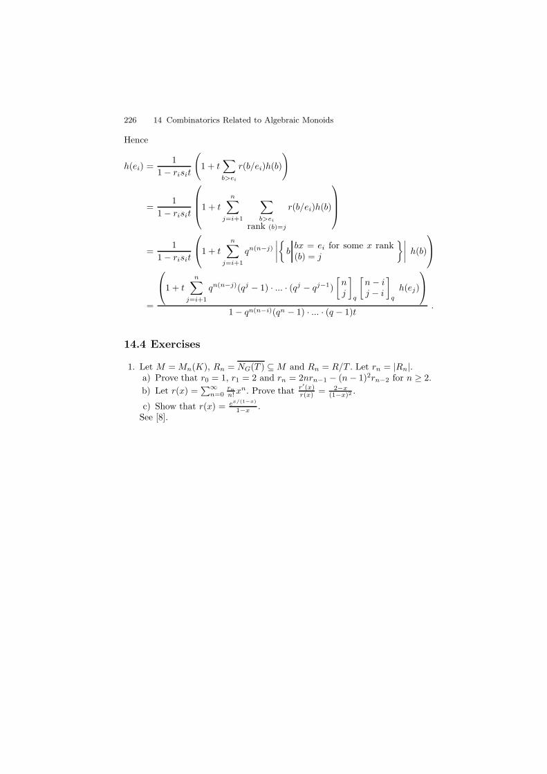
226 14 Combinatorics Related to Algebraic Monoids
Hence
h(ei) =1
1− risit
(1 + t
∑
b>ei
r(b/ei)h(b)
)
=1
1− risit
1 + t
n∑
j=i+1
∑
b>ei
rank (b)=j
r(b/ei)h(b)
=1
1− risit
1 + t
n∑
j=i+1
qn(n−j)
∣∣∣∣bbx = ei for some x rank(b) = j
∣∣∣∣ h(b)
=
1 + t
n∑
j=i+1
qn(n−j)(qj − 1) · ... · (qj − qj−1)
[nj
]
q
[n− ij − i
]
q
h(ej)
1− qn(n−i)(qn − 1) · ... · (q − 1)t.
14.4 Exercises
1. Let M = Mn(K), Rn = NG(T ) ⊆M and Rn = R/T . Let rn = |Rn|.a) Prove that r0 = 1, r1 = 2 and rn = 2nrn−1 − (n− 1)2rn−2 for n ≥ 2.
b) Let r(x) =∑∞n=0
rn
n! xn. Prove that r′(x)
r(x) = 2−x(1−x)2 .
c) Show that r(x) = ex/(1−x)
1−x .See [8].
15
Survey of Related Developments
In this chapter we describe several results that are directly related to thetheory of algebraic monoids. In each case we find some other areas of algebracoming into play. Although many of these technical issues are beyond thescope of this survey, we hope to provide the reader with an overview of someof the more striking related developments.
15.1 Complex Representation of Finite ReductiveMonoids
As is well known, a finite group G has the property that every finite dimen-sional complex representation of G is completely reducible. The situation forfinite monoids is entirely different and not nearly so well understood. Indeed,there is no effective characterization of finite monoids whose complex repre-sentations are all completely reducible. Until recently, it was not known thatC[Mn(Fq)] is a semisimple algebra.
The following result was made possible by the theory of reductive monoids.It is due to Okninski and Putcha [67].
Theorem 15.1. Let M be a finite monoid of Lie type. Then the monoid al-gebra C[M ] is semisimple.
Recall that a monoid of Lie type is a regular monoid M generated byidempotents and units, whose unit group is a group of Lie type. These monoidsare defined to satisfy a number of axioms relating to the BN -pair structureof G to the idempotents of M . See Theorem 10.4. In particular, any finitereductive monoid is a finite monoid of Lie type. The model example here isMn(Fq).
Corollary 15.2. Let M be as in the theorem. Then C[Mn(Fq)] is a semisimplealgebra.
228 15 Survey of Related Developments
This result was also obtained independently by Kovacs [49].As a consequence of their approach to Theorem 15.1, the authors obtain
the following important corollary.
Corollary 15.3. Any complex irreducible representation of M is induced fromsome irreducible representation ρ : P → G`n(C) of a parabolic subgroup P ⊆G with Ru(P ) ⊆ Ker(ρ).
The proof combines two opposing strategies.
a) Harish-Chandra’s theory of cuspidal representations,b) reduction to certain monoids of the form M = G ∪GeG ∪ 0.
In a subsequent paper [68] the authors turn the tables. They assume thatM is a finite monoid with unit groupG and zero element 0 ∈M , and semisim-ple monoid algebra C[M ]. From this, they obtain a relative notion of M -cuspidal irreducible representations for G. Harish-Chandra’s theory is thenrecovered as the special case where G is a finite group of Lie type and M is acanonical monoid [96]. See also §8.3 of [66].
15.2 Finite Semigroups and Highest Weight Categories
Recall from § 2.3.1 that a monoid S is regular if, for any x ∈ S, there existsa ∈ S such that xax = x. For such a semigroup, it is easy to see that there isan idempotent in each J-class of S. In fact, x is in the J-class of the idempotentxa. Thus,
S =⊔
J∈U(S)
J.
This may seem like a facile curiosity, imitating the much studied situation inring theory (the one attributed to von Neumann). However, there is some-thing of greater significance here, which was first discovered by Putcha [91].It turns out that the complex monoid algebra of a finite regular monoid is aquasihereditary algebra.
Definition 15.4. Let A be a finite dimensional algebra over K. Then A isquasihereditary if there is a chain of ideals (called a hereditary chain)
0 = I0 ⊆ I1 ⊆ · · · ⊆ Ir = A
such that, for j = 1, . . . , r,
a) Ij/Ij−1 is a projective A/Ij−1-module,b) I2
j = Ij ,c) IjRIj ⊆ Ij−1, where R is the radical of A.
15.2 Finite Semigroups and Highest Weight Categories 229
It turns out that this is equivalent to the property that Rep(A) is a highestweight category (see Theorem 9.10 for a good illustration, and [16] for theseminal paper). In the remainder of this section we indicate how to construct ahereditary chain of ideals for the monoid algebra of a finite regular semigroup.We also show how this brings about the corresponding structure of a highestweight category. To define a highest weight category one needs simple objects,standard objects and a weight poset.
Then let M be a finite regular monoid, and let U denote the poset of (reg-ular) J-classes of M . If e ∈ E(J), we write HJ for the H-class of e. By thetheory of Munn-Ponizovskii [15], the set Irr(M) of irreducible complex rep-resentations of M is in one-to-one correspondence with the set of irreduciblerepresentations of the various HJ :
Irr(M) =⊔
J∈U
Irr(HJ ).
This identification is obtained as follows. Let L = L(θ) be an irreduciblecomplex M -module. Then there exists a unique J-class J ∈ U such that
a) J · L 6= 0,b) J ′ · L = 0 for all J ′ 6≥ J .
If e ∈ E(J) is an idempotent, then e · L is an irreducible HJ -module. We saythat
θ < θ′
if J ′ ⊆ MJM . Then (Irr(M), <) is the weight poset of simple objects. Nowfor each θ ∈ Irr(HJ ) there is a primitive idempotent eθ ∈ C[M ] such thateθ < eJ and L(θ) ∼= C[M ]eθ/Reθ, where R is the radical of C[M ]. Define
∆(θ) = C[J ]eθ.
Here (∆(θ)|θ ∈ Irr(M) is the set of standard objects. The following theoremis due to Putcha (Theorem 2.1 of [91]).
Theorem 15.5. Let M be a finite regular monoid.
a) Then the category of finite-dimensional C[M ]-modules is a highest weightcategory.
b) C[M ] is a quasihereditary algebra.
The proof of Theorem 15.5 amounts to constructing a hereditary chain as inDefinition 15.4. But it turns out that there is a canonical such chain. LetU1 = J | the minimal J-class, U2 = J | J covers J1, and so on, so that
Um = J | J covers some K in Um−1.
Thus define
230 15 Survey of Related Developments
J1 = ∪J∈U1J
J2 = ∪J∈U2J
J3 = ∪J∈U3J
...
Let Ii = C[Ji], a two-sided ideal of C[M ], so that Ir = C[M ] for some r > 0.Consider
0 ⊆ I1 ⊆ I2 ⊆ · · · ⊆ Ir.
It turns out that this is the desired (canonical) hereditary chain.
15.3 Singularities of G-embeddings
It has been known for some time that any normal, spherical variety X hasrational singularities in characteristic zero. The essential idea here is containedin [76], where the proof is given for the affine case. The result for generalspherical varieties then follows easily from the affine case using basic local-global arguements from [13] or [36].
Furthermore, one can show that the reduction mod p of X is Frobeniussplit for large p. This is the best known method for obtaining geometric resultsabout singularities in characteristic p > 0.
Definition 15.6. Assume that charK = p > 0. If X is an algebraic varietyover K, denote by F : OX → F∗OX the absolute Frobenius morphism of X.We say that X is Frobenius split if there is a map σ ∈ HomOX (F∗OX ,OX)such that σ F is the identity on OX .
Rittatore obtains the following result in [122].
Theorem 15.7. Any normal G-embedding X is Frobenius split.
By a G-embedding we mean a G×G-variety, (X,x) with dense orbit (G×G) · x such that (G×G)x = (g, h) ∈ G×G | g = h.
Corollary 15.8. Any normal G-embedding X has rational singularities. Inparticular, it is a Cohen-Macaulay variety.
Rittatore derives Theorem 15.7, first for the “wonderful” G-embeddingand then derives the general case by using resolution of singularities. Noticethat any reductive monoid is a G-embedding. Furthermore, the wonderfulG-embedding is directly related to the canonical monoids ([96]) with groupG.
In the other direction, Popov has shown in [77], that the Kraft-Procesiconjecture (to the effect that the normalization of any reductive group orbitclosure has rational singularities, [50]) is false. He shows that such singularitiesmay even be non-Cohen-Macaulay.
15.4 Cohomology of G-embeddings 231
15.4 Cohomology of G-embeddings
LetX be a complete, nonsingularG-embedding over C. Assume also that thereis a birational G ×G morphism from X to the canonical compactification ofG. Assume also that K = C, the complex numbers. Let K ⊆ G be a maximal,compact subgroup in the classical topology, and let Z ⊆ X be the closure ofa maximal torus T ⊆ G. Assume that TK ⊆ T ∩K ⊆ K is a maximal torusof K. Since KTK = G and KZK is compact, we obtain
X = KZK.
Thus, we obtain a surjective, real analytic morphism
π : (K ×K)×Tk×TK Z −→ X
since Z is TK × TK-stable. Let
U = (K ×K)×Tk×TK Z .
The Weyl group W acts naturally on U, and π is constant on the W -orbits.Thus, W acts on H∗(U; Q) and we obtain a ring homomorphism
π∗ : H∗(X ; Q) −→ H∗(U; Q)W .
See [22] for details.
Theorem 15.9. π∗ : H∗(X ; Q) −→ H∗(U; Q)W is an isomorphism of rings.
Theorem 15.9 is due to DeConcini and Procesi [22]. They also computeH∗(U; Q) in [22] by extending some work of Danilov [19]. Notice that there isa fibration
U −→ K/TK ×K/TK
with fibre Z. Thus U may be regarded as a “relative” torus embedding.In [5] these same authors (along with Bifet) describe the rational coho-
mology ring of any complete symmetric variety by generators and relators.The authors first introduce a more general notion. A regular embeddingis a smooth algebraic variety X on which a connected affine algebraic groupG acts with finitely many orbits. Every orbit closure is smooth and is thetransverse intersection of the codimension one orbit closures which contain it.Moreover, the isotropy group of any x ∈ X must have a dense orbit in the nor-mal space to the orbit G · x ⊆ X . Examples of projective regular embeddingscan often be obtained from semisimple algebraic monoids M with zero, suchthat M\0 is smooth. The authors then determine the G-equivariant rationalcohomology algebra H∗
G(X) of any regular embedding X , by associating withX a “Stanley-Reisner system” (a generalization of the Stanley-Reisner algebraassociated with a simplicial complex). Using this construction, they constructan algebra which turns out to be H∗
G(X). If X is also compact, the coho-mology ring H∗(X) can be obtained as the quotient of H∗
G(X) by a certainregular sequence consisting of generators of H∗
G(∗), the one point G-space.For X a torus embedding, one recovers the Jurkiewicz-Danilov presentationof H∗(X) as discussed by Danilov in [19].
232 15 Survey of Related Developments
15.5 Horospherical Varieties
Definition 15.10. An embedding X of G/H is called horospherical if H con-tains a maximal unipotent subgroup of G.
Horospherical embeddings were first looked at systematically by Popovand Vinberg in [79]. They obtained the fundamental correspondence betweenthe poset of orbits and the poset of faces of the corresponding polyhedralcone. They also characterized normal and factorial horospherical embeddings.The results of [78] and [79] were cited by Luna and Vust (in their seminalpaper [56]) as a major catalyst in the development of the theory of sphericalembeddings. A partial generalization to the nonaffine case was carried out byPauer in [70, 71].
The technique of “horospherical degeneration” [76] has since become animportant method in the study of spherical varieties [1, 142].
15.6 Monoids associated with Kac-Moody Groups
In [43] Kac and Peterson start with a Kac-Moody Lie algebra g and constructa groupG, the associated Kac-Moody group. In [50] they introduce an algebra,the algebra of strongly regular functions on G.
Let F be an algebraically closed field of characteristic zero, and let g bea Lie algebra defined over F. Assuming that g comes from a symmetrizable,generalized Cartan matrix, they define (in [50]) the algebra F[G] of stronglyregular functions on G. They show that
F[G] =⊕
λ∈P+
L∗(λ)⊗ L(λ)
where P+ is the set of dominant weights of the weight lattice P . Since eachL(Λ) is integrable they obtain
j : G ⊆ Specm(F[G]),
the space of codimension one ideals of F[G]. However, j is not surjective unlessg is finite dimensional.
About the same time (1983), Slodowy [125] suggested that there should ex-ist a some kind of partial compactification G ⊆ Specm(F[G]) whose structuremight significantly help in the study of the deformation of certain singularities.He conjectured that
G = GTG
and he also anticipated the structure of T . Peterson suggested that G mightactually be a monoid.
Since then, Mokler [58, 59] approached these problems systematically. Hefirst constructs a monoid
15.6 Monoids associated with Kac-Moody Groups 233
G ⊆ End
(⊕
Λ∈P+
L(Λ)
)
directly, using the set of faces F = R ⊆ X of the Tits cone X , to defineprojections
e(R) :⊕
Λ∈P+
L(Λ) −→⊕
Λ∈P+
L(Λ).
G is then the submonoid of End
(⊕
Λ∈P+
L(Λ)
)generated by G∪ e(R) | R ∈
F. He then proves [58] that
G = G ⊆ End(⊕L(Λ))
the closure being taken in the sense of elementary, infinite dimensional, al-gebraic geometry (section 3 of [58]). He also obtains some decisive structuralinformation about G.
Induced by its action on X , the Weyl group W acts on the face lattice F
of X . A face R = R(Θ) of X is called special if the relative interior of Rmeets the closed fundamental chamber C of X . (The situation is similar towhat we encountered in § 7.2.) Let I be the set of vertices of the underlyingDynkin diagam of G. Then each special face of X corresponds to a subset ofI for which the associated Dynkin subdiagram is either empty, or has onlycomponents of infinite type.
Theorem 15.11.G =
⊔
R special
Ge(R)G .
For the proof see Proposition 2.26 of [58].Mokler continues his work in [59] by further investigating the structure of
Specm(F[G]). In [60], he obtains results generalizing the work of [105, 112, 73].
In particular, he determines the generalized Bruhat decomposition on M andthe length function on W .

References
1. I. V. Arzhantsev, Contractions of affine spherical manifolds, Mat. Sb.190(1999), 3-22.
2. M. F. Atiyah and I. G. MacDonald, “Commutative algebra”, Addison-Wesley,London, 1969.
3. M. K. Augustine, Congruences of monoids of Lie type In “Monoids and semi-groups with applications”, held at Berkeley, 1989, 324-333, World Sci. Pub-lishing, River Edge, NJ, 1991.
4. A. Bialynicki-Birula, Some theorems on actions of algebraic groups, Annalsof Math. 98(1973), 480-497.
5. E. Bifet, C. De Concini, C. Procesi, Cohomology of regular embeddings, Ad-vances in Math. 82(1990), 1-34.
6. A. Bjorner, M. Wachs, Bruhat order of Coxeter groups and shellability, Ad-vances in Math. 43(1982), 87-100.
7. A. Borel, Linear algebraic groups, Graduate Texts in Mathematics 126,Springer-Verlag, New York, 1991.
8. D. Borwein, S. Rankin, L. Renner, Enumeration of injective partial transfor-mations, Discrete Math. 73(1989), 291-296.
9. M. Brion, Quelques proprietes des espaces homogenes spheriques,Manuscripta Math. 55(1986), 191-198.
10. M. Brion, Sur la geometrie des varietes spheriques, Comment. Math. Helv.66(1991) 237-262.
11. M. Brion, Varietes spheriques, In, “Operations hamiltoniennes et operationsde groupes algebriques”, Notes de la session de S. M. F. Grenoble, 1997.
12. M. Brion, The behaviour at infinity of the Bruhat decomposition, Comment.Math. Helv. 73(1998), 137-174.
13. M. Brion, D. Luna, Th. Vust, Espace homogene spherique, Invent. Math.84(1986), 617-632.
14. C. Chevalley, Sur certain groupes simple, Tohoku Math. J. 7(1955),14-66.15. A. H. Clifford, G. B. Preston, Algebraic theory of semigroups, Vol.1, AMS
Surveys Vol. 7, Providence, Rhode Island, 1961.16. E. Cline, B. Parshall, L. Scott, Finite dimensional algebras and highest weight
categories, J. Reine Angew. Math. 391(1988), 85-99.17. D. A. Cox, The homogeneous coordinate ring of a toric variety, J. Algebraic
Geometry 4(1995), 17-50.
236 References
18. C. W. Curtis, Modular representations of finite groups with split BN pair,Springer Lecture Notes 131(1970), 57-95.
19. V. I. Danilov, The geometry of toric varieties, Russian Math. Surveys33(1978), 97-154.
20. C. De Concini, Normality and nonnormality of of certain semigroups andorbit closures, in: “Interesting algebraic varieties arising in algebraic trans-formation groups”, Encyclopedia of Mathematical Sciences vol.132, Subseries:Invariant Theory and Algebraic Transformation Groups, vol. III, Springer-Verlag, 2004, 15–35.
21. C. De Concini, C. Procesi Complete symmetric varieties, Springer LectureNotes in Mathematics 131(1983), 1-44.
22. C. De Concini, C. Procesi, Cohomology of compactifications of algebraicgroups, Duke Math. Journal 53(1986), 585-594.
23. S. Donkin, The blocks of a semisimple algebraic group, Journal of Algebra67(1980), 36-53.
24. S. Donkin, Good filtrations of rational modules for reductive groups, Proc.Symp. Pure Math. 47(1987), 69-80.
25. S. Donkin, On Schur algebras and related algebras IV. The blocks of the Schuralgebra, J. of Alg. 168(1994), 400-429.
26. S. Doty, Representation theory of reductive normal monoids, Trans. Amer.Math. Soc. 351(1999), 2539-2551.
27. R. R. Douglas, L. E. Renner, Uniqueness of product and coproduct decom-positions in rational homotopy theory, Trans. Amer. Math. Soc. 264(1981),165-180.
28. E. Elizondo, K. Kurano, K. Watanabe, The total coordinate ring of a normalprojective variety, Journal of Algebra 276(2004), 625-637.
29. R. Fossum, “The divisor class group of a Krull domain”, Springer Verlag,New York, 1973.
30. W. Fulton, “Intersection theory”, Springer Verlag, New York, 1984.31. W. Fulton, “Introduction to Toric Varieties”, Princeton University Press,
New Jersey, 1993.32. J. A. Green, On the structure of semigroups, Annals of Math. 54(1951), 163-
172.33. J. A. Green, Locally finite representations, Journal of Algebra 41(1976), 137-
171.34. F. D. Grosshans, Observable groups and Hilbert’s fourteenth problem, Amer.
J. Math. 41(1976), 229-253.35. F. D. Grosshans, Contractions of the actions of reductive groups in arbitrary
characteristic, Inv. Math. 107(1992),127-133.36. F. D. Grosshans, Constructing invariant polynomials via Tschirnhaus trans-
formations, Lecture Notes in Math. vol. 1278, Springer-Verlag, 1987.37. H. Hiller, “Geometry of Coxeter groups”, Pitman Advanced Publishing Pro-
gram, Research Notes in Mathematics vol. 54, Boston, 1982.38. R. Hartshorne, “Algebraic geometry”, Graduate Texts in Mathematics 52,
Springer-Verlag, New York, 1977.39. W. Huang, Reductive and semisimple algebraic monoids, Forum Mathe-
maticum 13(2001), 495-504.40. J. E. Humphreys, “Linear algebraic groups”, 3rd Ed., Graduate Texts in
Mathematics 21 Springer-Verlag, New York, 1987.
References 237
41. J. E. Humphreys, “Reflection groups and Coxeter groups”, Cambridge Uni-versity Press, Cambridge, 1990.
42. B. Iversen, The geometry of algebraic groups, Advances in Math. 20(1976),57-85.
43. V. Kac, D. Peterson, Infinite flag varieties and conjugacy theorems, Proc.Nat. Acad. Sci. 80(1983), 1778-1782.
44. V. Kac, D. Peterson, Regular functions on certain infinite dimensional groups,Progress in Math. 36, Birkhauser, Boston, 1983, 141-166.
45. S. S. Kannan, On the projective normality of wonderful compactifications ofsemisimple adjoint groups, Math. Z. 239(2002), 673-682.
46. S. Kato, A Borel-Weil-Bott type theorem for group completions, Journal ofAlgebra 259(2003), 572-580.
47. G. Kempf, F. Knudsen, D. Mumford, B. Saint-Donat, “Toroidal embeddingsI”, Springer Verlag, New York, 1973.
48. F. Knop, The Luna-Vust theory of spherical varieties, “Proceedings of theHyderabad Conference Conference on Algebraic Groups”, S. Ramanan et. al.Eds., NBHM, Manoj, 1991, 225-249.
49. L. Kovacs, Semigroup algebras of the full matrix group over a finite field,Proc. Amer. Math. Soc. 116(1992), 911-919.
50. H. Kraft, C. Procesi, On the geometry of conjugacy classes in classical groups,Comm. Math. Helv. 57(1982), 539-602.
51. Z. Li, The lattice of J-classes of (J, σ)-irreducible monoids II, Journal ofAlgebra 221(1999), 117-134.
52. Z. Li, M. S. Putcha, Types of reductive monoids Journal of Algebra 221(1999),102-116.
53. Z. Li and L. E. Renner, The lattice of J-classes of (J, σ)-irreducible monoids,Journal of Algebra 190(1997), 172-194.
54. P. Littelmann, C. Procesi, Equivariant cohomology of wonderful compactifica-tions, “Operator algebras, unitary representations, enveloping algebras, andinvariant theory”, 219-262, Progr. Math., 92, Birkhuser, Boston, MA, 1990.
55. D. Luna, Report on spherical varieties, notes, 1986.56. D. Luna, Th. Vust, Plongements d’espaces homogenes, Comment. Math. Helv.
58 (1983), 186-245.57. H. Matsumura, “Commutative algebra”, Benjamin/Cummings, Reading
Mass., 1980.58. C. Mokler, An analogue of a reductive algebraic monoid, whose unit group is
a Kac-Moody group, Mem. of the Amer. Math. Soc., to appear, submitted2003.
59. C. Mokler, The F-valued points of the algebra of strongly regular functions ofa Kac-Moody group, Transformation Groups 7(2002), 343-378.
60. C. Mokler, Extending the Bruhat order and the length function from the Weylgroup to the Weyl monoid, Journal of Algebra 275(2004), 815-855.
61. D. Mumford, “The red book of varieties and schemes”, Springer Lecture Notes1358, New York, 1988.
62. D. Mumford, J. Fogarty, F. Kirwan, “Geometric invariant theory”, SpringerVerlag, 1994.
63. W. D. Munn, Pseudo-inverses in semigroups, Proc. Cam. Phil. Soc. 57(1961),247-250.
64. K. S. S. Nambooripad, “Structure of regular semigroups I”, Mem. Amer.Math. Soc. 224(1979).
238 References
65. P. E. Newstead, “Introduction to moduli problems and orbit spaces”, TataInstitute Lectures on Mathematics, 51, Bombay, by the Narosa PublishingHouse, New Delhi, 1978.
66. J. Okninski, “Semigroups of matrices”, Series in Algebra vol. 6, World Sci-entific, 1998.
67. J. Okninski, M. S. Putcha, Complex representations of matrix semigroups,Trans. Amer. Math. Soc. 323(1991), 563-581.
68. J. Okninski, M. S. Putcha, Parabolic subgroups and cuspidal representationsof finite monoids, Int. J. Alg. Comp. 1(1991), 33-47.
69. A. Onishchik and E. Vinberg, “Lie groups and algebraic groups”, SpringerVerlag, 1990.
70. F. Pauer, Normale Einbettungen von G/U, Math. Ann. 257(1981), 371-396.71. F. Pauer, Glatte Einbettungen von G/U, Math. Ann. 262(1983), 421-429.72. E. A. Pennell, Generalized Bruhat order on reductive monoids, Ph. D. Thesis,
North Carolina State University, Raleigh, 1995.73. E. A. Pennell, M. S. Putcha, L. E. Renner, Analogue of the Bruhat-Chevalley
order for reductive monoids, Journal of Algebra 196(1997), 339-368.74. V. L. Popov, Stability criterion for the action of a semisimple group on a
factorial manifold, Izv. Akad. Nauk. USSR 34(1973), 527-535.75. V. L. Popov, Picard groups of homogeneous spaces of linear algebraic groups
and one-dimensional homogeneous vector bundles, Math. USSR-Izv. 8(1974),301-327.
76. V. L. Popov, Contraction of the actions of reductive algebraic groups, Math.USSR Sbornik, 58(1987), 311-368.
77. V. L. Popov, Singularities of closures of orbits, Israel Math. Conf. Proc. vol.7, Amer. Math. Soc., 1993, 133–141
78. V. L. Popov, Quasihomogeneous affine algebraic varieties of the group SL(2),Math. USSR-Izv. 4(1973), 793-831.
79. V. L. Popov, E. B. Vinberg, On a class of quasihomogeneous affine varieties,Math. USSR-Izv. 6(1972), 743-758.
80. R. A. Proctor, Classical Bruhat orders and lexicographic shallabillity, Journalof Algebra 77(1982), 104-126.
81. M. S. Putcha, Green’s relations on a connected algebraic monoid, Linear andMultilinear Algebra 12(1982), 37-50.
82. M. S. Putcha, “Linear algebraic monoids”, Cambridge University Press, 1988.83. M. S. Putcha, Determinant functions on algebraic monoids, Comm. in Alg.
11(1983), 695-710.84. M. S. Putcha, Regular linear algebraic monoids, Trans. Amer. Math. Soc.
290(1985), 615-626.85. M. S. Putcha, Monoids on groups with BN pair, Journal of Algebra 120(1989),
139-169.86. M. S. Putcha, Classification of monoids of Lie type, Journal of Algebra,
120(1994), 636-662.87. M. S. Putcha, Monoid Hecke algebras, Trans. Amer Math. Soc. 349(1997),
3517-3534.88. M. S. Putcha, Conjugacy classes in algebraic monoids, Teans. Amer. Math.
Soc. 303(1987), 529-540.89. M. S. Putcha, Conjugacy classes in algebraic monoids II, Can. J. of Math.
46(1994), 648-661.
References 239
90. M. S. Putcha, Conjugacy classes and nilpotent variety of a reductive monoid,Can. J. of Math. 50(1998), 829-844.
91. M. S. Putcha, Complex representations of finite monoids. II. Highest weightcategories and quivers, Journal of Algebra 205(1998), 53-76.
92. M. S. Putcha, Shellability in reductive monoids, Trans. Amer. Math. Soc.354(2002), 413-426.
93. M. S. Putcha, Bruhat-Chevalley order in reductive monoids, to appear.94. M. S. Putcha, Shellability in reductive monoids II, to appear.95. M. S. Putcha, L. E. Renner, The system of idempotents and lattice of J-classes
of reductive algebraic monoids, Journal of Algebra 116(1988), 385-399.96. M. S. Putcha, L. E. Renner, The canonical compactification of a finite group
of Lie type, Trans. Amer. Math. Soc. 337(1993), 305-319.97. M. S. Putcha, L. E. Renner, Morphisms and duality of monoids of Lie type,
Journal of Algebra 184(1996), 1025-1040.98. M. S. Putcha, L. E. Renner, The orbit structure of 2-reducible algebraic
monoids, J. Alg. Comb., to appear.99. L. E. Renner, “Automorphism groups of minimal algebras” UBC Thesis, 1978.
100. L. E. Renner, “Algebraic monoids”, UBC Thesis, Vancouver, 1982.101. L. E. Renner, Quasi-affine algebraic monoids, Semigroup Forum, 30(1984),
167-176.102. L. E. Renner, Reductive monoids are von Neumann regular, Journal of Alge-
bra 93(1985), 237-245.103. L. E. Renner, Classification of semisimple rank-one monoids, Trans. Amer.
Math. Soc. 287(1985), 457-473.104. L. E. Renner, Classification of semisimple algebraic monoids, Trans. Amer.
Math. Soc. 292(1985), 193-223.105. L. E. Renner, Analogue of the Bruhat decomposition for algebraic monoids,
Journal of Algebra 101(1986), 303-338.106. L. E. Renner, Connected algebraic monoids, Semigroup Forum 36(1987),365-
369.107. L. E. Renner, Conjugacy classes of semisimple elements and irreducible rep-
resentations of algebraic monoids, Comm. in Alg. 16(1988), 1933-1943.108. L. E. Renner, Completely regular algebraic monoids, J. Pure and Appl. Alg.
59(1989), 291-298.109. L. E. Renner, Classification of semisimple varieties, Journal of Algebra
122(1989), 275-287.110. L. E. Renner, Finite monoids of Lie type, in “Monoids and semigroups with
applications”, J. Rhodes Ed., World Scientific(1991), 278-287.111. L. E. Renner,The homotopy types of retracts of a fixed space, J. Pure Appl.
Alg. 69(1991), 295-299.112. L. E. Renner, Analogue of the Bruhat decomposition for algebraic monoids
II: the length function and the trichotomy, Journal of Algebra 175(1995),697-714.
113. L. E. Renner, The blocks of solvable algebraic monoids, Journal of Algebra188(1997), 272-291.
114. L. E. Renner, Modular representations of finite monoids of Lie type, J. ofPure and Appl. Alg. 138(1999), 279-296.
115. L. E. Renner, Distribution of products in finite monoids I: Combinatorics,International Journal of Algebra and Computation 9(1999), 693-708.
240 References
116. L. E. Renner, Distribution of products in finite monoids II: Algebra, Interna-tional Journal of Algebra and Computation 9(1999), 709-720.
117. L. E. Renner, Regular algebraic monoids, Semigroup Forum 63(2001), 107-113.
118. L. E. Renner, An explicit cell decomposition of the canonical compactificationof an algebraic group, Can. Math. Bull., 46(2003), 140-148.
119. J. Rhodes, Characters and complexity of finite semigroups, J. of Comb. The-ory 6(1969), 67-85.
120. A. Rittatore, Monoid algebrique et plongemont des groupes, Thesis de Uni-versite Joseph Fourier, Grenoble, 1997.
121. A. Rittatore, Algebraic monoids and group embeddings, TransformationGroups 3(1998), 375-396.
122. A. Rittatore, Reductive embeddings are Cohen-Macaulay, Proc. Amer. Math.Soc. 131(2003), 675-684.
123. A. Rittatore, Very flat reductive monoids, Publ. Mat. Urug. 9(2001), 93-121.124. J. P. Serre, “Linear representations of finite groups”, Springer Verlag, New
York, 1977.125. P. Slodowy, private communication, 1984.126. S. Smith, Irreducible modules and parabolic subgroups, Journal of Algebra
75(1982), 286-289.127. L. Solomon, The Bruhat decomposition, Tits system, and Iwahori ring for
the monoid of matrices over a finite field, Geom. Dedicata 36(1990), 15-49.128. L. Solomon, An introduction to reductive monoids, ”Semigroups, formal lan-
guages and groups”, J. Fountain, Ed., Kluwer Academic Publishers, 1995,295-352.
129. L. Solomon, Representations of the rook monoid, Journal of Algebra256(2002), 309-342.
130. T. A. Springer, Intersection cohomology of B × B-orbit closures in groupcompactifications, Journal of Algebra 258(2002), 71-111.
131. T. A. Springer, R. Steinberg, Conjugacy classes, Springer Lecture Notes131(1970), 167-266.
132. R. P. Stanley, “Combinatorics and commutive algebra”, (2nd Ed.),Birkhauser, New York, 1996.
133. R. Steinberg, “Endomorphisms of linear algebraic groups”, Mem. Amer.Math. Soc. 80(1968)
134. R. Steinberg, “Conjugacy classes in algebraic groups”, Springer Lecture Notes366, New York, 1974.
135. R. Steinberg, Variations on a theme of Chevalley, Pac. J. Math. 9(1959),875-891.
136. R. Steinberg, Regular elements of semisimple algebraic groups, Inst. desHautes Etudes Sci. Publ. Math. 25(1965), 49-80.
137. R. Steinberg, Torsion in reductive groups, Adv. in Math. 15(1975), 63-92.138. D. A. Timashev, Equivariant compactifications of reductive groups, Sbornik:
Mathematics 194 (2003), 589-616.139. D. A. Timashev, “Spherical embeddings”, EMS series, Springer-Verlag, in
preparation.140. J. Tits, Abstract and algebraic simple groups, Annals of Math. 80(1964), 313-
329.141. E. B. Vinberg, Complexity of actions of reductive groups, Functional Anal.
Appl. 20(1986), 1-13.
References 241
142. E. B. Vinberg, On reductive algebraic semigroups, Amer. Math. Soc. Transl.,Series 2, 169(1994), 145-182.
143. E. B. Vinberg, The asymptotic semigroup of a semisimple Lie group in “Semi-groups in algebra, geometry and analysis” 293-310, de Gruyter Exp. Math.,20, de Gruyter, Berlin, 1995.
144. Th. Vust, Operation de groupes reductif dans un type de cone presque ho-mogenes, Bull. Math Soc. France 102(1974), 317-334.
145. W. C. Waterhouse, The unit groups of affine algebraic monoids, Proc. Amer.Math. Soc. 85(1982), 506-508.

Index
Env(G0), 107G-embedding, 230
cohomology of, 2311-PSG, 66, 68, 85, 189
regular, 189
abelization, 74algebra
quasihereditary, 228algebraic group, 12
D-group, 13Borel subgroup of, 14nilpotent, 13parabolic subgroup of, 18radical of, 13reductive, 14semisimple, 14solvable, 13unipotent, 13unipotent radical of, 13
algebraic monoidJ-coirreducible, 75, 183J-irreducible, 97, 180
type of, 97asymtotic semigroup, 85completely regular, 46enveloping semigroup, 82flat, 81irreducible, 33locally simply connected, 75normal, 37opposite, 51reductive, 45
biordered set of, 93
regular, 35, 45regular in codimension one, 53semisimple, 61, 109, 187
2-reducible, 107semisimple element of, 154solvable, 40, 160
polarizable, 160algebraic set, 5
irreducible, 6irreducible components of, 7
augmented coneof G, 21of M , 62
Betti numbers, 180, 192bialgebra, 34big cell
for M , 58of G, 21
block, 153of K[G], 21of Mn(K), 159of solvable algebraic monoids, 163
Borel-Weil theorem, 20, 192Bruhat decomposition, 127Bruhat interchange, 143
canonical monoid, 174, 181, 216, 230nilpotent elements of, 203
Cartan matrix, 16, 117symmetrizable, generalized, 232
cell, 26Bialynicki-Birula, 187monoid, 188
244 Index
centralizerirreducibility of, 209of a semisimple element, 205orbit structure of, 208
chain conditionascending, 7
character, 13character monoid, 38coalgebra, 161codimension two condition, 11, 58colored cone, 64, 65colors, 65conjugacy classes
Putcha’s decomposition, 199coordinate ring
of Y , 7Coxeter group, 16cross section lattice, 47
of monoid of Lie type, 173shape of, 123sum of, 124
D-monoid, 38dimension
of A, 7of X, 7
divisorprime, 8principal, 9
divisor class group, 9, 182Dynkin diagram, 15, 171
extended, 16of Kac-Moody group, 233
embeddingelementary, 66simple, 64
enveloping semigroup, 82coordinate algebra of, 83type map of, 84
extension principle, 58
Frobenius split, 230function
strongly regular, 232
Gauss-Jordanalgorithm, 132elements, 133
reduced form, 134geometric invariant theory, 24good filtration, 153, 157Green’s relations, 27
highest weight category, 153, 156poset of, 158simple objects of, 158standard objects of, 158
homogeneous spacespherical, 64
idealof Y , 6prime
height one, 8idempotents, 35involution
of reductive monoid, 128isotropy subgroup, 24
join, 108
Kac-Moody group, 232
length functionon R, 135, 213
Lie-Kolchin theorem, 13linear algebraic monoid, 33
meet, 108monoid, 26
R-homogeneous, 221R-trivial, 220of Lie type, 48, 169, 172, 176, 227
congruence of, 175split, 179
regular, 228Morita equivalent, 165morphism
birational, 10dominant, 10finite, 10flat, 11of algebraic monoids, 34of semigroups, 26of varieties, 10separable, 12
multilined closure, 86, 111
noetherian
Index 245
integral domain, 8normal, 8
ring, 7topological space, 7
normalizationof a D-monoid, 39of a variety, 37of an algebraic monoid, 37, 89
orbit, 24
Poincare polynomial, 192polyhedral root system, 61, 76polytope
of a 2-reducible monoid, 118poset
Eulerian, 216of regular J-classes, 229ranked, 39shellable, 217
prime idealheight of, 7
projectionfrom WeW to WfW , 214
Putcha poset, 202of Mn(K), 203
quasi-ordering, 92quotient
adjoint, 155
Renner monoid, 127Bruhat-Chevalley order on, 140Iwahori-Hecke algebra of, 136normal form for elements of, 190, 213order preserving elements of, 137rank one elelments of, 188
representationcuspidal, 228highest weight vector of, 19irreducible
type of, 97irreducible modular, 176
apex of, 177weights of, 19
ring of invariants, 24root system, 16
base of, 16irreducible, 16
simple roots of, 16roots, 15, 16
sandwich matrix, 29Schur algebra, 160semidirect product, 35, 50semigroup, 26
archimedean, 30completely 0-simple, 29, 178completely regular, 30completely simple, 28congruence of, 26ideal of, 26idempotents of, 26inverse, 31, 127, 208kernel of, 27local property of, 75Rees matrix semigroup, 29regular, 27, 208regular element of, 27semilattice, 30semilattice of groups, 30strongly π-regular, 27unit regular, 208
semisimpleelement of M, 154, 179monoid algebra, 227
Stanley-Reisner ring, 217
Tits cone, 233special face of, 233
Tits system, 18analogue of, 212
torus embedding, 122type map, 47, 68, 91
analogue of, 212generally, 122of monoid of Lie type, 173
valuation, 67G-invariant, 64G × G-invariant, 70
varietyfibred product of, 83normal, 8spherical
affine, 21rational singularities of, 230related to the centralizer, 212
246 Index
weightof irreducible modular representation,
177weights
dominant, 18fundamental dominant, 18miniscule, 89
Weil zeta function, 184Weyl group, 16
length function on, 18
simple reflections of, 16
wonderful compactification, 188
Zariski
main theorem, 12
topology, 6
Zorn’s lemma, 7