LINEAR-PHASE FIR FILTERS 1.The amplitude response …eeweb.poly.edu/iselesni/EL713/zoom/linphase.pdf · LINEAR-PHASE FIR FILTERS 1.The amplitude response 2.Why linear-phase? 3.The

LINEAR-PHASE FIR FILTERS

1. The amplitude response

2. Why linear-phase?

3. The four types of linear-phase FIR filter

4. Amplitude response characteristics

5. Evaluating the amplitude response

6. Zero locations of linear-phase filters

7. Automatic zeros

8. Design by DFT-based interpolation

9. Design by general interpolation

I. Selesnick EL 713 Lecture Notes 1

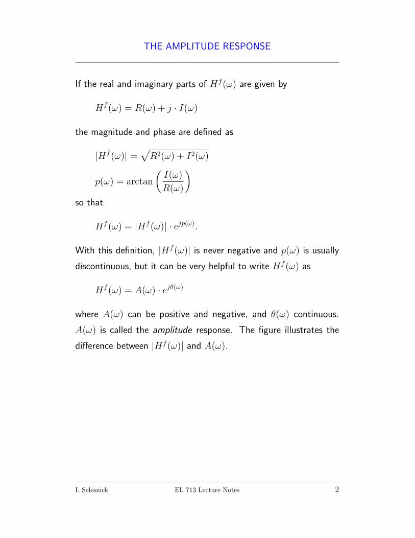
THE AMPLITUDE RESPONSE

If the real and imaginary parts of Hf(ω) are given by

Hf(ω) = R(ω) + j · I(ω)

the magnitude and phase are defined as

|Hf(ω)| =√R2(ω) + I2(ω)

p(ω) = arctan

(I(ω)

R(ω)

)so that

Hf(ω) = |Hf(ω)| · ejp(ω).

With this definition, |Hf(ω)| is never negative and p(ω) is usually

discontinuous, but it can be very helpful to write Hf(ω) as

Hf(ω) = A(ω) · ejθ(ω)

where A(ω) can be positive and negative, and θ(ω) continuous.

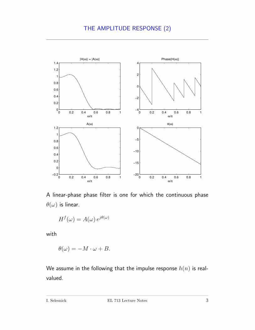
A(ω) is called the amplitude response. The figure illustrates the

difference between |Hf(ω)| and A(ω).


THE AMPLITUDE RESPONSE (2)

0 0.2 0.4 0.6 0.8 10

0.2

0.4

0.6

0.8

1

1.2

1.4

|H(ω)| = |A(ω)|

ω/π

0 0.2 0.4 0.6 0.8 1−4

−2

0

2

4

Phase{H(ω)}

ω/π

0 0.2 0.4 0.6 0.8 1−0.2

0

0.2

0.4

0.6

0.8

1

1.2

A(ω)

ω/π

0 0.2 0.4 0.6 0.8 1−20

−15

−10

−5

0

θ(ω)

ω/π

A linear-phase phase filter is one for which the continuous phase

θ(ω) is linear.

Hf(ω) = A(ω) ejθ(ω)

with

θ(ω) = −M · ω +B.

We assume in the following that the impulse response h(n) is real-

valued.


WHY LINEAR-PHASE?

If a discrete-time cosine signal

x1(n) = cos(ω1 n+ φ1)

is processed through a discrete-time filter with frequency response

Hf(ω) = A(ω) · ejθ(ω)

then the output signal is given by

y1(n) = A(ω1) cos(ω1 n+ φ1 + θ(ω1))

or

y1(n) = A(ω1) cos

(ω1

(n+

θ(ω1)

ω1

)+ φ1

).

The LTI system has the effect of scaling the cosine signal and de-

laying it by −θ(ω1)/ω1.

When does the system delay cosine signals with

different frequencies by the same amount?

=⇒ θ(ω)

ω= constant

=⇒ θ(ω) = K ω

=⇒ The phase is linear

The function θ(ω)/ω is called the phase delay. A linear phase filter

therefore has constant phase delay.


WHY LINEAR-PHASE: EXAMPLE

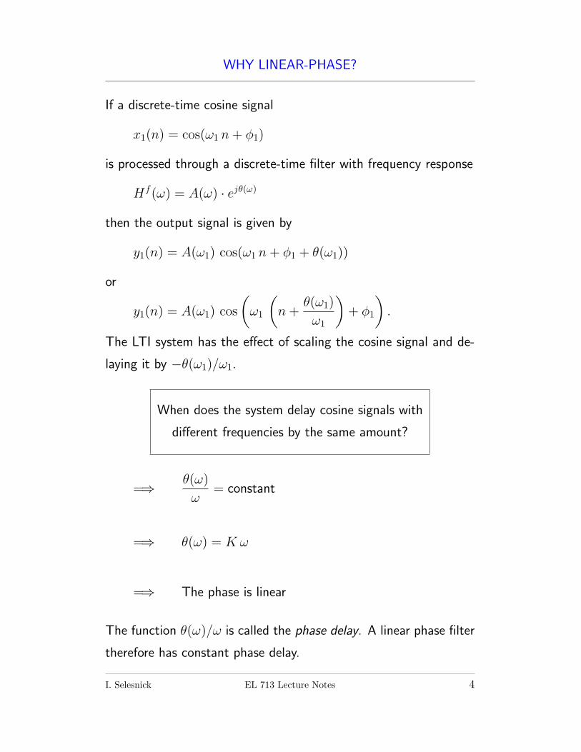
Consider an discrete-time filter described by the difference equation

y(n) =− 0.1821x(n) + 0.7865x(n− 1)− 0.6804x(n− 2) + x(n− 3)

+ 0.6804 y(n− 1)− 0.7865 y(n− 2) + 0.1821 y(n− 3).

When ω1 = 0.31π, then the delay is −θ(ω1)/ω1 = 2.45.

The delay is illustrated in the figure:

20 22 24 26 28 30 32 34 36 38 40−2

−1.5

−1

−0.5

0

0.5

1

1.5

2

x1(n

) (

INP

UT

)

20 22 24 26 28 30 32 34 36 38 40−2

−1.5

−1

−0.5

0

0.5

1

1.5

2

y1(n

) (

OU

TP

UT

)

Notice that the delay is fractional — the discrete-time samples are

not exactly reproduced in the output.

The fractional delay can be interpreted in this case as a delay of

the underlying continuous-time cosine signal.


WHY LINEAR-PHASE: EXAMPLE (2)

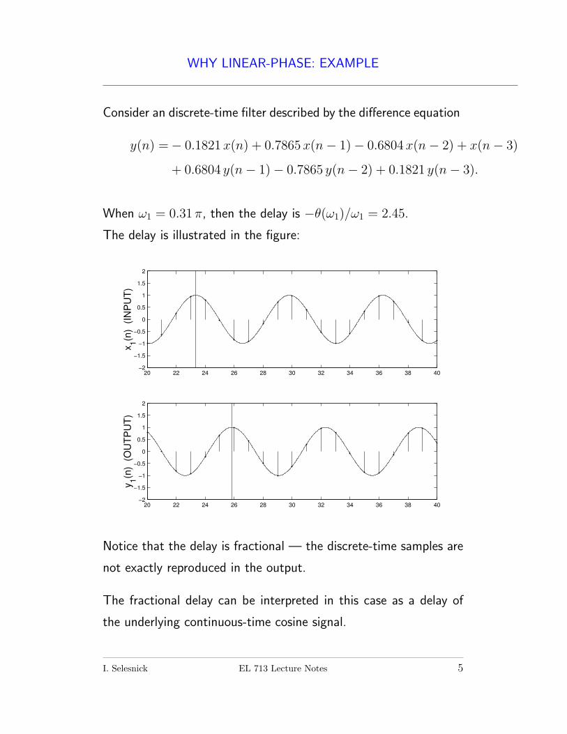
Consider the same system given on the previous slide, but let us

change the frequency of the cosine signal.

When ω2 = 0.47π, then the delay is −θ(ω2)/ω2 = 0.14.

20 22 24 26 28 30 32 34 36 38 40−2

−1.5

−1

−0.5

0

0.5

1

1.5

2

x2(n

) (

INP

UT

)

20 22 24 26 28 30 32 34 36 38 40−2

−1.5

−1

−0.5

0

0.5

1

1.5

2

y2(n

) (

OU

TP

UT

)

For this example, the delay depends on the

frequency, because this system does not have

linear phase.


WHY LINEAR-PHASE: MORE

From the previous slides, we see that a filter will delay different

frequency components of a signal by the same amount if the filter

has linear phase (constant phase delay).

In addition, when a narrow band signal (as in AM modulation) goes

through a filter, the envelop will be delayed by the group delay or

envelop delay of the filter. The amount by which the envelop is

delayed is independent of the carrier frequency only if the filter has

linear phase. (See page 214 in Mitra.)

Also, in applications like image processing, filters with non-linear

phase can introduce artifacts that are visually annoying.


FOUR TYPES OF LINEAR-PHASE FIR FILTERSSec 4.4.3

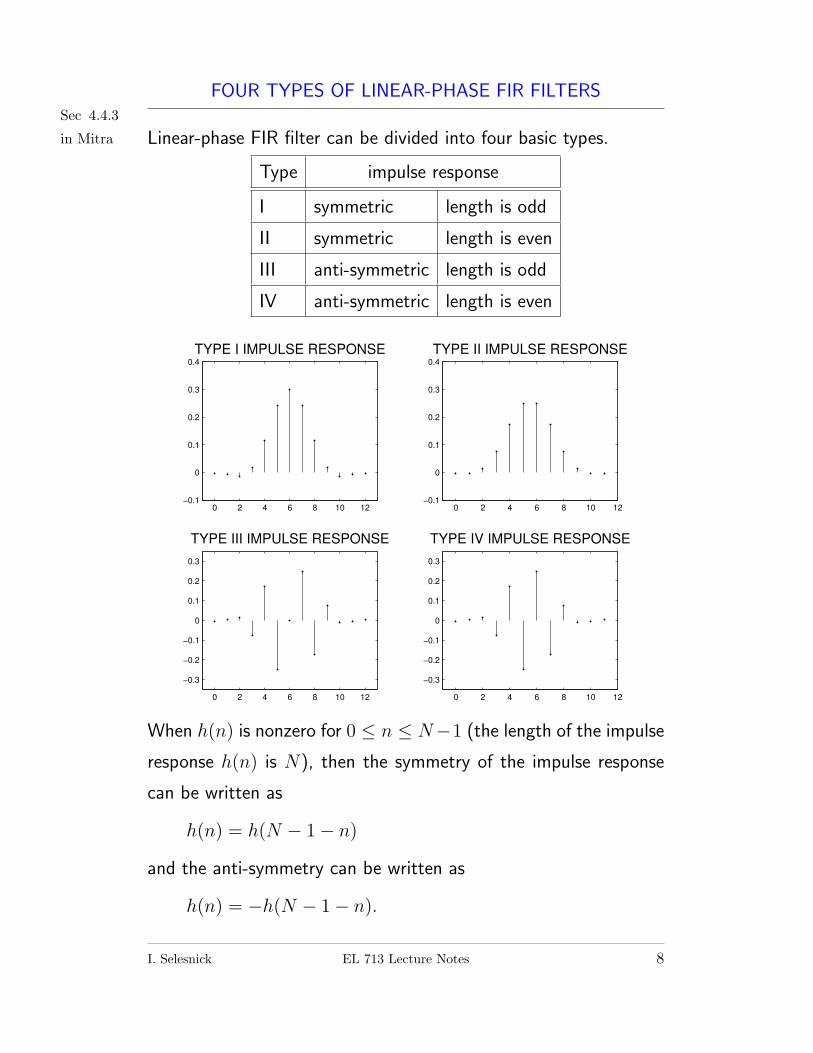
in Mitra Linear-phase FIR filter can be divided into four basic types.

Type impulse response

I symmetric length is odd

II symmetric length is even

III anti-symmetric length is odd

IV anti-symmetric length is even

0 2 4 6 8 10 12−0.1

0

0.1

0.2

0.3

0.4

TYPE I IMPULSE RESPONSE

0 2 4 6 8 10 12−0.1

0

0.1

0.2

0.3

0.4

TYPE II IMPULSE RESPONSE

0 2 4 6 8 10 12

−0.3

−0.2

−0.1

0

0.1

0.2

0.3

TYPE IV IMPULSE RESPONSE

0 2 4 6 8 10 12

−0.3

−0.2

−0.1

0

0.1

0.2

0.3

TYPE III IMPULSE RESPONSE

When h(n) is nonzero for 0 ≤ n ≤ N−1 (the length of the impulse

response h(n) is N), then the symmetry of the impulse response

can be written as

h(n) = h(N − 1− n)

and the anti-symmetry can be written as

h(n) = −h(N − 1− n).


FOUR TYPES OF LINEAR-PHASE FIR FILTERS

Important note: If the impulse response h(n) is complex-valued,

then to have linear-phase the impulse response should be conjugate-

symmetric or conjugate-anti-symmetry.


TYPE I: ODD-LENGTH SYMMETRIC

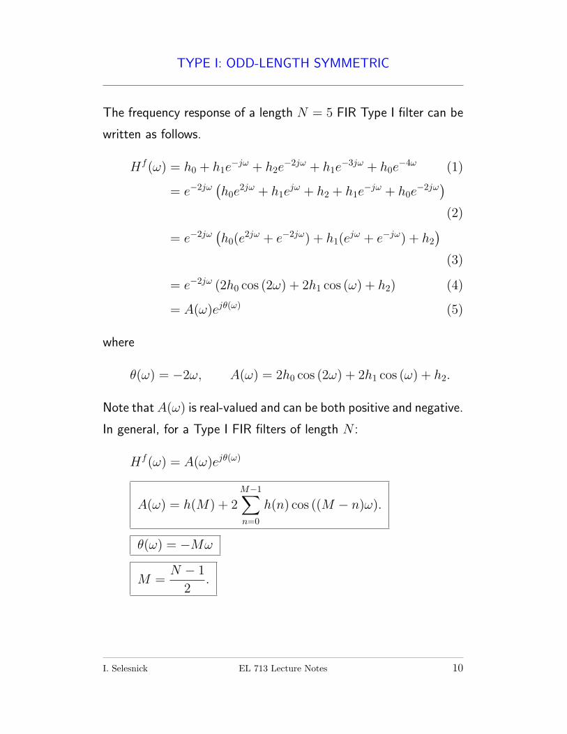
The frequency response of a length N = 5 FIR Type I filter can be

written as follows.

Hf(ω) = h0 + h1e−jω + h2e

−2jω + h1e−3jω + h0e

−4ω (1)

= e−2jω (h0e2jω + h1e

jω + h2 + h1e−jω + h0e

−2jω)(2)

= e−2jω (h0(e2jω + e−2jω) + h1(e

jω + e−jω) + h2)

(3)

= e−2jω (2h0 cos (2ω) + 2h1 cos (ω) + h2) (4)

= A(ω)ejθ(ω) (5)

where

θ(ω) = −2ω, A(ω) = 2h0 cos (2ω) + 2h1 cos (ω) + h2.

Note that A(ω) is real-valued and can be both positive and negative.

In general, for a Type I FIR filters of length N :

Hf(ω) = A(ω)ejθ(ω)

A(ω) = h(M) + 2M−1∑n=0

h(n) cos ((M − n)ω).

θ(ω) = −Mω

M =N − 1

2.


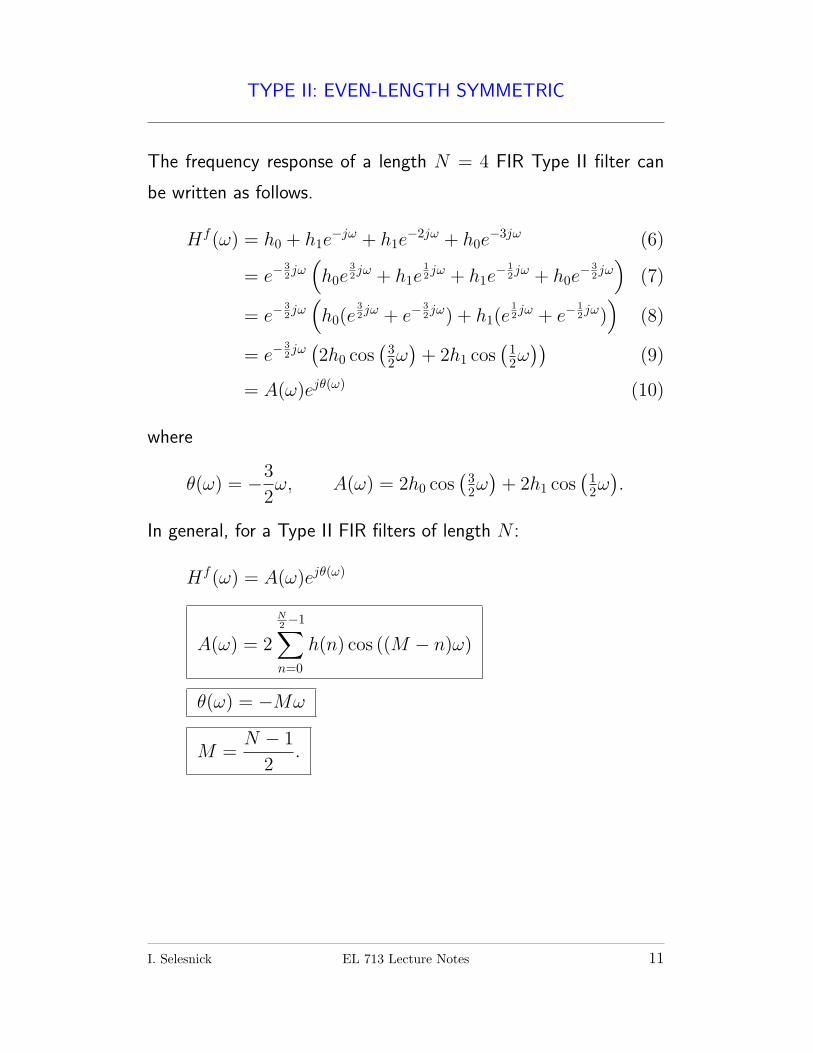
TYPE II: EVEN-LENGTH SYMMETRIC

The frequency response of a length N = 4 FIR Type II filter can

be written as follows.

Hf(ω) = h0 + h1e−jω + h1e

−2jω + h0e−3jω (6)

= e−32jω(h0e

32jω + h1e

12jω + h1e

− 12jω + h0e

− 32jω)

(7)

= e−32jω(h0(e

32jω + e−

32jω) + h1(e

12jω + e−

12jω))

(8)

= e−32jω(2h0 cos

(32ω)

+ 2h1 cos(1

2ω))

(9)

= A(ω)ejθ(ω) (10)

where

θ(ω) = −3

2ω, A(ω) = 2h0 cos

(32ω)

+ 2h1 cos(1

2ω).

In general, for a Type II FIR filters of length N :


A(ω) = 2

N2 −1∑n=0

h(n) cos ((M − n)ω)

θ(ω) = −Mω

M =N − 1

2.


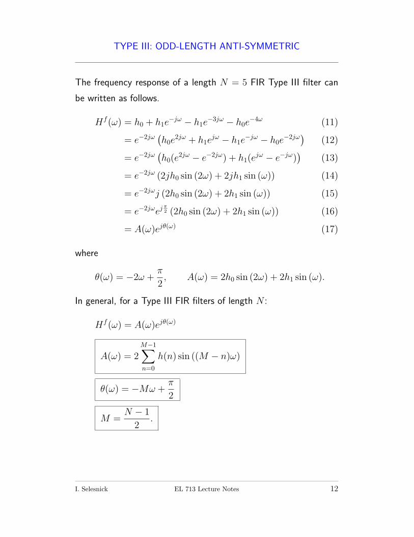
TYPE III: ODD-LENGTH ANTI-SYMMETRIC

The frequency response of a length N = 5 FIR Type III filter can


Hf(ω) = h0 + h1e−jω − h1e

−3jω − h0e−4ω (11)

= e−2jω (h0e2jω + h1e

jω − h1e−jω − h0e

−2jω) (12)

= e−2jω (h0(e2jω − e−2jω) + h1(e

jω − e−jω))

(13)

= e−2jω (2jh0 sin (2ω) + 2jh1 sin (ω)) (14)

= e−2jωj (2h0 sin (2ω) + 2h1 sin (ω)) (15)

= e−2jωejπ2 (2h0 sin (2ω) + 2h1 sin (ω)) (16)

= A(ω)ejθ(ω) (17)

where

θ(ω) = −2ω +π

2, A(ω) = 2h0 sin (2ω) + 2h1 sin (ω).

In general, for a Type III FIR filters of length N :


A(ω) = 2M−1∑n=0

h(n) sin ((M − n)ω)

θ(ω) = −Mω +π

2

M =N − 1

2.


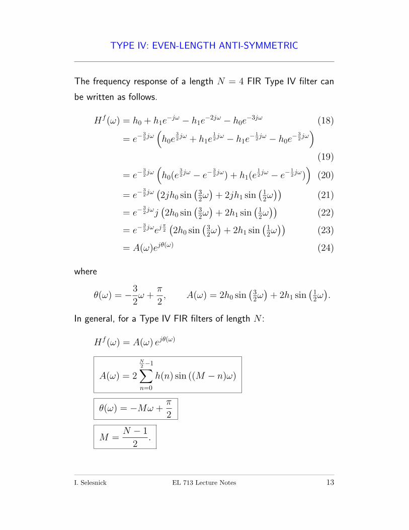
TYPE IV: EVEN-LENGTH ANTI-SYMMETRIC

The frequency response of a length N = 4 FIR Type IV filter can


Hf(ω) = h0 + h1e−jω − h1e

−2jω − h0e−3jω (18)

= e−32jω(h0e

32jω + h1e

12jω − h1e

− 12jω − h0e

− 32jω)

(19)

= e−32jω(h0(e

32jω − e−

32jω) + h1(e

12jω − e−

12jω))

(20)

= e−32jω(2jh0 sin

(32ω)

+ 2jh1 sin(1

2ω))

(21)

= e−32jωj

(2h0 sin

(32ω)

+ 2h1 sin(1

2ω))

(22)

= e−32jωej

π2

(2h0 sin

(32ω)

+ 2h1 sin(1

2ω))

(23)

= A(ω)ejθ(ω) (24)

where

θ(ω) = −3

2ω +

π

2, A(ω) = 2h0 sin

(32ω)

+ 2h1 sin(1

2ω).

In general, for a Type IV FIR filters of length N :

Hf(ω) = A(ω) ejθ(ω)

A(ω) = 2

N2 −1∑n=0


θ(ω) = −Mω +π

2

M =N − 1

2.


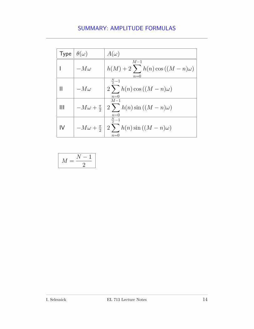
SUMMARY: AMPLITUDE FORMULAS

Type θ(ω) A(ω)

I −Mω h(M) + 2M−1∑n=0


II −Mω 2

N2 −1∑n=0


III −Mω + π2 2

M−1∑n=0


IV −Mω + π2 2

N2 −1∑n=0


M =N − 1

2


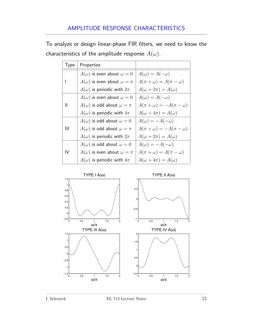
AMPLITUDE RESPONSE CHARACTERISTICS

To analyze or design linear-phase FIR filters, we need to know the

characteristics of the amplitude response A(ω).

Type Properties

A(ω) is even about ω = 0 A(ω) = A(−ω)

I A(ω) is even about ω = π A(π + ω) = A(π − ω)

A(ω) is periodic with 2π A(ω + 2π) = A(ω)

A(ω) is even about ω = 0 A(ω) = A(−ω)

II A(ω) is odd about ω = π A(π + ω) = −A(π − ω)


A(ω) is odd about ω = 0 A(ω) = −A(−ω)

III A(ω) is odd about ω = π A(π + ω) = −A(π − ω)


A(ω) is odd about ω = 0 A(ω) = −A(−ω)

IV A(ω) is even about ω = π A(π + ω) = A(π − ω)


0 0.5 1 1.5 2−0.2

0

0.2

0.4

0.6

0.8

1

1.2

TYPE I A(ω)

ω/π0 0.5 1 1.5 2

−1

−0.5

0

0.5

1

TYPE II A(ω)

ω/π

0 0.5 1 1.5 2−1.5

−1

−0.5

0

0.5

1

1.5

TYPE III A(ω)

ω/π0 0.5 1 1.5 2

−0.5

0

0.5

1

1.5

2

TYPE IV A(ω)

ω/π


EVALUATING THE AMPLITUDE RESPONSE

The frequency response Hf(ω) of an FIR filter can be evaluated

at L equally spaced frequencies between 0 and π using the DFT.

Consider a causal FIR filter with an impulse response h(n) of length-

N , with N ≤ L. Samples of the frequency response of the filter

can be written as

H

(2π

Lk

)=

N−1∑n=0

h(n)e−j2πL nk.

Define the L-point signal {g(n), 0 ≤ n ≤ L− 1} as

g(n) =

{h(n) 0 ≤ n ≤ N − 1

0 N ≤ n ≤ L− 1.

Then

H

(2π

Lk

)= G(k) = DFTL{g(n)}

where G(k) is the L-point DFT of g(n).

Types I and II

Suppose the FIR filter h(n) is either a Type I or a Type II FIR filter.

Then we have from above

Hf(ω) = A(ω) e−jMω

or

A(ω) = Hf(ω) ejMω.

Samples of the real-valued amplitude A(ω) can be obtained from

samples of the function Hf(ω) as:

A

(2π

Lk

)= H

(2π

Lk

)ejM

2πL k = G(k) ·WMk

L .


EVALUATING THE AMPLITUDE RESPONSE (2)

Therefore, the samples of the real-valued amplitude function can

be obtained by zero-padding h(n), taking the DFT, and multiplying

by the complex exponential. This can be written as:

A

(2π

Lk

)= DFTL{[h(n), 0L−N ]} · WMk

L .

Types III and IV

For Type III and Type IV FIR filters, we have

Hf(ω) = j e−jMω A(ω)

or

A(ω) = −j Hf(ω) ejMω.

Therefore, samples of the real-valued amplitude A(ω) can be ob-

tained from samples of the function Hf(ω) as:

A

(2π

Lk

)= −j H

(2π

Lk

)ejM

2πL k = −j G(k) · WMk

L .

Therefore, the samples of the real-valued amplitude function can

be obtained by zero-padding h(n), taking the DFT, and multiplying

by the complex exponential.

A

(2π

Lk

)= −j · DFTL{[h(n), 0L−N ]} · WMk

L .


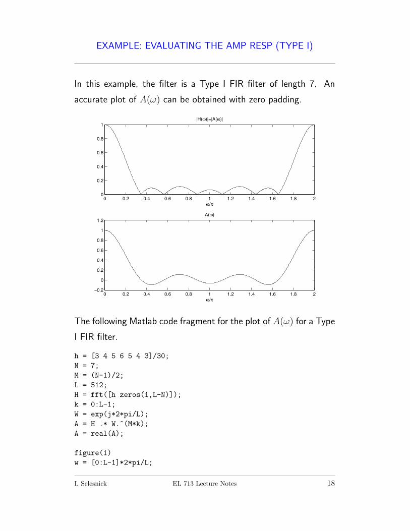
EXAMPLE: EVALUATING THE AMP RESP (TYPE I)

In this example, the filter is a Type I FIR filter of length 7. An

accurate plot of A(ω) can be obtained with zero padding.

0 0.2 0.4 0.6 0.8 1 1.2 1.4 1.6 1.8 20

0.2

0.4

0.6

0.8

1

|H(ω)|=|A(ω)|

ω/π

0 0.2 0.4 0.6 0.8 1 1.2 1.4 1.6 1.8 2−0.2

0

0.2

0.4

0.6

0.8

1

1.2

A(ω)

ω/π

The following Matlab code fragment for the plot of A(ω) for a Type

I FIR filter.

h = [3 4 5 6 5 4 3]/30;

N = 7;

M = (N-1)/2;

L = 512;

H = fft([h zeros(1,L-N)]);

k = 0:L-1;

W = exp(j*2*pi/L);

A = H .* W.^(M*k);

A = real(A);

figure(1)

w = [0:L-1]*2*pi/L;


subplot(2,1,1)

plot(w/pi,abs(H))

ylabel(’|H(\omega)| = |A(\omega)|’)

xlabel(’\omega/\pi’)

subplot(2,1,2)

plot(w/pi,A)

ylabel(’A(\omega)’)


print -deps type1

The command A = real(A) removes the imaginary part which is

equal to zero to within computer precision. Without this command,

Matlab takes A to be a complex vector and the following plot com-

mand will not be right.

Observe the symmetry of A(ω) due to h(n) being real-valued. Be-

cause of this symmetry, A(ω) is usually plotted for 0 ≤ ω ≤ π

only.


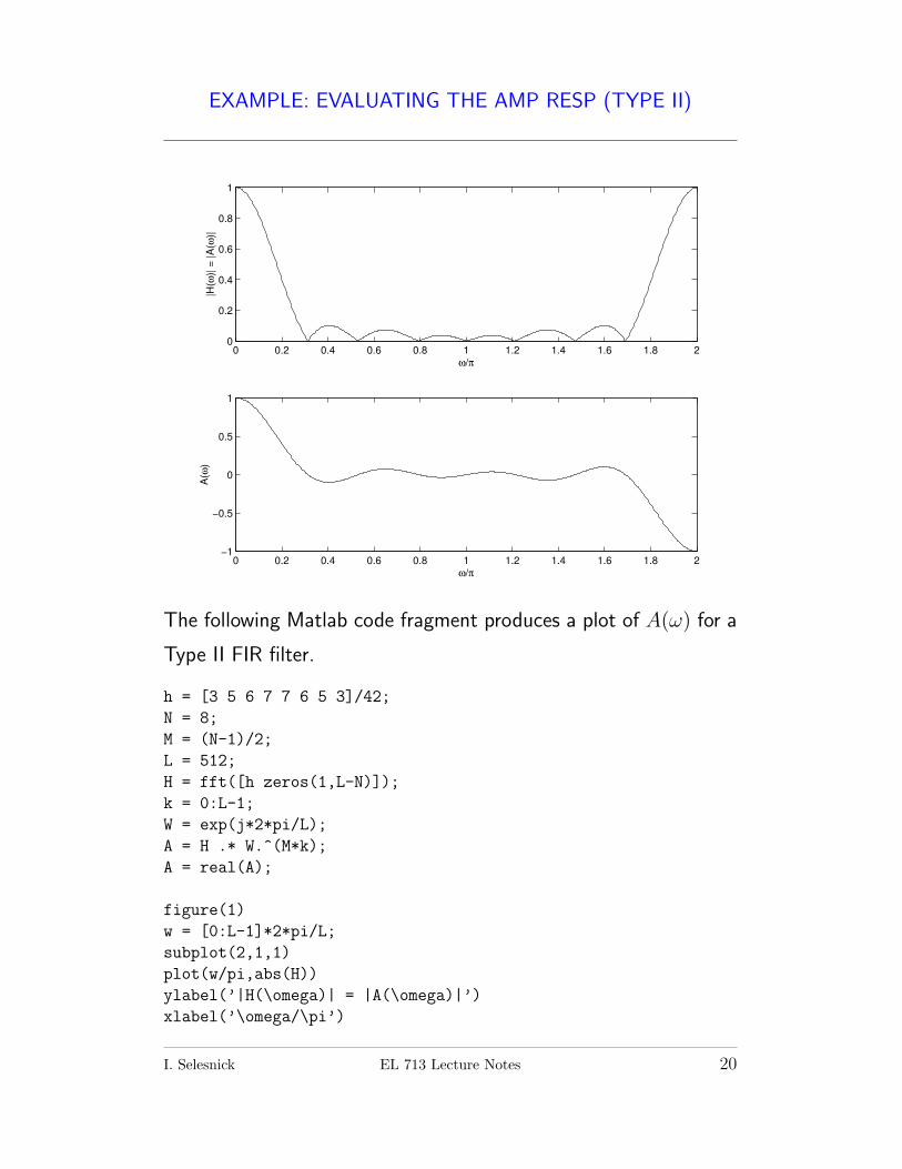
EXAMPLE: EVALUATING THE AMP RESP (TYPE II)

0 0.2 0.4 0.6 0.8 1 1.2 1.4 1.6 1.8 20

0.2

0.4

0.6

0.8

1

|H(ω

)| =

|A

(ω)|

ω/π

0 0.2 0.4 0.6 0.8 1 1.2 1.4 1.6 1.8 2−1

−0.5

0

0.5

1

A(ω

)

ω/π

The following Matlab code fragment produces a plot of A(ω) for a

Type II FIR filter.

h = [3 5 6 7 7 6 5 3]/42;

N = 8;

M = (N-1)/2;

L = 512;


k = 0:L-1;

W = exp(j*2*pi/L);

A = H .* W.^(M*k);

A = real(A);

figure(1)

w = [0:L-1]*2*pi/L;

subplot(2,1,1)

plot(w/pi,abs(H))

ylabel(’|H(\omega)| = |A(\omega)|’)



subplot(2,1,2)

plot(w/pi,A)

ylabel(’A(\omega)’)


print -deps type2

The imaginary part of the amplitude is zero. Notice that A(π) = 0.

In fact this will always be the case for a Type II FIR filter.

An exercise for the student: Describe how to obtain samples of

A(ω) for Type III and Type IV FIR filters. Modify the Matlab code

above for these types. Do you notice that A(ω) = 0 always for

special values of ω?


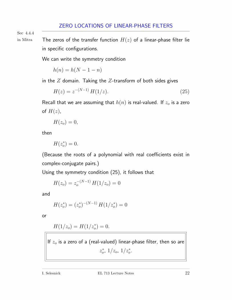
ZERO LOCATIONS OF LINEAR-PHASE FILTERSSec 4.4.4

in Mitra The zeros of the transfer function H(z) of a linear-phase filter lie

in specific configurations.

We can write the symmetry condition

h(n) = h(N − 1− n)

in the Z domain. Taking the Z-transform of both sides gives

H(z) = z−(N−1)H(1/z). (25)

Recall that we are assuming that h(n) is real-valued. If zo is a zero

of H(z),

H(zo) = 0,

then

H(z∗o) = 0.

(Because the roots of a polynomial with real coefficients exist in

complex-conjugate pairs.)

Using the symmetry condition (25), it follows that

H(zo) = z−(N−1)o H(1/zo) = 0

and

H(z∗o) = (z∗o)−(N−1)H(1/z∗o) = 0

or

H(1/zo) = H(1/z∗o) = 0.

If zo is a zero of a (real-valued) linear-phase filter, then so are

z∗o , 1/zo, 1/z∗o .


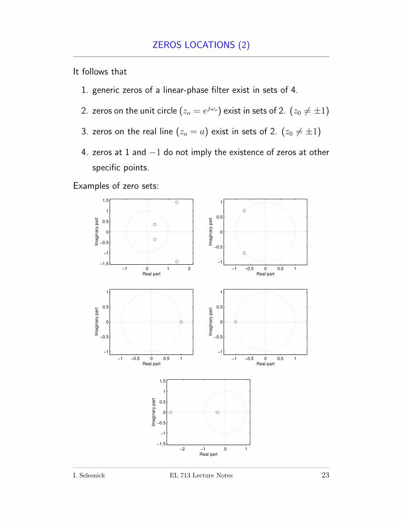
ZEROS LOCATIONS (2)

It follows that

1. generic zeros of a linear-phase filter exist in sets of 4.

2. zeros on the unit circle (zo = ejωo) exist in sets of 2. (z0 6= ±1)

3. zeros on the real line (zo = a) exist in sets of 2. (z0 6= ±1)

4. zeros at 1 and −1 do not imply the existence of zeros at other

specific points.

Examples of zero sets:

−1 0 1 2−1.5

−1

−0.5

0

0.5

1

1.5

Real part

Ima

gin

ary

pa

rt

−1 −0.5 0 0.5 1

−1

−0.5

0

0.5

1

Real part

Ima

gin

ary

pa

rt

−1 −0.5 0 0.5 1

−1

−0.5

0

0.5

1

Real part

Ima

gin

ary

pa

rt

−1 −0.5 0 0.5 1

−1

−0.5

0

0.5

1

Real part

Ima

gin

ary

pa

rt

−2 −1 0 1−1.5

−1

−0.5

0

0.5

1

1.5

Real part

Ima

gin

ary

pa

rt


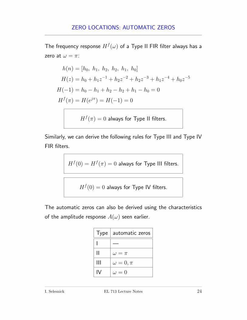
ZERO LOCATIONS: AUTOMATIC ZEROS

The frequency response Hf(ω) of a Type II FIR filter always has a

zero at ω = π:

h(n) = [h0, h1, h2, h2, h1, h0]

H(z) = h0 + h1z−1 + h2z

−2 + h2z−3 + h1z

−4 + h0z−5

H(−1) = h0 − h1 + h2 − h2 + h1 − h0 = 0

Hf(π) = H(ejπ) = H(−1) = 0

Hf(π) = 0 always for Type II filters.

Similarly, we can derive the following rules for Type III and Type IV

FIR filters.

Hf(0) = Hf(π) = 0 always for Type III filters.

Hf(0) = 0 always for Type IV filters.

The automatic zeros can also be derived using the characteristics

of the amplitude response A(ω) seen earlier.

Type automatic zeros

I —

II ω = π

III ω = 0, π

IV ω = 0


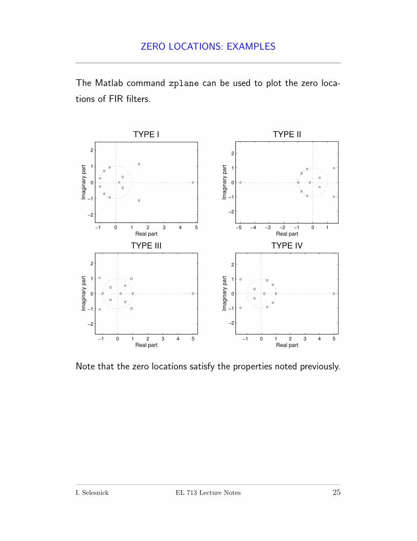
ZERO LOCATIONS: EXAMPLES

The Matlab command zplane can be used to plot the zero loca-

tions of FIR filters.

−1 0 1 2 3 4 5

−2

−1

0

1

2

Real part

Imagin

ary

part

TYPE I

−5 −4 −3 −2 −1 0 1

−2

−1

0

1

2

Real part

Imagin

ary

part

TYPE II

−1 0 1 2 3 4 5

−2

−1

0

1

2

Real part

Imagin

ary

part

TYPE III

−1 0 1 2 3 4 5

−2

−1

0

1

2

Real part

Imagin

ary

part

TYPE IV

Note that the zero locations satisfy the properties noted previously.


DESIGN OF FIR FILTERS BY DFT-BASED INTERPOLATION

One approach to the design of FIR filters is to ask that A(ω) pass

through a specified set of values. If the number of specified inter-

polation points is the same as the number of filter parameters, then

the filter is totally determined by the interpolation conditions, and

the filter can be found by solving a system of linear equations.

When the interpolation points are equally spaced between 0 and

2π, then this interpolation problem can be solved very efficiently

using the DFT.

To derive the DFT solution to the interpolation problem, recall the

formula relating the samples of the frequency response to the DFT.

In the case we are interested here, the number of samples is to be

the same as the length of the filter (L = N).

H

(2π

Nk

)=

N−1∑n=0

h(n)e−j2πN nk

= DFTN{h(n)}.

Types I and II

Recall the relation between A(ω) and Hf(ω) for a Type I and II

filter, to obtain

A

(2π

Nk

)= H

(2π

Nk

)· ejM

2πN k

= DFTN{h(n)} ·WMkN

Now we can related the N -point DFT of h(n) to the samples of

A(ω):

DFTN{h(n)} = A

(2π

Nk

)·W−Mk

N .


Finally, we can solve for the filter coefficients h(n).

h(n) = DFT−1N

{A

(2π

Nk

)·W−Mk

N

}.

Therefore, if the values A(2πN k)

are specified, we can then obtain

the filter coefficients h(n) that satisfies the interpolation conditions

by using the inverse DFT. It is important to note however, that the

specified values A(2πN k)

must posses the appropriate symmetry in

order for the result of the inverse DFT to be a real Type I or II FIR

filter.

Types III and IV

For Type III and IV filters, we have

A

(2π

Nk

)= −j ·H

(2π

Nk

)· ejM

2πN k

= −j · DFTN{h(n)} ·WMkN

Then we can related the N -point DFT of h(n) to the samples of

A(ω):

DFTN{h(n)} = j · A(

2π

Nk

)·W−Mk

N .

Solving for the filter coefficients h(n) gives:

h(n) = DFT−1N

{j · A

(2π

Nk

)·W−Mk

N

}.


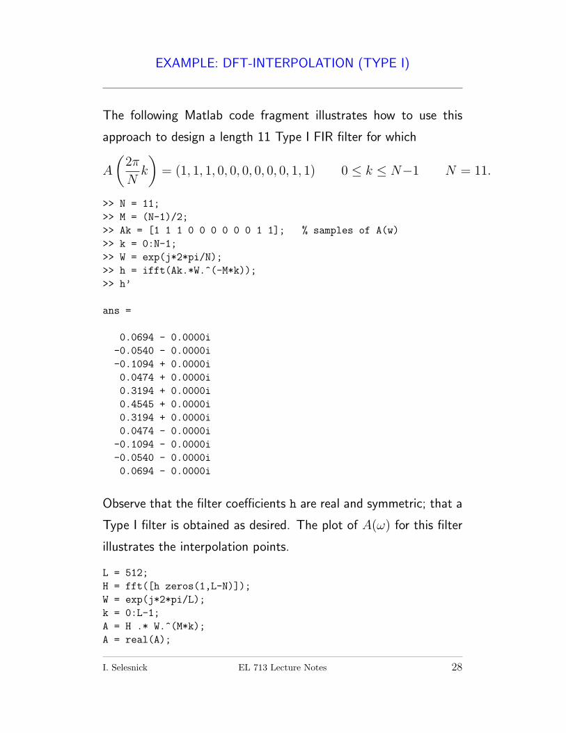
EXAMPLE: DFT-INTERPOLATION (TYPE I)

The following Matlab code fragment illustrates how to use this

approach to design a length 11 Type I FIR filter for which

A

(2π

Nk

)= (1, 1, 1, 0, 0, 0, 0, 0, 0, 1, 1) 0 ≤ k ≤ N−1 N = 11.

>> N = 11;

>> M = (N-1)/2;

>> Ak = [1 1 1 0 0 0 0 0 0 1 1]; % samples of A(w)

>> k = 0:N-1;

>> W = exp(j*2*pi/N);

>> h = ifft(Ak.*W.^(-M*k));

>> h’

ans =

0.0694 - 0.0000i

-0.0540 - 0.0000i

-0.1094 + 0.0000i

0.0474 + 0.0000i

0.3194 + 0.0000i

0.4545 + 0.0000i

0.3194 + 0.0000i

0.0474 - 0.0000i

-0.1094 - 0.0000i

-0.0540 - 0.0000i

0.0694 - 0.0000i

Observe that the filter coefficients h are real and symmetric; that a

Type I filter is obtained as desired. The plot of A(ω) for this filter

illustrates the interpolation points.

L = 512;


W = exp(j*2*pi/L);

k = 0:L-1;

A = H .* W.^(M*k);

A = real(A);


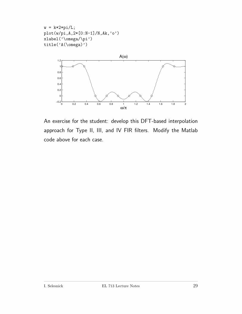
w = k*2*pi/L;

plot(w/pi,A,2*[0:N-1]/N,Ak,’o’)


title(’A(\omega)’)

0 0.2 0.4 0.6 0.8 1 1.2 1.4 1.6 1.8 2−0.2

0

0.2

0.4

0.6

0.8

1

1.2

ω/π

A(ω)

An exercise for the student: develop this DFT-based interpolation

approach for Type II, III, and IV FIR filters. Modify the Matlab

code above for each case.


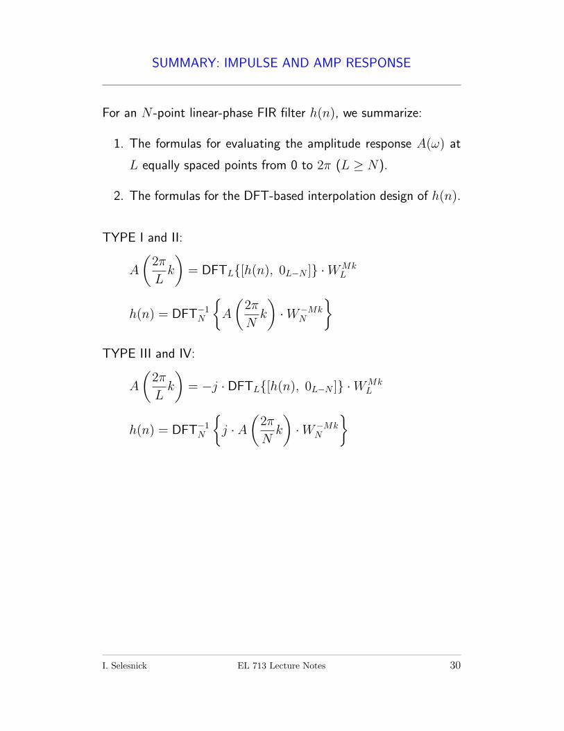
SUMMARY: IMPULSE AND AMP RESPONSE

For an N -point linear-phase FIR filter h(n), we summarize:

1. The formulas for evaluating the amplitude response A(ω) at

L equally spaced points from 0 to 2π (L ≥ N).

2. The formulas for the DFT-based interpolation design of h(n).

TYPE I and II:

A

(2π

Lk

)= DFTL{[h(n), 0L−N ]} ·WMk

L

h(n) = DFT−1N

{A

(2π

Nk

)·W−Mk

N

}TYPE III and IV:

A

(2π

Lk

)= −j · DFTL{[h(n), 0L−N ]} ·WMk

L

h(n) = DFT−1N

{j · A

(2π

Nk

)·W−Mk

N

}


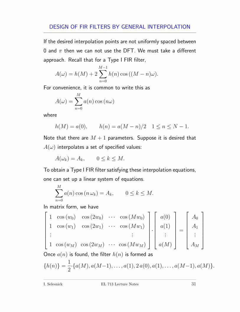
DESIGN OF FIR FILTERS BY GENERAL INTERPOLATION

If the desired interpolation points are not uniformly spaced between

0 and π then we can not use the DFT. We must take a different

approach. Recall that for a Type I FIR filter,

A(ω) = h(M) + 2M−1∑n=0

h(n) cos ((M − n)ω).

For convenience, it is common to write this as

A(ω) =M∑n=0

a(n) cos (nω)

where

h(M) = a(0), h(n) = a(M − n)/2 1 ≤ n ≤ N − 1.

Note that there are M + 1 parameters. Suppose it is desired that

A(ω) interpolates a set of specified values:

A(ωk) = Ak, 0 ≤ k ≤M.

To obtain a Type I FIR filter satisfying these interpolation equations,

one can set up a linear system of equations.M∑n=0

a(n) cos (nωk) = Ak, 0 ≤ k ≤M.

In matrix form, we have1 cos (w0) cos (2w0) · · · cos (Mw0)

1 cos (w1) cos (2w1) · · · cos (Mw1)...

...

1 cos (wM) cos (2wM) · · · cos (MwM)

·

a(0)

a(1)...

a(M)

=

A0

A1...

AM

Once a(n) is found, the filter h(n) is formed as

{h(n)} =1

2·{a(M), a(M−1), . . . , a(1), 2 a(0), a(1), . . . , a(M−1), a(M)}.


EXAMPLE

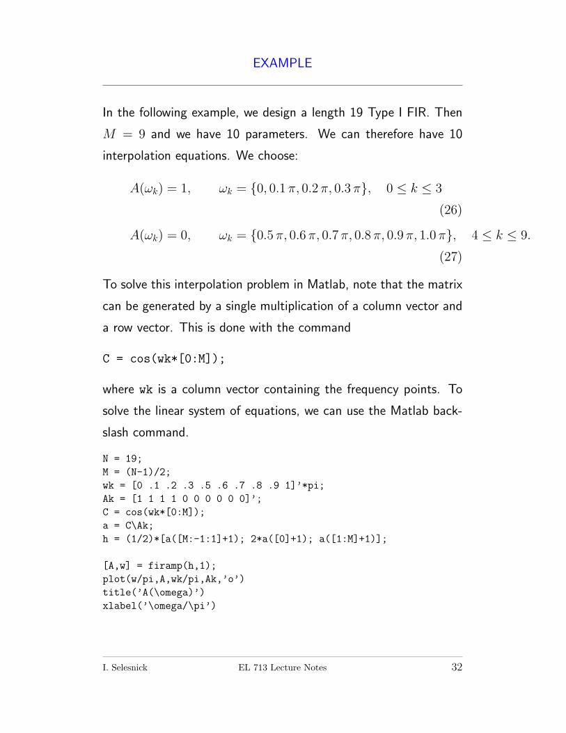
In the following example, we design a length 19 Type I FIR. Then

M = 9 and we have 10 parameters. We can therefore have 10

interpolation equations. We choose:

A(ωk) = 1, ωk = {0, 0.1 π, 0.2 π, 0.3π}, 0 ≤ k ≤ 3

(26)

A(ωk) = 0, ωk = {0.5π, 0.6π, 0.7 π, 0.8 π, 0.9 π, 1.0π}, 4 ≤ k ≤ 9.

(27)

To solve this interpolation problem in Matlab, note that the matrix

can be generated by a single multiplication of a column vector and

a row vector. This is done with the command

C = cos(wk*[0:M]);

where wk is a column vector containing the frequency points. To

solve the linear system of equations, we can use the Matlab back-

slash command.

N = 19;

M = (N-1)/2;

wk = [0 .1 .2 .3 .5 .6 .7 .8 .9 1]’*pi;

Ak = [1 1 1 1 0 0 0 0 0 0]’;

C = cos(wk*[0:M]);

a = C\Ak;

h = (1/2)*[a([M:-1:1]+1); 2*a([0]+1); a([1:M]+1)];

[A,w] = firamp(h,1);

plot(w/pi,A,wk/pi,Ak,’o’)

title(’A(\omega)’)



0 0.1 0.2 0.3 0.4 0.5 0.6 0.7 0.8 0.9 1−0.2

0

0.2

0.4

0.6

0.8

1

1.2

A(ω)

ω/π

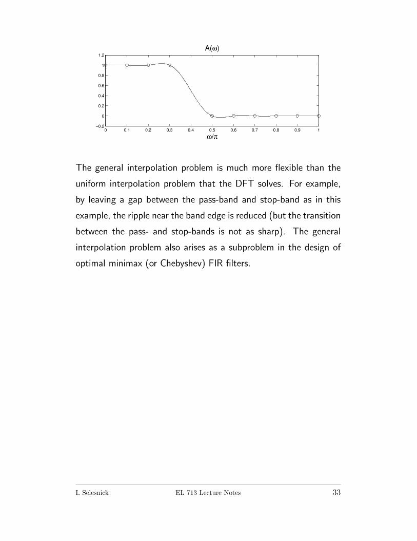
The general interpolation problem is much more flexible than the

uniform interpolation problem that the DFT solves. For example,

by leaving a gap between the pass-band and stop-band as in this

example, the ripple near the band edge is reduced (but the transition

between the pass- and stop-bands is not as sharp). The general

interpolation problem also arises as a subproblem in the design of

optimal minimax (or Chebyshev) FIR filters.


Documents

LINEAR-PHASE FIR FILTERS 1.The amplitude response …eeweb.poly.edu/iselesni/EL713/zoom/linphase.pdf · LINEAR-PHASE FIR FILTERS 1.The amplitude response 2.Why linear-phase? 3.The