Linear System Theoryand Design

Taesam Kang

Introduction to Course

Textbooks Chi-Tsong Chen, Linear System Theory

and Design Thomas Kailath, Linear Systems A. Naylor and G. Sell, Linear Operator

Theory in Engineering and Science G. Strang, Linear algebra and its

application

Contents of textbook1. Introduction2. Mathematical description of systems3. Linear algebra4. State space solution and realizations5. Stability6. Controllability and observability7. Minimal realizations and coprime fractions8. State feedback and state estimators9. Pole placement and model matching

Contents of textbook2. Mathematical description of systems

1. Definitions and system concept2. Linear and LTI systems3. Linearization4. Discrete-time systems

3. Linear algebra1. Basis, representation2. Linear algebraic equations3. Similarity transformation4. Diagonal and Jordan form5. Lyapunov equation6. Quadratic and positive definiteness7. SVD and norms

Contents of textbook4. State space solution and realizations

1. Solution of LTI equations2. Equivalent state equations3. Realizations(equivalency)4. Solution of LTV equations5. Time varying realizations

5. Stability1. I/O stability2. Internal stability3. Lyapunov theorem4. Stability of LTV systems

Contents of textbook6. Controllability and observability

1. Controllability and observability2. Canonical decomposition3. Conditions in Jordan form

7. Minimal realizations and coprime fractions1. Coprimeness and coprime fractions

8. State feedback and state estimators1. State feedback and estimators

9. Pole placement and model matching1. Unity feedback pole-placement

Overview Linear system theory/design introduces and illustrates

system concepts, various linear system representation, analysis and design methods, and mutual relationship.

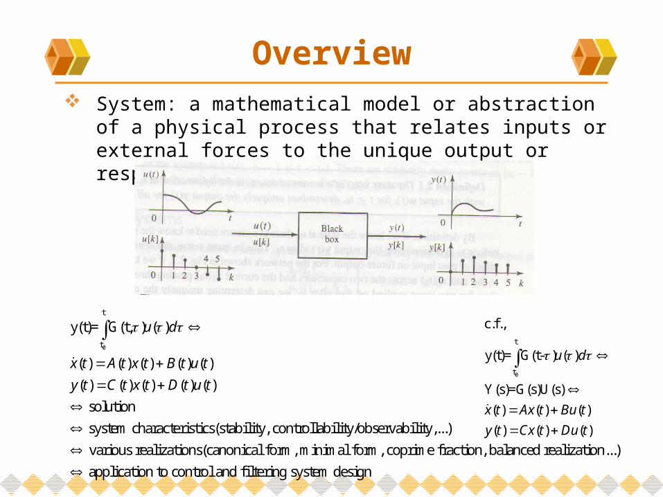
System: a mathematical model or abstraction of a physical process that relates inputs or external forces to the unique output or response of it.

Overview

0

t

t

y(t)= G(t, ) ( )

( ) ( ) ( ) ( ) ( )

( ) ( ) ( ) ( ) ( )

solution

system characteristics(stability, controllability/observability,...)

various realizations(canonical form, minimal form, cop

u d

x t A t x t B t u t

y t C t x t D t u t

rime fraction, balanced realization...)

application to control and filtering system design

0

t

t

c.f.,

y(t)= G(t- ) ( )

Y(s)=G(s)U(s)

( ) ( ) ( )

( ) ( ) ( )

u d

x t Ax t Bu t

y t Cx t Du t

Chapter 2. Mathematical Description of Systems

Week 1, 2

Description of Linear Systems

1

1

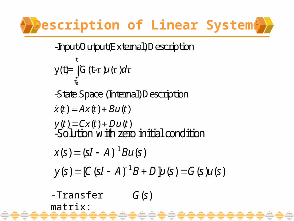
-Solution with zero initial condition

( ) ( ) ( )

( ) [ ( ) ] ( ) ( ) ( )

x s sI A Bu s

y s C sI A B D u s G s u s

0

t

t

-Input/Output(External) Description

y(t)= G(t- ) ( )

-State Space (Internal) Description

( ) ( ) ( )

( ) ( ) ( )

u d

x t Ax t Bu t

y t Cx t Du t

-Transfer matrix:

( )G s

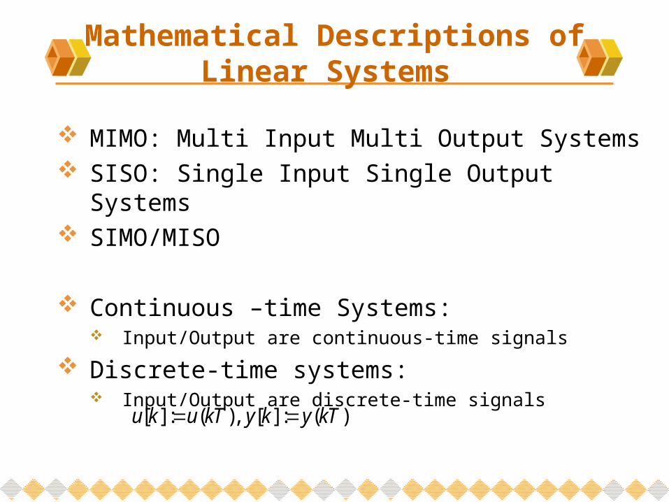
Mathematical Descriptions of Linear Systems

MIMO: Multi Input Multi Output Systems SISO: Single Input Single Output Systems SIMO/MISO

Continuous –time Systems: Input/Output are continuous-time signals

Discrete-time systems: Input/Output are discrete-time signals

[ ] : ( ), [ ] : ( )u k u kT y k y kT

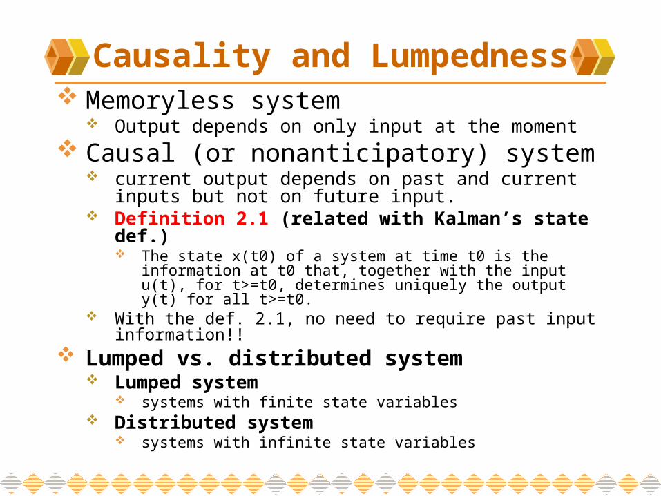
Causality and Lumpedness Memoryless system

Output depends on only input at the moment Causal (or nonanticipatory) system

current output depends on past and current inputs but not on future input.

Definition 2.1 (related with Kalman’s state def.) The state x(t0) of a system at time t0 is the information

at t0 that, together with the input u(t), for t>=t0, determines uniquely the output y(t) for all t>=t0.

With the def. 2.1, no need to require past input information!!

Lumped vs. distributed system Lumped system

systems with finite state variables Distributed system

systems with infinite state variables

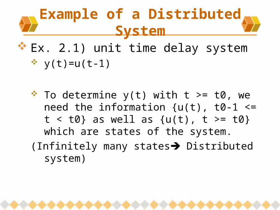
Example of a Distributed System

Ex. 2.1) unit time delay system y(t)=u(t-1)

To determine y(t) with t >= t0, we need the information {u(t), t0-1 <= t < t0} as well as {u(t), t >= t0} which are states of the system.

(Infinitely many states Distributed system)

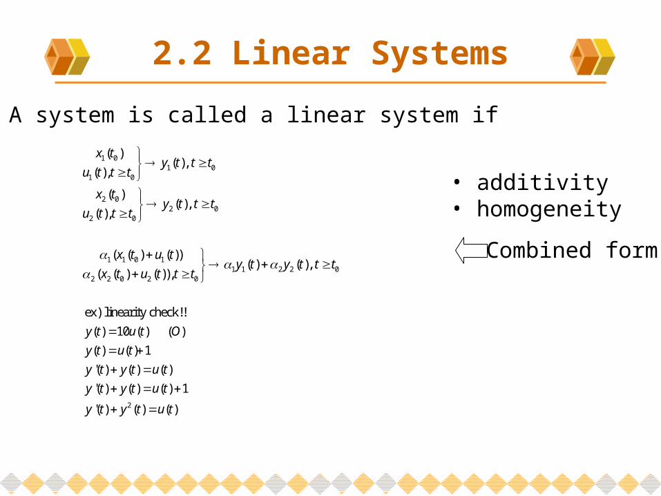
2.2 Linear Systems

1 01 0

1 0

2 02 0

2 0

1 1 0 11 1 2 2 0

2 2 0 2 0

( )( ),

( ),

( )( ),

( ),

( ( ) ( ))( ) ( ),

( ( ) ( )),

x ty t t t

u t t t

x ty t t t

u t t t

x t u ty t y t t t

x t u t t t

2

ex) linearity check!!

( ) 10 ( ) ( )

( ) ( ) 1

'( ) ( ) ( )

'( ) ( ) ( ) 1

'( ) ( ) ( )

y t u t O

y t u t

y t y t u t

y t y t u t

y t y t u t

• additivity• homogeneity

A system is called a linear system if

Combined form

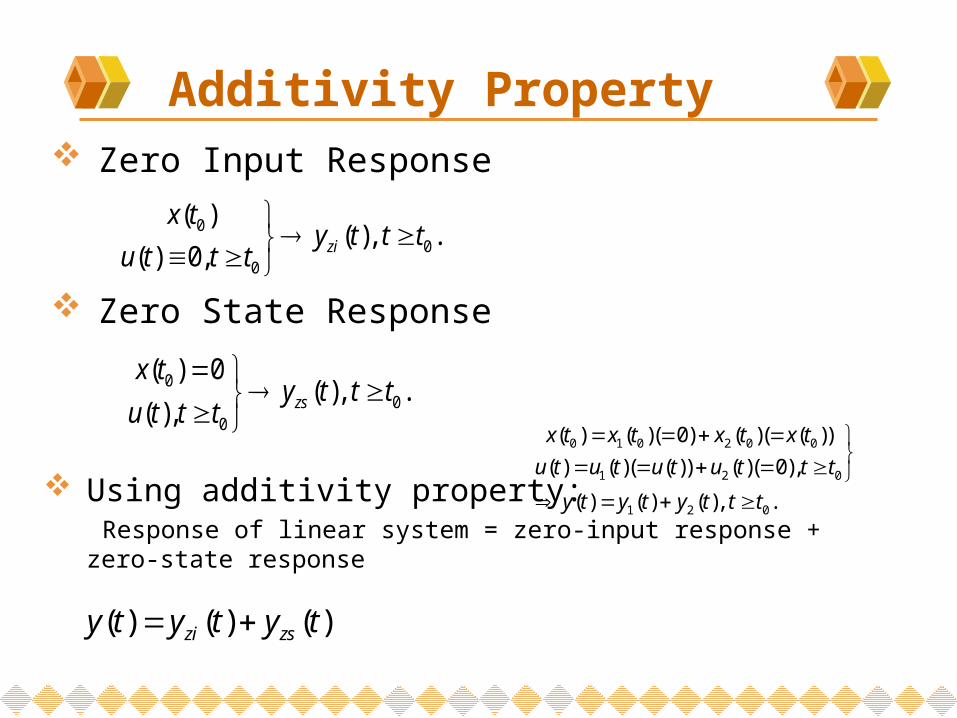
Additivity Property Zero Input Response

00

0

( )( ), .

( ) 0, zi

x ty t t t

u t t t

Zero State Response

00

0

( ) 0( ), .

( ), zs

x ty t t t

u t t t

Using additivity property: Response of linear system = zero-input response + zero-state

response

( ) ( ) ( )zi zsy t y t y t

0 1 0 2 0 0

1 2 0

1 2 0

( ) ( )( 0) ( )( ( ))

( ) ( )( ( )) ( )( 0),

( ) ( ) ( ), .

x t x t x t x t

u t u t u t u t t t

y t y t y t t t

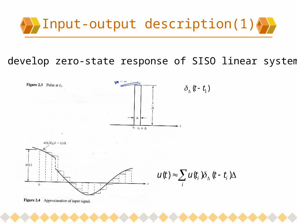
Input-output description(1)

1( )t t

( ) ( ) ( )i ii

u t u t t t

• develop zero-state response of SISO linear system

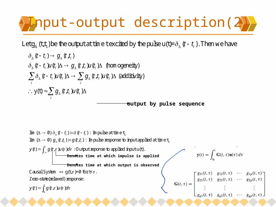
Input-output description(2)

Δ iLet g (t,t ) be the output at time t excited by the pulse u(t)= ( ). Then we haveit t

( ) ( , )

( ) ( ) ( , ) ( ) (homogeneity)

( ) ( ) ( , ) ( ) (additivity)

y(t) ( , ) ( )

i i

i i i i

i i i ii i

i ii

t t g t t

t t u t g t t u t

t t u t g t t u t

g t t u t

i

i

lim ( 0) ( ): ( ) : Impulse at time t

lim ( 0) ( , ): ( , ) : Impulse response to input applied at time t

( ) ( , ) ( ) : Output reponse to applied input u(t).

Causal System g(t, )=0

i i

i i

t t t t

g t t g t t

y t g t u d

0

for t< .

Zero-state(relaxed) response:

( ) ( , ) ( )t

ty t g t u d

output by pulse sequence

Denotes time at which impulse is applied

Denotes time at which output is observed

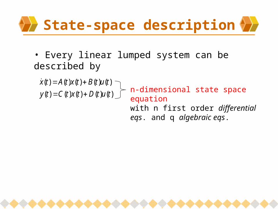
State-space description

( ) ( ) ( ) ( ) ( )

( ) ( ) ( ) ( ) ( )

x t A t x t B t u t

y t C t x t D t u t

• Every linear lumped system can be described by

n-dimensional state space equationwith n first order differential eqs. and q algebraic eqs.

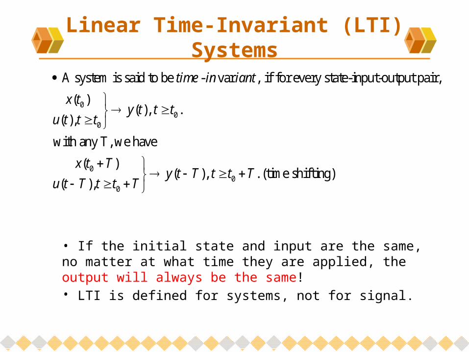
Linear Time-Invariant (LTI) Systems

00

0

00

0

A system is said to be - var , if for every state-input-output pair,

( )( ), .

( ),

with any T, we have

( )( ), . (time shifting)

( ),

time in iant

x ty t t t

u t t t

x t Ty t T t t T

u t T t t T

• If the initial state and input are the same, no matter at what time they are applied, the output will always be the same!• LTI is defined for systems, not for signal.

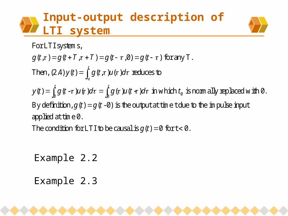
Input-output description of LTI system

0

00 0

For LTI systems,

( , ) ( , ) ( ,0) ( ) for any T.

Then, (2.4) ( ) ( , ) ( ) reduces to

( ) ( - ) ( ) ( ) ( - ) in which is normally replaced with 0.

By definition, ( )

t

t

t t

g t g t T T g t g t

y t g t u d

y t g t u d g u t d t

g t

( - 0) is the output at time t due to the impulse input

applied at time 0.

The condition for LTI to be causal is ( ) 0 for t 0.

g t

g t

Example 2.2

Example 2.3

Transfer-function matrix

-

0

-

0 0

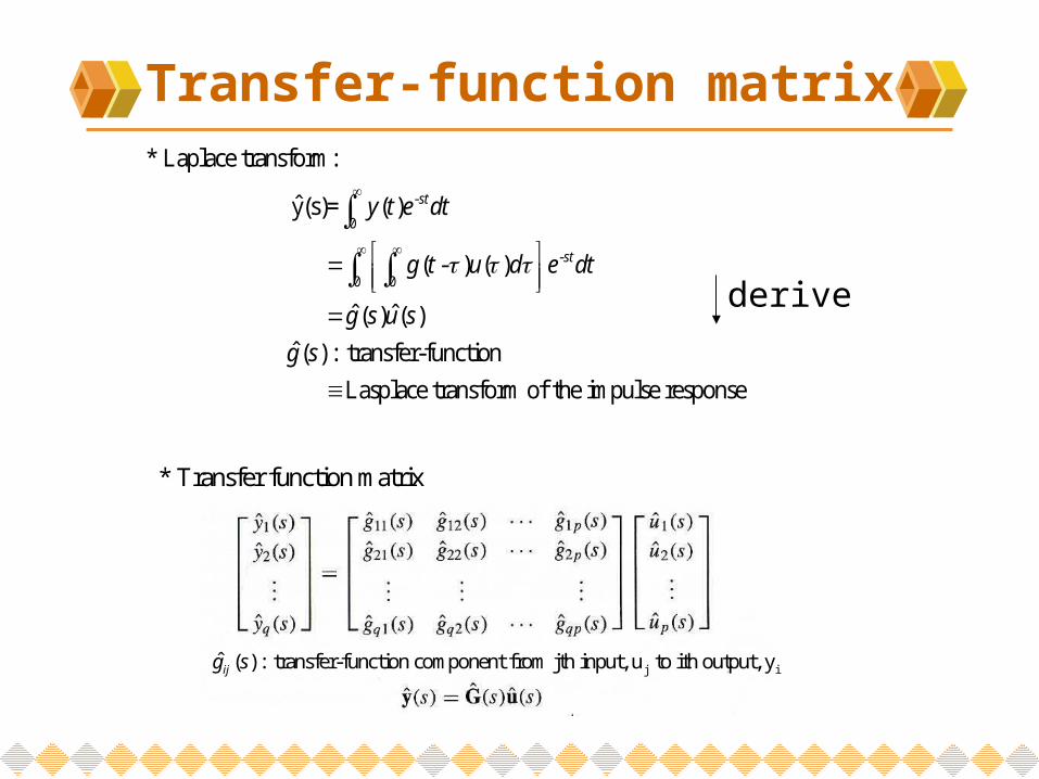
* Laplace transform:

y(s)= ( )

( - ) ( )

ˆ ˆ( ) ( )

ˆ ( ) : transfer-function

Lasplace transform of the impulse response

st

st

y t e dt

g t u d e dt

g s u s

g s

* Transfer function matrix

derive

j iˆ ( ) : transfer-function component from jth input, u to ith output, yijg s

Transfer matrix

Example 2.4

Example 2.5

Classification of transfer function

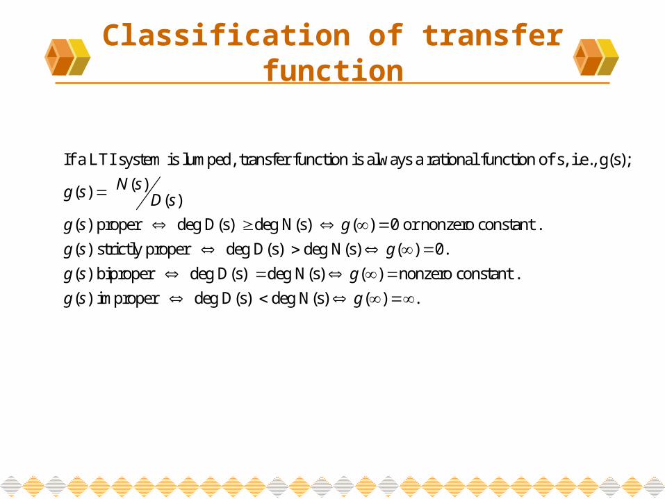
If a LTI system is lumped, transfer function is always a rational function of s, i.e., g(s);

( )( ) ( )

( ) proper deg D(s) deg N(s) ( ) 0 or nonzero constant .

( ) strictly proper deg D(

N sg s D s

g s g

g s

s) deg N(s) ( ) 0.

( ) biproper deg D(s) deg N(s) ( ) nonzero constant .

( ) improper deg D(s) deg N(s) ( ) .

g

g s g

g s g

Pole/Zero

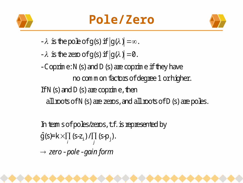
- is the pole of g(s) if g( ) .

- is the zero of g(s) if g( ) 0.

- Coprime: N(s) and D(s) are coprime if they have

no common factors of degree 1 or higher.

If N(s) and D(s) are cop

i j

rime, then

all roots of N(s) are zeros, and all roots of D(s) are poles.

In terms of poles/zeros, t.f. is represented by

g(s)=k (s-z ) / (s-p ).

- -

i j

zero pole gain form

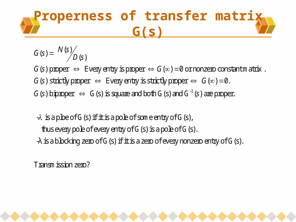
Properness of transfer matrix G(s)

( )( ) ( )

( ) proper Every entry is proper ( ) 0 or nonzero constant matrix .

( ) strictly proper Every entry is strictly proper ( ) 0.

( ) biproper G(s) is square and both G(s) and

N sG s D s

G s G

G s G

G s

-1 G ( ) are proper.

- is a ploe of G(s) if it is a pole of some entry of G(s),

thus every pole of every entry of G(s) is a pole of G(s).

-λ is a blocking zero of G(s) if it is a zero of every nonz

s

ero entry of G(s).

Transmission zero?

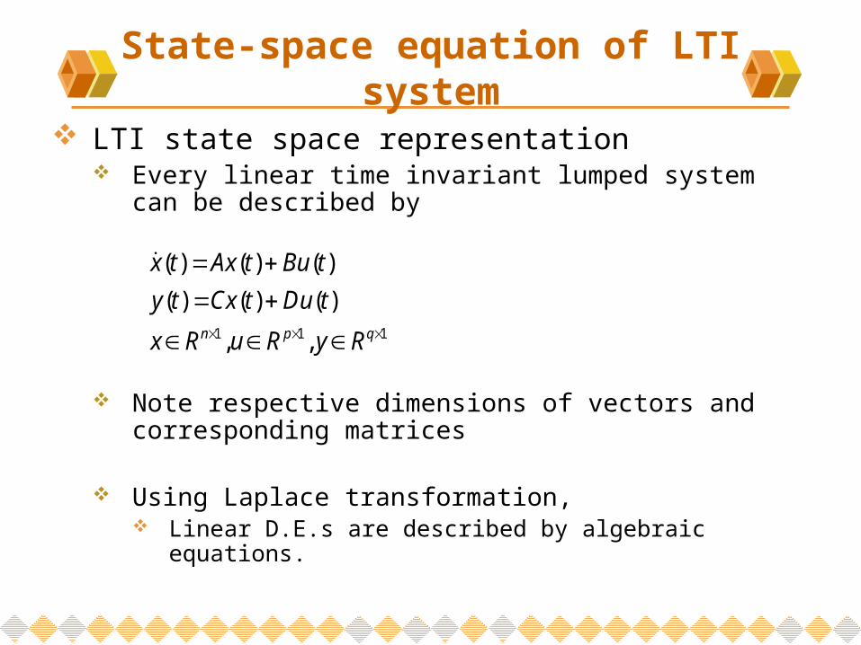
State-space equation of LTI system

LTI state space representation Every linear time invariant lumped system can be

described by

Note respective dimensions of vectors and corresponding matrices

Using Laplace transformation, Linear D.E.s are described by algebraic equations.

1 1 1

( ) ( ) ( )

( ) ( ) ( )

, ,n p q

x t Ax t Bu t

y t Cx t Du t

x R u R y R

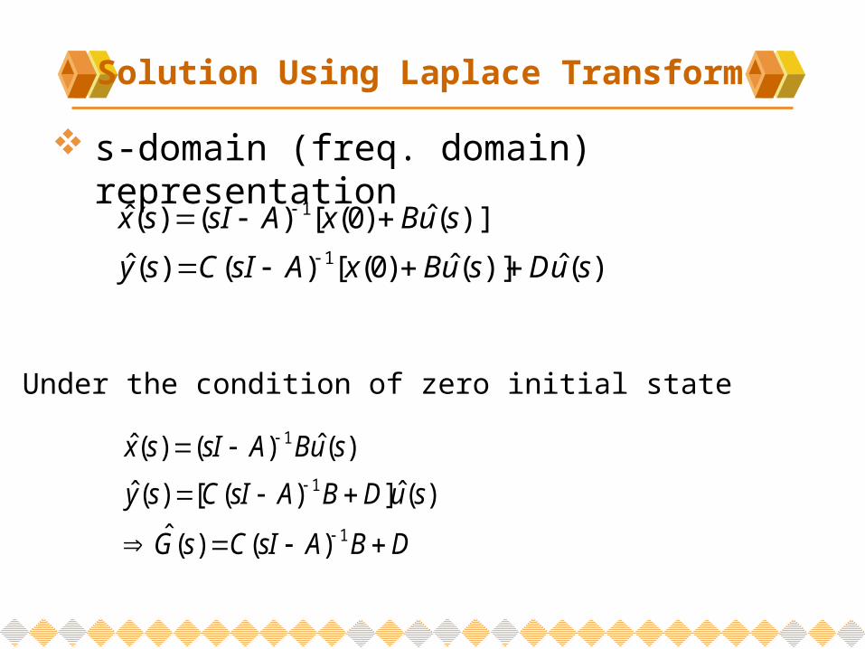
Solution Using Laplace Transform

s-domain (freq. domain) representation

)(ˆ)](ˆ)0([)()(ˆ

)](ˆ)0([)()(ˆ1

1

suDsuBxAsICsy

suBxAsIsx

1

1

1

ˆ ˆ( ) ( ) ( )

ˆ ˆ( ) [ ( ) ] ( )

ˆ ( ) ( )

x s sI A Bu s

y s C sI A B D u s

G s C sI A B D

Under the condition of zero initial state

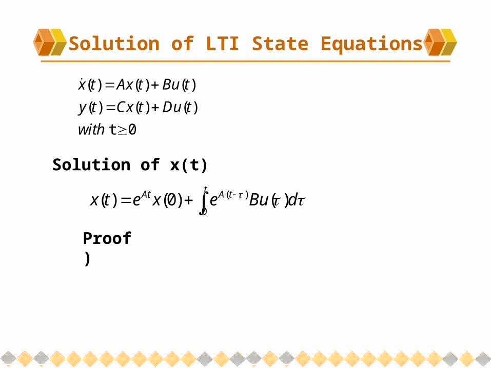
Solution of LTI State Equations

( ) ( ) ( )

( ) ( ) ( )

t 0

x t Ax t Bu t

y t Cx t Du t

with

dBuexetxt tAAt )()0()(0

)(

Solution of x(t)

Proof)

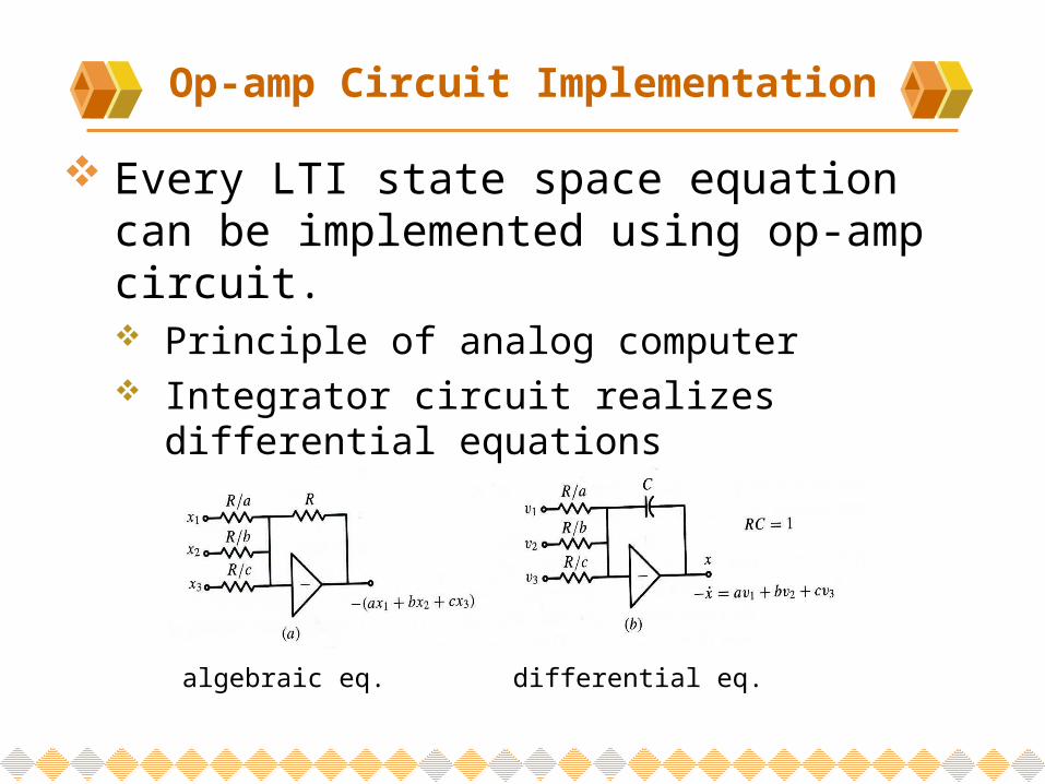
Op-amp Circuit Implementation

Every LTI state space equation can be implemented using op-amp circuit. Principle of analog computer Integrator circuit realizes differential

equations

algebraic eq. differential eq.

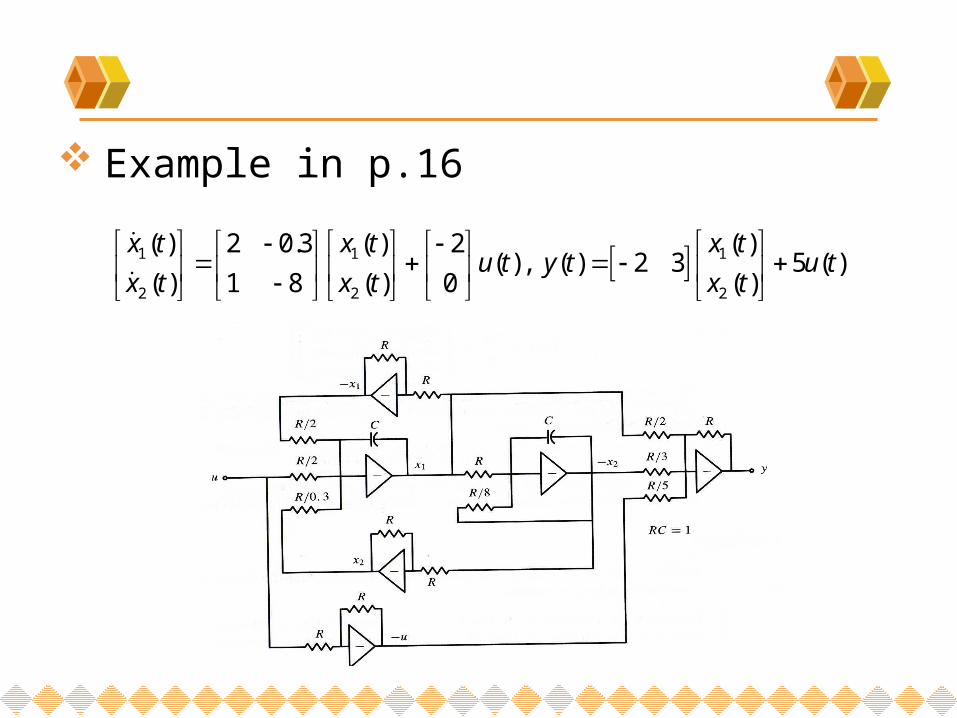
Example in p.16

1 1 1

2 2 2

( ) ( ) ( )2 0.3 2( ) , ( ) 2 3 5 ( )

( ) ( ) ( )1 8 0

x t x t x tu t y t u t

x t x t x t

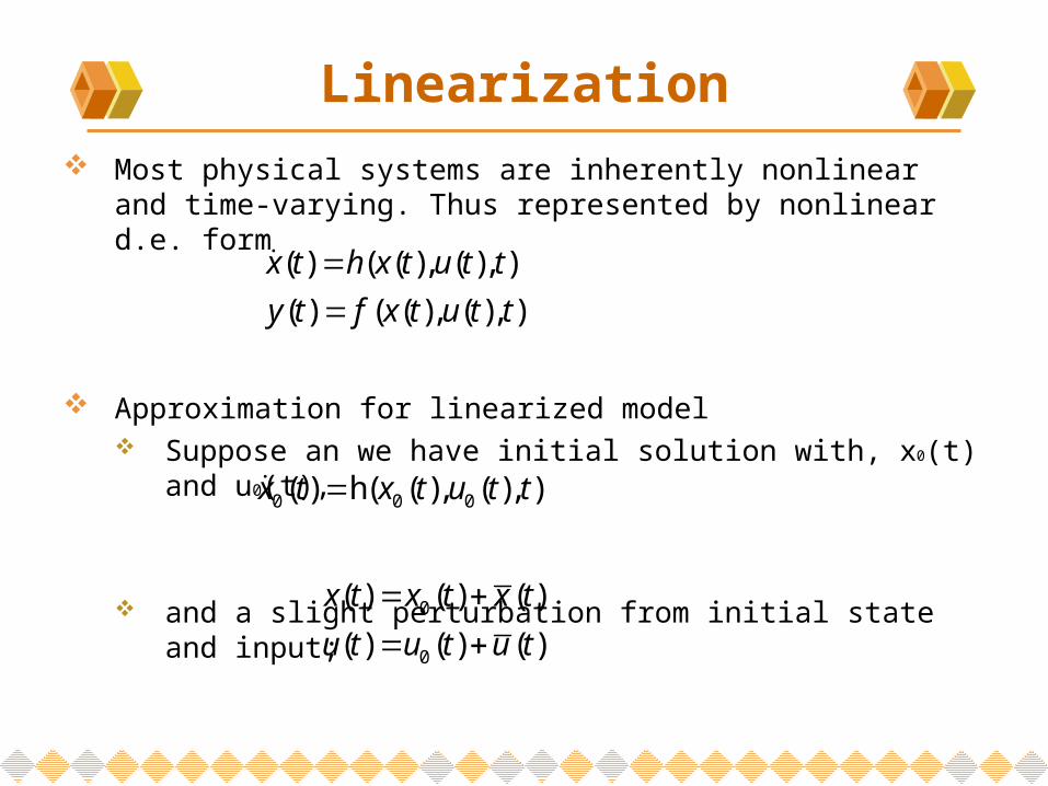
Linearization Most physical systems are inherently nonlinear and time-

varying. Thus represented by nonlinear d.e. form

Approximation for linearized model Suppose an we have initial solution with, x0(t) and u0(t),

and a slight perturbation from initial state and input;

( ) ( ( ), ( ), )

( ) ( ( ), ( ), )

x t h x t u t t

y t f x t u t t

0 0 0( ) h( ( ), ( ), )x t x t u t t

0

0

( ) ( ) ( )

( ) ( ) ( )

x t x t x t

u t u t u t

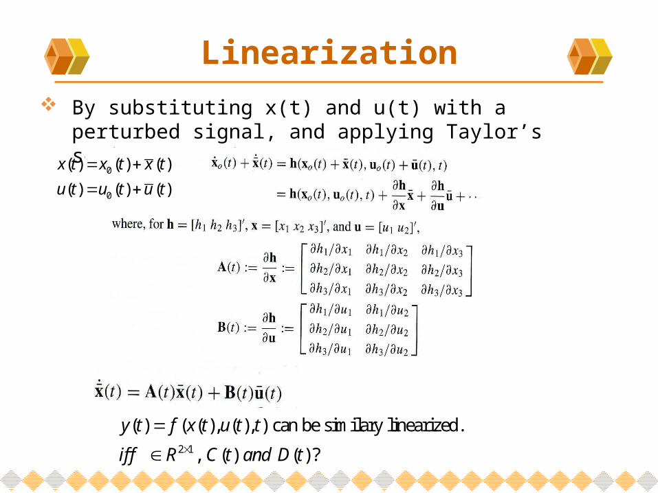
Linearization By substituting x(t) and u(t) with a perturbed signal,

and applying Taylor’s series expansion,

2 1

( ) ( ( ), ( ), ) can be similary linearized.

, ( ) ( )?

y t f x t u t t

if f R C t and D t

0

0

( ) ( ) ( )

( ) ( ) ( )

x t x t x t

u t u t u t

Example2.6

Spring-mass system with viscous friction Only viscous friction is considered

Example2.7

Dual spring-mass system Derive dynamic equations In (2.24), k1 k3

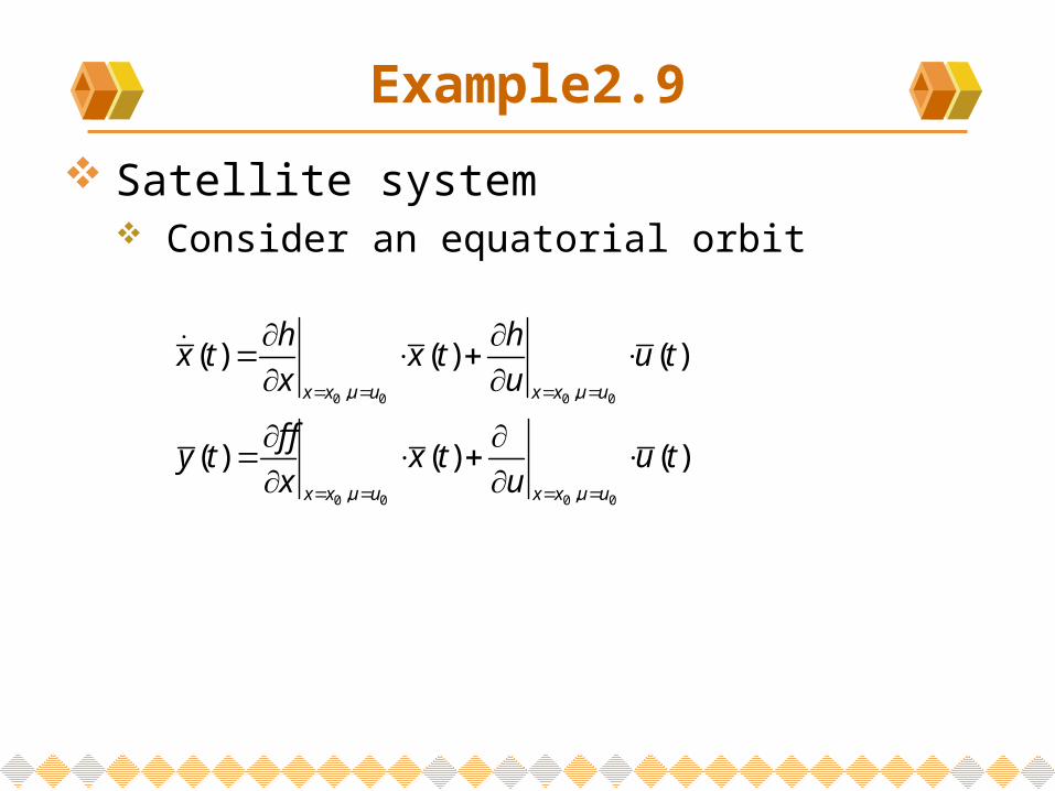
Example2.9

Satellite system Consider an equatorial orbit

0 0 0 0

0 0 0 0

, ,

, ,

( ) ( ) ( )

( ) ( ) ( )

x x u u x x u u

x x u u x x u u

h hx t x t u t

x u

f fy t x t u t

x u

Example 2.11

RLC networks KCL KVL

2.6 Discrete-Time Systems

Discrete-time system Obtained by sampling a continuous-time

system with sampling time, T. Denoted by u[k]:=u(kT), y[k]:=y(kT)

where k is an integer ranging from –infinity to +infinity

Kalman’s state definition holds in the same way.

Discrete time delay system is a lumped system, if delay is integer multiple of T. (as opposed to cont. system)

2.6 Discrete-Time Systems

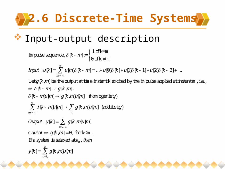
Input-output description1 if k=m

Impulse sequence, [ ] :0 if k m

: [ ] [ ] [ ] ... [0] [ ] [1] [ 1] [2] [ 2] ...

Let [ , ] be the output at time instant k excited by the impulse applied at instant m,m

k m

Input u k u m k m u k u k u k

g k m

0

i.e.,

[ ] [ , ].

[ ] [ ] [ , ] [ ] (homogeniety)

[ ] [ ] [ , ] [ ] (additivity)

: [ ] [ , ] [ ]

[ , ] 0, for k<m.

If a system is relaxed at ,

[ ] [ ,

m m

m

k m g k m

k m u m g k m u m

k m u m g k m u m

Output y k g k m u m

Causal g k m

k then

y k g k m

0

] [ ]k

m k

u m

Z-transform

0

0 0

0

0

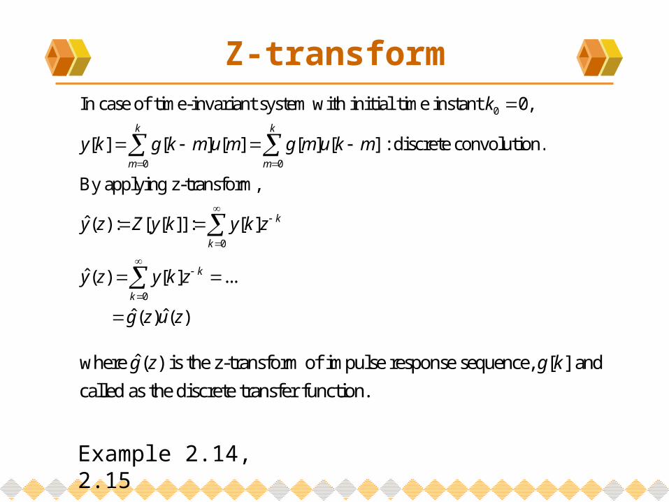
In case of time-invariant system with initial time instant 0,

[ ] [ ] [ ] [ ] [ ] : discrete convolution.

By applying z-transform,

ˆ( ) : [ [ ]] : [ ]

ˆ( ) [ ] ...

k k

m m

k

k

k

k

k

y k g k m u m g m u k m

y z Z y k y k z

y z y k z

ˆ ˆ ( ) ( )g z u z

Example 2.14, 2.15

ˆwhere ( ) is the z-transform of impulse response sequence, [ ] and

called as the discrete transfer function.

g z g k

Discrete-Time Systems

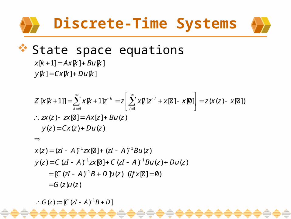
State space equations

0 1

1 1

1

[ 1] [ ] [ ]

[ ] [ ] [ ]

[ [ 1]] [ 1] [ ] [0] [0] ( ( ) [0])

( ) [0] [ ] ( )

( ) ( ) ( )

( ) ( ) [0] ( ) ( )

( ) ( ) [0] (

k l

k l

x k Ax k Bu k

y k Cx k Du k

Z x k x k z z x l z x x z x z x

zx z zx Ax z Bu z

y z Cx z Du z

x z zI A zx zI A Bu z

y z C zI A zx C zI A

1

1

) ( ) ( )

[ ( ) ] ( ) ( [0] 0)

( ) ( )

Bu z Du z

C zI A B D u z If x

G z u z

1( ) : [ ( ) ]G z C zI A B D

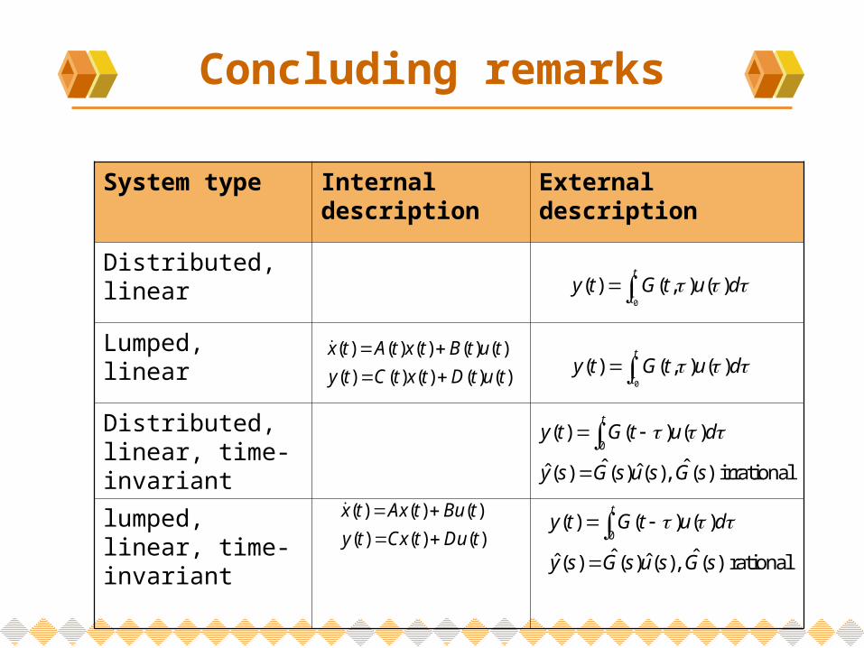
Concluding remarks

System type Internal description

External description

Distributed, linear

Lumped, linear

Distributed, linear, time-invariant

lumped, linear, time-invariant

0

( ) ( , ) ( )t

ty t G t u d

( ) ( ) ( ) ( ) ( )

( ) ( ) ( ) ( ) ( )

x t A t x t B t u t

y t C t x t D t u t

0

( ) ( , ) ( )t

ty t G t u d

0( ) ( ) ( )

ˆ ˆˆ ˆ( ) ( ) ( ), ( ) irrational

ty t G t u d

y s G s u s G s

( ) ( ) ( )

( ) ( ) ( )

x t Ax t Bu t

y t Cx t Du t

0

( ) ( ) ( )

ˆ ˆˆ ˆ( ) ( ) ( ), ( ) rational

ty t G t u d

y s G s u s G s

HW #1

Chap. 2 Problems: 2.7-2.10, 2.15,2.16