Lithology constraints from seismic waveforms: application ... · Lithology constraints from seismic waveforms: application to opal-A to opal-CT transition by Mohammad Maysami B.Sc.,

Lithology constraints from seismicwaveforms: application to opal-A to

opal-CT transition

by

Mohammad Maysami

B.Sc., Sharif University of Technology, 2005

A THESIS SUBMITTED IN PARTIAL FULFILMENT OFTHE REQUIREMENTS FOR THE DEGREE OF

MASTER OF APPLIED SCIENCE

in

The Faculty of Graduate Studies

(Geophysics)

THE UNIVERSITY OF BRITISH COLUMBIA

February 2008

c© Mohammad Maysami, 2008

Abstract

In this work, we present a new method for seismic waveform characteriza-tion, which is aimed at extracting detailed litho-stratigraphical informationfrom seismic data. We attempt to estimate the lithological attributes fromseismic data according to our parametric representation of stratigraphicalhorizons, where the parameter values provide us with a direct link to na-ture of lithological transitions. We test our method on a seismic datasetwith a strong diagenetic transition (opal-A to opal-CT transition). Givensome information from cutting samples of well, we use a percolation-basedmodel to construct the elastic profile of lithological transitions. Our goalis to match parametric representation for the diagenetic transition in bothreal data and synthetic data given by these elastic profiles. This match maybe interpreted as a well-seismic tie, which reveals lithological informationabout stratigraphical horizons.

ii

Table of Contents

Abstract . . . . . . . . . . . . . . . . . . . . . . . . . . . . . . . . . ii

Table of Contents . . . . . . . . . . . . . . . . . . . . . . . . . . . . iii

List of Figures . . . . . . . . . . . . . . . . . . . . . . . . . . . . . . iv

Acknowledgements . . . . . . . . . . . . . . . . . . . . . . . . . . . v

Dedication . . . . . . . . . . . . . . . . . . . . . . . . . . . . . . . . vi

1 Introduction . . . . . . . . . . . . . . . . . . . . . . . . . . . . . 1

2 Rock-physics model . . . . . . . . . . . . . . . . . . . . . . . . 52.1 The site percolation model . . . . . . . . . . . . . . . . . . . 52.2 Seismic response of the percolation model . . . . . . . . . . . 6

2.2.1 The seismic source function . . . . . . . . . . . . . . . 9

3 Seismic waveform characterization . . . . . . . . . . . . . . . 103.1 Detection by multiscale analysis . . . . . . . . . . . . . . . . 103.2 Segmentation . . . . . . . . . . . . . . . . . . . . . . . . . . . 113.3 Nonlinear parametric inversion . . . . . . . . . . . . . . . . . 13

3.3.1 Parametric representation . . . . . . . . . . . . . . . 13

4 Attribute analysis . . . . . . . . . . . . . . . . . . . . . . . . . 17

5 Opal-A to opal-CT transition and well-seismic tie . . . . . 22

6 Discussion and Conclusions . . . . . . . . . . . . . . . . . . . 27

Bibliography . . . . . . . . . . . . . . . . . . . . . . . . . . . . . . . 28

iii

List of Figures

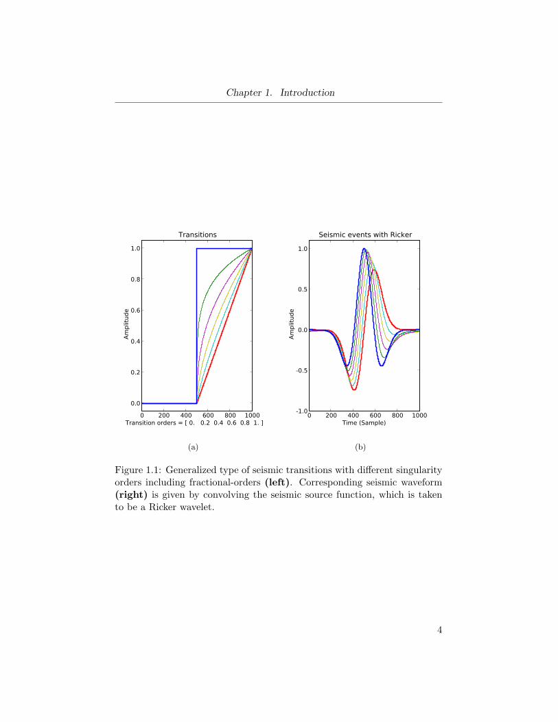
1.1 Generalized type of seismic transitions with different singular-ity orders including fractional-orders (left). Correspondingseismic waveform (right) is given by convolving the seismicsource function, which is taken to be a Ricker wavelet. . . . . 4

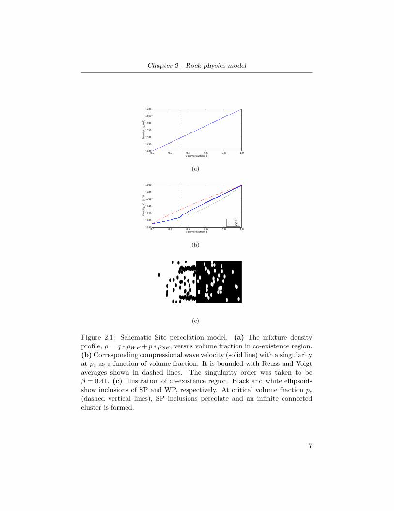
2.1 Schematic Site percolation model. (a) The mixture densityprofile, ρ = q ∗ ρWP + p ∗ ρSP , versus volume fraction inco-existence region. (b) Corresponding compressional wavevelocity (solid line) with a singularity at pc as a function ofvolume fraction. It is bounded with Reuss and Voigt aver-ages shown in dashed lines. The singularity order was takento be β = 0.41. (c) Illustration of co-existence region. Blackand white ellipsoids show inclusions of SP and WP, respec-tively. At critical volume fraction pc (dashed vertical lines),SP inclusions percolate and an infinite connected cluster isformed. . . . . . . . . . . . . . . . . . . . . . . . . . . . . . . 7

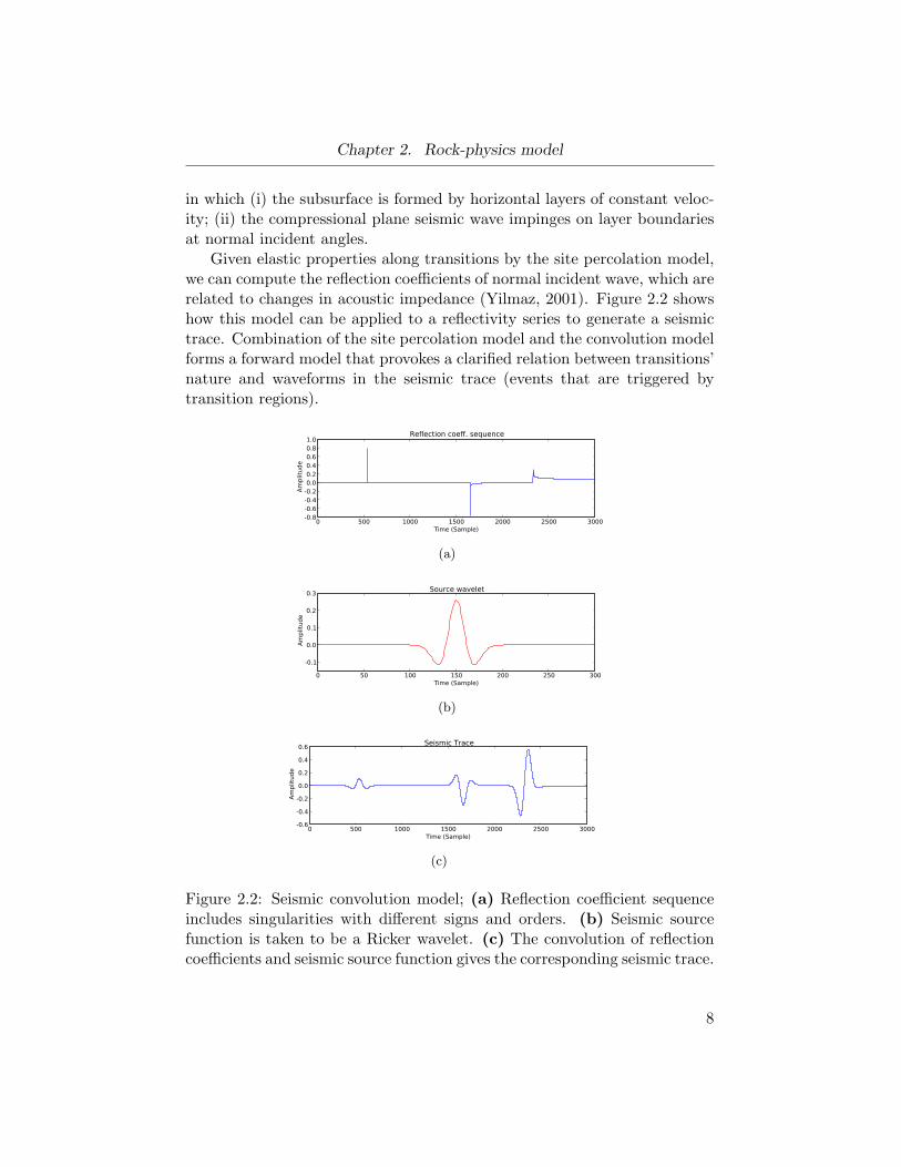
2.2 Seismic convolution model; (a) Reflection coefficient sequenceincludes singularities with different signs and orders. (b) Seis-mic source function is taken to be a Ricker wavelet. (c) Theconvolution of reflection coefficients and seismic source func-tion gives the corresponding seismic trace. . . . . . . . . . . . 8

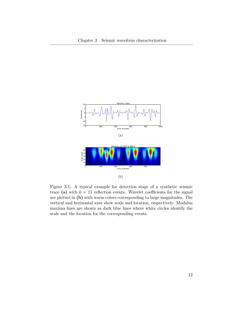
3.1 A typical example for detection stage of a synthetic seismictrace (a) with k = 11 reflection events. Wavelet coefficientsfor the signal are plotted in (b) with warm colors correspond-ing to large magnitudes. The vertical and horizontal axesshow scale and location, respectively. Modulus maxima linesare shown as dark blue lines where white circles identify thescale and the location for the corresponding events. . . . . . . 12

iv

List of Figures

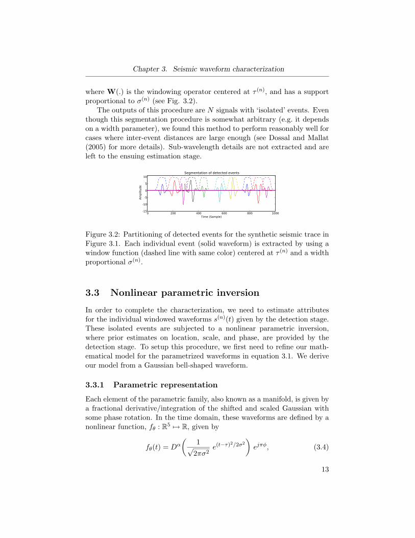
3.2 Partitioning of detected events for the synthetic seismic tracein Figure 3.1. Each individual event (solid waveform) is ex-tracted by using a window function (dashed line with samecolor) centered at τ (n) and a width proportional σ(n). . . . . 13

3.3 Parameter estimation for an individual event in Fig. 3.2. (a)Initial iteration of parameter estimation for the isolated eventwhere dashed blue line shows windowed event and solid redline shows our guess. (b) Final iteration of parameter esti-mation for the isolated event where the estimated waveformmatches the actual event. . . . . . . . . . . . . . . . . . . . . 15

3.4 Characterization results for the synthetic trace in Figure 3.1.(a) Estimated seismic trace is formed by superposition of allcharacterized events and compared with the original seismictrace. (b) The estimated attributes of events (τ, α) are com-pared to their actual values. . . . . . . . . . . . . . . . . . . . 16

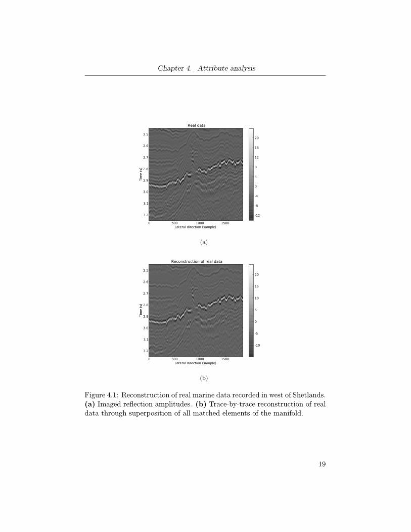
4.1 Reconstruction of real marine data recorded in west of Shet-lands. (a) Imaged reflection amplitudes. (b) Trace-by-tracereconstruction of real data through superposition of all matchedelements of the manifold. . . . . . . . . . . . . . . . . . . . . 19

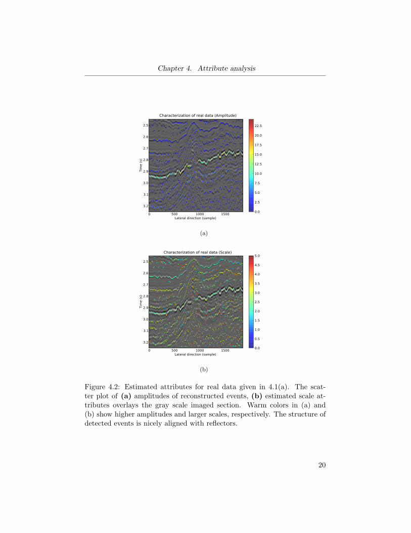
4.2 Estimated attributes for real data given in 4.1(a). The scatterplot of (a) amplitudes of reconstructed events, (b) estimatedscale attributes overlays the gray scale imaged section. Warmcolors in (a) and (b) show higher amplitudes and larger scales,respectively. The structure of detected events is nicely alignedwith reflectors. . . . . . . . . . . . . . . . . . . . . . . . . . . 20

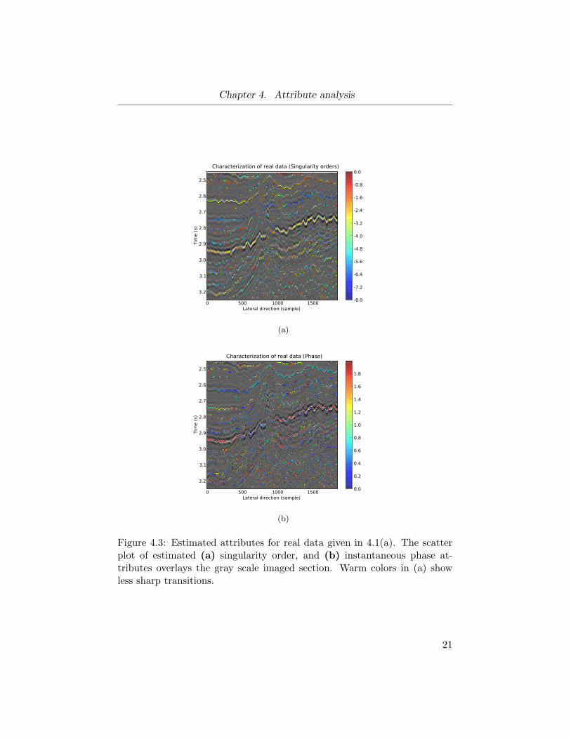
4.3 Estimated attributes for real data given in 4.1(a). The scat-ter plot of estimated (a) singularity order, and (b) instanta-neous phase attributes overlays the gray scale imaged section.Warm colors in (a) show less sharp transitions. . . . . . . . . 21

v

List of Figures

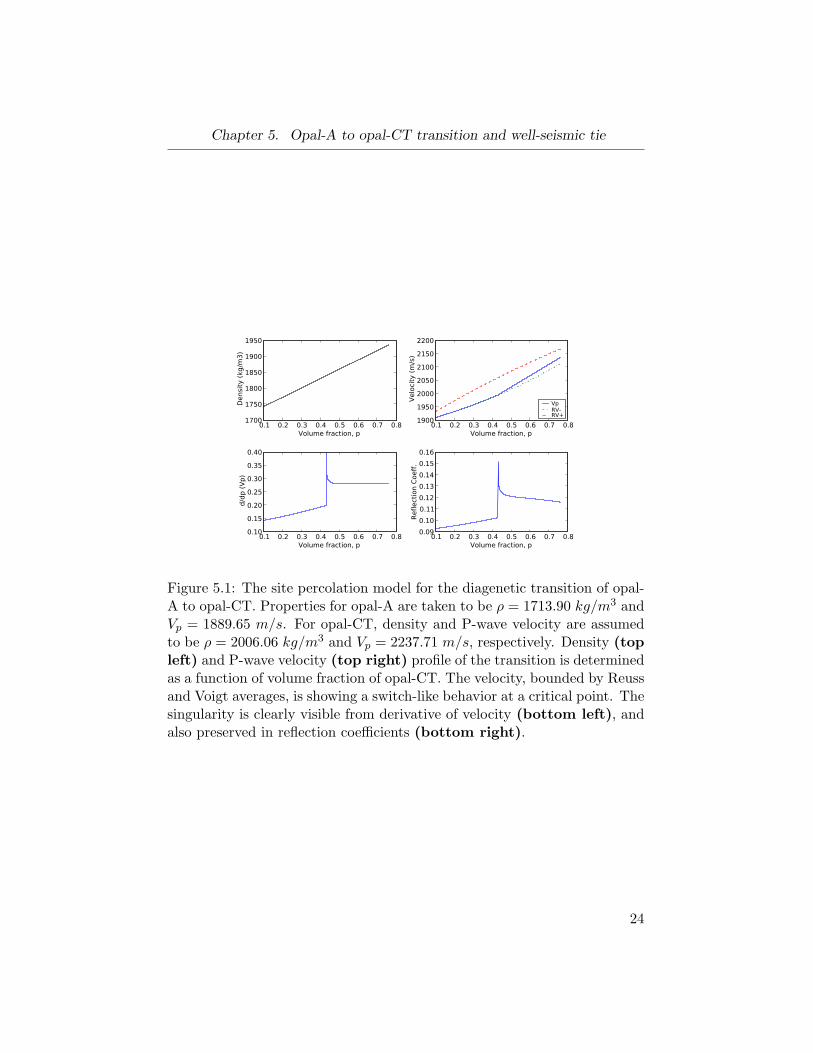
5.1 The site percolation model for the diagenetic transition ofopal-A to opal-CT. Properties for opal-A are taken to be ρ =1713.90 kg/m3 and Vp = 1889.65 m/s. For opal-CT, densityand P-wave velocity are assumed to be ρ = 2006.06 kg/m3

and Vp = 2237.71 m/s, respectively. Density (top left) andP-wave velocity (top right) profile of the transition is de-termined as a function of volume fraction of opal-CT. Thevelocity, bounded by Reuss and Voigt averages, is showinga switch-like behavior at a critical point. The singularity isclearly visible from derivative of velocity (bottom left), andalso preserved in reflection coefficients (bottom right). . . . 24

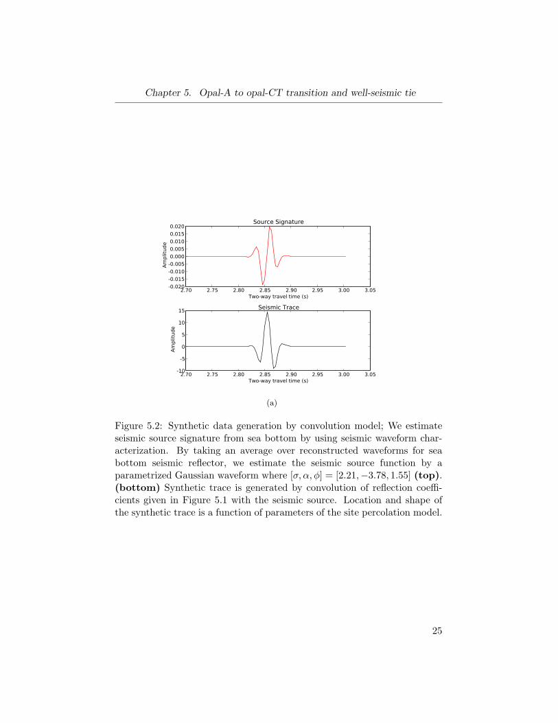
5.2 Synthetic data generation by convolution model; We estimateseismic source signature from sea bottom by using seismicwaveform characterization. By taking an average over recon-structed waveforms for sea bottom seismic reflector, we esti-mate the seismic source function by a parametrized Gaussianwaveform where [σ, α, φ] = [2.21,−3.78, 1.55] (top). (bot-tom) Synthetic trace is generated by convolution of reflec-tion coefficients given in Figure 5.1 with the seismic source.Location and shape of the synthetic trace is a function ofparameters of the site percolation model. . . . . . . . . . . . 25

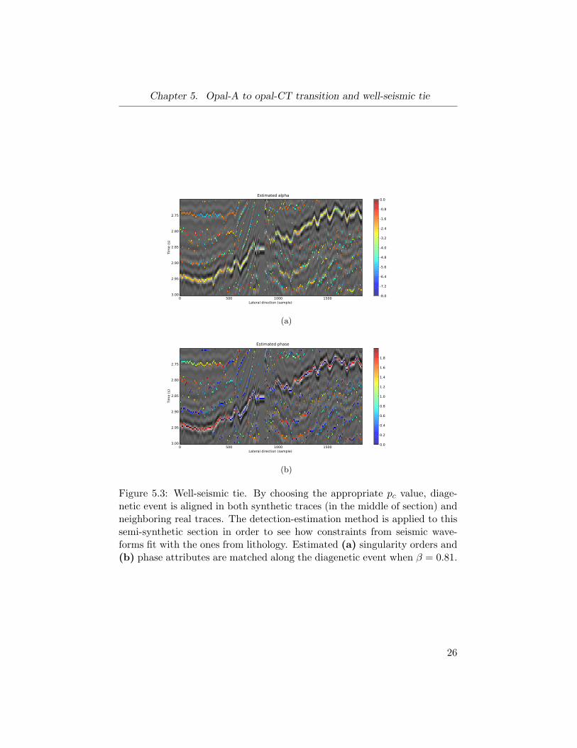
5.3 Well-seismic tie. By choosing the appropriate pc value, dia-genetic event is aligned in both synthetic traces (in the mid-dle of section) and neighboring real traces. The detection-estimation method is applied to this semi-synthetic section inorder to see how constraints from seismic waveforms fit withthe ones from lithology. Estimated (a) singularity orders and(b) phase attributes are matched along the diagenetic eventwhen β = 0.81. . . . . . . . . . . . . . . . . . . . . . . . . . . 26

vi

Acknowledgements

First and foremost, I would like to express my sincere gratitude to my su-pervisor, Dr. Felix J. Herrmann, for his great insight and wise guidancethroughout this research project. His serious research attitude will alwaysinspire me all my life.

My sincere thanks are also due to Dr. Oldenburg, Dr. Bostock, and Dr.Greif for their constructive suggestions as members of my thesis commit-tee. Their kindness and word of wisdom have always been the sources ofenlightenment to me.

I am also deeply indebted to Dr.Henryk Modzelewski for his great ad-vice and assistance regarding the computational and technical problems. Iam genuinely grateful to other SLIM (Seismic Laboratory for Imaging andModeling) team members for being there to help with any problems that Iencountered while studying there. Their intelligence, persistence and kind-ness made my stay at the University of British Columbia stimulating andenjoyable.

My wonderful parents deserve thanks for all the love they have given meand for always being so supportive and proud. I would like to thank mykind and loving sisters, whose altruism and compassion are inspiring.

The authors also thank David Wilkinson for constructive discussionsabout this research. Veritas DGC Company is gratefully thanked for the realdatasets. This work was in part financially supported by NSERC DiscoveryGrant 22R81254 and CRD Grant DNOISE 334810-05 of Felix J. Herrmannand was carried out as part of the CHARM project with support, securedthrough Chevron.

vii

http://www.veritasdgc.com

http://www.nserc.gc.ca/index.htm

http://slim.eos.ubc.ca/?module=articles&func=display&catid=43&aid=100

http://slim.eos.ubc.ca/?module=articles&func=view&catid=21

http://www.chevron.com/

To my parents,

who taught me how to love and how to be loved.

viii

Chapter 1

Introduction

In this study, we propose a novel method to identify and quantify generalizedlithological transitions, as long as their scale is above the seismic wavelength.In this method, we link the seismic waveforms to fractional-order transitionsthrough a parametric waveform inversion process. By using the percolationmodel proposed by Herrmann and Bernabe (2004), we show that smoothchanges (connectivity) in lithology may also give rise to a seismic reflec-tion. Consequently, a wider range of lithological transitions in depositionalenvironments, which is not given by other methods, exists in our model.The primary goals of this study are to answer two general questions: 1) isthe waveform quantification coherent with the stratigraphical structure ofseismic data; and 2) can we find a direct link between our quantificationof seismic waveforms and nature of associated lithological boundaries? Apositive answer to these question means that we have a tool, which providesus with increased insight into litho-stratigraphy structure of the subsurface.

Seismic surveys are a valuable tool to extract geological structure of thelithological boundaries in the subsurface. However, this method only imagesseismic reflectors and does not provide precise information on the associatedlithological transitions directly. Therefore, there is a crucial step in seismicimaging where observations are translated into models of the Earth struc-ture that are geologically valid. Using these models, we can extract thegeological and stratigraphical features of the subsurface. Transitions in thelithology are examples of these geological features, which are mathemati-cally represented by zero-order discontinuities (step functions) or first-orderramp functions in most cases. However, multiscale analysis on well andseismic data (Muller et al., 1992; Herrmann, 1997, 1998) showed that theserepresentations may not be rich enough to describe the different types oftransitions present in sedimentary basins. In reality, seismically-observedreflectors correspond to complex lithological changes typically composed ofsub-wavelength features or more gradational lithological transitions. Con-

sequently, valuable information is lost by assuming these transitions to begiven by step or ramp discontinuities. Instead, multiscale analysis on sedi-mentary records revealed the existence of transitions with varying singular-

1

Chapter 1. Introduction

ity orders (Herrmann, 1998, 2001; Herrmann et al., 2001; Herrmann, 2005).Singularities are points in a signal at which the derivative is undefined.This generalized type of fractional-order singularity is given by fractionallydifferentiating/integrating a zero-order discontinuity (see Fig. 1.1(a) for aschematic of fractional-order transitions). Lithological transitions have beenstudied from various perspectives. However, most of available models forlithological transitions lack a straightforward generalization to fractional-order transitions.

Lithological perspective: Classical seismic stratigraphical models (Pay-ton, 1977; Harms and Tackenberg, 1972) represent sub-wavelength lithologyvariation by multiple zero-order and first-order discontinuities. The sim-plicity of this assumption limits the ability of these models to constrainthe lithological structure. In that sense, fractional-order transitions pro-vide a more accurate parametric description to describe acoustic impedanceprofiles across the transitions by eliminating the superposition of multiplereflectors. In this perspective, variations in the acoustic impedance are in-terpreted as proxies for the lithology, e.g., observed seismic waveforms arethrough complex-trace attributes related to fining upward or coarsening up-ward sequences as shown in Herrmann et al. (2001).

Even though the above extension of transition models is proved to beuseful, two important aspects are missing, namely (i) a first principal rock-physical model that predicts the occurrence of fractional-order transitionsas a function of a smoothly varying lithology/composition and, (ii) a robustestimation technique, extracting information on the transition order frombandwidth limited seismic traces. In order to make prospect towards thesetwo aspects, we have to include more careful considerations regarding therock-physical and seismological aspects of our problem.

Rock-physical perspective: In this thesis, we look at how changes in therock-physical properties, such as the rock’s acoustic wave speed and density,are related to the volume fractions of a bi-compositional rock, e.g., a rockconsisting of a sand-shale or opal-A/CT mixture. From the rock-physicalperspective, transitions are described with their elastic profiles, e.g., velocityand density.

In this case, the traditional Hashin-Shtrikman (HS) bounds are used toconstrain the elastic moduli (see Hashin and Shtrikman (1962) for moredetails). Even though these bounds have proved to be useful in describ-ing the overall behavior of binary mixtures, this theory does not predict

2


sharp transitions in the rock properties as a function of the composition.By including the important concept of connectivity amongst the two com-ponents of the rock mixture, Herrmann and Bernabe (2004) have introduceda model predicting a critical volume fraction at which the stronger of thetwo mixing components connects. At that point, the overall strength of themixture grows with the size of the connected cluster, yielding a fractional-order transition for the seismic velocity. This model (HB model) impliessharp transitions even in cases where the rock’s composition and hence thedensity vary smoothly. Before transgressing the critical point, the velocitiespredicted by the HB model follows the lower HS-bound, followed by theoccurrence of sudden sharp increase in the velocity, which ends up at thevelocity predicted by the upper HS-bound.

Seismological perspective: Amongst reflection seismologists, the Earthsubsurface is often idealized as a stack of homogeneous layers separated byzero-order discontinuities. This model yields a spiky reflection coefficientsequence for which deconvolution methods have been derived, removing theseismic source signature. Despite recent developments (Saggaf and Robin-son, 2000), earth models consisting of a sparse set of different fractional-ordertransitions render conventional deconvolution techniques ineffective.

In this thesis, we present a two-stage method that handles this morecomplex situation and during which (i) reflection events are first detectedby a multiscale technique deriving from the work by Holschneider (1995),followed by (ii) a nonlinear parametric inversion technique. During the lat-ter, seismic attributes, including the illusive singularity orders, are estimatedfrom seismic waveforms extracted during the multiscale detection.

The thesis is organized as follows. First, we introduce the site perco-lation model and discuss the seismic response of this model, which we useas the “rock-physics” forward model. We proceed by presenting a seismicwaveform characterization method, which first extracts stratigraphical hori-zons by locating major features in the seismic data and then processes eachevent with an inversion where it is represented by only a few parametersassociated with a parametric waveform. We apply our method to a realdata and discuss the results in term of satisfying our expectations. We thenaim at recovering the geological details from seismic data by focusing on adiagenetic transition in the data. The percolation model provides us with asynthetic seismic reflector, which is then parametrized and matched to realdata. We describe how this tie can provide us with lithological insights fromthe seismic data.

3


0 200 400 600 800 1000Transition orders = [ 0. 0.2 0.4 0.6 0.8 1. ]

0.0

0.2

0.4

0.6

0.8

1.0

Am

plit

ude

Transitions

(a)

0 200 400 600 800 1000Time (Sample)

-1.0

-0.5

0.0

0.5

1.0

Am

plit

ude

Seismic events with Ricker

(b)

Figure 1.1: Generalized type of seismic transitions with different singularityorders including fractional-orders (left). Corresponding seismic waveform(right) is given by convolving the seismic source function, which is takento be a Ricker wavelet.

4

Chapter 2

Rock-physics model

The Earth’s subsurface consists of layers of different rock properties sepa-rated by transitions. Transitions are regions where the acoustic impedanceof the Earth changes rapidly with respect to the seismic wavelength. Thesesudden variations give rise to the reflection of seismic waves, which createssingularities in the recorded seismic trace. As reported in the literature,while abrupt lithofacies transition give rise to high-order (more sharp) sin-gularities, a more gradual transition leads to low-order (less sharp) singular-ities. Consequently, singularity orders reflect sharpness of the correspondinglithological boundary (Herrmann et al., 2001). Rock physicists try to im-pose these lithological constraints on the elastic properties as a functionof composition by using different models. Most of these models, however,generally assume that homogeneous mixing of facies can only give rise tosmooth and non-singular elastic properties and the existence of the singu-larities is related to rapid changes in composition only. In recent studieson upper-mantle transitions (Herrmann and Bernabe, 2004), a percolation-based model is proposed, which, unlike the previous models, unravels thesharp changes in seismic velocities across the transitions. Herrmann andBernabe (2004) predict that the singularity in elastic moduli and henceseismic velocity occurs at a critical volume fraction of end-members of themixture. The percolation model could explain the nature of various transi-tions from the properties of rocks. Other than excluding the limitations ofthe existing models as discussed earlier in the introduction, the model alsoprovides the scale invariance.

2.1 The site percolation model

The site percolation model assumes a simplified bi-compositional model torepresent microscale changes along the boundaries of layers. The facies inthis binary mixture are divided into a weak lithofacies at the top and astrong lithofacies in the deeper zone. The weak and strong materials aredenoted with WP and SP, respectively. The percolation model applies tothe co-existence region where both end-members of the binary mixture are

5

Chapter 2. Rock-physics model

involved. We assume the volume fraction of strong and weak material,given by p and q = 1− p, respectively, to depend on the vertical coordinateonly. While microscopic inclusions in the co-existence region are randomlydistributed (see Fig. 2.1(c)), percolation occurs at a threshold, at which the∞-cluster of SP inclusions is formed. The percolation threshold pc = p(zc),which corresponds to a critical depth zc is denoted by a vertical dashed linein Figure 2.1. The volume fraction p∗ of the ∞-cluster is given as

p∗ =

{0 if p < pc

p (p−pc1−pc )β if p ≥ pc,

where β is a positive real parameter related to the percolation model (seeHerrmann and Bernabe (2004) for more details). Accordingly, the elasticmoduli given by the model contain a singularity of order β. These moduligive rise to a linear gradient for density of the mixture as well as a wavespeed profile, which contains a switch-like singularity at pc (see Fig. 2.1(a),2.1(b)). While other models confine the seismic wave velocity in the Hashin-Shtrikman bounds (Hashin and Shtrikman, 1962), the percolation theorypredicts a definite velocity profile within those bounds (Mori and Tanaka,1973; Benveniste, 1987; Luo and Weng, 1987). In our implementation, wehave equivalently replaced these bounds with Reuss and Voigt averages (seeFig. 2.1(b)). The velocity change within these bounds is controlled by pc andβ, which are determined by the end-members of the mixture. Consequently,the order β is considered to be independent of the random emplacement ofinclusions.

2.2 Seismic response of the percolation model

The convolution model is widely used in seismic processing as a simplifiedmodel for the Earth response to the propagation of the seismic wave. Basedon this model, the recorded seismic trace at the surface can be written as

s(t) ∝ (ψ ∗ r)(t), (2.1)

where ψ shows the seismic source wavelet and r is the imaged travel-time re-flectivity sequence. Figure 1.1(b) shows various seismic waveforms given bythe convolution model in presence of fractional-order transitions. Accord-ingly, what seismic receivers records at the surface, can be thought of as theresponse of the Earth filtered through the source wavelet. The convolutionmodel uses a simple reflectivity series for modeling the Earth (Yilmaz, 2001)

6


0.0 0.2 0.4 0.6 0.8 1.0Volume fraction, p

1400

1450

1500

1550

1600

1650

1700

Densi

ty (

kg/m

3)

(a)

0.0 0.2 0.4 0.6 0.8 1.0Volume fraction, p

1680

1700

1720

1740

1760

1780

1800

Velo

city

, V

p (

m/s

)

VpRV-RV+

(b)

(c)

Figure 2.1: Schematic Site percolation model. (a) The mixture densityprofile, ρ = q ∗ ρWP + p ∗ ρSP , versus volume fraction in co-existence region.(b) Corresponding compressional wave velocity (solid line) with a singularityat pc as a function of volume fraction. It is bounded with Reuss and Voigtaverages shown in dashed lines. The singularity order was taken to beβ = 0.41. (c) Illustration of co-existence region. Black and white ellipsoidsshow inclusions of SP and WP, respectively. At critical volume fraction pc(dashed vertical lines), SP inclusions percolate and an infinite connectedcluster is formed.

7


in which (i) the subsurface is formed by horizontal layers of constant veloc-ity; (ii) the compressional plane seismic wave impinges on layer boundariesat normal incident angles.

Given elastic properties along transitions by the site percolation model,we can compute the reflection coefficients of normal incident wave, which arerelated to changes in acoustic impedance (Yilmaz, 2001). Figure 2.2 showshow this model can be applied to a reflectivity series to generate a seismictrace. Combination of the site percolation model and the convolution modelforms a forward model that provokes a clarified relation between transitions’nature and waveforms in the seismic trace (events that are triggered bytransition regions).

0 500 1000 1500 2000 2500 3000Time (Sample)

-0.8-0.6-0.4-0.20.00.20.40.60.81.0

Am

plit

ude

Reflection coeff. sequence

(a)

0 50 100 150 200 250 300Time (Sample)

-0.1

0.0

0.1

0.2

0.3

Am

plit

ude

Source wavelet

(b)

0 500 1000 1500 2000 2500 3000Time (Sample)

-0.6

-0.4

-0.2

0.0

0.2

0.4

0.6

Am

plit

ude

Seismic Trace

(c)

Figure 2.2: Seismic convolution model; (a) Reflection coefficient sequenceincludes singularities with different signs and orders. (b) Seismic sourcefunction is taken to be a Ricker wavelet. (c) The convolution of reflectioncoefficients and seismic source function gives the corresponding seismic trace.

8


2.2.1 The seismic source function

In real world, seismic sources are not ideal spikes. Therefore, we need tohave a preliminary knowledge of the seismic source wavelet to obtain theseismic response of the percolation model. However, in most geophysicalsurveys, the seismic source function ψ is unknown. For our purpose, weassume that the seismic source function has finite smoothness and wiggliness.Combining both conditions can allow us to determine the details of thefrequency content of the source function. The first condition is to limitthe high-frequency content by setting the asymptotic decay rate for highfrequencies. This is imposed by∫

R|ψ(ω)| |ω|γ dω <∞, (2.2)

which means the wavelet is γ-times continuously differentiable, i.e., ψ ∈ Cγ .Here, ψ(ω) =

∫ +∞−∞ ψ(t) e−jωt denotes the Fourier transform of ψ. The

second condition requires the wavelet ψ to be orthogonal with respect tosome finite-order polynomial,∫

Rtq ψ(x) dx = 0 for 0 ≤ q ≤M, (2.3)

hence describing its wiggliness. It defines the number of vanishing momentsof ψ and rules the differentiability of the Fourier transform at zero frequency.Knowing the source wavelet makes it possible to generate the seismic datausing the convolution model.

9

Chapter 3

Seismic waveformcharacterization

Here, our aim is two-fold: finding the locations of the reflectors, i.e., de-lineating the stratigraphy, and extracting information on the nature of thetransitions. For this purpose, we represent a vertical 1-D profile of the Earthas a weighted superposition of parametrized waveforms

s(t) =∑i∈I

ci ψαiσi (t− τi) e

jπφi , (3.1)

where t represents time, and ci and φi (0 ≤ φ < 2) are the amplitude andthe phase for the ith transition, respectively. Furthermore, ψαiσi (t− τi) showsa translated (τi) and scaled (σi) source wavelet ψ, which is fractionally dif-ferentiated (α < 0) or integrated (α > 0). The seismic source wavelet ψ canbe any arbitrary wavelet that satisfies the required conditions listed earlierin the discussion on seismic source functions. The parameters of interest,which we will hereafter refer to as attributes, in this case are the amplitudeci, the location τi, the scale σi, the singularity order αi, and the phase φi.Given the above representation, we present a new method, where the charac-terization problem is divided into two subproblems, namely detection stage,where the main events in the seismic data are located and extracted, andestimation stage, where the attributes for each individual waveform (event)are extracted by a nonlinear parametric inversion. Although we deal withdiscretized finite signals in our implementation, we use continuous signalnotation interchangeably.

3.1 Detection by multiscale analysis

The purpose of the detection step is to find the singularities (major events)in the seismic trace. The detection problem does not fit straightforwardlyinto the classical deconvolution framework due to the existence of fractional-order transitions in the subsurface. The variety of the singularity orders

10

Chapter 3. Seismic waveform characterization

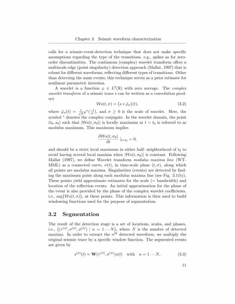
calls for a seismic-event-detection technique that does not make specificassumptions regarding the type of the transitions, e.g., spikes as for zero-order discontinuities. The continuous (complex) wavelet transform offers amultiscale edge (point singularity) detection approach (Mallat, 1997) that isrobust for different waveforms, reflecting different types of transitions. Otherthan detecting the main events, this technique serves as a prior estimate fornonlinear parametric inversion.

A wavelet is a function ϕ ∈ L2(R) with zero average. The complexwavelet transform of a seismic trace s can be written as a convolution prod-uct

Ws(t, σ) =(s ∗ ϕσ

)(t), (3.2)

where ϕσ(t) = 1√σϕ∗(−tσ ), and σ ≥ 0 is the scale of wavelet. Here, the

symbol ∗ denotes the complex conjugate. In the wavelet domain, the point(t0, s0) such that |Ws(t, σ0)| is locally maximum at t = t0 is referred to asmodulus maximum. This maximum implies

∂Ws(t, σ0)∂t

|t=t0 = 0,

and should be a strict local maximum in either half- neighborhood of t0 toavoid having several local maxima when |Ws(t, σ0)| is constant. FollowingMallat (1997), we define Wavelet transform modulus maxima line (WT-MML) as a connected curve, σ(t), in time-scale plane (t, σ), along whichall points are modulus maxima. Singularities (events) are detected by find-ing the maximum point along each modulus maxima line (see Fig. 3.1(b)).These points yield approximate estimates for the scale (= bandwidth) andlocation of the reflection events. An initial approximation for the phase ofthe event is also provided by the phase of the complex wavelet coefficients,i.e., arg{Ws(t, σ)}, at these points. This information is then used to buildwindowing functions used for the purpose of segmentation.

3.2 Segmentation

The result of the detection stage is a set of locations, scales, and phases,i.e., {(τ (n), σ(n), φ(n)) | n = 1 · · ·N}, where N is the number of detectedmaxima. In order to extract the nth detected waveform, we multiply theoriginal seismic trace by a specific window function. The segmented eventsare given by

s(n)(t) = W(τ (n), σ(n))s(t) with n = 1 · · ·N, (3.3)

11


0 200 400 600 800 1000Time (Sample)

-15

-10

-5

0

5

10

Am

plit

ude

Seismic trace

(a)

0 200 400 600 800Time (Sample)

0

10

20

30

40

50

Sca

le index

Modulus of CWT & MMLs

(b)

Figure 3.1: A typical example for detection stage of a synthetic seismictrace (a) with k = 11 reflection events. Wavelet coefficients for the signalare plotted in (b) with warm colors corresponding to large magnitudes. Thevertical and horizontal axes show scale and location, respectively. Modulusmaxima lines are shown as dark blue lines where white circles identify thescale and the location for the corresponding events.

12


where W(.) is the windowing operator centered at τ (n), and has a supportproportional to σ(n) (see Fig. 3.2).

The outputs of this procedure are N signals with ‘isolated’ events. Eventhough this segmentation procedure is somewhat arbitrary (e.g. it dependson a width parameter), we found this method to perform reasonably well forcases where inter-event distances are large enough (see Dossal and Mallat(2005) for more details). Sub-wavelength details are not extracted and areleft to the ensuing estimation stage.

0 200 400 600 800 1000Time (Sample)

-15

-10

-5

0

5

10

Am

plit

ude

Segmentation of detected events

Figure 3.2: Partitioning of detected events for the synthetic seismic trace inFigure 3.1. Each individual event (solid waveform) is extracted by using awindow function (dashed line with same color) centered at τ (n) and a widthproportional σ(n).

3.3 Nonlinear parametric inversion

In order to complete the characterization, we need to estimate attributesfor the individual windowed waveforms s(n)(t) given by the detection stage.These isolated events are subjected to a nonlinear parametric inversion,where prior estimates on location, scale, and phase, are provided by thedetection stage. To setup this procedure, we first need to refine our math-ematical model for the parametrized waveforms in equation 3.1. We deriveour model from a Gaussian bell-shaped waveform.

3.3.1 Parametric representation

Each element of the parametric family, also known as a manifold, is given bya fractional derivative/integration of the shifted and scaled Gaussian withsome phase rotation. In the time domain, these waveforms are defined by anonlinear function, fθ : R5 7→ R, given by

fθ(t) = Dα

(1√

2πσ2e(t−τ)2/2σ2

)ejπφ, (3.4)

13


with θ = [τ, σ, α, φ] the set of parameters and Dα the α-order integrationoperator. Here, we denote location, scale, singularity order, and phase byτ , σ, α, and φ, respectively. Motivated by the work of Wakin et al. (2005),we can define the manifold as

M [θ] = {fθ : θ ∈ Θ},

where Θ is the feasible parameter space. We will later show that M [θ] isa smooth manifold, i.e., it is differentiable with respect to its parameters(θ). We also assume that the relation θ 7→ fθ is a one-to-one mapping. Thenonlinear estimation procedure for each windowed waveform s(n)(t) consistsof finding the best-matched element of the family, which is equivalent tosolving the following minimization problems

θ(n) = arg minθ∈Θ

∥∥∥s(n) −M [θ]∥∥∥2

2with n = 1 · · ·N, (3.5)

where the objective function represents mismatch residual. Here, θ(n) signi-fies the estimated attributes with ˜ symbol denoting the approximation invalues. To solve the above optimization problem, the BFGS quasi-Newtonmethod (Nocedal and Wright, 1999; Kelley, 1999) is employed. In quasi-Newton methods, one does not need to compute the second derivatives of theobjective function for the Hessian matrix. Instead, the Hessian is updatedby analyzing successive gradients. Alternatively, a trust region method withthe Levenberg-Marquardt parameter (Kelley, 1999) can be used to solve theminimization problem. As with the BFGS method, trust region methodsalso require the manifold to be smooth. This requirement suggests for aformulation in the frequency domain where the fractional derivatives areknown analytically. The elements of the Gaussian waveform family in thefrequency domain are now given by (Blu and Unser, 2003)

fθ(ω) = (jω)−α/2+φ (−jω)−α/2−φ e−(σ2ω2)

2 e−jωτ , (3.6)

where ω is the frequency. fθ(ω) = F(fθ(t)) represents Fourier transform offθ(t) where F(.) is Fourier operator. One can show that the first two terms,which are responsible for both the fractional differentiation/integration andphase shift, are equivalent to ω−α e(jπφ). Analytical expressions for partialderivatives of the manifold in the frequency domain are given by

∂

∂τfθ(ω) = −jω fθ(ω),

∂

∂σfθ(ω) = −σω2 fθ(ω),

and

∂

∂αfθ(ω) = − ln(ω) fθ(ω),

∂

∂φfθ(ω) = jπ fθ(ω).

(3.7)

14


The gradients for the mismatch error e(n) are then given by

J(n)i =

∂e(n)

∂θi= 2

⟨s(n) −M [θ], γθi

⟩with θi ∈ θ, (3.8)

where γθi = ∂fθ∂θi

, and 〈., .〉 denotes inner product of two signals. One can

also think of J (n)i as the projected estimation error for each parameter. The

Jacobian matrix is given by J(n) = {J (n)i : i = 1 · · · 4}.

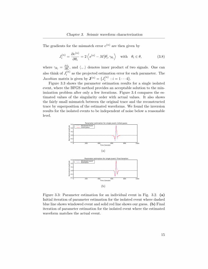
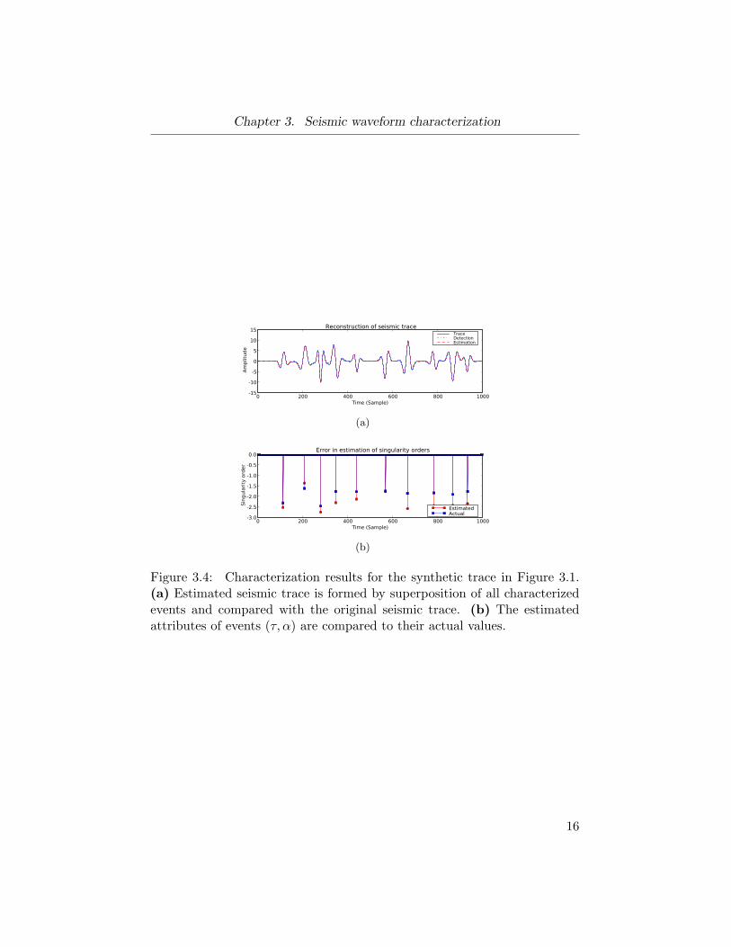
Figure 3.3 shows the parameter estimation results for a single isolatedevent, where the BFGS method provides an acceptable solution to the min-imization problem after only a few iterations. Figure 3.4 compares the es-timated values of the singularity order with actual values. It also showsthe fairly small mismatch between the original trace and the reconstructedtrace by superposition of the estimated waveforms. We found the inversionresults for the isolated events to be independent of noise below a reasonablelevel.

0 200 400 600 800 1000Time (Sample)

-0.2

-0.1

0.0

0.1

0.2

0.3

Norm

aliz

ed a

mplit

ude

Parameter estimation for single event: Initial guess

Windowed EventInitial guess

(a)

0 200 400 600 800 1000Time (Sample)

-0.2

-0.1

0.0

0.1

0.2

0.3

Norm

aliz

ed a

mplit

ude

Parameter estimation for single event: Final Iteration

Windowed eventEstimation

(b)

Figure 3.3: Parameter estimation for an individual event in Fig. 3.2. (a)Initial iteration of parameter estimation for the isolated event where dashedblue line shows windowed event and solid red line shows our guess. (b) Finaliteration of parameter estimation for the isolated event where the estimatedwaveform matches the actual event.

15


0 200 400 600 800 1000Time (Sample)

-15

-10

-5

0

5

10

15

Am

plit

ude

Reconstruction of seismic traceTraceDetectionEstimation

(a)

0 200 400 600 800 1000Time (Sample)

-3.0

-2.5

-2.0

-1.5

-1.0

-0.5

0.0

Sin

gula

rity

ord

er

Error in estimation of singularity orders

EstimatedActual

(b)

Figure 3.4: Characterization results for the synthetic trace in Figure 3.1.(a) Estimated seismic trace is formed by superposition of all characterizedevents and compared with the original seismic trace. (b) The estimatedattributes of events (τ, α) are compared to their actual values.

16

Chapter 4

Attribute analysis

To characterize the major singularities in our marine data-set from westShetlands, the detection-estimation method is applied to each trace of thetime-migrated 2-D seismic image individually. The results are summarizedin Figures 4.1, 4.2, and 4.3, where the vertical axis corresponds to the two-way travel time and horizontal axis shows lateral position. Although thereare trace-to-trace variations, major features in the original image are cap-tured and reconstructed quite accurately (see Fig. 4.1). Figure 4.2(a) showsthe modulus of the detected events, which is directly related to correspond-ing reflectors’ strength. Despite the existence of a relatively strong reflectionat approximately t = 2.9s (see Fig. 4.2(a)), there is only a slightly differencein the amplitudes of the reconstructed waveforms when compared to the realones (cf. Fig. 4.1(a) and 4.1(b)).

Aside from localized estimates of the reflector strength, our characteriza-tion also provides localized estimates for scale, singularity order, and phaseattributes (see Figures 4.2(b) and 4.3). The estimated values of the differ-ent attributes (color code) are plotted in Figures 4.2 and 4.3, overlaying theoriginal seismic image (gray scale). The singularity order predicts the localregularity of the imaged reflectors; the sharper the transition, the more neg-ative the order of singularity. As reported in the literature, the estimatedsingularity orders only express relative changes in the abruptness of the re-flectors since they contain a contribution of the seismic source wavelet. Thecontribution is given by α = αsrc + αabs, where αsrc shows the singularityorder for the seismic source wavelet and αabs is the absolute singularity or-der associated with the imaged reflectors. As opposed to singularity orderswhich are relatively insensitive to dispersion (Herrmann and Stark, 2000),estimates for the scale increase for deeper reflections. This observation isconsistent with dispersion, which leads to smaller values for scale, i.e., theratio bandwidth over central frequency (∆ω

ω0). Aside from dispersion effects,

changes in the estimated scale also depend on the characteristic scale of thetransitions. Finally, the phase attributes correspond to localized estimatesfor the instantaneous phase. As reported in the literature, this attributeallows us to distinguish between causal (coarsening upwards), anti-causal

17

Chapter 4. Attribute analysis

(fining upwards), and lobe-shaped transitions (Dessing, 1997), while esti-mates for the singularity orders help us to discriminate between “thin layersequences” (−1 ≤ αabs < 0), caused by acoustic impedance variations thatreturn to their initial value and step-like variations (0 ≤ αabs < 1) wherethe initial and transition values differ. The difference for the correspondingsingularity orders can be explained in terms of the well-known bright spotsand local phase rotations associated with tuning of sub-wavelength layerthicknesses. In that case, the opposite sign reflectors act as a differentiatoreffectively, reducing the order of the transition by one.

Other than giving us a trust in our characterization method, lateralconsistency of attributes along reflectors, as in Figure 4.2(b) and 4.3(a),has also important consequences for the interpretation of geological bound-aries. Variety of estimated singularity orders for different stratigraphicalhorizons suggests that there exist an aggregation of varying order transitionsother than zero-order steps and first-order ramp functions in the sedimentarybasin. Additionally, it admits the existence of a link between the attributevalues and type of the corresponding transitions. Accordingly, layer bound-aries can no longer be considered as strictly local, as in the case for jumpdiscontinuities. In the next section, we attempt to provide further lithologyinsights by zooming into the strong reflection event, where the estimatedattributes show interesting behavior along the reflector.

18


0 500 1000 1500Lateral direction (sample)

2.5

2.6

2.7

2.8

2.9

3.0

3.1

3.2

Tim

e (

s)

Real data

-12

-8

-4

0

4

8

12

16

20

(a)


2.5

2.6

2.7

2.8

2.9

3.0

3.1

3.2

Tim

e (

s)

Reconstruction of real data

-10

-5

0

5

10

15

20

(b)

Figure 4.1: Reconstruction of real marine data recorded in west of Shetlands.(a) Imaged reflection amplitudes. (b) Trace-by-trace reconstruction of realdata through superposition of all matched elements of the manifold.

19



2.5

2.6

2.7

2.8

2.9

3.0

3.1

3.2

Tim

e (

s)

Characterization of real data (Amplitude)

0.0

2.5

5.0

7.5

10.0

12.5

15.0

17.5

20.0

22.5

(a)


2.5

2.6

2.7

2.8

2.9

3.0

3.1

3.2

Tim

e (

s)

Characterization of real data (Scale)

0.0

0.5

1.0

1.5

2.0

2.5

3.0

3.5

4.0

4.5

5.0

(b)

Figure 4.2: Estimated attributes for real data given in 4.1(a). The scat-ter plot of (a) amplitudes of reconstructed events, (b) estimated scale at-tributes overlays the gray scale imaged section. Warm colors in (a) and(b) show higher amplitudes and larger scales, respectively. The structure ofdetected events is nicely aligned with reflectors.

20



2.5

2.6

2.7

2.8

2.9

3.0

3.1

3.2

Tim

e (

s)

Characterization of real data (Singularity orders)

-8.0

-7.2

-6.4

-5.6

-4.8

-4.0

-3.2

-2.4

-1.6

-0.8

0.0

(a)


2.5

2.6

2.7

2.8

2.9

3.0

3.1

3.2

Tim

e (

s)

Characterization of real data (Phase)

0.0

0.2

0.4

0.6

0.8

1.0

1.2

1.4

1.6

1.8

(b)

Figure 4.3: Estimated attributes for real data given in 4.1(a). The scatterplot of estimated (a) singularity order, and (b) instantaneous phase at-tributes overlays the gray scale imaged section. Warm colors in (a) showless sharp transitions.

21

Chapter 5

Opal-A to opal-CT transitionand well-seismic tie

The seismically imaged region in Figure 4.1(a) represents a subsection of theFaeroe-Shetland basin, where a commercial exploration well was drilled fordirect lithological calibration in 1999. Analysis of samples taken from theborehole revealed that the strong high-amplitude event, at t = 2.9s in theseismic section, represents a diagenetic event corresponding to the opal-A(Amorphous) to opal-CT (Cristobalite/Tridymite) transition (Davies et al.,2001; Davies and Cartwright, 2002). The primary deposition of opals islargely due to biogenic processes during which minute marine organismswith siliceous skeletons, including sponges, settle to the bottom of sea afterdying. The remains of these animals form non-crystalline opal (opal-A). In-terestingly, this form of opal is reported to gradually transform to opal-CTas a result of silica diagenesis, which is due to the increasing overburdenpressure in sedimentary rocks. In the second part of our study on the westShetlands dataset, we are concerned with extracting more information onthe lithological characteristics of stratigraphy that we know to exist. Inthis section, we zoom into the strong reflection present in the seismic im-age that corresponds to the diagenetic transition of opal-A to opal-CT. Wewill present an example of how these attributes can help us to interpretmicroscale transitions.

The diagenetic reflector starts at approximately t = 2.9s (left) and pro-gresses to t = 2.7s (right). The estimated attributes remain relativelyconstant along this reflector although the seismic amplitudes vary signifi-cantly. Studies on the cuttings of the well have revealed that the volumefraction of opal-CT changes from 10% to 76% along the boundary (Daviesand Cartwright, 2002). Assuming a linear gradient of the volume fraction,we use our site percolation model to build an elastic profile as a function ofthe volume fraction. For this purpose, elastic properties of opal-A and opal-CT are required as inputs for the percolation model. Since there are no wellmeasurements (sonic and density) available near the diagenetic transition,representative values of elastic moduli for both opal types are taken from

22

Chapter 5. Opal-A to opal-CT transition and well-seismic tie

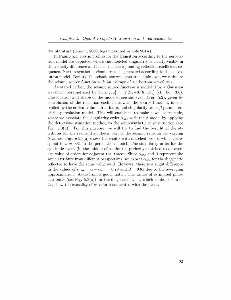
the literature (Guerin, 2000, logs measured in hole 904A).In Figure 5.1, elastic profiles for the transition according to the percola-

tion model are depicted, where the modeled singularity is clearly visible inthe velocity difference and hence the corresponding reflection coefficient se-quence. Next, a synthetic seismic trace is generated according to the convo-lution model. Because the seismic source signature is unknown, we estimatethe seismic source function with an average of sea bottom waveforms.

As stated earlier, the seismic source function is modeled by a Gaussianwaveform parametrized by [σ, αsrc, φ] = [2.21,−3.78, 1.55] (cf. Eq. 3.6).The location and shape of the modeled seismic event (Fig. 5.2), given byconvolution of the reflection coefficients with the source function, is con-trolled by the critical volume fraction pc and singularity order β parametersof the percolation model. This will enable us to make a well-seismic tie,where we associate the singularity order αabs with the β model by applyingthe detection-estimation method to the semi-synthetic seismic section (seeFig. 5.3(a)). For this purpose, we will try to find the best fit of the at-tributes for the real and synthetic part of the seismic reflector for varyingβ values. Figure 5.3(a) shows the results with matched orders, which corre-spond to β = 0.81 in the percolation model. The singularity order for thesynthetic event (in the middle of section) is perfectly matched to an aver-age value of orders for adjacent real traces. Since αabs and β represent thesame attribute from different perspectives, we expect αabs for the diageneticreflector to have the same value as β. However, there is a slight differencein the values of αabs = α − αsrc = 0.79 and β = 0.81 due to the averagingapproximation. Aside from a good match, The values of estimated phaseattributes (see Fig. 5.3(a)) for the diagenetic event, which is about zero or2π, show the causality of waveform associated with the event.

23


0.1 0.2 0.3 0.4 0.5 0.6 0.7 0.8Volume fraction, p

1700

1750

1800

1850

1900

1950

Densi

ty (

kg/m

3)


1900

1950

2000

2050

2100

2150

2200

Velo

city

(m

/s)

VpRV-RV+


0.10

0.15

0.20

0.25

0.30

0.35

0.40

d/d

p (

Vp)


0.09

0.10

0.11

0.12

0.13

0.14

0.15

0.16

Reflect

ion C

oeff

.

Figure 5.1: The site percolation model for the diagenetic transition of opal-A to opal-CT. Properties for opal-A are taken to be ρ = 1713.90 kg/m3 andVp = 1889.65 m/s. For opal-CT, density and P-wave velocity are assumedto be ρ = 2006.06 kg/m3 and Vp = 2237.71 m/s, respectively. Density (topleft) and P-wave velocity (top right) profile of the transition is determinedas a function of volume fraction of opal-CT. The velocity, bounded by Reussand Voigt averages, is showing a switch-like behavior at a critical point. Thesingularity is clearly visible from derivative of velocity (bottom left), andalso preserved in reflection coefficients (bottom right).

24


2.70 2.75 2.80 2.85 2.90 2.95 3.00 3.05Two-way travel time (s)

-0.020

-0.015

-0.010

-0.005

0.000

0.005

0.010

0.015

0.020

Am

plit

ude

Source Signature

2.70 2.75 2.80 2.85 2.90 2.95 3.00 3.05Two-way travel time (s)

-10

-5

0

5

10

15

Am

plit

ude

Seismic Trace

(a)

Figure 5.2: Synthetic data generation by convolution model; We estimateseismic source signature from sea bottom by using seismic waveform char-acterization. By taking an average over reconstructed waveforms for seabottom seismic reflector, we estimate the seismic source function by aparametrized Gaussian waveform where [σ, α, φ] = [2.21,−3.78, 1.55] (top).(bottom) Synthetic trace is generated by convolution of reflection coeffi-cients given in Figure 5.1 with the seismic source. Location and shape ofthe synthetic trace is a function of parameters of the site percolation model.

25



2.75

2.80

2.85

2.90

2.95

3.00

Tim

e (

s)

Estimated alpha

-8.0

-7.2

-6.4

-5.6

-4.8

-4.0

-3.2

-2.4

-1.6

-0.8

0.0

(a)


2.75

2.80

2.85

2.90

2.95

3.00

Tim

e (

s)

Estimated phase

0.0

0.2

0.4

0.6

0.8

1.0

1.2

1.4

1.6

1.8

(b)

Figure 5.3: Well-seismic tie. By choosing the appropriate pc value, diage-netic event is aligned in both synthetic traces (in the middle of section) andneighboring real traces. The detection-estimation method is applied to thissemi-synthetic section in order to see how constraints from seismic wave-forms fit with the ones from lithology. Estimated (a) singularity orders and(b) phase attributes are matched along the diagenetic event when β = 0.81.

26

Chapter 6

Discussion and Conclusions

In this thesis, we proposed a new approach to obtain lithological insightsfrom seismic data in which we model a wider class of transitions from bothlithological perspective (e.g. transitions from smooth connectivity in com-position) and mathematical representation perspective, i.e., fractional-orderdiscontinuities. This generalization provides us with more accurate and im-proved understanding of the subsurface geology.

The waveform characterization implies a representation for the geologicalrecord; where the detection stage extracts basic stratigraphy and estimationstage reveals the lithology of the subsurface. The singularity order andphase attributes especially, provide useful information on lithofacies. Theformer measures the transition sharpness and the latter can be used as a toolto distinguish between fining/coarsening upwards or lobe-shaped sequences.The characterization results on real data show a good alignment between thelocation of detected waveforms and seismic reflectors. As discussed earlier,the observed type of variations of attributes suggests that our parametricrepresentation can provide us with constraints on the lithological boundaries.We have also answered the second question posed in the introduction partby finding the link between characterization attributes and correspondinglithological transition for the known diagenetic transition.

Finally, the bottleneck of our seismic characterization method is the seg-mentation, which is somewhat arbitrary. Although we choose a smoothwindow function, segmentation step can still cause some edge distortion forindividual waveforms. Despite the fact that the estimation step assumesan accurate detection and windowing, the parametric inversion is able toreconstruct the distorted waveforms correctly in most cases. The segmenta-tion problem is more probable when the events are very close to each other.Some studies are in progress to show that a specific minimum distance be-tween different events is required in order to have an accurate recovery, i.e.,precise separation of the two events. Consequently, very close events arenot distinguishable and may be interpreted as one event with more negative(smaller) singularity order.

27

Bibliography

Benveniste, Y., 1987, A new approach to the application of mori-tanakastheory in composite materials: Mechanics of Material., 6, 147 – 157.

Blu, T. and M. Unser, 2003, A complete family of scaling functions:the (α, τ) fractional splines: Proceedings of the Twenty-Eighth IEEEInternational Conference on Acoustics, Speech, and Signal Processing(ICASSP’03), 505 – 508.

Davies, R. J. and J. Cartwright, 2002, A fossilized opal a to opal c/t trans-formation on the northeast atlantic margin: support for a significantlyelevated palaeogeothermal gradient during the neogene?: Basin Research,14, 467 – 486.

Davies, R. J., J. Cartwright, J. Pike, and C. Line, 2001, Early oligoceneinitiation of north atlantic deep water formation: Letters to Nature, 410,917 – 920.

Dessing, F., 1997, A Wavelet Transform Approach to Seismic Processing:PhD thesis, Delft University of Technology.

Dossal, C. and S. Mallat, 2005, Sparse spike deconvolution with minimumscale: Proceedings of Signal Processing with Adaptive Sparse StructuredRepresentations, 123 – 126. (http://spars05.irisa.fr/ACTES/PS2-11.pdf).

Guerin, G., 2000, Acoustic and thermal characterization of oil migration,gas hydrates formation and silica diagenesis: PhD thesis, Columbia Uni-versity.

Harms, J. C. and P. Tackenberg, 1972, Seismic signatures of sedimentationmodels: Geophysics, 37, 45 – 58.

Hashin, Z. and S. Shtrikman, 1962, On some variational principles inanisotropic and nonhomogeneous elasticity: Journal of the Mechanics andPhysics of Solids, 10, 335 – 342.

Herrmann, F. J., 1997, A Scaling Medium Representation, a Discussion onWell-Logs, Fractals and Waves: PhD thesis, Delft University of Technol-ogy.

28

Bibliography

——–, 1998, Multiscale analysis of well- and seismic data: MathematicalMethods in Geophysical Imaging V, SPIE, 3453, 180 – 208.

——–, 2001, Multi- and monoscale attributes for well- and seismic data:Chapter in the annual report of the Borehole Acoustics and Logging andReservoir Delineation Consortia at MIT.

——–, 2005, Seismic deconvolution by atomic decomposition: A parametricapproach with sparseness constraints: Integr. Computer-Aided Eng., 12,69 – 91.

Herrmann, F. J. and Y. Bernabe, 2004, Seismic singularities at upper man-tle discontinuities: a site percolation model: Geop. J. Int., 159, 949 – 960.

Herrmann, F. J., W. J. Lyons, and C. Stark, 2001, Seismic facies charac-terization by monoscale analysis: Geophysical Research Letters, 28, 3781– 3784.

Herrmann, F. J. and C. Stark, 2000, A scale attribute for texture in well-and seismic data: Presented at the Soc. Expl. Geoph.

Holschneider, M., 1995, Wavelets an analysis tool: Oxford Science Publi-cations.

Kelley, C. T., 1999, Iterative methods for optimization. Frontiers in AppliedMathematics, No. 18: SIAM.

Luo, H. and G. Weng, 1987, On eshelbys inclusion problem in a threephasespherically concentric solid and a modification of mori-tanakas method:Mechanics of Material, 6, 347 – 361.

Mallat, S., 1997, A wavelet tour of signal processing: Academic Press.

Mori, T. and K. Tanaka, 1973, Average stress in matrix and average elasticenergy of materials with misfitting inclusions: Acta Metallurgica, 21, 571– 574.

Muller, J., I. Bokn, and J. L. McCauley, 1992, Multifractal analysis ofpetrophysical data: Annales Geophysicae, 10, 735 – 761.

Nocedal, J. and S. J. Wright, 1999, Numerical optimization, 1st ed.Springer Series in Operations Research: Springer-Verlag.

Payton, C., ed., 1977, Seismic stratigraphy - applications to hydrocarbonexploration, chapter Stratigraphic models from seismic data. AAPG.

Saggaf, M. M. and E. A. Robinson, 2000, A unified framework for thedeconvolution of traces of nonwhite reflectivity: Geophysics, 65, 1660 –1676.

29

Bibliography

Wakin, M. B., D. L. Donoho, H. Choi, and R. G. Baraniuk, 2005, Themultiscale structure of non-differentiable image manifolds: SPIE WaveletsXI, 413 – 429.

Yilmaz, O., 2001, Seismic data analysis: Society of Exploration Geophysi-cists.

30

Documents

Lithology constraints from seismic waveforms: application ... · Lithology constraints from seismic waveforms: application to opal-A to opal-CT transition by Mohammad Maysami B.Sc.,