Topology and Intelligent Data Analysis�

V. Robins1, J. Abernethy2, N. Rooney2, and E. Bradley2

1 Department of Applied MathematicsResearch School of Physical Sciences and Engineering

The Australian National UniversityACT 0200 Australia

2 University of ColoradoDepartment of Computer Science

Boulder, CO 80309-0430

Abstract. A broad range of mathematical techniques, ranging fromstatistics to fuzzy logic, have been used to great advantage in intelligentdata analysis. Topology—the fundamental mathematics of shape—has todate been conspicuously absent from this repertoire. This paper showshow topology, properly reformulated for a finite-precision world, can beuseful in intelligent data analysis tasks.

1 Introduction

Topology is the fundamental descriptive machinery for shape. Putting its ideasinto real-world practice, however, is somewhat problematic, as traditional topol-ogy is an infinite-precision notion, and real data are both limited in extentand quantized in space and time. The field of computational topology grewout of this challenge[5,9]. Among the formalisms in this field is the notion ofvariable-resolution topology, where one analyzes the properties of the data—e.g.,the number of components and holes, and their sizes—at a variety of differentprecisions, and then deduces the topology from the limiting behavior of thosecurves. This framework, which was developed by one of the authors of this paper(Robins)[20,21,22], turns out to be an ideal tool for intelligent data analysis.

Our approach to assessing connectedness and components in a data set hasits roots in the work of Cantor. We define two points as epsilon (ε) connected ifthere is an ε-chain joining them; all points in an ε-connected set can be linkedby an ε-chain. For the purposes of this work, we use several of the fundamentalquantities introduced in [21]: the number C(ε) and maximum diameter D(ε) ofthe ε-connected components in a set, as well as the number I(ε) of ε-isolatedpoints—that is, ε-components that consist of a single point. As demonstratedin [20,22], one can compute all three quantities for a range of ε values and deducethe topological properties of the underlying set from their limiting behavior. Ifthe underlying set is connected, the behavior of C and D is easy to understand.� Supported by NSF #ACI-0083004 and a Grant in Aid from the University of Colo-

rado Council on Research and Creative Work.

M.R. Berthold et al. (Eds.): IDA 2003, LNCS 2810, pp. 111–122, 2003.c© Springer-Verlag Berlin Heidelberg 2003

112 V. Robins et al.

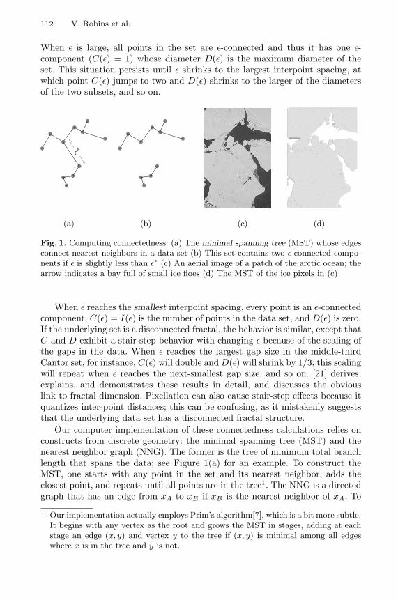
When ε is large, all points in the set are ε-connected and thus it has one ε-component (C(ε) = 1) whose diameter D(ε) is the maximum diameter of theset. This situation persists until ε shrinks to the largest interpoint spacing, atwhich point C(ε) jumps to two and D(ε) shrinks to the larger of the diametersof the two subsets, and so on.

∗ε

↗

(a) (b) (c) (d)

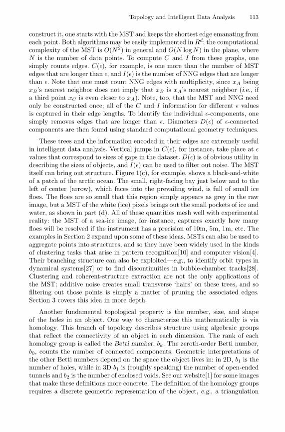
Fig. 1. Computing connectedness: (a) The minimal spanning tree (MST) whose edgesconnect nearest neighbors in a data set (b) This set contains two ε-connected compo-nents if ε is slightly less than ε∗ (c) An aerial image of a patch of the arctic ocean; thearrow indicates a bay full of small ice floes (d) The MST of the ice pixels in (c)

When ε reaches the smallest interpoint spacing, every point is an ε-connectedcomponent, C(ε) = I(ε) is the number of points in the data set, and D(ε) is zero.If the underlying set is a disconnected fractal, the behavior is similar, except thatC and D exhibit a stair-step behavior with changing ε because of the scaling ofthe gaps in the data. When ε reaches the largest gap size in the middle-thirdCantor set, for instance, C(ε) will double and D(ε) will shrink by 1/3; this scalingwill repeat when ε reaches the next-smallest gap size, and so on. [21] derives,explains, and demonstrates these results in detail, and discusses the obviouslink to fractal dimension. Pixellation can also cause stair-step effects because itquantizes inter-point distances; this can be confusing, as it mistakenly suggeststhat the underlying data set has a disconnected fractal structure.

Our computer implementation of these connectedness calculations relies onconstructs from discrete geometry: the minimal spanning tree (MST) and thenearest neighbor graph (NNG). The former is the tree of minimum total branchlength that spans the data; see Figure 1(a) for an example. To construct theMST, one starts with any point in the set and its nearest neighbor, adds theclosest point, and repeats until all points are in the tree1. The NNG is a directedgraph that has an edge from xA to xB if xB is the nearest neighbor of xA. To

1 Our implementation actually employs Prim’s algorithm[7], which is a bit more subtle.It begins with any vertex as the root and grows the MST in stages, adding at eachstage an edge (x, y) and vertex y to the tree if (x, y) is minimal among all edgeswhere x is in the tree and y is not.

Topology and Intelligent Data Analysis 113

construct it, one starts with the MST and keeps the shortest edge emanating fromeach point. Both algorithms may be easily implemented in Rd; the computationalcomplexity of the MST is O(N2) in general and O(N log N) in the plane, whereN is the number of data points. To compute C and I from these graphs, onesimply counts edges. C(ε), for example, is one more than the number of MSTedges that are longer than ε, and I(ε) is the number of NNG edges that are longerthan ε. Note that one must count NNG edges with multiplicity, since xA beingxB ’s nearest neighbor does not imply that xB is xA’s nearest neighbor (i.e., ifa third point xC is even closer to xA). Note, too, that the MST and NNG needonly be constructed once; all of the C and I information for different ε valuesis captured in their edge lengths. To identify the individual ε-components, onesimply removes edges that are longer than ε. Diameters D(ε) of ε-connectedcomponents are then found using standard computational geometry techniques.

These trees and the information encoded in their edges are extremely usefulin intelligent data analysis. Vertical jumps in C(ε), for instance, take place at εvalues that correspond to sizes of gaps in the dataset. D(ε) is of obvious utility indescribing the sizes of objects, and I(ε) can be used to filter out noise. The MSTitself can bring out structure. Figure 1(c), for example, shows a black-and-whiteof a patch of the arctic ocean. The small, right-facing bay just below and to theleft of center (arrow), which faces into the prevailing wind, is full of small icefloes. The floes are so small that this region simply appears as grey in the rawimage, but a MST of the white (ice) pixels brings out the small pockets of ice andwater, as shown in part (d). All of these quantities mesh well with experimentalreality: the MST of a sea-ice image, for instance, captures exactly how manyfloes will be resolved if the instrument has a precision of 10m, 5m, 1m, etc. Theexamples in Section 2 expand upon some of these ideas. MSTs can also be used toaggregate points into structures, and so they have been widely used in the kindsof clustering tasks that arise in pattern recognition[10] and computer vision[4].Their branching structure can also be exploited—e.g., to identify orbit types indynamical systems[27] or to find discontinuities in bubble-chamber tracks[28].Clustering and coherent-structure extraction are not the only applications ofthe MST; additive noise creates small transverse ‘hairs’ on these trees, and sofiltering out those points is simply a matter of pruning the associated edges.Section 3 covers this idea in more depth.

Another fundamental topological property is the number, size, and shapeof the holes in an object. One way to characterize this mathematically is viahomology. This branch of topology describes structure using algebraic groupsthat reflect the connectivity of an object in each dimension. The rank of eachhomology group is called the Betti number, bk. The zeroth-order Betti number,b0, counts the number of connected components. Geometric interpretations ofthe other Betti numbers depend on the space the object lives in: in 2D, b1 is thenumber of holes, while in 3D b1 is (roughly speaking) the number of open-endedtunnels and b2 is the number of enclosed voids. See our website[1] for some imagesthat make these definitions more concrete. The definition of the homology groupsrequires a discrete geometric representation of the object, e.g., a triangulation

114 V. Robins et al.

of subsets of 2D, and simplicial complexes in three or more dimensions. SeeMunkres[16] for further details.

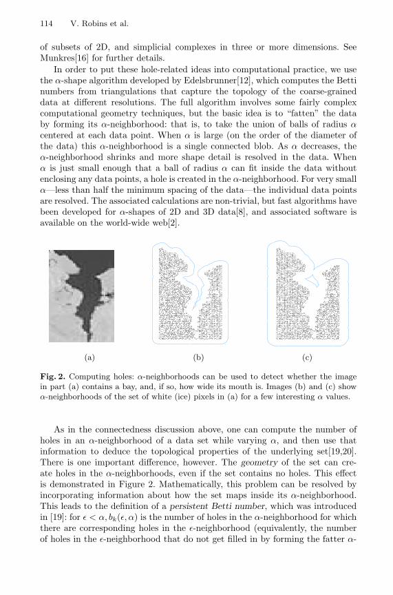
In order to put these hole-related ideas into computational practice, we usethe α-shape algorithm developed by Edelsbrunner[12], which computes the Bettinumbers from triangulations that capture the topology of the coarse-graineddata at different resolutions. The full algorithm involves some fairly complexcomputational geometry techniques, but the basic idea is to “fatten” the databy forming its α-neighborhood: that is, to take the union of balls of radius αcentered at each data point. When α is large (on the order of the diameter ofthe data) this α-neighborhood is a single connected blob. As α decreases, theα-neighborhood shrinks and more shape detail is resolved in the data. Whenα is just small enough that a ball of radius α can fit inside the data withoutenclosing any data points, a hole is created in the α-neighborhood. For very smallα—less than half the minimum spacing of the data—the individual data pointsare resolved. The associated calculations are non-trivial, but fast algorithms havebeen developed for α-shapes of 2D and 3D data[8], and associated software isavailable on the world-wide web[2].

(a) (b) (c)

Fig. 2. Computing holes: α-neighborhoods can be used to detect whether the imagein part (a) contains a bay, and, if so, how wide its mouth is. Images (b) and (c) showα-neighborhoods of the set of white (ice) pixels in (a) for a few interesting α values.

As in the connectedness discussion above, one can compute the number ofholes in an α-neighborhood of a data set while varying α, and then use thatinformation to deduce the topological properties of the underlying set[19,20].There is one important difference, however. The geometry of the set can cre-ate holes in the α-neighborhoods, even if the set contains no holes. This effectis demonstrated in Figure 2. Mathematically, this problem can be resolved byincorporating information about how the set maps inside its α-neighborhood.This leads to the definition of a persistent Betti number, which was introducedin [19]: for ε < α, bk(ε, α) is the number of holes in the α-neighborhood for whichthere are corresponding holes in the ε-neighborhood (equivalently, the numberof holes in the ε-neighborhood that do not get filled in by forming the fatter α-

Topology and Intelligent Data Analysis 115

neighborhood). These persistent Betti numbers are well defined for sequences ofcomplexes that provide successively better approximations to a manifold[19] andare computable using linear algebra techniques. Recently, Edelsbrunner and col-laborators have made a similar definition of persistent Betti number specificallyfor α-shapes, and devised an incremental algorithm for their calculation[11].

While the non-persistent holes effect makes it difficult to make a correct di-agnosis of the underlying topology, it has important implications for intelligentdata analysis because it gives us geometric information about the embedding ofthe set in the plane. This can be very useful in the context of coherent structureextraction. Consider a narrow bay in an icepack, as shown in Figure 2. In thiscase, b1(α) computed for the set of white (ice) pixels would be zero for α smallerthan half the width of the mouth of the bay, zero for α larger than the largestradius of its interior, and one in between—that is, where an α ball fits insidethe bay, but not through its mouth. Note that the α value where the spurioushole first appears is exactly the half-width of the entrance to the bay. If therewere a hole in the ice, rather than a bay, b1(α) would be a step function: zerowhen α is greater than the largest radius of the hole and one when it is less.This technique for finding and characterizing coherent structures whose definingproperties involve holes and gaps of various shapes—ponds, isthmuses, chan-nels, tunnels, etc.—is potentially quite useful in intelligent data analysis. Moreexamples and discussion follow in Section 2.

2 Coherent Structure Extraction

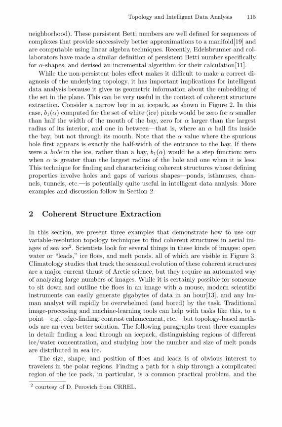
In this section, we present three examples that demonstrate how to use ourvariable-resolution topology techniques to find coherent structures in aerial im-ages of sea ice2. Scientists look for several things in these kinds of images: openwater or “leads,” ice floes, and melt ponds. all of which are visible in Figure 3.Climatology studies that track the seasonal evolution of these coherent structuresare a major current thrust of Arctic science, but they require an automated wayof analyzing large numbers of images. While it is certainly possible for someoneto sit down and outline the floes in an image with a mouse, modern scientificinstruments can easily generate gigabytes of data in an hour[13], and any hu-man analyst will rapidly be overwhelmed (and bored) by the task. Traditionalimage-processing and machine-learning tools can help with tasks like this, to apoint—e.g., edge-finding, contrast enhancement, etc.—but topology-based meth-ods are an even better solution. The following paragraphs treat three examplesin detail: finding a lead through an icepack, distinguishing regions of differentice/water concentration, and studying how the number and size of melt pondsare distributed in sea ice.

The size, shape, and position of floes and leads is of obvious interest totravelers in the polar regions. Finding a path for a ship through a complicatedregion of the ice pack, in particular, is a common practical problem, and the

2 courtesy of D. Perovich from CRREL.

116 V. Robins et al.

Fig. 3. The arctic ice pack is made up of open water, ice, and melt ponds, which imageas black, white, and grey, respectively. Studying the climatology of this system—theseasonal evolution of the different kinds of coherent structures—is a major currentthrust of Arctic science, and doing so requires an automated way of analyzing largenumbers of images.

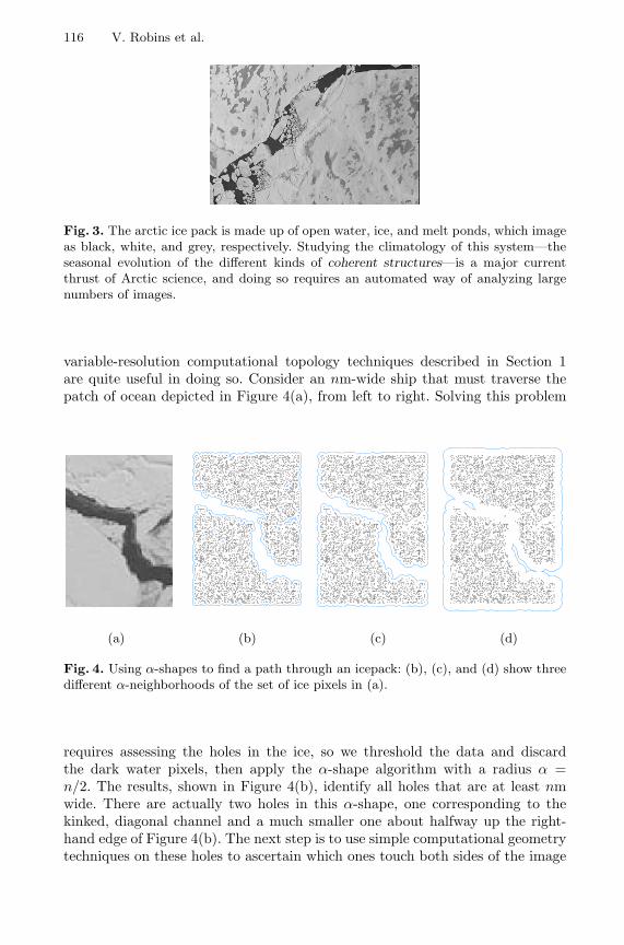
variable-resolution computational topology techniques described in Section 1are quite useful in doing so. Consider an nm-wide ship that must traverse thepatch of ocean depicted in Figure 4(a), from left to right. Solving this problem

(a) (b) (c) (d)

Fig. 4. Using α-shapes to find a path through an icepack: (b), (c), and (d) show threedifferent α-neighborhoods of the set of ice pixels in (a).

requires assessing the holes in the ice, so we threshold the data and discardthe dark water pixels, then apply the α-shape algorithm with a radius α =n/2. The results, shown in Figure 4(b), identify all holes that are at least nmwide. There are actually two holes in this α-shape, one corresponding to thekinked, diagonal channel and a much smaller one about halfway up the right-hand edge of Figure 4(b). The next step is to use simple computational geometrytechniques on these holes to ascertain which ones touch both sides of the image

Topology and Intelligent Data Analysis 117

and then determine which is the shortest3. Parts (c) and (d) of the Figure showthe effects of raising α beyond n/2m, demonstrating the relationship between thechannel shape and the holes in the α-neighborhood—e.g., successively resolvingthe various tight spots, or identifying regions of water that are at least α metersfrom ice.

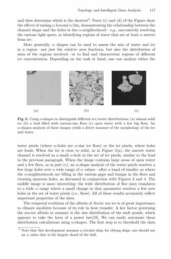
More generally, α shapes can be used to assess the mix of water and icein a region—not just the relative area fractions, but also the distribution ofsizes of the regions involved—or to find and characterize regions of differentice concentration. Depending on the task at hand, one can analyze either the

(a) (b) (c)

Fig. 5. Using α-shapes to distinguish different ice/water distributions: (a) almost-solidice (b) a lead filled with various-size floes (c) open water with a few big floes. Anα-shapes analysis of these images yields a direct measure of the morphology of the iceand water.

water pixels (where α-holes are α-size ice floes) or the ice pixels, where holesare leads. When the ice is close to solid, as in Figure 5(a), the narrow waterchannel is resolved as a small α-hole in the set of ice pixels, similar to the leadin the previous paragraph. When the image contains large areas of open waterand a few floes, as in part (c), an α-shape analysis of the water pixels resolves afew large holes over a wide range of α values—after a band of smaller αs wherethe α-neighborhoods are filling in the various gaps and bumps in the floes andcreating spurious holes, as discussed in conjunction with Figures 2 and 4. Themiddle image is more interesting; the wide distribution of floe sizes translatesto a wide α range where a small change in that parameter resolves a few newholes in the set of water pixels (i.e., floes). All of these results accurately reflectimportant properties of the data.

The temporal evolution of the albedo of Arctic sea ice is of great importanceto climate modelers because of its role in heat transfer. A key factor governingthe sea-ice albedo in summer is the size distribution of the melt ponds, whichappears to take the form of a power law[18]. We can easily automate thesedistribution calculations using α-shapes. The first step is to threshold the data

3 Note that this development assumes a circular ship; for oblong ships, one should usean α value that is the largest chord of the hull.

118 V. Robins et al.

0

0.5

1

1.5

2

2.5

3

-0.4 0 0.4 0.8

log(

Num

ber o

f Hol

es )

log( Alpha )

(a) (b) (c)

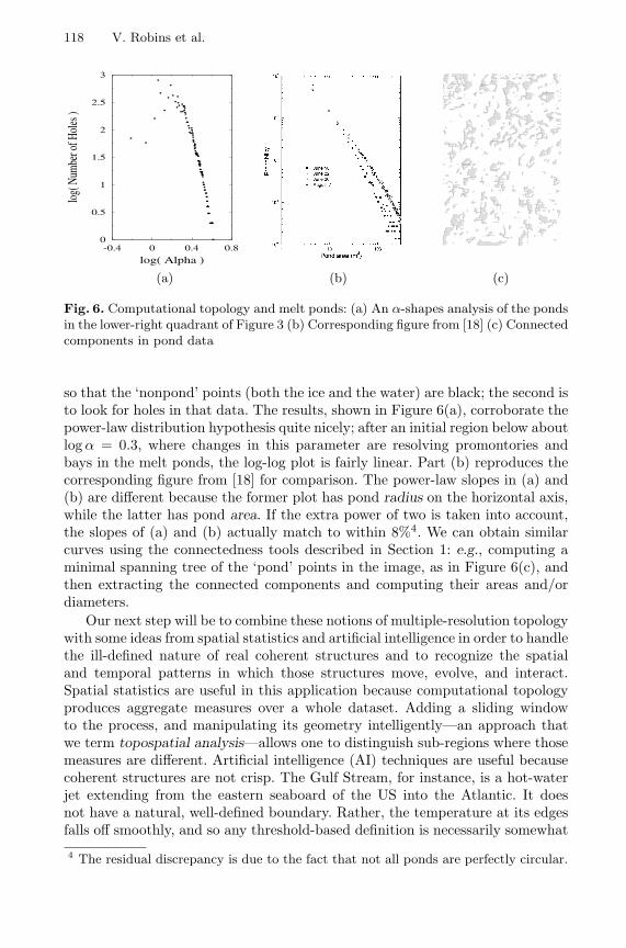
Fig. 6. Computational topology and melt ponds: (a) An α-shapes analysis of the pondsin the lower-right quadrant of Figure 3 (b) Corresponding figure from [18] (c) Connectedcomponents in pond data

so that the ‘nonpond’ points (both the ice and the water) are black; the second isto look for holes in that data. The results, shown in Figure 6(a), corroborate thepower-law distribution hypothesis quite nicely; after an initial region below aboutlog α = 0.3, where changes in this parameter are resolving promontories andbays in the melt ponds, the log-log plot is fairly linear. Part (b) reproduces thecorresponding figure from [18] for comparison. The power-law slopes in (a) and(b) are different because the former plot has pond radius on the horizontal axis,while the latter has pond area. If the extra power of two is taken into account,the slopes of (a) and (b) actually match to within 8%4. We can obtain similarcurves using the connectedness tools described in Section 1: e.g., computing aminimal spanning tree of the ‘pond’ points in the image, as in Figure 6(c), andthen extracting the connected components and computing their areas and/ordiameters.

Our next step will be to combine these notions of multiple-resolution topologywith some ideas from spatial statistics and artificial intelligence in order to handlethe ill-defined nature of real coherent structures and to recognize the spatialand temporal patterns in which those structures move, evolve, and interact.Spatial statistics are useful in this application because computational topologyproduces aggregate measures over a whole dataset. Adding a sliding windowto the process, and manipulating its geometry intelligently—an approach thatwe term topospatial analysis—allows one to distinguish sub-regions where thosemeasures are different. Artificial intelligence (AI) techniques are useful becausecoherent structures are not crisp. The Gulf Stream, for instance, is a hot-waterjet extending from the eastern seaboard of the US into the Atlantic. It doesnot have a natural, well-defined boundary. Rather, the temperature at its edgesfalls off smoothly, and so any threshold-based definition is necessarily somewhat

4 The residual discrepancy is due to the fact that not all ponds are perfectly circular.

Topology and Intelligent Data Analysis 119

arbitrary. Moreover, coherent structures are much easier to recognize than todescribe, let alone define in any formal way. The AI community has developeda variety of representations and techniques for problems like these, and thesesolutions mesh well with topospatial analysis.

3 Filtering

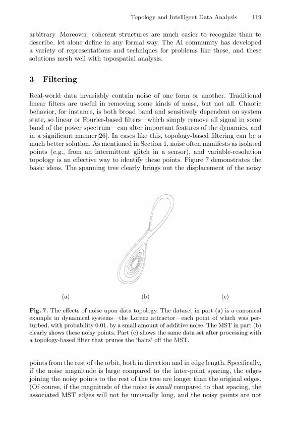
Real-world data invariably contain noise of one form or another. Traditionallinear filters are useful in removing some kinds of noise, but not all. Chaoticbehavior, for instance, is both broad band and sensitively dependent on systemstate, so linear or Fourier-based filters—which simply remove all signal in someband of the power spectrum—can alter important features of the dynamics, andin a significant manner[26]. In cases like this, topology-based filtering can be amuch better solution. As mentioned in Section 1, noise often manifests as isolatedpoints (e.g., from an intermittent glitch in a sensor), and variable-resolutiontopology is an effective way to identify these points. Figure 7 demonstrates thebasic ideas. The spanning tree clearly brings out the displacement of the noisy

(a) (b) (c)

Fig. 7. The effects of noise upon data topology. The dataset in part (a) is a canonicalexample in dynamical systems—the Lorenz attractor—each point of which was per-turbed, with probability 0.01, by a small amount of additive noise. The MST in part (b)clearly shows these noisy points. Part (c) shows the same data set after processing witha topology-based filter that prunes the ‘hairs’ off the MST.

points from the rest of the orbit, both in direction and in edge length. Specifically,if the noise magnitude is large compared to the inter-point spacing, the edgesjoining the noisy points to the rest of the tree are longer than the original edges.(Of course, if the magnitude of the noise is small compared to that spacing, theassociated MST edges will not be unusually long, and the noisy points are not

120 V. Robins et al.

so obvious.) This kind of separation of scale often arises when two processes areat work in the data—e.g., signal and noise. Because variable-resolution topologyis good at identifying scale separation, we can use it to identify and removethe noisy points. The first step is to look for a second peak in the edge-lengthdistribution of the MST (equivalently, a shoulder in the plot I(ε) of the numberof isolated points as a function of ε). The maximum edge length of the MSTof the non-noisy data occurs in the interval between the two peaks (or at thelocation of the I(ε) breakpoint). At that value, most of the noisy points—andfew of the regular points—are ε-isolated. The next step is to prune all MSTedges that exceed that length, removing the points at their termini5. Part (c) ofthe Figure shows the results; in this case, the topology-based filter removed 534of the 545 noisy points and 150 of the 7856 non-noisy points. This translatesto 98.0% success with a 1.9% false positive rate. These are promising results—better than any linear filter, and comparable to or better than the noise-reductiontechniques used by the dynamical systems community[3]. Increasing the pruninglength, as one would predict, decreases the false-positive rate; somewhat lessintuitively, though, larger pruning lengths do not appear to significantly affectthe success rate—until they become comparable to the length scales of the noise.As described in [23], these rates vary slightly for different types and amounts ofnoise, but remain close to 100% and 0%; even better, the topology-based filterdoes not disturb the dynamical invariants like the Lyapunov exponent.

While topology-based filtering is very effective, it does come with somecaveats. For example, the method simply removes noisy points; it does not de-duce where each one ‘should be’ and move it in that direction. There are severalobvious solutions to this, all of which add a bit more geometry into the recipe—e.g., averaging the two points on either side of the base of the edge that connectsan isolated point to the rest of the trajectory. Rasterized images bring up a dif-ferent set of problems, as noise does not move points around in these images, butrather reshades individual pixels. The computer vision community distinguishesthese two kinds of noise as “distortion” and “salt and pepper,” respectively. Be-cause the metric used in the MST captures distances between points, it is moreeffective at detecting the former than the latter. Space limitations preclude amore-thorough treatment of this issue here; for more details, see[6].

4 Conclusion

The mathematical framework of variable-resolution topology has tremendouspotential for intelligent data analysis. It is, among other things, an efficient way

5 The exact details of the pruning algorithm are somewhat more subtle than is impliedabove because not all noisy points are terminal nodes of the spanning tree. Thus,an algorithm that simply deletes all points whose connections to the rest of the treeare longer than the pruning length can sever connections to other points, or clustersof points. This is an issue if one noisy point creates a ‘bridge’ to another noisy pointand only one of the associated MST edges is longer than the pruning length.

Topology and Intelligent Data Analysis 121

to automate the process of finding and characterizing coherent structures. Fig-ure 6(b), for instance, was constructed by hand-processing roughly 2000 images,which required roughly 50 working days[17]; Figure 6(a) required only a fewminutes of CPU time. Because it reveals separation of scale, variable-resolutiontopology can also be useful in noise removal. In a series of numerical and labo-ratory experiments, a topology-based filter identified close to 100% of the noisypoints from dynamical system data sets, with a false-positive rate of only afew percent. Separation of scale is fundamental to many other processes whoseresults one might be interested in untangling, so this method is by no meanslimited to filtering applications—or to dynamical systems.

There have been a few other topology-based approaches to filtering. Mis-chaikow et al.[15], for example, use algebraic topology to construct a coarse-grained representation of the data. This effectively finesses the noise issue, andthus constitutes a form of filtering. Rather than use algebraic topology to con-struct a useful coarse-grained representation of the dynamics, our approach usesgeometric topology to remove noisy points while working in the original space,which allows us to obtain much finer-grained results.

A tremendous volume of papers on techniques for reasoning about the struc-ture of objects has appeared in various subfields of the computer science lit-erature. Very few of these papers focus on distilling out the topology of thecoherent structures in the data. Those that do either work at the pixel level(e.g., the work of Rosenfeld and collaborators [24]) or are hand-crafted for aparticular application (e.g., using wavelets to find vortices in images of sea sur-face temperature[14]), and all are constrained to two or three dimensions. Ourframework is algorithmically much more general, and it works in arbitrary di-mension. Many geographic information systems[25] and computer vision[4] toolsincorporate simple topological operations like adjacency or connectedness; these,too, generally only handle 2D gridded data, and none take varying resolutioninto account—let alone exploit it.

References

1. http://www.cs.colorado.edu/∼lizb/topology.html.2. http://www.alphashapes.org.3. H. Abarbanel. Analysis of Observed Chaotic Data. Springer, 1995.4. D. Ballard and C. Brown. Computer Vision. Prentice-Hall, 1982.5. M. Bern and D. Eppstein. Emerging challenges in computational topology, 1999.6. E. Bradley, V. Robins, and N. Rooney. Topology and pattern recognition. Preprint;

see www.cs.colorado.edu/∼lizb/publications.html.7. T. Cormen, C. Leiserson, R. Rivest, and C. Stein. Introduction to Algorithms. The

MIT Press, 2001. pp 570–573.8. C. Delfinado and H. Edelsbrunner. An incremental algorithm for Betti numbers of

simplicial complexes on the 3-sphere. Computer Aided Geometric Design, 12:771–784, 1995.

9. T. Dey, H. Edelsbrunner, and S. Guha. Computational topology. In B. Chazelle,J. Goodman, and R. Pollack, editors, Advances in Discrete and ComputationalGeometry. American Math. Society, Princeton, NJ, 1999.

122 V. Robins et al.

10. R. Duda and P. Hart. Pattern Classification. Wiley, New York, 1973.11. H. Edelsbrunner, D. Letscher, and A. Zomorodian. Topological persistence and

simplification. In IEEE Symposium on Foundations of Computer Science, pages454–463, 2000.

12. H. Edelsbrunner and E. Mucke. Three-dimensional alpha shapes. ACM Transac-tions on Graphics, 13:43–72, 1994.

13. U. Fayyad, D. Haussler, and P. Stolorz. KDD for science data analysis: Issuesand examples. In Proceedings of the ACM SIGKDD International Conference onKnowledge Discovery and Data Mining (KDD), 1996.

14. H. Li. Identification of coherent structure in turbulent shear flow with waveletcorrelation analysis. Transactions of the ASME, 120:778–785, 1998.

15. K. Mischaikow, M. Mrozek, J. Reiss, and A. Szymczak. Construction of symbolicdynamics from experimental time series. Physical Review Letters, 82:1144–1147,1999.

16. J. Munkres. Elements of Algebraic Topology. Benjamin Cummings, 1984.17. D. Perovich. Personal communication.18. D. Perovich, W. Tucker, and K. Ligett. Aerial observations of the evolution of

ice surface conditions during summer. Journal of Geophysical Research: Oceans,10.1029/2000JC000449, 2002.

19. V. Robins. Towards computing homology from finite approximations. TopologyProceedings, 24, 1999.

20. V. Robins. Computational Topology at Multiple Resolutions. PhD thesis, Universityof Colorado, June 2000.

21. V. Robins, J. Meiss, and E. Bradley. Computing connectedness: An exercise incomputational topology. Nonlinearity, 11:913–922, 1998.

22. V. Robins, J. Meiss, and E. Bradley. Computing connectedness: Disconnectednessand discreteness. Physica D, 139:276–300, 2000.

23. V. Robins, N. Rooney, and E. Bradley. Topology-based signal separation. Chaos.In review; see www.cs.colorado.edu/∼lizb/publications.html.

24. P. Saha and A. Rosenfeld. The digital topology of sets of convex voxels. GraphicalModels, 62:343–352, 2000.

25. S. Shekhar, M. Coyle, B. Goyal, D. Liu, and S. Sarkar. Data models in geographicinformation systems. Communications of the ACM, 40:103–111, 1997.

26. J. Theiler and S. Eubank. Don’t bleach chaotic data. Chaos, 3:771–782, 1993.27. K. Yip. KAM: A System for Intelligently Guiding Numerical Experimentation

by Computer. Artificial Intelligence Series. MIT Press, 1991.28. C. Zahn. Graph-theoretical methods for detecting and describing Gestalt clusters.

IEEE Transactions on Computers, C-20:68–86, 1971.