Segmenting the Papillary Muscles and theTrabeculae from High Resolution Cardiac CTthrough Restoration of Topological Handles

Mingchen Gao1,�, Chao Chen1,�, Shaoting Zhang1, Zhen Qian2,Dimitris Metaxas1, and Leon Axel3

1 CBIM Center, Rutgers University, Piscataway, NJ 088542 2 Piedmont Heart Institute, Atlanta, GA 30309

3 New York University, 660 First Avenue, New York, NY 10016

Abstract. We introduce a novel algorithm for segmenting the high res-olution CT images of the left ventricle (LV), particularly the papillarymuscles and the trabeculae. High quality segmentations of these struc-tures are necessary in order to better understand the anatomical functionand geometrical properties of LV. These fine structures, however, are ex-tremely challenging to capture due to their delicate and complex naturein both geometry and topology. Our algorithm computes the potentialmissing topological structures of a given initial segmentation. Using tech-niques from computational topology, e.g. persistent homology, our algo-rithm find topological handles which are likely to be the true signal. Tofurther increase accuracy, these proposals are measured by the saliencyand confidence from a trained classifier. Handles with high scores arerestored in the final segmentation, leading to high quality segmentationresults of the complex structures.

1 Introduction

Computed tomography (CT) is a very important imaging modality for diag-nosing cardiovascular diseases. Compared with other imaging modalities (suchas ultrasound and magnetic resonance imaging), CT is able to show detailedanatomic structures within the cardiac chambers [15]. Recent advances in CTtechnology allow a 320 multi-detector CT scanner to successfully capture thepapillary muscles and trabeculae at a resolution which has not been reachedbefore.

Most of the existing methods to perform cardiac segmentations [3,20,13] modelthe inner heart wall as a smooth surface, which does not include the papillarymuscles and the trabeculae at all. Zheng et al . [20] proposed an algorithm toautomatically segment the four chambers of the heart in four seconds. Ecabert etal . [5] presented a learning-based approach based on active shape model (ASM)for the segmentation of four chambers and major vessel trunks. Other modelsinclude, but are not limited to graph cut [7], atlas based segmentation [10] andlocal deformation [11].

� Both authors contributed equally to this work.

J.C. Gee et al. (Eds.): IPMI 2013, LNCS 7917, pp. 184–195, 2013.c© Springer-Verlag Berlin Heidelberg 2013

Restoration of Topological Handles in Cardiac Segmentation 185

These methods, although proven to be successful in various situations, are notdesigned to accurately segment smaller, complex structures such as the papillarymuscles and the trabeculae. Previous attempts [3,18] were able to capture thepapillary muscle, but could not segment trabeculae with satisfying quality. Gaoet al . [8] manually segmented one frame (at the end-diastole state) of an imagesequence of a cardiac cycle, and then deformed the segmentation to match theother frames. Although their method focused on preserving the fine structuresduring the deformation, it only enforced consistency of geometry [17], not oftopology. Accurately segmenting the complex structures of the papillary musclesand the trabeculae is still a challenging task. The reason is threefold. 1) Thedetailed structures are complex and small, making them hard to be distinguishedfrom noise. 2) Some trabeculae go through the ventricle cavity and are very thin.Existing methods often fail to segment them due to the smoothness prior. 3)Such complex structures have a very different nature from other parts such asfree wall and septum. Furthermore, trabeculae have a large variety of geometryand intensity even within the same cardiac image. This requires the segmentationmethod to be extremely adaptive in terms of parameters, making full automationvery difficult.

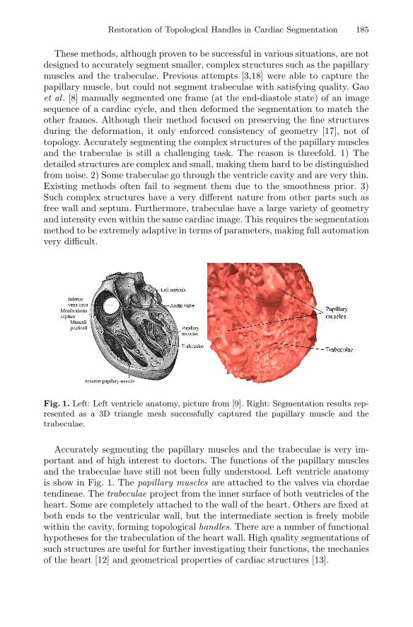
Fig. 1. Left: Left ventricle anatomy, picture from [9]. Right: Segmentation results rep-resented as a 3D triangle mesh successfully captured the papillary muscle and thetrabeculae.

Accurately segmenting the papillary muscles and the trabeculae is very im-portant and of high interest to doctors. The functions of the papillary musclesand the trabeculae have still not been fully understood. Left ventricle anatomyis show in Fig. 1. The papillary muscles are attached to the valves via chordaetendineae. The trabeculae project from the inner surface of both ventricles of theheart. Some are completely attached to the wall of the heart. Others are fixed atboth ends to the ventricular wall, but the intermediate section is freely mobilewithin the cavity, forming topological handles. There are a number of functionalhypotheses for the trabeculation of the heart wall. High quality segmentations ofsuch structures are useful for further investigating their functions, the mechanicsof the heart [12] and geometrical properties of cardiac structures [13].

186 M. Gao et al.

(a) (b) (c)

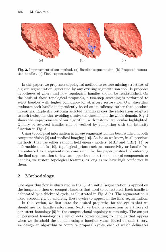
Fig. 2. Improvement of our method. (a) Baseline segmentation. (b) Proposed restora-tion handles. (c) Final segmentation.

In this paper, we propose a topological method to restore missing structures ofa given segmentation, generated by any existing segmentation tool. It proposeshypotheses of where and how topological handles should be reestablished. Onthe basis of those topological proposals, a two-step screening is performed toselect handles with higher confidence for structure restoration. Our algorithmevaluates each handle independently based on its saliency, rather than absoluteintensities. Explicitly restoring selected handles makes the restoration adaptiveto each trabecula, thus avoiding a universal threshold in the whole domain. Fig. 2shows the improvements of our algorithm, with restored trabeculae highlighted.Quality of restored handles can be verified by comparing with the intensityfunction in Fig. 3.

Using topological information in image segmentation has been studied in bothcomputer vision [2] and medical imaging [16]. As far as we know, in all previousmethods, that use either random field energy models (MRF and CRF) [14] ordeformable models [19], topological priors such as connectivity or handle-freeare enforced as a segmentation constraint. In this paper, instead of enforcingthe final segmentation to have an upper bound of the number of components orhandles, we restore topological features, as long as we have high confidence inthem.

2 Methodology

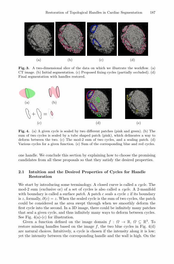
The algorithm flow is illustrated in Fig. 3. An initial segmentation is applied onthe image and then we compute handles that need to be restored. Each handle isdelineated by a thickened cycle, as illustrated in Fig. 3 (c). The segmentation isfixed accordingly, by enforcing these cycles to appear in the final segmentation.

In this section, we first state the desired properties for the cycles that weshould use for handle restoration. Next, we build a connection to a theory ofpersistent homology [6] in the computational topology community. The outputof persistent homology is a set of dots corresponding to handles that appearwhen we threshold the domain using a function value. Based on such theory,we design an algorithm to compute proposal cycles, each of which delineates

Restoration of Topological Handles in Cardiac Segmentation 187

(a) (b) (c) (d)

Fig. 3. A two-dimensional slice of the data on which we illustrate the workflow. (a)CT image. (b) Initial segmentation. (c) Proposed fixing cycles (partially occluded). (d)Final segmentation with handles restored.

(a) (b)

(c) (d) (e)

Fig. 4. (a) A given cycle is sealed by two different patches (pink and green). (b) Thesum of two cycles is sealed by a tube shaped patch (pink), which delineates a way todeform between the two. (c) The mod-2 sum of two cycles, and a sealing patch. (d)Various cycles for a given function. (e) Sum of the corresponding blue and red cycles.

one handle. We conclude this section by explaining how to choose the promisingcandidates from all these proposals so that they satisfy the desired properties.

2.1 Intuition and the Desired Properties of Cycles for HandleRestoration

We start by introducing some terminology. A closed curve is called a cycle. Themod-2 sum (exclusive or) of a set of cycles is also called a cycle. A 2-manifoldwith boundary is called a surface patch. A patch c seals a cycle z if its boundaryis z, formally, ∂(c) = z. When the sealed cycle is the sum of two cycles, the patchcould be considered as the area swept through when we smoothly deform thefirst cycle into the second. In a 3D image, there could be infinitely many patchesthat seal a given cycle, and thus infinitely many ways to deform between cycles.See Fig. 4(a)-(c) for illustration.

Given a function defined on the image domain f : Ω → R, Ω ⊆ R3. To

restore missing handles based on the image f , the two blue cycles in Fig. 4(d)are natural choices. Intuitively, a cycle is chosen if the intensity along it is low;yet the intensity between the corresponding handle and the wall is high. On the

188 M. Gao et al.

other hand, we need to propose a set of cycles such that any two of them wouldnot delineate the same trabecula. Furthermore, each trabecula should be coveredby a proposal. These intuitions lead to three properties need to be satisfied.

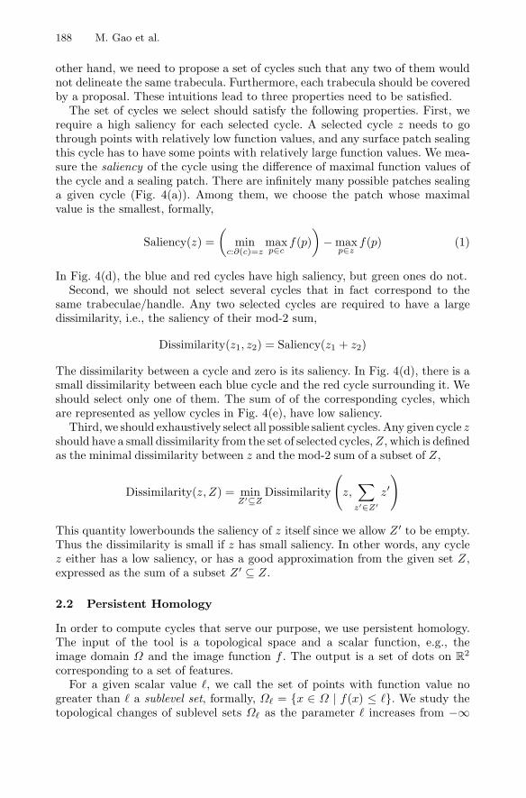
The set of cycles we select should satisfy the following properties. First, werequire a high saliency for each selected cycle. A selected cycle z needs to gothrough points with relatively low function values, and any surface patch sealingthis cycle has to have some points with relatively large function values. We mea-sure the saliency of the cycle using the difference of maximal function values ofthe cycle and a sealing patch. There are infinitely many possible patches sealinga given cycle (Fig. 4(a)). Among them, we choose the patch whose maximalvalue is the smallest, formally,

Saliency(z) =

(min

c:∂(c)=zmaxp∈c

f(p)

)−max

p∈zf(p) (1)

In Fig. 4(d), the blue and red cycles have high saliency, but green ones do not.Second, we should not select several cycles that in fact correspond to the

same trabeculae/handle. Any two selected cycles are required to have a largedissimilarity, i.e., the saliency of their mod-2 sum,

Dissimilarity(z1, z2) = Saliency(z1 + z2)

The dissimilarity between a cycle and zero is its saliency. In Fig. 4(d), there is asmall dissimilarity between each blue cycle and the red cycle surrounding it. Weshould select only one of them. The sum of of the corresponding cycles, whichare represented as yellow cycles in Fig. 4(e), have low saliency.

Third, we should exhaustively select all possible salient cycles. Any given cycle zshould have a small dissimilarity from the set of selected cycles,Z, which is definedas the minimal dissimilarity between z and the mod-2 sum of a subset of Z,

Dissimilarity(z, Z) = minZ′⊆Z

Dissimilarity

(z,

∑z′∈Z′

z′)

This quantity lowerbounds the saliency of z itself since we allow Z ′ to be empty.Thus the dissimilarity is small if z has small saliency. In other words, any cyclez either has a low saliency, or has a good approximation from the given set Z,expressed as the sum of a subset Z ′ ⊆ Z.

2.2 Persistent Homology

In order to compute cycles that serve our purpose, we use persistent homology.The input of the tool is a topological space and a scalar function, e.g., theimage domain Ω and the image function f . The output is a set of dots on R

2

corresponding to a set of features.For a given scalar value �, we call the set of points with function value no

greater than � a sublevel set, formally, Ω� = {x ∈ Ω | f(x) ≤ �}. We study thetopological changes of sublevel sets Ω� as the parameter � increases from −∞

Restoration of Topological Handles in Cardiac Segmentation 189

(a) function (b) � = b1 (c) � = b2

z3

(d) � = d2

z3

(e) � = d1

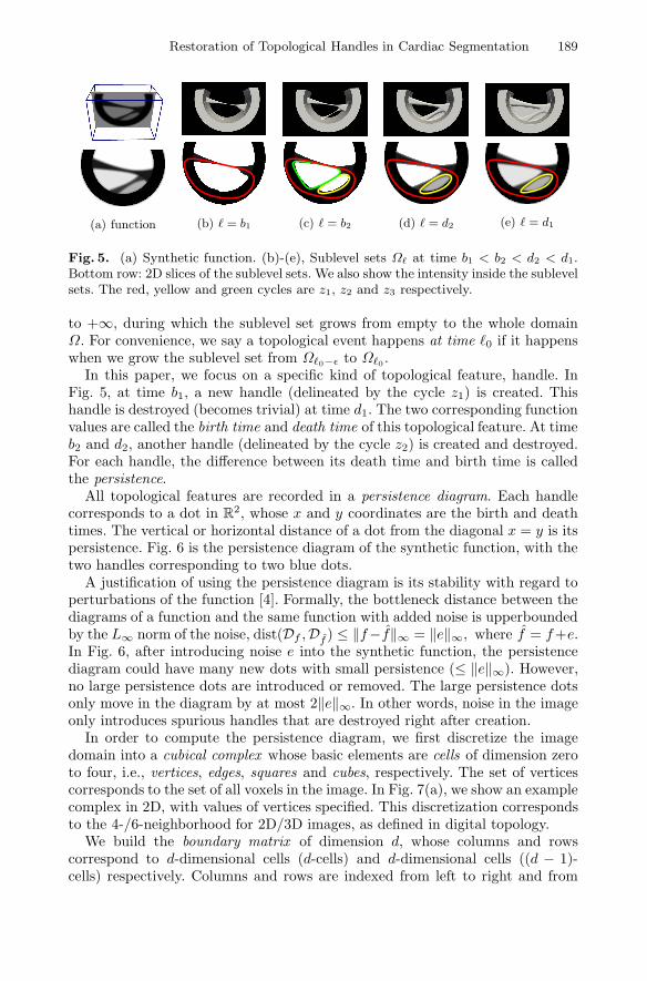
Fig. 5. (a) Synthetic function. (b)-(e), Sublevel sets Ω� at time b1 < b2 < d2 < d1.Bottom row: 2D slices of the sublevel sets. We also show the intensity inside the sublevelsets. The red, yellow and green cycles are z1, z2 and z3 respectively.

to +∞, during which the sublevel set grows from empty to the whole domainΩ. For convenience, we say a topological event happens at time �0 if it happenswhen we grow the sublevel set from Ω�0−ε to Ω�0 .

In this paper, we focus on a specific kind of topological feature, handle. InFig. 5, at time b1, a new handle (delineated by the cycle z1) is created. Thishandle is destroyed (becomes trivial) at time d1. The two corresponding functionvalues are called the birth time and death time of this topological feature. At timeb2 and d2, another handle (delineated by the cycle z2) is created and destroyed.For each handle, the difference between its death time and birth time is calledthe persistence.

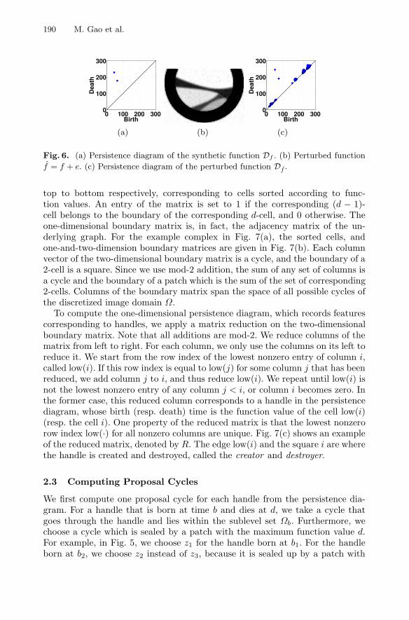
All topological features are recorded in a persistence diagram. Each handlecorresponds to a dot in R

2, whose x and y coordinates are the birth and deathtimes. The vertical or horizontal distance of a dot from the diagonal x = y is itspersistence. Fig. 6 is the persistence diagram of the synthetic function, with thetwo handles corresponding to two blue dots.

A justification of using the persistence diagram is its stability with regard toperturbations of the function [4]. Formally, the bottleneck distance between thediagrams of a function and the same function with added noise is upperboundedby the L∞ norm of the noise, dist(Df ,Df ) ≤ ‖f−f‖∞ = ‖e‖∞, where f = f+e.In Fig. 6, after introducing noise e into the synthetic function, the persistencediagram could have many new dots with small persistence (≤ ‖e‖∞). However,no large persistence dots are introduced or removed. The large persistence dotsonly move in the diagram by at most 2‖e‖∞. In other words, noise in the imageonly introduces spurious handles that are destroyed right after creation.

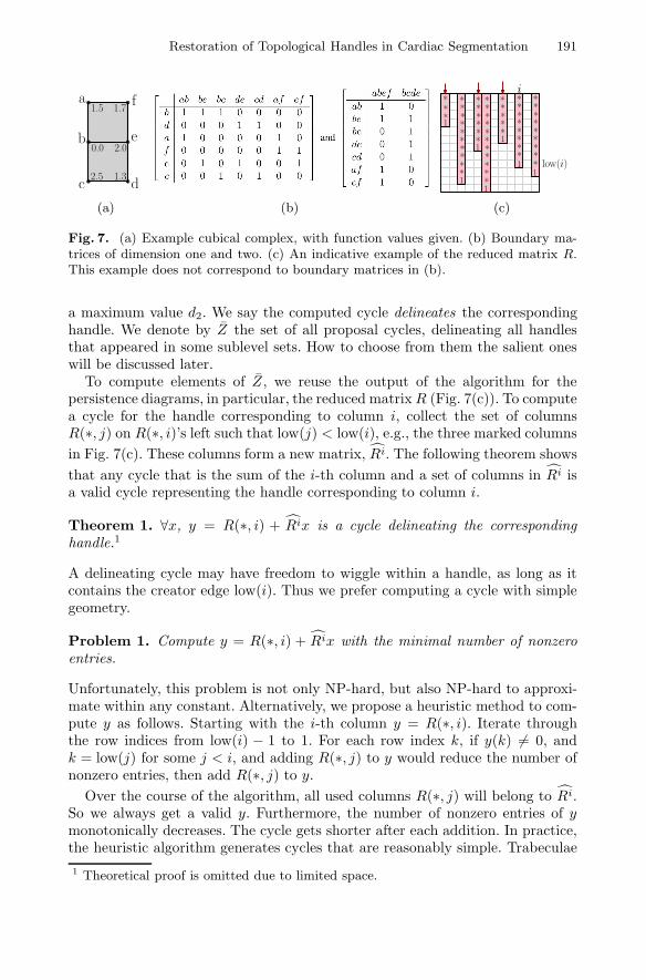
In order to compute the persistence diagram, we first discretize the imagedomain into a cubical complex whose basic elements are cells of dimension zeroto four, i.e., vertices, edges, squares and cubes, respectively. The set of verticescorresponds to the set of all voxels in the image. In Fig. 7(a), we show an examplecomplex in 2D, with values of vertices specified. This discretization correspondsto the 4-/6-neighborhood for 2D/3D images, as defined in digital topology.

We build the boundary matrix of dimension d, whose columns and rowscorrespond to d-dimensional cells (d-cells) and d-dimensional cells ((d − 1)-cells) respectively. Columns and rows are indexed from left to right and from

190 M. Gao et al.

0 100 200 3000

100

200

300

Birth

Dea

th

(a) (b)

0 100 200 3000

100

200

300

Birth

Dea

th

(c)

Fig. 6. (a) Persistence diagram of the synthetic function Df . (b) Perturbed function

f = f + e. (c) Persistence diagram of the perturbed function Df .

top to bottom respectively, corresponding to cells sorted according to func-tion values. An entry of the matrix is set to 1 if the corresponding (d − 1)-cell belongs to the boundary of the corresponding d-cell, and 0 otherwise. Theone-dimensional boundary matrix is, in fact, the adjacency matrix of the un-derlying graph. For the example complex in Fig. 7(a), the sorted cells, andone-and-two-dimension boundary matrices are given in Fig. 7(b). Each columnvector of the two-dimensional boundary matrix is a cycle, and the boundary of a2-cell is a square. Since we use mod-2 addition, the sum of any set of columns isa cycle and the boundary of a patch which is the sum of the set of corresponding2-cells. Columns of the boundary matrix span the space of all possible cycles ofthe discretized image domain Ω.

To compute the one-dimensional persistence diagram, which records featurescorresponding to handles, we apply a matrix reduction on the two-dimensionalboundary matrix. Note that all additions are mod-2. We reduce columns of thematrix from left to right. For each column, we only use the columns on its left toreduce it. We start from the row index of the lowest nonzero entry of column i,called low(i). If this row index is equal to low(j) for some column j that has beenreduced, we add column j to i, and thus reduce low(i). We repeat until low(i) isnot the lowest nonzero entry of any column j < i, or column i becomes zero. Inthe former case, this reduced column corresponds to a handle in the persistencediagram, whose birth (resp. death) time is the function value of the cell low(i)(resp. the cell i). One property of the reduced matrix is that the lowest nonzerorow index low(·) for all nonzero columns are unique. Fig. 7(c) shows an exampleof the reduced matrix, denoted by R. The edge low(i) and the square i are wherethe handle is created and destroyed, called the creator and destroyer.

2.3 Computing Proposal Cycles

We first compute one proposal cycle for each handle from the persistence dia-gram. For a handle that is born at time b and dies at d, we take a cycle thatgoes through the handle and lies within the sublevel set Ωb. Furthermore, wechoose a cycle which is sealed by a patch with the maximum function value d.For example, in Fig. 5, we choose z1 for the handle born at b1. For the handleborn at b2, we choose z2 instead of z3, because it is sealed up by a patch with

Restoration of Topological Handles in Cardiac Segmentation 191

a

b

c d

e

f1.5

0.0

2.5 1.3

2.0

1.7

(a) (b)

1

11

11

1

***

**********

**********

*********1

*

******

*****

********

i

low(i)

(c)

Fig. 7. (a) Example cubical complex, with function values given. (b) Boundary ma-trices of dimension one and two. (c) An indicative example of the reduced matrix R.This example does not correspond to boundary matrices in (b).

a maximum value d2. We say the computed cycle delineates the correspondinghandle. We denote by Z the set of all proposal cycles, delineating all handlesthat appeared in some sublevel sets. How to choose from them the salient oneswill be discussed later.

To compute elements of Z, we reuse the output of the algorithm for thepersistence diagrams, in particular, the reduced matrixR (Fig. 7(c)). To computea cycle for the handle corresponding to column i, collect the set of columnsR(∗, j) on R(∗, i)’s left such that low(j) < low(i), e.g., the three marked columns

in Fig. 7(c). These columns form a new matrix, Ri. The following theorem shows

that any cycle that is the sum of the i-th column and a set of columns in Ri isa valid cycle representing the handle corresponding to column i.

Theorem 1. ∀x, y = R(∗, i) + Rix is a cycle delineating the correspondinghandle.1

A delineating cycle may have freedom to wiggle within a handle, as long as itcontains the creator edge low(i). Thus we prefer computing a cycle with simplegeometry.

Problem 1. Compute y = R(∗, i) + Rix with the minimal number of nonzeroentries.

Unfortunately, this problem is not only NP-hard, but also NP-hard to approxi-mate within any constant. Alternatively, we propose a heuristic method to com-pute y as follows. Starting with the i-th column y = R(∗, i). Iterate throughthe row indices from low(i) − 1 to 1. For each row index k, if y(k) = 0, andk = low(j) for some j < i, and adding R(∗, j) to y would reduce the number ofnonzero entries, then add R(∗, j) to y.

Over the course of the algorithm, all used columns R(∗, j) will belong to Ri.So we always get a valid y. Furthermore, the number of nonzero entries of ymonotonically decreases. The cycle gets shorter after each addition. In practice,the heuristic algorithm generates cycles that are reasonably simple. Trabeculae

1 Theoretical proof is omitted due to limited space.

192 M. Gao et al.

usually correspond to thin handles, which leave limited space for cycles to wigglewithin.

2.4 Selecting Proposal Cycles Satisfying Desired Properties

From the set of all proposed cycles, Z, we select the set of promising ones using atwo level screening method. In the first level, we select cycles delineating handleswith persistence not less than a threshold θ.

In fact, the saliency of each delineating cycle as defined in Equation (1) isequal to the persistence of the handle. We abuse notations and say a proposedcycle has the same birth time, death time and persistence as its correspond-ing handle. The following theorem guarantees that the selected set of cycles,namely, Zθ = {z ∈ Z | persistence(z) ≥ θ}, satisfies the three desired propertieswe discussed in Section 2.1.

Theorem 2. (A) Any cycle in Zθ has a saliency at least θ;(B) The dissimilarity between any two cycles of Zθ is at least θ;(C) For any cycle z, its dissimilarity from Zθ is at most θ.

Although high persistence cycles lead to salient handles that are more likely fromtrabeculae, in practice, the first screening would inevitable select certain wrongcycles. Therefore, we use a classifier with geometrical features as the second levelscreening.

3 Experiments

The proposed algorithm was employed on 6 cardiac CT image at the end diastolicstate, where trabeculae structures are separated the most. The CT data wereacquired on a 320-MDCT scanner, using a conventional ECG-gated contrast-enhanced CT angiography protocol. The imaging protocol parameters include:prospectively triggered, single-beat, volumetric acquisition; detector width 0.5mm, voltage 120 KV, current 200− 550 mA.

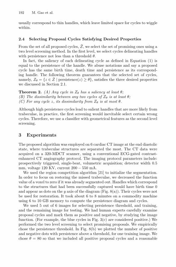
We used the region competition algorithm [21] to initialize the segmentation.In order to focus on restoring the missed trabeculae, we decreased the functionvalue of a voxel to zero if it was already segmented out. Handles which correspondto the structures that had been successfully captured would have birth time 0and appear as dots on the y axis of the diagram (Fig. 8(a)). Their cycles were notbe used for restoration. It took about 6 to 8 minutes on a commodity machineusing 6 to 10 GB memory to compute the persistence diagram and cycles.

We used 5 out of 6 images for selecting persistence threshold, and training,and the remaining image for testing. We had human experts carefully examineproposal cycles and mark them as positive and negative, by studying the imagefunction. (For example, the blue cycles in Fig. 3(c) are considered positive.) Weperformed the two level screening to select promising proposals. We empiricallychose the persistence threshold. In Fig. 8(b) we plotted the number of positiveand negative dots with persistence above a threshold, for one training image. Wechose θ = 80 so that we included all positive proposal cycles and a reasonable

Restoration of Topological Handles in Cardiac Segmentation 193

0 100 200 300 400 5000

100

200

300

400

500

Birth

Death

Positive

Negative

7080901001101200

50

100

150

200

250

300

350

400

Threshold

To

po

log

ica

l R

ep

airs

Positive

Negative

(a) (b)

Fig. 8. (a) Persistence diagram of one cardiac image. The persistence threshold ismarked as 80. (b) The relationship of persistence threshold and number of cycles.

number of negative ones from the training images. In the persistence diagramshown in Fig. 8(a), we drew the line y = x + θ. All dots above this line wereselected after the first level screening except the ones on the y axis. Notice thebig variation of the birth and death times of positive dots. This implies that itis impossible to detect them using an universal intensity prior.

(a) (b) (c) (d)

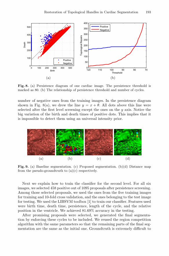
Fig. 9. (a) Baseline segmentation. (c) Proposed segmentation. (b)(d) Distance mapfrom the pseudo-groundtruth to (a)(c) respectively.

Next we explain how to train the classifier for the second level. For all siximages, we selected 458 positive out of 1095 proposals after persistence screening.Among those selected proposals, we used the ones from the five training imagesfor training and 10-fold cross validation, and the ones belonging to the test imagefor testing. We used the LIBSVM toolbox [1] to train our classifier. Features usedwere birth time, death time, persistence, length of the cycle, and the relativeposition in the ventricle. We achieved 81.69% accuracy in the testing.

After promising proposals were selected, we generated the final segmenta-tion by enforcing these cycles to be included. We reused the region competitionalgorithm with the same parameters so that the remaining parts of the final seg-mentation are the same as the initial one. Groundtruth is extremely difficult to

194 M. Gao et al.

get for this kind of data using manual segmentation. We generated the pseudo-groundtruth for the testing image by enforcing the human marked positive cycles.We compared the results of our method to that of a baseline segmentation gener-ated using the region competition method (Fig. 9) by showing the distance fromthe pseudo-groundtruth to each result. Distance was represented by different col-ors. Green, red and blue represented accurate segmentation, over segmentationand under segmentation, respectively. The trabeculae missing from the base-line segmentation had greater error. Our segmentation, as shown in Fig. 9(b),successfully captured more trabeculae. The distance error of the initial segmen-tation is 0.2108± 0.4973 voxel, whereas our segmentation method has distanceerror 0.1101± 0.3679 voxel.

4 Conclusion

In this paper, we proposed a novel left ventricle segmentation method. Our seg-mentation approach is generic and could be applied to other topologically com-plicated segmentation problems with complex topological structures. It wouldbe of theoretical interest if we build a quantitative relationship between thesignal-noise ratio of the image and the stability of the persistent diagram.

Acknowledgement. This work is supported by NIH-R21HL88354-01A1, Mul-tiscale Quantification of 3D LV Geometry from CT. The second author thanksProf. Herbert Edelsbrunner for helpful discussions.

References

1. Chang, C.-C., Lin, C.-J.: LIBSVM: A library for support vector machines. ACMTransactions on Intelligent Systems and Technology 2, 27:1–27:27 (2011)

2. Chen, C., Freedman, D., Lampert, C.H.: Enforcing topological constraints in ran-dom field image segmentation. In: CVPR, pp. 2089–2096 (2011)

3. Chen, T., Metaxas, D., Axel, L.: 3D cardiac anatomy reconstruction using highresolution CT data. In: Barillot, C., Haynor, D.R., Hellier, P. (eds.) MICCAI 2004.LNCS, vol. 3216, pp. 411–418. Springer, Heidelberg (2004)

4. Cohen-Steiner, D., Edelsbrunner, H., Harer, J.: Stability of persistence diagrams.Discrete & Computational Geometry 37(1), 103–120 (2007)

5. Ecabert, O., Peters, J., Schramm, H., Lorenz, C., von Berg, J., Walker, M., Vembar,M., Olszewski, M., Subramanyan, K., Lavi, G., Weese, J.: Automatic model-basedsegmentation of the heart in CT images. TMI 27(9), 1189–1201 (2008)

6. Edelsbrunner, H., Harer, J.: Computational topology: an introduction. Amer.Mathematical Society (2010)

7. Funka-Lea, G., Boykov, Y., Florin, C., Jolly, M.-P., Moreau-Gobard, R., Ramaraj,R., Rinck, D.: Automatic heart isolation for CT coronary visualization using graph-cuts. In: ISBI, pp. 614–617 (April 2006)

8. Gao, M., Huang, J., Zhang, S., Qian, Z., Voros, S., Metaxas, D., Axel, L.: 4Dcardiac reconstruction using high resolution CT images. In: Metaxas, D.N., Axel,L. (eds.) FIMH 2011. LNCS, vol. 6666, pp. 153–160. Springer, Heidelberg (2011)

9. Gray, H.: Anatomy of the human body. Lea & Febiger (1918)

Restoration of Topological Handles in Cardiac Segmentation 195

10. Isgum, I., Staring, M., Rutten, A., Prokop, M., Viergever, M., van Ginneken, B.:Multi-atlas-based segmentation with local decision fusion-application to cardiacand aortic segmentation in CT scans. TMI 28(7), 1000–1010 (2009)

11. Jolly, M.-P.: Automatic segmentation of the left ventricle in cardiac MR and CTimages. IJCV 70, 151–163 (2006)

12. Kulp, S., Gao, M., Zhang, S., Qian, Z., Voros, S., Metaxas, D., Axel, L.: Usinghigh resolution cardiac CT data to model and visualize patient-specific interactionsbetween trabeculae and blood flow. In: Fichtinger, G., Martel, A., Peters, T. (eds.)MICCAI 2011, Part I. LNCS, vol. 6891, pp. 468–475. Springer, Heidelberg (2011)

13. Lorenz, C., Berg, J.: A comprehensive shape model of the heart. Medical ImageAnalysis 10(4), 657–670 (2006)

14. Nowozin, S., Lampert, C.: Global connectivity potentials for random field models.In: CVPR, pp. 818–825 (2009)

15. Schoenhagen, P., Stillman, A., Halliburton, S., White, R.: CT of the heart: princi-ples, advances, clinical uses. Cleveland Clinic Journal of Medicine 72(2), 127–138(2005)

16. Segonne, F., Pacheco, J., Fischl, B.: Geometrically accurate topology-correction ofcortical surfaces using nonseparating loops. TMI 26(4), 518–529 (2007)

17. Shen, D., Herskovits, E., Davatzikos, C.: An adaptive-focus statistical shape modelfor segmentation and shape modeling of 3D brain structures. TMI 20(4), 257–270(2001)

18. Spreeuwers, L., Bangma, S., Meerwaldt, R., Vonken, E., Breeuwer, M.: Detection oftrabeculae and papillary muscles in cardiac MR images. Computers in Cardiology,415–418 (September 2005)

19. Sundaramoorthi, G., Yezzi, A.: Global regularizing flows with topology preserva-tion for active contours and polygons. TIP 16(3), 803–812 (2007)

20. Zheng, Y., Barbu, A., Georgescu, B., Scheuering, M., Comaniciu, D.: Four-chamberheart modeling and automatic segmentation for 3D cardiac CT volumes usingmarginal space learning and steerable features. TMI 27(11), 1668–1681 (2008)

21. Zhu, S., Yuille, A.: Region competition: Unifying snakes, region growing, andBayes/MDL for multiband image segmentation. PAMI 18(9), 884–900 (1996)