Local and global uniform convergence for elliptic problems on varying domains

J. Differential Equations 223 (2006) 1–32www.elsevier.com/locate/jde

Local and global uniform convergence for ellipticproblems on varying domains

Markus Biegerta, Daniel Danersb,∗aAbteilung Angewandte Analysis, Universität Ulm, 89069 Ulm, Germany

bSchool of Mathematics and Statistics, The University of Sydney, NSW 2006, Australia

Received 1 February 2005; revised 28 June 2005

Available online 9 September 2005

Abstract

The aim of the paper is to prove optimal results on local and global uniform convergenceof solutions to elliptic equations with Dirichlet boundary conditions on varying domains. Weassume that the limit domain be stable in the sense of Keldyš [Amer. Math. Soc. Transl. 51(1966) 1–73]. We further assume that the approaching domains satisfy a necessary conditionin the inside of the limit domain, and only require L2-convergence outside. As a consequence,uniform and L2-convergence are the same in the trivial case of homogenisation of a perforateddomain. We are also able to deal with certain cracking domains.© 2005 Elsevier Inc. All rights reserved.

Keywords: Elliptic partial differential equations; Domain perturbation; Uniform convergence; Shapestability

∗ Corresponding author. Fax: +61 2 9351 4534.E-mail addresses: [email protected] (M. Biegert), [email protected] (D. Daners).URLs: http://www.mathematik.uni-ulm.de/m5/biegert/ (M. Biegert),

http://www.maths.usyd.edu.au/u/daners/ (D. Daners).

0022-0396/$ - see front matter © 2005 Elsevier Inc. All rights reserved.doi:10.1016/j.jde.2005.07.015

http://www.elsevier.com/locate/jde

mailto:[email protected]

mailto:[email protected]

http://www.mathematik.uni-ulm.de/m5/biegert/

http://www.maths.usyd.edu.au/u/daners/

2 M. Biegert, D. Daners / J. Differential Equations 223 (2006) 1–32

1. Introduction

Given a sequence of open sets �n ⊂ RN , � > 0 and fn ∈ L∞(RN) we let un bethe unique (weak) solution of

−�u + �u = f in �n,

u = 0 on ��n.(1.1)

We extend un by zero outside �n to get a sequence of functions defined on RN .The aim of this paper is to study necessary and sufficient conditions on �n implyinguniform convergence, that is, convergence in L∞(RN) of un to the solution of

−�u + �u = f in �,

u = 0 on ��(1.2)

on a limit domain �. Convergence in L2 has obtained a lot of attention (see, forinstance, [9,10,12,18,22–26]), but there are not many results on uniform convergence if� is perturbed singularly (for smooth perturbations, see [19]). We make extensive use ofsophisticated comparison arguments, so the techniques cannot be applied to Neumannboundary conditions, and in fact many results are not true in that case (see [3]). Theresults in this paper generalise and complement earlier results in [1,4]. Related resultsproved by completely different techniques appear in [8]. Our results can be applied tosemi-linear elliptic equations and also to linear and non-linear parabolic equations inL∞ as shown in [1,13].

Throughout, we allow �n, � to be disconnected or unbounded. We will deal with twocases, namely local and global uniform convergence, that is, convergence in L∞

loc(RN)

or L∞(RN). Denote by u := R�(�)f the solution of (1.2) extended by zero outside�. We will only consider f ∈ L∞(RN), but emphasise that we could use f ∈ Lp(RN)

for p > N/2 as shown in Corollary 3.5.We will show in Section 3 that R�n

(�)f → R�(�)f in L∞(RN) or L∞loc(R

N) forall f ∈ L∞(RN) and all � > 0 if and only if this is the case for f ≡ 1 and some� > 0. This motivates the following definitions:

Definition 1.1. Let �n, � be open subsets of RN . We write

(1) �ngu−→ � if R�n

(�)1 → R�(�)1 in L∞(RN) for some � > 0 and say �n convergesto � globally uniformly;

(2) �nlu−→ � if R�n

(�)1 → R�(�)1 in L∞loc(R

N) for some � > 0 and say �n convergesto � locally uniformly.

Some sufficient conditions (regular convergence), such that �nlu−→ � are given in

[1] (not to be confused with the “regular perturbations” discussed in [19]). We willextend them significantly. Uniform convergence from the interior can be characterisedby requiring that there are no holes of non-zero capacity cut into � (see Theorem 8.3).

M. Biegert, D. Daners / J. Differential Equations 223 (2006) 1–32 3

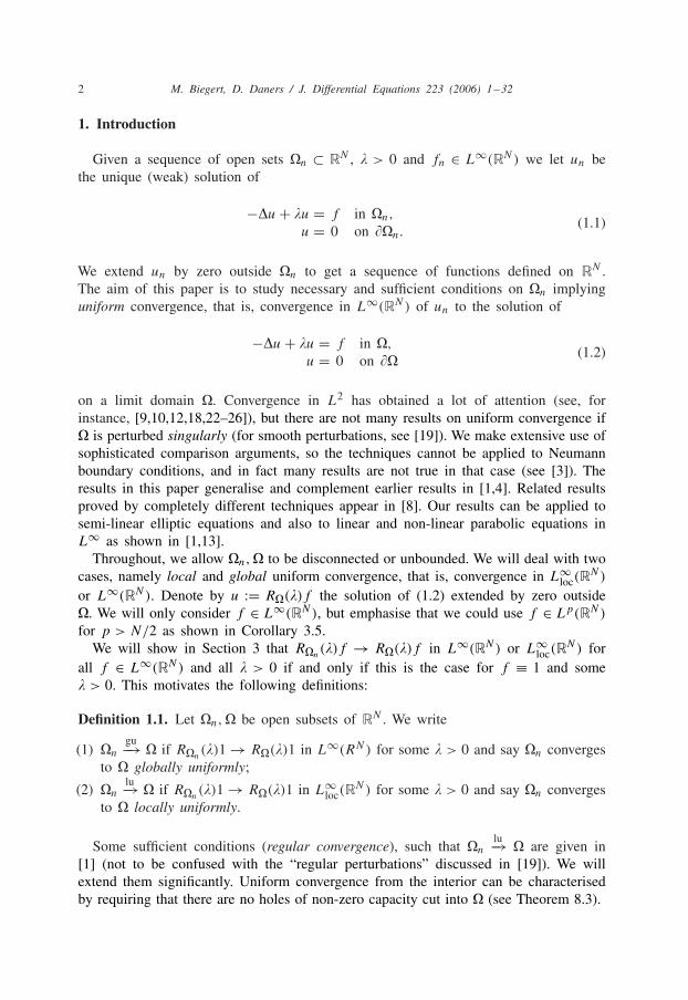
Fig. 1. Perforated domain.

Quite surprisingly, and contrary to our initial intuition, uniform convergence fromthe outside only requires a mild regularity assumption on the limit domain �, but noton the domains �n! The condition is that � be stable in the sense of Keldyš [21,Section V]. We will say � is uniformly stable. Note that this is not the same as thestability of � in [16] as used for L2-convergence in most papers on L2-convergencementioned above (see the appendix). Our proof works by localisation, separating thepart of �n at a positive distance from � and the part of �n close to �. The study ofthe part away from � leads to the case where the limit problem is trivial, and we onlyrequire L2-convergence. The part close to � is dealt with by using the stability of �.We refer to Section 8 for precise statements of these results.

In Section 5, we extensively discuss the case where the limit problem is trivial,that is, R�n

(�)1 → 0. We call this the vanishing case. The interesting fact is, thatthen, L2- and L∞-convergence are equivalent. In particular, our results show that inthe trivial case in homogenisation theory (see, for instance, [5, Theorem 1.3] or [23,Section 4]) convergence to zero is not just in L2, but uniform! Also, our results showthat in the “vanishing case” discussed in [7, Proposition 3.5] convergence is not only inL

(L2(RN)

)but even in L

(L∞(RN)

). A special case also appears in [4, Example 2.17].

Note however, that we do not require the measure of �n to converge to zero! A standardexample is a sequence of periodically perforated domains as shown in Fig. 1. Moreprecisely, �n is an open rectangle U with n closed balls of radius rn removed. If theyare such that nrN−2

n → ∞ if N �3 and n/| log rn| → ∞ if N = 2, then it is wellknown (see [23, Section 4]) that the solutions of (1.1) converge to zero in L2(RN).If we choose rn > 0 as above and such that nrN

n → 0, then the total measure (butnot capacity) of the balls converges to zero. Hence, meas(�n) → meas(U) �= 0 asn → ∞. Our theory shows that convergence is automatically in L∞(RN). Note thatthe geometric criteria from [1] do not apply to the above example.

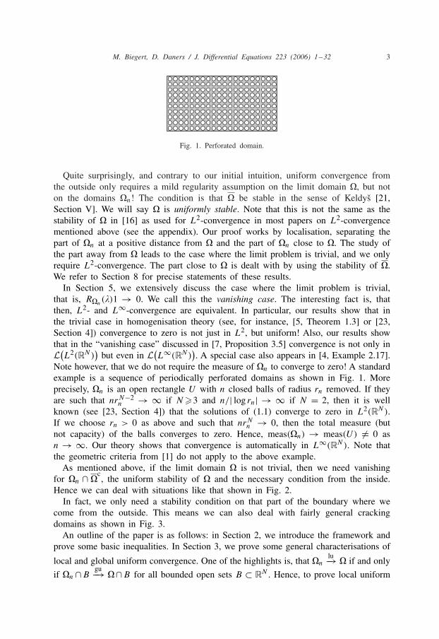
As mentioned above, if the limit domain � is not trivial, then we need vanishingfor �n ∩ �

c, the uniform stability of � and the necessary condition from the inside.

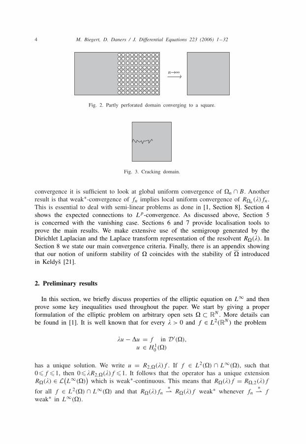
Hence we can deal with situations like that shown in Fig. 2.In fact, we only need a stability condition on that part of the boundary where we

come from the outside. This means we can also deal with fairly general crackingdomains as shown in Fig. 3.

An outline of the paper is as follows: in Section 2, we introduce the framework andprove some basic inequalities. In Section 3, we prove some general characterisations of

local and global uniform convergence. One of the highlights is, that �nlu−→ � if and only

if �n ∩Bgu−→ �∩B for all bounded open sets B ⊂ RN . Hence, to prove local uniform


n→∞

Fig. 2. Partly perforated domain converging to a square.

Fig. 3. Cracking domain.

convergence it is sufficient to look at global uniform convergence of �n ∩ B. Anotherresult is that weak∗-convergence of fn implies local uniform convergence of R�n

(�)fn.This is essential to deal with semi-linear problems as done in [1, Section 8]. Section 4shows the expected connections to Lp-convergence. As discussed above, Section 5is concerned with the vanishing case. Sections 6 and 7 provide localisation tools toprove the main results. We make extensive use of the semigroup generated by theDirichlet Laplacian and the Laplace transform representation of the resolvent R�(�). InSection 8 we state our main convergence criteria. Finally, there is an appendix showingthat our notion of uniform stability of � coincides with the stability of � introducedin Keldyš [21].

2. Preliminary results

In this section, we briefly discuss properties of the elliptic equation on L∞ and thenprove some key inequalities used throughout the paper. We start by giving a properformulation of the elliptic problem on arbitrary open sets � ⊂ RN . More details canbe found in [1]. It is well known that for every � > 0 and f ∈ L2(RN) the problem

�u − �u = f in D′(�),

u ∈ H 10 (�)

has a unique solution. We write u = R2,�(�)f . If f ∈ L2(�) ∩ L∞(�), such that0�f �1, then 0��R2,�(�)f �1. It follows that the operator has a unique extensionR�(�) ∈ L

(L∞(�)

)which is weak∗-continuous. This means that R�(�)f = R�,2(�)f

for all f ∈ L2(�) ∩ L∞(�) and that R�(�)fn∗⇀ R�(�)f weak∗ whenever fn

∗⇀ f

weak∗ in L∞(�).


By duality we define an operator on L1(�) by setting R1,�(�) := (R�(�))′. Byinterpolation we get operators Rp,�(�) on Lp(�) for all p ∈ (1, ∞). As R2,�(�) isself-adjoint we have Rp,�(�)f = Rq,�(�)f for all f ∈ Lp(�)∩Lq(�). If no confusionseems likely we simply write R�(�) for Rp,�(�). Consequently,

‖R�(�)‖L(Lp(�)) �1

�(2.1)

for all 1�p�∞ and � > 0. Also, for every f ∈ L∞(�) we have u := R�(�)f ∈ C(�),but u is not necessarily in H 1

0 (�). There are other characterisations of R�(�). Recallthat

H 1loc(R

N) := {u ∈ L2loc(R

N) : �iu ∈ L2loc(R

N) for i = 1, . . . , N}.

We then set

H 10,loc(�) := {u ∈ H 1

loc(RN) : �u ∈ H 1

0 (�) for all � ∈ D(RN)}.

If f ∈ L∞(�) it turns out (see [1, Proposition 1.3]) that u = R�(�)f if and only if

�u − �u = f in D′(�),

u ∈ H 10,loc(�) ∩ L∞(�).

Since we are working with varying domains we wish to define R�(�) to be an operatoron L∞(RN). To do so let i� ∈ L(Lp(�), Lp(RN)) denote the natural extension offunctions by zero, and r� ∈ L

(Lp(RN), Lp(�)

)the natural restriction to �. Then

R�(�) := i� ◦ R�(�) ◦ r� ∈ L(Lp(RN))

for all p ∈ [1, ∞]. Since ‖i�‖ = ‖r�‖ = 1 the operator R�(�) satisfies the sameestimate (2.1). The duals of i� and r� are i′� = r� and r ′

� = i� for all p ∈ [1, ∞),

so R�(�) has the same duality properties as R�(�). For this reason we identify R�(�)

with R�(�). Finally, by convention we set

R∅(�) := 0

for all � > 0 if � = ∅.The operator R�(�) has some useful monotonicity properties. If �1 ⊂ �2 are open

sets and 0�f1 �f2 ∈ L∞(�2), then

0�R�1(�)f1 �R�2(�)f2. (2.2)


In the sequel we shall use these properties without further comment. Denote by B(x, r)

the open ball in RN with radius r and centre x. Then clearly 1B(0,r)

∗⇀ 1 in L∞(RN),

so by construction of RRN (�) we have RRN (�)1B(0,r)

∗⇀ RRN (�)1. By the monotonicity

properties and Dini’s theorem it follows that

0�RRN (�)1B(0,r) ↗ RRN (�)1 = 1

�(2.3)

in C(RN) as r → ∞, that is, uniformly on compact subsets of RN . Also, it is wellknown (see, for instance, [1]) that

0�RB(0,r)(�)1 ↗ RRN (�)1 = 1

�(2.4)

in C(RN) as r → ∞. We shall frequently use the two facts in conjunction with theinequalities proved below. We need a characterisation of H 1

0,loc(�) involving capacity.

Recall that every u ∈ H 1loc(R

N) admits a quasi-continuous version u which is uniqueup to a polar set (see [17, Theorems 4.4 and 4.12]). Then we have

H 10,loc(�) = {u ∈ H 1

loc(RN) : u = 0 quasi-everywhere on �c}.

In what follows we do not distinguish between a function u ∈ H 1loc(R

N) and its quasi-continuous version. Several times we will make use of the following technical lemma:

Lemma 2.1. Let � ⊂ RN , � > 0. For ��0 let M := {x ∈ � : u(x) > �} and setu := R�(�)1. Then M ⊂ � is open and (u − �)+ = RM(�)(1 − ��).

Proof. Since u ∈ C(�) the set M is open, and u�� on Mc ∩ �. As (u − �)+ �u andu ∈ H 1

0,loc(�) we have u�� quasi-everywhere on �c. Hence, u�� quasi-everywhere

on Mc, so w := (u−�)+ ∈ H 1loc(R

N)∩L∞(RN) as well. By assumption w = 0 on Mc,so w ∈ H 1

0,loc(M) ∩ L∞(RN). As w = u − � on M , it follows that �w − �w = 1 − ��in D′(M). Now [1, Proposition 1.3] implies that w = RM(�)(1 − ��) as claimed. �

Note that the proof of the above lemma can be considerably simplified if M hasa smooth boundary and therefore H 1 functions have a proper trace on �M . Next weprove the first key inequality.

Theorem 2.2 (Intersection inequality). Let U, V ⊂ RN be open and � > 0. Then

‖RU∩B(�)1 − RV ∩B(�)1‖L∞(RN)

�‖RU(�)1 − RV (�)1‖L∞(B) (2.5)

for all open sets B ⊂ RN .


Proof. Fix open sets U, V, B ⊂ RN . Since RU∩B(�)1�RU(�)1 on RN and RV (�)1 =0 quasi-everywhere on V c we have

v := RU∩B(�)1 − ‖RU(�)1 − RV (�)1‖L∞(B) �0 (2.6)

quasi-everywhere on (U ∩ V ∩ B)c. As v ∈ C(U ∩ V ∩ B), the set

M := {x ∈ U ∩ V ∩ B : v(x) > 0}

is open. Moreover, by the above v�0 quasi-everywhere on (U ∩V ∩B)c. Hence, �v −�v = f in D′(U∩V ∩B) if we set f := 1−�‖RU(�)1−RV (�)1‖L∞(B). Now [1, Propo-sition 1.3] implies that v+ = RM(�)f . By domination v�v+ �RU∩V ∩B(�)1�RV ∩B(�)1on U ∩ V ∩ B. Combining this with (2.6) we get

RU∩B(�)1 − RV ∩B(�)1�‖RU(�)1 − RV (�)1‖L∞(B)

quasi-everywhere on RN . By interchanging the roles of U and V inequality (2.5)follows. �

Let T denote the topology of RN , that is, T consists of all open subsets of RN .Then (T , ⊂) is a partially ordered set. We have the following monotonicity properties:

Theorem 2.3 (Monotonicity theorem). Let � > 0 and p ∈ [1, ∞]. For f ∈ Lp(RN)

non-negative consider the mapping Df : T × T → H 1loc(R

N) given by

Df (�, B) := R�(�)f − R�∩B(�)f.

Then, for fixed B, the mapping Df (·, B) : T → Lp(RN) is increasing. Moreover, forfixed �, the mapping Df (�, ·) : T → Lp(RN) is decreasing.

Proof. We first give a proof in case p = ∞. Note that the monotonicity with respectto the second argument immediately follows from (2.2). Hence, it remains to prove themonotonicity in the first argument. To do so fix open sets B and �1 ⊂ �2 in RN . Forf ∈ L∞(RN) non-negative set

h := R�2∩B(�)f − R�2(�)f + R�1(�)f − R�1∩B(�)f ∈ H 1loc(R

N).

Then w := h+ ∈ H 1loc(R

N), w ∈ C(�1 ∩ B) and M := {x ∈ �1 ∩ B : h(x) > 0} isopen. Since h = R�2∩B(�)f − R�2(�)f �0 quasi-everywhere on �c

1 and since h =R�1(�)f − R�2(�)f �0 quasi-everywhere on Bc we get that w = 0 quasi-everywhereon Mc and then that w ∈ H 1

0,loc(M) ∩ L∞(RN). Moreover, since �w − �w = 0 inD′(M) it follows from [1, Proposition 1.3] that w = RM(�)0 = 0 quasi-everywhere on


RN = M ∪ Mc (note that M = ∅). Hence h�0 on RN , completing the proof of thetheorem in case p = ∞. If f ∈ Lp(RN) is non-negative, there exists a sequence of non-negative test functions fn ∈ D(RN), such that fn → f in Lp(RN). If �1 ⊂ �2 ⊂ RN

are open sets, then the above implies that Dfn(�1, B)�Dfn(�2, B). Taking the limitas n → ∞, we get Df (�1, B)�Df (�2, B) as claimed. �

Remark 2.4. Let �1 ⊂ �2 ⊂ RN be open and fixed. It follows from Theorem 2.3that R�1(�)1 − R�1∩B(�)1�R�2(�)1 − R�2∩B(�)1. Rewriting this inequality we getthat 0�R�2∩B(�)1 − R�1∩B(�)1�R�2(�)1 − R�1(�)1. Taking on both sides the norm‖ · ‖L∞(B) we get Theorem 2.2 in the case when U ⊂ V or V ⊂ U .

3. Local versus global uniform convergence

The purpose of this section is to give basic characterisations for local and globaluniform convergence. We will also show that local uniform convergence can be ob-tained by localisation from global uniform convergence. We first prove that uniformconvergence of R�(�)1 for some � > 0 implies convergence of R�n

(�) in the opera-tor norm in L

(L∞(RN)

). The theorem also assures that the notion of global uniform

convergence (gu−→) given in Definition 1.1 is independent of � > 0.

Theorem 3.1. Let �, �n ⊂ RN be open and � > 0. Then the following assertions areequivalent:

(1) R�n(�) → R�(�) in L

(L∞(RN)

);

(2) R�n(�)1 → R�(�)1 in L∞(RN).

If one of the two assertions holds for some � > 0, then they both hold for all � >

0. More generally, if (1) or (2) holds for some � > 0 and � ∈ C is such thatsupn∈N ‖R�n

(�)‖L(L∞) < ∞, then R�n(�) → R�(�) in L

(L∞(RN)

).

Proof. Obviously (1) implies (2). Suppose now that (2) holds. Since the operator normof a positive operator on T ∈ L(L∞(RN)) is given by ‖T 1‖∞ we get

‖R�n(�) − R�(�)‖L(L∞)

�‖R�n(�) − R�∩�n

(�)‖L(L∞) + ‖R�∩�n(�)1 − R�(�)‖L(L∞)

= ‖R�n(�)1 − R�∩�n

(�)1‖∞ + ‖R�∩�n(�)1 − R�(�)1‖∞.

Applying Theorem 2.2 with B = �n and �, respectively, we get

‖R�n(�)1 − R�∩�n

(�)1‖∞ + ‖R�∩�n(�)1 − R�(�)1‖∞ �2‖R�n

(�)1 − R�(�)1‖∞.

By assumption the last term converges to zero, and so (1) follows. Next, we prove thatif R�n

(�)1 → R�(�)1 for some ��0 then convergence takes place for all � > 0. In


the light of what we just proved this completes the proof of the theorem. Let �, � > 0,� �= � be fixed. We set g := 1 + (� − �)R�(�)1 and gn := g − (� − �)R�n

(�)g. Thenby the resolvent equation

R�(�)1 = R�(�)g and R�n(�)gn = R�n

(�)g. (3.1)

Using assumption (1) we have R�n(�)g → R�(�)g in L∞(RN) as n → ∞. Hence, by

(3.1) and the definition of g we get

limn→∞ gn = g − (� − �)R�(�)g = 1 + (� − �)R�(�)1 − (� − �)R�(�)1 = 1

in L∞(RN), showing that ‖R�n(�)(1 − gn)‖L∞ ��−1‖1 − gn‖L∞ → 0 as n → ∞.

Taking into account (3.1) we therefore conclude that

‖R�n(�)1 − R�(�)1‖L∞ � ‖R�n

(�)(1 − gn)‖L∞ + ‖R�n(�)gn − R�(�)1‖L∞

� 1

�‖1 − gn‖L∞ + ‖R�n

(�)g − R�(�)g‖L∞ n→∞−−−→ 0.

Finally, if M := supn∈N ‖R�n(�)‖L(L∞) < ∞, then simply replace 1/� by M in the

above estimate. �

We note that convergence in the operator norm implies convergence of finite partsof the spectrum and the corresponding projections (see [1, Section 7]). Before we statethe next result let us recall some common notation.

Definition 3.2 (Compact inclusion). Given U, V ⊂ RN we write U ⊂⊂ V if U, V aresets, such that U is compact and U ⊂ int(V ).

In particular note that, U is bounded if U ⊂⊂ V .

Theorem 3.3. Let �, �n ⊂ RN be open sets, � > 0, (fn) a bounded sequence inL∞(RN) and f ∈ L∞(RN). If R�n∩B(�)fn → R�∩B(�)f in L∞(RN) for all opensets B ⊂⊂ RN , then R�n

(�)fn → R�(�)f in L∞loc(R

N).

Proof. For every compact set K ⊂ RN we clearly have

‖R�n(�)fn − R�(�)f ‖L∞(K) �‖R�n

(�)fn − R�n∩B(�)fn‖L∞(K)

+‖R�n∩B(�)fn − R�∩B(�)f ‖L∞(K) + ‖R�∩B(�)f − R�(�)f ‖L∞(K). (3.2)


Setting M := sup{‖fn‖L∞(RN): n ∈ N}, we have

‖R�n(�)fn − R�n∩B(�)fn‖L∞(K) + ‖R�∩B(�)f − R�(�)f ‖L∞(K)

�M(‖R�n

(�)1−R�n∩B(�)1‖L∞(K)+‖R�∩B(�)1−R�(�)1‖L∞(K)

). (3.3)

Fix a compact set K ⊂ RN and ε > 0. By (2.4) there exists B ⊂⊂ RN , such that

‖RRN (�)1 − RB(�)1‖L∞(K) �ε

4M.

Using Theorem 2.3 with D1(�, B)�D1(RN, B) and D1(�n, B)�D1(R

N, B) we seethat

‖R�n(�)1 − R�n∩B(�)1‖L∞(K) + ‖R�(�)1 − R�∩B(�)1‖L∞(K)

�2‖RRN (�)1 − RB(�)1‖L∞(K) �ε

2M(3.4)

for all n ∈ N. Combining the above inequality with (3.2) and (3.3) we get

‖R�n(�)fn − R�(�)f ‖L∞(K) �

ε

2+ ‖R�n∩B(�)fn − R�∩B(�)f ‖L∞(K)

for all n ∈ N. By assumption there exists n0 ∈ N, such that

‖R�n∩B(�)fn − R�∩B(�)f ‖L∞(K) �ε

2

for all n�n0, leading to

‖R�n(�)fn − R�(�)f ‖L∞(K) �

ε

2+ ε

2= ε

for all n�n0. Since ε > 0 and K were arbitrary the theorem is proved. �

We next show that the notion of local uniform convergence (lu−→) given in Defini-

tion 1.1 is independent of � > 0. The theorem can be considered as a counterpart ofTheorem 3.1 in case of local uniform convergence. We will need the space

L∞0 (RN) := {

u ∈ L∞(RN) : there exists v ∈ C0(RN) with |u|�v

},

which is a closed subspace of L∞(RN).


Theorem 3.4. Suppose that �n, � ⊂ RN are open sets and � > 0. Then the followingassertions are equivalent:

(1) R�n(�)1 → R�(�)1 in L∞

loc(RN);

(2) R�n∩B(�)1 → R�∩B(�)1 in L∞(RN) for all open sets B ⊂⊂ RN ;

(3) R�n(�)fn → R�(�)f in L∞

loc(RN) whenever fn

∗⇀ f in L∞(RN);

(4) R�n(�)f → R�(�)f in L∞(RN) for all f ∈ L∞

0 (RN);(5) R�n

(�)f → R�(�)f in L∞loc(R

N) for all f ∈ L∞(RN) with compact support.

If one of the above assertions holds for some � > 0, then they all hold for every � > 0.

Proof. Suppose (1) holds. Given B ⊂⊂ RN we conclude from Theorem 2.2 that

‖R�n∩B(�)1 − R�∩B(�)1‖∞ �‖R�n(�)1 − R�(�)1‖L∞(B)

n→∞−−−→ 0,

proving (2). Next assume (2) holds. Suppose fn∗⇀ f in L∞(RN) and fix an arbitrary

open set B ⊂⊂ RN . Then

‖R�n∩B(�)fn − R�∩B(�)f ‖L∞(RN)

�‖R�n∩B(�) − R�∩B(�)‖L(L∞(RN))‖fn‖L∞(RN)

+‖R�∩B(�)fn − R�∩B(�)f ‖L∞(RN)

(3.5)

for all n ∈ N. By assumption and Theorem 2.2 we conclude that

‖R�n∩B(�)1 − R�∩B(�)1‖∞ �‖R�n(�)1 − R�(�)1‖L∞(B)

n→∞−−−→ 0,

and so by Theorem 3.1 we have that R�n∩B(�) → R�∩B(�) in L(L∞(RN)) for allopen sets B ⊂⊂ RN . Since fn is bounded in L∞(RN) the first term on the right-handside of (3.5) converges to zero. Since � ∩ B is bounded, R�∩B(�) is compact (see[1, Theorem 7.2]), so the second term also converges to zero. Hence (3) follows fromTheorem 3.3. Suppose now that (3) holds. If f ∈ L∞

0 (RN), then un := R�n(�)f →

u := R�(�)f in L∞loc(R

N) as n → ∞. By [1, Proposition 2.6] we have that w :=RRN (�)|f | ∈ C0(R

N). Now fix ε > 0 arbitrary. Since w ∈ C0(RN) there exists r > 0,

such that 0�w�ε/2 on B(0, r)c. Using domination |u|�w and |un|�w for all n ∈ N,so |un − u|�2w�ε on B(0, r)c. Since un → u in L∞

loc(RN) there exists n0 ∈ N, such

that |un − u|�ε almost everywhere on B(0, r). Combining the two estimates we get‖un − u‖∞ �ε for all n�n0. Since ε > 0 was arbitrary, (4) follows. It is obvious that(4) implies (5), so it remains to show that (5) implies (1). Let K ⊂ RN be a compactset and ε > 0 be arbitrary. By domination we have

0�R�n(�)1 − R�n

(�)1B(0,r) = R�n(�)1B(0,r)c �RRN (�)1B(0,r)c


for all n ∈ N. Hence (2.4) implies the existence of r > 0, such that

‖R�n(�)1 − R�n

(�)1B(0,r)‖L∞(K) �ε

3

for all n ∈ N. Similarly, for the same r > 0, ‖R�(�)1 − R�(�)1B(0,r)‖L∞(K) �ε/3.

Hence,

‖R�n(�)1 − R�(�)1‖L∞(K)

�‖R�n(�)1 − R�n

(�)1B(0,r)‖L∞(K)

+‖R�n(�)1B(0,r) − R�(�)1B(0,r)‖L∞(K)

+‖R�(�)1B(0,r) − R�(�)1‖L∞(K)

�‖R�n(�)1B(0,r) − R�(�)1B(0,r)‖L∞(RN)

+ 2

3ε

for all n ∈ N. By assumption (5) there exists n0 ∈ N such that

‖R�n(�)1B(0,r) − R�(�)1B(0,r)‖L∞(RN)

� ε

3

for all n�n0. Therefore, ‖R�n(�)1 − R�(�)1‖L∞(K) �ε for all n�n0. As ε > 0 and

K were arbitrary, (1) follows. To prove the last claim, suppose one of the assertionsholds for some � > 0. Then, by what we proved, all assertions hold for that � > 0,so in particular (2) holds. By Theorem 3.1 property (2) holds for every � > 0, soby what we proved, all assertions hold for every � > 0, completing the proof of thetheorem. �

In the above theorem, we have only considered fn, f ∈ L∞(RN). This is not nec-essary as we show below.

Corollary 3.5. If �nlu−→ �, then R�n

(�)f → R�(�)f in L∞loc(R

N) for all f ∈ Lp(RN)

with p > N/2. If �ngu−→ �, then convergence is in L∞(RN).

Proof. We know that there exists a constant C > 0 independent of the domain �, suchthat

‖R�(�)‖L(Lp,L∞) �C

(see [11]). Fix f ∈ Lp(RN) and ε > 0 arbitrary. Since Lp(RN) ∩ L∞(RN) isdense in Lp(RN) there exists g ∈ L∞(RN), such that ‖f − g‖p < ε/4C. Let nowB ⊂ RN be a bounded set. Then, by assumption, there exists n0 ∈ N, such that


‖R�n(�)g − R�(�)g‖L∞(B) < ε/2 for all n > n0. Hence,

‖R�n(�)f − R�(�)f ‖L∞(B)

�‖R�n(�)(f − g)‖L∞(B) + ‖R�n

(�)g − R�(�)g‖L∞(B)

+‖R�(�)(g − f )‖L∞(B) < 2C‖f − g‖p + ε

2� ε

2+ ε

2= ε

for all n > n0. Since ε > 0 was arbitrary the first assertion of the corollary follows. If

�ngu−→ � we simply replace B by RN in the above argument. �

We next collect some facts about the convergence of various intersections.

Theorem 3.6 (Intersection theorem). Let U, Un, V, Vn ⊂ RN be open sets. Then thefollowing assertions hold:

(1) If Ungu−→ U and Vn

gu−→ V , then Un ∩ Vngu−→ U ∩ V .

(2) If Unlu−→ U and Vn

lu−→ V , then Un ∩ Vnlu−→ U ∩ V .

(3) Unlu−→ U if and only if Un ∩ B

gu−→ U ∩ B for all open sets B ⊂⊂ RN .

Proof. To prove (1) fix � > 0. By definition of convergence and Theorem 3.1 we knowthat RUn(�)1 → RU(�)1 and RVn(�)1 → RV (�)1 in L∞(RN). Hence by Theorem 2.2

‖RUn∩Vn(�)1 − RU∩V (�)1‖∞�‖RUn∩Vn(�)1 − RU∩Vn(�)1‖∞ + ‖RU∩Vn(�)1 − RU∩V (�)1‖∞

�‖RUn(�)1 − RU(�)1‖∞ + ‖RVn(�)1 − RV (�)1‖∞n→∞−−−→ 0,

so (1) follows. Next we prove (2). It follows form Theorem 3.4 that Un ∩Bgu−→ U ∩B

and Vn ∩ Bgu−→ V ∩ B for all open sets B ⊂⊂ RN . By (1) we have (Un ∩ Vn) ∩ B

gu−→(U ∩ V ) ∩ B. Applying Theorem 3.3 we conclude that Un ∩ Vn

lu−→ U ∩ V , completingthe proof of (2). Assertion (3) is a consequence of Theorem 3.4. �

4. Connections to Lp-convergence

We naturally expect that convergence of R�n(�) in L∞(RN) implies convergence in

Lp(RN) for all p ∈ [1, ∞]. We will show that this is indeed the case. We first look atlocal uniform convergence.

Proposition 4.1. Let �, �n ⊂ RN be open sets and � > 0. If �nlu−→ � and p ∈ [1, ∞),

then R�n(�)f → R�(�)f in Lp(RN) for all f ∈ Lp(RN).


Proof. Denote by Cc(RN) ⊂ L∞

0 (RN) the set of continuous functions on RN withcompact support. First, note that Cc(R

N) is dense in Lp(RN) for all p ∈ [1, ∞). By(2.1) it is therefore sufficient to show that R�n

(�)f → R�(�)f in Lp(RN) for allf ∈ Cc(R

N). Splitting f ∈ Cc(RN) into positive and negative parts, it is sufficient to

consider non-negative f ∈ Cc(RN). The case p = 1 is the most difficult one, so we

consider it first. Suppose now that f ∈ D(RN) is non-negative and let B ⊂ RN be abounded open set with supp f ⊂ B. Then

‖R�n(�)f − R�(�)f ‖1

�‖R�n(�)f − R�∩�n

(�)f ‖1 + ‖R�∩�n(�)f − R�(�)f ‖1. (4.1)

We show that both terms on the right-hand side converge to zero. Since f �0 and� ∩ �n ⊂ �n, we have R�n

(�)f − R�∩�n(�)f �0. By definition of the operator on

L1(RN) as the dual of the one on L∞(RN) we therefore have

‖R�n(�)f − R�∩�n

(�)f ‖L1 = 〈R�n(�)f − R�∩�n

(�)f, 1〉= 〈f, R�n

(�)1 − R�∩�n(�)1〉�‖f ‖1‖R�n

(�)1 − R�∩�n(�)1‖L∞(B).

The last expression converges to zero since �nlu−→ � and thus � ∩ �n

lu−→ � byTheorem 3.6. The second term on the right-hand side of (4.1) converges to zero bya similar argument. Hence, R�n

(�)f → R�(�)f in L1(RN) for all f ∈ L1(RN). Letnow p ∈ (1, ∞) and set un := R�n

(�)f − R�(�)f . Then clearly

‖un‖p �‖un‖1/p1 ‖un‖1−1/p∞

for all n ∈ N. Since un → 0 in L1(RN) and un is bounded in L∞(RN), it followsthat un → 0 in Lp(RN) as claimed. �

We next consider global uniform convergence.

Proposition 4.2. Let �, �n ⊂ RN be open sets and � > 0. If �ngu−→ � and p ∈ [1, ∞],

then R�n(�) → R�(�) in L

(Lp(RN)

).

Proof. Recall from Theorem 3.1 that R�n(�) → R�(�) in L(L∞(RN)) if �n

gu−→ �.Since the operator on L∞(RN) is the dual of the one on L1(RN) it follows that theiroperator norms are the same, so

‖R�n(�) − R�(�)‖L(L1) = ‖R�n

(�) − R�(�)‖L(L∞) → 0


as n → ∞. Hence, R�n(�) → R�(�) in L(L1(RN)) if �n

gu−→ �. If p ∈ (1, ∞), theRiesz–Thorin interpolation theorem (see [6]) and the above imply that

‖R�n(�) − R�(�)‖L(Lp) � ‖R�n

(�) − R�(�)‖1/p

L(L1)‖R�n

(�) − R�(�)‖1−1/p

L(L∞)

= ‖R�n(�) − R�(�)‖L(L∞) → 0

as n → ∞, completing the proof of the proposition. �

Remark 4.3. (a) If p = ∞ the above shows that convergence is in L(Lp(RN)

)if

the resolvents converge strongly, that is, R�n(�)f → R�(�)f in L∞(RN) for all

f ∈ L∞(RN). Note however, that strong convergence for p ∈ [1, ∞) does not implyconvergence in the operator norm in general (see [12, Example 8.1])! The reason isthat functions in Lp(RN) decay at infinity in some sense if p ∈ [1, ∞), but not ifp = ∞.

(b) Also note that (strong) convergence of R�n(�) in L

(Lp(RN)

)for all p ∈ (0, ∞)

does not imply (strong) convergence in L(L∞(RN)

)(it does in the vanishing case

as shown in Section 5). The reason is that L2-convergence is not equivalent to L∞-convergence in general, and L2-convergence implies Lp-convergence for all p ∈ (1, ∞)

(see [12, Section 5]).

5. The vanishing case

In this section, we discuss extensively the case where the limit problem is trivial,that is, R�n

(�)1 → 0. For that we simply write �n → ∅. To derive our result wewill make use of the semigroup T�(t) generated by the Dirichlet Laplacian on � andrepresent the resolvent by means of its Laplace transform

R�(�) =∫ ∞

0e−�t T�(t) dt (5.1)

for all � > 0. We recall that T�(t) is a strongly continuous analytic semigroup ofcontractions on Lp(�) for 1�p < ∞ (see [14, Chapter I]), that is

‖T�(t)‖L(Lp(�)) �1 (1�p�∞). (5.2)

It is well known that

0�T�1(t)�T�2(t)�G(t) (5.3)

for all open sets �1 ⊂ �2 ⊂ RN and t > 0, where G(t) := TRN (t) is the Gaussiansemigroup on RN . Also, T�(t) has a kernel k�(t, x, y) dominated by the Gauss kernel


(see [14]). More precisely,

0�k�(t, x, y)�gt (x − y) := (4�t)−N/2 exp(−|x − y|2/4t) (5.4)

for all x, y ∈ RN and t > 0. By convention we set k�(t, x, y) = 0 for (x, y) outside� × �. Hence, for every 1�p�q �∞ there exists a constant C only depending onN , p and q, such that

‖T�(t)‖L(Lp(�),Lq(�)) �Ct− N

2 ( 1p

− 1q) (5.5)

for all t > 0. As a first step we characterise the vanishing case for L2-convergence.The result is related to [12, Theorem 4.4]. To do so we use the spectral bound of theDirichlet–Laplacian on � given by

�(�) = infu∈H 1

0 (�)

u�=0

‖∇u‖22

‖u‖22

.

Lemma 5.1. Let �n ⊂ RN be open sets. Then the following assertions are equivalent:

(1) �(�n) → ∞;(2) T�n

(t) → 0 in L(L2(RN)

)for some (all) t > 0;

(3) R�n(�) → 0 in L

(L2(RN)

)for some (all) � > 0.

Proof. Since −� and thus T�n(t) and R�n

(�) are self-adjoint on L2(�n) it follows fromstandard spectral mapping theorems (see [20, Section V.3.5] and [2, Corollary A-III.6.5])that

‖T�n(t)‖L(L2(�n)) = e−t�(�n) (5.6)

and

‖R�n(�)‖L(L2(�n)) = 1

� + �(�n).

Hence (1)–(3) are equivalent. �

We next show that L2-convergence implies L∞-convergence for the semigroups.

Theorem 5.2. Let �n ⊂ RN be open sets and suppose that T�n(t) → 0 in L

(L2(RN)

)for some t > 0. If 1�p�q �∞, then T�n

(t) → 0 in L(Lp(RN), Lq(RN)

)uniformly

with respect to t in closed subsets of (0, ∞).


Proof. By Lemma 5.1 it follows that T�n(t) → 0 in L

(L2(RN)

)for all t > 0. By the

semigroup property and (5.5), we have

‖T�n(t)‖L(Lp,Lq) �‖T�n

(�/2)‖L(Lq)‖T�n(t − �/2)‖L(Lp,Lq)

�C(t − �

2

)− N2 ( 1

p− 1

q)‖T�n

(�/2)‖L(Lq) �C(�

2

)− N2 ( 1

p− 1

q)‖T�n

(�/2)‖L(Lq)

for all t �� > 0 and n ∈ N. To get uniform convergence with respect to t in closedsubsets of (0, ∞), it is therefore sufficient to prove that T�n

(t) → 0 in L(Lq(RN)

)for

all t > 0. We first assume that q ∈ (1, ∞). By the Riesz–Thorin interpolation theorem(see [6]) it follows from (5.2) and (5.6) that

‖T�n(t)‖L(Lq(�n)) �e−�q�(�n)t , (5.7)

where �q ∈ (0, 1] is given by �q = 2/q if 2�q < ∞ and �q = 2 − 2/q if 1 < q �2.Hence, by Lemma 5.1 we have T�n

(t) → 0 in L(Lq(RN)

)for all t > 0. We next

look at the case q = ∞. Since T�n(t) is a positive operator it is sufficient to show

that T�n(t)1 → 0 in L∞(RN). Suppose that this is not the case. Then, after possibly

passing to a subsequence, there exist ε > 0 and xn ∈ �n, such that(T�n

(t)1)(xn)�ε

for all n ∈ N. Now observe that

(T�n

(t)1)(xn) = (

T�n(t)1B(xn,r)

)(xn) + (

T�n(t)1B(xn,r)c

)(xn)

for all n ∈ N and r > 0. By (5.4)

(T�n

(t)1B(xn,r)c)(xn)�

∫RN

gt (xn − y)1B(xn,r)c(y) dy =∫

|y|� r

gt (y) dy

for all n ∈ N and r > 0. Hence, we can choose r > 0 such that

(T�n

(t)1B(xn,r)c)(xn) <

ε

2

for all n ∈ N. Using (5.5) and what we already proved

‖T�n(t)1B(xn,r)‖∞ = ‖T�n

(t/2)T�n(t/2)1B(xn,r)‖∞

� ‖T�n(t/2)‖L(L2,L∞)‖T�n

(t/2)1B(xn,r)‖2

� C( t

2

)−N/4‖T�n(t/2)‖L(L2)‖1B(0,r)‖2

n→∞−−−→ 0.


By choice of xn and r > 0 we have

ε�(T�n

(t)1)(xn)�

ε

2+ ‖T�n

(t)1B(xn,r)‖∞

for all n ∈ N, so letting n → ∞ we get 0 < ε�ε/2. As this is not possible itfollows that T�n

(t)1 → 0 in L∞(RN). The case p = q = 1 follows since by duality‖T�n

(t)‖L(L1) = ‖T�n(t)‖L(L∞). �

We next provide a version of the above theorem for the elliptic problem.

Theorem 5.3. Let �n ⊂ RN be open sets and suppose that R�n(�) → 0 in L

(L2(RN)

)for some � > 0. If 1�p�q �∞ with

N

2

( 1

p− 1

q

)< 1, (5.8)

then R�n(�) → 0 in L

(Lp(RN), Lq(RN)

).

Proof. Fix ε > 0 arbitrary. By (5.5) and (5.8) there exists s > 0 such that

∫ s

0‖T�n

(t)‖L(Lp,Lq)e−�t dt �C

∫ s

0t− N

2

(1p

− 1q

)e−�t dt <

ε

2

for all n ∈ N. Using the Laplace transform representation (5.1) we get

‖R�n(�)‖L(Lp,Lq) �

∥∥∥∥∫ s

0e−�t T�n

(t) dt

∥∥∥∥L(Lp,Lq)

+∥∥∥∥∫ ∞

s

e−�t T�n(t) dt

∥∥∥∥L(Lp,Lq)

� ε

2+

∫ ∞

s

e−�t‖T�n(t)‖L(Lp,Lq) dt

for all n ∈ N. By Lemma 5.1 and Theorem 5.2 ‖T�n(t)‖L(Lp,Lq) → 0 uniformly with

respect to t �s. Hence, there exists n0 ∈ N, such that ‖T�n(t)‖L(Lp,Lq) < �ε/2 for all

n > n0 and t �s, so

‖R�n(�)‖L(Lp,Lq) �

ε

2+ �ε

2

∫ ∞

0e−�t dt = ε

2+ ε

2= ε

for all n > n0. As ε > 0 was arbitrary, the assertion of the proposition follows. �

The only new case covered in the above proposition is that R�n(�) → 0 in

L(Lp(RN)) for some p ∈ (1, ∞) implies convergence in L(Lq(RN), L∞(RN)) forN/2 < q �∞. The other cases are covered in [12, Theorem 5.4]. The following corol-lary is a simple consequence of Lemma 5.1, Theorems 5.2 and 5.3.


Corollary 5.4. Let � > 0 and (�n) a sequence of open sets. Then the followingassertions are equivalent:

(1) R�n(�) → 0 in L

(L2(RN)

);

(2) R�n(�) → 0 in L

(L∞(RN)

);

(3) T�n(t) → 0 in L

(L2(RN)

)for all t > 0;

(4) T�n(t) → 0 in L

(L∞(RN)

)for all t > 0;

(5) �(�n) → ∞.

From the above we deduce a version on local uniform convergence.

Corollary 5.5. Let � > 0 and (�n) a sequence of open sets. Then the followingassertions are equivalent:

(1) R�n(�)1 → 0 in L∞

loc(RN), that is, �n

lu−→ ∅;(2) there exists p ∈ (1, ∞), such that R�n

(�)f → 0 in Lp(RN) for all f ∈ Lp(RN);(3) �(�n ∩ B) → ∞ for every bounded open set B ⊂ RN .

Proof. The implication (1) ⇒ (2) follows from Proposition 4.1. By the uniform bound(2.1) and interpolation, convergence in Lp(RN) for some p ∈ (1, ∞) implies con-vergence in L2(RN). Now (2) ⇒ (3) follows from [12, Theorem 6.1], assuming that� = ∅. Suppose now that (3) holds. Then by Corollary 5.4 R�n∩B(�)1 → 0 in L∞(RN)

for every bounded open set B ⊂ RN . Now Theorem 3.4 implies (1). �

Note that in (2) of the above theorem, we cannot admit p = ∞ since this wouldimply global uniform convergence by Theorem 3.1. Hence (2) would not be equivalentto (1). Also compare to Remark 4.3.

6. Tools for localisation

In this section, we collect some more properties of heat semigroup T�(t) introducedin Section 5. These properties will be useful to prove localisation results. For everyε > 0 and N ∈ N we define

Cε := min{C�0 :

∫ ∞

C/2e−s2

sN−1 ds� ε�N/2

�N

}, (6.1)

where �N is the surface area of the unit sphere in RN . Clearly the function

C →∫ ∞

C/2e−s2

sN−1 ds


is continuous on [0, ∞) and decreasing to zero as C → ∞, so the above minimumexists. Moreover, since

�N := 2�N/2

�(N/2)and

∫ ∞

0e−s2

sN−1 ds = 1

2�(N/2),

we have Cε = 0 whenever ε�1. For an arbitrary set A ⊂ RN or point A ∈ RN and� > 0 we denote the open �-neighbourhood of A by

B(A, �) := {x ∈ RN : dist(x, A) < �}. (6.2)

The distance between two sets A, B ⊂ RN is defined by

dist(A, B) := inf(x,y)∈A×B

‖x − y‖. (6.3)

Lemma 6.1. Suppose that � ⊂ RN is an open set and that A, B ⊂ RN are twomeasurable sets, such that dist(A, B) > 0. Then for every ε > 0

‖T�(t)1A‖L∞(B) �ε

for all t > 0 with t−1/2dist(A, B)�Cε.

Proof. We first prove an auxiliary inequality involving the Gaussian semigroup G(t).If we fix � > 0 and represent G(t) by means of the Gauss kernel we get

G(t)1B(0,�)c(0) = (4�t)−N/2∫

|y|��e−|y|2/4t dy.

Evaluating the integral using spherical coordinates we see that

G(t)1B(0,�)c(0)� �N

(4�t)N/2

∫ ∞

�e−r2/4t rN−1 dr = �N

�N/2

∫ ∞

�/√

4t

e−s2sN−1 ds�ε

for all t > 0, such that �t−1/2 �Cε. Now set � := dist(A, B) and fix x ∈ B ∩ �arbitrary. Given ε > 0 the above inequality implies that

0�T�(t)1A(x)�G(t)1A(x)�G(t)1B(x,�)c(x) = G(t)1B(0,�)c(0)�ε

for all t > 0 with t−1/2��Cε. Since x ∈ B ∩ � was arbitrary and T�(t)1A = 0 on�c ∩ B, the assertion of the lemma follows. �


We next prove a weak parabolic maximum principle. Note that the assertion followsfrom the classical maximum principle if all sets involved have a C2 boundary.

Theorem 6.2 (Parabolic maximum principle). Let �1 ⊂ �2 ⊂ RN be open sets, ε, � >

0, and f ∈ L∞(RN) non-negative. If T�2(t)f (x)�ε for all x ∈ ��1 ∩ �2 and allt ∈ (0, �], then T�2(t)f (x)�T�1(t)f (x) + ε for all x ∈ �1 and all t ∈ (0, �].

Proof. Since T�1(t) is weak∗-continuous and L2(RN) ∩ L∞(RN) is weak∗-dense inL∞(RN) we may assume without loss of generality that f ∈ L2(RN) ∩ L∞(RN) isnon-negative. Set u2(t) := T�2(t)f , u1(t) := T�1(t)f and u := u2 − ε − u1. Thenu ∈ C

([0, ∞), L2(�1)) ∩ C∞(

(0, ∞), L2(�1)), u′ − �u = 0 and u+(t) ∈ H 1

0 (�1) forall t ∈ (0, �). We claim that

1

2

(‖u+(t)‖2

L2(�1)− ‖u+(�)‖2

L2(�1)

)= −

∫ t

�‖∇u+(s)‖2

L2(�1)ds (6.4)

for every �, t ∈ (0, �]. Letting � → 0+ and using that u+ ∈ C([0, �], L2(�1)

)we get

12‖u+(t)‖2

L2(�1)� 1

2‖u+(0)‖2L2(�1)

= 0,

that is, u(t, ·)�0 on �1 for t ∈ (0, �]. Since t ∈ (0, �] was arbitrary, u�0 andthe assertion of the theorem follows. Hence, it remains to prove (6.4). For n ∈ N

let jn() :=√

2 + 1/n2 − 1/n if �0 and jn() := 0 if < 0. Then obviously

jn ∈ C1(R), and 0�j ′n �1 for all n ∈ N. Hence, jn ◦ u ∈ C1

((0, ∞), L2(�2)

)and

1

2

d

dt‖(jn ◦ u)(t)‖2

L2(�2)= ⟨

j ′n(u(t))u′(t), jn(u(t))

⟩

= ⟨u′(t), j ′

n(u(t))jn(u(t))⟩ = ⟨

�u, j ′n(u(t))jn(u(t))

⟩

for all t > 0. If t, � > 0 we therefore get

1

2

(‖jn ◦ u(t)‖2

L2(�1)− ‖jn ◦ u(�)‖2

L2(�1)

)=

∫ t

�

⟨�u, j ′

n(u(s))jn(u(s))⟩ds.

Next observe that j ′n(u)jn(u) ↗ u+ and jn(u) ↗ u+ as n → ∞. Hence, by the

dominated convergence theorem

1

2

(‖u+(t)‖2

L2(�1)− ‖u+(�)‖2

L2(�1)

)=

∫ t

�〈�u(s), u+(s)〉 ds.


As u+(s) ∈ H 10 (�1) for s ∈ (0, �) we have 〈�u(s), u+(s)〉 = −〈∇u, ∇u+〉 =

−‖∇u+‖2L2(�1)

and hence (6.4) follows. �

For two sets we denote the symmetric difference by U$V := (U ∩V c)∪ (V ∩U c).

Lemma 6.3. Suppose that �1, �2 ⊂ RN are open sets and that A ⊂ RN is a measur-able set, such that dist(A, �2$�1) > 0. Then

‖T�2(t)1A − T�1(t)1A‖L∞(RN)

�ε

for all t > 0, such that t−1/2dist(A, �2$�1)�Cε/2, where Cε/2 is defined by (6.1).

Proof. First we look at the case where �1 ⊂ �2. Since � := dist(A, �2$�1) =dist(A, �2 \ �1) > 0, Lemma 6.1 implies that ‖T�2(t)1A‖L∞(�2\�1) �ε for all t >

0 with t−1/2��Cε. By the continuity of T�2(t)1A in �2 it follows in particularthat T�2(t)1A(x)�ε for all x ∈ ��1 ∩ �2 and all t > 0 with t−1/2��Cε. Apply-ing Theorem 6.2 we get that T�1(t)1A �T�2(t)1A �T�1(t)1A + ε on RN , and thus‖T�2(t)1A − T�1(t)1A‖

L∞(RN)�ε for all t > 0 with t−1/2��Cε. Hence, the assertion

of the lemma follows if �1 ⊂ �2. Let now �1, �2 be arbitrary open sets in RN . Thenby what we just proved we have

‖T�1(t)1A − T�2(t)1A‖L∞(RN)

� ‖T�1(t)1A − T�1∩�2(t)1A‖L∞(RN)

+‖T�1∩�2(t)1A − T�2(t)1A‖L∞(RN)

� ε

2+ ε

2= ε

all t > 0 with t−1/2��Cε/2 as claimed. �

7. Localisation theorems

Localisation of Convergence is an important tool to compare the behaviour of T�n(t)

with the behaviour of T�n∩U(t) on a fixed open set U . Moreover, it allows us togeneralise earlier results. For example, Corollary 5.4 is a particular case of Theorem 8.8if we replace � by the empty set. It seems to be more difficult to prove such alocalisation theorem directly for the elliptic case. So we prove it for the parabolic case(Theorem 7.3) first.

To simplify the statements of our results we need the following basic definitions.

Definition 7.1. Let � ⊂ RN be an open set. Then for n ∈ N we set An := {x ∈RN : dist(x, �c)�1/n} and for measurable functions f we set |f |n := ‖f ‖L∞(An). Weconsider the space

L∞d (�) := {

f : � → R measurable : |f |n < ∞ for all n ∈ N}


equipped with the metric

d(f, g) :=∞∑

n=1

2−n min(1, |f − g|n).

It is obvious that L∞d (RN) = L∞(RN). Moreover, if � is a bounded open set, then

L∞d (�) = L∞

loc(�). Let � be an arbitrary open set. Saying that fn → f in L∞d (�) is

equivalent to ‖fn − f ‖L∞(W) → 0 for all open sets W ⊂ � with dist(W, �c) > 0. Weintroduce the following notions of local convergence.

Definition 7.2. Let W be an open set. We write �ndu(W)−−−→ � if R�n

(�)1 → R�(�)1 inL∞

d (W) for some � > 0. We say that �n converges to � distantly uniformly on W . We

furthermore write �nlu(W)−−−→ � and �n

gu(W)−−−→ � if, for some � > 0, R�n(�)1 → R�(�)1

in L∞loc(W) and L∞(W), respectively.

Theorems 3.1 and 3.4 show that convergence in case W = RN is independent of� > 0, that is, R�n

(�)1 → R�(�)1 in the respective metrics for all � > 0 if this is truefor one particular � > 0. Also note that

�ngu(W)−−−→ � �⇒ �n

du(W)−−−→ � �⇒ �nlu(W)−−−→ �.

We continue with a first localisation theorem for the semigroup.

Theorem 7.3 (Parabolic localisation theorem). Suppose that U, �n ⊂ RN are opensets.

(1) If T�n∩U(t)1 → 0 in L∞(RN) for all t > 0, then T�n(t)1 → 0 in L∞

d (U) uniformlywith respect to t in closed subsets of (0, ∞).

(2) T�n∩U(t)1 → 0 in L∞loc(U) for all t > 0 if and only if T�n

(t)1 → 0 in L∞loc(U) for

all t > 0.

Proof. We start by proving (1). Fix W ⊂ U such that � := dist(W, �U) > 0. We needto prove that Tn(t)1 := T�n

(t)1 → 0 in L∞(W) uniformly with respect to t ∈ [s, ∞)

for all s > 0. Note that 0�Tn(t)1�1 for all n ∈ N and t �0 and thus 0�Tn(t)1 =Tn(s)Tn(t − s)1�Tn(s)1 for all t �s. Hence to prove (1) it is sufficient to show thatTn(t)1 → 0 in L∞(W) for all t > 0. Set Un := �n ∩ U and Sn(t) := TUn(t). LetV := {x ∈ RN : dist(x, W) < �/2} and fix ε > 0 arbitrary. Since dist(V c, W)��/2, itfollows from Lemma 6.1 that there exists tε > 0, such that ‖Tn(t)1V c‖L∞(W) < ε/4 forall t ∈ (0, tε] and n ∈ N. Since dist(V , �n \ Un)�dist(V , U c)��/2 it follows fromLemma 6.3 that

‖Tn(t)1V − Sn(t)1V ‖∞ <ε

4


for all t ∈ (0, tε] and n ∈ N. Combining the above,

‖Tn(t)1‖L∞(W) � ‖Tn(t)1V c‖L∞(W) + ‖Tn(t)1V − Sn(t)1V ‖∞ + ‖Sn(t)1V ‖L∞(W)

� ε

2+ ‖Sn(t)1‖L∞(W)

for all t ∈ (0, tε] and n ∈ N. Fix now t ∈ (0, tε]. By assumption Sn(t)1 → 0 inL∞(W), so there exists n0 ∈ N, such that ‖Sn(t)1‖L∞(W) < ε/2 for all n�n0. Henceby the above ‖Tn(t)1‖L∞(W) �ε/2 + ε/2 = ε for all n > n0. If t > tε, then

‖Tn(t)1‖L∞(W) = ‖Tn(tε)Tn(t − tε)1‖L∞(W) �‖Tn(tε)1‖L∞(W).

By assumption Sn(tε)1 → 0 in L∞(W), so there exists n0 ∈ N, such that

‖Sn(tε)1‖L∞(W) < ε/2

for all n�n0, and as before ‖Tn(t)1‖L∞(W) �ε for all n > n0. As ε, t > 0 were arbitrary(1) follows. We now prove (2). As 0�T�n∩U(t)1�T�n

(t)1 one of the implications isobvious. To prove the other let K ⊂ U be a compact set. Then there exists an openset V ⊂⊂ U containing K . One has that T�n∩V (t)1 → 0 in L∞(RN) for all t > 0. By(1) it follows that T�n

(t)1 → 0 in L∞(K) for all t > 0. Since K ⊂ U was arbitrary,(2) follows. �

The following result is a version of Corollary 5.5 for the parabolic case.

Corollary 7.4. Let �n ⊂ RN be open sets. Then the following assertions are equivalent:

(1) �nlu−→ ∅;

(2) T�n∩B(t)1 → 0 in L∞(RN) for all t > 0 and all open sets B ⊂⊂ RN ;(3) T�n

(t)1 → 0 in L∞loc(R

N).

Proof. Statements (1) and (2) are equivalent by Corollaries 5.4 and 5.5. Moreover, (3)implies (2) by domination. Suppose now (2) holds. Given a compact set K ⊂ RN wechoose an open set B ⊂⊂ RN , such that K ⊂ B. By (2) we know T�n∩B(t)1 → 0 inL∞(RN). Hence, Theorem 7.3 implies that T�n

(t)1 → 0 in L∞loc(B) for all t > 0. In

particular convergence is in L∞(K), so (3) follows. �

Now we are ready to transfer the above to the elliptic case.

Theorem 7.5 (Elliptic localisation theorem). Let U, �n ⊂ RN be open sets and � > 0.Then, the following assertions are equivalent:

(1) R�n∩U(�)1 → 0 in L∞d (U), that is, �n ∩ U

du(U)−−−→ ∅.

(2) R�n(�)1 → 0 in L∞

d (U), that is, �ndu(U)−−−→ ∅.


Proof. The implication (2) ⇒ (1) is obvious by domination. Assume now that (1)

holds. Then for every open set W ⊂ U with dist(W, U c) > 0 we have �n ∩ Wgu−→ ∅,

so Corollary 5.4 implies that T�n∩W(t)1 → 0 in L∞(RN). Applying Theorem 7.3 weget T�n

(t)1 → 0 in L∞d (W) for all such W ⊂ U . Hence, T�n

(t)1 → 0 in L∞d (U) for

all t > 0. Using the Laplace transform (5.1) and the dominated convergence theoremwe get that

‖R�n(�)1‖L∞(W) �

∫ ∞

0e−�t‖T�n

(t)1‖L∞(W) dt → 0

for all � > 0 and all open sets W ⊂ U with dist(W, U c) > 0. Hence (2) follows. �

Corollary 7.6. Let U, �n ⊂ RN be open sets. Then the following assertions are equiv-alent:

(1) R�n(�)1 → 0 in L∞

loc(U), that is, �nlu(U)−−−→ ∅.

(2) R�n∩U(�)1 → 0 in L∞loc(U), that is, �n ∩ U

lu(U)−−−→ ∅.

(3) R�n∩U(�)1 → 0 in L∞loc(R

N), that is, �n ∩ Ulu−→ ∅.

Proof. The implication (1) ⇒ (2) is obvious since 0�R�n∩U(�)1�R�n(�)1 by domi-

nation. Suppose now (2) holds. By Theorem 3.6 we have �nlu−→ ∅ if and only if �n ∩

Blu−→ ∅ for all bounded open sets B ⊂ RN . Hence we assume without loss of generality

that U is bounded. If f ∈ L∞(U), then by domination |R�n(�)f |�‖f ‖∞R�n

(�)1�‖f ‖∞/� for all n ∈ N. By assumption R�n

(�)1 → 0 in L∞loc(U), so by the dom-

inated convergence theorem ‖R�n(�)f ‖2 → 0 for all f ∈ L∞(U). By the uniform

bound (2.1) and the density of L∞(U) in L2(U) we have ‖R�n(�)f ‖2 → 0 for all

f ∈ L2(U). Hence Corollary 5.5 implies (3). If (3) holds, then by Theorem 3.6 wehave �n ∩B → ∅ whenever B is an open set with B ⊂⊂ U . Suppose now that K ⊂ U

is compact and that B is an open subset with K ⊂ B ⊂⊂ U . Since B is bounded (3)

implies that �n ∩ Bdu(B)−−−→ ∅. As dist(K, Bc) > 0 we conclude from Theorem 7.5 that

R�n(�)1 → 0 in L∞(K), so (1) follows. �

8. Conditions for global uniform convergence

In this section, we want to give conditions for global uniform convergence. Note

that they also provide conditions for local uniform convergence since �nlu−→ � if and

only if �n ∩ Bgu−→ � ∩ B for all open sets B ⊂⊂ RN by Theorem 3.6. Unlike in the

vanishing case, L2-convergence does not in general imply L∞-convergence. Indeed,if we let �n := B(0, 1) \ B(0, 1/n) and � := B(0, 1), then R�n

(�)1 → R�(�)1 inL2(RN), but not in L∞(RN). We will show next that in order to get L∞-convergence,we cannot cut holes of positive capacity in the interior of �. (By capacity we mean theusual 2-capacity as defined in [17].) More precisely, we have the following necessary


condition for L∞-convergence. We recall that dist(A, B) denotes the distance betweenthe sets A and B as defined in (6.3).

Theorem 8.1. Let �n, � ⊂ RN be open and � > 0. If �ngu−→ �, then

For every set C ⊂ � with infC

R�(�)1 > 0 there exists n0 ∈ N,

such that cap(�cn ∩ C) = 0 for all n > n0. (8.1)

If dist(C, ��) > 0, then infC R�(�)1 > 0. Finally, if �nlu−→ �, then for every compact

set K ⊂ � there exists n0 ∈ N, such that cap(K ∩ �cn) = 0 for all n > n0.

Proof. To prove (8.1) set u := R�(�)1, un := R�n(�)1 and suppose that C ⊂ �

is such that ε := infx∈C u(x) > 0. By assumption there exists n0 ∈ N, such that‖u − un‖L∞(RN)

�ε/2 for all n > n0. Hence |u − un| �ε/2 quasi-everywhere on RN .Since u(x)�ε for all x ∈ C one has that un �ε/2 quasi-everywhere on C for alln > n0. Since un = 0 quasi-everywhere on �c

n it follows that cap(C ∩ �cn) = 0 for all

n > n0, proving (8.1). Suppose now that � := dist(C, ��) > 0. Then by domination

(R�(�)1

)(x)�

(RB(x,�)(�)1

)(x) = (

RB(0,�)(�)1)(0) > 0 (8.2)

for all x ∈ C. To prove the remaining assertion let K ⊂ � be a compact set. Thenthere exists an open set B ⊂⊂ � containing K . By Theorem 3.6 it follows that

�n ∩ Bgu−→ � ∩ B. Since K is compact � := dist(K, �(� ∩ B)) > 0. Hence, condition

(8.1) is satisfied, and so there exists n0 ∈ N, such that K ∩ (�n ∩ B)c ⊃ K ∩ �cn has

capacity zero for all n > n0. �

Remark 8.2. If every �n is Dirichlet (Wiener) regular (that is, bounded solutions of

the Dirichlet problem on � are continuous up to the boundary) and �nlu−→ �, then for

every compact set K ⊂ � there exists n0 ∈ N, such that K \ �n = ∅ for all n > n0. If� is not Dirichlet regular, then it may happen that K \�n is never empty. For example,

take �n := B(0, 1) \ {0}, � := B(0, 1) and K := B(0, 1/2). Then �nlu−→ �, K ⊂ � is

compact and K \ �n = {0} �= ∅.

We next show that the necessary condition in Theorem 8.1 is sufficient if �n ap-proaches � from the inside.

Theorem 8.3. Let �, �n ⊂ RN be open sets with �n ⊂ � for all n ∈ N and � > 0. If

(8.1) holds, then �ngu−→ �.

Proof. Let �, ε > 0 be fixed and let u := R�(�)1. Setting �ε := {x ∈ � : u(x) > ε}Lemma 2.1 shows that (u − ε)+ = R�ε

(�)(1 − �ε). By assumption (8.1) there exists


n0 ∈ N, such that cap(�ε ∩ �cn) = 0 for all n > n0. Hence R�ε

(�) = R�ε∩�n(�) and

thus by domination

u − ε = R�ε(�)(1 − ε�)�R�ε∩�n

(�)(1 − ε�)�R�n(�)1�u

for all n > n0. Therefore ‖R�n(�)1−u‖∞ �ε for all n > n0. Since ε > 0 was arbitrary

the assertion of the theorem follows. �

Note that if � is not regular at a point x ∈ �� the above theorem tells us that if

�nlu−→ �, then x ∈ ��n, and x is not regular for �n for all n large enough! If x ∈ ��,

but x /∈ ��n for all n ∈ N large enough, then x is regular for � (compare to [1,Remark 3.4]).

We next establish equivalent conditions for global uniform convergence for generalsequences of �n. In conjunction with the localisation theorems from Section 7 theywill be used to get more convenient convergence criteria. We use various notions oflocal convergence as given in Definition 7.2.

Theorem 8.4. Let �, �n ⊂ RN be open sets. Then the following assertions are equiv-alent:

(1) �ngu−→ �.

(2) �n ∩ B(�, 1/k)gu−→ � as n, k → ∞ and �n

du(�c)−−−−→ ∅.

(3) There exists � > 0, such that R�n(�)1 → 0 in L∞

d (�c) and for every ε > 0 there

exist an open set B0 ⊂ RN with dist(�, Bc0) > 0 and N0 ∈ N such that

‖R�n∩B0(�)1 − R�(�)1‖∞ �ε

for all n > N0.

Proof. Throughout the proof we set Bk := B(�, 1/k). If (1) holds, then by Theorem 2.2

‖R�n∩Bk(�)1 − R�(�)1‖∞ = ‖R�n∩Bk

(�)1 − R�∩Bk(�)1‖∞

�‖R�n(�)1 − R�(�)1‖∞ → 0

as n, k → ∞. Similarly, for every open set U with dist(U, �) > 0 we have

‖R�n∩U(�)1‖∞ = ‖R�n∩U(�)1 − R�∩U(�)1‖∞ �‖R�n(�)1 − R�(�)1‖∞ → 0

as n → ∞. Hence (2) follows. If (2) holds, then for every �, ε > 0 there exists N0,such that ‖R�(�)1 − R�n∩Bk

(�)1‖L∞(RN)

�ε for all n, k�N0, so (3) follows if we set


B0 := B(�, 1/N0). Suppose now that (3) holds. Then, given ε > 0, there exists anopen set B0 and N1 ∈ N, such that ‖R�(�)1 − R�n∩B0(�)1‖∞ < ε for all n > N1. Set

wn := R�n(�)1 and Mε,n := {x ∈ �n ∩ B0 : wn(x) > ε}. Since wn → 0 in L∞

d (�c)

we can choose N2 ∈ N such that wn �ε quasi-everywhere on Bc0 for all n > N2.

Since wn ∈ C(�n ∩ B0) we also have wn �0 on (�n ∩ B0) \ Mε,n. Finally, wn = 0quasi-everywhere on �c

n, so wn − ε�0 quasi-everywhere on Mcε,n for all n > N0 :=

max{N1, N2}. Hence Lemma 2.1 implies that (wn − ε)+ = RMε,n(�)(1 − ε�), and thusby domination

R�n∩B0(�)1�wn �RMε,n(�)(1 − �ε) + ε�R�n(�)1 + ε

for all n > N0. Hence

‖R�(�)1 − R�n(�)1‖

L∞(RN)

�‖R�(�)1 − R�n∩B0(�)1‖L∞(RN)

+ ‖R�n∩B0(�)1 − R�n(�)1‖

L∞(RN)

< ε + ε = 2ε

for all n > N0. As ε > 0 was arbitrary (1) follows. �

To get approximation from the outside we need some regularity properties on �.

Definition 8.5 (Capacity regular). Let � ⊂ RN be an open set. Then z ∈ �� is calledregular in capacity for �, if cap(B(z, r) ∩ �c) > 0 for all r > 0. If every point of ��is regular in capacity for �, then � is called regular in capacity.

Definition 8.6 (Uniform stability). Let � ⊂ RN be open and � ⊂ �� closed. Then� is called uniformly (Dirichlet) stable on �, if � is regular in capacity and � ∪B(�, 1/n)

gu−→ � as n → ∞. We call � uniformly stable if the above holds with� = ��.

Remark 8.7. (a) In Appendix A, we show that our notion of uniform stability of �is the same as the stability of � introduced in Keldyš [21]. We emphasise that thisis not the same as the stability of � as used by Hedberg [16] and most papers onL2-convergence on varying domains! We explain the difference in Remark A.2 in theappendix.

(b) It also turns out that every uniformly stable domain is regular since we canapproach every open set by a sequence of smooth sets from the outside. Given thatR�n

(�)f converges uniformly to R�(�)f for all f ∈ L∞(RN) implies that R�(�)f ∈C(RN) for all such f . Hence � is regular by [1, Proposition 4.2].

The following theorem is an extension of Corollary 5.4. Note that (8.1) is alwayssatisfied in the vanishing case. Recall that �(U) is the spectral bound of the DirichletLaplacian on the open set U ⊂ RN .


Theorem 8.8. Let � ⊂ RN be a uniformly stable open set and � > 0. Then, thefollowing assertions are equivalent:

(1) R�n(�) → R�(�) in L

(L∞(RN)

), that is, �n

gu−→ �.(2) R�n

(�) → R�(�) in L(L2(RN)

)and (8.1) holds.

(3) �(�n ∩ �c) → ∞ and (8.1) holds.

If � is bounded, then the above assertions are equivalent to the following statement.

(4) �(�n \ �) → ∞ and for every compact set K ⊂ � there exists n0 ∈ N, such thatcap(K ∩ �c

n) = 0 for all n > n0.

Proof. By Theorem 8.1 and Proposition 4.2 statement (1) implies (2). If (2) holds,then R�n\�(�) → 0 in L(L2(RN)) and hence by Lemma 5.1 we get (3). If (3) holds,

then by Corollary 5.4 and Theorem 7.5 we have that �ndu(�

c)−−−−→ ∅. Next note that

�n ∩ � ⊂ �n ∩ B(�, 1/k) ⊂ B(�, 1/k) (8.3)

for all n, k ∈ N. Clearly �n satisfies (8.1) if and only if that is the case for � ∩ �n.

Hence �n ∩ �gu−→ � by Theorem 8.3. Fix �, ε > 0. There exists n1 ∈ N, such that

R�(�)1 − ε < R�n∩�(�)1 for all n > n0. By assumption B(�, 1/k)gu−→ �, so there

exists n2 ∈ N such that RB(�,1/k)(�)1 < R�(�)1 + ε for all k > n2. Hence by (8.3)and domination

R�(�)1 − ε�R�n∩�(�)1�R�n∩B(�,1/k)(�)1�RB(�,1/k)(�)1 < R�(�)1 + ε

for all n, k > n0 := max{n1, n2}. Since ε > 0 was arbitrary �n ∩ B(�, 1/k)gu−→ �

as n, k → ∞. Now Theorem 8.4 implies (1). Finally, note that if � is bounded andregular, then u := R�(�)1 ∈ C0(�). Since �� is compact, the set {x ∈ � : u(x)�ε} iscompact in �. Hence, (8.1) is equivalent to the assumption that for every compact setK ⊂ � there exists n0 ∈ N, such that cap(K ∩ �c

n) = 0 for all n > n0. This completesthe proof of the theorem. �

As a consequence of the above theorem we easily deduce the following facts.

Remark 8.9. (a) Let �n, � ⊂ RN be open sets and assume that � is uniformly stable.

If � ⊂ �n for all n ∈ N and �n \ �gu−→ ∅, then �n

gu−→ �.(b) Suppose that �n satisfies (8.1). If � is uniformly stable on � ⊂ �� and for every

k ∈ N we have dist(�n ∩ (B(�, 1/k) ∪ �)c, �) > 0 for n large, then �ngu−→ �. To see

this is a simple modification of the proof of Theorem 8.8. This covers examples likethe cracking domain shown in Fig. 3, where �n = � \ Cn and Cn are closed sets withCn+1 ⊂ Cn for all n ∈ N and � open. The set � is given by

⋂n∈N Cn (the end point

of the crack in Fig. 3).


Acknowledgements

This paper was initiated during a visit of M. Biegert at the University of Sydneypartly funded by a SESQUI grant. D. Daners is very grateful for the hospitality andsupport for a very pleasant stay at the University of Ulm. We thank W. Arendt andE.N. Dancer for helpful discussions.

Appendix A. Stability of bounded sets

The purpose of this section is to show that our definition of uniform stability of anopen set � coincides with the stability of � introduced in Keldyš [21, Section V] if� is bounded and int(�) = �.

We first recall the definition of stability given by Keldyš. Suppose that � is an openbounded set with int(�) = �. Let �n be Dirichlet regular open sets (called normal in[21]), such that � ⊂⊂ �n+1 ⊂⊂ �n for all n ∈ N and such that

⋂n∈N �n = �. Given

� ∈ C(RN), denote the unique solution of

−�v = 0 in �n,

v = � in �cn

(A.1)

by v�,n. By assumption �n is Dirichlet regular, which by definition means that v�,n ∈C(RN). Furthermore, denote by v� the Perron solution (see [21]) of the problem

−�v = 0 in �,

v = � in �c (A.2)

on the possibly irregular domain �. Then Keldyš calls � stable if v�,n → v� uniformlyon � for all � ∈ C(RN). It turns out that the definition of stability is independent ofthe particular sequence �n chosen. Since the uniform limit of continuous functions iscontinuous it follows that v� is continuous. Hence, if � is stable, then � is regular.Further note that if �, ∈ C(RN), ε > 0 and |�−| < ε on �1, then by the maximumprinciple for harmonic functions |v�,n − v,n| < ε on �1 for all n ∈ N. Hence, � is

stable if and only if v�,n → v� uniformly on � for all � in a dense subset of C(RN).In particular we can use � ∈ C2(RN). Since all sets �n are contained in a suitablebounded subset of RN (recall Definition 3.2) we have that supn∈N ‖R�n

(0)‖L(L∞) < ∞,so by Theorem 3.1 we can use � = 0 in our proofs. We now have the following result.

Theorem A.1. Let � ⊂ RN be a bounded set with int(�) = �. Then � is stable in

the sense of Keldyš if and only if � is uniformly stable, that is, B(�, 1/n)gu−→ � as

n → ∞.

Proof. First note that there always exist regular domains �n, such that

B(�, 1/(n + 1)) ⊂ �n ⊂⊂ B(�, 1/n)


(see [15, V.4.8]). Then by domination �ngu−→ � if and only if B(�, 1/n)

gu−→ �. Hence

we show that � is stable in the sense of Keldyš if and only if �ngu−→ �. First we assume

that � is stable. Set un := R�n(0)1 and �(x) := |x|2/2N . Then vn := un + � satisfies

(A.1). Since � is stable it follows that vn → v uniformly on �, where v is the solutionof (A.2). Since v is continuous and by monotonicity vn ↘ v, Dini’s theorem impliesthat vn → v uniformly on RN . Clearly u := v − � ∈ C0(�) satisfies −�u = 1. Hence,

u = R�(0)1 by [1, Theorem 2.5], showing that �ngu−→ �. Suppose now that �n

gu−→ �.Fix � ∈ C2(RN) and set f := ��. By assumption un := R�n

(0)f → u := R�(0)f .Since un, u ∈ C(RN) we have v�,n = u+� and v� = un +�, so v�,n → v� uniformlyon �. Hence � is stable as claimed. �

Remark A.2. (a) As mentioned before, stability of � in Keldyš [21] is not the sameas stability in Hedberg [16]. The difference is that Keldyš (see [21, Section V] calls� stable if v�,n → v� uniformly on � for all � ∈ C(RN), whereas Hedberg’s notionof stability is equivalent to the requirement that v�,n → v� uniformly on � for all� ∈ C(RN) for which v� ∈ C(�) (see [16, Theorem 11.8]).

(b) In both cases discussed in (a), stability is a local property of ��. We say thatx ∈ �� is a stable point of �� if v�,n(x) → v�(x) for all � ∈ C(RN) (see [21,Section V]). As usual, we call x regular if v� is continuous at x for all � ∈ C(RN).It turns out that the notion of stability used by Hedberg (and most papers on L2-convergence for varying domains) is equivalent to the fact that the set of regular andstable points of �� coincide (see [21, Theorem XIX] and [16, Theorem 11.8]). Stabilityof � in the sense of Keldyš is equivalent to saying that all points of �� are stablepoints (this follows from the definition and [21, Theorem XVII]). A domain in R3 witha Lebesgue cusp for instance is stable in the sense of Hedberg, but not in the senseof Keldyš, so the two definitions do not coincide. As a consequence we could assumein Theorem 8.8 that � be stable for L2-convergence (that is, in the sense of Hedberg)and regular as this is the same as the uniform stability.

References

[1] W. Arendt, D. Daners, Uniform convergence for elliptic problems on varying domains, Math. Nachr.,2005, to appear.

[2] W. Arendt, A. Grabosch, G. Greiner, U. Groh, H.P. Lotz, U. Moustakas, R. Nagel, F. Neubrander, U.Schlotterbeck, One-parameter semigroups of positive operators, Lecture Notes in Mathematics, vol.1184, Springer, Berlin, 1986.

[3] J.M. Arrieta, Neumann eigenvalue problems on exterior perturbations of the domain, J. DifferentialEquations 118 (1995) 54–103.

[4] J.M. Arrieta, Elliptic equations, principal eigenvalue and dependence on the domain, Comm. PartialDifferential Equations 21 (1996) 971–991.

[5] H. Attouch, Variational convergence for functions and operators, Applicable Mathematics Series,Pitman (Advanced Publishing Program), Boston, MA, 1984.

[6] J. Bergh, J. Löfström, Interpolation spaces: an introduction, Grundlehren der MathematischenWissenschaften, vol. 223, Springer, Berlin, 1976.

[7] D. Bucur, Uniform concentration-compactness for Sobolev spaces on variable domains, J. DifferentialEquations 162 (2000) 427–450.


[8] D. Bucur, Characterization of the uniform shape stability for elliptic problems, preprint, February2005, available at poncelet.sciences.univ-metz.fr/∼bucur/nonlin.pdf.

[9] D. Bucur, J.-P. Zolésio, Spectrum stability of an elliptic operator to domain perturbations, J. ConvexAnal. 5 (1998) 19–30.

[10] E.N. Dancer, The effect of domain shape on the number of positive solutions of certain nonlinearequations, J. Differential Equations 74 (1988) 120–156.

[11] D. Daners, A priori estimates for solutions to elliptic equations on non-smooth domains, Proc. Roy.Soc. Edinburgh Section A 132 (2002) 793–813.

[12] D. Daners, Dirichlet problems on varying domains, J. Differential Equations 188 (2003) 591–624.[13] D. Daners, Perturbation of semi-linear evolution equations under weak assumptions at initial time,

J. Differential Equations 210 (2005) 352–382.[14] E.B. Davies, Heat kernels and spectral theory, Cambridge Tracts in Mathematics, vol. 92, Cambridge

University Press, Cambridge, 1989.[15] D.E. Edmunds, W.D. Evans, Spectral Theory and Differential Operators, Clarendon Press, Oxford,

1987.[16] L.I. Hedberg, Approximation by harmonic functions, and stability of the Dirichlet problem, Exposition.

Math. 11 (1993) 193–259.[17] J. Heinonen, T. Kilpeläinen, O. Martio, Nonlinear Potential Theory of Degenerate Elliptic Equations,

Oxford Mathematical Monographs, Clarendon Press, New York, 1993.[18] A. Henrot, Continuity with respect to the domain for the Laplacian: a survey, Control Cybernet. 23

(1994) 427–443.[19] D. Henry, Perturbation of the boundary in boundary-value problems of partial differential equations,

London Mathematical Society Lecture Note Series, vol. 318, Cambridge University Press, Cambridge,2005.

[20] T. Kato, Perturbation Theory for Linear Operators, second ed., Grundlehren der MathematischenWissenschaften, vol. 132, Springer, Berlin, 1976.

[21] M.V. Keldyš, On the solvability and stability of the Dirichlet problem, Uspekhi Mat. Nauk 8 (1941)171–231 English Translation: Amer. Math. Soc. Transl. (2) 51 (1966) 1–73.

[22] J. López-Gómez, The maximum principle and the existence of principal eigenvalues for some linearweighted boundary value problems, J. Differential Equations 127 (1996) 263–294.

[23] J. Rauch, M. Taylor, Potential and scattering theory on wildly perturbed domains, J. Funct. Anal.18 (1975) 27–59.

[24] P. Stollmann, A convergence theorem for Dirichlet forms with applications to boundary value problemswith varying domains, Math. Z. 219 (1995) 275–287.

[25] F. Stummel, Perturbation theory for Sobolev spaces, Proc. Roy. Soc. Edinburgh Section A 73 (1975)5–49.

[26] J. Weidmann, Stetige Abhängigkeit der Eigenwerte und Eigenfunktionen elliptischerDifferentialoperatoren vom Gebiet, Math. Scand. 54 (1984) 51–69.

http://www.poncelet.sciences.univmetz.fr/~bucur/nonlin.pdf

Documents

Local and global uniform convergence for elliptic problems on varying domains