Location Estimation of Nodes in Underwater Acoustic Sensor

Paper Location Estimation of Nodes

in Underwater Acoustic Sensor NetworksB. S. Halakarnimath and A. V. Sutagundar

1 Research Scholar of VTU, Department of Computer Science and Engineering, S.G. Balekundri Institute of Technology,

Belagavi, Karnataka, India2 Department of Electronics and Communication, Basaveshwar Engineering College, Bagalkot, Karnataka, India

https://doi.org/10.26636/jtit.2021.145720

Abstract—The paper presents a location estimation scheme

for underwater acoustic sensor networks. During the first

phase, the sink node begins the trapezoid formation process

by activating the trapezoid formation agent. It stores relevant

information in the sink’s knowledge base and in the node’s

knowledge base, and also develops the search data structure

required for locating the node. During the second phase, the

position of the node is determined by utilizing the search data

structure. Identification of the location of all nodes by trav-

eling across the trajectory may be performed as well, as an

alternative approach. When identifying the location of one

node, the estimation is performed based on the search data

structure. When determining the position of all nodes, the

sink node agent travels along the defined trajectory and trans-

mits beacon messages which contain the real-time location at

specific points. The anchor node agent measures the signal

strength and localizes itself and begins estimating the loca-

tions of other nodes within the trapezoids, using location esti-

mation techniques. Various performance parameters are used

to validate the proposed scheme.

Keywords—location estimation, trapezoid, UASN.

1. Introduction

Location estimation for large scale mobile underwater

acoustic sensor networks (UASNs) is intriguing because

of harsh aqueous environments. Even though acous-

tic methods are suitable for underwater communication,

such features as moderate bandwidth and considerable fail-

ure rate impose specific constraints on location estima-

tion schemes [1]. Propagation delays, movement-caused

Doppler shifts, amplitude and phase fluctuations, and multi-

path obstruction are all factors that need to be taken into

consideration in location determination procedures. Some

of the localization-related issues are presented below [2]:

• need for a proper sound-speed variation model used

for location estimation,

• immersed sensor nodes need precise time synchro-

nization,

• efficient node mobility pattern for dynamic underwa-

ter conditions,

• impacts related to medium access control (MAC),

including contention fixing, transmission overhead,

localization accuracy and latency,

• implications of location estimation protocols for

location-based routing and clustering techniques.

In this paper, a computational geometrical-based localiza-

tion technique is presented. The proposed location estima-

tion scheme works in the following manner.

During the first stage, the sink node begins the trape-

zoid formation process on the sea surface by activating the

trapezoid formation agent (TFA) and by deploying an au-

tonomous underwater vehicle (AUV) to reach a particular

depth below the surface of the sea. The AUV travels across

the linear trajectory of a fixed length, at a specific depth,

and the TFA creates trapezoids in the upper and lower por-

tions of the path. The TFA stores the relevant information

in the sink knowledge base (SKB) and in the node knowl-

edge base (NKB). In the meantime, the TFA develops also

the SDS in order to locate the node in the easiest manner

possible.

During the second phase, position of the node is determined

by relying on two methods. The first method determines the

node’s location by utilizing the SDS, and the other consists

in finding the location of all the nodes by traveling across

the trajectory. In any case, the sink triggers the localization

agent (LA) and deploys the AUV to a specific depth under

the surface of the ocean.

In the case of finding the location of one node, the LA

moves directly to the trapezoid, which is given per the SDS,

and performs the localization process.

In the case of determining the position of all nodes, the

AUV traverses along the continuing trajectory and trans-

mits beacon messages which contain real-time locations

at specific points. The anchor agent (AA) at the anchor

node receives these beacon messages, measures the signal

strength and localizes itself based on the position of the

broadcast point and the received signal strength. The LA

begins the location estimating activity with the associated

trapezoids of the anchor nodes, relying on location estima-

tion techniques.

All agents keep updating the information to the respective

knowledge bases whenever the data is modified.

15

B. S. Halakarnimath and A. V. Sutagundar

2. Problem Statement

In a fixed area water network O, n uw-sensor nodes are

randomly placed. m is the number of reference nodes with

known locations and N is the total number of nodes ex-

isting in the network, where N = n + m. For a 2D lo-

calization problem N = [Nx,Ny], where Nx = {x1, x2, . . . ,,xn, Ny = {y1, y2, . . . , yn} and where the reference

nodes’ coordinates are Nx = {xn+1, xn+2, . . . , xn+m}, Ny ={yn+1, yn+2, . . . , yn+m}. The location of each uw-sensor

node i is appended with a third coordinate Zi, being the

depth of each uw-sensor node. The 2D problem is ex-

tended to 3D by appending the third coordinate to each

uw-sensor node location. The nx,y measurement could be

a physical reading indicating the relative position. Process

the monitoring area of ocean O, and divide the network

into trapezoids of variable sizes, find the trapezoid of O

containing the uw-sensor node uwi, and then estimate the

location of unlocalized uwi within that trapezoid. The aim

is to design and simulate the above task by creating trape-

zoids to facilitate efficient localization by considering the

dynamic characteristics of the ocean.

In the proposed location-estimation scheme, our research

additions are as follows:

• Setting up a network to perform the localization pro-

cess.

• Applying a computational geometry-based trape-

zoidal map forming numerous trapezoids of distinct

shapes.

• Developing the AUV’s path of travel and iteratively

submitting real-time position information.

• Creating appropriate node agencies for the proposed

MASD scheme.

• Developing methods for trapezoid formation, single-

node location estimation, and for localization of all

nodes.

• Simulating the proposed location estimation scheme.

• Evaluating the proposed MASD scheme based on dif-

ferent performance parameters.

3. Related Work

Range-free and range-based techniques are the two primary

classifications of location estimation techniques [3]. The

range-based schemes, such as time of arrival (ToA), time

difference of arrival (TDoA), angle of arrival (AoA), and

received signal strength indicator (RSSI) provide a rela-

tively precise location compared with range-free schemes.

The speed of underwater sound propagation encourages

the employment of range-based schemes for underwater

environments. The speed of sound depends on salinity,

density, and temperature. It changes continuously in un-

dersea conditions. Hence, an accurate time synchroniza-

tion model is also required. Assume that the sound speed

change remunerated by applying signal processing meth-

ods. Range-based systems, such as TDoA and ToA, achieve

relatively high accuracy levels but require more real-time

synchronization within uw-nodes, which increases the cost

of UASNs due to the additional hardware needed. Range-

free location finding algorithms are accessible if high

localization accuracy levels are not essential. In range-

free schemes, neighboring ranges or angle learning is

challenging to measure due to hardware limitations. Once

the range between uw-nodes has been estimated, range-

free techniques rely on trilateration to determine precise

locations.

In [4], energy models of acoustic waves are applied to de-

termine the location of acoustic sensors in physical net-

works. For the calculation of a specific target position,

efficiency and impact analyses are performed by applying

the Cramer-Rao bound (CRB). The ML approach provides

exceptionally reliable results and an enhanced level of ca-

pacity for location estimation based on multiple sources.

This approach is scalable and may cover more targets within

a predefined sensor area. The scheme requires some im-

provement in terms of parameter sensitivity analysis and se-

quential Bayesian estimation. The authors proposed a non-

distributed range-free method in [5] that presents a rough

location calculation of a sensor within a particular area,

instead of its exact position. A sensor node overhears bea-

cons from various anchor nodes and records their power

levels independently, measuring also the mode used by the

recorded power signals of each anchor node. Once col-

lected, the information is transmitted to the onshore sink

to identify the area in which the anchor node is present.

This approach is manageable, synchronization free and co-

operative. It is also resistant to changes in the speed of

sound.

In [6], an event-driven iterative distributed location estima-

tion method is proposed that produces excellent throughput,

still retaining a moderate percentage of beacon nodes. The

mobility model is a shortfall of this work. Localization

becomes more comfortable in undersea conditions if an-

chor/reference nodes are available within the network [7].

The link is adopted to succeed in the failures linked to

the balance of the line of sight (LOS). Underwater signal

reflection-enabled acoustic-based localization (UREAL) is

suitable for networks operating in shallow water environ-

ments. It offers the use of multi-modal directional undersea

piezoelectric transducers that are relied upon to create ei-

ther directional or omnidirectional beacons. To distinguish

between LOS/NLOS, RSSI is applied. To calculate the lo-

cation, AoA is applied. This scheme is independent of the

LOS link in performing the location estimation process.

The finite difference time domain (FDTD) approach is ap-

plied to estimate the reflection points for non-line of sight

(NLOS) positioning.

In [8], collision-free and collision-tolerant packet schedul-

ing techniques are proposed for location estimation in

single-hop underwater networks. Experimental analysis

16

Location Estimation of Nodes in Underwater Acoustic Sensor Networks

proves that sophisticated collision design takes less time

than its collision-free counterpart, when the average prob-

ability of packet loss is close to one. Authors in [9] de-

scribe different deployment approaches and their impacts on

localization-related performance. They consider the tetra-

hedron deployment scheme for a 3D environment that per-

forms better than cube deployment and random deployment

schemes in terms of providing better localization ratios,

minimizing localization errors, and maintaining better net-

work connectivity. They emphasize that their future work

should focus on designing a realistic model that considers

the various conditions experienced in underwater environ-

ments, including mobility issues, sound speed variations

and propagation losses. Harsh underwater environments re-

quire cooperation between the nodes for broader coverage

and better accuracy in identifying locations of the nodes.

For NLOS localization, the least square cooperative local-

ization method is considered in [10]. The authors analyze

consistency and efficiency of least square cooperative lo-

calization. The Fisher information matrix (FIM) is derived

for an NLOS bios model and proves that Gaussian bias pro-

duces the worst-case scenario, as well as that lower partial

ordering leads to the largest FIM.

RSS-based localization for UASNs is proposed in [11].

The system model considers various attenuation parame-

ters, spreading losses and issues related to the environment,

in order to account for acoustic propagation losses. The au-

thor examines semi-definite programming with frequency-

dependent RSS and RSS based to yield better localization

performance.

The method known as localization technique for underwa-

ter sensor networks (LOTUS) [3] estimates the nodes’ ap-

proximate location based on two reference/anchor nodes

only, by using fewer iterations and with local interactions.

Experimental results justified a reduction in overhead, im-

proved localization coverage and minimum localization er-

ror compared with large-scale localization. A collabora-

tive or n-hop multilateration primitive for higher accuracy

in two computation models, i.e. the centralized and the

distributed model, is presented in [12]. An atomic/collab-

orative multilateration used iteratively to compute the lo-

cations of unlocalized uw-sensors is adopted in [13]. The

method presented in [14] employs two-phase localization,

i.e. anchor node location estimation and other normal node

localization based on mobility prediction. Parameters of

mobility patterns are predicted by using the covariance al-

gorithm. Prediction errors are minimized by employing the

covariance algorithm.

In [15], the author presents a localization method using

the mobile beacon (LoMoB) range-free algorithm. Sensor

nodes receive bacon messages which contain location in-

formation, and are localized without communicating with

other nodes. The beacon points are projected on the sensor

nodes’ three-dimensional horizontal plane. Once the pro-

jection is made, the 3D localization problem is converted

into a 2D localization problem. The sensor node’s loca-

tion is estimated based on the potential locations, by using

a weighted mean of those potential locations. The author

compares his scheme with LDB and shows a significant

improvement in localization accuracy. The RSSI-assisted

mobile anchor node location determination scheme is pro-

posed in [16], aiming to reduce the location lead time and

to enhance the level of location accuracy. Using the mo-

bile anchor node’s trajectory, projection of the sensor node

is estimated by using the interpolation method support-

ing vector regression, which improves location accuracy.

A curve matching method is designed to reduce the locali-

zation lead time and to obtain the perpendicular distances,

along the mobile anchor node’s linear trajectory, from each

sensor node. The benefit of this scheme is that it requires

a one-time trajectory for the mobile anchor node to locate

other sensor nodes. To improve location accuracy even fur-

ther, the error within the actual perpendicular distance and

the estimated perpendicular distance in the curve matching

method could be reduced.

The multi-anchor nodes’ collaborative localization

(MANCL) [17] method classifies the entire localization

process into four sub-processes: ordinary node location

estimation process, iterative location estimating method,

enhanced 3D Euclidean distance calculation method, and

3D DV-Hop distance calculation method based on two-hop

anchor nodes. The enhanced 3D Euclidean distance cal-

culation process applies the transmission mechanism or

the voting mechanism to estimate the transient locations

of regular sensor nodes. During the 3D DV-Hop distance

calculation process, the ordinary node’s coordinates are

calculated based on the average two-hop anchor node

distance.

The double rate localization (DRL) method is described

in [18], relying on one anchor for performing localization

in multi-hop underwater acoustic networks (UANs). In this

scheme, the localization process is divided into high-rate

and low-rate transmission modes by selecting an appro-

priate bit duration to ensure the transmission rate and to

improve the accuracy of range measurements in multi-hop

networks. Optimized selection of reference nodes improves

the accuracy of localization performed with the help of one

anchor.

Most localization algorithms are synchronized with the

time frame, and it is not very easy to achieve accurate times.

In [19], the author proposes a localization scheme without

any time synchronization. The existing dive and rise (DNR)

scheme is enhanced for the purpose of the localization pro-

cess by excluding time synchronization. A specific anchor

node dives vertically and broadcasts beacon messages at

regular intervals to localize the sensor nodes. After a spe-

cific time, the anchor node rises vertically, broadcasting the

beacon messages. This entire process allows to identify the

distance between the anchor node and the nodes within the

transmission area, thus estimating the nodes’ position. This

scheme assumes that the nodes are motionless, which is im-

practical.

In [20], the authors develop a multi-period particle swarm

optimization (MP-PSO) algorithm that analyzes water mo-

17


bility patterns the seashore, for the purpose of the localiza-

tion process. The beacon nodes are located, and their ve-

locities are estimated using the range-based PSO algorithm.

Initially, the spatial mobility correlation of the underwater

objects (the nodes) is applied to estimate the velocity of

the undiscovered nodes and, their locations are predicted

thereafter. This algorithm offers more reliable localization

coverage and enhanced localization accuracy. Computation

complexity and energy consumption of this algorithm are

relatively high.

Papers [2], [4], [8], [9] focus primarily on traditional meth-

ods used for determining node locations, neglecting under-

sea conditions. Their authors present numerous techniques

that provide more insight into such issues as time synchro-

nization, network lifetime enhancement, as well as mobility

in localization processes, with empirical results shown, too.

Most of the existing algorithms focus on estimating the

nodes’ location by relying on autonomous underwater vehi-

cles, anchor nodes using geometrical structures, but neglect

the mobility of the nodes and their energy efficiency. The

survey shows also that computational geometry is to relied

upon while estimating node locations. There was a lack

of focus on the adoption of computational geometrical fun-

damental approaches in localization schemes. This factor

motivates us to design and simulate a geometrically-based

mechanism for forming trapezoids and finding the nodes’

location, with the dynamic sea conditions taken into con-

sideration. In article [21], a review has been conducted,

revealing the existing difficulties encountered in marine en-

vironments. In the review, the UWSN is introduced ini-

tially. Then, basic information concerning underwater con-

ditions and the localization technique are discussed. After

that, the article focuses on the UWSN architecture and

on the technologies used for localization purposes. Several

centralized and distributed localization techniques are pre-

sented in the paper. The estimation- and prediction-based

localization algorithms are presented as well. The locali-

zation algorithms are grouped based on range-free and

range-based schemes. Finally, the article focuses on the

difficulties impacting underwater acoustic communications

and underwater localization.

4. Proposed Work

In this section, the proposed localization scheme using

computational geometry is presented. Though this work fo-

cuses mainly on localization in 3D network architectures,

some issues, such as cluster creation, energy usage and

topology control are intrinsic. These issues play a signifi-

cant role in creating an efficient location estimation method.

This section described the network architecture, the trilat-

eration method, the agent technology, and the localization

scheme under consideration.

4.1. Network Environment

In two-dimensional UASN, sensor nodes are grounded at

the bottom of the sea. In the 3D variant, underwater sensor

nodes are deployed at various depths in order to cover the

desired area. The 3D UASN that this work is concerned

with consists of AUVs, ordinary uw-sensor nodes, and an-

chor nodes. Each node may operate in different modes.

In its active state, the node operates with full function-

ality. In the semi-active state, the sensor node is capa-

ble of sensing and receiving signals. In the inactive state,

the node is in not in the operating state, i.e. its residual

energy level is below the threshold value. It is assumed

that uw-nodes are allowed to transmit to/from anchor/ref-

erence nodes only. The sink node controls the operation

of AUV and obtains information that tasks have been per-

formed. Some anchor/reference that are more capable than

uw-sensors are randomly deployed at various sea levels and

are motionless. The nodes are deployed uniformly and ran-

domly throughout the targeted section of the sea. Each

node is capable of communicating, may be anchored, and

is movable. One sink node is installed onshore to control

all activities performed.

The range of capabilities of AUVs is higher than in the case

of uw-sensor and anchor nodes. The network model con-

sists of a few AUVs to avoid the extra costs. Uw-sensors

are deployed randomly by dropping them in the water. Uw-

sensor and anchor nodes collectively make up an ad-hoc

network operating on plane O. When the AUV is deployed

at a certain depth and travels, and it may calculate its co-

ordinates. In this work, the AUV helps the nodes estimate

their location. Some reference/anchor nodes are employed

on the seaplane to assist in the localization process. The

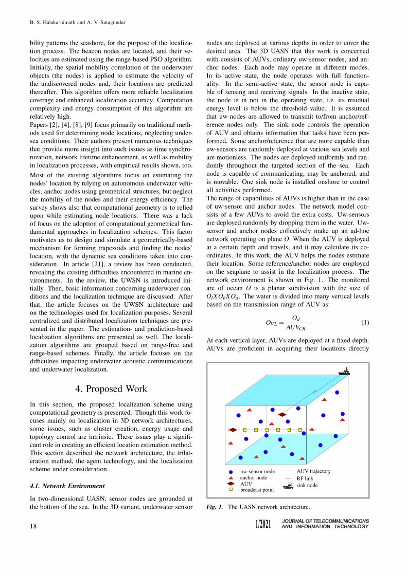
network environment is shown in Fig. 1. The monitored

are of ocean O is a planar subdivision with the size of

OlXObXOd . The water is divided into many vertical levels

based on the transmission range of AUV as:

OV L =Od

AUVCR. (1)

At each vertical layer, AUVs are deployed at a fixed depth.

AUVs are proficient in acquiring their locations directly

Fig. 1. The UASN network architecture.

18


Table 1

Abbreviations used

Definition Notation

Absorption model α(f)

Autonomous underwater vehicle AUV

Anchor ID AID

Trapezoid ID of anchor ANT

Neighbors of anchor’s node ANNT

Residual energy AER

Position of anchor A(X ,Y,Z)

AUV communication range AUVcr

Directive index DI

Detected threshold DT

Node energy threshold Eth

Geometrical spreading factor of propagation k

Length of the AUV’s linear trajectory L

Neighbor count NC

Node depth ND

Node ID Nid

Node’s trapezoid ID Ntid

Node position N(x,y,z)

Noise level NL

Propagation loss PL

Source level SL

from GPS. Assuming that the outline of each trapezoid Tior Tj (i, j≤ n) is disjoint without gaps and overlaps, i.e. the

trapezoid is located between Ti, j ⊆O and Ti∩Tj = /0, where

i, j≤ n. Since the AUV may transmit in all directions, sen-

sor nodes may be located in the upper and lower portions of

its linear trajectory. Anchor/reference nodes acquire their

positions whenever they are within the AUV’s transmission

range, by using the RSSI technique. Let us assume that the

deployment of anchor nodes forms a planar graph G(V, E),

where reference/anchor nodes are the vertices, and commu-

nication edges between these nodes are the segments/edges.

Table 1 presents the abbreviations used in this work.

4.2. Trilateration Method

Trilateration is a process of finding position by measuring

the distance using signal strengths from different sources.

In a trilateration scheme, the location of a uw-sensor ui may

be found if at least three localized nodes (signal sources)

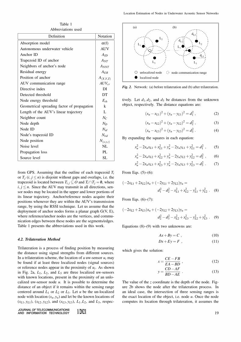
or reference nodes appear in the proximity of ui. As shown

in Fig. 2a, L1, L2, and L3 are three localized uw-sensors

with known locations, present in the proximity of an unlo-

calized uw-sensor node u. It is possible to determine the

distance of an object if it remains within the sensing range

centered around L1 or L2 or L3. Let u be the un-localized

node with location (xu,yu) and let be the known locations of

(xL1,yL1), (xL2,yL2), and (xL3,yL3), L1,L2, and L3, respec-

Fig. 2. Network: (a) before trilateration and (b) after trilateration.

tively. Let d1,d2, and d3 be distances from the unknown

object, respectively. The distance equations are:

(xu− xL1)2 +(yu− yL1)

2 = d21 , (2)

(xu− xL2)2 +(yu− yL2)

2 = d22 , (3)

(xu− xL3)2 +(yu− yL3)

2 = d23 . (4)

By expanding the squares in each equation:

x2u−2xuxL1 + x2

L1 + y2u−2yuyL1 + y2

L1 = d21 , (5)

x2u−2xuxL2 + x2


L2 = d22 , (6)

x2u−2xuxL3 + x2


L3 = d23 . (7)

From Eqs. (5)–(6):

(−2xL1 +2xL2)xu +(−2yL1 +2yL2)yu =

d21 −d2

2 − x2L1 + x2

L2− y2L1 + y2

L2 . (8)

From Eqs. (6)–(7):

(−2xL2 +2xL3)xu +(−2yL2 +2yL3)yu =

d22 −d2

3 − x2L2 + x2

L3− y2L2 + y2

L3 . (9)

Equations (8)–(9) with two unknowns are:

Ax+By = C , (10)

Dx+Ey = F , (11)

which gives the solution:

x =CE−FBEA−BD

, (12)

y =CD−AFBD−AE

. (13)

The value of the z coordinate is the depth of the node. Fig-

ure 2b shows the node after the trilateration process. In

an ideal case, the intersection of three sensing ranges is

the exact location of the object, i.e. node u. Once the node

computes its location through trilateration, it assumes the

19


role of a reference node R in order to further assist in deter-

mining the location of unlocalized nodes. In many cases,

distance computations are imprecise, because the sensing

range circles may not intersect at a single location. To

overcome this error, a maximum likelihood scheme may

be adopted to minimize the degree of imprecision in deter-

mining the location of a given node.

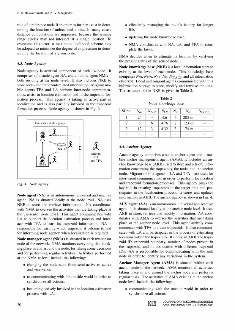
4.3. Node Agency

Node agency is acritical component of each uw-node. It

comprises of a static agent NA, and a mobile agent NMA –

both residing at the node level. It also includes NKB to

store node- and trapezoid-related information. Migrant mo-

bile agents TFA and LA perform inter-node communica-

tions, assist in location estimation and in the trapezoid for-

mation process. This agency is taking an active part in

localization and is also partially involved in the trapezoid

formation process. Node agency is shown in Fig. 3.

Fig. 3. Node agency.

Node agent (NA) is an autonomous, universal and reactive

agent. NA is situated locally at the node level. NA uses

NKB to store and retrieve information. NA coordinates

with NMA to oversee the activities that are taking place at

the uw-sensor node level. This agent communicates with

LA to support the location estimation process and inter-

acts with TFA to learn its trapezoid information. NA is

responsible for learning which trapezoid it belongs to and

for informing node agency when localization is required.

Node manager agent (NMA) is situated in each uw-sensor

node of the network. NMA monitors everything that is tak-

ing place in and around the node, for taking some decisions

and for performing regular activities. Activities performed

at the NMA at level include the following:

• changing the node state from semi-active to active

and vice-versa,

• to communicating with the outside world in order to

synchronize all actions,

• becoming actively involved in the location estimation

process with LA,

• effectively managing the node’s battery for longer

life,

• updating the node knowledge base,

• NMA coordinates with NA, LA, and TFA to com-

plete the tasks.

NMA decides when to estimate its location by verifying

the present status of the sensor node.

Node knowledge base (NKB) is a local information storage

existing at the level of each node. This knowledge base

comprises NID, NT ID, NER, ND, N(X ,Y,Z), and all information

observed. Local and migrant agents communicate with this

information storage to store, modify and retrieve the data.

The structure of the NKB is given in Table 2.

Table 2

Node knowledge base

Sl no. NID NT ID NER NC ND N(X ,Y,Z)

1 24 4 4.6 4 203 m –

2 5 6 4.76 2 123 m –

3 12 3 4.32 3 174 m –

4 – – – – – –

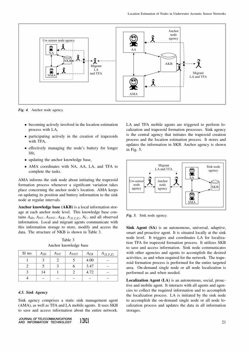
4.4. Anchor Agency

Anchor agency comprises a static anchor agent and a mo-

bile anchor management agent (AMA). It includes an an-

chor knowledge base (AKB) used to store and retrieve infor-

mation concerning the trapezoids, the node, and the anchor

node. Migrant mobile agents – LA and TFA – are used for

inter-agent communication in order to perform localization

and trapezoid formation processes. This agency plays the

key role in creating trapezoids in the target area and par-

ticipates in the localization process. It stores and updates

information in AKB. The anchor agency is shown in Fig. 4.

AUV agent (AA) is an autonomous, universal and reactive

agent. It is situated locally at the anchor node level. It uses

AKB to store, retrieve and modify information. AA coor-

dinates with AMA to oversee the activities that are taking

place at the anchor node level. This agent actively com-

municates with TFA to create trapezoids. It also communi-

cates with LA and participates in the process of estimating

locations within the trapezoids. It stores, in AKB, the trape-

zoid ID, trapezoid boundary, number of nodes present in

the trapezoid, and its association with different trapezoid

IDs. AA is responsible for communicating with the sink

node in order to identify any variations in the system.

Anchor Manager Agent (AMA) is situated within each

anchor node of the network. AMA monitors all activities

taking place in and around the anchor node and performs

regular tasks. The activities of AMA existing at the anchor

node level include the following:

• communicating with the outside world in order to

synchronize all actions,

20


Fig. 4. Anchor node agency.

• becoming actively involved in the location estimation

process with LA,

• participating actively in the creation of trapezoids

with TFA,

• effectively managing the node’s battery for longer

life,

• updating the anchor knowledge base,

• AMA coordinates with NA, AA, LA, and TFA to

complete the tasks.

AMA informs the sink node about initiating the trapezoid

formation process whenever a significant variation takes

place concerning the anchor node’s location. AMA keeps

on updating its position and battery information to the sink

node at regular intervals.

Anchor knowledge base (AKB) is a local information stor-

age at each anchor node level. This knowledge base con-

tains AID, ANT , ANNT , AER, A(X ,Y,Z), NC, and all observed

information. Local and migrant agents communicate with

this information storage to store, modify and access the

data. The structure of NKB is shown in Table 3.

Table 3

Anchor knowledge base

Sl no. AID ANT ANNT AER A(X ,Y,Z)

1 3 2 5 4.00 –

2 5 3 6 3.47 –

3 14 1 2 4.72 –

4 – – – – –

4.5. Sink Agency

Sink agency comprises a static sink management agent

(AMA), as well as TFA and LA mobile agents. It uses SKB

to save and access information about the entire network.

LA and TFA mobile agents are triggered to perform lo-

calization and trapezoid formation processes. Sink agency

is the central agency that initiates the trapezoid creation

process and the location estimation process. It stores and

updates the information in SKB. Anchor agency is shown

in Fig. 5.

Fig. 5. Sink node agency.

Sink Agent (SA) is an autonomous, universal, adaptive,

smart and proactive agent. It is situated locally at the sink

node level. It triggers and coordinates LA for localiza-

tion TFA for trapezoid formation process. It utilizes SKB

to save and access information. Sink node communicates

with other agencies and agents to accomplish the desired

activities, as and when required for the network. The trape-

zoid formation process is performed for the entire targeted

area. On-demand single node or all node localization is

performed as and when needed.

Localization Agent (LA) is an autonomous, social, proac-

tive and mobile agent. It interacts with all agents and agen-

cies to collect the required information and to accomplish

the localization process. LA is initiated by the sink node

to accomplish the on-demand single node or all node lo-

calization process and updates the data in all information

storages.

21


Trapezoid Formation Agent (TFA) is a mobile, self-

sufficient, proactive and social agent. The sink node trig-

gers TFA, and its primary objective is to create trapezoids

and to construct SDS for a given network. It communicates

with all agents and agencies to gather the required infor-

mation and to accomplish the trapezoid formation process.

It creates SDS during the creation of trapezoids. SDS is a

tree-based data structure that is better suited for the location

of trapezoids.

Sink Manager Agent (SMA) is situated in the network, at

the sink node. Its duties include the following:

• communicating with other components of the system

and synchronizing the actions,

• intimate sink agent to activate TFA through pre-

localization LA, while the localization, and maintain

SDS,

• associate in the location estimation process with LA

and trapezoid creation process with TFA,

• SMA manages, virtually, the batteries of the uw-

sensor and the anchor nodes, increasing their life,

• updating the SKB at regular intervals.

Sink Knowledge Base (SKB) is the sink node’s informa-

tion storage, accessible to TFA and LA mobile agents dur-

ing the trapezoid formation and localization process. This

knowledge base contains information on the energy level

of the entire network, on AUV’s trajectory, on trapezoid

information, as well as on the number of active and failed

nodes, as shown in Table 4. SA, SMA, LA, and TFA com-

municate with this information storage to retrieve, modify

and store information.

Table 4

Sink knowledge base

SN AID NID NT ID NER A/F Trajectory info

1 1 5 3 4.56 3/0 40 m, up

2 4 13 7 3.57 4/1 70 m, down

3 3 16 5 4.89 0/1 110 m, up

4 – – – – – –

4.6. Formation of Trapezoids

The sink node begins the process of creating clusters with

the support of TFA and AUV. AUV is deployed at fixed

depth levels of the ocean and traverses across the linear

trajectory. At each level of the linear trajectory, TFA acti-

vates the trapezoid formation model to divide the horizontal

plane into many vertical slabs whenever the anchor nodes

come within the transmission range of AUV, and it stores

the anchor nodes’ x coordinate in a structured manner on

the array, to create SDS. TFA divides each vertical slab

further into trapezoids, with the assistance of reference/an-

chor nodes. Each area of the vertical slab between two

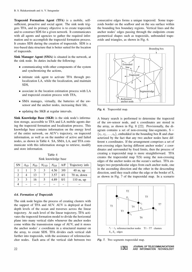
consecutive edges forms a unique trapezoid. Some trape-

zoids border on the seafloor and on the sea surface within

the bounding box boundary regions. Vertical lines and the

anchor nodes’ edges passing through the endpoints create

geometrical shapes such as trapezoids, unbounded trape-

zoids and triangles, as shown in Fig. 6.

Fig. 6. Trapezoidal map.

A binary search is performed to determine the trapezoid

of the uw-sensor node, and x coordinates are stored in

the array, as shown in Fig. 8 [22]. Provisionally, the di-

agram contains a set of non-crossing line-segments, S ={s1, s2, . . . ,sn}, embedded in the bounding box R and char-

acterized by the fact that any two anchor nodes have dif-

ferent x coordinates. If the arrangement comprises a set of

non-crossing edges having different anchor nodes’ x coor-

dinates and surrounded by fixed limits, then the process of

creating a trapezoidal map is more straightforward. TFA

creates the trapezoidal map T(S) using the non-crossing

edges of the anchor nodes on the ocean’s surface. TFA en-

larges two perpendicular edges from each anchor node, one

in the ascending direction and the other in the descending

direction, until they reach either the edge or the border of S,

as shown in Fig. 7 of the trapezoidal map. In a scenario

Fig. 7. Two segments trapezoidal map.

22


in which any two trapezoids are located next to each other,

then such trapezoids share a perpendicular edge. A double

connected edge is used in the formation of the trapezoidal

map.

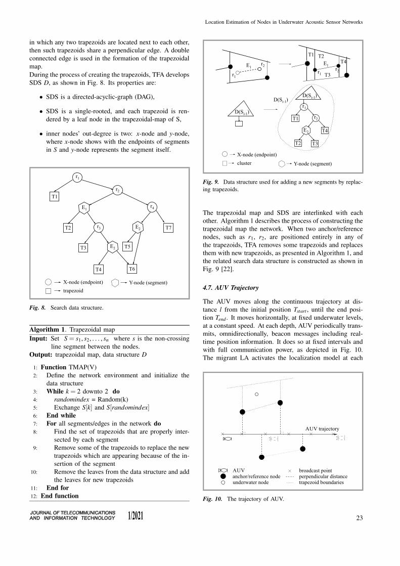
During the process of creating the trapezoids, TFA develops

SDS D, as shown in Fig. 8. Its properties are:

• SDS is a directed-acyclic-graph (DAG),

• SDS is a single-rooted, and each trapezoid is ren-

dered by a leaf node in the trapezoidal-map of S,

• inner nodes’ out-degree is two: x-node and y-node,

where x-node shows with the endpoints of segments

in S and y-node represents the segment itself.

Fig. 8. Search data structure.

Algorithm 1. Trapezoidal map

Input: Set S = s1, s2, . . . , sn where s is the non-crossing

line segment between the nodes.

Output: trapezoidal map, data structure D

1: Function TMAP(V)

2: Define the network environment and initialize the

data structure

3: While k = 2 downto 2 do

4: randomindex = Random(k)

5: Exchange S[k] and S[randomindex]6: End while

7: For all segments/edges in the network do

8: Find the set of trapezoids that are properly inter-

sected by each segment

9: Remove some of the trapezoids to replace the new

trapezoids which are appearing because of the in-

sertion of the segment

10: Remove the leaves from the data structure and add

the leaves for new trapezoids

11: End for

12: End function

Fig. 9. Data structure used for adding a new segments by replac-

ing trapezoids.

The trapezoidal map and SDS are interlinked with each

other. Algorithm 1 describes the process of constructing the

trapezoidal map the network. When two anchor/reference

nodes, such as r1, r2, are positioned entirely in any of

the trapezoids, TFA removes some trapezoids and replaces

them with new trapezoids, as presented in Algorithm 1, and

the related search data structure is constructed as shown in

Fig. 9 [22].

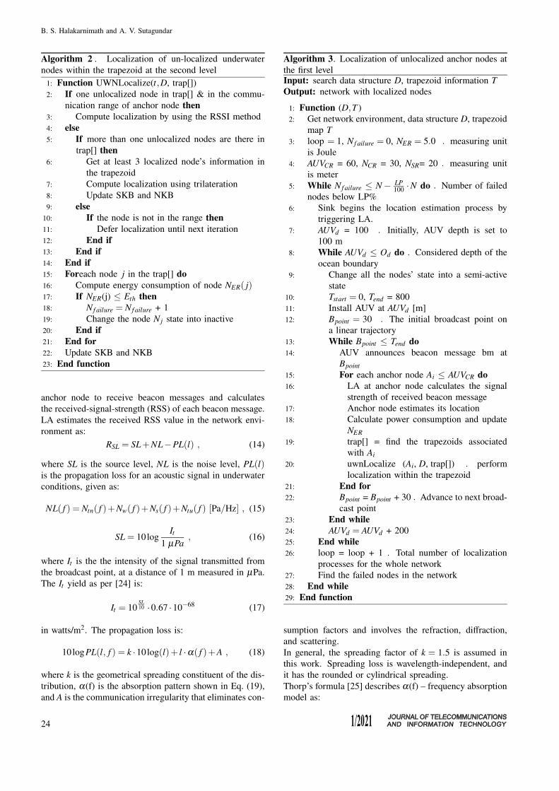
4.7. AUV Trajectory

The AUV moves along the continuous trajectory at dis-

tance l from the initial position Tstart , until the end posi-

tion Tend . It moves horizontally, at fixed underwater levels,

at a constant speed. At each depth, AUV periodically trans-

mits, omnidirectionally, beacon messages including real-

time position information. It does so at fixed intervals and

with full communication power, as depicted in Fig. 10.

The migrant LA activates the localization model at each

Fig. 10. The trajectory of AUV.

23


Algorithm 2 . Localization of un-localized underwater

nodes within the trapezoid at the second level

1: Function UWNLocalize(t,D, trap[])

2: If one unlocalized node in trap[] & in the commu-

nication range of anchor node then

3: Compute localization by using the RSSI method

4: else

5: If more than one unlocalized nodes are there in

trap[] then

6: Get at least 3 localized node’s information in

the trapezoid

7: Compute localization using trilateration

8: Update SKB and NKB

9: else

10: If the node is not in the range then

11: Defer localization until next iteration

12: End if

13: End if

14: End if

15: Foreach node j in the trap[] do

16: Compute energy consumption of node NER( j)17: If NER(j) ≤ Eth then

18: N f ailure = N f ailure + 1

19: Change the node N j state into inactive

20: End if

21: End for

22: Update SKB and NKB

23: End function

anchor node to receive beacon messages and calculates

the received-signal-strength (RSS) of each beacon message.

LA estimates the received RSS value in the network envi-

ronment as:

RSL = SL+NL−PL(l) , (14)

where SL is the source level, NL is the noise level, PL(l)is the propagation loss for an acoustic signal in underwater

conditions, given as:

NL( f ) = Ntn( f )+Nw( f )+Ns( f )+Ntu( f ) [Pa/Hz] , (15)

SL = 10logIt

1 µPa, (16)

where It is the the intensity of the signal transmitted from

the broadcast point, at a distance of 1 m measured in µPa.

The It yield as per [24] is:

It = 10SL10 ·0.67 ·10−68 (17)

in watts/m2. The propagation loss is:

10logPL(l, f ) = k ·10log(l)+ l ·α( f )+A , (18)

where k is the geometrical spreading constituent of the dis-

tribution, α(f) is the absorption pattern shown in Eq. (19),

and A is the communication irregularity that eliminates con-

Algorithm 3. Localization of unlocalized anchor nodes at

the first levelInput: search data structure D, trapezoid information TOutput: network with localized nodes

1: Function (D,T )

2: Get network environment, data structure D, trapezoid

map T3: loop = 1, N f ailure = 0, NER = 5.0 . measuring unit

is Joule

4: AUVCR = 60, NCR = 30, NSR= 20 . measuring unit

is meter

5: While N f ailure ≤ N− LP100 ·N do . Number of failed

nodes below LP%

6: Sink begins the location estimation process by

triggering LA.

7: AUVd = 100 . Initially, AUV depth is set to

100 m

8: While AUVd ≤ Od do . Considered depth of the

ocean boundary

9: Change all the nodes’ state into a semi-active

state

10: Tstart = 0, Tend = 800

11: Install AUV at AUVd [m]

12: Bpoint = 30 . The initial broadcast point on

a linear trajectory

13: While Bpoint ≤ Tend do

14: AUV announces beacon message bm at

Bpoint15: For each anchor node Ai ≤ AUVCR do

16: LA at anchor node calculates the signal

strength of received beacon message

17: Anchor node estimates its location

18: Calculate power consumption and update

NER19: trap[] = find the trapezoids associated

with Ai20: uwnLocalize (Ai, D, trap[]) . perform

localization within the trapezoid

21: End for

22: Bpoint = Bpoint + 30 . Advance to next broad-

cast point

23: End while

24: AUVd = AUVd + 200

25: End while

26: loop = loop + 1 . Total number of localization

processes for the whole network

27: Find the failed nodes in the network

28: End while

29: End function

sumption factors and involves the refraction, diffraction,

and scattering.

In general, the spreading factor of k = 1.5 is assumed in

this work. Spreading loss is wavelength-independent, and

it has the rounded or cylindrical spreading.

Thorp’s formula [25] describes α(f) – frequency absorption

model as:

24


α( f ) =

(

0.11f 2

f 2 +1+44

f 2

f 2 +4100

+2.75 ·10−4 f 2 +0.003)

·10−3 . (19)

Consider any announcement position is (x, y, z) along the

AUV’s linear path at each depth level, and (xr, yr, zr) being

any anchor node position on the ocean’s surface. z is 0, and

the y coordinate is linearly expressed by x due to the AUV’s

path, which is linear on the ocean’s surface. LA gets the

RSSI value vector of all announcement points and the x co-

ordinate vector of the announcement points and estimates

the position of an anchor node by using RSSI. Once the ref-

erence/anchor nodes have learned their locations, LA visits

each trapezoid and calculates the location of unlocalized

nodes, as described in Algorithm 2. Algorithm 3 describes

the process of estimating the location of nodes.

4.8. Single-node Localization

If a node moves within the trapezoid due to underwater

currents or other aquatic characteristics, then NA may de-

mand localization by asking the anchor node. The anchor

node initiates the location estimation process by triggering

LA and the procedure is given in Algorithm 4.

Algorithm 4. On-demand single-node localization

1: Function SN Localization(NID)2: The node realizes the need for location estimation

3: Uw-sensor transmits a request message to the anchor

node about the need for localization

4: Anchor node informs the sink node about the ini-

tiation of the localization process and provides

node details

5: Anchor triggers LA to initiate the localization pro-

cess

6: LA gets the information of NID and anchor node of

NID7: LA gets the trapezoid-id of NID using search-data-

structure

8: LA visits to trapezoid-id for localization

9: If LA finds at least 3 localized nodes (including an-

chor node) within the communication range of NIDin the trapezoid then

10: LA estimates the location of NID using the tri-

lateration technique

11: else

12: If LA finds NID is within the communication

range of anchor node then

13: LA estimates the location of NID using RSSI

14: else

15: Defer the location estimation process until the

next trapezoid formation process.

16: End if

17: End if

18: End function

The sink node initiates all-node localization at regular in-

tervals. The scheme is as below:

1. The sink node begins the trapezoid formation activ-

ity at each iteration by TFA. TFA divides the region

into perpendicular slabs and further divides these into

trapezoids. TFA counts the number of localized and

unlocalized nodes present in each trapezoid. TFA

stores relevant information in SKB, i.e. information

storage of the sink node, and also creates search data

structure D.

2. The sink node begins the localization process through

LA and deploys AUV at various depth levels. AUV

traverses along the linear trajectory from starting

point Tstart to endpoint Tend at each depth, with a con-

stant speed. AUV transmits beacon messages includ-

ing real time location information at fixed distances

and with a fixed transmission power, as depicted in

Fig. 10. At the anchor node, the LA receives these

messages and executes the localization model to es-

timate its location.

3. The anchor agent at each anchor node initiates the

localization process in its assigned trapezoids based

on the data given by TFA and SDS D.

4. At each trapezoid, LA performs the localization pro-

cess in the following manner:

• if the node is already localized, then LA updates

the localization knowledge base with such infor-

mation as uw-sensor node ID, uw-sensor node

energy level, trapezoid ID, adjacent trapezoids,

etc. LA changes its state from semi-active to

active;

• if the node is unlocalized, then LA looks for

at least three localized nodes which are there in

the trapezoids, within the communication range,

completes the localization process by using the

trilateration technique and changes the node sta-

tus into active;

• if the uw-sensor node is unlocalized and it is

within the communication range of the anchor

node, then LA applies the RSSI method to es-

timate its location;

• if an unlocalized uw-sensor node exists in the

trapezoid and it is out of the communication

range of the anchor node and of other nodes,

then the localization process is deferred until

the next iteration;

• the above steps are repeated to localize other

nodes in the trapezoid. LA changes the state of

all localized nodes from semi-active to active.

5. LA updates location-related information in SKB,

AKB, and NKB for future use.

25


6. Steps 1–5 are repeated until AUV reaches Tend of

each linear trajectory.

7. AUV is deployed at the next vertical level and repeats

steps 1–6 to cover the entire targeted area.

8. At the end of each localization period, all the under-

water sensor nodes change their status to semi-active

in order to preserve their energy levels.

Algorithm 2 describes the localization process within the

trapezoids.

4.9. Mobility in the Localization Problem

Movement of the nodes is unavoidable due to underwa-

ter currents and other underwater conditions. Each NA

maintains NKB, containing such information such as en-

ergy level, neighbor count and location points. The move-

ment of a node is severe in shallow waters due to numerous

human activities and unpredictable behavior of the sea envi-

ronment. On the contrary, in deep water, most of the time,

the movement of the nodes is not present at all or is very

much restricted. The agent may perform self-localization

in deep water by itself, provided the node is in communi-

cation with at least one node which knows its location. If

node A is already localized with NA(x,y) points and if NA ob-

serves that the node has changed its position, then LA at the

node performs re-localization, with the process explained

below:

1. LA obtains the location of the previous uw-sensor

node from the NKB and stores it as NPA(x,y) , and

NPAdepth (i.e. NP is the previous location of the node).

2. LA computes the distance to the uw-sensor node, i.e.

Ndist = Nspeed ·Nδ t , where Nδ t is the time difference

between the last localized time and the agent’s ob-

servation time, Nspeed is the speed of the uw-sensor

node, Ndist is the distance which is scalable. The

current position of the node is calculated as:

• assign NCAdepth = Get(ND), NC is the current

location of the uw-sensor node,

• compute d = NPAdepth −NCAdepth ,

• test if (d ≤ 0) and then NCAy = NPAy + d, i.e.

the node is moved downwards down,

• test if (d ≥ 0) and then NCAy = NPAy − d, i.e.

the node moved upwards.

3. Now, the location of mobile node A is (NCA? , NCAy ),

where the x coordinate is unknown. The distance

formula may be applied to find out the x coordinate

if the mobile node is capable of communicating with

at least one localized uw-sensor node, i.e. node B

with location (NCBx , NCBy ).

4. Find distance D between nodes A and B using RSSI.

5. RSSI = antenna gain + transmit power – path loss.

6. For non-mobile nodes A and B, antenna gain and

transmit power are both constant. Path loss is the

function of distance d. Hence, RSSI = f (d), d =f ′(RSSI).

7. For simplicity, consider node A points as (x1, y1)

instead of (NCA? , NCAy ) and node B points as (x2, y2)

instead of (NCBx , NCBy ) Calculate the unknown x1value by:

d =√

(x2− x1)2 +(y2− y1)2 . (20)

By taking a square on both the sides, we get:

d2 = (x2− x1)2 +(y2− y1)

2 , (21)

and:

d2− (y2− y1)2 = (x2− x1)

2 , (22)

where d, y1, y2 are known values. After solving RHS,

a constant value v becomes:

v = (x2− x1)2 . (23)

After removing the square on both sides Eq. (23)

becomes: √v = (x2− x1) , (24)

then:

x1 = x2−√

v . (25)

Now, the x coordinate of node A is computed and

the y coordinate is computed in Step 2.

8. The agent performed internal localization, and the

new coordinates of mobile node A are (NCAx , NCAy ).

The proposed work highlights the use of computational

geometry for estimating the location of unlocalized nodes.

It is supported by agent technology, which supports vari-

ous APIs for during the implementation phase. Modules for

trapezoid creation, SDS establishment and trajectory path

formation are designed using mathematical models and may

be implemented with suitable modifications. Anchor/refer-

ence nodes are considered at each stage of the proposed

work, and are therefore included in trapezoid creation, tra-

jectory path formation, SDS creation and location estima-

tion modules. Regular nodes predominantly included in

location estimation and mobility modules.

5. Simulation

The proposed uw-sensor node localization method is sim-

ulated and assessed based on various parameters. At the

initial stage of the simulation, all nodes are considered to be

characterized by equal power, equal sensing range and equal

transmission capability. The sink node switches all nodes

into semi-active state to preserve energy. The node location

estimation process is performed iteratively. At each step,

26


most of the nodes attempt to localize themselves and con-

sume energy. The simulation is terminated when the energy

level of 70% of all nodes falls below a specific threshold

value. Simulation models, procedures and performance pa-

rameters are discussed in this section.

5.1. Simulation Model

A monitored area with the size of 600×600×600 m is used

for UASN simulation purposes. Initially, uw-sensor nodes

are deployed randomly, beginning with 20 and with their

number increasing to 100 within the 3D space. Initially,

the sink node deploys AUV at AUVd and it then moves

along a continuing trajectory. AUV broadcasts location

information at regular intervals, 5L is set to 30 m. At

each vertical level, AUV travels linearly over a distance

of 600 m, with fixed frequency Tf = 24 kHz, sound level

SL = 100 dB and spreading factor k = 1.5. A few anchor

nodes are deployed randomly. A beacon message advances

linearly at a velocity of one m/s and makes announcements

one second intervals. The sink node is installed onshore.

In the propagation model, sensing range NSR, communica-

tion range NCR of an acoustic UASN node for single hop

communication and attenuation factor α( f ) are given in

Eq. (19), as per Ainslie and McColm [26].

Table 5

Simulation input data

Parameter Value

Width w 600 m

Length l 600 m

Depth d 600 m

Uw-sensor nodes n 100

Uw-sensor node communication range NCR 30 m

Temperature range 2–20◦CAUV communication range AUVCR 60 m

Anchor nodes 30

Transmission frequency Tf 24 kHz

Attenuation α 0.01-1.0

SL 100 dB

δL 30 m

Speed of ship v 5 m/s

k 1.5

The performance parameters are:

Localization ratio. It is the ratio of localized uw-sensor

nodes to the total number uw-sensor nodes in the network.

Energy consumption. It is calculated as total power con-

sumption of all nodes in one iteration. To obtain intensity

It with communication power Pt at an interval of 1 m from

the origin towards the recipient as per [24], the following

equation is used:

Pt = 2π D/t ·1 [m] , (26)

in watts, where D is the depth measured in meters and Itis taken from Eq. (17).

In each trapezoid, power consumption of m localized uw-

sensor nodes involved in the trilateration of packet size Psize,

is:

Pc =mPsize

m1024=

Psize

1024(27)

in watts/bit. Assume Ttactive is the total active time of a uw-

sensor node’s transceiver in seconds, per one iteration,

NER is the residual energy available at every uw-sensor

node in w/h. The ratio of the total residual energy to the

power required for one packet is the total active time of the

transceiver and is given by:

Tactive =NER

Pc. (28)

Since the uw-sensor node operates in different states, its

transceiver’s active period equals A seconds, and the node’s

battery life is given by:

Tli f etime =Tactive

Ttactive· A

24 ·60[days] . (29)

Localization accuracy. It’s the difference between the

original and the estimated location. If NE(x,y,z) is the calcu-

lated location of node and NA(x,y,z) is the original location,

localization accuracy is given as:

LE = |NE(x,y,z0−NA(x,y,z)| . (30)

The average location error is:

LEavg =1n

n

∑i=1

LEi . (31)

The location error is a vital factor if it is larger than a spec-

ified threshold value.

Network lifetime. It is the number of times the location

estimation process is performed until the energy level of

70% of the deployed uw-sensor nodes falls below a speci-

fied threshold value. To calculate it, we need to first obtain

the number of uw-sensor nodes m whose power level is

greater than the threshold value, i.e. the number of nodes mif (Tli f etime(i) ≤ Eth) for every node i in the system. To

ensure the network is connected, let PN be the percentage

share of uw-sensor nodes whose energy level is higher than

the threshold value. Here, Tli f etime is the total lifetime of

a uw-sensor node:

Nstable =PN

100·n , (32)

if m ≥ (n−Nstable), the network fails. The location es-

timation process is repeated after a specific condition is

satisfied.

5.2. Simulation Procedure

The proposed MASD scheme relies on specific simulation

parameters and the simulation process is repeated until 70%

27


of the uw-sensor nodes retain energy levels that are higher

than a specific threshold value. Algorithm 5 presents the

simulation procedure using pseudo-code.

Algorithm 5. Simulation procedure

1: Function Simulation

2: Setup the network system

3: Initialize agencies, nodes, state, knowledge base

4: Defining the AUVs trajectory

5: Formation of trapezoids by TFA over defined ocean

volume.

6: While energy of 70% of nodes higher than specified

threshold do

7: AUV moves along a fixed linear path

8: AUV announces beacon messages containing

real-time location

9: Anchor nodes re-localize themselves

10: LA begins location estimation process at each

trapezoid

11: LA stores the necessary data in the knowledge-

bases

12: End while

13: Convert uw-sensor node status into a semi-active

state after localization

14: End function

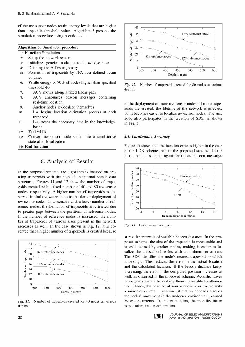
6. Analysis of Results

In the proposed scheme, the algorithm is focused on cre-

ating trapezoids with the help of an internal search data

structure. Figures 11 and 12 show the number of trape-

zoids created with a fixed number of 40 and 80 uw-sensor

nodes, respectively. A higher number of trapezoids is ob-

served in shallow waters, due to the denser deployment of

uw-sensor nodes. In a scenario with a lower number of ref-

erence nodes, the formation of trapezoids is restricted due

to greater gaps between the positions of reference nodes.

If the number of reference nodes is increased, the num-

ber of trapezoids of various sizes present in the network

increases as well. In the case shown in Fig. 12, it is ob-

served that a higher number of trapezoids is created because

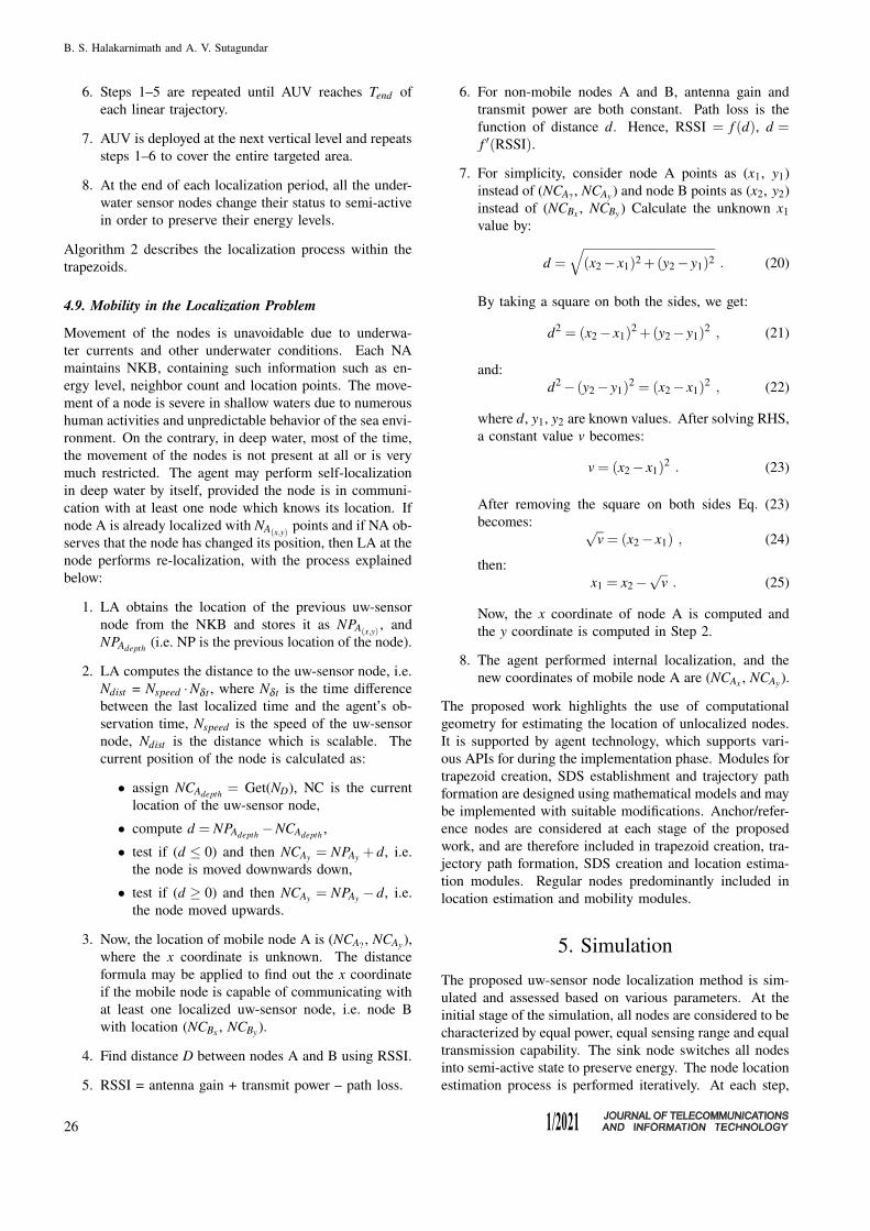
Fig. 11. Number of trapezoids created for 40 nodes at various

depths.

Fig. 12. Number of trapezoids created for 80 nodes at various

depths.

of the deployment of more uw-sensor nodes. If more trape-

zoids are created, the lifetime of the network is affected,

but it becomes easier to localize uw-sensor nodes. The sink

node also participates in the creation of SDS, as shown

in Fig. 8.

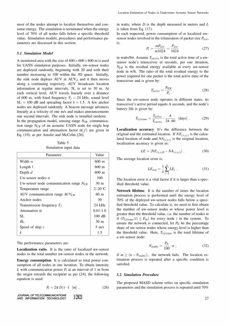
6.1. Localization Accuracy

Figure 13 shows that the location error is higher in the case

of the LDB scheme than in the proposed scheme. In the

recommended scheme, agents broadcast beacon messages

Fig. 13. Localization accuracy.

at regular intervals of variable beacon distance. In the pro-

posed scheme, the size of the trapezoid is measurable and

is well defined by anchor nodes, making it easier to lo-

calize the unlocalized nodes with a minimum error rate.

The SDS identifies the node’s nearest trapezoid to which

it belongs. This reduces the error in the actual location

and the calculated location. If the beacon distance keeps

increasing, the error in the computed position increases as

well, as observed in the proposed scheme. Acoustic waves

propagate spherically, making them vulnerable to attenua-

tion. Hence, the position of sensor nodes is estimated with

a minor error rate. Location estimation depends also on

the nodes’ movement in the undersea environment, caused

by water currents. In this calculation, the mobility factor

is not taken into consideration.

28


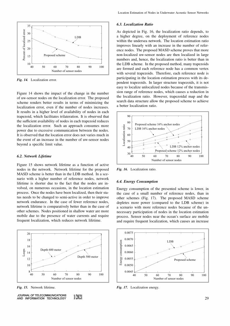
Fig. 14. Localization error.

Figure 14 shows the impact of the change in the number

of uw-sensor nodes on the localization error. The proposed

scheme renders better results in terms of minimizing the

localization error, even if the number of nodes increases.

It results in a higher level of availability of nodes in each

trapezoid, which facilitates trilateration. It is observed that

the sufficient availability of nodes in each trapezoid reduces

the localization error. Such an approach consumes more

power due to excessive communication between the nodes.

It is observed that the location error does not varies much in

the event of an increase in the number of uw-sensor nodes

beyond a specific limit value.

6.2. Network Lifetime

Figure 15 shows network lifetime as a function of active

nodes in the network. Network lifetime for the proposed

MASD scheme is better than in the LDB method. In a sce-

nario with a higher number of reference nodes, network

lifetime is shorter due to the fact that the nodes are in-

volved, on numerous occasions, in the location estimation

process. Once the nodes have been localized, then their sta-

tus needs to be changed to semi-active in order to improve

network endurance. In the case of fewer reference nodes,

network lifetime is comparatively better than in the case of

other schemes. Nodes positioned in shallow water are more

mobile due to the presence of water currents and require

frequent localization, which reduces network lifetime.

Fig. 15. Network lifetime.

6.3. Localization Ratio

As depicted in Fig. 16, the localization ratio depends, to

a higher degree, on the deployment of reference nodes

within the undersea network. The location estimation ratio

improves linearly with an increase in the number of refer-

ence nodes. The proposed MASD scheme proves that more

non-localized uw-sensor nodes are then localized in large

numbers and, hence, the localization ratio is better than in

the LDB scheme. In the proposed method, many trapezoids

are formed and each reference node has a common vertex

with several trapezoids. Therefore, each reference node is

participating in the location estimation process with its de-

pendent trapezoids. In larger structure trapezoids, it is not

easy to localize unlocalized nodes because of the transmis-

sion range of reference nodes, which causes a reduction in

the localization ratio. However, trapezoidal map and the

search data structure allow the proposed scheme to achieve

a better localization ratio.

Fig. 16. Localization ratio.

6.4. Energy Consumption

Energy consumption of the presented scheme is lower, in

the case of a small number of reference nodes, than in

other schemes (Fig. 17). The proposed MASD scheme

depletes more power (compared to the LDB scheme) in

a scenario with more reference nodes because of the un-

necessary participation of nodes in the location estimation

process. Sensor nodes near the ocean’s surface are mobile

and require frequent localization, which causes an increase

Fig. 17. Localization energy.

29


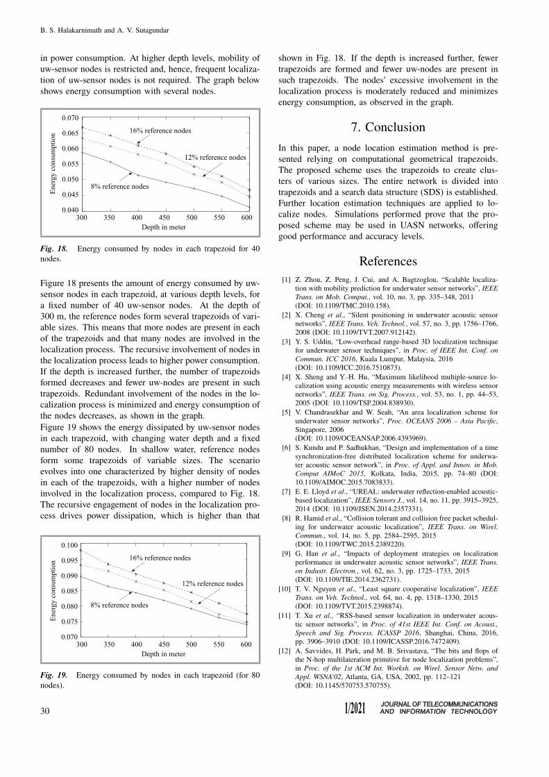
in power consumption. At higher depth levels, mobility of

uw-sensor nodes is restricted and, hence, frequent localiza-

tion of uw-sensor nodes is not required. The graph below

shows energy consumption with several nodes.

Fig. 18. Energy consumed by nodes in each trapezoid for 40

nodes.

Figure 18 presents the amount of energy consumed by uw-

sensor nodes in each trapezoid, at various depth levels, for

a fixed number of 40 uw-sensor nodes. At the depth of

300 m, the reference nodes form several trapezoids of vari-

able sizes. This means that more nodes are present in each

of the trapezoids and that many nodes are involved in the

localization process. The recursive involvement of nodes in

the localization process leads to higher power consumption.

If the depth is increased further, the number of trapezoids

formed decreases and fewer uw-nodes are present in such

trapezoids. Redundant involvement of the nodes in the lo-

calization process is minimized and energy consumption of

the nodes decreases, as shown in the graph.

Figure 19 shows the energy dissipated by uw-sensor nodes

in each trapezoid, with changing water depth and a fixed

number of 80 nodes. In shallow water, reference nodes

form some trapezoids of variable sizes. The scenario

evolves into one characterized by higher density of nodes

in each of the trapezoids, with a higher number of nodes

involved in the localization process, compared to Fig. 18.

The recursive engagement of nodes in the localization pro-

cess drives power dissipation, which is higher than that

Fig. 19. Energy consumed by nodes in each trapezoid (for 80

nodes).

shown in Fig. 18. If the depth is increased further, fewer

trapezoids are formed and fewer uw-nodes are present in

such trapezoids. The nodes’ excessive involvement in the

localization process is moderately reduced and minimizes

energy consumption, as observed in the graph.

7. Conclusion

In this paper, a node location estimation method is pre-

sented relying on computational geometrical trapezoids.

The proposed scheme uses the trapezoids to create clus-

ters of various sizes. The entire network is divided into

trapezoids and a search data structure (SDS) is established.

Further location estimation techniques are applied to lo-

calize nodes. Simulations performed prove that the pro-

posed scheme may be used in UASN networks, offering

good performance and accuracy levels.

References

[1] Z. Zhou, Z. Peng, J. Cui, and A. Bagtzoglou, “Scalable localiza-

tion with mobility prediction for underwater sensor networks”, IEEE

Trans. on Mob. Comput., vol. 10, no. 3, pp. 335–348, 2011

(DOI: 10.1109/TMC.2010.158).

[2] X. Cheng et al., “Silent positioning in underwater acoustic sensor

networks”, IEEE Trans. Veh. Technol., vol. 57, no. 3, pp. 1756–1766,

2008 (DOI: 10.1109/TVT.2007.912142).

[3] Y. S. Uddin, “Low-overhead range-based 3D localization technique

for underwater sensor techniques”, in Proc. of IEEE Int. Conf. on

Commun. ICC 2016, Kuala Lumpur, Malaysia, 2016

(DOI: 10.1109/ICC.2016.7510873).

[4] X. Sheng and Y.-H. Hu, “Maximum likelihood multiple-source lo-

calization using acoustic energy measurements with wireless sensor

networks”, IEEE Trans. on Sig. Process., vol. 53, no. 1, pp. 44–53,

2005 (DOI: 10.1109/TSP.2004.838930).

[5] V. Chandrasekhar and W. Seah, “An area localization scheme for

underwater sensor networks”, Proc. OCEANS 2006 – Asia Pacific,

Singapore, 2006

(DOI: 10.1109/OCEANSAP.2006.4393969).

[6] S. Kundu and P. Sadhukhan, “Design and implementation of a time

synchronization-free distributed localization scheme for underwa-

ter acoustic sensor network”, in Proc. of Appl. and Innov. in Mob.

Comput AIMoC 2015, Kolkata, India, 2015, pp. 74–80 (DOI:

10.1109/AIMOC.2015.7083833).

[7] E. E. Lloyd et al., “UREAL: underwater reflection-enabled acoustic-

based localization”, IEEE Sensors J., vol. 14, no. 11, pp. 3915–3925,

2014 (DOI: 10.1109/JSEN.2014.2357331).

[8] R. Hamid et al., “Collision tolerant and collision free packet schedul-

ing for underwater acoustic localization”, IEEE Trans. on Wirel.

Commun., vol. 14, no. 5, pp. 2584–2595, 2015

(DOI: 10.1109/TWC.2015.2389220).

[9] G. Han et al., “Impacts of deployment strategies on localization

performance in underwater acoustic sensor networks”, IEEE Trans.

on Industr. Electron., vol. 62, no. 3, pp. 1725–1733, 2015

(DOI: 10.1109/TIE.2014.2362731).

[10] T. V. Nguyen et al., “Least square cooperative localization”, IEEE

Trans. on Veh. Technol., vol. 64, no. 4, pp. 1318–1330, 2015

(DOI: 10.1109/TVT.2015.2398874).

[11] T. Xu et al., “RSS-based sensor localization in underwater acous-

tic sensor networks”, in Proc. of 41st IEEE Int. Conf. on Acoust.,

Speech and Sig. Process. ICASSP 2016, Shanghai, China, 2016,

pp. 3906–3910 (DOI: 10.1109/ICASSP.2016.7472409).

[12] A. Savvides, H. Park, and M. B. Srivastava, “The bits and flops of

the N-hop multilateration primitive for node localization problems”,

in Proc. of the 1st ACM Int. Worksh. on Wirel. Sensor Netw. and

Appl. WSNA’02, Atlanta, GA, USA, 2002, pp. 112–121

(DOI: 10.1145/570753.570755).

30


[13] A. Savvides, C. C. Han and M. B. Srivastava, “Dynamic fine-grained

localization in ad hoc networks of sensors”, in Proc. of the 7th Ann.

Int. Conf. on Mob. Comput. and Network. MobiCom’01, Rome, Italy,

2001, pp. 166–179, 2001

(DOI: https://doi.org/10.1145/381677.381693).

[14] G. Zhu et al., “A distributed localization scheme based on mobility

prediction for underwater wireless sensor networks”, in Proc. of the

26th Chinese Contr. and Decision Conf. CCDC 2014, Changsha,

China, 2014, pp. 4863–4867 (DOI: 10.1109/CCDC.2014.6853044).

[15] S. Lee and K. Kim, “Localization with a mobile beacon in under-

water acoustic sensor networks”, Sensors, vol. 12, no. 5, pp. 5486–

5501, 2012 (DOI: 10.3390/s120505486).

[16] Y. Sun et al., “A mobile anchor node assisted RSSI localization

scheme in underwater wireless sensor networks”, Sensors, vol. 19,

no. 20, 2019 (DOI: 10.3390/s19204369).

[17] C. Zhang et al., “A collaborative localization algorithm for UASNs”,

in Proc. of the Int. Conf. on Comput., Manag. and Telecommun.

ComManTel 2014, Da Nang, Vietnam, 2014, pp. 211–216

(DOI: 10.1109/ComManTel.2014.6825606).

[18] J. Gao et al., “A double rate localization algorithm with one anchor

for multi-hop underwater acoustic networks”, Sensors, vol. 17, no. 5,

pp. 984–1001, 2017 (DOI: 10.3390/s17050984.

[19] M. Beniwal, R. P. Singh, and A. Sangwan, “A localization scheme for

underwater sensor networks without time synchronization”, Wirel.

Pers. Commun., vol. 88, no. 3, 2016

(DOI: 10.1007/s11277-016-3175-2).

[20] Y. Zhang, J. Liang, S. Jiang, and W. Chen, “A localization method

for underwater wireless sensor networks based on mobility prediction

and particle swarm optimization algorithms”, Sensors, vol. 16, no. 2,

pp. 212, 2016 DOI: https://dx.doi.org/10.3390/s16020212.

[21] Xin Su, I. Ullah, X. Liu, and D. Choi, “A review of underwater

localization techniques algorithms and challenges”, J. of Sensors,

vol. 2020, no. 1, pp. 1–24, 2020 (DOI: 10.1155/2020/6403161).

[22] M. de Berg et al., Computational Geometry, 3 ed. Berlin, Heidel-

berg: Springer, 1983 (ISBN: 9783540779742).

[23] B. Zhang et al., “Received signal strength-based underwater acous-

tic localization considering stratification effect”, in Proc. of the

OCEANS 2016, Shanghai, China, 2016

(DOI: 10.1109/OCEANSAP.2016.7485561).

[24] R. J. Urick, Principles of Underwater Sound, 1 ed. New York:

McGraw-Hill, 1983 (ISBN: 9780070660878).

[25] W. H. Thorp, “Analytic description of the low frequency attenuation

coefficient”, J. of Acoustic. Soc. of America, vol. 42, no. 1, pp. 270,

1967 (DOI: 10.1121/1.1910566).

[26] W. Zhang et al., “Fault-tolerant relay node placement in wireless

sensor networks: Problems and algorithms”, in Proc. of the 26th

IEEE Int. Conf. on Comp. Commun. INFOCOM 2007, Barcelona,

Spain, 2007, pp. 1649–1657 (DOI: 10.1109/INFCOM.2007.193).

B. S. Halakarnimath received

his B.E. and M.Tech. degrees

in Computer Science and En-

gineering from VTU, Belagavi,

Karnataka, India. Presently, he

is a VTU research scholar pur-

suing his Ph.D. under the guid-

ance of Dr. A. V. Sutagundar, at

Basaveshwar Engineering Col-

lege, Bagalkot, Karnataka, In-

dia. He has authored one book

chapter and published five conference and journal papers.

His research areas include underwater acoustic wireless

sensor networks, machine learning, and algorithms. He

is a life member of IEI and ISTE organizations.

E-mail: [email protected]

Research Scholar of VTU

Department of Computer Science and Engineering

S.G. Balekundri Institute of Technology

Belagavi-590010, Karnataka, India

A. V. Sutagundar received his

B.E. and M.Tech. degrees in

Electronics and Communica-

tion Engineering from VTU,

Belagavi, Karnataka, India. He

received his Ph.D. in 2013

from VTU, Belagavi, India.

Presently, he is working as an

Associate Professor at the De-

partment of ECE, Basaveshwar

Engineering College, Bagalkot,

Karnataka, India. He has authored eight book chapters and

published more than 75 papers at international conferences

and in various journals. His research areas include IoT,

wireless sensor networks, machine learning, and digital

image processing.

E-mail: [email protected]

Department of Electronics and Communication

Basaveshwar Engineering College

Bagalkot-587102, Karnataka, India

31

Documents

Location Estimation of Nodes in Underwater Acoustic Sensor