Embed Size (px)
Citation preview
logcondens: Computations Related to Univariate
Log-Concave Density Estimation
Lutz DumbgenUniversity of Bern
Kaspar RufibachUniversity of Zurich
Abstract
Maximum likelihood estimation of a log-concave density has attracted considerableattention over the last few years. Several algorithms have been proposed to estimate sucha density. Two of those algorithms, an iterative convex minorant and an active set algo-rithm, are implemented in the R package logcondens. While these algorithms are discussedelsewhere, we describe in this paper the use of the logcondens package and discuss func-tions and datasets related to log-concave density estimation contained in the package. Inparticular, we provide functions to (1) compute the maximum likelihood estimate (MLE)as well as a smoothed log-concave density estimator derived from the MLE, (2) evaluatethe estimated density, distribution and quantile functions at arbitrary points, (3) computethe characterizing functions of the MLE, (4) sample from the estimated distribution, andfinally (5) perform a two-sample permutation test using a modified Kolmogorov-Smirnovtest statistic. In addition, logcondens makes two datasets available that have been usedto illustrate log-concave density estimation.
Keywords: log-concave, density estimation, Kolmogorov-Smirnov test, R.
1. Introduction
1.1. About this document
Although first uploaded to CRAN in 2006, a detailed description (beyond the package manual)of the functionality of the R package logcondens (Rufibach and Dumbgen 2010) had beenlacking so far. This document is an introduction to logcondens, based on Dumbgen andRufibach (2010), that not only discusses and illustrates the use of the implemented iterativeconvex minorant (ICMA) and the active set algorithm (ASA), but more functions thatare useful in connection with univariate log-concave density estimation. The package alsoprovides functions to evaluate quantities whose explicit computations are not immediate,such as distribution and quantile functions, the smoothed log-concave density estimator andthe corresponding distribution function, sampling from the different estimators, and a two-sample permutation test. In addition, the data sets analyzed in Dumbgen and Rufibach(2009) and Koenker and Mizera (2010) are provided as part of logcondens. Using the formerof these datasets we illustrate how logcondens can be used to explore data. The packageis available from the Comprehensive R Archive Network at http://CRAN.R-project.org/
package=logcondens.
2 logcondens: Computations Related to Univariate Log-Concave Density Estimation
This document was created using Sweave (Leisch 2002), LATEX (Knuth 1984; Lamport 1994),and R (R Development Core Team 2010). This means that all of the code has been checkedby R.
1.2. Log-concave density estimation
One way to nonparametrically estimate a density from univariate i.i.d. data is imposinga qualitative constraint such as monotonicity, convexity, or log-concavity. In contrast tosmoothing methods such as kernel estimation or roughness penalization, methods relyingon shape constraints are fully automatic, i.e. they do not necessitate any choice of tuningparameters such as a bandwidth or a penalty parameter. Choosing these tuning parameters isnotoriously involved, since typically their optimal values depend on properties of the unknowndensity to be estimated. To fix notation, let f be a probability density on R. We call f log-concave if it may be written as
f(x) = expϕ(x)
for some concave function ϕ : R → [−∞,∞). Based on a sample of i.i.d. random variablesX1, . . . , Xn ∈ R from f we seek to estimate this density via maximizing the normalizedlog-likelihood function
`(ϕ) = n−1n∑i=1
log f(Xi) = n−1n∑i=1
ϕ(Xi)
over all concave functions ϕ : R→ [−∞,∞) such that∫
expϕ(x) dx = 1. The resulting max-
imum likelihood estimators (MLEs) of ϕ and f are denoted by ϕ and f = exp ϕ, respectively.
Dumbgen and Rufibach (2009) show that the maximizer ϕ of ` is unique, piecewise linearon the interval [X(1), X(n)] with knots only at (some of the) observations X(i), and ϕ = −∞elsewhere. Here X(1) ≤ X(2) ≤ · · · ≤ X(n) are the ordered observations, and a “knot” of ϕ
is a location where this function changes slope. The MLEs ϕ, f and F are consistent withcertain rates of convergence, see Dumbgen and Rufibach (2009) and Balabdaoui, Rufibach,and Wellner (2009).
The merits of using a log-concave density have been extensively described in Balabdaouiet al. (2009), Cule, Gramacy, and Samworth (2009), and Walther (2009). The most relevantproperties, in our opinion, are:
� Many parametric models consist of log–concave densities, at least for large parts ofthe parameter space. Examples include: Normal, Uniform, Gamma(r, λ) for r ≥ 1,Beta(a, b) for a, b ≥ 1, generalized Pareto, Gumbel, Frechet, logistic or Laplace, tomention only some of these models. Therefore, assuming log–concavity offers a flexi-ble non–parametric alternative to purely parametric models. Note that a log–concavedensity need not be symmetric.
� Given that log-concavity seems to be a plausible assumption for many datasets oneencounters in applications, we also advocate the use of this package in routine dataanalysis. Instead of looking at a histogram (via hist()) or a kernel density estimatewhen exploring data we propose to additionally display the log-concave estimate, orits smoothed version described below, to get an idea about the distribution of the
Lutz Dumbgen, Kaspar Rufibach 3
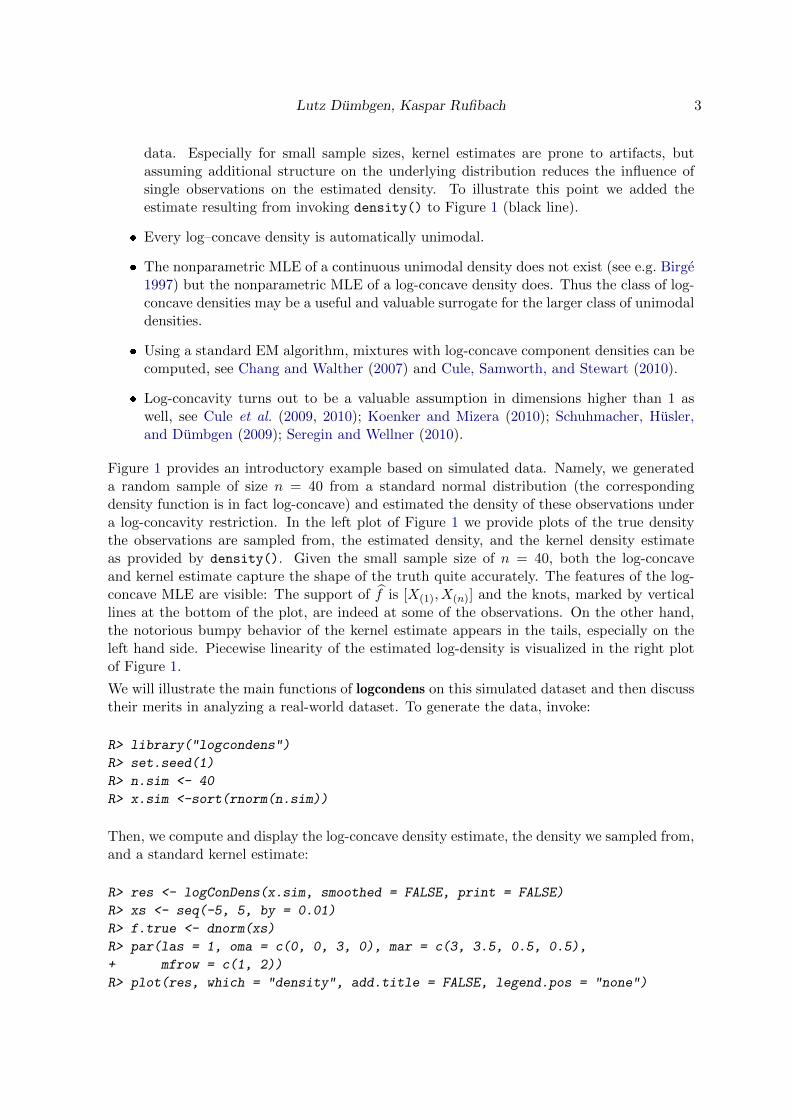
data. Especially for small sample sizes, kernel estimates are prone to artifacts, butassuming additional structure on the underlying distribution reduces the influence ofsingle observations on the estimated density. To illustrate this point we added theestimate resulting from invoking density() to Figure 1 (black line).
� Every log–concave density is automatically unimodal.
� The nonparametric MLE of a continuous unimodal density does not exist (see e.g. Birge1997) but the nonparametric MLE of a log-concave density does. Thus the class of log-concave densities may be a useful and valuable surrogate for the larger class of unimodaldensities.
� Using a standard EM algorithm, mixtures with log-concave component densities can becomputed, see Chang and Walther (2007) and Cule, Samworth, and Stewart (2010).
� Log-concavity turns out to be a valuable assumption in dimensions higher than 1 aswell, see Cule et al. (2009, 2010); Koenker and Mizera (2010); Schuhmacher, Husler,and Dumbgen (2009); Seregin and Wellner (2010).
Figure 1 provides an introductory example based on simulated data. Namely, we generateda random sample of size n = 40 from a standard normal distribution (the correspondingdensity function is in fact log-concave) and estimated the density of these observations undera log-concavity restriction. In the left plot of Figure 1 we provide plots of the true densitythe observations are sampled from, the estimated density, and the kernel density estimateas provided by density(). Given the small sample size of n = 40, both the log-concaveand kernel estimate capture the shape of the truth quite accurately. The features of the log-concave MLE are visible: The support of f is [X(1), X(n)] and the knots, marked by verticallines at the bottom of the plot, are indeed at some of the observations. On the other hand,the notorious bumpy behavior of the kernel estimate appears in the tails, especially on theleft hand side. Piecewise linearity of the estimated log-density is visualized in the right plotof Figure 1.
We will illustrate the main functions of logcondens on this simulated dataset and then discusstheir merits in analyzing a real-world dataset. To generate the data, invoke:
R> library("logcondens")
R> set.seed(1)
R> n.sim <- 40
R> x.sim <-sort(rnorm(n.sim))
Then, we compute and display the log-concave density estimate, the density we sampled from,and a standard kernel estimate:
R> res <- logConDens(x.sim, smoothed = FALSE, print = FALSE)
R> xs <- seq(-5, 5, by = 0.01)
R> f.true <- dnorm(xs)
R> par(las = 1, oma = c(0, 0, 3, 0), mar = c(3, 3.5, 0.5, 0.5),
+ mfrow = c(1, 2))
R> plot(res, which = "density", add.title = FALSE, legend.pos = "none")
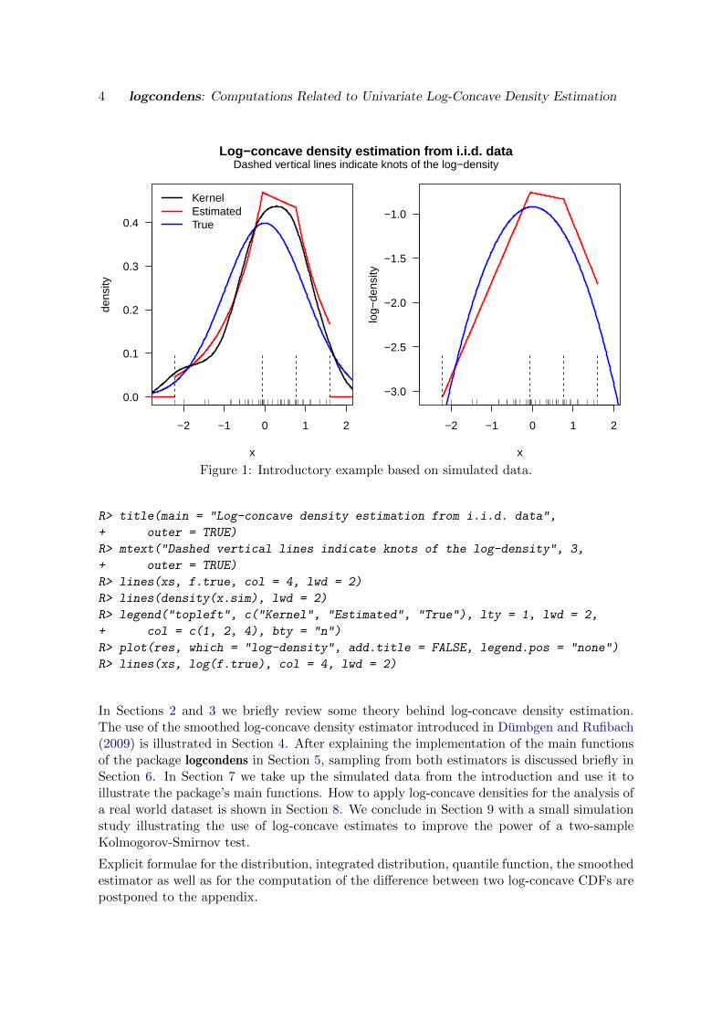
4 logcondens: Computations Related to Univariate Log-Concave Density Estimation
−2 −1 0 1 2
0.0
0.1
0.2
0.3
0.4
x
dens
ity
Log−concave density estimation from i.i.d. dataDashed vertical lines indicate knots of the log−density
KernelEstimatedTrue
−2 −1 0 1 2
−3.0
−2.5
−2.0
−1.5
−1.0
x
log−
dens
ity
Figure 1: Introductory example based on simulated data.
R> title(main = "Log-concave density estimation from i.i.d. data",
+ outer = TRUE)
R> mtext("Dashed vertical lines indicate knots of the log-density", 3,
+ outer = TRUE)
R> lines(xs, f.true, col = 4, lwd = 2)
R> lines(density(x.sim), lwd = 2)
R> legend("topleft", c("Kernel", "Estimated", "True"), lty = 1, lwd = 2,
+ col = c(1, 2, 4), bty = "n")
R> plot(res, which = "log-density", add.title = FALSE, legend.pos = "none")
R> lines(xs, log(f.true), col = 4, lwd = 2)
In Sections 2 and 3 we briefly review some theory behind log-concave density estimation.The use of the smoothed log-concave density estimator introduced in Dumbgen and Rufibach(2009) is illustrated in Section 4. After explaining the implementation of the main functionsof the package logcondens in Section 5, sampling from both estimators is discussed briefly inSection 6. In Section 7 we take up the simulated data from the introduction and use it toillustrate the package’s main functions. How to apply log-concave densities for the analysis ofa real world dataset is shown in Section 8. We conclude in Section 9 with a small simulationstudy illustrating the use of log-concave estimates to improve the power of a two-sampleKolmogorov-Smirnov test.
Explicit formulae for the distribution, integrated distribution, quantile function, the smoothedestimator as well as for the computation of the difference between two log-concave CDFs arepostponed to the appendix.
Lutz Dumbgen, Kaspar Rufibach 5
2. Computing the log-concave estimator
The general log-likelihood. As discussed in the introduction, our goal is to maximizethe functional `(ϕ) over all log-concave functions ϕ : R → [−∞,∞) such that exp(ϕ) is aprobability density. Let us first modify ` somewhat: For given support points x1 < x2 <· · · < xm and probability weights w1, w2, . . . , wm > 0 we consider
`(ϕ) =
m∑j=1
wjϕ(xj).
The standard setting. By default, x1 < x2 < . . . < xm are the different elements of{X1, X2, . . . , Xn}, and wj := n−1#{i ≤ n : Xi = xj}. In the idealized setting of i.i.d.observations Xi from a density f , the numbers m and n coincide, while xj = X(j) andwj = n−1. However, there could be tied observations, e.g. due to rounding errors, resultingin m < n support points.
An alternative setting. In case of very large sample sizes one may wish to reduce com-putation time and storage space by approximating the raw data Xi. Let x1 < x2 < · · · <xm be given support points such that [x1, xm] ⊃ [X(1), X(n)]. Then we define probabilityweights wj , 1 ≤ j ≤ m, as follows: If a raw observation Xi falls into [xj , xj+1], we addn−1(xj+1 −Xi)/(xj+1 − xj) to wj and n−1(Xi − xj)/(xj+1 − xj) to wj+1. That way we ap-proximate the empirical distribution of the raw data Xi by a discrete distribution
∑mj=1wjδxj
having the same mean and possibly larger variance. However one can show that the increasein variance is no larger than maxj<m(xj+1 − xj)2/4. Finally, pairs (xj , wj) with wj = 0 areremoved to reduce the dimension as much as possible.
We implemented automatic computation of weights and the binning algorithm described abovein the function preProcess in logcondens. This function is automatically invoked by thosefunctions that take the raw data as argument, specifically activeSetLogCon, icmaLogCon
and the functions that depend on them, most importantly logConDens. For a description ofhow to specify a user-defined grid we refer to the respective help files in logcondens.
The modified log-likelihood. To relax the constraint of f being a density and to geta criterion function to maximize over all concave functions, we employ the standard trick(cf. Silverman 1982, Theorem 3.1) of adding a Lagrange term to `, leading to the modifiedfunctional
L(ϕ) =
m∑j=1
wjϕ(xj)−∫R
expϕ(t) dt. (1)
With the same arguments as Dumbgen and Rufibach (2009) one can show that there ex-ists a unique concave function ϕ maximizing this functional L(·). It satisfies the equation∫
exp ϕ(t) dt = 1 and has the following additional properties: ϕ = −∞ on R \ [x1, xm], and ϕis continuous and piecewise linear on [x1, xm] with knots only in {x1, x2, . . . , xm}. Any suchfunction ϕ is fully specified by the vector ϕ = (ϕ(xj))
mj=1. We therefore restrict attention to
the set P(x1, x2, . . . , xm) of vectors ϕ ∈ Rm such that
ϕj+1 − ϕjxj+1 − xj
≥ ϕj − ϕj−1
xj − xj−1for i = 2, . . . ,m− 1.
6 logcondens: Computations Related to Univariate Log-Concave Density Estimation
This allows to rewrite the integral (1) as
L(ϕ) =
m∑j=1
wjϕj −m−1∑j=1
(xj+1 − xj)J(ϕj , ϕj+1)
with the auxiliary function
J(r, s) =
{(exp(r)− exp(s)
)/(r − s) if r 6= s,
exp(r) if r = s.
The constrained optimization problem we are now aiming to solve reads
ϕ = arg maxϕ∈P(x1,x2,...,xm)
L(ϕ),
where L is a strictly concave functional on Rm, see Dumbgen, Husler, and Rufibach (2010,Section 2). For more details on the computations leading to the final form of L we refer toDumbgen and Rufibach (2009). It is important to note that (iterative) maximization of thefunctional L yields the vector (ϕ(xj))
mj=1 and not the density estimate directly. However, due
to the piecewise linearity of the function ϕ the maximizing vector (ϕ(xj))mj=1 can be identified
with
ϕ(x) =
{ϕj + (x− xj)sj+1 for x ∈ [xj , xj+1], 1 ≤ j < m
−∞ for x ∈ R \ [x1, xm]
for x ∈ R, where sj+1 = ∆ϕj+1/∆xj+1 and ∆vj+1 := vj+1 − vj , 1 ≤ j < m, for any vector
v ∈ Rm. Finally, the density estimate at x is then simply f = exp ϕ, i.e. f = 0 outside[x1, xm]. These two functions are implemented in evaluateLogConDens. Computation ofadditional functions at a given point x is discussed in Section 5.2.
Approximation. From the definitions of L(ϕ) and J(r, s) above it is clear that numericalinaccuracies may occur whenever two consecutive components ϕj , ϕj+1 of the vector ϕ underconsideration are getting very close. This means that the argument ϕ has “flat” stretches.To avoid these numerical inaccuracies in computations, we approximate J and its derivativesin the implementation in logcondens by Taylor polynomials of degree four if |r − s| is small.Exact bounds and formulae for these polynomials are worked out in Dumbgen et al. (2010,Section 6). Similar approximations are also used to compute
∫F and F ∗, see the appendix.
An iterative convex minorant algorithm. First attempts to compute ϕ are described inRufibach (2007): Four different algorithms were proposed that all reliably found the maximumof L. However, not all are equally efficient. As a clear winner in the contest arranged in thatpaper in terms of speed came off the ICMA. For this reason, this algorithm was chosen to beimplemented in logcondens, as the function icmaLogCon. First proposed by Groeneboom andWellner (1992) and further detailed by Jongbloed (1998), the ICMA is especially tailored tomaximize a smooth objective function over particular convex cones by maximizing quadraticapproximations to the objective function via the pool-adjacent-violaters algorithm (PAVA).
Lutz Dumbgen, Kaspar Rufibach 7
An active set algorithm. For a description of active set algorithms see e.g. Fletcher(1987, Section 10.3) or Nocedal and Wright (1999, Section 16.4). The application to log-concave density estimation is discussed in considerable generality by Dumbgen et al. (2010,Section 3) and therefore omitted here. A key feature of an ASA is that it solves a finitenumber of unconstrained optimization problems. The function activeSetLogCon estimates alog-concave density via an ASA.
Related work. Note also the implementations of the above two algorithms for isotonicestimation in the R package isotone and the description in de Leeuw, Hornik, and Mair(2009). In a similar context, an ASA was used to compute an estimate in the ordered factorregression problem, see Rufibach (2010) and the R package OrdFacReg (Rufibach 2009).
Range of applicability. The minimal sample size that allows estimation of a log-concavedensity is n = 2. Estimating a log-concave density for n in the millions causes no problemson a laptop computer and depending on the resources may take a few minutes. Alternatively,to speed up computation time for large n, one can approximate the empirical distribution ofthe raw data by a discrete distribution with m << n support points as indicated before.
3. Characterization and properties of the estimator
In what follows let F be the distribution function corresponding to the density f = exp ϕ,and let F be the distribution function of the discrete measure
∑mj=1wjδxj . Using suitable
directional derivatives of the log-likelihood function, Dumbgen and Rufibach (2009) derivevarious useful facts about ϕ. Here are the two most relevant ones in the present context:
A characterization. Let ϕ be a concave function which is linear on all intervals [xj , xj+1],1 ≤ j < m, while ϕ = −∞ on R \ [x1, xm]. Defining F (x) :=
∫ x−∞ exp ϕ(r) dr, we assume
further that F (xm) = 1. Then ϕ = ϕ and F = F if, and only if, for arbitrary t ∈ [x1, xm],∫ t
x1
F (r) dr ≤∫ t
x1
F(r) dr
with equality in case of t being a knot of ϕ, i.e.
t ∈ S(ϕ) := {x1, xm} ∪{t ∈ (x1, xm) : ϕ′(t−) > ϕ′(t+)
}.
This characterization entails that F is rather close to F in the sense that F(t−) ≤ F (t) ≤ F(t)for any knot t of ϕ. It is also relevant for our algorithms, because
H(t, ϕ) :=
∫ t
x1
(F − F)(r) dr =d
du
∣∣∣u=0
L(ϕ+ u∆t) (2)
with ∆t(x) := min(x− t, 0). Suitable functions to compute H = H(·, ϕ) are implemented inlogcondens, see Section 5.
8 logcondens: Computations Related to Univariate Log-Concave Density Estimation
Further properties. Another remarkable property of F and F is the inequality∫h(x) dF (x) ≤
∫h(x) dF(x) for arbitrary convex h : R→ R.
In particular, setting h(x) = ±x and h(x) = x2 yields
Mean(F ) = Mean(F) =m∑j=1
wjxj = X (3)
andVar(F ) ≤ Var(F). (4)
4. Smoothing the log-concave density estimator
From Dumbgen and Rufibach (2009, Theorem 2.1) we know that ϕ is equal to 0 outside[x1, xm], i.e. ϕ has potentially sharp discontinuities at both ends of its support. In addition,the estimator ϕ may have quite sharp kinks; compare the mode of f in Figure 1. To over-come these minor inconveniences and for additional reasons elaborated in the analysis of thereliability data in Section 8, Dumbgen and Rufibach (2009) introduce a smoothed log-concavedensity estimator f∗, defined for some bandwidth γ > 0 as
f∗(x) =
∫ ∞−∞
φγ(x− y)f(y) dy,
i.e. the convolution of f with a Gaussian kernel φγ with mean 0 and standard deviation γ.By virtue of a celebrated result of Prekopa (1971), it is known that the class of log-concavedensities is closed under convolution, whence f∗ is log-concave, too. Due to the simplestructure of ϕ and our restriction to Gaussian kernels, one can deduce explicit formulae forf∗(x) and its distribution function F ∗(x) at any x, see Section 5.2 and Appendix C.
Choice of bandwidth. Let F ∗ be the distribution function of the smoothed density f∗.Note that F ∗ is the distribution function of X+Z with independent random variables X ∼ Fand Z ∼ N(0, γ2). Thus it follows from (3) that all distribution functions F ∗, F ,F have thesame mean X, whereas
Var(F ∗) = Var(F ) + γ2 ≤ Var(F) + γ2,
according to (4). Now consider the estimator
σ2 = n(n− 1)−1 Var(F) = n(n− 1)−1m∑j=1
wj(xj − X
)2.
In the standard setting, this is an unbiased estimator of Var(Xi). Hence, as proposed byDumbgen and Rufibach (2009, Section 3), the default value for γ is the square root of
γ2 = σ2 −Var(F ).
Lutz Dumbgen, Kaspar Rufibach 9
This yields an estimated distribution function F ∗ with standard deviation σ. Using γ = γalso makes f∗ a fully automatic estimator.
The variance of F can be computed explicitly as follows:
Var(F ) =
∫ xm
x1
(x− X)2f(x) dx
=m∑j=2
∆xj
((xj−1 − X)2J10(ϕj−1, ϕj) + (xj − X)2J10(ϕj , ϕj−1)
− (∆xj)2J11(ϕj−1, ϕj)
).
Here J10 equals the partial derivative of J(r, s) with respect to r, while J11 is the partialderivative of J with respect to r and s, see Dumbgen et al. (2010, Section 2) for a derivationand computational details.
5. Implementation and main functions
5.1. Function to compute the estimate
Using the simulated data from the introduction we now describe the function to estimate alog-concave density and the corresponding summary and plot methods.
The primary function of the package is logConDens which returns an object of class dlc. Adlc object is a list consisting of
� xn: the vector (Xi)ni=1 of original observations,
� x: the vector (xj)mj=1 of support points,
� w: the vector (wj)mj=1 of weights,
� phi: the estimated vector ϕ = (ϕ(xj))mj=1,
� IsKnot: the vector (1{xj is a knot of ϕ})mj=1,
� L: the value L(ϕ),
� Fhat: a vector (F (xj))mj=1 with values of the c.d.f. of f ,
� H: a vector (H(xj))mj=1 of directional derivatives (cf. (2) in Section 3),
as generated by activeSetLogCon. If smoothed = TRUE in the call of logConDens then dlc
additionally contains the entries
� f.smoothed: A vector that contains the values of f∗ either at an equidistant grid of 500values ranging from x− 0.1r to x + 0.1r for x = minj=1,...,m xj ,x = maxj=1,...,m xj , and
r = x− x if xs = NULL or the value of f∗ at the values of xs if a vector is provided asthe latter argument.
� F.smoothed: The values of F ∗n on the grid.
10 logcondens: Computations Related to Univariate Log-Concave Density Estimation
� gam: The computed value of γ.
� xs: Either the vector of 500 grid points or the initial vector xs of points at whichf.smoothed is to be computed.
Finally, the entry smoothed returns the value of the initial argument. Note that the knotscollected in IsKnot are not derived from ϕ but appear as a direct by-product of the active setalgorithm. The quantities Hj can be used to verify the characterization of the estimator interms of distribution function as elaborated in Dumbgen and Rufibach (2009). See Section 3for an illustration.
A summary and plot method are available for the class dlc. The summary method providessome basic quantities of the estimates whereas the plot method is intended to provide a quickway of standard plotting ϕ, f , and F and f∗, F ∗ (optional). For more tailor-made plots werecommend to extract the necessary quantities from the dlc object and plot them with thedesired modifications, as we do when generating Figure 3.
Note that to plot f and F we do not simply linearly interpolate the points exp ϕ(t) fort ∈ Sm(ϕ) but we rather compute f and F on a sufficiently fine grid of points using thefunction evaluateLogConDens, to display the shape of the estimated density and distributionfunction between knot points correctly.
5.2. Evaluation of the fitted estimators
Thanks to the simple structure of ϕ, closed formulae can be derived for ϕ, f , F , F−1 as wellas f∗, F ∗ on their respective domain, see Section 2 and the appendix for details. Theseformulae are implemented in logcondens via the two functions evaluateLogConDens andquantilesLogConDens.
To compute the process H = H(·, ϕ) in (2) one needs to be able to compute the integral of thedistribution functions F and F, at an arbitrary point t. Again, exploiting the structure of ϕ aclosed formula can be derived for
∫ tx1F (r) dr, see Appendix B. This formula is implemented
in the function intF in the package logcondens, and we use this function together with itscompanion intECDF (ECDF: empirical cumulative distribution function) for the empiricaldistribution function to compute the process D.
6. Sampling from the different estimators
Cule et al. (2010) describe Monte Carlo estimation of functionals of f (which may be one-or multidimensional) by sampling from a random vector (variable) X that has density f andplugging in these samples into the functionals of interest. In order to sample from f , theyuse a rejection sampling procedure, see Cule et al. (2010, Section 7.1), implemented as thefunction rlcd in Cule et al. (2009). In logcondens we implemented sampling not only fromf , but also from f∗ as the function rlogcon, using the quantile function F−1 implementedin quantilesLogConDens. Note that by making use of the quantile function F−1 in rlogcon
we generate a sample of a given size from f directly, without the need of rejecting (some of)the generated numbers. There is no need to implement the quantile function F ∗ for the sakeof simulating samples from F ∗, thanks to the fact that f∗ is the density of the convolution off with a given normal kernel.
Lutz Dumbgen, Kaspar Rufibach 11
Sampling from the estimate may serve at least two purposes: First, as described above,generated samples can be used to approximate functionals of f or f∗, as described in Culeet al. (2010). Second, in certain applications it may be the explicit goal to get simulatedsamples from an estimated density, see Section 8 below and Dumbgen and Rufibach (2009,Section 3).
7. Illustration of main functions on simulated example
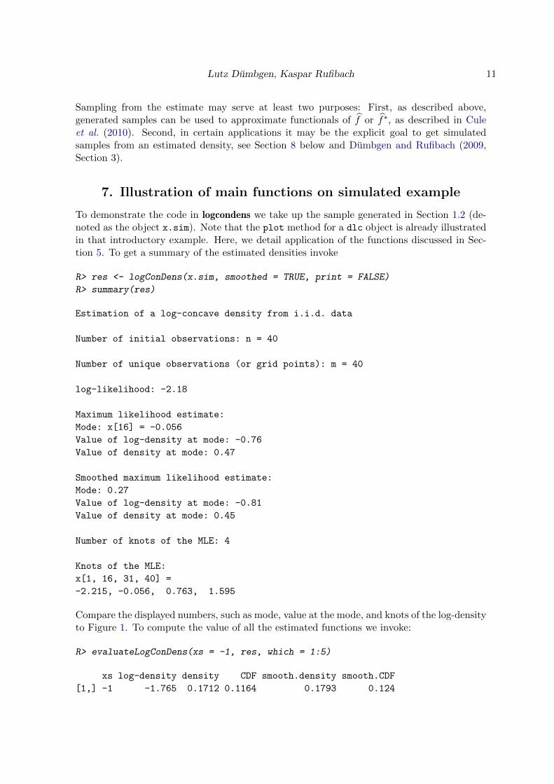
To demonstrate the code in logcondens we take up the sample generated in Section 1.2 (de-noted as the object x.sim). Note that the plot method for a dlc object is already illustratedin that introductory example. Here, we detail application of the functions discussed in Sec-tion 5. To get a summary of the estimated densities invoke
R> res <- logConDens(x.sim, smoothed = TRUE, print = FALSE)
R> summary(res)
Estimation of a log-concave density from i.i.d. data
Number of initial observations: n = 40
Number of unique observations (or grid points): m = 40
log-likelihood: -2.18
Maximum likelihood estimate:
Mode: x[16] = -0.056
Value of log-density at mode: -0.76
Value of density at mode: 0.47
Smoothed maximum likelihood estimate:
Mode: 0.27
Value of log-density at mode: -0.81
Value of density at mode: 0.45
Number of knots of the MLE: 4
Knots of the MLE:
x[1, 16, 31, 40] =
-2.215, -0.056, 0.763, 1.595
Compare the displayed numbers, such as mode, value at the mode, and knots of the log-densityto Figure 1. To compute the value of all the estimated functions we invoke:
R> evaluateLogConDens(xs = -1, res, which = 1:5)
xs log-density density CDF smooth.density smooth.CDF
[1,] -1 -1.765 0.1712 0.1164 0.1793 0.124
12 logcondens: Computations Related to Univariate Log-Concave Density Estimation
R> quantilesLogConDens(ps = 0.5, res)
ps quantile
[1,] 0.5 0.1688
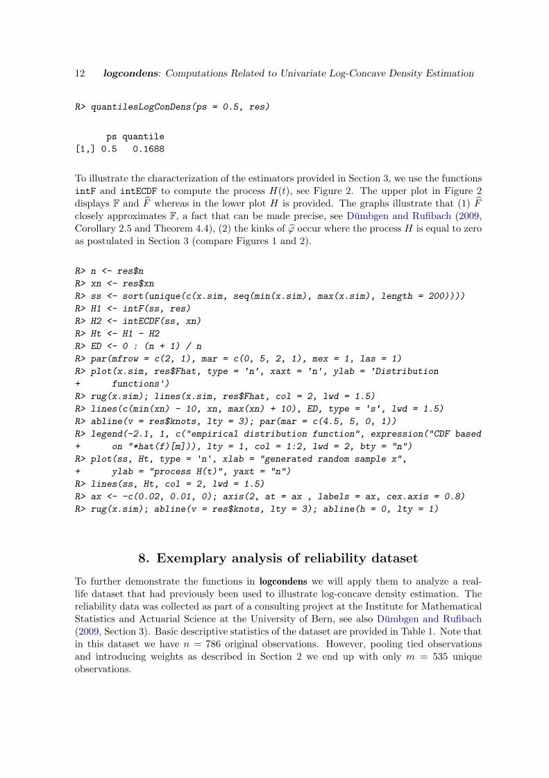
To illustrate the characterization of the estimators provided in Section 3, we use the functionsintF and intECDF to compute the process H(t), see Figure 2. The upper plot in Figure 2displays F and F whereas in the lower plot H is provided. The graphs illustrate that (1) Fclosely approximates F, a fact that can be made precise, see Dumbgen and Rufibach (2009,Corollary 2.5 and Theorem 4.4), (2) the kinks of ϕ occur where the process H is equal to zeroas postulated in Section 3 (compare Figures 1 and 2).
R> n <- res$n
R> xn <- res$xn
R> ss <- sort(unique(c(x.sim, seq(min(x.sim), max(x.sim), length = 200))))
R> H1 <- intF(ss, res)
R> H2 <- intECDF(ss, xn)
R> Ht <- H1 - H2
R> ED <- 0 : (n + 1) / n
R> par(mfrow = c(2, 1), mar = c(0, 5, 2, 1), mex = 1, las = 1)
R> plot(x.sim, res$Fhat, type = 'n', xaxt = 'n', ylab = 'Distribution
+ functions')
R> rug(x.sim); lines(x.sim, res$Fhat, col = 2, lwd = 1.5)
R> lines(c(min(xn) - 10, xn, max(xn) + 10), ED, type = 's', lwd = 1.5)
R> abline(v = res$knots, lty = 3); par(mar = c(4.5, 5, 0, 1))
R> legend(-2.1, 1, c("empirical distribution function", expression("CDF based
+ on "*hat(f)[m])), lty = 1, col = 1:2, lwd = 2, bty = "n")
R> plot(ss, Ht, type = 'n', xlab = "generated random sample x",
+ ylab = "process H(t)", yaxt = "n")
R> lines(ss, Ht, col = 2, lwd = 1.5)
R> ax <- -c(0.02, 0.01, 0); axis(2, at = ax , labels = ax, cex.axis = 0.8)
R> rug(x.sim); abline(v = res$knots, lty = 3); abline(h = 0, lty = 1)
8. Exemplary analysis of reliability dataset
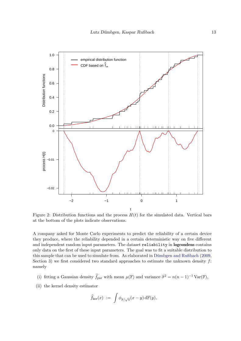
To further demonstrate the functions in logcondens we will apply them to analyze a real-life dataset that had previously been used to illustrate log-concave density estimation. Thereliability data was collected as part of a consulting project at the Institute for MathematicalStatistics and Actuarial Science at the University of Bern, see also Dumbgen and Rufibach(2009, Section 3). Basic descriptive statistics of the dataset are provided in Table 1. Note thatin this dataset we have n = 786 original observations. However, pooling tied observationsand introducing weights as described in Section 2 we end up with only m = 535 uniqueobservations.
Lutz Dumbgen, Kaspar Rufibach 13
0.0
0.2
0.4
0.6
0.8
1.0
x.sim
Dis
trib
utio
n fu
nctio
ns
empirical distribution function
CDF based on fm
−2 −1 0 1
t
proc
ess
H(t
)
−0.02
−0.01
0
Figure 2: Distribution functions and the process H(t) for the simulated data. Vertical barsat the bottom of the plots indicate observations.
A company asked for Monte Carlo experiments to predict the reliability of a certain devicethey produce, where the reliability depended in a certain deterministic way on five differentand independent random input parameters. The dataset reliability in logcondens containsonly data on the first of these input parameters. The goal was to fit a suitable distribution tothis sample that can be used to simulate from. As elaborated in Dumbgen and Rufibach (2009,Section 3) we first considered two standard approaches to estimate the unknown density f :namely
(i) fitting a Gaussian density fpar with mean µ(F) and variance σ2 = n(n− 1)−1 Var(F),
(ii) the kernel density estimator
fker(x) :=
∫φσ/√n(x− y) dF(y),
14 logcondens: Computations Related to Univariate Log-Concave Density Estimation
Variable n Minimum 1st Quartile Median 3rd Quartile Maximum IQR
reliability 786 1404.2 1632.2 1688.2 1735.6 1853.6 103.4
Table 1: Descriptive statistics of reliability data.
where φσ denotes the Normal density with mean 0 and variance σ2.
The very small bandwidth σ/√n was chosen to obtain a density with variance σ2 and to avoid
putting too much weight into the tails, which was crucial in the engineers’ application. Wethink that in general such undersmoothed density estimators are a simple way of depictingthe empirical distribution of raw data.
Looking at the data, approach (i) is clearly inappropriate because the reliability sample of sizen = 786 reveals a skewed and pronouncedly non-gaussian distribution. This can be seen inFigure 3, where the multimodal curve corresponds to fker, while the dashed line depicts fpar.Approach (ii) yielded Monte Carlo results agreeing well with measured reliabilities, but theengineers were not satisfied with the multimodality of fker. Choosing a kernel estimator withlarger bandwidth would overestimate the variance and put too much weight into the tails.Thus we agreed on a third approach and estimated f by the smoothed log-concave estimatorf∗ introduced in Section 4.
This density estimator is the skewed unimodal curve in Figure 3. Apart from the advantagesdescribed above – unimodality, variance equal to σ2, and not too heavy tails – it yieldedconvincing results in the Monte Carlo simulations, too. In addition and as expected, thekinks and the discontinuities at x1 and xm of f are smoothed out by f∗. Note that bothestimators f and f∗ are fully automatic.
Now, the primary goal of this data analysis was to provide simulated samples from the es-timated densities f and f∗. The function rlogcon that implements sampling from the dis-tribution that corresponds to f in the package logcondens is based on the quantile functionF−1, derived in Appendix A and implemented as quantilesLogConDens. Thanks to the factthat f∗ is the density of the convolution of f with a Gaussian kernel with standard deviationγ, a random number X∗ from f∗ can easily be obtained by computing X∗ = X + Y withindependent random variables X ∼ F and Y ∼ N(0, γ2).
To illustrate how the functions in logcondens can be used to explore different estimates, weprovide below the code that is used to generate Figure 3. Note that this is the same Figurealready displayed in Dumbgen and Rufibach (2009, Figure 2).
R> x.rel <- sort(reliability)
R> n <- length(x.rel)
R> mu <- mean(x.rel); sig <- sd(x.rel)
R> xs <- seq(1350, 1950, length.out = 500)
R> res <- logConDens(x.rel, smoothed = TRUE, print = FALSE, xs = xs)
R> f.smoothed <- res$f.smoothed
R> xs2 <- xs[(xs >= min(x.rel)) & (xs <= max(x.rel))]
R> f <- rep(NA, length(xs2))
R> for (i in 1:length(xs2)){f[i] <- evaluateLogConDens(xs2[i],
+ res)[, "density"]}
R> h <- sig / sqrt(n)
Lutz Dumbgen, Kaspar Rufibach 15
1400 1500 1600 1700 1800 1900
0.000
0.001
0.002
0.003
0.004
0.005
0.006log−concave fn
normal f nor
kernel f ker
log−concave smoothed fn*
Figure 3: Different estimates of the density of the reliability data.
R> f.kernel <- rep(NA, length(xs))
R> for (i in 1:length(xs)){f.kernel[i] <- mean(dnorm(xs[i], mean =
+ x.rel, sd = h))}
R> f.normal <- dnorm(xs, mean = mu, sd = sig)
R> par(las = 1, mar = c(3, 3.5, 0.5, 0.5))
R> plot(0, 0, type = 'n', xlim = c(1390, 1900), ylim =
+ c(0, 6.5 * 10^-3), ylab = "")
R> rug(x.rel)
R> lines(xs, f.normal, col = 3)
R> lines(xs, f.kernel, col = 4)
R> lines(xs, f.smoothed, lwd = 4, col = 5)
R> lines(xs2, f, col = 2)
R> segments(c(-1300, max(x.rel)), c(0, 0), c(min(x.rel), 2000),
+ c(0, 0), col = 2)
R> legend("topleft", c(expression("log-concave "*hat(f)[n]),
+ expression("normal "*hat(f)[nor]), expression("kernel "*hat(f)[ker]),
+ expression("log-concave smoothed "*hat(f)[n]*"*")),
+ lty = 1, lwd = 3, col = 2:5, bty = "n")
R> segments(res$knots, 0, res$knots, 0.002, lty = 2)
Finally, we illustrate how we can efficiently generate samples from f and f∗ and thus contentthe engineers that initiated this research. In addition, samples from the estimators could beused to approximate some functional of f or f∗, as described in Cule et al. (2010).
R> set.seed(1977)
16 logcondens: Computations Related to Univariate Log-Concave Density Estimation
R> rel_samples <- rlogcon(n = 20, x0 = x.rel)
The sorted sample of size n = 20 from the log-concave density estimator can be extractedusing
R> sort(rel_samples$X)
[1] 1511.954 1594.168 1621.873 1645.044 1663.611 1673.327 1674.606
[8] 1675.477 1689.173 1689.405 1696.573 1697.265 1710.816 1712.501
[15] 1716.976 1724.642 1730.252 1783.473 1792.702 1807.486
and one from the smoothed log-concave density estimator via
R> sort(rel_samples$X_star)
[1] 1514.480 1599.645 1615.953 1648.505 1662.295 1663.369 1677.193
[8] 1677.583 1685.057 1686.471 1689.579 1705.722 1707.009 1712.771
[15] 1718.095 1727.095 1727.765 1780.637 1785.171 1813.476
9. Smooth two-sample permutation test
Dumbgen and Rufibach (2009, Theorem 4.4) have shown that the distribution function esti-mators F and F are, under mild assumptions, asymptotically equivalent and F acts in thissense as a smoother of F. However, by imposing log-concavity efficiency gains in estimationseem plausible for small to moderate sample sizes. This leads us to the proposal of a smoothtest for distribution functions which we now describe.
Suppose the researcher is given two samples (Xi)n1i=1 and (Yi)
n2i=1 of independent random
variables Xi ∼ FX and Yj ∼ FY with unknown distribution functions FX , FY .
To test whether H0 : FX = FY versus H1 : FX 6= FY , a commonly used two-sample teststatistic is the Kolmogorov-Smirnov statistic, comparing the empirical distribution functionsFX and FY of the two samples:
K = K(FX ,FY ) :=(n1n2/(n1 + n2))
)1/2‖FX − FY ‖∞
where ‖f‖∞ := supx∈R |f(x)| for any function f : R → R. The limiting distribution of Kn
and the corresponding asymptotic test can be found in Durbin (1973).
If one imposes that FX and FY both have log-concave density functions, we propose thefollowing modified test statistic:
K = K(FX , FY ) =(n1n2/(n1 + n2))
)1/2‖FX − FY ‖∞where FX and FY are the log-concave distribution function estimators of FX and FY . Derivingthe limiting distribution of this statistic is a difficult task, but if one assumes that under H0 thepooled sample (Z1, Z2, . . . , Zn1+n2) := (X1, . . . , Xn1 , Y1, . . . , Yn2) has the same distribution as
(ZΠ1 , . . . , ZΠn1, ZΠn1+1 , . . . , ZΠn1+n2
)
Lutz Dumbgen, Kaspar Rufibach 17
where Π is a random permutation of {1, . . . , n1 + n2} not depending on the data one canperform a Monte Carlo permutation test of H0 as follows: Generate M independent copiesof Π and calculate the corresponding values of the test statistic K(1), K(2), . . . , K(M). Thena nonparametric p-value for H0 is given by
p =1 + #{i ≤M : K(i) ≥ K}
1 +M.
The null hypothesis H0 is rejected if p is not larger than the pre-specified significance level α.
Details on the computation of K(FX , FY ) as well as for K∗n(FX , FY ), the statistic based onthe smoothed log-concave distribution function estimates, are provided in Appendix E.
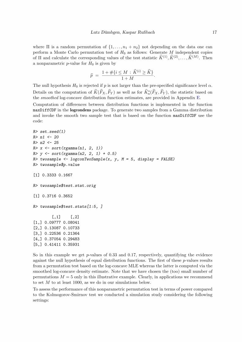
Computation of differences between distribution functions is implemented in the functionmaxDiffCDF in the logcondens package. To generate two samples from a Gamma distributionand invoke the smooth two sample test that is based on the function maxDiffCDF use thecode:
R> set.seed(1)
R> n1 <- 20
R> n2 <- 25
R> x <- sort(rgamma(n1, 2, 1))
R> y <- sort(rgamma(n2, 2, 1) + 0.5)
R> twosample <- logconTwoSample(x, y, M = 5, display = FALSE)
R> twosample$p.value
[1] 0.3333 0.1667
R> twosample$test.stat.orig
[1] 0.3716 0.3652
R> twosample$test.stats[1:5, ]
[,1] [,2]
[1,] 0.09777 0.08041
[2,] 0.13087 0.10733
[3,] 0.22536 0.21364
[4,] 0.37054 0.29483
[5,] 0.41411 0.35931
So in this example we get p-values of 0.33 and 0.17, respectively, quantifying the evidenceagainst the null hypothesis of equal distribution functions. The first of these p-values resultsfrom a permutation test based on the log-concave MLE whereas the latter is computed via thesmoothed log-concave density estimate. Note that we have chosen the (too) small number ofpermutations M = 5 only in this illustrative example. Clearly, in applications we recommendto set M to at least 1000, as we do in our simulations below.
To assess the performance of this nonparametric permutation test in terms of power comparedto the Kolmogorov-Smirnov test we conducted a simulation study considering the followingsettings:
18 logcondens: Computations Related to Univariate Log-Concave Density Estimation
Setting 1: n1 = 20 n2 = 25 X ∼ N(0, 1) vs. Y ∼ N(µ, 1)Setting 2: n1 = 20 n2 = 25 X ∼ Gam(2, 1) vs. Y ∼ Gam(2, 1) + µSetting 3: n1 = 20 n2 = 25 X ∼ Gam(2, 1) vs. Y ∼ Gam(τ, 1)
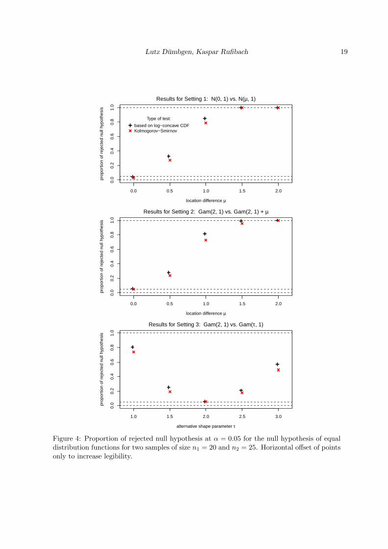
for µ ∈ {0, 0.5, 1, 1.5, 2} and τ ∈ {1, 1.5, 2, 2.5, 3}. We simulated each setting 1000 timesand M = 999 was used as argument in logconTwoSample. The number of rejected nullhypothesis when adopting a significance level of α = 0.05 are displayed in Figure 4. We find,in accordance with Cule et al. (2010, Section 9, Remark (ii)), that the test based on the log-concave CDF uniformly outperforms, for the rather moderate sample sizes we consider, theKolmogorov-Smirnov test. For very large sample sizes the difference in power between the twotests decreases (not shown). We therefore recommend to use the function logconTwoSample
to assess the null hypothesis of two identical distribution functions, especially when only fewor moderately many observations are available.
Note that this modified test is valid even if the assumption of log-concavity of the densityfunctions is violated. Such a violation would only affect the power.
Lutz Dumbgen, Kaspar Rufibach 19
0.0 0.5 1.0 1.5 2.0
0.0
0.2
0.4
0.6
0.8
1.0
location difference µ
prop
ortio
n of
rej
ecte
d nu
ll hy
poth
esis
Results for Setting 1: N(0, 1) vs. N(µ, 1)
Type of test:
based on log−concave CDFKolmogorov−Smirnov
0.0 0.5 1.0 1.5 2.0
0.0
0.2
0.4
0.6
0.8
1.0
location difference µ
prop
ortio
n of
rej
ecte
d nu
ll hy
poth
esis
Results for Setting 2: Gam(2, 1) vs. Gam(2, 1) + µ
1.0 1.5 2.0 2.5 3.0
0.0
0.2
0.4
0.6
0.8
1.0
alternative shape parameter τ
prop
ortio
n of
rej
ecte
d nu
ll hy
poth
esis
Results for Setting 3: Gam(2, 1) vs. Gam(τ, 1)
Figure 4: Proportion of rejected null hypothesis at α = 0.05 for the null hypothesis of equaldistribution functions for two samples of size n1 = 20 and n2 = 25. Horizontal offset of pointsonly to increase legibility.
20 logcondens: Computations Related to Univariate Log-Concave Density Estimation
10. Final remarks
In Koenker and Mizera (2010, Figure 3) quasi-concave density estimation, a generalizationof log-concave density estimation, was illustrated on radial and rotational velocities of theBright Star Catalog, see Hoffleit and Warren (1991). For convenience, we also included thisdataset in logcondens as a dataframe named brightstar.
A. Density, distribution and quantile function
Formulas to compute the log-density and density function at a given point x0 ∈ R are providedin Section 2. The distribution function estimator F and its integral I(t) :=
∫ tx1F (r) dr are
implemented in the functions evaluateLogConDens and intF. For completeness, we providehere the corresponding formulas. Note that (5) is also provided in Dumbgen et al. (2010,Theorem 2.1). Recall from Section 2 the function J . Here, we use a slightly generalizedversion, defined as
J(r, s, v) :=
∫ v
0exp((1− t)r + ts
)dt
for arbitrary r, s ∈ R and v ∈ [0, 1]. The relation J(r, s, v) = exp(r)J(0, s− r, v) holds, and
J(r, s, v) =
{ (exp(r)− exp(r + v(s− r))
)/(r − s) if r 6= s,
v exp(r) if r = s,
see also the manual of logcondens, especially the help file Jfunctions.
In what follows, we will use a simple generic parametric model. Namely, define for θ ∈ R aprobability density on [0, 1] as
gθ(x) := J(0, θ)−1 exp(θx) =
{θeθx/(eθ − 1) if θ 6= 0
1 if θ = 0.
The distribution and quantile function corresponding to gθ are given as
Gθ(r) =
{(eθr − 1)/(eθ − 1) if θ 6= 0
r if θ = 0
and
G−1θ (u) =
{log(1 + (eθ − 1)u
)/θ if θ 6= 0
u if θ = 0
for r, u ∈ [0, 1], respectively. Note that G−1θ is implemented as qloglin in logcondens. For
|θ| ≤ 10−6 a Taylor approximation is used, because
G−1θ (u) = u+ θu(1− u)/2 +O(θ2)
as θ → 0, uniformly in u ∈ [0, 1]. Now, let ϕ ∈ Rm where this vector is identified with afunction ϕ : R→ [−∞,∞) via
ϕ(x) :=
−∞ for x 6∈ [x1, xm] ,
ϕj +x− xj∆xj+1
∆ϕj+1 for x ∈ [xj , xj+1], 1 ≤ j < m ,
Lutz Dumbgen, Kaspar Rufibach 21
where ∆vj+1 := vj+1 − vj for any v ∈ Rm. Suppose further that f := exp(ϕ) is a probabilitydensity on R and let F be the corresponding distribution function. Then F (x1) = F1 := 0,and
F (xj) = Fj :=
j−1∑i=1
∆xj+1J(ϕi, ϕi+1) for 2 ≤ j ≤ m
with Fm = 1. For a proof we refer to Dumbgen et al. (2010, Theorem 2.1). To computethe quantile function of F , note that for any x ∈ [xj , xj+1] by again exploiting the specialstructure of ϕ,
F (x)− F (xj) =
∫ x
xj
exp(ϕ(t)) dt
=
∫ x
xj
exp(ϕj +
x− xj∆xj+1
∆ϕj+1
)dt
= ∆xj+1
∫ (x−xj)/∆xj+1
0exp(
(1− v)ϕj + vϕj+1
)dv
= ∆xj+1J(ϕj , ϕj+1,
x− xj∆xj+1
). (5)
Some tedious computations lead to the corresponding quantile function
F−1(u) = xj + ∆xj+1G−1∆xj+1∆ϕj+1
((u− Fj)/∆Fj+1
)for u ∈ [Fj , Fj+1], 1 ≤ j < m .
This function is the basis of quantilesLogConDens in logcondens.
B. The integral of F at an arbitrary x0
Recall the definition sj = ∆ϕj/∆xj from Section 2. In addition, we define fj = f(xj) forj = 1, . . . ,m. To be able to compute the process H = H(·, ϕ) introduced in (2) the aim is toderive an explicit formula for
Ij(x) =
∫ x
xj
F (r) dr
for any j = 1, . . . ,m− 1 and x ∈ [xj , xj+1]. Using (5) we can write
Ij(x) =
∫ x
xj
(Fj + ∆xj+1J
(ϕj , ϕj+1,
r − xj∆xj+1
))dr
= (x− xj)Fj + ∆xj+1
∫ x
xj
J(ϕj , ϕj+1,
r − xj∆xj+1
)dr.
But,∫ x
xj
J(ϕj , ϕj+1,
r − xj∆xj+1
)dr = ∆xj+1
∫ (x−xj)/∆xj+1
0J(ϕj , ϕj+1, y) dy (6)
= −s−1j+1
∫ (x−xj)/∆xj+1
0(exp(ϕj)− exp(ϕj + y∆ϕj+1)) dy
= −x− xj∆ϕj+1
fj + s−1j+1J
(ϕj , ϕj+1,
x− xj∆xj+1
).
22 logcondens: Computations Related to Univariate Log-Concave Density Estimation
Putting the pieces together we receive
Ij(x) = (x− xj)Fj + ∆xj+1
(s−1j+1J
(ϕj , ϕj+1,
x− xj∆xj+1
)− x− xj
∆ϕj+1fj
).
Specifically, for x = xj+1,
Ij(xj+1) = ∆xj+1
[Fj + s−1
j+1
(J(ϕj , ϕj+1, 1)− fj
)].
We finally get
I(t) =
∫ t
x1
F (r) dr =( i0∑i=1
Ii(xi+1))
+ Ii0(t)
where i0 = min{m− 1 , max{i : xi ≤ t}}.
Approximation for sj+1 → 0. Since we divide by sj+1 in the compuation of Ij(x) this ex-pression becomes numerically unstable or even undefined once the slope sj+1 of ϕ approachesor even equals 0. To avoid these problems, we compute the limit for a := sj+1 → 0 in theintegral in (6):
lima→0
∫ x
xj
J(ϕj , ϕj+1,
r − xj∆xj+1
)dr = lim
a→0
∫ (x−xj)/∆xj+1
0
exp(ϕj + y∆ϕj+1)− expϕja
dy
= fj lima→0
∫ (x−xj)/∆xj+1
0
exp(ya∆xj+1)− 1
ady
= fj
∫ (x−xj)/∆xj+1
0y∆xj+1 dy
= fj(x− xj)2
2∆xj+1.
This approximation is used in intF once sj+1 ≤ 10−6.
C. The smoothed log-concave density estimator
For γ > 0 and x ∈ R recall the density function φγ of a centered normal density as
φγ(x) =1√2πγ
exp(−x2/(2γ2)).
Its distribution function is denoted by Φγ . Elementary calculations reveal that for arbitrarynumbers a, x and γ > 0,
eayφγ(x− y) = exp(ax+ a2γ2/2)φγ(y − x− aγ2),
so that for real boundaries u < v,
qγ(x, a, u, v) :=
∫ v
uea(y−u)φγ(x− y) dy
= exp(a(x− u) + a2γ2/2)(Φγ(v − x− aγ2)− Φγ(u− x− aγ2)
)= exp(a(x− u) + a2γ2/2)
(Φγ(x− u+ aγ2)− Φγ(x− v + aγ2)
). (7)
Lutz Dumbgen, Kaspar Rufibach 23
The smoothed log-concave density estimator then amounts to
f∗(x) =
∫ ∞−∞
φγ(x− y)f(y) dy
=m∑j=2
∫ xj
xj−1
φγ(x− y)f(y) dy
=
m∑j=2
fj−1
∫ xj
xj−1
exp(sj(y − xj−1))φγ(x− y) dy
=
m∑j=2
fj−1 qγ(x, sj , xj−1, xj).
The function evaluateLogConDens implements f∗ in logcondens. However, note that it ismost convenient to compute f∗ via specifying smoothed = TRUE in logConDens.
In extreme situations, e.g. data sets containing extreme spacings, numerical problems mayoccur in (7). For it may happen that the exponent is rather large while the difference ofGaussian CDFs is very small. To moderate these problems, we are using the following boundsin the function Q00 implementing qγ in logcondens:
exp(−m2/2)(Φ(δ)− Φ(−δ)
)≤ Φ(b)− Φ(a) ≤ exp(−m2/2) cosh(mδ)
(Φ(δ)− Φ(−δ)
)for arbitrary numbers a < b and m := (a+ b)/2, δ := (b− a)/2.
D. The smoothed log-concave CDF estimator
Using partial integration, we get for arbitrary numbers x, a 6= 0 and real boundaries u < v:
Qγ(x, a, u, v) :=
∫ v
uea(y−u)Φγ(x− y) dy
=[a−1ea(y−u)Φγ(x− y)
]vy=u
+ a−1
∫ v
uea(y−u)φγ(x− y) dy
= +a−1(ea(v−u)Φγ(x− v)− Φγ(x− u)
)+ a−1qγ(x, a, u, v)
with qγ(x, a, u, v) as in (7). As a→ 0, this converges to
Qγ(x, 0, u, v) :=
∫ v
uΦγ(x− y) dy
=[(y − x)Φγ(x− y)
]vy=u
+
∫ v
u(y − x)φγ(x− y) dy
=[(y − x)Φγ(x− y)− γ2φγ(x− y)
]vy=u
= (x− u)Φγ(x− u)− (x− v)Φγ(x− v) + γ2(φγ(x− u)− φγ(x− v)
).
24 logcondens: Computations Related to Univariate Log-Concave Density Estimation
This leads to the formula
F ∗(x) =
∫ ∞−∞
Φγ(x− y)f(y) dy
=m∑j=2
∫ xj
xj−1
Φγ(x− y)f(y) dy
=m∑j=2
fj−1
∫ xj
xj−1
exp(sj(y − xj−1))Φγ(x− y) dy
=m∑j=2
fj−1Qγ(x, sj , xj−1, xj).
This representation is implemented in evaluateLogConDens and logConDens, where for nu-merical reasons, Qγ(x, sj , xj−1, xj) is replaced with Qγ(x, 0, xj−1, xj) in case of |sj | ≤ 10−6.
E. Computation of the two-sample test statistic
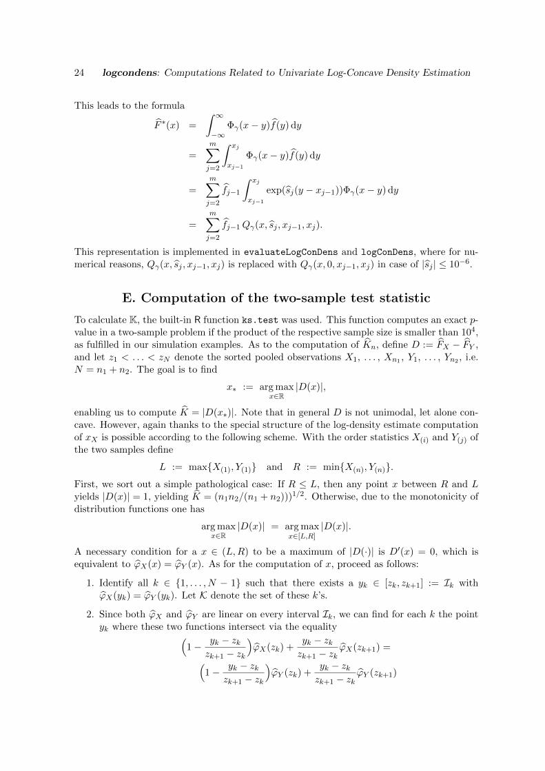
To calculate K, the built-in R function ks.test was used. This function computes an exact p-value in a two-sample problem if the product of the respective sample size is smaller than 104,as fulfilled in our simulation examples. As to the computation of Kn, define D := FX − FY ,and let z1 < . . . < zN denote the sorted pooled observations X1, . . . , Xn1 , Y1, . . . , Yn2 , i.e.N = n1 + n2. The goal is to find
x∗ := arg maxx∈R
|D(x)|,
enabling us to compute K = |D(x∗)|. Note that in general D is not unimodal, let alone con-cave. However, again thanks to the special structure of the log-density estimate computationof xX is possible according to the following scheme. With the order statistics X(i) and Y(j) ofthe two samples define
L := max{X(1), Y(1)} and R := min{X(n), Y(n)}.
First, we sort out a simple pathological case: If R ≤ L, then any point x between R and Lyields |D(x)| = 1, yielding K = (n1n2/(n1 + n2)))1/2. Otherwise, due to the monotonicity ofdistribution functions one has
arg maxx∈R
|D(x)| = arg maxx∈[L,R]
|D(x)|.
A necessary condition for a x ∈ (L,R) to be a maximum of |D(·)| is D′(x) = 0, which isequivalent to ϕX(x) = ϕY (x). As for the computation of x, proceed as follows:
1. Identify all k ∈ {1, . . . , N − 1} such that there exists a yk ∈ [zk, zk+1] := Ik withϕX(yk) = ϕY (yk). Let K denote the set of these k’s.
2. Since both ϕX and ϕY are linear on every interval Ik, we can find for each k the pointyk where these two functions intersect via the equality(
1− yk − zkzk+1 − zk
)ϕX(zk) +
yk − zkzk+1 − zk
ϕX(zk+1) =(1− yk − zk
zk+1 − zk
)ϕY (zk) +
yk − zkzk+1 − zk
ϕY (zk+1)
Lutz Dumbgen, Kaspar Rufibach 25
0 2 4 6
0.0
0.2
0.4
0.6
0.8
1.0
data
dist
ribut
ion
func
tions
Γ(2, 1)Γ(2, 1) + 0.5
Figure 5: Estimated empirical and log-concave distribution functions for Gam(2, 1) andGam(2, 1) + 0.5. Horizontal and vertical lines indicate location of largest difference betweenCDFs.
yielding
yk = zk − (ϕY (zk)− ϕX(zk))( ϕX(zk+1)− ϕX(zk)
zk+1 − zk− ϕY (zk+1)− ϕY (zk)
zk+1 − zk
)−1.
Note that if the denominator, the difference of slopes of ϕX and ϕY on [zk, zk+1], is zero thenthe two functions must match on that interval (otherwise they would not intersect). This inturn implies that the difference D is constant on that interval so that we can consider yk = zka possible point where the maximum of D occurs. Consequently, |D(·)| is maximal at one (ormore) points in the set
R = {L,R} ∪ {yk : k ∈ K}
and
Kn =(n1n2/(n1 + n2))
)1/2max{D(r) : r ∈ R}.
Figure 5 gives an example.
The computation of K∗n(FX , FY ) appears to be less straightforward than that of Kn(FX , FY ).In logconTwoSample we first approximate the function (D∗)′x = (∂/∂x)(D∗)(u, x) for u =z1 − 0.1 · (zN − z1) on a sufficiently dense equidistant grid (the number of elements in thatgrid can be provided to logconTwoSample using the argument n.grid). Then, similar to thecomputation of Kn(FX , FY ), we identify those grid intervals where (D∗)′x changes sign. Tofinally find the maximum of the latter function we then invoke uniroot to find the preciselocation of the zeros on these intervals, compute the value of (D∗)′x at each of these zerosand identify the largest of these values. In general, the computation of K∗n(FX , FY ) is more
26 logcondens: Computations Related to Univariate Log-Concave Density Estimation
time-consuming than that of Kn(FX , FY ). However, since on the level of CDFs the MLE andits smoothed version are very similar, differences with respect to the smooth two-sample testin terms of power are very small. For these reasons we omitted the smooth version of the testin our small simulation study reported on in Section 9.
Acknowledgments
We thank Dominic Schuhmacher, an associate editor and two referees for constructive com-ments. The work of Lutz Dumbgen was supported by the Swiss National Science Foundation.
References
Balabdaoui F, Rufibach K, Wellner JA (2009). “Limit Distribution Theory for MaximumLikelihood Estimation of a Log-Concave Density.” The Annals of Statistics, 37(3), 1299–1331.
Birge L (1997). “Estimation of Unimodal Densities Without Smoothness Assumptions.” TheAnnals of Statistics, 25(3), 970–981. ISSN 0090-5364.
Chang G, Walther G (2007). “Clustering with Mixtures of Log-Concave Distributions.” Com-putational Statistics & Data Analysis, 51, 6242–6251.
Cule M, Gramacy R, Samworth R (2009). “LogConcDEAD: An R Package for Maximum Like-lihood Estimation of a Multivariate Log-Concave Density.” Journal of Statistical Software,29(2). URL http://www.jstatsoft.org/v29/i02/.
Cule M, Samworth R, Stewart M (2010). “Maximum Likelihood Estimation of a Multidimen-sional Log-Concave Density.” Journal of the Royal Statistical Society B, 72(5), 545–607.
de Leeuw J, Hornik K, Mair P (2009). “Isotone Optimization in R: Pool-Adjacent-ViolatorsAlgorithm (PAVA) and Active Set Methods.” Journal of Statistical Software, 32(5), 1–24.ISSN 1548-7660. URL http://www.jstatsoft.org/v32/i05.
Dumbgen L, Husler A, Rufibach K (2010). “Active Set and EM Algorithms for Log-ConcaveDensities based on Complete and Censored Data.” Technical report, University of Bern.Available at arXiv:0707.4643.
Dumbgen L, Rufibach K (2009). “Maximum Likelihood Estimation of a Log-Concave Densityand its Distribution Function.” Bernoulli, 15, 40–68. ISSN 1350-7265.
Dumbgen L, Rufibach K (2010). “logcondens: Computations Related to Univariate Log-Concave Density Estimation.” Journal of Statistical Software, to appear.
Durbin J (1973). Distribution Theory for Tests based on the Sample Distribution Function.Society for Industrial and Applied Mathematics, Philadelphia, Pa. Conference Board ofthe Mathematical Sciences Regional Conference Series in Applied Mathematics, No. 9.
Fletcher R (1987). Practical Optimization. Wiley, Chichester.
Lutz Dumbgen, Kaspar Rufibach 27
Groeneboom P, Wellner JA (1992). Information Bounds and Nonparametric Maximum Like-lihood Estimation, volume 19 of DMV Seminar. Birkhauser Verlag, Basel. ISBN 3-7643-2794-4.
Hoffleit D, Warren W (1991). The Bright Star Catalog. 5th edition. Yale University Observa-tory, New Heaven.
Jongbloed G (1998). “The Iterative Convex Minorant Algorithm for Nonparametric Estima-tion.” Journal of Computational and Graphical Statistics, 7(3), 310–321. ISSN 1061-8600.
Knuth DE (1984). The TEXbook, volume A of Computers and Typesetting. Addison-Wesley,Reading, Massachusetts.
Koenker R, Mizera I (2010). “Quasi-concave Density Estimation.” The Annals of Statistics,38(5), 2998–3027.
Lamport L (1994). LATEX: A Document Preparation System. 2nd edition. Addison-Wesley,Reading, Massachusetts.
Leisch F (2002). “Dynamic Generation of Statistical Reports Using Literate Data Analysis.”In W Hardle, B Ronz (eds.), COMPSTAT 2002 – Proceedings in Computational Statistics,pp. 575–580. Physica Verlag, Heidelberg.
Nocedal J, Wright SJ (1999). Numerical optimization. Springer, New York.
Prekopa A (1971). “Logarithmic Concave Measures with Application to Stochastic Program-ming.” Acta Universitatis Szegediensis. Acta Scientiarum Mathematicarum, 32, 301–316.ISSN 0001-6969.
R Development Core Team (2010). R: A Language and Environment for Statistical Computing.R Foundation for Statistical Computing, Vienna, Austria. ISBN 3-900051-07-0, URL http:
//www.R-project.org.
Rufibach K (2007). “Computing Maximum Likelihood Estimators of a Log-Concave DensityFunction.” Journal of Statistical Computation and Simulation, 77, 561–574.
Rufibach K (2009). OrdFacReg: Least Squares, Logistic, and Cox-regression with Or-dered Predictors. R package version 1.0.1, URL http://CRAN.R-project.org/package=
OrdFacReg.
Rufibach K (2010). “An Active Set Algorithm to Estimate Parameters in Generalized LinearModels with Ordered Predictors.” Computational Statistics & Data Analysis, 54(6), 1442– 1456. doi:DOI:10.1016/j.csda.2010.01.014.
Rufibach K, Dumbgen L (2010). logcondens: Estimate a Log-Concave Probability Den-sity from iid Observations. R package version 2.0.1, URL http://www.biostat.uzh.ch/
aboutus/people/rufibach.html,http://www.staff.unibe.ch/duembgen.
Schuhmacher D, Husler A, Dumbgen L (2009). “Multivariate Log-Concave Distributions asa Nearly Parametric Model.” Technical report, University of Bern. URL http://www.
citebase.org/abstract?id=oai:arXiv.org:0907.0250.

28 logcondens: Computations Related to Univariate Log-Concave Density Estimation
Seregin A, Wellner JA (2010). “Nonparametric Estimation of Multivariate Convex-Transformed Densities.” The Annals of Statistics. To appear.
Silverman BW (1982). “On the Estimation of a Probability Density Function by the MaximumPenalized Likelihood Method.” The Annals of Statistics, 10(3), 795–810. ISSN 0090-5364.
Walther G (2009). “Inference and Modeling with Log-concave Distributions.” StatisticalScience, 24(3), 319–327.
Affiliation:
Lutz DumbgenInstitute of Mathematical Statistics and Actuarial ScienceUniversity of Bern3012 Bern, SwitzerlandTelephone: +41/0/31631-8802Fax: +41/0/31631-3805E-mail: [email protected]: http://www.staff.unibe.ch/duembgen
Kaspar RufibachBiostatistics UnitInstitute for Social and Preventive MedicineUniversity of Zurich8001 Zurich, SwitzerlandTelephone: +41/0/44634-4643Fax: +41/0/44634-4386E-mail: [email protected]: http://www.biostat.uzh.ch/aboutus/people/rufibach.html