Embed Size (px)
Citation preview
LogicView for FFB
USER MANUAL
L O G V I F F B M E
DEC / 13
Version 3

web: www.smar.com/contactus.asp
www.smar.com
Specifications and information are subject to change without notice.
Up-to-date address information is available on our website.
smar

Introduction
III
INTRODUCTION This configuration manual for the DF62, DF63, DF73, DF75, DF79, DF81, DF89, DF95 and DF97 controllers is divided as follows: 1. Ladder Logic: The control elements of a control strategy available in the LogicView for FFB are
described at chapter 1. The symbols and notation are in compliance with IEC-61131-3. 2. Function Blocks: The chapter 2 presents detailed descriptions of all function blocks available
in the LogicView for FFB. 3. LogicView for FFB: The chapter 3 describes Smar’s software LogicView for FFB. This is the
application used to configure the hardware of a control system (I/O Modules, Power Supplies, controllers, etc), and implement ladder logic (including ladder network elements and function blocks).
4. General example: The chapter 4 presents a general example using the LogicView for FFB. We suggest reading initially chapters 1 and 2 and then go to chapter 3 that describes clearly how to implement the elements described in the first two chapters. However, user is free to start reading from chapter 3 prior to the other ones and consult chapters 1 and 2 any time it is necessary.

User Manual
IV
NOTE
This document is a description of all function blocks and ladder logic elements implemented in the controllers DF62, DF63, DF73, DF75, DF79, DF81, DF89, DF95 and DF97. Besides this document presents a description of how to configure and edit ladder networks through Smar’s Logicview for FFB. This document also describes details of this software.
Smar reserves the right to change any part of this manual without prior notice.
Note that different versions of these controllers have different types of data, function blocks and generic characteristics.
Table of Contents
V
TABLE OF CONTENTS CHAPTER 1 - NETWORK ELEMENTS (LADDER ELEMENTS) .............................................................. 1.1
THE NETWORK ELEMENTS ..................................................................................................................................... 1.1 DEFINITIONS OF THE NETWORK TOOL BOX ELEMENTS (IEC-61131-3 STANDARD - LADDER) ..................... 1.1
NORMALLY OPEN CONTACT .................................................................................................................................................. 1.1 NORMALLY CLOSED CONTACT ............................................................................................................................................. 1.1 POSITIVE TRANSITION-SENSING CONTACT ........................................................................................................................ 1.1 NEGATIVE TRANSITION-SENSING CONTACT ...................................................................................................................... 1.1 COIL .......................................................................................................................................................................................... 1.1 NEGATED COIL ........................................................................................................................................................................ 1.1 SET (LATCH) COIL ................................................................................................................................................................... 1.1 RESET (UNLATCH) COIL ......................................................................................................................................................... 1.1 POSITIVE TRANSITION-SENSING COIL ................................................................................................................................. 1.2 NEGATIVE TRANSITION-SENSING COIL ............................................................................................................................... 1.2 RESET RETENTIVE (MEMORY) COIL ..................................................................................................................................... 1.2 SET RETENTIVE (MEMORY) COIL .......................................................................................................................................... 1.2 HORIZONTAL CONNECTING LINE .......................................................................................................................................... 1.2 VERTICAL CONNECTING LINE ............................................................................................................................................... 1.2 ELIMINATE VERTICAL CONNECTING LINE ........................................................................................................................... 1.2 DELETE OBJECT ...................................................................................................................................................................... 1.2 SELECTION .............................................................................................................................................................................. 1.2 ADD NOTE ................................................................................................................................................................................ 1.2
DEFINITIONS OF THE NETWORK TOOL BOX ELEMENTS (IEC-61131-3 STANDARD – OTHER LANGUAGES)1.3 NORMALLY OPEN CONTACT .................................................................................................................................................. 1.3 COIL .......................................................................................................................................................................................... 1.3
BOOLEAN LOGIC ....................................................................................................................................................... 1.4 NORMALLY OPEN RELAY ....................................................................................................................................................... 1.4 NORMALLY CLOSED RELAY ................................................................................................................................................... 1.4 LOGICAL FUNCTION OR ......................................................................................................................................................... 1.4 LOGICAL FUNCTION AND ....................................................................................................................................................... 1.5 BOOLEAN EQUATIONS ........................................................................................................................................................... 1.5 BOOLEAN ALGEBRA................................................................................................................................................................ 1.5
CHAPTER 2 - FUNCTION BLOCKS ......................................................................................................... 2.1
INTRODUCTION ......................................................................................................................................................... 2.1 EN INPUT AND EO OUTPUT ..................................................................................................................................... 2.1 AVAILABLE FUNCTION BLOCKS IN ALPHABETIC ORDER ................................................................................... 2.2 FUNCTION BLOCKS LISTED BY FUNCTIONAL GROUPS ...................................................................................... 2.4
TIMER/COUNTER FUNCTIONS ............................................................................................................................................... 2.4 DATA MANIPULATION FUNCTIONS........................................................................................................................................ 2.4 MATH FUNCTIONS ................................................................................................................................................................... 2.5 COMPARISON FUNCTIONS .................................................................................................................................................... 2.5 PROCESS CONTROL FUNCTIONS ......................................................................................................................................... 2.5 INPUT/OUTPUT FUNCTIONS .................................................................................................................................................. 2.6
TIME AND COUNT RELATED FUNCTIONS ............................................................................................................. 2.7 ACCUMULATOR TIMER (ACMT).............................................................................................................................................. 2.7 REDUCED ACCUMULATOR TIMER (ACMTR) ........................................................................................................................ 2.8 REDUCED ACCUMULATOR TIMER (ACMTH) ........................................................................................................................ 2.9 PULSE DOWN-COUNTER (CDN) ........................................................................................................................................... 2.10 REDUCED PULSE DOWN-COUNTER (CDNR) ..................................................................................................................... 2.11 PULSE UP-DOWN COUNTER (CTUD) ................................................................................................................................... 2.12 REDUCED PULSE UP-DOWN COUNTER (CUDR)................................................................................................................ 2.13 PULSE UP-COUNTER (CUP) ................................................................................................................................................. 2.14 REDUCED PULSE UP-COUNTER (CUPR) ............................................................................................................................ 2.15 REDUCED PULSE UP-COUNTER 2(CTUR) .......................................................................................................................... 2.16 RESET SET (RS) .................................................................................................................................................................... 2.17 REDUCED RESET SET (RSR) ............................................................................................................................................... 2.18 REAL TIME ALARM (RTA) ...................................................................................................................................................... 2.19 SET RESET (SR) .................................................................................................................................................................... 2.21 REDUCED SET RESET (SRR) ............................................................................................................................................... 2.22 OFF-DELAY TIMER (TOF) ...................................................................................................................................................... 2.23 REDUCED OFF-DELAY TIMER (TOFR) ................................................................................................................................. 2.24

User Manual
VI
ON-DELAY TIMER (TON) ....................................................................................................................................................... 2.25 REDUCED ON-DELAY TIMER (TONR) .................................................................................................................................. 2.26 PULSE TIMER (TP) ................................................................................................................................................................. 2.27 REDUCED PULSE TIMER (TPR) ............................................................................................................................................ 2.28
DATA MANIPULATION FUNCTIONS ...................................................................................................................... 2.29 BYTE TO INT CONVERSION (BINT) ...................................................................................................................................... 2.29 BYTE TO BITS CONVERSION (BTB) ..................................................................................................................................... 2.30 BOOLEAN TO INT CONVERSION (BTI1) ............................................................................................................................... 2.31 BCD TO INT CONVERSION (BTI2)......................................................................................................................................... 2.32 BITWISE LOGIC 1 (BWL1) ...................................................................................................................................................... 2.33 REDUCED BITWISE LOGIC 1 (BWL1R) ................................................................................................................................. 2.35 BITWISE LOGIC 2 (BWL2) ...................................................................................................................................................... 2.37 REDUCED BITWISE LOGIC 2 (BWL2R) ................................................................................................................................. 2.39 CONSTANTS (CONST) ........................................................................................................................................................... 2.41 INTEGER TO BOOLEAN CONVERSION (ITB1) ..................................................................................................................... 2.42 INTEGER TO BCD CONVERSION (ITB2) .............................................................................................................................. 2.43 FLOAT/LONG TO LONG CONVERSION (LONG) .................................................................................................................. 2.44 MULTIPLEXER FOR BOOLEAN INPUTS (MUX1) .................................................................................................................. 2.45 REDUCED MULTIPLEXER FOR BOOLEAN INPUTS (MUX1R) ............................................................................................ 2.46 MULTIPLEXER FOR FLOAT INPUTS (MUX2) ....................................................................................................................... 2.47 REDUCED MULTIPLEXER FOR FLOAT INPUTS (MUX2R) .................................................................................................. 2.48 BITWISE NOT FOR BOOLEAN INPUTS (NOT1) .................................................................................................................... 2.49 BITWISE NOT BIT A BIT (NOT2) ............................................................................................................................................ 2.50 OUTPUT BINARY SELECTION (OSEL) .................................................................................................................................. 2.51 BINARY SELECTION FOR BOOLEAN INPUTS (SEL1) ......................................................................................................... 2.52 BINARY SELECTION FOR FLOAT INPUTS (SEL2) ............................................................................................................... 2.53 TRUNCATION (TRC)............................................................................................................................................................... 2.54
MATHEMATICAL FUNCTIONS ................................................................................................................................ 2.55 ABSOLUTE VALUE (ABS) ...................................................................................................................................................... 2.55 ADDITION (ADD) ..................................................................................................................................................................... 2.56 REDUCED ADDITION (ADDR) ............................................................................................................................................... 2.57 BITWISE AND OF 2 TO 8 INPUTS (AND2-AND8) .................................................................................................................. 2.58 DIVISION (DIV) ........................................................................................................................................................................ 2.59 MODULUS (MDL) .................................................................................................................................................................... 2.60 MULTIPLICATION (MUL) ........................................................................................................................................................ 2.61 REDUCED MULTIPLICATION (MULR) ................................................................................................................................... 2.62 BITWISE NOT (NOT)............................................................................................................................................................... 2.63 BITWISE OR OF 2 TO 8 INPUTS (OR2-OR8) ........................................................................................................................ 2.64 SUBTRACTION (SBT) ............................................................................................................................................................. 2.65 SQUARE ROOT (SQR) ........................................................................................................................................................... 2.66
COMPARISON FUNCTIONS .................................................................................................................................... 2.67 QUAD ALARM (AI-SETA) ........................................................................................................................................................ 2.67 DOUBLE ALARM (ALM) .......................................................................................................................................................... 2.69 INEQUALITY (DIF) .................................................................................................................................................................. 2.71 EQUALITY (EQ) ...................................................................................................................................................................... 2.72 REDUCED EQUALITY (EQR) ................................................................................................................................................. 2.74 DECREASING SEQUENCE (GT) ............................................................................................................................................ 2.75 REDUCED DECREASING SEQUENCE (GTR) ...................................................................................................................... 2.76 DECREASING MONOTONIC SEQUENCE (GTE) .................................................................................................................. 2.77 REDUCED DECREASING MONOTONIC SEQUENCE (GTER) ............................................................................................. 2.79 LIMITER (LMT) ........................................................................................................................................................................ 2.80 INCREASING SEQUENCE (LT) .............................................................................................................................................. 2.81 REDUCED INCREASING SEQUENCE (LTR) ......................................................................................................................... 2.82 INCREASING MONOTONIC SEQUENCE (LTE) .................................................................................................................... 2.83 REDUCED INCREASING MONOTONIC SEQUENCE (LTER) ............................................................................................... 2.85 MAXIMUM (MAX) .................................................................................................................................................................... 2.86 REDUCED MAXIMUM (MAXR) ............................................................................................................................................... 2.87 MINIMUM (MIN) ....................................................................................................................................................................... 2.88 REDUCED MINIMUM (MINR) ................................................................................................................................................. 2.89
PROCESS CONTROL FUNCTIONS ........................................................................................................................ 2.90 ADVANCED PID (APID) .......................................................................................................................................................... 2.90 AUTOMATIC UP AND DOWN RAMP (ARAMP) ................................................................................................................... 2.100 ENHANCED PID (EPID) ........................................................................................................................................................ 2.102 ENHANCED TOT (ETOT) ...................................................................................................................................................... 2.110 LINEARIZATION (LIN) ........................................................................................................................................................... 2.113
Table of Contents
VII
LEAD LAG (LLAG) ................................................................................................................................................................. 2.115 MATHEMATICAL EQUATION FOR SIGNAL PROCESSING (MATH) .................................................................................. 2.118 PID CONTROLLER (PID) ...................................................................................................................................................... 2.120 PRESSURE AND TEMPERATURE COMPENSATION (PTC) .............................................................................................. 2.123 SET POINT GENERATOR (SPG) ......................................................................................................................................... 2.124 SAMPLE HOLD WITH UP AND DOWN (SMPL) ................................................................................................................... 2.127 STEP CONTROL (STP) ......................................................................................................................................................... 2.129 TOTALIZATION (TOT) ........................................................................................................................................................... 2.131 VALVE OPENING AND CLOSING CONTROL (VDA-OC) .................................................................................................... 2.133 CROSS LIMIT AND RATE-OF-CHANGE (XLIM) .................................................................................................................. 2.135
INPUT/OUTPUT FUNCTIONS ................................................................................................................................ 2.137 PULSE ACCUMULATOR (ACC) ........................................................................................................................................... 2.137 PULSE ACCUMULATOR (ACC_N) ....................................................................................................................................... 2.139 SIMPLE ANALOG INPUT (AI) ............................................................................................................................................... 2.141 ANALOG INPUTS FOR HART DEVICE (AIH) ....................................................................................................................... 2.143 ANALOG OUTPUTS FOR HART DEVICE (AOH) ................................................................................................................. 2.144 MULTIPLE ANALOG INPUTS (MAI)...................................................................................................................................... 2.145 MULTIPLE ANALOG INPUTS FOR IOR OR HART (MAIX) .................................................................................................. 2.146 MULTIPLE ANALOG OUTPUTS (MAO) ................................................................................................................................ 2.147 MULTIPLE ANALOG OUTPUTS FOR IOR OR HART (MAOX) ............................................................................................ 2.148 SYSTEM STATUS (STATUS) ............................................................................................................................................... 2.149 STATUS FOR HART VARIABLES (STSH) ............................................................................................................................ 2.151 TEMPERATURE (TEMP) ...................................................................................................................................................... 2.153
CHAPTER 3 - THE LOGICVIEW FOR FFB .............................................................................................. 3.1
INTRODUCTION ......................................................................................................................................................... 3.1 INSTALLATION ........................................................................................................................................................... 3.1 LICENSE ..................................................................................................................................................................... 3.1 USING THE LOGICVIEW FOR FFB ........................................................................................................................... 3.3
LAUNCHING THE APPLICATION ............................................................................................................................................. 3.3 INSTANCE MODE ..................................................................................................................................................................... 3.4 TEMPLATE MODE .................................................................................................................................................................... 3.9 SUPERVISION ONLY MODE .................................................................................................................................................. 3.11 SIMULATION MODE ............................................................................................................................................................... 3.12 VIEW MODE ............................................................................................................................................................................ 3.13 LADDER NETWORK EVALUATION ....................................................................................................................................... 3.13
ACKNOWLEDGING THE WORK AREA .................................................................................................................. 3.14 MAIN MENU .............................................................................................................................................................. 3.15
FILE MENU .............................................................................................................................................................................. 3.15 CREATE TEMPLATE .............................................................................................................................................................. 3.16 EXPORT TAGS FOR OPC BROWSING ................................................................................................................................. 3.17 EXPORT TAGS FOR SUPERVISION ..................................................................................................................................... 3.17 PRINT OPTIONS ..................................................................................................................................................................... 3.18 EDIT MENU ............................................................................................................................................................................. 3.23 META PARAMETERS ............................................................................................................................................................. 3.32 VIEW MENU ............................................................................................................................................................................ 3.39 LADDER MENU ....................................................................................................................................................................... 3.41 TOOLS MENU ......................................................................................................................................................................... 3.44 MODBUS ADDRESSES ATTRIBUTION ................................................................................................................................. 3.47 LOGIC LIBRARY ..................................................................................................................................................................... 3.55 HELP MENU ............................................................................................................................................................................ 3.62
TOOLBARS ............................................................................................................................................................... 3.63 MAIN BAR ............................................................................................................................................................................... 3.63 ZOOM BAR .............................................................................................................................................................................. 3.63 TOOLBOX ............................................................................................................................................................................... 3.64 COMMUNICATION TAB .......................................................................................................................................................... 3.74
HIERARCHY ............................................................................................................................................................. 3.84 INFORMATION ABOUT THE PROJECT ................................................................................................................................. 3.84 HARDWARE ............................................................................................................................................................................ 3.85 PROGRAMS .......................................................................................................................................................................... 3.107 VIRTUALS ............................................................................................................................................................................. 3.109 FF BLOCK DEFINITION ........................................................................................................................................................ 3.110
OBJECT PROPERTIES .......................................................................................................................................... 3.111 LADDER DRAWING AREA .................................................................................................................................... 3.112

User Manual
VIII
INSERT/REMOVE BLANK LINE ........................................................................................................................................... 3.112 OUTPUT .................................................................................................................................................................. 3.114 STATUS BAR .......................................................................................................................................................... 3.115
CHAPTER 4 - LADDER LOGIC EXAMPLE WITH LOGICVIEW FOR FFB .............................................. 4.1
PROCESS DESCRIPTION ......................................................................................................................................... 4.1 STARTING THE PROJECT ........................................................................................................................................ 4.1 CONFIGURING THE HARDWARE ............................................................................................................................ 4.1 DRAWING THE LADDER LOGIC ............................................................................................................................... 4.3 ALARM SIMULATION WITH THE SIMULATION OPTION ........................................................................................ 4.4
Chapter 1
1.1
NETWORK ELEMENTS (LADDER ELEMENTS) This section will help you understand the meaning of the network ladder elements and the network tools.
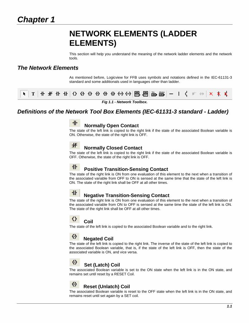
The Network Elements As mentioned before, Logicview for FFB uses symbols and notations defined in the IEC-61131-3 standard and some additionals used in languages other than ladder.
Fig 1.1 - Network Toolbox.
Definitions of the Network Tool Box Elements (IEC-61131-3 standard - Ladder)
Normally Open Contact The state of the left link is copied to the right link if the state of the associated Boolean variable is ON. Otherwise, the state of the right link is OFF.
Normally Closed Contact The state of the left link is copied to the right link if the state of the associated Boolean variable is OFF. Otherwise, the state of the right link is OFF.
Positive Transition-Sensing Contact The state of the right link is ON from one evaluation of this element to the next when a transition of the associated variable from OFF to ON is sensed at the same time that the state of the left link is ON. The state of the right link shall be OFF at all other times.
Negative Transition-Sensing Contact The state of the right link is ON from one evaluation of this element to the next when a transition of the associated variable from ON to OFF is sensed at the same time the state of the left link is ON. The state of the right link shall be OFF at all other times.
Coil The state of the left link is copied to the associated Boolean variable and to the right link.
Negated Coil The state of the left link is copied to the right link. The inverse of the state of the left link is copied to the associated Boolean variable, that is, if the state of the left link is OFF, then the state of the associated variable is ON, and vice versa.
Set (Latch) Coil The associated Boolean variable is set to the ON state when the left link is in the ON state, and remains set until reset by a RESET Coil.
Reset (Unlatch) Coil The associated Boolean variable is reset to the OFF state when the left link is in the ON state, and remains reset until set again by a SET coil.
User Manual
1.2
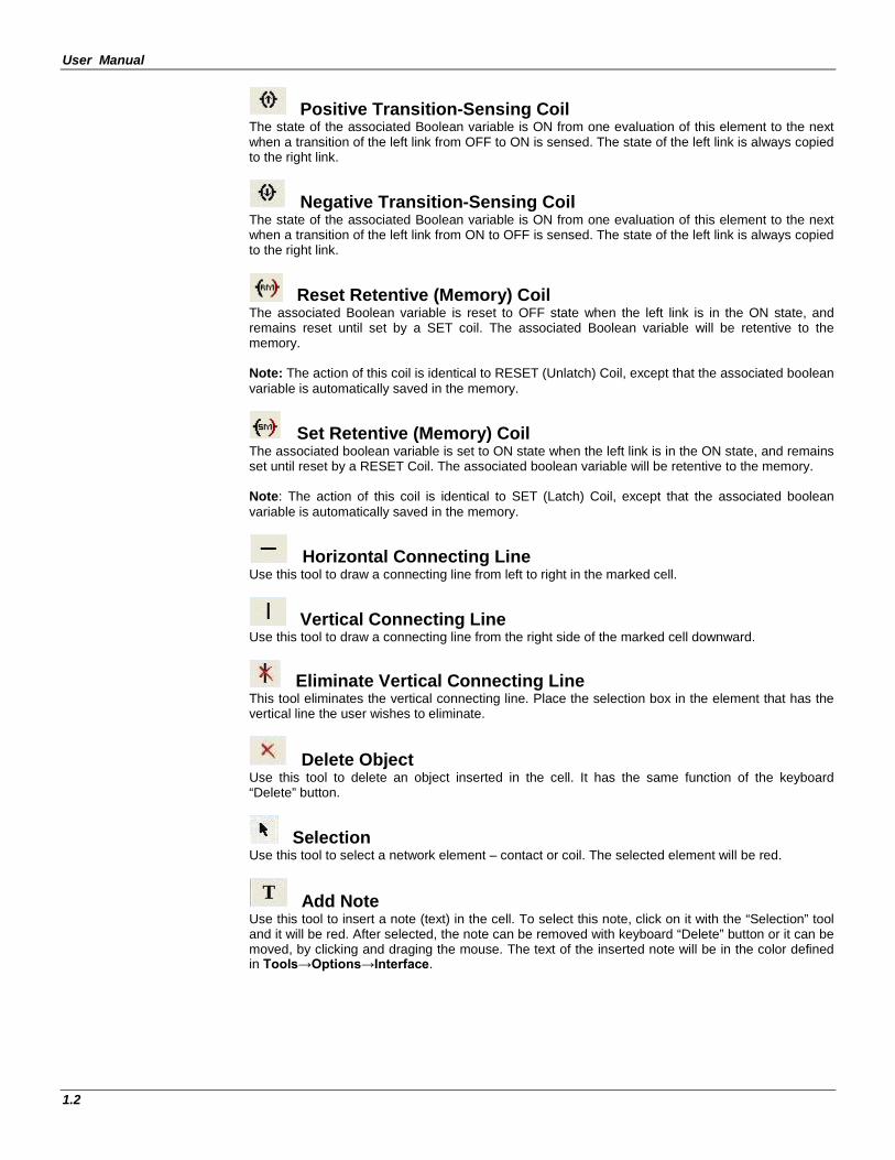
Positive Transition-Sensing Coil The state of the associated Boolean variable is ON from one evaluation of this element to the next when a transition of the left link from OFF to ON is sensed. The state of the left link is always copied to the right link.
Negative Transition-Sensing Coil The state of the associated Boolean variable is ON from one evaluation of this element to the next when a transition of the left link from ON to OFF is sensed. The state of the left link is always copied to the right link.
Reset Retentive (Memory) Coil The associated Boolean variable is reset to OFF state when the left link is in the ON state, and remains reset until set by a SET coil. The associated Boolean variable will be retentive to the memory. Note: The action of this coil is identical to RESET (Unlatch) Coil, except that the associated boolean variable is automatically saved in the memory.
Set Retentive (Memory) Coil The associated boolean variable is set to ON state when the left link is in the ON state, and remains set until reset by a RESET Coil. The associated boolean variable will be retentive to the memory. Note: The action of this coil is identical to SET (Latch) Coil, except that the associated boolean variable is automatically saved in the memory.
Horizontal Connecting Line Use this tool to draw a connecting line from left to right in the marked cell.
Vertical Connecting Line Use this tool to draw a connecting line from the right side of the marked cell downward.
Eliminate Vertical Connecting Line This tool eliminates the vertical connecting line. Place the selection box in the element that has the vertical line the user wishes to eliminate.
Delete Object Use this tool to delete an object inserted in the cell. It has the same function of the keyboard “Delete” button.
Selection Use this tool to select a network element – contact or coil. The selected element will be red.
Add Note Use this tool to insert a note (text) in the cell. To select this note, click on it with the “Selection” tool and it will be red. After selected, the note can be removed with keyboard “Delete” button or it can be moved, by clicking and draging the mouse. The text of the inserted note will be in the color defined in Tools→Options→Interface.
Network Elements (Ladder Elements)
1.3
Definitions of the Network Tool Box Elements (IEC-61131-3 standard – other languages)
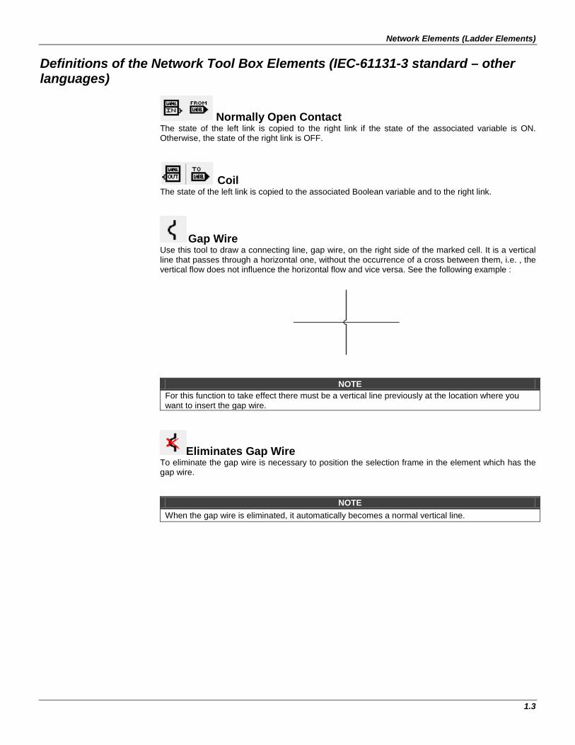
Normally Open Contact The state of the left link is copied to the right link if the state of the associated variable is ON. Otherwise, the state of the right link is OFF.
Coil The state of the left link is copied to the associated Boolean variable and to the right link.
Gap Wire Use this tool to draw a connecting line, gap wire, on the right side of the marked cell. It is a vertical line that passes through a horizontal one, without the occurrence of a cross between them, i.e. , the vertical flow does not influence the horizontal flow and vice versa. See the following example :
NOTE
For this function to take effect there must be a vertical line previously at the location where you want to insert the gap wire.
Eliminates Gap Wire To eliminate the gap wire is necessary to position the selection frame in the element which has the gap wire.
NOTE When the gap wire is eliminated, it automatically becomes a normal vertical line.
User Manual
1.4
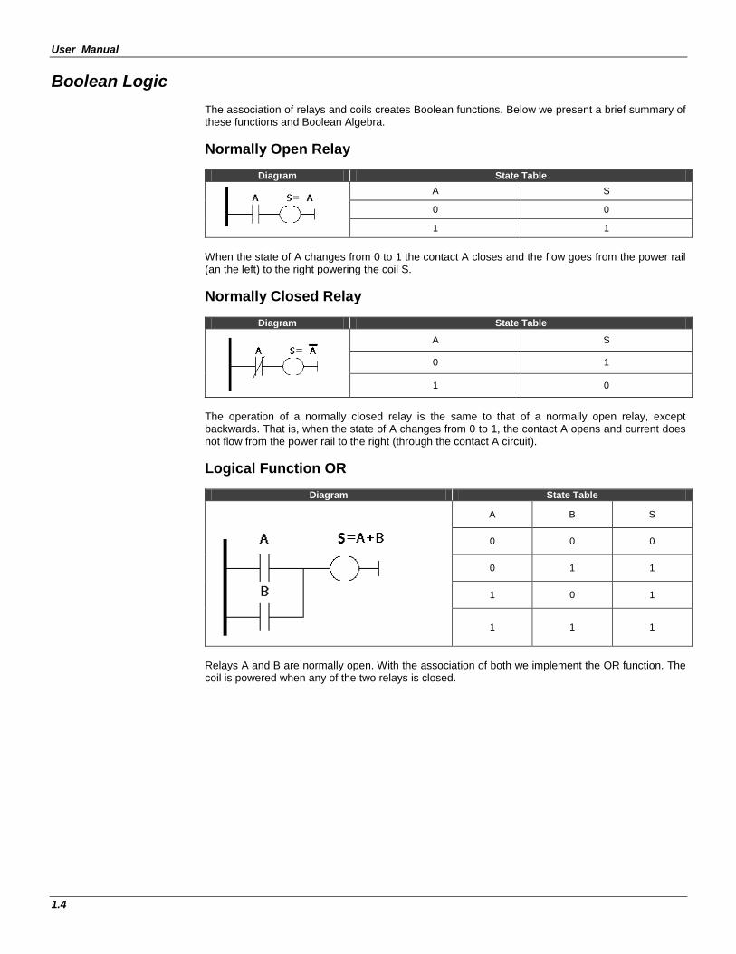
Boolean Logic The association of relays and coils creates Boolean functions. Below we present a brief summary of these functions and Boolean Algebra. Normally Open Relay
Diagram State Table
A S
0 0
1 1
When the state of A changes from 0 to 1 the contact A closes and the flow goes from the power rail (an the left) to the right powering the coil S. Normally Closed Relay
Diagram State Table
A S
0 1
1 0
The operation of a normally closed relay is the same to that of a normally open relay, except backwards. That is, when the state of A changes from 0 to 1, the contact A opens and current does not flow from the power rail to the right (through the contact A circuit). Logical Function OR
Diagram State Table
A B S
0 0 0
0 1 1
1 0 1
1 1 1
Relays A and B are normally open. With the association of both we implement the OR function. The coil is powered when any of the two relays is closed.
Network Elements (Ladder Elements)
1.5
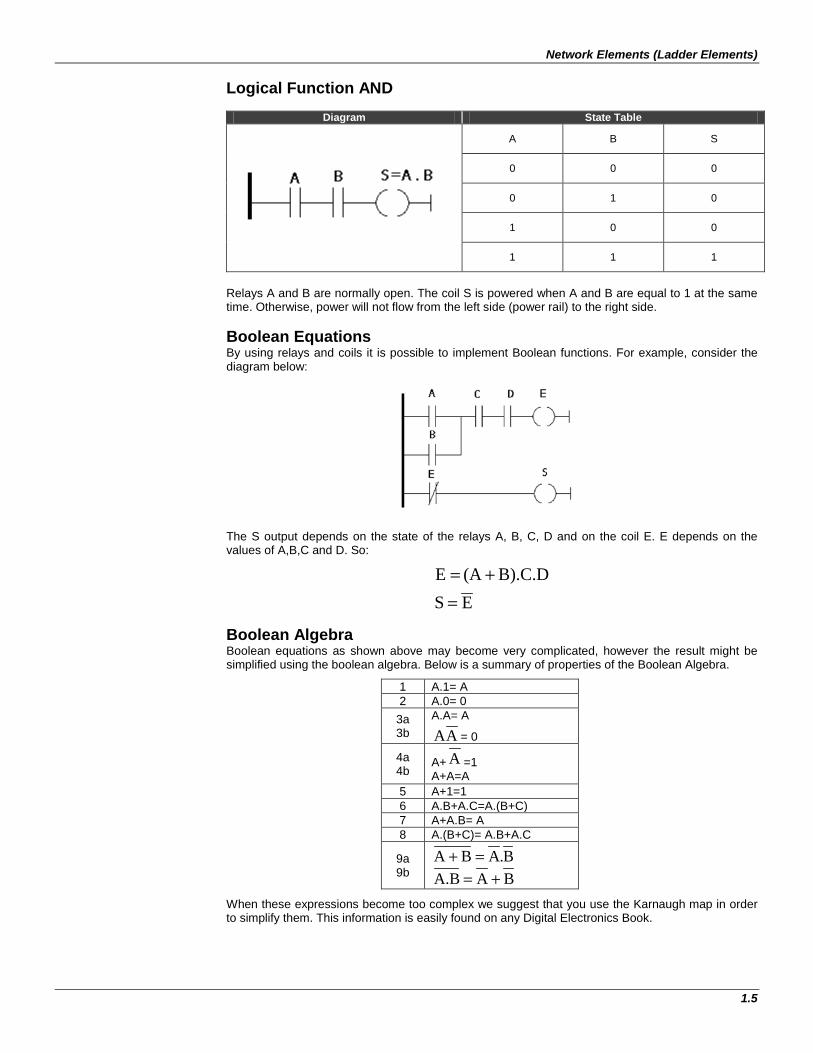
Logical Function AND
Diagram State Table
A B S
0 0 0
0 1 0
1 0 0
1 1 1
Relays A and B are normally open. The coil S is powered when A and B are equal to 1 at the same time. Otherwise, power will not flow from the left side (power rail) to the right side. Boolean Equations By using relays and coils it is possible to implement Boolean functions. For example, consider the diagram below:
The S output depends on the state of the relays A, B, C, D and on the coil E. E depends on the values of A,B,C and D. So:
ESB).C.D(A E
=+=
Boolean Algebra Boolean equations as shown above may become very complicated, however the result might be simplified using the boolean algebra. Below is a summary of properties of the Boolean Algebra.
1 A.1= A 2 A.0= 0
3a 3b
A.A= A
AA = 0
4a 4b
A+ A =1 A+A=A
5 A+1=1 6 A.B+A.C=A.(B+C) 7 A+A.B= A 8 A.(B+C)= A.B+A.C
9a 9b
B.ABA =+ BAA.B +=
When these expressions become too complex we suggest that you use the Karnaugh map in order to simplify them. This information is easily found on any Digital Electronics Book.

User Manual
1.6
Chapter 2
2.1
FUNCTION BLOCKS
Introduction This is a complete and updated reference of the Function Blocks (FB) supported by the DF62, DF63, DF73, DF75, DF79, DF81, DF89, DF95 and DF97 controllers. This chapter presents block diagrams with inputs, outputs, and configuration parameters. It also includes detailed explanations of each block, how they work, how to configure each one of them. Besides, a few examples are presented in order to help understand and utilize the Function Blocks. The data types used by LogicView for FFB are shown in the table below:
Reference Data Type Number of bits BOOL Boolean 1 LONG Integer 32 Unsigned FLOAT Float 32
Each function block has a table that shows all inputs, outputs, parameters and variables of each block. I - Inputs: They can be a variable from another FB, or from an I/O card, or user-configured. P - Parameters: They are the values internally used by the function blocks. O - Outputs: Variables resulting from the processing of the block.
ATTENTION A comma is not accepted in place of a decimal point. (E.g. for 9/5, you should write 1.8 instead of 1,8. If you write 1,8 the program will read 18.)
EN Input and EO Output Every function has an EN input and an EO output, except those with a “r” sub-index (e.g. TPr) and CTUr which has only EN input. EN input is set to enable the function block that should be processed. If EN is false, all outputs change to zero and the FB is not executed. EO changes to true logic to indicate that the function was successfully executed.
Function Blocks
2.2
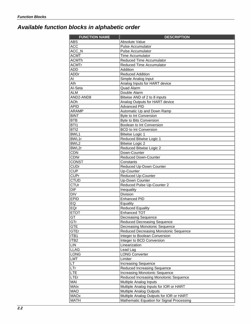
Available function blocks in alphabetic order
FUNCTION NAME DESCRIPTION ABS Absolute Value ACC Pulse Accumulator ACC_N Pulse Accumulator ACMT Time Accumulator ACMTh Reduced Time Accumulator ACMTr Reduced Time Accumulator ADD Addition ADDr Reduced Addition AI Simple Analog Input AIh Analog Inputs for HART device AI-Seta Quad Alarm ALM Double Alarm AND2-AND8 Bitwise AND of 2 to 8 inputs AOh Analog Outputs for HART device APID Advanced PID ARAMP Automatic Up and Down Ramp BINT Byte to Int Conversion BTB Byte to Bits Conversion BTI1 Boolean to Int Conversion BTI2 BCD to Int Conversion BWL1 Bitwise Logic 1 BWL1r Reduced Bitwise Logic 1 BWL2 Bitwise Logic 2 BWL2r Reduced Bitwise Logic 2 CDN Down-Counter CDNr Reduced Down-Counter CONST Constants CUDr Reduced Up-Down Counter CUP Up-Counter CUPr Reduced Up-Counter CTUD Up-Down Counter CTUr Reduced Pulse Up-Counter 2 DIF Inequality DIV Division EPID Enhanced PID EQ Equality EQr Reduced Equality ETOT Enhanced TOT GT Decreasing Sequence GTr Reduced Decreasing Sequence GTE Decreasing Monotonic Sequence GTEr Reduced Decreasing Monotonic Sequence ITB1 Integer to Boolean Conversion ITB2 Integer to BCD Conversion LIN Linearization LLAG Lead Lag LONG LONG Converter LMT Limiter LT Increasing Sequence LTr Reduced Increasing Sequence LTE Increasing Monotonic Sequence LTEr Reduced Increasing Monotonic Sequence MAI Multiple Analog Inputs MAIx Multiple Analog Inputs for IOR or HART MAO Multiple Analog Outputs MAOx Multiple Analog Outputs for IOR or HART MATH Mathematic Equation for Signal Processing
User Manual
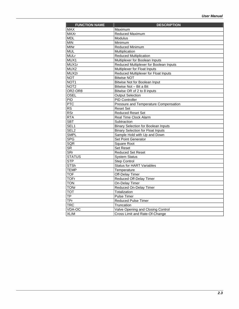
2.3
FUNCTION NAME DESCRIPTION MAX Maximum MAXr Reduced Maximum MDL Modulus MIN Minimum MINr Reduced Minimum MUL Multiplication MULr Reduced Multiplication MUX1 Multiplexer for Boolean Inputs MUX1r Reduced Multiplexer for Boolean Inputs MUX2 Multiplexer for Float Inputs MUX2r Reduced Multiplexer for Float Inputs NOT Bitwise NOT NOT1 Bitwise Not for Boolean Input NOT2 Bitwise Not – Bit a Bit OR2-OR8 Bitwise OR of 2 to 8 inputs OSEL Output Selection PID PID Controller PTC Pressure and Temperature Compensation RS Reset Set RSr Reduced Reset Set RTA Real Time Clock Alarm SBT Subtraction SEL1 Binary Selection for Boolean Inputs SEL2 Binary Selection for Float Inputs SMPL Sample Hold with Up and Down SPG Set Point Generator SQR Square Root SR Set Reset SRr Reduced Set Reset STATUS System Status STP Step Control STSh Status for HART Variables TEMP Temperature TOF Off-Delay Timer TOFr Reduced Off-Delay Timer TON On-Delay Timer TONr Reduced On-Delay Timer TOT Totalization TP Pulse Timer TPr Reduced Pulse Timer TRC Truncation VDA-OC Valve Opening and Closing Control XLIM Cross Limit and Rate-Of-Change
Function Blocks
2.4
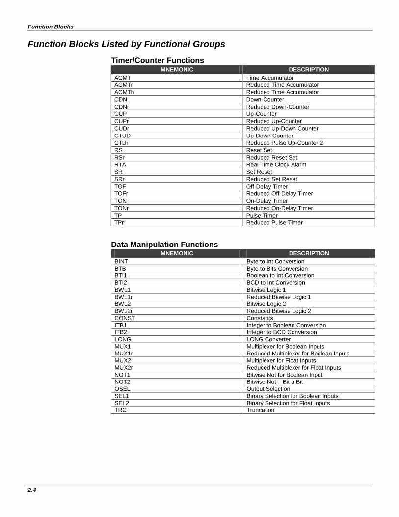
Function Blocks Listed by Functional Groups Timer/Counter Functions
MNEMONIC DESCRIPTION ACMT Time Accumulator ACMTr Reduced Time Accumulator ACMTh Reduced Time Accumulator CDN Down-Counter CDNr Reduced Down-Counter CUP Up-Counter CUPr Reduced Up-Counter CUDr Reduced Up-Down Counter CTUD Up-Down Counter CTUr Reduced Pulse Up-Counter 2 RS Reset Set RSr Reduced Reset Set RTA Real Time Clock Alarm SR Set Reset SRr Reduced Set Reset TOF Off-Delay Timer TOFr Reduced Off-Delay Timer TON On-Delay Timer TONr Reduced On-Delay Timer TP Pulse Timer TPr Reduced Pulse Timer
Data Manipulation Functions
MNEMONIC DESCRIPTION BINT Byte to Int Conversion BTB Byte to Bits Conversion BTI1 Boolean to Int Conversion BTI2 BCD to Int Conversion BWL1 Bitwise Logic 1 BWL1r Reduced Bitwise Logic 1 BWL2 Bitwise Logic 2 BWL2r Reduced Bitwise Logic 2 CONST Constants ITB1 Integer to Boolean Conversion ITB2 Integer to BCD Conversion LONG LONG Converter MUX1 Multiplexer for Boolean Inputs MUX1r Reduced Multiplexer for Boolean Inputs MUX2 Multiplexer for Float Inputs MUX2r Reduced Multiplexer for Float Inputs NOT1 Bitwise Not for Boolean Input NOT2 Bitwise Not – Bit a Bit OSEL Output Selection SEL1 Binary Selection for Boolean Inputs SEL2 Binary Selection for Float Inputs TRC Truncation
User Manual
2.5
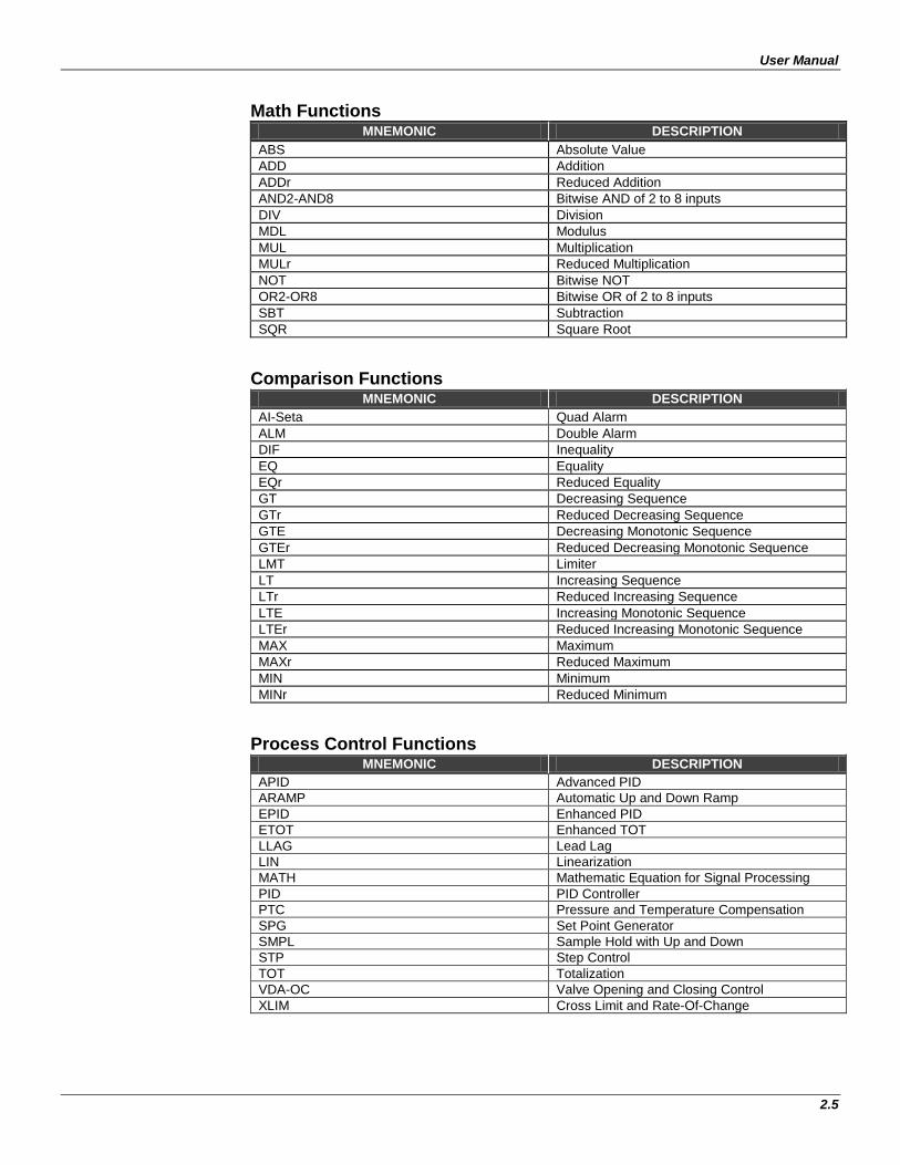
Math Functions
MNEMONIC DESCRIPTION ABS Absolute Value ADD Addition ADDr Reduced Addition AND2-AND8 Bitwise AND of 2 to 8 inputs DIV Division MDL Modulus MUL Multiplication MULr Reduced Multiplication NOT Bitwise NOT OR2-OR8 Bitwise OR of 2 to 8 inputs SBT Subtraction SQR Square Root
Comparison Functions
MNEMONIC DESCRIPTION AI-Seta Quad Alarm ALM Double Alarm DIF Inequality EQ Equality EQr Reduced Equality GT Decreasing Sequence GTr Reduced Decreasing Sequence GTE Decreasing Monotonic Sequence GTEr Reduced Decreasing Monotonic Sequence LMT Limiter LT Increasing Sequence LTr Reduced Increasing Sequence LTE Increasing Monotonic Sequence LTEr Reduced Increasing Monotonic Sequence MAX Maximum MAXr Reduced Maximum MIN Minimum MINr Reduced Minimum
Process Control Functions
MNEMONIC DESCRIPTION APID Advanced PID ARAMP Automatic Up and Down Ramp EPID Enhanced PID ETOT Enhanced TOT LLAG Lead Lag LIN Linearization MATH Mathematic Equation for Signal Processing PID PID Controller PTC Pressure and Temperature Compensation SPG Set Point Generator SMPL Sample Hold with Up and Down STP Step Control TOT Totalization VDA-OC Valve Opening and Closing Control XLIM Cross Limit and Rate-Of-Change

Function Blocks
2.6
Input/Output Functions
MNEMONIC DESCRIPTION ACC Pulse Accumulator ACC_N Pulse Accumulator AI Simple Analog Input AIh Analog Inputs for HART device AOh Analog Outputs for HART device MAI Multiple Analog Inputs MAIx Multiple Analog Inputs for IOR or HART MAO Multiple Analog Outputs MAOx Multiple Analog Outputs for IOR or HART STATUS System Status STSh Status for HART Variables TEMP Temperature
User Manual
2.7
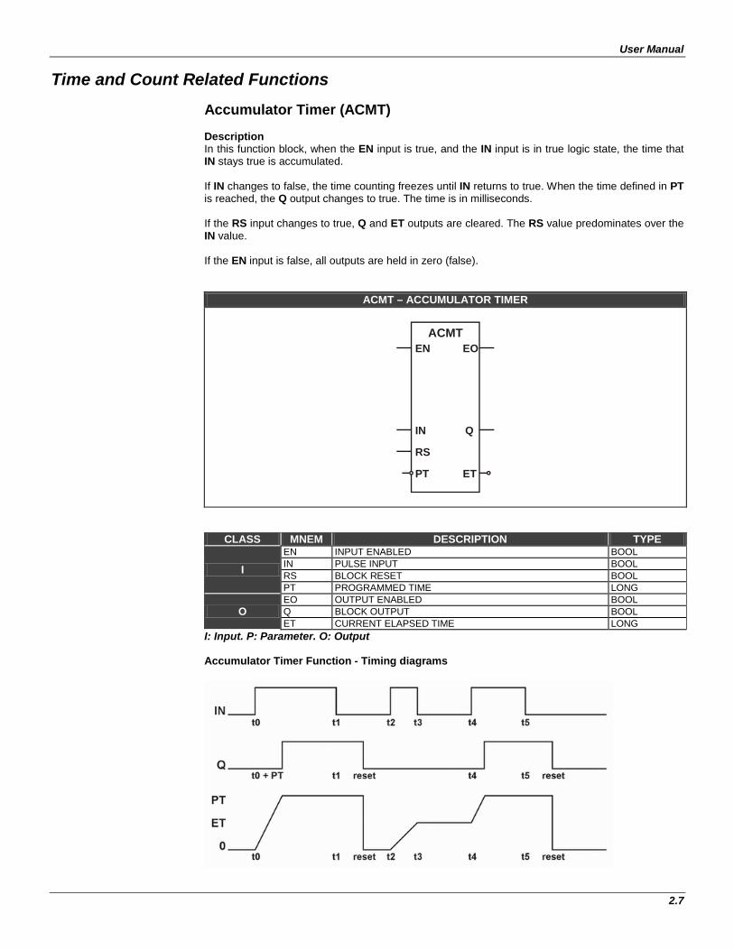
Time and Count Related Functions Accumulator Timer (ACMT) Description In this function block, when the EN input is true, and the IN input is in true logic state, the time that IN stays true is accumulated. If IN changes to false, the time counting freezes until IN returns to true. When the time defined in PT is reached, the Q output changes to true. The time is in milliseconds. If the RS input changes to true, Q and ET outputs are cleared. The RS value predominates over the IN value. If the EN input is false, all outputs are held in zero (false).
ACMT – ACCUMULATOR TIMER
ACMTEN EO
IN
PT
Q
ET
RS
CLASS MNEM DESCRIPTION TYPE
I EN INPUT ENABLED BOOL IN PULSE INPUT BOOL RS BLOCK RESET BOOL PT PROGRAMMED TIME LONG
O EO OUTPUT ENABLED BOOL Q BLOCK OUTPUT BOOL ET CURRENT ELAPSED TIME LONG
I: Input. P: Parameter. O: Output Accumulator Timer Function - Timing diagrams

Function Blocks
2.8
Reduced Accumulator Timer (ACMTr) This function block works exactly like the ACMT block, but it does not have the EN input and the EO output.
ACMTr - REDUCED ACCUMULATOR TIMER
ACMTrIN Q
RS
PT ET
CLASS MNEM DESCRIPTION TYPE
I IN PULSE INPUT BOOL RS BLOCK RESET BOOL PT PROGRAMMED TIME (MILISECONDS) LONG
O Q BLOCK OUTPUT BOOL ET CURRENT ELAPSED TIME (MILISECONDS) LONG
I: Input. P: Parameter. O: Output

User Manual
2.9
Reduced Accumulator Timer (ACMTh) This function block works exactly like the ACMTr block, but the time of ET output and PT input are configured in hours.
ACMTh - REDUCED ACCUMULATOR TIMER
ACMThIN Q
RS
PT ET
CLASS MNEM DESCRIPTION TYPE
I IN PULSE INPUT BOOL RS BLOCK RESET BOOL PT PROGRAMMED TIME (HOURS) LONG
O Q BLOCK OUTPUT BOOL ET CURRENT ELAPSED TIME (HOURS) LONG
I: Input. P: Parameter. O: Output
Function Blocks
2.10
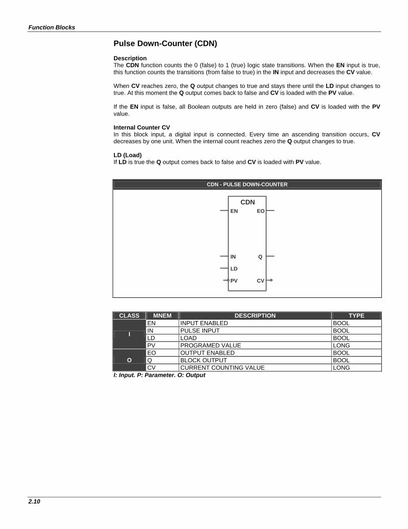
Pulse Down-Counter (CDN) Description The CDN function counts the 0 (false) to 1 (true) logic state transitions. When the EN input is true, this function counts the transitions (from false to true) in the IN input and decreases the CV value. When CV reaches zero, the Q output changes to true and stays there until the LD input changes to true. At this moment the Q output comes back to false and CV is loaded with the PV value. If the EN input is false, all Boolean outputs are held in zero (false) and CV is loaded with the PV value. Internal Counter CV In this block input, a digital input is connected. Every time an ascending transition occurs, CV decreases by one unit. When the internal count reaches zero the Q output changes to true. LD (Load) If LD is true the Q output comes back to false and CV is loaded with PV value.
CDN - PULSE DOWN-COUNTER
CDNEN EO
IN
PV
Q
CV
LD
CLASS MNEM DESCRIPTION TYPE
I
EN INPUT ENABLED BOOL IN PULSE INPUT BOOL LD LOAD BOOL PV PROGRAMED VALUE LONG
O EO OUTPUT ENABLED BOOL Q BLOCK OUTPUT BOOL CV CURRENT COUNTING VALUE LONG
I: Input. P: Parameter. O: Output
User Manual
2.11
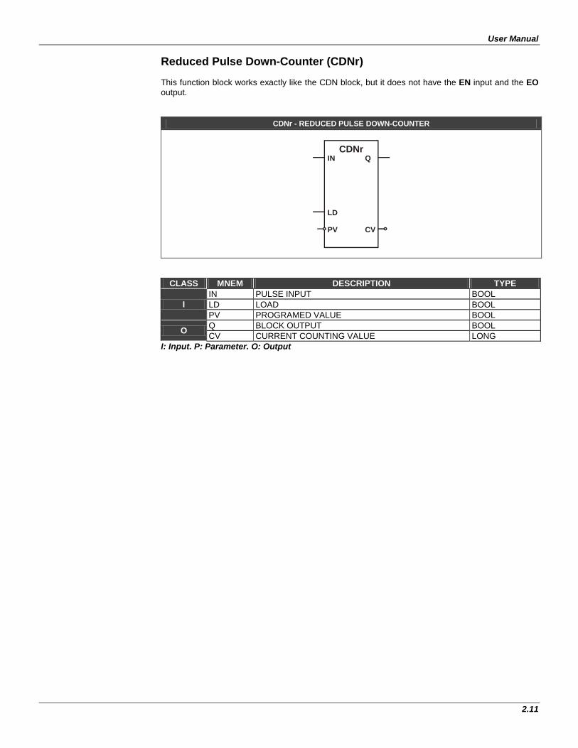
Reduced Pulse Down-Counter (CDNr) This function block works exactly like the CDN block, but it does not have the EN input and the EO output.
CDNr - REDUCED PULSE DOWN-COUNTER
CDNrIN Q
LD
PV CV
CLASS MNEM DESCRIPTION TYPE
I IN PULSE INPUT BOOL LD LOAD BOOL PV PROGRAMED VALUE BOOL
O Q BLOCK OUTPUT BOOL CV CURRENT COUNTING VALUE LONG
I: Input. P: Parameter. O: Output
Function Blocks
2.12
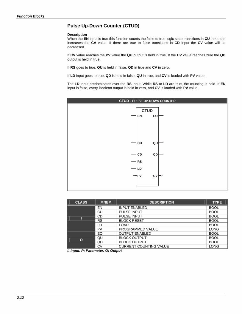
Pulse Up-Down Counter (CTUD) Description When the EN input is true this function counts the false to true logic state transitions in CU input and increases the CV value. If there are true to false transitions in CD input the CV value will be decreased. If CV value reaches the PV value the QU output is held in true. If the CV value reaches zero the QD output is held in true. If RS goes to true, QU is held in false, QD in true and CV in zero. If LD input goes to true, QD is held in false, QU in true, and CV is loaded with PV value. The LD input predominates over the RS input. While RS or LD are true, the counting is held. If EN input is false, every Boolean output is held in zero, and CV is loaded with PV value.
CTUD - PULSE UP-DOWN COUNTER
CTUDEN EO
CD
PV
QD
CV
RS
CU QU
LD
CLASS MNEM DESCRIPTION TYPE
I
EN INPUT ENABLED BOOL CU PULSE INPUT BOOL CD PULSE INPUT BOOL RS BLOCK RESET BOOL LD LOAD BOOL PV PROGRAMMED VALUE LONG
O
EO OUTPUT ENABLED BOOL QU BLOCK OUTPUT BOOL QD BLOCK OUTPUT BOOL CV CURRENT COUNTING VALUE LONG
I: Input. P: Parameter. O: Output
User Manual
2.13
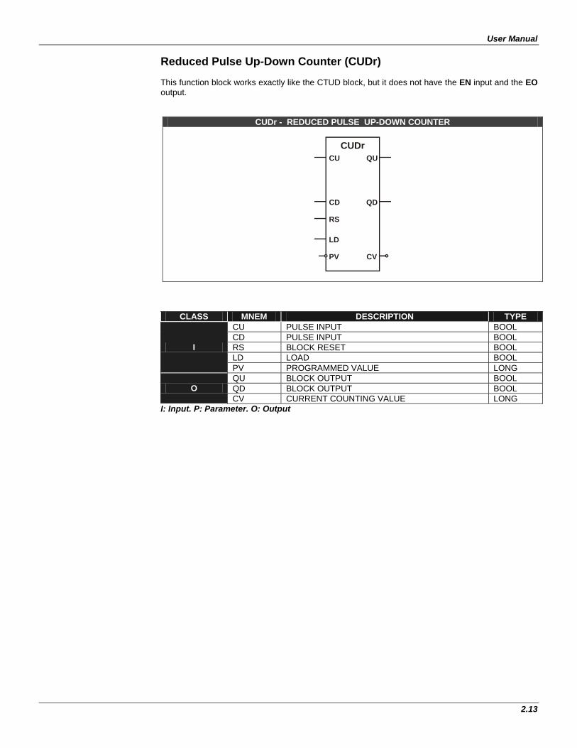
Reduced Pulse Up-Down Counter (CUDr) This function block works exactly like the CTUD block, but it does not have the EN input and the EO output.
CLASS MNEM DESCRIPTION TYPE
I
CU PULSE INPUT BOOL CD PULSE INPUT BOOL RS BLOCK RESET BOOL LD LOAD BOOL PV PROGRAMMED VALUE LONG
O QU BLOCK OUTPUT BOOL QD BLOCK OUTPUT BOOL CV CURRENT COUNTING VALUE LONG
I: Input. P: Parameter. O: Output
CUDr - REDUCED PULSE UP-DOWN COUNTER
CUDrCU QU
CD
PV
QD
CV
RS
LD
Function Blocks
2.14
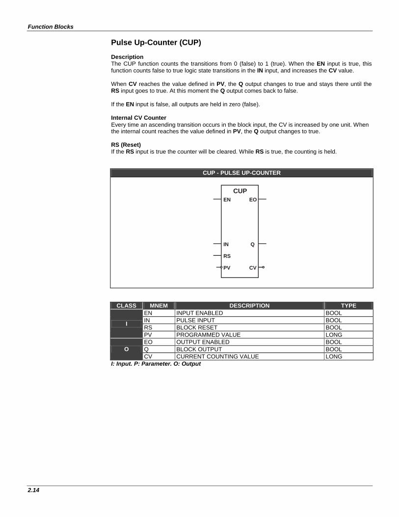
Pulse Up-Counter (CUP) Description The CUP function counts the transitions from 0 (false) to 1 (true). When the EN input is true, this function counts false to true logic state transitions in the IN input, and increases the CV value. When CV reaches the value defined in PV, the Q output changes to true and stays there until the RS input goes to true. At this moment the Q output comes back to false. If the EN input is false, all outputs are held in zero (false). Internal CV Counter Every time an ascending transition occurs in the block input, the CV is increased by one unit. When the internal count reaches the value defined in PV, the Q output changes to true. RS (Reset) If the RS input is true the counter will be cleared. While RS is true, the counting is held.
CUP - PULSE UP-COUNTER
CUPEN EO
IN
PV
Q
CV
RS
CLASS MNEM DESCRIPTION TYPE
I
EN INPUT ENABLED BOOL IN PULSE INPUT BOOL RS BLOCK RESET BOOL PV PROGRAMMED VALUE LONG
O EO OUTPUT ENABLED BOOL Q BLOCK OUTPUT BOOL CV CURRENT COUNTING VALUE LONG
I: Input. P: Parameter. O: Output

User Manual
2.15
Reduced Pulse Up-Counter (CUPr) This function block works exactly like the CUP block, but it does not have the EN input and the EO output.
CUPr - REDUCED PULSE UP-COUNTER
CUPrIN Q
RS
PV CV
CLASS MNEM DESCRIPTION TYPE
I IN PULSE INPUT BOOL RS BLOCK RESET BOOL PV PROGRAMMED VALUE LONG
O Q BLOCK OUTPUT BOOL CV CURRENT COUNTING VALUE LONG
I: Input. P: Parameter. O: Output
Function Blocks
2.16
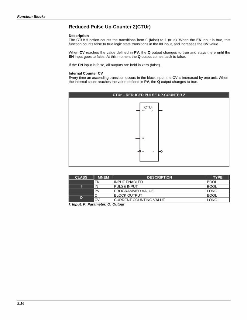
Reduced Pulse Up-Counter 2(CTUr) Description The CTUr function counts the transitions from 0 (false) to 1 (true). When the EN input is true, this function counts false to true logic state transitions in the IN input, and increases the CV value. When CV reaches the value defined in PV, the Q output changes to true and stays there until the EN input goes to false. At this moment the Q output comes back to false. If the EN input is false, all outputs are held in zero (false). Internal Counter CV Every time an ascending transition occurs in the block input, the CV is increased by one unit. When the internal count reaches the value defined in PV, the Q output changes to true.
CTUr – REDUCED PULSE UP-COUNTER 2
CTUrEN Q
CVPV
IN
CLASS MNEM DESCRIPTION TYPE
I EN INPUT ENABLED BOOL IN PULSE INPUT BOOL PV PROGRAMMED VALUE LONG
O Q BLOCK OUTPUT BOOL CV CURRENT COUNTING VALUE LONG
I: Input. P: Parameter. O: Output
User Manual
2.17
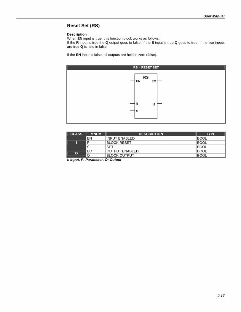
Reset Set (RS) Description When EN input is true, this function block works as follows: If the R input is true the Q output goes to false. If the S input is true Q goes to true. If the two inputs are true Q is held in false. If the EN input is false, all outputs are held in zero (false).
RS – RESET SET
CLASS MNEM DESCRIPTION TYPE
I EN INPUT ENABLED BOOL R BLOCK RESET BOOL S SET BOOL
O EO OUTPUT ENABLED BOOL Q BLOCK OUTPUT BOOL
I: Input. P: Parameter. O: Output
RS EN EO
R
S
Q
Function Blocks
2.18
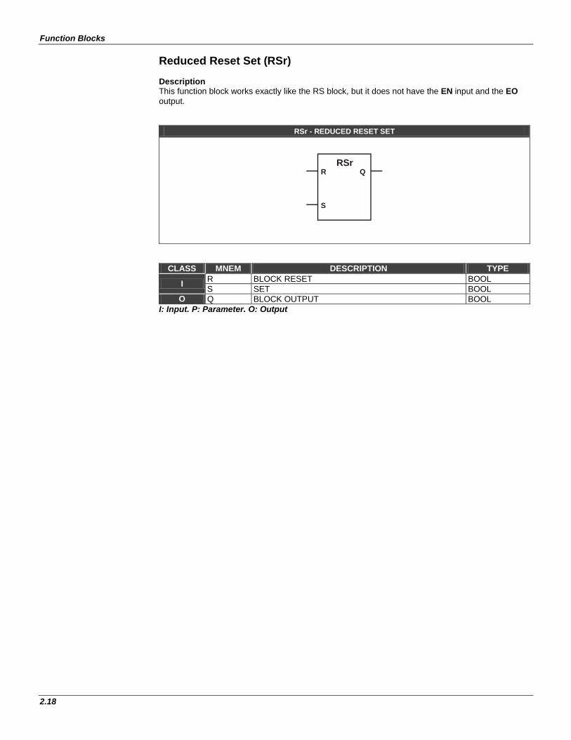
Reduced Reset Set (RSr) Description This function block works exactly like the RS block, but it does not have the EN input and the EO output.
RSr - REDUCED RESET SET
RSrR Q
S
CLASS MNEM DESCRIPTION TYPE
I R BLOCK RESET BOOL S SET BOOL
O Q BLOCK OUTPUT BOOL I: Input. P: Parameter. O: Output
User Manual
2.19
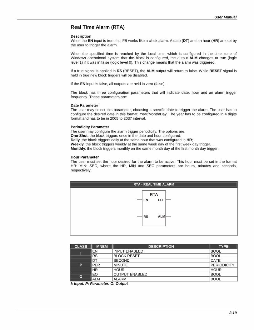
Real Time Alarm (RTA) Description When the EN input is true, this FB works like a clock alarm. A date (DT) and an hour (HR) are set by the user to trigger the alarm. When the specified time is reached by the local time, which is configured in the time zone of Windows operational system that the block is configured, the output ALM changes to true (logic level 1) if it was in false (logic level 0). This change means that the alarm was triggered. If a true signal is applied in RS (RESET), the ALM output will return to false. While RESET signal is held in true new block triggers will be disabled. If the EN input is false, all outputs are held in zero (false). The block has three configuration parameters that will indicate date, hour and an alarm trigger frequency. These parameters are: Date Parameter The user may select this parameter, choosing a specific date to trigger the alarm. The user has to configure the desired date in this format: Year/Month/Day. The year has to be configured in 4 digits format and has to be in 2005 to 2037 interval. Periodicity Parameter The user may configure the alarm trigger periodicity. The options are: One-Shot: the block triggers once in the date and hour configured; Daily: the block triggers daily at the same hour that was configured in HR; Weekly: the block triggers weekly at the same week day of the first week day trigger. Monthly: the block triggers monthly on the same month day of the first month day trigger. Hour Parameter The user must set the hour desired for the alarm to be active. This hour must be set in the format HR: MIN: SEC, where the HR, MIN and SEC parameters are hours, minutes and seconds, respectively.
RTA - REAL TIME ALARM
RTA
RS
EOEN
ALM
CLASS MNEM DESCRIPTION TYPE
I EN INPUT ENABLED BOOL RS BLOCK RESET BOOL
P DT SECOND DATE PER MINUTE PERIODICITY HR HOUR HOUR
O EO OUTPUT ENABLED BOOL ALM ALARM BOOL
I: Input. P: Parameter. O: Output

Function Blocks
2.20
IMPORTANT
1. The RTC (Real Time Clock) of the controller in which the RTA will be executed must be configured according to the official local time.
2. The RTC of the DFI302 controller can be configured manually, via Batch Download option of FBTools, and when available, automatically kept synchronized via SNTP. For futher information refer to the FBTools help and Server Manager appendix in the Studio302 manual, respectively.
3. The user has to take care with the changes at the beginning and end of daylight saving time.
The important thing is, when changing the time, for ahead or back, you must do the same change in the controller.

User Manual
2.21
Set Reset (SR) Description When EN input is true this function block works in this way: If the S input is true, the Q output goes to true. If the R input is true Q goes to false. If the two inputs are true Q is held in true. If the EN input is false, all outputs are held in zero (false).
SR - SET RESET
SREN EO
S
R
Q
CLASS MNEM DESCRIPTION TYPE
I EN INPUT ENABLED BOOL S SET BOOL R BLOCK RESET BOOL
O EO OUTPUT ENABLED BOOL Q BLOCK OUTPUT BOOL
I: Input. P: Parameter. O: Output
Function Blocks
2.22
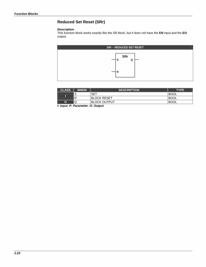
Reduced Set Reset (SRr) Description This function block works exactly like the SR block, but it does not have the EN input and the EO output.
SRr – REDUCED SET RESET
SRrS Q
R
CLASS MNEM DESCRIPTION TYPE
I S SET BOOL R BLOCK RESET BOOL
O Q BLOCK OUTPUT BOOL I: Input. P: Parameter. O: Output

User Manual
2.23
Off-Delay Timer (TOF) Description When the EN input is true, this function holds the true state of the IN input in the Q output for a time period previously defined, after the IN input changes to false. The time period is defined in PT parameter and its unit is milliseconds.
If IN changes to true, before Q goes to false, Q will stay on true state and the time period will start again in the moment that IN goes to false. If the EN input is false, all outputs are held in zero (false).
PT Input The PT input can be connected to a function block output, a FFB or a fixed value.
TOF - OFF-DELAY TIMER
TOFEN EO
IN
PT
Q
ET
CLASS MNEM DESCRIPTION TYPE
I EN INPUT ENABLED BOOL IN PULSE INPUT BOOL PT PROGRAMMED TIME LONG
O EO OUTPUT ENABLED BOOL Q BLOCK OUTPUT BOOL ET CURRENT ELAPSED TIME LONG
I: Input. P: Parameter. O: Output Off-Delay Timer Function - Timing diagrams
IN t0 t1 t2 t3 t4 t5
Q t5 + PT t0
ET t0 t1 t2 t3 t5 0
PT t1 + PT t2

Function Blocks
2.24
Reduced Off-Delay Timer (TOFr) This function block works exactly like the TOF block, but it does not have the EN input and the EO output.
TOFr - REDUCED OFF-DELAY TIMER
TOFrIN Q
PT ET
CLASS MNEM DESCRIPTION TYPE
I IN PULSE INPUT BOOL PT PROGRAMMED TIME LONG
O Q BLOCK OUTPUT BOOL ET CURRENT ELAPSED TIME LONG
I: Input. P: Parameter. O: Output
User Manual
2.25
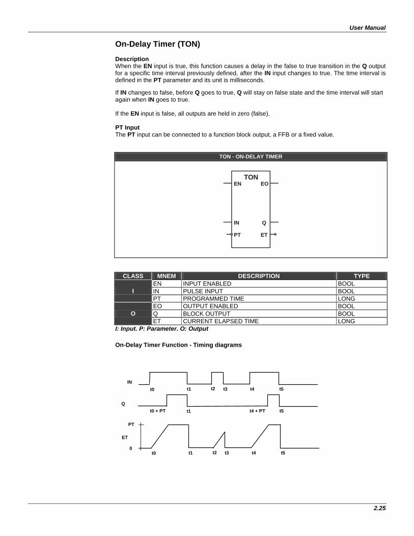
On-Delay Timer (TON) Description When the EN input is true, this function causes a delay in the false to true transition in the Q output for a specific time interval previously defined, after the IN input changes to true. The time interval is defined in the PT parameter and its unit is milliseconds.
If IN changes to false, before Q goes to true, Q will stay on false state and the time interval will start again when IN goes to true. If the EN input is false, all outputs are held in zero (false). PT Input The PT input can be connected to a function block output, a FFB or a fixed value.
TON - ON-DELAY TIMER
TONEN EO
IN
PT
Q
ET
CLASS MNEM DESCRIPTION TYPE
I EN INPUT ENABLED BOOL IN PULSE INPUT BOOL PT PROGRAMMED TIME LONG
O EO OUTPUT ENABLED BOOL Q BLOCK OUTPUT BOOL ET CURRENT ELAPSED TIME LONG
I: Input. P: Parameter. O: Output
On-Delay Timer Function - Timing diagrams
IN t0 t1 t2 t3 t4 t5
Q t5 t4 + PT t1 t0 + PT
ET
t0 t1 t2 t3 t4 t5 0
PT

Function Blocks
2.26
Reduced On-Delay Timer (TONr) This function block works exactly like the TON block, but it does not have the EN input and the EO output.
TONr - REDUCED TIMER ON-DELAY
TONrIN Q
PT ET
CLASS MNEM DESCRIPTION TYPE
I IN PULSE INPUT BOOL PT PROGRAMMED TIME LONG
O Q BLOCK OUTPUT BOOL ET CURRENT ELAPSED TIME LONG
I: Input. P: Parameter. O: Output
User Manual
2.27
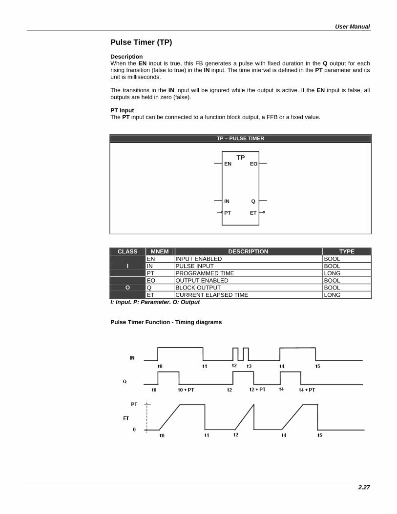
Pulse Timer (TP) Description When the EN input is true, this FB generates a pulse with fixed duration in the Q output for each rising transition (false to true) in the IN input. The time interval is defined in the PT parameter and its unit is milliseconds. The transitions in the IN input will be ignored while the output is active. If the EN input is false, all outputs are held in zero (false). PT Input The PT input can be connected to a function block output, a FFB or a fixed value.
TP – PULSE TIMER
TPEN EO
IN
PT
Q
ET
CLASS MNEM DESCRIPTION TYPE
I EN INPUT ENABLED BOOL IN PULSE INPUT BOOL PT PROGRAMMED TIME LONG
O EO OUTPUT ENABLED BOOL Q BLOCK OUTPUT BOOL ET CURRENT ELAPSED TIME LONG
I: Input. P: Parameter. O: Output Pulse Timer Function - Timing diagrams
Function Blocks
2.28
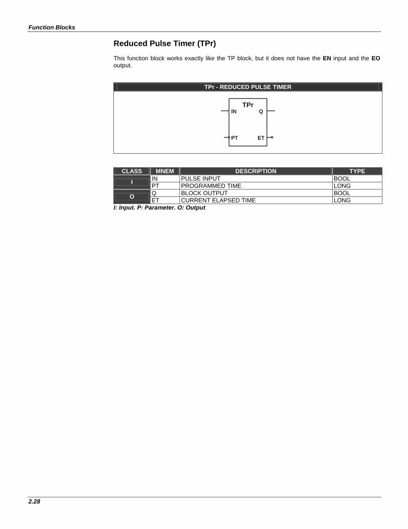
Reduced Pulse Timer (TPr) This function block works exactly like the TP block, but it does not have the EN input and the EO output.
TPr - REDUCED PULSE TIMER
TPrIN Q
PT ET
CLASS MNEM DESCRIPTION TYPE
I IN PULSE INPUT BOOL PT PROGRAMMED TIME LONG
O Q BLOCK OUTPUT BOOL ET CURRENT ELAPSED TIME LONG
I: Input. P: Parameter. O: Output
User Manual
2.29
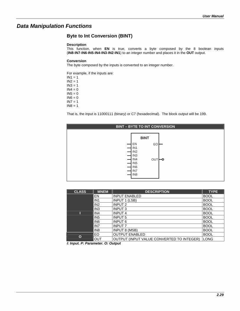
Data Manipulation Functions Byte to Int Conversion (BINT) Description This function, when EN is true, converts a byte composed by the 8 boolean inputs (IN8-IN7-IN6-IN5-IN4-IN3-IN2-IN1) to an integer number and places it in the OUT output. Conversion The byte composed by the inputs is converted to an integer number. For example, if the inputs are: IN1 = 1 IN2 = 1 IN3 = 1 IN4 = 0 IN5 = 0 IN6 = 0 IN7 = 1 IN8 = 1 That is, the input is 11000111 (binary) or C7 (hexadecimal). The block output will be 199.
BINT – BYTE TO INT CONVERSION
BINT
IN1IN2IN3IN4IN5IN6IN7IN8
EN EO
OUT
CLASS MNEM DESCRIPTION TYPE
I
EN INPUT ENABLED BOOL IN1 INPUT 1 (LSB) BOOL IN2 INPUT 2 BOOL IN3 INPUT 3 BOOL IN4 INPUT 4 BOOL IN5 INPUT 5 BOOL IN6 INPUT 6 BOOL IN7 INPUT 7 BOOL IN8 INPUT 8 (MSB) BOOL
O EO OUTPUT ENABLED BOOL OUT OUTPUT (INPUT VALUE CONVERTED TO INTEGER) LONG
I: Input. P: Parameter. O: Output
Function Blocks
2.30
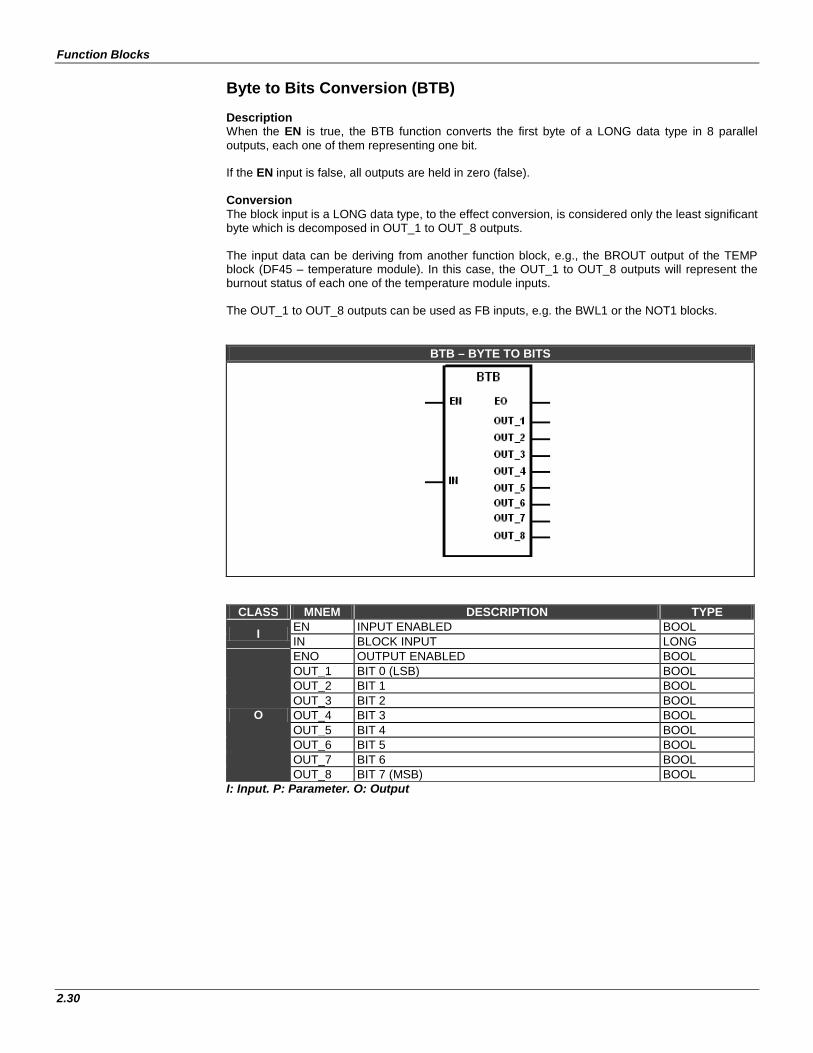
Byte to Bits Conversion (BTB) Description When the EN is true, the BTB function converts the first byte of a LONG data type in 8 parallel outputs, each one of them representing one bit. If the EN input is false, all outputs are held in zero (false). Conversion The block input is a LONG data type, to the effect conversion, is considered only the least significant byte which is decomposed in OUT_1 to OUT_8 outputs. The input data can be deriving from another function block, e.g., the BROUT output of the TEMP block (DF45 – temperature module). In this case, the OUT_1 to OUT_8 outputs will represent the burnout status of each one of the temperature module inputs. The OUT_1 to OUT_8 outputs can be used as FB inputs, e.g. the BWL1 or the NOT1 blocks.
BTB – BYTE TO BITS
CLASS MNEM DESCRIPTION TYPE
I EN INPUT ENABLED BOOL IN BLOCK INPUT LONG
O
ENO OUTPUT ENABLED BOOL OUT_1 BIT 0 (LSB) BOOL OUT_2 BIT 1 BOOL OUT_3 BIT 2 BOOL OUT_4 BIT 3 BOOL OUT_5 BIT 4 BOOL OUT_6 BIT 5 BOOL OUT_7 BIT 6 BOOL OUT_8 BIT 7 (MSB) BOOL
I: Input. P: Parameter. O: Output
User Manual
2.31
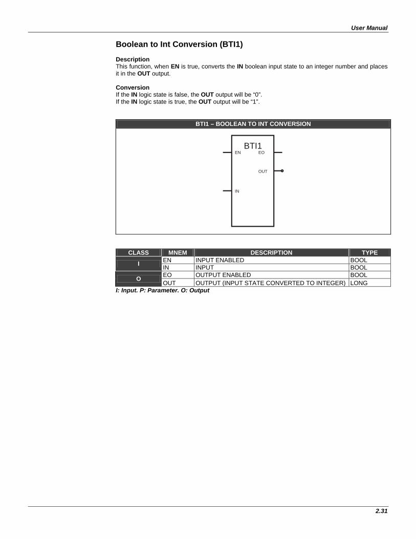
Boolean to Int Conversion (BTI1) Description This function, when EN is true, converts the IN boolean input state to an integer number and places it in the OUT output. Conversion If the IN logic state is false, the OUT output will be “0”. If the IN logic state is true, the OUT output will be “1”.
BTI1 – BOOLEAN TO INT CONVERSION
BTI1EN EO
OUT
IN
CLASS MNEM DESCRIPTION TYPE
I EN INPUT ENABLED BOOL IN INPUT BOOL
O EO OUTPUT ENABLED BOOL OUT OUTPUT (INPUT STATE CONVERTED TO INTEGER) LONG
I: Input. P: Parameter. O: Output
Function Blocks
2.32
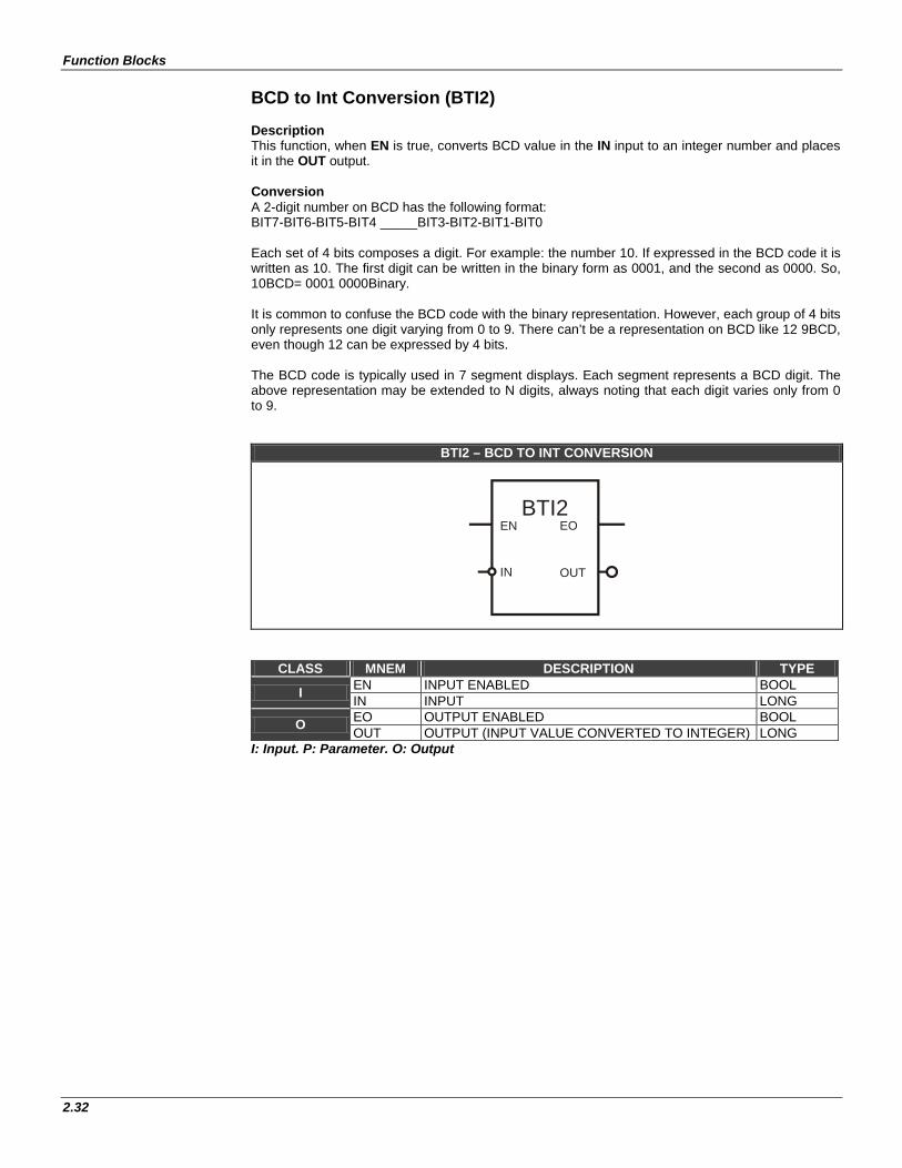
BCD to Int Conversion (BTI2) Description This function, when EN is true, converts BCD value in the IN input to an integer number and places it in the OUT output. Conversion A 2-digit number on BCD has the following format: BIT7-BIT6-BIT5-BIT4 _____BIT3-BIT2-BIT1-BIT0 Each set of 4 bits composes a digit. For example: the number 10. If expressed in the BCD code it is written as 10. The first digit can be written in the binary form as 0001, and the second as 0000. So, 10BCD= 0001 0000Binary. It is common to confuse the BCD code with the binary representation. However, each group of 4 bits only represents one digit varying from 0 to 9. There can’t be a representation on BCD like 12 9BCD, even though 12 can be expressed by 4 bits. The BCD code is typically used in 7 segment displays. Each segment represents a BCD digit. The above representation may be extended to N digits, always noting that each digit varies only from 0 to 9.
BTI2 – BCD TO INT CONVERSION
BTI2EOEN
OUTIN
CLASS MNEM DESCRIPTION TYPE
I EN INPUT ENABLED BOOL IN INPUT LONG
O EO OUTPUT ENABLED BOOL OUT OUTPUT (INPUT VALUE CONVERTED TO INTEGER) LONG
I: Input. P: Parameter. O: Output
User Manual
2.33
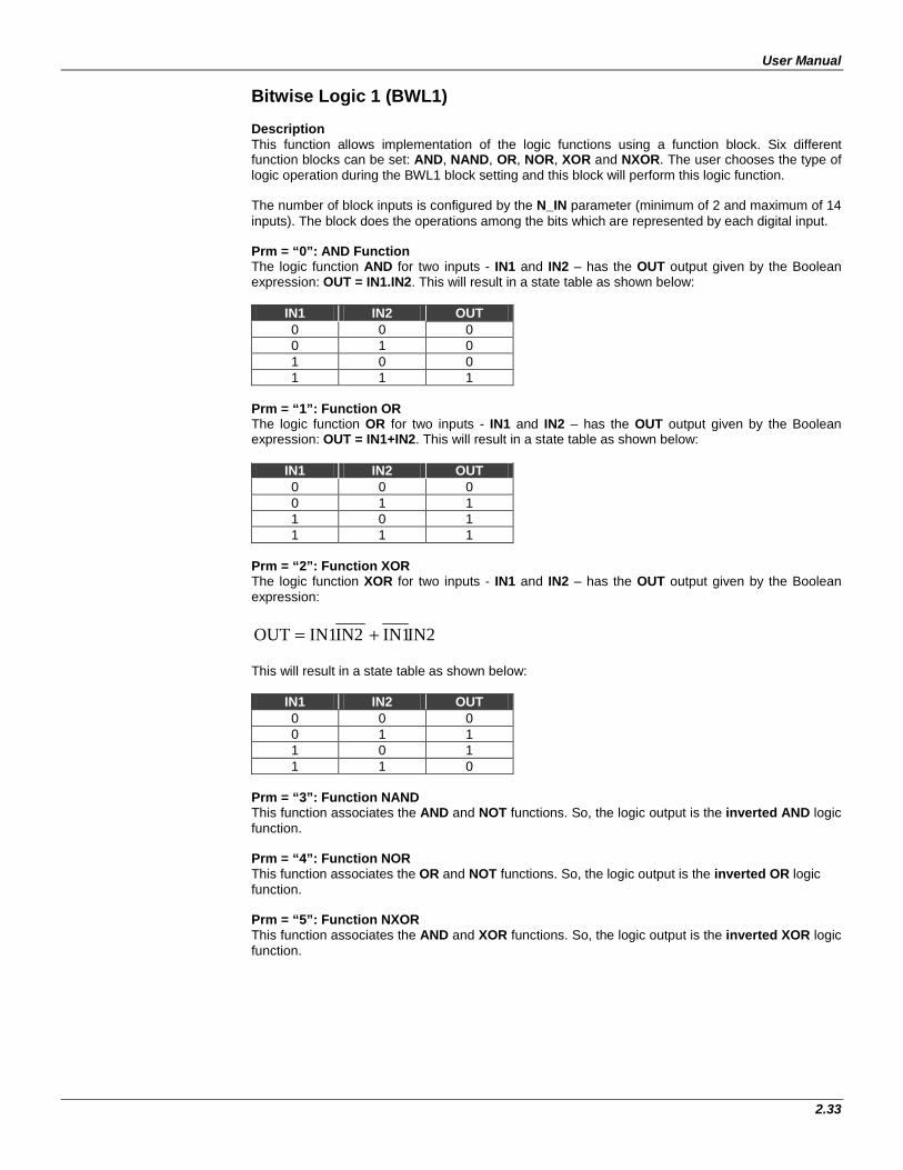
Bitwise Logic 1 (BWL1) Description This function allows implementation of the logic functions using a function block. Six different function blocks can be set: AND, NAND, OR, NOR, XOR and NXOR. The user chooses the type of logic operation during the BWL1 block setting and this block will perform this logic function. The number of block inputs is configured by the N_IN parameter (minimum of 2 and maximum of 14 inputs). The block does the operations among the bits which are represented by each digital input. Prm = “0”: AND Function The logic function AND for two inputs - IN1 and IN2 – has the OUT output given by the Boolean expression: OUT = IN1.IN2. This will result in a state table as shown below:
IN1 IN2 OUT 0 0 0 0 1 0 1 0 0 1 1 1
Prm = “1”: Function OR The logic function OR for two inputs - IN1 and IN2 – has the OUT output given by the Boolean expression: OUT = IN1+IN2. This will result in a state table as shown below:
IN1 IN2 OUT 0 0 0 0 1 1 1 0 1 1 1 1
Prm = “2”: Function XOR The logic function XOR for two inputs - IN1 and IN2 – has the OUT output given by the Boolean expression:
IN2IN1IN2IN1OUT += This will result in a state table as shown below:
IN1 IN2 OUT 0 0 0 0 1 1 1 0 1 1 1 0
Prm = “3”: Function NAND This function associates the AND and NOT functions. So, the logic output is the inverted AND logic function. Prm = “4”: Function NOR This function associates the OR and NOT functions. So, the logic output is the inverted OR logic function. Prm = “5”: Function NXOR This function associates the AND and XOR functions. So, the logic output is the inverted XOR logic function.
Function Blocks
2.34
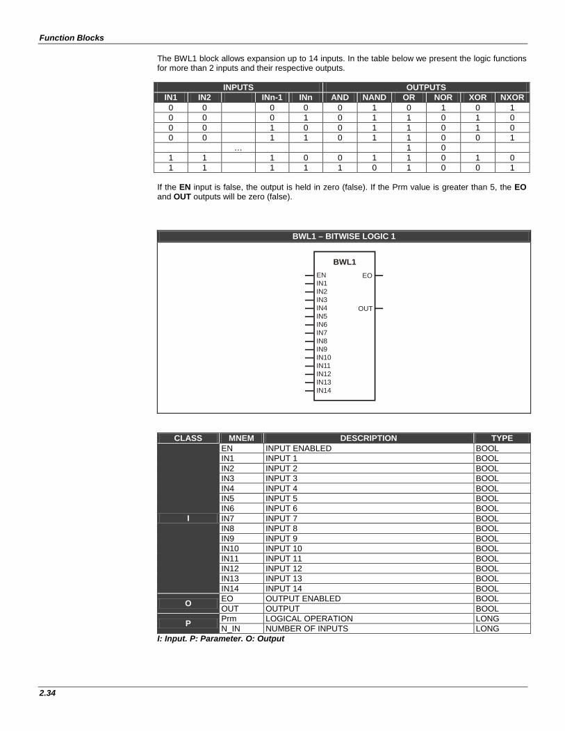
The BWL1 block allows expansion up to 14 inputs. In the table below we present the logic functions for more than 2 inputs and their respective outputs.
INPUTS OUTPUTS IN1 IN2 INn-1 INn AND NAND OR NOR XOR NXOR 0 0 0 0 0 1 0 1 0 1 0 0 0 1 0 1 1 0 1 0 0 0 1 0 0 1 1 0 1 0 0 0 1 1 0 1 1 0 0 1 … 1 0
1 1 1 0 0 1 1 0 1 0 1 1 1 1 1 0 1 0 0 1
If the EN input is false, the output is held in zero (false). If the Prm value is greater than 5, the EO and OUT outputs will be zero (false).
BWL1 – BITWISE LOGIC 1
BWL1EO
IN1IN2IN3IN4IN5IN6IN7IN8IN9IN10IN11IN12IN13IN14
EN
OUT
CLASS MNEM DESCRIPTION TYPE
I
EN INPUT ENABLED BOOL IN1 INPUT 1 BOOL IN2 INPUT 2 BOOL IN3 INPUT 3 BOOL IN4 INPUT 4 BOOL IN5 INPUT 5 BOOL IN6 INPUT 6 BOOL IN7 INPUT 7 BOOL IN8 INPUT 8 BOOL IN9 INPUT 9 BOOL IN10 INPUT 10 BOOL IN11 INPUT 11 BOOL IN12 INPUT 12 BOOL IN13 INPUT 13 BOOL IN14 INPUT 14 BOOL
O EO OUTPUT ENABLED BOOL OUT OUTPUT BOOL
P Prm LOGICAL OPERATION LONG N_IN NUMBER OF INPUTS LONG
I: Input. P: Parameter. O: Output
User Manual
2.35
Reduced Bitwise Logic 1 (BWL1r) Description This function allows implementation of the logic functions using a function block. Six different function blocks can be set: AND, NAND, OR, NOR, XOR and NXOR. The user chooses the type of logic operation during the BWL1r block setting and this block will perform this logic function. The block does the operations among the bits which are represented by the two digital inputs. Prm = “0”: AND Function The logic function AND, for the IN1 and IN2 inputs, has the OUT output given by the Boolean expression: OUT = IN1.IN2. This will result in a state table as shown below:
IN1 IN2 OUT 0 0 0 0 1 0 1 0 0 1 1 1
Prm = “1”: Function OR The logic function OR for the IN1 and IN2 inputs has the OUT output given by the Boolean expression: OUT = IN1+IN2. This will result in a state table as shown below:
IN1 IN2 OUT 0 0 0 0 1 1 1 0 1 1 1 1
Prm = “2”: Function XOR The logic function XOR for the IN1 and IN2 inputs has the OUT output given by the Boolean expression:
IN2IN1IN2IN1OUT += This will result in a state table as shown below:
IN1 IN2 OUT 0 0 0 0 1 1 1 0 1 1 1 0
Prm = “3”: Function NAND This function associates the AND and NOT functions. So, the logic output is the inverted AND logic function. Prm = “4”: Function NOR This function associates the OR and NOT functions. So, the logic output is the inverted OR logic function. Prm = “5”: Function NXOR This function associates the NOT and XOR functions. So, the logic output is the inverted XOR logic function.

Function Blocks
2.36
If the EN input is false, the output is held in zero (false). If the Prm value is greater than 5, the EO and OUT outputs will be zero (false).
BWL1r – REDUCED BITWISE LOGIC 1
EN
IN1
EO
OUT
IN2
BWL1r
CLASS MNEM DESCRIPTION TYPE
I EN INPUT ENABLED BOOL IN1 INPUT 1 BOOL IN2 INPUT 2 BOOL
O EO OUTPUT ENABLED BOOL OUT OUTPUT BOOL
P Prm LOGICAL OPERATION LONG I: Input. P: Parameter. O: Output
User Manual
2.37
Bitwise Logic 2 (BWL2) Description This function allows implementation of the logic functions using a function block. Six different function blocks can be set: AND, NAND, OR, NOR, XOR and NXOR. The user chooses the type of logic operation during the BWL2 block setting and this block will perform this logic function. The number of block inputs is configured by the N_IN parameter (minimum of 2 and maximum of 14 inputs). The block does the operations among the bits which are represented by each digital input. Prm = “0”: Function AND The logic function AND for two inputs - IN1 and IN2 – has the OUT output given by the Boolean expression: OUT = IN1.IN2. This will result in a state table as shown below: IN1= (BIT17)(BIT16)(BIT15)(BIT14)(BIT13)(BIT12)(BIT11)(BIT10) IN2= (BIT27)(BIT26)(BIT25)(BIT24)(BIT23)(BIT22)(BIT21)(BIT20) OUT= (BIT17ANDBIT27)…………………………(BIT10ANDBIT20) Example: IN1= 00001111 IN2= 11110000 OUT= 00000000 PRM = “1”: Function OR The logic function OR for two inputs - IN1 and IN2 – has the OUT output given by the Boolean expression: OUT = IN1+IN2. This will result in a state table as shown below: IN1= (BIT17)(BIT16)(BIT15)(BIT14)(BIT13)(BIT12)(BIT11)(BIT10) IN2= (BIT27)(BIT26)(BIT25)(BIT24)(BIT23)(BIT22)(BIT21)(BIT20) OUT= (BIT17ORBIT27)…………………………(BIT10ORBIT20) Example: IN1= 00001111 IN2= 11110000 OUT= 11111111 Prm = “2”: Function XOR The logic function XOR for two inputs - IN1 and IN2 – has the OUT output given by the Boolean expression:
This will result in a state table as shown below: IN1= (BIT17)(BIT16)(BIT15)(BIT14)(BIT13)(BIT12)(BIT11)(BIT10) IN2= (BIT27)(BIT26)(BIT25)(BIT24)(BIT23)(BIT22)(BIT21)(BIT20) OUT= (BIT17XORBIT27)…………………………(BIT10XORBIT20) Example: IN1= 01011100 IN2= 11110000 OUT= 10101100 Prm = “3”: Function NAND This function associates the AND and NOT functions. So, the logic output is the inverted AND logic function. Prm = “4”: Function NOR This function associates the OR and NOT functions. So, the logic output is the inverted OR logic function. Prm = “5”: Function NXOR This function associates the XOR and NOT functions. So, the logic output is the inverted XOR logic function. If the EN input is false, the output is held in zero (false). If the Prm value is greater than 5, the EO and OUT outputs will be zero (false).
Function Blocks
2.38
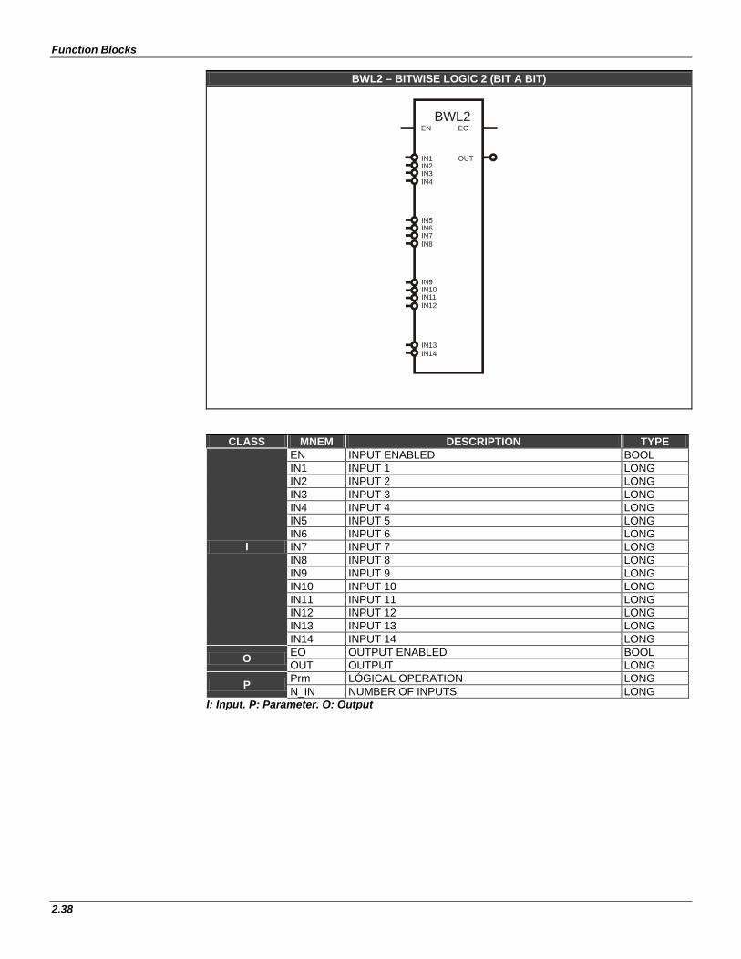
BWL2 – BITWISE LOGIC 2 (BIT A BIT)
BWL2EN EO
OUTIN1IN2IN3IN4
IN6IN7IN8
IN9IN10IN11IN12
IN13IN14
CLASS MNEM DESCRIPTION TYPE
I
EN INPUT ENABLED BOOL IN1 INPUT 1 LONG IN2 INPUT 2 LONG IN3 INPUT 3 LONG IN4 INPUT 4 LONG IN5 INPUT 5 LONG IN6 INPUT 6 LONG IN7 INPUT 7 LONG IN8 INPUT 8 LONG IN9 INPUT 9 LONG IN10 INPUT 10 LONG IN11 INPUT 11 LONG IN12 INPUT 12 LONG IN13 INPUT 13 LONG IN14 INPUT 14 LONG
O EO OUTPUT ENABLED BOOL OUT OUTPUT LONG
P Prm LÓGICAL OPERATION LONG N_IN NUMBER OF INPUTS LONG
I: Input. P: Parameter. O: Output
User Manual
2.39
Reduced Bitwise Logic 2 (BWL2r)
Description This function allows implementation of the logic functions using a function block. Six different function blocks can be set: AND, NAND, OR, NOR, XOR and NXOR. The user chooses the type of logic operation during the BWL2r block setting and this block will perform this logic function. The block does the operations among the bits which are represented by the two digital inputs. Prm = “0”: Function AND The logic function AND, for the IN1 and IN2 inputs, has the OUT output given by the Boolean expression: OUT = IN1.IN2. This will result in a state table as shown below: IN1= (BIT17)(BIT16)(BIT15)(BIT14)(BIT13)(BIT12)(BIT11)(BIT10) IN2= (BIT27)(BIT26)(BIT25)(BIT24)(BIT23)(BIT22)(BIT21)(BIT20) OUT= (BIT17ANDBIT27)…………………………(BIT10ANDBIT20) Example: IN1= 00001111 IN2= 11110000 OUT= 00000000 PRM = “1”: Function OR The logic function OR for the IN1 and IN2 inputs has the OUT output given by the Boolean expression: OUT = IN1+IN2. This will result in a state table as shown below: IN1= (BIT17)(BIT16)(BIT15)(BIT14)(BIT13)(BIT12)(BIT11)(BIT10) IN2= (BIT27)(BIT26)(BIT25)(BIT24)(BIT23)(BIT22)(BIT21)(BIT20) OUT= (BIT17ORBIT27)…………………………(BIT10ORBIT20) Example: IN1= 00001111 IN2= 11110000 OUT= 11111111 Prm = “2”: Function XOR The logic function XOR for the IN1 and IN2 inputs has the OUT output given by the Boolean expression:
This will result in a state table as shown below: IN1= (BIT17)(BIT16)(BIT15)(BIT14)(BIT13)(BIT12)(BIT11)(BIT10) IN2= (BIT27)(BIT26)(BIT25)(BIT24)(BIT23)(BIT22)(BIT21)(BIT20) OUT= (BIT17XORBIT27)…………………………(BIT10XORBIT20) Example: IN1= 01011100 IN2= 11110000 OUT= 10101100 Prm = “3”: Function NAND This function associates the AND and NOT functions. So, the logic output is the inverted AND logic function. Prm = “4”: Function NOR This function associates the OR and NOT functions. So, the logic output is the inverted OR logic function. Prm = “5”: Function NXOR This function associates the XOR and NOT functions. So, the logic output is the inverted XOR logic function.
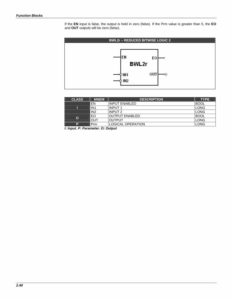
Function Blocks
2.40
If the EN input is false, the output is held in zero (false). If the Prm value is greater than 5, the EO and OUT outputs will be zero (false).
BWL2r – REDUCED BITWISE LOGIC 2
CLASS MNEM DESCRIPTION TYPE
I EN INPUT ENABLED BOOL IN1 INPUT 1 LONG IN2 INPUT 2 LONG
O EO OUTPUT ENABLED BOOL OUT OUTPUT LONG
P Prm LOGICAL OPERATION LONG I: Input. P: Parameter. O: Output
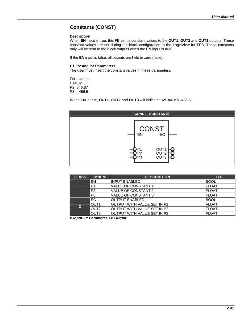
User Manual
2.41
Constants (CONST) Description When EN input is true, this FB sends constant values to the OUT1, OUT2 and OUT3 outputs. These constant values are set during the block configuration in the LogicView for FFB. These constants only will be sent to the block outputs when the EN input is true. If the EN input is false, all outputs are held in zero (false). P1, P2 and P3 Parameters The user must insert the constant values in these parameters. For example: P1= 32 P2=346.87 P3= -456.5 When EN is true, OUT1, OUT2 and OUT3 will indicate: 32/ 346.87/ -456.5.
CONST - CONSTANTS
CONSTEOEN
OUT1P1OUT2P2OUT3P3
CLASS MNEM DESCRIPTION TYPE
I
EN INPUT ENABLED BOOL P1 VALUE OF CONSTANT 1 FLOAT P2 VALUE OF CONSTANT 2 FLOAT P3 VALUE OF CONSTANT 3 FLOAT
O
EO OUTPUT ENABLED BOOL OUT1 OUTPUT WITH VALUE SET IN P1 FLOAT OUT2 OUTPUT WITH VALUE SET IN P2 FLOAT OUT3 OUTPUT WITH VALUE SET IN P3 FLOAT
I: Input. P: Parameter. O: Output
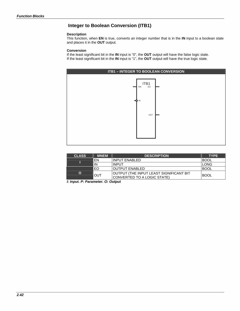
Function Blocks
2.42
Integer to Boolean Conversion (ITB1) Description This function, when EN is true, converts an integer number that is in the IN input to a boolean state and places it in the OUT output. Conversion If the least significant bit in the IN input is “0”, the OUT output will have the false logic state. If the least significant bit in the IN input is “1”, the OUT output will have the true logic state.
ITB1 – INTEGER TO BOOLEAN CONVERSION
ITB1EN EO
OUT
IN
CLASS MNEM DESCRIPTION TYPE
I EN INPUT ENABLED BOOL IN INPUT LONG
O EO OUTPUT ENABLED BOOL
OUT OUTPUT (THE INPUT LEAST SIGNIFICANT BIT CONVERTED TO A LOGIC STATE) BOOL
I: Input. P: Parameter. O: Output
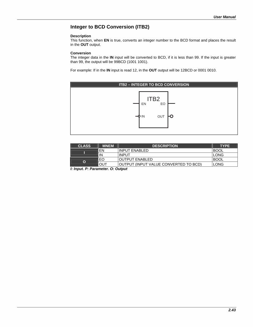
User Manual
2.43
Integer to BCD Conversion (ITB2) Description This function, when EN is true, converts an integer number to the BCD format and places the result in the OUT output. Conversion The integer data in the IN input will be converted to BCD, if it is less than 99. If the input is greater than 99, the output will be 99BCD (1001 1001). For example: If in the IN input is read 12, in the OUT output will be 12BCD or 0001 0010.
ITB2 – INTEGER TO BCD CONVERSION
ITB2EOEN
OUTIN
CLASS MNEM DESCRIPTION TYPE
I EN INPUT ENABLED BOOL IN INPUT LONG
O EO OUTPUT ENABLED BOOL OUT OUTPUT (INPUT VALUE CONVERTED TO BCD) LONG
I: Input. P: Parameter. O: Output
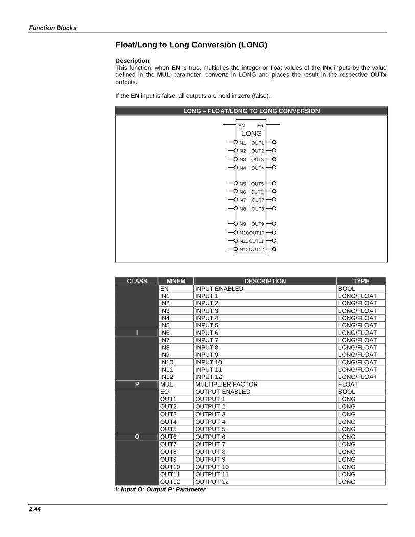
Function Blocks
2.44
Float/Long to Long Conversion (LONG)
Description This function, when EN is true, multiplies the integer or float values of the INx inputs by the value defined in the MUL parameter, converts in LONG and places the result in the respective OUTx outputs. If the EN input is false, all outputs are held in zero (false).
LONG – FLOAT/LONG TO LONG CONVERSION
EN E0
LONGIN1
IN2
IN3
IN4
IN5
IN6
IN7
IN8
IN9
IN10
IN11
IN12
OUT8
OUT9
OUT7
OUT6
OUT5
OUT4
OUT3
OUT2
OUT1
OUT10
OUT11
OUT12
CLASS MNEM DESCRIPTION TYPE
I
EN INPUT ENABLED BOOL IN1 INPUT 1 LONG/FLOAT IN2 INPUT 2 LONG/FLOAT IN3 INPUT 3 LONG/FLOAT IN4 INPUT 4 LONG/FLOAT IN5 INPUT 5 LONG/FLOAT IN6 INPUT 6 LONG/FLOAT IN7 INPUT 7 LONG/FLOAT IN8 INPUT 8 LONG/FLOAT IN9 INPUT 9 LONG/FLOAT IN10 INPUT 10 LONG/FLOAT IN11 INPUT 11 LONG/FLOAT IN12 INPUT 12 LONG/FLOAT
P MUL MULTIPLIER FACTOR FLOAT
O
EO OUTPUT ENABLED BOOL OUT1 OUTPUT 1 LONG OUT2 OUTPUT 2 LONG OUT3 OUTPUT 3 LONG OUT4 OUTPUT 4 LONG OUT5 OUTPUT 5 LONG OUT6 OUTPUT 6 LONG OUT7 OUTPUT 7 LONG OUT8 OUTPUT 8 LONG OUT9 OUTPUT 9 LONG OUT10 OUTPUT 10 LONG OUT11 OUTPUT 11 LONG OUT12 OUTPUT 12 LONG
I: Input O: Output P: Parameter
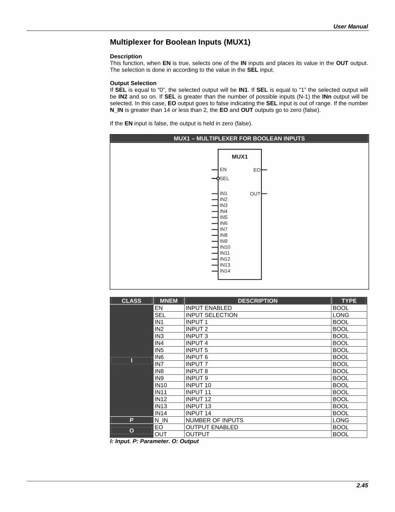
User Manual
2.45
Multiplexer for Boolean Inputs (MUX1) Description This function, when EN is true, selects one of the IN inputs and places its value in the OUT output. The selection is done in according to the value in the SEL input. Output Selection If SEL is equal to “0”, the selected output will be IN1. If SEL is equal to “1” the selected output will be IN2 and so on. If SEL is greater than the number of possible inputs (N-1) the INn output will be selected. In this case, EO output goes to false indicating the SEL input is out of range. If the number N_IN is greater than 14 or less than 2, the EO and OUT outputs go to zero (false).
If the EN input is false, the output is held in zero (false).
MUX1 – MULTIPLEXER FOR BOOLEAN INPUTS
MUX1
IN1IN2IN3IN4IN5IN6IN7IN8IN9IN10IN11IN12IN13IN14
EN EO
OUT
SEL
CLASS MNEM DESCRIPTION TYPE
I
EN INPUT ENABLED BOOL SEL INPUT SELECTION LONG IN1 INPUT 1 BOOL IN2 INPUT 2 BOOL IN3 INPUT 3 BOOL IN4 INPUT 4 BOOL IN5 INPUT 5 BOOL IN6 INPUT 6 BOOL IN7 INPUT 7 BOOL IN8 INPUT 8 BOOL IN9 INPUT 9 BOOL IN10 INPUT 10 BOOL IN11 INPUT 11 BOOL IN12 INPUT 12 BOOL IN13 INPUT 13 BOOL IN14 INPUT 14 BOOL
P N_IN NUMBER OF INPUTS LONG
O EO OUTPUT ENABLED BOOL OUT OUTPUT BOOL
I: Input. P: Parameter. O: Output
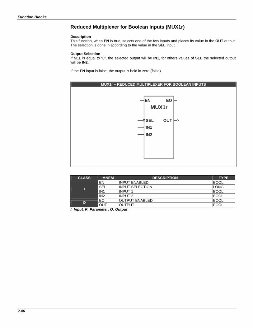
Function Blocks
2.46
Reduced Multiplexer for Boolean Inputs (MUX1r)
Description This function, when EN is true, selects one of the two inputs and places its value in the OUT output. The selection is done in according to the value in the SEL input. Output Selection If SEL is equal to “0”, the selected output will be IN1, for others values of SEL the selected output will be IN2.
If the EN input is false, the output is held in zero (false).
CLASS MNEM DESCRIPTION TYPE
I
EN INPUT ENABLED BOOL SEL INPUT SELECTION LONG IN1 INPUT 1 BOOL IN2 INPUT 2 BOOL
O EO OUTPUT ENABLED BOOL OUT OUTPUT BOOL
I: Input. P: Parameter. O: Output
MUX1r – REDUCED MULTIPLEXER FOR BOOLEAN INPUTS
EN EO
MUX1r
IN2
IN1
OUT SEL
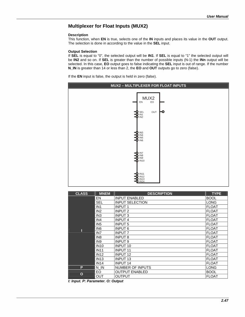
User Manual
2.47
Multiplexer for Float Inputs (MUX2) Description This function, when EN is true, selects one of the IN inputs and places its value in the OUT output. The selection is done in according to the value in the SEL input. Output Selection If SEL is equal to “0”, the selected output will be IN1. If SEL is equal to “1” the selected output will be IN2 and so on. If SEL is greater than the number of possible inputs (N-1) the INn output will be selected. In this case, EO output goes to false indicating the SEL input is out of range. If the number N_IN is greater than 14 or less than 2, the EO and OUT outputs go to zero (false).
If the EN input is false, the output is held in zero (false).
MUX2 – MULTIPLEXER FOR FLOAT INPUTS
MUX2EN EO
SELIN1IN2
OUT
IN4IN5IN6
IN7IN8IN9IN10
IN11IN12IN13IN14
CLASS MNEM DESCRIPTION TYPE
I
EN INPUT ENABLED BOOL SEL INPUT SELECTION LONG IN1 INPUT 1 FLOAT IN2 INPUT 2 FLOAT IN3 INPUT 3 FLOAT IN4 INPUT 4 FLOAT IN5 INPUT 5 FLOAT IN6 INPUT 6 FLOAT IN7 INPUT 7 FLOAT IN8 INPUT 8 FLOAT IN9 INPUT 9 FLOAT IN10 INPUT 10 FLOAT IN11 INPUT 11 FLOAT IN12 INPUT 12 FLOAT IN13 INPUT 13 FLOAT IN14 INPUT 14 FLOAT
P N_IN NUMBER OF INPUTS LONG
O EO OUTPUT ENABLED BOOL OUT OUTPUT FLOAT
I: Input. P: Parameter. O: Output
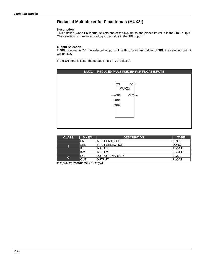
Function Blocks
2.48
Reduced Multiplexer for Float Inputs (MUX2r)
Description This function, when EN is true, selects one of the two inputs and places its value in the OUT output. The selection is done in according to the value in the SEL input.
Output Selection If SEL is equal to “0”, the selected output will be IN1, for others values of SEL the selected output will be IN2.
If the EN input is false, the output is held in zero (false).
MUX2r – REDUCED MULTIPLEXER FOR FLOAT INPUTS
EN EOMUX2r
IN1
IN2
SEL OUT
CLASS MNEM DESCRIPTION TYPE
I
EN INPUT ENABLED BOOL SEL INPUT SELECTION LONG IN1 INPUT 1 FLOAT IN2 INPUT 2 FLOAT
O EO OUTPUT ENABLED BOOL OUT OUTPUT FLOAT
I: Input. P: Parameter. O: Output
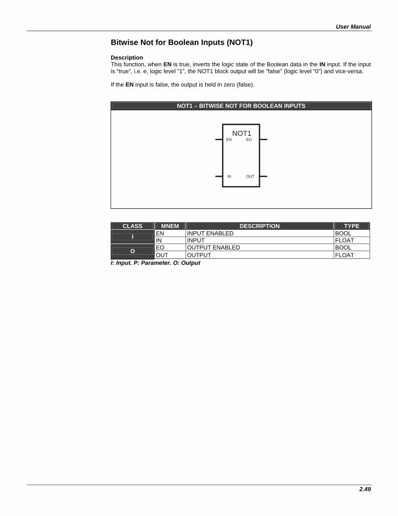
User Manual
2.49
Bitwise Not for Boolean Inputs (NOT1)
Description This function, when EN is true, inverts the logic state of the Boolean data in the IN input. If the input is “true”, i.e. e, logic level “1”, the NOT1 block output will be “false” (logic level “0”) and vice-versa. If the EN input is false, the output is held in zero (false).
NOT1 – BITWISE NOT FOR BOOLEAN INPUTS
NOT1EN EO
IN OUT
CLASS MNEM DESCRIPTION TYPE
I EN INPUT ENABLED BOOL IN INPUT FLOAT
O EO OUTPUT ENABLED BOOL OUT OUTPUT FLOAT
I: Input. P: Parameter. O: Output
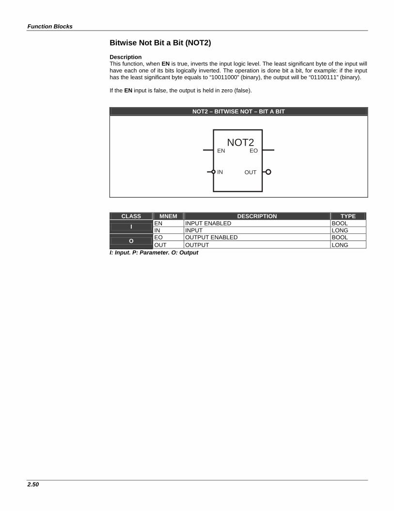
Function Blocks
2.50
Bitwise Not Bit a Bit (NOT2) Description This function, when EN is true, inverts the input logic level. The least significant byte of the input will have each one of its bits logically inverted. The operation is done bit a bit, for example: if the input has the least significant byte equals to “10011000” (binary), the output will be “01100111” (binary). If the EN input is false, the output is held in zero (false).
NOT2 – BITWISE NOT – BIT A BIT
NOT2EOEN
OUTIN
CLASS MNEM DESCRIPTION TYPE
I EN INPUT ENABLED BOOL IN INPUT LONG
O EO OUTPUT ENABLED BOOL OUT OUTPUT LONG
I: Input. P: Parameter. O: Output
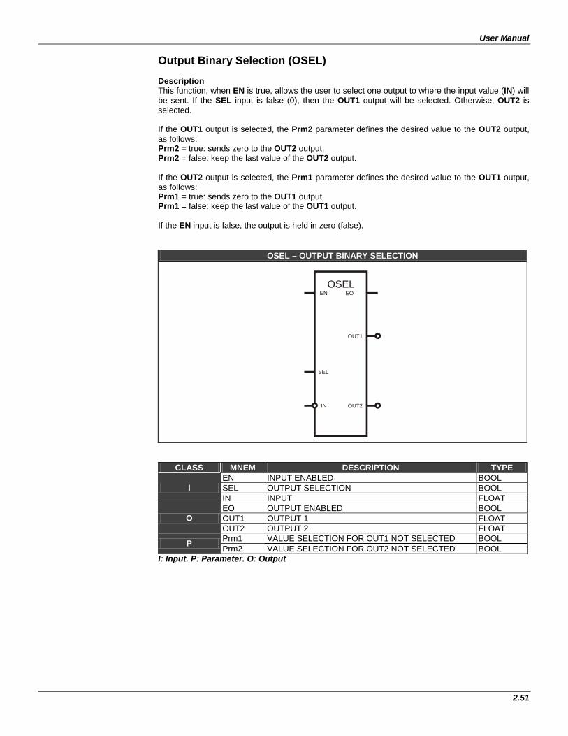
User Manual
2.51
Output Binary Selection (OSEL) Description This function, when EN is true, allows the user to select one output to where the input value (IN) will be sent. If the SEL input is false (0), then the OUT1 output will be selected. Otherwise, OUT2 is selected. If the OUT1 output is selected, the Prm2 parameter defines the desired value to the OUT2 output, as follows: Prm2 = true: sends zero to the OUT2 output. Prm2 = false: keep the last value of the OUT2 output. If the OUT2 output is selected, the Prm1 parameter defines the desired value to the OUT1 output, as follows: Prm1 = true: sends zero to the OUT1 output. Prm1 = false: keep the last value of the OUT1 output. If the EN input is false, the output is held in zero (false).
OSEL – OUTPUT BINARY SELECTION
OSELEN EO
SEL
IN OUT2
OUT1
CLASS MNEM DESCRIPTION TYPE
I EN INPUT ENABLED BOOL SEL OUTPUT SELECTION BOOL IN INPUT FLOAT
O EO OUTPUT ENABLED BOOL OUT1 OUTPUT 1 FLOAT OUT2 OUTPUT 2 FLOAT
P Prm1 VALUE SELECTION FOR OUT1 NOT SELECTED BOOL Prm2 VALUE SELECTION FOR OUT2 NOT SELECTED BOOL
I: Input. P: Parameter. O: Output
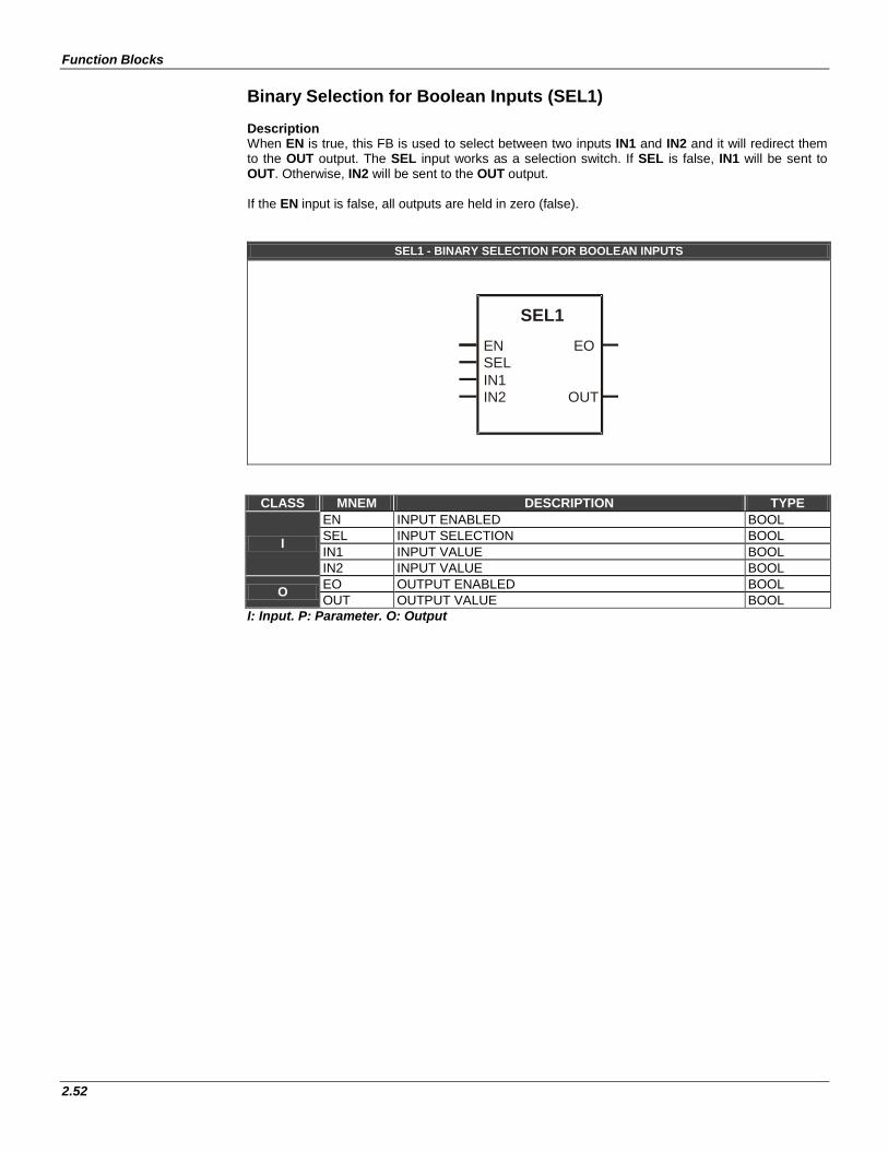
Function Blocks
2.52
Binary Selection for Boolean Inputs (SEL1) Description When EN is true, this FB is used to select between two inputs IN1 and IN2 and it will redirect them to the OUT output. The SEL input works as a selection switch. If SEL is false, IN1 will be sent to OUT. Otherwise, IN2 will be sent to the OUT output. If the EN input is false, all outputs are held in zero (false).
SEL1 - BINARY SELECTION FOR BOOLEAN INPUTS
CLASS MNEM DESCRIPTION TYPE
I
EN INPUT ENABLED BOOL SEL INPUT SELECTION BOOL IN1 INPUT VALUE BOOL IN2 INPUT VALUE BOOL
O EO OUTPUT ENABLED BOOL OUT OUTPUT VALUE BOOL
I: Input. P: Parameter. O: Output
SEL1
EN EO SEL IN1 IN2 OUT
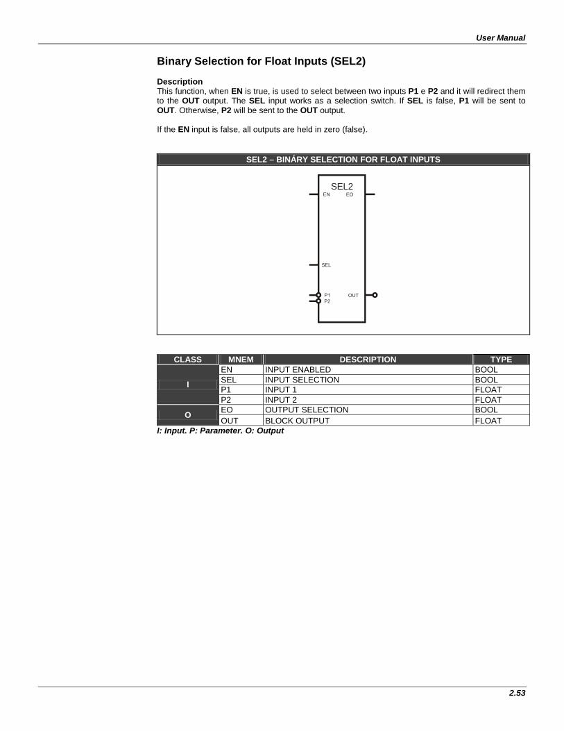
User Manual
2.53
Binary Selection for Float Inputs (SEL2) Description This function, when EN is true, is used to select between two inputs P1 e P2 and it will redirect them to the OUT output. The SEL input works as a selection switch. If SEL is false, P1 will be sent to OUT. Otherwise, P2 will be sent to the OUT output. If the EN input is false, all outputs are held in zero (false).
SEL2 – BINÁRY SELECTION FOR FLOAT INPUTS
SEL2EN EO
SEL
OUTP2
CLASS MNEM DESCRIPTION TYPE
I
EN INPUT ENABLED BOOL SEL INPUT SELECTION BOOL P1 INPUT 1 FLOAT P2 INPUT 2 FLOAT
O EO OUTPUT SELECTION BOOL OUT BLOCK OUTPUT FLOAT
I: Input. P: Parameter. O: Output
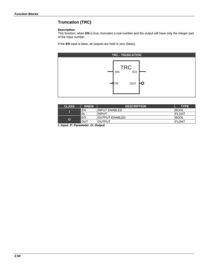
Function Blocks
2.54
Truncation (TRC) Description This function, when EN is true, truncates a real number and the output will have only the integer part of the input number. If the EN input is false, all outputs are held in zero (false).
TRC - TRUNCATION
TRCEOEN
OUTIN
CLASS MNEM DESCRIPTION TYPE
I EN INPUT ENABLED BOOL IN INPUT FLOAT
O EO OUTPUT ENABLED BOOL OUT OUTPUT FLOAT
I: Input. P: Parameter. O: Output
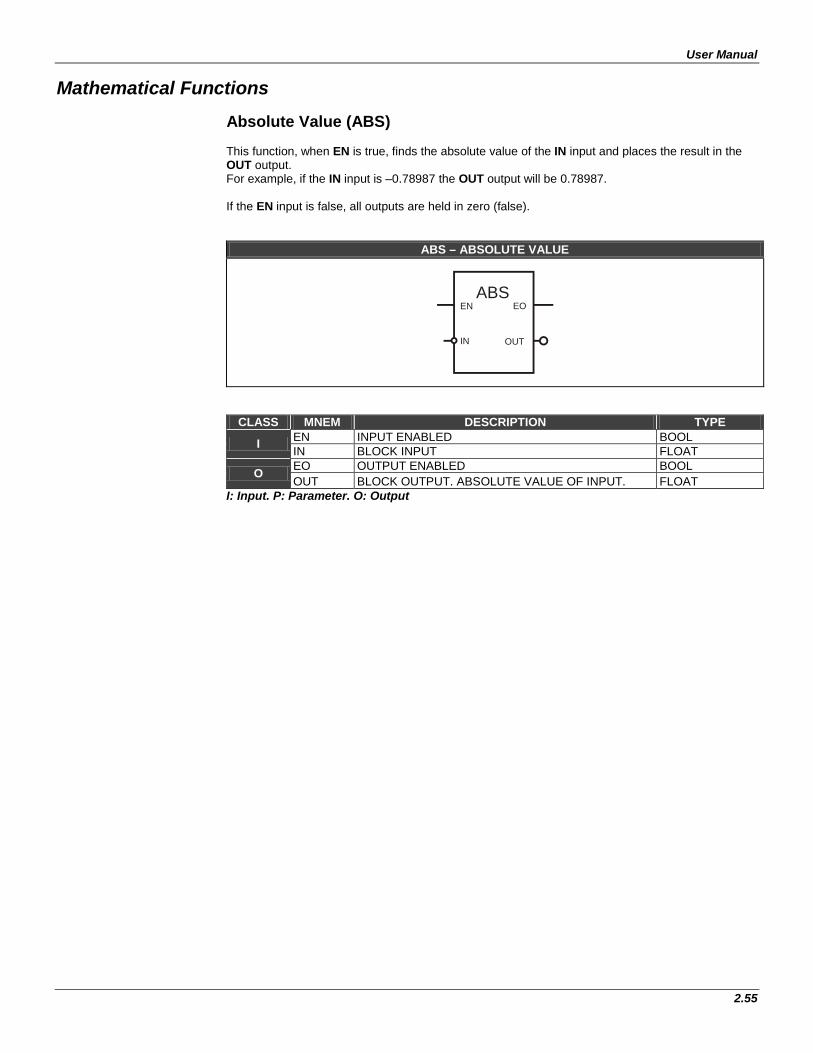
User Manual
2.55
Mathematical Functions Absolute Value (ABS) This function, when EN is true, finds the absolute value of the IN input and places the result in the OUT output. For example, if the IN input is –0.78987 the OUT output will be 0.78987. If the EN input is false, all outputs are held in zero (false).
ABS – ABSOLUTE VALUE
ABSEOEN
OUTIN
CLASS MNEM DESCRIPTION TYPE
I EN INPUT ENABLED BOOL IN BLOCK INPUT FLOAT
O EO OUTPUT ENABLED BOOL OUT BLOCK OUTPUT. ABSOLUTE VALUE OF INPUT. FLOAT
I: Input. P: Parameter. O: Output
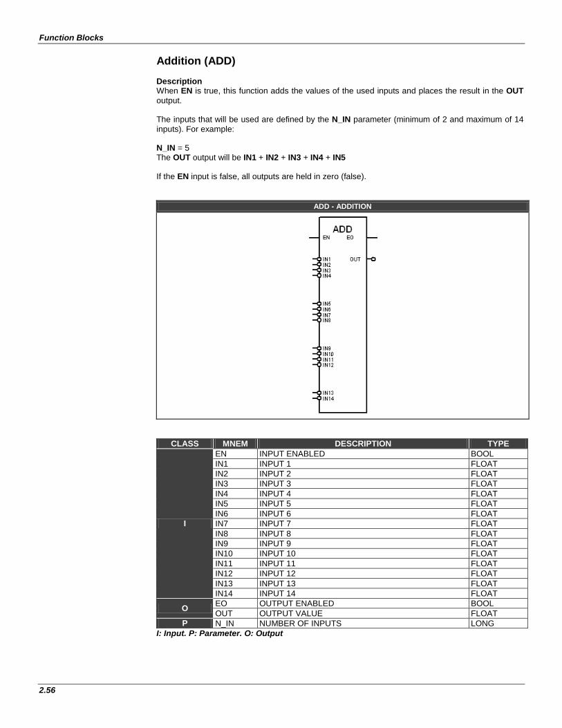
Function Blocks
2.56
Addition (ADD) Description When EN is true, this function adds the values of the used inputs and places the result in the OUT output. The inputs that will be used are defined by the N_IN parameter (minimum of 2 and maximum of 14 inputs). For example: N_IN = 5 The OUT output will be IN1 + IN2 + IN3 + IN4 + IN5 If the EN input is false, all outputs are held in zero (false).
ADD - ADDITION
CLASS MNEM DESCRIPTION TYPE
I
EN INPUT ENABLED BOOL IN1 INPUT 1 FLOAT IN2 INPUT 2 FLOAT IN3 INPUT 3 FLOAT IN4 INPUT 4 FLOAT IN5 INPUT 5 FLOAT IN6 INPUT 6 FLOAT IN7 INPUT 7 FLOAT IN8 INPUT 8 FLOAT IN9 INPUT 9 FLOAT IN10 INPUT 10 FLOAT IN11 INPUT 11 FLOAT IN12 INPUT 12 FLOAT IN13 INPUT 13 FLOAT IN14 INPUT 14 FLOAT
O EO OUTPUT ENABLED BOOL OUT OUTPUT VALUE FLOAT
P N_IN NUMBER OF INPUTS LONG I: Input. P: Parameter. O: Output

User Manual
2.57
Reduced Addition (ADDr) Description When EN is true, this function adds the values of the IN1 and IN2 inputs and places the result in the OUT output. If the EN input is false, all outputs are held in zero (false).
ADDr – REDUCED ADDITION
CLASS MNEM DESCRIPTION TYPE
I EN INPUT ENABLED BOOL IN1 INPUT 1 FLOAT IN2 INPUT 2 FLOAT
O EO OUTPUT ENABLED BOOL OUT OUTPUT VALUE FLOAT
I: Input. P: Parameter. O: Output

Function Blocks
2.58
Bitwise AND of 2 to 8 inputs (AND2-AND8) Description This function performs the bitwise AND for the inputs IN1 and IN2 up to IN8 and places the result in the OUT output. Truth table: If IN1 up to INn is equal to 1, OUT output will be equal to 1, otherwise will be 0.
AND – BITWISE AND
CLASS MNEM DESCRIPTION TYPE
I IN1 INPUT 1 BOOL INn INPUT n BOOL
O OUT OUTPUT VALUE BOOL I: Input. P: Parameter. O: Output
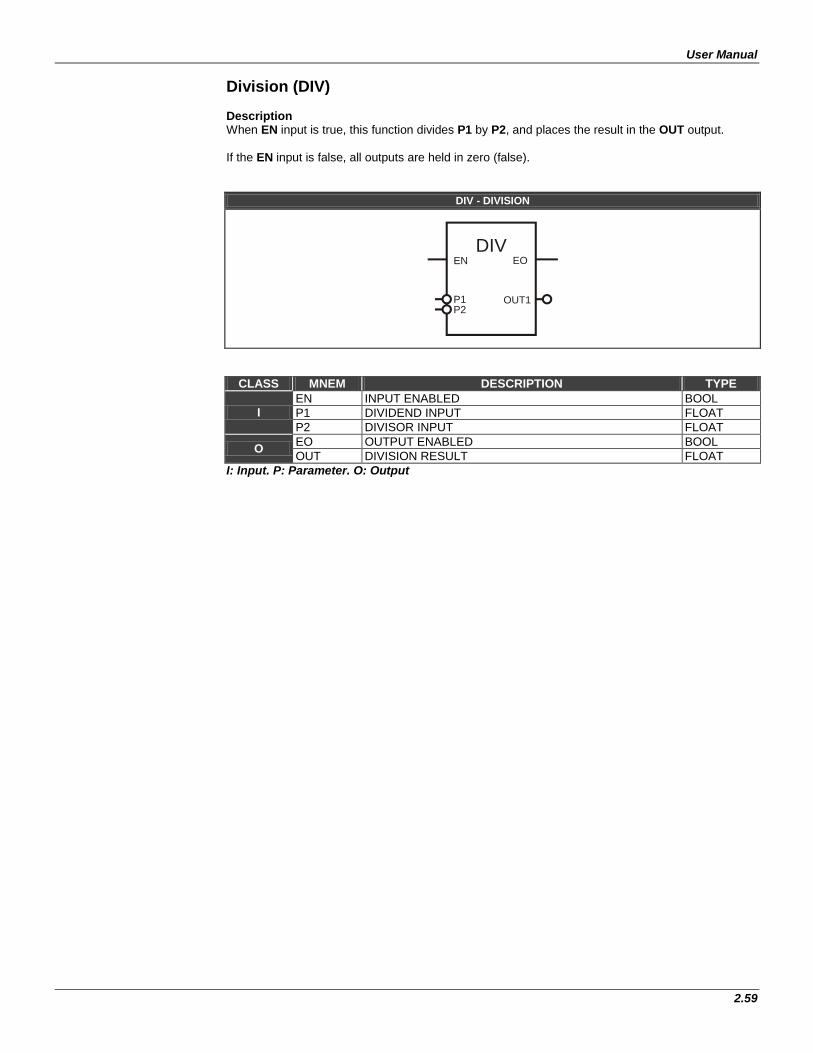
User Manual
2.59
Division (DIV) Description When EN input is true, this function divides P1 by P2, and places the result in the OUT output. If the EN input is false, all outputs are held in zero (false).
DIV - DIVISION
DIVEOEN
OUT1P1P2
CLASS MNEM DESCRIPTION TYPE
I EN INPUT ENABLED BOOL P1 DIVIDEND INPUT FLOAT P2 DIVISOR INPUT FLOAT
O EO OUTPUT ENABLED BOOL OUT DIVISION RESULT FLOAT
I: Input. P: Parameter. O: Output
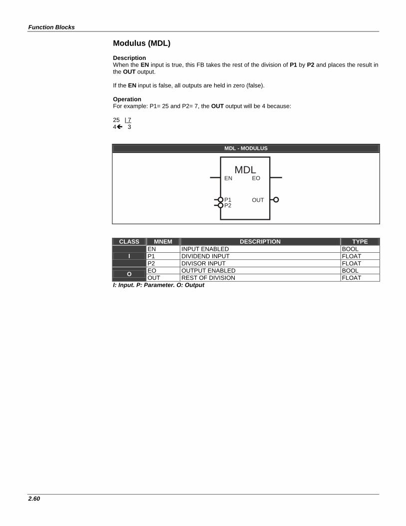
Function Blocks
2.60
Modulus (MDL) Description When the EN input is true, this FB takes the rest of the division of P1 by P2 and places the result in the OUT output. If the EN input is false, all outputs are held in zero (false). Operation For example: P1= 25 and P2= 7, the OUT output will be 4 because: 25 | 7 4 3
MDL - MODULUS
MDLEOEN
OUTP1P2
CLASS MNEM DESCRIPTION TYPE
I EN INPUT ENABLED BOOL P1 DIVIDEND INPUT FLOAT P2 DIVISOR INPUT FLOAT
O EO OUTPUT ENABLED BOOL OUT REST OF DIVISION FLOAT
I: Input. P: Parameter. O: Output
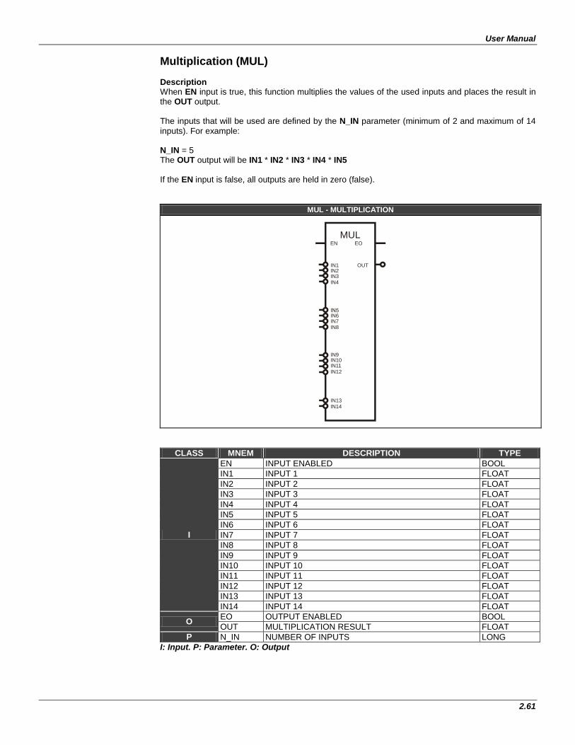
User Manual
2.61
Multiplication (MUL) Description When EN input is true, this function multiplies the values of the used inputs and places the result in the OUT output. The inputs that will be used are defined by the N_IN parameter (minimum of 2 and maximum of 14 inputs). For example: N_IN = 5 The OUT output will be IN1 * IN2 * IN3 * IN4 * IN5 If the EN input is false, all outputs are held in zero (false).
MUL - MULTIPLICATION
MULEN EO
IN1IN2IN3IN4
OUT
IN6IN7IN8
IN9IN10IN11IN12
IN13IN14
CLASS MNEM DESCRIPTION TYPE
I
EN INPUT ENABLED BOOL IN1 INPUT 1 FLOAT IN2 INPUT 2 FLOAT IN3 INPUT 3 FLOAT IN4 INPUT 4 FLOAT IN5 INPUT 5 FLOAT IN6 INPUT 6 FLOAT IN7 INPUT 7 FLOAT IN8 INPUT 8 FLOAT IN9 INPUT 9 FLOAT IN10 INPUT 10 FLOAT IN11 INPUT 11 FLOAT IN12 INPUT 12 FLOAT IN13 INPUT 13 FLOAT IN14 INPUT 14 FLOAT
O EO OUTPUT ENABLED BOOL OUT MULTIPLICATION RESULT FLOAT
P N_IN NUMBER OF INPUTS LONG I: Input. P: Parameter. O: Output

Function Blocks
2.62
Reduced Multiplication (MULr) Description When EN input is true, this function multiplies the values of the IN1 and IN2 inputs and places the result in the OUT output. If the EN input is false, all outputs are held in zero (false).
MULr – REDUCED MULTIPLICATION
EN
IN1
EO
OUTIN2
MULr
CLASS MNEM DESCRIPTION TYPE
I EN INPUT ENABLED BOOL IN1 INPUT 1 FLOAT IN2 INPUT 2 FLOAT
O EO OUTPUT ENABLED BOOL OUT MULTIPLICATION RESULT FLOAT
I: Input. P: Parameter. O: Output

User Manual
2.63
Bitwise NOT (NOT)
Description This function inverts the logic state of the Boolean data in the IN input. If the input is “true”, i.e., logic level “1”, the NOT block output will be “false” (logic level “0”) and vice versa.
NOT – BITWISE NOT
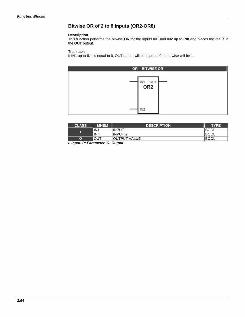
Function Blocks
2.64
Bitwise OR of 2 to 8 inputs (OR2-OR8) Description This function performs the bitwise OR for the inputs IN1 and IN2 up to IN8 and places the result in the OUT output. Truth table: If IN1 up to INn is equal to 0, OUT output will be equal to 0, otherwise will be 1.
OR – BITWISE OR
CLASS MNEM DESCRIPTION TYPE
I IN1 INPUT 1 BOOL INn INPUT n BOOL
O OUT OUTPUT VALUE BOOL I: Input. P: Parameter. O: Output
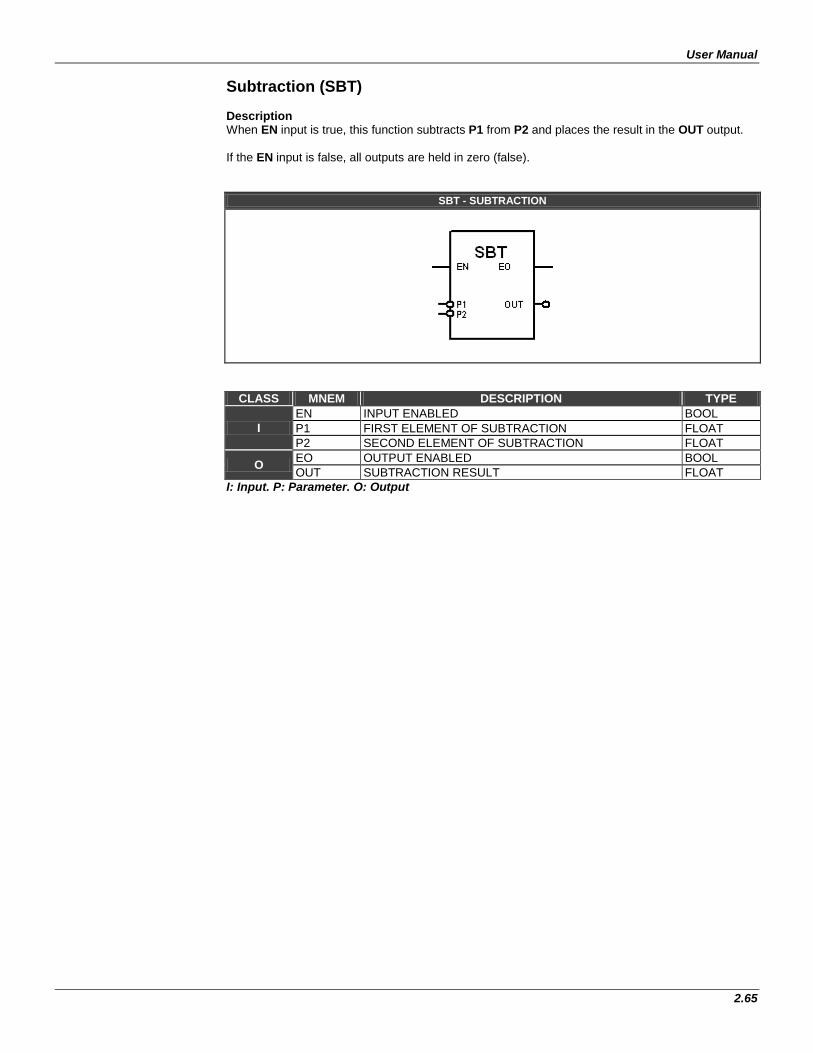
User Manual
2.65
Subtraction (SBT) Description When EN input is true, this function subtracts P1 from P2 and places the result in the OUT output. If the EN input is false, all outputs are held in zero (false).
SBT - SUBTRACTION
CLASS MNEM DESCRIPTION TYPE
I EN INPUT ENABLED BOOL P1 FIRST ELEMENT OF SUBTRACTION FLOAT P2 SECOND ELEMENT OF SUBTRACTION FLOAT
O EO OUTPUT ENABLED BOOL OUT SUBTRACTION RESULT FLOAT
I: Input. P: Parameter. O: Output
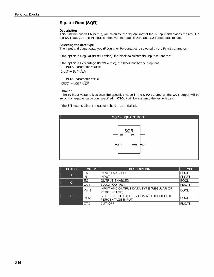
Function Blocks
2.66
Square Root (SQR) Description This function, when EN is true, will calculate the square root of the IN input and places the result in the OUT output. If the IN input is negative, the result is zero and EO output goes to false. Selecting the data type The input and output data type (Regular or Percentage) is selected by the Prm1 parameter. If the option is Regular (Prm1 = false), the block calculates the input square root. If the option is Percentage (Prm1 = true), the block has two sub-options: - PERC parameter = false:
- PERC parameter = true:
Leveling If the IN input value is less than the specified value in the CTO parameter, the OUT output will be zero. If a negative value was specified in CTO, it will be assumed the value is zero. If the EN input is false, the output is held in zero (false).
SQR – SQUARE ROOT
CLASS MNEM DESCRIPTION TYPE
I EN INPUT ENABLED BOOL IN INPUT FLOAT
O EO OUTPUT ENABLED BOOL OUT BLOCK OUTPUT FLOAT
P
Prm1 INPUT AND OUTPUT DATA TYPE (REGULAR OR PERCENTAGE) BOOL
PERC SELECTS THE CALCULATION MÉTHOD TO THE PERCENTAGE INPUT BOOL
CTO CUT-OFF FLOAT
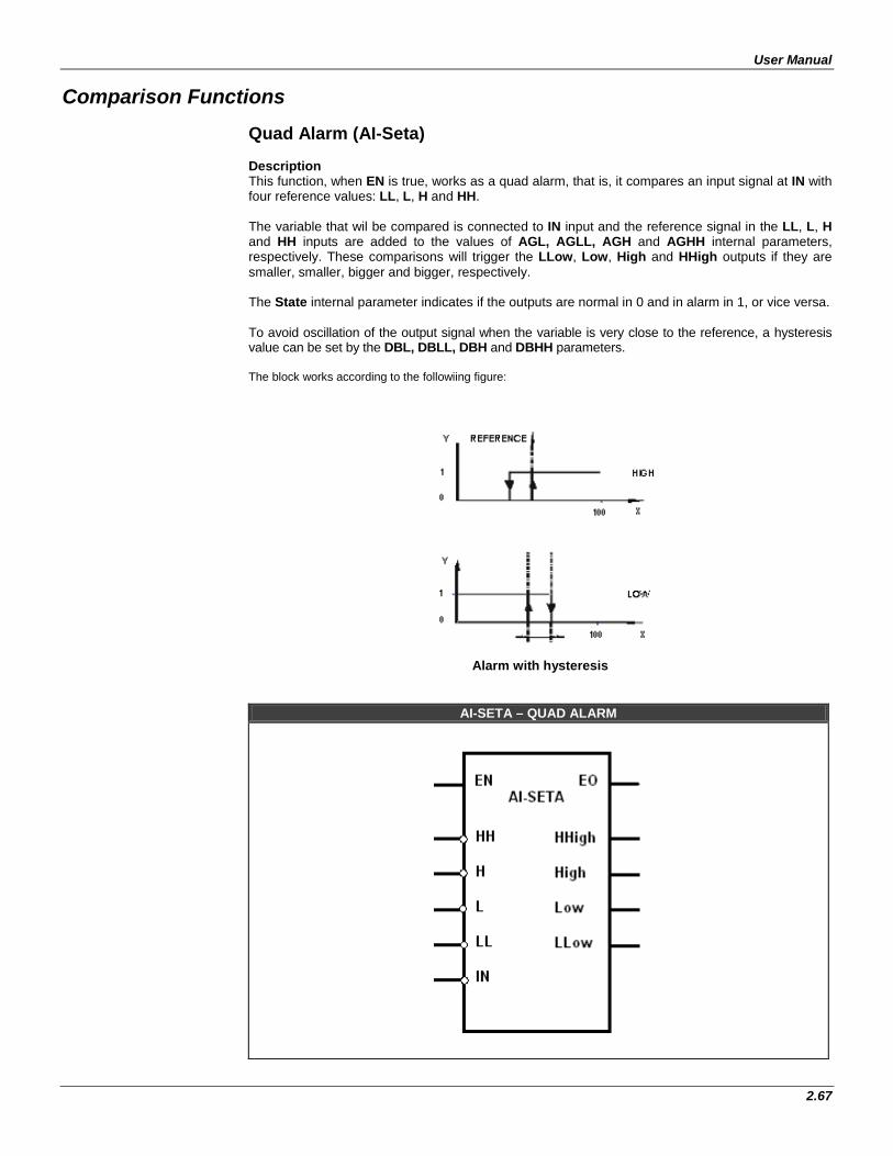
User Manual
2.67
Comparison Functions Quad Alarm (AI-Seta) Description This function, when EN is true, works as a quad alarm, that is, it compares an input signal at IN with four reference values: LL, L, H and HH. The variable that wil be compared is connected to IN input and the reference signal in the LL, L, H and HH inputs are added to the values of AGL, AGLL, AGH and AGHH internal parameters, respectively. These comparisons will trigger the LLow, Low, High and HHigh outputs if they are smaller, smaller, bigger and bigger, respectively. The State internal parameter indicates if the outputs are normal in 0 and in alarm in 1, or vice versa. To avoid oscillation of the output signal when the variable is very close to the reference, a hysteresis value can be set by the DBL, DBLL, DBH and DBHH parameters. The block works according to the followiing figure:
Alarm with hysteresis
AI-SETA – QUAD ALARM
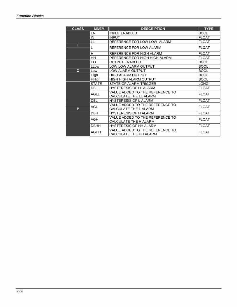
Function Blocks
2.68
CLASS MNEM DESCRIPTION TYPE
I
EN INPUT ENABLED BOOL IN INPUT FLOAT LL REFERENCE FOR LOW LOW ALARM FLOAT
L REFERENCE FOR LOW ALARM FLOAT
H REFERENCE FOR HIGH ALARM FLOAT HH REFERENCE FOR HIGH HIGH ALARM FLOAT
O
EO OUTPUT ENABLED BOOL LLow LOW LOW ALARM OUTPUT BOOL Low LOW ALARM OUTPUT BOOL High HIGH ALARM OUTPUT BOOL HHigh HIGH HIGH ALARM OUTPUT BOOL
P
STATE STATE OF ALARM TRIGGER LONG DBLL HYSTERESIS OF LL ALARM FLOAT
AGLL VALUE ADDED TO THE REFERENCE TO CALCULATE THE LL ALARM FLOAT
DBL HYSTERESIS OF L ALARM FLOAT
AGL VALUE ADDED TO THE REFERENCE TO CALCULATE THE L ALARM FLOAT
DBH HYSTERESIS OF H ALARM FLOAT
AGH VALUE ADDED TO THE REFERENCE TO CALCULATE THE H ALARM FLOAT
DBHH HYSTERESIS OF HH ALARM FLOAT
AGHH VALUE ADDED TO THE REFERENCE TO CALCULATE THE HH ALARM FLOAT
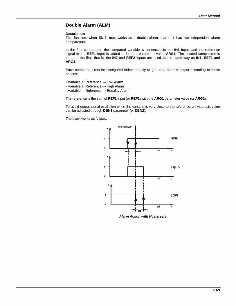
User Manual
2.69
Double Alarm (ALM) Description This function, when EN is true, works as a double alarm, that is, it has two independent alarm comparators. In the first comparator, the compared variable is connected to the IN1 input, and the reference signal in the REF1 input is added to internal parameter value ARG1. The second comparator is equal to the first, that is, the IN2 and REF2 inputs are used as the same way as IN1, REF1 and ARG1. Each comparator can be configured independently to generate alarm’s output according to these options: - Variable ≤ Reference → Low Alarm - Variable ≥ Reference → High Alarm - Variable = Reference → Equality Alarm The reference is the sum of REF1 input (or REF2) with the ARG1 parameter value (or ARG2). To avoid output signal oscillation when the variable is very close to the reference, a hysteresis value can be adjusted through DBN1 parameter (or DBN2). The block works as follows:
Alarm Action with Hysteresis
REFERENCE
HIGH
EQUAL
LOW
100
100
100
X
X
X
Y
1
0
Y
1
0
Y
1
0
Y
1
0
Y
1
0
Y
1
0
Y
1
0
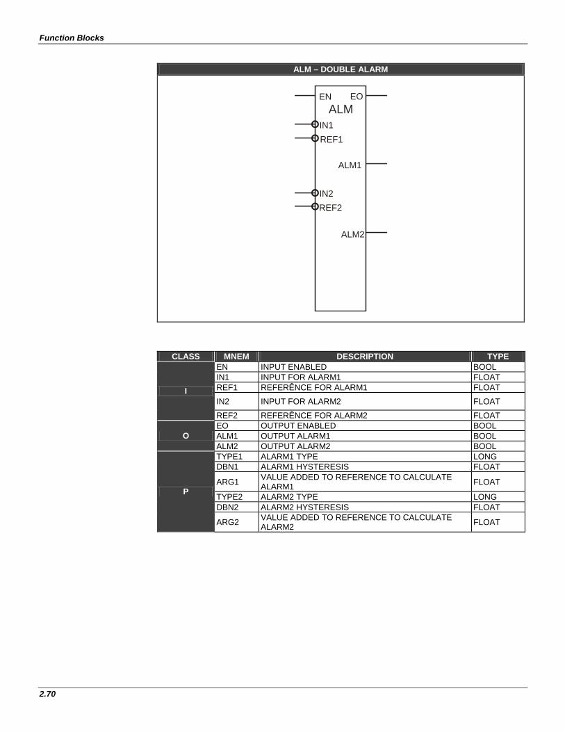
Function Blocks
2.70
ALM – DOUBLE ALARM
EOENALM
IN1REF1
ALM1
IN2REF2
ALM2
CLASS MNEM DESCRIPTION TYPE
I
EN INPUT ENABLED BOOL IN1 INPUT FOR ALARM1 FLOAT REF1 REFERÊNCE FOR ALARM1 FLOAT
IN2 INPUT FOR ALARM2 FLOAT
REF2 REFERÊNCE FOR ALARM2 FLOAT
O EO OUTPUT ENABLED BOOL ALM1 OUTPUT ALARM1 BOOL ALM2 OUTPUT ALARM2 BOOL
P
TYPE1 ALARM1 TYPE LONG DBN1 ALARM1 HYSTERESIS FLOAT
ARG1 VALUE ADDED TO REFERENCE TO CALCULATE ALARM1 FLOAT
TYPE2 ALARM2 TYPE LONG DBN2 ALARM2 HYSTERESIS FLOAT
ARG2 VALUE ADDED TO REFERENCE TO CALCULATE ALARM2 FLOAT
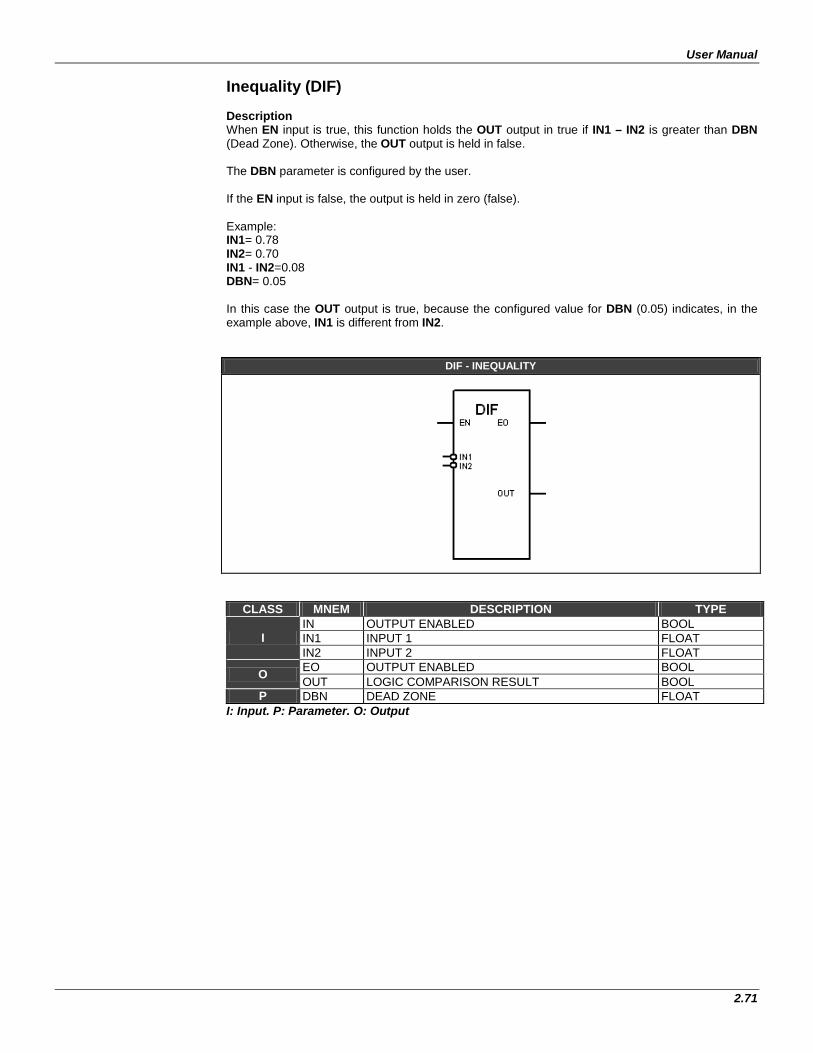
User Manual
2.71
Inequality (DIF) Description When EN input is true, this function holds the OUT output in true if IN1 – IN2 is greater than DBN (Dead Zone). Otherwise, the OUT output is held in false. The DBN parameter is configured by the user. If the EN input is false, the output is held in zero (false). Example: IN1= 0.78 IN2= 0.70 IN1 - IN2=0.08 DBN= 0.05 In this case the OUT output is true, because the configured value for DBN (0.05) indicates, in the example above, IN1 is different from IN2.
DIF - INEQUALITY
CLASS MNEM DESCRIPTION TYPE
I IN OUTPUT ENABLED BOOL IN1 INPUT 1 FLOAT IN2 INPUT 2 FLOAT
O EO OUTPUT ENABLED BOOL OUT LOGIC COMPARISON RESULT BOOL
P DBN DEAD ZONE FLOAT I: Input. P: Parameter. O: Output
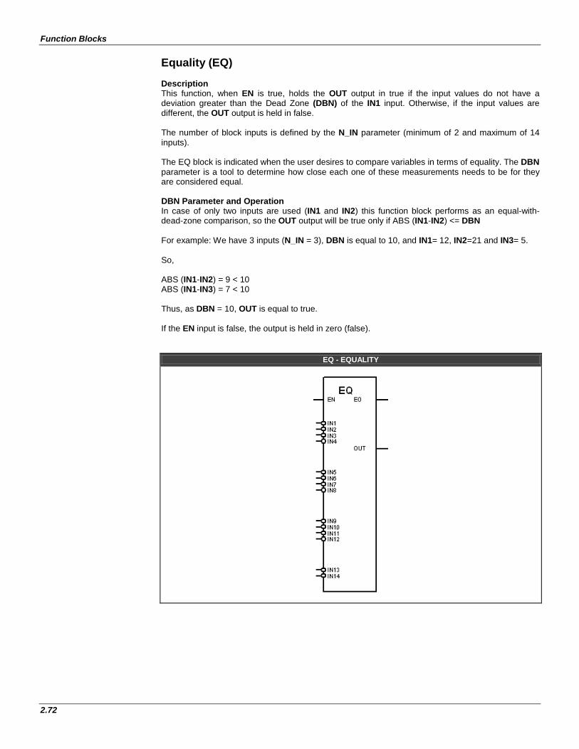
Function Blocks
2.72
Equality (EQ) Description This function, when EN is true, holds the OUT output in true if the input values do not have a deviation greater than the Dead Zone (DBN) of the IN1 input. Otherwise, if the input values are different, the OUT output is held in false. The number of block inputs is defined by the N_IN parameter (minimum of 2 and maximum of 14 inputs). The EQ block is indicated when the user desires to compare variables in terms of equality. The DBN parameter is a tool to determine how close each one of these measurements needs to be for they are considered equal. DBN Parameter and Operation In case of only two inputs are used (IN1 and IN2) this function block performs as an equal-with-dead-zone comparison, so the OUT output will be true only if ABS (IN1-IN2) <= DBN For example: We have 3 inputs (N_IN = 3), DBN is equal to 10, and IN1= 12, IN2=21 and IN3= 5. So, ABS (IN1-IN2) = 9 < 10 ABS (IN1-IN3) = 7 < 10 Thus, as DBN = 10, OUT is equal to true. If the EN input is false, the output is held in zero (false).
EQ - EQUALITY
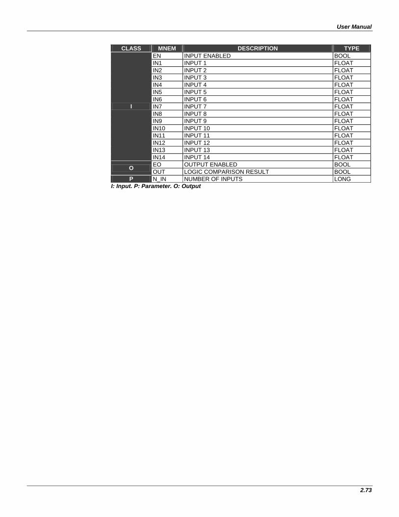
User Manual
2.73
CLASS MNEM DESCRIPTION TYPE
I
EN INPUT ENABLED BOOL IN1 INPUT 1 FLOAT IN2 INPUT 2 FLOAT IN3 INPUT 3 FLOAT IN4 INPUT 4 FLOAT IN5 INPUT 5 FLOAT IN6 INPUT 6 FLOAT IN7 INPUT 7 FLOAT IN8 INPUT 8 FLOAT IN9 INPUT 9 FLOAT IN10 INPUT 10 FLOAT IN11 INPUT 11 FLOAT IN12 INPUT 12 FLOAT IN13 INPUT 13 FLOAT IN14 INPUT 14 FLOAT
O EO OUTPUT ENABLED BOOL OUT LOGIC COMPARISON RESULT BOOL
P N_IN NUMBER OF INPUTS LONG I: Input. P: Parameter. O: Output
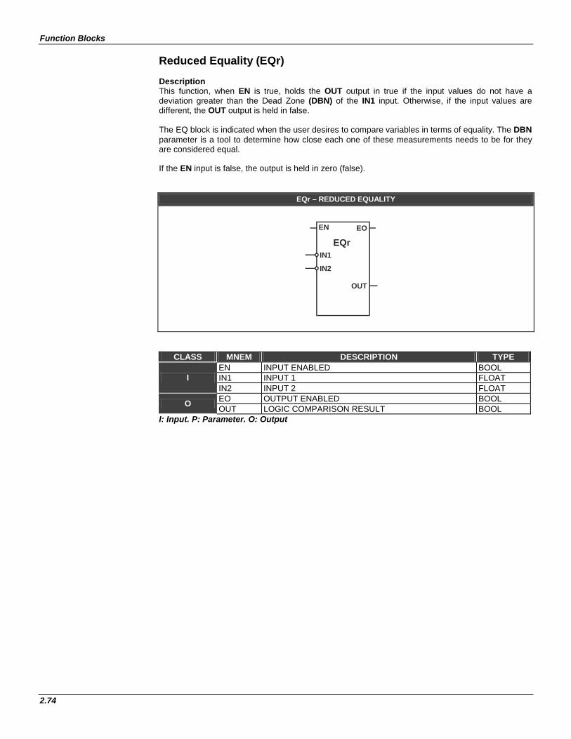
Function Blocks
2.74
Reduced Equality (EQr) Description This function, when EN is true, holds the OUT output in true if the input values do not have a deviation greater than the Dead Zone (DBN) of the IN1 input. Otherwise, if the input values are different, the OUT output is held in false. The EQ block is indicated when the user desires to compare variables in terms of equality. The DBN parameter is a tool to determine how close each one of these measurements needs to be for they are considered equal. If the EN input is false, the output is held in zero (false).
EQr – REDUCED EQUALITY
EN
IN1
EO
OUT
IN2
EQr
CLASS MNEM DESCRIPTION TYPE
I EN INPUT ENABLED BOOL IN1 INPUT 1 FLOAT IN2 INPUT 2 FLOAT
O EO OUTPUT ENABLED BOOL OUT LOGIC COMPARISON RESULT BOOL
I: Input. P: Parameter. O: Output
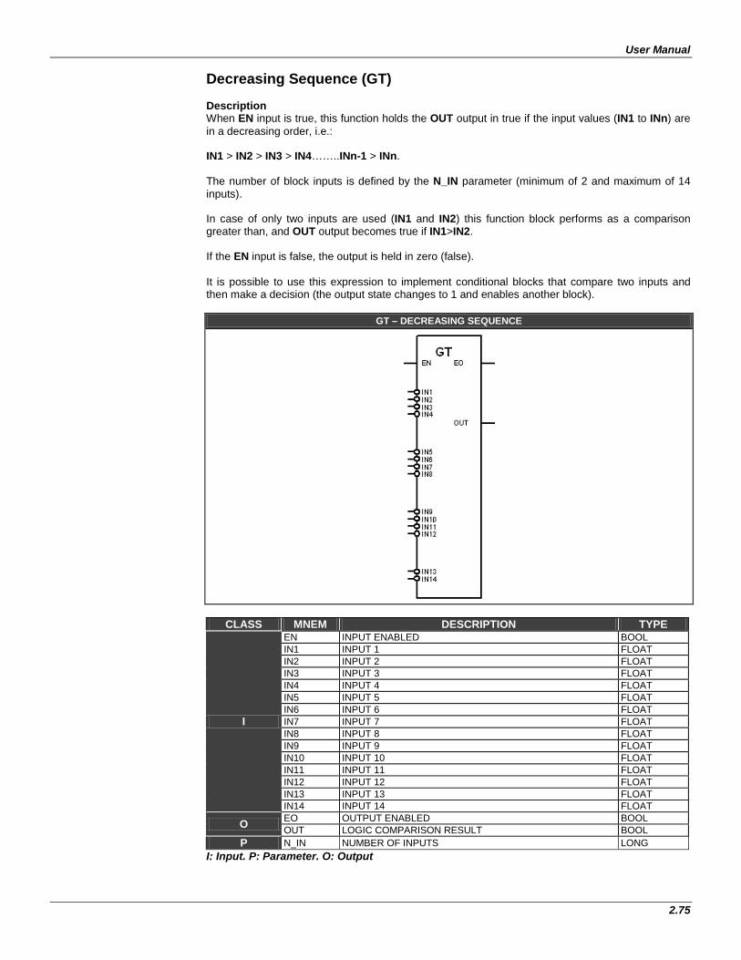
User Manual
2.75
Decreasing Sequence (GT) Description When EN input is true, this function holds the OUT output in true if the input values (IN1 to INn) are in a decreasing order, i.e.: IN1 > IN2 > IN3 > IN4……..INn-1 > INn. The number of block inputs is defined by the N_IN parameter (minimum of 2 and maximum of 14 inputs). In case of only two inputs are used (IN1 and IN2) this function block performs as a comparison greater than, and OUT output becomes true if IN1>IN2. If the EN input is false, the output is held in zero (false). It is possible to use this expression to implement conditional blocks that compare two inputs and then make a decision (the output state changes to 1 and enables another block).
GT – DECREASING SEQUENCE
CLASS MNEM DESCRIPTION TYPE
I
EN INPUT ENABLED BOOL IN1 INPUT 1 FLOAT IN2 INPUT 2 FLOAT IN3 INPUT 3 FLOAT IN4 INPUT 4 FLOAT IN5 INPUT 5 FLOAT IN6 INPUT 6 FLOAT IN7 INPUT 7 FLOAT IN8 INPUT 8 FLOAT IN9 INPUT 9 FLOAT IN10 INPUT 10 FLOAT IN11 INPUT 11 FLOAT IN12 INPUT 12 FLOAT IN13 INPUT 13 FLOAT IN14 INPUT 14 FLOAT
O EO OUTPUT ENABLED BOOL OUT LOGIC COMPARISON RESULT BOOL
P N_IN NUMBER OF INPUTS LONG I: Input. P: Parameter. O: Output
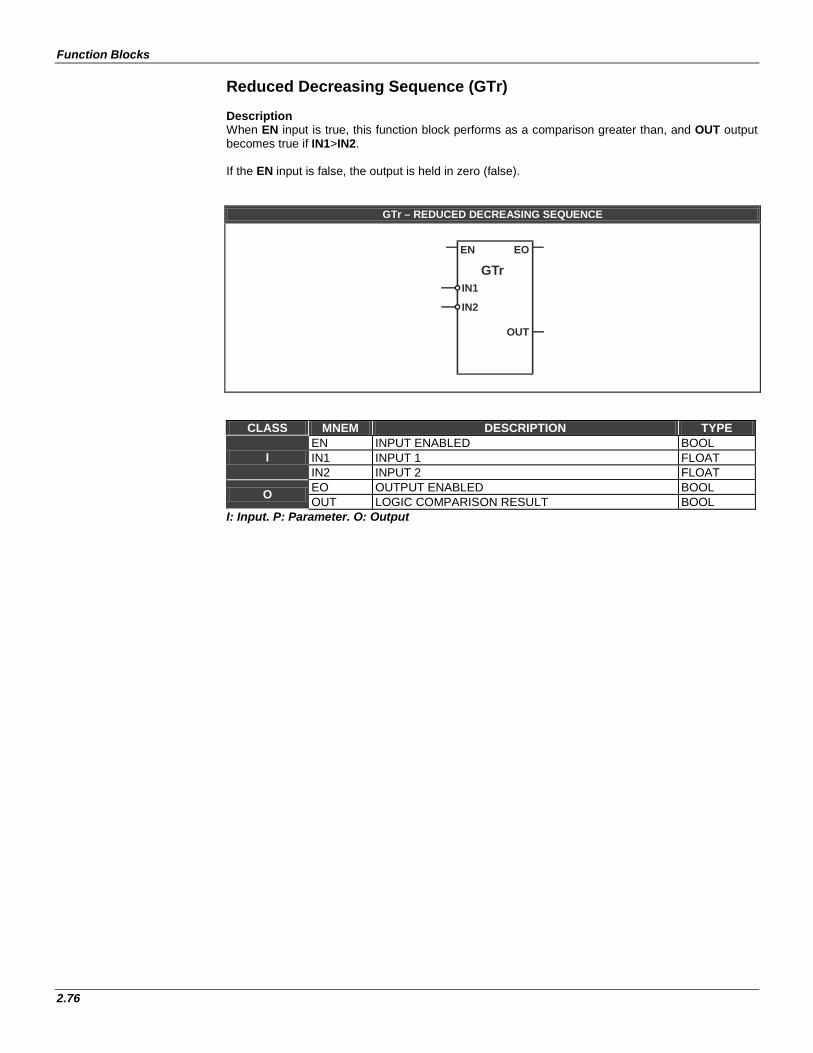
Function Blocks
2.76
Reduced Decreasing Sequence (GTr) Description When EN input is true, this function block performs as a comparison greater than, and OUT output becomes true if IN1>IN2. If the EN input is false, the output is held in zero (false).
GTr – REDUCED DECREASING SEQUENCE
EN
IN1
EO
OUT
IN2
GTr
CLASS MNEM DESCRIPTION TYPE
I EN INPUT ENABLED BOOL IN1 INPUT 1 FLOAT IN2 INPUT 2 FLOAT
O EO OUTPUT ENABLED BOOL OUT LOGIC COMPARISON RESULT BOOL
I: Input. P: Parameter. O: Output
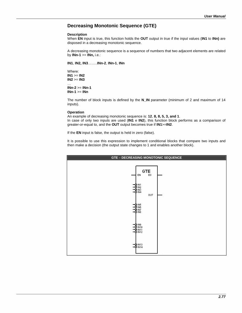
User Manual
2.77
Decreasing Monotonic Sequence (GTE) Description When EN input is true, this function holds the OUT output in true if the input values (IN1 to INn) are disposed in a decreasing monotonic sequence. A decreasing monotonic sequence is a sequence of numbers that two adjacent elements are related by INn-1 >= INn, i.e.: IN1, IN2, IN3……..INn-2, INn-1, INn Where: IN1 >= IN2 IN2 >= IN3 … INn-2 >= INn-1 INn-1 >= INn The number of block inputs is defined by the N_IN parameter (minimum of 2 and maximum of 14 inputs). Operation An example of decreasing monotonic sequence is: 12, 8, 8, 5, 3, and 1. In case of only two inputs are used (IN1 e IN2), this function block performs as a comparison of greater-or-equal to, and the OUT output becomes true if IN1>=IN2. If the EN input is false, the output is held in zero (false). It is possible to use this expression to implement conditional blocks that compare two inputs and then make a decision (the output state changes to 1 and enables another block).
GTE – DECREASING MONOTONIC SEQUENCE
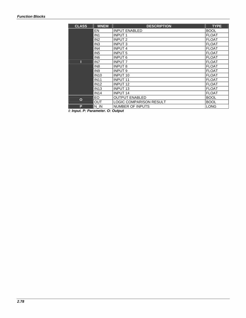
Function Blocks
2.78
CLASS MNEM DESCRIPTION TYPE
I
EN INPUT ENABLED BOOL IN1 INPUT 1 FLOAT IN2 INPUT 2 FLOAT IN3 INPUT 3 FLOAT IN4 INPUT 4 FLOAT IN5 INPUT 5 FLOAT IN6 INPUT 6 FLOAT IN7 INPUT 7 FLOAT IN8 INPUT 8 FLOAT IN9 INPUT 9 FLOAT IN10 INPUT 10 FLOAT IN11 INPUT 11 FLOAT IN12 INPUT 12 FLOAT IN13 INPUT 13 FLOAT IN14 INPUT 14 FLOAT
O EO OUTPUT ENABLED BOOL OUT LOGIC COMPARISON RESULT BOOL
P N_IN NUMBER OF INPUTS LONG I: Input. P: Parameter. O: Output
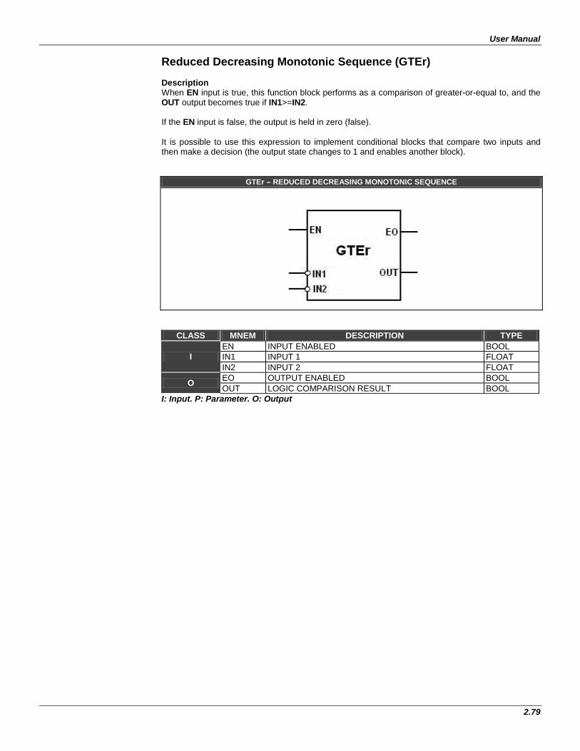
User Manual
2.79
Reduced Decreasing Monotonic Sequence (GTEr) Description When EN input is true, this function block performs as a comparison of greater-or-equal to, and the OUT output becomes true if IN1>=IN2. If the EN input is false, the output is held in zero (false). It is possible to use this expression to implement conditional blocks that compare two inputs and then make a decision (the output state changes to 1 and enables another block).
GTEr – REDUCED DECREASING MONOTONIC SEQUENCE
CLASS MNEM DESCRIPTION TYPE
I EN INPUT ENABLED BOOL IN1 INPUT 1 FLOAT IN2 INPUT 2 FLOAT
O EO OUTPUT ENABLED BOOL OUT LOGIC COMPARISON RESULT BOOL
I: Input. P: Parameter. O: Output
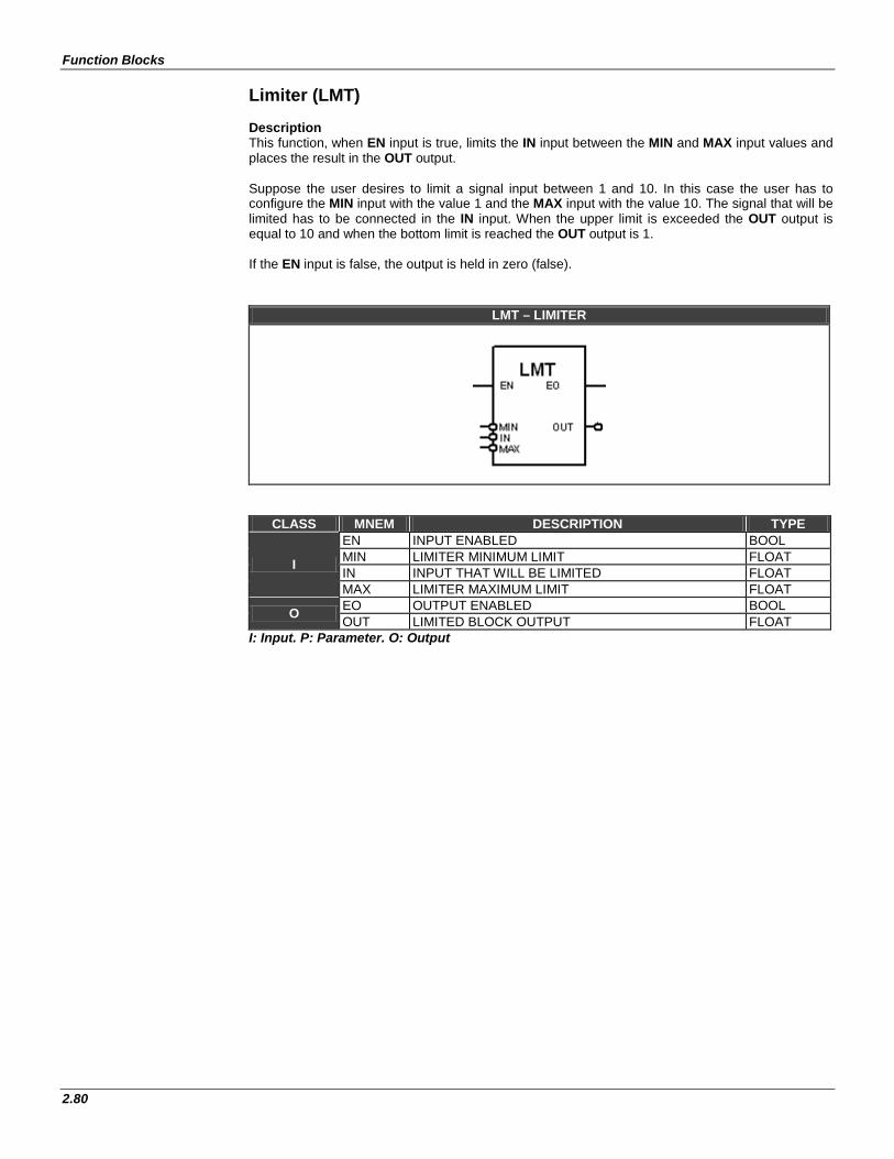
Function Blocks
2.80
Limiter (LMT) Description This function, when EN input is true, limits the IN input between the MIN and MAX input values and places the result in the OUT output. Suppose the user desires to limit a signal input between 1 and 10. In this case the user has to configure the MIN input with the value 1 and the MAX input with the value 10. The signal that will be limited has to be connected in the IN input. When the upper limit is exceeded the OUT output is equal to 10 and when the bottom limit is reached the OUT output is 1. If the EN input is false, the output is held in zero (false).
LMT – LIMITER
CLASS MNEM DESCRIPTION TYPE
I
EN INPUT ENABLED BOOL MIN LIMITER MINIMUM LIMIT FLOAT IN INPUT THAT WILL BE LIMITED FLOAT MAX LIMITER MAXIMUM LIMIT FLOAT
O EO OUTPUT ENABLED BOOL OUT LIMITED BLOCK OUTPUT FLOAT
I: Input. P: Parameter. O: Output
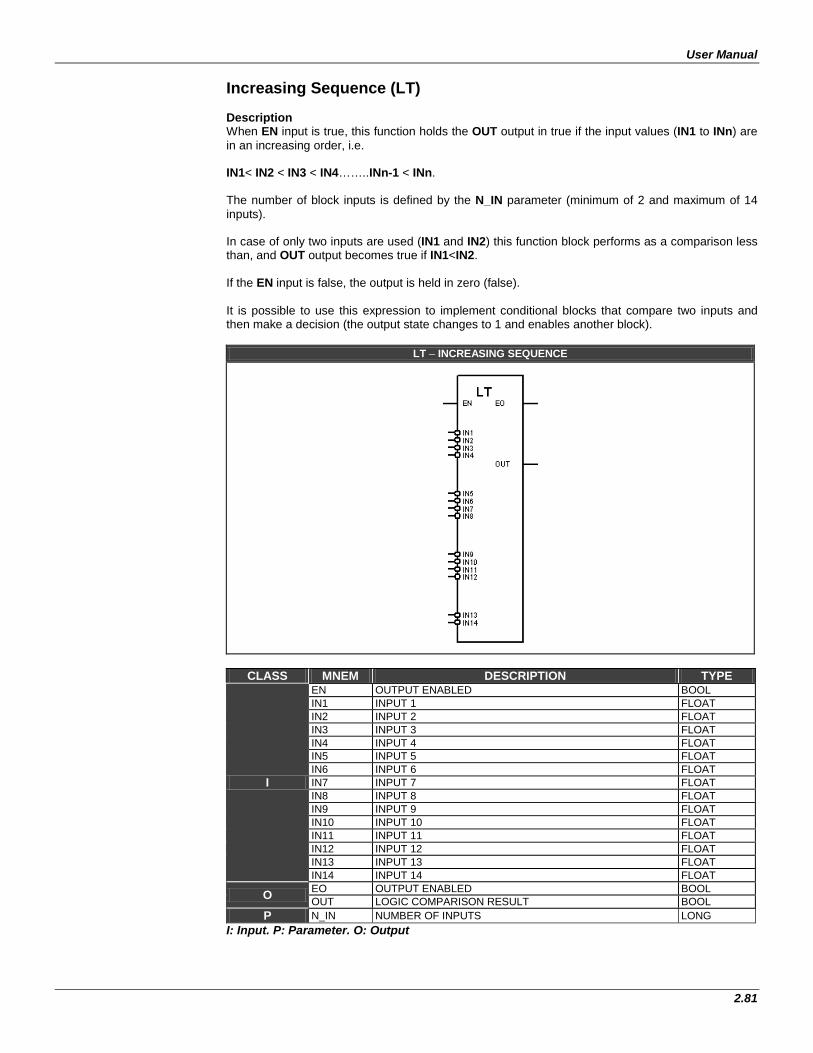
User Manual
2.81
Increasing Sequence (LT) Description When EN input is true, this function holds the OUT output in true if the input values (IN1 to INn) are in an increasing order, i.e. IN1< IN2 < IN3 < IN4……..INn-1 < INn. The number of block inputs is defined by the N_IN parameter (minimum of 2 and maximum of 14 inputs). In case of only two inputs are used (IN1 and IN2) this function block performs as a comparison less than, and OUT output becomes true if IN1<IN2. If the EN input is false, the output is held in zero (false). It is possible to use this expression to implement conditional blocks that compare two inputs and then make a decision (the output state changes to 1 and enables another block).
LT – INCREASING SEQUENCE
CLASS MNEM DESCRIPTION TYPE
I
EN OUTPUT ENABLED BOOL IN1 INPUT 1 FLOAT IN2 INPUT 2 FLOAT IN3 INPUT 3 FLOAT IN4 INPUT 4 FLOAT IN5 INPUT 5 FLOAT IN6 INPUT 6 FLOAT IN7 INPUT 7 FLOAT IN8 INPUT 8 FLOAT IN9 INPUT 9 FLOAT IN10 INPUT 10 FLOAT IN11 INPUT 11 FLOAT IN12 INPUT 12 FLOAT IN13 INPUT 13 FLOAT IN14 INPUT 14 FLOAT
O EO OUTPUT ENABLED BOOL OUT LOGIC COMPARISON RESULT BOOL
P N_IN NUMBER OF INPUTS LONG I: Input. P: Parameter. O: Output

Function Blocks
2.82
Reduced Increasing Sequence (LTr) Description When EN input is true, this function block performs as a comparison less than, and OUT output becomes true if IN1<IN2. If the EN input is false, the output is held in zero (false).
LTr – REDUCED INCREASING SEQUENCE
EN
IN1
EO
OUT
IN2
LTr
CLASS MNEM DESCRIPTION TYPE
I EN OUTPUT ENABLED BOOL IN1 INPUT 1 FLOAT IN2 INPUT 2 FLOAT
O EO OUTPUT ENABLED BOOL OUT LOGIC COMPARISON RESULT BOOL
I: Input. P: Parameter. O: Output
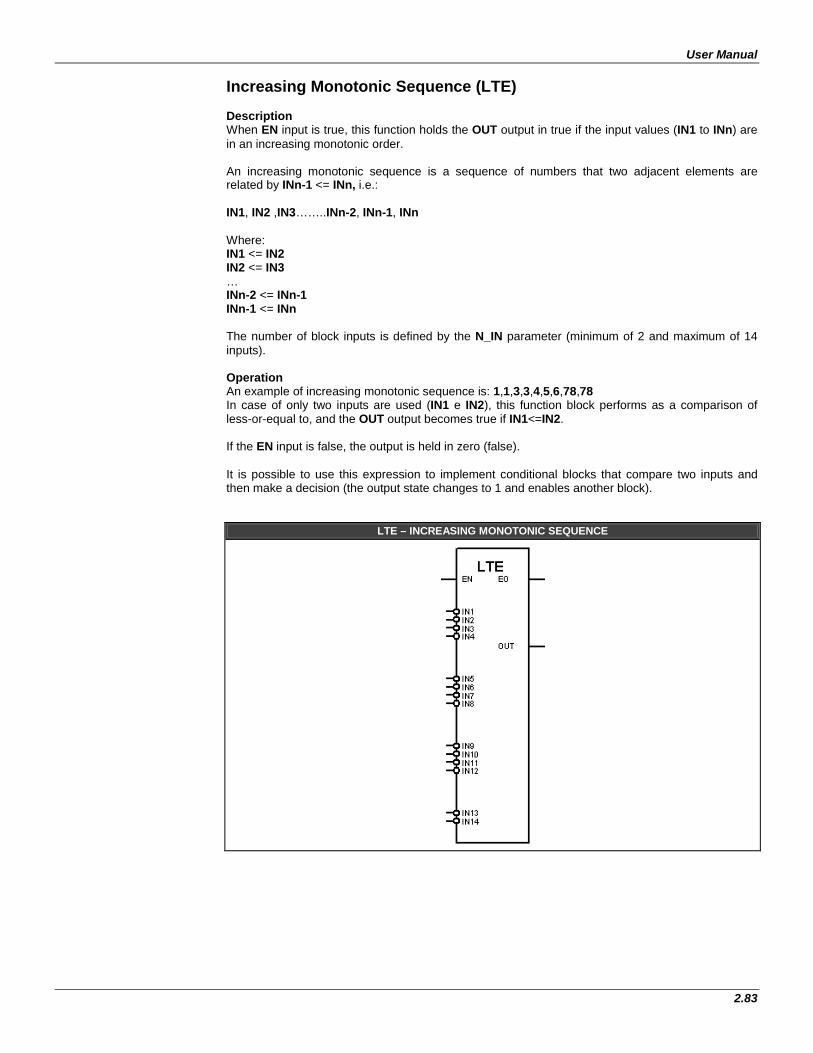
User Manual
2.83
Increasing Monotonic Sequence (LTE) Description When EN input is true, this function holds the OUT output in true if the input values (IN1 to INn) are in an increasing monotonic order. An increasing monotonic sequence is a sequence of numbers that two adjacent elements are related by INn-1 <= INn, i.e.: IN1, IN2 ,IN3……..INn-2, INn-1, INn Where: IN1 <= IN2 IN2 <= IN3 … INn-2 <= INn-1 INn-1 <= INn The number of block inputs is defined by the N_IN parameter (minimum of 2 and maximum of 14 inputs). Operation An example of increasing monotonic sequence is: 1,1,3,3,4,5,6,78,78 In case of only two inputs are used (IN1 e IN2), this function block performs as a comparison of less-or-equal to, and the OUT output becomes true if IN1<=IN2. If the EN input is false, the output is held in zero (false). It is possible to use this expression to implement conditional blocks that compare two inputs and then make a decision (the output state changes to 1 and enables another block).
LTE – INCREASING MONOTONIC SEQUENCE

Function Blocks
2.84
CLASS MNEM DESCRIPTION TYPE
I
EN INPUT ENABLED BOOL IN1 INPUT 1 FLOAT IN2 INPUT 2 FLOAT IN3 INPUT 3 FLOAT IN4 INPUT 4 FLOAT IN5 INPUT 5 FLOAT IN6 INPUT 6 FLOAT IN7 INPUT 7 FLOAT IN8 INPUT 8 FLOAT IN9 INPUT 9 FLOAT IN10 INPUT 10 FLOAT IN11 INPUT 11 FLOAT IN12 INPUT 12 FLOAT IN13 INPUT 13 FLOAT IN14 INPUT 14 FLOAT
O EO OUTPUT ENABLED BOOL OUT LOGIC COMPARISON RESULT BOOL
P N_IN NUMBER OF INPUTS LONG I: Input. P: Parameter. O: Output
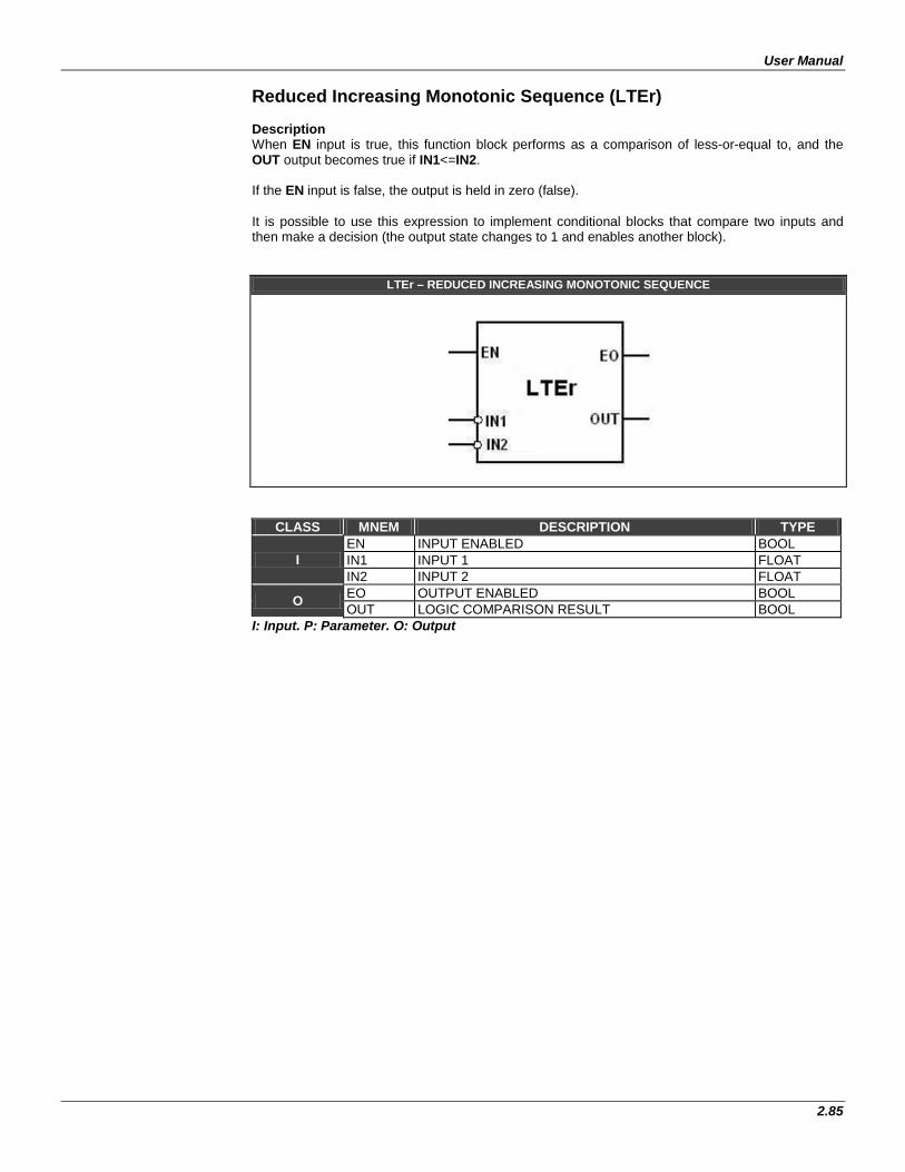
User Manual
2.85
Reduced Increasing Monotonic Sequence (LTEr) Description When EN input is true, this function block performs as a comparison of less-or-equal to, and the OUT output becomes true if IN1<=IN2. If the EN input is false, the output is held in zero (false). It is possible to use this expression to implement conditional blocks that compare two inputs and then make a decision (the output state changes to 1 and enables another block).
LTEr – REDUCED INCREASING MONOTONIC SEQUENCE
CLASS MNEM DESCRIPTION TYPE
I EN INPUT ENABLED BOOL IN1 INPUT 1 FLOAT IN2 INPUT 2 FLOAT
O EO OUTPUT ENABLED BOOL OUT LOGIC COMPARISON RESULT BOOL
I: Input. P: Parameter. O: Output
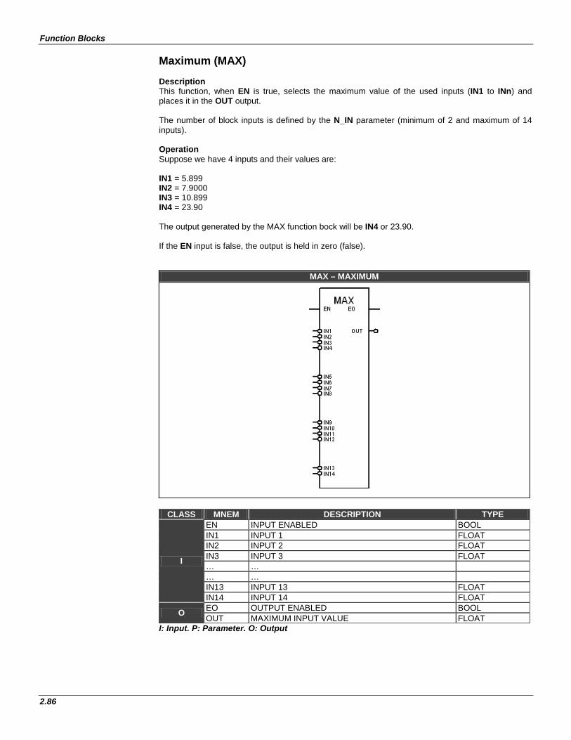
Function Blocks
2.86
Maximum (MAX) Description This function, when EN is true, selects the maximum value of the used inputs (IN1 to INn) and places it in the OUT output. The number of block inputs is defined by the N_IN parameter (minimum of 2 and maximum of 14 inputs). Operation Suppose we have 4 inputs and their values are: IN1 = 5.899 IN2 = 7.9000 IN3 = 10.899 IN4 = 23.90 The output generated by the MAX function bock will be IN4 or 23.90. If the EN input is false, the output is held in zero (false).
MAX – MAXIMUM
CLASS MNEM DESCRIPTION TYPE
I
EN INPUT ENABLED BOOL IN1 INPUT 1 FLOAT IN2 INPUT 2 FLOAT IN3 INPUT 3 FLOAT … … … … IN13 INPUT 13 FLOAT IN14 INPUT 14 FLOAT
O EO OUTPUT ENABLED BOOL OUT MAXIMUM INPUT VALUE FLOAT
I: Input. P: Parameter. O: Output
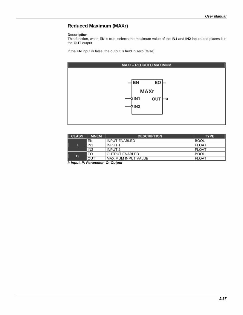
User Manual
2.87
Reduced Maximum (MAXr) Description This function, when EN is true, selects the maximum value of the IN1 and IN2 inputs and places it in the OUT output. If the EN input is false, the output is held in zero (false).
MAXr – REDUCED MAXIMUM
EN
IN1
EO
OUTIN2
MAXr
CLASS MNEM DESCRIPTION TYPE
I EN INPUT ENABLED BOOL IN1 INPUT 1 FLOAT IN2 INPUT 2 FLOAT
O EO OUTPUT ENABLED BOOL OUT MAXIMUM INPUT VALUE FLOAT
I: Input. P: Parameter. O: Output
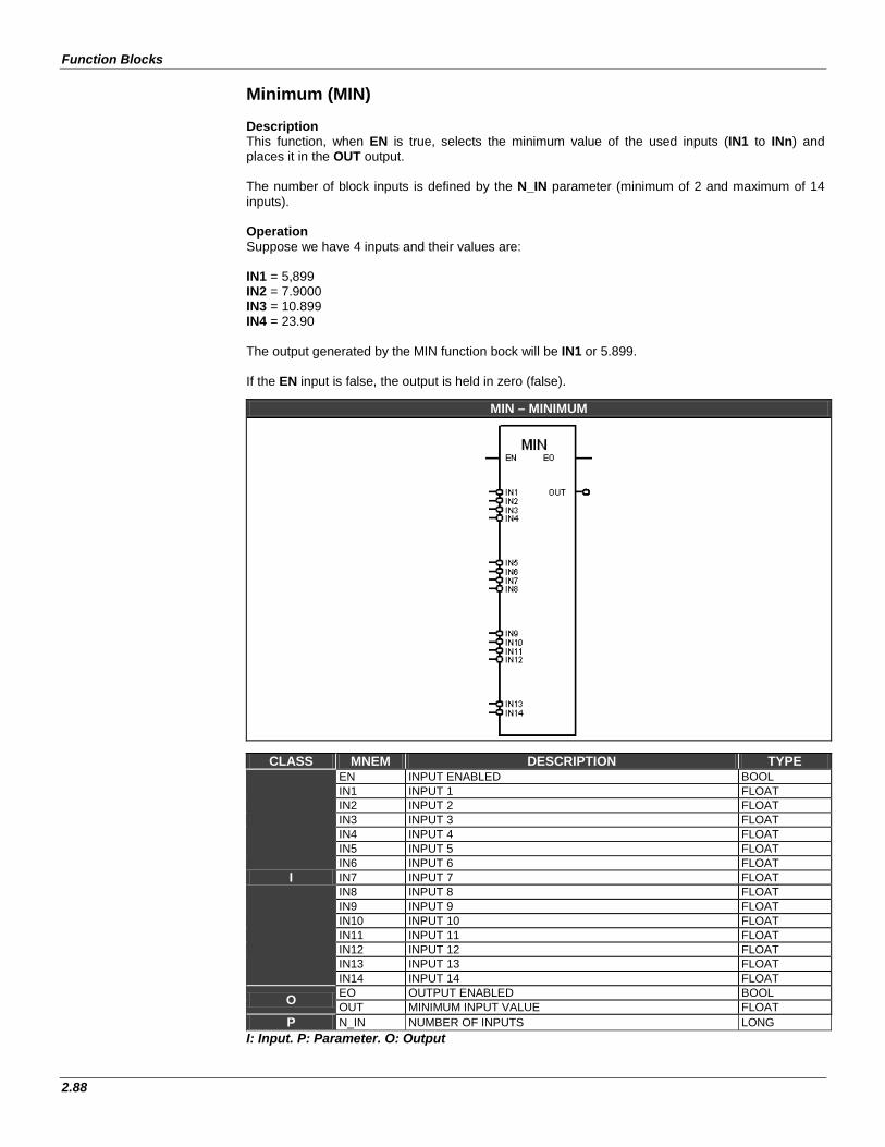
Function Blocks
2.88
Minimum (MIN) Description This function, when EN is true, selects the minimum value of the used inputs (IN1 to INn) and places it in the OUT output. The number of block inputs is defined by the N_IN parameter (minimum of 2 and maximum of 14 inputs). Operation Suppose we have 4 inputs and their values are: IN1 = 5,899 IN2 = 7.9000 IN3 = 10.899 IN4 = 23.90 The output generated by the MIN function bock will be IN1 or 5.899. If the EN input is false, the output is held in zero (false).
MIN – MINIMUM
CLASS MNEM DESCRIPTION TYPE
I
EN INPUT ENABLED BOOL IN1 INPUT 1 FLOAT IN2 INPUT 2 FLOAT IN3 INPUT 3 FLOAT IN4 INPUT 4 FLOAT IN5 INPUT 5 FLOAT IN6 INPUT 6 FLOAT IN7 INPUT 7 FLOAT IN8 INPUT 8 FLOAT IN9 INPUT 9 FLOAT IN10 INPUT 10 FLOAT IN11 INPUT 11 FLOAT IN12 INPUT 12 FLOAT IN13 INPUT 13 FLOAT IN14 INPUT 14 FLOAT
O EO OUTPUT ENABLED BOOL OUT MINIMUM INPUT VALUE FLOAT
P N_IN NUMBER OF INPUTS LONG I: Input. P: Parameter. O: Output

User Manual
2.89
Reduced Minimum (MINr) Description This function, when EN is true, selects the minimum value of the IN1 and IN2 inputs and places it in the OUT output. If the EN input is false, the output is held in zero (false).
MINr – REDUCED MINIMUM
CLASS MNEM DESCRIPTION TYPE
I EN INPUT ENABLED BOOL IN1 INPUT 1 FLOAT IN2 INPUT 2 FLOAT
O EO OUTPUT ENABLED BOOL OUT MINIMUM INPUT VALUE FLOAT
I: Input. P: Parameter. O: Output
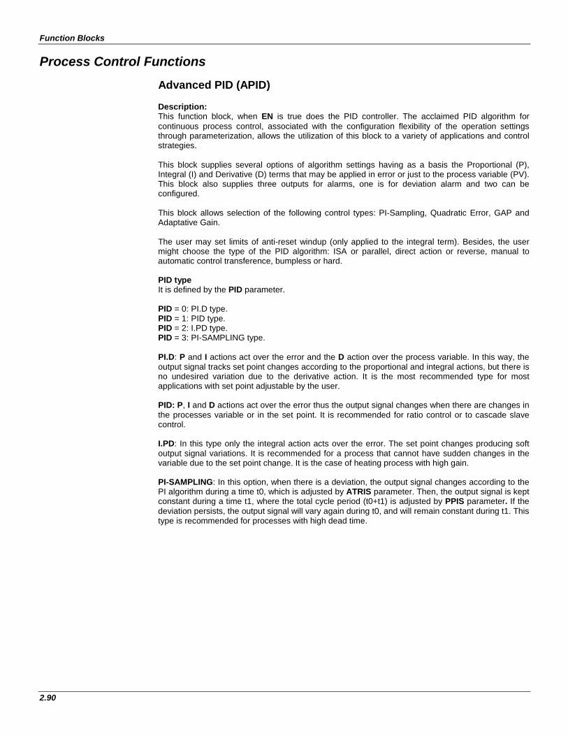
Function Blocks
2.90
Process Control Functions Advanced PID (APID)
Description: This function block, when EN is true does the PID controller. The acclaimed PID algorithm for continuous process control, associated with the configuration flexibility of the operation settings through parameterization, allows the utilization of this block to a variety of applications and control strategies. This block supplies several options of algorithm settings having as a basis the Proportional (P), Integral (I) and Derivative (D) terms that may be applied in error or just to the process variable (PV). This block also supplies three outputs for alarms, one is for deviation alarm and two can be configured. This block allows selection of the following control types: PI-Sampling, Quadratic Error, GAP and Adaptative Gain.
The user may set limits of anti-reset windup (only applied to the integral term). Besides, the user might choose the type of the PID algorithm: ISA or parallel, direct action or reverse, manual to automatic control transference, bumpless or hard. PID type It is defined by the PID parameter. PID = 0: PI.D type. PID = 1: PID type. PID = 2: I.PD type. PID = 3: PI-SAMPLING type. PI.D: P and I actions act over the error and the D action over the process variable. In this way, the output signal tracks set point changes according to the proportional and integral actions, but there is no undesired variation due to the derivative action. It is the most recommended type for most applications with set point adjustable by the user. PID: P, I and D actions act over the error thus the output signal changes when there are changes in the processes variable or in the set point. It is recommended for ratio control or to cascade slave control. I.PD: In this type only the integral action acts over the error. The set point changes producing soft output signal variations. It is recommended for a process that cannot have sudden changes in the variable due to the set point change. It is the case of heating process with high gain. PI-SAMPLING: In this option, when there is a deviation, the output signal changes according to the PI algorithm during a time t0, which is adjusted by ATRIS parameter. Then, the output signal is kept constant during a time t1, where the total cycle period (t0+t1) is adjusted by PPIS parameter. If the deviation persists, the output signal will vary again during t0, and will remain constant during t1. This type is recommended for processes with high dead time.
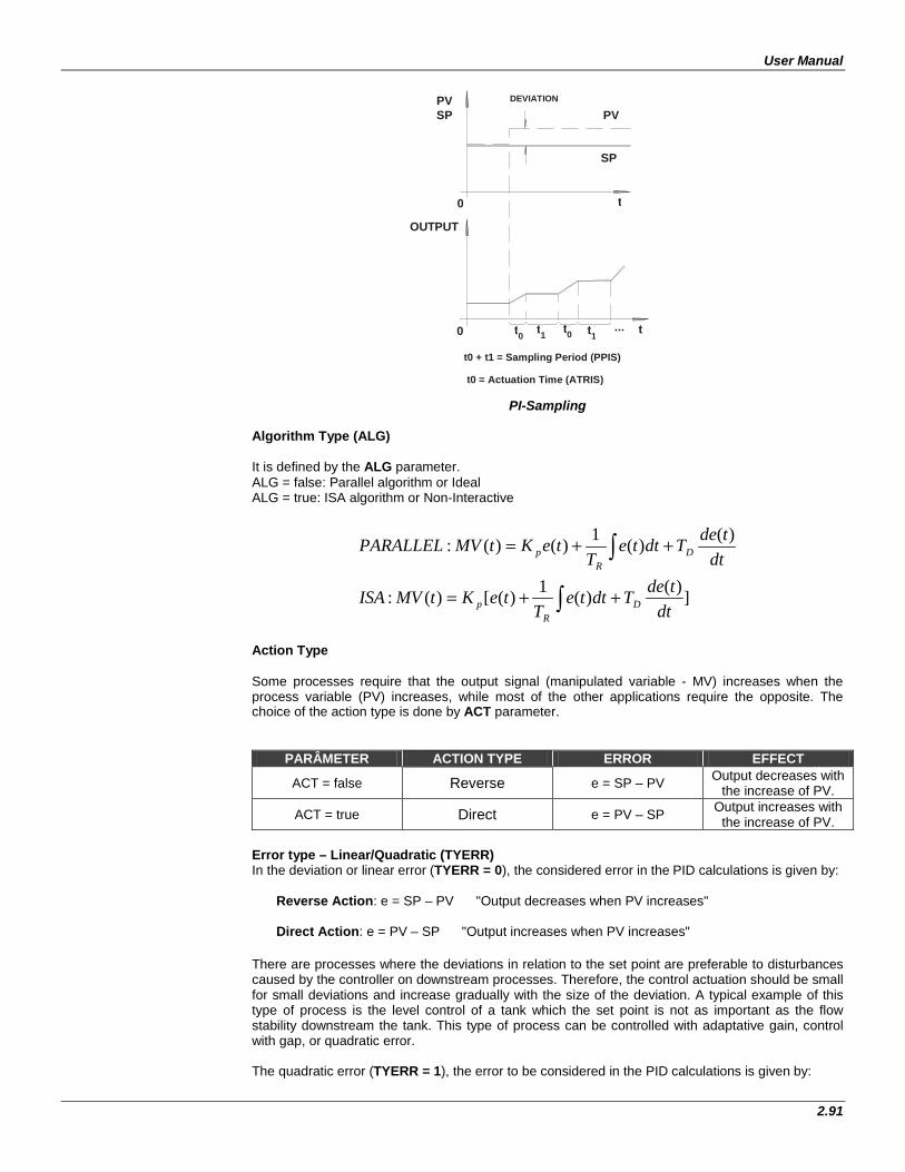
User Manual
2.91
PI-Sampling
Algorithm Type (ALG) It is defined by the ALG parameter. ALG = false: Parallel algorithm or Ideal ALG = true: ISA algorithm or Non-Interactive
])()(1)([)(:
)()(1)()(:
∫
∫
++=
++=
dttdeTdtte
TteKtMVISA
dttdeTdtte
TteKtMVPARALLEL
DR
p
DR
p
Action Type Some processes require that the output signal (manipulated variable - MV) increases when the process variable (PV) increases, while most of the other applications require the opposite. The choice of the action type is done by ACT parameter.
PARÂMETER ACTION TYPE ERROR EFFECT
ACT = false Reverse e = SP – PV Output decreases with the increase of PV.
ACT = true Direct e = PV – SP Output increases with the increase of PV.
Error type – Linear/Quadratic (TYERR) In the deviation or linear error (TYERR = 0), the considered error in the PID calculations is given by:
Reverse Action: e = SP – PV "Output decreases when PV increases"
Direct Action: e = PV – SP "Output increases when PV increases"
There are processes where the deviations in relation to the set point are preferable to disturbances caused by the controller on downstream processes. Therefore, the control actuation should be small for small deviations and increase gradually with the size of the deviation. A typical example of this type of process is the level control of a tank which the set point is not as important as the flow stability downstream the tank. This type of process can be controlled with adaptative gain, control with gap, or quadratic error.
The quadratic error (TYERR = 1), the error to be considered in the PID calculations is given by:
t0 + t1 t0 = Actuation Time (ATRIS)
= Sampling Period (PPIS)
PV SP
SP
0
0 t 0 t 0 t 1 t 1
t
t ...
PV DEVIATION
OUTPUT
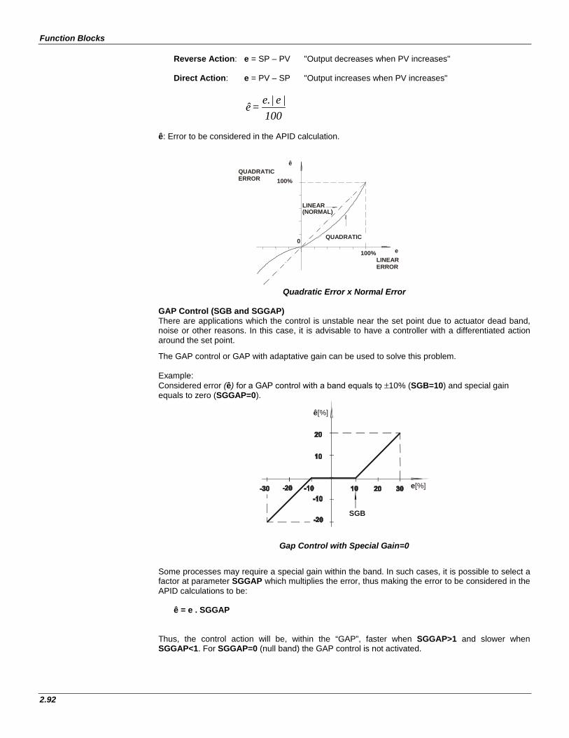
Function Blocks
2.92
Reverse Action: e = SP – PV "Output decreases when PV increases"
Direct Action: e = PV – SP "Output increases when PV increases"
100|e|e. = ê
ê: Error to be considered in the APID calculation.
Quadratic Error x Normal Error GAP Control (SGB and SGGAP) There are applications which the control is unstable near the set point due to actuator dead band, noise or other reasons. In this case, it is advisable to have a controller with a differentiated action around the set point. The GAP control or GAP with adaptative gain can be used to solve this problem. Example: Considered error (ê) for a GAP control with a band equals to ±10% (SGB=10) and special gain equals to zero (SGGAP=0).
Gap Control with Special Gain=0
Some processes may require a special gain within the band. In such cases, it is possible to select a factor at parameter SGGAP which multiplies the error, thus making the error to be considered in the APID calculations to be:
ê = e . SGGAP Thus, the control action will be, within the “GAP”, faster when SGGAP>1 and slower when SGGAP<1. For SGGAP=0 (null band) the GAP control is not activated.
SGB
e[%]
ê[%]
QUADRATIC ERROR
QUADRATIC
LINEAR (NORMAL)
ê
100%
0 100%
LINEAR ERROR
e
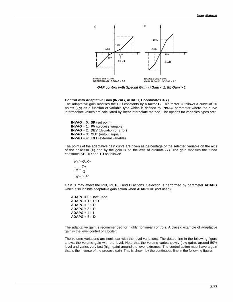
User Manual
2.93
GAP control with Special Gain a) Gain < 1, (b) Gain > 1
Control with Adaptative Gain (INVAG, ADAPG, Coordinates X/Y) The adaptative gain modifies the PID constants by a factor G. This factor G follows a curve of 10 points (x,y) as a function of variable type which is defined by INVAG parameter where the curve intermediate values are calculated by linear interpolate method. The options for variables types are:
INVAG = 0: SP (set point) INVAG = 1: PV (process variable) INVAG = 2: DEV (deviation or error) INVAG = 3: OUT (output signal) INVAG = 4: EXT (external variable).
The points of the adaptative gain curve are given as percentage of the selected variable on the axis of the abscissa (X) and by the gain G on the axis of ordinate (Y). The gain modifies the tuned constants KP, TR and TD as follows:
Gain G may affect the PID, PI, P, I and D actions. Selection is performed by parameter ADAPG which also inhibits adaptative gain action when ADAPG =0 (not used).
ADAPG = 0 : not used ADAPG = 1 : PID ADAPG = 2 : PI ADAPG = 3 : P ADAPG = 4 : I ADAPG = 5 : D
The adaptative gain is recommended for highly nonlinear controls. A classic example of adaptative gain is the level control of a boiler. The volume variations are nonlinear with the level variations. The dotted line in the following figure shows the volume gain with the level. Note that the volume varies slowly (low gain), around 50% level and varies very fast (high gain) around the level extremes. The control action must have a gain that is the inverse of the process gain. This is shown by the continuous line in the following figure.
a)
e e -10% -10%
20%
SGB SGB
BAND : SGB = 10% GAIN IN BAND : SGGAP = 0.5 RANGE : SGB = 10%
GAIN IN BAND : SGGAP = 2.0
-10%
10%
10% 10%
b)
DD
RR
PP
TGTGTT
KGK
.'
'
.'
=
=
=
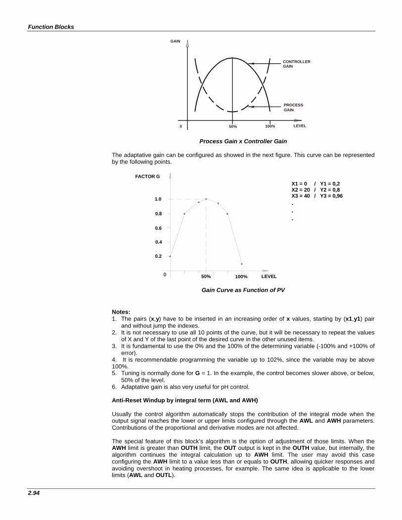
Function Blocks
2.94
Process Gain x Controller Gain The adaptative gain can be configured as showed in the next figure. This curve can be represented by the following points.
FACTOR G
1.0
50% 100% LEVEL
0.8
0.6
0.4
0.2
Gain Curve as Function of PV
Notes: 1. The pairs (x,y) have to be inserted in an increasing order of x values, starting by (x1,y1) pair
and without jump the indexes. 2. It is not necessary to use all 10 points of the curve, but it will be necessary to repeat the values
of X and Y of the last point of the desired curve in the other unused items. 3. It is fundamental to use the 0% and the 100% of the determining variable (-100% and +100% of
error). 4. It is recommendable programming the variable up to 102%, since the variable may be above 100%. 5. Tuning is normally done for G = 1. In the example, the control becomes slower above, or below,
50% of the level. 6. Adaptative gain is also very useful for pH control. Anti-Reset Windup by integral term (AWL and AWH)
Usually the control algorithm automatically stops the contribution of the integral mode when the output signal reaches the lower or upper limits configured through the AWL and AWH parameters. Contributions of the proportional and derivative modes are not affected. The special feature of this block’s algorithm is the option of adjustment of those limits. When the AWH limit is greater than OUTH limit, the OUT output is kept in the OUTH value, but internally, the algorithm continues the integral calculation up to AWH limit. The user may avoid this case configuring the AWH limit to a value less than or equals to OUTH, allowing quicker responses and avoiding overshoot in heating processes, for example. The same idea is applicable to the lower limits (AWL and OUTL).
GAIN
CONTROLLER GAIN
PROCESS GAIN
100% 50% 0 LEVEL
X1 = 0 / Y1 = 0,2 X2 = 20 / Y2 = 0,8 X3 = 40 / Y3 = 0,96 . . .
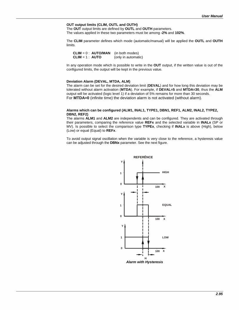
User Manual
2.95
OUT output limits (CLIM, OUTL and OUTH) The OUT output limits are defined by OUTL and OUTH parameters. The values applied in these two parameters must be among -2% and 102%. The CLIM parameter defines which mode (automatic/manual) will be applied the OUTL and OUTH limits.
CLIM = 0 : AUTO/MAN (in both modes) CLIM = 1 : AUTO (only in automatic)
In any operation mode which is possible to write in the OUT output, if the written value is out of the configured limits, the output will be kept in the previous value. Deviation Alarm (DEVAL, MTDA, ALM) The alarm can be set for the desired deviation limit (DEVAL) and for how long this deviation may be tolerated without alarm activation (MTDA). For example, if DEVAL=5 and MTDA=30, thus the ALM output will be activated (logic level 1) if a deviation of 5% remains for more than 30 seconds. For MTDA=0 (infinite time) the deviation alarm is not activated (without alarm). Alarms which can be configured (ALM1, INAL1, TYPE1, DBN1, REF1, ALM2, INAL2, TYPE2, DBN2, REF2) The alarms ALM1 and ALM2 are independents and can be configured. They are activated through their parameters, comparing the reference value REFx and the selected variable in INALx (SP or MV). Is possible to select the comparison type TYPEx, checking if INALx is above (High), below (Low) or equal (Equal) to REFx. To avoid output signal oscillation when the variable is very close to the reference, a hysteresis value can be adjusted through the DBNx parameter. See the next figure.
Alarm with Hysteresis
REFERÊNCE
HIGH
EQUAL
LOW
100
100
100
X
X
X
Y
1
0
Y
1
0
Y
1
0
H

Function Blocks
2.96
PID constants (KP, TR, TD, FB input and BIAS parameters) KP – Proportional gain. TR – Integral time in minutes/repeats, thus, bigger TR means less integral action. It can be understand as the necessary time to increase/decrease the output of error value (parallel PID), keeping it constant. TD – Derivative time is given in minutes. The derivative time is calculated using a false derivation, i.e., an action similar to a lead/lag controller, in which the lag constant is Alfa*TD. In this block implementation the Alfa factor is equal to 0.13. BIAS – This parameter will allow the adjustment of the initial output value (in percentage) when the control is transferred from manual to automatic. The applied value in this parameter has to be among 0% and 100%. The use of this input can be done through the selection of TRS parameter. FB – Through this input is possible to adjust the initial output value when the control is transferred to manual. The applied value in this input has to be among 0% and 100%. The use of this input can be done through the selection of TRS parameter. A/M Input (Automatic/Manual) If A/M is true, the APID will be in automatic control and if A/M is false the APID will be in manual control. Types of transference from Manual to Automatic (TRS) The output value of APID block is defined by the TRS parameter.
TRS = 0 (Bumpless) : In manual mode, the block output value is equal to the last output value in automatic mode. In this case it may write in the OUT output. When the block switches from manual to automatic, it starts the calculation from last output value in manual mode. TRS = 1 (Bumpless + BIAS) : In manual mode, the block output value is equal to the last output value in automatic mode. In this case it may write in the OUT output. When the block switches from manual to automatic, it starts the calculation from BIAS parameter value. TRS = 2 (Bumpless + FB) : In manual mode, the block output value is equal to the inserted value in the FB input. In this case it may not write in the OUT output. When the block switches from manual to automatic, it starts the calculation from FB input value.
TRS = 3 (Hard) : In manual mode, the block output value is equal to the last output value in automatic mode. In this case it may write in the OUT output. When the block switches from manual to automatic, it starts the calculation from last output value in manual mode + proportional term (KP x error).
TRS = 4 (Hard + BIAS) : In manual mode, the block output value is equal to the last output value in automatic mode. In this case it may write in the OUT output. When the block switches from manual to automatic, it starts the calculation from BIAS parameter value + proportional term (KP x error).
TRS = 5 (Hard + FB) : In manual mode, the block output value is equal to the inserted value in the FB input. In this case it may not write in the OUT output. When the block switches from manual to automatic, it starts the calculation from FB input value + proportional term (KP x error).
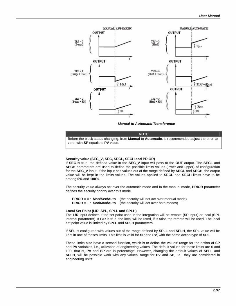
User Manual
2.97
Manual to Automatic Transference
NOTE Before the block status changing, from Manual to Automatic, is recommended adjust the error to zero, with SP equals to PV value.
Security value (SEC_V, SEC, SECL, SECH and PRIOR) If SEC is true, the defined value in the SEC_V input will pass to the OUT output. The SECL and SECH parameters are used to define the possible limits values (lower and upper) of configuration for the SEC_V input. If the input has values out of the range defined by SECL and SECH, the output value will be kept in the limits values. The values applied to SECL and SECH limits have to be among 0% and 100%. The security value always act over the automatic mode and to the manual mode, PRIOR parameter defines the security priority over this mode.
PRIOR = 0 : Man/Sec/Auto (the security will not act over manual mode) PRIOR = 1 : Sec/Man/Auto (the security will act over both modes)
Local Set Point (L/R, SPL, SPLL and SPLH) The L/R input defines if the set point used in the integration will be remote (SP input) or local (SPL internal parameter). If L/R is true, the local will be used, if is false the remote will be used. The local set point value is limited by SPLL and SPLH parameters. If SPL is configured with values out of the range defined by SPLL and SPLH, the SPL value will be kept in one of theses limits. This limit is valid for SP and PV, with the same action type of SPL. These limits also have a second function, which is to define the values’ range for the action of SP and PV variables, i.e., utilization of engineering values. The default values for these limits are 0 and 100, that is, PV and SP are in percentage. However, changing the default values of SPLL and SPLH, will be possible work with any values’ range for PV and SP, i.e., they are considered in engineering units.
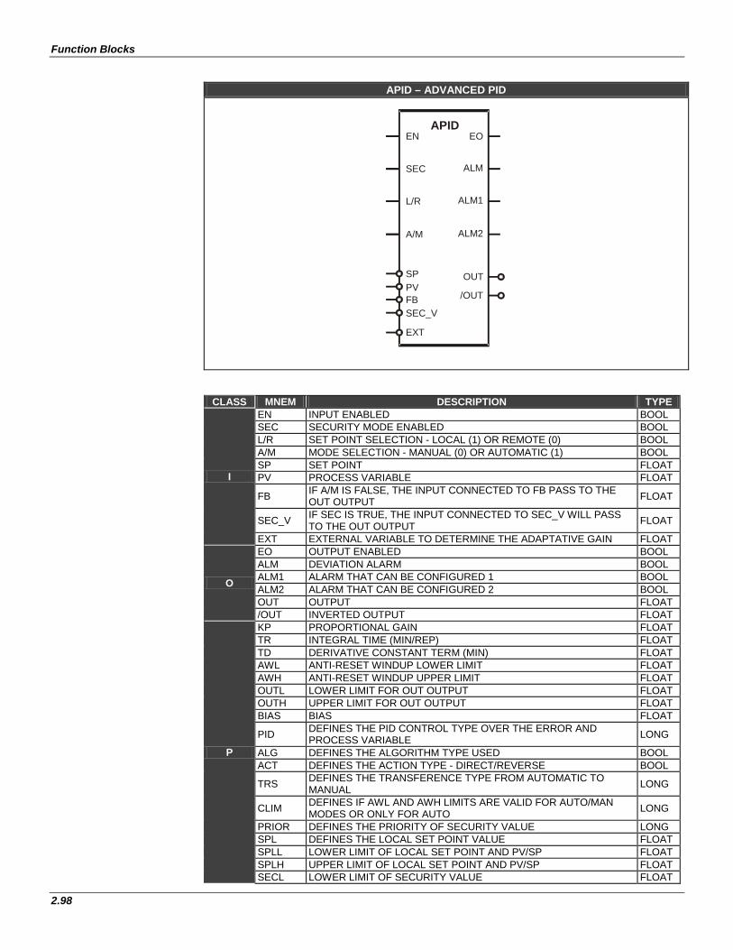
Function Blocks
2.98
APID – ADVANCED PID
CLASS MNEM DESCRIPTION TYPE
I
EN INPUT ENABLED BOOL SEC SECURITY MODE ENABLED BOOL L/R SET POINT SELECTION - LOCAL (1) OR REMOTE (0) BOOL A/M MODE SELECTION - MANUAL (0) OR AUTOMATIC (1) BOOL SP SET POINT FLOAT PV PROCESS VARIABLE FLOAT
FB IF A/M IS FALSE, THE INPUT CONNECTED TO FB PASS TO THE OUT OUTPUT FLOAT
SEC_V IF SEC IS TRUE, THE INPUT CONNECTED TO SEC_V WILL PASS TO THE OUT OUTPUT FLOAT
EXT EXTERNAL VARIABLE TO DETERMINE THE ADAPTATIVE GAIN FLOAT
O
EO OUTPUT ENABLED BOOL ALM DEVIATION ALARM BOOL ALM1 ALARM THAT CAN BE CONFIGURED 1 BOOL ALM2 ALARM THAT CAN BE CONFIGURED 2 BOOL OUT OUTPUT FLOAT /OUT INVERTED OUTPUT FLOAT
P
KP PROPORTIONAL GAIN FLOAT TR INTEGRAL TIME (MIN/REP) FLOAT TD DERIVATIVE CONSTANT TERM (MIN) FLOAT AWL ANTI-RESET WINDUP LOWER LIMIT FLOAT AWH ANTI-RESET WINDUP UPPER LIMIT FLOAT OUTL LOWER LIMIT FOR OUT OUTPUT FLOAT OUTH UPPER LIMIT FOR OUT OUTPUT FLOAT BIAS BIAS FLOAT
PID DEFINES THE PID CONTROL TYPE OVER THE ERROR AND PROCESS VARIABLE LONG
ALG DEFINES THE ALGORITHM TYPE USED BOOL ACT DEFINES THE ACTION TYPE - DIRECT/REVERSE BOOL
TRS DEFINES THE TRANSFERENCE TYPE FROM AUTOMATIC TO MANUAL LONG
CLIM DEFINES IF AWL AND AWH LIMITS ARE VALID FOR AUTO/MAN MODES OR ONLY FOR AUTO LONG
PRIOR DEFINES THE PRIORITY OF SECURITY VALUE LONG SPL DEFINES THE LOCAL SET POINT VALUE FLOAT SPLL LOWER LIMIT OF LOCAL SET POINT AND PV/SP FLOAT SPLH UPPER LIMIT OF LOCAL SET POINT AND PV/SP FLOAT SECL LOWER LIMIT OF SECURITY VALUE FLOAT
APID
SEC
A/M
PV FB SEC_V EXT
EN
ALM
ALM2
EO
OUT
L/R ALM1
SP
/OUT
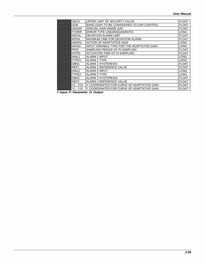
User Manual
2.99
SECH UPPER LIMIT OF SECURITY VALUE FLOAT SGB BAND (GAP) TO BE CONSIDERED TO GAP CONTROL FLOAT SGGAP SPECIAL GAIN INSIDE GAP FLOAT TYERR ERROR TYPE LINEAR/QUADRATIC LONG DEVAL DEVIATION ALARM LIMIT FLOAT MTDA MAXIMUM TIME FOR DEVIATION ALARM FLOAT ADAPG ACTION OF ADAPTATIVE GAIN LONG INVAG INPUT VARIABLE TYPE FOR THE ADAPTATIVE GAIN LONG PPIS SAMPLING PERIOD OF PI-SAMPLING FLOAT ATPIS ACTUATION TIME OF PI-SAMPLING FLOAT INAL1 ALARM 1 INPUT LONG TYPE1 ALARM 1 TYPE LONG DBN1 ALARM 1 HYSTERESIS FLOAT REF1 ALARM 1 REFERENCE VALUE FLOAT INAL2 ALARM 2 INPUT LONG TYPE2 ALARM 2 TYPE LONG DBN2 ALARM 2 HYSTERESIS FLOAT REF2 ALARM 2 REFERENCE VALUE FLOAT X1...X10 X COORDINATES FOR CURVE OF ADAPTATIVE GAIN FLOAT Y1...Y10 Y COORDINATES FOR CURVE OF ADAPTATIVE GAIN FLOAT
I: Input. P: Parameter. O: Output
Function Blocks
2.100
Automatic Up and Down Ramp (ARAMP) Description: This function, when EN is true, increases or decreases the OUT output in a linear way based on a pre- established time interval. This function block may be used to create a time database to an automatic set point generator when it is used together with the linearization block or a simple ramp. In a set point application the ARAMP block is prepared to generate a 0 to 100 % output in a time interval which tracking the set point curve. The ARAMP output will be connected to the input of the LIN function (linearization) set with a set point profile curve. Selecting the IN input and the OUT output formats (PERC parameter) PERC = false: the IN input and the OUT output values are given in percentage (0 – 100%). PERC = true: the IN input and the OUT output values are given in the 0 – 10000 format. Time Selection The block time basis can be selected in minutes, seconds or hours, according to the requirements of the application, by the parameter T_SEL. This parameter has the following values:0: seconds, 1: minutes, 2: hours.This selection affects directly the chosen value for the FTIME parameter. FTIME and IC_DC Parameter FTIME is the time which the output takes to change from 0 to 100 %. The change direction is given by the IC_DC input. If this input is true, the OUT output will be gradually decreased with speed defined by the FTIME parameter, otherwise, the output will be increased with the speed defined in the FTIME parameter. Pause Command The PAUSE command freezes the OUT output. So the output can be increased or decreased through the selection of the UP and DOWN inputs. UP and DOWN Command, ASPD Parameter The UP and DOWN inputs will advance or revert the OUT output to a desired value using the manual speed adjustment by the ASPD parameter. This parameter configures the speed of manual actuation. LOWL and HIGHL Parameter The LOWL parameter configures the bottom limit of the ramp generated by the ARAMP function block while the HIGHL parameter configures the upper limit of the output ramp. It starts from the value in the IN input and goes to the maximum value, set in the HIGHL parameter. If the input value is less than LOWL, the initial value of the ramp will be equal to LOWL. HIGH and LOW Alarms When the output ramp reaches the bottom limit (LOWL) or the upper limit (HIGHL), the alarms LOW and HIGH will be turned on. The LOW output goes to true if the bottom limit is reached. Similarly, if the upper limit is reached the output HIGH goes to true. ACCEL Parameter It is the manual acceleration of actuation. When the block output is a parabola, the ACCEL parameter allows fine adjustment of the output, allowing more definition of the output rate of change.
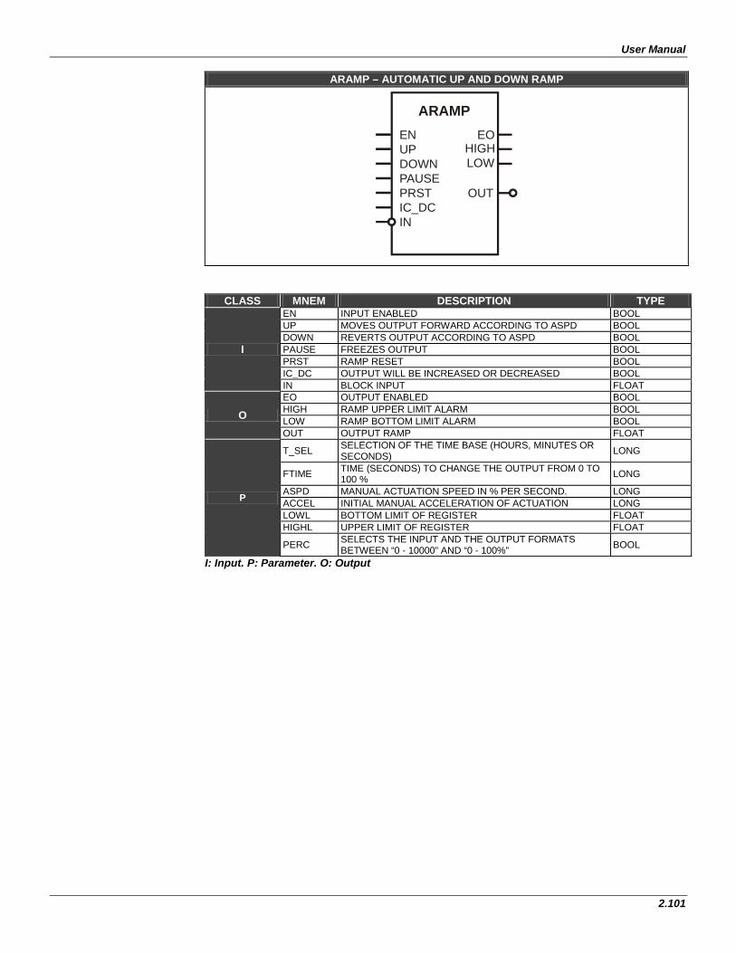
User Manual
2.101
ARAMP – AUTOMATIC UP AND DOWN RAMP
ARAMP
UPDOWNPAUSEPRSTIC_DCIN
ENHIGHLOW
EO
OUT
CLASS MNEM DESCRIPTION TYPE
I
EN INPUT ENABLED BOOL UP MOVES OUTPUT FORWARD ACCORDING TO ASPD BOOL DOWN REVERTS OUTPUT ACCORDING TO ASPD BOOL PAUSE FREEZES OUTPUT BOOL PRST RAMP RESET BOOL IC_DC OUTPUT WILL BE INCREASED OR DECREASED BOOL IN BLOCK INPUT FLOAT
O EO OUTPUT ENABLED BOOL HIGH RAMP UPPER LIMIT ALARM BOOL LOW RAMP BOTTOM LIMIT ALARM BOOL OUT OUTPUT RAMP FLOAT
P
T_SEL SELECTION OF THE TIME BASE (HOURS, MINUTES OR SECONDS) LONG
FTIME TIME (SECONDS) TO CHANGE THE OUTPUT FROM 0 TO 100 % LONG
ASPD MANUAL ACTUATION SPEED IN % PER SECOND. LONG ACCEL INITIAL MANUAL ACCELERATION OF ACTUATION LONG LOWL BOTTOM LIMIT OF REGISTER FLOAT HIGHL UPPER LIMIT OF REGISTER FLOAT
PERC SELECTS THE INPUT AND THE OUTPUT FORMATS BETWEEN “0 - 10000” AND “0 - 100%” BOOL
I: Input. P: Parameter. O: Output
Function Blocks
2.102
Enhanced PID (EPID)
Description: This function block, when EN is true does the PID controller. The acclaimed PID algorithm for continuous process control, associated with the configuration flexibility of the operation settings through parameterization, allows the utilization of this block to a variety of applications and control strategies. This block supplies several options of algorithm settings having as a basis the Proportional (P), Integral (I) and Derivative (D) terms that may be applied in error or just to the process variable (PV). This block also provide three outputs for alarms, one is for deviation alarm and two can be configured. This block allows selection of the following control types: PI-Sampling, Quadratic Error and GAP.
The user may set limits of anti-reset windup (only applied to the integral term). Besides, the user might choose the type of the PID algorithm: ISA or parallel, direct action or reverse, manual to automatic control transference, bumpless or hard. PID type It is defined by the PID parameter. PID = 0: PI.D type. PID = 1: PID type. PID = 2: I.PD type. PID = 3: PI-SAMPLING type. PI.D: P and I actions act over the error and the D action over the process variable. In this way, the output signal tracks set point changes according to the proportional and integral actions, but there is no undesired variation due to the derivative action. It is the most recommended type for most applications with set point adjustable by the user. PID: P, I and D actions act over the error thus the output signal changes when there are changes in the processes variable or in the set point. It is recommended for ratio control or to cascade slave control. I.PD: In this type only the integral action acts over the error. The set point changes producing soft output signal variations. It is recommended for a process that cannot have sudden changes in the variable due to the set point change. It is the case of heating process with high gain. PI-SAMPLING: In this option, when there is a deviation, the output signal changes according to the PI algorithm during a time t0, which is adjusted by ATRIS parameter. Then, the output signal is kept constant during a time t1, where the total cycle period (t0+t1) is adjusted by PPIS parameter. If the deviation persists, the output signal will vary again during t0, and will remain constant during t1. This type is recommended for processes with high dead time.
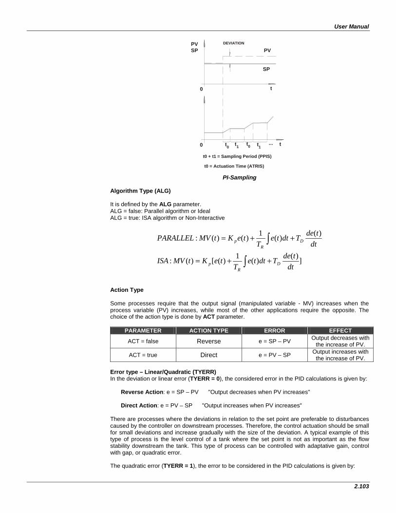
User Manual
2.103
PI-Sampling
Algorithm Type (ALG) It is defined by the ALG parameter. ALG = false: Parallel algorithm or Ideal ALG = true: ISA algorithm or Non-Interactive
])()(1)([)(:
)()(1)()(:
∫
∫
++=
++=
dttdeTdtte
TteKtMVISA
dttdeTdtte
TteKtMVPARALLEL
DR
p
DR
p
Action Type Some processes require that the output signal (manipulated variable - MV) increases when the process variable (PV) increases, while most of the other applications require the opposite. The choice of the action type is done by ACT parameter.
PARAMETER ACTION TYPE ERROR EFFECT
ACT = false Reverse e = SP – PV Output decreases with the increase of PV.
ACT = true Direct e = PV – SP Output increases with the increase of PV.
Error type – Linear/Quadratic (TYERR) In the deviation or linear error (TYERR = 0), the considered error in the PID calculations is given by:
Reverse Action: e = SP – PV "Output decreases when PV increases"
Direct Action: e = PV – SP "Output increases when PV increases"
There are processes where the deviations in relation to the set point are preferable to disturbances caused by the controller on downstream processes. Therefore, the control actuation should be small for small deviations and increase gradually with the size of the deviation. A typical example of this type of process is the level control of a tank where the set point is not as important as the flow stability downstream the tank. This type of process can be controlled with adaptative gain, control with gap, or quadratic error.
The quadratic error (TYERR = 1), the error to be considered in the PID calculations is given by:
t0 + t1 t0 = Actuation Time (ATRIS)
= Sampling Period (PPIS)
PV SP
SP
0
0 t 0 t 0 t 1 t 1
t
t ...
PV DEVIATION
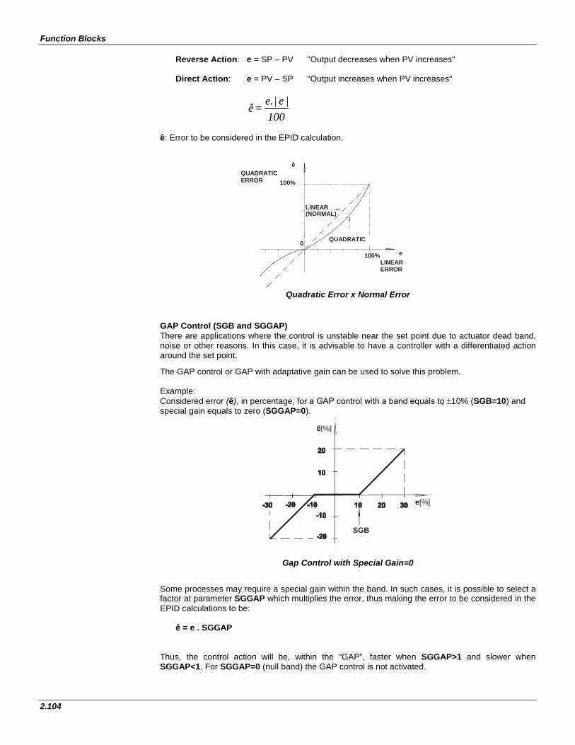
Function Blocks
2.104
Reverse Action: e = SP – PV "Output decreases when PV increases"
Direct Action: e = PV – SP "Output increases when PV increases"
100|e|e. = ê
ê: Error to be considered in the EPID calculation.
Quadratic Error x Normal Error
GAP Control (SGB and SGGAP) There are applications where the control is unstable near the set point due to actuator dead band, noise or other reasons. In this case, it is advisable to have a controller with a differentiated action around the set point. The GAP control or GAP with adaptative gain can be used to solve this problem. Example: Considered error (ê), in percentage, for a GAP control with a band equals to ±10% (SGB=10) and special gain equals to zero (SGGAP=0).
Gap Control with Special Gain=0
Some processes may require a special gain within the band. In such cases, it is possible to select a factor at parameter SGGAP which multiplies the error, thus making the error to be considered in the EPID calculations to be:
ê = e . SGGAP Thus, the control action will be, within the “GAP”, faster when SGGAP>1 and slower when SGGAP<1. For SGGAP=0 (null band) the GAP control is not activated.
SGB
e[%]
ê[%]
QUADRATIC ERROR
QUADRATIC
LINEAR (NORMAL)
ê
100%
0 100%
LINEAR ERROR
e
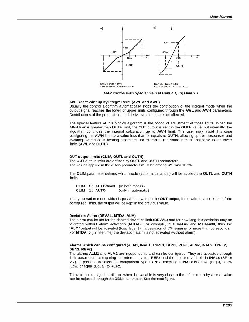
User Manual
2.105
GAP control with Special Gain a) Gain < 1, (b) Gain > 1
Anti-Reset Windup by integral term (AWL and AWH) Usually the control algorithm automatically stops the contribution of the integral mode when the output signal reaches the lower or upper limits configured through the AWL and AWH parameters. Contributions of the proportional and derivative modes are not affected. The special feature of this block’s algorithm is the option of adjustment of those limits. When the AWH limit is greater than OUTH limit, the OUT output is kept in the OUTH value, but internally, the algorithm continues the integral calculation up to AWH limit. The user may avoid this case configuring the AWH limit to a value less than or equals to OUTH, allowing quicker responses and avoiding overshoot in heating processes, for example. The same idea is applicable to the lower limits (AWL and OUTL). OUT output limits (CLIM, OUTL and OUTH) The OUT output limits are defined by OUTL and OUTH parameters. The values applied in these two parameters must be among -2% and 102%. The CLIM parameter defines which mode (automatic/manual) will be applied the OUTL and OUTH limits.
CLIM = 0 : AUTO/MAN (in both modes) CLIM = 1 : AUTO (only in automatic)
In any operation mode which is possible to write in the OUT output, if the written value is out of the configured limits, the output will be kept in the previous value. Deviation Alarm (DEVAL, MTDA, ALM) The alarm can be set for the desired deviation limit (DEVAL) and for how long this deviation may be tolerated without alarm activation (MTDA). For example, if DEVAL=5 and MTDA=30, thus the "ALM" output will be activated (logic level 1) if a deviation of 5% remains for more than 30 seconds. For MTDA=0 (infinite time) the deviation alarm is not activated (without alarm). Alarms which can be configured (ALM1, INAL1, TYPE1, DBN1, REF1, ALM2, INAL2, TYPE2, DBN2, REF2) The alarms ALM1 and ALM2 are independents and can be configured. They are activated through their parameters, comparing the reference value REFx and the selected variable in INALx (SP or MV). Is possible to select the comparison type TYPEx, checking if INALx is above (High), below (Low) or equal (Equal) to REFx. To avoid output signal oscillation when the variable is very close to the reference, a hysteresis value can be adjusted through the DBNx parameter. See the next figure.
a)
e e -10% -10%
20%
SGB SGB
BAND : SGB = 10% GAIN IN BAND : SGGAP = 0.5 RANGE : SGB = 10%
GAIN IN BAND : SGGAP = 2.0
-10%
10%
10% 10%
b)
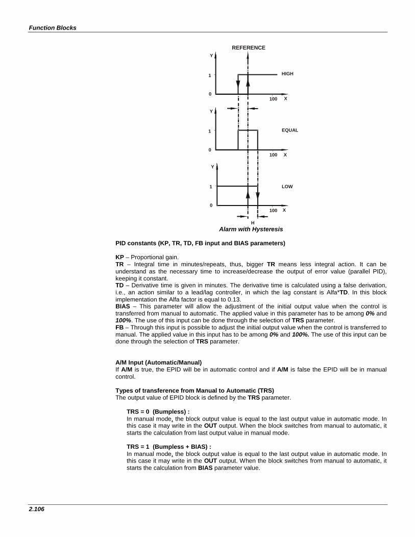
Function Blocks
2.106
Alarm with Hysteresis
PID constants (KP, TR, TD, FB input and BIAS parameters) KP – Proportional gain. TR – Integral time in minutes/repeats, thus, bigger TR means less integral action. It can be understand as the necessary time to increase/decrease the output of error value (parallel PID), keeping it constant. TD – Derivative time is given in minutes. The derivative time is calculated using a false derivation, i.e., an action similar to a lead/lag controller, in which the lag constant is Alfa*TD. In this block implementation the Alfa factor is equal to 0.13. BIAS – This parameter will allow the adjustment of the initial output value when the control is transferred from manual to automatic. The applied value in this parameter has to be among 0% and 100%. The use of this input can be done through the selection of TRS parameter. FB – Through this input is possible to adjust the initial output value when the control is transferred to manual. The applied value in this input has to be among 0% and 100%. The use of this input can be done through the selection of TRS parameter.
A/M Input (Automatic/Manual) If A/M is true, the EPID will be in automatic control and if A/M is false the EPID will be in manual control. Types of transference from Manual to Automatic (TRS) The output value of EPID block is defined by the TRS parameter.
TRS = 0 (Bumpless) : In manual mode, the block output value is equal to the last output value in automatic mode. In this case it may write in the OUT output. When the block switches from manual to automatic, it starts the calculation from last output value in manual mode. TRS = 1 (Bumpless + BIAS) : In manual mode, the block output value is equal to the last output value in automatic mode. In this case it may write in the OUT output. When the block switches from manual to automatic, it starts the calculation from BIAS parameter value.
REFERENCE
HIGH
EQUAL
LOW
100
100
100
X
X
X
Y
1
0
Y
1
0
Y
1
0
H
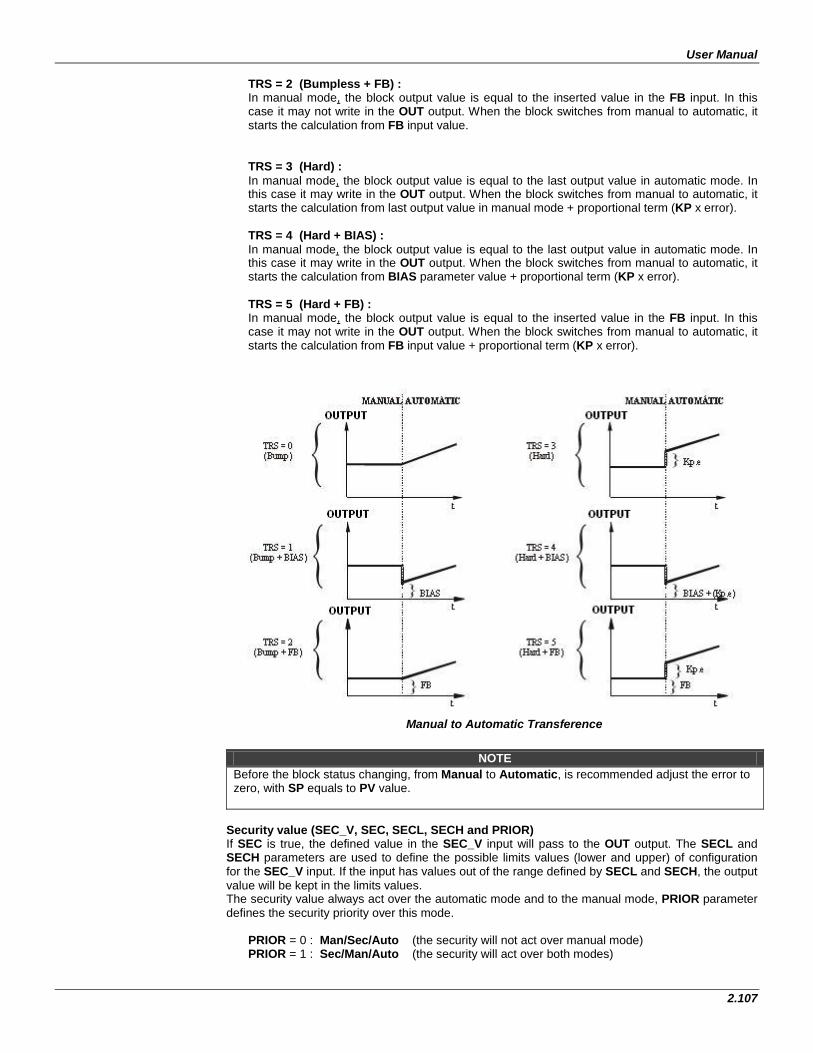
User Manual
2.107
TRS = 2 (Bumpless + FB) : In manual mode, the block output value is equal to the inserted value in the FB input. In this case it may not write in the OUT output. When the block switches from manual to automatic, it starts the calculation from FB input value.
TRS = 3 (Hard) : In manual mode, the block output value is equal to the last output value in automatic mode. In this case it may write in the OUT output. When the block switches from manual to automatic, it starts the calculation from last output value in manual mode + proportional term (KP x error).
TRS = 4 (Hard + BIAS) : In manual mode, the block output value is equal to the last output value in automatic mode. In this case it may write in the OUT output. When the block switches from manual to automatic, it starts the calculation from BIAS parameter value + proportional term (KP x error).
TRS = 5 (Hard + FB) : In manual mode, the block output value is equal to the inserted value in the FB input. In this case it may not write in the OUT output. When the block switches from manual to automatic, it starts the calculation from FB input value + proportional term (KP x error).
Manual to Automatic Transference
NOTE
Before the block status changing, from Manual to Automatic, is recommended adjust the error to zero, with SP equals to PV value.
Security value (SEC_V, SEC, SECL, SECH and PRIOR) If SEC is true, the defined value in the SEC_V input will pass to the OUT output. The SECL and SECH parameters are used to define the possible limits values (lower and upper) of configuration for the SEC_V input. If the input has values out of the range defined by SECL and SECH, the output value will be kept in the limits values. The security value always act over the automatic mode and to the manual mode, PRIOR parameter defines the security priority over this mode.
PRIOR = 0 : Man/Sec/Auto (the security will not act over manual mode) PRIOR = 1 : Sec/Man/Auto (the security will act over both modes)
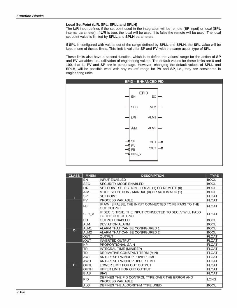
Function Blocks
2.108
Local Set Point (L/R, SPL, SPLL and SPLH) The L/R input defines if the set point used in the integration will be remote (SP input) or local (SPL internal parameter). If L/R is true, the local will be used, if is false the remote will be used. The local set point value is limited by SPLL and SPLH parameters. If SPL is configured with values out of the range defined by SPLL and SPLH, the SPL value will be kept in one of theses limits. This limit is valid for SP and PV, with the same action type of SPL. These limits also have a second function, which is to define the values’ range for the action of SP and PV variables, i.e., utilization of engineering values. The default values for these limits are 0 and 100, that is, PV and SP are in percentage. However, changing the default values of SPLL and SPLH, will be possible work with any values’ range for PV and SP, i.e., they are considered in engineering units.
EPID – ENHANCED PID
CLASS MNEM DESCRIPTION TYPE
I
EN INPUT ENABLED BOOL SEC SECURITY MODE ENABLED BOOL L/R SET POINT SELECTION – LOCAL (1) OR REMOTE (0) BOOL A/M MODE SELECTION - MANUAL (0) OR AUTOMATIC (1) BOOL SP SET POINT FLOAT PV PROCESS VARIABLE FLOAT
FB IF A/M IS FALSE, THE INPUT CONNECTED TO FB PASS TO THE OUT OUTPUT FLOAT
SEC_V IF SEC IS TRUE, THE INPUT CONNECTED TO SEC_V WILL PASS TO THE OUT OUTPUT FLOAT
O
EO OUTPUT ENABLED BOOL ALM DEVIATION ALARM BOOL ALM1 ALARM THAT CAN BE CONFIGURED 1 BOOL ALM2 ALARM THAT CAN BE CONFIGURED 2 BOOL OUT OUTPUT FLOAT /OUT INVERTED OUTPUT FLOAT
P
KP PROPORTIONAL GAIN FLOAT TR INTEGRAL TIME (MIN/REP) FLOAT TD DERIVATIVE CONSTANT TERM (MIN) FLOAT AWL ANTI-RESET WINDUP LOWER LIMIT FLOAT AWH ANTI-RESET WINDUP UPPER LIMIT FLOAT OUTL LOWER LIMIT FOR OUT OUTPUT FLOAT OUTH UPPER LIMIT FOR OUT OUTPUT FLOAT BIAS BIAS FLOAT
PID DEFINES THE PID CONTROL TYPE OVER THE ERROR AND PROCESS VARIABLE LONG
ALG DEFINES THE ALGORITHM TYPE USED BOOL
EPID
SEC
A/M
PV FB SEC_V
EN
ALM
ALM2
EO
OUT
L/R ALM1
SP
/OUT
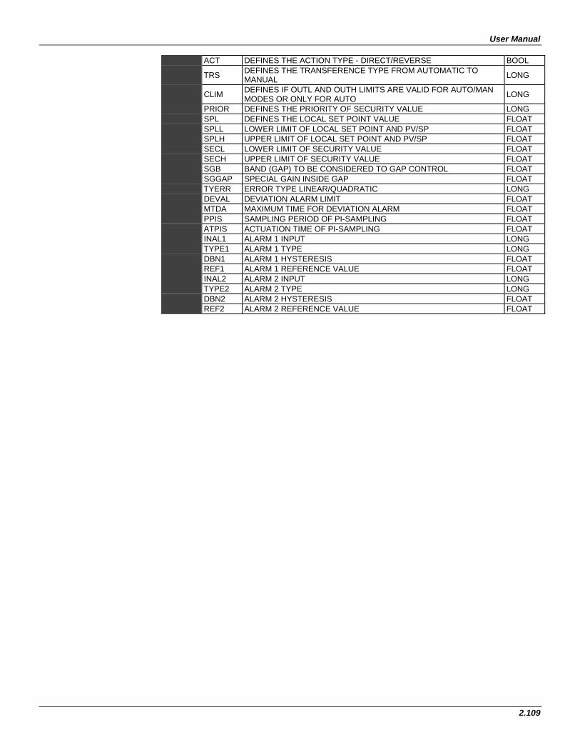
User Manual
2.109
ACT DEFINES THE ACTION TYPE - DIRECT/REVERSE BOOL
TRS DEFINES THE TRANSFERENCE TYPE FROM AUTOMATIC TO MANUAL LONG
CLIM DEFINES IF OUTL AND OUTH LIMITS ARE VALID FOR AUTO/MAN MODES OR ONLY FOR AUTO LONG
PRIOR DEFINES THE PRIORITY OF SECURITY VALUE LONG SPL DEFINES THE LOCAL SET POINT VALUE FLOAT SPLL LOWER LIMIT OF LOCAL SET POINT AND PV/SP FLOAT SPLH UPPER LIMIT OF LOCAL SET POINT AND PV/SP FLOAT SECL LOWER LIMIT OF SECURITY VALUE FLOAT SECH UPPER LIMIT OF SECURITY VALUE FLOAT SGB BAND (GAP) TO BE CONSIDERED TO GAP CONTROL FLOAT SGGAP SPECIAL GAIN INSIDE GAP FLOAT TYERR ERROR TYPE LINEAR/QUADRATIC LONG DEVAL DEVIATION ALARM LIMIT FLOAT MTDA MAXIMUM TIME FOR DEVIATION ALARM FLOAT PPIS SAMPLING PERIOD OF PI-SAMPLING FLOAT ATPIS ACTUATION TIME OF PI-SAMPLING FLOAT INAL1 ALARM 1 INPUT LONG TYPE1 ALARM 1 TYPE LONG DBN1 ALARM 1 HYSTERESIS FLOAT REF1 ALARM 1 REFERENCE VALUE FLOAT INAL2 ALARM 2 INPUT LONG TYPE2 ALARM 2 TYPE LONG DBN2 ALARM 2 HYSTERESIS FLOAT REF2 ALARM 2 REFERENCE VALUE FLOAT

Function Blocks
2.110
Enhanced TOT (ETOT) Description: This block gives the input totalization. This totalization is the integral of the input times a scale factor FCF that allows the user to configure the totalization in 3 different operation modes. If the application requires the computing of instantaneous totalized volume, use the ETOT function block to accomplish this task. The time basis of this calculation is seconds. The flow generally is given in Engineering Units (EU) by units of time. For example: A 1 m3/ s flow as input of the ETOT function block will have as output volume in m3. Suppose the application needs the energy value of an electrical device. The ETOT block allows calculating the value of this energy by the instantaneous power expression:
∫= dttPotEnergy )(
and Pot(t)= V(t).I(t), where V(t) is the instantaneous voltage and I(t) is the instantaneous current. OUT output and TU parameter The time interval while the output is totalized is according to the value set in TU. The OUT output is the totalization value.
MEM output It stores the totalization value before the last reset. HIGH and PHIGH outputs If the totalization becomes greater than or equal to the values configured in TRIP and PTRIP, the HIGH and PHIGH outputs are activated respectively. CutOff parameter The totalization is not performed if the input flow value is less than or equal to CutOff value.
FCF parameter The FCF parameter allows the ETOT function block to operate in 4 different modes: a) IN is FLOAT and represents flow in Engineering Units (EU): FCF must be equal to 1 to the totalization is done without any EU scale factor. (or adjust the factor that you wish to use) For example: The “Q” flow is measured in m3/h. One hour has 3600 seconds. So, the TU value must be equal to 3600. Suppose a constant flow of 60 m3/h. The totalization is given by the expression:
][60160*
36001)(*)( 3
)(sec
0
)(sec
0
)(sec
0
mdtdtdttINTUFCFtTOT
ondstondstondst
∫∫∫ ===
So, after 1 minute or 1/60 hour or 60 seconds the TOT value will be:
360
0
3 1601][ mdtmTOT == ∫
Each 1/60 hours or each 1 minute the block totalizes the input and shows this value in the output. Since: 60 m3_____________ 1 hour 1 m3_____________ t (time interval when the totalization is displayed) So, t= 1/60 h or 1 minute. b) IN is FLOAT and represents the flow in percentage: In this case the input will be seen as a percentage represented by a float number in the range 0 to 100%. FCF must be equal to the maximum flow value in engineering units (flow at 100%) to the totalization to be given in EU. The TU parameter setting is similar to the previous item. The totalization will be displayed in the EU configured.
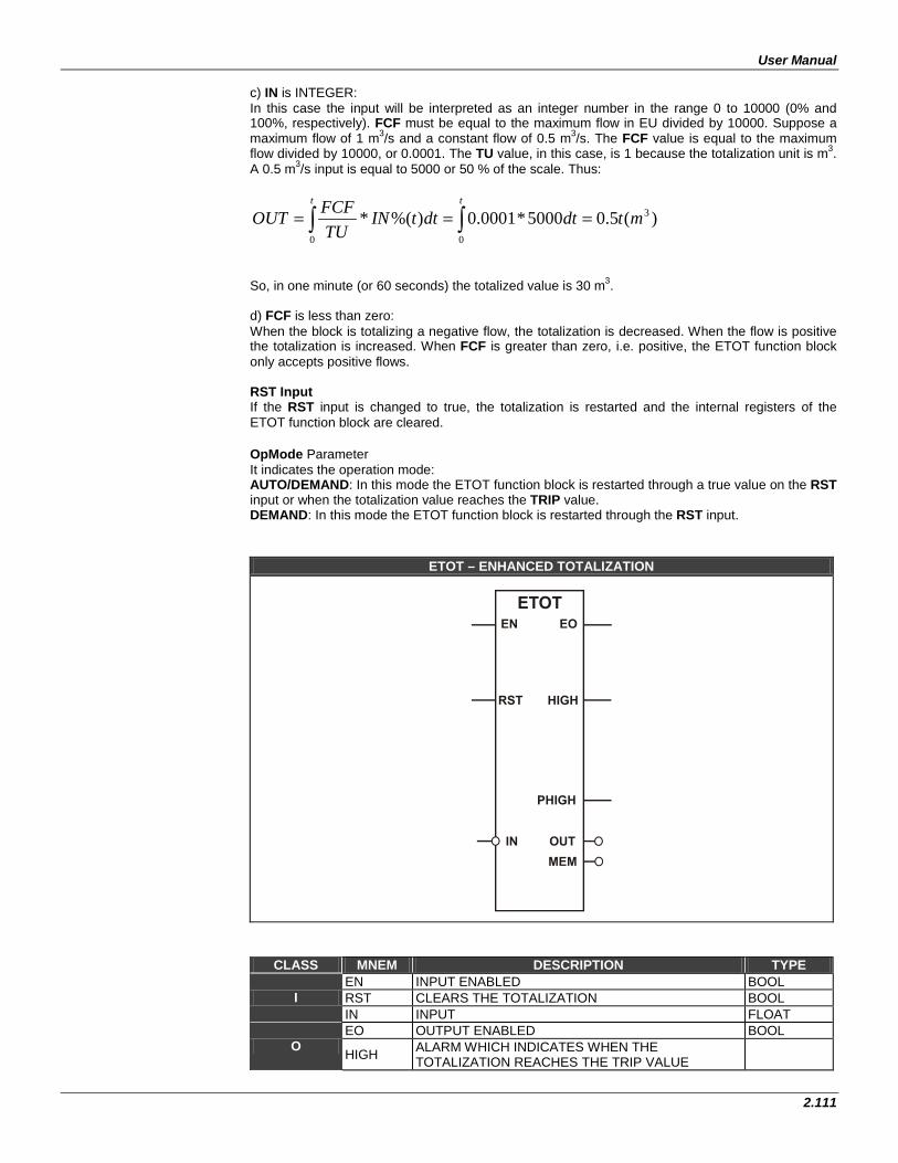
User Manual
2.111
c) IN is INTEGER: In this case the input will be interpreted as an integer number in the range 0 to 10000 (0% and 100%, respectively). FCF must be equal to the maximum flow in EU divided by 10000. Suppose a maximum flow of 1 m3/s and a constant flow of 0.5 m3/s. The FCF value is equal to the maximum flow divided by 10000, or 0.0001. The TU value, in this case, is 1 because the totalization unit is m3. A 0.5 m3/s input is equal to 5000 or 50 % of the scale. Thus:
)(5.05000*0001.0)%(*0
3
0∫∫ ===tt
mtdtdttINTUFCFOUT
So, in one minute (or 60 seconds) the totalized value is 30 m3. d) FCF is less than zero: When the block is totalizing a negative flow, the totalization is decreased. When the flow is positive the totalization is increased. When FCF is greater than zero, i.e. positive, the ETOT function block only accepts positive flows. RST Input If the RST input is changed to true, the totalization is restarted and the internal registers of the ETOT function block are cleared.
OpMode Parameter It indicates the operation mode: AUTO/DEMAND: In this mode the ETOT function block is restarted through a true value on the RST input or when the totalization value reaches the TRIP value. DEMAND: In this mode the ETOT function block is restarted through the RST input.
ETOT – ENHANCED TOTALIZATION
CLASS MNEM DESCRIPTION TYPE
I EN INPUT ENABLED BOOL RST CLEARS THE TOTALIZATION BOOL IN INPUT FLOAT
O EO OUTPUT ENABLED BOOL
HIGH ALARM WHICH INDICATES WHEN THE TOTALIZATION REACHES THE TRIP VALUE
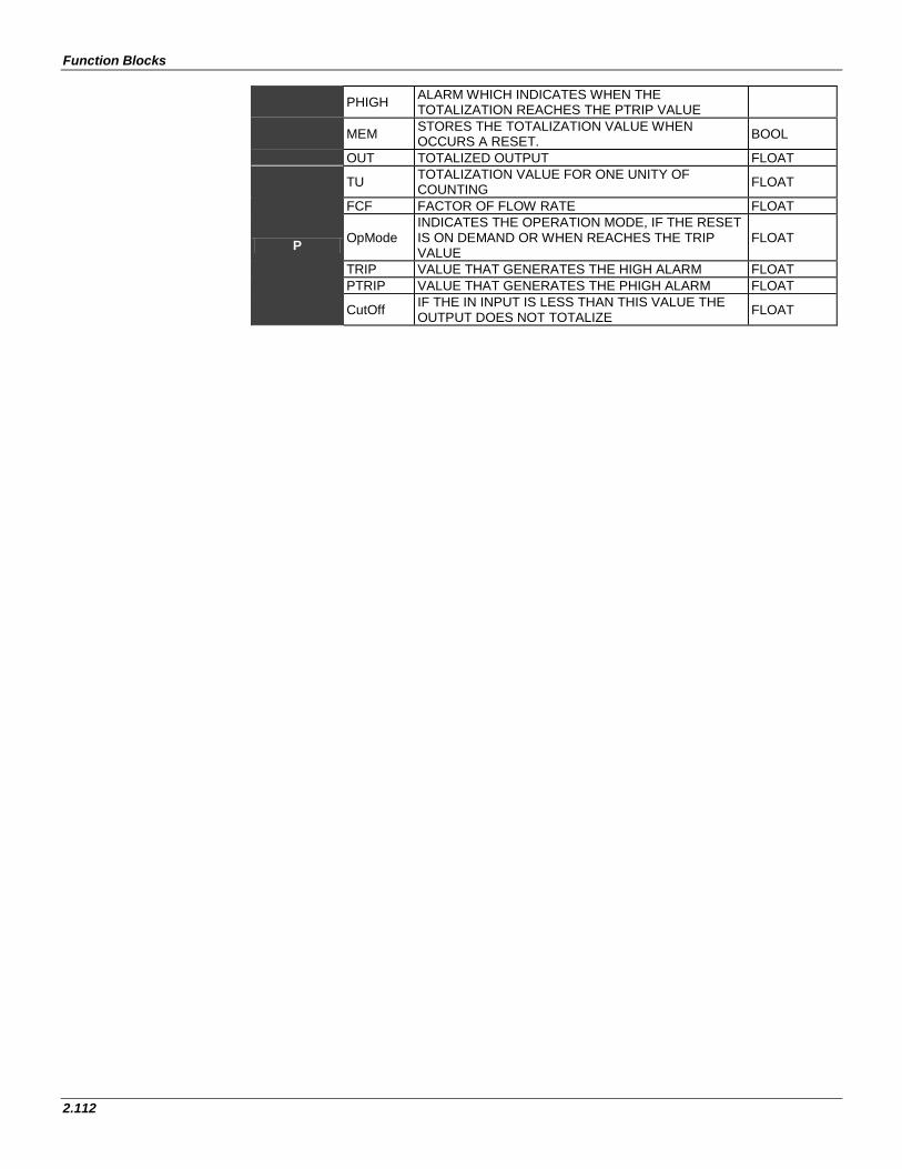
Function Blocks
2.112
PHIGH ALARM WHICH INDICATES WHEN THE TOTALIZATION REACHES THE PTRIP VALUE
MEM STORES THE TOTALIZATION VALUE WHEN OCCURS A RESET. BOOL
OUT TOTALIZED OUTPUT FLOAT
P
TU TOTALIZATION VALUE FOR ONE UNITY OF COUNTING FLOAT
FCF FACTOR OF FLOW RATE FLOAT
OpMode INDICATES THE OPERATION MODE, IF THE RESET IS ON DEMAND OR WHEN REACHES THE TRIP VALUE
FLOAT
TRIP VALUE THAT GENERATES THE HIGH ALARM FLOAT PTRIP VALUE THAT GENERATES THE PHIGH ALARM FLOAT
CutOff IF THE IN INPUT IS LESS THAN THIS VALUE THE OUTPUT DOES NOT TOTALIZE FLOAT
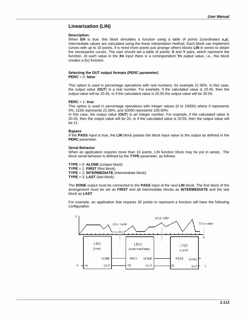
User Manual
2.113
Linearization (LIN) Description: When EN is true, this block simulates a function using a table of points (coordinates x,y). Intermediate values are calculated using the linear interpolation method. Each block can implement curves with up to 10 points, if is need more points just arrange others blocks LIN in series to obtain the necessaries curves. The user should set a table of points; X and Y pairs, which represent the function. At each value in the Xn input there is a correspondent Yn output value, i.e., this block creates a f(x) function. Selecting the OUT output formats (PERC parameter) PERC = 0: false: This option is used in percentage operations with real numbers, for example 21.56%. In this case, the output value (OUT) is a real number. For example, if the calculated value is 20.45, then the output value will be 20.45, or if the calculated value is 20.55 the output value will be 20.55. PERC = 1: true: This option is used in percentage operations with integer values (0 to 10000) where 0 represents 0%, 2156 represents 21.56%, and 10000 represents 100.00%. In this case, the output value (OUT) is an integer number. For example, if the calculated value is 20.45, then the output value will be 20, or if the calculated value is 20.55, then the output value will be 21. Bypass If the PASS input is true, the LIN block passes the block input value to the output as defined in the PERC parameter. Serial Behavior When an application requires more than 10 points, LIN function block may be put in series.. The block serial behavior is defined by the TYPE parameter, as follows: TYPE = 0: ALONE (unique block) TYPE = 1: FIRST (first block) TYPE = 2: INTERMEDIATE (intermediate block) TYPE = 3: LAST (last block) The DONE output must be connected to the PASS input of the next LIN block. The first block of the arrangement must be set as FIRST and all intermediate blocks as INTERMEDIATE and the last block as LAST. For example, an application that requires 30 points to represent a function will have the following configuration
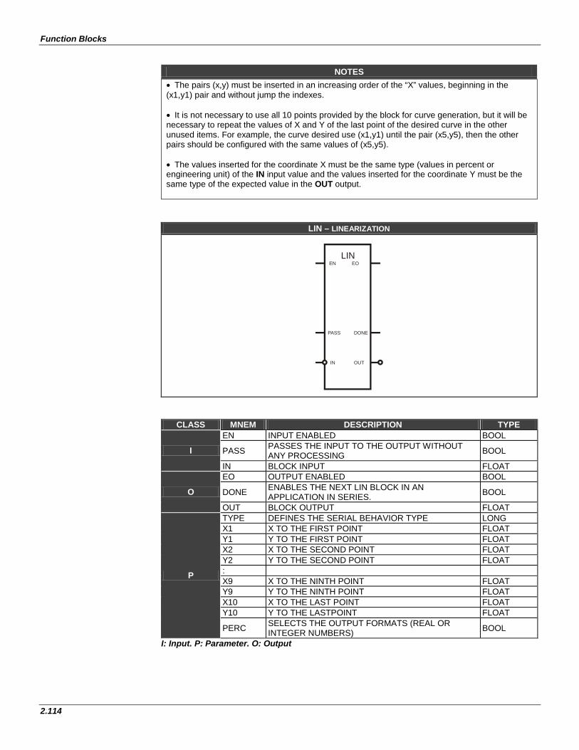
Function Blocks
2.114
NOTES
• The pairs (x,y) must be inserted in an increasing order of the “X” values, beginning in the (x1,y1) pair and without jump the indexes. • It is not necessary to use all 10 points provided by the block for curve generation, but it will be necessary to repeat the values of X and Y of the last point of the desired curve in the other unused items. For example, the curve desired use (x1,y1) until the pair (x5,y5), then the other pairs should be configured with the same values of (x5,y5). • The values inserted for the coordinate X must be the same type (values in percent or engineering unit) of the IN input value and the values inserted for the coordinate Y must be the same type of the expected value in the OUT output.
LIN – LINEARIZATION
LINEN EO
DONEPASS
IN OUT
CLASS MNEM DESCRIPTION TYPE
I
EN INPUT ENABLED BOOL
PASS PASSES THE INPUT TO THE OUTPUT WITHOUT ANY PROCESSING BOOL
IN BLOCK INPUT FLOAT
O
EO OUTPUT ENABLED BOOL
DONE ENABLES THE NEXT LIN BLOCK IN AN APPLICATION IN SERIES. BOOL
OUT BLOCK OUTPUT FLOAT
P
TYPE DEFINES THE SERIAL BEHAVIOR TYPE LONG X1 X TO THE FIRST POINT FLOAT Y1 Y TO THE FIRST POINT FLOAT X2 X TO THE SECOND POINT FLOAT Y2 Y TO THE SECOND POINT FLOAT : X9 X TO THE NINTH POINT FLOAT Y9 Y TO THE NINTH POINT FLOAT X10 X TO THE LAST POINT FLOAT Y10 Y TO THE LASTPOINT FLOAT
PERC SELECTS THE OUTPUT FORMATS (REAL OR INTEGER NUMBERS) BOOL
I: Input. P: Parameter. O: Output
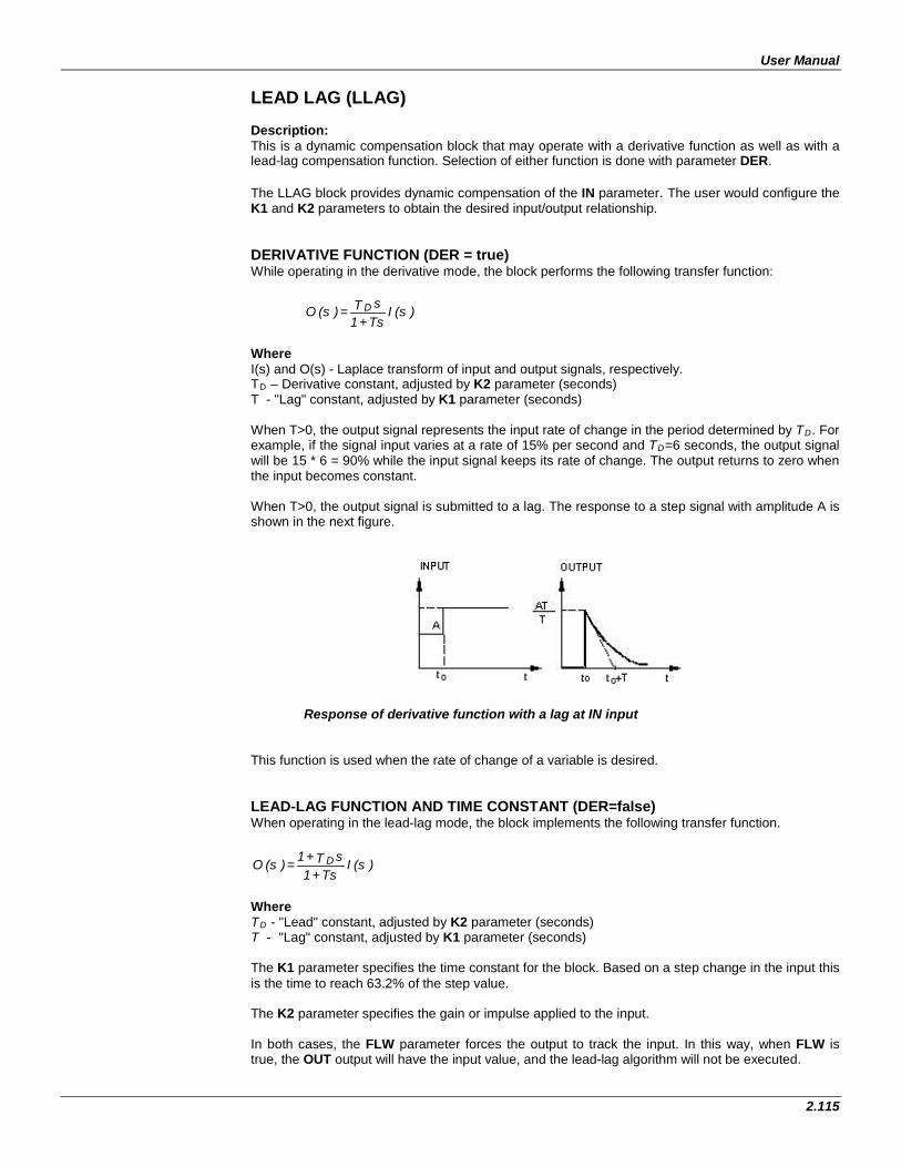
User Manual
2.115
LEAD LAG (LLAG) Description: This is a dynamic compensation block that may operate with a derivative function as well as with a lead-lag compensation function. Selection of either function is done with parameter DER. The LLAG block provides dynamic compensation of the IN parameter. The user would configure the K1 and K2 parameters to obtain the desired input/output relationship. DERIVATIVE FUNCTION (DER = true) While operating in the derivative mode, the block performs the following transfer function:
)(s I Ts + 1sT = )(s O D
Where I(s) and O(s) - Laplace transform of input and output signals, respectively. TD – Derivative constant, adjusted by K2 parameter (seconds) T - "Lag" constant, adjusted by K1 parameter (seconds) When T>0, the output signal represents the input rate of change in the period determined by TD. For example, if the signal input varies at a rate of 15% per second and TD=6 seconds, the output signal will be 15 * 6 = 90% while the input signal keeps its rate of change. The output returns to zero when the input becomes constant. When T>0, the output signal is submitted to a lag. The response to a step signal with amplitude A is shown in the next figure.
Response of derivative function with a lag at IN input This function is used when the rate of change of a variable is desired. LEAD-LAG FUNCTION AND TIME CONSTANT (DER=false) When operating in the lead-lag mode, the block implements the following transfer function.
)(s I Ts + 1
sT + 1 = )(s O D
Where TD - "Lead" constant, adjusted by K2 parameter (seconds) T - "Lag" constant, adjusted by K1 parameter (seconds) The K1 parameter specifies the time constant for the block. Based on a step change in the input this is the time to reach 63.2% of the step value. The K2 parameter specifies the gain or impulse applied to the input. In both cases, the FLW parameter forces the output to track the input. In this way, when FLW is true, the OUT output will have the input value, and the lead-lag algorithm will not be executed.
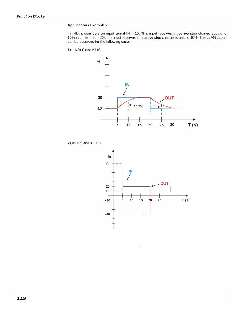
Function Blocks
2.116
Applications Examples: Initially, it considers an input signal IN = 10. This input receives a positive step change equals to 10% in t = 5s. In t = 20s, the input receives a negative step change equals to 10%. The LLAG action can be observed for the following cases: 1) K2= 0 and K1=5
T (s)
10
20
5 1510 2520
%
63,2%
IN
OUT
30
2) K2 = 5 and K1 = 0
T (s)
1020
5 1510 2520
%
IN
OUT
70
- 10
- 40
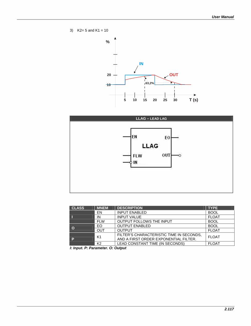
User Manual
2.117
3) K2= 5 and K1 = 10
T (s)
10
20
5 1510 2520
%
63,2%
IN
OUT
30
LLAG – LEAD LAG
CLASS MNEM DESCRIPTION TYPE
I EN INPUT ENABLED BOOL IN INPUT VALUE FLOAT FLW OUTPUT FOLLOWS THE INPUT BOOL
O EO OUTPUT ENABLED BOOL OUT OUTPUT FLOAT
P K1 FILTER’S CHARACTERISTIC TIME IN SECONDS, AND A FIRST ORDER EXPONENTIAL FILTER. FLOAT
K2 LEAD CONSTANT TIME (IN SECONDS) FLOAT I: Input. P: Parameter. O: Output
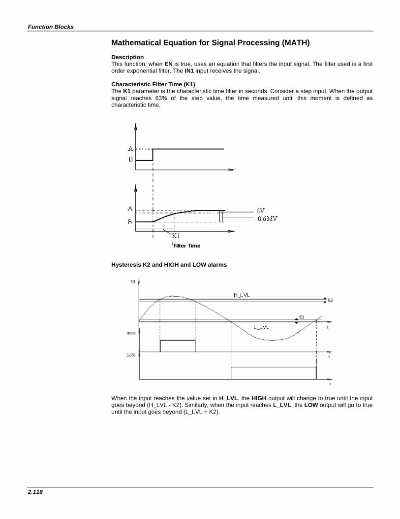
Function Blocks
2.118
Mathematical Equation for Signal Processing (MATH) Description This function, when EN is true, uses an equation that filters the input signal. The filter used is a first order exponential filter. The IN1 input receives the signal. Characteristic Filter Time (K1) The K1 parameter is the characteristic time filter in seconds. Consider a step input. When the output signal reaches 63% of the step value, the time measured until this moment is defined as characteristic time.
Hysteresis K2 and HIGH and LOW alarms
When the input reaches the value set in H_LVL, the HIGH output will change to true until the input goes beyond (H_LVL - K2). Similarly, when the input reaches L_LVL, the LOW output will go to true until the input goes beyond (L_LVL + K2).
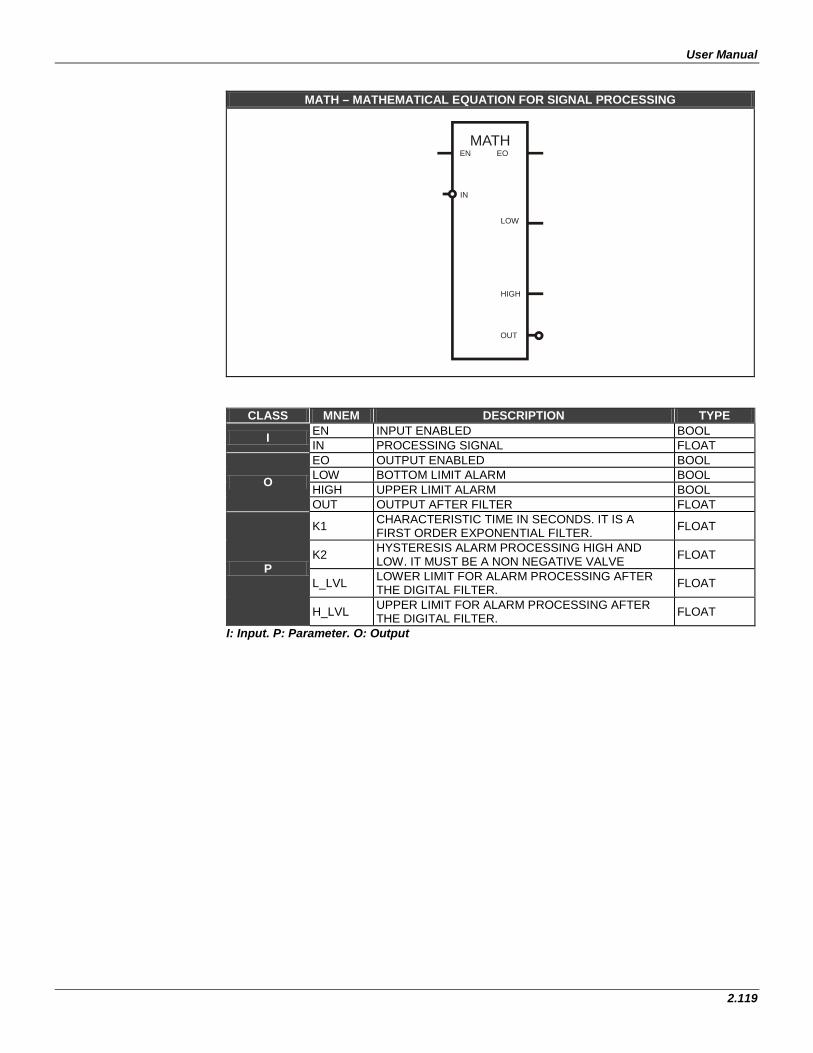
User Manual
2.119
MATH – MATHEMATICAL EQUATION FOR SIGNAL PROCESSING
MATHEN EO
IN
LOW
HIGH
OUT
CLASS MNEM DESCRIPTION TYPE
I EN INPUT ENABLED BOOL IN PROCESSING SIGNAL FLOAT
O
EO OUTPUT ENABLED BOOL LOW BOTTOM LIMIT ALARM BOOL HIGH UPPER LIMIT ALARM BOOL OUT OUTPUT AFTER FILTER FLOAT
P
K1 CHARACTERISTIC TIME IN SECONDS. IT IS A FIRST ORDER EXPONENTIAL FILTER. FLOAT
K2 HYSTERESIS ALARM PROCESSING HIGH AND LOW. IT MUST BE A NON NEGATIVE VALVE FLOAT
L_LVL LOWER LIMIT FOR ALARM PROCESSING AFTER THE DIGITAL FILTER. FLOAT
H_LVL UPPER LIMIT FOR ALARM PROCESSING AFTER THE DIGITAL FILTER. FLOAT
I: Input. P: Parameter. O: Output
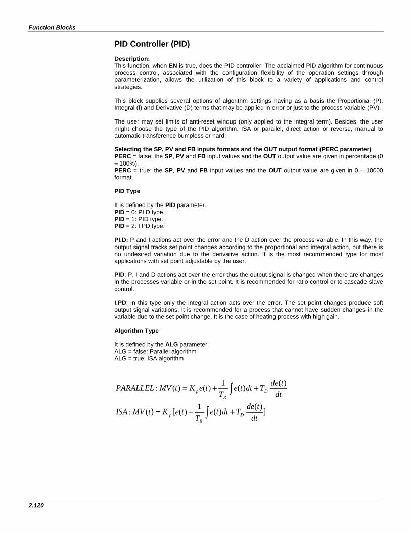
Function Blocks
2.120
PID Controller (PID) Description: This function, when EN is true, does the PID controller. The acclaimed PID algorithm for continuous process control, associated with the configuration flexibility of the operation settings through parameterization, allows the utilization of this block to a variety of applications and control strategies. This block supplies several options of algorithm settings having as a basis the Proportional (P), Integral (I) and Derivative (D) terms that may be applied in error or just to the process variable (PV). The user may set limits of anti-reset windup (only applied to the integral term). Besides, the user might choose the type of the PID algorithm: ISA or parallel, direct action or reverse, manual to automatic transference bumpless or hard. Selecting the SP, PV and FB inputs formats and the OUT output format (PERC parameter) PERC = false: the SP, PV and FB input values and the OUT output value are given in percentage (0 – 100%). PERC = true: the SP, PV and FB input values and the OUT output value are given in 0 – 10000 format. PID Type It is defined by the PID parameter. PID = 0: PI.D type. PID = 1: PID type. PID = 2: I.PD type. PI.D: P and I actions act over the error and the D action over the process variable. In this way, the output signal tracks set point changes according to the proportional and integral action, but there is no undesired variation due to the derivative action. It is the most recommended type for most applications with set point adjustable by the user. PID: P, I and D actions act over the error thus the output signal is changed when there are changes in the processes variable or in the set point. It is recommended for ratio control or to cascade slave control. I.PD: In this type only the integral action acts over the error. The set point changes produce soft output signal variations. It is recommended for a process that cannot have sudden changes in the variable due to the set point change. It is the case of heating process with high gain. Algorithm Type It is defined by the ALG parameter. ALG = false: Parallel algorithm ALG = true: ISA algorithm
])()(1)([)(:
)()(1)()(:
∫
∫
++=
++=
dttdeTdtte
TteKtMVISA
dttdeTdtte
TteKtMVPARALLEL
DR
p
DR
p
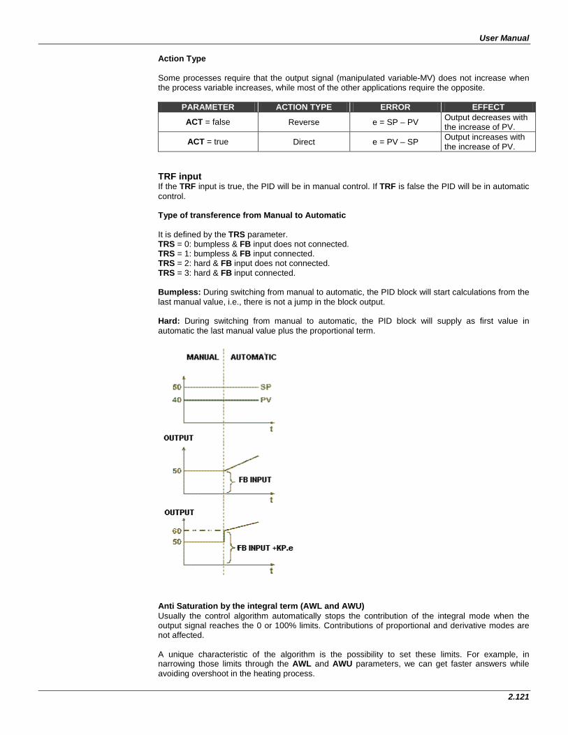
User Manual
2.121
Action Type Some processes require that the output signal (manipulated variable-MV) does not increase when the process variable increases, while most of the other applications require the opposite.
PARAMETER ACTION TYPE ERROR EFFECT
ACT = false Reverse e = SP – PV Output decreases with the increase of PV.
ACT = true Direct e = PV – SP Output increases with the increase of PV.
TRF input If the TRF input is true, the PID will be in manual control. If TRF is false the PID will be in automatic control. Type of transference from Manual to Automatic It is defined by the TRS parameter. TRS = 0: bumpless & FB input does not connected. TRS = 1: bumpless & FB input connected. TRS = 2: hard & FB input does not connected. TRS = 3: hard & FB input connected. Bumpless: During switching from manual to automatic, the PID block will start calculations from the last manual value, i.e., there is not a jump in the block output. Hard: During switching from manual to automatic, the PID block will supply as first value in automatic the last manual value plus the proportional term.
Anti Saturation by the integral term (AWL and AWU) Usually the control algorithm automatically stops the contribution of the integral mode when the output signal reaches the 0 or 100% limits. Contributions of proportional and derivative modes are not affected. A unique characteristic of the algorithm is the possibility to set these limits. For example, in narrowing those limits through the AWL and AWU parameters, we can get faster answers while avoiding overshoot in the heating process.
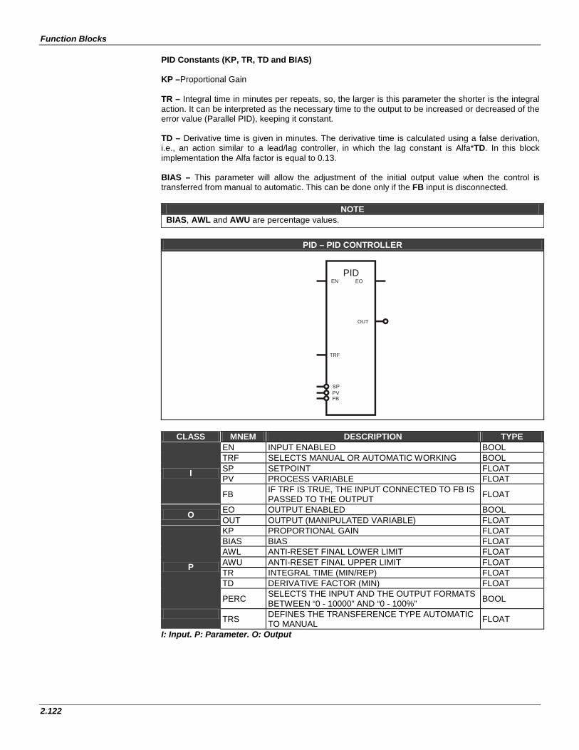
Function Blocks
2.122
PID Constants (KP, TR, TD and BIAS) KP –Proportional Gain TR – Integral time in minutes per repeats, so, the larger is this parameter the shorter is the integral action. It can be interpreted as the necessary time to the output to be increased or decreased of the error value (Parallel PID), keeping it constant. TD – Derivative time is given in minutes. The derivative time is calculated using a false derivation, i.e., an action similar to a lead/lag controller, in which the lag constant is Alfa*TD. In this block implementation the Alfa factor is equal to 0.13. BIAS – This parameter will allow the adjustment of the initial output value when the control is transferred from manual to automatic. This can be done only if the FB input is disconnected.
NOTE
BIAS, AWL and AWU are percentage values.
PID – PID CONTROLLER
PIDEN EO
TRF
OUT
PVFB
CLASS MNEM DESCRIPTION TYPE
I
EN INPUT ENABLED BOOL TRF SELECTS MANUAL OR AUTOMATIC WORKING BOOL SP SETPOINT FLOAT PV PROCESS VARIABLE FLOAT
FB IF TRF IS TRUE, THE INPUT CONNECTED TO FB IS PASSED TO THE OUTPUT FLOAT
O EO OUTPUT ENABLED BOOL OUT OUTPUT (MANIPULATED VARIABLE) FLOAT
P
KP PROPORTIONAL GAIN FLOAT BIAS BIAS FLOAT AWL ANTI-RESET FINAL LOWER LIMIT FLOAT AWU ANTI-RESET FINAL UPPER LIMIT FLOAT TR INTEGRAL TIME (MIN/REP) FLOAT TD DERIVATIVE FACTOR (MIN) FLOAT
PERC SELECTS THE INPUT AND THE OUTPUT FORMATS BETWEEN “0 - 10000” AND “0 - 100%” BOOL
TRS DEFINES THE TRANSFERENCE TYPE AUTOMATIC TO MANUAL FLOAT
I: Input. P: Parameter. O: Output
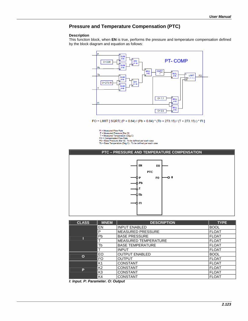
User Manual
2.123
Pressure and Temperature Compensation (PTC) Description This function block, when EN is true, performs the pressure and temperature compensation defined by the block diagram and equation as follows:
PTC – PRESSURE AND TEMPERATURE COMPENSATION
CLASS MNEM DESCRIPTION TYPE
I
EN INPUT ENABLED BOOL P MEASURED PRESSURE FLOAT Pb BASE PRESSURE FLOAT T MEASURED TEMPERATURE FLOAT Tb BASE TEMPERATURE FLOAT T INPUT FLOAT
O EO OUTPUT ENABLED BOOL FO OUTPUT FLOAT
P
K1 CONSTANT FLOAT K2 CONSTANT FLOAT K3 CONSTANT FLOAT K4 CONSTANT FLOAT
I: Input. P: Parameter. O: Output
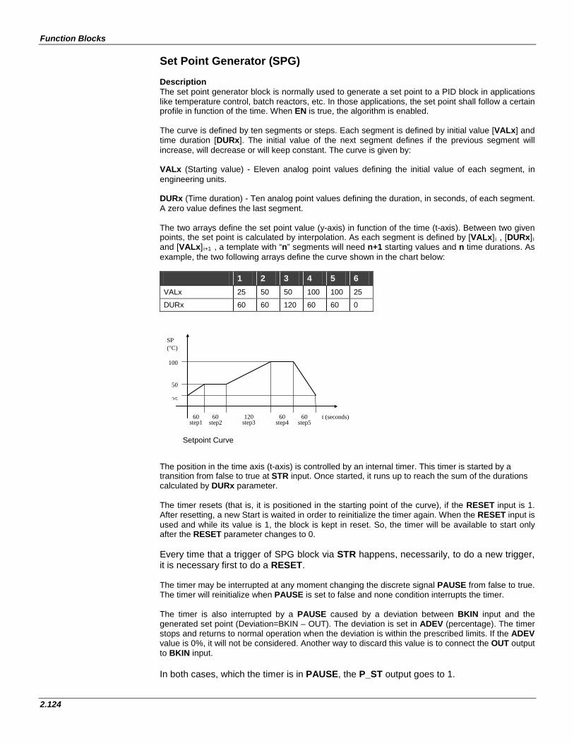
Function Blocks
2.124
Set Point Generator (SPG) Description The set point generator block is normally used to generate a set point to a PID block in applications like temperature control, batch reactors, etc. In those applications, the set point shall follow a certain profile in function of the time. When EN is true, the algorithm is enabled. The curve is defined by ten segments or steps. Each segment is defined by initial value [VALx] and time duration [DURx]. The initial value of the next segment defines if the previous segment will increase, will decrease or will keep constant. The curve is given by: VALx (Starting value) - Eleven analog point values defining the initial value of each segment, in engineering units. DURx (Time duration) - Ten analog point values defining the duration, in seconds, of each segment. A zero value defines the last segment. The two arrays define the set point value (y-axis) in function of the time (t-axis). Between two given points, the set point is calculated by interpolation. As each segment is defined by [VALx] i , [DURx] i and [VALx] i+1 , a template with “n” segments will need n+1 starting values and n time durations. As example, the two following arrays define the curve shown in the chart below: 1 2 3 4 5 6 VALx 25 50 50 100 100 25
DURx 60 60 120 60 60 0
t (seconds)
SP (°C) 100 50 25
60 60 120 60 60 step1 step2 step3 step4 step5
Setpoint Curve The position in the time axis (t-axis) is controlled by an internal timer. This timer is started by a transition from false to true at STR input. Once started, it runs up to reach the sum of the durations calculated by DURx parameter. The timer resets (that is, it is positioned in the starting point of the curve), if the RESET input is 1. After resetting, a new Start is waited in order to reinitialize the timer again. When the RESET input is used and while its value is 1, the block is kept in reset. So, the timer will be available to start only after the RESET parameter changes to 0. Every time that a trigger of SPG block via STR happens, necessarily, to do a new trigger, it is necessary first to do a RESET. The timer may be interrupted at any moment changing the discrete signal PAUSE from false to true. The timer will reinitialize when PAUSE is set to false and none condition interrupts the timer. The timer is also interrupted by a PAUSE caused by a deviation between BKIN input and the generated set point (Deviation=BKIN – OUT). The deviation is set in ADEV (percentage). The timer stops and returns to normal operation when the deviation is within the prescribed limits. If the ADEV value is 0%, it will not be considered. Another way to discard this value is to connect the OUT output to BKIN input. In both cases, which the timer is in PAUSE, the P_ST output goes to 1.
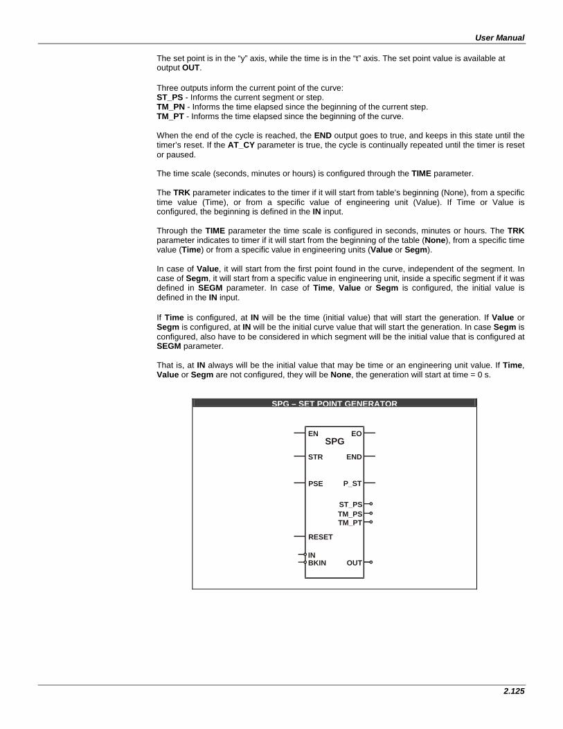
User Manual
2.125
The set point is in the “y” axis, while the time is in the “t” axis. The set point value is available at output OUT. Three outputs inform the current point of the curve: ST_PS - Informs the current segment or step. TM_PN - Informs the time elapsed since the beginning of the current step. TM_PT - Informs the time elapsed since the beginning of the curve. When the end of the cycle is reached, the END output goes to true, and keeps in this state until the timer’s reset. If the AT_CY parameter is true, the cycle is continually repeated until the timer is reset or paused. The time scale (seconds, minutes or hours) is configured through the TIME parameter. The TRK parameter indicates to the timer if it will start from table’s beginning (None), from a specific time value (Time), or from a specific value of engineering unit (Value). If Time or Value is configured, the beginning is defined in the IN input. Through the TIME parameter the time scale is configured in seconds, minutes or hours. The TRK parameter indicates to timer if it will start from the beginning of the table (None), from a specific time value (Time) or from a specific value in engineering units (Value or Segm). In case of Value, it will start from the first point found in the curve, independent of the segment. In case of Segm, it will start from a specific value in engineering unit, inside a specific segment if it was defined in SEGM parameter. In case of Time, Value or Segm is configured, the initial value is defined in the IN input. If Time is configured, at IN will be the time (initial value) that will start the generation. If Value or Segm is configured, at IN will be the initial curve value that will start the generation. In case Segm is configured, also have to be considered in which segment will be the initial value that is configured at SEGM parameter. That is, at IN always will be the initial value that may be time or an engineering unit value. If Time, Value or Segm are not configured, they will be None, the generation will start at time = 0 s.
SPG – SET POINT GENERATOR
SPGEN EO
STR
BKIN
END
OUT
PSE P_ST
IN
RESET
TM_PTTM_PSST_PS
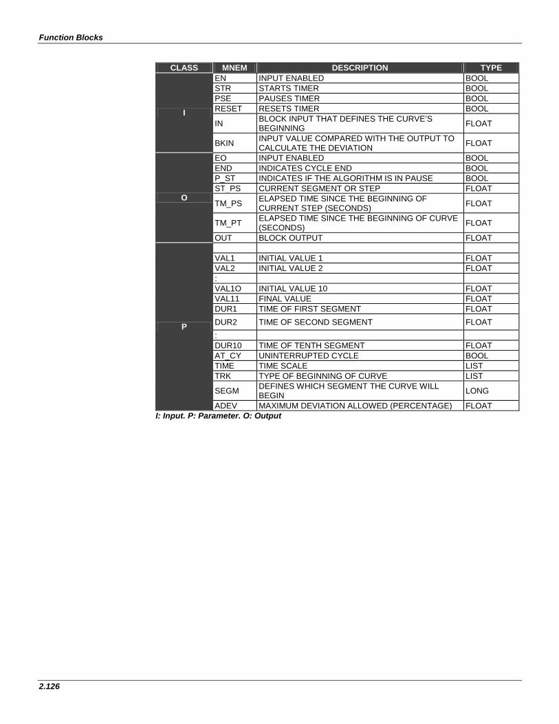
Function Blocks
2.126
CLASS MNEM DESCRIPTION TYPE
I
EN INPUT ENABLED BOOL STR STARTS TIMER BOOL PSE PAUSES TIMER BOOL RESET RESETS TIMER BOOL
IN BLOCK INPUT THAT DEFINES THE CURVE’S BEGINNING FLOAT
BKIN INPUT VALUE COMPARED WITH THE OUTPUT TO CALCULATE THE DEVIATION FLOAT
O
EO INPUT ENABLED BOOL END INDICATES CYCLE END BOOL P_ST INDICATES IF THE ALGORITHM IS IN PAUSE BOOL ST_PS CURRENT SEGMENT OR STEP FLOAT
TM_PS ELAPSED TIME SINCE THE BEGINNING OF CURRENT STEP (SECONDS) FLOAT
TM_PT ELAPSED TIME SINCE THE BEGINNING OF CURVE (SECONDS) FLOAT
OUT BLOCK OUTPUT FLOAT
P
VAL1 INITIAL VALUE 1 FLOAT VAL2 INITIAL VALUE 2 FLOAT : VAL1O INITIAL VALUE 10 FLOAT VAL11 FINAL VALUE FLOAT DUR1 TIME OF FIRST SEGMENT FLOAT DUR2 TIME OF SECOND SEGMENT FLOAT : DUR10 TIME OF TENTH SEGMENT FLOAT AT_CY UNINTERRUPTED CYCLE BOOL TIME TIME SCALE LIST TRK TYPE OF BEGINNING OF CURVE LIST
SEGM DEFINES WHICH SEGMENT THE CURVE WILL BEGIN LONG
ADEV MAXIMUM DEVIATION ALLOWED (PERCENTAGE) FLOAT I: Input. P: Parameter. O: Output
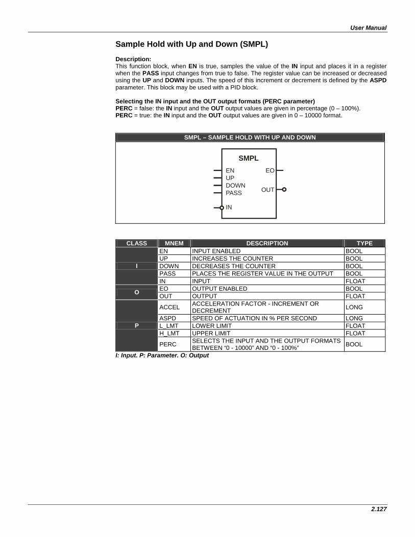
User Manual
2.127
Sample Hold with Up and Down (SMPL) Description: This function block, when EN is true, samples the value of the IN input and places it in a register when the PASS input changes from true to false. The register value can be increased or decreased using the UP and DOWN inputs. The speed of this increment or decrement is defined by the ASPD parameter. This block may be used with a PID block. Selecting the IN input and the OUT output formats (PERC parameter) PERC = false: the IN input and the OUT output values are given in percentage (0 – 100%). PERC = true: the IN input and the OUT output values are given in 0 – 10000 format.
SMPL – SAMPLE HOLD WITH UP AND DOWN
SMPL
OUT
EOUPDOWNPASS
IN
EN
CLASS MNEM DESCRIPTION TYPE
I
EN INPUT ENABLED BOOL UP INCREASES THE COUNTER BOOL DOWN DECREASES THE COUNTER BOOL PASS PLACES THE REGISTER VALUE IN THE OUTPUT BOOL IN INPUT FLOAT
O EO OUTPUT ENABLED BOOL OUT OUTPUT FLOAT
P
ACCEL ACCELERATION FACTOR - INCREMENT OR DECREMENT LONG
ASPD SPEED OF ACTUATION IN % PER SECOND LONG L_LMT LOWER LIMIT FLOAT H_LMT UPPER LIMIT FLOAT
PERC SELECTS THE INPUT AND THE OUTPUT FORMATS BETWEEN “0 - 10000” AND “0 - 100%” BOOL
I: Input. P: Parameter. O: Output
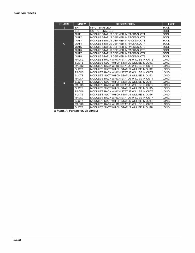
Function Blocks
2.128
CLASS MNEM DESCRIPTION TYPE
I EN INPUT ENABLED BOOL
O
EO OUTPUT ENABLED BOOL OUT1 MODULE STATUS DEFINED IN RACK1/SLOT1 BOOL OUT2 MODULE STATUS DEFINED IN RACK2/SLOT2 BOOL OUT3 MODULE STATUS DEFINED IN RACK3/SLOT3 BOOL OUT4 MODULE STATUS DEFINED IN RACK4/SLOT4 BOOL OUT5 MODULE STATUS DEFINED IN RACK5/SLOT5 BOOL OUT6 MODULE STATUS DEFINED IN RACK6/SLOT6 BOOL OUT7 MODULE STATUS DEFINED IN RACK7/SLOT7 BOOL OUT8 MODULE STATUS DEFINED IN RACK8/SLOT8 BOOL
P
RACK1 MODULE’S RACK WHICH STATUS WILL BE IN OUT1 LONG SLOT1 MODULE’S SLOT WHICH STATUS WILL BE IN OUT1 LONG RACK2 MODULE’S RACK WHICH STATUS WILL BE IN OUT2 LONG SLOT2 MODULE’S SLOT WHICH STATUS WILL BE IN OUT2 LONG RACK3 MODULE’S RACK WHICH STATUS WILL BE IN OUT3 LONG SLOT3 MODULE’S SLOT WHICH STATUS WILL BE IN OUT3 LONG RACK4 MODULE’S RACK WHICH STATUS WILL BE IN OUT4 LONG SLOT4 MODULE’S SLOT WHICH STATUS WILL BE IN OUT4 LONG RACK5 MODULE’S RACK WHICH STATUS WILL BE IN OUT5 LONG SLOT5 MODULE’S SLOT WHICH STATUS WILL BE IN OUT5 LONG RACK6 MODULE’S RACK WHICH STATUS WILL BE IN OUT6 LONG SLOT6 MODULE’S SLOT WHICH STATUS WILL BE IN OUT6 LONG RACK7 MODULE’S RACK WHICH STATUS WILL BE IN OUT7 LONG SLOT7 MODULE’S SLOT WHICH STATUS WILL BE IN OUT7 LONG RACK8 MODULE’S RACK WHICH STATUS WILL BE IN OUT8 LONG SLOT8 MODULE’S SLOT WHICH STATUS WILL BE IN OUT8 LONG
I: Input. P: Parameter. O: Output
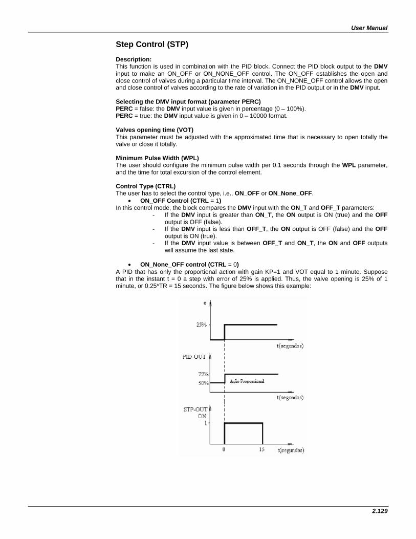
User Manual
2.129
Step Control (STP) Description: This function is used in combination with the PID block. Connect the PID block output to the DMV input to make an ON_OFF or ON_NONE_OFF control. The ON_OFF establishes the open and close control of valves during a particular time interval. The ON_NONE_OFF control allows the open and close control of valves according to the rate of variation in the PID output or in the DMV input. Selecting the DMV input format (parameter PERC) PERC = false: the DMV input value is given in percentage (0 – 100%). PERC = true: the DMV input value is given in 0 – 10000 format. Valves opening time (VOT) This parameter must be adjusted with the approximated time that is necessary to open totally the valve or close it totally. Minimum Pulse Width (WPL) The user should configure the minimum pulse width per 0.1 seconds through the WPL parameter, and the time for total excursion of the control element. Control Type (CTRL) The user has to select the control type, i.e., ON_OFF or ON_None_OFF.
• ON_OFF Control (CTRL = 1) In this control mode, the block compares the DMV input with the ON_T and OFF_T parameters:
- If the DMV input is greater than ON_T, the ON output is ON (true) and the OFF output is OFF (false).
- If the DMV input is less than OFF_T, the ON output is OFF (false) and the OFF output is ON (true).
- If the DMV input value is between OFF_T and ON_T, the ON and OFF outputs will assume the last state.
• ON_None_OFF control (CTRL = 0)
A PID that has only the proportional action with gain KP=1 and VOT equal to 1 minute. Suppose that in the instant t = 0 a step with error of 25% is applied. Thus, the valve opening is 25% of 1 minute, or 0.25*TR = 15 seconds. The figure below shows this example:
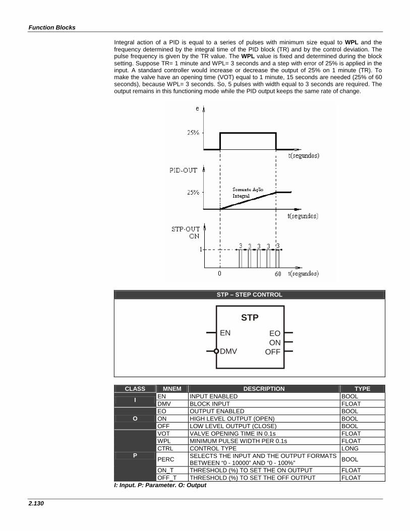
Function Blocks
2.130
Integral action of a PID is equal to a series of pulses with minimum size equal to WPL and the frequency determined by the integral time of the PID block (TR) and by the control deviation. The pulse frequency is given by the TR value. The WPL value is fixed and determined during the block setting. Suppose TR= 1 minute and WPL= 3 seconds and a step with error of 25% is applied in the input. A standard controller would increase or decrease the output of 25% on 1 minute (TR). To make the valve have an opening time (VOT) equal to 1 minute, 15 seconds are needed (25% of 60 seconds), because WPL= 3 seconds. So, 5 pulses with width equal to 3 seconds are required. The output remains in this functioning mode while the PID output keeps the same rate of change.
STP – STEP CONTROL
STPEN
DMV
EO
OFFON
CLASS MNEM DESCRIPTION TYPE
I EN INPUT ENABLED BOOL DMV BLOCK INPUT FLOAT
O EO OUTPUT ENABLED BOOL ON HIGH LEVEL OUTPUT (OPEN) BOOL OFF LOW LEVEL OUTPUT (CLOSE) BOOL
P
VOT VALVE OPENING TIME IN 0.1s FLOAT WPL MINIMUM PULSE WIDTH PER 0.1s FLOAT CTRL CONTROL TYPE LONG
PERC SELECTS THE INPUT AND THE OUTPUT FORMATS BETWEEN “0 - 10000” AND “0 - 100%” BOOL
ON_T THRESHOLD (%) TO SET THE ON OUTPUT FLOAT OFF_T THRESHOLD (%) TO SET THE OFF OUTPUT FLOAT
I: Input. P: Parameter. O: Output
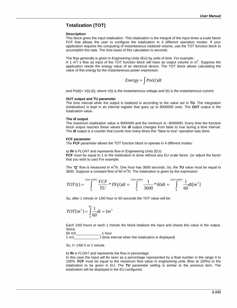
User Manual
2.131
Totalization (TOT) Description: This block gives the input totalization. This totalization is the integral of the input times a scale factor FCF that allows the user to configure the totalization in 3 different operation modes. If your application requires the computing of instantaneous totalized volume, use the TOT function block to accomplish this task. The time basis of this calculation is seconds. The flow generally is given in Engineering Units (EU) by units of time. For example: A 1 m3/ s flow as input of the TOT function block will have as output volume in m3. Suppose the application needs the energy value of an electrical device. The TOT block allows calculating the value of this energy by the instantaneous power expression:
∫= dttPotEnergy )(
and Pot(t)= V(t).I(t), where V(t) is the instantaneous voltage and I(t) is the instantaneous current. OUT output and TU parameter The time interval while the output is totalized is according to the value set in TU. The integration (totalization) is kept in an internal register that goes up to 8000000 units. The OUT output is the totalization value. The dl output The maximum totalization value is 8000000 and the minimum is –8000000. Every time the function block output reaches these values the dl output changes from false to true during a time interval. The dl output is a counter that counts how many times this "false to true" operation was done. FCF parameter The FCF parameter allows the TOT function block to operate in 4 different modes: a) IN is FLOAT and represents flow in Engineering Units (EU): FCF must be equal to 1 to the totalization is done without any EU scale factor. (or adjust the factor that you wish to use) For example: The “Q” flow is measured in m3/h. One hour has 3600 seconds. So, the TU value must be equal to 3600. Suppose a constant flow of 60 m3/h. The totalization is given by the expression:
][60160*
36001)(*)( 3
)(sec
0
)(sec
0
)(sec
0
mdtdtdttINTUFCFtTOT
ondstondstondst
∫∫∫ ===
So, after 1 minute or 1/60 hour or 60 seconds the TOT value will be:
360
0
3 1601][ mdtmTOT == ∫
Each 1/60 hours or each 1 minute the block totalizes the input and shows this value in the output. Since: 60 m3_____________ 1 hour 1 m3_____________ t (time interval when the totalization is displayed) So, t= 1/60 h or 1 minute. b) IN is FLOAT and represents the flow in percentage: In this case the input will be seen as a percentage represented by a float number in the range 0 to 100%. FCF must be equal to the maximum flow value in engineering units (flow at 100%) to the totalization to be given in EU. The TU parameter setting is similar to the previous item. The totalization will be displayed in the EU configured.
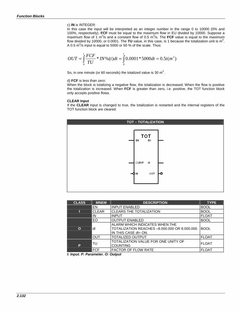
Function Blocks
2.132
c) IN is INTEGER: In this case the input will be interpreted as an integer number in the range 0 to 10000 (0% and 100%, respectively). FCF must be equal to the maximum flow in EU divided by 10000. Suppose a maximum flow of 1 m3/s and a constant flow of 0.5 m3/s. The FCF value is equal to the maximum flow divided by 10000, or 0.0001. The TU value, in this case, is 1 because the totalization unit is m3. A 0.5 m3/s input is equal to 5000 or 50 % of the scale. Thus:
)(5.05000*0001.0)%(*0
3
0∫∫ ===tt
mtdtdttINTUFCFOUT
So, in one minute (or 60 seconds) the totalized value is 30 m3. d) FCF is less than zero: When the block is totalizing a negative flow, the totalization is decreased. When the flow is positive the totalization is increased. When FCF is greater than zero, i.e. positive, the TOT function block only accepts positive flows. CLEAR Input If the CLEAR input is changed to true, the totalization is restarted and the internal registers of the TOT function block are cleared.
TOT – TOTALIZATION
CLASS MNEM DESCRIPTION TYPE
I EN INPUT ENABLED BOOL CLEAR CLEARS THE TOTALIZATION BOOL IN INPUT FLOAT
O
EO OUTPUT ENABLED BOOL
dl ALARM WHICH INDICATES WHEN THE TOTALIZATION REACHES –8.000.000 OR 8.000.000. IN THIS CASE dl= ON.
BOOL
OUT TOTALIZED OUTPUT FLOAT
P TU TOTALIZATION VALUE FOR ONE UNITY OF COUNTING FLOAT
FCF FACTOR OF FLOW RATE FLOAT I: Input. P: Parameter. O: Output
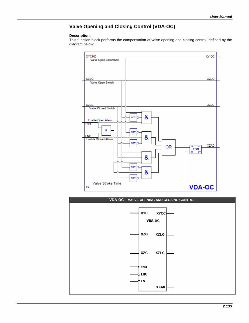
User Manual
2.133
Valve Opening and Closing Control (VDA-OC) Description: This function block performs the compensation of valve opening and closing control, defined by the diagram below:
VDA-OC – VALVE OPENING AND CLOSING CONTROL
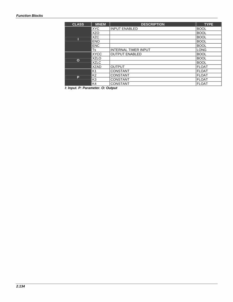
Function Blocks
2.134
CLASS MNEM DESCRIPTION TYPE
I
XYC INPUT ENABLED BOOL XZO BOOL XZC BOOL ENO BOOL ENC BOOL Ts INTERNAL TIMER INPUT LONG
O
XYCC OUTPUT ENABLED BOOL XZLO BOOL XZLC BOOL XZAD OUTPUT FLOAT
P
K1 CONSTANT FLOAT K2 CONSTANT FLOAT K3 CONSTANT FLOAT K4 CONSTANT FLOAT
I: Input. P: Parameter. O: Output
User Manual
2.135
Cross Limit and Rate-Of-Change (XLIM) Description: This function, when EN is true, limits a signal between static and dynamic values and also controls the rate of change. The OUT output (%) is the filtered result of the A input (%). Selecting the A and B input formats and the OUT output format (PERC parameter) PERC = false: the A and B input values and the OUT output value are given in percentage (0 - 100%). PERC = true: the A and B input values and the OUT output value are given in 0 – 10000 format. Static and Dynamic Limitation
• Static To limit statically a signal, the B input is disconnected. The A signal is limited between BL and BH (user’s settings).
• Dynamic If the B input is connected, it is possible to limit dynamically the A input through the B input. To achieve more flexibility, these limits are changeable with individual gain and bias. Rate of Change (MODE parameter) The rate of change limit may be applied in three ways, increasing, decreasing or in a specific direction. There are 4 types of rate of change available: MODE = 0 : none direction is verified. MODE = 1: verify only the negative direction. MODE = 2: verify only the positive direction. MODE = 4: verify both directions. BL and BH Parameters If A ≤ BL the OUT output is equal to BL. If BL < A < BH the OUT output is equal to A. If A ≥ BH the OUT output is equal to BH. GH and GL Parameters If A ≤ B.GL + BL, the OUT output is equal to B.GL+BL. If B.GL+BL < A < B.GH + BH, the OUT output is equal to A. If A ≥ B.GH + BH, the OUT output is equal to B.GH+BH. DB Parameter and LOW and HIGH Outputs This function has two outputs to indicate if the low (LOW) or high (HIGH) limits were reached. The DB parameter can be adjusted to generate a hysteresis, avoiding output oscillation while the variable is close to the limit value. RAT Parameter and ROC Output The ROC output goes to true when the signal rate of change reaches the value set in the parameter RAT. When the A input changes faster than RAT, the variation in the output is kept inside the value fixed by RAT until the A input signal decreases to a value inferior to RAT. The ROC alarm in this interval is on high logic level.
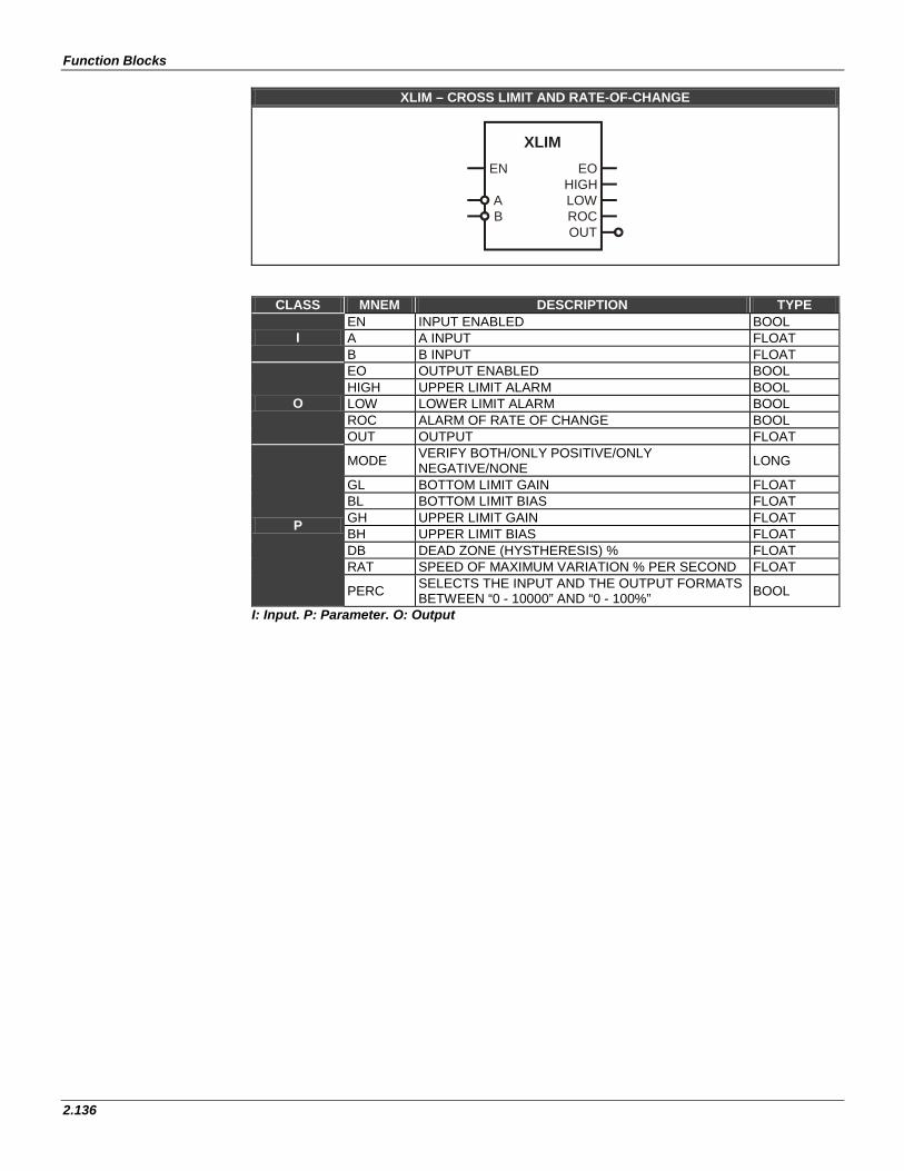
Function Blocks
2.136
XLIM – CROSS LIMIT AND RATE-OF-CHANGE
XLIMEN EO
AB
HIGHLOWROCOUT
CLASS MNEM DESCRIPTION TYPE
I EN INPUT ENABLED BOOL A A INPUT FLOAT B B INPUT FLOAT
O
EO OUTPUT ENABLED BOOL HIGH UPPER LIMIT ALARM BOOL LOW LOWER LIMIT ALARM BOOL ROC ALARM OF RATE OF CHANGE BOOL OUT OUTPUT FLOAT
P
MODE VERIFY BOTH/ONLY POSITIVE/ONLY NEGATIVE/NONE LONG
GL BOTTOM LIMIT GAIN FLOAT BL BOTTOM LIMIT BIAS FLOAT GH UPPER LIMIT GAIN FLOAT BH UPPER LIMIT BIAS FLOAT DB DEAD ZONE (HYSTHERESIS) % FLOAT RAT SPEED OF MAXIMUM VARIATION % PER SECOND FLOAT
PERC SELECTS THE INPUT AND THE OUTPUT FORMATS BETWEEN “0 - 10000” AND “0 - 100%” BOOL
I: Input. P: Parameter. O: Output
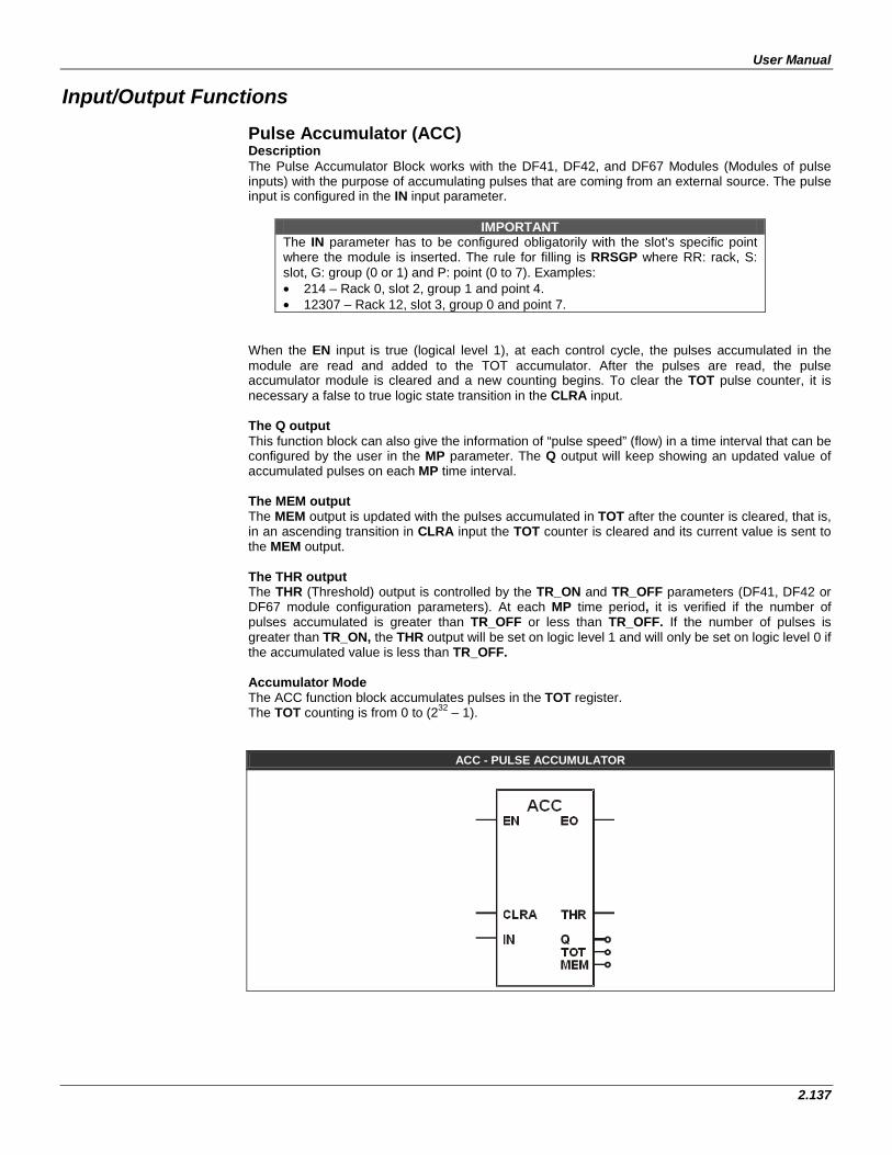
User Manual
2.137
Input/Output Functions Pulse Accumulator (ACC) Description The Pulse Accumulator Block works with the DF41, DF42, and DF67 Modules (Modules of pulse inputs) with the purpose of accumulating pulses that are coming from an external source. The pulse input is configured in the IN input parameter.
IMPORTANT The IN parameter has to be configured obligatorily with the slot’s specific point where the module is inserted. The rule for filling is RRSGP where RR: rack, S: slot, G: group (0 or 1) and P: point (0 to 7). Examples: • 214 – Rack 0, slot 2, group 1 and point 4. • 12307 – Rack 12, slot 3, group 0 and point 7.
When the EN input is true (logical level 1), at each control cycle, the pulses accumulated in the module are read and added to the TOT accumulator. After the pulses are read, the pulse accumulator module is cleared and a new counting begins. To clear the TOT pulse counter, it is necessary a false to true logic state transition in the CLRA input. The Q output This function block can also give the information of “pulse speed” (flow) in a time interval that can be configured by the user in the MP parameter. The Q output will keep showing an updated value of accumulated pulses on each MP time interval. The MEM output The MEM output is updated with the pulses accumulated in TOT after the counter is cleared, that is, in an ascending transition in CLRA input the TOT counter is cleared and its current value is sent to the MEM output. The THR output The THR (Threshold) output is controlled by the TR_ON and TR_OFF parameters (DF41, DF42 or DF67 module configuration parameters). At each MP time period, it is verified if the number of pulses accumulated is greater than TR_OFF or less than TR_OFF. If the number of pulses is greater than TR_ON, the THR output will be set on logic level 1 and will only be set on logic level 0 if the accumulated value is less than TR_OFF. Accumulator Mode The ACC function block accumulates pulses in the TOT register. The TOT counting is from 0 to (232 – 1).
ACC - PULSE ACCUMULATOR

Function Blocks
2.138
CLASS MNEM DESCRIPTION TYPE
I EN INPUT ENABLED BOOL CLRA CLEARS THE ACCUMULATOR BOOL
O
EO OUTPUT ENABLED BOOL THR THRESHOLD OUTPUT BOOL Q PULSES ACCUMULATED IN MP PERIOD LONG TOT ACCUMULATED PULSES VALUE LONG
MEM ACCUMULATED PULSE VALUES PROCEEDING FROM CN THAT ARE TRANSFERRED TO MEM LONG
P IN CHANNEL LONG I: Input. P: Parameter. O: Output
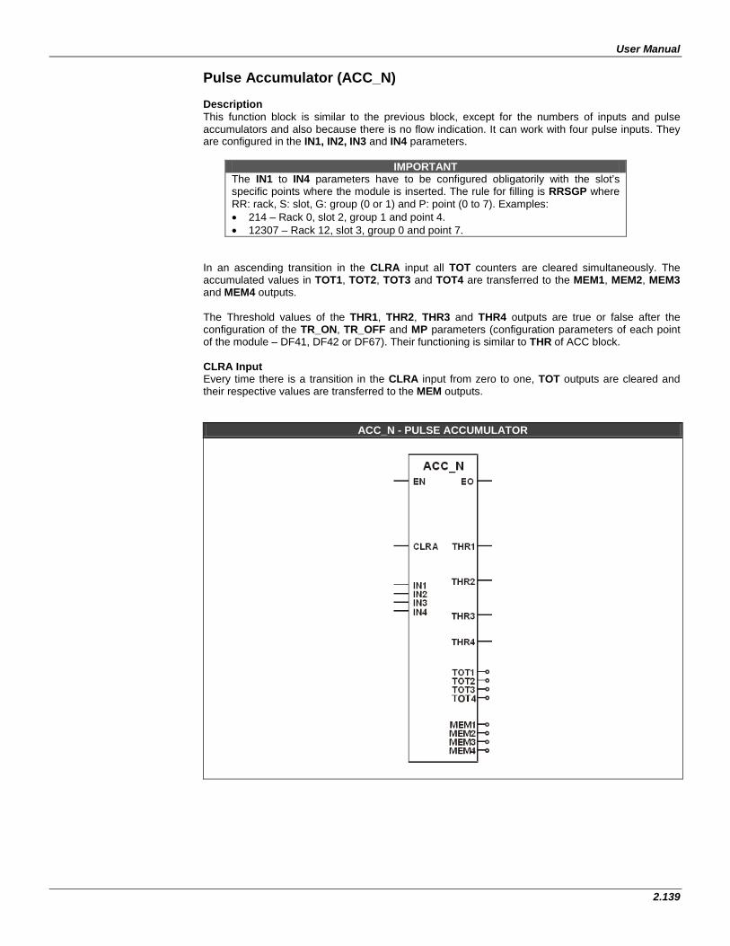
User Manual
2.139
Pulse Accumulator (ACC_N) Description This function block is similar to the previous block, except for the numbers of inputs and pulse accumulators and also because there is no flow indication. It can work with four pulse inputs. They are configured in the IN1, IN2, IN3 and IN4 parameters.
IMPORTANT The IN1 to IN4 parameters have to be configured obligatorily with the slot’s specific points where the module is inserted. The rule for filling is RRSGP where RR: rack, S: slot, G: group (0 or 1) and P: point (0 to 7). Examples: • 214 – Rack 0, slot 2, group 1 and point 4. • 12307 – Rack 12, slot 3, group 0 and point 7.
In an ascending transition in the CLRA input all TOT counters are cleared simultaneously. The accumulated values in TOT1, TOT2, TOT3 and TOT4 are transferred to the MEM1, MEM2, MEM3 and MEM4 outputs. The Threshold values of the THR1, THR2, THR3 and THR4 outputs are true or false after the configuration of the TR_ON, TR_OFF and MP parameters (configuration parameters of each point of the module – DF41, DF42 or DF67). Their functioning is similar to THR of ACC block. CLRA Input Every time there is a transition in the CLRA input from zero to one, TOT outputs are cleared and their respective values are transferred to the MEM outputs.
ACC_N - PULSE ACCUMULATOR
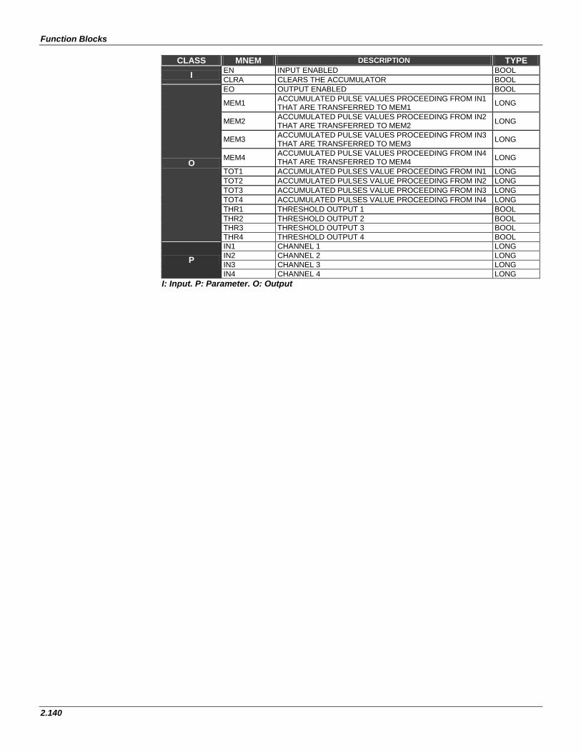
Function Blocks
2.140
I: Input. P: Parameter. O: Output
CLASS MNEM DESCRIPTION TYPE I EN INPUT ENABLED BOOL
CLRA CLEARS THE ACCUMULATOR BOOL
O
EO OUTPUT ENABLED BOOL
MEM1 ACCUMULATED PULSE VALUES PROCEEDING FROM IN1 THAT ARE TRANSFERRED TO MEM1 LONG
MEM2 ACCUMULATED PULSE VALUES PROCEEDING FROM IN2 THAT ARE TRANSFERRED TO MEM2 LONG
MEM3 ACCUMULATED PULSE VALUES PROCEEDING FROM IN3 THAT ARE TRANSFERRED TO MEM3 LONG
MEM4 ACCUMULATED PULSE VALUES PROCEEDING FROM IN4 THAT ARE TRANSFERRED TO MEM4 LONG
TOT1 ACCUMULATED PULSES VALUE PROCEEDING FROM IN1 LONG TOT2 ACCUMULATED PULSES VALUE PROCEEDING FROM IN2 LONG TOT3 ACCUMULATED PULSES VALUE PROCEEDING FROM IN3 LONG TOT4 ACCUMULATED PULSES VALUE PROCEEDING FROM IN4 LONG THR1 THRESHOLD OUTPUT 1 BOOL THR2 THRESHOLD OUTPUT 2 BOOL THR3 THRESHOLD OUTPUT 3 BOOL THR4 THRESHOLD OUTPUT 4 BOOL
P IN1 CHANNEL 1 LONG IN2 CHANNEL 2 LONG IN3 CHANNEL 3 LONG IN4 CHANNEL 4 LONG
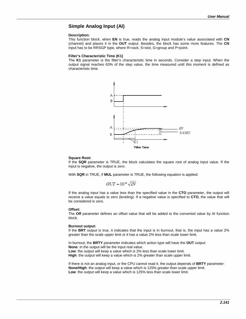
User Manual
2.141
Simple Analog Input (AI) Description: This function block, when EN is true, reads the analog input module’s value associated with CN (channel) and places it in the OUT output. Besides, the block has some more features. The CN input has to be RRSGP type, where R=rack, S=slot, G=group and P=point. Filter’s Characteristic Time (K1) The K1 parameter is the filter’s characteristic time in seconds. Consider a step input. When the output signal reaches 63% of the step value, the time measured until this moment is defined as characteristic time.
Square Root: If the SQR parameter is TRUE, the block calculates the square root of analog input value. If the input is negative, the output is zero. With SQR in TRUE, if MUL parameter is TRUE, the following equation is applied:
If the analog input has a value less than the specified value in the CTO parameter, the output will receive a value equals to zero (leveling). If a negative value is specified to CTO, the value that will be considered is zero. Offset: The Off parameter defines an offset value that will be added to the converted value by AI function block. Burnout output: If the BRT output is true, it indicates that the input is in burnout, that is, the input has a value 2% greater than the scale upper limit or it has a value 2% less than scale lower limit. In burnout, the BRTY parameter indicates which action type will have the OUT output: None: in the output will be the input real value. Low: the output will keep a value which is 2% less than scale lower limit. High: the output will keep a value which is 2% greater than scale upper limit. If there is not an analog input, or the CPU cannot read it, the output depends of BRTY parameter: None/High: the output will keep a value which is 125% greater than scale upper limit. Low: the output will keep a value which is 125% less than scale lower limit.
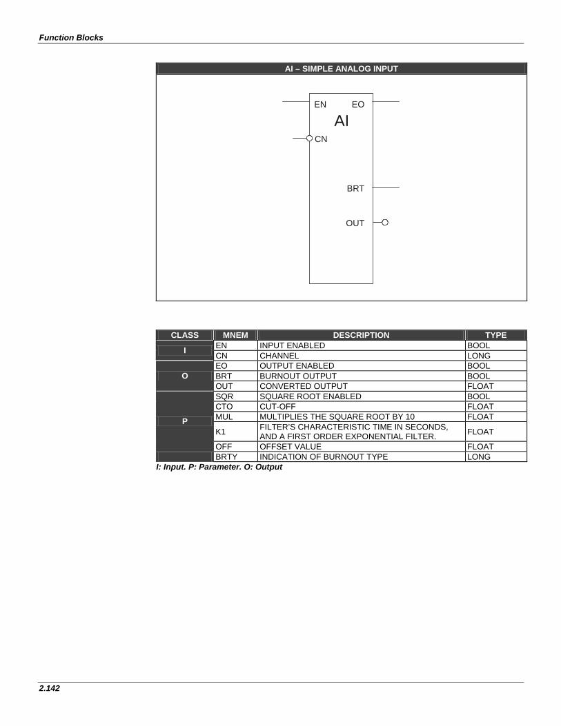
Function Blocks
2.142
AI – SIMPLE ANALOG INPUT
AIEN EO
CN
BRT
OUT
CLASS MNEM DESCRIPTION TYPE
I EN INPUT ENABLED BOOL CN CHANNEL LONG
O EO OUTPUT ENABLED BOOL BRT BURNOUT OUTPUT BOOL OUT CONVERTED OUTPUT FLOAT
P
SQR SQUARE ROOT ENABLED BOOL CTO CUT-OFF FLOAT MUL MULTIPLIES THE SQUARE ROOT BY 10 FLOAT
K1 FILTER’S CHARACTERISTIC TIME IN SECONDS, AND A FIRST ORDER EXPONENTIAL FILTER. FLOAT
OFF OFFSET VALUE FLOAT BRTY INDICATION OF BURNOUT TYPE LONG
I: Input. P: Parameter. O: Output
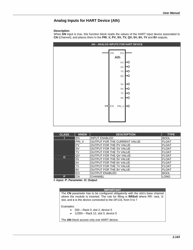
User Manual
2.143
Analog Inputs for HART Device (AIh) Description When EN input is true, this function block reads the values of the HART input device associated to CN (Channel), and places them in the PRI_V, PV, SV, TV, QV, 5V, 6V, 7V and 8V outputs.
AIh - ANALOG INPUTS FOR HART DEVICE
EN EO
AIh
8V
CN
7V
6V
5V
QV
TV
SV
PV
PRI_V
CLASS MNEM DESCRIPTION TYPE I EN INPUT ENABLED BOOL
O
PRI_V OUTPUT FOR THE CURRENT VALUE FLOAT PV OUTPUT FOR THE PV VALUE FLOAT SV OUTPUT FOR THE SV VALUE FLOAT TV OUTPUT FOR THE TV VALUE FLOAT QV OUTPUT FOR THE QV VALUE FLOAT 5V OUTPUT FOR THE 5V VALUE FLOAT 6V OUTPUT FOR THE 6V VALUE FLOAT 7V OUTPUT FOR THE 7V VALUE FLOAT 8V OUTPUT FOR THE 8V VALUE FLOAT EO OUTPUT ENABLED BOOL
P CN CHANNEL LONG I: Input. P: Parameter. O: Output
IMPORTANT The CN parameter has to be configured obligatorily with the slot’s base channel where the module is inserted. The rule for filling is RRSx0 where RR: rack, S: slot, and x is the device connected to the DF116, from 0 to 7 Examples:
• 200 – Rack 0, slot 2, device 0 • 12350 – Rack 12, slot 3, device 5
The AIh block access only one HART device.
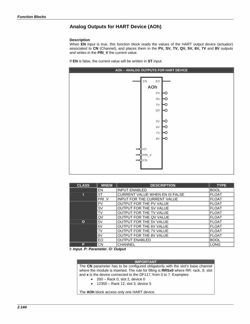
Function Blocks
2.144
Analog Outputs for HART Device (AOh) Description When EN input is true, this function block reads the values of the HART output device (actuator) associated to CN (Channel), and places them in the PV, SV, TV, QV, 5V, 6V, 7V and 8V outputs and writes in the PRI_V the current value. If EN is false, the current value will be written in ST input.
AOh – ANALOG OUTPUTS FOR HART DEVICE
AOhEN EO
PV
SV
TV
QV
5V
6V
7V
8V
PRI_V
CN
ST
CLASS MNEM DESCRIPTION TYPE
I EN INPUT ENABLED BOOL ST CURRENT VALUE WHEN EN IS FALSE FLOAT PRI_V INPUT FOR THE CURRENT VALUE FLOAT
O
PV OUTPUT FOR THE PV VALUE FLOAT SV OUTPUT FOR THE SV VALUE FLOAT TV OUTPUT FOR THE TV VALUE FLOAT QV OUTPUT FOR THE QV VALUE FLOAT 5V OUTPUT FOR THE 5V VALUE FLOAT 6V OUTPUT FOR THE 6V VALUE FLOAT 7V OUTPUT FOR THE 7V VALUE FLOAT 8V OUTPUT FOR THE 8V VALUE FLOAT EO OUTPUT ENABLED BOOL
P CN CHANNEL LONG I: Input. P: Parameter. O: Output
IMPORTANT The CN parameter has to be configured obligatorily with the slot’s base channel where the module is inserted. The rule for filling is RRSx0 where RR: rack, S: slot and x is the device connected to the DF117, from 0 to 7. Examples:
• 200 – Rack 0, slot 2, device 0 • 12350 – Rack 12, slot 3, device 5
The AOh block access only one HART device.
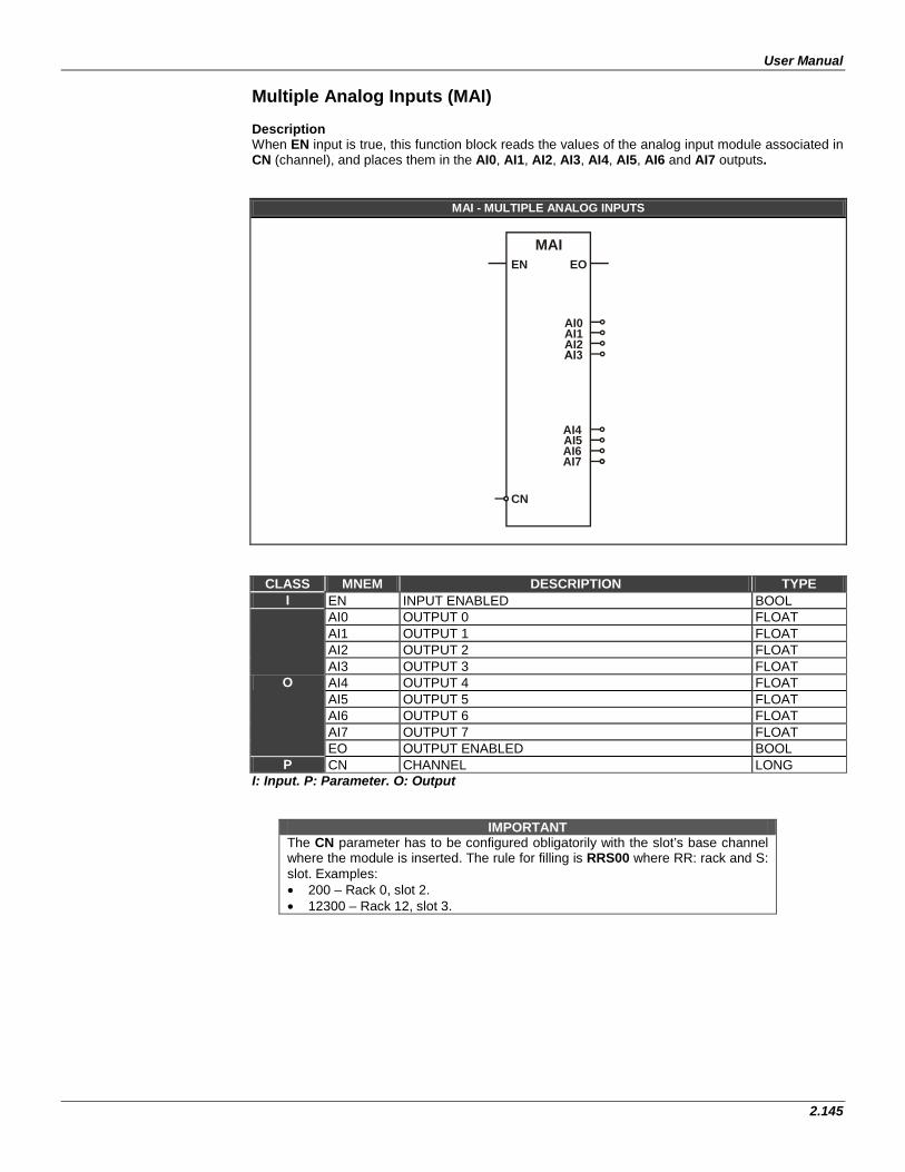
User Manual
2.145
Multiple Analog Inputs (MAI) Description When EN input is true, this function block reads the values of the analog input module associated in CN (channel), and places them in the AI0, AI1, AI2, AI3, AI4, AI5, AI6 and AI7 outputs.
MAI - MULTIPLE ANALOG INPUTS
MAIEN EO
AI0AI1AI2
AI4AI5AI6AI7
CN
CLASS MNEM DESCRIPTION TYPE I EN INPUT ENABLED BOOL
O
AI0 OUTPUT 0 FLOAT AI1 OUTPUT 1 FLOAT AI2 OUTPUT 2 FLOAT AI3 OUTPUT 3 FLOAT AI4 OUTPUT 4 FLOAT AI5 OUTPUT 5 FLOAT AI6 OUTPUT 6 FLOAT AI7 OUTPUT 7 FLOAT EO OUTPUT ENABLED BOOL
P CN CHANNEL LONG I: Input. P: Parameter. O: Output
IMPORTANT The CN parameter has to be configured obligatorily with the slot’s base channel where the module is inserted. The rule for filling is RRS00 where RR: rack and S: slot. Examples: • 200 – Rack 0, slot 2. • 12300 – Rack 12, slot 3.
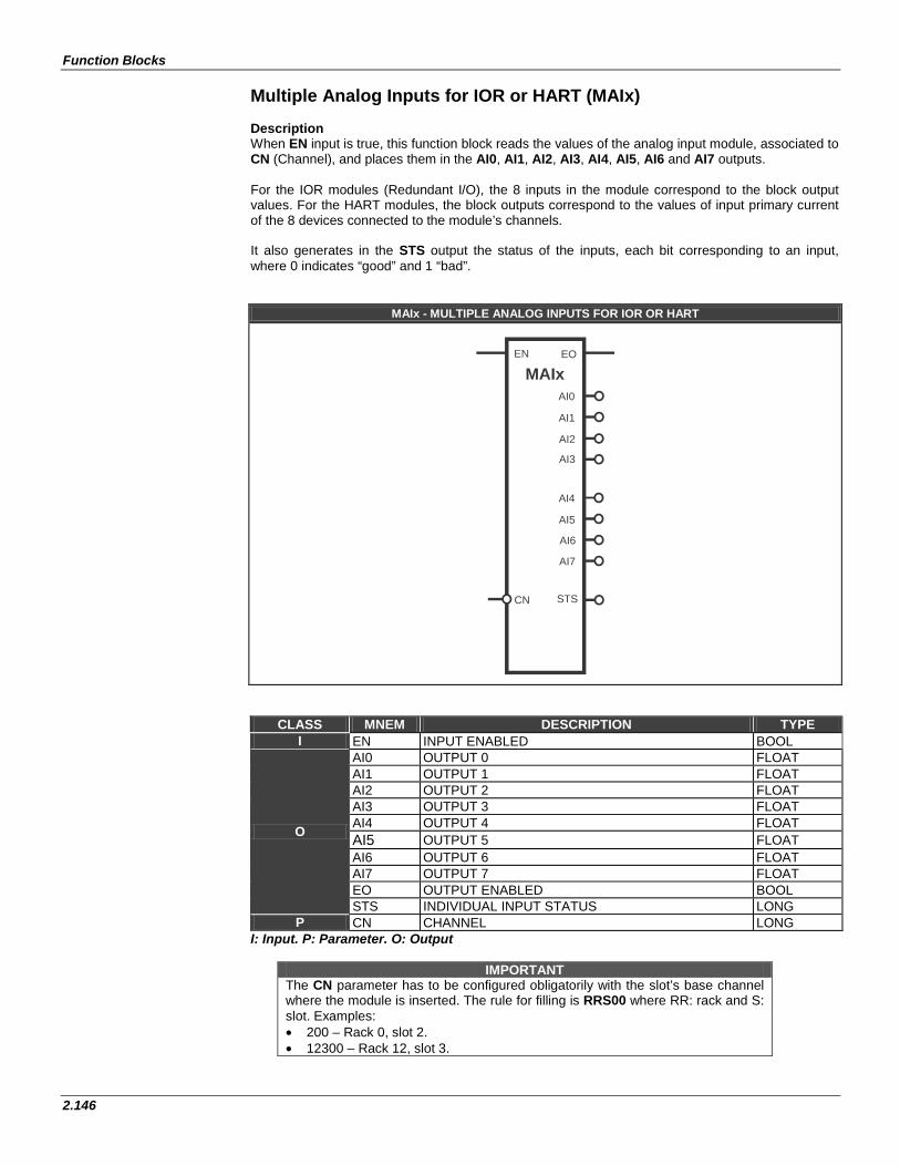
Function Blocks
2.146
Multiple Analog Inputs for IOR or HART (MAIx) Description When EN input is true, this function block reads the values of the analog input module, associated to CN (Channel), and places them in the AI0, AI1, AI2, AI3, AI4, AI5, AI6 and AI7 outputs. For the IOR modules (Redundant I/O), the 8 inputs in the module correspond to the block output values. For the HART modules, the block outputs correspond to the values of input primary current of the 8 devices connected to the module’s channels. It also generates in the STS output the status of the inputs, each bit corresponding to an input, where 0 indicates “good” and 1 “bad”.
MAIx - MULTIPLE ANALOG INPUTS FOR IOR OR HART
MAIxAI0
EN EO
AI1
AI2
AI3
CN STS
AI4
AI5
AI6
AI7
CLASS MNEM DESCRIPTION TYPE I EN INPUT ENABLED BOOL
O
AI0 OUTPUT 0 FLOAT AI1 OUTPUT 1 FLOAT AI2 OUTPUT 2 FLOAT AI3 OUTPUT 3 FLOAT AI4 OUTPUT 4 FLOAT AI5 OUTPUT 5 FLOAT AI6 OUTPUT 6 FLOAT AI7 OUTPUT 7 FLOAT EO OUTPUT ENABLED BOOL STS INDIVIDUAL INPUT STATUS LONG
P CN CHANNEL LONG I: Input. P: Parameter. O: Output
IMPORTANT The CN parameter has to be configured obligatorily with the slot’s base channel where the module is inserted. The rule for filling is RRS00 where RR: rack and S: slot. Examples: • 200 – Rack 0, slot 2. • 12300 – Rack 12, slot 3.
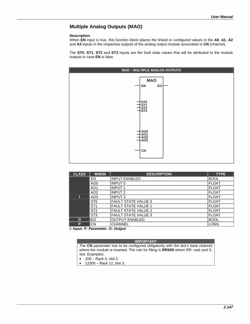
User Manual
2.147
Multiple Analog Outputs (MAO) Description When EN input is true, this function block places the linked or configured values in the A0, A1, A2 and A3 inputs in the respective outputs of the analog output module associated in CN (channel). The ST0, ST1, ST2 and ST3 inputs are the fault state values that will be attributed to the module outputs in case EN is false.
MAO – MULTIPLE ANALOG OUTPUTS
MAOEN EO
ST0ST1ST2
AO0AO1AO2AO3
CN
CLASS MNEM DESCRIPTION TYPE
I
EN INPUT ENABLED BOOL AO0 INPUT 0 FLOAT AO1 INPUT 1 FLOAT AO2 INPUT 2 FLOAT AO3 INPUT 3 FLOAT ST0 FAULT STATE VALUE 0 FLOAT ST1 FAULT STATE VALUE 1 FLOAT ST2 FAULT STATE VALUE 2 FLOAT ST3 FAULT STATE VALUE 3 FLOAT
O EO OUTPUT ENABLED BOOL P CN CHANNEL LONG
I: Input. P: Parameter. O: Output
IMPORTANT The CN parameter has to be configured obligatorily with the slot’s base channel where the module is inserted. The rule for filling is RRS00 where RR: rack and S: slot. Examples: • 200 – Rack 0, slot 2. • 12300 – Rack 12, slot 3.
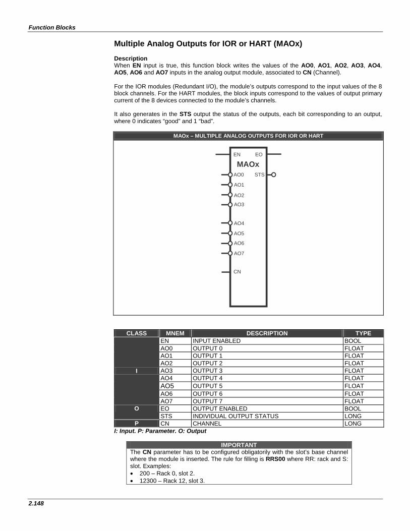
Function Blocks
2.148
Multiple Analog Outputs for IOR or HART (MAOx) Description When EN input is true, this function block writes the values of the AO0, AO1, AO2, AO3, AO4, AO5, AO6 and AO7 inputs in the analog output module, associated to CN (Channel). For the IOR modules (Redundant I/O), the module’s outputs correspond to the input values of the 8 block channels. For the HART modules, the block inputs correspond to the values of output primary current of the 8 devices connected to the module’s channels. It also generates in the STS output the status of the outputs, each bit corresponding to an output, where 0 indicates “good” and 1 “bad”.
MAOx – MULTIPLE ANALOG OUTPUTS FOR IOR OR HART
EN EO
AO0 STS
AO1
AO2
AO3
AO4
AO6
AO7
CN
AO5
MAOx
CLASS MNEM DESCRIPTION TYPE
I
EN INPUT ENABLED BOOL AO0 OUTPUT 0 FLOAT AO1 OUTPUT 1 FLOAT AO2 OUTPUT 2 FLOAT AO3 OUTPUT 3 FLOAT AO4 OUTPUT 4 FLOAT AO5 OUTPUT 5 FLOAT AO6 OUTPUT 6 FLOAT AO7 OUTPUT 7 FLOAT
O EO OUTPUT ENABLED BOOL STS INDIVIDUAL OUTPUT STATUS LONG
P CN CHANNEL LONG I: Input. P: Parameter. O: Output
IMPORTANT The CN parameter has to be configured obligatorily with the slot’s base channel where the module is inserted. The rule for filling is RRS00 where RR: rack and S: slot. Examples: • 200 – Rack 0, slot 2. • 12300 – Rack 12, slot 3.
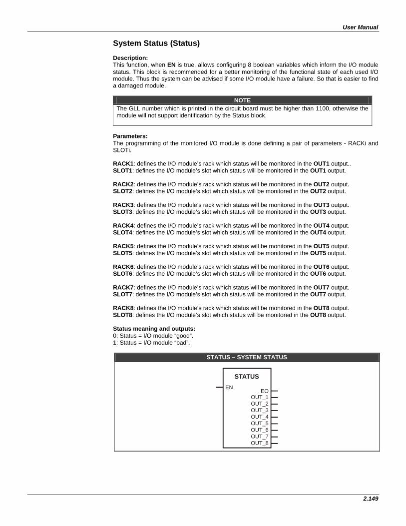
User Manual
2.149
System Status (Status) Description: This function, when EN is true, allows configuring 8 boolean variables which inform the I/O module status. This block is recommended for a better monitoring of the functional state of each used I/O module. Thus the system can be advised if some I/O module have a failure. So that is easier to find a damaged module.
NOTE The GLL number which is printed in the circuit board must be higher than 1100, otherwise the module will not support identification by the Status block.
Parameters: The programming of the monitored I/O module is done defining a pair of parameters - RACKi and SLOTi. RACK1: defines the I/O module’s rack which status will be monitored in the OUT1 output.. SLOT1: defines the I/O module’s slot which status will be monitored in the OUT1 output. RACK2: defines the I/O module’s rack which status will be monitored in the OUT2 output. SLOT2: defines the I/O module’s slot which status will be monitored in the OUT2 output. RACK3: defines the I/O module’s rack which status will be monitored in the OUT3 output. SLOT3: defines the I/O module’s slot which status will be monitored in the OUT3 output. RACK4: defines the I/O module’s rack which status will be monitored in the OUT4 output. SLOT4: defines the I/O module’s slot which status will be monitored in the OUT4 output. RACK5: defines the I/O module’s rack which status will be monitored in the OUT5 output. SLOT5: defines the I/O module’s slot which status will be monitored in the OUT5 output. RACK6: defines the I/O module’s rack which status will be monitored in the OUT6 output. SLOT6: defines the I/O module’s slot which status will be monitored in the OUT6 output. RACK7: defines the I/O module’s rack which status will be monitored in the OUT7 output. SLOT7: defines the I/O module’s slot which status will be monitored in the OUT7 output. RACK8: defines the I/O module’s rack which status will be monitored in the OUT8 output. SLOT8: defines the I/O module’s slot which status will be monitored in the OUT8 output. Status meaning and outputs: 0: Status = I/O module “good”. 1: Status = I/O module “bad”.
STATUS – SYSTEM STATUS
STATUS
EOOUT_1OUT_2OUT_3OUT_4OUT_5OUT_6OUT_7
EN
OUT_8

Function Blocks
2.150
CLASS MNEM DESCRIPTION TYPE
I EN INPUT ENABLED BOOL
O
EO OUTPUT ENABLED BOOL OUT1 MODULE STATUS DEFINED IN RACK1/SLOT1 BOOL OUT2 MODULE STATUS DEFINED IN RACK2/SLOT2 BOOL OUT3 MODULE STATUS DEFINED IN RACK3/SLOT3 BOOL OUT4 MODULE STATUS DEFINED IN RACK4/SLOT4 BOOL OUT5 MODULE STATUS DEFINED IN RACK5/SLOT5 BOOL OUT6 MODULE STATUS DEFINED IN RACK6/SLOT6 BOOL OUT7 MODULE STATUS DEFINED IN RACK7/SLOT7 BOOL OUT8 MODULE STATUS DEFINED IN RACK8/SLOT8 BOOL
P
RACK1 MODULE’S RACK WHICH STATUS WILL BE IN OUT1 LONG SLOT1 MODULE’S SLOT WHICH STATUS WILL BE IN OUT1 LONG RACK2 MODULE’S RACK WHICH STATUS WILL BE IN OUT2 LONG SLOT2 MODULE’S SLOT WHICH STATUS WILL BE IN OUT2 LONG RACK3 MODULE’S RACK WHICH STATUS WILL BE IN OUT3 LONG SLOT3 MODULE’S SLOT WHICH STATUS WILL BE IN OUT3 LONG RACK4 MODULE’S RACK WHICH STATUS WILL BE IN OUT4 LONG SLOT4 MODULE’S SLOT WHICH STATUS WILL BE IN OUT4 LONG RACK5 MODULE’S RACK WHICH STATUS WILL BE IN OUT5 LONG SLOT5 MODULE’S SLOT WHICH STATUS WILL BE IN OUT5 LONG RACK6 MODULE’S RACK WHICH STATUS WILL BE IN OUT6 LONG SLOT6 MODULE’S SLOT WHICH STATUS WILL BE IN OUT6 LONG RACK7 MODULE’S RACK WHICH STATUS WILL BE IN OUT7 LONG SLOT7 MODULE’S SLOT WHICH STATUS WILL BE IN OUT7 LONG RACK8 MODULE’S RACK WHICH STATUS WILL BE IN OUT8 LONG SLOT8 MODULE’S SLOT WHICH STATUS WILL BE IN OUT8 LONG
I: Input. P: Parameter. O: Output
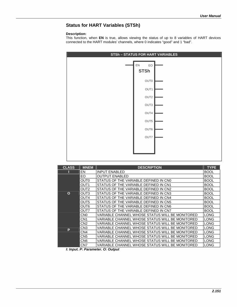
User Manual
2.151
Status for HART Variables (STSh) Description: This function, when EN is true, allows viewing the status of up to 8 variables of HART devices connected to the HART modules’ channels, where 0 indicates “good” and 1 “bad”.
STSh – STATUS FOR HART VARIABLES
STSh
OUT0
EN EO
OUT1
OUT2
OUT3
OUT4
OUT5
OUT6
OUT7
CLASS MNEM DESCRIPTION TYPE
I EN INPUT ENABLED BOOL
O
EO OUTPUT ENABLED BOOL OUT0 STATUS OF THE VARIABLE DEFINED IN CN0 BOOL OUT1 STATUS OF THE VARIABLE DEFINED IN CN1 BOOL OUT2 STATUS OF THE VARIABLE DEFINED IN CN2 BOOL OUT3 STATUS OF THE VARIABLE DEFINED IN CN3 BOOL OUT4 STATUS OF THE VARIABLE DEFINED IN CN4 BOOL OUT5 STATUS OF THE VARIABLE DEFINED IN CN5 BOOL OUT6 STATUS OF THE VARIABLE DEFINED IN CN6 BOOL OUT7 STATUS OF THE VARIABLE DEFINED IN CN7 BOOL
P
CN0 VARIABLE CHANNEL WHOSE STATUS WILL BE MONITORED LONG CN1 VARIABLE CHANNEL WHOSE STATUS WILL BE MONITORED LONG CN2 VARIABLE CHANNEL WHOSE STATUS WILL BE MONITORED LONG CN3 VARIABLE CHANNEL WHOSE STATUS WILL BE MONITORED LONG CN4 VARIABLE CHANNEL WHOSE STATUS WILL BE MONITORED LONG CN5 VARIABLE CHANNEL WHOSE STATUS WILL BE MONITORED LONG CN6 VARIABLE CHANNEL WHOSE STATUS WILL BE MONITORED LONG CN7 VARIABLE CHANNEL WHOSE STATUS WILL BE MONITORED LONG
I: Input. P: Parameter. O: Output

Function Blocks
2.152
IMPORTANT
The CN0...7 parameters must be configured with the channel of the HART variable whose status will be monitored. The rule for filling is RRSGP, where RR: rack; S: slot of HART module; G: group (position of the HART device in the module), and P: point indicating the variable that will be monitored, according to the following table: 0: PV 1: SV 2: TV 3: QV 4: 5V 5: 6V 6: 7V 7: 8V 8: primary current Examples: Monitor the TV status of the HART device connected to the second channel of the HART module that is on rack 3, slot 1: CNx= 3112 Monitor the PV status of the HART device connected to the fifth channel of the HART module that is on rack 12, slot 2: CNx= 12240 Monitor the primary current status of the HART device connected to the first channel of the HART module that is on rack 1, slot 0: CNx= 1008
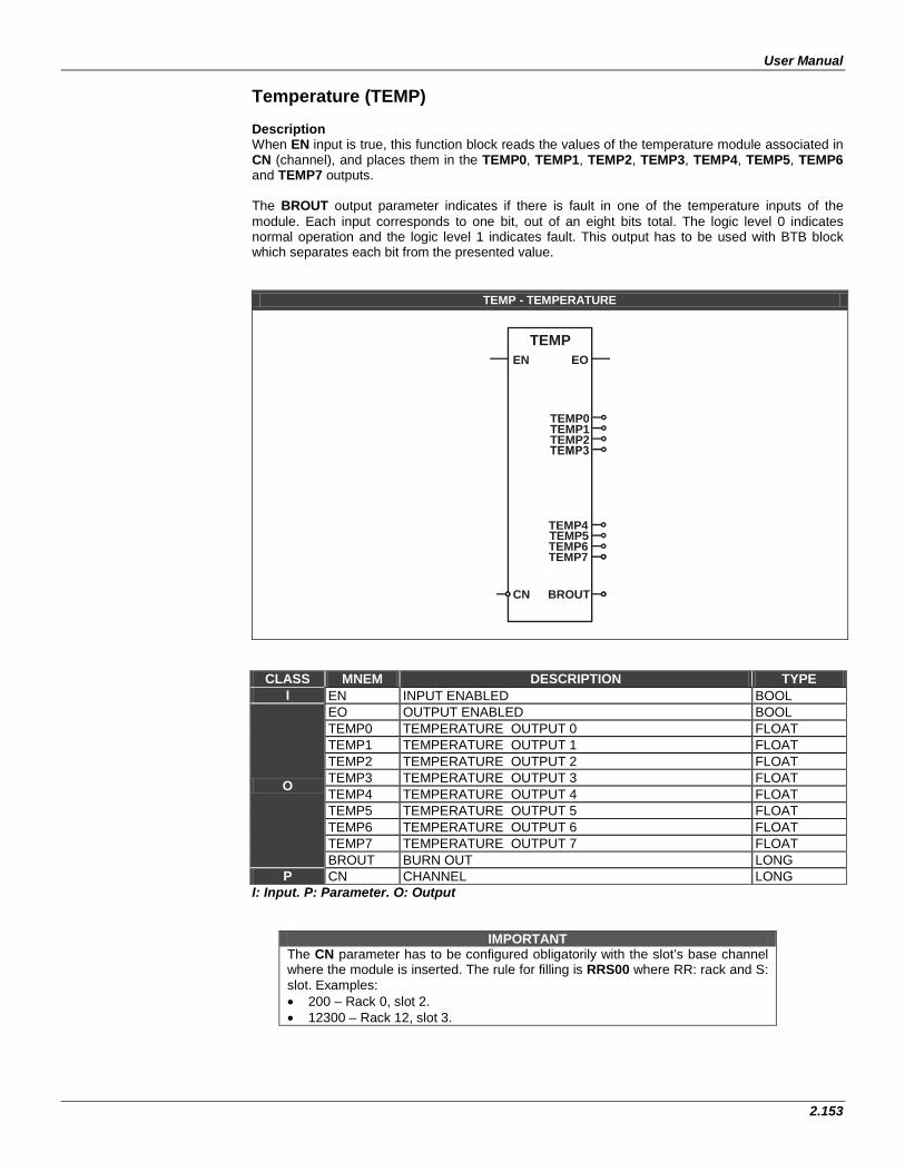
User Manual
2.153
Temperature (TEMP) Description When EN input is true, this function block reads the values of the temperature module associated in CN (channel), and places them in the TEMP0, TEMP1, TEMP2, TEMP3, TEMP4, TEMP5, TEMP6 and TEMP7 outputs. The BROUT output parameter indicates if there is fault in one of the temperature inputs of the module. Each input corresponds to one bit, out of an eight bits total. The logic level 0 indicates normal operation and the logic level 1 indicates fault. This output has to be used with BTB block which separates each bit from the presented value.
TEMP - TEMPERATURE
TEMPEN EO
TEMP0TEMP1TEMP2
TEMP4TEMP5TEMP6TEMP7
CN BROUT
CLASS MNEM DESCRIPTION TYPE I EN INPUT ENABLED BOOL
O
EO OUTPUT ENABLED BOOL TEMP0 TEMPERATURE OUTPUT 0 FLOAT TEMP1 TEMPERATURE OUTPUT 1 FLOAT TEMP2 TEMPERATURE OUTPUT 2 FLOAT TEMP3 TEMPERATURE OUTPUT 3 FLOAT TEMP4 TEMPERATURE OUTPUT 4 FLOAT TEMP5 TEMPERATURE OUTPUT 5 FLOAT TEMP6 TEMPERATURE OUTPUT 6 FLOAT TEMP7 TEMPERATURE OUTPUT 7 FLOAT BROUT BURN OUT LONG
P CN CHANNEL LONG I: Input. P: Parameter. O: Output
IMPORTANT The CN parameter has to be configured obligatorily with the slot’s base channel where the module is inserted. The rule for filling is RRS00 where RR: rack and S: slot. Examples: • 200 – Rack 0, slot 2. • 12300 – Rack 12, slot 3.

Function Blocks
2.154
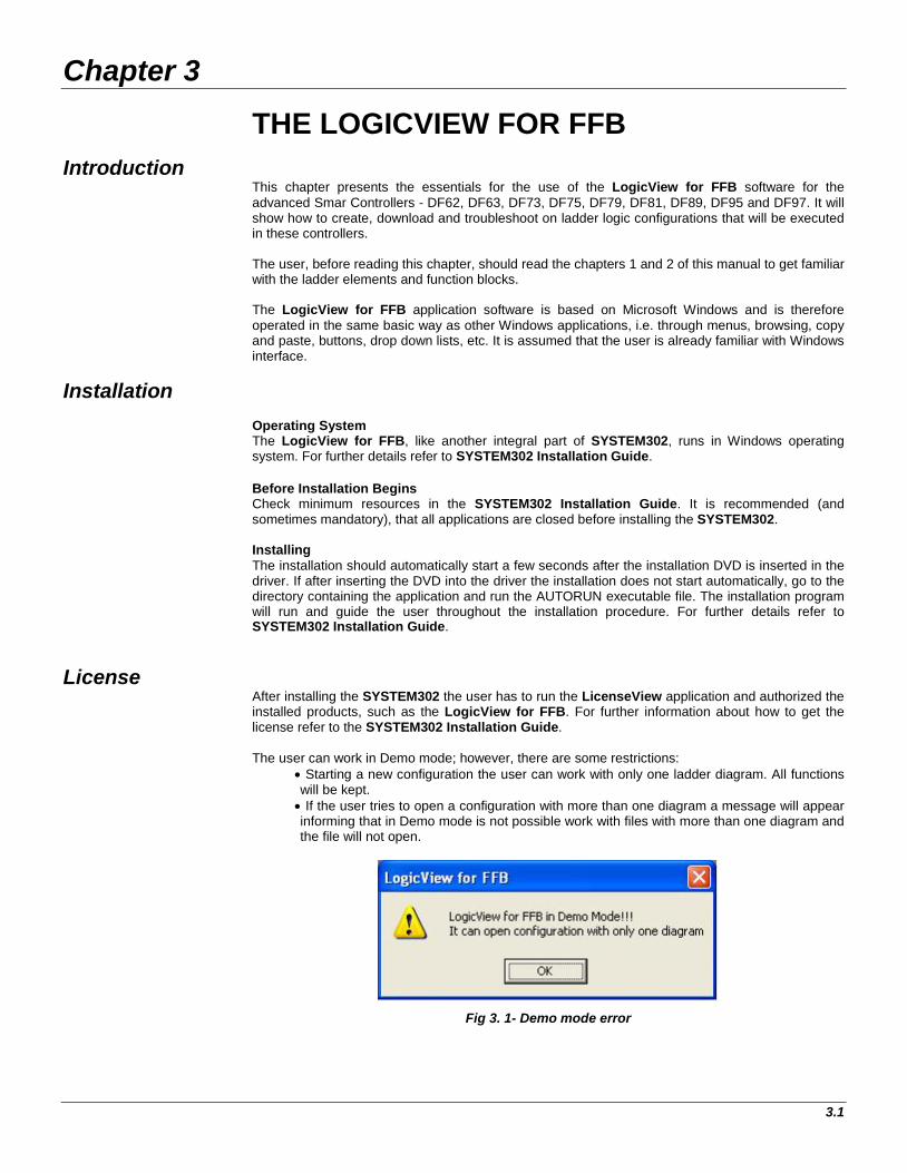
Chapter 3
3.1
THE LOGICVIEW FOR FFB
Introduction This chapter presents the essentials for the use of the LogicView for FFB software for the advanced Smar Controllers - DF62, DF63, DF73, DF75, DF79, DF81, DF89, DF95 and DF97. It will show how to create, download and troubleshoot on ladder logic configurations that will be executed in these controllers. The user, before reading this chapter, should read the chapters 1 and 2 of this manual to get familiar with the ladder elements and function blocks. The LogicView for FFB application software is based on Microsoft Windows and is therefore operated in the same basic way as other Windows applications, i.e. through menus, browsing, copy and paste, buttons, drop down lists, etc. It is assumed that the user is already familiar with Windows interface.
Installation Operating System The LogicView for FFB, like another integral part of SYSTEM302, runs in Windows operating system. For further details refer to SYSTEM302 Installation Guide. Before Installation Begins Check minimum resources in the SYSTEM302 Installation Guide. It is recommended (and sometimes mandatory), that all applications are closed before installing the SYSTEM302. Installing The installation should automatically start a few seconds after the installation DVD is inserted in the driver. If after inserting the DVD into the driver the installation does not start automatically, go to the directory containing the application and run the AUTORUN executable file. The installation program will run and guide the user throughout the installation procedure. For further details refer to SYSTEM302 Installation Guide.
License After installing the SYSTEM302 the user has to run the LicenseView application and authorized the installed products, such as the LogicView for FFB. For further information about how to get the license refer to the SYSTEM302 Installation Guide. The user can work in Demo mode; however, there are some restrictions:
• Starting a new configuration the user can work with only one ladder diagram. All functions will be kept.
• If the user tries to open a configuration with more than one diagram a message will appear informing that in Demo mode is not possible work with files with more than one diagram and the file will not open.
Fig 3. 1- Demo mode error
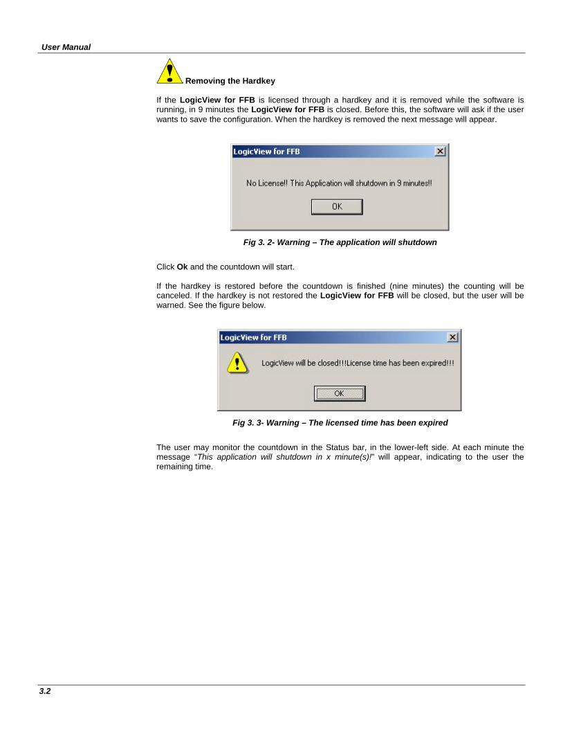
User Manual
3.2
Removing the Hardkey If the LogicView for FFB is licensed through a hardkey and it is removed while the software is running, in 9 minutes the LogicView for FFB is closed. Before this, the software will ask if the user wants to save the configuration. When the hardkey is removed the next message will appear.
Fig 3. 2- Warning – The application will shutdown
Click Ok and the countdown will start. If the hardkey is restored before the countdown is finished (nine minutes) the counting will be canceled. If the hardkey is not restored the LogicView for FFB will be closed, but the user will be warned. See the figure below.
Fig 3. 3- Warning – The licensed time has been expired
The user may monitor the countdown in the Status bar, in the lower-left side. At each minute the message “This application will shutdown in x minute(s)!” will appear, indicating to the user the remaining time.
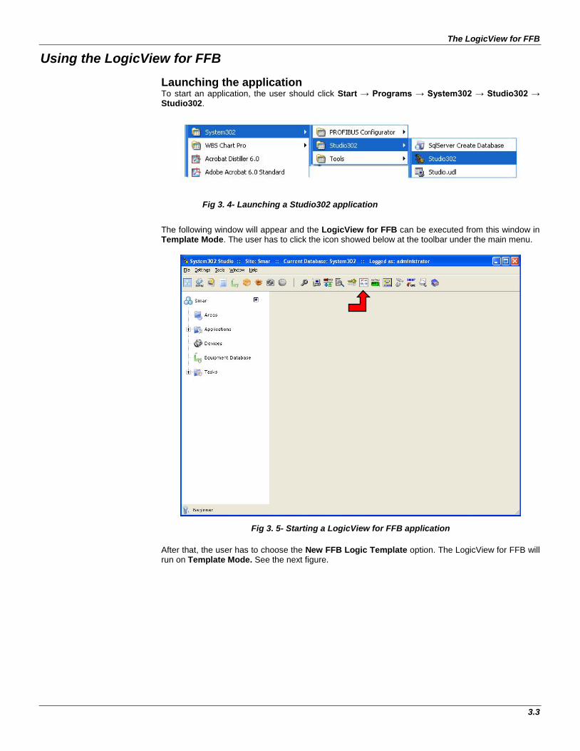
The LogicView for FFB
3.3
Using the LogicView for FFB Launching the application To start an application, the user should click Start → Programs → System302 → Studio302 → Studio302.
Fig 3. 4- Launching a Studio302 application
The following window will appear and the LogicView for FFB can be executed from this window in Template Mode. The user has to click the icon showed below at the toolbar under the main menu.
Fig 3. 5- Starting a LogicView for FFB application After that, the user has to choose the New FFB Logic Template option. The LogicView for FFB will run on Template Mode. See the next figure.
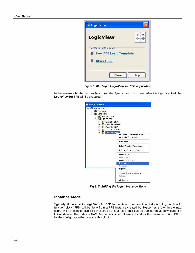
User Manual
3.4
Fig 3. 6- Starting a LogicView for FFB application
In the Instance Mode the user has to run the Syscon and from there, after the logic is edited, the LogicView for FFB will be executed.
Fig 3. 7- Editing the logic - Instance Mode Instance Mode Typically, the access to LogicView for FFB for creation or modification of discrete logic of flexible function block (FFB) will be done from a FFB instance created by Syscon as shown in the next figure. A FFB Instance can be considered as “real” block that can be transferred via download to a linking device. The instance HAS Device Descriptor information and for this reason is EXCLUSIVE for the configuration that contains this block.
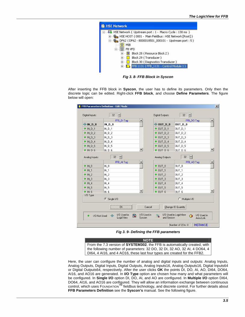
The LogicView for FFB
3.5
Fig 3. 8- FFB Block in Syscon
After inserting the FFB block in Syscon, the user has to define its parameters. Only then the discrete logic can be edited. Right-click FFB block, and choose Define Parameters. The figure below will open:
Fig 3. 9- Defining the FFB parameters
NOTE From the 7.3 version of SYSTEM302, the FFB is automatically created, with the following number of parameters: 32 DO, 32 DI, 32 AO, 32 AI, 4 DO64, 4 DI64, 4 AI16, and 4 AO16, these last four types are created for the FFB2.
Here, the user can configure the number of analog and digital inputs and outputs: Analog Inputs, Analog Outputs, Digital Inputs, Digital Outputs, Analog Inputs16, Analog Outputs16, Digital Inputs64 or Digital Outputs64, respectively. After the user clicks OK the points DI, DO, AI, AO, DI64, DO64, AI16, and AO16 are generated. In I/O Type option are chosen how many and what parameters will be configured. In Single I/O option DI, DO, AI, and AO are configured. In Multiple I/O option DI64, DO64, AI16, and AO16 are configured. They will allow an information exchange between continuous control, which uses FOUNDATIONTM fieldbus technology, and discrete control. For further details about FFB Parameters Definition see the Syscon’s manual. See the following figure.
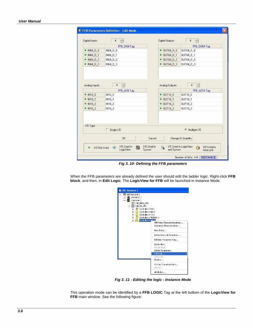
User Manual
3.6
Fig 3. 10- Defining the FFB parameters
When the FFB parameters are already defined the user should edit the ladder logic. Right-click FFB block, and then, in Edit Logic. The LogicView for FFB will be launched in Instance Mode.
Fig 3. 11 - Editing the logic - Instance Mode This operation mode can be identified by a FFB LOGIC Tag at the left bottom of the LogicView for FFB main window. See the following figure:
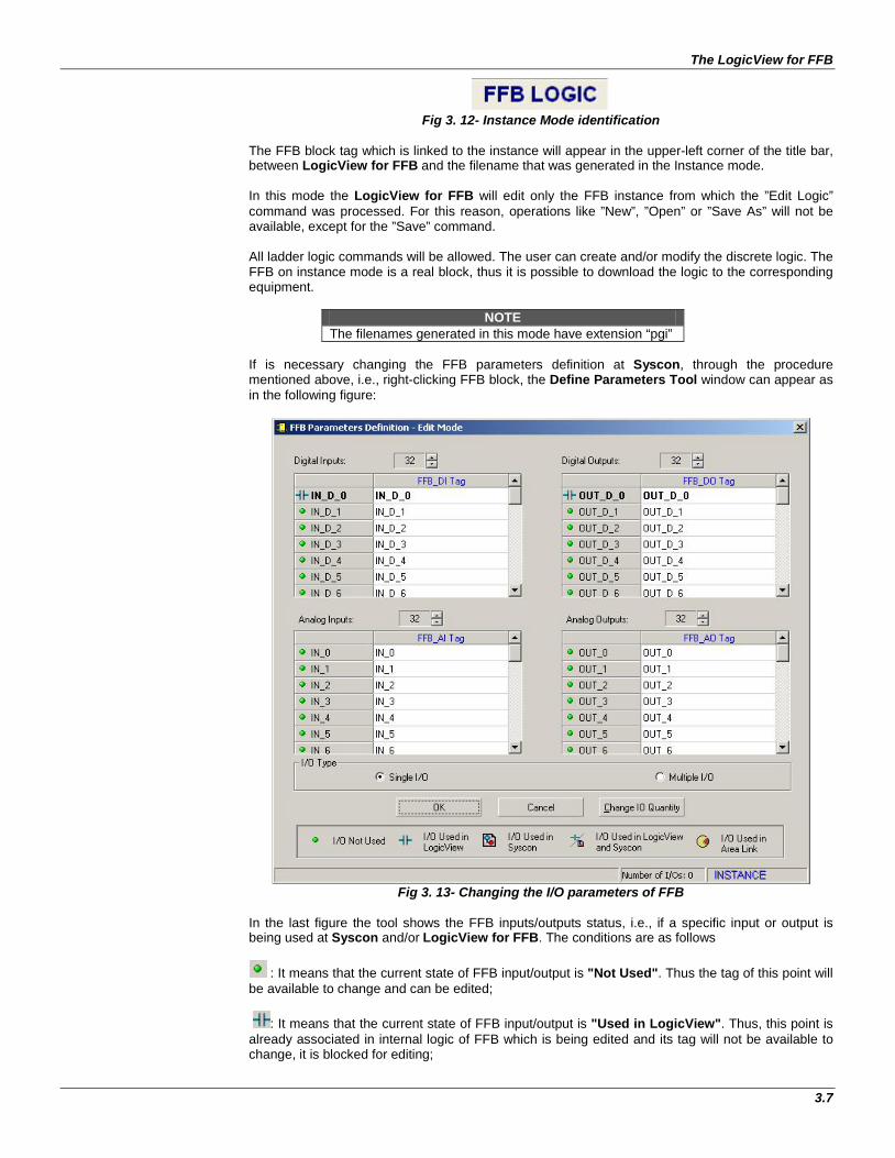
The LogicView for FFB
3.7
Fig 3. 12- Instance Mode identification
The FFB block tag which is linked to the instance will appear in the upper-left corner of the title bar, between LogicView for FFB and the filename that was generated in the Instance mode. In this mode the LogicView for FFB will edit only the FFB instance from which the ”Edit Logic” command was processed. For this reason, operations like ”New”, ”Open” or ”Save As” will not be available, except for the ”Save” command. All ladder logic commands will be allowed. The user can create and/or modify the discrete logic. The FFB on instance mode is a real block, thus it is possible to download the logic to the corresponding equipment.
NOTE The filenames generated in this mode have extension “pgi”
If is necessary changing the FFB parameters definition at Syscon, through the procedure mentioned above, i.e., right-clicking FFB block, the Define Parameters Tool window can appear as in the following figure:
Fig 3. 13- Changing the I/O parameters of FFB
In the last figure the tool shows the FFB inputs/outputs status, i.e., if a specific input or output is being used at Syscon and/or LogicView for FFB. The conditions are as follows
: It means that the current state of FFB input/output is "Not Used". Thus the tag of this point will be available to change and can be edited; : It means that the current state of FFB input/output is "Used in LogicView". Thus, this point is already associated in internal logic of FFB which is being edited and its tag will not be available to change, it is blocked for editing;
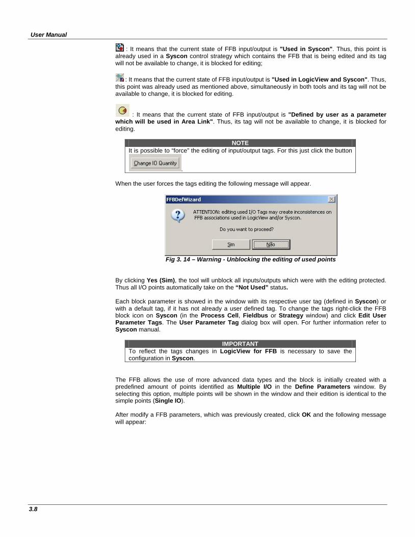
User Manual
3.8
: It means that the current state of FFB input/output is "Used in Syscon". Thus, this point is already used in a Syscon control strategy which contains the FFB that is being edited and its tag will not be available to change, it is blocked for editing;
: It means that the current state of FFB input/output is "Used in LogicView and Syscon". Thus, this point was already used as mentioned above, simultaneously in both tools and its tag will not be available to change, it is blocked for editing.
: It means that the current state of FFB input/output is "Defined by user as a parameter which will be used in Area Link". Thus, its tag will not be available to change, it is blocked for editing.
NOTE It is possible to “force” the editing of input/output tags. For this just click the button
. When the user forces the tags editing the following message will appear.
Fig 3. 14 – Warning - Unblocking the editing of used points
By clicking Yes (Sim), the tool will unblock all inputs/outputs which were with the editing protected. Thus all I/O points automatically take on the “Not Used” status. Each block parameter is showed in the window with its respective user tag (defined in Syscon) or with a default tag, if it has not already a user defined tag. To change the tags right-click the FFB block icon on Syscon (in the Process Cell, Fieldbus or Strategy window) and click Edit User Parameter Tags. The User Parameter Tag dialog box will open. For further information refer to Syscon manual.
IMPORTANT To reflect the tags changes in LogicView for FFB is necessary to save the configuration in Syscon.
The FFB allows the use of more advanced data types and the block is initially created with a predefined amount of points identified as Multiple I/O in the Define Parameters window. By selecting this option, multiple points will be shown in the window and their edition is identical to the simple points (Single IO). After modify a FFB parameters, which was previously created, click OK and the following message will appear:
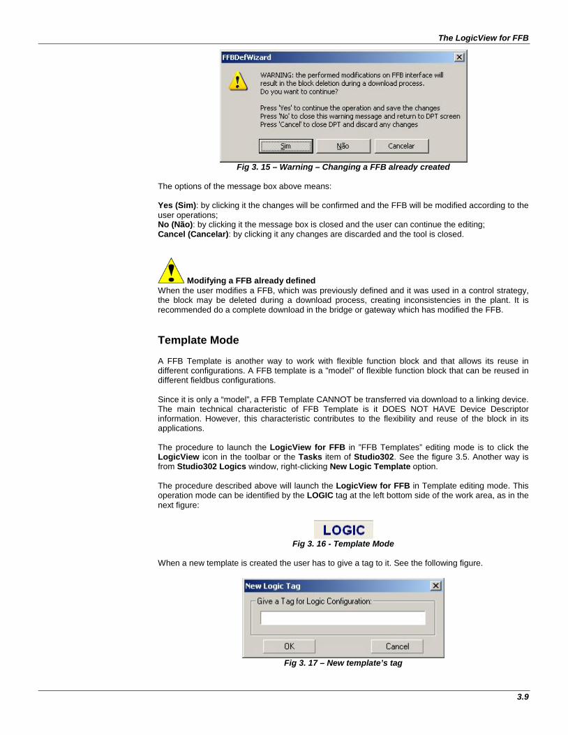
The LogicView for FFB
3.9
Fig 3. 15 – Warning – Changing a FFB already created
The options of the message box above means: Yes (Sim): by clicking it the changes will be confirmed and the FFB will be modified according to the user operations; No (Não): by clicking it the message box is closed and the user can continue the editing; Cancel (Cancelar): by clicking it any changes are discarded and the tool is closed.
Modifying a FFB already defined When the user modifies a FFB, which was previously defined and it was used in a control strategy, the block may be deleted during a download process, creating inconsistencies in the plant. It is recommended do a complete download in the bridge or gateway which has modified the FFB. Template Mode A FFB Template is another way to work with flexible function block and that allows its reuse in different configurations. A FFB template is a "model" of flexible function block that can be reused in different fieldbus configurations. Since it is only a “model”, a FFB Template CANNOT be transferred via download to a linking device. The main technical characteristic of FFB Template is it DOES NOT HAVE Device Descriptor information. However, this characteristic contributes to the flexibility and reuse of the block in its applications. The procedure to launch the LogicView for FFB in ”FFB Templates” editing mode is to click the LogicView icon in the toolbar or the Tasks item of Studio302. See the figure 3.5. Another way is from Studio302 Logics window, right-clicking New Logic Template option. The procedure described above will launch the LogicView for FFB in Template editing mode. This operation mode can be identified by the LOGIC tag at the left bottom side of the work area, as in the next figure:
Fig 3. 16 - Template Mode
When a new template is created the user has to give a tag to it. See the following figure.
Fig 3. 17 – New template’s tag
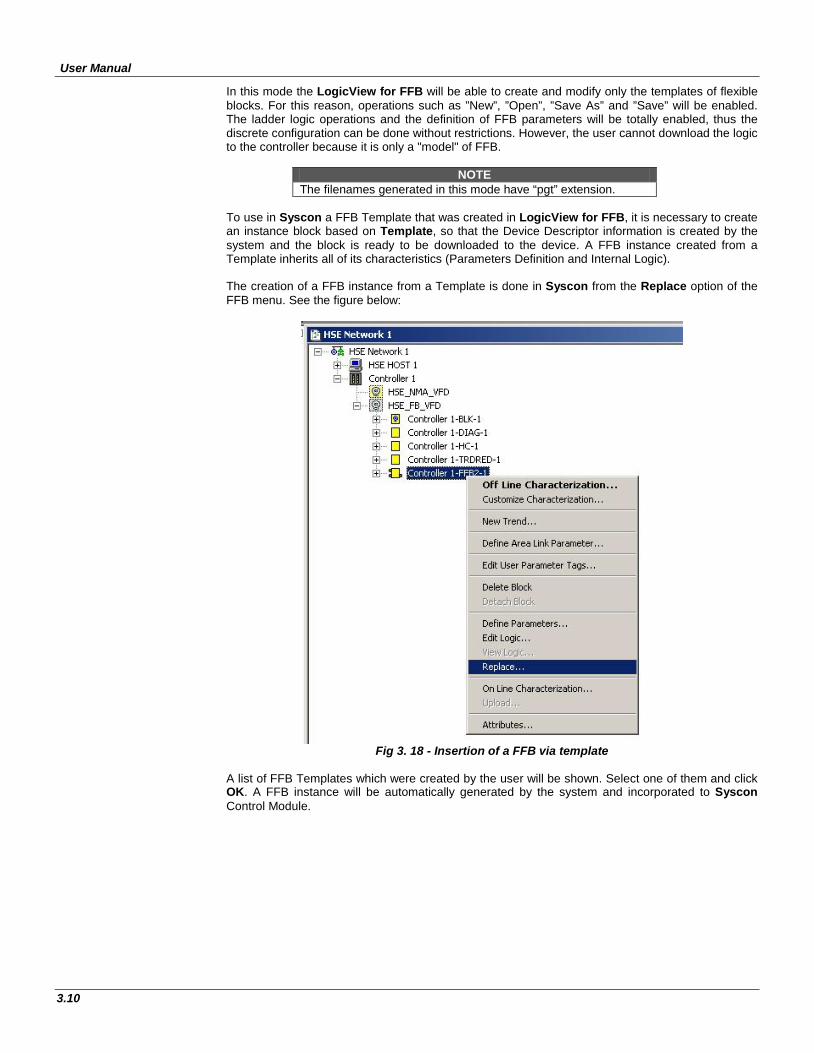
User Manual
3.10
In this mode the LogicView for FFB will be able to create and modify only the templates of flexible blocks. For this reason, operations such as ”New”, ”Open”, ”Save As” and ”Save” will be enabled. The ladder logic operations and the definition of FFB parameters will be totally enabled, thus the discrete configuration can be done without restrictions. However, the user cannot download the logic to the controller because it is only a "model" of FFB.
NOTE The filenames generated in this mode have “pgt” extension.
To use in Syscon a FFB Template that was created in LogicView for FFB, it is necessary to create an instance block based on Template, so that the Device Descriptor information is created by the system and the block is ready to be downloaded to the device. A FFB instance created from a Template inherits all of its characteristics (Parameters Definition and Internal Logic). The creation of a FFB instance from a Template is done in Syscon from the Replace option of the FFB menu. See the figure below:
Fig 3. 18 - Insertion of a FFB via template
A list of FFB Templates which were created by the user will be shown. Select one of them and click OK. A FFB instance will be automatically generated by the system and incorporated to Syscon Control Module.
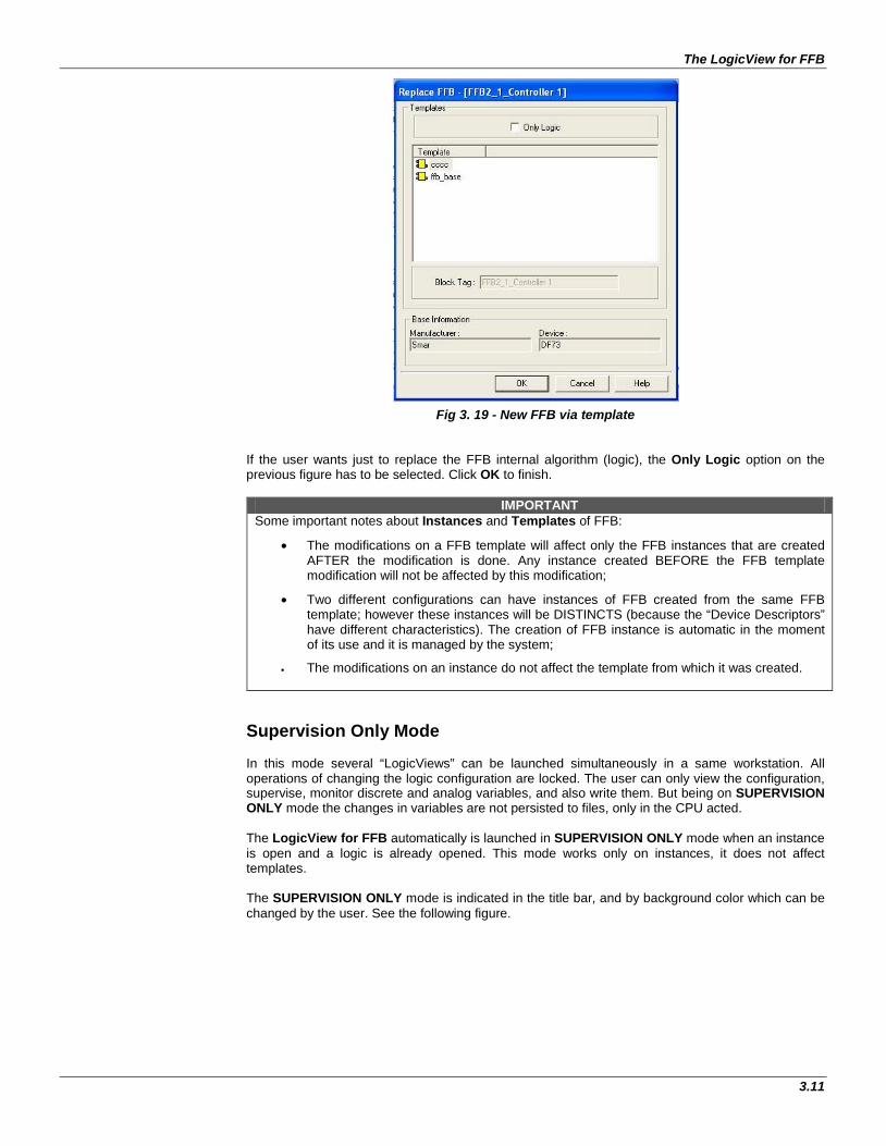
The LogicView for FFB
3.11
Fig 3. 19 - New FFB via template If the user wants just to replace the FFB internal algorithm (logic), the Only Logic option on the previous figure has to be selected. Click OK to finish.
IMPORTANT Some important notes about Instances and Templates of FFB:
• The modifications on a FFB template will affect only the FFB instances that are created AFTER the modification is done. Any instance created BEFORE the FFB template modification will not be affected by this modification;
• Two different configurations can have instances of FFB created from the same FFB template; however these instances will be DISTINCTS (because the “Device Descriptors” have different characteristics). The creation of FFB instance is automatic in the moment of its use and it is managed by the system;
• The modifications on an instance do not affect the template from which it was created.
Supervision Only Mode In this mode several “LogicViews” can be launched simultaneously in a same workstation. All operations of changing the logic configuration are locked. The user can only view the configuration, supervise, monitor discrete and analog variables, and also write them. But being on SUPERVISION ONLY mode the changes in variables are not persisted to files, only in the CPU acted. The LogicView for FFB automatically is launched in SUPERVISION ONLY mode when an instance is open and a logic is already opened. This mode works only on instances, it does not affect templates. The SUPERVISION ONLY mode is indicated in the title bar, and by background color which can be changed by the user. See the following figure.
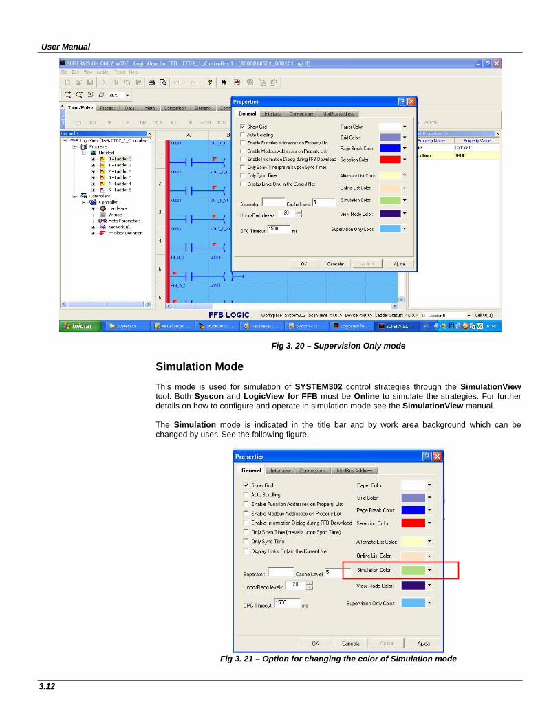
User Manual
3.12
Fig 3. 20 – Supervision Only mode Simulation Mode This mode is used for simulation of SYSTEM302 control strategies through the SimulationView tool. Both Syscon and LogicView for FFB must be Online to simulate the strategies. For further details on how to configure and operate in simulation mode see the SimulationView manual. The Simulation mode is indicated in the title bar and by work area background which can be changed by user. See the following figure.
Fig 3. 21 – Option for changing the color of Simulation mode
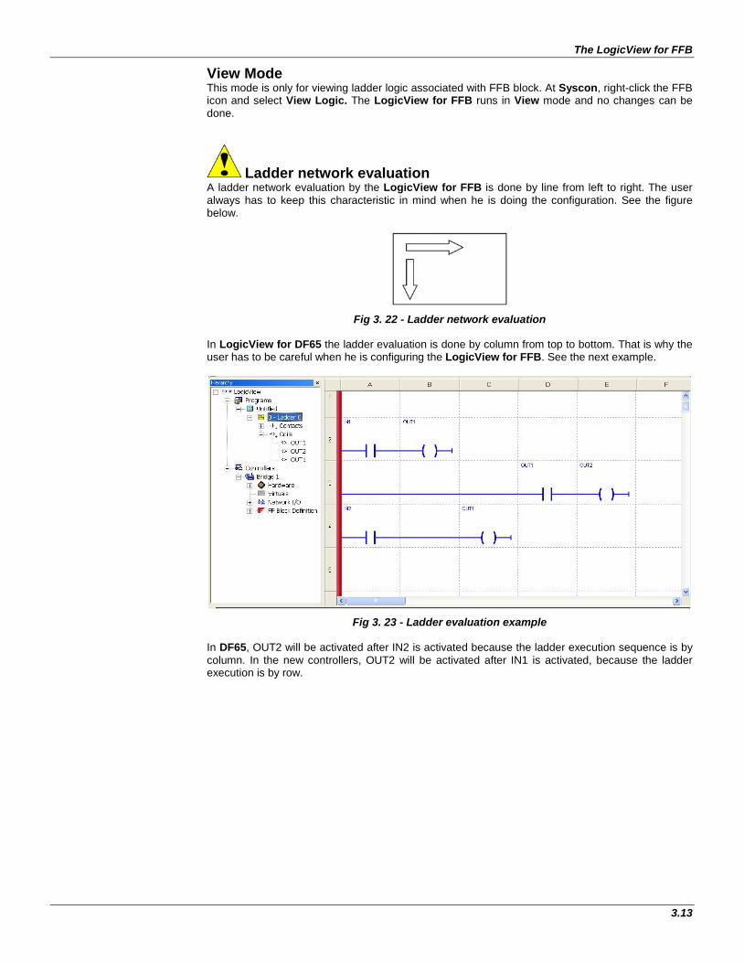
The LogicView for FFB
3.13
View Mode This mode is only for viewing ladder logic associated with FFB block. At Syscon, right-click the FFB icon and select View Logic. The LogicView for FFB runs in View mode and no changes can be done.
Ladder network evaluation A ladder network evaluation by the LogicView for FFB is done by line from left to right. The user always has to keep this characteristic in mind when he is doing the configuration. See the figure below.
Fig 3. 22 - Ladder network evaluation In LogicView for DF65 the ladder evaluation is done by column from top to bottom. That is why the user has to be careful when he is configuring the LogicView for FFB. See the next example.
Fig 3. 23 - Ladder evaluation example In DF65, OUT2 will be activated after IN2 is activated because the ladder execution sequence is by column. In the new controllers, OUT2 will be activated after IN1 is activated, because the ladder execution is by row.
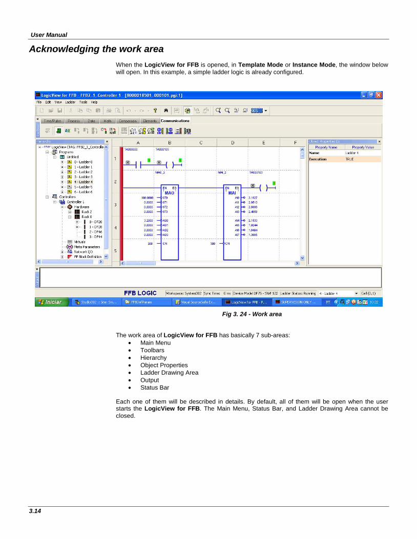
User Manual
3.14
Acknowledging the work area When the LogicView for FFB is opened, in Template Mode or Instance Mode, the window below will open. In this example, a simple ladder logic is already configured.
Fig 3. 24 - Work area The work area of LogicView for FFB has basically 7 sub-areas:
• Main Menu • Toolbars • Hierarchy • Object Properties • Ladder Drawing Area • Output • Status Bar
Each one of them will be described in details. By default, all of them will be open when the user starts the LogicView for FFB. The Main Menu, Status Bar, and Ladder Drawing Area cannot be closed.
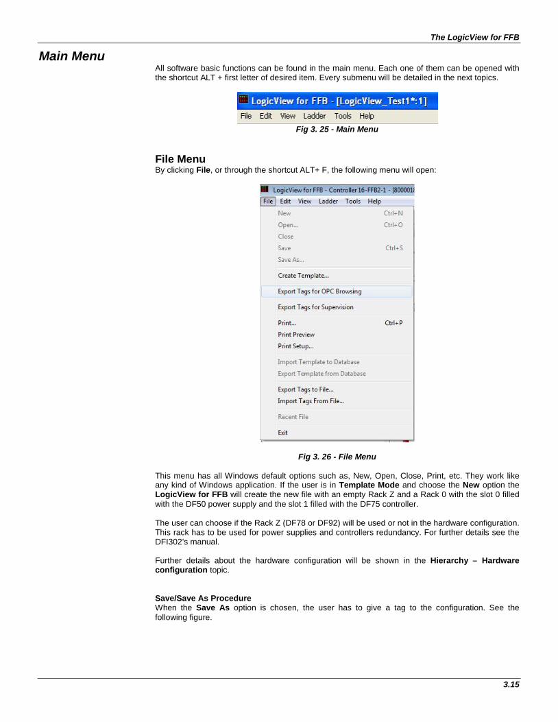
The LogicView for FFB
3.15
Main Menu All software basic functions can be found in the main menu. Each one of them can be opened with the shortcut ALT + first letter of desired item. Every submenu will be detailed in the next topics.
Fig 3. 25 - Main Menu
File Menu By clicking File, or through the shortcut ALT+ F, the following menu will open:
Fig 3. 26 - File Menu
This menu has all Windows default options such as, New, Open, Close, Print, etc. They work like any kind of Windows application. If the user is in Template Mode and choose the New option the LogicView for FFB will create the new file with an empty Rack Z and a Rack 0 with the slot 0 filled with the DF50 power supply and the slot 1 filled with the DF75 controller. The user can choose if the Rack Z (DF78 or DF92) will be used or not in the hardware configuration. This rack has to be used for power supplies and controllers redundancy. For further details see the DFI302’s manual. Further details about the hardware configuration will be shown in the Hierarchy – Hardware configuration topic. Save/Save As Procedure When the Save As option is chosen, the user has to give a tag to the configuration. See the following figure.
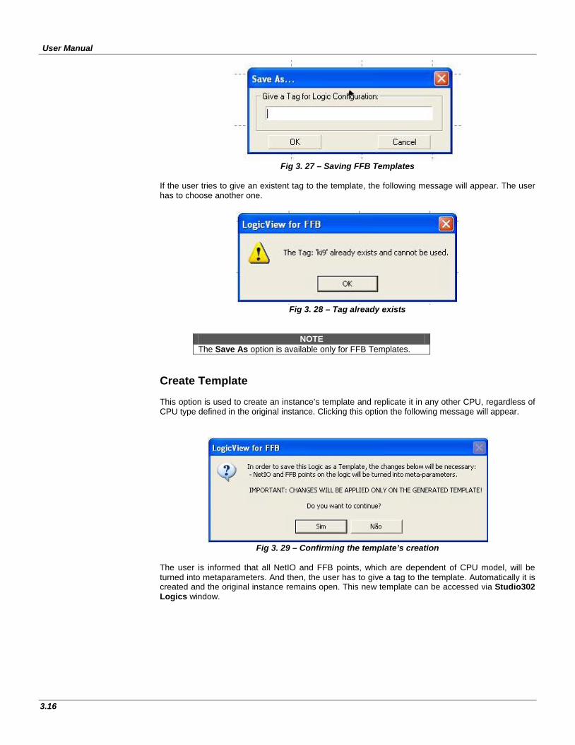
User Manual
3.16
Fig 3. 27 – Saving FFB Templates
If the user tries to give an existent tag to the template, the following message will appear. The user has to choose another one.
Fig 3. 28 – Tag already exists
NOTE The Save As option is available only for FFB Templates.
Create Template This option is used to create an instance’s template and replicate it in any other CPU, regardless of CPU type defined in the original instance. Clicking this option the following message will appear.
Fig 3. 29 – Confirming the template’s creation
The user is informed that all NetIO and FFB points, which are dependent of CPU model, will be turned into metaparameters. And then, the user has to give a tag to the template. Automatically it is created and the original instance remains open. This new template can be accessed via Studio302 Logics window.
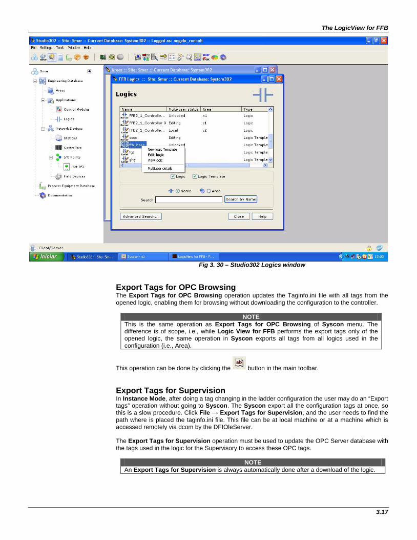
The LogicView for FFB
3.17
Fig 3. 30 – Studio302 Logics window
Export Tags for OPC Browsing The Export Tags for OPC Browsing operation updates the Taginfo.ini file with all tags from the opened logic, enabling them for browsing without downloading the configuration to the controller.
NOTE This is the same operation as Export Tags for OPC Browsing of Syscon menu. The difference is of scope, i.e., while Logic View for FFB performs the export tags only of the opened logic, the same operation in Syscon exports all tags from all logics used in the configuration (i.e., Area).
This operation can be done by clicking the button in the main toolbar. Export Tags for Supervision In Instance Mode, after doing a tag changing in the ladder configuration the user may do an “Export tags” operation without going to Syscon. The Syscon export all the configuration tags at once, so this is a slow procedure. Click File → Export Tags for Supervision, and the user needs to find the path where is placed the taginfo.ini file. This file can be at local machine or at a machine which is accessed remotely via dcom by the DFIOleServer. The Export Tags for Supervision operation must be used to update the OPC Server database with the tags used in the logic for the Supervisory to access these OPC tags.
NOTE An Export Tags for Supervision is always automatically done after a download of the logic.
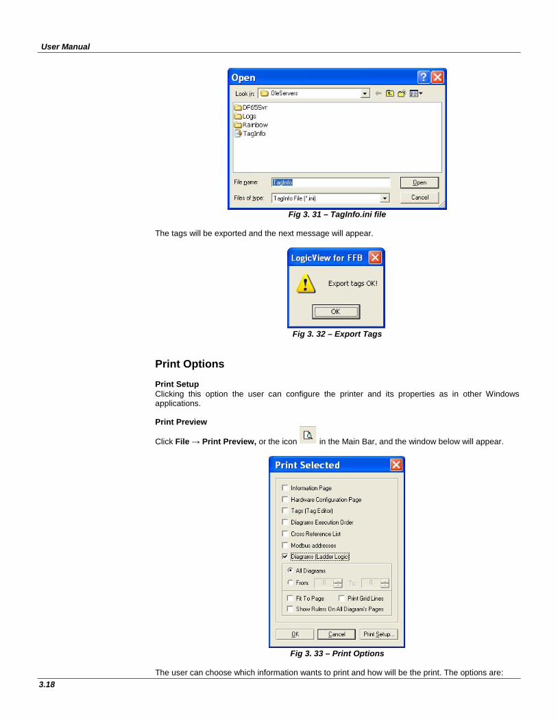
User Manual
3.18
Fig 3. 31 – TagInfo.ini file
The tags will be exported and the next message will appear.
Fig 3. 32 – Export Tags
Print Options Print Setup Clicking this option the user can configure the printer and its properties as in other Windows applications. Print Preview
Click File → Print Preview, or the icon in the Main Bar, and the window below will appear.
Fig 3. 33 – Print Options
The user can choose which information wants to print and how will be the print. The options are:
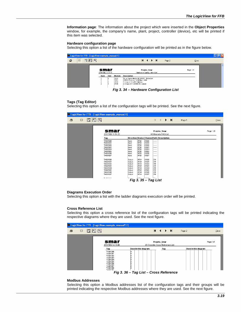
The LogicView for FFB
3.19
Information page: The information about the project which were inserted in the Object Properties window, for example, the company’s name, plant, project, controller (device), etc will be printed if this item was selected. Hardware configuration page Selecting this option a list of the hardware configuration will be printed as in the figure below.
Fig 3. 34 – Hardware Configuration List
Tags (Tag Editor) Selecting this option a list of the configuration tags will be printed. See the next figure.
Fig 3. 35 – Tag List
Diagrams Execution Order Selecting this option a list with the ladder diagrams execution order will be printed. Cross Reference List Selecting this option a cross reference list of the configuration tags will be printed indicating the respective diagrams where they are used. See the next figure.
Fig 3. 36 – Tag List – Cross Reference
Modbus Addresses Selecting this option a Modbus addresses list of the configuration tags and their groups will be printed indicating the respective Modbus addresses where they are used. See the next figure.
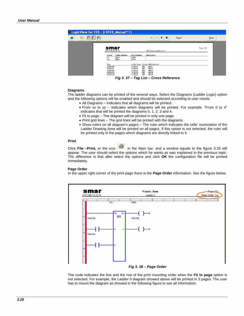
User Manual
3.20
Fig 3. 37 – Tag List – Cross Reference
Diagrams The ladder diagrams can be printed of the several ways. Select the Diagrams (Ladder Logic) option and the following options will be enabled and should be selected according to user needs:
• All Diagrams – Indicates that all diagrams will be printed. • From xx to yy – Indicates which diagrams will be printed. For example, “From 0 to 4” indicates that will be printed the diagrams 0, 1, 2, 3 and 4.
• Fit to page – The diagram will be printed in only one page. • Print grid lines – The grid lines will be printed with the diagrams. • Show rulers on all diagram’s pages – The ruler which indicates the cells’ numeration of the Ladder Drawing Area will be printed on all pages. If this option is not selected, the ruler will be printed only in the pages which diagrams are directly linked to it.
Click File→Print, or the icon in the Main bar, and a window equals to the figure 3.33 will appear. The user should select the options which he wants as was explained in the previous topic. The difference is that after select the options and click OK the configuration file will be printed immediately. Page Order In the upper right corner of the print page there is the Page Order information. See the figure below.
Fig 3. 38 – Page Order
The code indicates the line and the row of the print mounting order when the Fit to page option is not selected. For example, the Ladder 0 diagram showed above will be printed in 3 pages. The user has to mount the diagram as showed in the following figure to see all information:
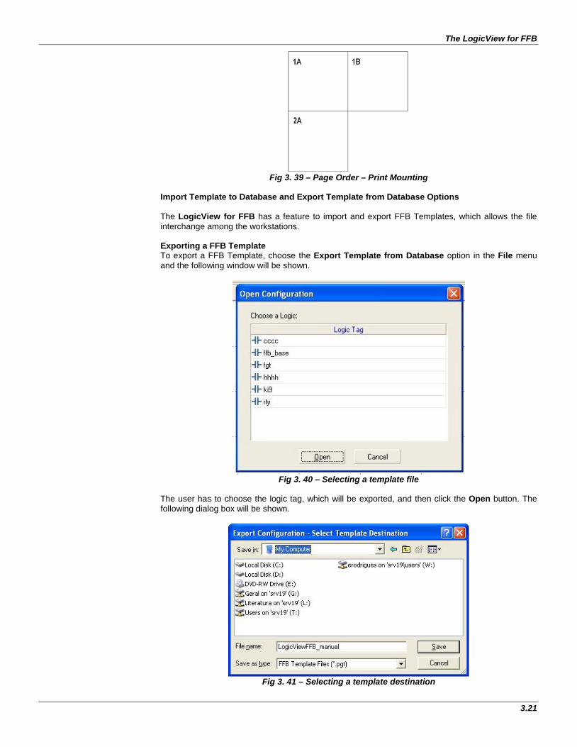
The LogicView for FFB
3.21
Fig 3. 39 – Page Order – Print Mounting
Import Template to Database and Export Template from Database Options The LogicView for FFB has a feature to import and export FFB Templates, which allows the file interchange among the workstations. Exporting a FFB Template To export a FFB Template, choose the Export Template from Database option in the File menu and the following window will be shown.
Fig 3. 40 – Selecting a template file
The user has to choose the logic tag, which will be exported, and then click the Open button. The following dialog box will be shown.
Fig 3. 41 – Selecting a template destination
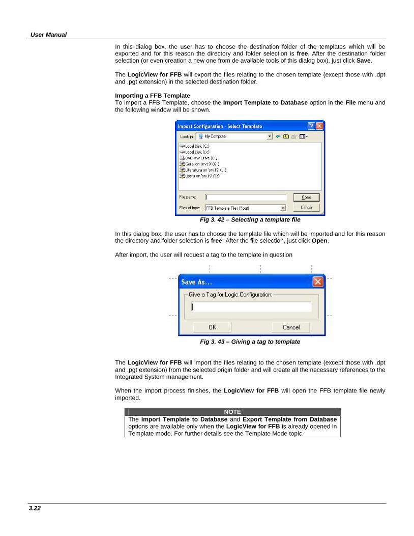
User Manual
3.22
In this dialog box, the user has to choose the destination folder of the templates which will be exported and for this reason the directory and folder selection is free. After the destination folder selection (or even creation a new one from de available tools of this dialog box), just click Save. The LogicView for FFB will export the files relating to the chosen template (except those with .dpt and .pgt extension) in the selected destination folder. Importing a FFB Template To import a FFB Template, choose the Import Template to Database option in the File menu and the following window will be shown.
Fig 3. 42 – Selecting a template file
In this dialog box, the user has to choose the template file which will be imported and for this reason the directory and folder selection is free. After the file selection, just click Open. After import, the user will request a tag to the template in question
Fig 3. 43 – Giving a tag to template
The LogicView for FFB will import the files relating to the chosen template (except those with .dpt and .pgt extension) from the selected origin folder and will create all the necessary references to the Integrated System management. When the import process finishes, the LogicView for FFB will open the FFB template file newly imported.
NOTE The Import Template to Database and Export Template from Database options are available only when the LogicView for FFB is already opened in Template mode. For further details see the Template Mode topic.
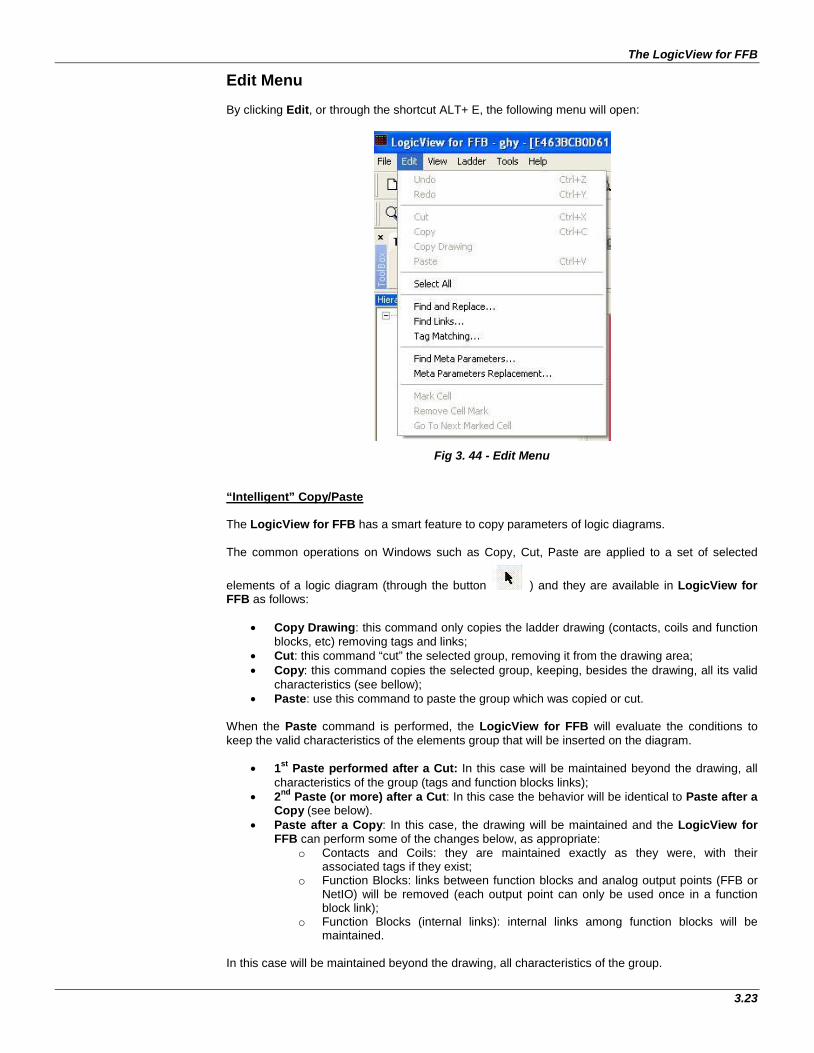
The LogicView for FFB
3.23
Edit Menu By clicking Edit, or through the shortcut ALT+ E, the following menu will open:
Fig 3. 44 - Edit Menu “Intelligent” Copy/Paste The LogicView for FFB has a smart feature to copy parameters of logic diagrams. The common operations on Windows such as Copy, Cut, Paste are applied to a set of selected
elements of a logic diagram (through the button ) and they are available in LogicView for FFB as follows:
• Copy Drawing: this command only copies the ladder drawing (contacts, coils and function blocks, etc) removing tags and links;
• Cut: this command “cut” the selected group, removing it from the drawing area; • Copy: this command copies the selected group, keeping, besides the drawing, all its valid
characteristics (see bellow); • Paste: use this command to paste the group which was copied or cut.
When the Paste command is performed, the LogicView for FFB will evaluate the conditions to keep the valid characteristics of the elements group that will be inserted on the diagram.
• 1st Paste performed after a Cut: In this case will be maintained beyond the drawing, all characteristics of the group (tags and function blocks links);
• 2nd Paste (or more) after a Cut: In this case the behavior will be identical to Paste after a Copy (see below).
• Paste after a Copy: In this case, the drawing will be maintained and the LogicView for FFB can perform some of the changes below, as appropriate:
o Contacts and Coils: they are maintained exactly as they were, with their associated tags if they exist;
o Function Blocks: links between function blocks and analog output points (FFB or NetIO) will be removed (each output point can only be used once in a function block link);
o Function Blocks (internal links): internal links among function blocks will be maintained.
In this case will be maintained beyond the drawing, all characteristics of the group.
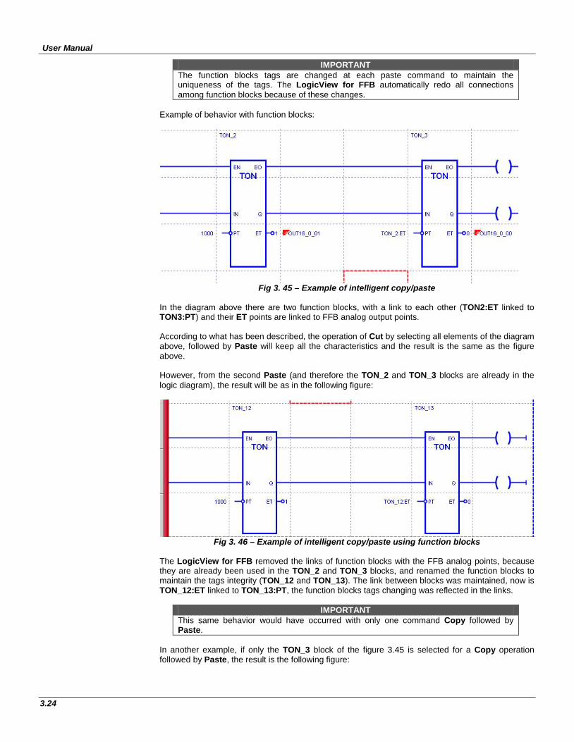
User Manual
3.24
IMPORTANT The function blocks tags are changed at each paste command to maintain the uniqueness of the tags. The LogicView for FFB automatically redo all connections among function blocks because of these changes.
Example of behavior with function blocks:
Fig 3. 45 – Example of intelligent copy/paste
In the diagram above there are two function blocks, with a link to each other (TON2:ET linked to TON3:PT) and their ET points are linked to FFB analog output points. According to what has been described, the operation of Cut by selecting all elements of the diagram above, followed by Paste will keep all the characteristics and the result is the same as the figure above. However, from the second Paste (and therefore the TON_2 and TON_3 blocks are already in the logic diagram), the result will be as in the following figure:
Fig 3. 46 – Example of intelligent copy/paste using function blocks
The LogicView for FFB removed the links of function blocks with the FFB analog points, because they are already been used in the TON_2 and TON_3 blocks, and renamed the function blocks to maintain the tags integrity (TON_12 and TON_13). The link between blocks was maintained, now is TON_12:ET linked to TON_13:PT, the function blocks tags changing was reflected in the links.
IMPORTANT This same behavior would have occurred with only one command Copy followed by Paste.
In another example, if only the TON_3 block of the figure 3.45 is selected for a Copy operation followed by Paste, the result is the following figure:
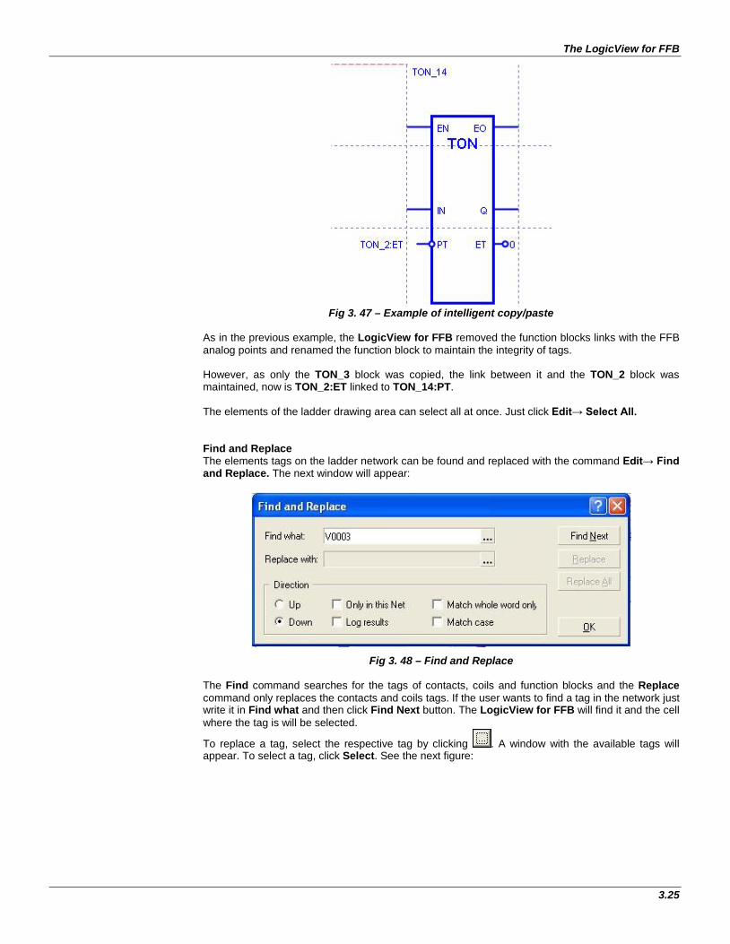
The LogicView for FFB
3.25
Fig 3. 47 – Example of intelligent copy/paste
As in the previous example, the LogicView for FFB removed the function blocks links with the FFB analog points and renamed the function block to maintain the integrity of tags. However, as only the TON_3 block was copied, the link between it and the TON_2 block was maintained, now is TON_2:ET linked to TON_14:PT. The elements of the ladder drawing area can select all at once. Just click Edit→ Select All. Find and Replace The elements tags on the ladder network can be found and replaced with the command Edit→ Find and Replace. The next window will appear:
Fig 3. 48 – Find and Replace The Find command searches for the tags of contacts, coils and function blocks and the Replace command only replaces the contacts and coils tags. If the user wants to find a tag in the network just write it in Find what and then click Find Next button. The LogicView for FFB will find it and the cell where the tag is will be selected.
To replace a tag, select the respective tag by clicking . A window with the available tags will appear. To select a tag, click Select. See the next figure:
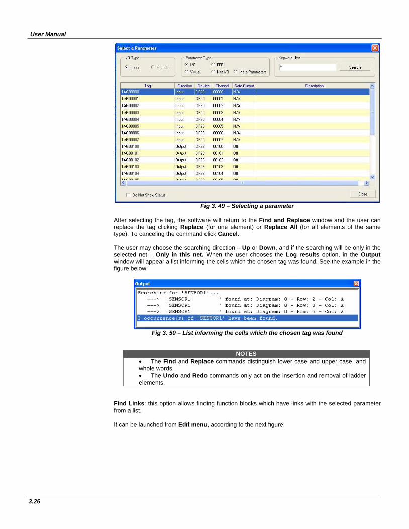
User Manual
3.26
Fig 3. 49 – Selecting a parameter
After selecting the tag, the software will return to the Find and Replace window and the user can replace the tag clicking Replace (for one element) or Replace All (for all elements of the same type). To canceling the command click Cancel. The user may choose the searching direction – Up or Down, and if the searching will be only in the selected net – Only in this net. When the user chooses the Log results option, in the Output window will appear a list informing the cells which the chosen tag was found. See the example in the figure below:
Fig 3. 50 – List informing the cells which the chosen tag was found
NOTES • The Find and Replace commands distinguish lower case and upper case, and whole words. • The Undo and Redo commands only act on the insertion and removal of ladder elements.
Find Links: this option allows finding function blocks which have links with the selected parameter from a list. It can be launched from Edit menu, according to the next figure:
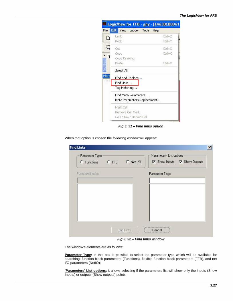
The LogicView for FFB
3.27
Fig 3. 51 – Find links option
When that option is chosen the following window will appear:
Fig 3. 52 – Find links window
The window’s elements are as follows: Parameter Type: in this box is possible to select the parameter type which will be available for searching: function block parameters (Functions), flexible function block parameters (FFB), and net I/O parameters (NetIO); 'Parameters' List options: it allows selecting if the parameters list will show only the inputs (Show Inputs) or outputs (Show outputs) points;
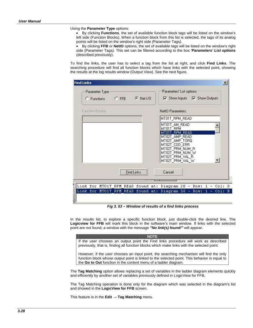
User Manual
3.28
Using the Parameter Type options: • By clicking Functions, the set of available function block tags will be listed on the window’s left side (Function Blocks). When a function block from this list is selected, the tags of its analog points will be listed on the window’s right side (Parameter Tags). • By clicking FFB or NetIO options, the set of available tags will be listed on the window’s right side (Parameter Tags). This set can be filtered according to the box 'Parameters' List options (described previously).
To find the links, the user has to select a tag from the list at right, and click Find Links. The searching procedure will find all function blocks which have links with the selected point, showing the results at the log results window (Output View). See the next figure.
Fig 3. 53 – Window of results of a find links process
In the results list, to explore a specific function block, just double-click the desired line. The Logicview for FFB will mark this block in the software’s main window. If links with the selected point are not found, a window with the message "No link(s) found!" will appear.
NOTE If the user chooses an output point the Find links procedure will work as described previously, that is, finding all function blocks which make links with the selected point. However, if the user chooses an input point, the searching mechanism will find the only function block whose output point is linked to the selected point. This behavior is equal to the Go to Out function in the context menu of a ladder diagram.
The Tag Matching option allows replacing a set of variables in the ladder diagram elements quickly and efficiently by another set of variables previously defined in LogicView for FFB. The Tag Matching operation is done only for the diagram which was selected in the diagram’s list and showed in the LogicView for FFB screen. This feature is in the Edit → Tag Matching menu.
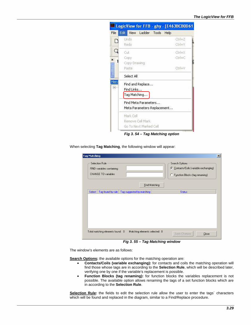
The LogicView for FFB
3.29
Fig 3. 54 – Tag Matching option
When selecting Tag Matching, the following window will appear:
Fig 3. 55 – Tag Matching window
The window’s elements are as follows: Search Options: the available options for the matching operation are:
• Contacts/Coils (variable exchanging): for contacts and coils the matching operation will find those whose tags are in according to the Selection Rule, which will be described later, verifying one by one if the variable’s replacement is possible.
• Function Blocks (tag renaming): for function blocks the variables replacement is not possible. The available option allows renaming the tags of a set function blocks which are in according to the Selection Rule.
Selection Rule: the fields to edit the selection rule allow the user to enter the tags´ characters which will be found and replaced in the diagram, similar to a Find/Replace procedure.
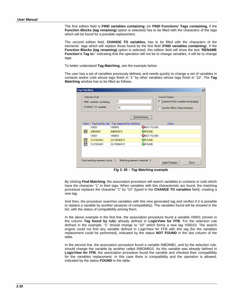
User Manual
3.30
The first edition field is FIND variables containing: (or FIND Functions’ Tags containing, if the Function Blocks (tag renaming) option is selected) has to be filled with the characters of the tags which will be found for a possible replacement. The second edition field, CHANGE TO variables, has to be filled with the characters of the elements´ tags which will replace those found by the first field (FIND variables containing). If the Function Blocks (tag renaming) option is selected, this edition field will show the text “RENAME Function’s Tag to:” indicating that the operation will not be to change variables, it will be to change tags. To better understand Tag Matching, see the example below. The user has a set of variables previously defined, and needs quickly to change a set of variables in contacts and/or coils whose tags finish in “1” by other variables whose tags finish in “10”. The Tag Matching window has to be filled as follows.
Fig 3. 56 – Tag Matching example
By clicking Find Matching, the association procedure will search variables in contacts or coils which have the character “1” in their tags. When variables with this characteristic are found, the matching procedure replaces the character “1” by “10” (typed in the CHANGE TO variables field), creating a new tag. And then, the procedure searches variables with this new generated tag and verifies if it is possible to replace a variable by another (analysis of compatibility). The variables found will be showed in the list, with the status of compatibility among them. In the above example in the first line, the association procedure found a variable V0001 (shown in the column Tag found by rule) already defined in LogicView for FFB. For the selection rule defined in the example, “1” should change to “10” which forms a new tag V00010. The search engine could not find any variable defined in LogicView for FFB with this tag (for the variables replacement could be performed), indicated by the status NOT FOUND in the last column of the table. In the second line, the association procedure found a variable INBOMB1, and by the selection rule, should change the variable by another called INBOMB10. As this variable was already defined in LogicView for FFB, the association procedure found the variable and checked their compatibility for the variables replacement. In this case there is compatibility and the operation is allowed, indicated by the status FOUND in the table.
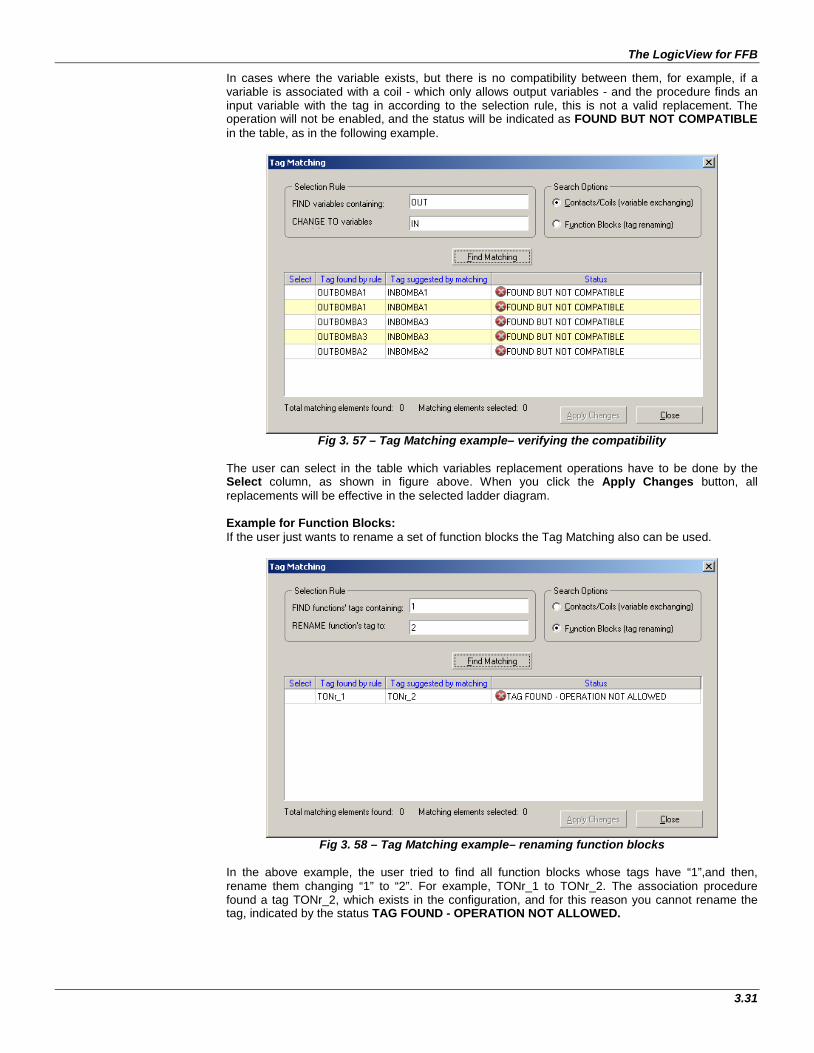
The LogicView for FFB
3.31
In cases where the variable exists, but there is no compatibility between them, for example, if a variable is associated with a coil - which only allows output variables - and the procedure finds an input variable with the tag in according to the selection rule, this is not a valid replacement. The operation will not be enabled, and the status will be indicated as FOUND BUT NOT COMPATIBLE in the table, as in the following example.
Fig 3. 57 – Tag Matching example– verifying the compatibility
The user can select in the table which variables replacement operations have to be done by the Select column, as shown in figure above. When you click the Apply Changes button, all replacements will be effective in the selected ladder diagram. Example for Function Blocks: If the user just wants to rename a set of function blocks the Tag Matching also can be used.
Fig 3. 58 – Tag Matching example– renaming function blocks
In the above example, the user tried to find all function blocks whose tags have “1”,and then, rename them changing “1” to “2”. For example, TONr_1 to TONr_2. The association procedure found a tag TONr_2, which exists in the configuration, and for this reason you cannot rename the tag, indicated by the status TAG FOUND - OPERATION NOT ALLOWED.
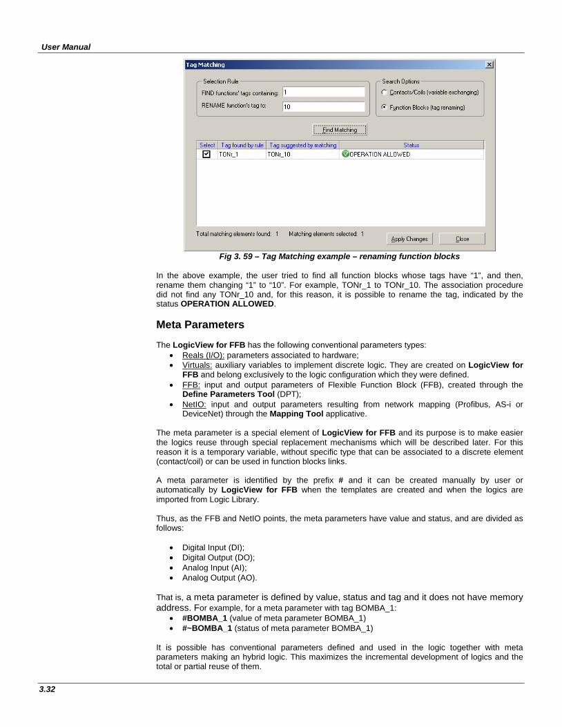
User Manual
3.32
Fig 3. 59 – Tag Matching example – renaming function blocks
In the above example, the user tried to find all function blocks whose tags have “1”, and then, rename them changing “1” to “10”. For example, TONr_1 to TONr_10. The association procedure did not find any TONr_10 and, for this reason, it is possible to rename the tag, indicated by the status OPERATION ALLOWED. Meta Parameters The LogicView for FFB has the following conventional parameters types:
• Reals (I/O): parameters associated to hardware; • Virtuals: auxiliary variables to implement discrete logic. They are created on LogicView for
FFB and belong exclusively to the logic configuration which they were defined. • FFB: input and output parameters of Flexible Function Block (FFB), created through the
Define Parameters Tool (DPT); • NetIO: input and output parameters resulting from network mapping (Profibus, AS-i or
DeviceNet) through the Mapping Tool applicative. The meta parameter is a special element of LogicView for FFB and its purpose is to make easier the logics reuse through special replacement mechanisms which will be described later. For this reason it is a temporary variable, without specific type that can be associated to a discrete element (contact/coil) or can be used in function blocks links. A meta parameter is identified by the prefix # and it can be created manually by user or automatically by LogicView for FFB when the templates are created and when the logics are imported from Logic Library. Thus, as the FFB and NetIO points, the meta parameters have value and status, and are divided as follows:
• Digital Input (DI); • Digital Output (DO); • Analog Input (AI); • Analog Output (AO).
That is, a meta parameter is defined by value, status and tag and it does not have memory address. For example, for a meta parameter with tag BOMBA_1:
• #BOMBA_1 (value of meta parameter BOMBA_1) • #~BOMBA_1 (status of meta parameter BOMBA_1)
It is possible has conventional parameters defined and used in the logic together with meta parameters making an hybrid logic. This maximizes the incremental development of logics and the total or partial reuse of them.
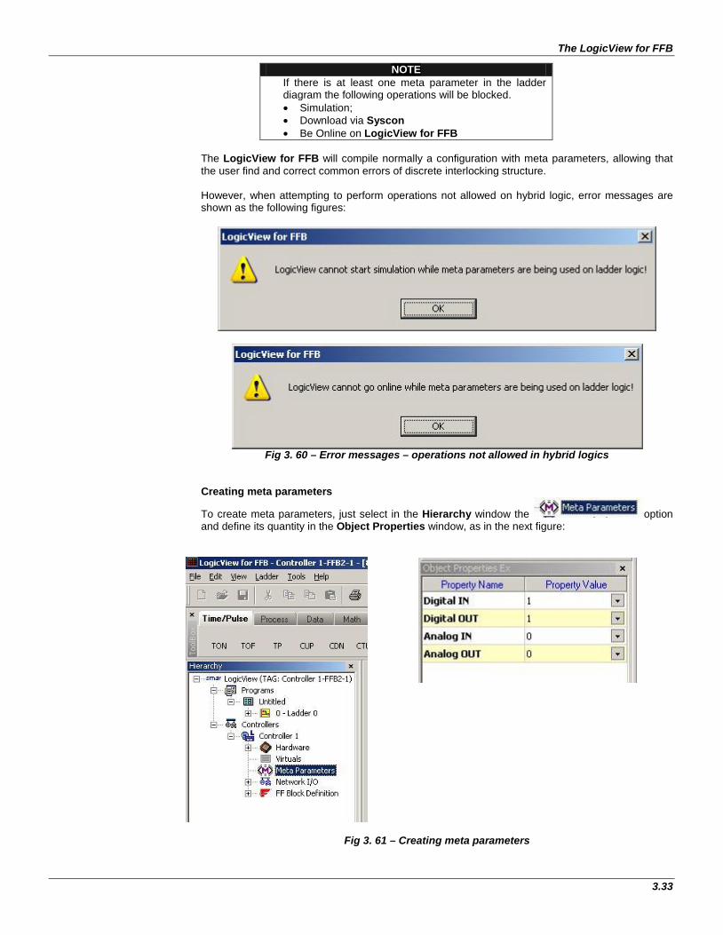
The LogicView for FFB
3.33
NOTE If there is at least one meta parameter in the ladder diagram the following operations will be blocked. • Simulation; • Download via Syscon • Be Online on LogicView for FFB
The LogicView for FFB will compile normally a configuration with meta parameters, allowing that the user find and correct common errors of discrete interlocking structure. However, when attempting to perform operations not allowed on hybrid logic, error messages are shown as the following figures:
Fig 3. 60 – Error messages – operations not allowed in hybrid logics
Creating meta parameters
To create meta parameters, just select in the Hierarchy window the option and define its quantity in the Object Properties window, as in the next figure:
Fig 3. 61 – Creating meta parameters
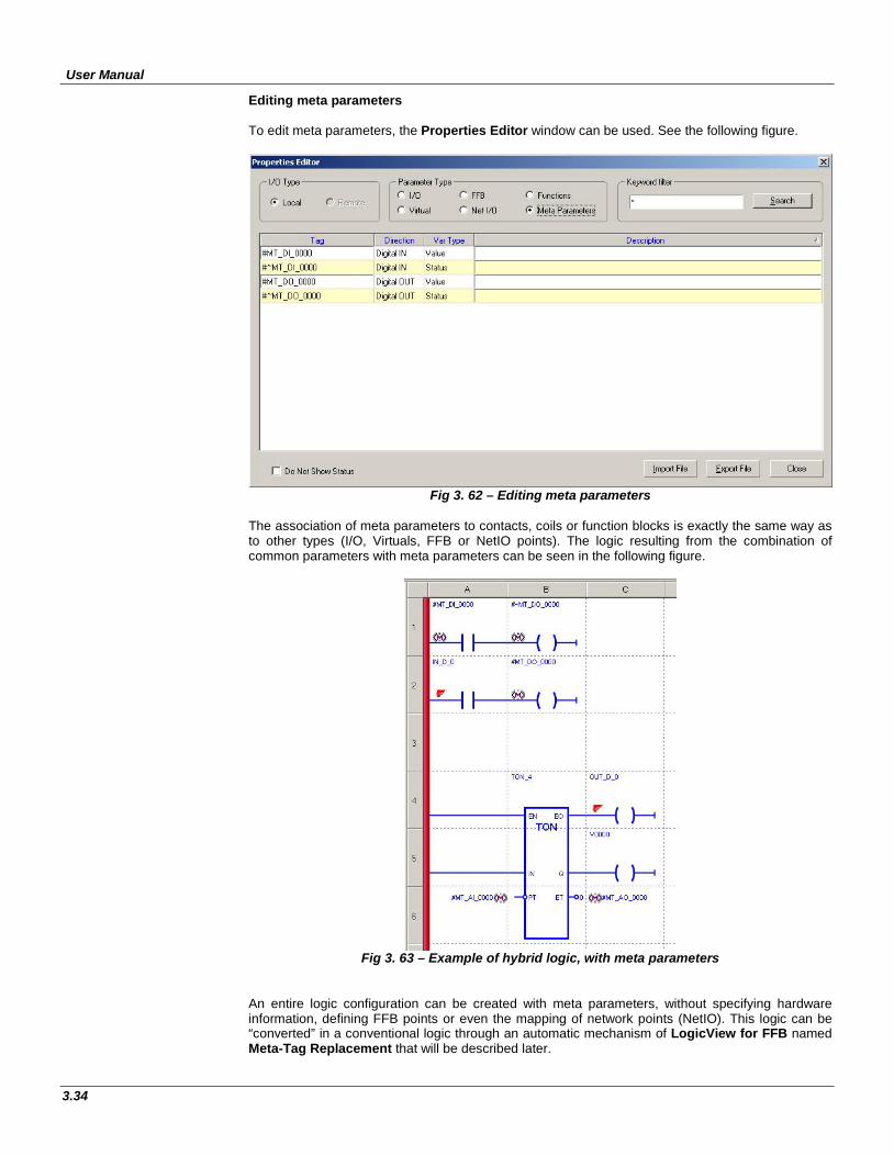
User Manual
3.34
Editing meta parameters To edit meta parameters, the Properties Editor window can be used. See the following figure.
Fig 3. 62 – Editing meta parameters
The association of meta parameters to contacts, coils or function blocks is exactly the same way as to other types (I/O, Virtuals, FFB or NetIO points). The logic resulting from the combination of common parameters with meta parameters can be seen in the following figure.
Fig 3. 63 – Example of hybrid logic, with meta parameters
An entire logic configuration can be created with meta parameters, without specifying hardware information, defining FFB points or even the mapping of network points (NetIO). This logic can be “converted” in a conventional logic through an automatic mechanism of LogicView for FFB named Meta-Tag Replacement that will be described later.
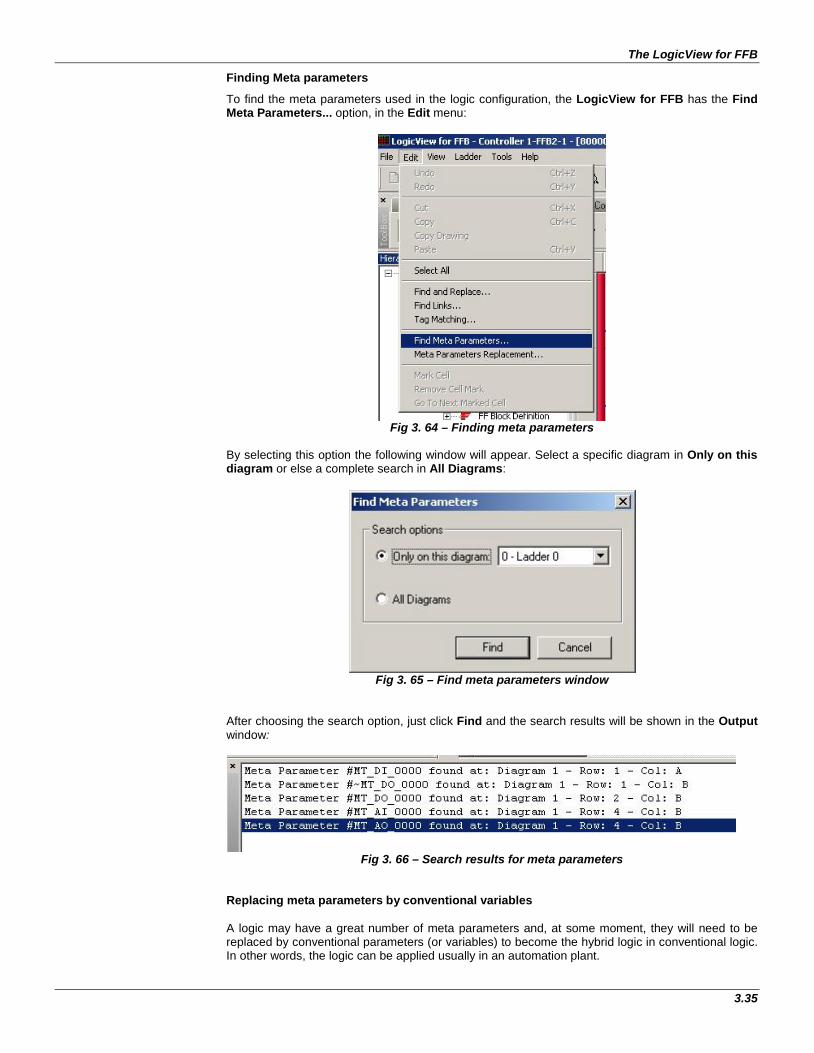
The LogicView for FFB
3.35
Finding Meta parameters
To find the meta parameters used in the logic configuration, the LogicView for FFB has the Find Meta Parameters... option, in the Edit menu:
Fig 3. 64 – Finding meta parameters
By selecting this option the following window will appear. Select a specific diagram in Only on this diagram or else a complete search in All Diagrams:
Fig 3. 65 – Find meta parameters window
After choosing the search option, just click Find and the search results will be shown in the Output window:
Fig 3. 66 – Search results for meta parameters
Replacing meta parameters by conventional variables A logic may have a great number of meta parameters and, at some moment, they will need to be replaced by conventional parameters (or variables) to become the hybrid logic in conventional logic. In other words, the logic can be applied usually in an automation plant.
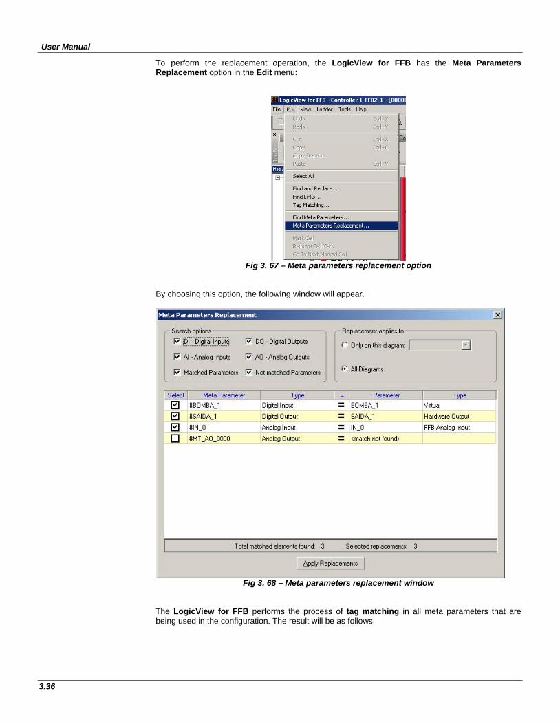
User Manual
3.36
To perform the replacement operation, the LogicView for FFB has the Meta Parameters Replacement option in the Edit menu:
Fig 3. 67 – Meta parameters replacement option
By choosing this option, the following window will appear.
Fig 3. 68 – Meta parameters replacement window
The LogicView for FFB performs the process of tag matching in all meta parameters that are being used in the configuration. The result will be as follows:

The LogicView for FFB
3.37
• Matched Parameters: They are variables (I/O, Virtuals, FFB or NetIO) whose tags are equivalents to the meta parameters tags. In the previous example, "#BOMBA_1" and "BOMBA_1" are equivalent tags. Besides the tags matching, an evaluation of type compatibility, between the meta parameter and the equivalent variable, is performed. For example, if the tags match, but the meta parameter is AI type while the corresponding variable is DO type, the replacement is not valid. When the types are compatible and the tags match, the table is automatically filled with a replacement “suggestion”.
• Not Matched Parameters: When the LogicView for FFB does not find a conventional
variable that can be suggested on the table, because it does not find a tag matching or because the variables are not compatible, the message <match not found> will be shown in the Parameter table column.
In this window also are available the following options:
• Search Options: it has the search options of the meta parameters that will be shown on the table: DI, DO, AI or AO;
• Matched Parameters: shows only the meta parameters that have a corresponding variable for replacement;
• Not Matched Parameters: shows only the meta parameters that does not have a corresponding variable for replacement;
• Replacement Applies to: this box allows choosing if the meta parameters replacement by conventional parameters will be applied to all logic diagrams or to a specific diagram.
The table columns have the following meaning:
• Select: Allows selecting or not the meta parameter for replacement in the logic configuration. Those that do not have an attributed conventional variable for replacement cannot be selected on this column.
• Meta Parameter: shows the meta parameters tags used in the logic configuration; • Type: identifies the meta parameter type (DI, DO, AI, AO); • Parameter: shows the conventional parameter tags that will replace the corresponding meta
parameters; • Type: identifies the conventional parameter type (Virtual, Hardware, FFB DI, etc).
On the table, the user can still make the choice of the conventional parameter that will replace the meta parameter in the logic. Therefore, either the suggestion offered by LogicView for FFB can be changed or fill the attributions whose status is <match not found>. To choose a variable just right-click the desired table line and choose Assign a parameter...option:
Fig 3. 69 – Meta parameters manual attribution
By clicking Assign a parameter..., the variable selection window will appear:
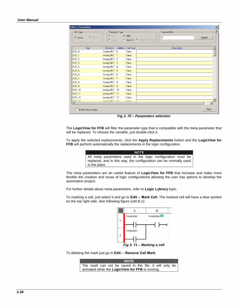
User Manual
3.38
Fig 3. 70 – Parameters selection
The LogicView for FFB will filter the parameter type that is compatible with the meta parameter that will be replaced. To choose the variable, just double-click it. To apply the selected replacements, click the Apply Replacements button and the LogicView for FFB will perform automatically the replacements in the logic configuration.
NOTE All meta parameters used in the logic configuration must be replaced, and in this way, the configuration can be normally used in the plant.
The meta parameters are an useful feature of LogicView for FFB that increase and make more flexible the creation and reuse of logic configurations allowing the user has options to develop the automation project. For further details about meta parameters, refer to Logic Lybrary topic. To marking a cell, just select it and go to Edit→ Mark Cell. The marked cell will have a blue symbol on the top right side. See following figure (cell B,1):
Fig 3. 71 – Marking a cell
To deleting the mark just go in Edit→ Remove Cell Mark.
NOTE The mark can not be saved in the file; it will only be activated while the LogicView for FFB is running.
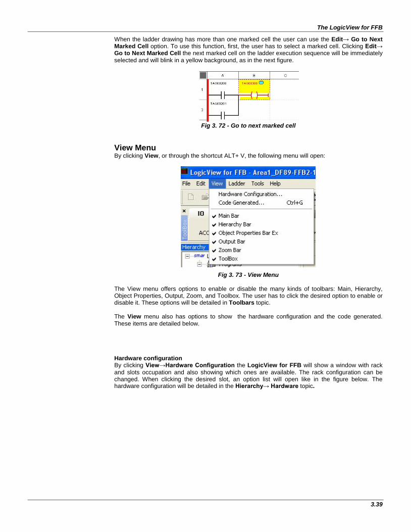
The LogicView for FFB
3.39
When the ladder drawing has more than one marked cell the user can use the Edit→ Go to Next Marked Cell option. To use this function, first, the user has to select a marked cell. Clicking Edit→ Go to Next Marked Cell the next marked cell on the ladder execution sequence will be immediately selected and will blink in a yellow background, as in the next figure.
Fig 3. 72 - Go to next marked cell
View Menu By clicking View, or through the shortcut ALT+ V, the following menu will open:
Fig 3. 73 - View Menu
The View menu offers options to enable or disable the many kinds of toolbars: Main, Hierarchy, Object Properties, Output, Zoom, and Toolbox. The user has to click the desired option to enable or disable it. These options will be detailed in Toolbars topic. The View menu also has options to show the hardware configuration and the code generated. These items are detailed below.
Hardware configuration By clicking View→Hardware Configuration the LogicView for FFB will show a window with rack and slots occupation and also showing which ones are available. The rack configuration can be changed. When clicking the desired slot, an option list will open like in the figure below. The hardware configuration will be detailed in the Hierarchy→ Hardware topic.
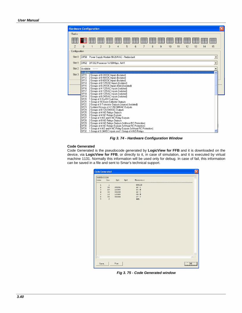
User Manual
3.40
Fig 3. 74 - Hardware Configuration Window Code Generated Code Generated is the pseudocode generated by LogicView for FFB and it is downloaded on the device, via LogicView for FFB, or directly to it, in case of simulation, and it is executed by virtual machine 1131. Normally this information will be used only for debug. In case of fail, this information can be saved in a file and sent to Smar’s technical support.
Fig 3. 75 - Code Generated window
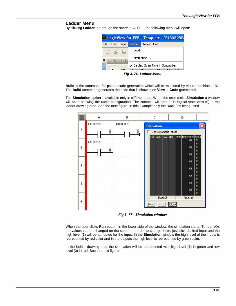
The LogicView for FFB
3.41
Ladder Menu By clicking Ladder, or through the shortcut ALT+ L, the following menu will open:
Fig 3. 76- Ladder Menu Build is the command for pseudocode generation which will be executed by virtual machine 1131. The Build command generates the code that is showed on View→ Code generated. The Simulation option is available only in offline mode. When the user clicks Simulation a window will open showing the racks configuration. The contacts will appear in logical state zero (0) in the ladder drawing area. See the next figure. In this example only the Rack 0 is being used.
Fig 3. 77 - Simulation window When the user clicks Run button, in the lower side of the window, the simulation starts. To real I/Os the values can be changed on the screen. In order to change them, just click desired input and the high level (1) will be attributed for the input. In the Simulation window the high level of the inputs is represented by red color and in the outputs the high level is represented by green color. In the ladder drawing area the simulation will be represented with high level (1) in green and low level (0) in red. See the next figure.
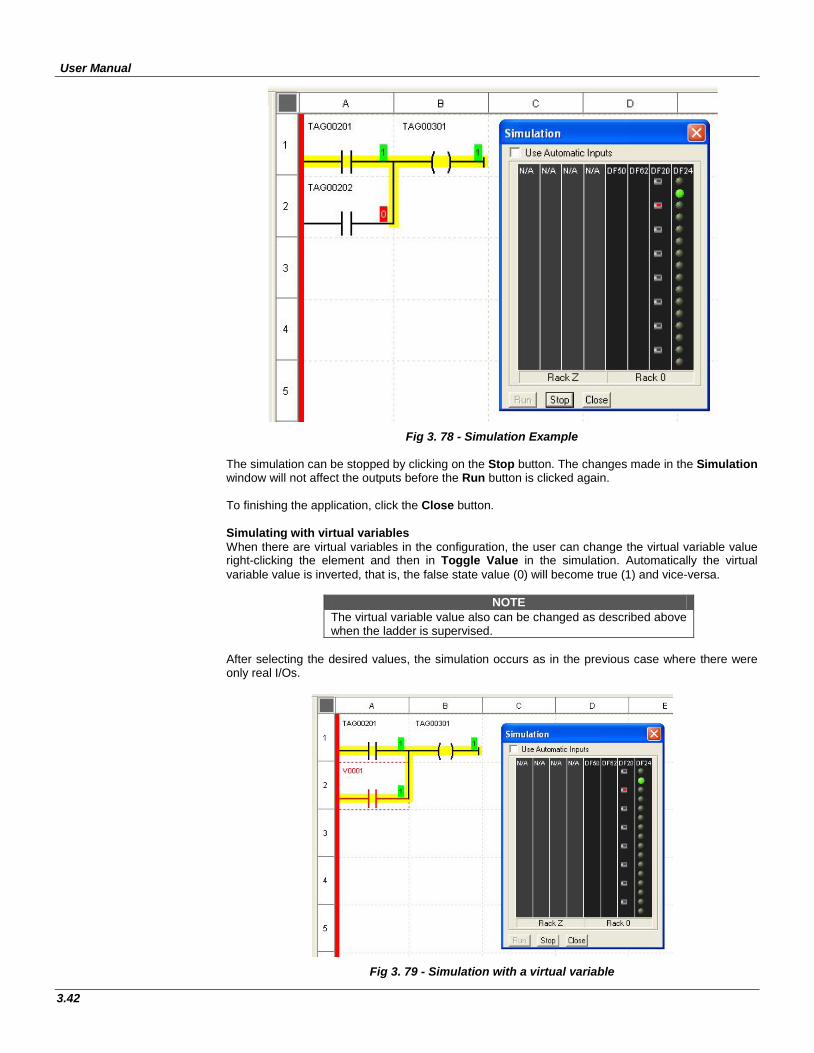
User Manual
3.42
Fig 3. 78 - Simulation Example
The simulation can be stopped by clicking on the Stop button. The changes made in the Simulation window will not affect the outputs before the Run button is clicked again. To finishing the application, click the Close button. Simulating with virtual variables When there are virtual variables in the configuration, the user can change the virtual variable value right-clicking the element and then in Toggle Value in the simulation. Automatically the virtual variable value is inverted, that is, the false state value (0) will become true (1) and vice-versa.
NOTE The virtual variable value also can be changed as described above when the ladder is supervised.
After selecting the desired values, the simulation occurs as in the previous case where there were only real I/Os.
Fig 3. 79 - Simulation with a virtual variable

The LogicView for FFB
3.43
NOTE
Any module can be used for simulation except the temperature, pulse and analog input modules. They cannot be simulated in this LogicView for FFB version. If in the simulation some functions are accessing those modules (MAI, TEMP, ACC and ACC_N) the analog outputs of these functions will keep always in zero.
The option Display Scan Time in Status bar will be always active and cannot be disabled. The Scan Time, showed at the LogicView for FFB bottom bar (Status Bar), is the scan time, which is the time that one logic cycle takes to be executed in the device. To choose the device in which the “scan time” will be monitored, the user has to click Stop/Run
icon , next to the icon used to connect to the Server. Besides serving to trigger or stop the ladder execution in the device, the icon Stop/Run is used to enable time scan requests, just to define the device. There will be always one device only on which the logic was downloaded. The information about the Scan Time can be obtained just connecting to the Server. This time will appear in the Status bar.
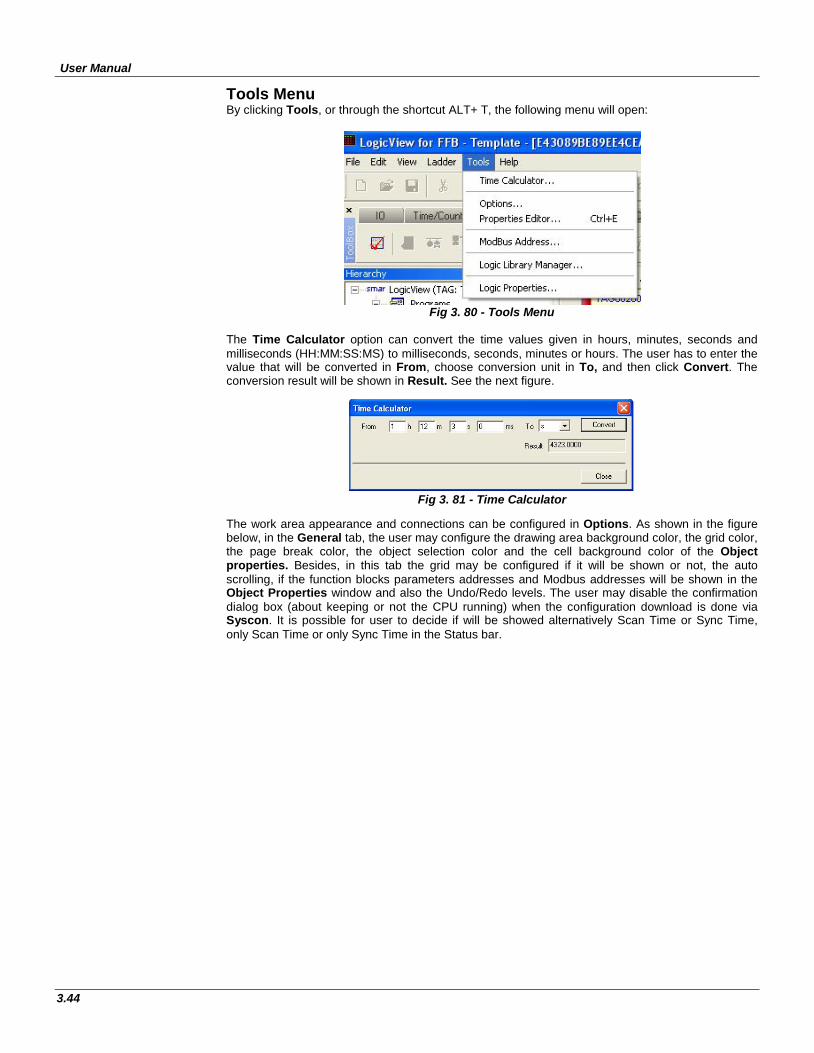
User Manual
3.44
Tools Menu By clicking Tools, or through the shortcut ALT+ T, the following menu will open:
Fig 3. 80 - Tools Menu
The Time Calculator option can convert the time values given in hours, minutes, seconds and milliseconds (HH:MM:SS:MS) to milliseconds, seconds, minutes or hours. The user has to enter the value that will be converted in From, choose conversion unit in To, and then click Convert. The conversion result will be shown in Result. See the next figure.
Fig 3. 81 - Time Calculator
The work area appearance and connections can be configured in Options. As shown in the figure below, in the General tab, the user may configure the drawing area background color, the grid color, the page break color, the object selection color and the cell background color of the Object properties. Besides, in this tab the grid may be configured if it will be shown or not, the auto scrolling, if the function blocks parameters addresses and Modbus addresses will be shown in the Object Properties window and also the Undo/Redo levels. The user may disable the confirmation dialog box (about keeping or not the CPU running) when the configuration download is done via Syscon. It is possible for user to decide if will be showed alternatively Scan Time or Sync Time, only Scan Time or only Sync Time in the Status bar.
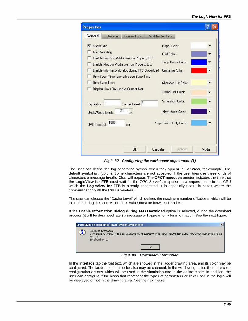
The LogicView for FFB
3.45
Fig 3. 82 - Configuring the workspace appearance (1) The user can define the tag separation symbol when they appear in TagView, for example. The default symbol is : (colon). Some characters are not accepted. If the user tries use these kinds of characters a message Invalid Char will appear. The OPCTimeout parameter indicates the time that the LogicView for FFB must wait for the OPC Server’s response to a request done to the CPU which the LogicView for FFB is already connected. It is especially useful in cases where the communication with the CPU is wireless. The user can choose the “Cache Level” which defines the maximum number of ladders which will be in cache during the supervision. This value must be between 1 and 9. If the Enable Information Dialog during FFB Download option is selected, during the download process (it will be described later) a message will appear, only for information. See the next figure.
Fig 3. 83 – Download information
In the Interface tab the font text, which are showed in the ladder drawing area, and its color may be configured. The ladder elements color also may be changed. In the window right side there are color configuration options which will be used in the simulation and in the online mode. In addition, the user can configure if the icons that represent the types of parameters or links used in the logic will be displayed or not in the drawing area. See the next figure.
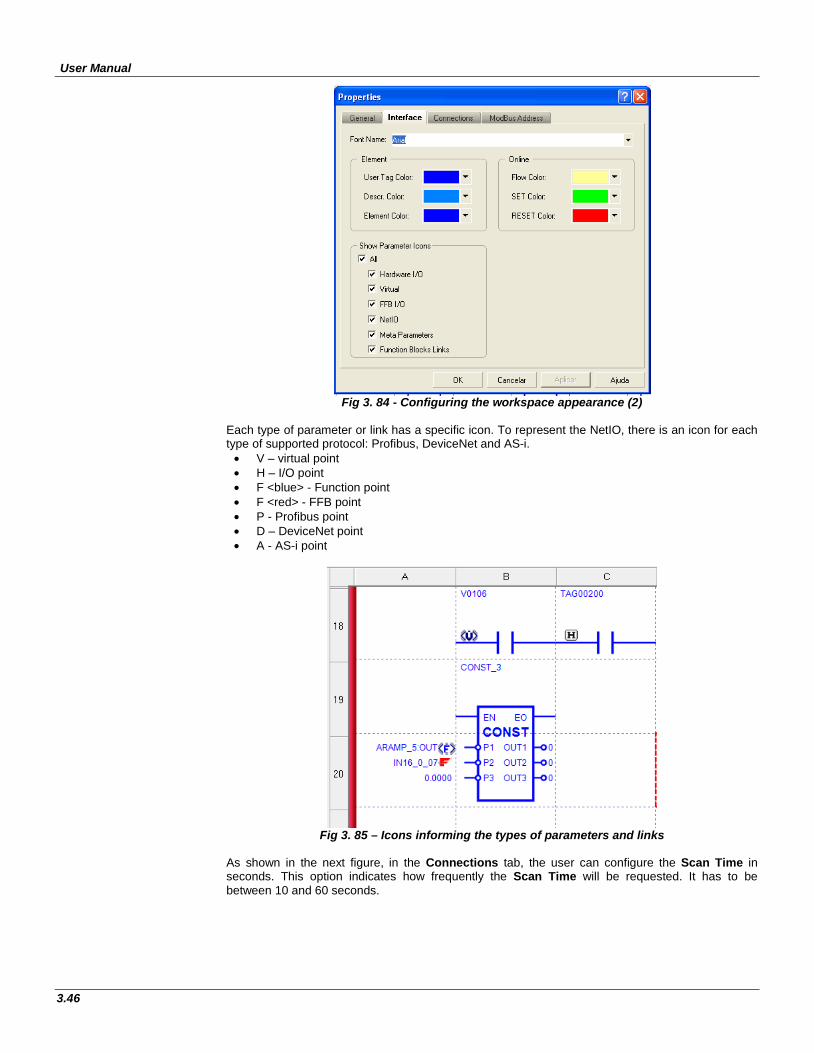
User Manual
3.46
Fig 3. 84 - Configuring the workspace appearance (2)
Each type of parameter or link has a specific icon. To represent the NetIO, there is an icon for each type of supported protocol: Profibus, DeviceNet and AS-i.
• V – virtual point • H – I/O point • F <blue> - Function point • F <red> - FFB point • P - Profibus point • D – DeviceNet point • A - AS-i point
Fig 3. 85 – Icons informing the types of parameters and links
As shown in the next figure, in the Connections tab, the user can configure the Scan Time in seconds. This option indicates how frequently the Scan Time will be requested. It has to be between 10 and 60 seconds.
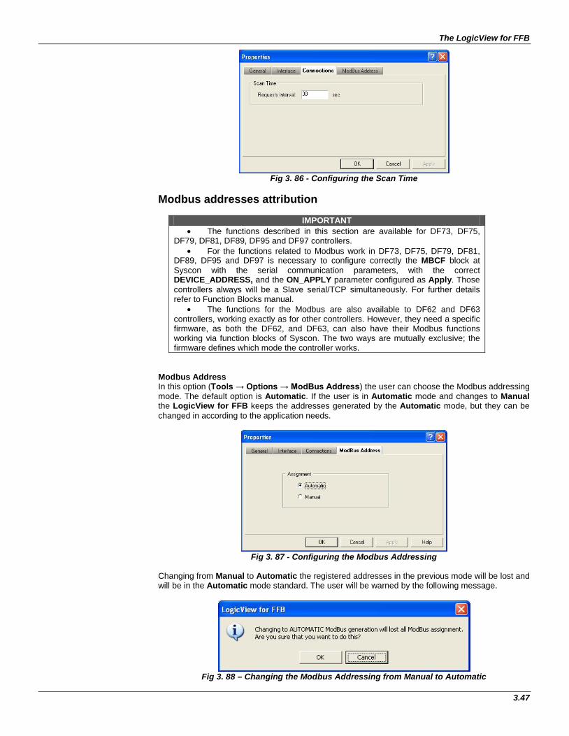
The LogicView for FFB
3.47
Fig 3. 86 - Configuring the Scan Time
Modbus addresses attribution
IMPORTANT • The functions described in this section are available for DF73, DF75,
DF79, DF81, DF89, DF95 and DF97 controllers. • For the functions related to Modbus work in DF73, DF75, DF79, DF81,
DF89, DF95 and DF97 is necessary to configure correctly the MBCF block at Syscon with the serial communication parameters, with the correct DEVICE_ADDRESS, and the ON_APPLY parameter configured as Apply. Those controllers always will be a Slave serial/TCP simultaneously. For further details refer to Function Blocks manual.
• The functions for the Modbus are also available to DF62 and DF63 controllers, working exactly as for other controllers. However, they need a specific firmware, as both the DF62, and DF63, can also have their Modbus functions working via function blocks of Syscon. The two ways are mutually exclusive; the firmware defines which mode the controller works.
Modbus Address In this option (Tools → Options → ModBus Address) the user can choose the Modbus addressing mode. The default option is Automatic. If the user is in Automatic mode and changes to Manual the LogicView for FFB keeps the addresses generated by the Automatic mode, but they can be changed in according to the application needs.
Fig 3. 87 - Configuring the Modbus Addressing
Changing from Manual to Automatic the registered addresses in the previous mode will be lost and will be in the Automatic mode standard. The user will be warned by the following message.
Fig 3. 88 – Changing the Modbus Addressing from Manual to Automatic
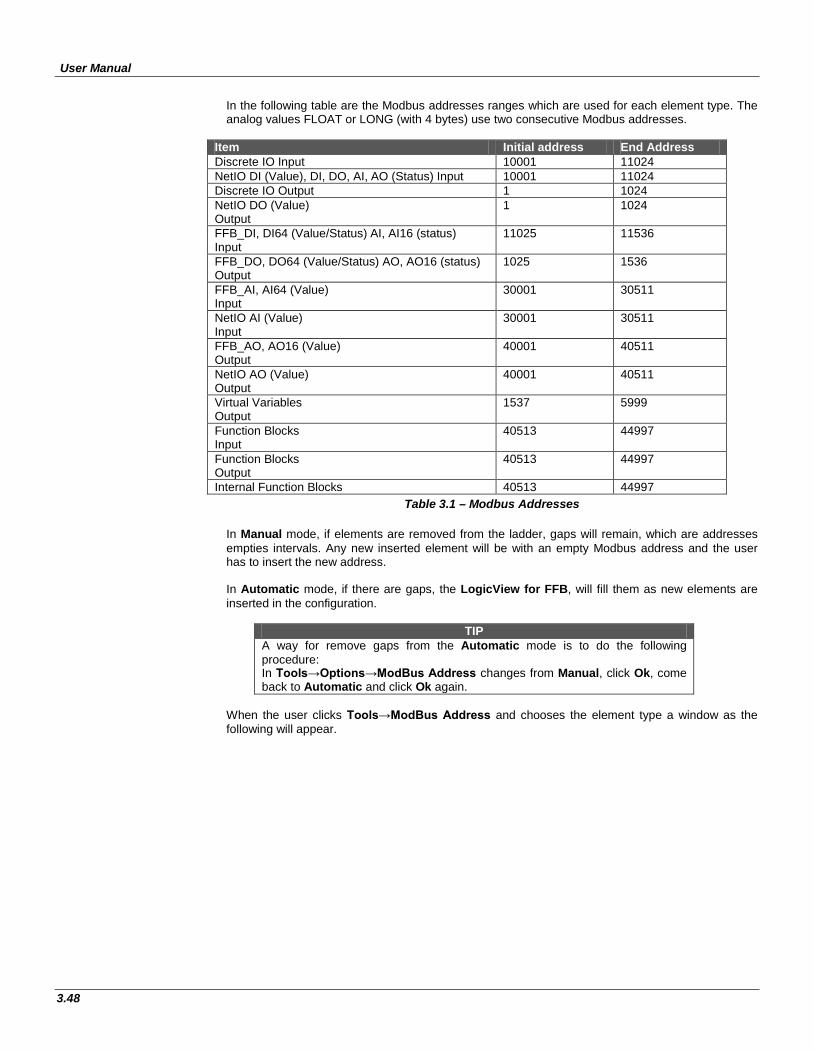
User Manual
3.48
In the following table are the Modbus addresses ranges which are used for each element type. The analog values FLOAT or LONG (with 4 bytes) use two consecutive Modbus addresses.
Item Initial address End Address Discrete IO Input 10001 11024 NetIO DI (Value), DI, DO, AI, AO (Status) Input 10001 11024 Discrete IO Output 1 1024 NetIO DO (Value) Output
1 1024
FFB_DI, DI64 (Value/Status) AI, AI16 (status) Input
11025 11536
FFB_DO, DO64 (Value/Status) AO, AO16 (status) Output
1025 1536
FFB_AI, AI64 (Value) Input
30001 30511
NetIO AI (Value) Input
30001 30511
FFB_AO, AO16 (Value) Output
40001 40511
NetIO AO (Value) Output
40001 40511
Virtual Variables Output
1537 5999
Function Blocks Input
40513 44997
Function Blocks Output
40513 44997
Internal Function Blocks 40513 44997 Table 3.1 – Modbus Addresses
In Manual mode, if elements are removed from the ladder, gaps will remain, which are addresses empties intervals. Any new inserted element will be with an empty Modbus address and the user has to insert the new address. In Automatic mode, if there are gaps, the LogicView for FFB, will fill them as new elements are inserted in the configuration.
TIP A way for remove gaps from the Automatic mode is to do the following procedure: In Tools→Options→ModBus Address changes from Manual, click Ok, come back to Automatic and click Ok again.
When the user clicks Tools→ModBus Address and chooses the element type a window as the following will appear.
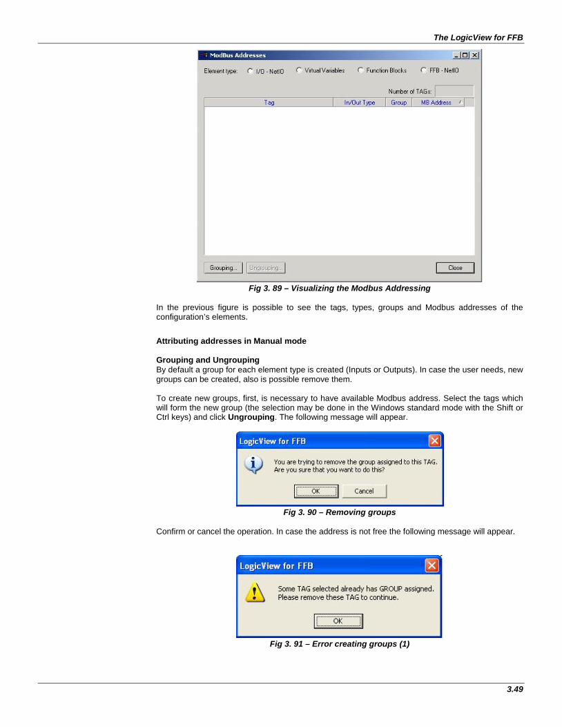
The LogicView for FFB
3.49
Fig 3. 89 – Visualizing the Modbus Addressing
In the previous figure is possible to see the tags, types, groups and Modbus addresses of the configuration’s elements.
Attributing addresses in Manual mode Grouping and Ungrouping By default a group for each element type is created (Inputs or Outputs). In case the user needs, new groups can be created, also is possible remove them. To create new groups, first, is necessary to have available Modbus address. Select the tags which will form the new group (the selection may be done in the Windows standard mode with the Shift or Ctrl keys) and click Ungrouping. The following message will appear.
Fig 3. 90 – Removing groups
Confirm or cancel the operation. In case the address is not free the following message will appear.
Fig 3. 91 – Error creating groups (1)
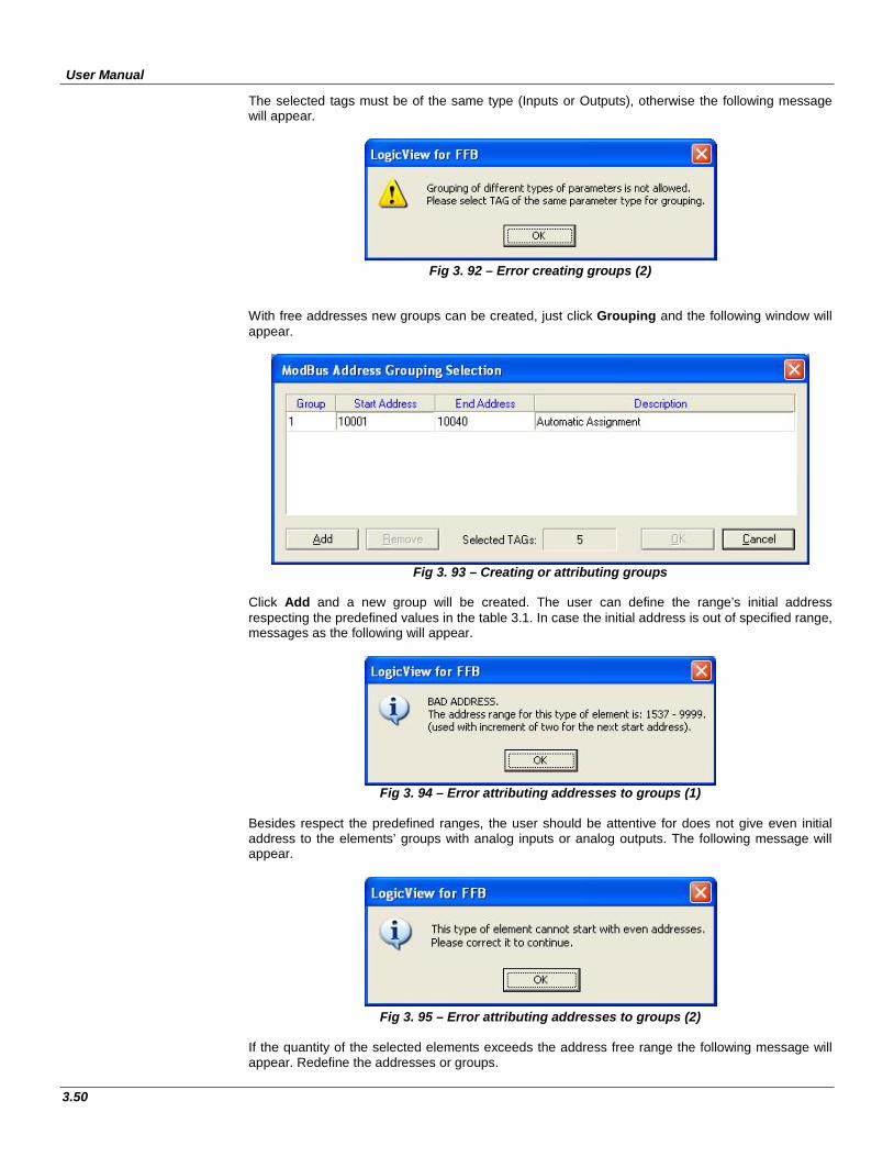
User Manual
3.50
The selected tags must be of the same type (Inputs or Outputs), otherwise the following message will appear.
Fig 3. 92 – Error creating groups (2)
With free addresses new groups can be created, just click Grouping and the following window will appear.
Fig 3. 93 – Creating or attributing groups
Click Add and a new group will be created. The user can define the range’s initial address respecting the predefined values in the table 3.1. In case the initial address is out of specified range, messages as the following will appear.
Fig 3. 94 – Error attributing addresses to groups (1)
Besides respect the predefined ranges, the user should be attentive for does not give even initial address to the elements’ groups with analog inputs or analog outputs. The following message will appear.
Fig 3. 95 – Error attributing addresses to groups (2)
If the quantity of the selected elements exceeds the address free range the following message will appear. Redefine the addresses or groups.
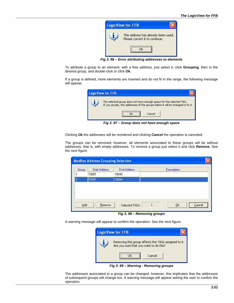
The LogicView for FFB
3.51
Fig 3. 96 – Error attributing addresses to elements
To attribute a group to an element, with a free address, just select it, click Grouping, then in the desired group, and double-click or click Ok. If a group is defined, more elements are inserted and do not fit in the range, the following message will appear.
Fig 3. 97 – Group does not have enough space
Clicking Ok the addresses will be reordered and clicking Cancel the operation is canceled. The groups can be removed; however, all elements associated to these groups will be without addresses, that is, with empty addresses. To remove a group just select it and click Remove. See the next figure.
Fig 3. 98 – Removing groups
A warning message will appear to confirm the operation. See the next figure.
Fig 3. 99 – Warning - Removing groups
The addresses associated to a group can be changed, however, this implicates that the addresses of subsequent groups will change too. A warning message will appear asking the user to confirm the operation.
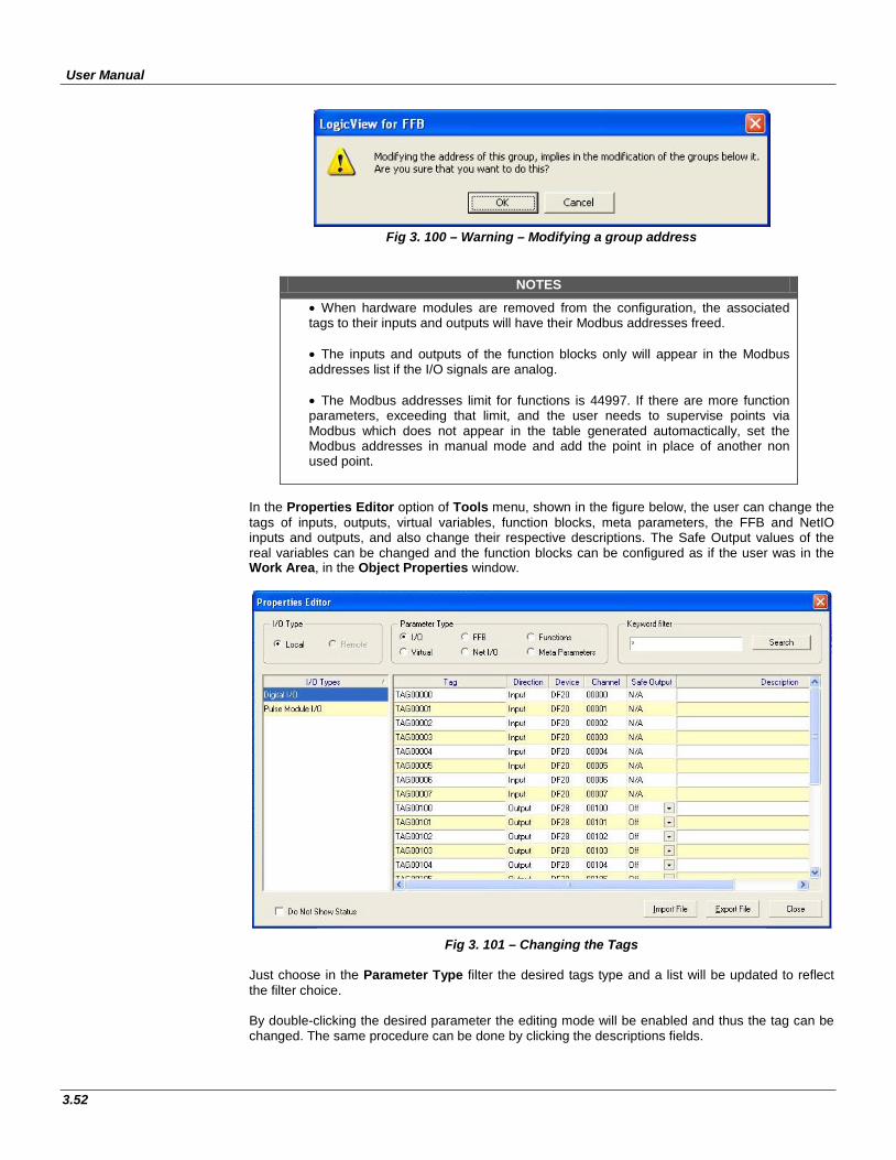
User Manual
3.52
Fig 3. 100 – Warning – Modifying a group address
NOTES
• When hardware modules are removed from the configuration, the associated tags to their inputs and outputs will have their Modbus addresses freed.
• The inputs and outputs of the function blocks only will appear in the Modbus addresses list if the I/O signals are analog.
• The Modbus addresses limit for functions is 44997. If there are more function parameters, exceeding that limit, and the user needs to supervise points via Modbus which does not appear in the table generated automactically, set the Modbus addresses in manual mode and add the point in place of another non used point.
In the Properties Editor option of Tools menu, shown in the figure below, the user can change the tags of inputs, outputs, virtual variables, function blocks, meta parameters, the FFB and NetIO inputs and outputs, and also change their respective descriptions. The Safe Output values of the real variables can be changed and the function blocks can be configured as if the user was in the Work Area, in the Object Properties window.
Fig 3. 101 – Changing the Tags
Just choose in the Parameter Type filter the desired tags type and a list will be updated to reflect the filter choice. By double-clicking the desired parameter the editing mode will be enabled and thus the tag can be changed. The same procedure can be done by clicking the descriptions fields.
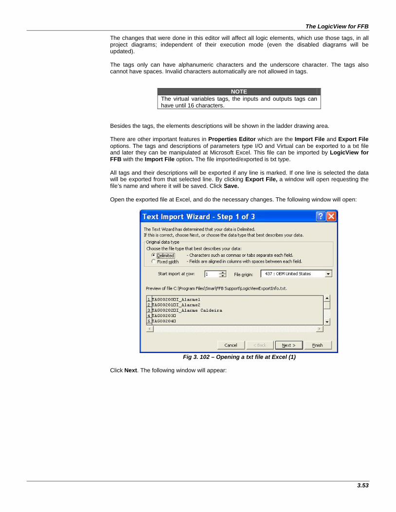
The LogicView for FFB
3.53
The changes that were done in this editor will affect all logic elements, which use those tags, in all project diagrams; independent of their execution mode (even the disabled diagrams will be updated). The tags only can have alphanumeric characters and the underscore character. The tags also cannot have spaces. Invalid characters automatically are not allowed in tags.
NOTE The virtual variables tags, the inputs and outputs tags can have until 16 characters.
Besides the tags, the elements descriptions will be shown in the ladder drawing area. There are other important features in Properties Editor which are the Import File and Export File options. The tags and descriptions of parameters type I/O and Virtual can be exported to a txt file and later they can be manipulated at Microsoft Excel. This file can be imported by LogicView for FFB with the Import File option. The file imported/exported is txt type. All tags and their descriptions will be exported if any line is marked. If one line is selected the data will be exported from that selected line. By clicking Export File, a window will open requesting the file’s name and where it will be saved. Click Save. Open the exported file at Excel, and do the necessary changes. The following window will open:
Fig 3. 102 – Opening a txt file at Excel (1)
Click Next. The following window will appear:
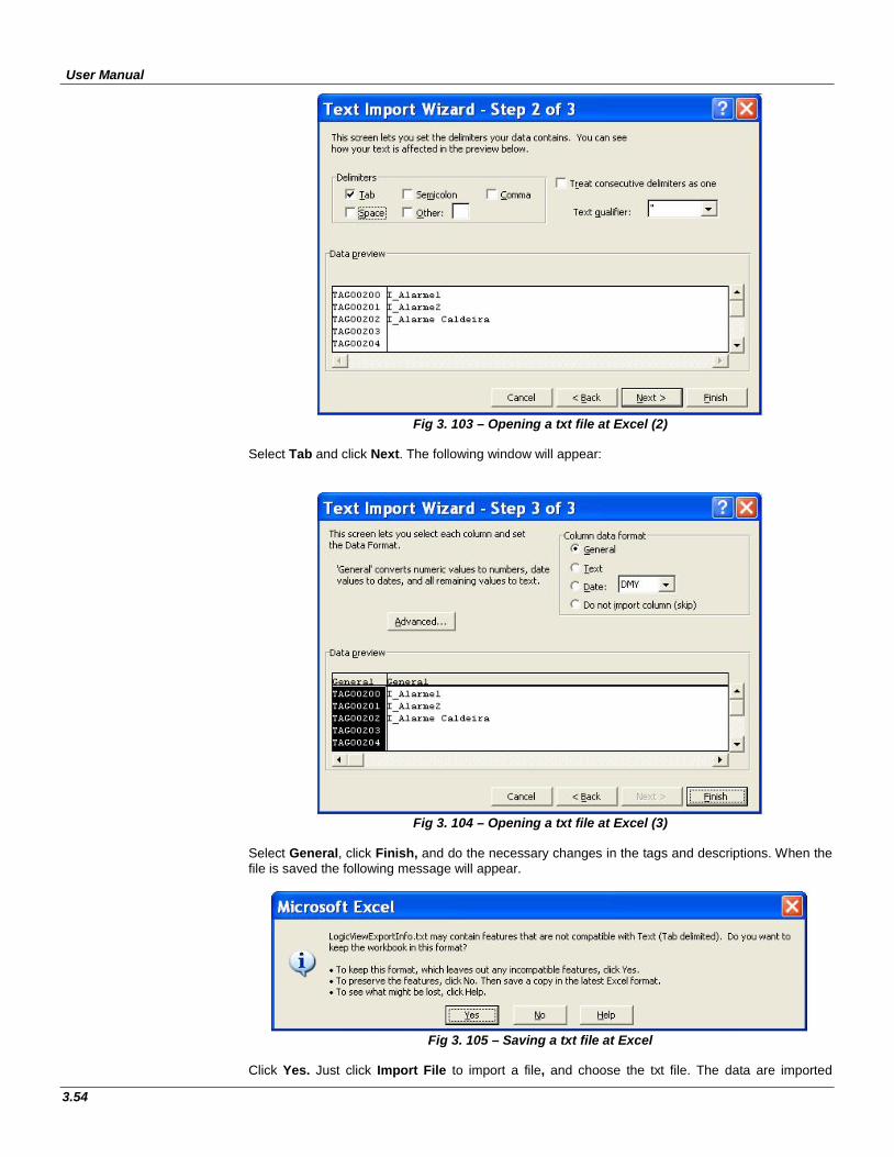
User Manual
3.54
Fig 3. 103 – Opening a txt file at Excel (2)
Select Tab and click Next. The following window will appear:
Fig 3. 104 – Opening a txt file at Excel (3)
Select General, click Finish, and do the necessary changes in the tags and descriptions. When the file is saved the following message will appear.
Fig 3. 105 – Saving a txt file at Excel
Click Yes. Just click Import File to import a file, and choose the txt file. The data are imported
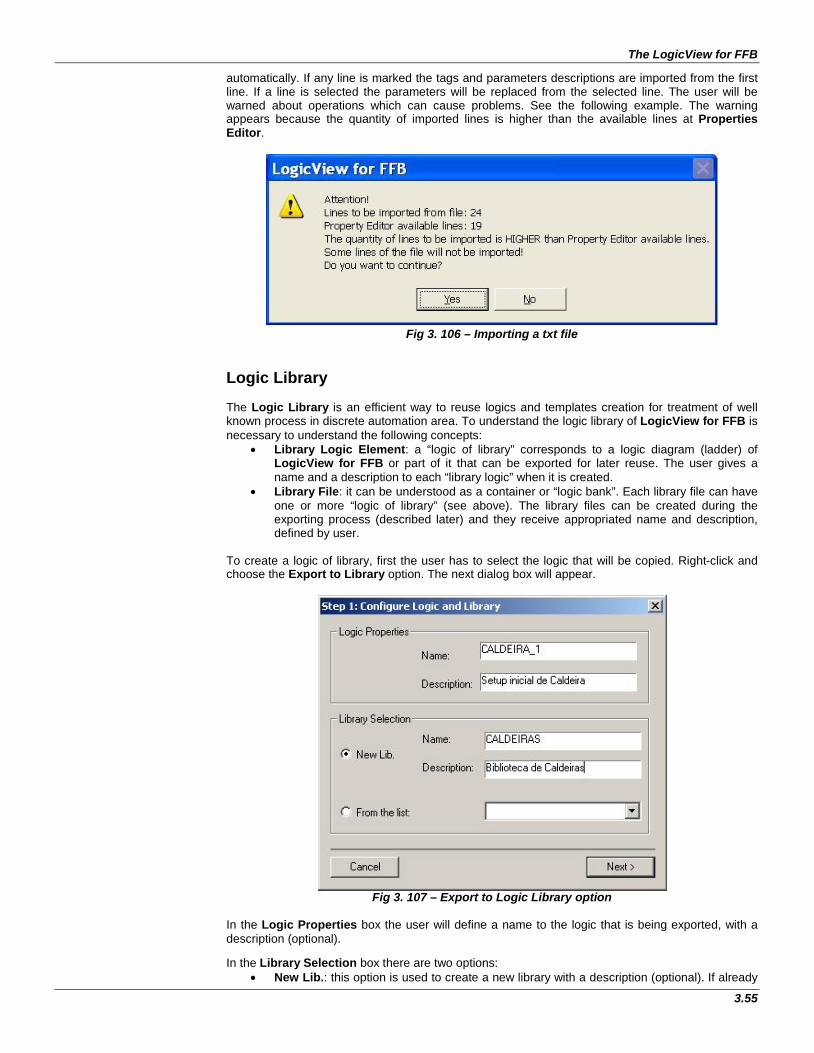
The LogicView for FFB
3.55
automatically. If any line is marked the tags and parameters descriptions are imported from the first line. If a line is selected the parameters will be replaced from the selected line. The user will be warned about operations which can cause problems. See the following example. The warning appears because the quantity of imported lines is higher than the available lines at Properties Editor.
Fig 3. 106 – Importing a txt file
Logic Library The Logic Library is an efficient way to reuse logics and templates creation for treatment of well known process in discrete automation area. To understand the logic library of LogicView for FFB is necessary to understand the following concepts:
• Library Logic Element: a “logic of library” corresponds to a logic diagram (ladder) of LogicView for FFB or part of it that can be exported for later reuse. The user gives a name and a description to each “library logic” when it is created.
• Library File: it can be understood as a container or “logic bank”. Each library file can have one or more “logic of library” (see above). The library files can be created during the exporting process (described later) and they receive appropriated name and description, defined by user.
To create a logic of library, first the user has to select the logic that will be copied. Right-click and choose the Export to Library option. The next dialog box will appear.
Fig 3. 107 – Export to Logic Library option
In the Logic Properties box the user will define a name to the logic that is being exported, with a description (optional). In the Library Selection box there are two options:
• New Lib.: this option is used to create a new library with a description (optional). If already
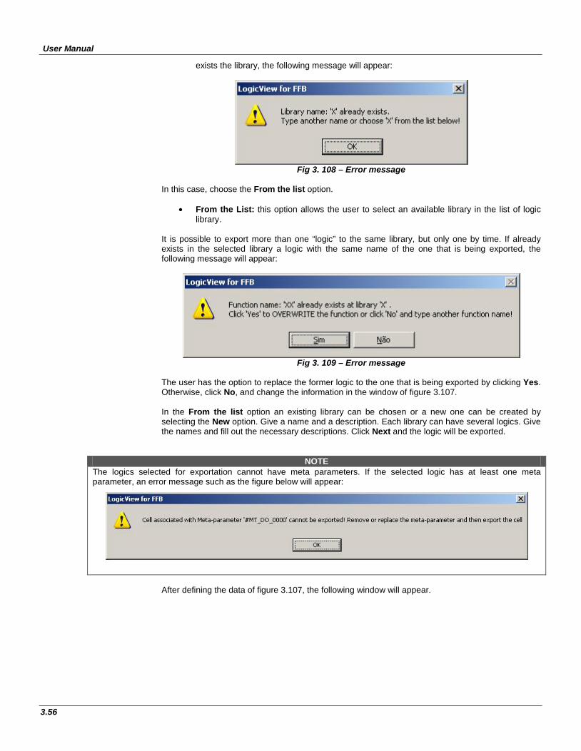
User Manual
3.56
exists the library, the following message will appear:
Fig 3. 108 – Error message
In this case, choose the From the list option.
• From the List: this option allows the user to select an available library in the list of logic library.
It is possible to export more than one “logic” to the same library, but only one by time. If already exists in the selected library a logic with the same name of the one that is being exported, the following message will appear:
Fig 3. 109 – Error message
The user has the option to replace the former logic to the one that is being exported by clicking Yes. Otherwise, click No, and change the information in the window of figure 3.107. In the From the list option an existing library can be chosen or a new one can be created by selecting the New option. Give a name and a description. Each library can have several logics. Give the names and fill out the necessary descriptions. Click Next and the logic will be exported.
NOTE The logics selected for exportation cannot have meta parameters. If the selected logic has at least one meta parameter, an error message such as the figure below will appear:
After defining the data of figure 3.107, the following window will appear.
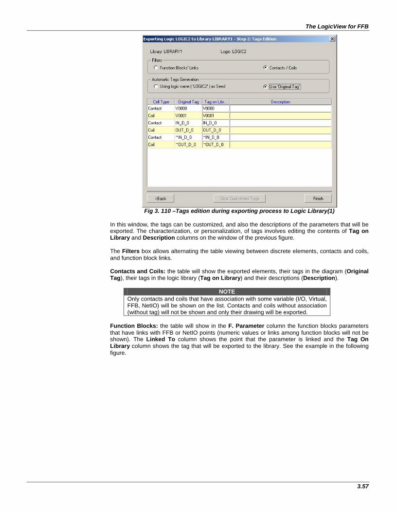
The LogicView for FFB
3.57
Fig 3. 110 –Tags edition during exporting process to Logic Library(1)
In this window, the tags can be customized, and also the descriptions of the parameters that will be exported. The characterization, or personalization, of tags involves editing the contents of Tag on Library and Description columns on the window of the previous figure. The Filters box allows alternating the table viewing between discrete elements, contacts and coils, and function block links. Contacts and Coils: the table will show the exported elements, their tags in the diagram (Original Tag), their tags in the logic library (Tag on Library) and their descriptions (Description).
NOTE Only contacts and coils that have association with some variable (I/O, Virtual, FFB, NetIO) will be shown on the list. Contacts and coils without association (without tag) will not be shown and only their drawing will be exported.
Function Blocks: the table will show in the F. Parameter column the function blocks parameters that have links with FFB or NetIO points (numeric values or links among function blocks will not be shown). The Linked To column shows the point that the parameter is linked and the Tag On Library column shows the tag that will be exported to the library. See the example in the following figure.
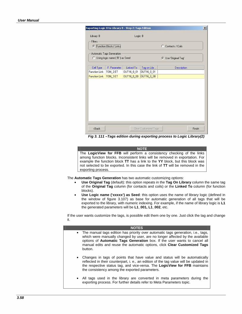
User Manual
3.58
Fig 3. 111 –Tags edition during exporting process to Logic Library(2)
NOTE The LogicView for FFB will perform a consistency checking of the links among function blocks. Inconsistent links will be removed in exportation. For example the function block TT has a link to the YY block, but this block was not selected to be exported. In this case the link of TT will be removed in the exporting process.
The Automatic Tags Generation has two automatic customizing options:
• Use Original Tag (default): this option repeats in the Tag On Library column the same tag of the Original Tag column (for contacts and coils) or the Linked To column (for function blocks).
• Use Logic name (‘xxxxx’) as Seed: this option uses the name of library logic (defined in the window of figure 3.107) as base for automatic generation of all tags that will be exported to the library, with numeric indexing. For example, if the name of library logic is L1 the generated parameters will be L1_001, L1_002, etc.
If the user wants customize the tags, is possible edit them one by one. Just click the tag and change it.
NOTES • The manual tags edition has priority over automatic tags generation, i.e., tags,
which were manually changed by user, are no longer affected by the available options of Automatic Tags Generation box. If the user wants to cancel all manual edits and reuse the automatic options, click Clear Customized Tags button.
• Changes in tags of points that have value and status will be automatically
reflected in their counterpart, i. e., an edition of the tag value will be updated in the respective status tag, and vice-versa. The LogicView for FFB maintains the consistency among the exported parameters.
• All tags used in the library are converted in meta parameters during the
exporting process. For further details refer to Meta Parameters topic.
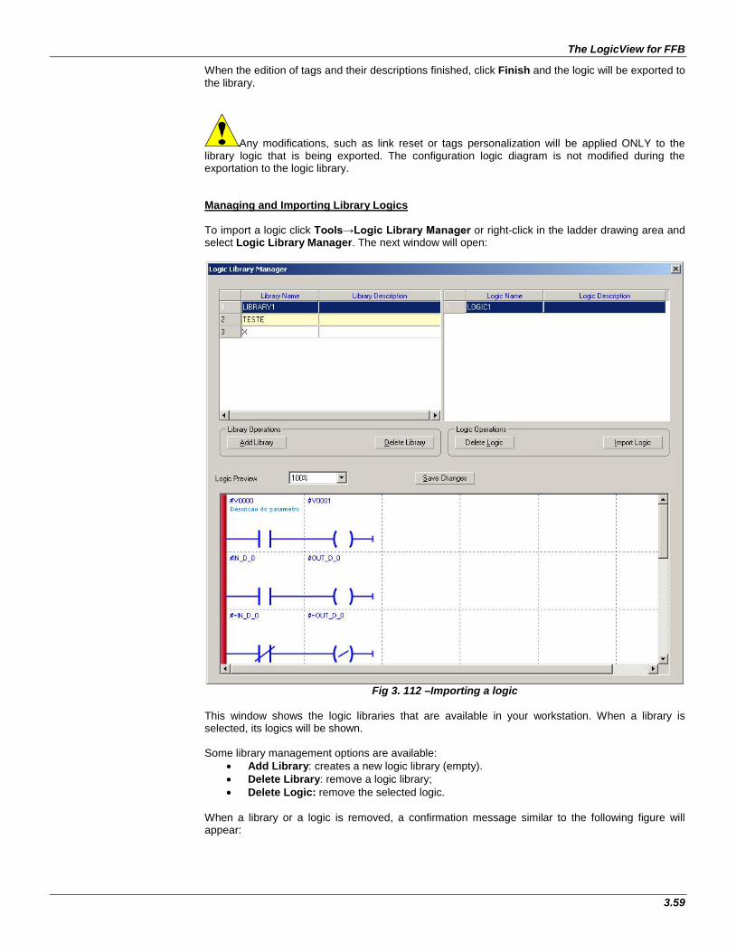
The LogicView for FFB
3.59
When the edition of tags and their descriptions finished, click Finish and the logic will be exported to the library.
Any modifications, such as link reset or tags personalization will be applied ONLY to the library logic that is being exported. The configuration logic diagram is not modified during the exportation to the logic library. Managing and Importing Library Logics To import a logic click Tools→Logic Library Manager or right-click in the ladder drawing area and select Logic Library Manager. The next window will open:
Fig 3. 112 –Importing a logic
This window shows the logic libraries that are available in your workstation. When a library is selected, its logics will be shown. Some library management options are available:
• Add Library: creates a new logic library (empty). • Delete Library: remove a logic library; • Delete Logic: remove the selected logic.
When a library or a logic is removed, a confirmation message similar to the following figure will appear:
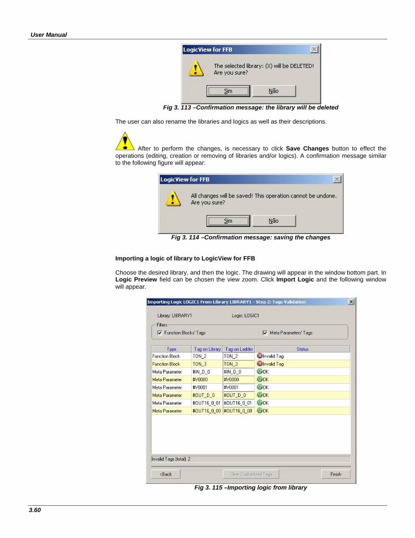
User Manual
3.60
Fig 3. 113 –Confirmation message: the library will be deleted
The user can also rename the libraries and logics as well as their descriptions.
After to perform the changes, is necessary to click Save Changes button to effect the operations (editing, creation or removing of libraries and/or logics). A confirmation message similar to the following figure will appear:
Fig 3. 114 –Confirmation message: saving the changes
Importing a logic of library to LogicView for FFB Choose the desired library, and then the logic. The drawing will appear in the window bottom part. In Logic Preview field can be chosen the view zoom. Click Import Logic and the following window will appear.
Fig 3. 115 –Importing logic from library
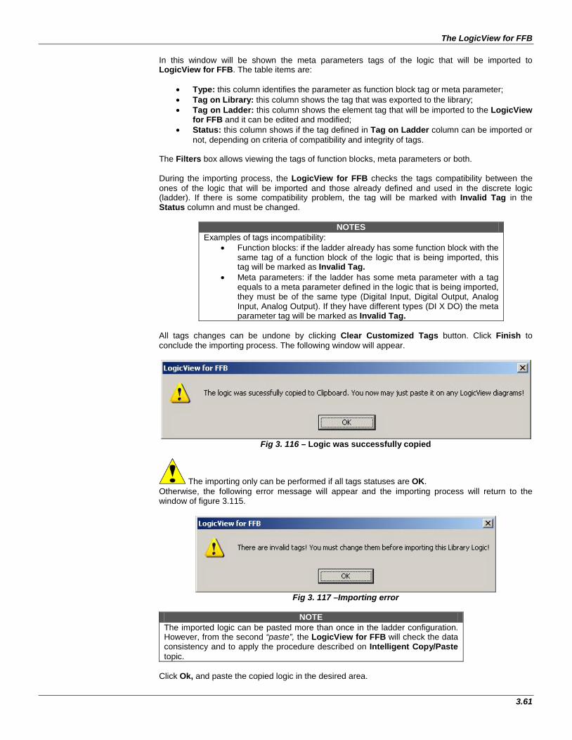
The LogicView for FFB
3.61
In this window will be shown the meta parameters tags of the logic that will be imported to LogicView for FFB. The table items are:
• Type: this column identifies the parameter as function block tag or meta parameter; • Tag on Library: this column shows the tag that was exported to the library; • Tag on Ladder: this column shows the element tag that will be imported to the LogicView
for FFB and it can be edited and modified; • Status: this column shows if the tag defined in Tag on Ladder column can be imported or
not, depending on criteria of compatibility and integrity of tags. The Filters box allows viewing the tags of function blocks, meta parameters or both. During the importing process, the LogicView for FFB checks the tags compatibility between the ones of the logic that will be imported and those already defined and used in the discrete logic (ladder). If there is some compatibility problem, the tag will be marked with Invalid Tag in the Status column and must be changed.
NOTES Examples of tags incompatibility:
• Function blocks: if the ladder already has some function block with the same tag of a function block of the logic that is being imported, this tag will be marked as Invalid Tag.
• Meta parameters: if the ladder has some meta parameter with a tag equals to a meta parameter defined in the logic that is being imported, they must be of the same type (Digital Input, Digital Output, Analog Input, Analog Output). If they have different types (DI X DO) the meta parameter tag will be marked as Invalid Tag.
All tags changes can be undone by clicking Clear Customized Tags button. Click Finish to conclude the importing process. The following window will appear.
Fig 3. 116 – Logic was successfully copied
The importing only can be performed if all tags statuses are OK. Otherwise, the following error message will appear and the importing process will return to the window of figure 3.115.
Fig 3. 117 –Importing error
NOTE
The imported logic can be pasted more than once in the ladder configuration. However, from the second “paste”, the LogicView for FFB will check the data consistency and to apply the procedure described on Intelligent Copy/Paste topic.
Click Ok, and paste the copied logic in the desired area.

User Manual
3.62
Help Menu By clicking Help, or through the shortcut ALT+ H, the following menu will open:
Fig 3. 118 - Help Menu
In this menu, the installed software version can be viewed and the software help is available.
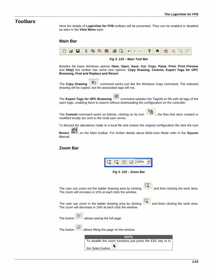
The LogicView for FFB
3.63
Toolbars Here the details of LogicView for FFB toolbars will be presented. They can be enabled or disabled as seen in the View Menu topic. Main Bar
Fig 3. 119 – Main Tool Bar Besides the basic Windows options (New, Open, Save, Cut, Copy, Paste, Print, Print Preview and Help) this toolbar has some new options: Copy Drawing, Commit, Export Tags for OPC Browsing, Find and Replace and Revert.
The Copy Drawing command works just like the Windows Copy command. The selected drawing will be copied, but the associated tags will not.
The Export Tags for OPC Browsing command updates the Taginfo.ini file with all tags of the open logic, enabling them to search without downloading the configuration on the controller.
The Commit command works as follows: clicking on its icon , the files that were created or modified locally are sent to the multi-user server. To discard the alterations made to a local file and restore the original configuration file click the icon
Revert, , on the Main toolbar. For further details about Multi-User Mode refer to the Syscon Manual.
Zoom Bar
Fig 3. 120 – Zoom Bar
The user can zoom out the ladder drawing area by clicking and then clicking the work area. The zoom will increase in 10% at each click the window.
The user can zoom in the ladder drawing area by clicking and them clicking the work area. The zoom will decrease in 10% at each click the window.
The button allows seeing the full page.
The button allows fitting the page on the window.
NOTE To disable the zoom functions just press the ESC key or in
the Select button
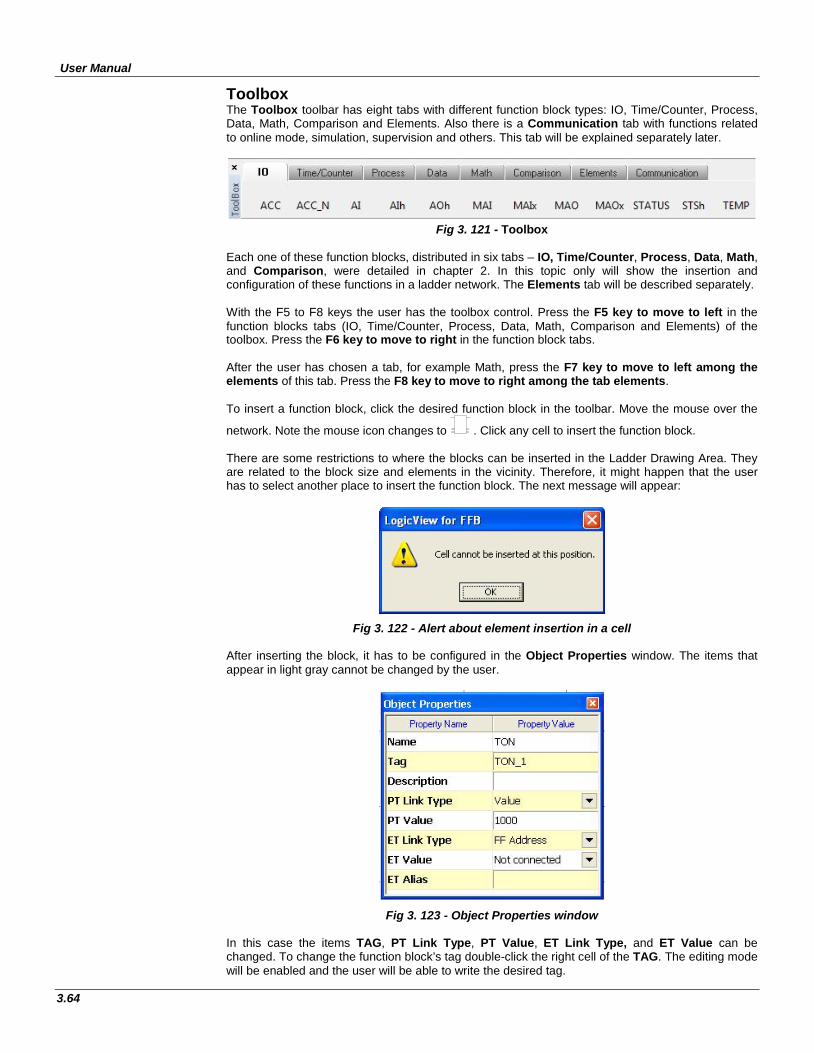
User Manual
3.64
Toolbox The Toolbox toolbar has eight tabs with different function block types: IO, Time/Counter, Process, Data, Math, Comparison and Elements. Also there is a Communication tab with functions related to online mode, simulation, supervision and others. This tab will be explained separately later.
Fig 3. 121 - Toolbox
Each one of these function blocks, distributed in six tabs – IO, Time/Counter, Process, Data, Math, and Comparison, were detailed in chapter 2. In this topic only will show the insertion and configuration of these functions in a ladder network. The Elements tab will be described separately. With the F5 to F8 keys the user has the toolbox control. Press the F5 key to move to left in the function blocks tabs (IO, Time/Counter, Process, Data, Math, Comparison and Elements) of the toolbox. Press the F6 key to move to right in the function block tabs. After the user has chosen a tab, for example Math, press the F7 key to move to left among the elements of this tab. Press the F8 key to move to right among the tab elements. To insert a function block, click the desired function block in the toolbar. Move the mouse over the
network. Note the mouse icon changes to . Click any cell to insert the function block. There are some restrictions to where the blocks can be inserted in the Ladder Drawing Area. They are related to the block size and elements in the vicinity. Therefore, it might happen that the user has to select another place to insert the function block. The next message will appear:
Fig 3. 122 - Alert about element insertion in a cell After inserting the block, it has to be configured in the Object Properties window. The items that appear in light gray cannot be changed by the user.
Fig 3. 123 - Object Properties window In this case the items TAG, PT Link Type, PT Value, ET Link Type, and ET Value can be changed. To change the function block’s tag double-click the right cell of the TAG. The editing mode will be enabled and the user will be able to write the desired tag.
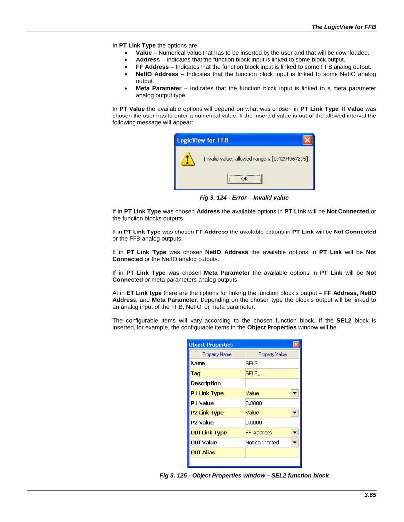
The LogicView for FFB
3.65
In PT Link Type the options are:
• Value – Numerical value that has to be inserted by the user and that will be downloaded. • Address – Indicates that the function block input is linked to some block output. • FF Address – Indicates that the function block input is linked to some FFB analog output. • NetIO Address – Indicates that the function block input is linked to some NetIO analog
output. • Meta Parameter – Indicates that the function block input is linked to a meta parameter
analog output type. In PT Value the available options will depend on what was chosen in PT Link Type. If Value was chosen the user has to enter a numerical value. If the inserted value is out of the allowed interval the following message will appear:
Fig 3. 124 - Error – Invalid value If in PT Link Type was chosen Address the available options in PT Link will be Not Connected or the function blocks outputs. If in PT Link Type was chosen FF Address the available options in PT Link will be Not Connected or the FFB analog outputs. If in PT Link Type was chosen NetIO Address the available options in PT Link will be Not Connected or the NetIO analog outputs. If in PT Link Type was chosen Meta Parameter the available options in PT Link will be Not Connected or meta parameters analog outputs. At in ET Link type there are the options for linking the function block’s output – FF Address, NetIO Address, and Meta Parameter. Depending on the chosen type the block’s output will be linked to an analog input of the FFB, NetIO, or meta parameter. The configurable items will vary according to the chosen function block. If the SEL2 block is inserted, for example, the configurable items in the Object Properties window will be:
Fig 3. 125 - Object Properties window – SEL2 function block

User Manual
3.66
In this case, the items TAG, P1 Link Type, P1 Value, P2 Link Type, P2 Value, OUT Link Type and OUT Value can be changed. To change the function block tag double-click the right cell of the TAG. The editing mode will be enabled and the user will be able to write the desired TAG. In P1 and P2 Link Type the options are:
• Value – Numerical value that has to be inserted by the user and that will be downloaded. • Address – Indicates that the function block input is linked to some block output. • FF Address – Indicates that the function block input is linked to some FFB analog output. • NetIO Address – Indicates that the function block input is linked to some NetIO analog
output. • Meta Parameter – Indicates that the function block input is linked to a meta parameter
analog output type.
In P1 and P2 Value the available options will depend on what was chosen in P1 and P2 Link Type, respectively. If Value was the choice, the user has to enter a numerical value. If Address was chosen in P1 and P2 Link Type, the available options in P1 and P2 Value will be Not Connected or the function blocks outputs. If FF Address was chosen in P1 and P2 Link Type, the available options in P1 and P2 Value will be Not Connected or the FFB analog outputs. If NetIO Address was chosen in P1 and P2 Link Type,the available options in P1 and P2 Value will be Not Connected or the NetIO analog outputs. If Meta Parameter was chosen in P1 and P2 Link Type, the available options in P1 and P2 Value will be Not Connected or the meta parameters analog outputs. The OUT Link Type can be a FF Address, NetIO Address, or Meta Parameter and, in this case, OUT Value can be Not Connected or the available links in FFB (FB Address), in the NetIO, or in the meta parameters. If a configuration is done in Syscon with a FFB which has DI, DO, AI and AO, and in LogicView for FFB configures a function such as timer, when the link types (PT and ET) as FF Address are defined, the AIs and AOs, which were created in FFB, will be available for link. Links among inputs and outputs of the function blocks Inputs and outputs can be linked. Select the function block and in the Object Properties window configure the link type which is necessary to the input – Address, FF Address, NetIO Address, or Meta Parameter. Choose the output which the input will be linked. In this situation, right-clicking a menu will appear. The penultimate menu item is Output Link, which shows all inputs that are linked to that output, according to the example showed in the next figure.
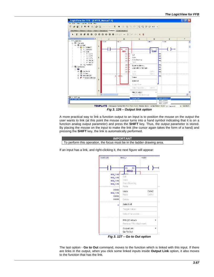
The LogicView for FFB
3.67
Fig 3. 126 – Output link option
A more practical way to link a function output to an input is to position the mouse on the output the user wants to link (at this point the mouse cursor turns into a hand symbol indicating that it is on a function analog output parameter) and press the SHIFT key. Thus, the output parameter is stored. By placing the mouse on the input to make the link (the cursor again takes the form of a hand) and pressing the SHIFT key, the link is automatically performed.
IMPORTANT To perform this operation, the focus must be in the ladder drawing area.
If an input has a link, and right-clicking it, the next figure will appear:
Fig 3. 127 – Go to Out option
The last option - Go to Out command, moves to the function which is linked with this input. If there are links in the output, when you click some linked inputs inside Output Link option, it also moves to the function that has the link.
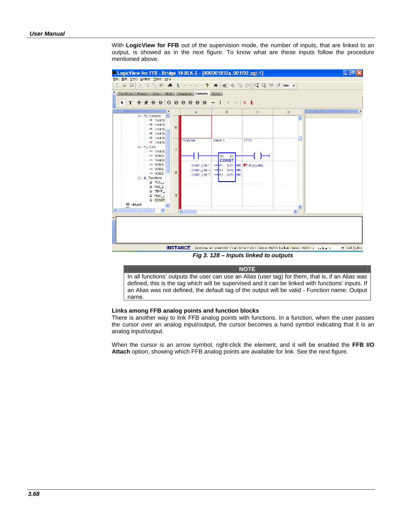
User Manual
3.68
With LogicView for FFB out of the supervision mode, the number of inputs, that are linked to an output, is showed as in the next figure. To know what are these inputs follow the procedure mentioned above.
Fig 3. 128 – Inputs linked to outputs
NOTE
In all functions’ outputs the user can use an Alias (user tag) for them, that is, if an Alias was defined, this is the tag which will be supervised and it can be linked with functions’ inputs. If an Alias was not defined, the default tag of the output will be valid - Function name: Output name.
Links among FFB analog points and function blocks There is another way to link FFB analog points with functions. In a function, when the user passes the cursor over an analog input/output, the cursor becomes a hand symbol indicating that it is an analog input/output. When the cursor is an arrow symbol, right-click the element, and it will be enabled the FFB I/O Attach option, showing which FFB analog points are available for link. See the next figure.
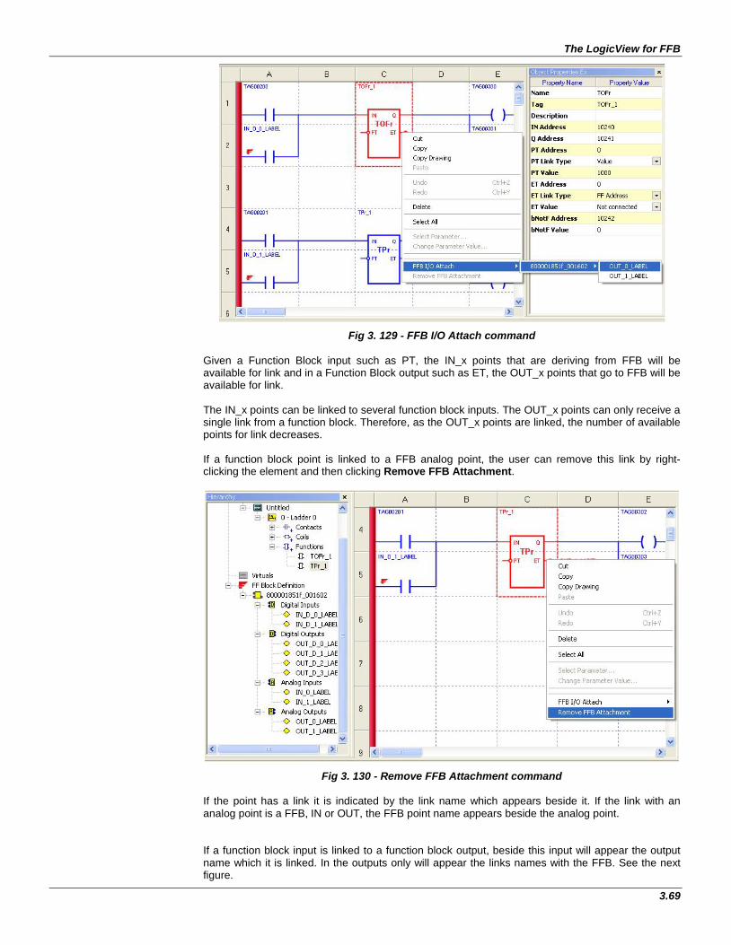
The LogicView for FFB
3.69
Fig 3. 129 - FFB I/O Attach command Given a Function Block input such as PT, the IN_x points that are deriving from FFB will be available for link and in a Function Block output such as ET, the OUT_x points that go to FFB will be available for link. The IN_x points can be linked to several function block inputs. The OUT_x points can only receive a single link from a function block. Therefore, as the OUT_x points are linked, the number of available points for link decreases. If a function block point is linked to a FFB analog point, the user can remove this link by right-clicking the element and then clicking Remove FFB Attachment.
Fig 3. 130 - Remove FFB Attachment command If the point has a link it is indicated by the link name which appears beside it. If the link with an analog point is a FFB, IN or OUT, the FFB point name appears beside the analog point. If a function block input is linked to a function block output, beside this input will appear the output name which it is linked. In the outputs only will appear the links names with the FFB. See the next figure.
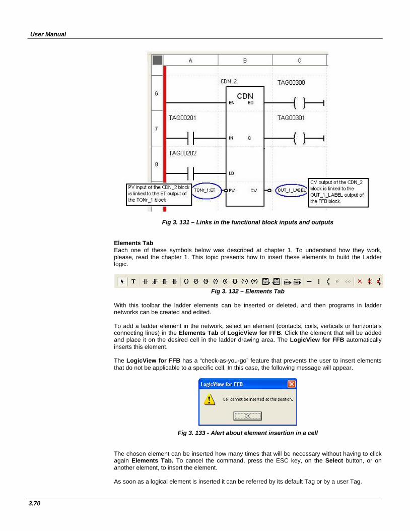
User Manual
3.70
Fig 3. 131 – Links in the functional block inputs and outputs
Elements Tab Each one of these symbols below was described at chapter 1. To understand how they work, please, read the chapter 1. This topic presents how to insert these elements to build the Ladder logic.
Fig 3. 132 – Elements Tab
With this toolbar the ladder elements can be inserted or deleted, and then programs in ladder networks can be created and edited. To add a ladder element in the network, select an element (contacts, coils, verticals or horizontals connecting lines) in the Elements Tab of LogicView for FFB. Click the element that will be added and place it on the desired cell in the ladder drawing area. The LogicView for FFB automatically inserts this element. The LogicView for FFB has a “check-as-you-go” feature that prevents the user to insert elements that do not be applicable to a specific cell. In this case, the following message will appear.
Fig 3. 133 - Alert about element insertion in a cell
The chosen element can be inserted how many times that will be necessary without having to click again Elements Tab. To cancel the command, press the ESC key, on the Select button, or on another element, to insert the element. As soon as a logical element is inserted it can be referred by its default Tag or by a user Tag.
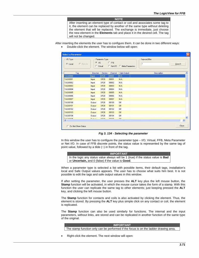
The LogicView for FFB
3.71
NOTE After inserting an element type of contact or coil and associates some tag to it, the element can be replaced by another of the same type without deleting the element that will be replaced. The exchange is immediate, just choose the new element in the Elements tab and place it in the desired cell. The tag will not be changed.
After inserting the elements the user has to configure them. It can be done in two different ways:
• Double-click the element. The window below will open:
Fig 3. 134 - Selecting the parameter
In this window the user has to configure the parameter type – I/O, Virtual, FFB, Meta Parameter or Net I/O. In case of FFB discrete points, the status value is represented by the same tag of point value, followed by a tilde (~) in front of the tag.
IMPORTANT In the logic any status value always will be 1 (true) if the status value is Bad or Uncertain, and 0 (false) if the value is Good.
When a parameter type is selected a list with possible items, their default tags, installation’s local and Safe Output values appears. The user has to choose what suits him best. It is not possible to edit the tags and safe output values in this window. If after setting the parameter, the user presses the ALT key plus the left mouse button, the Stamp function will be activated, in which the mouse cursor takes the form of a stamp. With this function the user can replicate the same tag to other elements; just keeping pressed the ALT key, and clicking the left mouse button. The Stamp function for contacts and coils is also activated by clicking the element. Thus, the element is stored. By pressing the ALT key plus simple click on any contact or coil, the element is replicated. The Stamp function can also be used similarly for functions. The internal and the input parameters, without links, are stored and can be replicated in another function of the same type of the original.
IMPORTANT The stamp function only can be performed if the focus is on the ladder drawing area.
• Right-click the element. The next window will open:
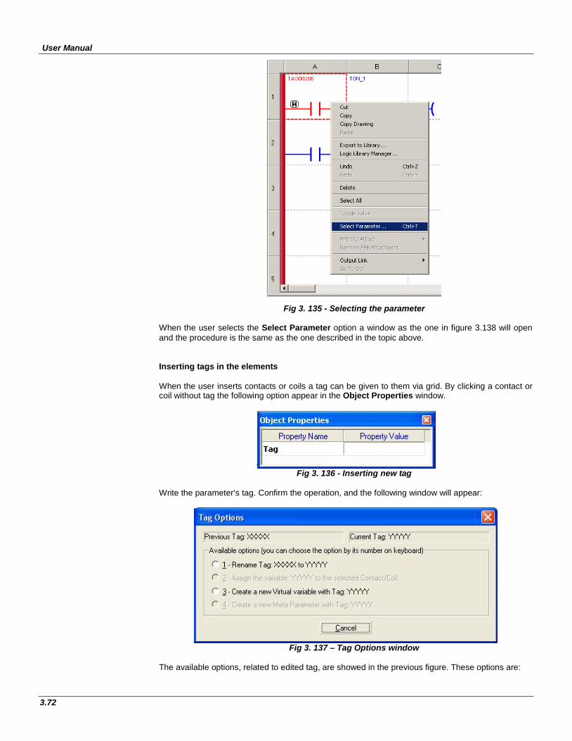
User Manual
3.72
Fig 3. 135 - Selecting the parameter When the user selects the Select Parameter option a window as the one in figure 3.138 will open and the procedure is the same as the one described in the topic above. Inserting tags in the elements When the user inserts contacts or coils a tag can be given to them via grid. By clicking a contact or coil without tag the following option appear in the Object Properties window.
Fig 3. 136 - Inserting new tag
Write the parameter’s tag. Confirm the operation, and the following window will appear:
Fig 3. 137 – Tag Options window
The available options, related to edited tag, are showed in the previous figure. These options are:
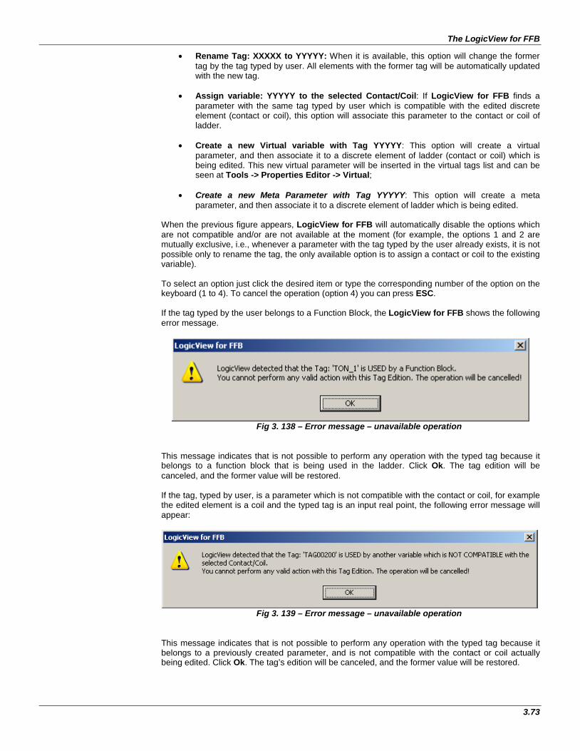
The LogicView for FFB
3.73
• Rename Tag: XXXXX to YYYYY: When it is available, this option will change the former tag by the tag typed by user. All elements with the former tag will be automatically updated with the new tag.
• Assign variable: YYYYY to the selected Contact/Coil: If LogicView for FFB finds a
parameter with the same tag typed by user which is compatible with the edited discrete element (contact or coil), this option will associate this parameter to the contact or coil of ladder.
• Create a new Virtual variable with Tag YYYYY: This option will create a virtual
parameter, and then associate it to a discrete element of ladder (contact or coil) which is being edited. This new virtual parameter will be inserted in the virtual tags list and can be seen at Tools -> Properties Editor -> Virtual;
• Create a new Meta Parameter with Tag YYYYY: This option will create a meta
parameter, and then associate it to a discrete element of ladder which is being edited. When the previous figure appears, LogicView for FFB will automatically disable the options which are not compatible and/or are not available at the moment (for example, the options 1 and 2 are mutually exclusive, i.e., whenever a parameter with the tag typed by the user already exists, it is not possible only to rename the tag, the only available option is to assign a contact or coil to the existing variable). To select an option just click the desired item or type the corresponding number of the option on the keyboard (1 to 4). To cancel the operation (option 4) you can press ESC. If the tag typed by the user belongs to a Function Block, the LogicView for FFB shows the following error message.
Fig 3. 138 – Error message – unavailable operation
This message indicates that is not possible to perform any operation with the typed tag because it belongs to a function block that is being used in the ladder. Click Ok. The tag edition will be canceled, and the former value will be restored. If the tag, typed by user, is a parameter which is not compatible with the contact or coil, for example the edited element is a coil and the typed tag is an input real point, the following error message will appear:
Fig 3. 139 – Error message – unavailable operation
This message indicates that is not possible to perform any operation with the typed tag because it belongs to a previously created parameter, and is not compatible with the contact or coil actually being edited. Click Ok. The tag’s edition will be canceled, and the former value will be restored.
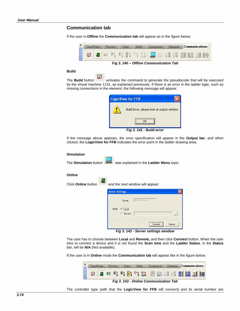
User Manual
3.74
Communication tab If the user is Offline the Communication tab will appear as in the figure below.
Fig 3. 140 – Offline Communication Tab
Build
The Build button activates the command to generate the pseudocode that will be executed by the virtual machine 1131, as explained previously. If there is an error in the ladder logic, such as missing connections in the element, the following message will appear.
Fig 3. 141 - Build error
If the message above appears, the error specification will appear in the Output bar, and when clicked, the LogicView for FFB indicates the error point in the ladder drawing area. Simulation
The Simulation button was explained in the Ladder Menu topic. Online
Click Online button and the next window will appear:
Fig 3. 142 - Server settings window
The user has to choose between Local and Remote, and then click Connect button. When the user tries to connect a device and it is not found the Scan time and the Ladder Status, in the Status bar, will be N/A (Not available). If the user is in Online mode the Communication tab will appear like in the figure below:
Fig 3. 143 - Online Communication Tab
The controller type (with that the LogicView for FFB will connect) and its serial number are
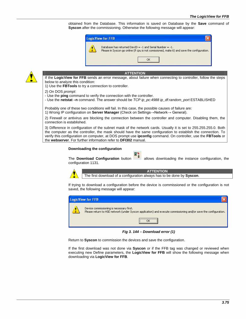
The LogicView for FFB
3.75
obtained from the Database. This information is saved on Database by the Save command of Syscon after the commissioning. Otherwise the following message will appear:
ATTENTION If the LogicView for FFB sends an error message, about failure when connecting to controller, follow the steps below to analyze this condition: 1) Use the FBTools to try a connection to controller.
2) On DOS prompt: - Use the ping command to verify the connection with the controller. - Use the netstat –n command. The answer should be TCP ip_pc:4988 ip_df:random_port ESTABLISHED Probably one of these two conditions will fail. In this case, the possible causes of failure are: 1) Wrong IP configuration on Server Manager (Check on Settings→Network→ General).
2) Firewall or antivirus are blocking the connection between the controller and computer. Disabling them, the connection is established.
3) Difference in configuration of the subnet mask of the network cards. Usually it is set to 255.255.255.0. Both the computer as the controller, the mask should have the same configuration to establish the connection. To verify this configuration on computer, at DOS prompt use ipconfig command. On controller, use the FBTools or the webserver. For further information refer to DFI302 manual.
Downloading the configuration
The Download Configuration button allows downloading the instance configuration, the configuration 1131.
ATTENTION
The first download of a configuration always has to be done by Syscon. If trying to download a configuration before the device is commissioned or the configuration is not saved, the following message will appear:
Fig 3. 144 – Download error (1) Return to Syscon to commission the devices and save the configuration. If the first download was not done via Syscon or if the FFB tag was changed or reviewed when executing new Define parameters, the LogicView for FFB will show the following message when downloading via LogicView for FFB.
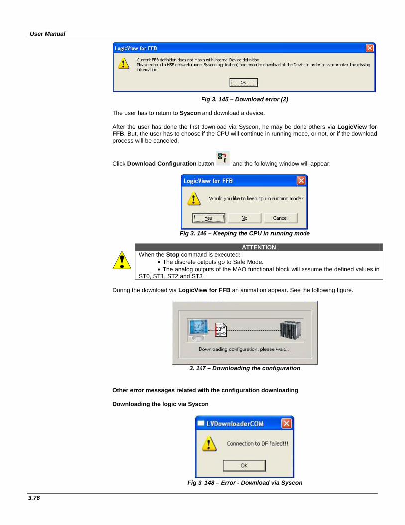
User Manual
3.76
Fig 3. 145 – Download error (2) The user has to return to Syscon and download a device. After the user has done the first download via Syscon, he may be done others via LogicView for FFB. But, the user has to choose if the CPU will continue in running mode, or not, or if the download process will be canceled.
Click Download Configuration button and the following window will appear:
Fig 3. 146 – Keeping the CPU in running mode
ATTENTION When the Stop command is executed:
• The discrete outputs go to Safe Mode. • The analog outputs of the MAO functional block will assume the defined values in
ST0, ST1, ST2 and ST3. During the download via LogicView for FFB an animation appear. See the following figure.
3. 147 – Downloading the configuration
Other error messages related with the configuration downloading
Downloading the logic via Syscon
Fig 3. 148 – Error - Download via Syscon
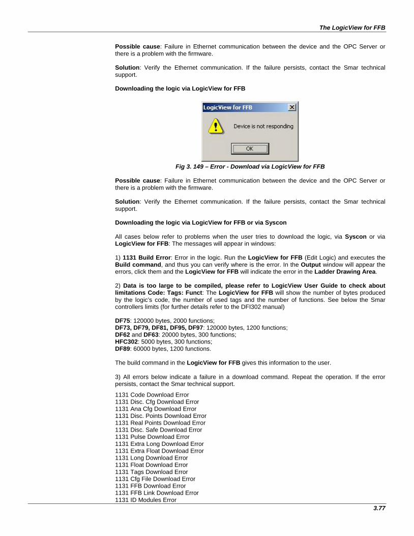
The LogicView for FFB
3.77
Possible cause: Failure in Ethernet communication between the device and the OPC Server or there is a problem with the firmware. Solution: Verify the Ethernet communication. If the failure persists, contact the Smar technical support. Downloading the logic via LogicView for FFB
Fig 3. 149 – Error - Download via LogicView for FFB
Possible cause: Failure in Ethernet communication between the device and the OPC Server or there is a problem with the firmware. Solution: Verify the Ethernet communication. If the failure persists, contact the Smar technical support. Downloading the logic via LogicView for FFB or via Syscon All cases below refer to problems when the user tries to download the logic, via Syscon or via LogicView for FFB: The messages will appear in windows: 1) 1131 Build Error: Error in the logic. Run the LogicView for FFB (Edit Logic) and executes the Build command, and thus you can verify where is the error. In the Output window will appear the errors, click them and the LogicView for FFB will indicate the error in the Ladder Drawing Area. 2) Data is too large to be compiled, please refer to LogicView User Guide to check about limitations Code: Tags: Funct: The LogicView for FFB will show the number of bytes produced by the logic’s code, the number of used tags and the number of functions. See below the Smar controllers limits (for further details refer to the DFI302 manual) DF75: 120000 bytes, 2000 functions; DF73, DF79, DF81, DF95, DF97: 120000 bytes, 1200 functions; DF62 and DF63: 20000 bytes, 300 functions; HFC302: 5000 bytes, 300 functions; DF89: 60000 bytes, 1200 functions. The build command in the LogicView for FFB gives this information to the user. 3) All errors below indicate a failure in a download command. Repeat the operation. If the error persists, contact the Smar technical support.
1131 Code Download Error 1131 Disc. Cfg Download Error 1131 Ana Cfg Download Error 1131 Disc. Points Download Error 1131 Real Points Download Error 1131 Disc. Safe Download Error 1131 Pulse Download Error 1131 Extra Long Download Error 1131 Extra Float Download Error 1131 Long Download Error 1131 Float Download Error 1131 Tags Download Error 1131 Cfg File Download Error 1131 FFB Download Error 1131 FFB Link Download Error 1131 ID Modules Error
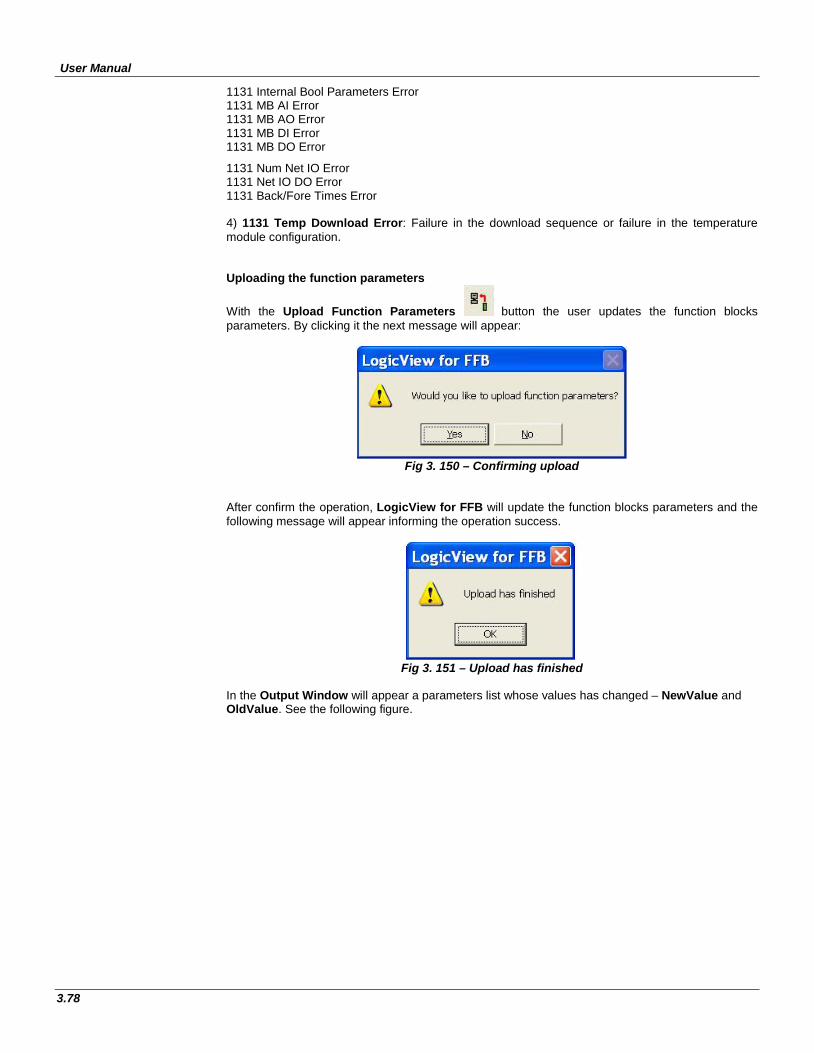
User Manual
3.78
1131 Internal Bool Parameters Error 1131 MB AI Error 1131 MB AO Error 1131 MB DI Error 1131 MB DO Error
1131 Num Net IO Error 1131 Net IO DO Error 1131 Back/Fore Times Error 4) 1131 Temp Download Error: Failure in the download sequence or failure in the temperature module configuration. Uploading the function parameters
With the Upload Function Parameters button the user updates the function blocks parameters. By clicking it the next message will appear:
Fig 3. 150 – Confirming upload
After confirm the operation, LogicView for FFB will update the function blocks parameters and the following message will appear informing the operation success.
Fig 3. 151 – Upload has finished
In the Output Window will appear a parameters list whose values has changed – NewValue and OldValue. See the following figure.
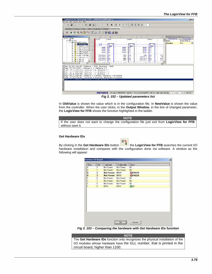
The LogicView for FFB
3.79
Fig 3. 152 – Updated parameters list
In OldValue is shown the value which is in the configuration file. In NewValue is shown the value from the controller. When the user clicks, in the Output Window, in the line of changed parameter, the LogicView for FFB shows the function highlighted in the ladder.
NOTE If the user does not want to change the configuration file just exit from LogicView for FFB without save it.
Get Hardware IDs
By clicking in the Get Hardware IDs button the LogicView for FFB searches the current I/O hardware installation and compares with the configuration done via software. A window as the following will appear:
Fig 3. 153 – Comparing the hardware with Get Hardware IDs function
NOTE
The Get Hardware IDs function only recognizes the physical installation of the I/O modules whose hardware have the GLL number, that is printed in the circuit board, higher than 1100.
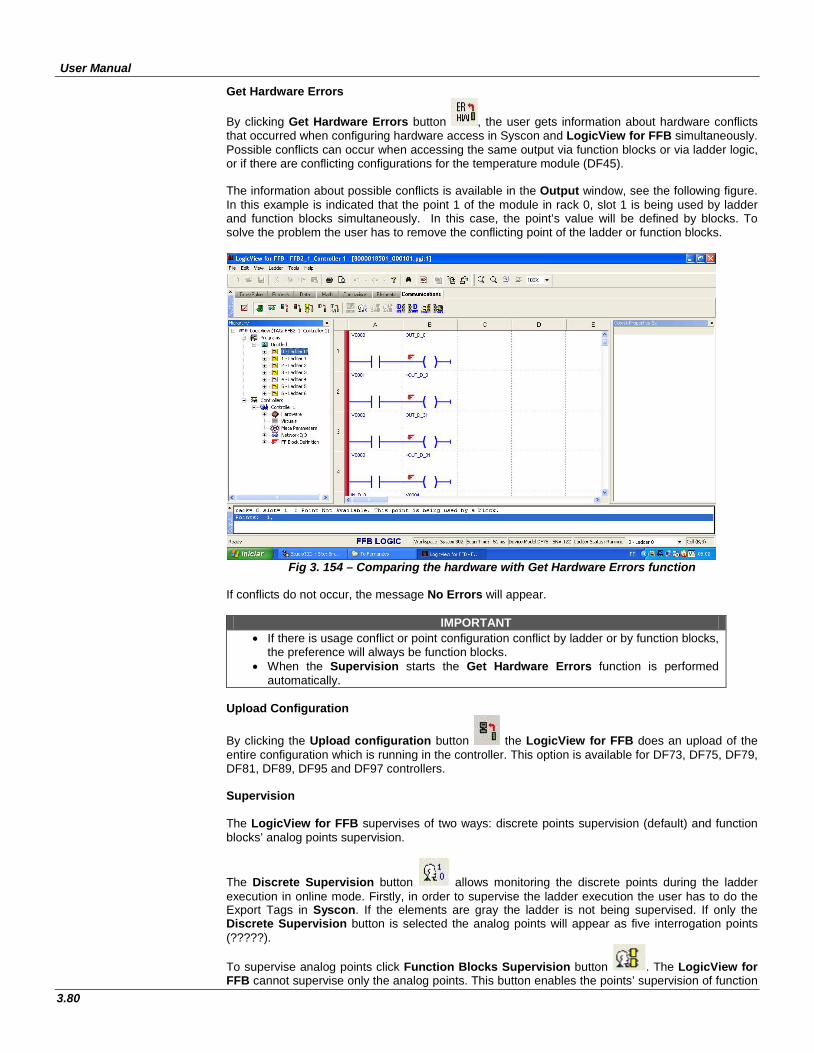
User Manual
3.80
Get Hardware Errors
By clicking Get Hardware Errors button , the user gets information about hardware conflicts that occurred when configuring hardware access in Syscon and LogicView for FFB simultaneously. Possible conflicts can occur when accessing the same output via function blocks or via ladder logic, or if there are conflicting configurations for the temperature module (DF45). The information about possible conflicts is available in the Output window, see the following figure. In this example is indicated that the point 1 of the module in rack 0, slot 1 is being used by ladder and function blocks simultaneously. In this case, the point’s value will be defined by blocks. To solve the problem the user has to remove the conflicting point of the ladder or function blocks.
Fig 3. 154 – Comparing the hardware with Get Hardware Errors function
If conflicts do not occur, the message No Errors will appear.
IMPORTANT • If there is usage conflict or point configuration conflict by ladder or by function blocks,
the preference will always be function blocks. • When the Supervision starts the Get Hardware Errors function is performed
automatically. Upload Configuration
By clicking the Upload configuration button the LogicView for FFB does an upload of the entire configuration which is running in the controller. This option is available for DF73, DF75, DF79, DF81, DF89, DF95 and DF97 controllers. Supervision The LogicView for FFB supervises of two ways: discrete points supervision (default) and function blocks’ analog points supervision.
The Discrete Supervision button allows monitoring the discrete points during the ladder execution in online mode. Firstly, in order to supervise the ladder execution the user has to do the Export Tags in Syscon. If the elements are gray the ladder is not being supervised. If only the Discrete Supervision button is selected the analog points will appear as five interrogation points (?????).
To supervise analog points click Function Blocks Supervision button . The LogicView for FFB cannot supervise only the analog points. This button enables the points’ supervision of function
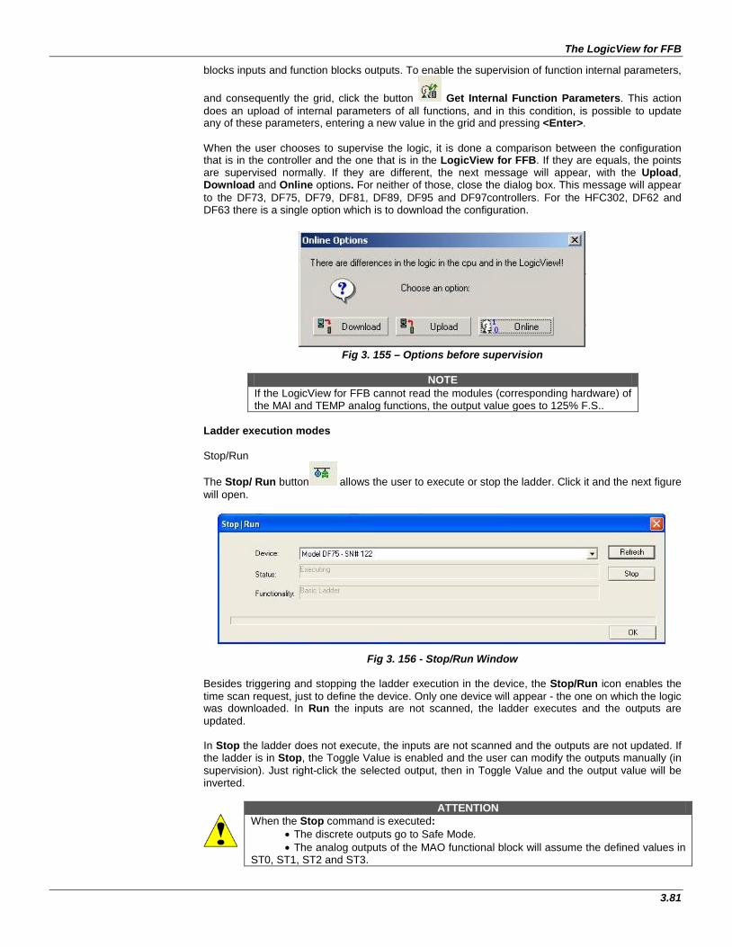
The LogicView for FFB
3.81
blocks inputs and function blocks outputs. To enable the supervision of function internal parameters,
and consequently the grid, click the button Get Internal Function Parameters. This action does an upload of internal parameters of all functions, and in this condition, is possible to update any of these parameters, entering a new value in the grid and pressing <Enter>. When the user chooses to supervise the logic, it is done a comparison between the configuration that is in the controller and the one that is in the LogicView for FFB. If they are equals, the points are supervised normally. If they are different, the next message will appear, with the Upload, Download and Online options. For neither of those, close the dialog box. This message will appear to the DF73, DF75, DF79, DF81, DF89, DF95 and DF97controllers. For the HFC302, DF62 and DF63 there is a single option which is to download the configuration.
Fig 3. 155 – Options before supervision
NOTE
If the LogicView for FFB cannot read the modules (corresponding hardware) of the MAI and TEMP analog functions, the output value goes to 125% F.S..
Ladder execution modes Stop/Run
The Stop/ Run button allows the user to execute or stop the ladder. Click it and the next figure will open.
Fig 3. 156 - Stop/Run Window Besides triggering and stopping the ladder execution in the device, the Stop/Run icon enables the time scan request, just to define the device. Only one device will appear - the one on which the logic was downloaded. In Run the inputs are not scanned, the ladder executes and the outputs are updated. In Stop the ladder does not execute, the inputs are not scanned and the outputs are not updated. If the ladder is in Stop, the Toggle Value is enabled and the user can modify the outputs manually (in supervision). Just right-click the selected output, then in Toggle Value and the output value will be inverted.
ATTENTION When the Stop command is executed:
• The discrete outputs go to Safe Mode. • The analog outputs of the MAO functional block will assume the defined values in
ST0, ST1, ST2 and ST3.
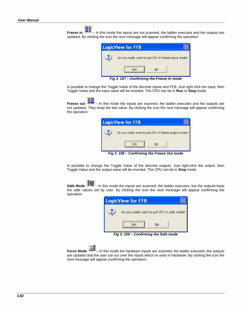
User Manual
3.82
Freeze in – In this mode the inputs are not scanned, the ladder executes and the outputs are updated. By clicking the icon the next message will appear confirming the operation:
Fig 3. 157 – Confirming the Freeze In mode
Is possible to change the Toggle Value of the discrete inputs and FFB. Just right-click the input, then Toggle Value and the input value will be inverted. The CPU can be in Run or Stop mode.
Freeze out – In this mode the inputs are scanned, the ladder executes and the outputs are not updated. They keep the last value. By clicking the icon the next message will appear confirming the operation:
Fig 3. 158 – Confirming the Freeze Out mode
Is possible to change the Toggle Value of the discrete outputs. Just right-click the output, then Toggle Value and the output value will be inverted. The CPU can be in Stop mode.
Safe Mode - In this mode the inputs are scanned, the ladder executes, but the outputs keep the safe values set by user. By clicking the icon the next message will appear confirming the operation:
Fig 3. 159 – Confirming the Safe mode
Force Mode – In this mode the hardware inputs are scanned, the ladder executes, the outputs are updated and the user can act over the inputs which no exist in hardware. By clicking the icon the next message will appear confirming the operation:
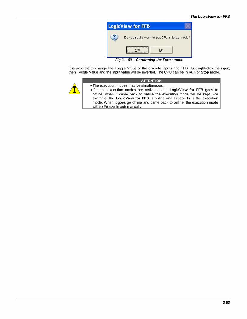
The LogicView for FFB
3.83
Fig 3. 160 – Confirming the Force mode
It is possible to change the Toggle Value of the discrete inputs and FFB. Just right-click the input, then Toggle Value and the input value will be inverted. The CPU can be in Run or Stop mode.
ATTENTION • The execution modes may be simultaneous. • If some execution modes are activated and LogicView for FFB goes to
offline, when it came back to online the execution mode will be kept. For example, the LogicView for FFB is online and Freeze In is the execution mode. When it goes go offline and came back to online, the execution mode will be Freeze In automatically.
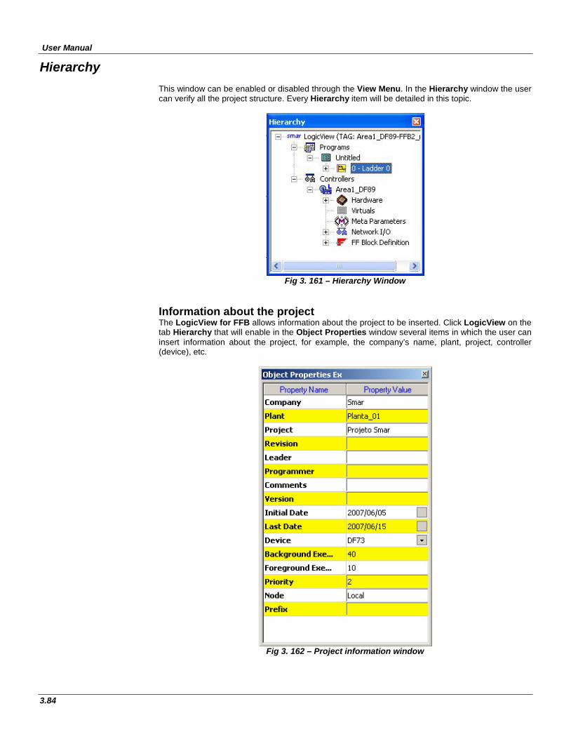
User Manual
3.84
Hierarchy This window can be enabled or disabled through the View Menu. In the Hierarchy window the user can verify all the project structure. Every Hierarchy item will be detailed in this topic.
Fig 3. 161 – Hierarchy Window
Information about the project The LogicView for FFB allows information about the project to be inserted. Click LogicView on the tab Hierarchy that will enable in the Object Properties window several items in which the user can insert information about the project, for example, the company’s name, plant, project, controller (device), etc.
Fig 3. 162 – Project information window
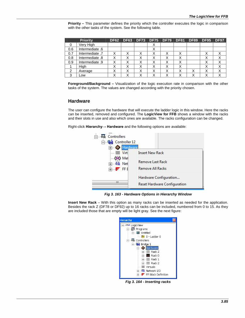
The LogicView for FFB
3.85
Priority – This parameter defines the priority which the controller executes the logic in comparison with the other tasks of the system. See the following table.
Priority DF62 DF63 DF73 DF75 DF79 DF81 DF89 DF95 DF97 0 Very High X
0.6 Intermediate .6 X 0.7 Intermediate .7 X X X X X X X X 0.8 Intermediate .8 X X X X X X X X 0.9 Intermediate .9 X X X X X X X X 1 High X X X X X X X X 2 Average X X X X X X X X X 3 Low X X X X X X X X X
Foreground/Background – Visualization of the logic execution rate in comparison with the other tasks of the system. The values are changed according with the priority chosen. Hardware The user can configure the hardware that will execute the ladder logic in this window. Here the racks can be inserted, removed and configured. The LogicView for FFB shows a window with the racks and their slots in use and also which ones are available. The racks configuration can be changed. Right-click Hierarchy→ Hardware and the following options are available:
Fig 3. 163 - Hardware Options in Hierarchy Window Insert New Rack – With this option as many racks can be inserted as needed for the application. Besides the rack Z (DF78 or DF92) up to 16 racks can be included, numbered from 0 to 15. As they are included those that are empty will be light gray. See the next figure:
Fig 3. 164 - Inserting racks
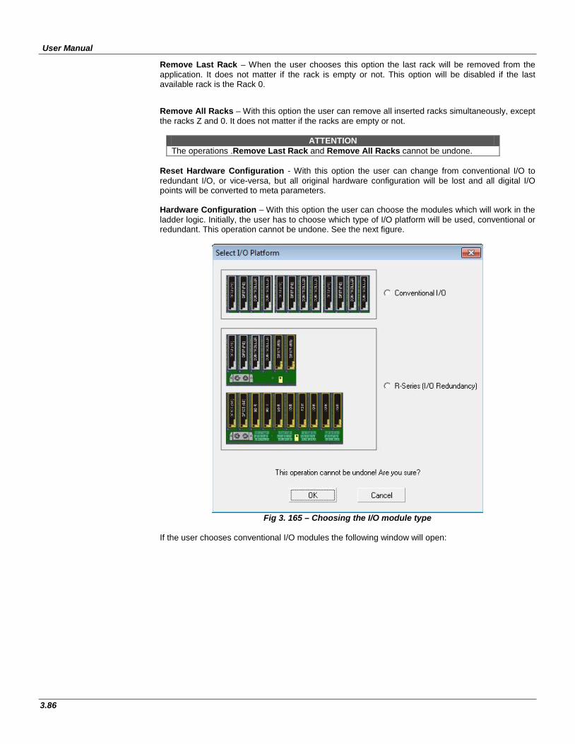
User Manual
3.86
Remove Last Rack – When the user chooses this option the last rack will be removed from the application. It does not matter if the rack is empty or not. This option will be disabled if the last available rack is the Rack 0. Remove All Racks – With this option the user can remove all inserted racks simultaneously, except the racks Z and 0. It does not matter if the racks are empty or not.
ATTENTION The operations .Remove Last Rack and Remove All Racks cannot be undone.
Reset Hardware Configuration - With this option the user can change from conventional I/O to redundant I/O, or vice-versa, but all original hardware configuration will be lost and all digital I/O points will be converted to meta parameters. Hardware Configuration – With this option the user can choose the modules which will work in the ladder logic. Initially, the user has to choose which type of I/O platform will be used, conventional or redundant. This operation cannot be undone. See the next figure.
Fig 3. 165 – Choosing the I/O module type
If the user chooses conventional I/O modules the following window will open:
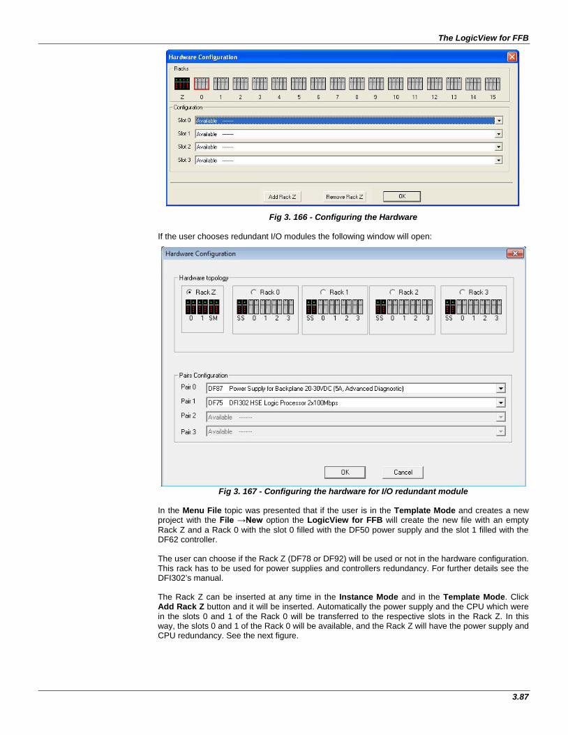
The LogicView for FFB
3.87
Fig 3. 166 - Configuring the Hardware If the user chooses redundant I/O modules the following window will open:
Fig 3. 167 - Configuring the hardware for I/O redundant module
In the Menu File topic was presented that if the user is in the Template Mode and creates a new project with the File →New option the LogicView for FFB will create the new file with an empty Rack Z and a Rack 0 with the slot 0 filled with the DF50 power supply and the slot 1 filled with the DF62 controller. The user can choose if the Rack Z (DF78 or DF92) will be used or not in the hardware configuration. This rack has to be used for power supplies and controllers redundancy. For further details see the DFI302’s manual. The Rack Z can be inserted at any time in the Instance Mode and in the Template Mode. Click Add Rack Z button and it will be inserted. Automatically the power supply and the CPU which were in the slots 0 and 1 of the Rack 0 will be transferred to the respective slots in the Rack Z. In this way, the slots 0 and 1 of the Rack 0 will be available, and the Rack Z will have the power supply and CPU redundancy. See the next figure.
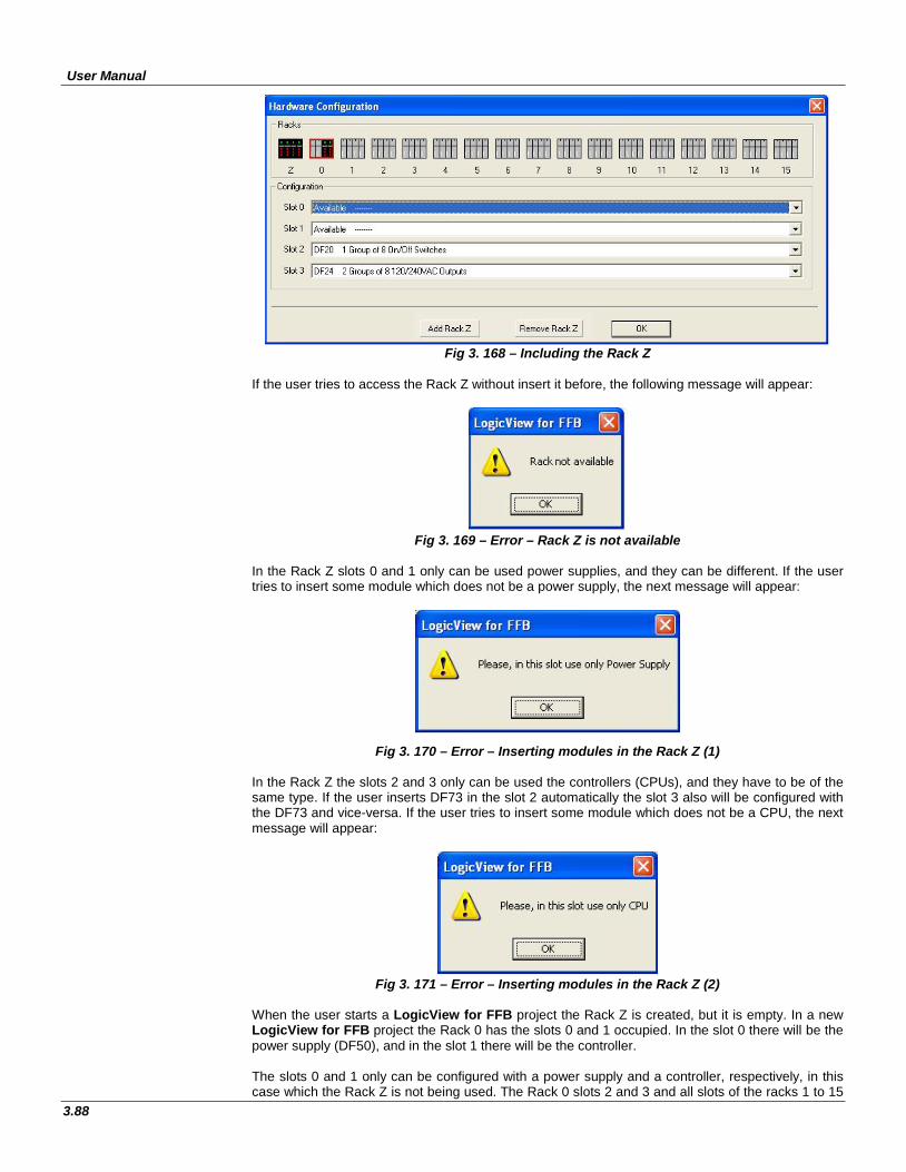
User Manual
3.88
Fig 3. 168 – Including the Rack Z
If the user tries to access the Rack Z without insert it before, the following message will appear:
Fig 3. 169 – Error – Rack Z is not available
In the Rack Z slots 0 and 1 only can be used power supplies, and they can be different. If the user tries to insert some module which does not be a power supply, the next message will appear:
Fig 3. 170 – Error – Inserting modules in the Rack Z (1) In the Rack Z the slots 2 and 3 only can be used the controllers (CPUs), and they have to be of the same type. If the user inserts DF73 in the slot 2 automatically the slot 3 also will be configured with the DF73 and vice-versa. If the user tries to insert some module which does not be a CPU, the next message will appear:
Fig 3. 171 – Error – Inserting modules in the Rack Z (2)
When the user starts a LogicView for FFB project the Rack Z is created, but it is empty. In a new LogicView for FFB project the Rack 0 has the slots 0 and 1 occupied. In the slot 0 there will be the power supply (DF50), and in the slot 1 there will be the controller. The slots 0 and 1 only can be configured with a power supply and a controller, respectively, in this case which the Rack Z is not being used. The Rack 0 slots 2 and 3 and all slots of the racks 1 to 15
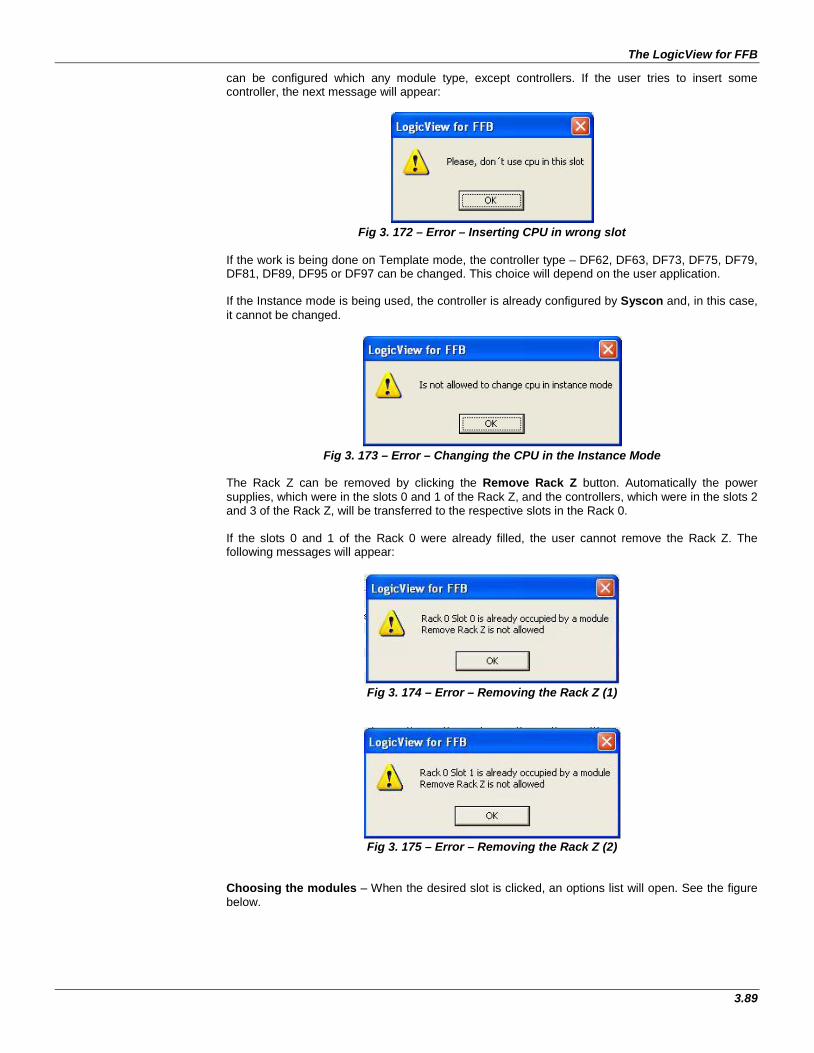
The LogicView for FFB
3.89
can be configured which any module type, except controllers. If the user tries to insert some controller, the next message will appear:
Fig 3. 172 – Error – Inserting CPU in wrong slot
If the work is being done on Template mode, the controller type – DF62, DF63, DF73, DF75, DF79, DF81, DF89, DF95 or DF97 can be changed. This choice will depend on the user application. If the Instance mode is being used, the controller is already configured by Syscon and, in this case, it cannot be changed.
Fig 3. 173 – Error – Changing the CPU in the Instance Mode
The Rack Z can be removed by clicking the Remove Rack Z button. Automatically the power supplies, which were in the slots 0 and 1 of the Rack Z, and the controllers, which were in the slots 2 and 3 of the Rack Z, will be transferred to the respective slots in the Rack 0. If the slots 0 and 1 of the Rack 0 were already filled, the user cannot remove the Rack Z. The following messages will appear:
Fig 3. 174 – Error – Removing the Rack Z (1)
Fig 3. 175 – Error – Removing the Rack Z (2)
Choosing the modules – When the desired slot is clicked, an options list will open. See the figure below.
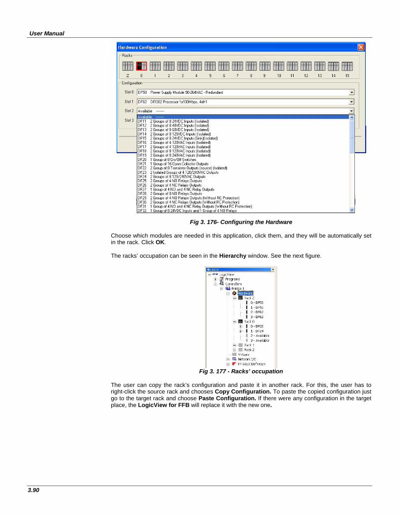
User Manual
3.90
Fig 3. 176- Configuring the Hardware Choose which modules are needed in this application, click them, and they will be automatically set in the rack. Click OK. The racks’ occupation can be seen in the Hierarchy window. See the next figure.
Fig 3. 177 - Racks’ occupation
The user can copy the rack’s configuration and paste it in another rack. For this, the user has to right-click the source rack and chooses Copy Configuration. To paste the copied configuration just go to the target rack and choose Paste Configuration. If there were any configuration in the target place, the LogicView for FFB will replace it with the new one.
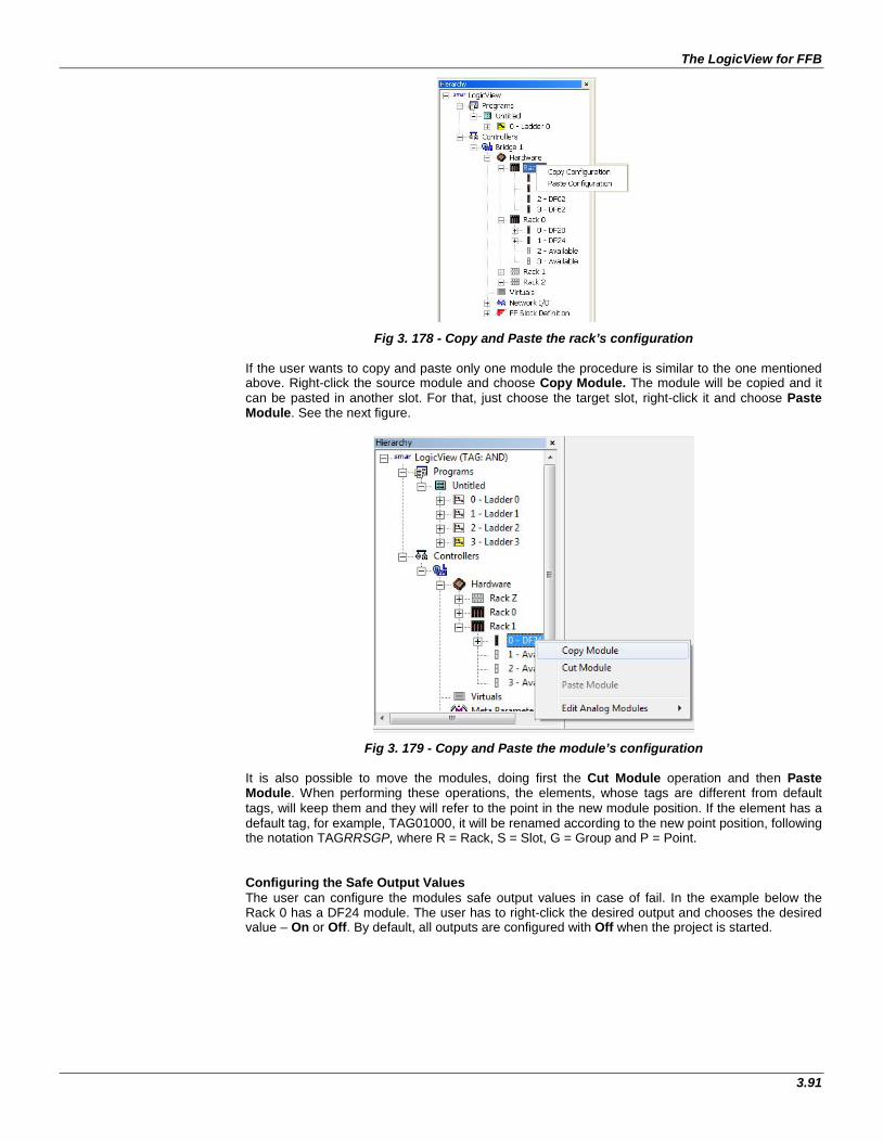
The LogicView for FFB
3.91
Fig 3. 178 - Copy and Paste the rack’s configuration
If the user wants to copy and paste only one module the procedure is similar to the one mentioned above. Right-click the source module and choose Copy Module. The module will be copied and it can be pasted in another slot. For that, just choose the target slot, right-click it and choose Paste Module. See the next figure.
Fig 3. 179 - Copy and Paste the module’s configuration It is also possible to move the modules, doing first the Cut Module operation and then Paste Module. When performing these operations, the elements, whose tags are different from default tags, will keep them and they will refer to the point in the new module position. If the element has a default tag, for example, TAG01000, it will be renamed according to the new point position, following the notation TAGRRSGP, where R = Rack, S = Slot, G = Group and P = Point. Configuring the Safe Output Values The user can configure the modules safe output values in case of fail. In the example below the Rack 0 has a DF24 module. The user has to right-click the desired output and chooses the desired value – On or Off. By default, all outputs are configured with Off when the project is started.
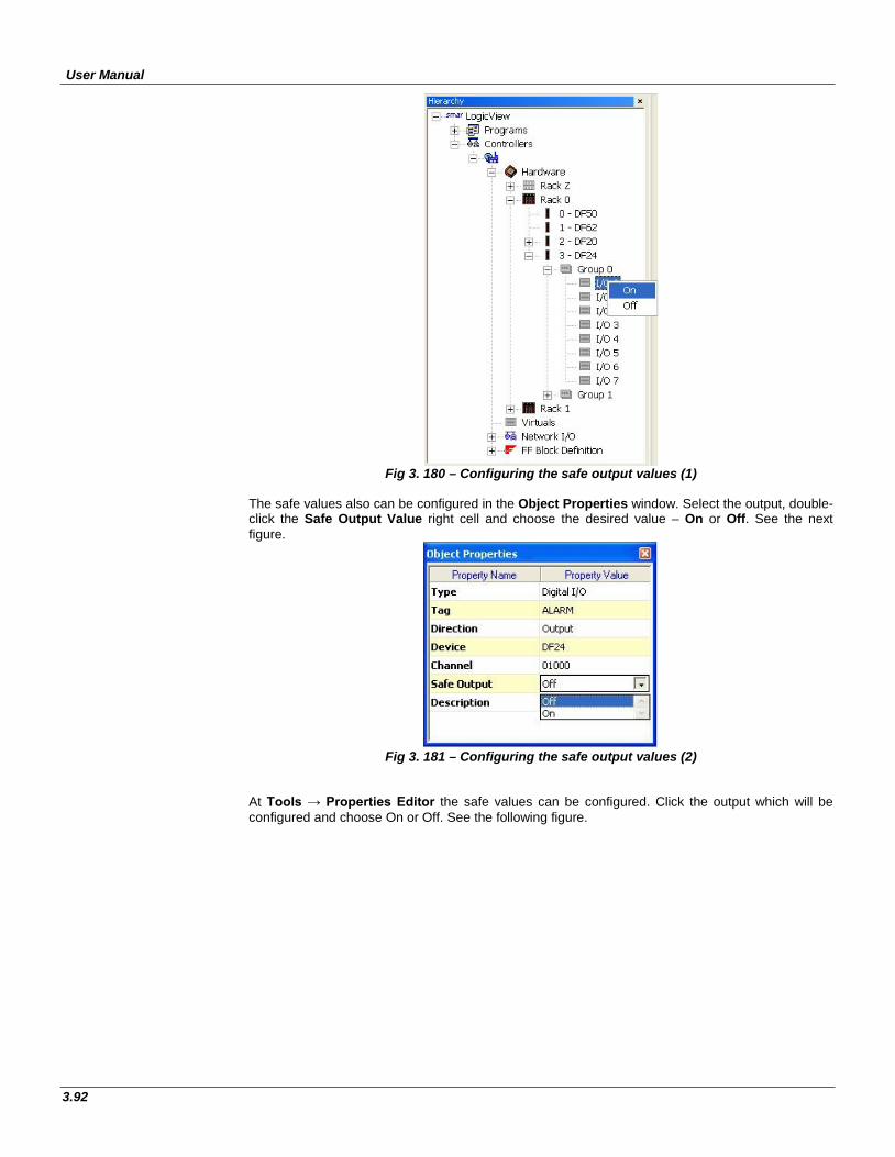
User Manual
3.92
Fig 3. 180 – Configuring the safe output values (1)
The safe values also can be configured in the Object Properties window. Select the output, double-click the Safe Output Value right cell and choose the desired value – On or Off. See the next figure.
Fig 3. 181 – Configuring the safe output values (2)
At Tools → Properties Editor the safe values can be configured. Click the output which will be configured and choose On or Off. See the following figure.
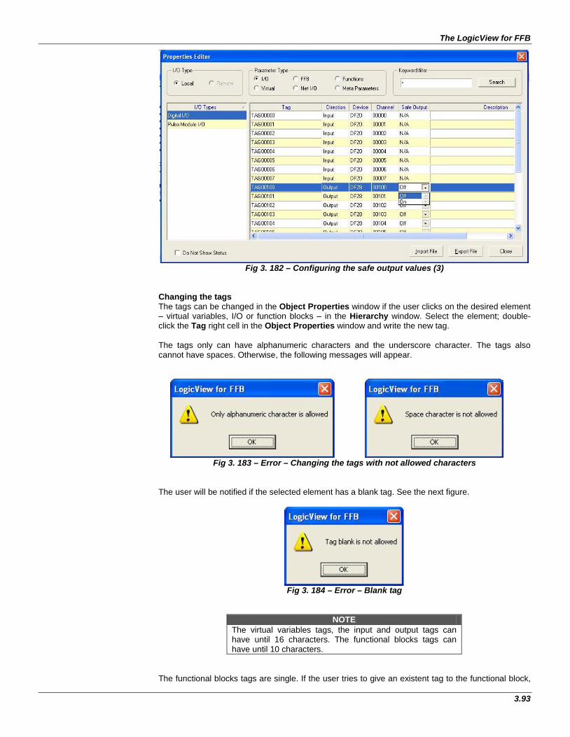
The LogicView for FFB
3.93
Fig 3. 182 – Configuring the safe output values (3)
Changing the tags The tags can be changed in the Object Properties window if the user clicks on the desired element – virtual variables, I/O or function blocks – in the Hierarchy window. Select the element; double-click the Tag right cell in the Object Properties window and write the new tag. The tags only can have alphanumeric characters and the underscore character. The tags also cannot have spaces. Otherwise, the following messages will appear.
Fig 3. 183 – Error – Changing the tags with not allowed characters
The user will be notified if the selected element has a blank tag. See the next figure.
Fig 3. 184 – Error – Blank tag
NOTE The virtual variables tags, the input and output tags can have until 16 characters. The functional blocks tags can have until 10 characters.
The functional blocks tags are single. If the user tries to give an existent tag to the functional block,
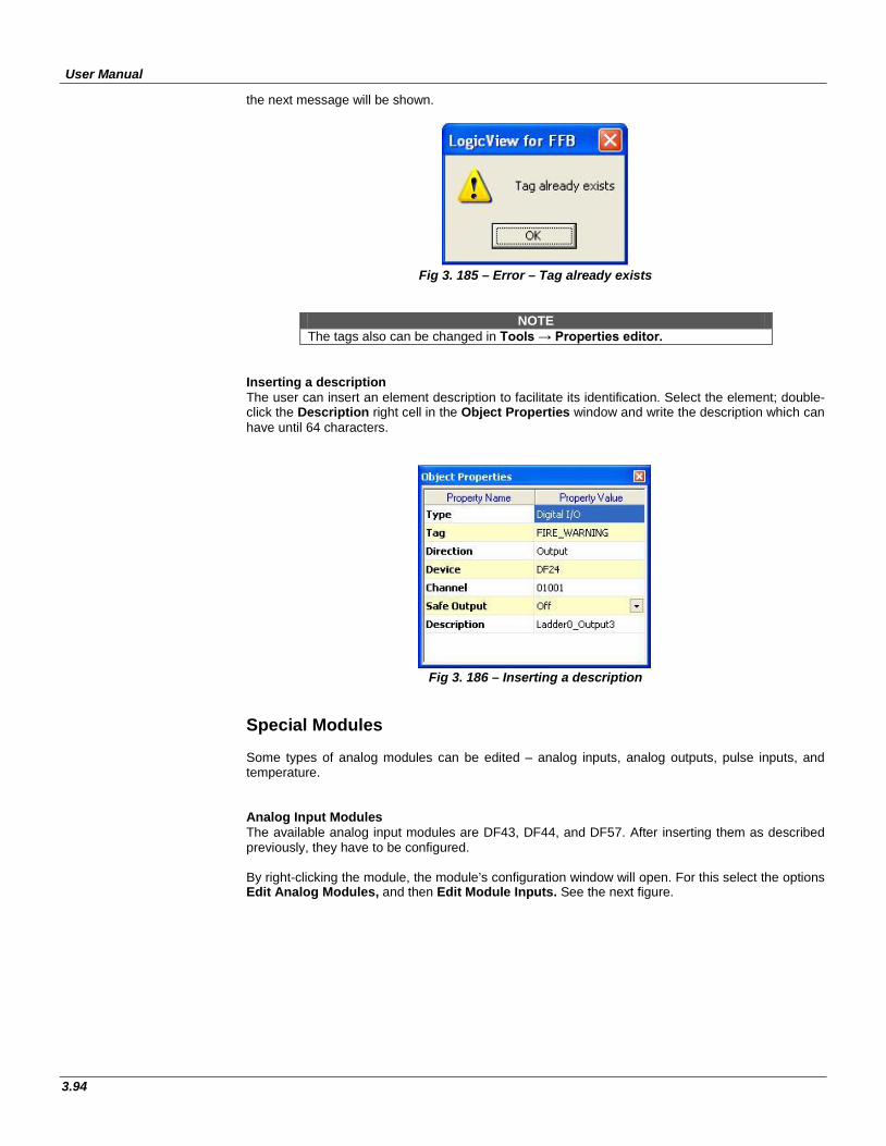
User Manual
3.94
the next message will be shown.
Fig 3. 185 – Error – Tag already exists
NOTE The tags also can be changed in Tools → Properties editor.
Inserting a description The user can insert an element description to facilitate its identification. Select the element; double-click the Description right cell in the Object Properties window and write the description which can have until 64 characters.
Fig 3. 186 – Inserting a description
Special Modules Some types of analog modules can be edited – analog inputs, analog outputs, pulse inputs, and temperature. Analog Input Modules The available analog input modules are DF43, DF44, and DF57. After inserting them as described previously, they have to be configured. By right-clicking the module, the module’s configuration window will open. For this select the options Edit Analog Modules, and then Edit Module Inputs. See the next figure.
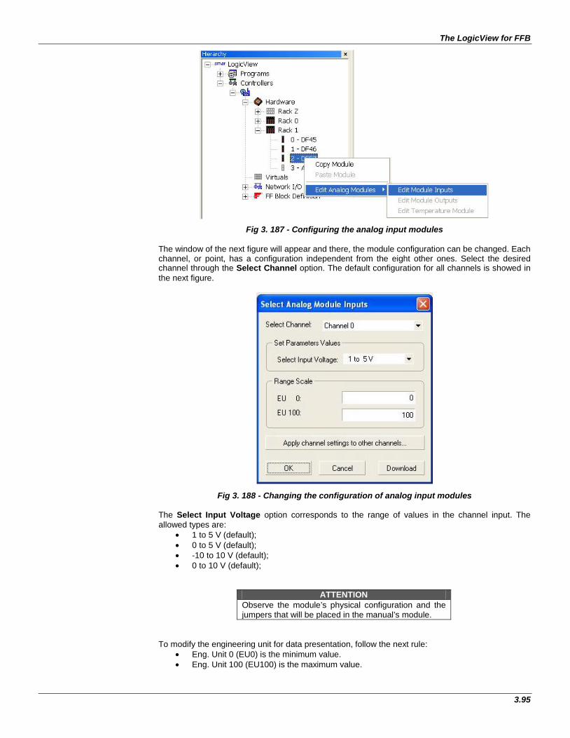
The LogicView for FFB
3.95
Fig 3. 187 - Configuring the analog input modules The window of the next figure will appear and there, the module configuration can be changed. Each channel, or point, has a configuration independent from the eight other ones. Select the desired channel through the Select Channel option. The default configuration for all channels is showed in the next figure.
Fig 3. 188 - Changing the configuration of analog input modules The Select Input Voltage option corresponds to the range of values in the channel input. The allowed types are:
• 1 to 5 V (default); • 0 to 5 V (default); • -10 to 10 V (default); • 0 to 10 V (default);
ATTENTION Observe the module’s physical configuration and the jumpers that will be placed in the manual’s module.
To modify the engineering unit for data presentation, follow the next rule:
• Eng. Unit 0 (EU0) is the minimum value. • Eng. Unit 100 (EU100) is the maximum value.
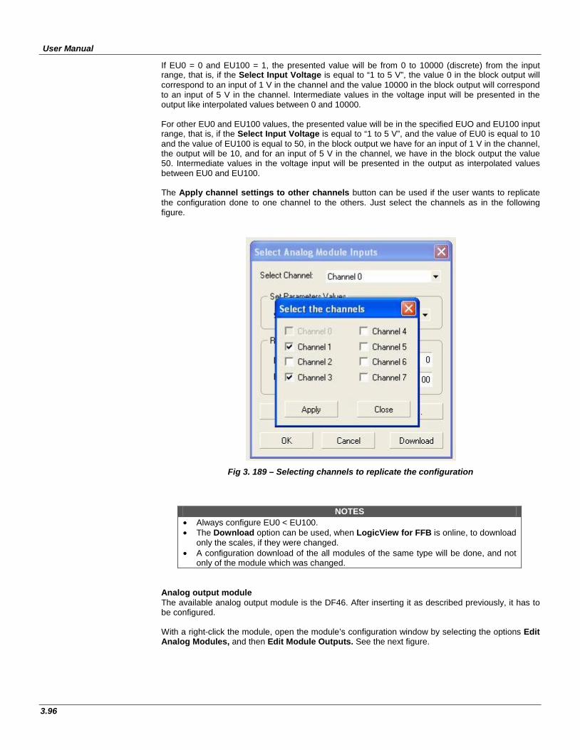
User Manual
3.96
If EU0 = 0 and EU100 = 1, the presented value will be from 0 to 10000 (discrete) from the input range, that is, if the Select Input Voltage is equal to “1 to 5 V”, the value 0 in the block output will correspond to an input of 1 V in the channel and the value 10000 in the block output will correspond to an input of 5 V in the channel. Intermediate values in the voltage input will be presented in the output like interpolated values between 0 and 10000. For other EU0 and EU100 values, the presented value will be in the specified EUO and EU100 input range, that is, if the Select Input Voltage is equal to “1 to 5 V”, and the value of EU0 is equal to 10 and the value of EU100 is equal to 50, in the block output we have for an input of 1 V in the channel, the output will be 10, and for an input of 5 V in the channel, we have in the block output the value 50. Intermediate values in the voltage input will be presented in the output as interpolated values between EU0 and EU100. The Apply channel settings to other channels button can be used if the user wants to replicate the configuration done to one channel to the others. Just select the channels as in the following figure.
Fig 3. 189 – Selecting channels to replicate the configuration
NOTES
• Always configure EU0 < EU100. • The Download option can be used, when LogicView for FFB is online, to download
only the scales, if they were changed. • A configuration download of the all modules of the same type will be done, and not
only of the module which was changed. Analog output module The available analog output module is the DF46. After inserting it as described previously, it has to be configured. With a right-click the module, open the module’s configuration window by selecting the options Edit Analog Modules, and then Edit Module Outputs. See the next figure.
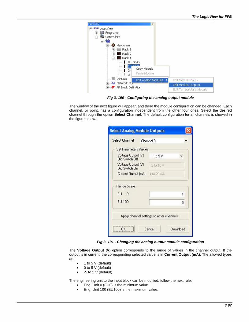
The LogicView for FFB
3.97
Fig 3. 190 - Configuring the analog output module The window of the next figure will appear, and there the module configuration can be changed. Each channel, or point, has a configuration independent from the other four ones. Select the desired channel through the option Select Channel. The default configuration for all channels is showed in the figure below.
Fig 3. 191 - Changing the analog output module configuration The Voltage Output (V) option corresponds to the range of values in the channel output. If the output is in current, the corresponding selected value is in Current Output (mA). The allowed types are:
• 1 to 5 V (default) • 0 to 5 V (default) • -5 to 5 V (default)
The engineering unit to the input block can be modified, follow the next rule:
• Eng. Unit 0 (EU0) is the minimum value. • Eng. Unit 100 (EU100) is the maximum value.
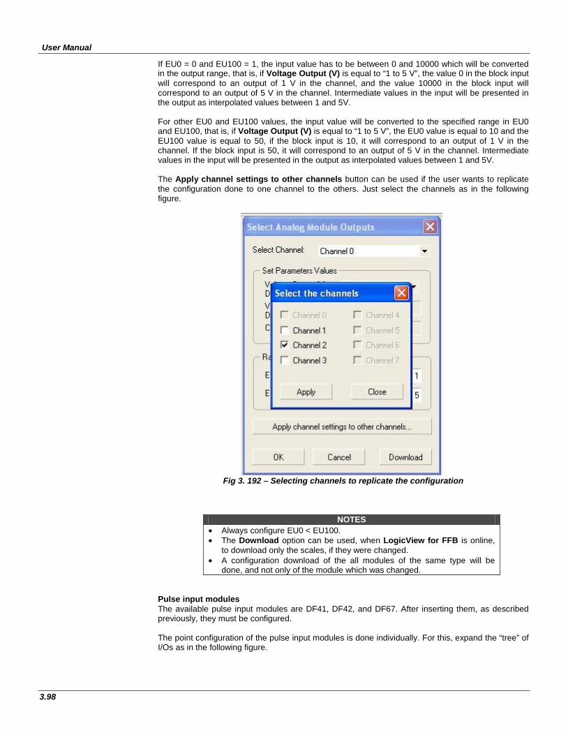
User Manual
3.98
If EU0 = 0 and EU100 = 1, the input value has to be between 0 and 10000 which will be converted in the output range, that is, if Voltage Output (V) is equal to “1 to 5 V”, the value 0 in the block input will correspond to an output of 1 V in the channel, and the value 10000 in the block input will correspond to an output of 5 V in the channel. Intermediate values in the input will be presented in the output as interpolated values between 1 and 5V. For other EU0 and EU100 values, the input value will be converted to the specified range in EU0 and EU100, that is, if Voltage Output (V) is equal to “1 to 5 V”, the EU0 value is equal to 10 and the EU100 value is equal to 50, if the block input is 10, it will correspond to an output of 1 V in the channel. If the block input is 50, it will correspond to an output of 5 V in the channel. Intermediate values in the input will be presented in the output as interpolated values between 1 and 5V. The Apply channel settings to other channels button can be used if the user wants to replicate the configuration done to one channel to the others. Just select the channels as in the following figure.
Fig 3. 192 – Selecting channels to replicate the configuration
NOTES • Always configure EU0 < EU100. • The Download option can be used, when LogicView for FFB is online,
to download only the scales, if they were changed. • A configuration download of the all modules of the same type will be
done, and not only of the module which was changed. Pulse input modules The available pulse input modules are DF41, DF42, and DF67. After inserting them, as described previously, they must be configured. The point configuration of the pulse input modules is done individually. For this, expand the “tree” of I/Os as in the following figure.
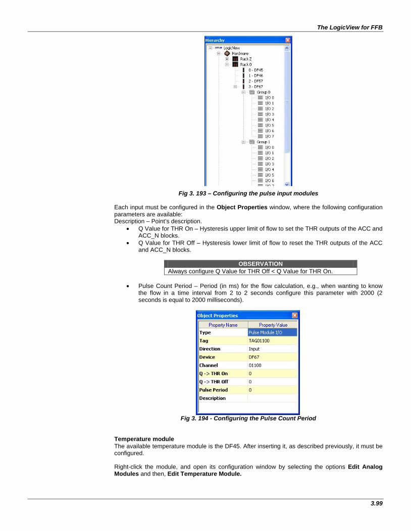
The LogicView for FFB
3.99
Fig 3. 193 – Configuring the pulse input modules
Each input must be configured in the Object Properties window, where the following configuration parameters are available: Description – Point’s description.
• Q Value for THR On – Hysteresis upper limit of flow to set the THR outputs of the ACC and ACC_N blocks.
• Q Value for THR Off – Hysteresis lower limit of flow to reset the THR outputs of the ACC and ACC_N blocks.
OBSERVATION
Always configure Q Value for THR Off < Q Value for THR On.
• Pulse Count Period – Period (in ms) for the flow calculation, e.g., when wanting to know the flow in a time interval from 2 to 2 seconds configure this parameter with 2000 (2 seconds is equal to 2000 milliseconds).
Fig 3. 194 - Configuring the Pulse Count Period
Temperature module The available temperature module is the DF45. After inserting it, as described previously, it must be configured. Right-click the module, and open its configuration window by selecting the options Edit Analog Modules and then, Edit Temperature Module.
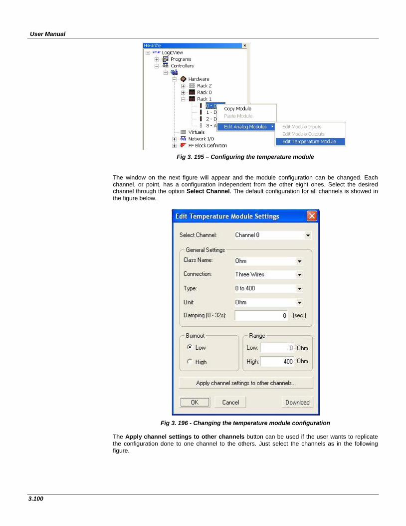
User Manual
3.100
Fig 3. 195 – Configuring the temperature module The window on the next figure will appear and the module configuration can be changed. Each channel, or point, has a configuration independent from the other eight ones. Select the desired channel through the option Select Channel. The default configuration for all channels is showed in the figure below.
Fig 3. 196 - Changing the temperature module configuration The Apply channel settings to other channels button can be used if the user wants to replicate the configuration done to one channel to the others. Just select the channels as in the following figure.
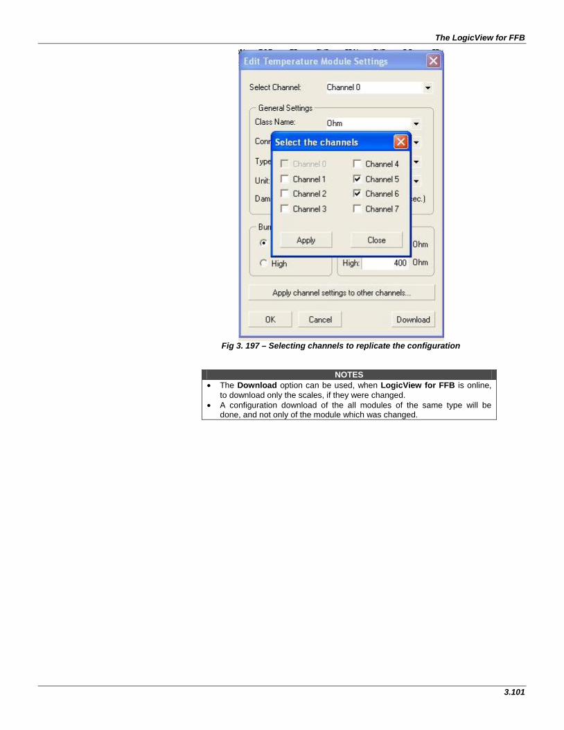
The LogicView for FFB
3.101
Fig 3. 197 – Selecting channels to replicate the configuration
NOTES • The Download option can be used, when LogicView for FFB is online,
to download only the scales, if they were changed. • A configuration download of the all modules of the same type will be
done, and not only of the module which was changed.
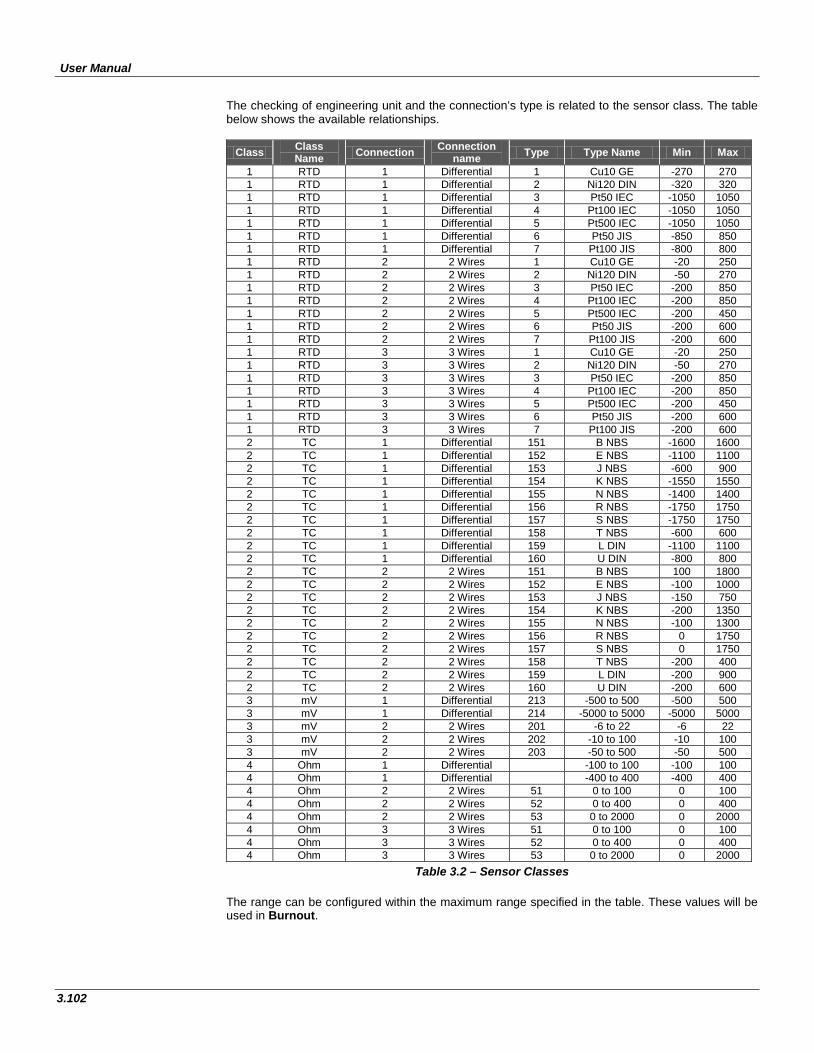
User Manual
3.102
The checking of engineering unit and the connection’s type is related to the sensor class. The table below shows the available relationships.
Class Class Name Connection Connection
name Type Type Name Min Max
1 RTD 1 Differential 1 Cu10 GE -270 270 1 RTD 1 Differential 2 Ni120 DIN -320 320 1 RTD 1 Differential 3 Pt50 IEC -1050 1050 1 RTD 1 Differential 4 Pt100 IEC -1050 1050 1 RTD 1 Differential 5 Pt500 IEC -1050 1050 1 RTD 1 Differential 6 Pt50 JIS -850 850 1 RTD 1 Differential 7 Pt100 JIS -800 800 1 RTD 2 2 Wires 1 Cu10 GE -20 250 1 RTD 2 2 Wires 2 Ni120 DIN -50 270 1 RTD 2 2 Wires 3 Pt50 IEC -200 850 1 RTD 2 2 Wires 4 Pt100 IEC -200 850 1 RTD 2 2 Wires 5 Pt500 IEC -200 450 1 RTD 2 2 Wires 6 Pt50 JIS -200 600 1 RTD 2 2 Wires 7 Pt100 JIS -200 600 1 RTD 3 3 Wires 1 Cu10 GE -20 250 1 RTD 3 3 Wires 2 Ni120 DIN -50 270 1 RTD 3 3 Wires 3 Pt50 IEC -200 850 1 RTD 3 3 Wires 4 Pt100 IEC -200 850 1 RTD 3 3 Wires 5 Pt500 IEC -200 450 1 RTD 3 3 Wires 6 Pt50 JIS -200 600 1 RTD 3 3 Wires 7 Pt100 JIS -200 600 2 TC 1 Differential 151 B NBS -1600 1600 2 TC 1 Differential 152 E NBS -1100 1100 2 TC 1 Differential 153 J NBS -600 900 2 TC 1 Differential 154 K NBS -1550 1550 2 TC 1 Differential 155 N NBS -1400 1400 2 TC 1 Differential 156 R NBS -1750 1750 2 TC 1 Differential 157 S NBS -1750 1750 2 TC 1 Differential 158 T NBS -600 600 2 TC 1 Differential 159 L DIN -1100 1100 2 TC 1 Differential 160 U DIN -800 800 2 TC 2 2 Wires 151 B NBS 100 1800 2 TC 2 2 Wires 152 E NBS -100 1000 2 TC 2 2 Wires 153 J NBS -150 750 2 TC 2 2 Wires 154 K NBS -200 1350 2 TC 2 2 Wires 155 N NBS -100 1300 2 TC 2 2 Wires 156 R NBS 0 1750 2 TC 2 2 Wires 157 S NBS 0 1750 2 TC 2 2 Wires 158 T NBS -200 400 2 TC 2 2 Wires 159 L DIN -200 900 2 TC 2 2 Wires 160 U DIN -200 600 3 mV 1 Differential 213 -500 to 500 -500 500 3 mV 1 Differential 214 -5000 to 5000 -5000 5000 3 mV 2 2 Wires 201 -6 to 22 -6 22 3 mV 2 2 Wires 202 -10 to 100 -10 100 3 mV 2 2 Wires 203 -50 to 500 -50 500 4 Ohm 1 Differential -100 to 100 -100 100 4 Ohm 1 Differential -400 to 400 -400 400 4 Ohm 2 2 Wires 51 0 to 100 0 100 4 Ohm 2 2 Wires 52 0 to 400 0 400 4 Ohm 2 2 Wires 53 0 to 2000 0 2000 4 Ohm 3 3 Wires 51 0 to 100 0 100 4 Ohm 3 3 Wires 52 0 to 400 0 400 4 Ohm 3 3 Wires 53 0 to 2000 0 2000
Table 3.2 – Sensor Classes The range can be configured within the maximum range specified in the table. These values will be used in Burnout.
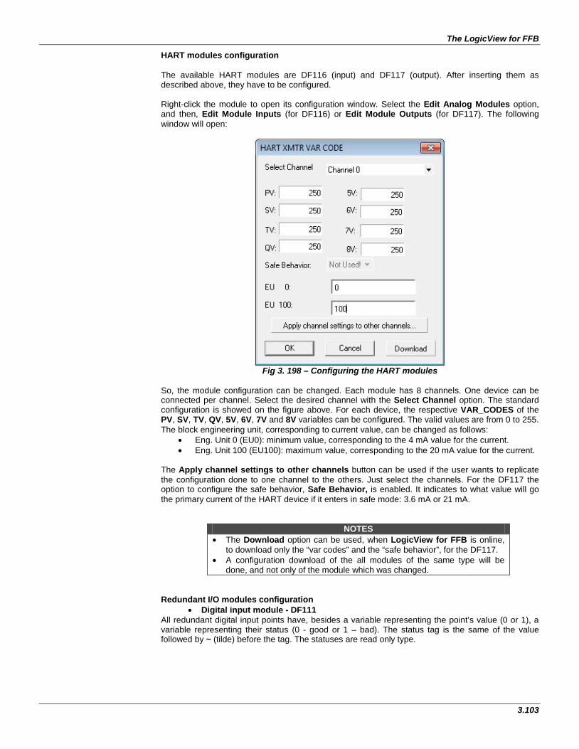
The LogicView for FFB
3.103
HART modules configuration The available HART modules are DF116 (input) and DF117 (output). After inserting them as described above, they have to be configured. Right-click the module to open its configuration window. Select the Edit Analog Modules option, and then, Edit Module Inputs (for DF116) or Edit Module Outputs (for DF117). The following window will open:
Fig 3. 198 – Configuring the HART modules
So, the module configuration can be changed. Each module has 8 channels. One device can be connected per channel. Select the desired channel with the Select Channel option. The standard configuration is showed on the figure above. For each device, the respective VAR_CODES of the PV, SV, TV, QV, 5V, 6V, 7V and 8V variables can be configured. The valid values are from 0 to 255. The block engineering unit, corresponding to current value, can be changed as follows:
• Eng. Unit 0 (EU0): minimum value, corresponding to the 4 mA value for the current. • Eng. Unit 100 (EU100): maximum value, corresponding to the 20 mA value for the current.
The Apply channel settings to other channels button can be used if the user wants to replicate the configuration done to one channel to the others. Just select the channels. For the DF117 the option to configure the safe behavior, Safe Behavior, is enabled. It indicates to what value will go the primary current of the HART device if it enters in safe mode: 3.6 mA or 21 mA.
NOTES • The Download option can be used, when LogicView for FFB is online,
to download only the “var codes” and the “safe behavior”, for the DF117. • A configuration download of the all modules of the same type will be
done, and not only of the module which was changed. Redundant I/O modules configuration
• Digital input module - DF111 All redundant digital input points have, besides a variable representing the point’s value (0 or 1), a variable representing their status (0 - good or 1 – bad). The status tag is the same of the value followed by ~ (tilde) before the tag. The statuses are read only type.
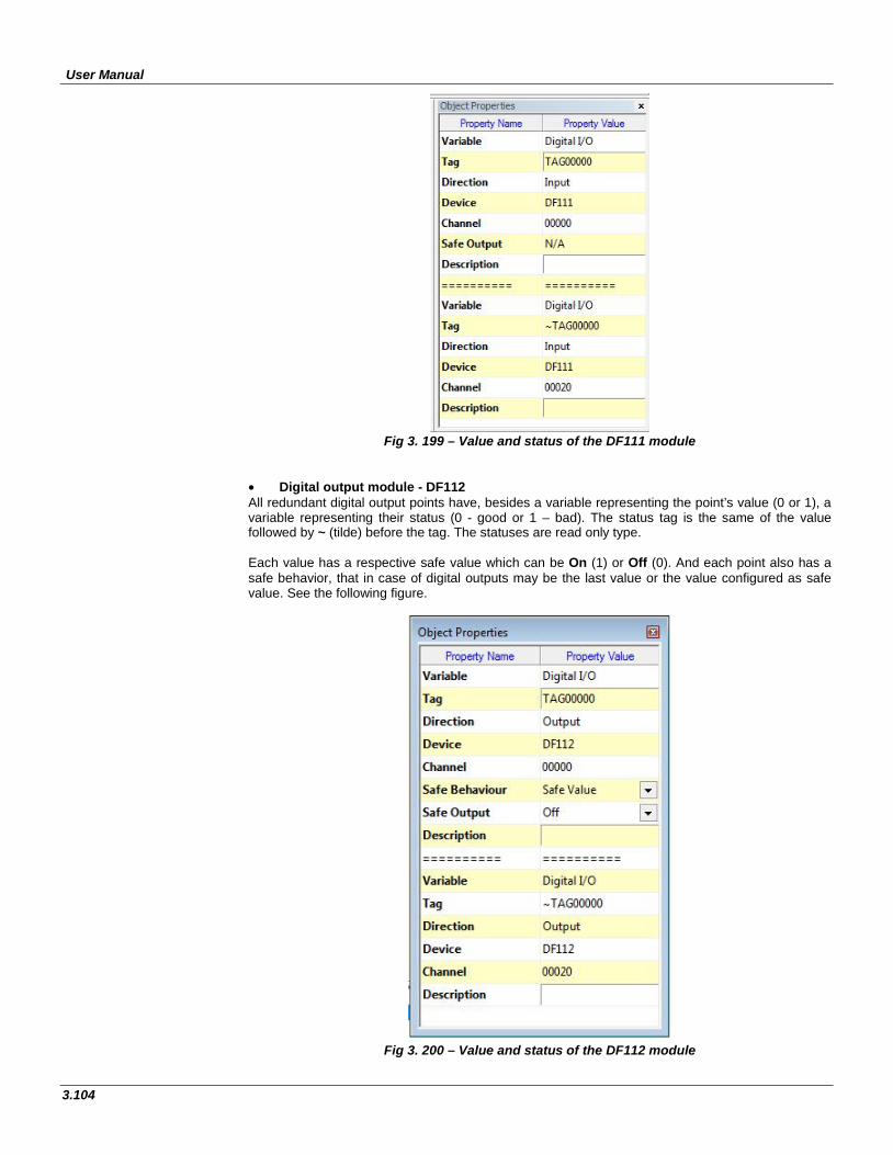
User Manual
3.104
Fig 3. 199 – Value and status of the DF111 module
• Digital output module - DF112 All redundant digital output points have, besides a variable representing the point’s value (0 or 1), a variable representing their status (0 - good or 1 – bad). The status tag is the same of the value followed by ~ (tilde) before the tag. The statuses are read only type. Each value has a respective safe value which can be On (1) or Off (0). And each point also has a safe behavior, that in case of digital outputs may be the last value or the value configured as safe value. See the following figure.
Fig 3. 200 – Value and status of the DF112 module
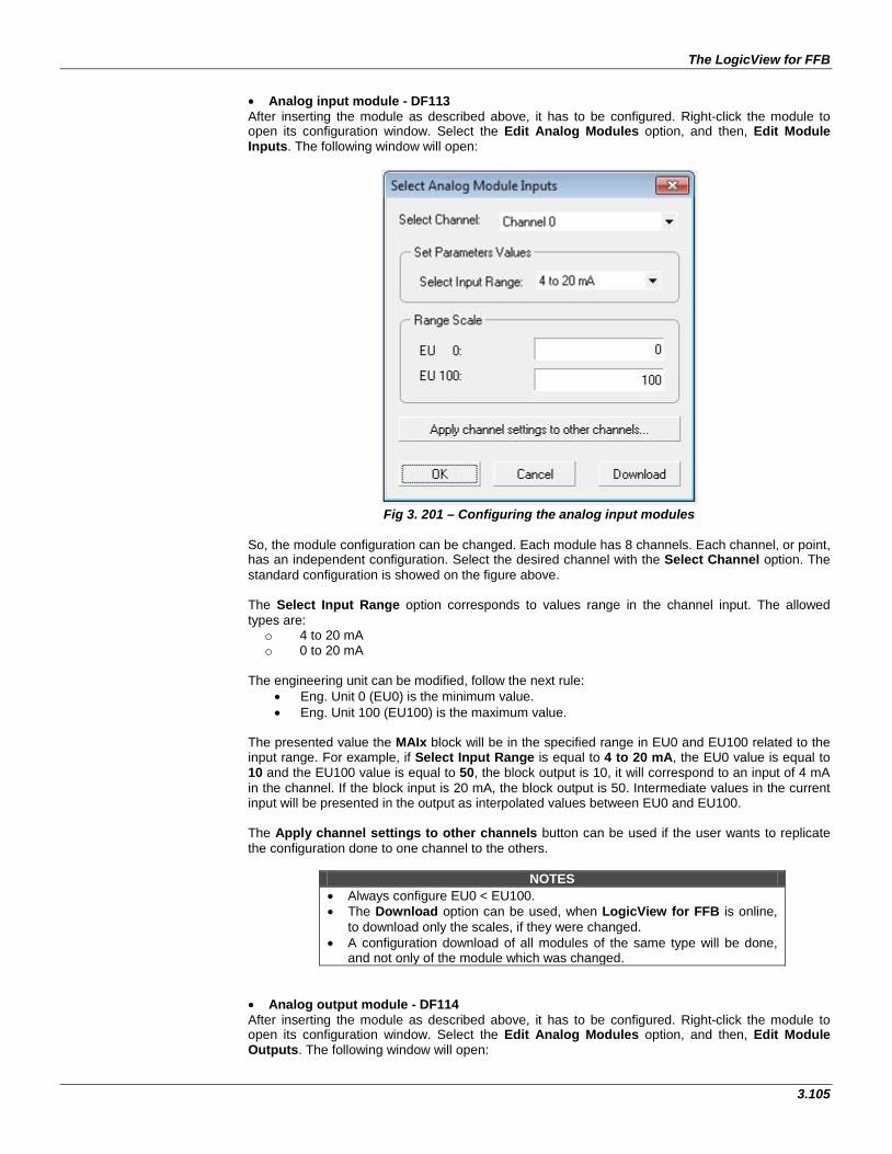
The LogicView for FFB
3.105
• Analog input module - DF113 After inserting the module as described above, it has to be configured. Right-click the module to open its configuration window. Select the Edit Analog Modules option, and then, Edit Module Inputs. The following window will open:
Fig 3. 201 – Configuring the analog input modules
So, the module configuration can be changed. Each module has 8 channels. Each channel, or point, has an independent configuration. Select the desired channel with the Select Channel option. The standard configuration is showed on the figure above. The Select Input Range option corresponds to values range in the channel input. The allowed types are:
o 4 to 20 mA o 0 to 20 mA
The engineering unit can be modified, follow the next rule:
• Eng. Unit 0 (EU0) is the minimum value. • Eng. Unit 100 (EU100) is the maximum value.
The presented value the MAIx block will be in the specified range in EU0 and EU100 related to the input range. For example, if Select Input Range is equal to 4 to 20 mA, the EU0 value is equal to 10 and the EU100 value is equal to 50, the block output is 10, it will correspond to an input of 4 mA in the channel. If the block input is 20 mA, the block output is 50. Intermediate values in the current input will be presented in the output as interpolated values between EU0 and EU100. The Apply channel settings to other channels button can be used if the user wants to replicate the configuration done to one channel to the others.
NOTES • Always configure EU0 < EU100. • The Download option can be used, when LogicView for FFB is online,
to download only the scales, if they were changed. • A configuration download of all modules of the same type will be done,
and not only of the module which was changed. • Analog output module - DF114 After inserting the module as described above, it has to be configured. Right-click the module to open its configuration window. Select the Edit Analog Modules option, and then, Edit Module Outputs. The following window will open:
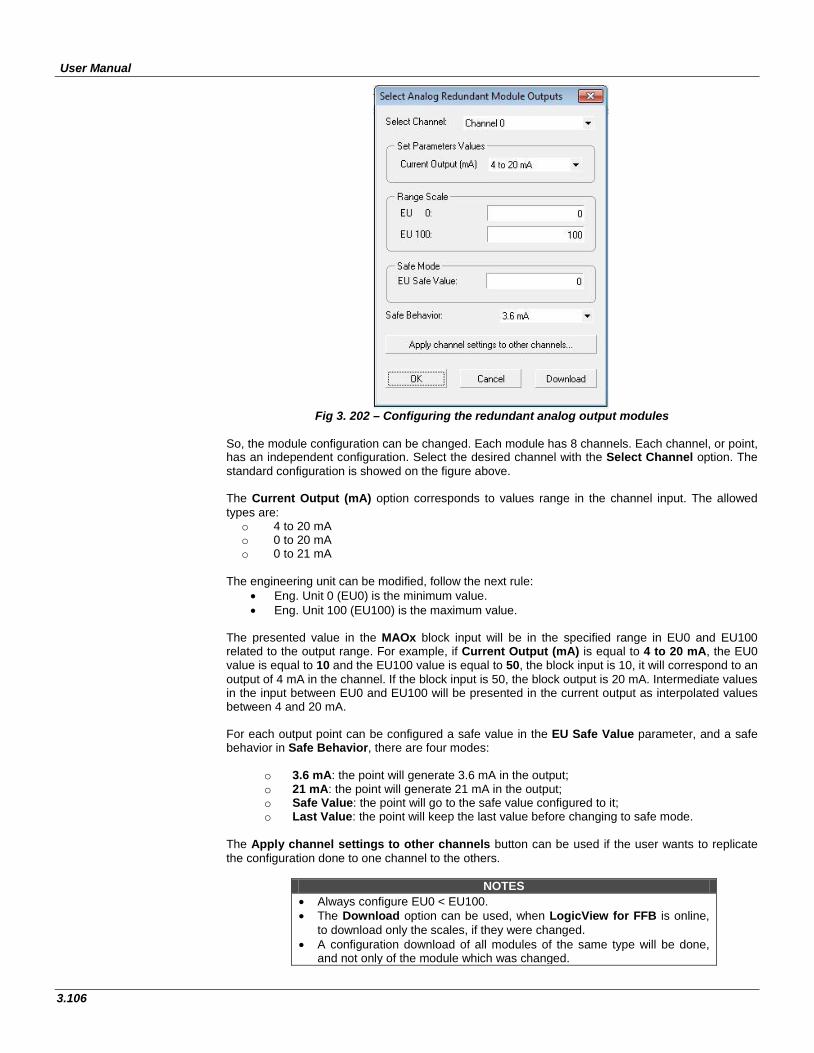
User Manual
3.106
Fig 3. 202 – Configuring the redundant analog output modules
So, the module configuration can be changed. Each module has 8 channels. Each channel, or point, has an independent configuration. Select the desired channel with the Select Channel option. The standard configuration is showed on the figure above. The Current Output (mA) option corresponds to values range in the channel input. The allowed types are:
o 4 to 20 mA o 0 to 20 mA o 0 to 21 mA
The engineering unit can be modified, follow the next rule:
• Eng. Unit 0 (EU0) is the minimum value. • Eng. Unit 100 (EU100) is the maximum value.
The presented value in the MAOx block input will be in the specified range in EU0 and EU100 related to the output range. For example, if Current Output (mA) is equal to 4 to 20 mA, the EU0 value is equal to 10 and the EU100 value is equal to 50, the block input is 10, it will correspond to an output of 4 mA in the channel. If the block input is 50, the block output is 20 mA. Intermediate values in the input between EU0 and EU100 will be presented in the current output as interpolated values between 4 and 20 mA. For each output point can be configured a safe value in the EU Safe Value parameter, and a safe behavior in Safe Behavior, there are four modes:
o 3.6 mA: the point will generate 3.6 mA in the output; o 21 mA: the point will generate 21 mA in the output; o Safe Value: the point will go to the safe value configured to it; o Last Value: the point will keep the last value before changing to safe mode.
The Apply channel settings to other channels button can be used if the user wants to replicate the configuration done to one channel to the others.
NOTES • Always configure EU0 < EU100. • The Download option can be used, when LogicView for FFB is online,
to download only the scales, if they were changed. • A configuration download of all modules of the same type will be done,
and not only of the module which was changed.
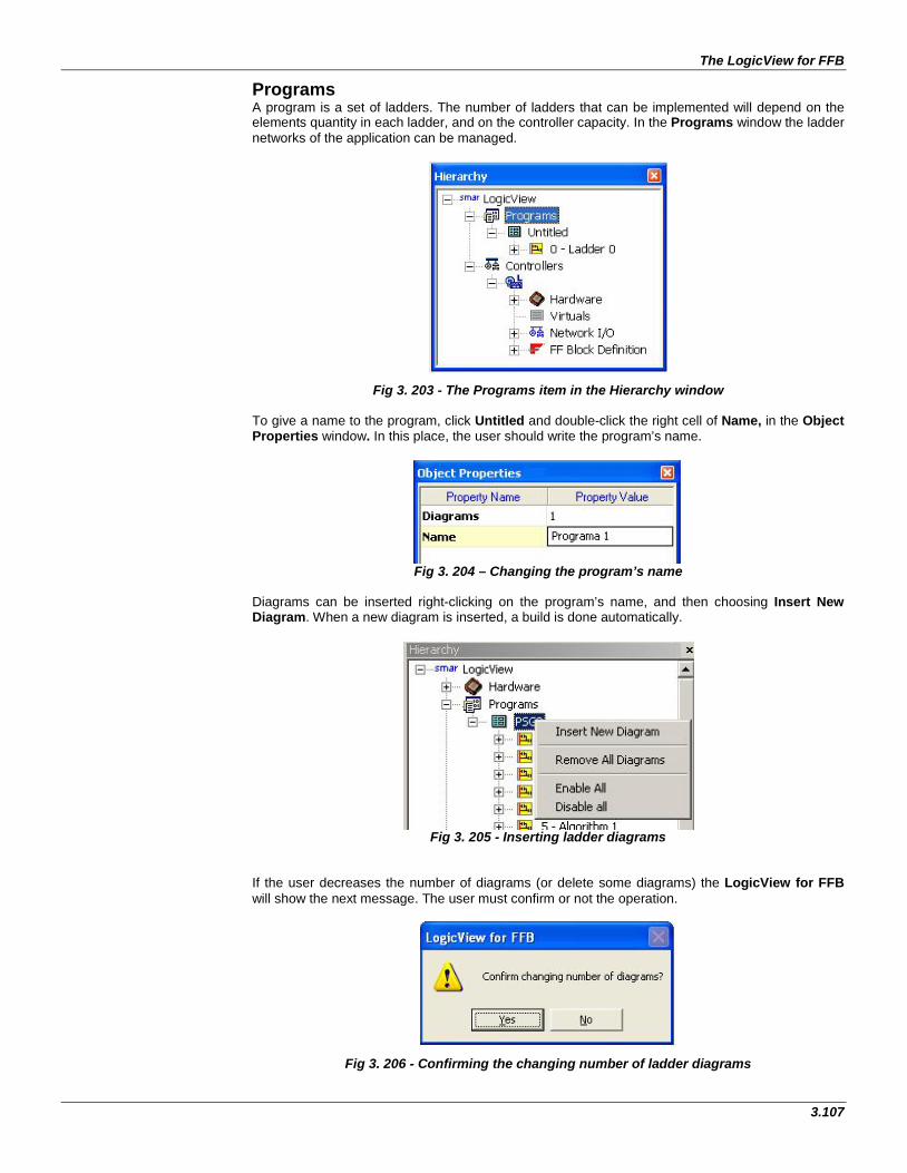
The LogicView for FFB
3.107
Programs A program is a set of ladders. The number of ladders that can be implemented will depend on the elements quantity in each ladder, and on the controller capacity. In the Programs window the ladder networks of the application can be managed.
Fig 3. 203 - The Programs item in the Hierarchy window To give a name to the program, click Untitled and double-click the right cell of Name, in the Object Properties window. In this place, the user should write the program’s name.
Fig 3. 204 – Changing the program’s name
Diagrams can be inserted right-clicking on the program’s name, and then choosing Insert New Diagram. When a new diagram is inserted, a build is done automatically.
Fig 3. 205 - Inserting ladder diagrams
If the user decreases the number of diagrams (or delete some diagrams) the LogicView for FFB will show the next message. The user must confirm or not the operation.
Fig 3. 206 - Confirming the changing number of ladder diagrams
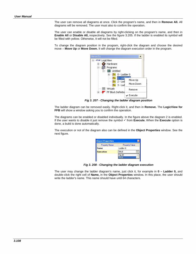
User Manual
3.108
The user can remove all diagrams at once. Click the program’s name, and then in Remove All. All diagrams will be removed. The user must also to confirm the operation. The user can enable or disable all diagrams by right-clicking on the program’s name, and then in Enable All or Disable All, respectively. See the figure 3.205. If the ladder is enabled its symbol will be filled with yellow. Otherwise, it will not be filled. To change the diagram position in the program, right-click the diagram and choose the desired move – Move Up or Move Down. It will change the diagram execution order in the program.
Fig 3. 207 - Changing the ladder diagram position
The ladder diagram can be removed easily. Right-click it, and then in Remove. The LogicView for FFB will show a window asking you to confirm the operation. The diagrams can be enabled or disabled individually. In the figure above the diagram 2 is enabled. If the user wants to disable it just remove the symbol from Execute. When the Execute option is done, a build is done automatically. The execution or not of the diagram also can be defined in the Object Properties window. See the next figure.
Fig 3. 208 - Changing the ladder diagram execution The user may change the ladder diagram’s name, just click it, for example in 0 – Ladder 0, and double-click the right cell of Name, in the Object Properties window. In this place, the user should write the ladder’s name. This name should have until 64 characters.
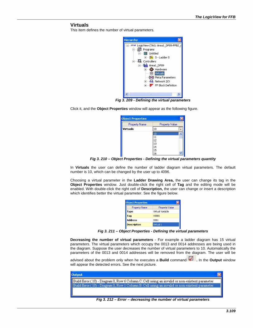
The LogicView for FFB
3.109
Virtuals This item defines the number of virtual parameters.
Fig 3. 209 - Defining the virtual parameters
Click it, and the Object Properties window will appear as the following figure.
Fig 3. 210 – Object Properties - Defining the virtual parameters quantity
In Virtuals the user can define the number of ladder diagram virtual parameters. The default number is 10, which can be changed by the user up to 4096. Choosing a virtual parameter in the Ladder Drawing Area, the user can change its tag in the Object Properties window. Just double-click the right cell of Tag and the editing mode will be enabled. With double-click the right cell of Description, the user can change or insert a description which identifies better the virtual parameter. See the figure below.
Fig 3. 211 – Object Properties - Defining the virtual parameters
Decreasing the number of virtual parameters - For example a ladder diagram has 15 virtual parameters. The virtual parameters which occupy the 0013 and 0014 addresses are being used in the diagram. Suppose the user decreases the number of virtual parameters to 10. Automatically the parameters of the 0013 and 0014 addresses will be removed from the diagram. The user will be
advised about the problem only when he executes a Build command . In the Output window will appear the detected errors. See the next picture.
Fig 3. 212 – Error – decreasing the number of virtual parameters
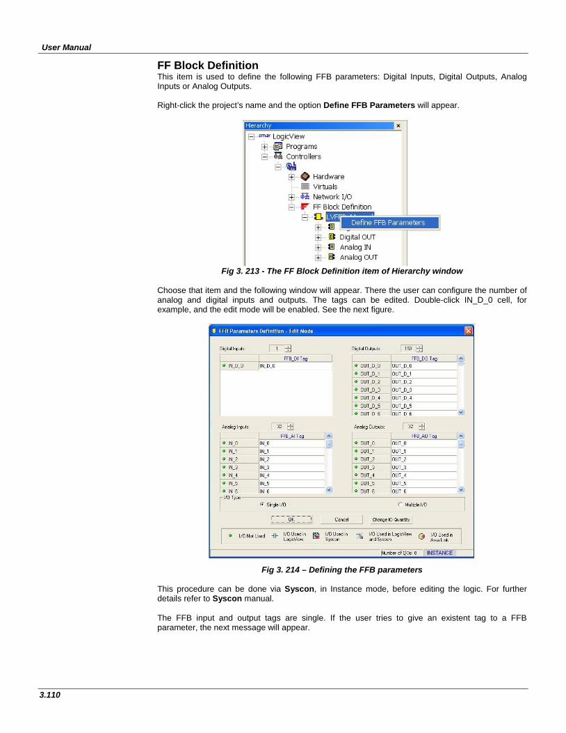
User Manual
3.110
FF Block Definition This item is used to define the following FFB parameters: Digital Inputs, Digital Outputs, Analog Inputs or Analog Outputs. Right-click the project’s name and the option Define FFB Parameters will appear.
Fig 3. 213 - The FF Block Definition item of Hierarchy window
Choose that item and the following window will appear. There the user can configure the number of analog and digital inputs and outputs. The tags can be edited. Double-click IN_D_0 cell, for example, and the edit mode will be enabled. See the next figure.
Fig 3. 214 – Defining the FFB parameters This procedure can be done via Syscon, in Instance mode, before editing the logic. For further details refer to Syscon manual. The FFB input and output tags are single. If the user tries to give an existent tag to a FFB parameter, the next message will appear.
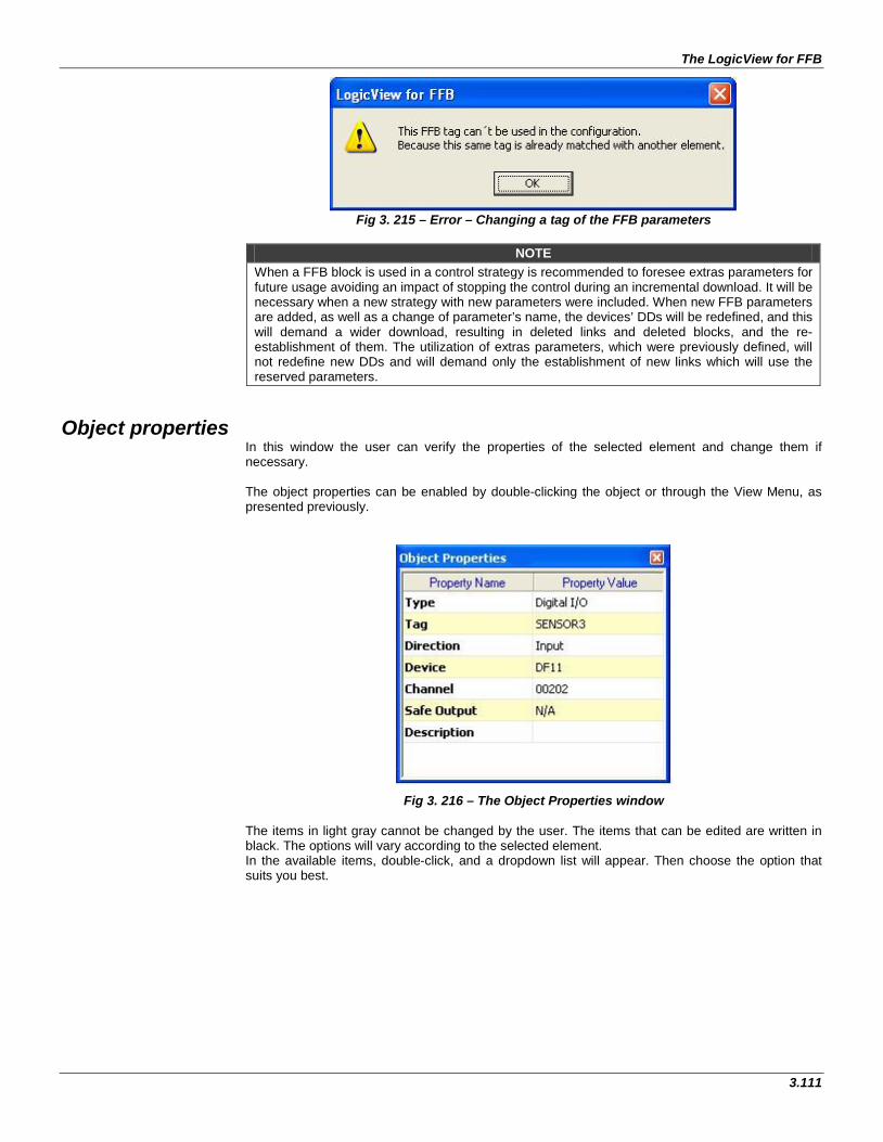
The LogicView for FFB
3.111
Fig 3. 215 – Error – Changing a tag of the FFB parameters
NOTE When a FFB block is used in a control strategy is recommended to foresee extras parameters for future usage avoiding an impact of stopping the control during an incremental download. It will be necessary when a new strategy with new parameters were included. When new FFB parameters are added, as well as a change of parameter’s name, the devices’ DDs will be redefined, and this will demand a wider download, resulting in deleted links and deleted blocks, and the re-establishment of them. The utilization of extras parameters, which were previously defined, will not redefine new DDs and will demand only the establishment of new links which will use the reserved parameters.
Object properties In this window the user can verify the properties of the selected element and change them if necessary. The object properties can be enabled by double-clicking the object or through the View Menu, as presented previously.
Fig 3. 216 – The Object Properties window
The items in light gray cannot be changed by the user. The items that can be edited are written in black. The options will vary according to the selected element. In the available items, double-click, and a dropdown list will appear. Then choose the option that suits you best.
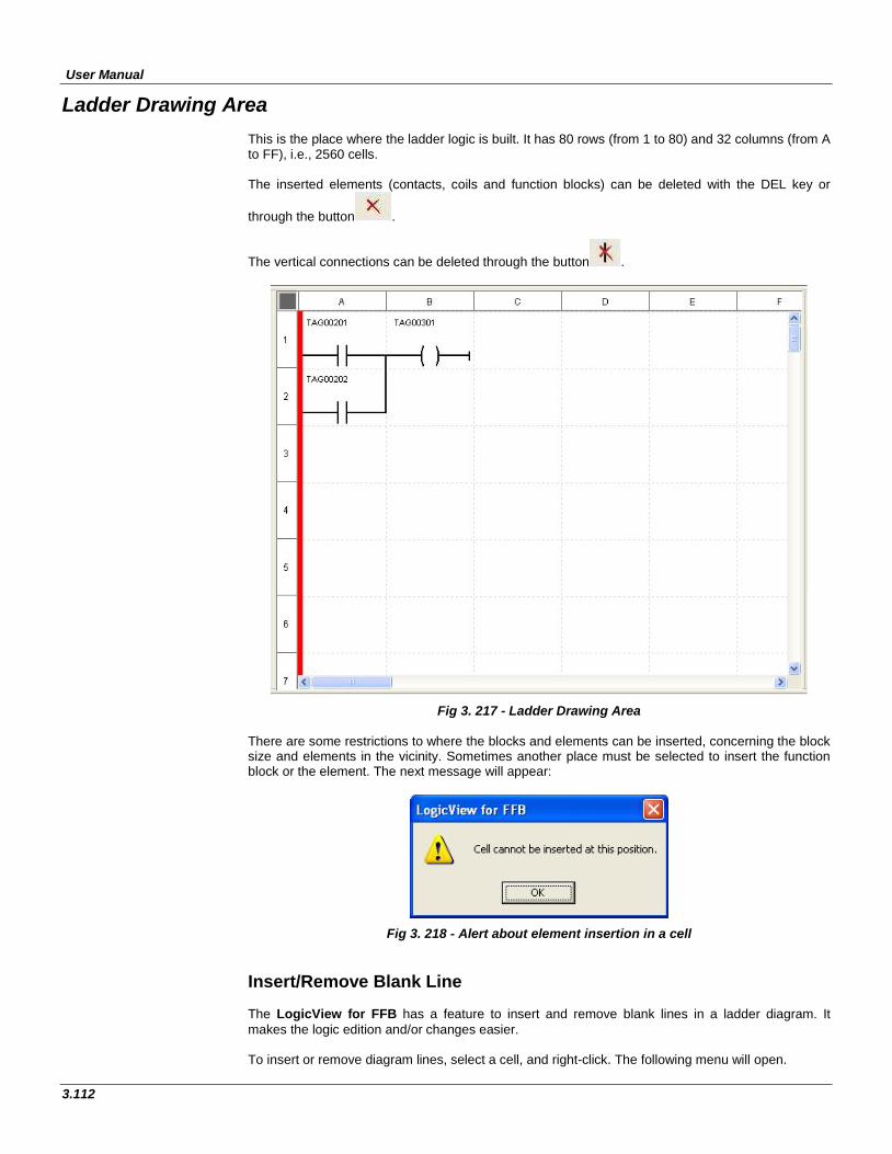
User Manual
3.112
Ladder Drawing Area This is the place where the ladder logic is built. It has 80 rows (from 1 to 80) and 32 columns (from A to FF), i.e., 2560 cells. The inserted elements (contacts, coils and function blocks) can be deleted with the DEL key or
through the button .
The vertical connections can be deleted through the button .
Fig 3. 217 - Ladder Drawing Area
There are some restrictions to where the blocks and elements can be inserted, concerning the block size and elements in the vicinity. Sometimes another place must be selected to insert the function block or the element. The next message will appear:
Fig 3. 218 - Alert about element insertion in a cell Insert/Remove Blank Line The LogicView for FFB has a feature to insert and remove blank lines in a ladder diagram. It makes the logic edition and/or changes easier. To insert or remove diagram lines, select a cell, and right-click. The following menu will open.
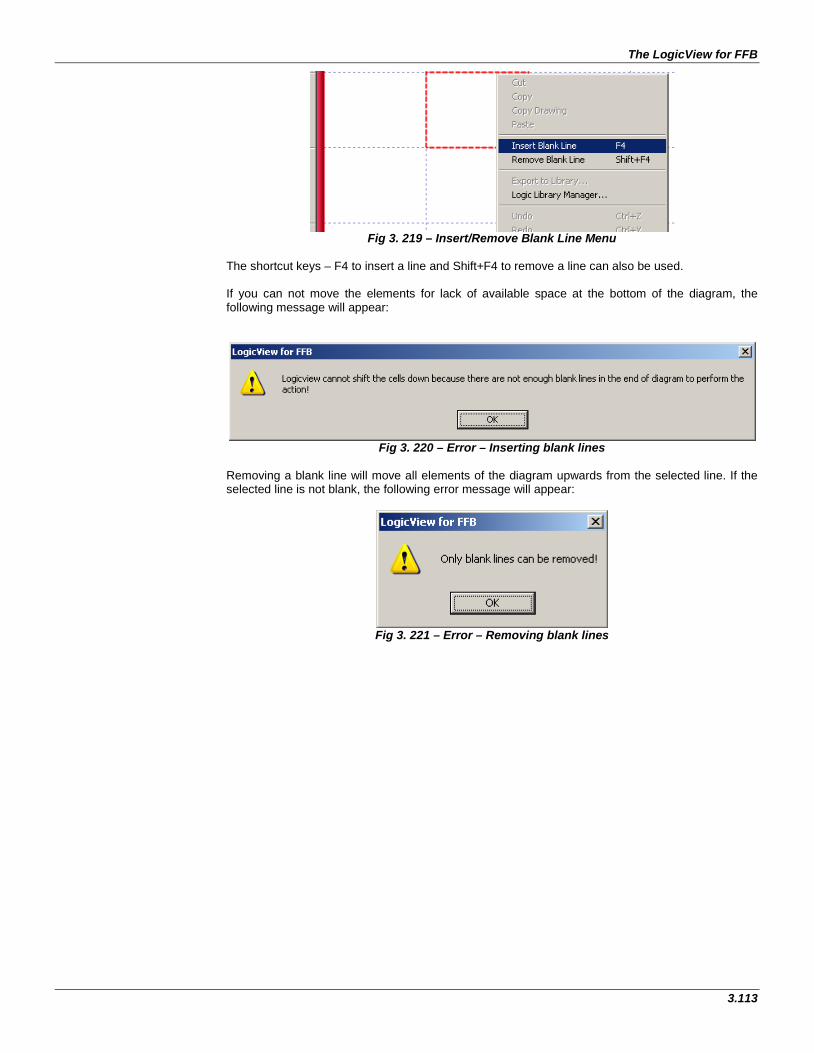
The LogicView for FFB
3.113
Fig 3. 219 – Insert/Remove Blank Line Menu
The shortcut keys – F4 to insert a line and Shift+F4 to remove a line can also be used. If you can not move the elements for lack of available space at the bottom of the diagram, the following message will appear:
Fig 3. 220 – Error – Inserting blank lines
Removing a blank line will move all elements of the diagram upwards from the selected line. If the selected line is not blank, the following error message will appear:
Fig 3. 221 – Error – Removing blank lines
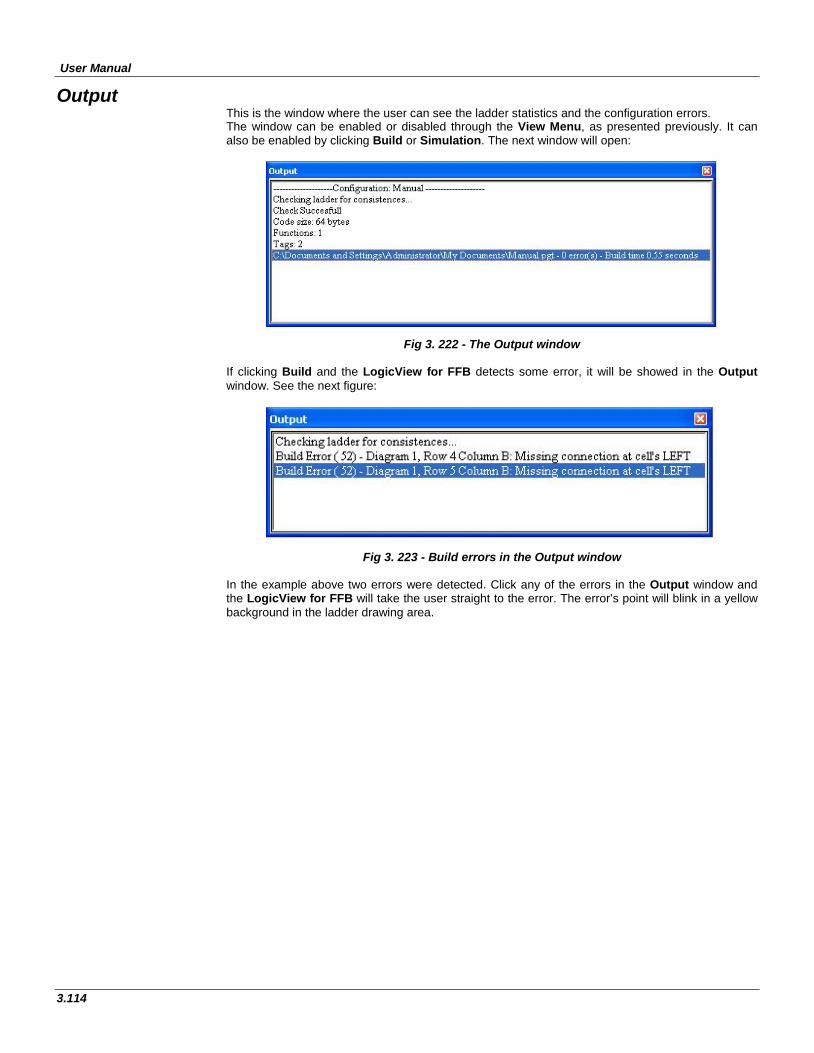
User Manual
3.114
Output This is the window where the user can see the ladder statistics and the configuration errors. The window can be enabled or disabled through the View Menu, as presented previously. It can also be enabled by clicking Build or Simulation. The next window will open:
Fig 3. 222 - The Output window
If clicking Build and the LogicView for FFB detects some error, it will be showed in the Output window. See the next figure:
Fig 3. 223 - Build errors in the Output window In the example above two errors were detected. Click any of the errors in the Output window and the LogicView for FFB will take the user straight to the error. The error’s point will blink in a yellow background in the ladder drawing area.
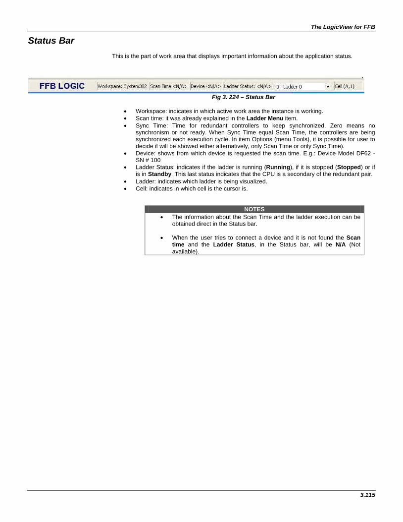
The LogicView for FFB
3.115
Status Bar This is the part of work area that displays important information about the application status.
Fig 3. 224 – Status Bar
• Workspace: indicates in which active work area the instance is working. • Scan time: it was already explained in the Ladder Menu item. • Sync Time: Time for redundant controllers to keep synchronized. Zero means no
synchronism or not ready. When Sync Time equal Scan Time, the controllers are being synchronized each execution cycle. In item Options (menu Tools), it is possible for user to decide if will be showed either alternatively, only Scan Time or only Sync Time).
• Device: shows from which device is requested the scan time. E.g.: Device Model DF62 - SN # 100
• Ladder Status: indicates if the ladder is running (Running), if it is stopped (Stopped) or if is in Standby. This last status indicates that the CPU is a secondary of the redundant pair.
• Ladder: indicates which ladder is being visualized. • Cell: indicates in which cell is the cursor is.
NOTES • The information about the Scan Time and the ladder execution can be
obtained direct in the Status bar.
• When the user tries to connect a device and it is not found the Scan time and the Ladder Status, in the Status bar, will be N/A (Not available).

User Manual
3.116
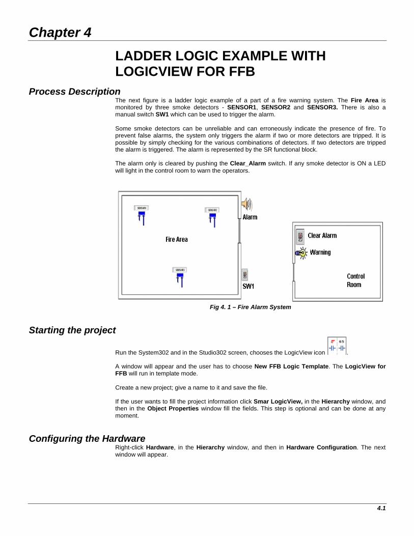
Chapter 4
4.1
LADDER LOGIC EXAMPLE WITH LOGICVIEW FOR FFB
Process Description The next figure is a ladder logic example of a part of a fire warning system. The Fire Area is monitored by three smoke detectors - SENSOR1, SENSOR2 and SENSOR3. There is also a manual switch SW1 which can be used to trigger the alarm. Some smoke detectors can be unreliable and can erroneously indicate the presence of fire. To prevent false alarms, the system only triggers the alarm if two or more detectors are tripped. It is possible by simply checking for the various combinations of detectors. If two detectors are tripped the alarm is triggered. The alarm is represented by the SR functional block. The alarm only is cleared by pushing the Clear_Alarm switch. If any smoke detector is ON a LED will light in the control room to warn the operators.
Fig 4. 1 – Fire Alarm System
Starting the project
Run the System302 and in the Studio302 screen, chooses the LogicView icon . A window will appear and the user has to choose New FFB Logic Template. The LogicView for FFB will run in template mode. Create a new project; give a name to it and save the file. If the user wants to fill the project information click Smar LogicView, in the Hierarchy window, and then in the Object Properties window fill the fields. This step is optional and can be done at any moment.
Configuring the Hardware Right-click Hardware, in the Hierarchy window, and then in Hardware Configuration. The next window will appear.
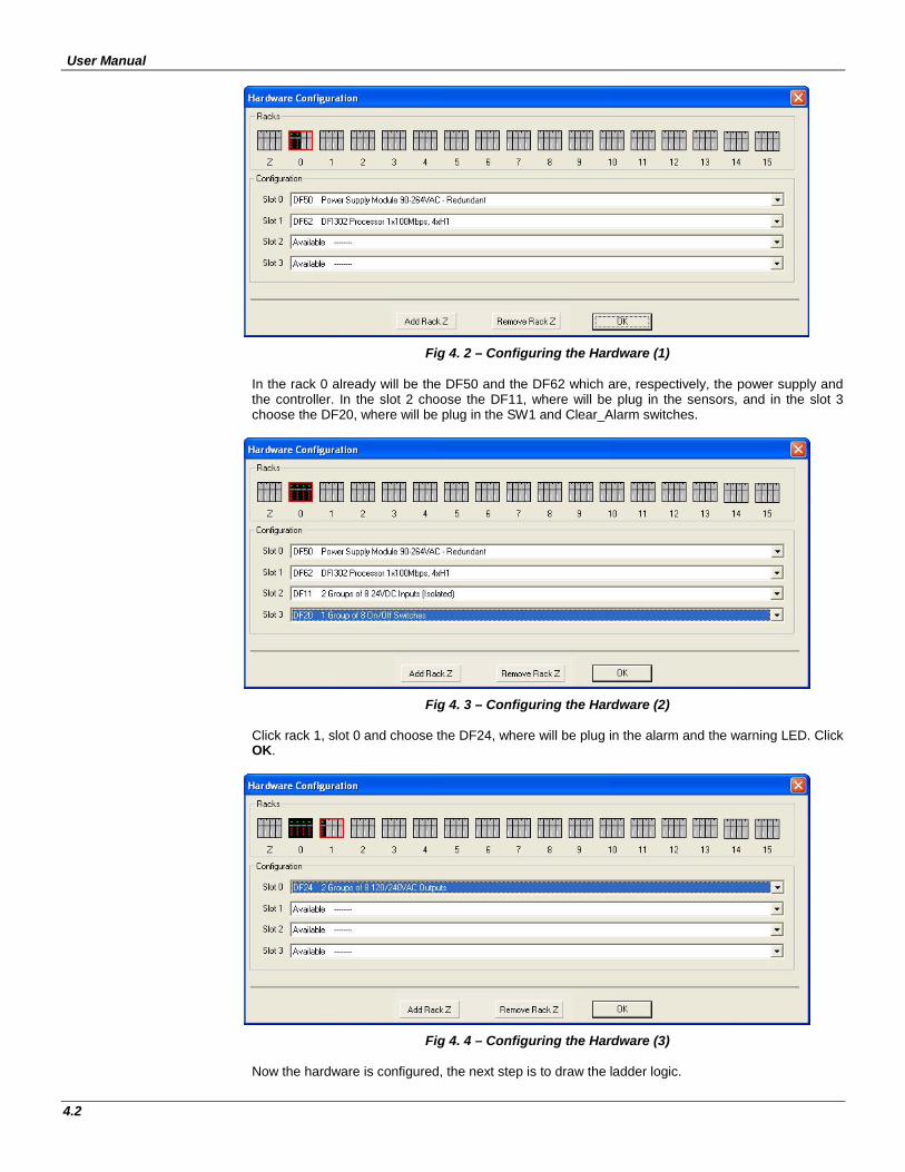
User Manual
4.2
Fig 4. 2 – Configuring the Hardware (1) In the rack 0 already will be the DF50 and the DF62 which are, respectively, the power supply and the controller. In the slot 2 choose the DF11, where will be plug in the sensors, and in the slot 3 choose the DF20, where will be plug in the SW1 and Clear_Alarm switches.
Fig 4. 3 – Configuring the Hardware (2) Click rack 1, slot 0 and choose the DF24, where will be plug in the alarm and the warning LED. Click OK.
Fig 4. 4 – Configuring the Hardware (3) Now the hardware is configured, the next step is to draw the ladder logic.
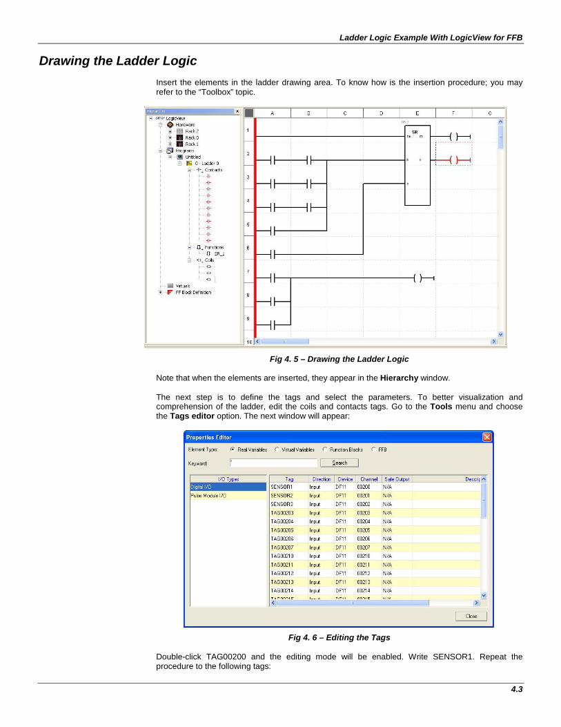
Ladder Logic Example With LogicView for FFB
4.3
Drawing the Ladder Logic Insert the elements in the ladder drawing area. To know how is the insertion procedure; you may refer to the “Toolbox” topic.
Fig 4. 5 – Drawing the Ladder Logic Note that when the elements are inserted, they appear in the Hierarchy window. The next step is to define the tags and select the parameters. To better visualization and comprehension of the ladder, edit the coils and contacts tags. Go to the Tools menu and choose the Tags editor option. The next window will appear:
Fig 4. 6 – Editing the Tags Double-click TAG00200 and the editing mode will be enabled. Write SENSOR1. Repeat the procedure to the following tags:
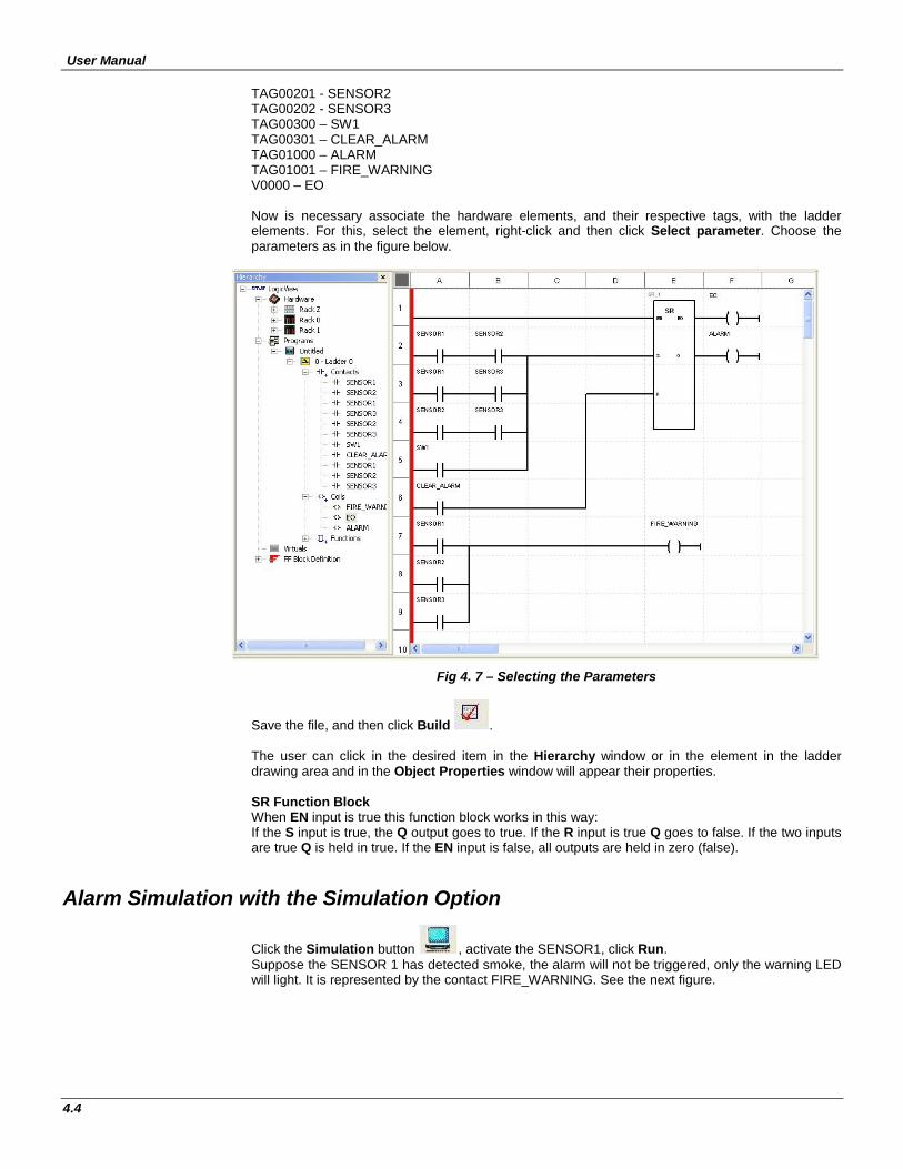
User Manual
4.4
TAG00201 - SENSOR2 TAG00202 - SENSOR3 TAG00300 – SW1 TAG00301 – CLEAR_ALARM TAG01000 – ALARM TAG01001 – FIRE_WARNING V0000 – EO Now is necessary associate the hardware elements, and their respective tags, with the ladder elements. For this, select the element, right-click and then click Select parameter. Choose the parameters as in the figure below.
Fig 4. 7 – Selecting the Parameters
Save the file, and then click Build . The user can click in the desired item in the Hierarchy window or in the element in the ladder drawing area and in the Object Properties window will appear their properties. SR Function Block When EN input is true this function block works in this way: If the S input is true, the Q output goes to true. If the R input is true Q goes to false. If the two inputs are true Q is held in true. If the EN input is false, all outputs are held in zero (false).
Alarm Simulation with the Simulation Option
Click the Simulation button , activate the SENSOR1, click Run. Suppose the SENSOR 1 has detected smoke, the alarm will not be triggered, only the warning LED will light. It is represented by the contact FIRE_WARNING. See the next figure.
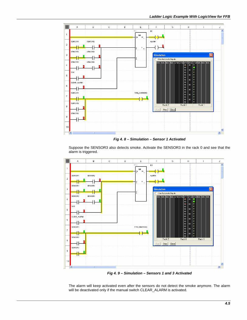
Ladder Logic Example With LogicView for FFB
4.5
Fig 4. 8 – Simulation – Sensor 1 Activated Suppose the SENSOR3 also detects smoke. Activate the SENSOR3 in the rack 0 and see that the alarm is triggered.
Fig 4. 9 – Simulation – Sensors 1 and 3 Activated The alarm will keep activated even after the sensors do not detect the smoke anymore. The alarm will be deactivated only if the manual switch CLEAR_ALARM is activated.
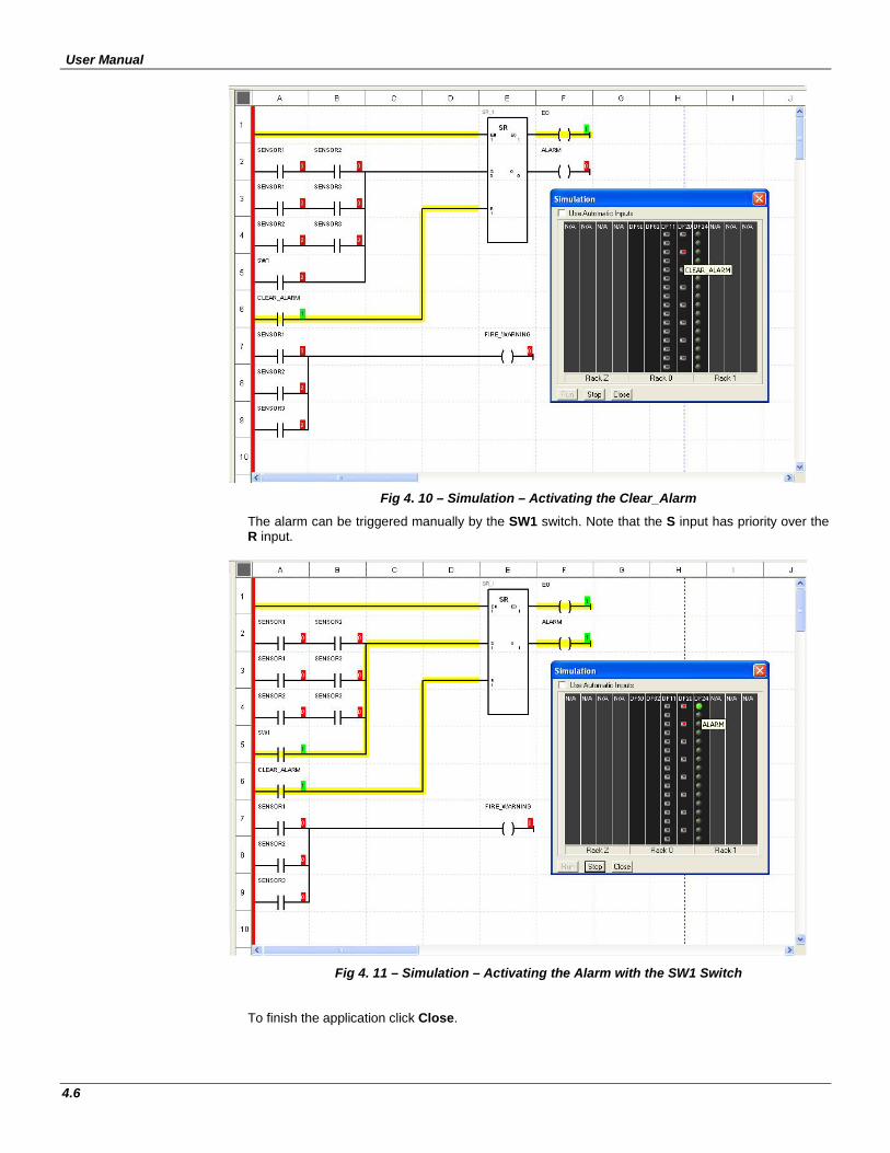
User Manual
4.6
Fig 4. 10 – Simulation – Activating the Clear_Alarm
The alarm can be triggered manually by the SW1 switch. Note that the S input has priority over the R input.
Fig 4. 11 – Simulation – Activating the Alarm with the SW1 Switch
To finish the application click Close.