Embed Size (px)
Citation preview
Logistic Regression: Univariate andMultivariate
1
Events and Logistic Regression
I Logisitic regression is used for modelling eventprobabilities.
I Example of an event: Mrs. Smith had a myocardialinfarction between 1/1/2000 and 31/12/2009.
I The occurrence of an event is a binary (dichotomous)variable. There are two possibilities: the event occurs or itdoes not occur.
I For this reason, event occurrence variables can always becoded with 0, 1 e.g.
Yi = 1 ⇐⇒ person i became pregnant in 2011.Yi = 0 ⇐⇒ person i did not become pregnant in 2011.
2

Measuring the Probability of an Event
I There are many equivalent ways of measuring theprobability of an event.
I We will use three:
1 probability of the event
2 odds in favour of the event
3 log-odds in favour of the event
I These are equivalent in the sense that if you know thevalue of one measure for an event you can compute thevalue of the other two measures for the same event
cf. measuring a distance in kilometres, statute miles ornautical miles
3
The Probability of an Event
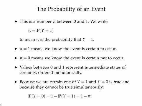
I This is a number π between 0 and 1. We write
π = P(Y = 1)
to mean π is the probability that Y = 1.
I π = 1 means we know the event is certain to occur.
I π = 0 means we know the event is certain not to occur.
I Values between 0 and 1 represent intermediate states ofcertainty, ordered monotonically.
I Because we are certain one of Y = 1 and Y = 0 is true andbecause they cannot be true simultaneously:
P(Y = 0) = 1 − P(Y = 1) = 1 − π.
4

Odds in Favour of an Event
I The odds in favour of an event is defined as theprobability the event occurs divided by the probability theevent does not occur.
I The odds in favour of Y = 1 is defined as:
ODDS(Y = 1) =P(Y = 1)P(Y 6= 1)
=P(Y = 1)P(Y = 0)
=π
1 − π.
I Note:
ODDS(Y = 0) =1
ODDS(Y = 1)=
1 − π
π.
so
ODDS(Y = 1)×ODDS(Y = 0) = 1.
5

Interpreting the Odds in Favour of an Event
I An odds is a number between 0 and ∞.
I An odds of 0 means we are certain the event does notoccur.
I An increased odds corresponds to increased belief in theoccurrence of the event.
I An odds of 1 corresponds to a probability of 1/2.
I An odds of ∞ corresponds to certainty the event occurs.
6

Log-odds in Favour of an Event
I The log odds in favour of an event is defined as the log ofthe odds in favour of the event:
log ODDS(Y = 1) = logP(Y = 1)P(Y = 0)
= logπ
1 − π.
I Note
log ODDS(Y = 1) = − log ODDS(Y = 0) = log1 − π
π
7

Interpreting the Log-odds in Favour of an Event
I A log-odds is a number between −∞ and ∞.
I A log odds of −∞ means we are certain the event doesnot occur.
I An increased log-odds corresponds to increased belief inthe occurrence of the event.
I A log-odds of 0 corresponds to a probability of 1/2.
I A log-odds of ∞ corresponds to certainty the event occurs.
8
Moving between Probability, Odds and Log-odds
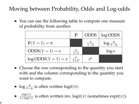
I You can use the following table to compute one measureof probability from another:
P ODDS log ODDS
P(Y = 1) = π π1−π log π
1−π
ODDS(Y = 1) = o o1+o log o
log ODDS(Y = 1) = x ex
1+ex ex
I Choose the row corresponding to the quantity you startwith and the column corresponding to the quantity youwant to compute.
I log π1−π is often written logit(π).
I exp(x)1+exp(x) is often written inv. logit(x) (sometimes expit(x)).
9
Motivation for (Multivariate) Logistic Regression
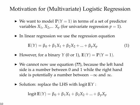
I We want to model P(Y = 1) in terms of a set of predictorvariables X1, X2,... Xp (for univariate regression p = 1).
I In linear regression we use the regression equation
E(Y) = β0 +β1X1 +β2X2 + ... +βpXp (1)
I However, for a binary Y (0 or 1), E(Y) = P(Y = 1).
I We cannot now use equation (??), because the left handside is a number between 0 and 1 while the right handside is potentially a number between −∞ and ∞.
I Solution: replace the LHS with logit EY :
logit E(Y) = β0 +β1X1 +β2X2 + ... +βpXp
10
Logistic Regression Equation Written on Three Scales
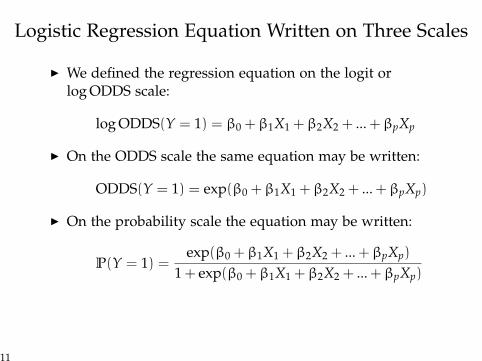
I We defined the regression equation on the logit orlog ODDS scale:
log ODDS(Y = 1) = β0 +β1X1 +β2X2 + ... +βpXp
I On the ODDS scale the same equation may be written:
ODDS(Y = 1) = exp(β0 +β1X1 +β2X2 + ... +βpXp)
I On the probability scale the equation may be written:
P(Y = 1) =exp(β0 +β1X1 +β2X2 + ... +βpXp)
1 + exp(β0 +β1X1 +β2X2 + ... +βpXp)
11

Interpreting the Intercept
I In order to obtain a simple interpretation of the interceptwe need to find a situation in which the other parameters(β1, ...,βp) vanish.
I This happens when X1, X2..., Xp are all equal to 0.
I Consequently we can interpret β0 in 3 equivalent ways:1 β0 is the log-odds in favour of Y = 1 when
X1 = X2... = Xp = 0.
2 β0 is such that exp(β0) is the odds in favour of Y = 1 whenX1 = X2... = Xp = 0.
3 β0 is such that exp(β0)1+exp(β0)
is the probability that Y = 1 whenX1 = X2... = Xp = 0.
I You can choose any one of these three interpretationswhen you make a report.
12
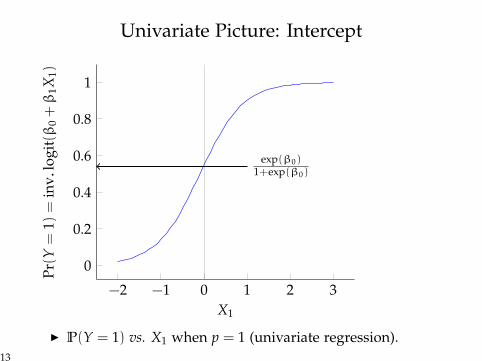
Univariate Picture: Intercept
−2 −1 0 1 2 3
0
0.2
0.4
0.6
0.8
1
X1
Pr(Y
=1)
=in
v.lo
git(β
0+β
1X1)
exp(β0)1+exp(β0)
I P(Y = 1) vs. X1 when p = 1 (univariate regression).13
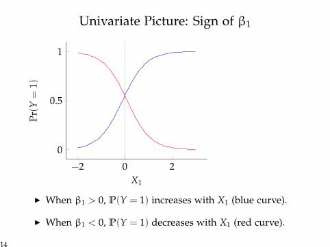
Univariate Picture: Sign of β1
−2 0 2
0
0.5
1
X1
Pr(Y
=1)
I When β1 > 0, P(Y = 1) increases with X1 (blue curve).
I When β1 < 0, P(Y = 1) decreases with X1 (red curve).
14
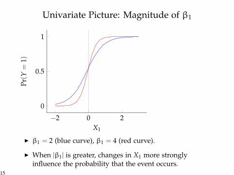
Univariate Picture: Magnitude of β1
−2 0 2
0
0.5
1
X1
Pr(Y
=1)
I β1 = 2 (blue curve), β1 = 4 (red curve).
I When |β1| is greater, changes in X1 more stronglyinfluence the probability that the event occurs.
15
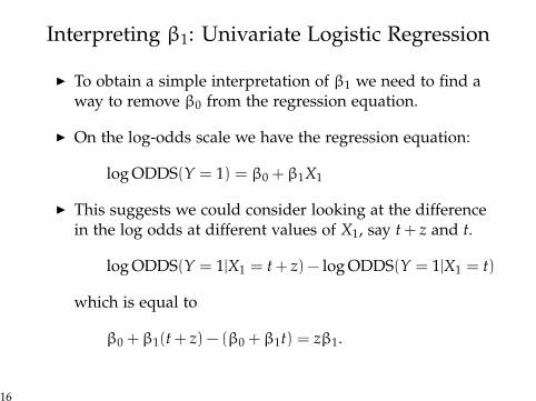
Interpreting β1: Univariate Logistic Regression
I To obtain a simple interpretation of β1 we need to find away to remove β0 from the regression equation.
I On the log-odds scale we have the regression equation:
log ODDS(Y = 1) = β0 +β1X1
I This suggests we could consider looking at the differencein the log odds at different values of X1, say t + z and t.
log ODDS(Y = 1|X1 = t + z) − log ODDS(Y = 1|X1 = t)
which is equal to
β0 +β1(t + z) − (β0 +β1t) = zβ1.
16
Interpreting β1: Univariate Logistic Regression
I By putting z = 1 we arrive at the following interpretationof β1:
β1 is the additive change in the log-odds in favour of Y = 1when X1 increases by 1 unit.
I We can write an equivalent second interpretation on theodds scale:
exp(β1) is the multiplicative change in the odds in favour ofY = 1 when X1 increases by 1 unit.
17
β1 as a Log-odds Ratio
I The first interpretation of β1 expresses the equation:
logODDS(Y = 1|X1 = t + z)
ODDS(Y = 1|X1 = t)= zβ1
whilst the second interpretation expresses the equation:
ODDS(Y = 1|X1 = t + z)ODDS(Y = 1|X1 = t)
= exp(zβ1).
I The quantity ODDS(Y=1|X1=t+z)ODDS(Y=1|X1=t) is the odds-ratio in favour
of Y = 1 for X1 = t + z vs. X1 = t.
18
Interpreting Coefficients in Multivariate LogisticRegression
I The interpretation of regression coefficients inmultivariate logistic regression is similar to theinterpretation in univariate regression.
I We dealt with β0 previously.
I In general the coefficient βk (corresponding to the variableXk) can be interpreted as follows:
βk is the additive change in the log-odds in favour of Y = 1when Xk increases by 1 unit, while the other predictor variablesremain unchanged.
I As in the univariate case, an equivalent interpretation canbe made on the odds scale.
19
Fitting a Logistic Regression in R
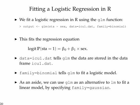
I We fit a logistic regression in R using the glm function:> output <- glm(sta ~ sex, data=icu1.dat, family=binomial)
I This fits the regression equation
logit P(sta = 1) = β0 +β1 × sex.
I data=icu1.dat tells glm the data are stored in the dataframe icu1.dat.
I family=binomial tells glm to fit a logistic model.
I As an aside, we can use glm as an alternative to lm to fit alinear model, by specifying family=gaussian.
20
Logistic Regression: glm Output in R
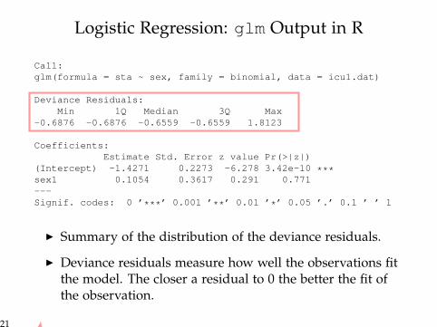
Call:glm(formula = sta ~ sex, family = binomial, data = icu1.dat)
Deviance Residuals:Min 1Q Median 3Q Max
-0.6876 -0.6876 -0.6559 -0.6559 1.8123
Coefficients:Estimate Std. Error z value Pr(>|z|)
(Intercept) -1.4271 0.2273 -6.278 3.42e-10 ***sex1 0.1054 0.3617 0.291 0.771---Signif. codes: 0 ’***’ 0.001 ’**’ 0.01 ’*’ 0.05 ’.’ 0.1 ’ ’ 1
I Summary of the distribution of the deviance residuals.
I Deviance residuals measure how well the observations fitthe model. The closer a residual to 0 the better the fit ofthe observation.
21
Logistic Regression: glm Output in R
Call:glm(formula = sta ~ sex, family = binomial, data = icu1.dat)
Deviance Residuals:Min 1Q Median 3Q Max
-0.6876 -0.6876 -0.6559 -0.6559 1.8123
Coefficients:Estimate Std. Error z value Pr(>|z|)
(Intercept) -1.4271 0.2273 -6.278 3.42e-10 ***sex1 0.1054 0.3617 0.291 0.771---Signif. codes: 0 ’***’ 0.001 ’**’ 0.01 ’*’ 0.05 ’.’ 0.1 ’ ’ 1
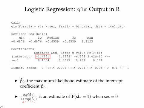
I β̂0, the maximum likelihood estimate of the interceptcoefficient β0.
I exp(β̂0)
1+exp(β̂0)is an estimate of P(sta = 1) when sex = 0
22
Logistic Regression: glm Output in R
Call:glm(formula = sta ~ sex, family = binomial, data = icu1.dat)
Deviance Residuals:Min 1Q Median 3Q Max
-0.6876 -0.6876 -0.6559 -0.6559 1.8123
Coefficients:Estimate Std. Error z value Pr(>|z|)
(Intercept) -1.4271 0.2273 -6.278 3.42e-10 ***sex1 0.1054 0.3617 0.291 0.771---Signif. codes: 0 ’***’ 0.001 ’**’ 0.01 ’*’ 0.05 ’.’ 0.1 ’ ’ 1
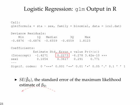
I SE(β̂0), the standard error of the maximum likelihoodestimate of β0.
23
Logistic Regression: glm Output in R
Call:glm(formula = sta ~ sex, family = binomial, data = icu1.dat)
Deviance Residuals:Min 1Q Median 3Q Max
-0.6876 -0.6876 -0.6559 -0.6559 1.8123
Coefficients:Estimate Std. Error z value Pr(>|z|)
(Intercept) -1.4271 0.2273 -6.278 3.42e-10 ***sex1 0.1054 0.3617 0.291 0.771---Signif. codes: 0 ’***’ 0.001 ’**’ 0.01 ’*’ 0.05 ’.’ 0.1 ’ ’ 1
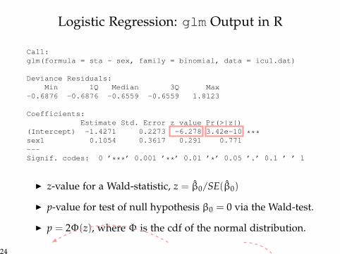
I z-value for a Wald-statistic, z = β̂0/SE(β̂0)
I p-value for test of null hypothesis β0 = 0 via the Wald-test.
I p = 2Φ(z), where Φ is the cdf of the normal distribution.
24
Logistic Regression: glm Output in R
Call:glm(formula = sta ~ sex, family = binomial, data = icu1.dat)
Deviance Residuals:Min 1Q Median 3Q Max
-0.6876 -0.6876 -0.6559 -0.6559 1.8123
Coefficients:Estimate Std. Error z value Pr(>|z|)
(Intercept) -1.4271 0.2273 -6.278 3.42e-10 ***sex1 0.1054 0.3617 0.291 0.771---Signif. codes: 0 ’***’ 0.001 ’**’ 0.01 ’*’ 0.05 ’.’ 0.1 ’ ’ 1
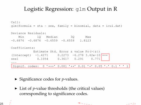
I Significance codes for p-values.
I List of p-value thresholds (the critical values)corresponding to significance codes.
25
Logistic Regression: glm Output in R
Call:glm(formula = sta ~ sex, family = binomial, data = icu1.dat)
Deviance Residuals:Min 1Q Median 3Q Max
-0.6876 -0.6876 -0.6559 -0.6559 1.8123
Coefficients:Estimate Std. Error z value Pr(>|z|)
(Intercept) -1.4271 0.2273 -6.278 3.42e-10 ***sex1 0.1054 0.3617 0.291 0.771---Signif. codes: 0 ’***’ 0.001 ’**’ 0.01 ’*’ 0.05 ’.’ 0.1 ’ ’ 1
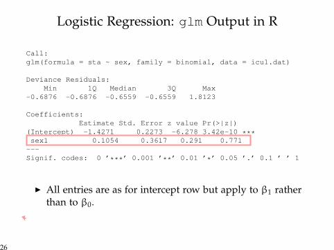
I All entries are as for intercept row but apply to β1 ratherthan to β0.
26
Computing a 95% Confidence Interval from glm
Coefficients:Estimate Std. Error z value Pr(>|z|)
(Intercept) -1.4271 0.2273 -6.278 3.42e-10 ***sex1 0.1054 0.3617 0.291 0.771---Signif. codes: 0 ’***’ 0.001 ’**’ 0.01 ’*’ 0.05 ’.’ 0.1 ’ ’ 1
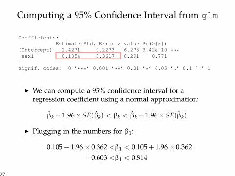
I We can compute a 95% confidence interval for aregression coefficient using a normal approximation:
β̂k − 1.96× SE(β̂k) < βk < β̂k + 1.96× SE(β̂k)
I Plugging in the numbers for β1:
0.105 − 1.96× 0.362 <β1 < 0.105 + 1.96× 0.362−0.603 <β1 < 0.814
27
Computing a 95% Confidence Interval on Odds Scale
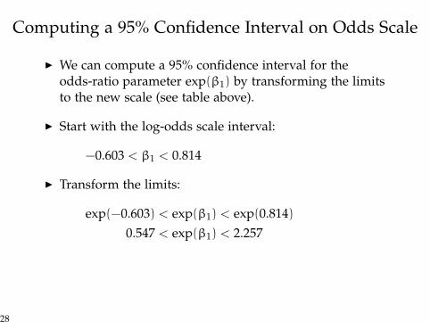
I We can compute a 95% confidence interval for theodds-ratio parameter exp(β1) by transforming the limitsto the new scale (see table above).
I Start with the log-odds scale interval:
−0.603 < β1 < 0.814
I Transform the limits:
exp(−0.603) < exp(β1) < exp(0.814)0.547 < exp(β1) < 2.257
28
Logistic Regression with Dummy Variables
I A dummy variable is a 0/1 representation of adichotomous catagorical variable.
I Such a numeric representation allows us to use categoricalvariables as predictors in a regression model.
I For example the dichotomous variable sex can be coded
sexi = 0 means individual i is malesexi = 1 means individual i is female
29
Logistic Regression with Dummy Variables
I Suppose we fit the regression specified by the equation
logit P(Yi = 1) = β0 +β1sexi.
I Recall one interpretation of β1:
exp(β1) is the multiplicative change in the odds in favour ofY = 1 as sex increases by 1 unit.
I The only unit increase possible is from 0 to 1, so we canwrite an interpretation in terms of male/female:
exp(β1) is multiplicative change of the odds in favour of Y = 1as a male becomes a female.
I A bit ridiculous, so better to say:
exp(β1) is the odds-ratio (in favour of Y = 1) for females vs.males.
30
Multivariate Logistic Regression Example
I Data on admisssions to an intensive care unit (ICU).
I sta - outcome variable, status on leaving: dead=1, alive=0.
I loc - level of consciousness: no coma/stupor=0, deepstupor=1, coma=2.
I sex - male=0, female=1.
I ser - service at ICU: medical=0, surgical=1.
I ser and sex are dummy variables
I loc is a categorical/factor variable with 3 levels.
31
Multivariate Logistic Regression ICU Example
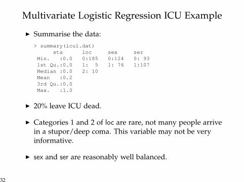
I Summarise the data:> summary(icu1.dat)
sta loc sex serMin. :0.0 0:185 0:124 0: 931st Qu.:0.0 1: 5 1: 76 1:107Median :0.0 2: 10Mean :0.23rd Qu.:0.0Max. :1.0
I 20% leave ICU dead.
I Categories 1 and 2 of loc are rare, not many people arrivein a stupor/deep coma. This variable may not be veryinformative.
I sex and ser are reasonably well balanced.
32
Multivariate Logistic Regression ICU Example
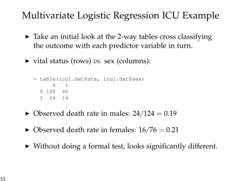
I Take an initial look at the 2-way tables cross classifyingthe outcome with each predictor variable in turn.
I vital status (rows) vs. sex (columns):
> table(icu1.dat$sta, icu1.dat$sex)0 1
0 100 601 24 16
I Observed death rate in males: 24/124 = 0.19
I Observed death rate in females: 16/76 = 0.21
I Without doing a formal test, looks significantly different.
33
Multivariate Logistic Regression ICU Example
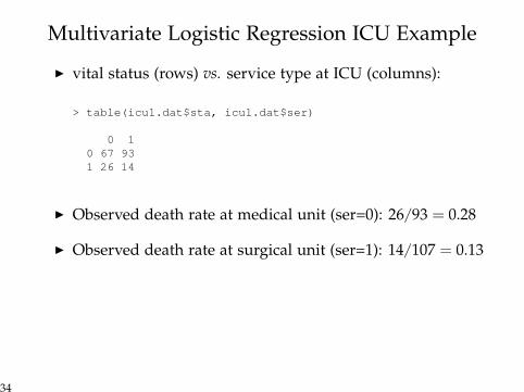
I vital status (rows) vs. service type at ICU (columns):
> table(icu1.dat$sta, icu1.dat$ser)
0 10 67 931 26 14
I Observed death rate at medical unit (ser=0): 26/93 = 0.28
I Observed death rate at surgical unit (ser=1): 14/107 = 0.13
34
Multivariate Logistic Regression ICU Example
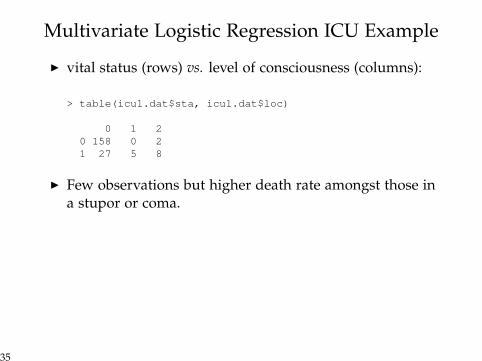
I vital status (rows) vs. level of consciousness (columns):
> table(icu1.dat$sta, icu1.dat$loc)
0 1 20 158 0 21 27 5 8
I Few observations but higher death rate amongst those ina stupor or coma.
35
Multivariate Logistic Regression ICU Example
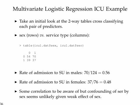
I Take an initial look at the 2-way tables cross classifyingeach pair of predictors.
I sex (rows) vs. service type (columns):
> table(icu1.dat$sex, icu1.dat$ser)
0 10 54 701 39 37
I Rate of admission to SU in males: 70/124 = 0.56
I Rate of admission to SU in females: 37/76 = 0.48
I Some correlation to be aware of but confounding of ser bysex seems unlikely given weak effect of sex.
36
Multivariate Logistic Regression ICU Example
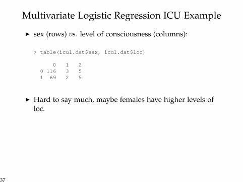
I sex (rows) vs. level of consciousness (columns):
> table(icu1.dat$sex, icu1.dat$loc)
0 1 20 116 3 51 69 2 5
I Hard to say much, maybe females have higher levels ofloc.
37
Multivariate Logistic Regression ICU Example
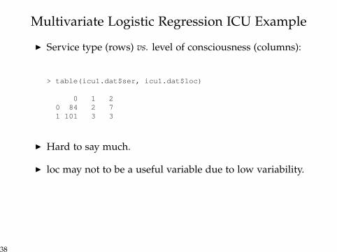
I Service type (rows) vs. level of consciousness (columns):
> table(icu1.dat$ser, icu1.dat$loc)
0 1 20 84 2 71 101 3 3
I Hard to say much.
I loc may not to be a useful variable due to low variability.
38
Multivariate Logistic Regression ICU Example
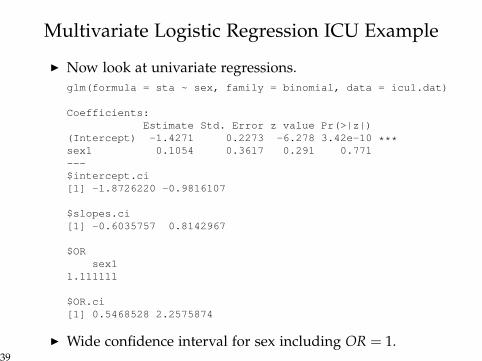
I Now look at univariate regressions.glm(formula = sta ~ sex, family = binomial, data = icu1.dat)
Coefficients:Estimate Std. Error z value Pr(>|z|)
(Intercept) -1.4271 0.2273 -6.278 3.42e-10 ***sex1 0.1054 0.3617 0.291 0.771---$intercept.ci[1] -1.8726220 -0.9816107
$slopes.ci[1] -0.6035757 0.8142967
$ORsex1
1.111111
$OR.ci[1] 0.5468528 2.2575874
I Wide confidence interval for sex including OR = 1.39
Multivariate Logistic Regression ICU Example
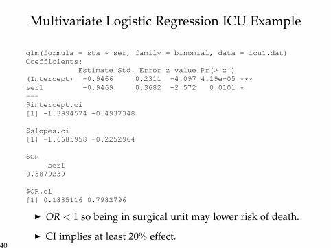
glm(formula = sta ~ ser, family = binomial, data = icu1.dat)Coefficients:
Estimate Std. Error z value Pr(>|z|)(Intercept) -0.9466 0.2311 -4.097 4.19e-05 ***ser1 -0.9469 0.3682 -2.572 0.0101 *---$intercept.ci[1] -1.3994574 -0.4937348
$slopes.ci[1] -1.6685958 -0.2252964
$ORser1
0.3879239
$OR.ci[1] 0.1885116 0.7982796
I OR < 1 so being in surgical unit may lower risk of death.
I CI implies at least 20% effect.40
Multivariate Logistic Regression ICU Example
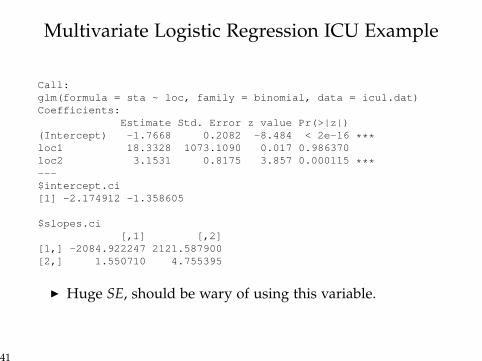
Call:glm(formula = sta ~ loc, family = binomial, data = icu1.dat)Coefficients:
Estimate Std. Error z value Pr(>|z|)(Intercept) -1.7668 0.2082 -8.484 < 2e-16 ***loc1 18.3328 1073.1090 0.017 0.986370loc2 3.1531 0.8175 3.857 0.000115 ***---$intercept.ci[1] -2.174912 -1.358605
$slopes.ci[,1] [,2]
[1,] -2084.922247 2121.587900[2,] 1.550710 4.755395
I Huge SE, should be wary of using this variable.
41
Multivariate Logistic Regression ICU Example
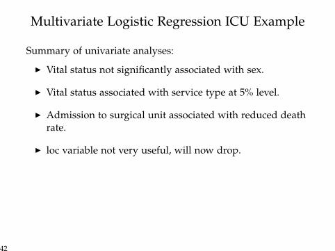
Summary of univariate analyses:
I Vital status not significantly associated with sex.
I Vital status associated with service type at 5% level.
I Admission to surgical unit associated with reduced deathrate.
I loc variable not very useful, will now drop.
42
Multivariate Logistic Regression ICU Example
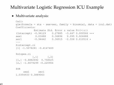
I Multivariate analysis:Call:glm(formula = sta ~ sex+ser, family = binomial, data = icu1.dat)Coefficients:
Estimate Std. Error z value Pr(>|z|)(Intercept) -0.96129 0.27885 -3.447 0.000566 ***sex1 0.03488 0.36896 0.095 0.924688ser1 -0.94442 0.36915 -2.558 0.010516 *---$intercept.ci[1] -1.5078281 -0.4147469
$slopes.ci[,1] [,2]
[1,] -0.6882692 0.758025[2,] -1.6679299 -0.220904
$ORsex1 ser1
1.0354933 0.3889063
43
Multivariate Logistic Regression ICU Example
Main Conclusions:I Univariate and multivariate parameter models show same
pattern of significance.
I Direction of association of service variable the same.
I Admission to surgical unit associated with reduced deathrate (OR = 0.39, 95% CI = (0.19, 0.80).
44
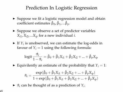
Prediction In Logistic Regression
I Suppose we fit a logistic regression model and obtaincoefficient estimates β̂0, β̂1, ...β̂p.
I Suppose we observe a set of predictor variablesXi1, Xi2, ...Xip for a new individual i.
I If Yi is unobserved, we can estimate the log-odds infavour of Yi = 1 using the following formula:
logitπ̂i
1 − π̂i= β̂0 + β̂1Xi1 + β̂2Xi2 + ... + β̂pXip
I Equivilently an estimate of the probability that Yi = 1:
π̂i =exp(β̂0 + β̂1Xi1 + β̂2Xi2 + ... + β̂pXip)
1 + exp(β̂0 + β̂1Xi1 + β̂2Xi2 + ... + β̂pXip)
I π̂i can be thought of as a prediction of Yi.45
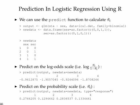
Prediction In Logistic Regression Using R
I We can use the predict function to calculate π̂i
> output <- glm(sta ~ sex, data=icu1.dat, family=binomial)> newdata <- data.frame(sex=as.factor(c(0,0,1,1)),
ser=as.factor(c(0,1,0,1)))
> newdatasex ser
1 0 02 0 13 1 04 1 1
I Predict on the log-odds scale (i.e. log π̂i1−π̂i
) :> predict(output, newdata=newdata)
1 2 3 4-0.9612875 -1.9057045 -0.9264096 -1.8708266
I Predict on the probability scale (i.e. π̂i) :> predict(output, newdata=newdata, type="response")
1 2 3 40.2766205 0.1294642 0.2836537 0.1334461
46
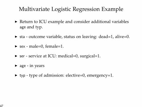
Multivariate Logistic Regression Example
I Return to ICU example and consider additional variablesage and typ.
I sta - outcome variable, status on leaving: dead=1, alive=0.
I sex - male=0, female=1.
I ser - service at ICU: medical=0, surgical=1.
I age - in years
I typ - type of admission: elective=0, emergency=1.
47
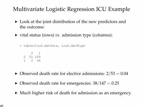
Multivariate Logistic Regression ICU Example
I Look at the joint distribution of the new predictors andthe outcome:
I vital status (rows) vs. admission type (columns):
> table(icu2.dat$sta, icu2.dat$typ)
0 10 51 1091 2 38
I Observed death rate for elective admissions: 2/53 = 0.04
I Observed death rate for emergencies: 38/147 = 0.25
I Much higher risk of death for admission as an emergency.
48
Multivariate Logistic Regression ICU Example
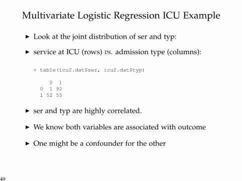
I Look at the joint distribution of ser and typ:
I service at ICU (rows) vs. admission type (columns):
> table(icu2.dat$ser, icu2.dat$typ)
0 10 1 921 52 55
I ser and typ are highly correlated.
I We know both variables are associated with outcome
I One might be a confounder for the other
49
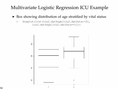
Multivariate Logistic Regression ICU Example
I Box showing distribution of age stratified by vital status> boxplot(list(icu2.dat$age[icu2.dat$sta==0],
icu2.dat$age[icu2.dat$sta==1]))
50
Multivariate Logistic Regression ICU Example
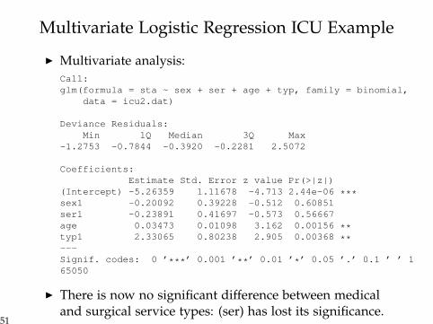
I Multivariate analysis:Call:glm(formula = sta ~ sex + ser + age + typ, family = binomial,
data = icu2.dat)
Deviance Residuals:Min 1Q Median 3Q Max
-1.2753 -0.7844 -0.3920 -0.2281 2.5072
Coefficients:Estimate Std. Error z value Pr(>|z|)
(Intercept) -5.26359 1.11678 -4.713 2.44e-06 ***sex1 -0.20092 0.39228 -0.512 0.60851ser1 -0.23891 0.41697 -0.573 0.56667age 0.03473 0.01098 3.162 0.00156 **typ1 2.33065 0.80238 2.905 0.00368 **---Signif. codes: 0 ’***’ 0.001 ’**’ 0.01 ’*’ 0.05 ’.’ 0.1 ’ ’ 165050
I There is now no significant difference between medicaland surgical service types: (ser) has lost its significance.
51
Multivariate Logistic Regression ICU Example
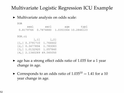
I Multivariate analysis on odds scale:$OR
sex1 ser1 age typ10.8179766 0.7874880 1.0353364 10.2846123
$OR.ci[,1] [,2]
[1,] 0.3791710 1.764602[2,] 0.3477894 1.783083[3,] 1.0132920 1.057860[4,] 2.1340289 49.565050
I age has a strong effect odds ratio of 1.035 for a 1 yearchange in age.
I Corresponds to an odds ratio of 1.03510 = 1.41 for a 10year change in age.
52
Multivariate Logistic Regression ICU Example
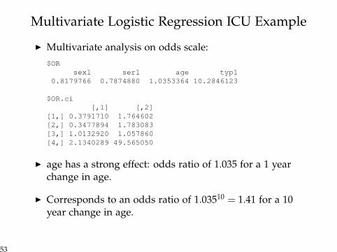
I Multivariate analysis on odds scale:$OR
sex1 ser1 age typ10.8179766 0.7874880 1.0353364 10.2846123
$OR.ci[,1] [,2]
[1,] 0.3791710 1.764602[2,] 0.3477894 1.783083[3,] 1.0132920 1.057860[4,] 2.1340289 49.565050
I age has a strong effect: odds ratio of 1.035 for a 1 yearchange in age.
I Corresponds to an odds ratio of 1.03510 = 1.41 for a 10year change in age.
53
Multivariate Logistic Regression ICU Example
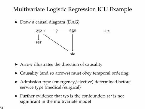
I Draw a causal diagram (DAG)
ser
typ sexage?
sta
I Arrow illustrates the direction of causality
I Causality (and so arrows) must obey temporal ordering
I Admission type (emergency/elective) determined beforeservice type (medical/surgical)
I Further evidence that typ is the confounder: ser is notsignificant in the multivariate model
54