Logistic Regression with Structured Sparsity

Nikhil S. Rao nrao2@wisc.edu

Robert D. Nowak nowak@ece.wisc.edu

Department of Electrical and Computer EngineeringUniversity of Wisconsin-Madison

Christopher R. Cox crcox@wisc.edu

Timothy T. Rogers ttrogers@wisc.edu

Department of Psychology

University of Wisconsin-Madison

Editor:

Abstract

Binary logistic regression with a sparsity constraint on the solution plays a vital role inmany high dimensional machine learning applications. In some cases, the features can begrouped together, so that entire subsets of features can be selected or zeroed out. In manyapplications, however, this can be very restrictive. In this paper, we are interested in a lessrestrictive form of structured sparse feature selection: we assume that while features can begrouped according to some notion of similarity, not all features in a group need be selectedfor the task at hand. This is sometimes referred to as a “sparse group” lasso procedure,and it allows for more flexibility than traditional group lasso methods. Our frameworkgeneralizes conventional sparse group lasso further by allowing for overlapping groups, anadditional flexiblity that presents further challenges. The main contribution of this paperis a new procedure called Sparse Overlapping Sets (SOS) lasso, a convex optimizationprogram that automatically selects similar features for learning in high dimensions. Weestablish consistency results for the SOSlasso for classification problems using the logisticregression setting, which specializes to results for the lasso and the group lasso, some knownand some new. In particular, SOSlasso is motivated by multi-subject fMRI studies in whichfunctional activity is classified using brain voxels as features, source localization problemsin Magnetoencephalography (MEG), and analyzing gene activation patterns in microarraydata analysis. Experiments with real and synthetic data demonstrate the advantages ofSOSlasso compared to the lasso and group lasso.

1. Introduction

Binary logistic regression plays a major role in many machine learning and signal processingapplications. In modern applications where the number of features far exceeds the numberof observations, one typically enforces the solution to contain only a few non zeros. Thelasso (Tibshirani, 1996) is a commonly used method to constrain the solution (henceforthalso referred to as the coe�cients) to be sparse. The notion of sparsity leads to moreinterpretable solutions in high dimensional machine learning applications, and has beenextensively studied in (Bach, 2010; Plan and Vershynin, 2012; Negahban et al., 2012; Bunea,2008), among others.

1

arX

iv:1

402.

4512

v1 [

cs.L

G]

18 F

eb 2

014

In many applications, we wish to impose structure on the sparsity pattern of the coe�-cients recovered. In particular, often it is known a priori that the optimal sparsity patternwill tend to involve clusters or groups of coe�cients, corresponding to pre-existing groups offeatures. The form of the groups is known, but the subset of groups that is relevant to theclassification task at hand is unknown. This prior knowledge reduces the space of possiblesparse coe�cients thereby potentially leading to better results than simple lasso methods.In such cases, the group lasso, with or without overlapping groups (Yuan and Lin, 2006)is used to recover the coe�cients. The group lasso forces all the coe�cients in a group tobe active at once: if a coe�cient is selected for the task at hand, then all the coe�cientsin that group are selected. When the groups overlap, a modification of the penalty allowsone to recover coe�cients that can be expressed as a union of groups (Jacob et al., 2009;Obozinski et al., 2011).

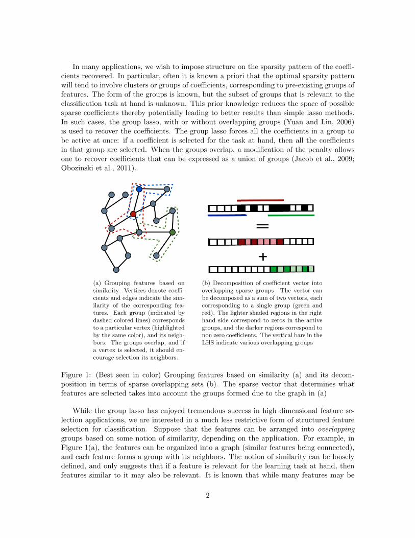
(a) Grouping features based onsimilarity. Vertices denote coe�-cients and edges indicate the sim-ilarity of the corresponding fea-tures. Each group (indicated bydashed colored lines) correspondsto a particular vertex (highlightedby the same color), and its neigh-bors. The groups overlap, and ifa vertex is selected, it should en-courage selection its neighbors.

(b) Decomposition of coe�cient vector intooverlapping sparse groups. The vector canbe decomposed as a sum of two vectors, eachcorresponding to a single group (green andred). The lighter shaded regions in the righthand side correspond to zeros in the activegroups, and the darker regions correspond tonon zero coe�cients. The vertical bars in theLHS indicate various overlapping groups

Figure 1: (Best seen in color) Grouping features based on similarity (a) and its decom-position in terms of sparse overlapping sets (b). The sparse vector that determines whatfeatures are selected takes into account the groups formed due to the graph in (a)

While the group lasso has enjoyed tremendous success in high dimensional feature se-lection applications, we are interested in a much less restrictive form of structured featureselection for classification. Suppose that the features can be arranged into overlappinggroups based on some notion of similarity, depending on the application. For example, inFigure 1(a), the features can be organized into a graph (similar features being connected),and each feature forms a group with its neighbors. The notion of similarity can be looselydefined, and only suggests that if a feature is relevant for the learning task at hand, thenfeatures similar to it may also be relevant. It is known that while many features may be

2

similar to each other, not all similar features are relevant for the specific learning problem.Figure 1(b) illustrates the pattern we are interested in. In such a setting, we want to select1 similar features (i.e., groups), but only a (sparse) subset of the features in the (selected)groups may themselves be selected. We propose a new procedure called Sparse OverlappingSets (SOS) lasso to reflect this situation in the coe�cients recovered.

As an example, consider the task of identifying relevant genes that play a role in pre-dicting a disease. Genes are organized into pathways (Subramanian et al., 2005), but notevery gene in a pathway might be relevant for prediction. At the same time, it is reason-able to assume that if a gene from a particular pathway is relevant, then other genes fromthe same pathway may also be relevant. In such applications, the group lasso may be tooconstraining while the lasso may be too under-constrained.

A major motivating factor for our approach comes from multitask learning. Multitasklearning can be e↵ective when features useful in one task are also useful for other tasks, andthe group lasso is a standard method for selecting a common subset of features (Louniciet al., 2009). In this paper, we consider the case where (1) the available features can beorganized into groups according to a notion of similarity and (2) features useful in one taskare similar, but not necessarily identical, to the features best suited for other tasks. Laterin the paper, we apply this idea to multi-subject fMRI prediction problems.

1.1 Past Work

When the groups of features do not overlap, (Simon et al., 2012) proposed the SparseGroup Lasso (SGL) to recover coe�cients that are both within- and across- group sparse.SGL and its variants for multitask learning has found applications in character recognition(Sprechmann et al., 2011, 2010), climate and oceanology applications (Chatterjee et al.,2011), and in gene selection in computational biology (Simon et al., 2012). In (Jenattonet al., 2010), the authors extended the method to handle tree structured sparsity patterns,and showed that the resulting optimization problem admits an e�cient implementation interms of proximal point operators. Along related lines, the exclusive lasso (Zhou et al.,2010) can be used when it is explicitly known that features in certain groups are nega-tively correlated. When the groups overlap, (Jacob et al., 2009; Obozinski et al., 2011)proposed a modification of the group lasso penalty so that the resulting coe�cients can beexpressed as a union of groups. They proposed a replication-based strategy for solving theproblem, which has since found application in computational biology (Jacob et al., 2009)and image processing (Rao et al., 2011), among others. The authors in (Mosci et al., 2010)proposed a method to solve the same problem in a primal-dual framework, that does notrequire coe�cient replication. Risk bounds for problems with structured sparsity inducingpenalties (including the lasso and group lasso) were obtained by (Maurer and Pontil, 2012)using Rademacher complexities. Sample complexity bounds for model selection in linearregression using the group lasso (with possibly overlapping groups) also exist (Rao et al.,2012). The results naturally hold for the standard group lasso (Yuan and Lin, 2006), sincenon overlapping groups are a special case.

For logistic regression, (Bach, 2010; Bunea, 2008; Negahban et al., 2012; Plan and Ver-shynin, 2012) and references therein have extensively characterized the sample complexity

1. A feature or group of features is “selected” if its corresponding regression coe�cient(s) is non zero

3

of identifying the correct model using `

1

regularized optimization. In (Plan and Vershynin,2012), the authors introduced a new optimization framework to solve the logistic regressionproblem: minimize 2 a linear cost function subject to a constraint on the `

1

norm of thesolution.

1.2 Our Contributions

In this paper, we consider an optimization problem of the form in (Plan and Vershynin,2012), but for coe�cients that can be expressed as a union of overlapping groups. Not onlyare only a few groups selected, but the selected groups themselves are also sparse. In thissense, our constraint can be seen as an extension of SGL (Simon et al., 2012) for overlappinggroups where the sparsity pattern lies in a union of groups. We are mainly interestedin classification problems, but the method can also be applied to regression settings, bymaking an appropriate change in the loss function of course. We consider a union-of-groups formulation as in (Jacob et al., 2009), but with an additional sparsity constrainton the selected groups. To this end, we analyze the Sparse Overlapping Sets (SOS) lasso,where the overlapping sets might correspond to coe�cients of features arbitrarily groupedaccording to the notion of similarity.

We introduce a function that when used to constrain the solutions, helps us in recov-ering sparsity patterns that can be expressed as a union of sparsely activated groups. Themain contribution of this paper is a theoretical analysis of the consistency of the SOSlassoestimator, under a logistic regression setting. Based on certain parameter settings, ourmethod reduces to other known cases of penalization for sparse high dimensional recovery.Specifically, our method generalizes the group lasso for logistic regression (Meier et al., 2008;Jacob et al., 2009), and also extends to handle groups that can arbitrarily overlap with eachother. We also recover results for the lasso for logistic regression (Bunea, 2008; Negahbanet al., 2012; Plan and Vershynin, 2012; Bach, 2010). In this sense, our work unifies the lasso,the group lasso as well as the sparse group lasso for logistic regression to handle overlappinggroups. To the best of our knowledge, this is the first paper that provides such a unifiedtheory and sample complexity bounds for all these methods.

In the case of linear regression and multitask learning, our work generalizes the work of(Sprechmann et al., 2010, 2011), where the authors consider a similar situation with nonoverlapping subsets of features. We assume that the features can arbitrarily overlap. Whenthe groups overlap, the methods mentioned above su↵er from a drawback: entire groupsare set to zero, in e↵ect zeroing out many coe�cients that might be relevant to the tasksat hand. This has undesirable e↵ects in many applications of interest, and the authors in(Jacob et al., 2009) propose a version of the group lasso to circumvent this issue.

We also test our regularizer on both toy and real datasets. Our experiments reinforce ourtheoretical results, and demonstrate the advantages of the SOSlasso over standard lasso andgroup lasso methods, when the features can indeed be grouped according to some notion ofsimilarity. We show that the SOSlasso is especially useful in multitask Functional MagneticResonance Imaging (fMRI) applications, and gene selection applications in computationalbiology.

2. The authors in (Plan and Vershynin, 2012) write the problem as a maximization. We minimize thenegative of the same function

4

To summarize, the main contributions of this paper are the following:

1. New regularizers for structured sparsity: We propose the Sparse OverlappingSets (SOS) lasso, a convex optimization problem that encourages the selection ofcoe�cients that are both within-and across- group sparse. The groups can arbitrarilyoverlap, and the pattern obtained can be represented as a union of a small number ofgroups. This generalizes other known methods, and provides a common regularizerthat can be used for any structured sparse problem with two levels of hierarchy 3:groups at a higher level, and singletons at the lower level.

2. New theory for logistic regression with structured sparsity: We provide atheoretical analysis for the consistency of the SOSlasso estimator, under the logisticobservation model. The general results we obtain specialize to the lasso, the grouplasso (with or without overlapping groups) and the sparse group lasso. We obtain abound on the sample complexity of the SOSlasso under both independent and corre-lated Gaussian measurement designs, and this in turn also translates to correspondingresults for the lasso and the group lasso. In this sense, we obtain a unified theory forperforming structured variable selection in high dimensions.

3. Applications: A major motivating application for this work is the analysis of multi-subject fMRI data (explained in more detail in Section 5.1). We apply the SOSlassoto fMRI data, and show that the results we obtain not only yield lower errors onhold-out test sets compared to previous methods, but also lead to more interpretableresults. To show it’s applicability to other domains, we also apply the method tobreast cancer data to detect genes that are relevant in the prediction of metastasis inbreast cancer tumors.

An initial draft of this work with an emphasis on a motivating application fMRI waspublished in (Rao et al., 2013). This paper develops theoretical results for the classifica-tion settings discussed in (Rao et al., 2013), and also presents some novel applications incomputational biology where similar notions can be applied to achieve significant gains overexisting methods. Our work here presents novel results for the group lasso with potentiallyoverlapping groups as well as the sparse group lasso for classification settings, as specialcases of the theory we develop.

1.3 Organization

The rest of the paper is organized as follows: in Section 2, we formally state our structuredsparse logistic regression problem and the main results of this paper. Then in Section 3,we argue that the regularizer we propose does indeed help in recovering coe�cient sparsitypatterns that are both within-and across group sparse, even when the groups overlap. InSection 4, we leverage ideas from (Plan and Vershynin, 2012) and derive measurementbounds and consistency results for the SOSlasso under a logistic regression setting. Wealso extend these results to handle data with correlations in their entries. We performexperiments on real and toy data in Section 5, before concluding the paper and mentioningavenues for future research in Section 6.

3. Further levels can also be added as in (Jenatton et al., 2010), but that is beyond the scope of this paper.

5

2. Main Results: Logistic Regression with Structured Sparsity

In this section, we formalize our problem. We first describe the notations that we use inthe sequel. Uppercase and lowercase bold letters indicate matrices and vectors respectively.We assume a sparse learning framework, with a feature matrix � 2 Rn⇥p. We assume eachelement of � to be distributed as a standard Gaussian random variable. Assuming the datato arise from a Gaussian distribution simplifies analysis, and allows us to leverage toolsfrom existing literature. Later in the paper, we will allow for correlations in the features aswell, reflecting a more realistic setting.

We focus on classification, and assume the following logistic regression model. Eachobservation y

i

2 {�1,+1}, i = 1, 2, . . . , n is randomly distributed according to the logisticmodel

P (yi

= 1) = f(h�i

,x

?i) (1)

where �

i

is the i

th row of �, and x

? 2 Rp is the (unknown) coe�cient vector of interest inour setting.

f(z) =exp(z)

1 + exp(z)

where z is a scalar.The coe�cient vector of interest is assumed to have a special structure. Specifically, we

assume that x 2 C ⇢ B

p

2

, where B

p

2

is the unit ball in Rp. This motivates the followingoptimization problem (Plan and Vershynin, 2012):

bx = argmin

x

nX

i=1

�y

i

h�i

,xi s.t. x 2 C (2)

The statistical accuracy of bx can be characterized in terms of the mean width of C, whichis defined as follows

Definition 1 Let g 2 N (0, I). The mean width of a set C is defined as

!(C) = Eg

sup

x2C�Chx, gi

�

where C � C denotes the Minkowski set di↵erence.

The next result follows immediately from Theorem 1.1, Corollary 1.2, and Corollary 3.3of (Plan and Vershynin, 2012).

Theorem 2 Let � 2 Rn⇥p be a matrix with i.i.d. standard Gaussian entries, and letC ⇢ B

p

2

. Assume x

?

kx?k2 2 C, and the observations follow the model (1) above. Let � > 0,and suppose

n � C�

�2

!(C)2

Then, with probability at least 1� 8 exp(�c�

2

n), the solution bx to the problem (2) satisfies

����bx� x

?

kx?k2

����2

2

�max(kx?k�1

, 1)

where C, c are positive constants.

6

In this paper, we construct a new penalty that produces a convex set C that encouragesstructured sparsity in the solution of (2). We show that the resulting optimization can bee�ciently solved. We bound the mean width of the set, which yields new bounds for logisticregression with structured sparsity, via Theorem 2.

2.1 A New Penalty for Structured Sparsity

We are interested in the following form of structured sparsity. Assume that the featurescan be organized into overlapping groups based on a user-defined measure of similarity,depending on the application. Moreover, assume that if a certain feature is relevant for thelearning task at hand, then features similar to it may also be relevant. These assumptionssuggest a structured pattern of sparsity in the coe�cients wherein a subset of the groupsare relevant to the learning task, and within the relevant groups a subset of the features areselected. In other words, x? 2 Rp has the following structure:

• its support is localized to a union of a subset of the groups, and

• its support is localized to a sparse subset within each such group

Assume that the features can be grouped according to similarity into M (possibly over-lapping) groups G = {G

1

, G

2

, . . . , G

M

} and consider the following definition of structuredsparsity.

Definition 3 We say that a vector x is (k,↵)-group sparse if x is supported on at mostk M groups and at most a fraction ↵ 2 (0, 1] of the features within each group.

Note that ↵ = 0 corresponds to x = 0.To encourage such sparsity patterns we define the following penalty. Given a group

G 2 G, we define the set

WG

= {w 2 Rp : w

i

= 0 if i 62 G}

We can then define

W(x) =

(w

G1 2 WG1 , w

G2 2 WG2 , . . . ,wGM 2 W

GM :X

G2Gw

G

= x

)

That is, each element of W(x) is a set of vectors, one from each WG

, such that the vectorssum to x. As shorthand, in the sequel we write {w

G

} 2 W(x) to mean a set of vectors thatform an element in W(x)

For any x 2 Rp, define

h(x) := inf{wG}2W(x)

X

G2G(↵

G

kwG

k2

+ �

G

kwG

k1

) (3)

where the ↵

G

,�

G

> 0 are constants that tradeo↵ the contributions of the `

2

and the `

1

norm terms per group, respectively. The logistic SOSlasso is the optimization in (2) withh(x) as defined in (3) determining the structure of the constraint set C, and hence the formof the solution bx. The `

2

penalty promotes the selection of only a subset of the groups, andthe `

1

penalty promotes the selection of only a subset of the features within a group.

7

Definition 4 We say the set of vectors {wG

} 2 W(x) is an optimal representation of x ifthey achieve the inf in (3).

The objective function in (3) is convex and coercive. Hence, 8x, an optimal representationalways exists.

The function h(x) yields a convex relaxation for (k,↵)-group sparsity. Define the con-straint set

C = {x : h(x) pkmax

G2G

⇣↵

G

+ �

G

p↵B

⌘, kxk

2

= 1} . (4)

We show that C is convex and contains all (k,↵)-group sparse vectors. We compute themean width of C in (4), and subsequently obtain the following result:

Theorem 5 Suppose there exists a coe�cient vector x? that is (k,↵)-group sparse. Supposethe data matrix � 2 Rn⇥p and observation model follow the setting in Theorem 2. Supposewe solve (2) for the constraint set given by (4). For � > 0, if the number of measurementssatisfies

n � C�

�2

k

maxG2G(↵G

+ �

G

p↵B)2

minG2G(↵G

+ �

G

)2(p2 log(M) +

pB)2

then the solution of the logistic SOSlasso satisfies����bx� x

?

kx?k2

����2

2

�max(kx?k�1

, 1)

Remarks

From here on, we set ↵

G

= 1 and �

G

= µ 8G 2 G. We do this to reduce clutter in thenotations and the subsequent results we obtain. All the results we obtain can easily beextended to incorporate ↵

G

and �

G

. Setting these values of ↵G

,�

G

yields the followingsample complexity bound in Theorem 5:

n � C�

�2

k

(1 + µ

p↵B)2

(1 + µ)2(p2 log(M) +

pB)2

The `

2

norm of the coe�cients x? a↵ects the Signal to Noise Ratio (SNR) of the mea-surements obtained, and subsequently the quality of the recovered signal. Specifically, ifkx?k

2

is large, then from (1), then depending on �

t

, ui

will be +1 or �1 with high probabil-ity. This corresponds to a high SNR regime, and the error in Theorem 5 is upper boundedby �. Conversely, if kx?k

2

is small, then again from (1) we see that the measurementsobtained will be ±1 with probability ⇡ 0.5. This corresponds to a low SNR regime, andthe recovery error will be bounded by kx?k�1, a large quantity.

We see that our result in Theorem 5 generalizes well known results in standard sparseand group sparse regression. Specifically, we note the following:

• When µ = 0, we get the same results as those for the group lasso. The result remainsthe same whether or not the groups overlap. The bound is given by

n � C�

�2

k(p2 log(M) +

pB)2

Note that this result is similar to that obtained for the linear regression case by theauthors in (Rao et al., 2012).

8

• When all the groups are singletons, (B = ↵ = 1) and µ = 0, the bound reduces tothat for the standard lasso, with M being the ambient dimension. In this case, wehave M = p, the ambient dimension, and

n � C�

�2

k log(p)

In this light, we see that the penalty proposed in (3) generalizes the lasso and the grouplasso, and allows one to recover signals that are sparse, group sparse, or a combination ofthe two structures. Moreover, to the best of our knowledge, these are the first known samplecomplexity bounds for the group lasso for logistic regression with overlapping groups, andthe sparse group lasso, both of which arise as special cases of the SOSlasso.

Problem (2) admits an e�cient solution. Specifically, we can use the variable replicationstrategy as in (Jacob et al., 2009) to reduce the problem to a sparse group lasso, and useproximal point methods to recover the coe�cient vector. We elaborate this in more detaillater in the paper.

3. Analysis of the SOSlasso Penalty

Recall the definition of h(x), from (3), and set ↵G

= 1, and �

G

= µ:

h(x) = inf{wG}2W(x)

X

G2Gkw

G

k2

+ µkwG

k1

(5)

For the remainder of the paper we work with these settings of ↵G

and �

G

. All of the resultscan be generalized to handle other choices. For example, it is sometimes desirable to choose↵

G

to be a function of the size of G. In the applications we consider later, the groups areall roughly the same size, so this flexibility isn’t required.

Note that the sum of the terms µkwG

k1

does not yield the standard `

1

norm of thevector x, but instead an `

1

�like term that is made up of a weighted sum of the absolutevalue of the coe�cients in the vector. The weight is proportional to the number of groupsto which a coordinate belongs.

Remarks :

The SOSlasso penalty can be seen as a generalization of di↵erent penalty functions previ-ously explored in the context of sparse linear and/or logistic regression:

• If each group in G is a singleton, then the SOSlasso penalty reduces to the standard `

1

norm, and the problem reduces to the lasso for logistic regression (Tibshirani, 1996;Bunea, 2008)

• if µ = 0 in (3), then we are left with the latent group lasso (Jacob et al., 2009;Obozinski et al., 2011; Rao et al., 2012). This allows us to recover sparsity patternsthat can be expressed as lying in a union of groups. If a group is selected, then allthe coe�cients in the group are selected.

• If the groups G 2 G are non overlapping, then (3) reduces to the sparse group lasso(Simon et al., 2012). Of course, for non overlapping groups, if µ = 0, then we get thestandard group lasso (Yuan and Lin, 2006).

9

Figure 2 shows the e↵ect that the parameter µ has on the shape of the “ball” kwG

k+µkw

G

k1

�, for a single two dimensional group G.

(a) µ = 0 (b) µ = 0.2 (c) µ = 1 (d) µ = 10

Figure 2: E↵ect of µ on the shape of the set kwG

k + µkwG

k1

�, for a two dimensionalgroup G. µ = 0 (a) yields the `

2

norm ball. As the value of µ in increased, the e↵ect of the`

1

norm term increases (b) (c). Finally as µ gets very large, the set resembles the `

1

ball(d).

3.1 Properties of SOSlasso Penalty

The example in Table 1 gives an insight into the kind of sparsity patterns preferred by thefunction h(x). We will tend to prefer solutions that have a small value of h(·). Consider3 instances of x 2 R10, and the corresponding group lasso, `

1

norm, and h(x) functionvalues. The vector is assumed to be made up of two groups, G

1

= {1, 2, 3, 4, 5} and G

2

={6, 7, 8, 9, 10}. h(x) is smallest when the support set is sparse within groups, and also whenonly one of the two groups is selected (column 5). The `

1

norm does not take into accountsparsity across groups (column 4), while the group lasso norm does not take into accountsparsity within groups (column 3). Since the groups do not overlap, the latent group lassopenalty reduces to the group lasso penalty and h(x) reduces to the sparse group lassopenalty.

Support ValuesP

G

kxG

k kxk1

PG

(kxG

k+ kxG

k1

){1, 4, 9} {3, 4, 7} 12 14 26

{1, 2, 3, 4, 5} {2, 5, 2, 4, 5} 8.602 18 26.602{1, 3, 4} {3, 4, 7} 8.602 14 22.602

Table 1: Di↵erent instances of a 10-d vector and their corresponding norms.

The next table shows that h(x) indeed favors solutions that are not only group sparse,but also exhibit sparsity within groups when the groups overlap. Consider again a 10-dimensional vector x with three overlapping groups {1, 2, 3, 4}, {3, 4, 5, 6, 7} and {7, 8, 9, 10}.Suppose the vector x = [0 0 1 0 1 0 1 0 0 0]T . From the form of the function in (3),we see that the vector can be seen as a sum of three vectors w

i

, i = 1, 2, 3, correspondingto the three groups listed above. Consider the following instances of the w

i

vectors, whichare all feasible solutions for the optimization problem in (5):

1. w

1

= [0 0 � 1 0 0 0 0 0 0 0]T , w

2

= [0 0 1 1 1 0 1 0 0 0]T ,w

3

= [0 0 0 0 0 0 0 0 0 0]T

10

2. w

1

= [0 0 1 0 0 0 0 0 0 0]T , w

2

= [0 0 0 0 1 0 0 0 0 0]T ,w

3

= [0 0 0 0 0 0 1 0 0 0]T

3. w

1

= [0 0 0 0 0 0 0 0 0 0]T , w

2

= [0 0 1 0 1 0 0 0 0 0]T ,w

3

= [0 0 0 0 0 0 1 0 0 0]T

4. w

1

= [0 0 0 0 0 0 0 0 0 0]T , w

2

= [0 0 1 0 1 0 1 0 0 0]T ,w

3

= [0 0 0 0 0 0 0 0 0 0]T

In the above list, the first instance corresponds to the case where the support is localizedto two groups, and one of these groups (group 2) has only one zero. The second casecorresponds to the case where all 3 groups have non zeros in them. The third case hassupport localized to two groups, and both groups are sparse. Finally, the fourth case has onlythe second group having non zero coe�cients, and this group is also sparse. Table 2 showsthat the smallest value of the sum of the terms is achieved by the fourth decomposition,and hence that will correspond to the optimal representation.

A = kw1

k+ µkw1

k1

B = kw2

k+ µkw2

k1

C = kw3

k+ µkw3

k1

A+B + C

1 + µ 2 + 4µ 0 3 + 5µ1 + µ 1 + µ 1 + µ 3 + 3µ0

p2 + 2µ 1 + µ 1 +

p2 + 3µ

0p3 + 3µ 0

p3 + 3µ

Table 2: Values of the sum of the `

1

and `

2

norms corresponding to the decompositionslisted above. Note that the optimal representation corresponds to the case w

1

= w

3

= 0,and w

2

being a sparse vector.

Lastly, we can show that h(x) is a norm. This will allow us to derive consistency resultsfor the optimization problems we are interested in in this paper.

Lemma 6 The function

h(x) = inf{wG}2W(x)

X

G2G(kw

G

k2

+ µkwG

k1

)

is a norm

Proof It is trivial to show that h(x) � 0 with equality i↵ x = 0. We now show positivehomogeneity. Suppose {w

G

} 2 W(x) is an optimal representation (Definition 4) of x, andlet � 2 R\{0}. Then,

PG2G wG

= x )P

G2G �wG

= �x. This leads to the following setof inequalities:

h(x) =X

G2G(kw

G

k2

+ µkwG

k1

) =1

|�|X

G2G(k�w

G

k2

+ µk�wG

k1

) � 1

|�|h(�x) (6)

Now, assuming {vG

} 2 W(�x) is an optimal representation of �x, we have thatP

G2GvG�

=x, and we get

h(�x) =X

G2G(kv

G

k2

+ µkvG

k1

) = |�|X

G2G

✓����v

G

�

����2

+ µ

����v

G

�

����1

◆� |�|h(x) (7)

11

Positive homogeneity follows from (6) and (7). The inequalities are a result of the possibilityof the vectors not corresponding to the respective optimal representations.

For the triangle inequality, again let {wG

} 2 W(x), {vG

} 2 W(y) correspond to theoptimal representation for x,y respectively. Then by definition,

h(x+ y) X

G2G(kw

G

+ v

G

k2

+ µkwG

+ v

G

k1

)

X

G2G(kw

G

k2

+ kvG

k2

+ µkwG

k1

+ µkvG

k1

)

= h(x) + h(y)

The first and second inequalities follow by definition and the triangle inequality respectively.

3.2 Solving the SOSlasso Problem

To solve the logistic regression problem, we make use of the MALSAR package (Zhou et al.,2012), modified to handle the loss function in (2), with the constraint given by (4). Wesolve the Lagrangian version of the problem:

x = argminx

nX

i=1

�y

i

h�i

,xi!

+ �

1

h(x) + �

2

kxk2

where �1

> 0 controls the amount by which we regularize the coe�cients to have structuredsparsity pattern, and �

2

> 0 prevents the coe�cients from taking very large values. We usethe “covariate duplication” method of (Jacob et al., 2009) to first reduce the problem tothe non overlapping sparse group lasso in an expanded space. One can then use proximalmethods to recover the coe�cients.

Proximal point methods progress by taking a step in the direction of the negative gra-dient, and applying a shrinkage/proximal point mapping to the iterate. This mapping canbe computed e�ciently for the non overlapping sparse group lasso, as it is a special caseof general hierarchical structured penalties (Jenatton et al., 2010). The proximal pointmapping can be seen as the composition of the standard soft thresholding and the groupsoft thresholding operators:

w = sign(wr) [|wr|� �µ]+

(wt+1

)G

=(w)

G

k(w)G

k [k(wG

k � �]+ if k(w)G

k 6= 0

(wt+1

)G

= 0 otherwise

where wr corresponds to the iterate after a gradient step and [·]+ = max (0, ·). Once thesolution is obtained in the duplicated space, we then recombine the duplicates to obtainthe solution in the original space. Finally, we perform a debiasing step to obtain the finalsolution.

12

4. Proof of Theorem 5 and Extensions to Correlated Data

In this section, we compute the mean width of the constraint set C in (4), which will beused to prove Theorem 5. First we define the following norm:

Definition 7 Given a set of M groups G, for any vector x and its optimal representation{w

G

} 2 W(x), nothing that x =P

G2G wG

, define

kxkG,0 =X

G2G1{kwGk6=0}

In the above definition, 1{·} is the indicator function. Define the set

Cideal

(k,↵) =

(x : x =

X

G2Gw

G

, kxkG,0 k, kwG

k0

↵|G| 8G 2 G)

(8)

We see that Cideal

(k,↵) contains (k,↵)-group sparse signals (Definition 3). From theabove definitions and our problem setup, our aim is to ideally solve the following optimiza-tion problem

bx = argmin

x

nX

i=1

�y

ti

h�ti

,x

t

i s.t. x 2 Cideal

(k,↵) (9)

However, the set Cideal

is not convex, and hence solving (9) will be hard in general. Weinstead consider a convex relaxation of the above problem. The convex relaxation of the(overlapping) group `

0

pseudo-norm is the (overlapping) group `

1

/`

2

norm. This leads tothe following result:

Lemma 8 The SOSlasso penalty (5) admits a convex relaxation of Cideal

(k,↵). Specifically,we can consider the set

C(k,↵) = {x : h(x) pk(1 + µ

p↵B)kxk

2

}

as a convex relaxation containing the set Cideal

(k,↵).

Proof Consider a (k,↵)-group sparse vector x 2 Cideal

(k,↵). For any such vector, thereexist vectors {v

G

} 2 W(x) such that the supports of vG

do not overlap. We then have the

13

following set of inequalities

h(x) = inf{wG}2W(x)

X

G2Gkw

G

k2

+ µkwG

k1

(i)

X

G2Gkv

G

k2

+ µ

X

G2Gkv

G

k1

(ii)

X

G2Gkv

G

k2

+ µ

p↵B

X

G2Gkv

G

k2

=⇣1 + µ

p↵B

⌘X

G2Gkv

G

k2

(iii)

pk

⇣1 + µ

p↵B

⌘ X

G2Gkv

G

k22

! 12

=pk

⇣1 + µ

p↵B

⌘kxk

2

where (i) follows from the definition of the function h(x) in (3), and (ii) and (iii) followfrom the fact that for any vector v 2 Rd we have kvk

1

pd kvk

2

.

Hence, we see that we can use (4) with ↵

G

= 1, �

G

= µ, which is the set in Lemma8 intersected with the unit Euclidean ball as a convex relaxation of C

ideal

to solve theSOSlasso problem.

4.1 Mean Width for the SOSlasso for Logistic Regression

We see that, the mean width of the constraint set plays a crucial role in determining theconsistency of the solution of the logistic regression problem. We now aim to find the meanwidth of the constraint set in (4). Before we do so, we restate Lemma 3.2 in (Rao et al.,2012) for the sake of completeness:

Lemma 9 Let q1

, . . . , q

L

be L, �-squared random variables with d-degrees of freedom. Then

E[ max1iL

q

i

] (p2 log(L) +

pd)2.

Lemma 10 Consider the set

C(k,↵) = {x : h(x) pk

⇣1 + µ

p↵B

⌘, kxk

2

= 1}

The mean width of this set is bounded as

!(C)2 1

(1 + µ)2k(1 + µ

pB↵)2(

plog(M) +

pB)2

Proof Let g ⇠ N (0, I), and for a given x, let {wG

} 2 W(x) be its optimal representation(Definition 4). Since x =

PG2G wG

, we have

14

maxx2C

g

T

x = maxx2C

g

T

X

G2Gw

G

= maxx2C

X

G2Gg

T

w

G

s.t. x =X

G2Gw

G

= max{wG}2W(x)

X

G2Gg

T

w

G

s.t.X

G2Gkw

G

k2

+ µkwG

k1

pk(1 + µ

pB↵)

(i)

max{wG}2W(x)

X

G2Gg

T

w

G

s.t.X

G2G(1 + µ)kw

G

k2

pk(1 + µ

pB↵)

= max{wG}2W(x)

X

G2Gg

T

w

G

s.t.X

G2Gkw

G

k2

pk(1 + µ

pB↵)

1 + µ

(10)

(ii)

=pk(1 + µ

pB↵)

1

1 + µ

maxG2G

kgG

k2

where we define g

G

to be the sub vector of g indexed by group G. (i) follows since theconstraint set is a superset of the constraint in the expression above it, from the fact thatkak

2

kak1

8a, and (ii) is a result of simple convex analysis.

The mean width is then bounded as

!(C) pk(1 + µ

pB↵)

1

1 + µ

EmaxG2G

kgG

k2

�(11)

Squaring both sides of (11), we get

!(C)2 k(1 + µ

pB↵)2

1

(1 + µ)2

E[max

G2Gkg

G

k2

]

�2

(iii)

k(1 + µ

pB↵)2

1

(1 + µ)2E"✓

maxG2G

kgG

k2

◆2

#

(iv)

= k(1 + µ

pB↵)2

1

(1 + µ)2EmaxG2G

kgG

k22

�

where (iii) follows from Jensen’s inequality and (iv) follows from the fact that the square ofthe maximum of non negative numbers is the same as the maximum of the squares. Now,note that since g is Gaussian, kg

G

k2 is a �

2 random variable with at most B degrees offreedom. From Lemma 9, we have

!(C)2 1

(1 + µ)2k(1 + µ

pB↵)2(

p2 log(M) +

pB)2 (12)

Lemma 10 and Theorem 2 lead directly to Theorem 5.

15

4.2 Extensions to Data with Correlated Entries

The results we proved above can be extended to data � with correlated Gaussian entriesas well (see (Raskutti et al., 2010) for results in linear regression settings). Indeed, in mostpractical applications we are interested in, the features are expected to contain correlations.For example, in the fMRI application that is one of the major motivating applications ofour work, it is reasonable to assume that voxels in the brain will exhibit correlation amongstthemselves at a given time instant. This entails scaling the number of measurements bythe condition number of the covariance matrix ⌃, where we assume that each row if themeasurement matrix � is sampled from a Gaussian (0,⌃) distribution. Specifically, weobtain the following generalization of the result in (Plan and Vershynin, 2012) for theSOSlasso with a correlated Gaussian design. We now consider the following constraint set:

Ccorr

= {x : h(x) 1

�

min

(⌃12 )

pk(1 + µ

p↵B), k⌃

12xk 1} (13)

We consider the set Ccorr

and not C in (4), since we require the constraint set to be asubset of the unit Euclidean ball. In the proof of Corollary 11 below, we will reduce theproblem to an optimization over variables of the form z = ⌃

12x, and hence we require

k⌃12x k

2

1. Enforcing this constraint leads to the corresponding upper bound on h(x).

Corollary 11 Let the entries of the data matrix � be sampled from a N (0,⌃) distribution.Suppose the measurements follow the model in (1). Suppose we wish to recover a (k,↵)�group sparse vector from the set C

corr

in (13). Suppose the true coe�cient vector x? satisfies

k⌃12x

?k = 1. Then, so long as the number of measurements n satisfies

n � C�

�2

k

(1 + µ)2(1 + µ

pB↵)2(

p2 log(M) +

pB)2(⌃)

the solution to (2) satisfies

kx� x

?k2 �

�

min

(⌃)

where �

min

(·), �max

(·) and (·) denote the minimum and maximum singular values andthe condition number of the corresponding matrices respectively.

Before we prove this result, we make note of the following lemma

Lemma 12 Suppose A 2 Rs⇥t, and let A

G

2 R|G|⇥t be the sub matrix of A formed byretaining the rows indexed by group G 2 G. Suppose �

max

(A) is the maximum singularvalue of A, and similarly for A

G

. Then

�

max

(A) � �

max

(AG

) 8G 2 G

Proof Consider an arbitrary vector x 2 Rp, and let G be the indices that are to indexedby G. We then have the following:

kAxk2 =����

A

G

x

A

¯

G

x

�����2

= kAG

xk2 + kA¯

G

xk2

) kAxk2 � kAG

xk2 (14)

16

We therefore have

�

max

(A) = supkxk=1

kAxk

� supkxk=1

kAG

xk

= �

max

(AG

)

where the inequality follows from (14).

We now proceed to prove Corollary 11.Proof Since the entries of the data matrices are correlated Gaussians, the inner productsin the objective function of the optimization problem (2) can be written as

h�i

,xi = h⌃12�0

i

,xi = h�0i

,⌃12xi

where �0i

⇠ N (0, I). Hence, we can replace x in our result in Theorem 5 by ⌃12x, and

make appropriate changes to the constraint set.We then see that the optimization problem we need to solve is

x = argminx

�nX

i=1

y

i

h�0i

,⌃12xi s.t. x 2 C

Defining z = ⌃12x, we can equivalently write the above optimization as

z = argmin�nX

i=1

y

i

h�0i

, zi s.t. z 2 ⌃12C (15)

where we define ⌃12C to be the set C, with each element multiplied by ⌃

12 . We see that (15)

is of the same form as (2), with the constraint set “scaled” by the matrix ⌃12 . We now need

to bound the mean width of the set ⌃12C. We thus obtain the following set of inequalities

maxz2⌃

12 C

g

T

z = maxx2C

g

T⌃12x

= maxx2C

(⌃12g)Tx

(i)

max{wG}2W(x)

X

G2G(⌃

12g)Tw

G

s.t.X

G2Gkw

G

k2

pk(1 + µ

pB↵)

�

min

(⌃12 )(1 + µ)

=

pk(1 + µ

pB↵)

�

min

(⌃12 )(1 + µ)

maxG2G

k[⌃12g]

G

k

=

pk(1 + µ

pB↵)

�

min

(⌃12 )(1 + µ)

maxG2G

k⌃12G

gk

where (i) follows from the same arguments used to obtain (10). By ⌃12G

, we mean the

|G|⇥ p sub matrix of ⌃12 obtained by retaining rows indexed by group G.

17

To compute the mean width, we need to find E[maxG2G k⌃

12G

gk2]. Now, since g ⇠N (0, I), ⌃

12G

g ⇠ N (0,⌃12G

(⌃12G

)T ). Hence, k⌃12G

gk2 �

max

(⌃12G

)kck2 where c ⇠ N (0, I|G|).kck2 ⇠ �

2

|G|, and we can again use Lemma 9 to obtain the following bound for the meanwidth:

!(⌃12C)2 k(1 + µ

pB↵)2

�

min

(⌃)(1 + µ)2(p2 log(M) +

pB)2

maxG2G

�

max

(⌃G

)

�

�

max

(⌃)k(1 + µ

pB↵)2

�

min

(⌃)(1 + µ)2(p

2 log(M) +pB)2 (16)

where the last inequality follows from Lemma 12.We then have that so long as the number of measurements n is larger than C�

�2 timesthe quantity in (16),

kz � z

?k2 =���⌃

12x�⌃

12x

?

���2

�

However, note that

�

min

(⌃)kx� x

?k2 ���⌃

12x�⌃

12x

?

���2

(17)

(16) and (17) combine to give the final result. Note that for the sake of keeping the ex-position simple, we have used Lemma 12 and bounded the number of measurements neededas a function of the maximum singular value of ⌃. However, the number of measurementsactually needed only depends on max

G2G �max

(⌃G

), which is typically much lesser.

5. Applications and Experiments

In this section, we perform experiments on both real and toy data, and show that thefunction proposed in (3) indeed recovers the kind of sparsity patterns we are interested inin this paper. First, we experiment with some toy data to understand the properties of thefunction h(x) and in turn, the solutions that are yielded from the optimization problem(2). Here, we take the opportunity to report results on linear regression problems as well.We then present results using two datasets from cognitive neuroscience and computationalbiology.

5.1 The SOSlasso for Multitask Learning

The SOS lasso is motivated in part by multitask learning applications. The group lassois a commonly used tool in multitask learning, and it encourages the same set of featuresto be selected across all tasks. As mentioned before, we wish to focus on a less restrictiveversion of multitask learning, where the main idea is to encourage sparsity patterns that aresimilar, but not identical, across tasks. Such a restriction corresponds to a scenario wherethe di↵erent tasks are related to each other, in that they use similar features, but are not

18

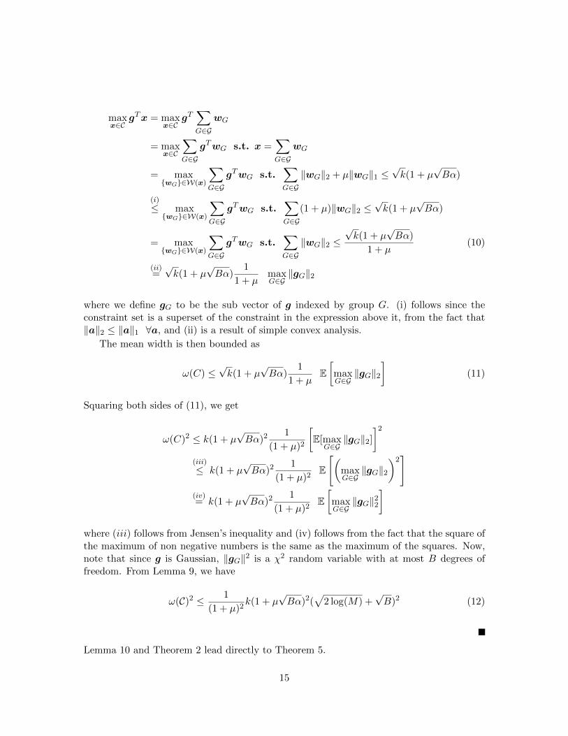
exactly identical. This is accomplished by defining subsets of similar features and searchingfor solutions that select only a few subsets (common across tasks) and a sparse number offeatures within each subset (possibly di↵erent across tasks). Figure 3 shows an example ofthe patterns that typically arise in sparse multitask learning applications, along with theone we are interested in. We see that the SOSlasso, with it’s ability to select a few groupsand only a few non zero coe�cients within those groups lends itself well to the scenario weare interested in.

(a) Sparse (b) Groupsparse

(c) Groupsparse plussparse

(d) Groupsparse andsparse

Figure 3: A comparison of di↵erent sparsity patterns in the multitask learning setting. Fig-ure (a) shows a standard sparsity pattern. An example of group sparse patterns promotedby Glasso (Yuan and Lin, 2006) is shown in Figure (b). In Figure (c), we show the pat-terns considered in (Jalali et al., 2010). Finally, in Figure (d), we show the patterns we areinterested in this paper. The groups are sets of rows of the matrix, and can overlap witheach other

A major application that we are motivated by is the analysis of multi-subject fMRIdata, where the goal is to predict a cognitive state from measured neural activity usingvoxels as features. Because brains vary in size and shape, neural structures can be alignedonly crudely. Moreover, neural codes can vary somewhat across individuals (Feredoes et al.,2007). Thus, neuroanatomy provides only an approximate guide as to where relevant infor-mation is located across individuals: a voxel useful for prediction in one participant suggeststhe general anatomical neighborhood where useful voxels may be found, but not the pre-cise voxel. Past work in inferring sparsity patterns across subjects has involved the use ofgroupwise regularization (van Gerven et al., 2009), using the logistic lasso to infer spar-sity patterns without taking into account the relationships across di↵erent subjects (Ryaliet al., 2010), or using the elastic net penalty to account for groupings among coe�cients(Rish et al., 2012). These methods do not exclusively take into account both the commonmacrostructure and the di↵erences in microstructure across brains, and the SOSlasso allowsone to model both the commonalities and the di↵erences across brains. Figure 4 sheds lighton the motivation, and the grouping of voxels across brains into overlapping sets

In the multitask learning setting, suppose the features are give by �t

, for tasks t ={1, 2, . . . , T }, and corresponding sparse vectors x

?

t

2 Rp. These vectors can be arrangedas columns of a matrix X

?. Suppose we are now given M groups G = {G1

, G

2

, . . .} withmaximum size B. Note that the groups will now correspond to sets of rows of X?.

19

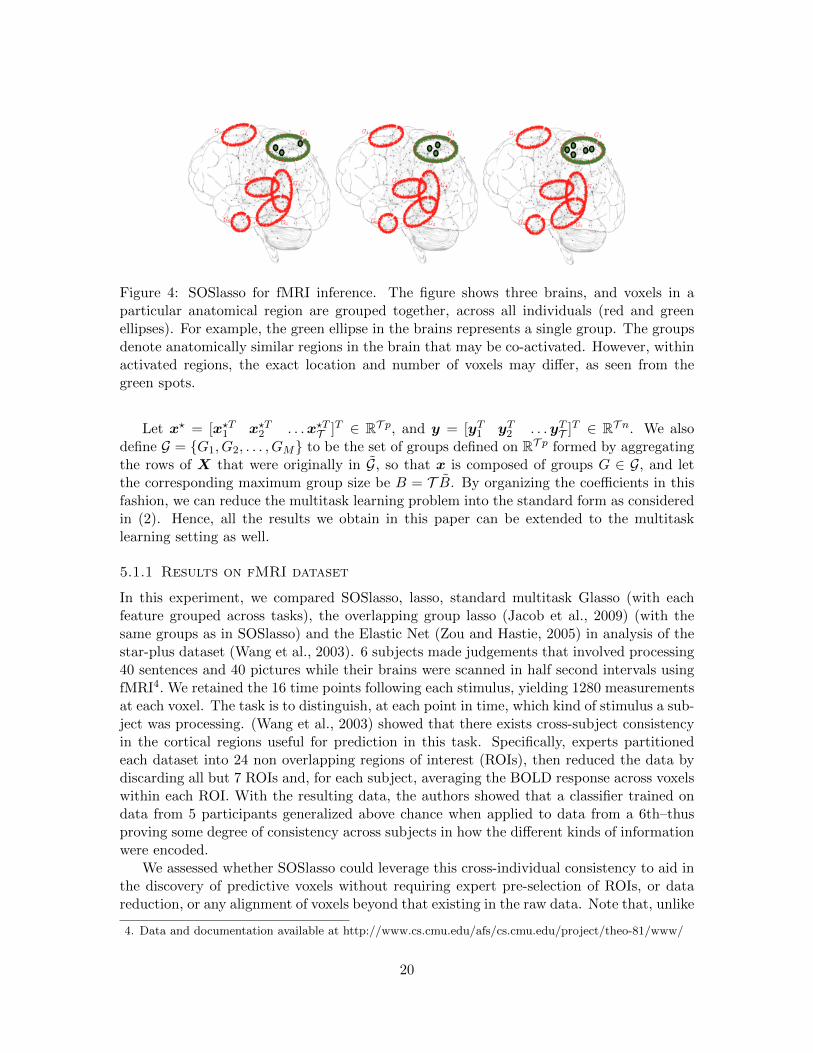
Figure 4: SOSlasso for fMRI inference. The figure shows three brains, and voxels in aparticular anatomical region are grouped together, across all individuals (red and greenellipses). For example, the green ellipse in the brains represents a single group. The groupsdenote anatomically similar regions in the brain that may be co-activated. However, withinactivated regions, the exact location and number of voxels may di↵er, as seen from thegreen spots.

Let x

? = [x?T

1

x

?T

2

. . .x

?T

T ]T 2 RT p, and y = [yT

1

y

T

2

. . .y

T

T ]T 2 RT n. We also

define G = {G1

, G

2

, . . . , G

M

} to be the set of groups defined on RT p formed by aggregatingthe rows of X that were originally in G, so that x is composed of groups G 2 G, and letthe corresponding maximum group size be B = T B. By organizing the coe�cients in thisfashion, we can reduce the multitask learning problem into the standard form as consideredin (2). Hence, all the results we obtain in this paper can be extended to the multitasklearning setting as well.

5.1.1 Results on fMRI dataset

In this experiment, we compared SOSlasso, lasso, standard multitask Glasso (with eachfeature grouped across tasks), the overlapping group lasso (Jacob et al., 2009) (with thesame groups as in SOSlasso) and the Elastic Net (Zou and Hastie, 2005) in analysis of thestar-plus dataset (Wang et al., 2003). 6 subjects made judgements that involved processing40 sentences and 40 pictures while their brains were scanned in half second intervals usingfMRI4. We retained the 16 time points following each stimulus, yielding 1280 measurementsat each voxel. The task is to distinguish, at each point in time, which kind of stimulus a sub-ject was processing. (Wang et al., 2003) showed that there exists cross-subject consistencyin the cortical regions useful for prediction in this task. Specifically, experts partitionedeach dataset into 24 non overlapping regions of interest (ROIs), then reduced the data bydiscarding all but 7 ROIs and, for each subject, averaging the BOLD response across voxelswithin each ROI. With the resulting data, the authors showed that a classifier trained ondata from 5 participants generalized above chance when applied to data from a 6th–thusproving some degree of consistency across subjects in how the di↵erent kinds of informationwere encoded.

We assessed whether SOSlasso could leverage this cross-individual consistency to aid inthe discovery of predictive voxels without requiring expert pre-selection of ROIs, or datareduction, or any alignment of voxels beyond that existing in the raw data. Note that, unlike

4. Data and documentation available at http://www.cs.cmu.edu/afs/cs.cmu.edu/project/theo-81/www/

20

(Wang et al., 2003), we do not aim to learn a solution that generalizes to a withheld subject.Rather, we aim to discover a group sparsity pattern that suggests a similar set of voxels in allsubjects, before optimizing a separate solution for each individual. If SOSlasso can exploitcross-individual anatomical similarity from this raw, coarsely-aligned data, it should showreduced cross-validation error relative to the lasso applied separately to each individual. Ifthe solution is sparse within groups and highly variable across individuals, SOSlasso shouldshow reduced cross-validation error relative to Glasso. Finally, if SOSlasso is finding usefulcross-individual structure, the features it selects should align at least somewhat with theexpert-identified ROIs shown by (Wang et al., 2003) to carry consistent information.

We trained the 5 classifiers using 4-fold cross validation to select the regularizationparameters, considering all available voxels without preselection. We group regions of 5⇥5⇥1 voxels and considered overlapping groups “shifted” by 2 voxels in the first 2 dimensions.5

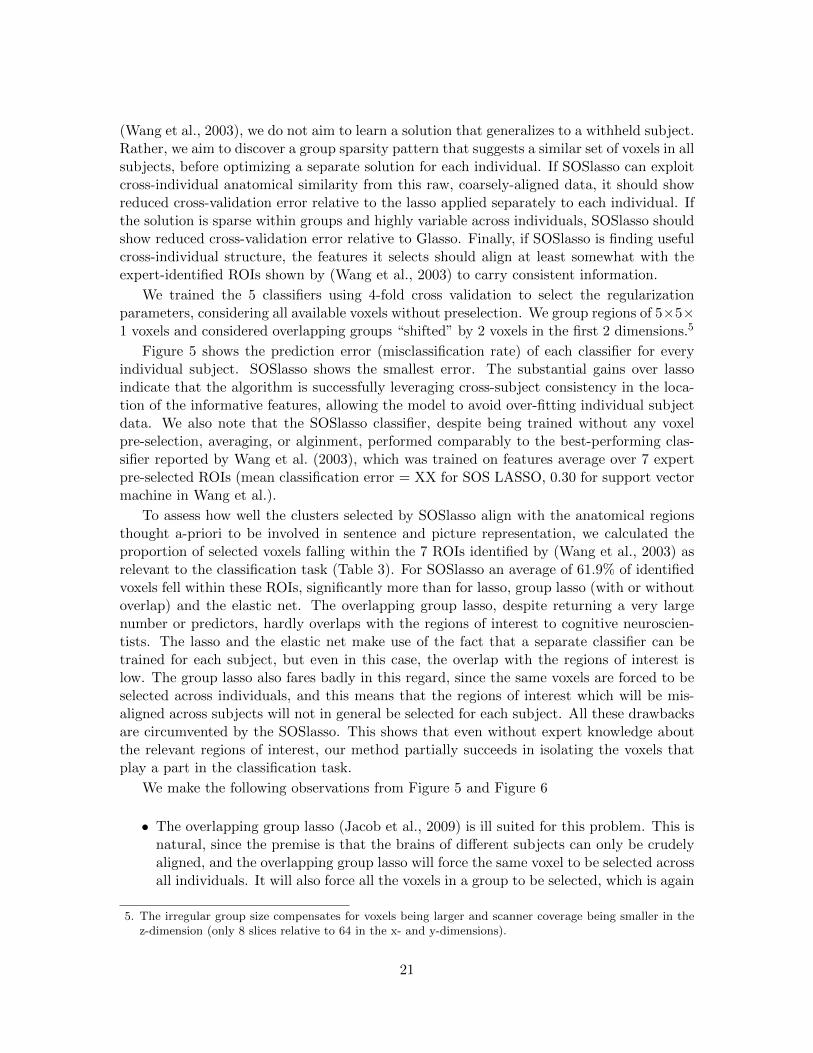
Figure 5 shows the prediction error (misclassification rate) of each classifier for everyindividual subject. SOSlasso shows the smallest error. The substantial gains over lassoindicate that the algorithm is successfully leveraging cross-subject consistency in the loca-tion of the informative features, allowing the model to avoid over-fitting individual subjectdata. We also note that the SOSlasso classifier, despite being trained without any voxelpre-selection, averaging, or alginment, performed comparably to the best-performing clas-sifier reported by Wang et al. (2003), which was trained on features average over 7 expertpre-selected ROIs (mean classification error = XX for SOS LASSO, 0.30 for support vectormachine in Wang et al.).

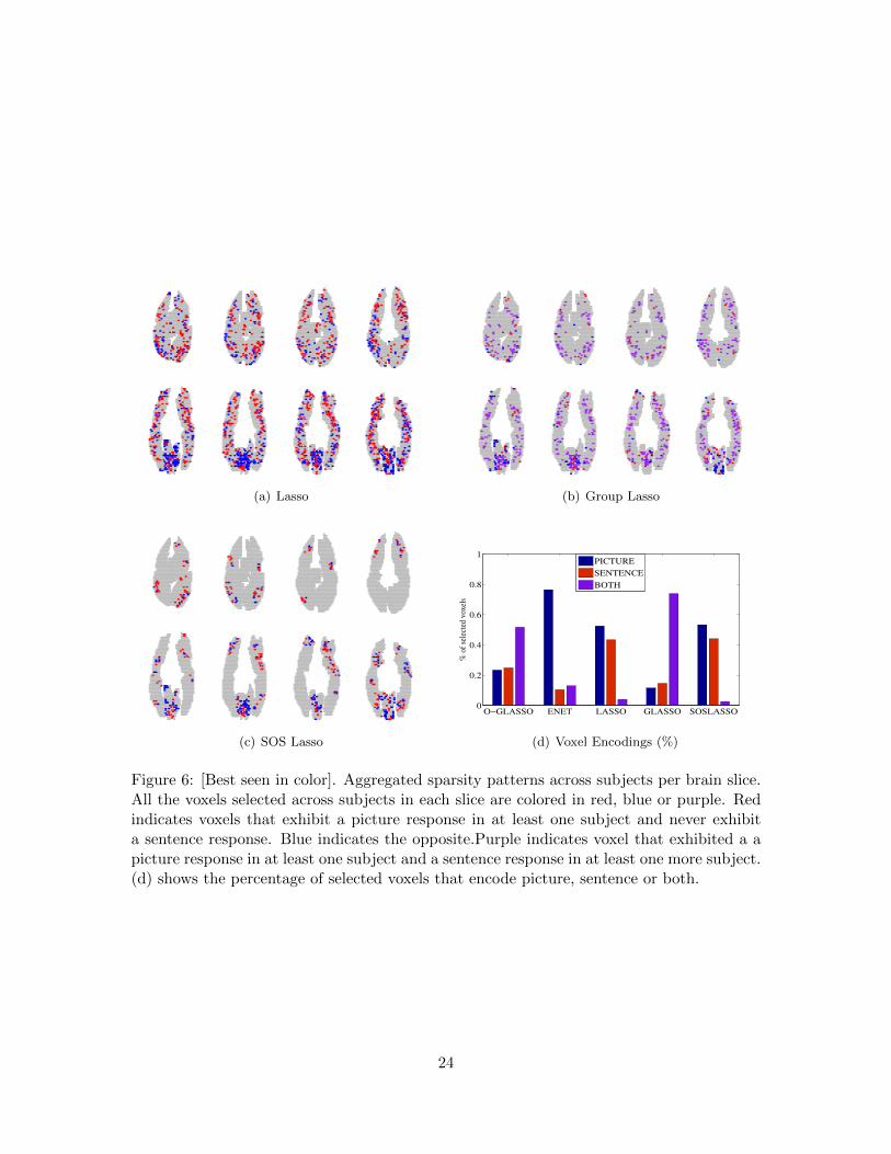
To assess how well the clusters selected by SOSlasso align with the anatomical regionsthought a-priori to be involved in sentence and picture representation, we calculated theproportion of selected voxels falling within the 7 ROIs identified by (Wang et al., 2003) asrelevant to the classification task (Table 3). For SOSlasso an average of 61.9% of identifiedvoxels fell within these ROIs, significantly more than for lasso, group lasso (with or withoutoverlap) and the elastic net. The overlapping group lasso, despite returning a very largenumber or predictors, hardly overlaps with the regions of interest to cognitive neuroscien-tists. The lasso and the elastic net make use of the fact that a separate classifier can betrained for each subject, but even in this case, the overlap with the regions of interest islow. The group lasso also fares badly in this regard, since the same voxels are forced to beselected across individuals, and this means that the regions of interest which will be mis-aligned across subjects will not in general be selected for each subject. All these drawbacksare circumvented by the SOSlasso. This shows that even without expert knowledge aboutthe relevant regions of interest, our method partially succeeds in isolating the voxels thatplay a part in the classification task.

We make the following observations from Figure 5 and Figure 6

• The overlapping group lasso (Jacob et al., 2009) is ill suited for this problem. This isnatural, since the premise is that the brains of di↵erent subjects can only be crudelyaligned, and the overlapping group lasso will force the same voxel to be selected acrossall individuals. It will also force all the voxels in a group to be selected, which is again

5. The irregular group size compensates for voxels being larger and scanner coverage being smaller in thez-dimension (only 8 slices relative to 64 in the x- and y-dimensions).

21

Method Avg. Overlap with ROI %OGlasso 27.18ENet 43.46Lasso 41.51Glasso 47.43

SOSlasso 61.90

Table 3: Mean Sparsity levels of the methods considered, and the average overlap with theprecomputed ROIs in (Wang et al., 2003)

O!Glasso E!Net Lasso Glasso SOSlasso0.2

0.25

0.3

0.35

0.4

0.45

0.5

0.55

Figure 5: Misclassification error on a hold out set for di↵erent methods, on a per subjectbasis. Each solid line connects the di↵erent errors obtained for a particular subject in thedataset.

undesirable from our perspective. This leads to a high number of voxels selected, anda high error.

• The elastic net (Zou and Hastie, 2005) treats each subject independently, and hencedoes not leverage the inter-subject similarity that we know exists across brains. Thefact that all correlated voxels are also picked, coupled with a highly noisy signal meansthat a large number of voxels are selected, and this not only makes the result hard tointerpret, but also leads to a large generalization error.

• The lasso (Tibshirani, 1996) is similar to the elastic net in that it does not leveragethe inter subject similarities. At the same time, it enforces sparsity in the solutions,and hence a fewer number of voxels are selected across individuals. It allows any taskcorrelated voxel to be selected, regardless of its spatial location, and that leads to ahighly distributed sparsity pattern (Figure 6(a)). It leads to a higher cross-validationerror, indicating that the ungrouped voxels are inferior predictors. Like the elasticnet, this leads to a poor generalization error (Figure 5). The distributed sparsitypattern, low overlap with predetermined Regions of Interest, and the high error onthe hold out set is what we believe makes the lasso a suboptimal procedure to use.

• The group lasso (Lounici et al., 2009) groups a single voxel across individuals. Thisallows for taking into account the similarities between subjects, but not the minor

22

di↵erences across subjects. Like the overlapping group lasso, if a voxel is selected forone person, the same voxel is forced to be selected for all people. This means, if avoxel encodes picture or sentence in a particular subject, then the same voxel is forcedto be selected across subjects, and can arbitrarily encode picture or sentence. Thisgives rise to a purple haze in Figure 6(b), and makes the result hard to interpret. Thepurple haze manifests itself due to the large number of ambiguous voxels in Figure6(d).

• Finally, the SOSlasso as we have argued helps in accounting for both the similaritiesand the di↵erences across subjects. This leads to the learning of a code that is atthe same time very sparse and hence interpretable, and leads to an error on the testset that is the best among the di↵erent methods considered. The SOSlasso (Figure6(c)) overcomes the drawbacks of lasso and Glasso by allowing di↵erent voxels to beselected per group. This gives rise to a spatially clustered sparsity pattern, while atthe same time selecting a negligible amount of voxels that encode both picture andsentences (Figure 6(d)). Also, the resulting sparsity pattern has a larger overlap withthe ROI’s than other methods considered.

5.2 Toy Data, Linear Regression

Although not the primary focus of this paper, we show that the method we propose canalso be applied to the linear regression setting. To this end, we consider simulated data anda multitask linear regression setting, and look to recover the coe�cient matrix. We also usethe simulated data to study the properties of the function we propose in (3).

The toy data is generated as follows: we consider T = 20 tasks, and consider overlappinggroups of size B = 6. The groups are defined so that neighboring groups overlap (G

1

={1, 2, . . . , 6}, G

2

= {5, 6, . . . , 10}, G

3

= {9, 10, . . . , 14}, . . . ). We consider a case withM = 100 groups, We set k = 10 groups to be active. We vary the sparsity level of theactive groups ↵ and obtain m = 100 Gaussian linear measurements corrupted with AdditiveWhite Gaussian Noise of standard deviation � = 0.1. We repeat this procedure 100 timesand average the results. To generate the coe�cient matrices X

?, we select k groups atrandom, and within the active groups, only retain fraction ↵ of the coe�cients, again atrandom. The retained locations are then populated with uniform [�1, 1] random variables.

The regularization parameters were clairvoyantly picked to minimize the Mean SquaredError (MSE) over a range of parameter values. The results of applying lasso, standardlatent group lasso (Jacob et al., 2009), Group lasso where each group corresponds to a rowof the sparse matrix, (Lounici et al., 2009) and our SOSlasso to these data are plotted inFigures 7(a), varying ↵.

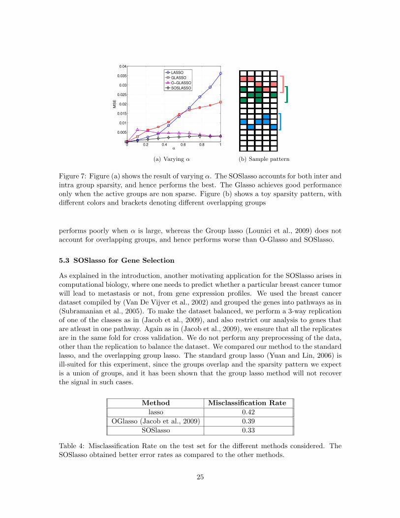
Figure 7(a) shows that, as the sparsity within the active group reduces (i.e. the activegroups become more dense), the overlapping group lasso performs progressively better.This is because the overlapping group lasso does not account for sparsity within groups,and hence the resulting solutions are far from the true solutions for small values of ↵.The SOSlasso however does take this into account, and hence has a lower error when theactive groups are sparse. Note that as ↵ ! 1, the SOSlasso approaches O-Glasso (Jacobet al., 2009). The Lasso (Tibshirani, 1996) does not account for group structure at all and

23

(a) Lasso (b) Group Lasso

(c) SOS Lasso

O!GLASSO ENET LASSO GLASSO SOSLASSO0

0.2

0.4

0.6

0.8

1

% o

f se

lecte

d v

ox

els

PICTURE

SENTENCE

BOTH

(d) Voxel Encodings (%)

Figure 6: [Best seen in color]. Aggregated sparsity patterns across subjects per brain slice.All the voxels selected across subjects in each slice are colored in red, blue or purple. Redindicates voxels that exhibit a picture response in at least one subject and never exhibita sentence response. Blue indicates the opposite.Purple indicates voxel that exhibited a apicture response in at least one subject and a sentence response in at least one more subject.(d) shows the percentage of selected voxels that encode picture, sentence or both.

24

0 0.2 0.4 0.6 0.8 10

0.005

0.01

0.015

0.02

0.025

0.03

0.035

0.04

!

MS

E

LASSO

GLASSO

O!GLASSO

SOSLASSO

(a) Varying ↵ (b) Sample pattern

Figure 7: Figure (a) shows the result of varying ↵. The SOSlasso accounts for both inter andintra group sparsity, and hence performs the best. The Glasso achieves good performanceonly when the active groups are non sparse. Figure (b) shows a toy sparsity pattern, withdi↵erent colors and brackets denoting di↵erent overlapping groups

performs poorly when ↵ is large, whereas the Group lasso (Lounici et al., 2009) does notaccount for overlapping groups, and hence performs worse than O-Glasso and SOSlasso.

5.3 SOSlasso for Gene Selection

As explained in the introduction, another motivating application for the SOSlasso arises incomputational biology, where one needs to predict whether a particular breast cancer tumorwill lead to metastasis or not, from gene expression profiles. We used the breast cancerdataset compiled by (Van De Vijver et al., 2002) and grouped the genes into pathways as in(Subramanian et al., 2005). To make the dataset balanced, we perform a 3-way replicationof one of the classes as in (Jacob et al., 2009), and also restrict our analysis to genes thatare atleast in one pathway. Again as in (Jacob et al., 2009), we ensure that all the replicatesare in the same fold for cross validation. We do not perform any preprocessing of the data,other than the replication to balance the dataset. We compared our method to the standardlasso, and the overlapping group lasso. The standard group lasso (Yuan and Lin, 2006) isill-suited for this experiment, since the groups overlap and the sparsity pattern we expectis a union of groups, and it has been shown that the group lasso method will not recoverthe signal in such cases.

Method Misclassification Rate

lasso 0.42OGlasso (Jacob et al., 2009) 0.39

SOSlasso 0.33

Table 4: Misclassification Rate on the test set for the di↵erent methods considered. TheSOSlasso obtained better error rates as compared to the other methods.

25

We trained a model using 4-fold cross validation on 80% of the data, and used theremaining 20% as a final test set. Table 4 shows the results obtained. We see that theSOSlasso penalty leads to lower classification errors as compared to the lasso or the latentgroup lasso. The errors reported are the ones obtained on the final (held out) test set.

6. Conclusions

In this paper, we introduced a function that can be used to constrain solutions of highdimensional variable selection problems so that they display both within and across groupsparsity. We generalized the sparse group lasso to cases with arbitrary overlap, and provedconsistency results for logistic regression settings. Our results unify the results between thelasso and the group lasso (with or without overlap), and reduce to those cases as specialcases. We also outlined the use of the function in multitask fMRI and computational biologyproblems.

From an algorithmic standpoint, when the groups overlap a lot, the replication procedureused in this paper might not be memory e�cient. Future work involves designing algorithmsthat preclude replication, while at the same time allowing for the SOS- sparsity patterns tobe generated.

From a cognitive neuroscience point of view, future work involves grouping the voxelsin more intelligent ways. Our method to group spatially co-located voxels yields resultsthat are significantly better than traditional lasso-based methods, but it remains to be seenwhether there are better motivated ways to group them. For example, one might considergrouping voxels based on functional connectivities, or take into account the geodesic distanceon the brain surface.

References

Francis Bach. Self-concordant analysis for logistic regression. Electronic Journal of Statis-tics, 4:384–414, 2010.

Florentina Bunea. Honest variable selection in linear and logistic regression models via `1and `1+ `2 penalization. Electronic Journal of Statistics, 2:1153–1194, 2008.

S. Chatterjee, A. Banerjee, and A. Ganguly. Sparse group lasso for regression on landclimate variables. In Data Mining Workshops (ICDMW), 2011 IEEE 11th InternationalConference on, pages 1–8. IEEE, 2011.

Eva Feredoes, Giulio Tononi, and Bradley R Postle. The neural bases of the short-termstorage of verbal information are anatomically variable across individuals. The Journalof Neuroscience, 27(41):11003–11008, 2007.

L. Jacob, G. Obozinski, and J. P. Vert. Group lasso with overlap and graph lasso. InProceedings of the 26th Annual International Conference on Machine Learning, pages433–440. ACM, 2009.

A. Jalali, P. Ravikumar, S. Sanghavi, and C. Ruan. A dirty model for multi-task learning.Advances in Neural Information Processing Systems, 23:964–972, 2010.

26

R. Jenatton, J. Mairal, G. Obozinski, and F. Bach. Proximal methods for hierarchicalsparse coding. arXiv preprint arXiv:1009.2139, 2010.

K. Lounici, M. Pontil, A. B. Tsybakov, and S. van de Geer. Taking advantage of sparsityin multi-task learning. arXiv preprint arXiv:0903.1468, 2009.

Andreas Maurer and Massimiliano Pontil. Structured sparsity and generalization. TheJournal of Machine Learning Research, 13:671–690, 2012.

Lukas Meier, Sara Van De Geer, and Peter Buhlmann. The group lasso for logistic regression.Journal of the Royal Statistical Society: Series B (Statistical Methodology), 70(1):53–71,2008.

Sofia Mosci, Silvia Villa, Alessandro Verri, and Lorenzo Rosasco. A primal-dual algorithmfor group sparse regularization with overlapping groups. In Advances in Neural Informa-tion Processing Systems, pages 2604–2612, 2010.

S. N. Negahban, P. Ravikumar, M. J Wainwright, and Bin Yu. A unified framework forhigh-dimensional analysis of m-estimators with decomposable regularizers. StatisticalScience, 27(4):538–557, 2012.

G. Obozinski, L. Jacob, and J.P. Vert. Group lasso with overlaps: The latent group lassoapproach. arXiv preprint arXiv:1110.0413, 2011.

Yaniv Plan and Roman Vershynin. Robust 1-bit compressed sensing and sparse logisticregression: A convex programming approach. 2012.

N. Rao, B. Recht, and R. Nowak. Universal measurement bounds for structured sparsesignal recovery. In Proceedings of AISTATS, volume 2102, 2012.

Nikhil Rao, Christopher Cox, Robert Nowak, and Timothy Rogers. Sparse overlappingsets lasso for multitask learning and fmri data analysis. Neural Information ProcessingSystems, 2013.

Nikhil S Rao, Robert D Nowak, Stephen J Wright, and Nick G Kingsbury. Convex ap-proaches to model wavelet sparsity patterns. In Image Processing (ICIP), 2011 18thIEEE International Conference on, pages 1917–1920. IEEE, 2011.

G. Raskutti, M. Wainwright, and B. Yu. Restricted eigenvalue properties for correlatedgaussian designs. Journal of Machine Learning Research, 11:2241–2259, 2010.

Irina Rish, Guillermo A Cecchia, Kyle Heutonb, Marwan N Balikic, and A Vania Apkari-anc. Sparse regression analysis of task-relevant information distribution in the brain. InProceedings of SPIE, volume 8314, page 831412, 2012.

Srikanth Ryali, Kaustubh Supekar, Daniel A Abrams, and Vinod Menon. Sparse logisticregression for whole brain classification of fmri data. NeuroImage, 51(2):752, 2010.

N. Simon, J. Friedman, T. Hastie, and R. Tibshirani. A sparse-group lasso. Journal ofComputational and Graphical Statistics, (just-accepted), 2012.

27

P. Sprechmann, I. Ramirez, G. Sapiro, and Y. Eldar. Collaborative hierarchical sparsemodeling. In Information Sciences and Systems (CISS), 2010 44th Annual Conferenceon, pages 1–6. IEEE, 2010.

Pablo Sprechmann, Ignacio Ramirez, Guillermo Sapiro, and Yonina C Eldar. C-hilasso: Acollaborative hierarchical sparse modeling framework. Signal Processing, IEEE Transac-tions on, 59(9):4183–4198, 2011.

Aravind Subramanian, Pablo Tamayo, Vamsi K Mootha, Sayan Mukherjee, Benjamin LEbert, Michael A Gillette, Amanda Paulovich, Scott L Pomeroy, Todd R Golub, Eric SLander, et al. Gene set enrichment analysis: a knowledge-based approach for interpretinggenome-wide expression profiles. Proceedings of the National Academy of Sciences of theUnited States of America, 102(43):15545–15550, 2005.

Robert Tibshirani. Regression shrinkage and selection via the lasso. Journal of the RoyalStatistical Society. Series B (Methodological), pages 267–288, 1996.

Marc J Van De Vijver, Yudong D He, Laura J van’t Veer, Hongyue Dai, Augusti-nus AM Hart, Dorien W Voskuil, George J Schreiber, Johannes L Peterse, Chris Roberts,Matthew J Marton, et al. A gene-expression signature as a predictor of survival in breastcancer. New England Journal of Medicine, 347(25):1999–2009, 2002.

Marcel van Gerven, Christian Hesse, Ole Jensen, and Tom Heskes. Interpreting single trialdata using groupwise regularisation. NeuroImage, 46(3):665–676, 2009.

X. Wang, T. M Mitchell, and R. Hutchinson. Using machine learning to detect cognitivestates across multiple subjects. CALD KDD project paper, 2003.

M. Yuan and Y. Lin. Model selection and estimation in regression with grouped variables.Journal of the Royal Statistical Society: Series B (Statistical Methodology), 68(1):49–67,2006.

J. Zhou, J. Chen, and J. Ye. Malsar: Multi-task learning via structural regularization, 2012.

Y. Zhou, R. Jin, and S. C. Hoi. Exclusive lasso for multi-task feature selection. In Proceed-ings of the International Conference on Artificial Intelligence and Statistics (AISTATS),2010.

Hui Zou and Trevor Hastie. Regularization and variable selection via the elastic net. Journalof the Royal Statistical Society: Series B (Statistical Methodology), 67(2):301–320, 2005.

28