Low complexity power efficient opportunistic schedulingproviding QoS in downlink

Vinod SharmaJoint work with Satya

Dept of Electrical Communication Engineering,Indian Institute of Science

Bangalore, India

January 14, 2014

1 / 38

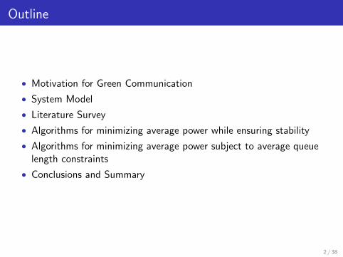
Outline

• Motivation for Green Communication

• System Model

• Literature Survey

• Algorithms for minimizing average power while ensuring stability

• Algorithms for minimizing average power subject to average queuelength constraints

• Conclusions and Summary

2 / 38

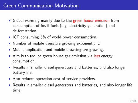
Green Communication Motivation

• Global warming mainly due to the green house emission fromconsumption of fossil fuels (e.g. electricity generation) andde-forestation.

• ICT consuming 3% of world power consumption.

• Number of mobile users are growing exponentially.

• Mobile application and mobile browsing are growing.

• Aim is to reduce green house gas emission via less energyconsumption.

• Results in smaller diesel generators and batteries, and also longerbattery life.

• Also reduces operation cost of service providers.

• Results in smaller diesel generators and batteries, and also longer lifetime.

3 / 38

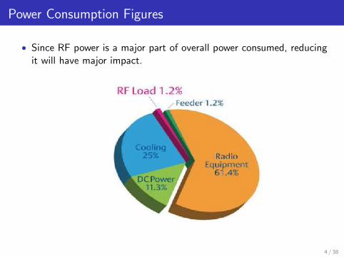
Power Consumption Figures

• Since RF power is a major part of overall power consumed, reducingit will have major impact.

4 / 38

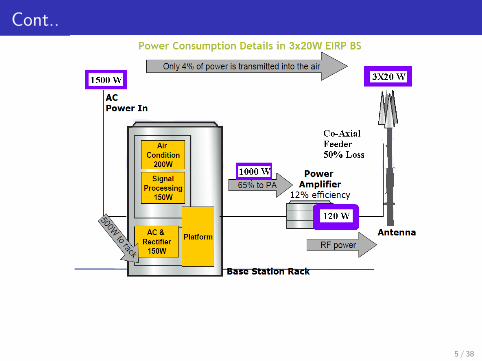
Cont..

5 / 38

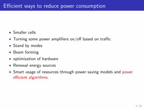
Efficient ways to reduce power consumption

• Smaller cells

• Turning some power amplifiers on/off based on traffic

• Stand by modes

• Beam forming

• optimization of hardware

• Renewal energy sources

• Smart usage of resources through power saving models and powerefficient algorithms.

6 / 38

Literature Survey ...

• Goldsmith and Varaiya (1997) consider single fading link andoptimize the rate.

• Berry-Gallager (2002) Energy- average- delay trade-off. [1], [2].

• Goyal et al. (2003) proved existence of an optimal mean delay policyand obtained some structural results.

• Satya et al. (2012) proposed delay and power optimal policies in asingle server queue when the power-rate is a linear function.

• Chen (2007) proposed an energy efficient scheduling with individualpacket delay constraints.

• Modiano, Tsitsiklis (2003) minimizes energy for sending a fixednumber of packets under given delay constraints.

• Neely (2009) optimizes power without knowledge of arrival rate andchannel stastics.

7 / 38

... Literature Survey ...

• Wang (2004) suboptimal policy which minimizes the average powerunder average queue and packet loss constraints.

• Sharma et al. (2010) optimal energy policies with energy harvestingsources.

• Joseph (2008) provides efficient MAC policies in the same setup.

• Salodkar et al. (2012) Implemented online algorithm by modifyingvalue iteration equation.

8 / 38

... Literature Survey

• MDP based optimal schemes are computationally complex for morethan one user.

• Learning algorithms may be too slow.

• Other algorithms may not guarantee QoS.

9 / 38

System Model

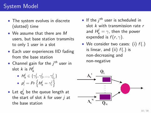
• The system evolves in discrete(slotted) time

• We assume that there are Musers, but base station transmitsto only 1 user in a slot

• Each user experiences IID fadingfrom the base station

• Channel gain for the j th user in

slot k is H jk

• H jk ∈ {γ

j1, γ

j2, ..., γ

jLj}

• pji = Pr

{H j

k = γji

}• Let qj

k be the queue length atthe start of slot k for user j atthe base station

• If the j th user is scheduled inslot k with transmission rate rand H j

k = γ, then the powerexpended is f (r , γ).

• We consider two cases: (i) f (.)is linear, and (ii) f (.) isnon-decreasing andnon-negative

10 / 38

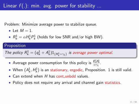
Linear f (.): min. avg. power for stability ...

Problem: Minimize average power to stabilize queue.

• Let M = 1.

• R1k = αH1

kP1k (holds for low SNR and/or high BW).

Proposition

The policy R1k = (q1

k + A1k)1{H1

k=γL}is average power optimal.

• Average power consumption for this policy is E [A]αγL

.

• When (A1k ,H

1k ) is an stationary, ergodic, Proposition. 1 is still valid.

• Can extend when H has cont,unbdd values.

• Policy does not require any arrival and channel gain statistics.

11 / 38

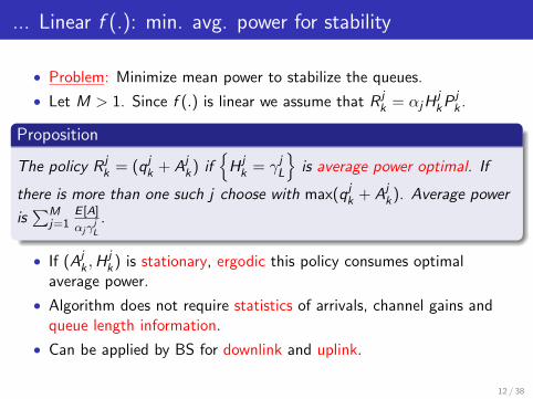
... Linear f (.): min. avg. power for stability

• Problem: Minimize mean power to stabilize the queues.

• Let M > 1. Since f (.) is linear we assume that R jk = αjH

jkP j

k .

Proposition

The policy R jk = (qj

k + Ajk) if

{H jk = γjL

}is average power optimal. If

there is more than one such j choose with max(qjk + Aj

k). Average power

is∑M

j=1E [A]

αjγjL

.

• If (Ajk ,H

jk) is stationary, ergodic this policy consumes optimal

average power.

• Algorithm does not require statistics of arrivals, channel gains andqueue length information.

• Can be applied by BS for downlink and uplink.

12 / 38

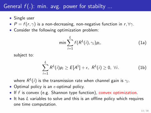
General f (.): min. avg. power for stabilty ...

• Single user

• P = f (r , γ) is a non-decreasing, non-negative function in r ,∀γ.

• Consider the following optimization problem:

minL∑

i=1

f (R1(i), γi )pi , (1a)

subject to:

L∑i=1

R1(i)pi ≥ E [A1] + ε, R1(i) ≥ 0, ∀i . (1b)

where R1(i) is the transmission rate when channel gain is γi .

• Optimal policy is an ε-optimal policy.

• If f is convex (e.g. Shannon type function), convex optimization.

• It has L variables to solve and this is an offline policy which requiresone time computation.

13 / 38

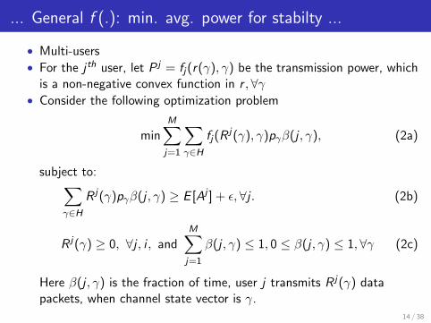
... General f (.): min. avg. power for stabilty ...

• Multi-users• For the j th user, let P j = fj(r(γ), γ) be the transmission power, which

is a non-negative convex function in r , ∀γ• Consider the following optimization problem

minM∑j=1

∑γ∈H

fj(R j(γ), γ)pγβ(j , γ), (2a)

subject to:∑γ∈H

R j(γ)pγβ(j , γ) ≥ E [Aj ] + ε, ∀j . (2b)

R j(γ) ≥ 0, ∀j , i , andM∑j=1

β(j , γ) ≤ 1, 0 ≤ β(j , γ) ≤ 1,∀γ (2c)

Here β(j , γ) is the fraction of time, user j transmits R j(γ) datapackets, when channel state vector is γ.

14 / 38

... General f (.): min. avg. power for stabilty

• We note that the global minimum leads to an ε−optimal policy.

• Objective function is non-convex and constraint set is convex.

• Local optima can be obtained using fmincon with multiple randominitial β(j , γ) and R j(γ).

15 / 38

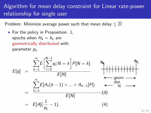
Algorithm for mean delay constraint for Linear rate-powerrelationship for single user

Problem: Minimize average power such that mean delay ≤ D.

• For the policy in Proposition. 1,epochs when Hk = hL aregeometrically distributed withparameter pL.

E [q] =

∞∑k=1

E

[N−1∑l=0

ql |N = k

]P[N = k]

E [N]

=

∞∑k=1

E [A1(k − 1) + ...+ Ak−1]P[N = k]

E [N](3)

= E [A](1

pL− 1). (4)

16 / 38

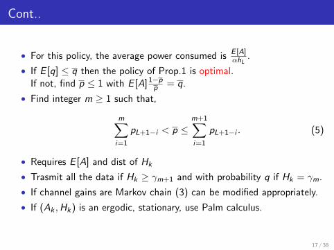
Cont..

• For this policy, the average power consumed is E [A]αhL

.

• If E [q] ≤ q then the policy of Prop.1 is optimal.If not, find p ≤ 1 with E [A]1−pp = q.

• Find integer m ≥ 1 such that,

m∑i=1

pL+1−i < p ≤m+1∑i=1

pL+1−i . (5)

• Requires E [A] and dist of Hk

• Trasmit all the data if Hk ≥ γm+1 and with probability q if Hk = γm.

• If channel gains are Markov chain (3) can be modified appropriately.

• If (Ak ,Hk) is an ergodic, stationary, use Palm calculus.

17 / 38

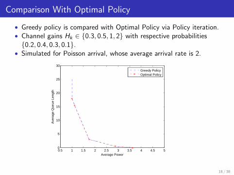
Comparison With Optimal Policy

• Greedy policy is compared with Optimal Policy via Policy iteration.• Channel gains Hk ∈ {0.3, 0.5, 1, 2} with respective probabilities{0.2, 0.4, 0.3, 0.1}.

• Simulated for Poisson arrival, whose average arrival rate is 2.

0.5 1 1.5 2 2.5 3 3.5 4 4.5 50

5

10

15

20

25

30

Average Power

Ave

rage

Que

ue L

engt

h

Greedy PolicyOptimal Policy

18 / 38

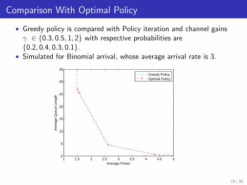
Comparison With Optimal Policy

• Greedy policy is compared with Policy iteration and channel gainsγ ∈ {0.3, 0.5, 1, 2} with respective probabilities are{0.2, 0.4, 0.3, 0.1}.

• Simulated for Binomial arrival, whose average arrival rate is 3.

1 1.5 2 2.5 3 3.5 4 4.5 50

5

10

15

20

25

30

35

Average Power

Ave

rage

Que

ue L

engt

h

Greedy PolicyOptimal Policy

19 / 38

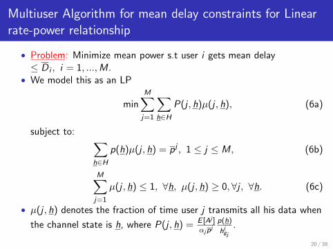
Multiuser Algorithm for mean delay constraints for Linearrate-power relationship

• Problem: Minimize mean power s.t user i gets mean delay≤ D i , i = 1, ...,M.

• We model this as an LP

minM∑j=1

∑h∈H

P(j , h)µ(j , h), (6a)

subject to: ∑h∈H

p(h)µ(j , h) = pj , 1 ≤ j ≤ M, (6b)

M∑j=1

µ(j , h) ≤ 1, ∀h, µ(j , h) ≥ 0, ∀j , ∀h. (6c)

• µ(j , h) denotes the fraction of time user j transmits all his data when

the channel state is h, where P(j , h) = E [Aj ]

αjpjp(h)

hjgj.

20 / 38

Cont..

• This opt problem is an LP with MLM variables can be solved quicklyfor reasonable M, L.

• Requires E [Aj ] and dist. of H jk .

21 / 38

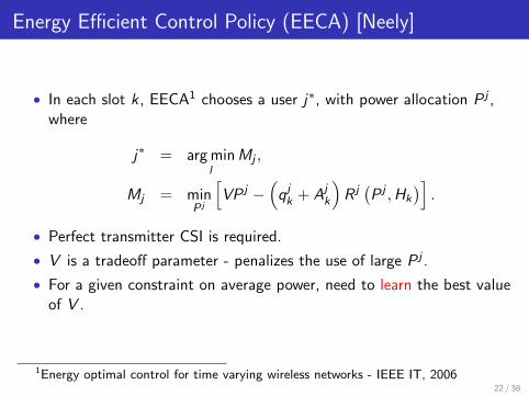
Energy Efficient Control Policy (EECA) [Neely]

• In each slot k , EECA1 chooses a user j∗, with power allocation P j ,where

j∗ = arg minl

Mj ,

Mj = minP j

[VP j −

(qjk + Aj

k

)R j(P j ,Hk

)].

• Perfect transmitter CSI is required.

• V is a tradeoff parameter - penalizes the use of large P j .

• For a given constraint on average power, need to learn the best valueof V .

1Energy optimal control for time varying wireless networks - IEEE IT, 200622 / 38

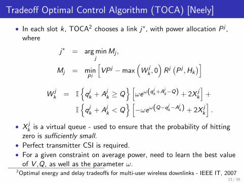
Tradeoff Optimal Control Algorithm (TOCA) [Neely]

• In each slot k , TOCA2 chooses a link j∗, with power allocation P j ,where

j∗ = arg minj

Mj ,

Mj = minP j

[VP j −max

(W j

k , 0)

R j(P j ,Hk

)]W j

k = I{

qjk + Aj

k ≥ Q}[

ωeω(qjk+Ajk−Q) + 2X j

k

]+

I{

qjk + Aj

k < Q}[−ωeω(Q−qjk−A

jk) + 2X j

k

].

• X jk is a virtual queue - used to ensure that the probability of hitting

zero is sufficiently small.• Perfect transmitter CSI is required.• For a given constraint on average power, need to learn the best value

of V ,Q, as well as the parameter ω.2Optimal energy and delay tradeoffs for multi-user wireless downlinks - IEEE IT, 2007

23 / 38

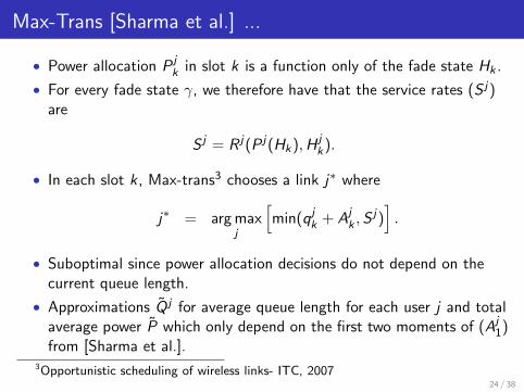
Max-Trans [Sharma et al.] ...

• Power allocation P jk in slot k is a function only of the fade state Hk .

• For every fade state γ, we therefore have that the service rates (S j)are

S j = R j(P j(Hk),H jk).

• In each slot k , Max-trans3 chooses a link j∗ where

j∗ = arg maxj

[min(qj

k + Ajk ,S

j)].

• Suboptimal since power allocation decisions do not depend on thecurrent queue length.

• Approximations Q̃ j for average queue length for each user j and totalaverage power P̃ which only depend on the first two moments of (Aj

1)from [Sharma et al.].

3Opportunistic scheduling of wireless links- ITC, 200724 / 38

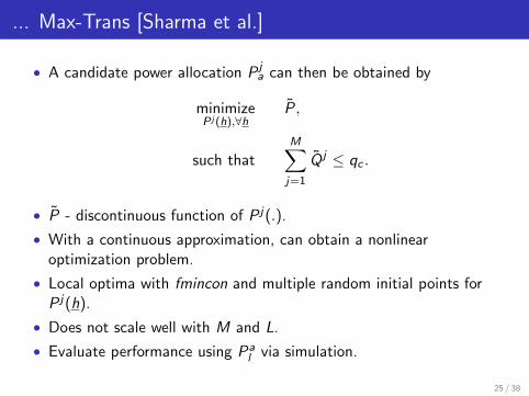
... Max-Trans [Sharma et al.]

• A candidate power allocation P ja can then be obtained by

minimizeP j (h),∀h

P̃,

such thatM∑j=1

Q̃ j ≤ qc .

• P̃ - discontinuous function of P j(.).

• With a continuous approximation, can obtain a nonlinearoptimization problem.

• Local optima with fmincon and multiple random initial points forP j(h).

• Does not scale well with M and L.

• Evaluate performance using Pal via simulation.

25 / 38

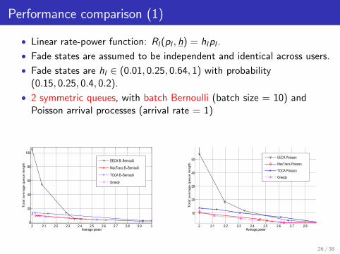
Performance comparison (1)

• Linear rate-power function: Rl(pl , h) = hlpl .

• Fade states are assumed to be independent and identical across users.

• Fade states are hl ∈ (0.01, 0.25, 0.64, 1) with probability(0.15, 0.25, 0.4, 0.2).

• 2 symmetric queues, with batch Bernoulli (batch size = 10) andPoisson arrival processes (arrival rate = 1)

2 2.1 2.2 2.3 2.4 2.5 2.6 2.7 2.8 2.9 30

20

40

60

80

100

Average power

To

tal a

ve

rag

e q

ue

ue

le

ng

th

EECA B−Bernoulli

MaxTrans B−Bernoulli

TOCA B−Bernoulli

Greedy

2 2.1 2.2 2.3 2.4 2.5 2.6 2.7 2.8

10

20

30

40

50

Average power

To

tal a

ve

rag

e q

ue

ue

le

ng

th

EECA Poisson

MaxTrans Poisson

TOCA Poisson

Greedy

26 / 38

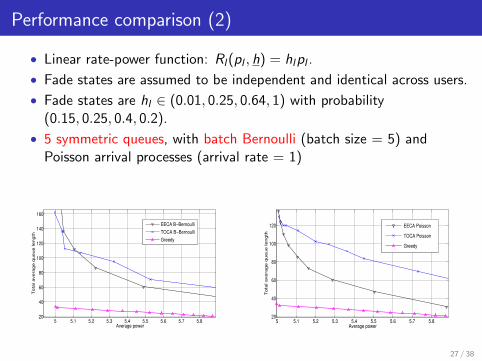
Performance comparison (2)

• Linear rate-power function: Rl(pl , h) = hlpl .

• Fade states are assumed to be independent and identical across users.

• Fade states are hl ∈ (0.01, 0.25, 0.64, 1) with probability(0.15, 0.25, 0.4, 0.2).

• 5 symmetric queues, with batch Bernoulli (batch size = 5) andPoisson arrival processes (arrival rate = 1)

5 5.1 5.2 5.3 5.4 5.5 5.6 5.7 5.820

40

60

80

100

120

140

160

Average power

To

tal a

ve

rag

e q

ue

ue

le

ng

th

EECA B−Bernoulli

TOCA B−Bernoulli

Greedy

5 5.1 5.2 5.3 5.4 5.5 5.6 5.7 5.820

40

60

80

100

120

Average power

To

tal a

ve

rag

e q

ue

ue

le

ng

th

EECA Poisson

TOCA Poisson

Greedy

27 / 38

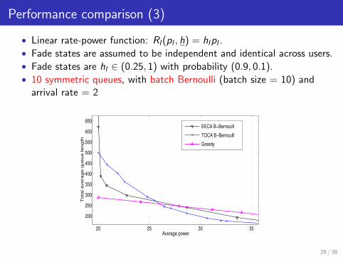
Performance comparison (3)

• Linear rate-power function: Rl(pl , h) = hlpl .• Fade states are assumed to be independent and identical across users.• Fade states are hl ∈ (0.25, 1) with probability (0.9, 0.1).• 10 symmetric queues, with batch Bernoulli (batch size = 10) and

arrival rate = 2

20 25 30 35

200

250

300

350

400

450

500

550

600

650

Average power

To

tal a

ve

rag

e q

ue

ue

le

ng

th

EECA B−Bernoulli

TOCA B−Bernoulli

Greedy

28 / 38

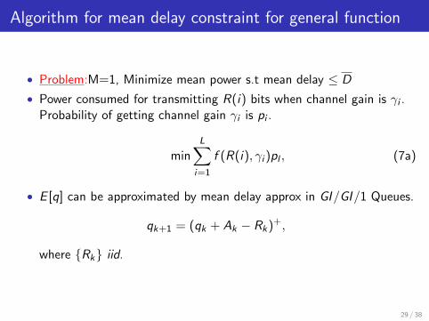
Algorithm for mean delay constraint for general function

• Problem:M=1, Minimize mean power s.t mean delay ≤ D

• Power consumed for transmitting R(i) bits when channel gain is γi .Probability of getting channel gain γi is pi .

minL∑

i=1

f (R(i), γi )pl , (7a)

• E [q] can be approximated by mean delay approx in GI/GI/1 Queues.

qk+1 = (qk + Ak − Rk)+,

where {Rk} iid.

29 / 38

Cont..

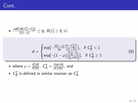
• ρdE [A](C2A+C2

R)2(1−ρ) ≤ q, R(i) ≥ 0, ∀i .

d =

exp[−2(1−ρ)3ρ

(1−C2R)

2

C2R+C2

A], if C 2

R < 1

exp[−(1− ρ)(C2

R−1)C2R+4C2

A], if C 2

R ≥ 1(8)

• where ρ = E [A]E [R] , C 2

A = Var(A)(E [A])2

, and

• C 2R is defined in similar manner as C 2

A.

30 / 38

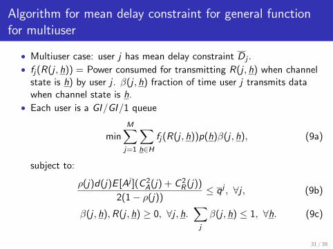
Algorithm for mean delay constraint for general functionfor multiuser

• Multiuser case: user j has mean delay constraint D j .

• fj(R(j , h)) = Power consumed for transmitting R(j , h) when channelstate is h) by user j . β(j , h) fraction of time user j transmits datawhen channel state is h.

• Each user is a GI/GI/1 queue

minM∑j=1

∑h∈H

fj(R(j , h))p(h)β(j , h), (9a)

subject to:

ρ(j)d(j)E [Aj ](C 2A(j) + C 2

R(j))

2(1− ρ(j))≤ qj , ∀j , (9b)

β(j , h),R(j , h) ≥ 0, ∀j , h.∑j

β(j , h) ≤ 1, ∀h. (9c)

31 / 38

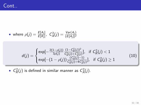
Cont..

• where ρ(j) =E [Aj ]E [Rj ]

, C 2A(j) =

Var(Aj )(E [Aj ])2

d(j) =

exp[−2(1−ρ(j))3ρ(j)

(1−C2R(j))

2

C2R(j)+C2

A(j)], if C 2

R(j) < 1

exp[−(1− ρ(j))(C2

R(j)−1)C2R(j)+4C2

A(j)], if C 2

R(j) ≥ 1(10)

• C 2R(j) is defined in similar manner as C 2

A(j).

32 / 38

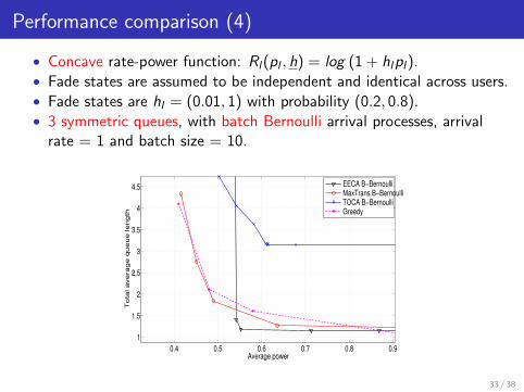
Performance comparison (4)

• Concave rate-power function: Rl(pl , h) = log (1 + hlpl).• Fade states are assumed to be independent and identical across users.• Fade states are hl = (0.01, 1) with probability (0.2, 0.8).• 3 symmetric queues, with batch Bernoulli arrival processes, arrival

rate = 1 and batch size = 10.

0.4 0.5 0.6 0.7 0.8 0.9

1

1.5

2

2.5

3

3.5

4

4.5

Average power

To

tal a

ve

rag

e q

ue

ue

le

ng

th

EECA B−BernoulliMaxTrans B−BernoulliTOCA B−BernoulliGreedy

33 / 38

Summary

• Developed low complexity power efficient algorithms that providestability of queues.

• Extended to the case of mean delay constraints.

• The power rate-power function can be linear or general.

• Have developed algorithms for other QoS constraints.

34 / 38

References

R. A. Berry and R. G. Gallager, “Communication over FadingChannels with Delay Constraints”, IEEE Transactions on InformationTheory, vol. 48, no. 5, PP. 1135-1149, 2002.

R. A. Berry, ” Power and Delay Trade-offs in Fading Channels“, June2000, Phd Thesis, MIT.

A. Chatzipapas, S. Alouf and V. Mancuso, “ On the Minimization ofPower Consumption in Base Stations using on/off PowerAmplifiers,”IEEE Online Conference on Green Communications ,pp.18-23, Sept. 2011

Dimitri P. Bertsekas, “Dynamic Programming and Optimal Control”,Second Edition, Vol-2.

W. Chen, U. Mitra and J.Neely, “Energy-efficient scheduling withindividual delay constraint over a fading channel”, Proc. of the 5thInt. Symposium on Modeling and Optimization in Mobile, Ad Hoc,and Wireless Networks,2007.

35 / 38

A. J. Goldsmith, P. Varaiya, “ Capacity of Fading Channels withChannel Side Information”, IEEE Transaction on Information Theory,vol.43, no.6, 1986-92, Nov 1997.

M. Goyal, A. Kumar and V. Sharma, “Power Constrained and Delayoptimal policies for Scheduling Transmission over a Fading Channel,”IEEE INFOCOM, pp. 311-320, 2003.

J. D. C, Little, “A Proof of the Queuing Formula: L=λW“,Operations Research, vol. 9, no. 3, pp. 383-387.

A. Fu. E. Modiano and J. Tsitsiklis, “Optimal Energy Allocation forDelay-Constrained Data Transmission over a Time-Varying channel”,Proc. IEEE INFOCOM, 2003.

D. J. Ma, A. M. Makowski, A. Shwartz, “Estimation and OptimalControl for Constrained Markov Chains”, IEEE Conf. on Decision andControl, Dec 1986.

Gerson A. S. M, “Low-power HF Microelectronics: A UnifiedApproach”,The Institution Of Engineering And Technology, 1996.

36 / 38

M. J. Neely, “Intelligent Packet Dropping for Optimal Energy- DelayTradeoffs in Wireless Downlinks”, IEEE Transactions on AutomaticControl, vol. 54, no. 3, March 2009.

S. Nitin, A. Bhorkar, A. Karandikar and V. S. Borkar, “An On-LineLearning Algorithm for Energy Efficient Delay Constrained Schedulingover a Fading Channel” IEEE Journal on Selected Areas inCommunications, Vol. 26, No. 4, May 2008.

A. Lalitha, S. Mondal, Satya Kumar. V, Vinod Sharma,“Power-Optimal Scheduling for a Green Base Station with DelayConstraints”, in Nineteenth Annual National Conference onCommunications (NCC), India, 2013.

V. Sharma, Utpal Mukherji, Vinay Joseph and Shrey Gupta, “OptimalEnergy Management Policies for Energy Harvesting Sensor Nodes”,IEEE Transactions on Wireless Communications , Vol.9 Issue 4, April2010.

37 / 38

V. Sharma, Utpal Mukherji and Vinay Joseph, “Efficient EnergyManagement Policies for Networks with Energy Harvesting SensorNodes”, 46th Annual Allerton COnference, pp. 375-383 Sep 2008

D. Tse, V. Pramod, “ Fundamentals of Wireless Communication”,Cambridge University, 2005.

Satya Kumar V, A. Lalitha, V. Sharma, “ Power and Delay OptimalPolicies for Wireless Systems”, National Conference onCommunications(NCC), India , Feb 2012.

H. Wang and N. Mandayam, “ A Simple Packet transmission Schemefor Wireless Data over Fading Channels”, IEEE Transactions onCommunications, vol. 50, no. 1, pp 125-144, 2004.

D. G. Luenberger, “Linear and Nonlinear Programming”, Springer,second edition, 2003.

38 / 38