Low-frequency coupled atmosphere-ocean variability in the southern Indian Ocean

ADVANCES IN ATMOSPHERIC SCIENCES, VOL. 29, NO. 3, 2012, 544–560

Low-Frequency Coupled Atmosphere–Ocean Variability

in the Southern Indian Ocean

FENG Junqiao∗1,2 (��), HU Dunxin1,2 (��), and YU Lejiang3 (��)

1Institute of Oceanology, Chinese Academy of Sciences, Qingdao 266071

2Key Laboratory of Ocean Circulation and Waves, Chinese Academy of Sciences, Qingdao 266071

3Applied Hydrometeorological Research Institute, Nanjing University of

Information Science and Technology, Nanjing 210044

(Received 27 June 2011; revised 28 November 2011)

ABSTRACT

The low-frequency atmosphere–ocean coupled variability of the southern Indian Ocean (SIO) was in-vestigated using observation data over 1958–2010. These data were obtained from ECMWF for sea levelpressure (SLP) and wind, from NCEP/NCAR for heat fluxes, and from the Hadley Center for SST. Toobtain the coupled air-sea variability, we performed SVD analyses on SST and SLP. The primary coupledmode represents 43% of the total square covariance and is featured by weak westerly winds along 45◦–30◦S.This weakened subtropical anticyclone forces fluctuations in a well-known subtropical dipole structure inthe SST via wind-induced processes. The SST changes in response to atmosphere forcing and is predictablewith a lead-time of 1–2 months. Atmosphere–ocean coupling of this mode is strongest during the australsummer. Its principle component is characterized by mixed interannual and interdecadal fluctuations. Thereis a strong relationship between the first mode and Antarctic Oscillation (AAO). The AAO can influencethe coupled processes in the SIO by modulating the subtropical high. The second mode, accounting for30% of the total square covariance, represents a 25-year period interdecadal oscillation in the strength of thesubtropical anticyclone that is accompanied by fluctuations of a monopole structure in the SST along the35◦–25◦S band. It is caused by subsidence of the atmosphere. The present study also shows that physicalprocesses of both local thermodynamic and ocean circulation in the SIO have a crucial role in the formationof the atmosphere–ocean covariability.

Key words: southern Indian Ocean, SST, SLP, Antarctic Oscillation

Citation: Feng, J. Q., D. X. Hu, and L. J. Yu, 2012: Low-frequency coupled atmosphere–ocean variabilityin the southern Indian Ocean. Adv. Atmos. Sci., 29(3), 544–560, doi: 10.1007/s00376-011-1096-2.

1. Introduction

Natural climate variability of low-frequency timescales from interannual to decadal has been the fo-cus of numerous studies. These climate variations arebelieved to arise from atmosphere–ocean interactions.The dynamics of both systems are thus coupled via ex-change processes at their common interface. Coupledvariability of the system occurs when the atmosphereresponds to forcing from the ocean and when the oceanresponds to forcing from the atmosphere. To under-stand and determine the mechanisms governing theseclimatic variations, it is vital to study the common

variability of both the ocean and the overlying atmo-spheric systems and to characterize the large-scale in-teractions between them. While a vast number of stud-ies have been devoted to SST and sea level pressure(SLP) fluctuations and their coupled variability overthe northern Atlantic and the northern Pacific Oceans(e.g., Deser and Blackmon, 1993; Kushnir, 1994; Latifand Barnett, 1996; Mann and Park, 1996), the South-ern Hemisphere has received little attention, except fora few studies on the southern Atlantic (e.g., Venegas etal., 1997, 1998; Sterl and Hazeleger, 2003; Fauchereauet al., 2003). Related research on the southern IndianOcean has been rare (Allan et al., 1995; Reason, 1999;

∗Corresponding author: FENG Junqiao, [email protected]

© China National Committee for International Association of Meteorology and Atmospheric Sciences (IAMAS), Institute of AtmosphericPhysics (IAP) and Science Press and Springer-Verlag Berlin Heidelberg 2012

NO. 3 FENG ET AL. 545

Reason, 2001; Fauchereau et al., 2003). However, thesouthern Indian Ocean is bounded by the Antarcticcircumpolar current to the south and receives oceanicwater mass transport or throughflow from the PacificOcean via the Indonesia throughflow. The location,shape, and topography of the subcontinent make SSThighly sensitive to circulation changes in the IndianOcean (Fauchereau et al., 2003). The southern IndianOcean not only plays an important role in the sur-rounding climate of continents like Africa (Reason andGodfred-Spenning, 1998), but it is also a main regionwhere the Asian monsoon water originates. Moreover,the study by Liu et al. (2006) showed that the IndianOcean Dipole (IOD) in the tropical Indian Ocean re-sponds to the southern high latitude climate almostinstantaneously, suggesting that the IOD signal ex-ists in the Southern Hemisphere. Nan et al (2009)pointed out that the Indian Ocean SST has an impor-tant bridging role in the Antarctic Oscillation (AAO)–East Asian Summer Monsoon relationship. Therefore,atmosphere–ocean interaction in the southern IndianOcean may have implications for other areas, espe-cially the northern Indian Ocean and Asia.

Most studies on Indian Ocean variability have onlyconsidered the tropical area north of 30◦S. If thesouthern boundary of the domain is situated farthersouth, additional SST anomalies in the southern In-dian Ocean emerge in a subtropical dipole mode, whichis phase-locked to the austral summer (Behera and Ya-magata, 2001; Reason, 2001; Reason, 2002). Huangand Shukla (2007) also discussed a subtropical dipolemode in the southern Indian Ocean; however, thatstudy still emphasized the tropical region. As is gen-erally known, the ex-tropical southern Indian Ocean isdominated by the lower tropospheric subtropical high.It is quite likely that atmospheric forcing has a crucialrole in the evolution of the subtropical dipole (Her-mes and Reason, 2005). Previous studies have shownthat this SST anomaly pattern is correlated with rain-fall in various regions of southern Africa (e.g., Rochaand Simmonds, 1997a, b; Goddard and Graham, 1999;Reason, 1999; Reason and Mulenga, 1999; Behera andYamagata, 2001). Surface heat flux, especially the la-tent heat variability, is strongly implicated in form-ing these SST anomalies (Behera and Yamagata, 2001;Suzuki et al., 2004; Hermes and Reason, 2005; Huangand Shukla, 2008). It has been suggested that mod-ulations of the subtropical atmospheric anticycloneare responsible for this latent heat flux variability, al-though the link between atmospheric variability andSST variability has not been precisely determined.Although the formation mechanism of the subtropi-cal SST anomalies is different from that in the trop-ics, the SST anomalies may also be ultimately driven

by coupled atmosphere–ocean interaction. Concern-ing decadal variability, Allan et al. (1995) presentedthe long-term fluctuations in the mean state of theclimate system over the Indian Ocean during australsummertime, showing the strengthening and weak-ening of oceanic and atmospheric variables on themultidecadal time scale. However, the interactionsand feedback mechanisms between the evolving SSTand atmosphere–ocean circulations are not well un-derstood. Knowledge of temporal and spatial covari-ability between ocean and atmosphere in the southernIndian Ocean remains inadequate.

In this study, we aimed to develop a preliminaryinsight into how the southern Indian Ocean systemvaries. Our first aim was to identify the principalmodes of the SST and the overlying atmospheric cir-culation, providing insight into the variability of thesouthern Indian Ocean coupled atmosphere–ocean sys-tem on low-frequency time scales. Our secondary goalwas to determine whether the southern Indian Oceanmodes of variability are connected to Antarctic Oscil-lation. Notably, the AAO is the dominant pattern ofnonseasonal tropospheric circulation variation south of20◦S, and it is characterized by pressure anomalies ofone sign centered in the Antarctic and anomalies of theopposite sign centered around 40◦–50◦S. The recenttrend in the Southern Hemisphere circulation is con-sistent with a systematic bias toward the high-indexpolarity of the AAO (Thompson and Solomon, 2002).In this study, it was also aimed to offer comprehensiveinsights into the southern Indian Ocean atmosphere–ocean coupled variability and to help the modelingstudies associated with these programs.

The paper is organized as follows. A brief descrip-tion of the datasets and methods is given in section 2.Section 3 introduces the main southern Indian Oceanicand atmospheric features. Section 4 presents the prin-cipal modes of behavior of the SST and the overlyingatmospheric circulation in the southern Indian Oceanobtained from EOF analyses. The results pertainingto the atmosphere–ocean coupling based on the singu-lar value decomposition (SVD) analysis are discussedin section 5, focusing on subtropical and mid-latituderegions. Finally, section 6 contains a summary and adiscussion of the main results obtained from this study.

2. Data and methodology

2.1 Data

We used SST data from the Hadley Center. Sealevel pressure, 850 hPa vector wind date were ob-tained from the European Centre for Medium-RangeWeather Forecasts (ECMWF); heat fluxes were de-

546 COUPLED VARIABILITY IN THE SOUTHERN INDIAN OCEAN VOL. 29

rived from the National Centers for EnvironmentalPrediction/National Center for Atmospheric Research(NCEP/NCAR) reanalysis dataset. These datasetsare available as monthly means over the period Jan-uary 1958 to June 2010. The geographical area ofinterest in our study is the southern Indian Ocean(55◦S–equator, 30◦–120◦E). The climatology of thesedatasets were calculated for each calendar month ateach grid point by averaging the data over 1958–2010.Monthly anomalies were then defined as deviationsfrom this mean annual cycle.

The AAO index used in this study was downloadedfrom the National Weather Service Climate Predic-tion Center (http://www.cpc.ncep.noaa.gov/). Theloading pattern of the AAO was defined as the firstleading mode from the EOF analysis of monthly meanheight anomalies in the South Hemisphere at 700 hPa(Mo, 2000). Year-round monthly mean anomaly datahave been used previously to obtain the loading pat-terns. AAO indices were constructed by projecting themonthly mean 700-hPa height anomalies onto the lead-ing EOF mode. In addition, the time series were nor-malized using the standard deviation of the monthlyindex (1979–2000).

2.2 Methods

EOF and SVD analyses were used to describe boththe independent and coupled variability of SST andSLP in the Southern Indian Ocean. While the EOFanalysis method has been widely applied in geophysicsresearch (e.g., Wallace and Jiang, 1990; Deser andBlackmon, 1993), the SVD analysis method has be-come more commonly used only in the last decade. Itis one of the most efficient ways to isolate the covari-ability between two fields (Wallace et al., 1992; Chengand Dunkerton, 1995; Leuliette and Wahr, 1999). Abrief description of the method follows here. UnlikeEOF analysis, in which two variables are used sep-arately, SVD is applied to the cross covariance ma-trix of them. Thus, the results describing the pri-mary coherent mode cannot be assumed to representthe primary oscillation mode of variability for each in-dividual field. The dominant modes explaining largefractions of squared covariance, with strong tempo-ral and spatial correlations, are often interpreted interms of dominant coherent modes of the data vec-tors. The heterogeneous correlation maps of the leftand right fields, which are the correlation coefficientbetween the time series of the left modes with theright field and vice versa, not only provide a measureof coherent between the fields but also represent thecausality between them in certain ways. For normal-ized input data, these heterogeneous correlation mapshave the same patterns as the corresponding left and

right singular vectors (Bretherton et al., 1992). Exam-ples of the application of the SVD analysis are givenin Bretherton et al. (1992) and Wallace et al. (1992).When the SVD analysis is performed, especially whenthe temporal dimension is far larger than the spatial,the resulted SVD modes are not always statisticallysignificant, hence they do not have a physical expla-nation. Therefore, Shen and Lau (1995), Iwasaka andWallace (1995) introduced the Monte Carlo techniqueto test the statistical significance of the SVD modes;Shi (1996) sketched the method that is also utilized inthe present paper.

Notably, due to its limitations, the SVD, undercertain circumstances, might produce paired patternsof no physical meaning (Newman and Sardeshmukh,1995; Cherry, 1997; Hu, 1997). Cherry (1997) pro-posed that, prior to the use of SVD, an EOF analysisshould be applied to each field to test whether thetwo sets of expansion coefficients from EOF analysisare strongly correlated and whether the patterns aregeophysically relevant. Therefore, we conducted EOFanalyses (see section 4) and tested whether such con-ditions were met.

In this method, the lead–lag correlation is em-ployed to illustrate the potential causal relationshipbetween two variables. Composite analysis is a com-mon way to present the responses associated with acertain climate condition by averaging the data overthe considered years. The Student’s t-test is used toassess the statistical significance of the results obtainedfrom composite and correlation analyses. The Morletwavelet analysis (Torrence and Compo, 1998) and lin-ear regression analyses were also utilized in this study.

3. Southern Indian Ocean atmosphere–oceanmean state

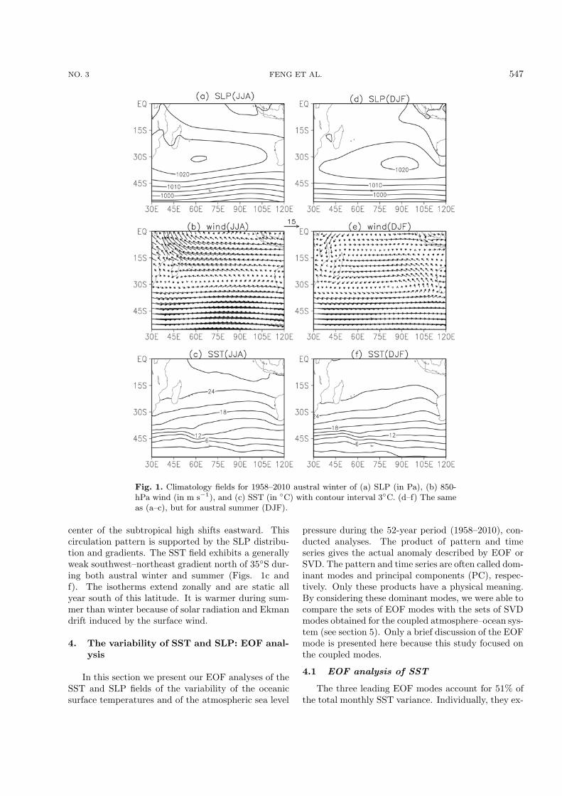
The mean summer and winter fields of SLP, 850-hPa vector wind, and SST, shown in Fig. 1, wereused to compute the 52-year (1958–2010) climatologyfrom the monthly means. Their distributions are dis-played in Figs. 1a–c for austral wintertime (June–July–August, JJA) and in Figs. 1d–f and for summer-time (December–January–February, DJF). The SLPand wind fields were dominated by the southern IndianOcean subtropical high, whose centers were locatednear (30◦S, 60◦E) and (35◦S, 90◦E) in austral winter(Figs. 1a and b) and summer (Figs. 1d and e), re-spectively. The mean surface winds over the southernIndian Ocean were dominated by an anticyclone; northand south of 30◦S the mean surface winds were pre-dominantly easterly/westerly in associated with thesubtropical high. These winds are more southeast-erly off Australia during austral summer, when the


Fig. 1. Climatology fields for 1958–2010 austral winter of (a) SLP (in Pa), (b) 850-hPa wind (in m s−1), and (c) SST (in ◦C) with contour interval 3◦C. (d–f) The sameas (a–c), but for austral summer (DJF).

center of the subtropical high shifts eastward. Thiscirculation pattern is supported by the SLP distribu-tion and gradients. The SST field exhibits a generallyweak southwest–northeast gradient north of 35◦S dur-ing both austral winter and summer (Figs. 1c andf). The isotherms extend zonally and are static allyear south of this latitude. It is warmer during sum-mer than winter because of solar radiation and Ekmandrift induced by the surface wind.

4. The variability of SST and SLP: EOF anal-ysis

In this section we present our EOF analyses of theSST and SLP fields of the variability of the oceanicsurface temperatures and of the atmospheric sea level

pressure during the 52-year period (1958–2010), con-ducted analyses. The product of pattern and timeseries gives the actual anomaly described by EOF orSVD. The pattern and time series are often called dom-inant modes and principal components (PC), respec-tively. Only these products have a physical meaning.By considering these dominant modes, we were able tocompare the sets of EOF modes with the sets of SVDmodes obtained for the coupled atmosphere–ocean sys-tem (see section 5). Only a brief discussion of the EOFmode is presented here because this study focused onthe coupled modes.

4.1 EOF analysis of SST

The three leading EOF modes account for 51% ofthe total monthly SST variance. Individually, they ex-


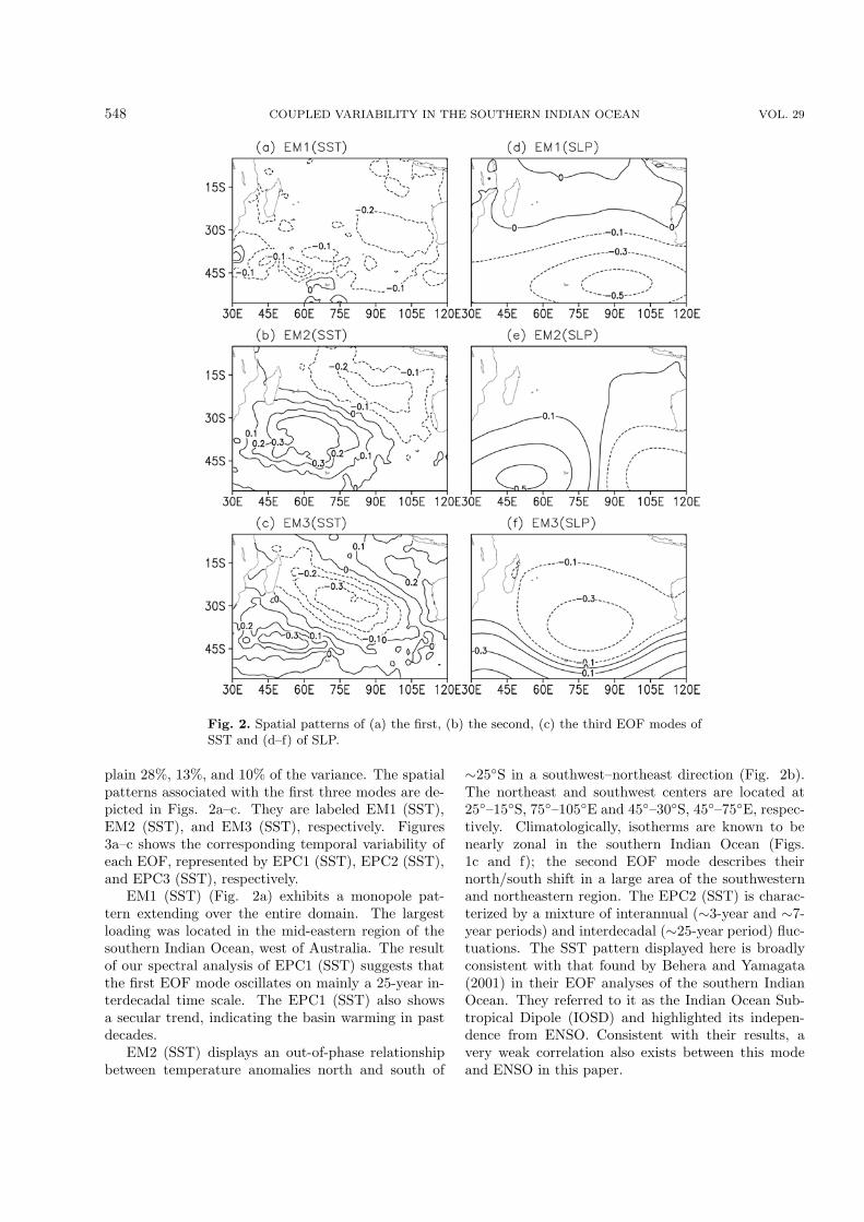
Fig. 2. Spatial patterns of (a) the first, (b) the second, (c) the third EOF modes ofSST and (d–f) of SLP.

plain 28%, 13%, and 10% of the variance. The spatialpatterns associated with the first three modes are de-picted in Figs. 2a–c. They are labeled EM1 (SST),EM2 (SST), and EM3 (SST), respectively. Figures3a–c shows the corresponding temporal variability ofeach EOF, represented by EPC1 (SST), EPC2 (SST),and EPC3 (SST), respectively.

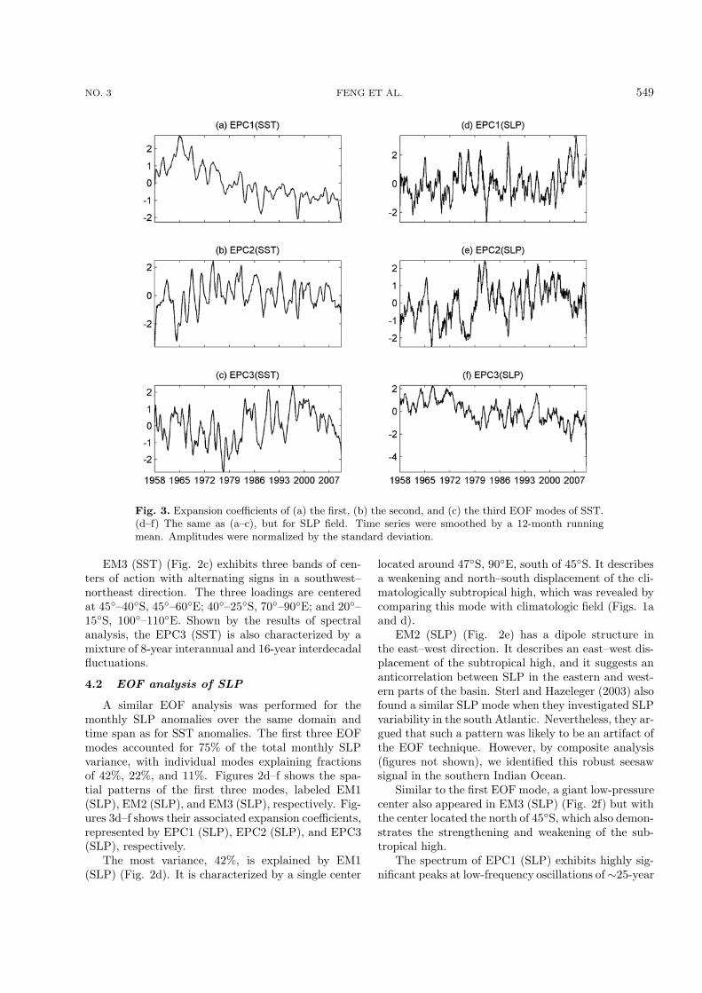
EM1 (SST) (Fig. 2a) exhibits a monopole pat-tern extending over the entire domain. The largestloading was located in the mid-eastern region of thesouthern Indian Ocean, west of Australia. The resultof our spectral analysis of EPC1 (SST) suggests thatthe first EOF mode oscillates on mainly a 25-year in-terdecadal time scale. The EPC1 (SST) also showsa secular trend, indicating the basin warming in pastdecades.

EM2 (SST) displays an out-of-phase relationshipbetween temperature anomalies north and south of

∼25◦S in a southwest–northeast direction (Fig. 2b).The northeast and southwest centers are located at25◦–15◦S, 75◦–105◦E and 45◦–30◦S, 45◦–75◦E, respec-tively. Climatologically, isotherms are known to benearly zonal in the southern Indian Ocean (Figs.1c and f); the second EOF mode describes theirnorth/south shift in a large area of the southwesternand northeastern region. The EPC2 (SST) is charac-terized by a mixture of interannual (∼3-year and ∼7-year periods) and interdecadal (∼25-year period) fluc-tuations. The SST pattern displayed here is broadlyconsistent with that found by Behera and Yamagata(2001) in their EOF analyses of the southern IndianOcean. They referred to it as the Indian Ocean Sub-tropical Dipole (IOSD) and highlighted its indepen-dence from ENSO. Consistent with their results, avery weak correlation also exists between this modeand ENSO in this paper.


Fig. 3. Expansion coefficients of (a) the first, (b) the second, and (c) the third EOF modes of SST.(d–f) The same as (a–c), but for SLP field. Time series were smoothed by a 12-month runningmean. Amplitudes were normalized by the standard deviation.

EM3 (SST) (Fig. 2c) exhibits three bands of cen-ters of action with alternating signs in a southwest–northeast direction. The three loadings are centeredat 45◦–40◦S, 45◦–60◦E; 40◦–25◦S, 70◦–90◦E; and 20◦–15◦S, 100◦–110◦E. Shown by the results of spectralanalysis, the EPC3 (SST) is also characterized by amixture of 8-year interannual and 16-year interdecadalfluctuations.

4.2 EOF analysis of SLP

A similar EOF analysis was performed for themonthly SLP anomalies over the same domain andtime span as for SST anomalies. The first three EOFmodes accounted for 75% of the total monthly SLPvariance, with individual modes explaining fractionsof 42%, 22%, and 11%. Figures 2d–f shows the spa-tial patterns of the first three modes, labeled EM1(SLP), EM2 (SLP), and EM3 (SLP), respectively. Fig-ures 3d–f shows their associated expansion coefficients,represented by EPC1 (SLP), EPC2 (SLP), and EPC3(SLP), respectively.

The most variance, 42%, is explained by EM1(SLP) (Fig. 2d). It is characterized by a single center

located around 47◦S, 90◦E, south of 45◦S. It describesa weakening and north–south displacement of the cli-matologically subtropical high, which was revealed bycomparing this mode with climatologic field (Figs. 1aand d).

EM2 (SLP) (Fig. 2e) has a dipole structure inthe east–west direction. It describes an east–west dis-placement of the subtropical high, and it suggests ananticorrelation between SLP in the eastern and west-ern parts of the basin. Sterl and Hazeleger (2003) alsofound a similar SLP mode when they investigated SLPvariability in the south Atlantic. Nevertheless, they ar-gued that such a pattern was likely to be an artifact ofthe EOF technique. However, by composite analysis(figures not shown), we identified this robust seesawsignal in the southern Indian Ocean.

Similar to the first EOF mode, a giant low-pressurecenter also appeared in EM3 (SLP) (Fig. 2f) but withthe center located the north of 45◦S, which also demon-strates the strengthening and weakening of the sub-tropical high.

The spectrum of EPC1 (SLP) exhibits highly sig-nificant peaks at low-frequency oscillations of ∼25-year


Table 1. Correlation coefficients between the three firstEOF modes of SST and SLP and between these modesand the AAO. Highly significant correlations exceeding the99% confidence level are in bold and italicized face.

EPC1 EPC2 EPC3AAO(SLP) (SLP) (SLP)

EPC1 (SST) −0.04 0.00 0.24 −0.00EPC2 (SST) −0.19 0.09 −0.25 0.21EPC3 (SST) −0.04 0.26 0.001 −0.00AAO −0.57 0.03 −0.14

period and interannual fluctuation of 3–4 years. Thespectra of EPC2 (SLP) show predominantly an 8-yearinterannual fluctuation and a 16-year interdecadal os-cillation. The spectra of EPC3 (SLP) show a signif-icant peak at an interdecadal oscillation with a ∼25-year period.

4.3 Relationship between ocean and atmo-sphere behaviors

To look for possible links between oceanic and at-mospheric fluctuations, the correlation coefficients be-tween the PCs of the three leading SST and SLPmodes were calculated (Table 1). As mentioned pre-viously, the AAO is an important phenomenon of theSouthern Hemisphere, and correlations with the timeseries of the AAO index were also included to test forpossible links with the Antarctic Oscillation.

The simultaneous correlation between EPC2 (SST)and EPC1 (SLP) is −0.19, significant at the 99% con-fidence level. Therefore, the first mode of the atmo-spheric variability is related to the second mode ofthe ocean variability. Lagged correlations betweenthese two expansion coefficients indicated that thetwo modes were correlated when the atmosphere led

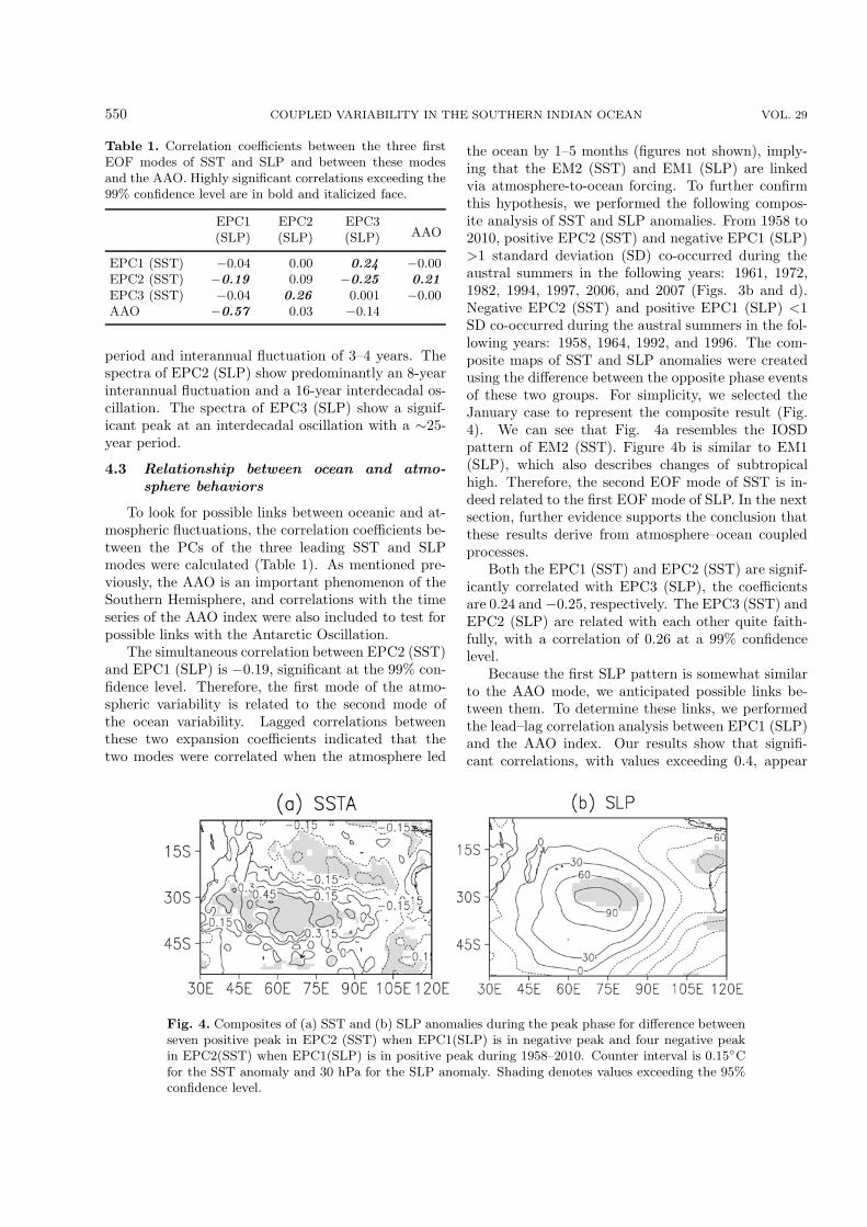
the ocean by 1–5 months (figures not shown), imply-ing that the EM2 (SST) and EM1 (SLP) are linkedvia atmosphere-to-ocean forcing. To further confirmthis hypothesis, we performed the following compos-ite analysis of SST and SLP anomalies. From 1958 to2010, positive EPC2 (SST) and negative EPC1 (SLP)>1 standard deviation (SD) co-occurred during theaustral summers in the following years: 1961, 1972,1982, 1994, 1997, 2006, and 2007 (Figs. 3b and d).Negative EPC2 (SST) and positive EPC1 (SLP) <1SD co-occurred during the austral summers in the fol-lowing years: 1958, 1964, 1992, and 1996. The com-posite maps of SST and SLP anomalies were createdusing the difference between the opposite phase eventsof these two groups. For simplicity, we selected theJanuary case to represent the composite result (Fig.4). We can see that Fig. 4a resembles the IOSDpattern of EM2 (SST). Figure 4b is similar to EM1(SLP), which also describes changes of subtropicalhigh. Therefore, the second EOF mode of SST is in-deed related to the first EOF mode of SLP. In the nextsection, further evidence supports the conclusion thatthese results derive from atmosphere–ocean coupledprocesses.

Both the EPC1 (SST) and EPC2 (SST) are signif-icantly correlated with EPC3 (SLP), the coefficientsare 0.24 and −0.25, respectively. The EPC3 (SST) andEPC2 (SLP) are related with each other quite faith-fully, with a correlation of 0.26 at a 99% confidencelevel.

Because the first SLP pattern is somewhat similarto the AAO mode, we anticipated possible links be-tween them. To determine these links, we performedthe lead–lag correlation analysis between EPC1 (SLP)and the AAO index. Our results show that signifi-cant correlations, with values exceeding 0.4, appear

Fig. 4. Composites of (a) SST and (b) SLP anomalies during the peak phase for difference betweenseven positive peak in EPC2 (SST) when EPC1(SLP) is in negative peak and four negative peakin EPC2(SST) when EPC1(SLP) is in positive peak during 1958–2010. Counter interval is 0.15◦Cfor the SST anomaly and 30 hPa for the SLP anomaly. Shading denotes values exceeding the 95%confidence level.


when AAO leads SLP by −2 to 1 months. The mostsignificant correlation coefficient of −0.57 appears atzero lag, indicating that this mode is highly associatedwith the AAO. In addition, the EPC2 (SST) was alsofound to be significantly correlated with the AAO.

The relationship revealed by these significant cor-relations is further explored in the next section.

5. SVD analysis of SST and SLP

To assess and confirm the relationships betweenSST and SLP variations, SVD analysis was performedon the cross-covariance matrix between them. Toexamine the statistical robustness of the results ob-tained from the SVD analysis, we performed a signif-icance test using a Monte Carlo approach. Our re-sults show that the first two modes for each pair ofvariables are well beyond the 95% confidence level.The covariance is also strongly concentrated in thefirst two modes, which isolate large-scale spatial fea-tures with low-frequency time scales. They indepen-dently explain 43% and 30% of the total square covari-ance, respectively. The coupled spatial patterns andexpansion coefficients corresponding to each variableof the first two modes are displayed in Figs. 5 and

6. The SST/SLP spatial patterns are labeled as SM1(SST)/SM1 (SLP) and SM2 (SST)/SM2 (SLP), re-spectively. The corresponding time series of expansioncoefficients are SPC1 (SST)/SPC1 (SLP) and SPC2(SST)/SPC2 (SLP), respectively. They are discussedseparately in the following sections.

5.1 The first SVD mode

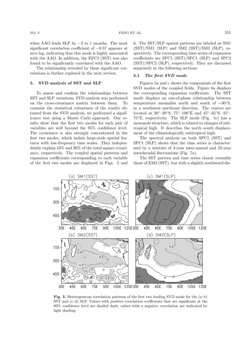
Figures 5a and c shows the components of the firstSVD modes of the coupled fields. Figure 6a displaysthe corresponding expansion coefficients. The SSTmode displays an out-of-phase relationship betweentemperature anomalies north and south of ∼30◦S,in a southwest–northeast direction. The centers arelocated at 30◦–20◦S, 75◦–100◦E and 45◦–35◦S, 45◦–75◦E, respectively. The SLP mode (Fig. 5c) has amonopole structure, which is related to changes of sub-tropical high. It describes the north–south displace-ment of the climatologically subtropical high.

The spectral analysis on both SPC1 (SST) andSPC1 (SLP) shows that the time series is character-ized by a mixture of 3-year inter-annual and 25-yearinterdecadal fluctuations (Fig. 7a).

The SST pattern and time series closely resemblethose of EM2 (SST), but with a slightly southward dis-

Fig. 5. Heterogeneous correlation patterns of the first two leading SVD mode for the (a–b)SST and (c–d) SLP. Values with positive correlation coefficients that are significant at the99% confidence level are shaded dark; values with a negative correlation are indicated bylight shading.


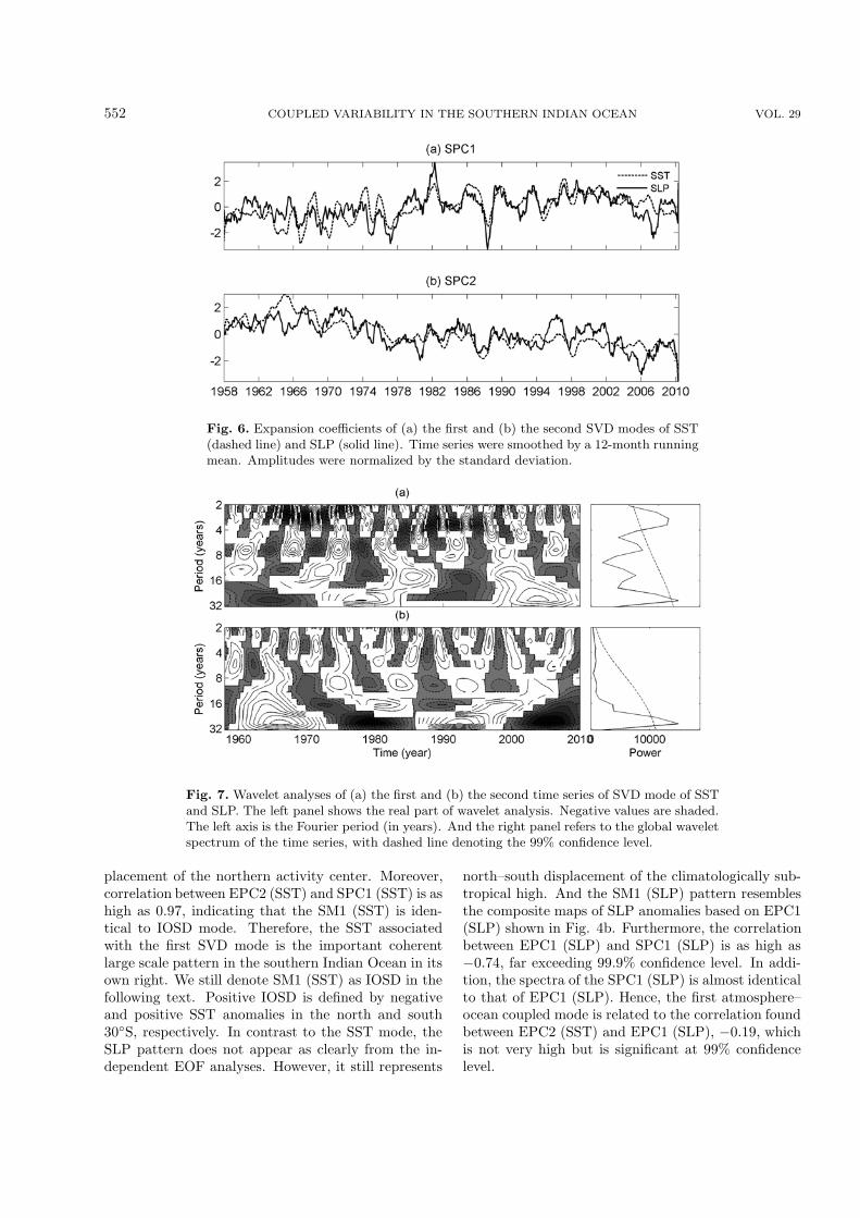
Fig. 6. Expansion coefficients of (a) the first and (b) the second SVD modes of SST(dashed line) and SLP (solid line). Time series were smoothed by a 12-month runningmean. Amplitudes were normalized by the standard deviation.

Fig. 7. Wavelet analyses of (a) the first and (b) the second time series of SVD mode of SSTand SLP. The left panel shows the real part of wavelet analysis. Negative values are shaded.The left axis is the Fourier period (in years). And the right panel refers to the global waveletspectrum of the time series, with dashed line denoting the 99% confidence level.

placement of the northern activity center. Moreover,correlation between EPC2 (SST) and SPC1 (SST) is ashigh as 0.97, indicating that the SM1 (SST) is iden-tical to IOSD mode. Therefore, the SST associatedwith the first SVD mode is the important coherentlarge scale pattern in the southern Indian Ocean in itsown right. We still denote SM1 (SST) as IOSD in thefollowing text. Positive IOSD is defined by negativeand positive SST anomalies in the north and south30◦S, respectively. In contrast to the SST mode, theSLP pattern does not appear as clearly from the in-dependent EOF analyses. However, it still represents

north–south displacement of the climatologically sub-tropical high. And the SM1 (SLP) pattern resemblesthe composite maps of SLP anomalies based on EPC1(SLP) shown in Fig. 4b. Furthermore, the correlationbetween EPC1 (SLP) and SPC1 (SLP) is as high as−0.74, far exceeding 99.9% confidence level. In addi-tion, the spectra of the SPC1 (SLP) is almost identicalto that of EPC1 (SLP). Hence, the first atmosphere–ocean coupled mode is related to the correlation foundbetween EPC2 (SST) and EPC1 (SLP), −0.19, whichis not very high but is significant at 99% confidencelevel.


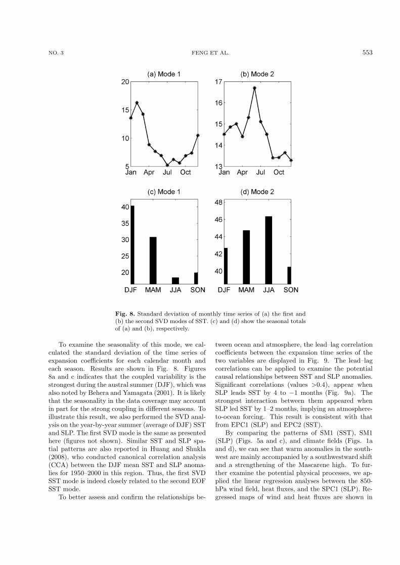
Fig. 8. Standard deviation of monthly time series of (a) the first and(b) the second SVD modes of SST. (c) and (d) show the seasonal totalsof (a) and (b), respectively.

To examine the seasonality of this mode, we cal-culated the standard deviation of the time series ofexpansion coefficients for each calendar month andeach season. Results are shown in Fig. 8. Figures8a and c indicates that the coupled variability is thestrongest during the austral summer (DJF), which wasalso noted by Behera and Yamagata (2001). It is likelythat the seasonality in the data coverage may accountin part for the strong coupling in different seasons. Toillustrate this result, we also performed the SVD anal-ysis on the year-by-year summer (average of DJF) SSTand SLP. The first SVD mode is the same as presentedhere (figures not shown). Similar SST and SLP spa-tial patterns are also reported in Huang and Shukla(2008), who conducted canonical correlation analysis(CCA) between the DJF mean SST and SLP anoma-lies for 1950–2000 in this region. Thus, the first SVDSST mode is indeed closely related to the second EOFSST mode.

To better assess and confirm the relationships be-

tween ocean and atmosphere, the lead–lag correlationcoefficients between the expansion time series of thetwo variables are displayed in Fig. 9. The lead–lagcorrelations can be applied to examine the potentialcausal relationships between SST and SLP anomalies.Significant correlations (values >0.4), appear whenSLP leads SST by 4 to −1 months (Fig. 9a). Thestrongest interaction between them appeared whenSLP led SST by 1–2 months, implying an atmosphere-to-ocean forcing. This result is consistent with thatfrom EPC1 (SLP) and EPC2 (SST).

By comparing the patterns of SM1 (SST), SM1(SLP) (Figs. 5a and c), and climate fields (Figs. 1aand d), we can see that warm anomalies in the south-west are mainly accompanied by a southwestward shiftand a strengthening of the Mascarene high. To fur-ther examine the potential physical processes, we ap-plied the linear regression analyses between the 850-hPa wind field, heat fluxes, and the SPC1 (SLP). Re-gressed maps of wind and heat fluxes are shown in


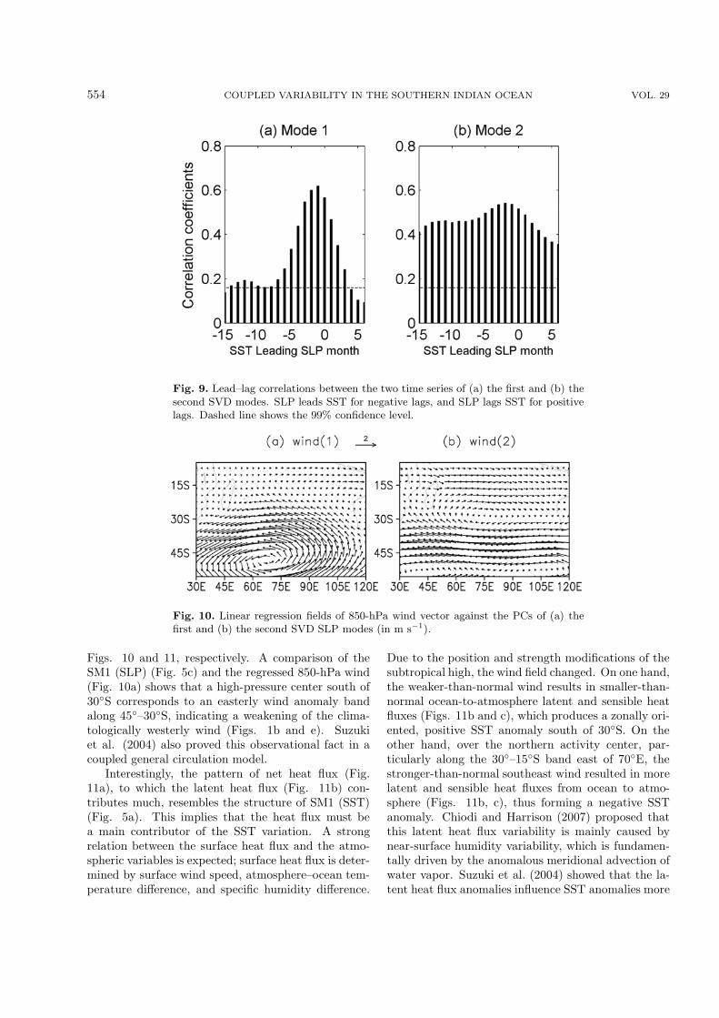
Fig. 9. Lead–lag correlations between the two time series of (a) the first and (b) thesecond SVD modes. SLP leads SST for negative lags, and SLP lags SST for positivelags. Dashed line shows the 99% confidence level.

Fig. 10. Linear regression fields of 850-hPa wind vector against the PCs of (a) thefirst and (b) the second SVD SLP modes (in m s−1).

Figs. 10 and 11, respectively. A comparison of theSM1 (SLP) (Fig. 5c) and the regressed 850-hPa wind(Fig. 10a) shows that a high-pressure center south of30◦S corresponds to an easterly wind anomaly bandalong 45◦–30◦S, indicating a weakening of the clima-tologically westerly wind (Figs. 1b and e). Suzukiet al. (2004) also proved this observational fact in acoupled general circulation model.

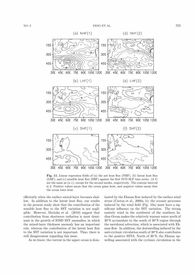
Interestingly, the pattern of net heat flux (Fig.11a), to which the latent heat flux (Fig. 11b) con-tributes much, resembles the structure of SM1 (SST)(Fig. 5a). This implies that the heat flux must bea main contributor of the SST variation. A strongrelation between the surface heat flux and the atmo-spheric variables is expected; surface heat flux is deter-mined by surface wind speed, atmosphere–ocean tem-perature difference, and specific humidity difference.

Due to the position and strength modifications of thesubtropical high, the wind field changed. On one hand,the weaker-than-normal wind results in smaller-than-normal ocean-to-atmosphere latent and sensible heatfluxes (Figs. 11b and c), which produces a zonally ori-ented, positive SST anomaly south of 30◦S. On theother hand, over the northern activity center, par-ticularly along the 30◦–15◦S band east of 70◦E, thestronger-than-normal southeast wind resulted in morelatent and sensible heat fluxes from ocean to atmo-sphere (Figs. 11b, c), thus forming a negative SSTanomaly. Chiodi and Harrison (2007) proposed thatthis latent heat flux variability is mainly caused bynear-surface humidity variability, which is fundamen-tally driven by the anomalous meridional advection ofwater vapor. Suzuki et al. (2004) showed that the la-tent heat flux anomalies influence SST anomalies more


Fig. 11. Linear regression fields of (a) the net heat flux (NHF), (b) latent heat flux(LHF), and (c) sensible heat flux (SHF) against the first SVD SLP time series. (d–f)are the same as (a–c), except for the second modes, respectively. The contour intervalis 2. Positive values mean that the ocean gains heat, and negative values mean thatthe ocean loses heat.

efficiently when the surface mixed-layer becomes shal-low. In addition to the latent heat flux, our resultsin the present study show that the contribution of thesensible heat flux to the SST variation is not negli-gible. However, Morioka et al. (2010) suggest thatcontribution from shortwave radiation is most domi-nant in the growth of IOSD SST anomalies, in whichthe mixed-layer thickness anomaly has an importantrole, whereas the contribution of the latent heat fluxto the SST variation is not important. Thus, there isstill disagreement regarding this issue.

As we know, the current in the upper ocean is dom-

inated by the Ekman flow induced by the surface windstress (Carton et al., 2000a, b); the oceanic processesinduced by the wind field (Fig. 10a) must have a sig-nificant influence on the SST variation. The strongeasterly wind in the southwest of the southern In-dian Ocean makes the relatively warmer water north of30◦S accumulate to the south of 30◦S region throughthe meridonal advection, which is associated with Ek-man flow. In addition, the downwelling induced by theanti-cyclonic circulation south of 30◦S also contributesto the positive SSTA. North of 30◦S, the Ekman up-welling associated with the cyclonic circulation in the


eastern region, to the west coast of Australia, also hassome contribution to the negative SSTA.

In summary, these characteristics of the wind–SSTrelationship reveal that wind-induced mechanisms, in-cluding heat flux variation and Ekman upwelling ordownwelling processes, drive the variations in theocean temperature. In return, the dipole pattern ofthe ocean temperature enhances the behavior of theoverlying atmospheric, though not very strongly; thesignificant correlation between the two time series ofexpansion coefficients (Fig. 9a) only appeared whenSST led SLP by 1–3 months. By employing a gen-eral circulation model, Reason and Godfred-Spenning(1998) also found that the response of the atmosphereto an idealized SST anomaly (warm in southern mid-latitudes, cool in southern tropics), similar to theIOSD pattern, can lead to changes in surface heatfluxes and in the strength of the south Indian subtrop-ical gyre that opposes the original SST anomaly. Ourresults are in good agreement with the model resultssuggested by Reason and Godfred-Spenning (1998).

5.2 The second mode

Figures 5b and d shows the second SST and SLPmodes, respectively. The corresponding expansion co-efficients are depicted in Fig. 6b. The SST mode ex-hibits a monopole pattern extending over the entiredomain and is similar to the first EOF mode patternof SST, but it has a large amplitude in a band ex-tending westward from the west coast of Australia tothe region east of Madagascar along 30◦S. The SLPalso has uniform polarity over the entire domain. Theactivity center of the mode is located near the cen-ter of the subtropical high (Figs. 1a, d). This modealso describes the strengthening and weakening of theanticyclone.

The results of our spectral analysis on both theSST and SLP expansion coefficients of the second SVDmode (Fig. 6b) indicate a dominant spectral peak at∼25 years (Fig. 7b). Negative values were seen inthe 1960s and 1990s, while positive ones were seen inthe late 1970s to early 1980s and 2000s. A negativetrend was also detected in both SST and SLP timeseries during 1958–2010, implying the secular basin-warming of SST and long-term SLP increasing in vari-ation, particularly along the north edge of subtropicalhigh. This variation may arise through a combinationof basin scale atmosphere–ocean interaction and a re-motely forced component (Reason et al., 1998).

The SST time series also compared well with EM1(SST) (Fig. 2a). The SLP time series and pattern forthe second SVD mode compared well with the thirdEOF mode of SLP (Fig. 2f). The correlation coeffi-cient was 0.56 between EPC3 (SLP) and SPC2 (SLP)

and was 0.75 between EPC1 (SST) and SPC2 (SST).So this mode is related to the correlation found be-tween EPC1 (SST) and EPC3 (SLP) (Table 1).

From Figs. 8b and d, we can see that this mode alsoshows strong seasonal variation and is active duringthe austral winter (JJA). This is further confirmed byapplying SVD analyses of year-by-year SST and SLPduring winter (average of JJA). The first mode alsopresents the same characters in both spatial patternand frequency features.

To investigate possible air–sea forcing mechanismsrelated to the second SVD mode, we examined thelead–lag correlation between the two time series, thelinear regression field of wind, and the heat fluxesassociated with it. The high degrees of correlation(Fig. 9b) between SPC2 (SST) and SPC2 (SLP) in-dicate strong oceanic response to atmosphere nearlysimultaneously, while the value is slightly higher whenthe SLP leads the SST by 1–2 months. Previous re-searchers (Deser and Blackmon, 1993; Kushnir, 1994)concluded from investigations of the North Atlanticthat interannual variability is primarily driven by theatmosphere, while interdecadal or longer-scale vari-ability is mainly associated with changes in the ocean.However, recently some other studies of the AtlanticOcean have suggested that atmospheric-to-ocean forc-ing on interdecadal time scales may be more impor-tant (e.g., Halliwell, 1996; Venegas et al., 1997). Thelead–lag correlation presented here somewhat supportsthis idea. In a word, the subsidence of atmosphere isthe main reason for the formation of the second SVDmode.

To understand the details of oceanic response tothe atmosphere, we next compared the SST patternwith the wind regression map (Fig. 10b). A giant cy-clone, with the center located along 28◦S (Fig. 10b),corresponding to the low SLP in Fig. 5d, can be seenjust over the strong cold SSTA center (Fig. 5b). Be-cause of such cyclonic circulation, temperature andhumidity differences between ocean and atmospherebecome larger. Consequently, the latent and sensibleheat fluxes increase, thus the ocean loses heat southof 28◦S (Figs. 11d–f). In addition, Ekman upwellingcaused by this strong cyclone also contributes to theSST cooling.

However, northwest of the Australia (Fig. 11d),the ocean gains heat from the atmosphere–ocean in-terface mainly because of the reduced latent and sen-sible heat flux from ocean to atmosphere (Figs. 11e, f),which is due to the weak-than-normal wind, whereasthe SSTA remains negative there. Thus the heat flux isno longer a reason for the SST cooling. From Fig. 10b,we can see that the northern branch of cyclone circula-tion north of 28◦S is dominated by westerly anomalies.


This westerly can induce a cold temperature advectionfrom mid-latitude to the low latitude by Ekman driftcurrent. Furthermore, the northern branch of the cy-clone can also make the relative cold water in the west-ern part of southern Indian Ocean accumulate to theeastern warm pool region by advection, contributingto the negative SSTA there. Consequently, the nega-tive SSTA to the northwest of Australia is mainly dueto the oceanic process forced by the overlying atmo-sphere.

5.3 Connection between AAO and coupledvariability

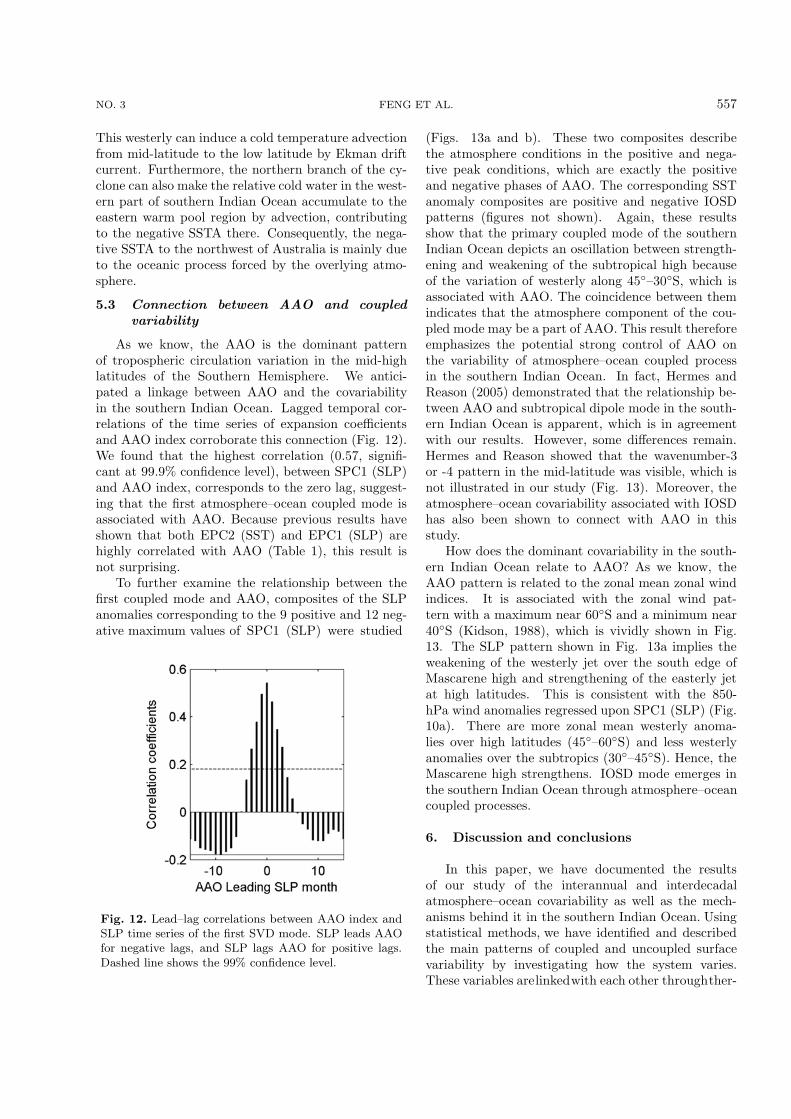
As we know, the AAO is the dominant patternof tropospheric circulation variation in the mid-highlatitudes of the Southern Hemisphere. We antici-pated a linkage between AAO and the covariabilityin the southern Indian Ocean. Lagged temporal cor-relations of the time series of expansion coefficientsand AAO index corroborate this connection (Fig. 12).We found that the highest correlation (0.57, signifi-cant at 99.9% confidence level), between SPC1 (SLP)and AAO index, corresponds to the zero lag, suggest-ing that the first atmosphere–ocean coupled mode isassociated with AAO. Because previous results haveshown that both EPC2 (SST) and EPC1 (SLP) arehighly correlated with AAO (Table 1), this result isnot surprising.

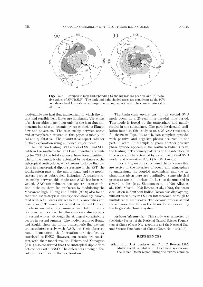
To further examine the relationship between thefirst coupled mode and AAO, composites of the SLPanomalies corresponding to the 9 positive and 12 neg-ative maximum values of SPC1 (SLP) were studied

Fig. 12. Lead–lag correlations between AAO index andSLP time series of the first SVD mode. SLP leads AAOfor negative lags, and SLP lags AAO for positive lags.Dashed line shows the 99% confidence level.

(Figs. 13a and b). These two composites describethe atmosphere conditions in the positive and nega-tive peak conditions, which are exactly the positiveand negative phases of AAO. The corresponding SSTanomaly composites are positive and negative IOSDpatterns (figures not shown). Again, these resultsshow that the primary coupled mode of the southernIndian Ocean depicts an oscillation between strength-ening and weakening of the subtropical high becauseof the variation of westerly along 45◦–30◦S, which isassociated with AAO. The coincidence between themindicates that the atmosphere component of the cou-pled mode may be a part of AAO. This result thereforeemphasizes the potential strong control of AAO onthe variability of atmosphere–ocean coupled processin the southern Indian Ocean. In fact, Hermes andReason (2005) demonstrated that the relationship be-tween AAO and subtropical dipole mode in the south-ern Indian Ocean is apparent, which is in agreementwith our results. However, some differences remain.Hermes and Reason showed that the wavenumber-3or -4 pattern in the mid-latitude was visible, which isnot illustrated in our study (Fig. 13). Moreover, theatmosphere–ocean covariability associated with IOSDhas also been shown to connect with AAO in thisstudy.

How does the dominant covariability in the south-ern Indian Ocean relate to AAO? As we know, theAAO pattern is related to the zonal mean zonal windindices. It is associated with the zonal wind pat-tern with a maximum near 60◦S and a minimum near40◦S (Kidson, 1988), which is vividly shown in Fig.13. The SLP pattern shown in Fig. 13a implies theweakening of the westerly jet over the south edge ofMascarene high and strengthening of the easterly jetat high latitudes. This is consistent with the 850-hPa wind anomalies regressed upon SPC1 (SLP) (Fig.10a). There are more zonal mean westerly anoma-lies over high latitudes (45◦–60◦S) and less westerlyanomalies over the subtropics (30◦–45◦S). Hence, theMascarene high strengthens. IOSD mode emerges inthe southern Indian Ocean through atmosphere–oceancoupled processes.

6. Discussion and conclusions

In this paper, we have documented the resultsof our study of the interannual and interdecadalatmosphere–ocean covariability as well as the mech-anisms behind it in the southern Indian Ocean. Usingstatistical methods, we have identified and describedthe main patterns of coupled and uncoupled surfacevariability by investigating how the system varies.These variables arelinkedwith each other throughther-


Fig. 13. SLP composite map corresponding to the highest (a) positive and (b) nega-tive values of SPC1(SLP). The dark and light shaded areas are significant at the 99%confidence level for positive and negative values, respectively. The counter interval is200 hPa.

modynamic like heat flux momentum, in which the la-tent and sensible heat fluxes are dominant. Variationsof such variables depend not only on the heat flux mo-mentum but also on oceanic processes such as Ekmanflow and advection. The relationship between oceanand atmosphere discussed in this paper is mainly lo-cal and qualitative. The quantitative aspect calls forfurther exploration using numerical experiments.

The first two leading SVD modes of SST and SLPfields in the southern Indian Ocean, together account-ing for 73% of the total variance, have been identified.The primary mode is characterized by weakness of thesubtropical anticyclone, which seems to force fluctua-tions in a subtropical dipole structure in the SST: thesouthwestern part at the mid-latitude and the north-eastern part at subtropical latitudes. A possible re-lationship between this mode and AAO has been re-vealed. AAO can influence atmosphere–ocean condi-tion in the southern Indian Ocean by modulating theMascarene high. Huang and Shukla (2008) also foundthat the extra-tropical atmospheric anomaly associ-ated with AAO forces surface heat flux anomalies andresults in SST anomalies related to the subtropicaldipole in austral spring, summer, and fall. In addi-tion, our results show that the same case also appearsin austral winter, although the strongest covariabilityoccurs in austral summer. The model results of Huangand Shukla show the initial atmospheric fluctuationsare associated closely with AAO, but their observedresults demonstrate the fluctuations are significantlycorrelated to ENSO. However, our results are consis-tent with their model results. Behera and Yamagata(2001) also considered that the subtropical dipole doesnot connect with ENSO. The differences among differ-ent results call for further exploration.

The basin-scale oscillations in the second SVDmode occur on a 25-year inter-decadal time period.This mode is forced by the atmosphere and mainlyresults in the subsidence. The periodic decadal oscil-lation found in this study is on a 25-year time scale.As shown in Figs. 7a and b, two complete episodeswith positive and negative phases occurred in thepast 50 years. In a couple of years, another positivephase episode appears in the southern Indian Ocean,the leading SST anomaly patterns on the interdecadaltime scale are characterized by a cold basin (2nd SVDmode) and a negative IOSD (1st SVD mode).

Importantly, we only considered the processes thatare active in the interface of ocean and atmosphereto understand the coupled mechanism, and the ex-planations given here are qualitative; some physicalprocesses are still unclear. In fact, as documented inseveral studies (e.g., Shannon et al., 1990; Allan etal., 1995; Mason, 1995; Reason et al., 1996), the oceancirculation in Southern Indian Ocean also displays sig-nificant variability in SST on intraseasonal through tomultidecadal time scales. The oceanic process shouldreceive more attention in the future for understandingthe large-scale climate system.

Acknowledgements. This study was supported by

the Major Project of the National Natural Science Founda-

tion of China (Grant No. 40890151) and the National Nat-

ural Science Foundation of China (Grant No. 41106016).

REFERENCES

Allan, R. J., J. A. Lindesay, and C. J. C. Reason, 1995:Multidecadal variability in the climate system overthe Indian Ocean region during the austral summer.


J. Climate, 8, 1853–1873.Behera, S. K., and T. Yamagata, 2001: Subtropical SST

dipole events in the southern Indian Ocean. Geophys.Res. Lett., 28, 327–330.

Bretherton, C. S., C. Smith, and J. M. Wallace, 1992:An intercomparison of methods for finding coupledpatterns in climate data. J. Climate, 5, 541–560.

Carton, J. A., G. Cherupin, X. Cao, and B. Giese, 2000a:A simple ocean data assimilation analysis of theglobal upper ocean 1950–1995. Part I: Methodology.Journal of Physical Oceanography, 30, 294–309.

Carton, J. A., G. Cherupin, X. Cao, and B. Giese, 2000b:A simple ocean data assimilation analysis of theglobal upper ocean 1950–1995. Part II: Results. Jour-nal of Physical Oceanography, 30, 311–326.

Cheng, X., and T. J. Dunkerton, 1995: Orthogonal rota-tion of spatial patterns derived from singular valuedecomposition analysis. J. Climate, 8, 2631–2643.

Cherry, S., 1997: Some comments on singular value de-composition analysis. J. Climate, 10, 1759–1761.

Chiodi, A. M., and D. E. Harrison, 2007: Mechanisms ofsummertime subtropical southern Indian Ocean Seasurface temperature variability: On the importanceof humidity anomalies and the meridional advectionof water vapor. J. Climate, 20, 4835–4852.

Deser, C., and M. L. Blackmon, 1993: Surface climatevariations over the North Atlantic Ocean during win-ter: 1900–1989. J. Climate, 6, 1743–1753.

Fauchereau, N., S. Trzaska, Y. Richard, P. Roucou,and P. Camberlin, 2003: Sea-surface temperatureco-variability in the southern Atlantic and IndianOceans and its connections with the atmospheric cir-culation in the southern hemisphere. Int. J. Clima-tol., 23, 663–677.

Goddard, L., and N. E. Graham, 1999: Importance of theIndian Ocean for simulating rainfall anomalies overeastern and southern Africa. J. Geophys. Res., 104,19099–19116.

Halliwell, G. R., 1996: Atmospheric circulation anoma-lies driving decadal/interdecadal SST anomalies inthe North Atlantic. ACCP Notes, III(1), 8–11.

Hermes, J. C., and C. J. C. Reason, 2005: Ocean modeldiagnosis if interannual coevolving SST variability inthe southern Indian and south Atlantic Oceans. J.Climate, 18, 2864–2882.

Hu, Q., 1997: On the uniqueness of the singular valuedecomposition in meteorological applications. J. Cli-mate, 10, 1762–1766.

Huang, B. H., and J. Shukla, 2007: Mechanisms for theinterannual variability in the tropical Indian Ocean.Part II: Regional processes. J. Climate, 20, 2937–2960.

Huang, B. H., and J. Shukla, 2008: Interannual variabil-ity of the South Indian Ocean in observations and acoupled model. Indian Journal of Marine Sciences,37, 13–34.

Iwasaka, N., and J. M. Wallace, 1995: Large scale airsea interaction in the Northern Hemisphere from aview point of variations of surface heat flux by SVD

analysis. J. Meteor. Soc. Japan, 73, 781–794.Kidson, J. W., 1988: Interannual variations in the South-

ern Hemisphere circulation. J. Climate, 1, 1177–1198.

Kushnir, Y., 1994: Interdecadal variations in North At-lantic sea surface temperature and associated atmo-spheric conditions. J. Climate, 7, 141–157.

Latif, M., and T. P. Barnett, 1996: Decadal climate vari-ability over the North Pacific and North America:Dynamics and predictability. J. Climate, 9, 2407–2423.

Leuliette, E. W., and J. M. Wahr, 1999: Cou-pled pattern analysis of sea surface temperatureand TOPEX/Poseidon sea surface height. J. Phys.Oceanogr., 29, 599–611.

Liu, N., Z. Jia, H. X. Chen, F. Hua, and Y. F. Li, 2006:Southern high latitude climate anomalies associatedwith the Indian Ocean dipole mode. Chinese Journalof Oceanology and Limnology, 24, 125–128.

Mann, M. E., and J. Park, 1996: Joint spatiotemporalmodes of surface temperature and sea level pressurevariability in the Northern Hemisphere during thelast century. J. Climate, 9, 2137–2162.

Mason, S. J., 1995: Sea-surface temperature—SouthAfrican rainfall associations, 1910–1989. Int. J. Cli-matol., 15, 119–135.

Mo, K. C., 2000: Relationships between low-frequencyvariability in the Southern Hemisphere and sea sur-face temperature anomalies. J. Climate, 13, 3599–3610.

Morioka, Y., T. Tozuka, and T. Yamagata, 2010: Cli-mate variability in the southern Indian Ocean as re-vealed by self-organizing maps. Climate Dyn., 35,1059–1072.

Nan, S. L., J. P. Li, X. J. Yuan, and P. Zhao, 2009: Bo-real spring Southern Hemisphere annular mode, In-dian Ocean sea surface temperature, and East Asiansummer monsoon. J. Geophys. Res., 14, D02103, doi:10.1029/2008JD01 0045.

Newman, M., and P. Sardeshmukh, 1995: A caveat con-cerning singular value decomposition. J. Climate, 8,352–360.

Reason, C. J. C., 1999: Interannual warm and cool eventsin the subtropical mid-latitude south Indian Oceanregion. Geophys. Res. Lett., 26, 215–218.

Reason, C. J. C., 2001: Subtropical Indian Ocean SSTdipole events and southern African rainfall. Geophys.Res. Lett., 28, 2225–2227.

Reason, C. J. C., 2002: Sensitivity of the southern Africancirculation to dipole sea-surface temperature pat-terns in the south Indian Ocean. Int. J. Climatol.,22, 377–393.

Reason, C. J. C., and C. R. Godfred-Spenning, 1998:SST variability in the South Indian Ocean and asso-ciated circulation and rainfall patterns over SouthernAfrica. Meteorology and Atmospheric Physics, 66,243–258.

Reason, C. J. C., and H. Mulenga, 1999: Relationshipsbetween South African rainfall and SST anomalies


in the southwest Indian Ocean. Int. J. Climatol., 19,1651–1673.

Reason, C. J. C., R. J. Allan, and J. A. Lindesay, 1996:Evidence for the influence of remote forcing on inter-decadal variability in the southern Indian Ocean. J.Geophys. Res., 101, 11876–11882.

Reason, C. J. C., C. R. Godfred-Spenning, R. J. Allan,and J. A. Lindesay, 1998: Air-sea interaction mecha-nisms and low frequency climate variability in theSouth Indian Ocean region. Int. J. Climatol., 18,391–405.

Rocha, A., and I. Simmonds, 1997a: Interannual variabil-ity of south–eastern African summer rainfall. Part 1:Relationships with air-sea interaction processes. Int.J. Climatol., 17, 235–265.

Rocha, A., and I. Simmonds, 1997b: Interannual variabil-ity of south–eastern African summer rainfall. Part 2:Modelling the impact of seasurface temperatures inrainfall and circulation. Int. J. Climatol., 17, 267–290.

Shannon, L. V., J. J. Agenbag, N. D. Walker, and J. R.E. Lutjeharms, 1990: A major perturbation in theAgulhas retroflection area in 1986. Deep-Sea Res., 3,493–512.

Shen, S., and K. M. Lau, 1995: Biennial oscillation associ-ated with the East Asian summer monsoon and trop-ical sea surface temperatures. J. Meteor. Soc. Japan,73, 105–124.

Shi, N., 1996: Confidence test of SVD method in the

study of climate diagnose. Meteorological Science andTechnology, 4, 5–6. (in Chinese)

Sterl, A., and W. Hazeleger, 2003: Coupled variabilityand air-sea interaction in the South Atlantic Ocean.Climate Dyn., 21, 559–571.

Suzuki, R., S. K. Behera, S. Iizuka, and T. Yamagata,2004: Indian Ocean subtropical dipole simulated us-ing a coupled general circulation model. J. Geophys.Res., 109, C09001, doi: 10.1029/2003JC001974.

Thompson, D. W. J., and S. Solomon, 2002: Inter-pretation of Recent Southern Hemisphere ClimateChange. Science, 296, 895–899.

Torrence, C., and G. P. Compo, 1998: A practical guideto wavelet analysis. Bull. Amer. Meteor. Soc., 79,61–78.

Venegas, S. A., L. A. Mysak, and D. N. Straub, 1997:Atmosphere–Ocean coupled variability in the SouthAtlantic. J. Climate, 10, 2904–2920.

Venegas, S. A., L. A. Mysak, and D. N. Straub, 1998:An interdecadal climate cycle in the South Atlanticand its links to other ocean basins. J. Geophys. Res.,103, 24723–24736.

Wallace, C. S., and Q. R. Jiang, 1990: Spatial patterns ofatmosphere–ocean interaction in the northern win-ter. J. Climate, 3, 990–998.

Wallace, J. M., C. Smith, and C. S. Bretherton, 1992:Singular value decomposition of wintertime sea sur-face temperature and 500-mb height anomalies. J.Climate, 5, 561–576.

Documents

Low-frequency coupled atmosphere-ocean variability in the southern Indian Ocean