Embed Size (px)
Citation preview
Low frequency vibration induced streaming in a Hele-Shaw cellM. Costalonga, P. Brunet, and H. Peerhossaini Citation: Physics of Fluids (1994-present) 27, 013101 (2015); doi: 10.1063/1.4905031 View online: http://dx.doi.org/10.1063/1.4905031 View Table of Contents: http://scitation.aip.org/content/aip/journal/pof2/27/1?ver=pdfcov Published by the AIP Publishing Articles you may be interested in Experimental and numerical study of buoyancy-driven single bubble dynamics in a vertical Hele-Shaw cell Phys. Fluids 26, 123303 (2014); 10.1063/1.4903488 Interaction of a synthetic jet with the flow over a low aspect ratio cylinder Phys. Fluids 25, 064104 (2013); 10.1063/1.4811710 Acoustic radiation by vortex induced flexible wall vibration J. Acoust. Soc. Am. 118, 2182 (2005); 10.1121/1.2011127 Kelvin–Helmholtz instability in a Hele-Shaw cell Phys. Fluids 14, 922 (2002); 10.1063/1.1446884 Gravitational instability of miscible fluids in a Hele-Shaw cell Phys. Fluids 14, 902 (2002); 10.1063/1.1431245
This article is copyrighted as indicated in the article. Reuse of AIP content is subject to the terms at: http://scitation.aip.org/termsconditions. Downloaded
to IP: 81.194.30.218 On: Mon, 05 Jan 2015 14:01:10
PHYSICS OF FLUIDS 27, 013101 (2015)
Low frequency vibration induced streaming in a Hele-Shawcell
M. Costalonga,1,2,a) P. Brunet,2 and H. Peerhossaini11Laboratoire Interdisciplinaire des Energies de Demain (LIED) - Université Paris Diderot,10 rue Alice Domon et Léonie Duquet, 75205 Paris cedex 13, France2Laboratoire Matière et Systèmes Complexes, UMR CNRS 7057, Université Paris Diderot,10 rue Alice Domon et Léonie Duquet, 75205 Paris cedex 13, France
(Received 16 May 2014; accepted 10 November 2014; published online 5 January 2015)
When an acoustic wave propagates in a fluid, it can generate a second order flowwhose characteristic time is much longer than the period of the wave. Within a range offrequency between ten and several hundred Hz, a relatively simple and versatile wayto generate streaming flow is to put a vibrating object in the fluid. The flow developsvortices in the viscous boundary layer located in the vicinity of the source of vibrations,leading in turn to an outer irrotational streaming called Rayleigh streaming. Becausethe flow originates from non-linear time-irreversible terms of the Navier-Stokes equa-tion, this phenomenon can be used to generate efficient mixing at low Reynolds num-ber, for instance in confined geometries. Here, we report on an experimental study ofsuch streaming flow induced by a vibrating beam in a Hele-Shaw cell of 2 mm spanusing long exposure flow visualization and particle-image velocimetry measurements.Our study focuses especially on the effects of forcing frequency and amplitude onflow dynamics. It is shown that some features of this flow can be predicted by simplescaling arguments and that this vibration-induced streaming facilitates the generationof vortices. C 2015 AIP Publishing LLC. [http://dx.doi.org/10.1063/1.4905031]
I. INTRODUCTION
It has been known since Faraday1 that a steady flow can emanate from a periodic forcing ina fluid, either mechanical vibrations or acoustic waves. A global feature of these fluid flows isthat they originate from time-irreversible convection terms of the Navier-Stokes equation2 and arethus attractive in overcoming some of the intrinsic challenges of low-Reynolds-number flows asfor active mixing,3 pumping,4 heat transfer,5 or particles sorting.6 Such streaming has been recentlyidentified to play a significant role in the mixing process occurring in the acinar region (In thecase of lungs, the acinar region corresponds to the groups of alveoli, linked by alveolated ducts,terminating the bronchioles.) of lungs.7
Acoustic-induced flows have recently received much attention8 due to the massive developmentof microfluidics. Acoustofluidics phenomena are considered especially promising within MHz fre-quency ranges,9 where acoustic wavelengths become comparable in size to the channel spans. Inthese situations, the flow is strongly influenced by the interplay between geometrical confinementand the size and shape of the transducer, and these constitute additional challenges in determiningoptimized flow conditions. Though various historical studies have focused on situations with muchlower forcing frequency, they showed that large-scale flows could be generated within tanks of tensof centimeters size, induced by mechanical vibrations of frequency from 1 to 100 Hz.10–12 In suchsituations, analytical and numerical study of the flow becomes more tractable.13,14
The present study aims to bridge the gap between these two approaches to streaming by analyz-ing the flow induced by a beam vibrating at low frequency in a cell filled with liquid confined
1070-6631/2015/27(1)/013101/11/$30.00 27, 013101-1 ©2015 AIP Publishing LLC
This article is copyrighted as indicated in the article. Reuse of AIP content is subject to the terms at: http://scitation.aip.org/termsconditions. Downloaded
to IP: 81.194.30.218 On: Mon, 05 Jan 2015 14:01:10
013101-2 Costalonga, Brunet, and Peerhossaini Phys. Fluids 27, 013101 (2015)
on two dimensions (Hele-Shaw cell). We aim to demonstrate that confinement makes our resultsrelevant and universal enough for a comparative understanding of phenomena occurring withinMHz acoustic forcing in microfluidics.
The paper is organized as follows: first, a summary description on vibration-induced streamingis presented in Sec. II. The experimental setup is described in Sec. III; then, in Sec. IV, we presentthe flow pattern qualitatively and show quantitative results based on velocity-field measurements.Finally, Sec. IV proposes theoretical considerations and Sec. V discusses the model and remainingopen issues and concludes by describing possible future work.
II. THEORETICAL GROUNDS
Vibration-induced streaming is a mean flow that arises from Reynolds stresses under wavepropagation15 and compressibility. That is, vibration-induced streaming is a second order effect thatcan be seen only at time scales greater than the period of the harmonic forcing. The usual way todescribe periodic forcing and couple it to fluid dynamics involves perturbation theory16,17 and thendeveloping velocity, pressure, and density fields as
v = v0 + ϵv1 + ϵ2v2, (1a)
p = p0 + ϵp1 + ϵ2p2, (1b)
ρ = ρ0 + ϵ ρ1 + ϵ2ρ2, (1c)
where ϵ = k A, k being the wavenumber and A being the amplitude of the wave. In this paper, inview of our operating frequency range (between 15 and 120 Hz), typical values of the wavelengthexceed 10 m, so much higher than any other characteristic length scale involved. The quantityϵ consequently remains very small in our experiments, yet it is not always the case in acousticstreaming phenomena, especially at frequencies greater than 1 MHz.8
The continuity and Navier-Stokes equations for a compressible Newtonian fluid yields
∂t ρ + ∇ · (ρv) = 0, (2a)
ρ∂tv + ρ(v · ∇)v = −∇p + η∇2v +13η∇(∇ · v), (2b)
where bulk viscosity is neglected. Here, we consider an initially unperturbed fluid, v0 = 0. Under theusual adiabatic and barotropic conditions, p = p(ρ) and can be expanded around ρ0 as
p = p0 + (ρ − ρ0)c2 +12(ρ − ρ0)2(∂ρc2)0, (3)
with c = (∂ρP)s the velocity of the sound wave. Injecting Eq. (3) in Eq. (2) and considering only theterms proportional to ϵ lead to the first-order equations
∂t ρ1 = −ρ0∇ · v1, (4a)
ρ0∂tv1 = −c2∇ρ1 + η∇2v1 +13η∇(∇ · v1). (4b)
Coupling these two equations and neglecting the viscous terms in Eq. (4a) yields to waveequations for v1, ρ1, and p1,16 as expected in classical linear acoustic theory. The second-order equa-tions, however, are more complex since terms in ϵ2 are either linear with respect to a second-orderquantity or a product of two first-order ones. Therefore, the Navier-Stokes becomes
ρ0∂tv2 + ρ1∂tv1 + ρ0(v1 · ∇)v1 = −c2∇ρ2 −12(∂ρc2)0∇ρ2
1 + η∇2v2 +
13η∇(∇ · v2). (5)
Depending in particular on the frequency of the wave, several forms of flows originate fromdifferent mechanisms.18 The first kind of flow, initially investigated by Rayleigh19 and further ex-plained by Schlichting,20 is boundary layer-induced regions of non-zero vorticity lie inside the viscousboundary layer around the vibrating object or acoustic transducer, the remaining region being globallyirrotational. The outer (Rayleigh) streaming is a consequence of the continuity of stresses betweenthe two regions. Stationary flow patterns, such as those of Tatsuno’s work with an oscillating cylin-der in a glycerine solution,21 can arise and exhibit two regions corresponding to the inner and outer
This article is copyrighted as indicated in the article. Reuse of AIP content is subject to the terms at: http://scitation.aip.org/termsconditions. Downloaded
to IP: 81.194.30.218 On: Mon, 05 Jan 2015 14:01:10
013101-3 Costalonga, Brunet, and Peerhossaini Phys. Fluids 27, 013101 (2015)
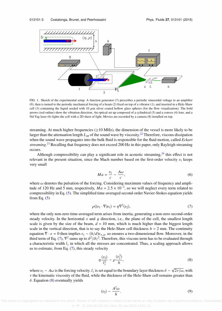
FIG. 1. Sketch of the experimental setup. A function generator (7) prescribes a periodic sinusoidal voltage to an amplifier(9), then is turned to the periodic mechanical forcing of a beam (2) fixed on top of a vibrator (1), and inserted in a Hele-Shawcell (3) containing the liquid seeded with 10 µm silver coated hollow glass spheres (for the flow visualization). The boldarrows (red online) show the vibration direction. An optical set up composed of a cylindrical (5) and a convex (4) lens, and aNd:Yag laser (6) lights the cell with a 2D sheet of light. Movies are recorded by a camera (8) installed on top.
streaming. At much higher frequencies (≥10 MHz), the dimension of the vessel is more likely to belarger than the attenuation length Latt of the sound wave by viscosity.22 Therefore, viscous dissipationwhen the sound wave propagates into the bulk fluid is responsible for the fluid motion, called Eckartstreaming.23 Recalling that frequency does not exceed 200 Hz in this paper, only Rayleigh streamingoccurs.
Although compressibility can play a significant role in acoustic streaming,24 this effect is notrelevant in the present situation, since the Mach number based on the first-order velocity v1 keepsvery small
Ma =v1
c∼ Aω
c, (6)
where ω denotes the pulsation of the forcing. Considering maximum values of frequency and ampli-tude of 120 Hz and 5 mm, respectively, Ma = 2.5 × 10⁻³, so we will neglect every term related tocompressibility in Eq. (5). The simplified time-averaged second-order Navier-Stokes equation yieldsfrom Eq. (5)
ρ⟨(v1 · ∇)v1⟩ = η∇2⟨v2⟩, (7)
where the only non-zero time-averaged term arises from inertia, generating a non-zero second-ordersteady velocity. In the horizontal x and y direction, i.e., the plane of the cell, the smallest lengthscale is given by the size of the beam, d = 10 mm, which is much higher than the biggest lengthscale in the vertical direction, that is to say the Hele-Shaw cell thickness h = 2 mm. The continuityequation ∇ · v = 0 then implies vz ∼ (h/d)vx, y, so ensures a two-dimensional flow. Moreover, in thethird term of Eq. (7), ∇2 sums up to ∂2/∂z2. Therefore, this viscous term has to be evaluated througha characteristic width lz in which all the stresses are concentrated. Thus, a scaling approach allowsus to estimate, from Eq. (7), this steady velocity
η⟨v2⟩l2z
∼ ρ⟨v2
1⟩h
, (8)
where v1 ∼ Aω is the forcing velocity. lz is set equal to the boundary layer thickness δ ∼√
2ν/ω, withν the kinematic viscosity of the fluid, while the thickness of the Hele-Shaw cell remains greater thanδ. Equation (8) eventually yields
⟨v2⟩ ∼ A2ω
h. (9)
This article is copyrighted as indicated in the article. Reuse of AIP content is subject to the terms at: http://scitation.aip.org/termsconditions. Downloaded
to IP: 81.194.30.218 On: Mon, 05 Jan 2015 14:01:10
013101-4 Costalonga, Brunet, and Peerhossaini Phys. Fluids 27, 013101 (2015)
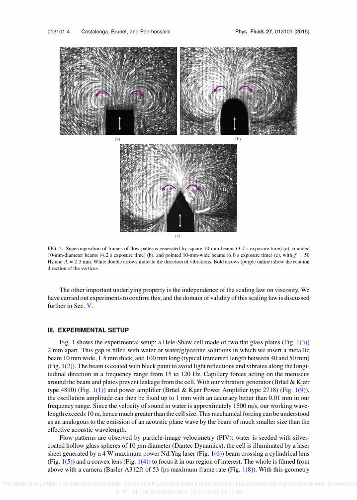
FIG. 2. Superimposition of frames of flow patterns generated by square 10-mm beams (3.7 s exposure time) (a), rounded10-mm-diameter beams (4.2 s exposure time) (b), and pointed 10-mm-wide beams (6.0 s exposure time) (c), with f = 50Hz and A = 2.3 mm. White double arrows indicate the direction of vibrations. Bold arrows (purple online) show the rotationdirection of the vortices.
The other important underlying property is the independence of the scaling law on viscosity. Wehave carried out experiments to confirm this, and the domain of validity of this scaling law is discussedfurther in Sec. V.
III. EXPERIMENTAL SETUP
Fig. 1 shows the experimental setup: a Hele-Shaw cell made of two flat glass plates (Fig. 1(3))2 mm apart. This gap is filled with water or water/glycerine solutions in which we insert a metallicbeam 10 mm wide, 1.5 mm thick, and 100 mm long (typical immersed length between 40 and 50 mm)(Fig. 1(2)). The beam is coated with black paint to avoid light reflections and vibrates along the longi-tudinal direction in a frequency range from 15 to 120 Hz. Capillary forces acting on the meniscusaround the beam and plates prevent leakage from the cell. With our vibration generator (Brüel & Kjærtype 4810) (Fig. 1(1)) and power amplifier (Brüel & Kjær Power Amplifier type 2718) (Fig. 1(9)),the oscillation amplitude can then be fixed up to 1 mm with an accuracy better than 0.01 mm in ourfrequency range. Since the velocity of sound in water is approximately 1500 m/s, our working wave-length exceeds 10 m, hence much greater than the cell size. This mechanical forcing can be understoodas an analogous to the emission of an acoustic plane wave by the beam of much smaller size than theeffective acoustic wavelength.
Flow patterns are observed by particle-image velocimetry (PIV): water is seeded with silver-coated hollow glass spheres of 10 µm diameter (Dantec Dynamics), the cell is illuminated by a lasersheet generated by a 4 W maximum power Nd:Yag laser (Fig. 1(6)) beam crossing a cylindrical lens(Fig. 1(5)) and a convex lens (Fig. 1(4)) to focus it in our region of interest. The whole is filmed fromabove with a camera (Basler A312f) of 53 fps maximum frame rate (Fig. 1(8)). With this geometry
This article is copyrighted as indicated in the article. Reuse of AIP content is subject to the terms at: http://scitation.aip.org/termsconditions. Downloaded
to IP: 81.194.30.218 On: Mon, 05 Jan 2015 14:01:10
013101-5 Costalonga, Brunet, and Peerhossaini Phys. Fluids 27, 013101 (2015)
and the direction of vibration of the metallic beam, two regions are of interest in this experimentalframework: a shear region on both sides of the beam and a compression region in front of it, so flowsshould arise from a combination of these sources.
IV. RESULTS
A. Flow patterns
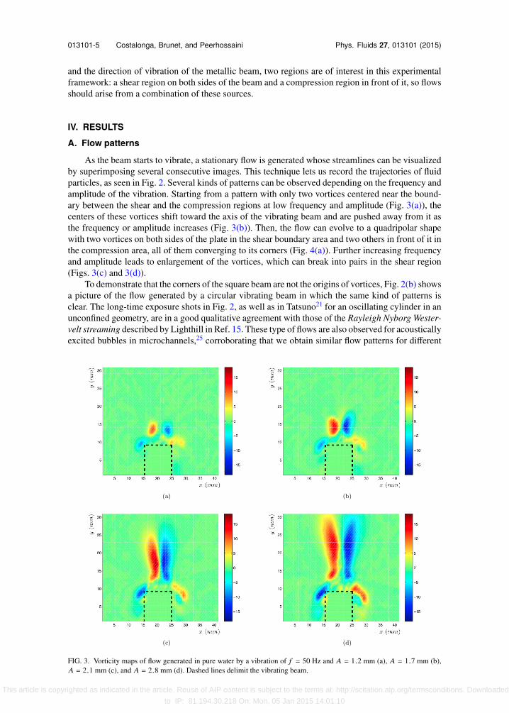
As the beam starts to vibrate, a stationary flow is generated whose streamlines can be visualizedby superimposing several consecutive images. This technique lets us record the trajectories of fluidparticles, as seen in Fig. 2. Several kinds of patterns can be observed depending on the frequency andamplitude of the vibration. Starting from a pattern with only two vortices centered near the bound-ary between the shear and the compression regions at low frequency and amplitude (Fig. 3(a)), thecenters of these vortices shift toward the axis of the vibrating beam and are pushed away from it asthe frequency or amplitude increases (Fig. 3(b)). Then, the flow can evolve to a quadripolar shapewith two vortices on both sides of the plate in the shear boundary area and two others in front of it inthe compression area, all of them converging to its corners (Fig. 4(a)). Further increasing frequencyand amplitude leads to enlargement of the vortices, which can break into pairs in the shear region(Figs. 3(c) and 3(d)).
To demonstrate that the corners of the square beam are not the origins of vortices, Fig. 2(b) showsa picture of the flow generated by a circular vibrating beam in which the same kind of patterns isclear. The long-time exposure shots in Fig. 2, as well as in Tatsuno21 for an oscillating cylinder in anunconfined geometry, are in a good qualitative agreement with those of the Rayleigh Nyborg Wester-velt streaming described by Lighthill in Ref. 15. These type of flows are also observed for acousticallyexcited bubbles in microchannels,25 corroborating that we obtain similar flow patterns for different
FIG. 3. Vorticity maps of flow generated in pure water by a vibration of f = 50 Hz and A = 1.2 mm (a), A = 1.7 mm (b),A = 2.1 mm (c), and A = 2.8 mm (d). Dashed lines delimit the vibrating beam.
This article is copyrighted as indicated in the article. Reuse of AIP content is subject to the terms at: http://scitation.aip.org/termsconditions. Downloaded
to IP: 81.194.30.218 On: Mon, 05 Jan 2015 14:01:10
013101-6 Costalonga, Brunet, and Peerhossaini Phys. Fluids 27, 013101 (2015)
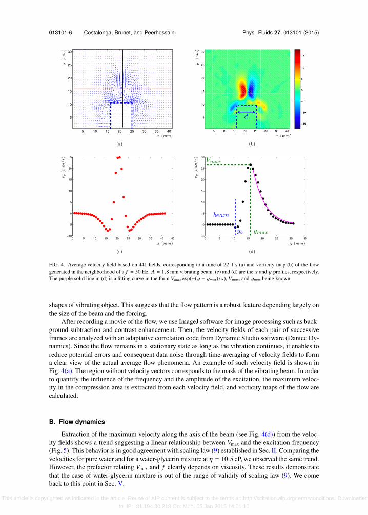
FIG. 4. Average velocity field based on 441 fields, corresponding to a time of 22.1 s (a) and vorticity map (b) of the flowgenerated in the neighborhood of a f = 50 Hz, A = 1.8 mm vibrating beam. (c) and (d) are the x and y profiles, respectively.The purple solid line in (d) is a fitting curve in the form Vmax exp(−(y − ymax)/s), Vmax, and ymax being known.
shapes of vibrating object. This suggests that the flow pattern is a robust feature depending largely onthe size of the beam and the forcing.
After recording a movie of the flow, we use ImageJ software for image processing such as back-ground subtraction and contrast enhancement. Then, the velocity fields of each pair of successiveframes are analyzed with an adaptative correlation code from Dynamic Studio software (Dantec Dy-namics). Since the flow remains in a stationary state as long as the vibration continues, it enables toreduce potential errors and consequent data noise through time-averaging of velocity fields to forma clear view of the actual average flow phenomena. An example of such velocity field is shown inFig. 4(a). The region without velocity vectors corresponds to the mask of the vibrating beam. In orderto quantify the influence of the frequency and the amplitude of the excitation, the maximum veloc-ity in the compression area is extracted from each velocity field, and vorticity maps of the flow arecalculated.
B. Flow dynamics
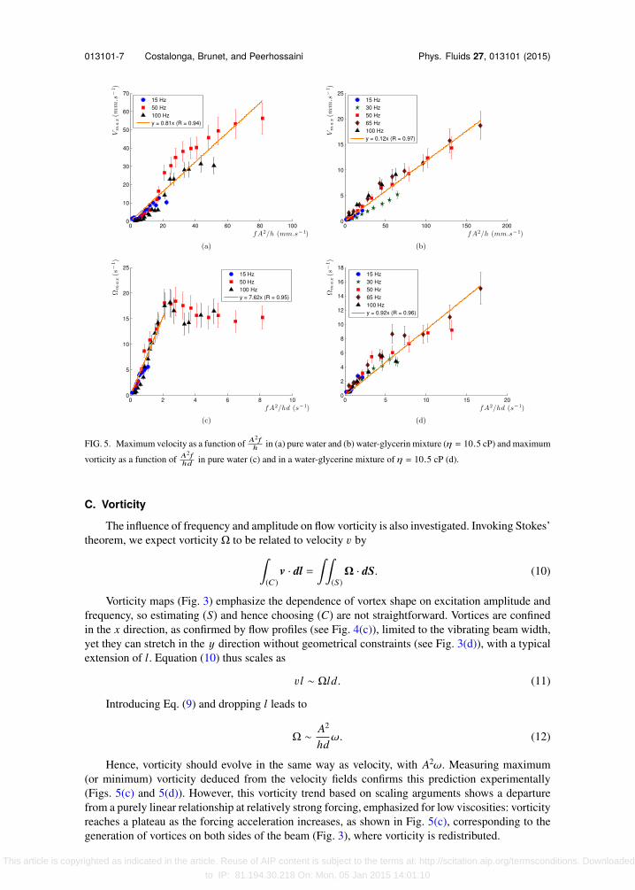
Extraction of the maximum velocity along the axis of the beam (see Fig. 4(d)) from the veloc-ity fields shows a trend suggesting a linear relationship between Vmax and the excitation frequency(Fig. 5). This behavior is in good agreement with scaling law (9) established in Sec. II. Comparing thevelocities for pure water and for a water-glycerin mixture at η = 10.5 cP, we observed the same trend.However, the prefactor relating Vmax and f clearly depends on viscosity. These results demonstratethat the case of water-glycerin mixture is out of the range of validity of scaling law (9). We comeback to this point in Sec. V.
This article is copyrighted as indicated in the article. Reuse of AIP content is subject to the terms at: http://scitation.aip.org/termsconditions. Downloaded
to IP: 81.194.30.218 On: Mon, 05 Jan 2015 14:01:10
013101-7 Costalonga, Brunet, and Peerhossaini Phys. Fluids 27, 013101 (2015)
FIG. 5. Maximum velocity as a function of A2 fh in (a) pure water and (b) water-glycerin mixture (η = 10.5 cP) and maximum
vorticity as a function of A2 fhd in pure water (c) and in a water-glycerine mixture of η = 10.5 cP (d).
C. Vorticity
The influence of frequency and amplitude on flow vorticity is also investigated. Invoking Stokes’theorem, we expect vorticity Ω to be related to velocity v by
(C)v · dl =
(S)Ω · dS. (10)
Vorticity maps (Fig. 3) emphasize the dependence of vortex shape on excitation amplitude andfrequency, so estimating (S) and hence choosing (C) are not straightforward. Vortices are confinedin the x direction, as confirmed by flow profiles (see Fig. 4(c)), limited to the vibrating beam width,yet they can stretch in the y direction without geometrical constraints (see Fig. 3(d)), with a typicalextension of l. Equation (10) thus scales as
v l ∼ Ωld. (11)
Introducing Eq. (9) and dropping l leads to
Ω ∼ A2
hdω. (12)
Hence, vorticity should evolve in the same way as velocity, with A2ω. Measuring maximum(or minimum) vorticity deduced from the velocity fields confirms this prediction experimentally(Figs. 5(c) and 5(d)). However, this vorticity trend based on scaling arguments shows a departurefrom a purely linear relationship at relatively strong forcing, emphasized for low viscosities: vorticityreaches a plateau as the forcing acceleration increases, as shown in Fig. 5(c), corresponding to thegeneration of vortices on both sides of the beam (Fig. 3), where vorticity is redistributed.
This article is copyrighted as indicated in the article. Reuse of AIP content is subject to the terms at: http://scitation.aip.org/termsconditions. Downloaded
to IP: 81.194.30.218 On: Mon, 05 Jan 2015 14:01:10
013101-8 Costalonga, Brunet, and Peerhossaini Phys. Fluids 27, 013101 (2015)
V. DISCUSSION
The scaling laws for both velocity and vorticity come out of a balance between inertia—generatinga steady flow from the periodic forcing—and viscous dissipation confined in the boundary layeraround the vibrating beam. This reasoning leads to independence on viscosity, which remains relevantonly if h ≪ δ. Since δ ∼
√ν/ω, a departure from this scaling may occur at low frequencies (see
Fig. 5(b)). To illustrate this behavior qualitatively, let us look at Fig. 6, corresponding to experimentsperformed with a water/glycerin mixture of η = 108.2 cP.
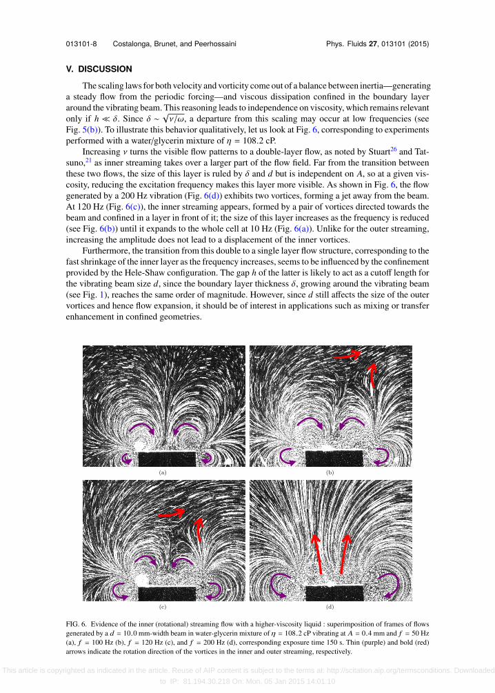
Increasing ν turns the visible flow patterns to a double-layer flow, as noted by Stuart26 and Tat-suno,21 as inner streaming takes over a larger part of the flow field. Far from the transition betweenthese two flows, the size of this layer is ruled by δ and d but is independent on A, so at a given vis-cosity, reducing the excitation frequency makes this layer more visible. As shown in Fig. 6, the flowgenerated by a 200 Hz vibration (Fig. 6(d)) exhibits two vortices, forming a jet away from the beam.At 120 Hz (Fig. 6(c)), the inner streaming appears, formed by a pair of vortices directed towards thebeam and confined in a layer in front of it; the size of this layer increases as the frequency is reduced(see Fig. 6(b)) until it expands to the whole cell at 10 Hz (Fig. 6(a)). Unlike for the outer streaming,increasing the amplitude does not lead to a displacement of the inner vortices.
Furthermore, the transition from this double to a single layer flow structure, corresponding to thefast shrinkage of the inner layer as the frequency increases, seems to be influenced by the confinementprovided by the Hele-Shaw configuration. The gap h of the latter is likely to act as a cutoff length forthe vibrating beam size d, since the boundary layer thickness δ, growing around the vibrating beam(see Fig. 1), reaches the same order of magnitude. However, since d still affects the size of the outervortices and hence flow expansion, it should be of interest in applications such as mixing or transferenhancement in confined geometries.
FIG. 6. Evidence of the inner (rotational) streaming flow with a higher-viscosity liquid : superimposition of frames of flowsgenerated by a d = 10.0 mm-width beam in water-glycerin mixture of η = 108.2 cP vibrating at A = 0.4 mm and f = 50 Hz(a), f = 100 Hz (b), f = 120 Hz (c), and f = 200 Hz (d), corresponding exposure time 150 s. Thin (purple) and bold (red)arrows indicate the rotation direction of the vortices in the inner and outer streaming, respectively.
This article is copyrighted as indicated in the article. Reuse of AIP content is subject to the terms at: http://scitation.aip.org/termsconditions. Downloaded
to IP: 81.194.30.218 On: Mon, 05 Jan 2015 14:01:10
013101-9 Costalonga, Brunet, and Peerhossaini Phys. Fluids 27, 013101 (2015)
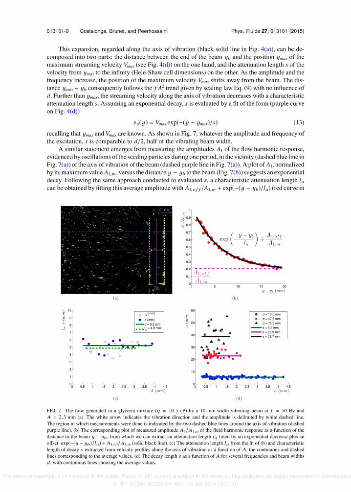
This expansion, regarded along the axis of vibration (black solid line in Fig. 4(a)), can be de-composed into two parts: the distance between the end of the beam yb and the position ymax of themaximum streaming velocity Vmax (see Fig. 4(d)) on the one hand, and the attenuation length s of thevelocity from ymax to the infinity (Hele-Shaw cell dimensions) on the other. As the amplitude and thefrequency increase, the position of the maximum velocity Vmax shifts away from the beam. The dis-tance ymax − yb consequently follows the f A2 trend given by scaling law Eq. (9) with no influence ofd. Further than ymax, the streaming velocity along the axis of vibration decreases with a characteristicattenuation length s. Assuming an exponential decay, s is evaluated by a fit of the form (purple curveon Fig. 4(d))
vy(y) = Vmax exp(−(y − ymax)/s) (13)
recalling that ymax and Vmax are known. As shown in Fig. 7, whatever the amplitude and frequency ofthe excitation, s is comparable to d/2, half of the vibrating beam width.
A similar statement emerges from measuring the amplitudes A1 of the flow harmonic response,evidenced by oscillations of the seeding particles during one period, in the vicinity (dashed blue line inFig. 7(a)) of the axis of vibration of the beam (dashed purple line in Fig. 7(a)). A plot of A1, normalizedby its maximum value A1,m, versus the distance y − yb to the beam (Fig. 7(b)) suggests an exponentialdecay. Following the same approach conducted to evaluated s, a characteristic attenuation length lacan be obtained by fitting this average amplitude with A1,o f f /A1,m + exp(−(y − yb)/la) (red curve in
FIG. 7. The flow generated in a glycerin mixture (η = 10.5 cP) by a 10 mm-width vibrating beam at f = 50 Hz andA = 2.3 mm (a). The white arrow indicates the vibration direction and the amplitude is delimited by white dashed line.The region in which measurements were done is indicated by the two dashed blue lines around the axis of vibration (dashedpurple line). (b) The corresponding plot of measured amplitude A1/A1,m of the fluid harmonic response as a function of thedistance to the beam y − yb, from which we can extract an attenuation length la fitted by an exponential decrease plus anoffset: exp(−(y − yb)/la) + A1,off/A1,m (solid black line). (c) The attenuation length la from the fit of (b) and characteristiclength of decay s extracted from velocity profiles along the axis of vibration as a function of A, the continuous and dashedlines corresponding to the average values. (d) The decay length s as a function of A for several frequencies and beam widthsd, with continuous lines showing the average values.
This article is copyrighted as indicated in the article. Reuse of AIP content is subject to the terms at: http://scitation.aip.org/termsconditions. Downloaded
to IP: 81.194.30.218 On: Mon, 05 Jan 2015 14:01:10
013101-10 Costalonga, Brunet, and Peerhossaini Phys. Fluids 27, 013101 (2015)
Fig. 7(b)), where A1,m is the maximal amplitude measured and A1,off a fitting parameter correspondingto an offset on A1. As for the slope s emanating from the velocity y-profile (Fig. 4(d)), the evaluationof la always returns a length close to d/2, whatever amplitude or frequency of the excitation withinour working range. In summary, the characteristic length of the decrease s of the second-order flowobtained from Fig. 4(d) is comparable to that extracted from the first-order oscillations of the flowin Fig. 7(b). Since this feature is not noticed in extended geometries, it could be attributed to thetwo-dimensional confinement of our geometry.
VI. CONCLUSION
Our study presents quantitative measurements on streaming flows forced by mechanical vibra-tions within a two-dimensionally confined geometry. We found behaviors which are analogous toacoustically forced streaming flows, because the vibrating object can be considered as a diffuser of anacoustic plane wave of wavelength much larger than the size of the vessel. This is typically the case inultrasonic wave-forced flows in microfluidics geometries. The results of our PIV measurements yieldsimple scaling laws for the maximal velocity and vorticity and show the limitations of these laws,especially in capturing the influence of viscosity and vibrating object size. The scaling law is validtypically when the size of the boundary layer is less than other characteristic length of the problem,primarily the thickness of the liquid gap. Therefore, the prescribed geometrical confinement must betaken into account in the flow structure and spatial reach.
Ongoing work concerns viscous and size effects as well as flow dynamics of the inner streaming.The authors are currently working to reduce the scale of their experiments in order to study that kindof streaming at microscale, particularly its efficiency in mixing.
ACKNOWLEDGMENTS
The authors are grateful to Julien Seznec, Laurent Réa, and Matthieu Receveur for their technicalsupport. We would like to thank Michael Baudoin and Professor Henrik Bruus for fruitful discussions.
1 M. Faraday, “On a peculiar class of acoustical figures; and on certain forms assumed by groups of particles upon vibratingelastic surfaces,” Philos. Trans. R. Soc. London 121, 299–340 (1831).
2 N. Riley, “Steady streaming,” Ann. Rev. Fluid Mech. 33, 43–65 (2001).3 C. Suri, K. Takenaka, H. Yanagida, Y. Kojima, and K. Koyama, “Chaotic mixing generated by acoustic streaming,” Ultra-
sonics 40(1–8), 393–396 (2002).4 Y. Choe and E. S. Kim, “Valveless micropump driven by acoustic streaming,” J. Micromech. Microeng. 23(4), 045005
(2013).5 N. P. Dhanalakshmi, R. Nagarajan, N. Sivagaminathan, and B. V. S. S. S. Prasad, “Acoustic enhancement of heat transfer
in furnace tubes,” Chem. Eng. Process. 59(0), 36–42 (2012).6 G. Destgeer, K. H. Lee, J. H. Jung, A. Alazzam, and H. J. Sung, “Continuous separation of particles in a pdms microfluidic
channel via travelling surface acoustic waves (tsaw),” Lab Chip 13, 4210–4216 (2013).7 H. Kumar, M. H. Tawhai, E. A. Hoffman, and C.-L. Lin, “Steady streaming: A key mixing mechanism in low-Reynolds-
number acinar flows,” Phys. Fluids 23(4), 041902 (2011).8 J. Friend and L. Y. Yeo, “Microscale acoustofluidics: Microfluidics driven via acoustics and ultrasonics,” Rev. Mod. Phys.
83(2), 647–704 (2011).9 X. Ding, P. Li, Sz-Chin Steven Lin, Z. S. Stratton, N. Nama, F. Guo, D. Slotcavage, X. Mao, J. Shi, F. Costanzo, and T. J.
Huang, “Surface acoustic wave microfluidics,” Lab Chip 13, 3626–3649 (2013).10 M. Tatsuno and P. W. Bearman, “A visual study of the flow around an oscillating circular cylinder at low Keulegan Carpenter
numbers and low Stokes numbers,” J. Fluid Mech. 211(2), 157–182 (1990).11 H. Dutsch, F. Durst, S. Becker, and H. Lienhart, “Low-Reynolds-number flow around an oscillating circular cylinder at low
Keulegan Carpenter numbers,” J. Fluid Mech. 360(4), 249–271 (1998).12 J. R. Elston, H. M. Blackburn, and J. Sheridan, “The primary and secondary instabilities of flow generated by an oscillating
circular cylinder,” J. Fluid Mech. 550(3), 359–389 (2006).13 C. P. Lee and T. G. Wang, “Outer acoustic streaming,” J. Acoust. Soc. Am. 88(5), 2367–2375 (1990).14 H. An, L. Cheng, and M. Zhao, “Direct numerical simulation of oscillatory flow around a circular cylinder at low
Keulegan–Carpenter number,” J. Fluid Mech. 666(1), 77–103 (2011).15 J. Lighthill, “Acoustic streaming,” J. Sound Vib. 61(3), 391–418 (1978).16 H. Bruus, Theoretical Microfluidics (Oxford University Press, 2008).17 S. S. Sadhal, “Acoustofluidics 13: Analysis of acoustic streaming by perturbation methods,” Lab Chip 12(13), 2292–2300
(2012).18 S. Boluriaan and P. Morris, “Acoustic streaming: From Rayleigh to today,” Int. J. Aeroacoustics 2(3), 255–292 (2003).
This article is copyrighted as indicated in the article. Reuse of AIP content is subject to the terms at: http://scitation.aip.org/termsconditions. Downloaded
to IP: 81.194.30.218 On: Mon, 05 Jan 2015 14:01:10
013101-11 Costalonga, Brunet, and Peerhossaini Phys. Fluids 27, 013101 (2015)
19 L. Rayleigh, “On the circulation of air observed in Kundt’s tube, and on some allied acoustical problems,” Philos. Trans. R.Soc. London 1776-1886 175, 1–21 (1884).
20 H. Schlichting, “Calculation of even periodic barrier currents,” Phys. Z. 33, 327–335 (1932).21 M. Tatsuno, “Circulatory streaming around an oscillating circular cylinder at low Reynolds numbers,” J. Phys. Soc. Jpn.
35(3), 915–920 (1973).22 M. F. Hamilton and D. T. Blackstock, Nonlinear Acoustics (Academic Press, 1998).23 C. Eckart, “Vortices and streams caused by sound waves,” Phys. Rev. 73(1), 68–76 (1948).24 Q. Qi, “The effect of compressibility on acoustic streaming near a rigid boundary for a plane traveling wave,” J. Acoust.
Soc. Am. 94(2), 1090–1098 (1993).25 C. Wang, B. Rallabandi, and S. Hilgenfeldt, “Frequency dependence and frequency control of microbubble streaming flows,”
Phys. Fluids 25(2), 022002 (2013).26 J. T. Stuart, “Double boundary layers in oscillatory viscous flow,” J. Fluid Mech. 24(4), 673–687 (1966).
This article is copyrighted as indicated in the article. Reuse of AIP content is subject to the terms at: http://scitation.aip.org/termsconditions. Downloaded
to IP: 81.194.30.218 On: Mon, 05 Jan 2015 14:01:10