Embed Size (px)
Citation preview
FACULDADE DE ENGENHARIA DA UNIVERSIDADE DO PORTO
Lymphatic Filariasis Detection in
microscopic images
Rui Pedro Menezes da Rosa Neves
Mestrado Integrado em Engenharia Informática e Computação
Supervisor at FEUP: António Miguel Pontes Pimenta Monteiro (PhD)
Supervisor at Fraunhofer: Fábio Filipe Costa Pinho (MSc)
June, 2016

© Rui Pedro Menezes da Rosa Neves, 2016
Lymphatic Filariasis Detection
Rui Pedro Menezes da Rosa Neves
Mestrado Integrado em Engenharia Informática e Computação
June, 2016

Summary
In Africa, the propagation of parasites like the lymphatic filariasis is complicating
seriously the efforts of health professionals to cure certain diseases. Although there are
medicines capable to treat the lymphatic filariasis, the condition needs to be discovered first,
which is not always an easy task having into account that in most countries affected by this
disease it can only be detected at night (nocturne). The lymphatic filariasis is, a parasitical
infection which can originate changes or ruptures in the lymphatic system as well as an
abnormal growth of certain areas of the body causing pain, incapacity and social stigma.
Approximately 1.23 billion people in 58 countries from all over the world are threatened
by this disease which requires a preventive treatment to stop its propagation which makes it
even more important for the existence of a mechanism that is less costly and more agile in the
analysis of a blood smear to verify the existence of microfilariae (little worms that are produced
by other adult worms while housed in the lymphatic system).
The lymphatic filariasis is caused by an infection with nematodes (“roundworms”) of the
Filariodidea family in which three types are inserted: Wuchereria bancrofti, responsible for 90%
of all cases; Brugia malayi, responsible for almost every remaining; B.timori also causing the
disease. All three have characteristics that can differentiate them and which allow them to be
identified.
The current identification process of the disease consists on the analysis of microfilariae in
a blood smear with a blood sample through a microscope and its identification by the observer.
Taking this into account, it is intended to develop image analysis and processing
techniques for the recognition and counting of the two principal types of filarial worms from a
thick blood smear. Also the use of a smartphone and a portable microscope makes the detection
possible without the need of a health professional and consequently can automate the process.
To make this possible an adapter smartphone-microscope can be used to obtain an image with
the magnification of 1000x. The images can then be analyzed in a server or in the smartphone, if
it has enough processing power for it. It is expected from this process that the need to resort to
labs to process the blood smear gets unnecessary making the process more accessible and agile
instead of costly and slow.
For the detection of the parasites from the acquired images it is intended to implement,
experiment and choose the more adequate operations. These comprise pre-processing operations
with the goal to enhance the acquired images and eliminate possible artifacts coming from the
acquisition system. However, the main operations should be those that allow the verification of
existence or nonexistence, recognition and classification of the pretended parasites. Processing
and analysis techniques that are common in these processes are based in the extraction of
features (e.g. SIRF, SURF, and FLANN) template similarity, edge detection and description of
contours and recognition of statistical patterns.
Once detected and recognized one or more parasites and its types, a rule should be defined
and used to declare the presence of the disease and its type.

Resumo
Em África, a propagação de parasitas como a filaríase linfática está a dificultar seriamente
os esforços dos profissionais de saúde para curar determinadas doenças. Apesar de existirem
medicamentos capazes de tratar a filaríase linfática, esta precisa primeiro, de ser detetada, o que
nem sempre é uma tarefa simples tendo em conta que na maioria dos países afetados por esta
doença, esta apenas pode ser detetada de noite (noturna). A filaríase linfática é, uma infeção
parasitária que pode gerar alterações ou ruturas no sistema linfático assim como um crescimento
anormal de certas regiões do corpo causando dor, incapacidade e estigma social.
Aproximadamente 1.23 biliões de pessoas em 58 países de todo o mundo são ameaçados
por esta doença que requer um tratamento preventivo para parar a sua propagação, o que torna
ainda mais importante, a existência de um mecanismo que seja mais acessível e mais ágil na
análise de uma amostra de sangue para verificar a existência de microfilárias (pequenos vermes
que são produzidos por outros vermes adultos enquanto alojados no sistema linfático).
A filaríase linfática é causada por uma infeção por nemátodos (vermes redondos) da
família Filariodidea, na qual, se inserem os três tipos: Wuchereria bancrofti, responsável por
90% de todos os casos; Brugia malayi, responsável por quase todos os restantes; B.timori
também causadora da doença. Todas as três têm características que permite diferenciá-las e
consequentemente identificá-las.
O método de deteção da doença atual, consiste na análise de microfilárias numa amostra de
sangue através de um microscópio e a sua identificação por um observador com as qualificações
necessárias.
Tendo isto em conta, é pretendido o desenvolvimento de técnicas de análise e
processamento de imagem para o reconhecimento e contagem dos dois principais tipos de
filárias a partir de uma lamela com uma amostra de sangue. O uso de um smartphone e de um
microscópio portátil também tornam a deteção possível sem a necessidade de um profissional de
saúde e, consequentemente, o processo pode ser automatizado.
Para tornar isto possível, um adaptador smartphone-microscópio pode ser usado para obter
uma imagem com uma magnificação de 1000x. Posteriormente, as imagens poderão ser

analisadas num servidor ou no smartphone, se este tiver capacidade de processamento suficiente
para o propósito. Deste processo, é esperado que a necessidade de recorrer a laboratórios para
processar a amostra de sangue se torne desnecessária, tornado o processo mais acessível e ágil
em vez de custoso e lento.
Para a deteção de parasitas a partir das imagens adquiridas, é pretendida a implementação,
teste e escolha das operações mais adequadas. Estas compreendem operações de pre-
processamento com o objetivo de melhorar as imagens adquiridas e eliminar possíveis artefatos
provenientes do sistema de aquisição. Contudo, as operações principais devem ser aquelas que
permitem a verificação da existência ou não existência, reconhecimento e classificação dos
parasitas pretendidos. Técnicas de análise e processamento que são comuns nestes processos são
baseadas em extração de características (ex. SIRF, SURF, FLANN), semelhança de texturas,
deteção de arestas e descrição de contornos e reconhecimento de padrões estatísticos.
Uma vez detetados e reconhecidos um ou mais parasitas e os seus tipos, uma regra deverá
ser definida e usada para declarar a presença da doença e o seu tipo.

Acknowledgments
I would like to thank Fraunhofer AICOS Portugal for providing a suitable environment and
all the tools necessary to make this work and Universidade do Porto, more directly to Faculdade
de Engenharia, for providing me a good background over the last few years.
Dr. Miguel Pimenta Monteiro, Eng. Fábio Pinho and Eng. Luís Rosado were key elements
in the supervision and guidance of my work so I would like to express my gratitude to them. A
thanks to Maria Vasconcelos, also from Fraunhofer, for being available to supply all the
material needed.
A special thanks to my family, my mom, my dad, my brother and my sister for all the
support during this entire journey because they were always there for me, in the good and the
bad. Also, to Inês, a special thanks for always believing in me and be by my side.
Finally, to all my friends, the ones that have been with me for this entire journey, the real
ones that will remain after it, I would like to express my happiness for having them and being
able to make part of their journey as well and for every laugh, fight and work we had together
because together, we made it here.
Rui Pedro Menezes da Rosa Neves


Attitude is a little thing that makes a big difference
Winston Churchill

Contents
1 Introduction ............................................................................................................. 1
1.1 Context ............................................................................................ 1
1.2 Motivation and Objectives .............................................................. 2
1.3 Dissertation structure....................................................................... 2
2 Lymphatic Filariasis Characterization ................................................................. 1
2.1 Biology, life cycle and transmission ............................................... 1
2.2 Filariasis Physiopathology .............................................................. 3
2.2.1 Asymptomatic stage ........................................................................ 4
2.2.2 Acute stage ...................................................................................... 4
2.2.3 Chronic Stage .................................................................................. 4
2.3 Diagnosis ......................................................................................... 5
2.3.1 Fresh exam technique ...................................................................... 5
2.3.2 Serologic Techniques ...................................................................... 5
2.3.3 Polymerase chain reaction (PCR) ................................................... 5
2.3.4 Imaging Technique .......................................................................... 6
3 Literature Review ................................................................................................... 7
3.1 Introduction ..................................................................................... 7
3.2 Techonology Review....................................................................... 7
3.2.1 Android ........................................................................................... 7
3.2.2 Skylight ........................................................................................... 8
3.2.3 Fraunhofer Microscope Prototype ................................................... 8
3.2.4 OpenCV ........................................................................................... 9
3.2.5 FastCV ........................................................................................... 10
3.3 Related Work ................................................................................ 10
3.3.1 Segmentation of Blood Cells Components ................................... 10 3.3.1.1 Pre-processing 10
3.3.1.2 Image Segmentation 10
3.3.1.3 Feature Detection and Classification 11
3.3.2 Parasite Detection .......................................................................... 12 3.3.2.1 Pre-processing 12
3.3.2.2 Image Segmentation 12
3.3.2.3 Feature Detection and Classification 12
3.4 Image Processing Techniques ....................................................... 13
3.4.1 Image Enhancement ...................................................................... 13
3.4.2 Morphological Image Processing .................................................. 16
3.4.3 Image Segmentation ...................................................................... 19
3.5 Machine Learning ......................................................................... 21
3.5.1 Feature Extraction ......................................................................... 21 3.5.1.1 SIFT (Scale-Invariant Feature Transform) 22
Stage 1: Scale Space Extrema Detection 22
Stage 2: Keypoint Localization 22
Stage 3: Orientation Assignment 23
Stage 4: Keypoint Descriptor 23
3.5.1.2 SURF (Speed UP Robust Features) 24
3.5.1.2.1 Interest Point Detection 24
3.5.1.2.2 Interest Point Description and Matching 25
3.5.2 Classification Methods .................................................................. 26 3.5.2.1 Support Vector Machines (SVMs) 26
3.5.2.2 Bayesian Classifiers 26
3.5.2.3 Decision Tree 27
3.5.2.4 k-Nearest Neighbor (kNN) 27
3.6 Relevant Remarks ......................................................................... 27
4 Lymphatic Filariasis Detection ............................................................................ 29
4.1 The Process Model ........................................................................ 30
4.2 Image Acquisition ......................................................................... 30
4.2.1 Image Dataset Requirements ......................................................... 31
4.2.2 Image Dataset Construction .......................................................... 31
4.3 Pre-Processing ............................................................................... 31
4.3.1 Image Cropping/Resize ................................................................. 32
4.3.2 Color Normalization ...................................................................... 33
4.3.3 Channel Subtraction and Median Filter......................................... 34
4.3.4 Morphological Operation to reduce background ........................... 35
4.4 Segmentation ................................................................................. 39
4.4.1 Adaptive Threshold ....................................................................... 39
4.4.2 Area threshold ............................................................................... 40
4.4.3 Attached Cells Removal ................................................................ 41 4.4.3.1 Pre-Processing 42
4.4.3.2 Segmentation 43
4.5 Filaria Reconstruction ................................................................... 44
4.6 Feature Extraction ......................................................................... 45
4.6.1 Color & Texture Features .............................................................. 46
4.6.2 Geometry Features ........................................................................ 48
4.7 Classification ................................................................................. 51
4.7.1 Classification Methods .................................................................. 51
4.7.2 Classification Results .................................................................... 52 4.7.2.1 k-Fold Cross Validation 54
5 Image Processing in Android ............................................................................... 56
5.1 Integration with MalariaScope Project .......................................... 56
5.2 Application Overview ................................................................... 57
5.3 Image Processing Integration ........................................................ 59
6 Results .................................................................................................................... 61
6.1 Results & Discussion .................................................................... 61
7 Conclusions and Future Work ............................................................................. 68
8 References .............................................................................................................. 69

xix
List of Figures
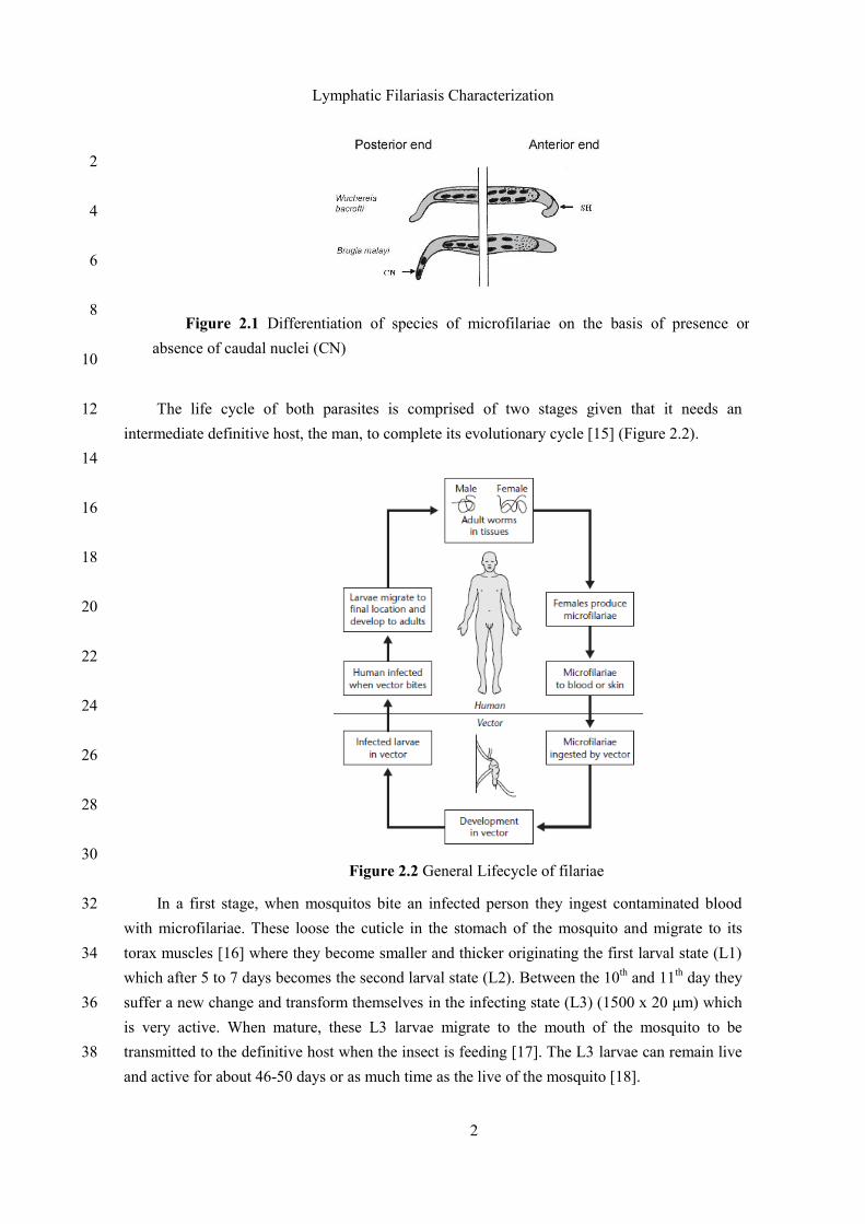
Figure 2.1 Differentiation of species of microfilariae on the basis of presence or
absence of caudal nuclei (CN) 2
Figure 2.2 General Lifecycle of filariae 2
Figure 2.3 Chronicle clinical manifestations of bancroftian lymphatic filariasis. A –
Inferior left member with lymphedema. B – Locker signal (arrows), normally
observed after digital compression in the affected member with lymphedema. C
– Elephantiasis 4
Figure 3.1 Skylight adaptor on the left. Skylight on microscope with mobile device
ready to take pictures. 8
Figure 3.2 Fraunhofer MalariaScope Microscope Prototype 9
Figure 3.3 Example of a microscopic image containing the parasite 9
Figure 3.4 Negative of an image 14
Figure 3.5 Thresholding method 14
Figure 3.6 Piecewise linear transformation 15
Figure 3.7 Histogram Equalization and results 15
Figure 3.8 Comparison between Gaussian and Median filters 16
Figure 3.9 Closing operation 19
Figure 3.10 Opening Operation 19
Figure 3.11 Edge Detection 20
Figure 3.12 Keypoint Descriptor 23
Figure 3.13 Box filters 25
Figure 3.14 Matching 26
Figure 4.1 Different stages of the methodology 30
Figure 4.2 Original image on the left. Segmented optical circle in the middle. After
cropping with diameter size on the right. Parasite of type Wuchereria bancrofti 32
Figure 4.3 Original image on the left. Segmented optical circle in the middle. After
cropping with diameter size on the right. Parasite of type Brugia malayi 33
Figure 4.4 Original image on the left. Negative of the original image in the middle.
Result of color normalization applied to the negative image and after cropping
on the right. Parasite of type Wuchereria bancrofti 34
xx
Figure 4.5 Original image on the left. Negative of the original image in the middle.
Result of color normalization applied to the negative image and after cropping
on the right. Parasite of type Brugia malayi 34
Figure 4.6 Images from both samples after channel subtraction and median filter.
Parasite of type Wuchereria bancrofti on the left and Brugia malayi on the right 35
Figure 4.7 Grayscale image with median filter applied on the left and resultant image
after morphological operation on the right. Background attached to filaria is
removed. Type: Wuchereria bancrofti 37
Figure 4.8 Grayscale image with median filter applied on the left and resultant image
after morphological operation on the right. Sample with low background. noise
Type: Brugia malayi 37
Figure 4.9 Image after morphological operation on the left. Results of pixel threshold
by 32 on the right. Type: Wuchereria bancrofti 38
Figure 4.10 Image after morphological operation on the left. Results of pixel threshold
by 32 on the right. Type: Brugia malayi 38
Figure 4.11 Result of Adaptive Threshold on both samples. Type: Wuchereria
bancrofti on the left and Brugia malayi on the right 40
Figure 4.12 Result of Area Threshold on both samples. Cells are removed. 41
Figure 4.13 Original cropped image on the left. Result of color normalization in the
cropped image in the middle. Grayscale conversion of the normalized image and
adittion of the result of the morphological operation. Type: Wuchereria bancrofti 42
Figure 4.14 Original cropped image on the left. Result of color normalization in the
cropped image in the middle. Grayscale conversion of the normalized image and
adittion of the result of the morphological operation. Type: Brugia malayi 42
Figure 4.15 Adaptive Threshold of the added image on the pre-processing. Type:
Wuchereria bancrofti on the right and Brugia malayi on the left 43
Figure 4.16 Cells that obey to the restrictions on the left and subtraction from the
result of area threshold image. Type: Wuchereria bancrofti 44
Figure 4.17 Broken filaria on the left after area threshold on the left. Final Result after
filaria reconstruction and removal of any extra body that may have reached this
phase on the right. Type: Brugia malayi 45
Figure 4.18 Support program flow to perform train and classification 51
Figure 5.1 a) Patient database, main screen after logo intro. b) Samples screen of 57
Figure 5.2 a) Screen when accessing a sample. b) Adding a view to a sample. c) Image
loaded to the view and ready to be analyzed (in blue) 58
Figure 5.3 a) Hitting the button to process an image, notification saying it will run in
background. b) Status screen of analysis running in background. c) Notification
of when the analysis is finished 58

xxi
Figure 5.4 Final result with the found parasite marked in green and respective
classification below 59
Figure 6.1 Well isolated filaria on the left. Image assigned to the + group on the left
due to some background attached to the filaria. Both filariae from type:
Wuchereria bancrofti 62
Figure 6.2 Image that will be assigned to the ++ group on the left due to having more
than one cell attached to the filaria. Image that will be assigned to the group – on
the right due to a missing piece. Types: Wuchereria bancrofti on the left and
Brugia malayi on the right 62

xxiii
List of Tables
Table 4.1 Results of machine learning algorithms in classification between parasite
and cells, using color, texture and geometry features 53
Table 4.2 Results of machine learning algorithms in classification between both types
of filariae, using color and texture features 53
Table 4.3 Visualization of k-Fold Crossing. Each column represents a group, each row
an iteration. 54
Table 4.4 Results of the classification with the optimized SVM 55
Table 6.1 Results of segmentation phase 63
Table 6.2 Results of final classification between parasite and cell 63
Table 6.3 Results of final classification between the two types of parasites 64
Table 6.4 Results of classification with different machine learning algorithms using
only geometry features 65
Table 6.5 Results of classification with different machine learning algorithms using
only texture features 65
Table 6.6 Results of classification with different machine learning algorithms using
only color features 66
Table 6.7 Results of classification of different machine learning algorithms using all
features (texture, color, geometry) 66

xxv
Symbols and abbreviatures
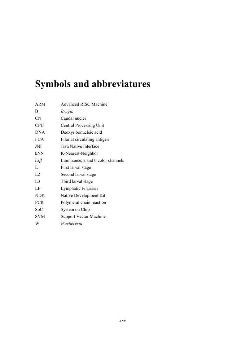
ARM Advanced RISC Machine
B Brugia
CN Caudal nuclei
CPU Central Processing Unit
DNA Deoxyribonucleic acid
FCA Filarial circulating antigen
JNI Java Native Interface
kNN K-Nearest-Neighbor
Luminance, a and b color channels
L1 First larval stage
L2 Second larval stage
L3 Third larval stage
LF Lymphatic Filariasis
NDK Native Development Kit
PCR Polymeral chain reaction
SoC System on Chip
SVM Support Vector Machine
W Wuchereria

xxvi
Chapter 1
Introduction 2
1.1 Context
The lymphatic Filariasis in humans, commonly known as elephantiasis, it’s one of the 4 4
most important tropical diseases identified by the World’s Health Organization along with
onchocerciasis, Chagas disease and leprosy [1]. It is an infectious disease which causes changes 6
in the lymphatic system and deformation of body parts causing pain and incapacity [2] and that
is acquired, normally in childhood, when filarial parasites are transmitted from person to person 8
through mosquito bites.
It is estimated that approximately 120 million people are currently infected in 73 countries 10
across the tropical and subtropical regions of Asia, Africa, Occidental Pacific and part of
Caribbean and South America and 1.23 billion live in areas where the Filariasis is capable of 12
transmission being therefore at risk [3].
The economic costs of this disease are huge, estimated over US$1 billion for year only for 14
India [4]. Besides this economic costs there are also social costs in the measure that this disease
besides causing pain and discomfort it also stigmatizes socially [5]. In fact, it is estimated that 16
40 million infected individuals are seriously incapacitated and disfigured by LF [6] and there
are studies that suggest that depression is prevalent in individuals with LF. 18
It is for this set of factors that the LF is considered a public health problem to eliminate
until 2020 [8]. Pursuing that goal, in 2000 there was launched the Global Program to Eliminate 20
Lymphatic Filariasis (GPELF) which recommends a strategy of chemoprevention that goes
through the massive administration of medicines (MMA) anthelmintic over the populations at 22
risk which implies an investment of at least US$ 154 million per year during the following 5
years [9]. 24
It is, therefore, in this context of massive utilization of medicines where there is no access
to a fast and efficient diagnosis, due to the inexistence of health professionals qualified and 26
Introduction
2
other means that are sophisticated and costly, that comes up the necessity of developing a
cheaper diagnosis system of easy execution and interpretation and practicable in areas of limited 2
access to quality health care.
The use of a mobile-based framework seems to accomplish these requirements once that it 4
comprises both a mobile-phone adaptable cheap microscope and an automatic analysis system.
The latter consists on automatically assessing the cellular blood components of blood smears as 6
well as the number of filarial parasites, which would replace the time-consuming expertise-
dependent standard procedure. 8
1.2 Motivation and Objectives
The main objectives of this project are summed up below: 10
Develop a robust automated image processing methodology capable of finding the
parasites and estimate the number of parasites in low-quality smartphone-acquired 12
thick blood smear images;
Develop a robust image processing methodology to differentiate the two types of 14
microfilariae (Wuchereria bancrofti and Brugia malayi)
Integration of image processing methodologies into mobile devices 16
1.3 Dissertation structure 18
Besides the introduction this thesis contains more six chapters. In chapter 1 we have the
identification and context of the problem, the motivation, and objectives for the solution (the 20
dissertation). In chapter 2 we present the biology of the parasites and describe the actual
techniques used to detect these parasites, followed by a review of image processing techniques 22
and similar projects in chapter 3. In chapter 4 the solution developed is presented. Chapter 5
will address the integration of the image processing methodology developed in Android, 24
presenting the mobile application. Following, in chapter 6, the results will be presented and
consequently, the discussion associated to those results. Finally, in chapter 7, conclusions and 26
future work are presented.
28
Chapter 2
Lymphatic Filariasis Characterization 2
Lymphatic Filariasis is a mosquito-borne disease [10] whose main symptoms are related
with the damage of the lymphatic system both in lymphatic ganglia and lymphatic vessels. 4
Approximately 90% of LF is caused by parasite worms of the type Wuchereria bancrofti, being
the majority of the remaining 10% caused by Brugia malayi [11]. On a general way these 6
worms are known as filariae.
2.1 Biology, life cycle and transmission 8
The filariae Wuchereria bancrofti (Cobbold, 1877) and Brugia malayi (Bucley & Edeson,
1956) are parasite nematodes belonging to the Filarial superfamily. They have as a preferential 10
habitat the tissues and the circulatory and lymphatic systems of the definitive host where they
can live for a period of 8 to 10 years [12]. They are threadlike, white milky colored, opaque, 12
with a smooth cuticle and present sexual dimorphism being the females bigger than males, 80-
100 x 0.25mm and 40 x 0.1 mm, respectively. The adults of both types are very identical in all 14
their characteristics being the females undistinguishable. However, the males from B. malayi
only have around half of the size of the males from W. bancrofti [13]. 16
After mating, millions of eggs, existent in the uterus of female worms hatch and give
origin to larval states, known as microfilariae which present a cuticle and measure in average 18
260-300 x 8 μm and have the somatic cores in a simple line where, in the case of W. bancrofti
don’t reach the caudal end while for the B. malayi the two last cores are separated and the last 20
one, very small, is isolated in the caudal apex [14] (Figure 2.1).
22
24
Lymphatic Filariasis Characterization
2
2
4
6
8
10
The life cycle of both parasites is comprised of two stages given that it needs an 12
intermediate definitive host, the man, to complete its evolutionary cycle [15] (Figure 2.2).
14
16
18
20
22
24
26
28
30
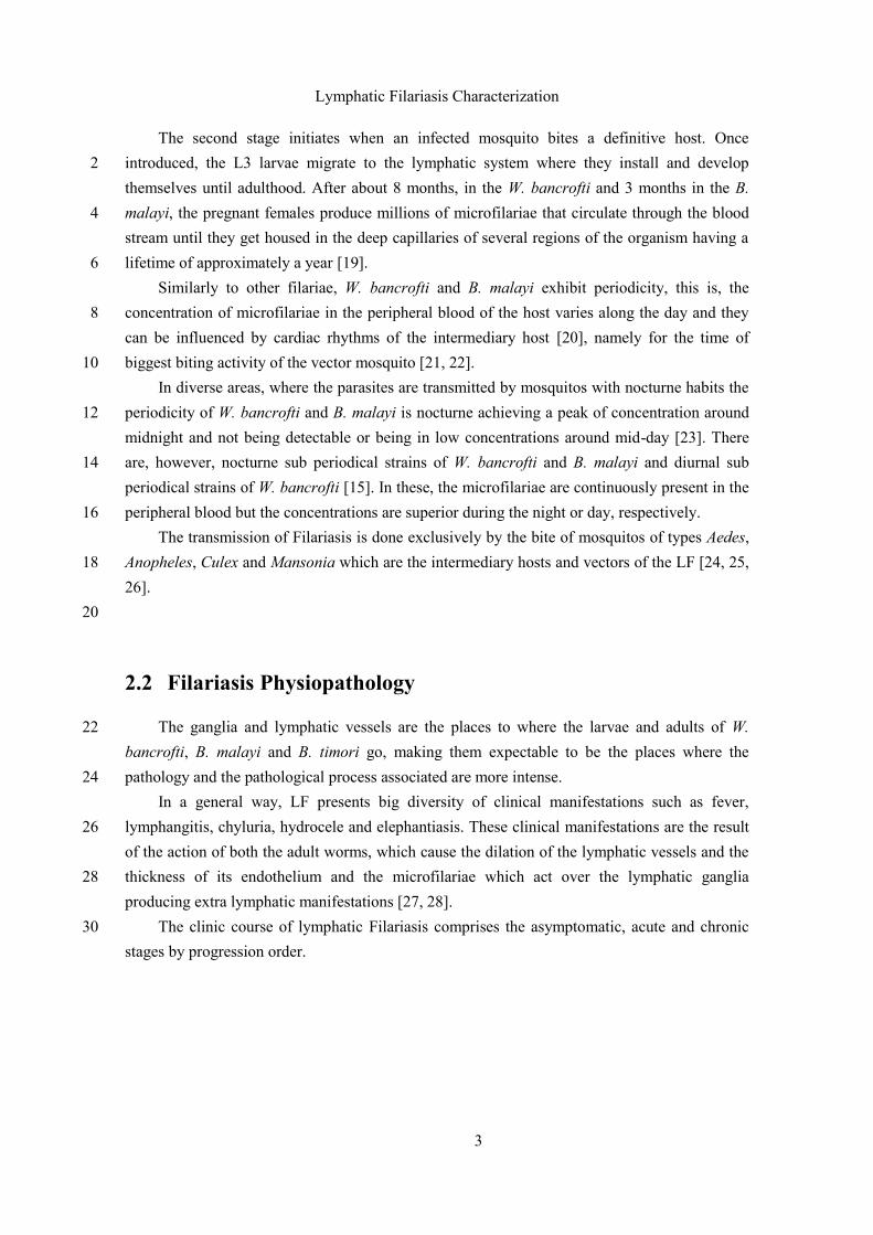
In a first stage, when mosquitos bite an infected person they ingest contaminated blood 32
with microfilariae. These loose the cuticle in the stomach of the mosquito and migrate to its
torax muscles [16] where they become smaller and thicker originating the first larval state (L1) 34
which after 5 to 7 days becomes the second larval state (L2). Between the 10th and 11
th day they
suffer a new change and transform themselves in the infecting state (L3) (1500 x 20 μm) which 36
is very active. When mature, these L3 larvae migrate to the mouth of the mosquito to be
transmitted to the definitive host when the insect is feeding [17]. The L3 larvae can remain live 38
and active for about 46-50 days or as much time as the live of the mosquito [18].
Figure 2.1 Differentiation of species of microfilariae on the basis of presence or
absence of caudal nuclei (CN)
Figure 2.2 General Lifecycle of filariae
Lymphatic Filariasis Characterization
3
The second stage initiates when an infected mosquito bites a definitive host. Once
introduced, the L3 larvae migrate to the lymphatic system where they install and develop 2
themselves until adulthood. After about 8 months, in the W. bancrofti and 3 months in the B.
malayi, the pregnant females produce millions of microfilariae that circulate through the blood 4
stream until they get housed in the deep capillaries of several regions of the organism having a
lifetime of approximately a year [19]. 6
Similarly to other filariae, W. bancrofti and B. malayi exhibit periodicity, this is, the
concentration of microfilariae in the peripheral blood of the host varies along the day and they 8
can be influenced by cardiac rhythms of the intermediary host [20], namely for the time of
biggest biting activity of the vector mosquito [21, 22]. 10
In diverse areas, where the parasites are transmitted by mosquitos with nocturne habits the
periodicity of W. bancrofti and B. malayi is nocturne achieving a peak of concentration around 12
midnight and not being detectable or being in low concentrations around mid-day [23]. There
are, however, nocturne sub periodical strains of W. bancrofti and B. malayi and diurnal sub 14
periodical strains of W. bancrofti [15]. In these, the microfilariae are continuously present in the
peripheral blood but the concentrations are superior during the night or day, respectively. 16
The transmission of Filariasis is done exclusively by the bite of mosquitos of types Aedes,
Anopheles, Culex and Mansonia which are the intermediary hosts and vectors of the LF [24, 25, 18
26].
20
2.2 Filariasis Physiopathology
The ganglia and lymphatic vessels are the places to where the larvae and adults of W. 22
bancrofti, B. malayi and B. timori go, making them expectable to be the places where the
pathology and the pathological process associated are more intense. 24
In a general way, LF presents big diversity of clinical manifestations such as fever,
lymphangitis, chyluria, hydrocele and elephantiasis. These clinical manifestations are the result 26
of the action of both the adult worms, which cause the dilation of the lymphatic vessels and the
thickness of its endothelium and the microfilariae which act over the lymphatic ganglia 28
producing extra lymphatic manifestations [27, 28].
The clinic course of lymphatic Filariasis comprises the asymptomatic, acute and chronic 30
stages by progression order.
Lymphatic Filariasis Characterization
4
2.2.1 Asymptomatic stage
The asymptomatic stage is characterized by the presence of microfilariae on the peripheral 2
blood, although there is no clinical manifestation of the LF. At least half of the patients with LF
are clinically asymptomatic [29]. 4
The asymptomatic stage is directly connected to the quality of the immunity response of
the patient [30, 31]. 6
2.2.2 Acute stage 8
The acute clinical manifestations of LF, are characterized by episodic attacks of
discomfort, fever and chills, for the appearance of swollen and painful lymphatic ganglia 10
(lymphadenitis), and inflammation of the lymphatic channels (lymphangitis) derived of the
block of lymphatic vessels which prevents the free circulation of lymph which has as a 12
consequence the swelling of members or scrotum (lymphedema) [29].
In male individuals the genitalia is frequently affected. The acute attacks can be uni or 14
bilateral and it is common that they occur in individuals with chronic manifestations [32].
16
2.2.3 Chronic Stage
The chronic stage of Filariasis develops usually between the 10th and 15
th years after the 18
occurrence of the first symptoms and it is characterized amongst other for a low density of the
microfilariae in the blood which can remain undetected. As the inflammatory process keeps 20
evolving the affected regions becomes harder in the subcutaneous layer due to the high
concentration of protein present in the liquid accumulated. An invasion of the subcutaneous 22
tissues is also verified with the consequent loss of elasticity of skin and development of
elephantiasis [20] (Figure 2.3). 24
26
28
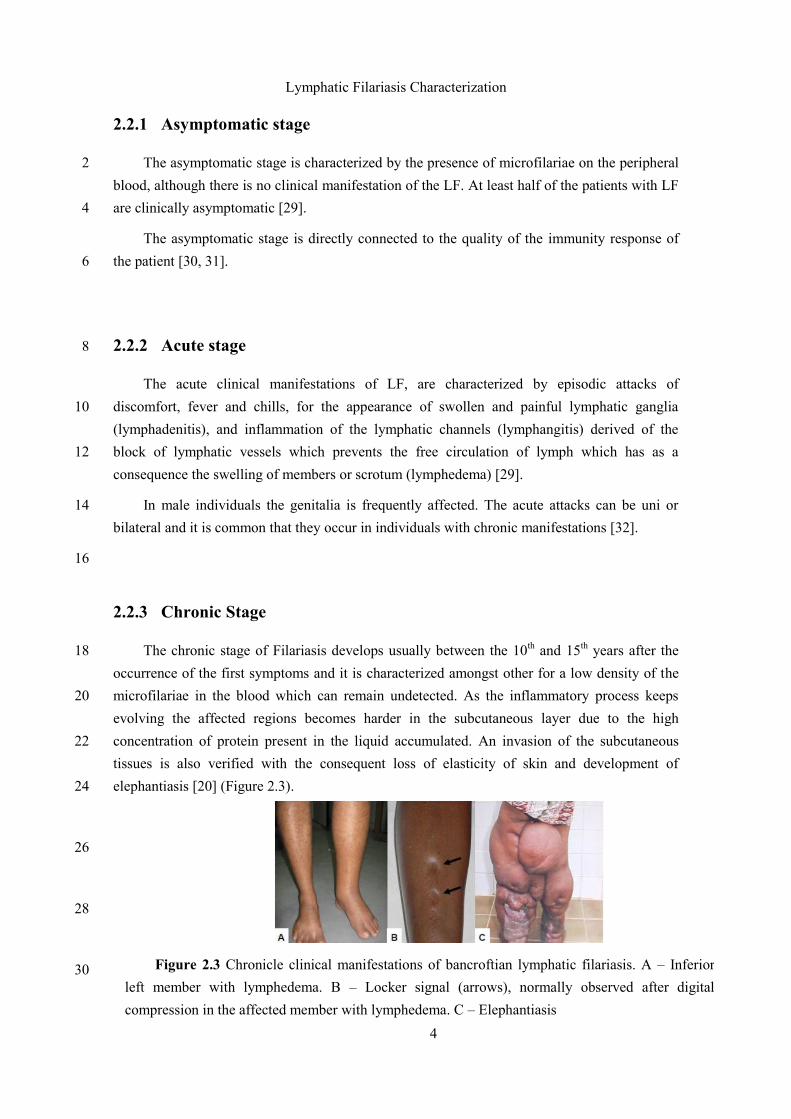
30 Figure 2.3 Chronicle clinical manifestations of bancroftian lymphatic filariasis. A – Inferior
left member with lymphedema. B – Locker signal (arrows), normally observed after digital
compression in the affected member with lymphedema. C – Elephantiasis
Lymphatic Filariasis Characterization
5
The chronic stage is related with the appearance of elephantiasis of members, breast and
genitalia, hydrocele and chyluria [33]. 2
2.3 Diagnosis 4
The diagnosis of Filariasis can be done by different parasitological, immunologic or
molecular methos and also by imaging techniques. 6
2.3.1 Fresh exam technique 8
The standard method used in the diagnosis of Filariasis consists on the observation and
counting directly on the optical microscope of a blood smear having in attention the periodicity 10
of the parasite [23]. The blood smear sample should be thick and stained with Giemsa or with
hematoxylin and eosin. 12
To increase the sensitivity of the method, concentration techniques can be used like
centrifugation and filtration [34]. 14
2.3.2 Serologic Techniques 16
The serologic techniques provide an alternative to the fresh exam technique. The infected
individuals have high level of antibodies ant filarial Ig4 on the blood and can be detected using 18
routine exams [35, 36, 37]. Using the same exams they can also search for the filarial circulating
antigen (FCA) [38]. 20
2.3.3 Polymerase chain reaction (PCR) 22
The PCR tests are highly specific and sensitive allowing the detection of the presence of
parasite DNA in infected individuals as well as intermediary hosts in bancroftian Filariasis and 24
by Brugia [39, 40].
26
Lymphatic Filariasis Characterization
6
2.3.4 Imaging Technique
Recently the ultrasound allowed locating and visualizing the movements of the adult living 2
worms of W. bancrofti and lymphatic dilation in patients with bancroftian Filariasis. This
technique allows the diagnosis in individuals classified as asymptomatic with microfilariae [41, 4
42].
Also the lymphoscintigraphy has shown in individuals classified as asymptomatic the 6
presence of lymphatic abnormalities in affected members of host individuals of microfilaria
[31]. 8
Chapter 3
Literature Review 2
3.1 Introduction
In this chapter, diverse image processing techniques are presented and their contribution 4
for parasite detection and blood cells segmentation. Initially there is a review of the
technologies that will be used in the project followed by the review of image processing 6
techniques and stages on similar projects like Detection of Malaria or Blood Cells
Segmentation. Lastly different and diverse image processing techniques are presented and 8
explained for the different stages of the processing: image enhancement, image segmentation,
feature extraction and classification of features. 10
3.2 Techonology Review
3.2.1 Android 12
Android is a mobile operating system based on the Linux core and it was developed by
Google. It is currently the most used mobile operating system in the world and in 2013 it 14
possessed the biggest percentage in world sales of mobile operating systems. In July 2013, the
application store had more than a billion applications available, downloaded more than 50 16
billion times. A study has shown that 71% of the programmers develop applications for the
Android system. The operating system code is made available by Google under an open source 18
license. Android is really popular in technology companies that need a customizable and low
cost software for high technology devices. As it is open source it has led to an encouragement of 20
a programmers community on adding resources or bringing Android to devices that initially
weren’t launched with the operating system. 22
Literature Review
8
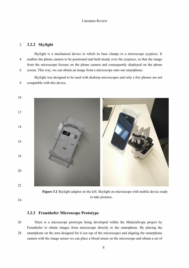
3.2.2 Skylight 2
Skylight is a mechanical device in which its base clamps to a microscope eyepiece. It
enables the phone camera to be positioned and held steady over the eyepiece, so that the image 4
from the microscope focuses on the phone camera and consequently displayed on the phone
screen. This way, we can obtain an image from a microscope onto our smartphone. 6
Skylight was designed to be used with desktop microscopes and only a few phones are not
compatible with this device. 8
10
12
14
16
18
20
22
24
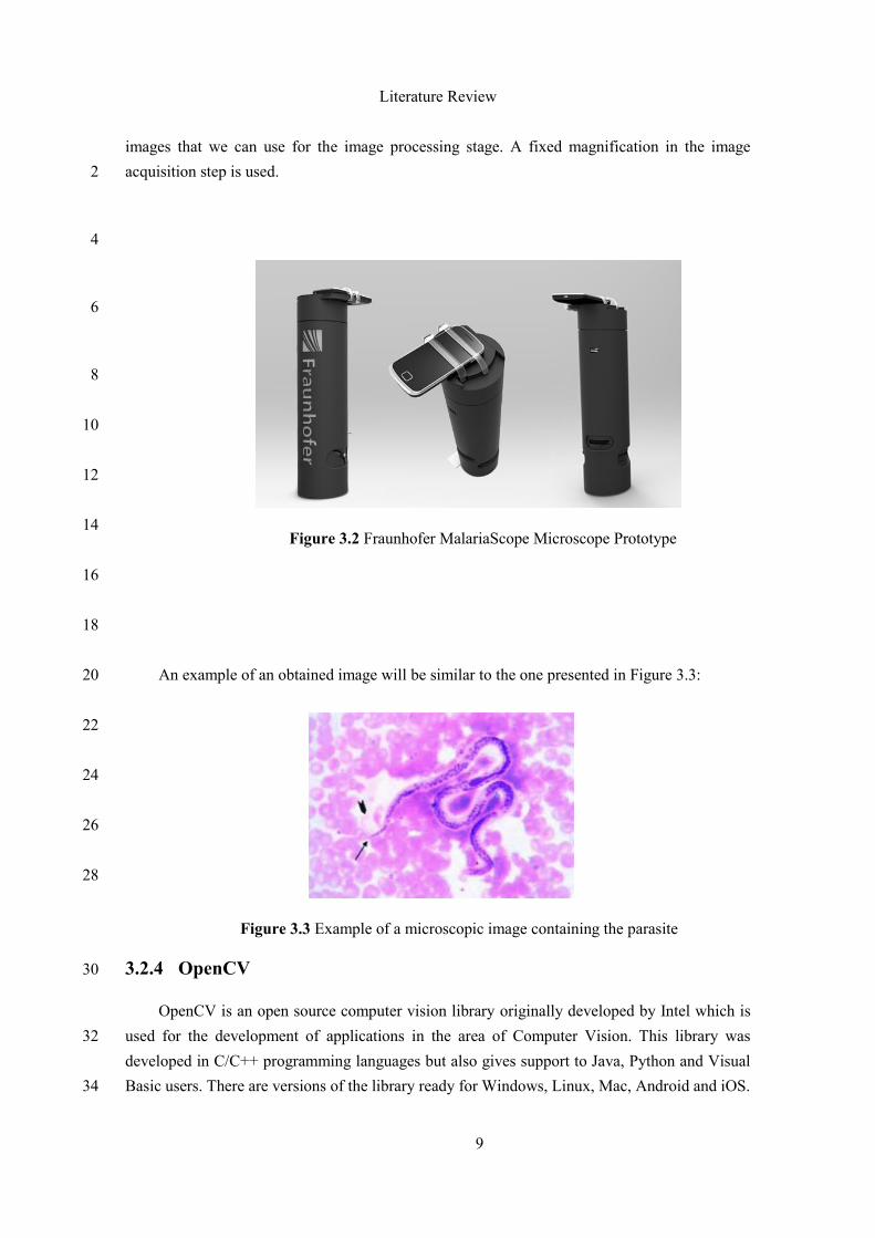
3.2.3 Fraunhofer Microscope Prototype
There is a microscope prototype being developed within the MalariaScope project by 26
Fraunhofer to obtain images from microscope directly to the smartphone. By placing the
smartphone on the area designed for it (on top of the microscope) and aligning the smartphone 28
camera with the image sensor we can place a blood smear on the microscope and obtain a set of
Figure 3.1 Skylight adaptor on the left. Skylight on microscope with mobile device ready
to take pictures.
Literature Review
9
images that we can use for the image processing stage. A fixed magnification in the image
acquisition step is used. 2
4
6
8
10
12
14
16
18
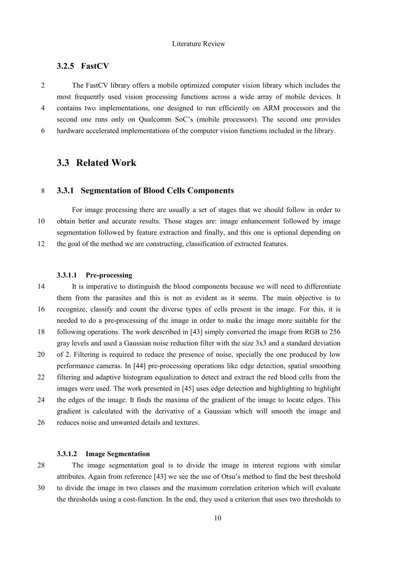
An example of an obtained image will be similar to the one presented in Figure 3.3: 20
22
24
26
28
3.2.4 OpenCV 30
OpenCV is an open source computer vision library originally developed by Intel which is
used for the development of applications in the area of Computer Vision. This library was 32
developed in C/C++ programming languages but also gives support to Java, Python and Visual
Basic users. There are versions of the library ready for Windows, Linux, Mac, Android and iOS. 34
Figure 3.2 Fraunhofer MalariaScope Microscope Prototype
Figure 3.3 Example of a microscopic image containing the parasite
Literature Review
10
3.2.5 FastCV
The FastCV library offers a mobile optimized computer vision library which includes the 2
most frequently used vision processing functions across a wide array of mobile devices. It
contains two implementations, one designed to run efficiently on ARM processors and the 4
second one runs only on Qualcomm SoC’s (mobile processors). The second one provides
hardware accelerated implementations of the computer vision functions included in the library. 6
3.3 Related Work
3.3.1 Segmentation of Blood Cells Components 8
For image processing there are usually a set of stages that we should follow in order to
obtain better and accurate results. Those stages are: image enhancement followed by image 10
segmentation followed by feature extraction and finally, and this one is optional depending on
the goal of the method we are constructing, classification of extracted features. 12
3.3.1.1 Pre-processing
It is imperative to distinguish the blood components because we will need to differentiate 14
them from the parasites and this is not as evident as it seems. The main objective is to
recognize, classify and count the diverse types of cells present in the image. For this, it is 16
needed to do a pre-processing of the image in order to make the image more suitable for the
following operations. The work described in [43] simply converted the image from RGB to 256 18
gray levels and used a Gaussian noise reduction filter with the size 3x3 and a standard deviation
of 2. Filtering is required to reduce the presence of noise, specially the one produced by low 20
performance cameras. In [44] pre-processing operations like edge detection, spatial smoothing
filtering and adaptive histogram equalization to detect and extract the red blood cells from the 22
images were used. The work presented in [45] uses edge detection and highlighting to highlight
the edges of the image. It finds the maxima of the gradient of the image to locate edges. This 24
gradient is calculated with the derivative of a Gaussian which will smooth the image and
reduces noise and unwanted details and textures. 26
3.3.1.2 Image Segmentation
The image segmentation goal is to divide the image in interest regions with similar 28
attributes. Again from reference [43] we see the use of Otsu’s method to find the best threshold
to divide the image in two classes and the maximum correlation criterion which will evaluate 30
the thresholds using a cost-function. In the end, they used a criterion that uses two thresholds to
Literature Review
11
discriminate background, red blood cells and leucocytes. They also use the watershed algorithm
to detect and separate two joined cells by computing and plotting as a height the shortest 2
distance between each pixel and the background where the peaks represent the center of the cell.
By applying a dilation process having both centers as seed points for the operation they could 4
recover the joined cells. The work described in [45] uses methods based on the thresholding of
luminance or color components of the image. 6
3.3.1.3 Feature Detection and Classification 8
In feature detection we need to extract the relevant features, in this case the blood cells that
will be classified, and we need some processing to find the features that characterize the blood 10
cells.
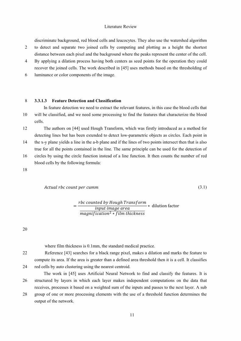
The authors on [44] used Hough Transform, which was firstly introduced as a method for 12
detecting lines but has been extended to detect low-parametric objects as circles. Each point in
the x-y plane yields a line in the a-b plane and if the lines of two points intersect then that is also 14
true for all the points contained in the line. The same principle can be used for the detection of
circles by using the circle function instead of a line function. It then counts the number of red 16
blood cells by the following formula:
18
(3.1)
20
where film thickness is 0.1mm, the standard medical practice.
Reference [43] searches for a black range pixel, makes a dilation and marks the feature to 22
compute its area. If the area is greater than a defined area threshold then it is a cell. It classifies
red cells by auto clustering using the nearest centroid. 24
The work in [45] uses Artificial Neural Network to find and classify the features. It is
structured by layers in which each layer makes independent computations on the data that 26
receives, processes it based on a weighted sum of the inputs and passes to the next layer. A sub
group of one or more processing elements with the use of a threshold function determines the 28
output of the network.
Literature Review
12
3.3.2 Parasite Detection
For parasite detection, the methods can be similar to those used in the early stages of blood 2
cell segmentation but they differ to find distinctive characteristics of the parasites because these
have unique features and need to be distinguished from the blood cells and sometimes they can 4
be mistaken with a blood cell due to similar shapes or in the malaria detection case, we need to
analyze the blood cell to check for the parasite inside of it. 6
3.3.2.1 Pre-processing
The authors of [46] and [47] converted the image to a gray scale space because the image 8
showed some degree of color variability and used a 5x5 median filter to substitute each pixel in
the image with the median value of the intensity level in the neighborhood which will result in 10
reduced sharp transitions in the pixel intensities which is the indication of random noise. In
reference [48] the authors firstly resize the image for magnification or to reduce image size to 12
speedup processing, reduces noise with also a 5x5 median filter and then enhances image
contrast by transforming the original images into the HSI because HSI color space highlights 14
some parasite information.
3.3.2.2 Image Segmentation 16
In the image segmentation process, the work from [46] segmented the blood cells by
converting the pre-processed image into a binary image with a threshold that maximally divides 18
the background from the foreground objects. As a single global threshold was not sufficient they
recurred to Otsu’s method to better divide the image into classes. 20
Reference [48] used histogram thresholding by getting the correspondent HSI image,
obtain the green component from RGB image and Hue and Saturation from HSI image and 22
determined the coordinates of bounding rectangles enclosing erythrocytes by using Otsu’s
algorithm to segment in green, Hue and Saturation components. It also did the same with other 24
algorithm similar to Otsu’s, named Zack’s algorithm, that locates global minimum points in an
image histogram which will be the threshold used to separate objects from background. Thus, 26
two techniques were tested here.
3.3.2.3 Feature Detection and Classification 28
To extract the features (infected and healthy erythrocytes), the work from [46] used the
difference of intensity distribution between possibly infected erythrocytes and healthy ones and 30
the area defined by the erythrocyte. This can be done because the gray-scale infected
erythrocytes have intensity values close to 0 (parasite nucleus). With the fact that parasite’s 32
cytoplasm appears lighter while parasite’s nuclei appears darker each possibly infected cell can
Literature Review
13
be divided into 3 regions using a multiple thresholding to segment them consequently
confirming an infected cell or not. Using a Bayes classifier divided in two stages the cells were 2
classified using probabilities. For the first stage infected red blood cells were separated from
normal ones through intensity differences. In the second stage a ratio of white to black area was 4
used to detect a false positive or a real infected red blood cell (through difference of intensity
from parasite’s nuclei and cytoplasm). 6
In reference [47] after the gray-scale conversion and median filtering the parasite’s will
have a darker color than the rest of the cells so an algorithm was developed to calculate the 8
average of the maximum and minimum pixel intensities and each pixel that had an intensity
higher than the average would be part of a possible parasite. Parameters like specificity and 10
sensitivity were used to evaluate the detection.
The work in [48] trained a multilayer back propagation Artificial Neural Network to 12
partition the image in two regions: erythrocytes and background and used two sets of features to
train two Artificial Neural Networks (one with RGB pixel values and other with both RGB and 14
HSI pixel values) and the features were divided into two classes: erythrocytes and background
pixel values. 16
18
3.4 Image Processing Techniques
Image processing is the method to perform operations on a digital image with the 20
goal of getting an enhanced image or extract the desired information from it. Image
processing involves many processing steps like: image acquisition, image enhancement, 22
image restoration, colour image processing, wavelets and multiresolution processing,
compression, morphological processing, segmentation, representation and description, 24
object recognition, tracking and knowledge base.
3.4.1 Image Enhancement 26
The aim of Image Enhancement is to improve the information in images for human
viewers better interpretability or perception and providing better input for other automated 28
processing techniques. This is achieved by modifying attributes of an image to make it more
suitable for a given task or specific observer [49]. Therefore, it is important to choose carefully 30
the attributes to modify best suit the needs because the following operations results will depend
on the enhancement that has been made. 32
The enhancements can be divided in two categories: spatial domain methods and
frequency domain methods. 34
Literature Review
14
Spatial domain techniques deal directly with the image pixels, applying to each pixel a
transformation resulting in a new pixel with the desired enhancement. 2
( ) , ( )- (3.2)
4
where T is the transformation and f(x,y) the pixel to modify. 6
For frequency domain techniques the image needs to be transferred first to the frequency
domain through the Fourier Transform and all the enhancements are applied to the Fourier 8
Transform of the image and then to get the resultant image it is needed to apply the Inverse
Fourier Transform. These are used to enhancement operations such as modifying the image 10
brightness, contrast or the distribution of gray levels, and so the image needs to be converted to
gray scale. 12
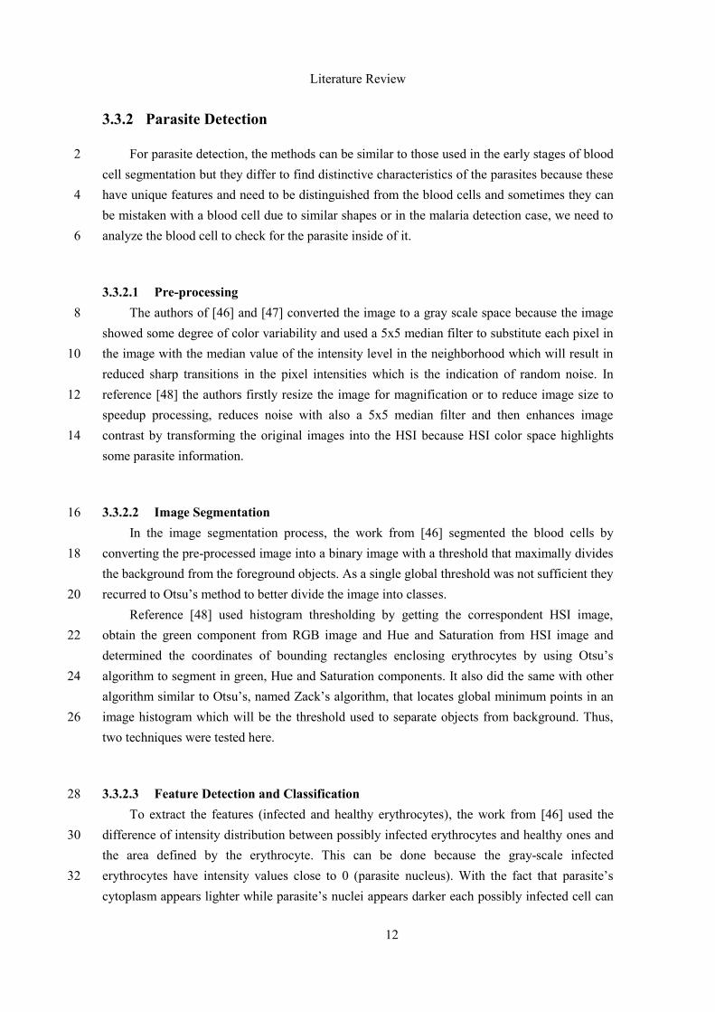
The most basic transformation T is to compute the negative of an image where the pixel
grays are inverted. Every pixel value from the original image is subtracted from 255. Negative 14
images can enhance the white or grey detail in the dark regions of the image and can make some
details clearer (e.g. in human body tissues) (Figure 3.4). 16
18
20
22
24
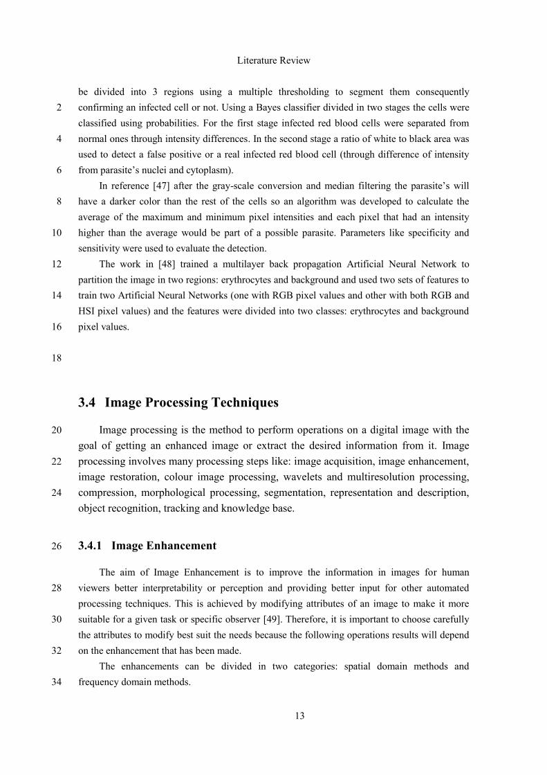
Threshold transformations are useful for segmentation where we want to isolate an object 26
from the background converting images into binary images by selecting a threshold that
maximally divides the image into two classes of intensities: one for the intensities of 28
background and the other for the intensities of the foreground (Figure 3.5).
30
32
34
36
Figure 3.4 Negative of an image
Figure 3.5 Thresholding method
Literature Review
15
Logarithmic transformations or fractional power-law transformations are used for
expanding lower gray pixel values into a wider range, while compressing the high values. The 2
opposite occurs when inverse logarithmic or power-law transformations, with and higher-than-1
exponent are used. 4
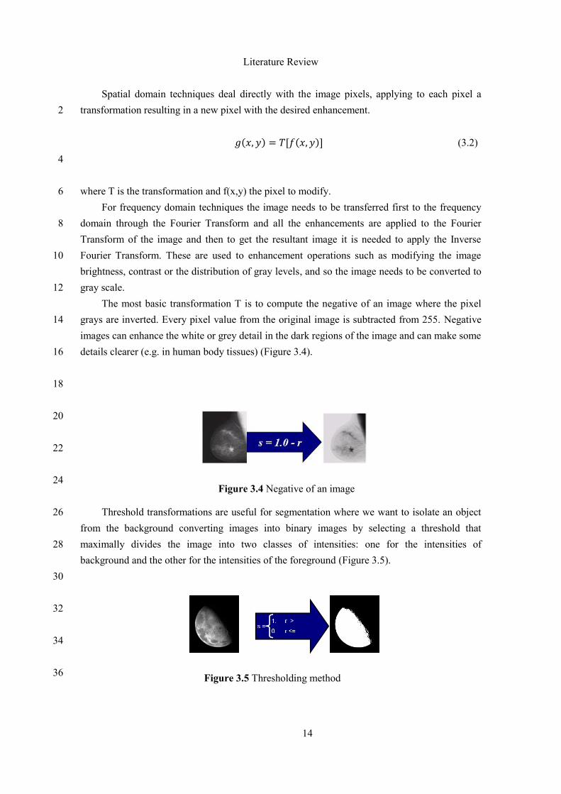
Piecewise linear transformations uses an arbitrary user-defined transform instead of a well-
defined mathematical function (Figure 3.6). 6
8
10
12
14
16
18
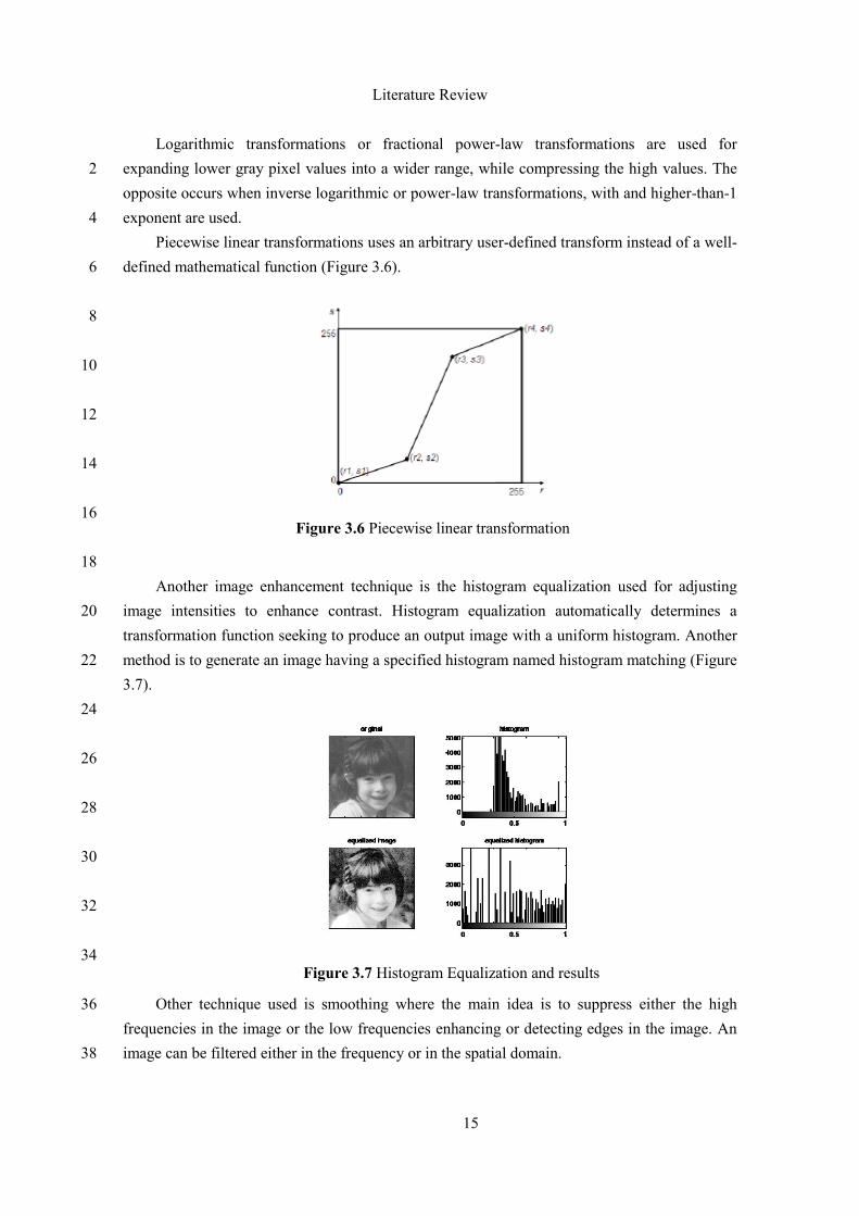
Another image enhancement technique is the histogram equalization used for adjusting
image intensities to enhance contrast. Histogram equalization automatically determines a 20
transformation function seeking to produce an output image with a uniform histogram. Another
method is to generate an image having a specified histogram named histogram matching (Figure 22
3.7).
24
26
28
30
32
34
Other technique used is smoothing where the main idea is to suppress either the high 36
frequencies in the image or the low frequencies enhancing or detecting edges in the image. An
image can be filtered either in the frequency or in the spatial domain. 38
Figure 3.6 Piecewise linear transformation
Figure 3.7 Histogram Equalization and results
Literature Review
16
The first one involves transforming the image into the frequency domain, multiplying it
with the frequency filter function and transform the result into the spatial domain again. The 2
corresponding process in the spatial domain is to convolve the input image with the filter
function. 4
We have to approximate the filter function with a discrete and finite kernel and we shift
this kernel over the image and multiply its value with the corresponding pixel values of the 6
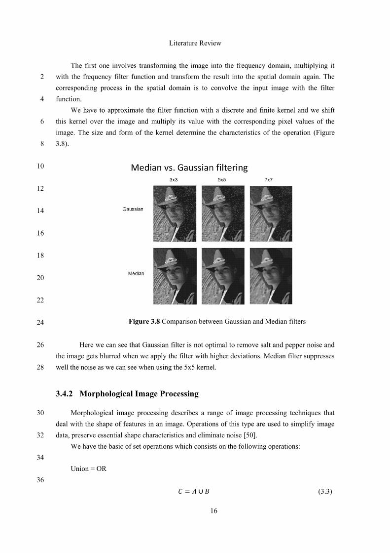
image. The size and form of the kernel determine the characteristics of the operation (Figure
3.8). 8
10
12
14
16
18
20
22
24
Here we can see that Gaussian filter is not optimal to remove salt and pepper noise and 26
the image gets blurred when we apply the filter with higher deviations. Median filter suppresses
well the noise as we can see when using the 5x5 kernel. 28
3.4.2 Morphological Image Processing
Morphological image processing describes a range of image processing techniques that 30
deal with the shape of features in an image. Operations of this type are used to simplify image
data, preserve essential shape characteristics and eliminate noise [50]. 32
We have the basic of set operations which consists on the following operations:
34
Union = OR
36
(3.3)
Figure 3.8 Comparison between Gaussian and Median filters
Literature Review
17
2
Produces a set that contains the elements of both A and B.
4
Intersection = AND
6
* + (3.4)
8
Produces a set that contains the elements that are in A and B. If they have no common
elements the sets are called disjoint. 10
Complement 12
(3.5)
14
Produces a set that contains the elements that are not contained in A
16
18
Reflection 20
* + (3.6)
22
Where p is a point (position) belonging to the original image I. 24
This operation reflects a point in relation to the origin (0,0).
26
Dilation and Erosion are basic morphological processing operations. They are employed as
the basic elements of many algorithms and are produced through the interaction of a structuring 28
set and a set of pixels of interest in the image.
A structuring element is a binary image (or mask) that allows us to define arbitrary 30
neighborhood structures and we can think of a binary image as the set of all pixel locations in
the foreground or background: 32
Literature Review
18
*( ) ( ) + (3.7)
2
A dilation of an image A by the structuring element B is given by the set operation:
4
* ( ) + (3.8)
where is the reflection of B about its origin followed by a shift s. 6
A dilation is used for repairing breaks and intrusions and can also be computed as an
erosion of the foreground and an erosion can be computed as a dilation of the background. 8
Thus, we represent erosion with the set operation:
10
* ( ) + (3.9)
12
Erosion can split apart joined objects and can strip away extrusions. It is used for shrinking
or thinning operations whereas dilation grows and thickens the objects in a binary image. 14
We can make joint operations with erosion and dilation that can be useful for smoothing
the contour of an object, eliminate thin protrusions, eliminate small holes and fill gaps in the 16
contour.
18
Opening operation is an erosion followed by a dilation: 20
( ) (3.10)
22
where stray foreground structures that are smaller than the B structuring element will
disappear and larger structures will remain in the image. 24
Closing operation is a dilation followed by an erosion:
26
( ) (3.11)
and it consists of filling the holes in the foreground that are smaller than B. 28
If we want to get the outline of the object we can apply an outline operation that consists of
a dilation followed by a subtraction and if we wish to skeletonize the object then we just need to 30
repeatedly run erosion and stop when the thickness is at 1 pixel.
Literature Review
19
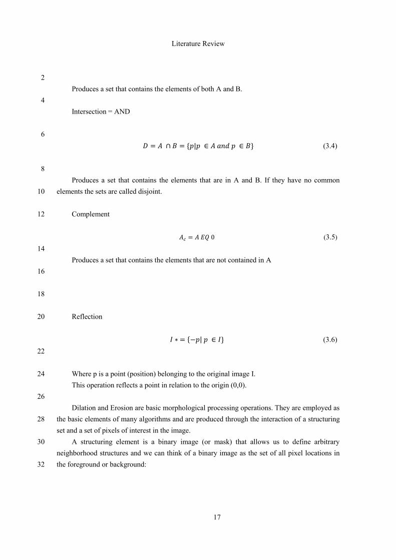
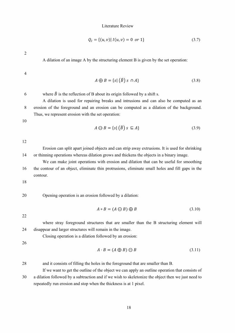
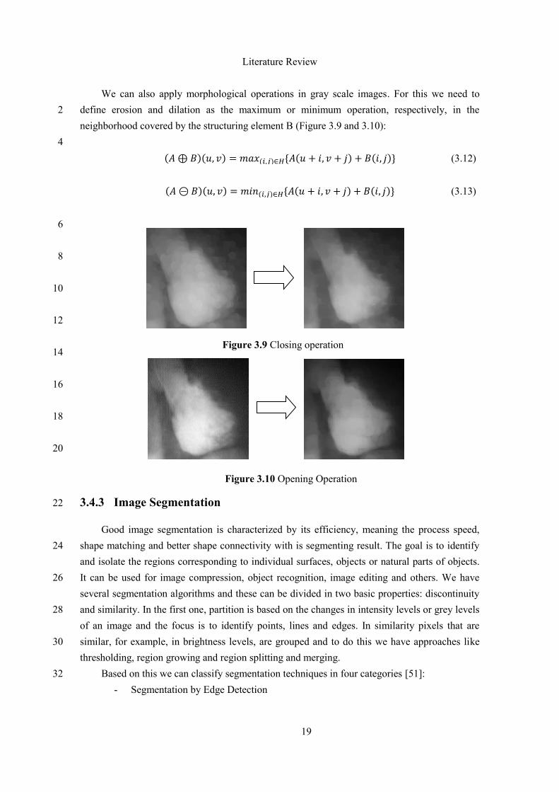
We can also apply morphological operations in gray scale images. For this we need to
define erosion and dilation as the maximum or minimum operation, respectively, in the 2
neighborhood covered by the structuring element B (Figure 3.9 and 3.10):
4
( )( ) ( ) * ( ) ( )+ (3.12)
( )( ) ( ) * ( ) ( )+ (3.13)
6
8
10
12
14
16
18
20
3.4.3 Image Segmentation 22
Good image segmentation is characterized by its efficiency, meaning the process speed,
shape matching and better shape connectivity with is segmenting result. The goal is to identify 24
and isolate the regions corresponding to individual surfaces, objects or natural parts of objects.
It can be used for image compression, object recognition, image editing and others. We have 26
several segmentation algorithms and these can be divided in two basic properties: discontinuity
and similarity. In the first one, partition is based on the changes in intensity levels or grey levels 28
of an image and the focus is to identify points, lines and edges. In similarity pixels that are
similar, for example, in brightness levels, are grouped and to do this we have approaches like 30
thresholding, region growing and region splitting and merging.
Based on this we can classify segmentation techniques in four categories [51]: 32
- Segmentation by Edge Detection
Figure 3.9 Closing operation
Figure 3.10 Opening Operation
Literature Review
20
- Segmentation by Thresholding
- Segmentation by Region based 2
- Segmentation by Feature based Clustering
4
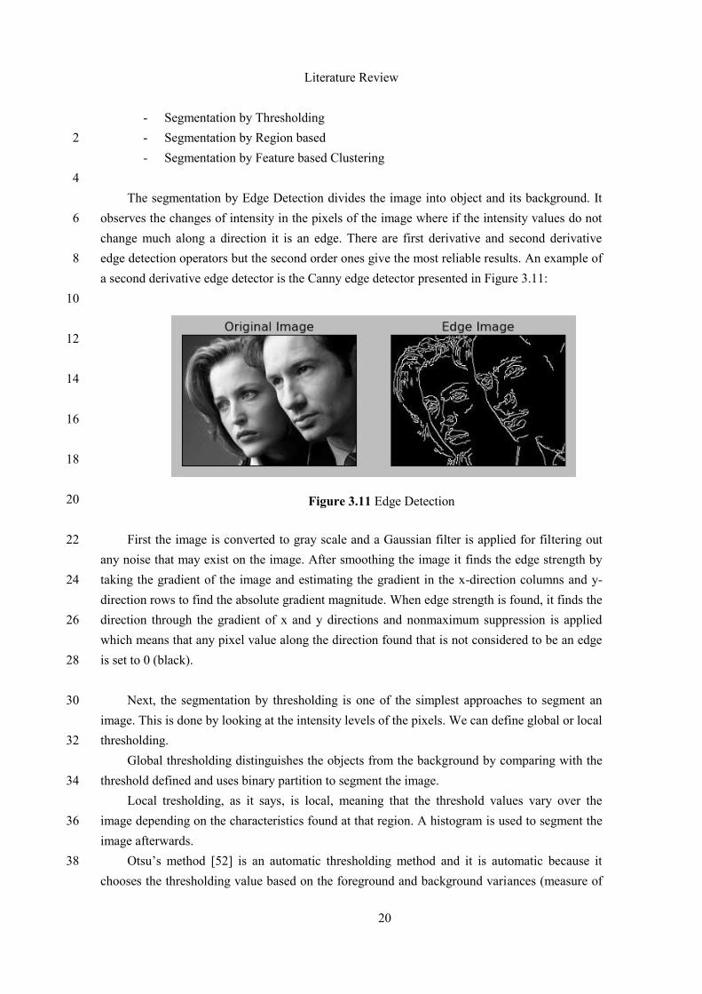
The segmentation by Edge Detection divides the image into object and its background. It
observes the changes of intensity in the pixels of the image where if the intensity values do not 6
change much along a direction it is an edge. There are first derivative and second derivative
edge detection operators but the second order ones give the most reliable results. An example of 8
a second derivative edge detector is the Canny edge detector presented in Figure 3.11:
10
12
14
16
18
20
First the image is converted to gray scale and a Gaussian filter is applied for filtering out 22
any noise that may exist on the image. After smoothing the image it finds the edge strength by
taking the gradient of the image and estimating the gradient in the x-direction columns and y-24
direction rows to find the absolute gradient magnitude. When edge strength is found, it finds the
direction through the gradient of x and y directions and nonmaximum suppression is applied 26
which means that any pixel value along the direction found that is not considered to be an edge
is set to 0 (black). 28
Next, the segmentation by thresholding is one of the simplest approaches to segment an 30
image. This is done by looking at the intensity levels of the pixels. We can define global or local
thresholding. 32
Global thresholding distinguishes the objects from the background by comparing with the
threshold defined and uses binary partition to segment the image. 34
Local tresholding, as it says, is local, meaning that the threshold values vary over the
image depending on the characteristics found at that region. A histogram is used to segment the 36
image afterwards.
Otsu’s method [52] is an automatic thresholding method and it is automatic because it 38
chooses the thresholding value based on the foreground and background variances (measure of
Figure 3.11 Edge Detection
Literature Review
21
spread) of each threshold. It iterates through all possible thresholding values and by checking
the pixels that fall in foreground or background it calculates a weighted variance based on that, 2
measuring the separability of two classes. The goal is to find the threshold value where the sum
of foreground and background spreads is at its minimum. To calculate the class-variance the 4
following formula is used:
6
( )
( ) ( ) ( ) (3.14)
8
The segmentation by region groups the pixels that are related to some object. The area that
is detected for segmentation should be closed. A single pixel is taken at first and the region 10
grows by comparing all the unallocated neighboring pixels through the difference of the pixel’s
intensity value and region’s mean intensity value. The one with the smallest difference gets 12
allocated to the respective region.
Finally, the segmentation by clustering groups the pixels based on its attributes. A cluster 14
contains a group of similar pixels that belong to a specific region and are different from the othe
regions. Images can also be grouped according to their content. In this case, grouping is made 16
according to some inherited characteristics of the pixels like shape, texture, etc. A well-known
clustering technique is the K-Means technique. 18
Choosing an initial number of centroids (K) the data points are assigned to the nearest
centroid minimizing the square of the distance from the data points to the cluster. 20
22
| ( ) |
(3.15)
3.5 Machine Learning
Machine learning is a core subarea of artificial intelligence. The goal is to create learning 24
algorithms that do the learning automatically without the need of human intervention or any
type of assistance. The learning is always based on some sort of observations or data, direct 26
experience or instruction. It learns from the past to behave better in the future.
3.5.1 Feature Extraction 28
A feature is a part of an image that contains interesting details. It is a general term since to
define a feature we need to know what is the goal of the image processing or which kind of 30
Literature Review
22
structures are we identifying hence which characteristics do they have (features). Some of the
most commonly used features are: edges, corners, blobs, etc. Gabor filters, shape based, texture 2
based, wavelet transforms, SIFT, SURF, Fourier descriptors, Haar transforms are amongst the
several techniques for feature extraction. 4
3.5.1.1 SIFT (Scale-Invariant Feature Transform)
A method is needed to be able to locate objects in an image containing other objects. This 6
method needs to be scale, rotation, and luminance invariant because we need to locate an object
in an image and this image will not always have the same magnification, color intensities or 8
rotation. SIFT provides a set of features of an object that are not affected by any of those
complications. This method is also very resilient to the effects of “noise” in the image [53]. 10
Stage 1: Scale Space Extrema Detection
To achieve scale invariance, SIFT looks for stable features across all possible scales using 12
a continuous function of scaling, constructing the scale space. It uses the Difference of Gaussian
filter for scale space because it is an efficient filter and has the same stability as the scale-14
normalized Laplacian of Gaussian (used in detection of edges, blobs).
The Difference of Gaussian algorithm is a gray scale image enhancement algorithm that 16
subtracts a blurred version of the original gray scale image from another blurred version of the
original image. These images are obtained by convolving the original gray scale image with 18
Gaussian kernels with different deviations, producing different blurs. This blur will suppress
only high frequency spatial information and by subtracting one image from the other we will 20
preserve the spatial information that lies between the ranges of frequencies that are preserved in
the two blurred images. 22
Stage 2: Keypoint Localization
This step goal is to find keypoints in the 3D scale space. 24
Some pixel is selected if it is larger or smaller than all its 26 neighbors, 8 on the same scale
and 9 on the scale above and below. 26
Here, points with low contrast and poorly localized along edge data are discarded.
28
This is done by calculating the Laplacian value for each key point found in stage 1. The 30
location of extremum, z is given by:
32
Literature Review
23
(3.16)
If the function value at z is below a threshold value the point is excluded (extrema with
low contrast). To eliminate key points with poor localization it is noted that in these cases there 2
is a large principle curvature across the edge but a small curvature in the perpendicular direction
in the difference of Gaussian function. If this difference is below the ratio of largest to smallest 4
eigenvector, from the 2x2 Hessian matrix at the location and scale of the keypoint, the keypoint
is rejected. 6
Stage 3: Orientation Assignment
By assigning a consistent orientation, the keypoint descriptor can be orientation invariant. 8
Assign dominant orientation as the orientation of the keypoint.
First, the Gaussian-smoothed image ( ) at the keypoint’s scale sigma is taken so that 10
all computations are performed in a scale-invariant manner. For an image sample ( ) at
scale sigma, the gradient magnitude, ( ) and orientation, ( ), are precomputed using 12
pixel differences:
Form an orientation histogram from gradient orientations of sample points. 14
Locate the highest peak in the histogram. Use this peak and any other local peak within
80% of the height of this peak to create a keypoint with that orientation. Some points might 16
have more than one orientation.
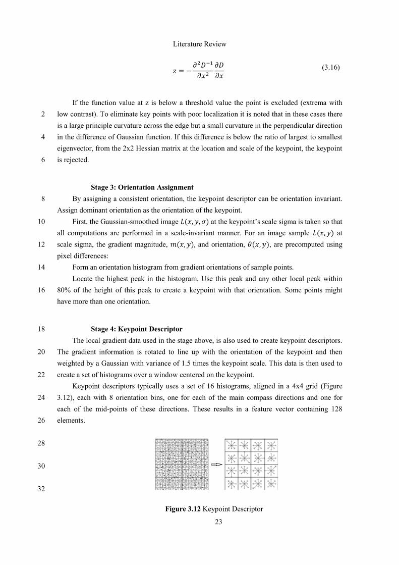
Stage 4: Keypoint Descriptor 18
The local gradient data used in the stage above, is also used to create keypoint descriptors.
The gradient information is rotated to line up with the orientation of the keypoint and then 20
weighted by a Gaussian with variance of 1.5 times the keypoint scale. This data is then used to
create a set of histograms over a window centered on the keypoint. 22
Keypoint descriptors typically uses a set of 16 histograms, aligned in a 4x4 grid (Figure
3.12), each with 8 orientation bins, one for each of the main compass directions and one for 24
each of the mid-points of these directions. These results in a feature vector containing 128
elements. 26
28
30
32
Figure 3.12 Keypoint Descriptor
Literature Review
24
2
These resulting vectors are known as SIFT keys and are used in a nearest-neighbors
approach to identify possible objects in an image [52]. 4
3.5.1.2 SURF (Speed UP Robust Features)
6
SURF is inspired by SIFT and the standard version of SURF is several times faster than
SIFT. SURF uses an integer approximation of the determinant of the Hessian matrix for blob 8
detection, which can be computed with three integer operations using a pre-computed integral
image and uses Haar wavelet for feature descriptor that can also be computed using an integral 10
image [54].
12
3.5.1.2.1 Interest Point Detection
Integral images are used. Integral images allow for fast computation of box type 14
convolution filters. The entry of an integral image ( ) at a location ( ) represents
the sum of all pixels in the input image I within a rectangular region formed by the origin and . 16
18
( ) ∑∑ ( )
(3.17)
20
The detector is based on the Hessian matrix and it detects blob-like structures at locations
where the determinant is maximum. The determinant is also used for scale selection. Given a 22
point ( ) in an image , the Hessian Matrix ( ) in at scale sigma is defined as:
24
( ) [
( ) ( )
( ) ( )]
(3.18)
Where ( ) is the convolution of the Gaussian second order derivative 26
( ) with the image I in point x. As we had seen in SIFT Gaussians are optimal for
scale-space analysis. 28
Literature Review
25
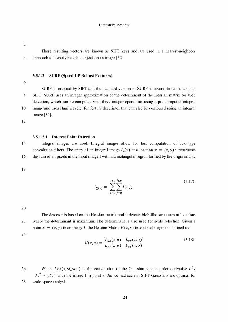
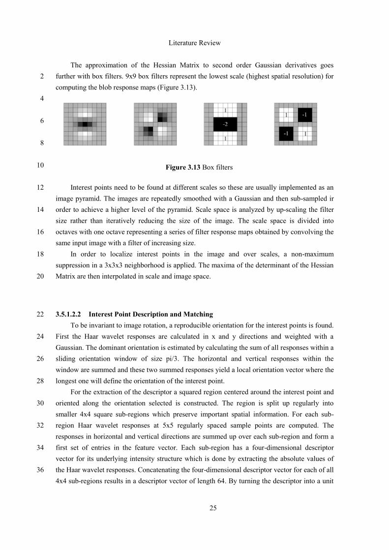
The approximation of the Hessian Matrix to second order Gaussian derivatives goes
further with box filters. 9x9 box filters represent the lowest scale (highest spatial resolution) for 2
computing the blob response maps (Figure 3.13).
4
6
8
10
Interest points need to be found at different scales so these are usually implemented as an 12
image pyramid. The images are repeatedly smoothed with a Gaussian and then sub-sampled ir
order to achieve a higher level of the pyramid. Scale space is analyzed by up-scaling the filter 14
size rather than iteratively reducing the size of the image. The scale space is divided into
octaves with one octave representing a series of filter response maps obtained by convolving the 16
same input image with a filter of increasing size.
In order to localize interest points in the image and over scales, a non-maximum 18
suppression in a 3x3x3 neighborhood is applied. The maxima of the determinant of the Hessian
Matrix are then interpolated in scale and image space. 20
3.5.1.2.2 Interest Point Description and Matching 22
To be invariant to image rotation, a reproducible orientation for the interest points is found.
First the Haar wavelet responses are calculated in x and y directions and weighted with a 24
Gaussian. The dominant orientation is estimated by calculating the sum of all responses within a
sliding orientation window of size pi/3. The horizontal and vertical responses within the 26
window are summed and these two summed responses yield a local orientation vector where the
longest one will define the orientation of the interest point. 28
For the extraction of the descriptor a squared region centered around the interest point and
oriented along the orientation selected is constructed. The region is split up regularly into 30
smaller 4x4 square sub-regions which preserve important spatial information. For each sub-
region Haar wavelet responses at 5x5 regularly spaced sample points are computed. The 32
responses in horizontal and vertical directions are summed up over each sub-region and form a
first set of entries in the feature vector. Each sub-region has a four-dimensional descriptor 34
vector for its underlying intensity structure which is done by extracting the absolute values of
the Haar wavelet responses. Concatenating the four-dimensional descriptor vector for each of all 36
4x4 sub-regions results in a descriptor vector of length 64. By turning the descriptor into a unit
Figure 3.13 Box filters
Literature Review
26
vector, contrast invariance is achieved. Wavelet responses are invariant to an offset in
illumination. 2
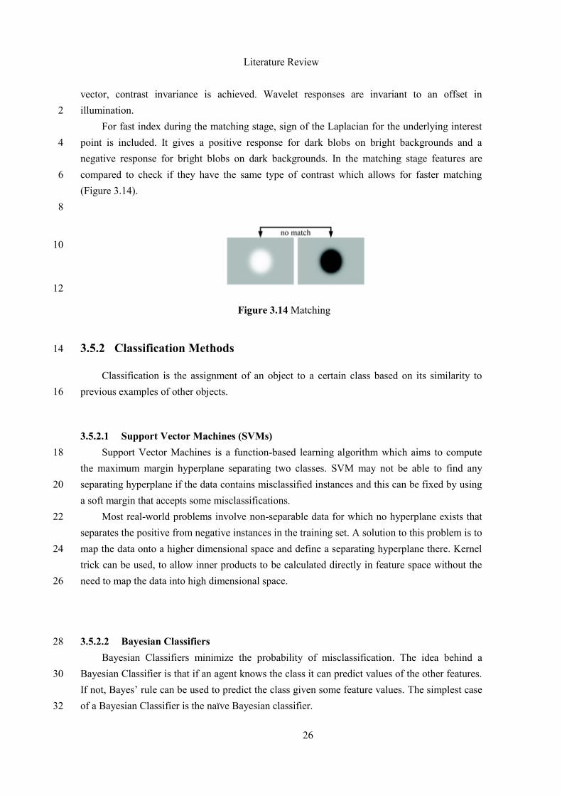
For fast index during the matching stage, sign of the Laplacian for the underlying interest
point is included. It gives a positive response for dark blobs on bright backgrounds and a 4
negative response for bright blobs on dark backgrounds. In the matching stage features are
compared to check if they have the same type of contrast which allows for faster matching 6
(Figure 3.14).
8
10
12
3.5.2 Classification Methods 14
Classification is the assignment of an object to a certain class based on its similarity to
previous examples of other objects. 16
3.5.2.1 Support Vector Machines (SVMs)
Support Vector Machines is a function-based learning algorithm which aims to compute 18
the maximum margin hyperplane separating two classes. SVM may not be able to find any
separating hyperplane if the data contains misclassified instances and this can be fixed by using 20
a soft margin that accepts some misclassifications.
Most real-world problems involve non-separable data for which no hyperplane exists that 22
separates the positive from negative instances in the training set. A solution to this problem is to
map the data onto a higher dimensional space and define a separating hyperplane there. Kernel 24
trick can be used, to allow inner products to be calculated directly in feature space without the
need to map the data into high dimensional space. 26
3.5.2.2 Bayesian Classifiers 28
Bayesian Classifiers minimize the probability of misclassification. The idea behind a
Bayesian Classifier is that if an agent knows the class it can predict values of the other features. 30
If not, Bayes’ rule can be used to predict the class given some feature values. The simplest case
of a Bayesian Classifier is the naïve Bayesian classifier. 32
Figure 3.14 Matching
Literature Review
27
3.5.2.3 Decision Tree
Decision Trees are trees that classify instances by sorting them based on feature values. 2
Each node in a decision tree represents a feature in an instance to be classified, and each branch
represents a value that the node can assume. Instances are classified starting at the root node and 4
sorted based on their feature’s values.
The feature that best divides the training data will be associated to the root node. The 6
source set gets split into sub-sets based on attribute values and this is made recursively for each
of the sub-sets until there is no more value on splitting again. The most well-known algorithm 8
for building decision-trees is the C4.5 and the most commonly selected attribute value test is
information gain which is based on the concept of entropy from information theory. The 10
information gain is the entropy reduction of a particular features achieved by learning the
classification. 12
3.5.2.4 k-Nearest Neighbor (kNN)
k-Nearest Neighbor is a lazy learning algorithm and its principle is that the instances 14
within a dataset will generally exist in close proximity to other instances that have similar
properties. If the instances are tagged with a classification label, then the value of the label of an 16
unclassified instance can be determined by observing the classes of its nearest neighbors. It
located the k nearest instances and determines its class by identifying the most common class on 18
the k nearest neighbors. The relative distance between the instances is determined by using a
distance metric (e.g. Euclidean distance, Manhattan distance). 20
3.6 Relevant Remarks 22
In relation to blood cells segmentation the work on [44] diluted samples with an
anticoagulant liquid to separate the cells and prevent their overlapping. The counting method 24
presented here had good results but blood cells that did not appear completely on the image
weren’t counted, like it would be done in a manual blood test, so improvements need to be made 26
in order to count those cells that appear cut. In [43] the authors they were able to discriminate
between red and white blood cells with their proposed framework. The software developed 28
could give the precise result of a blood test if appropriate calibration of the microscope was
used. The classification method based on nearest centroid performed well having a total 30
recognition rate of 98%. The work described in reference [45] used the layered feed-forward
Artificial Neural Network and was able to detect between complete and healthy, incomplete non 32
circular and sickled red blood cells. It had an accuracy of 81% counting red and white blood
Literature Review
28
cells and this accuracy can be improved by increasing the training of the Artificial Neural
Network. 2
For parasite detection, the work in reference [46] proposed method presents reasonable
results but in the results possible infected erythrocytes with low white/black ratio were 4
identified as infected which should only happen with a higher ratio level. When the erythrocyte
is in the very early trophozoite stage the cytoplasm is not very visible so the algorithm failed in 6
identifying those erythrocytes for some cases. A future work is to classify the parasite based on
shape and size. Reference [47] results had some false positives due to impurities or white blood 8
cells having the same color as the malaria parasite but overall it had a good performance on
identifying the infected cells and the malaria parasite although accuracy needs to be improved. 10
In reference [48] the accuracy of the method was 95% in detecting the presence of
plasmodium parasites which proved that Artificial Neural Network classifiers are reliable and 12
accurate. Artificial Neural Network based only on RGB colors performed better than the one
with RGB and HSI features. A technique for segmenting plasmodium parasites based on Zack’s 14
algorithm was developed which determines the best threshold value.
For image pre-processing, median filter could be a good option since almost all of the 16
proposed methods used it and stated it performed better than the Gaussian filter. In every
method images were converted to gray-scale except on the work from [48] which maintained 18
color and converted only to HSI in some cases. For image segmentation most of the methods
used thresholding (histogram, automatic, luminance), applying different algorithms to separate 20
blood cells from parasites or to segment blood cells only.
22
Lymphatic Filariasis Detection
29
Chapter 4
Lymphatic Filariasis Detection 2
As said before, lympathic Filariasis is a parasitic infection caused by nematodes of the type
Wuchereria and Brugia. Wuchereria bancrofti its responsible for 90% of the cases, Brugia 4
malayi is responsible for almost all of the remaining cases and B.timori falls out of the scope of
the project because it causes almost none of the cases. The unique features that characterize the 6
two main species (section 2.1) provide the basis for the actual method of Lymphatic Filariasis
detection which is the observation by microscope of a blood smear stained with Giemsa and the 8
manual identification of the parasites with special attention to their periodicity. The periodicity
depends on the type of parasite where there are parasites that have a maximum concentration 10
during the day and others during the night. That is the case of the two microfilariae that we need
to identify, which means that the blood collection needs to be done during the night. The 12
method is not an agile method and it always requires an health professional to perform the
analysis of the blood smear which difficults the task for regions like Africa where it is 14
impossible to analyze so many cases in so little time and where it is hard to have many health
professionals and acquire medical material to perform the analysis. 16
Given this, there is a need for a reliable detection method that is more agile and accessible
to detect the disease which is the goal of this project. 18
By acquiring microscopic images from a portable microscope into a smartphone, the
smartphone will be able to process those images using image processing techniques and analyze 20
the blood smears to verify whether there are parasites or not. As it is an autonomous system, it
doesn’t need any human intervention besides the image acquisition which makes a possible 22
solution for regions like Africa where a person that is not an health professional and doesn’t
have that much knowledge about the disease can still conduct the test on the smartphone that 24
will tell if the blood smear on analysis has infected parasites or not. As it will identify the two
types of parasites on the blood smear, this solution makes possible for the identification of 26
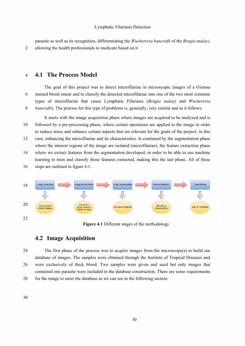
Lymphatic Filariasis Detection
30
parasite as well as its recognition, differentiating the Wuchereria bancrofti of the Brugia malayi,
allowing the health professionals to medicate based on it. 2
4.1 The Process Model 4
The goal of this project was to detect microfilariae in microscopic images of a Giemsa
stained blood smear and to classify the detected microfilariae into one of the two most common 6
types of microfilariae that cause Lymphatic Filariasis (Brugia malayi and Wuchereria
bancrofti). The process for this type of problems is, generally, very similar and as it follows. 8
It starts with the image acquisition phase where images are acquired to be analyzed and is
followed by a pre-processing phase, where certain operations are applied to the image in order 10
to reduce noise and enhance certain aspects that are relevant for the goals of the project, in this
case, enhancing the microfilariae and its characteristics. Is continued by the segmentation phase 12
where the interest regions of the image are isolated (microfilariae), the feature extraction phase
where we extract features from the segmentation developed, in order to be able to use machine 14
learning to train and classify those features extracted, making this the last phase. All of these
steps are outlined in figure 4.1. 16
18
20
22
4.2 Image Acquisition
The first phase of the process was to acquire images from the microscope(s) to build our 24
database of images. The samples were obtained through the Institute of Tropical Diseases and
were exclusively of thick blood. Two samples were given and used but only images that 26
contained one parasite were included in the database construction. There are some requirements
for the image to enter the database as we can see in the following section. 28
30
Figure 4.1 Different stages of the methodology
Lymphatic Filariasis Detection
31
4.2.1 Image Dataset Requirements
The thick blood smears must be collected by a specialized doctor; 2
The thick blood smears should be obtained from two different patients;
The images should be acquired with a 1000x magnification; 4
The images should be acquired with a low-cost commercial microscope or with a
microscope-smartphone adapter using a high resolution camera from a smartphone 6
device;
Every image must contain, at least, one parasite, except for the ones used for 8
testing the segmentation which contain only cells;
The database should have approximately the same number of images from each 10
sample;
The images should be annotated by a specialist; 12
4.2.2 Image Dataset Construction
The images were taken from a normal microscope using the Skylight adapter and from 14
Fraunhofer’s prototype. Only images with one parasite were added to the dataset, except for
some testing images that contained only cells, to test the segmentation results when there is no 16
parasite present. Due to scarcity of parasites in the samples, the number of different parasites
found on each sample is of 9 and 5 for Brugia malyi and Wuchereria bancrofti samples, 18
respectively. To address this problem, several images of the same parasite were taken, in
different positions on the optical circle, obtaining images with different light and background 20
conditions and with the sample upside down to simulate new parasites. Together, the dataset is
composed of a total of 109 images, 55 from the first sample and 54 from the second one. 22
4.3 Pre-Processing
In Pre-Processing the aim is to reduce the noise of the images and to enhance the details of 24
the structures that are relevant for the goals, to make it suitable for the next phase, which is
segmentation. The lesser noise in the image and the more visible and distinctive the relevant 26
structures are, the clearer the segmentation will be. In this phase, there will be three main steps.
The first one is to resize the image by cropping it, suppressing the size of it to the size of the 28
diameter of the optical circle found in the image. The second one is to reduce noise, performing
a color normalization, channel subtraction and applying a median filter. This color 30
normalization will make it possible to have the images from Brugia malayi and Wuchereria
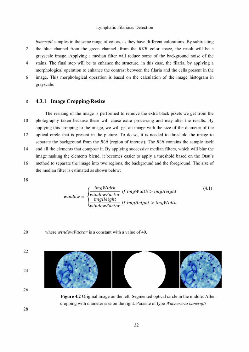
Lymphatic Filariasis Detection
32
bancrofti samples in the same range of colors, as they have different colorations. By subtracting
the blue channel from the green channel, from the color space, the result will be a 2
grayscale image. Applying a median filter will reduce some of the background noise of the
stains. The final step will be to enhance the structure, in this case, the filaria, by applying a 4
morphological operation to enhance the contrast between the filaria and the cells present in the
image. This morphological operation is based on the calculation of the image histogram in 6
grayscale.
4.3.1 Image Cropping/Resize 8
The resizing of the image is performed to remove the extra black pixels we get from the
photography taken because these will cause extra processing and may alter the results. By 10
applying this cropping to the image, we will get an image with the size of the diameter of the
optical circle that is present in the picture. To do so, it is needed to threshold the image to 12
separate the background from the ROI (region of interest). The ROI contains the sample itself
and all the elements that compose it. By applying successive median filters, which will blur the 14
image making the elements blend, it becomes easier to apply a threshold based on the Otsu’s
method to separate the image into two regions, the background and the foreground. The size of 16
the median filter is estimated as shown below:
18
{
(4.1)
where is a constant with a value of 40. 20
22
24
26
28
Figure 4.2 Original image on the left. Segmented optical circle in the middle. After
cropping with diameter size on the right. Parasite of type Wuchereria bancrofti
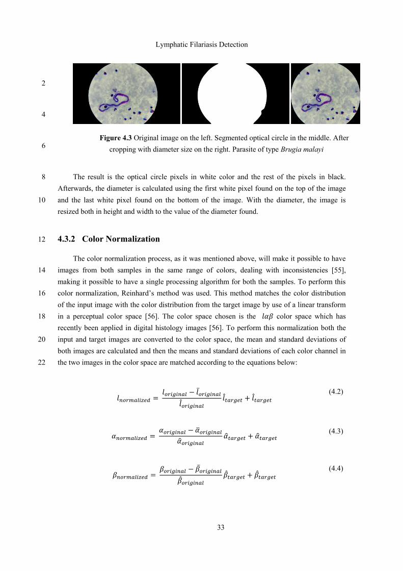
Lymphatic Filariasis Detection
33
2
4
6
The result is the optical circle pixels in white color and the rest of the pixels in black. 8
Afterwards, the diameter is calculated using the first white pixel found on the top of the image
and the last white pixel found on the bottom of the image. With the diameter, the image is 10
resized both in height and width to the value of the diameter found.
4.3.2 Color Normalization 12
The color normalization process, as it was mentioned above, will make it possible to have
images from both samples in the same range of colors, dealing with inconsistencies [55], 14
making it possible to have a single processing algorithm for both the samples. To perform this
color normalization, Reinhard’s method was used. This method matches the color distribution 16
of the input image with the color distribution from the target image by use of a linear transform
in a perceptual color space [56]. The color space chosen is the color space which has 18
recently been applied in digital histology images [56]. To perform this normalization both the
input and target images are converted to the color space, the mean and standard deviations of 20
both images are calculated and then the means and standard deviations of each color channel in
the two images in the color space are matched according to the equations below: 22
(4.2)
(4.3)
(4.4)
Figure 4.3 Original image on the left. Segmented optical circle in the middle. After
cropping with diameter size on the right. Parasite of type Brugia malayi
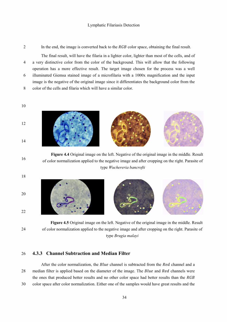
Lymphatic Filariasis Detection
34
In the end, the image is converted back to the color space, obtaining the final result. 2
The final result, will have the filaria in a lighter color, lighter than most of the cells, and of
a very distinctive color from the color of the background. This will allow that the following 4
operation has a more effective result. The target image chosen for the process was a well
illuminated Giemsa stained image of a microfilaria with a 1000x magnification and the input 6
image is the negative of the original image since it differentiates the background color from the
color of the cells and filaria which will have a similar color. 8
10
12
14
16
18
20
22
24
4.3.3 Channel Subtraction and Median Filter 26
After the color normalization, the channel is subtracted from the channel and a
median filter is applied based on the diameter of the image. The and channels were 28
the ones that produced better results and no other color space had better results than the
color space after color normalization. Either one of the samples would have great results and the 30
Figure 4.4 Original image on the left. Negative of the original image in the middle. Result
of color normalization applied to the negative image and after cropping on the right. Parasite of
type Wuchereria bancrofti
Figure 4.5 Original image on the left. Negative of the original image in the middle. Result
of color normalization applied to the negative image and after cropping on the right. Parasite of
type Brugia malayi
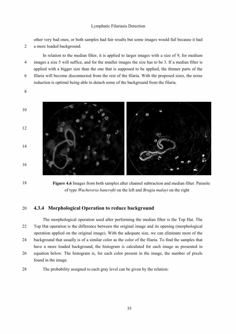
Lymphatic Filariasis Detection
35
other very bad ones, or both samples had fair results but some images would fail because it had
a more loaded background. 2
In relation to the median filter, it is applied to larger images with a size of 9, for medium
images a size 5 will suffice, and for the smaller images the size has to be 3. If a median filter is 4
applied with a bigger size than the one that is supposed to be applied, the thinner parts of the
filaria will become disconnected from the rest of the filaria. With the proposed sizes, the noise 6
reduction is optimal being able to detach some of the background from the filaria.
8
10
12
14
16
18
4.3.4 Morphological Operation to reduce background 20
The morphological operation used after performing the median filter is the Top Hat. The
Top Hat operation is the difference between the original image and its opening (morphological 22
operation applied on the original image). With the adequate size, we can eliminate most of the
background that usually is of a similar color as the color of the filaria. To find the samples that 24
have a more loaded background, the histogram is calculated for each image as presented in
equation below. The histogram is, for each color present in the image, the number of pixels 26
found in the image.
The probability assigned to each gray level can be given by the relation: 28
Figure 4.6 Images from both samples after channel subtraction and median filter. Parasite
of type Wuchereria bancrofti on the left and Brugia malayi on the right
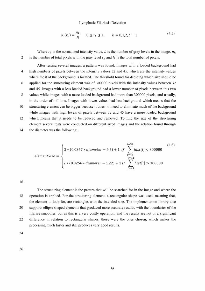
Lymphatic Filariasis Detection
36
( )
(4.5)
Where is the normalized intensity value, is the number of gray levels in the image,
is the number of total pixels with the gray level and is the total number of pixels. 2
After testing several images, a pattern was found. Images with a loaded background had
high numbers of pixels between the intensity values 32 and 45, which are the intensity values 4
where most of the background is located. The threshold found for deciding which size should be
applied for the structuring element was of 300000 pixels with the intensity values between 32 6
and 45. Images with a less loaded background had a lower number of pixels between this two
values while images with a more loaded background had more than 300000 pixels, and usually, 8
in the order of millions. Images with lower values had less background which means that the
structuring element can be bigger because it does not need to eliminate much of the background 10
while images with high levels of pixels between 32 and 45 have a more loaded background
which means that it needs to be reduced and removed. To find the size of the structuring 12
element several tests were conducted on different sized images and the relation found through
the diameter was the following: 14
{
( ) ∑ , -
( ) ∑ , -
(4.6)
16
The structuring element is the pattern that will be searched for in the image and where the
operation is applied. For the structuring element, a rectangular shape was used, meaning that, 18
the element to look for, are rectangles with the intended size. The implementation library also
supports ellipse shaped elements that produced more accurate results, with the boundaries of the 20
filariae smoother, but as this is a very costly operation, and the results are not of a significant
difference in relation to rectangular shapes, those were the ones chosen, which makes the 22
processing much faster and still produces very good results.
24
26
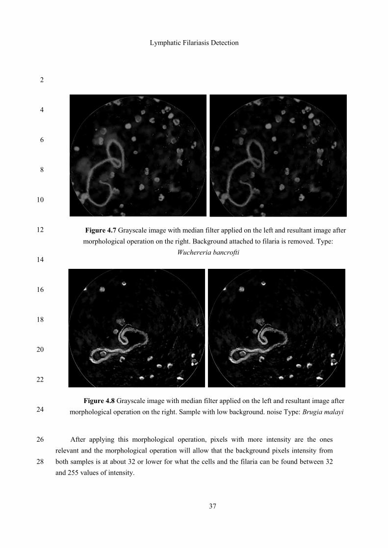
Lymphatic Filariasis Detection
37
2
4
6
8
10
12
14
16
18
20
22
24
After applying this morphological operation, pixels with more intensity are the ones 26
relevant and the morphological operation will allow that the background pixels intensity from
both samples is at about 32 or lower for what the cells and the filaria can be found between 32 28
and 255 values of intensity.
Figure 4.7 Grayscale image with median filter applied on the left and resultant image after
morphological operation on the right. Background attached to filaria is removed. Type:
Wuchereria bancrofti
Figure 4.8 Grayscale image with median filter applied on the left and resultant image after
morphological operation on the right. Sample with low background. noise Type: Brugia malayi
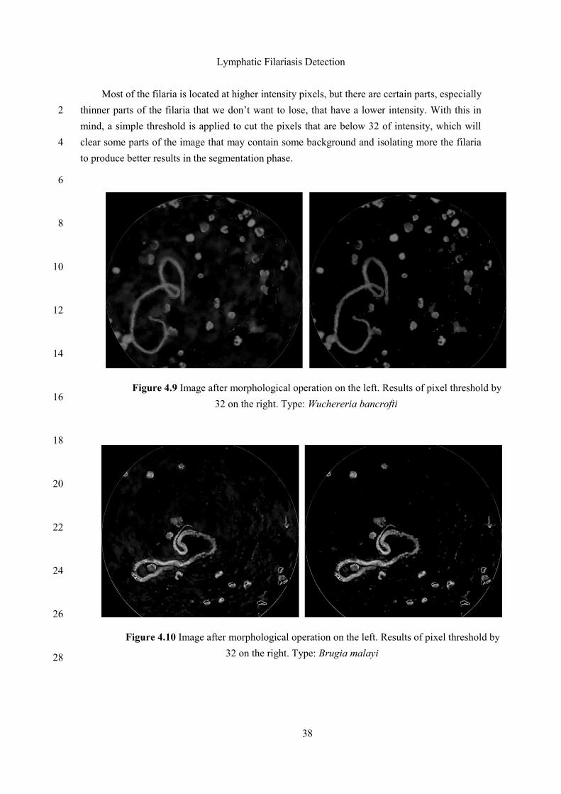
Lymphatic Filariasis Detection
38
Most of the filaria is located at higher intensity pixels, but there are certain parts, especially
thinner parts of the filaria that we don’t want to lose, that have a lower intensity. With this in 2
mind, a simple threshold is applied to cut the pixels that are below 32 of intensity, which will
clear some parts of the image that may contain some background and isolating more the filaria 4
to produce better results in the segmentation phase.
6
8
10
12
14
16
18
20
22
24
26
28
Figure 4.9 Image after morphological operation on the left. Results of pixel threshold by
32 on the right. Type: Wuchereria bancrofti
Figure 4.10 Image after morphological operation on the left. Results of pixel threshold by
32 on the right. Type: Brugia malayi
Lymphatic Filariasis Detection
39
4.4 Segmentation
The segmentation phase is where the regions of interest are isolated to be able to extract 2
features after. For this work, the regions of interest are the filariae, meaning that in the
segmentation phase, the aim is to remove everything that is not a filaria, or of importance to 4
maintain the structure of the filaria. Here, most of the cells that are within the sample will be
removed as well as the remaining background from the Pre-Processing. The segmentation 6
process has three phases. The first is to threshold the grayscale resulting image from pre-
processing, separating it in two different intensity values, 0 and 1, where 0 is black and 1 is 8
white, making it binary. The pixels with the highest intensity value will be the pixels that belong
to the interest regions, filaria, cells and background. Afterwards, another threshold is made, this 10
time an area thresholds to remove all the objects from the image that are smaller than a certain
size. This will remove the cells that are not attached to the filaria and the background. The latest 12
step, will be to remove the cells that are attached to the filaria because as they have a very
similar color to the filaria, they will be thresholded together with the filaria, making them one 14
single component.
4.4.1 Adaptive Threshold 16
To make the image binary, adaptive threshold was used. Adaptive threshold calculates a
threshold for small regions (mean of the block size of the neighborhood) instead of defining a 18
single threshold for the whole image. To calculate this threshold the adaptive Gaussian mean
function is being used. 20
( ) {
( ) ( )
(4.7)
( ) ( ) (4.8)
As there are varying lighting conditions on the samples, adaptive threshold produces a 22
much better result, whereas in the threshold performed through the Otsu’s Method, a single
threshold was found and the remaining of the background was segmented along with the filaria, 24
causing it to have background attached which would be difficult to remove afterwards.
26
28
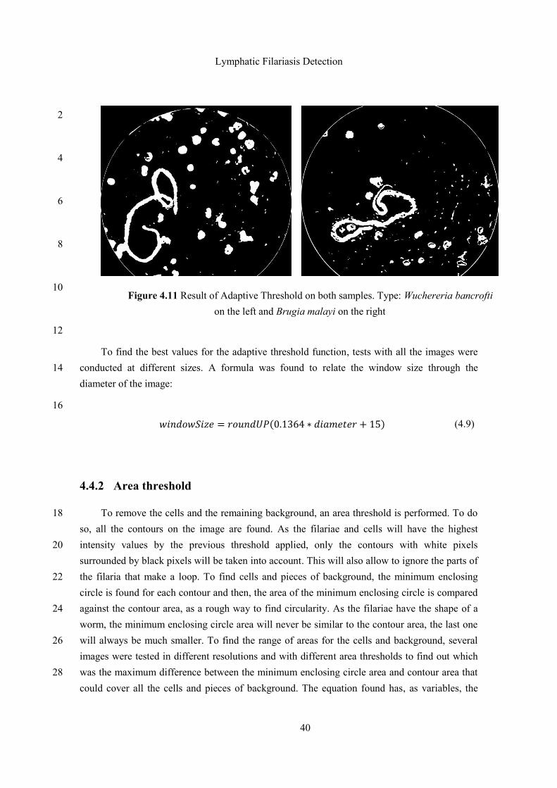
Lymphatic Filariasis Detection
40
2
4
6
8
10
12
To find the best values for the adaptive threshold function, tests with all the images were
conducted at different sizes. A formula was found to relate the window size through the 14
diameter of the image:
16
( ) (4.9)
4.4.2 Area threshold
To remove the cells and the remaining background, an area threshold is performed. To do 18
so, all the contours on the image are found. As the filariae and cells will have the highest
intensity values by the previous threshold applied, only the contours with white pixels 20
surrounded by black pixels will be taken into account. This will also allow to ignore the parts of
the filaria that make a loop. To find cells and pieces of background, the minimum enclosing 22
circle is found for each contour and then, the area of the minimum enclosing circle is compared
against the contour area, as a rough way to find circularity. As the filariae have the shape of a 24
worm, the minimum enclosing circle area will never be similar to the contour area, the last one
will always be much smaller. To find the range of areas for the cells and background, several 26
images were tested in different resolutions and with different area thresholds to find out which
was the maximum difference between the minimum enclosing circle area and contour area that 28
could cover all the cells and pieces of background. The equation found has, as variables, the
Figure 4.11 Result of Adaptive Threshold on both samples. Type: Wuchereria bancrofti
on the left and Brugia malayi on the right
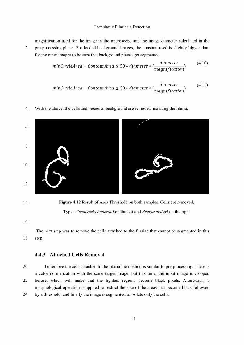
Lymphatic Filariasis Detection
41
magnification used for the image in the microscope and the image diameter calculated in the
pre-processing phase. For loaded background images, the constant used is slightly bigger than 2
for the other images to be sure that background pieces get segmented.
(
)
(4.10)
(
)
(4.11)
With the above, the cells and pieces of background are removed, isolating the filaria. 4
6
8
10
12
14
16
The next step was to remove the cells attached to the filariae that cannot be segmented in this
step. 18
4.4.3 Attached Cells Removal
To remove the cells attached to the filaria the method is similar to pre-processing. There is 20
a color normalization with the same target image, but this time, the input image is cropped
before, which will make that the lightest regions become black pixels. Afterwards, a 22
morphological operation is applied to restrict the size of the areas that become black followed
by a threshold, and finally the image is segmented to isolate only the cells. 24
Figure 4.12 Result of Area Threshold on both samples. Cells are removed.
Type: Wuchereria bancrofti on the left and Brugia malayi on the right
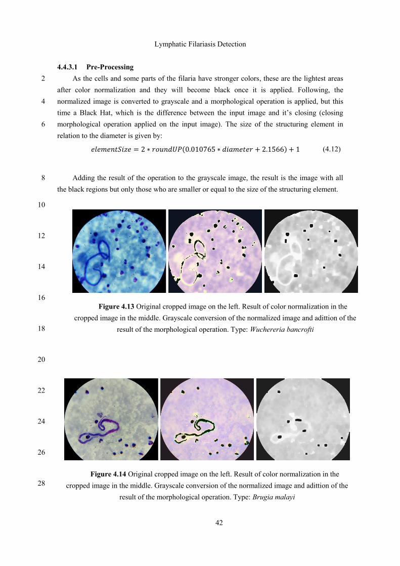
Lymphatic Filariasis Detection
42
4.4.3.1 Pre-Processing
As the cells and some parts of the filaria have stronger colors, these are the lightest areas 2
after color normalization and they will become black once it is applied. Following, the
normalized image is converted to grayscale and a morphological operation is applied, but this 4
time a Black Hat, which is the difference between the input image and it’s closing (closing
morphological operation applied on the input image). The size of the structuring element in 6
relation to the diameter is given by:
( ) (4.12)
Adding the result of the operation to the grayscale image, the result is the image with all 8
the black regions but only those who are smaller or equal to the size of the structuring element.
10
12
14
16
18
20
22
24
26
28
Figure 4.13 Original cropped image on the left. Result of color normalization in the
cropped image in the middle. Grayscale conversion of the normalized image and adittion of the
result of the morphological operation. Type: Wuchereria bancrofti
Figure 4.14 Original cropped image on the left. Result of color normalization in the
cropped image in the middle. Grayscale conversion of the normalized image and adittion of the
result of the morphological operation. Type: Brugia malayi
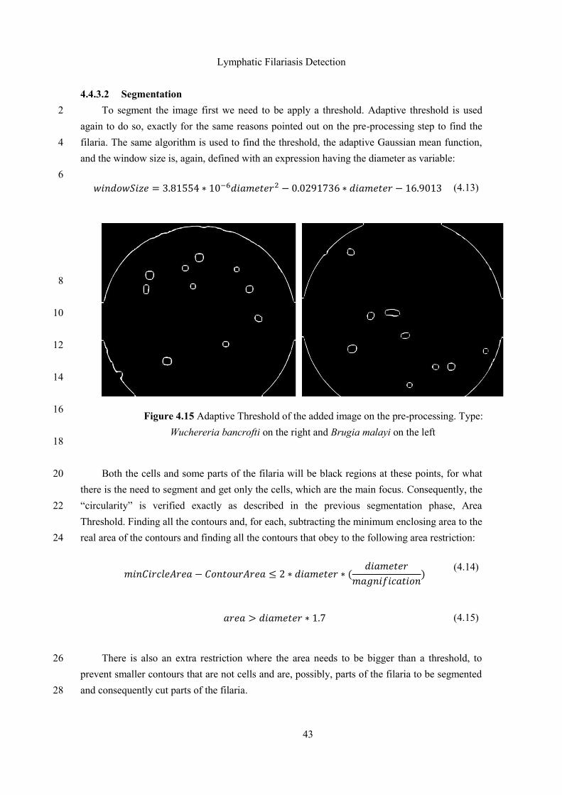
Lymphatic Filariasis Detection
43
4.4.3.2 Segmentation
To segment the image first we need to be apply a threshold. Adaptive threshold is used 2
again to do so, exactly for the same reasons pointed out on the pre-processing step to find the
filaria. The same algorithm is used to find the threshold, the adaptive Gaussian mean function, 4
and the window size is, again, defined with an expression having the diameter as variable:
6
(4.13)
8
10
12
14
16
18
Both the cells and some parts of the filaria will be black regions at these points, for what 20
there is the need to segment and get only the cells, which are the main focus. Consequently, the
“circularity” is verified exactly as described in the previous segmentation phase, Area 22
Threshold. Finding all the contours and, for each, subtracting the minimum enclosing area to the
real area of the contours and finding all the contours that obey to the following area restriction: 24
(
)
(4.14)
(4.15)
There is also an extra restriction where the area needs to be bigger than a threshold, to 26
prevent smaller contours that are not cells and are, possibly, parts of the filaria to be segmented
and consequently cut parts of the filaria. 28
Figure 4.15 Adaptive Threshold of the added image on the pre-processing. Type:
Wuchereria bancrofti on the right and Brugia malayi on the left
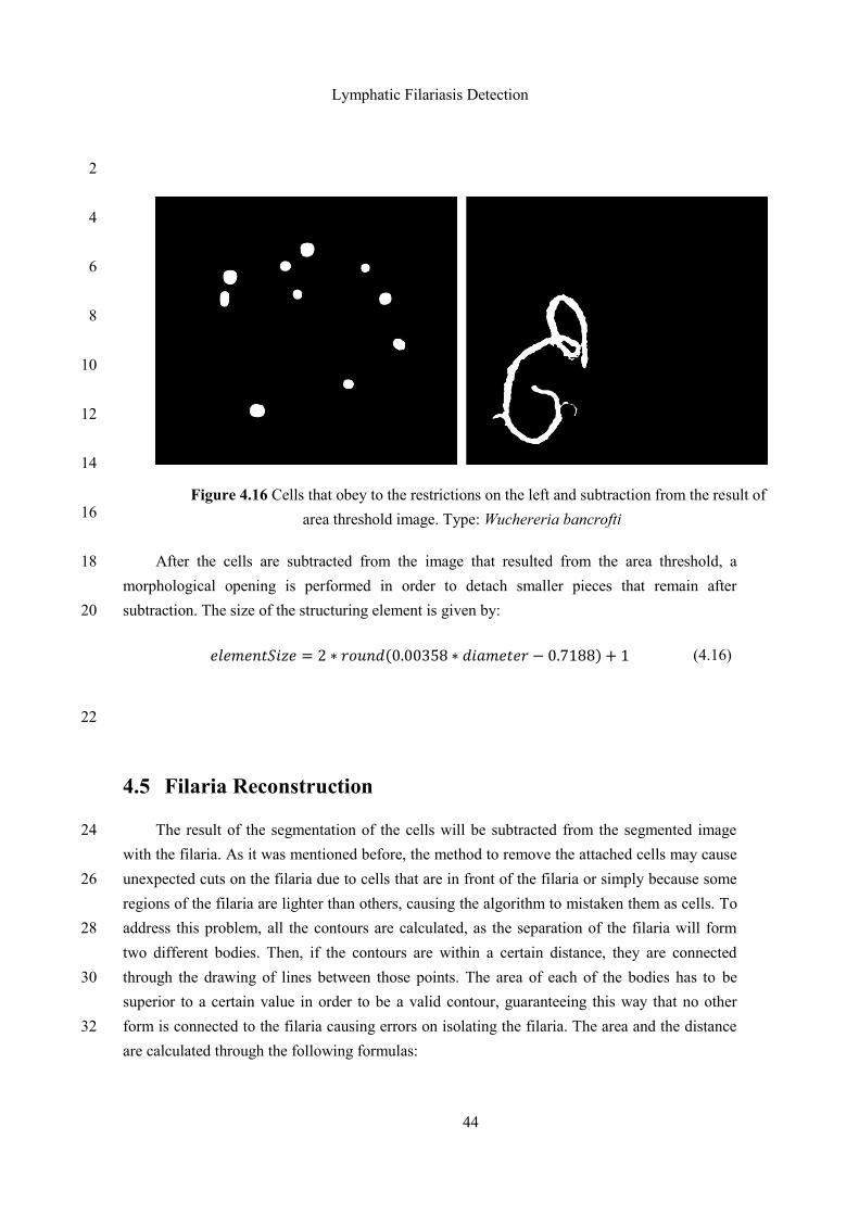
Lymphatic Filariasis Detection
44
2
4
6
8
10
12
14
16
After the cells are subtracted from the image that resulted from the area threshold, a 18
morphological opening is performed in order to detach smaller pieces that remain after
subtraction. The size of the structuring element is given by: 20
( ) (4.16)
22
4.5 Filaria Reconstruction
The result of the segmentation of the cells will be subtracted from the segmented image 24
with the filaria. As it was mentioned before, the method to remove the attached cells may cause
unexpected cuts on the filaria due to cells that are in front of the filaria or simply because some 26
regions of the filaria are lighter than others, causing the algorithm to mistaken them as cells. To
address this problem, all the contours are calculated, as the separation of the filaria will form 28
two different bodies. Then, if the contours are within a certain distance, they are connected
through the drawing of lines between those points. The area of each of the bodies has to be 30
superior to a certain value in order to be a valid contour, guaranteeing this way that no other
form is connected to the filaria causing errors on isolating the filaria. The area and the distance 32
are calculated through the following formulas:
Figure 4.16 Cells that obey to the restrictions on the left and subtraction from the result of
area threshold image. Type: Wuchereria bancrofti
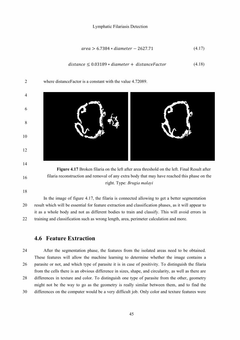
Lymphatic Filariasis Detection
45
(4.17)
(4.18)
where distanceFactor is a constant with the value 4.72089. 2
4
6
8
10
12
14
16
18
In the image of figure 4.17, the filaria is connected allowing to get a better segmentation
result which will be essential for feature extraction and classification phases, as it will appear to 20
it as a whole body and not as different bodies to train and classify. This will avoid errors in
training and classification such as wrong length, area, perimeter calculation and more. 22
4.6 Feature Extraction
After the segmentation phase, the features from the isolated areas need to be obtained. 24
These features will allow the machine learning to determine whether the image contains a
parasite or not, and which type of parasite it is in case of positivity. To distinguish the filaria 26
from the cells there is an obvious difference in sizes, shape, and circularity, as well as there are
differences in texture and color. To distinguish one type of parasite from the other, geometry 28
might not be the way to go as the geometry is really similar between them, and to find the
differences on the computer would be a very difficult job. Only color and texture features were 30
Figure 4.17 Broken filaria on the left after area threshold on the left. Final Result after
filaria reconstruction and removal of any extra body that may have reached this phase on the
right. Type: Brugia malayi
Lymphatic Filariasis Detection
46
capable of that distinction and consequently used here. As one type has disperse nuclei in the
body and the other has a body loaded with nuclei the differences will be clear. 2
So, three main groups of features were extracted: color features, texture features and
geometry features. 4
4.6.1 Color & Texture Features 6
For color and texture features there are two types of statistics that can be obtained from a
texture analysis. The first and second order statistics [57]. 8
First-order statistics can be taken from a calculated histogram of an image to quantitatively
describe the first-order statistical properties of the image [57]: 10
Mean. Average level of intensity
12
Variance. Variation of intensity around the mean
14
Skewness. Zero if histogram symmetrical around the mean, positive or negative depending
if it has been skewed above or lower the mean. 16
Kurtosis. Measure for flatness of the histogram. 18
20
Energy.
∑ ( )
(4.19)
Entropy. Measure of histogram uniformity. 22
∑ ( )
( ( )) (4.20)
For color features these calculations are made for color space.
Lymphatic Filariasis Detection
47
Second-order statistics are defined as the co-ocurrence matrix which is a square matrix of
dimension equal to the number of intensity levels in the image, for each distance and 2
orientation. As it has too many elements for texture analysis, some features can be calculated
using the co-ocurrence matrix to discriminate the texture and avoid costly computations: 4
Contrast. 6
∑
( ) (4.21)
Correlation. 8
∑
( )( )( )
(4.22)
Homogeneity.
∑
( )( )( )
(4.23)
10
Inverse Difference.
∑∑ ( )
( )
(5.4)
12
Entropy.
∑∑ ( )
( ( ))
(4.24)
14
16
Lymphatic Filariasis Detection
48
Maximum Probability.
( ) (4.25)
2
4
Absolute Value.
∑ ∑ ( )
(4.26)
4.6.2 Geometry Features 6
Geometry features can be obtained through boundary points, contour-based methods. Such
features are perimeter, perimeter-resultant measures such as area, circularity, solidity and so on. 8
Below, there are some shape based features presented and their calculation method [58]:
Area. Area of the shape that can be obtained through contour. 10
Perimeter. Perimeter of the shape that can be obtained through contours.
Convex Hull. Smallest convex that contains a shape. 12
Convexity. Ratio between the perimeter of the convex hull and the original shape.
14
(4.27)
16
Solidity. Whether a shape is convex or concave. Convex shapes have value 1 of Solidity.
18
(4.28)

Lymphatic Filariasis Detection
49
Circularity. How close is a shape from a circular form. 2
(4.29)
Rectangularity. How close is a shape from a rectangular form. 4
(4.30)
Thinness Ratio. 6
(4.31)
Euler Number. Difference between the contiguous parts and the number of holes in an 8
image.
10
(4.32)
Holes Area Ratio. Ratio between the sum of the holes areas and the area of the shape
12
(4.33)
14
16
Lymphatic Filariasis Detection
50
Eccentricity. It is the measure of aspect ratio and can be calculated through the ratio of the
length of major axis to the length of the minor axis. 2
(4.34)
4
Minimum Bounding Box Area. Minimum bounding box is the smallest rectangle that 6
contains every point of the shape. In the minimum bounding box the major axis is the length
and the minor axis the width. Therefore, the area of a rectangle is so: 8
(4.35)
10
Elongation. Another concept based on eccentricity. Shapes with large ratio will have an
elongation of 1 while shapes that are more symmetric will have an elongation of 0. 12
√
(4.36)
14
Minimum Enclosing Circle. Smallest circle that contains every point of the shape. Here, 16
the area, perimeter, radius of the circle can be obtained.
18
∑ ( )( )
(4.37)
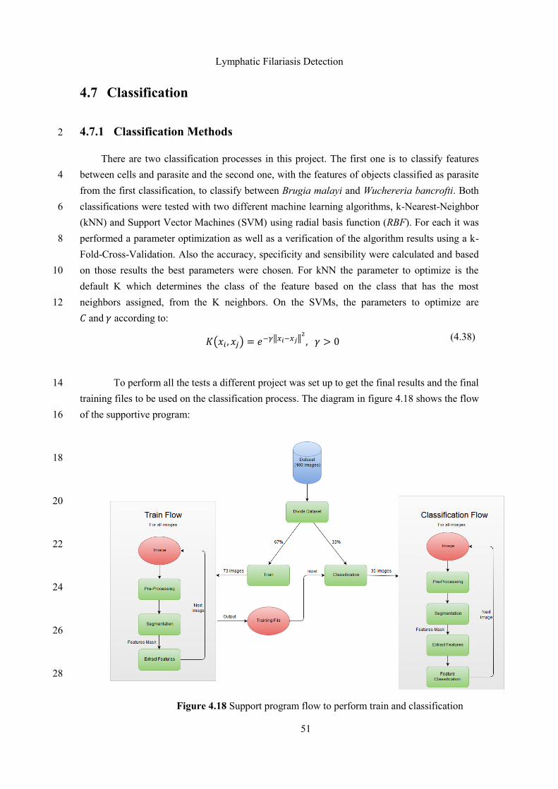
Lymphatic Filariasis Detection
51
4.7 Classification
4.7.1 Classification Methods 2
There are two classification processes in this project. The first one is to classify features
between cells and parasite and the second one, with the features of objects classified as parasite 4
from the first classification, to classify between Brugia malayi and Wuchereria bancrofti. Both
classifications were tested with two different machine learning algorithms, k-Nearest-Neighbor 6
(kNN) and Support Vector Machines (SVM) using radial basis function (RBF). For each it was
performed a parameter optimization as well as a verification of the algorithm results using a k-8
Fold-Cross-Validation. Also the accuracy, specificity and sensibility were calculated and based
on those results the best parameters were chosen. For kNN the parameter to optimize is the 10
default K which determines the class of the feature based on the class that has the most
neighbors assigned, from the K neighbors. On the SVMs, the parameters to optimize are 12
and according to:
( ) ‖ ‖
(4.38)
To perform all the tests a different project was set up to get the final results and the final 14
training files to be used on the classification process. The diagram in figure 4.18 shows the flow
of the supportive program: 16
18
20
22
24
26
28
Figure 4.18 Support program flow to perform train and classification
Lymphatic Filariasis Detection
52
The training and classification images were obtained by using the Monte Carlo’s 2
algorithm with image balancing where 67% of the dataset is for training and the remaining 33%
for classification dividing the dataset into 73 images for training and 36 images for 4
classification.
4.7.2 Classification Results 6
Both the kNN and SVM got impressive levels of accuracy when optimized. This also
depended on the features used in the training. To differentiate between cells and parasite, 8
geometry is a very important feature because the size of the filaria by itself will be a
determining parameter, but to differentiate between both types of parasite the geometry features 10
would confuse the algorithm and get lower results so the best way to differentiate both types is
to use only color and texture features as the texture from both filariae has significant 12
differences.
With the results presented in tables 4.1 and 4.2 the chosen algorithm was the SVM 14
using a radial basis function for both the first and second SVMs. The optimization process was
conducted by performing training and classification with different parameters and adjusting 16
them according to the previous results. The best results were with SVMs that had lower than 1
and for both, the SVM using with the value of 0.1 and with the value of 1 got optimal 18
results. For the first SVM it was needed to set class weights due to the disparity between the
positive and negative masks. The first SVM is the one to classify between parasite and cells and 20
the number of parasite features was of 76 while the number of negative features was of 16448
features in training. By setting class weights, the SVM knows of this disparity and classifies 22
based on it. Without the class weights the SVM failed in every classification, classifying
everything as cells but when the class weights were added the SVM produced optimal results. 24
For the second SVM this was not needed as the images used for training were evenly distributed
(55 belonging to the first sample and 54 belonging to the second). 26
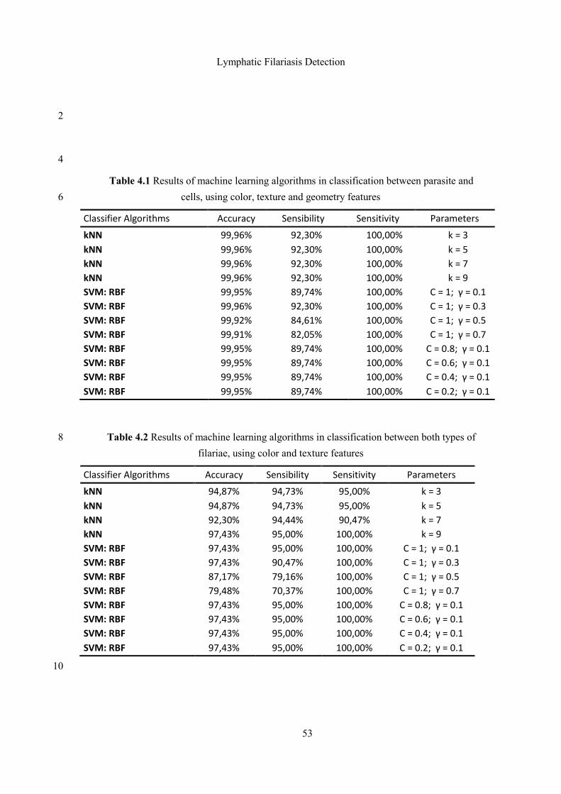
Lymphatic Filariasis Detection
53
2
4
Table 4.1 Results of machine learning algorithms in classification between parasite and
cells, using color, texture and geometry features 6
Classifier Algorithms Accuracy Sensibility Sensitivity Parameters
kNN 99,96% 92,30% 100,00% k = 3
kNN 99,96% 92,30% 100,00% k = 5
kNN 99,96% 92,30% 100,00% k = 7
kNN 99,96% 92,30% 100,00% k = 9
SVM: RBF 99,95% 89,74% 100,00% C = 1; γ = 0.1
SVM: RBF 99,96% 92,30% 100,00% C = 1; γ = 0.3
SVM: RBF 99,92% 84,61% 100,00% C = 1; γ = 0.5
SVM: RBF 99,91% 82,05% 100,00% C = 1; γ = 0.7
SVM: RBF 99,95% 89,74% 100,00% C = 0.8; γ = 0.1
SVM: RBF 99,95% 89,74% 100,00% C = 0.6; γ = 0.1
SVM: RBF 99,95% 89,74% 100,00% C = 0.4; γ = 0.1
SVM: RBF 99,95% 89,74% 100,00% C = 0.2; γ = 0.1
Table 4.2 Results of machine learning algorithms in classification between both types of 8
filariae, using color and texture features
Classifier Algorithms Accuracy Sensibility Sensitivity Parameters
kNN 94,87% 94,73% 95,00% k = 3
kNN 94,87% 94,73% 95,00% k = 5
kNN 92,30% 94,44% 90,47% k = 7
kNN 97,43% 95,00% 100,00% k = 9
SVM: RBF 97,43% 95,00% 100,00% C = 1; γ = 0.1
SVM: RBF 97,43% 90,47% 100,00% C = 1; γ = 0.3
SVM: RBF 87,17% 79,16% 100,00% C = 1; γ = 0.5
SVM: RBF 79,48% 70,37% 100,00% C = 1; γ = 0.7
SVM: RBF 97,43% 95,00% 100,00% C = 0.8; γ = 0.1
SVM: RBF 97,43% 95,00% 100,00% C = 0.6; γ = 0.1
SVM: RBF 97,43% 95,00% 100,00% C = 0.4; γ = 0.1
SVM: RBF 97,43% 95,00% 100,00% C = 0.2; γ = 0.1
10
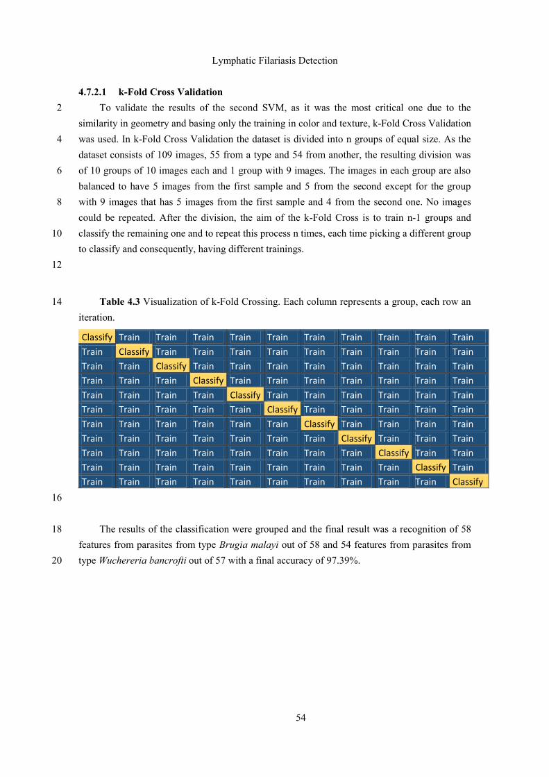
Lymphatic Filariasis Detection
54
4.7.2.1 k-Fold Cross Validation
To validate the results of the second SVM, as it was the most critical one due to the 2
similarity in geometry and basing only the training in color and texture, k-Fold Cross Validation
was used. In k-Fold Cross Validation the dataset is divided into n groups of equal size. As the 4
dataset consists of 109 images, 55 from a type and 54 from another, the resulting division was
of 10 groups of 10 images each and 1 group with 9 images. The images in each group are also 6
balanced to have 5 images from the first sample and 5 from the second except for the group
with 9 images that has 5 images from the first sample and 4 from the second one. No images 8
could be repeated. After the division, the aim of the k-Fold Cross is to train n-1 groups and
classify the remaining one and to repeat this process n times, each time picking a different group 10
to classify and consequently, having different trainings.
12
Table 4.3 Visualization of k-Fold Crossing. Each column represents a group, each row an 14
iteration.
Classify Train Train Train Train Train Train Train Train Train Train
Train Classify Train Train Train Train Train Train Train Train Train
Train Train Classify Train Train Train Train Train Train Train Train
Train Train Train Classify Train Train Train Train Train Train Train
Train Train Train Train Classify Train Train Train Train Train Train
Train Train Train Train Train Classify Train Train Train Train Train
Train Train Train Train Train Train Classify Train Train Train Train
Train Train Train Train Train Train Train Classify Train Train Train
Train Train Train Train Train Train Train Train Classify Train Train
Train Train Train Train Train Train Train Train Train Classify Train
Train Train Train Train Train Train Train Train Train Train Classify
16
The results of the classification were grouped and the final result was a recognition of 58 18
features from parasites from type Brugia malayi out of 58 and 54 features from parasites from
type Wuchereria bancrofti out of 57 with a final accuracy of 97.39%. 20

Lymphatic Filariasis Detection
55
2
4
Table 4.4 Results of the classification with the optimized SVM
Brugia malayi Wuchereria bancrofti
Brugia malayi 58 0
Wuchereria bancrofti 3 54
Classifier Algorithm Parameters Accuracy
SVM: RBF C = 1; γ = 0.1 97,39%
6
8
Image Processing in Android
56
Chapter 5
Image Processing in Android 2
The ultimate goal of this thesis work was to develop an automated image processing
methodology capable of detecting and classifying between the two types of filariae. This 4
automated methodology is to be integrated in the MalariaScope project, especially in its mobile-
application. In this chapter the MalariaScope project is presented as well as the application. 6
Later, the integration of the image processing methodology developed with the MalariaScope
application will be addressed. 8
5.1 Integration with MalariaScope Project 10
The MalariaScope project is a mobile-based solution to provide automatic detection of
Malaria in blood samples. It is used as a cheap alternative to microscopes, constituting a 12
prototype developed by Fraunhofer to obtain images from a blood sample which will be
analyzed with an automated image processing tool to detect the malaria parasite. The analysis to 14
perform has two main stages: the determination of the parasite density in a blood sample and the
identification of the species. As Lymphatic Filariasis is a severe problem in regions like Africa 16
where it is difficult the access to health specialists, medical equipment and staff to process all
the cases that exist, an automated tool would be a life changer and that is where this project 18
comes in. The idea is to use the same prototype and application for different automated image
processing methodologies in order to automate the detection of certain parasites which allows 20
anyone to use the application without the need of a specialist or an expensive microscope.
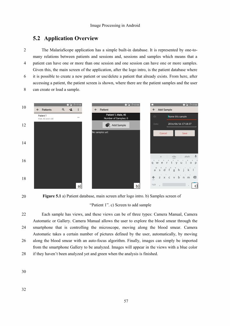
Image Processing in Android
57
5.2 Application Overview
The MalariaScope application has a simple built-in database. It is represented by one-to-2
many relations between patients and sessions and, sessions and samples which means that a
patient can have one or more than one session and one session can have one or more samples. 4
Given this, the main screen of the application, after the logo intro, is the patient database where
it is possible to create a new patient or use/delete a patient that already exists. From here, after 6
accessing a patient, the patient screen is shown, where there are the patient samples and the user
can create or load a sample. 8
10
12
14
16
18
20
Each sample has views, and these views can be of three types: Camera Manual, Camera 22
Automatic or Gallery. Camera Manual allows the user to explore the blood smear through the
smartphone that is controlling the microscope, moving along the blood smear. Camera 24
Automatic takes a certain number of pictures defined by the user, automatically, by moving
along the blood smear with an auto-focus algorithm. Finally, images can simply be imported 26
from the smartphone Gallery to be analyzed. Images will appear in the views with a blue color
if they haven’t been analyzed yet and green when the analysis is finished. 28
30
32
Figure 5.1 a) Patient database, main screen after logo intro. b) Samples screen of
“Patient 1”. c) Screen to add sample
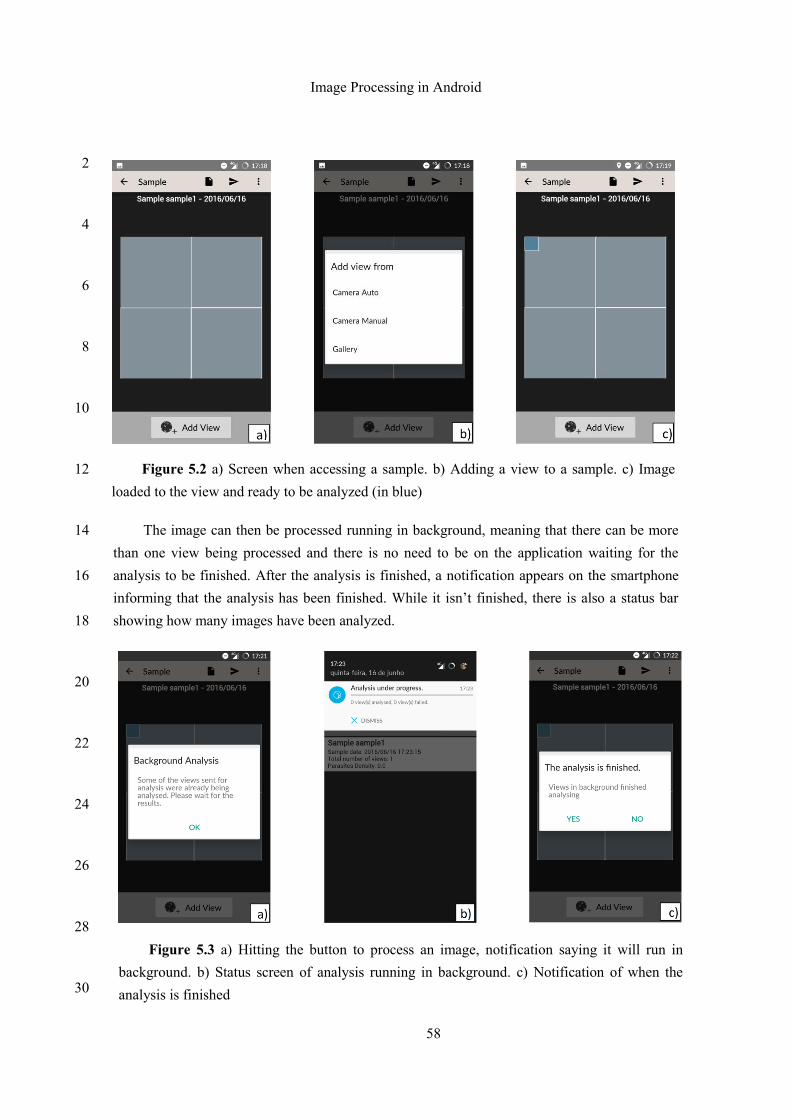
Image Processing in Android
58
2
4
6
8
10
12
The image can then be processed running in background, meaning that there can be more 14
than one view being processed and there is no need to be on the application waiting for the
analysis to be finished. After the analysis is finished, a notification appears on the smartphone 16
informing that the analysis has been finished. While it isn’t finished, there is also a status bar
showing how many images have been analyzed. 18
20
22
24
26
28
30
Figure 5.2 a) Screen when accessing a sample. b) Adding a view to a sample. c) Image
loaded to the view and ready to be analyzed (in blue)
Figure 5.3 a) Hitting the button to process an image, notification saying it will run in
background. b) Status screen of analysis running in background. c) Notification of when the
analysis is finished
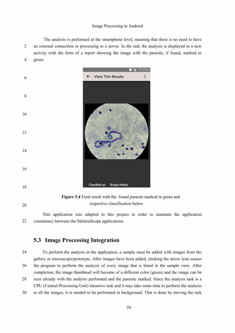
Image Processing in Android
59
The analysis is performed at the smartphone level, meaning that there is no need to have
an external connection or processing to a server. In the end, the analysis is displayed in a new 2
activity with the form of a report showing the image with the parasite, if found, marked in
green. 4
6
8
10
12
14
16
18
20
This application was adapted to this project in order to maintain the application
consistency between the MalariaScope applications. 22
5.3 Image Processing Integration
To perform the analysis in the application, a sample must be added with images from the 24
gallery or microscope/prototype. After images have been added, clicking the arrow icon causes
the program to perform the analysis of every image that is listed in the sample view. After 26
completion, the image thumbnail will become of a different color (green) and the image can be
seen already with the analysis performed and the parasite marked. Since the analysis task is a 28
CPU (Central-Processing-Unit) intensive task and it may take some time to perform the analysis
to all the images, it is needed to be performed in background. That is done by moving the task 30
Figure 5.4 Final result with the found parasite marked in green and
respective classification below
Image Processing in Android
60
from the User-Interface thread to another thread created by the class IntentService which
handles each request in turn using a worker thread. Therefore, the user can be viewing the 2
results or performing other analysis while the application is performing the image processing
operations. 4
The image processing methodology was integrated in the application using JNI (Java
Native Interface), which defines a way for managed code written in Java to interact with native 6
code written in C++. This way, the Java code can invoke the local functions written in C++. But
this is not enough as it is needed a cross-development tool to compile the C++ code. The tool, 8
supplied by Google, is the Android NDK (Native Development Kit). The NDK will allow the
application to run on Android devices. With the NDK there is direct access to the CPU and 10
hardware, and OpenCV functions in Java can be optimized invoking implementations in C++.
NDK is therefore, the right option to choose to integrate the methodology in native code, even 12
though it will need to be compiled for every architecture in order to work on the majority of
Android devices. OpenCV also has the libraries prepared for Android which need to be 14
integrated in the application in order to recognize the OpenCV functions. This is as simple as
add a module to the project and import the OpenCV Android module that can be downloaded 16
from their main page.
18
Results
61
Chapter 6
Results 2
In this chapter the results from segmentation and classification will be presented. Several
classifications with different features and different algorithms were performed in order to 4
choose the best classification algorithm with optimized parameters. The results for these
classifications will be presented in this chapter as well as a discussion about the different 6
classifications and consequently, the conclusions to be drawn. Afterwards, a discussion about
the deficiencies and strong points of the methodology will be addressed. 8
6.1 Results & Discussion
10
The segmentation phase was able to detect and segment all the filariae in the dataset. With
the dataset used, it is guaranteed that the filariae will be present in the final image. However, 12
some of the images may have some background or remaining cells from the attached cells
removal method in section 4.4.3 attached to the filaria. Therefore, to evaluate the segmentation 14
phase results, resulting images were assigned to 4 groups. Images of the filaria after
segmentation that have no background attached to its boundaries and no remaining cells were 16
considered well isolated, figure 6.1. Images with a low amount of background or one cell
attached to the filaria were assigned to the + group, figure 6.1. Images with a significant amount 18
of background attached to the boundaries or more than one cell were assigned to the ++ group
figure 6.2 For the contrary, images where the filaria is not complete (overly segmented) these 20
images were assigned to the – group, figure 6.2.
22
24
26
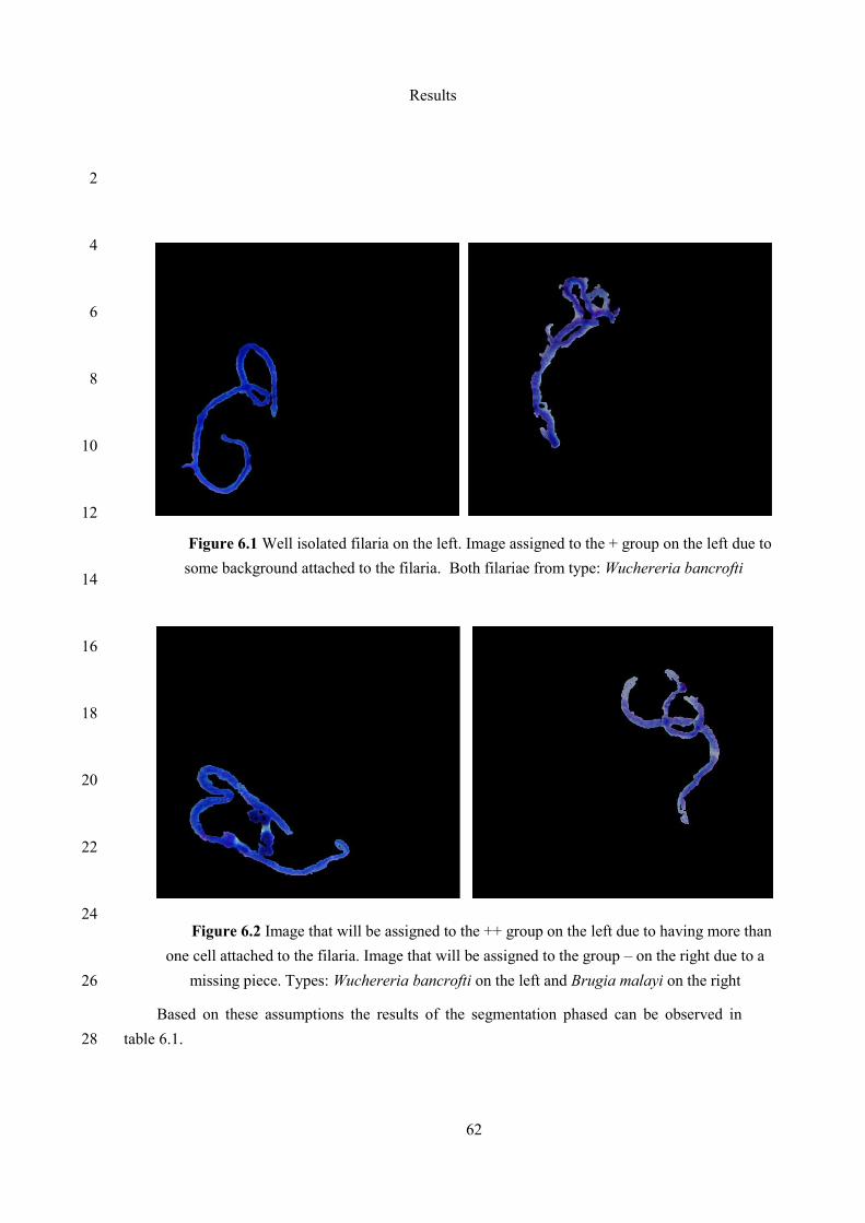
Results
62
2
4
6
8
10
12
14
16
18
20
22
24
26
Based on these assumptions the results of the segmentation phased can be observed in
table 6.1. 28
Figure 6.1 Well isolated filaria on the left. Image assigned to the + group on the left due to
some background attached to the filaria. Both filariae from type: Wuchereria bancrofti
Figure 6.2 Image that will be assigned to the ++ group on the left due to having more than
one cell attached to the filaria. Image that will be assigned to the group – on the right due to a
missing piece. Types: Wuchereria bancrofti on the left and Brugia malayi on the right
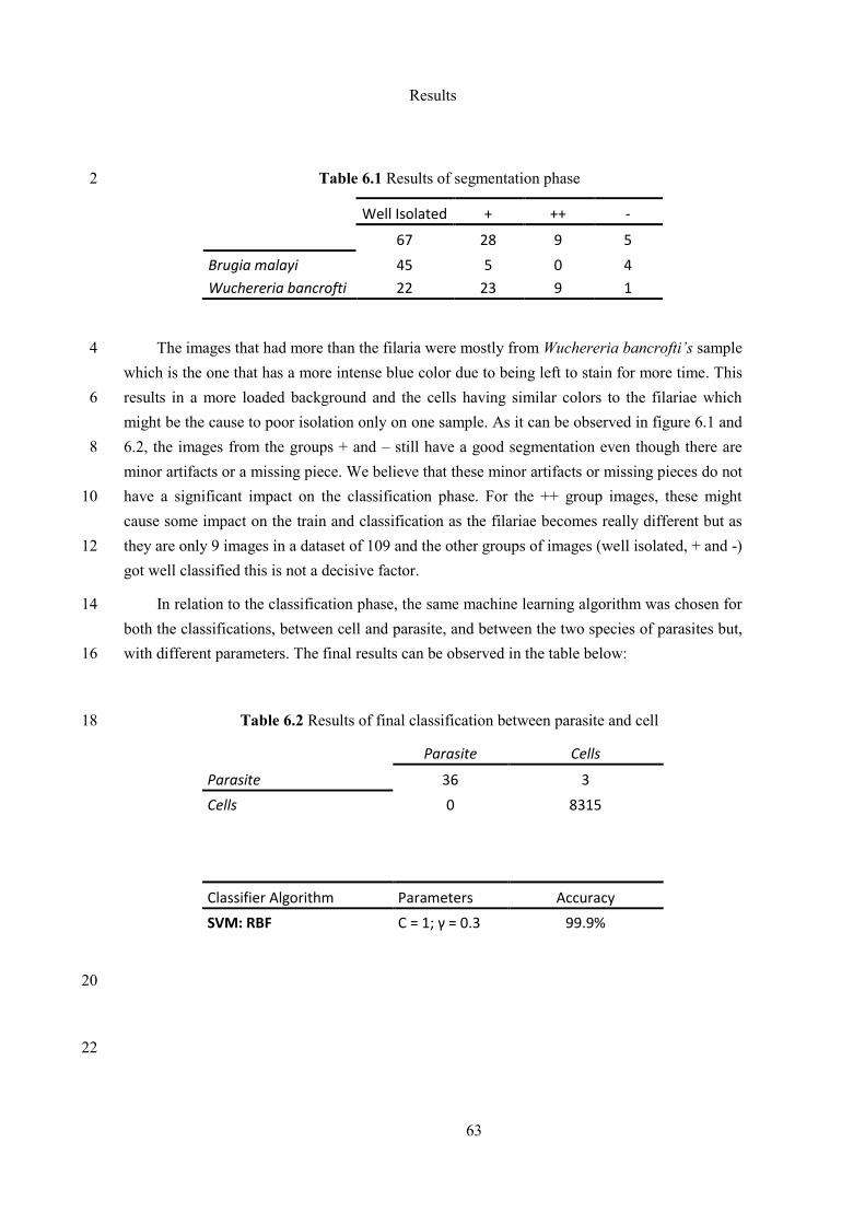
Results
63
Table 6.1 Results of segmentation phase 2
Well Isolated + ++ -
67 28 9 5
Brugia malayi 45 5 0 4
Wuchereria bancrofti 22 23 9 1
The images that had more than the filaria were mostly from Wuchereria bancrofti’s sample 4
which is the one that has a more intense blue color due to being left to stain for more time. This
results in a more loaded background and the cells having similar colors to the filariae which 6
might be the cause to poor isolation only on one sample. As it can be observed in figure 6.1 and
6.2, the images from the groups + and – still have a good segmentation even though there are 8
minor artifacts or a missing piece. We believe that these minor artifacts or missing pieces do not
have a significant impact on the classification phase. For the ++ group images, these might 10
cause some impact on the train and classification as the filariae becomes really different but as
they are only 9 images in a dataset of 109 and the other groups of images (well isolated, + and -) 12
got well classified this is not a decisive factor.
In relation to the classification phase, the same machine learning algorithm was chosen for 14
both the classifications, between cell and parasite, and between the two species of parasites but,
with different parameters. The final results can be observed in the table below: 16
Table 6.2 Results of final classification between parasite and cell 18
Parasite Cells
Parasite 36 3
Cells 0 8315
Classifier Algorithm Parameters Accuracy
SVM: RBF C = 1; γ = 0.3 99.9%
20
22
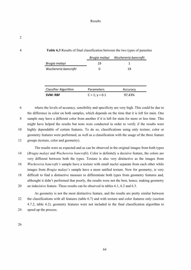
Results
64
2
Table 6.3 Results of final classification between the two types of parasites 4
Brugia malayi Wuchereria bancrofti
Brugia malayi 19 1
Wuchereria bancrofti 0 19
Classifier Algorithm Parameters Accuracy
SVM: RBF C = 1; γ = 0.1 97,43%
where the levels of accuracy, sensibility and specificity are very high. This could be due to 6
the difference in color on both samples, which depends on the time that it is left for stain. One
sample may have a different color from another if it is left for stain for more or less time. This 8
might have helped the results but tests were conducted in order to verify if the results were
highly dependable of certain features. To do so, classifications using only texture, color or 10
geometry features were performed, as well as a classification with the usage of the three feature
groups (texture, color and geometry). 12
The results were as expected and as can be observed in the original images from both types
(Brugia malayi and Wuchereria bancrofti). Color is definitely a decisive feature, the colors are 14
very different between both the types. Texture is also very distinctive as the images from
Wuchereria bancrofti’s sample have a texture with small nuclei separate from each other while 16
images from Brugia malayi’s sample have a more unified texture. Now for geometry, is very
difficult to find a distinctive measure to differentiate both types from geometry features and, 18
althought it didn’t performed that poorly, the results were not the best, hence, making geometry
an indecisive feature. These results can be observed in tables 6.1, 6.2 and 6.3. 20
As geometry is not the most distinctive feature, and the results are pretty similar between
the classifications with all features (table 6.7) and with texture and color features only (section 22
4.7.2, table 4.2), geometry features were not included in the final classification algorithm to
speed up the process. 24
26
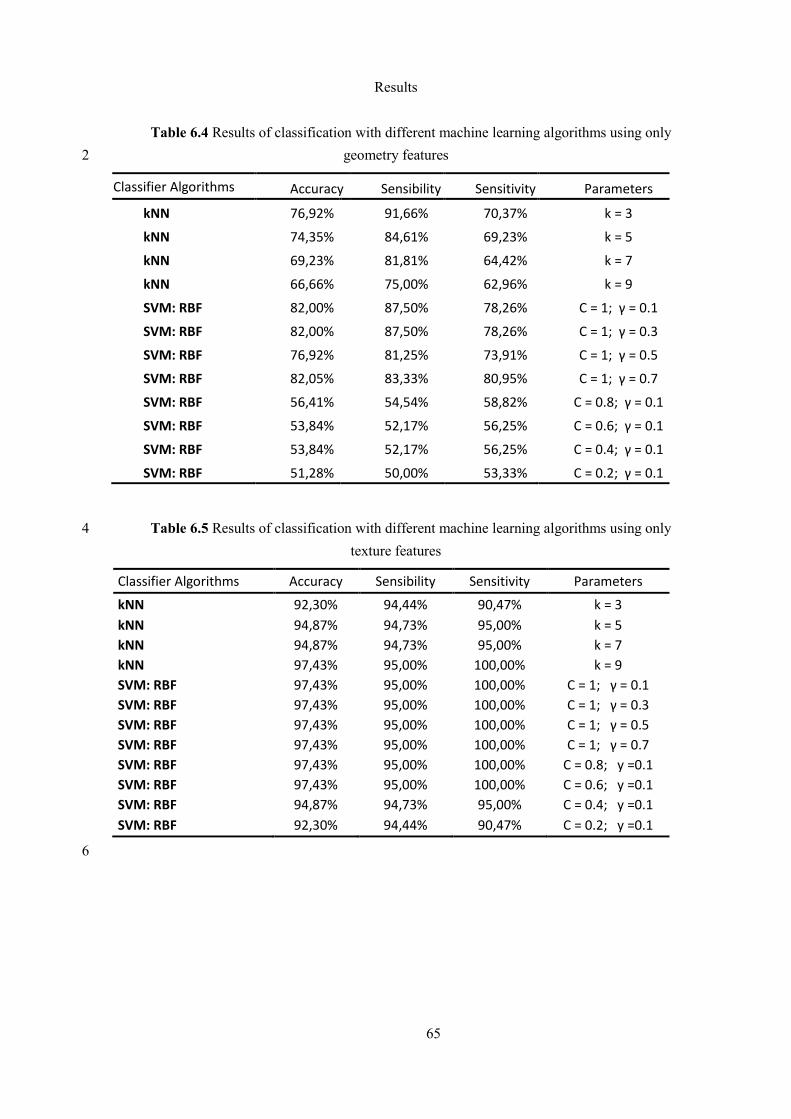
Results
65
Table 6.4 Results of classification with different machine learning algorithms using only
geometry features 2
Classifier Algorithms Accuracy Sensibility Sensitivity Parameters
kNN 76,92% 91,66% 70,37% k = 3
kNN 74,35% 84,61% 69,23% k = 5
kNN 69,23% 81,81% 64,42% k = 7
kNN 66,66% 75,00% 62,96% k = 9
SVM: RBF 82,00% 87,50% 78,26% C = 1; γ = 0.1
SVM: RBF 82,00% 87,50% 78,26% C = 1; γ = 0.3
SVM: RBF 76,92% 81,25% 73,91% C = 1; γ = 0.5
SVM: RBF 82,05% 83,33% 80,95% C = 1; γ = 0.7
SVM: RBF 56,41% 54,54% 58,82% C = 0.8; γ = 0.1
SVM: RBF 53,84% 52,17% 56,25% C = 0.6; γ = 0.1
SVM: RBF 53,84% 52,17% 56,25% C = 0.4; γ = 0.1
SVM: RBF 51,28% 50,00% 53,33% C = 0.2; γ = 0.1
Table 6.5 Results of classification with different machine learning algorithms using only 4
texture features
Classifier Algorithms Accuracy Sensibility Sensitivity Parameters
kNN 92,30% 94,44% 90,47% k = 3
kNN 94,87% 94,73% 95,00% k = 5
kNN 94,87% 94,73% 95,00% k = 7
kNN 97,43% 95,00% 100,00% k = 9
SVM: RBF 97,43% 95,00% 100,00% C = 1; γ = 0.1
SVM: RBF 97,43% 95,00% 100,00% C = 1; γ = 0.3
SVM: RBF 97,43% 95,00% 100,00% C = 1; γ = 0.5
SVM: RBF 97,43% 95,00% 100,00% C = 1; γ = 0.7
SVM: RBF 97,43% 95,00% 100,00% C = 0.8; y =0.1
SVM: RBF 97,43% 95,00% 100,00% C = 0.6; y =0.1
SVM: RBF 94,87% 94,73% 95,00% C = 0.4; y =0.1
SVM: RBF 92,30% 94,44% 90,47% C = 0.2; y =0.1
6
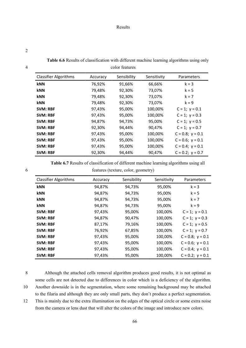
Results
66
2
Table 6.6 Results of classification with different machine learning algorithms using only
color features 4
Classifier Algorithms Accuracy Sensibility Sensitivity Parameters
kNN 76,92% 91,66% 66,66% k = 3
kNN 79,48% 92,30% 73,07% k = 5
kNN 79,48% 92,30% 73,07% k = 7
kNN 79,48% 92,30% 73,07% k = 9
SVM: RBF 97,43% 95,00% 100,00% C = 1; γ = 0.1
SVM: RBF 97,43% 95,00% 100,00% C = 1; γ = 0.3
SVM: RBF 94,87% 94,73% 95,00% C = 1; γ = 0.5
SVM: RBF 92,30% 94,44% 90,47% C = 1; γ = 0.7
SVM: RBF 97,43% 95,00% 100,00% C = 0.8; γ = 0.1
SVM: RBF 97,43% 95,00% 100,00% C = 0.6; γ = 0.1
SVM: RBF 97,43% 95,00% 100,00% C = 0.4; γ = 0.1
SVM: RBF 92,30% 94,44% 90,47% C = 0.2; γ = 0.7
Table 6.7 Results of classification of different machine learning algorithms using all
features (texture, color, geometry) 6
Classifier Algorithms Accuracy Sensibility Sensitivity Parameters
kNN 94,87% 94,73% 95,00% k = 3
kNN 94,87% 94,73% 95,00% k = 5
kNN 94,87% 94,73% 95,00% k = 7
kNN 94,87% 94,73% 95,00% k = 9
SVM: RBF 97,43% 95,00% 100,00% C = 1; γ = 0.1
SVM: RBF 94,87% 90,47% 100,00% C = 1; γ = 0.3
SVM: RBF 87,17% 79,16% 100,00% C = 1; γ = 0.5
SVM: RBF 76,92% 67,85% 100,00% C = 1; γ = 0.7
SVM: RBF 97,43% 95,00% 100,00% C = 0.8; γ = 0.1
SVM: RBF 97,43% 95,00% 100,00% C = 0.6; γ = 0.1
SVM: RBF 97,43% 95,00% 100,00% C = 0.4; γ = 0.1
SVM: RBF 97,43% 95,00% 100,00% C = 0.2; γ = 0.1
Although the attached cells removal algorithm produces good results, it is not optimal as 8
some cells are not detected due to differences in color which is a deficiency of the algorithm.
Another downside is in the segmentation, where some remaining background may be attached 10
to the filaria and although they are only small parts, they don’t produce a perfect segmentation.
This is mainly due to the extra illumination on the edges of the optical circle or some extra noise 12
from the camera or lens dust that will alter the colors of the image and introduce new colors.
Results
67
Although the classification got very good results, these results will be hard to maintain on
bigger datasets where the number and variability of the images is bigger. The dataset is small, as 2
the number of different filarias is reduced. So, the images to the filariae had to be taken in
different positions, shifting the sample and rotating it upside down to produce the effect of new 4
filariae. As the images will be different once the sample is shifted or rotated (different cells,
background, illumination) it covers well the fact that the number of filariae is reduced but this 6
might have helped in the classification phase.
Nonetheless, the algorithm does segment the parasite and classifies it accordingly whether 8
it has the extra bodies or not and the worst results are the ones with a little of background
attached to the boundaries of the filaria or some cells that have subsisted to the attached cells 10
removal. The filaria will be intact in the end of the segmentation and, if the image is on focus
and with no extra objects produced by dust on the camera or some extra light on the edges of the 12
optical circle, the algorithm produces very good results in segmentation having no background
attached to the filaria, hence, producing a smooth result. 14
Conclusions and Future Work
68
Chapter 7
Conclusions and Future Work 2
The aim of the project was to develop a robust image processing methodology for low
quality images acquired using the Fraunhofer mobile acquisition prototype or any other low cost 4
device like Skylight to detect and classify parasites that cause Lymphatic Filariasis into the two
most common types, Brugia malayi and Wuchereria bancrofti. The proposed algorithm 6
consisted on the segmentation of the parasite and classification in one of the two types. The
algorithms employed in the pre-processing and segmentation allowed the parasite to be 8
segmented correctly in low quality images with variance in lighting and color. The classification
phase results show a very good detection and discrimination achieving an accuracy of 99% to 10
classify between cell and filariae and between the two types of filariae. As discussed that can be
due to the small set of speciments provided by the Hygiene and Tropical Medical Institute. 12
For future work, the algorithm should be tested in high quality image datasets and other
low quality datasets without noticeable differences in coloration to test the accuracy and 14
reliability of the methodology. The Android application should be improved as it is a primary
version only to test the results on mobile. Although it is adapted to the MalariaScope application 16
this should be fully integrated in the application where it is possible to choose which type of
analysis the user wants to perform on the blood sample. The speed of the algorithm should also 18
be addressed as the high size used in the morphological operations and median filters is very
costly. Possibly, with the insertion of threads to perform the attached cells removal in parallel 20
with the segmentation the operations could become faster. The application can be extended to
other parasites that are very similar with the parasites presented in this work. 22
In conclusion, this work provides a robust methodology to find Lymphatic Filariasis
parasites and their types, which was never tried before, and a stable background work to expand 24
the detection to other parasites of the same type (Loa Loa) and extend the range of detection of
parasites in low quality images. 26
References
69
References
[1] Sharma B (2014) Lymphatic Filariasis and Chemotherapeutic Targets. Biochemestry & 2
Analytical Biochemestry 3: e147
[2] Wynd S, Melrose WD, Durrheim DN, Carron J, Gyapong M (2007) Understanding the 4
community impact of lymphatic Filariasis: a review of the sociocultural literature.
Bulletin World Health Organ 85: 493-498 6
[3] WHO. 2012. Global Programme to Eliminate Lymphatic Filariasis: progress report in
2011. Weekly Epidemiological Record, 87 (37):346–356 8
[4] Ramaiah KD et al. 2000. The economic burden of lymphatic Filariasis in India.
Parasitology Today, 16:251–253. 10
[5] http://www.who.int/mediacentre/factsheets/fs102/en/
[6] WHO. 2011. Global Programme to eliminate lymphatic Filariasis: progress report on 12
mass drug administration, 2010. Weekly Epidemiological Record; 86 (35):377-88.
[7] Ton TG, Mackenzie C, Molyneux DH. 2015.The burden of mental health in lymphatic 14
Filariasis. Infectious Disease Poverty, 30;4:34.
[8] http://www.who.int/neglected_diseases/mediacentre/WHA_50.29_Eng.pdf. 16
[9] WHO. 2015. Global Programme to eliminate lymphatic Filariasis: progress report on
mass drug administration, 2014. Weekly Epidemiological Record, 90 (38): 489-504. 18
[10] Ottesen EA, Duke BO, Karam M, Behbehani K, 1997. Strategies and tools for the
control/elimination of lymphatic Filariasis. Bulletin World Health Organization, 75: 20
491–503
[11] World Health Organization, 1995. Bridging the Gaps. The World Health Report. 22
Geneva: World Health Organization.
[12] Junior, EFS. 2014. Wuchereria bancrofti EM IMIGRANTES HAITIANOS NO 24
MUNICÍPIO DE MANAUS, AMAZONAS, BRASIL. Dissertação de mestrado
Universidade do Estado do Amazonas, Fundação de Medicina Tropical. 26
[13] Farrar, J., Hotez, P., Junghanss, T., Kang, G., Lalloo, D., White, N. J. 2014. Manson's
Tropical Diseases. 23th edition, Elsevier. 28
[14] Berengue, JG. 2007. Manual de parasitología: morfología y biología de los parásitos de
interés sanitário. Universitat: 31 30
References
70
[15] Paily, K P., Hoti, SL, Das PK. 2009. A review of the complexity of biology of
lymphatic filarial parasites. Parasitic Disease, 33(1&2):3–12 2
[16] Chen CC, Shih CM (1988) Exsheathment of microfi lariae of Brugia pahangi in the
susceptible and refractory strains of Aedes aegypti. Annals of Tropical Medicine and 4
Parasitology, 82:201–206
[17] Paily KP, Hoti SL, Manonmani A, Balaraman K. 1995. Longevity and migration of 6
Wuchereria bancrofti infective larvae and their distribution pattern in relation to the resting and
feeding behaviour of the vector mosquito, Culex quinquefasciatus. Annals of Tropical Medicine 8
and Parasitology, 89:39–47
[18] Neves, D, Melo, AL, Linardi, PM, Victor, RWA. 2005. Parasitologia Humana. 11ª ed. 10
Rio de Janeiro: Atheneu
[19] Silva Júnior, Edson Fidelis da. 2014. Wuchereria bancrofti em imigrantes haitianos no 12
município de Manaus, Amazonas, Brasil. Dissertação de Mestrado). Universidade do
Estado do Amazonas, Fundação de Medicina Tropical, 62 p. 14
[20] Vanamail P, Ramaiah KD (1991) Biting periodicity index of Culex quinquefasciatus and
its relationship with microfilaria periodicity in Pondicherry. Indian Journal Medical 16
Research, 93:379–383
[21] Weerasooriya MV, Mudalige MP, Gunawardena NK, Kimura E, Samarawickrema WA 18
1998. Microfi larial periodicity of Wuchereria bancrofti and man landing periodicity of
the vector Culex quinquefasciatus say in Matara, Sri Lanka. Ceylon Medical Journal, 20
43:78–83
[22] Simonsen PE, Niemann L, Meyrowitsch DW. 1997. Wuchereria bancrofti in Tanzania: 22
microfilarial periodicity and effect of blood sampling time on microfilarial intensities.
Tropical Medicine International Health, 2:153–158. 24
[23] Barbosa RM, Regis L, Vasconcelos R, Leal WS. 2010. Culex mosquitoes (Diptera:
Culicidae) egg laying in traps loaded with Bacillus thuringiensis variety israelensis and 26
baited with skatole. Journal Medical Entomology; 47(3): 345-348.
[24] ] Kaliwal MB, Kumar A, Shanbhag AB, Dash AP, Javali SB. 2010. Spatiotemporal 28
variations in adult density, abdominal status & indoor resting pattern of Culex
quinquefasciatus Say in Panaji, Goa, India. Indian Journal Medical Research; 131: 711-30
719.
[25] Stoops CA, Gionar YR, Rusmiarto S, Susapto D, Andris H, Elyazar IR, et al. 2010. 32
Laboratory and field testing of bednet traps for mosquito (Diptera: Culicidae) sampling
in West Java, Indonesia. Journal Vector Ecology; 35(1): 187-196. 34
[26] Dreyer G. Noroes J. Figueredo-Silva J. Piessens WF. 2000. Pathogenesis of lymphatic
disease in bancroftian Filariasis: a clinical perspective. Parasitology Today.;16(12): 544-36
8.
[27] Dreyer G. e Mattos D. 2007. Prevenção da elefantíase em áreas endêmicas de 38
bancroftose: realidade ou utopia. Prática Hospitalar, v. 9, p. 94-96.
References
71
[28] Chandy, A., Thakur, AS, Singh, MP, Manigauha, A. 2011. A review of neglected
tropical diseases: FilariasisAsian Pacific Journal of Tropical Medicine, 581-586 2
[29] Kabatereine NB, Malecela M, Lado M, Zaramba S, Amiel O,Kolaczinski JH. 2010. How
to (or not to) integrate vertical programmes for the control of major neglected tropical 4
diseases in sub-Saharan Africa. PLoS Neglected Tropical Disease; 4(6): e755
[30] Freedman DO, de Almeoda Filho PJ, Besh S. 1994. Lymphoscintraphic analysis of 6
lymphatic abnormalities in symptomatic and asymptomatic human Filariasis. Journal
Infectious Disease; 170: 927-933. 8
[31] Gasarasi DB, Premji ZG, Mujinja PG M, et al. 2000. Acute adenolymphangitis due to
bancroftian fi lariasis in Rufi ji district, south east Tanzania. Acta Tropicalia; 75:19–28. 10
[32] Guedes-Neto H.J. Saliture-Neto F.T. Feres-Júnior R. Castelli-Júnior V.Caffaro R.A.
2004. Estudo etiológico dos linfedemas baseado na classificação de Kinmonth, 12
modificada por Cordeiro. Jornal Vascular Brasileiro.
[33] BRASIL. Ministério da Saúde. 2010. Guia de Bolso Doenças Infecciosas e Parasitárias. 14
8ª ed. ampliada. Brasília, DF, Brasil
[34] http://www.cdc.gov/parasites/lymphaticFilariasis/diagnosis.html 16
[35] Jamail M, Andrew K, Junaidi D, et al. 2005. Field validation of sensitivity and specifi
city of rapid test for detection of Brugia malayi infection. Tropical Medicine 18
International Health; 10:99–104
[36] Lammie PJ, Weil G, Noordin R, et al. 2004R. ecombinant antigen-based antibody assays 20
for the diagnosis and surveillance of lymphatic Filariasis – a multicenter trial. Filaria
Journal; 3:9. 22
[37] Weerasooriya MV, Itoh M, Islam MZ, et al. 2003. Prevalence and levels of fi lariaspecifi
c urinary IgG4 among children less than five years of age and the association of antibody 24
positivity between children and their mothers. American Journal Tropical Medicine
Hygiene; 68:465–468. 26
[38] McCarthy. J. Diagnosis of lymphatic filarial infection. In: Nutman TB. Lymphatic
Filariasis. London: Imperial College Press; 2000, p. 127-141 28
[39] Williams SA, Laney SJ, Bierwert LA, et al. 2002. Development and standardization of a
rapid, PCR based method for the detection of Wuchereria bancrofti in mosquitoes, for 30
xenomonitoring the human prevalence of bancroftian Filariasis. Annals of Tropical
Medicine and Parasitology; 96: S41–S46. 32
[40] Fischer P, Boakye D, Hamburger J. 2003. Polymerase chain reaction-based detection of
lymphatic Filariasis. Medical Microbiology Immunology; 192:3–7. 34
[41] Dreyer G, Santos A, Norões J, et al. 1998. Ultrasonographic detection of living adult
Wuchereria bancrofti using a 3.5-MHz transducer American Journal Tropical Medicine 36
Hygiene; 59:399–403.
References
72
[42] Mand S, Marfo-Debrekyei Y, Dittrich M, et al. 2003. Animated documentation of the
filaria dance sign (FDS) in bancroftian fi lariasis. Filaria J; 2:3. 2
[43] R. Brad and D. Volovici, “BLOOD CELLS DETECTION FROM MICROSCOPIC
IMAGES,” vol. 2, pp. 2–5. 4
[44] M. Maitra, R. Kumar Gupta, and M. Mukherjee, “Detection and Counting of Red Blood
Cells in Blood Cell Images using Hough Transform,” Int. J. Comput. Appl., vol. 53, no. 6
16, pp. 13–17, 2012.
[45] N. D. Jambhekar, “Red Blood Cells Classification using Image Processing,” Sci. Res. 8
Report., vol. 1, no. 3, pp. 151–154, 2011.
[46] D. Anggraini, A. S. Nugroho, C. Pratama, I. E. Rozi, Aulia Arif Iskandar, and Reggio 10
Nurtanio Hartono, “Automated status identification of microscopic images obtained
from malaria thin blood smears,” Proc. 2011 Int. Conf. Electr. Eng. Informatics, ICEEI 12
2011, 2011.
[47] J. Somasekar, “An Image Processing Approach for Accurate Determination of 14
Parasitemia in Peripheral Blood Smear Images,” pp. 23–28, 2011.
[48] D. M. Memeu, K. A. Kaduki, a C. K. Mjomba, N. S. Muriuki, and L. Gitonga, 16
“Detection of plasmodium parasites from images of thin blood smears,” vol. 2013, no.
December, pp. 183–194, 2013. 18
[49] R. Maini and H. Aggarwal, “A comprehensive review of image enhancement
techniques,” arXiv Prepr. arXiv1003.4053, vol. 2, no. 3, pp. 8–13, 2010. 20
[50] Megha Goyal, “Morphological Image Processing,” vol. 8491, pp. 161–165, 2011.
[51] M. J. Kumar and R. V. K. Reddy, “Review on image segmentation techniques,” vol. 3, 22
no. 6, pp. 992–997, 2014.
[52] P. Smith, D. B. Reid, C. Environment, L. Palo, P. Alto, and P. L. Smith, “Smith et al. - 24
1979 - A Tlreshold Selection Method from Gray-Level Histograms,” vol. 20, no. 1, pp.
62–66, 1979. 26
[53] D. G. Lowe, “Distinctive image features from scale invariant keypoints,” Int’l J.
Comput. Vis., vol. 60, pp. 91–11020042, 2004. 28
[54] H. Bay, A. Ess, T. Tuytelaars, L. Van Gool, L. Van Gool, H. Baya, A. Essa, T.
Tuytelaarsb, and L. Van Goola, “Speeded-up robust features (SURF),” Comput. Vis. 30
image Underst., vol. 110, no. 3, pp. 346–359, 2008.
[55] S. Mallawaarachchi, G. V. A. Premalal, K. W. S. S. Wimalana, A. S. Liyanage, S. 32
Samarasinghe, and N. D. Nanayakkara, “Detection of microfilariae in peripheral blood
smears using image analysis,” 2013 IEEE 8th Int. Conf. Ind. Inf. Syst. ICIIS 2013 - 34
Conf. Proc., pp. 300–303, 2013.
36

References
73
[56] Quirke. P. Magee D., Treanor D., Crellin D., Shires M., Smith K., Mohee K., “Colour
Normalisation in Digital Histopathology Images,” Opt. Tissue Image Anal. Microsc. 2
Histopathol. Endosc. (MICCAI Work., pp. 100–111, 2009.
[57] A. Materka and M. Strzelecki, “Texture Analysis Methods – A Review,” Methods, vol. 4
11, pp. 1–33, 1998.
[58] M. Yang, K. Kpalma, and J. Ronsin, “A survey of shape feature extraction techniques,” 6
Pattern Recognit., vol. 2008, no. November, pp. 43–90, 2008.

References
74