Machine LearningICS 273A

Instructor: Max Welling

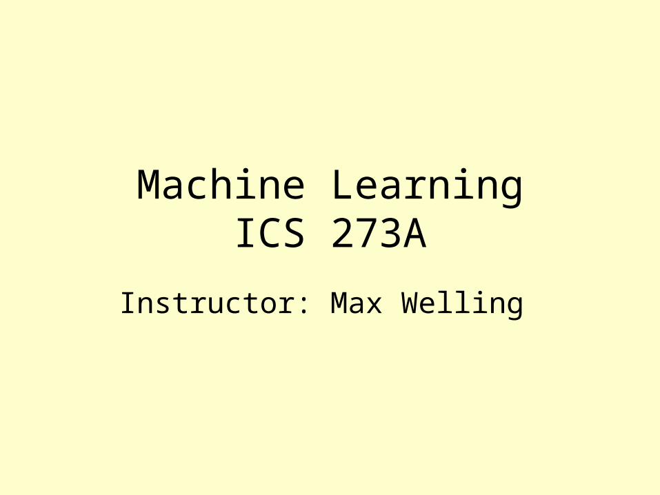
What is Expected?• Class• Homework

– Required, (answers will be provided)

• A Project– See webpage

• Quizzes – A quiz every Friday– Bring scantron form (buy in UCI bookstore)

• Final• Programming in MATLAB or R

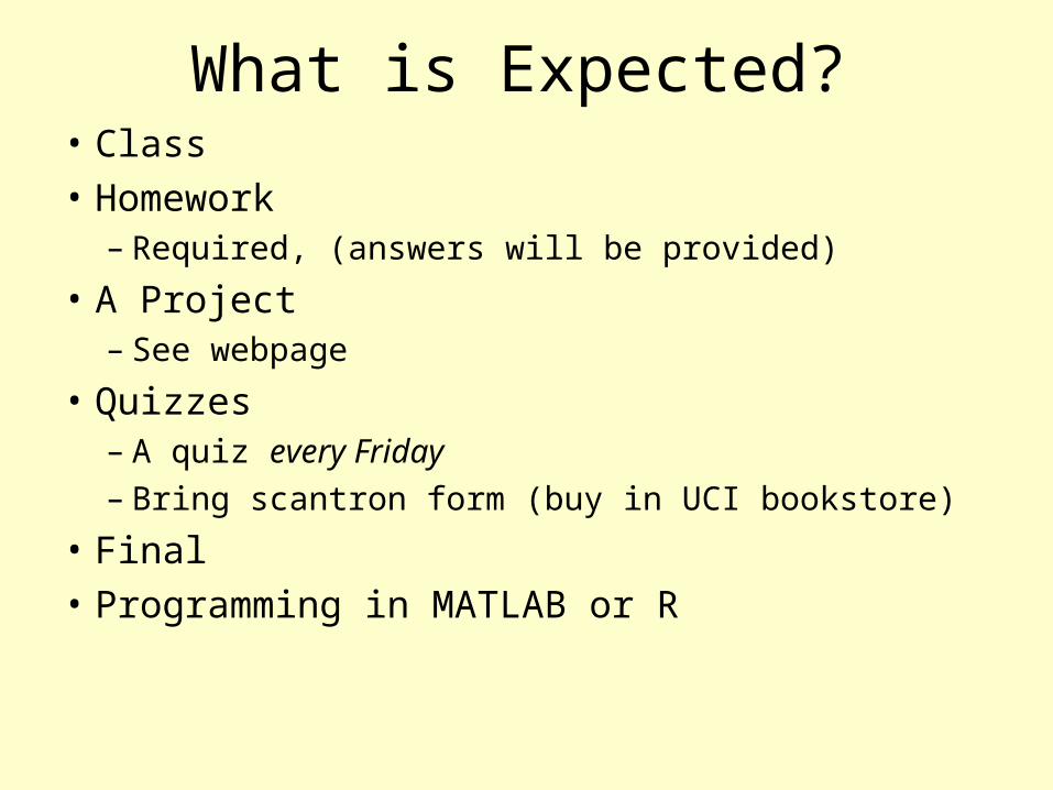
Syllabus• introduction: overview, examples, goals.

• Classification I: decision trees, random forests, boosting, k-nearest neighbors, Naïve Bayes, over-fitting, bias variance trade-off, cross-validation.

• Classification 2: neural networks: perceptron, logistic regression, multi-layer networks, back- propagation.

• Classification 3: kernel methods & support vector machines.

• Clustering & dimensionality reduction: (kernel) k-means, (kernel) PCA.

• Kernel design

• Nonlinear dimension reduction.

• (Kernel) Fisher linear discriminant analysis

• (Kernel) canonical correlation analysis

• Algorithm evaluation, hypothesis testing.

• week 9/10: project presentations.

Machine Learningaccording to

•The ability of a machine to improve its performance based on previous results.

•The process by which computer systems can be directed to improve their performance over time.

•Subspecialty of artificial intelligence concerned with developing methods for software to learn from experience or extract knowledge from examples in a database.

•The ability of a program to learn from experience — that is, to modify its execution on the basis of newly acquired information. •Machine learning is an area of artificial intelligence concerned with the development of techniques which allow computers to "learn". More specifically, machine learning is a method for creating computer programs by the analysis of data sets. Machine learning overlaps heavily with statistics, since both fields study the analysis of data, but unlike statistics, machine learning is concerned with the algorithmic complexity of computational implementations. ...

Some Examples

• ZIP code recognition• Loan application classification • Signature recognition• Voice recognition over phone• Credit card fraud detection• Spam filter• Collaborative Filtering: suggesting other products at Amazone.com • Marketing• Stock market prediction• Expert level chess and checkers systems• biometric identification (fingerprints, DNA, iris scan, face)• machine translation• web-search• document & information retrieval• camera surveillance• robosoccer• and so on and so on...

Why is this cool/important?

• Modern technologies generate data at an unprecedented scale.• The amount of data doubles every year.

“One petabyte is equivalent to the text in one billion books, yet many scientific instruments, including the Large Synoptic Survey Telescope, will soon be generating several petabytes annually”.

(2020 Computing: Science in an exponential world: Nature Published online: 22 March 2006)

• Computers dominate our daily lives• Science, industry, army, our social interactions etc.

We can no longer “eyeball” the images captured by some satellitefor interesting events, or check every webpage for some topic.

We need to trust computers to do the work for us.

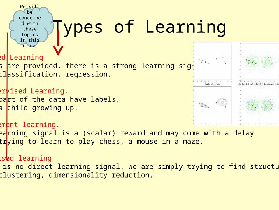
Types of Learning

• Supervised Learning• Labels are provided, there is a strong learning signal.• e.g. classification, regression.

• Semi-supervised Learning.

• Only part of the data have labels. • e.g. a child growing up.

• Reinforcement learning.• The learning signal is a (scalar) reward and may come with a delay.• e.g. trying to learn to play chess, a mouse in a maze.

• Unsupervised learning• There is no direct learning signal. We are simply trying to find structure in data.• e.g. clustering, dimensionality reduction.

We will be concerned with these topics in this class

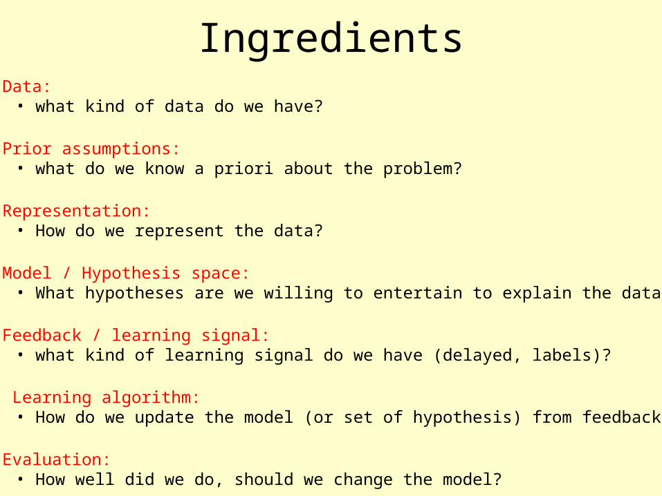
Ingredients• Data:

• what kind of data do we have?

• Prior assumptions:• what do we know a priori about the problem?

• Representation:• How do we represent the data?

• Model / Hypothesis space:• What hypotheses are we willing to entertain to explain the data?

• Feedback / learning signal:• what kind of learning signal do we have (delayed, labels)?

• Learning algorithm:• How do we update the model (or set of hypothesis) from feedback?

• Evaluation:• How well did we do, should we change the model?

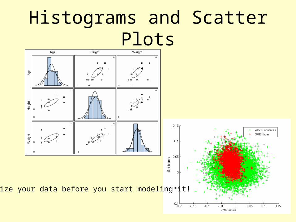
Histograms and Scatter Plots

Visualize your data before you start modeling it!

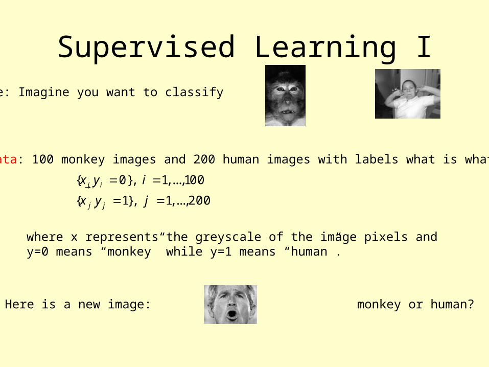
Supervised Learning IExample: Imagine you want to classify versus

Data: 100 monkey images and 200 human images with labels what is what.

,

,

{ 0}, 1,...,100

{ 1}, 1,...,200i i

j j

x y i

x y j

where x represents the greyscale of the image pixels andy=0 means “monkey” while y=1 means “human”.

Task: Here is a new image: monkey or human?

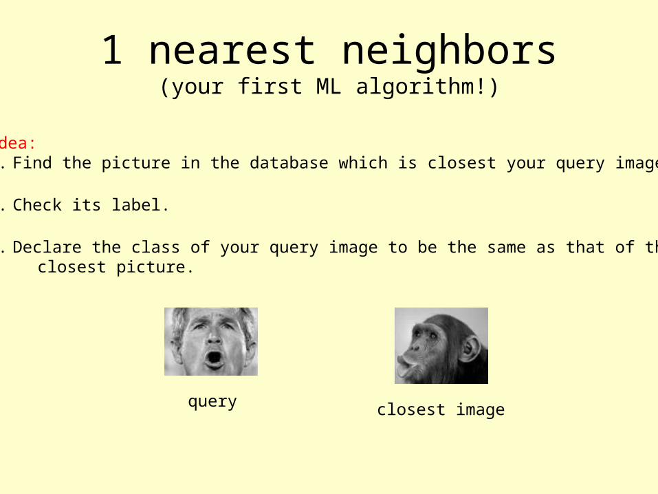
1 nearest neighbors(your first ML algorithm!)

Idea: 1. Find the picture in the database which is closest your query image.

2. Check its label.

3. Declare the class of your query image to be the same as that of the closest picture.

query closest image

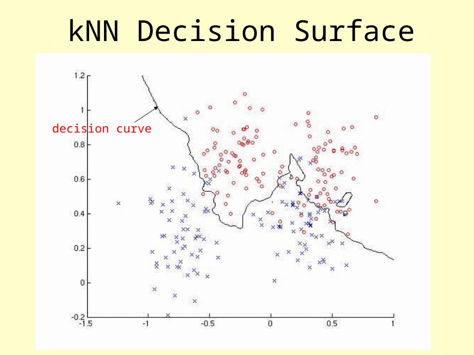
kNN Decision Surface

decision curve

Distance Metric

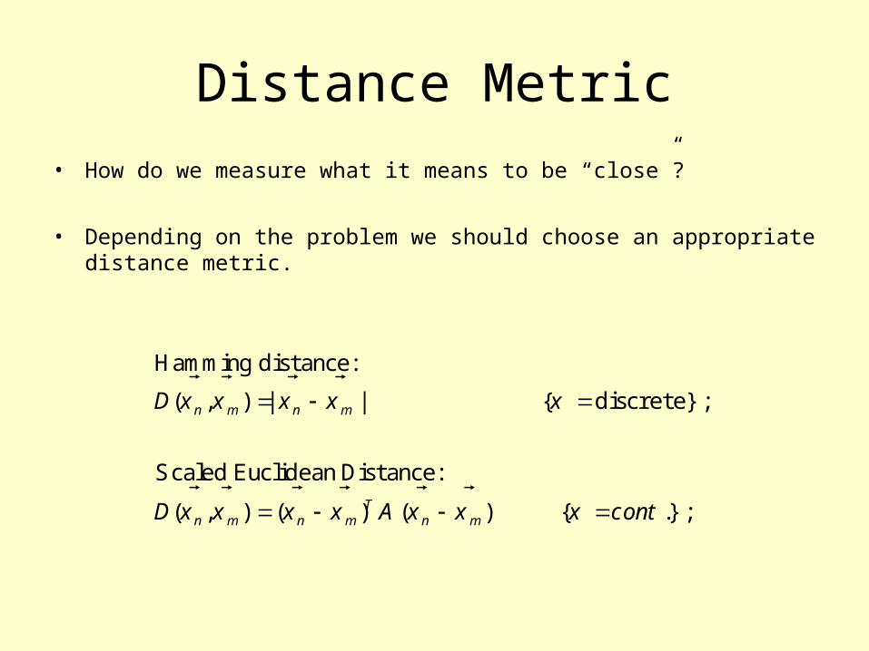
• How do we measure what it means to be “close”?

• Depending on the problem we should choose an appropriate distance metric.

Hamming distance:

( , ) | | { discrete};

Scaled EuclideanDistance:

( , ) ( ) ( ) { .};

n m n m

Tn m n m n m

D x x x x x

D x x x x A x x x cont

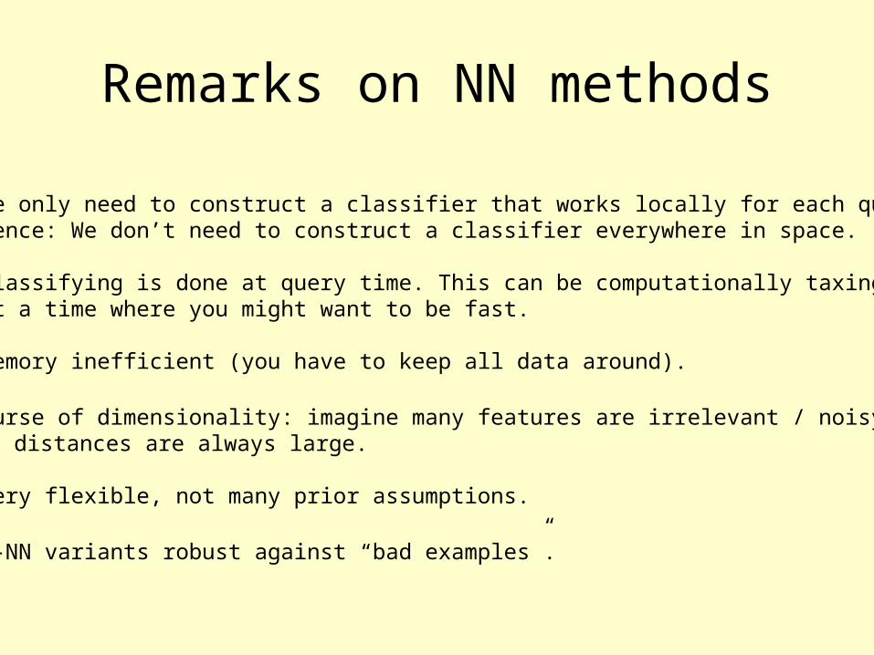
Remarks on NN methods

• We only need to construct a classifier that works locally for each query. Hence: We don’t need to construct a classifier everywhere in space.

• Classifying is done at query time. This can be computationally taxing at a time where you might want to be fast.

• Memory inefficient (you have to keep all data around).

• Curse of dimensionality: imagine many features are irrelevant / noisy distances are always large.

• Very flexible, not many prior assumptions.

• k-NN variants robust against “bad examples”.

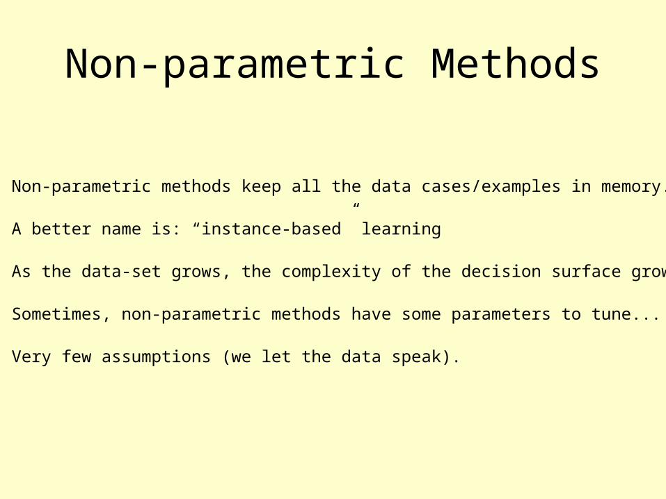
Non-parametric Methods

• Non-parametric methods keep all the data cases/examples in memory.

• A better name is: “instance-based” learning

• As the data-set grows, the complexity of the decision surface grows.

• Sometimes, non-parametric methods have some parameters to tune...

• Very few assumptions (we let the data speak).

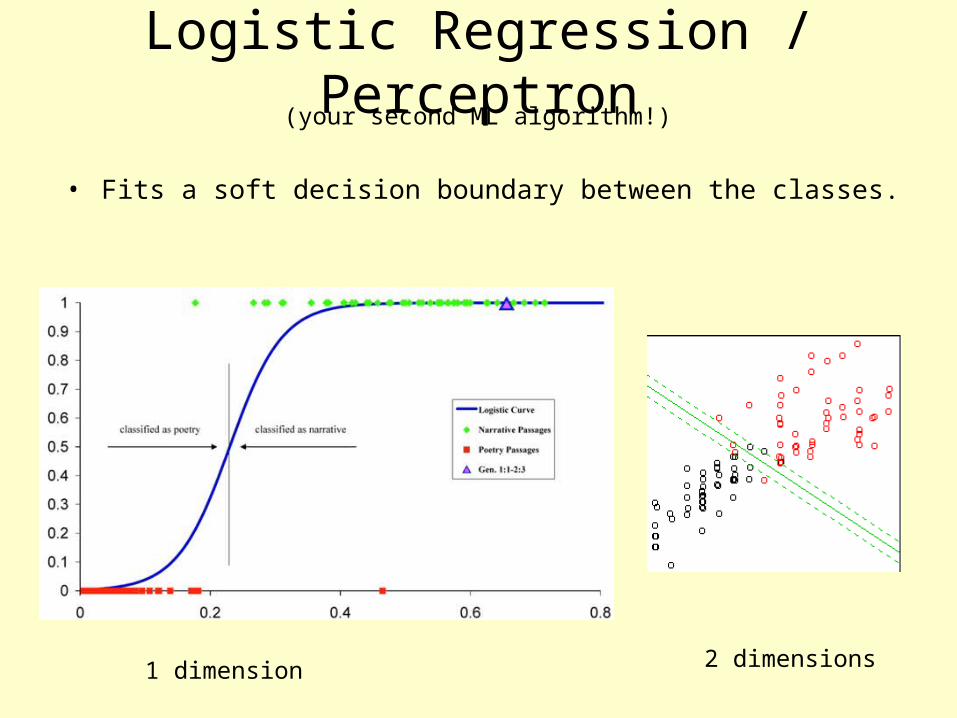
Logistic Regression / Perceptron

• Fits a soft decision boundary between the classes.

1 dimension 2 dimensions

(your second ML algorithm!)

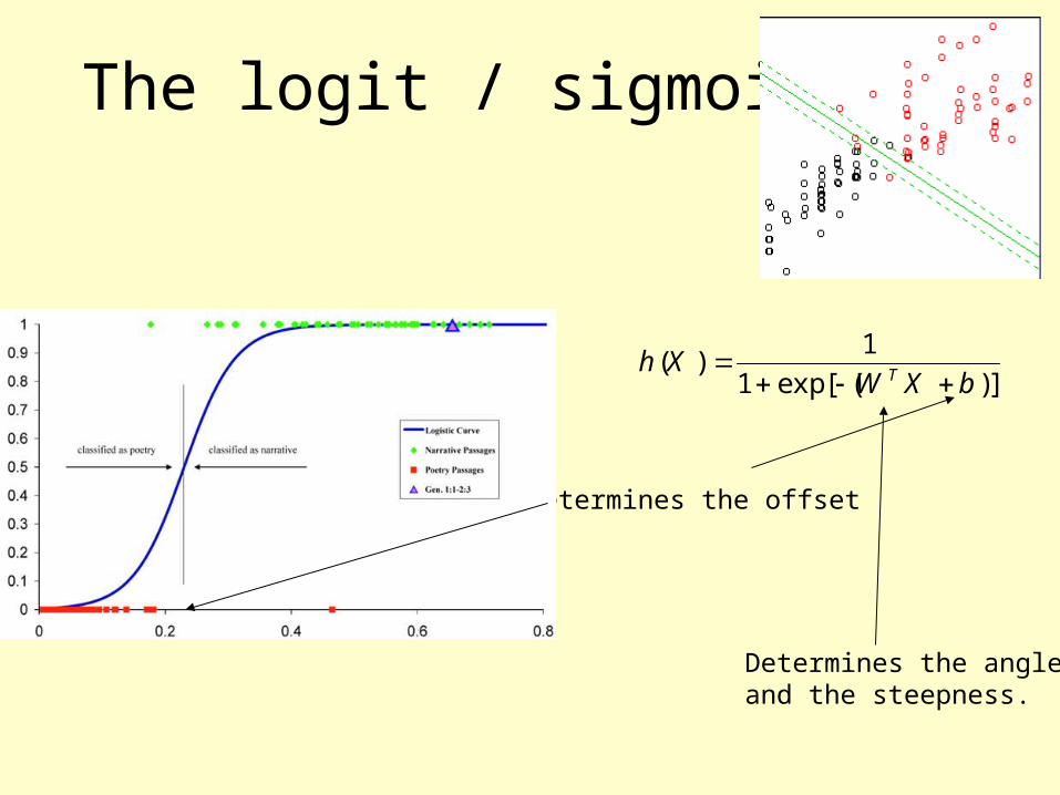
The logit / sigmoid

1( )

1 exp[ ( )]Th XW X b

Determines the offset

Determines the angleand the steepness.

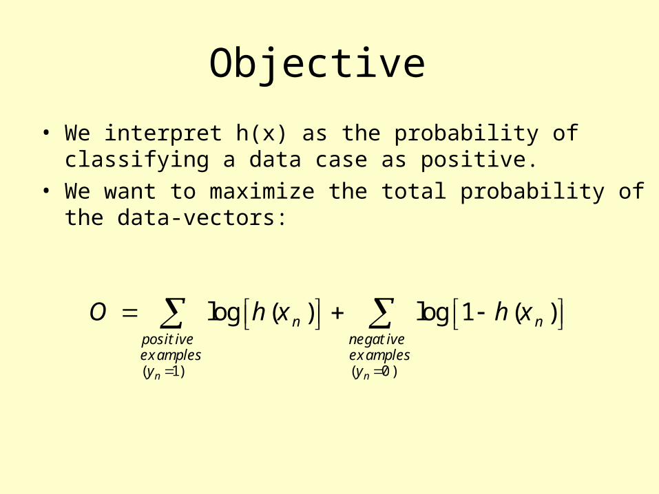
Objective

• We interpret h(x) as the probability of classifying a data case as positive.

• We want to maximize the total probability of the data-vectors:

( 1) ( 0)

log ( ) log 1 ( )

n n

n npositive negativeexamples examplesy y

O h x h x

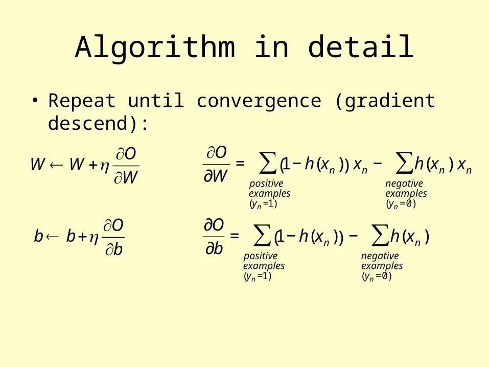
Algorithm in detail

• Repeat until convergence (gradient descend):

b

Obb

W

OWW

€

∂O∂W

= 1− h(xn )( ) xnpositiveexamples(yn =1)

∑ − h(xn )negativeexamples(yn =0)

∑ xn

∂O

∂b= 1− h(xn )( )positiveexamples(yn =1)

∑ − h(xn )negativeexamples(yn =0)

∑

A Note on Stochastic GD

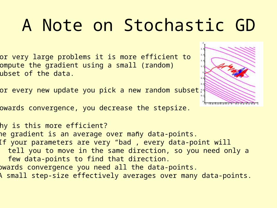
• For very large problems it is more efficient to compute the gradient using a small (random) subset of the data.

• For every new update you pick a new random subset.

• Towards convergence, you decrease the stepsize.

• Why is this more efficient?The gradient is an average over many data-points. If your parameters are very “bad”, every data-point will tell you to move in the same direction, so you need only a few data-points to find that direction.Towards convergence you need all the data-points. A small step-size effectively averages over many data-points.

Parametric Methods

• Parametric methods fit a finite set of parameters to the data.

• Unlike NP methods, this implies a maximum complexity for the model.

• “Assumption heavy”: by choosing the parameterized model you impose your prior assumptions (this can be an advantage when you have sound assumptions!)

• Classifier is build off-line. Classification is fast at query time.

• Easy on memory: samples are summarized through model parameters.

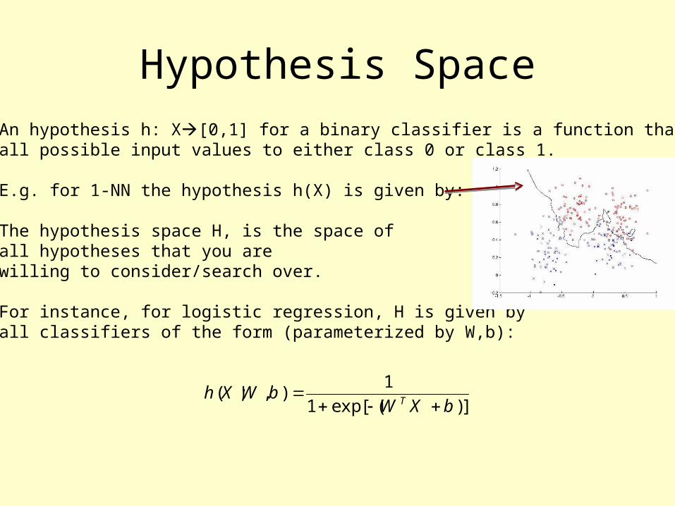
Hypothesis Space• An hypothesis h: X[0,1] for a binary classifier is a function that maps all possible input values to either class 0 or class 1.

• E.g. for 1-NN the hypothesis h(X) is given by:

• The hypothesis space H, is the space of all hypotheses that you are willing to consider/search over.

• For instance, for logistic regression, H is given by all classifiers of the form (parameterized by W,b):

1( ; , )

1 exp[ ( )]Th X W bW X b

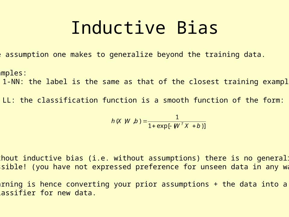
Inductive Bias• The assumption one makes to generalize beyond the training data.

• Examples:• 1-NN: the label is the same as that of the closest training example.

• LL: the classification function is a smooth function of the form:

• Without inductive bias (i.e. without assumptions) there is no generalization possible! (you have not expressed preference for unseen data in any way).

• Learning is hence converting your prior assumptions + the data into a classifier for new data.

1( ; , )

1 exp[ ( )]Th X W bW X b

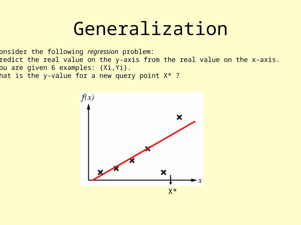
Generalization• Consider the following regression problem:• Predict the real value on the y-axis from the real value on the x-axis.• You are given 6 examples: {Xi,Yi}.• What is the y-value for a new query point X* ?

X*

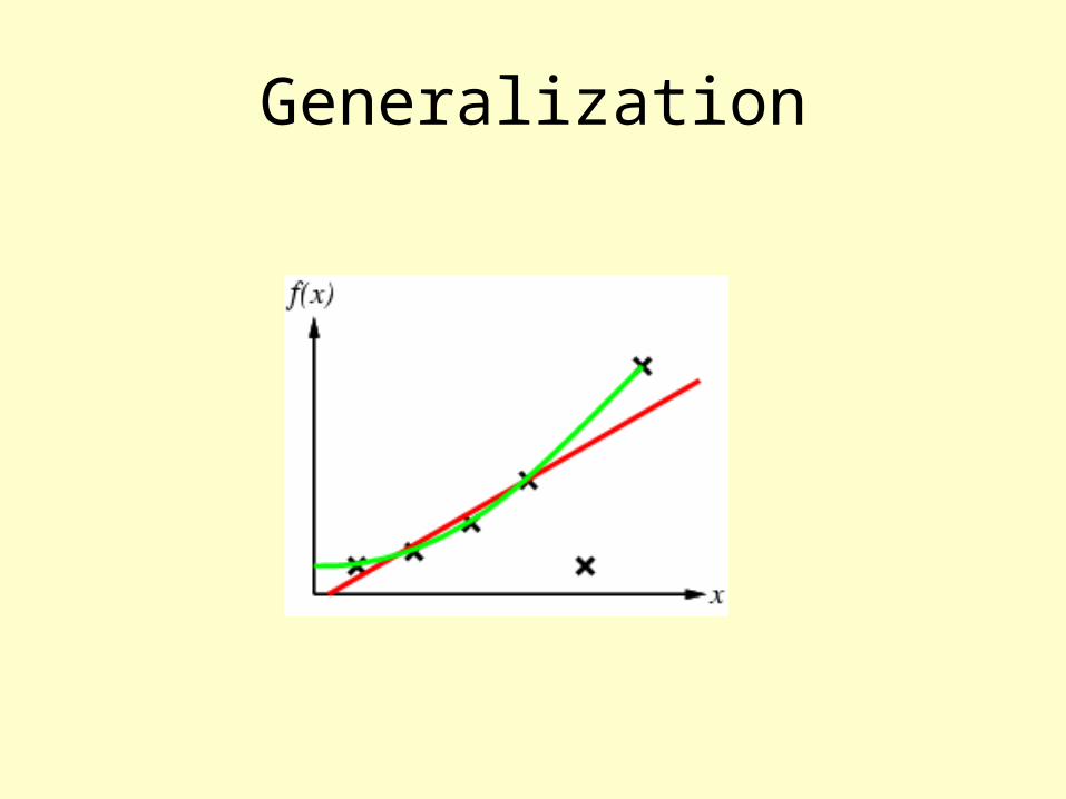
Generalization

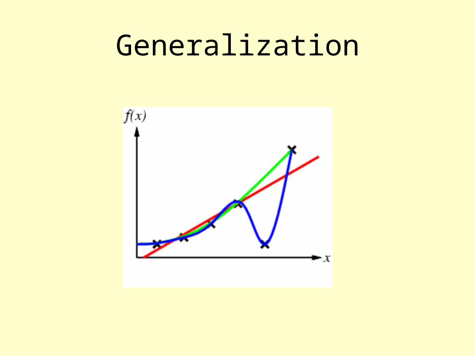
Generalization

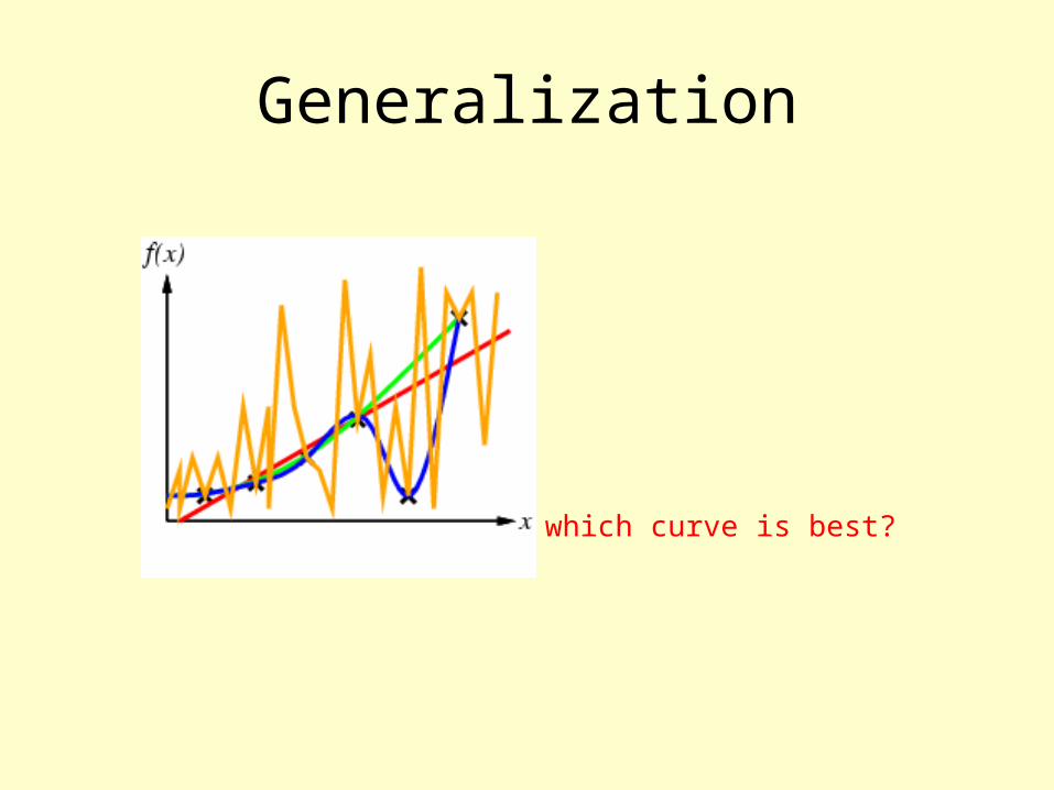
Generalization

which curve is best?

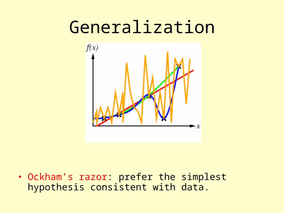
• Ockham’s razor: prefer the simplest hypothesis consistent with data.

Generalization

Generalization

Learning is concerned with accurate predictionof future data, not accurate prediction of training data.

(The single most important sentence you will see in the course)

Cross-validation

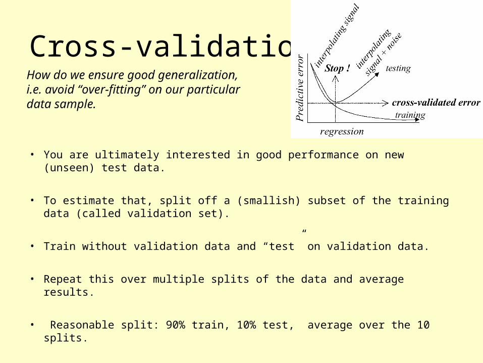
• You are ultimately interested in good performance on new (unseen) test data.

• To estimate that, split off a (smallish) subset of the training data (called validation set).

• Train without validation data and “test” on validation data.

• Repeat this over multiple splits of the data and average results.

• Reasonable split: 90% train, 10% test, average over the 10 splits.

How do we ensure good generalization,i.e. avoid “over-fitting” on our particular data sample.