Machine Learningmurphyk/MLbook/pml-intro-22may12.pdf · of probability theory. Probability theory can be applied to any problem involving uncertainty. In machine learning, uncertainty

Machine LearningA Probabilistic Perspective

Kevin P. Murphy

The MIT PressCambridge, MassachusettsLondon, England

1 Introduction

1.1 Machine learning: what and why?

We are drowning in information and starving for knowledge. — John Naisbitt.

We are entering the era of big data. For example, there are about 1 trillion web pages1; onehour of video is uploaded to YouTube every second, amounting to 10 years of content everyday2; the genomes of 1000s of people, each of which has a length of 3.8× 109 base pairs, havebeen sequenced by various labs; Walmart handles more than 1M transactions per hour and hasdatabases containing more than 2.5 petabytes (2.5× 1015) of information (Cukier 2010); and soon.This deluge of data calls for automated methods of data analysis, which is what machine

learning provides. In particular, we define machine learning as a set of methods that canautomatically detect patterns in data, and then use the uncovered patterns to predict futuredata, or to perform other kinds of decision making under uncertainty (such as planning how tocollect more data!).This books adopts the view that the best way to solve such problems is to use the tools

of probability theory. Probability theory can be applied to any problem involving uncertainty.In machine learning, uncertainty comes in many forms: what is the best prediction about thefuture given some past data? what is the best model to explain some data? what measurementshould I perform next? etc. The probabilistic approach to machine learning is closely related tothe field of statistics, but di�ers slightly in terms of its emphasis and terminology3.We will describe a wide variety of probabilistic models, suitable for a wide variety of data and

tasks. We will also describe a wide variety of algorithms for learning and using such models.The goal is not to develop a cook book of ad hoc techiques, but instead to present a unifiedview of the field through the lens of probabilistic modeling and inference. Although we will payattention to computational e�ciency, details on how to scale these methods to truly massivedatasets are better described in other books, such as (Rajaraman and Ullman 2011; Bekkermanet al. 2011).

1. http://googleblog.blogspot.com/2008/07/we-knew-web-was-big.html2. Source: http://www.youtube.com/t/press_statistics.3. Rob Tibshirani, a statistician at Stanford university, has created an amusing comparison between machine learningand statistics, available at http://www-stat.stanford.edu/~tibs/stat315a/glossary.pdf.

2 Chapter 1. Introduction

It should be noted, however, that even when one has an apparently massive data set, thee�ective number of data points for certain cases of interest might be quite small. In fact, dataacross a variety of domains exhibits a property known as the long tail, which means that afew things (e.g., words) are very common, but most things are quite rare (see Section 2.4.7 fordetails). For example, 20% of Google searches each day have never been seen before4. Thismeans that the core statistical issues that we discuss in this book, concerning generalizing fromrelatively small samples sizes, are still very relevant even in the big data era.

1.1.1 Types of machine learning

Machine learning is usually divided into two main types. In the predictive or supervisedlearning approach, the goal is to learn a mapping from inputs x to outputs y, given a labeledset of input-output pairs D = {(xi, yi)}Ni=1. Here D is called the training set, and N is thenumber of training examples.In the simplest setting, each training input xi is a D-dimensional vector of numbers, rep-

resenting, say, the height and weight of a person. These are called features, attributes orcovariates. In general, however, xi could be a complex structured object, such as an image, asentence, an email message, a time series, a molecular shape, a graph, etc.Similarly the form of the output or response variable can in principle be anything, but

most methods assume that yi is a categorical or nominal variable from some finite set,yi ∈ {1, . . . , C} (such as male or female), or that yi is a real-valued scalar (such as incomelevel). When yi is categorical, the problem is known as classification or pattern recognition,and when yi is real-valued, the problem is known as regression. Another variant, known asordinal regression, occurs where label space Y has some natural ordering, such as grades A–F.The second main type of machine learning is the descriptive or unsupervised learning

approach. Here we are only given inputs, D = {xi}Ni=1, and the goal is to find “interestingpatterns” in the data. This is sometimes called knowledge discovery. This is a much lesswell-defined problem, since we are not told what kinds of patterns to look for, and there is noobvious error metric to use (unlike supervised learning, where we can compare our predictionof y for a given x to the observed value).There is a third type of machine learning, known as reinforcement learning, which is

somewhat less commonly used. This is useful for learning how to act or behave when givenoccasional reward or punishment signals. (For example, consider how a baby learns to walk.)Unfortunately, RL is beyond the scope of this book, although we do discuss decision theoryin Section 5.7, which is the basis of RL. See e.g., (Kaelbling et al. 1996; Sutton and Barto 1998;Russell and Norvig 2010; Szepesvari 2010; Wiering and van Otterlo 2012) for more informationon RL.

4.http://certifiedknowledge.org/blog/are-search-queries-becoming-even-more-unique-statistics-from-google.

1.2. Supervised learning 3

(a) (b)

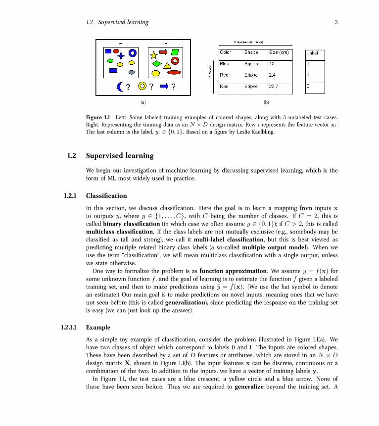
Figure 1.1 Left: Some labeled training examples of colored shapes, along with 3 unlabeled test cases.Right: Representing the training data as an N ×D design matrix. Row i represents the feature vector xi.The last column is the label, yi ∈ {0, 1}. Based on a figure by Leslie Kaelbling.

1.2 Supervised learning

We begin our investigation of machine learning by discussing supervised learning, which is theform of ML most widely used in practice.

1.2.1 Classification

In this section, we discuss classification. Here the goal is to learn a mapping from inputs xto outputs y, where y ∈ {1, . . . , C}, with C being the number of classes. If C = 2, this iscalled binary classification (in which case we often assume y ∈ {0, 1}); if C > 2, this is calledmulticlass classification. If the class labels are not mutually exclusive (e.g., somebody may beclassified as tall and strong), we call it multi-label classification, but this is best viewed aspredicting multiple related binary class labels (a so-called multiple output model). When weuse the term “classification”, we will mean multiclass classification with a single output, unlesswe state otherwise.One way to formalize the problem is as function approximation. We assume y = f(x) for

some unknown function f , and the goal of learning is to estimate the function f given a labeledtraining set, and then to make predictions using y = f(x). (We use the hat symbol to denotean estimate.) Our main goal is to make predictions on novel inputs, meaning ones that we havenot seen before (this is called generalization), since predicting the response on the training setis easy (we can just look up the answer).

1.2.1.1 Example

As a simple toy example of classification, consider the problem illustrated in Figure 1.1(a). Wehave two classes of object which correspond to labels 0 and 1. The inputs are colored shapes.These have been described by a set of D features or attributes, which are stored in an N ×Ddesign matrix X, shown in Figure 1.1(b). The input features x can be discrete, continuous or acombination of the two. In addition to the inputs, we have a vector of training labels y.In Figure 1.1, the test cases are a blue crescent, a yellow circle and a blue arrow. None of

these have been seen before. Thus we are required to generalize beyond the training set. A


reasonable guess is that blue crescent should be y = 1, since all blue shapes are labeled 1 in thetraining set. The yellow circle is harder to classify, since some yellow things are labeled y = 1and some are labeled y = 0, and some circles are labeled y = 1 and some y = 0. Consequentlyit is not clear what the right label should be in the case of the yellow circle. Similarly, the correctlabel for the blue arrow is unclear.

1.2.1.2 The need for probabilistic predictions

To handle ambiguous cases, such as the yellow circle above, it is desirable to return a probability.The reader is assumed to already have some familiarity with basic concepts in probability. Ifnot, please consult Chapter 2 for a refresher, if necessary.We will denote the probability distribution over possible labels, given the input vector x and

training set D by p(y|x,D). In general, this represents a vector of length C . (If there are just twoclasses, it is su�cient to return the single number p(y = 1|x,D), since p(y = 1|x,D) + p(y =0|x,D) = 1.) In our notation, we make explicit that the probability is conditional on the testinput x, as well as the training set D, by putting these terms on the right hand side of theconditioning bar |. We are also implicitly conditioning on the form of model that we use to makepredictions. When choosing between di�erent models, we will make this assumption explicit bywriting p(y|x,D,M), where M denotes the model. However, if the model is clear from context,we will drop M from our notation for brevity.Given a probabilistic output, we can always compute our “best guess” as to the “true label”

using

y = f(x) =C

argmaxc=1

p(y = c|x,D) (1.1)

This corresponds to the most probable class label, and is called the mode of the distributionp(y|x,D); it is also known as a MAP estimate (MAP stands for maximum a posteriori). Usingthe most probable label makes intuitive sense, but we will give a more formal justification forthis procedure in Section 5.7.Now consider a case such as the yellow circle, where p(y|x,D) is far from 1.0. In such a

case we are not very confident of our answer, so it might be better to say “I don’t know” insteadof returning an answer that we don’t really trust. This is particularly important in domainssuch as medicine and finance where we may be risk averse, as we explain in Section 5.7.Another application where it is important to assess risk is when playing TV game shows, suchas Jeopardy. In this game, contestants have to solve various word puzzles and answer a varietyof trivia questions, but if they answer incorrectly, they lose money. In 2011, IBM unveiled acomputer system called Watson which beat the top human Jeopardy champion. Watson uses avariety of interesting techniques (Ferrucci et al. 2010), but the most pertinent one for our presentpurposes is that it contains a module that estimates how confident it is of its answer. The systemonly chooses to “buzz in” its answer if su�ciently confident it is correct. Similarly, Google has asystem known as SmartASS (ad selection system) that predicts the probability you will click onan ad based on your search history and other user and ad-specific features (Metz 2010). Thisprobability is known as the click-through rate or CTR, and can be used to maximize expectedprofit. We will discuss some of the basic principles behind systems such as SmartASS later inthis book.


words

do

cu

me

nts

10 20 30 40 50 60 70 80 90 100

100

200

300

400

500

600

700

800

900

1000

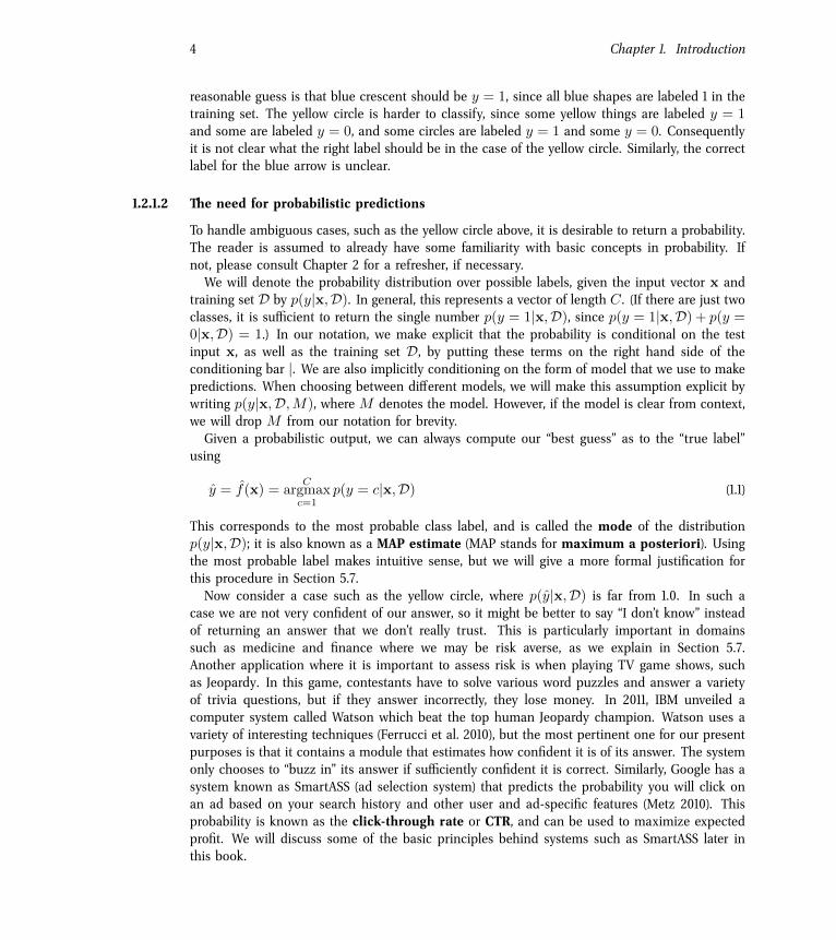
Figure 1.2 Subset of size 16242 x 100 of the 20-newsgroups data. We only show 1000 rows, for clarity.Each row is a document (represented as a bag-of-words bit vector), each column is a word. The redlines separate the 4 classes, which are (in descending order) comp, rec, sci, talk (these are the titles ofUSENET groups). We can see that there are subsets of words whose presence or absence is indicativeof the class. The data is available from http://cs.nyu.edu/~roweis/data.html. Figure generated bynewsgroupsVisualize.

1.2.1.3 Real-world applications

Classification is probably the most widely used form of machine learning, and has been usedto solve many interesting and often di�cult real-world problems. We have already mentionedsome important applciations. We give a few more examples below.

Document classification and email spam filtering

In document classification, the goal is to classify a document, such as a web page or emailmessage, into one of C classes, that is, to compute p(y = c|x,D), where x is some represen-tation of the text. A special case of this is email spam filtering, where the classes are spamy = 1 or ham y = 0.Most classifiers assume that the input vector x has a fixed size. A common way to represent

variable-length documents in feature-vector format is to use a bag of words representation.This is explained in detail in Section 3.4.4.1, but the basic idea is to define xij = 1 i� word joccurs in document i. If we apply this transformation to every document in our data set, we geta binary document × word co-occurrence matrix: see Figure 1.2 for an example. Essentially thedocument classification problem has been reduced to one that looks for subtle changes in thepattern of bits. For example, we may notice that most spam messages have a high probability ofcontaining the words “buy”, “cheap”, “viagra”, etc. In Exercise 8.1 and Exercise 8.2, you will gethands-on experience applying various classification techniques to the spam filtering problem.


(a) (b) (c)

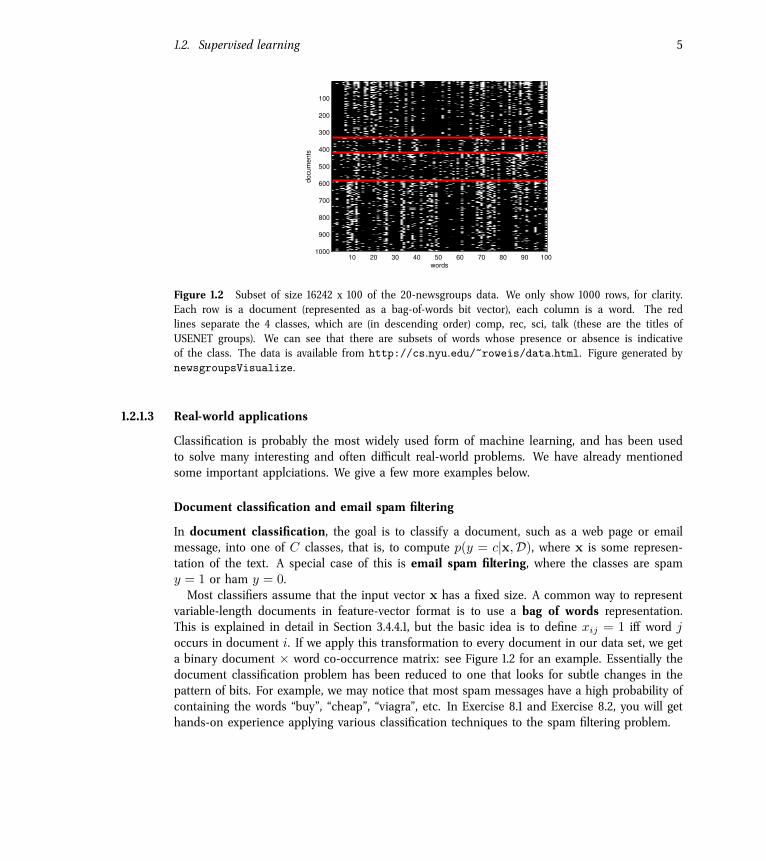
Figure 1.3 Three types of iris flowers: setosa, versicolor and virginica. Source: http://www.statlab.uni-heidelberg.de/data/iris/ . Used with kind permission of Dennis Kramb and SIGNA.

sepa

l len

gth

sepal length

sepa

l wid

thpe

tal l

engt

hpe

tal w

idth

sepal width petal length petal width

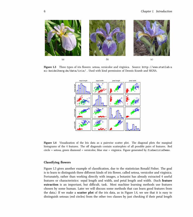
Figure 1.4 Visualization of the Iris data as a pairwise scatter plot. The diagonal plots the marginalhistograms of the 4 features. The o� diagonals contain scatterplots of all possible pairs of features. Redcircle = setosa, green diamond = versicolor, blue star = virginica. Figure generated by fisheririsDemo.

Classifying flowers

Figure 1.3 gives another example of classification, due to the statistician Ronald Fisher. The goalis to learn to distinguish three di�erent kinds of iris flower, called setosa, versicolor and virginica.Fortunately, rather than working directly with images, a botanist has already extracted 4 usefulfeatures or characteristics: sepal length and width, and petal length and width. (Such featureextraction is an important, but di�cult, task. Most machine learning methods use featureschosen by some human. Later we will discuss some methods that can learn good features fromthe data.) If we make a scatter plot of the iris data, as in Figure 1.4, we see that it is easy todistinguish setosas (red circles) from the other two classes by just checking if their petal length


true class = 7 true class = 2 true class = 1



(a)




(b)

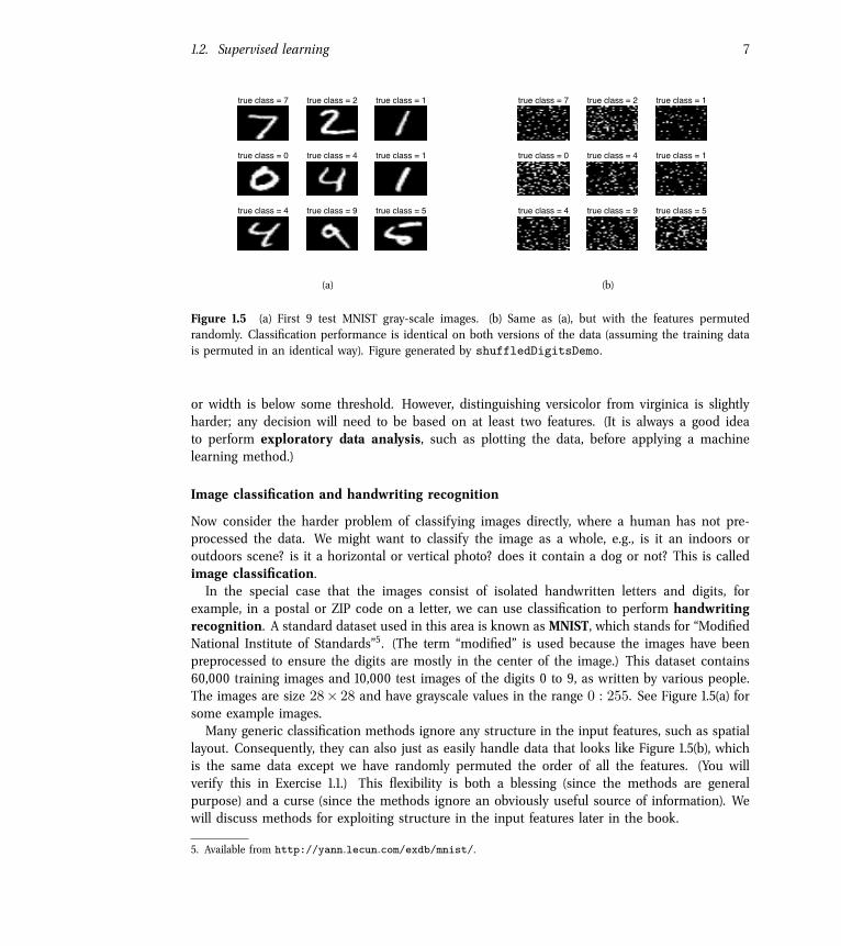
Figure 1.5 (a) First 9 test MNIST gray-scale images. (b) Same as (a), but with the features permutedrandomly. Classification performance is identical on both versions of the data (assuming the training datais permuted in an identical way). Figure generated by shuffledDigitsDemo.

or width is below some threshold. However, distinguishing versicolor from virginica is slightlyharder; any decision will need to be based on at least two features. (It is always a good ideato perform exploratory data analysis, such as plotting the data, before applying a machinelearning method.)

Image classification and handwriting recognition

Now consider the harder problem of classifying images directly, where a human has not pre-processed the data. We might want to classify the image as a whole, e.g., is it an indoors oroutdoors scene? is it a horizontal or vertical photo? does it contain a dog or not? This is calledimage classification.In the special case that the images consist of isolated handwritten letters and digits, for

example, in a postal or ZIP code on a letter, we can use classification to perform handwritingrecognition. A standard dataset used in this area is known as MNIST, which stands for “ModifiedNational Institute of Standards”5. (The term “modified” is used because the images have beenpreprocessed to ensure the digits are mostly in the center of the image.) This dataset contains60,000 training images and 10,000 test images of the digits 0 to 9, as written by various people.The images are size 28× 28 and have grayscale values in the range 0 : 255. See Figure 1.5(a) forsome example images.Many generic classification methods ignore any structure in the input features, such as spatial

layout. Consequently, they can also just as easily handle data that looks like Figure 1.5(b), whichis the same data except we have randomly permuted the order of all the features. (You willverify this in Exercise 1.1.) This flexibility is both a blessing (since the methods are generalpurpose) and a curse (since the methods ignore an obviously useful source of information). Wewill discuss methods for exploiting structure in the input features later in the book.

5. Available from http://yann.lecun.com/exdb/mnist/.


(a) (b)

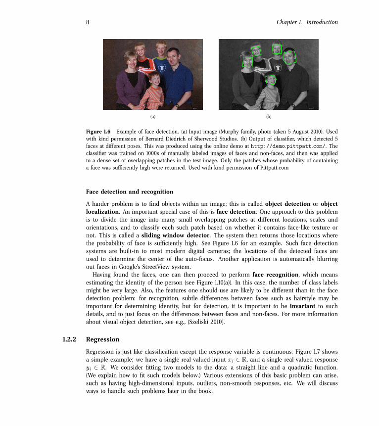
Figure 1.6 Example of face detection. (a) Input image (Murphy family, photo taken 5 August 2010). Usedwith kind permission of Bernard Diedrich of Sherwood Studios. (b) Output of classifier, which detected 5faces at di�erent poses. This was produced using the online demo at http://demo.pittpatt.com/. Theclassifier was trained on 1000s of manually labeled images of faces and non-faces, and then was appliedto a dense set of overlapping patches in the test image. Only the patches whose probability of containinga face was su�ciently high were returned. Used with kind permission of Pittpatt.com

Face detection and recognition

A harder problem is to find objects within an image; this is called object detection or objectlocalization. An important special case of this is face detection. One approach to this problemis to divide the image into many small overlapping patches at di�erent locations, scales andorientations, and to classify each such patch based on whether it contains face-like texture ornot. This is called a sliding window detector. The system then returns those locations wherethe probability of face is su�ciently high. See Figure 1.6 for an example. Such face detectionsystems are built-in to most modern digital cameras; the locations of the detected faces areused to determine the center of the auto-focus. Another application is automatically blurringout faces in Google’s StreetView system.Having found the faces, one can then proceed to perform face recognition, which means

estimating the identity of the person (see Figure 1.10(a)). In this case, the number of class labelsmight be very large. Also, the features one should use are likely to be di�erent than in the facedetection problem: for recognition, subtle di�erences between faces such as hairstyle may beimportant for determining identity, but for detection, it is important to be invariant to suchdetails, and to just focus on the di�erences between faces and non-faces. For more informationabout visual object detection, see e.g., (Szeliski 2010).

1.2.2 Regression

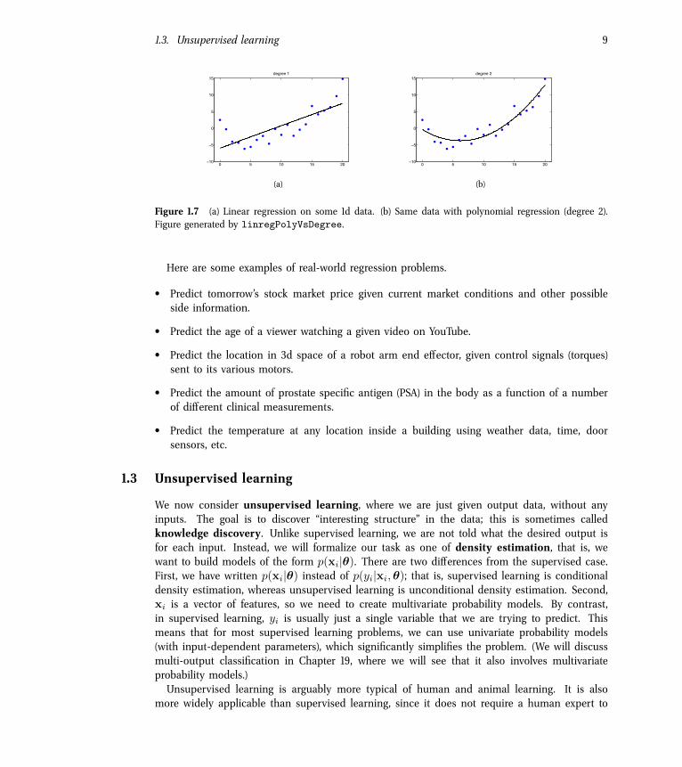
Regression is just like classification except the response variable is continuous. Figure 1.7 showsa simple example: we have a single real-valued input xi ∈ R, and a single real-valued responseyi ∈ R. We consider fitting two models to the data: a straight line and a quadratic function.(We explain how to fit such models below.) Various extensions of this basic problem can arise,such as having high-dimensional inputs, outliers, non-smooth responses, etc. We will discussways to handle such problems later in the book.

1.3. Unsupervised learning 9

0 5 10 15 20−10

−5

0

5

10

15degree 1

(a)

0 5 10 15 20−10

−5

0

5

10

15degree 2

(b)

Figure 1.7 (a) Linear regression on some 1d data. (b) Same data with polynomial regression (degree 2).Figure generated by linregPolyVsDegree.

Here are some examples of real-world regression problems.

• Predict tomorrow’s stock market price given current market conditions and other possibleside information.

• Predict the age of a viewer watching a given video on YouTube.

• Predict the location in 3d space of a robot arm end e�ector, given control signals (torques)sent to its various motors.

• Predict the amount of prostate specific antigen (PSA) in the body as a function of a numberof di�erent clinical measurements.

• Predict the temperature at any location inside a building using weather data, time, doorsensors, etc.

1.3 Unsupervised learning

We now consider unsupervised learning, where we are just given output data, without anyinputs. The goal is to discover “interesting structure” in the data; this is sometimes calledknowledge discovery. Unlike supervised learning, we are not told what the desired output isfor each input. Instead, we will formalize our task as one of density estimation, that is, wewant to build models of the form p(xi|θ). There are two di�erences from the supervised case.First, we have written p(xi|θ) instead of p(yi|xi,θ); that is, supervised learning is conditionaldensity estimation, whereas unsupervised learning is unconditional density estimation. Second,xi is a vector of features, so we need to create multivariate probability models. By contrast,in supervised learning, yi is usually just a single variable that we are trying to predict. Thismeans that for most supervised learning problems, we can use univariate probability models(with input-dependent parameters), which significantly simplifies the problem. (We will discussmulti-output classification in Chapter 19, where we will see that it also involves multivariateprobability models.)Unsupervised learning is arguably more typical of human and animal learning. It is also

more widely applicable than supervised learning, since it does not require a human expert to


55 60 65 70 75 8080

100

120

140

160

180

200

220

240

260

280

heightweight

(a)

55 60 65 70 75 8080

100

120

140

160

180

200

220

240

260

280

height

weight

K=2

(b)

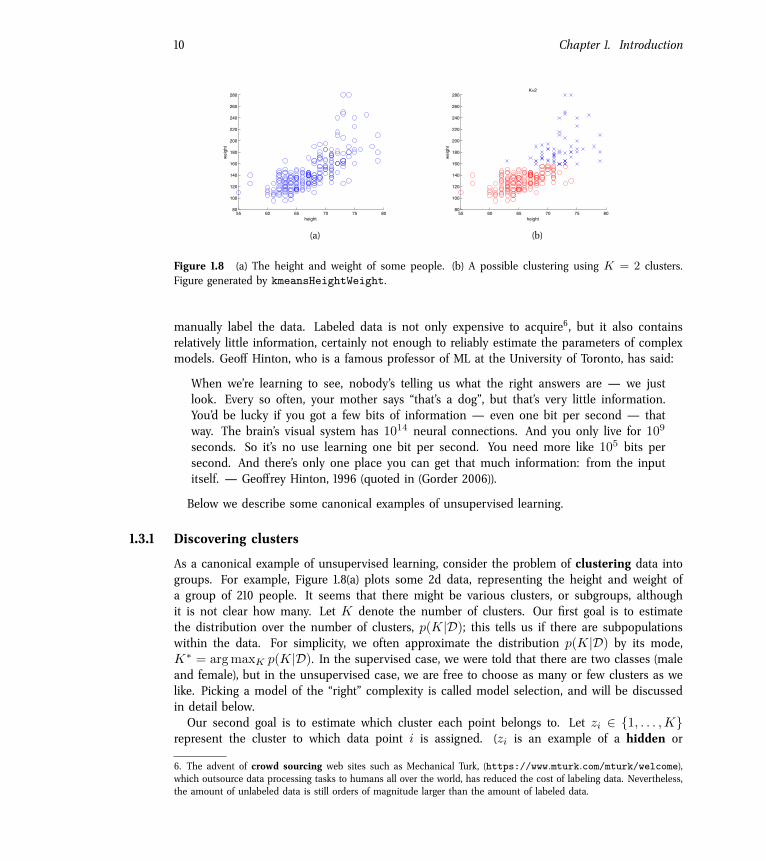
Figure 1.8 (a) The height and weight of some people. (b) A possible clustering using K = 2 clusters.Figure generated by kmeansHeightWeight.

manually label the data. Labeled data is not only expensive to acquire6, but it also containsrelatively little information, certainly not enough to reliably estimate the parameters of complexmodels. Geo� Hinton, who is a famous professor of ML at the University of Toronto, has said:

When we’re learning to see, nobody’s telling us what the right answers are — we justlook. Every so often, your mother says “that’s a dog”, but that’s very little information.You’d be lucky if you got a few bits of information — even one bit per second — thatway. The brain’s visual system has 1014 neural connections. And you only live for 109

seconds. So it’s no use learning one bit per second. You need more like 105 bits persecond. And there’s only one place you can get that much information: from the inputitself. — Geo�rey Hinton, 1996 (quoted in (Gorder 2006)).

Below we describe some canonical examples of unsupervised learning.

1.3.1 Discovering clusters

As a canonical example of unsupervised learning, consider the problem of clustering data intogroups. For example, Figure 1.8(a) plots some 2d data, representing the height and weight ofa group of 210 people. It seems that there might be various clusters, or subgroups, althoughit is not clear how many. Let K denote the number of clusters. Our first goal is to estimatethe distribution over the number of clusters, p(K|D); this tells us if there are subpopulationswithin the data. For simplicity, we often approximate the distribution p(K|D) by its mode,K∗ = argmaxK p(K|D). In the supervised case, we were told that there are two classes (maleand female), but in the unsupervised case, we are free to choose as many or few clusters as welike. Picking a model of the “right” complexity is called model selection, and will be discussedin detail below.Our second goal is to estimate which cluster each point belongs to. Let zi ∈ {1, . . . ,K}

represent the cluster to which data point i is assigned. (zi is an example of a hidden or

6. The advent of crowd sourcing web sites such as Mechanical Turk, (https://www.mturk.com/mturk/welcome),which outsource data processing tasks to humans all over the world, has reduced the cost of labeling data. Nevertheless,the amount of unlabeled data is still orders of magnitude larger than the amount of labeled data.


−8 −6 −4 −2 0 2 4 6 8

−4−20

24

−2

0

2

(a)

−50

5−4

−20

24

(b)

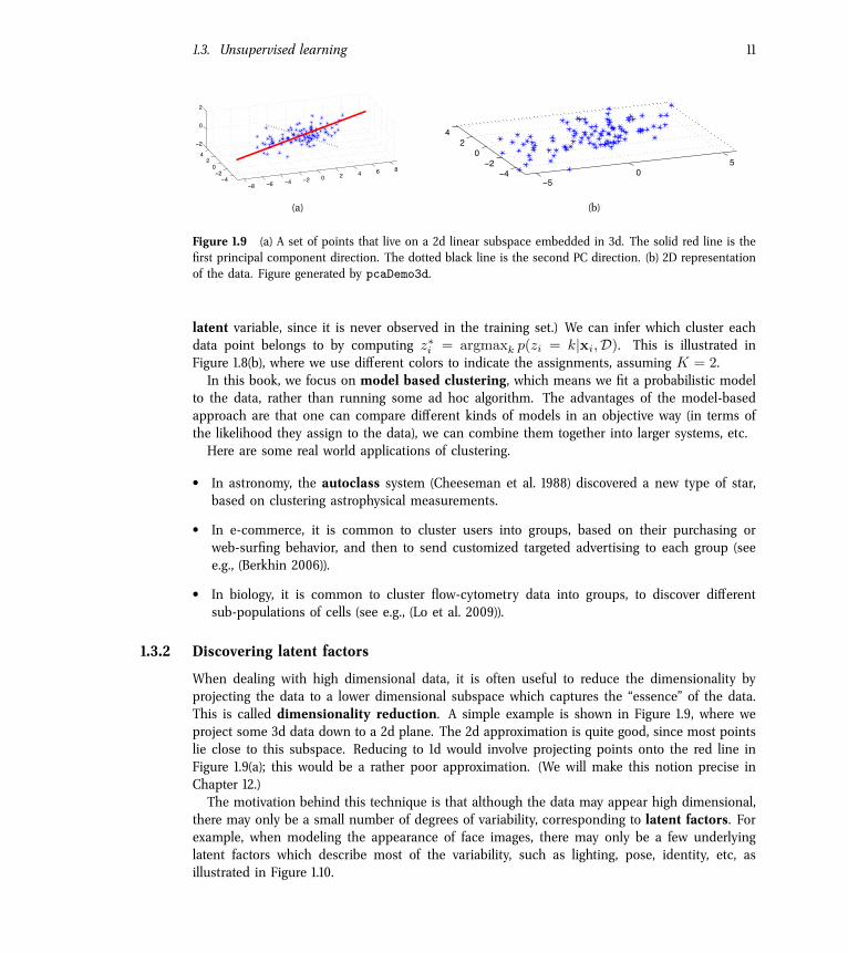
Figure 1.9 (a) A set of points that live on a 2d linear subspace embedded in 3d. The solid red line is thefirst principal component direction. The dotted black line is the second PC direction. (b) 2D representationof the data. Figure generated by pcaDemo3d.

latent variable, since it is never observed in the training set.) We can infer which cluster eachdata point belongs to by computing z∗i = argmaxk p(zi = k|xi,D). This is illustrated inFigure 1.8(b), where we use di�erent colors to indicate the assignments, assuming K = 2.In this book, we focus on model based clustering, which means we fit a probabilistic model

to the data, rather than running some ad hoc algorithm. The advantages of the model-basedapproach are that one can compare di�erent kinds of models in an objective way (in terms ofthe likelihood they assign to the data), we can combine them together into larger systems, etc.Here are some real world applications of clustering.

• In astronomy, the autoclass system (Cheeseman et al. 1988) discovered a new type of star,based on clustering astrophysical measurements.

• In e-commerce, it is common to cluster users into groups, based on their purchasing orweb-surfing behavior, and then to send customized targeted advertising to each group (seee.g., (Berkhin 2006)).

• In biology, it is common to cluster flow-cytometry data into groups, to discover di�erentsub-populations of cells (see e.g., (Lo et al. 2009)).

1.3.2 Discovering latent factors

When dealing with high dimensional data, it is often useful to reduce the dimensionality byprojecting the data to a lower dimensional subspace which captures the “essence” of the data.This is called dimensionality reduction. A simple example is shown in Figure 1.9, where weproject some 3d data down to a 2d plane. The 2d approximation is quite good, since most pointslie close to this subspace. Reducing to 1d would involve projecting points onto the red line inFigure 1.9(a); this would be a rather poor approximation. (We will make this notion precise inChapter 12.)The motivation behind this technique is that although the data may appear high dimensional,

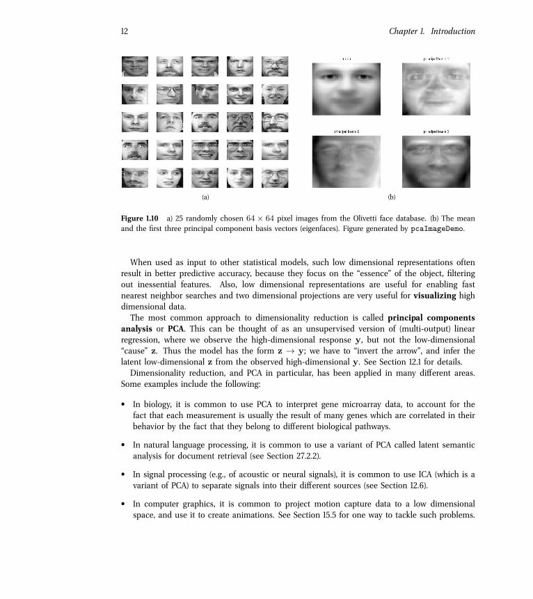
there may only be a small number of degrees of variability, corresponding to latent factors. Forexample, when modeling the appearance of face images, there may only be a few underlyinglatent factors which describe most of the variability, such as lighting, pose, identity, etc, asillustrated in Figure 1.10.


(a) (b)

Figure 1.10 a) 25 randomly chosen 64 × 64 pixel images from the Olivetti face database. (b) The meanand the first three principal component basis vectors (eigenfaces). Figure generated by pcaImageDemo.

When used as input to other statistical models, such low dimensional representations oftenresult in better predictive accuracy, because they focus on the “essence” of the object, filteringout inessential features. Also, low dimensional representations are useful for enabling fastnearest neighbor searches and two dimensional projections are very useful for visualizing highdimensional data.The most common approach to dimensionality reduction is called principal components

analysis or PCA. This can be thought of as an unsupervised version of (multi-output) linearregression, where we observe the high-dimensional response y, but not the low-dimensional“cause” z. Thus the model has the form z → y; we have to “invert the arrow”, and infer thelatent low-dimensional z from the observed high-dimensional y. See Section 12.1 for details.Dimensionality reduction, and PCA in particular, has been applied in many di�erent areas.

Some examples include the following:

• In biology, it is common to use PCA to interpret gene microarray data, to account for thefact that each measurement is usually the result of many genes which are correlated in theirbehavior by the fact that they belong to di�erent biological pathways.

• In natural language processing, it is common to use a variant of PCA called latent semanticanalysis for document retrieval (see Section 27.2.2).

• In signal processing (e.g., of acoustic or neural signals), it is common to use ICA (which is avariant of PCA) to separate signals into their di�erent sources (see Section 12.6).

• In computer graphics, it is common to project motion capture data to a low dimensionalspace, and use it to create animations. See Section 15.5 for one way to tackle such problems.

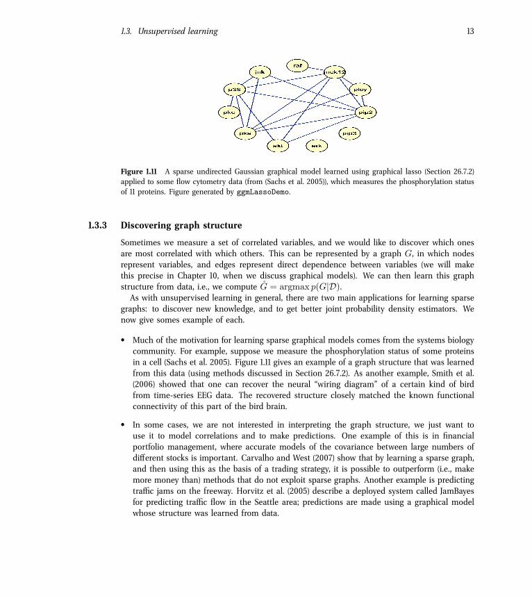
1.3. Unsupervised learning 13lambda=7.00, nedges=18

Figure 1.11 A sparse undirected Gaussian graphical model learned using graphical lasso (Section 26.7.2)applied to some flow cytometry data (from (Sachs et al. 2005)), which measures the phosphorylation statusof 11 proteins. Figure generated by ggmLassoDemo.

1.3.3 Discovering graph structure

Sometimes we measure a set of correlated variables, and we would like to discover which onesare most correlated with which others. This can be represented by a graph G, in which nodesrepresent variables, and edges represent direct dependence between variables (we will makethis precise in Chapter 10, when we discuss graphical models). We can then learn this graphstructure from data, i.e., we compute G = argmax p(G|D).As with unsupervised learning in general, there are two main applications for learning sparse

graphs: to discover new knowledge, and to get better joint probability density estimators. Wenow give somes example of each.

• Much of the motivation for learning sparse graphical models comes from the systems biologycommunity. For example, suppose we measure the phosphorylation status of some proteinsin a cell (Sachs et al. 2005). Figure 1.11 gives an example of a graph structure that was learnedfrom this data (using methods discussed in Section 26.7.2). As another example, Smith et al.(2006) showed that one can recover the neural “wiring diagram” of a certain kind of birdfrom time-series EEG data. The recovered structure closely matched the known functionalconnectivity of this part of the bird brain.

• In some cases, we are not interested in interpreting the graph structure, we just want touse it to model correlations and to make predictions. One example of this is in financialportfolio management, where accurate models of the covariance between large numbers ofdi�erent stocks is important. Carvalho and West (2007) show that by learning a sparse graph,and then using this as the basis of a trading strategy, it is possible to outperform (i.e., makemore money than) methods that do not exploit sparse graphs. Another example is predictingtra�c jams on the freeway. Horvitz et al. (2005) describe a deployed system called JamBayesfor predicting tra�c flow in the Seattle area; predictions are made using a graphical modelwhose structure was learned from data.


(a) (b)

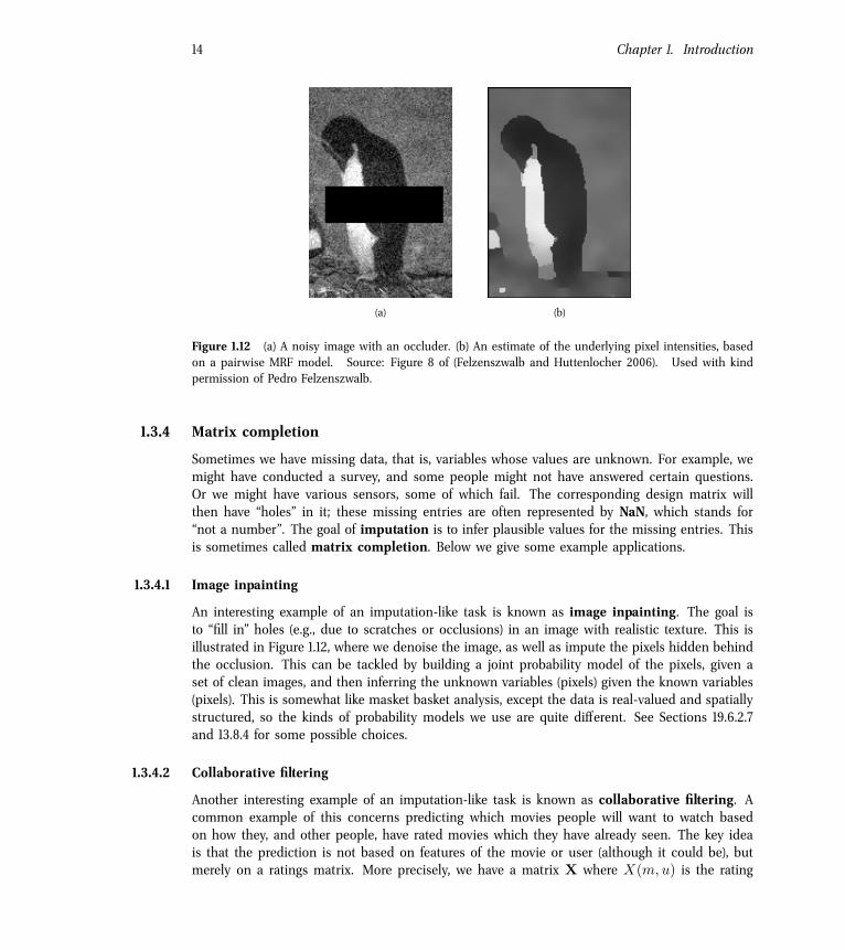
Figure 1.12 (a) A noisy image with an occluder. (b) An estimate of the underlying pixel intensities, basedon a pairwise MRF model. Source: Figure 8 of (Felzenszwalb and Huttenlocher 2006). Used with kindpermission of Pedro Felzenszwalb.

1.3.4 Matrix completion

Sometimes we have missing data, that is, variables whose values are unknown. For example, wemight have conducted a survey, and some people might not have answered certain questions.Or we might have various sensors, some of which fail. The corresponding design matrix willthen have “holes” in it; these missing entries are often represented by NaN, which stands for“not a number”. The goal of imputation is to infer plausible values for the missing entries. Thisis sometimes called matrix completion. Below we give some example applications.

1.3.4.1 Image inpainting

An interesting example of an imputation-like task is known as image inpainting. The goal isto “fill in” holes (e.g., due to scratches or occlusions) in an image with realistic texture. This isillustrated in Figure 1.12, where we denoise the image, as well as impute the pixels hidden behindthe occlusion. This can be tackled by building a joint probability model of the pixels, given aset of clean images, and then inferring the unknown variables (pixels) given the known variables(pixels). This is somewhat like masket basket analysis, except the data is real-valued and spatiallystructured, so the kinds of probability models we use are quite di�erent. See Sections 19.6.2.7and 13.8.4 for some possible choices.

1.3.4.2 Collaborative filtering

Another interesting example of an imputation-like task is known as collaborative filtering. Acommon example of this concerns predicting which movies people will want to watch basedon how they, and other people, have rated movies which they have already seen. The key ideais that the prediction is not based on features of the movie or user (although it could be), butmerely on a ratings matrix. More precisely, we have a matrix X where X(m,u) is the rating


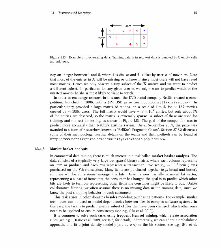
Figure 1.13 Example of movie-rating data. Training data is in red, test data is denoted by ?, empty cellsare unknown.

(say an integer between 1 and 5, where 1 is dislike and 5 is like) by user u of movie m. Notethat most of the entries in X will be missing or unknown, since most users will not have ratedmost movies. Hence we only observe a tiny subset of the X matrix, and we want to predicta di�erent subset. In particular, for any given user u, we might want to predict which of theunrated movies he/she is most likely to want to watch.In order to encourage research in this area, the DVD rental company Netflix created a com-

petition, launched in 2006, with a $1M USD prize (see http://netflixprize.com/). Inparticular, they provided a large matrix of ratings, on a scale of 1 to 5, for ∼ 18k moviescreated by ∼ 500k users. The full matrix would have ∼ 9 × 109 entries, but only about 1%of the entries are observed, so the matrix is extremely sparse. A subset of these are used fortraining, and the rest for testing, as shown in Figure 1.13. The goal of the competition was topredict more accurately than Netflix’s existing system. On 21 September 2009, the prize wasawarded to a team of researchers known as “BellKor’s Pragmatic Chaos”. Section 27.6.2 discussessome of their methodology. Further details on the teams and their methods can be found athttp://www.netflixprize.com/community/viewtopic.php?id=1537.

1.3.4.3 Market basket analysis

In commercial data mining, there is much interest in a task called market basket analysis. Thedata consists of a (typically very large but sparse) binary matrix, where each column representsan item or product, and each row represents a transaction. We set xij = 1 if item j waspurchased on the i’th transaction. Many items are purchased together (e.g., bread and butter),so there will be correlations amongst the bits. Given a new partially observed bit vector,representing a subset of items that the consumer has bought, the goal is to predict which otherbits are likely to turn on, representing other items the consumer might be likely to buy. (Unlikecollaborative filtering, we often assume there is no missing data in the training data, since weknow the past shopping behavior of each customer.)This task arises in other domains besides modeling purchasing patterns. For example, similar

techniques can be used to model dependencies between files in complex software systems. Inthis case, the task is to predict, given a subset of files that have been changed, which other onesneed to be updated to ensure consistency (see e.g., (Hu et al. 2010)).It is common to solve such tasks using frequent itemset mining, which create association

rules (see e.g., (Hastie et al. 2009, sec 14.2) for details). Alternatively, we can adopt a probabilisticapproach, and fit a joint density model p(x1, . . . , xD) to the bit vectors, see e.g., (Hu et al.


(a) (b)

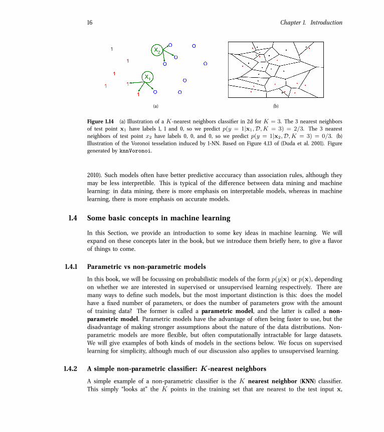
Figure 1.14 (a) Illustration of a K-nearest neighbors classifier in 2d for K = 3. The 3 nearest neighborsof test point x1 have labels 1, 1 and 0, so we predict p(y = 1|x1,D,K = 3) = 2/3. The 3 nearestneighbors of test point x2 have labels 0, 0, and 0, so we predict p(y = 1|x2,D,K = 3) = 0/3. (b)Illustration of the Voronoi tesselation induced by 1-NN. Based on Figure 4.13 of (Duda et al. 2001). Figuregenerated by knnVoronoi.

2010). Such models often have better predictive acccuracy than association rules, although theymay be less interpretible. This is typical of the di�erence between data mining and machinelearning: in data mining, there is more emphasis on interpretable models, whereas in machinelearning, there is more emphasis on accurate models.

1.4 Some basic concepts in machine learning

In this Section, we provide an introduction to some key ideas in machine learning. We willexpand on these concepts later in the book, but we introduce them briefly here, to give a flavorof things to come.

1.4.1 Parametric vs non-parametric models

In this book, we will be focussing on probabilistic models of the form p(y|x) or p(x), dependingon whether we are interested in supervised or unsupervised learning respectively. There aremany ways to define such models, but the most important distinction is this: does the modelhave a fixed number of parameters, or does the number of parameters grow with the amountof training data? The former is called a parametric model, and the latter is called a non-parametric model. Parametric models have the advantage of often being faster to use, but thedisadvantage of making stronger assumptions about the nature of the data distributions. Non-parametric models are more flexible, but often computationally intractable for large datasets.We will give examples of both kinds of models in the sections below. We focus on supervisedlearning for simplicity, although much of our discussion also applies to unsupervised learning.

1.4.2 A simple non-parametric classifier: K-nearest neighbors

A simple example of a non-parametric classifier is the K nearest neighbor (KNN) classifier.This simply “looks at” the K points in the training set that are nearest to the test input x,

1.4. Some basic concepts in machine learning 17

!3 !2 !1 0 1 2 3

!2

!1

0

1

2

3

4

5

train

(a)

p(y=1|data,K=10)

20 40 60 80 100

20

40

60

80

100

120

0

0.1

0.2

0.3

0.4

0.5

0.6

0.7

0.8

0.9

1

(b)

p(y=2|data,K=10)

20 40 60 80 100

20

40

60

80

100

120

0

0.1

0.2

0.3

0.4

0.5

0.6

0.7

0.8

0.9

1

(c)

!3 !2 !1 0 1 2 3!2

!1

0

1

2

3

4

5

predicted label, K=10

c1c2c3

(d)

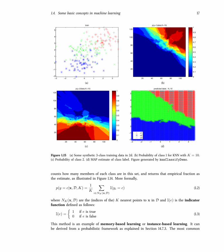
Figure 1.15 (a) Some synthetic 3-class training data in 2d. (b) Probability of class 1 for KNN with K = 10.(c) Probability of class 2. (d) MAP estimate of class label. Figure generated by knnClassifyDemo.

counts how many members of each class are in this set, and returns that empirical fraction asthe estimate, as illustrated in Figure 1.14. More formally,

p(y = c|x,D,K) =1

K

�

i∈NK(x,D)

I(yi = c) (1.2)

where NK(x,D) are the (indices of the) K nearest points to x in D and I(e) is the indicatorfunction defined as follows:

I(e) =

�1 if e is true0 if e is false

(1.3)

This method is an example of memory-based learning or instance-based learning. It canbe derived from a probabilistic framework as explained in Section 14.7.3. The most common


s

1

1

0

(a)

0 0.2 0.4 0.6 0.8 10

0.1

0.2

0.3

0.4

0.5

0.6

0.7

0.8

0.9

1

Fraction of data in neighborhood

Ed

ge

len

gth

of

cub

e

d=1

d=3

d=5d=7d=10

(b)

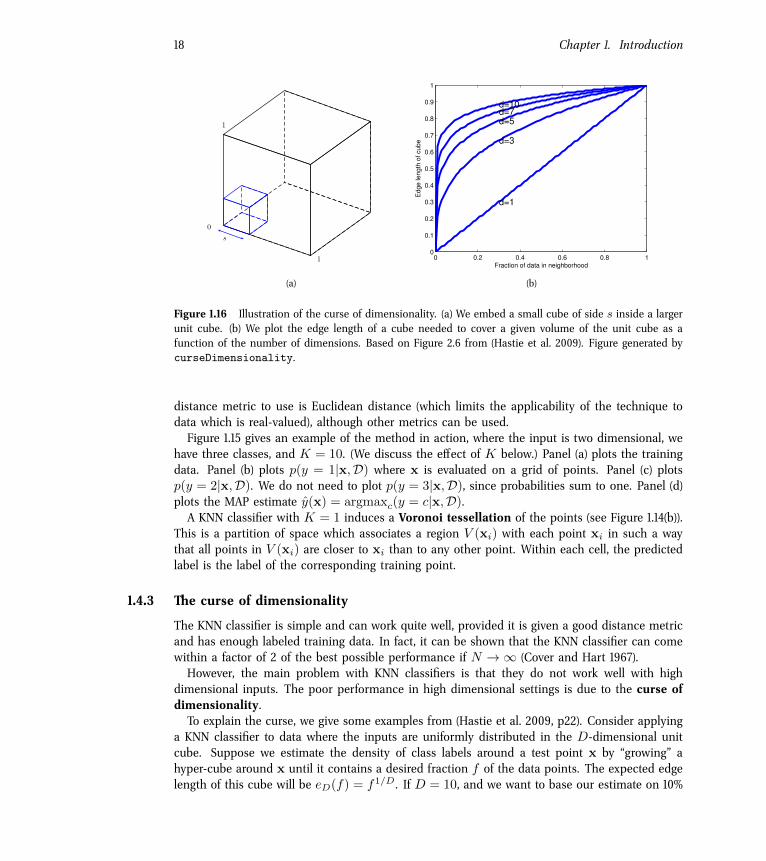
Figure 1.16 Illustration of the curse of dimensionality. (a) We embed a small cube of side s inside a largerunit cube. (b) We plot the edge length of a cube needed to cover a given volume of the unit cube as afunction of the number of dimensions. Based on Figure 2.6 from (Hastie et al. 2009). Figure generated bycurseDimensionality.

distance metric to use is Euclidean distance (which limits the applicability of the technique todata which is real-valued), although other metrics can be used.Figure 1.15 gives an example of the method in action, where the input is two dimensional, we

have three classes, and K = 10. (We discuss the e�ect of K below.) Panel (a) plots the trainingdata. Panel (b) plots p(y = 1|x,D) where x is evaluated on a grid of points. Panel (c) plotsp(y = 2|x,D). We do not need to plot p(y = 3|x,D), since probabilities sum to one. Panel (d)plots the MAP estimate y(x) = argmaxc(y = c|x,D).A KNN classifier with K = 1 induces a Voronoi tessellation of the points (see Figure 1.14(b)).

This is a partition of space which associates a region V (xi) with each point xi in such a waythat all points in V (xi) are closer to xi than to any other point. Within each cell, the predictedlabel is the label of the corresponding training point.

1.4.3 The curse of dimensionality

The KNN classifier is simple and can work quite well, provided it is given a good distance metricand has enough labeled training data. In fact, it can be shown that the KNN classifier can comewithin a factor of 2 of the best possible performance if N → ∞ (Cover and Hart 1967).However, the main problem with KNN classifiers is that they do not work well with high

dimensional inputs. The poor performance in high dimensional settings is due to the curse ofdimensionality.To explain the curse, we give some examples from (Hastie et al. 2009, p22). Consider applying

a KNN classifier to data where the inputs are uniformly distributed in the D-dimensional unitcube. Suppose we estimate the density of class labels around a test point x by “growing” ahyper-cube around x until it contains a desired fraction f of the data points. The expected edgelength of this cube will be eD(f) = f1/D . If D = 10, and we want to base our estimate on 10%


−3 −2 −1 0 1 2 30

0.05

0.1

0.15

0.2

0.25

0.3

0.35

0.4PDF

(a) (b)

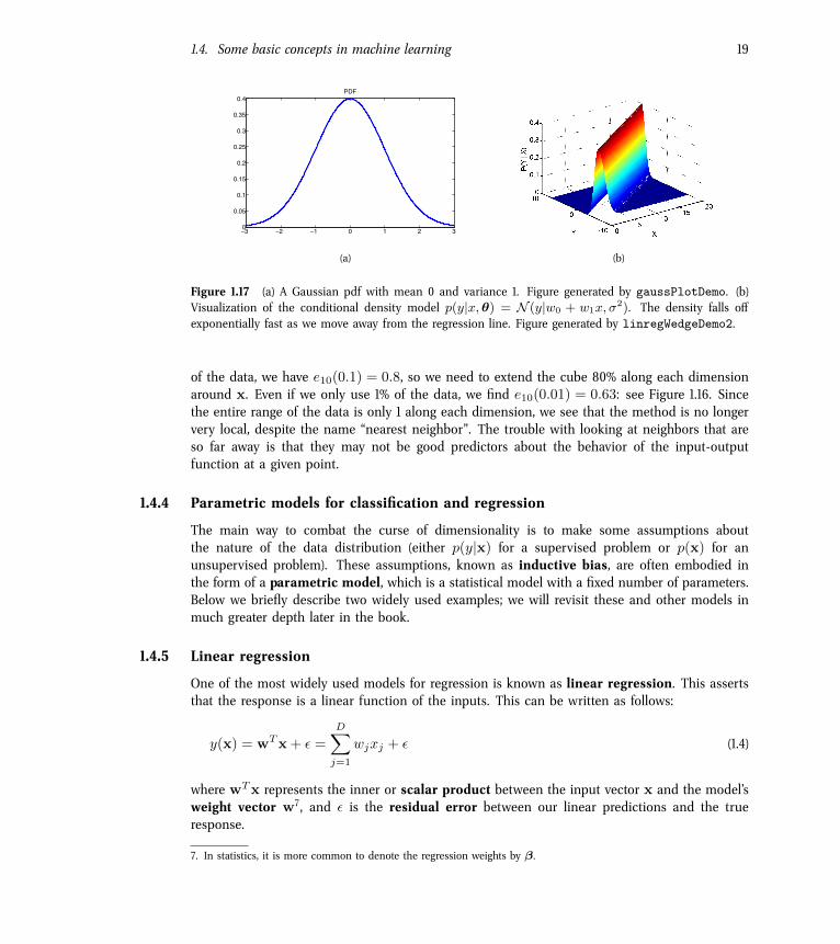
Figure 1.17 (a) A Gaussian pdf with mean 0 and variance 1. Figure generated by gaussPlotDemo. (b)Visualization of the conditional density model p(y|x,θ) = N (y|w0 + w1x,σ

2). The density falls o�exponentially fast as we move away from the regression line. Figure generated by linregWedgeDemo2.

of the data, we have e10(0.1) = 0.8, so we need to extend the cube 80% along each dimensionaround x. Even if we only use 1% of the data, we find e10(0.01) = 0.63: see Figure 1.16. Sincethe entire range of the data is only 1 along each dimension, we see that the method is no longervery local, despite the name “nearest neighbor”. The trouble with looking at neighbors that areso far away is that they may not be good predictors about the behavior of the input-outputfunction at a given point.

1.4.4 Parametric models for classification and regression

The main way to combat the curse of dimensionality is to make some assumptions aboutthe nature of the data distribution (either p(y|x) for a supervised problem or p(x) for anunsupervised problem). These assumptions, known as inductive bias, are often embodied inthe form of a parametric model, which is a statistical model with a fixed number of parameters.Below we briefly describe two widely used examples; we will revisit these and other models inmuch greater depth later in the book.

1.4.5 Linear regression

One of the most widely used models for regression is known as linear regression. This assertsthat the response is a linear function of the inputs. This can be written as follows:

y(x) = wTx+ � =D�

j=1

wjxj + � (1.4)

where wTx represents the inner or scalar product between the input vector x and the model’sweight vector w7, and � is the residual error between our linear predictions and the trueresponse.

7. In statistics, it is more common to denote the regression weights by β.


0 5 10 15 20−10

−5

0

5

10

15degree 14

(a)

0 5 10 15 20−10

−5

0

5

10

15degree 20

(b)

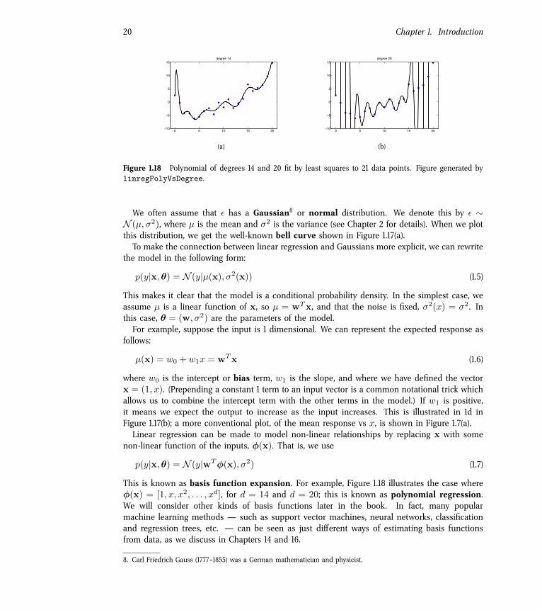
Figure 1.18 Polynomial of degrees 14 and 20 fit by least squares to 21 data points. Figure generated bylinregPolyVsDegree.

We often assume that � has a Gaussian8 or normal distribution. We denote this by � ∼N (µ,σ2), where µ is the mean and σ2 is the variance (see Chapter 2 for details). When we plotthis distribution, we get the well-known bell curve shown in Figure 1.17(a).To make the connection between linear regression and Gaussians more explicit, we can rewrite

the model in the following form:

p(y|x,θ) = N (y|µ(x),σ2(x)) (1.5)

This makes it clear that the model is a conditional probability density. In the simplest case, weassume µ is a linear function of x, so µ = wTx, and that the noise is fixed, σ2(x) = σ2. Inthis case, θ = (w,σ2) are the parameters of the model.For example, suppose the input is 1 dimensional. We can represent the expected response as

follows:

µ(x) = w0 + w1x = wTx (1.6)

where w0 is the intercept or bias term, w1 is the slope, and where we have defined the vectorx = (1, x). (Prepending a constant 1 term to an input vector is a common notational trick whichallows us to combine the intercept term with the other terms in the model.) If w1 is positive,it means we expect the output to increase as the input increases. This is illustrated in 1d inFigure 1.17(b); a more conventional plot, of the mean response vs x, is shown in Figure 1.7(a).Linear regression can be made to model non-linear relationships by replacing x with some

non-linear function of the inputs, φ(x). That is, we use

p(y|x,θ) = N (y|wTφ(x),σ2) (1.7)

This is known as basis function expansion. For example, Figure 1.18 illustrates the case whereφ(x) = [1, x, x2, . . . , xd], for d = 14 and d = 20; this is known as polynomial regression.We will consider other kinds of basis functions later in the book. In fact, many popularmachine learning methods — such as support vector machines, neural networks, classificationand regression trees, etc. — can be seen as just di�erent ways of estimating basis functionsfrom data, as we discuss in Chapters 14 and 16.

8. Carl Friedrich Gauss (1777–1855) was a German mathematician and physicist.


!10 !5 0 5 100

0.1

0.2

0.3

0.4

0.5

0.6

0.7

0.8

0.9

1

(a)

460 480 500 520 540 560 580 600 620 640

0

0.1

0.2

0.3

0.4

0.5

0.6

0.7

0.8

0.9

1

(b)

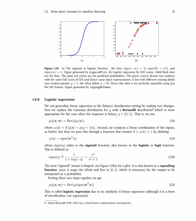
Figure 1.19 (a) The sigmoid or logistic function. We have sigm(−∞) = 0, sigm(0) = 0.5, andsigm(∞) = 1. Figure generated by sigmoidPlot. (b) Logistic regression for SAT scores. Solid black dotsare the data. The open red circles are the predicted probabilities. The green crosses denote two studentswith the same SAT score of 525 (and hence same input representation x) but with di�erent training labels(one student passed, y = 1, the other failed, y = 0). Hence this data is not perfectly separable using justthe SAT feature. Figure generated by logregSATdemo.

1.4.6 Logistic regression

We can generalize linear regression to the (binary) classification setting by making two changes.First we replace the Gaussian distribution for y with a Bernoulli distribution9,which is moreappropriate for the case when the response is binary, y ∈ {0, 1}. That is, we use

p(y|x,w) = Ber(y|µ(x)) (1.8)

where µ(x) = E [y|x] = p(y = 1|x). Second, we compute a linear combination of the inputs,as before, but then we pass this through a function that ensures 0 ≤ µ(x) ≤ 1 by defining

µ(x) = sigm(wTx) (1.9)

where sigm(η) refers to the sigmoid function, also known as the logistic or logit function.This is defined as

sigm(η) � 1

1 + exp(−η)=

eη

eη + 1(1.10)

The term “sigmoid” means S-shaped: see Figure 1.19(a) for a plot. It is also known as a squashingfunction, since it maps the whole real line to [0, 1], which is necessary for the output to beinterpreted as a probability.Putting these two steps together we get

p(y|x,w) = Ber(y|sigm(wTx)) (1.11)

This is called logistic regression due to its similarity to linear regression (although it is a formof classification, not regression!).

9. Daniel Bernoulli (1700–1782) was a Dutch-Swiss mathematician and physicist.


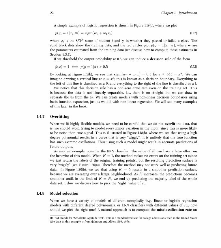
A simple example of logistic regression is shown in Figure 1.19(b), where we plot

p(yi = 1|xi,w) = sigm(w0 + w1xi) (1.12)

where xi is the SAT10 score of student i and yi is whether they passed or failed a class. Thesolid black dots show the training data, and the red circles plot p(y = 1|xi, w), where w arethe parameters estimated from the training data (we discuss how to compute these estimates inSection 8.3.4).If we threshold the output probability at 0.5, we can induce a decision rule of the form

y(x) = 1 ⇐⇒ p(y = 1|x) > 0.5 (1.13)

By looking at Figure 1.19(b), we see that sigm(w0 + w1x) = 0.5 for x ≈ 545 = x∗. We canimagine drawing a vertical line at x = x∗; this is known as a decision boundary. Everything tothe left of this line is classified as a 0, and everything to the right of the line is classified as a 1.We notice that this decision rule has a non-zero error rate even on the training set. This

is because the data is not linearly separable, i.e., there is no straight line we can draw toseparate the 0s from the 1s. We can create models with non-linear decision boundaries usingbasis function expansion, just as we did with non-linear regression. We will see many examplesof this later in the book.

1.4.7 Overfitting

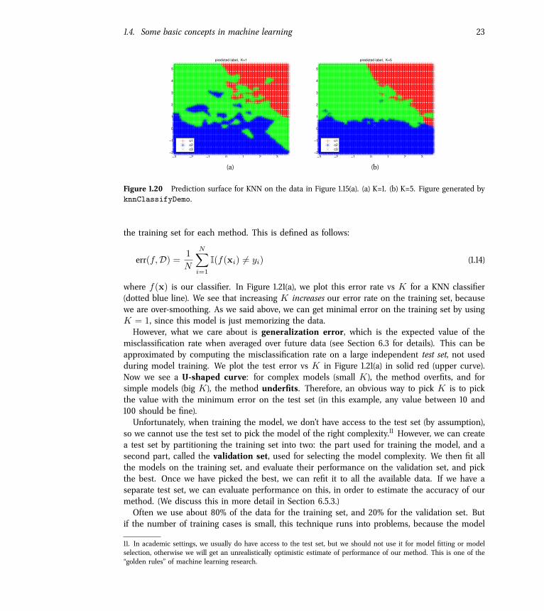
When we fit highly flexible models, we need to be careful that we do not overfit the data, thatis, we should avoid trying to model every minor variation in the input, since this is more likelyto be noise than true signal. This is illustrated in Figure 1.18(b), where we see that using a highdegree polynomial results in a curve that is very “wiggly”. It is unlikely that the true functionhas such extreme oscillations. Thus using such a model might result in accurate predictions offuture outputs.As another example, consider the KNN classifier. The value of K can have a large e�ect on

the behavior of this model. When K = 1, the method makes no errors on the training set (sincewe just return the labels of the original training points), but the resulting prediction surface isvery “wiggly” (see Figure 1.20(a)). Therefore the method may not work well at predicting futuredata. In Figure 1.20(b), we see that using K = 5 results in a smoother prediction surface,because we are averaging over a larger neighborhood. As K increases, the predictions becomessmoother until, in the limit of K = N , we end up predicting the majority label of the wholedata set. Below we discuss how to pick the “right” value of K .

1.4.8 Model selection

When we have a variety of models of di�erent complexity (e.g., linear or logistic regressionmodels with di�erent degree polynomials, or KNN classifiers with di�erent values of K ), howshould we pick the right one? A natural approach is to compute the misclassification rate on

10. SAT stands for “Scholastic Aptitude Test”. This is a standardized test for college admissions used in the United States(the data in this example is from (Johnson and Albert 1999, p87)).


!3 !2 !1 0 1 2 3!2

!1

0

1

2

3

4

5


c1c2c3

(a)

!3 !2 !1 0 1 2 3!2

!1

0

1

2

3

4

5


c1c2c3

(b)

Figure 1.20 Prediction surface for KNN on the data in Figure 1.15(a). (a) K=1. (b) K=5. Figure generated byknnClassifyDemo.

the training set for each method. This is defined as follows:

err(f,D) =1

N

N�

i=1

I(f(xi) �= yi) (1.14)

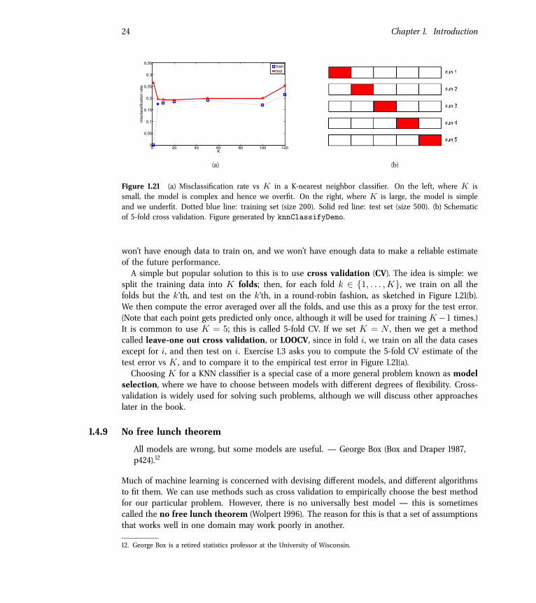
where f(x) is our classifier. In Figure 1.21(a), we plot this error rate vs K for a KNN classifier(dotted blue line). We see that increasing K increases our error rate on the training set, becausewe are over-smoothing. As we said above, we can get minimal error on the training set by usingK = 1, since this model is just memorizing the data.However, what we care about is generalization error, which is the expected value of the

misclassification rate when averaged over future data (see Section 6.3 for details). This can beapproximated by computing the misclassification rate on a large independent test set, not usedduring model training. We plot the test error vs K in Figure 1.21(a) in solid red (upper curve).Now we see a U-shaped curve: for complex models (small K ), the method overfits, and forsimple models (big K ), the method underfits. Therefore, an obvious way to pick K is to pickthe value with the minimum error on the test set (in this example, any value between 10 and100 should be fine).Unfortunately, when training the model, we don’t have access to the test set (by assumption),

so we cannot use the test set to pick the model of the right complexity.11 However, we can createa test set by partitioning the training set into two: the part used for training the model, and asecond part, called the validation set, used for selecting the model complexity. We then fit allthe models on the training set, and evaluate their performance on the validation set, and pickthe best. Once we have picked the best, we can refit it to all the available data. If we have aseparate test set, we can evaluate performance on this, in order to estimate the accuracy of ourmethod. (We discuss this in more detail in Section 6.5.3.)Often we use about 80% of the data for the training set, and 20% for the validation set. But

if the number of training cases is small, this technique runs into problems, because the model

11. In academic settings, we usually do have access to the test set, but we should not use it for model fitting or modelselection, otherwise we will get an unrealistically optimistic estimate of performance of our method. This is one of the“golden rules” of machine learning research.


0 20 40 60 80 100 1200

0.05

0.1

0.15

0.2

0.25

0.3

0.35

K

mis

clas

sific

atio

n ra

te

traintest

(a) (b)

Figure 1.21 (a) Misclassification rate vs K in a K-nearest neighbor classifier. On the left, where K issmall, the model is complex and hence we overfit. On the right, where K is large, the model is simpleand we underfit. Dotted blue line: training set (size 200). Solid red line: test set (size 500). (b) Schematicof 5-fold cross validation. Figure generated by knnClassifyDemo.

won’t have enough data to train on, and we won’t have enough data to make a reliable estimateof the future performance.A simple but popular solution to this is to use cross validation (CV). The idea is simple: we

split the training data into K folds; then, for each fold k ∈ {1, . . . ,K}, we train on all thefolds but the k’th, and test on the k’th, in a round-robin fashion, as sketched in Figure 1.21(b).We then compute the error averaged over all the folds, and use this as a proxy for the test error.(Note that each point gets predicted only once, although it will be used for training K−1 times.)It is common to use K = 5; this is called 5-fold CV. If we set K = N , then we get a methodcalled leave-one out cross validation, or LOOCV, since in fold i, we train on all the data casesexcept for i, and then test on i. Exercise 1.3 asks you to compute the 5-fold CV estimate of thetest error vs K , and to compare it to the empirical test error in Figure 1.21(a).Choosing K for a KNN classifier is a special case of a more general problem known as model

selection, where we have to choose between models with di�erent degrees of flexibility. Cross-validation is widely used for solving such problems, although we will discuss other approacheslater in the book.

1.4.9 No free lunch theorem

All models are wrong, but some models are useful. — George Box (Box and Draper 1987,p424).12

Much of machine learning is concerned with devising di�erent models, and di�erent algorithmsto fit them. We can use methods such as cross validation to empirically choose the best methodfor our particular problem. However, there is no universally best model — this is sometimescalled the no free lunch theorem (Wolpert 1996). The reason for this is that a set of assumptionsthat works well in one domain may work poorly in another.

12. George Box is a retired statistics professor at the University of Wisconsin.


As a consequence of the no free lunch theorem, we need to develop many di�erent types ofmodels, to cover the wide variety of data that occurs in the real world. And for each model,there may be many di�erent algorithms we can use to train the model, which make di�erentspeed-accuracy-complexity tradeo�s. It is this combination of data, models and algorithms thatwe will be studying in the subsequent chapters.

Exercises

Exercise 1.1 KNN classifier on shu�ed MNIST data

Run mnist1NNdemo and verify that the misclassification rate (on the first 1000 test cases) of MNIST of a1-NN classifier is 3.8%. (If you run it all on all 10,000 test cases, the error rate is 3.09%.) Modify the codeso that you first randomly permute the features (columns of the training and test design matrices), as inshuffledDigitsDemo, and then apply the classifier. Verify that the error rate is not changed.

Exercise 1.2 Approximate KNN classifiers

Use the Matlab/C++ code at http://people.cs.ubc.ca/~mariusm/index.php/FLANN/FLANN to per-form approximate nearest neighbor search, and combine it with mnist1NNdemo to classify the MNIST dataset. How much speedup do you get, and what is the drop (if any) in accuracy?

Exercise 1.3 CV for KNN

Use knnClassifyDemo to plot the CV estimate of the misclassification rate on the test set. Compare thisto Figure 1.21(a). Discuss the similarities and di�erences to the test error rate.

Documents

Machine Learningmurphyk/MLbook/pml-intro-22may12.pdf · of probability theory. Probability theory can be applied to any problem involving uncertainty. In machine learning, uncertainty