Embed Size (px)
Citation preview
Macroeconometrics
Teaching Notes and Exercises
Pau Roldan∗
New York University
Abstract
This document is a compilation of notes and exercises on basic topics in Macroeconometrics, which I collectedas a student both at UPF and NYU. All the programs, provided in an Appendix, were written together withEwout Verriest.
Contents
1 Invertibility and Equivalence 2
2 The Frequency Domain 4
3 The Hodrick-Prescott Filter 73.1 Computing the Cycle . . . . . . . . . . . . . . . . . . . . . . . . . . . . . . . . . . . . . . . . . . . 73.2 Gain and Phase of the Filter . . . . . . . . . . . . . . . . . . . . . . . . . . . . . . . . . . . . . . 8
4 The Kalman Filter 114.1 Preliminaries . . . . . . . . . . . . . . . . . . . . . . . . . . . . . . . . . . . . . . . . . . . . . . . 114.2 The Recursion . . . . . . . . . . . . . . . . . . . . . . . . . . . . . . . . . . . . . . . . . . . . . . 12
5 Log-Likelihood Estimation 165.1 Estimation of an MA(1) . . . . . . . . . . . . . . . . . . . . . . . . . . . . . . . . . . . . . . . . . 165.2 Estimation of a VAR(2) . . . . . . . . . . . . . . . . . . . . . . . . . . . . . . . . . . . . . . . . . 18
5.2.1 Estimation . . . . . . . . . . . . . . . . . . . . . . . . . . . . . . . . . . . . . . . . . . . . 195.2.2 Granger Causation . . . . . . . . . . . . . . . . . . . . . . . . . . . . . . . . . . . . . . . . 215.2.3 Beveridge-Nelson Output Gap . . . . . . . . . . . . . . . . . . . . . . . . . . . . . . . . . 22
5.3 Estimation of an SVAR . . . . . . . . . . . . . . . . . . . . . . . . . . . . . . . . . . . . . . . . . 235.3.1 Identification via Long-Run Restrictions . . . . . . . . . . . . . . . . . . . . . . . . . . . . 245.3.2 Implementation . . . . . . . . . . . . . . . . . . . . . . . . . . . . . . . . . . . . . . . . . . 25
6 Application: A New Keynesian Model 266.1 Equivalent System of Expectational Difference Equations . . . . . . . . . . . . . . . . . . . . . . 266.2 State-Space Form . . . . . . . . . . . . . . . . . . . . . . . . . . . . . . . . . . . . . . . . . . . . . 286.3 Numerical Implementation . . . . . . . . . . . . . . . . . . . . . . . . . . . . . . . . . . . . . . . . 296.4 Simulating data when (xt, πt, it) is known . . . . . . . . . . . . . . . . . . . . . . . . . . . . . . . 346.5 Bayesian Estimation of the New Keynesian Model . . . . . . . . . . . . . . . . . . . . . . . . . . 34
6.5.1 Priors . . . . . . . . . . . . . . . . . . . . . . . . . . . . . . . . . . . . . . . . . . . . . . . 366.5.2 Posteriors . . . . . . . . . . . . . . . . . . . . . . . . . . . . . . . . . . . . . . . . . . . . . 37
A Appendix: MatLab Codes 43A.1 Code for Section 2 . . . . . . . . . . . . . . . . . . . . . . . . . . . . . . . . . . . . . . . . . . . . 43A.2 Code for Section 3 . . . . . . . . . . . . . . . . . . . . . . . . . . . . . . . . . . . . . . . . . . . . 44A.3 Code for Section 5.1 . . . . . . . . . . . . . . . . . . . . . . . . . . . . . . . . . . . . . . . . . . . 44A.4 Code for Section 5.2 . . . . . . . . . . . . . . . . . . . . . . . . . . . . . . . . . . . . . . . . . . . 45A.5 Code for Section 5.3 . . . . . . . . . . . . . . . . . . . . . . . . . . . . . . . . . . . . . . . . . . . 47A.6 Code for Section 6 . . . . . . . . . . . . . . . . . . . . . . . . . . . . . . . . . . . . . . . . . . . . 48A.7 Code for Section 6.4 . . . . . . . . . . . . . . . . . . . . . . . . . . . . . . . . . . . . . . . . . . . 51A.8 Code for Section 6.5 . . . . . . . . . . . . . . . . . . . . . . . . . . . . . . . . . . . . . . . . . . . 53
∗Department of Economics, New York University, 19 West 4th Street, 6th Floor, New York, NY 100012. E-mail: [email protected]
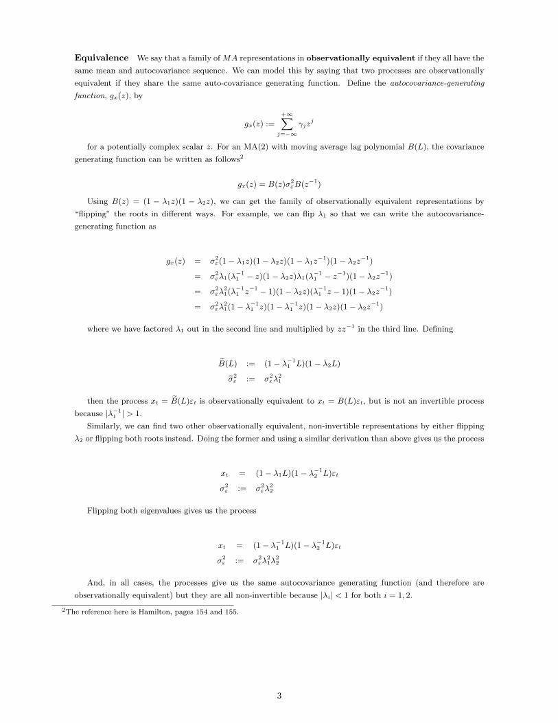
1 Invertibility and Equivalence
Consider a second-order moving average (or simply, MA(2)) process:
xt = B(L)εt
B(L) := 1 + θ1L+ θ2L2
where B(L) is the moving-average lag polynomial, L is the lag operator1 and εt ∼ iid N (0, σ2ε) is the
innovation to the process, with the no serial correlation property Eεtεs = 0, ∀t 6= s (that is, εt is a white noise
process).
Invertibility We want to derive conditions on θ1 and θ2 that allow us to invert the process, that is, to write
the MA(2) as an AR(∞) process εt = B(L)−1xt, which reads
εt =
+∞∑j=0
ηjxt−j
for some coefficients ηjj∈Z+ . The existence of B(L)−1 means that B(L)−1 is a non-explosive backward-
looking lag polynomial. A moving-average process is said to be invertible if the innovations of the process lie in
the space spanned by current and past values of the observables, a property that is especially useful if we wish
to, for example, recover shocks to the system from past observations of the original series.
In this case, we use the following proposition:
Proposition 1 An MA(q) process xt = B(L)εt is invertible iff the roots of B(z) = 0 lie outside the unit circle.
In our case, the characteristic equation is
1 + θ1z + θ2z2 = 0 (1)
Factoring the moving average operator as 1 + θ1z + θ2z2 = (1 − λ1z)(1 − λ2z), where λ1 and λ2 are the
eigenvalues of the characteristic equation (the conjugate of the roots), one can alternatively check for invertibility
using that |λi| < 1 for both i = 1, 2. In our case, the roots of equation (1) are
z1 = − θ12θ2
+
√θ21 − 4θ2
2θ2
z2 = − θ12θ2−√θ21 − 4θ2
2θ2
and we need |z1| > 1 and |z2| > 1, namely, zi /∈ [0, 1], for both i = 1, 2. To derive conditions, note that
B(z) = 1 + θ1z + θ2z2 = (1− λ1z)(1− λ2z) = 1− (λ1 + λ2)z − λ1λ2z
2
and therefore we must have
θ1 = λ1 + λ2
θ2 = λ1λ2
The condition |λ1| < 1 and |λ2| < 1 therefore collapses to the requirement that |θ2| = |λ1λ2| < 1, which is
a necessary condition for invertibility. On the other hand, |θ1| = |λ1 + λ2| ≤ |λ1|+ |λ2| < 2, namely |θ1| < 2 is
also a necessary condition for invertibility.
1The lag operator is the operator defined by Ljxt = xt−j , for any t, j ∈ N.
2
Equivalence We say that a family of MA representations in observationally equivalent if they all have the
same mean and autocovariance sequence. We can model this by saying that two processes are observationally
equivalent if they share the same auto-covariance generating function. Define the autocovariance-generating
function, gx(z), by
gx(z) :=
+∞∑j=−∞
γjzj
for a potentially complex scalar z. For an MA(2) with moving average lag polynomial B(L), the covariance
generating function can be written as follows2
gx(z) = B(z)σ2εB(z−1)
Using B(z) = (1 − λ1z)(1 − λ2z), we can get the family of observationally equivalent representations by
“flipping” the roots in different ways. For example, we can flip λ1 so that we can write the autocovariance-
generating function as
gx(z) = σ2ε(1− λ1z)(1− λ2z)(1− λ1z
−1)(1− λ2z−1)
= σ2ελ1(λ−1
1 − z)(1− λ2z)λ1(λ−11 − z
−1)(1− λ2z−1)
= σ2ελ
21(λ−1
1 z−1 − 1)(1− λ2z)(λ−11 z − 1)(1− λ2z
−1)
= σ2ελ
21(1− λ−1
1 z)(1− λ−11 z)(1− λ2z)(1− λ2z
−1)
where we have factored λ1 out in the second line and multiplied by zz−1 in the third line. Defining
B(L) := (1− λ−11 L)(1− λ2L)
σ2ε := σ2
ελ21
then the process xt = B(L)εt is observationally equivalent to xt = B(L)εt, but is not an invertible process
because |λ−11 | > 1.
Similarly, we can find two other observationally equivalent, non-invertible representations by either flipping
λ2 or flipping both roots instead. Doing the former and using a similar derivation than above gives us the process
xt = (1− λ1L)(1− λ−12 L)εt
σ2ε := σ2
ελ22
Flipping both eigenvalues gives us the process
xt = (1− λ−11 L)(1− λ−1
2 L)εt
σ2ε := σ2
ελ21λ
22
And, in all cases, the processes give us the same autocovariance generating function (and therefore are
observationally equivalent) but they are all non-invertible because |λi| < 1 for both i = 1, 2.
2The reference here is Hamilton, pages 154 and 155.
3
2 The Frequency Domain
In time-series macroeconomics we tend to study processes in the time domain, and study fluctuations that
occur across time periods. Alternatively, one can also study processes with respect to frequency, rather than
time. Instead of analyzing how the process changes over time, the frequency-domain approach studies how much
of the process lies within each given frequency band over a range of frequencies.
Stochastic processes can be converted between time- and frequency-domains with so-called Fourier trans-
forms, which translates time into a sum of waves of different frequencies, each of which represents a different
frequency. Formally, for a sequence of complex numbers xtt∈Z, the Fourier transform is a function dTx (ω)
defined by
dTx (ω) :=
T−1∑t=1
xte−iωt
The “inverse Fourier transform” then converts frequency back to a time function. In turn, the so-called
population spectrum of a stochastic process xt : t ∈ R, denoted by sx(ω), is the frequency-domain repre-
sentation of the process. Formally, it is the representation of xt as a weighted sum of periodic functions that
are orthogonal across different frequencies. In Economics, the reason we use this domain is because we typically
want to determine how important cycles of different frequencies are in accounting for the behavior of a random
variable, here xt.
By the so-called Cramer representation of the series, xt can be decomposed into periodic components
that are orthogonal across different frequencies that fluctuate within [−π, π], such that
xt =
∫ π
−πeiωtdZx(ω)
where i :=√−1, dZx(ω) is a mean-zero, complex-valued, continuous random vector in frequencies ω with
the property E[dZx(ω)dZx(ω)′] = sx(ω)dω, where sx(ω) is the population spectrum (defined below), and
E[dZx(ω)dZx(λ)′] = 0, for all frequencies λ 6= ω (the upper bar denotes the conjugate transpose). That is,
dZx(ω) is a complex-valued variable that is uncorrelated across frequencies and whose variance is proportional
to the spectral density at any given frequency ω. Cramer’s representation thus allow us to identify the time vari-
ations of the process through oscillations that occur at different frequencies: long-run dynamics are associated
with the low frequency components, while short-run dynamics correspond to the high frequency components.
Covariance-stationary processes Suppose that the process xt+∞t=−∞ above is covariance-stationary, and
that the covariances are absolutely summable (our main mixing condition), or
+∞∑j=−∞
|γj | < +∞
for any t ∈ Z, where γj := E[(yt − µ)(yt−j − µ)] and µ := E(yt) (note that neither of the first two moments
depend on t because of covariance-stationarity). To find the spectrum, first define the autocovariance-generating
function, gx(z), by
gx(z) :=
+∞∑j=−∞
γjzj
for some (possibly complex) scalar z. By De Moivre’s theorem, any value of z that lies on the complex unit
circle can be written as
z = cos(ω)− i sin(ω)
= e−iω
4
where ω is the radiant angle that z makes with the real axis (typically considered a frequency, or units of
time per cycle, in applications3).
If the autocovariance-generating function is evaluated at z = e−iω and divided by 2π, that is, if we apply a
Fourier transform on the sequence of autocovariances, then the resulting function is
sx(ω) :=1
2πgx(e−iω)
=1
2π
+∞∑j=−∞
γje−iωj
=1
2π
+∞∑j=−∞
γj [cos(ωj)− i sin(ωj)]
where the last line uses De Moivre’s theorem once again to say that
e−iωj = cos(ωj)− i sin(ωj)
For an absolutely summable process such as this, the population spectrum thus function exists and can
be used to compute all of the autocovariances.4 We can further write the population spectrum by using the
symmetry of the auto-covariance about zero (namely, γj = γ−j , for any j ∈ Z), such that
sx(ω) =1
2πγ0[cos(0)− i sin(0)]
+1
2π
+∞∑j=1
γj [cos(ωj) + cos(−ωj)− i sin(ωj)− i sin(−ωj)]
=1
2π
γ0 + 2
+∞∑j=1
γj cos(ωj)
where the second line uses that cos(0) = 1− sin(0) = 1 and that cos(−x) = − sin(x) and cos(−x) = − cos(x)
to simplify the first expression. This last representation of the spectrum clearly shows that, if the autocovariance
sequence is absolutely summable, then sx(ω) exists and is a continuous, real-valued function of ω.
Example There are convenient formulas to compute the spectrum of processes of the ARMA class (see
pages 154 and 155 in Hamilton). Here, we present a simple second-order autoregressive process (or AR(2)) for
illustration:
A(L)xt = εt
A(L) := 1− ρ1L− ρ2L2
where εt ∼ iid N (0, 1) is a serially uncorrelated process (white noise). We would like to plot the population
spectrum and the autocorrelation function for given parameterizations. In this case,
gx(z) = A(z)−1σ2εA(z−1)−1
gives the autocovariance-generating function of the process A(L)xt = εt, for A(L) a second-order polynomial,
σ2ε := E(ε2t ) (unity, in our case) and z some complex scalar. Again, evaluating the autocovariance-generating
function at z = e−iω and dividing by 2π will give us the spectral density:
3It is natural to use the measure of units of time (say, quarters) per cycle, call it λ. In this case, the fundamental relation is ω = 2π/λ.For example, a cycle of length 3 years corresponds to λ = 12 quarters per cycle, in which case ω = 2π
12= π
6.
4Therefore, if two processes share the same autocovariance-generating function, they exhibit the identical sequence of autocovariances.
5
sx(ω) =1
2π
[A(e−iω)−1σ2
εA(eiω)−1]
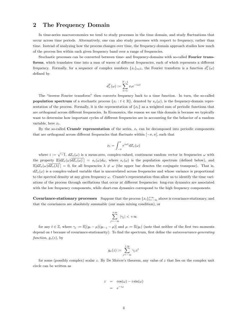
and A(e−iω) = 1 − ρ1e−iω − ρ2e−i2ω, in our case. The program in Appendix A.1 implements this formula.
Figure 1 shows the result for the calibrations (ρ1, ρ2) = (1.25,−0.3) and (ρ1, ρ2) = (1.7,−0.8).
−4 −3 −2 −1 0 1 2 3 40
10
20
30
40
50
60
70Population Spectrum (in quarters per cycle)
Quarters per cycle (ω)
Spe
ctru
m (
s x(ω))
ρ1=1.25; ρ2= − 0.3
ρ1=1.7; ρ2= − 0.8
Figure 1: Population Spectrum for two different calibrations of an AR(2).
What we find is that the spectrum is not well-behaved in the second calibration (it displays a bimodal
pattern), but it is in the first one. The reason is that the coefficients in the second calibration imply complex
roots, which explain the spikes in the spectrum, while those of the first calibration imply real roots, which
accounts for the bell-shaped spectrum. However, in both cases, the spectrum vanishes to zero in the long-run.
The autocovariance can be obtained by the definition γj := E[(yt − µ)(yt−j − µ)] directly or, in case we have
it at hand, from the population spectrum. The latter is established by the following two equivalent formulas
(see Proposition 6.1 in Hamilton, page 155), which follow from inverting the Fourier transform of the spectrum:
γk =
∫ π
−πsx(ω)eiωkdω (2)
γk =
∫ π
−πsx(ω) cos(ωk)dω
for any k ∈ Z. For instance, γ0 =∫ π−π sx(ω)dω is the variance, which we obtain by the sum of spectra
across different frequencies. This property shows that there is a bijective relation between time and frequency
domains: they are mutually exclusive in the sense that any feature of the data that can be interpreted from the
time-domain representation (through a Wold-like form), is also captured in the frequency-domain representation
(through a Cramer-like form).
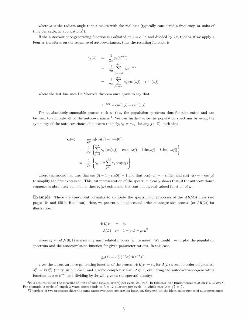
Figure 2 plots the autocorrelation for the calibrations (ρ1, ρ2) = (1.25,−0.3) and (ρ1, ρ2) = (1.7,−0.8), as
computed by the formula
φj :=γjγ0
with γj and γ0 given in (2). What we see is that the first calibration seems to exhibit, once again, well-
behaved patterns. The autocorrelation in the first calibration nicely fades out to zero for higher orders, as is to
be expected from a stationary autoregressive process. However, the second calibration exhibits waves of different
amplitude, which surely indicates nonstationarity.
6
−30 −20 −10 0 10 20 30−2
−1
0
1
2
3
4
5
6Auto−Correlation Function
Step−size (j)
φ j
ρ1=1.25; ρ2= − 0.3
ρ1=1.7; ρ2= − 0.8
Figure 2: Autocorrelation function for two different calibrations of an AR(2).
3 The Hodrick-Prescott Filter
Formally speaking, a filter is nothing but a function that maps sequences to sequences, that is, a map F that
transforms some sequence xt, such that F (xt) = yt.
In practice, filters are transformations of the data that intend to remove certain features that are of no
interest to the theoretical modeler and to isolate a fundamental driving process of core interest. In applied
macroeconomics, most filters are used to deattach the trend component from a cyclical one, in order to convert
the series into a covariance-stationary (and therefore, tractable) one.
The Hodrick-Prescott (henceforth, HP) filter assumes that trend (τt) and cycle (ct) components are linearly
related to each other by
xt = τt + ct
being xt the original series. The trend is a long-term, low-frequency component that evolves smoothly across
the sample, while the cycle is the stationary component that fluctuates around it at much higher frequencies.
In order to estimate the trend, the HP problem consists of minimizing the variance of the cycle subject to a
penalty for the variation in the second difference, or
τt = arg maxτtt∈Z
+∞∑t=−∞
[(xt − τt)2 + µ(τt+1 − 2τt + τt−1)2
](3)
where µ ≥ 0 is the Lagrange multiplier, which measures the relative weight put to the penalization of two-
period deviations and, therefore, the smoothness of the trend (higher values of µ imply more smooth trends and
higher-frequency implied cycles) and that is usually set to µ = 1600. The detrended series is an approximation
of its cyclical component, that is,
ct = xt − τt
3.1 Computing the Cycle
First, we will show that the cycle can be approximated by the formula
7
ct = H(L)xt
H(L) :=µ(1− L)2(1− L−1)2
1 + µ(1− L)2(1− L−1)2
To see why, differentiate (3) with respect to τt to have:
µ(τt − 2τt−1 + τt−2) + µ(τt+2 − 2τt+1 + τt) = (xt − τt) + 2µ(τt+1 − 2τt + τt−1)
Using that ct = xt − τt, grouping terms and using the lead operator5, we have
ct = µτt+2 − 4µτt+1 + 6µτt − 4µτt−1 + µτt−2
= (L−2 − 4L−1 + 6− 4L+ L2)µτt
= (1− 2L−1 + L−2 − 2L+ 4− 2L−1 + L2 − 2L+ 1)µτt
= (1− 2L+ L2)(1− 2L−1 + L−2)µτt
= (1− L)2(1− L−1)2µτt
Finally, because τt = xt−ct, then ct = (1−L)2(1−L−1)2µ(xt−ct), that is, [1+(1−L)2(1−L−1)2µ]ct =
(1− L)2(1− L−1)2µxt, or
ct =
[(1− L)2(1− L−1)2µ
1 + (1− L)2(1− L−1)2µ
]xt
as desired.
3.2 Gain and Phase of the Filter
We say that a filter F is a lag filter if yt = F (xt) can be written yt = Ψ(L)xt for some lag
polynomial Ψ(L), and it is two-sided distributed if there exists a sequence of absolutely summable
numbers gj+∞j=−∞ such that we can write
F (xt) =
+∞∑j=−∞
gjxt−j
where∑+∞j=−∞ gj < +∞ by the absolute summability condition. Clearly, the HP filter is a two-sided
distributed lag filter.
The so-called transfer function of a distributed lag filter gj+∞j=−∞ is the Fourier transform of the
filter coefficients, that is, a function g(ω) defined by
g(ω) :=
+∞∑j=−∞
gje−ωj
The gain of the filter, denoted G(ω), is defined to be the modulus of the transfer function, or
G(ω) := |g(ω)|5The lead operator is the inverse of the lag operator, with the property that L−jxt = xt+j , ∀t, j.
8
The phase of the filter is defined to be the arctan of the ratio between the imaginary part of the
transfer function, I(g(ω)), and the real part of the transfer function, R(g(ω)), namely
ϕ(ω) := arctan
(I(g(ω))
R(g(ω))
)Finally, as in the case of the spectral density, the transfer function can be written in polar coordinates
using the gain and the phase of the filter:
g(ω) = G(ω)eiϕ(ω)
It can further be shown that the filtered process can be expressed in terms of the transfer function
of the filter as well as in terms of the gain and the phase of it by using a Cramer decomposition on the
original series into waves of different frequencies, such that
yt =
∫ π
−πe−iωtg(ω)Zx(ω)dω
=
∫ π
−πG(ω) exp
−iω
(t− ϕ(ω)
ω
)Zx(ω)dω
which shows how the filter transforms the data: if the original series was written as the weighted sum
of different orthogonal periodic waves at different frequencies, the filter reweights the relative importance
of these frequencies, with the gain measuring the amplitude of the new waves (ifG(ω) > 1, then frequency
gains importance and the filtered sequence has more frequent waves; else, the variance of the series is
dampened by the gain) and the re-scaled phase measuring how much past or future information should
be incorporated in the filtered series.
Let us study the particular case of the HP filter. The transfer function is given by
g(ω) = H(e−iω)
=(1− e−iω)2(1− eiω)2µ
1 + (1− e−iω)2(1− eiω)2µ(4)
where we can write
(1− e−iω)2(1− eiω)2 = [1− 2e−iω + e−2iω][1− 2eiω + e2iω]
= 6 + e−2iω + e2iω − 4[eiω + 4e−iω]
= 6− 8 cos(ω) + 2 cos(2ω)
= 6− 8 cos(ω) + 2(2 cos2(ω)− 1)
= 4(1− cos(ω))2
where we have used 2 cos2(ω)− 1 = cos(2ω) in the fourth line6, and therefore
6This and a few of the other results I have taken from Ross Doppelt’s notes, available on his website. Another way to derive thesame result is to use the following steps:
[(1− eiω)(1− e−iω)]2 = [2− (e−iω − eiω)]2 = [2(1− cos(ω))]2 = 4(1− cos(ω))2
where we have used that eiω + e−iω = 2 cos(iω).
9
g(ω) =4µ(1− cos(ω))2
1 + 4µ(1− cos(ω))2
is the transfer function. Note that the gain is real-valued and positive, and therefore
G(ω) =4µ(1− cos(ω))2
1 + 4µ(1− cos(ω))2
as well, since the gain is the modulus of the transfer function. Moreover, we find
ϕ(ω) = 0 (5)
because I(g(ω)) = 0 as g(ω) ∈ R+ and arctan(0) = 0.
In sum, the gain of the HP filter at frequency ω is a real number, and the phase is zero. Therefore,
the filter does not use information from the past nor the future to reweight the series (because the phase
is zero), but rather focuses all its power in reshaping the waves by altering their frequencies with respect
to (the Cramer representation of) the original series. Interestingly, we have
G(ω) < 1
which means that frequency becomes less important in the cycle relative to the original series, as it is
to be expected from a filter that, in fact, is detrending the series, that is, subtracting the low-frequency
components that explain the fundamental long-run average behavior over time.
−3 −2 −1 0 1 2 30
0.1
0.2
0.3
0.4
0.5
0.6
0.7
0.8
0.9
1
Gain of HP filter (in quarters per cycle)
Quarters per cycle (ω)
G(ω
)
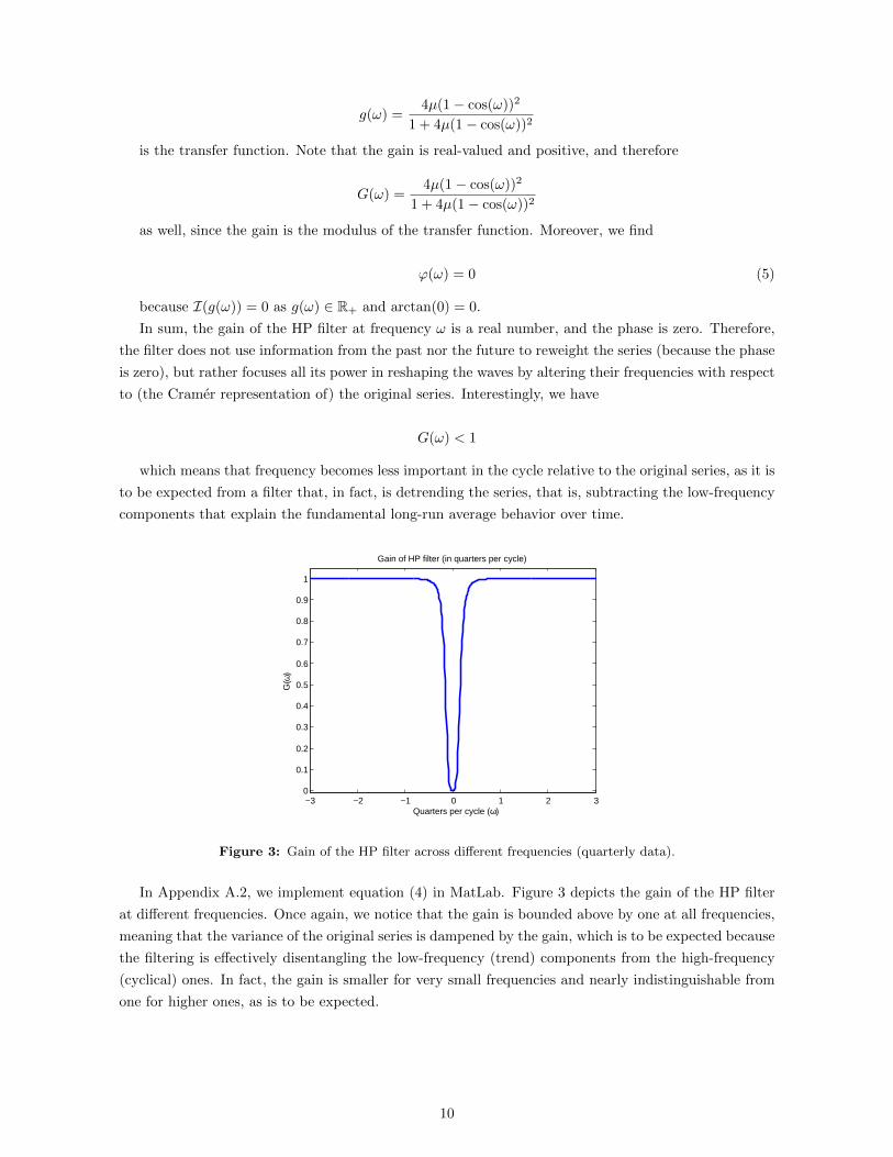
Figure 3: Gain of the HP filter across different frequencies (quarterly data).
In Appendix A.2, we implement equation (4) in MatLab. Figure 3 depicts the gain of the HP filter
at different frequencies. Once again, we notice that the gain is bounded above by one at all frequencies,
meaning that the variance of the original series is dampened by the gain, which is to be expected because
the filtering is effectively disentangling the low-frequency (trend) components from the high-frequency
(cyclical) ones. In fact, the gain is smaller for very small frequencies and nearly indistinguishable from
one for higher ones, as is to be expected.
10
4 The Kalman Filter
The Kalman Filter is an algorithm that allows us to make inference in linear dynamical systems that
typically contain Gaussian errors. In Macroeconomics it is useful because many models have solution
systems that, after appropriate (log-)linearization, can be written in the following so-called state-space
form:
St = ASt−1 +Bε1,t (6)
Xt = CSt +Dε2,t (7)
where Xt is an m × 1 vector of observables and St is an n × 1 vector of states, which may include
latent variables (for example, the white noise components of a moving average process). The terms ε1,t
and ε2,t are p× 1 and q × 1 innovation vectors distributed jointly according to(ε1,t
ε2,t
)∼ iid N
((0p
0q
),
(Q F
F ′ R
))(8)
The objects 0p and 0q are p× 1 and q × 1 vectors of zeros, respectively, and A, B, C, D, F , Q and
R are n× n, n× p, m× n, m× q, p× q, p× p and q × q matrices, respectively, of free parameters.
Equation (6) is the so-called state equation, according to which the state of the economy must be
Markovian. Equation (7) is called the measurement equation, which describes the existent depen-
dence between the state of the economy (or the variables that are latent in the dynamic system) and
the set of observable variables.
4.1 Preliminaries
The Kalman filtering problem is one of recursive Bayesian updating: we wish to obtain a recursive
algorithm for sequential updating of the projections of the system (in particular, the conditional mean
and variances of the process) by exploiting both the Gaussianity and linearity of the system. The
ultimate goal is to estimate the parameters in the coefficient matrices, and the derivation of the filter is
important for obtaining the exact representation of the likelihood function.
We motivate the Kalman filter here as an algorithm for calculating linear least square forecasts of
the state vector on the basis of data observed through date t. For this purpose, we use the following
notation:
St|t−1 := E[St|Xt−1; Θ]
Pt|t−1 := V[St|Xt−1; Θ]
= E[(St − St|t−1)(St − St|t−1)′|Xt−1; Θ]
as the period t ∈ N prior estimate of St (taken to be its conditional mean) and the corresponding
mean square error (MSE) (or variance) of the states conditional on the history of the observables7,
where Θ is the vector of parameters that are contained in the coefficient and covariance matrices. The
posterior conditional mean and MSE are denoted
7We adopt the standard notation Xt := X1, X1, . . . , Xt.
11
St|t := E[St|Xt; Θ]
Pt|t := V[St|Xt; Θ]
= E[(St − St|t)(St − St|t)′|Xt; Θ]
which we will compute by using the priors, as seen below. Similarly, the prior conditional mean and
MSE of the observables are denoted as follows:
Xt|t−1 := E[Xt|Xt−1; Θ]
Vt|t−1 := V[Xt|Xt−1; Θ]
= E[(Xt −Xt|t−1)(Xt −Xt|t−1)′|Xt−1; Θ]
Note we can find expressions of the last two objects by taking conditional expectations in the original
system, written as in (6)-(7). In particular, we have
Xt|t−1 = E[CSt +Dε2,t|Xt−1; Θ]
= CSt|t−1
Vt|t−1 = E[(CSt +Dε2,t − CSt|t−1)(S′tC′ + ε′2,tD
′ − S′t|t−1C′)|Xt−1; Θ]
= E[(C(St − St|t−1) +Dε2,t)((St − St|t−1)′C ′ + ε′2,tD′|Xt−1; Θ]
= E[(C(ASt−1 − St|t−1) + CBε1,t +Dε2,t)((ASt−1 − St|t−1)′C ′ + ε′1,tB′C ′ + ε′2,tD
′)|Xt−1; Θ]
= CAPt−1|t−1A′C ′ + CBQB′C ′ + CBFD′ +DF ′B′C ′ +DRD′
for any t ∈ N, where we have used that E[ε1,t|Xt−1; Θ] = E[ε2,t|Xt−1; Θ] = 0 (the innovations are
orthogonal to the history of the observables) and that St|t−1 = ASt−1, by taking conditional expectations
on the state equation (6) and using the orthogonality of the errors with respect to the history of the
observables.
4.2 The Recursion
Given these definitions, we can now inductively derive the the Kalman filter to get recursive expres-
sions for the priors St|t−1 and Pt|t−1, with which we enter period t, and the posteriors St|t and Pt|t,
with which we exit period t and which will be used to form new priors for period (t+ 1). The departure
point of the algorithm is to set initial estimates for S0|0 and P0|0 in oder to derive expressions for the
time-zero posteriors, S1|0 and P1|0, which will in turn be used to get the first-period priors, S1|1 and
P1|1. By induction, this formulas will be sufficient to establish a pattern for the recursion at any period
t ∈ N.
To start the algorithm, fix guesses for S0|0 and P0|0. Note that
S1 = AS0 +Bε1,1
X1 = CS1 +Dε2,1
= CAS0 + CBε1,1 +Dε2,1
12
by the state equation and the measurement equation, respectively. Taking conditional expectations8
in the two equations gives the prior estimates
S1|0 = AS0|0
X1|0 = CS1|0
by using the orthogonality of the innovations. Using our definitions above, the prior MSE’s are
P1|0 := E[(S1 − S1|0)(S1 − S1|0)′|X0; Θ]
= E[(A(S0 − S0|0) +Bε1,1)((S0 − S0|0)′A′ + ε′1,1B′)|X0; Θ]
= AP0|0A′ +BQB′ (9)
V1|0 := E[(X1 −X1|0)(X1 −X1|0)′|X0; Θ]
= E[(CA(S0 − S0|0) + CBε1,1 +Dε2,1)((S0 − S0|0)′A′C ′ + ε′1,1B′C ′ + ε′2,1D
′)|X0; Θ]
= CAP0|0A′C ′ + CBQB′C ′ + CBFD′ +DF ′B′C ′ +DRD′
= CP1|0C′ + CBFD′ +DF ′B′C ′ +DRD′ (10)
Finally, the prior covariance between X1 and S1 is
E[(S1 − S1|0)(X1 −X1|0)′|X0; Θ] = E[(A(S0 − S0|0) +Bε1,1)(CA(S0 − S0|0) + CBε1,1 +Dε2,1)′|X0; Θ]
= E[(A(S0 − S0|0) +Bε1,1)((S0 − S0|0)′A′C ′ + ε′1,1B′C ′ + ε′2,1D
′)|X0; Θ]
= AP0|0A′C ′ +BQB′C ′ +BFD′
= P1|0C′ +BFD′ (11)
That is, we have found that, given assumption (8) and the fact that linear combinations of normally
distributed random variables remain normal,
(S1
X1
)∼ iid N
((AS0|0
CAS0|0
),
(P1|0 P1|0C
′ +BFD′
CP ′1|0 +DF ′B′ CP1|0C′ + CBFD′ +DF ′B′C ′ +DRD′
))
where P1|0 is given in (9). The prior forecast error in the observables is, therefore
X1 −X1|0 = CS1 +Dε2,1 − CS1|0
= C(S1 − S1|0) +Dε2,1
Namely, the error that we make in forecasting the first-period actual realization of the observables,
using our prior, comes from the error in forecasting the state, weighted by the influence of the state on
the observables (first term), and the unpredictable innovation on the measurement specification of the
observables (second term).
8Throughout, “conditional” will be short for “conditional on Xt−1” if the expectation is taken in period t ∈ N.
13
We can now update these priors into posteriors about first-period forecasts and forecasts errors. For
this, we exploit the linearity and Gaussianity of the process. In particular, S1|1 can be evaluated using
the formula for updating a linear projection (optimal forecast of a linear and Gaussian process):
S1|1 = S1|0 + E[(S1 − S1|0)(X1 −X1|0)′|X0; Θ]V −11|0 (X1 −X1|0)
Using the results above, then
S1|1 = AS0|0 +K1|0(X1 −X1|0) (12)
where we have defined
K1|0 := (P1|0C′ +BFD′)[CP1|0C
′ + CBFD′ +DF ′B′C ′ +DRD′]−1 (13)
and recall that S1|0 = AS0|0, X1|0 = CS1|0 and that P1|0 is given in (9). Formula (12) gives the
first-period posterior of the state, as a function of the prior state and observables and the posterior
MSE of the state. It says that the posterior on the state, S1|1, differs from the prior of that period,
S1|0, depending on the forecast error that is made in the observables with respect to their posterior,
X1−X1|0, weighted by some matrix K1 that depends on the posterior mean square error of the forecast.
This matrix is called the Kalman gain (of period 1), and measures the degree of updating from the
prior to the posterior of the state in period 1. Quite intuitively, how much the guess is revised will
depend on how good the approximation is, namely how small is the variance of the prior. More noisy
priors will be updated more strongly into the posterior.
We still need an expression for the posterior MSE of the state’s forecast, P1|1. Recall that P1|1 :=
E[(S1 − S1|1)(S1 − S1|1)′], and we now know that S1|1 is given by (12). Using that P1|0 and V −11|0 are
transpose invariant matrices, we have
P1|1 = E[(S1 − S1|1)(S1 − S1|1)′|X0; Θ]
= E[((S1 − S1|0)− (P1|0C′ +BFD′)V −1
1|0 (X1 −X1|0))((S1 − S1|0)′
−(X1 −X1|0)′V −11|0 (CP1|0 +DF ′B′))|X0; Θ]
= P1|0 − E[(S1 − S1|0)(X1 −X1|0)′|X0; Θ]V −11|0 (CP1|0 +DF ′B′)
−(P1|0C′ +BFD′)V −1
1|0 E[(X1 −X1|0)(S1 − S1|0)′|X0; Θ]
+(P1|0C′ +BFD′)V −1
1|0 V1|0V−11|0 (CP1|0 +DF ′B′)
= P1|0 − (P1|0C′ +BFD′)V −1
1|0 (CP1|0 +DF ′B′)
−(P1|0C′ +BFD′)V −1
1|0 (CP1|0 +DF ′B′)
+(P1|0C′ +BFD′)V −1
1|0 (CP1|0 +DF ′B′)
= P1|0 − (P1|0C′ +BFD′)V −1
1|0︸ ︷︷ ︸=K1|0
(CP1|0 +DF ′B′) (14)
where we have used result (11) in the second last equality. Now, we can propagate (14) forward to
find the prior mean square error of the state forecast for the following period, P2|1. To do this, start
over at period t = 2 and take conditional expectations on the system written in state-space form to get
14
S2|1 = AS1|1
X2|1 = CS2|1
The forecast error (with respect to this prior) in the second period is, therefore,
S2 − S2|1 = A(S1 − S1|1) +Bε1,2
Hence, the mean square error of this forecast is
P2|1 = E[(S2 − S2|1)(S2 − S2|1)′|X1; Θ]
= E[(A(S1 − S1|1) +Bε1,2)(A(S1 − S1|1) +Bε1,2)′|X1; Θ]
= AP1|1A′ +BQB′
or, using formulas (14) and (10),
P2|1 = A
[P1|0−(P1|0C
′+BFD′)[CP1|0C
′+CBFD′+DF ′B′C ′+DRD′]−1
(CP1|0+DF ′B′)
]A′+BQB′
We have now sufficient conditions to state the general formulas of the recursive algorithm for any
given period t ∈ N, provided an initial guess for period zero. The following is the set of recursions that
describe fully the Kalman filter for the case of correlated innovation errors and any t ∈ N.
St|t−1 = ASt−1|t−1
Xt|t−1 = CSt|t−1
St|t = St|t−1 +Kt|t−1(Xt −Xt|t−1)
Pt|t = Pt|t−1 −Kt|t−1(CPt|t−1 +DF ′B′)
Pt|t−1 = APt−1|t−1A′ +BQB′
Vt|t−1 = CPt|t−1C′ + CBFD′ +DF ′B′C ′ +DRD′
where
Kt|t−1 := (Pt|t−1C′ +BFD′)V −1
t|t−1
is the period-t Kalman gain, and it is conventional to denote the subscript 0|−1 by 0, corresponding
to the initial guess. Note that the gain is higher for more precise prior variances on the observables (that
is, lower values in the diagonal entries of Vt|t−1). This makes intuitive sense: the prior forecast error on
the observables weights more into the updating rule for the state the more precise this forecast is.
15
5 Log-Likelihood Estimation
In this section, we explain log-likelihood estimation in practice through two examples: an MA(1)
and a VAR(2).
5.1 Estimation of an MA(1)
Consider the following MA(1) process:
xt = σεεt + θσεεt−1 (15)
where εt ∼ N (0, 1). We set σε = 1 and assume |θ| < 1. We want to compute the log-likelihood of
this model on a grid of points for the unknown parameter θ.
Say that we have data yT := ytTt=1, which has been sampled with replacement (that is, (yt) is an
i.i.d. sequence). Denote by p(yT |θ) the joint density of these data given the model at hand (in which
the only free parameter is θ). We want to maximize the probability that the observed data has been
generated by the model of study, namely
θML := arg maxθ∈Θ
p(yT |θ)
where Θ ⊆ R is the parameter set. By the i.i.d. assumption, we can write
p(yT |θ) =
T∏t=1
p(yT |θ)
However, the independence assumption is usually too restrictive for time series data (in which a
major point of work is, precisely, to determine patters of inter-temporal dependence), in which case we
can instead decompose the likelihood with a prediction error decomposition:
p(yT |θ) = p(yT |yT−1; θ)p(yT−1|θ)
= p(yT |yT−1; θ)p(yT−1|yT−2; θ)p(yT−2|θ)...
= p(y0|θ)T∏t=1
p(yt|yt−1; θ)
so that
log p(yT |θ) = log p(y0|θ) +
T∑t=1
log p(yt|yt−1; θ) (16)
The term log p(y0|θ) is often ignored in estimation, for its asymptotic contribution is nearly negligible.
To make progress, we want to obtain a functional form for p(yt|yt−1; θ) and sufficient statistics
describing the log-likelihood. For our reference, recall that the joint density of a scalar-valued Normal
random variable is Xt with mean µx and variance σ2x is
16
p(yT |µx, σ2x) =
T∏t=1
1√2πσ2
x
exp
− 1
2σ2x
(Xt − µx)2
(17)
The point of the matter if we have an MA(1) is that the relevant variables, εt and εt−1, are unob-
servable innovations and, therefore, latent variables. On paper, we could just invert the MA(1) to turn
it into an AR(∞) by recovering the history of observables that are implied by these shocks. In practice,
this approach requires the estimation of an infinite number of parameters, a problem of dimensionality
that cannot be dealt with without imposing a finite approximation to the system that can induce losses
of accuracy in the estimation.
Instead, since (15) is a linear model with Gaussian innovations, we use the Kalman filter. The first
step is to write the model in the state-space form, as seen in the system (6)-(7). Here,
(εt
εt−1
)=
(0 0
1 0
)(εt−1
εt−2
)+
(σε
0
)νt
xt = (σε σεθ)
(εt
εt−1
)
where νt ∼ iid N (0, 1) is white noise. In terms of system (6)-(7), this means that St ≡ (εt, εt−1)′ is
taken to be the state of the model, while Xt ≡ xt is the observable. Moreover,
A =
(0 0
1 0
)B =
(1
0
)C = (1 θ) D = F = R = 0 Q = 1
are the matrices of free parameters, where we have used already that σε = 1. Since we have no
information on the actual law of motion of the state, the state equation simply establishes that εt is
some white noise, while the second line is the identity εt−1 = εt−1. The measurement equation is the
evolution described by the original MA(1). Note since D = 0 that through the measurement equation
we can describe without noise (beyond the one encoded in the state itself) the relation between the
state, here chosen to be the two latent variables εt and εt−1, and the observable, here xt.
The key step is to gain information about the state through the Kalman filter. In particular, we want
to recursively obtain estimates for the one-step ahead forecast and its associated mean square error of
the latent variables. Using our recursions from before, we have that
St|t−1 = ASt−1|t−1
Xt|t−1 = CSt|t−1
St|t = St|t−1 +Kt|t−1(Xt −Xt|t−1)
Pt|t = Pt|t−1 −Kt|t−1CPt|t−1
Pt|t−1 = APt−1|t−1A′ +BB′
Vt|t−1 = CPt|t−1C′ +DD′
for any t ∈ N, where
Kt|t−1 := Pt|t−1C′V −1t|t−1
17
is the period-t Kalman gain.
Algorithm The likelihood function can be then set up using the following algorithm:
1. Initialize the Kalman filter by fixing initial guesses for the unconditional mean and mean square
error of the state. Here, we draw the state from its stationary distribution, namely S0 ∼ N (0, σ2εI2)
(with σ2ε = 1), so that
S0|0 =
(0
0
)P0|0 =
(1 0
0 1
)
This implies that the initial value of the observable variable is drawn from the distribution y0 ∼N (0, σ2
ε + σ2εθ
2) (again, with σ2ε = 1).
2. For each t ∈ 1, . . . , T, iteratively compute period-t density contribution to the likelihood function
(31) in its Gaussian form using (17) as a reference for the functional form. After looping across all
time periods, we should have constructed the object
log p(yT |θ) ≈T∑t=1
log p(yt|yt−1; θ)
= −T2
log 2π − T
2log Vt|t−1(θ)− 1
2
T∑t=1
(xt − xt|t−1(θ))2
Vt|t−1(θ)
where Vt|t−1(θ) and xt|t−1(θ) are given by the Kalman filter recursion described above (scalars in
this case).
3. Maximize the last expression over θ with a numerical optimizer. Or, in our case, plot the log-
likelihood over the grid for θ ∈ (−1, 1) and look for the grid point that yields the highest value of
the log-likelihood.
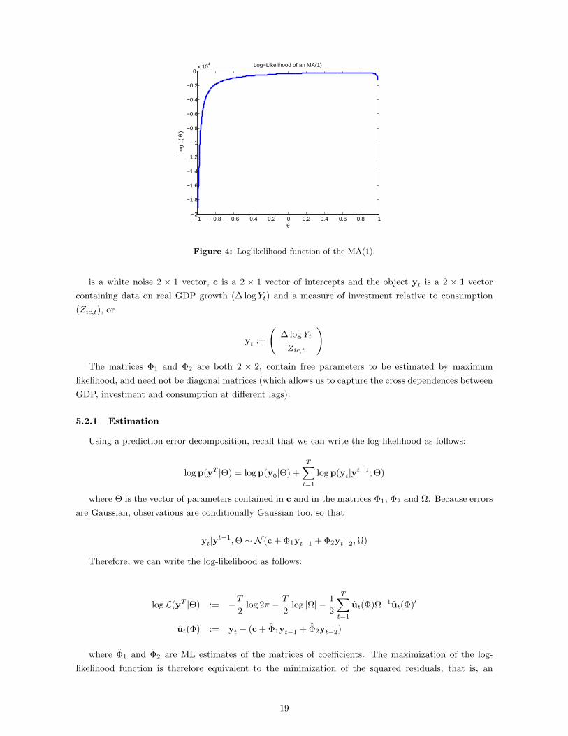
Appendix A.3 includes the code for implementing the algorithm. Figure 4 depicts the log-likelihood
function that results from it. We get that the value of the parameter for which the log-likelihood is
maximized is θML = 0.74.
Note that the log-likelihood is fairly flat for all grid points except for the extremes. At these points,
the process has a near-unit root and is ill-behaved, which drives the log-likelihood down to very low
levels.
5.2 Estimation of a VAR(2)
Consider the following reduced-form VAR(2) model9:
yt = c + Φ1yt−1 + Φ2yt−2 + ut (18)
for t ∈ 1, . . . , T, where
ut ∼ iid N (0,Ω)
9Henceforth, bold letters are vectors and capital letters are matrices.
18
−1 −0.8 −0.6 −0.4 −0.2 0 0.2 0.4 0.6 0.8 1−2
−1.8
−1.6
−1.4
−1.2
−1
−0.8
−0.6
−0.4
−0.2
0x 10
4 Log−Likelihood of an MA(1)
θ
log
L( θ
)
Figure 4: Loglikelihood function of the MA(1).
is a white noise 2 × 1 vector, c is a 2 × 1 vector of intercepts and the object yt is a 2 × 1 vector
containing data on real GDP growth (∆ log Yt) and a measure of investment relative to consumption
(Zic,t), or
yt :=
(∆ log Yt
Zic,t
)The matrices Φ1 and Φ2 are both 2 × 2, contain free parameters to be estimated by maximum
likelihood, and need not be diagonal matrices (which allows us to capture the cross dependences between
GDP, investment and consumption at different lags).
5.2.1 Estimation
Using a prediction error decomposition, recall that we can write the log-likelihood as follows:
log p(yT |Θ) = log p(y0|Θ) +
T∑t=1
log p(yt|yt−1; Θ)
where Θ is the vector of parameters contained in c and in the matrices Φ1, Φ2 and Ω. Because errors
are Gaussian, observations are conditionally Gaussian too, so that
yt|yt−1,Θ ∼ N (c + Φ1yt−1 + Φ2yt−2,Ω)
Therefore, we can write the log-likelihood as follows:
logL(yT |Θ) := −T2
log 2π − T
2log |Ω| − 1
2
T∑t=1
ut(Φ)Ω−1ut(Φ)′
ut(Φ) := yt − (c + Φ1yt−1 + Φ2yt−2)
where Φ1 and Φ2 are ML estimates of the matrices of coefficients. The maximization of the log-
likelihood function is therefore equivalent to the minimization of the squared residuals, that is, an
19
equation-by-equation OLS problem. This is because we are working with an unrestricted VAR, that is,
both lags of both variables appear in both equations of the system.
Taking first order conditions with respect to Ω gives us that
ΩML =1
T
T∑t=1
ut(Φ)ut(Φ)′ (19)
which of course needs the estimation of c, Φ1 and Φ2. For this, we use the GLS formula for the
special case of common regressors (indeed, recall that we are working here with an unrestricted VAR,
in which all lags of all variables appear in all equations). First, stack the observations by time period
by defining
y :=
y1
y2
...
yT−2
x′ :=
1T−2
∆ log Y−1
Zic,−1
∆ log Y−2
Zic,−2
u :=
u1
u2
...
uT−2
where ∆ log Y−1 is the first lag of the (T − 2)× 1 column vector ∆ log Y, and ∆ log Y−2, Zic,−1 and
Zic,−2 are defined similarly. Note that y is a 2(T − 2)× 1 vector, while x is a (T − 2)× 5 matrix. Stack
the coefficients of interest inside c, Φ1 and Φ2 in a 10× 1 column vector
β := [β′1, β′2]′ =
[c1, φ
111, φ
112, φ
211, φ
212; c2, φ
121, φ
122, φ
221, φ
222
]′where φnij denotes the (i, j)-entry of the matrix Φn, for n = 1, 2, and βj := [cj , φ
1j1, φ
1j2, φ
2j1, φ
2j2]
collects the coefficients corresponding to the j-th equation (for j = 1, 2). Then, our regression becomes
y = xβ + u
where
x := I2 ⊗ x
and ⊗ is the Kronecker product. Note that since I2 is 2 × 2 and x is (T − 2) × 5, then x is a
2(T − 2)× 10 matrix10, and so all dimensions agree. The formula for the GLS estimator is, then
βML = [x′(Ω−1 ⊗ I2)x]−1x′(Ω−1 ⊗ I2)y
= [I2 ⊗ (x′x)−1x′]y (20)
where the steps from the first to the second equality are non-trivial and involve the result x′(Ω−1 ⊗I2)x = I2⊗x′x. We implement, after stacking our variables appropriately, equation (20) in our MatLab
code (see Appendix A.4). Using (20) into (19) we will in turn be able to get OLS estimates of all of
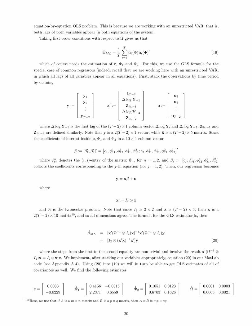
covariances as well. We find the following estimates
c =
[0.0033
−0.0229
]Φ1 =
[0.4156 −0.0315
2.2371 0.6559
]Φ2 =
[0.1651 0.0123
0.6703 0.1626
]Ω =
[0.0001 0.0003
0.0003 0.0021
]10Here, we use that if A is a m× n matrix and B is a p× q matrix, then A⊗B is mp× nq.
20
The results therefore say that an increase in the current growth rate of output affects positively next
period’s output, namely output is procylical at different lags. The same procyclicality property is true
for the ratio of investment and consumption.
5.2.2 Granger Causation
Granger causation is a way of testing how much (if at all) the predictive power of a time series
improves if the forecast is made conditional on the history of an additional regressor. Formally, a series
(yt) is said to fail to Granger-cause (xt) if the mean square error of xt based on the joint history
(xt−1, yt−1) is no smaller than the mean square error of the forecast based on the xt−1 history alone.
Recall that our model reads as follows:
[∆ log Yt
Zic,t
]=
(φ1
11 φ112
φ121 φ1
22
)[∆ log Yt−1
Zic,t−1
]+
(φ2
11 φ212
φ221 φ2
22
)[∆ log Yt−2
Zic,t−2
]+
[uyt
uzt
]
Then,
• Testing whether Zic does not Granger-cause ∆ log Yt is equivalent to the joint test:
H10 : φ1
12 = φ212 = 0
• Testing whether ∆ log Yt does not Granger-cause Zic is equivalent to the joint test:
H20 : φ1
21 = φ221 = 0
We test these hypotheses with a Wold test. Recall that we can write the hypothesis Hi0 above,
i = 1, 2, as
Hi0 : Riβ − ri = 0
with, in our case, ri = [0, 0]′ for both i = 1, 2 and R1 and R2 are selector matrices
R1 =
[0 0 1 0 0 0 0 0 0 0
0 0 0 0 1 0 0 0 0 0
]
R2 =
[0 0 0 0 0 0 1 0 0 0
0 0 0 0 0 0 0 0 1 0
]
Then, the Wald estimator
Wi := β′R′i(R′iVβRi)−1Riβ
is asymptotically distributed chisquare witt two degrees of freedom (as many as restrictions in the
model), where Vβ is the variance of the estimator, given by
Vβ = [x′(Ω−1 ⊗ I2)x]−1
which comes from asymptotic normality of β and the Delta method. We find W1 = 12.0547 and
W2 = 39.1193, with p-values 0.0024 and 3.2015× 10⁻⁹, respectively, meaning that both null hypotheses
21
are strongly rejected and that there is strong evidence for the two variables to Granger-cause each other.
5.2.3 Beveridge-Nelson Output Gap
Reduced-form VARs, very much like the one at hand here, can be used for multi-step and long-run
forecasting. This requires, in some applications, the extraction of the so-called stochastic trend of the
series. Following Beveridge and Nelson (1981), the stochastic trend of a series is the stochastic level to
which the series is expected to converge to. In our case, where yt is the Beveridge-Nelson measure,
yt − yt = limj→+∞
[j∑
h=1
Et(∆yt+h − µ∆y
)]where the left-hand side is the stochastic trend and the right-hand side measures long-run deviation
of growth from the average stationary level (that is, a measure of “catching up”). The stochastic trend
is therefore the level to which the series is expected to converge after all transient shocks die out.
In terms of our VAR(2), start by writing (18) as a VAR(1) by using the companion form:
zt = k +Azt−1 + vt
where
k =
(c
02×1
)zt =
(yt
yt−1
)A =
(Φ1 Φ2
I2×2 02×2
)vt =
(ut
02×1
)
That is, k, zt and vt are 4 × 1 and A is 4 × 4. It will be useful for what follows to iterate the
companion form backward and write
zt+h = Ahzt +
h−1∑i=0
Aik +
h−1∑i=0
Aivt+h−i (21)
We are only interested in determining the stochastic trend of the output gap, so we can design a
selector vector e1 such that
∆ log Yt = e′1zt
In this case, e1 = [1, 0, 0, 0]′ clearly does the job. Then, we can write
Et[∆ log Yt+h] = E[e′1zt+h|zt] = e′1Ahzt + e′1
h−1∑i=0
Aik
where we have used (21) in the last equality and the fact that the errors are spherical. Hence,
+∞∑h=1
Et[∆ log Yt+h − µ∆y] =
+∞∑h=1
[e′1A
hzt + e′1
h−1∑i=0
Aik− µ∆y
]
= e′1
(+∞∑i=0
Ah
)Azt + e′1
(+∞∑h=1
h−1∑i=0
Ai
)k−
+∞∑h=1
µ∆y
In the code (Appendix A.4), we check that all the eigenvalues of A are within the unit circle (though
22
some of them are complex numbers), in which case we have that∑+∞i=0 A
h = (I4×4 −A)−1, that is, the
geometric sum of matrices converges. We ignore the second and third terms because they are closely
related and likely to cancel each other out (alternatively, the results that we display here impose no
intercept in the original VAR and, therefore, zero mean in the processes).
In sum, we have that the output gap, given by the difference between output (in levels) and Beveridge-
Nelson stochastic trend of the growth rate of consumption is given by
Yt − Yt = e′1(I4×4 −A)−1Azt
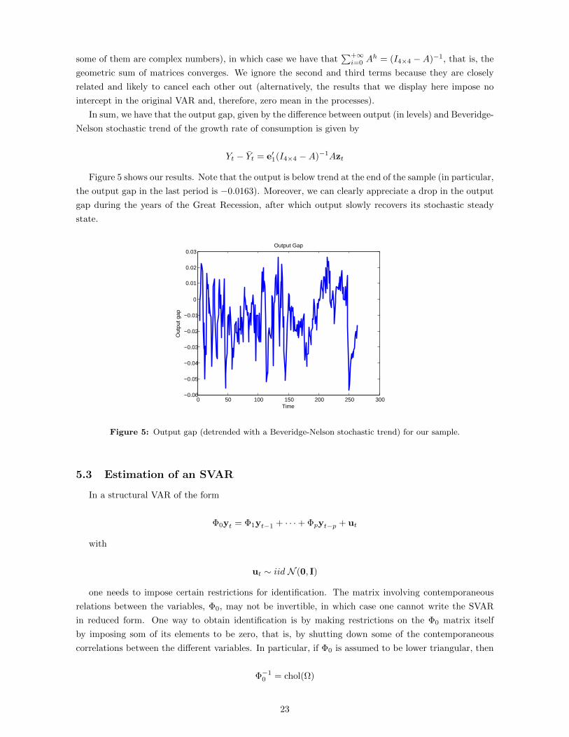
Figure 5 shows our results. Note that the output is below trend at the end of the sample (in particular,
the output gap in the last period is −0.0163). Moreover, we can clearly appreciate a drop in the output
gap during the years of the Great Recession, after which output slowly recovers its stochastic steady
state.
0 50 100 150 200 250 300−0.06
−0.05
−0.04
−0.03
−0.02
−0.01
0
0.01
0.02
0.03Output Gap
Time
Out
put g
ap
Figure 5: Output gap (detrended with a Beveridge-Nelson stochastic trend) for our sample.
5.3 Estimation of an SVAR
In a structural VAR of the form
Φ0yt = Φ1yt−1 + · · ·+ Φpyt−p + ut
with
ut ∼ iid N (0, I)
one needs to impose certain restrictions for identification. The matrix involving contemporaneous
relations between the variables, Φ0, may not be invertible, in which case one cannot write the SVAR
in reduced form. One way to obtain identification is by making restrictions on the Φ0 matrix itself
by imposing som of its elements to be zero, that is, by shutting down some of the contemporaneous
correlations between the different variables. In particular, if Φ0 is assumed to be lower triangular, then
Φ−10 = chol(Ω)
23
where chol(Ω) denotes the Cholesky decomposition11 of the covariance matrix Ω of the residuals in
the reduced-form VAR12. Although convenient, this method depends on the data at hand and cannot
be empirically vouched for on an a priori basis.
5.3.1 Identification via Long-Run Restrictions
Another class of weak restrictions that may hold across a large range of models are the so-called
long-run restrictions, which were first suggested by Blanchard and Quah (1989). The idea is that
there may be a subset of shocks that have permanent effects on some variables but not on others, and
shocks that have no permanent effects on any variable. Therefore, shocks can be split in permanent
ones and shocks that are neutral in the long run.
Suppose, as in Blanchard and Quah’s original example, that there are two structural shocks, one to
aggregate supply and another one to aggregate demand. In their original example,(φ0
11 φ012
φ021 φ0
22
)[ut
∆yt
]=
(φ1
11 φ112
φ121 φ1
22
)[ut−1
∆yt−1
]+
[εdt
εst
]where ut is unemployment, ∆yt is GDP growth and (εdt , ε
st ) are demand and supply shocks, respec-
tively. The identifying assumption that they use is that udt -shocks do not have a permanent effect on
GDP in levels.
To see what this restriction boils down to, we compute long run (level) effects. First, write the SVAR
in reduced form as [ut
∆yt
]= Φ−1
0 Φ1
[ut−1
∆yt−1
]+ Φ−1
0 εt
Where A1 := Φ−10 Φ1, we can then compute the long-run effects by summing all future changes in
GDP:
E
[+∞∑s=0
[ut+s
∆yt+s
]∣∣∣∣∣ εt]
=
+∞∑s=0
As1Φ−10 εt
= (I−A1)−1Φ−10 εt
provided that all the eigenvalues of A1 are within the unit circle, so that the sum converges. The
long-run restriction then amounts to imposing that the matrix (I−A1)−1Φ−10 is upper triangular, for in
this case it is indeed true that demand shocks will not have an effect on GDP in levels in the long run
(recall that GDP is the second variable in our vector of observables, while the demand shock is in the
first position in the vector of errors, so we indeed need a zero in the lower left corner of this matrix).
Therefore, we want to find a matrix Φ−10 such that
11The Cholesky decomposition is the decomposition of a positive-definite matrix into the product of a lower triangular matrix and itstranspose. That is, if A is positive definite (for example, a covariance matrix), then chol(A) = BB′ for some lower triangular matrix B.
12The reduced form VAR is such thatyt = A1yt−1 + · · ·+Apyt−p + vt
where Ai := Φ−10 Φi for every i = 1, . . . , p, and vt := Φ−1
0 ut, so that vt ∼ iid N (0,Ω), where Ω := (Φ−10 )(Φ−1
0 )′.
24
(I−A1)−1Φ−10 =
[• •0 •
](22)
Φ−10 (Φ−1
0 )′ = Ω
where Ω is the covariance matrix of the errors in the reduced-form VAR (recall footnote 2). This
suggests once again a Cholesky decomposition, but this time on the matrix
Q := (I−A1)−1Φ−10 (Φ−1
0 )′((I−A1)−1)′
This decomposition will work, because Q is positive definite (it is the square of (I − A1)−1Φ−10 )
and (I − A1)−1Φ−10 is lower triangular by our identifying restriction (recall the requirements for the
decomposition in footnote 1), so that
chol(Q) = (I−A1)−1Φ−10
since we want Ω = Φ−10 (Φ−1
0 )′.
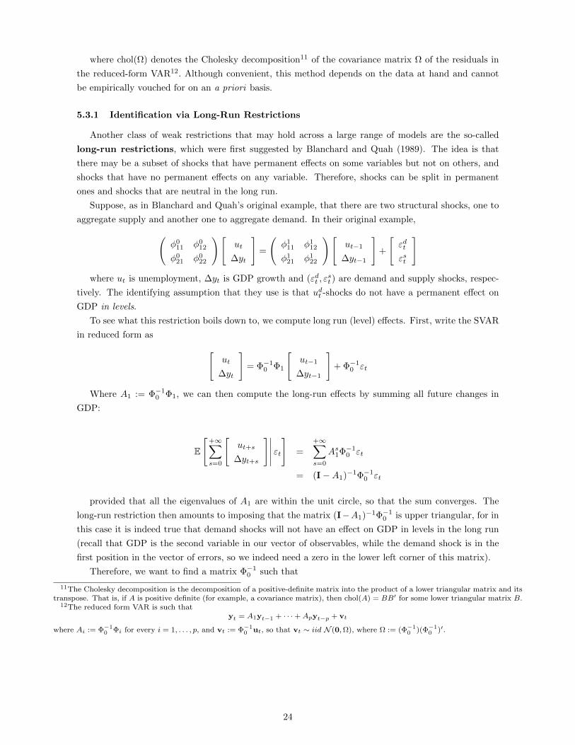
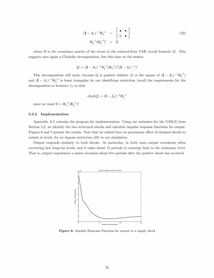
5.3.2 Implementation
Appendix A.5 contains the program for implementation. Using our estimates for the VAR(2) from
Section 5.2, we identify the two structural shocks and calculate impulse response functions for output.
Figures 6 and 7 present the results. Note that we indeed have no permanent effect of demand shocks to
output in levels, for we impose restriction (22) to our simulation.
Output responds similarly to both shocks. In particular, in both cases output overshoots when
recovering new long-run levels, and it takes about 15 periods to converge back to the stationary level.
That is, output experiences a minor recession about five periods after the positive shock has occurred.
0 5 10 15−1
0
1
2
3
4
5
6
7
8x 10
−3 (1) IRF of output for SUPPLY shocks
Number of periods ahead
Cha
nge
in o
utpu
t gro
wth
Figure 6: Impulse Response Function for output to a supply shock
25
0 5 10 15−1
0
1
2
3
4
5
6
7x 10
−3 (2) IRF of output for DEMAND shocks
Number of periods ahead
Cha
nge
in o
utpu
t gro
wth
Figure 7: Impulse Response Function for output to a demand shock
6 Application: A New Keynesian Model
We consider the following canonical New Keynesian model, which in general equilibrium and log-
linearized about the zero-inflation steady state can be written as follows:
xt = Et(xt+1)− σ[it − Et(πt+1)] + gt (23)
πt = κxt + βEt(πt+1) + ut (24)
it = φππt + φxxt + σiεit (25)
gt = ρggt−1 + σgεgt (26)
ut = ρuut−1 + σuεut (27)
The first equation is the dynamic IS equation, describing the optimal intertemporal trade-off
between inflation (πt) and the output gap of the economy (xt := yt − yNt , where yt is output and yNt is
output that would prevail in a frictionless economy with fully flexible prices). This equation arises from
the consumer’s Euler equation (assuming CRRA preferences) and equilibrium in the goods market. The
second equation is the New Keynesian Phillips curve, describing the relationship between current
inflation and future inflation and output gap. This equation arises from the Calvo sticky-price setting
and the fundamental law of motion for prices. The third equation is a standard Taylor rule from the
Central Bank, establishing how the nominal interest rate (it) reacts to the output gap and inflation.
The fourth and fifth equations say that the demand (gt) and cost-push (ut) shocks to the economy are
Markovian, with εit, εgt and εut being mutually independent, i.i.d. standard normal random variables.
6.1 Equivalent System of Expectational Difference Equations
We start by writing the model as a compact system of expectational linear first-order difference
equations, which will bridge the gap between the system in its original form above and in the state-
space form that will allow us to run the Kalman filter (see following subsection).
The first step is to split the collection of variables between endogenous (or jump variables) and
exogenous (or states variables). This will be key to write the system in the state-space form. Here:
26
zt :=
xt
πt
it
st :=
[gt
ut
]vt :=
εit
εgt
εut
are the vector of endogenous and exogenous variables and the vector of innovations, respectively.
Note:
vt ∼ iid N (03×1, I3×3)
We guess that the original system (23)-(27) of log-linearized equilibrium conditions can be written
in the following compact form:
A0zt = A1Et(zt+1) +A2st +A3vt (28)
B0st = B1st−1 +B2vt (29)
which is the expectational linear difference equation that we were after13, coupled with a state
equation in structural form. The matrices A3 and B2 describe the effects of innovations on the vector of
variables, A0 and B0 capture contemporaneous dependences across variables, and the remaining matrices
describe lagged cross dependences.
Our linear guess will be confirmed if we are able to find closed-form expressions for the matrices A0,
A1, A2, A3, B0, B1 and B2 as functions of the deep parameters of the model.
Firstly, given the Markovian structure that we have imposed on (26) and (27), these exogenous
processes can be easily fitted into the form of equation (29) by letting
B0 :=
[1 0
0 1
]B1 :=
[ρg 0
0 ρu
]B2 :=
[0 σg 0
0 0 σu
]so that the state equation reads
[gt
ut
]=
(ρg 0
0 ρu
)[gt−1
ut−1
]+
(0 σg 0
0 0 σu
) εit
εgt
εut
Note that there are no cross dependences between the two shocks, which are linear and conditionally
gaussian. This means that the first two moments of each process are sufficient statistics to describe
fully both the dynamics and the density of the process. The innovations have also no serial correlation.
These features will make it easier for us to apply the Kalman filter and evaluate the likelihood function.
On the other hand, we can write equation (28) as
1 0 σ
−κ 1 0
−φx −φπ 1
xt
πt
it
=
1 σ 0
0 β 0
0 0 0
Et(xt+1)
Et(πt+1)
Et(it+1)
+
1 0
0 1
0 0
[ gt
ut
]+
0 0 0
0 0 0
σu 0 0
εit
εgt
εut
which replicates equations (23), (24) and (25), and therefore
13More generally, we could try to fit the observables into an equation of the type A0zt = A1Et(zt+1)+Czt−1+A2st+A3vt. However,we anticipate here that C = 03×3 because the New Keynesian equilibrium system is dynamic, but only between adjacent periods. Notealso that our guess encodes the assumption that the model admits certainty equivalence.
27
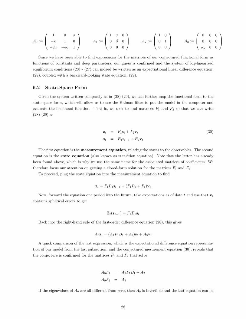
A0 :=
1 0 σ
−κ 1 0
−φx −φπ 1
A1 :=
1 σ 0
0 β 0
0 0 0
A2 :=
1 0
0 1
0 0
A3 :=
0 0 0
0 0 0
σu 0 0
Since we have been able to find expressions for the matrices of our conjectured functional form as
functions of constants and deep parameters, our guess is confirmed and the system of log-linearized
equilibrium conditions (23) - (27) can indeed be written as an expectiational linear difference equation,
(28), coupled with a backward-looking state equation, (29).
6.2 State-Space Form
Given the system written compactly as in (28)-(29), we can further map the functional form to the
state-space form, which will allow us to use the Kalman filter to put the model in the computer and
evaluate the likelihood function. That is, we seek to find matrices F1 and F2 so that we can write
(28)-(29) as
zt = F1st + F2vt (30)
st = B1st−1 +B2vt
The first equation is the measurement equation, relating the states to the observables. The second
equation is the state equation (also known as transition equation). Note that the latter has already
been found above, which is why we use the same name for the associated matrices of coefficients. We
therefore focus our attention on getting a closed-form solution for the matrices F1 and F2.
To proceed, plug the state equation into the measurement equation to find
zt = F1B1st−1 + (F1B2 + F1)vt
Now, forward the equation one period into the future, take expectations as of date t and use that vt
contains spherical errors to get
Et(zt+1) = F1B1st
Back into the right-hand side of the first-order difference equation (28), this gives
A0zt = (A1F1B1 +A2)st +A3vt
A quick comparison of the last expression, which is the expectational difference equation representa-
tion of our model from the last subsection, and the conjectured mesurement equation (30), reveals that
the conjecture is confirmed for the matrices F1 and F2 that solve
A0F1 = A1F1B1 +A2
A0F2 = A3
If the eigenvalues of A0 are all different from zero, then A0 is invertible and the last equation can be
28
solved to pin down the unique values for the F2 matrix:
F2 = A−10 A3
Similarly, F1 = A−10 (A1F1B1 +A2), which is a single equation to be solved for the implicit argument
F1. There are many ways to solve for F1 is closed form.
6.3 Numerical Implementation
Now, we suppose that the econometrician observes xt, πt and it without measurement error, which
in terms of our above notation means that F2 = 03×3. We use the state-space representation above to
simulate a long time series for these variables. Appendix A.6 includes the Matlab codes.
First, we create the A matrices above and feed them to our program. We propose a manual way to do
this, and also do it using the gensys.m package in MatLab. This package is able to run the model in its
expectational difference equation form without the need of running every step ourselves. The drawback
is that it has its own syntax, and we have to enter the variables in a specific form. Namely, where
yt := (xt, πt, it, gt, ut,Etxt+1,Etπt+1)′
is a stacked vector containing all of our endogenous variables, gensys.m uses
Γ0yt = Γ1yt−1 + Ψεt + Πηt
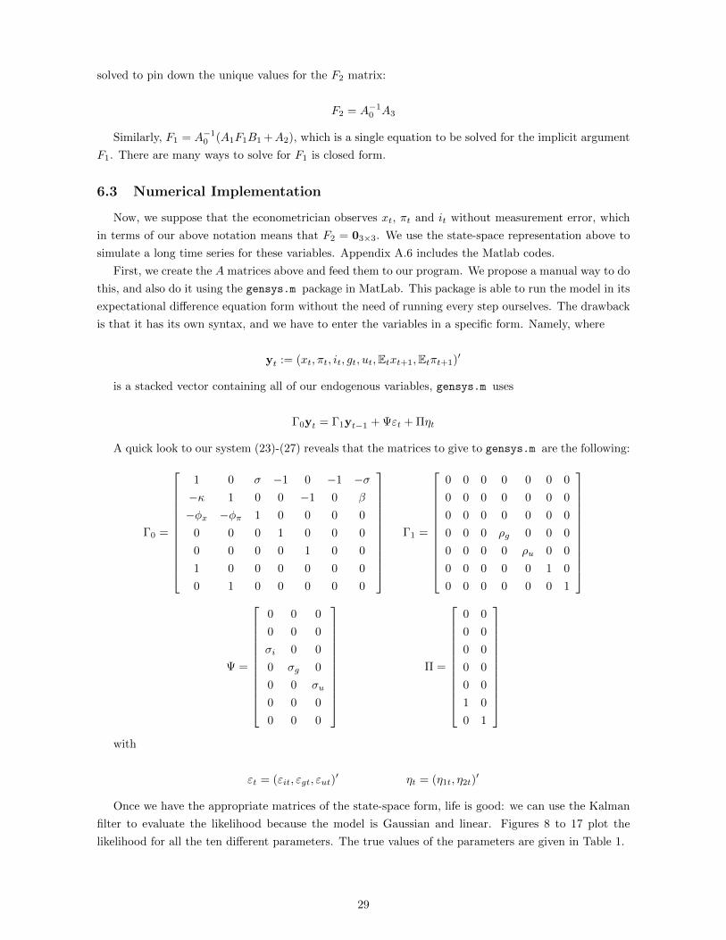
A quick look to our system (23)-(27) reveals that the matrices to give to gensys.m are the following:
Γ0 =
1 0 σ −1 0 −1 −σ−κ 1 0 0 −1 0 β
−φx −φπ 1 0 0 0 0
0 0 0 1 0 0 0
0 0 0 0 1 0 0
1 0 0 0 0 0 0
0 1 0 0 0 0 0
Γ1 =
0 0 0 0 0 0 0
0 0 0 0 0 0 0
0 0 0 0 0 0 0
0 0 0 ρg 0 0 0
0 0 0 0 ρu 0 0
0 0 0 0 0 1 0
0 0 0 0 0 0 1
Ψ =
0 0 0
0 0 0
σi 0 0
0 σg 0
0 0 σu
0 0 0
0 0 0
Π =
0 0
0 0
0 0
0 0
0 0
1 0
0 1
with
εt = (εit, εgt, εut)′ ηt = (η1t, η2t)
′
Once we have the appropriate matrices of the state-space form, life is good: we can use the Kalman
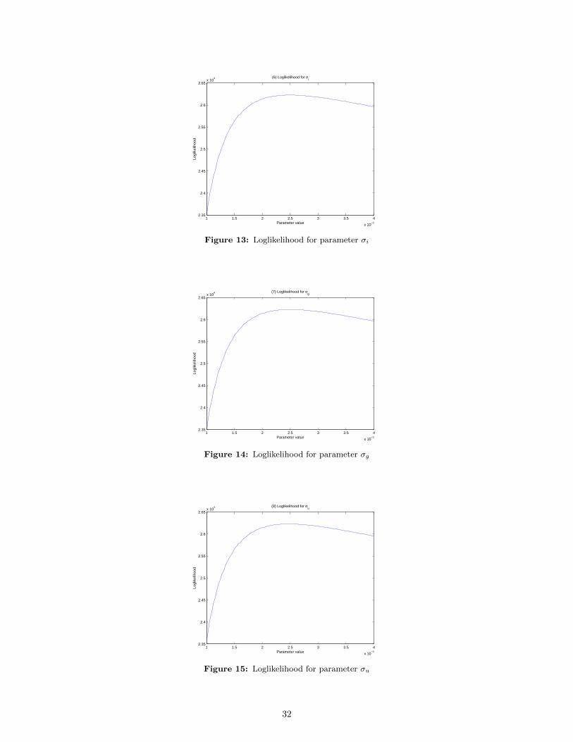
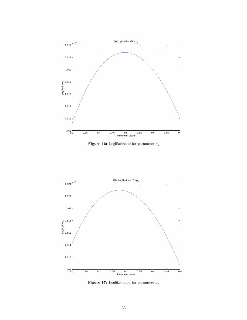
filter to evaluate the likelihood because the model is Gaussian and linear. Figures 8 to 17 plot the
likelihood for all the ten different parameters. The true values of the parameters are given in Table 1.
29
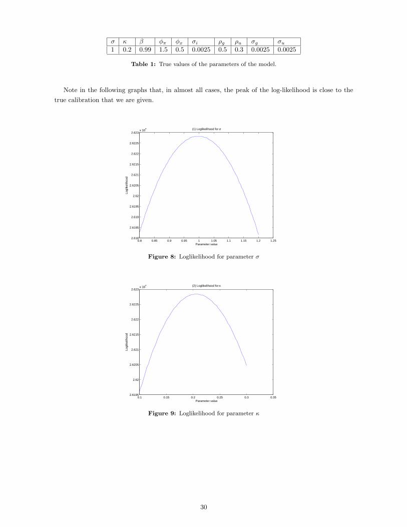
σ κ β φπ φx σi ρg ρu σg σu1 0.2 0.99 1.5 0.5 0.0025 0.5 0.3 0.0025 0.0025
Table 1: True values of the parameters of the model.
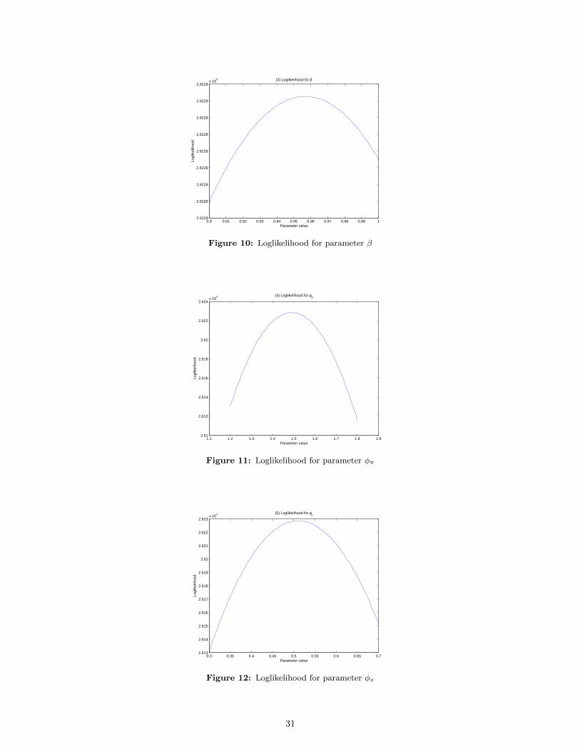
Note in the following graphs that, in almost all cases, the peak of the log-likelihood is close to the
true calibration that we are given.
0.8 0.85 0.9 0.95 1 1.05 1.1 1.15 1.2 1.252.618
2.6185
2.619
2.6195
2.62
2.6205
2.621
2.6215
2.622
2.6225
2.623x 10
4 (1) Loglikelihood for σ
Parameter value
Logl
ikel
ihoo
d
Figure 8: Loglikelihood for parameter σ
0.1 0.15 0.2 0.25 0.3 0.352.6195
2.62
2.6205
2.621
2.6215
2.622
2.6225
2.623x 10
4 (2) Loglikelihood for κ
Parameter value
Logl
ikel
ihoo
d
Figure 9: Loglikelihood for parameter κ
30
0.9 0.91 0.92 0.93 0.94 0.95 0.96 0.97 0.98 0.99 12.6228
2.6228
2.6228
2.6228
2.6228
2.6228
2.6228
2.6229
2.6229x 10
4 (3) Loglikelihood for β
Parameter value
Logl
ikel
ihoo
d
Figure 10: Loglikelihood for parameter β
1.1 1.2 1.3 1.4 1.5 1.6 1.7 1.8 1.92.61
2.612
2.614
2.616
2.618
2.62
2.622
2.624x 10
4 (4) Loglikelihood for φπ
Parameter value
Logl
ikel
ihoo
d
Figure 11: Loglikelihood for parameter φπ
0.3 0.35 0.4 0.45 0.5 0.55 0.6 0.65 0.72.613
2.614
2.615
2.616
2.617
2.618
2.619
2.62
2.621
2.622
2.623x 10
4 (5) Loglikelihood for φx
Parameter value
Logl
ikel
ihoo
d
Figure 12: Loglikelihood for parameter φx
31
1 1.5 2 2.5 3 3.5 4
x 10−3
2.35
2.4
2.45
2.5
2.55
2.6
2.65x 10
4 (6) Loglikelihood for σi
Parameter value
Logl
ikel
ihoo
d
Figure 13: Loglikelihood for parameter σi
1 1.5 2 2.5 3 3.5 4
x 10−3
2.35
2.4
2.45
2.5
2.55
2.6
2.65x 10
4 (7) Loglikelihood for σg
Parameter value
Logl
ikel
ihoo
d
Figure 14: Loglikelihood for parameter σg
1 1.5 2 2.5 3 3.5 4
x 10−3
2.35
2.4
2.45
2.5
2.55
2.6
2.65x 10
4 (8) Loglikelihood for σu
Parameter value
Logl
ikel
ihoo
d
Figure 15: Loglikelihood for parameter σu
32
0.3 0.35 0.4 0.45 0.5 0.55 0.6 0.65 0.72.61
2.612
2.614
2.616
2.618
2.62
2.622
2.624x 10
4 (9) Loglikelihood for ρg
Parameter value
Logl
ikel
ihoo
d
Figure 16: Loglikelihood for parameter ρg
0.1 0.15 0.2 0.25 0.3 0.35 0.4 0.45 0.52.61
2.612
2.614
2.616
2.618
2.62
2.622
2.624x 10
4 (10) Loglikelihood for ρu
Parameter value
Logl
ikel
ihoo
d
Figure 17: Loglikelihood for parameter ρu
33
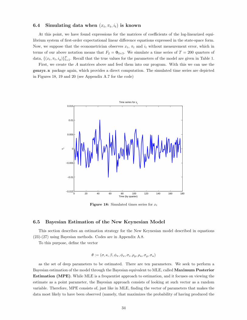
6.4 Simulating data when (xt, πt, it) is known
At this point, we have found expressions for the matrices of coefficients of the log-linearized equi-
librium system of first-order expectational linear difference equations expressed in the state-space form.
Now, we suppose that the econometrician observes xt, πt and it without measurement error, which in
terms of our above notation means that F2 = 03×3. We simulate a time series of T = 200 quarters of
data, (xt, πt, iy)Tt=1. Recall that the true values for the parameters of the model are given in Table 1.
First, we create the A matrices above and feed them into our program. With this we can use the
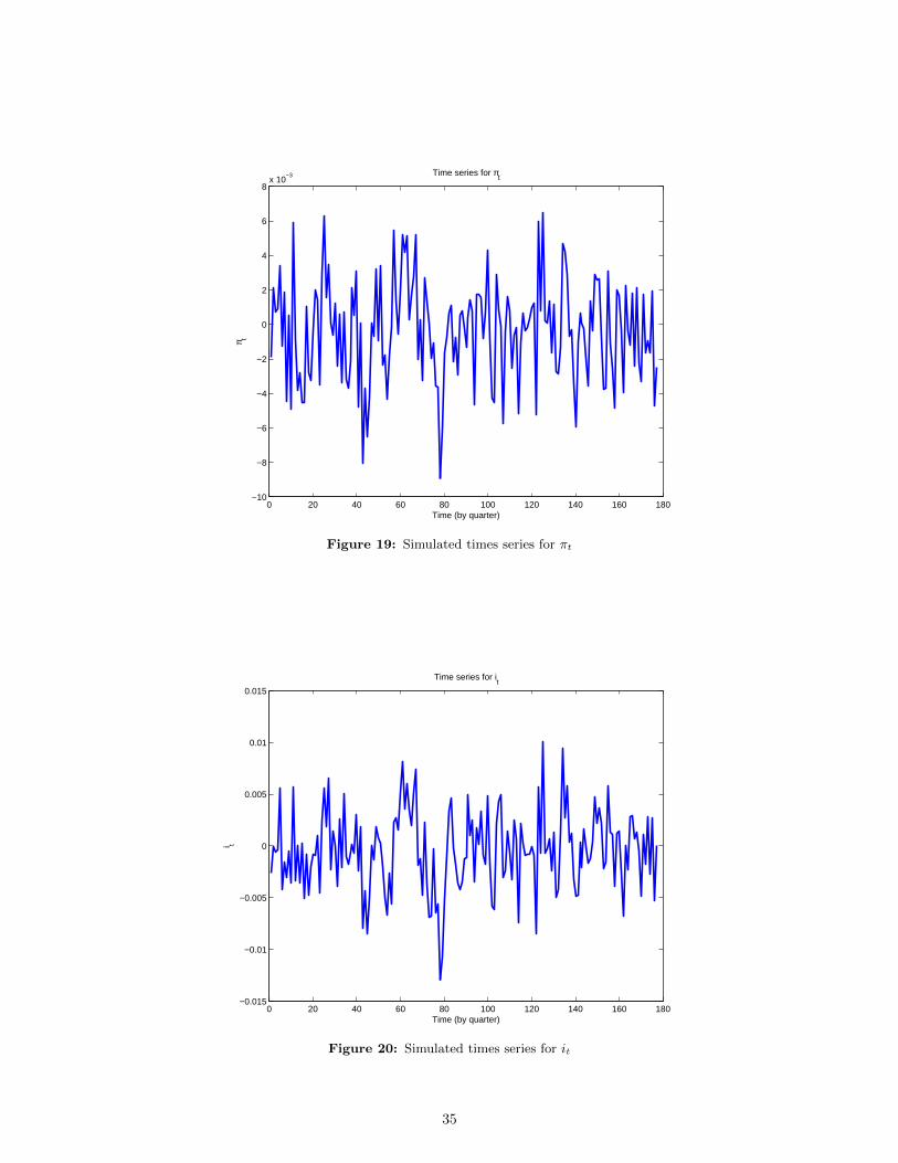
gensys.m package again, which provides a direct computation. The simulated time series are depicted
in Figures 18, 19 and 20 (see Appendix A.7 for the code)
0 20 40 60 80 100 120 140 160 180−0.015
−0.01
−0.005
0
0.005
0.01
0.015
Time (by quarter)
x t
Time series for xt
Figure 18: Simulated times series for xt
6.5 Bayesian Estimation of the New Keynesian Model
This section describes an estimation strategy for the New Keynesian model described in equations
(23)-(27) using Bayesian methods. Codes are in Appendix A.8.
To this purpose, define the vector
θ := (σ, κ, β, φπ, φx, σi, ρg, ρu, σg, σu)
as the set of deep parameters to be estimated. There are ten parameters. We seek to perform a
Bayesian estimation of the model through the Bayesian equivalent to MLE, called Maximum Posterior
Estimation (MPE). While MLE is a frequentist approach to estimation, and it focuses on viewing the
estimate as a point parameter, the Bayesian approach consists of looking at such vector as a random
variable. Therefore, MPE consists of, just like in MLE, finding the vector of parameters that makes the
data most likely to have been observed (namely, that maximizes the probability of having produced the
34
0 20 40 60 80 100 120 140 160 180−10
−8
−6
−4
−2
0
2
4
6
8x 10
−3
Time (by quarter)
π t
Time series for πt
Figure 19: Simulated times series for πt
0 20 40 60 80 100 120 140 160 180−0.015
−0.01
−0.005
0
0.005
0.01
0.015
Time (by quarter)
i t
Time series for it
Figure 20: Simulated times series for it
35
true data-generating process underlying the data at hand). Additionally, however, precision is enhanced
through the incorporation of out-of-sample information in the form of prior beliefs about the joint
distribution of the parameters, p(θ). That is, while MLE chooses
θMLE := arg maxθ∈Θ
p(y|θ)
as the point estimate, MPE focuses on maximizing the posterior density, that is
θMPE := arg maxθ∈Θ
p(θ|y)
where
p(θ|y) =p(y|θ)p(θ)∫
Θp(y|θ)p(θ)dθ
by Bayes’ rule, p(θ) is the prior density and p(y|θ) is the likelihood function. The likelihood function,
as would be the case in standard MLE, can be evaluated with an iterative procedure, which will in
this case be the Kalman filter because the system of equilibrium expectational equations is linear and
Gaussian. There is additional work to do, however, when choosing the prior joint density, p(θ).
Finally, we will have to write a program to evaluate the posterior as a function of θ, and use a
numerical search algorithm to find the argmax. Note that p(θ|y) involves an integral14, which can carry
computational difficulties. However, we may as well ignore it completely because it is constant in θ.
That is, since p(θ|y) ∝ p(y|θ)p(θ), namely
log p(θ|y) ∝ log p(y|θ) + log p(θ)
then we can maximize the right-hand side of the last equation without loss of generality.
6.5.1 Priors
As it is customary in the literature, we will select a prior density for each of the ten parameters at
hand and assume that parameters are uncorrelated with one another (namely, p(θi|θj) = p(θi), meaning
p(θi, θj) = p(θi)p(θj), for any θi, θj ∈ Θ). This means that we must form the collection of prior densities
pj(θj)10j=1 and compute the joint prior density simply by
p(θ) :=
10∏j=1
pj(θj)
where θj ∈ Θ, ∀j = 1, . . . , 10. The first aspect to consider when choosing prior densities is to limit
ourselves to the relevant parameter regions. Here, some parameters (such as σ or φπ) are bounded
below. Some others are in addition bounded above, like the correlations ρg and ρu or the discount factor
β.
All priors must be informed so that asymptotic precision can be significantly increased with respect
to MLE, but all information must come from outside of our sample. In our case, we know that the true
values of the parameters are as given in Table 1 and therefore we could in principle center all our priors
around these values. However, the true values will be typically unknown, and out-of-sample information
will have to be gathered in order to construct prior densities that can match the informed parametrical
calibrations.
14This acts as a normalization object, so that p(θ|y) integrates up to one and is, therefore, a proper density.
36
For this reason, we will use an exponential distribution for σ (with λ = 0.5), a beta distribution for β
(with αβ = 5 and ββ = 1), a gamma distribution for κ (with ακ = 3 and βκ = 2), σi (with ασi = 2 and
βσi = 1), σg (with ασg = 2 and βσg = 2), σu (with ασu = 2 and βσu = 2), and a normal distribution for
φπ (with µφπ = 0 and σφπ = 2), φx (with µφx = 0 and σφx = 2), ρg (with µρg = 0 and σρg = 2) and ρu
(with µρu = 0 and σρu = 2).
6.5.2 Posteriors
Once we have our informed priors, p(θ), we must evaluate the likelihood p(yT |θ), where yT :=
ytTt=1. Since we work with a time series, the classical iid assumption that is used in the cross-section
breaks down here. However, we can still decompose the likelihood with a prediction error decomposition:
p(yT |θ) = p(yT |yT−1; θ)p(yT−1|θ)
= p(yT |yT−1; θ)p(yT−1|yT−2; θ)p(yT−2|θ)...
= p(y0|θ)T∏t=1
p(yt|yt−1; θ)
so that
log p(yT |θ) = log p(y0|θ) +
T∑t=1
log p(yt|yt−1; θ) (31)
where the term log p(y0|θ) is often ignored in estimation, for its asymptotic contribution is nearly
negligible. To make progress, we want now to obtain a functional form for p(yt|yt−1, θ) and sufficient
statistics describing the log-likelihood. Since our system of first-order linear expectational equilibrium
difference equations can be written in the state-space form (recall section 2), then we can exploit both
linearity and gaussianity in the innovations by making use of the Kalman filter. The key step is to gain
information about the state through the filter. In particular, we want to recursively obtain estimates
for the one-step ahead forecast and its associated mean square error of the latent variables. With our
notation, the relevant updating equations of the filter are (recall Section 4):
st|t−1 = B1(θ)st−1|t−1
zt|t−1 = F1(θ)st|t−1
st|t = st|t−1 +Kt|t−1(zt − zt|t−1)
Pt|t = Pt|t−1 −Kt|t−1F1(θ)Pt|t−1
Pt|t−1 = B1(θ)Pt−1|t−1B′1(θ) +B2(θ)B′2(θ)
Vt|t−1 = F1(θ)Pt|t−1F′1(θ) + F2(θ)F ′2(θ)
where
Kt|t−1 := Pt|t−1F′1(θ)V −1
t|t−1
37
is the Kalman gain, we use the notation
st|t−1 := E[st|zt−1; θ
]zt|t−1 := E
[zt|zt−1; θ
]st|t := E
[st|zt; θ
]Pt|t := E
[(st − st|t)(st − st|t)
′|zt; θ]
Pt|t−1 := E[(st − st|t−1)(st − st|t−1)′|zt−1; θ
]Vt|t−1 := E
[(zt − zt|t−1)(zt − zt|t−1)′|zt−1; θ
]Vt|t := E
[(zt − zt|t)(zt − zt|t)
′|zt; θ]
for prior and posterior estimates of conditional means and variances with respect to mean forecasts,
and .|t−1 denotes old (prior, if t−1|t−1) or new (posterior, if t|t−1) information obtained as of period
t− 1.
The following describes the maximization algorithm:
1. Initialize the Kalman filter by fixing initial guesses for the unconditional mean and mean square
error of the state. Here, we draw the state from its stationary distribution, namely S0 ∼ N (0, σ2εI2)
(with σ2ε = 1), so that
S0|0 =
(0
0
)P0|0 =
(1 0
0 1
)This implies that the initial value of the observable variable is drawn from the distribution y0 ∼N (0, σ2
ε + σ2εθ
2) (again, with σ2ε = 1).
2. For each t ∈ 1, . . . , T, iteratively compute period-t density contribution to the likelihood function
(31) using the formula of the density for a Normally distributed random vector. After looping across
all time periods, we should have constructed the object
log p(yT |θ) ≈T∑t=1
log p(yt|yt−1; θ)
= −T2
log 2π − T
2log |Vt|t−1(θ)| − 1
2
T∑t=1
(zt − zt|t−1(θ))V −1t|t−1(θ)(zt − zt|t−1(θ))′
where Vt|t−1(θ) and zt|t−1(θ) are given by the Kalman filter recursion described above. Once more,
this formula comes from gaussianity of the innovations of the process in the state-space form, which
makes the whole process conditionally normal as well.
3. Add the prior density (as computed by the sum of prior log-densities, due to our independence
assumption) to obtain the object log p(yT |θ) + log p(θ), which is the posterior density. Maximize
the posterior density over θ with a numerical optimizer to obtain
θMPE = arg maxθ∈Θ
(log p(yT |θ) + log p(θ)
)as we sought.
38
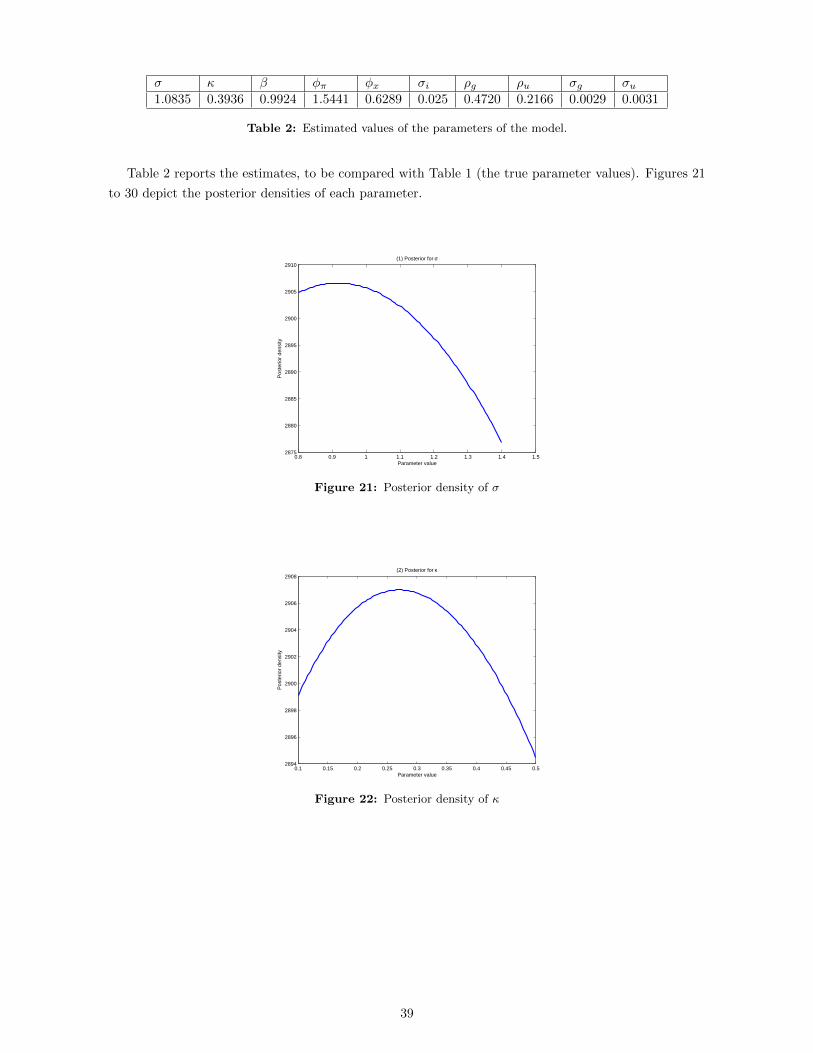
σ κ β φπ φx σi ρg ρu σg σu1.0835 0.3936 0.9924 1.5441 0.6289 0.025 0.4720 0.2166 0.0029 0.0031
Table 2: Estimated values of the parameters of the model.
Table 2 reports the estimates, to be compared with Table 1 (the true parameter values). Figures 21
to 30 depict the posterior densities of each parameter.
0.8 0.9 1 1.1 1.2 1.3 1.4 1.52875
2880
2885
2890
2895
2900
2905
2910(1) Posterior for σ
Parameter value
Pos
terio
r de
nsity
Figure 21: Posterior density of σ
0.1 0.15 0.2 0.25 0.3 0.35 0.4 0.45 0.52894
2896
2898
2900
2902
2904
2906
2908(2) Posterior for κ
Parameter value
Pos
terio
r de
nsity
Figure 22: Posterior density of κ
39
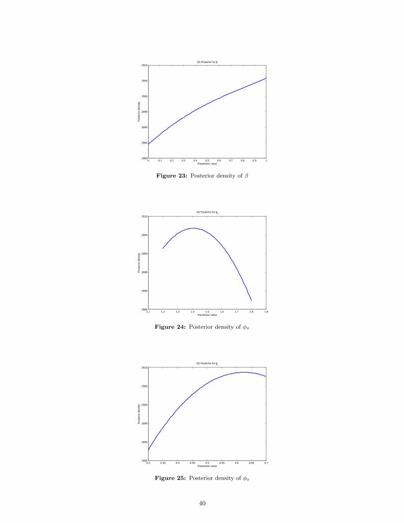
0 0.1 0.2 0.3 0.4 0.5 0.6 0.7 0.8 0.9 12880
2885
2890
2895
2900
2905
2910(3) Posterior for β
Parameter value
Pos
terio
r de
nsity
Figure 23: Posterior density of β
1.1 1.2 1.3 1.4 1.5 1.6 1.7 1.8 1.92885
2890
2895
2900
2905
2910
(4) Posterior for φπ
Parameter value
Pos
terio
r de
nsity
Figure 24: Posterior density of φπ
0.3 0.35 0.4 0.45 0.5 0.55 0.6 0.65 0.72885
2890
2895
2900
2905
2910
(5) Posterior for φx
Parameter value
Pos
terio
r de
nsity
Figure 25: Posterior density of φx
40
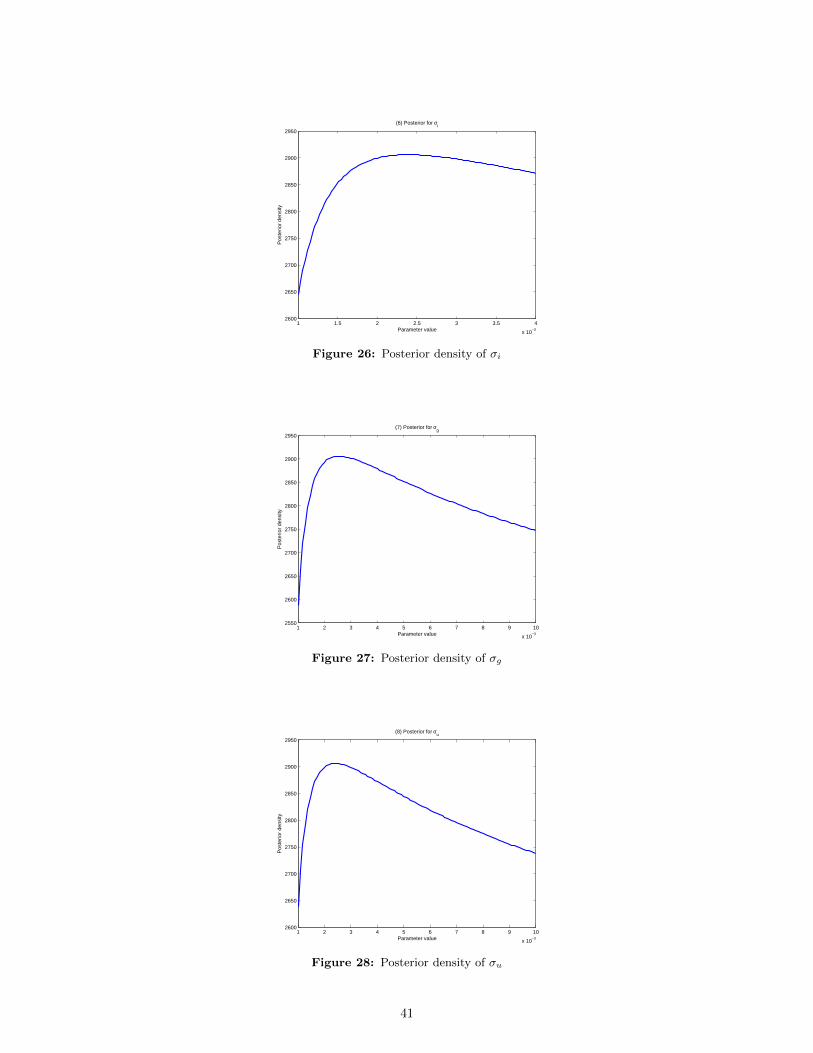
1 1.5 2 2.5 3 3.5 4
x 10−3
2600
2650
2700
2750
2800
2850
2900
2950
(6) Posterior for σi
Parameter value
Pos
terio
r de
nsity
Figure 26: Posterior density of σi
1 2 3 4 5 6 7 8 9 10
x 10−3
2550
2600
2650
2700
2750
2800
2850
2900
2950
(7) Posterior for σg
Parameter value
Pos
terio
r de
nsity
Figure 27: Posterior density of σg
1 2 3 4 5 6 7 8 9 10
x 10−3
2600
2650
2700
2750
2800
2850
2900
2950
(8) Posterior for σu
Parameter value
Pos
terio
r de
nsity
Figure 28: Posterior density of σu
41
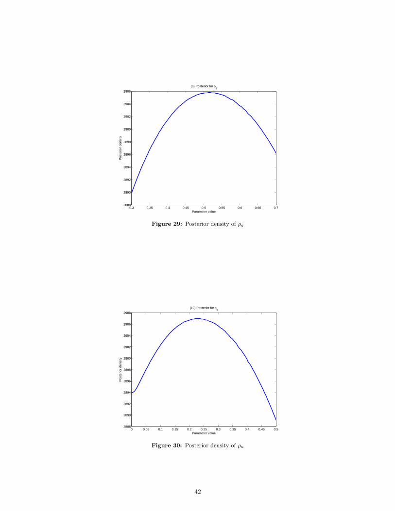
0.3 0.35 0.4 0.45 0.5 0.55 0.6 0.65 0.72888
2890
2892
2894
2896
2898
2900
2902
2904
2906
(9) Posterior for ρg
Parameter value
Pos
terio
r de
nsity
Figure 29: Posterior density of ρg
0 0.05 0.1 0.15 0.2 0.25 0.3 0.35 0.4 0.45 0.52888
2890
2892
2894
2896
2898
2900
2902
2904
2906
2908
(10) Posterior for ρu
Parameter value
Pos
terio
r de
nsity
Figure 30: Posterior density of ρu
42
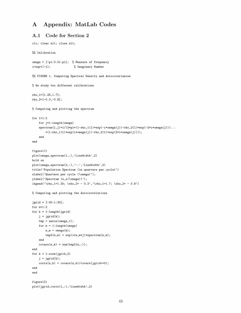
A Appendix: MatLab Codes
A.1 Code for Section 2
clc; clear all; close all;
%% Calibration
omega = [-pi:0.01:pi]; % Measure of frequency
i=sqrt(-1); % Imaginary Number
%% FIGURE 1. Computing Spectral Density and Autocovariances
% We study two different calibrations
rho_1=[1.25,1.7];
rho_2=[-0.3,-0.8];
% Computing and plotting the spectrum
for l=1:2
for j=1:length(omega)
spectrum(l,j)=1/(2*pi*(1-rho_1(l)*exp(-i*omega(j))-rho_2(l)*exp(-2*i*omega(j)))...
*(1-rho_1(l)*exp(i*omega(j))-rho_2(l)*exp(2*i*omega(j))));
end
end
figure(1)
plot(omega,spectrum(1,:),’LineWidth’,2)
hold on
plot(omega,spectrum(2,:),’-.’,’LineWidth’,2)
title(’Population Spectrum (in quarters per cycle)’)
xlabel(’Quarters per cycle (\omega)’);
ylabel(’Spectrum (s_x(\omega))’);
legend(’\rho_1=1.25; \rho_2= - 0.3’,’\rho_1=1.7; \rho_2= - 0.8’)
% Computing and plotting the Autocorrelations
jgrid = [-30:1:30];
for n=1:2
for k = 1:length(jgrid)
j = jgrid(k);
tmp = zeros(omega,1);
for m = 1:length(omega)
w_m = omega(m);
tmp2(n,m) = exp(i*w_m*j)*spectrum(n,m);
end
covars(n,k) = sum(tmp2(n,:));
end
for k = 1:size(jgrid,2)
j = jgrid(k);
corrs(n,k) = covars(n,k)/covars(jgrid==0);
end
end
figure(2)
plot(jgrid,corrs(1,:),’LineWidth’,2)
43
hold on
plot(jgrid,corrs(2,:),’-.’,’LineWidth’,2)
title(’Auto-Correlation Function’)
xlabel(’Step-size (j)’);
ylabel(’\rho_j’);
legend(’\rho_1=1.25; \rho_2= - 0.3’,’\rho_1=1.7; \rho_2= - 0.8’)
A.2 Code for Section 3
%% FIGURE 2. Computing the HP Filter’s Gain (the Phase is just zero)
mu=1600;
for k=1:length(omega)
gain(k)=(4*mu*(1-cos(omega(k)))^2)/(1+4*mu*(1-cos(omega(k)))^2);
end
figure(3)
plot(omega,gain,’LineWidth’,2)
title(’Gain of HP filter (in quarters per cycle)’)
xlabel(’Quarters per cycle (\omega)’);
ylabel(’G(\omega)’);
ylim([-.01 1.05])
xlim([-3 3])
A.3 Code for Section 5.1
clear all; close all; clc;
tic
% Estimating an MA(1)
load ma_data.txt
X = ma_data; % the time series
T = size(X,1); % number of observations
% Read matrices for the Kalman filter of an MA(1)
thetagrid = -0.99:0.001:0.99; % values of theta we consider
A = [0 0 ; 1 0];
B = [1 0];
B=B’;
Cmat = [ones(size(thetagrid,2),1) thetagrid’]; % contains a 2x1 vector
%C = [1 theta] in different rows, for every value of theta we consider
% Set initial guesses for the Kalman filter
S_init = zeros(2,1); % S_0|0
P_init = eye(2); % P_0|0
% Set up the likelihood for every value of theta
logLLvec = zeros(size(thetagrid,2),1);
for i = 1: size(thetagrid,2)
C = Cmat(i,:); % C-matrix for this value of theta
logLL = 0; % initiate loglikelihood
S_cond_lag = zeros(2,T); % contains S_t|t-1 (2 by 1) for every t
44
S_cond = zeros(2,T); % contains S_t|t (2 by 1) for every t
X_cond_lag = zeros(1,T); % contains x_t|t-1 scalar for every t
P_cond_lag = zeros(2,2,T); % contains P_t|t-1 (2 by 2) for every t
P_cond = zeros(2,2,T); % contains P_t|t (2 by 2) for every t
V_cond_lag = zeros(1,T); % contains V_t|t-1 scalar for every t
for t = 1:T % iterate the Kalman filter
if t==1 % use initial values for S_t|t and P_t|t
S_cond_lag(:,1) = A*S_init;
X_cond_lag(:,1) = C*S_cond_lag(:,t);
P_cond_lag(:,:,1) = A*P_init*A’ + B*B’;
V_cond_lag(1,1) = C*P_cond_lag(:,:,t)*C’;
S_cond(:,1) = S_cond_lag(:,t) + (P_cond_lag(:,:,t)*C’*...
(V_cond_lag(1,t)^(-1)))*(X(t) - X_cond_lag(1,t));
P_cond(:,:,1) = P_cond_lag(:,:,t) - (P_cond_lag(:,:,t)*C’*...
(V_cond_lag(1,t)^(-1)))*C*P_cond_lag(:,:,t);
else
S_cond_lag(:,t) = A*S_cond(:,t-1);
X_cond_lag(:,t) = C*S_cond_lag(:,t);
P_cond_lag(:,:,t) = A*P_cond(:,:,t-1)*A’ + B*B’;
V_cond_lag(1,t) = C*P_cond_lag(:,:,t)*C’;
S_cond(:,t) = S_cond_lag(:,t) + (P_cond_lag(:,:,t)*C’*...
(V_cond_lag(1,t)^(-1)))*(X(t) - X_cond_lag(1,t));
P_cond(:,:,t) = P_cond_lag(:,:,t) - (P_cond_lag(:,:,t)*C’*...
(V_cond_lag(1,t)^(-1)))*C*P_cond_lag(:,:,t);
end
% Update the likelihood:
logLL = logLL - 0.5 * log(V_cond_lag(1,t)) - 0.5 * (X(t) - ...
X_cond_lag(1,t))*(V_cond_lag(1,t)^(-1))*(X(t) - X_cond_lag(1,t));
end
logLLvec(i) = logLL; % total likelihood for this theta value
end
figure(1)
plot(thetagrid, logLLvec,’LineWidth’,2)
title(’Loglikelihood of an MA(1)’)
xlabel(’\theta’)
ylabel(’log L( \theta )’)
[maxLL, maxindex] = max(logLLvec);
thetahat = thetagrid(maxindex)
toc
A.4 Code for Section 5.2
clear all; close all; clc;
tic
%% 0. PRELIMINARIES AND CALIBRATION
% First, we load the data. Since data is in the .mat form, all variables
% have been created for us
load ps2.mat
T=size(date,1); % Sample size
%% 1. OLS ESTIMATION OF THE VAR(2)
45
YY=zeros(2,T);
ZZ=zeros(5,T);
for t=3:T
YY(:,t)=[dlnY(t);Zic(t)];
ZZ(:,t)=[1;YY(:,t-1);YY(:,t-2)]; % 1 constant, and 4 regressors
end
Y=YY(:,3:end);
Z=ZZ(:,3:end);
Ystack=[dlnY(3:end);Zic(3:end)];
Xbar = Z’;
betaGLShat = (kron(eye(2),((Xbar’*Xbar)^(-1))*Xbar’))*Ystack
uhat = zeros(2,T-2);
for t = 3:T
u(1,t) = YY(1,t)-Xbar(t-2,:)*betaGLShat(1:5,1); % residual from first equation
u(2,t) = YY(2,t)-Xbar(t-2,:)*betaGLShat(6:10,1); % residual from second equation
end
Omega_hat=(1/(T-2))*(u*u’) % covariance matrix
%% 2. TEST FOR GRANGER CAUSALITY
% Run a Wald test to test the hypotheses:
% (i) H_0 : beta1 = beta2 = 0 ("Zic does not Granger-cause dlnY")
% (ii) H_0 : gamma1 = gamma2 = 0 ("dlnY does not Granger-cause Zic")
R1=[0 0 1 0 0 0 0 0 0 0; 0 0 0 0 1 0 0 0 0 0];
R2=[0 0 0 0 0 0 1 0 0 0; 0 0 0 0 0 0 0 0 1 0];
r=zeros(2,1);
U = kron(eye(2),Xbar);
VXi=(U’*(kron(Omega_hat^(-1),eye(T-2)))*U)^(-1);
% Testing "Zic does not Granger-cause dlnY"
W1=betaGLShat’*R1’*((R1*VXi*R1’)^(-1))*R1*betaGLShat
pvalue1=1-chi2cdf(W1,2)
% Testing "dlnY does not Granger-cause Zic"
W2=betaGLShat’*R2’*((R2*VXi*R2’)^(-1))*R2*betaGLShat
pvalue2=1-chi2cdf(W2,2)
%% 3. BEVERIDGE-NELSON OUTPUT GAP
outputgap = zeros(T-2,1);
ybar = zeros(T-2,1); % Stochastic trend from B&N
e1 = [1 0 0 0]’; % Selector vector
Ahat = [0.4156 -0.0315 0.1652 0.0123;2.2371 0.6559 0.6703 0.1626; 1 0 0 0;0 1 0 0];
for t = 1:T-2
Zt = [dlnY(t+2); Zic(t+2); dlnY(t+1); Zic(t+1)];
ybar(t,1) = dlnY(t+2) + e1’*(eye(4)-Ahat)^(-1)*Zt;
outputgap(t) = dlnY(t+2)-ybar(t); % messed up time indices but you get the point
end
figure(1)
plot(3:T, outputgap,’LineWidth’,2)
title(’Output Gap’)
xlabel(’Time’);
ylabel(’Output gap’);
disp(’The output gap at the end of the sample is:’)
outputgap(end)
46
%% Last Updated: Apr 23th, 2013
A.5 Code for Section 5.3
%% Blanchard-Quah (1989)
% Step 1: Estimate the VAR(2) by SUR/GLS
clear; clc;
load ps2.mat
Y = [dlnY(3:end) Zic(3:end)];
N = size(Y,1); % number of observations
X = [ones(N,1) dlnY(2:end-1) Zic(2:end-1) dlnY(1:end-2) Zic(1:end-2)];
beta = (X’*X) \ (X’*Y) % GLS estimator = 5x2 matrix
epshat = Y-X*beta; % residuals = epsilon_hat
Omega = (epshat’*epshat)/N % covar matrix of epsilons
% Create G1 from the estimated beta matrix (dropping the constant)
G1 = [beta(2:end,1)’; beta(2:end,2)’; 1 0 0 0; 0 1 0 0]
G1inv = (eye(4) - G1)^(-1);
options = optimset(’Display’, ’off’);
Omega2 = zeros(4,4);
Omega2(1:2,1:2) = Omega;
% Solve for G2 using long run restriction on g22 via Cholesky decomposition
bla = G1inv*Omega2*G1inv’;
H = chol(bla(1:2,1:2))’ % long run effect
G2 = inv(G1inv(1:2,1:2))*H;
G2 = G2’
% Back out the shocks
eta = zeros(size(epshat,1), 2);
for t = 1:length(eta)
eta(t,:) = G2^(-1)*epshat(t,:)’;
end
eta = eta’;
%Impulse responses
G2 = [G2; 0 0; 0 0];
T=15;
time = 0:T;
NT=length(time) ;
IRF_y_s= zeros(NT,1);
IRF_y_d= zeros(NT,1);
sel_y = [1 0 0 0] ;
sel_s = [1 0]’;
sel_d = [0 1]’;
for it = 1:NT
j = time(it);
IRF_y_s(it) = sel_y*((G1^j)*G2)*sel_s;
IRF_y_d(it) = sel_y*((G1^j)*G2)*sel_d;
end
% Plot IRF
figure(1)
plot(time, IRF_y_s,’LineWidth’,2)
title(’(1) IRF of output for SUPPLY shocks’)
47
xlabel(’Number of periods ahead’);
ylabel(’Change in output growth’);
% Plot IRF
figure(2)
plot(time, IRF_y_d,’LineWidth’,2)
title(’(2) IRF of output for DEMAND shocks’)
xlabel(’Number of periods ahead’);
ylabel(’Change in output growth’);
A.6 Code for Section 6
%% Simulation of a New Keynesian Economy
% Calibration
sigma = 1;
kappa = 0.2;
beta = 0.99;
phi_pi = 1.5;
phi_x = 0.5;
sigma_i = 0.0025;
sigma_g = 0.0025;
sigma_u = 0.0025;
rho_g = 0.5;
rho_u = 0.3;
%% Gensys method:
% function [G1,C,impact,fmat,fwt,ywt,gev,eu,loose]=gensys(g0,g1,c,psi,pi,div)
% System given as
% g0*y(t)=g1*y(t-1)+c+psi*z(t)+pi*eta(t),
% with z an exogenous variable process and eta being endogenously determined
% one-step-ahead expectational errors. Returned system is
% y(t)=G1*y(t-1)+C+impact*z(t)+ywt*inv(I-fmat*inv(L))*fwt*z(t+1) .
% State y_t = [x pi i g u E(x’) E(pi’)]
% Errors psi = [eps_i eps_g eps_u]
g0 = [1 0 sigma -1 0 -1 -sigma; -kappa 1 0 0 -1 0 -beta; -phi_x -phi_pi 1 0 0 0 0; ...
0 0 0 1 0 0 0; 0 0 0 0 1 0 0; 1 0 0 0 0 0 0; 0 1 0 0 0 0 0];
g1 = [zeros(3,7); 0 0 0 rho_g 0 0 0; 0 0 0 0 rho_u 0 0; 0 0 0 0 0 1 0; 0 0 0 0 0 0 1];
c = zeros(7,1); % no constant
psi = [zeros(2,3); sigma_i 0 0; 0 sigma_g 0; 0 0 sigma_u; zeros(2,3)];
pim = [zeros(5,2); eye(2)];
% Call gensys
[G1,C,G2,fmat,fwt,ywt,gev,eu,loose]=gensys(g0,g1,c,psi,pim);
G1
G2
% Create G3 which selects Z from y
G3 = [1 0 0 0 0 0 0; 0 1 0 0 0 0 0; 0 0 1 0 0 0 0]
%% Alternative method to check the output of GENSYS
48
% Define A0, A1, A2, A3 for the 3 DSGE equations, where Z = [x; pi; i],
% S = [g; u] and eps = [eps_i; eps_g; eps_u]
A0 = [ 1 0 sigma; -kappa 1 0; -phi_x -phi_pi 1];
A1 = [1 sigma 0; 0 beta 0; 0 0 0];
A2 = [1 0; 0 1; 0 0];
A3 = [0 0 0; 0 0 0; sigma_i 0 0];
% Define B1, B2 for the two state equations: St = B1*S_t-1 + B2*eps_t
B1 = [rho_g 0; 0 rho_u];
B2 = [0 sigma_g 0; 0 0 sigma_u];
% Guessing Z_t = F0*S_t + F1*eps_t, we calculate F0 and F1:
F0 = fsolve(@(x) A1*x*B1 - A0*x + A2, zeros(3,2));
F1 = A0\A3; % inv(A0)*A3
G1alt = F0*B1
G2alt = F0*B2+F1
%% Now, generate a time series for Z = [x; pi; i] using the GENSYS output
% Note: the three epsilon-components are iid standard normal random variables
T = 2000; % Number of periods that we simulate
% First, generate three epsilon sequences [eps_i; eps_g; eps_u]
tmp1 = randn(3, T);
eps_sim = tmp1; % 3xT
% eps_i_sim = tmp1(1,:); % 1xT
% eps_g_sim = tmp1(2,:); % 1xT
% eps_u_sim = tmp1(3,:); % 1xT
% Now, use the gensys output (G1, G2) to generate random y_t vectors
y_sim = zeros(7,T);
for t = 2:T
y_sim(:,t) = G1*y_sim(:,t-1) + G2*eps_sim(:,t);
end
cutoff = ceil(0.20*T);
y_sim = y_sim(:,cutoff:end); % Drop the first observations
Z_sim = G3*y_sim; % Keep only x, pi and i as observables, and use these as input in the Kalman filter
% Z_sim = y_sim(1:3,:); % alternative way to do this
% Parameters = [sigma, kappa, beta, phi_pi, phi_x, sigma_i, sigma_g, sigma_u, rho_g, rho_u];
sigma0 = 1.2;
kappa0 = 0.3;
beta0 = 0.98;
phi_pi0 = 1.7;
phi_x0 = 0.3;
sigma_i0 = 0.01;
sigma_g0 = 0.01;
sigma_u0 = 0.01;
rho_g0 = 0.2;
rho_u0 = 0.2;
% Transform the parameter space
% Note: for beta, I first take the inverse logit transform to make sure
% it’s between 0 and 1
init = [log(sigma0), kappa0, log(beta0)-log(1-beta0), phi_pi0, phi_x0, ...
log(sigma_i0), log(sigma_g0), log(sigma_u0), rho_g0, rho_u0];
49
% lb = zeros(10,1); % lower bound; all parameters have to be positive!
% ub = [10, 10, 1, 10, 10, 10, 10, 10, 1, 1];
% logLL = @(x) loglikelihood(x, Z_sim);
options = optimset(’MaxIter’, 5000, ’MaxFunEvals’, 5000, ’Display’, ’off’);
[est,fval,exitflag] = fminsearch(@(x) -loglikelihood(x,Z_sim),init,options);
sigma_sim = exp(est(1))
kappa_sim = est(2)
beta_sim = exp(est(3))/(1+exp(est(3))) % logit transform
phi_pi_sim = est(4)
phi_x_sim = est(5)
sigma_i_sim = exp(est(6))
sigma_g_sim = exp(est(7))
sigma_u_sim = exp(est(8))
rho_g_sim = est(9)
rho_u_sim = est(10)
%% Plot loglikelihood functions for every parameter
N = 100; % number of gridpoints
% Function ’loglikelihood2’ does the same as the other one, but does not
% rescale parameters, since we take them as given in what follows below
%% 1) Plot for sigma
grid1 = linspace(0.80,1.20,N);
logLL1 = zeros(N,1);
for i = 1:N
sigma = grid1(i);
kappa = 0.2;
beta = 0.99;
phi_pi = 1.5;
phi_x = 0.5;
sigma_i = 0.0025;
sigma_g = 0.0025;
sigma_u = 0.0025;
rho_g = 0.5;
rho_u = 0.3;
xvec = [sigma, kappa, beta, phi_pi, phi_x, sigma_i, sigma_g, sigma_u, rho_g, rho_u];
logLL1(i,1) = loglikelihood2(xvec,Z_sim);
end
[maxLL, maxindex] = max(logLL1);
max_sigma = grid1(maxindex)
figure(1)
plot(grid1, logLL1)
title(’(1) Loglikelihood for \sigma’)
xlabel(’Parameter value’);
ylabel(’Loglikelihood’);
saveas(figure(1),’Fig1’, ’png’)
saveas(figure(1),’Fig1’, ’pdf’)
%% 2) Plot for kappa
[The code continues in a similar fashion for the rest of the parameters]
50
A.7 Code for Section 6.4
clear all; close all; clc;
%% PART 1 - Simulation of 200 quarters of the New Keynesian economy
% Calibration
sigma = 1;
kappa = 0.2;
beta = 0.99;
phi_pi = 1.5;
phi_x = 0.5;
sigma_i = 0.0025;
sigma_g = 0.0025;
sigma_u = 0.0025;
rho_g = 0.5;
rho_u = 0.3;
%% 1.1 Gensys method:
% function [G1,C,impact,fmat,fwt,ywt,gev,eu,loose]=gensys(g0,g1,c,psi,pi,div)
% System given as
% g0*y(t)=g1*y(t-1)+c+psi*z(t)+pi*eta(t),
% with z an exogenous variable process and eta being endogenously determined
% one-step-ahead expectational errors. Returned system is
% y(t)=G1*y(t-1)+C+impact*z(t)+ywt*inv(I-fmat*inv(L))*fwt*z(t+1) .
% State y_t = [x pi i g u E(x’) E(pi’)]
% Errors psi = [eps_i eps_g eps_u]
g0 = [1 0 sigma -1 0 -1 -sigma; -kappa 1 0 0 -1 0 -beta; -phi_x -phi_pi 1 0 0 0 0;...
0 0 0 1 0 0 0; 0 0 0 0 1 0 0; 1 0 0 0 0 0 0; 0 1 0 0 0 0 0];
g1 = [zeros(3,7); 0 0 0 rho_g 0 0 0; 0 0 0 0 rho_u 0 0; 0 0 0 0 0 1 0; 0 0 0 0 0 0 1];
c = zeros(7,1); % no constant
psi = [zeros(2,3); sigma_i 0 0; 0 sigma_g 0; 0 0 sigma_u; zeros(2,3)];
pim = [zeros(5,2); eye(2)];
% Call gensys
[G1,C,G2,fmat,fwt,ywt,gev,eu,loose]=gensys(g0,g1,c,psi,pim);
G1
G2
% Create G3 which will select Z:=(x,pi,i) from y (the whole vector of data)
G3 = [1 0 0 0 0 0 0; 0 1 0 0 0 0 0; 0 0 1 0 0 0 0]
%% 1.2 Alternatively, if we don’t want to use gensys:
% We write the system in its state-space form, found in Part 1.
% Define the A0, A1, A2, A3 matrices for the 3 equations, where
% Z = [x; pi; i], S = [g; u] and eps = [eps_i; eps_g; eps_u]
A0 = [ 1 0 sigma; -kappa 1 0; -phi_x -phi_pi 1];
A1 = [1 sigma 0; 0 beta 0; 0 0 0];
A2 = [1 0; 0 1; 0 0];
A3 = [0 0 0; 0 0 0; sigma_i 0 0];
51
% Define also the B1, B2 matrices for the state equation:
% B0*St = B1*S_t-1+B2*eps_t
% where B0 is the identity because there are no contemporaneous
% correlations.
B1 = [rho_g 0; 0 rho_u];
B2 = [0 sigma_g 0; 0 0 sigma_u];
% Using the guess from equation (9), Z_t = F0*S_t + F1*eps_t, we calculate
% F0 and F1:
F0 = fsolve(@(x) A1*x*B1 - A0*x + A2, zeros(3,2)); % from equation (10)
F1 = A0\A3; % from equation (11)
G1alt = F0*B1 % To be compared with gensys’ "G1" above
G2alt = F0*B2+F1 % To be compared with gensys’ "G2" above
%% 1.3 Now, generate a time series for Z = [x; pi; i] using the matrices above
% Note: the three epsilon-components are iid standard normal random variables
T = 220; % Number of periods that we simulate
% First, generate three epsilon sequences [eps_i; eps_g; eps_u]
randommatrix = randn(3, T); % Create a 3-by-T matrix of random numbers between 0 and 1
eps_sim = randommatrix; % 3-by-T vector of simulated innovations
% eps_i_sim = tmp1(1,:); % 1xT
% eps_g_sim = tmp1(2,:); % 1xT
% eps_u_sim = tmp1(3,:); % 1xT
% Now, use the gensys output (G1, G2) to generate random y_t vectors,
% according to the system of equilibrium equations as written in equation
% (12) in Appendix 2
y_sim = zeros(7,T);
for t = 2:T
y_sim(:,t) = G1*y_sim(:,t-1) + G2*eps_sim(:,t);
end
cutoff = ceil(0.20*T);
y_sim = y_sim(:,cutoff:end); % Drop the first observations to eliminate
% spurious dependence on initial values
Z_sim = G3*y_sim; % Recall that we keep only x, pi and i as observables,
% (G3 was defined as a selector matrix) and use these
% as input in the Kalman filter when we evaluate logLL
% Z_sim = y_sim(1:3,:); % alternative way to do this
figure(1)
plot(Z_sim(1,:),’LineWidth’,2) % Times series for x_t
xlabel(’Time (by quarter)’)
ylabel(’x_t’)
title(’Time series for x_t’)
saveas(figure(1),’xt’, ’pdf’)
52
figure(2)
plot(Z_sim(2,:),’LineWidth’,2) % Times series for pi_t
xlabel(’Time (by quarter)’)
ylabel(’\pi_t’)
title(’Time series for \pi_t’)
saveas(figure(2),’pit’, ’pdf’)
figure(3)
plot(Z_sim(3,:),’LineWidth’,2) % Times series for i_t
xlabel(’Time (by quarter)’)
ylabel(’i_t’)
title(’Time series for i_t’)
saveas(figure(3),’it’, ’pdf’)
A.8 Code for Section 6.5
%% Prior and Likelihood
% Parameters are theta: = [sigma, kappa, beta, phi_pi, phi_x, sigma_i,
% sigma_g, sigma_u, rho_g, rho_u]; We initiate the algorithm using initial
% values that differ little from the true values
sigma0 = 1.2;
kappa0 = 0.3;
beta0 = 0.98;
phi_pi0 = 1.7;
phi_x0 = 0.3;
sigma_i0 = 0.01;
sigma_g0 = 0.01;
sigma_u0 = 0.01;
rho_g0 = 0.2;
rho_u0 = 0.2;
% Now, we transform the parameter space to limit ourselves to the correct
% parameter space.
% The vector of initial values is:
init = [log(sigma0), kappa0, log(beta0)-log(1-beta0), phi_pi0, phi_x0,...
log(sigma_i0), log(sigma_g0), log(sigma_u0), rho_g0, rho_u0];
% My priors:
% Sigma ---> Exponential
lambda_sigma=0.5;
% Kappa ---> gamma
alpha_kappa=3;
beta_kappa=2;
% beta ---> beta distribution
alpha_beta=5;
beta_beta=1;
% phi_pi ---> Normal
mu_phipi=0;
sigma_phipi=2;
% phi_x ---> Normal
mu_phix=0;
53
sigma_phix=2;
% sigma_i ---> gamma
alpha_sigmai=2;
beta_sigmai=2;
% sigma_g ---> gamma
alpha_sigmag=2;
beta_sigmag=2;
% sigma_u ---> gamma
alpha_sigmau=2;
beta_sigmau=2;
% rho_g ---> Normal
mu_rhog=0;
sigma_rhog=2;
% rho_u ---> Normal
mu_rhou=0;
sigma_rhou=2;
priors=[lambda_sigma, alpha_kappa, beta_kappa, alpha_beta, beta_beta, ...
mu_phipi, sigma_phipi, mu_phix, sigma_phix, alpha_sigmai, beta_sigmai, ...
alpha_sigmag, beta_sigmag, alpha_sigmau, beta_sigmau, mu_rhog, sigma_rhog, ...
mu_rhou, sigma_rhou];
% lb = zeros(10,1); % lower bound; all parameters have to be positive!
% ub = [10, 10, 1, 10, 10, 10, 10, 10, 1, 1];
% logLL = @(x) loglikelihood(x, Z_sim);
options = optimset(’MaxIter’, 5000, ’MaxFunEvals’, 5000, ’Display’, ’off’);
[est,fval,exitflag] = fminsearch(@(x) -loglikelihood(x,Z_sim,priors),init,options);
sigma_sim = exp(est(1))
kappa_sim = est(2)
beta_sim = exp(est(3))/(1+exp(est(3))) % logit transform
phi_pi_sim = est(4)
phi_x_sim = est(5)
sigma_i_sim = exp(est(6))
sigma_g_sim = exp(est(7))
sigma_u_sim = exp(est(8))
rho_g_sim = est(9)
rho_u_sim = est(10)
%% Plot posterior functions for every parameter
N = 100; % number of gridpoints
% Function ’loglikelihood2’ does the same as the other one, but does not
% rescale parameters, since we take them as given in what follows below
%% 1) Plot for sigma
grid1 = linspace(0.80,1.40,N);
logLL1 = zeros(N,1);
for i = 1:N
sigma = grid1(i);
kappa = 0.2;
beta = 0.99;
phi_pi = 1.5;
phi_x = 0.5;
sigma_i = 0.0025;
sigma_g = 0.0025;
sigma_u = 0.0025;
54
rho_g = 0.5;
rho_u = 0.3;
xvec = [sigma, kappa, beta, phi_pi, phi_x, sigma_i, sigma_g, sigma_u, rho_g, rho_u];
logLL1(i,1) = loglikelihood2(xvec,Z_sim,priors);
end
[maxLL, maxindex] = max(logLL1);
max_sigma = grid1(maxindex)
figure(4)
plot(grid1, logLL1,’LineWidth’,2)
title(’(1) Posterior for \sigma’)
xlabel(’Parameter value’);
ylabel(’Posterior density’);
saveas(figure(4),’Fig1’, ’png’)
saveas(figure(4),’Fig1’, ’pdf’)
%% 2) Plot for kappa
grid2 = linspace(0.10,0.50,N);
logLL2 = zeros(N,1);
for i = 1:N
sigma = 1;
kappa = grid2(i);
beta = 0.99;
phi_pi = 1.5;
phi_x = 0.5;
sigma_i = 0.0025;
sigma_g = 0.0025;
sigma_u = 0.0025;
rho_g = 0.5;
rho_u = 0.3;
xvec = [sigma, kappa, beta, phi_pi, phi_x, sigma_i, sigma_g, sigma_u, rho_g, rho_u];
logLL2(i,1) = loglikelihood2(xvec,Z_sim,priors);
end
[maxLL, maxindex] = max(logLL2);
max_kappa = grid2(maxindex)
figure(5)
plot(grid2, logLL2,’LineWidth’,2)
title(’(2) Posterior for \kappa’)
xlabel(’Parameter value’);
ylabel(’Posterior density’);
saveas(figure(5),’Fig2’, ’png’)
saveas(figure(5),’Fig2’, ’pdf’)
%% 3) Plot for beta
grid3 = linspace(0,1,N);
logLL3 = zeros(N,1);
for i = 1:N
sigma = 1;
kappa = 0.2;
beta = grid3(i);
phi_pi = 1.5;
phi_x = 0.5;
sigma_i = 0.0025;
sigma_g = 0.0025;
sigma_u = 0.0025;
rho_g = 0.5;
55
rho_u = 0.3;
xvec = [sigma, kappa, beta, phi_pi, phi_x, sigma_i, sigma_g, sigma_u, rho_g, rho_u];
logLL3(i,1) = loglikelihood2(xvec,Z_sim,priors);
end
[maxLL, maxindex] = max(logLL3);
max_beta = grid3(maxindex)
figure(6)
plot(grid3, logLL3,’LineWidth’,2)
title(’(3) Posterior for \beta’)
xlabel(’Parameter value’);
ylabel(’Posterior density’);
saveas(figure(6),’Fig3’, ’png’)
saveas(figure(6),’Fig3’, ’pdf’)
%% 4) Plot for phi_pi
grid4 = linspace(1.2,1.8,N);
logLL4 = zeros(N,1);
for i = 1:N
sigma = 1;
kappa = 0.2;
beta = 0.99;
phi_pi = grid4(i);
phi_x = 0.5;
sigma_i = 0.0025;
sigma_g = 0.0025;
sigma_u = 0.0025;
rho_g = 0.5;
rho_u = 0.3;
xvec = [sigma, kappa, beta, phi_pi, phi_x, sigma_i, sigma_g, sigma_u, rho_g, rho_u];
logLL4(i,1) = loglikelihood2(xvec,Z_sim,priors);
end
[maxLL, maxindex] = max(logLL4);
max_phi_pi = grid4(maxindex)
figure(7)
plot(grid4, logLL4,’LineWidth’,2)
title(’(4) Posterior for \phi_\pi’)
xlabel(’Parameter value’);
ylabel(’Posterior density’);
saveas(figure(7),’Fig4’, ’png’)
saveas(figure(7),’Fig4’, ’pdf’)
%% 5) Plot for phi_x
grid5 = linspace(0.3,0.7,N);
logLL5 = zeros(N,1);
for i = 1:N
sigma = 1;
kappa = 0.2;
beta = 0.99;
phi_pi = 1.5;
phi_x = grid5(i);
sigma_i = 0.0025;
sigma_g = 0.0025;
sigma_u = 0.0025;
rho_g = 0.5;
rho_u = 0.3;
56
xvec = [sigma, kappa, beta, phi_pi, phi_x, sigma_i, sigma_g, sigma_u, rho_g, rho_u];
logLL5(i,1) = loglikelihood2(xvec,Z_sim,priors);
end
[maxLL, maxindex] = max(logLL5);
max_phi_x = grid5(maxindex)
figure(8)
plot(grid5, logLL5,’LineWidth’,2)
title(’(5) Posterior for \phi_x’)
xlabel(’Parameter value’);
ylabel(’Posterior density’);
saveas(figure(8),’Fig5’, ’png’)
saveas(figure(8),’Fig5’, ’pdf’)
%% 6) Plot for sigma_i
grid6 = linspace(0.001,0.004,N);
logLL6 = zeros(N,1);
for i = 1:N
sigma = 1;
kappa = 0.2;
beta = 0.99;
phi_pi = 1.5;
phi_x = 0.5;
sigma_i = grid6(i);
sigma_g = 0.0025;
sigma_u = 0.0025;
rho_g = 0.5;
rho_u = 0.3;
xvec = [sigma, kappa, beta, phi_pi, phi_x, sigma_i, sigma_g, sigma_u, rho_g, rho_u];
logLL6(i,1) = loglikelihood2(xvec,Z_sim,priors);
end
[maxLL, maxindex] = max(logLL6);
max_sigma_i = grid6(maxindex)
figure(9)
plot(grid6, logLL6,’LineWidth’,2)
title(’(6) Posterior for \sigma_i’)
xlabel(’Parameter value’);
ylabel(’Posterior density’);
saveas(figure(9),’Fig6’, ’png’)
saveas(figure(9),’Fig6’, ’pdf’)
%% 7) Plot for sigma_g
grid7 = linspace(0.001,0.01,N);
logLL7 = zeros(N,1);
for i = 1:N
sigma = 1;
kappa = 0.2;
beta = 0.99;
phi_pi = 1.5;
phi_x = 0.5;
sigma_i = 0.0025;
sigma_g = grid7(i);
sigma_u = 0.0025;
rho_g = 0.5;
rho_u = 0.3;
57
xvec = [sigma, kappa, beta, phi_pi, phi_x, sigma_i, sigma_g, sigma_u, rho_g, rho_u];
logLL7(i,1) = loglikelihood2(xvec,Z_sim,priors);
end
[maxLL, maxindex] = max(logLL7);
max_sigma_g = grid7(maxindex)
figure(10)
plot(grid7, logLL7,’LineWidth’,2)
title(’(7) Posterior for \sigma_g’)
xlabel(’Parameter value’);
ylabel(’Posterior density’);
saveas(figure(10),’Fig7’, ’png’)
saveas(figure(10),’Fig7’, ’pdf’)
%% 8) Plot for sigma_u
grid8 = linspace(0.001,0.01,N);
logLL8 = zeros(N,1);
for i = 1:N
sigma = 1;
kappa = 0.2;
beta = 0.99;
phi_pi = 1.5;
phi_x = 0.5;
sigma_i = 0.0025;
sigma_g = 0.0025;
sigma_u = grid8(i);
rho_g = 0.5;
rho_u = 0.3;
xvec = [sigma, kappa, beta, phi_pi, phi_x, sigma_i, sigma_g, sigma_u, rho_g, rho_u];
logLL8(i,1) = loglikelihood2(xvec,Z_sim,priors);
end
[maxLL, maxindex] = max(logLL8);
max_sigma_u = grid8(maxindex)
figure(11)
plot(grid8, logLL8,’LineWidth’,2)
title(’(8) Posterior for \sigma_u’)
xlabel(’Parameter value’);
ylabel(’Posterior density’);
saveas(figure(11),’Fig8’, ’png’)
saveas(figure(11),’Fig8’, ’pdf’)
%% 9) Plot for rho_g
grid9 = linspace(0.3,0.7,N);
logLL9 = zeros(N,1);
for i = 1:N
sigma = 1;
kappa = 0.2;
beta = 0.99;
phi_pi = 1.5;
phi_x = 0.5;
sigma_i = 0.0025;
sigma_g = 0.0025;
sigma_u = 0.0025;
rho_g = grid9(i);
rho_u = 0.3;
xvec = [sigma, kappa, beta, phi_pi, phi_x, sigma_i, sigma_g, sigma_u, rho_g, rho_u];
58
logLL9(i,1) = loglikelihood2(xvec,Z_sim,priors);
end
[maxLL, maxindex] = max(logLL9);
max_rho_g = grid9(maxindex)
figure(12)
plot(grid9, logLL9,’LineWidth’,2)
title(’(9) Posterior for \rho_g’)
xlabel(’Parameter value’);
ylabel(’Posterior density’);
saveas(figure(12),’Fig9’, ’png’)
saveas(figure(12),’Fig9’, ’pdf’)
%% 10) Plot for rho_u
grid10 = linspace(0,0.5,N);
logLL10 = zeros(N,1);
for i = 1:N
sigma = 1;
kappa = 0.2;
beta = 0.99;
phi_pi = 1.5;
phi_x = 0.5;
sigma_i = 0.0025;
sigma_g = 0.0025;
sigma_u = 0.0025;
rho_g = 0.5;
rho_u = grid10(i);
xvec = [sigma, kappa, beta, phi_pi, phi_x, sigma_i, sigma_g, sigma_u, rho_g, rho_u];
logLL10(i,1) = loglikelihood2(xvec,Z_sim,priors);
end
[maxLL, maxindex] = max(logLL10);
max_rho_u = grid10(maxindex)
figure(13)
plot(grid10, logLL10,’LineWidth’,2)
title(’(10) Posterior for \rho_u’)
xlabel(’Parameter value’);
ylabel(’Posterior density’);
saveas(figure(13),’Fig10’, ’png’)
saveas(figure(13),’Fig10’, ’pdf’)
%%
save results_PS3.mat
%% Last updated: Sept. 17th, 2013
Likelihood function
function posterior = loglikelihood(x, Z_sim, priors)
sigma = exp(x(1));
kappa = x(2);
beta = exp(x(3))/(1+exp(x(3)));
phi_pi = x(4);
phi_x = x(5);
sigma_i = exp(x(6));
sigma_g = exp(x(7));
sigma_u = exp(x(8));
rho_g = x(9);
59
rho_u = x(10);
% Z_sim = y_sim(1:3,:); % Keep only x, pi and i as observables; selector matrix
G3 = [1 0 0 0 0 0 0; 0 1 0 0 0 0 0; 0 0 1 0 0 0 0];
T = size(Z_sim,2); % Number of (simulated) observations
% % Define A0, A1, A2, A3 for the 3 DSGE equations, where Z = [x; pi; i],
% % S = [g; u] and eps = [eps_i; eps_g; eps_u]
% A0 = [ 1 0 sigma; -kappa 1 0; -phi_x -phi_pi 1];
% A1 = [1 sigma 0; 0 beta 0; 0 0 0];
% A2 = [1 0; 0 1; 0 0];
% A3 = [0 0 0; 0 0 0; sigma_i 0 0];
% % Define G1, G2 for the two state equations: St = G1*S_t-1 + G2*eps_t
% G1 = [rho_g 0; 0 rho_u];
% G2 = [0 sigma_g 0; 0 0 sigma_u];
%
% % Guessing Z_t = F0*S_t + F1*eps_t, we calculate F0 and F1:
% F0 = fsolve(@(x) A1*x*G1 - A0*x + A2, zeros(3,2));
% F1 = A0\A3; % inv(A0)*A3
% State y_t = [x pi i g u E(x’) E(pi’)]
% Errors psi = [eps_i eps_g eps_u]
g0 = [1 0 sigma -1 0 -1 -sigma; -kappa 1 0 0 -1 0 -beta; -phi_x -phi_pi 1 0 0 0 0; 0 0 0 1 0 0 0; ...
0 0 0 0 1 0 0; 1 0 0 0 0 0 0; 0 1 0 0 0 0 0];
g1 = [zeros(3,7); 0 0 0 rho_g 0 0 0; 0 0 0 0 rho_u 0 0; 0 0 0 0 0 1 0; 0 0 0 0 0 0 1];
c = zeros(7,1); % no constant
psi = [zeros(2,3); sigma_i 0 0; 0 sigma_g 0; 0 0 sigma_u; zeros(2,3)];
pim = [zeros(5,2); eye(2)];
% Call gensys
[G1,C,G2,fmat,fwt,ywt,gev,eu,loose]=gensys(g0,g1,c,psi,pim);
%% Initiate the Kalman filter
% Set initial guesses for the Kalman filter
S_init = zeros(7,1); % S_0_0
P_init = eye(7); % P_0_0
% % Set up the likelihood
logLL = 0; % initiate loglikelihood
S_cond_lag = zeros(7,T); % contains S_t_t-1 (7 by 1) for every t
S_cond = zeros(7,T); % contains S_t_t (7 by 1) for every t
Z_cond_lag = zeros(3,T); % contains Z_t_t-1 (3 by 1) for every t
P_cond_lag = zeros(7,7,T); % contains P_t_t-1 (7 by 7) for every t
P_cond = zeros(7,7,T); % contains P_t_t (7 by 7) for every t
V_cond_lag = zeros(3,3,T); % contains V_t_t-1 (3 by 3) for every t
for t = 1:T % iterate the Kalman filter
if t==1 % use initial values for S_t_t and P_t_t
S_cond_lag(:,1) = G1*S_init;
P_cond_lag(:,:,1) = G1*P_init*G1’ + G2*G2’;
Z_cond_lag(:,1) = G3*S_cond_lag(:,1);
V_cond_lag(:,:,1) = G3*P_cond_lag(:,:,1)*G3’;
S_cond(:,1) = S_cond_lag(:,1) + (P_cond_lag(:,:,1)’*G3’*inv(V_cond_lag(:,:,1)))*(Z_sim(:,1) - Z_cond_lag(:,1));
P_cond(:,:,1) = P_cond_lag(:,:,1) - (P_cond_lag(:,:,1)’*G3’*inv(V_cond_lag(:,:,1)))*G3*P_cond_lag(:,:,1);
else
60
S_cond_lag(:,t) = G1*S_cond(:,t-1);
P_cond_lag(:,:,t) = G1*P_cond(:,:,t-1)*G1’ + G2*G2’;
Z_cond_lag(:,t) = G3*S_cond_lag(:,t);
V_cond_lag(:,:,t) = G3*P_cond_lag(:,:,t)*G3’;
S_cond(:,t) = S_cond_lag(:,t) + (P_cond_lag(:,:,t)’*G3’*inv(V_cond_lag(:,:,t)))*(Z_sim(:,t) - Z_cond_lag(:,t));
P_cond(:,:,t) = P_cond_lag(:,:,t) - (P_cond_lag(:,:,t)’*G3’*inv(V_cond_lag(:,:,t)))*G3*P_cond_lag(:,:,t);
% V_cond_lag(:,:,t)
end
% Update the likelihood:
logLL = logLL - 0.5 * log(det(V_cond_lag(:,:,t))) - 0.5 * (Z_sim(:,t) - ...
Z_cond_lag(:,t))’*inv(V_cond_lag(:,:,t))*(Z_sim(:,t) - Z_cond_lag(:,t));
end
% Add the priors to the likelihood
lpriorsigma=pdf(’exp’,sigma,priors(1));
lpriorkappa=pdf(’gam’,kappa,priors(2),priors(3));
lpriorbeta=pdf(’beta’,beta,priors(4),priors(5));
lpriorphipi=pdf(’norm’,phi_pi,priors(6),priors(7));
lpriorphix=pdf(’norm’,phi_x,priors(8),priors(9));
lpriorsigmai=pdf(’gam’,sigma_i,priors(10),priors(11));
lpriorsigmag=pdf(’gam’,sigma_g,priors(12),priors(13));
lpriorsigmau=pdf(’gam’,sigma_u,priors(14),priors(15));
lpriorrhog=pdf(’norm’,rho_g,priors(16),priors(17));
lpriorrhou=pdf(’norm’,rho_u,priors(18),priors(19));
logprior = lpriorsigma + lpriorkappa + lpriorbeta + lpriorphipi + lpriorphix +...
lpriorsigmai + lpriorsigmag + lpriorsigmau + lpriorrhog + lpriorrhou;
posterior = logLL + logprior;
end
61


![Exercises basics.ppt [Kompatibilitätsmodus]susi.theochem.tuwien.ac.at/events/ws2017/notes/tutorial-Basic... · Exercises: In the following you find some suggestions for exercises,](https://img.pdfslide.net/doc/110x75/605a5e97c1a84c6efe003e2f/exercises-kompatibilittsmodussusitheochemtuwienacateventsws2017notestutorial-basic.jpg)