1

Macroeconomic Aspects of Ghana’s Export Performance

Aude L. Pujula

Louisiana State University

Department of Agricultural Economics & Agribusiness

30, Martin D. Woodin Hall

Baton Rouge, LA, 70803

Phone: (225) 578-7268

Email: apujul1@tigers.lsu.edu

and

Hector O. Zapata

Louisiana State University

Executive Director of International Programs

Past Presidents of the LSU Alumni Association Alumni Professor

Department of Agricultural Economics & Agribusiness

108, Hatcher Hall

Baton Rouge, LA, 70803

Phone: (225) 578-8242

Email: hzapata@lsu.edu

Selected Paper prepared for presentation at the Southern Agricultural Economics

Association (SAEA) Annual Meeting, Orlando, Florida, February 3-5, 2013.

Copyright 2013 by, Aude L. Pujula and Hector O. Zapata. All rights reserved. Readers may

make verbatim copies of this document for non-commercial purposes by any means, provided that

this copyright notice appears on all such copies.

2

Macroeconomic Aspects of Ghana’s Export Performance

Abstract

This study examines the role of price competitiveness and foreign activity in Ghana’s export

performance. Using an augmented VAR model in conjunction with modified Wald tests, causal

relationships are tested between real effective exchange rates, foreign GDP and both total and

agricultural export volumes. The results show that improvements in price competitiveness have been

the principal driver of total export volumes. However, none of the traditional factors of export

performance have had a significant effect on agricultural exports. In addition, using a VAR-

MGARCH-in-mean model, we found that third-country exchange rates volatility have negatively

affected Ghana’s export growth. These results confirm the effectiveness of Ghana’s market-oriented

policies that started with the inception of the economic recovery program in 1983 but call for more

policy efforts to offset the adverse impact of exchange rates volatility on the export sector.

Introduction

Ghana is the economic success story of Africa. In 2011, its gross domestic product (GDP)

growth was as high as 14.4%1. This growth is seemingly related to the development of exports,

an important sector of Ghana’s economy (37% of GDP2) that has increased at a fast pace for the

past three decades. This performance is the fruit of Ghana’s steady commitment to stabilize its

economy and boost its export sector. Since 1983, many market-oriented reforms have been

implemented. Two of the key macroeconomic reforms were the realignment of exchange rates

and inflation control. Both of these reforms have drastically improved Ghana’s export price

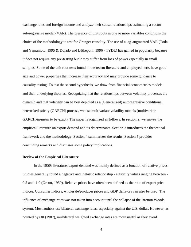
competitiveness as captured by the real effective exchange rate (REER) (figure 1).

1 GDP Growth Annual (%). World Development Indicators, The World Bank (2012).

2 Exports of Goods and Services (%GDP). World Development Indicators, The World Bank (2012).

3

Figure 1: Ghana's Export Price Competitiveness (REER) — 1984:Q1 to 2010:Q4

The transition to a more liberalized, specialized and export-oriented economy may have

increased Ghana’s exposure to risk. Indeed, despite efforts to reinforce other sectors of the

economy and diversify its export base, Ghana remains heavily dependent on export receipts that

come from a limited number of commodities and countries. Export demand theory suggests that

foreign income and price competitiveness are the main determinants of a country’s export

performance as measured by changes in export volumes. But unpredictable exchange rates lead

to revenue uncertainty. In this case, decision theory suggests that, to avoid losses, export firms

will not be willing to make investments such as adopting new technologies, diversifying their

productions or expanding their operations. The effect is accentuated if producers are risk-averse

(e.g., Hooper and Kohlhagen, 1978) and if risk management tools are limited, which is generally

the case in developing countries. As a result, in the aggregate, export volumes will fall.

In this context, a question emerges: “Do exchange rates, inflation and foreign income

have had an effect on Ghana’s export performance and if so, how?” The null hypotheses that this

research seeks to test are: 1. Price competitiveness and foreign income have not caused-in-mean

Ghana’s export volumes. 2. Exchange rates volatility has not impacted Ghana’s export volumes.

To test the first hypothesis, we recognize the possible endogeneity between export volumes,

0

100

200

300

400

500

600

Q1-

1984

Q2-

1986

Q3-

1988

Q4-

1990

Q1-

1993

Q2-

1995

Q3-

1997

Q4-

1999

Q1-

2002

Q2-

2004

Q3-

2006

Q4-

2008

Rea

l Eff

ecti

ve E

xch

ang

e R

ate

4

exchange rates and foreign income and analyze their causal relationships estimating a vector

autoregressive model (VAR). The presence of unit roots in one or more variables conditions the

choice of the methodology to test for Granger causality. The use of a lag-augmented VAR (Toda

and Yamamoto, 1995 & Dolado and Lütkepohl, 1996 - TYDL) has gained in popularity because

it does not require any pre-testing but it may suffer from loss of power especially in small

samples. Some of the unit root tests found in the recent literature and employed here, have good

size and power properties that increase their accuracy and may provide some guidance to

causality testing. To test the second hypothesis, we draw from financial econometrics models

and their underlying theories. Recognizing that the relationships between volatility processes are

dynamic and that volatility can be best depicted as a (Generalized) autoregressive conditional

heteroskedasticity (GARCH) process, we use multivariate volatility models (multivariate

GARCH-in-mean to be exact). The paper is organized as follows. In section 2, we survey the

empirical literature on export demand and its determinants. Section 3 introduces the theoretical

framework and the methodology. Section 4 summarizes the results. Section 5 provides

concluding remarks and discusses some policy implications.

Review of the Empirical Literature

In the 1950s literature, export demand was mainly defined as a function of relative prices.

Studies generally found a negative and inelastic relationship - elasticity values ranging between -

0.5 and -1.0 (Orcutt, 1950). Relative prices have often been defined as the ratio of export price

indices. Consumer indices, wholesale/producer prices and GDP deflators can also be used. The

influence of exchange rates was not taken into account until the collapse of the Bretton Woods

system. Most authors use bilateral exchange rates, especially against the U.S. dollar. However, as

pointed by Ott (1987), multilateral weighted exchange rates are more useful as they avoid

5

erroneous generalizations and allow for third-country impacts. Subsequent to Johnson (1958)’s

statement that export demand depends critically on the world’s income elasticity, foreign income

has been included in export demand models along with relative prices. Studies have generally

found a positive and elastic relationship (e.g., Houthakker and Magee, 1969). Goldstein and

Khan (1978) remark that if a country’s exports correspond to the residual demand of the rest of

the world, the elasticity may not be positive. Developing countries are usually residual suppliers

(Mullor-Sebastian, 1990). In pioneer studies, export demand was measured regressing (ordinary

least squares - OLS) a set of limited variables on export volumes. Overtime, models have been

increasingly refined by: 1) relaxing assumptions; 2) adding more information, and 3) using

modern econometric techniques. In the mid-eighties, studies using dynamic models started to

flourish in the export demand literature and VAR or VECM have been widely used to test both

long and short-run effects of relative prices and foreign income on export volumes. A

straightforward extension to this approach is to test for Granger causality. Surprisingly, very few

authors have analyzed causal relationships in the framework of export demand models.

Export demand models have also been augmented with measures of volatility and in

particular exchange rate volatility. It is intuitively argued that the impact of exchange rates

volatility is significant and negative but the alternative hypothesis has also been considered. The

vast empirical literature has however failed to resolve this ambiguity. Different measures of

exchange rates can be found in the literature. As a rule of thumb, early literature uses nominal

exchange rates while real exchange rates are more commonly found in latest works. McKenzie

(1999) concludes that the impact of using one or another is trivial. Both effective and bilateral

exchange rates have been used but very few works have looked at “third-country” exchange rates

effects. The diversity of methodologies that can be found in the literature is vast. Bahmani-

6

Oskooee and Hegerty (2007) listed more than ten types of volatility measures. The most

commonly used approach appears to be a moving standard deviation (e.g., Koray and Lastrapes,

1989). However, with the advancements in financial econometrics that have taken place in the

80’s, an increasing number of studies started to model exchange rate volatility as a GARCH

process. This approach allows capturing the unpredictable part of volatility and is considered by

some authors as the most efficient (e.g., Seabra, 1995). Studies have generally included exchange

rate volatility in linear regressions or in VAR/VECM models. A major drawback of these

approaches is their inefficiency as, independently from the measure of volatility, the estimation

is always done in two steps. Conversely, the multivariate GARCH-in-mean (MGARCH-M)

model allows the joint estimation of exchange rates conditional volatility and its impact on trade.

McKenzie (1999) emphasized both the usefulness and underuse of MGARCH-M models. To our

knowledge, only Kroner and Lastrapes (1993) have modeled the effect of exchange rates

volatility on exports using a MGARCH-M model. The research review of Bahmani-Oskooee and

Hegerty (2007) reveals that no new contribution to the literature has used MGARCH-M models

since McKenzie (1999)’s research review. The unpopularity of these models could be due to

their complexity. Indeed, the number of parameters to be estimated increases rapidly with the

number of variables and lags. Consequently, large samples are required to use these models,

complicating the analysis at the sectoral level and for developing countries.

To our knowledge, only Sackey (2001) and Bhattarai and Armah (2005) have analyzed

Ghana’s export demand. They both applied cointegration techniques and confirmed the existence

of a long-run equilibrium between exports and its determinants. Sackey (2001) found a positive

relationship between foreign income and export performance while Bhattarai and Armah (2005)

found a negative relationship (although not significant). Both studies concluded that Ghana’s

7

currency depreciations led to an improvement in Ghana’s export performance. Only Sackey

(2001) analyzed causal relationships and found that export volumes have been caused by real

effective exchange rates but not by foreign income. Note that none of these studies have taken

into account exchange rates volatility. Also, they confined their work to annual total exports

from 1962 to 1996 (Sackey, 2001) and 1970 to 2000 (Bhattarai and Armah, 2005). An analysis

of agricultural exports only seems important considering the share of agricultural exports in total

exports (35.3%3). Note also that both studies used exchange rates that may not reflect Ghana’s

trading patterns. Indeed, Bhattarai and Armah (2005) simply used bilateral exchange rates

between the $US and Ghana’s currency, the Ghanaian Cedi, while Sackey (2001) opted for a

trade-weighted exchange rate that only included France, Italy, Japan, the Netherlands, Germany

and the U.S. as Ghana’s main trading partners.

Theoretical Framework, Methods and Data

Theoretical Framework: Export Demand and Decision Theories

One way of explaining export performance is to embrace the theory underlying export

demand models. The above-reviewed literature showed that it is also the most adopted approach

in empirical studies. Two main models and their respective sets of assumptions are defined in the

theoretical literature namely, the imperfect substitutes model and the perfect substitutes model.

We chose to adopt the theory underlying imperfect substitutes models for several reasons. First,

this model dominates the empirical literature whether studied trade flows are mainly composed

of differentiated goods or not. Second, nontraditional exports4 share in Ghana’s total exports has

increased considerably. Third, the validity of the law of one price for commodities remains

3 Own calculations based on FAOSTAT (Food and Agriculture Organization-FAO, 2012) data.

4 For the most part, nontraditional exports do not fall in the primary commodity category in Ghana.

8

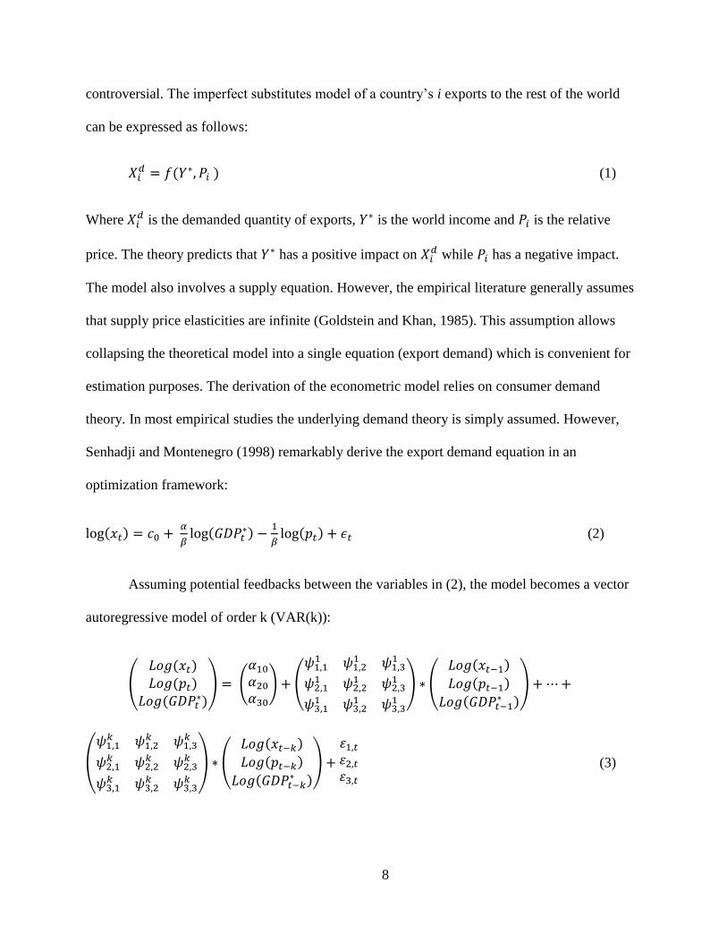
controversial. The imperfect substitutes model of a country’s i exports to the rest of the world

can be expressed as follows:

(1)

Where is the demanded quantity of exports, is the world income and is the relative

price. The theory predicts that has a positive impact on while has a negative impact.

The model also involves a supply equation. However, the empirical literature generally assumes

that supply price elasticities are infinite (Goldstein and Khan, 1985). This assumption allows

collapsing the theoretical model into a single equation (export demand) which is convenient for

estimation purposes. The derivation of the econometric model relies on consumer demand

theory. In most empirical studies the underlying demand theory is simply assumed. However,

Senhadji and Montenegro (1998) remarkably derive the export demand equation in an

optimization framework:

(2)

Assuming potential feedbacks between the variables in (2), the model becomes a vector

autoregressive model of order k (VAR(k)):

(

) (

) (

) (

)

(

) (

)

(3)

9

In accordance with decision theory, the model given in (2) should include a measure of

volatility. Volatility makes exporters more uncertain about the revenues they will receive which

eventually decreases trade volumes in the aggregate (Krugman and Obstfeld, 2003). The effect

of uncertainty on trade increases with the degree of risk aversion, an assumption that we follow

in this research. Given the model in (2), there is at least one source of volatility that could affect

export volumes namely, exchange rates. Traders can limit this risk using foreign exchange

markets and the more they are risk adverse, the more they will cover in the foreign exchange

market (Ethier, 1973). We nevertheless assume that a portion of the foreign exchange exposure

remains uncovered (Hooper and Kohlhagen, 1978) and that this proportion is greater in the case

of developing countries where forward markets are underdeveloped (Canales-Kriljenko, 2004).

Cushman (1986) highlighted the importance of taking into account “third-country” exchange rate

risk providing theoretical and empirical considerations to their effect on trade. Substitution

effects (imports/exports from country to another) are the bedrock of Cushman’s theory but we

have also to consider that most countries do not trade with their own currencies but with the so-

called vehicle currencies like the Euro and the $US.

Econometric Methods

In order to measure if some variables have affected export performance, we shall test

causal relationships as defined by Granger (1969). The choice of the methodology directly

depends on the properties of the series. Thus, prior to causality testing, the order of integration of

the series is determined. If the series are found to be stationary, a VAR shall be entertained. If

the variables are integrated of the same order, a VECM would be the most appropriate. If the

series are d-integrated and non-cointegrated, the VAR would be estimated in d-differences.

10

Finally if the order of the variables is uncertain or if the variables are of different order (e.g., I(0)

and I(1)), causality should be tested following the TYDL procedure.

From the above, we understand the importance of correctly identifying the model that

would approximate the true data generating process (DGP) of the series. Dickey-Fuller - DF

(1979) and Phillips-Perron - PP (1988) unit root tests are uncontestably the most widely used to

identify the order of integration despite proven drawbacks. DF tests assume that errors are iid

with zero mean. This restrictive assumption creates severe size distortions. Monte Carlo studies

have shown inaccuracies in the size of DF-type tests, especially in the presence of large and

negative MA coefficients. Both augmented Dickey-Fuller (ADF) and PP tests were intended to

palliate to this drawback by accommodating dependent errors. ADF tests follow a parametric

approach and assume that the error structure is autoregressive. PP tests (Zα and MZt) are more

flexible and involve the semi-parametric estimation of the long-run variance with Kernel

estimators. However, PP tests also suffer from size distortions when the root of the error process

is close to one, in part because of the use of Kernel estimators. Modified PP tests (MZα, MZt and

MSB – Stock, 1990), used in combination with an autoregressive estimator of the long-run

variance instead of a Kernel estimator, notably improve PP tests size properties (Perron and Ng,

1996). Monte Carlo simulations have shown that DF-type tests have also low power. The use of

generalized least squares (GLS) as a detrending method notably improves the power of unit root

tests. Elliot, Rothenberg and Stock (1996) popularized this method in a DF framework (ERS

tests or DFGLS

tests). Ng and Perron (2001) brilliantly integrated GLS detrending techniques to

modified PP tests in an attempt to ally the size properties of modified PP tests with the power

properties of GLS-detrending-based tests (MGLS

tests). Another extension to their tests is the use

of GLS-detrending to estimate the long-run autoregressive variance ( ̅GLS). More importantly,

11

their work tackles the problem of lag selection that arises when estimating the long-run variance

with the autoregressive spectral density estimator (Perron and Ng, 1996). They provide a new

class of selection criteria (MIC) that do not suffer from the over-fitting problems of other criteria

(AIC and BIC) in presence of large and negative MA errors. A slight modification of these

criteria is the use of OLS-detrended data instead of GLS-detrended data in their construction

(Perron and Qu, 2007). Lag selection is not only an issue in M-tests. Indeed, some DF-type tests

involve the selection of the number of lagged differences to include in order to whiten the

residuals. Wu (2010) has considered this issue in DF-GLS tests (ERS tests). They show that the

use of sequential t-test to select the lag length improves the power of DF-type tests.

The TYDL approach is a simple procedure that involves the estimation of a VAR(k) in

levels where k is the optimal lag length based on some selection criterion (e.g., AIC). Once the

lag length is determined, a VAR(p=k+dmax) is estimated where dmax is the maximum order of

integration. This procedure is valid only if dmax ≤ k. Consider the following VAR equation from

(3):

∑

∑

∑

(4)

In order to test the null hypothesis that P does not Granger cause X, the linear restriction

H0:

is imposed and the modified Wald (MWALD) test is computed.

Asymptotically, this test has a χ2

(J) distribution (J is the number of restrictions), even in the

presence of integration or cointegration (Toda and Yamamoto, 1995). One of the drawbacks of

this approach is that the results may suffer from an over-fit of the VAR (Toda and Yamamoto,

12

1995). A direct consequence is their poor performance in small samples as shown by Zapata and

Rambaldi (1997).

In order to measure the impact of exchange rates risk on export volumes, we estimate a

bivariate GARCH-M model. Different MGARCH models are available to support the study of

GARCH-in-mean effects but the constant-correlation model of Bollerslev (1990) is used here.

The advantage of this model is that the number of parameters to be estimated is relatively low. It

is however quite restrictive as it assumes a time-invariant conditional correlation. As in a

univariate GARCH model, an MGARCH consists of a mean equation and a variance equation. In

our case, the mean equations corresponds to a VAR. As indicated by its name, the estimated

variances are actually conditional variances. Each one follows a GARCH process and models

volatility. The measurement of volatility’s effects implies augmenting the VAR with the

conditional variances. The resulting model is a VAR-MGARCH-M model. As an example, the

bivariate VAR(k)-GARCH(1,1)-M model is detailed below. It is constituted of an augmented

bivariate VAR(k) where and are the rates of change of export volumes and exchange

rates (“own-country” or “third-country”) respectively:

(5)

(6)

Assuming GARCH(1,1) errors, the volatility equations can be expressed as:

(

) (

) (

) (

) (

) (

) (7)

13

Assuming further that the conditional correlation between and is time-invariant

( which implies that , the volatility equations reduce to:

(8)

(9)

While economic series rarely follow a GARCH of an higher order than (1,1), the

assumption of a VAR(1) would be in most cases too restrictive and misleading. Thus, the best-

fitting VAR will be used instead. The whole model is simultaneously estimated with maximum

likelihood estimation (MLE) methods and using the algorithm Broyden-Fletcher-Goldfarb-

Shanno (BFGS). Of particular interest is the significance of exchange rates volatility in the

export volume equation although we do not rule out the possibility that the volatility of exports

growth may also have an effect on exchange rates changes. To test that exchange rates volatility

have an effect on export volumes, we will test: .

Data

In order to test the first hypothesis, this research uses annual data from 1970 to 2009 and

analyzes both total and agricultural exports. Annual Ghana’s total nominal exports in millions of

$US are from the IMF, Direction of Trade Statistics (DOTS). Total export volumes (TX) were

obtained deflating annual total exports with the export price index. Annual Ghana’s agricultural

nominal exports in millions of $US are from the trade statistics database of the FAO

(FAOSTAT). Agricultural exports (AX) were deflated with the export value index computed by

the FAO. In an attempt to reflect Ghana’s trade patterns, we use REER for relative prices and

trade-weighted foreign GDP (TWFGDP) for World income. Both indices have been computed

14

by the authors. The base year is 2000. To test the second hypothesis, we use monthly data.

“Third-country” effects are measured using bilateral nominal exchange rates between the $US

and the Euro. Ghana’s monthly real total exports are from the IMF/DOTS. Exchange rates are

from the Global Insight website (diverse sources). The analysis runs from January 2002

(circulation of the Euro) to February 2012. To study “own-country” exchange rate risk effects,

we use nominal bilateral exchange rates between the Ghanaian Cedi (GHS) and the $US. The

analysis uses data starting on January 1984.

Results

Hypothesis 1

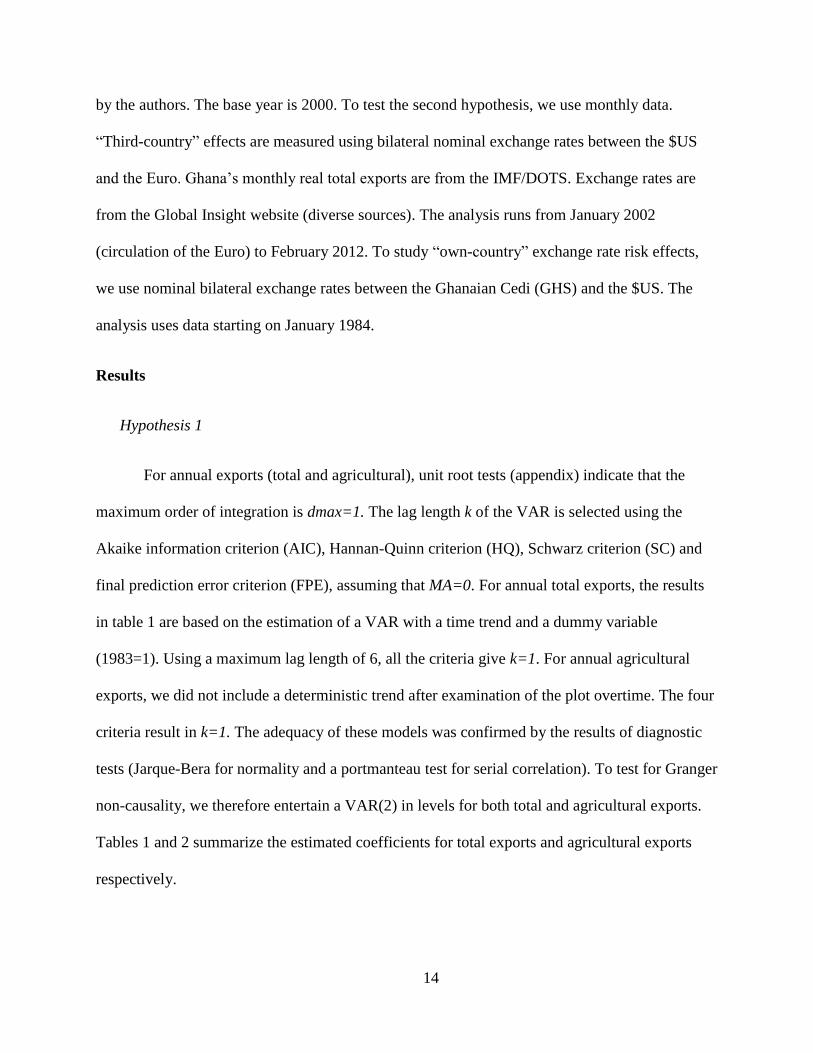
For annual exports (total and agricultural), unit root tests (appendix) indicate that the

maximum order of integration is dmax=1. The lag length k of the VAR is selected using the

Akaike information criterion (AIC), Hannan-Quinn criterion (HQ), Schwarz criterion (SC) and

final prediction error criterion (FPE), assuming that MA=0. For annual total exports, the results

in table 1 are based on the estimation of a VAR with a time trend and a dummy variable

(1983=1). Using a maximum lag length of 6, all the criteria give k=1. For annual agricultural

exports, we did not include a deterministic trend after examination of the plot overtime. The four

criteria result in k=1. The adequacy of these models was confirmed by the results of diagnostic

tests (Jarque-Bera for normality and a portmanteau test for serial correlation). To test for Granger

non-causality, we therefore entertain a VAR(2) in levels for both total and agricultural exports.

Tables 1 and 2 summarize the estimated coefficients for total exports and agricultural exports

respectively.

15

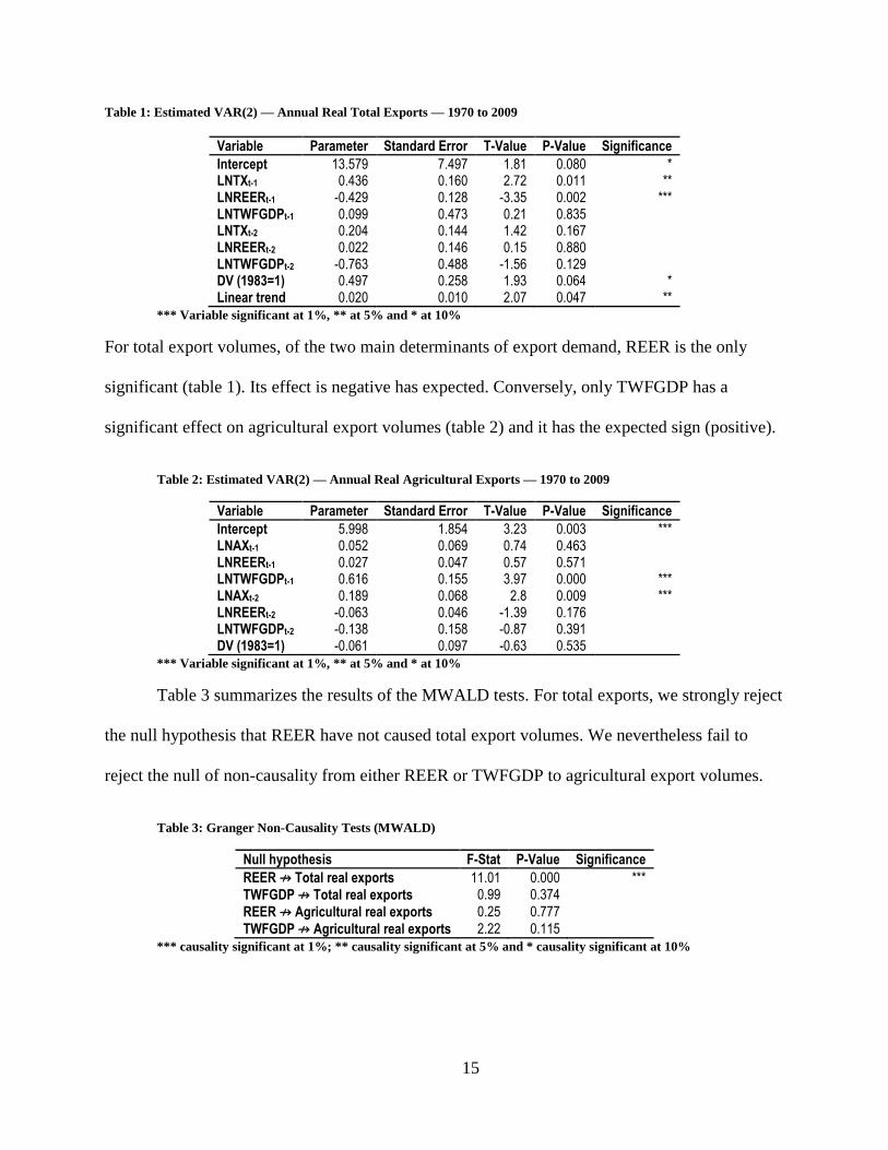
Table 1: Estimated VAR(2) — Annual Real Total Exports — 1970 to 2009

Variable Parameter Standard Error T-Value P-Value Significance

Intercept 13.579 7.497 1.81 0.080 * LNTXt-1 0.436 0.160 2.72 0.011 ** LNREERt-1 -0.429 0.128 -3.35 0.002 *** LNTWFGDPt-1 0.099 0.473 0.21 0.835 LNTXt-2 0.204 0.144 1.42 0.167 LNREERt-2 0.022 0.146 0.15 0.880 LNTWFGDPt-2 -0.763 0.488 -1.56 0.129 DV (1983=1) 0.497 0.258 1.93 0.064 * Linear trend 0.020 0.010 2.07 0.047 **

*** Variable significant at 1%, ** at 5% and * at 10%

For total export volumes, of the two main determinants of export demand, REER is the only

significant (table 1). Its effect is negative has expected. Conversely, only TWFGDP has a

significant effect on agricultural export volumes (table 2) and it has the expected sign (positive).

Table 2: Estimated VAR(2) — Annual Real Agricultural Exports — 1970 to 2009

Variable Parameter Standard Error T-Value P-Value Significance

Intercept 5.998 1.854 3.23 0.003 *** LNAXt-1 0.052 0.069 0.74 0.463 LNREERt-1 0.027 0.047 0.57 0.571 LNTWFGDPt-1 0.616 0.155 3.97 0.000 *** LNAXt-2 0.189 0.068 2.8 0.009 *** LNREERt-2 -0.063 0.046 -1.39 0.176 LNTWFGDPt-2 -0.138 0.158 -0.87 0.391 DV (1983=1) -0.061 0.097 -0.63 0.535

*** Variable significant at 1%, ** at 5% and * at 10%

Table 3 summarizes the results of the MWALD tests. For total exports, we strongly reject

the null hypothesis that REER have not caused total export volumes. We nevertheless fail to

reject the null of non-causality from either REER or TWFGDP to agricultural export volumes.

Table 3: Granger Non-Causality Tests (MWALD)

Null hypothesis F-Stat P-Value Significance

REER ↛ Total real exports 11.01 0.000 ***

TWFGDP ↛ Total real exports 0.99 0.374

REER ↛ Agricultural real exports 0.25 0.777

TWFGDP ↛ Agricultural real exports 2.22 0.115

*** causality significant at 1%; ** causality significant at 5% and * causality significant at 10%

16

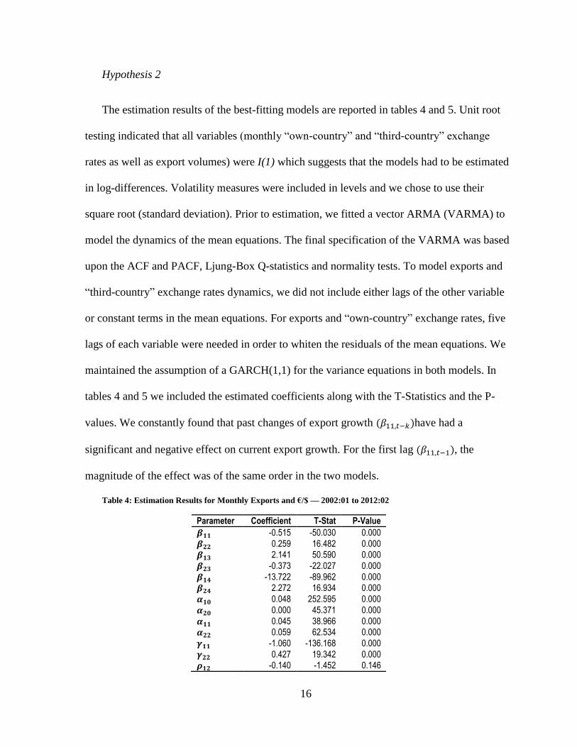
Hypothesis 2

The estimation results of the best-fitting models are reported in tables 4 and 5. Unit root

testing indicated that all variables (monthly “own-country” and “third-country” exchange

rates as well as export volumes) were I(1) which suggests that the models had to be estimated

in log-differences. Volatility measures were included in levels and we chose to use their

square root (standard deviation). Prior to estimation, we fitted a vector ARMA (VARMA) to

model the dynamics of the mean equations. The final specification of the VARMA was based

upon the ACF and PACF, Ljung-Box Q-statistics and normality tests. To model exports and

“third-country” exchange rates dynamics, we did not include either lags of the other variable

or constant terms in the mean equations. For exports and “own-country” exchange rates, five

lags of each variable were needed in order to whiten the residuals of the mean equations. We

maintained the assumption of a GARCH(1,1) for the variance equations in both models. In

tables 4 and 5 we included the estimated coefficients along with the T-Statistics and the P-

values. We constantly found that past changes of export growth have had a

significant and negative effect on current export growth. For the first lag , the

magnitude of the effect was of the same order in the two models.

Table 4: Estimation Results for Monthly Exports and €/$ — 2002:01 to 2012:02

Parameter Coefficient T-Stat P-Value

-0.515 -50.030 0.000

0.259 16.482 0.000

2.141 50.590 0.000

-0.373 -22.027 0.000

-13.722 -89.962 0.000

2.272 16.934 0.000

0.048 252.595 0.000

0.000 45.371 0.000

0.045 38.966 0.000

0.059 62.534 0.000

-1.060 -136.168 0.000

0.427 19.342 0.000

-0.140 -1.452 0.146

17

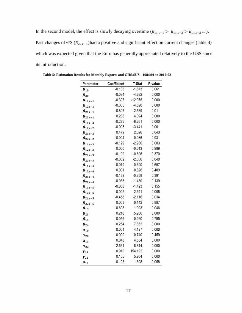
In the second model, the effect is slowly decaying overtime .

Past changes of €/$ had a positive and significant effect on current changes (table 4)

which was expected given that the Euro has generally appreciated relatively to the US$ since

its introduction.

Table 5: Estimation Results for Monthly Exports and GHS/$US - 1984:01 to 2012:02

Parameter Coefficient T-Stat P-value

-0.105 -1.873 0.061

-0.034 -4.692 0.000

-0.397 -12.075 0.000

-0.005 -4.590 0.000

-0.805 -2.539 0.011

0.288 4.094 0.000

-0.235 -6.261 0.000

-0.005 -3.441 0.001

0.479 2.026 0.043

-0.004 -0.086 0.931

-0.129 -2.936 0.003

0.000 -0.013 0.989

-0.199 -0.896 0.370

-0.082 -2.056 0.040

-0.019 -0.390 0.697

0.001 0.826 0.409

-0.189 -0.858 0.391

-0.038 -1.480 0.139

-0.058 -1.423 0.155

0.002 2.641 0.008

-0.458 -2.116 0.034

0.003 0.142 0.887

0.608 1.993 0.046

0.216 5.206 0.000

0.056 0.260 0.795

0.254 7.852 0.000

0.001 4.127 0.000

0.000 0.740 0.459

0.048 4.554 0.000

2.631 8.814 0.000

0.910 154.192 0.000

0.155 5.904 0.000

0.103 1.898 0.058

18

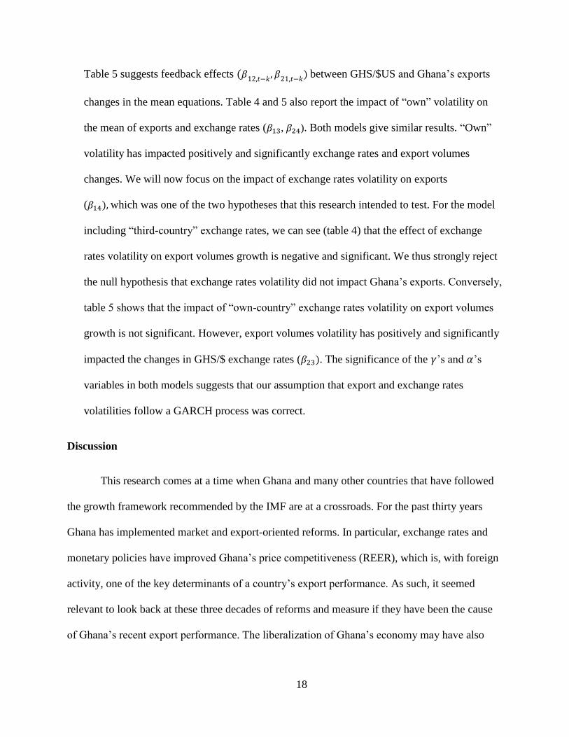
Table 5 suggests feedback effects

between GHS/$US and Ghana’s exports

changes in the mean equations. Table 4 and 5 also report the impact of “own” volatility on

the mean of exports and exchange rates ( , ). Both models give similar results. “Own”

volatility has impacted positively and significantly exchange rates and export volumes

changes. We will now focus on the impact of exchange rates volatility on exports

( which was one of the two hypotheses that this research intended to test. For the model

including “third-country” exchange rates, we can see (table 4) that the effect of exchange

rates volatility on export volumes growth is negative and significant. We thus strongly reject

the null hypothesis that exchange rates volatility did not impact Ghana’s exports. Conversely,

table 5 shows that the impact of “own-country” exchange rates volatility on export volumes

growth is not significant. However, export volumes volatility has positively and significantly

impacted the changes in GHS/$ exchange rates ( . The significance of the ’s and ’s

variables in both models suggests that our assumption that export and exchange rates

volatilities follow a GARCH process was correct.

Discussion

This research comes at a time when Ghana and many other countries that have followed

the growth framework recommended by the IMF are at a crossroads. For the past thirty years

Ghana has implemented market and export-oriented reforms. In particular, exchange rates and

monetary policies have improved Ghana’s price competitiveness (REER), which is, with foreign

activity, one of the key determinants of a country’s export performance. As such, it seemed

relevant to look back at these three decades of reforms and measure if they have been the cause

of Ghana’s recent export performance. The liberalization of Ghana’s economy may have also

19

increased the exposure of exporters to risk such as exchange rates volatility, and as a

consequence, hampered export volumes growth.

In order to test the hypothesis that both price competitiveness and foreign income have

not caused-in-mean Ghana’s export performance, we followed the TYDL procedure which

consists in estimating an augmented VAR and used a modified Wald statistic. This choice was

supported by results from the most recent unit root testing procedures. We decided to analyze

both total and agricultural exports given the importance of agricultural products in total exports.

We used annual data from 1970 to 2009. Export performance was measured by export volumes,

price competitiveness by REER and foreign activity, by the trade-weighted foreign GDP. Based

on the causality tests, we conclude that while total export volumes have been driven by REER,

none of the two assumed main factors of export performance have caused agricultural export

volumes.

To test the hypothesis that exchange rates volatility had not impacted Ghana’s export

growth, we wanted to measure the effect of both own- and third-country exchange rates volatility

as the latter have been generally overlooked in the literature. We drew from financial

econometrics and used two bivariate VAR-GARCH-in-mean models. Although rarely used in

agricultural economics works, this type of models present many advantages. In particular they

allow simultaneously estimating the conditional variances (volatility) and mean equations which

confer these tests efficiency. We used monthly real exports and nominal exchange rates.

Considering that the Euro and the $US are the two main vehicle currencies for Ghana’s exported

products, we used monthly €/$US exchange rates to test “third-country” effects and Cedi/$ to

test “own-country” effects. After estimation of the two models, it seems that “third-country”

20

exchange rates volatility have deeply depressed Ghana’s export growth while Ghana’s exchange

rates volatility do not have had any effect.

What the results first tell us is that the policy framework that has been followed by Ghana

under the recommendations of the IMF and other bilateral and multilateral agencies has

successfully encouraged exports. Improvements in price competitiveness via inflation control

and exchange rates realignment have been the principal drivers of total export volumes. This

conclusion may encourage other developing countries to consider some of these reforms to frame

their development strategies. After all, Ghana has not only been successful at developing its

export sector but also at fulfilling its development goal of becoming a middle-income country by

2020.

Second, the lack of causation between price competitiveness and agricultural exports can

be explained by our original assumption that exports are imperfect substitutes. In particular, it

would suggest that agricultural exports are obedient to the Law of one price. Third, for both total

and agricultural exports, foreign activity did not seem to have influenced export performance.

We would have expected that as the World income has been recently steadily growing, the

demand for Ghana’s products would have increased. This could confirm that Ghana is a residual

supplier (Goldstein and Khan, 1978).

Forth and last, the downside of these liberal policies is that they have indeed increased

risk exposure. This assessment only suggests that exporters could benefit from using currency

risk management tools. Both non-hedging and hedging options can be considered provided that

they are available in Ghana.

21

Future research will have to consider and measure the effect of non-price factors on

Ghana’s exports growth and in particular in the agricultural sector. When longer time series

become available for Ghana, the bivariate MGARCH-M could be expanded to include all

relevant factors of export performance. In particular, the effect of foreign income volatility on

Ghana’s exports would be interesting to study considering the impact of global recessions on

Ghana’s trading partners which may have increased their income volatility.

References

Bahmani-Oskooee, M. "Determinants of international trade flows: The Case of Developing

Countries." Journal of Development Economics 20,1(1986):107-123.

Bahmani-Oskooee, M and S.W. Hegerty. "Exchange Rate Volatility and Trade Flows: A Review

Article." Journal of Economic Studies, 34,3(2007):211-55.

Bhattarai, D. K., and M. K. Armah. “The Effects of Exchange Rate on the Trade Balance in

Ghana: Evidence from Cointegration Analysis”. Cottingham United Kingdom: Centre for

Economic Policy Business School, University of Hull Cottingham. Research

Memorandum 52(August 2005).

Bollerslev, T.. "Modelling the Coherence in Short-Run Nominal Exchange Rates: A Multivariate

Generalized Arch Model." The Review of Economics and Statistics, 72,3(1990):498-505.

Canales-Kriljenko, J.I. “Foreign Exchange Market Organization in Selected Developing and

Transition Economies: A Survey”. IMF Working Paper (April 2004).

Cushman, D.O.. "Has Exchange Risk Depressed International Trade? The Impact of Third-

Country Exchange Risk." Journal of International Money and Finance, 5,3(1986):361-

79.

22

Dickey, D. A. and W. A. Fuller. "Distribution of the Estimators for Autoregressive Time Series

With a Unit Root." Journal of the American Statistical Association 74,366(1979):427-

431.

Dolado, J.J. and H. Lütkepohl. "Making Wald Tests Work for Cointegrated Var Systems."

Econometric Reviews, 15,4(1996):369-86.

Elliot, G., T.J. Rothenberg, and J.H. Stock. “Efficient Tests for an Autoregressive Unit Root,”

Econometrica, 64(1996):813‐836.

Ethier, W. "International Trade and the Forward Exchange Market." The American Economic

Review, 63,3(1973):494-503.

Goldstein, M. and M. S. Khan. "The Supply and Demand for Exports: A Simultaneous

Approach." The Review of Economics and Statistics, 60,2(1978):275-286.

Goldstein, M. and M.S. Khan. “Income and Price Effects in Foreign Trade”. In Handbook of

International Economics, ed. by Ronald W. Jones and Peter B. Kenen. (North Holland),

(1985):1042-1099.

Granger, C. W. J. "Investigating Causal Relations by Econometric Models and Cross-Spectral

Methods." Econometrica, 37,3(1969):424-38.

Hooper, P., and S. W. Kohlhagen. “The effect of exchange rate uncertainty on the prices and

volume of international trade”. Journal of International Economics, 8,4(1978):483-511.

Hooper, P., K. Johnson and J. Marquez. “Trade Elasticities for the G-7 Countries.” Princeton

Studies in International Economics, 87 (August 2000).

Houthakker, H. S. and S. P. Magee. "Income and Price Elasticities in World Trade." The Review

of Economics and Statistics 51,2(1969):111-125.

23

Koray, F. and W.D. Lastrapes. "Real Exchange Rate Volatility and U.S. Bilateral Trade: A Var

Approach." The Review of Economics and Statistics, 71,4(1989):708-12.

Kroner, K. F. and W. D. Lastrapes. “The impact of exchange rate volatility on international

trade: Reduced form estimates using the GARCH-in-mean model”. Journal of

International Money and Finance, 12,3(1993):298-318.

Krugman, P.R and M. Obstfeld. “International Economics: Theory and Policy”. Addison

Wesley; 6 edition (July 26, 2002)

McKenzie, M.D. "The Impact of Exchange Rate Volatility on International Trade Flows."

Journal of Economic Surveys, 13,1(1999):71-106.

Mullor-Sebastian, A. “Export Instability and Policy Implications for Developing Countries as

Residual Suppliers”. IMF Working Paper No. 90/44(1990): 1-26.

Ng, S. and P. Perron. “Lag Length Selection and the Construction of Unit Root Tests with Good

Size and Power”. Econometrica, 69,6(2001):1519-1554.

Orcutt, G. H. "Measurement of Price Elasticities in International Trade." The Review of

Economics and Statistics, 32,2(1950): 117-132.

Ott, M. “Have U.S. Exports Been Larger than Reported?” St. Louis Federal Reserve Bank

Review (February 1987).

Perron, P. and S. Ng. “Useful Modifications to some Unit Root Tests with Dependent Errors and

their Local Asymptotic Properties”. The Review of Economic Studies, 63,3(1996):435-

463.

Perron, P. and Z. Qu. “A simple modification to improve the finite sample properties of Ng and

Perron’s unit root tests. Economic Letters, 94 (2007):12‐19.

24

Phillips, P. C. B. and P. Perron. "Testing for a unit root in time series regression." Biometrika

75,2(1988):335-346.

Sackey, H.A. “External Aid Inflows and the Real Exchange Rate in Ghana.” AERC Research

Paper 110. African Economic Research Consortium, Nairobi, November 2001.

Stock, J. H.. “A class of tests for integration and cointegration”. Manuscript. Kennedy School of

Government, Harvard University, Cambridge, MA (1991).

Seabra, F. "Short-Run Exchange Rate Uncertainty in Latin America." Applied Economics,

27,5(1995):441-50.

Senhadji, A. and C. Montenegro. “Time-Series Estimation of Structural Import Demand

Equations: A Cross-Country Analysis”. IMF Staff Papers. 45(1998):236-268.

Toda, H. Y. and T. Yamamoto. "Statistical inference in vector autoregressions with possibly

integrated processes." Journal of Econometrics,66,1-2(1995):225-250.

Wu, S. “Lag-length Selection in DF-GLS Unit Root Tests”. Communications in Statistics-

Simulation and Computation, 39(2010):1590-1604.

Zapata, H.O. and A.N. Rambaldi. “Monte Carlo evidence on cointegration causation”.

Oxford Bulletin of Economics and Statistics, 59,2(1997): 285-298.

25

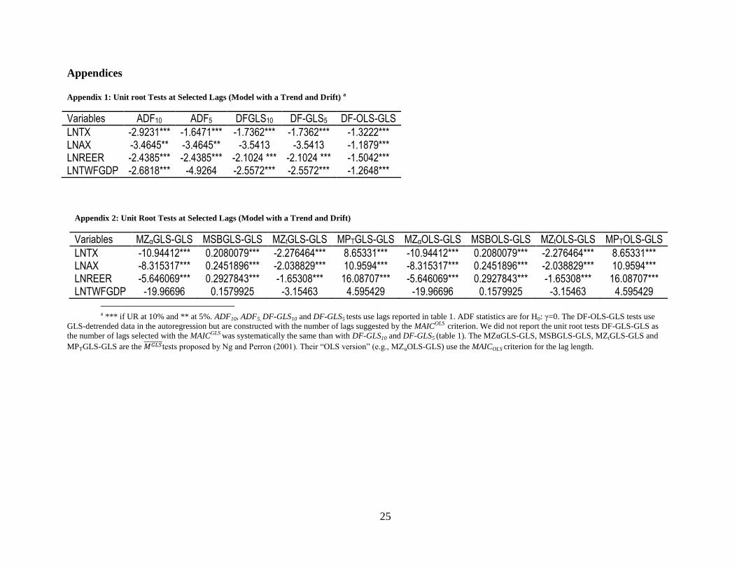
Appendices

Appendix 1: Unit root Tests at Selected Lags (Model with a Trend and Drift) a

Variables ADF10 ADF5 DFGLS10 DF-GLS5 DF-OLS-GLS

LNTX -2.9231*** -1.6471*** -1.7362*** -1.7362*** -1.3222*** LNAX -3.4645** -3.4645** -3.5413 -3.5413 -1.1879*** LNREER -2.4385*** -2.4385*** -2.1024 *** -2.1024 *** -1.5042*** LNTWFGDP -2.6818*** -4.9264 -2.5572*** -2.5572*** -1.2648***

Appendix 2: Unit Root Tests at Selected Lags (Model with a Trend and Drift)

Variables MZαGLS-GLS MSBGLS-GLS MZtGLS-GLS MPTGLS-GLS MZαOLS-GLS MSBOLS-GLS MZtOLS-GLS MPTOLS-GLS

LNTX -10.94412*** 0.2080079*** -2.276464*** 8.65331*** -10.94412*** 0.2080079*** -2.276464*** 8.65331*** LNAX -8.315317*** 0.2451896*** -2.038829*** 10.9594*** -8.315317*** 0.2451896*** -2.038829*** 10.9594*** LNREER -5.646069*** 0.2927843*** -1.65308*** 16.08707*** -5.646069*** 0.2927843*** -1.65308*** 16.08707*** LNTWFGDP -19.96696 0.1579925 -3.15463 4.595429 -19.96696 0.1579925 -3.15463 4.595429

a *** if UR at 10% and ** at 5%. ADF10, ADF5, DF-GLS10 and DF-GLS5 tests use lags reported in table 1. ADF statistics are for H0: γ=0. The DF-OLS-GLS tests use

GLS-detrended data in the autoregression but are constructed with the number of lags suggested by the MAICOLS criterion. We did not report the unit root tests DF-GLS-GLS as

the number of lags selected with the MAICGLS was systematically the same than with DF-GLS10 and DF-GLS5 (table 1). The MZαGLS-GLS, MSBGLS-GLS, MZtGLS-GLS and

MPTGLS-GLS are the ̅̅ ̅̅ ̅̅ ̅tests proposed by Ng and Perron (2001). Their “OLS version” (e.g., MZαOLS-GLS) use the MAICOLS criterion for the lag length.

26

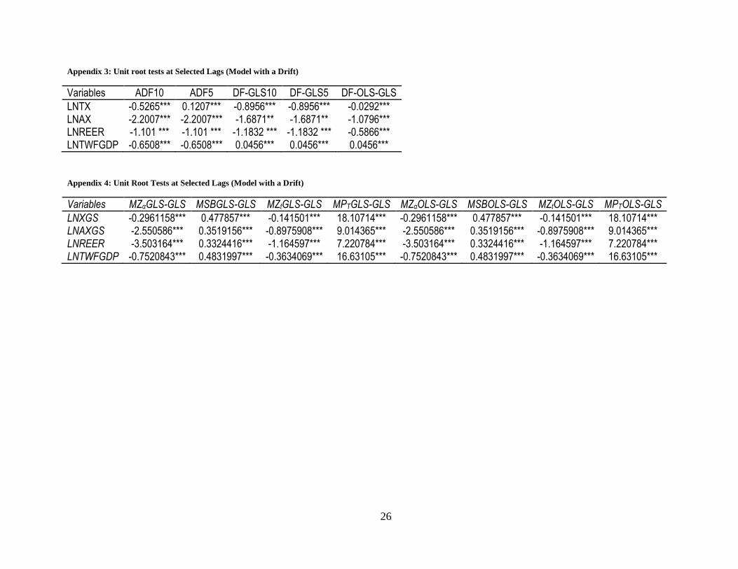
Appendix 3: Unit root tests at Selected Lags (Model with a Drift)

Variables ADF10 ADF5 DF-GLS10 DF-GLS5 DF-OLS-GLS

LNTX -0.5265*** 0.1207*** -0.8956*** -0.8956*** -0.0292*** LNAX -2.2007*** -2.2007*** -1.6871** -1.6871** -1.0796*** LNREER -1.101 *** -1.101 *** -1.1832 *** -1.1832 *** -0.5866*** LNTWFGDP -0.6508*** -0.6508*** 0.0456*** 0.0456*** 0.0456***

Appendix 4: Unit Root Tests at Selected Lags (Model with a Drift)

Variables MZαGLS-GLS MSBGLS-GLS MZtGLS-GLS MPTGLS-GLS MZαOLS-GLS MSBOLS-GLS MZtOLS-GLS MPTOLS-GLS

LNXGS -0.2961158*** 0.477857*** -0.141501*** 18.10714*** -0.2961158*** 0.477857*** -0.141501*** 18.10714*** LNAXGS -2.550586*** 0.3519156*** -0.8975908*** 9.014365*** -2.550586*** 0.3519156*** -0.8975908*** 9.014365*** LNREER -3.503164*** 0.3324416*** -1.164597*** 7.220784*** -3.503164*** 0.3324416*** -1.164597*** 7.220784*** LNTWFGDP -0.7520843*** 0.4831997*** -0.3634069*** 16.63105*** -0.7520843*** 0.4831997*** -0.3634069*** 16.63105***