Embed Size (px)
DESCRIPTION
Production planning and control
Citation preview
© 2006 Prentice Hall, Inc. 4 – 1
FORECASTINGFORECASTING
Synonyms of the word ‘Forecast’Synonyms of the word ‘Forecast’ PredictPredict
EstimateEstimate
ProjectProject
CalculateCalculate
AnticipateAnticipate
ForetellForetell
GuessGuess
ConjectureConjecture
© 2006 Prentice Hall, Inc. 4 – 2
OutlineOutline
Chapter 4 (Main text book)Chapter 4 (Main text book)
Global Company Profile: Tupperware Global Company Profile: Tupperware CorporationCorporation
What Is Forecasting?What Is Forecasting? Forecasting Time HorizonsForecasting Time Horizons
The Influence of Product Life CycleThe Influence of Product Life Cycle
Types Of ForecastsTypes Of Forecasts
© 2006 Prentice Hall, Inc. 4 – 3
Outline – ContinuedOutline – Continued
The Strategic Importance Of The Strategic Importance Of ForecastingForecasting Human ResourcesHuman Resources
CapacityCapacity
Supply-Chain ManagementSupply-Chain Management
Seven Steps In The Forecasting Seven Steps In The Forecasting SystemSystem
© 2006 Prentice Hall, Inc. 4 – 4
Outline – ContinuedOutline – Continued
Forecasting ApproachesForecasting Approaches Overview of Qualitative MethodsOverview of Qualitative Methods
Overview of Quantitative MethodsOverview of Quantitative Methods
© 2006 Prentice Hall, Inc. 4 – 5
Outline – ContinuedOutline – Continued Time-series ForecastingTime-series Forecasting
Decomposition of a Time SeriesDecomposition of a Time Series Naïve ApproachNaïve Approach Moving AveragesMoving Averages Exponential SmoothingExponential Smoothing Exponential Smoothing with Trend Exponential Smoothing with Trend
AdjustmentAdjustment Trend ProjectionsTrend Projections Seasonal Variations in DataSeasonal Variations in Data Cyclical Variations in DataCyclical Variations in Data
© 2006 Prentice Hall, Inc. 4 – 6
Outline – ContinuedOutline – Continued
Associative Forecasting Methods: Associative Forecasting Methods: Regression and Correlation Regression and Correlation AnalysisAnalysis Using Regression Analysis to Using Regression Analysis to
ForecastForecast
Standard Error of the EstimateStandard Error of the Estimate
Correlation Coefficients for Correlation Coefficients for Regression LinesRegression Lines
Multiple-Regression AnalysisMultiple-Regression Analysis
© 2006 Prentice Hall, Inc. 4 – 7
Outline – ContinuedOutline – Continued
Monitoring And Controlling Monitoring And Controlling ForecastsForecasts Adaptive SmoothingAdaptive Smoothing
Focus ForecastingFocus Forecasting
© 2006 Prentice Hall, Inc. 4 – 8
Learning ObjectivesLearning Objectives
When you complete this chapter, you When you complete this chapter, you should be able to :should be able to :
Identify or Define:Identify or Define:
Forecasting Forecasting
Types of forecasts Types of forecasts
Time horizons Time horizons
Approaches to forecastsApproaches to forecasts
© 2006 Prentice Hall, Inc. 4 – 9
Learning ObjectivesLearning Objectives
When you complete this chapter, you When you complete this chapter, you should be able to :should be able to :
Describe or Explain:Describe or Explain:
Moving averagesMoving averages
Exponential smoothingExponential smoothing
Trend projectionsTrend projections
Regression and correlation analysisRegression and correlation analysis
Measures of forecast accuracyMeasures of forecast accuracy

© 2006 Prentice Hall, Inc. 4 – 10
Forecasting at TupperwareForecasting at Tupperware
Each of 50 profit centers around the Each of 50 profit centers around the world is responsible for world is responsible for computerized monthly, quarterly, computerized monthly, quarterly, and 12-month sales projectionsand 12-month sales projections
These projections are aggregated by These projections are aggregated by region, then globally, at region, then globally, at Tupperware’s World HeadquartersTupperware’s World Headquarters
Tupperware uses all techniques Tupperware uses all techniques discussed in textdiscussed in text
© 2006 Prentice Hall, Inc. 4 – 11
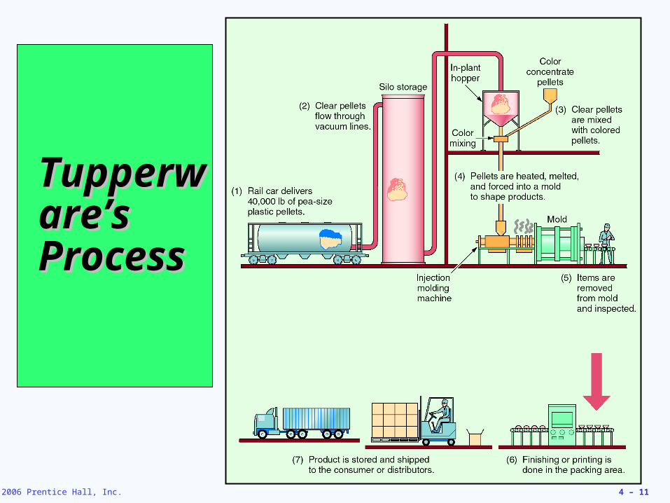
TupperTupperware’s ware’s ProcessProcess

© 2006 Prentice Hall, Inc. 4 – 12
Three Key Factors for Three Key Factors for TupperwareTupperware
The number of registered The number of registered “consultants” or sales “consultants” or sales representativesrepresentatives
The percentage of currently “active” The percentage of currently “active” dealers (this number changes each dealers (this number changes each week and month)week and month)
Sales per active dealer, on a weekly Sales per active dealer, on a weekly basisbasis
© 2006 Prentice Hall, Inc. 4 – 13
Forecast by ConsensusForecast by Consensus
Although inputs come from sales, Although inputs come from sales, marketing, finance, and production, marketing, finance, and production, final forecasts are the consensus of final forecasts are the consensus of all participating managersall participating managers
The final step is Tupperware’s The final step is Tupperware’s version of the “version of the “jury of executive jury of executive opinion”opinion”
© 2006 Prentice Hall, Inc. 4 – 14
What is Forecasting?What is Forecasting?
Process of Process of predicting a future predicting a future eventevent
Underlying basis of Underlying basis of
all business all business decisionsdecisions ProductionProduction
InventoryInventory
PersonnelPersonnel
FacilitiesFacilities
??
© 2006 Prentice Hall, Inc. 4 – 15
We may classify forecasting We may classify forecasting problems along several dimensions:problems along several dimensions: Time horizonTime horizon
Sector or Type – Economic , Sector or Type – Economic , Technological, or demand forecastsTechnological, or demand forecasts
Method (approach) adopted – Method (approach) adopted – subjective (qualitative) or objective subjective (qualitative) or objective (quantitative)(quantitative)
Forecasting DimensionsForecasting Dimensions
© 2006 Prentice Hall, Inc. 4 – 16
Short-range forecastShort-range forecast Up to 1 year, generally less than 3 monthsUp to 1 year, generally less than 3 months Purchasing, job scheduling, workforce Purchasing, job scheduling, workforce
levels, job assignments, production levelslevels, job assignments, production levels
Medium-range forecastMedium-range forecast 3 months to 3 years3 months to 3 years Sales and production planning, budgetingSales and production planning, budgeting
Long-range forecastLong-range forecast 33++ years years New product planning, facility location, New product planning, facility location,
research and developmentresearch and development
Forecasting Time HorizonsForecasting Time Horizons
© 2006 Prentice Hall, Inc. 4 – 17
Distinguishing DifferencesDistinguishing Differences
Medium/long rangeMedium/long range forecasts deal with forecasts deal with more comprehensive issues and support more comprehensive issues and support management decisions regarding management decisions regarding planning and products, plants and planning and products, plants and processesprocesses
Short-termShort-term forecasting usually employs forecasting usually employs different methodologies than longer-term different methodologies than longer-term forecastingforecasting
Short-termShort-term forecasts tend to be more forecasts tend to be more accurate than longer-term forecastsaccurate than longer-term forecasts
© 2006 Prentice Hall, Inc. 4 – 18
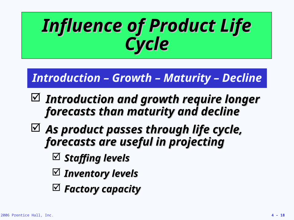
Influence of Product Life Influence of Product Life CycleCycle
Introduction and growth require longer Introduction and growth require longer forecasts than maturity and declineforecasts than maturity and decline
As product passes through life cycle, As product passes through life cycle, forecasts are useful in projectingforecasts are useful in projecting Staffing levelsStaffing levels
Inventory levelsInventory levels
Factory capacityFactory capacity
Introduction – Growth – Maturity – Decline
© 2006 Prentice Hall, Inc. 4 – 19
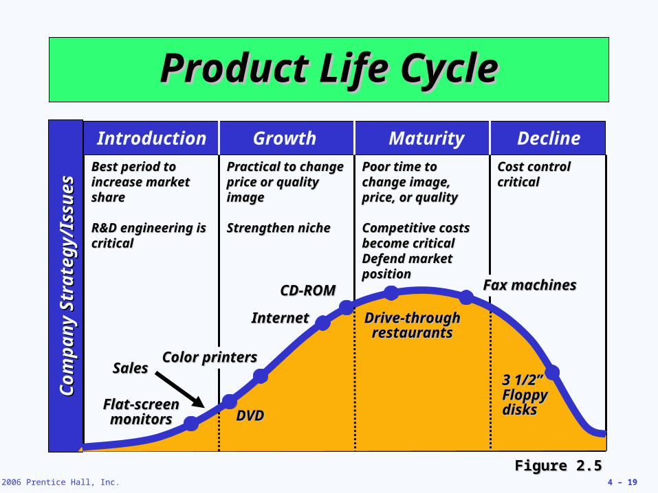
Product Life CycleProduct Life Cycle
Best period to Best period to increase market increase market shareshare
R&D engineering is R&D engineering is criticalcritical
Practical to change Practical to change price or quality price or quality imageimage
Strengthen nicheStrengthen niche
Poor time to Poor time to change image, change image, price, or qualityprice, or quality
Competitive costs Competitive costs become criticalbecome criticalDefend market Defend market positionposition
Cost control Cost control criticalcritical
Introduction Growth Maturity Decline
Co
mp
an
y S
tra
teg
y/Is
sue
sC
om
pa
ny
Str
ate
gy/
Issu
es
InternetInternet
Flat-screen Flat-screen monitorsmonitors
SalesSales
DVDDVD
CD-ROMCD-ROM
Drive-through Drive-through restaurantsrestaurants
Fax machinesFax machines
3 1/2” 3 1/2” Floppy Floppy disksdisks
Color printersColor printers
Figure 2.5Figure 2.5
© 2006 Prentice Hall, Inc. 4 – 20
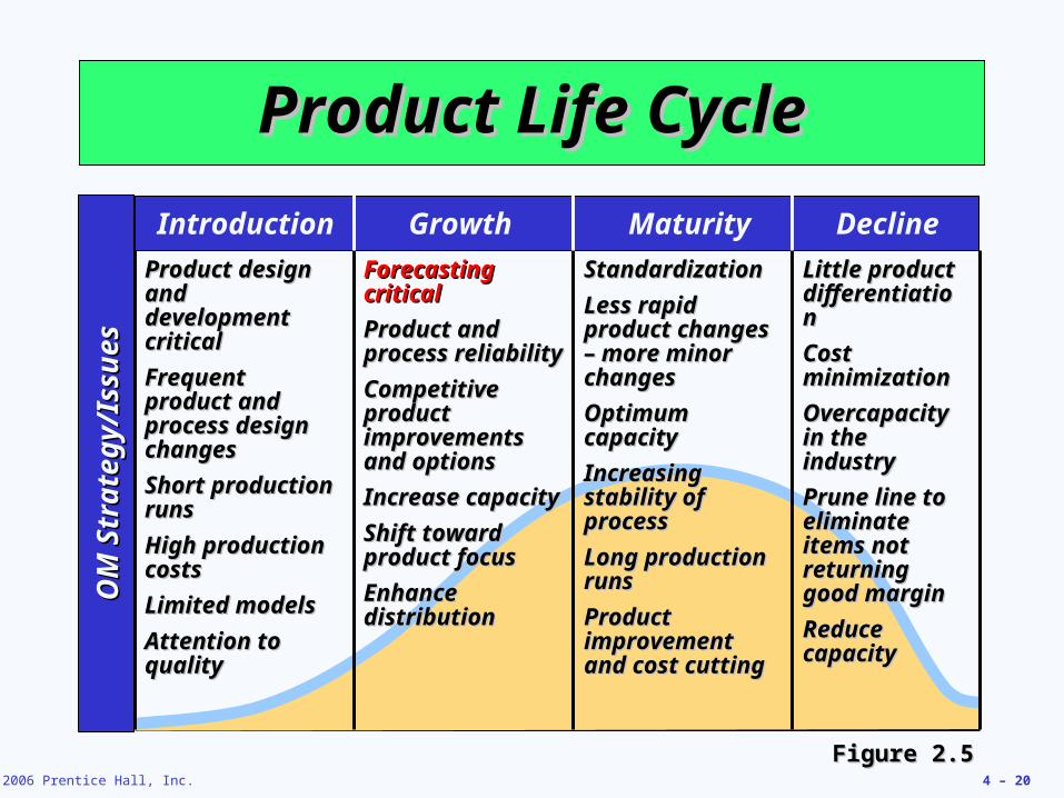
Product Life CycleProduct Life Cycle
Product design Product design and and development development criticalcritical
Frequent Frequent product and product and process design process design changeschanges
Short production Short production runsruns
High production High production costscosts
Limited modelsLimited models
Attention to Attention to qualityquality
Introduction Growth Maturity Decline
OM
Str
ate
gy
/Issu
es
OM
Str
ate
gy
/Issu
es
Forecasting Forecasting criticalcritical
Product and Product and process process reliabilityreliability
Competitive Competitive product product improvements improvements and optionsand options
Increase capacityIncrease capacity
Shift toward Shift toward product focusproduct focus
Enhance Enhance distributiondistribution
StandardizationStandardization
Less rapid Less rapid product changes product changes – more minor – more minor changeschanges
Optimum Optimum capacitycapacity
Increasing Increasing stability of stability of processprocess
Long production Long production runsruns
Product Product improvement and improvement and cost cuttingcost cutting
Little product Little product differentiationdifferentiation
Cost Cost minimizationminimization
Overcapacity Overcapacity in the in the industryindustry
Prune line to Prune line to eliminate eliminate items not items not returning returning good margingood margin
Reduce Reduce capacitycapacity
Figure 2.5Figure 2.5
© 2006 Prentice Hall, Inc. 4 – 21
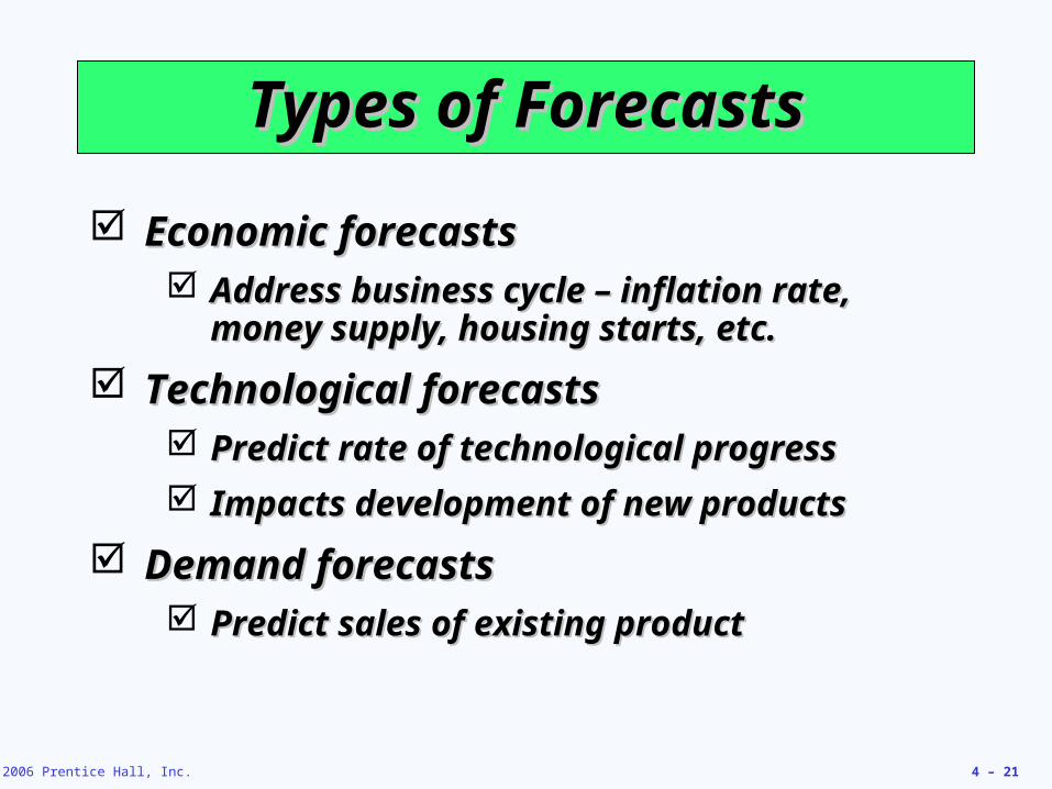
Types of ForecastsTypes of Forecasts
Economic forecastsEconomic forecasts Address business cycle – inflation rate, Address business cycle – inflation rate,
money supply, housing starts, etc.money supply, housing starts, etc.
Technological forecastsTechnological forecasts Predict rate of technological progressPredict rate of technological progress
Impacts development of new productsImpacts development of new products
Demand forecastsDemand forecasts Predict sales of existing productPredict sales of existing product
© 2006 Prentice Hall, Inc. 4 – 22
Strategic Importance of Strategic Importance of ForecastingForecasting
Human Resources – Hiring, training, Human Resources – Hiring, training, laying off workerslaying off workers
Capacity – Capacity shortages can Capacity – Capacity shortages can result in undependable delivery, loss result in undependable delivery, loss of customers, loss of market shareof customers, loss of market share
Supply-Chain Management – Good Supply-Chain Management – Good supplier relations and price advancesupplier relations and price advance
© 2006 Prentice Hall, Inc. 4 – 23
Seven Steps in ForecastingSeven Steps in Forecasting
Determine the use of the forecastDetermine the use of the forecast
Select the items to be forecastedSelect the items to be forecasted
Determine the time horizon of the Determine the time horizon of the forecastforecast
Select the forecasting model(s)Select the forecasting model(s)
Gather the dataGather the data
Make the forecastMake the forecast
Validate and implement resultsValidate and implement results
© 2006 Prentice Hall, Inc. 4 – 24
The Realities! (Characteristics The Realities! (Characteristics of Forecasts)of Forecasts)
Forecasts are seldom perfectForecasts are seldom perfect. (They . (They usually appear with error.)usually appear with error.)
Most techniques assume an Most techniques assume an underlying stability in the systemunderlying stability in the system. . (A good forecast is more than a (A good forecast is more than a single number - includes some single number - includes some measure of anticipated error)measure of anticipated error)
© 2006 Prentice Hall, Inc. 4 – 25
The Realities! (Characteristics The Realities! (Characteristics of Forecasts)of Forecasts)
Product family and aggregated forecasts are Product family and aggregated forecasts are more accurate than individual product more accurate than individual product forecastsforecasts
The longer the forecast horizon, the less The longer the forecast horizon, the less accurate the forecast will be. accurate the forecast will be. (tomorrow’s (tomorrow’s prediction of Dow Jones’ index vs next year’s prediction of Dow Jones’ index vs next year’s prediction)prediction)
Forecasts should not be used to the Forecasts should not be used to the
exclusion of known informationexclusion of known information
© 2006 Prentice Hall, Inc. 4 – 26
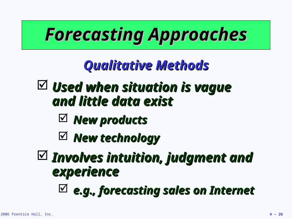
Forecasting ApproachesForecasting Approaches
Used when situation is vague Used when situation is vague and little data existand little data exist New productsNew products
New technologyNew technology
Involves intuition, judgment and Involves intuition, judgment and experienceexperience e.g., forecasting sales on Internete.g., forecasting sales on Internet
Qualitative MethodsQualitative Methods
© 2006 Prentice Hall, Inc. 4 – 27
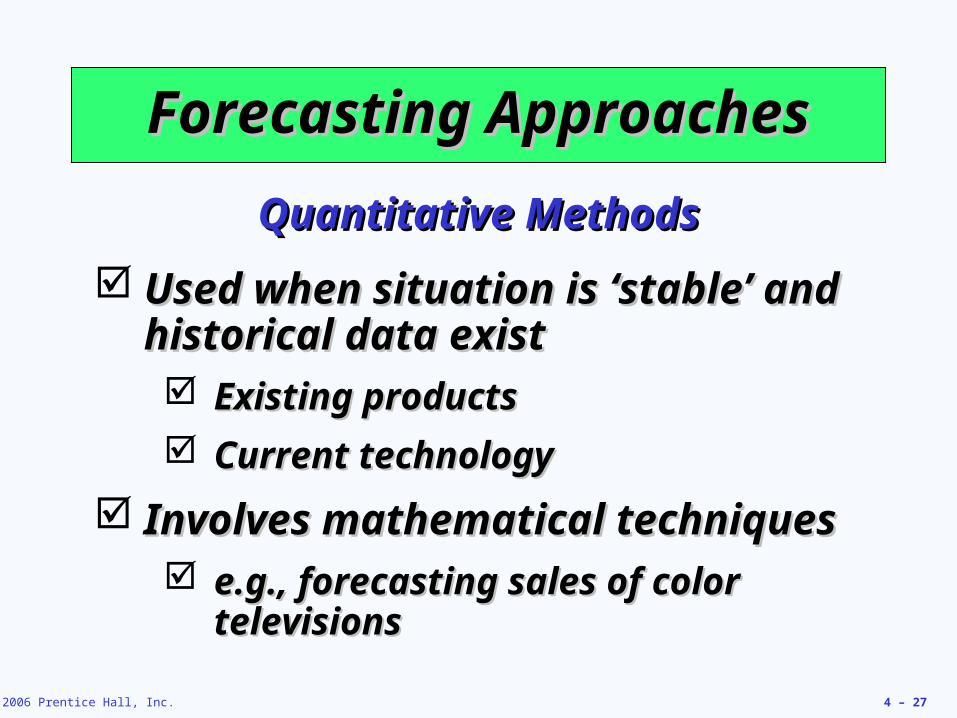
Forecasting ApproachesForecasting Approaches
Used when situation is ‘stable’ and Used when situation is ‘stable’ and historical data existhistorical data exist Existing productsExisting products
Current technologyCurrent technology
Involves mathematical techniquesInvolves mathematical techniques e.g., forecasting sales of color e.g., forecasting sales of color
televisionstelevisions
Quantitative MethodsQuantitative Methods
© 2006 Prentice Hall, Inc. 4 – 28
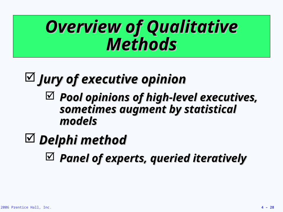
Overview of Qualitative Overview of Qualitative MethodsMethods
Jury of executive opinionJury of executive opinion Pool opinions of high-level Pool opinions of high-level
executives, sometimes augment by executives, sometimes augment by statistical modelsstatistical models
Delphi methodDelphi method Panel of experts, queried iterativelyPanel of experts, queried iteratively
© 2006 Prentice Hall, Inc. 4 – 29
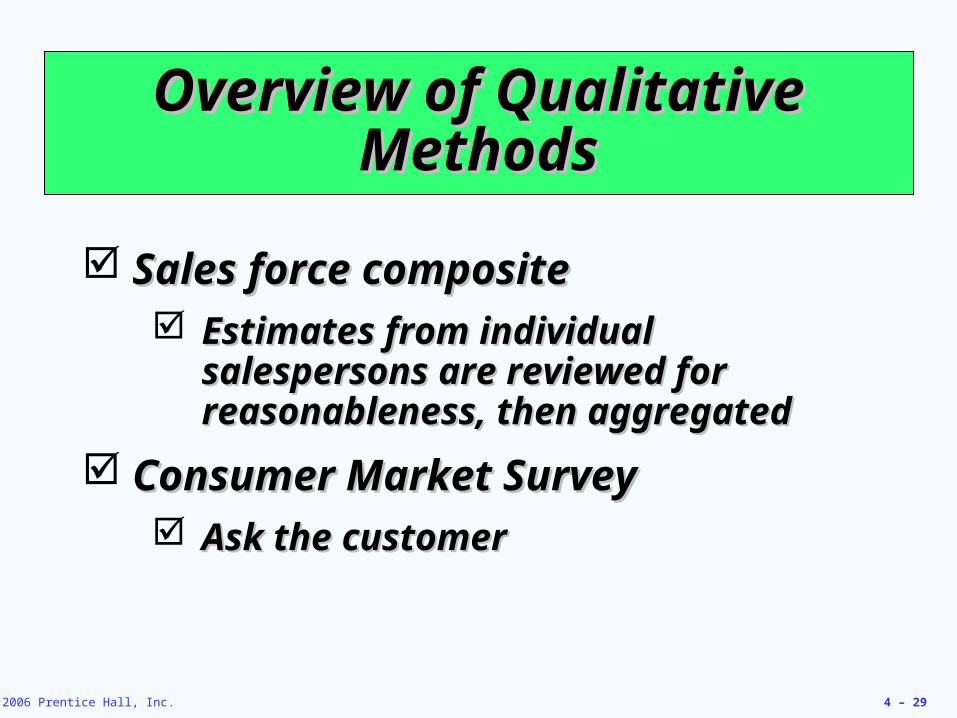
Overview of Qualitative Overview of Qualitative MethodsMethods
Sales force compositeSales force composite Estimates from individual Estimates from individual
salespersons are reviewed for salespersons are reviewed for reasonableness, then aggregated reasonableness, then aggregated
Consumer Market SurveyConsumer Market Survey Ask the customerAsk the customer
© 2006 Prentice Hall, Inc. 4 – 30
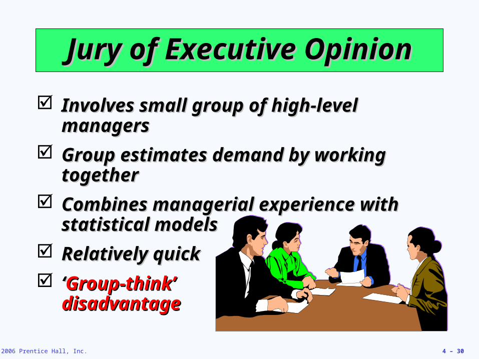
Involves small group of high-level Involves small group of high-level managersmanagers
Group estimates demand by working Group estimates demand by working togethertogether
Combines managerial experience with Combines managerial experience with statistical modelsstatistical models
Relatively quickRelatively quick
‘‘Group-think’Group-think’disadvantagedisadvantage
Jury of Executive OpinionJury of Executive Opinion
© 2006 Prentice Hall, Inc. 4 – 31
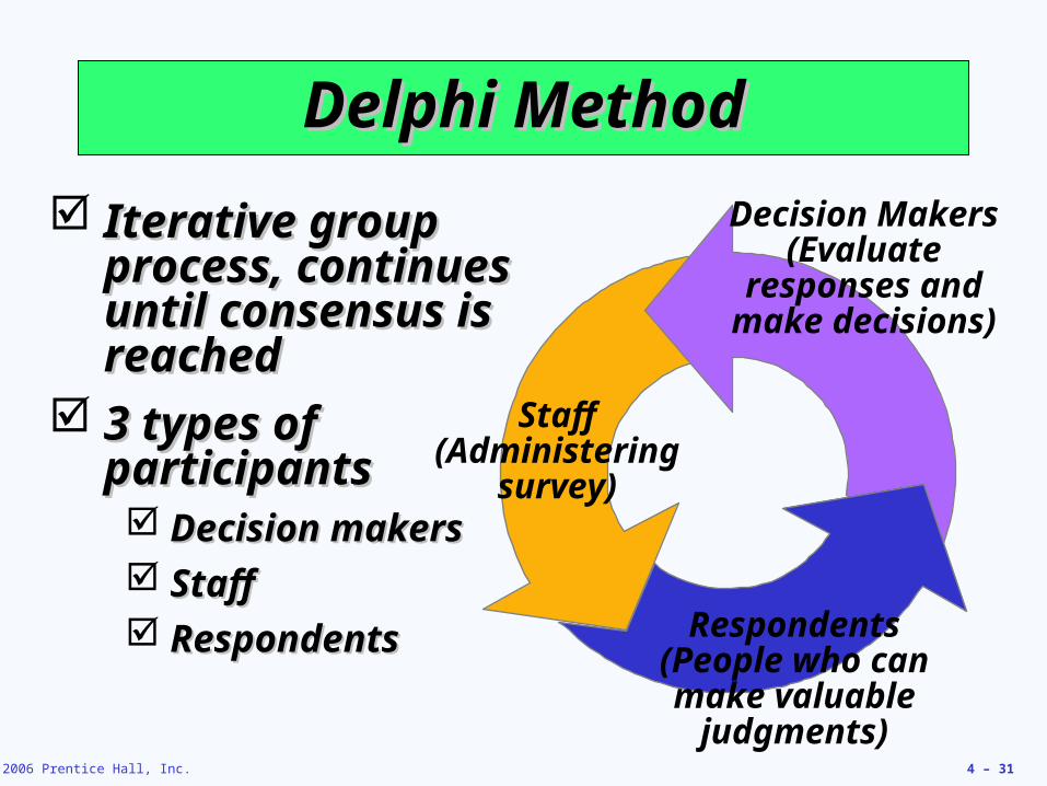
Delphi MethodDelphi Method
Iterative group Iterative group process, process, continues until continues until consensus is consensus is reachedreached
3 types of 3 types of participantsparticipants Decision makersDecision makers StaffStaff RespondentsRespondents
Staff(Administering
survey)
Decision Makers(Evaluate
responses and make decisions)
Respondents(People who can make valuable
judgments)
© 2006 Prentice Hall, Inc. 4 – 32
Sales Force CompositeSales Force Composite
Each salesperson projects his or Each salesperson projects his or her salesher sales
Combined at district and national Combined at district and national levelslevels
Sales reps know customers’ wantsSales reps know customers’ wants
Tends to be Tends to be overly optimisticoverly optimistic
© 2006 Prentice Hall, Inc. 4 – 33
Consumer Market SurveyConsumer Market Survey
Ask customers about purchasing Ask customers about purchasing plansplans
What consumers say, and what What consumers say, and what they actually do are often differentthey actually do are often different
Sometimes difficult to answerSometimes difficult to answer
© 2006 Prentice Hall, Inc. 4 – 34
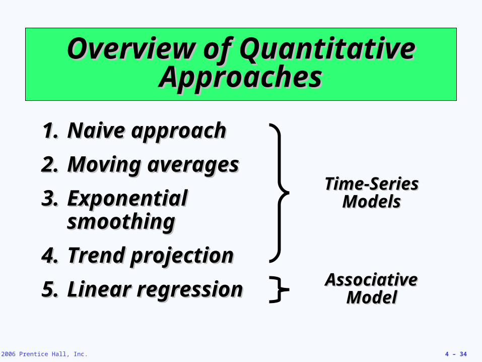
Overview of Quantitative Overview of Quantitative ApproachesApproaches
1.1. Naive approachNaive approach
2.2. Moving averagesMoving averages
3.3. Exponential Exponential smoothingsmoothing
4.4. Trend projectionTrend projection
5.5. Linear regressionLinear regression
Time-Series Time-Series ModelsModels
Associative Associative ModelModel
© 2006 Prentice Hall, Inc. 4 – 35
Set of evenly spaced numerical Set of evenly spaced numerical datadata Obtained by observing response Obtained by observing response
variable at regular time periodsvariable at regular time periods
Forecast based only on past Forecast based only on past valuesvalues Assumes that factors influencing Assumes that factors influencing
past and present will continue past and present will continue influence in futureinfluence in future
Time Series ForecastingTime Series Forecasting
© 2006 Prentice Hall, Inc. 4 – 36
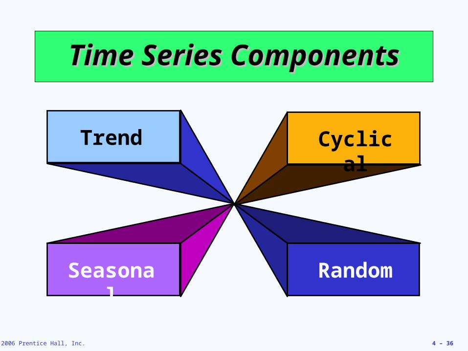
Trend
Seasonal
Cyclical
Random
Time Series ComponentsTime Series Components
© 2006 Prentice Hall, Inc. 4 – 37
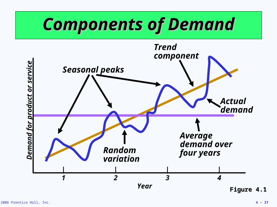
Components of DemandComponents of DemandD
eman
d f
or
pro
du
ct o
r se
rvic
e
| | | |1 2 3 4
Year
Average demand over four years
Seasonal peaks
Trend component
Actual demand
Random variation
Figure 4.1Figure 4.1
© 2006 Prentice Hall, Inc. 4 – 38
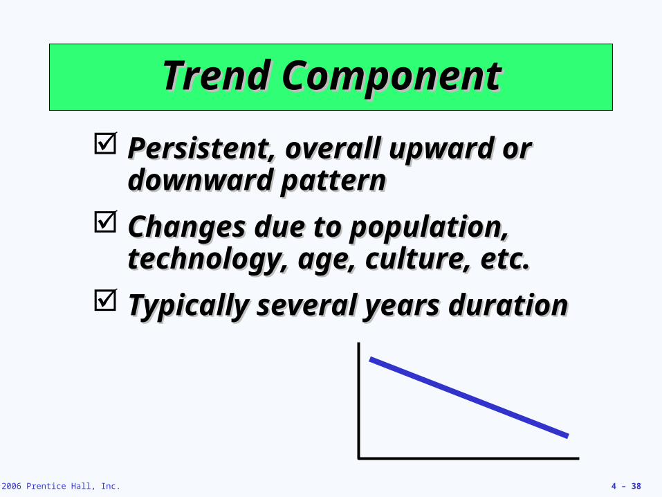
Persistent, overall upward or Persistent, overall upward or downward patterndownward pattern
Changes due to population, Changes due to population, technology, age, culture, etc.technology, age, culture, etc.
Typically several years Typically several years duration duration
Trend ComponentTrend Component
© 2006 Prentice Hall, Inc. 4 – 39
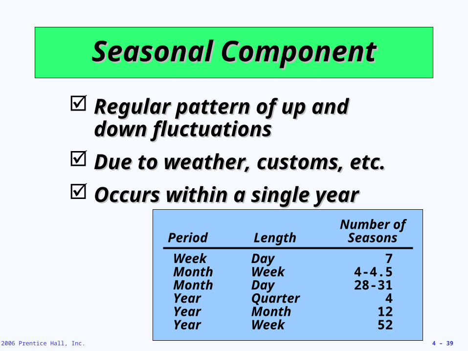
Regular pattern of up and Regular pattern of up and down fluctuationsdown fluctuations
Due to weather, customs, etc.Due to weather, customs, etc.
Occurs within a single year Occurs within a single year
Seasonal ComponentSeasonal Component
Number ofPeriod Length Seasons
Week Day 7Month Week 4-4.5Month Day 28-31Year Quarter 4Year Month 12Year Week 52
© 2006 Prentice Hall, Inc. 4 – 40
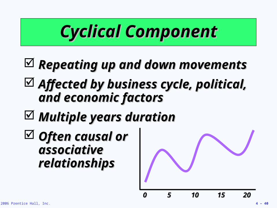
Repeating up and down movementsRepeating up and down movements
Affected by business cycle, political, Affected by business cycle, political, and economic factorsand economic factors
Multiple years durationMultiple years duration
Often causal or Often causal or associative associative relationshipsrelationships
Cyclical ComponentCyclical Component
00 55 1010 1515 2020
© 2006 Prentice Hall, Inc. 4 – 41
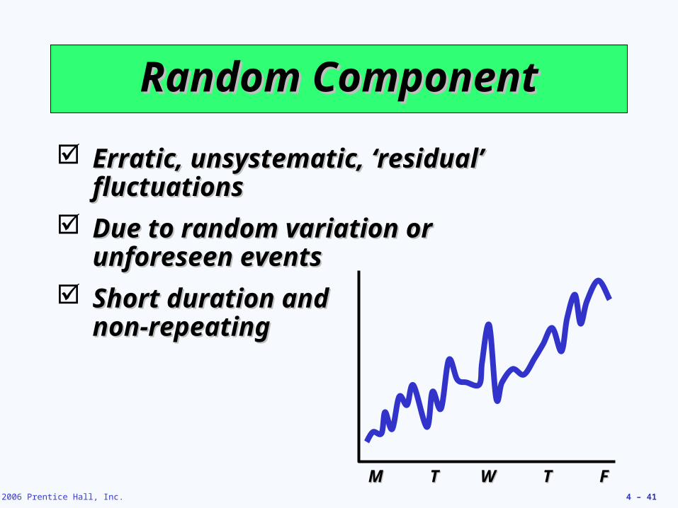
Erratic, unsystematic, ‘residual’ Erratic, unsystematic, ‘residual’ fluctuationsfluctuations
Due to random variation or Due to random variation or unforeseen eventsunforeseen events
Short duration and Short duration and non-repeating non-repeating
Random ComponentRandom Component
MM TT WW TT FF
© 2006 Prentice Hall, Inc. 4 – 42
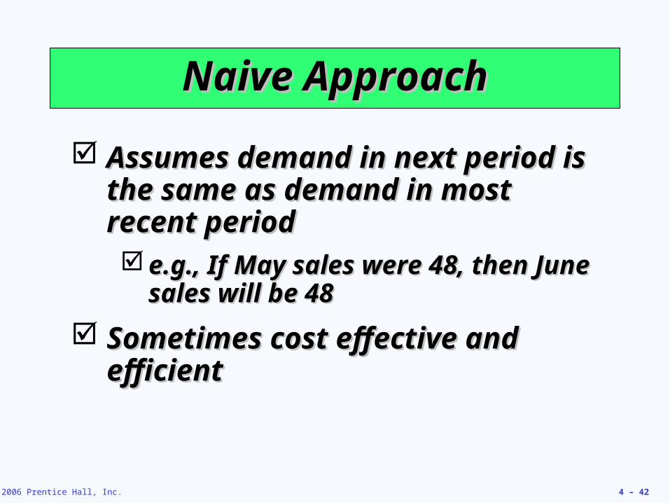
Naive ApproachNaive Approach
Assumes demand in next period is Assumes demand in next period is the same as demand in most the same as demand in most recent periodrecent period e.g., If May sales were 48, then June e.g., If May sales were 48, then June
sales will be 48sales will be 48
Sometimes cost effective and Sometimes cost effective and efficientefficient
© 2006 Prentice Hall, Inc. 4 – 43
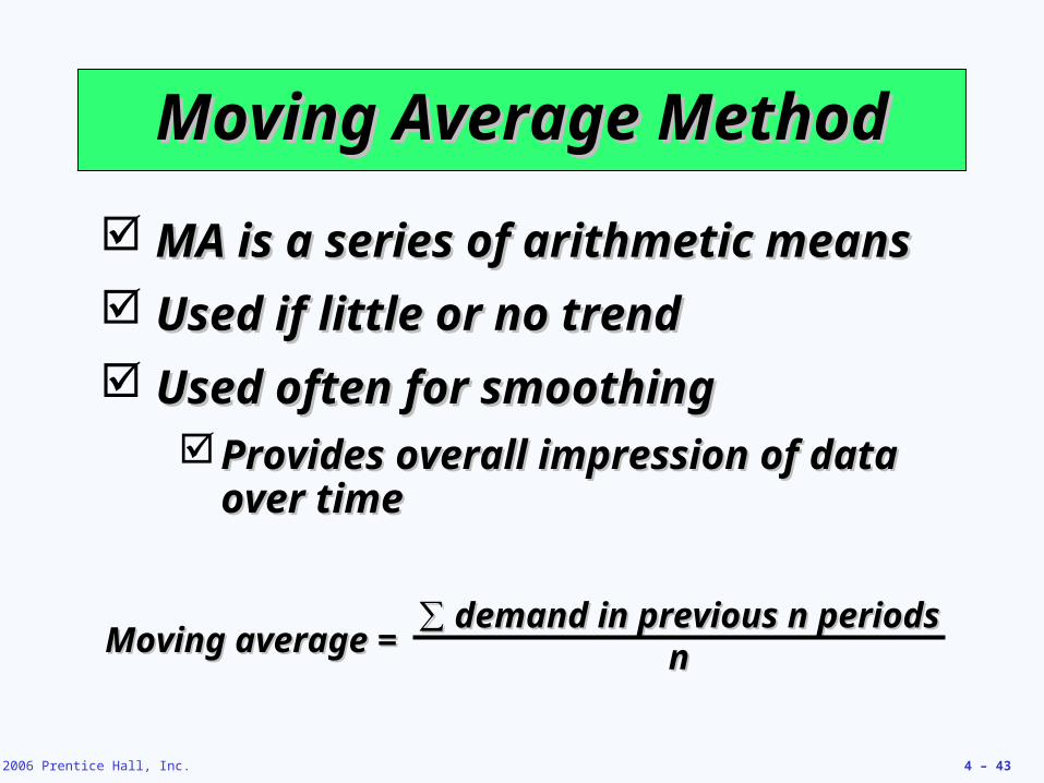
MA is a series of arithmetic means MA is a series of arithmetic means
Used if little or no trendUsed if little or no trend
Used often for smoothingUsed often for smoothingProvides overall impression of data Provides overall impression of data
over timeover time
Moving Average MethodMoving Average Method
Moving average =Moving average =∑∑ demand in previous n periodsdemand in previous n periods
nn
© 2006 Prentice Hall, Inc. 4 – 44
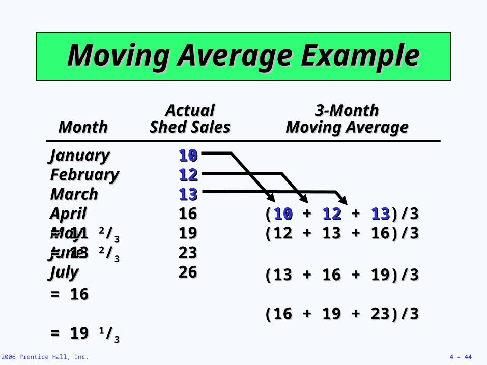
JanuaryJanuary 1010FebruaryFebruary 1212MarchMarch 1313AprilApril 1616MayMay 1919JuneJune 2323JulyJuly 2626
ActualActual 3-Month3-MonthMonthMonth Shed SalesShed Sales Moving AverageMoving Average
(12 + 13 + 16)/3 = 13 (12 + 13 + 16)/3 = 13 22//33
(13 + 16 + 19)/3 = 16(13 + 16 + 19)/3 = 16(16 + 19 + 23)/3 = 19 (16 + 19 + 23)/3 = 19 11//33
Moving Average ExampleMoving Average Example
101012121313
((1010 + + 1212 + + 1313)/3 = 11 )/3 = 11 22//33
© 2006 Prentice Hall, Inc. 4 – 45
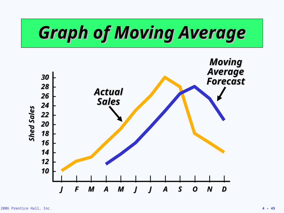
Graph of Moving AverageGraph of Moving Average
| | | | | | | | | | | |
JJ FF MM AA MM JJ JJ AA SS OO NN DD
Sh
ed S
ales
Sh
ed S
ales
30 30 –28 28 –26 26 –24 24 –22 22 –20 20 –18 18 –16 16 –14 14 –12 12 –10 10 –
Actual Actual SalesSales
Moving Moving Average Average ForecastForecast
© 2006 Prentice Hall, Inc. 4 – 46
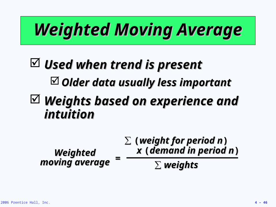
Used when trend is present Used when trend is present Older data usually less importantOlder data usually less important
Weights based on experience and Weights based on experience and intuitionintuition
Weighted Moving AverageWeighted Moving Average
WeightedWeightedmoving averagemoving average ==
∑∑ ((weight for period nweight for period n)) x x ((demand in period ndemand in period n))
∑∑ weightsweights
© 2006 Prentice Hall, Inc. 4 – 47
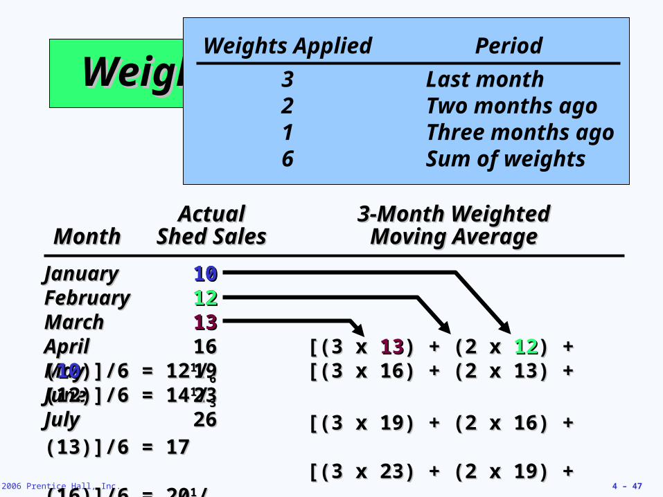
JanuaryJanuary 1010FebruaryFebruary 1212MarchMarch 1313AprilApril 1616MayMay 1919JuneJune 2323JulyJuly 2626
ActualActual 3-Month Weighted3-Month WeightedMonthMonth Shed SalesShed Sales Moving AverageMoving Average
[(3 x 16) + (2 x 13) + (12)]/6 = 14[(3 x 16) + (2 x 13) + (12)]/6 = 1411//33
[(3 x 19) + (2 x 16) + (13)]/6 = 17[(3 x 19) + (2 x 16) + (13)]/6 = 17[(3 x 23) + (2 x 19) + (16)]/6 = 20[(3 x 23) + (2 x 19) + (16)]/6 = 2011//22
Weighted Moving AverageWeighted Moving Average
101012121313
[(3 x [(3 x 1313) + (2 x ) + (2 x 1212) + () + (1010)]/6 = 12)]/6 = 1211//66
Weights Applied Period
3 Last month2 Two months ago1 Three months ago6 Sum of weights
© 2006 Prentice Hall, Inc. 4 – 48
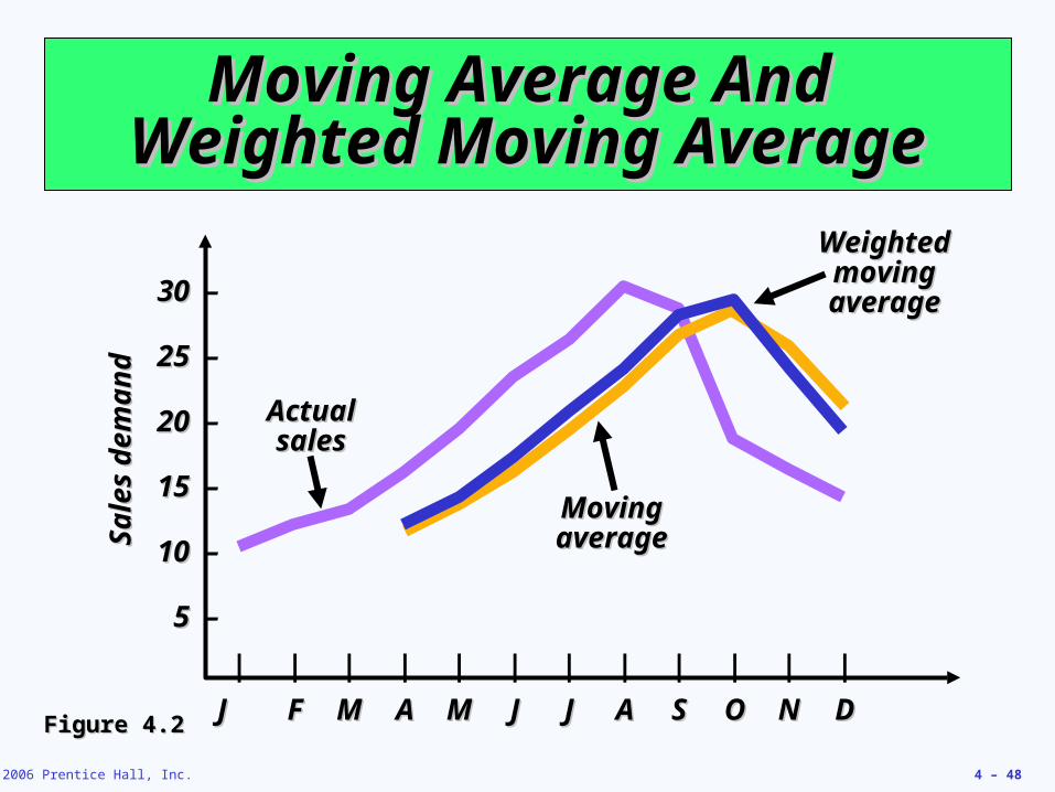
Moving Average And Moving Average And Weighted Moving AverageWeighted Moving Average
30 30 –
25 25 –
20 20 –
15 15 –
10 10 –
5 5 –
Sa
les
de
man
dS
ale
s d
em
and
| | | | | | | | | | | |
JJ FF MM AA MM JJ JJ AA SS OO NN DD
Actual Actual salessales
Moving Moving averageaverage
Weighted Weighted moving moving averageaverage
Figure 4.2Figure 4.2
© 2006 Prentice Hall, Inc. 4 – 49
Increasing n smoothens the Increasing n smoothens the forecast but makes it less sensitive forecast but makes it less sensitive to changesto changes
Do not forecast trends wellDo not forecast trends well
Require extensive historical dataRequire extensive historical data
Potential Problems WithPotential Problems With Moving Average Moving Average
© 2006 Prentice Hall, Inc. 4 – 50
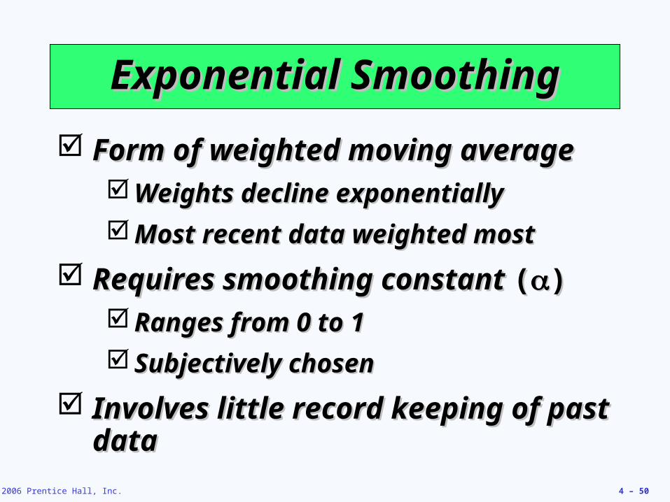
Form of weighted moving averageForm of weighted moving average Weights decline exponentiallyWeights decline exponentially
Most recent data weighted mostMost recent data weighted most
Requires smoothing constant Requires smoothing constant (()) Ranges from 0 to 1Ranges from 0 to 1
Subjectively chosenSubjectively chosen
Involves little record keeping of past Involves little record keeping of past datadata
Exponential SmoothingExponential Smoothing
© 2006 Prentice Hall, Inc. 4 – 51
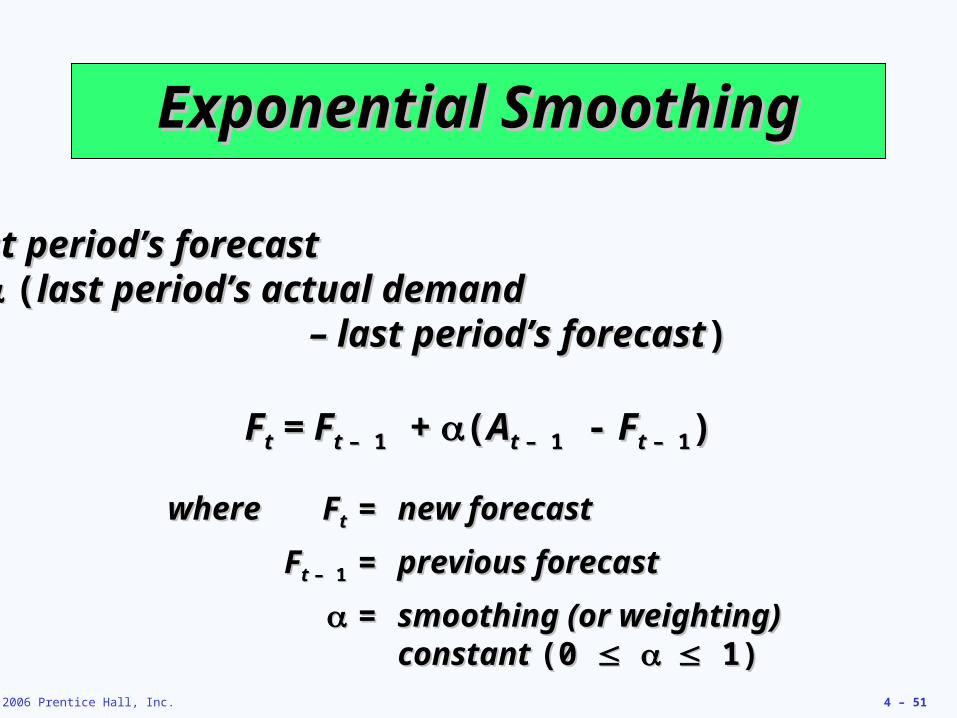
Exponential SmoothingExponential Smoothing
New forecast =New forecast = last period’s forecastlast period’s forecast+ + ((last period’s actual demand last period’s actual demand
– – last period’s forecastlast period’s forecast))
FFtt = F = Ft t – 1– 1 + + ((AAt t – 1– 1 - - F Ft t – 1– 1))
wherewhere FFtt == new forecastnew forecast
FFt t – 1– 1 == previous forecastprevious forecast
== smoothing (or weighting) smoothing (or weighting) constant constant (0 (0 1) 1)
© 2006 Prentice Hall, Inc. 4 – 52
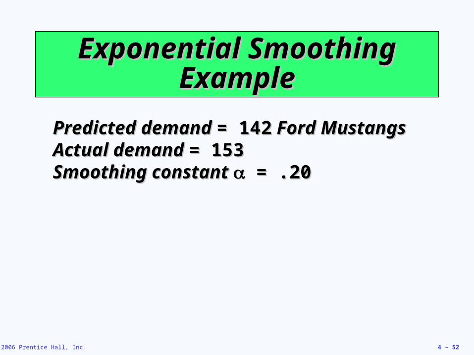
Exponential Smoothing Exponential Smoothing ExampleExample
Predicted demand Predicted demand = 142= 142 Ford Mustangs Ford MustangsActual demand Actual demand = 153= 153Smoothing constant Smoothing constant = .20 = .20
© 2006 Prentice Hall, Inc. 4 – 53
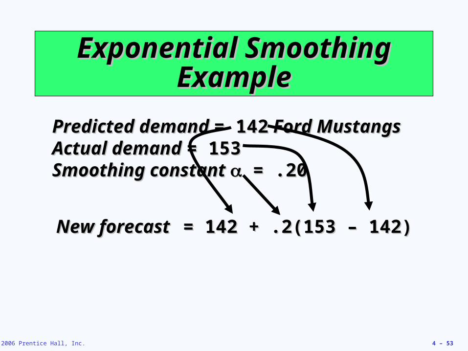
Exponential Smoothing Exponential Smoothing ExampleExample
Predicted demand Predicted demand = 142= 142 Ford Mustangs Ford MustangsActual demand Actual demand = 153= 153Smoothing constant Smoothing constant = .20 = .20
New forecastNew forecast = 142 + .2(153 – 142)= 142 + .2(153 – 142)
© 2006 Prentice Hall, Inc. 4 – 54
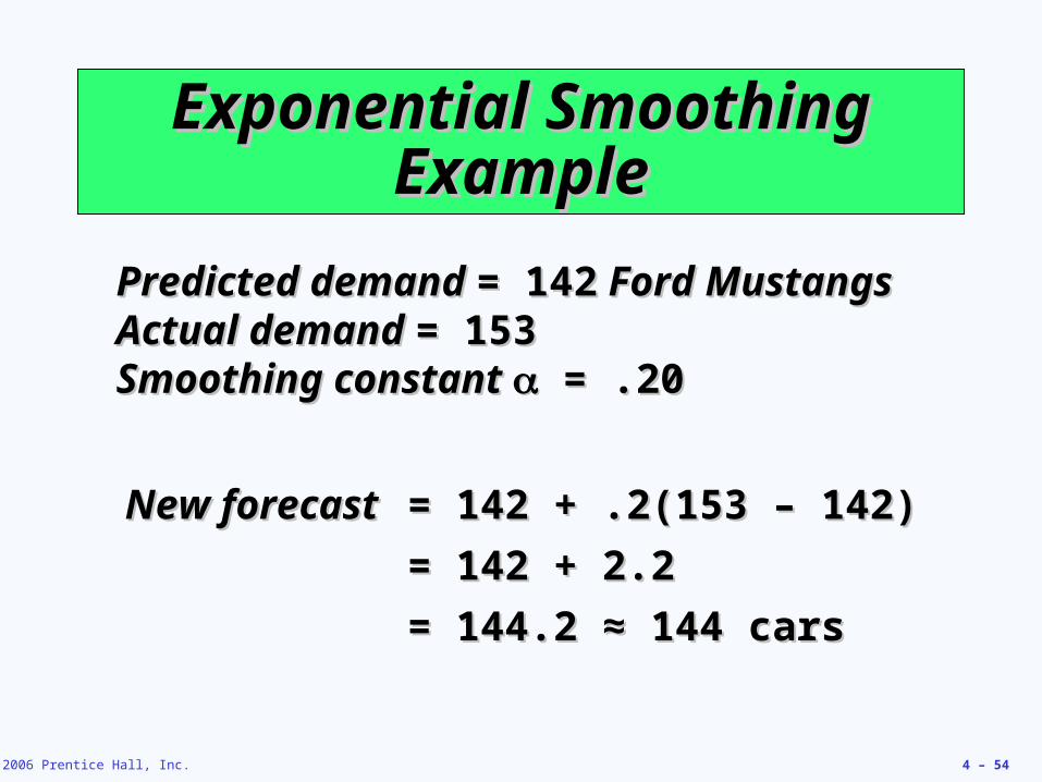
Exponential Smoothing Exponential Smoothing ExampleExample
Predicted demand Predicted demand = 142= 142 Ford Mustangs Ford MustangsActual demand Actual demand = 153= 153Smoothing constant Smoothing constant = .20 = .20
New forecastNew forecast = 142 + .2(153 – 142)= 142 + .2(153 – 142)
= 142 + 2.2= 142 + 2.2
= 144.2 ≈ 144 cars= 144.2 ≈ 144 cars
© 2006 Prentice Hall, Inc. 4 – 55
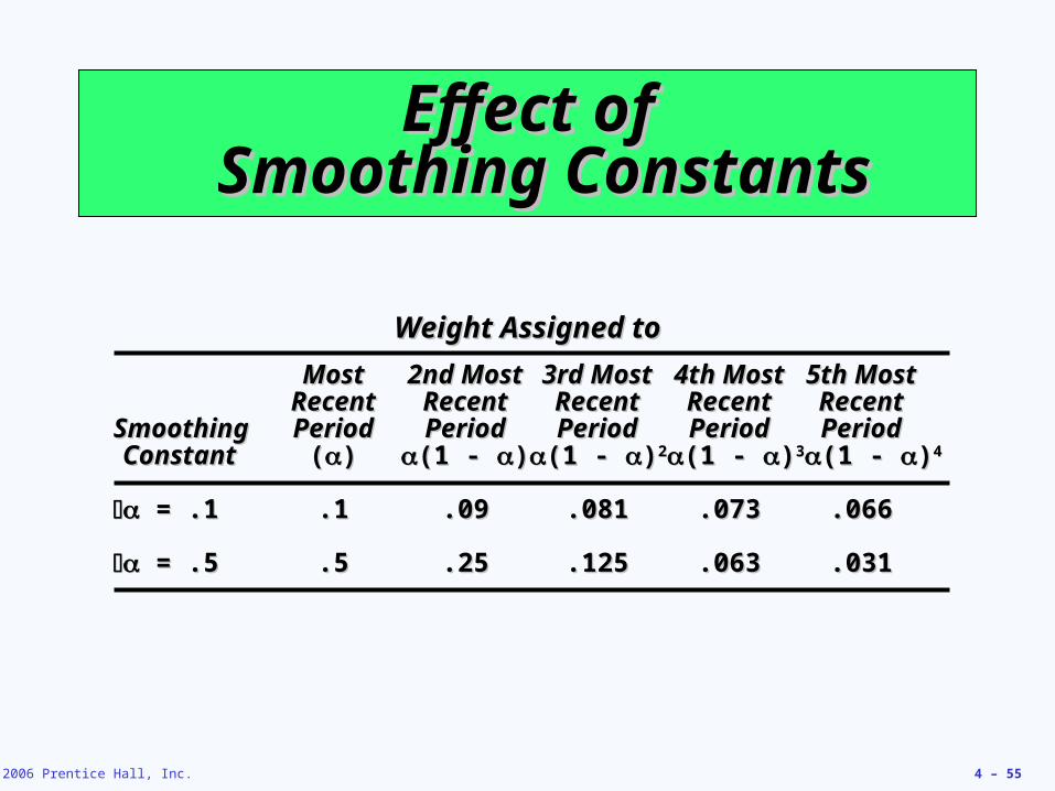
Effect ofEffect of Smoothing Constants Smoothing Constants
Weight Assigned toWeight Assigned to
MostMost 2nd Most2nd Most 3rd Most3rd Most 4th Most4th Most 5th Most5th MostRecentRecent RecentRecent RecentRecent RecentRecent RecentRecent
SmoothingSmoothing PeriodPeriod PeriodPeriod PeriodPeriod PeriodPeriod PeriodPeriodConstantConstant (()) (1 - (1 - )) (1 - (1 - ))22 (1 - (1 - ))33 (1 - (1 - ))44
= .1= .1 .1.1 .09.09 .081.081 .073.073 .066.066
= .5= .5 .5.5 .25.25 .125.125 .063.063 .031.031
© 2006 Prentice Hall, Inc. 4 – 56
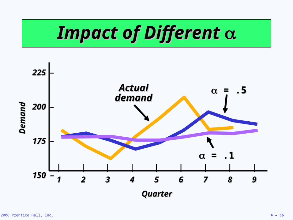
Impact of Different Impact of Different
225 225 –
200 200 –
175 175 –
150 150 –| | | | | | | | |
11 22 33 44 55 66 77 88 99
QuarterQuarter
De
ma
nd
De
ma
nd
= .1= .1
Actual Actual demanddemand
= .5= .5
© 2006 Prentice Hall, Inc. 4 – 57
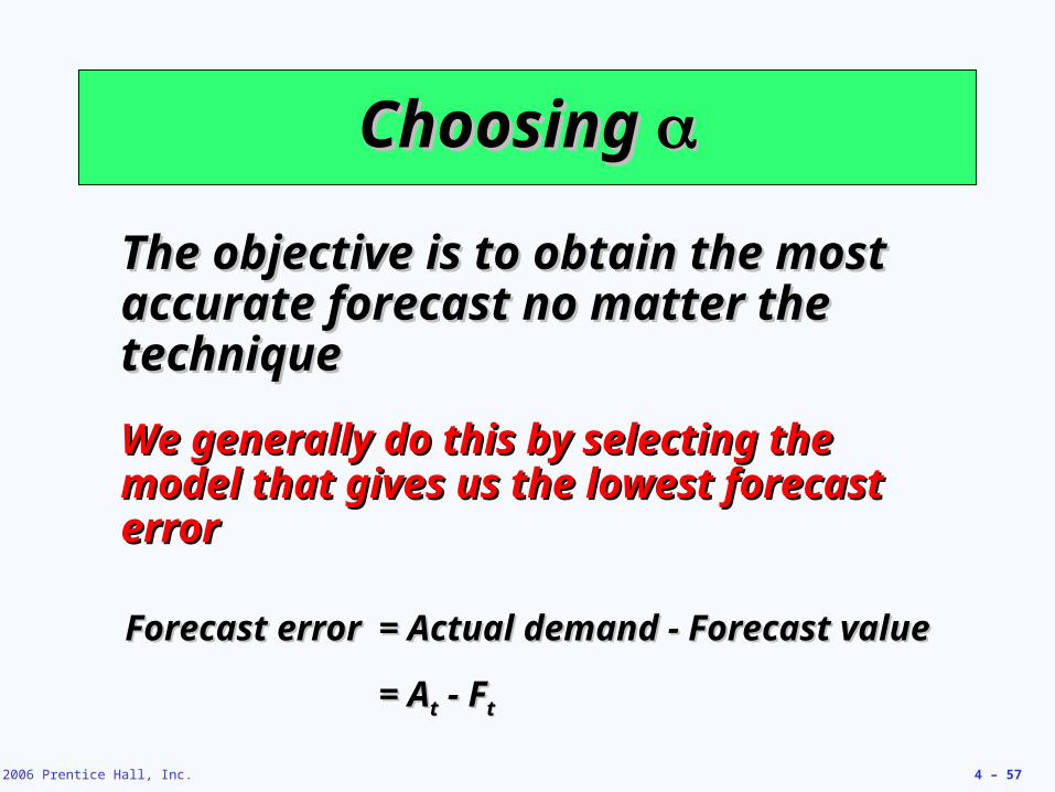
Choosing Choosing
The objective is to obtain the most The objective is to obtain the most accurate forecast no matter the accurate forecast no matter the techniquetechnique
We generally do this by selecting the We generally do this by selecting the model that gives us the lowest forecast model that gives us the lowest forecast errorerror
Forecast errorForecast error = Actual demand - Forecast value= Actual demand - Forecast value
= A= Att - F - Ftt
© 2006 Prentice Hall, Inc. 4 – 58
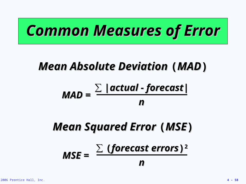
Common Measures of ErrorCommon Measures of Error
Mean Absolute Deviation Mean Absolute Deviation ((MADMAD))
MAD =MAD =∑∑ |actual - forecast||actual - forecast|
nn
Mean Squared Error Mean Squared Error ((MSEMSE))
MSE =MSE =∑∑ ((forecast errorsforecast errors))22
nn
© 2006 Prentice Hall, Inc. 4 – 59
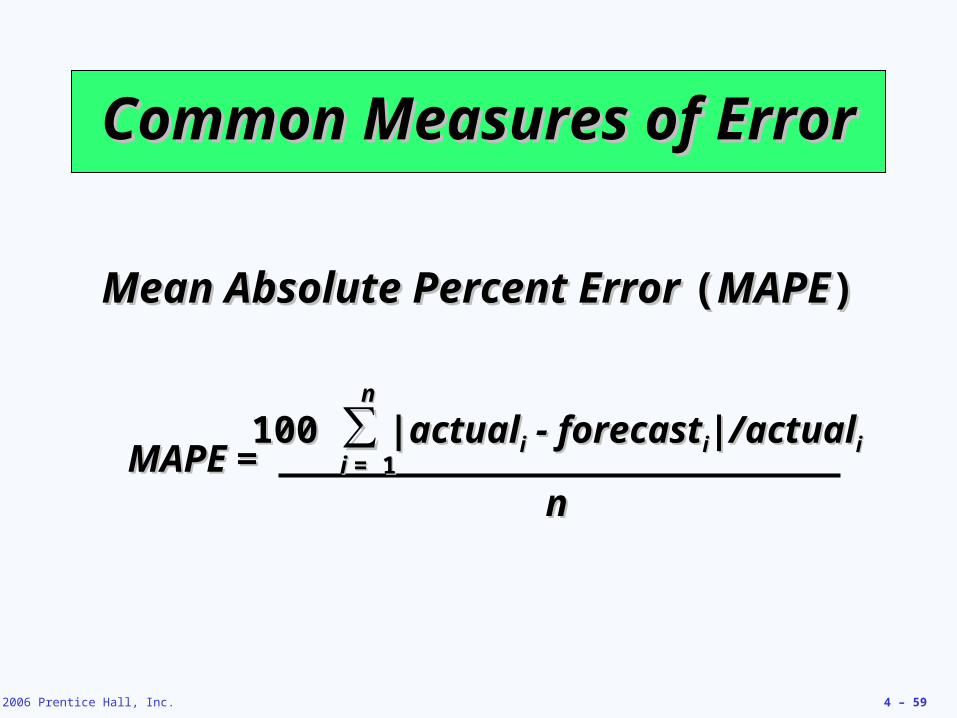
Common Measures of ErrorCommon Measures of Error
Mean Absolute Percent Error Mean Absolute Percent Error ((MAPEMAPE))
MAPE =MAPE =100 100 ∑∑ |actual |actualii - forecast - forecastii|/actual|/actualii
nn
nn
i i = 1= 1
© 2006 Prentice Hall, Inc. 4 – 60
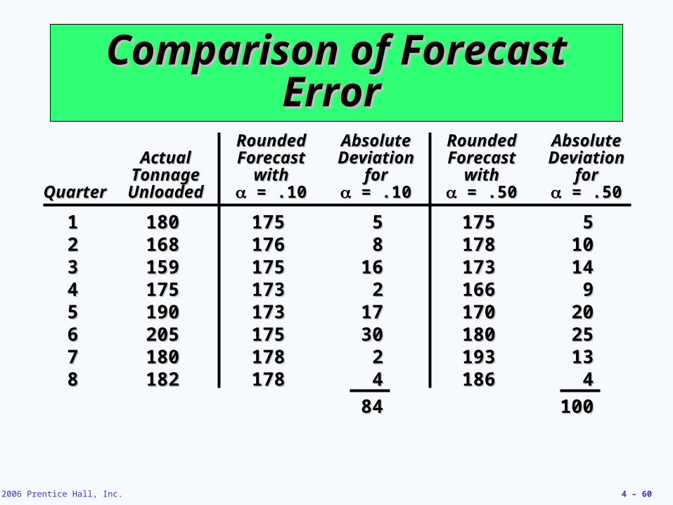
Comparison of Forecast Comparison of Forecast Error Error
RoundedRounded AbsoluteAbsolute RoundedRounded AbsoluteAbsoluteActualActual ForecastForecast DeviationDeviation ForecastForecast DeviationDeviation
TonnageTonnage withwith forfor withwith forforQuarterQuarter UnloadedUnloaded = .10 = .10 = .10 = .10 = .50 = .50 = .50 = .50
11 180180 175175 55 175175 5522 168168 176176 88 178178 101033 159159 175175 1616 173173 141444 175175 173173 22 166166 9955 190190 173173 1717 170170 202066 205205 175175 3030 180180 252577 180180 178178 22 193193 131388 182182 178178 44 186186 44
8484 100100
© 2006 Prentice Hall, Inc. 4 – 61
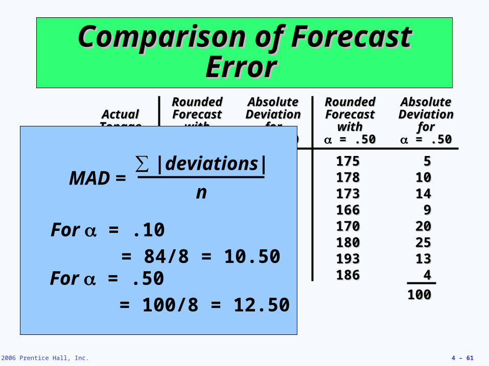
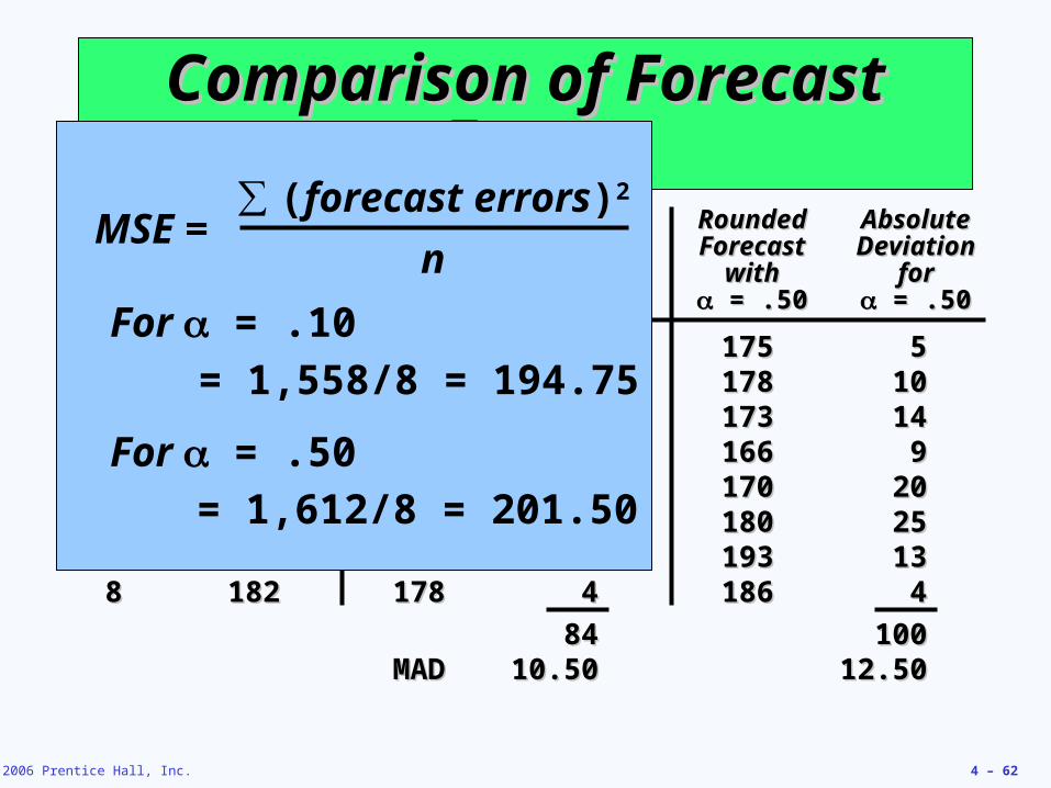
Comparison of Forecast Comparison of Forecast Error Error
RoundedRounded AbsoluteAbsolute RoundedRounded AbsoluteAbsoluteActualActual ForecastForecast DeviationDeviation ForecastForecast DeviationDeviationTonageTonage withwith forfor withwith forfor
QuarterQuarter UnloadedUnloaded = .10 = .10 = .10 = .10 = .50 = .50 = .50 = .50
11 180180 175175 55 175175 5522 168168 176176 88 178178 101033 159159 175175 1616 173173 141444 175175 173173 22 166166 9955 190190 173173 1717 170170 202066 205205 175175 3030 180180 252577 180180 178178 22 193193 131388 182182 178178 44 186186 44
8484 100100
MAD =∑ |deviations|
n
= 84/8 = 10.50
For = .10
= 100/8 = 12.50
For = .50
© 2006 Prentice Hall, Inc. 4 – 62
Comparison of Forecast Comparison of Forecast Error Error
RoundedRounded AbsoluteAbsolute RoundedRounded AbsoluteAbsoluteActualActual ForecastForecast DeviationDeviation ForecastForecast DeviationDeviationTonageTonage withwith forfor withwith forfor
QuarterQuarter UnloadedUnloaded = .10 = .10 = .10 = .10 = .50 = .50 = .50 = .50
11 180180 175175 55 175175 5522 168168 176176 88 178178 101033 159159 175175 1616 173173 141444 175175 173173 22 166166 9955 190190 173173 1717 170170 202066 205205 175175 3030 180180 252577 180180 178178 22 193193 131388 182182 178178 44 186186 44
8484 100100MADMAD 10.5010.50 12.5012.50
= 1,558/8 = 194.75
For = .10
= 1,612/8 = 201.50
For = .50
MSE =∑ (forecast errors)2
n
© 2006 Prentice Hall, Inc. 4 – 63
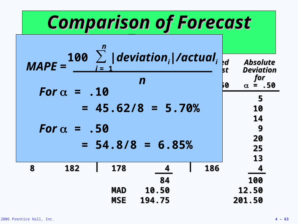
Comparison of Forecast Comparison of Forecast Error Error
RoundedRounded AbsoluteAbsolute RoundedRounded AbsoluteAbsoluteActualActual ForecastForecast DeviationDeviation ForecastForecast DeviationDeviationTonageTonage withwith forfor withwith forfor
QuarterQuarter UnloadedUnloaded = .10 = .10 = .10 = .10 = .50 = .50 = .50 = .50
11 180180 175175 55 175175 5522 168168 176176 88 178178 101033 159159 175175 1616 173173 141444 175175 173173 22 166166 9955 190190 173173 1717 170170 202066 205205 175175 3030 180180 252577 180180 178178 22 193193 131388 182182 178178 44 186186 44
8484 100100MADMAD 10.5010.50 12.5012.50MSEMSE 194.75194.75 201.50201.50
= 45.62/8 = 5.70%
For = .10
= 54.8/8 = 6.85%
For = .50
MAPE =100 ∑ |deviationi|/actuali
n
n
i = 1
© 2006 Prentice Hall, Inc. 4 – 64
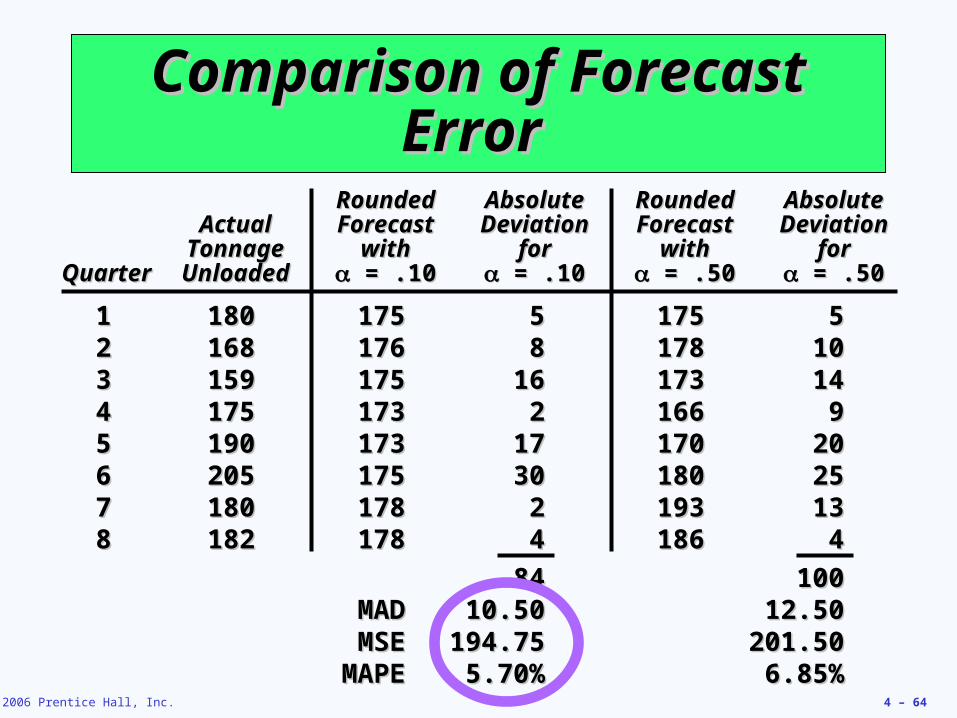
Comparison of Forecast Comparison of Forecast Error Error
RoundedRounded AbsoluteAbsolute RoundedRounded AbsoluteAbsoluteActualActual ForecastForecast DeviationDeviation ForecastForecast DeviationDeviation
TonnageTonnage withwith forfor withwith forforQuarterQuarter UnloadedUnloaded = .10 = .10 = .10 = .10 = .50 = .50 = .50 = .50
11 180180 175175 55 175175 5522 168168 176176 88 178178 101033 159159 175175 1616 173173 141444 175175 173173 22 166166 9955 190190 173173 1717 170170 202066 205205 175175 3030 180180 252577 180180 178178 22 193193 131388 182182 178178 44 186186 44
8484 100100MADMAD 10.5010.50 12.5012.50MSEMSE 194.75194.75 201.50201.50
MAPEMAPE 5.70%5.70% 6.85%6.85%
© 2006 Prentice Hall, Inc. 4 – 65
Comparison of Forecast Comparison of Forecast Error Error
Verify the values for MSE and MAPEVerify the values for MSE and MAPE
as shown for the previous as shown for the previous
example and submit with example and submit with
assignment 2. Use excel.assignment 2. Use excel.
© 2006 Prentice Hall, Inc. 4 – 66
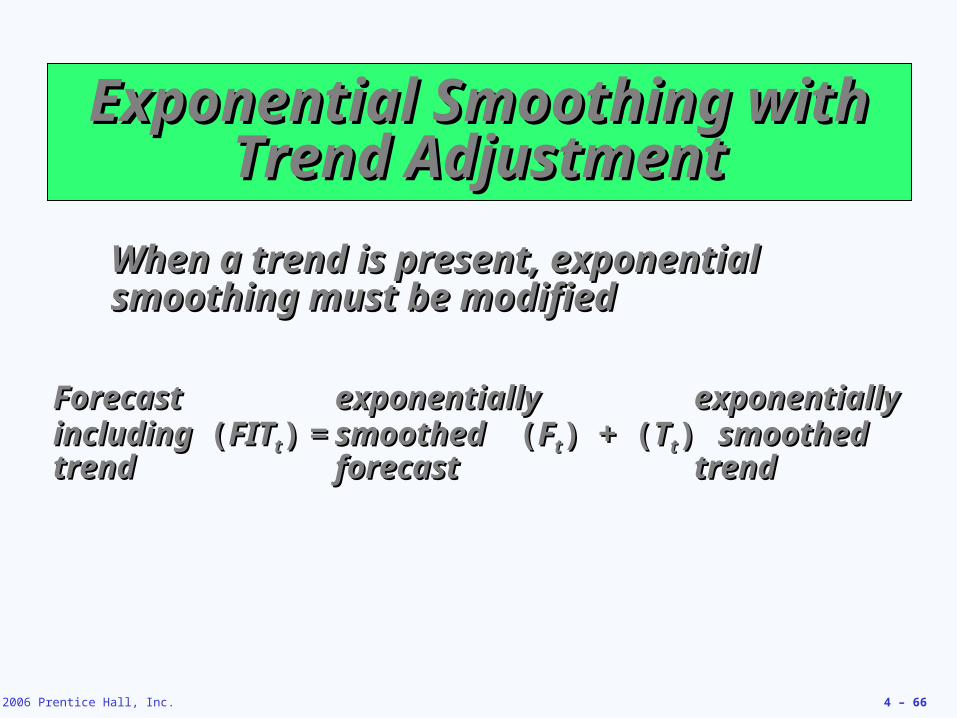
Exponential Smoothing with Exponential Smoothing with Trend AdjustmentTrend Adjustment
When a trend is present, exponential When a trend is present, exponential smoothing must be mosmoothing must be modifieddified
Forecast Forecast including including ((FITFITtt)) = = trendtrend
exponentiallyexponentially exponentiallyexponentiallysmoothed smoothed ((FFtt)) + + ((TTtt)) smoothedsmoothedforecastforecast trendtrend
© 2006 Prentice Hall, Inc. 4 – 67
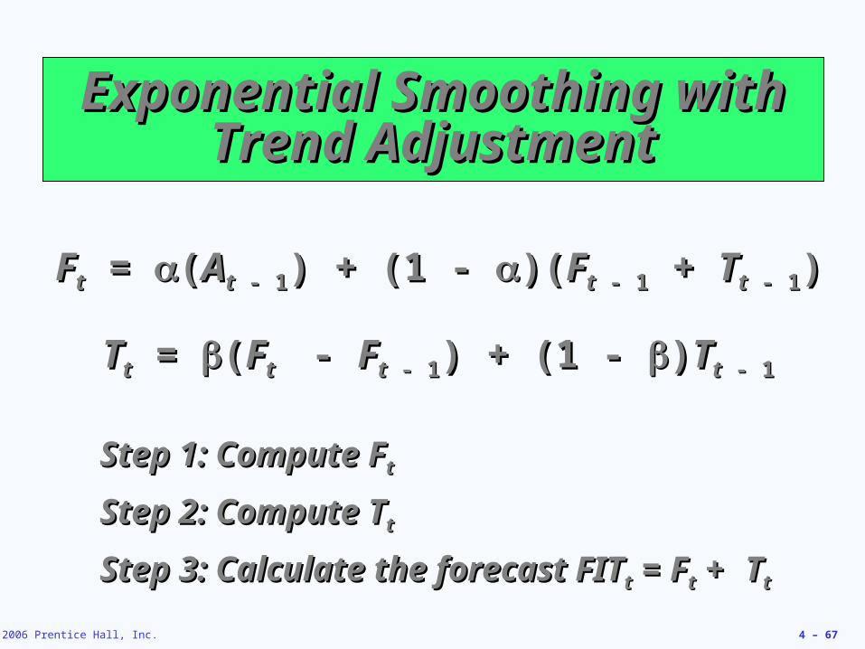
Exponential Smoothing with Exponential Smoothing with Trend AdjustmentTrend Adjustment
FFtt = = ((AAtt - 1 - 1) + (1 - ) + (1 - )()(FFtt - 1 - 1 + + TTtt - 1 - 1))
TTtt = = ((FFtt - - FFtt - 1 - 1) + (1 - ) + (1 - ))TTtt - 1 - 1
Step 1: Compute FStep 1: Compute Ftt
Step 2: Compute TStep 2: Compute Ttt
Step 3: Calculate the forecast FITStep 3: Calculate the forecast FITtt == F Ftt + + TTtt
© 2006 Prentice Hall, Inc. 4 – 68
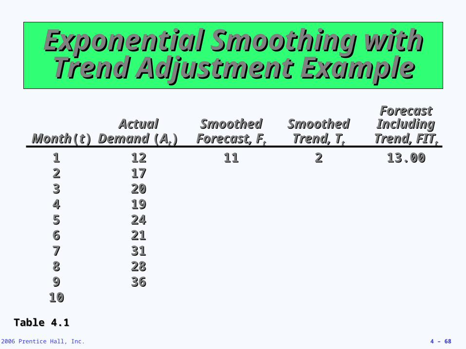
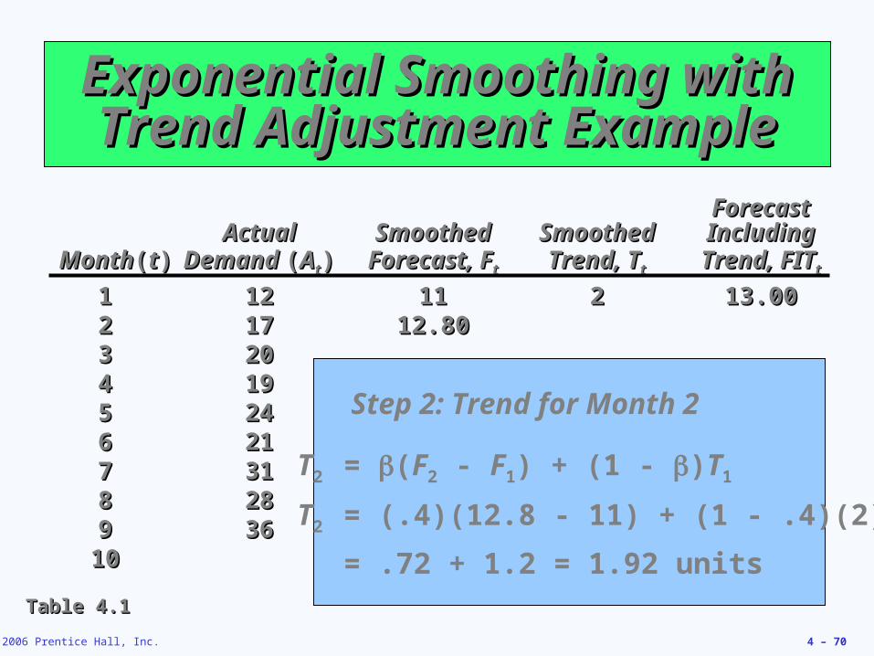
Exponential Smoothing with Exponential Smoothing with Trend Adjustment ExampleTrend Adjustment Example
ForecastForecastActualActual SmoothedSmoothed SmoothedSmoothed IncludingIncluding
MonthMonth((tt)) Demand Demand ((AAtt)) Forecast, FForecast, Ftt Trend, TTrend, Ttt Trend, FITTrend, FITtt
11 1212 1111 22 13.0013.0022 171733 202044 191955 242466 212177 313188 282899 3636
1010
Table 4.1Table 4.1
© 2006 Prentice Hall, Inc. 4 – 69
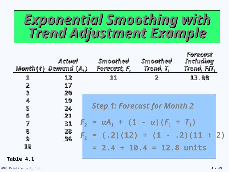
Exponential Smoothing with Exponential Smoothing with Trend Adjustment ExampleTrend Adjustment Example
ForecastForecastActualActual SmoothedSmoothed SmoothedSmoothed IncludingIncluding
MonthMonth((tt)) Demand Demand ((AAtt)) Forecast, FForecast, Ftt Trend, TTrend, Ttt Trend, FITTrend, FITtt
11 1212 1111 22 13.0013.0022 171733 202044 191955 242466 212177 313188 282899 3636
1010
Table 4.1Table 4.1
F2 = A1 + (1 - )(F1 + T1)
F2 = (.2)(12) + (1 - .2)(11 + 2)
= 2.4 + 10.4 = 12.8 units
Step 1: Forecast for Month 2
© 2006 Prentice Hall, Inc. 4 – 70
Exponential Smoothing with Exponential Smoothing with Trend Adjustment ExampleTrend Adjustment Example
ForecastForecastActualActual SmoothedSmoothed SmoothedSmoothed IncludingIncluding
MonthMonth((tt)) Demand Demand ((AAtt)) Forecast, FForecast, Ftt Trend, TTrend, Ttt Trend, FITTrend, FITtt
11 1212 1111 22 13.0013.0022 1717 12.8012.8033 202044 191955 242466 212177 313188 282899 3636
1010
Table 4.1Table 4.1
T2 = (F2 - F1) + (1 - )T1
T2 = (.4)(12.8 - 11) + (1 - .4)(2)
= .72 + 1.2 = 1.92 units
Step 2: Trend for Month 2
© 2006 Prentice Hall, Inc. 4 – 71
Exponential Smoothing with Exponential Smoothing with Trend Adjustment ExampleTrend Adjustment Example
ForecastForecastActualActual SmoothedSmoothed SmoothedSmoothed IncludingIncluding
MonthMonth((tt)) Demand Demand ((AAtt)) Forecast, FForecast, Ftt Trend, TTrend, Ttt Trend, FITTrend, FITtt
11 1212 1111 22 13.0013.0022 1717 12.8012.80 1.921.9233 202044 191955 242466 212177 313188 282899 3636
1010
Table 4.1Table 4.1
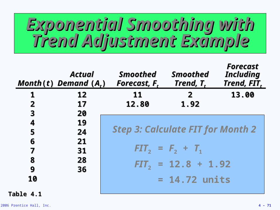
FIT2 = F2 + T1
FIT2 = 12.8 + 1.92
= 14.72 units
Step 3: Calculate FIT for Month 2
© 2006 Prentice Hall, Inc. 4 – 72
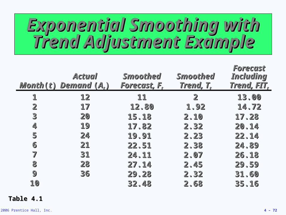
Exponential Smoothing with Exponential Smoothing with Trend Adjustment ExampleTrend Adjustment Example
ForecastForecastActualActual SmoothedSmoothed SmoothedSmoothed IncludingIncluding
MonthMonth((tt)) Demand Demand ((AAtt)) Forecast, FForecast, Ftt Trend, TTrend, Ttt Trend, FITTrend, FITtt
11 1212 1111 22 13.0013.0022 1717 12.8012.80 1.921.92 14.7214.7233 202044 191955 242466 212177 313188 282899 3636
1010
Table 4.1Table 4.1
15.1815.18 2.102.10 17.2817.2817.8217.82 2.322.32 20.1420.1419.9119.91 2.232.23 22.1422.1422.5122.51 2.382.38 24.8924.8924.1124.11 2.072.07 26.1826.1827.1427.14 2.452.45 29.5929.5929.2829.28 2.322.32 31.6031.6032.4832.48 2.682.68 35.1635.16
© 2006 Prentice Hall, Inc. 4 – 73
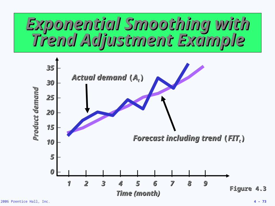
Exponential Smoothing with Exponential Smoothing with Trend Adjustment ExampleTrend Adjustment Example
Figure 4.3Figure 4.3
| | | | | | | | |
11 22 33 44 55 66 77 88 99
Time (month)Time (month)
Pro
du
ct d
eman
dP
rod
uct
dem
and
35 35 –
30 30 –
25 25 –
20 20 –
15 15 –
10 10 –
5 5 –
0 0 –
Actual demand Actual demand ((AAtt))
Forecast including trend Forecast including trend ((FITFITtt))
© 2006 Prentice Hall, Inc. 4 – 74
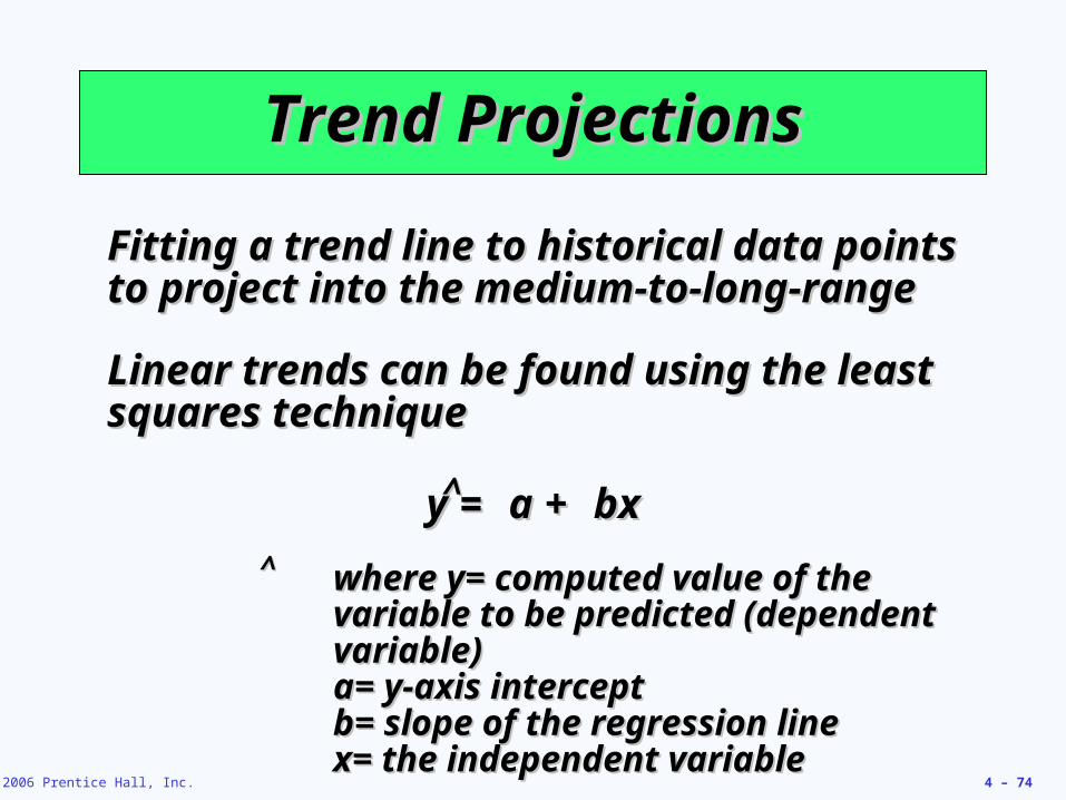
Trend ProjectionsTrend Projections
Fitting a trend line to historical data points Fitting a trend line to historical data points to project into the medium-to-long-rangeto project into the medium-to-long-range
Linear trends can be found using the least Linear trends can be found using the least squares techniquesquares technique
y y = = a a + + bxbx^̂
where ywhere y= computed value of the = computed value of the variable to be predicted (dependent variable to be predicted (dependent variable)variable)aa= y-axis intercept= y-axis interceptbb= slope of the regression line= slope of the regression linexx= the independent variable= the independent variable
^̂
© 2006 Prentice Hall, Inc. 4 – 75
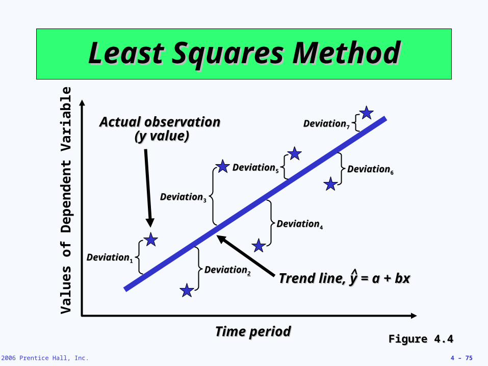
Least Squares MethodLeast Squares Method
Time periodTime period
Va
lue
s o
f D
ep
end
en
t V
ari
able
Figure 4.4Figure 4.4
DeviationDeviation11
DeviationDeviation55
DeviationDeviation77
DeviationDeviation22
DeviationDeviation66
DeviationDeviation44
DeviationDeviation33
Actual observation Actual observation (y value)(y value)
Trend line, y = a + bxTrend line, y = a + bx^̂
© 2006 Prentice Hall, Inc. 4 – 76
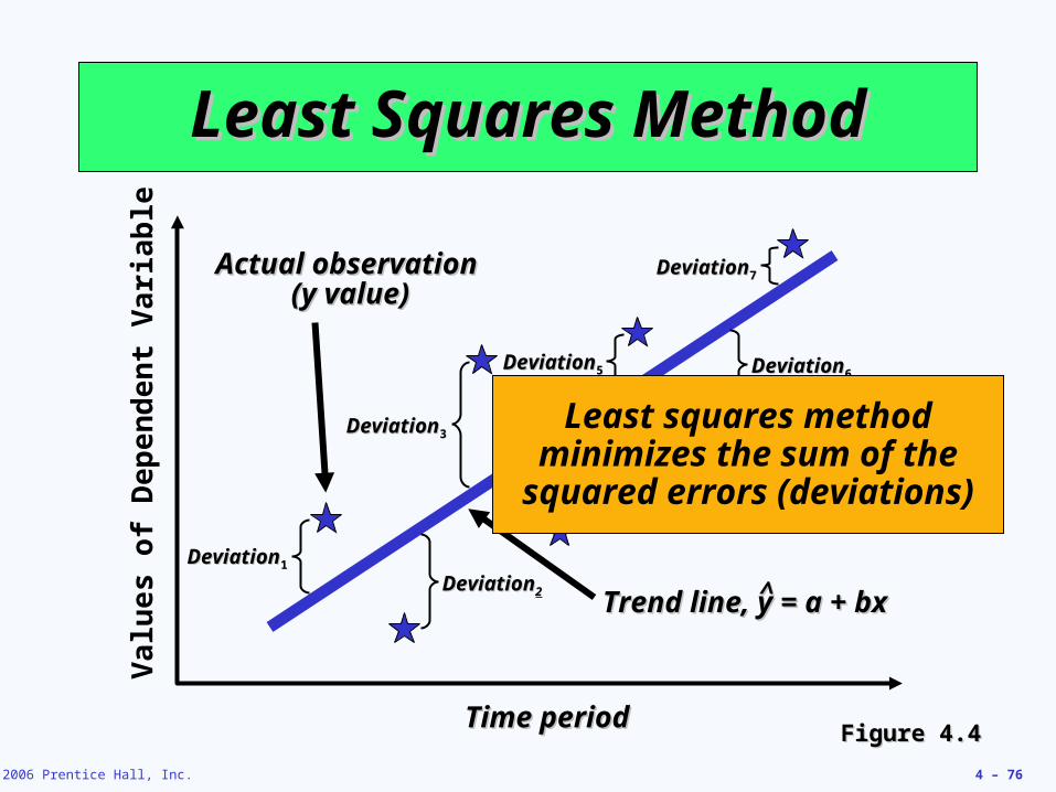
Least Squares MethodLeast Squares Method
Time periodTime period
Va
lue
s o
f D
ep
end
en
t V
ari
able
Figure 4.4Figure 4.4
DeviationDeviation11
DeviationDeviation55
DeviationDeviation77
DeviationDeviation22
DeviationDeviation66
DeviationDeviation44
DeviationDeviation33
Actual observation Actual observation (y value)(y value)
Trend line, y = a + bxTrend line, y = a + bx^̂
Least squares method minimizes the sum of the
squared errors (deviations)
© 2006 Prentice Hall, Inc. 4 – 77
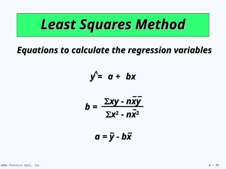
Least Squares MethodLeast Squares Method
Equations to calculate the regression variablesEquations to calculate the regression variables
b =b =xy - nxyxy - nxy
xx22 - nx - nx22
y y = = a a + + bxbx^̂
a = y - bxa = y - bx
© 2006 Prentice Hall, Inc. 4 – 78
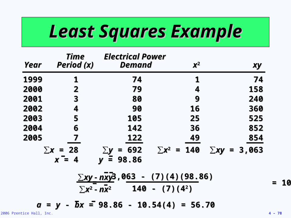
Least Squares ExampleLeast Squares Example
b b = = = 10.54= = = 10.54∑∑xy - nxyxy - nxy
∑∑xx22 - nx - nx22
3,063 - (7)(4)(98.86)3,063 - (7)(4)(98.86)
140 - (7)(4140 - (7)(422))
aa = = yy - - bxbx = 98.86 - 10.54(4) = 56.70 = 98.86 - 10.54(4) = 56.70
TimeTime Electrical Power Electrical Power YearYear Period (x)Period (x) DemandDemand xx22 xyxy
19991999 11 7474 11 747420002000 22 7979 44 15815820012001 33 8080 99 24024020022002 44 9090 1616 36036020032003 55 105105 2525 52552520042004 66 142142 3636 85285220052005 77 122122 4949 854854
∑∑xx = 28 = 28 ∑∑yy = 692 = 692 ∑∑xx22 = 140 = 140 ∑∑xyxy = 3,063 = 3,063xx = 4 = 4 yy = 98.86 = 98.86
© 2006 Prentice Hall, Inc. 4 – 79
Least Squares ExampleLeast Squares Example
b b = = = 10.54= = = 10.54xy - nxyxy - nxy
xx22 - nx - nx22
3,063 - (7)(4)(98.86)3,063 - (7)(4)(98.86)
140 - (7)(4140 - (7)(422))
aa = = yy - - bxbx = 98.86 - 10.54(4) = 56.70 = 98.86 - 10.54(4) = 56.70
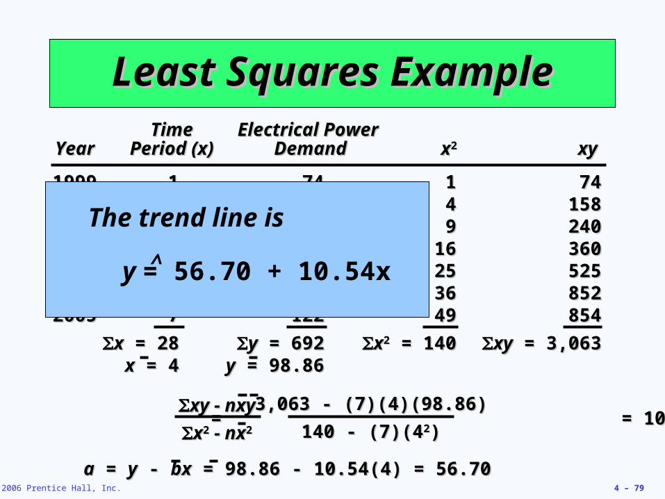
TimeTime Electrical Power Electrical Power YearYear Period (x)Period (x) DemandDemand xx22 xyxy
19991999 11 7474 11 747420002000 22 7979 44 15815820012001 33 8080 99 24024020022002 44 9090 1616 36036020032003 55 105105 2525 52552520042004 66 142142 3636 85285220052005 77 122122 4949 854854
xx = 28 = 28 yy = 692 = 692 xx22 = 140 = 140 xyxy = 3,063 = 3,063xx = 4 = 4 yy = 98.86 = 98.86
The trend line is
y = 56.70 + 10.54x^
© 2006 Prentice Hall, Inc. 4 – 80
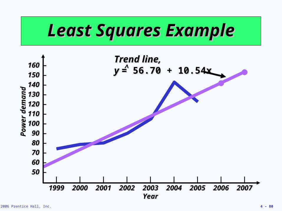
Least Squares ExampleLeast Squares Example
| | | | | | | | |19991999 20002000 20012001 20022002 20032003 20042004 20052005 20062006 20072007
160 160 –
150 150 –
140 140 –
130 130 –
120 120 –
110 110 –
100 100 –
90 90 –
80 80 –
70 70 –
60 60 –
50 50 –
YearYear
Po
wer
dem
and
Po
wer
dem
and
Trend line,Trend line,y y = 56.70 + 10.54x= 56.70 + 10.54x^̂
© 2006 Prentice Hall, Inc. 4 – 82
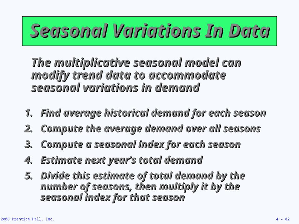
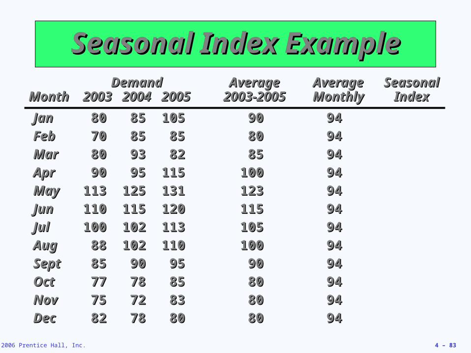
Seasonal Variations In DataSeasonal Variations In Data
The multiplicative seasonal model can The multiplicative seasonal model can modify trend data to accommodate modify trend data to accommodate seasonal variations in demandseasonal variations in demand
1.1. Find average historical demand for each season Find average historical demand for each season
2.2. Compute the average demand over all seasons Compute the average demand over all seasons
3.3. Compute a seasonal index for each season Compute a seasonal index for each season
4.4. Estimate next year’s total demandEstimate next year’s total demand
5.5. Divide this estimate of total demand by the Divide this estimate of total demand by the number of seasons, then multiply it by the number of seasons, then multiply it by the seasonal index for that seasonseasonal index for that season
© 2006 Prentice Hall, Inc. 4 – 83
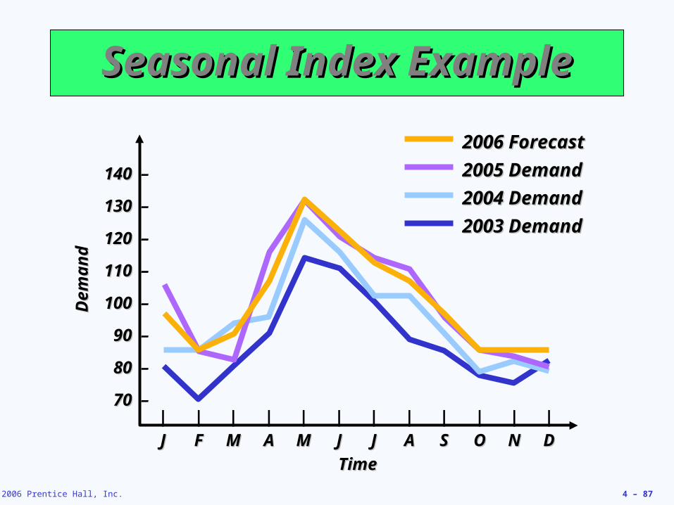
Seasonal Index ExampleSeasonal Index Example
JanJan 8080 8585 105105 9090 9494
FebFeb 7070 8585 8585 8080 9494
MarMar 8080 9393 8282 8585 9494
AprApr 9090 9595 115115 100100 9494
MayMay 113113 125125 131131 123123 9494
JunJun 110110 115115 120120 115115 9494
JulJul 100100 102102 113113 105105 9494
AugAug 8888 102102 110110 100100 9494
SeptSept 8585 9090 9595 9090 9494
OctOct 7777 7878 8585 8080 9494
NovNov 7575 7272 8383 8080 9494
DecDec 8282 7878 8080 8080 9494
DemandDemand AverageAverage AverageAverage Seasonal Seasonal MonthMonth 20032003 20042004 20052005 2003-20052003-2005 MonthlyMonthly IndexIndex
© 2006 Prentice Hall, Inc. 4 – 84
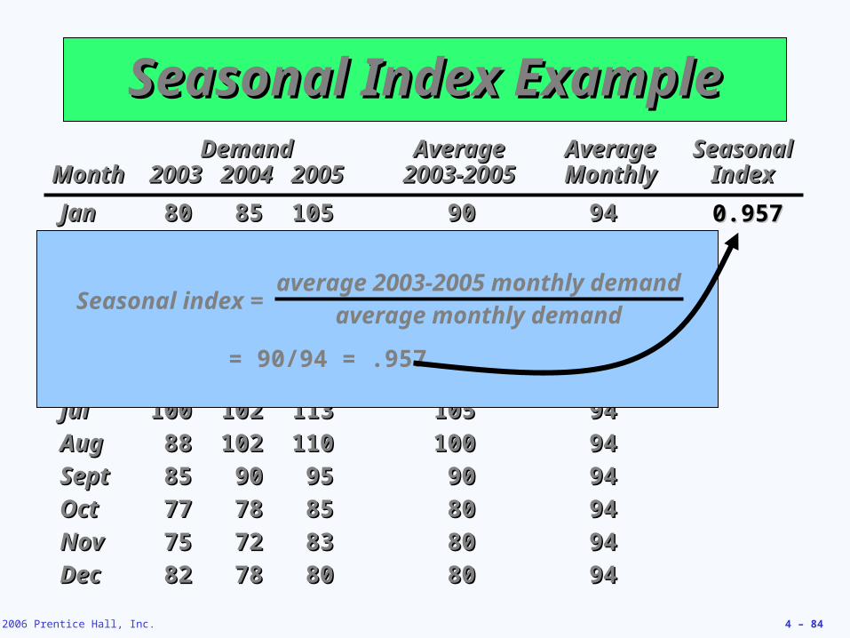
Seasonal Index ExampleSeasonal Index Example
JanJan 8080 8585 105105 9090 9494
FebFeb 7070 8585 8585 8080 9494
MarMar 8080 9393 8282 8585 9494
AprApr 9090 9595 115115 100100 9494
MayMay 113113 125125 131131 123123 9494
JunJun 110110 115115 120120 115115 9494
JulJul 100100 102102 113113 105105 9494
AugAug 8888 102102 110110 100100 9494
SeptSept 8585 9090 9595 9090 9494
OctOct 7777 7878 8585 8080 9494
NovNov 7575 7272 8383 8080 9494
DecDec 8282 7878 8080 8080 9494
DemandDemand AverageAverage AverageAverage Seasonal Seasonal MonthMonth 20032003 20042004 20052005 2003-20052003-2005 MonthlyMonthly IndexIndex
0.9570.957
Seasonal index = average 2003-2005 monthly demand
average monthly demand
= 90/94 = .957
© 2006 Prentice Hall, Inc. 4 – 85
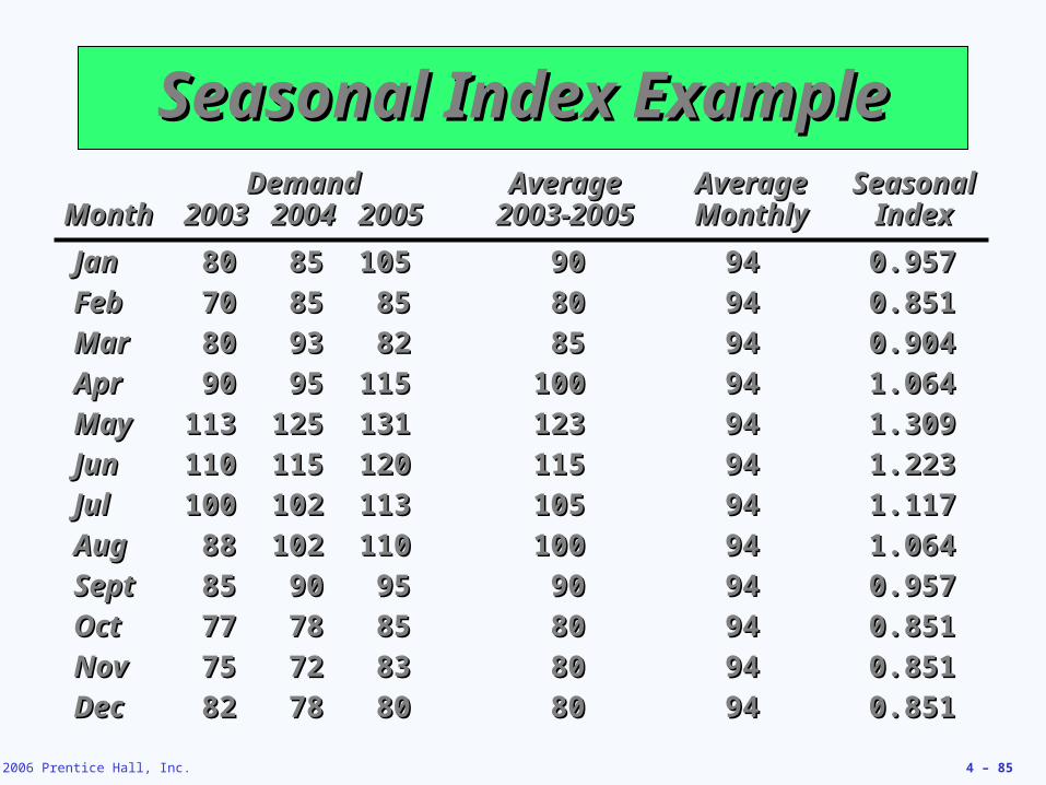
Seasonal Index ExampleSeasonal Index Example
JanJan 8080 8585 105105 9090 9494 0.9570.957
FebFeb 7070 8585 8585 8080 9494 0.8510.851
MarMar 8080 9393 8282 8585 9494 0.9040.904
AprApr 9090 9595 115115 100100 9494 1.0641.064
MayMay 113113 125125 131131 123123 9494 1.3091.309
JunJun 110110 115115 120120 115115 9494 1.2231.223
JulJul 100100 102102 113113 105105 9494 1.1171.117
AugAug 8888 102102 110110 100100 9494 1.0641.064
SeptSept 8585 9090 9595 9090 9494 0.9570.957
OctOct 7777 7878 8585 8080 9494 0.8510.851
NovNov 7575 7272 8383 8080 9494 0.8510.851
DecDec 8282 7878 8080 8080 9494 0.8510.851
DemandDemand AverageAverage AverageAverage Seasonal Seasonal MonthMonth 20032003 20042004 20052005 2003-20052003-2005 MonthlyMonthly IndexIndex
© 2006 Prentice Hall, Inc. 4 – 86
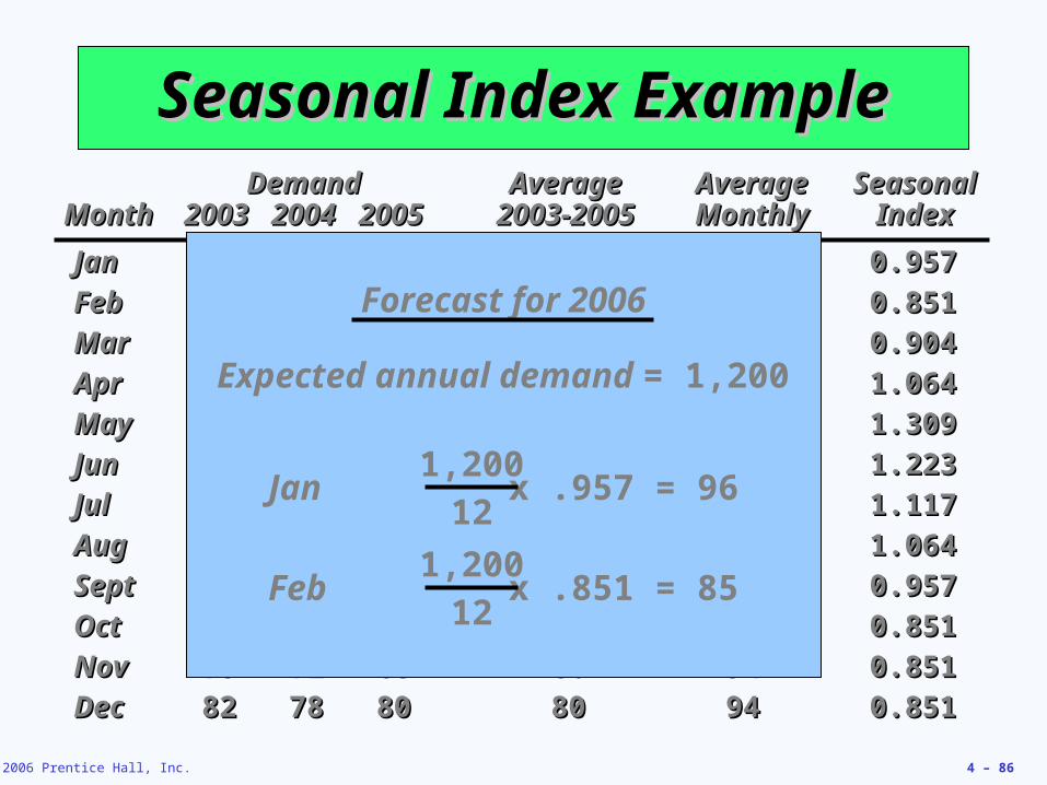
Seasonal Index ExampleSeasonal Index Example
JanJan 8080 8585 105105 9090 9494 0.9570.957
FebFeb 7070 8585 8585 8080 9494 0.8510.851
MarMar 8080 9393 8282 8585 9494 0.9040.904
AprApr 9090 9595 115115 100100 9494 1.0641.064
MayMay 113113 125125 131131 123123 9494 1.3091.309
JunJun 110110 115115 120120 115115 9494 1.2231.223
JulJul 100100 102102 113113 105105 9494 1.1171.117
AugAug 8888 102102 110110 100100 9494 1.0641.064
SeptSept 8585 9090 9595 9090 9494 0.9570.957
OctOct 7777 7878 8585 8080 9494 0.8510.851
NovNov 7575 7272 8383 8080 9494 0.8510.851
DecDec 8282 7878 8080 8080 9494 0.8510.851
DemandDemand AverageAverage AverageAverage Seasonal Seasonal MonthMonth 20032003 20042004 20052005 2003-20052003-2005 MonthlyMonthly IndexIndex
Expected annual demand = 1,200
Jan x .957 = 961,200
12
Feb x .851 = 851,200
12
Forecast for 2006
© 2006 Prentice Hall, Inc. 4 – 87
Seasonal Index ExampleSeasonal Index Example
140 140 –
130 130 –
120 120 –
110 110 –
100 100 –
90 90 –
80 80 –
70 70 –| | | | | | | | | | | |
JJ FF MM AA MM JJ JJ AA SS OO NN DD
TimeTime
Dem
and
Dem
and
2006 Forecast2006 Forecast
2005 Demand 2005 Demand
2004 Demand2004 Demand
2003 Demand2003 Demand
© 2006 Prentice Hall, Inc. 4 – 88
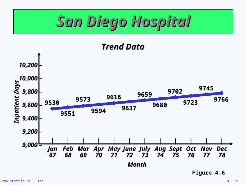
San Diego HospitalSan Diego Hospital
10,200 10,200 –
10,000 10,000 –
9,800 9,800 –
9,600 9,600 –
9,400 9,400 –
9,200 9,200 –
9,000 9,000 –| | | | | | | | | | | |
JanJan FebFeb MarMar AprApr MayMay JuneJune JulyJuly AugAug SeptSept OctOct NovNov DecDec6767 6868 6969 7070 7171 7272 7373 7474 7575 7676 7777 7878
MonthMonth
Inp
atie
nt
Day
sIn
pat
ien
t D
ays
95309530
95519551
95739573
95949594
96169616
96379637
96599659
96809680
97029702
97239723
97459745
97669766
Figure 4.6Figure 4.6
Trend DataTrend Data
© 2006 Prentice Hall, Inc. 4 – 89
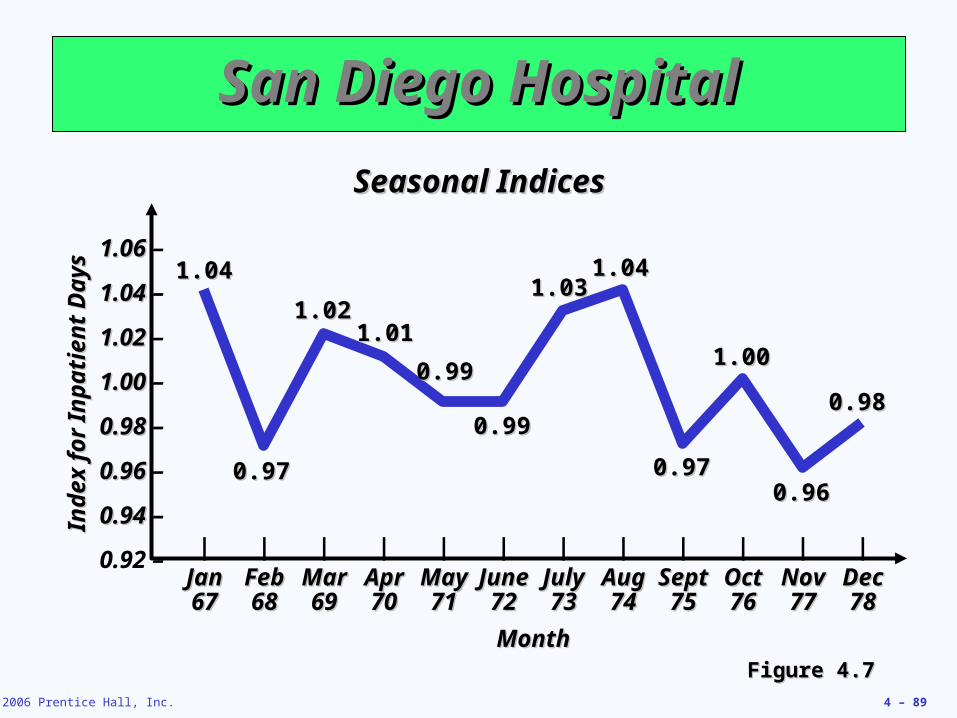
San Diego HospitalSan Diego Hospital
1.06 1.06 –
1.04 1.04 –
1.02 1.02 –
1.00 1.00 –
0.98 0.98 –
0.96 0.96 –
0.94 0.94 –
0.92 – | | | | | | | | | | | |JanJan FebFeb MarMar AprApr MayMay JuneJune JulyJuly AugAug SeptSept OctOct NovNov DecDec6767 6868 6969 7070 7171 7272 7373 7474 7575 7676 7777 7878
MonthMonth
Ind
ex f
or
Inp
atie
nt
Day
sIn
dex
fo
r In
pat
ien
t D
ays 1.041.04
1.021.021.011.01
0.990.99
1.031.031.041.04
1.001.00
0.980.98
0.970.97
0.990.99
0.970.970.960.96
Figure 4.7Figure 4.7
Seasonal IndicesSeasonal Indices
© 2006 Prentice Hall, Inc. 4 – 90
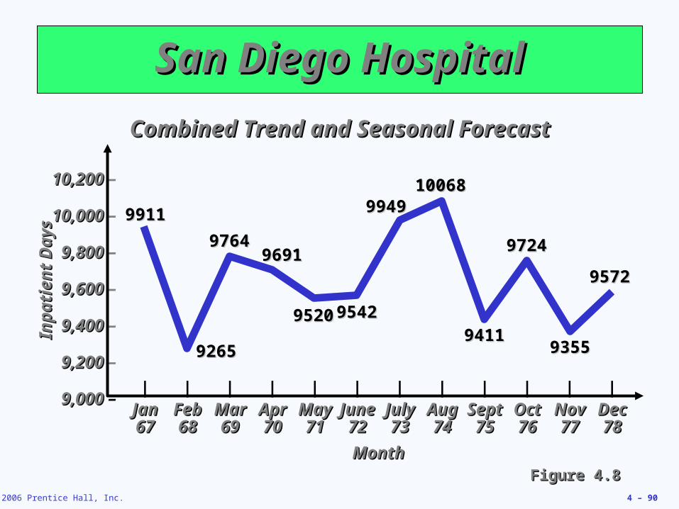
San Diego HospitalSan Diego Hospital
10,200 10,200 –
10,000 10,000 –
9,800 9,800 –
9,600 9,600 –
9,400 9,400 –
9,200 9,200 –
9,000 9,000 –| | | | | | | | | | | |
JanJan FebFeb MarMar AprApr MayMay JuneJune JulyJuly AugAug SeptSept OctOct NovNov DecDec6767 6868 6969 7070 7171 7272 7373 7474 7575 7676 7777 7878
MonthMonth
Inp
atie
nt
Day
sIn
pat
ien
t D
ays
Figure 4.8Figure 4.8
99119911
92659265
97649764
95209520
96919691
94119411
99499949
97249724
95429542
93559355
1006810068
95729572
Combined Trend and Seasonal ForecastCombined Trend and Seasonal Forecast
© 2006 Prentice Hall, Inc. 4 – 91
Associative ForecastingAssociative Forecasting
Used when changes in one or more Used when changes in one or more independent variables can be used to predict independent variables can be used to predict
the changes in the dependent variablethe changes in the dependent variable
Most common technique is linear Most common technique is linear regression analysisregression analysis
We apply this technique just as we did We apply this technique just as we did in the time series examplein the time series example
© 2006 Prentice Hall, Inc. 4 – 92
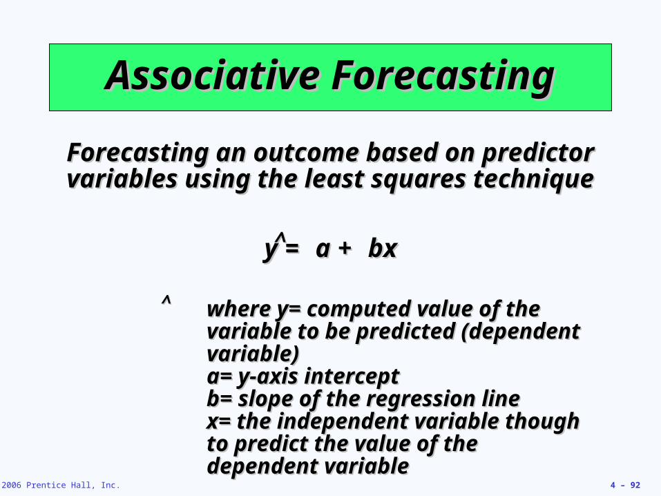
Associative ForecastingAssociative Forecasting
Forecasting an outcome based on predictor Forecasting an outcome based on predictor variables using the least squares techniquevariables using the least squares technique
y y = = a a + + bxbx^̂
where ywhere y= computed value of the = computed value of the variable to be predicted (dependent variable to be predicted (dependent variable)variable)aa= y-axis intercept= y-axis interceptbb= slope of the regression line= slope of the regression linexx= the independent variable though = the independent variable though to predict the value of the to predict the value of the dependent variabledependent variable
^̂
© 2006 Prentice Hall, Inc. 4 – 93
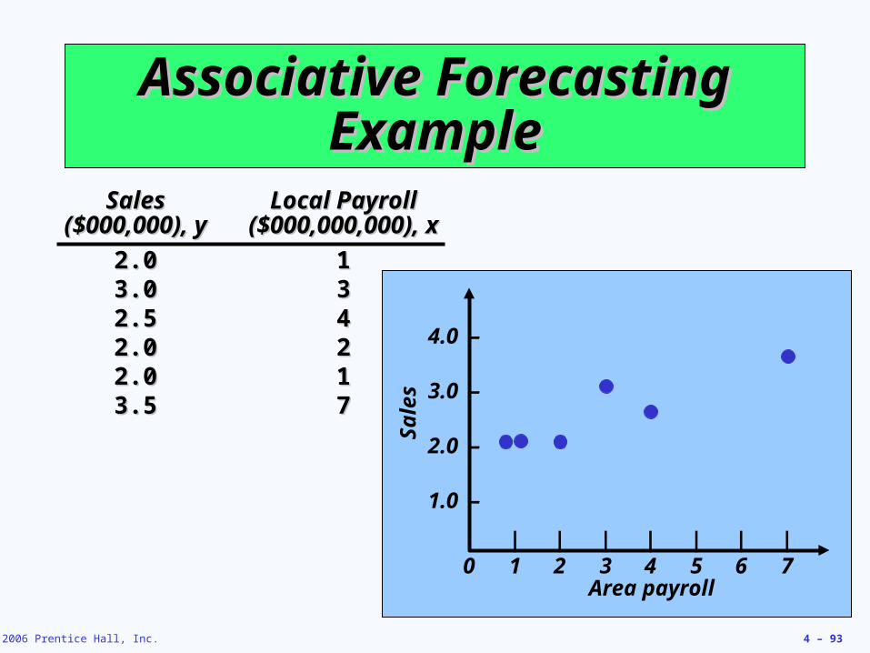
Associative Forecasting Associative Forecasting ExampleExample
SalesSales Local PayrollLocal Payroll($000,000), y($000,000), y ($000,000,000), x($000,000,000), x
2.02.0 113.03.0 332.52.5 442.02.0 222.02.0 113.53.5 77
4.0 –
3.0 –
2.0 –
1.0 –
| | | | | | |0 1 2 3 4 5 6 7
Sal
es
Area payroll
© 2006 Prentice Hall, Inc. 4 – 94
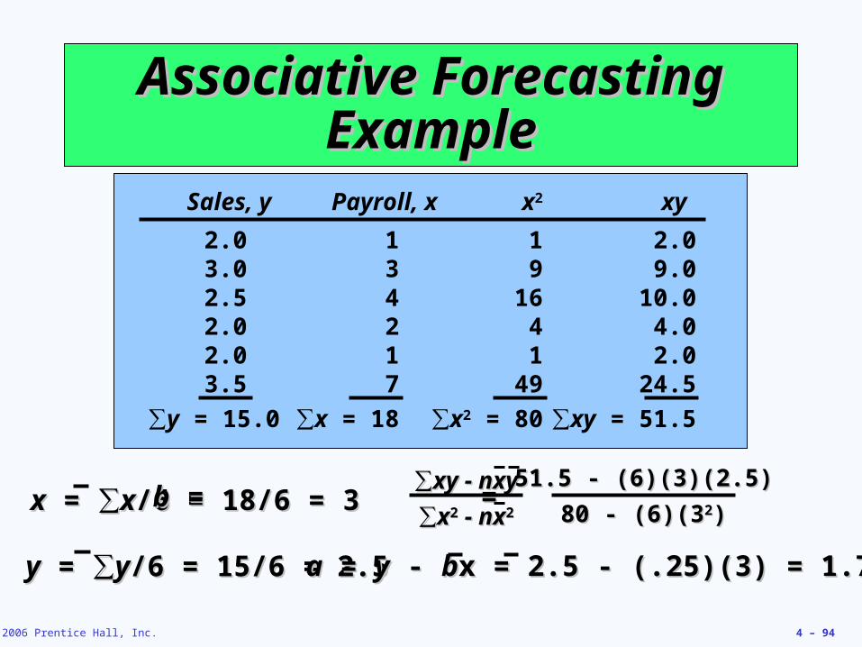
Associative Forecasting Associative Forecasting ExampleExample
Sales, y Payroll, x x2 xy
2.0 1 1 2.03.0 3 9 9.02.5 4 16 10.02.0 2 4 4.02.0 1 1 2.03.5 7 49 24.5
∑y = 15.0 ∑x = 18 ∑x2 = 80 ∑xy = 51.5
xx = = ∑∑xx/6 = 18/6 = 3/6 = 18/6 = 3
yy = = ∑∑yy/6 = 15/6 = 2.5/6 = 15/6 = 2.5
bb = = = .25 = = = .25∑∑xy - nxyxy - nxy
∑∑xx22 - nx - nx22
51.5 - (6)(3)(2.5)51.5 - (6)(3)(2.5)
80 - (6)(380 - (6)(322))
aa = = yy - - bbx = 2.5 - (.25)(3) = 1.75x = 2.5 - (.25)(3) = 1.75
© 2006 Prentice Hall, Inc. 4 – 95
Associative Forecasting Associative Forecasting ExampleExample
4.0 –
3.0 –
2.0 –
1.0 –
| | | | | | |0 1 2 3 4 5 6 7
Sal
es
Area payroll
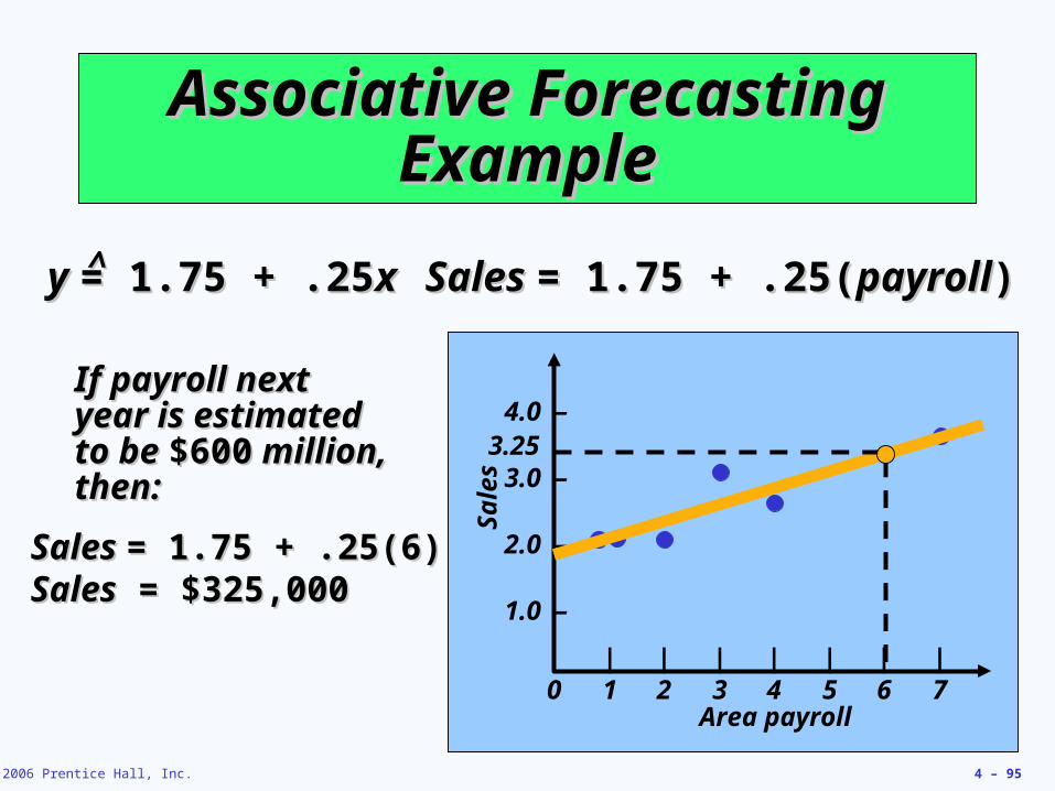
y y = 1.75 + .25= 1.75 + .25xx^̂ Sales Sales = 1.75 + .25(= 1.75 + .25(payrollpayroll))
If payroll next year If payroll next year is estimated to be is estimated to be $600$600 million, then: million, then:
Sales Sales = 1.75 + .25(6)= 1.75 + .25(6)SalesSales = $325,000 = $325,000
3.25
© 2006 Prentice Hall, Inc. 4 – 96
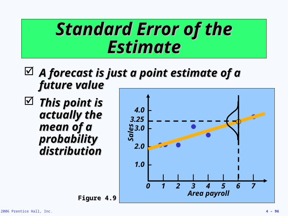
Standard Error of the Standard Error of the EstimateEstimate
A forecast is just a point estimate of a A forecast is just a point estimate of a future valuefuture value
This point is This point is actually the actually the mean of a mean of a probability probability distributiondistribution
Figure 4.9Figure 4.9
4.0 –
3.0 –
2.0 –
1.0 –
| | | | | | |0 1 2 3 4 5 6 7
Sal
es
Area payroll
3.25
© 2006 Prentice Hall, Inc. 4 – 97
Standard Error of the Standard Error of the EstimateEstimate
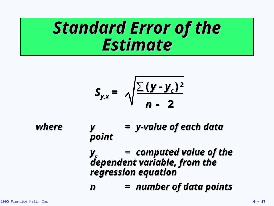
wherewhere yy == y-value of each data y-value of each data pointpoint
yycc == computed value of the computed value of the dependent variable, from the dependent variable, from the regression equationregression equation
nn == number of data pointsnumber of data points
SSy,xy,x = =∑∑((y - yy - ycc))22
n n - 2- 2
© 2006 Prentice Hall, Inc. 4 – 98
Standard Error of the Standard Error of the EstimateEstimate
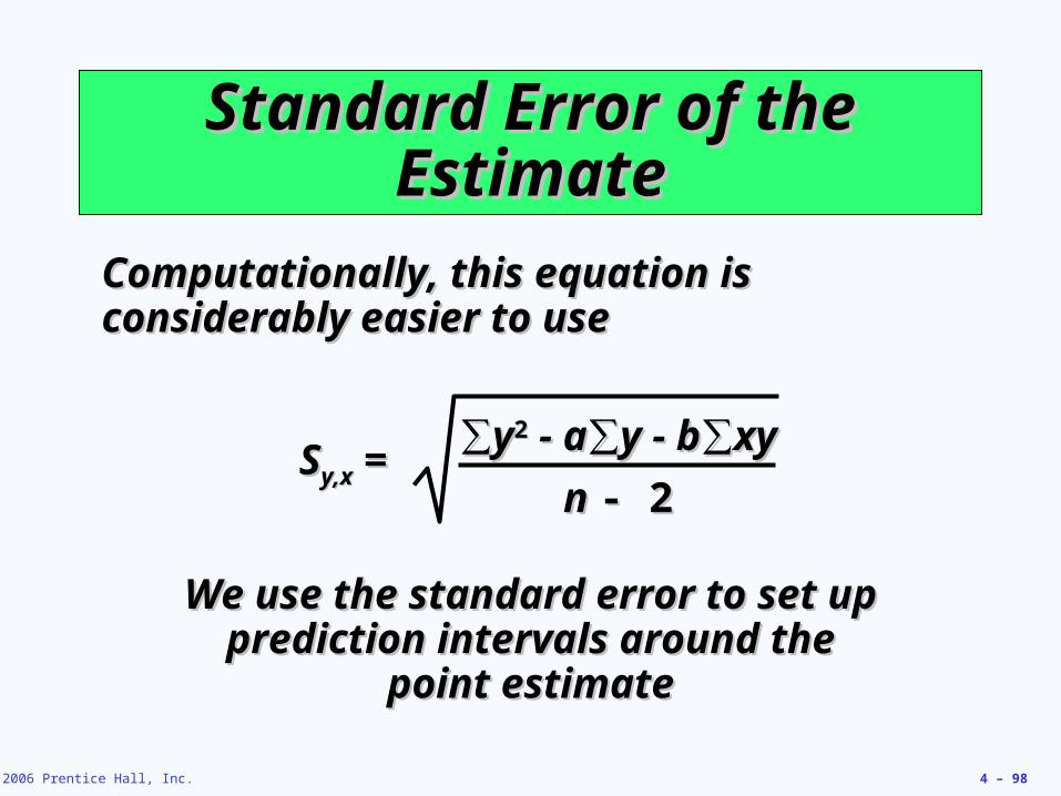
Computationally, this equation is Computationally, this equation is considerably easier to useconsiderably easier to use
We use the standard error to set up We use the standard error to set up prediction intervals around the prediction intervals around the
point estimatepoint estimate
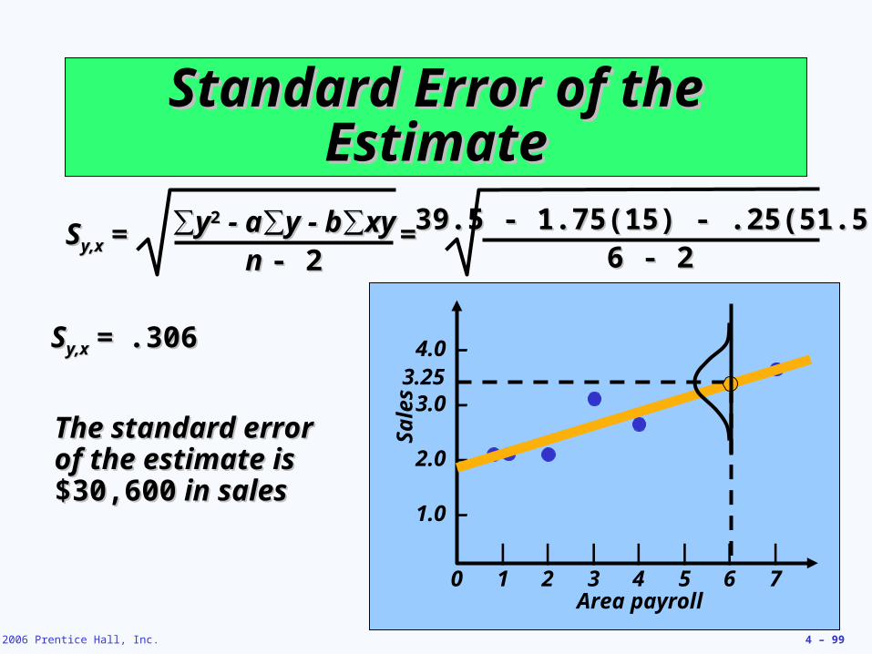
SSy,xy,x = =∑∑yy22 - a - a∑∑y - by - b∑∑xyxy
n n - 2- 2
© 2006 Prentice Hall, Inc. 4 – 99
Standard Error of the Standard Error of the EstimateEstimate
4.0 –
3.0 –
2.0 –
1.0 –
| | | | | | |0 1 2 3 4 5 6 7
Sal
es
Area payroll
3.25
SSy,xy,x = = = =∑∑yy22 - a - a∑∑y - by - b∑∑xyxyn n - 2- 2
39.5 - 1.75(15) - .25(51.5)39.5 - 1.75(15) - .25(51.5)6 - 26 - 2
SSy,xy,x = = .306.306
The standard error The standard error of the estimate is of the estimate is $30,600$30,600 in sales in sales
© 2006 Prentice Hall, Inc. 4 – 100
How strong is the linear How strong is the linear relationship between the relationship between the variables?variables?
Correlation does not necessarily Correlation does not necessarily imply causality!imply causality!
Coefficient of correlation, r, Coefficient of correlation, r, measures degree of associationmeasures degree of association Values range from Values range from -1-1 to to +1+1
CorrelationCorrelation
© 2006 Prentice Hall, Inc. 4 – 101
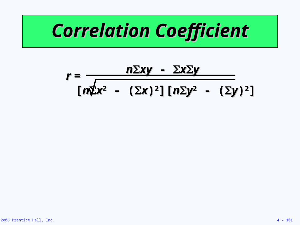
Correlation CoefficientCorrelation Coefficient
r = r = nnxyxy - - xxy y
[[nnxx22 - ( - (xx))22][][nnyy22 - ( - (yy))22]]
© 2006 Prentice Hall, Inc. 4 – 102
Correlation CoefficientCorrelation Coefficient
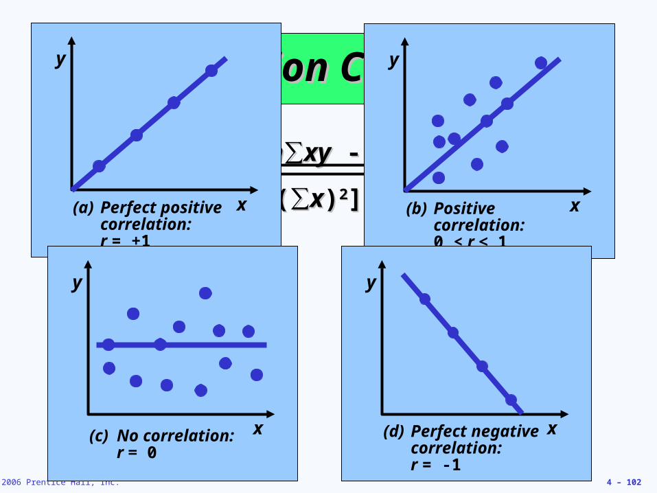
r = r = nn∑∑xyxy - - ∑∑xx∑∑y y
[[nn∑∑xx22 - ( - (∑∑xx))22][][nn∑∑yy22 - ( - (∑∑yy))22]]
y
x(a) Perfect positive correlation: r = +1
y
x(b) Positive correlation: 0 < r < 1
y
x(c) No correlation: r = 0
y
x(d) Perfect negative correlation: r = -1
© 2006 Prentice Hall, Inc. 4 – 103
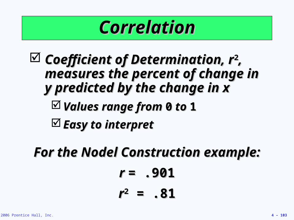
Coefficient of Determination, rCoefficient of Determination, r22, , measures the percent of change in measures the percent of change in y predicted by the change in xy predicted by the change in x Values range from Values range from 00 to to 11
Easy to interpretEasy to interpret
CorrelationCorrelation
For the Nodel Construction example:For the Nodel Construction example:
r r = .901= .901
rr22 = .81 = .81

© 2006 Prentice Hall, Inc. 4 – 104
Multiple Regression Multiple Regression AnalysisAnalysis
If more than one independent variable is to be If more than one independent variable is to be used in the model, linear regression can be used in the model, linear regression can be
extended to multiple regression to extended to multiple regression to accommodate several independent variablesaccommodate several independent variables
y y = = a a + + bb11xx11 + b + b22xx22 … …^̂
Computationally, this is quite Computationally, this is quite complex and generally done on the complex and generally done on the
computercomputer
© 2006 Prentice Hall, Inc. 4 – 105
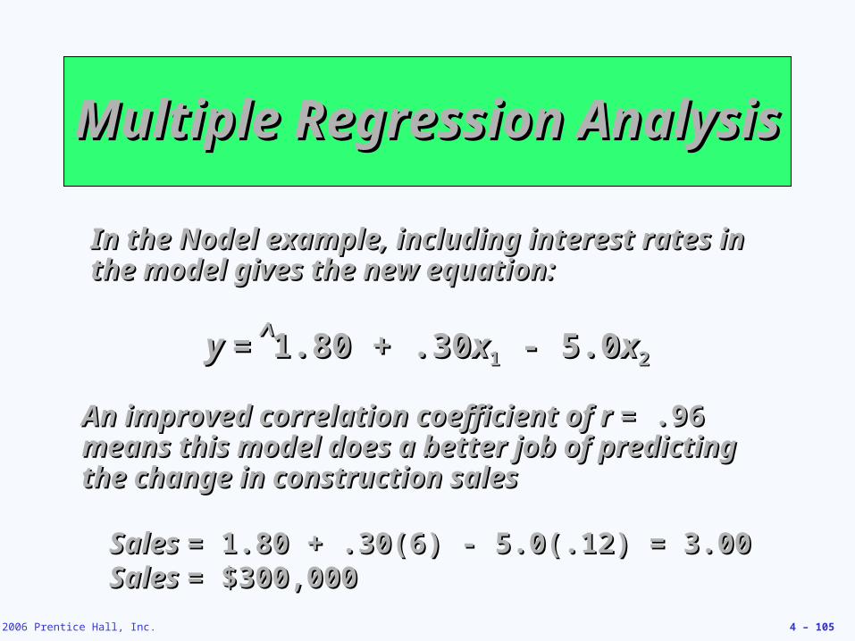
Multiple Regression Multiple Regression AnalysisAnalysis
y y = 1.80 + .30= 1.80 + .30xx11 - 5.0 - 5.0xx22^̂
In the Nodel example, including interest rates in In the Nodel example, including interest rates in the model gives the new equation:the model gives the new equation:
An improved correlation coefficient of r An improved correlation coefficient of r = .96= .96 means this model does a better job of predicting means this model does a better job of predicting the change in construction salesthe change in construction sales
Sales Sales = 1.80 + .30(6) - 5.0(.12) = 3.00= 1.80 + .30(6) - 5.0(.12) = 3.00Sales Sales = $300,000= $300,000
© 2006 Prentice Hall, Inc. 4 – 106
Measures how well the forecast is Measures how well the forecast is predicting actual valuespredicting actual values
Ratio of running sum of forecast errors Ratio of running sum of forecast errors (RSFE) to mean absolute deviation (MAD)(RSFE) to mean absolute deviation (MAD) Good tracking signal has low valuesGood tracking signal has low values
If forecasts are continually high or low, the If forecasts are continually high or low, the forecast has a forecast has a bias errorbias error
Monitoring and Controlling Monitoring and Controlling ForecastsForecasts
Tracking SignalTracking Signal
© 2006 Prentice Hall, Inc. 4 – 107
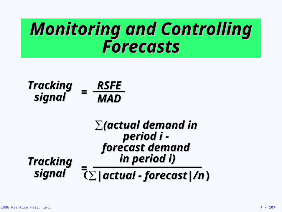
Monitoring and Controlling Monitoring and Controlling ForecastsForecasts
Tracking Tracking signalsignal
RSFERSFEMADMAD==
Tracking Tracking signalsignal ==
∑∑(actual demand in (actual demand in period i - period i -
forecast demand forecast demand in period i)in period i)
∑∑|actual - forecast|/n|actual - forecast|/n))
© 2006 Prentice Hall, Inc. 4 – 108
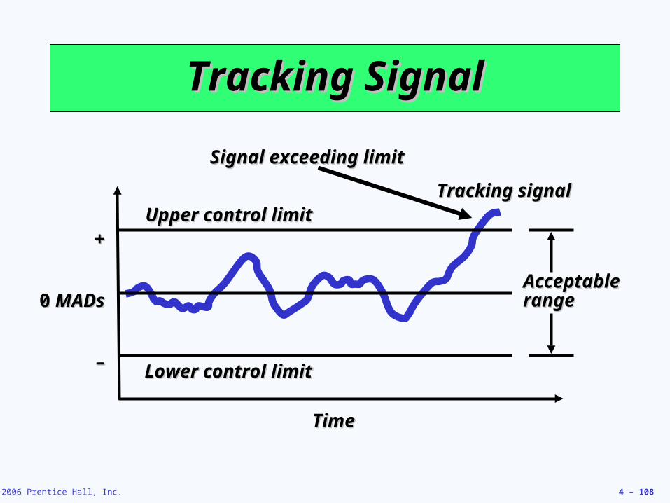
Tracking SignalTracking Signal
Tracking signalTracking signal
++
00 MADs MADs
––
Upper control limitUpper control limit
Lower control limitLower control limit
TimeTime
Signal exceeding limitSignal exceeding limit
Acceptable Acceptable rangerange
© 2006 Prentice Hall, Inc. 4 – 109
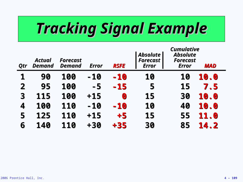
Tracking Signal ExampleTracking Signal ExampleCumulativeCumulative
AbsoluteAbsolute AbsoluteAbsoluteActualActual ForecastForecast ForecastForecast ForecastForecast
QtrQtr DemandDemand DemandDemand ErrorError RSFERSFE ErrorError ErrorError MADMAD
11 9090 100100 -10-10 -10-10 1010 1010 10.010.022 9595 100100 -5-5 -15-15 55 1515 7.57.533 115115 100100 +15+15 00 1515 3030 10.010.044 100100 110110 -10-10 -10-10 1010 4040 10.010.055 125125 110110 +15+15 +5+5 1515 5555 11.011.066 140140 110110 +30+30 +35+35 3030 8585 14.214.2
© 2006 Prentice Hall, Inc. 4 – 110
CumulativeCumulativeAbsoluteAbsolute AbsoluteAbsolute
ActualActual ForecastForecast ForecastForecast ForecastForecastQtrQtr DemandDemand DemandDemand ErrorError RSFERSFE ErrorError ErrorError MADMAD
11 9090 100100 -10-10 -10-10 1010 1010 10.010.022 9595 100100 -5-5 -15-15 55 1515 7.57.533 115115 100100 +15+15 00 1515 3030 10.010.044 100100 110110 -10-10 -10-10 1010 4040 10.010.055 125125 110110 +15+15 +5+5 1515 5555 11.011.066 140140 110110 +30+30 +35+35 3030 8585 14.214.2
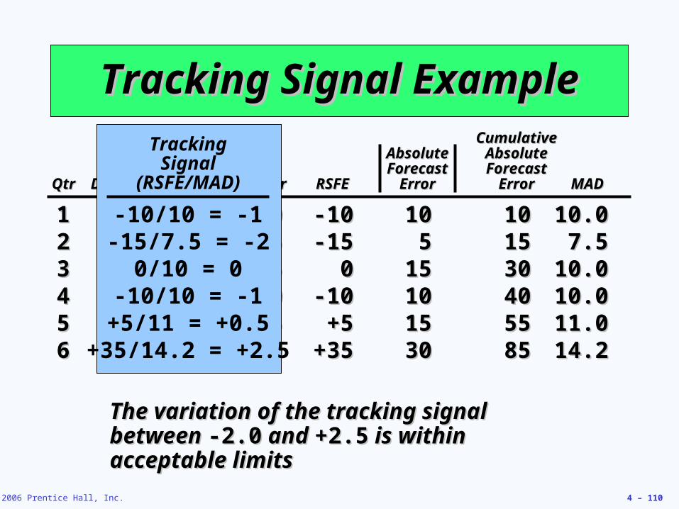
Tracking Signal ExampleTracking Signal ExampleTracking
Signal(RSFE/MAD)
-10/10 = -1-15/7.5 = -2
0/10 = 0-10/10 = -1
+5/11 = +0.5+35/14.2 = +2.5
The variation of the tracking signal The variation of the tracking signal between between -2.0-2.0 and and +2.5+2.5 is within acceptable is within acceptable limitslimits
© 2006 Prentice Hall, Inc. 4 – 111
Adaptive ForecastingAdaptive Forecasting
It’s possible to use the computer to It’s possible to use the computer to continually monitor forecast error and continually monitor forecast error and adjust the values of the adjust the values of the and and coefficients used in exponential coefficients used in exponential smoothing to continually minimize smoothing to continually minimize forecast errorforecast error
This technique is called adaptive This technique is called adaptive smoothingsmoothing
© 2006 Prentice Hall, Inc. 4 – 112
Focus ForecastingFocus Forecasting
Developed at American Hardware Supply, Developed at American Hardware Supply, focus forecasting is based on two principles:focus forecasting is based on two principles:
1.1. Sophisticated forecasting models are not Sophisticated forecasting models are not always better than simple modelsalways better than simple models
2.2. There is no single techniques that should There is no single techniques that should be used for all products or servicesbe used for all products or services
This approach uses historical data to test This approach uses historical data to test multiple forecasting models for individual itemsmultiple forecasting models for individual items
The forecasting model with the lowest error is The forecasting model with the lowest error is then used to forecast the next demandthen used to forecast the next demand
© 2006 Prentice Hall, Inc. 4 – 113
Forecasting in the Service Forecasting in the Service SectorSector
Presents unusual challengesPresents unusual challenges Special need for short term recordsSpecial need for short term records
Needs differ greatly as function of Needs differ greatly as function of industry and productindustry and product
Holidays and other calendar eventsHolidays and other calendar events
Unusual eventsUnusual events
© 2006 Prentice Hall, Inc. 4 – 114
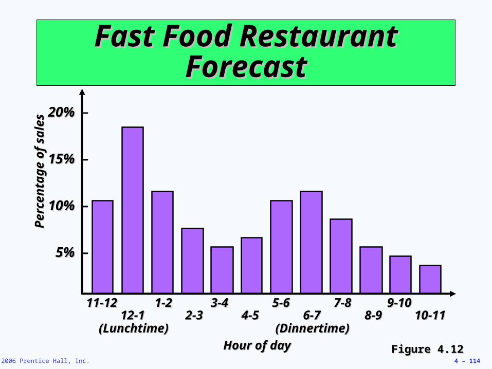
Fast Food Restaurant Fast Food Restaurant ForecastForecast
20% 20% –
15% 15% –
10% 10% –
5% 5% –
11-1211-12 1-21-2 3-43-4 5-65-6 7-87-8 9-109-1012-112-1 2-32-3 4-54-5 6-76-7 8-98-9 10-1110-11
(Lunchtime)(Lunchtime) (Dinnertime)(Dinnertime)
Hour of dayHour of day
Per
cen
tag
e o
f sa
les
Per
cen
tag
e o
f sa
les
Figure 4.12Figure 4.12