MANE 4240 & CIVL 4240Introduction to Finite Elements

Shape functions in 1D

Prof. Suvranu De

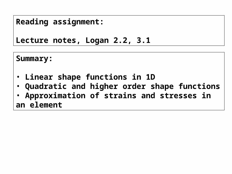
Reading assignment:

Lecture notes, Logan 2.2, 3.1

Summary:

• Linear shape functions in 1D • Quadratic and higher order shape functions• Approximation of strains and stresses in an element

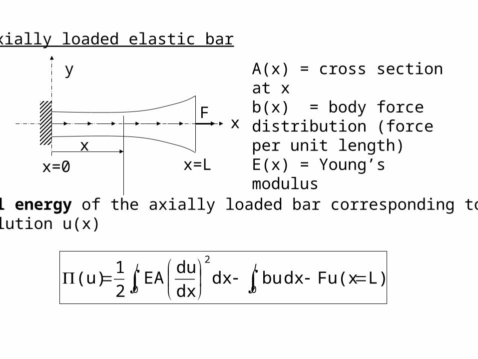
Axially loaded elastic bar

x

y

x=0 x=L

A(x) = cross section at xb(x) = body force distribution (force per unit length)E(x) = Young’s modulus

x

F

Potential energy of the axially loaded bar corresponding to the exact solution u(x)

L)Fu(xdxbudxdx

duEA

2

1(u)

00

2

LL

Finite element formulation, takes as its starting point, not the strong formulation, but the Principle of Minimum Potential Energy.

Task is to find the function ‘w’ that minimizes the potential energy of the system

From the Principle of Minimum Potential Energy, that function ‘w’ is the exact solution.

L)Fw(xdxbwdxdx

dwEA

2

1(w)

00

2

LL

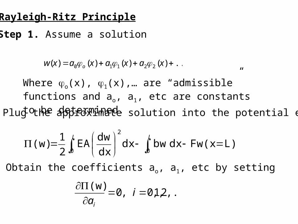
Step 1. Assume a solution

...)()()()( 22110 xaxaxaxw o

Where o(x), 1(x),… are “admissible” functions and ao, a1, etc are constants to be determined.

Step 2. Plug the approximate solution into the potential energy

L)Fw(xdxbwdxdx

dwEA

2

1(w)

00

2

LL

Step 3. Obtain the coefficients ao, a1, etc by setting

,...2,1,0,0(w)

iai

Rayleigh-Ritz Principle

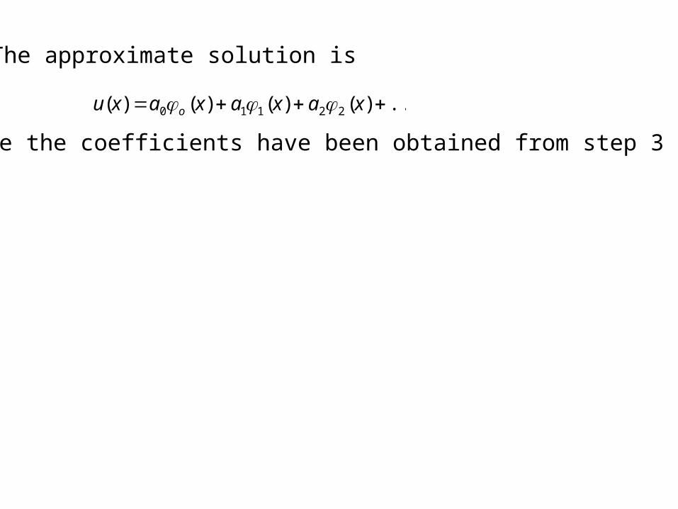
The approximate solution is

...)()()()( 22110 xaxaxaxu o

Where the coefficients have been obtained from step 3

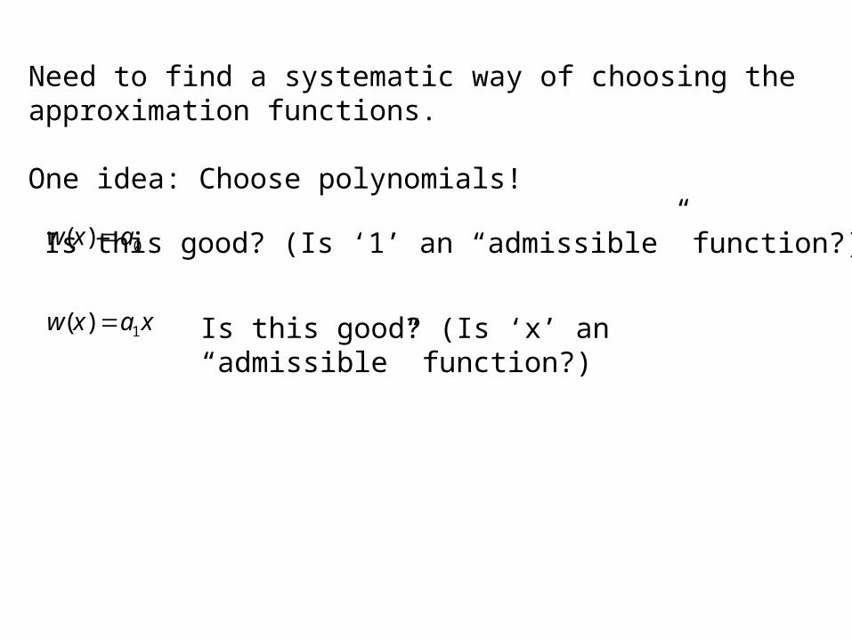
Need to find a systematic way of choosing the approximation functions.

One idea: Choose polynomials!

0)( axw Is this good? (Is ‘1’ an “admissible” function?)

Is this good? (Is ‘x’ an “admissible” function?)xaxw 1)(

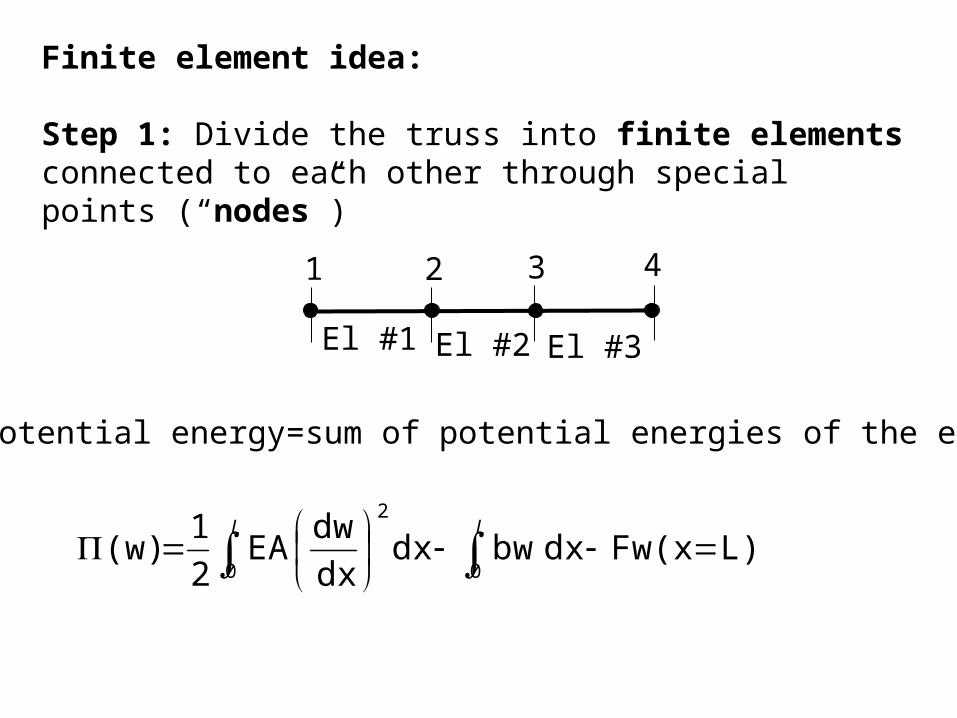
Finite element idea:

Step 1: Divide the truss into finite elements connected to each other through special points (“nodes”)

El #1 El #2 El #3

1 2 3 4

L)Fw(xdxbwdxdx

dwEA

2

1(w)

00

2

LL

Total potential energy=sum of potential energies of the elements

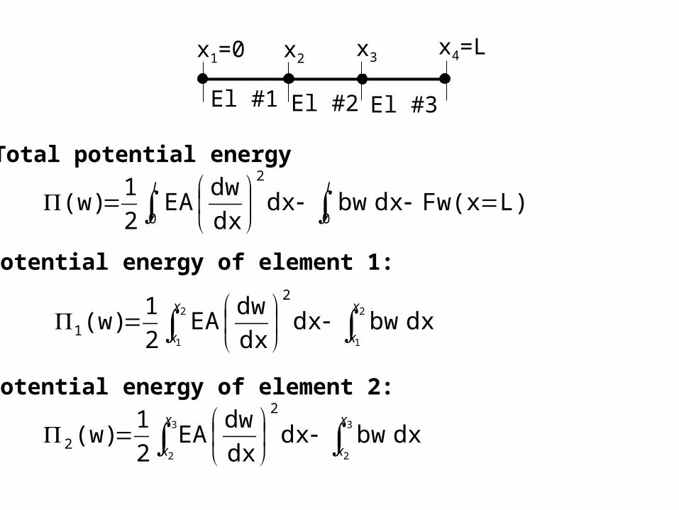
El #1 El #2 El #3

x1=0 x2 x3x4=L

dxbwdxdx

dwEA

2

1(w)

2

1

2

1

2

1

x

x

x

x

L)Fw(xdxbwdxdx

dwEA

2

1(w)

00

2

LL

Total potential energy

Potential energy of element 1:

dxbwdxdx

dwEA

2

1(w)

3

2

3

2

2

2

x

x

x

x

Potential energy of element 2:

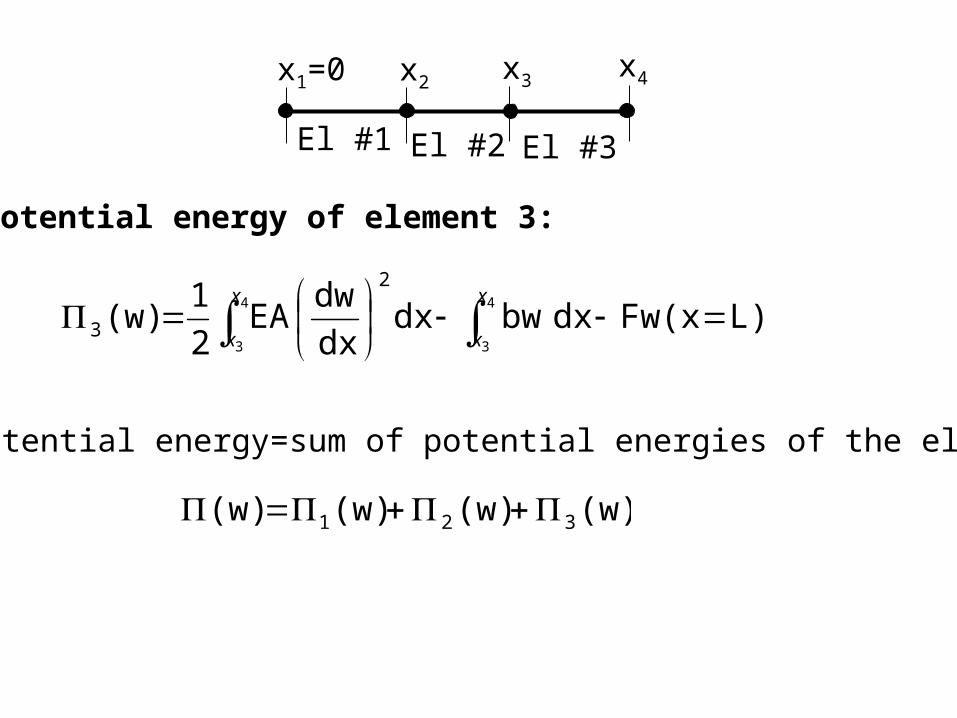
El #1 El #2 El #3

x1=0 x2 x3x4

Total potential energy=sum of potential energies of the elements

Potential energy of element 3:

(w)(w)(w)(w) 321

L)Fw(xdxbwdxdx

dwEA

2

1(w)

4

3

4

3

2

3

x

x

x

x

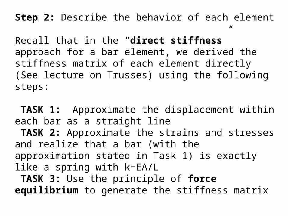
Step 2: Describe the behavior of each element

Recall that in the “direct stiffness” approach for a bar element, we derived the stiffness matrix of each element directly (See lecture on Trusses) using the following steps:

TASK 1: Approximate the displacement within each bar as a straight line TASK 2: Approximate the strains and stresses and realize that a bar (with the approximation stated in Task 1) is exactly like a spring with k=EA/L TASK 3: Use the principle of force equilibrium to generate the stiffness matrix

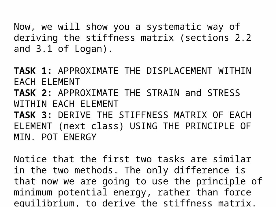
Now, we will show you a systematic way of deriving the stiffness matrix (sections 2.2 and 3.1 of Logan).

TASK 1: APPROXIMATE THE DISPLACEMENT WITHIN EACH ELEMENT TASK 2: APPROXIMATE THE STRAIN and STRESS WITHIN EACH ELEMENT TASK 3: DERIVE THE STIFFNESS MATRIX OF EACH ELEMENT (next class) USING THE PRINCIPLE OF MIN. POT ENERGY

Notice that the first two tasks are similar in the two methods. The only difference is that now we are going to use the principle of minimum potential energy, rather than force equilibrium, to derive the stiffness matrix.

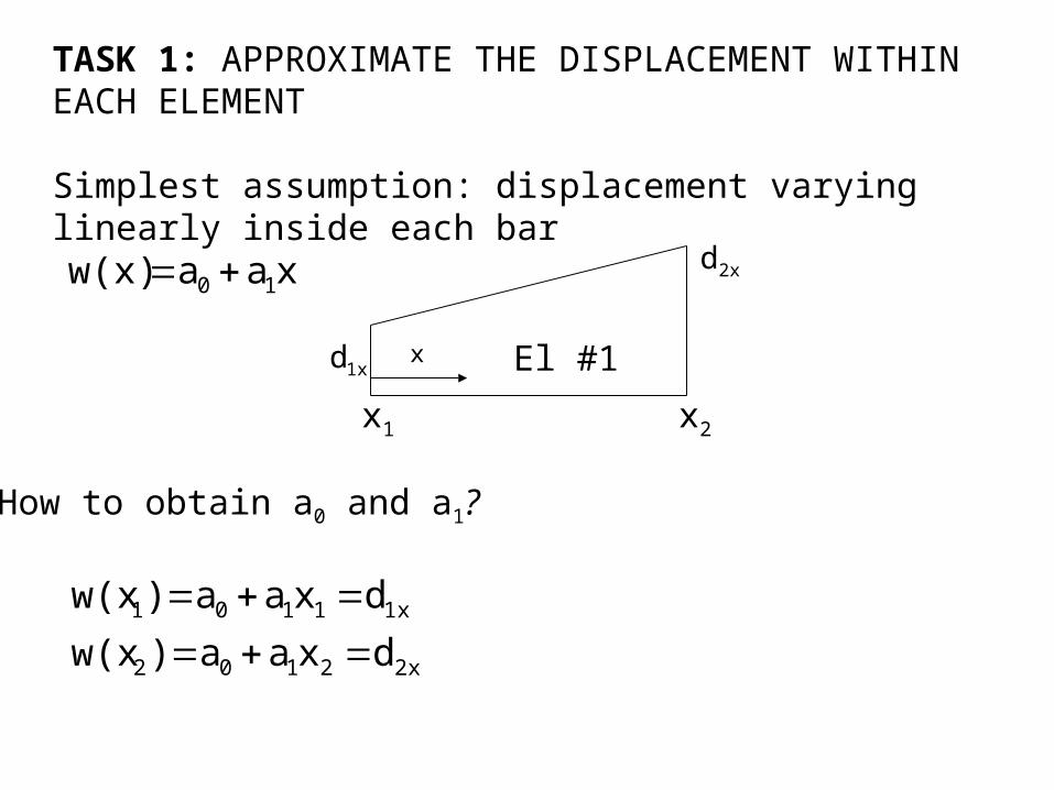
TASK 1: APPROXIMATE THE DISPLACEMENT WITHIN EACH ELEMENT

Simplest assumption: displacement varying linearly inside each bar

xaaw(x) 10 2xd

1xd x

x1 x2

El #1

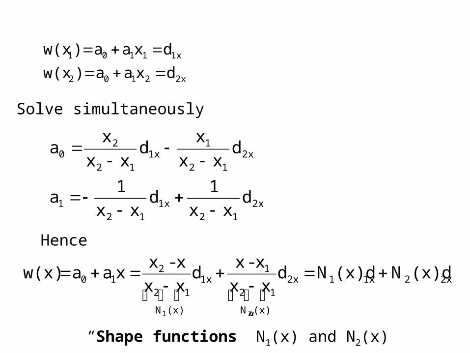
How to obtain a0 and a1?

2x2102

1x1101

dxaa)w(x

dxaa)w(x

2x2102

1x1101

dxaa)w(x

dxaa)w(x

Solve simultaneously

2x12

1x12

1

2x12

11x

12

20

dxx

1d

xx

1a

dxx

xd

xx

xa

2x21x12x

(x)N

12

11x

(x)N

12

210 (x)dN(x)dNd

xx

x-xd

xx

x-xxaaw(x)

21

Hence

“Shape functions” N1(x) and N2(x)

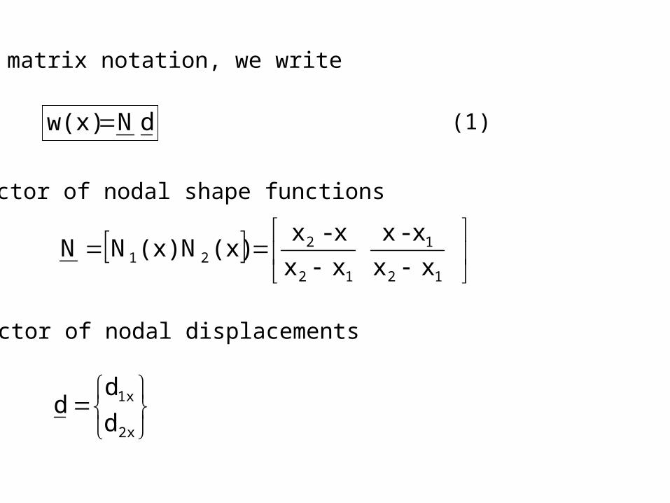
In matrix notation, we write

dNw(x)

Vector of nodal shape functions

12

1

12

221 xx

x-x

xx

x-x(x)N(x)NN

Vector of nodal displacements

2x

1x

d

dd

(1)

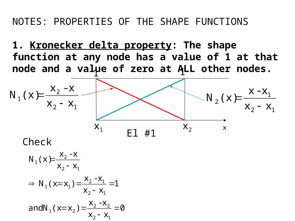
NOTES: PROPERTIES OF THE SHAPE FUNCTIONS

1. Kronecker delta property: The shape function at any node has a value of 1 at that node and a value of zero at ALL other nodes.

xx1 x2El #1

12

21 xx

x-x(x)N

12

12 xx

x-x(x)N

1 1

0xx

x-x)x(xNand

1xx

x-x)x(xN

xx

x-x(x)N

12

2221

12

1211

12

21

Check

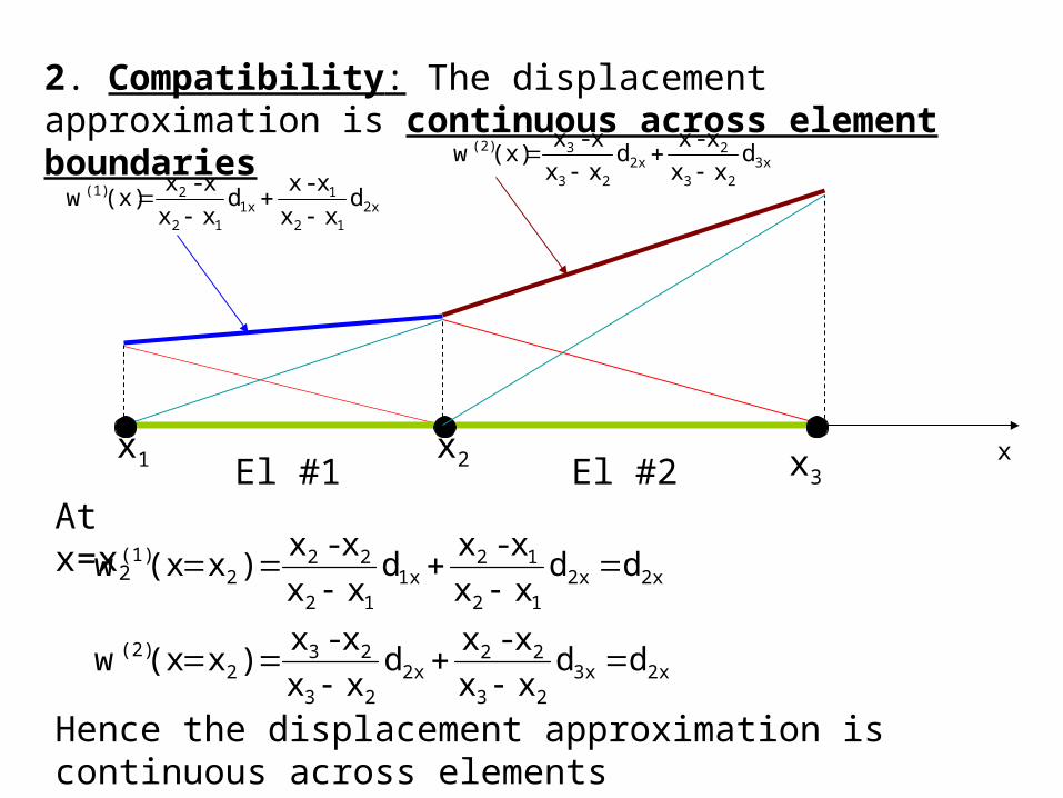
2. Compatibility: The displacement approximation is continuous across element boundaries

2x3x23

222x

23

232

(2)

2x2x12

121x

12

222

(1)

ddxx

x-xd

xx

x-x)x(xw

ddxx

x-xd

xx

x-x)x(xw

xx1 x2El #1

2x12

11x

12

2(1) dxx

x-xd

xx

x-x(x)w

3x23

22x

23

3(2) dxx

x-xd

xx

x-x(x)w

x3El #2At x=x2

Hence the displacement approximation is continuous across elements

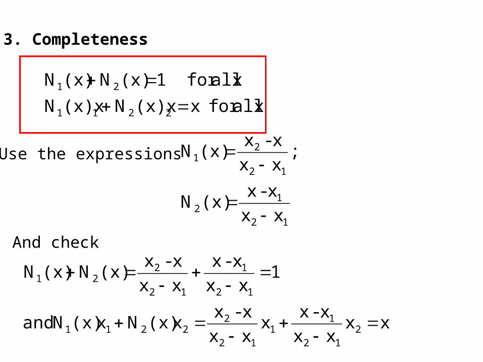
3. Completeness

xallforx(x)xN(x)xN

xallfor1(x)N(x)N

2211

21

Use the expressions

And check12

12

12

21

xx

x-x(x)N

;xx

x-x(x)N

xxxx

x-xx

xx

x-xx(x)Nx(x)Nand

1xx

x-x

xx

x-x(x)N(x)N

212

11

12

22211

12

1

12

221

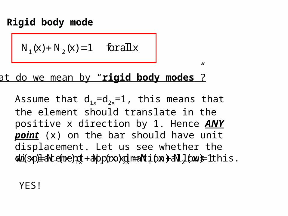
Rigid body mode

What do we mean by “rigid body modes”?

Assume that d1x=d2x=1, this means that the element should translate in the positive x direction by 1. Hence ANY point (x) on the bar should have unit displacement. Let us see whether the displacement approximation allows this.

1(x)N(x)N(x)dN(x)dNw(x) 212x21x1

YES!

1 2N (x) N (x) 1 for all x

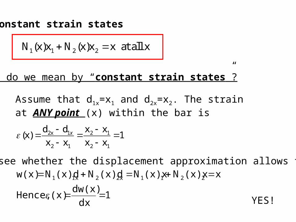
Constant strain states

1 1 2 2N (x)x N (x)x x at all x

What do we mean by “constant strain states”?

Assume that d1x=x1 and d2x=x2. The strain at ANY point (x) within the bar is

1dx

dw(x)(x) Hence,

x(x)xN(x)xN(x)dN(x)dNw(x) 22112x21x1

YES!

2x 1 2 1

2 1 2 1

d d x x(x) 1

x x x xx

Let us see whether the displacement approximation allows this.

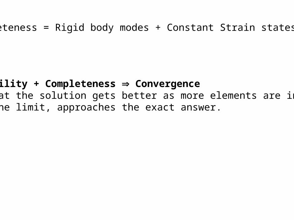
Completeness = Rigid body modes + Constant Strain states

Compatibility + Completeness ConvergenceEnsure that the solution gets better as more elements are introducedand, in the limit, approaches the exact answer.

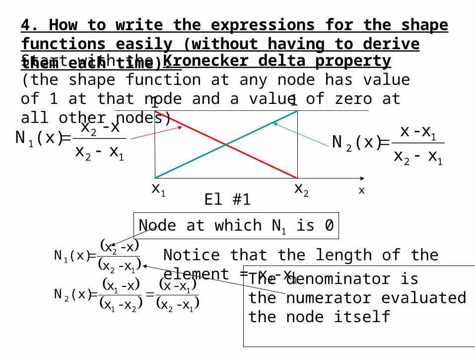
4. How to write the expressions for the shape functions easily (without having to derive them each time):

12

1

21

12

12

21

x-x

x-x

x-x

x-x(x)N

x-x

x-x(x)N

xx1 x2El #1

12

21 xx

x-x(x)N

12

12 xx

x-x(x)N

1 1

Start with the Kronecker delta property (the shape function at any node has value of 1 at that node and a value of zero at all other nodes)

Notice that the length of the element = x2-x1

Node at which N1 is 0

The denominator is the numerator evaluated at the node itself

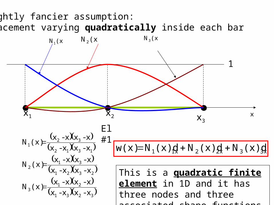
A slightly fancier assumption: displacement varying quadratically inside each bar

3231

213

2321

312

1312

321

x-xx-x

x-xx-x(x)N

x-xx-x

x-xx-x(x)N

x-xx-x

x-xx-x(x)N

xx1 x2

El #1

(x)N1(x)N3

x3

1

(x)N2

3x32x21x1 (x)dN(x)dN(x)dNw(x)

This is a quadratic finite element in 1D and it has three nodes and three associated shape functions per element.

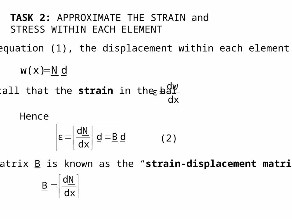
TASK 2: APPROXIMATE THE STRAIN and STRESS WITHIN EACH ELEMENT

dNw(x)

From equation (1), the displacement within each element

dx

dwε Recall that the strain in the bar

Hence

dBddx

Ndε

(2)

The matrix B is known as the “strain-displacement matrix”

dx

NdB

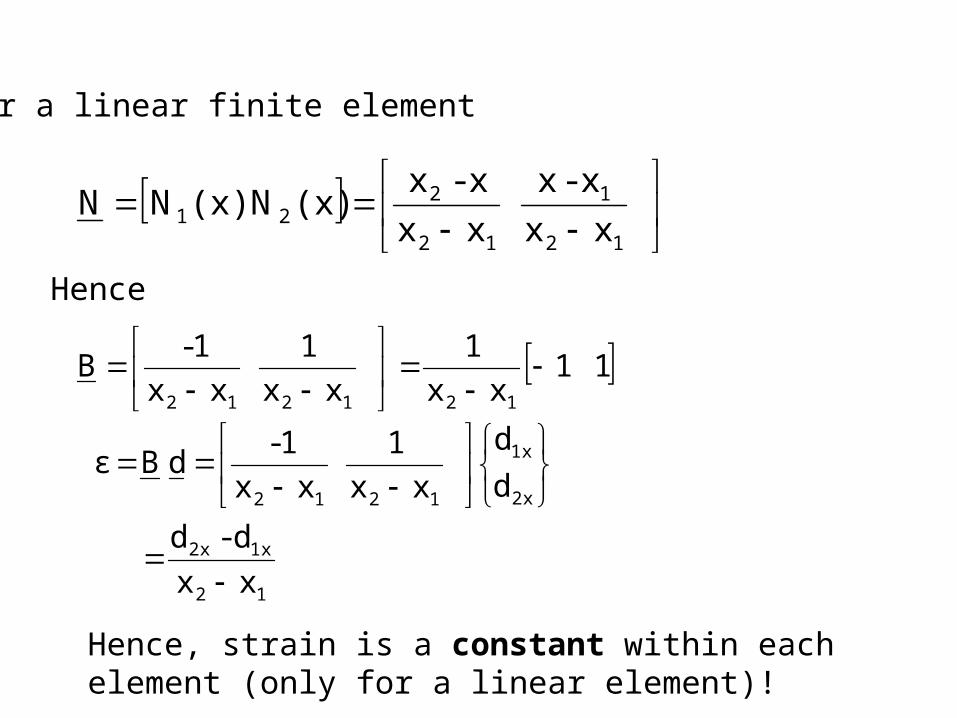
For a linear finite element

11xx

1

xx

1

xx

1-B

121212

12

1

12

221 xx

x-x

xx

x-x(x)N(x)NN

Hence

12

1x2x

2x

1x

1212

xx

d-d

d

d

xx

1

xx

1-dBε

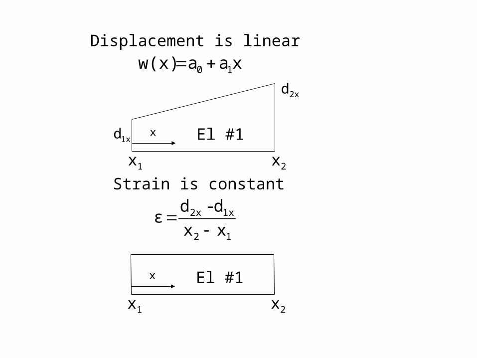
Hence, strain is a constant within each element (only for a linear element)!

2xd

1xd x

x1 x2

El #1

x

x1 x2

El #1

xaaw(x) 10 Displacement is linear

Strain is constant

12

1x2x

xx

d-dε

dx

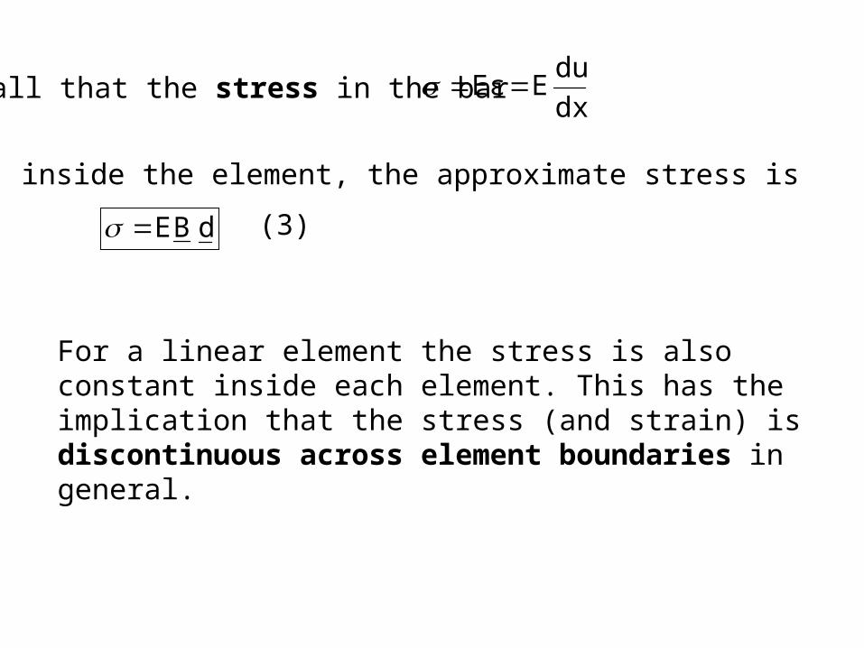
duEEε Recall that the stress in the bar

Hence, inside the element, the approximate stress is

dBE (3)

For a linear element the stress is also constant inside each element. This has the implication that the stress (and strain) is discontinuous across element boundaries in general.

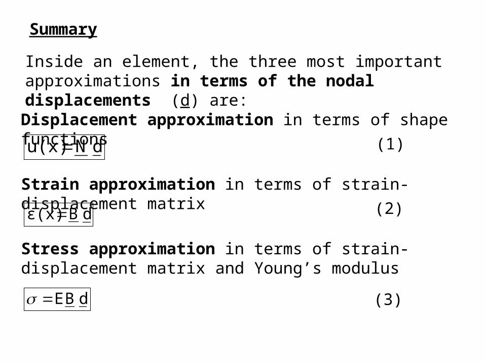
Inside an element, the three most important approximations in terms of the nodal displacements (d) are:

dBE

(1)

Displacement approximation in terms of shape functions

dNu(x)

dBε(x)

Strain approximation in terms of strain-displacement matrix

(2)

Stress approximation in terms of strain-displacement matrix and Young’s modulus

(3)

Summary

For a linear element

Displacement approximation in terms of shape functions

2x

1x

12

1

12

2

d

d

xx

x-x

xx

x-xu(x)

Strain approximation

Stress approximation

Summary

2x

1x

12 d

d11

xx

1ε

2x

1x

12 d

d11

xx

E