Embed Size (px)
Citation preview
Quantum LogicQuantum Logic
Marek Perkowski
SourcesSources
Mosca, Hayes, Ekert,Lee Spectorin collaboration withHerbert J. Bernstein, Howard Barnum, Nikhil Swamy{lspector, hbernstein, hbarnum,nikhil_swamy}@hampshire.edu}
School of Cognitive Science, School of Natural ScienceInstitute for Science and Interdisciplinary Studies (ISIS)Hampshire College
Origin of slides: John Hayes, Peter Shor, MartinLukac, Mikhail Pivtoraiko, Alan Mishchenko, PawelKerntopf, Mosca, Ekert
IntroductionIntroduction• Short-Term Objectives
• Long-Term Objectives
• Prerequisite
Introduce Quantum Computing Basics to interested students at KAIST.Especially non-physics students
Engage into AI/CS/Math Research projects benefiting from QuantumComputing. Continue our previous projects in quantum computing
- No linear algebra or quantum mechanics assumed- A ECE, math, physics or CS background would bebeneficial, practically-oriented class.
IntroductionIntroduction
• MainTextbookQuantum Computation&Quantum Information
Michael A. NielsenIsaac L. Chuang
ISBN: 0 521 63503 9PaperbackISBN: 0 521 63235 8 Hardback
Cost: $48.00 New Paperback$35.45 Used Paperback
(http://www.amazon.com)also in KAIST bookstore
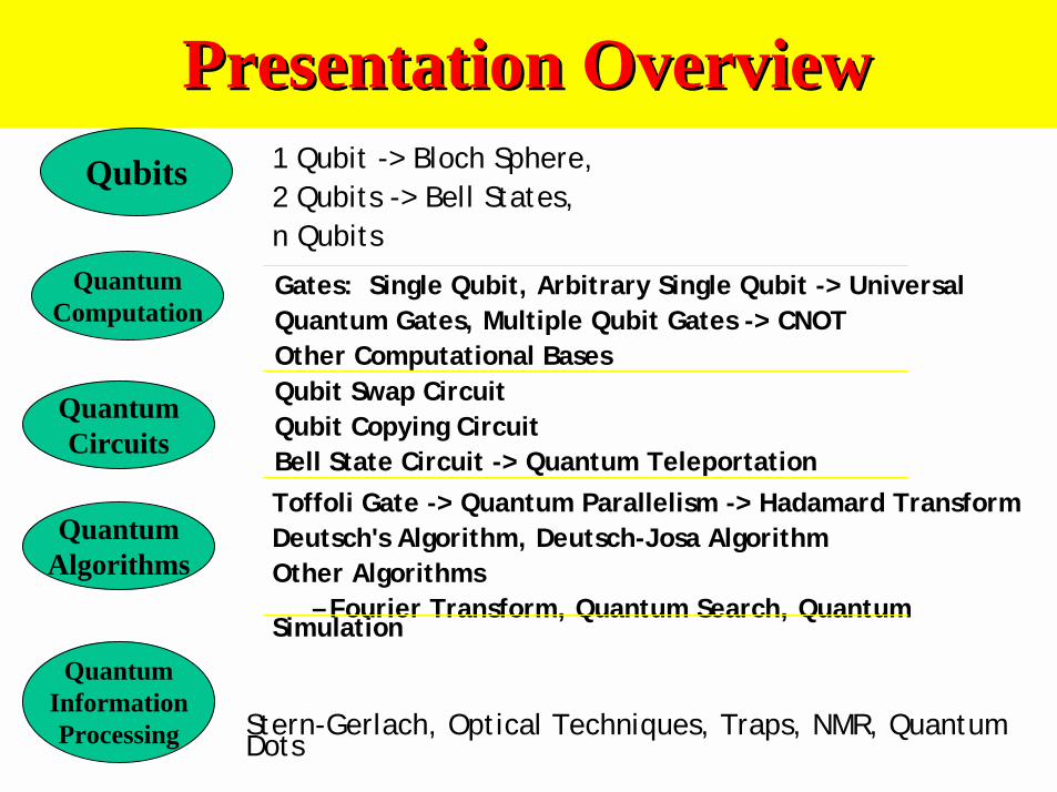
Presentation OverviewPresentation OverviewQubits
QuantumComputation
QuantumCircuits
QuantumAlgorithms
QuantumInformationProcessing
1 Qubit -> Bloch Sphere,2 Qubits -> Bell States,n Qubits
Gates: Single Qubit, Arbitrary Single Qubit -> UniversalQuantum Gates, Multiple Qubit Gates -> CNOTOther Computational BasesQubit Swap CircuitQubit Copying CircuitBell State Circuit -> Quantum TeleportationToffoli Gate -> Quantum Parallelism -> Hadamard TransformDeutsch's Algorithm, Deutsch-Josa AlgorithmOther Algorithms – Fourier Transform, Quantum Search, QuantumSimulation
Stern-Gerlach, Optical Techniques, Traps, NMR, QuantumDots
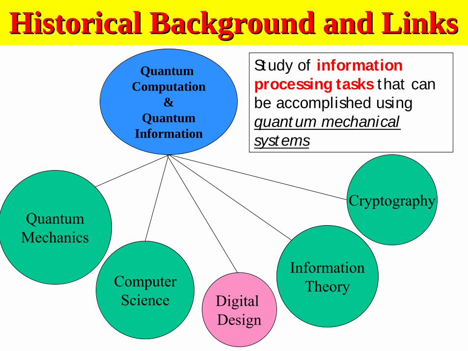
Historical Background and LinksHistorical Background and LinksQuantum
Computation&
QuantumInformation
ComputerScience
InformationTheory
CryptographyQuantum
Mechanics
Study of informationprocessing tasks that canbe accomplished usingquantum mechanicalsystems
Digital Design
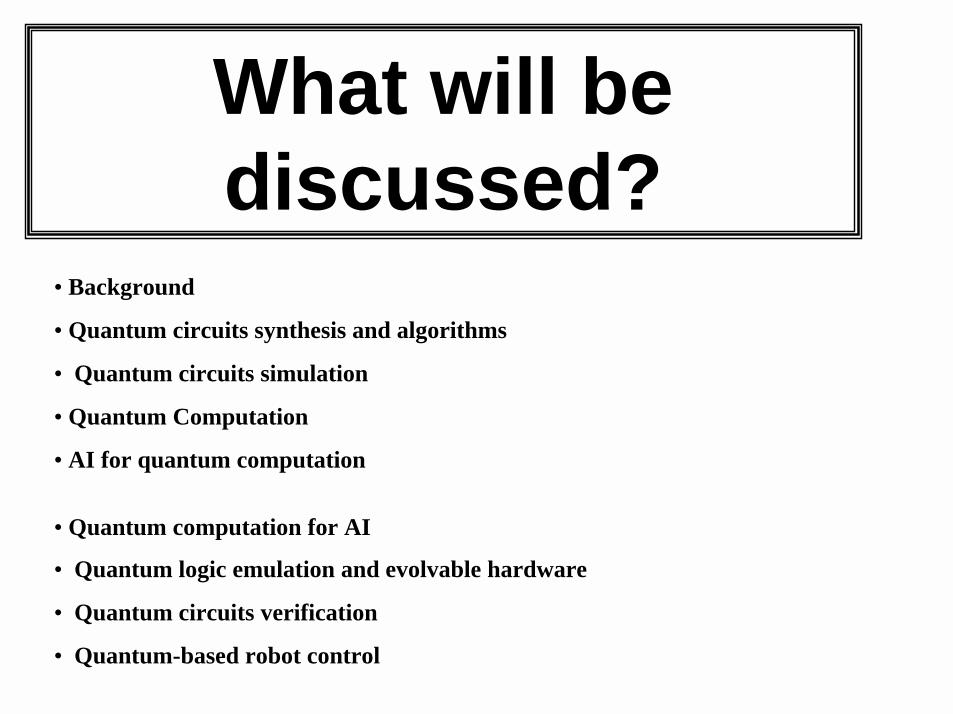
What will bediscussed?
• Background
• Quantum circuits synthesis and algorithms
• Quantum circuits simulation
• Quantum Computation
• AI for quantum computation
• Quantum computation for AI
• Quantum logic emulation and evolvable hardware
• Quantum circuits verification
• Quantum-based robot control
What is quantumWhat is quantumcomputation?computation?
• Computation with coherent atomic-scaledynamics.
• The behavior of a quantum computer isgoverned by the laws of quantummechanics.
Why bother with quantumWhy bother with quantumcomputation?computation?
• Moore’s Law: We hit the quantum level2010~2020.• Quantum computation is more powerfulthan classical computation.• More can be computed in less time—thecomplexity classes are different!
The power of quantumThe power of quantumcomputationcomputation
• In quantum systems possibilities count,even if they never happen!
• Each of exponentially many possibilitiescan be used to perform a part of acomputation at the same time.
Nobody understands quantumNobody understands quantummechanicsmechanics
“No, you’re not going to be able to understand it. . .. You see, my physics students don’t understand iteither. That is because I don’t understand it.Nobody does. ... The theory of quantumelectrodynamics describes Nature as absurd fromthe point of view of common sense. And it agreesfully with an experiment. So I hope that you canaccept Nature as She is -- absurd.
Richard Feynman
Absurd but taken seriously (not justAbsurd but taken seriously (not justquantum mechanics but alsoquantum mechanics but also
quantum computation)quantum computation)
• Under active investigation by many of the topphysics labs around the world (including CalTech,MIT, AT&T, Stanford, Los Alamos, UCLA, Oxford,l’Université de Montréal, University of Innsbruck,IBM Research . . .)
• In the mass media (including The New York Times,The Economist, American Scientist, ScientificAmerican, . . .)
• Here.
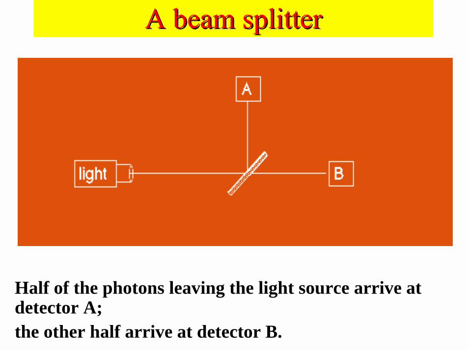
A beam splitterA beam splitter
Half of the photons leaving the light source arrive atdetector A;the other half arrive at detector B.
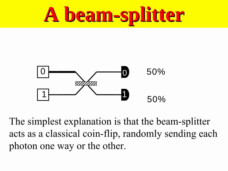
A beam-splitterA beam-splitter
0
1
0
1
%50
%50
The simplest explanation is that the beam-splitteracts as a classical coin-flip, randomly sending eachphoton one way or the other.
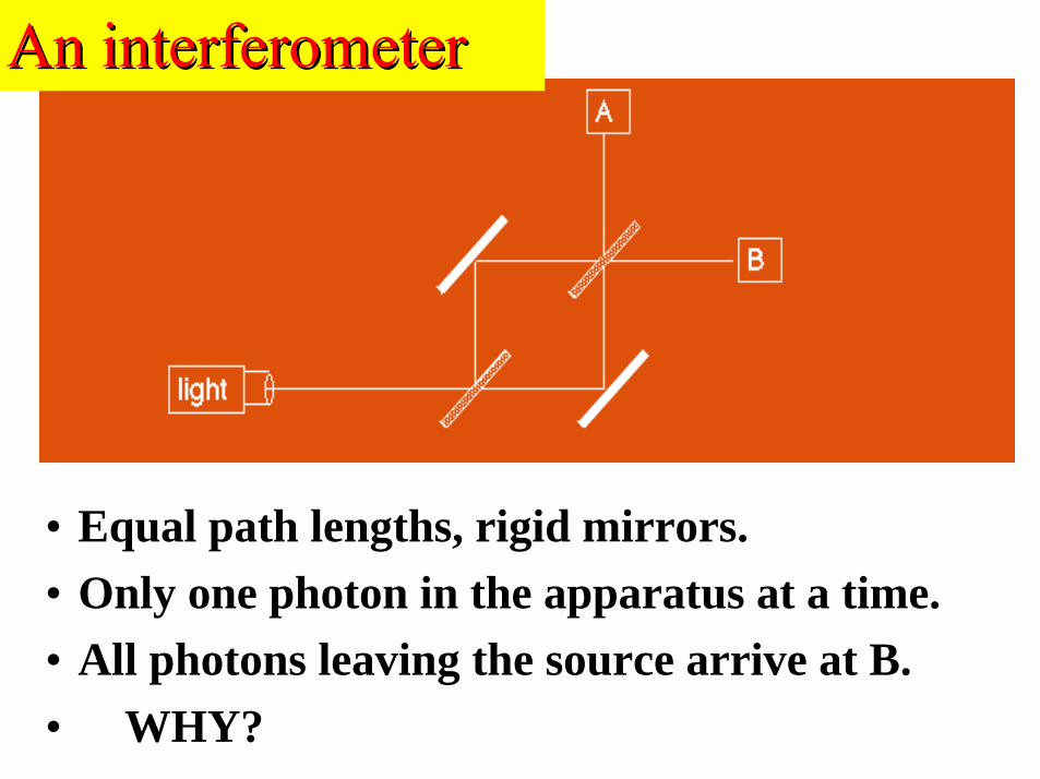
An interferometerAn interferometer
• Equal path lengths, rigid mirrors.• Only one photon in the apparatus at a time.• All photons leaving the source arrive at B.• WHY?
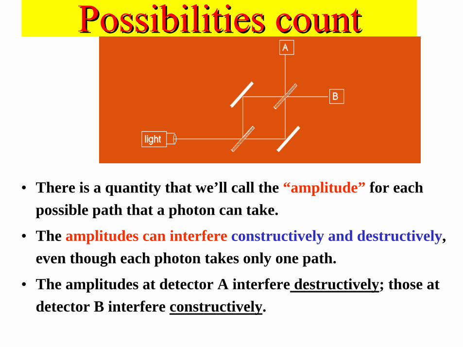
Possibilities countPossibilities count
• There is a quantity that we’ll call the “amplitude” for eachpossible path that a photon can take.
• The amplitudes can interfere constructively and destructively,even though each photon takes only one path.
• The amplitudes at detector A interfere destructively; those atdetector B interfere constructively.

Calculating interferenceCalculating interference• Arrows for each possibility.• Arrows rotate; speed depends on frequency.• Arrows flip 180o at mirrors, rotate 90o counter-clockwise
when reflected from beam splitters.• Add arrows and square the length of the result to determine
the probability for any possibility.
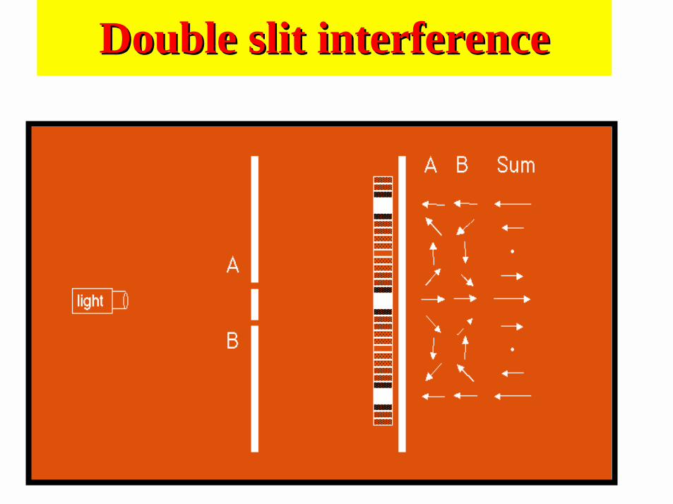
Double slit interferenceDouble slit interference
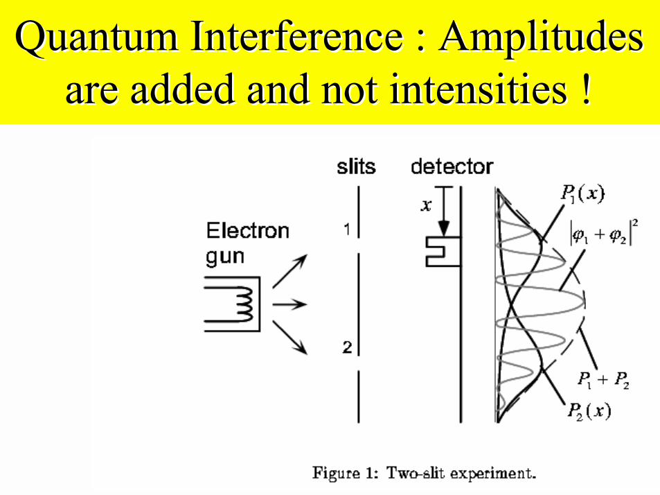
Quantum Interference : AmplitudesQuantum Interference : Amplitudesare added and not intensities !are added and not intensities !
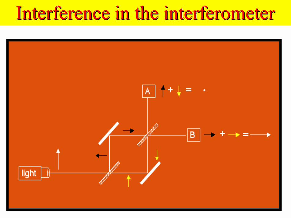
Interference in the interferometerInterference in the interferometer
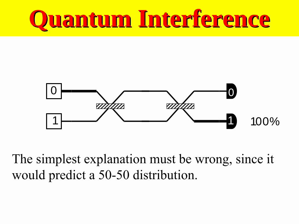
Quantum InterferenceQuantum Interference
0
1
0
1 %100
The simplest explanation must be wrong, since itwould predict a 50-50 distribution.
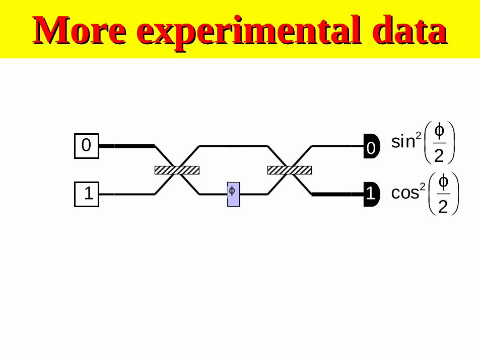
More experimental dataMore experimental data
0
1
0
1
ϕ2
cos2ϕ
ϕ2
sin2
0
1
0
1
ϕ2
cos2ϕ
ϕ2
sin2
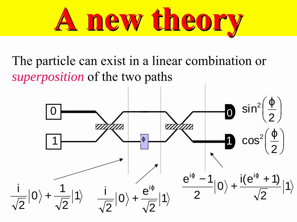
1210
2i + 1
2e0
2i iϕ
+
The particle can exist in a linear combination orsuperposition of the two paths
12
)1e(i02
1e ii ++− ϕϕ
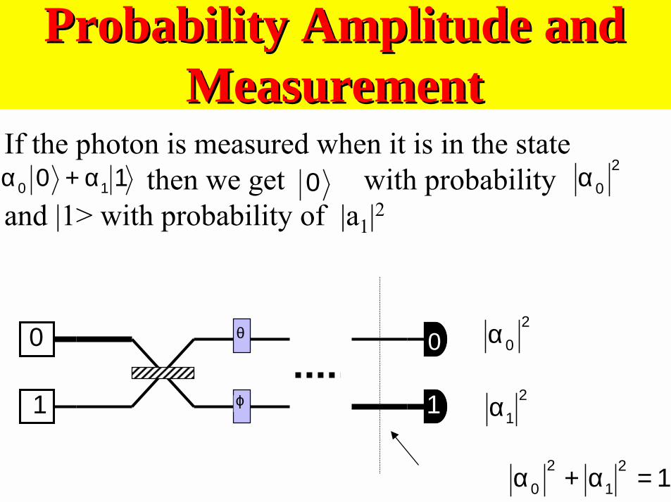
Probability Amplitude andProbability Amplitude andMeasurementMeasurement
0
1
0
1ϕ
20α
If the photon is measured when it is in the state then we get with probability
and |1> with probability of |a1|210 10 α+α
θ
21α
20α0
121
20 =α+α
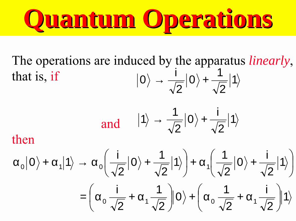
Quantum OperationsQuantum OperationsThe operations are induced by the apparatus linearly,that is, if
andthen
+α+
+α→α+α 12i0
211
210
2i10 1010
1210
2i0 +→
12i0
211 +→
12i
210
21
2i
1010
α+α+
α+α=
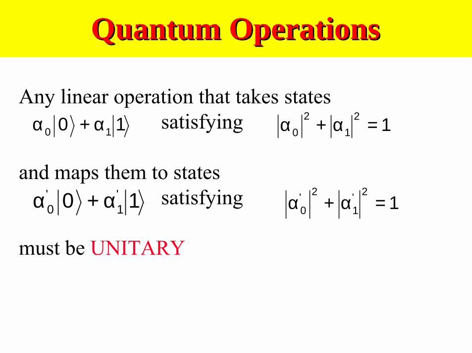
Quantum OperationsQuantum Operations
Any linear operation that takes statessatisfying
and maps them to statessatisfying
must be UNITARY
121
20 =α+α10 10 α+α
10 '1
'0 α+α 1
2'1
2'0 =α+α
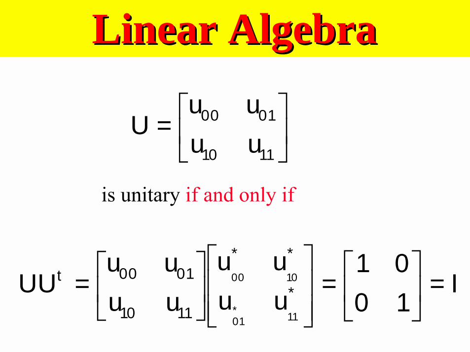
Linear AlgebraLinear Algebra
I1001
uuuu
uuuu
UU *
**
1110
0100t
11*01
1000 =
=
=
=
1110
0100
uuuu
U
is unitary if and only if
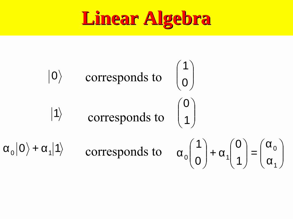
Linear AlgebraLinear Algebra
10 10 α+α
0
01
1
10
αα
=
α+
α
1
010 1
001
corresponds to
corresponds to
corresponds to
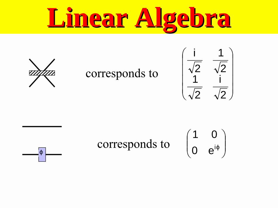
Linear AlgebraLinear Algebra
2i
21
21
2i
corresponds to
corresponds toϕ
ϕie0
01
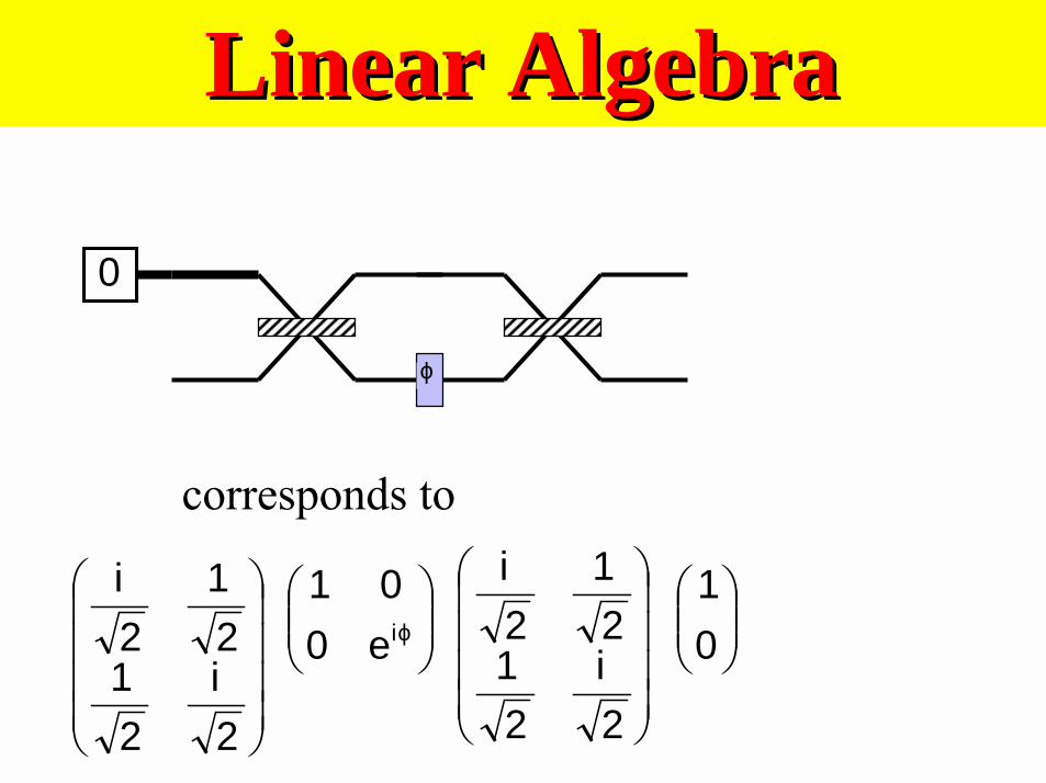
Linear AlgebraLinear Algebra
0
ϕ
corresponds to
01
2i
21
21
2i
ϕie0
01
2i
21
21
2i
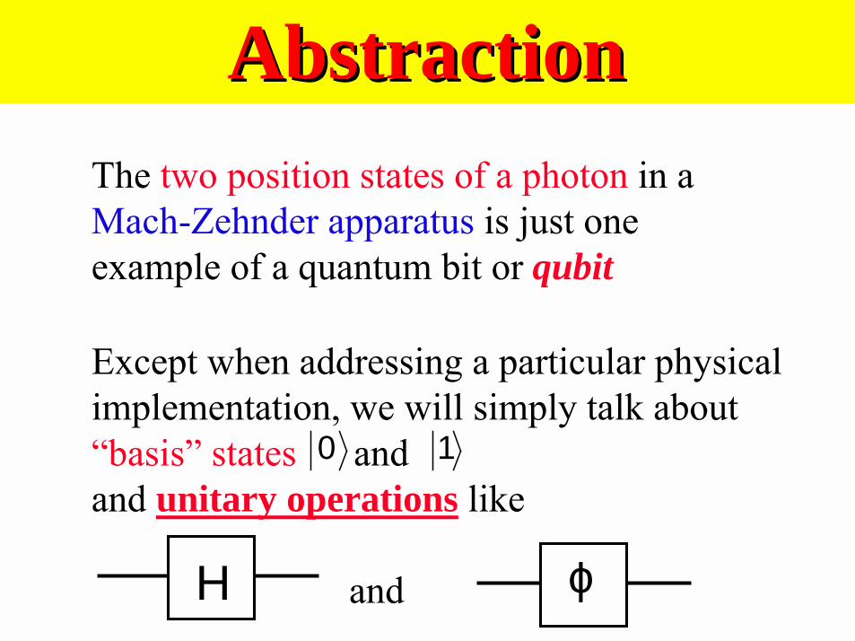
AbstractionAbstractionThe two position states of a photon in aMach-Zehnder apparatus is just oneexample of a quantum bit or qubit
Except when addressing a particular physicalimplementation, we will simply talk about“basis” states andand unitary operations like
and
0 1
H ϕ
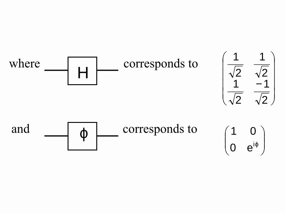
where corresponds toH
ϕ
−21
21
21
21
and corresponds to
ϕie0
01
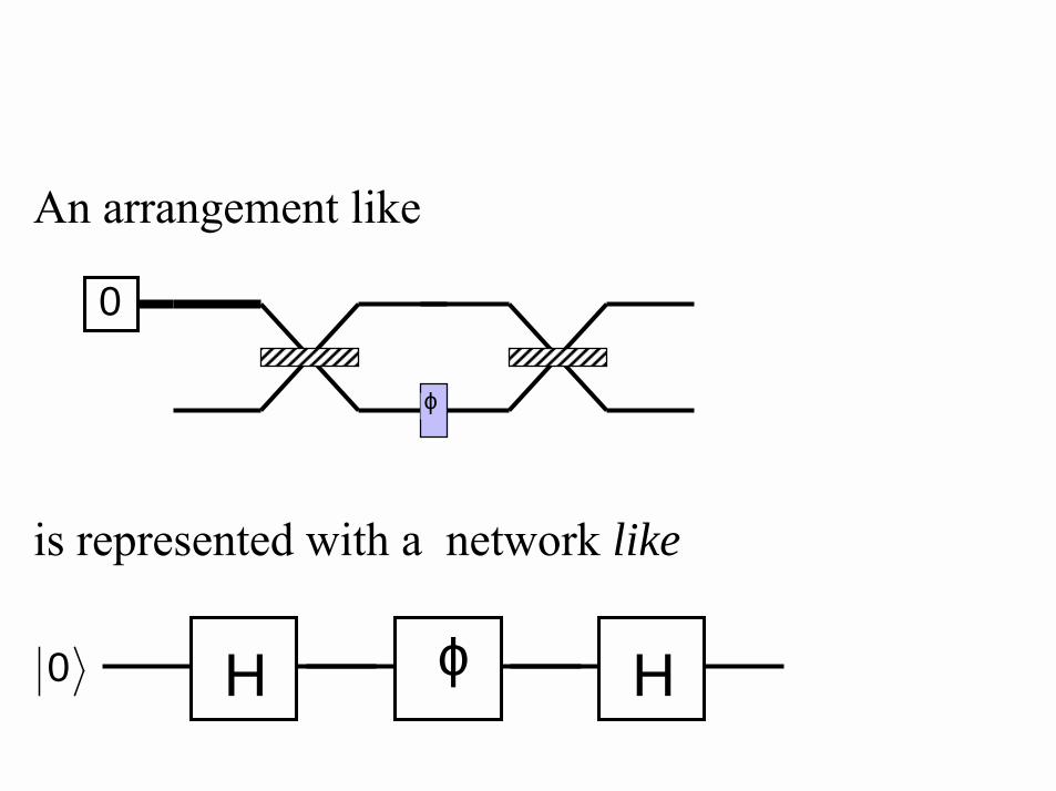
An arrangement like
0
ϕ
is represented with a network like
H ϕ H0
More than one More than one qubitqubit
( )10 10 α+α
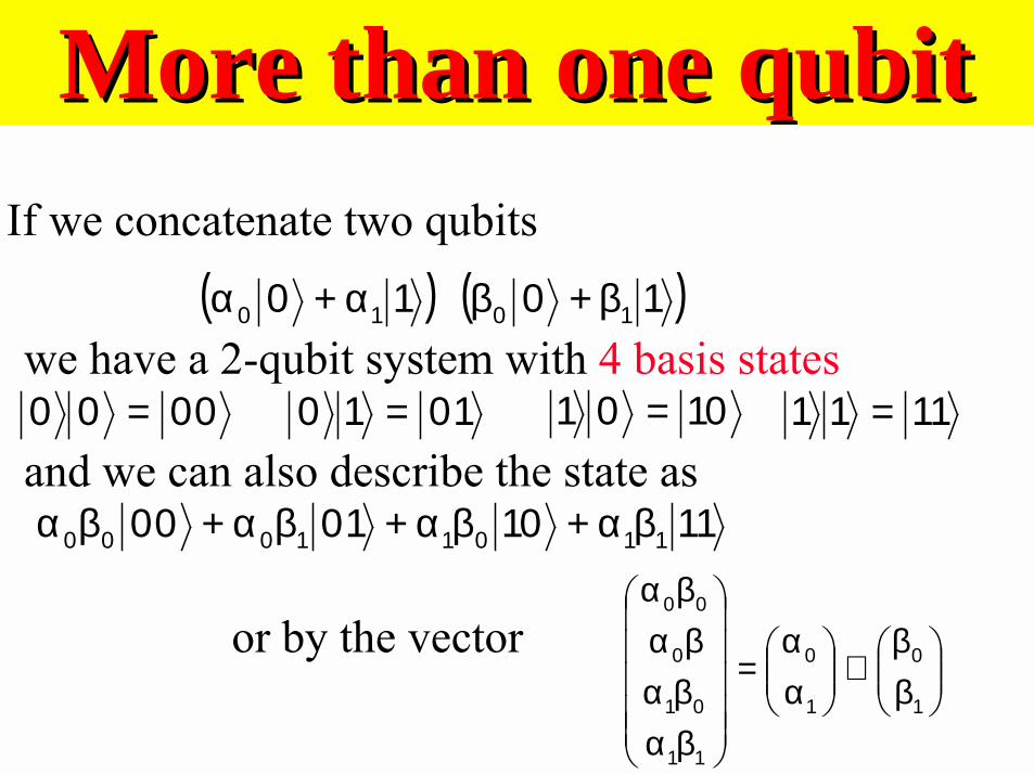
If we concatenate two qubits
11100100 11011000 βα+βα+βα+βα
( )10 10 β+βwe have a 2-qubit system with 4 basis states
0000 = 0110 = 1001 = 1111 =and we can also describe the state as
or by the vector
ββ
⊗
αα
=
βαβαβαβα
1
0
1
0
11
01
0
00
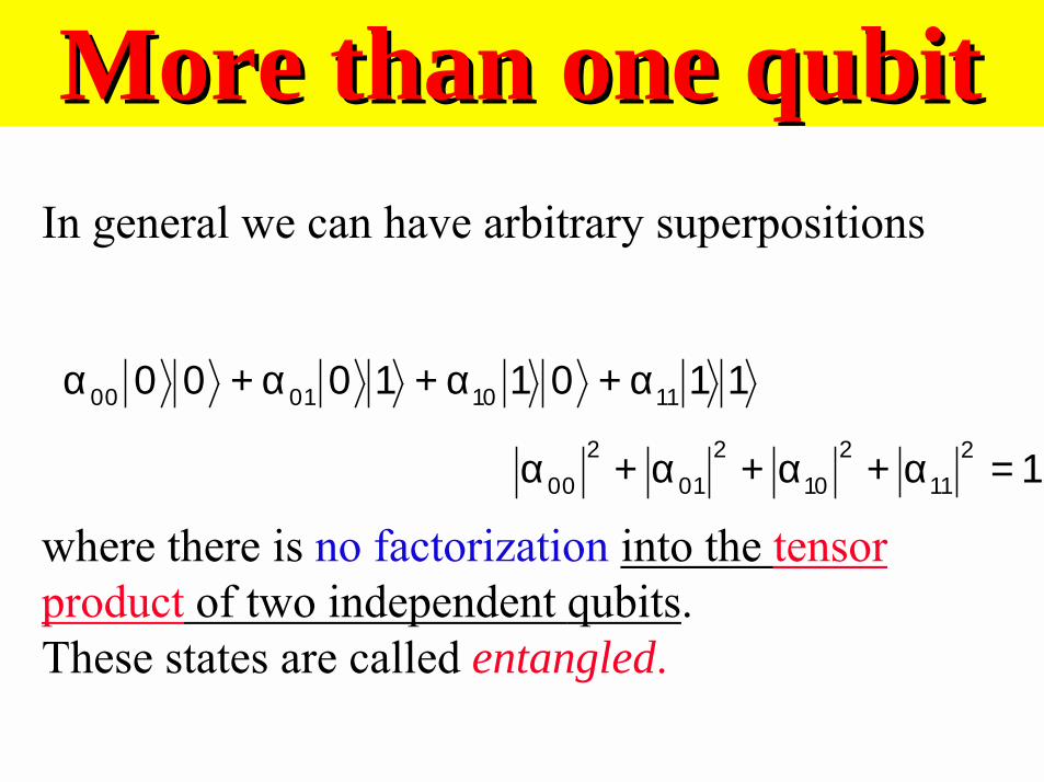
More than one More than one qubitqubitIn general we can have arbitrary superpositions
11011000 11100100 α+α+α+α
1211
210
201
200 =α+α+α+α
where there is no factorization into the tensorproduct of two independent qubits.These states are called entangled.
EntanglementEntanglement• Qubits in a multi-qubit system are not
independent—they can become“entangled.”
• To represent the state of n qubits weuse 2n complex number amplitudes.
Measuring multi-Measuring multi-qubit qubit systemssystems
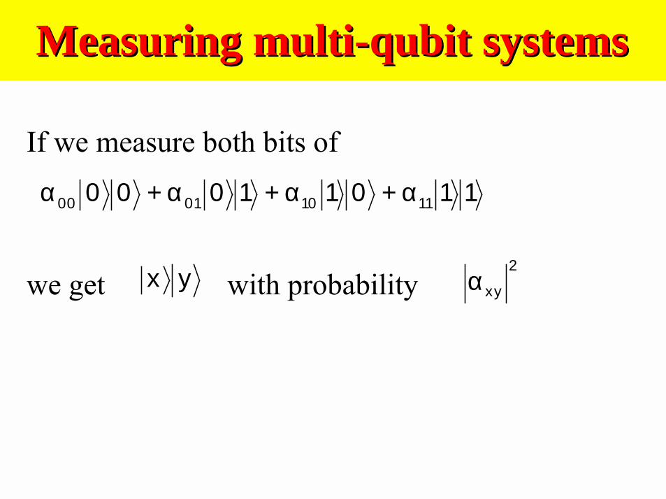
If we measure both bits of
we get with probability
11011000 11100100 α+α+α+α
yx 2xyα
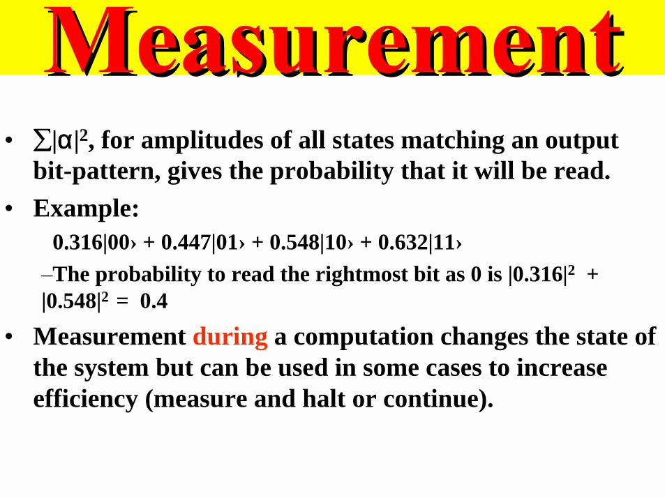
• ∑∑∑∑|αααα|2, for amplitudes of all states matching an outputbit-pattern, gives the probability that it will be read.
• Example: 0.316|00› + 0.447|01› + 0.548|10› + 0.632|11›–The probability to read the rightmost bit as 0 is |0.316|2 +|0.548|2 = 0.4
• Measurement during a computation changes the state ofthe system but can be used in some cases to increaseefficiency (measure and halt or continue).
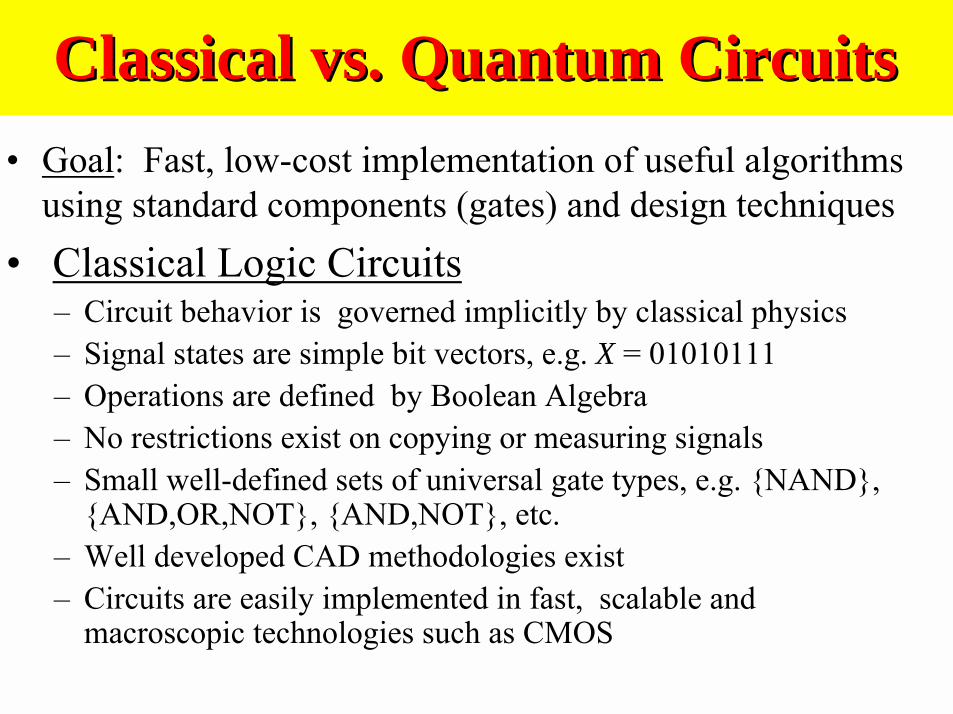
• Goal: Fast, low-cost implementation of useful algorithmsusing standard components (gates) and design techniques
• Classical Logic Circuits– Circuit behavior is governed implicitly by classical physics– Signal states are simple bit vectors, e.g. X = 01010111– Operations are defined by Boolean Algebra– No restrictions exist on copying or measuring signals– Small well-defined sets of universal gate types, e.g. {NAND},
{AND,OR,NOT}, {AND,NOT}, etc.– Well developed CAD methodologies exist– Circuits are easily implemented in fast, scalable and
macroscopic technologies such as CMOS
Classical vs. Quantum CircuitsClassical vs. Quantum Circuits
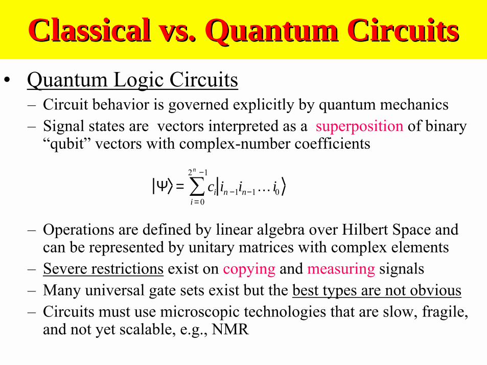
• Quantum Logic Circuits– Circuit behavior is governed explicitly by quantum mechanics– Signal states are vectors interpreted as a superposition of binary
“qubit” vectors with complex-number coefficients
– Operations are defined by linear algebra over Hilbert Space andcan be represented by unitary matrices with complex elements
– Severe restrictions exist on copying and measuring signals– Many universal gate sets exist but the best types are not obvious– Circuits must use microscopic technologies that are slow, fragile,
and not yet scalable, e.g., NMR
Classical vs. Quantum CircuitsClassical vs. Quantum Circuits
Ψ = ci in −1in−1… i0i =0
2n −1
∑
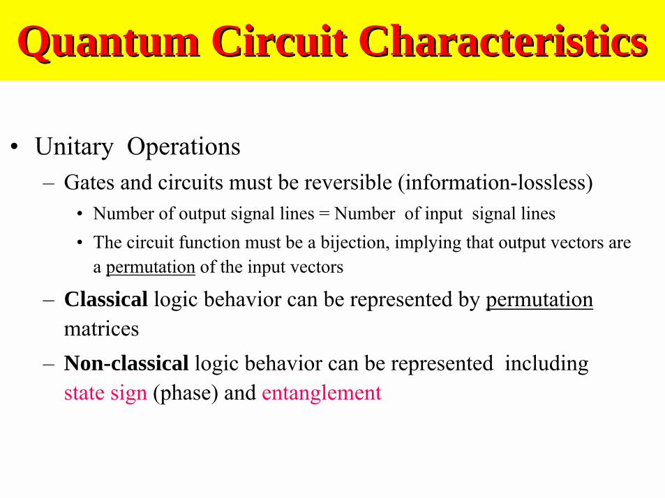
• Unitary Operations– Gates and circuits must be reversible (information-lossless)
• Number of output signal lines = Number of input signal lines• The circuit function must be a bijection, implying that output vectors are
a permutation of the input vectors
– Classical logic behavior can be represented by permutationmatrices
– Non-classical logic behavior can be represented includingstate sign (phase) and entanglement
Quantum Circuit CharacteristicsQuantum Circuit Characteristics
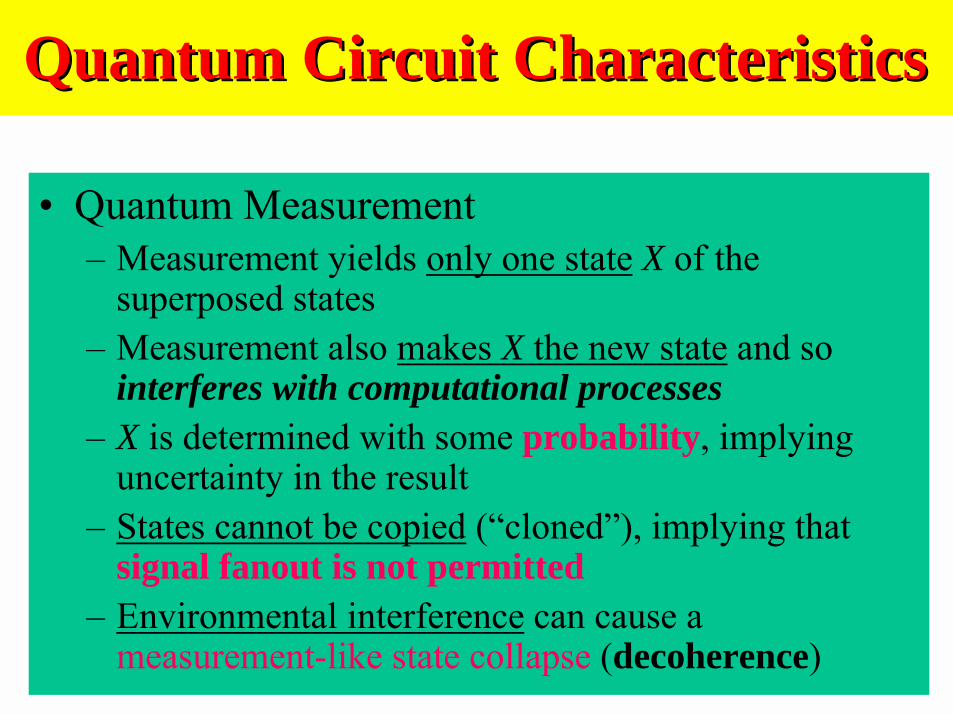
• Quantum Measurement– Measurement yields only one state X of the
superposed states– Measurement also makes X the new state and so
interferes with computational processes– X is determined with some probability, implying
uncertainty in the result– States cannot be copied (“cloned”), implying that
signal fanout is not permitted– Environmental interference can cause a
measurement-like state collapse (decoherence)
Quantum Circuit CharacteristicsQuantum Circuit Characteristics
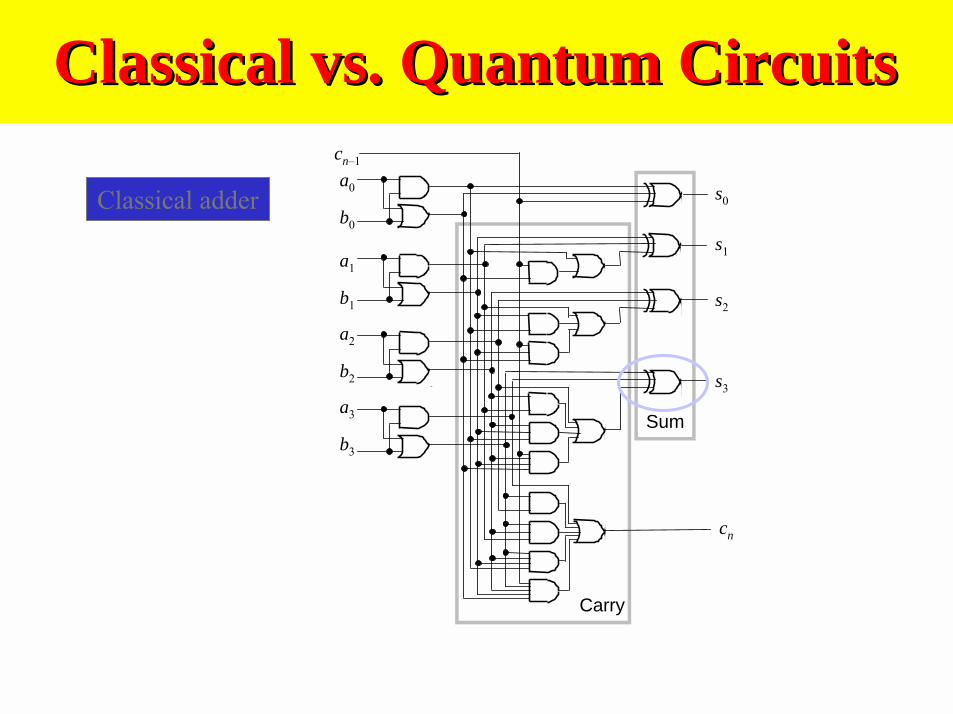
Classical vs. Quantum CircuitsClassical vs. Quantum Circuits
Classical adder
cn–1
s0
s1
s2
s3
cn
a0
b0
a1
b1
a3
b3
a2
b2
Sum
Carry
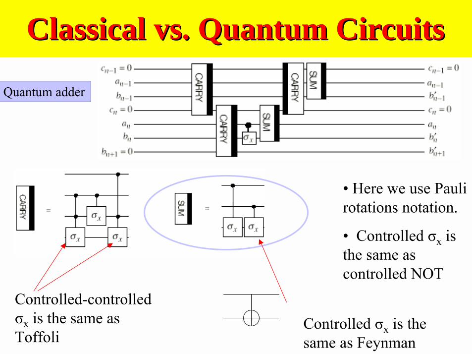
Classical vs. Quantum CircuitsClassical vs. Quantum Circuits
Quantum adder
• Here we use Paulirotations notation.
• Controlled σx isthe same ascontrolled NOT
Controlled σx is thesame as Feynman
Controlled-controlledσx is the same asToffoli
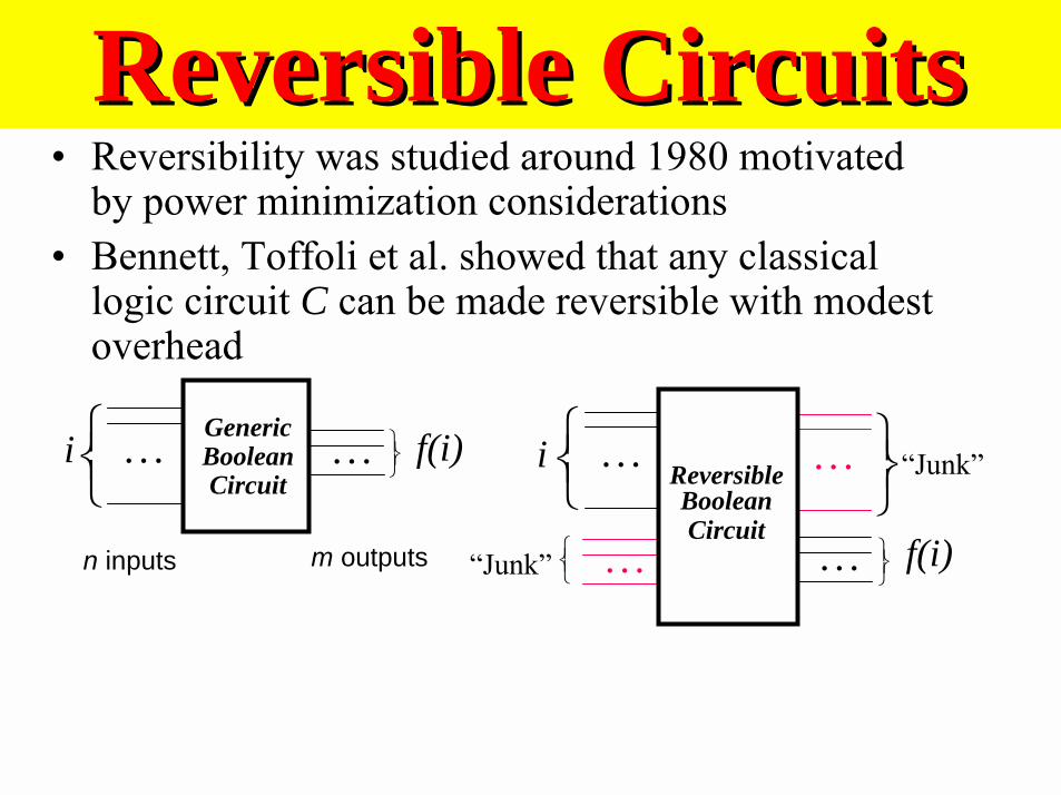
Reversible CircuitsReversible Circuits• Reversibility was studied around 1980 motivated
by power minimization considerations• Bennett, Toffoli et al. showed that any classical
logic circuit C can be made reversible with modestoverhead
……
n inputs
GenericBooleanCircuit
m outputs
f(i)i …
ReversibleBooleanCircuit
…
f(i)
…
…
“Junk”i
“Junk”
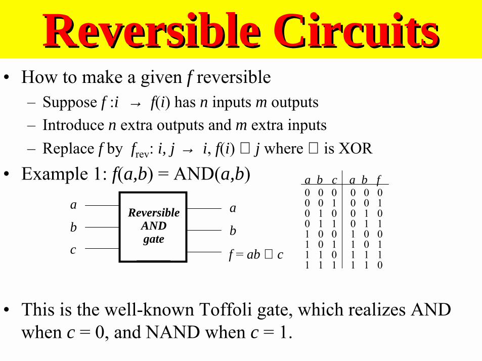
• How to make a given f reversible– Suppose f :i → f(i) has n inputs m outputs– Introduce n extra outputs and m extra inputs– Replace f by frev: i, j → i, f(i) ⊕ j where ⊕ is XOR
• Example 1: f(a,b) = AND(a,b)
• This is the well-known Toffoli gate, which realizes ANDwhen c = 0, and NAND when c = 1.
Reversible CircuitsReversible Circuits
ReversibleANDgate
a
b
f = ab ⊕ c
a
bc
a b c a b f0 0 0 0 0 00 0 1 0 0 10 1 0 0 1 00 1 1 0 1 11 0 0 1 0 01 0 1 1 0 11 1 0 1 1 11 1 1 1 1 0
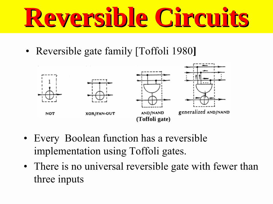
• Reversible gate family [Toffoli 1980]
Reversible CircuitsReversible Circuits
(Toffoli gate)
• Every Boolean function has a reversibleimplementation using Toffoli gates.
• There is no universal reversible gate with fewer thanthree inputs
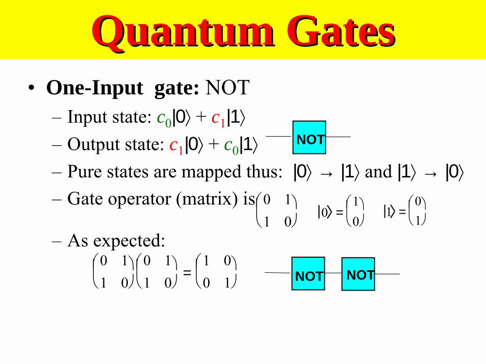
Quantum GatesQuantum Gates• One-Input gate: NOT
– Input state: c0|0⟩ + c1|1⟩– Output state: c1|0⟩ + c0|1⟩– Pure states are mapped thus: |0⟩ → |1⟩ and |1⟩ → |0⟩– Gate operator (matrix) is
– As expected:0 11 0
0 11 0
=
1 00 1
NOT
NOTNOT
0 11 0
0 =
10
1 =
01
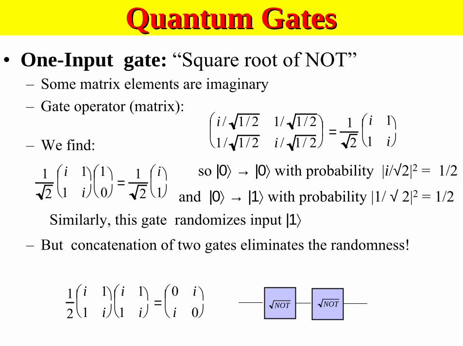
Quantum GatesQuantum Gates• One-Input gate: “Square root of NOT”
– Some matrix elements are imaginary– Gate operator (matrix):
– We find:
so |0⟩ → |0⟩ with probability |i/√2|2 = 1/2
and |0⟩ → |1⟩ with probability |1/ √ 2|2 = 1/2 Similarly, this gate randomizes input |1⟩– But concatenation of two gates eliminates the randomness!
i / 1/ 2 1/ 1/ 21/ 1/ 2 i / 1/ 2
=
12
i 11 i
12
i 11 i
10
=
12
i1
12
i 11 i
i 11 i
=
0 ii 0
NOTNOT
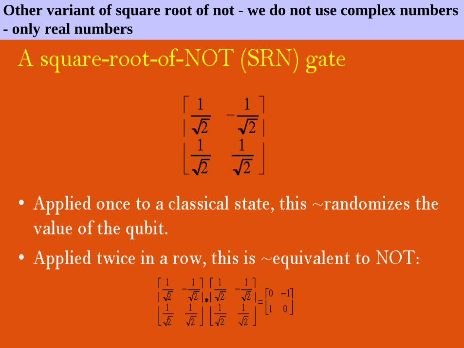
Other variant of square root of not - we do not use complex numbers- only real numbers

Quantum GatesQuantum Gates• One-Input gate: Hadamard
– Maps |0⟩ → 1/ √ 2 |0⟩ + 1/ √ 2 |1⟩ and |1⟩ → 1/ √ 2 |0⟩ – 1/ √ 2 |1⟩.
– Ignoring the normalization factor 1/ √ 2, we can write|xx⟩ → (-1)xx |xx⟩ – |1 –– xx⟩
• One-Input gate: Phase shift
12
1 11 −1
H
1 00 eiφ
φ
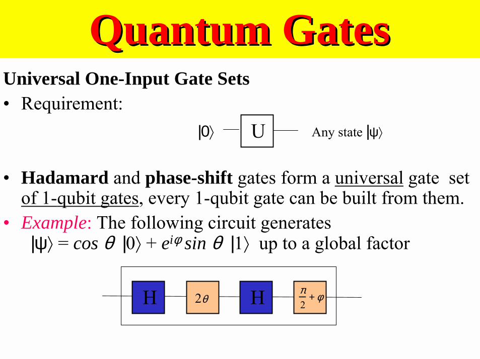
Universal One-Input Gate Sets• Requirement:
• Hadamard and phase-shift gates form a universal gate setof 1-qubit gates, every 1-qubit gate can be built from them.
• Example: The following circuit generates |ψ⟩ = cos θ |0⟩ + eiφ sin θ |1⟩ up to a global factor
Quantum GatesQuantum Gates
U|0⟩ Any state |ψ⟩
2θH H π2
+ φ
Other Quantum GatesOther Quantum Gates
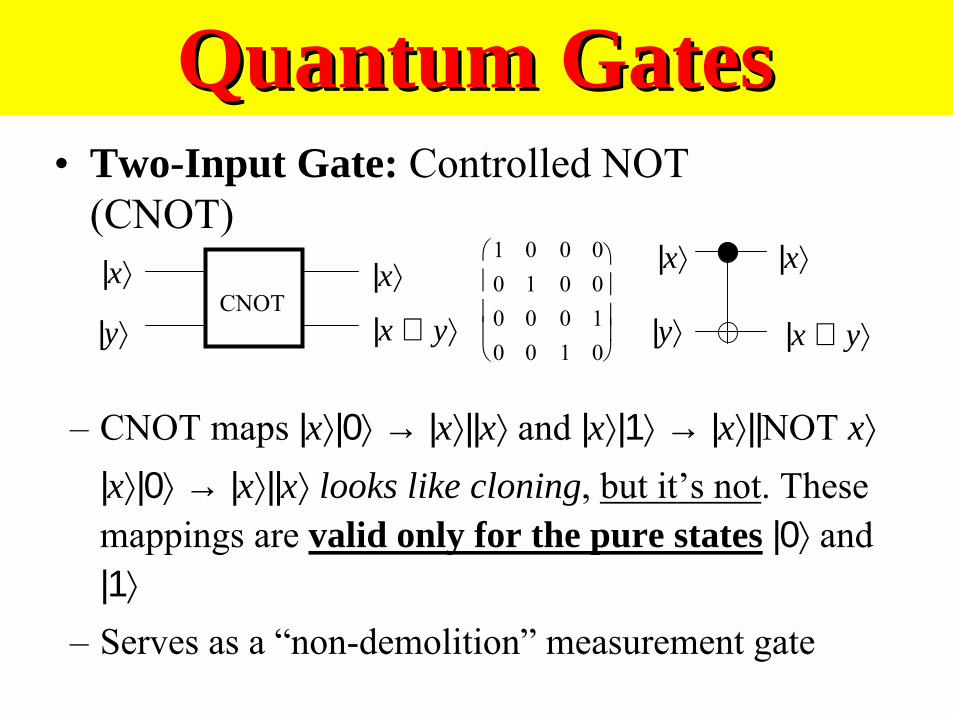
• Two-Input Gate: Controlled NOT(CNOT)
Quantum GatesQuantum Gates
|x⟩
|y⟩
|x⟩
|x ⊕ y⟩ CNOT
1 0 0 00 1 0 00 0 0 10 0 1 0
– CNOT maps |x⟩|0⟩ → |x⟩||x⟩ and |x⟩|1⟩ → |x⟩||NOT x⟩
|x⟩|0⟩ → |x⟩||x⟩ looks like cloning, but it’s not. Thesemappings are valid only for the pure states |0⟩ and|1⟩
– Serves as a “non-demolition” measurement gate
|x⟩
|y⟩
|x⟩
|x ⊕ y⟩
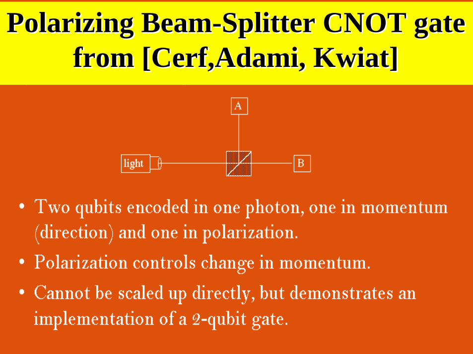
Polarizing Beam-Splitter CNOT gatePolarizing Beam-Splitter CNOT gatefrom [from [CerfCerf,,AdamiAdami, , KwiatKwiat]]
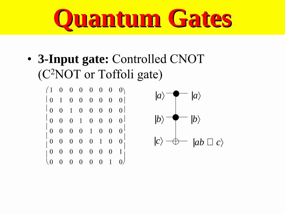
• 3-Input gate: Controlled CNOT(C2NOT or Toffoli gate)
Quantum GatesQuantum Gates
1 0 0 0 0 0 0 00 1 0 0 0 0 0 00 0 1 0 0 0 0 00 0 0 1 0 0 0 00 0 0 0 1 0 0 00 0 0 0 0 1 0 00 0 0 0 0 0 0 10 0 0 0 0 0 1 0
|b⟩
|c⟩
|b⟩
|ab ⊕ c⟩
|a⟩ |a⟩
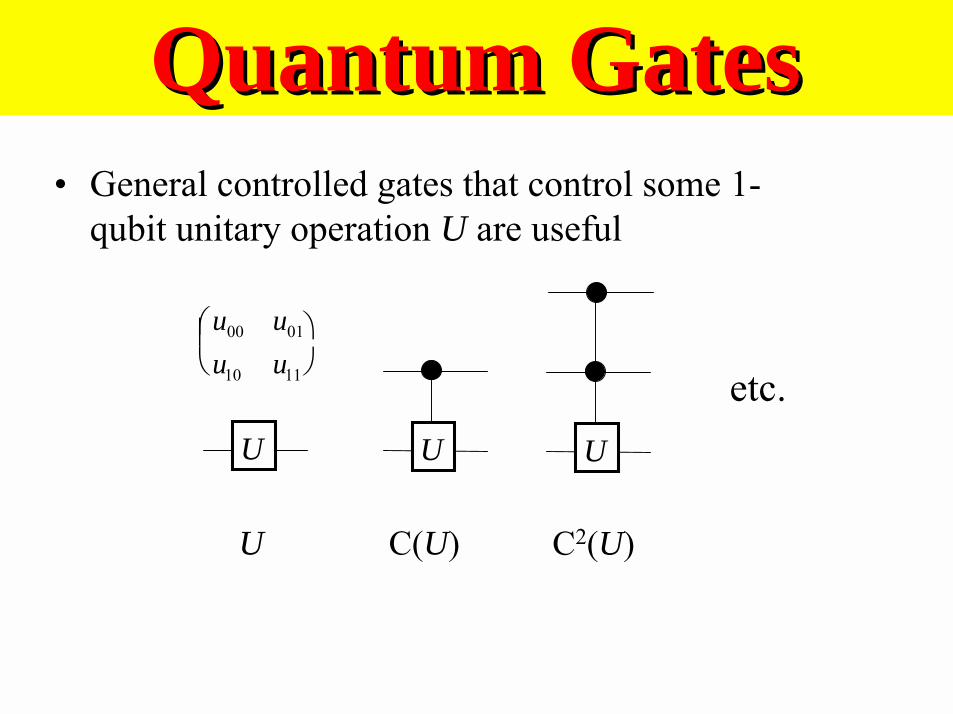
• General controlled gates that control some 1-qubit unitary operation U are useful
Quantum GatesQuantum Gates
U
u00 u01
u10 u11
C(U)
U
C2(U)
U
U
etc.
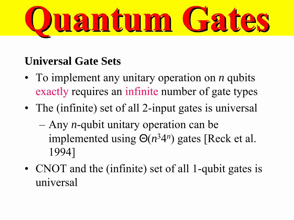
Universal Gate Sets• To implement any unitary operation on n qubits
exactly requires an infinite number of gate types• The (infinite) set of all 2-input gates is universal
– Any n-qubit unitary operation can beimplemented using Θ(n34n) gates [Reck et al.1994]
• CNOT and the (infinite) set of all 1-qubit gates isuniversal
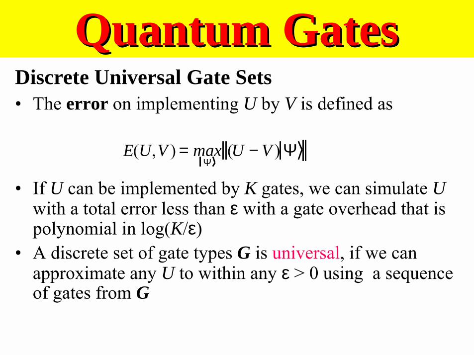
Discrete Universal Gate Sets• The error on implementing U by V is defined as
• If U can be implemented by K gates, we can simulate Uwith a total error less than ε with a gate overhead that ispolynomial in log(K/ε)
• A discrete set of gate types G is universal, if we canapproximate any U to within any ε > 0 using a sequenceof gates from G
Quantum GatesQuantum Gates
E(U,V ) = maxΨ
(U − V ) Ψ
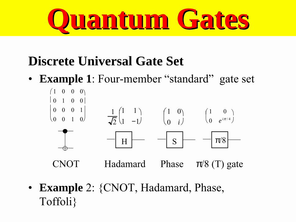
Discrete Universal Gate Set• Example 1: Four-member “standard” gate set
Quantum GatesQuantum Gates
1 0 0 00 1 0 00 0 0 10 0 1 0
1
21 11 −1
H
1 00 i
S π/8
1 00 e iπ / 4
CNOT Hadamard Phase π/8 (T) gate
• Example 2: {CNOT, Hadamard, Phase,Toffoli}
• A quantum (combinational) circuit is a sequence ofquantum gates, linked by “wires”
• The circuit has fixed “width” corresponding to thenumber of qubits being processed
• Logic design (classical and quantum) attempts to findcircuit structures for needed operations that are– Functionally correct– Independent of physical technology– Low-cost, e.g., use the minimum number of qubits or gates
• Quantum logic design is not well developed!
Quantum CircuitsQuantum Circuits
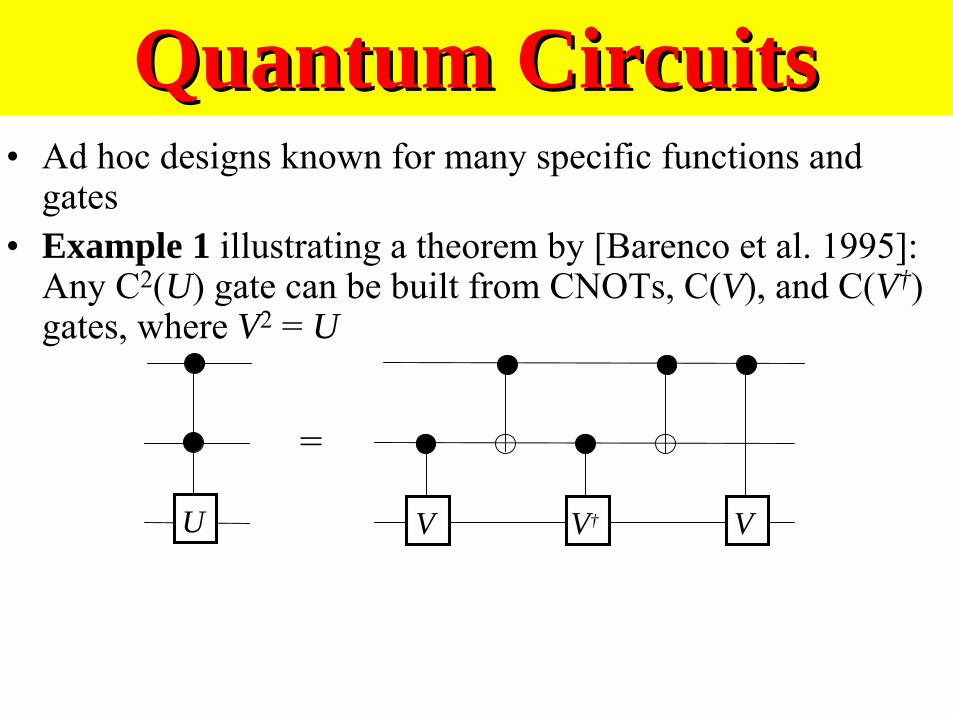
• Ad hoc designs known for many specific functions andgates
• Example 1 illustrating a theorem by [Barenco et al. 1995]:Any C2(U) gate can be built from CNOTs, C(V), and C(V†)gates, where V2 = U
Quantum CircuitsQuantum Circuits
V V† V
=
U
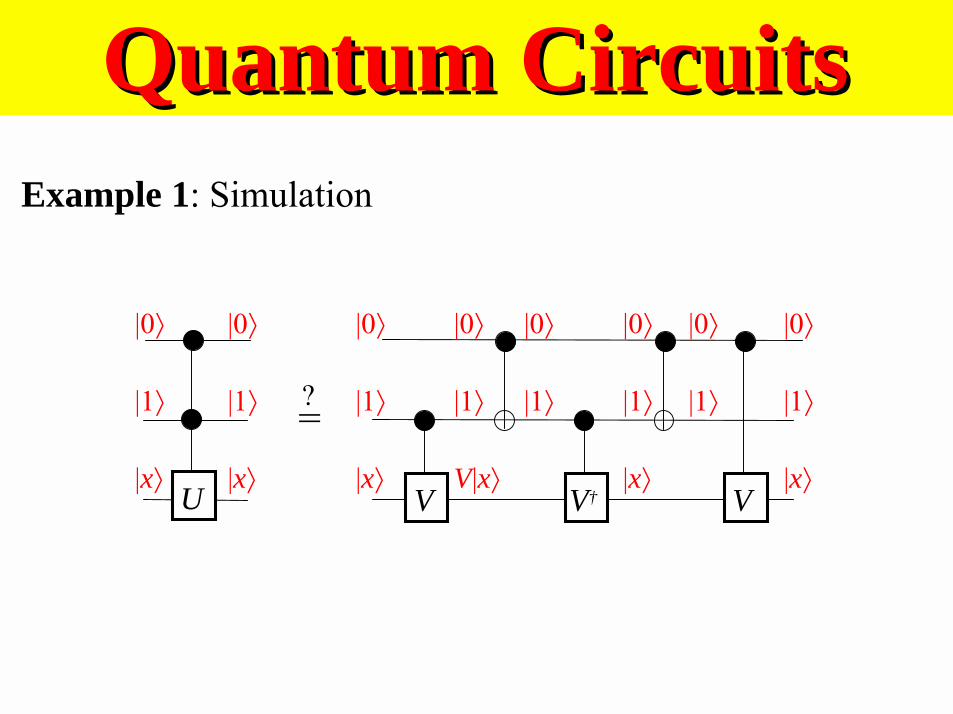
Example 1: Simulation
Quantum CircuitsQuantum Circuits
|0⟩
|1⟩
|x⟩
|0⟩
|1⟩
|x⟩
|0⟩
|1⟩
|x⟩V V† V
=
U
|0⟩
|1⟩
V|x⟩
|0⟩
|1⟩
|0⟩
|1⟩
|x⟩
|0⟩
|1⟩
|0⟩
|1⟩
|x⟩
?
Quantum CircuitsQuantum Circuits
|1⟩
|1⟩
|x⟩
|1⟩
|1⟩
|x⟩
|1⟩
|1⟩
U|x⟩V V† V
=
U
|1⟩
|1⟩
V|x⟩
|1⟩
|0⟩
|1⟩
|0⟩
V|x⟩
|1⟩
|1⟩
|1⟩
|1⟩
U|x⟩
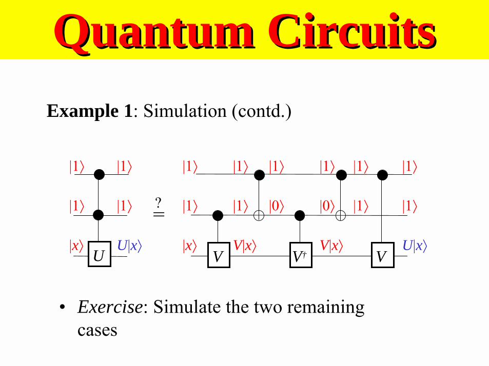
Example 1: Simulation (contd.)
?
• Exercise: Simulate the two remainingcases
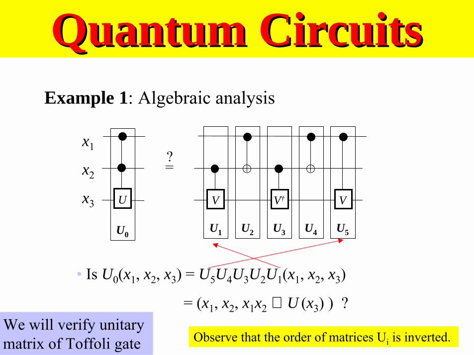
Quantum CircuitsQuantum CircuitsExample 1: Algebraic analysis
U4U2 U3U1 U5U0
V V† V
=
U
?x1
x2
x3
• Is U0(x1, x2, x3) = U5U4U3U2U1(x1, x2, x3)
= (x1, x2, x1x2 ⊕ U (x3) ) ?We will verify unitarymatrix of Toffoli gate Observe that the order of matrices Ui is inverted.
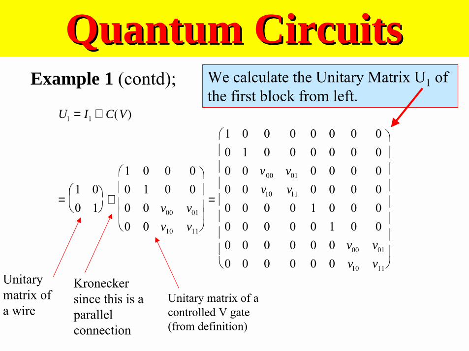
Quantum CircuitsQuantum CircuitsExample 1 (contd);
U1 = I1 ⊗ C(V)
=1 00 1
⊗
1 0 0 00 1 0 00 0 v00 v01
0 0 v10 v11
=
1 0 0 0 0 0 0 00 1 0 0 0 0 0 00 0 v00 v01 0 0 0 00 0 v10 v11 0 0 0 00 0 0 0 1 0 0 00 0 0 0 0 1 0 00 0 0 0 0 0 v00 v01
0 0 0 0 0 0 v10 v11
Kroneckersince this is aparallelconnection
Unitarymatrix ofa wire
Unitary matrix of acontrolled V gate(from definition)
We calculate the Unitary Matrix U1 ofthe first block from left.
Quantum CircuitsQuantum CircuitsExample 1 (contd);
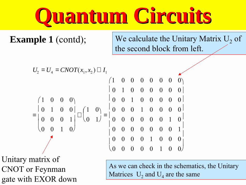
U2 = U4 = CNOT(x1, x2 ) ⊗ I1
=
1 0 0 00 1 0 00 0 0 10 0 1 0
⊗1 00 1
=
1 0 0 0 0 0 0 00 1 0 0 0 0 0 00 0 1 0 0 0 0 00 0 0 1 0 0 0 00 0 0 0 0 0 1 00 0 0 0 0 0 0 10 0 0 0 1 0 0 00 0 0 0 0 1 0 0
We calculate the Unitary Matrix U2 ofthe second block from left.
Unitary matrix ofCNOT or Feynmangate with EXOR down
As we can check in the schematics, the UnitaryMatrices U2 and U4 are the same
Quantum CircuitsQuantum CircuitsExample 1 (contd);
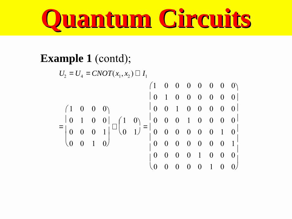
U2 = U4 = CNOT(x1, x2 ) ⊗ I1
=
1 0 0 00 1 0 00 0 0 10 0 1 0
⊗1 00 1
=
1 0 0 0 0 0 0 00 1 0 0 0 0 0 00 0 1 0 0 0 0 00 0 0 1 0 0 0 00 0 0 0 0 0 1 00 0 0 0 0 0 0 10 0 0 0 1 0 0 00 0 0 0 0 1 0 0
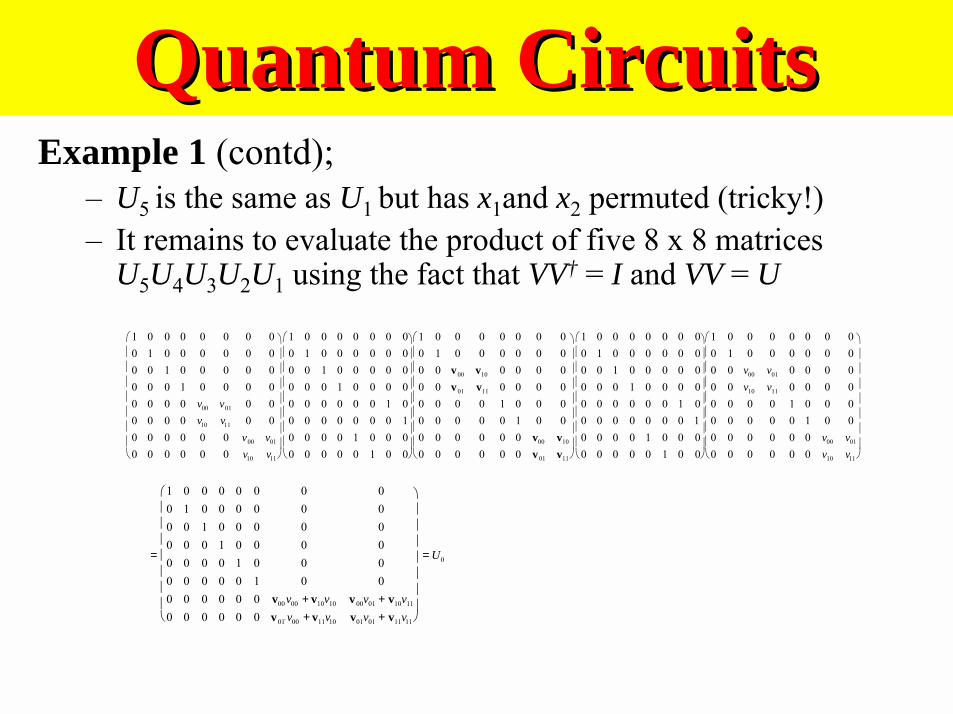
Quantum CircuitsQuantum CircuitsExample 1 (contd);
– U5 is the same as U1 but has x1and x2 permuted (tricky!)– It remains to evaluate the product of five 8 x 8 matrices
U5U4U3U2U1 using the fact that VV† = I and VV = U
1 0 0 0 0 0 0 00 1 0 0 0 0 0 00 0 1 0 0 0 0 00 0 0 1 0 0 0 00 0 0 0 v00 v01 0 00 0 0 0 v10 v11 0 00 0 0 0 0 0 v00 v01
0 0 0 0 0 0 v10 v11
1 0 0 0 0 0 0 00 1 0 0 0 0 0 00 0 1 0 0 0 0 00 0 0 1 0 0 0 00 0 0 0 0 0 1 00 0 0 0 0 0 0 10 0 0 0 1 0 0 00 0 0 0 0 1 0 0
1 0 0 0 0 0 0 00 1 0 0 0 0 0 00 0 v00 v10 0 0 0 00 0 v01 v11 0 0 0 00 0 0 0 1 0 0 00 0 0 0 0 1 0 00 0 0 0 0 0 v00 v10
0 0 0 0 0 0 v01 v11
1 0 0 0 0 0 0 00 1 0 0 0 0 0 00 0 1 0 0 0 0 00 0 0 1 0 0 0 00 0 0 0 0 0 1 00 0 0 0 0 0 0 10 0 0 0 1 0 0 00 0 0 0 0 1 0 0
1 0 0 0 0 0 0 00 1 0 0 0 0 0 00 0 v00 v01 0 0 0 00 0 v10 v11 0 0 0 00 0 0 0 1 0 0 00 0 0 0 0 1 0 00 0 0 0 0 0 v00 v01
0 0 0 0 0 0 v10 v11
=
1 0 0 0 0 0 0 00 1 0 0 0 0 0 00 0 1 0 0 0 0 00 0 0 1 0 0 0 00 0 0 0 1 0 0 00 0 0 0 0 1 0 00 0 0 0 0 0 v00v00 + v10v10 v00v01 + v10v11
0 0 0 0 0 0 v01̀ v00 + v11v10 v01v01 + v11v11
= U0
Quantum CircuitsQuantum CircuitsExample 1 (contd);
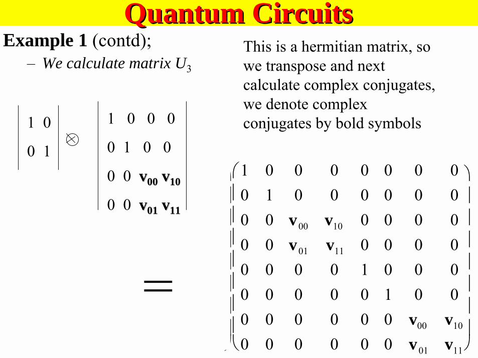
– We calculate matrix U3
00000
00
1 0 0 0 0 0 0 00 1 0 0 0 0 0 00 0 v00 v10 0 0 0 00 0 v01 v11 0 0 0 00 0 0 0 1 0 0 00 0 0 0 0 1 0 00 0 0 0 0 0 v00 v10
0 0 0 0 0 0 v01 v11
This is a hermitian matrix, sowe transpose and nextcalculate complex conjugates,we denote complexconjugates by bold symbols1 0
0 1
1 0 0 0
0 1 0 0
0 0 vv0000 vv1010
0 0 vv0101 v v1111
Quantum CircuitsQuantum CircuitsExample 1 (contd);
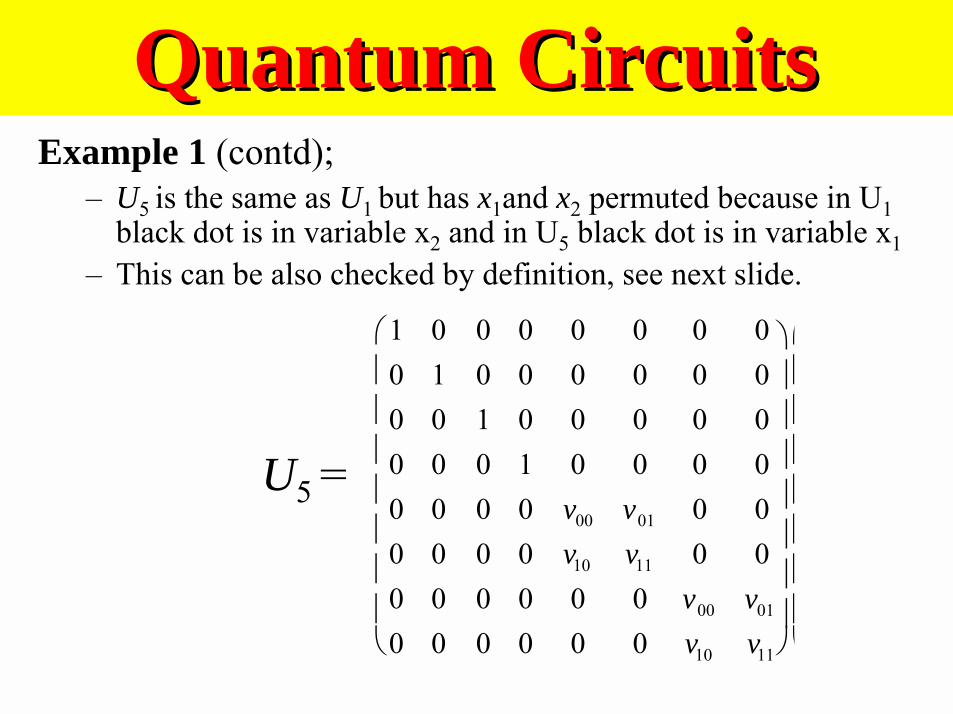
– U5 is the same as U1 but has x1and x2 permuted because in U1black dot is in variable x2 and in U5 black dot is in variable x1
– This can be also checked by definition, see next slide.
1 0 0 0 0 0 0 00 1 0 0 0 0 0 00 0 1 0 0 0 0 00 0 0 1 0 0 0 00 0 0 0 v00 v01 0 00 0 0 0 v10 v11 0 00 0 0 0 0 0 v00 v01
0 0 0 0 0 0 v10 v11
U5 =
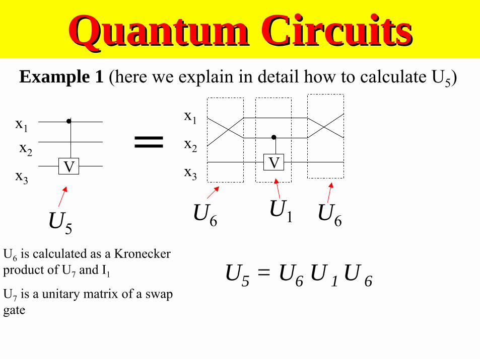
Quantum CircuitsQuantum CircuitsExample 1 (here we explain in detail how to calculate U5)
.x1
x2
x3V
U5
x1
x2
x3V
U1
.
U6 U6
U6 is calculated as a Kroneckerproduct of U7 and I1
U7 is a unitary matrix of a swapgate
U5 = U6 U 1 U 6
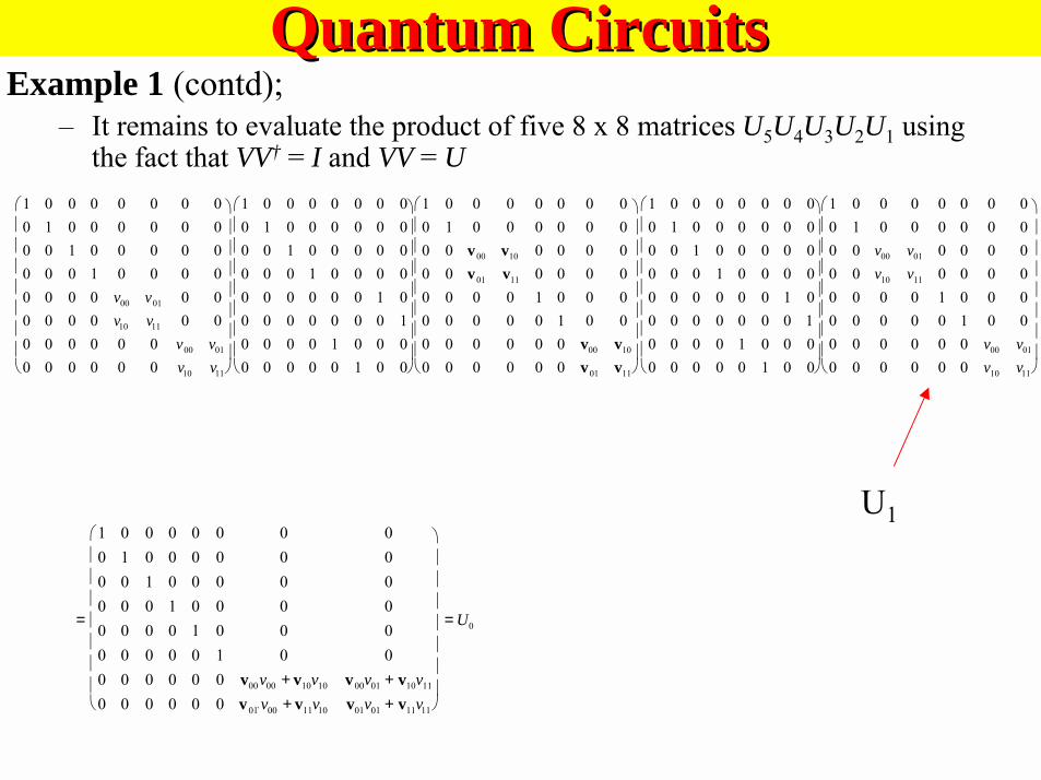
Quantum CircuitsQuantum CircuitsExample 1 (contd);
– It remains to evaluate the product of five 8 x 8 matrices U5U4U3U2U1 usingthe fact that VV† = I and VV = U
1 0 0 0 0 0 0 00 1 0 0 0 0 0 00 0 1 0 0 0 0 00 0 0 1 0 0 0 00 0 0 0 v00 v01 0 00 0 0 0 v10 v11 0 00 0 0 0 0 0 v00 v01
0 0 0 0 0 0 v10 v11
1 0 0 0 0 0 0 00 1 0 0 0 0 0 00 0 1 0 0 0 0 00 0 0 1 0 0 0 00 0 0 0 0 0 1 00 0 0 0 0 0 0 10 0 0 0 1 0 0 00 0 0 0 0 1 0 0
1 0 0 0 0 0 0 00 1 0 0 0 0 0 00 0 v00 v10 0 0 0 00 0 v01 v11 0 0 0 00 0 0 0 1 0 0 00 0 0 0 0 1 0 00 0 0 0 0 0 v00 v10
0 0 0 0 0 0 v01 v11
1 0 0 0 0 0 0 00 1 0 0 0 0 0 00 0 1 0 0 0 0 00 0 0 1 0 0 0 00 0 0 0 0 0 1 00 0 0 0 0 0 0 10 0 0 0 1 0 0 00 0 0 0 0 1 0 0
1 0 0 0 0 0 0 00 1 0 0 0 0 0 00 0 v00 v01 0 0 0 00 0 v10 v11 0 0 0 00 0 0 0 1 0 0 00 0 0 0 0 1 0 00 0 0 0 0 0 v00 v01
0 0 0 0 0 0 v10 v11
=
1 0 0 0 0 0 0 00 1 0 0 0 0 0 00 0 1 0 0 0 0 00 0 0 1 0 0 0 00 0 0 0 1 0 0 00 0 0 0 0 1 0 00 0 0 0 0 0 v00v00 + v10v10 v00v01 + v10v11
0 0 0 0 0 0 v 01̀ v00 + v11v10 v01v01 + v11v11
= U0
U1

Quantum CircuitsQuantum Circuits• Implementing a Half Adder
– Problem: Implement the classical functions sum =x1 ⊕ x0 and carry = x1x0
• Generic design:|x1⟩
Uadd|x0⟩
|y1⟩
|y0⟩
|x1⟩
|x0⟩
|y1⟩ ⊕ carry|y0⟩ ⊕ sum
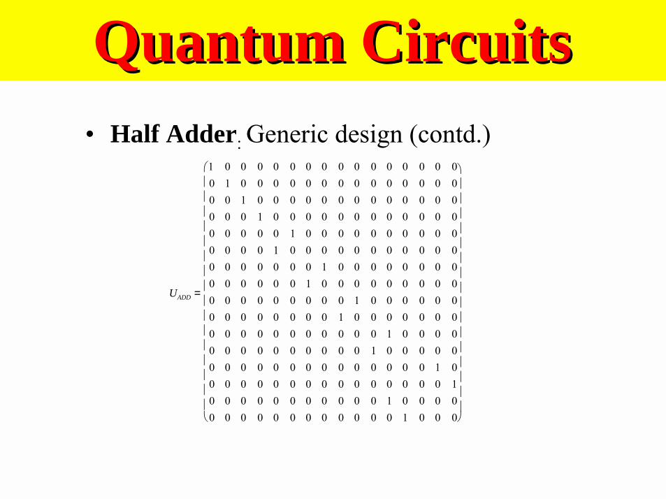
Quantum CircuitsQuantum Circuits• Half Adder: Generic design (contd.)
UADD =
1 0 0 0 0 0 0 0 0 0 0 0 0 0 0 00 1 0 0 0 0 0 0 0 0 0 0 0 0 0 00 0 1 0 0 0 0 0 0 0 0 0 0 0 0 00 0 0 1 0 0 0 0 0 0 0 0 0 0 0 00 0 0 0 0 1 0 0 0 0 0 0 0 0 0 00 0 0 0 1 0 0 0 0 0 0 0 0 0 0 00 0 0 0 0 0 0 1 0 0 0 0 0 0 0 00 0 0 0 0 0 1 0 0 0 0 0 0 0 0 00 0 0 0 0 0 0 0 0 1 0 0 0 0 0 00 0 0 0 0 0 0 0 1 0 0 0 0 0 0 00 0 0 0 0 0 0 0 0 0 0 1 0 0 0 00 0 0 0 0 0 0 0 0 0 1 0 0 0 0 00 0 0 0 0 0 0 0 0 0 0 0 0 0 1 00 0 0 0 0 0 0 0 0 0 0 0 0 0 0 10 0 0 0 0 0 0 0 0 0 0 1 0 0 0 00 0 0 0 0 0 0 0 0 0 0 0 1 0 0 0
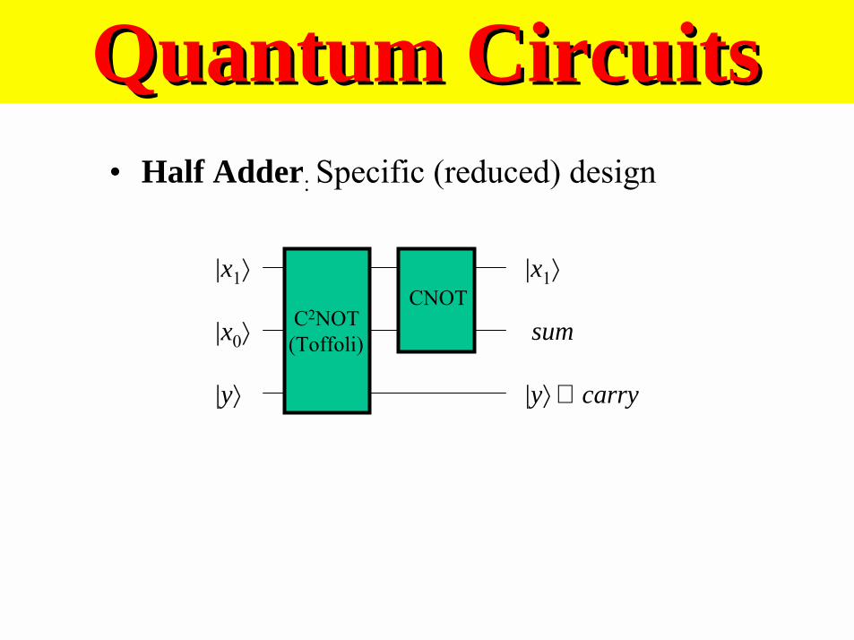
Quantum CircuitsQuantum Circuits• Half Adder: Specific (reduced) design
|x1⟩
|x0⟩
|y⟩
|x1⟩
|y⟩ ⊕ carry
sum C2NOT(Toffoli)
CNOT