Martingales and Stopping Times - Stanford Universitypsimin/presentations/martingales.pdf · Martingales and Stopping Times Use of martingales in obtaining bounds and analyzing algorithms

MartingalesConcentration Results for Martingales

Stopping TimesConclusion

Martingales and Stopping TimesUse of martingales in obtaining bounds and analyzing algorithms

Paris Siminelakis

School of Electrical and Computer Engineering at the National TechnicalUnivercity of Athens

24/3/2010

Paris Siminelakis Martingales and Stopping Times



Outline1 Martingales

FiltrationConditional ExpectationMartingales

2 Concentration Results for MartingalesLipschitz ConditionBoundsQuick ApplicationsOccupancy RevisedTraveling Salesman

3 Stopping TimesBasicsWald’s Equation

Server Routing4 Conclusion





Filtration

A σ-field (Ω,F) consists of a sample space Ω and a collectionof subsets F satisfying the following conditions :

1 Contains the empty set (∅ ∈ F).2 Is closed under complement(E ∈ F⇒ E ∈ F).3 Is closed under countable union and intersection.

Given the σ-field (Ω,F) with F = 2Ω, a filter (sometimes alsocalled a filtration) is a nested sequence F0 ⊆ F1 ⊆ . . . ⊆ Fn ofsubsets of 2Ω such that :

1 F0 = ∅,Ω(no information).2 Fn = 2Ω(full information).3 for 0 ≤ i ≤ n, (Ω,Fi ) is a σ-field(partial information).

Essentially a filter is a sequence of σ-fields such that eachnew σ-field corresponds to the additional information thatbecomes available at each step and thus the furtherrefinement of the sample space Ω.





Filtration-Examples

Binary Strings : Consider w a binary string size n. A filter for thesample space Ω = 0, 1n could be the sequence of sets Fi such thateach set corresponds to thepartitioning of the samplespace according to the first ibits.

Americans: Let Ω be the sample space of all Americans.Define therandom variable X, denoting the weight of a randomly chosenAmerican. A filter with respect to Ω could be:

F0 is the trivial σ-field(no information - no partition).F1 is the σ-field generated by partioning Ω according to sex.F2 is the σ-field generated by the refinement of the previouspartion into sets of different heights.F3 is the further refinement based on age.F4 is the partition into sigleton sets





Conditional Expectation

The expectation of a random variable X conditioned on anevent A can be viewed as a function of a random variable Ywhich takes constant real values for every different outcome ofA. In other words :

E[X |A] = E[X |Y ] = E[X |Y = y ] = f (y)

If the outcome of the event A or equivalently the value of thevariable Y is not known then the conditional expectation itselfis a random variable, denoted f(Y).





Americans

Consider the example about Americans. We saw that we candefine a filter on the sample space by partitioning appropriately thesample space. Let F0 ⊆ F1 ⊆ . . . ⊆ F4 be the filter we mentionedearlier.Define Xi = E[X |Fi ], for 0 ≤ i ≤ 4. Then :

X0 = E[X ] denotes the average weight of an American.

X1 = E[X |F1] denotes the average weight of Americans as afunction of their sex.

X2 = E[X |F2] denotes the average weight as a function oftheir sex and height.

X3 = E[X |F3] denotes the average weight as a function oftheir sex, height and age.

Whereas X4 = E[X |F4] = X corresponds to the weight of anindividual American.





6-Sided Unbiased die

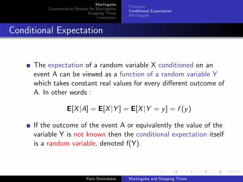
Consider n independent throws of an unbiased 6-sided die. For0 ≤ i ≤ 6, let Xi denote the number of times the value iappears. Then :

E[X1|X2] =n − X2

6− 1

E[X1|X2X3] =n − X2 − X3

4

These equations define the expected value of the randomvariable X1 given the number of times 2 and 3 appear. Ofcourse the variables X2,X3 are random themselves if they arenot given.





Martingales

Martingales originally referred to systems of betting in which aplayer doubled his stake each time he lost a bet.

Definition

Let (Ω,F,Pr) be a propability space with a filter F0,F1, . . ..Suppose that X0,X1, . . . are random variables such that for alli ≥ 0,Xi is Fi measurable (constant over each block in thepartition generating Fi ). The sequence X0, . . . ,Xn is a martingaleprovided that for all i ≥ 0

E[Xi+1|Fi ] = Xi





Edge Exposure Martingale

Let G be a random graph on the vertex set V = 1, . . . , n obtainedby intepedently choosing to include each possible edge withpropability p. The underlying propability space is called Gn,p.

Arbitarily label the m = n(n − 1)/2 edges with the sequence1, . . . ,m. For 1 ≤ i ≤ m, define the inidcator random variable Ijwhich takes value 1 if edge j is present in G, and has value 0otherwise. These indicator variables are independent and each takesvalue 1 with propability p.

Consider any real-valued function F defined over the space of allgraphs, e.g., the clique number. The edge exposure martingale isdefined to be the sequence of random variables X0, . . . ,Xm suchthat :

Xk = E[F (G )|I1, . . . , Ik ]

while X0 = E[F (G )] and Xm = F (G ).





Edge Exposure Martingale

Consider that m = n = 3,and F (G ) = chromatic number we willshow that the sequence X0, . . . ,Xm is indeed a martingale.Specifically that the following property holds : E[Xi+1|Fi ] = Xi .





Vertex Exposure Martingale

Let again consider the propability space Gn,p mentioned earlier.

For 1 ≤ i ≤ n,let Ei be the set of all possible edges with bothend-points in 1, . . . , n.Define the indicator random variablesIj for all j ∈ Ei .

Again consider any real valued fucntion F(G). The vertexexposure martingale is defined to be the sequence of ofrandom variables X0, . . . ,Xn such that :

Xi+1 = E[F (G )|Ij∀j ∈ Ei ]

The vertex exposure martingale reveals the induced graph Gi

generated by only the first i nodes.





Expected Running Time

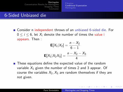
Let T be the running time of a randomized algorithm A that usesa total of n random bits, on a specific input. Clearly T is a randomvariable whose value depends in the random bits.

Observe that T is Fn measurable, but in general is not Fi

measurable for i < n.

Define the conditional expectation Ti = E[T |Fi ] where Fi isthe σ-field with the i-first bits known. Observe thatT0 = E[T ] and Tn = T .

Ti is a function of the values of the first i random bitsdenoting the expected running time for a random choice ofthe remaining n-i bits. The sequence of random variablesT0,T1, . . . ,Tn is a martingale.




Lipschitz ConditionBoundsQuick ApplicationsOccupancy RevisedTraveling Salesman

Why martingales are usefull?

We have seen various example of filters and the correspondingmartingales. They have the nasty habit to come up in a variety ofapplications.

We may view the σ-field sequence F0 ⊆ F1 ⊆ . . . ⊆ Fn asrepresenting the evolution of the algorithm, with each succesiveσ-field providing more information about the behaviour of thealgorithm.

The random variables T0,T1, . . . ,Tn represent the changingexpectation of the running time as more information is revealedabout the random choices. As we will see later, if it can be shownthat the absolute difference |Ti − Ti−1| is suitably bounded, thenthe random variable Tn behaves like T0 in the limit.

We mainly utilize martingales in obtaining concentration bounds.





Lipschitz Condition

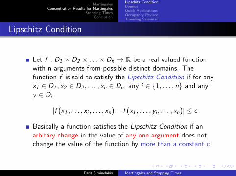
Let f : D1 × D2 × . . .× Dn → R be a real valued functionwith n arguments from possible distinct domains. Thefunction f is said to satisfy the Lipschitz Condition if for anyx1 ∈ D1 , x2 ∈ D2 , . . . , xn ∈ Dn, any i ∈ 1, . . . , n and anyy ∈ Di

|f (x1 , . . . , xi , . . . , xn)− f (x1 , . . . , yi , . . . , xn)| ≤ c

Basically a function satisfies the Lipschitz Condition if anarbitary change in the value of any one argument does notchange the value of the function by more than a constant c.





Azuma-Hoeffding Inequality

Theorem

Let (Y ,F) be a martingale, and suppose that there exists asequence K1,K1, . . . ,Kn of real numbers such that|Yi − Yi−1| ≤ Kn for all i(bounded difference condition). Then :

P(|Yn − Y0| ≥ x) ≤ 2exp(−1

2x2/

n∑i=1

K 2i ), x > 0





Proof I

We begin the proof with an elementary inequality that stems fromthe convexity of g(d) = eψd .

eψd ≤ 1

2(1− d)e−ψ +

1

2(1 + d)e+ψ |d | ≤ 1.

Applying this to a random variable D having mean 0 and |D| ≤ 1we obtain

E(eψD) ≤ 1

2(e−ψ + e+ψ) ≤ e

12ψ

2

. (1)

By applying the Markov Inequality we have :

P(Yn − Y0 ≥ x) ≤ e−θxE(eθ(Yn−Y0)). (2)

Writing Dn = Yn − Yn−1, we have that :

E(eθ(Yn−Y0)) = E(eθ(Yn−1−Y0)eθDn).





Proof II

Conditioning on Fn−1, using the fact that Yn−1 − Y0 isFn−1-measurable and applying (1) to the random variable Dn/Kn,we obtain :

E(eθ(Yn−Y0)|Fn−1) = eθ(Yn−1−Y0)E(eθDn |Fn−1) ≤ eθ(Yn−1−Y0)exp(1

2θ2K 2

n )

Taking expectation of the above inequality, using the fact thatE[E[X |Y ]] = E[X ] and then iterating we find that :

E(eθ(Yn−Y0)) ≤ E(eθ(Yn−1−Y0))exp(1

2θ2K 2

n ) ≤ exp(1

2θ2

n∑i=1

K 2i )

Applying (2)which is known as the Bernstein Inequality we obtain :

P(Yn − Y0 ≥ x) ≤ exp(−θx +1

2θ2

n∑i=1

K 2i )





Proof III

Suppose x > 0, the value that minimizes the exponent isθ = x/

∑ni=1 K 2

i . Thus we have :

P(Yn − Y0 ≥ x) ≤ exp(−1

2x2

n∑i=1

K 2i )

The same argument is valid with Yn − Y0 replaced with Y0 − Yn,and the claim of the theorem follows by adding the two boundstogether.

The Azuma-Hoeffding inequality can be generalized ifak ≤ Yk − Yk−1 ≤ bk to yield :

P(|Yn − Y0| ≥ x) ≤ 2exp(−2x2/

n∑i=1

(bk − ak)2), x > 0

The application of the Azuma-Hoeffding inequality is sometimescalled ”the method of bounded differences”.





Connection with Chernoff Bound

Let Z1, . . . ,Zn be independent random variables that take values 0or 1 each with propability p.

The random variable S =∑n

i=1 Zi has the binomial distributionwith parameters n and p.

Define a maritngale sequence X0, . . . ,Xn by setting X0 = E[S ],and,for 1 ≤ i ≤ n, Xi = E[S |Z1, . . . ,Zi ]. It is clear that |Xi − Xi−1| ≤ 1,since fixing the value of one variable Zi can only affect the expectedvalue of the sum by at most 1.

It follows that the propability that S deviates from its expectedvalue is bounded by :

P(|Xn − X0| ≥ x) ≤ 2exp(− x2

2n)

Which is a weaker result than can be inferred from the Chernoffbound approach.





Bin Packing

Given n items with random sizes X = (X1, . . . ,Xn) uniformly distributedin the interval [0,1] and unlimited collection of unit size bins. Theproblem is to find the minimum number of bins required to store all theitems,denoted Bn. It can be shown that Bn grows approximately linearlyin n : E[Bn]→ c · n. How close is Bn to its mean value :

Define for i ≤ n , Yi = E(Bn|Fi ), where Fi is the σ − fieldgenerated by X1, . . . ,Xi .

It easily seen that (Y ,F) is a martingale. Because the items aredistributed between [0,1] we derive that |Yi − Yi−1| ≤ 1.

Applying the Azuma inequalitywith∑n

i=1 K 2i = n, we get :

P(|Yn − Y0| ≥ x) ≤ 2exp(−1

2x2/n)

setting x = εn we see that the chance that Bn deviates from itsmean by εn decays exponentially in n.





Chromatic Number

Given a random graph G in Gn,p, the chromatic number χ(G) is theminimum number of colors needed in order to color all vertices of thegraph so that no adjacent vertices have the same color. We use thevertex exposure martingale to obtain a concentration result for χ(G).

Let Gi be the random subgraph induced by the set of vertices1, . . . , i , let Z0 = E[χ(G )] and let :

Zi = E[χ(G )|G1, . . . ,Gi ].

Since a vertex uses no more than one new color, again we have thatthe gap between Zi and Zi−1 is at most 1. Applying theAzuma-Hoeffding inequality ,we obtain :

P(|Zn − Z0| ≥ λ√

n) ≤ 2exp(−λ2/2)

The result holds without knowing the mean. We must note that byusing the generalized version of the inequality we obtained a betterbound.





Pattern Matching

Let X = (X1, . . . ,Xn) be a sequence of characters chosen independentlyand uniformly at random from an alphabet Σ, where |Σ| = s. LetB = (B1, . . . ,Bk) be a fixed string of k characters from Σ. Let F be thenumber of occurences of B in the random string X.The expectation of Fis E[F ] = (n − k + 1)( 1

s )k

Define the martingale sequence Zi = E[F |X1, . . . ,Xi ].

Since each character in the string X cannot participate in no morethan k possible matches, we have that the function F satisfies thelipschitz condition for bound k . Thus we have that :|Zi − Zi−1| ≤ k .

By applying the general Azuma-Hoeffding inequality we have :

P(|Zn − Z0| ≥ ε) ≤ 2exp(−ε2/2nk2)





Balls and Bins

Suppose we are throwing m balls independently and uniformly at randomat n bins. Let Xi denote the random variable representing the bin intowhich the ith ball falls. Let F be the number of empty bins after the mballs are thrown. Then the sequence: Zi = E[F |X1, . . . ,Xi ] is amartingale.

The function F = f (X1, . . . ,Xm) satisfies the Lipschitz Conditionwith bound 1. Because changing the bin where the ith ball was, willeither decrease F by 1(relocate to an empty bin), increase F by 1(relocate to a non-empty bin) or stay the same.

Applying the Azuma inequality we obtain :

P(|Zn − Z0| ≥ x) ≤ 2exp(−1

2x2/m)

This result can be improved by taken more care in bounding thedifference |Zi − Zi−1|.





Occupancy Revised

In the Balls and Bins setting we will obtain tighter concentration bounds.Let Z0, . . . ,Zm be the martingale sequence defined earlier. Define z(Y , t)as the expectation of Z given that Y bins are empty at time t. Thepropability that none of these bins does not receive a ball during the lastm − t time units is (1− 1/n)m−t .

By linearity of expectation, we obtain that the number of these binsthat remain empty is given by :

E[Z |Yt ] = z(Y , t) = Yt(1− 1

n)m−t

where the random variable Yt denotes the number of empty bins attime t.

Then for the martingale sequence we have :

Zt−1 = z(Yt−1, t − 1) = Yt−1(1− 1

n)m−t+1





Analysis I

Suppose we are at time t − 1, so that the values of Yt−1,Zt−1 aredetermined. At time t there are two possibilities :

1 With propability 1−Yt−1/n, the tth ball goes into a currentlynon-empty bin. Then Yt = Yt−1 and we have :

Zt = z(Yt , t) = z(Yt−1, t) = Yt−1(1− 1

n)m−t

2 With propability Yt−1/n, the tth ball goes into a currentlyempty bin. Then Yt = Yt−1 − 1 and we have :

Zt = z(Yt , t) = z(Yt−1 − 1, t) = (Yt−1 − 1)(1− 1

n)m−t





Analysis II

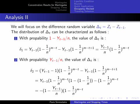
We will focus on the difference random variable ∆t = Zt − Zt−1.The distribution of ∆t can be characterized as follows :

1 With propability 1− Yt−1/n, the value of ∆t is :

δ1 = Yt−1(1− 1

n)m−t −Yt−1(1− 1

n)m−t+1 =

Yt−1

n(1− 1

n)m−t

2 With propability Yt−1/n, the value of ∆t is :

δ2 = (Yt−1 − 1)(1− 1

n)m−t − Yt−1(1− 1

n)m−t+1

= Yt−1(1− 1

n)m−t(1− (1− 1

n))− (1− 1

n)m−t

= −(1− Yt−1

n)(1− 1

n)m−t





Analysis III

Observing that 0 ≤ Yt−1 ≤ n, and using δ1 and δ2 for the upperand lower bound respectively we obtain :

−(1− 1

n)m−t ≤ ∆t ≤ (1− 1

n)m−t

For 1 ≤ i ≤ m, we set ct = (1− 1n )m−t , and we have that

|Zt − Zt−1| ≤ ct . Consequently :

m∑t=1

c2t =

1− (1− 1/n)2m

1− (1− 1/n)2=

n2 − µ2

2n − 1

where we used the geometric series sum and the expected valueµ = n(1− 1/n)m.Invoking Azuma-Hoeffding inequality now gives :

P(|Zn − µ| ≥ λ) ≤ 2exp(−λ2(n − 1/2)

n2 − µ2)





Traveling Salesman Problem

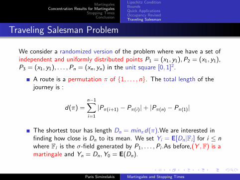
We consider a randomized version of the problem where we have a set ofindependent and uniformly distributed points P1 = (x1, y1),P2 = (x1, y1),P3 = (x1, y1), . . . ,Pn = (xn, yn) in the unit square [0, 1]2.

A route is a permutation π of 1, . . . , n. The total length of thejourney is :

d(π) =n−1∑i=1

|Pπ(i+1) − Pπ(i)|+ |Pπ(n) − Pπ(1)|

The shortest tour has length Dn = minπd(π).We are interested infinding how close is Dn to its mean. We set Yi = E[Dn|Fi ] for i ≤ nwhere Fi is the σ-field generated by P1, . . . ,Pi .As before,(Y ,F) is amartingale and Yn = Dn,Y0 = E(Dn).





Analysis I

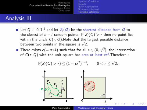
We will try to obtain a bounding difference condition for Dn. Let Dn(i)be the minimal-length tour through all points except i, and note thatE[Dn(i)|Fi ] = E[Dn(i)|Fi−1].

The vital inequality is :

Dn(i) ≤ Dn ≤ Dn(i) + 2Zi , i ≤ n − 1

where Zi is the shortest distance from Pi to one of the pointsPi+1, . . . ,Pn.

It is obvious that Dn ≥ Dn(i) .Since every tour of the n pointsincludes a tour of all the points except i . For the second inequalitywe argue that,let Pj be the closest point to Pi amongst the setPi+1, . . . ,Pn,a (sub-optimal) tour could be when we arrive at Pj

to visit Pi and return.

We must note that because the space is continuous we can comearbitarily close to Pj without visiting it. Thus we have a valid tour.





Analysis II

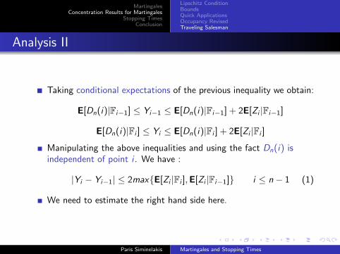
Taking conditional expectations of the previous inequality we obtain:

E[Dn(i)|Fi−1] ≤ Yi−1 ≤ E[Dn(i)|Fi−1] + 2E[Zi |Fi−1]

E[Dn(i)|Fi ] ≤ Yi ≤ E[Dn(i)|Fi ] + 2E[Zi |Fi ]

Manipulating the above inequalities and using the fact Dn(i) isindependent of point i . We have :

|Yi − Yi−1| ≤ 2maxE[Zi |Fi ],E[Zi |Fi−1] i ≤ n − 1 (1)

We need to estimate the right hand side here.





Analysis III

Let Q ∈ [0, 1]2 and let Zi (Q) be the shortest distance from Q tothe closest of n − i random points. If Zi (Q) > r then no point lieswithin the circle C (r ,Q).Note that the largest possible distancebetween two points in the square is

√2.

There exists c(= π/4) such that for all r ∈ (0,√

2], the intersectionof C (r ,Q) with the unit square has area at least cr 2.Therefore :

P(Zi (Q) > r) ≤ (1− cr 2)n−i , 0 < r ≤√

2.





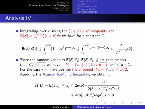
Analysis IV

Integrating over x, using the (1 + x) < ex inequality andE[X ] =

∫∞0

P(X > x)dx we have for a constant C :

E(Zi (Q)) ≤∫ √2

0

(1− cr 2)n−idr ≤∫ √2

0

e−cr2(n−i)dr <

C√n − i

(2)

Since the random variables E[Zi |Fi ],E[Zi |Fi−1] are each smallerthan C/

√n − i we have : |Yi − Yi−1| ≤ 2C/

√n − i for i ≤ n − 1.

For the case i = n, we use the trivial bound |Yn − Yn−1| ≤ 2√

2.Applying the Azuma-Hoeffding Inequality, we obtain :

P(|Dn − E(Dn)| ≥ x) ≤ 2exp(− x2

2(8 +∑n−1

i=1 4C 2/i

≤ exp(−Ax2/logn), x > 0.





Analysis V

It can be shown that 1√nE(Dn)→ τ as n→∞ so using the

previous result :

P(|Dn − τ√

n| ≥ ε√

n) ≤ 2exp(−Bε2n

logn) ε > 0

for some positive constant B and all large n.




BasicsWald’s Equation

Server Routing

Stopping Times

Consider again the betting martingale we saw at the beginning. Due tothe martingale property if the number of games is initially fixed then theexpected gain from the sequence of games is zero.

Suppose now that the number of games is not fixed. What happensif the gambler plays a random number of games or even betteraccording to a strategy?

For example a gambler could be playing until he doubles his originalassets. There are many strategies that one can conjure but not allof them are possible to quantify and analyze.





Server Routing

Stopping Times

Definition

A non-negative, integer-valued random variable T is a stoppingtime for the sequence Zn, n ≥ 0 if the event T=n depends onlyon the value of the random variables Z1, . . . ,Zn.

Essentially a stopping time corresponds to a strategy for determiningwhen to stop a sequence based only on the outcomes seen so far.

A stopping time could be the first time the gamble has won at least100 dollars or lost 50 dollars.

Letting T be the last time the gambler wins before he loses wouldnot be a stopping time since determining whether T=n cannot bedone without knowing Zn+1.





Server Routing

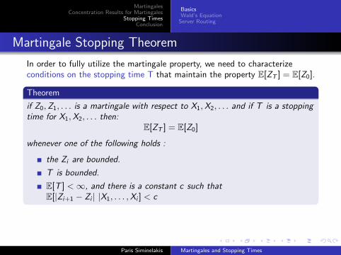
Martingale Stopping Theorem

In order to fully utilize the martingale property, we need to characterizeconditions on the stopping time T that maintain the property E[ZT ] = E[Z0].

Theorem

if Z0,Z1, . . . is a martingale with respect to X1,X2, . . . and if T is a stoppingtime for X1,X2, . . . then:

E[ZT ] = E[Z0]

whenever one of the following holds :

the Zi are bounded.

T is bounded.

E[T ] <∞, and there is a constant c such thatE[|Zi+1 − Zi | |X1, . . . ,Xi ] < c





Server Routing

Betting Strategy

We will use the martinale stopping theorem to derive a simple solution to thegambler’s ruin problem. Let Z0 = 0, let Xi be the amount won on the ithgame and Zi be the total amount won after i games.Assume that the playerquits the game when has either won W or lost L. What is the propabilitythat he wins W dollars before he loses L?

Let T be the first time has either won W or lost L. Then T is astopping time for the sequence X1,X2, . . ..

The sequence Z1,Z2, . . . is a martingale and the values are clearlybounded.

let q be the propability first winning W .We apply the MartingaleStopping Theorem :

E[ZT ] = E[Z0] = 0 and E[ZT ] = W · q − L(1− q)

q =L

W + L





Server Routing

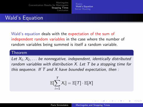
Wald’s Equation

Wald’s equation deals with the expectation of the sum ofindependent random variables in the case where the number ofrandom variables being summed is itself a random variable.

Theorem

Let X1,X2, . . . be nonnegative, independent, identically distributedrandom variables with distribution X. Let T be a stopping time forthis sequence. If T and X have bounded expectation, then :

E[T∑i=1

Xi ] = E[T ] · E[X ]





Server Routing

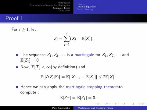
Proof I

For i ≥ 1, let :

Zi =i∑

j=1

(Xj − E[X ]).

The sequence Z1,Z2, . . . is a martingale for X1,X2, . . . andE[Z1] = 0

Now, E[T ] <∞(by definition) and

E[|∆Zi |Fi ] = E[|Xi+1 − E[X ]|] ≤ 2E[X ].

Hence we can apply the martingale stopping theoremtocompute :

E[ZT ] = E[Z1] = 0.





Server Routing

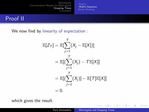
Proof II

We now find by linearity of expectation :

E[ZT ] = E[T∑j=1

(Xj − E[X ])]

= E[(T∑j=1

(Xj)− TE[X ]]

= E[(T∑j=1

(Xj)]− E[T ]E[X ]]

= 0.

which gives the result.





Server Routing

Las Vegas Algorithms

Wald’s equation can arise in the analysis of Las Vegas algorithms, whichalways give the right answer but have variable running times.

In a Las Vegas algorithm we often repeatedly perform somerandomized subroutine that may or may not return the right answer.

We then use some determenistic checking subroutine to determinewhether or not the answer is correct; If it is correct then itterminates, otherwise the algorithm runs the subroutine again.

If N is the number of trials until a correct answer is found and if Xi

is the running time for the two subroutines (randomized routine anddetermenistic checking routine).Then as long as Xi are independentand identically distributed with distribution X, Wald’s equation givesthat the expected running time of the algorithm is:

E[T∑i=1

Xi ] = E[T ] · E[X ]





Server Routing

Server Routing

Consider a set of n servers communicating through a sharedchannel.Time is divided in time slots, and at each one any serverthat needs to send a packet can transmit through the channel.

If exactly one packet is sent at that time, the transmission iscompleted. If there are more than one, none is succesfull. Packetsnot sent, are stored in the server’s buffer until they are transmitted.Servers follow the following protocol :

Randomized Protocol

At each time slot, if the server’s buffer is not empty then with propability1/n it attempts to send the first package in its buffer.

What is the expected number of time slots used until all servershave sent at least one packet ?





Server Routing

Server Routing

Let N be the number of packets succesfully sent until each server hassuccessfully sent at least one packet. Let ti be the time slot in which theith succesfully transmitted packet is sent. Starting from time t0 = 0, andlet ri = ti − ti−1.

Then T, the number of time slots until each server successfullysends at least one packet, is given by :

T =N∑i=1

ri .

We see that N is independent of ri , and N is bounded inexpectation;thus is a stopping time.





Server Routing

Server Routing

The propability that a packet is successfully sent in a given time slotis :

p =

(n

1

)(

1

n)(1− 1

n)n−1 ≈ e−1

The ri each have a geometric distribution with parameter p, so :

E[ri ] = 1/p ≈ e.

The sender of a succesfully transimited packet is uniformlydistributed amongst the n servers, independent of previous steps.Using the analysis of the Coupon Collector’s problem we deducethat E[n] = nH(n) = n lnn + On.

We now use Wald’s identity to compute :

E[T ] = E[N∑i=1

]ri ] = E[N]E[ri ] =nH(n)

p≈ en lnn.




Concluding Remarks

Using martingales we can obtain bounds even under complexdependencies between the random variables.

It is not necessary to know the mean value inorder to seekconcentration results.

Appropriately defining martingales and using their propertiesfinds great application in analyzing and designing randomizedalgorithms,e.g Las Vegas algorithms.




Further Reading

R.Motwani, P.RaghavanRandomized Algorithms.Cambridge University Press, 1995.

M.Mitzenmacher, E.UpfalPropability and ComputingCambridge University Press, 2005.

G.Grimmet, D.StirzakerPropability and Random ProcessesOxford University Press, 2001.

M.Habib,C.McDiarmid,J.Ramirez-Alfonsin,B.ReedPropabilistic Methodsfor Algorithmic Descrete MathematicsSpringer, 1998


Documents

Martingales and Stopping Times - Stanford Universitypsimin/presentations/martingales.pdf · Martingales and Stopping Times Use of martingales in obtaining bounds and analyzing algorithms