Embed Size (px)
Citation preview
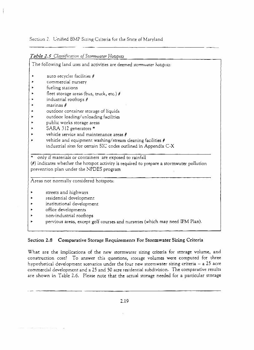
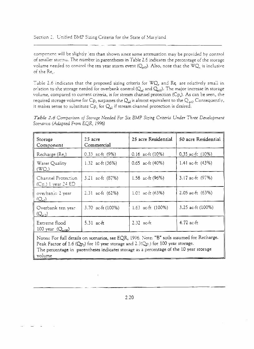
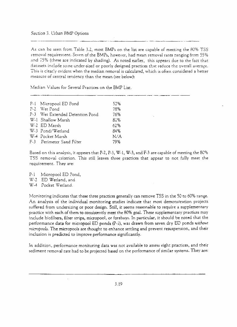
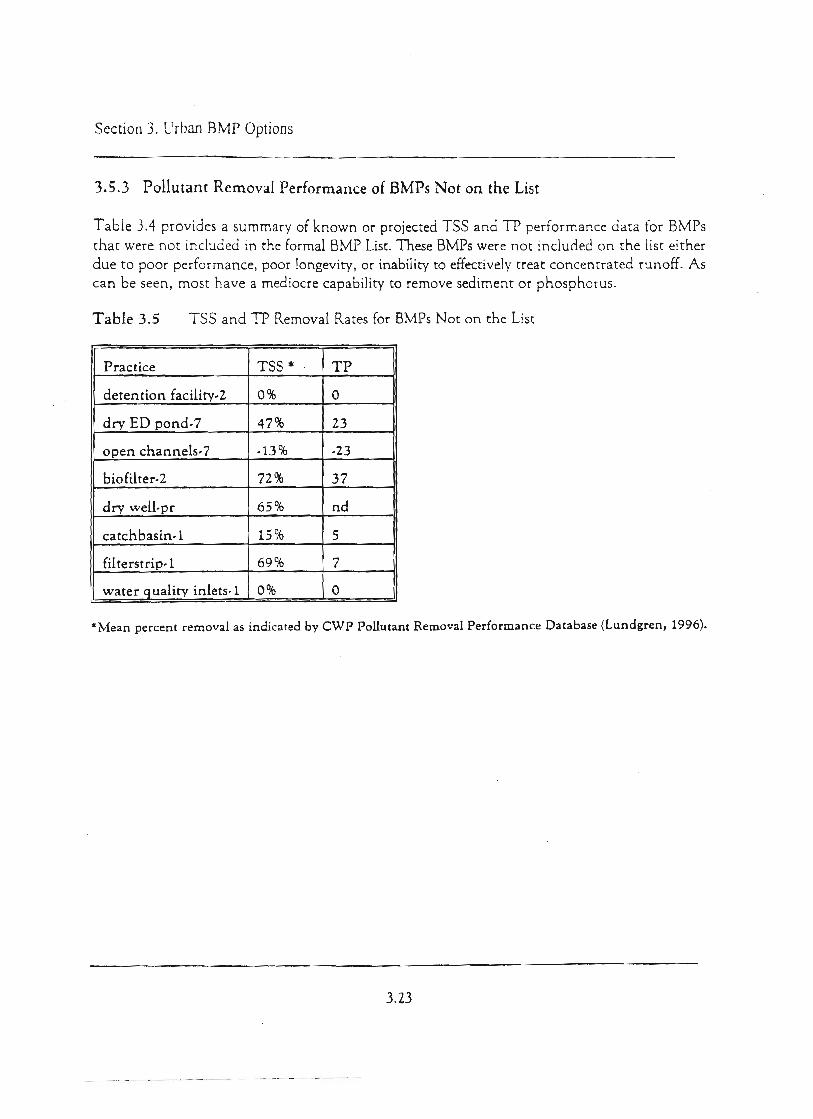
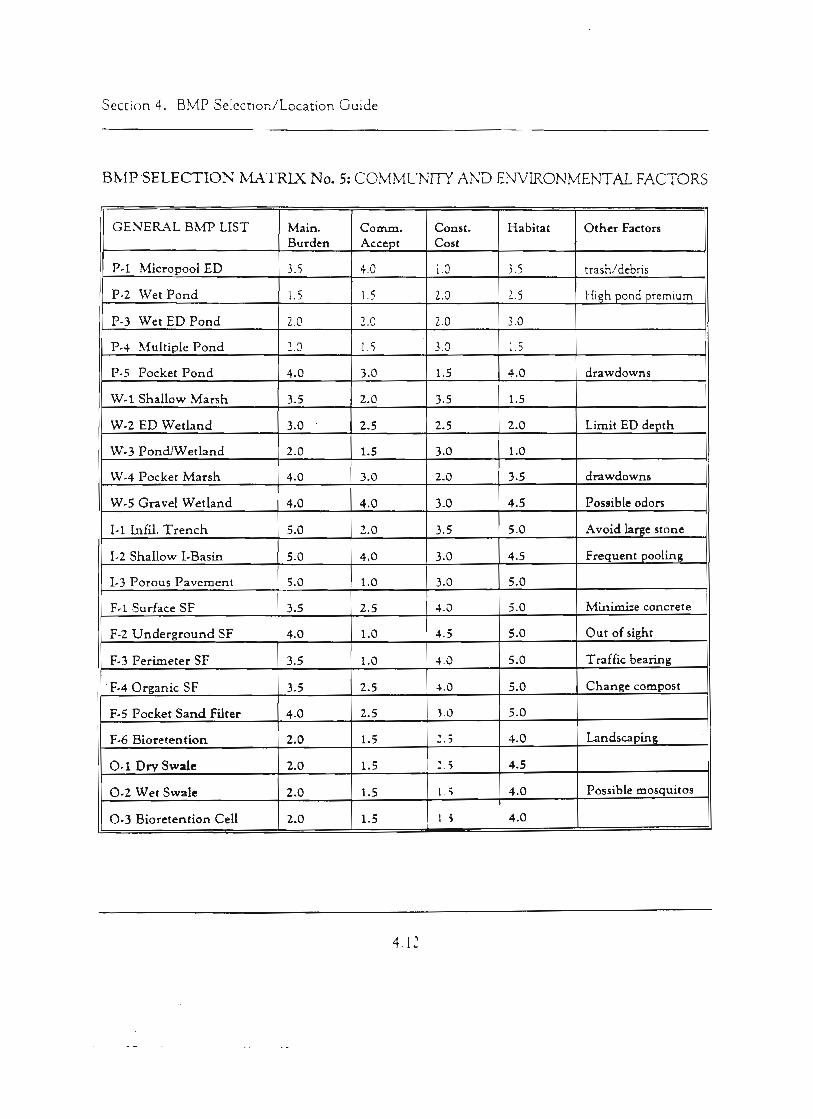
Maryland’s Urban Stormwater Best Management
Practices by Era Proposal
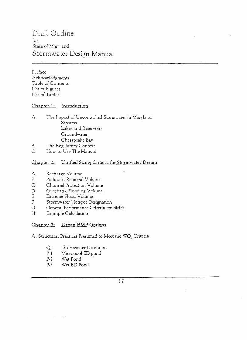
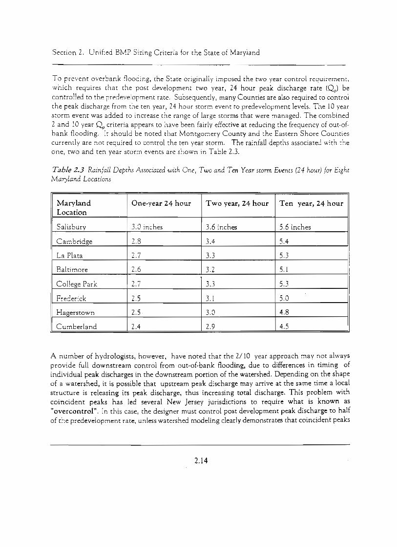
Draft October 2009 Introduction The Maryland Department of Environment (MDE) is proposing to change how it reports on the implementation of stormwater management to the Chesapeake Bay Program (CBP). This effort has been initiated because urban best management practice (BMP) information throughout Maryland is limited due to inadequate reporting, which underestimates the total number of BMPs that have been implemented. Using Chesapeake Bay Program (CBP) developed acres since 1985, there should be approximately 457,429 acres of urban land controlled by stormwater management in Maryland, but as of 2009, the reporting has only shown approximately 200,000 acres. To better reflect actual implementation, MDE proposes a change in the reporting to the CBP from individual urban BMPs to four BMP categories defined by Maryland's predominate stormwater management eras. MDE has already begun to use the stormwater management by era analysis for showing progress toward Tributary Strategy and BayStat Milestones and believes that it will also be appropriate for the CBP model and Total Maximum Daily Load (TMDL) analysis. The major stormwater management eras for this analysis are described below and depicted in Figure 1. Major Stormwater Management Eras Prior to any stormwater management in the State, urban runoff was directed into nearby waterways with little thought of either volume control or water quality treatment. In 1982, the Maryland General Assembly passed the State's first Stormwater Management law. While this law focused primarily on flood control, a preferred order of BMP implementation was established for treating water quality. Local ordinances and programs necessary to address the requirements of the new stormwater management law were completed by 1985. Because stormwater management programs did not occur statewide until this time, MDE proposes that urban land developed before 1985 be recorded with no pollutant load reductions. Local programs, criteria, and associated BMPs to address the 1982 Stormwater Management law were implemented in Maryland from 1985 through 2001. Pollutant removal efficiencies for the BMPs implemented during this era are based upon CBP guidance.1 Additionally, an analysis of MDE's Urban Best Management Practice database and a survey of Maryland Counties were used to determine the proportional coverage of each BMP type.2 Based upon these data and analysis, MDE proposes that CBP urban land data between 1985 and 2001 be recorded with pollutant removal efficiencies of 50% for total suspended solids, 30% for total phosphorus, and 20% for total nitrogen.
1
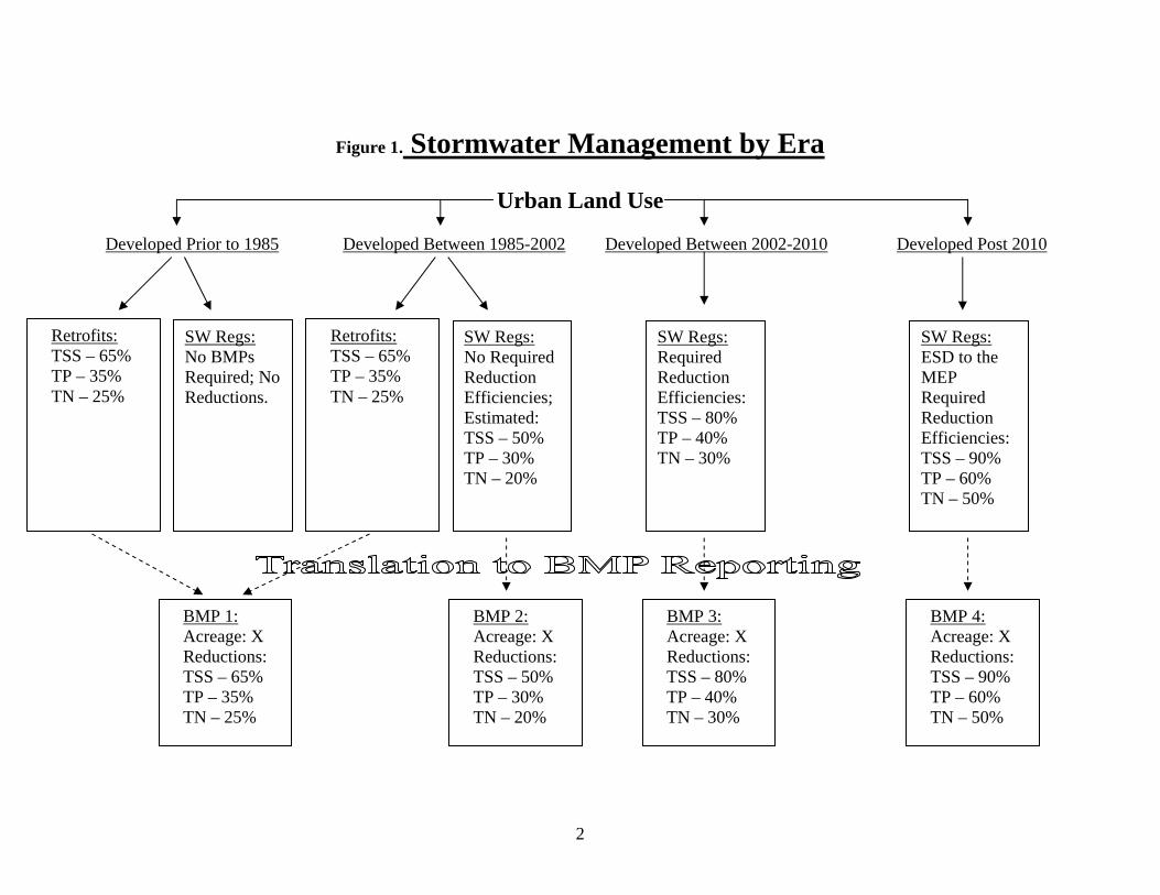
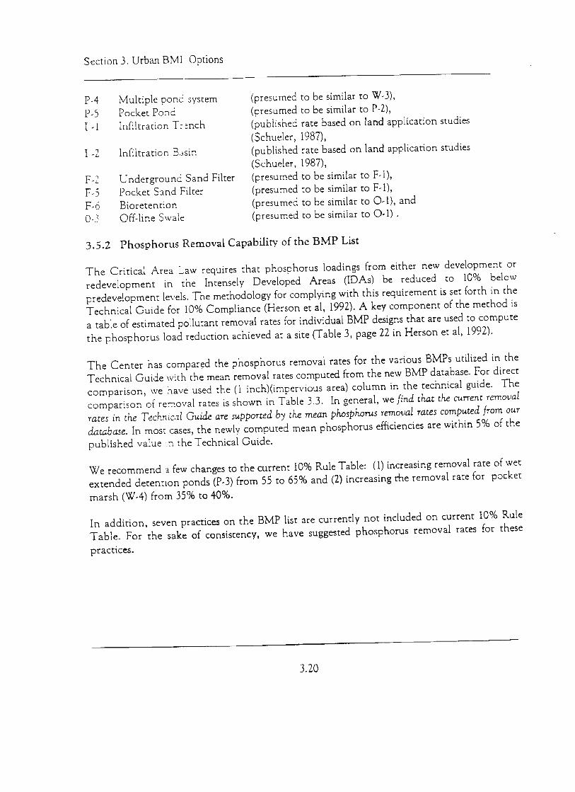
Figure 1. Stormwater Management by Era
Urban Land Use Developed Prior to 1985 Developed Between 1985-2002 Developed Between 2002-2010 Developed Post 2010
BMP 4: Acreage: X Reductions: TSS – 90% TP – 60% TN – 50%
BMP 3: Acreage: X Reductions: TSS – 80% TP – 40% TN – 30%
BMP 2: Acreage: X Reductions: TSS – 50% TP – 30% TN – 20%
BMP 1: Acreage: X Reductions: TSS – 65% TP – 35% TN – 25%
SW Regs: ESD to the MEP Required Reduction Efficiencies: TSS – 90% TP – 60% TN – 50%
SW Regs: Required Reduction Efficiencies: TSS – 80% TP – 40% TN – 30%
SW Regs: No Required Reduction Efficiencies; Estimated: TSS – 50% TP – 30% TN – 20%
Retrofits: TSS – 65% TP – 35% TN – 25%
Retrofits: TSS – 65% TP – 35% TN – 25%
SW Regs: No BMPs Required; No Reductions.
2
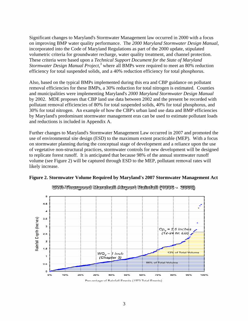
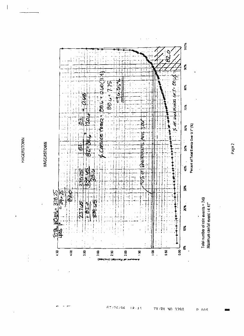
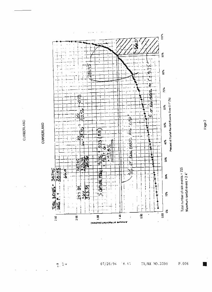
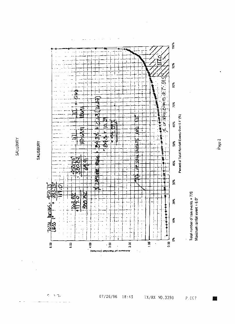
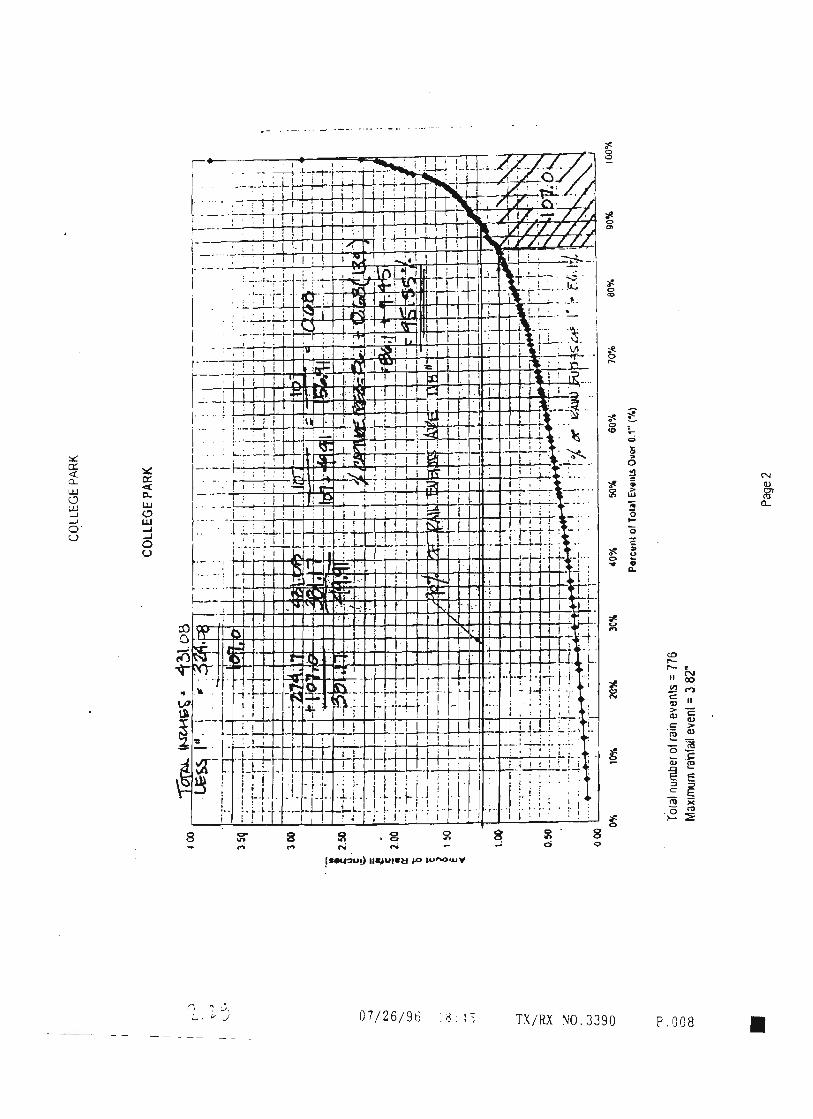
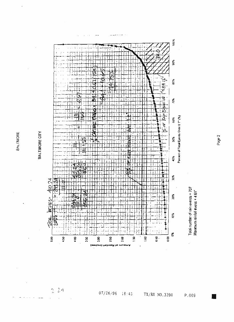
Significant changes to Maryland's Stormwater Management law occurred in 2000 with a focus on improving BMP water quality performance. The 2000 Maryland Stormwater Design Manual, incorporated into the Code of Maryland Regulations as part of the 2000 update, stipulated volumetric criteria for groundwater recharge, water quality treatment, and channel protection. These criteria were based upon a Technical Support Document for the State of Maryland Stormwater Design Manual Project,3 where all BMPs were required to meet an 80% reduction efficiency for total suspended solids, and a 40% reduction efficiency for total phosphorus. Also, based on the typical BMPs implemented during this era and CBP guidance on pollutant removal efficiencies for these BMPs, a 30% reduction for total nitrogen is estimated. Counties and municipalities were implementing Maryland's 2000 Maryland Stormwater Design Manual by 2002. MDE proposes that CBP land use data between 2002 and the present be recorded with pollutant removal efficiencies of 80% for total suspended solids, 40% for total phosphorus, and 30% for total nitrogen. An example of how the CBP's urban land use data and BMP efficiencies by Maryland's predominant stormwater management eras can be used to estimate pollutant loads and reductions is included in Appendix A. Further changes to Maryland's Stormwater Management Law occurred in 2007 and promoted the use of environmental site design (ESD) to the maximum extent practicable (MEP). With a focus on stormwater planning during the conceptual stage of development and a reliance upon the use of vegetative non-structural practices, stormwater controls for new development will be designed to replicate forest runoff. It is anticipated that because 98% of the annual stormwater runoff volume (see Figure 2) will be captured through ESD to the MEP, pollutant removal rates will likely increase. Figure 2. Stormwater Volume Required by Maryland's 2007 Stormwater Management Act
3
Based upon CBP efficiencies for similar BMPs, MDE conservatively estimates that ESD to the MEP will meet pollutant removal efficiencies of 90% for total suspended solids, 60% for total phosphorus, and 50% for total nitrogen.4 Future monitoring of ESD to the MEP will be used to validate these estimates or to propose new pollutant removal efficiencies to the CBP for BMPs implemented beyond 2010. Watershed restoration of older urban areas with little or no stormwater management is a primary target of Maryland's National Pollutant Discharge Elimination System (NPDES) municipal stormwater permits, and Maryland's Small Creeks and Estuaries and Stormwater Pollution Cost Share Programs. Because stormwater retrofits are a combination of newer BMPs as required by Maryland's 2000 stormwater management act and other BMP types similar to those implemented between 1985 - 2001, MDE has decided to pick the mean of these two stormwater management eras for reduction efficiencies. Thus pollutant removal efficiencies of 65% for total suspended solids, 35% for total phosphorus, and 25% for total nitrogen have been estimated. The land areas restored are a combination of pre-1985 development, where no stormwater management was required, and land developed between 1985 and 2002 where traditional flood control BMPs are often enhanced with water quality features. MDE proposes initially to evenly divide the data on acres restored between these two eras. As NPDES stormwater permittees begin to report data in a GIS format, restoration data and coverage will be more accurately defined and appropriated accordingly. Bibliography 1 Weammert, Sarah E. 2007. The Mid-Atlantic Water Program (MAWP) reviewed BMP efficiencies implemented and reported by the Chesapeake Bay watershed jurisdictions prior to 2003. University of Maryland, College Park, MD. 2 A Survey by Baish, Alexander S. and Caliri, Marisa J., 2009. Overall Average Stormwater Effluent Removal Efficiencies for TN, TP, and TSS in Maryland from 1984-2002. Johns Hopkins University, School of Engineering, Baltimore, MD. 3 Claytor, Rich, and Schueler, T.R., 1997. Technical Support Document for the State of Maryland Stormwater Design Manual Project. Water Management Administration, Maryland Department of the Environment, Baltimore, MD. 4 2000 Maryland Stormwater Design Manual, Supplement 1, 2008. Maryland Department of the Environment, Baltimore, Baltimore, MD.
4

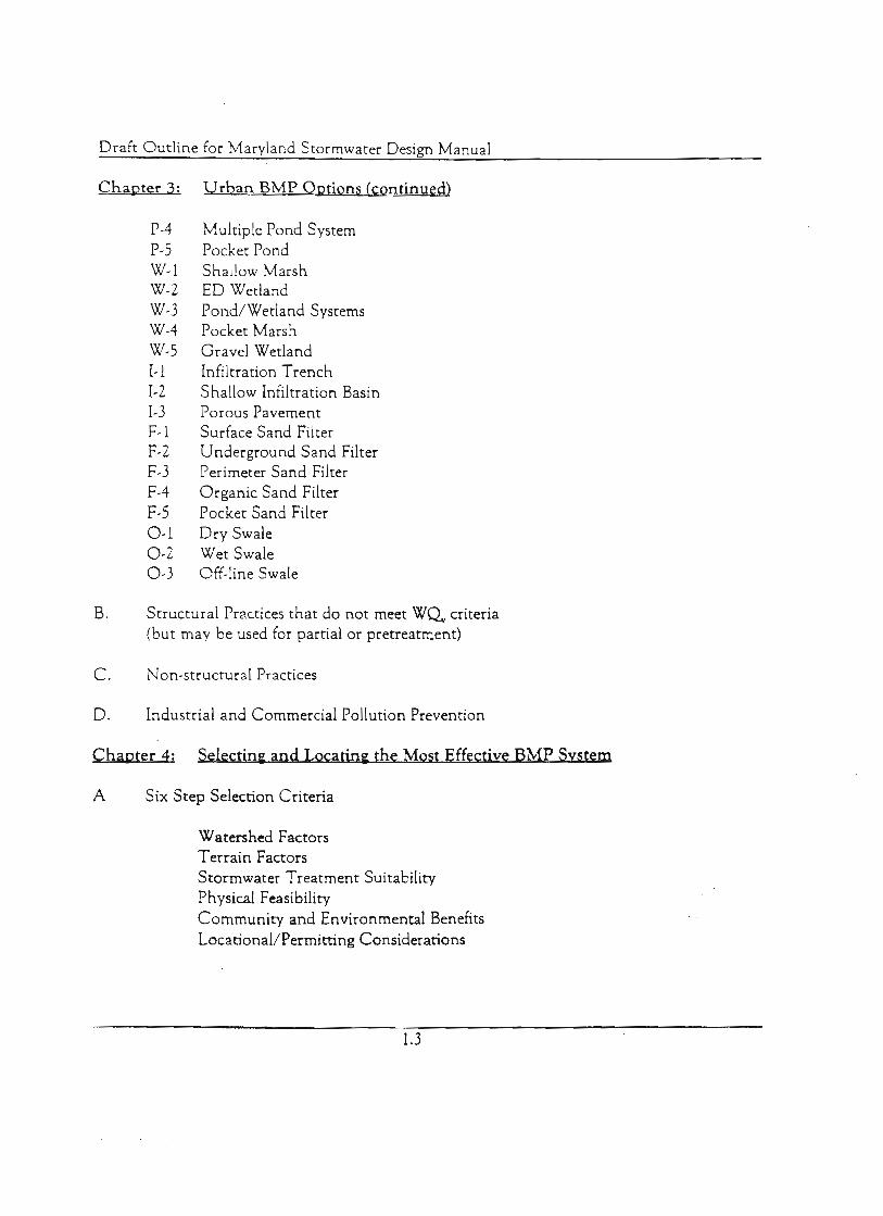
Appendix A Example of Applying Pollutant Removal Efficiencies by Stormwater Management Era
Maryland Stormwater Management by Program Era
Chesapeake Bay Program Urban Data Total Nitrogen Total Phosphorus Total Suspended Solids
Stormwater Program Era
Total Acres
Impervious Acres
Baseline Load
(lbs/yr) SWM
Reduction
Reduced Load
(lbs/yr)
Baseline Load
(lbs/yr) SWM
Reduction
Reduced Load
(lbs/yr) Baseline Load
(Tons/yr) SWM
Reduction
Reduced Load
(Tons/yr)
Pre - 1985 1,009,014 188,340 3,758,087 0% 0 507,342 0% 0 75,162 0% 0 1985 - 2001 320,683 46,164 983,819 20% 196,764 132,816 30% 39,845 19,676 50% 9,838 2002 - 2009 91,410 28,576 517,504 30% 155,251 69,863 40% 27,945 10,350 80% 8,280
Restoration 65,784 13,292 260,591 25% 65,148 35,180 35% 12,313 5,212 65% 3,388
Total Loads: 1,486,891 276,372 5,520,001 417,163 745,200 80,103 110,400 21,506 Calculations:
1) Baseline load estimated using 0.226*((0.05+0.9*(30/100))*0.9*42)*emc*acres and assumes zero reduction 2) Load reduction attributed to SWM estimated using 0.226*((0.05+0.9*(30/100))*0.9*42)*emc*acres*reduction 3) Runoff EMC used for load estimates (TN = 2 mg/l, TP = 0.27 mg/l, TSS = 80 mg/l) 4) Restoration acres are evenly distributed between Pre-1985 and 1985-2001 land use data. For example, Total Acres 1985-2001 = (353,575-(65,784/2)) Reference Notes: 1) Total Urban Acres is derived from CBP 5.1 and 5.2 2) Pollutant Concentrations obtained from the CBP 5.2 and, Claytor, Rich, and Schueler, T.R., 1997. "Technical Support Document for the State of Maryland Stormwater Design Manual Project." Water Management Administration, Maryland Department of the Environment, Baltimore, MD. 3) Pollutant load calculations and reductions based upon the Simple Method, Schueler, T.R., 1987. "Controlling Urban Runoff: A Practical Manual for Planning and Designing Urban BMPs." Metropolitan Washington Council of Governments, Wash., DC. 4) Pollutant Load Reductions for 2002 to Present from Claytor, Rich, and Schueler, T.R., 1997. Technical Support Document for the State of Maryland Stormwater Design Manual Project. Water Management Administration, Maryland Department of the Environment, Baltimore, MD. 5) Pollutant Load Reductions for 1985-2002 from Baldwin, Andrew H., Ph. D., and Weammert, Sarah E., and Simpson, Tom W., Ph. D., 2007. The Mid-Atlantic Water Program (MAWP) housed at the University Of Maryland (UMD) led a project during 2006-2007 to review and refine definition and effectiveness estimates for BMPs implemented and reported by the Chesapeake Bay watershed jurisdictions prior to 2003. 6) Pollutant Load Reductions also based upon Baish, Alexander S. and Caliri, Marisa J., 2009 "Overall Average Stormwater Effluent Removal Efficiencies for TN, TP, and TSS in Maryland from 1984-2002." Johns Hopkins University, Baltimore, MD.
Maryland Department of the Environment, 2009
6
Average Nutrient and Sediment Effluent
Removal Efficiencies for Stormwater Best Management Practices
Implemented in Maryland 1984-2002
Alexander S. Baish
and Marisa J. Caliri, Students
Department of
Geology and Environmental Engineering Johns Hopkins University
Baltimore, MD 21218
January 2009 I. Introduction The Maryland Department of the Environment (MDE), Sediment, Stormwater, and Dam Safety Program (SSDS), in charting the progress of stormwater management found it necessary to determine valid pollutant reduction rates for common Chesapeake Bay pollutants for the three predominant stormwater management eras in Maryland. Before 1984, there was little reduction in stormwater pollutants because best management practices (BMPs) were not required statewide. Since 2002, Maryland's stormwater management program has required that the BMPs implemented reduce total phosphorus (TP) by 40% and total suspended sediments (TSS) by 80%. However, there is a major knowledge gap regarding the reduction rates for the stormwater management practices that were built between 1984 and 2002, or the middle era. The Johns Hopkins University (JHU) team focused on this middle era to determine what stormwater BMPs were employed in Maryland and how they functioned. These BMPs were organized by category, rate of implementation, and degree of land coverage. A literature review of the BMPs used in Maryland during this era was conducted by the JHU team to determine pollutant reduction capabilities. Finally, the team used these data to estimate average pollutant reduction rates for TN, TP, and TSS that can be reasonably expected from the implementation of Maryland's stormwater management program between the years 1984-2002.
II. Literature Review of BMP Removal Efficiency The JHU team performed an exhaustive literature review of BMP pollutant removal efficiencies used by local regulatory agencies and found in published studies. The recommended pollutant removal efficiencies put forth in this paper are often based upon the raw data presented within these studies rather than on the final determination made in the studies. Often, the final reduction rates in these studies reflected a great deal of policy rather than science. The work groups and regulatory bodies tended to use the raw data as a scientifically based starting point, but adapted the numbers either to promote the use of certain BMPs or to reflect other benefits separate from stormwater treatment, for example, the creation of ecologically important habitat. The JHU team was tasked with determining an average pollutant removal percentage for Maryland’s middle era of stormwater management based on published data regardless of policy ramifications. The number of studies reviewed, range of pollutant removal values, and widely different methods used, all contribute to a great deal of variability when examining BMPs and efficiency rates. A guiding principle for the JHU team came from the discussions of the Chesapeake Bay Program (CBP) as it considered adjusting its model to fit new BMP data, “It is very important that…modeling activities be conservative, rather than optimistic.” When available data did not follow statistical patterns or converge upon an easily discernable value for average removal efficiency, the JHU team erred on the side of “realistic conservatism,” operating under the assumption that when making decisions about widely ranging values, they should be within the realm of reason, but lean toward underestimating true BMP removal efficiencies rather than overestimating them. One particular local study was used extensively by the JHU team. In support of the CBP, a professional review of available literature, studies, and expert assessments, was performed by the Mid-Atlantic Water Program (MAWP) and Dr. Andy Baldwin. A premise of the review was to get data from actual BMPs as opposed to laboratory or controlled tests of perfectly maintained BMPs. The results, while heavily qualified, formed the basis of the removal efficiencies used in the CBP's 5.0 Watershed Model. The robust nature of the review and statistical analysis used to determine these initial numbers for the CBP made it a good basis for the JHU team's research into BMPs implemented in Maryland between 1984-2002 and their efficiencies. The JHU review of pollutant removal efficiencies for stormwater BMPs is provided below. Dry Detention Ponds Removal Rates: TN 10%, TP 30%, TSS 50% Dry detention ponds (DPs) was one of the most common BMPs implemented during the middle era of stormwater management in Maryland. These were also one of the most difficult BMPs to assess for average removal efficiencies for reasons the CBP discovered in 2006-2007. DPs were primarily designed to dampen the “first flush” of runoff from impervious acreage, slow channel erosion and decrease peak floods to streams. They were not designed
2
specifically for nutrient and sediment removal. It is generally accepted that DPs have some of the lowest removal efficiencies among pond-like stormwater management structures. Few reliable studies have been performed on the removal efficiencies of DPs, and among these studies, removal rates, especially for TN, are widely variable. In Dr. Baldwin’s statistical assessments, average removal efficiencies for DPs were 10% for TN, 40% for TP, and 50% for TSS. The report found that there was considerable evidence of skewing for TSS toward low removal efficiencies, skewing of TP toward higher efficiencies, and so few data points for TN that, in terms of skewing estimates, “meaningful inference cannot be made.” The report also made note of “considerable variability in removal efficiency, as reflected by high standard deviations” among the multiple studies examined. A review of the statistical histograms of various studies shows a negative skewing of the TSS average primarily because of four studies where an increase in TSS occurred from the DPs discharge. These studies were most likely accurate reflections of DPs that had been improperly maintained (filling with organic matter that was being flushed out by each storm event, flooding rather than draining and causing large quantities of stormwater to bypass the BMP altogether, etc). For reasons of conservatism, the JHU team was inclined to accept the MAWP’s recommendation of TSS removal efficiency of 50% for DPs. The statistical histograms also show a positive skewing of the suggested TP removal average by three of the 15 studies. These three studies concluded TP removal efficiency for DPs was in the 80-90% range. The remaining 12 studies in the histograms display an almost bell-like curve of predicted efficiencies around 30-40%. For reasons of conservatism, the JHU team felt that the MAWP suggested average of 35% was close to adequate, but that a marginal drop to 30% would ensure that the removal efficiencies of TP for DPs would not be overestimated. On the issue of TN removal, only six relevant studies were deemed accurate and rigorous enough to be considered by Dr. Baldwin and the MAWP. Although there was a high standard of deviation among these studies, and no clear pattern in the histograms, the average of the findings was simply accepted as a baseline for CBP use. Due to the robust nature of the literature review performed by the MAWP, the JHU team was unable to uncover additional DP studies done with a similar level of accuracy. Because biological activity and plant uptake in DPs would provide at least some level of nitrogen removal, the JHU team believes that a 10% removal rate as recommended by MAWP is a conservative reflection of this biological activity and appropriate for the purposes of this study. Extended Detention Structure/Dry Removal Rates: TN 20%, TP 20%, TSS 60% The MAWP recommendations to the CBP were 20% for TN, 20% for TP, and 60% for TSS. These removal rates were based upon several recent multiple site studies that showed consistent results. The data indicate that a 60% removal efficiency for TSS is reasonable. Also, evidence from the most recent studies shows that a TN removal rate in the 15-30% range is possible, however, much closer to the 15% than 30%. These efficiencies make sense in
3
terms of comparison to DPs, as the longer stormwater is detained, the higher TSS and TN removal rates should be. The average TP removal rate for the three multiple site studies was exactly 20%. The single site studies documented a significantly higher efficiency for TP; however, the 20% seems a more reasonable assessment. Although more TP may precipitate out in extended detention as compared to DPs, the anaerobic conditions in the bottom of EDs created by an extended 24 hour effluent discharge time results in phosphate release from the soil. This should result in a lower TP removal rate for EDs than for DPs. Wet Ponds/Wetlands Removal Rates: TN 20%, TP 45%, TSS 60% The MAWP recommendations to the CBP were 20% for TN, 45% for TP, and 60% for TSS. There were many more single site studies available for WPs than multiple site studies. While the removal rates for the single site studies tended to be lower, the data were still well within the range of efficiencies found in the multiple site studies. Also, the median and means for both groups of studies were close and the statistical histograms showed a low degree of skewing. The JHU team was satisfied by the analysis of the MAWP and its removal efficiencies for WPs. The analysis of studies seemed statistically sound and the efficiencies themselves reasonable, i.e., as good as or better than ED removal efficiencies. Oil/Grit Separators Removal Rates: TN 0%, TP 0%, TSS 0% Studies by MDE and the Metropolitan Washington Council of Governments showed that oil/grit separators (OGSs) have extremely small storage volumes compared to the impervious surface areas they drain, very short detention times, and a high tendency to leave much sediment in suspension. Total sediment volumes in OGSs remained the same or decreased overtime, indicating high rates of resuspension and flushing of TSS in effluent. A comprehensive Federal Highway Administration report on BMPs supported OGSs inability to eliminate TSS but also TN and TP from stormwater. Due to their short detention times, even particulate forms of nitrogen and phosphorous are not removed. The JHU team decided that based on these reviews, OGSs were assigned removal rates of 0% for TN, TP, and TSS. Underground Storage Vault Removal Rates: TN 0%, TP 0%, TSS 0% Underground storage structures (UGS) are designed primarily for flood control in much the same manner as a DP. When it comes to pollutants, UGSs are much less efficient because they are constructed of cement instead of earth, soil, and vegetation. Removal rates indicated in the literature for these structures are minimal for TN, 20% for TP, and 60% for TSS. These removal rates however are based upon a Northern Virginia Study that required weekly
4
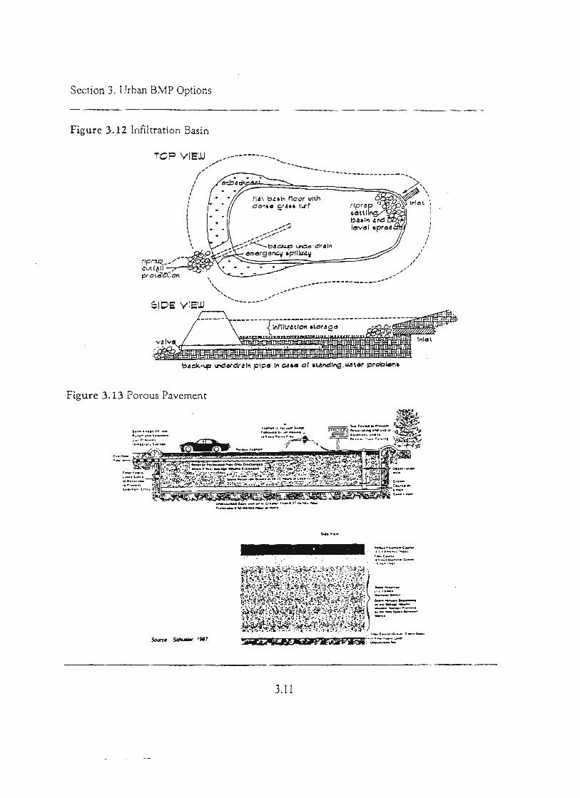
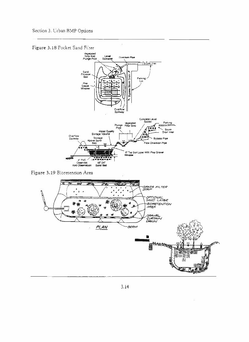
cleaning and maintenance of its test facility to maintain these efficiencies. To be conservative, the JHU team relied upon previously mentioned research regarding similar structures such as OGSs where maintenance is infrequent at best. In these situations, UGSs can loose efficiency and even become sediment sources. For this reason, the JHU team decided to view these structures conservatively and apply zero reduction rates for TN, TP, and TSS. Infiltration Trench/Basin and Dry Well with/without Exfiltration Removal Rates: TN 60%, TP 60%, TSS 90% The United States Environmental Protection Agency (EPA) carried out a literature review in 1999 similar to the MAWP. This literature review cited several studies from Maryland. Both EPA's report and the California Stormwater BMP Handbook (2003), stated that because there is no effluent flow from infiltration trenches and basins, all stormwater infiltrates into the surrounding soil and a 100% reduction in the load discharged to surface waters. However, numerous studies also state that effluent from such trenches and basins, if not allowed to infiltrate would be less efficient and estimate reduction rates of 60% for TN, 60% for TP, and 90% for TSS. Among MDE's Urban BMP database, some infiltration trenches (IT, ITCE), all infiltration basins (IB), and all dry wells (DW) have no effluent because all inflow is designed to infiltrate into the surrounding soil. The JHU team came across several studies in Maryland that showed large failure rates for infiltration BMPs within two years of implementation. The most common reasons for failure are due to clogging, poor maintenance, or the siting of these BMPs in areas of poor soil permeability. For these reason, the JHU team believes that few of these BMPs will be capable of 100% infiltration and a more conservative decision is to use the removal efficiencies of 60% for TN, 60% for TP, and 90% for TSS. Several infiltration BMPs are not designed for infiltrating the entire amount of runoff and are know as Water Quality Exfiltration Trenches (ITWQE), which process only the first flush of water from impervious surfaces during a storm event, and a Partial Exfiltration Trench (ITPE), which has an under drain in the trench so not all runoff infiltrates into the surrounding soil. Based upon EPA's literature review of BMPs with these characteristics, the JHU team assigned effluent removal efficiency rates of 60% for TN, 60% for TP, and 90% for TSS. Bioretention Removal Rates: TN 35%, TP 80%, TSS 90% Although there was a great deal of literature describing Bioretention (BIO, BR) as a BMP, there were comparatively very few studies completed on its removal efficiencies. Most of the studies were completed by Dr. Davis at the University of Maryland or in a few locations in Prince George’s County, where the practice was developed. However, most of these studies were either performed in a laboratory or in well maintained sample BMPs.
5
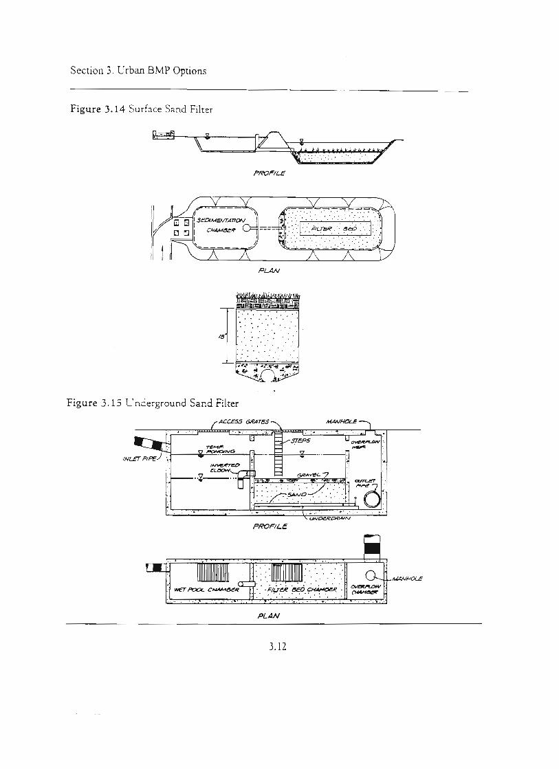
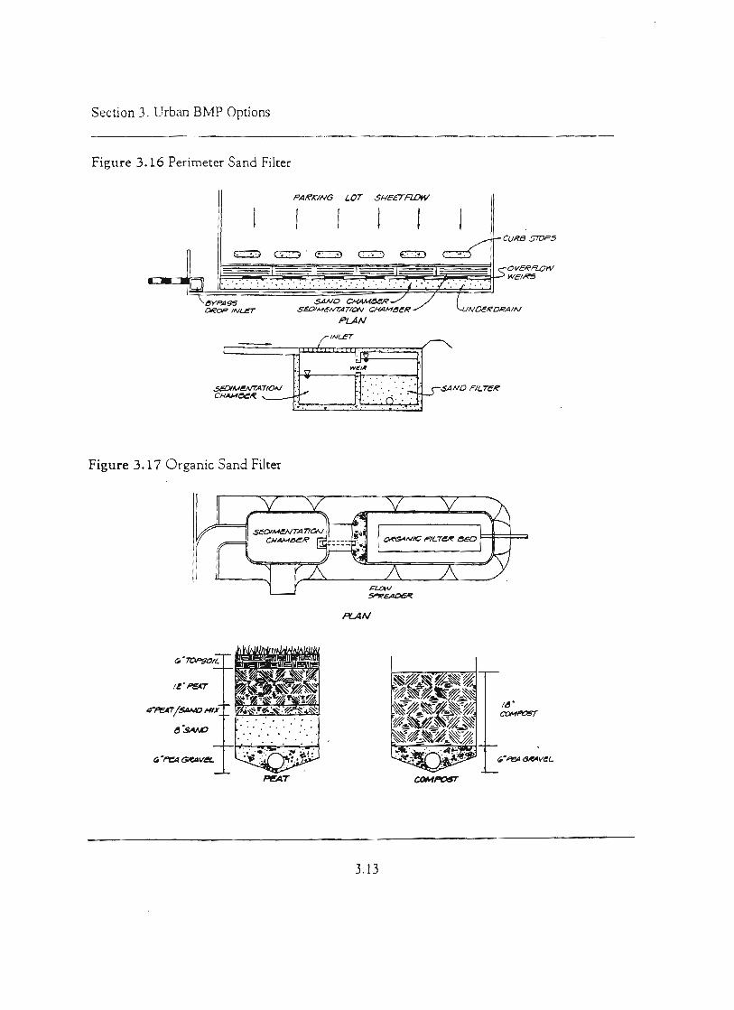
Most studies showed that BIOs are remarkably efficient at TSS removal, ranging from 86-99% removal with more studies toward the upper end of that range. As noted above, because few of these studies tended to be from actual field conditions, the JHU team felt it could not assign the BIO a higher than 90% TSS removal efficiency. Davis and other studies tended to distribute TP removal findings evenly about 71-90%. The JHU team felt comfortable assigning a realistic and conservative removal efficiency of 80% to TP. The TN removal efficiency ranged more widely and some BIOs actually produce TN by promoting nitrification between precipitation events. Other structures effectively infiltrated or promoted the organism uptake of TN, causing this wide range of removal efficiencies. The JHU team recognized a general range of 25-45% TN removal efficiency for most studies, and settled on the middle of this range. Porous Pavement Removal Rates: TN 80%, TP 65%, TSS 90% Although there are limited studies on Porous Pavement (PP) due to its relative status as a new technology, several of the long-term studies were performed in Maryland and Virginia. An EPA document from 1999 estimated removal efficiencies of 82-95% TSS, 65% TP, and 80-85% TN based on these studies which were located in Rockville, MD and Prince William, VA. An article in Government Engineering in 2005 cited this EPA document, and highlighted the consistency of its results compared to three other studies. Averages of these studies came to 91% TSS removal, 66% TP removal, and 72% TN removal. The JHU team, choosing to weight the local, long-term studies slightly heavier than the studies of unknown location, generally agrees with the EPA removal efficiencies. Sand Filter Removal Rates: TN 0%, TP 55%, TSS 80% Sand filters (SF) implemented in Maryland between 1984-2002 were likely modeled after the Delaware/DC or the Austin models. Both are constructed below grade and tend to be smaller scale structure than an open at-grade structure. Based on a Federal Highway Administration Database of BMPs as well as the California Stormwater BMP Handbook, SFs, depending on the media used within them, could have an average TSS removal efficiency of 80%. This rate is more heavily weighted toward the lower FHWA database numbers, for conservatism. A TP removal efficiency rate of 55% was chosen which is well within the range of all literature. There is discrepancy for the TN removal efficiencies. The California Handbook and the FHWA database, which includes data from the Delaware/DC SF, indicated highly variable results for TN removal. The Austin SF has been show to actually be a source of TN due to nitrification in the sand beds between precipitation events. For these reasons, the JHU team has conservatively decided that sand filters have a negligible TN removal rate.
6
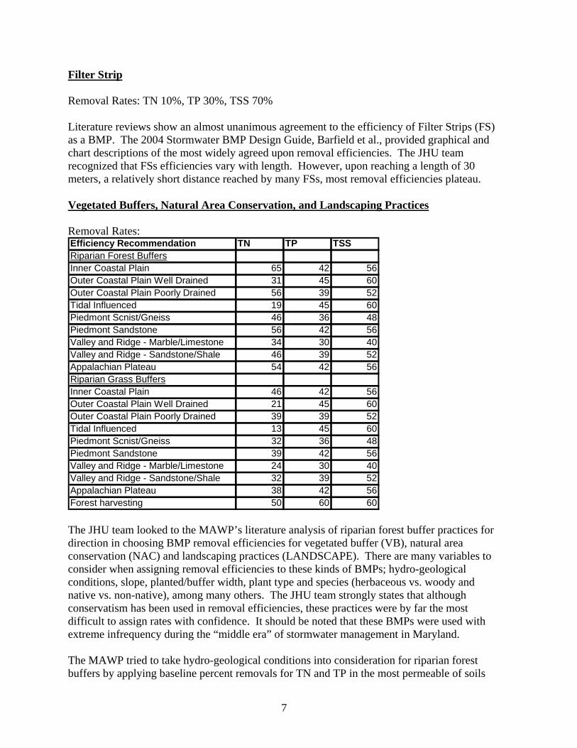
Filter Strip Removal Rates: TN 10%, TP 30%, TSS 70% Literature reviews show an almost unanimous agreement to the efficiency of Filter Strips (FS) as a BMP. The 2004 Stormwater BMP Design Guide, Barfield et al., provided graphical and chart descriptions of the most widely agreed upon removal efficiencies. The JHU team recognized that FSs efficiencies vary with length. However, upon reaching a length of 30 meters, a relatively short distance reached by many FSs, most removal efficiencies plateau. Vegetated Buffers, Natural Area Conservation, and Landscaping Practices Removal Rates: Efficiency Recommendation TN TP TSSRiparian Forest BuffersInner Coastal Plain 65 42 56Outer Coastal Plain Well Drained 31 45 60Outer Coastal Plain Poorly Drained 56 39 52Tidal Influenced 19 45 60Piedmont Scnist/Gneiss 46 36 48Piedmont Sandstone 56 42 56Valley and Ridge - Marble/Limestone 34 30 40Valley and Ridge - Sandstone/Shale 46 39 52Appalachian Plateau 54 42 56Riparian Grass BuffersInner Coastal Plain 46 42 56Outer Coastal Plain Well Drained 21 45 60Outer Coastal Plain Poorly Drained 39 39 52Tidal Influenced 13 45 60Piedmont Scnist/Gneiss 32 36 48Piedmont Sandstone 39 42 56Valley and Ridge - Marble/Limestone 24 30 40Valley and Ridge - Sandstone/Shale 32 39 52Appalachian Plateau 38 42 56Forest harvesting 50 60 60 The JHU team looked to the MAWP’s literature analysis of riparian forest buffer practices for direction in choosing BMP removal efficiencies for vegetated buffer (VB), natural area conservation (NAC) and landscaping practices (LANDSCAPE). There are many variables to consider when assigning removal efficiencies to these kinds of BMPs; hydro-geological conditions, slope, planted/buffer width, plant type and species (herbaceous vs. woody and native vs. non-native), among many others. The JHU team strongly states that although conservatism has been used in removal efficiencies, these practices were by far the most difficult to assign rates with confidence. It should be noted that these BMPs were used with extreme infrequency during the “middle era” of stormwater management in Maryland. The MAWP tried to take hydro-geological conditions into consideration for riparian forest buffers by applying baseline percent removals for TN and TP in the most permeable of soils
7
and subtracting value from these baseline rates as soils and groundwater conditions becameprogressively less conducive to infiltration of stormwater and uptake of nutrients. The JHU team examined Maryland hydro-geological maps to determine the dominant hydro-geologicaregime in each county. It has always been a con
l
vention to have TP removal values be 75% of TSS removal values, so e TSS removal rates were calculated up from the nutrient rates. Also as a convention, it is
ty of vegetation types, but are “natural areas that help maintain redevelopment hydrology” in general. The JHU team recognized that these areas could be
.
ve
thassumed that grass buffers are 70% as efficient at reducing TN as riparian forest buffers. The MAWP calculated down these TN values for grass buffers, but kept TP and TSS values the same as for forest buffers. NACs include a wide variepalmost any habitat, from forest retention to non-tidal wetlands, but understood the concept behind this BMP was to preserve the natural riparian vegetation adjacent to streams and runsConsidering this, the JHU team assigned the riparian forest buffer removal rates to NACs. These riparian forest buffers are supposed to be designed to mimic removal rates of natural, native riparian vegetation and floodplain ecosystems. The JHU team felt that the conservatiremoval rates of these artificially planted BMPs would be a conservative estimate for the removal rates of the natural habitats they are meant to mimic. Grass Swales Removal Rates: TN 0%, TP 35%, TSS 65%
st of BMPs, are simply gently sloping grass
hanne meant to slow water, promote sediment drop, and soak up nutrients. Federal
TN.
moval. The JHU team agreed to use the lower bound of this range in its calculations. The
Grass Swales, abbreviated SW in the MDE lic lsHighway Administration, the Idaho Department of Environmental Quality (IDEQ), and StormwaterQuality.org all provided percent removal study syntheses for TSS, TP, and The TSS removal efficiency numbers had a small range of variation, inside a range of 65-68%reTP removal efficiency numbers ranged from 29-43%, with one value for the IDEQ as low as 15%. Considering that the IDEQ gives maintenance officials two maintenance schedules for their grass swales, one to promote nutrient removal and one not to promote nutrient removal, the JHU team took Idaho’s estimate of 15% removal as a conservative estimate by the IDEQ, and agreed to focus on the studies in the 29-43% range. The TN removal efficiencies were of mixed results, but often grass swales proved to be nitrogen producers, as natural organic buildup of clippings and leaves tended to break down and promote nitrification between storm events.
8
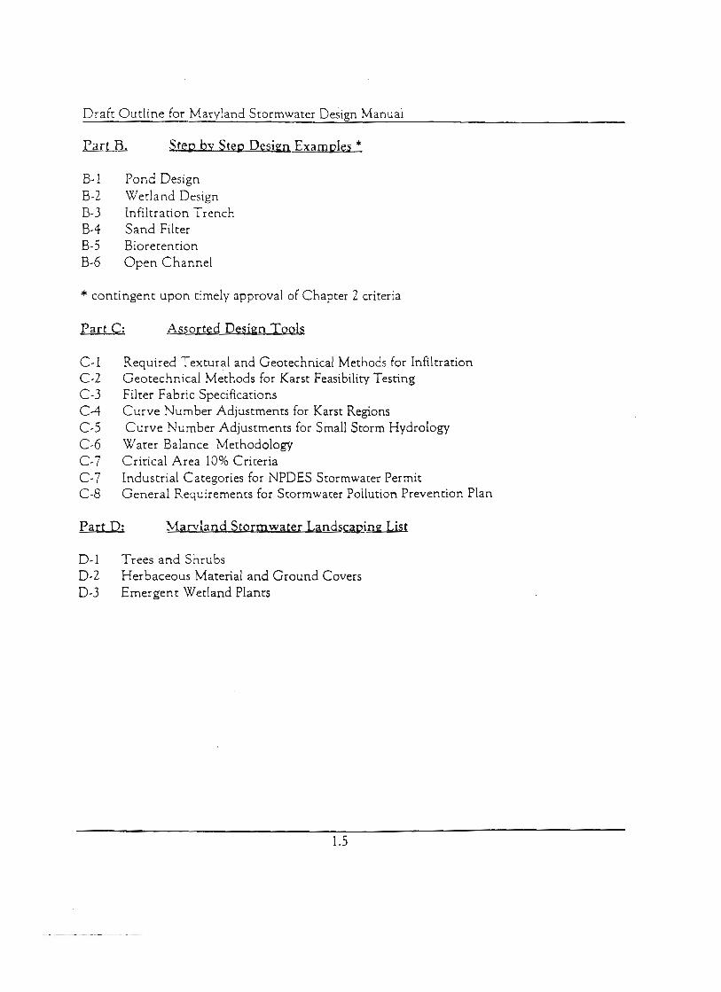
III. Removal Efficiencies by Stormwater Management Era (1984 -2002)
rogram for only a w counties within the Patuxent watershed. As a result, there are unequal amounts of data
ded in MDE’s database, the JHU am issued a survey to all local stormwater contacts. The survey provided a list BMPs
use
MPs by County. The technique worked by summing the acreage of land drained by a l
ped
tructure Efficiencies Efficiencies moval
Efficiencies Drain Area (by percent of total)
P % 2%
Percent Removal = 0)*(0.3052 03052 = 3.0P Percent Removal = (0.30)* (0.3052) = 0.09156 = 9.156%
ed with all other BMPs used the County to determine a cumulative percent removal rate. The JHU team believes that
, TP,
MDE’s Urban Stormwater BMP Database was developed initially as a pilot pfeprovided for each county. Additionally, although it was required, many of the counties were reluctant to provide MDE with information creating a number of gaps within the given data.Because this database is the only source of BMP prevalence in Maryland, it is presumed to bethe most accurate data available. This database was queried for the years 1984-2002 and the frequency of use of each BMP was calculated by percentage. In order to further verify the accuracy of the information provitecommonly implemented between and 1984-2002 and asked local administrators to report on the frequency based on local data. These values were then compared to the frequency ofvalue generated from MDE's database. For 21 of the 23 counties that responded, the results ranged from general concurrence with MDE's database to very precise. This proved satisfactory to the JHU team in establishing a pattern of general accuracy of MDE's database. The JHU team next used a method of “relative abundance” to determine the coverage of Bspecific BMP within each county and then dividing it by the acreage of land drained by alstormwater BMPs for that county. A weighted BMP removal efficiency was then develoby multiplying the relative abundance of each BMP by the pollutant removal efficiencies determined in Part II. Literature Review of BMP Removal Efficiency. An example of these calculations is shown in Example 1 below for a Dry Pond (DP). Example 1: Weighted BMP Removal Efficiencies
TN Removal TP Removal TSS ReSD 10 30% 50% 30.5 TN (0.1 ) = 0. 52% TTSS Percent Removal = (0.50)* (0.3052) = 0.1526 = 15.26% These calculations were performed for each BMP and then summinthese calculations effectively estimate an overall BMP removal rate for each county for Maryland's Stormwater Management Program between the years 1984-2002. Statewide removal efficiencies were calculated as well. Table 1 below shows removal rates for TNand TSS by county and by State.
9
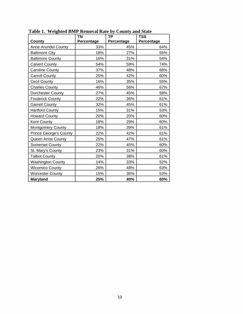
Table 1. Weighted BMP Removal Rate by County and State TN TP TSS
ge County Percentage Percentage PercentaAnne Arundel County 33% 45% 64%Baltimore City %18% 27% 55Baltimore County 16% 31% 54%Calvert County 54% 59% 74%Caroline County 37% 48% 68%Carroll County 25% 42% 60%Cecil County 16% 35% 55%Charles County 46% 56% 67%Dorchester County 27% 45% 58%Frederick County 22% 36% 61%Garrett County 32% 45% 61%Hartford County 15% 31% 53%Howard County 20% 20% 60%Kent County 18% 29% 60%Montgomery County 18% 39% 61%Prince George's County 22% 42% 61%Queen Anne County 25% 47% 61%Somerset County 22% 45% 60%St. Mary's County 23% 31% 60%Talbot County 20% 38% 61%Washington County 14% 33% 52%Wicomico County 26% 48% 63%Worcester County 15% 36% 53%Maryland 25% 40% 60%
10
References
. Marm, and T. Cahill, 2005. Stormwater Management with Porous Pavements, Government Engineering.
Baldwi d T.W. Simpson. Dry Detention Ponds and Hydrodynamic Structures Best Management Practice Definition and Nutrient and Sediment Reduction
Baldwi ert, and T.W. Simpson. Dry Extended Detention Basins Best
Management Practice Definition and Nutrient and Sediment Reduction Efficiencies For
Baldwi
Management Practice Definition and Nutrient and Sediment Reduction Efficiencies For
Barfiel
Guide Volume 2 Vegetative Biofilters.
Baysav water Solutions. BaySeparator System: F-95 Sediment Removal Efficiency Data.
Califor 2003. Bioretention, California Stormwater BMP Handbook.
Califor ter Quality Association, 2003. Infiltration Basin, California Stormwater BMP Handbook.
Califor ality Association, 2003. Infiltration Trench, California Stormwater BMP Handbook.
Califor ality Association, 2003. Media Filter, California Stormwater BMP Handbook.
Chin, K.K. , R. Field, M.L. O'Shea (1993). Integrated Stormwater Management. Boca Raton, Florida: Lewis Publishers.
Claytor, R., T. Schueler, et al., 2000. “2000 Maryland Stormwater Design Manual.” Maryland Department of the Environment, Volumes I & II.
Claytor Document for the State of Maryland Stormwater Design Manual Project.” Center for Watershed Protection Maryland Department of the Environment.
Adams, M., C
n, A.H., S.E. Weammert, an
Efficiencies For use in calibration of the Chesapeake Bay Program’s Phase 5.0 Watershed Model.
n, A.H., S.E. Weamm
use in calibration of the Chesapeake Bay Program’s Phase 5.0 Watershed Model.
n, A.H., S.E. Weammert, and T.W. Simpson. Urban Wet Ponds and Wetlands Best
use in calibration of the Chesapeake Bay Program’s Phase 5.0 Watershed Model.
d, B.J., M.L. Clar, T.P. O’Connor. Stormwater Best Management Practice Design
er Technologies, Inc. Engineering Storm
nia Stormwater Quality Association,
nia Stormwa
nia Stormwater Qu
nia Stormwater Qu
, R., T. Schueler, et al., 1997. “Technical Support
11
Davis, A.P., Shokouhian, M., Sharma, H., and Minami, C. Water Environ. Res., 78(3), 284-293 (2006).
eacon, J., The Microbial World: The Nitrogen cycle and Nitrogen fixation, Institute of Cell
uPage County, 2008. Underground Detention Basins, Best Management Practices Manual
lover, C.R., 1991. Selection of Fertilizers, NM State.
IDEQ, wale (Vegetated Swale), Storm Water Best Management Practices Catalog.
EQ, 2005. Wet Vault/Tank, Storm Water Best Management Practices Catalog.
Jacobs, J., F. McKenzie. Long-term effects of nitrogen fertilizer on nitrogen fixation in grazed perennial ryegrass/white clover dairy pastures in south west Victoria, Department of
e
ew Jersey Stormwater Authority “Standard for Dry Wells.” 2004. New Jersey Stormwater
tahre, P., B. Urbonas (1993). Stormwater; Best Management Practices and Detention for
tormwater Management Fact Sheet: Infiltration Basin. Retrieved January 14, 2009, from
.S. Department of Transportation. Fact Sheet Detention Tanks and Vaults, Federal Highway
.S. EPA, 1999. Storm Water Technology Fact Sheet Infiltration Trench, Office of Water,
Dand Molecular Biology, The University of Edinburgh.
DPractice Standard.
G
2005. Biofiltration S
ID
Natural Resources and Environment. Massachusetts Strategic Envirotechnology Partnership, 2003. Stormwater Technology:
Stormceptor (Hydro Conduit, formerly CSR New England Pipe), Stormceptor Fact Sheet.
Masters, G.M., W.P. Ela (2008). Introduction to Environmental Engineering and Scienc
Third Edition. Upper Saddle River, New Jersey: Pearson Education, Inc.
NBest Management Practices Manual.
SWater Quality, Drainage, and CSO Management. Englewood Cliffs, New Jersey: A Simon & Schuster Company.
Stormwater Management Fact Sheet: Grassed Swales. Retrieved January 14, 2009, from
Infiltration Basin Web site: http://stormwatercenter.net
SInfiltration Basin Web site: http://stormwatercenter.net
UAdministration.
UWashington, D.C..
12

13
.S. EPA, 1999. Storm Water Technology Fact Sheet Porous Pavement, Office of Water,
UWashington, D.C..
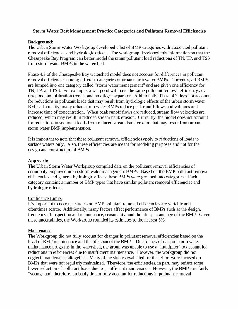
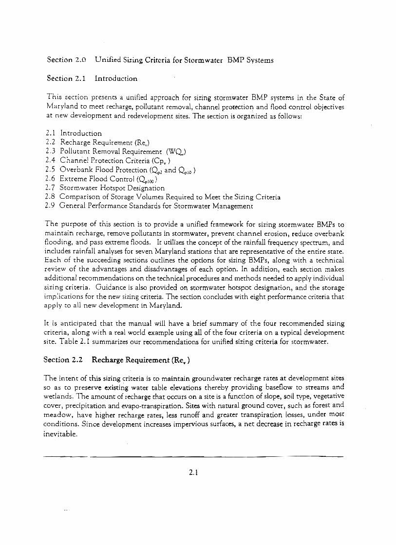
Storm Water Best Management Practice Categories and Pollutant Removal Efficiencies
Background: The Urban Storm Water Workgroup developed a list of BMP categories with associated pollutantremoval efficiencies and hydrologic effects. The workgroup developed this information so that theChesapeake Bay Program can better model the urban pollutant load reductions of TN, TP, and TSSfrom storm water BMPs in the watershed.
Phase 4.3 of the Chesapeake Bay watershed model does not account for differences in pollutantremoval efficiencies among different categories of urban storm water BMPs. Currently, all BMPsare lumped into one category called “storm water management” and are given one efficiency forTN, TP, and TSS. For example, a wet pond will have the same pollutant removal efficiency as adry pond, an infiltration trench, and an oil/grit separator. Additionally, Phase 4.3 does not accountfor reductions in pollutant loads that may result from hydrologic effects of the urban storm waterBMPs. In reality, many urban storm water BMPs reduce peak runoff flows and volumes andincrease time of concentration. When peak runoff flows are reduced, stream flow velocities arereduced, which may result in reduced stream bank erosion. Currently, the model does not accountfor reductions in sediment loads from reduced stream bank erosion that may result from urbanstorm water BMP implementation.
It is important to note that these pollutant removal efficiencies apply to reductions of loads tosurface waters only. Also, these efficiencies are meant for modeling purposes and not for thedesign and construction of BMPs.
Approach:The Urban Storm Water Workgroup compiled data on the pollutant removal efficiencies ofcommonly employed urban storm water management BMPs. Based on the BMP pollutant removalefficiencies and general hydrologic effects these BMPs were grouped into categories. Eachcategory contains a number of BMP types that have similar pollutant removal efficiencies andhydrologic effects.
Confidence LimitsIt’s important to note the studies on BMP pollutant removal efficiencies are variable andoftentimes scarce. Additionally, many factors affect performance of BMPs such as the design,frequency of inspection and maintenance, seasonality, and the life span and age of the BMP. Giventhese uncertainties, the Workgroup rounded its estimates to the nearest 5%.
MaintenanceThe Workgroup did not fully account for changes in pollutant removal efficiencies based on thelevel of BMP maintenance and the life span of the BMPs. Due to lack of data on storm watermaintenance programs in the watershed, the group was unable to use a “multiplier” to account forreductions in efficiencies due to insufficient maintenance. However, the workgroup did notneglect maintenance altogether. Many of the studies evaluated for this effort were focused onBMPs that were not regularly maintained. Therefore, the efficiencies, in part, may reflect somelower reduction of pollutant loads due to insufficient maintenance. However, the BMPs are fairly“young” and, therefore, probably do not fully account for reductions in pollutant removal

efficiencies due to aging BMPs.
Low Impact Development/Environmental Site DesignThe Workgroup decided not to include Low Impact Development (LID) or Environmental SiteDesign as a BMP Category because no jurisdiction is reporting the number of acres under LID. Jurisdictions are reporting number of acres under certain BMP practices that can be considered acomponent of LID, such as bioretention or rooftop disconnection. These practices are alreadyaccounted for in the BMP categories. In the future, if more and more jurisdictions use LID andstart to report the number of acres under LID, then a separate category.
Treatment TrainsTreatment trains are a number of BMPs that are connected in series to treat the same volume ofrunoff. The Workgroup has concluded that there is not enough hard data to account for pollutantremoval efficiencies for “treatment trains”. Funding opportunities to obtain literature and fielddata are currently being pursued.
The following table summarizes the BMP categories and the pollutant removal efficiencies. Seethe Support Document for a complete list of BMP types, BMP definitions, pollutant removalefficiencies, and references that were used in this analysis.
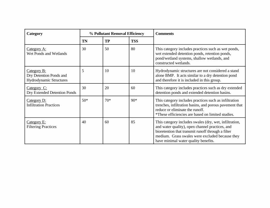
Category % Pollutant Removal Efficiency Comments
TN TP TSS
Category A:Wet Ponds and Wetlands
30 50 80 This category includes practices such as wet ponds,wet extended detention ponds, retention ponds,pond/wetland systems, shallow wetlands, andconstructed wetlands.
Category B:Dry Detention Ponds andHydrodynamic Structures
5 10 10 Hydrodynamic structures are not considered a standalone BMP. It acts similar to a dry detention pondand therefore it is included in this group.
Category C:Dry Extended Detention Ponds
30 20 60 This category includes practices such as dry extendeddetention ponds and extended detention basins.
Category D:Infiltration Practices
50* 70* 90* This category includes practices such as infiltrationtrenches, infiltration basins, and porous pavement thatreduce or eliminate the runoff.*These efficiencies are based on limited studies.
Category E:Filtering Practices
40 60 85 This category includes swales (dry, wet, infiltration,and water quality), open channel practices, andbioretention that transmit runoff through a filtermedium. Grass swales were excluded because theyhave minimal water quality benefits.
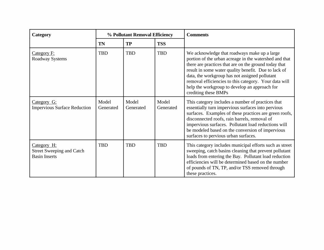
Category % Pollutant Removal Efficiency Comments
TN TP TSS
Category F:Roadway Systems
TBD TBD TBD We acknowledge that roadways make up a largeportion of the urban acreage in the watershed and thatthere are practices that are on the ground today thatresult in some water quality benefit. Due to lack ofdata, the workgroup has not assigned pollutantremoval efficiencies to this category. Your data willhelp the workgroup to develop an approach forcrediting these BMPs
Category G:Impervious Surface Reduction
ModelGenerated
ModelGenerated
ModelGenerated
This category includes a number of practices thatessentially turn impervious surfaces into pervioussurfaces. Examples of these practices are green roofs,disconnected roofs, rain barrels, removal ofimpervious surfaces. Pollutant load reductions willbe modeled based on the conversion of impervioussurfaces to pervious urban surfaces.
Category H:Street Sweeping and CatchBasin Inserts
TBD TBD TBD This category includes municipal efforts such as streetsweeping, catch basins cleaning that prevent pollutantloads from entering the Bay. Pollutant load reductionefficiencies will be determined based on the numberof pounds of TN, TP, and/or TSS removed throughthese practices.
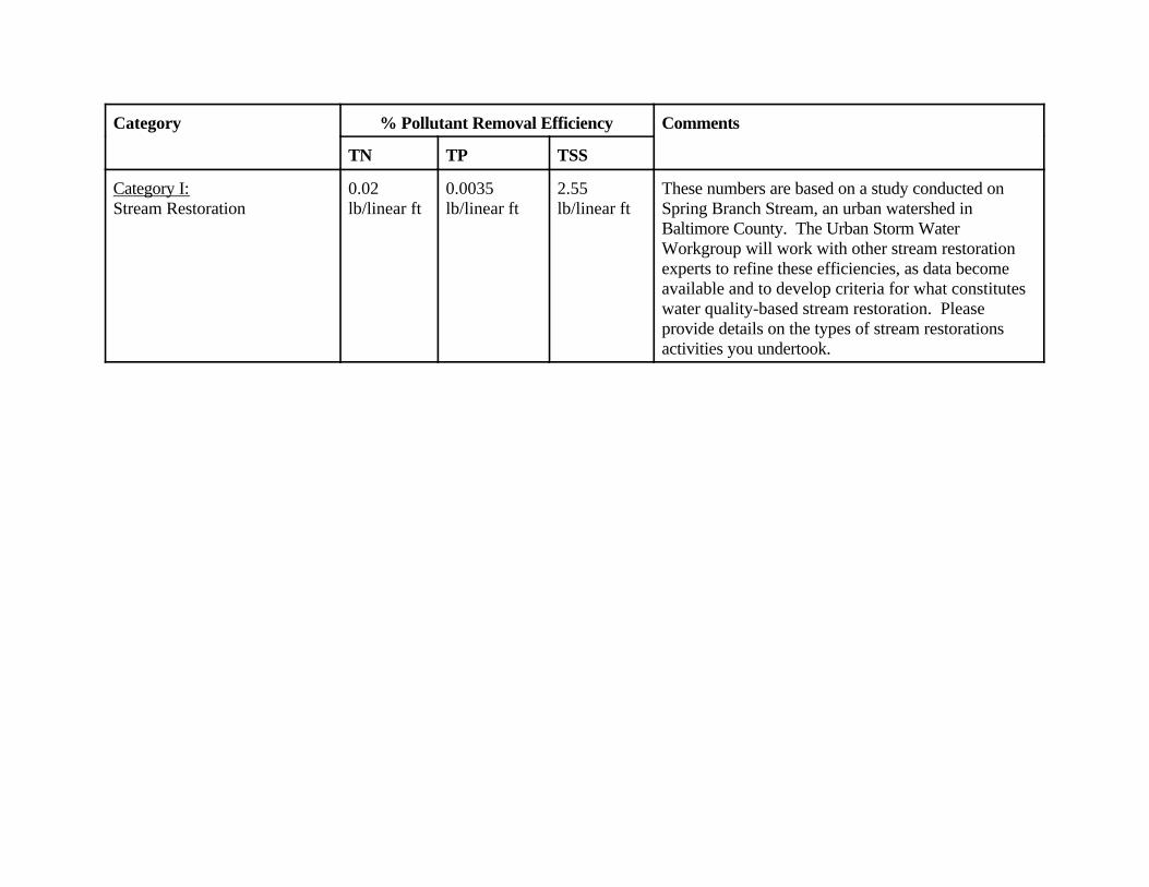
Category % Pollutant Removal Efficiency Comments
TN TP TSS
Category I:Stream Restoration
0.02lb/linear ft
0.0035lb/linear ft
2.55lb/linear ft
These numbers are based on a study conducted onSpring Branch Stream, an urban watershed inBaltimore County. The Urban Storm WaterWorkgroup will work with other stream restorationexperts to refine these efficiencies, as data becomeavailable and to develop criteria for what constituteswater quality-based stream restoration. Pleaseprovide details on the types of stream restorationsactivities you undertook.