Matchings on infinite graphs

Probab. Theory Relat. FieldsDOI 10.1007/s00440-012-0453-0

Matchings on infinite graphs

Charles Bordenave · Marc Lelarge · Justin Salez

Received: 7 February 2011 / Accepted: 5 September 2012© Springer-Verlag 2012

Abstract Elek and Lippner (Proc. Am. Math. Soc. 138(8), 2939–2947, 2010) showedthat the convergence of a sequence of bounded-degree graphs implies the existenceof a limit for the proportion of vertices covered by a maximum matching. We providea characterization of the limiting parameter via a local recursion defined directly onthe limit of the graph sequence. Interestingly, the recursion may admit multiple solu-tions, implying non-trivial long-range dependencies between the covered vertices.We overcome this lack of correlation decay by introducing a perturbative parameter(temperature), which we let progressively go to zero. This allows us to uniquely iden-tify the correct solution. In the important case where the graph limit is a unimodularGalton–Watson tree, the recursion simplifies into a distributional equation that can besolved explicitly, leading to a new asymptotic formula that considerably extends thewell-known one by Karp and Sipser for Erdos-Rényi random graphs.

Keywords Matching · Heilmann-Lieb Theorem · Local weak convergence ·Random sparse graphs

Mathematics Subject Classification Primary 60C05 · Secondary 82B20 · 05C80

C. BordenaveInstitut de Mathématiques, Université de Toulouse, CNRS, Toulouse, Francee-mail: [email protected]

M. Lelarge (B)INRIA-Ecole Normale Supérieure, Paris, Francee-mail: [email protected]

J. SalezUniversité Paris Diderot-LPMA, Paris, Francee-mail: [email protected]

123

C. Bordenave et al.

1 Introduction

A matching on a finite graph G = (V, E) is a subset of pairwise non-adjacent edgesM ⊆ E . The |V | − 2|M | isolated vertices of (V, M) are said to be exposed by M . Welet M(G) denote the set of all possible matchings on G. The matching number of Gis defined as

ν(G) = maxM∈M(G)

|M |, (1)

and those M which achieve this maximum—or equivalently, have the fewest exposedvertices—are called maximum matchings. The normalized matching number of G issimply ν(G)/|V |.

Our results belong to the theory of convergent graph sequences. Convergence ofbounded degree graph sequences was defined by Benjamini and Schramm [7], Aldousand Steele [2], see also Aldous and Lyons [1]. The notion of local weak convergencehas then inspired a lot of work [8,11,13,16,26]. In [17], it is shown that the convergenceof a sequence of bounded-degree graphs guarantees the existence of a limit for theirnormalized matching numbers. We provide a characterization of the limiting parametervia a local recursion defined directly on the limit of the graph sequence. In the importantcase where the graph limit is a unimodular Galton–Watson tree, the recursion simplifiesinto a distributional equation that can be solved explicitly, leading to a new asymptoticformula.

A classical example in this context is the Erdos-Rényi random graph with averagedegree c on n vertices, denoted by G(n, c/n) : as n → ∞, G(n, c/n) converges inthe local weak sense to a Galton–Watson tree with degree distribution Poisson withparameter c. In this case, Karp and Sipser [22] showed that

ν(G(n, c/n))

n−−−→n→∞ 1 − tc + e−ctc + ctce−ctc

2, (2)

where tc ∈ (0, 1) is the smallest root of t = e−ce−ct(we will see in the sequel that

the convergence is almost sure). The explicit formula (2) rests on the analysis ofa heuristic algorithm now called Karp-Sipser algorithm. The latter is based on thefollowing observation : if e ∈ E is a pendant edge (i.e. an edge incident to a vertex ofdegree one) in G = (V, E), then there is always a maximum matching that contains e,so all edges that are adjacent to e may be deleted without affecting ν(G). The first stageof the algorithm consists in iterating this until no more pendant edge is present. Thisis the leaf-removal process. G is thus simplified into a sub-graph with only isolatedvertices, matched pairs, and a so-called core with minimum degree at least two. Aslong as that core is non-empty, one of its edges is selected uniformly at random, theadjacent edges are deleted, and the whole process starts again. When the algorithmstops, the remaining edges clearly form a matching on G, but its size may be far belowν(G) due to the sub-optimal removals on the core.

On G(n, c/n), the dynamics of the deletion process can be approximated in then → ∞ limit by differential equations which can be explicitly solved. In particular,

123


the asymptotic size of both the optimal part constructed in the first stage, and thesub-optimal part constructed on the core can be evaluated up to an o(n) correctingterm (which has been later refined, see [4]). Moreover, the second part happens tobe almost perfect, in the sense that only o(n) vertices are exposed in the core. Thisguarantees that the overall construction is asymptotically optimal, and the asymptoticformula for ν(Gn) follows. More recently, the same technique has been applied toanother class of random graphs with a fixed log-concave degree profile [10], resultingin the asymptotical existence of an almost perfect matching on these graphs:

ν(Gn)

|Vn| −−−→n→∞

1

2. (3)

In both cases, the proof of optimality—and hence the asymptotic formula for ν(Gn)—relies on the fact that the second stage exposes only o(n) vertices, which is bound to failas soon as one considers more general graph ensembles where the core does not neces-sarily admits an almost-perfect matching. We give simple examples in the Appendix.By using a completely different approach—namely establishing and solving an appro-priate recursive distributional equation (a usual ingredient of the objective method,see [3])—we manage to obtain a general formula that considerably extends the aboveresults.

The rest of our paper is organized as follows: we state our main results in Sect. 2.In Sect. 3, we extend the Boltzmann-Gibbs distribution over matchings on a finitegraph to infinite graphs. This will allow us to derive our Theorem 1 in Sect. 4. Wedeal with the specific cases of trees (and random graphs) in Sect. 5. We end the paperwith an Appendix presenting simple examples of graphs for which the limiting localrecursion admit multiple solutions.

2 Results

Let us start with a brief recall on local weak convergence (see [2,7] for details). A rootedgraph (G, ◦) is a graph G = (V, E) together with the specification of a particularvertex ◦ ∈ V , called the root. We let G denote the set of all locally finite connectedrooted graphs considered up to rooted isomorphism, i.e. (G1, ◦1) ≡ (G2, ◦2) if thereexists a bijection γ : V1 → V2 that preserves roots (γ (◦1) = ◦2) and adjacency(uv ∈ E1 ⇐⇒ γ (u)γ (v) ∈ E2). In the space G, a sequence {(Gn, ◦n); n ∈ N}converges locally to (G, ◦) if for every radius k ∈ N, there is nk ∈ N such that

n ≥ nk �⇒ [Gn, ◦n]k ≡ [G, ◦]k .

Here, [G, ◦]k denotes the finite rooted subgraph induced by the vertices lying at graph-distance at most k from ◦. It is not hard to construct a distance which metrizes thisnotion of convergence and turns G into a complete separable metric space. We can thusimport the usual machinery of weak convergence of probability measures on Polishspaces (see e.g. [9]). We define P(G) as the set of probability measure on G. There isa natural procedure for turning a finite deterministic graph G = (V, E) into a random

123

C. Bordenave et al.

element of G : one simply chooses uniformly at random a vertex ◦ ∈ V to be the root,and then restrains G to the connected component of ◦. The resulting law is denoted byU(G) ∈ P(G). If (Gn)n∈N is a sequence of finite graphs such that (U(Gn))n∈N admitsa weak limit ρ ∈ P(G), we call ρ the random weak limit of the sequence (Gn)n∈N.Finally, for any d ≥ 0, we define Gd as the space of all rooted connected graphs withmaximal degree no more than d.

Rather than just graphs G = (V, E), it will be sometimes convenient to work withdiscrete networks G = (V, E,M), in which the additional specification of a markmap M : E → N allows to attach useful local information to edges, such as theirabsence/presence in a certain matching. We then simply require the isomorphisms inthe above definition to preserve these marks.

The first main implication of our work is that the local weak convergence of asequence of graphs is enough to guarantee the convergence of their normalized match-ing numbers to a quantity that can be described directly on the random weak limit ofthe graph sequence.

Theorem 1 Let Gn = (Vn, En), n ∈ N, be a sequence of finite graphs admitting arandom weak limit ρ. Then,

ν(Gn)

|Vn| −−−→n→∞ γ, (4)

where γ ∈ [0, 12 ] is defined by a recursion defined directly on the random weak

limit ρ.

We refer to Sect. 3.1 for a description of the recursion defining γ .Since the work of Heilmann and Lieb [21], it is known that the thermodynamic

limit for monomer-dimer systems exists and basic properties of this limit are derivedfor lattices. In particular, [21, Lemma 8.7] shows the convergence of the normalizedmatching number when the underlying graph is a lattice. More recently, Elek andLippner [17] extended this result by using the framework of local weak convergencefor bounded degree graphs. Here we remove the bounded degree assumption. Moreimportantly, the approach in [17] is non-constructive. In contrast, we provide a charac-terization of γ in terms of a local recursion defined directly on the random weak limitρ. We postpone the discussion on how to actually compute γ from ρ to Subsect. 3.1.Our approach starts as in [21] with the introduction of a natural family of probabilitydistributions on the set of matchings parametrized by a single parameter z > 0 calledthe Boltzmann-Gibbs distribution. The analysis in [21] concentrates on the propertiesof the partition function, also known as the matching polynomial, from which a resultlike (4) can be deduced. Our analysis differs from this approach and concentrates onthe analysis of the local marginals of the Boltzmann-Gibbs distribution, in a similarspirit as in the (non-rigorous) work of Zdeborová and Mézard [27]. As in [27] and[20], we start from an elementary formal recursion satisfied by the matching polyno-mials, and deduce an exact recursion for the local marginals of the Boltzmann-Gibbsdistribution on any finite graph. A careful analysis of the contractivity properties ofthis recursion allows us to define the monomer-dimer model on infinite graphs (seeTheorem 6), and to define their “normalized matching number” (see Theorem 10).

123


We should stress that the analysis of the marginal probabilities is essential for our sec-ond main result, namely the explicit computation of the matching number when thelocal weak limit is a Galton–Watson tree. Although simple adaptations of the argumentin [21] would yield a result like Theorem 1, the limit would be given in an implicitway which would not be sufficient to get our second main result.

As many other classical graph sequences, Erdos-Rényi graphs and random graphswith a prescribed degree profile admit almost surely a particularly simple randomweak limit, namely a unimodular Galton–Watson (UGW) tree (see Example 1.1 in [1]).This random rooted tree is parametrized by a probability distribution π ∈ P(N) withfinite mean, called its degree distribution. It is obtained by a Galton–Watson branchingprocess where the root has offspring distribution π and all other genitors have offspringdistribution π ∈ P(N) defined by

∀n ∈ N, πn = (n + 1)πn+1∑

k kπk. (5)

Thanks to the markovian nature of the branching process, the recursion defining γ

simplifies into a recursive distributional equation, which has been explicitly solvedby the authors in a different context [12].

Theorem 2 With the notation of Theorem 1, if the random weak limit ρ is a UGWtree with degree distribution π , we have the explicit formula

γ = 1 − maxt∈[0,1] F(t)

2,

where

F(t) = tφ′(1 − t) + φ(1 − t) + φ

(

1 − φ′(1 − t)

φ′(1)

)

− 1,

and φ(t) = ∑

n πntn is the moment generating function of the degree distribution π .

Differentiating the above expression, we see that any t achieving the maximummust satisfy

φ′(1)t = φ′(

1 − φ′(1 − t)

φ′(1)

)

. (6)

For Erdos-Rényi random graphs with connectivity c, the degree of the limiting UGWtree is Poisson with parameter c (i.e. φ(t) = exp(ct − c)), so that (6) becomest = e−ce−ct

. We thus recover precisely Karp and Sipser’s formula (2). Similarly, forrandom graphs with a prescribed degree sequence, the log-concave assumption madeby Bohmann and Frieze guarantees that the above maximum is achieved at t = 0 withF(0) = 0, hence (3) follows automatically.

A classical area of combinatorial optimization is formed by bipartite matching[25]. We end this section, with a specialization of our results to bipartite graphs

123

C. Bordenave et al.

G = (V = V a ∪ V b, E). The natural limit for a sequence of bipartite graphs isthe following hierarchal Galton–Watson tree parameterized by two distributions on N

with finite first moment, πa and πb and a parameter λ ∈ [0, 1]. We denote πa and πb

the corresponding distributions given by the transformation (5). We also denote φa

and φb the generating functions of πa and πb. The hierarchal Galton–Watson tree isthen defined as follows: with probability λ, the root has offspring distribution πa , allodd generation genitors have offspring distribution πb and all even generation genitorshave offspring distribution πa ; similarly with probability 1 −λ, the root has offspringdistribution πb, all odd generation genitors have offspring distribution πa and all evengeneration genitors have offspring distribution πb. In the first (resp. second) case, wesay that the root and all even generations are of type a (resp. b) and all the odd genera-tions are of type b (resp. a). To get a unimodular hierarchal Galton–Watson (UHGW)tree with degree distributions πa and πb, we need to have: λφa ′(1) = (1 − λ)φb ′(1),so that

λ = φb ′(1)

φa ′(1) + φb ′(1). (7)

Theorem 3 With the notation of Theorem 1, assume that the random weak limit ρ isa UHGW tree with degree distributions πa, πb. If πa and πb have finite first moment,then

γ = φb ′(1)

φa ′(1) + φb ′(1)

(

1 − maxt∈[0,1] Fa(t)

)

, (8)

where Fa is defined by:

Fa(t) = φa(

1 − φb ′(1 − t)

φb ′(1)

)

− φa ′(1)

φb ′(1)

(

1 − φb(1 − t) − tφb ′(1 − t))

.

Note that if φa(x) = φb(x), we find the same limit as in Theorem 2. Note that it isnot obvious from formula (8) that our expression for γ is symmetric in a and b as itshould. In the forthcoming Sect. 5.2, Eq. (30) gives an alternative symmetric formulafor γ which simplifies to (8) thanks to (7).

Note also that our Theorem 3 computes the independence number of random bipar-tite graphs. Recall that a set of vertices in a graph G is said to be independent if no twoof them are adjacent. The cardinality of any largest independent set of points in G isknown as the independence number of G or the stability number of G and is denotedby α(G). By Konig’s theorem, we know that for any bipartite graph G with vertexset V, α(G) + ν(G) = |V |. The fact that a limit for α(Gn)

|Vn | exists, has been provedrecently in [5] for Erdos-Rényi and random regular graphs. The actual value for thislimit is unknown except for Erdos-Rényi graphs with mean degree c < e. In this case,the leaf-removal algorithm allows to compute explicitly the limit which agrees with(8) with φa(x) = φb(x) = exp(cx − x).

Motivated by some applications for Cuckoo Hashing [15,18], recent results havebeen obtained in the particular case where πa(k) = 1 for some k ≥ 3 and πb is a

123


Poisson distribution with parameter αk. These degree distributions arise if one considera sequence of bipartite graphs with �αm� nodes of type a (called the items), m nodesof type b (called the locations) and each node of type a is connected with k nodes oftype b chosen uniformly at random (corresponding to the assigned locations the itemcan be stored in). The result in this domain, obtained in [19] follows (see Sect. 5.3)from our Theorem 3, namely:

Corollary 4 Under the assumption of Theorem 3 and with πa(k) = 1 for some k ≥ 3and πb is a Poisson distribution with parameter αk. Let ξ be the unique solution ofthe equation:

k = ξ(1 − e−ξ )

1 − e−ξ − ξe−ξ, and, αc = ξ

k(1 − e−ξ )k−1 .

• for α ≤ αc, all (except op(n)) vertices of type a are covered, i.e. ν(Gn)|V a

n | −−−→n→∞ 1.

• for α > αc, we have:

ν(Gn)

|V an | −−−→

n→∞ 1 − 1

α

(

e−ξ∗ + ξ∗e−ξ∗ + ξ∗

k(1 − e−ξ∗

) − 1

)

, (9)

where ξ∗ = kαx∗ and x∗ is the largest solution of x = (

1 − e−kαx)k−1

.

In words, αc is the load threshold: if α ≤ αc, there is an assignment of the �αm�items to a table with m locations that respects the choices of all items, whereas forα > αc, such an assignement does not exist and (9) gives the maximal number ofitems assigned without collision. Note that results in [15,18] are slightly different inthe sense that for the specific sequence of random graphs described above (i.e. uniformhypergraphs), they show that for α < αc all vertices of type a are covered with highprobability. It is shown in [23] how to get such results from Corollary 4 under theadditional assumption that the sequence of graphs are uniform hypergraphs.

3 The monomer-dimer model

We start with the case of a finite graph G = (V, E). Consider a natural family ofprobability distributions on the set of matchings M(G), parameterized by a singleparameter z > 0 called the temperature (note that the standard temperature T inphysics would correspond to z = e−1/T but this will not be important here): for anyM ∈ M(G),

μzG(M) = z|V |−2|M|

PG(z), (10)

where PG is the matching polynomial, PG(z) = ∑

M∈M(G) z|V |−2|M|. In statisticalphysics, this is called the monomer-dimer model at temperature z on G (see [21] for acomplete treatment). We let Mz

G denote a random element of M(G) with law μzG , and

123

C. Bordenave et al.

we call it a Boltzmann random matching at temperature z on G. Note that the lowestdegree coefficient of PG is precisely the number of largest matchings on G. Therefore,Mz

G converges in law to a uniform largest matching as the temperature z tends to zero.We define the root-exposure probability (REP) of the rooted graph (G, ◦) as

Rz[G, ◦] = μzG (◦ is exposed). (11)

3.1 Local recursions to compute γ

Before starting with the proof, we explain (whithout proofs) how to compute γ in(4). For a finite graph, our computation of γ follows exactly the approach of Godsil[20]. We recall Godsil’s notion of the path-tree associated with a rooted graph G: ifG is any rooted graph with root ◦, we define its path-tree TG as the rooted tree whosevertex-set consists of all finite simple paths starting at the root ◦; whose edges are thepairs {P, P ′} of the form P = v1 . . . vn, P ′ = v1 . . . vnvn+1(n ≥ 1); whose root isthe single-vertex path ◦. By a finite simple path, we mean here a finite sequence ofdistinct vertices v1 . . . vn (n ≥ 1) such that vivi+1 ∈ E for all 1 ≤ i < n.

It is well-known since Godsil’s result [20] that path-trees capture considerableinformation about matchings in general graph and are easier to work with than thegraph itself. For a rooted graph [G, ◦], let T[G,◦] be the associated path-tree and considerthe corresponding system of equations (where u � v if u is a child of v):

∀v ∈ T[G,◦], xv = 1

1 + ∑

u�v

(∑

w�u xw

)−1 . (12)

For any finite rooted graph [G, ◦], (12) has a unique solution in [0, 1]T[G,◦] and wedenote the value taken at the root by x◦(G). Then x◦(G) is exactly the probability forthe root ◦ of being exposed in a uniform maximal matching. In particular, we have

ν(G) =∑

v∈V

1 − xv(G)

2.

This argument follows from [20] and will be a special case of our analysis.For an infinite graph with bounded degree, it turns out that it is not always possible

to make sense of the local recursions (12). However, our analysis will show that forany z > 0, the infinite set of equations:

∀v ∈ T[G,◦], xv(z) = 1

1 + ∑

u�v

(

z2 + ∑

w�u xw(z))−1 ,

has a unique solution in [0, 1]T[G,◦] and the value taken by the root is exactly Rz[G, ◦](which is the probability for the root ◦ of being exposed in a Boltzmann randommatching at temperature z when the graph G is finite). Then our Theorem 11 will implythat for any sequence of finite graphs (Gn = (Vn, En))n∈N satisfying |En| = O(|Vn|)

123


and having ρ as a random weak limit,

ν(Gn)

|Vn| −−−→n→∞

1 − Eρ

[

limz→0 Rz]

2,

and limz→0 Rz[G, ◦] is actually the largest solution to (12). From a practical pointof view, it is possible to compute an approximation of Rz[G, ◦] by looking at asufficient large ball centered at the root ◦, see [24]. Moreover our analysis will showthat the quantity Eρ

[Rz]

is a good approximation of Eρ

[

limz→0 Rz]

as soon as|En| = O(|Vn|) (see Lemma 12).

3.2 Extension of the model on infinite graphs with bounded degree

Let G − ◦ be the graph obtained from G by removing its root ◦. Since the matchingsof G that expose ◦ are exactly the matchings of G − ◦, we have the identity

Rz[G, ◦] = z PG−◦(z)PG(z)

, (13)

which already shows that the REP is an analytic function of the temperature. Theremarkable fact that its domain of analyticity contains the right complex half-plane

H+ = {z ∈ C; �(z) > 0}

is a consequence of the powerful Heilmann-Lieb theorem [21, Theorem 4.2] (see [14]for generalizations). The key to the study of the REP is the following elementary butfundamental local recursion:

Rz[G, ◦] = z2

(

z2 +∑

v∼◦Rz[G − ◦, v]

)−1

. (14)

Clearly, this recursion determines uniquely the functional Rz on the class of finiterooted graphs, and may thus be viewed as an inductive definition of the REP. Remark-ably enough, this alternative characterization allows for a continuous extension toinfinite graphs with bounded degree, even though the above recursion never ends. Welet H denote the space of analytic functions on H+, equipped with its usual topologyof uniform convergence on compact sets. Our fundamental lemma is as follows:

Theorem 5 (The fundamental local lemma)

1. For every fixed z ∈ H+, the local recursion (14) determines a unique Rz : Gd →zH+.

2. For every fixed [G, ◦] ∈ Gd , z �→ Rz[G, ◦] is analytic.3. The resulting mapping [G, ◦] ∈ Gd �−→ R(·)[G, ◦] ∈ H is continuous.

123

C. Bordenave et al.

This local lemma has strong implications for the monomer-dimer model, whichwe now list. The first one is the existence of an infinite volume limit for the Gibbs-Boltzmann distribution.

Theorem 6 (Monomer-dimer model on infinite graphs) Consider a graph G ∈ Gd

and a temperature z > 0. For any finite matching M of G, the cylinder-event marginalsdefined by

μzG(M ⊆ M) = z−2|M|

2|M|∏

k=1

Rz[G − {v1, . . . , vk−1}, vk],

are consistent and independent of the ordering v1, . . . v2|M| of the vertices spanned byM. They thus determine a unique probability distribution μz

G over the matchings ofG. It coincides with the former definition in the case where G is finite, and extends itcontinuously in the following sense : for any ◦ ∈ V and any sequence ([Gn, ◦n])n∈N ∈Gd

N converging to [G, ◦],

[Gn, ◦n,Mn] d−−−→n→∞ [G, ◦,M],

in the local weak sense for random networks, where Mn has law μzGn

and M has lawμz

G.

Although it is not our concern here, we obtain as a by-product the strong con-vergence of the logarithm of the matching polynomial, also called free energy in themonomer-dimer model:

Corollary 7 Let (Gn)n∈N be a sequence of finite graphs with bounded degree admit-ting a random weak limit [G, ◦]. The following convergence holds in the analytic senseon H+,

1

|Vn| logPGn (z)

PGn (1)−−−→n→∞

z∫

1

Eρ[Rs[G, ◦]]s

ds,

where Eρ[Rs[G, ◦]] denotes the expectation under the measure ρ of the variableRs[G, ◦].

A similar result was established in [21] for the lattice case, and in [6] under arestrictive large girth assumption.

3.3 Proof of Theorem 5: the fundamental lemma

The local recursion (14) involves mappings of the form:

φz,d : (x1, . . . , xd) �→ z2

(

z2 +d

∑

i=1

xi

)−1

,

123


where d ∈ N. In the following lemma, we gather a few elementary properties of thistransformation, which are immediate to check but will be of constant use throughoutthe paper.

Lemma 8 (Elementary properties) For any d ∈ N and z ∈ H+,

1. φz,d maps analytically zH+ × · · · × zH+ into zH+2. |φz,d | is uniformly bounded by |z|/�(z) on zH+ × · · · × zH+.

From part 1, it follows that the REP of a finite rooted graph belongs to H, whenviewed as a function of the temperature z. Part 2 and Montel’s theorem guarantee thatthe family of all those REPs is relatively compact in H. Note that relative compactnessalso plays a central role in [21]. Combined with the following uniqueness property athigh temperature, it will quickly lead to the proof of Theorem 5.

The local recursion (14) also involves graph transformations of the form [G, ◦] �→[G − ◦, v], where v ∼ ◦. Starting from a given [G, ◦] ∈ Gd , we let Succ∗[G, ◦] ⊆ Gd

denote the (denumerable) set of all rooted graphs that can be obtained by successivelyapplying finitely many such transformations.

Lemma 9 (Uniqueness at high temperature) Let [G, ◦] ∈ Gd and z ∈ H+ such that�(z) >

√d. If

R1z ,R2

z : Succ∗[G, ◦] → zH+

both satisfy the local recursion (14) then R1z = R2

z .

Proof Set α = 2|z|/�(z) and β = �(z)−2. From (14) and part two of Lemma 8 it isclear that the absolute difference � = |R1

z − R2z | must satisfy

�[G, ◦] ≤ α and �[G, ◦] ≤ β∑

v∼◦�[G − ◦, v].

In turn, each�[G−◦, v] appearing in the second upper-bound may be further expandedinto β

∑

w∼v,w �=◦ �[G − ◦ − v,w]. Iterating this procedure k times, one obtains

�[G, ◦] ≤ βkdkα. Taking the infimum over all k yields �[G, ◦] = 0, since theassumption �(z) >

√d means precisely βd < 1. ��

Proof of Theorem 5 For clarity, we divide the proof in three parts : we first define aspecific solution which satisfies (14) and is analytic. We will then prove this solutionis unique and continuous. This will prove parts one–three of Theorem 5.

Analytic existence. Fix [G, ◦] ∈ Gd , and consider an arbitrary collection of H+ →zH+ analytic functions z �→ R0

z [H, i], indexed by the elements [H, i] ∈ Succ∗[G, ◦].For every n ≥ 1, define recursively

Rnz [H, i] = z2

⎛

⎝z2 +∑

j∼i

Rn−1z [H − i, j]

⎞

⎠

−1

, (15)

123

C. Bordenave et al.

for all z ∈ H+ and [H, i] ∈ Succ∗[G, ◦]. By Lemma 8, each sequence(

z �→ Rnz [H, i])n∈N

is relatively compact in H. Consequently, their joint collec-tion as [H, i] varies in the denumerable set Succ∗[G, ◦] is relatively compact inthe product space HSucc∗[G,◦]. Passing to the limit in (15), we see that any pre-limitRz : Succ∗[G, ◦] → zH+ must automatically satisfy (14) for each z ∈ H+. ByLemma 9, this determines uniquely the value of Rz[G, ◦] for z with sufficiently largereal part, and hence everywhere in H+ by analyticity. To sum up, we have just provedthe following : for every [G, ◦] ∈ Gd , the limit

Rz[G, ◦] := limn→∞ Rn

z [G, ◦] (16)

exists in H, satisfies the recursion (14), and does not depend upon the choice of theinitial condition R0

z : Succ∗[G, ◦] → zH+ (provided that the latter is analytic inz ∈ H+).

Pointwise uniqueness. Let us now show that any S : Succ∗[G, ◦] → zH+ satisfy-ing the recursion (14) at a fixed value z = z0 ∈ H+ must coincide with the z = z0 spe-cialization of the analytic solution constructed above. For each [H, i] ∈ Succ∗[G, ◦],the constant initial function R0

z [H, i] := S[H, i] is trivially analytic from H+ to zH+,so the iteration (15) must converge to the analytic solution Rz . Since Rn

z0= S for all

n ∈ N, we obtain Rz0 = S, as desired.Continuity. Finally, assume that ([Gn, ◦])n≥1 ∈ Gd

N converges locally to [G, ◦],and let us show that

Rz[Gn, ◦] H−−−→n→∞ Rz[G, ◦]. (17)

It is routine that, up to rooted isomorphisms, G, G1, G2, . . . may be represented on acommon vertex set, in such a way that for each fixed k ∈ N, [Gn, ◦]k = [G, ◦]k forall n ≥ nk . By construction, any simple path v1 . . . vk starting from the root in G isnow also a simple path starting from the root in each Gn, n ≥ nk , so the H−valuedsequence (z �→ Rz[Gn − {v1, . . . , vk−1}, vk])n≥nk

is well defined, and relatively com-pact (Lemma 8). Again, the denumerable collection of all sequences obtained by lettingthe simple path v1 . . . vk vary in [G, ◦] is relatively compact for the product topology,and any pre-limit must by construction satisfy (14). By pointwise uniqueness, theconvergence (17) must hold. ��

3.4 Proof of Theorem 6: convergence of the Boltzmann distribution

Consider an infinite [G, ◦] ∈ Gd , and let ([Gn, ◦])n≥1 be a sequence of finite rootedconnected graphs converging locally to [G, ◦]. As above, represent G, G1, G2, . . . ona common vertex set, in such a way that for each k ∈ N, [Gn, ◦]k = [G, ◦]k for alln ≥ nk . Now fix an arbitrary finite matching M in G, and denote by v1, . . . , v2|M| thevertices spanned by M , in any order. By construction, M is also a matching of Gn forlarge enough n. But the matchings of Gn that contain M are in 1 − 1 correspondence

123


with the matchings of Gn − {v1, . . . , v2|M|}, and hence

μzGn

(M ⊆ M) = PGn−{v1,...,v2|M|}(z)PGn (z)

= z−2M2M∏

k=1

Rz[Gn − {v1, . . . , vk−1}, vk].

But [Gn − {v1, . . . , vk−1}, vk] converges locally to [G − {v1, . . . , vk−1}, vk], so bycontinuity of Rz ,

μzGn

(M ⊆ M) −−−→n→∞ z−2M

2M∏

k=1

Rz[G − {v1, . . . , vk−1}, vk].

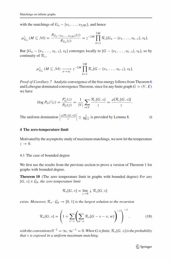
Proof of Corollary 7 Analytic convergence of the free energy follows from Theorem 6and Lebesgue dominated convergence Theorem, since for any finite graph G = (V, E)

we have

(log PG)′(z) = P ′G(z)

PG(z)= 1

|V |∑

◦∈V

Rz[G, ◦]z

= ρ[Rz[G, ◦]]z

.

The uniform domination∣

∣

∣

ρ[Rz [G,◦]]z

∣

∣

∣ ≤ 1R(z) is provided by Lemma 8. ��

4 The zero-temperature limit

Motivated by the asymptotic study of maximum matchings, we now let the temperaturez → 0.

4.1 The case of bounded degree

We first use the results from the previous section to prove a version of Theorem 1 forgraphs with bounded degree.

Theorem 10 (The zero temperature limit in graphs with bounded degree) For any[G, ◦] ∈ Gd , the zero temperature limit

R∗[G, ◦] = limz→0

↓ Rz[G, ◦]

exists. Moreover, R∗ : Gd → [0, 1] is the largest solution to the recursion

R∗[G, ◦] =⎛

⎝1 +∑

v∼◦

(

∑

w∼v

R∗[G − ◦ − v,w])−1

⎞

⎠

−1

, (18)

with the conventions 0−1 = ∞,∞−1 = 0. When G is finite, R∗[G, ◦] is the probabilitythat ◦ is exposed in a uniform maximum matching.

123

C. Bordenave et al.

Proof Fix [G, ◦] ∈ Gd . First, we claim that z �→ Rz[G, ◦] is non-decreasing on R+.Indeed, this is obvious if G is reduced to ◦, since in that case the REP is simply one. Itthen inductively extends to any finite graph [G, ◦], because iterating twice (14) gives

Rz[G, ◦] =⎛

⎝1 +∑

v∼◦

(

z2 +∑

w∼v

Rz[G − ◦ − v,w])−1

⎞

⎠

−1

. (19)

For the infinite case, [G, ◦] is the local limit of the sequence of finite truncations([G, ◦]n)n∈N, where, for n ≥ 1, [G, ◦]n denotes the finite rooted subgraph inducedby the vertices lying at graph-distance at most n from ◦. So by continuity of the REP,Rz[G, ◦] = limn→∞ Rz[G, ◦]n must be non-decreasing in z as well. This guaranteesthe existence of the [0, 1]−valued limit

R∗[G, ◦] = limz→0

↓ Rz[G, ◦].

Moreover, taking the z → 0 limit in (19) guarantees the recursive formula (18).Finally, consider S∗ : Succ∗[G, ◦] → [0, 1] satisfying the recursion (18). Let us

show by induction over n ∈ N that for every [H, i] ∈ Succ∗[G, ◦] and z > 0,

S∗[H, i] ≤ Rz[H, i]2n . (20)

The statement is trivial when n = 0 (Rz[H, i]0 = 1), and is preserved from n to n +1because

Rz[H, i]2n+2 =⎛

⎜

⎝1 +∑

j∼i

⎛

⎝z2 +∑

k∼ j

Rz[H − i − j, k]2n

⎞

⎠

−1⎞

⎟

⎠

−1

≥⎛

⎜

⎝1 +∑

j∼i

⎛

⎝

∑

k∼ j

S∗[H − i − j, k]⎞

⎠

−1⎞

⎟

⎠

−1

= S∗[H − i, j].

Letting n → ∞ and then z → 0 in (20) yields S∗ ≤ R∗, which completes the proof��

This naturally raises the following question : may the zero temperature limit beinterchanged with the infinite volume limit, as suggested by the diagram below?

123


Unfortunately, the recursion (18) may admit several distinct solutions, and thistranslates as follows : in the limit of zero temperature, correlation decay breaks forthe monomer–dimer model, in the precise sense that the functional R∗ : Gd → [0, 1]is no longer continuous with respect to local convergence. For example, one can easilyconstruct an infinite rooted tree [T, ◦] with bounded degree such that

limn→∞ ↓ R∗[T, ◦]2n �= lim

n→∞ ↑ R∗[T, ◦]2n+1.

Indeed, consider the case of T being the graph on N rooted at 0 = ◦, where twointegers share an edge if they differ by one. Then, a straightforward computation givesR∗[T, ◦]2n = 1/2 while R∗[T, ◦]2n+1 = 0. Despite this lack of correlation decay,the interchange of limits turns out to be valid “on average”, i.e. when looking at auniformly chosen vertex ◦.

Theorem 11 (The limiting matching number of bounded-degree graph sequences)Let ρ be a probability distribution over Gd . For any sequence of finite graphs (Gn =(Vn, En))n∈N satisfying |En| = O(|Vn|) and having ρ as a random weak limit,

ν(Gn)

|Vn| −−−→n→∞

1 − Eρ [R∗]

2.

In order to get our Theorem 1, we need to remove the bounded degree assumption.This is done below. In the case where the limit ρ is a (two-level) Galton–Watsontree, the recursion (18) simplifies into a recursive distributional equation (RDE). Thecomputations for these cases are done in Sect. 5.

Proof of Theorem 11 Let G = (V, E) be a finite graph and M be any maximal match-ing of G. Then

∑

v∈V

1(v is exposed in M) = |V | − 2∑

e∈E

1(e ∈ M).

In particular, if ρ = U(G), we have the elementary identity

Eρ [R∗] = 1 − 2ν(G)

|V | . (21)

The proof of Theorem 11 will easily follow from the following uniform control:

Lemma 12 (Uniform continuity around the zero-temperature point) Let G = (V, E)

be a finite graph. For any 0 < z < 1,

Eρ

[Rz] + |E |

|V |log 2

log z≤ Eρ [R∗] ≤ Eρ

[Rz]

. (22)

Indeed, let ρ be a probability distribution on Gd , and let (Gn = (Vn, En))n∈N bea sequence of finite graphs with |Vn| = O(|En|), whose random weak limit is ρ. For

123

C. Bordenave et al.

each n ∈ N, set ρn = U(Gn). With these notations, proving Theorem 11 amounts toestablish:

Eρn [R∗] −−−→n→∞ Eρ [R∗] . (23)

However, since ρn �⇒ ρ, and since each Rz, z > 0 is continuous and bounded, wehave for every z > 0,

Eρn [Rz] −−−→n→∞ Eρ[Rz].

Thus, setting C = supn∈N

|En ||Vn | and letting n → ∞ in (22), we see that for any z < 1,

Eρ

[Rz] + C

log 2

log z≤ lim inf

n→∞ Eρn [R∗] ≤ lim supn→∞

Eρn [R∗] ≤ Eρ

[Rz]

.

Letting finally z → 0, we obtain exactly (23), and it only remains to show Lemma 12.

Proof of Theorem 12 Fix 0 < z < 1. Since z �→ Eρ

[Rz]

is non-decreasing, we have

Eρ [R∗] ≤ Eρ

[Rz] ≤ −1

log z

1∫

z

s−1Eρ [Rs] ds.

Use Eρ [Rs] = s P ′G (s)

|V |PG (s) to rewrite this as

Eρ [R∗] ≤ Eρ

[Rz] ≤ 1

|V | log zlog

PG(z)

PG(1).

Now, PG(1) is the total number of matchings and is thus clearly at most 2|E |, whilePG(z) is at least z|V |−2ν(G). Using (21), these two bounds yield to

Eρ [R∗] ≤ Eρ

[Rz] ≤ 1

|V | log z

(|V |Eρ [R∗] log z − |E | log 2)

.

This gives (22). ��

4.2 The case of unbounded degree

In this section, we establish Theorem 1 in full generality, removing the restriction ofbounded degree from Theorem 11. To this end, we introduce the d-truncation Gd

(d ∈ N) of a graph G = (V, E), obtained from G by isolating all vertices with degreemore than d, i.e. removing any edge incident to them. This transformation is clearly

123


continuous with respect to local convergence. Moreover, its effect on the matchingnumber can be easily controlled:

ν(Gd) ≤ ν(G) ≤ ν(Gd) + #{v ∈ V ; degG(v) > d}. (24)

Now, consider a sequence of finite graphs (Gn)n∈N admitting a random weak limit(G, ◦). First, fixing d ∈ N, we may apply Theorem 11 to the sequence (Gd

n)n∈N toobtain:

ν(Gdn)

|Vn| −−−→n→∞

1 − Eρd [R∗]

2,

where ρd is the d-truncation of ρ. Second, we may rewrite (24) as

∣

∣

∣

∣

ν(Gdn)

|Vn| − ν(Gn)

|Vn|∣

∣

∣

∣

≤ #{v ∈ Vn; degGn(v) > d}

|Vn| .

Letting n → ∞, we obtain

lim supn→∞

∣

∣

∣

∣

1 − ρd [R∗]

2− ν(Gn)

|Vn|∣

∣

∣

∣

≤ ρ (deg(◦) > d),

This last line is, by an elementary application of Cauchy criterion, enough to guaranteethe convergence promised by Theorem 1, i.e.

ν(Gn)

|Vn| −−−→n→∞ γ, where γ := lim

d→∞1 − Eρd [R∗]

2. (25)

Note that because of the possible absence of correlation decay, the largest solutionR∗[G, ◦] is not a continuous function of (G, ◦) ∈ G. In particular, we do not knowwhether it is always the case that

γ = 1 − Eρ[R∗]2

, (26)

as established in Theorem 11 for graphs with bounded degree. However, (26) holdsin the particular cases where we have an explicit formula for Eρ[R∗] which dependscontinuously upon the degree distribution as will be the case in Sect. 5.

5 Computations on (hierarchal) Galton–Watson trees

5.1 The case of Galton–Watson trees

We now investigate the special case where the limiting random graph is a UGW tree T .Specifically, we fix a distribution π ∈ P(N) with finite support (we will relax thisassumption in the sequel) and we consider a UGW tree T with degree distribution π as

123

C. Bordenave et al.

defined in Sect. 2. The random matchings MzT , z ≥ 0 are perfectly well-defined, and

all the previously established results for graphs with bounded degree hold almostsurely. However, the self-similar recursive structure of T gives to the fixed-pointcharacterizations (14) and (18) a very special form that is worth making explicit.

Before we start, let us insist on the fact that Rz[T ] (z > 0) is random: it is thequenched probability that the root is exposed at temperature z, given the random treeT . In light of Theorem 1, it becomes important to ask for its distribution. Let P ([0, 1])denote the space of Borel probability measures on [0, 1]. Given z > 0, ν ∈ P (N) andμ ∈ P ([0, 1]), we denote by �ν,z(μ) the law of the [0, 1]−valued r.v.

Y= z2

z2 + ∑Ni=1 Xi

,

where N ∼ ν and X1, X2, . . . ∼ μ, all of them being independent. This defines anoperator �ν,z on P ([0, 1]). The corresponding fixed point equation μ = �ν,z(μ)

belongs to the general class of recursive distributional equations, or RDE. Equiva-lently, it can be rewritten as

Xd= z2

z2 + ∑Ni=1 Xi

,

where X1, X2, . . . are i.i.d. copies of the unknown random variable X . Note that thesame RDE appears in the analysis of the spectrum and rank of adjacency matrices ofrandom graphs [11,12]. With this notations in hands, the infinite system of equations(14) defining Rz[T ] clearly leads to the following distributional characterization:

Lemma 13 For any z > 0,Rz[T ] has distribution �π,z(μz), where μz is a solutionto the RDE μz = �π,z(μz).

The same program can be carried out in the zero temperature limit. Specifically,given ν, ν′ ∈ P(N) and μ ∈ P ([0, 1]), we define �ν,ν′(μ) as the law of the [0, 1]-valued r.v.

Y = 1

1 + ∑Ni=1

(

∑Ni′

j=1 Xi j

)−1 , (27)

where N ∼ ν,Ni′ ∼ ν′, and Xi j ∼ μ, all of them being independent. This defines an

operator �ν,ν′ on P ([0, 1]) whose fixed points will play a crucial role in our study.Then, Theorem 10 implies:

Lemma 14 The random variable R∗[T ] has law �π,π (μ∗), where μ∗ is the largestsolution to the RDE μ∗ = �π,π (μ∗).

Recall that the mean of �π,π (μ∗) gives precisely the asymptotic size of a maximummatching for any sequence of finite random graphs whose random weak limit is T(Theorem 11). We will solve this RDE in the next section in the more general set-up ofUHGW trees. Combined with Theorem 1 and a simple continuity argument to removethe bounded degree assumption, this will prove Theorem 2.

123


5.2 The case of hierarchal Galton–Watson trees

As in previous section, we first assume that both πa and πb have a finite support.We can define a RDE but with some care about the types a and b. The correspondingresults read as follows:

Lemma 15 For any z > 0, conditionally on the root being of type b (resp. a), Rz[T ]has distribution �πb,z(μ

az ) (resp. �πb,z(μ

bz )), where μa

z is a solution to the RDE:

μaz = �πa ,z ◦ �πb,z(μ

az ),

and μbz = �πb,z(μ

az ).

For z = 0: conditionally on the root being of type a (resp. b), the random variableR∗[T ] has law �πa ,πb (μa∗) (resp. �πb,πa (μb∗)), where μa∗ is the largest solution tothe RDE

μa∗ = �πa ,πb (μa∗), (28)

and μb∗ is the largest solution to the RDE μb∗ = �πb,πa (μb∗).

We now analyze the RDE (28). We define:

Fa(x) = φa(

1 − φb(1 − x))

− φa ′(1)

φb ′(1)

(

1 − φb(1 − x) − xφb ′(1 − x))

. (29)

Observe that

Fa ′(x) = φa ′(1)

φb ′(1)φb ′′(1 − x)

(

φa(1 − φb(1 − x)) − x)

.

Hence any x where Fa admits a local maximum must satisfy x = φa(1 −φb(1 − x)).We define the historical records of Fa as the set of x ∈ [0, 1] such that x = φa(1 −φb(1 − x)) and for any 0 ≤ y < x, Fa(x) > Fa(y) (the latter condition being emptyif x = 0).

Theorem 16 If p1 < · · · < pr are the locations of the historical records of Fa, thenthe RDE (28) admits exactly r solutions; moreover, these solutions can be stochasti-cally ordered, say μ1< · · · <μr , and for any i ∈ {1, . . . , r},• μi ((0, 1]) = pi ;• �πa ,πb (μi ) has mean Fa(pi ).

The proof of Theorem 16 relies on two lemmas.

Lemma 17 The operators �πa ,πb and �πa ,πb are continuous (with respect to weakconvergence) and strictly increasing (with respect to stochastic ordering) on P ([0, 1]).

123

C. Bordenave et al.

Proof of Lemma 17 It follows directly from the fact that, for any n ≥ 0 and anyn1, . . . , nn ≥ 0, the mapping

x �→ 1

1 + ∑ni=1

(

∑nij=1 xi j

)−1

is continuous and increasing from [0, 1]n1+...+nn to [0, 1]. ��Lemma 18 For any μ ∈ P ([0, 1]), letting p = μ ((0, 1]), we have

1. �πa ,πb (μ) ((0, 1]) = φa(1 − φb(1 − p)),2. if �πa ,πb (μ) ≤ μ, then the mean of �πa ,πb (μ) is at least Fa(p),3. if �πa ,πb (μ) ≥ μ, then the mean of �πa ,πb (μ) is at most Fa(p);

In particular, if μ is a fixed point of �πa ,πb , then p = φa(1−φb(1−p)) and �πa ,πb (μ)

has mean Fa(p).

Proof of Lemma 18 In Eq. (27) it is clear that Y > 0 if and only if for anyi ∈ {1, . . . ,N }, there exists j ∈ {1, . . . ,Ni

′} such that Xi j > 0. With the nota-tion introduced above, this rewrites:

�πa ,πb (μ) ((0, 1]) = φa(

1 − φb (1 − μ ((0, 1])))

,

hence the first result follows.Now let X ∼ μ, Y ∼ �πa ,πb (μ),N a ∼ πa, N a ∼ πa , and let S, S1, . . . have

the distribution of the sum of a πb-distributed number of i.i.d. copies of X , all thesevariables being independent. Observe that

1

1+∑N a

i=1 Si−1

=(

1 −∑N a

i=1 Si−1

1 + ∑N a

i=1 Si−1

)

1{∀i=1...N a ,Si >0}

= 1{∀i=1...N a ,Si >0}−N a∑

j=1

S j−1

1+S−1j +∑

1≤i≤N a ,i �= j Si−1

1{∀i=1...N a ,Si >0}

Then, �πa ,πb (μ) has mean

E

[

1

1 + ∑N a

i=1 Si−1

]

= P(∀i = 1 . . . N a, Si > 0

)

−∞∑

k=1

kπak E

[

S−1

S−1 + 1 + ∑k−1i=1 Si

−11{S>0,∀i=1...k−1,Si >0}

]

= φa(1 − φb(1 − p)) − φa ′(1)

×E

[

S−1

S−1 + 1 + ∑N a

i=1 Si−1

1{

S>0,∀i=1... N a ,Si >0}

]

= φa(1 − φb(1 − p)) − φa ′(1)E

[

Y

Y + S1{S>0}

]

,

123


where the second and last lines follow from (5) and Y ∼ �πa ,πb (μ), respectively.Now, for any s > 0, x �→ x/(x + s) is increasing and hence, depending on whether�π,π (μ) ≥ μ or �πa ,πb (μ) ≤ μ,�πa ,πb (μ) has mean at most/least:

φa(1 − φb(1 − p)) − φa ′(1)E

[

X

X + S1{S>0}

]

= φa(1 − φb(1 − p)) − φa ′(1)

×E

[

X

X + ∑N b

i=1 Xi

1{N ∗≥1}

]

,

with Xi are i.i.d. copies of X independent of N b ∼ πb and N ∗ = ∑N b

i=1 1{Xi >0}.Now if X ′ is the law of X conditioned on {X > 0}, and X ′

i are i.i.d. copies of X ′, byexchangeability, we find

E

[

X

X + ∑N b

i=1 Xi

1{N ∗≥1}

]

= pE

[

X ′

X ′ + ∑N ∗i=1 X ′

i

1{N ∗≥1}

]

= pE

[

1

1 + N ∗ 1{N ∗≥1}]

.

Hence finally, depending on whether �π,π (μ) ≥ μ or �πa ,πb (μ) ≤ μ,�πa ,πbμ,

�πa ,πb (μ) has mean at most/least:

φa(1 − φb(1 − p)) − pφa ′(1)E

[

1

1 + N ∗ 1{N ∗≥1}]

But using the definition (5) and the combinatorial identity (n + 1)(n

d

) = (d + 1)(n+1

d+1

)

,one easily derive:

φa (1 − φb(1 − p)) − pφa ′(1)E

[

1

1 + N ∗ 1{N ∗≥1}]

= φa(1 − φb(1 − p)) − pφa ′(1)∑

n≥1

πnb

n∑

d=1

(

n

d

)

pd(1 − p)n−d

d + 1

= Fa(p).

Proof of Theorem 16 Let p ∈ [0, 1] such that φa(1 − φb(1 − p)) = p, and defineμ0 = Bernoulli(p). From Lemma 18 we know that �πa ,πb (μ0) ((0, 1]) = p, andsince Bernoulli((p)) is the largest element of P([0, 1]) putting mass p on (0, 1], wehave �πa ,πb (μ0) ≤ μ0. Immediately, Lemma 17 guarantees that the limit

μ∞ = limk→∞ ↘ �k

πa ,πb (μ0)

exists in P ([0, 1]) and is a fixed point of �πa ,πb . Moreover, by Fatou’s lemma, thenumber p∞ = μ∞ ((0, 1]) must satisfy p∞ ≤ p. But then the mean of �πa ,πb (μ∞)

must be both

• equal to Fa(p∞) by Lemma 18 with μ = μ∞;

123

C. Bordenave et al.

• at least Fa(p) since this holds for all �πa ,πb ◦ �kπa ,πb (μ0), k ≥ 1 (Lemma 18

with μ = �kπa ,πb (μ0)).

We have just shown both Fa(p) ≤ Fa(p∞) and p∞ ≤ p. From this, we now deducethe one-to-one correspondence between historical records of Fa and fixed points of�πa ,πb . We treat each inclusion separately:

1. If Fa admits an historical record at p, then clearly p∞ = p, so μ∞ is a fixed pointsatisfying μ∞ ((0, 1]) = p.

2. Conversely, considering a fixed point μ with μ ((0, 1]) = p, we want to deducethat Fa admits an historical record at p. We first claim that μ is the above definedlimit μ∞. Indeed, μ ≤ Bernoulli(p) implies μ ≤ μ∞ (�πa ,πb is increasing), andin particular p ≤ p∞. Therefore, p = p∞ and Fa(p) = Fa(p∞). In other words,the two ordered distributions �πa ,πb (μ) ≤ �πa ,πb (μ∞) share the same mean,hence are equal. This ensures μ = μ∞. Now, if q < p is any historical recordlocation, we know from part 1 that

ν∞ = limk→∞ ↘ �k

πa ,πb (Bernoulli(q))

is a fixed point of �πa ,πb satisfying ν∞ ((0, 1]) = q. But q < p, so Bernoulli(q) <

Bernoulli(p), hence ν∞ ≤ μ∞. Moreover, this limit inequality is strict becauseν∞ ((0, 1]) = q < p = μ∞ ((0, 1]). Consequently, �πa ,πb (ν∞) < �πa ,πb (μ∞)

and taking expectations, Fa(q) < Fa(p). Thus, Fa admits an historical recordat p. ��

We may now finish the proof of Theorem 3.

Proof of Theorem 3: case of bounded degrees We assume that πa and πb have bounded

support. Recall (7), so that we have λ = φb ′(1)

φa ′(1)+φb ′(1), where λ is the probability that

the root is of type a. Theorems 11, 16 and Lemma 15 give:

ν(Gn)

|Vn| −−−→n→∞

λ(1 − maxx∈[0,1] Fa(x)) + (1 − λ)(1 − maxx∈[0,1] Fb(x))

2, (30)

where Fa is defined in (29) and Fb is defined similarly by

Fb(x) = φb (

1 − φa(1 − x)) − φb ′(1)

φa ′(1)

(

1 − φa(1 − x) − xφa ′(1 − x))

. (31)

For any x which is an historical record of Fa , we define y = φb(1 − x) so thatφa(1 − y) = x . Then we have:

λ(1−Fa(x)) = λ

(

1−φa(1−y)+φa ′(1)

(

1

φb ′(1)− φb(1−φa(1−y))

φb ′(1)−yφa(1−y)

))

= (1 − λ)(1 − Fb(y)).

123


By symmetry, this directly implies that λ(1 − maxx∈[0,1] Fa(x)) = (1 − λ)(1 −maxx∈[0,1] Fb(x)) so that (30) is equivalent to (8). This proves Theorems 2 and 3 fordistributions with bounded support.

Proof of Theorem 3: general case To keep notation simple, we only prove Theorem2. The following proof clearly extends to the case of UHGW trees. Let G1, G2, . . . befinite random graphs whose local weak limit is a Galton–Watson tree T , and assumethat the degree distribution π of T (with generating function φ) has a finite mean :φ′(1) = ∑

n nπn < ∞. For any rooted graph G and any fixed integer d ≥ 1, recallthat Gd is the graph obtained from G by deleting all edges adjacent to a vertex v

whenever deg(v) > d. Hence T d is a Galton–Watson tree whose degree distributionπd is defined by

∀i ≥ 0, πdi = πi 1i≤d + 1i=0

∑

k≥d+1

πk .

By Theorem 1, Eq. (25) and our weaker version of Theorem 2 for distributions withbounded support,

ν(Gn)

|Vn| −−−→n→∞ lim

d→∞ minx∈[0,1] gd(x), (32)

with φd(x) = ∑dk=0 πk xk and

gd(x) = 1 − 1

2(1 − x)φ′

d(x) − 1

2φd(x) − 1

2φd

(

1 − φ′d(x)

φ′d(1)

)

.

Also, as d → ∞, we have φd → φ and φ′d → φ′ uniformly on [0, 1], so

minx∈[0,1] gd(x) −−−→

n→∞ minx∈[0,1] g(x), (33)

with g(x) = 1 − 12 (1 − x)φ′(x) − 1

2φ(x) − 12φ

(

1 − φ′(x)φ′(1)

)

. Finally, combining (32)

and (33), we easily obtain the desired

ν(Gn)

|Vn| −−−→n→∞ min

x∈[0,1] g(x). ��

5.3 Proof of Corollary 4

Note that in Corollary 4, we divide ν(Gn) by |V an | = �αm� instead of |V a

n | + |V bn | =

�αm�+m, so that by Theorem 3, we have ν(Gn)|V a

n | −−−→n→∞ mint∈[0,1] 1− Fa(t). We have

123

C. Bordenave et al.

φa(x) = xk, φb(x) = eαk(x−1) so that we have:

Fa(x) =(

1 − e−kαx)k − 1

α

(

1 − e−kαx − kαxe−kαx)

Fa ′(x) = k2αe−kαx(

(

1 − e−kαx)k−1 − x

)

.

Let x∗ be defined as in Corollary 4 as the largest solution to x = (

1 − e−kαx)k−1

. Itis easy to check (see Section 6 in [23] for a more general analysis) that

mint∈[0,1] 1 − Fa(t) = min{1, 1 − Fa(x∗)}.

Setting ξ∗ = kαx∗, we have ξ∗kα

= (1 − e−ξ∗)k−1, so that

mint∈[0,1] 1 − Fa(t) = min

{

1, 1 − 1

α

(

e−ξ∗ + ξ∗e−ξ∗ + ξ∗

k(1 − e−ξ∗

) − 1

)}

.

Since z �→ z(1−e−z)1−e−z−ze−z is increasing in z, we see that ξ∗ ≥ ξ if and only if α ≥ αc and

we get

mint∈[0,1] 1 − Fa(t) = 1 − 1(α ≥ αc)

1

α

(

e−ξ∗ + ξ∗e−ξ∗ + ξ∗

k(1 − e−ξ∗

) − 1

)

.

Acknowledgments We would like to thank Andrea Montanari and Guilhem Semerjian for explaining usa key idea for the proof of Lemma 12, as well as Nikolaos Fountoulakis, David Gamarnik, James Martinand Johan Wästlund for interesting discussions. The authors acknowledge the support of the French AgenceNationale de la Recherche (ANR) under reference ANR-11-JS02-005-01 (GAP project).

Appendix: uniqueness and non-uniqueness at zero temperature

Consider a sequence (Gn = (Vn, En))n∈N of finite graphs whose local weak limitunder uniform rooting is a UGW tree T . Let φ(t) = ∑

πntn be the generating functionof the degree distribution π of T , and for t ∈ [0, 1] set

F(t) = tφ′(1 − t) + φ(1 − t) + φ

(

1 − φ′(1 − t)

φ′(1)

)

− 1.

From Theorem 16, we know that there is a.s. a unique solution to the local recursionat temperature z = 0 on T (correlation decay) if and only if the first local extremumof F is a global maximum. In that case, the convergence

ν(Gn)

|Vn| −−−→n→∞

1 − maxt∈[0,1] F(t)

2(34)

123


1.00.7 0.90.80.60.50.40.13

0.14

0.15

0.16

0.17

0.18

0.19

0.20

0.21

0.22

0.0 0.1 0.2 0.3 0.6 1.00.50.40.30.065

0.070

0.075

0.080

0.085

0.090

0.095

0.0

0.100

0.1

0.105

0.90.2 0.80.7 0.80.70.050

0.055

0.060

0.065

0.070

0.075

0.60.50.0 1.00.40.1 0.3 0.90.2

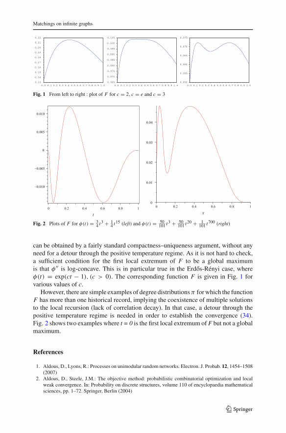
Fig. 1 From left to right : plot of F for c = 2, c = e and c = 3

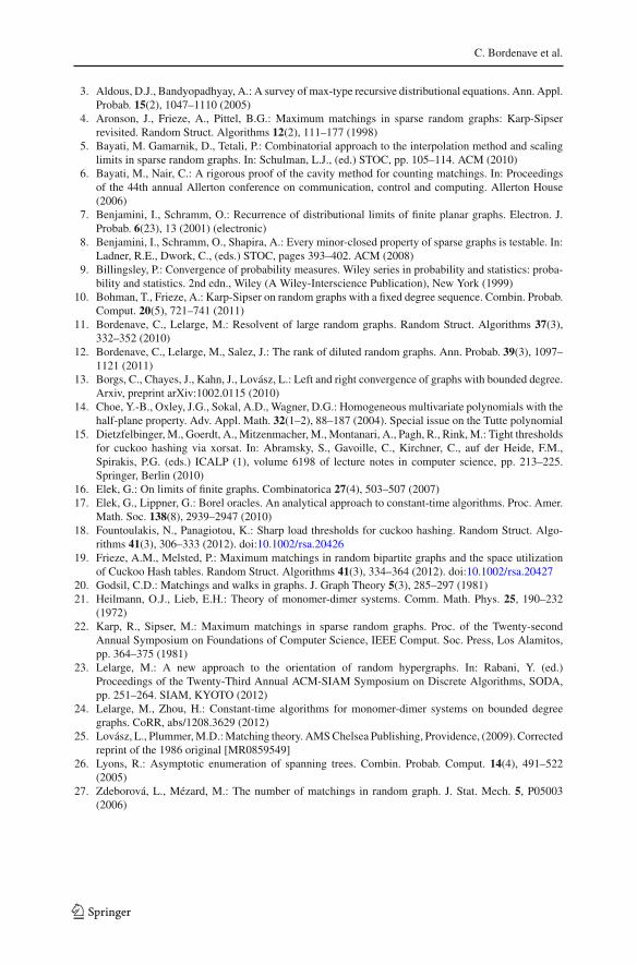
Fig. 2 Plots of F for φ(t) = 34 t3 + 1

4 t15 (left) and φ(t) = 50101 t3 + 50

101 t20 + 1101 t700 (right)

can be obtained by a fairly standard compactness–uniqueness argument, without anyneed for a detour through the positive temperature regime. As it is not hard to check,a sufficient condition for the first local extremum of F to be a global maximumis that φ′′ is log-concave. This is in particular true in the Erdos-Rényi case, whereφ(t) = exp(ct − 1), (c > 0). The corresponding function F is given in Fig. 1 forvarious values of c.

However, there are simple examples of degree distributions π for which the functionF has more than one historical record, implying the coexistence of multiple solutionsto the local recursion (lack of correlation decay). In that case, a detour through thepositive temperature regime is needed in order to establish the convergence (34).Fig. 2 shows two examples where t = 0 is the first local extremum of F but not a globalmaximum.

References

1. Aldous, D., Lyons, R.: Processes on unimodular random networks. Electron. J. Probab. 12, 1454–1508(2007)

2. Aldous, D., Steele, J.M.: The objective method: probabilistic combinatorial optimization and localweak convergence. In: Probability on discrete structures, volume 110 of encyclopaedia mathematicalsciences, pp. 1–72. Springer, Berlin (2004)

123

C. Bordenave et al.

3. Aldous, D.J., Bandyopadhyay, A.: A survey of max-type recursive distributional equations. Ann. Appl.Probab. 15(2), 1047–1110 (2005)

4. Aronson, J., Frieze, A., Pittel, B.G.: Maximum matchings in sparse random graphs: Karp-Sipserrevisited. Random Struct. Algorithms 12(2), 111–177 (1998)

5. Bayati, M. Gamarnik, D., Tetali, P.: Combinatorial approach to the interpolation method and scalinglimits in sparse random graphs. In: Schulman, L.J., (ed.) STOC, pp. 105–114. ACM (2010)

6. Bayati, M., Nair, C.: A rigorous proof of the cavity method for counting matchings. In: Proceedingsof the 44th annual Allerton conference on communication, control and computing. Allerton House(2006)

7. Benjamini, I., Schramm, O.: Recurrence of distributional limits of finite planar graphs. Electron. J.Probab. 6(23), 13 (2001) (electronic)

8. Benjamini, I., Schramm, O., Shapira, A.: Every minor-closed property of sparse graphs is testable. In:Ladner, R.E., Dwork, C., (eds.) STOC, pages 393–402. ACM (2008)

9. Billingsley, P.: Convergence of probability measures. Wiley series in probability and statistics: proba-bility and statistics. 2nd edn., Wiley (A Wiley-Interscience Publication), New York (1999)

10. Bohman, T., Frieze, A.: Karp-Sipser on random graphs with a fixed degree sequence. Combin. Probab.Comput. 20(5), 721–741 (2011)

11. Bordenave, C., Lelarge, M.: Resolvent of large random graphs. Random Struct. Algorithms 37(3),332–352 (2010)

12. Bordenave, C., Lelarge, M., Salez, J.: The rank of diluted random graphs. Ann. Probab. 39(3), 1097–1121 (2011)

13. Borgs, C., Chayes, J., Kahn, J., Lovász, L.: Left and right convergence of graphs with bounded degree.Arxiv, preprint arXiv:1002.0115 (2010)

14. Choe, Y.-B., Oxley, J.G., Sokal, A.D., Wagner, D.G.: Homogeneous multivariate polynomials with thehalf-plane property. Adv. Appl. Math. 32(1–2), 88–187 (2004). Special issue on the Tutte polynomial

15. Dietzfelbinger, M., Goerdt, A., Mitzenmacher, M., Montanari, A., Pagh, R., Rink, M.: Tight thresholdsfor cuckoo hashing via xorsat. In: Abramsky, S., Gavoille, C., Kirchner, C., auf der Heide, F.M.,Spirakis, P.G. (eds.) ICALP (1), volume 6198 of lecture notes in computer science, pp. 213–225.Springer, Berlin (2010)

16. Elek, G.: On limits of finite graphs. Combinatorica 27(4), 503–507 (2007)17. Elek, G., Lippner, G.: Borel oracles. An analytical approach to constant-time algorithms. Proc. Amer.

Math. Soc. 138(8), 2939–2947 (2010)18. Fountoulakis, N., Panagiotou, K.: Sharp load thresholds for cuckoo hashing. Random Struct. Algo-

rithms 41(3), 306–333 (2012). doi:10.1002/rsa.2042619. Frieze, A.M., Melsted, P.: Maximum matchings in random bipartite graphs and the space utilization

of Cuckoo Hash tables. Random Struct. Algorithms 41(3), 334–364 (2012). doi:10.1002/rsa.2042720. Godsil, C.D.: Matchings and walks in graphs. J. Graph Theory 5(3), 285–297 (1981)21. Heilmann, O.J., Lieb, E.H.: Theory of monomer-dimer systems. Comm. Math. Phys. 25, 190–232

(1972)22. Karp, R., Sipser, M.: Maximum matchings in sparse random graphs. Proc. of the Twenty-second

Annual Symposium on Foundations of Computer Science, IEEE Comput. Soc. Press, Los Alamitos,pp. 364–375 (1981)

23. Lelarge, M.: A new approach to the orientation of random hypergraphs. In: Rabani, Y. (ed.)Proceedings of the Twenty-Third Annual ACM-SIAM Symposium on Discrete Algorithms, SODA,pp. 251–264. SIAM, KYOTO (2012)

24. Lelarge, M., Zhou, H.: Constant-time algorithms for monomer-dimer systems on bounded degreegraphs. CoRR, abs/1208.3629 (2012)

25. Lovász, L., Plummer, M.D.: Matching theory. AMS Chelsea Publishing, Providence, (2009). Correctedreprint of the 1986 original [MR0859549]

26. Lyons, R.: Asymptotic enumeration of spanning trees. Combin. Probab. Comput. 14(4), 491–522(2005)

27. Zdeborová, L., Mézard, M.: The number of matchings in random graph. J. Stat. Mech. 5, P05003(2006)

123

http://dx.doi.org/10.1002/rsa.20426

http://dx.doi.org/10.1002/rsa.20427

Documents

Matchings on infinite graphs