Math3806 Lecture Note 3 Appendix

Heng Peng

January 29, 2021

P1. Given X1,X2, . . . ,Xn are independent random variables, havea same distribution with mean µ and variance σ2, then

X̄ =1

n

n∑i=1

Xi → µ, as n→∞

(Law of Large number)

√n(X̄ − µ) ∼ N (0, σ2), as n→∞

(Central Limited Theorem)

I Law of large number and Central limited theorem can beextended to multivariate dimensional random vectors.

I logarithm of normal likelihood

logn∏

i=1

f (Xi ) =n∑

i=1

log f (Xi ) =n∑

i=1

{−1

2log(2πσ2)−(Xi − µ)2

2σ2}

P3. Rewrite the normal density function

f (x) =1

(2π)12 (σ2)

12

e−12

(x−µ)(σ2)−1(x−µ)

(2π)12 ∼ (2π)

p2 , x ∼ X , µ ∼ µ, σ2 ∼ Σ or |Σ|

P4. Quantile values of Normal population. If X ∼ N (µ, σ2), then

P(|X − µ| ≥ σ) ≈ 1− .683 = .317,

P(|X − µ| ≥ 2σ) ≈ 1− .954 = .046 < 0.05.

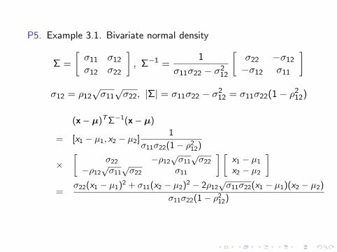
P5. Example 3.1. Bivariate normal density

Σ =

[σ11 σ12

σ12 σ22

], Σ−1 =

1

σ11σ22 − σ212

[σ22 −σ12

−σ12 σ11

]σ12 = ρ12

√σ11√σ22, |Σ| = σ11σ22 − σ2

12 = σ11σ22(1− ρ212)

(x− µ)TΣ−1(x− µ)

= [x1 − µ1, x2 − µ2]1

σ11σ22(1− ρ212)

×[

σ22 −ρ12√σ11√σ22

−ρ12√σ11√σ22 σ11

] [x1 − µ1

x2 − µ2

]=

σ22(x1 − µ1)2 + σ11(x2 − µ2)2 − 2ρ12√σ11σ22(x1 − µ1)(x2 − µ2)

σ11σ22(1− ρ212)

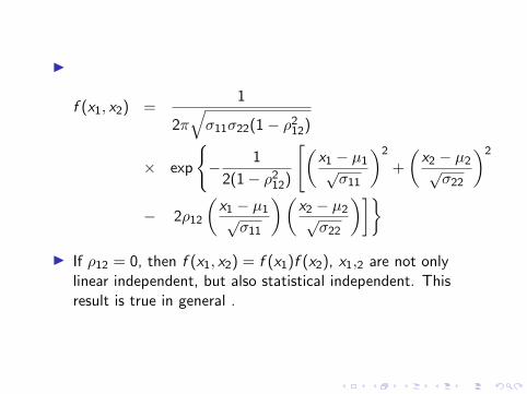
I

f (x1, x2) =1

2π√σ11σ22(1− ρ2

12)

× exp

{− 1

2(1− ρ212)

[(x1 − µ1√σ11

)2

+

(x2 − µ2√σ22

)2

− 2ρ12

(x1 − µ1√σ11

)(x2 − µ2√σ22

)]}I If ρ12 = 0, then f (x1, x2) = f (x1)f (x2), x1,2 are not only

linear independent, but also statistical independent. Thisresult is true in general .

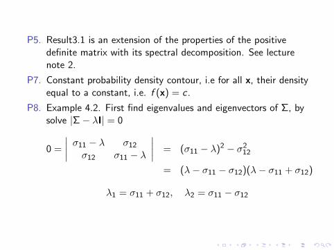
P5. Result3.1 is an extension of the properties of the positivedefinite matrix with its spectral decomposition. See lecturenote 2.

P7. Constant probability density contour, i.e for all x, their densityequal to a constant, i.e. f (x) = c .

P8. Example 4.2. First find eigenvalues and eigenvectors of Σ, bysolve |Σ− λI| = 0

0 =

∣∣∣∣ σ11 − λ σ12

σ12 σ11 − λ

∣∣∣∣ = (σ11 − λ)2 − σ212

= (λ− σ11 − σ12)(λ− σ11 + σ12)

λ1 = σ11 + σ12, λ2 = σ11 − σ12

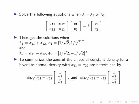
I Solve the following equations when λ = λ1 or λ2[σ11 σ12

σ12 σ11

] [e1

e2

]= λ

[e1

e2

]I Then get the solutions whenλ1 = σ11 + σ12, e1 = [1/

√2, 1/√

2]T ,andλ2 = σ11 − σ12, e2 = [1/

√2,−1/

√2]T

I To summarize, the axes of the ellipse of constant density for abivariate normal density with σ11 = σ22 are determined by

±c√σ11 + σ12

[1√2

1√2

], and ± c

√σ11 − σ12

[1√2−1√

2

]

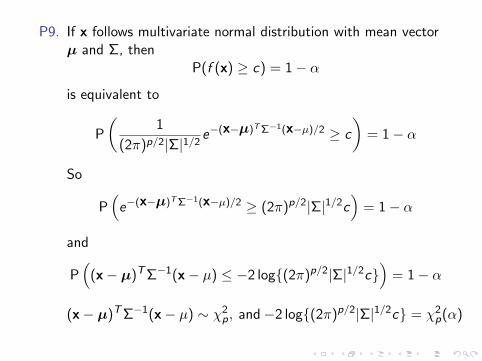
P9. If x follows multivariate normal distribution with mean vectorµ and Σ, then

P(f (x) ≥ c) = 1− α

is equivalent to

P

(1

(2π)p/2|Σ|1/2e−(x−µ)T Σ−1(x−µ)/2 ≥ c

)= 1− α

So

P(e−(x−µ)T Σ−1(x−µ)/2 ≥ (2π)p/2|Σ|1/2c

)= 1− α

and

P(

(x− µ)TΣ−1(x− µ) ≤ −2 log{(2π)p/2|Σ|1/2c})

= 1− α

(x− µ)TΣ−1(x− µ) ∼ χ2p, and−2 log{(2π)p/2|Σ|1/2c} = χ2

p(α)

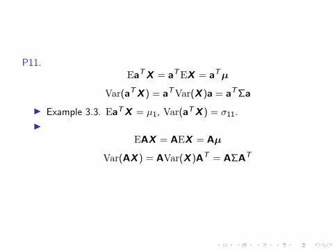
P11.EaTX = aTEX = aTµ

Var(aTX ) = aTVar(X )a = aTΣa

I Example 3.3. EaTX = µ1, Var(aTX ) = σ11.

IEAX = AEX = Aµ

Var(AX ) = AVar(X )AT = AΣAT

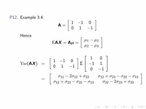
P12. Example 3.4.

A =

[1 −1 00 1 −1

]Hence

EAX = Aµ =

[µ1 − µ2

µ2 − µ3

]

Var(AX ) =

[1 −1 00 1 −1

]Σ

1 0−1 10 −1

=

[σ11 − 2σ12 + σ22 σ12 + σ23 − σ22 − σ13

σ12 + σ23 − σ22 − σ13 σ22 − 2σ23 + σ33

]

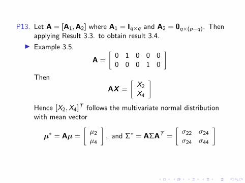
P13. Let A = [A1,A2] where A1 = Iq×q and A2 = 0q×(p−q). Thenapplying Result 3.3. to obtain result 3.4.

I Example 3.5.

A =

[0 1 0 0 00 0 0 1 0

]Then

AX =

[X2

X4

]Hence [X2,X4]T follows the multivariate normal distributionwith mean vector

µ∗ = Aµ =

[µ2

µ4

], and Σ∗ = AΣAT =

[σ22 σ24

σ24 σ44

]

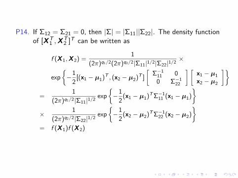
P14. If Σ12 = Σ21 = 0, then |Σ| = |Σ11||Σ22|. The density functionof [XT

1 ,XT2 ]T can be written as

f (X 1,X 2) =1

(2π)q1/2(2π)q2/2|Σ11|1/2|Σ22|1/2×

exp

{−1

2[(x1 − µ1)T , (x2 − µ2)T ]

[Σ−1

11 00 Σ−1

22

] [x1 − µ1

x2 − µ2

]}=

1

(2π)q1/2|Σ11|1/2exp

{−1

2(x1 − µ1)TΣ−1

11 (x1 − µ1)

}× 1

(2π)q2/2|Σ22|1/2exp

{−1

2(x2 − µ2)TΣ−1

22 (x2 − µ2)

}= f (X 1)f (X 2)

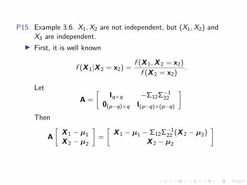
P15. Example 3.6. X1,X2 are not independent, but (X1,X2) andX3 are independent.

I First, it is well known

f (X 1|X 2 = x2) =f (X 1,X 2 = x2)

f (X 2 = x2).

Let

A =

[Iq×q −Σ12Σ−1

22

0(p−q)×q I(p−q)×(p−q)

]Then

A

[X 1 − µ1

X 2 − µ2

]=

[X 1 − µ1 − Σ12Σ−1

22 (X 2 − µ2)X 2 − µ2

]

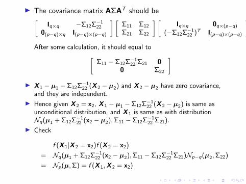
I The covariance matrix AΣAT should be[Iq×q −Σ12Σ−1

22

0(p−q)×q I(p−q)×(p−q)

] [Σ11 Σ12

Σ21 Σ22

] [Iq×q 0q×(p−q)

(−Σ12Σ−122 )T I(p−q)×(p−q)

]After some calculation, it should equal to[

Σ11 − Σ12Σ−122 Σ21 0

0 Σ22

]I X 1 − µ1 − Σ12Σ−1

22 (X 2 − µ2) and X 2 − µ2 have zero covariance,and they are independent.

I Hence given X 2 = x2, X 1 − µ1 − Σ12Σ−122 (X 2 − µ2) is same as

unconditional distribution, and X 1 is same as with distributionNq(µ1 + Σ12Σ−1

22 (x2 − µ2),Σ11 − Σ12Σ−122 Σ21).

I Check

f (X 1|X 2 = x2)f (X 2 = x2)

= Nq(µ1 + Σ12Σ−122 (x2 − µ2),Σ11 − Σ12Σ−1

22 Σ21)Np−q(µ2,Σ22)

= Np(µ,Σ) = f (X 1,X 2 = x2)

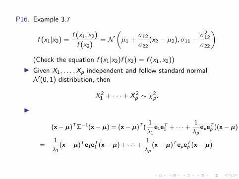
P16. Example 3.7

f (x1|x2) =f (x1, x2)

f (x2)= N

(µ1 +

σ12

σ22(x2 − µ2), σ11 −

σ212

σ22

)(Check the equation f (x1|x2)f (x2) = f (x1, x2))

I Given X1, . . . ,Xp independent and follow standard normalN (0, 1) distribution, then

X 21 + · · ·+ X 2

p ∼ χ2p.

I

(x− µ)TΣ−1(x− µ) = (x− µ)T (1

λ1e1e

T1 + · · ·+ 1

λpepe

Tp )(x− µ)

=1

λ1(x− µ)Te1e

T1 (x− µ) + · · ·+ 1

λp(x− µ)Tepe

Tp (x− µ)

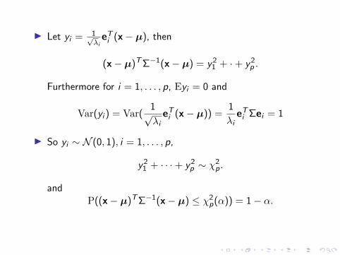
I Let yi = 1√λieTi (x− µ), then

(x− µ)TΣ−1(x− µ) = y21 + ·+ y2

p .

Furthermore for i = 1, . . . , p, Eyi = 0 and

Var(yi ) = Var(1√λieTi (x− µ)) =

1

λieTi Σei = 1

I So yi ∼ N (0, 1), i = 1, . . . , p,

y21 + · · ·+ y2

p ∼ χ2p.

andP((x− µ)TΣ−1(x− µ) ≤ χ2

p(α)) = 1− α.

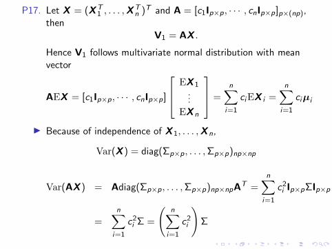
P17. Let X = (XT1 , . . . ,X

Tn )T and A = [c1Ip×p, · · · , cnIp×p]p×(np),

thenV1 = AX .

Hence V1 follows multivariate normal distribution with meanvector

AEX = [c1Ip×p, · · · , cnIp×p]

EX 1...

EX n

=n∑

i=1

ciEX i =n∑

i=1

ciµi

I Because of independence of X 1, . . . ,X n,

Var(X ) = diag(Σp×p, . . . ,Σp×p)np×np

Var(AX ) = Adiag(Σp×p, . . . ,Σp×p)np×npAT =

n∑i=1

c2i Ip×pΣIp×p

=n∑

i=1

c2i Σ =

(n∑

i=1

c2i

)Σ

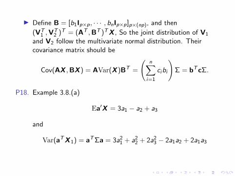
I Define B = [b1Ip×p, · · · , bnIp×p]p×(np), and then

(VT1 ,V

T2 )T = (AT ,BT )TX , So the joint distribution of V1

and V2 follow the multivariate normal distribution. Theircovariance matrix should be

Cov(AX ,BX ) = AVar(X )BT =

(n∑

i=1

cibi

)Σ = bTcΣ.

P18. Example 3.8.(a)

Ea′X = 3a1 − a2 + a3

and

Var(aTX 1) = aTΣa = 3a21 + a2

2 + 2a23 − 2a1a2 + 2a1a3

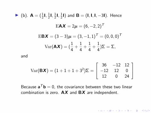
I (b). A = ( 12 I,

12 I,

12 I,

12 I) and B = (I, I, I,−3I). Hence

EAX = 2µ = (6,−2, 2)T

EBX = (3− 3)µ = (3,−1, 1)T = (0, 0, 0)T

Var(AX ) = (1

4+

1

4+

1

4+

1

4)Σ = Σ,

and

Var(BX ) = (1 + 1 + 1 + 32)Σ =

36 −12 12−12 12 012 0 24

Because aTb = 0, the covariance between these two linearcombination is zero. AX and BX are independent.

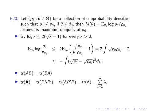
P20. Let {pθ : θ ∈ Θ} be a collection of subprobability densitiessuch that pθ 6= pθ0 if θ 6= θ0, then M(θ) = Eθ0 log pθ/pθ0

attains its maximum uniquely at θ0.

I By log x ≤ 2(√x − 1) for every x > 0,

Eθ0 logpθpθ0

≤ 2Eθ0

(√pθpθ0

− 1

)= 2

∫√pθpθ0 − 2

≤ −∫

(√pθ −

√pθ0)2dµ.

I tr(AB) = tr(BA)

I tr(A) = tr(PΛP ′) = tr(ΛP ′P) = tr(Λ) =n∑

i=1λi

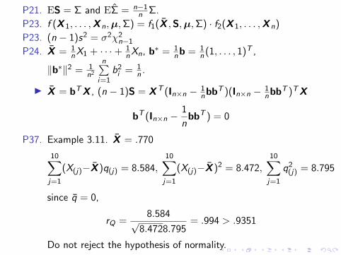
P21. ES = Σ and EΣ̂ = n−1n Σ.

P23. f (X 1, . . . ,X n,µ,Σ) = f1(X̄ ,S,µ,Σ) · f2(X 1, . . . ,X n)

P23. (n − 1)s2 = σ2χ2n−1

P24. X̄ = 1nX1 + · · ·+ 1

nXn, b∗ = 1nb = 1

n (1, . . . , 1)T ,

‖b∗‖2 = 1n2

n∑i=1

b2i = 1

n .

I X̄ = bTX , (n − 1)S = XT (In×n − 1nbb

T )(In×n − 1nbb

T )TX

bT (In×n −1

nbbT ) = 0

P37. Example 3.11. X̄ = .770

10∑j=1

(X(j)−X̄ )q(j) = 8.584,10∑j=1

(X(j)−X̄ )2 = 8.472,10∑j=1

q2(j) = 8.795

since q̄ = 0,

rQ =8.584√

8.4728.795= .994 > .9351

Do not reject the hypothesis of normality.

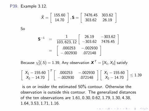
P39. Example 3.12.

X̄ =

[155.6014.70

],S =

[7476.45 303.62303.62 26.19

]So

S−1 =1

103, 623, 12

[26.19 −303.62−303.62 7476.45

]=

[.000253 −.002930−.002930 .072148

]Because χ2

2(.5) = 1.39, Any observation XT = [X1,X2] satisfy[X1 − 155.60X2 − 14.70

]T [.000253 −.002930−.002930 .072148

] [X1 − 155.60X2 − 14.70

]≤ 1.39

is on or insider the estimated 50% contour. Otherwise theobservation is outside this contour. The generalized distancesof the ten observations are 1.61, 0.30, 0.62, 1.79, 1.30, 4.38,1.64, 3.53, 1.71, 1.16.