Embed Size (px)
Citation preview
MathematicalAnalysis
Volume I
Elias Zakon
University of Windsor
Saylor URL: http://www.saylor.org/courses/ma241/ The Saylor Foundation
Copyright Notice
Mathematical Analysis Ic� 1975 Elias Zakonc� 2004 Bradley J. Lucier and Tamara Zakon
Distributed under a Creative Commons Attribution 3.0 Unported (CC BY 3.0) license made
possible by funding from The Saylor Foundation’s Open Textbook Challenge in order to beincorporated into Saylor.org’s collection of open courses available at http://www.saylor.org.
Full license terms may be viewed at: http://creativecommons.org/licenses/by/3.0/. Firstpublished by The Trillia Group, http://www.trillia.com, as the second volume of The Zakon
Series on Mathematical Analysis.
First published: May 20, 2004. This version released: July 11, 2011.
Technical Typist: Betty Gick. Copy Editor: John Spiegelman.
Saylor URL: http://www.saylor.org/courses/ma241/ The Saylor Foundation
Contents∗
Preface ix
About the Author xi
Chapter 1. Set Theory 1
1–3. Sets and Operations on Sets. Quantifiers . . . . . . . . . . . . . . . . . . . . . . . . . . .1Problems in Set Theory . . . . . . . . . . . . . . . . . . . . . . . . . . . . . . . . . . . . . . . . . 6
4–7. Relations. Mappings . . . . . . . . . . . . . . . . . . . . . . . . . . . . . . . . . . . . . . . . . . . . . . .8Problems on Relations and Mappings . . . . . . . . . . . . . . . . . . . . . . . . . . .14
8. Sequences . . . . . . . . . . . . . . . . . . . . . . . . . . . . . . . . . . . . . . . . . . . . . . . . . . . . . . . . 15
9. Some Theorems on Countable Sets . . . . . . . . . . . . . . . . . . . . . . . . . . . . . . . .18Problems on Countable and Uncountable Sets . . . . . . . . . . . . . . . . . . 21
Chapter 2. Real Numbers. Fields 23
1–4. Axioms and Basic Definitions . . . . . . . . . . . . . . . . . . . . . . . . . . . . . . . . . . . . .23
5–6. Natural Numbers. Induction . . . . . . . . . . . . . . . . . . . . . . . . . . . . . . . . . . . . . .27Problems on Natural Numbers and Induction . . . . . . . . . . . . . . . . . . . 32
7. Integers and Rationals . . . . . . . . . . . . . . . . . . . . . . . . . . . . . . . . . . . . . . . . . . . .34
8–9. Upper and Lower Bounds. Completeness . . . . . . . . . . . . . . . . . . . . . . . . . .36Problems on Upper and Lower Bounds . . . . . . . . . . . . . . . . . . . . . . . . . 40
10. Some Consequences of the Completeness Axiom . . . . . . . . . . . . . . . . . . .43
11–12. Powers With Arbitrary Real Exponents. Irrationals . . . . . . . . . . . . . . . 46Problems on Roots, Powers, and Irrationals . . . . . . . . . . . . . . . . . . . . .50
13. The Infinities. Upper and Lower Limits of Sequences . . . . . . . . . . . . . .53Problems on Upper and Lower Limits of Sequences in E∗ . . . . . . . 60
Chapter 3. Vector Spaces. Metric Spaces 63
1–3. The Euclidean n-space, En . . . . . . . . . . . . . . . . . . . . . . . . . . . . . . . . . . . . . . . 63Problems on Vectors in En . . . . . . . . . . . . . . . . . . . . . . . . . . . . . . . . . . . . . 69
4–6. Lines and Planes in En . . . . . . . . . . . . . . . . . . . . . . . . . . . . . . . . . . . . . . . . . . .71Problems on Lines and Planes in En . . . . . . . . . . . . . . . . . . . . . . . . . . . .75
∗ “Starred” sections may be omitted by beginners.
Saylor URL: http://www.saylor.org/courses/ma241/ The Saylor Foundation
vi Contents
7. Intervals in En . . . . . . . . . . . . . . . . . . . . . . . . . . . . . . . . . . . . . . . . . . . . . . . . . . . 76Problems on Intervals in En . . . . . . . . . . . . . . . . . . . . . . . . . . . . . . . . . . . .79
8. Complex Numbers . . . . . . . . . . . . . . . . . . . . . . . . . . . . . . . . . . . . . . . . . . . . . . . .80Problems on Complex Numbers . . . . . . . . . . . . . . . . . . . . . . . . . . . . . . . . 83
∗9. Vector Spaces. The Space Cn. Euclidean Spaces . . . . . . . . . . . . . . . . . . 85Problems on Linear Spaces . . . . . . . . . . . . . . . . . . . . . . . . . . . . . . . . . . . . . 89
∗10. Normed Linear Spaces . . . . . . . . . . . . . . . . . . . . . . . . . . . . . . . . . . . . . . . . . . . .90Problems on Normed Linear Spaces. . . . . . . . . . . . . . . . . . . . . . . . . . . . .93
11. Metric Spaces . . . . . . . . . . . . . . . . . . . . . . . . . . . . . . . . . . . . . . . . . . . . . . . . . . . . 95Problems on Metric Spaces . . . . . . . . . . . . . . . . . . . . . . . . . . . . . . . . . . . . . 98
12. Open and Closed Sets. Neighborhoods . . . . . . . . . . . . . . . . . . . . . . . . . . .101Problems on Neighborhoods, Open and Closed Sets . . . . . . . . . . . .106
13. Bounded Sets. Diameters . . . . . . . . . . . . . . . . . . . . . . . . . . . . . . . . . . . . . . . .108Problems on Boundedness and Diameters . . . . . . . . . . . . . . . . . . . . . .112
14. Cluster Points. Convergent Sequences . . . . . . . . . . . . . . . . . . . . . . . . . . . 114Problems on Cluster Points and Convergence . . . . . . . . . . . . . . . . . . 118
15. Operations on Convergent Sequences . . . . . . . . . . . . . . . . . . . . . . . . . . . . 120Problems on Limits of Sequences . . . . . . . . . . . . . . . . . . . . . . . . . . . . . . 123
16. More on Cluster Points and Closed Sets. Density . . . . . . . . . . . . . . . . 135Problems on Cluster Points, Closed Sets, and Density . . . . . . . . . .139
17. Cauchy Sequences. Completeness . . . . . . . . . . . . . . . . . . . . . . . . . . . . . . . . 141Problems on Cauchy Sequences . . . . . . . . . . . . . . . . . . . . . . . . . . . . . . . .144
Chapter 4. Function Limits and Continuity 149
1. Basic Definitions . . . . . . . . . . . . . . . . . . . . . . . . . . . . . . . . . . . . . . . . . . . . . . . . 149Problems on Limits and Continuity . . . . . . . . . . . . . . . . . . . . . . . . . . . .157
2. Some General Theorems on Limits and Continuity . . . . . . . . . . . . . . . 161More Problems on Limits and Continuity . . . . . . . . . . . . . . . . . . . . . .166
3. Operations on Limits. Rational Functions . . . . . . . . . . . . . . . . . . . . . . . 170Problems on Continuity of Vector-Valued Functions . . . . . . . . . . . .174
4. Infinite Limits. Operations in E∗ . . . . . . . . . . . . . . . . . . . . . . . . . . . . . . . . 177Problems on Limits and Operations in E∗ . . . . . . . . . . . . . . . . . . . . . 180
5. Monotone Functions . . . . . . . . . . . . . . . . . . . . . . . . . . . . . . . . . . . . . . . . . . . . 181Problems on Monotone Functions . . . . . . . . . . . . . . . . . . . . . . . . . . . . . 185
6. Compact Sets . . . . . . . . . . . . . . . . . . . . . . . . . . . . . . . . . . . . . . . . . . . . . . . . . . . 186Problems on Compact Sets . . . . . . . . . . . . . . . . . . . . . . . . . . . . . . . . . . . . 189
∗7. More on Compactness . . . . . . . . . . . . . . . . . . . . . . . . . . . . . . . . . . . . . . . . . . . 192
Saylor URL: http://www.saylor.org/courses/ma241/ The Saylor Foundation
Contents vii
8. Continuity on Compact Sets. Uniform Continuity . . . . . . . . . . . . . . . .194Problems on Uniform Continuity; Continuity on Compact Sets . 200
9. The Intermediate Value Property . . . . . . . . . . . . . . . . . . . . . . . . . . . . . . . . 203Problems on the Darboux Property and Related Topics . . . . . . . . 209
10. Arcs and Curves. Connected Sets . . . . . . . . . . . . . . . . . . . . . . . . . . . . . . . .211Problems on Arcs, Curves, and Connected Sets . . . . . . . . . . . . . . . . 215
∗11. Product Spaces. Double and Iterated Limits . . . . . . . . . . . . . . . . . . . . . 218∗Problems on Double Limits and Product Spaces . . . . . . . . . . . . . . 224
12. Sequences and Series of Functions . . . . . . . . . . . . . . . . . . . . . . . . . . . . . . . 227Problems on Sequences and Series of Functions . . . . . . . . . . . . . . . . 233
13. Absolutely Convergent Series. Power Series . . . . . . . . . . . . . . . . . . . . . . 237More Problems on Series of Functions . . . . . . . . . . . . . . . . . . . . . . . . . 245
Chapter 5. Differentiation and Antidifferentiation 251
1. Derivatives of Functions of One Real Variable . . . . . . . . . . . . . . . . . . . .251Problems on Derived Functions in One Variable . . . . . . . . . . . . . . . 257
2. Derivatives of Extended-Real Functions . . . . . . . . . . . . . . . . . . . . . . . . . .259Problems on Derivatives of Extended-Real Functions . . . . . . . . . . 265
3. L’Hopital’s Rule . . . . . . . . . . . . . . . . . . . . . . . . . . . . . . . . . . . . . . . . . . . . . . . . .266Problems on L’Hopital’s Rule . . . . . . . . . . . . . . . . . . . . . . . . . . . . . . . . . 269
4. Complex and Vector-Valued Functions on E1 . . . . . . . . . . . . . . . . . . . . 271Problems on Complex and Vector-Valued Functions on E1 . . . . . 275
5. Antiderivatives (Primitives, Integrals) . . . . . . . . . . . . . . . . . . . . . . . . . . . .278Problems on Antiderivatives . . . . . . . . . . . . . . . . . . . . . . . . . . . . . . . . . . .285
6. Differentials. Taylor’s Theorem and Taylor’s Series . . . . . . . . . . . . . . .288Problems on Taylor’s Theorem . . . . . . . . . . . . . . . . . . . . . . . . . . . . . . . . 296
7. The Total Variation (Length) of a Function f : E1 → E . . . . . . . . . . 300Problems on Total Variation and Graph Length . . . . . . . . . . . . . . . 306
8. Rectifiable Arcs. Absolute Continuity . . . . . . . . . . . . . . . . . . . . . . . . . . . .308Problems on Absolute Continuity and Rectifiable Arcs . . . . . . . . . 314
9. Convergence Theorems in Differentiation and Integration . . . . . . . . 314Problems on Convergence in Differentiation and Integration . . . .321
10. Sufficient Condition of Integrability. Regulated Functions . . . . . . . . 322Problems on Regulated Functions . . . . . . . . . . . . . . . . . . . . . . . . . . . . . 329
11. Integral Definitions of Some Functions . . . . . . . . . . . . . . . . . . . . . . . . . . . 331Problems on Exponential and Trigonometric Functions . . . . . . . . 338
Index 341
Saylor URL: http://www.saylor.org/courses/ma241/ The Saylor Foundation

Saylor URL: http://www.saylor.org/courses/ma241/ The Saylor Foundation
Preface
This text is an outgrowth of lectures given at the University of Windsor,Canada. One of our main objectives is updating the undergraduate analysisas a rigorous postcalculus course. While such excellent books as Dieudonne’sFoundations of Modern Analysis are addressed mainly to graduate students,we try to simplify the modern Bourbaki approach to make it accessible tosufficiently advanced undergraduates. (See, for example, §4 of Chapter 5.)
On the other hand, we endeavor not to lose contact with classical texts,still widely in use. Thus, unlike Dieudonne, we retain the classical notion of aderivative as a number (or vector), not a linear transformation. Linear mapsare reserved for later (Volume II) to give a modern version of differentials .Nor do we downgrade the classical mean-value theorems (see Chapter 5, §2) orRiemann–Stieltjes integration, but we treat the latter rigorously in Volume II,inside Lebesgue theory. First, however, we present the modern Bourbaki theoryof antidifferentiation (Chapter 5, §5 ff.), adapted to an undergraduate course.
Metric spaces (Chapter 3, §11 ff.) are introduced cautiously, after the n-space En, with simple diagrams in E2 (rather than E3), and many “advancedcalculus”-type exercises, along with only a few topological ideas. With someadjustments, the instructor may even limit all to En or E2 (but not just to thereal line, E1), postponing metric theory to Volume II. We do not hesitate to
deviate from tradition if this simplifies cumbersome formulations , unpalatableto undergraduates. Thus we found useful some consistent , though not very
usual , conventions (see Chapter 5, §1 and the end of Chapter 4, §4), andan early use of quantifiers (Chapter 1, §1–3), even in formulating theorems.Contrary to some existing prejudices, quantifiers are easily grasped by studentsafter some exercise, and help clarify all essentials.
Several years’ class testing led us to the following conclusions:
(1) Volume I can be (and was) taught even to sophomores, though they onlygradually learn to read and state rigorous arguments. A sophomore oftendoes not even know how to start a proof. The main stumbling blockremains the ε, δ-procedure. As a remedy, we provide most exercises withexplicit hints, sometimes with almost complete solutions, leaving onlytiny “whys” to be answered.
(2) Motivations are good if they are brief and avoid terms not yet known.Diagrams are good if they are simple and appeal to intuition.
Saylor URL: http://www.saylor.org/courses/ma241/ The Saylor Foundation
x Preface
(3) Flexibility is a must. One must adapt the course to the level of the class.“Starred” sections are best deferred. (Continuity is not affected.)
(4) “Colloquial” language fails here. We try to keep the exposition rigorousand increasingly concise, but readable.
(5) It is advisable to make the students preread each topic and prepare ques-tions in advance, to be answered in the context of the next lecture.
(6) Some topological ideas (such as compactness in terms of open coverings)are hard on the students. Trial and error led us to emphasize the se-quential approach instead (Chapter 4, §6). “Coverings” are treated inChapter 4, §7 (“starred”).
(7) To students unfamiliar with elements of set theory we recommend ourBasic Concepts of Mathematics for supplementary reading. (At Windsor,this text was used for a preparatory first-year one-semester course.) Thefirst two chapters and the first ten sections of Chapter 3 of the presenttext are actually summaries of the corresponding topics of the author’sBasic Concepts of Mathematics, to which we also relegate such topics asthe construction of the real number system, etc.
For many valuable suggestions and corrections we are indebted to H. Atkin-son, F. Lemire, and T. Traynor. Thanks!
Publisher’s Notes
Chapters 1 and 2 and §§1–10 of Chapter 3 in the present work are sum-maries and extracts from the author’s Basic Concepts of Mathematics, alsopublished by the Trillia Group. These sections are numbered according totheir appearance in the first book.
Several annotations are used throughout this book:∗ This symbol marks material that can be omitted at first reading.
⇒ This symbol marks exercises that are of particular importance.
Saylor URL: http://www.saylor.org/courses/ma241/ The Saylor Foundation
About the Author
Elias Zakon was born in Russia under the czar in 1908, and he was sweptalong in the turbulence of the great events of twentieth-century Europe.
Zakon studied mathematics and law in Germany and Poland, and later hejoined his father’s law practice in Poland. Fleeing the approach of the GermanArmy in 1941, he took his family to Barnaul, Siberia, where, with the rest ofthe populace, they endured five years of hardship. The Leningrad Institute ofTechnology was also evacuated to Barnaul upon the siege of Leningrad, andthere he met the mathematician I. P. Natanson; with Natanson’s encourage-ment, Zakon again took up his studies and research in mathematics.
Zakon and his family spent the years from 1946 to 1949 in a refugee campin Salzburg, Austria, where he taught himself Hebrew, one of the six or sevenlanguages in which he became fluent. In 1949, he took his family to the newlycreated state of Israel and he taught at the Technion in Haifa until 1956. InIsrael he published his first research papers in logic and analysis.
Throughout his life, Zakon maintained a love of music, art, politics, history,law, and especially chess; it was in Israel that he achieved the rank of chessmaster.
In 1956, Zakon moved to Canada. As a research fellow at the University ofToronto, he worked with Abraham Robinson. In 1957, he joined the mathemat-ics faculty at the University of Windsor, where the first degrees in the newlyestablished Honours program in Mathematics were awarded in 1960. Whileat Windsor, he continued publishing his research results in logic and analysis.In this post-McCarthy era, he often had as his house-guest the prolific andeccentric mathematician Paul Erdos, who was then banned from the UnitedStates for his political views. Erdos would speak at the University of Windsor,where mathematicians from the University of Michigan and other Americanuniversities would gather to hear him and to discuss mathematics.
While at Windsor, Zakon developed three volumes on mathematical analysis,which were bound and distributed to students. His goal was to introducerigorous material as early as possible; later courses could then rely on thismaterial. We are publishing here the latest complete version of the second ofthese volumes, which was used in a two-semester class required of all second-year Honours Mathematics students at Windsor.
Saylor URL: http://www.saylor.org/courses/ma241/ The Saylor Foundation

Saylor URL: http://www.saylor.org/courses/ma241/ The Saylor Foundation
Chapter 1
Set Theory
§§1–3. Sets and Operations on Sets. Quantifiers
A set is a collection of objects of any specified kind. Sets are usually denotedby capitals. The objects belonging to a set are called its elements or members.We write x ∈ A if x is a member of A, and x 6∈ A if it is not.
A = {a, b, c, . . . } means that A consists of the elements a, b, c, . . . . Inparticular, A = {a, b} consists of a and b; A = {p} consists of p alone. Theempty or void set, ∅, has no elements. Equality (=) means logical identity .
If all members of A are also in B, we call A a subset of B (and B a superset
of A), and write A ⊆ B or B ⊇ A. It is an axiom that the sets A and B are
equal (A = B) if they have the same members, i.e.,
A ⊆ B and B ⊆ A.
If, however, A ⊆ B but B 6⊆ A (i.e., B has some elements not in A), we call Aa proper subset of B and write A ⊂ B or B ⊃ A. “⊆” is called the inclusion
relation.
Set equality is not affected by the order in which elements appear. Thus{a, b} = {b, a}. Not so for ordered pairs (a, b).1 For such pairs,
(a, b) = (x, y) iff2 a = x and b = y,
but not if a = y and b = x. Similarly, for ordered n-tuples ,
(a1, a2, . . . , an) = (x1, x2, . . . , xn) iff ak = xk, k = 1, 2, . . . , n.
We write {x | P (x)} for “the set of all x satisfying the condition P (x).”Similarly, {(x, y) | P (x, y)} is the set of all ordered pairs for which P (x, y)holds; {x ∈ A | P (x)} is the set of those x in A for which P (x) is true.
1 See Problem 6 for a definition.2 Short for if and only if ; also written ⇐⇒.
Saylor URL: http://www.saylor.org/courses/ma241/ The Saylor Foundation
2 Chapter 1. Set Theory
For any sets A and B, we define their union A ∪ B, intersection A ∩ B,difference A−B, and Cartesian product (or cross product) A×B, as follows:
A ∪B is the set of all members of A and B taken together :
{x | x ∈ A or x ∈ B}.3
A ∩B is the set of all common elements of A and B:
{x ∈ A | x ∈ B}.
A−B consists of those x ∈ A that are not in B:
{x ∈ A | x 6∈ B}.
A×B is the set of all ordered pairs (x, y), with x ∈ A and y ∈ B:
{(x, y) | x ∈ A, y ∈ B}.
Similarly, A1×A2×· · ·×An is the set of all ordered n-tuples (x1, . . . , xn) suchthat xk ∈ Ak, k = 1, 2, . . . , n. We write An for A×A× · · · × A (n factors).
A and B are said to be disjoint iff A ∩ B = ∅ (no common elements).Otherwise, we say that A meets B (A ∩ B 6= ∅). Usually all sets involved aresubsets of a “master set” S, called the space. Then we write −X for S −X ,and call −X the complement of X (in S). Various other notations are likewisein use.
Examples.
Let A = {1, 2, 3}, B = {2, 4}. ThenA ∪B = {1, 2, 3, 4}, A ∩B = {2}, A−B = {1, 3},A×B = {(1, 2), (1, 4), (2, 2), (2, 4), (3, 2), (3, 4)}.
If N is the set of all naturals (positive integers), we could also write
A = {x ∈ N | x < 4}.
Theorem 1.
(a) A ∪ A = A; A ∩ A = A;
(b) A ∪B = B ∪A, A ∩B = B ∩A;(c) (A ∪B) ∪ C = A ∪ (B ∪ C); (A ∩B) ∩ C = A ∩ (B ∩ C);(d) (A ∪B) ∩ C = (A ∩ C) ∪ (B ∩ C);(e) (A ∩B) ∪ C = (A ∪ C) ∩ (B ∪ C).
3 The word “or” is used in the inclusive sense: “P or Q” means “P or Q or both .”
Saylor URL: http://www.saylor.org/courses/ma241/ The Saylor Foundation
§§1–3. Sets and Operations on Sets. Quantifiers 3
The proof of (d) is sketched in Problem 1. The rest is left to the reader.
Because of (c), we may omit brackets in A∪B ∪C and A∩B ∩C; similarlyfor four or more sets. More generally, we may consider whole families of sets,i.e., collections of many (possibly infinitely many) sets. IfM is such a family,we define its union,
⋃M, to be the set of all elements x, each belonging to at
least one set of the family. The intersection of M, denoted⋂M, consists of
those x that belong to all sets of the family simultaneously . Instead, we alsowrite
⋃
{X | X ∈M} and⋂
{X | X ∈M}, respectively.
Often we can number the sets of a given family:
A1, A2, . . . , An, . . . .
More generally, we may denote all sets of a familyM by some letter (say, X)with indices i attached to it (the indices may, but need not , be numbers). ThefamilyM then is denoted by {Xi} or {Xi | i ∈ I}, where i is a variable indexranging over a suitable set I of indices (“index notation”). In this case, theunion and intersection ofM are denoted by such symbols as
⋃
{Xi | i ∈ I} =⋃
i
Xi =⋃
Xi =⋃
i∈I
Xi;
⋂
{Xi | i ∈ I} =⋂
i
Xi =⋂
Xi =⋂
i∈I
Xi.
If the indices are integers, we may write
m⋃
n=1
Xn,∞⋃
n=1
Xn,m⋂
n=k
Xn, etc.
Theorem 2 (De Morgan’s duality laws). For any sets S and Ai (i ∈ I), thefollowing are true:
(i) S −⋃
i
Ai =⋂
i
(S − Ai); (ii) S −⋂
i
Ai =⋃
i
(S − Ai).
(If S is the entire space, we may write −Ai for S−Ai, −⋃
Ai for S−⋃
Ai,etc.)
Before proving these laws, we introduce some useful notation.
Logical Quantifiers. From logic we borrow the following abbreviations.
“(∀x ∈ A) . . .” means “For each member x of A, it is true that . . . .”
“(∃x ∈ A) . . .” means “There is at least one x in A such that . . . .”
“(∃! x ∈ A) . . . ” means “There is a unique x in A such that . . . .”
Saylor URL: http://www.saylor.org/courses/ma241/ The Saylor Foundation
4 Chapter 1. Set Theory
The symbols “(∀x ∈ A)” and “(∃x ∈ A)” are called the universal andexistential quantifiers , respectively. If confusion is ruled out, we simply write“(∀x),” “(∃x),” and “(∃ ! x)” instead. For example, if we agree that m, ndenote naturals , then
“(∀n) (∃m) m > n”
means “For each natural n, there is a natural m such that m > n.” We givesome more examples.
Let M = {Ai | i ∈ I} be an indexed set family. By definition, x ∈ ⋃
Ai
means that x is in at least one of the sets Ai, i ∈ I. In other words, there is at
least one index i ∈ I such that x ∈ Ai; in symbols,
(∃ i ∈ I) x ∈ Ai.
Thus we note that
x ∈⋃
i∈I
Ai iff [(∃ i ∈ I) x ∈ Ai].
Similarly,
x ∈⋂
i
Ai iff [(∀ i ∈ I) x ∈ Ai].
Also note that x /∈ ⋃
Ai iff x is in none of the Ai, i.e.,
(∀ i) x /∈ Ai.
Similarly, x /∈ ⋂
Ai iff x fails to be in some Ai, i.e.,
(∃ i) x /∈ Ai. (Why?)
We now use these remarks to prove Theorem 2(i). We have to show thatS − ⋃
Ai has the same elements as⋂
(S − Ai), i.e., that x ∈ S − ⋃
Ai iffx ∈ ⋂
(S − Ai). But, by our definitions, we have
x ∈ S −⋃
Ai ⇐⇒ [x ∈ S, x /∈⋃
Ai]
⇐⇒ (∀ i) [x ∈ S, x 6∈ Ai]
⇐⇒ (∀ i) x ∈ S − Ai
⇐⇒ x ∈⋂
(S − Ai),
as required.
One proves part (ii) of Theorem 2 quite similarly. (Exercise!)
We shall now dwell on quantifiers more closely. Sometimes a formula P (x)holds not for all x ∈ A, but only for those with an additional property Q(x).This will be written as
(∀x ∈ A | Q(x)) P (x),
Saylor URL: http://www.saylor.org/courses/ma241/ The Saylor Foundation
§§1–3. Sets and Operations on Sets. Quantifiers 5
where the vertical stroke stands for “such that.” For example, if N is againthe naturals, then the formula
(∀x ∈ N | x > 3) x ≥ 4 (1)
means “for each x ∈ N such that x > 3, it is true that x ≥ 4.” In other words,for naturals, x > 3 =⇒ x ≥ 4 (the arrow stands for “implies”). Thus (1) canalso be written as
(∀x ∈ N) x > 3 =⇒ x ≥ 4.
In mathematics, we often have to form the negation of a formula that startswith one or several quantifiers. It is noteworthy, then, that each universal
quantifier is replaced by an existential one (and vice versa), followed by thenegation of the subsequent part of the formula. For example, in calculus, a realnumber p is called the limit of a sequence x1, x2, . . . , xn, . . . iff the followingis true:
For every real ε > 0, there is a natural k (depending on ε) such that, forall natural n > k, we have |xn − p| < ε.
If we agree that lower case letters (possibly with subscripts) denote real num-bers, and that n, k denote naturals (n, k ∈ N), this sentence can be writtenas
(∀ ε > 0) (∃ k) (∀n > k) |xn − p| < ε. (2)
Here the expressions “(∀ ε > 0)” and “(∀n > k)” stand for “(∀ ε | ε > 0)”and “(∀n | n > k)”, respectively (such self-explanatory abbreviations will alsobe used in other similar cases).
Now, since (2) states that “for all ε > 0” something (i.e., the rest of (2)) istrue, the negation of (2) starts with “there is an ε > 0” (for which the rest ofthe formula fails). Thus we start with “(∃ ε > 0)”, and form the negation ofwhat follows, i.e., of
(∃ k) (∀n > k) |xn − p| < ε.
This negation, in turn, starts with “(∀ k)”, etc. Step by step, we finally arriveat
(∃ ε > 0) (∀ k) (∃n > k) |xn − p| ≥ ε.
Note that here the choice of n > k may depend on k. To stress it, we oftenwrite nk for n. Thus the negation of (2) finally emerges as
(∃ ε > 0) (∀ k) (∃nk > k) |xnk− p| ≥ ε. (3)
The order in which the quantifiers follow each other is essential . For exam-ple, the formula
(∀n ∈ N) (∃m ∈ N) m > n
Saylor URL: http://www.saylor.org/courses/ma241/ The Saylor Foundation
6 Chapter 1. Set Theory
(“each n ∈ N is exceeded by some m ∈ N”) is true, but
(∃m ∈ N) (∀n ∈ N) m > n
is false. However, two consecutive universal quantifiers (or two consecutive
existential ones) may be interchanged. We briefly write
“(∀x, y ∈ A)” for “(∀x ∈ A) (∀ y ∈ A),”
and
“(∃x, y ∈ A)” for “(∃x ∈ A) (∃ y ∈ A),” etc.
We conclude with an important remark. The universal quantifier in a for-mula
(∀x ∈ A) P (x)
does not imply the existence of an x for which P (x) is true. It is only meantto imply that there is no x in A for which P (x) fails .
The latter is true even if A = ∅; we then say that “(∀x ∈ A) P (x)” isvacuously true. For example, the formula ∅ ⊆ B, i.e.,
(∀x ∈ ∅) x ∈ B,
is always true (vacuously).
Problems in Set Theory
1. Prove Theorem 1 (show that x is in the left-hand set iff it is in theright-hand set). For example, for (d),
x ∈ (A ∪B) ∩ C ⇐⇒ [x ∈ (A ∪B) and x ∈ C]⇐⇒ [(x ∈ A or x ∈ B), and x ∈ C]⇐⇒ [(x ∈ A, x ∈ C) or (x ∈ B, x ∈ C)].
2. Prove that
(i) −(−A) = A;
(ii) A ⊆ B iff −B ⊆ −A.
3. Prove that
A−B = A ∩ (−B) = (−B)− (−A) = −[(−A) ∪B].
Also, give three expressions forA∩B and A∪B, in terms of complements.
4. Prove the second duality law (Theorem 2(ii)).
Saylor URL: http://www.saylor.org/courses/ma241/ The Saylor Foundation
§§1–3. Sets and Operations on Sets. Quantifiers 7
5. Describe geometrically the following sets on the real line:
(i) {x | x < 0}; (ii) {x | |x| < 1};(iii) {x | |x− a| < ε}; (iv) {x | a < x ≤ b};(v) {x | |x| < 0}.
6. Let (a, b) denote the set{{a}, {a, b}}
(Kuratowski’s definition of an ordered pair).
(i) Which of the following statements are true?
(a) a ∈ (a, b); (b) {a} ∈ (a, b);
(c) (a, a) = {a}; (d) b ∈ (a, b);
(e) {b} ∈ (a, b); (f) {a, b} ∈ (a, b).
(ii) Prove that (a, b) = (u, v) iff a = u and b = v.[Hint: Consider separately the two cases a = b and a 6= b, noting that {a, a} =
{a}. Also note that {a} 6= a.]
7. Describe geometrically the following sets in the xy-plane.
(i) {(x, y) | x < y};(ii) {(x, y) | x2 + y2 < 1};(iii) {(x, y) | max
(
|x|, |y|)
< 1};(iv) {(x, y) | y > x2};(v) {(x, y) | |x|+ |y| < 4};(vi) {(x, y) | (x− 2)2 + (y + 5)2 ≤ 9};(vii) {(x, y) | x = 0};(viii) {(x, y) | x2 − 2xy + y2 < 0};(ix) {(x, y) | x2 − 2xy + y2 = 0}.
8. Prove that
(i) (A ∪B)× C = (A× C) ∪ (B × C);(ii) (A ∩B)× (C ∩D) = (A× C) ∩ (B ×D);
(iii) (X × Y )− (X ′ × Y ′) = [(X ∩X ′)× (Y − Y ′)] ∪ [(X −X ′)× Y ].
[Hint: In each case, show that an ordered pair (x, y) is in the left-hand set iff it is
in the right-hand set, treating (x, y) as one element of the Cartesian product.]
9. Prove the distributive laws
(i) A ∩⋃
Xi =⋃
(A ∩Xi);
(ii) A ∪⋂
Xi =⋂
(A ∪Xi);
Saylor URL: http://www.saylor.org/courses/ma241/ The Saylor Foundation
8 Chapter 1. Set Theory
(iii)(⋂
Xi
)
−A =⋂
(Xi −A);(iv)
(⋃
Xi
)
−A =⋃
(Xi −A);(v)
⋂
Xi ∪⋂
Yj =⋂
i, j(Xi ∪ Yj);4
(vi)⋃
Xi ∩⋃
Yj =⋃
i, j(Xi ∩ Yj).
10. Prove that
(i)(⋃
Ai
)
×B =⋃
(Ai ×B);
(ii)(⋂
Ai
)
×B =⋂
(Ai ×B);
(iii)(⋂
iAi
)
×(⋂
j Bj
)
=⋂
i,j(Ai ×Bi);
(iv)(⋃
iAi
)
×(⋃
j Bj
)
=⋃
i, j(Ai ×Bj).
§§4–7. Relations. Mappings
In §§1–3, we have already considered sets of ordered pairs , such as Cartesianproducts A × B or sets of the form {(x, y) | P (x, y)} (cf. §§1–3, Problem 7).If the pair (x, y) is an element of such a set R, we write
(x, y) ∈ R,treating (x, y) as one thing. Note that this does not imply that x and y takenseparately are members of R (in which case we would write x, y ∈ R). We callx, y the terms of (x, y).
In mathematics, it is customary to call any set of ordered pairs a relation.For example, all sets listed in Problem 7 of §§1–3 are relations. Since relationsare sets , equality R = S for relations means that they consist of the sameelements (ordered pairs), i.e., that
(x, y) ∈ R⇐⇒ (x, y) ∈ S.
If (x, y) ∈ R, we call y an R-relative of x; we also say that y is R-relatedto x or that the relation R holds between x and y (in this order). Instead of(x, y) ∈ R, we also write xRy, and often replace “R” by special symbols like<, ∼, etc. Thus, in case (i) of Problem 7 above, “xRy” means that x < y.
Replacing all pairs (x, y) ∈ R by the inverse pairs (y, x), we obtain a newrelation, called the inverse of R and denoted R−1. Clearly, xR−1y iff yRx;thus
R−1 = {(x, y) | yRx} = {(y, x) | xRy}.
4 Here we work with two set families, {Xi | i ∈ I} and {Yj | j ∈ J}; similarly in other
such cases.
Saylor URL: http://www.saylor.org/courses/ma241/ The Saylor Foundation

§§4–7. Relations. Mappings 9
Hence R, in turn, is the inverse of R−1; i.e.,
(R−1)−1 = R.
For example, the relations < and > between numbers are inverse to each other;so also are the relations ⊆ and ⊇ between sets. (We may treat “⊆” as the nameof the set of all pairs (X, Y ) such that X ⊆ Y in a given space.)
If R contains the pairs (x, x′), (y, y′), (z, z′), . . . , we shall write
R =
(
x y zx′ y′ z′
· · ·)
; e.g., R =
(
1 4 1 32 2 1 1
)
. (1)
To obtain R−1, we simply interchange the upper and lower rows in (1).
Definition 1.
The set of all left terms x of pairs (x, y) ∈ R is called the domain of R,denoted DR. The set of all right terms of these pairs is called the range
of R, denoted D′R. Clearly, x ∈ DR iff xRy for some y. In symbols,
x ∈ DR ⇐⇒ (∃ y) xRy; similarly, y ∈ D′R ⇐⇒ (∃x) xRy.
In (1), DR is the upper row, and D′R is the lower row. Clearly,
DR−1 = D′R and D′
R−1 = DR.
For example, if
R =
(
1 4 12 2 1
)
,
then
DR = D′R−1 = {1, 4} and D′
R = DR−1 = {1, 2}.
Definition 2.
The image of a set A under a relation R (briefly, the R-image of A) is theset of all R-relatives of elements of A, denoted R[A]. The inverse image
of A under R is the image of A under the inverse relation, i.e., R−1[A].If A consists of a single element, A = {x}, then R[A] and R−1[A] are alsowritten R[x] and R−1[x], respectively, instead of R[{x}] and R−1[{x}].
Example.
Let
R =
(
1 1 1 2 2 3 3 3 3 71 3 4 5 3 4 1 3 5 1
)
, A = {1, 2}, B = {2, 4}.
Saylor URL: http://www.saylor.org/courses/ma241/ The Saylor Foundation
10 Chapter 1. Set Theory
Then
R[1] = {1, 3, 4}; R[2] = {3, 5}; R[3] = {1, 3, 4, 5}R[5] = ∅; R−1[1] = {1, 3, 7}; R−1[2] = ∅;R−1[3] = {1, 2, 3}; R−1[4] = {1, 3}; R[A] = {1, 3, 4, 5};R−1[A] = {1, 3, 7}; R[B] = {3, 5}.
By definition, R[x] is the set of all R-relatives of x. Thus
y ∈ R[x] iff (x, y) ∈ R; i.e., xRy.More generally, y ∈ R[A] means that (x, y) ∈ R for some x ∈ A. In symbols,
y ∈ R[A]⇐⇒ (∃x ∈ A) (x, y) ∈ R.Note that R[A] is always defined.
We shall now consider an especially important kind of relation.
Definition 3.
A relation R is called a mapping (map), or a function, or a transfor-
mation, iff every element x ∈ DR has a unique R-relative, so that R[x]consists of a single element. This unique element is denoted by R(x) andis called the function value at x (under R). Thus R(x) is the only memberof R[x].1
If, in addition, different elements of DR have different images, R is called aone-to-one (or one-one) map. In this case,
x 6= y (x, y ∈ DR) implies R(x) 6= R(y);
equivalently,
R(x) = R(y) implies x = y.
In other words, no two pairs belonging to R have the same left, or the sameright, terms. This shows that R is one to one iff R−1, too, is a map.2 Mappingsare often denoted by the letters f , g, h, F , ψ, etc.
1 Equivalently, R is a map iff (x, y) ∈ R and (x, z) ∈ R implies that y = z. (Why?)2 Note that R−1 always exists as a relation , but it need not be a map. For example,
f =
(1 2 3 4
2 3 3 8
)
is a map, but
f−1 =
(2 3 3 81 2 3 4
)
is not. (Why?) Here f is not one to one.
Saylor URL: http://www.saylor.org/courses/ma241/ The Saylor Foundation
§§4–7. Relations. Mappings 11
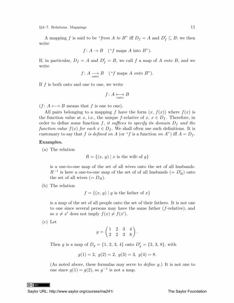
A mapping f is said to be “from A to B” iff Df = A and D′f ⊆ B; we then
write
f : A→ B (“f maps A into B”).
If, in particular, Df = A and D′f = B, we call f a map of A onto B, and we
write
f : A −→onto
B (“f maps A onto B”).
If f is both onto and one to one, we write
f : A←→onto
B
(f : A←→ B means that f is one to one).
All pairs belonging to a mapping f have the form (x, f(x)) where f(x) isthe function value at x, i.e., the unique f -relative of x, x ∈ Df . Therefore, inorder to define some function f , it suffices to specify its domain Df and the
function value f(x) for each x ∈ Df . We shall often use such definitions. It iscustomary to say that f is defined on A (or “f is a function on A”) iff A = Df .
Examples.
(a) The relation
R = {(x, y) | x is the wife of y}
is a one-to-one map of the set of all wives onto the set of all husbands.R−1 is here a one-to-one map of the set of of all husbands (= D′
R) ontothe set of all wives (= DR).
(b) The relation
f = {(x, y) | y is the father of x}
is a map of the set of all people onto the set of their fathers. It is not oneto one since several persons may have the same father (f -relative), andso x 6= x′ does not imply f(x) 6= f(x′).
(c) Let
g =
(
1 2 3 42 2 3 8
)
.
Then g is a map of Dg = {1, 2, 3, 4} onto D′g = {2, 3, 8}, with
g(1) = 2, g(2) = 2, g(3) = 3, g(4) = 8.
(As noted above, these formulas may serve to define g.) It is not one toone since g(1) = g(2), so g−1 is not a map.
Saylor URL: http://www.saylor.org/courses/ma241/ The Saylor Foundation
12 Chapter 1. Set Theory
(d) Consider
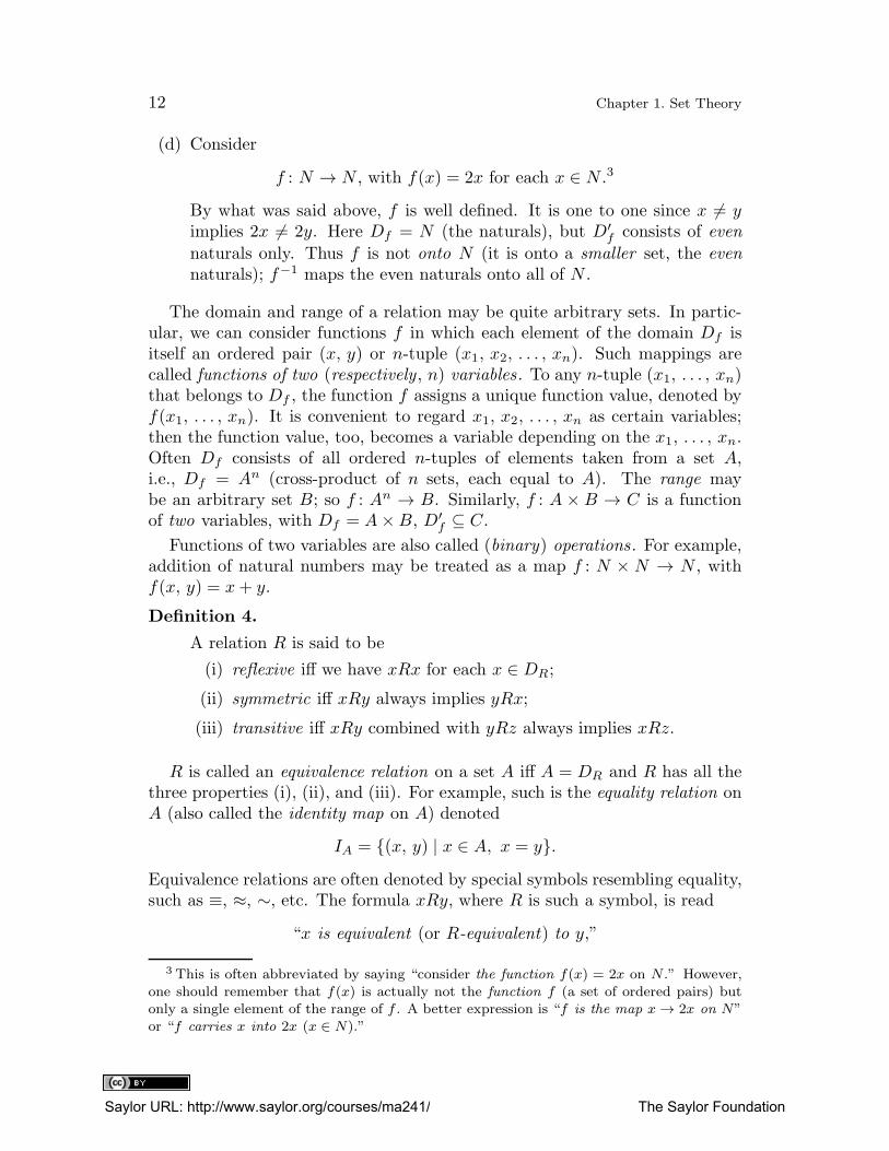
f : N → N , with f(x) = 2x for each x ∈ N .3
By what was said above, f is well defined. It is one to one since x 6= yimplies 2x 6= 2y. Here Df = N (the naturals), but D′
f consists of even
naturals only. Thus f is not onto N (it is onto a smaller set, the even
naturals); f−1 maps the even naturals onto all of N .
The domain and range of a relation may be quite arbitrary sets. In partic-ular, we can consider functions f in which each element of the domain Df isitself an ordered pair (x, y) or n-tuple (x1, x2, . . . , xn). Such mappings arecalled functions of two (respectively , n) variables. To any n-tuple (x1, . . . , xn)that belongs to Df , the function f assigns a unique function value, denoted byf(x1, . . . , xn). It is convenient to regard x1, x2, . . . , xn as certain variables;then the function value, too, becomes a variable depending on the x1, . . . , xn.Often Df consists of all ordered n-tuples of elements taken from a set A,i.e., Df = An (cross-product of n sets, each equal to A). The range maybe an arbitrary set B; so f : An → B. Similarly, f : A × B → C is a functionof two variables, with Df = A×B, D′
f ⊆ C.Functions of two variables are also called (binary) operations . For example,
addition of natural numbers may be treated as a map f : N × N → N , withf(x, y) = x+ y.
Definition 4.
A relation R is said to be
(i) reflexive iff we have xRx for each x ∈ DR;
(ii) symmetric iff xRy always implies yRx;
(iii) transitive iff xRy combined with yRz always implies xRz.
R is called an equivalence relation on a set A iff A = DR and R has all thethree properties (i), (ii), and (iii). For example, such is the equality relation onA (also called the identity map on A) denoted
IA = {(x, y) | x ∈ A, x = y}.Equivalence relations are often denoted by special symbols resembling equality,such as ≡, ≈, ∼, etc. The formula xRy, where R is such a symbol, is read
“x is equivalent (or R-equivalent) to y,”
3 This is often abbreviated by saying “consider the function f(x) = 2x on N .” However,
one should remember that f(x) is actually not the function f (a set of ordered pairs) butonly a single element of the range of f . A better expression is “f is the map x → 2x on N”
or “f carries x into 2x (x ∈ N).”
Saylor URL: http://www.saylor.org/courses/ma241/ The Saylor Foundation
§§4–7. Relations. Mappings 13
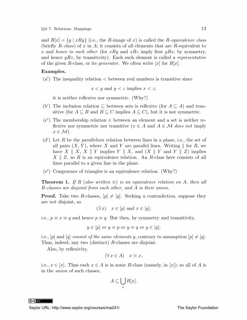
and R[x] = {y | xRy} (i.e., the R-image of x) is called the R-equivalence class
(briefly R-class) of x in A; it consists of all elements that are R-equivalent tox and hence to each other (for xRy and xRz imply first yRx, by symmetry,and hence yRz, by transitivity). Each such element is called a representative
of the given R-class, or its generator . We often write [x] for R[x].
Examples.
(a′) The inequality relation < between real numbers is transitive since
x < y and y < z implies x < z;
it is neither reflexive nor symmetric. (Why?)
(b′) The inclusion relation ⊆ between sets is reflexive (for A ⊆ A) and tran-sitive (for A ⊆ B and B ⊆ C implies A ⊆ C), but it is not symmetric.
(c′) The membership relation ∈ between an element and a set is neither re-flexive nor symmetric nor transitive (x ∈ A and A ∈ M does not implyx ∈M).
(d′) Let R be the parallelism relation between lines in a plane, i.e., the set ofall pairs (X, Y ), where X and Y are parallel lines. Writing ‖ for R, wehave X ‖ X , X ‖ Y implies Y ‖ X , and (X ‖ Y and Y ‖ Z) impliesX ‖ Z, so R is an equivalence relation. An R-class here consists of alllines parallel to a given line in the plane.
(e′) Congruence of triangles is an equivalence relation. (Why?)
Theorem 1. If R (also written ≡) is an equivalence relation on A, then all
R-classes are disjoint from each other, and A is their union.
Proof. Take two R-classes, [p] 6= [q]. Seeking a contradiction, suppose theyare not disjoint, so
(∃x) x ∈ [p] and x ∈ [q];
i.e., p ≡ x ≡ q and hence p ≡ q. But then, by symmetry and transitivity,
y ∈ [p]⇔ y ≡ p⇔ y ≡ q ⇔ y ∈ [q];
i.e., [p] and [q] consist of the same elements y, contrary to assumption [p] 6= [q].Thus, indeed, any two (distinct) R-classes are disjoint.
Also, by reflexivity,
(∀x ∈ A) x ≡ x,
i.e., x ∈ [x]. Thus each x ∈ A is in some R-class (namely, in [x]); so all of A isin the union of such classes,
A ⊆⋃
x
R[x].
Saylor URL: http://www.saylor.org/courses/ma241/ The Saylor Foundation
14 Chapter 1. Set Theory
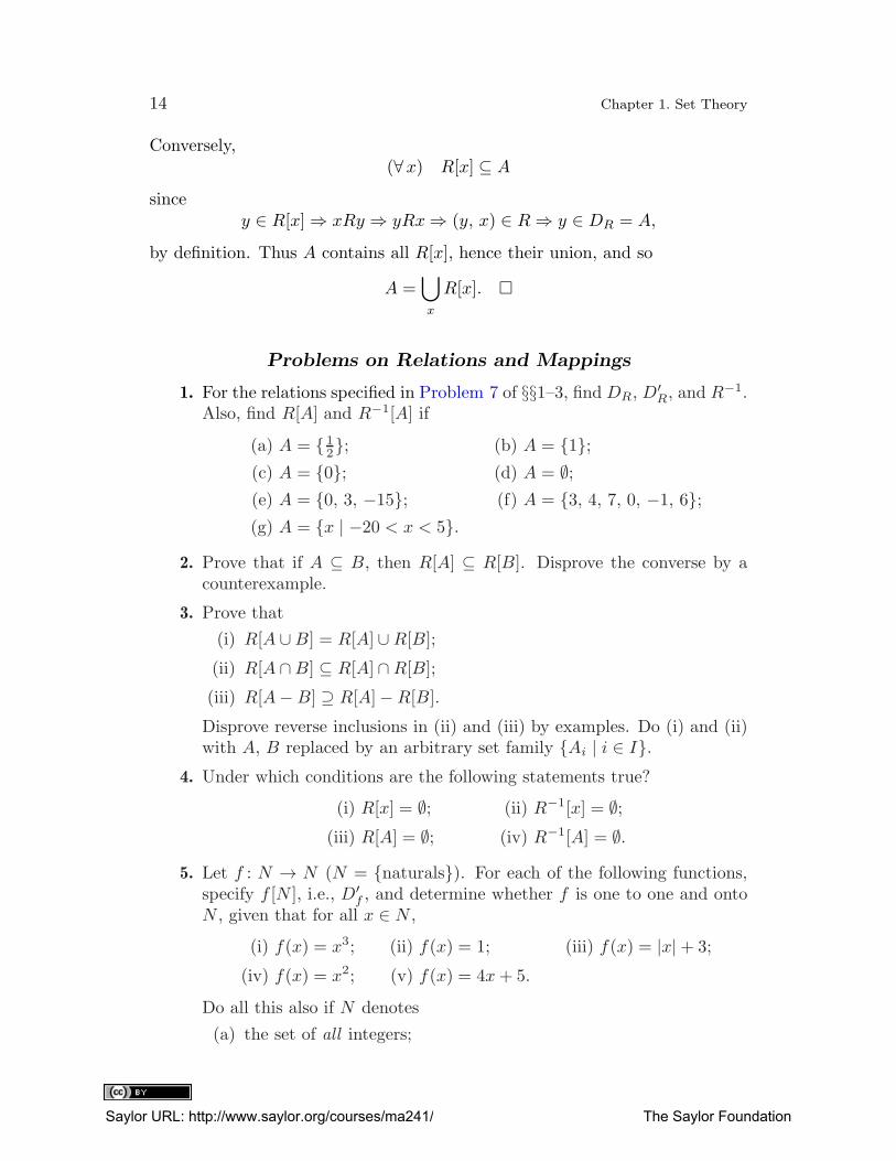
Conversely,(∀x) R[x] ⊆ A
sincey ∈ R[x]⇒ xRy ⇒ yRx⇒ (y, x) ∈ R⇒ y ∈ DR = A,
by definition. Thus A contains all R[x], hence their union, and so
A =⋃
x
R[x]. �
Problems on Relations and Mappings
1. For the relations specified in Problem 7 of §§1–3, find DR, D′R, and R
−1.Also, find R[A] and R−1[A] if
(a) A = { 12}; (b) A = {1};
(c) A = {0}; (d) A = ∅;(e) A = {0, 3, −15}; (f) A = {3, 4, 7, 0, −1, 6};(g) A = {x | −20 < x < 5}.
2. Prove that if A ⊆ B, then R[A] ⊆ R[B]. Disprove the converse by acounterexample.
3. Prove that
(i) R[A ∪B] = R[A] ∪R[B];
(ii) R[A ∩B] ⊆ R[A] ∩R[B];
(iii) R[A−B] ⊇ R[A]−R[B].
Disprove reverse inclusions in (ii) and (iii) by examples. Do (i) and (ii)with A, B replaced by an arbitrary set family {Ai | i ∈ I}.
4. Under which conditions are the following statements true?
(i) R[x] = ∅; (ii) R−1[x] = ∅;(iii) R[A] = ∅; (iv) R−1[A] = ∅.
5. Let f : N → N (N = {naturals}). For each of the following functions,specify f [N ], i.e., D′
f , and determine whether f is one to one and ontoN , given that for all x ∈ N ,
(i) f(x) = x3; (ii) f(x) = 1; (iii) f(x) = |x|+ 3;
(iv) f(x) = x2; (v) f(x) = 4x+ 5.
Do all this also if N denotes
(a) the set of all integers;
Saylor URL: http://www.saylor.org/courses/ma241/ The Saylor Foundation
§§4–7. Relations. Mappings 15
(b) the set of all reals.
6. Prove that for any mapping f and any sets A, B, Ai (i ∈ I),(a) f−1[A ∪B] = f−1[A] ∪ f−1[B];
(b) f−1[A ∩B] = f−1[A] ∩ f−1[B];
(c) f−1[A−B] = f−1[A]− f−1[B];
(d) f−1[⋃
iAi] =⋃
i f−1[Ai];
(e) f−1[⋂
iAi] =⋂
i f−1[Ai].
Compare with Problem 3.[Hint: First verify that x ∈ f−1[A] iff x ∈ Df and f(x) ∈ A.]
7. Let f be a map. Prove that
(a) f [f−1[A]] ⊆ A;(b) f [f−1[A]] = A if A ⊆ D′
f ;
(c) if A ⊆ Df and f is one to one, A = f−1[f [A]].
Is f [A] ∩B ⊆ f [A ∩ f−1[B]]?
8. Is R an equivalence relation on the set J of all integers, and, if so, whatare the R-classes, if
(a) R = {(x, y) | x− y is divisible by a fixed n};(b) R = {(x, y) | x− y is odd};(c) R = {(x, y) | x− y is a prime}.
(x, y, n denote integers.)
9. Is any relation in Problem 7 of §§1–3 reflexive? Symmetric? Transitive?
10. Show by examples that R may be
(a) reflexive and symmetric, without being transitive;
(b) reflexive and transitive without being symmetric.
Does symmetry plus transitivity imply reflexivity? Give a proof orcounterexample.
§8. Sequences1By an infinite sequence (briefly sequence) we mean a mapping (call it u) whosedomain is N (all natural numbers 1, 2, 3, . . . ); Du may also contain 0.
1 This section may be deferred until Chapter 2, §13.
Saylor URL: http://www.saylor.org/courses/ma241/ The Saylor Foundation
16 Chapter 1. Set Theory
A finite sequence is a map u in which Du consists of all positive (or non-negative) integers less than a fixed integer p. The range D′
u of any sequence umay be an arbitrary set B; we then call u a sequence of elements of B, or in
B. For example,
u =
(
1 2 3 4 . . . n . . .2 4 6 8 . . . 2n . . .
)
(1)
is a sequence with
Du = N = {1, 2, 3, . . . }
and with function values
u(1) = 2, u(2) = 4, u(n) = 2n, n = 1, 2, 3, . . . .
Instead of u(n) we usually write un (“index notation”), and call un the nthterm of the sequence. If n is treated as a variable, un is called the general termof the sequence, and {un} is used to denote the entire (infinite) sequence, aswell as its range D′
u (whichever is meant, will be clear from the context). Theformula {un} ⊆ B means that D′
u ⊆ B, i.e., that u is a sequence in B. Todetermine a sequence, it suffices to define its general term un by some formulaor rule.2 In (1) above, un = 2n.
Often we omit the mention of Du = N (since it is known) and give only therange D′
u. Thus instead of (1), we briefly write
2, 4, 6, . . . , 2n, . . .
or, more generally,
u1, u2, . . . , un, . . . .
Yet it should be remembered that u is a set of pairs (a map).
If all un are distinct (different from each other), u is a one-to-one map. How-ever, this need not be the case. It may even occur that all un are equal (then uis said to be constant); e.g., un = 1 yields the sequence 1, 1, 1, . . . , 1, . . . , i.e.,
u =
(
1 2 3 . . . n . . .1 1 1 . . . 1 . . .
)
. (2)
Note that here u is an infinite sequence (since Du = N), even though itsrange D′
u has only one element, D′u = {1}. (In sets , repeated terms count
as one element; but the sequence u consists of infinitely many distinct pairs
(n, 1).) If all un are real numbers, we call u a real sequence. For such sequences,we have the following definitions.
2 However, such a formula may not exist; the un may even be chosen “at random.”
Saylor URL: http://www.saylor.org/courses/ma241/ The Saylor Foundation
§8. Sequences 17
Definition 1.
A real sequence {un} is said to be monotone (or monotonic) iff it is eithernondecreasing , i.e.,
(∀n) un ≤ un+1,
or nonincreasing , i.e.,
(∀n) un ≥ un+1.
Notation: {un}↑ and {un}↓, respectively. If instead we have the strict
inequalities un < un+1 (respectively, un > un+1), we call {un} strictly
monotone (increasing or decreasing).
A similar definition applies to sequences of sets .
Definition 2.
A sequence of sets A1, A2, . . . , An, . . . is said to be monotone iff it iseither expanding , i.e.,
(∀n) An ⊆ An+1,
or contracting , i.e.,(∀n) An ⊇ An+1.
Notation: {An}↑ and {An}↓, respectively. For example, any sequence ofconcentric solid spheres (treated as sets of points), with increasing radii,is expanding; if the radii decrease, we obtain a contracting sequence.
Definition 3.
Let {un} be any sequence, and let
n1 < n2 < · · · < nk < · · ·be a strictly increasing sequence of natural numbers. Select from {un}those terms whose subscripts are n1, n2, . . . , nk, . . . . Then the sequence{unk
} so selected (with kth term equal to unk), is called the subsequence
of {un}, determined by the subscripts nk, k = 1, 2, 3, . . . .
Thus (roughly) a subsequence is any sequence obtained from {un} by drop-ping some terms, without changing the order of the remaining terms (this isensured by the inequalities n1 < n2 < · · · < nk < · · · where the nk are thesubscripts of the remaining terms). For example, let us select from (1) thesubsequence of terms whose subscripts are primes (including 1). Then thesubsequence is
2, 4, 6, 10, 14, 22, . . . ,
i.e.,u1, u2, u3, u5, u7, u11, . . . .
Saylor URL: http://www.saylor.org/courses/ma241/ The Saylor Foundation
18 Chapter 1. Set Theory
All these definitions apply to finite sequences accordingly. Observe thatevery sequence arises by “numbering” the elements of its range (the terms): u1is the first term, u2 is the second term, and so on. By so numbering, we putthe terms in a certain order , determined by their subscripts 1, 2, 3, . . . (likethe numbering of buildings in a street, of books in a library, etc.). The questionnow arises: Given a set A, is it always possible to “number” its elements by
integers? As we shall see in §9, this is not always the case. This leads us tothe following definition.
Definition 4.
A set A is said to be countable iff A is contained in the range of somesequence (briefly, the elements of A can be put in a sequence).
If, in particular, this sequence can be chosen finite, we call A a finite
set. (The empty set is finite.)
Sets that are not finite are said to be infinite.
Sets that are not countable are said to be uncountable.
Note that all finite sets are countable. The simplest example of an infinitecountable set is N = {1, 2, 3, . . . }.
§9. Some Theorems on Countable Sets1We now derive some corollaries of Definition 4 in §8.Corollary 1. If a set A is countable or finite, so is any subset B ⊆ A.
For if A ⊂ D′u for a sequence u, then certainly B ⊆ A ⊆ D′
u.
Corollary 2. If A is uncountable (or just infinite), so is any superset B ⊇ A.
For, if B were countable or finite, so would be A ⊆ B, by Corollary 1.
Theorem 1. If A and B are countable, so is their cross product A×B.
Proof. If A or B is ∅, then A×B = ∅, and there is nothing to prove.
Thus let A and B be nonvoid and countable. We may assume that they fill
two infinite sequences, A = {an}, B = {bn} (repeat terms if necessary). Then,by definition, A×B is the set of all ordered pairs of the form
(an, bm), n, m ∈ N.Call n+m the rank of the pair (an, bm). For each r ∈ N , there are r− 1 pairsof rank r:
(a1, br−1), (a2, br−2), . . . , (ar−1, b1). (1)
1 This section may be deferred until Chapter 5, §4.
Saylor URL: http://www.saylor.org/courses/ma241/ The Saylor Foundation
§9. Some Theorems on Countable Sets 19
We now put all pairs (an, bm) in one sequence as follows. We start with
(a1, b1)
as the first term; then take the two pairs of rank three,
(a1, b2), (a2, b1);
then the three pairs of rank four, and so on. At the (r − 1)st step, we take allpairs of rank r, in the order indicated in (1).
Repeating this process for all ranks ad infinitum, we obtain the sequence ofpairs
(a1, b1), (a1, b2), (a2, b1), (a1, b3), (a2, b2), (a3, b1), . . . ,
in which u1 = (a1, b1), u2 = (a1, b2), etc.
By construction, this sequence contains all pairs of all ranks r, hence all pairsthat form the set A × B (for every such pair has some rank r and so it musteventually occur in the sequence). Thus A×B can be put in a sequence. �
Corollary 3. The set R of all rational numbers2 is countable.
Proof. Consider first the set Q of all positive rationals, i.e.,
fractionsn
m, with n, m ∈ N .
We may formally identify them with ordered pairs (n, m), i.e., with N × N .We call n+m the rank of (n, m). As in Theorem 1, we obtain the sequence
1
1,1
2,2
1,1
3,2
2,3
1,1
4,2
3,3
2,4
1, . . . .
By dropping reducible fractions and inserting also 0 and the negative rationals,we put R into the sequence
0, 1, −1, 1
2, −1
2, 2, −2, 1
3, −1
3, 3, −3, . . . , as required. �
Theorem 2. The union of any sequence {An} of countable sets is countable.
Proof. As each An is countable, we may put
An = {an1, an2, . . . , anm, . . . }.(The double subscripts are to distinguish the sequences representing differentsets An.) As before, we may assume that all sequences are infinite. Now,
⋃
nAn
obviously consists of the elements of all An combined , i.e., all anm (n, m ∈ N).We call n+m the rank of anm and proceed as in Theorem 1, thus obtaining
⋃
n
An = {a11, a12, a21, a13, a22, a31, . . . }.
2 A number is rational iff it is the ratio of two integers, p/q, q 6= 0.
Saylor URL: http://www.saylor.org/courses/ma241/ The Saylor Foundation
20 Chapter 1. Set Theory
Thus⋃
nAn can be put in a sequence. �
Note 1. Theorem 2 is briefly expressed as
“Any countable union of countable sets is a countable set .”
(The term“countable union” means “union of a countable family of sets”, i.e., afamily of sets whose elements can be put in a sequence {An}.) In particular,if A and B are countable, so are A ∪B, A ∩B, and A−B (by Corollary 1).
Note 2. From the proof it also follows that the range of any double se-
quence {anm} is countable. (A double sequence is a function u whose domainDu is N × N ; say, u : N × N → B. If n, m ∈ N , we write unm for u(n, m);here unm = anm.)
To prove the existence of uncountable sets, we shall now show that theinterval
[0, 1) = {x | 0 ≤ x < 1}of the real axis is uncountable.
We assume as known the fact that each real number x ∈ [0, 1) has a uniqueinfinite decimal expansion
0.x1, x2, . . . , xn, . . . ,
where the xn are the decimal digits (possibly zeros), and the sequence {xn}does not terminate in nines (this ensures uniqueness).3
Theorem 3. The interval [0, 1) of the real axis is uncountable.
Proof. We must show that no sequence can comprise all of [0, 1). Indeed,given any {un}, write each term un as an infinite decimal fraction; say,
un = 0.an1, an2, . . . , anm, . . . .
Next, construct a new decimal fraction
z = 0.x1, x2, . . . , xn, . . . ,
choosing its digits xn as follows.
If ann (i.e., the nth digit of un) is 0, put xn = 1; if, however, ann 6= 0, putxn = 0. Thus, in all cases, xn 6= ann, i.e., z differs from each un in at least one
decimal digit (namely, the nth digit). It follows that z is different from all unand hence is not in {un}, even though z ∈ [0, 1).
Thus, no matter what the choice of {un} was, we found some z ∈ [0, 1) notin the range of that sequence. Hence no {un} contains all of [0, 1). �
Note 3. By Corollary 2, any superset of [0, 1), e.g., the entire real axis, isuncountable. See also Problem 4 below.
3 For example, instead of 0.49999 . . . , we write 0.50000 . . . .
Saylor URL: http://www.saylor.org/courses/ma241/ The Saylor Foundation
§9. Some Theorems on Countable Sets 21
Note 4. Observe that the numbers ann used in the proof of Theorem 3 formthe diagonal of the infinitely extending square composed of all anm. Therefore,the method used above is called the diagonal process (due to G. Cantor).
Problems on Countable and Uncountable Sets
1. Prove that if A is countable but B is not, then B − A is uncountable.[Hint: If B − A were countable, so would be
(B − A) ∪ A ⊇ B. (Why?)
Use Corollary 1.]
2. Let f be a mapping, and A ⊆ Df . Prove that
(i) if A is countable, so is f [A];
(ii) if f is one to one and A is uncountable, so is f [A].
[Hints: (i) If A = {un}, then
f [A] = {f(u1), f(u2), . . . , f(un), . . . }.
(ii) If f [A] were countable, so would be f−1[f [A]], by (i). Verify that
f−1[f [A]] = A
here; cf. Problem 7 in §§4–7.]
3. Let a, b be real numbers (a < b). Define a map f on [0, 1) by
f(x) = a+ x(b− a).Show that f is one to one and onto the interval [a, b) = {x | a ≤ x < b}.From Problem 2, deduce that [a, b) is uncountable. Hence, by Problem1, so is (a, b) = {x | a < x < b}.
4. Show that between any real numbers a, b (a < b) there are uncountably
many irrationals , i.e., numbers that are not rational.[Hint: By Corollary 3 and Problems 1 and 3, the set (a, b) − R is uncountable.Explain in detail.]
5. Show that every infinite set A contains a countably infinite set, i.e., aninfinite sequence of distinct terms.[Hint: Fix any a1 ∈ A; A cannot consist of a1 alone, so there is another element
a2 ∈ A− {a1}. (Why?)
Again, A 6= {a1, a2}, so there is an a3 ∈ A− {a1, a2}. (Why?) Continue thusly adinfinitum to obtain the required sequence {an}. Why are all an distinct?]
∗6. From Problem 5, prove that if A is infinite, there is a map f : A → Athat is one to one but not onto A.[Hint: With an as in Problem 5, define f(an) = an+1. If, however, x is none of thean, put f(x) = x. Observe that f(x) = a1 is never true, so f is not onto A. Show,
however, that f is one to one.]
Saylor URL: http://www.saylor.org/courses/ma241/ The Saylor Foundation
22 Chapter 1. Set Theory
∗7. Conversely (cf. Problem 6), prove that if there is a map f : A→ A thatis one to one but not onto A, then A contains an infinite sequence {an}of distinct terms.[Hint: As f is not onto A, there is a1 ∈ A such that a1 /∈ f [A]. (Why?) Fix a1 and
define
a2 = f(a1), a3 = f(a2), . . . , an+1 = f(an), . . . ad infinitum.
To prove distinctness, show that each an is distinct from all am with m > n. For a1,
this is true since a1 /∈ f [A], whereas am ∈ f [A] (m > 1). Then proceed inductively.]
Saylor URL: http://www.saylor.org/courses/ma241/ The Saylor Foundation
Chapter 2
Real Numbers. Fields
§§1–4. Axioms and Basic Definitions
Real numbers can be constructed step by step: first the integers, then therationals, and finally the irrationals.1 Here, however, we shall assume theset of all real numbers, denoted E1, as already given, without attempting toreduce this notion to simpler concepts. We shall also accept without definition(as primitive concepts) the notions of the sum (a+ b) and the product , (a · b)or (ab), of two real numbers, as well as the inequality relation < (read “lessthan”). Note that x ∈ E1 means “x is in E1,” i.e., “x is a real number .”
It is an important fact that all arithmetic properties of reals can be deducedfrom several simple axioms, listed (and named) below.
Axioms of Addition and Multiplication
I (closure laws). The sum x + y, and the product xy, of any real numbers
are real numbers themselves. In symbols,
(∀x, y ∈ E1) (x+ y) ∈ E1 and (xy) ∈ E1.
II (commutative laws).
(∀x, y ∈ E1) x+ y = y + x and xy = yx.
III (associative laws).
(∀x, y, z ∈ E1) (x+ y) + z = x+ (y + z) and (xy)z = x(yz).
IV (existence of neutral elements).
(a) There is a (unique) real number , called zero (0), such that , for all
real x, x+ 0 = x.
1 See the author’s Basic Concepts of Mathematics, Chapter 2, §15.
Saylor URL: http://www.saylor.org/courses/ma241/ The Saylor Foundation
24 Chapter 2. Real Numbers. Fields
(b) There is a (unique) real number , called one (1), such that 1 6= 0and , for all real x, x · 1 = x.
In symbols,
(a) (∃! 0 ∈ E1) (∀x ∈ E1) x+ 0 = x;
(b) (∃! 1 ∈ E1) (∀x ∈ E1) x · 1 = x, 1 6= 0.
(The real numbers 0 and 1 are called the neutral elements of addition andmultiplication, respectively.)
V (existence of inverse elements).
(a) For every real x, there is a (unique) real , denoted −x, such that
x+ (−x) = 0.
(b) For every real x other than 0, there is a (unique) real , denoted x−1,such that x · x−1 = 1.
In symbols,
(a) (∀x ∈ E1) (∃!−x ∈ E1) x+ (−x) = 0;
(b) (∀x ∈ E1 | x 6= 0) (∃! x−1 ∈ E1) xx−1 = 1.
(The real numbers −x and x−1 are called, respectively, the additive in-
verse (or the symmetric) and the multiplicative inverse (or the reciprocal)of x.)
VI (distributive law).
(∀x, y, z ∈ E1) (x+ y)z = xz + yz.
Axioms of Order
VII (trichotomy). For any real x and y, we have
either x < y or y < x or x = y
but never two of these relations together .
VIII (transitivity).
(∀x, y, z ∈ E1) x < y and y < z implies x < z.
IX (monotonicity of addition and multiplication). For any x, y, z ∈ E1, we
have
(a) x < y implies x+ z < y + z;
(b) x < y and z > 0 implies xz < yz.
An additional axiom will be stated in §§8–9.
Saylor URL: http://www.saylor.org/courses/ma241/ The Saylor Foundation
§§1–4. Axioms and Basic Definitions 25
Note 1. The uniqueness assertions in Axioms IV and V are actually re-dundant since they can be deduced from other axioms. We shall not dwell onthis.
Note 2. Zero has no reciprocal ; i.e., for no x is 0x = 1. In fact, 0x = 0.
For, by Axioms VI and IV,
0x+ 0x = (0 + 0)x = 0x = 0x+ 0.
Cancelling 0x (i.e., adding −0x on both sides), we obtain 0x = 0, by Axioms IIIand V(a).
Note 3. Due to Axioms VII and VIII, real numbers may be regarded asgiven in a certain order under which smaller numbers precede the larger ones.(This is why we speak of “axioms of order .”) The ordering of real numbers canbe visualized by “plotting” them as points on a directed line (“the real axis”)in a well-known manner. Therefore, E1 is also often called “the real axis ,” andreal numbers are called “points”; we say “the point x” instead of “the number
x.”
Observe that the axioms only state certain properties of real numbers withoutspecifying what these numbers are. Thus we may treat the reals as just any
mathematical objects satisfying our axioms, but otherwise arbitrary. Indeed,our theory also applies to any other set of objects (numbers or not), providedthey satisfy our axioms with respect to a certain relation of order (<) andcertain operations (+) and (·), which may, but need not, be ordinary additionand multiplication. Such sets exist indeed. We now give them a name.
Definition 1.
A field is any set F of objects, with two operations (+) and (·) definedin it in such a manner that they satisfy Axioms I–VI listed above (withE1 replaced by F , of course).
If F is also endowed with a relation < satisfying Axioms VII to IX, wecall F an ordered field .
In this connection, postulates I to IX are called axioms of an (ordered) field .
By Definition 1, E1 is an ordered field. Clearly, whatever follows from theaxioms must hold not only in E1 but also in any other ordered field. Thuswe shall henceforth state our definitions and theorems in a more general way,speaking of ordered fields in general instead of E1 alone.
Definition 2.
An element x of an ordered field is said to be positive if x > 0 or negativeif x < 0.
Here and below, “x > y” means the same as “y < x.” We also write“x ≤ y” for “x < y or x = y”; similarly for “x ≥ y.”
Saylor URL: http://www.saylor.org/courses/ma241/ The Saylor Foundation
26 Chapter 2. Real Numbers. Fields
Definition 3.
For any elements x, y of a field, we define their difference
x− y = x+ (−y).
If y 6= 0, we also define the quotient of x by y
x
y= xy−1,
also denoted by x/y.
Note 4. Division by 0 remains undefined .
Definition 4.
For any element x of an ordered field, we define its absolute value,
|x| ={
x if x ≥ 0 and
−x if x < 0.
It follows that |x| ≥ 0 always ; for if x ≥ 0, then
|x| = x ≥ 0;
and if x < 0, then
|x| = −x > 0. (Why?)
Moreover,
−|x| ≤ x ≤ |x|,for,
if x ≥ 0, then |x| = x;
and
if x < 0, then x < |x| since |x| > 0.
Thus, in all cases,
x ≤ |x|.
Similarly one shows that
−|x| ≤ x.
As we have noted, all rules of arithmetic (dealing with the four arithmeticoperations and inequalities) can be deduced from Axioms I through IX andthus apply to all ordered fields, along with E1. We shall not dwell on theirdeduction, limiting ourselves to a few simple corollaries as examples.2
2 For more examples, see the author’s Basic Concepts of Mathematics, Chapter 2, §§3–4.
Saylor URL: http://www.saylor.org/courses/ma241/ The Saylor Foundation
§§1–4. Axioms and Basic Definitions 27
Corollary 1 (rule of signs).
(i) a(−b) = (−a)b = −(ab);(ii) (−a)(−b) = ab.
Proof. By Axiom VI,
a(−b) + ab = a[(−b) + b] = a · 0 = 0.
Thusa(−b) + ab = 0.
By definition, then, a(−b) is the additive inverse of ab, i.e.,
a(−b) = −(ab).
Similarly, we show that(−a)b = −(ab)
and that−(−a) = a.
Finally, (ii) is obtained from (i) when a is replaced by −a. �
Corollary 2. In an ordered field , a 6= 0 implies
a2 = (a · a) > 0.
(Hence 1 = 12 > 0.)
Proof. If a > 0, we may multiply by a (Axiom IX(b)) to obtain
a · a > 0 · a = 0, i.e., a2 > 0.
If a < 0, then −a > 0; so we may multiply the inequality a < 0 by −a andobtain
a(−a) < 0(−a) = 0;
i.e., by Corollary 1,−a2 < 0,
whencea2 > 0. �
§§5–6. Natural Numbers. Induction
The element 1 was introduced in Axiom IV(b). Since addition is also assumedknown, we can use it to define, step by step, the elements
2 = 1 + 1, 3 = 2 + 1, 4 = 3 + 1, etc.
Saylor URL: http://www.saylor.org/courses/ma241/ The Saylor Foundation
28 Chapter 2. Real Numbers. Fields
If this process is continued indefinitely, we obtain what is called the set N ofall natural elements in the given field F . In particular, the natural elements ofE1 are called natural numbers . Note that
(∀n ∈ N) n+ 1 ∈ N.∗A more precise approach to natural elements is as follows.1 A subset S of
a field F is said to be inductive iff
(i) 1 ∈ S and
(ii) (∀x ∈ S) x+ 1 ∈ S.Such subsets certainly exist; e.g., the entire field F is inductive since
1 ∈ F and (∀x ∈ F ) x+ 1 ∈ F.Define N as the intersection of all inductive sets in F .
∗Theorem 1. The set N so defined is inductive itself . In fact , it is the “small-
est” inductive subset of F (i .e., contained in any other such subset).
Proof. We have to show that
(i) 1 ∈ N , and
(ii) (∀x ∈ N) x+ 1 ∈ N .
Now, by definition, the unity 1 is in each inductive set; hence it also belongsto the intersection of such sets, i.e., to N . Thus 1 ∈ N , as claimed.
Next, take any x ∈ N . Then, by our definition of N , x is in each inductiveset S; thus, by property (ii) of such sets, also x + 1 is in each such S; hencex+ 1 is in the intersection of all inductive sets, i.e.,
x+ 1 ∈ N,and so N is inductive, indeed.
Finally, by definition, N is the common part of all such sets and hencecontained in each. �
For applications, Theorem 1 is usually expressed as follows.
Theorem 1′ (first induction law). A proposition P (n) involving a natural nholds for all n ∈ N in a field F if
(i) it holds for n = 1, i .e., P (1) is true; and
(ii) whenever P (n) holds for n = m, it holds for n = m+ 1, i .e.,
P (m) =⇒ P (m+ 1).
1 At a first reading, one may omit all “starred” passages and simply assume Theorems 1′
and 2′ below as additional axioms, without proof.
Saylor URL: http://www.saylor.org/courses/ma241/ The Saylor Foundation
§§5–6. Natural Numbers. Induction 29
∗Proof. Let S be the set of all those n ∈ N for which P (n) is true,
S = {n ∈ N | P (n)}.We have to show that actually each n ∈ N is in S, i.e., N ⊆ S.
First, we show that S is inductive.
Indeed, by assumption (i), P (1) is true; so 1 ∈ S.Next, let x ∈ S. This means that P (x) is true. By assumption (ii), however,
this implies P (x+ 1), i.e., x+ 1 ∈ S. Thus1 ∈ S and (∀x ∈ S) x+ 1 ∈ S;
S is inductive.
Then, by Theorem 1 (second clause), N ⊆ S, and all is proved. �
This theorem is used to prove various properties of N “by induction.”
Examples.
(a) If m, n ∈ N , then also m+ n ∈ N and mn ∈ N .
To prove the first property, fix any m ∈ N . Let P (n) mean
m+ n ∈ N (n ∈ N).
Then
(i) P (1) is true, for as m ∈ N , the definition of N yields m + 1 ∈ N ,i.e., P (1).
(ii) P (k)⇒ P (k + 1) for k ∈ N . Indeed,
P (k)⇒ m+ k ∈ N ⇒ (m+ k) + 1 ∈ N⇒ m+ (k + 1) ∈ N ⇒ P (k + 1).
Thus, by Theorem 1′, P (n) holds for all n; i.e.,
(∀n ∈ N) m+ n ∈ Nfor any m ∈ N .
To prove the same for mn, we let P (n) mean
mn ∈ N (n ∈ N)
and proceed similarly.
(b) If n ∈ N , then n− 1 = 0 or n− 1 ∈ N .
For an inductive proof, let P (n) mean
n− 1 = 0 or n− 1 ∈ N (n ∈ N).
Then proceed as in (a).
Saylor URL: http://www.saylor.org/courses/ma241/ The Saylor Foundation
30 Chapter 2. Real Numbers. Fields
(c) In an ordered field , all naturals are ≥ 1.
Indeed, let P (n) mean that
n ≥ 1 (n ∈ N).
Then
(i) P (1) holds since 1 = 1.
(ii) P (m)⇒ P (m+ 1) for m ∈ N , since
P (m)⇒ m ≥ 1⇒ (m+ 1) > 1⇒ P (m+ 1).
Thus Theorem 1′ yields the result.
(d) In an ordered field , m, n ∈ N and m > n implies m− n ∈ N .
For an inductive proof, fix any m ∈ N and let P (n) mean
m− n ≤ 0 or m− n ∈ N (n ∈ N).
Use (b).
(e) In an ordered field , m, n ∈ N and m < n+ 1 implies m ≤ n.For, by (d), m > n would imply m − n ∈ N , hence m − n ≥ 1, or
m ≥ n+ 1, contrary to m < n+ 1.
Our next theorem states the so-called well-ordering property of N .
Theorem 2 (well-ordering of N). In an ordered field , each nonvoid set A ⊆ Nhas a least member (i .e., one that exceeds no other element of A).
Proof outline.2 Given ∅ 6= A ⊆ N , let P (n) be the proposition “Any subset
of A containing elements ≤ n has a least member” (n ∈ N). Use Theorem 1′
and Example (e). �
This theorem yields a new form of the induction law.
Theorem 2′ (second induction law). A proposition P (n) holds for all n ∈ Nin an ordered field if
(i′) P (1) holds and
(ii′) whenever P (n) holds for all naturals less than some m ∈ N , then P (n)also holds for n = m.
Proof. Assume (i′) and (ii′). Seeking a contradiction,3 suppose there are somen ∈ N (call them “bad”) for which P (n) fails . Then these “bad” naturals forma nonvoid subset of N , call it A.
2 For a more detailed proof, see Basic Concepts of Mathematics, Chapter 2, §5, Theorem 2.3 We are using a “proof by contradiction” or “indirect proof.” Instead of proving our
assertion directly , we show that the opposite is impossible, being contradictory.
Saylor URL: http://www.saylor.org/courses/ma241/ The Saylor Foundation
§§5–6. Natural Numbers. Induction 31
By Theorem 2, A has a least member m. Thus m is the least natural forwhich P (n) fails. It follows that all n less than m do satisfy P (n). But then,by our assumption (ii′), P (n) also holds for n = m, which is impossible for, byconstruction, m is “bad” (it is in A). This contradiction shows that there areno “bad” naturals. Thus all is proved. �
Note 1. All the preceding arguments hold also if, in our definition of Nand all formulations, the unity 1 is replaced by 0 or by some k (±k ∈ N).Then, however, the conclusions must be changed to say that P (n) holds for allintegers n ≥ k (instead of “n ≥ 1”). We then say that “induction starts withk.”
An analogous induction law also applies to definitions of concepts C(n).
A notion C(n) involving a natural n is regarded as defined for each n ∈ N(in E1) if
(i) it is defined for n = 1 and
(ii) some rule is given that expresses C(n+ 1) in terms of C(1), . . . , C(n).
(Note 1 applies here, too.)
C(n) itself need not be a number ; it may be of quite general nature.
We shall adopt this principle as a kind of logical axiom, without proof(though it can be proved in a similar manner as Theorems 1′ and 2′). The un-derlying intuitive idea is a “step-by-step” process—first, we define C(1); then,as C(1) is known, we may use it to define C(2); next, once both are known,we may use them to define C(3); and so on, ad infinitum. Definitions basedon that principle are called inductive or recursive. The following examples areimportant.
Examples (continued).
(f) For any element x of a field, we define its nth power xn and its n-multiple
nx by
(i) x1 = 1x = x;
(ii) xn+1 = xnx (respectively, (n+ 1)x = nx+ x).
We may think of it as a step-by-step definition:
x1 = x, x2 = x1x, x3 = x2x, etc.
(g) For each natural number n, we define its factorial n! by
1! = 1, (n+ 1)! = n! (n+ 1);
e.g., 2! = 1! (2) = 2, 3! = 2! (3) = 6, etc. We also define 0! = 1.
Saylor URL: http://www.saylor.org/courses/ma241/ The Saylor Foundation
32 Chapter 2. Real Numbers. Fields
(h) The sum and product of n field elements x1, x2, . . . , xn, denoted by
n∑
k=1
xk andn∏
k=1
xk
or
x1 + x2 + · · ·+ xn and x1x2 · · ·xn, respectively,are defined recursively.
Sums are defined by
(i)1
∑
k=1
xk = x1;
(ii)n+1∑
k=1
xk =
( n∑
k=1
xk
)
+ xn+1, n = 1, 2, . . . .
Thusx1 + x2 + x3 = (x1 + x2) + x3,
x1 + x2 + x3 + x4 = (x1 + x2 + x3) + x4, etc.
Products are defined by
(i)1∏
k=1
xk = x1;
(ii)n+1∏
k=1
xk =
( n∏
k=1
xk
)
· xn+1.
(i) Given any objects x1, x2, . . . , xn, . . . , the ordered n-tuple
(x1, x2, . . . , xn)
is defined inductively by
(i) (x1) = x1 (i.e., the ordered “one-tuple” (x1) is x1 itself) and
(ii) (x1, x2, . . . , xn+1) = ((x1, . . . , xn), xn+1), i.e., the ordered (n+1)-tuple is a pair (y, xn+1) in which the first term y is itself an orderedn-tuple, (x1, . . . , xn); for example,
(x1, x2, x3) = ((x1, x2), x3), etc.
Problems on Natural Numbers and Induction
1. Complete the missing details in Examples (a), (b), and (d).
2. Prove Theorem 2 in detail.
Saylor URL: http://www.saylor.org/courses/ma241/ The Saylor Foundation
§§5–6. Natural Numbers. Induction 33
3. Suppose xk < yk, k = 1, 2, . . . , in an ordered field. Prove by inductionon n that
(a)n∑
k=1
xk <n∑
k=1
yk;
(b) if all xk, yk are greater than zero, then
n∏
k=1
xk <
n∏
k=1
yk.
4. Prove by induction that
(i) 1n = 1;
(ii) a < b⇒ an < bn if a > 0.
Hence deduce that
(iii) 0 ≤ an < 1 if 0 ≤ a < 1;
(iv) an < bn ⇒ a < b if b > 0; proof by contradiction.
5. Prove the Bernoulli inequalities: For any element ε of an ordered field,
(i) (1 + ε)n ≥ 1 + nε if ε > −1;(ii) (1− ε)n ≥ 1− nε if ε < 1; n = 1, 2, 3, . . . .
6. For any field elements a, b and natural numbers m, n, prove that
(i) aman = am+n; (ii) (am)n = amn;
(iii) (ab)n = anbn; (iv) (m+ n)a = ma+ na;
(v) n(ma) = (nm) · a; (vi) n(a+ b) = na+ nb.
[Hint: For problems involving two natural numbers, fix m and use induction on n].
7. Prove that in any field,
an+1 − bn+1 = (a− b)n∑
k=0
akbn−k, n = 1, 2, 3, . . . .
Hence for r 6= 1n∑
k=0
ark = a1− rn+1
1− r
(sum of n terms of a geometric series).
8. For n > 0 define
(
n
k
)
=
n!
k! (n− k)! , 0 ≤ k ≤ n,
0, otherwise.
Saylor URL: http://www.saylor.org/courses/ma241/ The Saylor Foundation
34 Chapter 2. Real Numbers. Fields
Verify Pascal’s law ,(
n+ 1
k + 1
)
=
(
n
k
)
+
(
n
k + 1
)
.
Then prove by induction on n that
(i) (∀ k | 0 ≤ k ≤ n)(
n
k
)
∈ N ; and
(ii) for any field elements a and b,
(a+ b)n =
n∑
k=0
(
n
k
)
akbn−k, n ∈ N (the binomial theorem).
What value must 00 take for (ii) to hold for all a and b?
9. Show by induction that in an ordered field F any finite sequencex1, . . . , xn has a largest and a least term (which need not be x1 orxn). Deduce that all of N is an infinite set, in any ordered field.
10. Prove in E1 that
(i)
n∑
k=1
k =1
2n(n+ 1);
(ii)n∑
k=1
k2 =1
6n(n+ 1)(2n+ 1);
(iii)
n∑
k=1
k3 =1
4n2(n+ 1)2;
(iv)n∑
k=1
k4 =1
30n(n+ 1)(2n+ 1)(3n2 + 3n− 1).
§7. Integers and Rationals
All natural elements of a field F , their additive inverses, and 0 are called theintegral elements of F , briefly integers.
An element x ∈ F is said to be rational iff x =p
qfor some integers p and q
(q 6= 0); x is irrational iff it is not rational.
We denote by J the set of all integers, and by R the set of all rationals, inF . Every integer p is also a rational since p can be written as p/q with q = 1.Thus
R ⊇ J ⊃ N.
Saylor URL: http://www.saylor.org/courses/ma241/ The Saylor Foundation
§7. Integers and Rationals 35
In an ordered field,
N = {x ∈ J | x > 0}. (Why?)
Theorem 1. If a and b are integers (or rationals) in F , so are a+ b and ab.
Proof. For integers, this follows from Examples (a) and (d) in §§5–6; one onlyhas to distinguish three cases:
(i) a, b ∈ N ;
(ii) −a ∈ N , b ∈ N ;
(iii) a ∈ N , −b ∈ N .
The details are left to the reader (see Basic Concepts of Mathematics, Chap-ter 2, §7, Theorem 1).
Now let a and b be rationals, say,
a =p
qand b =
r
s,
where p, q, r, s ∈ J and q, s 6= 0. Then, as is easily seen,
a± b = ps± qrqs
and ab =pr
qs,
where qs 6= 0; and qs and pr are integers by the first part of the proof (sincep, q, r, s ∈ J).
Thus a± b and ab are fractions with integral numerators and denominators.Hence, by definition, a± b ∈ R and ab ∈ R. �
Theorem 2. In any field F , the set R of all rationals is a field itself , underthe operations defined in F , with the same neutral elements 0 and 1. Moreover ,R is an ordered field if F is . (We call R the rational subfield of F .)
Proof. We have to check that R satisfies the field axioms.
The closure law I follows from Theorem 1.
Axioms II, III, and VI hold for rationals because they hold for all elementsof F ; similarly for Axioms VII to IX if F is ordered.
Axiom IV holds in R because the neutral elements 0 and 1 belong to R;indeed, they are integers, hence certainly rationals.
To verify Axiom V, we must show that −x and x−1 belong to R if x does.If, however,
x =p
q(p, q ∈ J, q 6= 0),
then
−x =−pq,
where again −p ∈ J by the definition of J ; thus −x ∈ R.
Saylor URL: http://www.saylor.org/courses/ma241/ The Saylor Foundation
36 Chapter 2. Real Numbers. Fields
If, in addition, x 6= 0, then p 6= 0, and
x =p
qimplies x−1 =
q
p. (Why?)
Thus x−1 ∈ R. �
Note. The representation
x =p
q(p, q ∈ J)
is not unique in general; in an ordered field, however, we can always chooseq > 0, i.e., q ∈ N (take p ≤ 0 if x ≤ 0).
Among all such q there is a least one by Theorem 2 of §§5–6. If x = p/q,with this minimal q ∈ N , we say that the rational x is given in lowest terms.
§§8–9. Upper and Lower Bounds. Completeness Axiom
A subset A of an ordered field F is said to be bounded below (or left bounded)iff there is p ∈ F such that
(∀x ∈ A) p ≤ x;A is bounded above (or right bounded) iff there is q ∈ F such that
(∀x ∈ A) x ≤ q.In this case, p and q are called, respectively, a lower (or left) bound and anupper (or right) bound, of A. If both exist, we simply say that A is bounded
(by p and q). The empty set ∅ is regarded as (“vacuously”) bounded by any pand q (cf. the end of Chapter 1, §3).
The bounds p and q may, but need not , belong to A. If a left bound pis itself in A, we call it the least element or minimum of A, denoted minA.Similarly, if A contains an upper bound q, we write q = maxA and call q thelargest element or maximum of A. However, A may well have no minimum ormaximum.
Note 1. A finite set A 6= ∅ always has a minimum and a maximum(see Problem 9 of §§5–6).
Note 2. A set A can have at most one maximum and at most one minimum.For if it had two maxima q, q′, then
q ≤ q′
(since q ∈ A and q′ is a right bound); similarly
q′ ≤ q;
Saylor URL: http://www.saylor.org/courses/ma241/ The Saylor Foundation
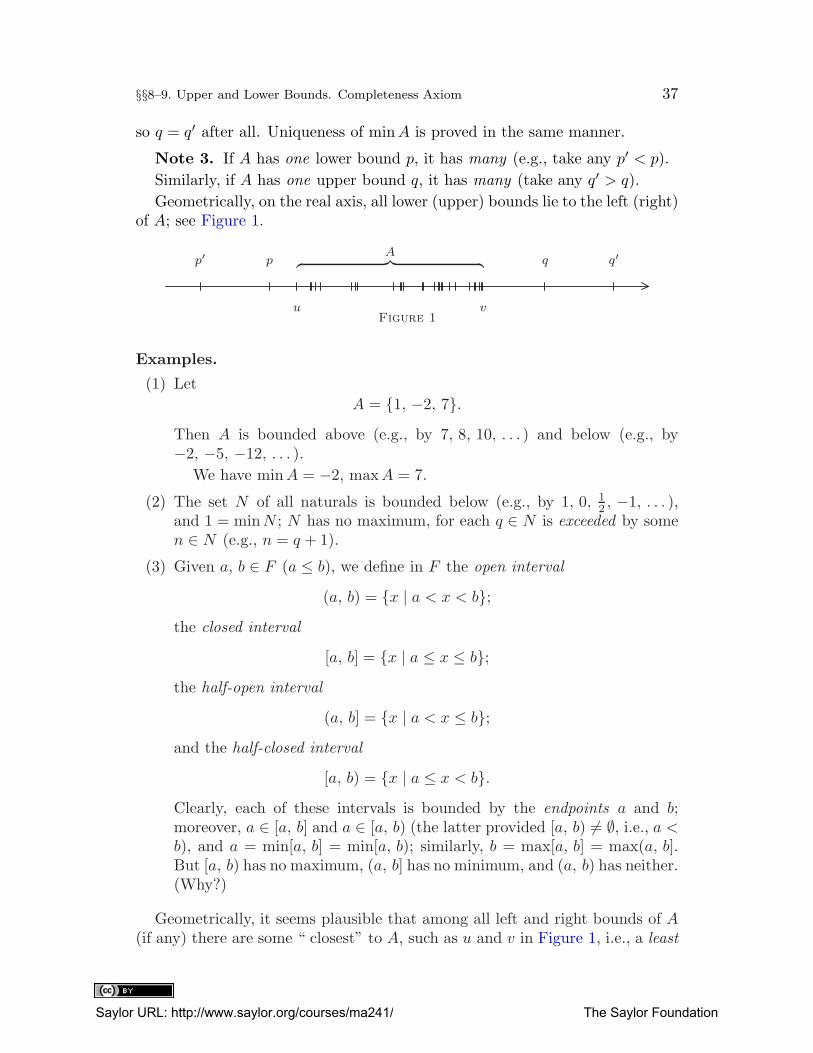
§§8–9. Upper and Lower Bounds. Completeness Axiom 37
so q = q′ after all. Uniqueness of minA is proved in the same manner.
Note 3. If A has one lower bound p, it has many (e.g., take any p′ < p).
Similarly, if A has one upper bound q, it has many (take any q′ > q).
Geometrically, on the real axis, all lower (upper) bounds lie to the left (right)of A; see Figure 1.
p′ p
u
q q′
vFigure 1
A︷ ︸︸ ︷
Examples.
(1) Let
A = {1, −2, 7}.Then A is bounded above (e.g., by 7, 8, 10, . . . ) and below (e.g., by−2, −5, −12, . . . ).
We have minA = −2, maxA = 7.
(2) The set N of all naturals is bounded below (e.g., by 1, 0, 12 , −1, . . . ),
and 1 = minN ; N has no maximum, for each q ∈ N is exceeded by somen ∈ N (e.g., n = q + 1).
(3) Given a, b ∈ F (a ≤ b), we define in F the open interval
(a, b) = {x | a < x < b};the closed interval
[a, b] = {x | a ≤ x ≤ b};the half-open interval
(a, b] = {x | a < x ≤ b};and the half-closed interval
[a, b) = {x | a ≤ x < b}.Clearly, each of these intervals is bounded by the endpoints a and b;moreover, a ∈ [a, b] and a ∈ [a, b) (the latter provided [a, b) 6= ∅, i.e., a <b), and a = min[a, b] = min[a, b); similarly, b = max[a, b] = max(a, b].But [a, b) has no maximum, (a, b] has no minimum, and (a, b) has neither.(Why?)
Geometrically, it seems plausible that among all left and right bounds of A(if any) there are some “ closest” to A, such as u and v in Figure 1, i.e., a least
Saylor URL: http://www.saylor.org/courses/ma241/ The Saylor Foundation
38 Chapter 2. Real Numbers. Fields
upper bound v and a greatest lower bound u. These are abbreviated
lubA and glbA
and are also called the supremum and infimum of A, respectively; briefly,
v = supA, u = inf A.
However, this assertion, though valid in E1, fails to materialize in manyother fields such as the field R of all rationals (cf. §§11–12). Even for E1, itcannot be proved from Axioms I through IX.
On the other hand, this property is of utmost importance for mathematicalanalysis; so we introduce it as an axiom (for E1), called the completeness
axiom. It is convenient first to give a general definition.
Definition 1.
An ordered field F is said to be complete iff every nonvoid right-boundedsubset A ⊂ F has a supremum (i.e., a lub) in F .
Note that we use the term “complete” only for ordered fields.
With this definition, we can give the tenth and final axiom for E1.
X (completeness axiom). The real field E1 is complete in the above sense.That is , each right-bounded set A ⊂ E1 has a supremum (supA) in E1,provided A 6= ∅.
The corresponding assertion for infima can now be proved as a theorem.
Theorem 1. In a complete field F (such as E1), every nonvoid left-bounded
subset A ⊂ F has an infimum (i .e., a glb).
Proof. Let B be the (nonvoid) set of all lower bounds of A (such bounds existsince A is left bounded). Then, clearly, no member of B exceeds any memberof A, and so B is right bounded by an element of A. Hence, by the assumedcompleteness of F , B has a supremum in F , call it p.
We shall show that p is also the required infimum of A, thus completing theproof.
Indeed, we have
(i) p is a lower bound of A. For, by definition, p is the least upper bound ofB. But, as shown above, each x ∈ A is an upper bound of B. Thus
(∀x ∈ A) p ≤ x.
(ii) p is the greatest lower bound of A. For p = supB is not exceeded by anymember of B. But, by definition, B contains all lower bounds of A; so pis not exceeded by any of them, i.e.,
p = glbA = inf A. �
Saylor URL: http://www.saylor.org/courses/ma241/ The Saylor Foundation
§§8–9. Upper and Lower Bounds. Completeness Axiom 39
Note 4. The lub and glb of A (if they exist) are unique. For inf A is,by definition, the maximum of the set B of all lower bounds of A, and henceunique, by Note 2; similarly for the uniqueness of supA.
Note 5. Unlike minA and maxA, the glb and lub of A need not belong toA. For example, if A is the interval (a, b) in E1 (a < b) then, as is easily seen,
a = inf A and b = supA,
though a, b /∈ A. Thus supA and inf A may exist , though maxA and minA do
not .
On the other hand, if
q = maxA (p = minA),
then also
q = supA (p = inf A). (Why?)
Theorem 2. In an ordered field F , we have q = supA (A ⊂ F ) iff
(i) (∀x ∈ A) x ≤ q and
(ii) each field element p < q is exceeded by some x ∈ A; i .e.,
(∀ p < q) (∃x ∈ A) p < x.
Equivalently ,
(ii′) (∀ ε > 0) (∃x ∈ A) q − ε < x; (ε ∈ F ).Similarly , p = inf A iff
(∀x ∈ A) p ≤ x and (∀ ε > 0) (∃x ∈ A) p+ ε > x.
Proof. Condition (i) states that q is an upper bound of A, while (ii) impliesthat no smaller element p is such a bound (since it is exceeded by some x inA). When combined, (i) and (ii) state that q is the least upper bound.
Moreover, any element p < q can be written as q− ε (ε > 0). Hence (ii) canbe rephrased as (ii′).
The proof for inf A is quite analogous. �
Corollary 1. Let b ∈ F and A ⊂ F in an ordered field F . If each element
x of A satisfies x ≤ b (x ≥ b), so does supA (inf A, respectively), provided it
exists in F .
In fact, the condition
(∀x ∈ A) x ≤ bmeans that b is a right bound of A. However, supA is the least right bound,so supA ≤ b; similarly for inf A.
Saylor URL: http://www.saylor.org/courses/ma241/ The Saylor Foundation
40 Chapter 2. Real Numbers. Fields
Corollary 2. In any ordered field , ∅ 6= A ⊆ B implies
supA ≤ supB and inf A ≥ inf B,
as well as
inf A ≤ supA,
provided the suprema and infima involved exist .
Proof. Let p = inf B and q = supB.
As q is a right bound of B,
x ≤ q for all x ∈ B.
But A ⊆ B, so B contains all elements of A. Thus
x ∈ A⇒ x ∈ B ⇒ x ≤ q;so, by Corollary 1, also
supA ≤ q = supB,
as claimed.
Similarly, one gets inf A ≥ inf B.
Finally, if A 6= ∅, we can fix some x ∈ A. Theninf A ≤ x ≤ supA,
and all is proved. �
Problems on Upper and Lower Bounds
1. Complete the proofs of Theorem 2 and Corollaries 1 and 2 for infima.Prove the last clause of Note 4.
2. Prove that F is complete iff each nonvoid left-bounded set in F has aninfimum.
3. Prove that if A1, A2, . . . , An are right bounded (left bounded) in F , sois
n⋃
k=1
Ak.
4. Prove that if A = (a, b) is an open interval (a < b), then
a = inf A and b = supA.
5. In an ordered field F , let ∅ 6= A ⊂ F . Let c ∈ F and let cA denote theset of all products cx (x ∈ A); i.e.,
cA = {cx | x ∈ A}.
Saylor URL: http://www.saylor.org/courses/ma241/ The Saylor Foundation
§§8–9. Upper and Lower Bounds. Completeness Axiom 41
Prove that
(i) if c ≥ 0, then
sup(cA) = c · supA and inf(cA) = c · inf A;
(ii) if c < 0, then
sup(cA) = c · inf A and inf(cA) = c · supA.
In both cases, assume that the right-side supA (respectively, inf A) ex-ists.
6. From Problem 5(ii) with c = −1, obtain a new proof of Theorem 1.[Hint: If A is left bounded, show that (−1)A is right bounded and use its supremum.]
7. Let A and B be subsets of an ordered field F . Assuming that therequired lub and glb exist in F , prove that
(i) if (∀x ∈ A) (∀ y ∈ B) x ≤ y, then supA ≤ inf B;
(ii) if (∀x ∈ A) (∃ y ∈ B) x ≤ y, then supA ≤ supB;
(iii) if (∀ y ∈ B) (∃x ∈ A) x ≤ y, then inf A ≤ inf B.
[Hint for (i): By Corollary 1, (∀ y ∈ B) supA ≤ y, so supA ≤ inf B. (Why?)]
8. For any two subsets A and B of an ordered field F , let A + B denotethe set of all sums x+ y with x ∈ A and y ∈ B; i.e.,
A+B = {x+ y | x ∈ A, y ∈ B}.Prove that if supA = p and supB = q exist in F , then
p+ q = sup(A+B);
similarly for infima.[Hint for sup: By Theorem 2, we must show that
(i) (∀x ∈ A) (∀ y ∈ B) x+ y ≤ p+ q (which is easy) and
(ii′) (∀ ε > 0) (∃ x ∈ A) (∃ y ∈ B) x+ y > (p+ q)− ε.
Fix any ε > 0. By Theorem 2,
(∃ x ∈ A) (∃ y ∈ B) p− ε
2< x and q − ε
2< y. (Why?)
Then
x+ y >(
p− ε
2
)
+(
q − ε
2
)
= (p+ q)− ε,
as required.]
9. In Problem 8 let A and B consist of positive elements only, and let
AB = {xy | x ∈ A, y ∈ B}.Prove that if supA = p and supB = q exist in F , then
pq = sup(AB);
Saylor URL: http://www.saylor.org/courses/ma241/ The Saylor Foundation
42 Chapter 2. Real Numbers. Fields
similarly for infima.[Hint: Use again Theorem 2(ii′). For sup(AB), take
0 < ε < (p+ q)min{p, q}
and
x > p− ε
p+ qand y > q − ε
p+ q;
show that
xy > pq − ε+ε2
(p+ q)2> pq − ε.
For inf(AB), let s = inf B and r = inf A; choose d < 1, with
0 < d <ε
1 + r + s.
Now take x ∈ A and y ∈ B with
x < r + d and y < s+ d,
and show that
xy < rs + ε.
Explain!]
10. Prove that
(i) if (∀ ε > 0) a ≥ b− ε, then a ≥ b;(ii) if (∀ ε > 0) a ≤ b+ ε, then a ≤ b.
11. Prove the principle of nested intervals: If [an, bn] are closed intervals ina complete ordered field F , with
[an, bn] ⊇ [an+1, bn+1], n = 1, 2, . . . ,
then∞⋂
n=1
[an, bn] 6= ∅.
[Hint: Let
A = {a1, a2, . . . , an, . . . }.
Show that A is bounded above by each bn.
Let p = supA. (Does it exist?)
Show that
(∀n) an ≤ p ≤ bn,
i.e.,
p ∈ [an, bn].]
Saylor URL: http://www.saylor.org/courses/ma241/ The Saylor Foundation
§§8–9. Upper and Lower Bounds. Completeness Axiom 43
12. Prove that each bounded set A 6= ∅ in a complete field F is containedin a smallest closed interval [a, b] (so [a, b] is contained in any other[c, d] ⊇ A).
Show that this fails if “closed” is replaced by “open.”[Hint: Take a = inf A, b = supA].
13. Prove that if A consists of positive elements only, then q = supA iff
(i) (∀x ∈ A) x ≤ q and
(ii) (∀ d > 1) (∃ x ∈ A) q/d < x.
[Hint: Use Theorem 2.]
§10. Some Consequences of the Completeness Axiom
The ancient Greek geometer and scientist Archimedes was first to observe thateven a large distance y can be measured by a small yardstick x; one only hasto mark x off sufficiently many times. Mathematically, this means that, givenany x > 0 and any y, there is an n ∈ N such that nx > y. This fact, known asthe Archimedean property , holds not only in E1 but also in many other orderedfields. Such fields are called Archimedean. In particular, we have the followingtheorem.
Theorem 1. Any complete field F (e.g ., E1) is Archimedean.1
That is , given any x, y ∈ F (x > 0) in such a field , there is a natural n ∈ Fsuch that nx > y.
Proof by contradiction. Suppose this fails. Thus, given y, x ∈ F (x > 0),assume that there is no n ∈ N with nx > y.
Then
(∀n ∈ N) nx ≤ y;
i.e., y is an upper bound of the set of all products nx (n ∈ N). Let
A = {nx | n ∈ N}.
Clearly, A is bounded above (by y) and A 6= ∅; so, by the assumed com-pleteness of F , A has a supremum, say, q = supA.
As q is an upper bound, we have (by the definition of A) that nx ≤ q for alln ∈ N , hence also (n+ 1)x ≤ q; i.e.,
nx ≤ q − xfor all n ∈ N (since n ∈ N ⇒ n+ 1 ∈ N).
1 However, there also are incomplete Archimedean fields (see Note 2 in §§11–12).
Saylor URL: http://www.saylor.org/courses/ma241/ The Saylor Foundation
44 Chapter 2. Real Numbers. Fields
Thus q−x (which is less than q for x > 0) is another upper bound of all nx,i.e., of the set A.
This is impossible, however, since q = supA is the least upper bound of A.
This contradiction completes the proof. �
Corollary 1. In any Archimedean (hence also in any complete) field F , theset N of all natural elements has no upper bounds, and the set J of all integers
has neither upper nor lower bounds. Thus
(∀ y ∈ F ) (∃ m, n ∈ N) −m < y < n.
Proof. Given any y ∈ F , one can use the Archimedean property (with x = 1)to find an n ∈ N such that
n · 1 > y, i.e., n > y.
Similarly, there is an m ∈ N such that
m > −y, i.e., −m < y.
This proves our last assertion and shows that no y ∈ F can be a right boundof N (for y < n ∈ N), or a left bound of J (for y > −m ∈ J). �
Theorem 2. In any Archimedean (hence also in any complete) field F , eachleft (right) bounded set A of integers (∅ 6= A ⊂ J) has a minimum (maximum,respectively).
Proof. Suppose ∅ 6= A ⊆ J , and A has a lower bound y.
Then Corollary 1 (last part) yields a natural m, with −m < y, so that
(∀x ∈ A) −m < x,
and so x+m > 0.
Thus, by addingm to each x ∈ A, we obtain a set (call it A+m) of naturals .2
Now, by Theorem 2 of §§5–6, A +m has a minimum; call it p. As p is theleast of all sums x+m, p−m is the least of all x ∈ A; so p−m = minA exists,as claimed.
Next, let A have a right bound z. Then look at the set of all additive inverses−x of points x ∈ A; call it B.
Clearly, B is left bounded (by −z), so it has a minimum, say, u = minB.Then −u = maxA. (Verify!) �
In particular, given any x ∈ F (F Archimedean), let [x] denote the great-est integer ≤ x (called the integral part of x). We thus obtain the followingcorollary.
2 This is the main point—geometrically, we have “shifted” A to the right by m, so that
its elements became positive integers: A+m ⊆ N .
Saylor URL: http://www.saylor.org/courses/ma241/ The Saylor Foundation
§10. Some Consequences of the Completeness Axiom 45
Corollary 2. Any element x of an Archimedean field F has an integral part
[x]. It is the unique integer n such that
n ≤ x < n+ 1.
(It exists , by Theorem 2.)
Any ordered field has the so-called density property :
If a < b in F , there is x ∈ F such that a < x < b; e.g., take
x =a+ b
2.
We shall now show that, in Archimedean fields, x can be chosen rational ,even if a and b are not. We refer to this as the density of rationals in anArchimedean field.
Theorem 3 (density of rationals). Between any elements a and b (a < b) of
an Archimedean field F (such as E1), there is a rational r ∈ F with
a < r < b.
Proof. Let p = [a] (the integral part of a). The idea of the proof is to startwith p and to mark off a small “yardstick”
1
n< b− a
several (m) times, until
p+m
nlands inside (a, b);
then r = p+ mn is the desired rational.
We now make it precise. As F is Archimedean, there are m, n ∈ N suchthat
n(b− a) > 1 and m( 1
n
)
> a− p.
We fix the least such m (it exists, by Theorem 2 in §§5–6). Then
a− p < m
n, but
m− 1
n≤ a− p
(by the minimality of m). Hence
a < p+m
n≤ a+ 1
n< a+ (b− a),
since 1n < b− a. Setting
r = p+m
n,
Saylor URL: http://www.saylor.org/courses/ma241/ The Saylor Foundation
46 Chapter 2. Real Numbers. Fields
we find
a < r < a+ b− a = b. �
Note. Having found one rational r1,
a < r1 < b,
we can apply Theorem 3 to find another r2 ∈ R,
r1 < r2 < b,
then a third r3 ∈ R,r2 < r3 < b,
and so on. Continuing this process indefinitely, we obtain infinitely many
rationals in (a, b).
§§11–12. Powers With Arbitrary Real Exponents. Irrationals
In complete fields, one can define ar for any a > 0 and r ∈ E1 (for r ∈ N , see§§5–6, Example (f)). First of all, we have the following theorem.
Theorem 1. Given a ≥ 0 in a complete field F , and a natural number n ∈ E1,there always is a unique element p ∈ F , p ≥ 0, such that
pn = a.
It is called the nth root of a, denoted
n√a or a1/n.
(Note that n√a ≥ 0, by definition.)
A direct proof, from the completeness axiom, is sketched in Problems 1 and2 below. We shall give a simpler proof in Chapter 4, §9, Example (a). Atpresent, we omit it and temporarily take Theorem 1 for granted. Hence weobtain the following result.
Theorem 2. Every complete field F (such as E1) has irrational elements ,i .e., elements that are not rational .
In particular ,√2 is irrational .1
Proof. By Theorem 1, F has the element
p =√2 with p2 = 2.
1 As usual, we write√a for 2
√a.
Saylor URL: http://www.saylor.org/courses/ma241/ The Saylor Foundation
§§11–12. Powers With Arbitrary Real Exponents. Irrationals 47
Seeking a contradiction, suppose√2 is rational, i.e.,
√2 =
m
n
for some m, n ∈ N in lowest terms (see §7, final note).Then m and n are not both even (otherwise, reduction by 2 would yield a
smaller n). From m/n =√2, we obtain
m2 = 2n2;
so m2 is even.
Only even elements have even squares, however.2 Thus m itself must beeven; i.e., m = 2r for some r ∈ N . It follows that
4r2 = m2 = 2n2, i.e., 2r2 = n2
and, by the same argument, n must be even.
This contradicts the fact that m and n are not both even, and this contra-diction shows that
√2 must be irrational. �
Note 1. Similarly, one can prove the irrationality of√a where a ∈ N and
a is not the square of a natural. See Problem 3 below for a hint.
Note 2. Theorem 2 shows that the field R of all rationals is not com-
plete (for it contains no irrationals), even though it is Archimedean (see Prob-lem 6). Thus the Archimedean property does not imply completeness (but seeTheorem 1 of §10).
Next, we define ar for any rational number r > 0.
Definition 1.
Given a ≥ 0 in a complete field F , and a rational number
r =m
n(m, n ∈ N ⊆ E1),
we define
ar = n√am.
Here we must clarify two facts.
(1) If n = 1, we have
ar = am/1 = 1√am = am.
2 For if m is odd , then m = 2q − 1 for some q ∈ N , and hence
m2 = (2q − 1)2 = 4q2 − 4q + 1 = 4q(q − 1) + 1
is an odd number.
Saylor URL: http://www.saylor.org/courses/ma241/ The Saylor Foundation
48 Chapter 2. Real Numbers. Fields
If m = 1, we get
ar = a1/n = n√a.
Thus Definition 1 agrees with our previous definitions of am and n√a
(m, n ∈ N).
(2) If r is written as a fraction in two different ways ,
r =m
n=p
q,
then, as is easily seen,
n√am = q
√ap = ar,
and so our definition is unambiguous (independent of the particular rep-resentation of r).
Indeed,m
n=p
qimplies mq = np,
whence
amq = apn,
i.e.,
(am)q = (ap)n;
cf. §§5–6, Problem 6.
By definition, however,
( n√am)n = am and ( q
√ap)q = ap.
Substituting this in (am)q = (ap)n, we get
( n√am)nq = ( q
√ap)nq,
whencen√am = q
√ap.
Thus Definition 1 is valid, indeed.
By using the results of Problems 4 and 6 of §§5–6, the reader will easilyobtain analogous formulas for powers with positive rational exponents, namely,
aras = ar+s; (ar)s = ars; (ab)r = arbr; ar < as if 0 < a < 1 and r > s;
a < b iff ar < br (a, b, r > 0); ar > as if a > 1 and r > s; 1r = 1(1)
Henceforth we assume these formulas known, for rational r, s > 0.
Next, we define ar for any real r > 0 and any element a > 1 in a completefield F .
Saylor URL: http://www.saylor.org/courses/ma241/ The Saylor Foundation
§§11–12. Powers With Arbitrary Real Exponents. Irrationals 49
Let Aar denote the set of all members of F of the form ax, with x ∈ R and0 < x ≤ r; i.e.,
Aar = {ax | 0 < x ≤ r, x rational}.By the density of rationals in E1 (Theorem 3 of §10), such rationals x do exist;thus Aar 6= ∅.
Moreover, Aar is right bounded in F . Indeed, fix any rational number y > r.By the formulas in (1), we have, for any positive rational x ≤ r,
ay = ax+(y−x) = axay−x > ax
since a > 1 and y − x > 0 implies
ay−x > 1.
Thus ay is an upper bound of all ax in Aar.
Hence, by the assumed completeness of F , supAar exists . So we may define
ar = supAar.3
We also put
a−r =1
ar.
If 0 < a < 1 (so that 1a > 1), we put
ar =(1
a
)−r
and a−r =1
ar,
where(1
a
)r
= supA1/a,r,
as above.
Summing up, we have the following definitions.
Definition 2.
Given a > 0 in a complete field F , and r ∈ E1, we define the following.
(i) If r > 0 and a > 1, then
ar = supAar = sup{ax | 0 < x ≤ r, x rational}.
(ii) If r > 0 and 0 < a < 1, then ar = 1(1/a)r , also written (1/a)−r.
(iii) a−r = 1/ar. (This defines powers with negative exponents as well.)
3 Note that, if r is a positive rational itself, then ar is the largest ax with x ≤ r (where ar
and ax are as in Definition 1); thus ar = maxAar = supAar , and so our present definition
agrees with Definition 1. This excludes ambiguities.
Saylor URL: http://www.saylor.org/courses/ma241/ The Saylor Foundation
50 Chapter 2. Real Numbers. Fields
We also define 0r = 0 for any real r > 0, and a0 = 1 for any a ∈ F , a 6= 0;00 remains undefined .
The power ar is also defined if a < 0 and r is a rational mn with n odd
because ar = n√am has sense in this case. (Why?) This does not work for
other values of r. Therefore, in general, we assume a > 0.
Again, it is easy to show that the formulas in (1) remain also valid for powerswith real exponents (see Problems 8–13 below), provided F is complete.
Problems on Roots, Powers, and Irrationals
The problems marked by ⇒ are theoretically important. Study them!
1. Let n ∈ N in E1; let p > 0 and a > 0 be elements of an ordered field F .Prove that
(i) if pn > a, then (∃ x ∈ F ) p > x > 0 and xn > a;
(ii) if pn < a, then (∃ x ∈ F ) x > p and xn < a.
[Hint: For (i), put
x = p− d, with 0 < d < p.
Use the Bernoulli inequality (Problem 5(ii) in §§5–6) to find d such that
xn = (p− d)n > a,
i.e.,(
1− d
p
)n>
a
pn.
Solving for d, show that this holds if
0 < d <pn − a
npn−1< p. (Why does such a d exist?)
For (ii), if pn < a, then1
pn>
1
a.
Use (i) with a and p replaced by 1/a and 1/p.]
2. Prove Theorem 1 assuming that
(i) a > 1;
(ii) 0 < a < 1 (the cases a = 0 and a = 1 are trivial).
[Hints: (i) Let
A = {x ∈ F | x ≥ 1, xn > a}.
Show that A is bounded below (by 1) and A 6= ∅ (e.g., a+ 1 ∈ A—why?).
By completeness, put p = inf A.
Then show that pn = a (i.e., p is the required n√a).
Indeed, if pn > a, then Problem 1 would yield an x ∈ A with
x < p = inf A. (Contradiction!)
Saylor URL: http://www.saylor.org/courses/ma241/ The Saylor Foundation
§§11–12. Powers With Arbitrary Real Exponents. Irrationals 51
Similarly, use Problem 1 to exclude pn < a.
To prove uniqueness, use Problem 4(ii) of §§5–6.Case (ii) reduces to (i) by considering 1/a instead of a.]
3. Prove Note 1.[Hint: Suppose first that a is not divisible by any square of a prime, i.e.,
a = p1p2 · · · pm,
where the pk are distinct primes. (We assume it known that each a ∈ N is the
product of [possibly repeating] primes.) Then proceed as in the proof of Theorem 2,replacing “even” by “divisible by pk.”
The general case, a = p2b, reduces to the previous case since√a = p
√b.]
4. Prove that if r is rational and q is not, then r ± q is irrational; so alsoare rq, q/r, and r/q if r 6= 0.[Hint: Assume the opposite and find a contradiction.]
⇒5. Prove the density of irrationals in a complete field F : If a < b (a, b ∈ F ),there is an irrational x ∈ F with
a < x < b
(hence infinitely many such irrationals x). See also Chapter 1, §9,Problem 4.[Hint: By Theorem 3 of §10,
(∃ r ∈ R) a√2 < r < b
√2, r 6= 0. (Why?)
Put x = r/√2; see Problem 4].
6. Prove that the rational subfield R of any ordered field is Archimedean.[Hint: If
x =k
mand y =
p
q(k, m, p, q ∈ N),
then nx > y for n = mp+ 1].
7. Verify the formulas in (1) for powers with positive rational exponentsr, s.
8. Prove that
(i) ar+s = aras and
(ii) ar−s = ar/as for r, s ∈ E1 and a ∈ F (a > 0).4
[Hints: For (i), if r, s > 0 and a > 1, use Problem 9 in §§8–9 to get
aras = supAar supAas = sup(AarAas).
4 In Problems 8–13, F is assumed complete. In a later chapter, we shall prove the formulasin (1) more simply. Thus the reader may as well omit their present verification. The problems
are, however, useful as exercises.
Saylor URL: http://www.saylor.org/courses/ma241/ The Saylor Foundation

52 Chapter 2. Real Numbers. Fields
Verify that
AarAas = {axay | x, y ∈ R, 0 < x ≤ r, 0 < y ≤ s}= {az | z ∈ R, 0 < z ≤ r + s} = Aa, r+s.
Hence deduce that
aras = sup(Aa, r+s) = ar+s
by Definition 2.
For (ii), if r > s > 0 and a > 1, then by (i),
ar−sas = ar;
so
ar−s =ar
as.
For the cases r < 0 or s < 0, or 0 < a < 1, use the above results and Defini-
tion 2(ii)(iii).]
9. From Definition 2 prove that if r > 0 (r ∈ E1), then
a > 1⇐⇒ ar > 1
for a ∈ F (a > 0).
10. Prove for r, s ∈ E1 that
(i) r < s⇔ ar < as if a > 1;
(ii) r < s⇔ ar > as if 0 < a < 1.
[Hints: (i) By Problems 8 and 9,
as = ar+(s−r) = aras−r > ar
since as−r > 1 if a > 1 and s− r > 0.
(ii) For the case 0 < a < 1, use Definition 2(ii).]
11. Prove that
(a · b)r = arbr and(a
b
)r
=ar
br
for r ∈ E1 and positive a, b ∈ F .[Hint: Proceed as in Problem 8.]
12. Given a, b > 0 in F and r ∈ E1, prove that
(i) a > b⇔ ar > br if r > 0, and
(ii) a > b⇔ ar < br if r < 0.
[Hint:
a > b ⇐⇒ a
b> 1 ⇐⇒
(a
b
)r> 1
if r > 0 by Problems 9 and 11].
Saylor URL: http://www.saylor.org/courses/ma241/ The Saylor Foundation
§§11–12. Powers With Arbitrary Real Exponents. Irrationals 53
13. Prove that(ar)s = ars
for r, s ∈ E1 and a ∈ F (a > 0).[Hint: First let r, s > 0 and a > 1. To show that
(ar)s = ars = supAa, rs = sup{axy | x, y ∈ R, 0 < xy ≤ rs},
use Problem 13 in §§8–9. Thus prove that
(i) (∀x, y ∈ R | 0 < xy ≤ rs) axy ≤ (ar)s, which is easy, and
(ii) (∀ d > 1) (∃ x, y ∈ R | 0 < xy ≤ rs) (ar)s < daxy .
Fix any d > 1 and put b = ar. Then
(ar)s = bs = supAbs = sup{by | y ∈ R, 0 < y ≤ s}.
Hence there is some y ∈ R, 0 < y ≤ s such that
(ar)s < d12 (ar)y . (Why?)
Fix that y. Now
ar = supAar = sup{ax | x ∈ R, 0 < x ≤ r};
so
(∃ x ∈ R | 0 < x ≤ r) ar < d12y ax. (Why?)
Combining all and using the formulas in (1) for rationals x, y, obtain
(ar)s < d12 (ar)y < d
12 (d
12y ax)y = daxy,
thus proving (ii)].
§13. The Infinities. Upper and Lower Limits of Sequences
I. The Infinities. As we have seen, a set A 6= ∅ in E1 has a lub (glb) if Ais bounded above (respectively, below), but not otherwise.
In order to avoid this inconvenient restriction, we now add to E1 two newobjects of arbitrary nature, and call them “minus infinity” (−∞) and “plusinfinity” (+∞), with the convention that −∞ < +∞ and −∞ < x < +∞ forall x ∈ E1.
It is readily seen that with this convention, the laws of transitivity andtrichotomy (Axioms VII and VIII) remain valid.
The set consisting of all reals and the two infinities is called the extended
real number system. We denote it by E∗ and call its elements extended real
numbers. The ordinary reals are also called finite numbers , while ±∞ are theonly two infinite elements of E∗. (Caution: They are not real numbers.)
At this stage we do not define any operations involving ±∞. (This willbe done later.) However, the notions of upper and lower bound, maximum,
Saylor URL: http://www.saylor.org/courses/ma241/ The Saylor Foundation
54 Chapter 2. Real Numbers. Fields
minimum, supremum, and infimum are defined in E∗ exactly as in E1. Inparticular,
−∞ = minE∗ and +∞ = maxE∗.
Thus in E∗ all sets are bounded .
It follows that in E∗ every set A 6= ∅ has a lub and a glb. For if A has nonein E1, it still has the upper bound +∞ in E∗, which in this case is the unique
(hence also the least) upper bound; thus supA = +∞.1 Similarly, inf A = −∞if there is no other lower bound.2 As is readily seen, all properties of lub and glb
stated in §§8–9 remain valid in E∗ (with the same proof). The only exceptionis Theorem 2(ii′) in the case q = +∞ (respectively, p = −∞) since +∞− εand −∞+ ε make no sense. Part (ii) of Theorem 2 is valid.
We can now define intervals in E∗ exactly as in E1 (§§8–9, Example (3)),allowing also infinite values of a, b, x. For example,
(−∞, a) = {x ∈ E∗ | −∞ < x < a} = {x ∈ E1 | x < a};(a, +∞) = {x ∈ E1 | a < x};
(−∞, +∞) = {x ∈ E∗ | −∞ < x < +∞} = E1;
[−∞, +∞] = {x ∈ E∗ | −∞ ≤ x ≤ +∞}; etc.
Intervals with finite endpoints are said to be finite; all other intervals are calledinfinite. The infinite intervals
(−∞, a), (−∞, a], (a, +∞), [a, +∞), a ∈ E1,
are actually subsets of E1, as is (−∞, +∞). Thus we shall speak of infiniteintervals in E1 as well.
II. Upper and Lower Limits.3 In Chapter 1, §§1–3 we already mentionedthat a real number p is called the limit of a sequence {xn} ⊆ E1 (p = limxn)iff
(∀ ε > 0) (∃ k) (∀n > k) |xn − p| < ε, i.e., p− ε < xn < p+ ε, (1)
where ε ∈ E1 and n, k ∈ N .
This may be stated as follows:
For sufficiently large n (n > k), xn becomes and stays as close to p as welike (“ε-close”).
1 This is true unless A consists of −∞ alone, in which case supA = −∞.2 It is also customary to define sup ∅ = −∞ and inf ∅ = +∞. This is the only case where
supA < inf A.3 This topic may be deferred until Chapter 3, §14. It presupposes Chapter 1, §8.
Saylor URL: http://www.saylor.org/courses/ma241/ The Saylor Foundation
§13. The Infinities. Upper and Lower Limits of Sequences 55
We also define (in E1 and E∗)
limn→∞
xn = +∞⇐⇒ (∀ a ∈ E1) (∃ k) (∀n > k) xn > a and (2)
limn→∞
xn = −∞ ⇐⇒ (∀ b ∈ E1) (∃ k) (∀n > k) xn < b. (3)
Note that (2) and (3) make sense in E1, too, since the symbols ±∞ do notoccur on the right side of the formulas. Formula (2) means that xn becomesarbitrarily large (larger than any a ∈ E1 given in advance) for sufficiently largen (n > k). The interpretation of (3) is analogous. A more general and unifiedapproach will now be developed for E∗ (allowing infinite terms xn, too).
Let {xn} be any sequence in E∗. For each n, let An be the set of all termsfrom xn onward , i.e.,
{xn, xn+1, . . . }.For example,
A1 = {x1, x2, . . . }, A2 = {x2, x3, . . .}, etc.The An form a contracting sequence (see Chapter 1, §8) since
A1 ⊇ A2 ⊇ · · · .
Now, for each n, let
pn = inf An and qn = supAn,
also denotedpn = inf
k≥nxk and qn = sup
k≥nxk.
(These infima and suprema always exist in E∗, as noted above.) Since An ⊇An+1, Corollary 2 of §§8–9 yields
inf An ≤ inf An+1 ≤ supAn+1 ≤ supAn.
Thus
p1 ≤ p2 ≤ · · · ≤ pn ≤ pn+1 ≤ · · · ≤ qn+1 ≤ qn ≤ · · · ≤ q2 ≤ q1, (4)
and so {pn}↑, while {qn}↓ in E∗. We also see that each qm is an upper bound
of all pn and henceqm ≥ sup
npn (= lub of all pn).
This, in turn, shows that this sup (call it L) is a lower bound of all qm, and so
L ≤ infmqm.
We putinfmqm = L.
Saylor URL: http://www.saylor.org/courses/ma241/ The Saylor Foundation
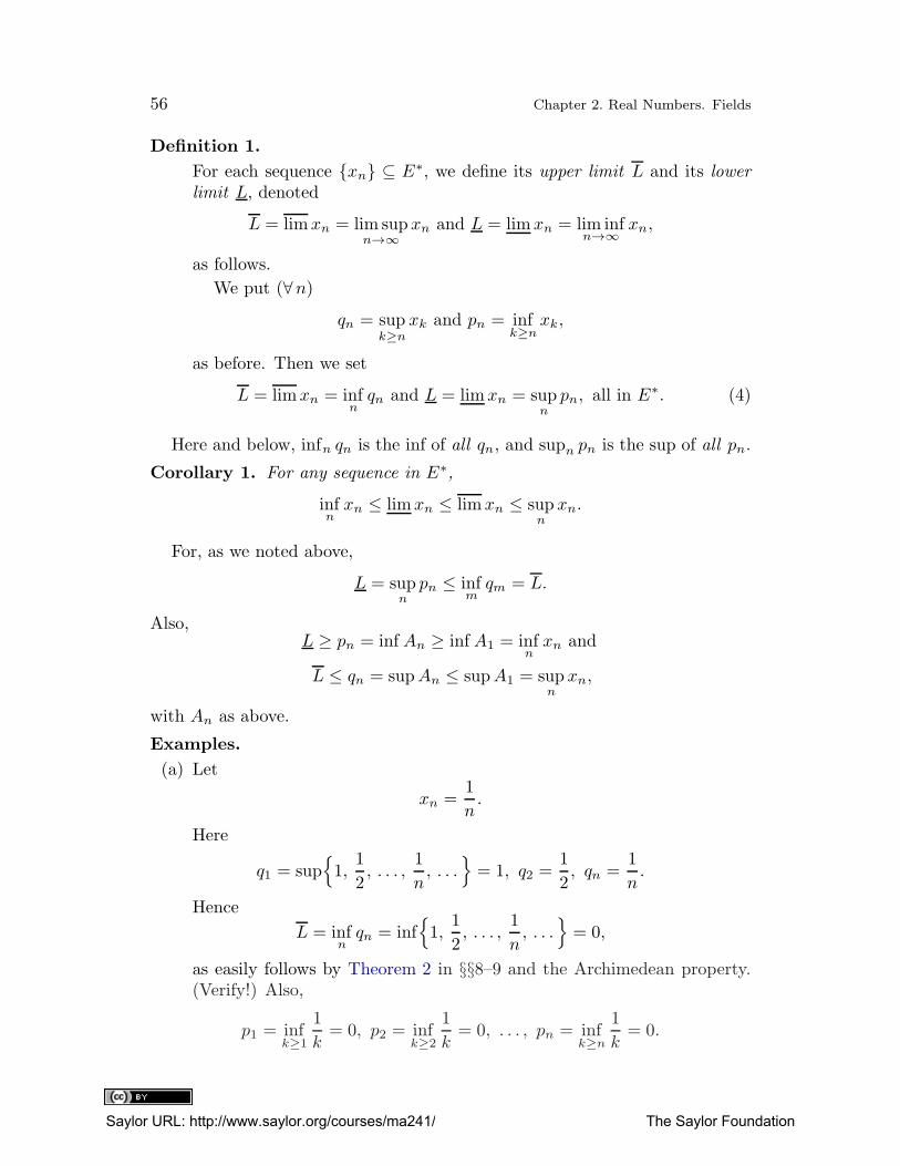
56 Chapter 2. Real Numbers. Fields
Definition 1.
For each sequence {xn} ⊆ E∗, we define its upper limit L and its lower
limit L, denoted
L = limxn = lim supn→∞
xn and L = limxn = lim infn→∞
xn,
as follows.
We put (∀n)qn = sup
k≥nxk and pn = inf
k≥nxk,
as before. Then we set
L = limxn = infnqn and L = limxn = sup
npn, all in E
∗. (4)
Here and below, infn qn is the inf of all qn, and supn pn is the sup of all pn.
Corollary 1. For any sequence in E∗,
infnxn ≤ limxn ≤ limxn ≤ sup
nxn.
For, as we noted above,
L = supnpn ≤ inf
mqm = L.
Also,L ≥ pn = inf An ≥ inf A1 = inf
nxn and
L ≤ qn = supAn ≤ supA1 = supnxn,
with An as above.
Examples.
(a) Let
xn =1
n.
Here
q1 = sup{
1,1
2, . . . ,
1
n, . . .
}
= 1, q2 =1
2, qn =
1
n.
Hence
L = infnqn = inf
{
1,1
2, . . . ,
1
n, . . .
}
= 0,
as easily follows by Theorem 2 in §§8–9 and the Archimedean property.(Verify!) Also,
p1 = infk≥1
1
k= 0, p2 = inf
k≥2
1
k= 0, . . . , pn = inf
k≥n
1
k= 0.
Saylor URL: http://www.saylor.org/courses/ma241/ The Saylor Foundation
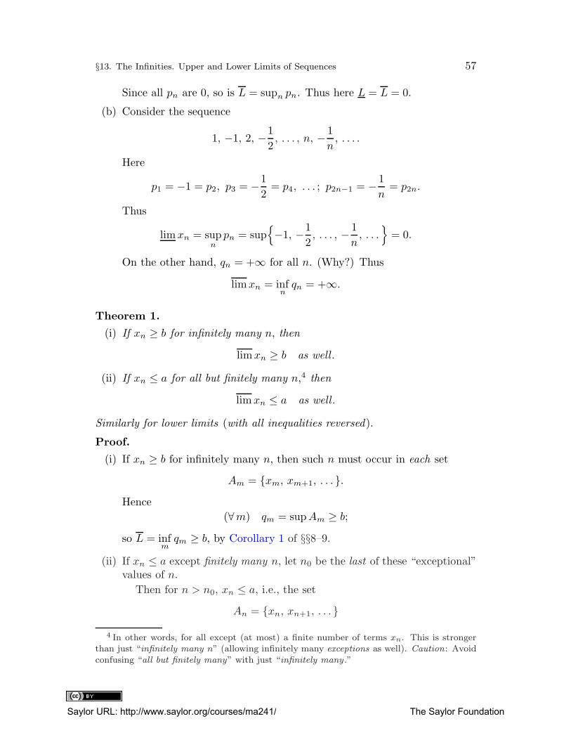
§13. The Infinities. Upper and Lower Limits of Sequences 57
Since all pn are 0, so is L = supn pn. Thus here L = L = 0.
(b) Consider the sequence
1, −1, 2, −1
2, . . . , n, − 1
n, . . . .
Here
p1 = −1 = p2, p3 = −1
2= p4, . . . ; p2n−1 = − 1
n= p2n.
Thus
limxn = supnpn = sup
{
−1, −1
2, . . . , − 1
n, . . .
}
= 0.
On the other hand, qn = +∞ for all n. (Why?) Thus
limxn = infnqn = +∞.
Theorem 1.
(i) If xn ≥ b for infinitely many n, then
limxn ≥ b as well .
(ii) If xn ≤ a for all but finitely many n,4 then
limxn ≤ a as well .
Similarly for lower limits (with all inequalities reversed).
Proof.
(i) If xn ≥ b for infinitely many n, then such n must occur in each set
Am = {xm, xm+1, . . . }.Hence
(∀m) qm = supAm ≥ b;
so L = infmqm ≥ b, by Corollary 1 of §§8–9.
(ii) If xn ≤ a except finitely many n, let n0 be the last of these “exceptional”values of n.
Then for n > n0, xn ≤ a, i.e., the set
An = {xn, xn+1, . . . }
4 In other words, for all except (at most) a finite number of terms xn. This is strongerthan just “infinitely many n” (allowing infinitely many exceptions as well). Caution: Avoid
confusing “all but finitely many” with just “infinitely many .”
Saylor URL: http://www.saylor.org/courses/ma241/ The Saylor Foundation
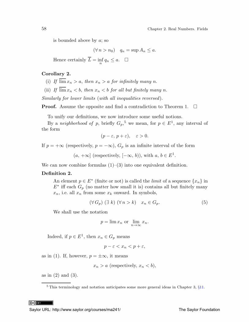
58 Chapter 2. Real Numbers. Fields
is bounded above by a; so
(∀n > n0) qn = supAn ≤ a.
Hence certainly L = infnqn ≤ a. �
Corollary 2.
(i) If limxn > a, then xn > a for infinitely many n.
(ii) If limxn < b, then xn < b for all but finitely many n.
Similarly for lower limits (with all inequalities reversed).
Proof. Assume the opposite and find a contradiction to Theorem 1. �
To unify our definitions, we now introduce some useful notions.
By a neighborhood of p, briefly Gp,5 we mean, for p ∈ E1, any interval of
the form
(p− ε, p+ ε), ε > 0.
If p = +∞ (respectively, p = −∞), Gp is an infinite interval of the form
(a, +∞] (respectively, [−∞, b)), with a, b ∈ E1.
We can now combine formulas (1)–(3) into one equivalent definition.
Definition 2.
An element p ∈ E∗ (finite or not) is called the limit of a sequence {xn} inE∗ iff each Gp (no matter how small it is) contains all but finitely manyxn, i.e. all xn from some xk onward. In symbols,
(∀Gp) (∃ k) (∀n > k) xn ∈ Gp. (5)
We shall use the notation
p = limxn or limn→∞
xn.
Indeed, if p ∈ E1, then xn ∈ Gp means
p− ε < xn < p+ ε,
as in (1). If, however, p = ±∞, it means
xn > a (respectively, xn < b),
as in (2) and (3).
5 This terminology and notation anticipates some more general ideas in Chapter 3, §11.
Saylor URL: http://www.saylor.org/courses/ma241/ The Saylor Foundation
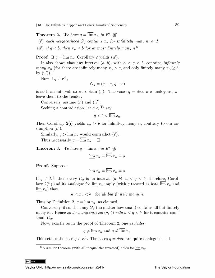
§13. The Infinities. Upper and Lower Limits of Sequences 59
Theorem 2. We have q = limxn in E∗ iff
(i′) each neighborhood Gq contains xn for infinitely many n, and
(ii′) if q < b, then xn ≥ b for at most finitely many n.6
Proof. If q = limxn, Corollary 2 yields (ii′).
It also shows that any interval (a, b), with a < q < b, contains infinitely
many xn (for there are infinitely many xn > a, and only finitely many xn ≥ b,by (ii′)).
Now if q ∈ E1,Gq = (q − ε, q + ε)
is such an interval, so we obtain (i′). The cases q = ±∞ are analogous; weleave them to the reader.
Conversely, assume (i′) and (ii′).
Seeking a contradiction, let q < L; say,
q < b < limxn.
Then Corollary 2(i) yields xn > b for infinitely many n, contrary to our as-sumption (ii′).
Similarly, q > limxn would contradict (i′).
Thus necessarily q = limxn. �
Theorem 3. We have q = limxn in E∗ iff
limxn = limxn = q.
Proof. Supposelimxn = limxn = q.
If q ∈ E1, then every Gq is an interval (a, b), a < q < b; therefore, Corol-
lary 2(ii) and its analogue for limxn imply (with q treated as both limxn andlimxn) that
a < xn < b for all but finitely many n.
Thus by Definition 2, q = limxn, as claimed.
Conversely, if so, then any Gq (no matter how small) contains all but finitelymany xn. Hence so does any interval (a, b) with a < q < b, for it contains somesmall Gq.
Now, exactly as in the proof of Theorem 2, one excludes
q 6= limxn and q 6= limxn.
This settles the case q ∈ E1. The cases q = ±∞ are quite analogous. �
6 A similar theorem (with all inequalities reversed) holds for limxn.
Saylor URL: http://www.saylor.org/courses/ma241/ The Saylor Foundation
60 Chapter 2. Real Numbers. Fields
Problems on Upper and Lower Limits of Sequences in E∗
1. Complete the missing details in the proofs of Theorems 2 and 3, Corol-lary 1, and Examples (a) and (b).
2. State and prove the analogues of Theorems 1 and 2 and Corollary 2 forlimxn.
3. Find limxn and limxn if
(a) xn = c (constant);
(b) xn = −n;(c) xn = n; and
(d) xn = (−1)nn− n.Does limxn exist in each case?
⇒4. A sequence {xn} is said to cluster at q ∈ E∗, and q is called its clusterpoint , iff each Gq contains xn for infinitely many values of n.
Show that both L and L are cluster points (L the least and L thelargest).[Hint: Use Theorem 2 and its analogue for L.
To show that no p < L (or q > L) is a cluster point, assume the opposite and
find a contradiction to Corollary 2.]
⇒5. Prove that
(i) lim(−xn) = − limxn and
(ii) lim(axn) = a · limxn if 0 ≤ a < +∞.
6. Prove thatlimxn < +∞ (limxn > −∞)
iff {xn} is bounded above (below) in E1.
7. Prove that if {xn} and {yn} are bounded in E1, then
limxn + lim yn ≥ lim(xn + yn) ≥ limxn + lim yn
≥ lim(xn + yn) ≥ limxn + lim yn.
[Hint: Prove the first inequality and then use that and Problem 5(i) for the others.]
⇒8. Prove that if p = limxn in E1, then
lim(xn + yn) = p+ lim yn;
similarly for L.
⇒9. Prove that if {xn} is monotone, then limxn exists in E∗. Specifically,if {xn}↑, then
limxn = supnxn,
Saylor URL: http://www.saylor.org/courses/ma241/ The Saylor Foundation
§13. The Infinities. Upper and Lower Limits of Sequences 61
and if {xn}↓, thenlimxn = inf
nxn.
⇒10. Prove that
(i) if limxn = +∞ and (∀n) xn ≤ yn, then also lim yn = +∞, and
(ii) if limxn = −∞ and (∀n) yn ≤ xn, then also lim yn = −∞.
11. Prove that if xn ≤ yn for all n, then
limxn ≤ lim yn and limxn ≤ lim yn.
Saylor URL: http://www.saylor.org/courses/ma241/ The Saylor Foundation

Saylor URL: http://www.saylor.org/courses/ma241/ The Saylor Foundation
Chapter 3
Vector Spaces. Metric Spaces
§§1–3. The Euclidean n-Space, En
By definition, the Euclidean n-space En is the set of all possible ordered n-tuples of real numbers, i.e., the Cartesian product
E1 × E1 × · · · × E1 (n times).
In particular, E2 = E1 × E1 = {(x, y) | x, y ∈ E1},
E3 = E1 ×E1 ×E1 = {(x, y, z) | x, y, z ∈ E1},
and so on. E1 itself is a special case of En (n = 1).
In a familiar way, pairs (x, y) can be plotted as points of the xy-plane, oras “vectors” (directed line segments) joining (0, 0) to such points. Therefore,the pairs (x, y) themselves are called points or vectors in E2; similarly for E3.
In En (n > 3), there is no actual geometric representation, but it is con-venient to use geometric language in this case, too. Thus any ordered n-tuple(x1, x2, . . . , xn) of real numbers will also be called a point or vector in En, andthe single numbers x1, x2, . . . , xn are called its coordinates or components . Apoint in En is often denoted by a single letter (preferably with a bar or anarrow above it), and then its n components are denoted by the same letter,with subscripts (but without the bar or arrow). For example,
x = (x1, . . . , xn), ~u = (u1, . . . , un), etc.;
x = (0, −1, 2, 4) is a point (vector) in E4 with coordinates 0, −1, 2, and 4(in this order). The formula x ∈ En means that x = (x1, . . . , xn) is a point(vector) in En. Since such “points” are ordered n-tuples, x and y are equal(x = y) iff the corresponding coordinates are the same, i.e., x1 = y1, x2 = y2,. . . , xn = yn (see Problem 1 below).
The point whose coordinates are all 0 is called the zero-vector or the origin,denoted~0 or 0. The vector whose kth component is 1, and the other components
Saylor URL: http://www.saylor.org/courses/ma241/ The Saylor Foundation
64 Chapter 3. Vector Spaces. Metric Spaces
are 0, is called the kth basic unit vector , denoted ~ek. There are exactly n suchvectors,
~e1 = (1, 0, 0, . . . , 0), ~e2 = (0, 1, 0, . . . , 0), . . . , ~en = (0, . . . , 0, 1).
In E3, we often write i, j, and k for ~e1, ~e2, ~e3, and (x, y, z) for (x1, x2, x3).Similarly in E2. Single real numbers are called scalars (as opposed to vectors).
Definitions.
Given x = (x1, . . . , xn) and y = (y1, . . . , yn) in En, we define the fol-lowing.
1. The sum of x and y,
x+ y = (x1 + y1, x2 + y2, . . . , xn + yn) (hence x+ 0 = x).1
2. The dot product , or inner product , of x and y,
x · y = x1y1 + x2y2 + · · ·+ xnyn.
3. The distance between x and y,
ρ(x, y) =√
(x1 − y1)2 + (x2 − y2)2 + · · ·+ (xn − yn)2 .
4. The absolute value, or length, of x,
|x| =√
x21 + x22 + · · ·+ x2n = ρ(x, 0) =√x · x
(three formulas that are all equal by Definitions 2 and 3).
5. The inverse of x,
−x = (−x1, −x2, . . . , −xn).
6. The product of x by a scalar c ∈ E1,
cx = xc = (cx1, cx2, . . . , cxn);
in particular, (−1)x = (−x1, −x2, . . . , −xn) = −x, 1x = x, and 0x = 0.
7. The difference of x and y,
x− y =−→yx = (x1 − y1, x2 − y2, . . . , xn − yn).
In particular, x− 0 = x and 0− x = −x. (Verify!)
Note 1. Definitions 2–4 yield scalars, while the rest are vectors.
Note 2. We shall not define inequalities (<) in En (n ≥ 2), nor shallwe define vector products other than the dot product (2), which is a scalar .(However, cf. §8.)
1 Sums of three or more vectors are defined by induction, as in Chapter 2, §§5–6.
Saylor URL: http://www.saylor.org/courses/ma241/ The Saylor Foundation
§§1–3. The Euclidean n-Space, En 65
Note 3. From Definitions 3, 4, and 7, we obtain ρ(x, y) = |x− y|. (Verify!)Note 4. We often write x/c for (1/c)x, where c ∈ E1, c 6= 0.
Note 5. In E1, x = (x1) = x1. Thus, by Definition 4,
|x| =√
x21 = |x1|,
where |x1| is defined as in Chapter 2, §§1–4, Definition 4. Thus the two defini-tions agree.
We call x a unit vector iff its length is 1, i.e., |x| = 1. Note that if x 6= 0,then x/|x| is a unit vector, since
∣
∣
∣
x
|x|∣
∣
∣=
√
x21|x|2 + · · ·+ x2n
|x|2 = 1.
The vectors x and y are said to be orthogonal or perpendicular (x ⊥ y) iffx · y = 0 and parallel (x ‖ y) iff x = ty or y = tx for some t ∈ E1. Note thatx ⊥ 0 and x ‖ 0.Examples.
If x = (0, −1, 4, 2) and y = (2, 2, −3, 2) are vectors in E4, then
x+ y = (2, 1, 1, 4);
x− y = (−2, −3, 7, 0);ρ(x, y) = |x− y| =
√
22 + 32 + 72 + 02 =√62 ;
(x+ y) · (x− y) = 2(−2) + 1(−3) + 7 + 0 = 0.
So (x+ y) ⊥ (x− y) here.
Theorem 1. For any vectors x, y, and z ∈ En and any a, b ∈ E1, we have
(a) x+ y and ax are vectors in En (closure laws);
(b) x+ y = y + x (commutativity of vector addition);
(c) (x+ y) + z = x+ (y + z) (associativity of vector addition);
(d) x+ 0 = 0 + x = x, i .e., 0 is the neutral element of addition;
(e) x+ (−x) = 0, i .e., −x is the additive inverse of x;
(f) a(x+ y) = ax+ ay and (a+ b)x = ax+ bx (distributive laws);
(g) (ab)x = a(bx);
(h) 1x = x.
Proof. Assertion (a) is immediate from Definitions 1 and 6. The rest followsfrom corresponding properties of real numbers.
Saylor URL: http://www.saylor.org/courses/ma241/ The Saylor Foundation
66 Chapter 3. Vector Spaces. Metric Spaces
For example, to prove (b), let x = (x1, . . . , xn), y = (y1, . . . , yn). Then bydefinition, we have
x+ y = (x1 + y1, . . . , xn + yn) and y + x = (y1 + x1, . . . , yn + xn).
The right sides in both expressions, however, coincide since addition is com-mutative in E1. Thus x+ y = y + x, as claimed; similarly for the rest, whichwe leave to the reader. �
Theorem 2. If x = (x1, . . . , xn) is a vector in En, then, with ek as above,
x = x1e1 + x2e2 + · · ·+ xnen =n∑
k=1
xkek.
Moreover, if x =∑n
k=1 akek for some ak ∈ E1, then necessarily ak = xk,k = 1, . . . , n.
Proof. By definition,
e1 = (1, 0, . . . , 0), e2 = (0, 1, . . . , 0), . . . , en = (0, 0, . . . , 1).
Thus
x1e1 = (x1, 0, . . . , 0), x2e2 = (0, x2, . . . , 0), . . . , xnen = (0, 0, . . . , xn).
Adding up componentwise, we obtain
n∑
k=1
xkek = (x1, x2, . . . , xn) = x,
as asserted.
Moreover, if the xk are replaced by any other ak ∈ E1, the same processyields
(a1, . . . , an) = x = (x1, . . . , xn),
i.e., the two n-tuples coincide, whence ak = xk, k = 1, . . . , n. �
Note 6. Any sum of the form
m∑
k=1
akxk (ak ∈ E1, xk ∈ En)
is called a linear combination of the vectors xk (whose number m is arbitrary).Thus Theorem 2 shows that any x ∈ En can be expressed, in a unique way, as
a linear combination of the n basic unit vectors. In E3, we write
x = x1i+ x2j + x3k.
Saylor URL: http://www.saylor.org/courses/ma241/ The Saylor Foundation
§§1–3. The Euclidean n-Space, En 67
Note 7. If, as above, some vectors are numbered (e.g., x1, x2, . . . , xm),we denote their components by attaching a second subscript; for example, thecomponents of x1 are x11, x12, . . . , x1n.
Theorem 3. For any vectors x, y, and z ∈ En and any a, b ∈ E1, we have
(a) x · x ≥ 0, and x · x > 0 iff x 6= 0;
(b) (ax) · (by) = (ab)(x · y);(c) x · y = y · x (commutativity of inner products);
(d) (x+ y) · z = x · z + y · z (distributive law).
Proof. To prove these properties, express all in terms of the components of x,y, and z, and proceed as in Theorem 1. �
Note that (b) implies x · 0 = 0 (put a = 1, b = 0).
Theorem 4. For any vectors x and y ∈ En and any a ∈ E1, we have the
following properties:
(a′) |x| ≥ 0, and |x| > 0 iff x 6= 0.
(b′) |ax| = |a||x|.(c′) |x · y| ≤ |x| |y|, or , in components,
( n∑
k=1
xkyk
)2
≤( n∑
k=1
x2k
)( n∑
k=1
y2k
)
(Cauchy–Schwarz inequality).
Equality , |x · y| = |x| |y|, holds iff x ‖ y.(d′) |x+ y| ≤ |x|+ |y| and
∣
∣|x| − |y|∣
∣ ≤ |x− y| (triangle inequalities).
Proof. Property (a′) follows from Theorem 3(a) since
|x|2 = x · x (see Definition 4).
For (b′), use Theorem 3(b), to obtain
(ax) · (ax) = a2(x · x) = a2|x|2.By Definition 4, however,
(ax) · (ax) = |ax|2.Thus
|ax|2 = a2|x|2
so that |ax| = |a||x|, as claimed.
Now we prove (c′). If x ‖ y then x = ty or y = tx; so |x · y| = |x||y| followsby (b′). (Verify!)
Saylor URL: http://www.saylor.org/courses/ma241/ The Saylor Foundation
68 Chapter 3. Vector Spaces. Metric Spaces
Otherwise, x 6= ty and y 6= tx for all t ∈ E1. Then we obtain, for all t ∈ E1,
0 6= |tx− y|2 =n∑
k=1
(txk − yk)2 = t2n∑
k=1
x2k − 2tn∑
k=1
xkyk +n∑
k=1
y2k.
Thus, setting
A =
n∑
k=1
x2k, B = 2
n∑
k=1
xkyk, and C =
n∑
k=1
y2k,
we see that the quadratic equation
0 = At2 −Bt+ C
has no real solutions in t, so its discriminant, B2−4AC, must be negative; i.e.,
4
( n∑
k=1
xkyk
)2
− 4
( n∑
k=1
x2k
)( n∑
k=1
y2k
)
< 0,
proving (c′).
To prove (d′), use Definition 2 and Theorem 3(d), to obtain
|x+ y|2 = (x+ y) · (x+ y) = x · x+ y · y + 2x · y = |x|2 + |y|2 + 2x · y.But x · y ≤ |x| |y| by (c′). Thus we have
|x+ y|2 ≤ |x|2 + |y|2 + 2|x| |y| = (|x|+ |y|)2,whence |x+ y| ≤ |x|+ |y|, as required.
Finally, replacing here x by x− y, we have
|x− y|+ |y| ≥ |x− y + y| = |x|, or |x− y| ≥ |x| − |y|.Similarly, replacing y by y − x, we get |x− y| ≥ |y| − |x|. Hence
|x− y| ≥ ±(
|x| − |y|)
,
i.e., |x− y| ≥∣
∣|x| − |y|∣
∣, proving the second formula in (d′). �
Theorem 5. For any points x, y, and z ∈ En, we have
(i) ρ(x, y) ≥ 0, and ρ(x, y) = 0 iff x = y;
(ii) ρ(x, y) = ρ(y, x);
(iii) ρ(x, z) ≤ ρ(x, y) + ρ(y, z) (triangle inequality).
Proof.
(i) By Definition 3 and Note 3, ρ(x, y) = |x−y|; therefore, by Theorem 4(a′),ρ(x, y) = |x− y| ≥ 0.
Also, |x − y| > 0 iff x − y 6= 0, i.e., iff x 6= y. Hence ρ(x, y) 6= 0 iffx 6= y, and assertion (i) follows.
Saylor URL: http://www.saylor.org/courses/ma241/ The Saylor Foundation
§§1–3. The Euclidean n-Space, En 69
(ii) By Theorem 4(b′), |x− y| = |(−1)(y − x)| = |y − x|, so (ii) follows.
(iii) By Theorem 4(d′),
ρ(x, y) + ρ(y, z) = |x− y|+ |y − z| ≥ |x− y + y − z| = ρ(x, z). �
Note 8. We also have |ρ(x, y) − ρ(z, y)| ≤ ρ(x, z). (Prove it!) The twotriangle inequalities have a simple geometric interpretation (which explainstheir name). If x, y, and z are treated as the vertices of a triangle, we obtainthat the length of a side, ρ(x, z) never exceeds the sum of the two other sidesand is never less than their difference.
As E1 is a special case of En (in which “vectors” are single numbers), allour theory applies to E1 as well. In particular, distances in E1 are defined byρ(x, y) = |x − y| and obey the three laws of Theorem 5. Dot products in E1
become ordinary products xy. (Why?) From Theorems 4(b′)(d′), we have
|a| |x| = |ax|; |x+ y| ≤ |x|+ |y|; |x− y| ≥∣
∣|x| − |y|∣
∣ (a, x, y ∈ E1).
Problems on Vectors in En
1. Prove by induction on n that
(x1, x2, . . . , xn) = (y1, y2, . . . , yn) iff xk = yk, k = 1, 2, . . . , n.
[Hint: Use Problem 6(ii) of Chapter 1, §§1–3, and Example (i) in Chapter 2, §§5-6.]
2. Complete the proofs of Theorems 1 and 3 and Notes 3 and 8.
3. Given x = (−1, 2, 0, −7), y = (0, 0, −1, −2), and z = (2, 4, −3, −3)in E4, express x, y, and z as linear combinations of the basic unitvectors. Also, compute their absolute values, their inverses, as well astheir mutual sums, differences, dot products, and distances. Are any ofthem orthogonal? Parallel?
4. With x, y, and z as in Problem 3, find scalars a, b, and c such that
ax+ by + cz = u,
when(i) u = e1; (ii) u = e3;
(iii) u = (−2, 4, 0, 1); (iv) u = 0.
5. A finite set of vectors x, x2, . . . , xm is said to be dependent iff there arescalars a1, . . . , am, not all zero, such that
m∑
k=1
akxk = 0,
Saylor URL: http://www.saylor.org/courses/ma241/ The Saylor Foundation
70 Chapter 3. Vector Spaces. Metric Spaces
and independent otherwise. Prove the independence of the followingsets of vectors:
(a) e1, e2, . . . , en in En;
(b) (1, 2, −3, 4) and (2, 3, 0, 0) in E4;
(c) (2, 0, 0), (4, −1, 3), and (0, 4, 1) in E3;
(d) the vectors x, y, and z of Problem 3.
6. Prove (for E2 and E3) that
x · y = |x| |y| cosα,
where α is the angle between the vectors−→0x and
−→0y ; we denote α by
〈x, y〉.[Hint: Consider the triangle 0xy, with sides x =
−→0x , y =
−→0y , and
−→xy = ~y − ~x (see
Definition 7). By the law of cosines,
|~x|2 + |~y|2 − 2|~x| |~y| cosα = |~y − ~x|2.
Now substitute |~x|2 = ~x · ~x, |~y|2 = ~y · ~y, and
|~y − ~x|2 = (~y − ~x) · (~y − ~x) = ~y · ~y + ~x · ~x− 2~x · ~y. (Why?)
Then simplify.]
7. Motivated by Problem 6, define in En
〈x, y〉 = arccosx · y|x| |y| if x and y are nonzero.
(Why does an angle with such a cosine exist?) Prove that
(i) x ⊥ y iff cos〈x, y〉 = 0, i.e., 〈x, y〉 = π
2;
(ii)n∑
k=1
cos2〈x, ek〉 = 1.
8. Continuing Problems 3 and 7, find the cosines of the angles between
the sides ,−→xy ,
−→yz , and
−→zx of the triangle xyz, with x, y, and z as in
Problem 3.
9. Find a unit vector in E4, with positive components, that forms equalangles with the axes, i.e., with the basic unit vectors (see Problem 7).
10. Prove for En that if u is orthogonal to each of the basic unit vectors e1,e2, . . . , en, then u = 0. Deduce that
u = 0 iff (∀ x ∈ En) x · u = 0.
Saylor URL: http://www.saylor.org/courses/ma241/ The Saylor Foundation
§§1–3. The Euclidean n-Space, En 71
11. Prove that x and y are parallel iff
x1y1
=x2y2
= · · · = xnyn
= c (c ∈ E1),
where “xk/yk = c” is to be replaced by “xk = 0” if yk = 0.
12. Use induction on n to prove the Lagrange identity (valid in any field),
( n∑
k=1
x2k
)( n∑
k=1
y2k
)
−( n∑
k=1
xkyk
)2
=∑
1≤i<k≤n
(xiyk − xkyi)2.
Hence find a new proof of Theorem 4(c′).
13. Use Problem 7 and Theorem 4(c′) (“equality”) to show that two nonzerovectors x and y in En are parallel iff cos〈x, y〉 = ±1.
14. (i) Prove that |x+ y| = |x| + |y| iff x = ty or y = tx for some t ≥ 0;equivalently, iff cos〈x, y〉 = 1 (see Problem 7).
(ii) Find similar conditions for |x− y| = |x|+ |y|.[Hint: Look at the proof of Theorem 4(d′).]
§§4–6. Lines and Planes in En
I. To obtain a line in E2 or E3 passing through two points a and b, we takethe vector
~u =−→ab = b− a
and, so to say, “stretch” it indefinitely in both directions, i.e., multiply ~u byall possible scalars t ∈ E1. Then the set of all points x of the form
x = a+ t~u
is the required line. It is natural to adopt this as a definition in En as well.Below, a 6= b.
Definition 1.
The line ab through the points a, b ∈ En (also called the line through a,in the direction of the vector ~u = b− a) is the set of all points x ∈ En ofthe form
x = a+ t~u = a+ t(b− a),where t varies over E1. We call t a variable real parameter and ~u adirection vector for ab. Thus
Line ab = {x ∈ En | x = a+ t~u for some t ∈ E1}, ~u = b− a 6= 0. (1)
Saylor URL: http://www.saylor.org/courses/ma241/ The Saylor Foundation
72 Chapter 3. Vector Spaces. Metric Spaces
The formula
x = a+ t~u, or x = a+ t(b− a),
is called the parametric equation of the line. (We briefly say “the line x =a + t~u.”) It is equivalent to n simultaneous equations in terms of coordinates ,namely,
xk = ak + tuk = ak + t(bk − ak), k = 1, 2, . . . , n. (2)
Note 1. As the vector ~u is anyway being multiplied by all real numbers t,the line (as a set of points) will not change if ~u is replaced by some c~u (c ∈ E1,c 6= 0). In particular, taking c = 1/|~u|, we may replace ~u by ~u/|~u|, a unit
vector . We may as well assume that ~u is a unit vector itself.
If we let t vary not over all of E1 but only over some interval in E1, we obtainwhat is called a line segment .1 In particular, we define the open line segment
L(a, b), the closed line segment L[a, b], the half-open line segment L(a, b], andthe half-closed line segment L[a, b), as we did for E1.
Definition 2.
Given ~u = b− a, we set
(i) L(a, b) = {a+ t~u | 0 < t < 1};2 (ii) L[a, b] = {a+ t~u | 0 ≤ t ≤ 1};(iii) L(a, b] = {a+ t~u | 0 < t ≤ 1}; (iv) L[a, b) = {a+ t~u | 0 ≤ t < 1};
In all cases, a and b are called the endpoints of the segment; ρ(a, b) =|b− a| is its length; and 1
2(a+ b) is its midpoint .
Note that in E1, line segments simply become intervals , (a, b), [a, b], etc.
II. To describe a plane in E3, we fix one of its points, a, and a vector
~u =→ab perpendicular to the plane (imagine a vertical pencil standing at a on
the horizontal plane of the table). Then a point x lies on the plane iff ~u ⊥ −→ax .
It is natural to accept this as a definition in En as well.
Definition 3.
Given a point a ∈ En and a vector ~u 6= ~0, we define the plane (also calledhyperplane if n > 3) through a, orthogonal to ~u, to be the set of all x ∈ En
such that ~u ⊥ −→ax , i.e., ~u · (x− a) = 0, or, in terms of components,
n∑
k=1
uk(xk − ak) = 0, where ~u 6= ~0 (i.e., not all values uk are 0). (3)
1 We reserve the name “interval” for other kinds of sets (cf. §7).2 This is an abbreviation for “{x ∈ En | x = a+ t~u for some t ∈ E1, 0 < t < 1}.”
Saylor URL: http://www.saylor.org/courses/ma241/ The Saylor Foundation
§§4–6. Lines and Planes in En 73
We briefly say
“the plane ~u · (x− a) = 0” or “the plane
n∑
k=1
uk(xk − ak) = 0”
(this being the equation of the plane). Removing brackets in (3), we have
u1x2 + u2x2 + · · ·+ unxn = c, or ~u · x = c, where c =
n∑
k−1
ukak, ~u 6= ~0. (4)
An equation of this form is said to be linear in x1, x2, . . . , xn.
Theorem 1. A set A ⊆ En is a plane (hyperplane) iff A is exactly the set of
all x ∈ En satisfying (4) for some fixed c ∈ E1 and ~u = (u1, . . . , un) 6= 0.
Proof. Indeed, as we saw above, each plane has an equation of the form (4).Conversely, any equation of that form (with, say, u1 6= 0) can be written as
u1
(
x1 −c
u1
)
+ u2x2 + u3x3 + · · ·+ unxn = 0.
Then, setting a1 = c/u1 and ak = 0 for k ≥ 2, we transform it into (3), which is,by definition, the equation of a plane through a = (c/u1, 0, . . . , 0), orthogonalto ~u = (u1, . . . , un). �
Thus, briefly, planes are exactly all sets with linear equations (4). In thisconnection, equation (4) is called the general equation of a plane. The vector ~uis said to be normal to the plane. Clearly, if both sides of (4) are multiplied bya nonzero scalar q, one obtains an equivalent equation (representing the same
set). Thus we may replace uk by quk, i.e., ~u by q~u, without affecting the plane.In particular, we may replace ~u by the unit vector ~u/|~u|, as in lines (this iscalled the normalization of the equation). Thus
~u
|~u| · (x− a) = 0 (5)
and
x = a+ t~u
|~u| (6)
are the normalized (or normal) equations of the plane (3) and line (1), respec-tively.
Note 2. The equation xk = c (for a fixed k) represents a plane orthogonal
to the basic unit vector ~ek or, as we shall say, to the kth axis . The equationresults from (4) if we take ~u = ~ek so that uk = 1, while ui = 0 (i 6= k). Forexample, x1 = c is the equation of a plane orthogonal to ~e1; it consists of allx ∈ En, with x1 = c (while the other coordinates of x are arbitrary). In E2, itis a line. In E1, it consists of c alone.
Saylor URL: http://www.saylor.org/courses/ma241/ The Saylor Foundation
74 Chapter 3. Vector Spaces. Metric Spaces
Two planes (respectively, two lines) are said to be perpendicular to eachother iff their normal vectors (respectively, direction vectors) are orthogonal;similarly for parallelism. A plane ~u · x = c is said to be perpendicular to a line
x = a+ t~v iff ~u ‖ ~v; the line and the plane are parallel iff ~u ⊥ ~v.Note 3. When normalizing, as in (5) or (6), we actually have two choices
of a unit vector, namely, ±~u/|~u|. If one of them is prescribed , we speak of adirected plane (respectively, line).
Examples.
(a) Let a = (0, −1, 2), b = (1, 1, 1), and c = (3, 1, −1) in E3. Then the lineab has the parametric equation x = a+t(b− a) or, in coordinates, writingx, y, z for x1, x2, x3,
x = 0 + t(1− 0) = t, y = −1 + 2t, z = 2− t.
This may be rewritten
t =x
1=y + 1
2=z − 2
−1 ,
where ~u = (1, 2, −1) is the direction vector (composed of the denomina-tors). Normalizing and dropping t, we have
x
1/√6=y + 1
2/√6=
z − 2
−1/√6
(the so-called symmetric form of the normal equations).
Similarly, for the line bc, we obtain
t =x− 1
2=y − 1
0=z − 1
−2 ,
where “t = (y − 1)/0” stands for “y−1 = 0.” (It is customary to use thisnotation.)
(b) Let a = (1, −2, 0, 3) and ~u = (1, 1, 1, 1) in E4. Then the plane normalto ~u through a has the equation (x− a) · ~u = 0, or
(x1 − 1) · 1 + (x2 + 2) · 1 + (x3 − 0) · 1 + (x4 − 3) · 1 = 0,
or x1 + x2 + x3 + x4 = 2. Observe that, by formula (4), the coeffi-cients of x1, x2, x3, x4 are the components of the normal vector ~u (here(1, 1, 1, 1)).
Now define a map f : E4 → E1 setting f(x) = x1 + x2 + x3 + x4 (theleft-hand side of the equation). This map is called the linear functional
corresponding to the given plane. (For another approach, see Problems 4–6 below.)
Saylor URL: http://www.saylor.org/courses/ma241/ The Saylor Foundation
§§4–6. Lines and Planes in En 75
(c) The equation x+3y−2z = 1 represents a plane in E3, with ~u = (1, 3, −2).The point a = (1, 0, 0) lies on the plane (why?), so the plane equationmay be written (x− a) · ~u = 0 or x · ~u = 1, where x = (x, y, z) and a and~u are as above.
Problems on Lines and Planes in En
1. Let a = (−1, 2, 0, −7), b = (0, 0, −1, 2), and c = (2, 4, −3, −3) bepoints in E4. Find the symmetric normal equations (see Example (a)) ofthe lines ab, bc, and ca. Are any two of the lines perpendicular? Parallel?On the line ab, find some points inside L(a, b) and some outside L[a, b].Also, find the symmetric equations of the line through c that is
(i) parallel to ab; (ii) perpendicular to ab.
2. With a and b as in Problem 1, find the equations of the two planes thattrisect, and are perpendicular to, the line segment L[a, b].
3. Given a line x = a+ t~u (~u = b− a 6= ~0) in En, define f : E1 → En by
f(t) = a+ t~u for t ∈ E1.
Show that L[a, b] is exactly the f -image of the interval [0, 1] in E1, withf(0) = a and f(1) = b, while f [E1] is the entire line. Also show that fis one to one.[Hint: t 6= t′ implies |f(t)− f(t′)| 6= 0. Why?]
4. A map f : En → E1 is called a linear functional iff
(∀ x, y ∈ En) (∀ a, b ∈ E1) f(ax+ by) = af(x) + bf(y).
Show by induction that f preserves linear combinations; that is,
f
( m∑
k=1
akxk
)
=m∑
k=1
akf(xk)
for any ak ∈ E1 and xk ∈ En.
5. From Problem 4 prove that a map f : En → E1 is a linear functional iffthere is ~u ∈ En such that
(∀ x ∈ En) f(x) = ~u · x (“representation theorem”).
[Hint: If f is a linear functional, write each x ∈ En as x =∑n
k=1 xk ek (§§1–3,Theorem 2). Then
f(x) = f
( m∑
k=1
xkek
)
=n∑
k=1
xkf(ek).
Setting uk = f(ek) ∈ E1 and ~u = (u1, . . . , un), obtain f(x) = ~u · x, as required. Forthe converse, use Theorem 3 in §§1–3.]
Saylor URL: http://www.saylor.org/courses/ma241/ The Saylor Foundation
76 Chapter 3. Vector Spaces. Metric Spaces
6. Prove that a set A ⊆ En is a plane iff there is a linear functional f(Problem 4), not identically zero, and some c ∈ E1 such that
A = {x ∈ En | f(x) = c}.(This could serve as a definition of planes in En.)[Hint: A is a plane iff A = {x | ~u · x = c}. Put f(x) = ~u · x and use Problem 5. Show
that f 6≡ 0 iff ~u 6= ~0 by Problem 10 of §§1–3.]
7. Prove that the perpendicular distance of a point p to a plane ~u · x = cin En is
ρ(p, x0) =|~u · p− c||~u| .
(x0 is the orthogonal projection of p, i.e., the point on the plane such
that−→px0 ‖ ~u.)
[Hint: Put ~v = ~u/|~u|. Consider the line x = p + t~v. Find t for which p + t~v lies on
both the line and plane. Find |t|.]
8. A globe (solid sphere) in En, with center p and radius ε > 0, is the set{x | ρ(x, p) < ε}, denoted Gp(ε). Prove that if a, b ∈ Gp(ε), then alsoL[a, b] ⊆ Gp(ε). Disprove it for the sphere Sp(ε) = {x | ρ(x, p) = ε}.[Hint: Take a line through p.]
§7. Intervals in En
0
Y
X
a p
bq
a1 b1c
a2
b2
P Q
Figure 2
Consider the rectangle in E2 shownin Figure 2. Its interior (withoutthe perimeter) consists of all points(x, y) ∈ E2 such that
a1 < x < b1 and a2 < y < b2;
i.e.,
x ∈ (a1, b1) and y ∈ (a2, b2).
Thus it is the Cartesian product of
two line intervals , (a1, b1) and (a2, b2). To include also all or some sides,we would have to replace open intervals by closed, half-closed, or half-openones. Similarly, Cartesian products of three line intervals yield rectangularparallelepipeds in E3. We call such sets in En intervals .
Definitions.
1. By an interval in En we mean the Cartesian product of any n intervalsin E1 (some may be open, some closed or half-open, etc.).
Saylor URL: http://www.saylor.org/courses/ma241/ The Saylor Foundation
§7. Intervals in En 77
2. In particular, given
a = (a1, . . . , an) and b = (b1, . . . , bn)
with
ak ≤ bk, k = 1, 2, . . . , n,
we define the open interval (a, b), the closed interval [a, b], the half-open
interval (a, b], and the half-closed interval [a, b) as follows:
(a, b) = {x | ak < xk < bk, k = 1, 2, . . . , n}= (a1, b1)× (a2, b2)× · · · × (an, bn);
[a, b] = {x | ak ≤ xk ≤ bk, k = 1, 2, . . . , n}= [a1, b1]× [a2, b2]× · · · × [an, bn];
(a, b] = {x | ak < xk ≤ bk, k = 1, 2, . . . , n}= (a1, b1]× (a2, b2]× · · · × (an, bn];
[a, b) = {x | ak ≤ xk < bk, k = 1, 2, . . . , n}= [a1, b1)× [a2, b2)× · · · × [an, bn).
In all cases, a and b are called the endpoints of the interval. Their distance
ρ(a, b) = |b− a|
is called its diagonal . The n differences
bk − ak = ℓk (k = 1, . . . , n)
are called its n edge-lengths. Their product
n∏
k=1
ℓk =n∏
k=1
(bk − ak)
is called the volume of the interval (in E2 it is its area, in E1 its length). Thepoint
c =1
2(a+ b)
is called its center or midpoint . The set difference
[a, b]− (a, b)
is called the boundary of any interval with endpoints a and b; it consists of 2n“faces” defined in a natural manner. (How?)
We often denote intervals by single letters, e.g., A = (a, b), and write dA for“diagonal of A” and vA or volA for “volume of A.” If all edge-lengths bk − ak
Saylor URL: http://www.saylor.org/courses/ma241/ The Saylor Foundation
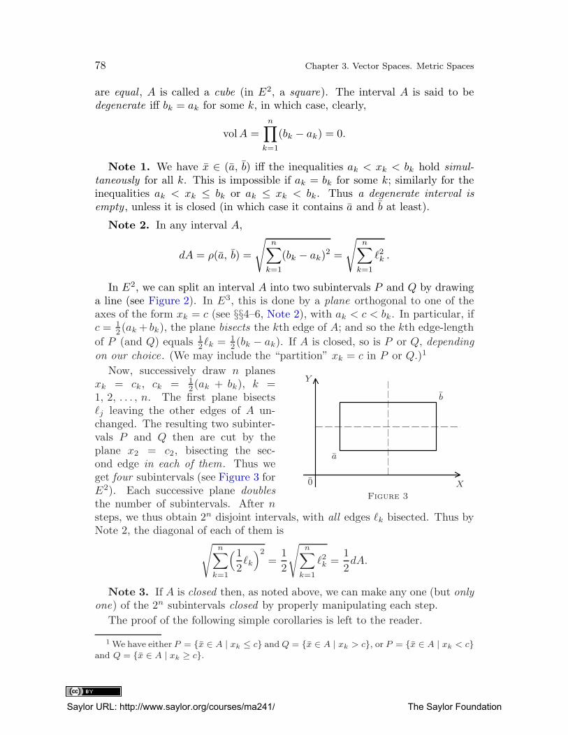
78 Chapter 3. Vector Spaces. Metric Spaces
are equal , A is called a cube (in E2, a square). The interval A is said to bedegenerate iff bk = ak for some k, in which case, clearly,
volA =n∏
k=1
(bk − ak) = 0.
Note 1. We have x ∈ (a, b) iff the inequalities ak < xk < bk hold simul-
taneously for all k. This is impossible if ak = bk for some k; similarly for theinequalities ak < xk ≤ bk or ak ≤ xk < bk. Thus a degenerate interval is
empty , unless it is closed (in which case it contains a and b at least).
Note 2. In any interval A,
dA = ρ(a, b) =
√
n∑
k=1
(bk − ak)2 =
√
n∑
k=1
ℓ2k .
In E2, we can split an interval A into two subintervals P and Q by drawinga line (see Figure 2). In E3, this is done by a plane orthogonal to one of theaxes of the form xk = c (see §§4–6, Note 2), with ak < c < bk. In particular, ifc = 1
2 (ak + bk), the plane bisects the kth edge of A; and so the kth edge-length
of P (and Q) equals 12ℓk = 1
2 (bk − ak). If A is closed, so is P or Q, depending
on our choice. (We may include the “partition” xk = c in P or Q.)1
a
b
0
Y
X
Figure 3
Now, successively draw n planesxk = ck, ck = 1
2(ak + bk), k =1, 2, . . . , n. The first plane bisectsℓj leaving the other edges of A un-changed. The resulting two subinter-vals P and Q then are cut by theplane x2 = c2, bisecting the sec-ond edge in each of them. Thus weget four subintervals (see Figure 3 forE2). Each successive plane doubles
the number of subintervals. After nsteps, we thus obtain 2n disjoint intervals, with all edges ℓk bisected. Thus byNote 2, the diagonal of each of them is
√
n∑
k=1
(1
2ℓk
)2
=1
2
√
n∑
k=1
ℓ2k =1
2dA.
Note 3. If A is closed then, as noted above, we can make any one (but onlyone) of the 2n subintervals closed by properly manipulating each step.
The proof of the following simple corollaries is left to the reader.
1 We have either P = {x ∈ A | xk ≤ c} and Q = {x ∈ A | xk > c}, or P = {x ∈ A | xk < c}and Q = {x ∈ A | xk ≥ c}.
Saylor URL: http://www.saylor.org/courses/ma241/ The Saylor Foundation
§7. Intervals in En 79
Corollary 1. No distance between two points of an interval A exceeds dA, itsdiagonal . That is , (∀ x, y ∈ A) ρ(x, y) ≤ dA.Corollary 2. If an interval A contains p and q, then also L[p, q] ⊆ A.Corollary 3. Every nondegenerate interval in En contains rational points ,i .e., points whose coordinates are all rational .
(Hint: Use the density of rationals in E1 for each coordinate separately.)
Problems on Intervals in En
(Here A and B denote intervals .)
1. Prove Corollaries 1–3.
2. Prove that if A ⊆ B, then dA ≤ dB and vA ≤ vB.
3. Give an appropriate definition of a “face” and a “vertex” of A.
4. Find the edge-lengths of A = (a, b) in E4 if
a = (1, −2, 4, 0) and b = (2, 0, 5, 3).
Is A a cube? Find some rational points in it. Find dA and vA.
5. Show that the sets P and Q as defined in footnote 1 are intervals , indeed.In particular, they can be made half-open (half-closed) if A is half-open(half-closed).[Hint: Let A = (a, b],
P = {x ∈ A | xk ≤ c}, and Q = {x ∈ A | xk > c}.
To fix ideas, let k = 1, i.e., cut the first edge. Then let
p = (c, a2, . . . , an) and q = (c, b2, . . . , bn) (see Figure 2),
and verify that P = (a, q] and Q = (p, b]. Give a proof.]
6. In Problem 5, assume that A is closed , and make Q closed. (Prove it!)
7. In Problem 5 show that (with k fixed) the kth edge-lengths of P and Qequal c− ak and bk − c, respectively, while for i 6= k the edge-length ℓiis the same in A, P , and Q, namely, ℓi = bi − ai.[Hint: If k = 1, define p and q as in Problem 5.]
8. Prove that if an interval A is split into subintervals P and Q (P∩Q = ∅),then vA = vP + vQ.[Hint: Use Problem 7 to compute vA, vP , and vQ. Add up.]
Give an example. (Take A as in Problem 4 and split it by the planex4 = 1.)
∗9. Prove the additivity of the volume of intervals, namely, if A is subdivided ,in any manner , into m mutually disjoint subintervals A1, A2, . . . , Am
Saylor URL: http://www.saylor.org/courses/ma241/ The Saylor Foundation
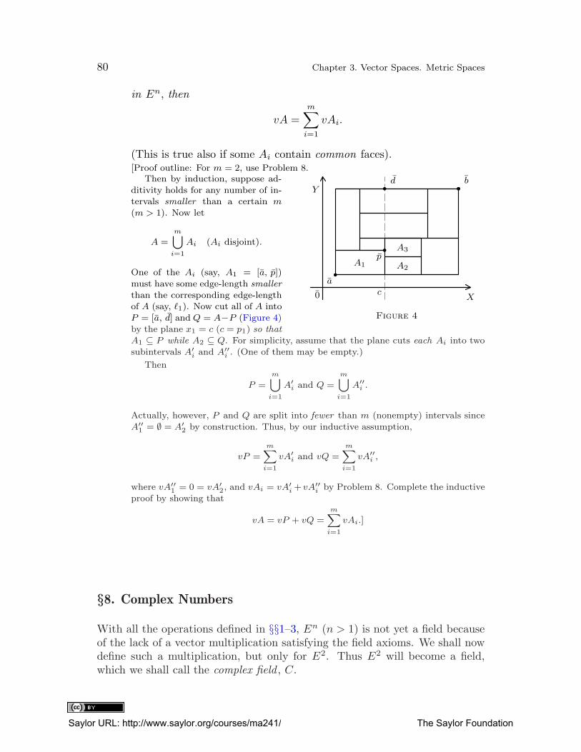
80 Chapter 3. Vector Spaces. Metric Spaces
in En, then
vA =m∑
i=1
vAi.
(This is true also if some Ai contain common faces).[Proof outline: For m = 2, use Problem 8.
0
Y
X
ac
p
bd
A1 A2
A3
Figure 4
Then by induction, suppose ad-
ditivity holds for any number of in-tervals smaller than a certain m
(m > 1). Now let
A =m⋃
i=1
Ai (Ai disjoint).
One of the Ai (say, A1 = [a, p])
must have some edge-length smaller
than the corresponding edge-lengthof A (say, ℓ1). Now cut all of A into
P = [a, d] and Q = A−P (Figure 4)by the plane x1 = c (c = p1) so that
A1 ⊆ P while A2 ⊆ Q. For simplicity, assume that the plane cuts each Ai into two
subintervals A′i and A′′
i . (One of them may be empty.)
Then
P =
m⋃
i=1
A′i and Q =
m⋃
i=1
A′′i .
Actually, however, P and Q are split into fewer than m (nonempty) intervals since
A′′1 = ∅ = A′
2 by construction. Thus, by our inductive assumption,
vP =
m∑
i=1
vA′i and vQ =
m∑
i=1
vA′′i ,
where vA′′1 = 0 = vA′
2, and vAi = vA′i +vA′′
i by Problem 8. Complete the inductive
proof by showing that
vA = vP + vQ =m∑
i=1
vAi.]
§8. Complex Numbers
With all the operations defined in §§1–3, En (n > 1) is not yet a field becauseof the lack of a vector multiplication satisfying the field axioms. We shall nowdefine such a multiplication, but only for E2. Thus E2 will become a field,which we shall call the complex field , C.
Saylor URL: http://www.saylor.org/courses/ma241/ The Saylor Foundation
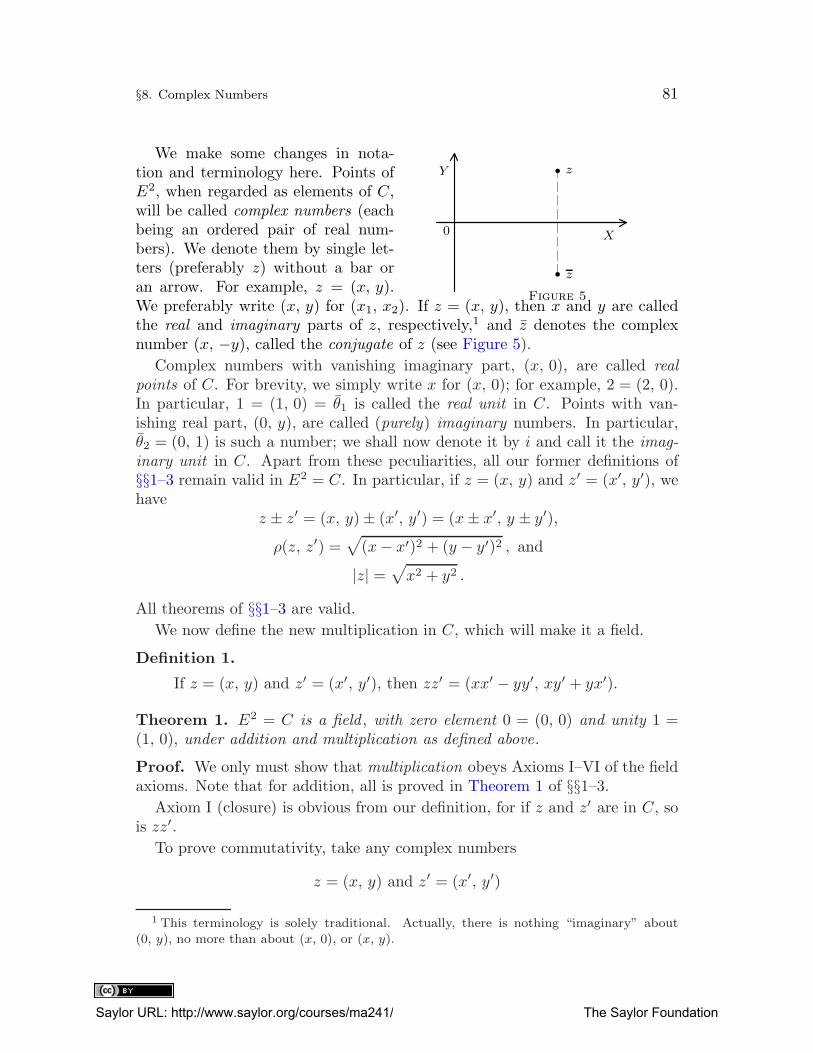
§8. Complex Numbers 81
0
Y
X
z
z
Figure 5
We make some changes in nota-tion and terminology here. Points ofE2, when regarded as elements of C,will be called complex numbers (eachbeing an ordered pair of real num-bers). We denote them by single let-ters (preferably z) without a bar oran arrow. For example, z = (x, y).We preferably write (x, y) for (x1, x2). If z = (x, y), then x and y are calledthe real and imaginary parts of z, respectively,1 and z denotes the complexnumber (x, −y), called the conjugate of z (see Figure 5).
Complex numbers with vanishing imaginary part, (x, 0), are called real
points of C. For brevity, we simply write x for (x, 0); for example, 2 = (2, 0).In particular, 1 = (1, 0) = θ1 is called the real unit in C. Points with van-ishing real part, (0, y), are called (purely) imaginary numbers. In particular,θ2 = (0, 1) is such a number; we shall now denote it by i and call it the imag-
inary unit in C. Apart from these peculiarities, all our former definitions of§§1–3 remain valid in E2 = C. In particular, if z = (x, y) and z′ = (x′, y′), wehave
z ± z′ = (x, y)± (x′, y′) = (x± x′, y ± y′),ρ(z, z′) =
√
(x− x′)2 + (y − y′)2 , and|z| =
√
x2 + y2 .
All theorems of §§1–3 are valid.
We now define the new multiplication in C, which will make it a field.
Definition 1.
If z = (x, y) and z′ = (x′, y′), then zz′ = (xx′ − yy′, xy′ + yx′).
Theorem 1. E2 = C is a field , with zero element 0 = (0, 0) and unity 1 =(1, 0), under addition and multiplication as defined above.
Proof. We only must show that multiplication obeys Axioms I–VI of the fieldaxioms. Note that for addition, all is proved in Theorem 1 of §§1–3.
Axiom I (closure) is obvious from our definition, for if z and z′ are in C, sois zz′.
To prove commutativity, take any complex numbers
z = (x, y) and z′ = (x′, y′)
1 This terminology is solely traditional. Actually, there is nothing “imaginary” about
(0, y), no more than about (x, 0), or (x, y).
Saylor URL: http://www.saylor.org/courses/ma241/ The Saylor Foundation
82 Chapter 3. Vector Spaces. Metric Spaces
and verify that zz′ = z′z. Indeed, by definition,
zz′ = (xx′ − yy′, xy′ + yx′) and z′z = (x′x− y′y, x′y + y′x);
but the two expressions coincide by the commutative laws for real numbers.Associativity and distributivity are proved in a similar manner.
Next, we show that 1 = (1, 0) satisfies Axiom IV(b), i.e., that 1z = z forany complex number z = (x, y). In fact, by definition, and by axioms for E1,
1z = (1, 0) (x, y) = (1x− 0y, 1y + 0x) = (x− 0, y + 0) = (x, y) = z.
It remains to verify Axiom V(b), i.e., to show that each complex numberz = (x, y) 6= (0, 0) has an inverse z−1 such that zz−1 = 1. It turns out thatthe inverse is obtained by setting
z−1 =( x
|z|2 , −y
|z|2)
.
In fact, we then get
zz−1 =( x2
|z|2 +y2
|z|2 , −xy
|z|2 +yx
|z|2)
=(x2 + y2
|z|2 , 0)
= (1, 0) = 1
since x2 + y2 = |z|2, by definition. This completes the proof. �
Corollary 1. i2 = −1; i .e., (0, 1)(0, 1) = (−1, 0).Proof. By definition, (0, 1)(0, 1) = (0 · 0− 1 · 1, 0 · 1 + 1 · 0) = (−1, 0). �
Thus C has an element i whose square is −1, while E1 has no such element,by Corollary 2 in Chapter 2, §§1–4. This is no contradiction since that corollaryholds in ordered fields only. It only shows that C cannot be made an ordered
field.
However, the “real points” in C form a subfield that can be ordered bysetting
(x, 0) < (x′, 0) iff x < x′ in E1.2
Then this subfield behaves exactly like E1.3 Therefore, it is customary not todistinguish between “real points in C” and “real numbers,” identifying (x, 0)with x. With this convention, E1 simply is a subset (and a subfield) of C.Henceforth, we shall simply say that “x is real” or “x ∈ E1” instead of “x =(x, 0) is a real point.” We then obtain the following result.
Theorem 2. Every z ∈ C has a unique representation as
z = x+ yi,
2 The proof is left as an exercise (Problem 1′ below).3 This can be made precise by using the notion of isomorphism (see Basic Concepts of
Mathematics, Chapter 2, §14). We shall not go deeper into this topic here.
Saylor URL: http://www.saylor.org/courses/ma241/ The Saylor Foundation
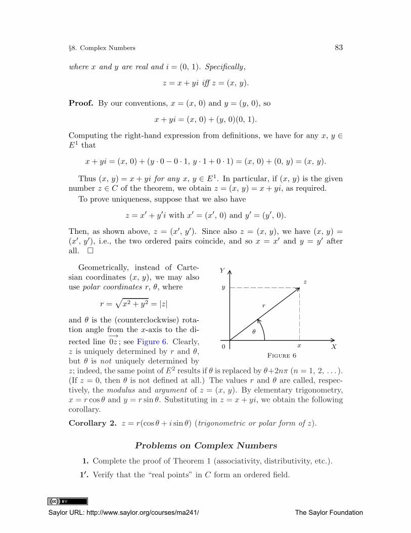
§8. Complex Numbers 83
where x and y are real and i = (0, 1). Specifically ,
z = x+ yi iff z = (x, y).
Proof. By our conventions, x = (x, 0) and y = (y, 0), so
x+ yi = (x, 0) + (y, 0)(0, 1).
Computing the right-hand expression from definitions, we have for any x, y ∈E1 that
x+ yi = (x, 0) + (y · 0− 0 · 1, y · 1 + 0 · 1) = (x, 0) + (0, y) = (x, y).
Thus (x, y) = x+ yi for any x, y ∈ E1. In particular, if (x, y) is the givennumber z ∈ C of the theorem, we obtain z = (x, y) = x+ yi, as required.
To prove uniqueness, suppose that we also have
z = x′ + y′i with x′ = (x′, 0) and y′ = (y′, 0).
Then, as shown above, z = (x′, y′). Since also z = (x, y), we have (x, y) =(x′, y′), i.e., the two ordered pairs coincide, and so x = x′ and y = y′ afterall. �
y
Y
θ
x X0
z
r
Figure 6
Geometrically, instead of Carte-sian coordinates (x, y), we may alsouse polar coordinates r, θ, where
r =√
x2 + y2 = |z|
and θ is the (counterclockwise) rota-tion angle from the x-axis to the di-
rected line−→0z ; see Figure 6. Clearly,
z is uniquely determined by r and θ,but θ is not uniquely determined byz; indeed, the same point of E2 results if θ is replaced by θ+2nπ (n = 1, 2, . . . ).(If z = 0, then θ is not defined at all.) The values r and θ are called, respec-tively, the modulus and argument of z = (x, y). By elementary trigonometry,x = r cos θ and y = r sin θ. Substituting in z = x+ yi, we obtain the followingcorollary.
Corollary 2. z = r(cos θ + i sin θ) (trigonometric or polar form of z).
Problems on Complex Numbers
1. Complete the proof of Theorem 1 (associativity, distributivity, etc.).
1′. Verify that the “real points” in C form an ordered field.
Saylor URL: http://www.saylor.org/courses/ma241/ The Saylor Foundation
84 Chapter 3. Vector Spaces. Metric Spaces
2. Prove that zz = |z|2. Deduce that z−1 = z/|z|2 if z 6= 0.4
3. Prove thatz + z′ = z + z′ and zz′ = z · z′.
Hence show by induction that
zn = (z)n, n = 1, 2, . . . , andn∑
k=1
akzk =n∑
k=1
akzk.
4. Defineeθi = cos θ + i sin θ.
Describe eθi geometrically. Is |eθi| = 1?
5. Compute
(a)1 + 2i
3− i ;
(b) (1 + 2i)(3− i); and
(c)x+ 1 + i
x+ 1− i , x ∈ E1.
Do it in two ways: (i) using definitions only and the notation (x, y) forx+ yi; and (ii) using all laws valid in a field.
6. Solve the equation (2, −1)(x, y) = (3, 2) for x and y in E1.
7. Letz = r(cos θ + i sin θ),
z′ = r′(cos θ′ + i sin θ′), and
z′′ = r′′(cos θ′′ + i sin θ′′)
as in Corollary 2. Prove that z = z′z′′ if
r = |z| = r′r′′, i.e., |z′z′′| = |z′| |z′′|, and θ = θ′ + θ′′.
Discuss the following statement: To multiply z′ by z′′ means to rotate−→0z′
counterclockwise by the angle θ′′ and to multiply it by the scalar r′′ =|z′′|. Consider the cases z′′ = i and z′′ = −1.[Hint: Remove brackets in
r(cos θ + i sin θ) = r′(cos θ′ + i sin θ′) · r′′(cos θ′′ + i sin θ′′)
and apply the laws of trigonometry.]
8. By induction, extend Problem 7 to products of n complex numbers, andderive de Moivre’s formula, namely, if z = r(cos θ + i sin θ), then
zn = rn(cos(nθ) + i sin(nθ)).
4 Recall that z means “conjugate of z.”
Saylor URL: http://www.saylor.org/courses/ma241/ The Saylor Foundation
§8. Complex Numbers 85
Use it to find, for n = 1, 2, . . . ,
(a) in; (b) (1 + i)n; (c)1
(1 + i)n.
9. From Problem 8, prove that for every complex number z 6= 0, there areexactly n complex numbers w such that
wn = z;
they are called the nth roots of z.[Hint: If
z = r(cos θ + i sin θ) and w = r′(cos θ′ + i sin θ′),
the equation wn = z yields, by Problem 8,
(r′)n = r and nθ′ = θ,
and conversely.
While this determines r′ uniquely, θ may be replaced by θ+2kπ without affectingz. Thus
θ′ =θ + 2kπ
n, k = 1, 2, . . . .
Distinct points w result only from k = 0, 1, . . . , n− 1 (then they repeat cyclically).
Thus n values of w are obtained.]
10. Use Problem 9 to find in C
(a) all cube roots of 1; (b) all fourth roots of 1.
Describe all nth roots of 1 geometrically.
∗§9. Vector Spaces. The Space Cn. Euclidean Spaces
I. We shall now follow the pattern of En to obtain the general notion of avector space (just as we generalized E1 to define fields).
Let V be a set of arbitrary elements (not necessarily n-tuples), called “vec-tors” or “points,” with a certain operation (call it “addition,” +) somehowdefined in V . Let F be any field (e.g., E1 or C); its elements will be calledscalars; its zero and unity will be denoted by 0 and 1, respectively. Supposethat yet another operation (“multiplication of scalars by vectors”) has beendefined that assigns to every scalar c ∈ F and every vector x ∈ V a certainvector, denoted cx or xc and called the c-multiple of x. Furthermore, sup-pose that this multiplication and addition in V satisfy the nine laws specified
in Theorem 1 of §§1–3. That is, we have closure:
(∀x, y ∈ V ) (∀ c ∈ F ) x+ y ∈ V and cx ∈ V .
Saylor URL: http://www.saylor.org/courses/ma241/ The Saylor Foundation
86 Chapter 3. Vector Spaces. Metric Spaces
Vector addition is commutative and associative. There is a unique zero-vector ,~0, such that
(∀x ∈ V ) x+~0 = x,
and each x ∈ V has a unique inverse, −x, such that
x+ (−x) = ~0.
We have distributivity :
a(x+ y) = ax+ ay and (a+ b)x = ax+ bx.
Finally, we have1x = x
and(ab)x = a(bx)
(a, b ∈ F ; x, y ∈ V ).
In this case, V together with these two operations is called a vector space
(or a linear space) over the field F ; F is called its scalar field , and elements ofF are called the scalars of V .
Examples.
(a) En is a vector space over E1 (its scalar field).
(a′) Rn, the set of all rational points of En (i.e., points with rational coordi-nates) is a vector space over R, the rationals in E1. (Note that we couldtake R as a scalar field for all of En; this would yield another vectorspace, En over R, not to be confused with En over E1, i.e., the ordinaryEn.)
(b) Let F be any field, and let Fn be the set of all ordered n-tuples of elementsof F , with sums and scalar multiples defined as in En (with F playingthe role of E1). Then Fn is a vector space over F (proof as in Theorem 1of §§1–3).
(c) Each field F is a vector space (over itself) under the addition and multi-plication defined in F . Verify!
(d) Let V be a vector space over a field F , and letW be the set of all possiblemappings
f : A→ V
from some arbitrary set A 6= ∅ into V . Define the sum f + g of two suchmaps by setting
(f + g)(x) = f(x) + g(x) for all x ∈ A.1
1 Here “f+g” must be treated as one letter (function symbol); “(f+g)(x)” means “h(x),”
where h = f + g; similarly for such symbols as af , etc.
Saylor URL: http://www.saylor.org/courses/ma241/ The Saylor Foundation
∗§9. Vector Spaces. The Space Cn. Euclidean Spaces 87
Similarly, given a ∈ F and f ∈W , define the map af by
(af)(x) = af(x).
Under these operations, W is a vector space over the same field F , witheach map f : A→ V treated as a single “vector” in W . (Verify!)
Vector spaces over E1 (respectively, C) are called real (respectively, complex )linear spaces. Complex spaces can always be transformed into real ones byrestricting their scalar field C to E1 (treated as a subfield of C).
II. An important example of a complex linear space is Cn, the set of allordered n-tuples
x = (x1, . . . , xn)
of complex numbers xk (now treated as scalars), with sums and scalar multiplesdefined as in En. In order to avoid confusion with conjugates of complexnumbers, we shall not use the bar notation x for a vector in this section,writing simply x for it. Dot products in Cn are defined by
x · y =n∑
k=1
xkyk,
where yk is the conjugate of the complex number yk (see §8), and hence a scalar
in C. Note that yk = yk if yk ∈ E1. Thus, for vectors with real components,
x · y =n∑
k=1
xkyk,
as in En. The reader will easily verify (exactly as for En) that, for x, y ∈ Cn
and a, b ∈ C, we have the following properties:
(i) x · y ∈ C; thus x · y is a scalar , not a vector.
(ii) x · x ∈ E1, and x · x ≥ 0; moreover, x · x = 0 iff x = ~0. (Thus the dot
product of a vector by itself is a real number ≥ 0.)
(iii) x · y = y · x (= conjugate of y · x). Commutativity fails in general.
(iv) (ax) · (by) = (ab)(x · y). Hence (iv′) (ax) · y = a(x · y) = x · (ay).(v) (x+ y) · z = x · z + y · z and (v′) z · (x+ y) = z · x+ z · y.Observe that (v′) follows from (v) by (iii). (Verify!)
III. Sometimes (but not always) dot products can also be defined in real orcomplex linear spaces other than En or Cn, in such a manner as to satisfy thelaws (i)–(v), hence also (v′), listed above, with C replaced by E1 if the spaceis real. If these laws hold, the space is called Euclidean. For example, En is areal Euclidean space and Cn is a complex one.
Saylor URL: http://www.saylor.org/courses/ma241/ The Saylor Foundation
88 Chapter 3. Vector Spaces. Metric Spaces
In every such space, we define absolute values of vectors by
|x| =√x · x.
(This root exists in E1 by formula (ii).) In particular, this applies to En
and Cn. Then given any vectors x, y and a scalar a, we obtain as before thefollowing properties:
(a′) |x| ≥ 0; and |x| = 0 iff x = ~0.
(b′) |ax| = |a| |x|.(c′) Triangle inequality : |x+ y| ≤ |x|+ |y|.(d′) Cauchy–Schwarz inequality : |x · y| ≤ |x| |y|, and |x · y| = |x| |y| iff x ‖ y
(i.e., x = ay or y = ax for some scalar a).
We prove only (d′); the rest is proved as in Theorem 4 of §§1–3.If x · y = 0, all is trivial, so let z = x · y = rc 6= 0, where r = |x · y| and c has
modulus 1, and let y′ = cy. For any (variable) t ∈ E1, consider |tx + y′|. Bydefinition and (v), (iii), and (iv),
|tx+ y′|2 = (tx+ y′) · (tx+ y′)
= tx · tx+ y′ · tx+ tx · y′ + y′ · y′
= t2(x · x) + t(y′ · x) + t(x · y′) + (y′ · y′)since t = t. Now, since cc = 1,
x · y′ = x · (cy) = (cx) · y = crc = r = |x · y|.Similarly,
y′ · x = x · y′ = r = r = |x · y|, x · x = |x|2, and y′ · y′ = y · y = |y|2.Thus we obtain
(∀ t ∈ E1) |tx+ cy|2 = t2|x|2 + 2t|x · y|+ |y|2. (1)
Here |x|2, 2|x · y|, and |y|2 are fixed real numbers. We treat them as coeffi-cients in t of the quadratic trinomial
f(t) = t2|x|2 + 2t|x · y|+ |y|2.
Now if x and y are not parallel, then cy 6= −tx, and so
|tx+ cy| = |tx+ y′| 6= 0
for any t ∈ E1. Thus by (1), the quadratic trinomial has no real roots; henceits discriminant,
4|x · y|2 − 4(|x| |y|)2,is negative, so that |x · y| < |x| |y|.
Saylor URL: http://www.saylor.org/courses/ma241/ The Saylor Foundation
∗§9. Vector Spaces. The Space Cn. Euclidean Spaces 89
If, however, x ‖ y, one easily obtains |x · y| = |x| |y|, by (b′). (Verify.)
Thus |x · y| = |x| |y| or |x · y| < |x| |y| according to whether x ‖ y or not. �
In any Euclidean space, we define distances by ρ(x, y) = |x − y|. Planes ,lines , and line segments are defined exactly as in En. Thus
line pq = {p+ t(q − p) | t ∈ E1} (in real and complex spaces alike).
Problems on Linear Spaces
1. Prove that Fn in Example (b) is a vector space, i.e., that it satisfies alllaws stated in Theorem 1 in §§1–3; similarly for W in Example (d).
2. Verify that dot products in Cn obey the laws (i)–(v′). Which of theselaws would fail if these products were defined by
x · y =n∑
k=1
xkyk instead of x · y =n∑
k=1
xkyk?
How would this affect the properties of absolute values given in (a′)–(d′)?
3. Complete the proof of formulas (a′)–(d′) for Euclidean spaces. Whatchange would result if property (ii) of dot products were restated as
“x · x ≥ 0 and ~0 ·~0 = 0”?
4. Define orthogonality, parallelism and angles in a general Euclidean spacefollowing the pattern of §§1–3 (text and Problem 7 there). Show that
u = ~0 iff u is orthogonal to all vectors of the space.
5. Define the basic unit vectors ek in Cn exactly as in En, and proveTheorem 2 in §§1–3 for Cn (replacing E1 by C). Also, do Problem 5(a)of §§1–3 for Cn.
6. Define hyperplanes in Cn as in Definition 3 of §§4–6, and proveTheorem 1 stated there, for Cn. Do also Problems 4–6 there for Cn
(replacing E1 by C) and Problem 4 there for vector spaces in general(replacing E1 by the scalar field F ).
7. Do Problem 3 of §§4–6 for general Euclidean spaces (real or complex).Note: Do not replace E1 by C in the definition of a line and a linesegment.
8. A finite set of vectors B = {x1, . . . , xm} in a linear space V over F issaid to be independent iff
(∀ a1, a2, . . . , am ∈ F )( m∑
i=1
aixi = ~0 =⇒ a1 = a2 = · · · = am = 0
)
.
Prove that if B is independent, then
(i) ~0 /∈ B;
Saylor URL: http://www.saylor.org/courses/ma241/ The Saylor Foundation
90 Chapter 3. Vector Spaces. Metric Spaces
(ii) each subset of B is independent (∅ counts as independent); and(iii) if for some scalars ai, bi ∈ F ,
m∑
i=1
aixi =
m∑
i=1
bixi,
then ai = bi, i = 1, 2, . . . , m.
9. Let V be a vector space over F and let A ⊆ V . By the span of A in V ,denoted span(A), is meant the set of all “linear combinations” of vectorsfrom A, i.e., all vectors of the form
m∑
i=1
aixi, ai ∈ F, xi ∈ A, m ∈ N.2
Show that span(A) is itself a vector space V ′ ⊆ V (a subspace of V )over the same field F , with the operations defined in V . (We say thatA spans V ′.) Show that in En and Cn, the basic unit vectors span theentire space.
∗§10. Normed Linear Spaces
By a normed linear space (briefly normed space) is meant a real or complexvector space E in which every vector x is associated with a real number |x|,called its absolute value or norm, in such a manner that the properties (a′)–(c′)of §9 hold.1 That is, for any vectors x, y ∈ E and scalar a, we have
(i) |x| ≥ 0;
(i′) |x| = 0 iff x = ~0;
(ii) |ax| = |a| |x|; and(iii) |x+ y| ≤ |x|+ |y| (triangle inequality).
Mathematically, the existence of absolute values in E amounts to that of amap (called a norm map) x→ |x| on E, i.e., a map ϕ : E → E1, with functionvalues ϕ(x) written as |x|, satisfying the laws (i)–(iii) above. Often such a mapcan be chosen in many ways (not necessarily via dot products, which may notexist in E), thus giving rise to different norms on E. Sometimes we write ‖x‖for |x| or use other similar symbols.
Note 1. From (iii), we also obtain |x− y| ≥∣
∣|x| − |y|∣
∣ exactly as in En.
2 If A = ∅, then span(A) = {~0} by definition.1 Roughly, it is a vector space (over E1 or C) in which “well-behaved” absolute values are
defined, resembling those in En.
Saylor URL: http://www.saylor.org/courses/ma241/ The Saylor Foundation
∗§10. Normed Linear Spaces 91
Examples.
(A) Each Euclidean space (§9), such as En or Cn, is a normed space, withnorm defined by
|x| =√x · x ,
as follows from formulas (a′)–(c′) in §9. In En and Cn, one can alsoequivalently define
|x| =√
n∑
k=1
|xk|2,
where x = (x1, . . . , xn). This is the so-called standard norm, usuallypresupposed in En (Cn).
(B) One can also define other, “nonstandard ,” norms on En and Cn. Forexample, fix some real p ≥ 1 and put
|x|p =
( n∑
k=1
|xk|p)
1p.
One can show that |x|p so defined satisfies (i)–(iii) and thus is a norm
(see Problems 5–7 below).
(C) Let W be the set of all bounded maps
f : A→ E
from a set A 6= ∅ into a normed space E, i.e., such that
(∀ t ∈ A) |f(t)| ≤ cfor some real constant c > 0 (dependent on f but not on t). Define f + gand af as in Example (d) of §9 so that W becomes a vector space. Also,put
‖f‖ = supt∈A|f(t)|,
i.e., the supremum of all |f(t)|, with t ∈ A. Due to boundedness, thissupremum exists in E1, so ‖f‖ ∈ E1.
It is easy to show that ‖f‖ is a norm on W . For example, we verify(iii) as follows.
By definition, we have for f, g ∈W and x ∈ A,|(f + g)(x)| = |f(x) + g(x)|
≤ |f(x)|+ |g(x)|≤ sup
t∈A|f(t)|+ sup
t∈A|g(t)|
= ‖f‖+ ‖g‖.
(1)
Saylor URL: http://www.saylor.org/courses/ma241/ The Saylor Foundation
92 Chapter 3. Vector Spaces. Metric Spaces
(The first inequality is true because (iii) holds in the normed space E towhich f(x) and g(x) belong.) By (1), ‖f‖+ ‖g‖ is an upper bound of allexpressions |(f + g)(x)|, x ∈ A. Thus
‖f‖+ ‖g‖ ≥ supx∈A|(f + g)(x)| = ‖f + g‖.
Note 2. Formula (1) also shows that the map f + g is bounded and henceis a member of W . Quite similarly we see that af ∈ W for any scalar a andf ∈W . Thus we have the closure laws for W . The rest is easy.
In every normed (in particular, in each Euclidean) space E, we define dis-
tances by
ρ(x, y) = |x− y| for all x, y ∈ E.
Such distances depend, of course, on the norm chosen for E; thus we call themnorm-induced distances. In particular, using the standard norm in En and Cn
(Example (A)), we have
ρ(x, y) =
√
n∑
k=1
|xk − yk|2 .
Using the norm of Example (B), we get
ρ(x, y) =
( n∑
k=1
|xk − yk|p)
1p
instead. In the space W of Example (C), we have
ρ(f, g) = ‖f − g‖ = supx∈A|f(x)− g(x)|.
Proceeding exactly as in the proof of Theorem 5 in §§1–3, we see that norm-induced distances obey the three laws stated there. (Verify!) Moreover, bydefinition,
ρ(x+ u, y + u) = |(x+ u)− (y + u)| = |x− y| = ρ(x, y).
Thus we have
ρ(x, y) = ρ(x+ u, y + u) for norm-induced distances; (2)
i.e., the distance ρ(x, y) does not change if both x and y are “translated” by
one and the same vector u. We call such distances translation-invariant .
A more general theory of distances will be given in §§11ff.
Saylor URL: http://www.saylor.org/courses/ma241/ The Saylor Foundation
∗§10. Normed Linear Spaces 93
Problems on Normed Linear Spaces
1. Show that distances in normed spaces obey the laws stated in Theorem 5of §§1–3.
2. Complete the proof of assertions made in Example (C) and Note 2.
3. Define |x| = x1 for x = (x1, . . . , xn) in Cn or En. Is this a norm? Which
(if any) of the laws (i)–(iii) does it obey? How about formula (2)?
4. Do Problem 3 in §§4–6 for a general normed space E, with lines definedas in En (see also Problem 7 in §9). Also, show that contracting se-quences of line segments in E are f -images of contracting sequences ofintervals in E1. Using this fact, deduce from Problem 11 in Chapter 2,§§8–9, an analogue for line segments in E, namely, if
L[an, bn] ⊇ L[an+1, bn+1], n = 1, 2, . . . ,
then∞⋂
n=1
L[an, bn] 6= ∅.
5. Take for granted the lemma that
a1/pb1/q ≤ a
p+b
q
if a, b, p, q ∈ E1 with a, b ≥ 0 and p, q > 0, and
1
p+
1
q= 1.
(A proof will be suggested in Chapter 5, §6, Problem 11.) Use it toprove Holder’s inequality , namely, if p > 1 and 1
p + 1q = 1, then
n∑
k=1
|xkyk| ≤( n∑
k=1
|xk|p)
1p( n∑
k=1
|yk|q)
1qfor any xk, yk ∈ C.
[Hint: Let
A =
( n∑
k=1
|xk|p) 1
p
and B =
( n∑
k=1
|yk|q) 1
q
.
If A = 0 or B = 0, then all xk or all yk vanish, and the required inequality is trivial.
Thus assume A 6= 0 and B 6= 0. Then, setting
a =|xk|pAp
and b =|yk|qBq
in the lemma, obtain
|xkyk|AB
≤ |xk|ppAp
+|yk|qqBq
, k = 1, 2, . . . , n.
Saylor URL: http://www.saylor.org/courses/ma241/ The Saylor Foundation
94 Chapter 3. Vector Spaces. Metric Spaces
Now add up these n inequalities, substitute the values of A and B, and simplify.]
6. Prove the Minkowski inequality ,
( n∑
k=1
|xk + yk|p)
1p≤
( n∑
k=1
|xk|p)
1p+
( n∑
k=1
|yk|p)
1p
for any real p ≥ 1 and xk, yk ∈ C.[Hint: If p = 1, this follows by the triangle inequality in C. If p > 1, let
A =
n∑
k=1
|xk + yk|p 6= 0.
(If A = 0, all is trivial.) Then verify (writing “∑
” for “∑n
k=1” for simplicity)
A =∑
|xk + yk||xk + yk|p−1 ≤∑
|xk||xk + yk|p−1 +∑
|yk||xk + yk|p−1
Now apply Holder’s inequality (Problem 5) to each of the last two sums, with q =
p/(p− 1), so that (p− 1)q = p and 1/p = 1− 1/q. Thus obtain
A ≤(∑
|xk|p) 1
p(∑
|xk + yk|p) 1
q+
(∑
|yk|p) 1
p(∑
|xk + yk|p) 1
q.
Then divide by A1q = (
∑ |xk + yk|p)1q and simplify.]
7. Show that Example (B) indeed yields a norm for Cn and En.[Hint: For the triangle inequality, use Problem 6. The rest is easy.]
8. A sequence {xm} of vectors in a normed space E (e.g., in En or Cn) issaid to be bounded iff
(∃ c ∈ E1) (∀m) |xm| < c,
i.e., iff supm |xm| is finite.Denote such sequences by single letters, x = {xm}, y = {ym}, etc.,
and define
x+ y = {xm + ym}, and ax = {axm} for any scalar a.
Also let
|x| = supm|xm|.
Show that, with these definitions, the set M of all bounded infinitesequences in E becomes a normed space (in which every such sequenceis to be treated as a single vector, and the scalar field is the same asthat of E).
Saylor URL: http://www.saylor.org/courses/ma241/ The Saylor Foundation
§11. Metric Spaces 95
§11. Metric Spaces
I. In §§1–3, we defined distances ρ(x, y) for points x, y in En using theformula
ρ(x, y) =
√
n∑
k=1
(xk − yk)2 = |x− y|.
This actually amounts to defining a certain function ρ of two variables x, y ∈En. We also showed that ρ obeys the three laws of Theorem 5 there. (We callthem metric laws.)
Now, as will be seen, such functions ρ can also be defined in other sets,using quite different defining formulas. In other words, given any set S 6= ∅of arbitrary elements, one can define in it, so to say, “fancy distances” ρ(x, y)satisfying the same three laws. It turns out that it is not the particular formulaused to define ρ but rather the preservation of the three laws that is mostimportant for general theoretical purposes.
Thus we shall assume that a function ρ with the same three properties hasbeen defined, in some way or other , for a set S 6= ∅, and propose to study theconsequences of the three metric laws alone, without assuming anything else.(In particular, no operations other than ρ, or absolute values, or inequalities <,need be defined in S.) All results so obtained will, of course, apply to distancesin En (since they obey the metric laws), but they will also apply to other cases
where the metric laws hold .
The elements of S (though arbitrary) will be called “points ,” usually denotedby p, q, x, y, z (sometimes with bars, etc.); ρ is called a metric for S. Wesymbolize it by
ρ : S × S → E1
since it is function defined on S × S (pairs of elements of S) into E1. Thus weare led to the following definition.
Definition 1.
A metric space is a set S 6= ∅ together with a function
ρ : S × S → E1
(called a metric for S) satisfying the metric laws (axioms):
For any x, y, and z in S, we have
(i) ρ(x, y) ≥ 0, and (i’) ρ(x, y) = 0 iff x = y;
(ii) ρ(x, y) = ρ(y, x) (symmetry law); and
(iii) ρ(x, z) ≤ ρ(x, y) + ρ(y, z) (triangle law).
Saylor URL: http://www.saylor.org/courses/ma241/ The Saylor Foundation
96 Chapter 3. Vector Spaces. Metric Spaces
Thus a metric space is a pair (S, ρ), namely, a set S and a metric ρ for it.In general, one can define many different metrics
ρ, ρ′, ρ′′, . . .
for the same S. The resulting spaces
(S, ρ), (S, ρ′), (S, ρ′′), . . .
then are regarded as different . However, if confusion is unlikely, we simplywrite S for (S, ρ). We write “p ∈ (S, ρ)” for “p ∈ S with metric ρ,” and“A ⊆ (S, ρ)” for “A ⊆ S in (S, ρ).”
Examples.
(1) In En, we always assume
ρ(x, y) = |x− y| (the “standard metric”)
unless stated otherwise.1 By Theorem 5 in §§1–3, (En, ρ) is a metricspace.
(2) However, one can define for En many other “nonstandard” metrics. Forexample,
ρ′(x, y) =
( n∑
k=1
|xk − yk|p)1/p
for any real p ≥ 1
likewise satisfies the metric laws (a proof is suggested in §10, Problems 5–7); similarly for Cn.
(3) Any set S 6= ∅ can be “metrized” (i.e., endowed with a metric) by setting
ρ(x, y) = 1 if x 6= y, and ρ(x, x) = 0.
(Verify the metric laws!) This is the so-called discrete metric. The space(S, ρ) so defined is called a discrete space.
(4) Distances (“mileages”) on the surface of our planet are actually measuredalong circles fitting in the curvature of the globe (not straight lines). Onecan show that they obey the metric laws and thus define a (nonstandard)metric for S = (surface of the globe).
(5) A mapping f : A→ E1 is said to be bounded iff
(∃K ∈ E1) (∀x ∈ A) |f(x)| ≤ K.
1 Similarly in other normed spaces (§10), such as Cn. (A reader who has omitted the
“starred” §10 will consider En only.)
Saylor URL: http://www.saylor.org/courses/ma241/ The Saylor Foundation
§11. Metric Spaces 97
For a fixed A 6= ∅, let W be the set of all such maps (each being treatedas a single “point” of W ). Metrize W by setting, for f, g ∈W ,
ρ(f, g) = supx∈A|f(x)− g(x)|.
(Verify the metric laws; see a similar proof in §10.)
II. We now define “balls” in any metric space (S, ρ).
Definition 2.
Given p ∈ (S, ρ) and a real ε > 0, we define the open ball or globe withcenter p and radius ε (briefly “ε-globe about p”), denoted
Gp or Gp(ε) or G(p; ε),
to be the set of all x ∈ S such that
ρ(x, p) < ε.
Similarly, the closed ε-globe about p is
Gp = Gp(ε) = {x ∈ S | ρ(x, p) ≤ ε}.
The ε-sphere about p is defined by
Sp(ε) = {x ∈ S | ρ(x, p) = ε}.
Note. An open globe in E3 is an ordinary solid sphere (without its surfaceSp(ε)), as known from geometry. In E2, an open globe is a disc (the interiorof a circle). In E1, the globe Gp(ε) is simply the open interval
(p− ε, p+ ε),
while Gp(ε) is the closed interval
[p− ε, p+ ε].
The shape of the globes and spheres depends on the metric ρ. It may becomerather strange for various unusual metrics. For example, in the discrete space
(Example (3)), any globe of radius < 1 consists of its center alone, while Gp(2)contains the entire space. (Why?) See also Problems 1, 2, and 4.
III. Now take any nonempty set
A ⊆ (S, ρ).
The distances ρ(x, y) in S are, of course, also defined for points of A (sinceA ⊆ S), and the metric laws remain valid in A. Thus A is likewise a (smaller)metric space under the metric ρ “inherited” from S; we only have to restrictthe domain of ρ to A×A (pairs of points from A). The set A with this metric
Saylor URL: http://www.saylor.org/courses/ma241/ The Saylor Foundation
98 Chapter 3. Vector Spaces. Metric Spaces
is called a subspace of S. We shall denote it by (A, ρ), using the same letter ρ,or simply by A. Note that A with some other metric ρ′ is not called a subspaceof (S, ρ).
By definition, points in (A, ρ) have the same distances as in (S, ρ). However,globes and spheres in (A, ρ) must consist of points from A only, with centersin A. Denoting such a globe by
G∗p(ε) = {x ∈ A | ρ(x, p) < ε},
we see that it is obtained by restricting Gp(ε) (the corresponding globe in S)to points of A, i.e., removing all points not in A. Thus
G∗p(ε) = A ∩Gp(ε);
similarly for closed globes and spheres. A∩Gp(ε) is often called the relativized(to A) globe Gp(ε). Note that p ∈ G∗
p(ε) since ρ(p, p) = 0 < ε, and p ∈ A.For example, let R be the subspace of E1 consisting of rationals only. Then
the relativized globe G∗p(ε) consists of all rationals in the interval
Gp(ε) = (p− ε, p+ ε),
and it is assumed here that p is rational itself.
IV. A few remarks are due on the extended real number system E∗ (seeChapter 2, §13). As we know, E∗ consists of all reals and two additionalelements, ±∞, with the convention that −∞ < x < +∞ for all x ∈ E1.The standard metric ρ does not apply to E∗. However, one can metrize E∗ invarious other ways. The most common metric ρ′ is suggested in Problems 5 and6 below. Under that metric, globes turn out to be finite and infinite intervals
in E∗.
Instead of metrizing E∗, we may simply adopt the convention that intervalsof the form
(a, +∞] and [−∞, a), a ∈ E1,
will be called “globes” about +∞ and −∞, respectively (without specifyingany “radii”). Globes about finite points may remain as they are in E1. Thisconvention suffices for most purposes of limit theory. We shall use it often (aswe did in Chapter 2, §13).
Problems on Metric Spaces
The “arrowed” problems should be noted for later work.
1. Show that E2 becomes a metric space if distances ρ(x, y) are definedby
(a) ρ(x, y) = |x1 − y1|+ |x2 − y2| or(b) ρ(x, y) = max{|x1 − y1|, |x2 − y2|},
Saylor URL: http://www.saylor.org/courses/ma241/ The Saylor Foundation
§11. Metric Spaces 99
where x = (x1, x2) and y = (y1, y2). In each case, describe G0(1)and S0(1). Do the same for the subspace of points with nonnegative
coordinates.
2. Prove the assertions made in the text about globes in a discrete space.Find an empty sphere in such a space. Can a sphere contain the entirespace?
3. Show that ρ in Examples (3) and (5) obeys the metric axioms.
4. Let M be the set of all positive integers together with the “point” ∞.Metrize M by setting
ρ(m, n) =∣
∣
∣
1
m− 1
n
∣
∣
∣, with the convention that
1
∞ = 0.
Verify the metric axioms. Describe G∞( 12), S∞( 1
2), and G1(1).
⇒5. Metrize the extended real number system E∗ by
ρ′(x, y) = |f(x)− f(y)|,where the function
f : E∗ −→onto
[−1, 1]
is defined by
f(x) =x
1 + |x| if x is finite, f(−∞) = −1, and f(+∞) = 1.
Compute ρ′(0, +∞), ρ′(0, −∞), ρ′(−∞, +∞), ρ′(0, 1), ρ′(1, 2), andρ′(n, +∞). Describe G0(1), G+∞(1), and G−∞( 12 ). Verify the metricaxioms (also when infinities are involved).
⇒6. In Problem 5, show that the function f is one to one, onto [−1, 1], andincreasing ; i.e.,
x < x′ implies f(x) < f(x′) for x, x′ ∈ E∗.
Also show that the f -image of an interval (a, b) ⊆ E∗ is the interval(f(a), f(b)). Hence deduce that globes in E∗ (with ρ′ as in Problem 5)are intervals in E∗ (possibly infinite).[Hint: For a finite x, put
y = f(x) =x
1 + |x| .
Solving for x (separately in the cases x ≥ 0 and x < 0), show that
(∀ y ∈ (−1, 1)) x = f−1(y) =y
1− |y| ;
thus x is uniquely determined by y, i.e., f is one to one and onto—each y ∈ (−1, 1)
corresponds to some x ∈ E1. (How about ±1?)
Saylor URL: http://www.saylor.org/courses/ma241/ The Saylor Foundation
100 Chapter 3. Vector Spaces. Metric Spaces
To show that f is increasing, consider separately the three cases x < 0 < x′,x < x′ < 0 and 0 < x < x′ (also for infinite x and x′).]
7. Continuing Problems 5 and 6, consider (E1, ρ′) as a subspace of (E∗, ρ′)with ρ′ as in Problem 5. Show that globes in (E1, ρ′) are exactly allopen intervals in E∗. For example, (0, 1) is a globe. What are its centerand radius under ρ′ and under the standard metric ρ?
8. Metrize the closed interval [0, +∞] in E∗ by setting
ρ(x, y) =
∣
∣
∣
∣
1
1 + x− 1
1 + y
∣
∣
∣
∣
,
with the conventions 1 + (+∞) = +∞ and 1/(+∞) = 0. Verify themetric axioms. Describe Gp(1) for arbitrary p ≥ 0.
9. Prove that if ρ is a metric for S, then another metric ρ′ for S is givenby
(i) ρ′(x, y) = min{1, ρ(x, y)};
(ii) ρ′(x, y) =ρ(x, y)
1 + ρ(x, y).
In case (i), show that globes Gp(ε) of radius ε ≤ 1 are the same under ρand ρ′. In case (ii), prove that any Gp(ε) in (S, ρ) is also a globe Gp(ε
′)in (S, ρ′) of radius
ε′ =ε
1 + ε,
and any globe of radius ε′ < 1 in (S, ρ′) is also a globe in (S, ρ). (Findthe converse formula for ε as well!)[Hint for the triangle inequality in (ii): Let a = ρ(x, z), b = ρ(x, y), and c = ρ(y, z),so that a ≤ b+ c. The required inequality is
a
1 + a≤ b
1 + b+
c
1 + c.
Simplify it and show that it follows from a ≤ b+ c.]
10. Prove that if (X, ρ′) and (Y, ρ′′) are metric spaces, then a metric ρ forthe set X × Y is obtained by setting, for x1, x2 ∈ X and y1, y2 ∈ Y ,
(i) ρ((x1, y1), (x2, y2)) = max{ρ′(x1, x2), ρ′′(y1, y2)}; or(ii) ρ((x1, y1), (x2, y2)) =
√
ρ′(x1, x2)2 + ρ′′(y1, y2)2 .
[Hint: For brevity, put ρ′12 = ρ′(x1, x2), ρ′′12 = ρ′′(y1, y2), etc. The triangle inequal-
ity in (ii),√
(ρ′13)2 + (ρ′′13)
2 ≤√
(ρ′12)2 + (ρ′′12)
2 +√
(ρ′23)2 + (ρ′′23)
2 ,
is verified by squaring both sides, isolating the remaining square root on the right
side, simplifying, and squaring again. Simplify by using the triangle inequalities validin X and Y , i.e.,
ρ′13 ≤ ρ′12 + ρ′23 and ρ′′13 ≤ ρ′′12 + ρ′′23.
Saylor URL: http://www.saylor.org/courses/ma241/ The Saylor Foundation
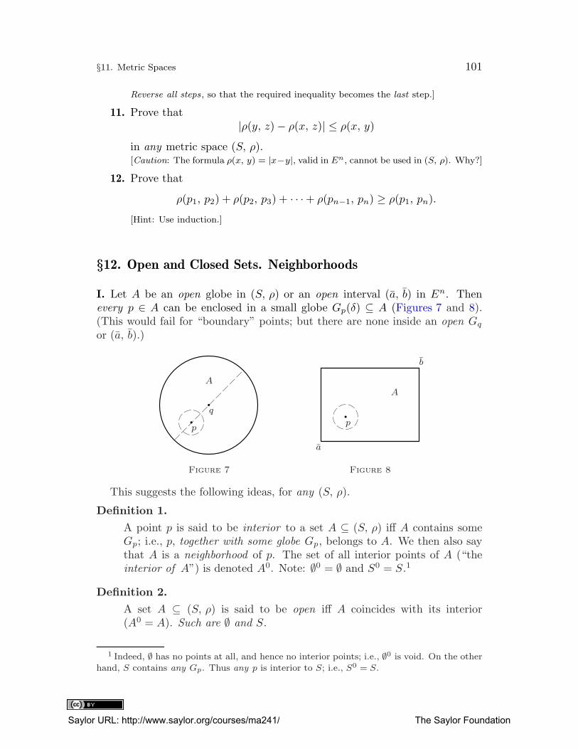
§11. Metric Spaces 101
Reverse all steps, so that the required inequality becomes the last step.]
11. Prove that|ρ(y, z)− ρ(x, z)| ≤ ρ(x, y)
in any metric space (S, ρ).[Caution: The formula ρ(x, y) = |x−y|, valid in En, cannot be used in (S, ρ). Why?]
12. Prove that
ρ(p1, p2) + ρ(p2, p3) + · · ·+ ρ(pn−1, pn) ≥ ρ(p1, pn).[Hint: Use induction.]
§12. Open and Closed Sets. Neighborhoods
I. Let A be an open globe in (S, ρ) or an open interval (a, b) in En. Thenevery p ∈ A can be enclosed in a small globe Gp(δ) ⊆ A (Figures 7 and 8).(This would fail for “boundary” points; but there are none inside an open Gq
or (a, b).)
q
p
A
Figure 7
a
b
A
p
Figure 8
This suggests the following ideas, for any (S, ρ).
Definition 1.
A point p is said to be interior to a set A ⊆ (S, ρ) iff A contains someGp; i.e., p, together with some globe Gp, belongs to A. We then also saythat A is a neighborhood of p. The set of all interior points of A (“theinterior of A”) is denoted A0. Note: ∅0 = ∅ and S0 = S.1
Definition 2.
A set A ⊆ (S, ρ) is said to be open iff A coincides with its interior(A0 = A). Such are ∅ and S.
1 Indeed, ∅ has no points at all, and hence no interior points; i.e., ∅0 is void. On the other
hand, S contains any Gp. Thus any p is interior to S; i.e., S0 = S.
Saylor URL: http://www.saylor.org/courses/ma241/ The Saylor Foundation
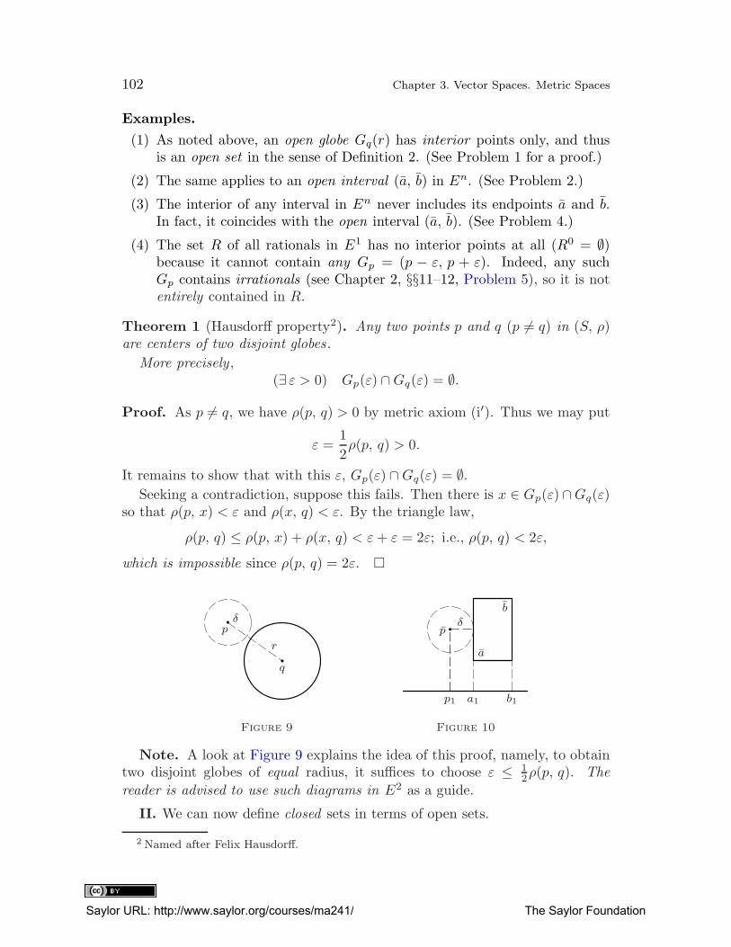
102 Chapter 3. Vector Spaces. Metric Spaces
Examples.
(1) As noted above, an open globe Gq(r) has interior points only, and thusis an open set in the sense of Definition 2. (See Problem 1 for a proof.)
(2) The same applies to an open interval (a, b) in En. (See Problem 2.)
(3) The interior of any interval in En never includes its endpoints a and b.In fact, it coincides with the open interval (a, b). (See Problem 4.)
(4) The set R of all rationals in E1 has no interior points at all (R0 = ∅)because it cannot contain any Gp = (p − ε, p + ε). Indeed, any suchGp contains irrationals (see Chapter 2, §§11–12, Problem 5), so it is notentirely contained in R.
Theorem 1 (Hausdorff property2). Any two points p and q (p 6= q) in (S, ρ)are centers of two disjoint globes.
More precisely ,(∃ ε > 0) Gp(ε) ∩Gq(ε) = ∅.
Proof. As p 6= q, we have ρ(p, q) > 0 by metric axiom (i′). Thus we may put
ε =1
2ρ(p, q) > 0.
It remains to show that with this ε, Gp(ε) ∩Gq(ε) = ∅.Seeking a contradiction, suppose this fails. Then there is x ∈ Gp(ε) ∩Gq(ε)
so that ρ(p, x) < ε and ρ(x, q) < ε. By the triangle law,
ρ(p, q) ≤ ρ(p, x) + ρ(x, q) < ε+ ε = 2ε; i.e., ρ(p, q) < 2ε,
which is impossible since ρ(p, q) = 2ε. �
p
q
δ
r
Figure 9
p1 a1 b1
a
b
pδ
Figure 10
Note. A look at Figure 9 explains the idea of this proof, namely, to obtaintwo disjoint globes of equal radius, it suffices to choose ε ≤ 1
2ρ(p, q). The
reader is advised to use such diagrams in E2 as a guide.
II. We can now define closed sets in terms of open sets.
2 Named after Felix Hausdorff.
Saylor URL: http://www.saylor.org/courses/ma241/ The Saylor Foundation
§12. Open and Closed Sets. Neighborhoods 103
Definition 3.
A set A ⊆ (S, ρ) is said to be closed iff its complement −A = S − A isopen, i.e., has interior points only.
That is, each p ∈ −A (outside A) is in some globe Gp ⊆ −A so that
A ∩Gp = ∅.
Examples (continued).
(5) The sets ∅ and S are closed, for their complements, S and ∅, are open, asnoted above. Thus a set may be both closed and open (“clopen”).
(6) All closed globes in (S, ρ) and all closed intervals in En are closed sets byDefinition 3. Indeed (see Figures 9 and 10), if A = Gq(r) or A = [a, b],then any point p outside A can be enclosed in a globe Gp(δ) disjoint fromA; so, by Definition 3, A is closed (see Problem 12).
(7) A one-point set {q} (also called “singleton”) in (S, ρ) is always closed, forany p outside {q} (p 6= q) is in a globe disjoint from {q} by Theorem 1.
In a discrete space (§11, Example (3)), {q} is also open since it is anopen globe, {q} = Gq(
12) (why?); so it is “clopen.” Hence, in such a space,
all sets are “clopen”. For p ∈ A implies {p} = Gp(12) ⊆ A; similarly for
−A. Thus A and −A have interior points only, so both are open.
(8) The interval (a, b] in E1 is neither open nor closed . (Why?)
∗III. (The rest of this section may be deferred until Chapter 4, §10.)Theorem 2. The union of any finite or infinite family of open sets Ai (i ∈ I),denoted
⋃
i∈I
Ai,
is open itself . So also isn⋂
i=1
Ai
for finitely many open sets . (This fails for infinitely many sets Ai; see Prob-
lem 11 below .)
Proof. We must show that any point p of A =⋃
iAi is interior to A.
Now if p ∈ ⋃
iAi, p is in some Ai, and it is an interior point of Ai (for Ai
is open, by assumption). Thus there is a globe
Gp ⊆ Ai ⊆ A,
as required.
Saylor URL: http://www.saylor.org/courses/ma241/ The Saylor Foundation
104 Chapter 3. Vector Spaces. Metric Spaces
For finite intersections, it suffices to consider two open sets A and B (forn sets, all then follows by induction). We must show that each p ∈ A ∩ B isinterior to A ∩B.
Now as p ∈ A and A is open, we have some Gp(δ′) ⊆ A. Similarly, there is
Gp(δ′′) ⊆ B. Then the smaller of the two globes, call it Gp, is in both A and
B, soGp ⊆ A ∩B
and p is interior to A ∩B, indeed. �
Theorem 3. If the sets Ai (i ∈ I) are closed, so is⋂
i∈I
Ai
(even for infinitely many sets). So also is
n⋃
i=1
Ai
for finitely many closed sets Ai. (Again, this fails for infinitely many sets Ai.)
Proof. Let A =⋂
i∈I Ai. To prove that A is closed, we show that −A is open.
Now by set theory (see Chapter 1, §§1–3, Theorem 2),
−A = −⋂
i
Ai =⋃
i
(−Ai),
where the (−Ai) are open (for the Ai are closed). Thus by Theorem 2, −A is
open, as required.
The second assertion (as to⋃n
i=1Ai) follows quite similarly. �
Corollary 1. A nonempty set A ⊆ (S, ρ) is open iff A is a union of open
globes.
For if A is such a union, it is open by Theorem 2. Conversely, if A is open,then each p ∈ A is in some Gp ⊆ A. All such Gp (p ∈ A) cover all of A, soA ⊆ ⋃
p∈AGp. Also,⋃
p∈AGp ⊆ A since all Gp are in A. Thus
A =⋃
p∈A
Gp.
Corollary 2. Every finite set F in a metric space (S, ρ) is closed .
Proof. If F = ∅, F is closed by Example (5). If F 6= ∅, let
F = {p1, . . . , pn} =n⋃
k=1
{pk}.
Now by Example (7), each {pk} is closed; hence so is F by Theorem 3. �
Saylor URL: http://www.saylor.org/courses/ma241/ The Saylor Foundation
§12. Open and Closed Sets. Neighborhoods 105
Note. The family of all open sets in a given space (S, ρ) is denoted by G;that of all closed sets, by F . Thus “A ∈ G” means that A is open; “A ∈ F”means that A is closed . By Theorems 2 and 3, we have
(∀A, B ∈ G) A ∪B ∈ G and A ∩B ∈ G;
similarly for F . This is a kind of “closure law.” We say that F and G are“closed under finite unions and intersections.”
In conclusion, consider any subspace (A, ρ) of (S, ρ). As we know from §11,it is a metric space itself, so it has its own open and closed sets (which mustconsist of points of A only). We shall now show that they are obtained fromthose of (S, ρ) by intersecting the latter sets with A.
Theorem 4. Let (A, ρ) be a subspace of (S, ρ). Then the open (closed) sets
in (A, ρ) are exactly all sets of the form A ∩ U , with U open (closed) in S.
Proof. Let G be open in (A, ρ). By Corollary 1, G is the union of some openglobes G∗
i (i ∈ I) in (A, ρ). (For brevity, we omit the centers and radii; wealso omit the trivial case G = ∅.)
As was shown in §11, however, G∗i = A ∩Gi, where Gi is an open globe in
(S, ρ). Thus
G =⋃
i
G∗i =
⋃
i
(A ∩Gi) = A ∩⋃
i
Gi,
by set theory (see Chapter 1, §§1–3, Problem 9).
Again by Corollary 1, U =⋃
iGi is an open set in (S, ρ). Thus G has theform
A ∩⋃
i
Gi = A ∩ U,
with U open in S, as asserted.
Conversely, assume the latter, and let p ∈ G. Then p ∈ A and p ∈ U . AsU is open in (S, ρ), there is a globe Gp in (S, ρ) such that p ∈ Gp ⊆ U . Asp ∈ A, we have
p ∈ A ∩Gp ⊆ A ∩ U.
However, A ∩Gp is a globe in (A, ρ), call it G∗p. Thus
p ∈ G∗p ⊆ A ∩ U = G;
i.e., p is an interior point of G in (A, ρ). We see that each p ∈ G is interior toG, as a set in (A, ρ), so G is open in (A, ρ).
This proves the theorem for open sets. Now let F be closed in (A, ρ). Thenby Definition 3, A − F is open in (A, ρ). (Of course, when working in (A, ρ),we replace S by A in taking complements.) Let G = A−F , so F = A−G, andG is open in (A, ρ). By what was shown above, G = A ∩ U with U open in S.
Saylor URL: http://www.saylor.org/courses/ma241/ The Saylor Foundation
106 Chapter 3. Vector Spaces. Metric Spaces
ThusF = A−G = A− (A ∩ U) = A− U = A ∩ (−U)
by set theory. Here −U = S−U is closed in (S, ρ) since U is open there. ThusF = A ∩ (−U), as required.
The proof of the converse (for closed sets) is left as an exercise. �
Problems on Neighborhoods, Open and Closed Sets
⇒1. Verify Example (1).[Hint: Given p ∈ Gq(r), let
δ = r − ρ(p, q) > 0. (Why > 0?)
Use the triangle law to show that
x ∈ Gp(δ) ⇒ ρ(x, q) < r ⇒ x ∈ Gq(r).]
⇒2. Check Example (2); see Figure 8.[Hint: If p ∈ (a, b), choose δ less than the 2n numbers
pk − ak and bk − pk, k = 1, . . . , n;
then show that Gp(δ) ⊆ (a, b).]
3. Prove that if p ∈ Gq(r) in En, then Gq(r) contains a cube [c, d] withc 6= d and with center p.[Hint: By Example (1), there isGp(δ) ⊆ Gq(r). Inscribe inGp(
12δ) a cube of diagonal
δ. Find its edge-length (δ/√n). Then use it to find the coordinates of the endpoints,
c and d (given p, the center). Prove that [c, d] ⊆ Gp(δ).]
4. Verify Example (3).[Hint: To show that no interior points of [a, b] are outside (a, b), let p /∈ (a, b). Then
at least one of the inequalities ak < pk or pk < bk fails. (Why?) Let it be a1 < p1,say, so p1 ≤ a1.
Now take any globe Gp(δ) about p and prove that it is not contained in [a, b]
(so p cannot be an interior point). For this purpose, as in Problem 3, show thatGp(δ) ⊇ [c, d] with c1 < p1 ≤ a1. Deduce that c ∈ Gp(δ), but c /∈ [a, b]; so
Gp(δ) 6⊆ [a, b].]
5. Prove that each open globe Gq(r) in En is a union of cubes (which can
be made open, closed, half-open, etc., as desired). Also, show that eachopen interval (a, b) 6= ∅ in En is a union of open (or closed) globes.[Hint for the first part: By Problem 3, each p ∈ Gq(r) is in a cube Cp ⊆ Gq(r). Show
that Gq(r) =⋃
Cp.]
6. Show that every globe in En contains rational points, i.e., those withrational coordinates only (we express it by saying that the set Rn ofsuch points is dense in En); similarly for the set In of irrational points(those with irrational coordinates).[Hint: First check it with globes replaced by cubes (c, d); see §7, Corollary 3. Then
use Problem 3 above.]
Saylor URL: http://www.saylor.org/courses/ma241/ The Saylor Foundation
§12. Open and Closed Sets. Neighborhoods 107
7. Prove that if x ∈ Gq(r) in En, there is a rational point p (Problem 6)and a rational number δ > 0 such that x ∈ Gp(δ) ⊆ Gq(r). Deduce thateach globe Gq(r) in E
n is a union of rational globes (those with rationalcenters and radii). Similarly, show that Gq(r) is a union of intervalswith rational endpoints.[Hint for the first part: Use Problem 6 and Example (1).]
8. Prove that if the points p1, . . . , pn in (S, ρ) are distinct , there is anε > 0 such that the globes G(pk; ε) are disjoint from each other, fork = 1, 2, . . . , n.
9. Do Problem 7, with Gq(r) replaced by an arbitrary open set G 6= ∅ inEn.
10. Show that every open set G 6= ∅ in En is infinite (∗even uncountable;see Chapter 1, §9).[Hint: Choose Gq(r) ⊆ G. By Problem 3, Gp(r) ⊃ L[c, d], a line segment.]
11. Give examples to show that an infinite intersection of open sets may notbe open, and an infinite union of closed sets may not be closed.[Hint: Show that
∞⋂
n=1
(
− 1
n,1
n
)
= {0}
and∞⋃
n=2
[ 1
n, 1− 1
n
]
= (0, 1).]
12. Verify Example (6) as suggested in Figures 9 and 10.[Hints: (i) For Gq(r), take
δ = ρ(p, q)− r > 0. (Why > 0?)
(ii) If p /∈ [a, b], at least one of the 2n inequalities ak ≤ pk or pk ≤ bk fails (why?),
say, p1 < a1. Take δ = a1 − p1.
In both (i) and (ii) prove that A ∩Gp(δ) = ∅ (proceed as in Theorem 1).]
∗13. Prove the last parts of Theorems 3 and 4.
∗14. Prove that A0, the interior of A, is the union of all open globes containedin A (assume A0 6= ∅). Deduce that A0 is an open set, the largest
contained in A.3
∗15. For sets A, B ⊆ (S, ρ), prove that
(i) (A ∩B)0 = A0 ∩B0;
(ii) (A0)0 = A0; and
(iii) if A ⊆ B then A0 ⊆ B0.
3 That is, the one that contains all other open subsets of A.
Saylor URL: http://www.saylor.org/courses/ma241/ The Saylor Foundation
108 Chapter 3. Vector Spaces. Metric Spaces
[Hint for (ii): A0 is open by Problem 14.]
16. Is A0 ∪B0 = (A ∪B)0?[Hint: See Example (4). Take A = R, B = E1 − R.]
17. Prove that if M and N are neighborhoods of p in (S, ρ), then
(a) p ∈M ∩N ;
(b) M ∩N is a neighborhood of p;
∗(c) so is M0; and
(d) so also is each set P ⊆ S such that P ⊇M or P ⊇ N .
[Hint for (c): See Problem 14.]
18. The boundary of a set A ⊆ (S, ρ) is defined by
bdA = −[A0 ∪ (−A)0];thus it consists of points that fail to be interior in A or in −A.
Prove that the following statements are true:
(i) S = A0 ∪ bdA ∪ (−A)0, all disjoint.(ii) bdS = ∅, bd ∅ = ∅.
∗(iii) A is open iff A ∩ bdA = ∅; A is closed iff A ⊇ bdA.
(iv) In En,
bdGp(r) = bdGp(r) = Sp(r)
(the sphere with center p and radius r). Is this true in all metricspaces?[Hint: Consider Gp(
12) in a discrete space; see §11, Example (3).]
(v) In En, if (a, b) 6= ∅, thenbd(a, b] = bd[a, b) = bd(a, b) = bd[a, b] = [a, b]− (a, b).
(vi) In En, (Rn)0 = ∅; hence bdRn = En (Rn as in Problem 6).
19. Verify Example (8) for intervals in En.
§13. Bounded Sets. Diameters
I. Geometrically, the diameter of a closed globe in En could be defined asthe maximum distance between two of its points. In an open globe in En, thereis no “maximum” distance (why?), but we still may consider the supremum ofall distances inside the globe. Moreover, this makes sense in any set A ⊆ (S, ρ).Thus we accept it as a general definition, for any such set.
Saylor URL: http://www.saylor.org/courses/ma241/ The Saylor Foundation
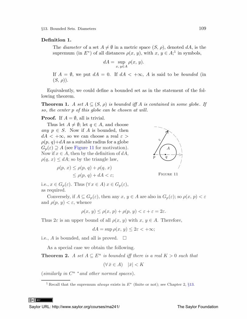
§13. Bounded Sets. Diameters 109
Definition 1.
The diameter of a set A 6= ∅ in a metric space (S, ρ), denoted dA, is thesupremum (in E∗) of all distances ρ(x, y), with x, y ∈ A;1 in symbols,
dA = supx, y∈A
ρ(x, y).
If A = ∅, we put dA = 0. If dA < +∞, A is said to be bounded (in(S, ρ)).
Equivalently, we could define a bounded set as in the statement of the fol-lowing theorem.
Theorem 1. A set A ⊆ (S, ρ) is bounded iff A is contained in some globe. Ifso, the center p of this globe can be chosen at will .
Proof. If A = ∅, all is trivial.
εp q
A
Figure 11
Thus let A 6= ∅; let q ∈ A, and chooseany p ∈ S. Now if A is bounded, thendA < +∞, so we can choose a real ε >ρ(p, q)+dA as a suitable radius for a globeGp(ε) ⊇ A (see Figure 11 for motivation).Now if x ∈ A, then by the definition of dA,ρ(q, x) ≤ dA; so by the triangle law,
ρ(p, x) ≤ ρ(p, q) + ρ(q, x)
≤ ρ(p, q) + dA < ε;
i.e., x ∈ Gp(ε). Thus (∀x ∈ A) x ∈ Gp(ε),as required.
Conversely, if A ⊆ Gp(ε), then any x, y ∈ A are also in Gp(ε); so ρ(x, p) < εand ρ(p, y) < ε, whence
ρ(x, y) ≤ ρ(x, p) + ρ(p, y) < ε+ ε = 2ε.
Thus 2ε is an upper bound of all ρ(x, y) with x, y ∈ A. Therefore,dA = sup ρ(x, y) ≤ 2ε < +∞;
i.e., A is bounded, and all is proved. �
As a special case we obtain the following.
Theorem 2. A set A ⊆ En is bounded iff there is a real K > 0 such that
(∀ x ∈ A) |x| < K
(similarly in Cn ∗and other normed spaces).
1 Recall that the supremum always exists in E∗ (finite or not); see Chapter 2, §13.
Saylor URL: http://www.saylor.org/courses/ma241/ The Saylor Foundation
110 Chapter 3. Vector Spaces. Metric Spaces
Proof. By Theorem 1 (choosing 0 for p), A is bounded iff A is contained insome globe G0(ε) about 0. That is,
(∀ x ∈ A) x ∈ G0(ε) or ρ(x, 0) = |x| < ε.
Thus ε is the required K. (∗The proof for normed spaces is the same.) �
Note 1. In E1, this means that
(∀x ∈ A) −K < x < K;
i.e., A is bounded by −K and K. This agrees with our former definition, givenin Chapter 2, §§8–9.
Caution: Upper and lower bounds are not defined in (S, ρ), in general.
Examples.
(1) ∅ is bounded, with d∅ = 0, by definition.
(2) Let A = [a, b] in En, with d = ρ(a, b) its diagonal. By Corollary 1 in §7,d is the largest distance in A. In nonclosed intervals, we still have
d = supx, y∈A
ρ(x, y) = dA < +∞ (see Problem 10(ii)).
Thus all intervals in En are bounded .
(3) Each globe Gp(ε) in (S, ρ) is bounded, with dGp(ε) ≤ 2ε < +∞, as wasshown in the proof of Theorem 1. See, however, Problems 5 and 6 below.
(4) All of En is not bounded, under the standard metric, for if En had a finitediameter d, no distance in En would exceed d; but ρ(−de1, de1) = 2d, acontradiction!
(5) On the other hand, under the discrete metric (§11, Example (3)), any set(even the entire space) is contained in Gp(3) and hence bounded. Thesame applies to the metric ρ′ defined for E∗ in Problem 5 of §11, sincedistances under that metric never exceed 2, and so E∗ ⊆ Gp(3) for anychoice of p.
Note 2. This shows that boundedness depends on the metric ρ. A set maybe bounded under one metric and not bounded under another. A metric ρ issaid to be bounded iff all sets are bounded under ρ (as in Example (5)).
Problem 9 of §11 shows that any metric ρ can be transformed into a bounded
one, even preserving all sufficiently small globes; in part (i) of the problem, eventhe radii remain the same if they are ≤ 1.
Note 3. An idea similar to that of diameter is often used to define distancesbetween sets . If A 6= ∅ and B 6= ∅ in (S, ρ), we define ρ(A, B) to be the infimum
of all distances ρ(x, y), with x ∈ A and y ∈ B. In particular, if B = {p} (a
Saylor URL: http://www.saylor.org/courses/ma241/ The Saylor Foundation
§13. Bounded Sets. Diameters 111
singleton), we write ρ(A, p) for ρ(A, B). Thus
ρ(A, p) = infx∈A
ρ(x, p).
II. The definition of boundedness extends, in a natural manner, to sequencesand functions. We briefly write {xm} ⊆ (S, ρ) for a sequence of points in (S, ρ),and f : A→ (S, ρ) for a mapping of an arbitrary set A into the space S. Insteadof “infinite sequence with general term xm,” we say “the sequence xm.”
Definition 2.
A sequence {xm} ⊆ (S, ρ) is said to be bounded iff its range is boundedin (S, ρ), i.e., iff all its terms xm are contained in some globe in (S, ρ).
In En, this means (by Theorem 2) that
(∀m) |xm| < K
for some fixed K ∈ E1.2
Definition 3.
A function f : A → (S, ρ) is said to be bounded on a set B ⊆ A iff theimage set f [B] is bounded in (S, ρ); i.e. iff all function values f(x), withx ∈ B, are in some globe in (S, ρ).
In En, this means that
(∀x ∈ B) |f(x)| < K
for some fixed K ∈ E1.2
If B = A, we simply say that f is bounded .
Note 4. If S = E1 or S = E∗, we may also speak of upper and lower
bounds. It is customary to call sup f [B] also the supremum of f on B anddenote it by symbols like
supx∈B
f(x) or sup{f(x) | x ∈ B}.
In the case of sequences, we often write supm xm or sup xm instead; similarlyfor infima, maxima, and minima.
Examples.
(a) The sequence
xm =1
min E1
is bounded since all terms xm are in the interval (0, 2) = G1(1). We haveinf xm = 0 and sup xm = maxxm = 1.
2 ∗Similarly in Cn and other normed spaces.
Saylor URL: http://www.saylor.org/courses/ma241/ The Saylor Foundation
112 Chapter 3. Vector Spaces. Metric Spaces
(b) The sequence
xm = m in E1
is bounded below (by 1) but not above. We have inf xm = minxm = 1and supxm = +∞ (in E∗).
(c) Define f : E1 → E1 by
f(x) = 2x.
This map is bounded on each finite interval B = (a, b) since f [B] =(2a, 2b) is itself an interval and hence bounded. However, f is notbounded on all of E1 since f [E1] = E1 is not a bounded set.
(d) Under a bounded metric ρ, all functions f : A→ (S, ρ) are bounded.
(e) The so-called identity map on S, f : S → (S, ρ), is defined by
f(x) = x.
Clearly, f carries each set B ⊆ S onto itself; i.e., f [B] = B. Thus f isbounded on B iff B is itself a bounded set in (S, ρ).
(f) Define f : E1 → E1 by
f(x) = sinx.
Then f [E1] = [−1, 1] is a bounded set in the range space E1. Thus f isbounded on E1 (briefly, bounded).
Problems on Boundedness and Diameters
1. Show that if a set A in a metric space is bounded, so is each subsetB ⊆ A.
2. Prove that if the sets A1, A2, . . . , An in (S, ρ) are bounded, so is
n⋃
k=1
Ak.
Disprove this for infinite unions by a counterexample.[Hint: By Theorem 1, each Ak is in some Gp(εk), with one and the same center
p. If the number of the globes is finite, we can put max(ε1, . . . , εn) = ε, so Gp(ε)contains all Ak. Verify this in detail.]
⇒3. From Problems 1 and 2 show that a set A in (S, ρ) is bounded iff it iscontained in a finite union of globes,
n⋃
k=1
G(pk; εk).
Saylor URL: http://www.saylor.org/courses/ma241/ The Saylor Foundation
§13. Bounded Sets. Diameters 113
4. A set A in (S, ρ) is said to be totally bounded iff for every ε > 0 (nomatter how small), A is contained in a finite union of globes of radiusε. By Problem 3, any such set is bounded. Disprove the converse by acounterexample.[Hint: Take an infinite set in a discrete space.]
5. Show that distances between points of a globe Gp(ε) never exceed 2ε.(Use the triangle inequality!) Hence infer that dGp(ε) ≤ 2ε. Give anexample where dGp(ε) < 2ε. Thus the diameter of a globe may be less
than twice its radius.[Hint: Take a globe Gp(
12) in a discrete space.]
6. Show that in En (∗as well as in Cn and any other normed linear space6= {0}), the diameter of a globe Gp(ε) always equals 2ε (twice its radius).[Hint: By Problem 5, 2ε is an upper bound of all ρ(x, y) with x, y ∈ Gp(ε).
To show that there is no smaller upper bound, prove that any number
2ε − 2r (r > 0)
is exceeded by some ρ(x, y); e.g., take x and y on some line through p,
x = p+ t~u,
choosing suitable values for t to get ρ(x, y) = |x− y| > 2ε− 2r.]
7. Prove that in En, a set A is bounded iff it is contained in an interval .
8. Prove thatρ(A, B) ≤ ρ(A, p) + ρ(p, B).
Disproveρ(A, B) < ρ(A, p) + ρ(p, B)
by an example.
9. Find sup xn, inf xn, maxxn, and minxn (if any) for sequences withgeneral term
(a) n;
(b) (−1)n(2− 22−n);
(c) 1− 2
n;
(d)n(n− 1)
(n+ 2)2.
Which are bounded in E1?
10. Prove the following about lines and line segments.
(i) Show that any line segment in En is a bounded set, but the entireline is not.
(ii) Prove that the diameter of L(a, b) and of (a, b) equals ρ(a, b).
Saylor URL: http://www.saylor.org/courses/ma241/ The Saylor Foundation
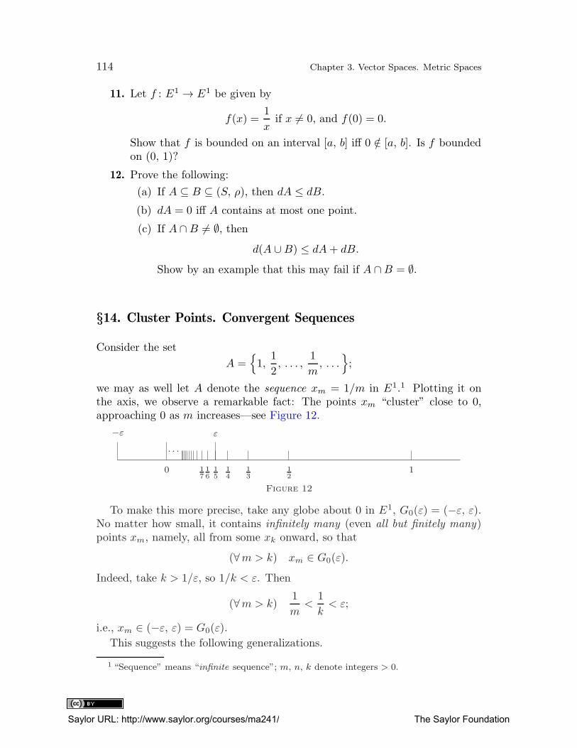
114 Chapter 3. Vector Spaces. Metric Spaces
11. Let f : E1 → E1 be given by
f(x) =1
xif x 6= 0, and f(0) = 0.
Show that f is bounded on an interval [a, b] iff 0 /∈ [a, b]. Is f boundedon (0, 1)?
12. Prove the following:
(a) If A ⊆ B ⊆ (S, ρ), then dA ≤ dB.
(b) dA = 0 iff A contains at most one point.
(c) If A ∩B 6= ∅, thend(A ∪B) ≤ dA+ dB.
Show by an example that this may fail if A ∩B = ∅.
§14. Cluster Points. Convergent Sequences
Consider the set
A ={
1,1
2, . . . ,
1
m, . . .
}
;
we may as well let A denote the sequence xm = 1/m in E1.1 Plotting it onthe axis, we observe a remarkable fact: The points xm “cluster” close to 0,approaching 0 as m increases—see Figure 12.
−ε ε
0 112
13
14
15
16
17
· · ·
Figure 12
To make this more precise, take any globe about 0 in E1, G0(ε) = (−ε, ε).No matter how small, it contains infinitely many (even all but finitely many)points xm, namely, all from some xk onward, so that
(∀m > k) xm ∈ G0(ε).
Indeed, take k > 1/ε, so 1/k < ε. Then
(∀m > k)1
m<
1
k< ε;
i.e., xm ∈ (−ε, ε) = G0(ε).
This suggests the following generalizations.
1 “Sequence” means “infinite sequence”; m, n, k denote integers > 0.
Saylor URL: http://www.saylor.org/courses/ma241/ The Saylor Foundation
§14. Cluster Points. Convergent Sequences 115
Definition 1.
A set, or sequence, A ⊆ (S, ρ) is said to cluster at a point p ∈ S (notnecessarily p ∈ A), and p is called its cluster point or accumulation point ,iff every globe Gp about p contains infinitely many points (respectively,terms) of A. (Thus only infinite sets can cluster .)
Note 1. In sequences (unlike sets) an infinitely repeating term counts asinfinitely many terms. For example, the sequence 0, 1, 0, 1, . . . clusters at 0and 1 (why?); but its range, {0, 1}, has no cluster points (being finite). Thisdistinction is, however, irrelevant if all terms xm are distinct , i.e., different fromeach other. Then we may treat sequences and sets alike.
Definition 2.
A sequence {xm} ⊆ (S, ρ) is said to converge or tend to a point p in S,and p is called its limit , iff every globe Gp(ε) about p (no matter howsmall) contains all but finitely many terms xm.2 In symbols,
(∀ ε > 0) (∃ k) (∀m > k) xm ∈ Gp(ε), i.e., ρ(xm, p) < ε. (1)
If such a p exists, we call {xm} a convergent sequence (in (S, ρ));otherwise, a divergent one. The notation is
xm → p, or limxm = p, or limm→∞
xm = p.
In En,3 ρ(xm, p) = |xm − p|; thus formula (1) turns into
xm → p in En iff (∀ ε > 0) (∃ k) (∀m > k) |xm − p| < ε. (2)
Since “all but finitely many” (as in Definition 2) implies “infinitely many” (asin Definition 1), any limit is also a cluster point . Moreover, we obtain thefollowing result.
Corollary 1. If xm → p, then p is the unique cluster point of {xm}. (Thus a
sequence with two or more cluster points , or none at all , diverges .)
For if p 6= q, the Hausdorff property (Theorem 1 of §12) yields an ε suchthat
Gp(ε) ∩Gq(ε) = ∅.
As xm → p, Gp(ε) leaves out at most finitely many xm, and only these canpossibly be in Gq(ε). (Why?) Thus q fails to satisfy Definition 1 and hence isno cluster point. Hence limxm (if it exists) is unique.
2 That is, Gp(ε) leaves out at most finitely many terms xm, say, x1, x2, . . . , xk, whereasin Definition 1, Gp(ε) may leave out even infinitely many points of A.
3 ∗Similarly for sequences in Cn and in other normed spaces (§10).
Saylor URL: http://www.saylor.org/courses/ma241/ The Saylor Foundation
116 Chapter 3. Vector Spaces. Metric Spaces
Corollary 2.
(i) We have xm → p in (S, ρ) iff ρ(xm, p)→ 0 in E1.
Hence
(ii) xm → p in En iff |xm − p| → 0 and
(iii) xm → 0 in En iff |xm| → 0.
Proof. By (2), we have ρ(xm, p)→ 0 in E1 if
(∀ ε > 0) (∃ k) (∀m > k) |ρ(xm, p)− 0| = ρ(xm, p) < ε.
By (1), however, this means that xm → p, proving our first assertion. The resteasily follows from it, since ρ(xm, p) = |xm − p| in En. �
Corollary 3. If xm tends to p, then so does each subsequence xmk.
For xm → p means that each Gp leaves out at most finitely many xm. Thiscertainly still holds if we drop some terms, passing to {xmk
}.Note 2. A similar argument shows that the convergence or divergence of
{xm}, and its limit or cluster points, are not affected by dropping or adding
a finite number of terms ; similarly for cluster points of sets . For example, if{xm} tends to p, so does {xm+1} (the same sequence without x1).
We leave the following two corollaries as exercises.
Corollary 4. If {xm} splits into two subsequences, each tending to the same
limit p, then also xm → p.
Corollary 5. If {xm} converges in (S, ρ), it is bounded there. (See Problem 4.)
Of course, the convergence or divergence of {xm} and its clustering dependon the metric ρ and the space S. Our theory applies to any (S, ρ). In particu-lar, it applies to E∗, with the metric ρ′ of Problem 5 in §11. Recall that underthat metric, globes about ±∞ have the form (a, +∞] and [−∞, a), respec-tively. Thus limits and cluster points in (E∗, ρ′) coincide with those definedin Chapter 2, §13, (formulas (1)–(3) and Definition 2 there).4 Our theory thenapplies to infinite limits as well, and generalizes Chapter 2, §13.Examples.
(a) Let
xm = p for all m
(such sequences are called constant). As p ∈ Gp, any Gp contains all
xm. Thus xm → p, by Definition 2. We see that each constant sequence
converges to the common value of its terms .
4 The second part of Chapter 2, §13, should be reviewed at this stage.
Saylor URL: http://www.saylor.org/courses/ma241/ The Saylor Foundation
§14. Cluster Points. Convergent Sequences 117
(b) In our introductory example, we showed that
limm→∞
1
m= 0 in E1
and that 0 is the (unique) cluster point of the set A = {1, 12 , . . . }. Here
0 /∈ A.(c) The sequence
0, 1, 0, 1, . . .
has two cluster points, 0 and 1, so it diverges by Corollary 1. (It “os-cillates” from 0 to 1.) This shows that a bounded sequence may diverge.The converse to Corollary 5 fails.
(d) The sequence
xm = m
(or the set N of all naturals) has no cluster points in E1, for a globe ofradius < 1
2 (with any center p ∈ E1) contains at most one xm, and henceno p satisfies Definition 1 or 2.
However, {xm} does cluster in (E∗, ρ′), and even has a limit there,namely +∞. (Prove it!)
(e) The set R of all rationals in E1 clusters at each p ∈ E1. Indeed, anyglobe
Gp(ε) = (p− ε, p+ ε)
contains infinitely many rationals (see Chapter 2, §10, Theorem 3), andthis means that each p ∈ E1 is a cluster point of R.
(f) The sequence
1, 1, 2,1
2, 3,
1
3, . . . (with x2k =
1
kand x2k−1 = k)
has only one cluster point, 0, in E1; yet it diverges, being unbounded (seeCorollary 5). In (E∗, ρ′), it has two cluster points, 0 and +∞. (Verify!)
(g) The lim and lim of any sequence in E∗ are cluster points (cf. Chapter 2,§13, Theorem 2 and Problem 4). Thus in E∗, all sequences cluster .
(h) Let
A = [a, b], a < b.
Then A clusters exactly at all its points , for if p ∈ A, then any globe
Gp(ε) = (p− ε, p+ ε)
overlaps with A (even with (a, b)) and so contains infinitely many pointsof A, as required. Even the endpoints a and b are cluster points of A (and
Saylor URL: http://www.saylor.org/courses/ma241/ The Saylor Foundation
118 Chapter 3. Vector Spaces. Metric Spaces
of (a, b), (a, b], and [a, b)). On the other hand, no point outside A is acluster point. (Why?)
(i) In a discrete space (§11, Example (3)), no set can cluster, since smallglobes, such as Gp(
12), are singletons . (Explain!)
Example (h) shows that a set A may equal the set of its cluster points (callit A′); i.e.,
A = A′.
Such sets are said to be perfect . Sometimes we have A ⊆ A′, A′ ⊆ A, A′ = S(as in Example (e)), or A′ = ∅. We conclude with the following result.
Corollary 6. A set A ⊆ (S, ρ) clusters at p iff each globe Gp (about p) containsat least one point of A other than p.5
Indeed, assume the latter. Then, in particular, each globe
Gp
( 1
n
)
, n = 1, 2, . . . ,
contains some point of A other than p; call it xn. We can make the xn distinct
by choosing each time xn+1 closer to p than xn is. It easily follows that eachGp(ε) contains infinitely many points of A (the details are left to the reader),as required. The converse is obvious.
Problems on Cluster Points and Convergence
1. Is the Archimedean property (see Chapter 2, §10) involved in the proofthat
limm→∞
1
m= 0?
2. Prove Note 2 and Corollaries 4 and 6.
3. Verify Example (c) in detail.6
4. Prove Corollary 5.[Hint: Fix some Gp(ε). Use Definition 2. If Gp(ε) leaves out x1, x2, . . . , xk, take a
larger radius r greater than
ρ(xm, p), m = 1, 2, . . . , k.
Then the enlarged globe Gp(r) contains all xm. Use Theorem 1 in §13.]
5. Show that xm = m tends to +∞ in E∗. Does it contradict Corollary 5?
6. Show that E1 is a perfect set in E1: E1 = (E1)′. Is E1 a perfect set inE∗? Why?
5 This corollary does not apply to cluster points of sequences.6 In particular, show that there are no other cluster points.
Saylor URL: http://www.saylor.org/courses/ma241/ The Saylor Foundation
§14. Cluster Points. Convergent Sequences 119
⇒7. Review Problems 2 and 4 of Chapter 2, §13. (Do them if not donebefore.)
8. Verify Examples (f) and (h).
9. Explain Example (i) in detail.
10. In the following cases find the set A′ of all cluster points of A in E1. IsA′ ⊆ A? Is A ⊆ A′? Is A perfect? Give a precise proof.
(a) A consists of all points of the form
1
nand 1 +
1
n, n = 1, 2, . . . ;
i.e., A is the sequence
{
1, 2,1
2, 1
1
2, . . . ,
1
n, 1 +
1
n, . . .
}
.
Does it converge?
(b) A is the set of all rationals in (0, 1). Answer: A′ = [0, 1]. Why?
(c) A is the union of the intervals
[ 2n
2n+ 1,2n+ 1
2n+ 2
]
, n = 0, 1, 2, . . . .
(d) A consists of all points of the form
2−n and 2−n + 2−n−k, n, k ∈ N .
11. Can a sequence {xm} ⊆ E1 cluster at each p ∈ E1?[Hint: See Example (e).]
12. Prove that if
p = supA or p = inf A in E1
(∅ 6= A ⊆ E1), and if p /∈ A, then p is a cluster point of A.[Hint: Take Gp(ε) = (p− ε, p+ ε). Use Theorem 2 of Chapter 2, §§8–9.]
13. Prove that a set A ⊆ (S, ρ) clusters at p iff every neighborhood of p(see §12, Definition 1) contains infinitely many points of A; similarly forsequences. How about convergence? State it in terms of cubic neigh-borhoods in En.
14. Discuss Example (h) for nondegenerate intervals in En. Give a proof.
15. Prove that a set A 6= ∅ clusters at p (p /∈ A) iff ρ(p, A) = 0. (See §13,Note 3.)
16. Show that in En (∗and in any other normed space 6= {0}), the clusterpoints of any globe Gp(ε) form exactly the closed globe Gp(ε), and that
Saylor URL: http://www.saylor.org/courses/ma241/ The Saylor Foundation
120 Chapter 3. Vector Spaces. Metric Spaces
Gp(ε) is perfect. Is this true in other spaces? (Consider a discrete
space!)[Hint: Given q ∈ Gp(ε) in En, show that any Gq(δ) overlaps with the line pq. Show
also that no point outside Gq(ε) is a cluster point of Gp(ε).]
17. (Cantor’s set.) Remove from [0, 1] the open middle third(1
3,2
3
)
.
From the remaining closed intervals[
0,1
3
]
and[2
3, 1
]
,
remove their open middles,(1
9,2
9
)
and(7
9,8
9
)
.
Do the same with the remaining four closed intervals, and so on, adinfinitum. The set P which remains after all these (infinitely many)removals is called Cantor’s set .
Show that P is perfect.[Hint: If p /∈ P , then either p is in one of the removed open intervals, or p /∈ [0, 1].In both cases, p is no cluster point of P . (Why?) Thus no p outside P is a cluster
point.
On the other hand, if p ∈ P , show that any Gp(ε) contains infinitely manyendpoints of removed open intervals, all in P ; thus p ∈ P ′. Deduce that P = P ′.]
§15. Operations on Convergent Sequences1Sequences in E1 and C can be added and multiplied termwise; for example,adding {xm} and {ym}, one obtains the sequence with general term xm + ym.This leads to important theorems, valid also for En (∗and other normed spaces).Theorem 1 below states, roughly, that the limit of the sum {xm + ym} equals
the sum of limxm and lim ym (if these exist), and similarly for products andquotients (when they are defined).2
Theorem 1. Let xm → q, ym → r, and am → a in E1 or C (the complex
field). Then
(i) xm ± ym → q ± r;1 This section (and the rest of this chapter) may be deferred until Chapter 4, §2. Then
Theorems 1 and 2 may be combined with the more general theorems of Chapter 4, §3. (It is
rather a matter of taste which to do first.)2 Theorem 1 is known as “continuity of addition, multiplication, and division” (for reasons
to be clarified later). Note the restriction a 6= 0 in (iii).
Saylor URL: http://www.saylor.org/courses/ma241/ The Saylor Foundation
§15. Operations on Convergent Sequences 121
(ii) amxm → aq;
(iii)xmam→ q
aif a 6= 0 and for all m ≥ 1, am 6= 0.
This also holds if the xm, ym, q, and r are vectors in En (∗or in another normed
space), while the am and a are scalars for that space.
Proof. (i) By formula (2) of §14, we must show that
(∀ ε > 0) (∃ k) (∀m > k) |xm ± ym − (q ± r)| < ε.
Thus we fix an arbitrary ε > 0 and look for a suitable k. Since xm → q andym → r, there are k′ and k′′ such that
(∀m > k′) |xm − q| <ε
2
and
(∀m > k′′) |ym − r| <ε
2
(as ε is arbitrary , we may as well replace it by 12ε). Then both inequalities hold
for m > k, k = max(k′, k′′). Adding them, we obtain
(∀m > k) |xm − q|+ |ym − r| < ε.
Hence by the triangle law,
|xm − q ± (ym − r)| < ε, i.e., |xm ± ym − (q ± r)| < ε for m > k,
as required. �
This proof of (i) applies to sequences of vectors as well, without any change.The proof of (ii) and (iii) is sketched in Problems 1–4 below.
Note 1. By induction, parts (i) and (ii) hold for sums and products of anyfinite (but fixed) number of suitable convergent sequences.
Note 2. The theorem does not apply to infinite limits q, r, a.
Note 3. The assumption a 6= 0 in Theorem 1(iii) is important. It ensuresnot only that q/a is defined but also that at most finitely many am can vanish
(see Problem 3). Since we may safely drop a finite number of terms (see Note 2in §14), we can achieve that no am is 0, so that xm/am is defined . It is withthis understanding that part (iii) of the theorem has been formulated. Thenext two theorems are actually special cases of more general propositions to beproved in Chapter 4, §§3 and 5. Therefore, we only state them here, leavingthe proofs as exercises, with some hints provided.
Theorem 2 (componentwise convergence). We have xm → p in En (∗Cn) iffeach of the n components of xm tends to the corresponding component of p,i .e., iff xmk → pk, k = 1, 2, . . . , n, in E1(C). (See Problem 8 for hints .)
Saylor URL: http://www.saylor.org/courses/ma241/ The Saylor Foundation
122 Chapter 3. Vector Spaces. Metric Spaces
Theorem 3. Every monotone sequence {xn} ⊆ E∗ has a finite or infinite
limit, which equals supn xn if {xn}↑ and infn xn if {xn}↓. If {xn} is monotone
and bounded in E1, its limit is finite (by Corollary 1 of Chapter 2, §13).The proof was requested in Problem 9 of Chapter 2, §13. See also Chapter 4,
§5, Theorem 1. An important application is the following.
Example (the number e).
Let xn =(
1 +1
n
)n
in E1. By the binomial theorem,
xn = 1 + 1 +n(n− 1)
2!n2+n(n− 1)(n− 2)
3!n3+ · · ·
+n(n− 1) · · · (n− (n− 1))
n!nn
= 2 +(
1− 1
n
) 1
2!+
(
1− 1
n
)(
1− 2
n
) 1
3!+ · · ·
+(
1− 1
n
)(
1− 2
n
)
· · ·(
1− n− 1
n
) 1
n!.
If n is replaced by n + 1, all terms in this expansion increase, as doestheir number. Thus xn < xn+1, i.e., {xn}↑. Moreover, for n > 1,
2 < xn < 2 +1
2!+ · · ·+ 1
n!≤ 2 +
1
2+ · · ·+ 1
2n−1
= 2 +1
2
(
1 + · · ·+ 1
2n−2
)
= 2 +1
2
1−(1
2
)n−1
1
2
< 2 + 1 = 3.
Thus 2 < xn < 3 for n > 1. Hence 2 < supn xn ≤ 3; and by Theorem 3,supn xn = limxn. This limit, denoted by e, plays an important role inanalysis. It can be shown that it is irrational, and (to within 10−20)e = 2.71828182845904523536 . . . . In any case,
2 < e = limn→∞
(
1 +1
n
)n
≤ 3. (1)
The following corollaries are left as exercises for the reader.
Corollary 1. Suppose limxm = p and lim ym = q exist in E∗.
(a) If p > q, then xm > ym for all but finitely many m.
(b) If xm ≤ ym for infinitely many m, then p ≤ q; i .e., limxm ≤ lim ym.
This is known as passage to the limit in inequalities . Caution: The strict
inequalities xm < ym do not imply p < q but only p ≤ q. For example, let
xm =1
mand ym = 0.
Saylor URL: http://www.saylor.org/courses/ma241/ The Saylor Foundation
§15. Operations on Convergent Sequences 123
Then(∀m) xm > ym;
yet limxm = lim ym = 0.
Corollary 2. Let xm → p in E∗, and let c ∈ E∗ (finite or not). Then the
following are true:
(a) If p > c (respectively, p < c), we have xm > c (xm < c) for all but finitelymany m.
(b) If xm ≤ c (respectively, xm ≥ c) for infinitely many m, then p ≤ c (p ≥ c).
One can prove this from Corollary 1, with ym = c (or xm = c) for all m.
Corollary 3 (rule of intermediate sequence). If xm → p and ym → p in E∗
and if xm ≤ zm ≤ ym for all but finitely many m, then also zm → p.
Theorem 4 (continuity of the distance function). If
xm → p and ym → q in a metric space (S, ρ),
then
ρ(xm, ym)→ ρ(p, q) in E1.
Hint: Show that
|ρ(xm, ym)− ρ(p, q)| ≤ ρ(xm, p) + ρ(q, ym)→ 0
by Theorem 1.
Problems on Limits of Sequences
See also Chapter 2, §13.1. Prove that if xm → 0 and if {am} is bounded in E1 or C, then
amxm → 0.
This is true also if the xm are vectors and the am are scalars (or viceversa).[Hint: If {am} is bounded, there is a K ∈ E1 such that
(∀m) |am| < K.
As xm → 0,
(∀ ε > 0) (∃ k) (∀m > k) |xm| < ε
K(why?),
so |amxm| < ε.]
2. Prove Theorem 1(ii).[Hint: By Corollary 2(ii)(iii) in §14, we must show that amxm − aw → 0. Now
amxm − aq = am(xm − q) + (am − a)q,
Saylor URL: http://www.saylor.org/courses/ma241/ The Saylor Foundation
124 Chapter 3. Vector Spaces. Metric Spaces
where xm − q → 0 and am − a → 0 by Corollary 2 of §14. Hence by Problem 1,
am(xm − q) → 0 and (am − a)q → 0
(treat q as a constant sequence and use Corollary 5 in §14). Now apply Theorem 1(i).]
3. Prove that if am → a and a 6= 0 in E1 or C, then
(∃ ε > 0) (∃ k) (∀m > k) |am| ≥ ε.
(We briefly say that the am are bounded away from 0, form > k.) Henceprove the boundedness of { 1
am} for m > k.
[Hint: For the first part, proceed as in the proof of Corollary 1 in §14, with xm = am,p = a, and q = 0.
For the second part, the inequalities
(∀m > k)∣∣∣1
am
∣∣∣ ≤ 1
ε
lead to the desired result.]
4. Prove that if am → a 6= 0 in E1 or C, then
1
am→ 1
a.
Use this and Theorem 1(ii) to prove Theorem 1(iii), noting that
xmam
= xm ·1
am.
[Hint: Use Note 3 and Problem 3 to find that
(∀m > k)∣∣∣1
am− 1
a
∣∣∣ =
1
|a| |am − a| 1
|am| ,
where{ 1
am
}
is bounded and1
|a| |am − a| → 0. (Why?)
Hence, by Problem 1,∣∣∣1
am− 1
a
∣∣∣ → 0. Proceed.]
5. Prove Corollaries 1 and 2 in two ways:
(i) Use Definition 2 of Chapter 2, §13 for Corollary 1(a), treating in-finite limits separately ; then prove (b) by assuming the oppositeand exhibiting a contradiction to (a).
(ii) Prove (b) first by using Corollary 2 and Theorem 3 of Chapter 2,§13; then deduce (a) by contradiction.
6. Prove Corollary 3 in two ways (cf. Problem 5).
7. Prove Theorem 4 as suggested, and also without using Theorem 1(i).
8. Prove Theorem 2.[Hint: If xm → p, then
(∀ ε > 0) (∃ q) (∀m > q) ε > |xm − p| ≥ |xmk − pk|. (Why?)
Saylor URL: http://www.saylor.org/courses/ma241/ The Saylor Foundation
§15. Operations on Convergent Sequences 125
Thus by definition xmk → pk, k = 1, 2, . . . , n.
Conversely, if so, use Theorem 1(i)(ii) to obtain
n∑
k=1
xmk~ek →n∑
k=1
pk~ek,
with ~ek as in Theorem 2 of §§1–3].
8′. In Problem 8, prove the converse part from definitions . (Fix ε > 0, etc.)
9. Find the following limits in E1, in two ways: (i) using Theorem 1,justifying each step; (ii) using definitions only.
(a) limm→∞
m+ 1
m; (b) lim
m→∞3m+ 2
2m− 1;
(c) limn→∞
1
1 + n2; (d) lim
n→∞n(n− 1)
1− 2n2.
[Solution of (a) by the first method: Treat
m+ 1
m= 1 +
1
m
as the sum of xm = 1 (constant) and
ym =1
m→ 0 (proved in §14).
Thus by Theorem 1(i),
m+ 1
m= xm + ym → 1 + 0 = 1.
Second method: Fix ε > 0 and find k such that
(∀m > k)∣∣∣m+ 1
m− 1
∣∣∣ < ε.
Solving for m, show that this holds if m >1
ε. Thus take an integer k >
1
ε, so
(∀m > k)∣∣∣m+ 1
m− 1
∣∣∣ < ε.
Caution: One cannot apply Theorem 1(iii) directly , treating (m + 1)/m as thequotient of xm = m+1 and am = m, because xm and am diverge in E1. (Theorem 1
does not apply to infinite limits.) As a remedy, we first divide the numerator and
denominator by a suitable power of m (or n).]
10. Prove that
|xm| → +∞ in E∗ iff1
xm→ 0 (xm 6= 0).
11. Prove that if
xm → +∞ and ym → q 6= −∞ in E∗,
Saylor URL: http://www.saylor.org/courses/ma241/ The Saylor Foundation
126 Chapter 3. Vector Spaces. Metric Spaces
thenxm + ym → +∞.
This is written symbolically as
“+∞+ q = +∞ if q 6= −∞.”
Do also“−∞+ q = −∞ if q 6= +∞.”
Prove similarly that
“(+∞) · q = +∞ if q > 0”
and“(+∞) · q = −∞ if q < 0.”
[Hint: Treat the cases q ∈ E1, q = +∞, and q = −∞ separately. Use definitions.]
12. Find the limit (or lim and lim) of the following sequences in E∗:
(a) xn = 2 · 4 · · · 2n = 2nn!;
(b) xn = 5n− n3;
(c) xn = 2n4 − n3 − 3n2 − 1;
(d) xn = (−1)nn!;
(e) xn =(−1)nn!
.
[Hint for (b): xn = n(5− n2); use Problem 11.]
13. Use Corollary 4 in §14, to find the following:
(a) limn→∞
(−1)n1 + n2
;
(b) limn→∞
1− n+ (−1)n2n+ 1
.
14. Find the following.
(a) limn→∞
1 + 2 + · · ·+ n
n2;
(b) limn→∞
n∑
k=1
k2
n3 + 1;
(c) limn→∞
n∑
k=1
k3
n4 − 1.
[Hint: Compute∑n
k=1 km using Problem 10 of Chapter 2, §§5–6.]
What is wrong with the following “solution” of (a):1
n2→ 0,
2
n2→ 0,
etc.; hence the limit is 0?
Saylor URL: http://www.saylor.org/courses/ma241/ The Saylor Foundation
§15. Operations on Convergent Sequences 127
15. For each integer m ≥ 0, let
Smn = 1m + 2m + · · ·+ nm.
Prove by induction on m that
limn→∞
Smn
(n+ 1)m+1=
1
m+ 1.
[Hint: First prove that
(m+ 1)Smn = (n+ 1)m+1 − 1−m−1∑
i=0
(m+ 1
i
)
Smi
by adding up the binomial expansions of (k + 1)m+1, k = 1, . . . , n.]
16. Prove that
limn→∞
qn = +∞ if q > 1; limn→∞
qn = 0 if |q| < 1; limn→∞
1n = 1.
[Hint: If q > 1, put q = 1 + d, d > 0. By the binomial expansion,
qn = (1 + d)n = 1 + nd+ · · ·+ dn > nd → +∞. (Why?)
If |q| < 1, then∣∣ 1q
∣∣ > 1; so lim
∣∣ 1q
∣∣n = +∞; use Problem 10.]
17. Prove that
limn→∞
n
qn= 0 if |q| > 1, and lim
n→∞n
qn= +∞ if 0 < q < 1.
[Hint: If |q| > 1, use the binomial as in Problem 16 to obtain
|q|n >1
2n(n− 1)d2, n ≥ 2, so
n
|q|n <2
(n− 1)d2→ 0.
Use Corollary 3 with
xn = 0, |zn| =n
|q|n , and yn =2
(n− 1)d2
to get |zn| → 0; hence also zn → 0 by Corollary 2(iii) of §14. In case 0 < q < 1, use10.]
18. Let r, a ∈ E1. Prove that
limn→∞
nra−n = 0 if |a| > 1.
[Hint: If r > 1 and a > 1, use Problem 17 with q = a1/r to get na−n/r → 0. As
0 < nra−n = (na−n/r)r ≤ na−n/r → 0,
obtain nra−n → 0.
If r < 1, then nra−n < na−n → 0. What if a < −1?]
Saylor URL: http://www.saylor.org/courses/ma241/ The Saylor Foundation
128 Chapter 3. Vector Spaces. Metric Spaces
19. (Geometric series.) Prove that if |q| < 1, then
limn→∞
(a+ aq + · · ·+ aqn−1) =a
1− q .
[Hint:
a(1 + q + · · ·+ qn−1) = a1− qn
1− q,
where qn → 0, by Problem 16.]
20. Let 0 < c < +∞. Prove that
limn→∞
n√c = 1.
[Hint: If c > 1, put n√c = 1 + dn, dn > 0. Expand c = (1 + dn)n to show that
0 < dn <c
n→ 0,
so dn → 0 by Corollary 3.]
21. Investigate the following sequences for monotonicity, lim, lim, and lim.(In each case, find suitable formula, or formulas, for the general term.)
(a) 2, 5, 10, 17, 26, . . . ;
(b) 2, −2, 2, −2, . . . ;(c) 2, −2, −6, −10, −14, . . . ;(d) 1, 1, −1, −1, 1, 1, −1, −1, . . . ;
(e)3 · 21,4 · 64,5 · 109
,6 · 1416
, . . . .
22. Do Problem 21 for the following sequences.
(a)1
2 · 3 ,−83 · 4 ,
27
4 · 5 ,−645 · 6 ,
125
6 · 7 , . . . ;
(b)2
9, −5
9,8
9, −13
9, . . . ;
(c)2
3, −2
5,4
7, −4
9,6
11, − 6
13, . . . ;
(d) 1, 3, 5, 1, 1, 3, 5, 2, 1, 3, 5, 3, . . . , 1, 3, 5, n, . . . ;
(e) 0.9, 0.99, 0.999, . . . ;
(f) +∞, 1, +∞, 2, +∞, 3, . . . ;
(g) −∞, 1, −∞, 12, . . . , −∞, 1
n, . . . .
23. Do Problem 20 as follows: If c ≥ 1, { n√c}↓. (Why?) By Theorem 3,
p = limn→∞
n√c exists and
(∀n) 1 ≤ p ≤ n√c, i.e., 1 ≤ pn ≤ c.
Saylor URL: http://www.saylor.org/courses/ma241/ The Saylor Foundation
§15. Operations on Convergent Sequences 129
By Problem 16, p cannot be > 1, so p = 1.
In case 0 < c < 1, consider n√
1/c and use Theorem 1(iii).
24. Prove the existence of limxn and find it when xn is defined inductivelyby
(i) x1 =√2 , xn+1 =
√2xn ;
(ii) x1 = c > 0, xn+1 =√c2 + xn ;
(iii) x1 = c > 0, xn+1 =cxnn+ 1
; hence deduce that limn→∞
cn
n!= 0.
[Hint: Show that the sequences are monotone and bounded in E1 (Theorem 3).
For example, in (ii) induction yields
xn < xn+1 < c+ 1. (Verify!)
Thus limxn = limxn+1 = p exists. To find p, square the equation
xn+1 =√
c2 + xn (given)
and use Theorem 1 to get
p2 = c2 + p. (Why?)
Solving for p (noting that p > 0), obtain
p = limxn =1
2(1 +
√
4c2 + 1);
similarly in cases (i) and (iii).]
25. Find limxn in E1 or E∗ (if any), given that
(a) xn = (n+ 1)q − nq, 0 < q < 1;
(b) xn =√n (√n+ 1−√n);
(c) xn =1√
n2 + k;
(d) xn = n(n+ 1)cn, with |c| < 1;
(e) xn =n√
m∑
k=1
ank , with ak > 0;
(f) xn =3 · 5 · 7 · · · (2n+ 1)
2 · 5 · 8 · · · (3n− 1).
[Hints:
(a) 0 < xn = nq[(
1 +1
n
)q− 1
]
< nq(
1 +1
n− 1
)
= nq−1 → 0. (Why?)
(b) xn =1
1 +√
1 + 1/n, where 1 <
√
1 +1
n< 1 +
1
n→ 1, so xn → 1
2. (Why?)
(c) Verify thatn√
n2 + n≤ xn ≤ n√
n2 + 1,
Saylor URL: http://www.saylor.org/courses/ma241/ The Saylor Foundation
130 Chapter 3. Vector Spaces. Metric Spaces
so xn → 1 by Corollary 3. (Give a proof.)
(d) See Problems 17 and 18.
(e) Let a = max(a1, . . . , am). Prove that a ≤ xn ≤ a n√m. Use Problem 20.]
The following are some harder but useful problems of theoretical importance.The explicit hints should make them not too hard.
26. Let {xn} ⊆ E1. Prove that if xn → p in E1, then also
limn→∞
1
n
n∑
i=1
xi = p
(i.e., p is also the limit of the sequence of the arithmetic means of thexn).[Solution: Fix ε > 0. Then
(∃ k) (∀n > k) p− ε
4< xn < p+
ε
4.
Adding n− k inequalities, get
(n− k)(
p− ε
4
)
<
n∑
i=k+1
xi < (n− k)(
p+ε
4
)
.
With k so fixed, we thus have
(∀n > k)n− k
n
(
p− ε
4
)
<1
n(xk+1 + · · ·+ xn) <
n− k
n
(
p+ε
4
)
. (i)
Here, with k and ε fixed,
limn→∞
n− k
n
(
p− ε
4
)
= p− ε
4.
Hence, as p− 12ε < p− 1
4ε, there is k′ such that
(∀n > k′) p− ε
2<
n− k
n
(
p− ε
4
)
.
Similarly,
(∃ k′′) (∀n > k′′)n− k
n
(
p+ε
4
)
< p+ε
2.
Combining this with (i), we have, for K′ = max(k, k′, k′′),
(∀n > K′) p− ε
2<
1
n(xk+1 + · · ·+ xn) < p+
ε
2. (ii)
Now with k fixed,
limn→∞
1
n(x1 + x2 + · · ·+ xk) = 0.
Hence
(∃K′′) (∀n > K′′) − ε
2<
1
n(x1 + · · ·+ xk) <
ε
2.
Saylor URL: http://www.saylor.org/courses/ma241/ The Saylor Foundation
§15. Operations on Convergent Sequences 131
Let K = max(K′, K′′). Then combining with (ii), we have
(∀n > K) p− ε <1
n(x1 + · · ·+ xn) < p+ ε,
and the result follows.]
26′ Show that the result of Problem 26 holds also for infinite limits p =±∞ ∈ E∗.
27. Prove that if xn → p in E∗ (xn > 0), then
limn→∞
n√x1x2 · · ·xn = p.
[Hint: Let first 0 < p < +∞. Given ε > 0, use density to fix δ > 1 so close to 1 that
p− ε <p
δ< p < pδ < p+ ε.
As xn → p,
(∃ k) (∀n > k)p4√δ< xn < p
4√δ.
Continue as in Problem 26, replacing ε by δ, and multiplication by addition (also
subtraction by division, etc., as shown above).3 Find a similar solution for the casep = +∞. Note the result of Problem 20.]
28. Disprove by counterexamples the converse implications in Problems 26and 27. For example, consider the sequences
1, −1, 1, −1, . . .and
1
2, 2,
1
2, 2,
1
2, 2, . . . .
29. Prove the following.
(i) If {xn} ⊂ E1 and limn→∞
(xn+1 − xn) = p in E∗, thenxnn→ p.
(ii) If {xn} ⊂ E1 (xn > 0) and ifxn+1
xn→ p ∈ E∗, then n
√xn → p.
Disprove the converse statements by counterexamples.[Hint: For (i), let y1 = x1 and yn = xn − xn−1, n = 2, 3, . . . . Then yn → p and
1
n
n∑
i=1
yi =xn
n,
so Problems 26 and 26′ apply.
For (ii), use Problem 27. See Problem 28 for examples.]
30. From Problem 29 deduce that
(a) limn→∞
n√n! = +∞;
3 Another solution (reducing all to Problem 26) will be obtained by applying logarithms.
Saylor URL: http://www.saylor.org/courses/ma241/ The Saylor Foundation
132 Chapter 3. Vector Spaces. Metric Spaces
(b) limn→∞
n+ 1
n!= 0;
(c) limn→∞
n
√
nn
n!= e;
(d) limn→∞
1
nn√n! =
1
e;
(e) limn→∞
n√n = 1.
31. Prove that
limn→∞
xn =a+ 2b
3,
given
x0 = a, x1 = b, and xn+2 =1
2(xn + xn+1).
[Hint: Show that the differences dn = xn − xn−1 form a geometric sequence, with
ratio q = − 12, and xn = a+
∑nk=1 dk. Then use the result of Problem 19.]
⇒32. For any sequence {xn} ⊆ E1, prove that
limxn ≤ lim1
n
n∑
i=1
xi ≤ lim1
n
n∑
i=1
xi ≤ limxn.
Hence find a new solution of Problems 26 and 26′.[Proof for lim: Fix any k ∈ N . Put
c =
k∑
i=1
xi and b = supi≥k
xi.
Verify that(∀n > k) xk+1 + xk+2 + · · ·+ xn ≤ (n− k)b.
Add c on both sides and divide by n to get
(∀n > k)1
n
n∑
i=1
xi ≤c
n+
n− k
nb. (i*)
Now fix any ε > 0, and first let |b| < +∞. Asc
n→ 0 and
n− k
nb → b, there is
nk > k such that
(∀n > nk)c
n<
ε
2and
n− k
nb < b+
ε
2.
Thus by (i∗),
(∀n > nk)1
n
n∑
i=1
xi ≤ ε+ b.
This clearly holds also if b = supi≥k
xi = +∞. Hence also
supn≥nk
1
n
n∑
i=1
xi ≤ ε+ supi≥k
xi.
Saylor URL: http://www.saylor.org/courses/ma241/ The Saylor Foundation
§15. Operations on Convergent Sequences 133
As k and ε were arbitrary , we may let first k → +∞, then ε → 0, to obtain
lim1
n
n∑
i=1
xi ≤ limk→∞
supi≥k
xi = limxn. (Explain!)]
⇒33. Given {xn} ⊆ E1, xn > 0, prove that
limxn ≤ lim n√x1x2 · · ·xn and lim n
√x1x2 · · ·xn ≤ limxn.
Hence obtain a new solution for Problem 27.[Hint: Proceed as suggested in Problem 32, replacing addition by multiplication.]
34. Given xn, yn ∈ E1 (yn > 0), with
xn → p ∈ E∗ and bn =n∑
i=1
yi → +∞,
prove that
limn→∞
∑ni=1 xiyi
∑ni=1 yi
= p.
Note that Problem 26 is a special case of Problem 34 (take all yn = 1).[Hint for a finite p: Proceed as in Problem 26. However, before adding the n − k
inequalities, multiply by yi and obtain
(
p− ε
4
) n∑
i=k+1
yi <
n∑
i=k+1
xiyi <(
p+ε
4
) n∑
i=k+1
yi.
Put bn =n∑
i=1
yi and show that
1
bn
n∑
i=k+1
xiyi = 1− 1
bn
k∑
i=1
xiyi,
where bn → +∞ (by assumption), so
1
bn
k∑
i=1
xiyi → 0 (for a fixed k).
Proceed. Find a proof for p = ±∞.]
35. Do Problem 34 by considering lim and lim as in Problem 32.
[Hint: Replacec
nby
c
bn, where bn =
n∑
i=1
yi → +∞.]
36. Prove that if un, vn ∈ E1, with {vn}↑ (strictly) and vn → +∞, and if
limn→∞
un − un−1
vn − vn−1= p (p ∈ E∗),
then also
limn→∞
unvn
= p.
Saylor URL: http://www.saylor.org/courses/ma241/ The Saylor Foundation
134 Chapter 3. Vector Spaces. Metric Spaces
[Hint: The result of Problem 34, with
xn =un − un−1
vn − vn−1and yn = vn − vn−1.
leads to the final result.]
37. From Problem 36 obtain a new solution for Problem 15. Also prove that
limn→∞
( Smn
nm+1− 1
m+ 1
)
=1
2.
[Hint: For the first part, put
un = Smn and vn = nm+1.
For the second, put
un = (m+ 1)Smn − nm+1 and vn = nm(m+ 1).]
38. Let 0 < a < b < +∞. Define inductively: a1 =√ab and b1 = 1
2 (a+ b);
an+1 =√
anbn and bn+1 =1
2(an + bn), n = 1, 2, . . . .
Then an+1 < bn+1 for
bn+1 − an+1 =1
2(an + bn)−
√
anbn =1
2(√
bn −√an)
2 > 0.
Deduce that
a < an < an+1 < bn+1 < bn < b,
so {an}↑ and {bn}↓. By Theorem 3, an → p and bn → q for somep, q ∈ E1. Prove that p = q, i.e.,
lim an = lim bn.
(This is Gauss ’s arithmetic–geometric mean of a and b.)[Hint: Take limits of both sides in bn+1 = 1
2(an + bn) to get q = 1
2(p+ q).]
39. Let 0 < a < b in E1. Define inductively a1 = a, b1 = b,
an+1 =2anbnan + bn
, and bn+1 =1
2(an + bn), n = 1, 2, . . . .
Prove that √ab = lim
n→∞an = lim
n→∞bn.
[Hint: Proceed as in Problem 38.]
40. Prove the continuity of dot multiplication, namely, if
xn → q and yn → r in En
Saylor URL: http://www.saylor.org/courses/ma241/ The Saylor Foundation
§15. Operations on Convergent Sequences 135
(∗or in another Euclidean space; see §9), thenxn · yn → q · r.
§16. More on Cluster Points and Closed Sets. Density
I. The notions of cluster point and closed set (§§12, 14) can be characterizedin terms of convergent sequences. We start with cluster points.
Theorem 1.
(i) A sequence {xm} ⊆ (S, ρ) clusters at a point p ∈ S iff it has a subsequence
{xmn} converging to p.1
(ii) A set A ⊆ (S, ρ) clusters at p ∈ S iff p is the limit of some sequence {xn}of points of A other than p; if so, the terms xn can be made distinct.
Proof. (i) If p = limn→∞ xmn, then by definition each globe about p contains
all but finitely many xmn, hence infinitely many xm. Thus p is a cluster point.
Conversely, if so, consider in particular the globes
Gp
( 1
n
)
, n = 1, 2, . . . .
By assumption, Gp(1) contains some xm. Thus fix
xm1∈ Gp(1).
Next, choose a term
xm2∈ Gp
(1
2
)
with m2 > m1.
(Such terms exist since Gp(12) contains infinitely many xm.) Next, fix
xm3∈ Gp
(1
3
)
, with m3 > m2 > m1,
and so on.
Thus, step by step (inductively), select a sequence of subscripts
m1 < m2 < · · · < mn < · · ·that determines a subsequence (see Chapter 1, §8) such that
(∀n) xmn∈ Gp
( 1
n
)
, i.e., ρ(xmn, p) <
1
n→ 0,
1 Therefore, cluster points of {xm} are also called subsequential limits.
Saylor URL: http://www.saylor.org/courses/ma241/ The Saylor Foundation
136 Chapter 3. Vector Spaces. Metric Spaces
whence ρ(xmn, p) → 0, or xmn
→ p. (Why?) Thus we have found a subse-quence xmn
→ p, and assertion (i) is proved.
Assertion (ii) is proved quite similarly—proceed as in the proof of Corollary 6in §14; the inequalities m1 < m2 < · · · are not needed here. �
Examples.
(a) Recall that the set R of all rationals clusters at each p ∈ E1 (§14,Example (e)). Thus by Theorem 1(ii), each real p is the limit of a se-
quence of rationals. See also Problem 6 of §12 for p in En.
(b) The sequence0, 1, 0, 1, . . .
has two convergent subsequences,
x2n = 1→ 1 and x2n−1 = 0→ 0.
Thus by Theorem 1(i), it clusters at 0 and 1.
Interpret Example (f) and Problem 10(a) in §14 similarly.
As we know, even infinite sets may have no cluster points (take N in E1).However, a bounded infinite set or sequence in En (∗or Cn) must cluster. Thisimportant theorem (due to Bolzano and Weierstrass) is proved next.
Theorem 2 (Bolzano–Weierstrass).
(i) Each bounded infinite set or sequence A in En (∗or Cn) has at least one
cluster point p there (possibly outside A).
(ii) Thus each bounded sequence in En (∗Cn) has a convergent subsequence.
Proof. Take first a bounded sequence {zm} ⊆ [a, b] in E1. Let
p = lim zm.
By Theorem 2(i) of Chapter 2, §13, {zm} clusters at p. Moreover, as
a ≤ zm ≤ b,we have
a ≤ inf zm ≤ p ≤ sup zm ≤ bby Corollary 1 of Chapter 2, §13. Thus
p ∈ [a, b] ⊆ E1,
and so {zm} clusters in E1.
Assertion (ii) now follows—for E1—by Theorem 1(i) above.
Next, take
{zm} ⊆ E2, zm = (xm, ym); xm, ym ∈ E1.
Saylor URL: http://www.saylor.org/courses/ma241/ The Saylor Foundation
§16. More on Cluster Points and Closed Sets. Density 137
If {zm} is bounded, all zm are in some square [a, b]. (Why?) Let
a = (a1, a2) and b = (b1, b2).
Then
a1 ≤ xm ≤ b1 and a2 ≤ ym ≤ b2 in E1.
Thus by the first part of the proof, {xm} has a convergent subsequence
xmk→ p1 for some p1 ∈ [a1, b1].
For simplicity, we henceforth write xm for xmk, ym for ymk
, and zm for zmk.
Thus zm = (xm, ym) is now a subsequence, with xm → p1, and a2 ≤ ym ≤ b2,as before.
We now reapply this process to {ym} and obtain a subsubsequence
ymi→ p2 for some p2 ∈ [a2, b2].
The corresponding terms xmistill tend to p1 by Corollary 3 of §14. Thus we
have a subsequence
zmi= (xmi
, ymi)→ (p1, p2) in E2
by Theorem 2 in §15. Hence p = (p1, p2) is a cluster point of {zm}. Note thatp ∈ [a, b] (see above). This proves the theorem for sequences in E2 (hence inC).
The proof for En is similar; one only has to take subsequences n times .(∗The same applies to Cn with real components replaced by complex ones.)
Now take a bounded infinite set A ⊂ En (∗Cn). Select from it an infinitesequence {zm} of distinct points (see Chapter 1, §9, Problem 5). By what wasshown above, {zm} clusters at some point p, so each Gp contains infinitelymany distinct points zm ∈ A. Thus by definition, A clusters at p. �
Note 1. We have also proved that if {zm} ⊆ [a, b] ⊂ En, then {zm} has acluster point in [a, b]. (This applies to closed intervals only.)
Note 2. The theorem may fail in spaces other than En (∗Cn). For example,in a discrete space, all sets are bounded, but no set can cluster.
II. Cluster points are closely related to the following notion.
Definition 1.
The closure of a set A ⊆ (S, ρ), denoted A, is the union of A and the setof all cluster points of A (call it A′). Thus A = A ∪A′.
Theorem 3. We have p ∈ A in (S, ρ) iff each globe Gp(δ) about p meets A,i .e.,
(∀ δ > 0) A ∩Gp(δ) 6= ∅.
Saylor URL: http://www.saylor.org/courses/ma241/ The Saylor Foundation
138 Chapter 3. Vector Spaces. Metric Spaces
Equivalently , p ∈ A iff
p = limn→∞
xn for some {xn} ⊆ A.
The proof is as in Corollary 6 of §14 and Theorem 1. (Here, however, thexn need not be distinct or different from p.) The details are left to the reader.
This also yields the following new characterization of closed sets (cf. §12).Theorem 4. A set A ⊆ (S, ρ) is closed iff one of the following conditions
holds .
(i) A contains all its cluster points (or has none); i .e., A ⊇ A′.
(ii) A = A.
(iii) A contains the limit of each convergent sequence {xn} ⊆ A (if any).2
Proof. Parts (i) and (ii) are equivalent since
A ⊇ A′ ⇐⇒ A = A ∪A′ = A. (Explain!)
Now let A be closed. If p /∈ A, then p ∈ −A; therefore, by Definition 3 in§12, some Gp fails to meet A (Gp∩A = ∅). Hence no p ∈ −A is a cluster point,or the limit of a sequence {xn} ⊆ A. (This would contradict Definitions 1 and2 of §14.) Consequently, all such cluster points and limits must be in A, asclaimed.
Conversely, suppose A is not closed, so −A is not open. Then −A has anoninterior point p; i.e., p ∈ −A but no Gp is entirely in −A. This means thateach Gp meets A. Thus
p ∈ A (by Theorem 3),
and
p = limn→∞
xn for some {xn} ⊆ A (by the same theorem),
even though p /∈ A (for p ∈ −A).We see that (iii) and (ii), hence also (i), fail if A is not closed and hold if A
is closed. (See the first part of the proof.) Thus the theorem is proved. �
The following corollaries are left as exercises (see Problems 6–9).
Corollary 1. ∅ = ∅.Corollary 2. A ⊆ B =⇒ A ⊆ B.
Corollary 3. A is always a closed set ⊇ A.
2 Property (iii) is often called the sequential closedness of A.
Saylor URL: http://www.saylor.org/courses/ma241/ The Saylor Foundation
§16. More on Cluster Points and Closed Sets. Density 139
Corollary 4. A ∪B = A∪B (the closure of A∪B equals the union of A and
B).
III. As we know, the rationals are dense in E1 (Theorem 3 of Chapter 2,§10). This means that every globe Gp(δ) = (p − δ, p + δ) in E1 containsrationals. Similarly (see Problem 6 in §12), the set Rn of all rational points isdense in En. We now generalize this idea for arbitrary sets in a metric space(S, ρ).
Definition 2.
Given A ⊆ B ⊆ (S, ρ), we say that A is dense in B iff each globe Gp,
p ∈ B, meets A. By Theorem 3, this means that each p ∈ B is in A; i.e.,
p = limn→∞
xn for some {xn} ⊆ A.
Equivalently, A ⊆ B ⊆ A.3
Summing up, we have the following:
A is open iff A = A0.
A is closed iff A = A; equivalently , iff A ⊇ A′.
A is dense in B iff A ⊆ B ⊆ A.A is perfect iff A = A′.4
Problems on Cluster Points, Closed Sets, and Density
1. Complete the proof of Theorem 1(ii).
2. Prove that R = E1 and Rn = En (Example (a)).
3. Prove Theorem 2 for E3. Prove it for En (∗and Cn) by induction on n.
4. Verify Note 2.
5. Prove Theorem 3.
6. Prove Corollaries 1 and 2.
7. Prove that (A ∪B)′ = A′ ∪B′.[Hint: Show by contradiction that p /∈ (A′ ∪ B′) excludes p ∈ (A ∪ B)′. Hence(A ∪B)′ ⊆ A′ ∪B′. Then show that A′ ⊆ (A ∪B)′, etc.]
8. From Problem 7, deduce that A ∪ B is closed if A and B are. Thenprove Corollary 4. By induction, extend both assertions to any finite
number of sets.
3 If B is closed (e.g., if B = S) this means that A = B. Why?4 See §14, the remarks following Example (i).
Saylor URL: http://www.saylor.org/courses/ma241/ The Saylor Foundation
140 Chapter 3. Vector Spaces. Metric Spaces
9. From Theorem 4, prove that if the sets Ai (i ∈ I) are closed, so is⋂
i∈I Ai.
10. Prove Corollary 3 from Theorem 3. Deduce that A = A and provefootnote 3.[Hint: Consider Figure 7 and Example (1) in §12 when using Theorem 3 (twice).]
11. Prove that A is contained in any closed superset of A and is the inter-section of all such supersets.[Hint: Use Corollaries 2 and 3.]
12. (i) Prove that a bounded sequence {xm} ⊆ En (∗Cn) converges to piff p is its only cluster point.
(ii) Disprove it for
(a) unbounded {xm} and(b) other spaces.
[Hint: For (i), if xm → p fails, some Gp leaves out infinitely many xm. These xm
form a bounded subsequence that, by Theorem 2, clusters at some q 6= p. (Why?)
Thus q is another cluster point (contradiction!).
For (ii), consider (a) Example (f) in §14 and (b) Problem 10 in §14, with (0, 2]as a subspace of E1.]
13. In each case of Problem 10 in §14, find A. Is A closed? (Use Theorem 4.)
14. Prove that if {bn} ⊆ B ⊆ A in (S, ρ), there is a sequence {an} ⊆ A suchthat ρ(an, bn)→ 0. Hence an → p iff bn → p.[Hint: Choose an ∈ Gbn (1/n).]
15. We have, by definition,
p ∈ A0 iff (∃ δ > 0) Gp(δ) ⊆ A;hence
p /∈ A0 iff (∀ δ > 0) Gp(δ) 6⊆ A, i.e., Gp(δ)− A 6= ∅.(See Chapter 1, §§1–3.) Find such quantifier formulas for p ∈ A, p /∈ A,p ∈ A′, and p /∈ A′.[Hint: Use Corollary 6 in §14, and Theorem 3 in §16.]
16. Use Problem 15 to prove that
(i) −(A) = (−A)0 and
(ii) −(A0) = −A.17. Show that
A ∩ (−A) = bdA (boundary of A);
cf. §12, Problem 18. Hence prove again that A is closed iff A ⊇ bdA.[Hint: Use Theorem 4 and Problem 16 above.]
Saylor URL: http://www.saylor.org/courses/ma241/ The Saylor Foundation
§16. More on Cluster Points and Closed Sets. Density 141
∗18. A set A is said to be nowhere dense in (S, ρ) iff (A)0 = ∅. Show thatCantor’s set P (§14, Problem 17) is nowhere dense.[Hint: P is closed, so P = P .]
∗19. Give another proof of Theorem 2 for E1.[Hint: Let A ⊆ [a, b]. Put
Q = {x ∈ [a, b] | x exceeds infinitely many points (or terms) of A}.
Show that Q is bounded and nonempty, so it has a glb, say, p = inf A. Show that A
clusters at p.]
∗20. For any set A ⊆ (S, ρ) define
GA(ε) =⋃
x∈A
Gx(ε).
Prove that
A =∞⋂
n=1
GA
( 1
n
)
.
∗21. Prove that
A = {x ∈ S | ρ(x, A) = 0}; see §13, Note 3.
Hence deduce that a set A in (S, ρ) is closed iff
(∀x ∈ S) ρ(x, A) = 0 =⇒ x ∈ A.
§17. Cauchy Sequences. Completeness
A convergent sequence is characterized by the fact that its terms xm become(and stay) arbitrarily close to its limit, asm→ +∞. Due to this, however, theyalso get close to each other ; in fact, ρ(xm, xn) can be made arbitrarily smallfor sufficiently large m and n. It is natural to ask whether the latter property,in turn, implies the existence of a limit. This problem was first studied byAugustin-Louis Cauchy (1789–1857). Thus we shall call such sequences Cauchysequences. More precisely, we formulate the following.
Definition 1.
A sequence {xm} ⊆ (S, ρ) is called a Cauchy sequence (we briefly saythat “{xm} is Cauchy”) iff, given any ε > 0 (no matter how small), wehave ρ(xm, xn) < ε for all but finitely many m and n. In symbols,
(∀ ε > 0) (∃ k) (∀m, n > k) ρ(xm, xn) < ε. (1)
Saylor URL: http://www.saylor.org/courses/ma241/ The Saylor Foundation
142 Chapter 3. Vector Spaces. Metric Spaces
Observe that here we only deal with terms xm, xn, not with any other point.The limit (if any) is not involved, and we do not have to know it in advance.We shall now study the relationship between property (1) and convergence.
Theorem 1. Every convergent sequence {xm} ⊆ (S, ρ) is Cauchy.
Proof. Let xm → p. Then given ε > 0, there is a k such that
(∀m > k) ρ(xm, p) <ε
2.
As this holds for any m > k, it also holds for any other term xn with n > k.Thus
(∀m, n > k) ρ(xm, p) <ε
2and ρ(p, xn) <
ε
2.
Adding and using the triangle inequality, we get
ρ(xm, xn) ≤ ρ(xm, p) + ρ(p, xn) < ε,
and (1) is proved. �
Theorem 2. Every Cauchy sequence {xm} ⊆ (S, ρ) is bounded.
Proof. We must show that all xm are in some globe. First we try an arbitraryradius ε. Then by (1), there is k such that ρ(xm, xn) < ε for m, n > k. Fixsome n > k. Then
(∀m > k) ρ(xm, xn) < ε, i.e., xm ∈ Gxn(ε).
Thus the globe Gxn(ε) contains all xm except possibly the k terms x1, . . . , xk.
To include them as well, we only have to take a larger radius r, greater thanρ(xm, xn), m = 1, . . . , k. Then all xm are in the enlarged globe Gxn
(r). �
Note 1. In E1, under the standard metric, only sequences with finite limitsare regarded as convergent. If xn → ±∞, then {xn} is not even a Cauchysequence in E1 (in view of Theorem 2); but in E∗, under a suitable metric
(cf. Problem 5 in §11), it is convergent (hence also Cauchy and bounded).
Theorem 3. If a Cauchy sequence {xm} clusters at a point p, then xm → p.
Proof. We want to show that xm → p, i.e., that
(∀ ε > 0) (∃ k) (∀m > k) ρ(xm, p) < ε.
Thus we fix ε > 0 and look for a suitable k. Now as {xm} is Cauchy, there isa k such that
(∀m, n > k) ρ(xm, xn) <ε
2.
Also, as p is a cluster point, the globe Gp(ε2) contains infinitely many xn, so we
can fix one with n > k (k as above). Then ρ(xn, p) <ε2 and, as noted above,
also ρ(xm, xn) <ε2for m > k. Hence
(∀m > k) ρ(xm, xn) + ρ(xn, p) < ε,
Saylor URL: http://www.saylor.org/courses/ma241/ The Saylor Foundation
§17. Cauchy Sequences. Completeness 143
implying ρ(xm, p) ≤ ρ(xm, xn) + ρ(xn, p) < ε, as required. �
Note 2. It follows that a Cauchy sequence can have at most one clusterpoint p, for p is also its limit and hence unique; see §14, Corollary 1.
These theorems show that Cauchy sequences behave very much like conver-gent ones. Indeed, our next theorem (a famous result by Cauchy) shows that,in En (∗and Cn) the two kinds of sequences coincide.
Theorem 4 (Cauchy’s convergence criterion). A sequence {xm} in En (∗orCn) converges if and only if it is a Cauchy sequence.
Proof. If {xm} converges, it is Cauchy by Theorem 1.
Conversely, let {xm} be a Cauchy sequence. Then by Theorem 2, it isbounded. Hence by the Bolzano–Weierstrass theorem (Theorem 2 of §16), ithas a cluster point p. Thus by Theorem 3 above, it converges to p, and all isproved. �
Unfortunately, this theorem (along with the Bolzano–Weierstrass theoremused in its proof) does not hold in all metric spaces. It even fails in somesubspaces of E1. For example, we have
xm =1
m→ 0 in E1.
By Theorem 1, this sequence, being convergent, is also a Cauchy sequence.Moreover, it still preserves (1) even if we remove the point 0 from E1 sincethe distances ρ(xm, xn) remain the same. However, in the resulting subspaceS = E1 − {0}, the sequence no longer converges because its limit (and uniquecluster point) 0 has disappeared, leaving a “gap” in its place. Thus we have aCauchy sequence in S, without a limit or cluster points , so Theorem 4 fails inS (along with the Bolzano–Weierstrass theorem).
Quite similarly, both theorems fail in (0, 1) (but not in [0, 1]) as a subspaceof E1. By analogy to incomplete ordered fields, it is natural to say that Sis “incomplete” because of the missing cluster point 0, and call a space (orsubspace) “complete” if it has no such “gaps,” i.e., if Theorem 4 holds in it.Thus we define as follows.
Definition 2.
A metric space (or subspace) (S, ρ) is said to be complete iff every Cauchysequence in S converges to some point p in S.
Similarly, a set A ⊆ (S, ρ) is called complete iff each Cauchy sequence{xm} ⊆ A converges to some point p in A, i.e., iff (A, ρ) is complete as ametric subspace of (S, ρ).
In particular, En (∗and Cn) are complete by Theorem 4. The sets (0, 1)and E1−{0} are incomplete in E1, but [0, 1] is complete. Indeed, we have thefollowing theorem.
Saylor URL: http://www.saylor.org/courses/ma241/ The Saylor Foundation
144 Chapter 3. Vector Spaces. Metric Spaces
∗Theorem 5.
(i) Every closed set in a complete space is complete itself .
(ii) Every complete set A ⊆ (S, ρ) is necessarily closed.1
Proof. (i) Let A be a closed set in a complete space (S, ρ). We have to showthat Theorem 4 holds in A (as it does in S). Thus we fix any Cauchy sequence{xm} ⊆ A and prove that it converges to some p in A.
Now, since S is complete, the Cauchy sequence {xm} has a limit p in S. AsA is closed , however, that limit must be in A by Theorem 4 in §16. Thus (i)is proved.
(ii) Now let A be complete in a metric space (S, ρ). To prove that A isclosed, we again use Theorem 4 of §16. Thus we fix any convergent sequence{xm} ⊆ A, xm → p ∈ S, and show that p must be in A.
Now, since {xm} converges in S, it is a Cauchy sequence, in S as well as
in A. Thus by the assumed completeness of A, it has a limit q in A. Then,however, the uniqueness of lim
m→∞xm (in S) implies that p = q ∈ A, so that p is
in A, indeed. �
Problems on Cauchy Sequences
1. Without using Theorem 4, prove that if {xn} and {yn} are Cauchysequences in E1 (or C), so also are
(i) {xn + yn} and (ii) {xnyn}.
2. Prove that if {xm} and {ym} are Cauchy sequences in (S, ρ), then thesequence of distances
ρ(xm, ym), m = 1, 2, . . . ,
converges in E1.[Hint: Show that this sequence is Cauchy in E1; then use Theorem 4.]
3. Prove that a sequence {xm} is Cauchy in (S, ρ) iff
(∀ ε > 0) (∃ k) (∀m > k) ρ(xm, xk) < ε.
4. Two sequences {xm} and {ym} are called concurrent iff
ρ(xm, ym)→ 0.
Notation: {xm} ≈ {ym}. Prove the following.
(i) If one of them is Cauchy or convergent, so is the other, andlimxm = lim ym (if it exists).
1 Here (S, ρ) itself need not be complete.
Saylor URL: http://www.saylor.org/courses/ma241/ The Saylor Foundation
§17. Cauchy Sequences. Completeness 145
(ii) If any two sequences converge to the same limit, they are concur-rent.
5. Show that if {xm} and {ym} are Cauchy sequences in (S, ρ), then
limm→∞
ρ(xm, ym)
does not change if {xm} or {ym} is replaced by a concurrent sequence(see Problems 4 and 2).
Call
limm→∞
ρ(xm, ym)
the “distance”
ρ({xm}, {ym})between {xm} and {ym}. Prove that such “distances” satisfy all met-ric axioms, except that ρ({xm}, {ym}) may be 0 even for different se-quences. (When?)
Also, show that if
(∀m) xm = a and ym = b (constant),
then ρ({xm}, {ym}) = ρ(a, b).
5′. Continuing Problems 4 and 5, show that the concurrence relation (≈)is reflexive, symmetric, and transitive (Chapter 1, §§4–7), i.e., an equiv-
alence relation. That is, given {xm}, {ym} in S, prove that
(a) {xm} ≈ {xm} (reflexivity);(b) if {xm} ≈ {ym} then {ym} ≈ {xm} (symmetry);
(c) if {xm} ≈ {ym} and {ym} ≈ {zm}, then {xm} ≈ {zm} (transitiv-ity).
∗5′′. From Problem 4 deduce that the set of all sequences in (S, ρ) splits intodisjoint equivalence classes (as defined in Chapter 1, §§4–7) under therelation of concurrence (≈). Show that all sequences of one and thesame class either converge to the same limit or have no limit at all, andeither none of them is Cauchy or all are Cauchy.
6. Give examples of incomplete metric spaces possessing complete sub-spaces.
7. Prove that if a sequence {xm} ⊆ (S, ρ) is Cauchy then it has a subse-quence {xmk
} such that
(∀ k) ρ(xmk, xmk+1
) < 2−k.
8. Show that every discrete space (S, ρ) is complete.
Saylor URL: http://www.saylor.org/courses/ma241/ The Saylor Foundation
146 Chapter 3. Vector Spaces. Metric Spaces
∗9. Let C be the set of all Cauchy sequences in (S, ρ); we denote them bycapitals, e.g., X = {xm}. Let
X∗ = {Y ∈ C | Y ≈ X}denote the equivalence class of X under concurrence, ≈ (see Problems 2,5′, and 5′′). We define
σ(X∗, Y ∗) = ρ({xm}, {ym}) = limm→∞
ρ(xm, ym).
By Problem 5, this is unambiguous , for ρ({xm}, {ym}) does not de-pend on the particular choice of {xm} ∈ X∗ and {ym} ∈ Y ∗; andlim ρ(xm, ym) exists by Problem 2.
Show that σ is a metric for the set of all equivalence classes X∗
(X ∈ C); call this set C∗.∗10. Continuing Problem 9, let x∗ denote the equivalence class of the se-
quence with all terms equal to x; let C′ be the set of all such “constant”equivalence classes (it is a subset of C∗).
Show that C′ is dense in (C∗, σ), i.e., C′ = C∗ under the metric σ.(See §16, Definition 2.)[Hint: Fix any “point” X∗ ∈ C∗ and any globe G(X∗; ε) about X∗ in (C∗, σ). We
must show that it contains some x∗ ∈ C′.
By definition, X∗ is the equivalence class of some Cauchy sequence X = {xm} in
(S, ρ), so
(∃ k) (∀m, n > k) ρ(xm, xn) <ε
2.
Fix some x = xn (n > k) and consider the equivalence class x∗ of the sequence{x, x, . . . , x, . . . }; thus, x∗ ∈ C′, and
σ(X∗, x∗) = limm→∞
ρ(xm, x) ≤ ε
2. (Why?)
Thus x∗ ∈ G(X∗, ε), as required.]
∗11. Two metric spaces (S, ρ) and (T, σ) are said to be isometric iff there isa map f : S ←→
ontoT such that
(∀x, y ∈ S) ρ(x, y) = σ(f(x), f(y)).
Show that the spaces (S, ρ) and (C′, σ) of Problem 10 are isometric.Note that it is customary not to distinguish between two isometricspaces, treating each of them as just an “isometric copy” of the other.Indeed, distances in each of them are alike.[Hint: Define f(x) = x∗.]
∗12. Continuing Problems 9 to 11, show that the space (C∗, σ) is complete.Thus prove that for every metric space (S, ρ), there is a complete metric
space (C∗, σ) containing an isometric copy C′ of S, with C′ dense in
C∗. C∗ is called a completion of (S, ρ).
Saylor URL: http://www.saylor.org/courses/ma241/ The Saylor Foundation
§17. Cauchy Sequences. Completeness 147
[Hint: Take a Cauchy sequence {X∗m} in (C∗, σ). By Problem 10, each globe
G(X∗m; 1
m) contains some x∗
m ∈ C′, where x∗m is the equivalence class of
{xm, xm, . . . , xm, . . . },
and σ(X∗m, x∗
m) < 1m
→ 0. Thus by Problem 4, {x∗m} is Cauchy in (C∗, σ), as is
{X∗m}. Deduce that X = {xm} ∈ C, and X∗ = lim
m→∞X∗
m in (C∗, σ).]
Saylor URL: http://www.saylor.org/courses/ma241/ The Saylor Foundation

Saylor URL: http://www.saylor.org/courses/ma241/ The Saylor Foundation
Chapter 4
Function Limits and Continuity
§1. Basic Definitions
We shall now consider functions whose domains and ranges are sets in somefixed (but otherwise arbitrary) metric spaces (S, ρ) and (T, ρ′), respectively.We write
f : A→ (T, ρ′)
for a function f with Df = A ⊆ (S, ρ) and D′f ⊆ (T, ρ′). S is called the
domain space, and T the range space, of f .
I. Given such a function, we often have to investigate its “local behavior”near some point p ∈ S. In particular, if p ∈ A = Df (so that f(p) is defined) wemay ask: Is it possible to make the function values f(x) as near as we like (“ε-near”) to f(p) by keeping x sufficiently close (“δ-close”) to p, i.e., inside somesufficiently small globe Gp(δ)?
1 If this is the case, we say that f is continuous
at p. More precisely, we formulate the following definition.
Definition 1.
A function f : A → (T, ρ′), with A ⊆ (S, ρ), is said to be continuous at
p iff p ∈ A and, moreover, for each ε > 0 (no matter how small) there is
δ > 0 such that ρ′(f(x), f(p)) < ε for all x ∈ A ∩Gp(δ). In symbols,
(∀ ε > 0) (∃ δ > 0) (∀x ∈ A ∩Gp(δ))
{
ρ′(f(x), f(p)) < ε, or
f(x) ∈ Gf(p)(ε).(1)
If (1) fails , we say that f is discontinuous at p and call p a discontinuity
point of f . This is also the case if p /∈ A (since f(p) is not defined).
If (1) holds for each p in a set B ⊆ A, we say that f is continuous on B. Ifthis is the case for B = A, we simply say that f is continuous .
1 Of course, for f(x) to exist, x must also be in A = Df ; thus x ∈ A∩Gp(δ). We say that
x is δ-close to p iff ρ(x, p) < δ.
Saylor URL: http://www.saylor.org/courses/ma241/ The Saylor Foundation
150 Chapter 4. Function Limits and Continuity
Sometimes we prefer to keep x near p but different from p. We then replaceGp(δ) in (1) by the set Gp(δ)− {p}, i.e., the globe without its center , denotedG¬p(δ) and called the deleted δ-globe about p. This is even necessary if p /∈ Df .Replacing f(p) in (1) by some q ∈ T , we then are led to the following definition.
Definition 2.
Given f : A → (T, ρ′), A ⊆ (S, ρ), p ∈ S, and q ∈ T , we say that f(x)tends to q as x tends to p (f(x)→ q as x→ p) iff for each ε > 0 there is
δ > 0 such that ρ′(f(x), q) < ε for all x ∈ A ∩G¬p(δ). In symbols,
(∀ ε > 0) (∃ δ > 0) (∀x ∈ A ∩G¬p(δ))
{
ρ′(f(x), q) < ε, i.e.,
f(x) ∈ Gq(ε).(2)
This means that f(x) is ε-close to q when x is δ-close to p and x 6= p.2
If (2) holds for some q, we call q a limit of f at p. There may be no such q.We then say that f has no limit at p, or that this limit does not exist. If thereis only one such q (for a given p), we write q = lim
x→pf(x).
Note 1. Formula (2) holds “vacuously” (see Chapter 1, §§1–3, end remark)if A ∩ G¬p(δ) = ∅ for some δ > 0. Then any q ∈ T is a limit at p, so a limitexists but is not unique. (We discard the case where T is a singleton.)
Note 2. However, uniqueness is ensured if A∩G¬p(δ) 6= ∅ for all δ > 0, aswe prove below.
Observe that by Corollary 6 of Chapter 3, §14, the set A clusters at p iff
(∀ δ > 0) A ∩G¬p(δ) 6= ∅. (Explain!)
Thus we have the following corollary.
Corollary 1. If A clusters at p in (S, ρ), then a function f : A→ (T, p′) canhave at most one limit at p; i .e.,
limx→p
f(x) is unique (if it exists).3
In particular , this holds if A ⊇ (a, b) ⊂ E1 (a < b) and p ∈ [a, b].
Proof. Suppose f has two limits, q and r, at p. By the Hausdorff property,
Gq(ε) ∩Gr(ε) = ∅ for some ε > 0.
Also, by (2), there are δ′, δ′′ > 0 such that
(∀x ∈ A ∩G¬p(δ′)) f(x) ∈ Gq(ε) and
(∀x ∈ A ∩G¬p(δ′′)) f(x) ∈ Gr(ε).
2 Observe that the choice of δ depends on ε in both (1) and (2).3 Because of this, some authors restrict Definition 2 to the case where A clusters at p.
However, this has its disadvantages (e.g., Corollary 2 fails).
Saylor URL: http://www.saylor.org/courses/ma241/ The Saylor Foundation
§1. Basic Definitions 151
Let δ = min(δ′, δ′′). Then for x ∈ A∩G¬p(δ), f(x) is in both Gq(ε) and Gr(ε),and such an x exists since A ∩G¬p(δ) 6= ∅ by assumption.
But this is impossible since Gq(ε) ∩Gr(ε) = ∅ (a contradiction!). �
For intervals , see Chapter 3, §14, Example (h).
Corollary 2. f is continuous at p (p ∈ Df ) iff f(x)→ f(p) as x→ p.
The straightforward proof from definitions is left to the reader.
Note 3. In formula (2), we excluded the case x = p by assuming thatx ∈ A ∩ G¬p(δ). This makes the behavior of f at p itself irrelevant. Thus for
the existence of a limit q at p, it does not matter whether p ∈ Df or whether
f(p) = q. But both conditions are required for continuity at p (see Corollary 2and Definition 1).
Note 4. Observe that if (1) or (2) holds for some δ, it certainly holds forany δ′ ≤ δ. Thus we may always choose δ as small as we like. Moreover, asx is limited to Gp(δ), we may disregard, or change at will, the function valuesf(x) for x /∈ Gp(δ) (“local character of the limit notion”).
II. Limits in E∗. If S or T is E∗ (or E1), we may let x → ±∞ orf(x)→ ±∞. For a precise definition, we rewrite (2) in terms of globes Gp andGq:
(∀Gq) (∃Gp) (∀x ∈ A ∩G¬p) f(x) ∈ Gq . (2′)
This makes sense also if p = ±∞ or q = ±∞. We only have to use ourconventions as to G±∞, or the metric ρ′ for E∗, as explained in Chapter 3, §11.
For example, consider
“f(x)→ q as x→ +∞” (A ⊆ S = E∗, p = +∞, q ∈ (T, ρ′)).
Here Gp has the form (a, +∞], a ∈ E1, and G¬p = (a, +∞), while Gq = Gq(ε),as usual. Noting that x ∈ G¬p means x > a (x ∈ E1), we can rewrite (2′) as
(∀ ε > 0) (∃ a ∈ E1) (∀x ∈ A | x > a) f(x) ∈ Gq(ε), or ρ′(f(x), q) < ε. (3)
This means that f(x) becomes arbitrarily close to q for large x (x > a).
Next consider “f(x) → +∞ as x → −∞.” Here G¬p = (−∞, a) andGq = (b,+∞]. Thus formula (2′) yields (with S = T = E∗, and x varying overE1)
(∀ b ∈ E1) (∃ a ∈ E1) (∀x ∈ A | x < a) f(x) > b; (4)
similarly in other cases, which we leave to the reader.
Note 5. In (3), we may take A = N (the naturals). Then f : N → (T, ρ′)is a sequence in T . Writing m for x, set um = f(m) and a = k ∈ N to obtain
(∀ ε > 0) (∃ k) (∀m > k) um ∈ Gq(ε); i.e., ρ′(um, q) < ε.
Saylor URL: http://www.saylor.org/courses/ma241/ The Saylor Foundation
152 Chapter 4. Function Limits and Continuity
This coincides with our definition of the limit q of a sequence {um} (seeChapter 3, §14). Thus limits of sequences are a special case of function limits.Theorems on sequences can be obtained from those on functions f : A→ (T, ρ′)by simply taking A = N and S = E∗ as above.
Note 6. Formulas (3) and (4) make sense also if S = E1 (respectively,S = T = E1) since they do not involve any mention of ±∞. We shall use suchformulas also for functions f : A → T , with A ⊆ S ⊆ E1 or T ⊆ E1, as thecase may be.
III. Relative Limits and Continuity. Sometimes the desired result (1)or (2) does not hold in full , but only with A replaced by a smaller set B ⊆ A.Thus we may have
(∀ ε > 0) (∃ δ > 0) (∀x ∈ B ∩G¬p(δ)) f(x) ∈ Gq(ε).
In this case, we call q a relative limit of f at p over B and write
“f(x)→ q as x→ p over B”
or
limx→p, x∈B
f(x) = q (if q is unique);
B is called the path over which x tends to p. If, in addition, p ∈ Df andq = f(p), we say that f is relatively continuous at p over B; then (1) holdswith A replaced by B. Again, if this holds for every p ∈ B, we say that fis relatively continuous on B. Clearly, if B = A = Df , this yields ordinary
(nonrelative) limits and continuity. Thus relative limits and continuity aremore general .
Note that for limits over a path B, x is chosen from B or B − {p} only.Thus the behavior of f outside B becomes irrelevant, and so we may arbitrarilyredefine f on −B. For example, if p /∈ B but limx→p, x∈B f(x) = q exists, wemay define f(p) = q, thus making f relatively continuous at p (over B). Wealso may replace (S, ρ) by (B, ρ) (if p ∈ B), or restrict f to B, i.e., replacef by the function g : B → (T, ρ′) defined by g(x) = f(x) for x ∈ B (briefly,g = f on B).4
A particularly important case is
A ⊆ S ⊆ E∗, e.g., S = E1.
Then inequalities are defined in S, so we may take
B = {x ∈ A | x < p} (points in A, preceding p).
4 The function g is called the restriction of f to B denoted fB or f |B. Thus f is relatively
continuous on B iff fB is continuous.
Saylor URL: http://www.saylor.org/courses/ma241/ The Saylor Foundation
§1. Basic Definitions 153
Then, writing Gq for Gq(ε) and a = p− δ, we obtain from formula (2)
(∀Gq) (∃ a < p) (∀x ∈ A | a < x < p) f(x) ∈ Gq. (5)
If (5) holds, we call q a left limit of f at p and write
“f(x)→ q as x→ p−” (“x tends to p from the left”).
If, in addition, q = f(p), we say that f is left continuous at p. Similarly, taking
B = {x ∈ A | x > p},
we obtain right limits and continuity. We write
f(x)→ q as x→ p+
iff q is a right limit of f at p, i.e., if (5) holds with all inequalities reversed.
If the set B in question clusters at p, the relative limit (if any) is unique.We then denote the left and right limit, respectively, by f(p−) and f(p+), andwe write
limx→p−
f(x) = f(p−) and limx→p+
f(x) = f(p+). (6)
Corollary 3. With the previous notation, if f(x) → q as x → p over a path
B, and also over D, then f(x)→ q as x→ p over B ∪D.
Hence if Df ⊆ E∗ and p ∈ E∗, we have
q = limx→p
f(x) iff q = f(p−) = f(p+). (Exercise!)
We now illustrate our definitions by a diagram in E2 representing a functionf : E1 → E1 by its graph, i.e., points (x, y) such that y = f(x).
Here
Gq(ε) = (q − ε, q + ε)
is an interval on the y-axis . The dotted lines show how to construct an interval
(p− δ, p+ δ) = Gp
on the x-axis , satisfying formula (1) in Figure 13, formulas (5) and (6) inFigure 14, or formula (2) in Figure 15. The point Q in each diagram belongs
to the graph; i.e., Q = (p, f(p)). In Figure 13, f is continuous at p (and also atp1). However, it is only left-continuous at p in Figure 14, and it is discontinuousat p in Figure 15, though f(p−) and f(p+) exist. (Why?)
Examples.
(a) Let f : A→ T be constant on B ⊆ A; i.e.,
f(x) = q for a fixed q ∈ T and all x ∈ B.
Saylor URL: http://www.saylor.org/courses/ma241/ The Saylor Foundation
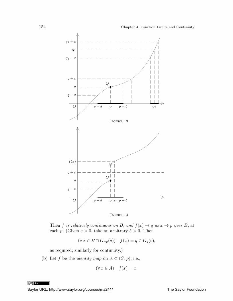
154 Chapter 4. Function Limits and Continuity
O pp− δ p+ δ p1
q
q − ε
q + ε
q1
q1 − ε
q1 + ε
Q
Figure 13
O pp− δ p+ δx
f(x)
q
q − ε
q + ε
Q
Figure 14
Then f is relatively continuous on B, and f(x)→ q as x→ p over B, ateach p. (Given ε > 0, take an arbitrary δ > 0. Then
(∀x ∈ B ∩G¬p(δ)) f(x) = q ∈ Gq(ε),
as required; similarly for continuity.)
(b) Let f be the identity map on A ⊂ (S, ρ); i.e.,
(∀x ∈ A) f(x) = x.
Saylor URL: http://www.saylor.org/courses/ma241/ The Saylor Foundation
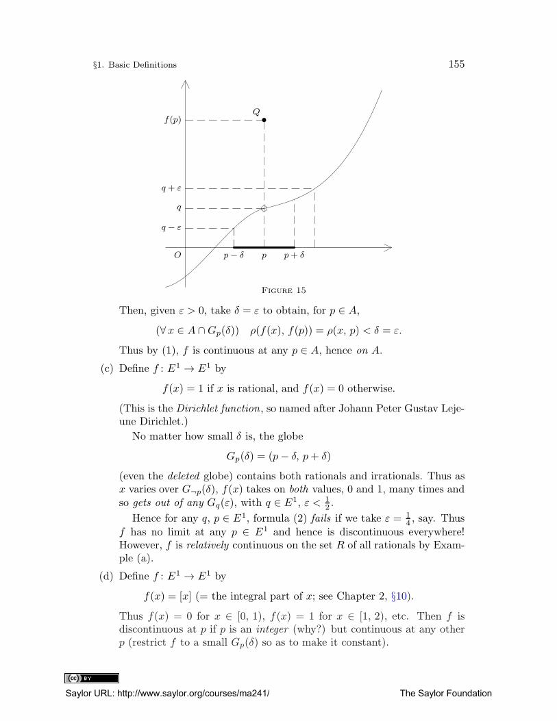
§1. Basic Definitions 155
O pp− δ p+ δ
q
q − ε
q + ε
Qf(p)
Figure 15
Then, given ε > 0, take δ = ε to obtain, for p ∈ A,(∀x ∈ A ∩Gp(δ)) ρ(f(x), f(p)) = ρ(x, p) < δ = ε.
Thus by (1), f is continuous at any p ∈ A, hence on A.
(c) Define f : E1 → E1 by
f(x) = 1 if x is rational, and f(x) = 0 otherwise.
(This is the Dirichlet function, so named after Johann Peter Gustav Leje-une Dirichlet.)
No matter how small δ is, the globe
Gp(δ) = (p− δ, p+ δ)
(even the deleted globe) contains both rationals and irrationals. Thus asx varies over G¬p(δ), f(x) takes on both values, 0 and 1, many times andso gets out of any Gq(ε), with q ∈ E1, ε < 1
2 .
Hence for any q, p ∈ E1, formula (2) fails if we take ε = 14 , say. Thus
f has no limit at any p ∈ E1 and hence is discontinuous everywhere!However, f is relatively continuous on the set R of all rationals by Exam-ple (a).
(d) Define f : E1 → E1 by
f(x) = [x] (= the integral part of x; see Chapter 2, §10).Thus f(x) = 0 for x ∈ [0, 1), f(x) = 1 for x ∈ [1, 2), etc. Then f isdiscontinuous at p if p is an integer (why?) but continuous at any otherp (restrict f to a small Gp(δ) so as to make it constant).
Saylor URL: http://www.saylor.org/courses/ma241/ The Saylor Foundation
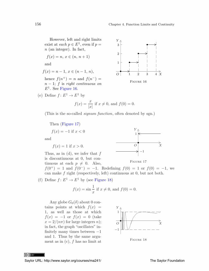
156 Chapter 4. Function Limits and Continuity
O
Y
X
1
2
3
1 2 3 4
Figure 16
However, left and right limitsexist at each p ∈ E1, even if p =n (an integer). In fact,
f(x) = n, x ∈ (n, n+ 1)
and
f(x) = n− 1, x ∈ (n− 1, n),
hence f(n+) = n and f(n−) =n − 1; f is right continuous on
E1. See Figure 16.
(e) Define f : E1 → E1 by
f(x) =x
|x| if x 6= 0, and f(0) = 0.
(This is the so-called signum function, often denoted by sgn.)
O
Y
X
1
−1
Figure 17
Then (Figure 17)
f(x) = −1 if x < 0
and
f(x) = 1 if x > 0.
Thus, as in (d), we infer that fis discontinuous at 0, but con-tinuous at each p 6= 0. Also,f(0+) = 1 and f(0−) = −1. Redefining f(0) = 1 or f(0) = −1, wecan make f right (respectively, left) continuous at 0, but not both.
(f) Define f : E1 → E1 by (see Figure 18)
f(x) = sin1
xif x 6= 0, and f(0) = 0.
O
Y
X
1
−1
Figure 18
Any globe G0(δ) about 0 con-tains points at which f(x) =1, as well as those at whichf(x) = −1 or f(x) = 0 (takex = 2/(nπ) for large integers n);in fact, the graph “oscillates” in-finitely many times between −1and 1. Thus by the same argu-ment as in (c), f has no limit at
Saylor URL: http://www.saylor.org/courses/ma241/ The Saylor Foundation
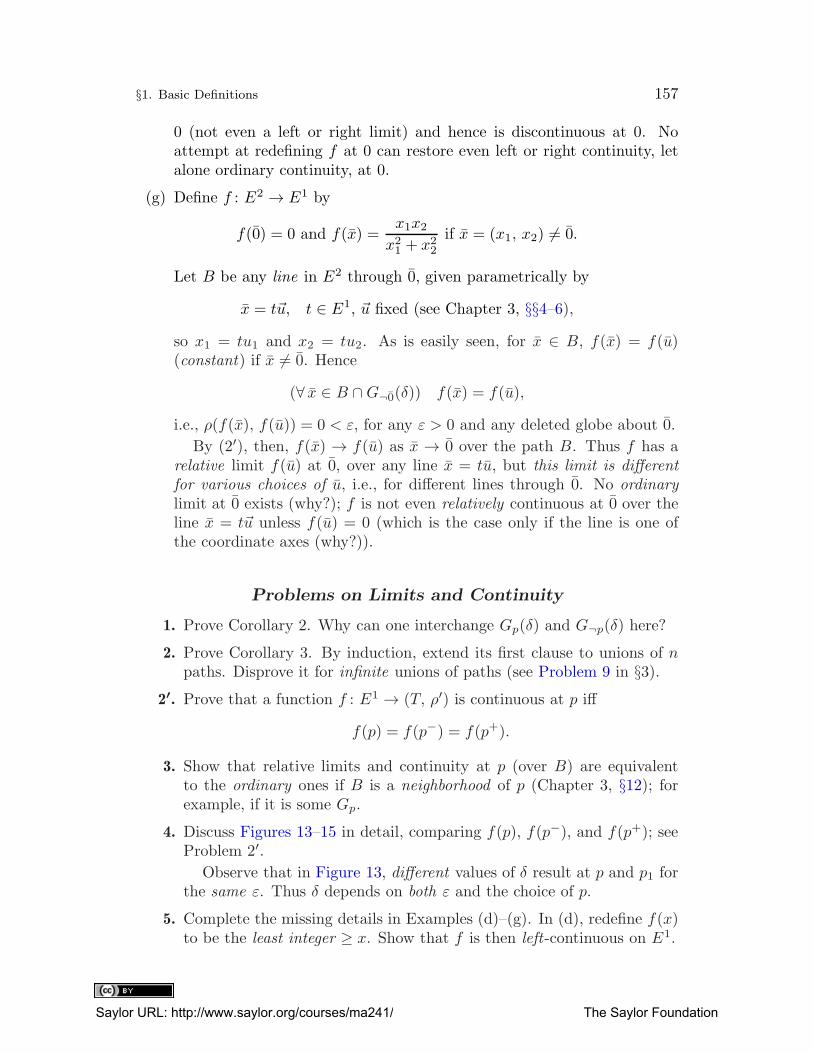
§1. Basic Definitions 157
0 (not even a left or right limit) and hence is discontinuous at 0. Noattempt at redefining f at 0 can restore even left or right continuity, letalone ordinary continuity, at 0.
(g) Define f : E2 → E1 by
f(0) = 0 and f(x) =x1x2x21 + x22
if x = (x1, x2) 6= 0.
Let B be any line in E2 through 0, given parametrically by
x = t~u, t ∈ E1, ~u fixed (see Chapter 3, §§4–6),
so x1 = tu1 and x2 = tu2. As is easily seen, for x ∈ B, f(x) = f(u)(constant) if x 6= 0. Hence
(∀ x ∈ B ∩G¬0(δ)) f(x) = f(u),
i.e., ρ(f(x), f(u)) = 0 < ε, for any ε > 0 and any deleted globe about 0.
By (2′), then, f(x) → f(u) as x → 0 over the path B. Thus f has arelative limit f(u) at 0, over any line x = tu, but this limit is different
for various choices of u, i.e., for different lines through 0. No ordinary
limit at 0 exists (why?); f is not even relatively continuous at 0 over theline x = t~u unless f(u) = 0 (which is the case only if the line is one ofthe coordinate axes (why?)).
Problems on Limits and Continuity
1. Prove Corollary 2. Why can one interchange Gp(δ) and G¬p(δ) here?
2. Prove Corollary 3. By induction, extend its first clause to unions of npaths. Disprove it for infinite unions of paths (see Problem 9 in §3).
2′. Prove that a function f : E1 → (T, ρ′) is continuous at p iff
f(p) = f(p−) = f(p+).
3. Show that relative limits and continuity at p (over B) are equivalentto the ordinary ones if B is a neighborhood of p (Chapter 3, §12); forexample, if it is some Gp.
4. Discuss Figures 13–15 in detail, comparing f(p), f(p−), and f(p+); seeProblem 2′.
Observe that in Figure 13, different values of δ result at p and p1 forthe same ε. Thus δ depends on both ε and the choice of p.
5. Complete the missing details in Examples (d)–(g). In (d), redefine f(x)to be the least integer ≥ x. Show that f is then left-continuous on E1.
Saylor URL: http://www.saylor.org/courses/ma241/ The Saylor Foundation
158 Chapter 4. Function Limits and Continuity
6. Give explicit definitions (such as (3)) for
(a) limx→+∞
f(x) = −∞; (b) limx→−∞
f(x) = q;
(c) limx→p
f(x) = +∞; (d) limx→p
f(x) = −∞;
(e) limx→p−
f(x) = +∞; (f) limx→p+
f(x) = −∞.
In each case, draw a diagram (such as Figures 13–15) and determinewhether the domain and range of f must both be in E∗.
7. Define f : E1 → E1 by
f(x) =x2 − 1
x− 1if x 6= 1, and f(1) = 0.
Show that limx→1 f(x) = 2 exists, yet f is discontinuous at p = 1. Makeit continuous by redefining f(1).[Hint: For x 6= 1, f(x) = x+ 1. Proceed as in Example (b), using the deleted globe
G¬p(δ).]
8. Find limx→p f(x) and check continuity at p in the following cases, assum-ing that Df = A is the set of all x ∈ E1 for which the given expressionfor f(x) has sense. Specify that set.5
(a) limx→2
(2x2 − 3x− 5); (b) limx→1
3x+ 2
2x− 1;
(c) limx→−1
(x2 − 4
x+ 2− 1
)
; (d) limx→2
x3 − 8
x− 2;
(e) limx→a
x4 − a4x− a ; (f) lim
x→0
( x
x+ 1
)3
;
(g) limx→−1
( 1
x2 + 1
)2
.
[Example solution: Find limx→1
5x2 − 1
2x+ 3.
Here
f(x) =5x2 − 1
2x+ 3; A = E1 −
{
−3
2
}
; p = 1.
We show that f is continuous at p, and so (by Corollary 2)
limx→p
f(x) = f(p) = f(1) =4
5.
Using formula (1), we fix an arbitrary ε > 0 and look for a δ such that
(∀x ∈ A ∩Gp(δ)) ρ(f(x), f(1)) = |f(x)− f(1)| < ε, i.e.,∣∣∣5x2 − 1
2x+ 3− 4
5
∣∣∣ < ε;
5 In (d) and (e), p /∈ A, yet one can restore continuity as in Problem 7. (Reduce the
fraction by x− p for x 6= p and define f(p) accordingly.)
Saylor URL: http://www.saylor.org/courses/ma241/ The Saylor Foundation
§1. Basic Definitions 159
or, by putting everything over a common denominator and using properties of abso-lute values,
|x− 1| |25x+ 17|5|2x+ 3| < ε whenever |x− 1| < δ and x ∈ A. (6)
(Usually in such problems, it is desirable to factor out x− p.)
By Note 4, we may assume 0 < δ ≤ 1. Then |x− 1| < δ implies −1 ≤ x− 1 ≤ 1,
i.e., 0 ≤ x ≤ 2, so
5 |2x+ 3| ≥ 15 and |25x+ 17| ≤ 67.
Hence (6) will certainly hold if
|x− 1| 6715
< ε, i.e., if |x− 1| < 15ε
67.
To achieve it, we choose δ = min(1, 15ε/67). Then, reversing all steps, we obtain
(6), and hence limx→1
f(x) = f(1) = 4/5.]
9. Find (using definitions, such as (3))
(a) limx→+∞
1
x; (b) lim
x→−∞3x+ 2
2x− 1;
(c) limx→+∞
x3
1− x2 ; (d) limx→3+
x− 1
x− 3;
(e) limx→3−
x− 1
x− 3; (f) lim
x→3
∣
∣
∣
x− 1
x− 3
∣
∣
∣.
10. Prove that if
limx→p
f(x) = q ∈ En (∗Cn),
then for each scalar c,
limx→p
cf(x) = cq.
11. Define f : E1 → E1 by
f(x) = x · sin 1
xif x 6= 0, and f(0) = 0.
Show that f is continuous at p = 0, i.e.,
limx→0
f(x) = f(0) = 0.
Draw an approximate graph (it is contained between the lines y = ±x).[Hint:
∣∣∣x · sin 1
x− 0
∣∣∣ ≤ |x|.]
∗12. Discuss the statement: f is continuous at p iff
(∀Gf(p)) (∃Gp) f [Gp] ⊆ Gf(p).
Saylor URL: http://www.saylor.org/courses/ma241/ The Saylor Foundation
160 Chapter 4. Function Limits and Continuity
13. Define f : E1 → E1 by
f(x) = x if x is rational
and
f(x) = 0 otherwise.
Show that f is continuous at 0 but nowhere else. How about relative
continuity?
14. Let A = (0, +∞) ⊂ E1. Define f : A→ E1 by
f(x) = 0 if x is irrational
and
f(x) =1
nif x =
m
n(in lowest terms)
for some natural m and n. Show that f is continuous at each irrational,but at no rational, point p ∈ A.[Hints: If p is irrational , fix ε > 0 and an integer k > 1/ε. In Gp(1), there are onlyfinitely many irreducible fractions
m
n> 0 with n ≤ k,
so one of them, call it r, is closest to p. Put
δ = min(1, |r − p|)
and show that
(∀x ∈ A ∩Gp(δ)) |f(x)− f(p)| = f(x) < ε,
distinguishing the cases where x is rational and irrational.
If p is rational , use the fact that each Gp(δ) contains irrationals x at which
f(x) = 0 =⇒ |f(x)− f(p)| = f(p).
Take ε < f(p).]
15. Given two reals, p > 0 and q > 0, define f : E1 → E1 by
f(0) = 0 and f(x) =(x
p
)
·[ q
x
]
if x 6= 0;
here [q/x] is the integral part of q/x.
(i) Is f left or right continuous at 0?
(ii) Same question with f(x) = [x/p](q/x).
16. Prove that if (S, ρ) is discrete, then all functions f : S → (T, ρ′) arecontinuous. What if (T, ρ′) is discrete but (S, ρ) is not?
Saylor URL: http://www.saylor.org/courses/ma241/ The Saylor Foundation
§2. Some General Theorems on Limits and Continuity 161
§2. Some General Theorems on Limits and Continuity
I. In §1 we gave the so-called “ε, δ” definition of continuity. Now we presentanother (equivalent) formulation, known as the sequential one. Roughly, itstates that f is continuous iff it carries convergent sequences {xm} ⊆ Df into
convergent “image sequences” {f(xm)}. More precisely, we have the followingtheorem.
Theorem 1 (sequential criterion of continuity). (i) A function
f : A→ (T, ρ′), with A ⊆ (S, ρ),
is continuous at a point p ∈ A iff for every sequence {xm} ⊆ A such that
xm → p in (S, ρ), we have f(xm)→ f(p) in (T, ρ′). In symbols ,
(∀ {xm} ⊆ A | xm → p) f(xm)→ f(p). (1′)
(ii) Similarly, a point q ∈ T is a limit of f at p (p ∈ S) iff
(∀ {xm} ⊆ A− {p} | xm → p) f(xm)→ q. (2′)
Note that in (2′) we consider only sequences of terms other than p.
Proof. We first prove (ii). Suppose q is a limit of f at p, i.e. (see §1),
(∀ ε > 0) (∃ δ > 0) (∀x ∈ A ∩G¬p(δ)) f(x) ∈ Gq(ε). (2)
Thus, given ε > 0, there is δ > 0 (henceforth fixed) such that
f(x) ∈ Gq(ε) whenever x ∈ A, x 6= p, and x ∈ Gp(δ). (3)
We want to deduce (2′). Thus we fix any sequence
{xm} ⊆ A− {p}, xm → p.1
Then
(∀m) xm ∈ A and xm 6= p,
and Gp(δ) contains all but finitely many xm. Then these xm satisfy the con-ditions stated in (3). Hence f(xm) ∈ Gq(ε) for all but finitely many m. As εis arbitrary, this implies f(xm) → q (by the definition of lim
m→∞f(xm)), as is
required in (2′). Thus (2) =⇒ (2′).
Conversely, suppose (2) fails , i.e., its negation holds. (See the rules forforming negations of such formulas in Chapter 1, §§1–3.) Thus
(∃ ε > 0) (∀ δ > 0) (∃x ∈ A ∩G¬p(δ)) f(x) /∈ Gq(ε) (4)
1 If no such sequence exists, then (2′) is vacuously true and there is nothing to prove.
Saylor URL: http://www.saylor.org/courses/ma241/ The Saylor Foundation
162 Chapter 4. Function Limits and Continuity
by the rules for quantifiers. We fix an ε satisfying (4), and let
δm =1
m, m = 1, 2, . . . .
By (4), for each δm there is xm (depending on δm) such that
xm ∈ A ∩G¬p
( 1
m
)
(5)
andf(xm) /∈ Gq(ε), m = 1, 2, 3, . . . (6)
We fix these xm. As xm ∈ A and xm 6= p, we obtain a sequence
{xm} ⊆ A− {p}.Also, as xm ∈ Gp(
1m), we have ρ(xm, p) < 1/m → 0, and hence xm → p.
On the other hand, by (6), the image sequence {f(xm)} cannot converge to q(why?), i.e., (2′) fails . Thus we see that (2′) fails or holds accordingly as (2)does .
This proves assertion (ii). Now, by setting q = f(p) in (2) and (2′), we alsoobtain the first clause of the theorem, as to continuity. �
Note 1. The theorem also applies to relative limits and continuity over apath B (just replace A by B in the proof), as well as to the cases p = ±∞and q = ±∞ in E∗ (for E∗ can be treated as a metric space; see the end ofChapter 3, §11).
If the range space (T, ρ′) is complete (Chapter 3, §17), then the imagesequences {f(xm)} converge iff they are Cauchy . This leads to the followingcorollary.
Corollary 1. Let (T, ρ′) be complete, such as En. Let a map f : A→ T with
A ⊆ (S, ρ) and a point p ∈ S be given. Then for f to have a limit at p,it suffices that {f(xm)} be Cauchy in (T, ρ′) whenever {xm} ⊆ A − {p} and
xm → p in (S, ρ).
Indeed, as noted above, all such {f(xm)} converge. Thus it only remains toshow that they tend to one and the same limit q, as is required in part (ii) ofTheorem 1. We leave this as an exercise (Problem 1 below).∗Theorem 2 (Cauchy criterion for functions). With the assumptions of Corol-
lary 1, the function f has a limit at p iff for each ε > 0, there is δ > 0 such
that
ρ′(f(x), f(x′)) < ε for all x, x′ ∈ A ∩G¬p(δ).2
In symbols ,
(∀ ε > 0) (∃ δ > 0) (∀x, x′ ∈ A ∩G¬p(δ)) ρ′(f(x), f(x′)) < ε. (7)
2 That is, f(x) is ε-close to f(x′) when x and x′ are δ-close to p, but not equal to p.
Saylor URL: http://www.saylor.org/courses/ma241/ The Saylor Foundation
§2. Some General Theorems on Limits and Continuity 163
Proof. Assume (7). To show that f has a limit at p, we use Corollary 1. Thuswe take any sequence
{xm} ⊆ A− {p} with xm → p
and show that {f(xm)} is Cauchy, i.e.,(∀ ε > 0) (∃ k) (∀m,n > k) ρ′(f(xm), f(xn)) < ε.
To do this, fix an arbitrary ε > 0. By (7), we have
(∀x, x′ ∈ A ∩G¬p(δ)) ρ′(f(x), f(x′)) < ε, (7′)
for some δ > 0. Now as xm → p, there is k such that
(∀m, n > k) xm, xn ∈ Gp(δ).
As {xm} ⊆ A− {p}, we even have xm, xn ∈ A ∩G¬p(δ). Hence by (7′),
(∀m, n > k) ρ′(f(xm), f(xn)) < ε;
i.e., {f(xm)} is Cauchy , as required in Corollary 1, and so f has a limit at p.This shows that (7) implies the existence of that limit.
The easy converse proof is left to the reader. (See Problem 2.) �
II. Composite Functions. The composite of two functions
f : S → T and g : T → U ,
denotedg ◦ f (in that order),
is by definition a map of S into U given by
(g ◦ f)(x) = g(f(x)), s ∈ S.Our next theorem states, roughly, that g ◦ f is continuous if g and f are. Weshall use Theorem 1 to prove it.
Theorem 3. Let (S, ρ), (T, ρ′), and (U, ρ′′) be metric spaces. If a function
f : S → T is continuous at a point p ∈ S, and if g : T → U is continuous at the
point q = f(p), then the composite function g ◦ f is continuous at p.
Proof. The domain of g ◦ f is S. So take any sequence
{xm} ⊆ S with xm → p.
As f is continuous at p, formula (1′) yields f(xm) → f(p), where f(xm) is inT = Dg. Hence, as g is continuous at f(p), we have
g(f(xm))→ g(f(p)), i.e., (g ◦ f)(xm)→ (g ◦ f)(p),and this holds for any {xm} ⊆ S with xm → p. Thus g ◦ f satisfies condition(1′) and is continuous at p. �
Saylor URL: http://www.saylor.org/courses/ma241/ The Saylor Foundation
164 Chapter 4. Function Limits and Continuity
Caution: The fact that
limx→p
f(x) = q and limy→q
g(y) = r
does not imply
limx→p
g(f(x)) = r
(see Problem 3 for counterexamples).
Indeed, if {xm} ⊆ S−{p} and xm → p, we obtain, as before, f(xm)→ q, butnot f(xm) 6= q. Thus we cannot re-apply formula (2′) to obtain g(f(xm))→ rsince (2′) requires that f(xm) 6= q. The argument still works if g is continuousat q (then (1′) applies) or if f(x) never equals q (then f(xm) 6= q). It evensuffices that f(x) 6= q for x in some deleted globe about p (see §1, Note 4).Hence we obtain the following corollary.
Corollary 2. With the notation of Theorem 3, suppose
f(x)→ q as x→ p, and g(y)→ r as y → q.
Then
g(f(x))→ r as x→ p,
provided, however, that
(i) g is continuous at q, or
(ii) f(x) 6= q for x in some deleted globe about p, or
(iii) f is one to one, at least when restricted to some G¬p(δ).
Indeed, (i) and (ii) suffice, as was explained above. Thus assume (iii). Thenf can take the value q at most once, say, at some point
x0 ∈ G¬p(δ).
As x0 6= p, let
δ′ = ρ(x0, p) > 0.
Then x0 /∈ G¬p(δ′), so f(x) 6= q on G¬p(δ
′), and case (iii) reduces to (ii).
We now show how to apply Corollary 2.
Note 2. Suppose we know that
r = limy→q
g(y) exists.
Using this fact, we often pass to another variable x, setting y = f(x) where fis such that q = limx→p f(x) for some p. We shall say that the substitution (or
Saylor URL: http://www.saylor.org/courses/ma241/ The Saylor Foundation
§2. Some General Theorems on Limits and Continuity 165
“change of variable”) y = f(x) is admissible if one of the conditions (i), (ii), or(iii) of Corollary 2 holds.3 Then by Corollary 2,
limy→q
g(y) = r = limx→p
g(f(x))
(yielding the second limit).
Examples.
(A) Let
h(x) =(
1 +1
x
)x
for |x| ≥ 1.
Then
limx→+∞
h(x) = e.
For a proof, let n = f(x) = [x] be the integral part of x. Then forx > 1,
(
1 +1
n+ 1
)n
≤ h(x) ≤(
1 +1
n
)n+1
. (Verify!) (8)
As x→ +∞, n tends to +∞ over integers, and by rules for sequences,
limn→∞
(
1 +1
n
)n+1
= limn→∞
(
1 +1
n
)(
1 +1
n
)n
= 1 · limn→∞
(
1 +1
n
)n
= 1 · e = e,
with e as in Chapter 3, §15. Similarly one shows that also
limn→∞
(
1 +1
n+ 1
)n
= e.
Thus (8) implies that also limx→+∞
h(x) = e (see Problem 6 below).
Remark. Here we used Corollary 2(ii) with
f(x) = [x], q = +∞, and g(n) =(
1 +1
n
)n
.
The substitution n = f(x) is admissible since f(x) = n never equals +∞, itslimit, thus satisfying Corollary 2(ii).
(B) Quite similarly, one shows that also
limx→−∞
(
1 +1
x
)x
= e.
See Problem 5.
3 In particular, the so-called linear substitution y = ax + b (a, b ∈ E1, a 6= 0) is always
admissible since f(x) = ax+ b yields a one-to-one map.
Saylor URL: http://www.saylor.org/courses/ma241/ The Saylor Foundation
166 Chapter 4. Function Limits and Continuity
(C) In Examples (A) and (B), we now substitute x = 1/z. This is admissibleby Corollary 2(ii) since the dependence between x and z is one to one.Then
z =1
x→ 0+ as x→ +∞, and z → 0− as x→ −∞.
Thus (A) and (B) yield
limz→0+
(1 + z)1/z = limz→0−
(1 + z)1/z = e.
Hence by Corollary 3 of §1, we obtain
limz→0
(1 + z)1/z = e. (9)
More Problems on Limits and Continuity
1. Complete the proof of Corollary 1.[Hint: Consider {f(xm)} and {f(x′
m)}, with
xm → p and x′m → p.
By Chapter 3, §14, Corollary 4, p is also the limit of
x1, x′1, x2, x
′2, . . . ,
so, by assumption,
f(x1), f(x′1), . . . converges (to q, say).
Hence {f(xm)} and {f(x′m)} must have the same limit q. (Why?)]
∗2. Complete the converse proof of Theorem 2 (cf. proof of Theorem 1 inChapter 3, §17).
3. Define f, g : E1 → E1 by setting
(i) f(x) = 2; g(y) = 3 if y 6= 2, and g(2) = 0; or
(ii) f(x) = 2 if x is rational and f(x) = 2x otherwise; g as in (i).
In both cases, show that
limx→1
f(x) = 2 and limy→2
g(y) = 3 but not limx→1
g(f(x)) = 3.4
4. Prove Theorem 3 from “ε, δ” definitions. Also prove (both ways) that iff is relatively continuous on B, and g on f [B], then g ◦ f is relativelycontinuous on B.
4 In case (ii), disprove the existence of limx→1 g(f(x)).
Saylor URL: http://www.saylor.org/courses/ma241/ The Saylor Foundation
§2. Some General Theorems on Limits and Continuity 167
5. Complete the missing details in Examples (A) and (B).[Hint for (B): Verify that
(
1− 1
n+ 1
)−n−1=
( n
n+ 1
)−n−1=
(n+ 1
n
)n+1=
(
1 +1
n
)(
1 +1
n
)n→ e.]
⇒6. Given f, g, h : A→ E∗, A ⊆ (S, ρ), with
f(x) ≤ h(x) ≤ g(x)for x ∈ G¬p(δ) ∩A for some δ > 0. Prove that if
limx→p
f(x) = limx→p
g(x) = q,
then alsolimx→p
h(x) = q.
Use Theorem 1.[Hint: Take any
{xm} ⊆ A− {p} with xm → p.
Then f(xm) → q, g(xm) → q, and
(∀xm ∈ A ∩G¬p(δ)) f(xm) ≤ h(xm) ≤ g(xm).
Now apply Corollary 3 of Chapter 3, §15.]
⇒7. Given f, g : A→ E∗, A ⊆ (S, ρ), with f(x)→ q and g(x)→ r as x→ p(p ∈ S), prove the following:
(i) If q > r, then
(∃ δ > 0) (∀x ∈ A ∩G¬p(δ)) f(x) > g(x).
(ii) (Passage to the limit in inequalities.) If
(∀ δ > 0) (∃x ∈ A ∩G¬p(δ)) f(x) ≤ g(x),then q ≤ r. (Observe that here A clusters at p necessarily, so thelimits are unique.)[Hint: Proceed as in Problem 6; use Corollary 1 of Chapter 3, §15.]
8. Do Problems 6 and 7 using only Definition 2 of §1.[Hint: Here prove 7(ii) first.]
9. Do Examples (a)–(d) of §1 using Theorem 1.[Hint: For (c), use also Example (a) in Chapter 3, §16.]
10. Addition and multiplication in E1 may be treated as functions
f, g : E2 → E1
withf(x, y) = x+ y and g(x, y) = xy.
Saylor URL: http://www.saylor.org/courses/ma241/ The Saylor Foundation
168 Chapter 4. Function Limits and Continuity
Show that f and g are continuous on E2 (see footnote 2 in Chapter 3,§15). Similarly, show that the standard metric
ρ(x, y) = |x− y|is a continuous mapping from E2 to E1.[Hint: Use Theorems 1, 2, and, 4 of Chapter 3, §15 and the sequential criterion.]
11. Using Corollary 2 and formula (9), find limx→0
(1±mx)1/x for a fixed m ∈N .
⇒12. Let a > 0 in E1. Prove that limx→0
ax = 1.
[Hint: Let n = f(x) be the integral part of 1x
(x 6= 0). Verify that
a−1/(n+1) ≤ ax ≤ a1/n if a ≥ 1,
with inequalities reversed if 0 < a < 1. Then proceed as in Example (A), noting that
limn→∞
a1/n = 1 = limn→∞
a−1/(n+1)
by Problem 20 of Chapter 3, §15. (Explain!)]
⇒13. Given f, g : A→ E∗, A ⊆ (S, ρ), with
f ≤ g for x in G¬p(δ) ∩A.Prove that
(a) if limx→p
f(x) = +∞, then also limx→p
g(x) = +∞;
(b) if limx→p
g(x) = −∞, then also limx→p
f(x) = −∞.
Do it it two ways:
(i) Use definitions only, such as (2′) in §1.(ii) Use Problem 10 of Chapter 2, §13 and the sequential criterion.
⇒14. Prove that
(i) if a > 1 in E1, then
limx→+∞
ax
x= +∞ and lim
x→+∞a−x
x= 0;
(ii) if 0 < a < 1, then
limx→+∞
ax
x= 0 and lim
x→+∞a−x
x= +∞;
(iii) if a > 1 and 0 ≤ q ∈ E1, then
limx→+∞
ax
xq= +∞ and lim
x→+∞a−x
xq= 0;
Saylor URL: http://www.saylor.org/courses/ma241/ The Saylor Foundation

§2. Some General Theorems on Limits and Continuity 169
(iv) if 0 < a < 1 and 0 ≤ q ∈ E1, then
limx→+∞
ax
xq= 0 and lim
x→+∞a−x
xq= +∞.
[Hint: (i) From Problems 17 and 10 of Chapter 3, §15, obtain
liman
n= +∞.
Then proceed as in Examples (A)–(C); (iii) reduces to (i) by the method used inProblem 18 of Chapter 3, §15.]
⇒∗15. For a map f : (S, ρ) → (T, ρ′), show that the following statements areequivalent:
(i) f is continuous on S.
(ii) (∀A ⊆ S) f [A] ⊆ f [A].(iii) (∀B ⊆ T ) f−1[B] ⊇ f−1[B].
(iv) f−1[B] is closed in (S, ρ) whenever B is closed in (T, ρ′).
(v) f−1[B] is open in (S, ρ) whenever B is open in (T, ρ′).
[Hints: (i) =⇒ (ii): Use Theorem 3 of Chapter 3, §16 and the sequential criterion to
show thatp ∈ A =⇒ f(p) ∈ f [A].
(ii) =⇒ (iii): Let A = f−1[B]. Then f [A] ⊆ B, so by (ii),
f [A] ⊆ f [A] ⊆ B.
Hencef−1[B] = A ⊆ f−1[f [A]] ⊆ f−1[B]. (Why?)
(iii) =⇒ (iv): If B is closed, B = B (Chapter 3, §16, Theorem 4(ii)), so by (iii),
f−1[B] = f−1[B] ⊇ f−1[B]; deduce (iv).
(iv) =⇒ (v): Pass to complements in (iv).
(v) =⇒ (i): Assume (v). Take any p ∈ S and use Definition 1 in §1.]
16. Let f : E1 → E1 be continuous. Define g : E1 → E2 by
g(x) = (x, f(x)).
Prove that
(a) g and g−1 are one to one and continuous;
(b) the range of g, i.e., the set
D′g = {(x, f(x)) | x ∈ E1},
is closed in E2.
[Hint: Use Theorem 2 of Chapter 3, §15, Theorem 4 of Chapter 3, §16, and thesequential criterion.]
Saylor URL: http://www.saylor.org/courses/ma241/ The Saylor Foundation
170 Chapter 4. Function Limits and Continuity
§3. Operations on Limits. Rational Functions
I. A function f : A→ T is said to be real if its range D′f lies in E1, complex
if D′f ⊆ C, vector valued if D′
f is a subset of En, and scalar valued if D′f lies in
the scalar field of En. (∗In the latter two cases, we use the same terminology ifEn is replaced by some other (fixed) normed space under consideration.) Thedomain A may be arbitrary.
For such functions one can define various operations whenever they are de-fined for elements of their ranges , to which the function values f(x) belong.Thus as in Chapter 3, §9, we define the functions f±g, fg, and f/g “pointwise,”setting
(f ± g)(x) = f(x)± g(x), (fg)(x) = f(x) g(x), and(f
g
)
(x) =f(x)
g(x)
whenever the right side expressions are defined. We also define |f | : A → E1
by
(∀x ∈ A) |f |(x) = |f(x)|.
In particular, f±g is defined if f and g are both vector valued or both scalarvalued, and fg is defined if f is vector valued while g is scalar valued; similarlyfor f/g. (However, the domain of f/g consists of those x ∈ A only for whichg(x) 6= 0.)
In the theorems below, all limits are at some (arbitrary, but fixed) point pof the domain space (S, ρ). For brevity, we often omit “x→ p.”
Theorem 1. For any functions f, g, h : A→ E1(C), A ⊆ (S, ρ), we have the
following:
(i) If f, g, h are continuous at p (p ∈ A), so are f ± g and fh. So also is
f/h, provided h(p) 6= 0; similarly for relative continuity over B ⊆ A.
(ii) If f(x)→ q, g(x)→ r, and h(x)→ a (all , as x→ p over B ⊆ A), then(a) f(x)± g(x)→ q ± r;(b) f(x)h(x)→ qa; and
(c)f(x)
h(x)→ q
a, provided a 6= 0.
All this holds also if f and g are vector valued and h is scalar valued .
For a simple proof, one can use Theorem 1 of Chapter 3, §15. (An indepen-dent proof is sketched in Problems 1–7 below.)
We can also use the sequential criterion (Theorem 1 in §2). To prove (ii),take any sequence
{xm} ⊆ B − {p}, xm → p.
Saylor URL: http://www.saylor.org/courses/ma241/ The Saylor Foundation
§3. Operations on Limits. Rational Functions 171
Then by the assumptions made,
f(xm)→ q, g(xm)→ r, and h(xm)→ a.
Thus by Theorem 1 of Chapter 3, §15,
f(xm)± g(xm)→ q ± r, f(xm)g(xm)→ qa, andf(xm)
g(xm)→ q
a.
As this holds for any sequence {xm} ⊆ B − {p} with xm → p, our assertion(ii) follows by the sequential criterion; similarly for (i).
Note 1. By induction, the theorem also holds for sums and products of anyfinite number of functions (whenever such products are defined).
Note 2. Part (ii) does not apply to infinite limits q, r, a; but it does applyto limits at p = ±∞ (take E∗ with a suitable metric for the space S).
Note 3. The assumption h(x) → a 6= 0 (as x → p over B) implies thath(x) 6= 0 for x in B ∩ G¬p(δ) for some δ > 0; see Problem 5 below. Thus thequotient function f/h is defined on B ∩G¬p(δ) at least .
II. If the range space of f is En (∗or Cn), then each function value f(x) isa vector in that space; thus it has n real (∗respectively, complex) components,denoted
fk(x), k = 1, 2, . . . , n.
Here we may treat fk as a mapping of A = Df into E1 (∗or C); it carrieseach point x ∈ A into fk(x), the kth component of f(x). In this manner, eachfunction
f : A→ En (Cn)
uniquely determines n scalar-valued maps
fk : A→ E1 (C),
called the components of f . Notation: f = (f1, . . . , fn).
Conversely, given n arbitrary functions
fk : A→ E1 (C), k = 1, 2, . . . , n,
one can define f : A→ En (Cn) by setting
f(x) = (f1(x), f2(x), . . . , fn(x)).
Then obviously f = (f1, f2, . . . , fn). Thus the fk in turn determine f uniquely.To define a function f : A→ En (Cn) means to give its n components fk. Notethat
f(x) = (f1(x), . . . , fn(x)) =
n∑
k=1
ekfk(x), i.e., f =
n∑
k=1
ekfk, (1)
Saylor URL: http://www.saylor.org/courses/ma241/ The Saylor Foundation
172 Chapter 4. Function Limits and Continuity
where the ek are the n basic unit vectors; see Chapter 3, §§1–3, Theorem 2.Our next theorem shows that the limits and continuity of f reduce to those ofthe fk.
Theorem 2 (componentwise continuity and limits). For any function f : A→En (Cn), with A ⊆ (S, ρ) and with f = (f1, . . . , fn), we have that
(i) f is continuous at p (p ∈ A) iff all its components fk are, and
(ii) f(x)→ q as x→ p (p ∈ S) iff
fk(x)→ qk as x→ p (k = 1, 2, . . . , n),
i .e., iff each fk has , as its limit at p, the corresponding component of q.
Similar results hold for relative continuity and limits over a path B ⊆ A.We prove (ii). If f(x)→ q as x→ p then, by definition,
(∀ ε > 0) (∃ δ > 0) (∀x ∈ A ∩G¬p(δ)) ε > |f(x)− q| =√
n∑
k=1
|fk(x)− qk|2 ;
in turn, the right-hand side of the inequality given above is no less than each
|fk(x)− qk|, k = 1, 2, . . . , n.
Thus
(∀ ε > 0) (∃ δ > 0) (∀x ∈ A ∩G¬p(δ)) |fk(x)− qk| < ε;
i.e., fk(x)→ qk, k = 1, . . . , n.
Conversely, if each fk(x)→ qk, then Theorem 1(ii) yields
n∑
k=1
ekfk(x)→n∑
k=1
ekqk.1
By formula (1), then, f(x) → q (for∑n
k=1 ekqk = q). Thus (ii) is proved;similarly for (i) and for relative limits and continuity.
Note 4. Again, Theorem 2 holds also for p = ±∞ (but not for infinite q).
Note 5. A complex function f : A → C may be treated as f : A → E2.Thus it has two real components: f = (f1, f2). Traditionally, f1 and f2 arecalled the real and imaginary parts of f , also denoted by fre and fim, so
f = fre + i · fim.
By Theorem 2, f is continuous at p iff fre and fim are.
1 Here we treat ek as a constant function , with values ek (cf. §1, Example (a)).
Saylor URL: http://www.saylor.org/courses/ma241/ The Saylor Foundation
§3. Operations on Limits. Rational Functions 173
Example.
The complex exponential is the function f : E1 → C defined by
f(x) = cosx+ i · sinx, also written f(x) = exi.
As we shall see later, the sine and the cosine functions are continuous.Hence so is f by Theorem 2.
III. Next, consider functions whose domain is a set in En (∗or Cn). We callthem functions of n real (∗or complex ) variables, treating x = (x1, . . . , xn) asa variable n-tuple. The range space may be arbitrary.
In particular, a monomial in n variables is a map on En (∗or Cn) given bya formula of the form
f(x) = axm1
1 xm2
2 · · ·xmn
n = a ·n∏
k=1
xmk
k ,
where the mk are fixed integers ≥ 0 and a ∈ E1 (∗or a ∈ C).2 If a 6= 0, thesum m =
∑nk=1mk is called the degree of the monomial. Thus
f(x, y, z) = 3x2yz3 = 3x2y1z3
defines a monomial of degree 6, in three real (or complex) variables x, y, z.(We often write x, y, z for x1, x2, x3.)
A polynomial is any sum of a finite number of monomials; its degree is, bydefinition, that of its leading term, i.e., the one of highest degree. (There maybe several such terms, of equal degree.) For example,
f(x, y, z) = 3x2yz3 − 2xy7
defines a polynomial of degree 8 in x, y, z. Polynomials of degree 1 are some-times called linear .
A rational function is the quotient f/g of two polynomials f and g on En
(∗or Cn).3 Its domain consists of those points at which g does not vanish. Forexample,
h(x, y) =x2 − 3xy
xy − 1
defines a rational function on points (x, y), with xy 6= 1. Polynomials andmonomials are rational functions with denominator 1.
Theorem 3. Any rational function (in particular , every polynomial) in one
or several variables is continuous on all of its domain.
2 We also allow a to be a vector , while the xk are scalars.3 This is valid also if one allows the coefficients of f to be vectors (provided those of g,
and the variables xk, remain scalars).
Saylor URL: http://www.saylor.org/courses/ma241/ The Saylor Foundation
174 Chapter 4. Function Limits and Continuity
Proof. Consider first a monomial of the form
f(x) = xk (k fixed);
it is called the kth projection map because it “projects” each x ∈ En (∗Cn)onto its kth component xk.
Given any ε > 0 and p, choose δ = ε. Then
(∀ x ∈ Gp(δ)) |f(x)− f(p)| = |xk − pk| ≤√
n∑
i=1
|xi − pi|2 = ρ(x, p) < ε.
Hence by definition, f is continuous at each p. Thus the theorem holds forprojection maps.
However, any other monomial, given by
f(x) = axm1
1 xm2
2 · · ·xmnn ,
is the product of finitely many (namely of m = m1+m2+ · · ·+mn) projectionmaps multiplied by a constant a. Thus by Theorem 1, it is continuous. Soalso is any finite sum of monomials (i.e., any polynomial), and hence so isthe quotient f/g of two polynomials (i.e., any rational function) wherever it isdefined, i.e., wherever the denominator does not vanish. �
IV. For functions on En (∗or Cn), we often consider relative limits over a
line of the form
x = p+ t~ek (parallel to the kth axis, through p);
see Chapter 3, §§4–6, Definition 1. If f is relatively continuous at p over that
line, we say that f is continuous at p in the kth variable xk (because the othercomponents of x remain constant , namely, equal to those of p, as x runs overthat line). As opposed to this, we say that f is continuous at p in all n variables
jointly if it is continuous at p in the ordinary (not relative) sense. Similarly,we speak of limits in one variable, or in all of them jointly.
Since ordinary continuity implies relative continuity over any path, jointcontinuity in all n variables always implies that in each variable separately ,but the converse fails (see Problems 9 and 10 below); similarly for limits at p.
Problems on Continuity of Vector-Valued Functions
1. Give an “ε, δ” proof of Theorem 1 for f ± g.[Hint: Proceed as in Theorem 1 of Chapter 3, §15, replacing max(k′, k′′) by δ =
min(δ′, δ′′). Thus fix ε > 0 and p ∈ S. If f(x) → q and g(x) → r as x → p over B,
then (∃ δ′, δ′′ > 0) such that
(∀x ∈ B ∩G¬p(δ′)) |f(x)− q| < ε
2and (∀x ∈ B ∩G¬p(δ
′′)) |g(x)− r| < ε
2.
Put δ = min(δ′, δ′′), etc.]
Saylor URL: http://www.saylor.org/courses/ma241/ The Saylor Foundation
§3. Operations on Limits. Rational Functions 175
In Problems 2, 3, and 4, E = En (∗or another normed space), F is its scalarfield, B ⊆ A ⊆ (S, ρ), and x→ p over B.
2. For a function f : A→ E prove that
f(x)→ q ⇐⇒ |f(x)− q| → 0,
equivalently, iff f(x)− q → 0.[Hint: Proceed as in Chapter 3, §14, Corollary 2.]
3. Given f : A → (T, ρ′), with f(x) → q as x → p over B. Show that forsome δ > 0, f is bounded on B ∩G¬p(δ), i.e.,
f [B ∩G¬p(δ)] is a bounded set in (T, ρ′).
Thus if T = E, there is K ∈ E1 such that
(∀x ∈ B ∩G¬p(δ)) |f(x)| < K
(Chapter 3, §13, Theorem 2).
4. Given f, h : A → E1 (C) (or f : A → E, h : A → F ), prove that if oneof f and h has limit 0 (respectively, 0), while the other is bounded onB ∩G¬p(δ), then h(x)f(x)→ 0 (0).
5. Given h : A → E1 (C), with h(x) → a as x → p over B, and a 6= 0.Prove that
(∃ ε, δ > 0) (∀x ∈ B ∩G¬p(δ)) |h(x)| ≥ ε,i.e., h(x) is bounded away from 0 on B ∩G¬p(δ). Hence show that 1/his bounded on B ∩G¬p(δ).[Hint: Proceed as in the proof of Corollary 1 in §1, with q = a and r = 0. Then use
(∀x ∈ B ∩G¬p(δ))∣∣∣
1
h(x)
∣∣∣ ≤ 1
ε.]
6. Using Problems 1 to 5, give an independent proof of Theorem 1.[Hint: Proceed as in Problems 2 and 4 of Chapter 3, §15 to obtain Theorem 1(ii).Then use Corollary 2 of §1.]
7. Deduce Theorems 1 and 2 of Chapter 3, §15 from those of the presentsection, setting A = B = N , S = E∗, and p = +∞.[Hint: See §1, Note 5.]
8. Redo Problem 8 of §1 in two ways:
(i) Use Theorem 1 only.
(ii) Use Theorem 3.
[Example for (i): Find limx→1
(x2 + 1).
Here f(x) = x2 + 1, or f = gg + h, where h(x) = 1 (constant) and g(x) = x(identity map). As h and g are continuous (§1, Examples (a) and (b)), so is f by
Theorem 1. Thus limx→1
f(x) = f(1) = 12 + 1 = 2.
Saylor URL: http://www.saylor.org/courses/ma241/ The Saylor Foundation
176 Chapter 4. Function Limits and Continuity
Or, using Theorem 1(ii), limx→1
(x2 + 1) = limx→1
x2 + limx→1
1, etc.]
9. Define f : E2 → E1 by
f(x, y) =x2y
(x4 + y2), with f(0, 0) = 0.
Show that f(x, y)→ 0 as (x, y)→ (0, 0) along any straight line through0, but not over the parabola y = x2 (then the limit is 1
2). Deduce that
f is continuous at 0 = (0, 0) in x and y separately , but not jointly .
10. Do Problem 9, setting
f(x, y) = 0 if x = 0, and f(x, y) =|y|x2· 2−|y|/x2
if x 6= 0.4
11. Discuss the continuity of f : E2 → E1 in x and y jointly and separately,at 0, when
(a) f(x, y) =x2y2
x2 + y2, f(0, 0) = 0;
(b) f(x, y) = integral part of x+ y;
(c) f(x, y) = x+xy
|x| if x 6= 0, f(0, y) = 0;
(d) f(x, y) =xy
|x| + x sin1
yif xy 6= 0, and f(x, y) = 0 otherwise;
(e) f(x, y) =1
xsin(x2 + |xy|) if x 6= 0, and f(0, y) = 0.
[Hints: In (c) and (d), |f(x, y)| ≤ |x|+ |y|; in (e), use | sinα| ≤ |α|.]
4 Use Problem 14 in §2 for limit computations.
Saylor URL: http://www.saylor.org/courses/ma241/ The Saylor Foundation
§4. Infinite Limits. Operations in E∗ 177
§4. Infinite Limits. Operations in E∗
As we have noted, Theorem 1 of §3 does not apply to infinite limits ,1 even ifthe function values f(x), g(x), h(x) remain finite (i.e., in E1). Only in certaincases (stated below) can we prove some analogues.
There are quite a few such separate cases. Thus, for brevity, we shall adopta kind of mathematical shorthand. The letter q will not necessarily denote aconstant ; it will stand for
“a function f : A→ E1, A ⊆ (S, ρ), such that f(x)→ q ∈ E1 as x→ p.”2
Similarly, “0” and “±∞” will stand for analogous expressions, with q replacedby 0 and ±∞, respectively.
For example, the “shorthand formula” (+∞) + (+∞) = +∞ means
“The sum of two real functions, with limit +∞ at p (p ∈ S), is itself afunction with limit +∞ at p.”3
The point p is fixed, possibly ±∞ (if A ⊆ E∗). With this notation, we havethe following theorems.
Theorems.
1. (±∞) + (±∞) = ±∞.
2. (±∞) + q = q + (±∞) = ±∞.
3. (±∞) · (±∞) = +∞.
4. (±∞) · (∓∞) = −∞.
5. | ±∞| = +∞.
6. (±∞) · q = q · (±∞) = ±∞ if q > 0.
7. (±∞) · q = q · (±∞) = ∓∞ if q < 0.
8. −(±∞) = ∓∞.
9.(±∞)
q= (±∞) · 1
qif q 6= 0.
10.q
(±∞)= 0.
11. (+∞)+∞ = +∞.
12. (+∞)−∞ = 0.
13. (+∞)q = +∞ if q > 0.
1 It even has no meaning since operations on ±∞ have not been defined.2 Note that q is finite throughout.3 Similarly for (−∞) + (−∞) = −∞. Both combined are written as “(±∞) + (±∞) =
±∞.”
Saylor URL: http://www.saylor.org/courses/ma241/ The Saylor Foundation
178 Chapter 4. Function Limits and Continuity
14. (+∞)q = 0 if q < 0.
15. If q > 1, then q+∞ = +∞ and q−∞ = 0.
16. If 0 < q < 1, then q+∞ = 0 and q−∞ = +∞.
We prove Theorems 1 and 2, leaving the rest as problems. (Theorems 11–16are best postponed until the theory of logarithms is developed.)
1. Let f(x) and g(x)→ +∞ as x→ p. We have to show that
f(x) + g(x)→ +∞,
i.e., that
(∀ b ∈ E1) (∃ δ > 0) (∀x ∈ A ∩G¬p(δ)) f(x) + g(x) > b
(we may assume b > 0). Thus fix b > 0. As f(x) and g(x)→ +∞, thereare δ′, δ′′ > 0 such that
(∀x ∈ A ∩G¬p(δ′)) f(x) > b and (∀x ∈ A ∩G¬p(δ
′′)) g(x) > b.
Let δ = min(δ′, δ′′). Then
(∀x ∈ A ∩G¬p(δ)) f(x) + g(x) > b+ b > b,
as required; similarly for the case of −∞.
2. Let f(x) → +∞ and g(x) → q ∈ E1. Then there is δ′ > 0 such that forx in A ∩G¬p(δ
′), |q − g(x)| < 1, so that g(x) > q − 1.
Also, given any b ∈ E1, there is δ′′ such that
(∀x ∈ A ∩G¬p(δ′′)) f(x) > b− q + 1.
Let δ = min(δ′, δ′′). Then
(∀x ∈ A ∩G¬p(δ)) f(x) + g(x) > (b− q + 1) + (q − 1) = b,
as required; similarly for the case of f(x)→ −∞.
Caution: No theorems of this kind exist for the following cases (which there-fore are called indeterminate expressions):
(+∞) + (−∞), (±∞) · 0, ±∞±∞ ,
0
0, (±∞)0, 00, 1±∞. (1∗)
In these cases, it does not suffice to know only the limits of f and g. Itis necessary to investigate the functions themselves to give a definite answer,since in each case the answer may be different, depending on the properties off and g. The expressions (1∗) remain indeterminate even if we consider thesimplest kind of functions, namely sequences, as we show next.
Saylor URL: http://www.saylor.org/courses/ma241/ The Saylor Foundation
§4. Infinite Limits. Operations in E∗ 179
Examples.
(a) Let
um = 2m and vm = −m.
(This corresponds to f(x) = 2x and g(x) = −x.) Then, as is readily seen,
um → +∞, vm → −∞, and um + vm = 2m−m = m→ +∞.If, however, we take xm = 2m and ym = −2m, then
xm + ym = 2m− 2m = 0;
thus xm+ym is constant , with limit 0 (for the limit of a constant functionequals its value; see §1, Example (a)).
Next, let
um = 2m and zm = −2m+ (−1)m.
Then again
um → +∞ and zm → −∞, but um + zm = (−1)m;
um + zm “oscillates” from −1 to 1 as m→ +∞, so it has no limit at all.
These examples show that (+∞) + (−∞) is indeed an indeterminateexpression since the answer depends on the nature of the functions in-volved. No general answer is possible.
(b) We now show that 1+∞ is indeterminate.
Take first a constant {xm}, xm = 1, and let ym = m. Then
xm → 1, ym → +∞, and xym
m = 1m = 1 = xm → 1.
If, however, xm = 1+ 1m and ym = m, then again ym → +∞ and xm → 1
(by Theorem 10 above and Theorem 1 of Chapter 3, §15), but
xym
m =(
1 +1
m
)m
does not tend to 1; it tends to e > 2, as shown in Chapter 3, §15. Thusagain the result depends on {xm} and {ym}.
In a similar manner, one shows that the other cases (1∗) are indeterminate.
Note 1. It is often useful to introduce additional “shorthand” conventions.Thus the symbol ∞ (unsigned infinity) might denote a function f such that
|f(x)| → +∞ as x→ p;
we then also write f(x) → ∞. The symbol 0+ (respectively, 0−) denotes afunction f such that
f(x)→ 0 as x→ p
Saylor URL: http://www.saylor.org/courses/ma241/ The Saylor Foundation
180 Chapter 4. Function Limits and Continuity
and, moreover ,
f(x) > 0 (f(x) < 0, respectively) on some G¬p(δ).
We then have the following additional formulas:
(i)(±∞)
0+= ±∞,
(±∞)
0−= ∓∞.
(ii) If q > 0, thenq
0+= +∞ and
q
0−= −∞.
(iii)∞0
=∞.
(iv)q
∞ = 0.
The proof is left to the reader.
Note 2. All these formulas and theorems hold for relative limits, too.
So far, we have defined no arithmetic operations in E∗. To fill this gap(at least partially), we shall henceforth treat Theorems 1–16 above not only as
certain limit statements (in “shorthand”) but also as definitions of certain op-erations in E∗. For example, the formula (+∞)+(+∞) = +∞ shall be treatedas the definition of the actual sum of +∞ and +∞ in E∗, with +∞ regardedthis time as an element of E∗ (not as a function). This convention defines thearithmetic operations for certain cases only; the indeterminate expressions (1∗)remain undefined, unless we decide to assign them some meaning.
In higher analysis, it indeed proves convenient to assign a meaning to atleast some of them. We shall adopt these (admittedly arbitrary) conventions:
{
(±∞) + (∓∞) = (±∞)− (±∞) = +∞; 00 = 1;
0 · (±∞) = (±∞) · 0 = 0 (even if 0 stands for the zero-vector).(2∗)
Caution: These formulas must not be treated as limit theorems (in “short-hand”). Sums and products of the form (2∗) will be called “unorthodox .”
Problems on Limits and Operations in E∗
1. Show by examples that all expressions (1∗) are indeterminate.
2. Give explicit definitions for the following “unsigned infinity” limit state-ments:
(a) limx→p
f(x) =∞; (b) limx→p+
f(x) =∞; (c) limx→∞
f(x) =∞.
3. Prove at least some of Theorems 1–10 and formulas (i)–(iv) in Note 1.
Saylor URL: http://www.saylor.org/courses/ma241/ The Saylor Foundation
§4. Infinite Limits. Operations in E∗ 181
4. In the following cases, find lim f(x) in two ways: (i) use definitions only;(ii) use suitable theorems and justify each step accordingly.
(a) limx→∞
1
x(= 0). (b) lim
x→∞x(x− 1)
1− 3x2.
(c) limx→2+
x2 − 2x+ 1
x2 − 3x+ 2. (d) lim
x→2−
x2 − 2x+ 1
x2 − 3x+ 2.
(e) limx→2
x2 − 2x+ 1
x2 − 3x+ 2(=∞).
[Hint: Before using theorems, reduce by a suitable power of x.]
5. Let
f(x) =n∑
k=0
akxk and g(x) =
m∑
k=0
bkxk (an 6= 0, bm 6= 0).
Find limx→∞
f(x)
g(x)if (i) n > m; (ii) n < m; and (iii) n = m (n, m ∈ N).
6. Verify commutativity and associativity of addition and multiplicationin E∗, treating Theorems 1–16 and formulas (2∗) as definitions. Showby examples that associativity and commutativity (for three terms ormore) would fail if, instead of (2∗), the formula (±∞)+ (∓∞) = 0 wereadopted.[Hint: For sums, first suppose that one of the terms in a sum is +∞; then the sum
is +∞. For products, single out the case where one of the factors is 0; then consider
the infinite cases.]
7. Continuing Problem 6, verify the distributive law (x+ y)z = xz + yz inE∗, assuming that x and y have the same sign (if infinite), or that z ≥ 0.Show by examples that it may fail in other cases; e.g., if x = −y = +∞,z = −1.
§5. Monotone Functions
A function f : A → E∗, with A ⊆ E∗, is said to be nondecreasing on a setB ⊆ A iff
x ≤ y implies f(x) ≤ f(y) for x, y ∈ B.
It is said to be nonincreasing on B iff
x ≤ y implies f(x) ≥ f(y) for x, y ∈ B.
Notation: f↑ and f↓ (on B), respectively.
Saylor URL: http://www.saylor.org/courses/ma241/ The Saylor Foundation
182 Chapter 4. Function Limits and Continuity
In both cases, f is said to be monotone or monotonic on B. If f is also oneto one on B (i.e., when restricted to B), we say that it is strictly monotone
(increasing if f↑ and decreasing if f↓).Clearly, f is nondecreasing iff the function −f = (−1)f is nonincreasing.
Thus in proofs, we need consider only the case f↑. The case f↓ reduces to itby applying the result to −f .Theorem 1. If a function f : A → E∗ (A ⊆ E∗) is monotone on A, it has a
left and a right (possibly infinite) limit at each point p ∈ E∗.
In particular , if f↑ on an interval (a, b) 6= ∅, thenf(p−) = sup
a<x<pf(x) for p ∈ (a, b]
and
f(p+) = infp<x<b
f(x) for p ∈ [a, b).
(In case f↓, interchange “sup” and “inf.”)
Proof. To fix ideas, assume f↑.Let p ∈ E∗ and B = {x ∈ A | x < p}. Put q = sup f [B] (this sup always
exists in E∗; see Chapter 2, §13). We shall show that q is a left limit of f at p(i.e., a left limit over B).
There are three possible cases:
(1) If q is finite, any globe Gq is an interval (c, d), c < q < d, in E1. Asc < q = sup f [B], c cannot be an upper bound of f [B] (why?), so c isexceeded by some f(x0), x0 ∈ B. Thus
c < f(x0), x0 < p.
Hence as f↑, we certainly have
c < f(x0) ≤ f(x) for all x > x0 (x ∈ B).
Moreover, as f(x) ∈ f [B], we have
f(x) ≤ sup f [B] = q < d,
so c < f(x) < d; i.e., f(x) ∈ (c, d) = Gq.
We have thus shown that
(∀Gq) (∃x0 < p) (∀x ∈ B | x0 < x) f(x) ∈ Gq ,
so q is a left limit at p.
(2) If q = +∞, the same proof works with Gq = (c, +∞]. Verify!
(3) If q = −∞, then
(∀x ∈ B) f(x) ≤ sup f [B] = −∞,
Saylor URL: http://www.saylor.org/courses/ma241/ The Saylor Foundation
§5. Monotone Functions 183
i.e., f(x) ≤ −∞, so f(x) = −∞ (constant) on B. Hence q is also a leftlimit at p (§1, Example (a)).
In particular, if f↑ on A = (a, b) with a, b ∈ E∗ and a < b, then B =(a, p) for p ∈ (a, b]. Here p is a cluster point of the path B (Chapter 3, §14,Example (h)), so a unique left limit f(p−) exists. By what was shown above,
q = f(p−) = sup f [B] = supa<x<p
f(x), as claimed.
Thus all is proved for left limits.
The proof for right limits is quite similar; one only has to set
B = {x ∈ A | x > p}, q = inf f [B]. �
Note 1. The second clause of Theorem 1 holds even if (a, b) is only asubset of A, for the limits in question are not affected by restricting f to (a, b).(Why?) The endpoints a and b may be finite or infinite.
Note 2. If Df = A = N (the naturals), then by definition, f : N → E∗ is asequence with general term xm = f(m), m ∈ N (see §1, Note 2). Then settingp = +∞ in the proof of Theorem 1, we obtain Theorem 3 of Chapter 3, §15.(Verify!)
Example.
The exponential function F : E1 → E1 to the base a > 0 is given by
F (x) = ax.
It is monotone (Chapter 2, §§11–12, formula (1)), so F (0−) and F (0+)exist . By the sequential criterion (Theorem 1 of §2), we may use a suitablesequence to find F (0+), and we choose xm = 1
m→ 0+. Then
F (0+) = limm→∞
F( 1
m
)
= limm→∞
a1/m = 1
(see Chapter 3, §15, Problem 20).
Similarly, taking xm = − 1m→ 0−, we obtain F (0−) = 1. Thus
F (0+) = F (0−) = limx→0
F (x) = limx→0
ax = 1.
(See also Problem 12 of §2.)Next, fix any p ∈ E1. Noting that
F (x) = ax = ap+x−p = apax−p,
we set y = x− p. (Why is this substitution admissible?) Then y → 0 asx→ p, so we get
limx→p
F (x) = lim ap · limx→p
ax−p = ap limy→0
ay = ap · 1 = ap = F (p).
Saylor URL: http://www.saylor.org/courses/ma241/ The Saylor Foundation
184 Chapter 4. Function Limits and Continuity
As limx→p F (x) = F (p), F is continuous at each p ∈ E1. Thus all
exponentials are continuous .
Theorem 2. If a function f : A→ E∗ (A ⊆ E∗) is nondecreasing on a finite
or infinite interval B = (a, b) ⊆ A and if p ∈ (a, b), then
f(a+) ≤ f(p−) ≤ f(p) ≤ f(p+) ≤ f(b−), (1)
and for no x ∈ (a, b) do we have
f(p−) < f(x) < f(p) or f(p) < f(x) < f(p+);1
similarly in case f↓ (with all inequalities reversed).
Proof. By Theorem 1, f↑ on (a, p) implies
f(a+) = infa<x<p
f(x) and f(p−) = supa<x<p
f(x);
thus certainly f(a+) ≤ f(p−). As f↑, we also have f(p) ≥ f(x) for all x ∈(a, p); hence
f(p) ≥ supa<x<p
f(x) = f(p−).
Thusf(a+) ≤ f(p−) ≤ f(p);
similarly for the rest of (1).
Moreover, if a < x < p, then f(x) ≤ f(p−) sincef(p−) = sup
a<x<pf(x).
If, however, p ≤ x < b, then f(p) ≤ f(x) since f↑. Thus we never have
f(p−) < f(x) < f(p). Similarly, one excludes f(p) < f(x) < f(p+). Thiscompletes the proof. �
Note 3. If f(p−), f(p+), and f(p) exist (all finite), then
|f(p)− f(p−)| and |f(p+)− f(p)|are called, respectively, the left and right jumps of f at p; their sum is the(total) jump at p. If f is monotone, the jump equals |f(p+)− f(p−)|.
For a graphical example, consider Figure 14 in §1. Here f(p) = f(p−) (bothfinite), so the left jump is 0. However, f(p+) > f(p), so the right jump isgreater than 0. Since
f(p) = f(p−) = limx→p−
f(x),
f is left continuous (but not right continuous) at p.
1 In other words, the interval [f(p−), f(p+)] contains no f(x) except f(p).
Saylor URL: http://www.saylor.org/courses/ma241/ The Saylor Foundation
§5. Monotone Functions 185
Theorem 3. If f : A→ E∗ is monotone on a finite or infinite interval (a, b)contained in A, then all its discontinuities in (a, b), if any , are “jumps ,” that
is , points p at which f(p−) and f(p+) exist, but f(p−) 6= f(p) or f(p+) 6= f(p).2
Proof. By Theorem 1, f(p−) and f(p+) exist at each p ∈ (a, b).
If, in addition, f(p−) = f(p+) = f(p), then
limx→p
f(x) = f(p)
by Corollary 3 of §1, so f is continuous at p. Thus discontinuities occur onlyif f(p−) 6= f(p) or f(p+) 6= f(p). �
Problems on Monotone Functions
1. Complete the proofs of Theorems 1 and 2. Give also an independent(analogous) proof for nonincreasing functions.
2. Discuss Examples (d) and (e) of §1 again using Theorems 1–3.
3. Show that Theorem 3 holds also if f is piecewise monotone on (a, b),i.e., monotone on each of a sequence of intervals whose union is (a, b).
4. Consider the monotone function f defined in Problems 5 and 6 of Chap-ter 3, §11. Show that under the standard metric in E1, f is continuouson E1 and f−1 is continuous on (0, 1). Additionally, discuss continuityunder the metric ρ′.
⇒5. Prove that if f is monotone on (a, b) ⊆ E∗, it has at most countablymany discontinuities in (a, b).[Hint: Let f↑. By Theorem 3, all discontinuities of f correspond to mutually disjoint
intervals (f(p−), f(p+)) 6= ∅. (Why?) Pick a rational from each such interval, sothese rationals correspond one to one to the discontinuities and form a countable set
(Chapter 1, §9)].
6. Continuing Problem 17 of Chapter 3, §14, let
G11 =(1
3,2
3
)
, G21 =(1
9,2
9
)
, G22 =(7
9,8
9
)
, and so on;
that is, Gmi is the ith open interval removed from [0, 1] at the mth stepof the process (i = 1, 2, . . . , 2m−1, m = 1, 2, . . . ad infinitum).
Define F : [0, 1]→ E1 as follows:
(i) F (0) = 0;
(ii) if x ∈ Gmi, then F (x) =2i− 1
2m; and
2 Note that f(p−) and f(p+) may not exist if f is not monotone. See Examples (c) and
(f) in §1.
Saylor URL: http://www.saylor.org/courses/ma241/ The Saylor Foundation
186 Chapter 4. Function Limits and Continuity
(iii) if x is in none of the Gmi (i.e., x ∈ P ), then
F (x) = sup{
F (y) | y ∈⋃
m,i
Gmi, y < x}
.
Show that F is nondecreasing and continuous on [0, 1]. (F is calledCantor’s function.)
7. Restate Theorem 3 for the case where f is monotone on A, where A isa (not necessarily open) interval. How about the endpoints of A?
§6. Compact Sets
We now pause to consider a very important kind of sets. In Chapter 3, §16,we showed that every sequence {zm} taken from a closed interval [a, b] in En
must cluster in it (Note 1 of Chapter 3, §16).1 There are other sets with thesame remarkable property. This leads us to the following definition.
Definition 1.
A set A ⊆ (S, ρ) is said to be sequentially compact (briefly compact) iffevery sequence {xm} ⊆ A clusters at some point p in A.
If all of S is compact, we say that the metric space (S, ρ) is compact.2
Examples.
(a) Each closed interval in En is compact (see above).
(a′) However, nonclosed intervals, and En itself, are not compact.
For example, the sequence xn = 1/n is in (0, 1] ⊂ E1, but clustersonly at 0, outside (0, 1]. As another example, the sequence xn = n hasno cluster points in E1. Thus (0, 1] and E1 fail to be compact (eventhough E1 is complete); similarly for En (∗and Cn).
(b) Any finite set A ⊆ (S, ρ) is compact. Indeed, an infinite sequence in sucha set must have at least one infinitely repeating term p ∈ A. Then bydefinition, this p is a cluster point (see Chapter 3, §14, Note 1).
(c) The empty set is “vacuously” compact (it contains no sequences).
(d) E∗ is compact. See Example (g) in Chapter 3, §14.
Other examples can be derived from the theorems that follow.
1 Think of [a, b] as of a container so “compact” that it “squeezes” into clustering any
sequence that is inside it, and it supplies the cluster point.2 Hence A is compact iff (A, ρ) is compact as a subspace of (S, ρ). Note that {xm} clusters
at p iff there is a subsequence xmk→ p (Chapter 3, §16, Theorem 1).
Saylor URL: http://www.saylor.org/courses/ma241/ The Saylor Foundation
§6. Compact Sets 187
Theorem 1. If a set B ⊆ (S, ρ) is compact , so is any closed subset A ⊆ B.
Proof. We must show that each sequence {xm} ⊆ A clusters at some p ∈ A.However, as A ⊆ B, {xm} is also in B, so by the compactness of B, it clustersat some p ∈ B. Thus it remains to show that p ∈ A as well.
Now by Theorem 1 of Chapter 3, §16, {xm} has a subsequence xmk→ p.
As {xmk} ⊆ A and A is closed , this implies p ∈ A (Theorem 4 in Chapter 3,
§16). �
Theorem 2. Every compact set A ⊆ (S, ρ) is closed .
Proof. Given that A is compact, we must show (by Theorem 4 in Chapter 3,§16) that A contains the limit of each convergent sequence {xm} ⊆ A.
Thus let xm → p, {xm} ⊆ A. As A is compact, the sequence {xm} clustersat some q ∈ A, i.e., has a subsequence xmk
→ q ∈ A. However, the limit of thesubsequence must be the same as that of the entire sequence. Thus p = q ∈ A;i.e., p is in A, as required. �
Theorem 3. Every compact set A ⊆ (S, ρ) is bounded .
Proof. By Problem 3 in Chapter 3, §13, it suffices to show that A is containedin some finite union of globes. Thus we fix some arbitrary radius ε > 0 and,seeking a contradiction, assume that A cannot be covered by any finite number
of globes of that radius.
Then if x1 ∈ A, the globe Gx1(ε) does not cover A, so there is a point x2 ∈ A
such that
x2 /∈ Gx1(ε), i.e., ρ(x1, x2) ≥ ε.
By our assumption, A is not even covered by Gx1(ε) ∪Gx2
(ε). Thus there is apoint x3 ∈ A with
x3 /∈ Gx1(ε) and x3 /∈ Gx2
(ε), i.e., ρ(x3, x1) ≥ ε and ρ(x3, x2) ≥ ε.
Again, A is not covered by⋃3
i=1Gxi(ε), so there is a point x4 ∈ A not in that
union; its distances from x1, x2, and x3 must therefore be ≥ ε.Since A is never covered by any finite number of ε-globes, we can continue
this process indefinitely (by induction) and thus select an infinite sequence{xm} ⊆ A, with all its terms at least ε-apart from each other.
Now as A is compact, this sequence must have a convergent subsequence{xmk
}, which is then certainly Cauchy (by Theorem 1 of Chapter 3, §17). Thisis impossible, however, since its terms are at distances ≥ ε from each other,contrary to Definition 1 in Chapter 3, §17. This contradiction completes theproof. �
Note 1. We have actually proved more than was required, namely, that nomatter how small ε > 0 is , A can be covered by finitely many globes of radius
Saylor URL: http://www.saylor.org/courses/ma241/ The Saylor Foundation
188 Chapter 4. Function Limits and Continuity
ε with centers in A. This property is called total boundedness (Chapter 3, §13,Problem 4).
Note 2. Thus all compact sets are closed and bounded. The converse fails
in metric spaces in general (see Problem 2 below). In En (∗and Cn), however,the converse is likewise true, as we show next.
Theorem 4. In En (∗and Cn) a set is compact iff it is closed and bounded .
Proof. In fact, if a set A ⊆ En (∗Cn) is bounded, then by the Bolzano–Weierstrass theorem, each sequence {xm} ⊆ A has a convergent subsequencexmk
→ p. If A is also closed, the limit point p must belong to A itself.
Thus each sequence {xm} ⊆ A clusters at some p in A, so A is compact.
The converse is obvious. �
Note 3. In particular, every closed globe in En (∗or Cn) is compact sinceit is bounded and closed (Chapter 3, §12, Example (6)), so Theorem 4 applies.
We conclude with an important theorem, due to G. Cantor.
Theorem 5 (Cantor’s principle of nested closed sets). Every contracting se-
quence of nonvoid compact sets,
F1 ⊇ F2 ⊇ · · · ⊇ Fm ⊇ · · · ,in a metric space (S, ρ) has a nonvoid intersection; i .e., some p belongs to allFm.
For complete sets Fm, this holds as well, provided the diameters of the sets
Fm tend to 0: dFm → 0.
Proof. We prove the theorem for complete sets first.
As Fm 6= ∅, we can pick a point xm from each Fm to obtain a sequence{xm}, xm ∈ Fm. Since dFm → 0, it is easy to see that {xm} is a Cauchy
sequence. (The details are left to the reader.) Moreover,
(∀m) xm ∈ Fm ⊆ F1.
Thus {xm} is a Cauchy sequence in F1, a complete set (by assumption).
Therefore, by the definition of completeness (Chapter 3, §17), {xm} has alimit p ∈ F1. This limit remains the same if we drop a finite number of terms,say, the first m−1 of them. Then we are left with the sequence xm, xm+1, . . . ,which, by construction, is entirely contained in Fm (why?), with the same limitp. Then, however, the completeness of Fm implies that p ∈ Fm as well. As mis arbitrary here, it follows that (∀m) p ∈ Fm, i.e.,
p ∈∞⋂
m=1
Fm, as claimed.
The proof for compact sets is analogous and even simpler. Here {xm} need
Saylor URL: http://www.saylor.org/courses/ma241/ The Saylor Foundation
§6. Compact Sets 189
not be a Cauchy sequence. Instead, using the compactness of F1, we selectfrom {xm} a subsequence xmk
→ p ∈ F1 and then proceed as above. �
Note 4. In particular, in En we may let the sets Fm be closed intervals
(since they are compact). Then Theorem 5 yields the principle of nested in-
tervals: Every contracting sequence of closed intervals in En has a nonempty
intersection. (For an independent proof, see Problem 8 below.)
Problems on Compact Sets
1. Complete the missing details in the proof of Theorem 5.
2. Verify that any infinite set in a discrete space is closed and bounded butnot compact .[Hint: In such a space no sequence of distinct terms clusters.]
3. Show that En is not compact, in three ways:
(i) from definitions (as in Example (a′));
(ii) from Theorem 4; and
(iii) from Theorem 5, by finding in En a contracting sequence of infiniteclosed sets with a void intersection. For example, in E1 take theclosed sets Fm = [m, +∞), m = 1, 2, . . . . (Are they closed?)
4. Show that E∗ is compact under the metric ρ′ defined in Problems 5 and6 in Chapter 3, §11. Is E1 a compact set under that metric?[Hint: For the first part, use Theorem 2 of Chapter 2, §13, noting that Gq is also aglobe under ρ′. For the second, consider the sequence xn = n.]
5. Show that a set A ⊆ (S, ρ) is compact iff every infinite subset B ⊆ Ahas a cluster point p ∈ A.[Hint: Select from B a sequence {xm} of distinct terms. Then the cluster points of{xm} are also those of B. (Why?)]
6. Prove the following.
(i) If A and B are compact, so is A ∪ B, and similarly for unions of
n sets .
(ii) If the sets Ai (i ∈ I) are compact, so is⋂
i∈I Ai, even if I is infinite.
Disprove (i) for unions of infinitely many sets by a counterexample.[Hint: For (ii), verify first that
⋂
i∈I Ai is sequentially closed . Then use Theorem 1.]
7. Prove that if xm → p in (S, ρ), then the set
B = {p, x1, x2, . . . , xm, . . . }is compact.[Hint: If B is finite, see Example (b). If not, use Problem 5, noting that any infinite
subset of B defines a subsequence xmk→ p, so it clusters at p.]
Saylor URL: http://www.saylor.org/courses/ma241/ The Saylor Foundation
190 Chapter 4. Function Limits and Continuity
8. Prove, independently, the principle of nested intervals in En, i.e., The-orem 5 with
Fm = [am, bm] ⊆ En,
wheream = (am1, . . . , amn) and bm = (bm1, . . . , bmn).
[Hint: As Fm+1 ⊆ Fm, am+1 and bm+1 are in Fm; hence by properties of closedintervals,
amk ≤ am+1, k ≤ bm+1, k ≤ bmk, k = 1, 2, . . . , n.
Fixing k, let Ak be the set of all amk, m = 1, 2, . . . . Show that Ak is bounded aboveby each bmk, so let pk = supAk in E1. Then
(∀m) amk ≤ pk ≤ bmk . (Why?)
Unfixing k, obtain such inequalities for k = 1, 2, . . . , n. Let p = (p1, . . . , pk). Then
(∀m) p ∈ [am, bm], i.e., p ∈⋂
Fm, as required.
Note that the theorem fails for nonclosed intervals, even in E1; e.g., take Fm =
(0, 1/m] and show that⋂
m Fm = ∅.]
9. From Problem 8, obtain a new proof of the Bolzano–Weierstrass theo-rem.[Hint: Let {xm} ∈ [a, b] ⊆ En; put F0 = [a, b] and set
dF0 = ρ(a, b) = d (diagonal of F0).
Bisecting the edges of F0, subdivide F0 into 2n intervals of diagonal d/2;3 one of
them must contain infinitely many xm. (Why?) Let F1 be one such interval; make
it closed and subdivide it into 2n subintervals of diagonal d/22. One of them, F2,
contains infinitely many xm; make it closed, etc.
Thus obtain a contracting sequence of closed intervals Fm with
dFm =d
2m, m = 1, 2, . . . .
From Problem 8, obtain
p ∈∞⋂
m=1
Fm.
Show that {xm} clusters at p.]
⇒10. Prove the Heine–Borel theorem: If a closed interval F0 ⊂ En is covered
by a family of open sets Gi (i ∈ I), i .e.,
F0 ⊆⋃
i∈I
Gi,
then it can always be covered by a finite number of these Gi.[Outline of proof: Let dF0 = d. Seeking a contradiction, suppose F0 cannot becovered by any finite number of the Gi.
3 This is achieved by drawing n planes perpendicular to the axes (Chapter 3, §§4–6).
Saylor URL: http://www.saylor.org/courses/ma241/ The Saylor Foundation
§6. Compact Sets 191
As in Problem 9, subdivide F0 into 2n intervals of diagonal d/2. At least one
of them cannot be covered by finitely many Gi. (Why?) Choose one such interval,
make it closed , call it F1, and subdivide it into 2n subintervals of diagonal d/22.
One of these, F2, cannot be covered by finitely many Gi; make it closed and repeatthe process indefinitely.
Thus obtain a contracting sequence of closed intervals Fm with
dFm =d
2m, m = 1, 2, . . . .
From Problem 8 (or Theorem 5), get p ∈ ⋂Fm.
As p ∈ F0, p is in one of the Gi; call it G. As G is open, p is its interior point,so let G ⊇ Gp(ε). Now take m so large that d/2m = dFm < ε. Show that then
Fm ⊆ Gp(ε) ⊆ G.
Thus (contrary to our choice of the Fm) Fm is covered by a single set Gi. This
contradiction completes the proof.]
11. Prove that if {xm} ⊆ A ⊆ (S, ρ) and A is compact, then {xm} convergesiff it has a single cluster point.[Hint: Proceed as in Problem 12 of Chapter 3, §16.]
12. Prove that if ∅ 6= A ⊆ (S, ρ) and A is compact, there are two pointsp, q ∈ A such that dA = ρ(p, q).[Hint: As A is bounded (Theorem 3), dA < +∞. By the properties of suprema,
(∀n) (∃xn, yn ∈ A) dA− 1
n< ρ(xn, yn) ≤ dA. (Explain!)
By compactness, {xn} has a subsequence xnk→ p ∈ A. For brevity, put x′
k = xnk,
y′k = ynk. Again, {y′k} has a subsequence y′km
→ q ∈ A. Also,
dA− 1
nkm
< ρ(x′km
, y′km) ≤ dA.
Passing to the limit (as m → +∞), obtain
dA ≤ ρ(p, q) ≤ dA
by Theorem 4 in Chapter 3, §15.]
13. Given nonvoid sets A, B ⊆ (S, ρ), define
ρ(A, B) = inf{ρ(x, y) | x ∈ A, y ∈ B}.
Prove that if A and B are compact and nonempty, there are p ∈ A andq ∈ B such that ρ(p, q) = ρ(A, B). Give an example to show that thismay fail if A and B are not compact (even if they are closed in E1).[Hint: For the first part, proceed as in Problem 12.]
14. Prove that every compact set is complete. Disprove the converse byexamples.
Saylor URL: http://www.saylor.org/courses/ma241/ The Saylor Foundation
192 Chapter 4. Function Limits and Continuity
∗§7. More on Compactness
Another useful approach to compactness is based on the notion of a covering
of a set (already encountered in Problem 10 in §6). We say that a set F iscovered by a family of sets Gi (i ∈ I) iff
F ⊆⋃
i∈I
Gi.
If this is the case, {Gi} is called a covering of F . If the sets Gi are open, wecall the set family {Gi} an open covering . The covering {Gi} is said to be finite(infinite, countable, etc.) iff the number of the sets Gi is.
If {Gi} is an open covering of F , then each point x ∈ F is in some Gi and isits interior point (for Gi is open), so there is a globe Gx(εx) ⊆ Gi. In general,the radii εx of these globes depend on x, i.e., are different for different pointsx ∈ F . If, however, they can be chosen all equal to some ε, then this ε is calleda Lebesgue number for the covering {Gi} (so named after Henri Lebesgue).Thus ε is a Lebesgue number iff for every x ∈ F , the globe Gx(ε) is contained
in some Gi. We now obtain the following theorem.
Theorem 1 (Lebesgue). Every open covering {Gj} of a sequentially compact
set F ⊆ (S, ρ) has at least one Lebesgue number ε. In symbols ,
(∃ ε > 0) (∀x ∈ F ) (∃ i) Gx(ε) ⊆ Gi. (1)
Proof. Seeking a contradiction, assume that (1) fails , i.e., its negation holds.As was explained in Chapter 1, §§1–3, this negation is
(∀ ε > 0) (∃xε ∈ F ) (∀ i) Gxε(ε) 6⊆ Gi
(where we write xε for x since here x may depend on ε). As this is supposedto hold for all ε > 0, we take successively
ε = 1,1
2, . . . ,
1
n, . . . .
Then, replacing “xε” by “xn” for convenience, we obtain
(∀n) (∃xn ∈ F ) (∀ i) Gxn
( 1
n
)
* Gi. (2)
Thus for each n, there is some xn ∈ F such that the globe Gxn( 1n ) is not
contained in any Gi. We fix such an xn ∈ F for each n, thus obtaining asequence {xn} ⊆ F . As F is compact (by assumption), this sequence clustersat some p ∈ F .
The point p, being in F , must be in some Gi (call it G), together with some
globe Gp(r) ⊆ G. As p is a cluster point, even the smaller globe Gp(r2 ) contains
Saylor URL: http://www.saylor.org/courses/ma241/ The Saylor Foundation
∗§7. More on Compactness 193
infinitely many xn. Thus we may choose n so large that 1n <
r2 and xn ∈ Gp(
r2 ).
For that n, Gxn( 1n ) ⊆ Gp(r) because
(
∀x ∈ Gxn
( 1
n
))
ρ(x, p) ≤ ρ(x, xn) + ρ(xn, p) <1
n+r
2<r
2+r
2= r.
As Gp(r) ⊆ G (by construction), we certainly have
Gxn
( 1
n
)
⊆ Gp(r) ⊆ G.
However, this is impossible since by (2) no Gxn( 1n ) is contained in any Gi.
This contradiction completes the proof. �
Our next theorem might serve as an alternative definition of compactness.In fact, in topology (which studies spaces more general than metric spaces),this is is the basic definition of compactness. It generalizes Problem 10 in §6.Theorem 2 (generalized Heine–Borel theorem). A set F ⊆ (S, ρ) is compact
iff every open covering of F has a finite subcovering .
That is , whenever F is covered by a family of open sets Gi (i ∈ I), F can
also be covered by a finite number of these Gi.
Proof. Let F be sequentially compact, and let F ⊆ ⋃
Gi, all Gi open. Wehave to show that {Gi} reduces to a finite subcovering.
By Theorem 1, {Gi} has a Lebesgue number ε satisfying (1). We fix thisε > 0. Now by Note 1 in §6, we can cover F by a finite number of ε-globes,
F ⊆n⋃
k=1
Gxk(ε), xk ∈ F.
Also by (1), each Gxk(ε) is contained in some Gi; call it Gik . With the Gik so
fixed, we have
F ⊆n⋃
k=1
Gxk(ε) ⊆
n⋃
k=1
Gik .
Thus the sets Gik constitute the desired finite subcovering, and the “only if”in the theorem is proved.
Conversely, assume the condition stated in the theorem. We have to showthat F is sequentially compact, i.e., that every sequence {xm} ⊆ F clusters atsome p ∈ F .
Seeking a contradiction, suppose F contains no cluster points of {xm}. Thenby definition, each point x ∈ F is in some globe Gx containing at most finitely
many xm. The set F is covered by these open globes, hence also by finitelymany of them (by our assumption). Then, however, F contains at most finitely
many xm (namely, those contained in the so-selected globes), whereas the
Saylor URL: http://www.saylor.org/courses/ma241/ The Saylor Foundation
194 Chapter 4. Function Limits and Continuity
sequence {xm} ⊆ F was assumed infinite. This contradiction completes theproof. �
§8. Continuity on Compact Sets. Uniform Continuity
I. Some additional important theorems apply to functions that are contin-uous on a compact set (see §6).Theorem 1. If a function f : A→ (T, ρ′), A ⊆ (S, ρ), is relatively continuous
on a compact set B ⊆ A, then f [B] is a compact set in (T, ρ′). Briefly ,
the continuous image of a compact set is compact .
Proof. To show that f [B] is compact, we take any sequence {ym} ⊆ f [B] andprove that it clusters at some q ∈ f [B].
As ym ∈ f [B], ym = f(xm) for some xm in B. We pick such an xm ∈ B foreach ym, thus obtaining a sequence {xm} ⊆ B with
f(xm) = ym, m = 1, 2, . . . .
Now by the assumed compactness of B, the sequence {xm} must cluster atsome p ∈ B. Thus it has a subsequence xmk
→ p. As p ∈ B, the function fis relatively continuous at p over B (by assumption). Hence by the sequentialcriterion (§2), xmk
→ p implies f(xmk)→ f(p); i.e.,
ymk→ f(p) ∈ f [B].
Thus q = f(p) is the desired cluster point of {ym}. �
This theorem can be used to prove the compactness of various sets.
Examples.
(1) A closed line segment L[a, b] in En (∗and in other normed spaces) iscompact, for, by definition,
L[a, b] = {a+ t~u | 0 ≤ t ≤ 1}, where ~u = b− a.Thus L[a, b] is the image of the compact interval [0, 1] ⊆ E1 under themap f : E1 → En, given by f(t) = a + t~u, which is continuous byTheorem 3 of §3. (Why?)
(2) The closed solid ellipsoid in E3,
{
(x, y, z)∣
∣
∣
x2
a2+y2
b2+z2
c2≤ 1
}
,
is compact, being the image of a compact globe under a suitable contin-uous map. The details are left to the reader as an exercise.
Saylor URL: http://www.saylor.org/courses/ma241/ The Saylor Foundation
§8. Continuity on Compact Sets. Uniform Continuity 195
Lemma 1. Every nonvoid compact set F ⊆ E1 has a maximum and a mini-
mum.
Proof. By Theorems 2 and 3 of §6, F is closed and bounded. Thus F has aninfimum and a supremum in E1 (by the completeness axiom), say, p = inf Fand q = supF . It remains to show that p, q ∈ F .
Assume the opposite, say, q /∈ F . Then by properties of suprema, each globeGq(δ) = (q − δ, q + δ) contains some x ∈ B (specifically, q − δ < x < q) otherthan q (for q /∈ B, while x ∈ B). Thus
(∀ δ > 0) F ∩G¬q(δ) 6= ∅;
i.e., F clusters at q and hence must contain q (being closed). However, sinceq /∈ F , this is the desired contradiction, and the lemma is proved. �
The next theorem has many important applications in analysis.
Theorem 2 (Weierstrass).
(i) If a function f : A → (T, ρ′) is relatively continuous on a compact set
B ⊆ A, then f is bounded on B; i.e., f [B] is bounded .
(ii) If , in addition, B 6= ∅ and f is real (f : A → E1), then f [B] has a
maximum and a minimum; i .e., f attains a largest and a least value at
some points of B.
Proof. Indeed, by Theorem 1, f [B] is compact, so it is bounded, as claimedin (i).
If further B 6= ∅ and f is real, then f [B] is a nonvoid compact set in E1, soby Lemma 1, it has a maximum and a minimum in E1. Thus all is proved. �
Note 1. This and the other theorems of this section hold, in particular, ifB is a closed interval in En or a closed globe in En (∗or Cn) (because thesesets are compact—see the examples in §6). This may fail, however, if B isnot compact, e.g., if B = (a, b). For a counterexample, see Problem 11 inChapter 3, §13.Theorem 3. If a function f : A→ (T, ρ′), A ⊆ (S, ρ), is relatively continuous
on a compact set B ⊆ A and is one to one on B (i .e., when restricted to B),then its inverse, f−1, is continuous on f [B].1
Proof. To show that f−1 is continuous at each point q ∈ f [B], we apply thesequential criterion (Theorem 1 in §2). Thus we fix a sequence {ym} ⊆ f [B],ym → q ∈ f [B], and prove that f−1(ym)→ f−1(q).
1 Note that f need not be one to one on all of its domain A, only on B. Thus f−1 neednot be a mapping on f [A], but it is one on f [B]. (We use “f−1” here to denote the inverse
of f so restricted.)
Saylor URL: http://www.saylor.org/courses/ma241/ The Saylor Foundation
196 Chapter 4. Function Limits and Continuity
Let f−1(ym) = xm and f−1(q) = p so that
ym = f(xm), q = f(p), and xm, p ∈ B.
We have to show that xm → p, i.e., that
(∀ ε > 0) (∃ k) (∀m > k) ρ(xm, p) < ε.
Seeking a contradiction, suppose this fails , i.e., its negation holds. Then(see Chapter 1, §§1–3) there is an ε > 0 such that
(∀ k) (∃mk > k) ρ(xmk, p) ≥ ε, (1)
where we write “mk” for “m” to stress that themk may be different for differentk. Thus by (1), we fix some mk for each k so that (1) holds, choosing step by
step,mk+1 > mk, k = 1, 2, . . . .
Then the xmkform a subsequence of {xm}, and the corresponding ymk
=f(xmk
) form a subsequence of {ym}. Henceforth, for brevity, let {xm} and{ym} themselves denote these two subsequences. Then as before, xm ∈ B,ym = f(xm) ∈ f [B], and ym → q, q = f(p). Also, by (1),
(∀m) ρ(xm, p) ≥ ε (xm stands for xmk). (2)
Now as {xm} ⊆ B and B is compact, {xm} has a (sub)subsequence
xmi→ p′ for some p′ ∈ B.
As f is relatively continuous on B, this implies
f(xmi) = ymi
→ f(p′).
However, the subsequence {ymi} must have the same limit as {ym}, i.e., f(p).
Thus f(p′) = f(p), whence p = p′ (for f is one to one on B), so xmi→ p′ = p.
This contradicts (2), however, and thus the proof is complete.2 �
Examples (continued).
(3) For a fixed n ∈ N , define f : [0, +∞)→ E1 by
f(x) = xn.
Then f is one to one (strictly increasing) and continuous (being a mono-
mial ; see §3). Thus by Theorem 3, f−1 (the nth root function) is relativelycontinuous on each interval
f [[a, b]] = [an, bn],
hence on [0, +∞).
2 We call f bicontinuous if (as in our case) both f and f−1 are continuous.
Saylor URL: http://www.saylor.org/courses/ma241/ The Saylor Foundation
§8. Continuity on Compact Sets. Uniform Continuity 197
See also Example (a) in §6 and Problem 1 below.
II. Uniform Continuity. If f is relatively continuous on B, then bydefinition,
(∀ ε > 0) (∀ p ∈ B) (∃ δ > 0) (∀x ∈ B ∩Gp(δ)) ρ′(f(x), f(p)) < ε. (3)
Here, in general, δ depends on both ε and p (see Problem 4 in §1); that is, givenε > 0, some values of δ may fit a given p but fail (3) for other points.
It may occur, however, that one and the same δ (depending on ε only)satisfies (3) for all p ∈ B simultaneously, so that we have the stronger formula
(∀ ε > 0) (∃ δ > 0) (∀ p, x ∈ B | ρ(x, p) < δ) ρ′(f(x), f(p)) < ε.3 (4)
Definition 1.
If (4) is true, we say that f is uniformly continuous on B.
Clearly, this implies (3), but the converse fails.4
Theorem 4. If a function f : A→ (T, ρ′), A ⊆ (S, ρ), is relatively continuous
on a compact set B ⊂ A, then f is also uniformly continuous on B.
Proof (by contradiction). Suppose f is relatively continuous on B, but (4)fails . Then there is an ε > 0 such that
(∀ δ > 0) (∃ p, x ∈ B) ρ(x, p) < δ, and yet ρ′(f(x), f(p)) ≥ ε;
here p and x depend on δ. We fix such an ε and let
δ = 1,1
2, . . . ,
1
m, . . . .
Then for each δ (i.e., each m), we get two points xm, pm ∈ B with
ρ(xm, pm) <1
m(5)
and
ρ′(f(xm), f(pm)) ≥ ε, m = 1, 2, . . . . (6)
Thus we obtain two sequences, {xm} and {pm}, in B. As B is compact,{xm} has a subsequence xmk
→ q (q ∈ B). For simplicity, let it be {xm} itself;thus
xm → q, q ∈ B.
3 In other words, f(x) and f(p) are ε-close for any p, x ∈ B with ρ(p, x) < δ.4 See Example (h) below.
Saylor URL: http://www.saylor.org/courses/ma241/ The Saylor Foundation
198 Chapter 4. Function Limits and Continuity
Hence by (5), it easily follows that also pm → q (because ρ(xm, pm) → 0; seeProblem 4 in Chapter 3, §17). By the assumed relative continuity of f on B,it follows that
f(xm)→ f(q) and f(pm)→ f(q) in (T, ρ′).
This, in turn, implies that ρ′(f(xm), f(pm))→ 0, which is impossible, in viewof (6). This contradiction completes the proof. �
One type of uniformly continuous functions are so-called contraction map-
pings . We define them in Example (a) below and hence derive a few noteworthyspecial cases. Some of them are so-called isometries (see Problems, footnote 5).
Examples.
(a) A function f : A → (T, ρ′), A ⊆ (S, ρ), is called a contraction map (onA) iff
ρ(x, y) ≥ ρ′(f(x), f(y)) for all x, y ∈ A.
Any such map is uniformly continuous on A. In fact, given ε > 0, wesimply take δ = ε. Then (∀x, p ∈ A)
ρ(x, p) < δ implies ρ′(f(x), f(p)) ≤ ρ(x, p) < δ = ε,
as required in (3).
(b) As a special case, consider the absolute value map (norm map) given by
f(x) = |x| on En (∗or another normed space).
It is uniformly continuous on En because
∣
∣|x| − |p|∣
∣ ≤ |x− p|, i.e., ρ′(f(x), f(p)) ≤ ρ(x, p),
which shows that f is a contraction map, so Example (a) applies.
(c) Other examples of contraction maps are
(1) constant maps (see §1, Example (a)) and
(2) projection maps (see the proof of Theorem 3 in §3).Verify!
(d) Define f : E1 → E1 by
f(x) = sinx
Saylor URL: http://www.saylor.org/courses/ma241/ The Saylor Foundation
§8. Continuity on Compact Sets. Uniform Continuity 199
By elementary trigonometry, | sinx| ≤ |x|. Thus (∀x, p ∈ E1)
|f(x)− f(p)| = | sinx− sin p|
= 2∣
∣
∣sin
1
2(x− p) · cos 1
2(x+ p)
∣
∣
∣
≤ 2∣
∣
∣sin
1
2(x− p)
∣
∣
∣
≤ 2 · 12|x− p| = |x− p|,
and f is a contraction map again. Hence the sine function is uniformly
continuous on E1; similarly for the cosine function.
(e) Given ∅ 6= A ⊆ (S, ρ), define f : S → E1 by
f(x) = ρ(x, A) where ρ(x, A) = infy∈A
ρ(x, y).
It is easy to show that
(∀x, p ∈ S) ρ(x, A) ≤ ρ(x, p) + ρ(p, A),
i.e.,
f(x) ≤ ρ(p, x) + f(p), or f(x)− f(p) ≤ ρ(p, x).Similarly, f(p)− f(x) ≤ ρ(p, x). Thus
|f(x)− f(p)| ≤ ρ(p, x);i.e., f is uniformly continuous (being a contraction map).
(f) The identity map f : (S, ρ)→ (S, ρ), given by
f(x) = x,
is uniformly continuous on S since
ρ(f(x), f(p)) = ρ(x, p) (a contraction map!).
However, even relative continuity could fail if the metric in the domain
space S were not the same as in S when regarded as the range space
(e.g., make ρ′ discrete!)
(g) Define f : E1 → E1 by
f(x) = a+ bx (b 6= 0).
Then
(∀x, p ∈ E1) |f(x)− f(p)| = |b| |x− p|;i.e.,
ρ(f(x), f(p)) = |b| ρ(x, p).
Saylor URL: http://www.saylor.org/courses/ma241/ The Saylor Foundation
200 Chapter 4. Function Limits and Continuity
Thus, given ε > 0, take δ = ε/|b|. Thenρ(x, p) < δ =⇒ ρ(f(x), f(p)) = |b| ρ(x, p) < |b| δ = ε,
proving uniform continuity.
(h) Let
f(x) =1
xon B = (0, +∞).
Then f is continuous on B, but not uniformly so. Indeed, we can provethe negation of (4), i.e.,
(∃ ε > 0) (∀ δ > 0) (∃x, p ∈ B) ρ(x, p) < δ and ρ′(f(x), f(p)) ≥ ε. (4′)
Take ε = 1 and any δ > 0. We look for x, p such that
|x− p| < δ and |f(x)− f(p)| ≥ ε,i.e.,
∣
∣
∣
1
x− 1
p
∣
∣
∣≥ 1.
This is achieved by taking
p = min(
δ,1
2
)
, x =p
2. (Verify!)
Thus (4) fails on B = (0, +∞), yet it holds on [a, +∞) for any a > 0.(Verify!)
Problems on Uniform Continuity ;Continuity on Compact Sets
1. Prove that if f is relatively continuous on each compact subset of D,then it is relatively continuous on D.[Hint: Use Theorem 1 of §2 and Problem 7 in §6.]
2. Do Problem 4 in Chapter 3, §17, and thus complete the last details inthe proof of Theorem 4.
3. Give an example of a continuous one-to-one map f such that f−1 is notcontinuous.[Hint: Show that any map is continuous on a discrete space (S, ρ).]
4. Give an example of a continuous function f and a compact set D ⊆(T, ρ′) such that f−1[D] is not compact.[Hint: Let f be constant on E1.]
5. Complete the missing details in Examples (1) and (2) and (c)–(h).
6. Show that every polynomial of degree one on En (∗or Cn) is uniformlycontinuous.
Saylor URL: http://www.saylor.org/courses/ma241/ The Saylor Foundation
§8. Continuity on Compact Sets. Uniform Continuity 201
7. Show that the arcsine function is uniformly continuous on [−1, 1].[Hint: Use Example (d) and Theorems 3 and 4.]
⇒8. Prove that if f is uniformly continuous on B, and if {xm} ⊆ B isa Cauchy sequence, so is {f(xm)}. (Briefly, f preserves Cauchy se-quences.) Show that this may fail if f is only continuous in the ordinary
sense. (See Example (h).)
9. Prove that if f : S → T is uniformly continuous on B ⊆ S, and g : T → Uis uniformly continuous on f [B], then the composite function g ◦ f isuniformly continuous on B.
10. Show that the functions f and f−1 in Problem 5 of Chapter 3, §11 arecontraction maps ,5 hence uniformly continuous. By Theorem 1, findagain that (E∗, ρ′) is compact.
11. Let A′ be the set of all cluster points of A ⊆ (S, ρ). Let f : A→ (T, ρ′)be uniformly continuous on A, and let (T, ρ′) be complete.
(i) Prove that limx→p f(x) exists at each p ∈ A′.
(ii) Thus define f(p) = limx→p f(x) for each p ∈ A′ − A, and show
that f so extended is uniformly continuous on the set A = A∪A′.6
(iii) Consider, in particular, the case A = (a, b) ⊆ E1, so that
A = A′ = [a, b].
[Hint: Take any sequence {xm} ⊆ A, xm → p ∈ A′. As it is Cauchy (why?), so is
{f(xm)} by Problem 8. Use Corollary 1 in §2 to prove existence of limx→p f(x).
For uniform continuity, use definitions; in case (iii), use Theorem 4.]
12. Prove that if two functions f, g with values in a normed vector spaceare uniformly continuous on a set B, so also are f ±g and af for a fixedscalar a.
For real functions, prove this also for f ∨ g and f ∧ g defined by
(f ∨ g)(x) = max(f(x), g(x))
and
(f ∧ g)(x) = min(f(x), g(x)).
[Hint: After proving the first statements, verify that
max(a, b) =1
2(a+ b+ |b− a|) and min(a, b) =
1
2(a+ b− |b− a|)
and use Problem 9 and Example (b).]
5 They even are so-called isometries; a map f : (S, ρ) → (T, ρ′) is an isometry iff for all xand y in S, ρ(x, y) = ρ′(f(x), f(y)).
6 It is an easier problem to prove ordinary continuity. Do that first.
Saylor URL: http://www.saylor.org/courses/ma241/ The Saylor Foundation
202 Chapter 4. Function Limits and Continuity
13. Let f be vector valued and h scalar valued, with both uniformly contin-uous on B ⊆ (S, ρ).
Prove that
(i) if f and h are bounded on B, then hf is uniformly continuous onB;
(ii) the function f/h is uniformly continuous on B if f is bounded onB and h is “bounded away” from 0 on B, i.e.,
(∃ δ > 0) (∀x ∈ B) |h(x)| ≥ δ.
Give examples to show that without these additional conditions, hf andf/h may not be uniformly continuous (see Problem 14 below).
14. In the following cases, show that f is uniformly continuous on B ⊆ E1,but only continuous (in the ordinary sense) on D, as indicated, with0 < a < b < +∞.
(a) f(x) =1
x2; B = [a, +∞); D = (0, 1).
(b) f(x) = x2; B = [a, b]; D = [a, +∞).
(c) f(x) = sin1
x; B and D as in (a).
(d) f(x) = x cosx; B and D as in (b).
15. Prove that if f is uniformly continuous on B, it is so on each subsetA ⊆ B.
16. For nonvoid sets A, B ⊆ (S, ρ), define
ρ(A, B) = inf{ρ(x, y) | x ∈ A, y ∈ B}.Prove that if ρ(A, B) > 0 and if f is uniformly continuous on each of Aand B, it is so on A ∪B.
Show by an example that this fails if ρ(A, B) = 0, even if A∩B = ∅(e.g., take A = [0, 1], B = (1, 2] in E1, making f constant on each of Aand B).
Note, however, that if A and B are compact , A ∩ B = ∅ implies
ρ(A, B) > 0. (Prove it using Problem 13 in §6.) Thus A ∩ B = ∅suffices in this case.
17. Prove that if f is relatively continuous on each of the disjoint closed sets
F1, F2, . . . , Fn,
it is relatively continuous on their union
F =
n⋃
k=1
Fk;
Saylor URL: http://www.saylor.org/courses/ma241/ The Saylor Foundation
§8. Continuity on Compact Sets. Uniform Continuity 203
hence (see Problem 6 of §6) it is uniformly continuous on F if the Fk
are compact.[Hint: Fix any p ∈ F . Then p is in some Fk, say, p ∈ F1. As the Fk are disjoint,p /∈ F2, . . . , Fp; hence p also is no cluster point of any of F2, . . . , Fn (for they are
closed).
Deduce that there is a globe Gp(δ) disjoint from each of F2, . . . , Fn, so thatF ∩ Gp(δ) = F1 ∩ Gp(δ). From this it is easy to show that relative continuity of f
on F follows from relative continuity on F1.]
⇒18. Let p0, p1, . . . , pm be fixed points in En (∗or in another normed space).Let
f(t) = pk + (t− k)(pk+1 − pk)whenever k ≤ t ≤ k + 1, t ∈ E1, k = 0, 1, . . . , m− 1.
Show that this defines a uniformly continuous mapping f of the in-terval [0, m] ⊆ E1 onto the “polygon”
m−1⋃
k=0
L[pk, pk+1].
In what case is f one to one? Is f−1 uniformly continuous on eachL[pk, pk+1]? On the entire polygon?[Hint: First prove ordinary continuity on [0, m] using Theorem 1 of §3. (For the
points 1, 2, . . . , m− 1, consider left and right limits.) Then use Theorems 1–4.]
19. Prove the sequential criterion for uniform continuity : A functionf : A → T is uniformly continuous on a set B ⊆ A iff for any two(not necessarily convergent) sequences {xm} and {ym} in B, withρ(xm, ym) → 0, we have ρ′(f(xm), f(ym)) → 0 (i.e., f preserves con-
current pairs of sequences; see Problem 4 in Chapter 3, §17).
§9. The Intermediate Value Property
Definition 1.
A function f : A → E∗ is said to have the intermediate value property ,or Darboux property ,1 on a set B ⊆ A iff, together with any two function
values f(p) and f(p1) (p, p1 ∈ B), it also takes all intermediate values
between f(p) and f(p1) at some points of B.
In other words, the image set f [B] contains the entire interval betweenf(p) and f(p1) in E
∗.
1 This property is named after Jean Gaston Darboux, who investigated it for derivatives
(see Chapter 5, §2, Theorem 4).
Saylor URL: http://www.saylor.org/courses/ma241/ The Saylor Foundation
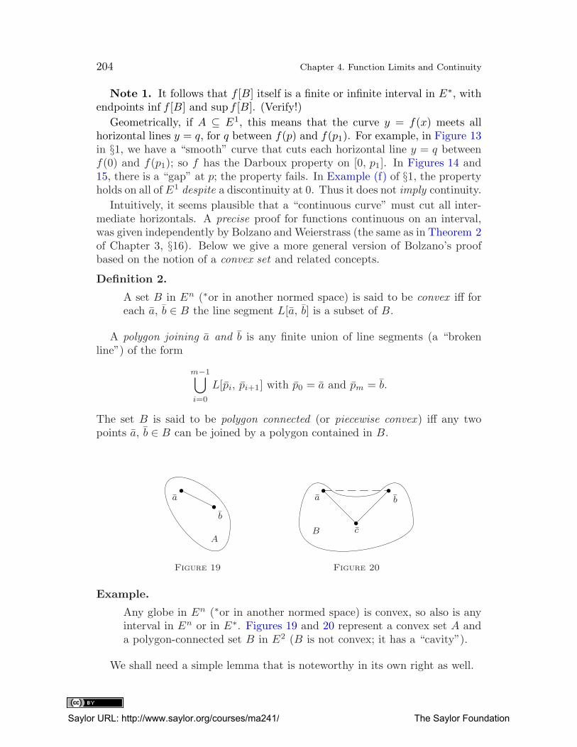
204 Chapter 4. Function Limits and Continuity
Note 1. It follows that f [B] itself is a finite or infinite interval in E∗, withendpoints inf f [B] and sup f [B]. (Verify!)
Geometrically, if A ⊆ E1, this means that the curve y = f(x) meets allhorizontal lines y = q, for q between f(p) and f(p1). For example, in Figure 13in §1, we have a “smooth” curve that cuts each horizontal line y = q betweenf(0) and f(p1); so f has the Darboux property on [0, p1]. In Figures 14 and15, there is a “gap” at p; the property fails. In Example (f) of §1, the propertyholds on all of E1 despite a discontinuity at 0. Thus it does not imply continuity.
Intuitively, it seems plausible that a “continuous curve” must cut all inter-mediate horizontals. A precise proof for functions continuous on an interval,was given independently by Bolzano and Weierstrass (the same as in Theorem 2of Chapter 3, §16). Below we give a more general version of Bolzano’s proofbased on the notion of a convex set and related concepts.
Definition 2.
A set B in En (∗or in another normed space) is said to be convex iff foreach a, b ∈ B the line segment L[a, b] is a subset of B.
A polygon joining a and b is any finite union of line segments (a “brokenline”) of the form
m−1⋃
i=0
L[pi, pi+1] with p0 = a and pm = b.
The set B is said to be polygon connected (or piecewise convex ) iff any twopoints a, b ∈ B can be joined by a polygon contained in B.
a
b
A
Figure 19
a
c
b
Figure 20
B
Example.
Any globe in En (∗or in another normed space) is convex, so also is anyinterval in En or in E∗. Figures 19 and 20 represent a convex set A anda polygon-connected set B in E2 (B is not convex; it has a “cavity”).
We shall need a simple lemma that is noteworthy in its own right as well.
Saylor URL: http://www.saylor.org/courses/ma241/ The Saylor Foundation
§9. The Intermediate Value Property 205
Lemma 1 (principle of nested line segments). Every contracting sequence of
closed line segments L[pm, qm] in En (∗or in any other normed space) has a
nonvoid intersection; i .e., there is a point
p ∈∞⋂
m=1
L[pm, qm].
Proof. Use Cantor’s theorem (Theorem 5 of §6) and Example (1) in §8. �
We are now ready for Bolzano’s theorem. The proof to be used is typical ofso-called “bisection proofs .” (See also §6, Problems 9 and 10 for such proofs.)
Theorem 1. If f : B → E1 is relatively continuous on a polygon-connected
set B in En (∗or in another normed space), then f has the Darboux property
on B.
In particular , if B is convex and if f(p) < c < f(q) for some p, q ∈ B, thenthere is a point r ∈ L(p, q) such that f(r) = c.
Proof. First, let B be convex . Seeking a contradiction, suppose p, q ∈ B with
f(p) < c < f(q),
yet f(x) 6= c for all x ∈ L(p, q).Let P be the set of all those x ∈ L[p, q] for which f(x) < c, i.e.,
P = {x ∈ L[p, q] | f(x) < c},and let
Q = {x ∈ L[p, q] | f(x) > c}.Then p ∈ P , q ∈ Q, P ∩Q = ∅, and P ∪Q = L[p, q] ⊆ B. (Why?)
Now let
r0 =1
2(p+ q)
be the midpoint on L[p, q]. Clearly, r0 is either in P or in Q. Thus it bisectsL[p, q] into two subsegments, one of which must have its left endpoint in P and
its right endpoint in Q.2
We denote this particular closed segment by L[p1, q1], p1 ∈ P , q1 ∈ Q. Wethen have
L[p1, q1] ⊆ L[p, q] and |p1 − q1| =1
2|p− q|. (Verify!)
Now we bisect L[p1, q1] and repeat the process. Thus let
r1 =1
2(p1 + q1).
2 Indeed, if r0 ∈ P , this holds for L[r0, q]. If r0 ∈ Q, take L[p, r0].
Saylor URL: http://www.saylor.org/courses/ma241/ The Saylor Foundation
206 Chapter 4. Function Limits and Continuity
By the same argument, we obtain a closed subsegment L[p2, q2] ⊆ L[p1, q1],with p2 ∈ P , q2 ∈ Q, and
|p2 − q2| =1
2|p1 − q1| =
1
4|p− q|.
Next, we bisect L[p2, q2], and so on. Continuing this process indefinitely, weobtain an infinite contracting sequence of closed line segments L[pm, qm] suchthat
(∀m) pm ∈ P, qm ∈ Q,and
|pm − qm| =1
2m|p− q| → 0 as m→ +∞.
By Lemma 1, there is a point
r ∈∞⋂
m=1
L[pm, qm].
This implies that
(∀m) |r − pm| ≤ |pm − qm| → 0,
whence pm → r. Similarly, we obtain qm → r.
Now since r ∈ L[p, q] ⊆ B, the function f is relatively continuous at r overB (by assumption). By the sequential criterion, then,
f(pm)→ f(r) and f(qm)→ f(r).
Moreover, f(pm) < c < f(qm) (for pm ∈ P and qm ∈ Q). Letting m → +∞,we pass to limits (Chapter 3, §15, Corollary 1) and get
f(r) ≤ c ≤ f(r),
so that r is neither in P nor in Q, which is a contradiction. This completesthe proof for a convex B.
The extension to polygon-connected sets is left as an exercise (see Problem2 below). Thus all is proved. �
Note 2. In particular, the theorem applies if B is a globe or an interval.
Thus continuity on an interval implies the Darboux property . The conversefails , as we have noted. However, for monotone functions, we obtain the fol-lowing theorem.
Theorem 2. If a function f : A → E1 is monotone and has the Darboux
property on a finite or infinite interval (a, b) ⊆ A ⊆ E1, then it is continuous
on (a, b).
Proof. Seeking a contradiction, suppose f is discontinuous at some p ∈ (a, b).
Saylor URL: http://www.saylor.org/courses/ma241/ The Saylor Foundation
§9. The Intermediate Value Property 207
For definiteness, let f↑ on (a, b). Then by Theorems 2 and 3 in §5, wehave either f(p−) < f(p) or f(p) < f(p+) or both, with no function values in
between.
On the other hand, since f has the Darboux property, the function valuesf(x) for x in (a, b) fill an entire interval (see Note 1). Thus it is impossiblefor f(p) to be the only function value between f(p−) and f(p+) unless f isconstant near p, but then it is also continuous at p, which we excluded. Thiscontradiction completes the proof.3 �
Note 3. The theorem holds (with a similar proof) for nonopen intervals aswell, but the continuity at the endpoints is relative (right at a, left at b).
Theorem 3. If f : A → E1 is strictly monotone and continuous when re-
stricted to a finite or infinite interval B ⊆ A ⊆ E1, then its inverse f−1 has
the same properties on the set f [B] (itself an interval , by Note 1 and Theo-
rem 1).4
Proof. It is easy to see that f−1 is increasing (decreasing) if f is; the proof isleft as an exercise. Thus f−1 is monotone on f [B] if f is so on B. To provethe relative continuity of f−1, we use Theorem 2, i.e., show that f−1 has theDarboux property on f [B].
Thus let f−1(p) < c < f−1(q) for some p, q ∈ f [B]. We look for an r ∈ f [B]such that f−1(r) = c, i.e., r = f(c). Now since p, q ∈ f [B], the numbers f−1(p)and f−1(q) are in B, an interval . Hence also the intermediate value c is in B;thus it belongs to the domain of f , and so the function value f(c) exists . Itthus suffices to put r = f(c) to get the result. �
Examples.
(a) Define f : E1 → E1 by
f(x) = xn for a fixed n ∈ N .
As f is continuous (being a monomial), it has the Darboux propertyon E1. By Note 1, setting B = [0, +∞), we have f [B] = [0, +∞).(Why?) Also, f is strictly increasing on B. Thus by Theorem 3, the
inverse function f−1 (i.e., the nth root function) exists and is continuous
on f [B] = [0, +∞).
If n is odd , then f−1 has these properties on all of E1, by a similarproof; thus n
√x exists for x ∈ E1.
(b) Logarithmic functions. From the example in §5, we recall that the expo-
3 More formally, if, say, f(p) < f(p+), let f(p) < c < f(p+) ≤ f(p′), p′ ∈ (p, b). (Such a
p′ exists since f↑, and f(p+) = inf{f(x) | p < x < b}; see §5, Theorem 1.) By the Darbouxproperty, f(x) = c for some x ∈ (a, b), but this contradicts Theorem 2 in §5.
4 We write “f” for “f restricted to B” as well; cf. also footnote 1 in §8.
Saylor URL: http://www.saylor.org/courses/ma241/ The Saylor Foundation
208 Chapter 4. Function Limits and Continuity
nential function given by
F (x) = ax (a > 0)
is continuous and strictly monotone on E1.5 Its inverse, F−1, is calledthe logarithmic function to the base a, denoted loga. By Theorem 3, it iscontinuous and strictly monotone on F [E1].
To fix ideas, let a > 1, so F↑ and (F−1)↑. By Note 1, F [E1] is aninterval with endpoints p and r, where
p = inf F [E1] = inf{ax | −∞ < x < +∞}
and
r = supF [E1] = sup{ax | −∞ < x < +∞}.
Now by Problem 14(iii) of §2 (with q = 0),
limx→+∞
ax = +∞ and limx→−∞
ax = 0.
As F↑, we use Theorem 1 in §5 to obtain
r = sup ax = limx→+∞
ax = +∞ and p = limx→−∞
ax = 0.
Thus F [E1], i.e., the domain of loga, is the interval (p, r) = (0, +∞). Itfollows that loga x is uniquely defined for x in (0, +∞); it is called thelogarithm of x to the base a.
The range of loga (i.e. of F−1) is the same as the domain of F , i.e., E1.Thus if a > 1, loga x increases from −∞ to +∞ as x increases from 0 to+∞. Hence
limx→+∞
loga x = +∞ and limx→0+
loga x = −∞,
provided a > 1.
If 0 < a < 1, the values of these limits are interchanged (since F↓ inthis case), but otherwise the results are the same.
If a = e, we write lnx or log x for loga x, and we call lnx the natural
logarithm of x. Its inverse is, of course, the exponential f(x) = ex, alsowritten exp(x). Thus by definition, ln ex = x and
x = exp(lnx) = elnx (0 < x < +∞). (1)
(c) The power function g : (0, +∞)→ E1 is defined by
g(x) = xa for a fixed real a.
5 We exclude the case a = 1 here.
Saylor URL: http://www.saylor.org/courses/ma241/ The Saylor Foundation
§9. The Intermediate Value Property 209
If a > 0, we also define g(0) = 0. For x > 0, we have
xa = exp(lnxa) = exp(a · lnx).Thus by the rules for composite functions (Theorem 3 and Corollary 2 in§2), the continuity of g on (0, +∞) follows from that of exponential andlog functions. If a > 0, g is also continuous at 0. (Exercise!)
Problems on the Darboux Property and Related Topics
1. Prove Note 1.
1′. Prove Note 3.
1′′. Prove continuity at 0 in Example (c).
2. Prove Theorem 1 for polygon-connected sets.[Hint: If
B ⊇m−1⋃
i=0
L[pi, pi+1]
with
f(p0) < c < f(pm),
show that for at least one i, either c = f(pi) or f(pi) < c < f(pi+1). Then replaceB in the theorem by the convex segment L[pi, pi+1].]
3. Show that, if f is strictly increasing on B ⊆ E, then f−1 has the sameproperty on f [B], and both are one to one; similarly for decreasingfunctions.
4. For functions on B = [a, b] ⊂ E1, Theorem 1 can be proved thusly: If
f(a) < c < f(b),
let
P = {x ∈ B | f(x) < c}and put r = supP .
Show that f(r) is neither greater nor less than c, and so necessarilyf(r) = c.[Hint: If f(r) < c, continuity at r implies that f(x) < c on some Gr(δ) (§2,Problem 7), contrary to r = supP . (Why?)]
5. Continuing Problem 4, prove Theorem 1 in all generality , as follows.Define
g(t) = p+ t(q − p), 0 ≤ t ≤ 1.
Then g is continuous (by Theorem 3 in §3), and so is the compositefunction h = f ◦ g, on [0, 1]. By Problem 4, with B = [0, 1], there is at ∈ (0, 1) with h(t) = c. Put r = g(t), and show that f(r) = c.
Saylor URL: http://www.saylor.org/courses/ma241/ The Saylor Foundation
210 Chapter 4. Function Limits and Continuity
6. Show that every equation of odd degree, of the form
f(x) =n∑
k=0
akxk = 0 (n = 2m− 1),
has at least one solution for x in E1.[Hint: Show that f takes both negative and positive values as x → −∞ or x → +∞;thus by the Darboux property, f must also take the intermediate value 0 for some
x ∈ E1.]
7. Prove that if the functions f : A → (0, +∞) and g : A → E1 are bothcontinuous, so also is the function h : A→ E1 given by
h(x) = f(x)g(x).
[Hint: See Example (c)].
8. Using Corollary 2 in §2, and limit properties of the exponential and logfunctions, prove the “shorthand” Theorems 11–16 of §4.
8′. Find limx→+∞
(
1 +1
x
)
√x
.
8′′. Similarly, find a new solution of Problem 27 in Chapter 3, §15, reducingit to Problem 26.
9. Show that if f : E1 → E∗ has the Darboux property on B (e.g., if B isconvex and f is relatively continuous on B) and if f is one to one on B,then f is necessarily strictly monotone on B.
10. Prove that if two real functions f, g are relatively continuous on [a, b](a < b) and
f(x)g(x) > 0 for x ∈ [a, b],
then the equation
(x− a)f(x) + (x− b)g(x) = 0
has a solution between a and b; similarly for the equation
f(x)
x− a +g(x)
x− b = 0 (a, b ∈ E1).
10′. Similarly, discuss the solutions of
2
x− 4+
9
x− 1+
1
x− 2= 0.
Saylor URL: http://www.saylor.org/courses/ma241/ The Saylor Foundation
§10. Arcs and Curves. Connected Sets 211
§10. Arcs and Curves. Connected Sets
A deeper insight into continuity and the Darboux property can be gained bygeneralizing the notions of a convex set and polygon-connected set to obtainso-called connected sets.
I. As a first step, we consider arcs and curves.
Definition 1.
A set A ⊆ (S, ρ) is called an arc iff A is a continuous image of a compactinterval [a, b] ⊂ E1, i.e., iff there is a continuous mapping
f : [a, b] −→onto
A.
If, in addition, f is one to one, A is called a simple arc with endpoints
f(a) and f(b).
If instead f(a) = f(b), we speak of a closed curve.
A curve is a continuous image of any finite or infinite interval in E1.
Corollary 1. Each arc is a compact (hence closed and bounded) set (byTheorem 1 of §8).Definition 2.
A set A ⊆ (S, ρ) is said to be arcwise connected iff every two pointsp, q ∈ A are in some simple arc contained in A. (We then also say the pand q can be joined by an arc in A.)
Examples.
(a) Every closed line segment L[a, b] in En (∗or in any other normed space)is a simple arc (consider the map f in Example (1) of §8).
(b) Every polygon
A =m−1⋃
i=0
L[pi, pi+1]
is an arc (see Problem 18 in §8). It is a simple arc if the half-closedsegments L[pi, pi+1) do not intersect and the points pi are distinct, forthen the map f in Problem 18 of §8 is one to one.
(c) It easily follows that every polygon-connected set is also arcwise con-
nected ; one only has to show that every polygon joining two points p0, pmcan be reduced to a simple polygon (not a self-intersecting one). SeeProblem 2.
However, the converse is false. For example, two discs in E2 connectedby a parabolic arc form together an arcwise- (but not polygonwise-) con-nected set.
Saylor URL: http://www.saylor.org/courses/ma241/ The Saylor Foundation
212 Chapter 4. Function Limits and Continuity
(d) Let f1, f2, . . . , fn be real continuous functions on an interval I ⊆ E1.Treat them as components of a function f : I → En,
f = (f1, . . . , fn).
Then f is continuous by Theorem 2 in §3. Thus the image set f [I] is acurve in En; it is an arc if I is a closed interval.
Introducing a parameter t varying over I, we obtain the parametric
equations of the curve, namely,
xk = fk(t), k = 1, 2, . . . , n.
Then as t varies over I, the point x = (x1, . . . , xn) describes the curvef [I]. This is the usual way of treating curves in En (∗and Cn).
It is not hard to show that Theorem 1 in §9 holds also if B is only arcwise
connected (see Problem 3 below). However, much more can be proved byintroducing the general notion of a connected set. We do this next.
∗II. For this topic, we shall need Theorems 2–4 of Chapter 3, §12, andProblem 15 of Chapter 4, §2. The reader is advised to review them. In partic-ular, we have the following theorem.
Theorem 1. A function f : (A, ρ)→ (T, ρ′) is continuous on A iff f−1[B] isclosed in (A, ρ) for each closed set B ⊆ (T, ρ′); similarly for open sets.
Indeed, this is part of Problem 15 in §2 with (S, ρ) replaced by (A, ρ).
Definition 3.
A metric space (S, ρ) is said to be connected iff S is not the union P ∪Qof any two nonvoid disjoint closed sets; it is disconnected otherwise.1
A set A ⊆ (S, ρ) is called connected iff (A, ρ) is connected as a subspace
of (S, ρ); i.e., iff A is not a union of two disjoint sets P, Q 6= ∅ that areclosed (hence also open) in (A, ρ), as a subspace of (S, ρ).
Note 1. By Theorem 4 of Chapter 3, §12, this means that
P = A ∩ P1 and Q = A ∩Q1
for some sets P1, Q1 that are closed in (S, ρ). Observe that, unlike compactsets, a set that is closed or open in (A, ρ) need not be closed or open in (S, ρ).
Examples.
(a′) ∅ is connected.(b′) So is any one-point set {p}. (Why?)
1 The term “closed” may be replaced by “open” here, for P and Q are open as well, eachbeing the complement of the other closed set. Similarly, if they are open, they are both open
and closed (briefly, “clopen”).
Saylor URL: http://www.saylor.org/courses/ma241/ The Saylor Foundation
§10. Arcs and Curves. Connected Sets 213
(c′) Any finite set of two or more points is disconnected. (Why?)
Other examples are provided by the theorems that follow.
Theorem 2. The only connected sets in E1 are exactly all convex sets, i .e., fi-nite and infinite intervals , including E1 itself .
Proof. The proof that such intervals are exactly all convex sets in E1 is leftas an exercise.
We now show that each connected set A ⊆ E1 is convex, i.e., that a, b ∈ Aimplies (a, b) ⊆ A.
Seeking a contradiction, suppose p /∈ A for some p ∈ (a, b), a, b ∈ A. Let
P = A ∩ (−∞, p) and Q = A ∩ (p, +∞).
Then A = P ∪ Q, a ∈ P , b ∈ Q, and P ∩ Q = ∅. Moreover, (−∞, p) and(p, +∞) are open sets in E1. (Why?) Hence P and Q are open in A, eachbeing the intersection of A with a set open in E1 (see Note 1 above). AsA = P ∪Q, with P ∩Q = ∅, it follows that A is disconnected . This shows thatif A is connected in E1, it must be convex.
Conversely, let A be convex in E1. The proof that A is connected is analmost exact copy of the proof given for Theorem 1 of §9, so we only brieflysketch it here.2
If A were disconnected, then A = P ∪ Q for some disjoint sets P, Q 6= ∅,both closed in A. Fix any p ∈ P and q ∈ Q. Exactly as in Theorem 1 of §9,select a contracting sequence of line segments (intervals) [pm, qm] ⊆ A suchthat pm ∈ P , qm ∈ Q, and |pm − qm| → 0, and obtain a point
r ∈∞⋂
m=1
[pm, qm] ⊆ A,
so that pm → r, qm → r, and r ∈ A. As the sets P and Q are closed in(A, ρ), Theorem 4 of Chapter 3, §16 shows that both P and Q must contain thecommon limit r of the sequences {pm} ⊆ P and {qm} ⊆ Q. This is impossible,however, since P ∩ Q = ∅, by assumption. This contradiction shows that Acannot be disconnected. Thus all is proved. �
Note 2. By the same proof, any convex set in a normed space is connected .In particular, En and all other normed spaces are connected themselves.3
Theorem 3. If a function f : A → (T, ρ′) with A ⊆ (S, ρ) is relatively con-
tinuous on a connected set B ⊆ A, then f [B] is a connected set in (T, ρ′).4
2 Note that the same proof holds also for A in any normed space.3 See also Corollary 3 below (note that it presupposes Corollary 2, hence Theorem 2).4 Briefly, any continuous image of a connected set is connected itself .
Saylor URL: http://www.saylor.org/courses/ma241/ The Saylor Foundation
214 Chapter 4. Function Limits and Continuity
Proof. By definition (§1), relative continuity on B becomes ordinary continu-ity when f is restricted to B. Thus we may treat f as a mapping of B into
f [B], replacing S and T by their subspaces B and f [B].
Seeking a contradiction, suppose f [B] is disconnected, i.e.,
f [B] = P ∪Q
for some disjoint sets P, Q 6= ∅ closed in (f [B], ρ′). Then by Theorem 1, withT replaced by f [B], the sets f−1[P ] and f−1[Q] are closed in (B, ρ). They alsoare nonvoid and disjoint (as are P and Q) and satisfy
B = f−1[P ∪Q] = f−1[P ] ∪ f−1[Q]
(see Chapter 1, §§4–7, Problem 6). Thus B is disconnected, contrary to as-sumption. �
Corollary 2. All arcs and curves are connected sets (by Definition 2 and
Theorems 2 and 3).
Lemma 1. A set A ⊆ (S, ρ) is connected iff any two points p, q ∈ A are in
some connected subset B ⊆ A. Hence any arcwise connected set is connected .
Proof. Seeking a contradiction, suppose the condition stated in Lemma 1holds but A is disconnected, so A = P ∪Q for some disjoint sets P 6= ∅, Q 6= ∅,both closed in (A, ρ).
Pick any p ∈ P and q ∈ Q. By assumption, p and q are in some connectedset B ⊆ A. Treat (B, ρ) as a subspace of (A, ρ), and let
P ′ = B ∩ P and Q′ = B ∩Q.
Then by Theorem 4 of Chapter 3, §12, P ′ and Q′ are closed in B. Also, theyare disjoint (for P and Q are) and nonvoid (for p ∈ P ′, q ∈ Q′), and
B = B ∩ A = B ∩ (P ∪Q) = (B ∩ P ) ∪ (B ∩Q) = P ′ ∪Q′.
Thus B is disconnected, contrary to assumption. This contradiction proves thelemma (the converse proof is trivial).
In particular, if A is arcwise connected, then any points p, q in A are insome arc B ⊆ A, a connected set by Corollary 2. Thus all is proved. �
Corollary 3. Any convex or polygon-connected set (e.g ., a globe) in En (orin any other normed space) is arcwise connected , hence connected .
Proof. Use Lemma 1 and Example (c) in part I of this section. �
Caution: The converse fails . A connected set need not be arcwise connected,
let alone polygon connected (see Problem 17). However, we have the followingtheorem.
Saylor URL: http://www.saylor.org/courses/ma241/ The Saylor Foundation
§10. Arcs and Curves. Connected Sets 215
Theorem 4. Every open connected set A in En (∗or in another normed space)is also arcwise connected and even polygon connected .
Proof. If A = ∅, this is “vacuously” true, so let A 6= ∅ and fix a ∈ A.Let P be the set of all p ∈ A that can be joined with a by a polygon K ⊆ A.
Let Q = A − P . Clearly, a ∈ P , so P 6= ∅. We shall show that P is open,i.e., that each p ∈ P is in a globe Gp ⊆ P .
Thus we fix any p ∈ P . As A is open and p ∈ A, there certainly is a globeGp contained in A. Moreover, as Gp is convex, each point x ∈ Gp is joinedwith p by the line segment L[x, p] ⊆ Gp. Also, as p ∈ P , some polygon K ⊆ Ajoins p with a. Then
K ∪ L[x, p]is a polygon joining x and a, and hence by definition x ∈ P . Thus each x ∈ Gp
is in P , so that Gp ⊆ P , as required, and P is open (also open in A as a
subspace).
Next, we show that the set Q = A− P is open as well. As before, if Q 6= ∅,fix any q ∈ Q and a globe Gq ⊆ A, and show that Gq ⊆ Q. Indeed, if somex ∈ Gq were not in Q, it would be in P , and thus it would be joined with a(fixed above) by a polygon K ⊆ A. Then, however, q itself could be so joined
by the polygonL[q, x] ∪K,
implying that q ∈ P , not q ∈ Q. This shows that Gq ⊂ Q indeed, as claimed.
Thus A = P ∪ Q with P, Q disjoint and open (hence clopen) in A. Theconnectedness of A then implies that Q = ∅. (P is not empty, as has beennoted.) Hence A = P . By the definition of P , then, each point b ∈ A can bejoined to a by a polygon. As a ∈ A was arbitrary, A is polygon connected. �
Finally, we obtain a stronger version of the intermediate value theorem.
Theorem 5. If a function f : A→ E1 is relatively continuous on a connected
set B ⊆ A ⊆ (S, ρ), then f has the Darboux property on B.
In fact, by Theorems 3 and 2, f [B] is a connected set in E1, i.e., an interval .This, however, implies the Darboux property.
Problems on Arcs, Curves, and Connected Sets
1. Discuss Examples (a) and (b) in detail. In particular, verify that L[a, b]is a simple arc. (Show that the map f in Example (1) of §8 is one to
one.)
2. Show that each polygon
K =m−1⋃
i=0
L[pi, pi+1]
Saylor URL: http://www.saylor.org/courses/ma241/ The Saylor Foundation
216 Chapter 4. Function Limits and Continuity
can be reduced to a simple polygon P (P ⊆ K) joining p0 and pm.[Hint: First, show that if two line segments have two or more common points, they
lie in one line. Then use induction on the number m of segments in K. Draw adiagram in E2 as a guide.]
3. Prove Theorem 1 of §9 for an arcwise connected B ⊆ (S, ρ).[Hint: Proceed as in Problems 4 and 5 in §9, replacing g by some continuous mapf : [a, b] −→
ontoB.]
4. Define f as in Example (f) of §1. Let
Gab = {(x, y) ∈ E2 | a ≤ x ≤ b, y = f(x)}.
(Gab is the graph of f over [a, b].) Prove the following:
(i) If a > 0, then Gab is a simple arc in E2.
(ii) If a ≤ 0 ≤ b, Gab is not even arcwise connected.
[Hints: (i) Prove that f is continuous on [a, b], a > 0, using the continuity of thesine function. Then use Problem 16 in §2, restricting f to [a, b].
(ii) For a contradiction, assume 0 is joined by a simple arc to some p ∈ Gab.]
5. Show that each arc is a continuous image of [0, 1].[Hint: First, show that any [a, b] ⊆ E1 is such an image. Then use a suitable
composite mapping.]
∗6. Prove that a function f : B → E1 on a compact set B ⊆ E1 must becontinuous if its graph,
{(x, y) ∈ E2 | x ∈ B, y = f(x)},
is a compact set (e.g., an arc) in E2.[Hint: Proceed as in the proof of Theorem 3 of §8.]
∗7. Prove that A is connected iff there is no continuous map
f : A −→onto{0, 1}.5
[Hint: If there is such a map, Theorem 1 shows that A is disconnected. (Why?)
Conversely, if A = P ∪Q (P, Q as in Definition 3), put f = 0 on P and f = 1 on Q.
Use again Theorem 1 to show that f so defined is continuous on A.]
∗8. Let B ⊆ A ⊆ (S, ρ). Prove that B is connected in S iff it is connectedin (A, ρ).
∗9. Suppose that no two of the sets Ai (i ∈ I) are disjoint. Prove that if allAi are connected, so is A =
⋃
i∈I Ai.[Hint: If not, let A = P ∪ Q (P, Q as in Definition 3). Let Pi = Ai ∩ P and
Qi = Ai ∩Q, so Ai = Pi ∪Qi, i ∈ I.
5 That is, onto a two-point set {0} ∪ {1}.
Saylor URL: http://www.saylor.org/courses/ma241/ The Saylor Foundation
§10. Arcs and Curves. Connected Sets 217
At least one of the Pi, Qi must be ∅ (why?); say, Qj = ∅ for some j ∈ I. Then(∀ i) Qi = ∅, for Qi 6= ∅ implies Pi = ∅, whence
Ai = Qi ⊆ Q =⇒ Ai ∩Aj = ∅ (since Aj ⊆ P ),
contrary to our assumption. Deduce that Q =⋃
i Qi = ∅. (Contradiction!)]
∗10. Prove that if {An} is a finite or infinite sequence of connected sets andif
(∀n) An ∩ An+1 6= ∅,
then
A =⋃
n
An
is connected.[Hint: Let Bn =
⋃nk=1 Ak. Use Problem 9 and induction to show that the Bn are
connected and no two are disjoint. Verify that A =⋃
n Bn and apply Problem 9 to
the sets Bn.]
∗11. Given p ∈ A, A ⊆ (S, ρ), let Ap denote the union of all connected subsetsof A that contain p (one of them is {p}); Ap is called the p-component
of A. Prove that
(i) Ap is connected (use Problem 9);
(ii) Ap is not contained in any other connected set B ⊆ A with p ∈ B;
(iii) (∀ p, q ∈ A) Ap ∩ Aq = ∅ iff Ap 6= Aq; and
(iv) A =⋃{Ap | p ∈ A}.
[Hint for (iii): If Ap ∩ Aq 6= ∅ and Ap 6= Aq , then B = Ap ∪ Aq is a connected set
larger than Ap, contrary to (ii).]
∗12. Prove that if A is connected, so is its closure (Chapter 3, §16,Definition 1), and so is any set D such that A ⊆ D ⊆ A.[Hints: First show that D is the “least” closed set in (D, ρ) that contains A(Problem 11 in Chapter 3, §16 and Theorem 4 of Chapter 3, §12). Next, seeking
a contradiction, let D = P ∪Q, P ∩Q = ∅, P, Q 6= ∅, clopen in D. Then
A = (A ∩ P ) ∪ (A ∩Q)
proves A disconnected , for if A ∩ P = ∅, say, then A ⊆ Q ⊂ D (why?), contrary to
the minimality of D; similarly for A ∩Q = ∅.]∗13. A set is said to be totally disconnected iff its only connected subsets are
one-point sets and ∅.Show that R (the rationals) has this property in E1.
∗14. Show that any discrete space is totally disconnected (see Problem 13).
∗15. From Problems 11 and 12 deduce that each component Ap is closed
(Ap = Ap).
Saylor URL: http://www.saylor.org/courses/ma241/ The Saylor Foundation
218 Chapter 4. Function Limits and Continuity
∗16. Prove that a set A ⊆ (S, ρ) is disconnected iff A = P ∪Q, with P, Q 6= ∅,and each of P, Q disjoint from the closure of the other: P ∩ Q = ∅ =P ∩Q.[Hint: By Problem 12, the closure of P in (A, ρ) (i.e., the least closed set in (A, ρ)that contains P ) is
A ∩ P = (P ∪Q) ∩ P = (P ∩ P ) ∪ (Q ∩ P ) = P ∪ ∅ = P,
so P is closed in A; similarly for Q. Prove the converse in the same manner.]
∗17. Give an example of a connected set that is not arcwise connected.[Hint: The set G0b (a = 0) in Problem 4 is the closure of G0b − {0} (verify!), andthe latter is connected (why?); hence so is G0b by Problem 12.]
∗§11. Product Spaces. Double and Iterated Limits
Given two metric spaces (X, ρ1) and (Y, ρ2), we may consider the Cartesianproduct X × Y , suitably metrized . Two metrics for X × Y are suggested inProblem 10 in Chapter 3, §11. We shall adopt the first of them as follows.
Definition 1.
By the product of two metric spaces (X, ρ1) and (Y, ρ2) is meant thespace (X × Y, ρ), where the metric ρ is defined by
ρ((x, y), (x′, y′)) = max{ρ1(x, x′), ρ2(y, y′)} (1)
for x, x′ ∈ X and y, y′ ∈ Y .
Thus the distance between (x, y) and (x′, y′) is the larger of the two distances
ρ1(x, x′) in X and ρ2(y, y
′) in Y .
The verification that ρ in (1) is, indeed, a metric is left to the reader. We nowobtain the following theorem.
Theorem 1.
(i) A globe G(p, q)(ε) in (X×Y, ρ) is the Cartesian product of the correspond-
ing ε-globes in X and Y ,
G(p, q)(ε) = Gp(ε)×Gq(ε).
(ii) Convergence of sequences {(xm, ym)} in X × Y is componentwise. Thatis , we have
(xm, ym)→ (p, q) in X × Y iff xm → p in X and ym → q in Y .
Saylor URL: http://www.saylor.org/courses/ma241/ The Saylor Foundation
∗§11. Product Spaces. Double and Iterated Limits 219
Again, the easy proof is left as an exercise.
In this connection, recall that by Theorem 2 of Chapter 3, §15, convergencein E2 is componentwise as well , even though the standard metric in E2 is notthe product metric (1); it is rather the metric (ii) of Problem 10 in Chapter 3,§11. We might have adopted this second metric for X × Y as well. Then part(i) of Theorem 1 would fail, but part (ii) would still follow by making
ρ1(xm, p) <ε√2and ρ2(ym, q) <
ε√2.
It follows that, as far as convergence is concerned, the two choices of ρ are
equivalent .
Note 1. More generally, two metrics for a space S are said to be equivalentiff exactly the same sequences converge (to the same limits) under both metrics.Then also all function limits are the same since they reduce to sequential limits,by Theorem 1 of §2; similarly for such notions as continuity, compactness,completeness, closedness, openness, etc.
In view of this, we shall often call X×Y a product space (in the wider sense)even if its metric is not the ρ of formula (1) but equivalent to it. In this sense,E2 is the product space E1 ×E1, and X × Y is its generalization.
Various ideas valid in E2 extend quite naturally to X × Y . Thus functionsdefined on a set A ⊆ X × Y may be treated as functions of two variables x,y such that (x, y) ∈ A. Given (p, q) ∈ X × Y , we may consider ordinary orrelative limits at (p, q), e.g., limits over a path
B = {(x, y) ∈ X × Y | y = q}
(briefly called the “line y = q”). In this case, y remains fixed (y = q) whilex→ p; we then speak of limits and continuity in one variable x, as opposed tothose in both variables jointly , i.e., the ordinary limits (cf. §3, part IV).
Some other kinds of limits are to be defined below. For simplicity, we con-sider only functions f : (X×Y )→ (T, ρ′) defined on all of X×Y . If confusionis unlikely, we write ρ for all metrics involved (such as ρ′ in T ). Below, p and qalways denote cluster points of X and Y , respectively (this justifies the “lim”notation). Of course, our definitions apply in particular to E2 as the simplestspecial case of X × Y .
Definition 2.
A function f : (X × Y ) → (T, ρ′) is said to have the double limit s ∈ Tat (p, q), denoted
s = limx→py→q
f(x, y),
iff for each ε > 0, there is a δ > 0 such that f(x, y) ∈ Gs(ε) whenever
Saylor URL: http://www.saylor.org/courses/ma241/ The Saylor Foundation
220 Chapter 4. Function Limits and Continuity
x ∈ G¬p(δ) and y ∈ G¬q(δ). In symbols,
(∀ ε > 0) (∃ δ > 0) (∀x ∈ G¬p(δ)) (∀ y ∈ G¬q(δ)) f(x, y) ∈ Gs(ε). (2)
Observe that this is the relative limit over the path
D = (X − {p})× (Y − {q})excluding the two “lines” x = p and y = q. If f were restricted to D, thiswould coincide with the ordinary nonrelative limit (see §1), denoted
s = lim(x, y)→(p, q)
f(x, y),
where only the point (p, q) is excluded. Then we would have
(∀ ε > 0) (∃ δ > 0) (∀ (x, y) ∈ G¬(p,q)(δ)) f(x, y) ∈ Gs(ε). (3)
Now consider limits in one variable, say,
limy→q
f(x, y) with x fixed .
If this limit exists for each choice of x from some set B ⊆ X , it defines afunction
g : B → T
with valueg(x) = lim
y→qf(x, y), x ∈ B.
This means that
(∀x ∈ B) (∀ ε > 0) (∃ δ > 0) (∀ y ∈ G¬q(δ)) ρ(g(x), f(x, y)) < ε. (4)
Here, in general, δ depends on both ε and x. However, in some cases (re-sembling uniform continuity), one and the same δ (depending on ε only) fitsall choices of x from B. This suggests the following definition.
Definition 3.
With the previous notation, suppose
limy→q
f(x, y) = g(x) exists for each x ∈ B (B ⊆ X).
We say that this limit is uniform in x (on B), and we write
“g(x) = limy→q
f(x, y) (uniformly for x ∈ B),”
iff for each ε > 0, there is a δ > 0 such that ρ(g(x), f(x, y)) < ε for all
x ∈ B and all y ∈ G¬q(δ). In symbols,
(∀ ε > 0) (∃ δ > 0) (∀x ∈ B) (∀ y ∈ G¬q(δ)) ρ(g(x), f(x, y)) < ε. (5)
Saylor URL: http://www.saylor.org/courses/ma241/ The Saylor Foundation
∗§11. Product Spaces. Double and Iterated Limits 221
Usually, the set B in formulas (4) and (5) is a deleted neighborhood of p inX , e.g.,
B = G¬p(r), or B = X − {p}.
Assume (4) for such a B, so
limy→q
f(x, y) = g(x) exists for each x ∈ B.
If, in addition,
limx→p
g(x) = s
exists, we call s the iterated limit of f at (p, q) (first in y, then in x), denoted
limx→p
limy→q
f(x, y).
This limit is obtained by first letting y → q (with x fixed) and then lettingx→ p. Quite similarly, we define
limy→q
limx→p
f(x, y).
In general, the two iterated limits (if they exist) are different , and theirexistence does not imply that of the double limit (2), let alone (3), nor does itimply the equality of all these limits. (See Problems 4ff below.) However, wehave the following theorem.
Theorem 2 (Osgood). Let (T, ρ′) be complete. Assume the existence of the
following limits of the function f : X × Y → T :
(i) limy→q
f(x, y) = g(x) (uniformly for x ∈ X − {p}) and
(ii) limx→p
f(x, y) = h(y) for y ∈ Y − {q}.1
Then the double limit and the two iterated limits of f at (p, q) exist and all
three coincide.
Proof. Let ε > 0. By our assumption (i), there is a δ > 0 such that
(∀x ∈ X − {p}) (∀ y ∈ G¬q(δ)) ρ(g(x), f(x, y)) <ε
4(cf. (5)). (5′)
Now take any y′, y′′ ∈ G¬q(δ). By assumption (ii), there is an x′ ∈ X −{p}so close to p that
ρ(h(y′), f(x′, y′)) <ε
4and ρ(h(y′′), f(x′, y′′)) <
ε
4. (Why?)
1 Actually, it suffices to assume the existence of the limits (i) and (ii) for x in some G¬p(r)
and y in some G¬q(r). Of course, it does not matter which of the two limits is uniform.
Saylor URL: http://www.saylor.org/courses/ma241/ The Saylor Foundation
222 Chapter 4. Function Limits and Continuity
Hence, using (5′) and the triangle law (repeatedly), we obtain for such y′, y′′
ρ(h(y′), h(y′′)) ≤ ρ(h(y′), f(x′, y′)) + ρ(f(x′, y′), g(x′))
+ ρ(g(x′), f(x′, y′′)) + ρ(f(x′, y′′), h(y′′))
<ε
4+ε
4+ε
4+ε
4= ε.
It follows that the function h satisfies the Cauchy criterion of Theorem 2 in
§2. (It does apply since T is complete.) Thus limy→q h(y) exists , and, byassumption (ii), it equals lim
y→qlimx→p
f(x, y) (which therefore exists).
Let then H = limy→q
h(y). With δ as above, fix some y0 ∈ G¬q(δ) so close to qthat
ρ(h(y0), H) <ε
4.
Also, using assumption (ii), choose a δ′ > 0 (δ′ ≤ δ) such that
ρ(h(y0), f(x, y0)) <ε
4for x ∈ G¬p(δ
′).
Combining with (5′), obtain (∀x ∈ G¬p(δ′))
ρ(H, g(x)) ≤ ρ(H, h(y0)) + ρ(h(y0), f(x, y0)) + ρ(f(x, y0), g(x)) <3ε
4. (6)
Thus(∀x ∈ G¬p(δ
′)) ρ(H, g(x)) < ε.
Hence limx→p g(x) = H, i.e., the second iterated limit, limx→p
limy→q
f(x, y), likewiseexists and equals H.
Finally, with the same δ′ ≤ δ, we combine (6) and (5′) to obtain
(∀x ∈ G¬p(δ′)) (∀ y ∈ G¬q(δ
′))
ρ(H, f(x, y)) ≤ ρ(H, g(x)) + ρ(g(x), f(x, y)) <3ε
4+ε
4= ε.
Hence the double limit (2) also exists and equals H. �
Note 2. The same proof works also with f restricted to (X−{p})×(Y −{q})so that the “lines” x = p and y = q are excluded from Df . In this case,formulas (2) and (3) mean the same; i.e.,
limx→py→q
f(x, y) = lim(x, y)→(p, q)
f(x, y).
Note 3. In Theorem 2, we may take E∗ (suitably metrized) for X or Yor T . Then the theorem also applies to limits at ±∞, and infinite limits. Wemay also take X = Y = N ∪{+∞} (the naturals together with +∞), with thesame E∗-metric, and consider limits at p = q = +∞. Moreover, by Note 2, wemay restrict f to N × N , so that f : N × N → T becomes a double sequence
Saylor URL: http://www.saylor.org/courses/ma241/ The Saylor Foundation
∗§11. Product Spaces. Double and Iterated Limits 223
(Chapter 1, §9). Writing m and n for x and y, and umn for f(x, y), we thenobtain Osgood’s theorem for double sequences (also called the Moore–Smith
theorem) as follows.
Theorem 2′. Let {umn} be a double sequence in a complete space (T, ρ′). If
limn→∞
umn = qm exists for each m
and if
limm→∞
umn = pn (uniformly in n) likewise exists,
then the double limit and the two iterated limits of {umn} exist and
limm→∞n→∞
umn = limn→∞
limm→∞
umn = limm→∞
limn→∞
umn.
Here the assumption that limm→∞ umn = pn (uniformly in n) means, by(5), that
(∀ ε > 0) (∃ k) (∀n) (∀m > k) ρ(umn, pn) < ε. (7)
Similarly, the statement “ limm→∞n→∞
umn = s” (see (2)) is tantamount to
(∀ ε > 0) (∃ k) (∀m, n > k) ρ(umn, s) < ε. (8)
Note 4. Given any sequence {xm} ⊆ (S, ρ), we may consider the doublelimit lim
m→∞n→∞
ρ(xm, xn) in E1. By using (8), one easily sees that
limm→∞n→∞
ρ(xm, xn) = 0
iff
(∀ ε > 0) (∃ k) (∀m, n > k) ρ(xm, xn) < ε,
i.e., iff {xm} is a Cauchy sequence. Thus Cauchy sequences are those for which
limm→∞n→∞
ρ(xm, xn) = 0.
Theorem 3. In every metric space (S, ρ), the metric ρ : (S × S) → E1 is a
continuous function on the product space S × S.Proof. Fix any (p, q) ∈ S × S. By Theorem 1 of §2, ρ is continuous at (p, q)iff
ρ(xm, ym)→ ρ(p, q) whenever (xm, ym)→ (p, q),
i.e., whenever xm → p and ym → q. However, this follows by Theorem 4 inChapter 3, §15. Thus continuity is proved. �
Saylor URL: http://www.saylor.org/courses/ma241/ The Saylor Foundation
224 Chapter 4. Function Limits and Continuity
Problems on Double Limits and Product Spaces
1. Prove Theorem 1(i). Prove Theorem 1(ii) for both choices of ρ, as sug-gested.
2. Formulate Definitions 2 and 3 for the cases
(i) p = q = s = +∞;
(ii) p = +∞, q ∈ E1, s = −∞;
(iii) p ∈ E1, q = s = −∞; and
(iv) p = q = s = −∞.
3. Prove Theorem 2′ from Theorem 2 using Theorem 1 of §2. Give a directproof as well.
4. Define f : E2 → E1 by
f(x, y) =xy
x2 + y2if (x, y) 6= (0, 0), and f(0, 0) = 0;
see §1, Example (g). Show that
limy→0
limx→0
f(x, y) = 0 = limx→0
limy→0
f(x, y),
but
limx→0y→0
f(x, y) does not exist.
Explain the apparent failure of Theorem 2.
4′. Define f : E2 → E1 by
f(x, y) = 0 if xy = 0 and f(x, y) = 1 otherwise.
Show that f satisfies Theorem 2 at (p, q) = (0, 0), but
lim(x, y)→(p, q)
f(x, y)
does not exist.
5. Do Problem 4, with f defined as in Problems 9 and 10 of §3.6. Define f as in Problem 11 of §3. Show that for (c), we have
lim(x, y)→(0, 0)
f(x, y) = limx→0y→0
f(x, y) = limx→0
limy→0
f(x, y) = 0,
but limy→0
limx→0
f(x, y) does not exist; for (d),
limy→0
limx→0
f(x, y) = 0,
Saylor URL: http://www.saylor.org/courses/ma241/ The Saylor Foundation
∗§11. Product Spaces. Double and Iterated Limits 225
but the iterated limits do not exist; and for (e), lim(x, y)→(0, 0)
f(x, y) failsto exist, but
limx→0y→0
f(x, y) = limy→0
limx→0
f(x, y) = limx→0
limy→0
f(x, y) = 0.
Give your comments.
7. Find (if possible) the ordinary, the double, and the iterated limits of fat (0, 0) assuming that f(x, y) is given by one of the expressions below,and f is defined at those points of E2 where the expression has sense.
(i)x2
x2 + y2; (ii)
y sinxy
x2 + y2;
(iii)x+ 2y
x− y ; (iv)x3y
x6 + y2;
(v)x2 − y2x2 + y2
; (vi)x5 + y4
(x2 + y2)2;
(vii)y + x · 2−y2
4 + x2; (viii)
sinxy
sinx · sin y .
8. Solve Problem 7 with x and y tending to +∞.
9. Consider the sequence umn in E1 defined by
umn =m+ 2n
m+ n.
Show that
limm→∞
limn→∞
umn = 2 and limn→∞
limm→∞
umn = 1,
but the double limit fails to exist. What is wrong here? (See Theo-rem 2′.)
10. Prove Theorem 2, with (i) replaced by the weaker assumption (“subuni-form limit”)
(∀ ε > 0) (∃ δ > 0) (∀x ∈ G¬p(δ)) (∀ y ∈ G¬q(δ)) ρ(g(x), f(x, y)) < ε
and with iterated limits defined by
s = limx→p
limy→q
f(x, y)
iff (∀ ε > 0)
(∃ δ′ > 0) (∀x ∈ G¬p(δ′)) (∃ δ′′x > 0) (∀ y ∈ G¬q(δ
′′x)) ρ(f(x, y), s) < ε.
Saylor URL: http://www.saylor.org/courses/ma241/ The Saylor Foundation
226 Chapter 4. Function Limits and Continuity
11. Does the continuity of f on X × Y imply the existence of (i) iteratedlimits? (ii) the double limit?[Hint: See Problem 6.]
12. Show that the standard metric in E1 is equivalent to ρ′ of Problem 7 inChapter 3, §11.
13. Define products of n spaces and prove Theorem 1 for such productspaces.
14. Show that the standard metric in En is equivalent to the product metricfor En treated as a product of n spaces E1. Solve a similar problem forCn.[Hint: Use Problem 13.]
15. Prove that {(xm, ym)} is a Cauchy sequence in X × Y iff {xm} and{ym} are Cauchy. Deduce that X × Y is complete iff X and Y are.
16. Prove that X × Y is compact iff X and Y are.[Hint: See the proof of Theorem 2 in Chapter 3, §16, for E2.]
17. (i) Prove the uniform continuity of projection maps P1 and P2 onX × Y , given by P1(x, y) = x and P2(x, y) = y.
(ii) Show that for each open set G in X × Y , P1[G] is open in X andP2[G] is open in Y .[Hint: Use Corollary 1 of Chapter 3, §12.]
(iii) Disprove (ii) for closed sets by a counterexample.[Hint: Let X × Y = E2. Let G be the hyperbola xy = 1. Use Theorem 4 ofChapter 3, §16 to prove that G is closed.]
18. Prove that if X × Y is connected, so are X and Y .[Hint: Use Theorem 3 of §10 and the projection maps P1 and P2 of Problem 17.]
19. Prove that if X and Y are connected, so is X × Y under the productmetric.[Hint: Using suitable continuous maps and Theorem 3 in §10, show that any two
“lines” x = p and y = q are connected sets in X × Y . Then use Lemma 1 andProblem 10 in §10.]
20. Prove Theorem 2 under the weaker assumptions stated in footnote 1.
21. Prove the following:
(i) Ifg(x) = lim
y→qf(x, y) and H = lim
x→py→q
f(x, y)
exist for x ∈ G¬p(r) and y ∈ G¬q(r), then
limx→p
limy→q
f(x, y) = H.
Saylor URL: http://www.saylor.org/courses/ma241/ The Saylor Foundation
∗§11. Product Spaces. Double and Iterated Limits 227
(ii) If the double limit and one iterated limit exist, they are necessarilyequal.
22. In Theorem 2, add the assumptions
h(y) = f(p, y) for y ∈ Y − {q}and
g(x) = f(x, q) for x ∈ X − {p}.Then show that
lim(x, y)→(p, q)
f(x, y)
exists and equals the double limits.[Hint: Show that here (5) holds also for x = p and y ∈ G¬q(δ) and for y = q and
x ∈ G¬p(δ).]
23. From Problem 22 prove that a function f : (X × Y ) → T is continuousat (p, q) if
f(p, y) = limx→p
f(x, y) and f(x, q) = limy→q
f(x, y)
for (x, y) in some G(p, q)(δ), and at least one of these limits is uniform.
§12. Sequences and Series of Functions
I. Letf1, f2, . . . , fm, . . .
be a sequence of mappings from a common domain A into a metric space(T, ρ′).1 For each (fixed) x ∈ A, the function values
f1(x), f2(x), . . . , fm(x), . . .
form a sequence of points in the range space (T, ρ′). Suppose this sequenceconverges for each x in a set B ⊆ A. Then we can define a function f : B → Tby setting
f(x) = limm→∞
fm(x) for all x ∈ B.
This means that
(∀ ε > 0) (∀x ∈ B) (∃ k) (∀m > k) ρ′(fm(x), f(x)) < ε. (1)
Here k depends not only on ε but also on x, since each x yields a different
sequence {fm(x)}. However, in some cases (resembling uniform continuity), k
1 We briefly denote such a sequence by fm : A → (T, ρ′).
Saylor URL: http://www.saylor.org/courses/ma241/ The Saylor Foundation
228 Chapter 4. Function Limits and Continuity
depends on ε only ; i.e., given ε > 0, one and the same k fits all x in B. Insymbols, this is indicated by changing the order of quantifiers, namely,
(∀ ε > 0) (∃ k) (∀x ∈ B) (∀m > k) ρ′(fm(x), f(x)) < ε. (2)
Of course, (2) implies (1), but the converse fails (see examples below). Thissuggests the following definitions.
Definition 1.
With the above notation, we call f the pointwise limit of a sequence offunctions fm on a set B (B ⊆ A) iff
f(x) = limm→∞
fm(x) for all x in B;
i.e., formula (1) holds. We then write
fm → f (pointwise) on B.
In case (2), we call the limit uniform (on B) and write
fm → f (uniformly) on B.
II. If the fm are real, complex, or vector valued (§3), we can also definesm =
∑mk=1 fk (= sum of the first m functions) for each m, so
(∀x ∈ A) (∀m) sm(x) =m∑
k=1
fk(x).
The sm form a new sequence of functions on A. The pair of sequences
({fm}, {sm})is called the (infinite) series with general term fm; sm is called its mth partial
sum. The series is often denoted by symbols like∑
fm,∑
fm(x), etc.
Definition 2.
The series∑
fm on A is said to converge (pointwise or uniformly) to afunction f on a set B ⊆ A iff the sequence {sm} of its partial sums doesas well.
We then call f the sum of the series and write
f(x) =
∞∑
k=1
fk(x) or f =
∞∑
m=1
fm = lim sm
(pointwise or uniformly) on B.
Note that series of constants ,∑
cm, may be treated as series of constantfunctions fm, with fm(x) = cm for x ∈ A.
Saylor URL: http://www.saylor.org/courses/ma241/ The Saylor Foundation
§12. Sequences and Series of Functions 229
If the range space is E1 or E∗, we also consider infinite limits,
limm→∞
fm(x) = ±∞.
However, a series for which
∞∑
m=1
fm = lim sm
is infinite for some x is regarded as divergent (i.e., not convergent) at that x.
III. Since convergence of series reduces to that of sequences {sm}, we shallfirst of all consider sequences. The following is a simple and useful test foruniform convergence of sequences fm : A→ (T, ρ′).
Theorem 1. Given a sequence of functions fm : A→ (T, ρ′), let B ⊆ A and
Qm = supx∈B
ρ′(fm(x), f(x)).
Then fm → f (uniformly on B) iff Qm → 0.
Proof. If Qm → 0, then by definition
(∀ ε > 0) (∃ k) (∀m > k) Qm < ε.
However, Qm is an upper bound of all distances ρ′(fm(x), f(x)), x ∈ B. Hence(2) follows.
Conversely, if
(∀x ∈ B) ρ′(fm(x), f(x)) < ε,
then
ε ≥ supx∈B
ρ′(fm(x), f(x)),
i.e., Qm ≤ ε. Thus (2) implies
(∀ ε > 0) (∃ k) (∀m > k) Qm ≤ ε
and Qm → 0. �
Examples.
(a) We have
limn→∞
xn = 0 if |x| < 1 and limn→∞
xn = 1 if x = 1.
Thus, setting fn(x) = xn, consider B = [0, 1] and C = [0, 1).
We have fn → 0 (pointwise) on C and fn → f (pointwise) on B, withf(x) = 0 for x ∈ C and f(1) = 1. However, the limit is not uniform on
Saylor URL: http://www.saylor.org/courses/ma241/ The Saylor Foundation
230 Chapter 4. Function Limits and Continuity
C, let alone on B. Indeed,
Qn = supx∈C|fn(x)− f(x)| = 1 for each n.2
Thus Qn does not tend to 0, and uniform convergence fails by Theorem 1.
(b) In Example (a), let D = [0, a], 0 < a < 1. Then fn → f (uniformly) on
D because, in this case,
Qn = supx∈D|fn(x)− f(x)| = sup
x∈D|xn − 0| = an → 0.
(c) Let
fn(x) = x2 +sinnx
n, x ∈ E1.
For a fixed x,
limn→∞
fn(x) = x2 since∣
∣
∣
sinnx
n
∣
∣
∣≤ 1
n→ 0.
Thus, setting f(x) = x2, we have fn → f (pointwise) on E1. Also,
|fn(x)− f(x)| =∣
∣
∣
sinnx
n
∣
∣
∣≤ 1
n.
Thus (∀n) Qn ≤ 1n → 0. By Theorem 1, the limit is uniform on all of
E1.
Note 1. Example (a) shows that the pointwise limit of a sequence of con-tinuous functions need not be continuous. Not so for uniform limits, as thefollowing theorem shows.
Theorem 2. Let fm : A→ (T, ρ′) be a sequence of functions on A ⊆ (S, ρ). Iffm → f (uniformly) on a set B ⊆ A, and if the fm are relatively (or uniformly)continuous on B, then the limit function f has the same property .
Proof. Fix ε > 0. As fm → f (uniformly) on B, there is a k such that
(∀x ∈ B) (∀m ≥ k) ρ′(fm(x), f(x)) <ε
4. (3)
Take any fm with m > k, and take any p ∈ B. By continuity, there is δ > 0,with
(∀x ∈ B ∩Gp(δ)) ρ′(fm(x), fm(p)) <ε
4. (4)
2 Here
Qn = supx∈C
|xn − 0| = sup0≤x<1
xn = limx→1
xn = 1
by Theorem 1 of §5, because xn increases with x ր 1, i.e., each fn is a monotone function
on C. Note that all fn are continuous on B = [0, 1], but f = lim fn is discontinuous at 1.
Saylor URL: http://www.saylor.org/courses/ma241/ The Saylor Foundation
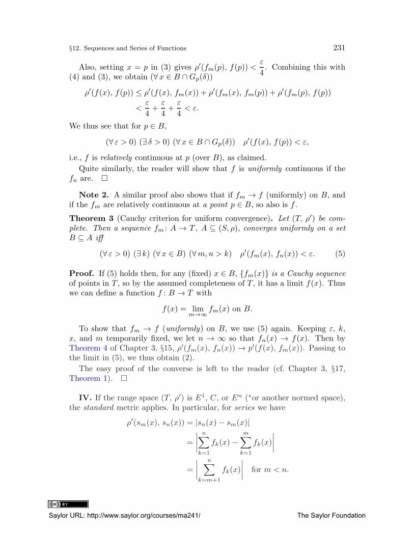
§12. Sequences and Series of Functions 231
Also, setting x = p in (3) gives ρ′(fm(p), f(p)) <ε
4. Combining this with
(4) and (3), we obtain (∀x ∈ B ∩Gp(δ))
ρ′(f(x), f(p)) ≤ ρ′(f(x), fm(x)) + ρ′(fm(x), fm(p)) + ρ′(fm(p), f(p))
<ε
4+ε
4+ε
4< ε.
We thus see that for p ∈ B,
(∀ ε > 0) (∃ δ > 0) (∀x ∈ B ∩Gp(δ)) ρ′(f(x), f(p)) < ε,
i.e., f is relatively continuous at p (over B), as claimed.
Quite similarly, the reader will show that f is uniformly continuous if thefn are. �
Note 2. A similar proof also shows that if fm → f (uniformly) on B, andif the fm are relatively continuous at a point p ∈ B, so also is f .
Theorem 3 (Cauchy criterion for uniform convergence). Let (T, ρ′) be com-
plete. Then a sequence fm : A → T , A ⊆ (S, ρ), converges uniformly on a set
B ⊆ A iff
(∀ ε > 0) (∃ k) (∀x ∈ B) (∀m,n > k) ρ′(fm(x), fn(x)) < ε. (5)
Proof. If (5) holds then, for any (fixed) x ∈ B, {fm(x)} is a Cauchy sequence
of points in T , so by the assumed completeness of T , it has a limit f(x). Thuswe can define a function f : B → T with
f(x) = limm→∞
fm(x) on B.
To show that fm → f (uniformly) on B, we use (5) again. Keeping ε, k,x, and m temporarily fixed, we let n → ∞ so that fn(x) → f(x). Then byTheorem 4 of Chapter 3, §15, ρ′(fm(x), fn(x))→ p′(f(x), fm(x)). Passing tothe limit in (5), we thus obtain (2).
The easy proof of the converse is left to the reader (cf. Chapter 3, §17,Theorem 1). �
IV. If the range space (T, ρ′) is E1, C, or En (∗or another normed space),the standard metric applies. In particular, for series we have
ρ′(sm(x), sn(x)) = |sn(x)− sm(x)|
=
∣
∣
∣
∣
n∑
k=1
fk(x)−m∑
k=1
fk(x)
∣
∣
∣
∣
=
∣
∣
∣
∣
n∑
k=m+1
fk(x)
∣
∣
∣
∣
for m < n.
Saylor URL: http://www.saylor.org/courses/ma241/ The Saylor Foundation
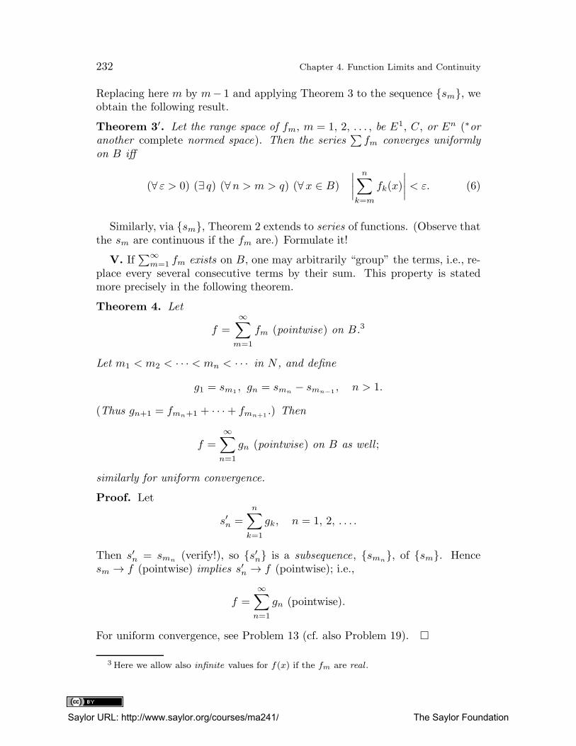
232 Chapter 4. Function Limits and Continuity
Replacing here m by m− 1 and applying Theorem 3 to the sequence {sm}, weobtain the following result.
Theorem 3′. Let the range space of fm, m = 1, 2, . . . , be E1, C, or En (∗oranother complete normed space). Then the series
∑
fm converges uniformly
on B iff
(∀ ε > 0) (∃ q) (∀n > m > q) (∀x ∈ B)
∣
∣
∣
∣
n∑
k=m
fk(x)
∣
∣
∣
∣
< ε. (6)
Similarly, via {sm}, Theorem 2 extends to series of functions. (Observe thatthe sm are continuous if the fm are.) Formulate it!
V. If∑∞
m=1 fm exists on B, one may arbitrarily “group” the terms, i.e., re-place every several consecutive terms by their sum. This property is statedmore precisely in the following theorem.
Theorem 4. Let
f =∞∑
m=1
fm (pointwise) on B.3
Let m1 < m2 < · · · < mn < · · · in N , and define
g1 = sm1, gn = smn
− smn−1, n > 1.
(Thus gn+1 = fmn+1 + · · ·+ fmn+1.) Then
f =∞∑
n=1
gn (pointwise) on B as well ;
similarly for uniform convergence.
Proof. Let
s′n =
n∑
k=1
gk, n = 1, 2, . . . .
Then s′n = smn(verify!), so {s′n} is a subsequence, {smn
}, of {sm}. Hencesm → f (pointwise) implies s′n → f (pointwise); i.e.,
f =∞∑
n=1
gn (pointwise).
For uniform convergence, see Problem 13 (cf. also Problem 19). �
3 Here we allow also infinite values for f(x) if the fm are real .
Saylor URL: http://www.saylor.org/courses/ma241/ The Saylor Foundation
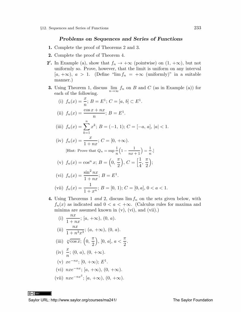
§12. Sequences and Series of Functions 233
Problems on Sequences and Series of Functions
1. Complete the proof of Theorems 2 and 3.
2. Complete the proof of Theorem 4.
2′. In Example (a), show that fn → +∞ (pointwise) on (1, +∞), but notuniformly so. Prove, however, that the limit is uniform on any interval[a, +∞), a > 1. (Define “lim fn = +∞ (uniformly)” in a suitablemanner.)
3. Using Theorem 1, discuss limn→∞
fn on B and C (as in Example (a)) foreach of the following.
(i) fn(x) =x
n; B = E1; C = [a, b] ⊂ E1.
(ii) fn(x) =cosx+ nx
n; B = E1.
(iii) fn(x) =
n∑
k=1
xk; B = (−1, 1); C = [−a, a], |a| < 1.
(iv) fn(x) =x
1 + nx; C = [0, +∞).
[Hint: Prove that Qn = sup1
n
(
1− 1
nx+ 1
)
=1
n.]
(v) fn(x) = cosn x; B =(
0,π
2
)
, C =[1
4,π
2
)
;
(vi) fn(x) =sin2 nx
1 + nx; B = E1.
(vii) fn(x) =1
1 + xn; B = [0, 1); C = [0, a], 0 < a < 1.
4. Using Theorems 1 and 2, discuss lim fn on the sets given below, withfn(x) as indicated and 0 < a < +∞. (Calculus rules for maxima andminima are assumed known in (v), (vi), and (vii).)
(i)nx
1 + nx; [a, +∞), (0, a).
(ii)nx
1 + n3x3; (a, +∞), (0, a).
(iii) n√cosx;
(
0,π
2
)
, [0, a], a <π
2.
(iv)x
n; (0, a), (0, +∞).
(v) xe−nx; [0, +∞); E1.
(vi) nxe−nx; [a, +∞), (0, +∞).
(vii) nxe−nx2
; [a, +∞), (0, +∞).
Saylor URL: http://www.saylor.org/courses/ma241/ The Saylor Foundation
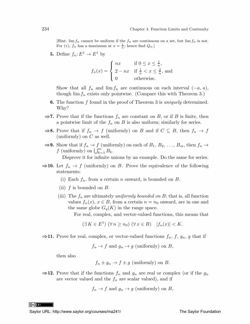
234 Chapter 4. Function Limits and Continuity
[Hint: lim fn cannot be uniform if the fn are continuous on a set, but lim fn is not.
For (v), fn has a maximum at x = 1n; hence find Qn.]
5. Define fn:E1 → E1 by
fn(x) =
nx if 0 ≤ x ≤ 1n ,
2− nx if 1n< x ≤ 2
n, and
0 otherwise.
Show that all fn and lim fn are continuous on each interval (−a, a),though lim fn exists only pointwise. (Compare this with Theorem 3.)
6. The function f found in the proof of Theorem 3 is uniquely determined.Why?
⇒7. Prove that if the functions fn are constant on B, or if B is finite, thena pointwise limit of the fn on B is also uniform; similarly for series.
⇒8. Prove that if fn → f (uniformly) on B and if C ⊆ B, then fn → f(uniformly) on C as well.
⇒9. Show that if fn → f (uniformly) on each of B1, B2, . . . , Bm, then fn →f (uniformly) on
⋃mk=1Bk.
Disprove it for infinite unions by an example. Do the same for series.
⇒10. Let fn → f (uniformly) on B. Prove the equivalence of the followingstatements:
(i) Each fn, from a certain n onward, is bounded on B.
(ii) f is bounded on B.
(iii) The fn are ultimately uniformly bounded on B; that is, all functionvalues fn(x), x ∈ B, from a certain n = n0 onward, are in one andthe same globe Gq(K) in the range space.
For real, complex, and vector-valued functions, this means that
(∃K ∈ E1) (∀n ≥ n0) (∀x ∈ B) |fn(x)| < K.
⇒11. Prove for real, complex, or vector-valued functions fn, f , gn, g that if
fn → f and gn → g (uniformly) on B,
then also
fn ± gn → f ± g (uniformly) on B.
⇒12. Prove that if the functions fn and gn are real or complex (or if the gnare vector valued and the fn are scalar valued), and if
fn → f and gn → g (uniformly) on B,
Saylor URL: http://www.saylor.org/courses/ma241/ The Saylor Foundation
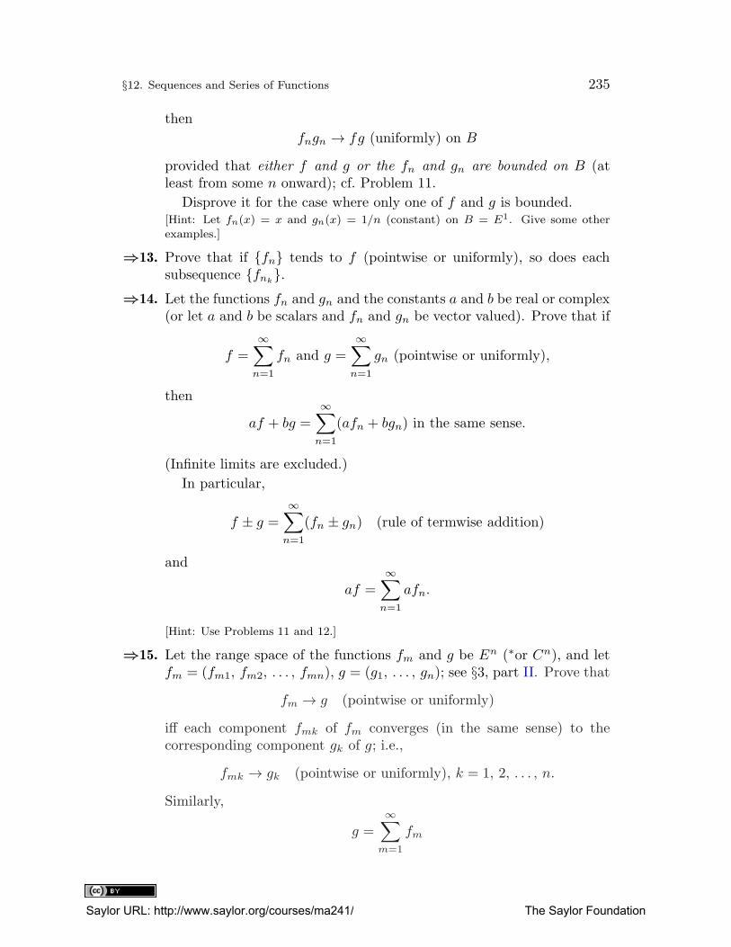
§12. Sequences and Series of Functions 235
then
fngn → fg (uniformly) on B
provided that either f and g or the fn and gn are bounded on B (atleast from some n onward); cf. Problem 11.
Disprove it for the case where only one of f and g is bounded.[Hint: Let fn(x) = x and gn(x) = 1/n (constant) on B = E1. Give some other
examples.]
⇒13. Prove that if {fn} tends to f (pointwise or uniformly), so does eachsubsequence {fnk
}.⇒14. Let the functions fn and gn and the constants a and b be real or complex
(or let a and b be scalars and fn and gn be vector valued). Prove that if
f =∞∑
n=1
fn and g =∞∑
n=1
gn (pointwise or uniformly),
then
af + bg =
∞∑
n=1
(afn + bgn) in the same sense.
(Infinite limits are excluded.)
In particular,
f ± g =
∞∑
n=1
(fn ± gn) (rule of termwise addition)
and
af =∞∑
n=1
afn.
[Hint: Use Problems 11 and 12.]
⇒15. Let the range space of the functions fm and g be En (∗or Cn), and letfm = (fm1, fm2, . . . , fmn), g = (g1, . . . , gn); see §3, part II. Prove that
fm → g (pointwise or uniformly)
iff each component fmk of fm converges (in the same sense) to thecorresponding component gk of g; i.e.,
fmk → gk (pointwise or uniformly), k = 1, 2, . . . , n.
Similarly,
g =∞∑
m=1
fm
Saylor URL: http://www.saylor.org/courses/ma241/ The Saylor Foundation
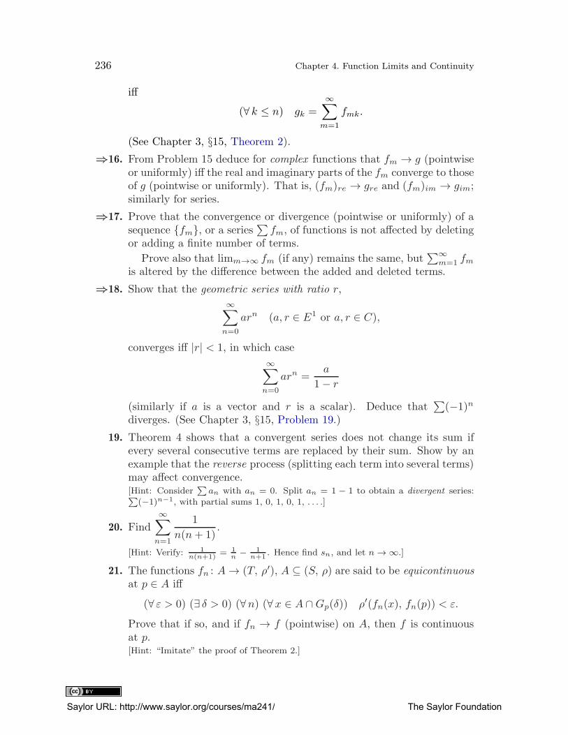
236 Chapter 4. Function Limits and Continuity
iff
(∀ k ≤ n) gk =∞∑
m=1
fmk.
(See Chapter 3, §15, Theorem 2).
⇒16. From Problem 15 deduce for complex functions that fm → g (pointwiseor uniformly) iff the real and imaginary parts of the fm converge to thoseof g (pointwise or uniformly). That is, (fm)re → gre and (fm)im → gim;similarly for series.
⇒17. Prove that the convergence or divergence (pointwise or uniformly) of asequence {fm}, or a series
∑
fm, of functions is not affected by deletingor adding a finite number of terms.
Prove also that limm→∞ fm (if any) remains the same, but∑∞
m=1 fmis altered by the difference between the added and deleted terms.
⇒18. Show that the geometric series with ratio r,
∞∑
n=0
arn (a, r ∈ E1 or a, r ∈ C),
converges iff |r| < 1, in which case
∞∑
n=0
arn =a
1− r
(similarly if a is a vector and r is a scalar). Deduce that∑
(−1)ndiverges. (See Chapter 3, §15, Problem 19.)
19. Theorem 4 shows that a convergent series does not change its sum ifevery several consecutive terms are replaced by their sum. Show by anexample that the reverse process (splitting each term into several terms)may affect convergence.[Hint: Consider
∑an with an = 0. Split an = 1 − 1 to obtain a divergent series:
∑(−1)n−1, with partial sums 1, 0, 1, 0, 1, . . . .]
20. Find
∞∑
n=1
1
n(n+ 1).
[Hint: Verify: 1n(n+1)
= 1n− 1
n+1. Hence find sn, and let n → ∞.]
21. The functions fn : A→ (T, ρ′), A ⊆ (S, ρ) are said to be equicontinuousat p ∈ A iff
(∀ ε > 0) (∃ δ > 0) (∀n) (∀x ∈ A ∩Gp(δ)) ρ′(fn(x), fn(p)) < ε.
Prove that if so, and if fn → f (pointwise) on A, then f is continuousat p.[Hint: “Imitate” the proof of Theorem 2.]
Saylor URL: http://www.saylor.org/courses/ma241/ The Saylor Foundation
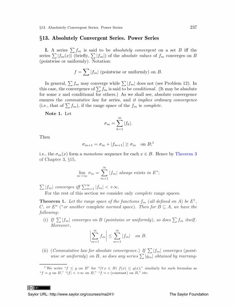
§13. Absolutely Convergent Series. Power Series 237
§13. Absolutely Convergent Series. Power Series
I. A series∑
fm is said to be absolutely convergent on a set B iff theseries
∑ |fm(x)| (briefly, ∑ |fm|) of the absolute values of fm converges on B(pointwise or uniformly). Notation:
f =∑
|fm| (pointwise or uniformly) on B.
In general,∑
fm may converge while∑ |fm| does not (see Problem 12). In
this case, the convergence of∑
fm is said to be conditional . (It may be absolutefor some x and conditional for others.) As we shall see, absolute convergenceensures the commutative law for series, and it implies ordinary convergence
(i.e., that of∑
fm), if the range space of the fm is complete.
Note 1. Let
σm =
m∑
k=1
|fk|.
Then
σm+1 = σm + |fm+1| ≥ σm on B;1
i.e., the σm(x) form a monotone sequence for each x ∈ B. Hence by Theorem 3of Chapter 3, §15,
limm→∞
σm =∞∑
m=1
|fm| always exists in E∗;
∑ |fm| converges iff∑∞
m=1 |fm| < +∞.
For the rest of this section we consider only complete range spaces.
Theorem 1. Let the range space of the functions fm (all defined on A) be E1,C, or En (∗or another complete normed space). Then for B ⊆ A, we have the
following :
(i) If∑ |fm| converges on B (pointwise or uniformly), so does
∑
fm itself .Moreover ,
∣
∣
∣
∣
∞∑
m=1
fm
∣
∣
∣
∣
≤∞∑
m=1
|fm| on B.
(ii) (Commutative law for absolute convergence.) If∑ |fm| converges (point-
wise or uniformly) on B, so does any series∑ |gm| obtained by rearrang-
1 We write “f ≤ g on B” for “(∀ x ∈ B) f(x) ≤ g(x);” similarly for such formulas as
“f = g on B,” “|f | < +∞ on B,” “f = c (constant) on B,” etc.
Saylor URL: http://www.saylor.org/courses/ma241/ The Saylor Foundation
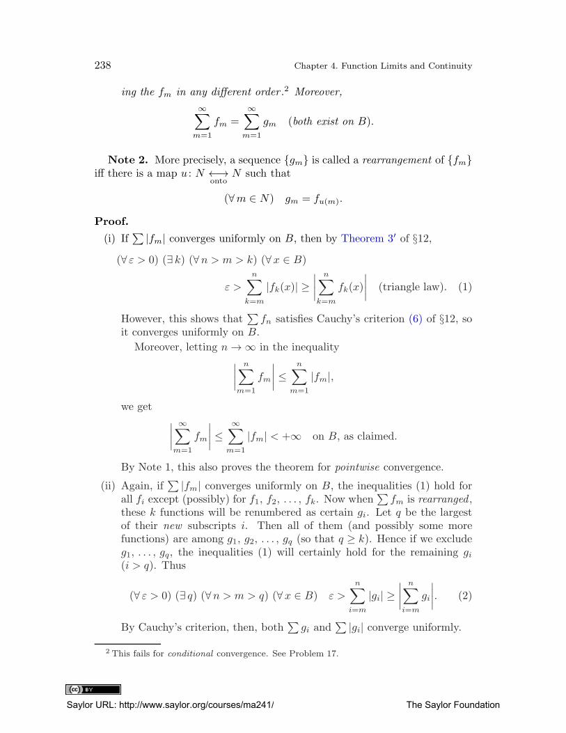
238 Chapter 4. Function Limits and Continuity
ing the fm in any different order .2 Moreover,
∞∑
m=1
fm =
∞∑
m=1
gm (both exist on B).
Note 2. More precisely, a sequence {gm} is called a rearrangement of {fm}iff there is a map u : N ←→
ontoN such that
(∀m ∈ N) gm = fu(m).
Proof.
(i) If∑ |fm| converges uniformly on B, then by Theorem 3′ of §12,
(∀ ε > 0) (∃ k) (∀n > m > k) (∀x ∈ B)
ε >n∑
k=m
|fk(x)| ≥∣
∣
∣
∣
n∑
k=m
fk(x)
∣
∣
∣
∣
(triangle law). (1)
However, this shows that∑
fn satisfies Cauchy’s criterion (6) of §12, soit converges uniformly on B.
Moreover, letting n→∞ in the inequality∣
∣
∣
∣
n∑
m=1
fm
∣
∣
∣
∣
≤n∑
m=1
|fm|,
we get∣
∣
∣
∣
∞∑
m=1
fm
∣
∣
∣
∣
≤∞∑
m=1
|fm| < +∞ on B, as claimed.
By Note 1, this also proves the theorem for pointwise convergence.
(ii) Again, if∑ |fm| converges uniformly on B, the inequalities (1) hold for
all fi except (possibly) for f1, f2, . . . , fk. Now when∑
fm is rearranged ,these k functions will be renumbered as certain gi. Let q be the largestof their new subscripts i. Then all of them (and possibly some morefunctions) are among g1, g2, . . . , gq (so that q ≥ k). Hence if we excludeg1, . . . , gq, the inequalities (1) will certainly hold for the remaining gi(i > q). Thus
(∀ ε > 0) (∃ q) (∀n > m > q) (∀x ∈ B) ε >n∑
i=m
|gi| ≥∣
∣
∣
∣
n∑
i=m
gi
∣
∣
∣
∣
. (2)
By Cauchy’s criterion, then, both∑
gi and∑ |gi| converge uniformly.
2 This fails for conditional convergence. See Problem 17.
Saylor URL: http://www.saylor.org/courses/ma241/ The Saylor Foundation
§13. Absolutely Convergent Series. Power Series 239
Moreover, by construction, the two partial sums
sk =k
∑
i=1
fi and s′q =
q∑
i=1
gi
can differ only in those terms whose original subscripts (before the re-arrangement) were > k. By (1), however, any finite sum of such terms is
less than ε in absolute value. Thus |s′q − sk| < ε.
This argument holds also if k in (1) is replaced by a larger integer.(Then also q increases, since q ≥ k as noted above.) Thus we may letk → +∞ (hence also q → +∞) in the inequality |s′q − sk| < ε, with εfixed. Then
sk →∞∑
m=1
fm and s′q →∞∑
i=1
gi,
so∣
∣
∣
∣
∞∑
i=1
gi −∞∑
m=1
fm
∣
∣
∣
∣
≤ ε.
Now let ε→ 0 to get
∞∑
i=1
gi =
∞∑
m=1
fm;
similarly for pointwise convergence. �
II. Next, we develop some simple tests for absolute convergence.
Theorem 2 (comparison test). Suppose
(∀m) |fm| ≤ |gm| on B.
Then
(i)∞∑
m=1
|fm| ≤∞∑
m=1
|gm| on B;
(ii)∞∑
m=1
|fm| = +∞ implies
∞∑
m=1
|gm| = +∞ on B; and
(iii) If∑
|gm| converges (pointwise or uniformly) on B, so does∑
|fm|.
Proof. Conclusion (i) follows by letting n→∞ in
n∑
m=1
|fm| ≤n∑
m=1
|gm|.
In turn, (ii) is a direct consequence of (i).
Saylor URL: http://www.saylor.org/courses/ma241/ The Saylor Foundation
240 Chapter 4. Function Limits and Continuity
Also, by (i),
∞∑
m=1
|gm| < +∞ implies∞∑
m=1
|fm| < +∞.
This proves (iii) for the pointwise case (see Note 1). The uniform case followsexactly as in Theorem 1(i) on noting that
n∑
k=m
|fk| ≤n∑
k=m
|gk|
and that the functions |fk| and |gk| are real (so Theorem 3′ in §12 does ap-ply). �
Theorem 3 (Weierstrass “M -test”). If∑
Mn is a convergent series of real
constants Mn ≥ 0 and if
(∀n) |fn| ≤Mn
on a set B, then∑ |fn| converges uniformly on B.3 Moreover ,
∞∑
n=1
|fn| ≤∞∑
n=1
Mn on B.
Proof. Use Theorem 2 with |gn| =Mn, noting that∑ |gn| converges uniformly
since the |gn| are constant (§12, Problem 7). �
Examples.
(a) Let
fn(x) =(1
2sinx
)n
on E1.
Then
(∀n) (∀x ∈ E1) |fn(x)| ≤ 2−n,
and∑
2−n converges (geometric series with ratio 12 ; see §12, Problem 18).
Thus, settingMn = 2−n in Theorem 3, we infer that the series∑ | 12 sinx|n
converges uniformly on E1, as does∑
( 12 sinx)n; moreover,
∞∑
n=1
|fn| ≤∞∑
n=1
2−n = 1.
3 So does∑
fn itself if the range space is as in Theorem 1. Note that for series with
positive terms, absolute and ordinary convergence coincide.
Saylor URL: http://www.saylor.org/courses/ma241/ The Saylor Foundation
§13. Absolutely Convergent Series. Power Series 241
Theorem 4 (necessary condition of convergence). If∑
fm or∑ |fm| con-
verges on B (pointwise or uniformly), then |fm| → 0 on B (in the same sense).
Thus a series cannot converge unless its general term tends to 0 (respec-tively, 0).
Proof. If∑
fm = f , say, then sm → f and also sm−1 → f . Hence
sm − sm−1 → f − f = 0.
However, sm − sm−1 = fm. Thus fm → 0, and |fm| → 0, as claimed.
This holds for pointwise and uniform convergence alike (see Problem 14 in§12). �
Caution: The condition |fm| → 0 is necessary but not sufficient . Indeed,there are divergent series with general term tending to 0, as we show next.
Examples (continued).
(b)∞∑
n=1
1
n= +∞ (the so-called harmonic series).
Indeed, by Note 1,
∞∑
n=1
1
nexists (in E∗),
so Theorem 4 of §12 applies. We group the series as follows:
∑ 1
n= 1 +
1
2+
(1
3+
1
4
)
+(1
5+
1
6+
1
7+
1
8
)
+(1
9+ · · ·+ 1
16
)
+ · · ·
≥ 1
2+
1
2+
(1
4+
1
4
)
+(1
8+
1
8+
1
8+
1
8
)
+( 1
16+ · · ·+ 1
16
)
+ · · · .
Each bracketed expression now equals 12 . Thus
∑ 1
n≥
∑
gm, gm =1
2.
As gm does not tend to 0,∑
gm diverges , i.e.,∑∞
m=1 gm is infinite, byTheorem 4. A fortiori, so is
∑∞n=1
1n .
Theorem 5 (root and ratio tests). A series of constants∑
an (|an| 6= 0)converges absolutely if
lim n√
|an| < 1 or lim( |an+1||an|
)
< 1.
Saylor URL: http://www.saylor.org/courses/ma241/ The Saylor Foundation
242 Chapter 4. Function Limits and Continuity
It diverges if
lim n√
|an| > 1 or lim( |an+1||an|
)
> 1.4
It may converge or diverge if
lim n√
|an| = 1
or if
lim( |an+1||an|
)
≤ 1 ≤ lim( |an+1||an|
)
.
(The an may be scalars or vectors.)
Proof. If lim n√
|an| < 1, choose r > 0 such that
lim n√
|an| < r < 1.
Then by Corollary 2 of Chapter 2, §13, n√
|an| < r for all but finitely many n.Thus, dropping a finite number of terms (§12, Problem 17), we may assumethat
|an| < rn for all n.
As 0 < r < 1, the geometric series∑
rn converges. Hence so does∑ |an| by
Theorem 2.
In the case
lim( |an+1||an|
)
< 1,
we similarly obtain (∃m) (∀n ≥ m) |an+1| < |an|r; hence by induction,
(∀n ≥ m) |an| ≤ |am|rn−m. (Verify!)
Thus∑ |an| converges, as before.
If lim n√
|an| > 1, then by Corollary 2 of Chapter 2, §13, |an| > 1 for infinitelymany n. Hence |an| cannot tend to 0, and so
∑
an diverges by Theorem 4.
Similarly, if
lim( |an+1||an|
)
> 1,
then |an+1| > |an| for all but finitely many n, so |an| cannot tend to 0 again.5 �
Note 3. We have
lim( |an+1||an|
)
≤ lim n√
|an| ≤ lim n√
|an| ≤ lim( |an+1||an|
)
.6
4 Note that we have “lim”, not “lim” here. However, often “lim” and “lim” coincide. This
is the case when the limit exists (see Chapter 2, §13, Theorem 3).5 This inference would be false if we only had lim(|an+1|/|an|) > 1. Why?6 For a proof, use Problem 33 of Chapter 3, §15 with x1 = |a1| and xk+1 = |ak+1|/|ak|.
Saylor URL: http://www.saylor.org/courses/ma241/ The Saylor Foundation
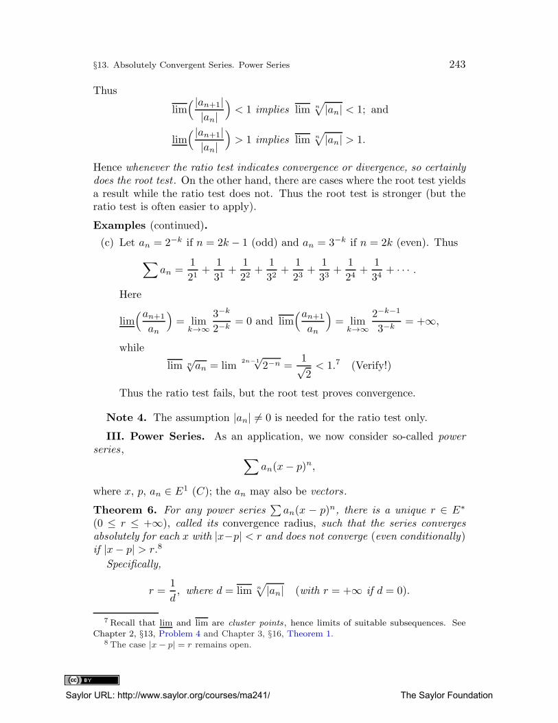
§13. Absolutely Convergent Series. Power Series 243
Thus
lim( |an+1||an|
)
< 1 implies lim n√
|an| < 1; and
lim( |an+1||an|
)
> 1 implies lim n√
|an| > 1.
Hence whenever the ratio test indicates convergence or divergence, so certainly
does the root test . On the other hand, there are cases where the root test yieldsa result while the ratio test does not. Thus the root test is stronger (but theratio test is often easier to apply).
Examples (continued).
(c) Let an = 2−k if n = 2k − 1 (odd) and an = 3−k if n = 2k (even). Thus
∑
an =1
21+
1
31+
1
22+
1
32+
1
23+
1
33+
1
24+
1
34+ · · · .
Here
lim(an+1
an
)
= limk→∞
3−k
2−k= 0 and lim
(an+1
an
)
= limk→∞
2−k−1
3−k= +∞,
while
lim n√an = lim
2n−1√2−n =
1√2< 1.7 (Verify!)
Thus the ratio test fails, but the root test proves convergence.
Note 4. The assumption |an| 6= 0 is needed for the ratio test only.
III. Power Series. As an application, we now consider so-called power
series,∑
an(x− p)n,
where x, p, an ∈ E1 (C); the an may also be vectors.
Theorem 6. For any power series∑
an(x − p)n, there is a unique r ∈ E∗
(0 ≤ r ≤ +∞), called its convergence radius, such that the series converges
absolutely for each x with |x−p| < r and does not converge (even conditionally)if |x− p| > r.8
Specifically,
r =1
d, where d = lim n
√
|an| (with r = +∞ if d = 0).
7 Recall that lim and lim are cluster points, hence limits of suitable subsequences. SeeChapter 2, §13, Problem 4 and Chapter 3, §16, Theorem 1.
8 The case |x− p| = r remains open.
Saylor URL: http://www.saylor.org/courses/ma241/ The Saylor Foundation
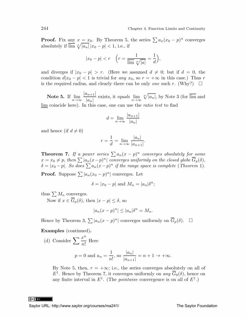
244 Chapter 4. Function Limits and Continuity
Proof. Fix any x = x0. By Theorem 5, the series∑
an(x0 − p)n converges
absolutely if lim n√
|an| |x0 − p| < 1, i.e., if
|x0 − p| < r(
r =1
lim n√
|a|=
1
d
)
,
and diverges if |x0 − p| > r. (Here we assumed d 6= 0; but if d = 0, thecondition d|x0 − p| < 1 is trivial for any x0, so r = +∞ in this case.) Thus ris the required radius, and clearly there can be only one such r. (Why?) �
Note 5. If limn→∞
|an+1||an|
exists, it equals limn→∞
n√
|an|, by Note 3 (for lim and
lim coincide here). In this case, one can use the ratio test to find
d = limn→∞
|an+1||an|
and hence (if d 6= 0)
r =1
d= lim
n→∞|an||an+1|
.
Theorem 7. If a power series∑
an(x − p)n converges absolutely for some
x = x0 6= p, then∑ |an(x−p)n| converges uniformly on the closed globe Gp(δ),
δ = |x0−p|. So does∑
an(x−p)n if the range space is complete (Theorem 1).
Proof. Suppose∑ |an(x0 − p)n| converges. Let
δ = |x0 − p| and Mn = |an|δn;
thus∑
Mn converges.
Now if x ∈ Gp(δ), then |x− p| ≤ δ, so
|an(x− p)n| ≤ |an|δn =Mn.
Hence by Theorem 3,∑ |an(x− p)n| converges uniformly on Gp(δ). �
Examples (continued).
(d) Consider∑ xn
n!Here
p = 0 and an =1
n!, so
|an||an+1|
= n+ 1→ +∞.
By Note 5, then, r = +∞; i.e., the series converges absolutely on all ofE1. Hence by Theorem 7, it converges uniformly on any G0(δ), hence onany finite interval in E1. (The pointwise convergence is on all of E1.)
Saylor URL: http://www.saylor.org/courses/ma241/ The Saylor Foundation
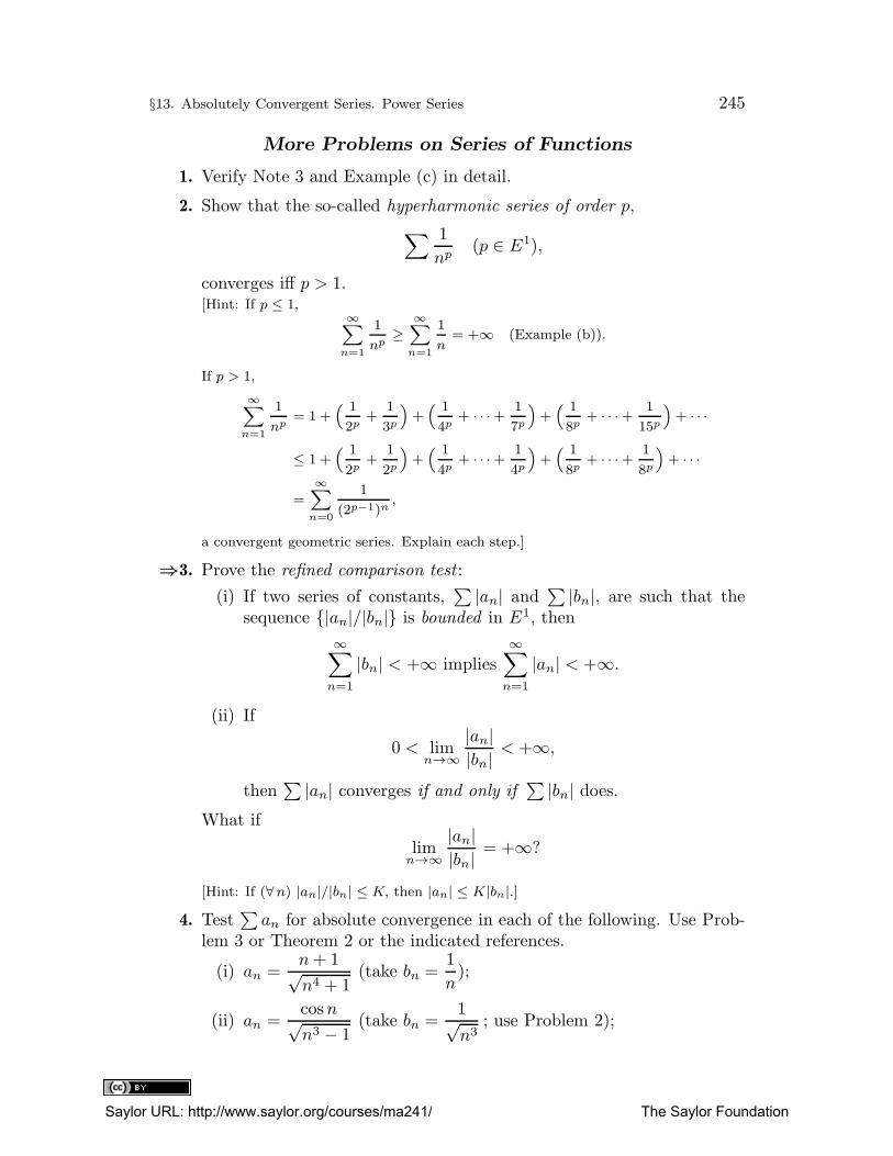
§13. Absolutely Convergent Series. Power Series 245
More Problems on Series of Functions
1. Verify Note 3 and Example (c) in detail.
2. Show that the so-called hyperharmonic series of order p,
∑ 1
np(p ∈ E1),
converges iff p > 1.[Hint: If p ≤ 1,
∞∑
n=1
1
np≥
∞∑
n=1
1
n= +∞ (Example (b)).
If p > 1,
∞∑
n=1
1
np= 1 +
( 1
2p+
1
3p
)
+( 1
4p+ · · ·+ 1
7p
)
+( 1
8p+ · · ·+ 1
15p
)
+ · · ·
≤ 1 +( 1
2p+
1
2p
)
+( 1
4p+ · · ·+ 1
4p
)
+( 1
8p+ · · ·+ 1
8p
)
+ · · ·
=
∞∑
n=0
1
(2p−1)n,
a convergent geometric series. Explain each step.]
⇒3. Prove the refined comparison test :
(i) If two series of constants,∑ |an| and
∑ |bn|, are such that thesequence {|an|/|bn|} is bounded in E1, then
∞∑
n=1
|bn| < +∞ implies∞∑
n=1
|an| < +∞.
(ii) If
0 < limn→∞
|an||bn|
< +∞,
then∑ |an| converges if and only if
∑ |bn| does.What if
limn→∞
|an||bn|
= +∞?
[Hint: If (∀n) |an|/|bn| ≤ K, then |an| ≤ K|bn|.]
4. Test∑
an for absolute convergence in each of the following. Use Prob-lem 3 or Theorem 2 or the indicated references.
(i) an =n+ 1√n4 + 1
(take bn =1
n);
(ii) an =cosn√n3 − 1
(take bn =1√n3
; use Problem 2);
Saylor URL: http://www.saylor.org/courses/ma241/ The Saylor Foundation
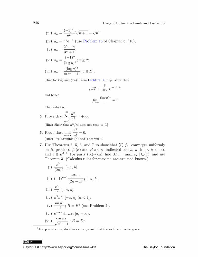
246 Chapter 4. Function Limits and Continuity
(iii) an =(−1)nnp
(√n+ 1−√n) ;
(iv) an = n5e−n (use Problem 18 of Chapter 3, §15);
(v) an =2n + n
3n + 1;
(vi) an =(−1)n(logn)q
;n ≥ 2;
(vii) an =(logn)q
n(n2 + 1), q ∈ E1.
[Hint for (vi) and (vii): From Problem 14 in §2, show that
limy→+∞
y
(log y)q= +∞
and hence
limn→∞
(log n)q
n= 0.
Then select bn.]
5. Prove that∞∑
n=1
nn
n!= +∞.
[Hint: Show that nn/n! does not tend to 0.]
6. Prove that limn→∞
xn
n!= 0.
[Hint: Use Example (d) and Theorem 4.]
7. Use Theorems 3, 5, 6, and 7 to show that∑ |fn| converges uniformly
on B, provided fn(x) and B are as indicated below, with 0 < a < +∞and b ∈ E1.9 For parts (ix)–(xii), find Mn = maxx∈B |fn(x)| and useTheorem 3. (Calculus rules for maxima are assumed known.)
(i)x2n
(2n)!; [−a, b].
(ii) (−1)n+1 x2n−1
(2n− 1)!; [−a, b].
(iii)xn
nn; [−a, a].
(iv) n3xn; [−a, a] (a < 1).
(v)sinnx
n2; B = E1 (use Problem 2).
(vi) e−nx sinnx; [a, +∞).
(vii)cosnx√n3 + 1
; B = E1.
9 For power series, do it in two ways and find the radius of convergence.
Saylor URL: http://www.saylor.org/courses/ma241/ The Saylor Foundation
§13. Absolutely Convergent Series. Power Series 247
(viii) an cosnx, with
∞∑
n=1
|an| < +∞; B = E1.
(ix) xne−nx; [0, +∞).
(x) xnenx; (−∞, 12].
(xi) (x · log x)n, fn(0) = 0;[
−3
2,3
2
]
.
(xii)( log x
x
)n
; [1, +∞).
(xiii)q(q − 1) · · · (q − n+ 1)xn
n!, q ∈ E1;
[
−1
2,1
2
]
.
⇒8. (Summation by parts .) Let fn, hn, and gn be real or complex functions(or let fn and hn be scalar valued and gn be vector valued). Let fn =hn − hn−1 (n ≥ 2). Verify that (∀m > n > 1)
m∑
k=n+1
fkgk =m∑
k=n+1
(hk − hk−1)gk
= hmgm − hngn+1 −m−1∑
k=n+1
hk(gk+1 − gk).
[Hint: Rearrange the sum.]
⇒9. (Abel’s test .) Let the fn, gn, and hn be as in Problem 8, withhn =
∑ni=1 fi. Suppose that
(i) the range space of the gn is complete;
(ii) |gn| → 0 (uniformly) on a set B; and
(iii) the partial sums hn =∑n
i=1 fi are uniformly bounded on B; i.e.,
(∃K ∈ E1) (∀n) |hn| < K on B.
Then prove that∑
fkgk converges uniformly on B if∑ |gn+1−gn| does.
(This always holds if the gn are real and gn ≥ gn+1 on B.)[Hint: Let ε > 0. Show that
(∃ k) (∀m > n > k)m∑
i=n+1
|gi+1 − gi| < ε and |gn| < ε on B.
Then use Problem 8 to show that
∣∣∣∣
m∑
i=n+1
figi
∣∣∣∣ < 3Kε.
Apply Theorem 3′ of §12.]
Saylor URL: http://www.saylor.org/courses/ma241/ The Saylor Foundation
248 Chapter 4. Function Limits and Continuity
⇒ 9′. Prove that if∑
an is a convergent series of constants an ∈ E1 and if{bn} is a bounded monotone sequence in E1, then
∑
anbn converges.[Hint: Let bn → b. Write
anbn = an(bn − b) + anb
and use Problem 9 with fn = an and gn = bn − b.]
⇒10. Prove the Leibniz test for alternating series: If {bn}↓ and bn → 0 inE1, then
∑
(−1)nbn converges, and the sum∑∞
n=1(−1)nbn differs from
sn =∑n
k=1(−1)kbk by bn+1 at most.[Hint: Use Problem 9′.]
⇒11. (Dirichlet test .) Let the fn, gn, and hn be as in Problem 8 with∑∞
n=0 fnuniformly convergent on B to a function f , and with
hn = −∞∑
i=n+1
fi on B.
Suppose that
(i) the range space of the gn is complete; and
(ii) there is K ∈ E1 such that
|g0|+∞∑
n=0
|gn+1 − gn| < K on B.
Show that∑
fngn converges uniformly on B.[Proof outline: We have
|gn| =∣∣∣∣g0 +
n−1∑
i=0
(gi+1 − gi)
∣∣∣∣ ≤ |g0|+
n−1∑
i=0
|gi+1 − gi| < K by (ii).
Also,
|hn| =∣∣∣∣
n∑
i=0
fi − f
∣∣∣∣ → 0 (uniformly) on B
by assumption. Hence
(∀ ε > 0) (∃ k) (∀n > k) |hn| < ε on B.
Using Problem 8, obtain
(∀m > n > k)
∣∣∣∣
m∑
i=n+i
figi
∣∣∣∣ < 2Kε.]
12. Prove that if 0 < p ≤ 1, then∑ (−1)n
npconverges conditionally .
[Hint: Use Problems 11 and 2.]
Saylor URL: http://www.saylor.org/courses/ma241/ The Saylor Foundation
§13. Absolutely Convergent Series. Power Series 249
⇒13. Continuing Problem 14 in §12, prove that if ∑ |fn| and∑ |gn| converge
on B (pointwise or uniformly), then so do the series∑
|afn + bgn|,∑
|fn ± gn|, and∑
|afn|.
[Hint: |afn + bgn| ≤ |a||fn|+ |b||gn|. Use Theorem 2.]
For the rest of the section, we define
x+ = max(x, 0) and x− = max(−x, 0).
⇒14. Given {an} ⊂ E∗ show the following:
(i)∑
a+n +∑
a−n =∑ |an|.
(ii) If∑
a+n < +∞ or∑
a−n < +∞, then∑
an =∑
a+n −∑
a−n .
(iii) If∑
an converges conditionally , then∑
a+n = +∞ =∑
a−n .
(iv) If∑ |an| < +∞, then for any {bn} ⊂ E1,
∑
|an ± bn| < +∞ iff∑
|bn| <∞;
moreover,∑
an ±∑
bn =∑
(an ± bn) if∑
bn exists.
[Hint: Verify that |an| = a+n + a−n and an = a+n − a−n . Use the rules of §4.]
⇒15. (Abel’s theorem.) Show that if a power series
∞∑
n=0
an(x− p)n (an ∈ E, x, p ∈ E1)
converges for some x = x0 6= p, it converges uniformly on [p, x0] (or[x0, p] if x0 < p).[Proof outline: First let p = 0 and x0 = 1. Use Problem 11 with
fn = an and gn(x) = xn = (x− p)n.
As fn = an1n = an(x0 − p)n, the series∑
fn converges by assumption. The
convergence is uniform since the fn are constant. Verify that if x = 1, then
∞∑
k=1
|gk+1 − gk| = 0,
and if 0 ≤ x < 1, then
∞∑
k=0
|gk+1 − gk| =∞∑
k=0
xk|x− 1| = (1− x)
∞∑
k=0
xk = 1 (a geometric series).
Also, |g0(x)| = x0 = 1. Thus by Problem 11 (with K = 2),∑
fngn convergesuniformly on [0, 1], proving the theorem for p = 0 and x0 = 1. The general case
reduces to this case by the substitution x− p = (x0 − p)y. Verify!]
Saylor URL: http://www.saylor.org/courses/ma241/ The Saylor Foundation
250 Chapter 4. Function Limits and Continuity
16. Prove that if0 < lim an ≤ lim an < +∞,
then the convergence radius of∑
an(x− p)n is 1.
17. Show that a conditionally convergent series∑
an (an ∈ E1) can berearranged so as to diverge, or to converge to any prescribed sum s.[Proof for s ∈ E1: Using Problem 14(iii), take the first partial sum
a+1 + · · ·+ a+m > s.
Then adjoin terms
−a−1 , −a−2 , . . . , −a−n
until the partial sum becomes less than s. Then add terms a+k until it exceeds s.
Then adjoin terms −a−k until it becomes less than s, and so on.
As a+k → 0 and a−k → 0 (why?), the rearranged series tends to s. (Why?)
Give a similar proof for s = ±∞. Also, make the series oscillate, with no sum.]
18. Prove that if a power series∑
an(x−p)n converges at some x = x0 6= p,it converges absolutely (pointwise) on Gp(δ) if δ ≤ |x0 − p|.[Hint: By Theorem 6, δ ≤ |x0 − p| ≤ r (r = convergence radius). Fix any x ∈ Gp(δ).
Show that the line→px, when extended, contains a point x1 such that |x − p| <
|x1 − p| < δ ≤ r. By Theorem 6, the series converges absolutely at x1, hence at x as
well, by Theorem 7.]
Saylor URL: http://www.saylor.org/courses/ma241/ The Saylor Foundation
Chapter 5
Differentiation and Antidifferentiation
§1. Derivatives of Functions of One Real Variable
In this chapter, “E” will always denote any one of E1, E∗, C (the complexfield), En, ∗or another normed space. We shall consider functions f : E1 → Eof one real variable with values in E. Functions f : E1 → E∗ (admitting finiteand infinite values) are said to be extended real . Thus f : E1 → E may be real,extended real, complex, or vector valued.
Operations in E∗ were defined in Chapter 4, §4. Recall, in particular, ourconventions (2∗) there. Due to them, addition, subtraction, and multiplicationare always defined in E∗ (with sums and products possibly “unorthodox”).
To simplify formulations, we shall also adopt the convention that
f(x) = 0 unless defined otherwise.
(“0” stands also for the zero-vector in E if E is a vector space.) Thus eachfunction f is defined on all of E1. For convenience, we call f(x) “finite” iff(x) 6= ±∞ (also if it is a vector).
Definition 1.
For each function f : E1 → E, we define its derived function f ′ : E1 → Eby setting, for every point p ∈ E1,
f ′(p) =
limx→p
f(x)− f(p)x− p if this limit exists (finite or not);
0, otherwise.
(1)
Thus f ′(p) is always defined.
If the limit in (1) exists, we call it the derivative of f at p.
If, in addition, this limit is finite, we say that f is differentiable at p.
If this holds for each p in a set B ⊆ E1, we say that f has a deriva-
tive (respectively, is differentiable) on B, and we call the function f ′ the
Saylor URL: http://www.saylor.org/courses/ma241/ The Saylor Foundation
252 Chapter 5. Differentiation and Antidifferentiation
derivative of f on B.1
If the limit in (1) is one sided (with x → p− or x → p+), we call it aone-sided (left or right) derivative at p, denoted f ′
− or f ′+.
Note that the formula f ′(p) = 0 holds also if f has no derivative at p. Onthe other hand, f ′(p) 6= 0 implies that f ′(p) is a genuine derivative.
Definition 2.
Given a function f : E1 → E, we define its nth derived function (or derivedfunction of order n), denoted f (n) : E1 → E, by induction:
f (0) = f, f (n+1) = [f (n)]′, n = 0, 1, 2, . . . .
Thus f (n+1) is the derived function of f (n). By our conventions, f (n) isdefined on all of E1 for each n and each function f : E1 → E. We havef (1) = f ′, and we write f ′′ for f (2), f ′′′ for f (3), etc. We say that f has nderivatives at a point p iff the limits
limx→q
f (k)(x)− f (k)(q)
x− qexist for all q in a neighborhood Gp of p and for k = 0, 1, . . . , n− 2, and also
limx→p
f (n−1)(x)− f (n−1)(p)
x− pexists. If all these limits are finite, we say that f is n times differentiable onI; similarly for one-sided derivatives.
It is an important fact that differentiability implies continuity .
Theorem 1. If a function f : E1 → E is differentiable at a point p ∈ E1, it iscontinuous at p, and f(p) is finite (even if E = E∗).
Proof. Setting ∆x = x− p and ∆f = f(x)− f(p), we have the identity
|f(x)− f(p)| =∣
∣
∣
∆f
∆x· (x− p)
∣
∣
∣for x 6= p. (2)
By assumption,
f ′(p) = limx→p
∆f
∆x
exists and is finite. Thus as x→ p, the right side of (2) (hence the left side aswell) tends to 0, so
limx→p|f(x)− f(p)| = 0, or lim
x→pf(x) = f(p),
1 If B is an interval , the derivative at its endpoints (if in B) need be one sided only, as
x → p over B (see next).
Saylor URL: http://www.saylor.org/courses/ma241/ The Saylor Foundation
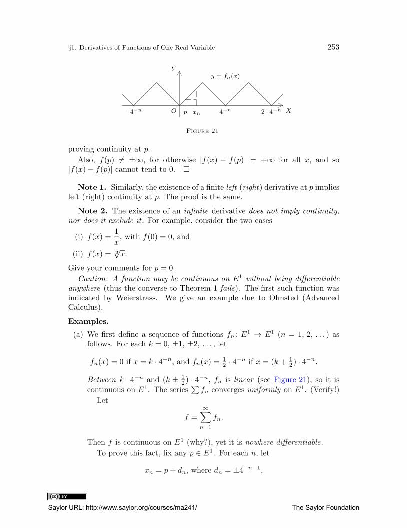
§1. Derivatives of Functions of One Real Variable 253
O
Y
X−4−n p xn 4−n 2 · 4−n
y = fn(x)
Figure 21
proving continuity at p.
Also, f(p) 6= ±∞, for otherwise |f(x) − f(p)| = +∞ for all x, and so|f(x)− f(p)| cannot tend to 0. �
Note 1. Similarly, the existence of a finite left (right) derivative at p impliesleft (right) continuity at p. The proof is the same.
Note 2. The existence of an infinite derivative does not imply continuity,
nor does it exclude it . For example, consider the two cases
(i) f(x) =1
x, with f(0) = 0, and
(ii) f(x) = 3√x.
Give your comments for p = 0.
Caution: A function may be continuous on E1 without being differentiable
anywhere (thus the converse to Theorem 1 fails). The first such function wasindicated by Weierstrass. We give an example due to Olmsted (AdvancedCalculus).
Examples.
(a) We first define a sequence of functions fn : E1 → E1 (n = 1, 2, . . . ) as
follows. For each k = 0, ±1, ±2, . . . , let
fn(x) = 0 if x = k · 4−n, and fn(x) =12 · 4−n if x = (k + 1
2 ) · 4−n.
Between k · 4−n and (k ± 12) · 4−n, fn is linear (see Figure 21), so it is
continuous on E1. The series∑
fn converges uniformly on E1. (Verify!)
Let
f =
∞∑
n=1
fn.
Then f is continuous on E1 (why?), yet it is nowhere differentiable.
To prove this fact, fix any p ∈ E1. For each n, let
xn = p+ dn, where dn = ±4−n−1,
Saylor URL: http://www.saylor.org/courses/ma241/ The Saylor Foundation
254 Chapter 5. Differentiation and Antidifferentiation
choosing the sign of dn so that p and xn are in the same half of a “saw-tooth” in the graph of fn (Figure 21). Then
fn(xn)− fn(p) = ±dn = ±(xn − p). (Why?)
Also,
fm(xn)− fm(p) = ±dn if m ≤ n
but vanishes for m > n. (Why?)
Thus, when computing f(xn)− f(p), we may replace
f =
∞∑
m=1
fm by f =
n∑
m=1
fm.
Sincefm(xn)− fm(p)
xn − p= ±1 for m ≤ n,
the fractionf(xn)− f(p)
xn − pis an integer , odd if n is odd and even if n is even. Thus this fractioncannot tend to a finite limit as n → ∞, i.e., as dn = 4−n−1 → 0 andxn = p+ dn → p. A fortiori, this applies to
limx→p
f(x)− f(p)x− p .
Thus f is not differentiable at any p.
The expressions f(x)−f(p) and x−p, briefly denoted ∆f and ∆x, are calledthe increments of f and x (at p), respectively.2 We now show that for differ-
entiable functions, ∆f and ∆x are “nearly proportional” when x approachesp; that is,
∆f
∆x= c+ δ(x)
with c constant and limx→p δ(x) = 0.
Theorem 2. A function f : E1 → E is differentiable at p, and f ′(p) = c, iffthere is a finite c ∈ E and a function δ : E1 → E such that lim
x→pδ(x) = δ(p) = 0,
and such that
∆f = [c+ δ(x)]∆x for all x ∈ E1. (3)
2 This notation is rather incomplete but convenient. One only has to remember that both
∆f and ∆x depend on x and p.
Saylor URL: http://www.saylor.org/courses/ma241/ The Saylor Foundation
§1. Derivatives of Functions of One Real Variable 255
Proof. If f is differentiable at p, put c = f ′(p). Define δ(p) = 0 and
δ(x) =∆f
∆x− f ′(p) for x 6= p.
Then limx→p δ(x) = f ′(p)− f ′(p) = 0 = δ(p). Also, (3) follows.
Conversely, if (3) holds, then
∆f
∆x= c+ δ(x)→ c as x→ p (since δ(x)→ 0).
Thus by definition,
c = limx→p
∆f
∆x= f ′(p) and f ′(p) = c is finite. �
Theorem 3 (chain rule). Let the functions g : E1 → E1 (real) and f : E1 → E(real or not) be differentiable at p and q, respectively , where q = g(p). Then
the composite function h = f ◦ g is differentiable at p, and
h′(p) = f ′(q)g′(p).
Proof. Setting
∆h = h(x)− h(p) = f(g(x))− f(g(p)) = f(g(x))− f(q),we must show that
limx→p
∆h
∆x= f ′(q)g′(p) 6= ±∞.
Now as f is differentiable at q, Theorem 2 yields a function δ : E1 → E suchthat limx→q δ(x) = δ(q) = 0 and such that
(∀ y ∈ E1) f(y)− f(q) = [f ′(q) + δ(y)]∆y, ∆y = y − q.Taking y = g(x), we get
(∀x ∈ E1) f(g(x))− f(q) = [f ′(q) + δ(g(x))][g(x)− g(p)],where
g(x)− g(p) = y − q = ∆y and f(g(x))− f(q) = ∆h,
as noted above. Hence
∆h
∆x= [f ′(q) + δ(g(x))] · g(x)− g(p)
x− p for all x 6= p.
Let x→ p. Then we obtain h′(p) = f ′(q)g′(p), for, by the continuity of δ ◦ gat p (Chapter 4, §2, Theorem 3),
limx→p
δ(g(x)) = δ(g(p)) = δ(q) = 0. �
Saylor URL: http://www.saylor.org/courses/ma241/ The Saylor Foundation
256 Chapter 5. Differentiation and Antidifferentiation
The proofs of the next two theorems are left to the reader.
Theorem 4. If f , g, and h are real or complex and are differentiable at p, soare
f ± g, hf , and f
h
(the latter if h(p) 6= 0), and at the point p we have
(i) (f ± g)′ = f ′ ± g′;(ii) (hf)′ = hf ′ + h′f ; and
(iii)(f
h
)′=hf ′ − h′f
h2.
All this holds also if f and g are vector valued and h is scalar valued. It also
applies to infinite (even one-sided) derivatives, except when the limits involved
become indeterminate (Chapter 4, §4).Note 3. By induction, if f , g, and h are n times differentiable at a point
p, so are f ± g and hf , and, denoting by(
nk
)
the binomial coefficients, we have
(i∗) (f ± g)(n) = f (n) ± g(n); and
(ii∗) (hf)(n) =n∑
k=0
(
n
k
)
h(k)f (n−k).
Formula (ii∗) is known as the Leibniz formula; its proof is analogous to thatof the binomial theorem. It is symbolically written as (hf)(n) = (h+ f)n, withthe last term interpreted accordingly.3
Theorem 5 (componentwise differentiation). A function f : E1 → En(Cn) isdifferentiable at p iff each of its n components (f1, . . . , fn) is , and then
f ′(p) = (f ′1(p), . . . , f
′n(p)) =
n∑
k=1
f ′k(p)ek,
with ek as in Theorem 2 of Chapter 3, §§1–3.In particular, a complex function f : E1 → C is differentiable iff its real and
imaginary parts are, and f ′ = f ′re + i · f ′
im (Chapter 4, §3, Note 5).
Examples (continued).
(b) Consider the complex exponential
f(x) = cosx+ i · sinx = exi (Chapter 4, §3).We assume the derivatives of cosx and sinx to be known (see Problem 8).By Theorem 5, we have
f ′(x) = − sinx+ i · cosx = cos(x+ 12π) + i · sin(x+ 1
2π) = e(x+12π)i.
3 In this connection, recall again the notation introduced in Chapter 4, §3 and also in
footnote 1 of Chapter 3, §9 and footnote 1 of Chapter 4, §13. We shall use it throughout.
Saylor URL: http://www.saylor.org/courses/ma241/ The Saylor Foundation
§1. Derivatives of Functions of One Real Variable 257
Hence by induction,
f (n)(x) = e(x+12nπ)i, n = 1, 2, . . . . (Verify!)
(c) Define f : E1 → E3 by
f(x) = (1, cosx, sinx), x ∈ E1.
Here Theorem 5 yields
f ′(p) = (0, − sin p, cos p), p ∈ E1.
For a fixed p = p0, we may consider the line
x = a+ t~u,
where
a = f(p0) and ~u = f ′(p0) = (0, − sin p0, cos p0).
This is, by definition, the tangent vector at p0 to the curve f [E1] in E3.
More generally, if f : E1 → E is differentiable at p and continuous on someglobe about p, we define the tangent at p to the curve f [Gp] (in E) to be theline
x = f(p) + t · f ′(p);
f ′(p) is its direction vector in E, while t is the variable real parameter. For realfunctions f : E1 → E1, we usually consider not f [E1] but the curve y = f(x)in E2, i.e., the set
{(x, y) | y = f(x), x ∈ E1}.The tangent to that curve at p is the line through (p, f(p)) with slope f ′(p).
In conclusion, let us note that differentiation (i.e., taking derivatives) is alocal limit process at some point p. Hence (cf. Chapter 4, §1, Note 4) theexistence and the value of f ′(p) is not affected by restricting f to some globe
Gp about p or by arbitrarily redefining f outside Gp. For one-sided derivatives,we may replace Gp by its corresponding “half.”
Problems on Derived Functions in One Variable
1. Prove Theorems 4 and 5, including (i∗) and (ii∗). Do it for dot productsas well.
2. Verify Note 2.
3. Verify Example (a).
3′. Verify Example (b).
4. Prove that if f has finite one-sided derivatives at p, it is continuous at p.
Saylor URL: http://www.saylor.org/courses/ma241/ The Saylor Foundation
258 Chapter 5. Differentiation and Antidifferentiation
5. Restate and prove Theorems 2 and 3 for one-sided derivatives.
6. Prove that if the functions fi : E1 → E∗ (C) are differentiable at p, so
is their product, and
(f1f2 · · · fm)′ =m∑
i=1
(f1f2 · · · fi−1f′ifi+1 · · ·fm) at p.
7. A function f : E1 → E is said to satisfy a Lipschitz condition (L) of
order α (α > 0) at p iff
(∃ δ > 0) (∃K ∈ E1) (∀x ∈ G¬p(δ)) |f(x)− f(p)| ≤ K|x− p|α.Prove the following:
(i) This implies continuity at p but not conversely ; take
f(x) =1
ln |x| , f(0) = 0.
[Hint: For the converse, start with Problem 14(iii) of Chapter 4, §2.]
(ii) L of order α > 1 implies differentiability at p, with f ′(p) = 0.
(iii) Differentiability implies L of order 1, but not conversely. (Take
f(x) = x sin1
x, f(0) = 0, p = 0;
then even one-sided derivatives fail to exist.)
8. Letf(x) = sinx and g(x) = cosx.
Show that f and g are differentiable on E1, with
f ′(p) = cos p and g′(p) = − sin p for each p ∈ E1.
Hence prove for n = 0, 1, 2, . . . that
f (n)(p) = sin(
p+nπ
2
)
and g(n)(p) = cos(
p+nπ
2
)
.
[Hint: Evaluate ∆f as in Example (d) of Chapter 4, §8. Then use the continuity off and the formula
limz→0
sin z
z= lim
z→0
z
sin z= 1.
To prove the latter, note that
| sin z| ≤ |z| ≤ | tan z|,
whence
1 ≤ z
sin z≤ 1
| cos z| → 1;
similarly for g.]
Saylor URL: http://www.saylor.org/courses/ma241/ The Saylor Foundation
§1. Derivatives of Functions of One Real Variable 259
9. Prove that if f is differentiable at p then
f ′(p) = limx→p+
y→p−
f(x)− f(y)x− y 6= ±∞;
i.e., (∀ ε > 0) (∃ δ > 0) (∀x ∈ (p, p+ δ)) (∀ y ∈ (p− δ, p))∣
∣
∣
f(x)− f(y)x− y − f ′(p)
∣
∣
∣< ε.
Disprove the converse by redefining f at p (note that the above limitdoes not involve f(p)).[Hint: If y < p < x then
∣∣∣f(x)− f(y)
x− y− f ′(p)
∣∣∣ ≤
∣∣∣f(x)− f(p)
x− y− x− p
x− yf ′(p)
∣∣∣+
∣∣∣f(p)− f(y)
x− y− p− y
x− yf ′(p)
∣∣∣
≤∣∣∣f(x)− f(p)
x− p− f ′(p)
∣∣∣+
∣∣∣f(p)− f(y)
p− y− f ′(p)
∣∣∣ → 0.]
10. Prove that if f is twice differentiable at p, then
f ′′(x) = limh→0
f(p+ h) − 2f(p) + f(p− h)h2
6= ±∞.
Does the converse hold (cf. Problem 9)?
11. In Example (c), find the three coordinate equations of the tangent lineat p = 1
2π.
12. Judging from Figure 22 in §2, discuss the existence, finiteness, and signof the derivatives (or one-sided derivatives) of f at the points pi indi-cated.
13. Let f : En → E be linear , i.e., such that
(∀ x, y ∈ En) (∀ a, b ∈ E1) f(ax+ by) = af(x) + bf(y).
Prove that if g : E1 → En is differentiable at p, so is h = f ◦ g andh′(p) = f(g′(p)).[Hint: f is continuous since f(x) =
∑nk=1 xkf(ek). See Problem 5 in Chapter 3,
§§4–6.]
§2. Derivatives of Extended-Real Functions
For a while (in §§2 and 3), we limit ourselves to extended-real functions. Below,f and g are real or extended real (f, g : E1 → E∗). We assume, however, thatthey are not constantly infinite on any interval (a, b), a < b.
Saylor URL: http://www.saylor.org/courses/ma241/ The Saylor Foundation
260 Chapter 5. Differentiation and Antidifferentiation
Lemma 1. If f ′(p) > 0 at some p ∈ E1, then
x < p < y
implies
f(x) < f(p) < f(y)
for all x, y in a sufficiently small globe Gp(δ) = (p− δ, p+ δ).1
Similarly , if f ′(p) < 0, then x < p < y implies f(x) > f(p) > f(y) for x, yin some Gp(δ).
Proof. If f ′(p) > 0, the “0” case in Definition 1 of §1, is excluded, so
f ′(p) = limx→p
∆f
∆x> 0.
Hence we must also have ∆f/∆x > 0 for x in some Gp(δ).
It follows that ∆f and ∆x have the same sign in Gp(δ); i.e.,
f(x)− f(p) > 0 if x > p and f(x)− f(p) < 0 if x < p.
(This implies f(p) 6= ±∞. Why?) Hence
x < p < y =⇒ f(x) < f(p) < f(y),
as claimed; similarly in case f ′(p) < 0. �
Corollary 1. If f(p) is the maximum or minimum value of f(x) for x in some
Gp(δ), then f′(p) = 0; i .e., f has a zero derivative, or none at all , at p.
For, by Lemma 1, f ′(p) 6= 0 excludes a maximum or minimum at p. (Why?)
Note 1. Thus f ′(p) = 0 is a necessary condition for a local maximum orminimum at p. It is insufficient , however. For example, if f(x) = x3, f has nomaxima or minima at all, yet f ′(0) = 0. For sufficient conditions, see §6.
Figure 22 illustrates these facts at the points p2, p3, . . . , p11. Note that inFigure 22, the isolated points P, Q, R belong to the graph.
Geometrically, f ′(p) = 0 means that the tangent at p is horizontal, or thata two-sided tangent does not exist at p.
Theorem 1. Let f : E1 → E∗ be relatively continuous on an interval [a, b],with f ′ 6= 0 on (a, b). Then f is strictly monotone on [a, b], and f ′ is sign-
constant there (possibly 0 at a and b), with f ′ ≥ 0 if f↑, and f ′ ≤ 0 if f↓.Proof. By Theorem 2 of Chapter 4, §8, f attains a least value m, and a largest
value M , at some points of [a, b]. However, neither can occur at an interior
point p ∈ (a, b), for, by Corollary 1, this would imply f ′(p) = 0, contrary toour assumption.
1 This does not mean that f is monotone on any Gp (see Problem 6). We shall only say
in such cases that f increases at the point p.
Saylor URL: http://www.saylor.org/courses/ma241/ The Saylor Foundation
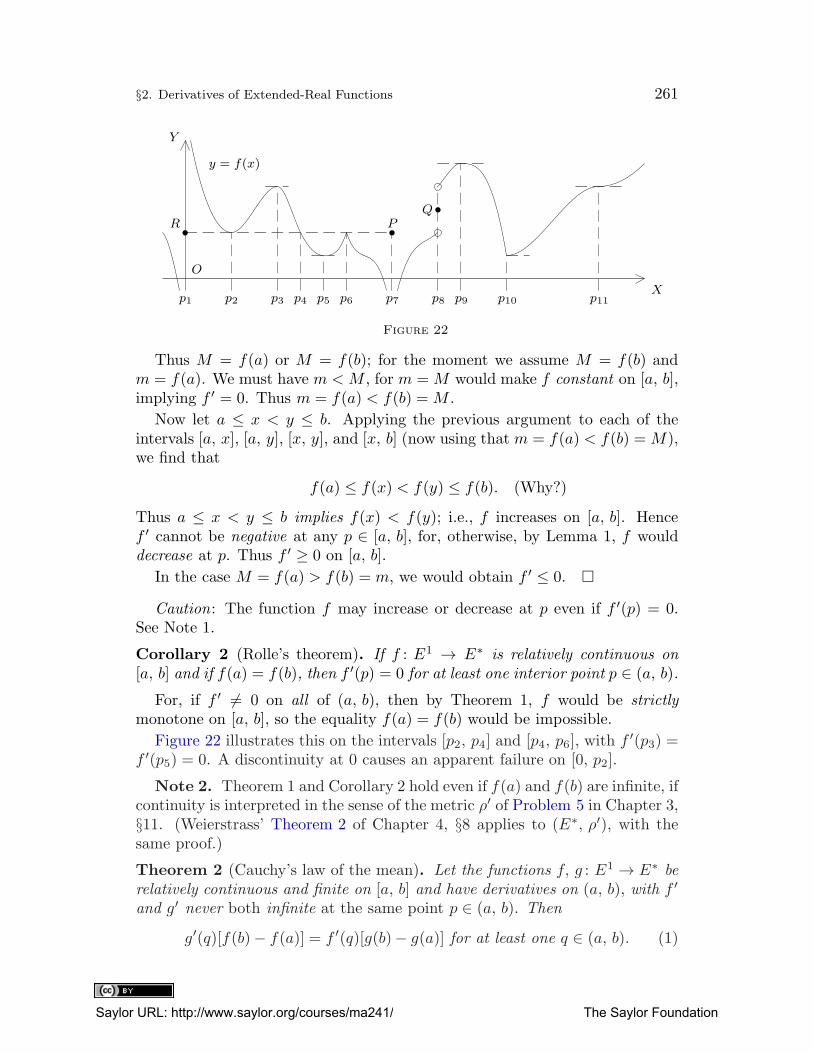
§2. Derivatives of Extended-Real Functions 261
O
Y
Xp1 p2 p3 p4 p5 p6 p7 p8 p9 p10 p11
Figure 22
R PQ
y = f(x)
Thus M = f(a) or M = f(b); for the moment we assume M = f(b) andm = f(a). We must have m < M , for m =M would make f constant on [a, b],implying f ′ = 0. Thus m = f(a) < f(b) =M .
Now let a ≤ x < y ≤ b. Applying the previous argument to each of theintervals [a, x], [a, y], [x, y], and [x, b] (now using that m = f(a) < f(b) =M),we find that
f(a) ≤ f(x) < f(y) ≤ f(b). (Why?)
Thus a ≤ x < y ≤ b implies f(x) < f(y); i.e., f increases on [a, b]. Hencef ′ cannot be negative at any p ∈ [a, b], for, otherwise, by Lemma 1, f woulddecrease at p. Thus f ′ ≥ 0 on [a, b].
In the case M = f(a) > f(b) = m, we would obtain f ′ ≤ 0. �
Caution: The function f may increase or decrease at p even if f ′(p) = 0.See Note 1.
Corollary 2 (Rolle’s theorem). If f : E1 → E∗ is relatively continuous on
[a, b] and if f(a) = f(b), then f ′(p) = 0 for at least one interior point p ∈ (a, b).
For, if f ′ 6= 0 on all of (a, b), then by Theorem 1, f would be strictly
monotone on [a, b], so the equality f(a) = f(b) would be impossible.
Figure 22 illustrates this on the intervals [p2, p4] and [p4, p6], with f′(p3) =
f ′(p5) = 0. A discontinuity at 0 causes an apparent failure on [0, p2].
Note 2. Theorem 1 and Corollary 2 hold even if f(a) and f(b) are infinite, ifcontinuity is interpreted in the sense of the metric ρ′ of Problem 5 in Chapter 3,§11. (Weierstrass’ Theorem 2 of Chapter 4, §8 applies to (E∗, ρ′), with thesame proof.)
Theorem 2 (Cauchy’s law of the mean). Let the functions f, g : E1 → E∗ be
relatively continuous and finite on [a, b] and have derivatives on (a, b), with f ′
and g′ never both infinite at the same point p ∈ (a, b). Then
g′(q)[f(b)− f(a)] = f ′(q)[g(b)− g(a)] for at least one q ∈ (a, b). (1)
Saylor URL: http://www.saylor.org/courses/ma241/ The Saylor Foundation
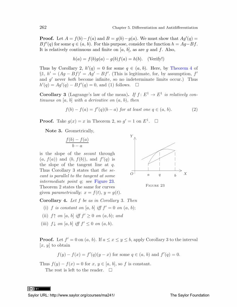
262 Chapter 5. Differentiation and Antidifferentiation
Proof. Let A = f(b)−f(a) and B = g(b)−g(a). We must show that Ag′(q) =Bf ′(q) for some q ∈ (a, b). For this purpose, consider the function h = Ag−Bf .It is relatively continuous and finite on [a, b], as are g and f . Also,
h(a) = f(b)g(a)− g(b)f(a) = h(b). (Verify!)
Thus by Corollary 2, h′(q) = 0 for some q ∈ (a, b). Here, by Theorem 4 of§1, h′ = (Ag − Bf)′ = Ag′ − Bf ′. (This is legitimate, for, by assumption, f ′
and g′ never both become infinite, so no indeterminate limits occur.) Thush′(q) = Ag′(q)−Bf ′(q) = 0, and (1) follows. �
Corollary 3 (Lagrange’s law of the mean). If f : E1 → E1 is relatively con-
tinuous on [a, b] with a derivative on (a, b), then
f(b)− f(a) = f ′(q)(b− a) for at least one q ∈ (a, b). (2)
Proof. Take g(x) = x in Theorem 2, so g′ = 1 on E1. �
O
Y
Xa bq
Figure 23
Note 3. Geometrically,
f(b)− f(a)b− a
is the slope of the secant through(a, f(a)) and (b, f(b)), and f ′(q) isthe slope of the tangent line at q.Thus Corollary 3 states that the se-
cant is parallel to the tangent at some
intermediate point q; see Figure 23.Theorem 2 states the same for curvesgiven parametrically : x = f(t), y = g(t).
Corollary 4. Let f be as in Corollary 3. Then
(i) f is constant on [a, b] iff f ′ = 0 on (a, b);
(ii) f↑ on [a, b] iff f ′ ≥ 0 on (a, b); and
(iii) f↓ on [a, b] iff f ′ ≤ 0 on (a, b).
Proof. Let f ′ = 0 on (a, b). If a ≤ x ≤ y ≤ b, apply Corollary 3 to the interval[x, y] to obtain
f(y)− f(x) = f ′(q)(y − x) for some q ∈ (a, b) and f ′(q) = 0.
Thus f(y)− f(x) = 0 for x, y ∈ [a, b], so f is constant.
The rest is left to the reader. �
Saylor URL: http://www.saylor.org/courses/ma241/ The Saylor Foundation
§2. Derivatives of Extended-Real Functions 263
Theorem 3 (inverse functions). Let f : E1 → E1 be relatively continuous and
strictly monotone on an interval I ⊆ E1. Let f ′(p) 6= 0 at some interiorpoint p ∈ I. Then the inverse function g = f−1 (with f restricted to I) has a
derivative at q = f(p), and
g′(q) =1
f ′(p).
(If f ′(p) = ±∞, then g′(q) = 0.)
Proof. By Theorem 3 of Chapter 4, §9, g = f−1 is strictly monotone andrelatively continuous on f [I], itself an interval. If p is interior to I, then q = f(p)is interior to f [I]. (Why?)
Now if y ∈ f [I], we set
∆g = g(y)− g(q), ∆y = y − q, x = f−1(y) = g(y), and f(x) = y
and obtain
∆g
∆y=g(y)− g(q)y − q =
x− pf(x)− f(p) =
∆x
∆ffor x 6= p.
Now if y → q, the continuity of g at q yields g(y) → g(q); i.e., x → p. Also,x 6= p iff y 6= q, for f and g are one-to-one functions. Thus we may substitutey = f(x) or x = g(y) to get
g′(q) = limy→q
∆g
∆y= lim
x→p
∆x
∆f=
1
limx→p
(∆f/∆x)=
1
f ′(p),2 (2′)
where we use the convention 1∞ = 0 if f ′(p) =∞. �
Examples.
(A) Let
f(x) = loga |x| with f(0) = 0.
Let p > 0. Then (∀x > 0)
∆f = f(x)− f(p) = loga x− loga p = loga(x/p)
= logap+ (x− p)
p= loga
(
1 +∆x
p
)
.
Thus∆f
∆x= loga
(
1 +∆x
p
)1/∆x
.
2 More precisely, we are replacing the x by g(y) in (x− p)/[f(x)− f(p)] by Corollary 2 of
Chapter 4, §2 to obtain g′(q). The steps in (2′) should be reversed .
Saylor URL: http://www.saylor.org/courses/ma241/ The Saylor Foundation
264 Chapter 5. Differentiation and Antidifferentiation
Now let z = ∆x/p. (Why is this substitution admissible?) Then usingthe formula
limz→0
(1 + z)1/z = e (see Chapter 4, §2, Example (C))
and the continuity of the log and power functions, we obtain
f ′(p) = limx→p
∆f
∆x= lim
z→0loga[(1 + z)1/z]1/p = loga e
1/p =1
ploga e.
The same formula results also if p < 0, i.e., |p| = −p. At p = 0, f hasone-sided derivatives (±∞) only (verify!), so f ′(0) = 0 by Definition 1in §1.
(B) The inverse of the loga function is the exponential g : E1 → E1, with
g(y) = ay (a > 0, a 6= 1).
By Theorem 3, we have
(∀ q ∈ E1) g′(q) =1
f ′(p), p = g(q) = aq.
Thus
g′(q) =1
1ploga e
=p
loga e=
aq
loga e.
Symbolically,
(loga |x|)′ =1
xloga e (x 6= 0); (ax)′ =
ax
loga e= ax ln a. (3)
In particular, if a = e, we have loge a = 1 and loga x = lnx; hence
(ln |x|)′ = 1
x(x 6= 0) and (ex)′ = ex (x ∈ E1). (4)
(C) The power function g : (0, +∞)→ E1 is given by
g(x) = xa = exp(a · lnx) for x > 0 and fixed a ∈ E1.
By the chain rule (§1, Theorem 3), we obtain
g′(x) = exp(a · lnx) · ax= xa · a
x= a · xa−1.
Thus we have the symbolic formula
(xa)′ = a · xa−1 for x > 0 and fixed a ∈ E1. (5)
Saylor URL: http://www.saylor.org/courses/ma241/ The Saylor Foundation
§2. Derivatives of Extended-Real Functions 265
Theorem 4 (Darboux). If f : E1 → E∗ is relatively continuous and has a
derivative on an interval I, then f ′ has the Darboux property (Chapter 4, §9)on I.
Proof. Let p, q ∈ I and f ′(p) < c < f ′(q). Put g(x) = f(x) − cx. Assumeg′ 6= 0 on (p, q) and find a contradiction to Theorem 1. Details are left to thereader. �
Problems on Derivatives of Extended-Real Functions
1. Complete the missing details in the proof of Theorems 1, 2, and 4,Corollary 4, and Lemma 1.[Hint for converse to Corollary 4(ii): Use Lemma 1 for an indirect proof.]
2. Do cases p ≤ 0 in Example (A).
3. Show that Theorems 1, 2, and 4 and Corollaries 2 to 4 hold also if fis discontinuous at a and b but f(a+) and f(b−) exist and are finite.(In Corollary 2, assume also f(a+) = f(b−); in Theorems 1 and 4 andCorollary 2, finiteness is unnecessary.)[Hint: Redefine f(a) and f(b).]
4. Under the assumptions of Corollary 3, show that f ′ cannot stay infiniteon any interval (p, q), a ≤ p < q ≤ b.[Hint: Apply Corollary 3 to the interval [p, q].]
5. Justify footnote 1.[Hint: Let
f(x) = x+ 2x2 sin1
x2with f(0) = 0.
At 0, find f ′ from Definition 1 in §1. Use also Problem 8 of §1. Show that f is notmonotone on any G0(δ).]
6. Show that f ′ need not be continuous or bounded on [a, b] (under thestandard metric), even if f is differentiable there.[Hint: Take f as in Problem 5.]
7. With f as in Corollaries 3 and 4, prove that if f ′ ≥ 0 (f ′ ≤ 0) on (a, b)and if f ′ is not constantly 0 on any subinterval (p, q) 6= ∅, then f isstrictly monotone on [a, b].
8. Let x = f(t), y = g(t), where t varies over an open interval I ⊆ E1, de-fine a curve in E2 parametrically. Prove that if f and g have derivativeson I and f ′ 6= 0, then the function h = f−1 has a derivative on f [I],and the slope of the tangent to the curve at t0 equals g′(t0)/f ′(t0).[Hint: The word “curve” implies that f and g are continuous on I (Chapter 4, §10),so Theorems 1 and 3 apply, and h = f−1 is a function . Also, y = g(h(x)). UseTheorem 3 of §1.]
9. Prove that if f is continuous and has a derivative on (a, b) and if f ′
has a finite or infinite (even one-sided) limit at some p ∈ (a, b), then
Saylor URL: http://www.saylor.org/courses/ma241/ The Saylor Foundation
266 Chapter 5. Differentiation and Antidifferentiation
this limit equals f ′(p). Deduce that f ′ is continuous at p if f ′(p−) andf ′(p+) exist.[Hint: By Corollary 3, for each x ∈ (a, b), there is some qx between p and x suchthat
f ′(qx) =∆f
∆x→ f ′(p) as x → p.
Set y = qx, so limy→p f ′(y) = f ′(p).]
10. From Theorem 3 and Problem 8 in §1, deduce the differentiation formu-las
(arcsinx)′ =1√
1− x2; (arccosx)′ =
−1√1− x2
; (arctanx)′ =1
1 + x2.
11. Prove that if f has a derivative at p, then f(p) is finite, provided f isnot constantly infinite on any interval (p, q) or (q, p), p 6= q.
[Hint: If f(p) = ±∞, each Gp has points at which ∆f∆x
= +∞, as well as those x
with ∆f∆x
= −∞.]
§3. L’Hopital’s Rule
We shall now prove a useful rule for resolving indeterminate limits. Below, G¬p
denotes a deleted globe G¬p(δ) in E1, or one about ±∞ of the form (a, +∞)
or (−∞, a). For one-sided limits, replace G¬p by its appropriate “half.”
Theorem 1 (L’Hopital’s rule). Let f, g : E1 → E∗ be differentiable on G¬p,with g′ 6= 0 there. If |f(x)| and |g(x)| tend both to +∞,1 or both to 0, as x→ pand if
limx→p
f ′(x)
g′(x)= r exists in E∗,
then also
limx→p
f(x)
g(x)= r;
similarly for x→ p+ or x→ p−.
Proof. It suffices to consider left and right limits. Both combined then yieldthe two-sided limit.
First, let −∞ ≤ p < +∞,
limx→p+
|f(x)| = limx→p+
|g(x)| = +∞ and limx→p+
f ′(x)
g′(x)= r (finite).
1 This includes the cases f(x) → ±∞ and g(x) → ±∞.
Saylor URL: http://www.saylor.org/courses/ma241/ The Saylor Foundation
§3. L’Hopital’s Rule 267
Then given ε > 0, we can fix a > p (a ∈ G¬p) such that
∣
∣
∣
f ′(x)
g′(x)− r
∣
∣
∣< ε, for all x in the interval (p, a). (1)
Now apply Cauchy’s law of the mean (§2, Theorem 2) to each interval [x, a],p < x < a. This yields, for each such x, some q ∈ (x, a) with
g′(q)[f(x)− f(a)] = f ′(q)[g(x)− g(a)].
As g′ 6= 0 (by assumption), g(x) 6= g(a) by Theorem 1, §2, so we may divideto obtain
f(x)− f(a)g(x)− g(a) =
f ′(q)
g′(q), where p < x < q < a.
This combined with (1) yields
∣
∣
∣
f(x)− f(a)g(x)− g(a) − r
∣
∣
∣< ε,
or, setting
F (x) =1− f(a)/f(x)1− g(a)/g(x) ,
we have∣
∣
∣
f(x)
g(x)· F (x)− r
∣
∣
∣< ε for all x inside (p, a). (2)
As |f(x)| and |g(x)| → +∞ (by assumption), we have F (x)→ 1 as x→ p+.Hence by rules for right limits, there is b ∈ (p, a) such that for all x ∈ (p, b),both |F (x) − 1| < ε and F (x) > 1
2 . (Why?) For such x, formula (2) holds aswell. Also,
1
|F (x)| < 2 and |r − rF (x)| = |r| |1− F (x)| < |r| ε.
Combining this with (2), we have for x ∈ (p, b)
∣
∣
∣
f(x)
g(x)− r
∣
∣
∣=
1
|F (x)|∣
∣
∣
f(x)
g(x)F (x)− rF (x)
∣
∣
∣
< 2∣
∣
∣
f(x)
g(x)· F (x)− r + r − rF (x)
∣
∣
∣
< 2ε(1 + |r|).
Thus, given ε > 0, we found b > p such that
∣
∣
∣
f(x)
g(x)− r
∣
∣
∣< 2ε(1 + |r|), x ∈ (p, b).
Saylor URL: http://www.saylor.org/courses/ma241/ The Saylor Foundation
268 Chapter 5. Differentiation and Antidifferentiation
As ε is arbitrary , we have limx→p+
f(x)
g(x)= r, as claimed.
The case limx→p+ f(x) = limx→p+ g(x) = 0 is simpler. As before, we obtain
∣
∣
∣
f(x)− f(a)g(x)− g(a) − r
∣
∣
∣< ε.
Here we may as well replace “a” by any y ∈ (p, a). Keeping y fixed, let x→ p+.Then f(x)→ 0 and g(x)→ 0, so we get
∣
∣
∣
f(y)
g(y)− r
∣
∣
∣≤ ε for any y ∈ (p, a).
As ε is arbitrary, this implies limy→p+
f(y)
g(y)= r. Thus the case x→ p+ is settled
for a finite r.
The cases r = ±∞ and x → p− are analogous, and we leave them to thereader. �
Note 1. limf(x)
g(x)may exist even if lim
f ′(x)
g′(x)does not. For example, take
f(x) = x+ sinx and g(x) = x.
Then
limx→+∞
f(x)
g(x)= lim
x→+∞
(
1 +sinx
x
)
= 1 (why?),
butf ′(x)
g′(x)= 1 + cosx
does not tend to any limit as x→ +∞.
Note 2. The rule fails if the required assumptions are not satisfied, e.g., ifg′ has zero values in each G¬p; see Problem 4 below.
Often it is useful to combine L’Hopital’s rule with some known limit formu-las, such as
limz→0
(1 + z)1/z = e or limx→0
x
sinx= 1 (see §1, Problem 8).
Examples.
(a) limx→+∞
lnx
x= lim
x→+∞(lnx)′
1= lim
x→+∞1
x= 0.
(b) limx→0
ln(1 + x)
x= lim
x→0
1/(1 + x)
1= 1.
(c) limx→0
x− sinx
x3= lim
x→0
1− cosx
3x2= lim
x→0
sinx
6x=
1
6limx→0
sinx
x=
1
6.
(Here we had to apply L’Hopital’s rule repeatedly .)
Saylor URL: http://www.saylor.org/courses/ma241/ The Saylor Foundation
§3. L’Hopital’s Rule 269
(d) Consider
limx→0+
e−1/x
x.
Taking derivatives (even n times), one gets
limx→0+
e−1/x
n! xn+1, n = 1, 2, 3, . . . (always indeterminate!).
Thus the rule gives no results. In this case, however, a simple device helps(see Problem 5 below).
(e) limn→∞ n1/n does not have the form 00 or ∞
∞ , so the rule does not applydirectly. Instead we compute
limn→∞
lnn1/n = limn→∞
lnn
n= 0 (Example (a)).
Hencen1/n = exp(lnn1/n)→ exp(0) = e0 = 1
by the continuity of exponential functions. The answer is then 1.
Problems on L’Hopital’s Rule
Elementary differentiation formulas are assumed known.
1. Complete the proof of L’Hopital’s rule. Verify that the differentiabilityassumption may be replaced by continuity plus existence of finite orinfinite (but not both together infinite) derivatives f ′ and g′ on G¬p
(same proof).
2. Show that the rule fails for complex functions. See, however, Problems 3,7, and 8.[Hint: Take p = 0 with
f(x) = x and g(x) = x+ x2ei/x2
= x+ x2
(
cos1
x2+ i · sin 1
x2
)
.
Then
limx→0
f(x)
g(x)= 1, though lim
x→0
f ′(x)
g′(x)= lim
x→0
1
g′(x)= 0.
Indeed, g′(x)− 1 = (2x− 2i/x)ei/x2
. (Verify!) Hence
|g′(x)|+ 1 ≥ |2x− 2i/x| (for |ei/x2 | = 1),
so
|g′(x)| ≥ −1 +2
x. (Why?)
Deduce that ∣∣∣
1
g′(x)
∣∣∣ ≤
∣∣∣
x
2− x
∣∣∣ → 0.]
Saylor URL: http://www.saylor.org/courses/ma241/ The Saylor Foundation
270 Chapter 5. Differentiation and Antidifferentiation
3. Prove the “simplified rule of L’Hopital” for real or complex functions(also for vector-valued f and scalar-valued g): If f and g are differen-tiable at p, with g′(p) 6= 0 and f(p) = g(p) = 0, then
limx→p
f(x)
g(x)=f ′(p)
g′(p).
[Hint:f(x)
g(x)=
f(x)− f(p)
g(x)− g(p)=
∆f
∆x
/∆g
∆x→ f ′(p)
g′(p).]
4. Why does limx→+∞
f(x)
g(x)not exist, though lim
x→+∞f ′(x)
g′(x)does , in the fol-
lowing example? Verify and explain.
f(x) = e−2x(cosx+ 2 sinx), g(x) = e−x(cosx+ sinx).
[Hint: g′ vanishes many times in each G+∞. Use the Darboux property for the
proof.]
5. Find limx→0+
e−1/x
x.
[Hint: Substitute z = 1x→ +∞. Then use the rule.]
6. Verify that the assumptions of L’Hopital’s rule hold, and find the fol-lowing limits.
(a) limx→0
ex − e−x
ln(e− x) + x− 1;
(b) limx→0
ex − e−x − 2x
x− sinx;
(c) limx→0
(1 + x)1/x − ex
;
(d) limx→0+
(xq lnx), q > 0;
(e) limx→+∞
(x−q lnx), q > 0;
(f) limx→0+
xx;
(g) limx→+∞
(xqa−x), a > 1, q > 0;
(h) limx→0
( 1
x2− cotan2 x
)
;
(i) limx→+∞
(π
2− arctanx
)1/ lnx
;
(j) limx→0
( sinx
x
)1/(1−cosx)
.
Saylor URL: http://www.saylor.org/courses/ma241/ The Saylor Foundation
§3. L’Hopital’s Rule 271
7. Prove L’Hopital’s rule for f : E1 → En (C) and g : E1 → E1, with
limk→p|f(x)| = 0 = lim
x→p|g(x)|, p ∈ E∗ and r ∈ En,
leaving the other assumptions unchanged.
[Hint: Apply the rule to the components of fg
(respectively, to(
fg
)
reand
(fg
)
im).]
8. Let f and g be complex and differentiable on G¬p, p ∈ E1. Let
limx→p
f(x) = limx→p
g(x) = 0, limx→p
f ′(x) = q, and limx→p
g′(x) = r 6= 0.
Prove that limx→p
f(x)
g(x)=q
r.
[Hint:f(x)
g(x)=
f(x)
x− p
/g(x)
x− p.
Apply Problem 7 to find
limx→p
f(x)
x− pand lim
x→p
g(x)
x− p.]
∗9. Do Problem 8 for f : E1 → Cn and g : E1 → C.
§4. Complex and Vector-Valued Functions on E1The theorems of §§2–3 fail for complex and vector-valued functions (see Prob-lem 3 below and Problem 2 in §3). However, some analogues hold. In a sense,they even are stronger, for, unlike the previous theorems, they do not requirethe existence of a derivative on an entire interval I ⊆ E1, but only on I −Q,where Q is a countable set , i.e., one contained in the range of a sequence,Q ⊆ {pm}. (We henceforth presuppose §9 of Chapter 1.)
In the following theorem, due to N. Bourbaki,1 g : E1 → E∗ is extended real
while f may also be complex or vector valued. We call it the finite increments
law since it deals with “finite increments” f(b)−f(a) and g(b)−g(a). Roughly,it states that |f ′| ≤ g′ implies a similar inequality for increments.
Theorem 1 (finite increments law). Let f : E1 → E and g : E1 → E∗ be
relatively continuous and finite on a closed interval I = [a, b] ⊆ E1, and have
derivatives2 with |f ′| ≤ g′, on I −Q where Q ⊆ {p1, p2, . . . , pm, . . . }. Then|f(b)− f(a)| ≤ g(b)− g(a). (1)
1 This is the pen name of a famous school of twentieth-century French mathematicians.2 Actually, right derivatives suffice, as will follow from the proof. (Left derivatives suffice
as well.)
Saylor URL: http://www.saylor.org/courses/ma241/ The Saylor Foundation
272 Chapter 5. Differentiation and Antidifferentiation
The proof is somewhat laborious, but worthwhile. (At a first reading, onemay omit it, however.) We outline some preliminary ideas.
Given any x ∈ I, suppose first that x > pm for at least one pm ∈ Q. In thiscase, we put
Q(x) =∑
pm<x
2−m;
here the summation is only over those m for which pm < x. If, however, thereare no pm ∈ Q with pm < x, we put Q(x) = 0. Thus Q(x) is defined forall x ∈ I. It gives an idea as to “how many” pm (at which f may have noderivative) precede x. Note that x < y implies Q(x) ≤ Q(y). (Why?) Also,
Q(x) ≤∞∑
m=1
2−m = 1.
Our plan is as follows. To prove (1), it suffices to show that for some fixed
K ∈ E1, we have
(∀ ε > 0) |f(b)− f(a)| ≤ g(b)− g(a) +Kε,
for then, letting ε→ 0, we obtain (1). We choose
K = b− a+Q(b), with Q(x) as above.
Temporarily fixing ε > 0, let us call a point r ∈ I “good” iff
|f(r)− f(a)| ≤ g(r)− g(a) + [r − a+Q(r)]ε (2)
and “bad” otherwise. We shall show that b is “good.” First, we prove a lemma.
Lemma 1. Every “good” point r ∈ I (r < b) is followed by a whole interval
(r, s), r < s ≤ b, consisting of “good” points only .
Proof. First let r /∈ Q, so by assumption, f and g have derivatives at r, with
|f ′(r)| ≤ g′(r).
Suppose g′(r) < +∞. Then (treating g′ as a right derivative) we can find s > r(s ≤ b) such that, for all x in the interval (r, s),
∣
∣
∣
g(x)− g(r)x− r − g′(r)
∣
∣
∣<ε
2(why?);
similarly for f . Multiplying by x− r, we get
|f(x)− f(r)− f ′(r)(x− r)| < (x− r) ε2and
|g(x)− g(r)− g′(r)(x− r)| < (x− r) ε2,
Saylor URL: http://www.saylor.org/courses/ma241/ The Saylor Foundation
§4. Complex and Vector-Valued Functions on E1 273
and hence by the triangle inequality (explain!),
|f(x)− f(r)| ≤ |f ′(r)|(x− r) + (x− r) ε2
and
g′(r)(x− r) + (x− r) ε2< g(x)− g(r) + (x− r)ε.
Combining this with |f ′(r)| ≤ g′(r), we obtain
|f(x)− f(r)| ≤ g(x)− g(r) + (x− r)ε whenever r < x < s. (3)
Now as r is “good,” it satisfies (2); hence, certainly, as Q(r) ≤ Q(x),
|f(r)− f(a)| ≤ g(r)− g(a) + (r − a)ε+Q(x)ε whenever r < x < s.
Adding this to (3) and using the triangle inequality again, we have
|f(x)− f(a)| ≤ g(x)− g(a) + [x− a+Q(x)]ε for all x ∈ (r, s).
By definition, this shows that each x ∈ (r, s) is “good,” as claimed. Thusthe lemma is proved for the case r ∈ I −Q, with g′(r) < +∞.
The cases g′(r) = +∞ and r ∈ Q are left as Problems 1 and 2. �
We now return to Theorem 1.
Proof of Theorem 1. Seeking a contradiction, suppose b is “bad,” and letB 6= ∅ be the set of all “bad” points in [a, b]. Let
r = inf B, r ∈ [a, b].
Then the interval [a, r) can contain only “good” points, i.e., points x such that
|f(x)− f(a)| ≤ g(x)− g(a) + [x− a+Q(x)]ε.
As x < r implies Q(x) ≤ Q(r), we have
|f(x)− f(a)| ≤ g(x)− g(a) + [x− a+Q(r)]ε for all x ∈ [a, r). (4)
Note that [a, r) 6= ∅, for by (2), a is certainly “good” (why?), and soLemma 1 yields a whole interval [a, s) of “good” points contained in [a, r).
Letting x→ r in (4) and using the continuity of f at r, we obtain (2). Thusr is “good” itself. Then, however, Lemma 1 yields a new interval (r, q) of“good” points. Hence [a, q) has no “bad” points, and so q is a lower bound of
the set B of “bad” points in I, contrary to q > r = glbB. This contradictionshows that b must be “good,” i.e.,
|f(b)− f(a)| ≤ g(b)− g(a) + [b− a+Q(b)]ε.
Now, letting ε→ 0, we obtain formula (1), and all is proved. �
Saylor URL: http://www.saylor.org/courses/ma241/ The Saylor Foundation
274 Chapter 5. Differentiation and Antidifferentiation
Corollary 1. If f : E1 → E is relatively continuous and finite on I = [a, b] ⊆E1, and has a derivative on I −Q, then there is a real M such that
|f(b)− f(a)| ≤M(b− a) and M ≤ supt∈I−Q
|f ′(t)|. (5)
Proof. LetM0 = sup
t∈I−Q|f ′(t)|.
IfM0 < +∞, put M =M0 ≥ |f ′| on I−Q, and take g(x) =Mx in Theorem 1.Then g′ =M ≥ |f ′| on I −Q, so formula (1) yields (5) since
g(b)− g(a) =Mb−Ma =M(b− a).If, however, M0 = +∞, let
M =∣
∣
∣
f(b)− f(a)b− a
∣
∣
∣< M0.
Then (5) clearly is true. Thus the required M exists always.3 �
Corollary 2. Let f be as in Corollary 1. Then f is constant on I iff f ′ = 0on I −Q.
Proof. If f ′ = 0 on I −Q, then M = 0 in Corollary 1, so Corollary 1 yields,for any subinterval [a, x] (x ∈ I), |f(x) − f(a)| ≤ 0; i.e., f(x) = f(a) for allx ∈ I. Thus f is constant on I.
Conversely, if so, then f ′ = 0, even on all of I. �
Corollary 3. Let f, g : E1 → E be relatively continuous and finite on I =[a, b], and differentiable on I −Q. Then f − g is constant on I iff f ′ = g′ onI −Q.
Proof. Apply Corollary 2 to the function f − g. �
We can now also strengthen parts (ii) and (iii) of Corollary 4 in §2.Theorem 2. Let f be real and have the properties stated in Corollary 1. Then
(i) f↑ on I = [a, b] iff f ′ ≥ 0 on I −Q; and
(ii) f↓ on I iff f ′ ≤ 0 on I −Q.
Proof. Let f ′ ≥ 0 on I −Q. Fix any x, y ∈ I (x < y) and define g(t) = 0 onE1. Then |g′| = 0 ≤ f ′ on I −Q. Thus g and f satisfy Theorem 1 (with theirroles reversed) on I, and certainly on the subinterval [x, y]. Thus we have
f(y)− f(x) ≥ |g(y)− g(x)| = 0, i.e., f(y) ≥ f(x) whenever y > x in I,
so f↑ on I.3 Note that M as defined here depends on a and b. So does M0.
Saylor URL: http://www.saylor.org/courses/ma241/ The Saylor Foundation
§4. Complex and Vector-Valued Functions on E1 275
Conversely, if f↑ on I, then for every p ∈ I, we must have f ′(p) ≥ 0, forotherwise, by Lemma 1 of §2, f would decrease at p. Thus f ′ ≥ 0, even on all
of I, and (i) is proved. Assertion (ii) is proved similarly. �
Problems on Complex and Vector-Valued Functions on E11. Do the case g′(r) = +∞ in Lemma 1.
[Hint: Show that there is s > r with
g(x)− g(r) ≥ (|f ′(r)|+ 1)(x− r) ≥ |f(x)− f(r)| for x ∈ (r, s).
Such x are “good.”]
2. Do the case r = pn ∈ Q in Lemma 1.[Hint: Show by continuity that there is s > r such that (∀x ∈ (r, s))
|f(x)− f(r)| < ε
2n+1and |g(x)− g(r)| < ε
2n+1.
Show that all such x are “good” since x > r = pn implies
2−n +Q(r) ≤ Q(x). (Why?)]
3. Show that Corollary 3 in §2 (hence also Theorem 2 in §2) fails for com-plex functions.[Hint: Let f(x) = exi = cos x+ i · sinx. Verify that |f ′| = 1 yet f(2π)− f(0) = 0.]
4. (i) Verify that all propositions of §4 hold also if f ′ and g′ are onlyright derivatives on I −Q.
(ii) Do the same for left derivatives. (See footnote 2.)
5. (i) Prove that if f : E1 → E is continuous and finite on I = (a, b) anddifferentiable on I −Q, and if
supt∈I−Q
|f ′(t)| < +∞,
then f is uniformly continuous on I.
(ii) Moreover, if E is complete (e.g., E = En), then f(a+) and f(b−)exist and are finite.
[Hints: (i) Use Corollary 1. (ii) See the “hint” to Problem 11(iii) of Chapter 4, §8.]
6. Prove that if f is as in Theorem 2, with f ′ ≥ 0 on I − Q and f ′ > 0at some p ∈ I, then f(a) < f(b). Do it also with f ′ treated as a right
derivative (see Problem 4).
7. Let f, g : E1 → E1 be relatively continuous on I = [a, b] and have rightderivatives f ′
+ and g′+ (finite or infinite, but not both infinite) on I−Q.
(i) Prove that if
mg′+ ≤ f ′+ ≤Mg′+ on I −Q
Saylor URL: http://www.saylor.org/courses/ma241/ The Saylor Foundation
276 Chapter 5. Differentiation and Antidifferentiation
for some fixed m, M ∈ E1, then
m[g(b)− g(a)] ≤ f(b)− f(a) ≤M [g(b)− g(a)].[Hint: Apply Theorem 2 and Problem 4 to each of Mg − f and f −mg.]
(ii) Hence prove that
m0(b− a) ≤ f(b)− f(a) ≤M0(b− a),where
m0 = inf f ′+[I −Q] and M0 = sup f ′
+[I −Q] in E∗.
[Hint: Take g(x) = x if m0 ∈ E1 or M0 ∈ E1. The infinite case is simple.]
8. (i) Let f : (a, b)→ E be finite, continuous, with a right derivative on(a, b). Prove that q = lim
x→a+f ′+(x) exists (finite) iff
q = limx, y→a+
f(x)− f(y)x− y ,
i.e., iff
(∀ ε > 0) (∃ c > a) (∀x, y ∈ (a, c) | x 6= y)∣
∣
∣
f(x)− f(y)x− y −q
∣
∣
∣< ε.
[Hints: If so, let y → x+ (keeping x fixed) to obtain
(∀ x ∈ (a, c)) |f ′+(x)− q| ≤ ε. (Why?)
Conversely, if limx→a+
f ′+(x) = q, then
(∀ ε > 0) (∃ c > a) (∀ t ∈ (a, c)) |f ′+(t)− q| < ε.
Put
M = supa<t<c
|f ′+(t)− q| ≤ ε (why ≤ ε?)
and
h(t) = f(t)− tq, t ∈ (a, b).
Apply Corollary 1 and Problem 4 to h on the interval [x, y] ⊆ (a, c), to get
|f(y)− f(x)− (y − x)q| ≤ M(y − x) ≤ ε(y − x).
Proceed.]
(ii) Prove similar statements for the cases q = ±∞ and x→ b−.[Hint: In case q = ±∞, use Problem 7(ii) instead of Corollary 1.]
9. From Problem 8 deduce that if f is as indicated and if f ′+ is left contin-
uous at some p ∈ (a, b), then f also has a left derivative at p.
If f ′+ is also right continuous at p, then f ′
+(p) = f ′−(p) = f ′(p).
[Hint: Apply Problem 8 to (a, p) and (p, b).]
Saylor URL: http://www.saylor.org/courses/ma241/ The Saylor Foundation
§4. Complex and Vector-Valued Functions on E1 277
10. In Problem 8, prove that if, in addition, E is complete and if
q = limx→a+
f ′+(x) 6= ±∞ (finite),
then f(a+) 6= ±∞ exists, and
limx→a+
f(x)− f(a+)x− a = q;
similarly in case limx→b− f′+(x) = r.
If both exist, set f(a) = f(a+) and f(b) = f(b−). Show that then fbecomes relatively continuous on [a, b], with f ′
+(a) = q and f ′−(b) = r.
[Hint: Iflim
x→a+f ′+(x) = q 6= ±∞,
then f ′+ is bounded on some subinterval (a, c), a < c ≤ b (why?), so f is uniformly
continuous on (a, c), by Problem 5, and f(a+) exists. Let y → a+, as in the hint to
Problem 8.]
11. Do Problem 9 in §2 for complex and vector-valued functions.[Hint: Use Corollary 1 of §4.]
12. Continuing Problem 7, show that the equalities
m =f(b)− f(a)
b− a =M
hold iff f is linear , i.e., f(x) = cx + d for some c, d ∈ E1, and thenc = m =M .
13. Let f : E1 → C be as in Corollary 1, with f 6= 0 on I. Let g be the realpart of f ′/f .
(i) Prove that |f |↑ on I iff g ≥ 0 on I −Q.
(ii) Extend Problem 4 to this result.
14. Define f : E1 → C by
f(x) =
{
x2ei/x = x2(
cos1
x+ i · sin 1
x
)
if x > 0, and
0 if x ≤ 0.
Show that f is differentiable on I = (−1, 1), yet f ′[I] is not a convexset in E2 = C (thus there is no analogue to Theorem 4 of §2).
Saylor URL: http://www.saylor.org/courses/ma241/ The Saylor Foundation
278 Chapter 5. Differentiation and Antidifferentiation
§5. Antiderivatives (Primitives, Integrals)
Given f : E1 → E, we often have to find a function F such that F ′ = f on I,or at least on I −Q.1 We also require F to be relatively continuous and finiteon I. This process is called antidifferentiation or integration.
Definition 1.
We call F : E1 → E a primitive, or antiderivative, or an indefinite inte-
gral , of f on I iff
(i) F is relatively continuous and finite on I, and
(ii) F is differentiable, with F ′ = f , on I −Q at least.
We then write
F =
∫
f, or F (x) =
∫
f(x) dx, on I.
(The latter is classical notation.)
If such an F exists (which is not always the case), we shall say that∫
f exists on I, or that f has a primitive (or antiderivative) on I, or thatf is primitively integrable (briefly integrable) on I.
If F ′ = f on a set B ⊆ I, we say that∫
f is exact on B and call F anexact primitive on B. Thus if Q = ∅,
∫
f is exact on all of I.
Note 1. Clearly, if F ′ = f , then also (F + c)′ = f for a finite constantc. Thus the notation F =
∫
f is rather incomplete; it means that F is one
of many primitives. We now show that all of them have the form F + c (or∫
f + c).
Theorem 1. If F and G are primitive to f on I, then G−F is constant on I.
Proof. By assumption, F and G are relatively continuous and finite on I;hence so is G− F . Also, F ′ = f on I −Q and G′ = f on I − P . (Q and P arecountable, but possibly Q 6= P .)
Hence both F ′ and G′ equal f on I−S, where S = P ∪Q, and S is countableitself by Theorem 2 of Chapter 1, §9.
Thus by Corollary 3 in §4, F ′ = G′ on I − S implies G − F = c (constant)on each [x, y] ⊆ I; hence G− F = c (or G = F + c) on I. �
Definition 2.
If F =∫
f on I and if a, b ∈ I (where a ≤ b or b ≤ a), we define∫ b
a
f =
∫ b
a
f(x) dx = F (b)− F (a), also written F (x)∣
∣
∣
b
a. (1)
1 In this section, Q, P , and S shall denote countable sets, F ′, G′, and H′ are finite
derivatives, and I is a finite or infinite nondegenerate interval in E1.
Saylor URL: http://www.saylor.org/courses/ma241/ The Saylor Foundation
§5. Antiderivatives (Primitives, Integrals) 279
This expression is called the definite integral of f from a to b.2
The definite integral of f from a to b is independent of the particular choiceof the primitive F for f , and thus unambiguous , for if G is another primitive,Theorem 1 yields G = F + c, so
G(b)−G(a) = F (b) + c− [F (a) + c] = F (b)− F (a),
and it does not matter whether we take F or G.
Note that∫ b
af(x) dx, or
∫ b
af , is a constant in the range space E (a vector
if f is vector valued). The “x” in∫ b
af(x) dx is a “dummy variable” only, and
it may be replaced by any other letter. Thus
∫ b
a
f(x) dx =
∫ b
a
f(y) dy = F (b)− F (a).
On the other hand, the indefinite integral is a function: F : E1 → E.
Note 2. We may, however, vary a or b (or both) in (1). Thus, keeping afixed and varying b, we can define a function
G(t) =
∫ t
a
f = F (t)− F (a), t ∈ I.
Then G′ = F ′ = f on I, and G(a) = F (a) − F (a) = 0. Thus if∫
f existson I, f has a (unique) primitive G on I such that G(a) = 0. (It is unique byTheorem 1. Why?)
Examples.
(a) Let
f(x) =1
xand F (x) = ln |x|, with F (0) = f(0) = 0.
Then F ′ = f and F =∫
f on (−∞, 0) and on (0, +∞) but not on E1,since F is discontinuous at 0, contrary to Definition 1. We compute
∫ 2
1
f = ln 2− ln 1 = ln 2.
(b) On E1, let
f(x) =|x|x
and F (x) = |x|, with f(0) = 1.
Here F is continuous and F ′ = f on E1 − {0}. Thus F =∫
f on E1,exact on E1 − {0}. Here I = E1, Q = {0}.
2 The numbers a and b are called the bounds of the integral.
Saylor URL: http://www.saylor.org/courses/ma241/ The Saylor Foundation
280 Chapter 5. Differentiation and Antidifferentiation
We compute
∫ 2
−2
f = F (2)− F (−2) = 2− 2 = 0
(even though f never vanishes on E1).
Basic properties of integrals follow from those of derivatives. Thus we havethe following.
Corollary 1 (linearity). If∫
f and∫
g exist on I, so does∫
(pf + qg) for any
scalars p, q (in the scalar field of E).3 Moreover , for any a, b ∈ I, we obtain
(i)
∫ b
a
(pf + qg) = p
∫ b
a
f + q
∫ b
a
g;
(ii)
∫ b
a
(f ± g) =∫ b
a
f ±∫ b
a
g; and
(iii)
∫ b
a
pf = p
∫ b
a
f .
Proof. By assumption, there are F and G such that
F ′ = f on I −Q and G′ = g on I − P .
Thus, setting S = P ∪Q and H = pF + qG, we have
H ′ = pF ′ + qG′ = pf + qg on I − S,
with P , Q, and S countable. Also, H = pF + qG is relatively continuous andfinite on I, as are F and G.
Thus by definition, H =∫
(pf + qg) exists on I, and by (1),
∫ b
a
(pf+qg) = H(b)−H(a) = pF (b)+qG(b)−pF (a)−qG(a) = p
∫ b
a
f+q
∫ b
a
g,
proving (i∗).
With p = 1 and q = ±1, we obtain (ii∗).
Taking q = 0, we get (iii∗). �
Corollary 2. If both∫
f and∫
|f | exist on I = [a, b], then
∣
∣
∣
∫ b
a
f∣
∣
∣≤
∫ b
a
|f |.
3 In the case f, g : E1 → E∗ (C), we assume p, q ∈ E1 (C). If f and g are scalar valued,
we also allow p and q to be vectors in E.
Saylor URL: http://www.saylor.org/courses/ma241/ The Saylor Foundation
§5. Antiderivatives (Primitives, Integrals) 281
Proof. As before, let
F ′ = f and G′ = |f | on I − S (S = Q ∪ P , all countable),where F and G are relatively continuous and finite on I and G =
∫
|f | is real .Also, |F ′| = |f | = G′ on I − S. Thus by Theorem 1 of §4,
|F (b)− F (a)| ≤ G(b)−G(a) =∫ b
a
|f |. �
Corollary 3. If∫
f exists on I = [a, b], exact on I −Q, then
∣
∣
∣
∫ b
a
f∣
∣
∣≤M(b− a)
for some real
M ≤ supt∈I−Q
|f(t)|.
This is simply Corollary 1 of §4, when applied to a primitive, F =∫
f .
Corollary 4. If F =∫
f on I and f = g on I −Q, then F is also a primitive
of g, and∫ b
a
f =
∫ b
a
g for a, b ∈ I.
(Thus we may arbitrarily redefine f on a countable Q.)
Proof. Let F ′ = f on I−P . Then F ′ = g on I−(P ∪Q). The rest is clear. �
Corollary 5 (integration by parts). Let f and g be real or complex (or let
f be scalar valued and g vector valued), both relatively continuous on I and
differentiable on I −Q. Then if∫
f ′g exists on I, so does∫
fg′, and we have
∫ b
a
fg′ = f(b)g(b)− f(a)g(a)−∫ b
a
f ′g for any a, b ∈ I. (2)
Proof. By assumption, fg is relatively continuous and finite on I, and
(fg)′ = fg′ + f ′g on I −Q.
Thus, setting H = fg, we have H =∫
(fg′ + f ′g) on I. Hence by Corollary 1,if∫
f ′g exists on I, so does∫
((fg′ + f ′g)− f ′g) =∫
fg′, and∫ b
a
fg′ +
∫ b
a
f ′g =
∫ b
a
(fg′ + f ′g) = H(b)−H(a) = f(b)g(b)− f(a)g(a).
Thus (2) follows. �
The proof of the next three corollaries is left to the reader.
Saylor URL: http://www.saylor.org/courses/ma241/ The Saylor Foundation
282 Chapter 5. Differentiation and Antidifferentiation
Corollary 6 (additivity of the integral). If∫
f exists on I then, for a, b, c ∈ I,we have
(i)
∫ b
a
f =
∫ c
a
f +
∫ b
c
f ;
(ii)
∫ a
a
f = 0; and
(iii)
∫ a
b
f = −∫ b
a
f .
Corollary 7 (componentwise integration). A function f : E1 → En (Cn)is integrable on I iff all its components (f1, f2, . . . , fn) are, and then (byTheorem 5 in §1)
∫ b
a
f =(
∫ b
a
f1, . . . ,
∫ b
a
fn
)
=
n∑
k=1
~ek
∫ b
a
fk for any a, b ∈ I.
Hence if f is complex ,
∫ b
a
f =
∫ b
a
fre + i ·∫ b
a
fim
(see Chapter 4, §3, Note 5).
Examples (continued).
(c) Define f : E1 → E3 by
f(x) = (a · cosx, a · sinx, 2cx), a, c ∈ E1.
Verify that∫ π
0
f(x) dx = (a · sinx, −a · cosx, cx2)∣
∣
∣
π
0= (0, 2a, cπ2) = 2a~j + cπ2~k.
(d)
∫ π
0
eix dx =
∫ π
0
(cosx+ i · sinx) dx = (sinx− i · cosx)∣
∣
∣
π
0= 2i.
Corollary 8. If f = 0 on I −Q, then∫
f exists on I, and
∣
∣
∣
∫ b
a
f∣
∣
∣=
∫ b
a
|f | = 0 for a, b ∈ I.
Theorem 2 (change of variables). Suppose g : E1 → E1 (real) is differentiableon I, while f : E1 → E has a primitive on g[I],4 exact on g[I −Q].
4 Note that g[I] is an interval , for g has the Darboux property (Chapter 4, §9, Note 1).
Saylor URL: http://www.saylor.org/courses/ma241/ The Saylor Foundation
§5. Antiderivatives (Primitives, Integrals) 283
Then∫
f(
g(x))
g′(x) dx (i .e.,
∫
(f ◦ g)g′)
exists on I, and for any a, b ∈ I, we have∫ b
a
f(
g(x))
g′(x) dx =
∫ q
p
f(y) dy, where p = g(a) and q = g(b). (3)
Thus, using classical notation, we may substitute y = g(x), provided that we
also substitute dy = g′(x) dx and change the bounds of integrals (3). Here wetreat the expressions dy and g′(x) dx purely formally, without assigning themany separate meaning outside the context of the integrals.
Proof. Let F =∫
f on g[I], and F ′ = f on g[I − Q]. Then the compositefunction H = F ◦ g is relatively continuous and finite on I. (Why?) ByTheorem 3 of §1,
H ′(x) = F ′(g(x))
g′(x) for x ∈ I −Q;
i.e.,H ′ = (F ′ ◦ g)g′ on I −Q.
Thus H =∫
(f ◦ g)g′ exists on I, and∫ b
a
(f ◦ g)g′ = H(b)−H(a) = F(
g(b))
− F(
g(a))
= F (q)− F (p) =∫ q
p
f. �
Note 3. The theorem does not require that g be one to one on I, but ifit is, then one can drop the assumption that
∫
f is exact on g[I − Q]. (SeeProblem 4.)
Examples (continued).
(e) Find
∫ π/2
0
sin2 x · cosx dx.
Here f(y) = y2, y = g(x) = sinx, dy = cosx dx, F (y) = y3/3, a = 0,b = π/2, p = sin 0 = 0, and q = sin(π/2) = 1, so (3) yields
∫ π/2
0
sin2 x · cosx dx =
∫ 1
0
y2 dy =y3
3
∣
∣
∣
1
0=
1
3− 0 =
1
3.
For real functions, we obtain some inferences dealing with inequalities .
Theorem 3. If f, g : E1 → E1 are integrable on I = [a, b], then we have the
following :
(i) f ≥ 0 on I −Q implies∫ b
af ≥ 0.
(i′) f ≤ 0 on I −Q implies∫ b
af ≤ 0.
Saylor URL: http://www.saylor.org/courses/ma241/ The Saylor Foundation
284 Chapter 5. Differentiation and Antidifferentiation
(ii) f ≥ g on I −Q implies
∫ b
a
f ≥∫ b
a
g (dominance law).
(iii) If f ≥ 0 on I −Q and a ≤ c ≤ d ≤ b, then∫ b
a
f ≥∫ d
c
f (monotonicity law).
(iv) If∫ b
af = 0, and f ≥ 0 on I −Q, then f = 0 on some I −P , P countable.
Proof. By Corollary 4, we may redefine f on Q so that our assumptions in(i)–(iv) hold on all of I. Thus we write “I” for “I −Q.”
By assumption, F =∫
f and G =∫
g exist on I. Here F and G are relativelycontinuous and finite on I = [a, b], with F ′ = f and G′ = g on I−P , for anothercountable set P (this P cannot be omitted). Now consider the cases (i)–(iv).(P is fixed henceforth.)
(i) Let f ≥ 0 on I; i.e., F ′ = f ≥ 0 on I −P . Then by Theorem 2 in §4, F↑on I = [a, b]. Hence F (a) ≤ F (b), and so
∫ b
a
f = F (b)− F (a) ≥ 0.
One proves (i′) similarly.
(ii) If f − g ≥ 0, then by (i),
∫ b
a
(f − g) =∫ b
a
f −∫ b
a
g ≥ 0,
so∫ b
af ≥
∫ b
ag, as claimed.
(iii) Let f ≥ 0 on I and a ≤ c ≤ d ≤ b. Then by (i),
∫ c
a
f ≥ 0 and
∫ b
d
f ≥ 0.
Thus by Corollary 6,
∫ b
a
f =
∫ c
a
f +
∫ d
c
f +
∫ b
d
f ≥∫ d
c
f,
as asserted.
(iv) Seeking a contradiction, suppose∫ b
af = 0, f ≥ 0 on I, yet f(p) > 0 for
some p ∈ I − P (P as above), so F ′(p) = f(p) > 0.
Saylor URL: http://www.saylor.org/courses/ma241/ The Saylor Foundation
§5. Antiderivatives (Primitives, Integrals) 285
Now if a ≤ p < b, Lemma 1 of §2 yields F (c) > F (p) for some c ∈ (p, b].Then by (iii),
∫ b
a
f ≥∫ c
p
f = F (c)− F (p) > 0,
contrary to∫ b
af = 0; similarly in case a < p ≤ b. �
Note 4. Hence∫ b
a
|f | = 0 implies f = 0 on [a, b]− P
(P countable), even for vector-valued functions (for |f | is always real , and soTheorem 3 applies).
However,∫ b
af = 0 does not suffice, even for real functions (unless f is sign-
constant). For example,
∫ 2π
0
sinx dx = 0, yet sinx 6≡ 0 on any I − P .
See also Example (b).
Corollary 9 (first law of the mean). If f is real and∫
f exists on [a, b], exacton (a, b), then
∫ b
a
f = f(q)(b− a) for some q ∈ (a, b).
Proof. Apply Corollary 3 in §2 to the function F =∫
f . �
Caution: Corollary 9 may fail if∫
f is inexact at some p ∈ (a, b). (Exactnesson [a, b] − Q does not suffice, as it does not in Corollary 3 of §2, used here.)
Thus in Example (b) above,∫ 2
−2f = 0. Yet for no q is f(q)(2 + 2) = 0, since
f(q) = ±1. The reason is that∫
f is inexact just at 0, an interior point of[−2, 2].
Problems on Antiderivatives
1. Prove in detail Corollaries 3, 4, 6, 7, 8, and 9 and Theorem 3(i′) and(iv).
2. In Examples (a) and (b) discuss continuity and differentiability of f andF at 0. In (a) show that
∫
f does not exist on any interval (−a, a).[Hint: Use Theorem 1.]
3. Show that Theorem 2 holds also if g is relatively continuous on I anddifferentiable on I −Q.
Saylor URL: http://www.saylor.org/courses/ma241/ The Saylor Foundation
286 Chapter 5. Differentiation and Antidifferentiation
4. Under the assumptions of Theorem 2, show that if g is one to one on I,then automatically
∫
f is exact on g[I −Q] (Q countable).[Hint: If F =
∫f on g[I], then
F ′ = f on g[I]− P , P countable.
Let Q = g−1[P ]. Use Problem 6 of Chapter 1, §§4–7 and Problem 2 of Chapter 1,§9 to show that Q is countable and g[I]− P = g[I −Q].]
5. Prove Corollary 5 for dot products f · g of vector-valued functions.
6. Prove that if∫
f exists on [a, p] and [p, b], then it exists on [a, b]. Byinduction, extend this to unions of n adjacent intervals.[Hint: Choose F =
∫f on [a, p] and G =
∫f on [p, b] such that F (p) = G(p).
(Why do such F, G exist?) Then construct a primitive H =∫f that is relatively
continuous on all of [a, b].]
7. Prove the weighted law of the mean: If g is real and nonnegative onI = [a, b], and if
∫
g and∫
gf exist on I for some f : E1 → E, thenthere is a finite c ∈ E with
∫ b
a
gf = c
∫ b
a
g.
(The value c is called a g-weighted mean of f .)
[Hint: If∫ ba g > 0, put
c =
∫ b
agf
/∫ b
ag.
If∫ bag = 0, use Theorem 3(i) and (iv) to show that also
∫ bagf = 0, so any c will do.]
8. In Problem 7, prove that if, in addition, f is real and has the Darbouxproperty on I, then c = f(q) for some q ∈ I (the second law of the
mean).
[Hint: Choose c as in Problem 7. If∫ ba g > 0, put
m = inf f [I] and M = sup f [I], in E∗,
so m ≤ f ≤ M on I. Deduce that
m
∫ b
ag ≤
∫ b
agf ≤ M
∫ b
ag,
whence m ≤ c ≤ M .
If m < c < M , then f(x) < c < f(y) for some x, y ∈ I (why?), so the Darboux
property applies.
If c = m, then g · (f − c) ≥ 0 and Theorem 3(iv) yields gf = gc on I−P . (Why?)
Deduce that f(q) = c if g(q) 6= 0 and q ∈ I − P . (Why does such a q exist?)
What if c = M?]
9. Taking g(x) ≡ 1 in Problem 8, obtain a new version of Corollary 9.State it precisely!
Saylor URL: http://www.saylor.org/courses/ma241/ The Saylor Foundation
§5. Antiderivatives (Primitives, Integrals) 287
⇒10. Prove that if F =∫
f on I = (a, b) and f is right (left) continuous andfinite at p ∈ I, then
f(p) = F ′+(p) (respectively, F
′−(p)).
Deduce that if f is continuous and finite on I, all its primitives on Iare exact on I.[Hint: Fix ε > 0. If f is right continuous at p, there is c ∈ I (c > p), with
|f(x)− f(p)| < ε for x ∈ [p, c).
Fix such an x. Let
G(t) = F (t)− tf(p), t ∈ E1.
Deduce that G′(t) = f(t)− f(p) for t ∈ I −Q.
By Corollary 1 of §4,
|G(x)−G(p)| = |F (x)− F (p)− (x− p)f(p)| ≤ M(x − p),
with M ≤ ε. (Why?) Hence
∣∣∣∆F
∆x− f(p)
∣∣∣ ≤ ε for x ∈ [p, c),
and so
limx→p+
∆F
∆x= f(p) (why?);
similarly for a left-continuous f .]
11. State and solve Problem 10 for the case I = [a, b].
12. (i) Prove that if f is constant (f = c 6= ±∞) on I −Q, then
∫ b
a
f = (b− a)c for a, b ∈ I.
(ii) Hence prove that if f = ck 6= ±∞ on
Ik = [ak, ak+1), a = a0 < a1 < · · · < an = b,
then∫
f exists on [a, b], and
∫ b
a
f =
n−1∑
k=0
(ak+1 − ak)ck.
Show that this is true also if f = ck 6= ±∞ on Ik −Qk.
[Hint: Use Problem 6.]
13. Prove that if∫
f exists on each In = [an, bn], where
an+1 ≤ an ≤ bn ≤ bn+1, n = 1, 2, . . . ,
Saylor URL: http://www.saylor.org/courses/ma241/ The Saylor Foundation
288 Chapter 5. Differentiation and Antidifferentiation
then∫
f exists on
I =
∞⋃
n=1
[an, bn],
itself an interval with endpoints a = inf an and b = sup bn, a, b ∈ E∗.[Hint: Fix some c ∈ I1. Define
Hn(t) =
∫ t
cf on In, n = 1, 2, . . . .
Prove that
(∀n ≤ m) Hn = Hm on In (since {In}↑).
Thus Hn(t) is the same for all n such that t ∈ In, so we may simply write H for
Hn on I =⋃∞
n=1 In. Show that H =∫f on all of I; verify that I is, indeed, an
interval .]
14. Continuing Problem 13, prove that∫
f exists on an interval I iff it existson each closed subinterval [a, b] ⊆ I.[Hint: Show that each I is the union of an expanding sequence In = [an, bn]. Forexample, if I = (a, b), a, b ∈ E1, put
an = a+1
nand bn = b− 1
nfor large n (how large?),
and show that
I =⋃
n
[an, bn] over such n.]
§6. Differentials. Taylor’s Theorem and Taylor’s Series
Recall (Theorem 2 of §1) that a function f is differentiable at p iff
∆f = f ′(p)∆x+ δ(x)∆x,
with limx→p δ(x) = δ(p) = 0. It is customary to write df for f ′(p)∆x ando(∆x) for δ(x)∆x;1 df is called the differential of f (at p and x). Thus
∆f = df + o(∆x);
i.e., df approximates ∆f to within o(∆x).
More generally, given any function f : E1 → E and p, x ∈ E1, we define
dnf = dnf(p, x) = f (n)(p)(x− p)n, n = 0, 1, 2, . . . , (1)
1 This is the so-called “little o” notation. Given g : E1 → E1, we write o(g(x)) for any
expression of the form δ(x)g(x), with δ(x) → 0. In our case, g(x) = ∆x.
Saylor URL: http://www.saylor.org/courses/ma241/ The Saylor Foundation
§6. Differentials. Taylor’s Theorem and Taylor’s Series 289
where f (n) is the nth derived function (Definition 2 in §1); dnf is called thenth differential , or differential of order n, of f (at p and x). In particular,d1f = f ′(p)∆x = df .2 By our conventions, dnf is always defined, as is f (n).
As we shall see, good approximations of ∆f (suggested by Taylor) can oftenbe obtained by using higher differentials (1), as follows:
∆f = df +d2f
2!+d3f
3!+ · · ·+ dnf
n!+Rn, n = 1, 2, 3, . . . , (2)
where
Rn = ∆f −n∑
k=1
dkf
k!(the “remainder term”)
is the error of the approximation. Substituting the values of ∆f and dkf andtransposing f(p), we have
f(x) = f(p)+f ′(p)
1!(x− p) + f ′′(p)
2!(x− p)2 + · · ·+ f (n)(p)
n!(x− p)n +Rn. (3)
Formula (3) is known as the nth Taylor expansion of f about p (with remain-der term Rn to be estimated). Usually we treat p as fixed and x as variable.Writing Rn(x) for Rn and setting
Pn(x) =
n∑
k=0
f (k)(p)
k!(x− p)k,
we have
f(x) = Pn(x) +Rn(x).
The function Pn : E1 → E so defined is called the nth Taylor polynomial for
f about p. Thus (3) yields approximations of f by polynomials Pn, n =1, 2, 3, . . . . This is one way of interpreting it. The other (easy to remem-ber) one is (2), which gives approximations of ∆f by the dkf . It remains,however, to find a good estimate for Rn. We do it next.
Theorem 1 (Taylor). Let the function f : E1 → E and its first n derived
functions be relatively continuous and finite on an interval I and differentiable
on I −Q (Q countable). Let p, x ∈ I. Then formulas (2) and (3) hold , with
Rn =1
n!
∫ x
p
f (n+1)(t) · (x− t)n dt (“integral form of Rn”) (3′)
and
|Rn| ≤Mn|x− p|n+1
(n+ 1)!for some real Mn ≤ sup
t∈I−Q|f (n+1)(t)|. (3′′)
2 Footnote 2 of §1 applies to dnf , as it does to ∆f (and to Rn defined below).
Saylor URL: http://www.saylor.org/courses/ma241/ The Saylor Foundation
290 Chapter 5. Differentiation and Antidifferentiation
Proof. By definition, Rn = f − Pn, or
Rn = f(x)− f(p)−n∑
k=1
f (k)(p)(x− p)k
k!.
We use the right side as a “pattern” to define a function h : E1 → E. Thistime, we keep x fixed (say, x = a ∈ I) and replace p by a variable t. Thus weset
h(t) = f(a)− f(t)− f ′(t)
1!(a− t)− · · · − f (n)(t)
n!(a− t)n for all t ∈ E1. (4)
Then h(p) = Rn and h(a) = 0. Our assumptions imply that h is relativelycontinuous and finite on I, and differentiable on I −Q. Differentiating (4), wesee that all cancels out except for one term
h′(t) = −f (n+1)(t)(a− t)nn!
, t ∈ I −Q. (Verify!) (5)
Hence by Definitions 1 and 2 of §5,
−h(t) = 1
n!
∫ a
t
f (n+1)(s)(a− s)n ds on I
and
1
n!
∫ a
p
f (n+1)(t)(a− t)n dt = −h(a) + h(p) = 0 +Rn = Rn (for h(p) = Rn).
As x = a, (3′) is proved.
Next, let
M = supt∈I−Q
|f (n+1)(t)|.
If M < +∞, define
g(t) =M(t− a)n+1
(n+ 1)!for t ≥ a and g(t) = −M (a− t)n+1
(n+ 1)!for t ≤ a.
In both cases,
g′(t) =M|a− t|nn!
≥ |h′(t)| on I −Q by (5).
Hence, applying Theorem 1 in §4 to the functions h and g on the interval [a, p](or [p, a]), we get
|h(p)− h(a)| ≤ |g(p)− g(a)|,or
|Rn − 0| ≤M |a− p|n+1
(n+ 1)!.
Saylor URL: http://www.saylor.org/courses/ma241/ The Saylor Foundation
§6. Differentials. Taylor’s Theorem and Taylor’s Series 291
Thus (3′′) follows, with Mn =M .
Finally, if M = +∞, we put
Mn = |Rn|(n+ 1)!
|a− p|n+1< M. �
For real functions, we obtain some additional estimates of Rn.
Theorem 1′. If f is real and n + 1 times differentiable on I, then for p 6= x(p, x ∈ I), there are qn, q
′n in the interval (p, x) (respectively , (x, p)) such that
Rn =f (n+1)(qn)
(n+ 1)!(x− p)n+1 (5′)
and
Rn =f (n+1)(q′n)
n!(x− p)(x− q′n)n. (5′′)
(Formulas (5′) and (5′′) are known as the Lagrange and Cauchy forms of
Rn, respectively.)
Proof. Exactly as in the proof of Theorem 1, we obtain the function h andformula (5). By our present assumptions, h is differentiable (hence continuous)on I, so we may apply to it Cauchy’s law of the mean (Theorem 2 of §2) onthe interval [a, p] (or [p, a] if p < a), where a = x ∈ I.
For this purpose, we shall associate h with another suitable function g (tobe specified later). Then by Theorem 2 of §2, there is a real q ∈ (a, p) (respec-tively, q ∈ (p, a)) such that
g′(q)[h(a)− h(p)] = h′(q)[g(a)− g(p)].Here by the previous proof, h(a) = 0, h(p) = Rn, and
h′(q) = −f(n+1)
n!(a− q)n.
Thus
g′(q) ·Rn =f (n+1)(q)
n!(a− q)n[g(a)− g(p)]. (6)
Now define g byg(t) = a− t, t ∈ E1.
Theng(a)− g(p) = −(a− p) and g′(q) = −1,
so (6) yields (5′′) (with q′n = q and a = x).
Similarly, setting g(t) = (a − t)n+1, we obtain (5′). (Verify!) Thus all isproved. �
Saylor URL: http://www.saylor.org/courses/ma241/ The Saylor Foundation
292 Chapter 5. Differentiation and Antidifferentiation
Note 1. In (5′) and (5′′), the numbers qn and q′n depend on n and aredifferent in general (qn 6= q′n), for they depend on the choice of the function g.Since they are between p and x, they may be written as
qn = p+ θn(x− p) and q′n = p+ θ′n(x− p),
where 0 < θn < 1 and 0 < θ′n < 1. (Explain!)
Note 2. For any function f : E1 → E, the Taylor polynomials Pn are partialsums of a power series, called the Taylor series for f (about p). We say that fadmits such a series on a set B iff the series converges to f on B; i.e.,
f(x) = limn→∞
Pn(x) =
∞∑
n=1
f (n)(p)
n!(x− p)n 6= ±∞ for x ∈ B. (7)
This is clearly the case iff
limn→∞
Rn(x) = limn→∞
[f(x)− Pn(x)] = 0 for x ∈ B;
briefly, Rn → 0. Thus
f admits a Taylor series (about p) iff Rn → 0.
Caution: The convergence of the series alone (be it pointwise or uniform)does not suffice. Sometimes the series converges to a sum other than f(x); then(7) fails . Thus all depends on the necessary and sufficient condition: Rn → 0.
Before giving examples, we introduce a convenient notation.
Definition 1.
We say that f is of class CDn, or continuously differentiable n times , on aset B iff f is n times differentiable on B, and f (n) is relatively continuouson B. Notation: f ∈ CDn (on B).
If this holds for each n ∈ N , we say that f is infinitely differentiable
on B and write f ∈ CD∞ (on B).
The notation f ∈ CD0 means that f is finite and relatively continuous(all on B).
Examples.
(a) Let
f(x) = ex on E1.
Then
(∀n) f (n)(x) = ex,
so f ∈ CD∞ on E1. At p = 0, f (n)(p) = 1, so we obtain by Theorem 1′
Saylor URL: http://www.saylor.org/courses/ma241/ The Saylor Foundation
§6. Differentials. Taylor’s Theorem and Taylor’s Series 293
(using (5′) and Note 1)
ex = 1 +x
1!+x2
2!+ · · ·+ xn
n!+
eθnx
(n+ 1)!xn+1, 0 < θn < 1. (8)
Thus on an interval [−a, a],
ex ≈ 1 +x
1!+x2
2!+ · · ·+ xn
n!
to within an error Rn (> 0 if x > 0) with
|Rn| < eaan+1
(n+ 1)!,
which tends to 0 as n→ +∞. For a = 1 = x, we get
e = 1 +1
1!+
1
2!+ · · ·+ 1
n!+Rn with 0 < Rn <
e1
(n+ 1)!. (9)
Taking n = 10, we have
e ≈ 2.7182818|011463845 . . .with a nonnegative error of no more than
e
11!= 0.00000006809869 . . . ;
all digits are correct before the vertical bar.
(b) Let
f(x) = e−1/x2
with f(0) = 0.
As limx→0 f(x) = 0 = f(0), f is continuous at 0.3 We now show thatf ∈ CD∞ on E1.
For x 6= 0, this is clear; moreover, induction yields
f (n)(x) = e−1/x2
x−3nSn(x),
where Sn is a polynomial in x of degree 2(n−1) (this is all we need knowabout Sn). A repeated application of L’Hopital’s rule then shows that
limx→0
f (n)(x) = 0 for each n.
To find f ′(0), we have to use the definition of a derivative:
f ′(0) = limx→0
f(x)− f(0)x− 0
,
3 At other points, f is continuous by the continuity of exponentials.
Saylor URL: http://www.saylor.org/courses/ma241/ The Saylor Foundation
294 Chapter 5. Differentiation and Antidifferentiation
or by L’Hopital’s rule,
f ′(0) = limx→0
f ′(x)
1= 0.
Using induction again, we get
f (n)(0) = 0, n = 1, 2, . . . .
Thus, indeed, f has finite derivatives of all orders at each x ∈ E1, includ-ing x = 0, so f ∈ CD∞ on E1, as claimed.
Nevertheless, any attempt to use formula (3) at p = 0 yields nothing.As all f (n) vanish at 0, so do all terms except Rn. Thus no approximation
by polynomials results—we only get Pn = 0 on E1 and Rn(x) = e−1/x2
.Rn does not tend to 0 except at x = 0, so f admits no Taylor series about
0 (except on E = {0}).4
Taylor’s theorem also yields sufficient conditions for maxima and minima,as we see in the following theorem.
Theorem 2. Let f : E1 → E∗ be of class CDn on Gp(δ) for an even number
n ≥ 2, and let
f (k)(p) = 0 for k = 1, 2, . . . , n− 1,
while
f (n)(p) < 0 (respectively , f (n)(p) > 0).
Then f(p) is the maximum (respectively , minimum) value of f on some Gp(ε),ε ≤ δ.
If , however , these conditions hold for some odd n ≥ 1 (i .e., the first non-
vanishing derivative at p is of odd order), f has no maximum or minimum
at p.
Proof. As
f (k)(p) = 0, k = 1, 2, . . . , n− 1,
Theorem 1′ (with n replaced by n− 1) yields
f(x) = f(p) + f (n)(qn)(x− p)n
n!for all x ∈ Gp(δ),
with qn between x and p.
Also, as f ∈ CDn, f (n) is continuous at p. Thus if f (n)(p) < 0, then f (n) < 0on some Gp(ε), 0 < ε ≤ δ. However, x ∈ Gp(ε) implies qn ∈ Gp(ε), so
f (n)(qn) < 0,
4 Taylor’s series with p = 0 is often called the Maclaurin series (though without proper
justification). As we see, it may fail even if f ∈ CD∞ near 0.
Saylor URL: http://www.saylor.org/courses/ma241/ The Saylor Foundation
§6. Differentials. Taylor’s Theorem and Taylor’s Series 295
while(x− p)n ≥ 0 if n is even.
It follows that
f (n)(qn)(x− p)n
n!≤ 0,
and so
f(x) = f(p) + f (n)(qn)(x− p)n
n!≤ f(p) for x ∈ Gp(ε),
i.e., f(p) is the maximum value of f on Gp(ε), as claimed.
Similarly, in the case f (n)(p) > 0, a minimum would result.
If, however, n is odd , then (x − p)n is negative for x < p but positive forx > p. The same argument then shows that f(x) < f(p) on one side of p andf(x) > f(p) on the other side; thus no local maximum or minimum can existat p. This completes the proof. �
Examples.
(a′) Letf(x) = x2 on E1 and p = 0.
Thenf ′(x) = 2x and f ′′(x) = 2 > 0,
sof ′(0) = 0 and f ′′(0) = 2 > 0.
By Theorem 2, f(p) = 02 = 0 is a minimum value.
It turns out to be a minimum on all of E1. Indeed, f ′(x) > 0 for x > 0,and f ′ < 0 for x < 0, so f strictly decreases on (−∞, 0) and increases on(0, +∞).
Actually, even without using Theorem 2, the last argument yields theanswer.
(b′) Letf(x) = lnx on (0, +∞).
Then
f ′(x) =1
x> 0 on all of (0,+∞).
This shows that f strictly increases everywhere and hence can have nomaximum or minimum anywhere. The same follows by the second partof Theorem 2, with n = 1.
(b′′) In Example (b′), consider also
f ′′(x) = − 1
x2< 0.
Saylor URL: http://www.saylor.org/courses/ma241/ The Saylor Foundation
296 Chapter 5. Differentiation and Antidifferentiation
In this case, f ′′ has no bearing on the existence of a maximum or minimumbecause f ′ 6= 0. Still, the formula f ′′ < 0 does have a certain meaning. Infact, if f ′′(p) < 0 and f ∈ CD2 on Gp(δ), then (using the same argumentas in Theorem 2) the reader will easily find that
f(x) ≤ f(p) + f ′(p)(x− p) for x in some Gp(ε), 0 < ε ≤ δ. (10)
Since y = f(p)+f ′(p)(x−p) is the equation of the tangent at p, it followsthat f(x) ≤ y; i.e., near p the curve lies below the tangent at p.
Similarly, f ′′(p) > 0 and f ∈ CD2 on Gp(δ) implies that the curve nearp lies above the tangent.
Problems on Taylor’s Theorem
1. Complete the proofs of Theorems 1, 1′, and 2.
2. Verify Note 1 and Examples (b) and (b′′).
3. Taking g(t) = (a− t)s, s > 0, in (6), find
Rn =f (n+1)(q)
n! s(x− p)s(x− q)n+1−s (Schloemilch–Roche remainder).
Obtain (5′) and (5′′) from it.
4. Prove that Pn (as defined) is the only polynomial of degree n such that
f (k)(p) = P (k)n (p), k = 0, 1, . . . , n.
[Hint: Differentiate Pn n times to verify that it satisfies this property.
For uniqueness, suppose this also holds for
P (x) =n∑
k−0
ak(x− p)k.
Differentiate P n times to show that
P (k)(p) = f (k)(p) = akk!,
so P = Pn. (Why?)]
5. With Pn as defined, prove that if f is n times differentiable at p, then
f(x)− Pn(x) = o((x− p)n) as x→ p
(Taylor’s theorem with Peano remainder term).[Hint: Let R(x) = f(x)− Pn(x) and
δ(x) =R(x)
(x− p)nwith δ(p) = 0.
Using the “simplified” L’Hopital rule (Problem 3 in §3) repeatedly n times, provethat limx→p δ(x) = 0.]
Saylor URL: http://www.saylor.org/courses/ma241/ The Saylor Foundation
§6. Differentials. Taylor’s Theorem and Taylor’s Series 297
6. Use Theorem 1′ with p = 0 to verify the following expansions, and provethat limn→∞Rn = 0.
(a) sinx = x− x3
3!+x5
5!− · · · − (−1)mx2m−1
(2m− 1)!+
(−1)mx2m+1
(2m+ 1)!cos θmx
for all x ∈ E1;
(b) cosx = 1− x2
2!+x4
4!− · · ·+ (−1)mx2m
(2m)!− (−1)mx2m+2
(2m+ 2)!sin θmx for
all x ∈ E1.
[Hints: Let f(x) = sinx and g(x) = cos x. Induction shows that
f (n)(x) = sin(
x+nπ
2
)
and g(n)(x) = cos(
x+nπ
2
)
.
Using formula (5′), prove that
|Rn(x)| ≤∣∣∣
xn+1
(n+ 1)!
∣∣∣ → 0.
Indeed, xn/n! is the general term of a convergent series
∑ xn
n!(see Chapter 4, §13, Example (d)).
Thus xn/n! → 0 by Theorem 4 of the same section.]
7. For any s ∈ E1 and n ∈ N , define(
s
n
)
=s(s− 1) · · · (s− n+ 1)
n!with
(
s
0
)
= 1.
Then prove the following.
(i) limn→∞
n
(
s
n
)
= 0 if s > 0.
(ii) limn→∞
(
s
n
)
= 0 if s > −1.
(iii) For any fixed s ∈ E1 and x ∈ (−1, 1),
limn→∞
(
s
n
)
nxn = 0;
hence
limn→∞
(
s
n
)
xn = 0.
[Hints: (i) Let an =∣∣∣n(s
n
)∣∣∣. Verify that
an = |s|∣∣∣1− s
1
∣∣∣
∣∣∣1− s
2
∣∣∣ · · ·
∣∣∣1− s
n− 1
∣∣∣.
Saylor URL: http://www.saylor.org/courses/ma241/ The Saylor Foundation
298 Chapter 5. Differentiation and Antidifferentiation
If s > 0, {an}↓ for n > s + 1, so we may put L = lim an = lim a2n ≥ 0. (Explain!)Prove that
a2n
an<
∣∣∣1− s
2n
∣∣∣n→ e−
12s as n → ∞,
so for large n,a2n
an< e−
12s + ε; i.e., a2n < (e−
12s + ε)an.
With ε fixed, let n → ∞ to get L ≤ (e−12s+ε)L. Then with ε → 0, obtain Le
12s ≤ L.
As e12s > 1 (for s > 0), this implies L = 0, as claimed.
(ii) For s > −1, s+ 1 > 0, so by (i),
(n+ 1)(s+ 1
n+ 1
)
→ 0; i.e., (s+ 1)(s
n
)
→ 0. (Why?)
(iii) Use the ratio test to show that the series∑(s
n
)
nxn converges when |x| < 1.
Then apply Theorem 4 of Chapter 4, §13.]
8. Continuing Problems 6 and 7, prove that
(1 + x)s =n∑
k=0
(
s
k
)
xk +Rn(x),
where Rn(x)→ 0 if either |x| < 1, or x = 1 and s > −1, or x = −1 ands > 0.[Hints: (a) If 0 ≤ x ≤ 1, use (5′) for
Rn−1(x) =(s
n
)
xn(1 + θnx)s−n, 0 < θn < 1. (Verify!)
Deduce that |Rn−1(x)| ≤∣∣∣
(s
n
)
xn∣∣∣ → 0. Use Problem 7(iii) if |x| < 1 or Problem 7(ii)
if x = 1.
(b) If −1 ≤ x < 0, write (5′′) as
Rn−1(x) =(s
n
)
nxn(1 + θ′nx)s−1
( 1− θ′n1 + θ′nx
)n−1. (Check!)
As −1 ≤ x < 0, the last fraction is ≤ 1. (Why?) Also,
(1 + θ′nx)s−1 ≤ 1 if s > 1, and ≤ (1 + x)s−1 if s ≤ 1.
Thus, with x fixed, these expressions are bounded , while(s
n
)
nxn → 0 by Problem 7(i)
or (iii). Deduce that Rn−1 → 0, hence Rn → 0.]
9. Prove that
ln(1 + x) =n∑
k=1
(−1)k+1xk
k+Rn(x),
where limn→∞Rn(x) = 0 if −1 < x ≤ 1.[Hints: If 0 ≤ x ≤ 1, use formula (5′).
If −1 < x < 0, use formula (6) with g(t) = ln(1 + t) to obtain
Rn(x) =ln(1 + x)
(−1)n
( 1− θn
1 + θnx· x
)n.
Saylor URL: http://www.saylor.org/courses/ma241/ The Saylor Foundation
§6. Differentials. Taylor’s Theorem and Taylor’s Series 299
Proceed as in Problem 8.]
10. Prove that if f : E1 → E∗ is of class CD1 on [a, b] and if −∞ < f ′′ < 0on (a, b), then for each x0 ∈ (a, b),
f(x0) >f(b)− f(a)
b− a (x0 − a) + f(a);
i.e., the curve y = f(x) lies above the secant through (a, f(a)) and(b, f(b)).[Hint: This formula is equivalent to
f(x0)− f(a)
x0 − a>
f(b)− f(a)
b− a,
i.e., the average of f ′ on [a, x0] is strictly greater than the average of f ′ on [a, b],
which follows because f ′ decreases on (a, b). (Explain!)]
11. Prove that if a, b, r, and s are positive reals and r + s = 1, then
arbs ≤ ra+ sb.
(This inequality is important for the theory of so-called Lp-spaces.)[Hints: If a = b, all is trivial.
Therefore, assume a < b. Then
a = (r + s)a < ra + sb < b.
Use Problem 10 with x0 = ra + sb ∈ (a, b) and
f(x) = lnx, f ′′(x) = − 1
x2< 0.
Verify that
x0 − a = x0 − (r + s)a = s(b− a)
and r · ln a = (1− s) ln a; hence deduce that
r · ln a+ s · ln b− ln a = s(ln b− ln a) = s(f(b)− f(a)).
After substitutions, obtain
f(x0) = ln(ra + sb) > r · ln a+ s · ln b = ln(arbs).]
12. Use Taylor’s theorem (Theorem 1′) to prove the following inequalities:
(a) 3√1 + x < 1 +
x
3if x > −1, x 6= 0.
(b) cosx > 1− 1
2x2 if x 6= 0.
(c)x
1 + x2< arctanx < x if x > 0.
(d) x > sinx > x− 1
6x3 if x > 0.
Saylor URL: http://www.saylor.org/courses/ma241/ The Saylor Foundation
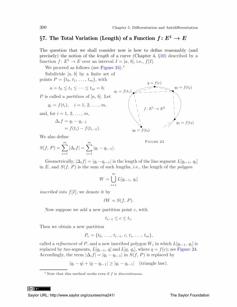
300 Chapter 5. Differentiation and Antidifferentiation
§7. The Total Variation (Length) of a Function f : E1 → E
The question that we shall consider now is how to define reasonably (andprecisely) the notion of the length of a curve (Chapter 4, §10) described by afunction f : E1 → E over an interval I = [a, b], i.e., f [I].
We proceed as follows (see Figure 24).1
q0 = f(t0)
q1 = f(t1)q2 = f(t2)
q3 = f(t3)
q = f(c)
f : E1 → E2
Figure 24
Subdivide [a, b] by a finite set ofpoints P = {t0, t1, . . . , tm}, with
a = t0 ≤ t1 ≤ · · · ≤ tm = b;
P is called a partition of [a, b]. Let
qi = f(ti), i = 1, 2, . . . , m,
and, for i = 1, 2, . . . , m,
∆if = qi − qi−1
= f(ti)− f(ti−1).
We also define
S(f, P ) =
m∑
i=1
|∆if | =m∑
i=1
|qi − qi−1|.
Geometrically, |∆if | = |qi−qi−1| is the length of the line segment L[qi−1, qi]in E, and S(f, P ) is the sum of such lengths, i.e., the length of the polygon
W =m⋃
i=1
L[qi−1, qi]
inscribed into f [I]; we denote it by
ℓW = S(f, P ).
Now suppose we add a new partition point c, with
ti−1 ≤ c ≤ ti.
Then we obtain a new partition
Pc = {t0, . . . , ti−1, c, ti, . . . , tm},called a refinement of P , and a new inscribed polygonWc in which L[qi−1, qi] isreplaced by two segments, L[qi−1, q] and L[q, qi], where q = f(c); see Figure 24.Accordingly, the term |∆if | = |qi − qi−1| in S(f, P ) is replaced by
|qi − q|+ |q − qi−1| ≥ |qi − qi−1| (triangle law).
1 Note that this method works even if f is discontinuous.
Saylor URL: http://www.saylor.org/courses/ma241/ The Saylor Foundation
§7. The Total Variation (Length) of a Function f : E1 → E 301
It follows that
S(f, P ) ≤ S(f, Pc); i.e., ℓW ≤ ℓWc.
Hence we obtain the following result.
Corollary 1. The sum S(f, P ) = ℓW cannot decrease when P is refined .
Thus when new partition points are added, S(f, P ) grows in general; i.e.,it approaches some supremum value (finite or not). Roughly speaking, theinscribed polygon W gets “closer” to the curve. It is natural to define thedesired length of the curve to be the lub of all lengths ℓW , i.e., of all sumsS(f, P ) resulting from the various partitions P . This supremum is also calledthe total variation of f over [a, b], denoted Vf [a, b].
2
Definition 1.
Given any function f : E1 → E, and I = [a, b] ⊂ E1, we set
Vf [I] = Vf [a, b] = supPS(f, P ) = sup
P
m∑
i=1
|f(ti)− f(ti−1)| ≥ 0 in E∗, (1)
where the supremum is over all partitions P = {t0, . . . , tm} of I. We callVf [I] the total variation, or length, of f on I. Briefly, we denote it by Vf .
Note 1. If f is continuous on [a, b], the image set A = f [I] is an arc
(Chapter 4, §10). It is customary to call Vf [I] the length of that arc, denotedℓfA or briefly ℓA. Note, however, that there may well be another functiong, continuous on an interval J , such that g[J ] = A but Vf [I] 6= Vg[J ], andso ℓfA 6= ℓgA. Thus it is safer to say “the length of A as described by f on
I.” Only for simple arcs (where f is one to one), is “ℓA” unambiguous. (SeeProblems 6–8.)
In the propositions below, f is an arbitrary function, f : E1 → E.
Theorem 1 (additivity of Vf ). If a ≤ c ≤ b, thenVf [a, b] = Vf [a, c] + Vf [c, b];
i .e., the length of the whole equals the sum of the lengths of the parts .
Proof. Take any partition P = {t0, . . . , tm} of [a, b]. If c /∈ P , refine P to
Pc = {t0, . . . , ti, c, ti, . . . , tm}.Then by Corollary 1, S(f, P ) ≤ S(f, Pc).
Now Pc splits into partitions of [a, c] and [c, b], namely,
P ′ = {t0, . . . , ti−1, c} and P ′′ = {c, ti, . . . , tm},
2 We also call it the length of f over [a, b]. Observe that, for real f : E1 → E1, this is not
the length of the graph in the usual sense (which is a curve in E2). See the end of §8.
Saylor URL: http://www.saylor.org/courses/ma241/ The Saylor Foundation
302 Chapter 5. Differentiation and Antidifferentiation
so that
S(f, P ′) + S(f, P ′′) = S(f, Pc). (Verify!)
Hence (as Vf is the lub of the corresponding sums),
Vf [a, c] + Vf [c, d] ≥ S(f, Pc) ≥ S(f, P ).
As P is an arbitrary partition of [a, b], we also have
Vf [a, c] + Vf [c, b] ≥ supS(f, P ) = Vf [a, b].
Thus it remains to show that, conversely,
Vf [a, b] ≥ Vf [a, c] + Vf [c, b].
The latter is trivial if Vf [a, b] = +∞. Thus assume Vf [a, b] = K < +∞. LetP ′ and P ′′ be any partitions of [a, c] and [c, b], respectively. Then P ∗ = P ′∪P ′′
is a partition of [a, b], and
S(f, P ′) + S(f, P ′′) = S(f, P ∗) ≤ Vf [a, b] = K,
whence
S(f, P ′) ≤ K − S(f, P ′′).
Keeping P ′′ fixed and varying P ′, we see that K−S(f, P ′′) is an upper boundof all S(f, P ′) over [a, c]. Hence
Vf [a, c] ≤ K − S(f, P ′′)
or
S(f, P ′′) ≤ K − Vf [a, c].
Similarly, varying P ′′, we now obtain
Vf [c, b] ≤ K − Vf [a, c]
or
Vf [a, c] + Vf [c, b] ≤ K = Vf [a, b],
as required. Thus all is proved. �
Corollary 2 (monotonicity of Vf ). If a ≤ c ≤ d ≤ b, then
Vf [c, d] ≤ Vf [a, b].
Proof. By Theorem 1,
Vf [a, b] = Vf [a, c] + Vf [c, d] + Vf [d, b] ≥ Vf [c, d]. �
Saylor URL: http://www.saylor.org/courses/ma241/ The Saylor Foundation
§7. The Total Variation (Length) of a Function f : E1 → E 303
Definition 2.
If Vf [a, b] < +∞, we say that f is of bounded variation on I = [a, b], andthat the set f [I] is rectifiable (by f on I).
Corollary 3. For each t ∈ [a, b],
|f(t)− f(a)| ≤ Vf [a, b].Hence if f is of bounded variation on [a, b], it is bounded on [a, b].
Proof. If t ∈ [a, b], let P = {a, t, b}, so|f(t)− f(a)| ≤ |f(t)− f(a)|+ |f(b)− f(t)| = S(f, P ) ≤ Vf [a, b],
proving our first assertion.3 Hence
(∀ t ∈ [a, b]) |f(t)| ≤ |f(t)− f(a)|+ |f(a)| ≤ Vf [a, b] + |f(a)|.This proves the second assertion. �
Note 2. Neither boundedness, nor continuity, nor differentiability of f on[a, b] implies Vf [a, b] < +∞, but boundedness of f ′ does . (See Problems 1 and3.)
Corollary 4. A function f is finite and constant on [a, b] iff Vf [a, b] = 0.
The proof is left to the reader. (Use Corollary 3 and the definitions.)
Theorem 2. Let f, g, h be real or complex (or let f and g be vector valued
and h scalar valued). Then on any interval I = [a, b], we have
(i) V|f | ≤ Vf ;(ii) Vf±g ≤ Vf + Vg; and
(iii) Vhf ≤ sVf + rVh, with r = supt∈I |f(t)| and s = supt∈I |h(t)|.Hence if f , g, and h are of bounded variation on I, so are f±g, hf , and |f |.
Proof. We first prove (iii).
Take any partition P = {t0, . . . , tm} of I. Then|∆ihf | = |h(ti)f(ti)− h(ti−1)f(ti−1)|
≤ |h(ti)f(ti)− h(ti−1)f(ti)|+ |h(ti−1)f(ti)− h(ti−1)f(ti−1)|= |f(ti)||∆ih|+ |h(ti−1)||∆if |≤ r|∆ih|+ s|∆if |.
Adding these inequalities, we obtain
S(hf, P ) ≤ r · S(h, P ) + s · S(f, P ) ≤ rVh + sVf .
3 By our conventions, it also follows that |f(a)| is a finite constant, and so is Vf [a, b]+|f(a)|if Vf [a, b] < +∞.
Saylor URL: http://www.saylor.org/courses/ma241/ The Saylor Foundation
304 Chapter 5. Differentiation and Antidifferentiation
As this holds for all sums S(hf, P ), it holds for their supremum, so
Vhf = supS(hf, P ) ≤ rVh + sVf ,
as claimed.
Similarly, (i) follows from∣
∣|f(ti)| − |f(ti−1)|∣
∣ ≤ |f(ti)− f(ti−1)|.The analogous proof of (ii) is left to the reader.
Finally, (i)–(iii) imply that Vf , Vf±g, and Vhf are finite if Vf , Vg, and Vhare. This proves our last assertion. �
Note 3. Also f/h is of bounded variation on I if f and h are, provided his bounded away from 0 on I; i.e.,
(∃ ε > 0) |h| ≥ ε on I.
(See Problem 5.)
Special theorems apply in case the range space E is E1 or En (∗or Cn).
Theorem 3.
(i) A real function f is of bounded variation on I = [a, b] iff f = g − h for
some nondecreasing real functions g and h on I.
(ii) If f is real and monotone on I, it is of bounded variation there.
Proof. We prove (ii) first.
Let f↑ on I. If P = {t0, . . . , tm}, thenti ≥ ti−1 implies f(ti) ≥ f(ti−1).
Hence ∆if ≥ 0; i.e., |∆if | = ∆if . Thus
S(f, P ) =m∑
i=1
|∆if | =m∑
i=1
∆if =m∑
i=1
[f(ti)− f(ti−1)]
= f(tm)− f(t0) = f(b)− f(a)for any P . (Verify!) This implies that also
Vf [I] = supS(f, P ) = f(b)− f(a) < +∞.Thus (ii) is proved.
Now for (i), let f = g − h with g↑ and h↑ on I. By (ii), g and h are ofbounded variation on I. Hence so is f = g − h by Theorem 2 (last clause).
Conversely, suppose Vf [I] < +∞. Then define
g(x) = Vf [a, x], x ∈ I, and h = g − f on I,
so f = g − h, and it only remains to show that g↑ and h↑.
Saylor URL: http://www.saylor.org/courses/ma241/ The Saylor Foundation
§7. The Total Variation (Length) of a Function f : E1 → E 305
To prove it, let a ≤ x ≤ y ≤ b. Then Theorem 1 yields
Vf [a, y]− Vf [a, x] = Vf [x, y];
i.e.,
g(y)− g(x) = Vf [x, y] ≥ |f(y)− f(x)| ≥ 0 (by Corollary 3). (2)
Hence g(y) ≥ g(x). Also, as h = g − f , we have
h(y)− h(x) = g(y)− f(y)− [g(x)− f(x)]= g(y)− g(x)− [f(y)− f(x)]≥ 0 by (2).
Thus h(y) ≥ h(x). We see that a ≤ x ≤ y ≤ b implies g(x) ≤ g(y) andh(x) ≤ h(y), so h↑ and g↑, indeed. �
Theorem 4.
(i) A function f : E1 → En (∗Cn) is of bounded variation on I = [a, b] iffall of its components (f1, f2, . . . , fn) are.
(ii) If this is the case, then finite limits f(p+) and f(q−) exist for every
p ∈ [a, b) and q ∈ (a, b].
Proof.
(i) Take any partition P = {t0, . . . , tm} of I. Then
|fk(ti)− fk(ti−1)|2 ≤n∑
j=1
|fj(ti)− fj(ti−1)|2 = |f(ti)− f(ti−1)|2;
i.e., |∆ifk| ≤ |∆if |, i = 1, 2, . . . , m. Thus
(∀P ) S(fk, P ) ≤ S(f, P ) ≤ Vf ,and Vfk ≤ Vf follows. Thus
Vf < +∞ implies Vfk < +∞, k = 1, 2, . . . , n.
The converse follows by Theorem 2 since f =∑n
k=1 fk~ek. (Explain!)
(ii) For real monotone functions, f(p+) and f(q−) exist by Theorem 1 ofChapter 4, §5. This also applies if f is real and of bounded variation, forby Theorem 3,
f = g − h with g↑ and h↑ on I,and so
f(p+) = g(p+)− h(p+) and f(q−) = g(q−)− h(q−) exist.The limits are finite since f is bounded on I by Corollary 3.
Saylor URL: http://www.saylor.org/courses/ma241/ The Saylor Foundation
306 Chapter 5. Differentiation and Antidifferentiation
Via components (Theorem 2 of Chapter 4, §3), this also applies tofunctions f : E1 → En. (Why?) In particular, (ii) applies to complex
functions (treat C as E2) (∗and so it extends to functions f : E1 → Cn
as well). �
We also have proved the following corollary.
Corollary 5. A complex function f : E1 → C is of bounded variation on [a, b]iff its real and imaginary parts are. (See Chapter 4, §3, Note 5.)
Problems on Total Variation and Graph Length
1. In the following cases show that Vf [I] = +∞, though f is bounded onI. (In case (iii), f is continuous, and in case (iv), it is even differentiableon I.)
(i) For I = [a, b] (a < b), f(x) =
{
1 if x ∈ R (rational), and
0 if x ∈ E1 −R.(ii) f(x) = sin
1
x; f(0) = 0; I = [a, b], a ≤ 0 ≤ b, a < b.
(iii) f(x) = x · sin π
2x; f(0) = 0; I = [0, 1].
(iv) f(x) = x2 sin1
x2; f(0) = 0; I = [0, 1].
[Hints: (i) For any m there is P , with
|∆if | = 1, i = 1, 2, . . . , m,
so S(f, P ) = m → +∞.
(iii) Let
Pm ={
0,1
m,
1
m− 1, . . . ,
1
2, 1
}
.
Prove that S(f, Pm) ≥ ∑mk=1
1k→ +∞.]
2. Let f : E1 → E1 be monotone on each of the intervals
[ak−1, ak], k = 1, . . . , n (“piecewise monotone”).
Prove that
Vf [a0, an] =
n∑
k=1
|f(ak)− f(ak−1)|.
In particular, show that this applies if f(x) =∑n
i=1 cixi (polynomial),
with ci ∈ E1.[Hint: It is known that a polynomial of degree n has at most n real roots. Thus itis piecewise monotone, for its derivative vanishes at finitely many points (being of
degree n− 1). Use Theorem 1 in §2.]
Saylor URL: http://www.saylor.org/courses/ma241/ The Saylor Foundation
§7. The Total Variation (Length) of a Function f : E1 → E 307
⇒3. Prove that if f is finite and relatively continuous on I = [a, b], with abounded derivative, |f ′| ≤M , on I −Q (see §4), then
Vf [a, b] ≤M(b− a).
However, we may have Vf [I] < +∞, and yet |f ′| = +∞ at some p ∈ I.[Hint: Take f(x) = 3
√x on [−1, 1].]
4. Complete the proofs of Corollary 4 and Theorems 2 and 4.
5. Prove Note 3.[Hint: If |h| ≥ ε on I, show that
∣∣∣
1
h(ti)− 1
h(ti−1)
∣∣∣ ≤ |∆ih|
ε2
and hence
S( 1
h, P
)
≤ S(h, P )
ε2≤ Vh
ε2.
Deduce that 1h
is of bounded variation on I if h is. Then apply Theorem 2(iii) to1h· f .]
6. Let g : E1 → E1 (real) and f : E1 → E be relatively continuous onJ = [c, d] and I = [a, b], respectively, with a = g(c) and b = g(d). Let
h = f ◦ g.
Prove that if g is one to one on J , then
(i) g[J ] = I, so f and h describe one and the same arc A = f [I] = h[J ];
(ii) Vf [I] = Vh[J ]; i.e., ℓfA = ℓhA.
[Hint for (ii): Given P = {a = t0, . . . , tm = b}, show that the points si = g−1(ti)form a partition P ′ of J = [c, d], with S(h, P ′) = S(f, P ). Hence deduce Vf [I] ≤Vh[J].
Then prove that Vh[J] ≤ Vf [I], taking an arbitrary P ′ = {c = s0, . . . , sm = d},and defining P = {t0, . . . , tm}, with ti = g(si). What if g(c) = b, g(d) = a?]
7. Prove that if f, h : E1 → E are relatively continuous and one to one onI = [a, b] and J = [c, d], respectively, and if
f [I] = h[J ] = A
(i.e., f and h describe the same simple arc A), then
ℓfA = ℓhA.
Thus for simple arcs, ℓfA is independent of f .[Hint: Define g : J → E1 by g = f−1 ◦ h. Use Problem 6 and Chapter 4, §9,Theorem 3. First check that Problem 6 works also if g(c) = b and g(d) = a, i.e., g↓on J.]
Saylor URL: http://www.saylor.org/courses/ma241/ The Saylor Foundation
308 Chapter 5. Differentiation and Antidifferentiation
8. Let I = [0, 2π] and define f, g, h : E1 → E2 (C) by
f(x) = (sinx, cosx),
g(x) = (sin 3x, cos 3x),
h(x) =(
sin1
x, cos
1
x
)
with h(0) = (0, 1).
Show that f [I] = g[I] = h[I] (the unit circle; call it A), yet ℓfA = 2π,ℓgA = 6π, while Vh[I] = +∞. (Thus the result of Problem 7 fails forclosed curves and nonsimple arcs.)
9. In Theorem 3, define two functions G, H : E1 → E1 by
G(x) =1
2[Vf [a, x] + f(x)− f(a)]
and
H(x) = G(x)− f(x) + f(a).
(G and H are called, respectively, the positive and negative variation
functions for f .) Prove that
(i) G↑ and H↑ on [a, b];
(ii) f(x) = G(x)− [H(x)− f(a)] (thus the functions f and g of Theo-rem 3 are not unique);
(iii) Vf [a, x] = G(x) +H(x);
(iv) if f = g − h, with g↑ and h↑ on [a, b], then
VG[a, b] ≤ Vg[a, b], and VH [a, b] ≤ Vh[a, b];
(v) G(a) = H(a) = 0.
∗10. Prove that if f : E1 → En (Cn) is of bounded variation on I = [a, b],then f has at most countably many discontinuities in I.[Hint: Apply Problem 5 of Chapter 4, §5. Proceed as in the proof of Theorem 4 in§7. Finally, use Theorem 2 of Chapter 1, §9.]
§8. Rectifiable Arcs. Absolute Continuity
If a function f : E1 → E is of bounded variation (§7) on an interval I = [a, b],we can define a real function vf on I by
vf (x) = Vf [a, x] (= total variation of f on [a, x]) for x ∈ I;vf is called the total variation function, or length function, generated by f onI. Note that vf↑ on I. (Why?) We now consider the case where f is also
Saylor URL: http://www.saylor.org/courses/ma241/ The Saylor Foundation
§8. Rectifiable Arcs. Absolute Continuity 309
relatively continuous on I, so that the set A = f [I] is a rectifiable arc (see §7,Note 1 and Definition 2).
Definition 1.
A function f : E1 → E is (weakly) absolutely continuous1 on I = [a, b] iffVf [I] < +∞ and f is relatively continuous on I.
Theorem 1. The following are equivalent :
(i) f is (weakly) absolutely continuous on I = [a, b];
(ii) vf is finite and relatively continuous on I; and
(iii) (∀ ε > 0) (∃ δ > 0) (∀x, y ∈ I | 0 ≤ y − x < δ) Vf [x, y] < ε.
Proof. We shall show that (ii) ⇒ (iii) ⇒ (i) ⇒ (ii).
(ii) ⇒ (iii). As I = [a, b] is compact , (ii) implies that vf is uniformly
continuous on I (Theorem 4 of Chapter 4, §8). Thus
(∀ ε > 0) (∃ δ > 0) (∀x, y ∈ I | 0 ≤ y − x < δ) vf (y)− vf (x) < ε.
However,
vf (y)− vf (x) = Vf [a, y]− Vf [a, x] = Vf [x, y]
by additivity (Theorem 1 in §7). Thus (iii) follows.(iii) ⇒ (i). By Corollary 3 of §7, |f(x) − f(y)| ≤ Vf [x, y]. Therefore, (iii)
implies that
(∀ ε > 0) (∃ δ > 0) (∀x, y ∈ I | |x− y| < δ) |f(x)− f(y)| < ε,
and so f is relatively (even uniformly) continuous on I.
Now with ε and δ as in (iii), take a partition P = {t0, . . . , tm} of I so finethat
ti − ti−1 < δ, i = 1, 2, . . . , m.
Then (∀ i) Vf [ti−1, ti] < ε. Adding up these m inequalities and using theadditivity of Vf , we obtain
Vf [I] =m∑
i=1
Vf [ti−1, ti] < mε < +∞.
Thus (i) follows, by definition.
That (i) ⇒ (ii) is given as the next theorem. �
1 In this section, we use this notion in a weaker sense than customary. The usual stronger
version is given in Problem 2. We study it in Volume 2, Chapter 7, §11.
Saylor URL: http://www.saylor.org/courses/ma241/ The Saylor Foundation
310 Chapter 5. Differentiation and Antidifferentiation
Theorem 2. If Vf [I] < +∞ and if f is relatively continuous at some p ∈ I(over I = [a, b]), then the same applies to the length function vf .
Proof. We consider left continuity first, with a < p ≤ b.Let ε > 0. By assumption, there is δ > 0 such that
|f(x)− f(p)| < ε
2when |x− p| < δ and x ∈ [a, p].
Fix any such x. Also, Vf [a, p] = supP S(f, P ) over [a, p]. Thus
Vf [a, p]−ε
2<
k∑
i=1
|∆if |
for some partition
P = {t0 = a, . . . , tk−1, tk = p} of [a, p]. (Why?)
We may assume tk−1 = x, x as above. (If tk−1 6= x, add x to P .) Then
|∆kf | = |f(p)− f(x)| <ε
2,
and hence
Vf [a, p]−ε
2<
k−1∑
i=1
|∆if |+ |∆kf | <k−1∑
i=1
|∆if |+ε
2≤ Vf [a, tk−1] +
ε
2. (1)
However,
Vf [a, p] = vf (p)
and
Vf [a, tk−1] = Vf [a, x] = vf (x).
Thus (1) yields
|vf (p)− vf (x)| = Vf [a, p]− Vf [a, x] < ε for x ∈ [a, p] with |x− p| < δ.
This shows that vf is left continuous at p.
Right continuity is proved similarly on noting that
vf (x)− vf (p) = Vf [p, b]− Vf [x, b] for p ≤ x < b. (Why?)
Thus vf is, indeed, relatively continuous at p. Observe that vf is also ofbounded variation on I, being monotone and finite (see Theorem 3(ii) of §7).
This completes the proof of both Theorem 2 and Theorem 1. �
We also have the following.
Saylor URL: http://www.saylor.org/courses/ma241/ The Saylor Foundation
§8. Rectifiable Arcs. Absolute Continuity 311
Corollary 1. If f is real and absolutely continuous on I = [a, b] (weakly),so are the nondecreasing functions g and h (f = g − h) defined in Theorem 3of §7.
Indeed, the function g as defined there is simply vf . Thus it is relativelycontinuous and finite on I by Theorem 1. Hence so also is h = f − g. Both areof bounded variation (monotone!) and hence absolutely continuous (weakly).
Note 1. The proof of Theorem 1 shows that (weak) absolute continuity
implies uniform continuity . The converse fails, however (see Problem 1(iv)in §7).
We now apply our theory to antiderivatives (integrals).
Corollary 2. If F =∫
f on I = [a, b] and if f is bounded (|f | ≤ K ∈ E1) onI −Q (Q countable), then F is weakly absolutely continuous on I.
(Actually, even the stronger variety of absolute continuity follows. See Chap-ter 7, §11, Problem 17).
Proof. By definition, F =∫
f is finite and relatively continuous on I, so weonly have to show that VF [I] < +∞. This, however, easily follows by Problem 3of §7 on noting that F ′ = f on I − S (S countable). Details are left to thereader. �
Our next theorem expresses arc length in the form of an integral.
Theorem 3. If f : E1 → E is continuously differentiable on I = [a, b] (§6),then vf =
∫
|f ′| on I and
Vf [a, b] =
∫ b
a
|f ′|.
Proof. Let a < p < x ≤ b, ∆x = x− p, and∆vf = vf (x)− vf (p) = Vf [p, x]. (Why?)
As a first step, we shall show that
∆vf∆x
≤ sup[p,x]
|f ′|. (2)
For any partition P = {p = t0, . . . , tm = x} of [p, x], we have
S(f, P ) =m∑
i=1
|∆if | ≤m∑
i=1
sup[ti−1,ti]
|f ′| (ti − ti−1) ≤ sup[p,x]
|f ′|∆x.
Since this holds for any partition P , we have
Vf [p, x] ≤ sup[p,x]
|f ′|∆x,
which implies (2).
Saylor URL: http://www.saylor.org/courses/ma241/ The Saylor Foundation
312 Chapter 5. Differentiation and Antidifferentiation
On the other hand,
∆vf = Vf [p, x] ≥ |f(x)− f(p)| = |∆f |.Combining, we get
∣
∣
∣
∆f
∆x
∣
∣
∣≤ ∆vf
∆x≤ sup
[p,x]
|f ′| < +∞ (3)
since f ′ is relatively continuous on [a, b], hence also uniformly continuous andbounded. (Here we assumed a < p < x ≤ b. However, (3) holds also ifa ≤ x < p < b, with ∆vf = −V [x, p] and ∆x < 0. Verify!)
Now∣
∣|f ′(p)| − |f ′(x)|∣
∣ ≤ |f ′(p)− f ′(x)| → 0 as x→ p,
so, taking limits as x→ p, we obtain
limx→p
∆vf∆x
= |f ′(p)|.
Thus vf is differentiable at each p in (a, b), with v′f (p) = |f ′(p)|. Also, vf is
relatively continuous and finite on [a, b] (by Theorem 1).2 Hence vf =∫
|f ′|on [a, b], and we obtain
∫ b
a
|f ′| = vf (b)− vf (a) = Vf [a, b], as asserted. � (4)
Note 2. If the range space E is En (∗or Cn), f has n components
f1, f2, . . . , fn.
By Theorem 5 in §1, f ′ = (f ′1, f
′2, . . . , f
′n), so
|f ′| =√
n∑
k=1
|f ′k|2 ,
and we get
Vf [a, b] =
∫ b
a
√
n∑
k=1
|f ′k|2 =
∫ b
a
√
n∑
k=1
|f ′k(t)|2 dt (classical notation). (5)
In particular, for complex functions, we have (see Chapter 4, §3, Note 5)
Vf [a, b] =
∫ b
a
√
f ′re(t)
2 + f ′im(t)
2 dt. (6)
In practice, formula (5) is used when a curve is given parametrically by
xk = fk(t), k = 1, 2, . . . , n,
2 Note that (3) implies the finiteness of vf (p) and vf (x).
Saylor URL: http://www.saylor.org/courses/ma241/ The Saylor Foundation
§8. Rectifiable Arcs. Absolute Continuity 313
with the fk differentiable on [a, b]. Curves in E2 are often given in nonpara-
metric form as
y = F (x), F : E1 → E1.
Here F [I] is not the desired curve but simply a set in E1. To apply (5) here,we first replace “y = F (x)” by suitable parametric equations,
x = f1(t) and y = f2(t);
i.e., we introduce a function f : E1 → E, with f = (f1, f2). An obvious (butnot the only) way of achieving it is to set
x = f1(t) = t and y = f2(t) = F (t)
so that f ′1 = 1 and f ′
2 = F ′. Then formula (5) may be written as
Vf [a, b] =
∫ b
a
√
1 + F ′(x)2 dx, f(x) = (x, F (x)). (7)
Example.
Find the length of the circle
x2 + y2 = r2.
Here it is convenient to use the parametric equations
x = r cos t and y = r sin t,
i.e., to define f : E1 → E2 by
f(t) = (r cos t, r sin t),
or, in complex notation,
f(t) = reti.
Then the circle is obtained by letting t vary through [0, 2π]. Thus (5)yields
Vf [0, 2π] =
∫ b
a
r√
cos2 t+ sin2 t dt = r
∫ b
a
1 dt = rt∣
∣
∣
2π
0= 2rπ.
Note that f describes the same circle A = f [I] over I = [0, 4π]. Moregenerally, we could let t vary through any interval [a, b] with b − a ≥2π. However, the length, Vf [a, b], would change (depending on b − a).This is because the circle A = f [I] is not a simple arc (see §7, Note 1),so ℓA depends on f and I, and one must be careful in selecting bothappropriately.
Saylor URL: http://www.saylor.org/courses/ma241/ The Saylor Foundation
314 Chapter 5. Differentiation and Antidifferentiation
Problems on Absolute Continuity and Rectifiable Arcs
1. Complete the proofs of Theorems 2 and 3, giving all missing details.
⇒2. Show that f is absolutely continuous (in the weaker sense) on [a, b] iffor every ε > 0 there is δ > 0 such that
m∑
i=1
|f(ti)− f(si)| < ε whenever
m∑
i=1
(ti − si) < δ and
a ≤ s1 ≤ t1 ≤ s2 ≤ t2 ≤ · · · ≤ sm ≤ tm ≤ b.
(This is absolute continuity in the stronger sense.)
3. Prove that vf is strictly monotone on [a, b] iff f is not constant on anynondegenerate subinterval of [a, b].[Hint: If x < y, Vf [x, y] > 0, by Corollary 4 of §7].
4. With f, g, h as in Theorem 2 of §7, prove that if f, g, h are absolutelycontinuous (in the weaker sense) on I, so are f ± g, hf , and |f |; so alsois f/h if (∃ ε > 0) |h| ≥ ε on I.
5. Prove the following:
(i) If f ′ is finite and 6= 0 on I = [a, b], so also is v′f (with one-sided
derivatives at the endpoints of the interval); moreover,
∣
∣
∣
f ′
v′f
∣
∣
∣= 1 on I.
Thus show that f ′/v′f is the tangent unit vector (see §1).(ii) Under the same assumptions, F = f ◦ v−1
f is differentiable on
J = [0, vf (b)] (with one-sided derivatives at the endpoints of theinterval) and F [J ] = f [I]; i.e., F and f describe the same simplearc, with VF [I] = Vf [I].
Note that this is tantamount to a change of parameter . Settings = vf (t), i.e., t = v−1
f (s), we have f(t) = f(v−1f (s)) = F (s), with
the arclength s as parameter .
§9. Convergence Theorems in Differentiation and Integration
Given
Fn =
∫
fn or F ′n = fn, n = 1, 2, . . . ,
what can one say about∫
lim fn or (limFn)′ if the limits exist? Below we give
some answers, for complete range spaces E (such as En). Roughly, we have
Saylor URL: http://www.saylor.org/courses/ma241/ The Saylor Foundation
§9. Convergence Theorems in Differentiation and Integration 315
limF ′n = (limFn)
′ on I −Q if
(a) {Fn(p)} converges for at least one p ∈ I and
(b) {F ′n} converges uniformly .
Here I is a finite or infinite interval in E1 and Q is countable. We include in
Q the endpoints of I (if any), so I −Q ⊆ I0 (= interior of I).
Theorem 1. Let Fn : E1 → E (n = 1, 2, . . . ) be finite and relatively continu-
ous on I and differentiable on I −Q. Suppose that
(a) limn→∞ Fn(p) exists for some p ∈ I;(b) F ′
n → f 6= ±∞ (uniformly) on J −Q for each finite subinterval J ⊆ I;(c) E is complete.
Then
(i) limn→∞ Fn = F exists uniformly on each finite subinterval J ⊆ I;(ii) F =
∫
f on I; and
(iii) (limFn)′ = F ′ = f = limn→∞ F ′
n on I −Q.
Proof. Fix ε > 0 and any subinterval J ⊆ I of length δ < ∞, with p ∈ J (pas in (a)). By (b), F ′
n → f (uniformly) on J −Q, so there is a k such that form, n > k,
|F ′n(t)− f(t)| <
ε
2, t ∈ J −Q; (1)
hence
supt∈J−Q
|F ′m(t)− F ′
n(t)| ≤ ε. (Why?) (2)
Now apply Corollary 1 in §4 to the function h = Fm − Fn on J . Then foreach x ∈ J , |h(x)− h(p)| ≤M |x− p|, where
M ≤ supt∈J−Q
|h′(t)| ≤ ε
by (2). Hence for m, n > k, x ∈ J and
|Fm(x)− Fn(x)− Fm(p) + Fn(p)| ≤ ε|x− p| ≤ εδ. (3)
As ε is arbitrary , this shows that the sequence
{Fn − Fn(p)}satisfies the uniform Cauchy criterion (Chapter 4, §12, Theorem 3). Thus as Eis complete, {Fn−Fn(p)} converges uniformly on J . So does {Fn}, for {Fn(p)}converges, by (a). Thus we may set
F = limFn (uniformly) on J ,
Saylor URL: http://www.saylor.org/courses/ma241/ The Saylor Foundation
316 Chapter 5. Differentiation and Antidifferentiation
proving assertion (i).1
Here by Theorem 2 of Chapter 4, §12, F is relatively continuous on each
such J ⊆ I, hence on all of I. Also, letting m → +∞ (with n fixed), we haveFm → F in (3), and it follows that for n > k and x ∈ Gp(δ) ∩ I.
|F (x)− Fn(x)− F (p) + Fn(p)| ≤ ε|x− p| ≤ εδ. (4)
Having proved (i), we may now treat p as just any point in I. Thus formula(4) holds for any globe Gp(δ), p ∈ I. We now show that
F ′ = f on I −Q; i.e., F =
∫
f on I.
Indeed, if p ∈ I − Q, each Fn is differentiable at p (by assumption), andp ∈ I0 (since I −Q ⊆ I0 by our convention). Thus for each n, there is δn > 0such that
∣
∣
∣
∆Fn
∆x− F ′
n(p)∣
∣
∣=
∣
∣
∣
Fn(x)− Fn(p)
x− p − F ′n(p)
∣
∣
∣<ε
2(5)
for all x ∈ G¬p(δn); Gp(δn) ⊆ I.By assumption (b) and by (4), we can fix n so large that
|F ′n(p)− f(p)| <
ε
2
and so that (4) holds for δ = δn. Then, dividing by |∆x| = |x− p|, we have∣
∣
∣
∆F
∆x− ∆Fn
∆x
∣
∣
∣≤ ε.
Combining with (5), we infer that for each ε > 0, there is δ > 0 such that∣
∣
∣
∆F
∆x−f(p)
∣
∣
∣≤
∣
∣
∣
∆F
∆x−∆Fn
∆x
∣
∣
∣+∣
∣
∣
∆Fn
∆x−F ′
n(p)∣
∣
∣+ |F ′
n(p)−f(p)| < 2ε, x ∈ Gp(δ).
This shows that
limx→p
∆F
∆x= f(p) for p ∈ I −Q,
i.e., F ′ = f on I −Q, with f finite by assumption, and F finite by (4). As Fis also relatively continuous on I, assertion (ii) is proved, and (iii) follows sinceF = limFn and f = limF ′
n. �
Note 1. The same proof also shows that Fn → F (uniformly) on each closed
subinterval J ⊆ I if F ′n → f (uniformly) on J − Q for all such J (with the
other assumptions unchanged). In any case, we then have Fn → F (pointwise)on all of I.
We now apply Theorem 1 to antiderivatives .
1 Indeed, any J can be enlarged to include p, so (3) applies to it. Note that in (3) we may
as well vary x inside any set of the form I ∩Gp(δ).
Saylor URL: http://www.saylor.org/courses/ma241/ The Saylor Foundation
§9. Convergence Theorems in Differentiation and Integration 317
Theorem 2. Let the functions fn : E1 → E, n = 1, 2, . . . , have antideriva-
tives , Fn =∫
fn, on I. Suppose E is complete and fn → f (uniformly) on
each finite subinterval J ⊆ I, with f finite there. Then∫
f exists on I, and∫ x
p
f =
∫ x
p
limn→∞
fn = limn→∞
∫ x
p
fn for any p, x ∈ I. (6)
Proof. Fix any p ∈ I. By Note 2 in §5, we may choose
Fn(x) =
∫ x
p
fn for x ∈ I.
Then Fn(p) =∫ p
pfn = 0, and so limn→∞ Fn(p) = 0 exists, as required in The-
orem 1(a).
Also, by definition, each Fn is relatively continuous and finite on I anddifferentiable, with F ′
n = fn, on I − Qn. The countable sets Qn need not bethe same, so we replace them by
Q =
∞⋃
n=1
Qn
(including in Q also the endpoints of I, if any). Then Q is countable (seeChapter 1, §9, Theorem 2), and I − Q ⊆ I − Qn, so all Fn are differentiableon I −Q, with F ′
n = fn there.
Additionally, by assumption,
fn → f (uniformly)
on finite subintervals J ⊆ I. Hence
F ′n → f (uniformly) on J −Q
for all such J , and so the conditions of Theorem 1 are satisfied.
By that theorem, then,
F =
∫
f = limFn exists on I
and, recalling that
Fn(x) =
∫ x
p
fn,
we obtain for x ∈ I∫ x
p
f = F (x)− F (p) = limFn(x)− limFn(p) = limFn(x)− 0 = lim
∫ x
p
fn.
As p ∈ I was arbitrary, and f = lim fn (by assumption), all is proved. �
Saylor URL: http://www.saylor.org/courses/ma241/ The Saylor Foundation
318 Chapter 5. Differentiation and Antidifferentiation
Note 2. By Theorem 1, the convergence∫ x
p
fn →∫ x
p
f (i.e., Fn → F )
is uniform in x (with p fixed), on each finite subinterval J ⊆ I.We now “translate” Theorems 1 and 2 into the language of series.
Corollary 1. Let E and the functions Fn : E1 → E be as in Theorem 1.
Suppose the series∑
Fn(p)
converges for some p ∈ I, and∑
F ′n
converges uniformly on J −Q, for each finite subinterval J ⊆ I.Then
∑
Fn converges uniformly on each such J , and
F =
∞∑
n=1
Fn
is differentiable on I −Q, with
F ′ =
( ∞∑
n=1
Fn
)′=
∞∑
n−1
F ′n there. (7)
In other words, the series can be differentiated termwise.
Proof. Let
sn =n∑
k=1
Fk, n = 1, 2, . . . ,
be the partial sums of∑
Fn. From our assumptions, it then follows that thesn satisfy all conditions of Theorem 1. (Verify!) Thus the conclusions of Theo-rem 1 hold, with Fn replaced by sn.
We have F = lim sn and F ′ = (lim sn)′ = lim s′n, whence (7) follows. �
Corollary 2. If E and the fn are as in Theorem 2 and if∑
fn converges
uniformly to f on each finite interval J ⊆ I, then∫
f exists on I, and
∫ x
p
f =
∫ x
p
∞∑
n=1
fn =∞∑
n=1
∫ x
p
fn for any p, x ∈ I. (8)
Briefly, a uniformly convergent series can be integrated termwise.
Saylor URL: http://www.saylor.org/courses/ma241/ The Saylor Foundation
§9. Convergence Theorems in Differentiation and Integration 319
Theorem 3 (power series). Let r be the convergence radius of
∑
an(x− p)n, an ∈ E, p ∈ E1.
Suppose E is complete. Set
f(x) =∞∑
n=0
an(x− p)n on I = (p− r, p+ r).
Then the following are true:
(i) f is differentiable and has an exact antiderivative on I.
(ii) f ′(x) =∞∑
n=1
nan(x− p)n−1 and
∫ x
p
f =
∞∑
n=0
ann+ 1
(x− p)n+1, x ∈ I.
(iii) r is also the convergence radius of the two series in (ii).
(iv)
∞∑
n=0
an(x− p)n is exactly the Taylor series for f(x) on I about p.
Proof. We prove (iii) first.
By Theorem 6 of Chapter 4, §13, r = 1/d, where
d = lim n√an.
Let r′ be the convergence radius of∑
nan(x− p)n−1, so
r′ =1
d′with d′ = lim n
√nan.
However, lim n√n = 1 (see §3, Example (e)). It easily follows that
d′ = lim n√nan = 1 · lim n
√an = d.2
Hence r′ = 1/d′ = 1/d = r.
The convergence radius of∑ an
n+ 1(x− p)n+1 is determined similarly. Thus
(iii) is proved.
Next, let
fn(x) = an(x− p)n and Fn(x) =ann+ 1
(x− p)n+1, n = 0, 1, 2, . . . .
Then the Fn are differentiable on I, with F ′n = fn there. Also, by Theorems 6
and 7 of Chapter 4, §13, the series∑
F ′n =
∑
an(x− p)n
2 For a proof, treat d and d′ as subsequential limits (Chapter 4, §16, Theorem 1; Chapter 2,
§13, Problem 4).
Saylor URL: http://www.saylor.org/courses/ma241/ The Saylor Foundation
320 Chapter 5. Differentiation and Antidifferentiation
converges uniformly on each closed subinterval J ⊆ I = (p− r, p+ r).3 Thusthe functions Fn satisfy all conditions of Corollary 1, with Q = ∅, and the fnsatisfy Corollary 2. By Corollary 1, then,
F =∞∑
n=1
Fn
is differentiable on I, with
F ′(x) =∞∑
n=1
F ′n(x) =
∞∑
n=1
an(x− p)n = f(x)
for all x ∈ I. Hence F is an exact antiderivative of f on I, and (8) yields thesecond formula in (ii).
Quite similarly, replacing Fn and F by fn and f , one shows that f is differ-entiable on I, and the first formula in (ii) follows. This proves (i) as well.
Finally, to prove (iv), we apply (i)–(iii) to the consecutive derivatives of fand obtain
f (k)(x) =
∞∑
n=k
n(n− 1) · · · (n− k + 1)an(x− p)n−k
for each x ∈ I and k ∈ N .
If x = p, all terms vanish except the first term (n = k), i.e., k! ak. Thusf (k)(p) = k! ak, k ∈ N . We may rewrite it as
an =f (n)(p)
n!, n = 0, 1, 2, . . . ,
since f (0)(p) = f(p) = a0. Assertion (iv) now follows since
f(x) =
∞∑
n=0
an(x− p)n =
∞∑
n=0
f (n)(p)
n!(x− p)n, x ∈ I, as required. �
Note 3. If∑
an(x− p)n converges also for x = p− r or x = p+ r, so doesthe integrated series
∑
an(x− p)n+1
n+ 1
since we may include such x in I. However, the derived series∑
nan(x−p)n−1
need not converge at such x. (Why?) For example (see §6, Problem 9), theexpansion
ln(1 + x) = x− x2
2+x3
3− · · ·
3 For our present theorem, it suffices to show that it holds on any closed globe J = Gp(δ),
δ < r. We may therefore limit ourselves to such J (see Note 1).
Saylor URL: http://www.saylor.org/courses/ma241/ The Saylor Foundation
§9. Convergence Theorems in Differentiation and Integration 321
converges for x = 1 but the derived series
1− x+ x2 − · · ·
does not.
In this respect, there is the following useful rule for functions f : E1 → Em
(∗Cm).
Corollary 3. Let a function f : E1 → Em (∗Cm) be relatively continuous on
[p, x0] (or [x0, p]), x0 6= p.4 If
f(x) =
∞∑
n=0
an(x− p)n for p ≤ x < x0 (respectively, x0 < x ≤ p),
and if∑
an(x0 − p)n converges, then necessarily
f(x0) =
∞∑
n=0
an(x0 − p)n.
The proof is sketched in Problems 4 and 5.
Thus in the above example, f(x) = ln(1 + x) defines a continuous functionon [0, 1], with
f(x) =∞∑
n=1
(−1)n−1 xn
non [0, 1].
We gave a direct proof in §6, Problem 9. However, by Corollary 3, it sufficesto prove this for [0, 1), which is much easier. Then the convergence of
∞∑
n=1
(−1)n−1
n
yields the result for x = 1 as well.
Problems on Convergence in Differentiation and Integration
1. Complete all proof details in Theorems 1 and 3, Corollaries 1 and 2, andNote 3.
2. Show that assumptions (a) and (c) in Theorem 1 can be replaced byFn → F (pointwise) on I. (In this form, the theorem applies to incom-
plete spaces E as well.)[Hint: Fn → F (pointwise), together with formula (3), implies Fn → F (uniformly)
on I.]
4 Relative continuity at x0 suffices.
Saylor URL: http://www.saylor.org/courses/ma241/ The Saylor Foundation
322 Chapter 5. Differentiation and Antidifferentiation
3. Show that Theorem 1 fails without assumption (b), even if Fn → F(uniformly) and if F is differentiable on I.[Hint: For a counterexample, try Fn(x) =
1nsinnx, on any nondegenerate I. Verify
that Fn → 0 (uniformly), yet (b) and assertion (iii) fail.]
4. Prove Abel’s theorem (Chapter 4, §13, Problem 15) for series∑
an(x− p)n,
with all an in Em (∗or in Cm) but with x, p ∈ E1.[Hint: Split an(x− p)n into components.]
5. Prove Corollary 3.[Hint: By Abel’s theorem (see Problem 4), we may put
∞∑
n=0
an(x− p)n = F (x)
uniformly on [p, x0] (respectively, [x0, p]). This implies that F is relatively contin-
uous at x0. (Why?) So is f , by assumption. Also f = F on [p, x0) ((x0, p]). Showthat
f(x0) = lim f(x) = limF (x) = F (x0)
as x → x0 from the left (right).]
6. In the following cases, find the Taylor series of F about 0 by integratingthe series of F ′. Use Theorem 3 and Corollary 3 to find the convergenceradius r and to investigate convergence at −r and r. Use (b) to find aformula for π.
(a) F (x) = ln(1 + x);
(b) F (x) = arctanx;
(c) F (x) = arcsinx.
7. Prove that∫ x
0
ln(1− t)t
dt =∞∑
n=1
xn
n2for x ∈ [−1, 1].
[Hint: Use Theorem 3 and Corollary 3. Take derivatives of both sides.]
§10. Sufficient Condition of Integrability. Regulated Functions
In this section, we shall determine a large family of functions that do haveantiderivatives. First, we give a general definition, valid for any range space(T, p) (not necessarily E). The domain space remains E1.
Saylor URL: http://www.saylor.org/courses/ma241/ The Saylor Foundation
§10. Sufficient Condition of Integrability. Regulated Functions 323
Definition 1.
A function f : E1 → (T, p) is said to be regulated on an interval I ⊆ E1,with endpoints a < b, iff the limits f(p−) and f(p+), other than ±∞,1
exist at each p ∈ I. However, at the endpoints a, b, if in I, we onlyrequire f(a+) and f(b−) to exist.
Examples.
(a) If f is relatively continuous and finite on I, it is regulated.
(b) Every real monotone function is regulated (see Chapter 4, §5, Theorem 1).
(c) If f : E1 → En (∗Cn) has bounded variation on I, it is regulated (§7,Theorem 4).2
(d) The characteristic function of a set B, denoted CB , is defined by
CB(x) = 1 if x ∈ B and CB = 0 on −B.
For any interval J ⊆ E1, CJ is regulated on E1.
(e) A function f is called a step function on I iff I can be represented as theunion, I =
⋃
k Ik, of a sequence of disjoint intervals Ik such that f is con-stant and 6= ±∞ on each Ik. Note that some Ik may be singletons , {p}.3
If the number of the Ik is finite, we call f a simple step function.
When the range space T is E, we can give the following convenientalternative definition. If, say, f = ak 6= ±∞ on Ik, then
f =∑
k
akCIk on I,
where CIk is as in (d). Note that∑
k akCIk(x) always exists for disjointIk. (Why?)
Each simple step function is regulated . (Why?)
Theorem 1. Let the functions f, g, h be real or complex (or let f, g be vector
valued and h scalar valued).
If they are regulated on I, so are f ± g, fh, and |f |; so also is f/h if h is
bounded away from 0 on I, i .e., (∃ ε > 0) |h| ≥ ε on I.
The proof, based on the usual limit properties, is left to the reader.
We shall need two lemmas. One is the famous Heine–Borel lemma.
1 This restriction is necessary in integration only, in the case T = E1 or T = E∗.2 Actually, this applies to any f : E1 → E, with E complete and Vf [I] < +∞ (Problem 7).3 The endpoints of the Ik may be treated as such degenerate intervals.
Saylor URL: http://www.saylor.org/courses/ma241/ The Saylor Foundation
324 Chapter 5. Differentiation and Antidifferentiation
Lemma 1 (Heine–Borel). If a closed interval A = [a, b] in E1 (or En) is
covered by open sets Gi (i ∈ I), i.e.,
A ⊆⋃
i∈I
Gi,
then A can be covered by a finite number of these Gi.
The proof was sketched in Problem 10 of Chapter 4, §6.Note 1. This fails for nonclosed intervals A. For example, let
A = (0, 1) ⊆ E1 and Gn =( 1
n, 1
)
.
Then
A =
∞⋃
n=1
Gn (verify!), but not A ⊆m⋃
n=1
Gn
for any finite m. (Why?)
The lemma also fails for nonopen sets Gi. For example, cover A by singletons
{x}, x ∈ A. Then none of the {x} can be dropped!
Lemma 2. If a function f : E1 → T is regulated on I = [a, b], then f can be
uniformly approximated by simple step functions on I.
That is , for any ε > 0, there is a simple step function g, with ρ(f, g) ≤ εon I; hence
supx∈I
ρ(f(x), g(x)) ≤ ε.
Proof. By assumption, f(p−) exists for each p ∈ (a, b], and f(p+) exists forp ∈ [a, b), all finite.
Thus, given ε > 0 and any p ∈ I, there is Gp(δ) (δ depending on p) suchthat ρ(f(x), r) < ε whenever r = f(p−) and x ∈ (p− δ, p), and ρ(f(x), s) < εwhenever s = f(p+) and x ∈ (p, p+ δ); x ∈ I.
We choose such a Gp(δ) for every p ∈ I. Then the open globes Gp = Gp(δ)cover the closed interval I = [a, b], so by Lemma 1, I is covered by a finite
number of such globes, say,
I ⊆n⋃
k=1
Gpk(δk), a ∈ Gp1
, a ≤ p1 < p2 < · · · < pn ≤ b.
We now define the step function g on I as follows.
If x = pk, we put
g(x) = f(pk), k = 1, 2, . . . , n.
If x ∈ [a, p1), theng(x) = f(p−1 ).
Saylor URL: http://www.saylor.org/courses/ma241/ The Saylor Foundation
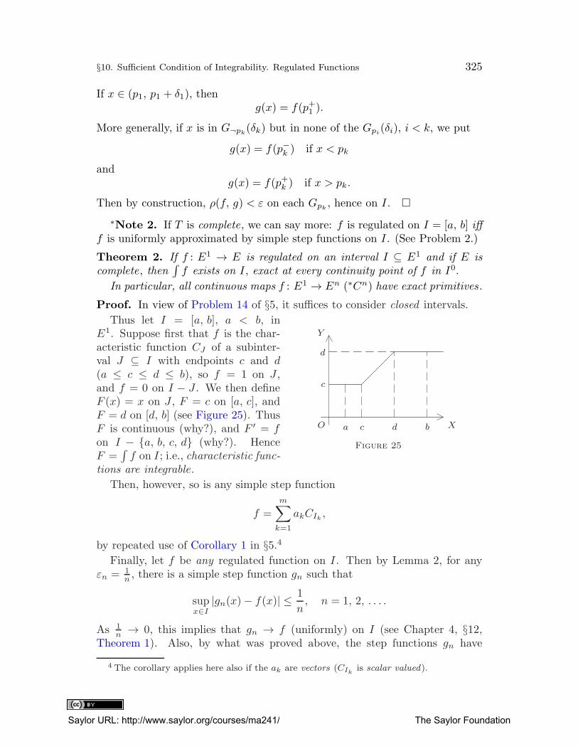
§10. Sufficient Condition of Integrability. Regulated Functions 325
If x ∈ (p1, p1 + δ1), theng(x) = f(p+1 ).
More generally, if x is in G¬pk(δk) but in none of the Gpi
(δi), i < k, we put
g(x) = f(p−k ) if x < pk
andg(x) = f(p+k ) if x > pk.
Then by construction, ρ(f, g) < ε on each Gpk, hence on I. �
∗Note 2. If T is complete, we can say more: f is regulated on I = [a, b] ifff is uniformly approximated by simple step functions on I. (See Problem 2.)
Theorem 2. If f : E1 → E is regulated on an interval I ⊆ E1 and if E is
complete, then∫
f exists on I, exact at every continuity point of f in I0.
In particular, all continuous maps f : E1 → En (∗Cn) have exact primitives.
Proof. In view of Problem 14 of §5, it suffices to consider closed intervals.
O
Y
Xa c d b
c
d
Figure 25
Thus let I = [a, b], a < b, inE1. Suppose first that f is the char-acteristic function CJ of a subinter-val J ⊆ I with endpoints c and d(a ≤ c ≤ d ≤ b), so f = 1 on J ,and f = 0 on I − J . We then defineF (x) = x on J , F = c on [a, c], andF = d on [d, b] (see Figure 25). ThusF is continuous (why?), and F ′ = fon I − {a, b, c, d} (why?). HenceF =
∫
f on I; i.e., characteristic func-tions are integrable.
Then, however, so is any simple step function
f =m∑
k=1
akCIk ,
by repeated use of Corollary 1 in §5.4Finally, let f be any regulated function on I. Then by Lemma 2, for any
εn = 1n , there is a simple step function gn such that
supx∈I|gn(x)− f(x)| ≤
1
n, n = 1, 2, . . . .
As 1n→ 0, this implies that gn → f (uniformly) on I (see Chapter 4, §12,
Theorem 1). Also, by what was proved above, the step functions gn have
4 The corollary applies here also if the ak are vectors (CIk is scalar valued).
Saylor URL: http://www.saylor.org/courses/ma241/ The Saylor Foundation
326 Chapter 5. Differentiation and Antidifferentiation
antiderivatives, hence so has f (Theorem 2 in §9); i.e., F =∫
f exists on I, asclaimed. Moreover,
∫
f is exact at continuity points of f in I0 (Problem 10 in§5). �
In view of the sufficient condition expressed in Theorem 2, we can now re-place the assumption “
∫
f exists” in our previous theorems by “f is regulated”(provided E is complete). For example, let us now review Problems 7 and 8in §5.Theorem 3 (weighted law of the mean). Let f : E1 → E (E complete) and
g : E1 → E1 be regulated on I = [a, b], with g ≥ 0 on I.5 Then the following
are true:
(i) There is a finite c ∈ E (called the “g-weighted mean of f on I”) such
that∫ b
agf = c
∫ b
ag.
(ii) If f , too, is real and has the Darboux property on I, then c = f(q) for
some q ∈ I.
Proof. Indeed, as f and g are regulated, so is gf by Theorem 1. Hence byTheorem 2,
∫
f and∫
gf exist on I. The rest follows as in Problems 7 and 8of §5. �
Theorem 4 (second law of the mean). Suppose f and g are real , f is monotone
with f =∫
f ′ on I, and g is regulated on I; I = [a, b]. Then
∫ b
a
fg = f(a)
∫ q
a
g + f(b)
∫ b
q
g for some q ∈ I. (1)
Proof. To fix ideas, let f↑; i.e., f ′ ≥ 0 on I.
The formula f =∫
f ′ means that f is relatively continuous (hence regulated)on I and differentiable on I −Q (Q countable). As g is regulated,
∫ x
a
g = G(x)
does exist on I, so G has similar properties, with G(a) =∫ a
ag = 0.
By Theorems 1 and 2,∫
fG′ =∫
fg exists on I. (Why?) Hence byCorollary 5 in §5, so does
∫
Gf ′, and we have
∫ b
a
fg =
∫ b
a
fG′ = f(x)G(x)∣
∣
∣
b
a−
∫ b
a
Gf ′ = f(b)G(b)−∫ b
a
Gf ′.
Now G has the Darboux property on I (being relatively continuous), and
5 One can also assume g ≤ 0 on I; in this case, simply apply the theorem to −g.
Saylor URL: http://www.saylor.org/courses/ma241/ The Saylor Foundation
§10. Sufficient Condition of Integrability. Regulated Functions 327
f ′ ≥ 0. Also,∫
G and∫
Gf ′ exist on I. Thus by Problems 7 and 8 in §5,∫ b
a
Gf ′ = G(q)
∫ b
a
f ′ = G(q)f(x)∣
∣
∣
b
a, q ∈ I.
Combining all, we obtain the required result (1) since∫
fg = f(b)G(b)−∫ b
a
Gf ′
= f(b)G(b)− f(b)G(q) + f(a)G(q)
= f(b)
∫ b
q
g + f(a)
∫ q
a
g. �
We conclude with an application to infinite series. Given f : E1 → E, wedefine
∫ ∞
a
f = limx→+∞
∫ x
a
f and
∫ a
−∞f = lim
x→−∞
∫ a
x
f
if these integrals and limits exist.
We say that∫∞af and
∫ a
−∞ f converge iff they exist and are finite.
Theorem 5 (integral test of convergence). If f : E1 → E1 is nonnegative and
nonincreasing on I = [a, +∞), then
∫ ∞
a
f converges iff
∞∑
n=1
f(n) does .
Proof. As f↓, f is regulated, so∫
f exists on I = [a, +∞). We fix somenatural k ≥ a and define
F (x) =
∫ x
k
f for x ∈ I.
By Theorem 3(iii) in §5, F↑ on I. Thus by monotonicity,
limx→+∞
F (x) = limx→+∞
∫ x
k
f =
∫ ∞
k
f
exists in E∗; so does∫ k
af . Since
∫ x
a
f =
∫ k
a
f +
∫ x
k
f,
where∫ k
af is finite by definition, we have
∫ ∞
a
f < +∞ iff
∫ ∞
k
f < +∞.
Saylor URL: http://www.saylor.org/courses/ma241/ The Saylor Foundation
328 Chapter 5. Differentiation and Antidifferentiation
Similarly,∞∑
n=1
f(n) < +∞ iff
∞∑
n=k
f(n) < +∞.
Thus we may replace “a” by “k.”
Let
In = [n, n+ 1), n = k, k + 1, . . . ,
and define two step functions, g and h, constant on each In, by
h = f(n) and g = f(n+ 1) on In, n ≥ k.
Since f↓, we have g ≤ f ≤ h on all In, hence on J = [k, +∞). Therefore,
∫ x
k
g ≤∫ x
k
f ≤∫ x
k
h for x ∈ J .
Also,∫ m
k
h =
m−1∑
n=k
∫ n+1
n
h =
m−1∑
n=k
f(n),
since h = f(n) (constant) on [n, n+ 1), and so
∫ n+1
n
h(x) dx = f(n)
∫ n+1
n
1 dx = f(n) · x∣
∣
∣
n+1
n= f(n)(n+ 1− n) = f(n).
Similarly,∫ m
k
g =m−1∑
n=k
f(n+ 1) =m∑
n=k+1
f(n).
Thus we obtain
m∑
n=k+1
f(n) =
∫ m
k
g ≤∫ m
k
f ≤∫ m
k
h =
m−1∑
n=k
f(n),
or, letting m→∞,
∞∑
n=k+1
f(n) ≤∫ ∞
k
f ≤∞∑
n=k
f(n).
Hence∫∞kf is finite iff
∞∑
n=1
f(n) is, and all is proved. �
Saylor URL: http://www.saylor.org/courses/ma241/ The Saylor Foundation
§10. Sufficient Condition of Integrability. Regulated Functions 329
Examples (continued).
(f) Consider the hyperharmonic series
∑ 1
np(Problem 2 of Chapter 4, §13).
Let
f(x) =1
xp, x ≥ 1.
If p = 1, then f(x) = 1/x, so∫ x
1f = lnx→ +∞ as x → +∞. Hence
∑
1/n diverges.
If p 6= 1, then∫ ∞
1
f = limx→+∞
∫ x
1
f = limx→+∞
x1−p
1− p∣
∣
∣
x
1,
so∫∞1f converges or diverges according as p > 1 or p < 1, and the same
applies to the series∑
1/np.
(g) Even nonregulated functions may be integrable. Such is Dirichlet’s func-
tion (Example (c) in Chapter 4, §1). Explain, using the countability ofthe rationals.
Problems on Regulated Functions
In Problems 2, 5, 6, and 8, we drop the restriction that f(p−) and f(p+) arefinite. We only require them to exist in (T, p). If T = E∗, a suitable metricfor E∗ is presupposed.
1. Complete all details in the proof of Theorems 1–3.
1′ Explain Examples (a)–(g).
∗2. Prove Note 2. More generally, assuming T to be complete, prove that if
gn → f (uniformly) on I = [a, b]
and if the gn are regulated on I, so is f .[Hint: Fix p ∈ (a, b]. Use Theorem 2 of Chapter 4, §11 with
X = [a, p], Y = N ∪ {+∞}, q = +∞, and F (x, n) = gn(x).
Thus show that
f(p−) = limx→p−
limn→∞
gn(x) exists;
similarly for f(p+).]
3. Given f, g : E1 → E1, define f ∨ g and f ∧ g as in Problem 12 of Chap-ter 4, §8. Using the hint given there, show that f ∨ g and f ∧ g areregulated if f and g are.
Saylor URL: http://www.saylor.org/courses/ma241/ The Saylor Foundation
330 Chapter 5. Differentiation and Antidifferentiation
4. Show that the function g ◦ f need not be regulated even if g and f are.[Hint: Let
f(x) = x · sin 1
x, g(x) =
x
|x| , and f(0) = g(0) = 0 with I = [0, 1].
Proceed.]
⇒5. Given f : E1 → (T, ρ), regulated on I, put
j(p) = max{
ρ(
f(p), f(p−))
, ρ(
f(p), f(p+))
, ρ(
f(p−), f(p+))}
;
call it the jump at p.
(i) Prove that f is discontinuous at p ∈ I0 iff j(p) > 0, i.e., iff
(∃n ∈ N) j(p) >1
n.
(ii) For a fixed n ∈ N , prove that a closed subinterval J ⊆ I containsat most finitely many x with j(x) > 1/n.[Hint: Otherwise, there is a sequence of distinct points xm ∈ J, j(xm) > 1
n,
hence a subsequence xmk→ p ∈ J. (Why?) Use Theorem 1 of Chapter 4, §2,
to show that f(p−) or f(p+) fails to exist.]
⇒6. Show that if f : E1 → (T, ρ) is regulated on I, then it has at most count-ably many discontinuities in I; all are of the “jump” type (Problem 5).[Hint: By Problem 5, any closed subinterval J ⊆ I contains, for each n, at most
finitely many discontinuities x with j(x) > 1/n. Thus for n = 1, 2, . . . , obtain
countably many such x.]
7. Prove that if E is complete, all maps f : E1 → E, with Vf [I] < +∞ onI = [a, b], are regulated on I.[Hint: Use Corollary 1, Chapter 4, §2, to show that f(p−) and f(p+) exist.
Say,
xn → p with xn < p (xn, p ∈ I),
but {f(xn)} is not Cauchy. Then find a subsequence, {xnk}↑, and ε > 0 such that
|f(xnk+1)− f(xnk
) |≥ ε, k = 1, 3, 5, . . . .
Deduce a contradiction to Vf [I] < +∞.
Provide a similar argument for the case xn > p.]
8. Prove that if f : E1 → (T, ρ) is regulated on I, then f [B] (the closureof f [B]) is compact in (T, ρ) whenever B is a compact subset of I.
[Hint: Given {zm} in f [B], find {ym} ⊆ f [B] such that ρ(zm, ym) → 0 (use
Theorem 3 of Chapter 3, §16). Then “imitate” the proof of Theorem 1 in Chap-ter 4, §8 suitably. Distinguish the cases:
(i) all but finitely many xm are < p;
(ii) infinitely many xm exceed p; or
(iii) infinitely many xm equal p.]
Saylor URL: http://www.saylor.org/courses/ma241/ The Saylor Foundation
§11. Integral Definitions of Some Functions 331
§11. Integral Definitions of Some Functions
By Theorem 2 in §10,∫
f exists on I whenever the function f : E1 → E isregulated on I, and E is complete. Hence whenever such an f is given, we candefine a new function F by setting
F =
∫ x
a
f
on I for some a ∈ I. This is a convenient method of obtaining new continuousfunctions, differentiable on I−Q (Q countable). We shall now apply it to obtainnew definitions of some functions previously defined in a rather strenuous step-by-step manner.
I. Logarithmic and Exponential Functions. From our former defini-tions, we proved that
lnx =
∫ x
1
1
tdt, x > 0.
Now we want to treat this as a definition of logarithms. We start by setting
f(t) =1
t, t ∈ E1, t 6= 0,
and f(0) = 0.
Then f is continuous on I = (0, +∞) and J = (−∞, 0), so it has an exact
primitive on I and J separately (not on E1). Thus we can now define the logfunction on I by
∫ x
1
1
tdt = log x (also written lnx) for x > 0. (1)
By the very definition of an exact primitive, the log function is continuousand differentiable on I = (0, +∞); its derivative on I is f . Thus we again havethe symbolic formula
(log x)′ =1
x, x > 0.
If x < 0, we can consider log(−x). Then the chain rule (Theorem 3 of §1)yields
(log(−x))′ = 1
x. (Verify!)
Hence
(log |x|)′ = 1
xfor x 6= 0. (2)
Other properties of logarithms easily follow from (1). We summarize themnow.
Saylor URL: http://www.saylor.org/courses/ma241/ The Saylor Foundation
332 Chapter 5. Differentiation and Antidifferentiation
Theorem 1.
(i) log 1 =
∫ 1
1
1
tdt = 0.
(ii) log x < log y whenever 0 < x < y.
(iii) limx→+∞
log x = +∞ and limx→0+
log x = −∞.
(iv) The range of log is all of E1.
(v) For any positive x, y ∈ E1,
log(xy) = log x+ log y and log(x
y
)
= log x− log y.
(vi) log ar = r · log a, a > 0, r ∈ N .
(vii) log e = 1, where e = limn→∞
(
1 +1
n
)n
.
Proof.
(ii) By (2), (log x)′ > 0 on I = (0, +∞), so log x is increasing on I.
(iii) By Theorem 5 in §10,
limx→+∞
log x =
∫ ∞
1
1
tdt = +∞
since∞∑
n=1
1
n= +∞ (Chapter 4, §13, Example (b)).
Hence, substituting y = 1/x, we obtain
limy→0+
log y = limx→+∞
log1
x.
However, by Theorem 2 in §5 (substituting s = 1/t),
log1
x=
∫ 1/x
1
1
tdt = −
∫ x
1
1
sds = − log x.
Thus
limy→0+
log y = limx→+∞
log1
x= − lim
x→+∞log x = −∞
as claimed. (We also proved that log 1x = − log x.)
(iv) Assertion (iv) now follows by the Darboux property (as in Chapter 4, §9,Example (b)).
Saylor URL: http://www.saylor.org/courses/ma241/ The Saylor Foundation
§11. Integral Definitions of Some Functions 333
(v) With x, y fixed, we substitute t = xs in∫ xy
1
1
tdt = log xy
and obtain
log xy =
∫ xy
1
1
tdt =
∫ y
1/x
1
sds
=
∫ 1
1/x
1
sds+
∫ y
1
1
sds
= − log1
x+ log y
= log x+ log y.
Replacing y by 1/y here, we have
logx
y= log x+ log
1
y= log x− log y.
Thus (v) is proved, and (vi) follows by induction over r.
(vii) By continuity,
log e = limx→e
log x = limn→∞
log(
1 +1
n
)n
= limn→∞
log(1 + 1/n)
1/n,
where the last equality follows by (vi). Now, L’Hopital’s rule yields
limx→0
log(1 + x)
x= lim
x→0
1
1 + x= 1.
Letting x run over 1n → 0, we get (vii). �
Note 1. Actually, (vi) holds for any r ∈ E1, with ar as in Chapter 2,§§11–12. One uses the techniques from that section to prove it first for rationalr, and then it follows for all real r by continuity. However, we prefer not to usethis now.
Next, we define the exponential function (“exp”) to be the inverse of thelog function. This inverse function exists; it is continuous (even differentiable)and strictly increasing on its domain (by Theorem 3 of Chapter 4, §9 andTheorem 3 of Chapter 5, §2) since the log function has these properties. From(log x)′ = 1/x we get, as in §2,
(expx)′ = expx (cf. §2, Example (B)). (3)
The domain of the exponential is the range of its inverse, i.e., E1 (cf. Theo-rem 1(iv)). Thus expx is defined for all x ∈ E1. The range of exp is the domain
Saylor URL: http://www.saylor.org/courses/ma241/ The Saylor Foundation
334 Chapter 5. Differentiation and Antidifferentiation
of log, i.e., (0, +∞). Hence expx > 0 for all x ∈ E1. Also, by definition,
exp(log x) = x for x > 0, (4)
exp 0 = 1 (cf. Theorem 1(i)), and (5)
exp r = er for r ∈ N. (6)
Indeed, by Theorem 1(vi) and (vii), log er = r · log e = r. Hence (6) follows.If the definitions and rules of Chapter 2, §§11–12 are used, this proof evenworks for any r by Note 1. Thus our new definition of exp agrees with the old
one.
Our next step is to give a new definition of ar, for any a, r ∈ E1 (a > 0).We set
ar = exp(r · log a) or (7)
log ar = r · log a (r ∈ E1). (8)
In case r ∈ N , (8) becomes Theorem 1(vi). Thus for natural r, our newdefinition of ar is consistent with the previous one. We also obtain, for a, b > 0,
(ab)r = arbr; ars = (ar)s; ar+s = aras; (r, s ∈ E1). (9)
The proof is by taking logarithms. For example,
log(ab)r = r log ab = r(log a+ log b) = r · log a+ r · log b= log ar + log br = log(arbr).
Thus (ab)r = arbr. Similar arguments can be given for the rest of (9) and otherlaws stated in Chapter 2, §§11–12.
We can now define the exponential to the base a (a > 0) and its inverse, loga,as before (see the example in Chapter 4, §5 and Example (b) in Chapter 4, §9).The differentiability of the former is now immediate from (7), and the restfollows as before.
II. Trigonometric Functions. These shall now be defined in a preciseanalytic manner (not based on geometry).
We start with an integral definition of what is usually called the principal
value of the arcsine function,
arcsinx =
∫ x
0
1√1− t2
dt.
We shall denote it by F (x) and set
f(x) =1√
1− x2on I = (−1, 1).
(F = f = 0 on E1 − I.) Thus by definition, F =∫
f on I.
Saylor URL: http://www.saylor.org/courses/ma241/ The Saylor Foundation
§11. Integral Definitions of Some Functions 335
Note that∫
f exists and is exact on I since f is continuous on I. Thus
F ′(x) = f(x) =1√
1− x2> 0 for x ∈ I,
and so F is strictly increasing on I. Also, F (0) =∫ 0
0f = 0.
We also define the number π by setting
π
2= 2 arcsin
√
1
2= 2F (c) = 2
∫ c
0
f, c =
√
1
2. (10)
Then we obtain the following theorem.
Theorem 2. F has the limits
F (1−) =π
2and F (−1+) = −π
2.
Thus F becomes relatively continuous on I = [−1, 1] if one sets
F (1) =π
2and F (−1) = −π
2,
i .e.,
arcsin 1 =π
2and arcsin(−1) = −π
2. (11)
Proof. We have
F (x) =
∫ x
0
f =
∫ c
0
f +
∫ x
c
f, c =
√
1
2.
By substituting s =√1− t2 in the last integral and setting, for brevity, y =√
1− x2 , we obtain∫ x
c
f =
∫ x
c
1√1− t2
dt =
∫ c
y
1√1− s2
ds = F (c)− F (y). (Verify!)
Now as x → 1−, we have y =√1− x2 → 0, and hence F (y) → F (0) = 0 (for
F is continuous at 0). Thus
F (1−) = limx→1−
F (x) = limy→0
(
∫ c
0
f +
∫ c
y
f)
=
∫ c
0
f + F (c) = 2
∫ c
0
f =π
2.
Similarly, one gets F (−1+) = −π/2. �
The function F as redefined in Theorem 2 will be denoted by F0. It isa primitive of f on the closed interval I (exact on I). Thus F0(x) =
∫ x
0f ,
−1 ≤ x ≤ 1, and we may now write
π
2=
∫ 1
0
f and π =
∫ 0
−1
f +
∫ 1
0
f =
∫ 1
−1
f .
Saylor URL: http://www.saylor.org/courses/ma241/ The Saylor Foundation
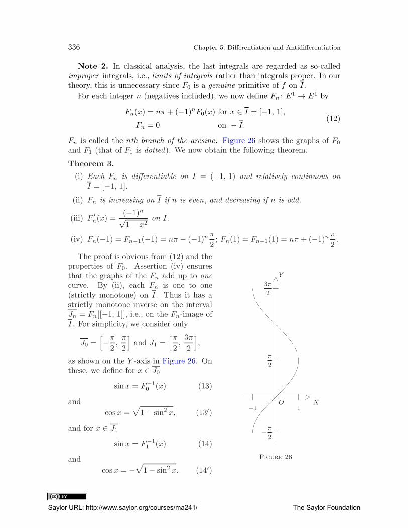
336 Chapter 5. Differentiation and Antidifferentiation
Note 2. In classical analysis, the last integrals are regarded as so-calledimproper integrals, i.e., limits of integrals rather than integrals proper. In ourtheory, this is unnecessary since F0 is a genuine primitive of f on I.
For each integer n (negatives included), we now define Fn : E1 → E1 by
Fn(x) = nπ + (−1)nF0(x) for x ∈ I = [−1, 1],Fn = 0 on − I.
(12)
Fn is called the nth branch of the arcsine. Figure 26 shows the graphs of F0
and F1 (that of F1 is dotted). We now obtain the following theorem.
Theorem 3.
(i) Each Fn is differentiable on I = (−1, 1) and relatively continuous on
I = [−1, 1].(ii) Fn is increasing on I if n is even, and decreasing if n is odd .
(iii) F ′n(x) =
(−1)n√1− x2
on I.
(iv) Fn(−1) = Fn−1(−1) = nπ − (−1)nπ2; Fn(1) = Fn−1(1) = nπ + (−1)nπ
2.
O
Y
X
−π
2
π
2
3π
2
−1 1
Figure 26
The proof is obvious from (12) and theproperties of F0. Assertion (iv) ensuresthat the graphs of the Fn add up to one
curve. By (ii), each Fn is one to one(strictly monotone) on I. Thus it has astrictly monotone inverse on the intervalJn = Fn[[−1, 1]], i.e., on the Fn-image ofI. For simplicity, we consider only
J0 =[
−π2,π
2
]
and J1 =[π
2,3π
2
]
,
as shown on the Y -axis in Figure 26. Onthese, we define for x ∈ J0
sinx = F−10 (x) (13)
and
cosx =√
1− sin2 x, (13′)
and for x ∈ J1sinx = F−1
1 (x) (14)
and
cosx = −√
1− sin2 x. (14′)
Saylor URL: http://www.saylor.org/courses/ma241/ The Saylor Foundation
§11. Integral Definitions of Some Functions 337
On the rest of E1, we define sinx and cosx periodically by setting
sin(x+ 2nπ) = sinx and cos(x+ 2nπ) = cosx, n = 0, ±1, ±2, . . . . (15)
Note that by Theorem 3(iv),
F−10
(π
2
)
= F−11
(π
2
)
= 1.
Thus (13) and (14) both yield sinπ/2 = 1 for the common endpoint π/2 of J0and J1, so the two formulas are consistent. We also have
sin(
−π2
)
= sin(3π
2
)
= −1,
in agreement with (15). Thus the sine and cosine functions (briefly, s and c)are well defined on E1.
Theorem 4. The sine and cosine functions (s and c) are differentiable, hencecontinuous , on all of E1, with derivatives s′ = c and c′ = −s; that is ,
(sinx)′ = cosx and (cosx)′ = − sinx.
Proof. It suffices to consider the intervals J0 and J1, for, by (15), all propertiesof s and c repeat themselves, with period 2π, on the rest of E1.
By (13),
s = F−10 on J0 =
[
−π2,π
2
]
,
where F0 is differentiable on I = (−1, 1). Thus Theorem 3 of §2 shows that sis differentiable on J0 = (−π/2, π/2) and that
s′(q) =1
F ′0(p)
whenever p ∈ I and q = F0(p);
i.e., q ∈ J and p = s(q). However, by Theorem 3(iii),
F ′0(p) =
1√
1− p2.
Hence
s′(q) =√
1− sin2 q = cos q = c(q), q ∈ J.
This proves the theorem for interior points of J0 as far as s is concerned.
As
c =√
1− s2 = (1− s2) 12 on J0 (by (13)),
we can use the chain rule (Theorem 3 in §1) to obtain
c′ =1
2(1− s2)− 1
2 (−2s)s′ = −s
Saylor URL: http://www.saylor.org/courses/ma241/ The Saylor Foundation
338 Chapter 5. Differentiation and Antidifferentiation
on noting that s′ = c = (1− s2) 12 on J0. Similarly, using (14), one proves that
s′ = c and c′ = −s on J1 (interior of J1).
Next, let q be an endpoint , say, q = π/2. We take the left derivative
s′−(q) = limx→q−
s(x)− s(q)x− q , x ∈ J0.
By L’Hopital’s rule, we get
s′−(q) = limx→q−
s′(x)
1= lim
x→q−
c(x)
since s′ = c on J0. However, s = F−10 is left continuous at q (why?); hence so
is c =√1− s2. (Why?) Therefore,
s′−(q) = limx→q−
c(x) = c(q), as required.
Similarly, one shows that s′+(q) = c(q). Hence s′(q) = c(q) and c′(q) = −s(q),as before. �
The other trigonometric functions reduce to s and c by their defining for-mulas
tanx =sinx
cosx, cot x =
cosx
sinx, secx =
1
cosx, and cosecx =
1
sinx,
so we shall not dwell on them in detail. The various trigonometric laws easilyfollow from our present definitions; for hints, see the problems below.
Problems on Exponential and Trigonometric Functions
1. Verify formula (2).
2. Prove Note 1, as suggested (using Chapter 2, §§11–12).3. Prove formulas (1) of Chapter 2, §§11–12 from our new definitions.
4. Complete the missing details in the proofs of Theorems 2–4.
5. Prove that
(i) sin 0 = sin(nπ) = 0;
(ii) cos 0 = cos(2nπ) = 1;
(iii) sinπ
2= 1;
(iv) sin(
−π2
)
= −1;
(v) cos(
±π2
)
= 0;
(vi) | sinx| ≤ 1 and | cosx| ≤ 1 for x ∈ E1.
Saylor URL: http://www.saylor.org/courses/ma241/ The Saylor Foundation
§11. Integral Definitions of Some Functions 339
6. Prove that
(i) sin(−x) = − sinx and
(ii) cos(−x) = cosx for x ∈ E1.
[Hint: For (i), let h(x) = sin x+sin(−x). Show that h′ = 0; hence h is constant, say,
h = q on E1. Substitute x = 0 to find q. For (ii), use (13)–(15).]
7. Prove the following for x, y ∈ E1:
(i) sin(x+ y) = sinx cos y + cosx sin y; hence sin(
x+π
2
)
= cosx.
(ii) cos(x+ y) = cosx cos y − sinx sin y; hence cos(
x+π
2
)
= − sinx.
[Hint for (i): Fix x, y and let p = x+ y. Define h : E1 → E1 by
h(t) = sin t cos(p− t) + cos t sin(p− t), t ∈ E1.
Proceed as in Problem 6. Then let t = x.]
8. With Jn as in the text, show that the sine increases on Jn if n is evenand decreases if n is odd. How about the cosine? Find the endpointsof Jn.
Saylor URL: http://www.saylor.org/courses/ma241/ The Saylor Foundation

Saylor URL: http://www.saylor.org/courses/ma241/ The Saylor Foundation
Index
Abel’s convergence test, 247
Abel’s theorem for power series, 249, 322
Absolute value
in an ordered field, 26
in En, 64in Euclidean spaces, 88
in normed linear spaces, 90
Absolutely continuous functions (weakly),
309
Absolutely convergent series of functions,
237
rearrangement of, 238tests for, 239
Accumulation points, 115. See also Cluster
point
Additivityof definite integrals, 282
of total variation, 301
of volume of intervals in En, 79
Alternating series, 248
Admissible change of variable, 165
Angle between vectors in En, 70
Antiderivative, 278. See also Integral, in-
definite
Antidifferentiation, 278. See also Integra-tion
Arcs, 211
as connected sets, 214
endpoints of, 211length of, 301, 311
rectifiable, 309simple, 211
Archimedean field, see Field, Archimedean
Archimedean property, 43
Arcwise connected set, 211
Arithmetic-geometric mean, Gauss’s, 134
Associative laws
in a field, 23of vector addition in En, 65
Axioms
of arithmetic in a field, 23of a metric, 95
of order in an ordered field, 24
Basic unit vector in En, 64
Bernoulli inequalities, 33
Binary operations, 12. See also Functions
Binomial theorem, 34
Bolzano theorem, 205
Bolzano–Weierstrass theorem, 136
Boundaryof intervals in En, 77
of sets in metric spaces, 108
Boundedfunctions on sets in metric spaces, 111
sequences in metric spaces, 111sets in metric spaces, 109
sets in ordered fields, 36
variation, 303left-bounded sets in ordered fields, 36
right-bounded sets in ordered fields, 36
totally bounded sets in a metric space,188
uniformly bounded sequences of func-tions, 234
C (the complex field), 80complex numbers, 81; see also Complex
numbers
Cartesian coordinates in, 83de Moivre’s formula, 84
imaginary numbers in, 81
imaginary unit in, 81is not an ordered field, 82
polar coordinates in, 83real points in, 81
real unit in, 81
Cn (complex n-space), 87as a Euclidean space, 88
as a normed linear space, 91componentwise convergence of sequences
in, 121
Saylor URL: http://www.saylor.org/courses/ma241/ The Saylor Foundation
342 Index
dot products in, 87standard norm in, 91
Cantor’s diagonal process, 21. See also
Sets
Cantor’s function, 186
Cantor’s principle of nested closed sets,
188
Cantor’s set, 120
Cartesian coordinates in C, 83
Cartesian product of sets (×), 2
intervals in En as Cartesian products ofintervals in E1, 76
Cauchy criterionfor function limits, 162
for uniform convergence of sequences of
functions, 231
Cauchy form of the remainder term of
Taylor expansions, 291
Cauchy sequences in metric spaces, 141
Cauchy’s convergence criterion for se-
quences in metric spaces, 143
Cauchy’s laws of the mean, 261
Cauchy-Schwarz inequalityin En, 67
in Euclidean spaces, 88
Center of an interval in En, 77
Change of variable, admissible, 165
Chain rule for differentiation of composite
functions, 255
Change of variables in definite integrals,
282
Characteristic functions of sets, 323
Clopensets in metric spaces, 103
Closedcurve, 211
globe in a metric space, 97
interval in an ordered field, 37interval in En, 77
line segment in En, 72
sets in metric spaces, 103, 138
Closures of sets in metric spaces, 137
Closure laws
in a field, 23
in En, 65of integers in a field, 35
of rationals in a field, 35
Cluster points
of sequences in E∗, 60of sequences and sets in metric spaces,
115
Commutative lawsin a field, 23
of addition of vectors in En, 65
of inner products of vectors in En, 67
Compact sets, 186, 193
Cantor’s principle of nested closed sets,
188are totally bounded, 188
in E1, 195
continuity on, 194generalized Heine–Borel theorem, 193
Heine–Borel theorem, 324sequentially, 186
Comparison test, 239
refined, 245
Complement of a set (−), 2
Completemetric spaces, 143
ordered fields, 38; see also Field, com-
plete ordered
Completeness axiom, 38
Completion of metric spaces, 146
Complex exponential, 173
derivatives of the, 256
Complex field, see C
Complex functions, 170
Complex numbers, 81. See also C
conjugate of, 81
imaginary part of, 81nth roots of, 85
polar form of, 83
real part of, 81trigonometric form of, 83
Complex vector spaces, 87
Componentwisecontinuity of functions, 172
convergence of sequences, 121
differentiation, 256integration, 282
limits of functions, 172
Composite functions, 163
chain rule for derivatives of, 255
continuity of, 163
Concurrent sequences, 144
Conditionally convergent series of func-
tions, 237
rearrangement of, 250
Conjugate of complex numbers, 81
Connected sets, 212
arcs as, 214
Saylor URL: http://www.saylor.org/courses/ma241/ The Saylor Foundation
Index 343
arcwise-, 211curves as, 214
polygon-, 204
Continuous functions
on metric spaces, 149
differentiable functions are, 252left, 153
relatively, 152
right, 153uniformly, 197
(weakly) absolutely continuous, 309
Continuity. See also Continuous functions
componentwise, 172
in one variable, 174jointly, 174
of addition and multiplication in E1, 168
of composite functions, 163of inverse functions, 195, 207
of the exponential function, 184of the logarithmic function, 208
of the power function, 209
of the standard metric on E1, 168of the sum, product, and quotient of
functions, 170
on compact sets, 194sequential criterion for, 161
uniform, 197
Contracting sequence of sets, 17
Contraction mapping, 198
Convergence of sequences of functionsCauchy criterion for uniform, 231
convergence of integrals and derivatives,315
pointwise, 228
uniform, 228
Convergence radius of power series, 243
Convergence tests for seriesAbel’s test, 247
comparison test, 239
Dirichlet test, 248integral test, 327
Leibniz test for alternating series, 248
ratio test, 241refined comparison test, 245
root test, 241Weierstrass M-test for functions, 240
Convergent
absolutely convergent series of functions,237
conditionally convergent series of func-tions, 237
sequences of functions, 228; see also
Limits of sequences of functionssequences in metric spaces, 115
series of functions, 228; see also Limits
of series of functions
Convex sets, 204
piecewise, 204
Coordinate equations of a line in En, 72
Countable set, 18
rational numbers as a, 19
Countable union of sets, 20
Covering, open, 192
Cross product of sets (×), 2
Curves, 211
as connected sets, 214closed, 211
length of, 300parametric equations of, 212
tangent to, 257
Darboux property, 203
Bolzano theorem, 205
of the derivative, 265
de Moivre’s formula, 84
Definite integrals, 279additivity of, 282
change of variables in, 282
dominance law for, 284first law of the mean for, 285
integration by parts, 281
linearity of, 280monotonicity law for, 284
weighted law of the mean for, 286, 326
Degenerate intervals in En, 78
Degree
of a monomial, 173of a polynomial, 173
Deleted δ-globes about points in metricspaces, 150
Dense subsets in metric spaces, 139
Densityof an ordered field, 45
of rationals in an Archimedean field, 45
Dependent vectorsin En, 69
Derivatives of functions on E1, 251convergence of, 315
Darboux property of, 265
derivative of the exponential function,264
derivative of the inverse function, 263derivative of the logarithmic function,
263
Saylor URL: http://www.saylor.org/courses/ma241/ The Saylor Foundation
344 Index
derivative of the power function, 264with extended-real values, 259
left, 252
one-sided, 252right, 252
Derived functions on E1, 251
nth, 252
Diagonal of an interval in En, 77
Diagonal process, Cantor’s, 21. See also
Sets
Diameterof sets in metric spaces, 109
Difference
of elements of a field, 26of sets (−), 2
Differentials of functions on E1, 288
of order n, 289
Differentiable functions on E1, 251Cauchy’s laws of the mean, 261
cosine function, 337
are continuous, 252exponential function, 333
infinitely, 292logarithmic function, 332
n-times continuously, 292
n-times, 252nowhere, 253
Rolle’s theorem, 261
sine function, 337
Differentiation, 251
chain rule for, 255
componentwise, 256of power series, 319
rules for sums, products, and quotients,
256termwise differentiation of series, 318
Directed
lines in En, 74planes in En, 74
Direction vectors of lines in En, 71
Dirichlet function, 155, 329
Dirichlet test, 248
Disconnected sets, 212totally, 217
Discontinuity points of functions on metric
spaces, 149
Discontinuous functions on metric spaces,
149
Discretemetric, 96
metric space, 96
Disjoint sets, 2
Distance
between a point and a plane in En, 76
between sets in metric spaces, 110between two vectors in En, 64
between two vectors in Euclidean spaces,
89in normed linear spaces, 92
norm-induced, 92translation-invariant, 92
Distributive laws
in En, 65
in a field, 24of inner products of vectors in En, 67
of union and intersection of sets, 7
Divergentsequences in metric spaces, 115
Domain
of a relation, 9of a sequence, 15
space of functions on metric spaces, 149
Double limits of functions, 219, 221
Double sequence, 20, 222, 223
Dot product
in Cn, 87
in En, 64
Duality laws, de Morgan’s, 3. See also Sets
e (the number), 122, 165, 293
E1 (the real numbers), 23. See also Field,
complete orderedassociative laws in, 23
axioms of arithmetic in, 23
axioms of order in, 24closure laws in, 23
commutative laws in, 23
continuity of addition and multiplicationin, 168
continuity of the standard metric on,168
distributive law in, 24
inverse elements in, 24monotonicity in, 24
neighborhood of a point in, 58
natural numbers in, 28neutral elements in, 23
transitivity in, 24trichotomy in, 24
En (Euclidean n-space), 63. See also Vec-
tors in En
convex sets in, 204
as a Euclidean space, 88
Saylor URL: http://www.saylor.org/courses/ma241/ The Saylor Foundation
Index 345
as a normed linear space, 91associativity of vector addition in, 65
additive inverses of vector addition, 65
basic unit vector in, 64Bolzano-Weierstrass theorem, 136
Cauchy-Schwarz inequality in, 67closure laws in, 65
commutativity of vector addition in, 65
componentwise convergence of sequencesin, 121
distributive laws in, 65
globe in, 76hyperplanes in, 72; see also Planes in
En
intervals in, 76; see also Intervals in En
line segments in, 72; see also Line seg-
ments in En
linear functionals on, 74, 75; see also
Linear functionals on En
lines in, 71; see also Lines in En
neutral element of vector addition in, 65
planes in, 72; see also Planes in En
point in, 63
scalar of, 64
scalar product in, 64sphere in, 76
standard metric in, 96
standard norm in, 91triangle inequality of the absolute value
in, 67triangle inequality of the distance in, 68
unit vector in, 65
vectors in, 63zero vector in, 63
E∗ (extended real numbers), 53as a metric space, 98
cluster point of a sequence in, 60globes in, 98
indeterminate expressions in, 178
intervals in, 54limits of sequences in, 58
metrics for, 99
neighborhood of a point in, 58operations in, 177
unorthodox operations in, 180
Edge-lengths of an interval in En, 77
Elements of a set (∈), 1Empty set (∅), 1Endpoints
of an interval in En, 77
of line segments in En, 72
Equality of sets, 1
Equicontinuous functions, 236
Equivalence class relative to an equivalence
relation, 13generator of an, 13
representative of an, 13
Equivalence relation, 12equivalence class relative to an, 13
Euclidean n-space, see En
Euclidean spaces, 87as normed linear spaces, 91
absolute value in, 88Cn as a, 88
Cauchy-Schwarz inequality in, 88
distance in, 89En as a, 88
line segments in, 89
lines in, 89planes in, 89
triangle inequality in, 88
Exact primitive, 278
Existential quantifier (∃), 4Expanding sequence of sets, 17
Exponential, complex, 173
Exponential function, 183, 333continuity of the, 184
derivative of the, 264
inverse of the, 208
Extended real numbers, see E∗.
Factorials, definition of, 31
Family of sets, 3
intersection of a (⋂), 3
union of a (⋃), 3
Fields, 25associative laws in, 23
axioms of arithmetic in, 23
binomial theorem, 34closure laws in, 23
commutative laws in, 23
difference of elements in, 26distributive law in, 24
first induction law in, 28inductive definitions in, 31
inductive sets in, 28
integers in, 34inverse elements in, 24
irrationals in, 34
Lagrange identity in, 71natural elements in, 28
neutral elements in, 23quotients of elements in, 26
rational subfields of, 35
Saylor URL: http://www.saylor.org/courses/ma241/ The Saylor Foundation
346 Index
rationals in, 34
Fields, Archimedean, 43. See also Fields,
ordered
density of rationals in, 45integral parts of elements of, 44
Fields, complete ordered, 38. See also
Field, Archimedean
Archimedean property of, 43
completeness axiom, 38density of irrationals in, 51
existence of irrationals in, 46
powers with rational exponents in, 47powers with real exponents in, 50
principle of nested intervals in, 42roots in, 46
Fields, ordered, 25. See also Field
absolute value in, 26axioms of order in, 24
Bernoulli inequalities in, 33bounded sets in, 36
closed intervals in, 37
density of, 45greatest lower bound (glb) of sets in, 38
half-closed intervals in, 37
half-open intervals in, 37infimum (inf) of sets in, 38
intervals in, 37
least upper bound (lub) of sets in, 37monotonicity in, 24
negative elements in, 25open intervals in, 37
positive elements in, 25
rational subfield in, 35second induction law in, 30
supremum (sup) of sets in, 38
transitivity in, 24trichotomy in, 24
well-ordering of naturals in, 30
Finite
increments law, 271
intervals, 54sequence, 16
set, 18
First
induction law, 28
law of the mean, 285
Functions, 10. See also Functions on E1
and Functions on metric spaces
binary operations, 12bounded, 96
Cantor’s function, 186characteristic, 323
complex, 170
Dirichlet function, 155, 329equicontinuous, 236
graphs of, 153
isometry, 201limits of sequences of, see Limits of se-
quences of functionslimits of series of, see Limits of series of
functions
monotone, 181nondecreasing, 181
nonincreasing, 181
one-to-one, 10onto, 11
product of, 170quotient of, 170
real, 170
scalar-valued, 170sequences of, 227; see also Sequences of
functions
series of, 228; see also Limits of series offunctions
signum function (sgn), 156strictly monotone, 182
sum of, 170
function value, 10uniformly continuous, 197
vector-valued, 170
Functions on E1
antiderivatives of, 278
definite integrals of, 279derivatives of, 251
derived, 251
differentials of, 288; see also Differentialsof functions on E1
differentiable, 251; see also Differentiable
functions on E1
exact primitives of, 278
of bounded variation, 303indefinite integrals of, 278
integrable, 278; see also Integrable func-
tions on E1
length of, 301
Lipschitz condition for, 258
negative variation functions for, 308nowhere differentiable, 253
positive variation functions for, 308primitives of, 278
regulated, see Regulated functions
simple step, 323step, 323
total variation of, 301
(weakly) absolutely continuous, 309
Functions on metric spaces,149
Saylor URL: http://www.saylor.org/courses/ma241/ The Saylor Foundation
Index 347
bounded, 111continuity of composite, 163
continuity of the sum, product, and quo-
tient of, 170continuous, 149
discontinuous, 149discontinuity points of, 149
domain space of, 149
limits of, 150projection maps, 174, 198, 226
range space of, 149
General term of a sequence, 16
Generator of an equivalence class, 13
Geometric series
limit of, 128, 236sum of n terms of a, 33
Globesclosed globes in metric spaces, 97
deleted δ-globes about points in metric
spaces, 150in En, 76
in E∗, 98
open globes in metric space, 97
Graphs of functions, 153
Greatest lower bound (glb) of a set in anordered field, 38
Half-closed
interval in an ordered field, 37
interval in En, 77line segment in En, 72
Half-openinterval in an ordered field, 37
interval in En, 77
line segment in En, 72
Harmonic series, 241
Hausdorff property, 102
Heine–Borel theorem, 324
generalized, 193
Holder’s inequality, 93
Hyperharmonic series, 245, 329
Hyperplanes in En, 72. See also Planes inEn
iff (“if and only if”), 1
Image
of a set under a relation, 9
Imaginary
part of complex numbers, 81numbers in C, 81
unit in C, 81
Inclusion relation of sets (⊆), 1
Incrementsfinite increments law, 271
of a function, 254
Independentvectors in En, 70
Indeterminate expressions in E∗, 178
Index notation, 16. See also Sequence
Induction, 27
first induction law, 28inductive definitions, 31; see also Induc-
tive definitionsproof by, 29
second induction law, 30
Inductive definitions, 31
factorial, 31powers with natural exponents, 31
ordered n-tuple, 32products of n field elements, 32
sum of n field elements, 32
Inductive sets in a field, 28
Infimum (inf) of a set in an ordered field,38
Infinite
countably, 21intervals, 54
sequence, 15
set, 18
Infinityplus and minus, 53
unsigned, 179
Inner products of vectors in En, 64commutativity of, 67
distributive law of, 67
Integers in a field, 34closure of addition and multiplication of,
35
Integrability, sufficient conditions for, 322.
See also Regulated functions on inter-vals in E1
Integrable functions on E1, 278. See also
Regulated functions on intervals in E1
Dirichlet function, 329
primitively, 278
Integral part of elements of Archimedeanfields, 44
Integral test of convergence of series, 315
Integrals
convergence of, 315definite, 279; see also Definite integrals
indefinite, 278
Saylor URL: http://www.saylor.org/courses/ma241/ The Saylor Foundation
348 Index
Integration, 278componentwise, 282
by parts, 281
of power series, 319
Interior
of a set in a metric space, 101
points of a set in a metric space, 101
Intermediate value property, 203
Intersection
of a family of sets (⋂), 3
of closed sets in metric spaces, 104of open sets in metric spaces, 103
of sets (∩), 2Intervals in En, 76
boundary of, 77center of, 77
closed, 77degenerate, 78
diagonal of, 77
edge-lengths of, 77endpoints of, 77
half-closed, 77
half-open, 77midpoints of, 77
open, 77principle of nested, 189
volume of, 77
Intervals in E1
partitions of, 300
Intervals in E∗, 54
finite, 54
infinite, 54
Intervals in an ordered field, 37closed, 37
half-closed, 37half-open, 37
open, 37
principle of nested, 42
Inverse elementsin a field, 24
of vector addition in En, 64, 65
Inverse function, see Inverse of a relationcontinuity of the, 195, 207 derivative of
the, 263
Inverse image of a set under a relation, 9
Inverse pair, 8
Inverse of a relation, 8
Irrationalsdensity of irrationals in a complete field,
51existence of irrationals in a complete
field, 46
in a field, 34
Isometric metric spaces, 146
Isometry, 201. See also Functions
Iterated limits of functions, 221, 221
Jumps of regulated functions, 330
Kuratowski’s definition of ordered pairs, 7
Lagrange form of the remainder term of
Taylor expansions, 291
Lagrange identity, 71
Lagrange’s law of the mean, 262
Laws of the meanCauchy’s, 261
first, 285Lagrange’s, 262
second, 286, 326
weighted, 286, 326
Leading term of a polynomial, 173
Least upper bound (lub) of a set in an or-
dered field, 37
Lebesgue number of a covering, 192
Left
bounded sets in an ordered field, 36continuous functions, 153
derivatives of functions, 252
jump of a function, 184limits of functions, 153
Leibniz
formula for derivatives of a product, 256
test for convergence of alternating series,248
Length
function, 308
of arcs, 301, 311of curves, 300
of functions, 301
of line segments in En, 72of polygons, 300
of vectors in En, 64
L’Hopital’s rule, 266
Limits of functions
Cauchy criterion for, 162componentwise, 172
double, 219, 221
iterated, 221, 221jointly, 174
left, 153on E∗, 151
in metric spaces, 150
Saylor URL: http://www.saylor.org/courses/ma241/ The Saylor Foundation
Index 349
limits in one variable, 174L’Hopital’s rule, 266
relative, 152
relative, over a line, 174right, 153
subuniform, 225uniform, 220, 230
Limits of sequences
in E1, 5, 54
in E∗, 55, 58, 152in metric spaces, 115
lower, 56subsequential limits, 135
upper, 56
Limits of sequences of functions
pointwise, 228uniform, 228
Limits of series of functions
pointwise, 228uniform, 228
Weierstrass M-test, 240
Linear combinations of vectors in En, 66
Line segments in En, 72
closed, 72endpoints of, 72
half-closed, 72half-open, 72
length of, 72
midpoint of, 72open, 72
principle of nested, 205
Linear functionals on En, 74, 75equivalence between planes and nonzero,
76
representation theorem for, 75
Linear polynomials, 173
Linear spaces, see Vector spaces
Linearity of the definite integral, 280
Lines in En, 71
coordinate equations of, 72
directed, 74direction vectors of, 71
normalized equation of, 73
parallel, 74parametric equations of, 72
perpendicular, 74symmetric form of the normal equations
of, 74
Lipschitz condition, 258
Localmaximum and minimum of functions,
260
Logarithmic function, 208continuity of the, 208
derivative of the, 263
integral definition of the, 331as the inverse of the exponential func-
tion, 208natural logarithm (lnx), 208
properties of the, 332
Logical formula, negation of a, 5
Logical quantifier, see Quantifier, logical
Lower bound of a set in an ordered field,
36
Lower limit of a sequence, 56
Maclaurin series, 294
Mapping, see Functioncontraction, 198
projection, 174, 198, 226
Master set, 2
Maximumlocal, of a function, 260, 294
of a set in an ordered field, 36
Mean, laws of. See Laws of the mean
Metrics, 95. See also Metric spaces
axioms of, 95
discrete, 96equivalent, 219
for E∗, 99
standard metric in En, 96
Metric spaces, 95. See also Metrics
accumulation points of sets or sequences
in, 115boundaries of sets in, 108
bounded functions on sets in, 111bounded sequences in, 111
bounded sets in, 109
Cauchy sequences in, 141Cauchy’s convergence criterion for se-
quences in, 143
clopen sets in, 103closed balls in, 97
closed sets in, 103, 138closures of sets in, 137
compact sets in, 186
complete, 143completion of, 146
concurrent sequences in, 144
connected, 212constant sequences in, 116
continuity of the metric on, 223convergent sequences in, 115
cluster points of sets or sequences in,
Saylor URL: http://www.saylor.org/courses/ma241/ The Saylor Foundation
350 Index
115deleted δ-globes about points in, 150
diameter of sets in, 109
disconnected, 212dense subsets in, 139
discrete, 96distance between sets in, 110
divergent sequences in, 115
En as a metric space, 96E∗ as a metric space, 98
functions on, 149; see also Functions on
metric spacesHausdorff property in, 102
interior of a set in a, 101interior points of sets in, 101
isometric, 146
limits of sequences in, 115nowhere dense sets in, 141
open balls in, 97
open sets in, 101open globes in, 97
neighborhoods of points in, 101perfect sets in, 118
product of, 218
sequentially compact sets in, 186spheres in, 97
totally bounded sets in, 113
Midpointsof line segments in En, 72
of intervals in En, 77
Minimum
local, of a function, 260, 294
of a set in an ordered field, 36
Minkowski inequality, 94
Monomials in n variables, 173. See also
Polynomials in n variables
degree of, 173
Monotone sequence of numbers, 17nondecreasing, 17
nonincreasing, 17strictly, 17
Monotone functions, 181
left and right limits of, 182nondecreasing, 181
nonincreasing, 181
strictly, 182
Monotone sequence of sets, 17
Monotonicityin an ordered field, 24
of definite integrals, 284
Moore–Smith theorem, 223
de Morgan’s duality laws, 3. See also Sets
Natural elements in a field, 28well-ordering of naturals in an ordered
field, 30
Natural numbers in E1, 28
Negation of a logical formula, 5
Negative
elements of an ordered field, 25
variation functions, 308
Neighborhoodof a point in E1, 58
of a point in E∗, 58
of a point in a metric space, 101
Neutral elementsin a field, 23
of vector addition in En, 65
Nondecreasing
functions, 181sequences of numbers, 17
Nonincreasing
functions, 181
sequences of numbers, 17
Normal to a plane in En, 73
Normalized equations
of a line, 73of a plane, 73
Normed linear spaces, 90
absolute value in, 90
Cn as a, 91distances in, 92
En as a, 91Euclidean spaces as, 91
norm in, 90
translation-invariant distances in, 92triangle inequality in, 90
Norms
in normed linear spaces, 90
standard norm in Cn, 91standard norm in En, 91
Nowhere dense sets in metric spaces, 141
Openball in a metric space, 97
covering, 192
globe in a metric space, 97interval in an ordered field, 37
interval in En, 77
line segment in En, 72sets in a metric space, 101
Ordered field, see Field, ordered
Ordered n-tuple, 1
inductive definition of an, 32
Saylor URL: http://www.saylor.org/courses/ma241/ The Saylor Foundation
Index 351
Ordered pair, 1inverse, 8
Kuratowski’s definition of an, 7
Orthogonal vectors in En, 65
Orthogonal projectionof a point onto a plane in En, 76
Osgood’s theorem, 221, 223
Parallel
lines in En, 74planes in En, 74
vectors in En, 65
Parametric equationsof curves in En, 212
of lines in En, 72
Partitions of intervals in E1, 300
refinements of, 300
Pascal’s law, 34
Peano form of the remainder term of Tay-
lor expansions, 296
Perfect sets in metric spaces, 118
Cantor’s set, 120
Perpendicularlines in En, 74
planes in En, 74vectors in En, 65
Piecewise convex sets, 204
Planes in En, 72
directed, 74
distance between points and, 76equation of, 73
equivalence of nonzero linear functionalsand, 76
general equation of, 73
normal to, 73normalized equations of, 73
orthogonal projection of a point onto, 76
parallel, 74perpendicular, 74
Point in En, 63
distance from a plane to a, 76orthogonal projection onto a plane, 76
Pointwise limits
of sequences of functions, 228of series of functions, 228
Polar coordinates in C, 83
Polar form of complex numbers, 83
Polygons
connected sets, 204joining two points, 204
length of, 300
Polygon-connected sets, 204
Polynomials in n variables, 173
continuity of, 173degree of, 173
leading term of, 173
linear, 173
Positive
elements of an ordered field, 25
variation functions, 308
Power function, 208
continuity of the, 209derivative of the, 264
Power series, 243
Abel’s theorem for, 249differentiation of, 319
integration of, 319
radius of convergence of, 243Taylor series, 292
Powerswith natural exponents in a field, 31
with rational exponents in a complete
field, 47with real exponents in a complete field,
50
Primitive, 278. See also Integral, indefinite
exact, 278
Principle of nestedclosed sets, 188
intervals in complete ordered fields, 189
intervals in En, 189intervals in ordered fields, 42
line segments, 205
Products of functions, 170
derivatives of, 256
Leibniz formula for derivatives of, 256
Product of metric spaces, 218
Projection maps, 174, 198, 226
Proper subset of a set (⊂), 1
Quantifier, logical, 3existential (∃), 4universal (∀), 4
Quotient of elements of a field, 26
Quotient of functions, 170
derivatives of, 256
Radius of convergence of a power series,
243
Range
of a relation, 9of a sequence, 16
space of functions on metric spaces, 149
Saylor URL: http://www.saylor.org/courses/ma241/ The Saylor Foundation
352 Index
Ratio test for convergence of series, 241
Rational functions, 173continuity of, 173
Rational numbers, 19
as a countable set, 19
Rationalsclosure laws of, 35
density of rationals in an Archimedeanfield, 45
incompleteness of, 47
in a field, 34as a subfield, 35
Real
functions, 170
numbers, see E1
part of complex numbers, 81
points in C, 81vector spaces, 87
unit in C, 81
Rearrangement
of absolutely convergent series of func-tions, 238
of conditionally convergent series offunctions, 250
Rectifiable
arc, 309
set, 303
Recursive definition, 31. See also Inductive
definition
Refined comparison test for convergence of
series, 245
Refinements of partitions in E1, 300
Reflexive relation, 12
Regulated functions on intervals in E1, 323
approximation by simple step functions,
324characteristic functions of intervals, 323
jumps of, 330are integrable, 325
simple step functions, 323
Relation, 8. See also Sets
domain of a, 9equivalence, 12
image of a set under a, 9inverse, 8
inverse image of a set under a, 9
range of a, 9reflexive, 12
symmetric, 12
transitive, 12
Relative
continuity of functions, 152, 174
limits of functions, 152, 174
Remainder term of Taylor expansions, 289Cauchy form of the, 291
integral form of the, 289
Lagrange form of the, 291Peano form of the, 296
Schloemilch–Roche form of the, 296
Representative of an equivalence class, 13
Right
bounded sets in an ordered field, 36continuous functions, 153
derivatives of functions, 252jump of a function, 184
limits of functions, 153
Rolle’s theorem, 261
Root test for convergence of series, 241
Roots
in C, 85
in a complete field, 46
Scalar field of a vector space, 86
Scalar productsin En, 64
Scalar-valued functions, 170
Scalars
of En, 64
of a vector space, 86
Schloemilch–Roche form of the remainderterm of Taylor expansions, 296
Second induction law, 30
Second law of the mean, 286, 326
Sequences, 15bounded, 111
Cauchy, 141Cauchy’s convergence criterion for, 143
concurrent, 144
constant, 116convergent, 115
divergent, 115
domain of, 15double, 20, 222, 223
cluster points of sequences in E∗, 60finite, 16
general terms of, 16
index notation, 16infinite, 15
limits of sequences in E1, 5, 54
limits of sequences in E∗, 55, 58, 152limits of sequences in metric spaces, 115
lower limits of, 56monotone sequences of numbers, 17
monotone sequences of sets, 17
Saylor URL: http://www.saylor.org/courses/ma241/ The Saylor Foundation
Index 353
nondecreasing sequences of numbers, 17nonincreasing sequences of numbers, 17
range of, 16
of functions, 227; see also Sequences offunctions
strictly monotone sequences of numbers,17
subsequences of, 17
subsequential limits of, 135totally bounded, 188
upper limits of, 56
Sequences of functionslimits of, see Limits of sequences of
functionsuniformly bounded, 234
Sequential criterion
for continuity, 161for uniform continuity, 203
Sequentially compact sets, 186
Series. See also Series of functions
Abel’s test for convergence of, 247
alternating, 248geometric, 128, 236
harmonic, 241
hyperharmonic, 245, 329integral test of convergence of, 327
Leibniz test for convergence of alternat-ing series, 248
ratio test for convergence of, 241
refined comparison test, 245root test for convergence of, 241
summation by parts, 247
Series of functions, 228; see also Limits of
series of functionsabsolutely convergent, 237
conditionally convergent, 237
convergent, 228Dirichlet test, 248
differentiation of, 318
divergent, 229integration of, 318
limit of geometric series, 128power series, 243; see also Power series
rearrangement of, 238
sum of n terms of a geometric series, 33
Sets, 1
Cantor’s diagonal process, 21
Cantor’s set, 120Cartesian product of (×), 2
characteristic functions of, 323compact, 186, 193
complement of a set (−), 2
connected, 212convex, 204
countable, 18
countable union of, 20cross product of (×), 2
diagonal process, Cantor’s, 21difference of (−), 2
disjoint, 2
distributive laws of, 7contracting sequence of, 17
elements of (∈), 1empty set (∅), 1equality of, 1
expanding sequence of, 17family of, 3
finite, 18
inclusion relation of, 1infinite, 18
intersection of a family of (⋂), 3
intersection of (∩), 2master set, 2
monotone sequence of, 17de Morgan’s duality laws, 3
perfect sets in metric spaces, 118
piecewise convex, 204polygon-connected, 204
proper subset of a set (⊂), 1
rectifiable, 303relation, 8
sequentially compact, 186subset of a set (⊆), 1
superset of a set (⊇), 1
uncountable, 18union of a family of (
⋃), 3
union of (∪), 2Signum function (sgn), 156
Simple arcs, 211
endpoints of, 211
Simple step functions, 323
approximating regulated functions, 324
Singleton, 103
Span of a set of vectors in a vector space,90
Spherein En, 76
in a metric space, 97
Step functions, 323
simple, 323
Strictly monotone functions, 182
Subsequence of a sequence, 17
Subsequential limits, 135
Subset of a set (⊆), 1
Saylor URL: http://www.saylor.org/courses/ma241/ The Saylor Foundation
354 Index
proper (⊂), 1
Subuniform limits of functions, 225
Sum of functions, 170
Summation by parts, 247
Superset of a set (⊇), 1
Supremum (sup) of a bounded set in anordered field, 38
Symmetric relation, 12
Tangent
lines to curves, 257vectors to curves, 257
unit tangent vectors, 314
Taylor. See also Taylor expansionsexpansions, 289
polynomial, 289
series, 292; see also power seriesseries about zero (Maclaurin series), 294
Taylor expansions, 289. See also Remain-der term of Taylor expansions
for the cosine function, 297
for the exponential function, 293for the logarithmic function, 298
for the power function, 298for the sine function, 297
Termwise
differentiation of series of functions, 318integration of series of functions, 318
Total variation, 301
additivity of, 301function, 308
Totally bounded sets in metric spaces, 113
Totally disconnected sets, 217
Transitive relation, 12
Transitivity in an ordered field, 24
Triangle inequality
in Euclidean spaces, 88in normed linear spaces, 90
of the absolute value in En, 67
of the distance in En, 68
Trichotomy in an ordered field, 24
Trigonometric form of complex numbers,83
Trigonometric functions
arcsine, 334cosine, 336
integral definitions of, 334
sine, 336
Uncountable set, 18Cantor’s diagonal process, 21
the real numbers as a, 20
Uniform continuity, 197sequential criterion for, 203
Uniform limits
of functions, 220, 230
of sequences of functions, 228of series of functions, 228
Uniformly continuous functions, 197
Unioncountable, 20
of a family of sets (⋃), 3
of closed sets in metric spaces, 104of open sets in metric spaces, 103
of sets (∪), 2Unit vector
tangent, 314in En, 65
Universal quantifier (∀), 4Unorthodox operations in E∗, 180
Upper bound of a set in an ordered field,36
Upper limit of a sequence, 56
Variation
bounded, 303
negative variation functions, 308positive variation functions, 308
total; see Total variation
Vector-valued functions, 170
Vectors in En, 63
absolute value of, 64angle between, 70
basic unit, 64
components of, 63coordinates of, 63
dependent, 69
difference of, 64distance between two, 64
dot product of two, 64independent, 70
inner product of two, 64; see also Inner
products of vectors in En
inverse of, 65
length of, 64
linear combination of, 66orthogonal, 65
parallel, 65perpendicular, 65
sum of, 64
unit, 65zero, 63
Vector spaces, 86
complex, 87
Saylor URL: http://www.saylor.org/courses/ma241/ The Saylor Foundation
Index 355
Euclidean spaces, 87normed linear spaces, 90
real, 87
scalar field of, 86span of a set of vectors in, 90
Volume of an interval in En, 77additivity of the, 79
Weierstrass M-test for convergence of se-ries, 240
Weighted law of the mean, 286, 326
Well-ordering property, 30
Zero vector in En, 63
Saylor URL: http://www.saylor.org/courses/ma241/ The Saylor Foundation