Embed Size (px)
Citation preview
ISSN 1937 - 1055
VOLUME 3, 2017
INTERNATIONAL JOURNAL OF
MATHEMATICAL COMBINATORICS
EDITED BY
THE MADIS OF CHINESE ACADEMY OF SCIENCES AND
ACADEMY OF MATHEMATICAL COMBINATORICS & APPLICATIONS, USA
September, 2017
Vol.3, 2017 ISSN 1937-1055
International Journal of
Mathematical Combinatorics
(www.mathcombin.com)
Edited By
The Madis of Chinese Academy of Sciences and
Academy of Mathematical Combinatorics & Applications, USA
September, 2017
Aims and Scope: The International J.Mathematical Combinatorics (ISSN 1937-1055)
is a fully refereed international journal, sponsored by the MADIS of Chinese Academy of Sci-
ences and published in USA quarterly comprising 110-160 pages approx. per volume, which
publishes original research papers and survey articles in all aspects of Smarandache multi-spaces,
Smarandache geometries, mathematical combinatorics, non-euclidean geometry and topology
and their applications to other sciences. Topics in detail to be covered are:
Smarandache multi-spaces with applications to other sciences, such as those of algebraic
multi-systems, multi-metric spaces,· · · , etc.. Smarandache geometries;
Topological graphs; Algebraic graphs; Random graphs; Combinatorial maps; Graph and
map enumeration; Combinatorial designs; Combinatorial enumeration;
Differential Geometry; Geometry on manifolds; Low Dimensional Topology; Differential
Topology; Topology of Manifolds; Geometrical aspects of Mathematical Physics and Relations
with Manifold Topology;
Applications of Smarandache multi-spaces to theoretical physics; Applications of Combi-
natorics to mathematics and theoretical physics; Mathematical theory on gravitational fields;
Mathematical theory on parallel universes; Other applications of Smarandache multi-space and
combinatorics.
Generally, papers on mathematics with its applications not including in above topics are
also welcome.
It is also available from the below international databases:
Serials Group/Editorial Department of EBSCO Publishing
10 Estes St. Ipswich, MA 01938-2106, USA
Tel.: (978) 356-6500, Ext. 2262 Fax: (978) 356-9371
http://www.ebsco.com/home/printsubs/priceproj.asp
and
Gale Directory of Publications and Broadcast Media, Gale, a part of Cengage Learning
27500 Drake Rd. Farmington Hills, MI 48331-3535, USA
Tel.: (248) 699-4253, ext. 1326; 1-800-347-GALE Fax: (248) 699-8075
http://www.gale.com
Indexing and Reviews: Mathematical Reviews (USA), Zentralblatt Math (Germany), Refer-
ativnyi Zhurnal (Russia), Mathematika (Russia), Directory of Open Access (DoAJ), Interna-
tional Statistical Institute (ISI), International Scientific Indexing (ISI, impact factor 1.730),
Institute for Scientific Information (PA, USA), Library of Congress Subject Headings (USA).
Subscription A subscription can be ordered by an email directly to
Linfan Mao
The Editor-in-Chief of International Journal of Mathematical Combinatorics
Chinese Academy of Mathematics and System Science
Beijing, 100190, P.R.China
Email: [email protected]
Price: US$48.00

Editorial Board (4th)
Editor-in-Chief
Linfan MAO
Chinese Academy of Mathematics and System
Science, P.R.China
and
Academy of Mathematical Combinatorics &
Applications, USA
Email: [email protected]
Deputy Editor-in-Chief
Guohua Song
Beijing University of Civil Engineering and
Architecture, P.R.China
Email: [email protected]
Editors
Arindam Bhattacharyya
Jadavpur University, India
Email: [email protected]
Said Broumi
Hassan II University Mohammedia
Hay El Baraka Ben M’sik Casablanca
B.P.7951 Morocco
Junliang Cai
Beijing Normal University, P.R.China
Email: [email protected]
Yanxun Chang
Beijing Jiaotong University, P.R.China
Email: [email protected]
Jingan Cui
Beijing University of Civil Engineering and
Architecture, P.R.China
Email: [email protected]
Shaofei Du
Capital Normal University, P.R.China
Email: [email protected]
Xiaodong Hu
Chinese Academy of Mathematics and System
Science, P.R.China
Email: [email protected]
Yuanqiu Huang
Hunan Normal University, P.R.China
Email: [email protected]
H.Iseri
Mansfield University, USA
Email: [email protected]
Xueliang Li
Nankai University, P.R.China
Email: [email protected]
Guodong Liu
Huizhou University
Email: [email protected]
W.B.Vasantha Kandasamy
Indian Institute of Technology, India
Email: [email protected]
Ion Patrascu
Fratii Buzesti National College
Craiova Romania
Han Ren
East China Normal University, P.R.China
Email: [email protected]
Ovidiu-Ilie Sandru
Politechnica University of Bucharest
Romania
ii International Journal of Mathematical Combinatorics
Mingyao Xu
Peking University, P.R.China
Email: [email protected]
Guiying Yan
Chinese Academy of Mathematics and System
Science, P.R.China
Email: [email protected]
Y. Zhang
Department of Computer Science
Georgia State University, Atlanta, USA
Famous Words:
Few things are impossible in themselves; and it is often for want of will, rather
than of means, that man fails to succeed.
By La Rocheforcauld, a French writer.
International J.Math. Combin. Vol.3(2017), 1-9
Smarandache Curves of Curves lying on Lightlike Cone in R31
Tanju Kahraman1 and Hasan Huseyin Ugurlu2
1. Celal Bayar University, Department of Mathematics, Manisa-Turkey.
2. Gazi University, Gazi Faculty of Education, Mathematics Teaching Program, Ankara-Turkey.
E-mail: [email protected], [email protected]
Abstract: In this paper, we consider the notion of the Smarandache curves by considering
the asymptotic orthonormal frames of curves lying fully on lightlike cone in Minkowski 3-
space R31. We give the relationships between Smarandache curves and curves lying on lightlike
cone in R31.
Key Words: Minkowski 3-space, Smarandache curves, lightlike cone, curvatures.
AMS(2010): 53A35, 53B30, 53C50
§1. Introduction
In the study of the fundamental theory and the characterizations of space curves, the related
curves for which there exist corresponding relations between the curves are very interesting and
an important problem. The most fascinating examples of such curves are associated curves
and special curves. Recently, a new special curve is called Smarandache curve is defined by
Turgut and Yılmaz in Minkowski space-time [9]. These curves are called Smarandache curves:
If a regular curve in Euclidean 3-space, whose position vector is composed by Frenet vectors on
another regular curve, then the curve is called a Smarandache Curve. Then, Ali have studied
Smarandache curves in the Euclidean 3-space E3[1]. Kahraman and Ugurlu have studied dual
Smarandache curves of curves lying on unit dual sphere S2
in dual space D3 [3] and they have
studied dual Smarandache curves of curves lying on unit dual hyperbolic sphere H20 in D3
1
[4]. Also, Kahraman, Onder and Ugurlu have studied Blaschke approach to dual Smarandache
curves [2]
In this paper, we consider the notion of the Smarandache curves by means of the asymptotic
orthonormal frames of curves lying fully on Lightlike cone in Minkowski 3-space R31. We show
the relationships between frames and curvatures of Smarandache curves and curves lying on
lightlike cone in R31.
§2. Preliminaries
The Minkowski 3-space R31 is the real vector space R
3 provided with the standart flat metric
1Received November 25, 2016, Accepted August 2, 2017.
2 Tanju Kahraman and Hasan Huseyin Ugurlu
given by
〈 , 〉 = −dx21 + dx2
2 + dx23
where (x1, x2, x3) is a rectangular coordinate system of IR31. An arbitrary vector ~v = (v1, v2, v3)
in R31 can have one of three Lorentzian causal characters; it can be spacelike if 〈~v,~v〉 > 0 or
~v = 0, timelike if 〈~v,~v〉 < 0 and null (lightlike) if 〈~v,~v〉 = 0 and ~v 6= 0. Similarly, an arbitrary
curve ~x = ~x(s) can locally be spacelike, timelike or null (lightlike), if all of its velocity vectors
~x′(s) are respectively spacelike, timelike or null (lightlike) [6, 7]. We say that a timelike vector
is future pointing or past pointing if the first compound of the vector is positive or negative,
respectively. For any vectors ~a = (a1, a2, a3) and~b = (b1, b2, b3) in R31, in the meaning of Lorentz
vector product of ~a and ~b is defined by
~a ×~b =
∣∣∣∣∣∣∣∣
e1 −e2 −e3
a1 a2 a3
b1 b2 b3
∣∣∣∣∣∣∣∣= (a2b3 − a3b2, a1b3 − a3b1, a2b1 − a1b2).
Denote by{
~T , ~N, ~B}
the moving Frenet along the curve x(s) in the Minkowski space R31.
For an arbitrary spacelike curve x(s) in the space R31, the following Frenet formulae are given
([8]),
~T ′
~N ′
~B′
=
0 κ 0
−εκ 0 τ
0 ετ 0
~T
~N
~B
where⟨
~T , ~T⟩
= 1,⟨
~N, ~N⟩
= ε = ±1,⟨
~B, ~B⟩
= −ε,⟨
~T , ~N⟩
=⟨
~T , ~B⟩
=⟨
~N, ~B⟩
= 0 and κ
and τ are curvature and torsion of the spacelike curve x(s) respectively [10]. Here, ε determines
the kind of spacelike curve x(s). If ε = 1, then x(s) is a spacelike curve with spacelike first
principal normal ~N and timelike binormal ~B. If ε = −1, then x(s) is a spacelike curve with
timelike principal normal ~N and spacelike binormal ~B [8]. Furthermore, for a timelike curve
x(s) in the space R31, the following Frenet formulae are given in as follows,
~T ′
~N ′
~B′
=
0 κ 0
κ 0 τ
0 −τ 0
~T
~N
~B
where⟨
~T , ~T⟩
= −1,⟨
~N, ~N⟩
=⟨
~B, ~B⟩
= 1,⟨
~T , ~N⟩
=⟨
~T , ~B⟩
=⟨
~N, ~B⟩
= 0 and κ and τ
are curvature and torsion of the timelike curve x(s) respectively [10].
Curves lying on lightlike cone are examined using moving asymptotic frame which is de-
noted by {~x, ~α, ~y} along the curve x(s) lying fully on lightlike cone in the Minkowski space
R31.
For an arbitrary curve x(s) lying on lightlike cone in R31, the following asymptotic frame
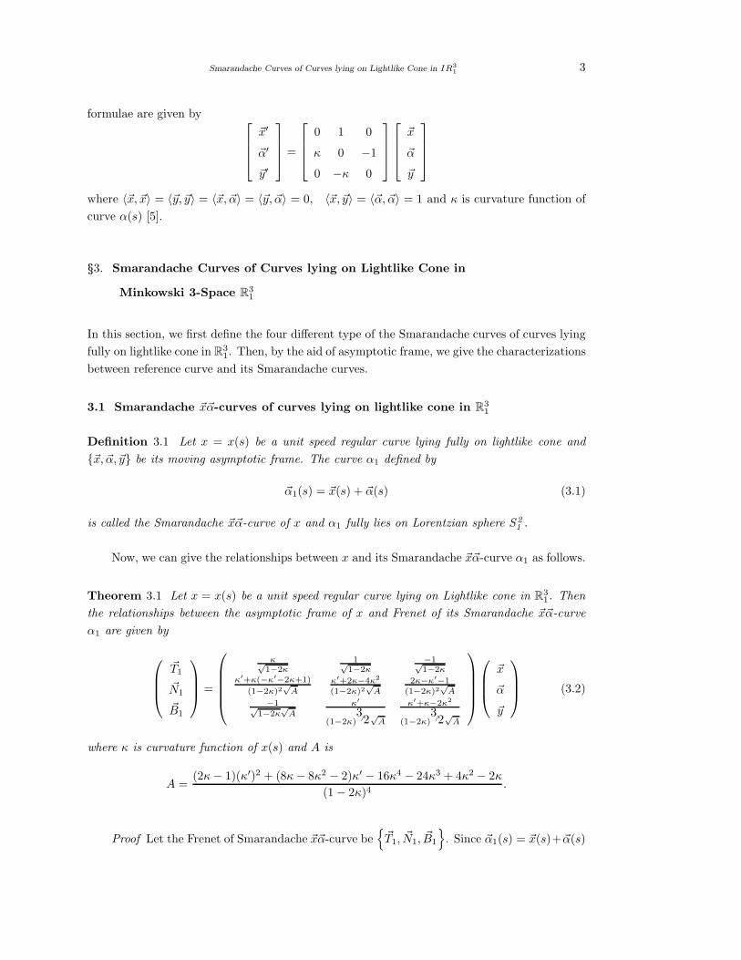
Smarandache Curves of Curves lying on Lightlike Cone in IR31 3
formulae are given by
~x′
~α′
~y′
=
0 1 0
κ 0 −1
0 −κ 0
~x
~α
~y
where 〈~x, ~x〉 = 〈~y, ~y〉 = 〈~x, ~α〉 = 〈~y, ~α〉 = 0, 〈~x, ~y〉 = 〈~α, ~α〉 = 1 and κ is curvature function of
curve α(s) [5].
§3. Smarandache Curves of Curves lying on Lightlike Cone in
Minkowski 3-Space R31
In this section, we first define the four different type of the Smarandache curves of curves lying
fully on lightlike cone in R31. Then, by the aid of asymptotic frame, we give the characterizations
between reference curve and its Smarandache curves.
3.1 Smarandache ~x~α-curves of curves lying on lightlike cone in R31
Definition 3.1 Let x = x(s) be a unit speed regular curve lying fully on lightlike cone and
{~x, ~α, ~y} be its moving asymptotic frame. The curve α1 defined by
~α1(s) = ~x(s) + ~α(s) (3.1)
is called the Smarandache ~x~α-curve of x and α1 fully lies on Lorentzian sphere S2
1.
Now, we can give the relationships between x and its Smarandache ~x~α-curve α1 as follows.
Theorem 3.1 Let x = x(s) be a unit speed regular curve lying on Lightlike cone in R31. Then
the relationships between the asymptotic frame of x and Frenet of its Smarandache ~x~α-curve
α1 are given by
~T1
~N1
~B1
=
κ√1−2κ
1√1−2κ
−1√1−2κ
κ′+κ(−κ′−2κ+1)
(1−2κ)2√
Aκ′+2κ−4κ2
(1−2κ)2√
A2κ−κ′−1
(1−2κ)2√
A
−1√1−2κ
√A
κ′
(1−2κ)3/2
√A
κ′+κ−2κ2
(1−2κ)3/2
√A
~x
~α
~y
(3.2)
where κ is curvature function of x(s) and A is
A =(2κ − 1)(κ′)2 + (8κ − 8κ2 − 2)κ′ − 16κ4 − 24κ3 + 4κ2 − 2κ
(1 − 2κ)4.
Proof Let the Frenet of Smarandache ~x~α-curve be{
~T1, ~N1, ~B1
}. Since ~α1(s) = ~x(s)+~α(s)
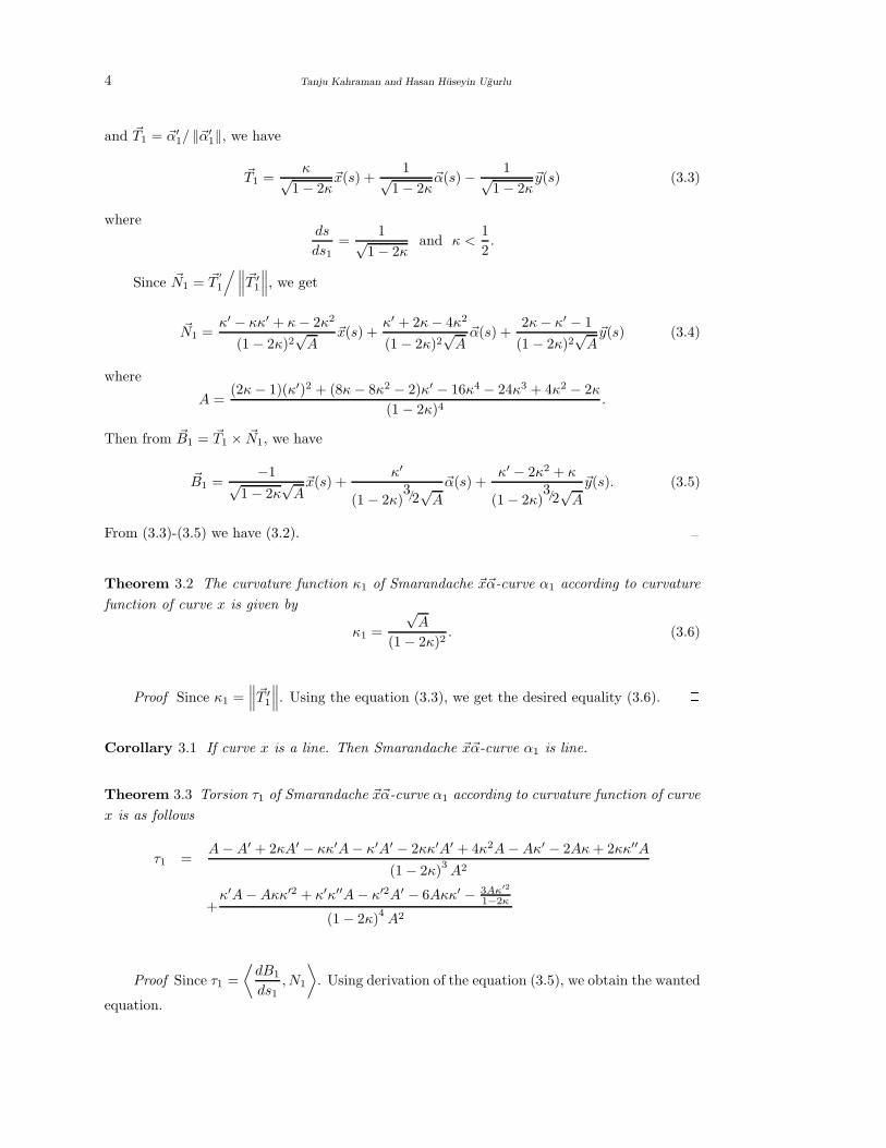
4 Tanju Kahraman and Hasan Huseyin Ugurlu
and ~T1 = ~α′1/ ‖~α′
1‖, we have
~T1 =κ√
1 − 2κ~x(s) +
1√1 − 2κ
~α(s) − 1√1 − 2κ
~y(s) (3.3)
whereds
ds1=
1√1 − 2κ
and κ <1
2.
Since ~N1 = ~T′
1
/∥∥∥~T ′1
∥∥∥, we get
~N1 =κ′ − κκ′ + κ − 2κ2
(1 − 2κ)2√
A~x(s) +
κ′ + 2κ− 4κ2
(1 − 2κ)2√
A~α(s) +
2κ− κ′ − 1
(1 − 2κ)2√
A~y(s) (3.4)
where
A =(2κ − 1)(κ′)2 + (8κ − 8κ2 − 2)κ′ − 16κ4 − 24κ3 + 4κ2 − 2κ
(1 − 2κ)4.
Then from ~B1 = ~T1 × ~N1, we have
~B1 =−1√
1 − 2κ√
A~x(s) +
κ′
(1 − 2κ)3/2
√A
~α(s) +κ′ − 2κ2 + κ
(1 − 2κ)3/2
√A
~y(s). (3.5)
From (3.3)-(3.5) we have (3.2). 2Theorem 3.2 The curvature function κ1 of Smarandache ~x~α-curve α1 according to curvature
function of curve x is given by
κ1 =
√A
(1 − 2κ)2. (3.6)
Proof Since κ1 =∥∥∥~T ′
1
∥∥∥. Using the equation (3.3), we get the desired equality (3.6). 2Corollary 3.1 If curve x is a line. Then Smarandache ~x~α-curve α1 is line.
Theorem 3.3 Torsion τ1 of Smarandache ~x~α-curve α1 according to curvature function of curve
x is as follows
τ1 =A − A′ + 2κA′ − κκ′A − κ′A′ − 2κκ′A′ + 4κ2A − Aκ′ − 2Aκ + 2κκ′′A
(1 − 2κ)3A2
+κ′A − Aκκ′2 + κ′κ′′A − κ′2A′ − 6Aκκ′ − 3Aκ′2
1−2κ
(1 − 2κ)4A2
Proof Since τ1 =
⟨dB1
ds1, N1
⟩. Using derivation of the equation (3.5), we obtain the wanted
equation. 2
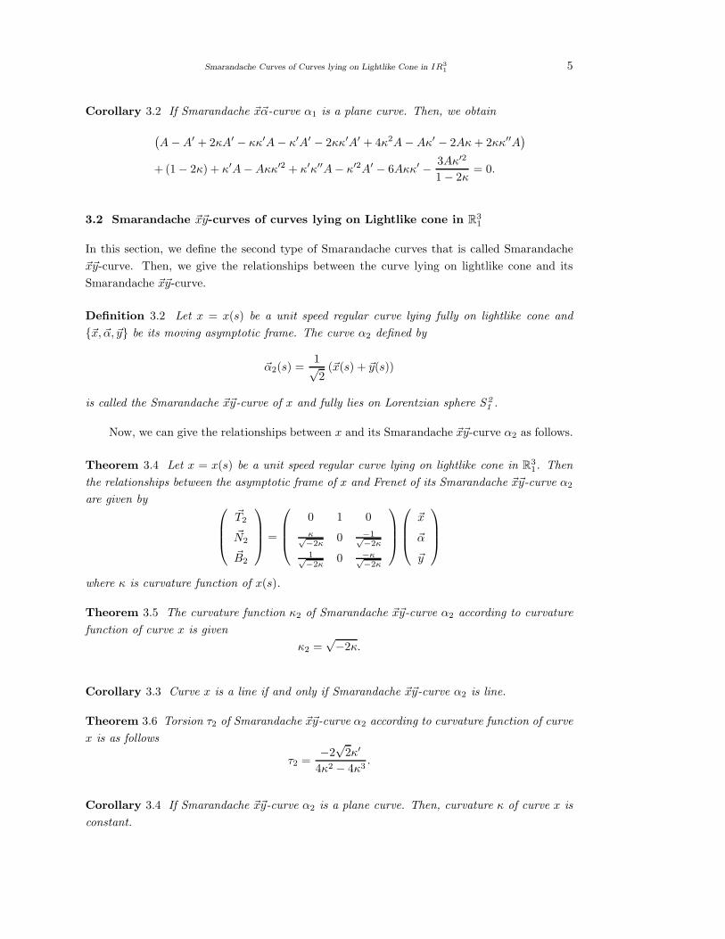
Smarandache Curves of Curves lying on Lightlike Cone in IR31 5
Corollary 3.2 If Smarandache ~x~α-curve α1 is a plane curve. Then, we obtain
(A − A′ + 2κA′ − κκ′A − κ′A′ − 2κκ′A′ + 4κ2A − Aκ′ − 2Aκ + 2κκ′′A
)
+ (1 − 2κ) + κ′A − Aκκ′2 + κ′κ′′A − κ′2A′ − 6Aκκ′ − 3Aκ′2
1 − 2κ= 0.
3.2 Smarandache ~x~y-curves of curves lying on Lightlike cone in R31
In this section, we define the second type of Smarandache curves that is called Smarandache
~x~y-curve. Then, we give the relationships between the curve lying on lightlike cone and its
Smarandache ~x~y-curve.
Definition 3.2 Let x = x(s) be a unit speed regular curve lying fully on lightlike cone and
{~x, ~α, ~y} be its moving asymptotic frame. The curve α2 defined by
~α2(s) =1√2
(~x(s) + ~y(s))
is called the Smarandache ~x~y-curve of x and fully lies on Lorentzian sphere S2
1.
Now, we can give the relationships between x and its Smarandache ~x~y-curve α2 as follows.
Theorem 3.4 Let x = x(s) be a unit speed regular curve lying on lightlike cone in R31. Then
the relationships between the asymptotic frame of x and Frenet of its Smarandache ~x~y-curve α2
are given by
~T2
~N2
~B2
=
0 1 0
κ√−2κ
0 −1√−2κ
1√−2κ
0 −κ√−2κ
~x
~α
~y
where κ is curvature function of x(s).
Theorem 3.5 The curvature function κ2 of Smarandache ~x~y-curve α2 according to curvature
function of curve x is given
κ2 =√−2κ.
Corollary 3.3 Curve x is a line if and only if Smarandache ~x~y-curve α2 is line.
Theorem 3.6 Torsion τ2 of Smarandache ~x~y-curve α2 according to curvature function of curve
x is as follows
τ2 =−2
√2κ′
4κ2 − 4κ3.
Corollary 3.4 If Smarandache ~x~y-curve α2 is a plane curve. Then, curvature κ of curve x is
constant.
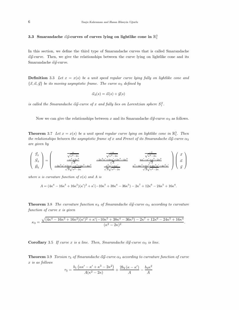
6 Tanju Kahraman and Hasan Huseyin Ugurlu
3.3 Smarandache ~α~y-curves of curves lying on lightlike cone in R31
In this section, we define the third type of Smarandache curves that is called Smarandache
~α~y-curve. Then, we give the relationships between the curve lying on lightlike cone and its
Smarandache ~α~y-curve.
Definition 3.3 Let x = x(s) be a unit speed regular curve lying fully on lightlike cone and
{~x, ~α, ~y} be its moving asymptotic frame. The curve α3 defined by
~α3(s) = ~α(s) + ~y(s)
is called the Smarandache ~α~y-curve of x and fully lies on Lorentzian sphere S2
1.
Now we can give the relationships between x and its Smarandache ~α~y-curve α3 as follows.
Theorem 3.7 Let x = x(s) be a unit speed regular curve lying on lightlike cone in R31. Then
the relationships between the asymptotic frame of x and Frenet of its Smarandache ~α~y-curve α3
are given by
~T3
~N3
~B3
=
κ√κ2−2κ
−κ√κ2−2κ
−1√κ2−2κ
−κ4+2κ3
√A
−2κ2κ′+4κκ′
+2κ3−4κ2√
A
κκ′−κ′+κ3−2κ2√
A
−3κ2κ′+5κκ′−κ4
+4κ3−4κ2
√A√
κ2−2κ
κ2κ′−κκ′
√A√
κ2−2κ
κ5−4κ4+4κ3
+2κ3κ′−4κ2κ′
√A√
κ2−2κ
~x
~α
~y
where κ is curvature function of x(s) and A is
A = (4κ4 − 16κ3 + 16κ2)(κ′)2 + κ′(−10κ5 + 38κ4 − 36κ3) − 2κ7 + 12κ6 − 24κ5 + 16κ4.
Theorem 3.8 The curvature function κ3 of Smarandache ~α~y-curve α3 according to curvature
function of curve x is given
κ3 =
√(4κ4 − 16κ3 + 16κ2)(κ′)2 + κ′(−10κ5 + 38κ4 − 36κ3) − 2κ7 + 12κ6 − 24κ5 + 16κ4
(κ2 − 2κ)2.
Corollary 3.5 If curve x is a line. Then, Smarandache ~α~y-curve α3 is line.
Theorem 3.9 Torsion τ3 of Smarandache ~α~y-curve α3 according to curvature function of curve
x is as follows
τ3 =b1
(κκ′ − κ′ + κ3 − 2κ2
)
A(κ2 − 2κ)+
2b2 (κ − κ′)
A− b3κ
2
A
Smarandache Curves of Curves lying on Lightlike Cone in IR31 7
where b1, b2 and b3 are
b1 = −6κ(κ′)2 + 9κ2κ′ + 5(κ′)2 + 5κκ′′ − 4κ3κ′ − 8κκ′
+(3κ2κ′ − 5κκ′ + κ4 − 4κ3 + 4κ2)
(A′
2A+
κκ′ − κ′
κ2 − 2κ
)
b2 = (κ2 − κ)κ′′ + (2κ − 1)(κ′)2 − (κ2κ′ − κκ′)
(A′
2A+
κκ′ − κ′
κ2 − 2κ
)
b3 = (5κ2 − 16κ + 12)κ2κ′ + (2κ − 8)κ(κ′)2 + 2κ3κ′′
−(2κ3κ′ − 4κ2κ′ + κ5 − 4κ4 + 4κ3)
(A′
2A+
κκ′ − κ′
κ2 − 2κ
).
Corollary 3.6 If Smarandache ~α~y-curve α3 is a plane curve. Then, we obtain
b1
(κκ′ − κ′ + κ3 − 2κ2
)+ (κ2 − 2κ)
(2b2 (κ − κ′) − b3κ
2)
= 0.
3.4 Smarandache ~x~α~y-curves of curves lying on lightlike cone in R31
In this section, we define the fourth type of Smarandache curves that is called Smarandache
~x~α~y-curve. Then, we give the relationships between the curve lying on lightlike cone and its
Smarandache ~x~α~y-curve.
Definition 3.4 Let x = x(s) be a unit speed regular curve lying fully on Lightlike cone and
{~x, ~α, ~y} be its moving asymptotic frame. The curves α4 and α5 defined by
(i) ~α4(s) = 1√3
(~x(s) + ~α(s) + ~y(s));
(ii) ~α5(s) = −~x(s) + ~α(s) + ~y(s)
are called the Smarandache ~x~α~y-curves of x and fully lies on Lorentzian sphere S2
1and hyper-
bolic sphere H 30 .
Now, we can give the relationships between x and its Smarandache ~x~α~y-curve α4 on
Lorentzian sphere S2
1as follows.
Theorem 3.10 Let x = x(s) be a unit speed regular curve lying on lightlike cone in R31. Then
the relationships between the asymptotic frame of x and Frenet of its Smarandache ~x~α~y-curve
α4 are given by
~T4
~N4
~B4
=
κ√κ2−4κ+1
1−κ√κ2−4κ+1
−1√κ2−4κ+1
a1√2a1c1+b21
b1√2a1c1+b21
c1√2a1c1+b21
c1(1−κ)+b1√κ2−4κ+1
√2a1c1+b21
c1κ+a1√κ2−4κ+1
√2a1c1+b21
a1(κ−1)−b1κ√κ2−4κ+1
√2a1c1+b21
~x
~α
~y
8 Tanju Kahraman and Hasan Huseyin Ugurlu
where κ is curvature function of x(s) and a1, b1, c1 are
a1 =
√3(κ′ − 2κκ′ − 5κ2 + 5κ3 − κ4 + κ)
(κ2 − 4κ + 1)2
b1 =
√3(2κ + κ′ − 8κ2 + 2κκ′ + 2κ3)
(κ2 − 4κ + 1)2
c1 =
√3(−2κ′ + κκ′ + 5κ − 5κ2 + κ3 − 1)
(κ2 − 4κ + 1)2.
Theorem 3.11 The curvature function κ4 of Smarandache ~x~α~y-curve α4 according to curvature
function of curve x is given
κ4 =√
2a1c1 + b21.
Corollary 3.7 If curve x is a line. Then, Smarandache ~x~α~y-curve α4 is line.
Theorem 3.12 Torsion τ4 of Smarandache ~x~α~y-curve α4 according to curvature function of
curve x is as follows
τ4 =a2c1 + b1b2 + a1c2√
2a1c1 + b21
where a2, b2 and c2 are
a2 =
√3(c′1 − c′1κ − c1κ′ + b′1 + c1κ2 + a1κ) −
√3(c1 − c1κ + b1)
(κκ′
−2κ′
κ2−4κ+1
+a′
1c1+a1c′1+b1b′12a1c1+b21
)
(κ2 − 4κ + 1)√
2a1c1 + b21
b2 =
√3(c′1κ + c1κ′ + a′
1 + c1 − c1κ + b1 + a1κ − a1κ2 + b1κ2) −√
3(c1κ + a1)
(κκ′
−2κ′
κ2−4κ+1
+a′
1c1+a1c′1+b1b′12a1c1+b21
)
(κ2 − 4κ + 1)√
2a1c1 + b21
c2 =
√3(a′
1κ − a′
1 + a1κ′ − b′1κ − b1κ′ − c1κ − a1) −√
3(a1κ − a1 − b1κ)
(κκ′
−2κ′
κ2−4κ+1
+a′
1c1+a1c′1+b1b′12a1c1+b2
1
)
(κ2 − 4κ + 1)√
2a1c1 + b21
.
Corollary 3.8 If Smarandache ~x~α~y-curve α4 is a plane curve. Then, we obtain
a2c1 + b1b2 + a1c2 = 0.
Results of statement (ii) can be given by using the similar ways used for the statement (i).
References
[1] Ali A. T., Special Smarandache Curves in the Euclidean Space, International J.Math.
Combin., Vol.2, 2010 30-36.
[2] Kahraman T., Onder, M. Ugurlu, H.H. Blaschke approach to dual Smarandache curves,
Journal of Advanced Research in Dynamical and Control Systems, 5(3) (2013) 13-25.
[3] Kahraman T., Ugurlu H. H., Dual Smarandache Curves and Smarandache Ruled Surfaces,
Smarandache Curves of Curves lying on Lightlike Cone in IR31 9
Mathematical Sciences and Applications E-Notes, Vol.2 No.1(2014), 83-98.
[4] Kahraman T., Ugurlu H. H., Dual Smarandache Curves of a Curve lying on unit Dual
Hyperbolic Sphere, The Journal of Mathematics and Computer Science, 14 (2015), 326-
344.
[5] Liu Huili., Curves in the Lightlike Cone, Contributions to Algebra and Geometry, Vol. 45,
No.1(2004), 291-303.
[6] Lopez Rafael., Differential Geometry of Curves and Surfaces in Lorentz-Minkowski Space,
Mini-Course taught at the Instituto de Matematica e Estatistica (IME-USP), University
of Sao Paulo, Brasil, 2008.
[7] O’Neill B., Semi-Riemannian Geometry with Applications to Relativity, Academic Press,
London,1983.
[8] Onder M., Kocayigit H., Candan E., Differential equations characterizing timelike and
spacelike curves of constant breadth in Minkowski 3-space E31 , J. Korean Math. Soc., 48
(2011), No.4, pp. 49-866.
[9] Turgut M., Yılmaz S., Smarandache Curves in Minkowski Space-time, International. J.
Math. Comb., Vol.3(2008), 51-55.
[10] Walrave J., Curves and Surfaces in Minkowski Space, Doctoral thesis, K. U. Leuven, Fac.
Of Science, Leuven, 1995.
International J.Math. Combin. Vol.3(2017), 10-21
On ((r1, r2), m, (c1, c2))-Regular Intuitionistic Fuzzy Graphs
N.R.Santhi Maheswari
(Department of Mathematics, G. Venkataswamy Naidu College, Kovilpatti-628502, Tamil Nadu, India)
C.Sekar
(Post Graduate Extension Centre, Nagercoil-629901,Tamil Nadu, India)
E-mail: [email protected], [email protected]
Abstract: In this paper, ((r1, r2), m, (c1, c2))-regular intuitionistic fuzzy graph and totally
((r1, r2), m, (c1, c2))-regular intuitionistic fuzzy graphs are introduced. A relation between
((r1, r2), m, (c1, c2))-regularity and totally ((r1, r2), m, (c1, c2))-regularity on Intuitionistic
fuzzy graph is studied. A necessary and sufficient condition under which they are equiv-
alent is provided. Also, ((r1, r2), m, (c1, c2))-regularity on some intuitionistic fuzzy graphs
whose underlying crisp graphs is a cycle is studied with some specific membership functions.
Key Words: Degree and total degree of a vertex in intuitionistic fuzzy graph, dm-degree
and total dm-degree of a vertex in intuitionistic fuzzy graph, (m, (c1, c2))- intuitionistic
regular fuzzy graphs, totally (m, (c1, c2))-intuitionistic regular fuzzy graphs.
AMS(2010): 05C12, 03E72, 05C72
§1. Introduction
In 1965, Lofti A. Zadeh [18] introduced the concept of fuzzy subset of a set as method of
representing the phenomena of uncertainty in real life situation. K.T.Attanassov [1]introduced
the concept of intuitionistic fuzzy sets as a generalization of fuzzy sets. K.T.Atanassov added
a new component( which determines the degree of non-membership) in the definition of fuzzy
set. The fuzzy sets give the degree of membership of an element in a given set(and the non-
membership degree equals one minus the degree of membership), while intuitionistic fuzzy sets
give both a degree of membership and a degree of non-membership which are more-or-less
independent from each other, the only requirement is that the sum of these two degrees is not
greater than one.
Intuitionistic fuzzy sets have been applied in a wide variety of fields including computer
science, engineering, mathematics, medicine, chemistry and economics [1, 2]. Azriel Rosenfeld
introduced the concept of fuzzy graphs in 1975 [5]. It has been growing fast and has numerous
application in various fields. Bhattacharya [?] gave some remarks on fuzzy graphs, and some
operations on fuzzy graphs were introduced by Morderson and Peng [9].
1Received October 12, 2016, Accepted May 12, 2017.
On ((r1, r2), m, (c1, c2))-Regular Intuitionistic Fuzzy Graphs 11
Krassimir T Atanassov [2] introduced the intuitionistic fuzzy graph theory. R.Parvathi and
M.G.Karunambigai [8] introduced intuitionistic fuzzy graphs as a special case of Atanassov’s
IFG and discussed some properties of regular intuitionistic fuzzy graphs [6]. M.G. Karunambigai
and R.Parvathi and R.Buvaneswari introduced constant intuitionistic fuzzy graphs [7]. M.
Akram, W. Dudek [3] introduced the regular intuitionistic fuzzy graphs. M.Akram and Bijan
Davvaz [4] introduced the notion of strong intuitionistic fuzzy graphs and discussed some of
their properties.
N.R.Santhi Maheswari and C.Sekar introduced d2- degree of vertex in fuzzy graphs and
introduced (r, 2, k)-regular fuzzy graphs and totally (r, 2, k)-regular fuzzy graphs [11]. S.Ravi
Narayanan and N.R.Santhi Maheswari introduced ((2, (c1, c2)-regular bipolar fuzzy graphs [13].
Also, they introduced dm-degree, total dm-degree, of a vertex in fuzzy graphs and introduced an
m-neighbourly irregular fuzzy graphs [12, 15], (m, k)-regular fuzzy graphs [14, 15] and (r, m, k)-
regular fuzzy graphs [15, 16].
N.R.Santhi Maheswari and C.Sekar introduced dm- degree of a vertex in intuitionistic fuzzy
graphs and introduced (m, (c1, c2))-regular fuzzy graphs and totally (m, (c1, c2))-regular fuzzy
graphs [17]. These motivates us to introduce ((r1, r2), m, (c1, c2))-regular intuitionistic fuzzy
graphs and totally ((r1, r2), m, (c1, c2))-regular intuitionistic fuzzy graphs.
§2. Preliminaries
We present some known definitions related to fuzzy graphs and intuitionistic fuzzy graphs for
ready reference to go through the work presented in this paper.
Definition 2.1([9]) A fuzzy graph G : (σ, µ) is a pair of functions (σ, µ), where σ : V →[0,1]
is a fuzzy subset of a non empty set V and µ : V XV →[0, 1] is a symmetric fuzzy relation on
σ such that for all u, v in V , the relation µ(u, v) ≤ σ(u) ∧ σ(v) is satisfied. A fuzzy graph G is
called complete fuzzy graph if the relation µ(u, v) = σ(u) ∧ σ(v) is satisfied.
Definition 2.2([12]) Let G : (σ, µ) be a fuzzy graph. The dm-degree of a vertex u in G is
dm(u) =∑
µm(uv), where µm(uv) = sup{µ(uu1)∧µ(u1u2)∧. . . , µ(um−1v) : u, u1, u2, . . . , um−1, v
is the shortest path connecting u and v of length m}. Also, µ(uv) = 0, for uv not in E.
Definition 2.3([12]) Let G : (σ, µ) be a fuzzy graph on G∗ : (V, E). The total dm-degree of a
vertex u ∈ V is defined as tdm(u) =∑
µm(uv) + σ(u) = dm(u) + σ(u).
Definition 2.4([12]) If each vertex of G has the same dm - degree k, then G is said to be an
(m, k)-regular fuzzy graph.
Definition 2.5([12]) If each vertex of G has the same total dm - degree k, then G is said to be
totally (m, k)-regular fuzzy graph.
Definition 2.6([15, 16]) If each vertex of G has the same degree r and has the same dm-degree
k, then G is said to be (r, m, k)-regular fuzzy graph.
12 N.R.Santhi Maheswaria and C.Sekar
Definition 2.7([15, 16]) If each vertex of G has the same total degree r and has the same total
dm-degree k, then G is said to be totally (r, m, k)-regular fuzzy.
Definition 2.8([7]) An intuitionistic fuzzy graph with underlying set V is defined to be a pair
G = (V, E) where
(1) V = {v1, v2, v3, · · · , vn} such that µ1 : V → [0, 1] and γ1 : V → [0, 1] denote the
degree of membership and nonmembership of the element vi ∈ V, (i = 1, 2, 3, · · · , n),such that
0 ≤ µ1(vi) + γ1(vi) ≤ 1;
(2) E ⊆ V ×V where µ2 : V ×V → [0, 1] and γ2 : V ×V → [0, 1] are such that µ2(vi, vj) ≤min{µ1(vi), µ1(vj)} and γ2(vi, vj) ≤ max{γ1(vi), γ1(vj)} and 0 ≤ µ2(vi, vj) + γ2(vi, vj) ≤ 1 for
every (vi, vj) ∈ E, (i, j = 1, 2, · · · , n).
Definition 2.9([7]) If vi, vj ∈ V ⊆ G, the µ-strength of connectedness between two vertices vi
and vj is defined as µ∞2 (vi, vj) = sup{µk
2(vi, vj) : k = 1, 2, · · · , n} and γ-strength of connected-
ness between two vertices vi and vj is defined as γ∞2 (vi, vj) = inf{γk
2 (vi, vj) : k = 1, 2, · · · , n}.If u and v are connected by means of paths of length k then µk
2(u, v) is defined as sup
{µ2(u, v1)∧µ2(v1, v2)∧ · · · ∧µ2(vk−1, v) : (u, v1, v2, · · · , vk−1, v) ∈ V } and γk2 (u, v) is defined as
inf {γ2(u, v1) ∨ γ2(v1, v2) ∨ · · · ∨ γ2(vk−1, v) : (u, v1, v2, · · · , vk−1, v) ∈ V }.
Definition 2.10([7]) Let G = (V, E) be an intuitionistic fuzzy graph on G∗(V, E). Then the
degree of a vertex vi ∈ G is defined by d(vi) = (dµ1(vi), dγ1(vi)), where dµ1 (vi) =∑
µ2(vi, vj)
and dγ1(vi) =∑
γ2(vi, vj) for (vi, vj) ∈ E and µ2(vi, vj) = 0 and γ2(vi, vj) = 0 for (vi, vj) /∈ E.
Definition 2.11([7]) Let G = (V, E) be an Intuitionistic fuzzy graph on G∗(V, E). Then
the total degree of a vertex vi ∈ G is defined by td(vi) = (tdµ1(vi), tdγ1(vi)),where tdµ1(vi) =
dµ1(vi) + µ1(vi) and tdγ1(vi) = dγ1(vi) + γ1(vi).
Definition 2.12([17]) Let G = (V, E) be an intuitionistic fuzzy graph on G∗(V, E). Then
the dm - degree of a vertex v ∈ G is defined by d(m)(v) = (d(m)µ1(v), d(m)γ1
(v)), where
d(m)µ1(v) =
∑µ
(m)2 (u, v) where µ
(m)2 (u, v) = sup{µ2(u, u1) ∧ µ2(u1, u2) ∧ · · · ∧ µ2(um−1, v) :
u, u1, u2, · · · , um−1, v is the shortest path connecting u and v of length m)} and d(m)γ1(v) =∑
γ(m)2 (u, v), where γ
(m)2 (u, v)=inf {γ2(u, u1)∨γ2(u1, u2)∨· · ·∨γ2(um−1, v) : u, u1, u2, · · · , um−1, v
is the shortest path connecting u and v of length m}. The minimum dm-degree of G is δm(G)
=∧{(d(m)µ1(v), d(m)γ1
(v)) : v ∈ V }.The maximum dm-degree ofG is ∆m(G)=∨{(d(m)µ1
(v), d(m)γ1(v)) : v ∈ V }..
Definition 2.13([17]) Let G : (V, E) be an intuitionistic fuzzy graph on G∗(V, E). If all
the vertices of G have same dm- degree c1,c2, then G is said to be a (m, (c1, c2))- regular
intuitionistic fuzzy graph.
Definition 2.14([17]) Let G = (V, E) be an intuitionistic fuzzy graph on G∗(V, E). Then
the total dm-degree of a vertex v ∈ G is defined by td(m)(v)= (td(m)µ1(v), td(m)γ1
(v)), where
td(m)µ1(v) = d(m)µ1
(v) + µ1(v) and td(m)γ1(v) = d(m)γ1
(v) + γ1(v). The minimum tdm-degree
of G is tδm(G) = ∧{(td(m)µ1(v), td(m)γ1
(v)) : v ∈ V }. The maximum tdm-degree of G is
t∆m(G) = ∨{(td(m)µ1(v), td(m)γ1
(v)) : v ∈ V }.
On ((r1, r2), m, (c1, c2))-Regular Intuitionistic Fuzzy Graphs 13
Definition 2.15([17]) Let G = (V, E) be an intuitionistic fuzzy graph on G∗(V, E). If each
vertex of G has same total dm - degree c1,c2, then G is said to be totally (m,(c1,c2)) - regular
intuitionistic fuzzy graph.
§3. ((r1, r2), m, (c1, c2))- Regular intuitionistic Fuzzy Graphs
Definition 3.1 Let G : (V, E) be an intuitionistic fuzzy graph on G∗(V, E). If d(v) = (r1, r2)
and d(m)(v) = (c1, c2) for all v ∈ V , then G is said to be ((r1, r2), m, (c1, c2))-regular intuition-
istic fuzzy graph. That is, if each vertex of G has the same degree (r1, r2) and has the same
dm-degree (c1, c2), then G is said to be ((r1, r2), m, (c1, c2))-regular intuitionistic fuzzy graph.
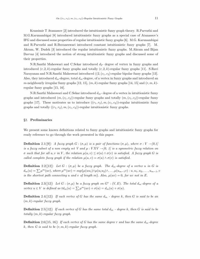
Example 3.2 Consider an intuitionistic fuzzy graph on G∗(V, E), a cycle of length 7.
u1(0.2, 0.3)
(0.3, 0.4)
u2(0.3, 0.4)
u3(0.4, 0.5)
(0.3, 0.4)
(0.3, 0.4)
u4(0.5, 0.4)(0.3, 0.4)
u5(0.2, 0.3)
(0.3, 0.4)
u6(0.5, 0.4)
u7(0.6, 0.4)
(0.3, 0.4)
(0.3, 0.4)
Figure 1
Here, dµ1(u) = 0.6; dγ1(u) = 0.8; d(u) = (0.6, 0.8) for all u ∈ V .
d(3)µ1(u1) = (0.3 ∧ 0.3 ∧ 0.3) + (0.3 ∧ 0.3 ∧ 0.3) = 0.3 + 0.3 = 0.6;
d(3)γ1(u1) = (0.4 ∨ 0.4 ∨ 0.4) + (0.4 ∨ 0.4 ∨ 0.4) = (0.4) + (0.4) = 0.8;
d(3)(u1) = (0.6, 0.8); d(3)(u2) = (0.6, 0.8); d(3)(u3) = (0.6, 0.8);
d(3)(u4) = (0.6, 0.8); d(3)(u5) = (0.6, 0.8); d(3)(u6) = (0.6, 0.8); d(3)(u7) = (0.6, 0.8).
Hence G is ((0.6, 0.8), 3, (0.6, 0.8))-regular intuitionistic fuzzy graph.
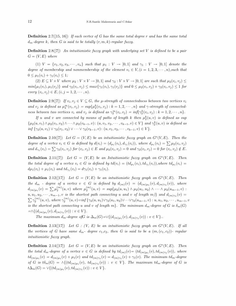
Example 3.3 Consider an intuitionistic fuzzy graph on G∗(V, E), a cycle of length 6.
u(0.5, 0.4) v(0.5, 0.4) w(0.5, 0.4)
x(0.5, 0.4)y(0.5, 0.4)z(0.5, 0.4)
(0.3, 0.4)
(0.1, 0.2) (0.3, 0.4)
(0.1, 0.2)
(0.3, 0.4)(0.1, 0.2)
Figure 2
14 N.R.Santhi Maheswaria and C.Sekar
dµ1(u) = 0.4; dγ1(u) = 0.6; d(u) = (0.4, 0.6);
d(3)µ1(u) = sup{(0.1 ∧ 0.3 ∧ 0.1), (0.3 ∧ 0.1 ∧ 0.3)} = sup{0.1, 0.1} = 0.1;
d(3)γ1(u) = inf{(0.2 ∨ 0.4 ∨ 0.2), (0.4 ∨ 0.2 ∨ 0.4)} = inf{0.4, 0.4} = 0.4;
d(3)(u) = (0.1, 0.4), d(3)(u) = (0.1, 0.4), for all u ∈ V.
Here, G is ((0.4, 0.6), 3, (0.1, 0.4))- regular intuitionistic fuzzy graph.
Example 3.4 Non regular intuitionistic fuzzy graphs which is (m, (c1, c2))-regular intuitionistic
fuzzy graph.
Let G : (V, E) be an intuitionistic fuzzy graph such that G∗(V, E), a path on 2m vertices.
Let all the edges of G have the same membership value (c1, c2). Then,
For i = 1, 2, · · · , m,
d(m)µ1(vi) = {µ(ei) ∧ µ(ei+1) ∧ · · · ∧ µ(em−2+i) ∧ µ(em−1+i)}
= {c1 ∧ c1 ∧ · · · ∧ c1},
d(m)µ1(vi) = c1,
d(m)γ1(vi) = {γ(ei) ∨ γ(ei+1) ∨ · · · ∨ γ(em−2+i) ∨ γ(em−1+i)}
= {c2 ∨ c2 ∨ · · · ∨ c2}
d(m)γ1(vi) = c2,
d(m)µ1(vm+i) = {µ(ei) ∧ µ(ei+1) ∧ · · · ∧ µ(em−2+i) ∧ µ(em−1+i)}
= {c1 ∧ c1 ∧ · · · ∧ c1},
d(m)µ1(vm+i) = c1,
d(m)γ1(vm+i) = {γ(ei) ∨ γ(ei+1) ∨ · · · ∨ γ(em−2+i) ∨ γ(em−1+i)}
= {c2 ∨ c2 ∨ · · · ∨ c2},
d(m)γ1(vm+i) = c2.
Hence G is (m, (c1, c2)) - regular intuitionistic fuzzy graph.
For i = 2, 3, · · · , 2m− 1,
dµ(vi) = µ(ei−1) + µ(ei) = c1 + c1 = 2c1;
dγ(vi) = γ(ei−1) + γ(ei) = c2 + c2 = 2c2;
d(vi) = (2c1, 2c2) = (k1, k2) where k1 = 2c1 and k2 = 2c2;
dµ(v1) = µ(e1) = c1 and dγ(v1) = γ(e1) = c2,
So, d(v1) = (c1, c2), dµ(v2m) = µ(e2m−1) = c1 and dγ(v2m) = γ(e2m−1) = c2.
So, d(v2m) = (c1, c2). Therefore, d(v1) 6= d(vi) 6= d(v2m) for i = 2, 3, · · · , 2m − 1.
On ((r1, r2), m, (c1, c2))-Regular Intuitionistic Fuzzy Graphs 15
Hence G is non regular intuitionistic fuzzy graph which is (m, (c1, c2))-regular intuitionistic
fuzzy graph.
Example 3.5 Let G : (V, E) be an intuitionistic fuzzy graph such that G∗(V, E), an even cycle
of length ≥ 2m + 1.
Let
µ(ei) =
k1l if i is odd
membership value x≥ k1 if i is even
and
γ(ei) =
k2 if i is odd
membership value y ≤ k2 if i is even
where x, y are not constant functions. Then,
d(m)µ1(v) = min{k1, x} + min{x, k1} = k1 + k1 = 2k1 = c1, where c1 = 2k1
d(m)γ1(v) = max{k2, y} + max{y, k2} = k2 + k2 = 2k2 = c2, where c2 = 2k2.
So, d(m)(v) = (c1, c2), for all v ∈ V.
Case 1. Let G : (A, B) be an intuitionistic fuzzy graph such that G∗(V, E), an even cycle of
length ≤ 2m+2. Then d(vi)=(x+c1, y+c2), for all i = 1, 2, · · · , 2m+1. Hence G is non-regular
(m, (c1, c2))-regular intuitionistic fuzzy graph.
Case 2. Let G : (A, B) be an intuitionistic fuzzy graph such that G∗(V, E), an odd cycle of
length ≤ 2m + 1. Then d(v1) = (c1, c2) + (c1, c2) = (2c1, 2c2) and d(vi) = (x + c1, y + c2), for
all i = 2, 3, · · · , 2m. Hence G is non-regular (m, (c1, c2))-regular intuitionistic fuzzy graph.
§4. Totally ((r1, r2), m, (c1, c2))- Regular Intuitionistic Fuzzy Graphs
Definition 4.1 Let G : (A, B) be an intuitionistic fuzzy graph on G∗(V, E). If each vertex of G
has the same total degree (r1, r2) and same total dm-degree (c1, c2) , then G is said to be totally
((r1, r2), m, (c1, c2))- regular intuitionistic fuzzy graph.
Example 4.2 In Figure 2, td(3)(v) = d(3)(v) + A(v) = (0.1,0.4)+(0.5,0.4)=(0.6,0.8) for all
v ∈ V. td(v) = d(v) + A(v) = (0.4, 0.6) + (0.5, 0.4) = (0.9, 1.0) for all v ∈ V Hence G is
((0.9,1.0),3,(0.6,0.8))- regular intuitionistic fuzzy graph.
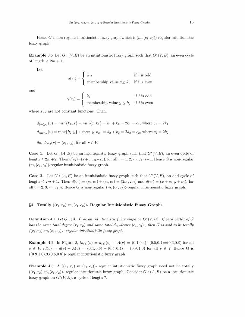
Example 4.3 A ((r1, r2), m, (c1, c2))- regular intuitionistic fuzzy graph need not be totally
((r1, r2), m, (c1, c2))- regular intuitionistic fuzzy graph. Consider G : (A, B) be a intuitionistic
fuzzy graph on G∗(V, E), a cycle of length 7.
16 N.R.Santhi Maheswaria and C.Sekar
a(0.4, 0.5) b(0.5, 0.4)
c(0.4, 0.5)
d(0.5, 0.4)
e(0.4, 0.5)f(0.5, 0.4)
g(0.4, 0.5)
h(0.5, 0.4)
(0.2, 0.3)
(0.3, 0.4)
(0.2, 0.3)
(0.3, 0.4)
(0.2, 0.3)
(0.3, 0.4)
(0.2, 0.3)
(0.3, 0.4)
Figure 3
Here d(v) = (0.5, 0.7) for all v ∈ V and d(3)(v) = (0.4, 0.8), for all v ∈ V . But td(3)(a) =
(0.4, 0.8) + (0.4, 0.5) = (0.8, 1.3), td(3)(b) = (0.4, 0.8) + (0.5, 0.4) = (0.9, 1.2). Hence G is
((0.5,0.7), 3 , (0.4,0.8)) - regular intuitionistic fuzzy graph.
But td3(a) 6= td3(b). Hence G is not totally ((r1, r2), 3, (c1, c2)) - regular intuitionistic
fuzzy graph.
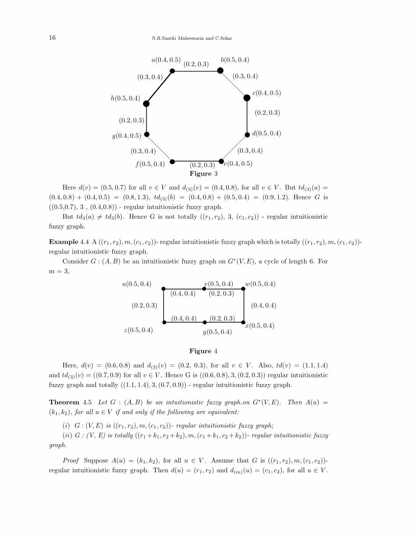
Example 4.4 A ((r1, r2), m, (c1, c2))- regular intuitionistic fuzzy graph which is totally ((r1, r2), m, (c1, c2))-
regular intuitionistic fuzzy graph.
Consider G : (A, B) be an intuitionistic fuzzy graph on G∗(V, E), a cycle of length 6. For
m = 3,
u(0.5, 0.4) v(0.5, 0.4) w(0.5, 0.4)
x(0.5, 0.4)y(0.5, 0.4)z(0.5, 0.4)
(0.2, 0.3)
(0.4, 0.4) (0.2, 0.3)
(0.4, 0.4)
(0.2, 0.3)(0.4, 0.4)
Figure 4
Here, d(v) = (0.6, 0.8) and d(3)(v) = (0.2, 0.3), for all v ∈ V . Also, td(v) = (1.1, 1.4)
and td(3)(v) = ((0.7, 0.9) for all v ∈ V . Hence G is ((0.6, 0.8), 3, (0.2, 0.3)) regular intuitionistic
fuzzy graph and totally ((1.1, 1.4), 3, (0.7, 0.9)) - regular intuitionistic fuzzy graph.
Theorem 4.5 Let G : (A, B) be an intuitionistic fuzzy graph.on G∗(V, E). Then A(u) =
(k1, k2), for all u ∈ V if and only if the following are equivalent:
(i) G : (V, E) is ((r1, r2), m, (c1, c2))- regular intuitionistic fuzzy graph;
(ii) G : (V, E) is totally ((r1 +k1, r2 +k2), m, (c1 +k1, c2 +k2))- regular intuitionistic fuzzy
graph.
Proof Suppose A(u) = (k1, k2), for all u ∈ V . Assume that G is ((r1, r2), m, (c1, c2))-
regular intuitionistic fuzzy graph. Then d(u) = (r1, r2) and d(m)(u) = (c1, c2), for all u ∈ V .
On ((r1, r2), m, (c1, c2))-Regular Intuitionistic Fuzzy Graphs 17
So, td(u) = d(u) + A(u) and td(m)(u) = d(m)(u) + A(u) ⇒ td(u) = (r1, r2) + (k1, k2) and
td(m)(u) = (c1, c2) + (k1, k2). So, td(u) = (r1 + k1, r2 + k2), td(m)(u) = (c1 + k1, c2 + k2). Hence
G is totally ((r1 + k1, r2 + k2), m, (c1 + k1, c2 + k2)) - regular intuitionistic fuzzy graph. Thus
(i) ⇒ (ii) is proved.
Now, suppose G is totally ((r1 + k1, r2 + k2), m, (c1 + k1, c2 + k2))- regular intuitionistic
fuzzy graph. Then td(u) = (r1 + k1, r2 + k2) and td(m)(u) = (c1 + k1, c2 + k2), for all u ∈V ⇒ d(u) + A(u) = (r1 + k1, r2 + k2) and d(m)(u) + A(u) = (c1 + k1, c2 + k2), for all u ∈V ⇒ d(u) + (k1, k2) = (r1, r2) + (k1, k2) and d(m)(u) + (k1, k2) = (c1, c2) + (k1, k2), for all
u ∈ V ⇒d(u)= (r1, r2) and d(m)(u) = (c1, c2), for all u ∈ V . Hence G is ((r1, r2), m, (c1, c2))-
regular intuitionistic fuzzy graph. Thus (ii) ⇒ (i) is proved. Hence (i) and (ii) are equivalent.
Conversely, suppose (i) and (ii) are equivalent. Suppose A(u) is not constant function,
then A(u) 6= A(w), for atleast one pair u, v ∈ V . Let G be a ((r1, r2), m, (c1, c2)) - regular
intuitionistic fuzzy graph and totally ((r1+k1, r2+k2), m, (c1+k1, c2+k2))- regular intuitionistic
fuzzy graph. Then d(m)(u) = d(m)(w) = (c1, c2) and d(u) = d(w) = (r1, r2). Also, td(m)(u) =
d(m)(u) + A(u) = (c1, c2) + A(u) and td(m)(w) = d(m)(w) + A(w) = (c1, c2) + A(w), td(u) =
d(u) + A(u) = (r1, r2) + A(u) and td(w) = d(w) + A(w) = (r1, r2) + A(w). Since A(u) 6=A(w), (c1, c2) + A(u) 6= (c1, c2) + A(w) and (r1, r2) + A(u) 6= (r1, r2) + A(w) ⇒ td(m)(u) 6=td(m)(w) and td(u) 6= td(w). So, G is not totally ((r1 +k1, r2 +k2), m, (c1 +k1, c2 +k2))- regular
intuitionistic fuzzy graph. Which is a contradiction.
Now let G be a totally ((r1 + k1, r2 + k2), m, (c1 + k1, c2 + k2)) - regular intuitionistic fuzzy
graph. Then td(m)(u) = td(m)(w) and td(u) = td(w) ⇒ d(m)(u) + A(u) = d(m)(w) + A(w)
and d(u) + A(u) = d(w) + A(w) ⇒ d(m)(u) − d(m)(w) = A(w) − A(u) 6= 0 and d(u) − d(w) =
A(w) − A(u) 6= 0 ⇒ d(m)(u) 6= d(m)(w) and d(u) 6= d(w). So, G is not ((r1, r2), m, (c1, c2))
- regular intuitionistic fuzzy graph. Which is a contradiction. Hence A(u) = (k1, k2), for all
u ∈ V . 2Theorem 4.6 If an intuitionistic fuzzy graph G : (A, B) is both ((r1, r2), m, (c1, c2)) - regular
intuitionistic fuzzy graph and totally ((r1, r2), m, (c1, c2)) - regular intuitionistic fuzzy graph then
A is constant function.
Proof Let G be a ((s1, s2), m, (k1, k2)) - regular intuitionistic fuzzy graph and totally
((s3, s4), m, (k3, k4)) - regular intuitionistic fuzzy graph. Then, let d(m)(u) = (k1, k2), td(m)(u) =
(k3, k4), d(u) = (s1, s2), td(u) = (s3, s4) for all u ∈ v. Now, td(m)(u) = (k3, k4) and td(u) =
(s3, s4) for all u ∈ v ⇒ d(m)(u) + A(u) = (k3, k4) and d(u) + A(u) = (s3, s4) for all u ∈ v ⇒(k1, k2)+A(u) = (k3, k4) and (s1, s2)+A(u) = (s3, s4) for all u ∈ v ⇒ A(u) = (k3, k4)− (k1, k2)
and A(u) = (s3, s4) − (s1, s2) for all u ∈ v ⇒ A(u) = (k3 − k1, k4 − k2) and A(u) =
(s3 − s1), (s4 − s2) for all u ∈ v. Hence A(u) is constant function. 2§5. ((r1, r2), m, (c1, c2))- Regularity on a Cycle with Some Specific
Membership Functions
Theorem 5.1 For any m ≥ 1, Let G : (A, B) be an intuitionistic fuzzy graph such that
G∗(V, E), a cycle of length ≥ 2m. If B is constant function then G is ((r1, r2), m, (c1, c2)) -
18 N.R.Santhi Maheswaria and C.Sekar
regular intuitionistic fuzzy graph, where (k1, k2) = 2B(uv).
Proof Suppose B is a constant function say B(uv) = (c1, c2), for all uv ∈ E. Then dµ(u)=
sup {(c1 ∧ c1 ∧ · · · ∧ c1), (c1 ∧ c1 ∧ · · · ∧ c1)} = c1 for all v ∈ V . dγ(u) = inf{(c2 ∨ c2 ∨ · · · ∨ c2),
(c2∨c2∨· · ·∨c2)} = c2 for all v ∈ V . d(m)(v) = (c1, c2) and d(v) = (c1, c2)+(c1, c2) = 2(c1, c2).
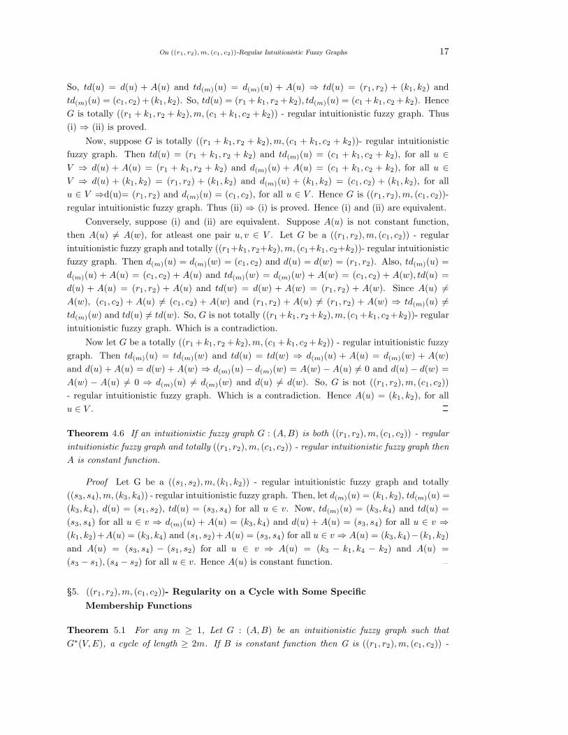
Hence G is ((r1, r2), m, (c1, c2)) - regular intuitionistic fuzzy graph. 2Remark 5.2 The Converse of above theorem need not be true.
Example 5.3 Consider an intuitionistic fuzzy graph on G∗(V, E).
u(0.3, 0.4) v(0.4, 0.5)
w(0.3, 0.5)
x(0.3, 0.4)y(0.4, 0.5)
z(0.3, 0.5)
(0.2, 0.3)
(0.3, 0.4)
(0.2, 0.3)
(0.3, 0.4)
(0.2, 0.3)
(0.3, 0.4)
Figure 5
Here, d(u) = (0.5, 0.7) and d(3)(u) = (0.3, 0.4), for all u ∈ V . Hence G is ((0.5, 0.7), 3, (0.3, 0.4))-
regular intuitionistic fuzzy graph. But B is not a constant function.
Theorem 5.4 For any m ≥ 1, let G : (A, B) be an intuitionistic fuzzy graph such that G∗(V, E),
a cycle of length ≥ 2m + 1. If B is constant function, then G is ((r1, r2), m, (c1, c2)) - regular
intuitionistic fuzzy graph, where (r1, r2) = 2B(uv) and (c1, c2) = 2B(uv).
Proof Suppose B is constant function say B(uv) = (c1, c2), for all uv ∈ E. Then,
d(m)µ1(v)= {c1 ∧ c1 ∧ · · · ∧ c1} + {c1 ∧ c1 ∧ · · · ∧ c1} = c1 + c1 = 2c1, d(m)γ1
= {c2 ∨ c2 ∨· · · ∨ c2} + {c2 ∨ c2 ∨ · · · ∨ c2} = c2 + c2 = 2c2 , for all v ∈ V . So,d(m)(v) = 2(c1, c2), for all
u ∈ V . Also, d(v) = (c1, c2) + (c1, c2) = 2(c1, c2) Hence G is (2(c1, c2), m, 2(c1, c2)) - regular
intuitionistic fuzzy graph. 2Theorem 5.5 For any m ≥ 1, let G : (A, B) be an intuitionistic fuzzy graph such that G∗(V, E),
a cycle of length ≥ 2m + 1. If the alternate edges have the same membership values and same
non membership values, then G is ((r1, r2), m, (c1, c2)) - regular intuitionistic fuzzy graph.
Proof If the alternate edges have same membership and same non membership values then,
let
µ(ei) =
k1 if i is odd
k2 if i is evenγ(ei) =
k3 if i is odd
k4 if i is even
Here, we have 4 possible cases.
Case 1. Suppose k1 ≤ k2 and k3 ≥ k4.
On ((r1, r2), m, (c1, c2))-Regular Intuitionistic Fuzzy Graphs 19
d(m)µ1(v) = min{k1, k2} + min{k1, k2} = k1 + k1 = 2k1;
d(m)γ1(v) = max{k3, k4} + max{k3, k4} = k3 + k3 = 2k3;
d(m)(v) = (2k1, 2k3) and d(v) = (k1, k3) + (k2, k4) = (k1 + k2, k3 + k4).
Case 2. Suppose k1 ≤ k2 and k3 ≤ k4.
d(m)µ1(v) = min{k1, k2} + min{k1, k2} = k1 + k1 = 2k1;
d(m)γ1(v) = max{k3, k4} + max{k3, k4} = k4 + k4 = 2k4;
d(m)(v) = (2k1, 2k4) and d(v) = (k1, k3) + (k2, k4) = (k1 + k2, k3 + k4).
Case 3. Suppose k1 ≥ k2 and k3 ≤ k4.
d(m)µ1(v) = min{k1, k2} + min{k1, k2} = k2 + k2 = 2k2;
d(m)γ1(v) = max{k3, k4} + max{k3, k4} = k4 + k4 = 2k4;
d(m)(v) = (2k2, 2k4) and d(v) = (k1, k3) + (k2, k4) = (k1 + k2, k3 + k4).
Case 4. Suppose k1 ≥ k2 and k3 ≥ k4.
d(m)µ1(v) = min{k1, k2} + min{k1, k2} = k2 + k2 = 2k2;
d(m)γ1(v) = max{k3, k4} + max{k3, k4} = k3 + k3 = 2k3;
d(m)(v) = (2k2, 2k3) and d(v) = (k1, k3) + (k2, k4) = (k1 + k2, k3 + k4).
Thus, d(v) = (r1, r2) and d(m)(v) = (c1, c2) for all v ∈ V . Hence G is ((r1, r2), m, (c1, c2))-
regular intuitionistic fuzzy graph. 2Remark 5.6 Even if the alternate edges of an intuitionistic fuzzy graph whose underlying
graph is an even cycle of length ≥ 2m + 2 having same membership values and same non
membership values, then G need not be totally ((r1, r2), m, (c1, c2))- regular intuitionistic fuzzy
graph, since if A = (µ1, γ1) is not a constant function, G is not totally ((r1, r2), m, (c1, c2)) -
regular intuitionistic fuzzy graph, for any m ≥ 1.
Theorem 5.7 For any m ≥ 1, let G : (A, B) be an intuitionistic fuzzy graph on G∗ : (V, E), a
cycle of length ≥ 2m + 1. Let k2 ≥ k1, k4 ≥ k3 and let
µ(ei) =
k1 if i is odd
k2 if i is evenγ(ei) =
k3 if i is odd
k4 if i is even
Then, G is ((r1, r2), m, (c1, c2))- regular intuitionistic fuzzy graph.
Proof We consider cases following.
Case 1. Let G : (A, B) be an intuitionistic fuzzy graph on G∗(V, E), an even cycle of length
≤ 2m + 2. Then by theorem 5.3, G is ((r1, r2), m, (c1, c2)) - regular intuitionistic fuzzy graph.
Case 2. Let G = (A, B) be an intuitionistic fuzzy graph on G∗(V, E) an odd cycle of length
≥ 2m + 1. For any m ≥ 1, d(m)(v) = (2k1, 2k4), for all v ∈ V . But d(v1) = (k1, k3) + (k1, k3) =
2(k1, k3) and d(vi) = (k1, k3)+(k2, k4) = ((k1+k2), (k3+k4)) So, d(vi) 6= d(v1) for i = 2, 3, . . . , m
20 N.R.Santhi Maheswaria and C.Sekar
Hence G is not ((r1, r2), m, (c1, c2))-regular intuitionistic fuzzy graph. 2Remark 5.8 Let G : (A, B) be an intuitionistic fuzzy graph such that G∗(V, E) is a cycle of
length ≥ 2m + 1. Even if let
µ(ei) =
k1 if i is odd
k2 if i is evenγ(ei) =
k3 if i is odd
k4 if i is even
Then G need not be totally ((r1, r2), m, (c1, c2))- regular intuitionistic fuzzy graph, since if A =
(µ1, γ1) is not a constant function, G is not totally ((r1, r2), m, (c1, c2))- regular intuitionistic
fuzzy graph.
Acknowledgement
This work is supported by F.No:4-4/2014-15, MRP- 5648/15 of the University Grant Commis-
sion, SERO, Hyderabad.
References
[1] K.T.Atanassov, Instuitionistic Fuzzy Sets: Theory, Applications, Studies in Fuzziness and
Soft Computing, Heidelberg, New York, Physica-Verl.,1999.
[2] K.T.Atanassov, G.Pasi,R.Yager, V,atanassov, Intuitionistic fuzzy graph interpretations of
multi-person multi-criteria decision making, EUSFLAT Conf., 2003, 177-182.
[3] M. Akram, W. Dudek, Regular intuitionistic fuzzy graphs, Neural Computing and Appli-
cation, 1007/s00521-011-0772-6.
[4] M.Akram, B.Davvaz, Strong intuitionistic fuzzy graphs, Filomat, 26:1 (2012), 177-196.
[5] P.Bhattacharya, Some remarks on fuzzy graphs, Pattern Recognition Lett., 6(1987), 297-
302.
[6] M.G.Karunambigai and R.Parvathi and R.Buvaneswari,Constant intuitionistic fuzzy graphs,
NIFS, 17 (2011), 1, 37-47.
[7] M.G.Karunambigai, S.Sivasankar and K.Palanivel, Some properties of regular Intuitionistic
fuzzy graph, International Journal of Mathematics and Computation, Vol.26, No.4(2015).
[8] R.Parvathi and M.G.Karunambigai, Intuitionistic fuzzy graphs, Journal of Computational
Intelligence: Theory and Applications, (2006) 139-150.
[9] John N.Moderson and Premchand S. Nair, Fuzzy graphs and Fuzzy hypergraphs, Physica
Verlag, Heidelberg(2000).
[10] A.Rosenfeld, fuzzy graphs, in:L.A. Zadekh and K.S. Fu, M. Shimura(EDs) Fuzzy Sets and
Their Applications, Academic Press, Newyork, 77-95, 1975.
[11] N.R.Santhi Maheswari and C.Sekar, On (r, 2, k)- regular fuzzy graph, Journal of Combi-
natorics and Mathematicsal Combinatorial Computing, 97(2016),pp.11-21.
[12] N. R.Santhi Maheswari and C. Sekar, On m-neighbourly irregular fuzzy graphs, Interna-
tional Journal of Mathematics and Soft Computing, 5(2)(2015).
On ((r1, r2), m, (c1, c2))-Regular Intuitionistic Fuzzy Graphs 21
[13] S.Ravi Narayanan and N.R.Santhi Maheswari, On (2, (c1, c2))-regular bipolar fuzzy graphs,
International Journal of Mathematics and Soft Computing, 5(2)(2015).
[14] N.R.Santhi Maheswari and C.Sekar, On (m, k)- regular fuzzy graphs, International Journal
of Mathematical Archieve, 7(1),2016,1-7.
[15] N.R. SanthiMaheswari, A Study on Distance d-Regular and Neighborly Irregular Graphs,
Ph.D Thesis, Manonmaniam Sundaranar University, Tirunelveli, 2014.
[16] N.R.Santhi Maheswari and C.Sekar, On (r, m, k)- regular fuzzy graphs, International Jour-
nal of Mathematical Combinatorics, Vol.1(2016), 18-26.
[17] N.R.Santhi Maheswari and C.Sekar, On (m, (c1, c2))- regular intuitionistic fuzzy graphs,
International Journal of Modern Sciences and Engineering Technology (IJMSET), Vol.2,
Issue 12,2015, pp21-30.
[18] L.A. Zadeh, Fuzzy sets, Information and Control, 8(1965), 338-353.
International J.Math. Combin. Vol.3(2017), 22-31
Minimum Dominating Color Energy of a Graph
P.Siva Kota Reddy1, K.N.Prakasha2 and Gavirangaiah K3
1. Department of Mathematics, Siddaganga Institute of Technology, B.H.Road, Tumkur-572 103, India
2. Department of Mathematic, Vidyavardhaka College of Engineering, Mysuru- 570 002, India
3. Department of Mathematics, Government First Grade Collge, Tumkur-562 102, India
E-mail: reddy [email protected], [email protected], [email protected]
Abstract: In this paper, we introduce the concept of minimum dominating color energy of
a graph, EDc (G) and compute the minimum dominating color energy ED
c (G) of few families
of graphs. Further, we establish the bounds for minimum dominating color energy.
Key Words: Minimum dominating set, Smarandachely dominating, minimum dominating
color eigenvalues, minimum dominating color energy of a graph.
AMS(2010): 05C50
§1. Introduction
Let G be a graph with n vertices v1, v2, · · · , vn and m edges. Let A = (aij) be the adjacency
matrix of the graph. The eigenvalues λ1, λ2, · · · , λn of A, assumed in non increasing order, are
the eigenvalues of the graph G. As A is real symmetric, the eigenvalues of G are real with sum
equal to zero. The energy E(G) of G is defined to be the sum of the absolute values of the
eigenvalues of G.
E(G) =n∑
i=1
|λi|. (1)
The concept of graph energy originates from chemistry to estimate the total π-electron
energy of a molecule. In chemistry the conjugated hydrocarbons can be represented by a graph
called molecular graph. Here every carbon atom is represented by a vertex and every carbon-
carbon bond by an edge and hydrogen atoms are ignored. The eigenvalues of the molecular
graph represent the energy level of the electron in the molecule. An interesting quantity in
Huckel theory is the sum of the energies of all the electrons in a molecule, the so called π-
electron energy of a molecule.
Prof.Chandrashekara Adiga et al.[5] have defined color energy Ec(G) of a graph G. Rajesh
Khanna et al.[2] have defined the minimum dominating energy. Motivated by these two papers,
we introduced the concept of minimum dominating color energy EDc (G) of a graph G and
computed minimum dominating chromatic energies of star graph, complete graph, crown graph,
and cocktail party graphs. Upper and lower bounds for EDc (G) are also established.
This paper is organized as follows. In section 3, we define minimum dominating color
energy of a graph. In section 4,minimum dominating color spectrum and minimum dominating
1Received December 19, 2016, Accepted August 13, 2017.
Minimum Dominating Color Energy of a Graph 23
color energies are derived for some families of graphs. In section 5 Some properties of minimum
dominating color energy of a graph are discussed. In section 6 bounds for minimum dominating
color energy of a graph are obtained. section 7 consist some open problems.
§2. Minimum Dominating Energy of a Graph
Let G be a simple graph of order n with vertex set V = v1, v2, v3, · · · , vn and edge set E. A
subset D ⊆ V is a dominating set if D is a dominating set and every vertex of V −D is adjacent
to at least one vertex in D, and generally, for ∀O ⊂ V with 〈O〉G isomorphic to a special graph,
for instance a tree, a Smarandachely dominating set DS on O of G is such a subset DS ⊆ V −O
that every vertex of V −DS−O is adjacent to at least one vertex in DS . Obviously, if O = ∅, DS
is nothing else but the usual dominating set of graph. Any dominating set with minimum car-
dinality is called a minimum dominating set. Let D be a minimum dominating set of a graph G.
The minimum dominating matrix of G is the n×n matrix defined by AD(G) = (aij) ([2]) where
aij =
1 if vi and vj are adjacent,
1 if i = j and vi ∈ D,
0 otherwise
The characteristic polynomial of AD(G) is denoted by fn(G, λ) = det(λI − AD(G)). The
minimum dominating eigenvalues of the graph G are the eigenvalues of AD(G).
Since AD(G) is real and symmetric, its eigenvalues are real numbers and are labelled in
non-increasing order λ1 ≥ λ2 ≥ λ3 ≥ · · · ≥ λn The minimum dominating energy of G is defined
as
EDc (G) =
n∑
i=1
|λi|. (2)
§3. Coloring and Color Energy
A coloring of graph G is a coloring of its vertices such that no two adjacent vertices receive the
same color. The minimum number of colors needed for coloring of a graph G is called chromatic
number and is denoted by χ(G) ([19]).
Consider the vertex colored graph. Then entries of the matrix Ac(G) are as follows ([5]):
If c(vi) is the color of vi, then
aij =
1 if vi and vj are adjacent with c(vi) 6= c(vj),
−1 if vi and vj are non-adjacent with c(vi) = c(vj),
0 otherwise.
The characteristic polynomial of Ac(G) is denoted by fn(G, ρ) = det(ρI − Ac(G)). The
color eigenvalues of the graph G are the eigenvalues of Ac(G).
Since Ac(G) is real and symmetric, its eigen values are real numbers and are labelled in
24 P.Siva Kota Reddy, K.N.Prakasha and Gavirangaiah K
non-increasing order ρ1 ≥ ρ2 ≥ ρ3 ≥ · · · ≥ ρn The color energy of G is defined as
Ec(G) =
n∑
i=1
|ρi|. (3)
§4. The Minimum Dominating Color Energy of a Graph
Let G be a simple graph of order n with vertex set V = v1, v2, v3, · · · , vn and edge set E. Let
D be the minimum dominating set of a graph G. The minimum dominating color matrix of G
is the n × n matrix defined by ADc (G) = (aij) where
aij =
1 if vi and vj are adjacent with c(vi) 6= c(vj) or if i = j and vi ∈ D,
−1 if vi and vj are non adjacent with c(vi) = c(vj),
0 otherwise
The characteristic polynomial of ADc (G) is denoted by fn(G, λ) = det(λI − AD
c (G)). The
minimum dominating color eigenvalues of the graph G are the eigenvalues of ADc (G).
Since ADc (G) is real and symmetric, its eigenvalues are real numbers and are labelled in
non-increasing order λ1 ≥ λ2 ≥ λ3.... ≥ λn The minimum dominating color energy of G is
defined as
EDc (G) =
n∑
i=1
|λi|. (4)
If the color used is minimum then the energy is called minimum dominating chromatic
energy and it is denoted by EDχ (G). Note that the trace of AD
c (G) = |D|.
§5. Minimum Dominating Color Energy of Some Standard Graphs
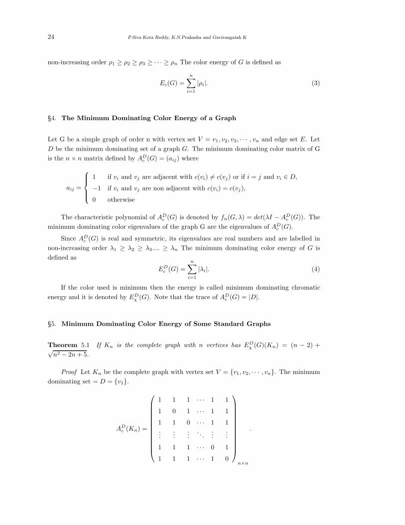
Theorem 5.1 If Kn is the complete graph with n vertices has EDχ (G)(Kn) = (n − 2) +√
n2 − 2n + 5.
Proof Let Kn be the complete graph with vertex set V = {v1, v2, · · · , vn}. The minimum
dominating set = D = {v1}.
ADc (Kn) =
1 1 1 · · · 1 1
1 0 1 · · · 1 1
1 1 0 · · · 1 1...
......
. . ....
...
1 1 1 · · · 0 1
1 1 1 · · · 1 0
n×n
.
Minimum Dominating Color Energy of a Graph 25
Its characteristic polynomial is
[λ + 1]n−2[λ2 − (n − 1)λ − 1].
The minimum dominating color eigenvalues are
specD(Kn) =
−1
n−1+√
(n2−2n+5)
2
n−1−√
(n2−2n+5)
2
n − 2 1 1
.
The minimum dominating color energy for complete graph is
EDχ (Kn) = | − 1|(n − 2) + | (n − 1) +
√(n2 − 2n + 5)
2|
+| (n − 1) −√
(n2 − 2n + 5)
2|
= (n − 2) +√
(n2 − 2n + 3),
i.e.,
EDχ (G)(Kn) = (n − 2) +
√(n2 − 2n + 5). 2
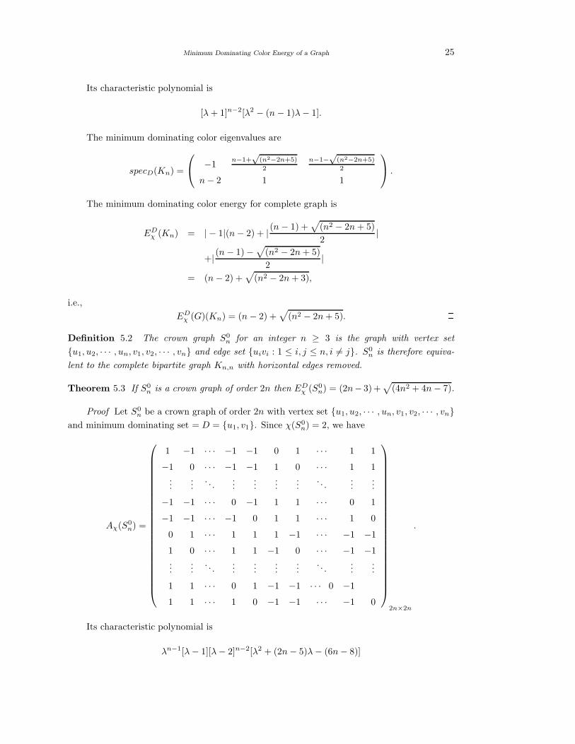
Definition 5.2 The crown graph S0n for an integer n ≥ 3 is the graph with vertex set
{u1, u2, · · · , un, v1, v2, · · · , vn} and edge set {uivi : 1 ≤ i, j ≤ n, i 6= j}. S0n is therefore equiva-
lent to the complete bipartite graph Kn,n with horizontal edges removed.
Theorem 5.3 If S0n is a crown graph of order 2n then ED
χ (S0n) = (2n− 3)+
√(4n2 + 4n − 7).
Proof Let S0n be a crown graph of order 2n with vertex set {u1, u2, · · · , un, v1, v2, · · · , vn}
and minimum dominating set = D = {u1, v1}. Since χ(S0n) = 2, we have
Aχ(S0n) =
1 −1 · · · −1 −1 0 1 · · · 1 1
−1 0 · · · −1 −1 1 0 · · · 1 1...
.... . .
......
......
. . ....
...
−1 −1 · · · 0 −1 1 1 · · · 0 1
−1 −1 · · · −1 0 1 1 · · · 1 0
0 1 · · · 1 1 1 −1 · · · −1 −1
1 0 · · · 1 1 −1 0 · · · −1 −1...
.... . .
......
......
. . ....
...
1 1 · · · 0 1 −1 −1 · · · 0 −1
1 1 · · · 1 0 −1 −1 · · · −1 0
2n×2n
.
Its characteristic polynomial is
λn−1[λ − 1][λ − 2]n−2[λ2 + (2n − 5)λ − (6n − 8)]
26 P.Siva Kota Reddy, K.N.Prakasha and Gavirangaiah K
and its minimum dominating color eigenvalues are
specDχ (S0
n) =
0 1 2
−(2n−5)+√
(4n2+4n−7)
2
−(2n−5)−√
(4n2+4n−7)
2
n − 1 1 n − 2 1 1
.
The minimum dominating color energy of S0n is
EDχ (S0
n) = |0|(n − 1) + |1|(n − 1) + |2| + |−(2n − 5) +√
(4n2 + 4n − 7)
2|
+|−(2n− 5) −√
(4n2 + 4n − 7)
2|
= (2n − 3) +√
4n2 + 4n − 7,
i.e.,
EDχ (S0
n) = (2n − 3) +√
4n2 + 4n − 7. 2.
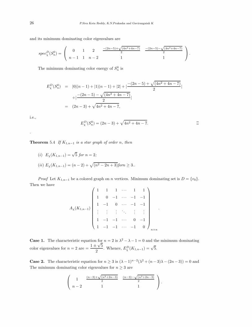
Theorem 5.4 If K1,n−1 is a star graph of order n, then
(i) Eχ(K1,n−1) =√
5 for n = 2;
(ii) Eχ(K1,n−1) = (n − 2) +√
(n2 − 2n + 3)forn ≥ 3..
Proof Let K1,n−1 be a colored graph on n vertices. Minimum dominating set is D = {v0}.Then we have
Aχ(K1,n−1)
1 1 1 · · · 1 1
1 0 −1 · · · −1 −1
1 −1 0 · · · −1 −1...
......
. . ....
...
1 −1 −1 · · · 0 −1
1 −1 −1 · · · −1 0
n×n
.
Case 1. The characteristic equation for n = 2 is λ2 −λ− 1 = 0 and the minimum dominating
color eigenvalues for n = 2 are =1 ±
√5
2. Whence, ED
χ (K1,n−1) =√
5.
Case 2. The characteristic equation for n ≥ 3 is (λ− 1)n−2(λ2 + (n− 3)λ− (2n− 3)) = 0 and
The minimum dominating color eigenvalues for n ≥ 3 are
1
(n−3)+√
(n2+2n−3)
2
(n−3)−√
(n2+2n−3)
2
n − 2 1 1
.
Minimum Dominating Color Energy of a Graph 27
Its minimum dominating color energy is
EDχ (K1,n−1) = |1|(n − 2) + |n − 3 +
√(n2 + 2n − 3)
2|
+|n − 3 −√
(n2 + 2n − 3)
2|
= (n − 2) +√
(n2 − 2n + 3).
Therefore,
EDχ (K1,n−1) = (n − 2) +
√(n2 − 2n + 3). 2
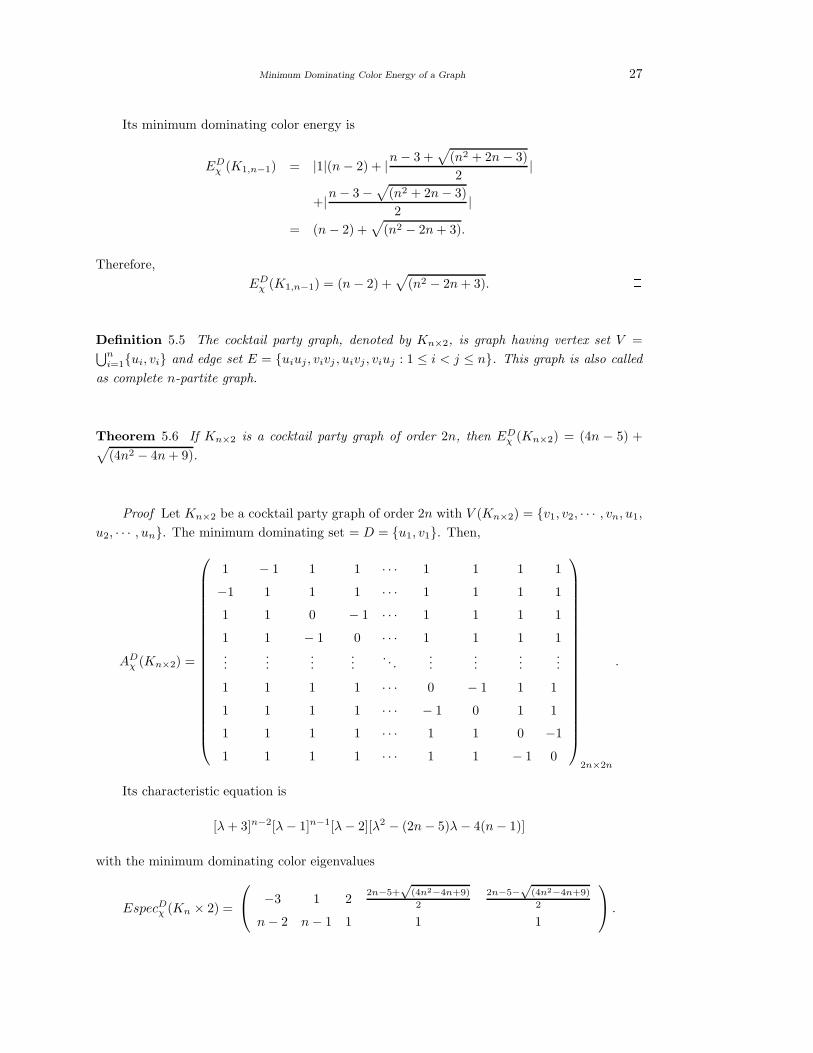
Definition 5.5 The cocktail party graph, denoted by Kn×2, is graph having vertex set V =⋃ni=1{ui, vi} and edge set E = {uiuj , vivj , uivj , viuj : 1 ≤ i < j ≤ n}. This graph is also called
as complete n-partite graph.
Theorem 5.6 If Kn×2 is a cocktail party graph of order 2n, then EDχ (Kn×2) = (4n − 5) +√
(4n2 − 4n + 9).
Proof Let Kn×2 be a cocktail party graph of order 2n with V (Kn×2) = {v1, v2, · · · , vn, u1,
u2, · · · , un}. The minimum dominating set = D = {u1, v1}. Then,
ADχ (Kn×2) =
1 − 1 1 1 · · · 1 1 1 1
−1 1 1 1 · · · 1 1 1 1
1 1 0 − 1 · · · 1 1 1 1
1 1 − 1 0 · · · 1 1 1 1...
......
.... . .
......
......
1 1 1 1 · · · 0 − 1 1 1
1 1 1 1 · · · − 1 0 1 1
1 1 1 1 · · · 1 1 0 −1
1 1 1 1 · · · 1 1 − 1 0
2n×2n
.
Its characteristic equation is
[λ + 3]n−2[λ − 1]n−1[λ − 2][λ2 − (2n − 5)λ − 4(n − 1)]
with the minimum dominating color eigenvalues
EspecDχ (Kn × 2) =
−3 1 2
2n−5+√
(4n2−4n+9)
2
2n−5−√
(4n2−4n+9)
2
n − 2 n − 1 1 1 1
.
28 P.Siva Kota Reddy, K.N.Prakasha and Gavirangaiah K
and the minimum dominating color energy,
EDχ (Kn × 2) = | − 3|(n − 2) + 1(n − 1) + |2| + |2n − 5 +
√(4n2 − 4n + 9)
2|
+|2n− 5 −√
(4n2 − 4n + 9)
2|
= (4n − 5) +√
(4n2 − 4n + 9).
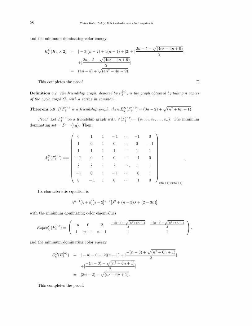
This completes the proof. 2Definition 5.7 The friendship graph, denoted by F
(n)3 , is the graph obtained by taking n copies
of the cycle graph C3 with a vertex in common.
Theorem 5.8 If F(n)3 is a friendship graph, then ED
χ (F(n)3 ) = (3n − 2) +
√(n2 + 6n + 1).
Proof Let F(n)3 be a friendship graph with V (F
(n)3 ) = {v0, v1, v2, . . . , vn}. The minimum
dominating set = D = {v3}. Then,
ADχ (F
(n)3 ) ==
0 1 1 − 1 · · · −1 0
1 0 1 0 · · · 0 − 1
1 1 1 1 · · · 1 1
−1 0 1 0 · · · −1 0...
......
.... . .
......
−1 0 1 − 1 · · · 0 1
0 − 1 1 0 · · · 1 0
(2n+1)×(2n+1)
.
Its characteristic equation is
λn−1[λ + n][λ − 2]n−1[λ2 + (n − 3)λ + (2 − 3n)]
with the minimum dominating color eigenvalues
EspecDχ (F
(n)3 ) =
−n 0 2
−(n−3)+√
(n2+6n+1)
2
−(n−3)−√
(n2+6n+1)
2
1 n − 1 n − 1 1 1
.
and the minimum dominating color energy
EDχ (F
(n)3 ) = | − n| + 0 + |2|(n − 1) + |−(n − 3) +
√(n2 + 6n + 1)
2|
+|−(n − 3) −√
(n2 + 6n + 1)
2|
= (3n − 2) +√
(n2 + 6n + 1).
This completes the proof. 2
Minimum Dominating Color Energy of a Graph 29
§6. Properties of Minimum Dominating Color Energy of a Graph
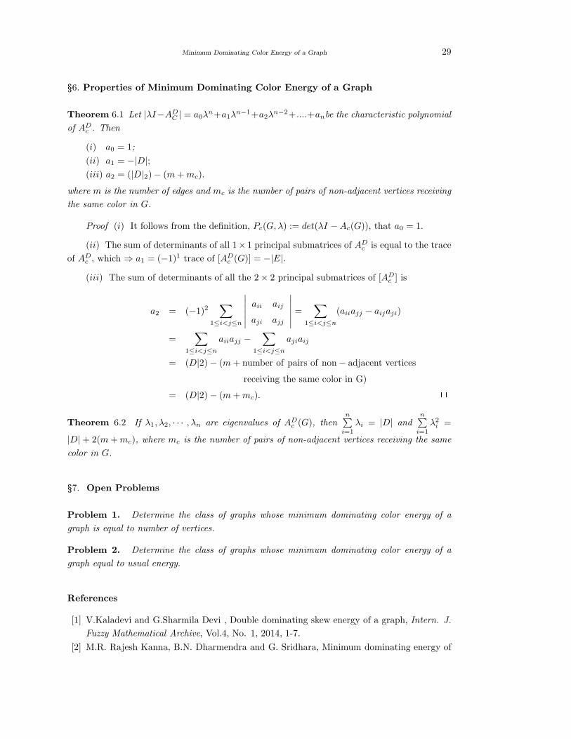
Theorem 6.1 Let |λI−ADC | = a0λ
n+a1λn−1+a2λ
n−2+....+anbe the characteristic polynomial
of ADc . Then
(i) a0 = 1;
(ii) a1 = −|D|;(iii) a2 = (|D|2) − (m + mc).
where m is the number of edges and mc is the number of pairs of non-adjacent vertices receiving
the same color in G.
Proof (i) It follows from the definition, Pc(G, λ) := det(λI − Ac(G)), that a0 = 1.
(ii) The sum of determinants of all 1× 1 principal submatrices of ADc is equal to the trace
of ADc , which ⇒ a1 = (−1)1 trace of [AD
c (G)] = −|E|.
(iii) The sum of determinants of all the 2 × 2 principal submatrices of [ADc ] is
a2 = (−1)2∑
1≤i<j≤n
∣∣∣∣∣∣aii aij
aji ajj
∣∣∣∣∣∣=
∑
1≤i<j≤n
(aiiajj − aijaji)
=∑
1≤i<j≤n
aiiajj −∑
1≤i<j≤n
ajiaij
= (D|2) − (m + number of pairs of non − adjacent vertices
receiving the same color in G)
= (D|2) − (m + mc). 2Theorem 6.2 If λ1, λ2, · · · , λn are eigenvalues of AD
c (G), thenn∑
i=1
λi = |D| andn∑
i=1
λ2i =
|D| + 2(m + mc), where mc is the number of pairs of non-adjacent vertices receiving the same
color in G.
§7. Open Problems
Problem 1. Determine the class of graphs whose minimum dominating color energy of a
graph is equal to number of vertices.
Problem 2. Determine the class of graphs whose minimum dominating color energy of a
graph equal to usual energy.
References
[1] V.Kaladevi and G.Sharmila Devi , Double dominating skew energy of a graph, Intern. J.
Fuzzy Mathematical Archive, Vol.4, No. 1, 2014, 1-7.
[2] M.R. Rajesh Kanna, B.N. Dharmendra and G. Sridhara, Minimum dominating energy of
30 P.Siva Kota Reddy, K.N.Prakasha and Gavirangaiah K
a graph, International Journal of Pure and Applied Mathematics, Volume 85 No. 4 2013,
707-718.
[3] I. Gutman,B. Zhou, Laplacian energy of a graph, Linear Algebra and its Applications,
414(2006), 29-37.
[4] C. Adiga and C. S. Shivakumaraswamy, Bounds on the largest minimum degree eigenvalues
of graphs, Int.Math.Forum., 5(37)(2010), 1823-1831.
[5] C. Adiga, E. Sampathkumar and M. A. Sriraj, Color energy of a graph, Proc.Jangjeon
Math.Soc., 16(3)(2013), 335-351.
[6] R.Balakrishnan, Energy of a Graph, Proceedings of the KMA National Seminar on Graph
Theory and Fuzzy Mathematics, August (2003), 28-39.
[7] R. B. Bapat and S. Pati, Energy of a graph is never an odd integer, Bull. Kerala Math.
Assoc., 1(2004), 129-132.
[8] Fan. R. K. Chung, Spectral graph theory, CBMS Regional Conference Series in Mathemat-
ics, No.92, 1997.
[9] C. A. Coulson, On the calculation of the energy in unsaturated hydrocarbons molecules.
Proc.Cambridge.Phil.Soc, 36(1940), 201-203.
[10] D. M. Cvetkovic, M. Doob, H Sachs, Spectra of Graphs- Theory and Applications, Academic
Press, new York, 1980.
[11] I. Gutman, The energy of a graph, Ber. Math. Stat. Sekt. Forschungsz. Graz, 103(1978),
1-22.
[12] I. Gutman, Hyperenergetic molecular graphs, J. Serb.Chem., 64(1999), 199-205.
[13] I. Gutman, The energy of a graph: old and new results, Combinatorics and Applications,
A. Betten, A. Khoner, R. Laue and A. Wassermann, eds., Springer, Berlin, 2001, 196-211.
[14] V. Nikiforov, Graphs and matrices with maximal energy, J.Math. Anal. Appl., 327(2007),
735-738.
[15] S. Pirzada and I. Gutman, Energy of a graph is never the square root of an odd integer,
Applicable Analysis and Discrete Mathematics, 2(2008), 118-121.
[16] H. S. Ramane, I. Gutman and D. S. Revankar, Distance equienergetic graphs, MATCH
Commun. Math. Comput. Chem., 60(2008), 473-484.
[17] H. S. Ramane, H. B. Walikar, S. B. Rao, B. D. Acharya, P. R. Hampiholi, S. R. Jog, I. Gut-
man, Spectra and energies of iterated line graphs of regular graphs, Applied Mathematical
Letters, 18(2005), 679-682.
[18] E. Sampathkumar, Graphs and matrices, Proceeding’s of the Workshop on Graph Theory
Applied to Chemistry, Eds. B. D. Acharya, K. A. Germina and R. Natarajan, CMS Pala,
No 39, 2010, 23-26.
[19] E. Sampathkumar and M. A. Sriraj, Vertex labeled/colored graphs, matrices and signed
graphs, J. of Combinatorics, Information and System Sciences, to appear.
[20] D. Stevanovic and G. Indulal, The distance spectrum and energy of the composition of
regular graphs, Appl. Math. Lett., 22(2009), 1136-1140.
[21] T. Aleksic, Upper bounds for Laplacian energy of graphs. MATCH Commun. Math.
Comput. Chem., 60 (2008) 435-439.
[22] N. N. M. de Abreu, C. T. M. Vinagre, A. S. Bonifacio, I.Gutman, The Laplacian energy
Minimum Dominating Color Energy of a Graph 31
of some Laplacian integral graphs. MATCH Commun. Math. Comput. Chem., 60(2008),
447 - 460.
[23] J. Liu, B. Liu, On relation between energy and Laplacian energy. MATCH Commun.
Math. Comput. Chem. 61(2009), 403-406.
[24] G. H. Fath-Tabar, A. R. Ashrafi, I. Gutman, Note on Laplacian energy of graphs. Bull.
Acad. Serbe Sci. Arts (Cl. Math. Natur.), 137(2008), 1-10.
[25] M. Robbiano, R. Jimenez, Applications of a theorem by Ky Fan in the theory of Laplacian
energy of graphs. MATCH Commun. Math. Comput. Chem. 62(2009), 537-552.
[26] D. Stevanovic, I. Stankovic, M. Milosevic, More on the relation between energy and Lapla-
cian energy of graphs. MATCH Commun. Math. Comput. Chem. 61(2009), 395-401.
[27] H. Wang, H. Hua, Note on Laplacian energy of graphs. MATCH Commun. Math. Comput.
Chem., 59(2008), 373-380.
[28] B. Zhou, New upper bounds for Laplacian energy. MATCH Commun. Math. Comput.
Chem., 62(2009), 553-560.
[29] B. Zhou, I. Gutman, Nordhaus-Gaddum-type relations for the energy and Laplacian energy
of graphs. Bull. Acad. Serbe Sci. Arts (Cl. Math. Natur.) 134(2007), 1-11.
[30] B. Zhou, On the sum of powers of the Laplacian eigenvalues of graphs. Lin. Algebra Appl.,
429(2008), 2239-2246.
[31] B. Zhou, I. Gutman, T. Aleksic, A note on Laplacian energy of graphs. MATCH Commun.
Math. Comput. Chem., 60(2008), 441-446.
[32] B. Zhou, I. Gutman, On Laplacian energy of graphs. MATCH Commun. Math. Comput.
[33] H. B. Walikar and H. S. Ramane, Energy of some cluster graphs, Kragujevac Journal of
Science, 23(2001), 51-62.
[34] B.J. McClelland, Properties of the latent roots of a matrix: The estimation of pi-electron
energies. J. Chem. Phys., 54(1971), 640 - 643.
[35] M. Fiedler, Additive compound matrices and an inequality for eigenvalues of symmetric
stochastic matrices, Czech. Math. J., 24(99) 392-402 (1974).
International J.Math. Combin. Vol.3(2017), 32-38
Cohen-Macaulay of Ideal I2 (G)
Abbas Alilou
(Department of Mathematics Azarbaijan Shahid, Madani University Tabriz, Iran)
E-mail: [email protected]
Abstract: In this paper, we study the Cohen-Macaulay of ideal I2 (G), where I2 (G) =
〈xyz | x − y − z is 2 − path in G〉. Also, we determined the 2-projective dimension R-
module, R/I2 (G) denoted by pd2 (G) of some graphs.
Key Words: Cohen-Macaulay, projective dimension, ideal, path.
AMS(2010): 05E15
§1. Introduction
A simple graph is a pair G = (V, E), where V = V (G) and E = E(G) are the sets of vertices
and edges of G, respectively. A walk is an alternating sequence of vertices and connecting
edges. A path is a walk that does not include any vertex twice, except that its first vertex
might be the same as its last. A path with length n denotes by P−n. In a graph G, the
distance between two distinct vertices x and y, denoted by d(x, y), is the length of the shortest
path connecting x and y, if such a path exists: otherwise, we set d(x, y) = ∞. The diameter
of a graph G is diam(G) = sup {d(x, y) : x and y are distinct vertices of G}. Also, a cycle
is a path that begins and ends on the same vertex. A cycle with length n denotes by Cn.
A graph G is said to be connected if there exists a path between any two distinct vertices,
and it is complete if it is connected with diameter one. We use Kn to denote the complete
graph with n vertices. For a positive integer r, a complete r-partite graph is one in which
each vertex is joined to every vertex that is not in the some subset. The complete bipartite
graph with part sizes m and n is denoted by Km,n. The graph K1,n−1 is called a star graph
in which the vertex with degree n − 1 is called the center of the graph. For any graph G, we
denote N [x] = {y ∈ V (G) : (x, y) is an edge of G}. Recall that the projective dimension of an
R-module M , denoted by pd(M), is the length of the minimal free resolution of M , that is,
pd(M) = max {I| βi,j(M) 6= 0 for some j}. There is a strong connection between the topology
of the simplicial complex and the structure of the free resolution of K[∆]. Let βi,j(∆) denotes
the N -graded Betti numbers of the Stanley-Reisner ring K[∆].
To any finite simple graph G with the vertex set V (G) = {x1, · · · , xn} and the edge set
E(G), one can attach an ideal in the Polynomial rings R = K [x1, · · · , xn] over the field K,
where ideal l2(G) is called the edge ideal of G such that l2(G) =< xyz| x − y − z is 2 −1Received December 19, 2016, Accepted August 13, 2017.
Cohen-Macaulay of Ideal I2 (G) 33
path in G >. Also the edge ring of G, denoted by K(G) is defined to be the quotient ring
K(G) = R/I2(G). Edge ideals and edge rings were first introduced by Villarreal [9] and then
they have been studied by many authors in order to examine their algebraic properties according
to the combinatorial data of graphs. In this paper, we denote Sn for a star graph with n + 1
vertices. Let R = K [x1, · · · , xn] be a polynomial ring over a field K with the grading induced by
deg(xi) = di, where di is a positive integer. If M =⊕∞
i=0 Mi is a finitely generated N -graded
module over R, its Hilbert function and Hilbert series are defined by H(M, i) = l(Mi) and
F (M, t) =∑∞
i=0 H(M, i)ti respectively, where l(Mi) denotes the length of Mi as a K-module,
in our case l(Mi) = dimK(Mi).
§2. Cohen-Macaulay of Ideal I2(G) and pd2(G) of Some Graph G
Definition 2.1 Let G be a graph with vertex set V . Then a subset A ⊆ V is a 2-vertex cover
for G if for every path xyz of G we have {x, y, z}∩A 6= ∅. A 2-minimal vertex cover of G is a
subset A of V such that A is a 2-vertex cover, and no proper subset of A is a vertex cover for
G. The smallest cardinality of a 2-vertex cover of G is called the 2-vertex covering number of
G and is denoted by a02(G).
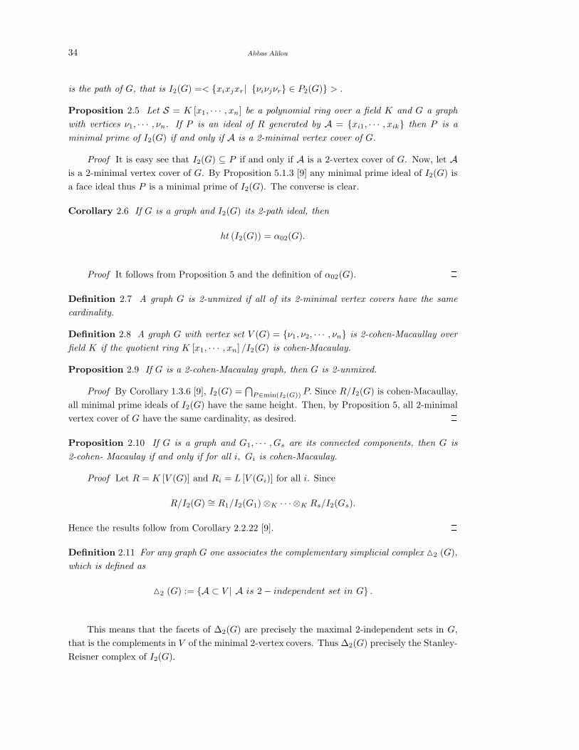
Example 2.2 Let G be a graph shown in the figure. Then the set {x2, x4, x7} is a 2-minimal
vertex cover of G and a02(G) = 3.
x1
x2
x3
x4
x5
x6
x7
Figure 1
Definition 2.3 Let G be a graph with vertex set V. A subset A ⊆ V is a k-independent if for
even x of A we have degG[S] ≤ k − 1. The maximum possible cardinality of an k-independent
set of G, denoted β0k(G), is called the k-independence number of G. It is easy see that
α02(G) + β02(G) = |V (G)|.
Definition 2.4 Let G be a graph without isolated vertices, Let S = K [x1, · · · , xn] the polynomial
ring on the vertices of G over some fixed field K. The 2-pathes ideal I2(G) associated to the
graph G is the ideal of S generated by the set of square-free monomials xixjxr such that νiνjνr
34 Abbas Alilou
is the path of G, that is I2(G) =< {xixjxr| {νiνjνr} ∈ P2(G)} > .
Proposition 2.5 Let S = K [x1, · · · , xn] be a polynomial ring over a field K and G a graph
with vertices ν1, · · · , νn. If P is an ideal of R generated by A = {xi1, · · · , xik} then P is a
minimal prime of I2(G) if and only if A is a 2-minimal vertex cover of G.
Proof It is easy see that I2(G) ⊆ P if and only if A is a 2-vertex cover of G. Now, let Ais a 2-minimal vertex cover of G. By Proposition 5.1.3 [9] any minimal prime ideal of I2(G) is
a face ideal thus P is a minimal prime of I2(G). The converse is clear. 2Corollary 2.6 If G is a graph and I2(G) its 2-path ideal, then
ht (I2(G)) = α02(G).
Proof It follows from Proposition 5 and the definition of α02(G). 2Definition 2.7 A graph G is 2-unmixed if all of its 2-minimal vertex covers have the same
cardinality.
Definition 2.8 A graph G with vertex set V (G) = {ν1, ν2, · · · , νn} is 2-cohen-Macaullay over
field K if the quotient ring K [x1, · · · , xn] /I2(G) is cohen-Macaulay.
Proposition 2.9 If G is a 2-cohen-Macaulay graph, then G is 2-unmixed.
Proof By Corollary 1.3.6 [9], I2(G) =⋂
P∈min(I2(G)) P. Since R/I2(G) is cohen-Macaullay,
all minimal prime ideals of I2(G) have the same height. Then, by Proposition 5, all 2-minimal
vertex cover of G have the same cardinality, as desired. 2Proposition 2.10 If G is a graph and G1, · · · , Gs are its connected components, then G is
2-cohen- Macaulay if and only if for all i, Gi is cohen-Macaulay.
Proof Let R = K [V (G)] and Ri = L [V (Gi)] for all i. Since
R/I2(G) ∼= R1/I2(G1) ⊗K · · · ⊗K Rs/I2(Gs).
Hence the results follow from Corollary 2.2.22 [9]. 2Definition 2.11 For any graph G one associates the complementary simplicial complex △2 (G),
which is defined as
△2 (G) := {A ⊂ V | A is 2 − independent set in G} .
This means that the facets of ∆2(G) are precisely the maximal 2-independent sets in G,
that is the complements in V of the minimal 2-vertex covers. Thus ∆2(G) precisely the Stanley-
Reisner complex of I2(G).
Cohen-Macaulay of Ideal I2 (G) 35
It is easy see that ω (∆2(G)) = {{x, y, z} | xyz ∈ P3(G)}. Therefore I2(G) = I∆2(G), and
so G is 2 − C − M graph if and only if the simplicial complex ∆2(G) is cohen-Macaulay.
Now, we can show the following propositiori.
Proposition 2.12 The following statements hold:
(a) For any n ≥ 1 the complete graph Kn is cohen-Macaulay;
(b) The complete bipartite graph Km,n is cohen-Macaulay if and only if m + n ≤ 4.
Proof (a) Since ∆2(Kn) =< {x, y} | x, y ∈ V (Kn) >, thus ∆2(Kn) is connected l-
dimensional simplicial complex, then by Corohary 5.3.7 [9], ∆2(Kn) is cohen-Macaula so Kn is
cohen-Macaulay.
(b) If m + n ≤ 4, then Km,n∼= P2, P3, C4. It is easy to see that ∆2(Km,n) is c. So Km,n
is cohen-Macaulay.
Conversely, let Km,n is cohen-Macaulay and m + n ≥ 5. Take V1 = {x1, · · · , xn} and
V2 = {y1, · · · , ym} are the partite sets of Km,n. One has
∆2(Km,n) =< {x1, · · · , xn} , {y1, · · · , ym} , {xi, yj} | 1 ≤ i ≤ n, 1 ≤ j ≤ m >
. Since m+n ≥ 5, ∆2(Km,n) is not pure simplicial complex. Then, by 5.3.12 [9] ∆2(Km,n)
is not cohen-Macaulay, a contradiction, as desired. 2Now, we present a result about the Hilbert series of K[∆2(Kn)] and K[∆2(Km,n)].
Proposition 2.13 If ∆2(Kn) and ∆2(Km,n) are the complementary simplicial complexes Kn
and Km,n respectively, then
(a) F (K[∆2(Kn)], z) = 1 + nz/(1 − z) + n(n − 1)/2(1 − z)2;
(b) F (K[∆2(Kn,m)], z) = 1/(1 − z)n + 1/(1 − z)m + m.nz2/(1 − z)2 − 1.
Proof (a) Since ∆2(Kn) =< {x, y} | x, y ∈ V (Kn) > hence dime ∆2(Kn) = 1 and
f−1(Kn) = 1, f0, (Kn) = n and f1(Kn) =(n2
)= n(n − 1)/2. By Corollary 5.4.5 [9]. We have
F (K[∆2(Kn)], z) = 1 + nz/1 − z + n(n − 1)/2.z2/2(1 − z)2.
(b) Let {x1, · · · , xn} and {y1, · · · , ym} are the parties sets of Km,n. Since
∆2(Km,n) =< {x1, · · · , xn} , {y1, · · · , ym} , {xi, yj} | 1 ≤ i ≤ n, 1 ≤ j ≤ m >
Then it is easy see that f1 (∆2(Km,n)) = f1 (∆(Km,n))+mn and fi (∆2(Km,n)) = fi (∆(Km,n))
for all i 6= 1. ln the other hand, by 6.6.6[9], F (K[∆2(Kn)], z) = 1/(1 − z)n − 1., Thus
F (K[∆2(Kn)], z) = 1/(1 − z)n + 1/(1 − z)m + m.nz2/(1 − z)2 − 1.
This completes the proof. 2Corollary 2.14 F (K [∆2(Sn)] , z) = 1/(1 − z)n + nz2/(1 − z)2 + z/(1 − z).
36 Abbas Alilou
Proof It follows from Proposition 2.13 with assume m = 1. 2In this section we mainly present basic properties of 2-shellable graphs.
Lemma 2.15 Let G be a graph and x be a vertex of degree 1 in G and let y ∈ N(x) and
G′
= G − ({y} ∪ N(y)) . Then ∆2(G′
) = lK∆2(G) ({x, y}) . Moreover F is a facet of ∆2(G′
) if
and only if F ∪ {x, y} is a facet of ∆2(G).
Proof (a) Let F ∈ lK∆2(G) ({x, y}) . Then F ∈ ∆2(G), x, y /∈ F and F ∪ {x, y} ∈ ∆2(G).
This implies that (F ∪ {x, y}) ∩ N [y] = ∅ and F ⊆ (V − {x, y}) ∪ N [y] = (V − y) ∪ N [y] =
V (G′
). Thus F is 2-independent in G′
, it follows that F ∈ ∆2(G′
). Conversely let F ∈ ∆2(G′
),
then F is 2-independent in G′
and F ∩ (x ∪ [y]) = ∅. Therefore F ∪ {x, y} is 2-independent in
G and so F ∪ {x, y} ∈ ∆2(G), F ∪ {x, y} = ∅. Thus F ∈ lK∆2(G) ({x, y}) . Finaly from part
one follows that F is a facet of ∆2(G′
) if and only if F ∪ {x, y} is a facet of ∆2(G). 2Definition 2.16 Fix a field K and set R = K[x1, · · · , xn]. If G is a graph with vertex
set V (G) = {x1, x2, · · · , xn}, we define the projective dimension of G to be the 2-projective
dimension R- module R/I2(G), and we will write pd2(G) = pd (R/l2(G)).
Proposition 2.17 If G is a graph and {x, y} is a edge of G, then
P2(G) ≤ max {P2 (G − (N [x] ∪ N [y])) + deg(x) + deg(y)
− |N [x] ∩ N [y]|, P2(G − x) + 1, P2(G − y) + 1} .
Proof Let N [x] = {x1, · · · , xξ} and N [y] = {y1, · · · , yr}. It is easy to see that
I2(G) : xy = (I2(G) − (N [x] ∪ N [y]) , x1, · · · , xξ, y1, · · · , yr) .
Now, let
R′
= K[V(G −
(N [x]
⋃N [y]
))].
Then
depth(R/I2(G) : xy) = depth(R′
/I2(G − (N [x] ∪ N [y]).
And so by Auslander-Buchsbaum formula, we have
pd2(R/I2(x) : xy) = pd2(G − (N [x] ∪ N [y]) + deg(x) + deg(y) − |N [x] ∩ N [y]|,pd2(R/I2(x), x) = pd2(G − x) + 1,
pd2(R/I2(x), y) = pd2(G − y) + 1.
On the other hand by Proposition 2.10, together with the exact sequence
0 −→ R/I2(G) : xy −→ R/I2(G) −→ R/I2(G)xy −→ 0,
Cohen-Macaulay of Ideal I2 (G) 37
it follows that
P2(G) ≤ max {P2(G − (N [x] ∪ N [y])) + deg(x) + deg(y)
− |N [x] ∩ N [y]|, P2(G − x) + 1, P2(G − y) + 1} . 2Proposition 2.18 Let G be a graph and I2(G) is path ideal of G. Then
Bight (I2(G)) ≤ pd2(G).
Proof Let P be a minimal vertex cover with maximal cardinality. Then by Proposition
2.5, P is an associated prime of R/I2(G), so
pd2(G) = pd (R/I2(G)) ≥ pdRp(Rp/I2(G)Rp) = dimRp = htP. 2
Proposition 2.19 Let Kn denote the complete graph on n vertices and let Km,n denote the
complete bipartite graph on m + n vertices.
(a) pd2(Kn) = n − 2;
(b) pd2(Km,n) = m + n − 2.
Proof (a) The proof is by induction on n. If n = 2 or 3, then the result easy follows. Let
n ≥ 4 and suppose that for every complete graphs Kn of other less than n the result is true.
Since Bight (I2 (Kn)) = n− 2 then by Proposition pd2(Kn) ≥ n− 2. On the other hand by the
inductive hypothesis, we have pd2(Kn−1) = n − 3. So by Proposition 2.17,
pd2(Kn) ≤ max {n − 2, n − 2} .
(b) Again we use by induction on m + n. If m + n = 2 or 3, then it is easy to see that
pd2(Km,n) = 0 or 1. Let m + n ≥ 4 and suppose that for every complete bipartite graph
Km,n of order less than m + n the result is true. Since Bight (I2 (Km,n)) = m + n − 2 then
pd2(Km,n) ≥ m + n − 2. Also, by the inductive hypothesis we have pd2(Km−1,n) = m + n − 3
and pd2(Km,n−1) = m + n − 3. So by Proposition2.17,
pd2(Km,n) ≤ max {m + n − 2, pd2(Km−1,n) + 1, pd2(Km,n−1) + 1 = m + n − 2} .
This completes the proof. 2Corollary 2.20 Let Sn denote the star graph on n + 1 vertices and Sm,n denote the double
star, then pd2(Sm,n) = m + n.
Proof It follows from Proposition 2.19 with assume m = 1 and it is easy to see that
BightI2 (Sm,n) = m + n, and so by Proposition 2.17, it follows that
pd2 (Sm,n) = m + n. 2
38 Abbas Alilou
References
[1] A. Conca, J. Herzog, Castelnuovo Mumford regularity of products of ideals, Collect. Math.,
54, (2003), No. 2, 137-152.
[2] H. Dao, C. Huneke, and J. Schweig, Projective dimension and independence complex ho-
mology, (to appear).
[3] A. Dochtermann and A. Engstrom, Algebraic properties of edge via combinatorial topology,
Electron. J. Combin., 16 (2009), Special volume in honor of Anders Bjorneg Reseearch
Paper 2.
[4] D. Ferrarello, The complement of a dtree is cohen-Macaulay, Math. Scand., 99(2006), 161-
167.
[5] J. Herzog, T. Hibi, Monomial Ideals, Graduate Texts in Mathematics, Springer-Verlag,
2011.
[6] J. Herzog, T. Hibi, X. Zheng, Monomial ideals whose powers have a linear resolution, Math.
Scand., 95 (2004), 23-32.
[7] C. Peskine and L. Szpiro, Dimension projective iinite et oohomologie locale, Inst. Hautes
Etudes Sci. Publ. Math., 42 (1973) 47-119.
[8] N. Terai, Alexander duality theorem and Stanley-Reisner rings. Free resolutions of co-
ordinate rings of projective varieties and related topics (Japanese) (Kyoto, 1998), Surhi-
aisekikenkyusho Kokyurokn, No. 1078 (I999), 174- 184.
[9] R. Villarreal, Monomial Algebras(Second edition), March 26, 2015 by Chapman and Hall/CRC.
International J.Math. Combin. Vol.3(2017), 39-50
Slant Submanifolds of a Conformal (k, µ)-Contact Manifold
Siddesha M.S.
(Department of mathematics, New Horizon College of Engineering, Bangalore, India)
Bagewadi C.S.
(Department of Mathematics, Kuvempu University, Shankaraghatta, Shimoga, Karnataka, India)
E-mail: prof [email protected]
Abstract: In this paper, we study the geometry of slant submanifolds of conformal (k, µ)-
contact manifold when the tensor field Q is parallel. Further, we give a necessary and
sufficient condition for a 3-dimensional slant submanifold of a 5-dimensional conformal (k, µ)-
contact manifold to be a proper slant submanifold.
Key Words: (k, µ)-contact manifold; conformal (k, µ)-contact manifold; slant submani-
fold.
AMS(2010): 53C25, 53C40, 53D15.
§1. Introduction
Let (M2n, J, g) be a Hermitian manifold of even dimension 2n, where J and g are the complex
structure and Hermitian metric respectively. Then (M2n, J, g) is a locally conformal Kahler
manifold if there is an open cover {Ui}i∈I of M2n and a family {fi}i∈I of C∞ functions fi :
Ui → R such that each local metric gi = exp(−fi)g|Ui is Kahlerian. Here g|Ui = ι∗i g where
ιi : Ui → M2n is the inclusion. Also (M2n, J, g) is globally conformal Kahler if there is a C∞
function f : M2n → R such that the metric exp(f)g is Kahlerian [11]. In 1955, Libermann [14]
initiated the study of locally conformal Kahler manifolds. The geometrical conditions for locally
conformal Kahler manifold have been obtained by Visman [22] and examples of these locally
conformal Kahler manifolds were given by Triceri in 1982 [21]. In 2001, Banaru [2] succeeded
to classify the sixteen classes of almost Hermitian Kirichenko’s tensors. The locally conformal
Kahler manifold is one of the sixteen classes of almost Hermitian manifolds. It is known that
there is a close relationship between Kahler and contact metric manifolds because Kahlerian
structures can be made into contact structures by adding a characteristic vector field ξ. The
contact structures consists of Sasakian and non-Sasakian cases. In 1972, Kenmotsu introduced
a class of contact metric manifolds, called Kenmotsu manifolds, which are not Sasakian [13].
Later in 1995, Blair, Koufogiorgos and Papantoniou [4] introduced the notion of (k, µ)-contact
manifold which consists of both Sasakian and non-Sasakian.
1Received January 9, 2017, Accepted August 15, 2017.
40 Siddesha M.S. and Bagewadi C.S.
On the other hand, Chen [7] introduced the notion of slant submanifold for an almost
Hermitian manifold, as a generalization of both holomorphic and totally real submanifolds.
Examples of slant submanifolds of C2 and C4 were given by Chen and Tazawa [8, 9, 10], while
slant submanifolds of Kaehler manifold were given by Maeda, Ohnita and Udagawa [17]. The
notion of slant immersion of a Riemannian manifold into an almost contact metric manifold
was introduced by Lotta [15] and he has proved some properties of such immersions. Later,
the study of slant submanifolds was enriched by the authors of [6, 12, 16, 18, 19] and many
others. Recently, the authors of [1] introduced conformal Sasakian manifold and studied slant
submanifolds of the conformal Sasakian manifold. As a generalization to the work of [1] in
[20], we defined conformal (k, µ)-contact manifold and studied invariant and anti-invariant
submanifolds of it. Our aim in the present paper is to extend the study of slant submanifold
to the setting of conformal (k, µ)-contact manifold.
The paper is organized as follows: In section 2, we recall the notion and some results of
(k, µ)-contact manifold and their submanifolds, which are used for further study. In section 3,
we introduce a conformal (k, µ)-contact manifold and give some properties of submanifolds of
it. Section 4 deals with the study of slant submaifolds of (k, µ)-contact manifold. Section 5
is devoted to the study of characterization of three-dimensional slant submanifolds of (k, µ)-
contact manifold via covariant derivative of T and T 2, where T is the tangent projection of
(k, µ)-contact manifold.
§2. Preliminaries
2.1 (k, µ)-Contact Manifold
Let M be a (2n + 1)-dimensional almost contact metric manifold with structure (φ, ξ, η, g),
where φ, ξ, η are the tensor fields of type (1, 1), (1, 0), (0, 1) respectively, and g is a Riemannian
metric on M satisfying
φ2 = −I + η ⊗ ξ, η(ξ) = 1, φξ = 0, η · φ = 0,
g(φX, φY ) = g(X, Y ) − η(X)η(Y ), η(X) = g(X, ξ), (2.1)
for all vector fields X, Y on M . An almost contact metric structure becomes a contact metric
structure if
g(X, φY ) = dη(X, Y ).
Then the 1-form η is contact form and ξ is a characteristic vector field.
We now define a (1, 1) tensor field h by h = 12Lξφ, where L denotes the Lie differentiation,
then h is symmetric and satisfies hφ = −φh. Further, a q-dimensional distribution on a manifold
M is defined as a mapping D on M which assigns to each point p ∈ M , a q-dimensional subspace
Dp of TpM .
Slant Submanifolds of a Conformal (k, µ)-Contact Manifold 41
The (k, µ)-nullity distribution of a contact metric manifold M(φ, ξ, η, g) is a distribution
N(k, µ) : p → Np(k, µ) = {Z ∈ TpM : R(X, Y )Z = k[g(Y, Z)X − g(X, Z)Y ]
+µ[g(Y, Z)hX − g(X, Z)hY ]}
for all X, Y ∈ TM . Hence if the characteristic vector field ξ belongs to the (k, µ)-nullity
distribution, then we have
R(X, Y )ξ = k[η(Y )X − η(X)Y ] + µ[η(Y )hX − η(X)hY ]. (2.2)
The contact metric manifold satisfying the relation (2.2) is called (k, µ) contact metric
manifold [4]. It consists of both k-nullity distribution for µ = 0 and Sasakian for k = 1. A
(k, µ)-contact metric manifold M(φ, ξ, η, g) satisfies
(∇X φ)Y = g(X + hX, Y )ξ − η(Y )(X + hX) (2.3)
for all X, Y ∈ TM , where ∇ denotes the Riemannian connection with respect to g. From (2.3),
we have
∇X ξ = −φX − φhX (2.4)
for all X, Y ∈ TM .
2.2 Submanifold
Assume M is a submanifold of a (k, µ)-contact manifold M . Let g and ∇ be the induced Rie-
mannian metric and connections of M , respectively. Then the Gauss and Weingarten formulae
are given respectively, by
∇XY = ∇XY + σ(X, Y ), ∇XN = −ANX + ∇⊥XN (2.5)
for all X, Y on TM and N ∈ T⊥M , where ∇⊥ is the normal connection and A is the shape
operator of M with respect to the unit normal vector N . The second fundamental form σ and
the shape operator A are related by:
g(σ(X, Y ), N) = g(ANX, Y ). (2.6)
Let R and R denote the curvature tensor of M and M , then, the Gauss and Ricci equations
are given by
g(R(X, Y )Z, W ) = g(R(X, Y )Z, W ) − g(σ(X, W ), σ(Y, Z)) + g(σ(X, Z), σ(Y, W )),
g(R(X, Y )N1, N2) = g(R⊥(X, Y )N1, N2) − g([A1, A2]X, Y )
for all X, Y, Z, W ∈ TM , N1, N2 ∈ T⊥M and A1, A2 are shape operators corresponding to
N1, N2 respectively.
For each x ∈ M and X ∈ TxM , we decompose φX into tangential and normal components
42 Siddesha M.S. and Bagewadi C.S.
as:
φX = TX + FX, (2.7)
where, T is an endomorphism and F is normal valued 1-form on TxM . Similarly, for any
N ∈ T⊥x M , we decompose φV into tangential and normal components as:
φN = tN + fN, (2.8)
where, t is a tangent valued 1-form and f is an endomorphism on T⊥x M .
2.3 Slant Submanifolds of an Almost Contact Metric Manifold
For any x ∈ M and X ∈ TxM such that X, ξ are linearly independent, the angle θ(x) ∈ [0, π2 ]
between φX and TxM is a constant θ, that is θ does not depend on the choice of X and x ∈ M .
θ is called the slant angle of M in M . Invariant and anti-invariant submanifolds are slant
submanifolds with slant angle θ equal to 0 and π2 , respectively [?]. A slant submanifold which
is neither invariant nor anti-invariant is called a proper slant submanifold.
We mention the following results for later use.
Theorem 2.1([6]) Let M be a submanifold of an almost contact metric manifold M such that
ξ ∈ TM . Then, M is slant if and only if there exists a constant λ ∈ [0, 1] such that
T 2 = −λ(I − η ⊗ ξ). (2.9)
Further more, if θ is the slant angle of M , then λ = cos2θ.
Corollary 2.1([6]) Let M be a slant submanifold of an almost contact metric manifold M with
slant angle θ. Then, for any X, Y ∈ TM , we have
g(TX, TY ) = cos2θ(g(X, Y ) − η(X)η(Y )), (2.10)
g(FX, FY ) = sin2θ(g(X, Y ) − η(X)η(Y )). (2.11)
Lemma 2.1([15]) Let M be a slant submanifold of an almost contact metric manifold M with
slant angle θ. Then, at each point x of M , Q|D has only one eigenvalue λ1 = −cos2θ.
Lemma 2.2([15]) Let M be a 3-dimensional slant submanifold of an almost contact metric
manifold M . Suppose that M is not anti invariant. If p ∈ M , then in a neighborhood of p,
there exist vector fields e1, e2 tangent to M , such that ξ, e1, e2 is a local orthonormal frame
satisfying
Te1 = (cosθ)e2, T e2 = −(cosθ)e1. (2.12)
§3. Conformal (k, µ)-Contact Manifold
A smooth manifold (M2n+1, φ, ξ, η, g) is called a conformal (k, µ)-contact manifold of a (k, µ)-
Slant Submanifolds of a Conformal (k, µ)-Contact Manifold 43
contact structure (M2n+1, φ, ξ, η, g) if, there is a positive smooth function f : M2n+1 → R such
that
g = exp(f)g, φ = φ, η = (exp(f))12 η, ξ = (exp(−f))
12 ξ. (3.1)
Example 3.1 Let R2n+1 be the (2n+1)-dimensional Euclidean space spanned by the orthogonal
basis {ξ, X1, X2, · · · , Xn, Y1, Y2, · · · , Yn} and the Lie bracket defined as in [?]. Then, the almost
contact metric structure (φ, ξ, η, g) defined by
φ
(n∑
i=1
(Xi
∂
∂xi+ Yi
∂
∂yi+ z
∂
∂z
))=
n∑
i=1
(Yi
∂
∂xi− Xi
∂
∂yi
)+
n∑
i=1
Yiyi ∂
∂z,
g = exp(−f){η ⊗ η +1
4
n∑
i=1
{(dxi)2 + (dyi)2}},
η = (exp(−f))12
{1
2(dz −
n∑
i=1
yidxi)
},
ξ = (exp(f))12
{2
∂
∂z
},
where f =∑n
i=1(xi)2 + (yi)2 + z2.
It is easy to reveal that (R2n+1, φ, ξ, η, g) is not a (k, µ)-contact manifold, but R2n+1 with
the structure (φ, ξ, η, g) defined by
φ = φ,
g = η ⊗ η +1
4
n∑
i=1
{(dxi)2 + (dyi)2},
η =1
2(dz −
n∑
i=1
yidxi),
ξ = 2∂
∂z,
is a (k, µ)-space form.
Let M be a conformal (k, µ)-contact manifold, let ∇ and ∇ denote the Riemannian con-
nections of M with respect to metrics g and g, respectively. Using the Koszul formula, we
obtain the following relation between the connections ∇ and ∇
∇XY = ∇XY +1
2{ω(X)Y + ω(Y )X − g(X, Y )ω♯} (3.2)
such that ω(X) = X(f) and ω♯ = gradf is a vector field metrically equivalent to 1-form ω, that
is g(ω♯, X) = ω(X).
44 Siddesha M.S. and Bagewadi C.S.
Then with a straight forward computation we will have
exp(−f)(R(X, Y, Z, W )) = R(X, Y, Z, W ) +1
2{B(X, Z)g(Y, W ) − B(Y, Z)
g(X, W ) + B(Y, W )g(X, Z) − B(X, W )g(Y, Z)}
+1
4‖ω♯‖2{g(X, Z)g(Y, W ) − g(Y, Z)g(X, W )} (3.3)
for all vector fields X, Y, Z, W on M , where B = ∇ω − 12ω ⊗ ω and R, R are the curvature
tensors of M related to connections of ∇ and ∇, respectively. Furthermore, by the relations,
(2.1), (2.3) and (3.2) we get
(∇X φ)Y = (exp(f))12 {g(X + hX, Y )ξ − η(Y )(X + hX)}
−1
2{ω(φY )X − ω(Y )φX + g(X, Y )φω♯ − g(X, φY )ω♯} (3.4)
∇X ξ = −(exp(f))12 {φX + φhX} +
1
2{η(X)ω♯ − ω(ξ)X} (3.5)
for all vector fields X, Y on M . Now assume M is a submanifold of a conformal (k, µ)-contact
manifold M and ∇, R are the connection, curvature tensor on M , respectively, and g is an
induced metric on M .
For all X, Y ∈ TM and N ∈ T⊥M , from the Gauss, Weingarten formulas and (3.4), we
obtain the following relations:
(∇XT )Y = AFY X + tσ(X, Y ) + (exp(f))12 {g(X + hX, Y )ξ − η(Y )(X + hX)}
−1
2{ω(φY )X − ω(Y )TX + g(X, Y )(φω♯)⊤ − g(X, TY )(ω♯)⊤}, (3.6)
(∇XF )Y = fσ(X, Y ) − σ(X, TY ) +1
2{ω(Y )FX − g(X, Y )Fω♯ + g(X, TY )ω♯⊥}, (3.7)
(∇X t)N = AfNX − PANX − 1
2{ω(φN)X − ω(N)PX + g(X, tN)(ω♯)⊤}, (3.8)
(∇Xf)N = −σ(X, tN) − FANX +1
2{ω(N)FX + g(X, tN)(ω♯)⊥}, (3.9)
where, g = g|M, η = η|M, ξ = ξ|M and φ = φ|M .
§4 Slant Submanifolds of Conformal (k, µ)-Contact Manifolds
In this section, we prove a characterization theorem for slant submanifolds of a conformal
(k, µ)-contact manifold.
Theorem 4.1 Let M be a slant submanifold of conformal (k, µ)-contact manifold M such that
ω♯ ∈ T⊥M and ξ ∈ TM . Then Q is parallel if and only if one of the following is true:
(i) M is anti-invariant;
(ii) dim(M) ≥ 3;
(iii)M is trivial.
Slant Submanifolds of a Conformal (k, µ)-Contact Manifold 45
Proof Let θ be the slant angle of M in M , then for any X, Y ∈ TM and by equation (2.9),
we infer
T 2Y = QY = cos2θ(−Y + η(Y )ξ). (4.1)
⇒ Q(∇XY ) = cos2θ(−∇XY + η(∇XY )ξ). (4.2)
Differentiating (4.1) covariantly with respect to X , we get
∇XQY = cos2θ(−∇XY + η(∇XY )ξ − g(Y,∇Xξ)ξ + η(Y )∇Xξ). (4.3)
Subtracting (4.2) from (4.3), we obtain
(∇XQ)Y = cos2θ[g(∇XY, ξ)ξ + η(Y )∇Xξ]. (4.4)
If Q is parallel, then from (??) it follows that either cos(θ) = 0 i.e. M is anti-invariant or
g(∇XY, ξ)ξ + η(Y )∇Xξ = 0. (4.5)
We know g(∇Xξ, ξ) = 0, since g(∇Xξ, ξ) = −g(ξ,∇Xξ), which implies ∇Xξ ∈ D.
Suppose ∇Xξ 6= 0, then (4.5) yields η(Y ) = 0 i.e. Y ∈ D. But then (4.5) implies
∇Xξ ∈ D⊥⊕ < ξ >, which is absurd.
Hence ∇Xξ = 0 and therefore either D = 0 or we can take at least two linearly independent
vectors X and TX to span D. In this case the eigenvalue must be non-zero as θ = π2 has already
been taken. Hence dim(M) ≥ 3. 2Now, we state the the main result of this section.
Theorem 4.2 Let M be a slant submanifold of conformal (k, µ)-contact manifold M such that
ξ ∈ TM . Then M is slant if and only if
(1) The endomorphism Q|D has only one eigen value at each point of M ;
(2) There exists a function λ : M → [0, 1] such that
(∇XQ)Y = λ{(exp(f))12 [g(Y, TX + ThX)ξ − η(Y )(TX + ThX)]
−1
2{ω(ξ)g(X, Y )ξ − η(X)ω(Y )ξ + ω(ξ)η(Y )X − η(X)η(Y )ω♯T }}, (4.6)
for any X, Y ∈ TM . Moreover, if θ is the slant angle of M , then λ = cos2θ.
Proof Statement 1 gets from Lemma (2.1). So, it remains to prove statement 2. Let M
be a slant submanifold, then by (4.4) we have
(∇XQ)Y = cos2θ(−g(Y,∇Xξ) + η(Y )∇Xξ). (4.7)
By putting (3.5) in (4.7), we find (4.6). Conversely, let λ1(x) is the only eigenvalue of Q|Dat each point x ∈ M and Y ∈ D be a unit eigenvector associated with λ1, i.e., QY = λ1Y .
46 Siddesha M.S. and Bagewadi C.S.
Then from statement (2), we have
X(λ1)Y + λ1∇XY = ∇X(QY ) = Q(∇XY ) + λ{(exp(f))12 g(X, TY + ThY )ξ
−1
2{ω(ξ)g(X, Y )ξ − η(X)ω(Y )ξ}}, (4.8)
for any X ∈ TM . Since both ∇XY and Q(∇XY ) are perpendicular to Y , we conclude that
X(λ1) = 0. Hence λ1 is constant. So it remains to prove M is slant. For proof one can refer to
Theorem (4.3) in [6].
§5. Slant Submanifolds of Dimension Three
Theorem 5.1 Let M be a 3-dimensional proper slant submanifold of a conformal (k, µ)-contact
manifold M , such that ξ ∈ TM , then
(∇XT )Y = cos2θ(exp(f))12 {g(X + hX, Y )ξ − η(Y )(X + hX)} +
1
2{ω(ξ)g(TX, Y )ξ
−η(X)ω(TY )ξ + ω(ξ)η(Y )TX − η(X)η(Y )Tω♯T } (5.1)
for any X, Y ∈ TM and θ is the slant angle of M .
Proof Let X, Y ∈ TM and p ∈ M . Let ξ, e1, e2 be the orthonormal frame in a neighborhood
U of p given by Lemma (2.2). Put ξ|U = e0 and let αji be the structural 1-forms defined by
∇Xei =2∑
j=0
αjiej . (5.2)
In view of orthonormal frame ξ, e1, e2, we have
Y = η(Y )e0 + g(Y, e1)e1 + g(Y, e2)e2. (5.3)
Thus, we get
(∇XT )Y = η(Y )(∇XT )e0 + g(Y, e1)(∇XT )e1 + g(Y, e2)(∇XT )e2. (5.4)
Therefore, for obtaining (∇XT )Y , we have to get (∇XT )e0, (∇XT )e1 and (∇XT )e2. By
applying (3.5), we get
(∇XT )e0 = ∇X(Te0) − T (∇Xe0)
= (exp(f))12 (T 2X + T 2hX) +
1
2{ω(ξ)TX − η(X)Tω♯T }. (5.5)
Slant Submanifolds of a Conformal (k, µ)-Contact Manifold 47
Moreover, by using (2.12) we obtain
(∇XT )e1 = ∇X(Te1) − T (∇Xe1)
= ∇X((cosθ)e2) − T (α01(X)e0 + α1
1(X)e1 + α21(X)e2)
= (cosθ)α02(X)e0. (5.6)
Similarly, we get
(∇XT )e2 = −(cosθ)α01(X)e0. (5.7)
By substituting (5.5)-(5.7) in (5.4), we have
(∇XT )Y = (exp(f))12 η(Y )(T 2X + T 2hX) +
1
2{η(Y )ω(ξ)TX − η(X)η(Y )Tω♯T }
+cos(θ){g(Y, e1)α02(X)e0 − g(Y, e2)α
01(X)e0}. (5.8)
Now, we obtain α01(X) and α0
2(X) as follows:
α01(X) = g(∇Xe1, e0)
= Xg(e1, e0) − g(e1,∇Xe0)
= −(exp(f))12 g(e2, X + hX) +
1
2{ω(ξ)g(e1, X) − η(X)ω(e1)} (5.9)
and similarly we get
α02(X) = cosθg(e1, X) + cosθg(e1, hX). (5.10)
By using (5.9) and (5.10) in (5.8) and in view of (5.3) and (2.9) we obtain (5.1). 2From, Theorems 4.3 and 5.4, we can state the following:
Corollary 5.1 Let M be a three dimensional submanifold of a (k, µ)-contact manifold tangent
to ξ. Then the following statements are equivalent:
(1) M is slant;
(2) (∇XT )Y = cos2θ(exp(f))12 {g(X + hX, Y )ξ − η(Y )(X + hX)} + 1
2{ω(ξ)g(TX, Y )ξ
−η(X)ω(TY )ξ + ω(ξ)η(Y )TX − η(X)η(Y )Tω♯T };
(3) (∇XQ)Y = λ{(exp(f))12 [g(X, TX + ThX)ξ − η(Y )(TX + ThX)]− 1
2{ω(ξ)g(X, Y )ξ
−η(X)ω(Y )ξ + ω(ξ)η(Y )X − η(X)η(Y )ω♯T }}.
The next result characterizes 3-dimensional slant submanifold in terms of the Weingarten
map.
Theorem 5.2 Let M be a 3-dimensional proper slant submanifold of a conformal (k, µ)-contact
48 Siddesha M.S. and Bagewadi C.S.
manifold M , such that ξ ∈ TM . Then, there exists a function C : M → [0, 1] such that
AFXY = AFY X + C(exp(f))12 (η(X)(Y + hY ) − η(Y )(X + hX)) + ω(ξ)g(TX, Y )ξ
+g(X, TY )ω♯ +1
2{η(X)ω(TY )ξ − η(Y )ω(TX)ξ + η(X)ω(ξ)TY
−η(Y )ω(ξ)TX − ω(X)TY + ω(Y )TX + ω(TX)Y − ω(TY )X}, (5.11)
for any X, Y ∈ TM . Moreover in this case, if θ is the slant angle of M then we have C = sin2θ.
Proof Let X, Y ∈ TM and M is a slant submanifold. From (3.6) and Theorem 5.1, we
have
tσ(X, Y ) = (λ − 1)(exp(f))12 {g(Y, X + hX)ξ − η(Y )(X + hX)} +
1
2{ω(ξ)g(X, TY )ξ
−η(X)ω(TY )ξ + ω(ξ)η(Y )TX − η(X)η(Y )Tω♯T
+ ω(TY )X − ω(Y )TX
+g(X, Y )Tω♯ − g(X, TY )ω♯} − AFY X. (5.12)
Now by using the fact that σ(X, Y ) = σ(Y, X), we obtain (5.11). 2Next, we assume that M is a three dimensional proper slant submanifold M of a five-
dimensional conformal (k, µ)-contact manifold M with slant angle θ. Then for a unit tangent
vector field e1 of M perpendicular to ξ, we put
e2 = (secθ)Te1, e3 = ξ, e4 = (cscθ)Fe1, e5 = (cscθ)Fe2. (5.13)
It is easy to show that e1 = −(secθ)Te2 and by using Corollary 2.1, {e1, e2, e3, e4, e5} form
an orthonormal frame such that e1, e2, e3 are tangent to M and e4, e5 are normal to M . Also
we have
te4 = −sinθe1, te5 = −sinθe2, fe4 = −cosθe5, fe5 = −cosθe4. (5.14)
If we put σrij = g(σ(ei, ej), er), i, j = 1, 2, 3, r = 4, 5, then we have the following result:
Lemma 5.1 In the above conditions, we have
σ412 = σ5
11, σ422 = σ5
12,
σ413 = σ5
23 = −(exp(f))12 sinθ
σ432 = σ4
33 = σ533 = σ5
13 = 0. (5.15)
Proof Apply (5.11) by setting X = e1 and Y = e2, we obtain
Ae4e2 = Ae5e1 + (cotθ){ω(ξ)ξ − ω♯ + ω(e1)e1 + ω(e2)e2}.
Slant Submanifolds of a Conformal (k, µ)-Contact Manifold 49
Using (2.6) in the above relation, we get
σ412 = σ5
11, σ422 = σ5
12, σ423 = σ5
13.
Further, by taking X = e1 and Y = e3 in (5.11), we have
Ae4e3 = −(exp(f))12 (sinθ)(e1 + he1). (5.16)
After applying (2.6) in (5.16), we obtain
σ413 = −(exp(f))
12 (sinθ), σ4
23 = σ433 = 0.
In the similar manner by putting X = e2 and Y = e3, we get
σ523 = −(exp(f))
12 (sinθ), σ5
33 = 0. 2References
[1] E. Abedi and R. Bahrami Ziabari, Slant submanifolds of a conformal Sasakian manifold,
Acta Universitatis Apulensis, 40 (2014), 35-49.
[2] M. Banaru, A new characterization of the Gray Hervella classes of almost Hermitian mani-
fold, 8th International Conference on Differential Geometry and its Applications, August
(2001), Opava Czech Republic, 27-31.
[3] D.E. Blair, Contact manifolds in Riemannian geometry, Lecture notes in Math., 509,
Springer-Verlag, Berlin, (1976).
[4] D.E. Blair, T. Koufogiorgos and B.J. Papantoniou, Contact metric manifolds satisfyng a
nullity condition, Israel J. Math., 91 (1995), 189-214.
[5] E. Boeckx, A full classification of contact metric (k, µ)-spaces, Illinois J. Math. 44 (2000),
212-219.
[6] J.L. Cabrerizo, A. Carriazo and L.M. Fernandez, Slant submanifolds in Sasakian mani-
folds, Glasgow Math. J., 42 (2000), 125-138.
[7] B.Y. Chen, Slant immersions, Bull. Aust. Math. Soc., 41 (1990), 135-147.
[8] B.Y. Chen, Geometry of slant submanifolds, Katholieke Universiteit Leuven, (1990).
[9] B.Y. Chen and Y. Tazawa, Slant surfaces with codimension 2, Ann. Fac. Sci. Toulouse
Math., 11(3) (1990), 29-43.
[10] B.Y. Chen and Y. Tazawa, Slant submanifolds in complex Euclidean spaces, Tokyo J.
Math., 14(1) (1991), 101-120.
[11] S. Dragomir and L. Ornea, Locally conformal Kaehler geometry, Prog. Math., 155 (1998).
[12] R.S. Gupta, S.M. Khursheed Haider and M.H. Shahid, Slant submanifolds of a Kenmotsu
manifold, Radovi Matematicki, Vol. 12 (2004), 205-214.
[13] K. Kenmotsu, A class of almost contact Riemannian manifolds, Tohoku Math. J., 24
(1972), 93-103.
50 Siddesha M.S. and Bagewadi C.S.
[14] P. Libermann, Sur les structure infinitesimals regulieres, Bull Soc. Math. France, 83
(1955), 195-224.
[15] A. Lotta, Slant submanifolds in contact geometry, Bull. Math. Soc. Roum., 39 (1996),
183-198.
[16] A. Lotta, Three dimensional slant submanifolds of K-contact manifolds, Balkan J. Geom.
Appl., 3(1) (1998), 37-51.
[17] S. Maeda, Y. Ohnita and S. Udagawa, On slant immersions into Kaehler manifolds, Kodai
Math. J., 16 (1993), 205-219.
[18] M.S. Siddesha and C.S. Bagewadi, On slant submanifolds of (k, µ)-contact manifold, Dif-
ferential Geometry-Dynamical Systems, 18 (2016), 123-131.
[19] M.S. Siddesha and C.S. Bagewadi, Semi-slant submanifolds of (k, µ)-contact manifold,
Commun. Fac. Sci. Univ. Ser. A1 Math. Stat., 67(2) (2017), XX-XX.
[20] M.S. Siddesha and C.S. Bagewadi, Submanifolds of a conformal (k, µ)-contact manifold,
Acta Mathematica Academiae Paedagogicae Nyegyhiensis (Accepted for publication).
[21] F. Tricerri, Some examples of Locally conformal Kaehler manifolds, Rend. Sem. Mat.
Torino, 40 (1982), 81-92.
[22] I. Vaisman, A geometry condition for locally conformal Kaehler manifolds to be Kaehler,
Geom. Dedic., 10(1-4) (1981), 129-134.
International J.Math. Combin. Vol.3(2017), 51-56
Operations of n-Wheel Graph via Topological Indices
V. Lokesha and T. Deepika
(Department of studies in Mathematics, Vijayanagara Sri Krishnadevaraya University, Ballari, India)
E-mail: [email protected]; [email protected]
Abstract: In this paper, we discussed the Topological indices viz., Wiener, Harmonic,
Geometric-Arithmetic(GA), first and second Zagreb indices of n-wheel graphs with bridges
using operator techniques.
Key Words: n-wheel graph, subdivision operator, line graph, complement of n-wheel,
wiener index, harmonic, GA, first and second zagreb indices.
AMS(2010): 05C12.
§1. Introduction
For vertices u, v ∈ V (G), the distance between u and v in G, denoted by dG(u, v), is the length
of a shortest (u, v)-path in G and let dG(v) be the degree of a vertex v ∈ V (G). A topological
index of a graph is a real number related to the graph; it does not depend on labeling or pic-
torial representation of a graph. In theoretical chemistry, molecular structure descriptors (also
called topological indices) are used for modeling physicochemical, pharmacologic, toxicologic,
biological and other properties of chemical compounds [4]. There exist several types of such in-
dices, especially those based on vertex and edge distances. One of the most intensively studied
topological indices is the Wiener index.
The Wiener index [17], defined as the sum of all distances between pairs of vertices u and
v in a graph G is given by
W (G) =∑
uv∈E(G)
d(u, v)
Another few degree based topological indices are defined as follows:
The Harmonic index according to [13] is given by
H(G) =∑
uv∈E(G)
2
du + dv
1Received October 22, 2016, Accepted August 16, 2017.

52 V. Lokesha and T. Deepika
The geometric-arithmetic index of a graph G [3], denoted by GA(G) and is defined by
GA(G) =∑
uv∈E(G)
2√
du.dv
du + dv
The first and second Zagreb indices [10] is defined as
M1(G) =∑
u∈V (G)
d2u, M2(G) =
∑
uv∈E(G)
du.dv
Throughout paper, we have used n-wheel graph with standard operators.
The n-wheel graph is defined as the graph K1 + Cn where K1 is the singleton graph and
Cn is the cycle graph. The center of the wheel is called the hub and the edges joining the hub
and vertices of Cn are called the spokes.
The well known operators are recalled [7, 9, 10].
Adding a additional edge on top most vertex of two or more graphs is defined as bridge
operator.
The subdivision graph S(G) of a graph G is the graph obtained by inserting an additional
vertex into each edge of G.
The Line graph L(G) of a graph G is the graph whose vertices correspond to the edges
of G with two vertices being adjacent in L(G) if and only if the corresponding edges in G are
adjacent in G.
Complement graph or inverse of a graph G is a graph G′ on the same vertices such that
two distinct vertices of G′ are adjacent if and only if they are not adjacent in G.
The paper is starting with the preliminaries needed for our study. Section 2, construction of
bridge operator in a wheel graph results on different topological indices are discussed. Section 3,
complement of wheel graph of constructed graph results are established. Section 4, Subdivision
operator of constructed graph results are shown. Final section deals with the line graph of
constructed graph results are highlighted.
§2. Distance and Degree-Based Indices of n-Wheel Graph with Bridge Operator
In this section, we constructed a n-wheel graph by attaching bridge at top most vertex of a
graphs and established the results on different topological indices.
Here, we denote the edge set of n-wheel graph Gn, then Ei = {e = uv ∈ E(G)|du + dv =
i, ∀i = 1, 2, · · · , n}.
Theorem 2.1 Let Gn be attached wheel graphs of n vertices with bridge operator bk, k > 0,
then the harmonic index is
H(Gn, bk) = (bk + 1)
[n3 + 8n2 + 3n − 42
3n2 + 15n + 18
]+
23bk + 16
28.
Operations of n-Wheel Graph via Topological Indices 53
Proof Consider two wheel graphs with 4 vertices (n ≥ 4), if a bridge is attached, there are
E6, E7, E8 edges for B(G1, G2) = B(G1, G2, ; v1, v2).
(i) The number of edges is 7bk + 6
The number of wheel graphs and bridges will increases in a graph G4 then the harmonic
index is:
H(G4, bk) =59bk + 52
28.
Similarly, if we consider two wheel graphs with 5 vertices, if a bridge is attached, there are
E6, E7, E8 edges.
(ii) The number of edges is 9bk + 8.
(iii) The number of wheel graphs and bridges will increases in a graph G5 then the harmonic
index is
H(G5, bk) =218bk + 197
84.
The total number of edges in Gn is (2n − 1)bk + 2(n − 1).
Computing for n vertices with bk bridges of Gn the harmonic index is
H(Gn, bk) = (bk + 1)
[n3 + 8n2 + 3n − 42
3n2 + 15n + 18
]+
23bk + 16
28. 2
Theorem 2.2 The geometric-arithmetic index of a bridge operator formed by Gn is
GA(Gn, bk) = (bk + 1)
[√3(n − 2)√n − 1
+4√
n − 1
2n − 1+ n − 3
]+
8√
3(bk + 1)
7+ 2bk.
Proof If a bridge is formed for two wheel graphs with 4 vertices, having E6, E7, E8 edges
and using equation (i), then geometric-arithmetic index is
GA(G4, bk) =4(3
√3 + 7)(bk + 1)
7
Similarly, For n = 5. Using (ii), then Geometric-Arithmetic index of G4 is
GA(G5, bk) = 2(bk + 1)4√
3 + 21
7+
4√
3 + 7
7+ 5bk.
Computing for n vertices bk bridges of Gn the geometric-arithmetic index is
GA(Gn, bk) = (bk + 1)
[√3(n − 2)√n − 1
+4√
n − 1
2n − 1+ n − 3
]+
8√
3(bk + 1)
7+ 2bk. 2
Theorem 2.3 The Gn of a bridge operator for wiener index is
W (Gn, bk) = n2(bk + 1) − 3n(bk + 1) + 3bk + 2.
54 V. Lokesha and T. Deepika
Proof We adopted the proof technique of Theorem 2.1 and using equations (i) and (ii) in
the wiener indices for n = 4 and n = 5 is
W (G4, bk) = 7bk + 6.
and
W (G5, bk) = 13bk + 12.
Computing for the wiener index of graph Gn is
W (Gn, bk) = n2(bk + 1) − 3n(bk + 1) + 3bk + 2. 2§3. Complement of a Constructed Graph
In this segment, a complement of a wheel graphs connected with the number of bridges bk
(constructed graph) for n ≥ 5 with respect to different topological indices are established.
Theorem 3.1 Let G′
n be a complement of constructed graph then harmonic index is
H(G′
n, bk) = (bk + 1)
[(n − 3)(n − 4)2
2+
2(n − 4)
2n − 7
]+
bk
n − 3.
Proof In G′
n having (n − 1) vertices with E2, E3, E4 edges. Therefore,
(iv) the total number of edges is 2(bk + 1).
Hence, the harmonic index is
H(G′
n, bk) = (bk + 1)
[(n − 3)(n − 4)2
2+
2(n − 4)
2n − 7
]+
bk
n − 3. 2
Theorem 3.2 The geometric-arithmetic index of G′
n is
GA(G′
n, bk) = (bk + 1)
[(n − 3)(n − 4)
2+
2(n − 4)√
(n − 4)(n − 3)
2n − 7
]+ bk.
Proof The proof technique is applied as in Theorem 3.1. Hence using equation (iv) we get
the required result.
GA(G′
n, bk) = (bk + 1)
[(n − 3)(n − 4)
2+
2(n − 4)√
(n − 4)(n − 3)
2n − 7
]+ bk. 2
Theorem 3.3 Let G′
n of wiener index is
W (G′
n, bk) = (bk + 1)
[(n − 1)(n − 4)
2
]+ bk.
Operations of n-Wheel Graph via Topological Indices 55
Proof Let n = 4, 5, 6, 7, · · · having distance bk, 3bk + 2, 6bk + 5,· · · , then the wiener index
is
W (G′
n, bk) = (bk + 1)
[(n − 1)(n − 4)
2
]+ bk. 2
Observation 3.3 If n = 4, H(G′
n, bk)=GA(G′
n, bk)=W (G′
n, bk)=bk.
§4. Subdivision of Constructed Graph on Degree-Based Indices
In this section, the subdivision operator of constructed graph (Gn) are highlighted.
Theorem 4.1 Let S(Gn) be a subdivision operator of constructed graph then,
(1) H [S(Gn, bk)] = 2(bk + 1)
[3n2 + 2n − 11
5(n + 1)
]+
15bk + 12
12;
(2) GA[S(Gn, bk)] = (bk + 1)
[6√
6(n + 1)(n − 2) + 10(n− 1)√
n + 2 + 5√
2(n + 1)
5(n + 1)
]+
bk
2;
(3) M1[S(Gn, bk)] = (bk + 1)(n2 + 7n − 1);
(4) M2[S(Gn, bk)] = (bk + 1)(22n− 25) + 16bk.
Proof A subdivision Gn graph having (3n − 2) vertices and 4(n − 1) edges among which
2(n− 1) vertices are of degree 2, (n− 2) vertices are of degree 3, n vertices are of degree (n− 1)
and by attaching bridge there exists 2bk edges and bk vertices having degree 2. Here also,
adopted the similar proof techniques of earlier theorems we obtained the required results. 2§5. Line Graph of Constructed Graph
In this section, the Line graph of bridge graph of n wheel graph related to different topological
indices are discussed. The following results are observed.
Theorem 5.1 Let L(Gn) be the line graph of constructed graph then
(1) H [L(Gn, bk)] = 2(bk + 1)
[(n − 3)
8+
2(n − 2)
(n + 4)+
(n − 1)(n − 2)
4n+
2
(n + 5)+
2
9
]+
bk
5;
(2) GA[L(Gn, bk)] = 2(bk+1)
[n − 3
2+
4√
n(n − 2)
(n + 4)+
(n − 1)(n − 2)
4+
2√
5n
(n + 5)+
4√
5
9
]+bk;
(3) M1[L(Gn, bk)] = (bk + 1)[n3 − n2 + 16n− 7];
(4) M2[L(Gn, bk)] =(bk + 1)
2
[n4 − 3n3 + 18n2 + 20n − 16
]+ 25bk.
Proof Consider L(Gn) be the line graph of wheel graph using bridge graph. In Gn there
are two copies of 2(n−1) vertices and total number of edges exists 6(n−1) and bk when bridge
is attached. Hence the results are proved by adopting same proof technique used in the earlier
sections. 2
56 V. Lokesha and T. Deepika
§6. Conclusion
In this paper, degree based and distance based indices for different types of operators on wheel
graphs are studied. This type of relationships may be useful to connectivity between graph
structures or chemical structures.
References
[1] A.R. Bindusree, V. Lokesha and P.S. Ranjini, ABC index on subdivision graphs and line
graphs, IOSR J. of Math., Vol. 1 (2014), pp. 01-06.
[2] A.R. Bindusree, I. Naci Cangul, V. Lokesha and A. Sinan Cevik, Zagreb polynomials of
three graph operators, Filomat, Vol. 30(7) (2016), pp. 1979-1986.
[3] K.C. Das, On geometric arithmetic index of graphs, MATCH Commun. Math. Comput.
Chem., Vol. 64 (2010), pp. 619 - 630.
[4] I. Gutman, Polansky O.E., Mathematical Concepts in Organic Chemistry, Springer, Berlin,
1986.
[5] F. Harary, Graph Theory, Addison-Wesely, Reading, 1969.
[6] M. H. Khalifeh, H. Yousefi-Azari and A. R. Ashrafi, The first and second Zagreb indices
of some graph operations, Discrete Appl. Math., Vol. 157 (2009), pp. 804 - 811.
[7] V. Lokesha, A. Usha, P.S. Ranjini and T. Deepika, Harmonic index of cubic polyhedral
graphs using bridge graphs, App. Math. Sci., Vol. 9 (2015), pp. 4245-4253.
[8] V. Lokesha, B. Shwetha Shetty, Phani Raju. M and P.S. Ranjini, Sum-Connectivity index
and average distance of trees, Int. J. Math. Combin., Vol. 4 (2015) pp. 92-98.
[9] P. S. Ranjini, V. Lokesha and M. A. Rajan, On Zagreb indices of the subdivision graphs,
Int. J. Math. Sc. Eng. Appl., Vol. 4 (2010), pp. 221 - 228.
[10] P.S. Ranjini, V. Lokesha, On the Zagreb indices of the line graphs of the subdivision graphs,
Appl. Math. Comput., Vol. 218 (2011), pp. 699 - 702.
[11] P.S. Ranjini, V. Lokesha, M.A. Rajan, On the Shultz index of the subdivision graphs, Adv.
Stud. Contemp. Math., Vol. 21(3) (2011), pp. 279 - 290.
[12] P.S. Ranjini, V. Lokesha and Phani Raju M, Bounds on Szeged index and the Pi index
interms of Second Zagreb index, Int. J. of Math. Combin., Vol. 1 (2012), pp. 47-51.
[13] B. Shwetha Shetty, V. Lokesha and P. S. Ranjini, On the Harmonic index of graph opera-
tions, Transactions on Combinatorics, Vol. 4(4), (2015), pp. 5-14.
[14] R. Todeschini, V. Consonni, Handbook of Molecular Descriptors, Wiley − VCH, Weinheim
2000.
[15] Xinli Xu, Relationships between Harmonic index and other topological indices, Applied
Mathematical Sciences, Vol. 6(41) (2012), pp. 2013 - 2018.
[16] Y. Yuan, B. Zhou and N. Trinajstic, On geometric arithmetic index, J. Math.Chem.,, Vol.
47 (2010), pp. 833 - 841.
[17] Yan, W., Yang, B. Y., and Yeh, Y. N. Wiener indices and polynomials of five graph
operators, precision. moscito.org /by-publ/recent/oper.
[18] B. Zhou, I. Gutman, B. Furtula and Z.Du, On two types of geometric arithmetic index,
Chem.Phys. Lett., Vol. 482 (2009), pp. 153 - 155.
International J.Math. Combin. Vol.3(2017), 57-70
Complexity of Linear and General Cyclic Snake Networks
E. M. Badr
Scientific Computing Department, Faculty of Computers and Informatics
Benha University, Egypt.
E-mail: [email protected]
B. Mohamed
Mathematics Department, Faculty of Science
Menoufia University, Egypt.
Abstract: In this paper we prove that the number of spanning trees of the linear and
general cyclic snake networks is the same using the combinatorial approach. We derive the
explicit formulas for the subdivided fan network S(Fn) and the subdivided ladder graph
S(Ln) . Finally, we calculate their spanning trees entropy and compare it between them.
Key Words: Number of spanning trees, Cyclic snakes networks, Entropy
AMS(2010): 05C05, 05C30
§1. Introduction
The complexity (the number of spanning trees) τ(G) of a finite connected undirected graph
G is defined as the total number of distinct connected acyclic spanning subgraphs. There are
many techniques to compute this number. Kirchhoff [1] gave the famous matrix tree theorem.
In which τ(G) = any cofactor of L (G ) , where L (G ) is equal to the degree matrix D (G )
of G minus the adjacency matrix A (G ) of G .
There are other methods for calculating t(G). Let µ1 > µ2 > · · · > µp denote the eigenval-
ues of H matrix of a p point graph. Then it is easily shown thatµp = 0. In 1974, Kelmans and
Chelnokov [2] shown that, τ(G) = 1p
∏p−1k=1 µk. The formula for the number of spanning trees in
a d-regular graph G can be expressed as t(G) = 1p
∏p−1k=1(d − µk) where λ0 = λ1, λ2, · · · , λp−1
are the eigenvalues of the corresponding adjacency matrix of the graph. However, for a few
special families of graphs there exist simple formulas that make it much easier to calculate and
determine the number of corresponding spanning trees especially when these numbers are very
large. One of the first such results is due to Cayley [3] who showed that complete graph on n
vertices, Kn has nn−2 spanning trees that he showed τ(Kn) = nn−2, n > 2. Clark [4] proved
that τ(Kp,q) = pq−1qp−1, p, q > 1, where Kp,q is the complete bipartite graph with bipartite
sets containing p and q vertices, respectively.
1Received December 05, 2016, Accepted August 18, 2017.
58 E. M. Badr and B. Mohamed
Therefore, many works derive formulas to calculate the complexity for some classes of
graphs. Bogdanowicz [5] derived the explicit formula for the fan network if n > 1,
τ(Fn) =1√5[(
3 +√
5
2)n − (
3 −√
5
2)n].
Sedlacek [6] proposed a formula for the number of spanning trees in a ladder graph. The
ladder Ln is the Cartesian product of P2 and Pn. The number of spanning trees in Ln is given
by
τ(Ln) =
√3
6[(2 +
√3)n − (2 −
√3)n]
for n > 1. A. Modabish and M. El Marraki investigated the number of spanning trees in the
star flower planar graph [7]. In [8], E.M. Badr and B.Mohamed derived the explicit formulas
for triangular snake (∆k − snake),double triangular snake (2∆k − snake) and the total graph
of path Pn(T (Pn)). Badr and Mohamed [9] derived the explicit formulas for the subdivision of
ladder, fan, wheel, triangular snake (∆k-snake), double triangular snake (2∆k-snake) and the
total graph of path Pn(T (Pn) ).
In this paper we prove that the number of spanning trees of the linear and general cyclic
snake networks is the same using the combinatorial approach. We derive the explicit formulas
for the subdivided fan network S(Fn) and the subdivided ladder graph S(Ln) . Finally, we
calculate their spanning trees entropy and compare it between them.
§2. Preliminary Notes
The combinatorial method involves the operation of contraction of an edge. An edge e of a
graph G is said to be contracted if it is deleted and its ends are identified. The resulting graph
is denoted by G.e . Also we denote by G− e the graph obtained from G by deleting the edge e.
Theorem 2.1([10]) Let G be a planar graph (multiple edges are allowed in here). Then for
any edge e,
τ(G) = τ(G − e) + τ(G · e).
Remark 2.2 If G’ is obtained from G by removing all the pendant edges of G, then
τ(G′
) = τ(G).
Remark 2.3 If G’ is obtained from G by removing all the loops of G, then τ(G′
) = τ(G).
Remark 2.4 If G’ is obtained from G by removing one or more than one multiple edges of G,
then τ(G′
) < τ(G).
Definition 2.5([11]) A triangular snake (∆k-snake) is a connected graph in which all blocks
are triangles and the block-cut-point graph is a path.
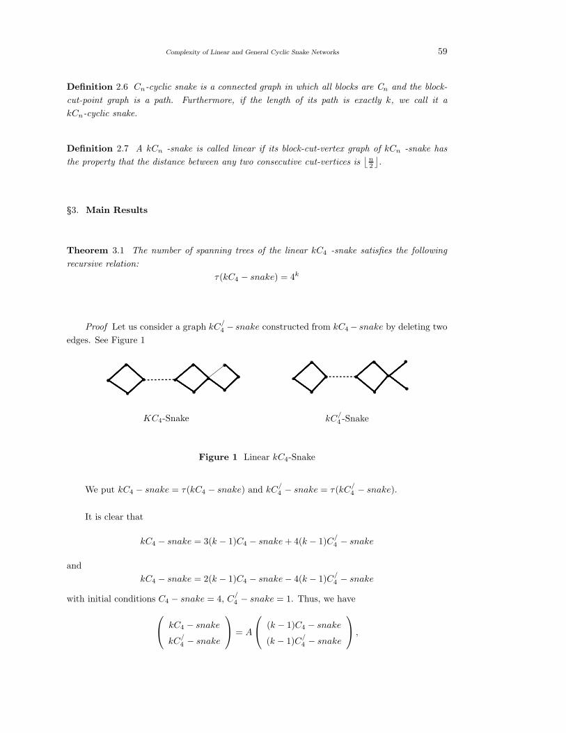
Complexity of Linear and General Cyclic Snake Networks 59
Definition 2.6 Cn-cyclic snake is a connected graph in which all blocks are Cn and the block-
cut-point graph is a path. Furthermore, if the length of its path is exactly k, we call it a
kCn-cyclic snake.
Definition 2.7 A kCn -snake is called linear if its block-cut-vertex graph of kCn -snake has
the property that the distance between any two consecutive cut-vertices is⌊
n2
⌋.
§3. Main Results
Theorem 3.1 The number of spanning trees of the linear kC4 -snake satisfies the following
recursive relation:
τ(kC4 − snake) = 4k
Proof Let us consider a graph kC/4 − snake constructed from kC4 − snake by deleting two
edges. See Figure 1
KC4-Snake kC/4 -Snake
Figure 1 Linear kC4-Snake
We put kC4 − snake = τ(kC4 − snake) and kC/4 − snake = τ(kC
/4 − snake).
It is clear that
kC4 − snake = 3(k − 1)C4 − snake + 4(k − 1)C/4 − snake
and
kC4 − snake = 2(k − 1)C4 − snake − 4(k − 1)C/4 − snake
with initial conditions C4 − snake = 4, C/4 − snake = 1. Thus, we have
kC4 − snake
kC/4 − snake
= A
(k − 1)C4 − snake
(k − 1)C/4 − snake
,
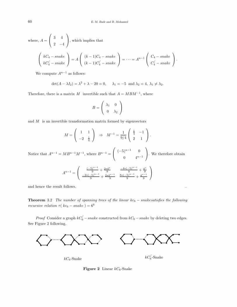
60 E. M. Badr and B. Mohamed
where, A =
3 4
2 −4
, which implies that
kC4 − snake
kC/4 − snake
= A
(k − 1)C4 − snake
(k − 1)C/4 − snake
= · · · = An−1
C4 − snake
C/4 − snake
.
We compute An−1 as follows:
det(A − λI2) = λ2 + λ − 20 = 0, λ1 = −5 and λ2 = 4, λ1 6= λ2.
Therefore, there is a matrix M invertible such that A = MBM−1, where
B =
λ1 0
0 λ2
and M is an invertible transformation matrix formed by eigenvectors
M =
1 1
−2 14
⇒ M−1 =
1
9/4
14 −1
2 1
.
Notice that An−1 = MBn−1M−1, where Bn−1 =
(−5)n−1 0
0 4n−1
. We therefore obtain
An−1 =
(−5)n−1
9 + 2∗4n
9−4∗(−5)n−1
9 + 4n
9
−2∗(−5)n−1
9 + 2∗4n−1
98∗(−5)n−1
9 + 4n−1
9
and hence the result follows. 2Theorem 3.2 The number of spanning trees of the linear kc6 − snakesatisfies the following
recursive relation τ( kc6 − snake ) = 6k
Proof Consider a graph kC/6 −snake constructed from kC6−snake by deleting two edges.
See Figure 2 following.
kC6-Snake kC/6 -Snake
Figure 2 Linear kC6-Snake
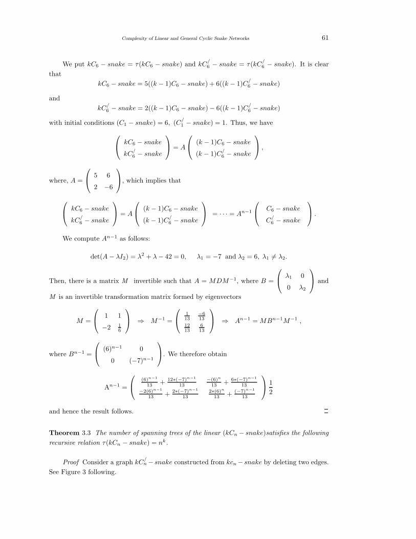
Complexity of Linear and General Cyclic Snake Networks 61
We put kC6 − snake = τ(kC6 − snake) and kC/6 − snake = τ(kC
/6 − snake). It is clear
that
kC6 − snake = 5((k − 1)C6 − snake) + 6((k − 1)C/6 − snake)
and
kC/6 − snake = 2((k − 1)C6 − snake) − 6((k − 1)C
/6 − snake)
with initial conditions (C1 − snake) = 6, (C/1 − snake) = 1. Thus, we have
kC6 − snake
kC/6 − snake
= A
(k − 1)C6 − snake
(k − 1)C/6 − snake
,
where, A =
5 6
2 −6
, which implies that
kC6 − snake
kC/6 − snake
= A
(k − 1)C6 − snake
(k − 1)C/6 − snake
= · · · = An−1
C6 − snake
C/6 − snake
.
We compute An−1 as follows:
det(A − λI2) = λ2 + λ − 42 = 0, λ1 = −7 and λ2 = 6, λ1 6= λ2.
Then, there is a matrix M invertible such that A = MDM−1, where B =
λ1 0
0 λ2
and
M is an invertible transformation matrix formed by eigenvectors
M =
1 1
−2 16
⇒ M−1 =
113
−613
1213
613
⇒ An−1 = MBn−1M−1 ,
where Bn−1 =
(6)n−1 0
0 (−7)n−1
. We therefore obtain
An−1 =
(6)n−1
13 + 12∗(−7)n−1
13−(6)n
13 + 6∗(−7)n−1
13
−2(6)n−1
13 + 2∗(−7)n−1
132∗(6)n
13 + (−7)n−1
13
1
2
and hence the result follows. 2Theorem 3.3 The number of spanning trees of the linear (kCn − snake)satisfies the following
recursive relation τ(kCn − snake) = nk.
Proof Consider a graph kC/n − snake constructed from kcn − snake by deleting two edges.
See Figure 3 following.
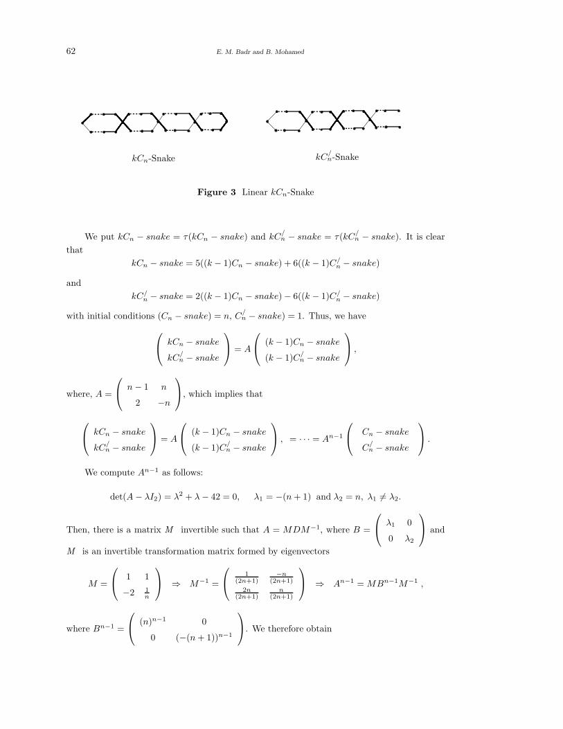
62 E. M. Badr and B. Mohamed
kCn-Snake kC/n-Snake
Figure 3 Linear kCn-Snake
We put kCn − snake = τ(kCn − snake) and kC/n − snake = τ(kC
/n − snake). It is clear
that
kCn − snake = 5((k − 1)Cn − snake) + 6((k − 1)C/n − snake)
and
kC/n − snake = 2((k − 1)Cn − snake) − 6((k − 1)C/
n − snake)
with initial conditions (Cn − snake) = n, C/n − snake) = 1. Thus, we have
kCn − snake
kC/n − snake
= A
(k − 1)Cn − snake
(k − 1)C/n − snake
,
where, A =
n − 1 n
2 −n
, which implies that
kCn − snake
kC/n − snake
= A
(k − 1)Cn − snake
(k − 1)C/n − snake
, = · · · = An−1
Cn − snake
C/n − snake
.
We compute An−1 as follows:
det(A − λI2) = λ2 + λ − 42 = 0, λ1 = −(n + 1) and λ2 = n, λ1 6= λ2.
Then, there is a matrix M invertible such that A = MDM−1, where B =
λ1 0
0 λ2
and
M is an invertible transformation matrix formed by eigenvectors
M =
1 1
−2 1n
⇒ M−1 =
1(2n+1)
−n(2n+1)
2n(2n+1)
n(2n+1)
⇒ An−1 = MBn−1M−1 ,
where Bn−1 =
(n)n−1 0
0 (−(n + 1))n−1
. We therefore obtain
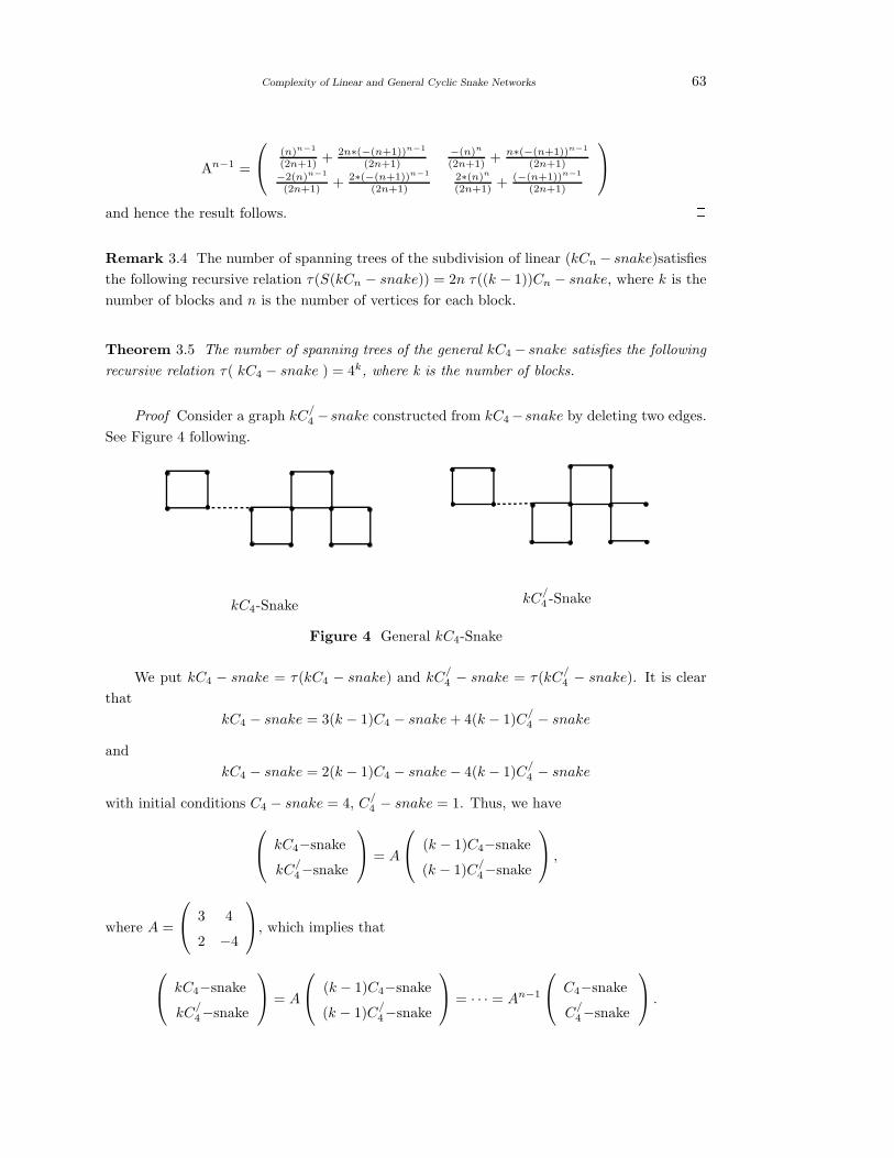
Complexity of Linear and General Cyclic Snake Networks 63
An−1 =
(n)n−1
(2n+1) + 2n∗(−(n+1))n−1
(2n+1)−(n)n
(2n+1) + n∗(−(n+1))n−1
(2n+1)
−2(n)n−1
(2n+1) + 2∗(−(n+1))n−1
(2n+1)2∗(n)n
(2n+1) + (−(n+1))n−1
(2n+1)
and hence the result follows. 2Remark 3.4 The number of spanning trees of the subdivision of linear (kCn − snake)satisfies
the following recursive relation τ(S(kCn − snake)) = 2n τ((k − 1))Cn − snake, where k is the
number of blocks and n is the number of vertices for each block.
Theorem 3.5 The number of spanning trees of the general kC4 − snake satisfies the following
recursive relation τ( kC4 − snake ) = 4k, where k is the number of blocks.
Proof Consider a graph kC/4 −snake constructed from kC4−snake by deleting two edges.
See Figure 4 following.
kC4-Snake kC/4 -Snake
Figure 4 General kC4-Snake
We put kC4 − snake = τ(kC4 − snake) and kC/4 − snake = τ(kC
/4 − snake). It is clear
that
kC4 − snake = 3(k − 1)C4 − snake + 4(k − 1)C/4 − snake
and
kC4 − snake = 2(k − 1)C4 − snake − 4(k − 1)C/4 − snake
with initial conditions C4 − snake = 4, C/4 − snake = 1. Thus, we have
kC4−snake
kC/4−snake
= A
(k − 1)C4−snake
(k − 1)C/4−snake
,
where A =
3 4
2 −4
, which implies that
kC4−snake
kC/4−snake
= A
(k − 1)C4−snake
(k − 1)C/4−snake
= · · · = An−1
C4−snake
C/4−snake
.
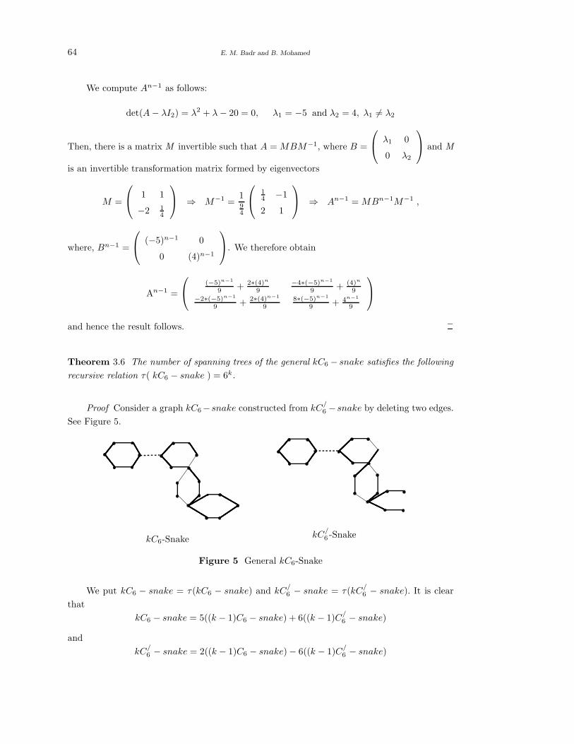
64 E. M. Badr and B. Mohamed
We compute An−1 as follows:
det(A − λI2) = λ2 + λ − 20 = 0, λ1 = −5 and λ2 = 4, λ1 6= λ2
Then, there is a matrix M invertible such that A = MBM−1, where B =
λ1 0
0 λ2
and M
is an invertible transformation matrix formed by eigenvectors
M =
1 1
−2 14
⇒ M−1 =
194
14 −1
2 1
⇒ An−1 = MBn−1M−1 ,
where, Bn−1 =
(−5)n−1 0
0 (4)n−1
. We therefore obtain
An−1 =
(−5)n−1
9 + 2∗(4)n
9−4∗(−5)n−1
9 + (4)n
9
−2∗(−5)n−1
9 + 2∗(4)n−1
98∗(−5)n−1
9 + 4n−1
9
and hence the result follows. 2Theorem 3.6 The number of spanning trees of the general kC6 − snake satisfies the following
recursive relation τ( kC6 − snake ) = 6k.
Proof Consider a graph kC6−snake constructed from kC/6 −snake by deleting two edges.
See Figure 5.
kC6-Snake kC/6 -Snake
Figure 5 General kC6-Snake
We put kC6 − snake = τ(kC6 − snake) and kC/6 − snake = τ(kC
/6 − snake). It is clear
that
kC6 − snake = 5((k − 1)C6 − snake) + 6((k − 1)C/6 − snake)
and
kC/6 − snake = 2((k − 1)C6 − snake) − 6((k − 1)C
/6 − snake)
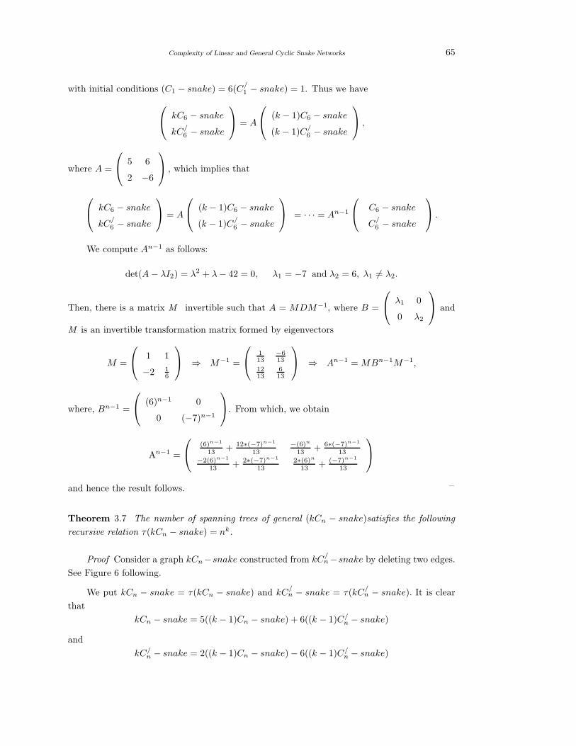
Complexity of Linear and General Cyclic Snake Networks 65
with initial conditions (C1 − snake) = 6(C/1 − snake) = 1. Thus we have
kC6 − snake
kC/6 − snake
= A
(k − 1)C6 − snake
(k − 1)C/6 − snake
,
where A =
5 6
2 −6
, which implies that
kC6 − snake
kC/6 − snake
= A
(k − 1)C6 − snake
(k − 1)C/6 − snake
= · · · = An−1
C6 − snake
C/6 − snake
.
We compute An−1 as follows:
det(A − λI2) = λ2 + λ − 42 = 0, λ1 = −7 and λ2 = 6, λ1 6= λ2.
Then, there is a matrix M invertible such that A = MDM−1, where B =
λ1 0
0 λ2
and
M is an invertible transformation matrix formed by eigenvectors
M =
1 1
−2 16
⇒ M−1 =
113
−613
1213
613
⇒ An−1 = MBn−1M−1,
where, Bn−1 =
(6)n−1 0
0 (−7)n−1
. From which, we obtain
An−1 =
(6)n−1
13 + 12∗(−7)n−1
13−(6)n
13 + 6∗(−7)n−1
13
−2(6)n−1
13 + 2∗(−7)n−1
132∗(6)n
13 + (−7)n−1
13
and hence the result follows. 2Theorem 3.7 The number of spanning trees of general (kCn − snake)satisfies the following
recursive relation τ(kCn − snake) = nk.
Proof Consider a graph kCn−snake constructed from kC/n−snake by deleting two edges.
See Figure 6 following.
We put kCn − snake = τ(kCn − snake) and kC/n − snake = τ(kC
/n − snake). It is clear
that
kCn − snake = 5((k − 1)Cn − snake) + 6((k − 1)C/n − snake)
and
kC/n − snake = 2((k − 1)Cn − snake) − 6((k − 1)C/
n − snake)
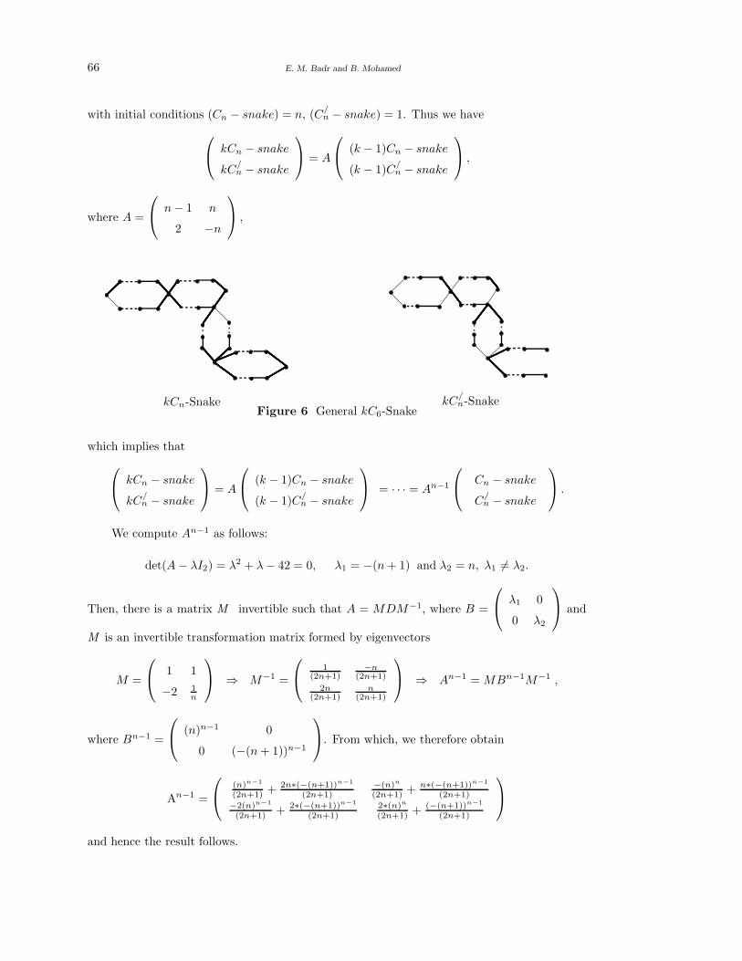
66 E. M. Badr and B. Mohamed
with initial conditions (Cn − snake) = n, (C/n − snake) = 1. Thus we have
kCn − snake
kC/n − snake
= A
(k − 1)Cn − snake
(k − 1)C/n − snake
,
where A =
n − 1 n
2 −n
,
kCn-Snake kC/n-Snake
Figure 6 General kC6-Snake
which implies that
kCn − snake
kC/n − snake
= A
(k − 1)Cn − snake
(k − 1)C/n − snake
= · · · = An−1
Cn − snake
C/n − snake
.
We compute An−1 as follows:
det(A − λI2) = λ2 + λ − 42 = 0, λ1 = −(n + 1) and λ2 = n, λ1 6= λ2.
Then, there is a matrix M invertible such that A = MDM−1, where B =
λ1 0
0 λ2
and
M is an invertible transformation matrix formed by eigenvectors
M =
1 1
−2 1n
⇒ M−1 =
1(2n+1)
−n(2n+1)
2n(2n+1)
n(2n+1)
⇒ An−1 = MBn−1M−1 ,
where Bn−1 =
(n)n−1 0
0 (−(n + 1))n−1
. From which, we therefore obtain
An−1 =
(n)n−1
(2n+1) + 2n∗(−(n+1))n−1
(2n+1)−(n)n
(2n+1) + n∗(−(n+1))n−1
(2n+1)
−2(n)n−1
(2n+1) + 2∗(−(n+1))n−1
(2n+1)2∗(n)n
(2n+1) + (−(n+1))n−1
(2n+1)
and hence the result follows. 2
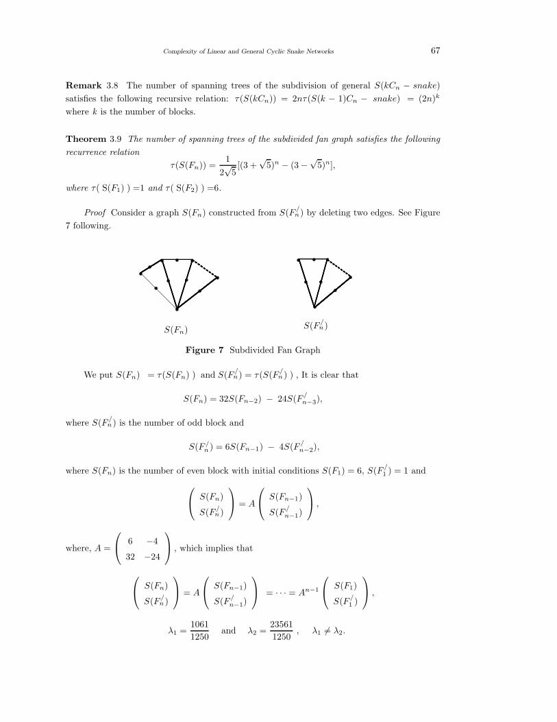
Complexity of Linear and General Cyclic Snake Networks 67
Remark 3.8 The number of spanning trees of the subdivision of general S(kCn − snake)
satisfies the following recursive relation: τ(S(kCn)) = 2nτ(S(k − 1)Cn − snake) = (2n)k
where k is the number of blocks.
Theorem 3.9 The number of spanning trees of the subdivided fan graph satisfies the following
recurrence relation
τ(S(Fn)) =1
2√
5[(3 +
√5)n − (3 −
√5)n],
where τ( S(F1) ) =1 and τ( S(F2) ) =6.
Proof Consider a graph S(Fn) constructed from S(F/n) by deleting two edges. See Figure
7 following.
S(Fn) S(F/n)
Figure 7 Subdivided Fan Graph
We put S(Fn) = τ(S(Fn) ) and S(F/n) = τ(S(F
/n ) ) , It is clear that
S(Fn) = 32S(Fn−2) − 24S(F/n−3),
where S(F/n) is the number of odd block and
S(F /n ) = 6S(Fn−1) − 4S(F
/n−2),
where S(Fn) is the number of even block with initial conditions S(F1) = 6, S(F/1 ) = 1 and
S(Fn)
S(F/n)
= A
S(Fn−1)
S(F/n−1)
,
where, A =
6 −4
32 −24
, which implies that
S(Fn)
S(F/n )
= A
S(Fn−1)
S(F/n−1)
= · · · = An−1
S(F1)
S(F/1 )
,
λ1 =1061
1250and λ2 =
23561
1250, λ1 6= λ2.
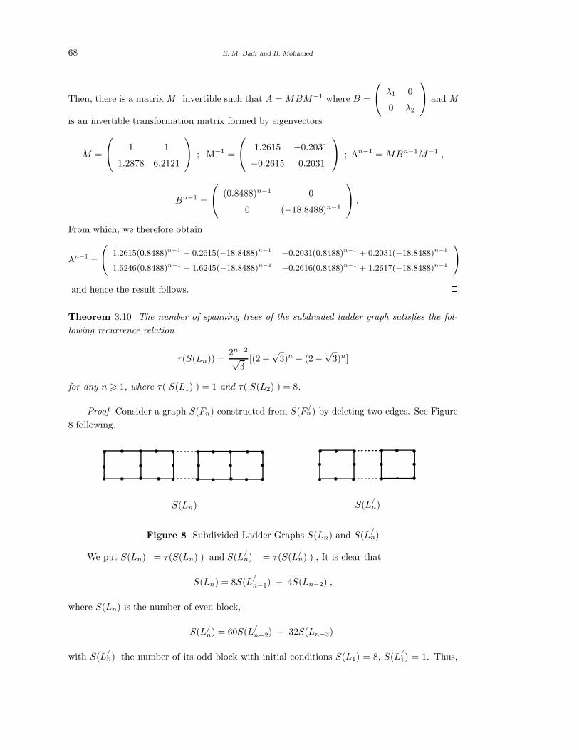
68 E. M. Badr and B. Mohamed
Then, there is a matrix M invertible such that A = MBM−1 where B =
λ1 0
0 λ2
and M
is an invertible transformation matrix formed by eigenvectors
M =
1 1
1.2878 6.2121
; M−1 =
1.2615 −0.2031
−0.2615 0.2031
; An−1 = MBn−1M−1 ,
Bn−1 =
(0.8488)n−1 0
0 (−18.8488)n−1
.
From which, we therefore obtain
An−1 =
1.2615(0.8488)n−1 − 0.2615(−18.8488)n−1 −0.2031(0.8488)n−1 + 0.2031(−18.8488)n−1
1.6246(0.8488)n−1 − 1.6245(−18.8488)n−1 −0.2616(0.8488)n−1 + 1.2617(−18.8488)n−1
and hence the result follows. 2Theorem 3.10 The number of spanning trees of the subdivided ladder graph satisfies the fol-
lowing recurrence relation
τ(S(Ln)) =2n−2
√3
[(2 +√
3)n − (2 −√
3)n]
for any n > 1, where τ( S(L1) ) = 1 and τ( S(L2) ) = 8.
Proof Consider a graph S(Fn) constructed from S(F/n) by deleting two edges. See Figure
8 following.
S(Ln) S(L/n)
Figure 8 Subdivided Ladder Graphs S(Ln) and S(L/n)
We put S(Ln) = τ(S(Ln) ) and S(L/n) = τ(S(L
/n) ) , It is clear that
S(Ln) = 8S(L/n−1) − 4S(Ln−2) ,
where S(Ln) is the number of even block,
S(L/n) = 60S(L
/n−2) − 32S(Ln−3)
with S(L/n) the number of its odd block with initial conditions S(L1) = 8, S(L
/1) = 1. Thus,
Complexity of Linear and General Cyclic Snake Networks 69
we have S(Ln)
S(L/n)
= A
S(Ln−1)
S(L/n−1)
,
where A =
8 −4
60 −32
, which implies that
S(Ln)
S(L/n)
= A
S(Ln−1)
S(L/n−1)
= · · · = An−1
S(L1)
S(L/1)
,
λ1 = 0.49 and λ2 = −24.49 , λ1 6= λ2.
Then, there is a matrix M invertible such that A = MBM−1 where B =
λ1 0
0 λ2
and M
is an invertible transformation matrix formed by eigenvectors
M =
1 1
1.8775 8.1225
; M−1 =
1.3006 −0.1601
−0.3006 0.1601
; An−1 = MBn−1M−1 ,
with Bn−1 =
(0.49)n−1 0
0 (−24.49)n−1
. From which, we therefore obtain
An−1 =
1.3006(0.49)n−1 − 0.3006(−24.49)n−1 −0.1601(0.49)n−1 + 0.1601(−24.49)n−1
2.4419(0.49)n−1 − 2.4416(−24.49)n−1 −0.3022(0.49)n−1 + 1.3004(−24.49)n−1
and hence the result follows. 2§4. Spanning Tree Entropy
The entropy of spanning trees of a network or the asymptotic complexity is a quantitative
measure of the number of spanning trees and it characterizes the network structure. We use
this entropy to quantify the robustness of networks. The most robust network is the network
that has the highest entropy. We can calculate its spanning tree entropy which is a finite number
and a very interesting quantity characterizing the network structure, defined as in [15, 16] as:
Z(G) = limV (G)→∞
ln τ(G)
|V (G)| ,
Z(KC4−snake) = limn→∞
ln 4k
3k + 1= 0.4621,
Z(KC6−snake) = limn→∞
ln 6k
5k + 1= 0.3584
70 E. M. Badr and B. Mohamed
Z(KCn − snake) = limk→∞
lnnk
(n − 1)k + 1=
ln(n)
n − 1,
Z(S(Fn)) = limn→∞
ln( 12√
5∗ (3 +
√5)n − (3 −
√5)n)
3n + 1= ln(
3
√3 +
√5) = 0.5513
Z(S(Ln)) = limn→∞
ln(2n−2√
3∗ (2 +
√3)n − (2 −
√3)n)
5n − 2= ln(
5
√2 +
√3) +
ln(2)
5= 0.4020
§5. Conclusion
In this paper, we described how to propose the combinatorial approach to facilitate the cal-
culation of the number of spanning trees in linear and general cyclic snake networks. In par-
ticular, we derived the explicit formulas for the linear kc4 − snake, linear kc6 − snake and
linear kcn − snake . Finally, we derived explicit formulas for the general kc4 − snake, general
kc6 − snake and general kcn − snake.
References
[1] G.Kirchhoff, Uber die Auflosung der Gleichungen, auf welche man bei der Untersuchung
der, Linearen Verteilung galvanischer Strme gefhrt wird, Ann. Phys. Chem, 72 (1847),
497-508.
[2] Kelmans A.K. and V.M.Chelnokov, A certain polynomial of a graph and graphs with an
extremal number of trees, J. Comb. Theory, 16 (1974), 197-214.
[3] G.A. , A theorem on trees. Quart, J. Math., 23 (1889), 276-378.
[4] L.Clark, On the enumeration of complete multipartite graph, Bull. Inst. Combin. Appl.,
38 (2003) 50-60.
[5] R.Zbigniew Bogdanowicz, Formulas for the Number of Spanning Trees in a Fan, Applied
Mathematical Sciences, Vol. 2, no. 16, (2008) 781-786
[6] J.Sedlacek, On the Spanning Trees of Finite Graphs, Cas. Pestovani Mat., 94 (1969)
217-221.
[7] A.Modabish, M. El Marrak, Counting the number of spanning trees in the star flower
planar map, Applied Mathematical Sciences, Vol. 6, no. 49, (2012) 2411 - 2418
[8] E.M.Badr and B.Mohamed, Generating recursive formulas for the number of spanning
trees in cyclic snakes networks, 4th International conference on Mathematics & Information
Science, 05-07 Feb.(2015), Cairo, Egypt.
[9] E.M.Badr and B. Mohamed, Enumeration of the number of Spanning Trees for the Sub-
division Technique of Five New Classes of Graphs, Applied Mathematical Sciences, Vol.9,
No. 147 (2015), 7327-7334.
[10] W.Feussner, Zur Berechnung der Stromstarke in netzformigen Letern, Ann. Phys, 320
(1904), 385-394.
[11] A.Rosa, Cyclic steiner Triple Systems and Labelings of Triangular Cacti, Scientia, 5 (1967),
87-95.
Complexity of Linear and General Cyclic Snake Networks 71
[12] G.Chartrand and L. Lesniak, Graphs and Digraphs, Chapman and hall/CRC, Boca Raton,
London, New York, Washinton, D. C., 1996.
International J.Math. Combin. Vol.3(2017), 72-80
Strong Domination Number of Some Cycle Related Graphs
Samir K. Vaidya
(Department of Mathematics, Saurashtra University, Rajkot - 360 005, Gujarat, India)
Raksha N. Mehta
(Atmiya Institute of Technology and Science ,Rajkot - 360 005, Gujarat, India)
E-mail: [email protected], [email protected]
Abstract: Let G = (V (G), E(G)) be a graph and u, v ∈ V (G). If uv ∈ E(G) and
deg(u) ≥ deg(v), then we say that u strongly dominates v or v weakly dominates u. A subset
D of V (G) is called a strong dominating set of G if every vertex v ∈ V (G) − D is strongly
dominated by some u ∈ D. The smallest cardinality of strong dominating set is called
a strong domination number. In this paper we explore the concept of strong domination
number and investigate strong domination number of some cycle related graphs.
Key Words: Dominating strong set, Smarandachely strong dominating set, strong domi-
nation number, d−balanced graph.
AMS(2010): 05C69, 05C76.
§1. Introduction
In this paper we consider finite, undirected, connected and simple graph G. The vertex set and
edge set of the graph G is denoted by V (G) and E(G) respectively. For any graph theoretic
terminology and notations we rely upon Chartrand and Lesniak [2]. We denote the degree of a
vertex v in a graph G by deg(v). The maximum and minimum degree of the graph G is denoted
by △(G) and δ(G) respectively.
A subset D ⊆ V (G) is independent if no two vertices in D are adjacent. A set D ⊆ V (G)
of vertices in the graph G is called a dominating set if every vertex v ∈ V (G) is either an
element of D or is adjacent to an element of D. A dominating set D is a minimal dominating
set if no proper subset D′ ⊂ D is a dominating set. The domination number γ(G) of G is the
minimum cardinality of a minimal dominating set of the graph G. A detailed bibliography on
the concept of domination can be found in Hedetniemi and Laskar [7] as well as Cockayne and
Hedetniemi [3]. A dominating set D ⊆ V (G) is called an independent dominating set if it is
also an independent set. The minimum cardinality of an independent dominating set in G is
called the independent domination number i(G) of the graph G. For the better understanding
of domination and its related concepts we refer to Haynes et al [6].
1Received October 04, 2016, Accepted August 21, 2017.
Strong Domination Number of Some Cycle Related Graphs 73
We will give some definitions which are useful for the present work.
Definition 1.1([10]) For graph G and uv ∈ E(G), we say u strongly dominates v (v weakly
dominates u ) if deg(u) ≥ deg(v).
Definition 1.2([10]) A subset D is a strong(weak) dominating set sd − set(wd − set) if ev-
ery vertex v ∈ V (G) − D is strongly(weakly) dominated by some u in D. The strong(weak)
domination number γst(G)(γw(G)) is the minimum cardinality of a sd − set(wd − set).
Generally, for a subset O ⊂ V (G) with 〈O〉G isomorphic to a special graph, for instance
a tree, a subset DS of V (G) is a Smarandachely strong(weak) dominating set of G on O if
every vertex v ∈ V (G) − D − O is strongly(weakly) dominated by some vertex in DS. Clearly,
if O = ∅, DS is nothing else but the strong dominating set of G.
The concepts of strong and weak domination were introduced by Sampathkumar and
Pushpa Latha [10]. In the same paper they have defined the following concepts.
Definition 1.3 The independent strong(weak) domination number ist(G) (iw(G)) of the graph
G is the minimum cardinality of a strongly(weakly) dominating set which is independent set.
Definition 1.4 Let G = (V (G), E(G)) be a graph and D ⊂ V (G). Then D is s-full (w-full) if
every u ∈ D strongly (weakly) dominates some v ∈ V (G) − D.
Definition 1.5 A graph G is domination balanced (d-balanced) if there exists an sd-set D1 and
a wd-set D2 such that D1 ∩ D2 = φ.
Several results on the concepts of strong and weak domination have also been explored
by Domke et al [4]. The bounds on strong domination number and the influence of special
vertices on strong domination is discussed by Rautenbach [8,9] while Hattingh and Henning
have investigated bounds on strong domination number of connected graphs in [5]. For regular
graphs γst = γw = γ as reported by Swaminathan and Thangaraju in [11]. Therefore we
consider the graph G which is not regular.
§2. Main Results
We begin with propositions which are useful for further results.
Proposition 2.1([10]) For a graph G of order n, γ ≤ γst ≤ n −△(G).
Proposition 2.2([1]) For a nontrivial path Pn,
γst(Pn) = ⌈n3 ⌉ and γw(Pn) =
⌈n
3
⌉if n ≡ 1(mod 3)
⌈n
3
⌉+ 1 otherwise
Proposition 2.3([1]) For cycle Cn, γst(Cn) = γw(Cn) = γ(Cn) = ⌈n3 ⌉.
Proposition 2.4([11]) For any non regular graph G, γst(G)+△(G) = n and γw(G)+δ(G) = n
74 Samir K. Vaidya and Raksha N. Mehta
if and only if
(1) for every vertex u of degree δ, V (G) − N [u] is an independent set and every vertex in
N(u) is adjacent to every vertex in V (G) − N(u).
(2) for every vertex v of degree △, V (G)−N [v] is independent, each vertex in V (G)−N(v) is
of degree ≥ δ+1 and no vertex of N(v) strongly dominates two or more vertices of V (G)−N [v].
Proposition 2.5([10]) For a graph G, the following statements are equivalent.
(1) G is d-balanced;
(3) There exists an sd-set D which is s-full;
(3) There exists an wd-set D which is w-full.
Theorem 2.6 Let G be the graph of order n. If there exists a vertex u1 with deg(u1) = △ and
deg(ui) = m, where 2 ≤ i ≤ n then, γst(G) = γ(G).
Proof Let G be the graph of order n and let u1 be the vertex with deg(u1) = △(G). The
set V (G) − N(u1) contains the vertices of degree m. It is clear that the graph G contains two
types of vertices: a vertex of degree △ and remaining vertices of degree m. The vertex u1 ∈ γst
- set as it is of maximum degree.
To prove the result we consider following two cases.
Case 1. N [u1] = V (G).
If N [u1] = V (G) implies that γ(G) = 1. Hence deg(D) > deg(V (G) − D). Therefore
u1 ∈ D strongly dominates V (G) − D. Thus γst(G) = γ(G) = 1.
Case 2. N [u1] 6= V (G).
Let us partition the vertex set V (G) into V1 and V2. Now to construct a dominating
set or a strong dominating set of minimum cardinality the vertex u1 must belong to every
strong dominating set. So let N [u1] ∈ V1 and remaining n − △ − 1 vertices are in V2. Now
the vertices in V2 are of degree m. Thus the vertices V2 forms a regular graph. For regular
graphs γ(G) = γst(G) = γw(G). Let k be the domination number of vertex set V2. Therefore
γ(G) = γst(G) = γst(V1) + γst(V2) = 1 + k.
In any case, if G contains a vertex of degree △(G) and remaining vertices of same degree
m then γst(G) = γ(G). 2Corollary 2.7 γ(K1,n) = γst(K1,n) = ist(K1,n) = 1.
Corollary 2.8 γ(Wn) = γst(Wn) = ist(Wn) = 1.
Definition 2.9 One point union C(k)n of k copies of cycle Cn is the graph obtained by taking
v as a common vertex such that any two cycles C(i)n and C
(j)n (i 6= j) are edge disjoint and do
not have any vertex in common except v.
Corollary 2.10 γst(C(k)n ) = γ(C
(k)n ) = 1 + k⌈n−3
3 ⌉, for n ≥ 3.
Proof Let vp1 , vp
2 , . . . vpn be the vertices of pth copy of cycle Cn for 1 ≤ p ≤ k, k ∈ N and
Strong Domination Number of Some Cycle Related Graphs 75
v be the common vertex in graph Ckn such that v = v1
1 = v21 = v3
1 = · · · = vp1 . Consequently
|V (Ckn)| = kn − k + 1.
The deg(v) = 2k which is of maximum degree, then it must be in every dominating set D
and the vertex v will dominate 2k + 1 vertices.
Now to dominate the remaining k disconnected copies of path each of length n − 3 we
require minimum k⌈
n−33
⌉vertices.
This implies that γ(Ckn) ≥ 1 + k
⌈n−3
3
⌉. Let us partition the vertex set V (Ck
n) into V1(Ckn)
and V2(Ckn) such that V (Ck
n) = V1(Ckn)⋃
V2(Ckn) depending on the degree of vertices. Let
V1(Ckn) contain N [v] which forms a star graph K1,2k. Thus, from above Corollary 2.7 γ(K1,n) =
1. Let V2(Ckn) contain the remaining vertices, that is, |V2(C
kn)| = |V (Ck
n)| - |V1(Ckn)| = kn−k+1
−(2k + 1) = kn − 3k in k copies. Thus, in one copy there are n − 3 vertices which forms a
path of order n − 3. Therefore, from above Proposition 2.2, γ(Pn−3) =⌈
n−33
⌉. For k copies of
path the domination number is γ[k(Pn−3)] = k⌈
n−33
⌉. Hence, γ(Ck
n) = γ(K1,n) + γ[k(Pn−3)]
= 1 + k⌈
n−33
⌉, for n ≥ 3. Therefore D is a dominating set of minimum cardinality. Thus, D is
also the strong dominating set of minimum cardinality. Therefore,
γst(C(k)n ) = γ(C(k)
n ) = 1 + k⌈n − 3
3⌉,
for n ≥ 3. 2Definition 2.11 Duplication of a vertex vi by a new edge e′ = u′v′ in a graph G results into a
graph G′ such that N(u′) = {vi, v′} and N(v′) = {vi, u
′}.
Theorem 2.12 If G′ is the graph obtained by duplication of each vertex of graph G by a new
edge then γst(G′) = γ(G′) = n.
Proof Let V (G) be the set of vertices and E(G) be the set of edges for the graph G.
Let us denote vertices of graph G by u1, u2, u3 · · · , un. Hence |V (G)| = n and |E(G)| = m.
Each vertex of G is duplicated by a new edge. Let us denote these new added vertices by
v1, v2, v3 · · · , vn and w1, w2, w3 · · · , wn respectively. Hence, the obtained graph G′ contains
3n vertices and 3n + m edges. Thus the degree of ui (1 ≤ i ≤ n) will increase by two and
the degree of vi and wi (1 ≤ i ≤ n) is two. The graph G′ contains n vertex disjoint cycles of
order 3. By Proposition 2.3, γst(C3) = 1. Thus minimum n vertices are essential to strongly
dominate n vertex disjoint cycles. Hence, γst(G′) ≥ n. Since ui are the vertices of maximum
degree, they must be in every strong dominating set. We claim that it is enough to take ui
in strong dominating set as the vertices vi and wi are adjacent to a common vertex ui. Thus,
D = {u1, u2, u3 · · · , un} is the only strong dominating set with minimum cardinality. Hence,
γst(G′) = γ(G′) = n. 2
Theorem 2.13 If G′ is the graph obtained by duplication of each vertex of graph G by a new
edge then G′ is d− balanced.
Proof As argued in Theorem 2.12, D = {u1, u2, u3 · · · , un} is the only strong dominating
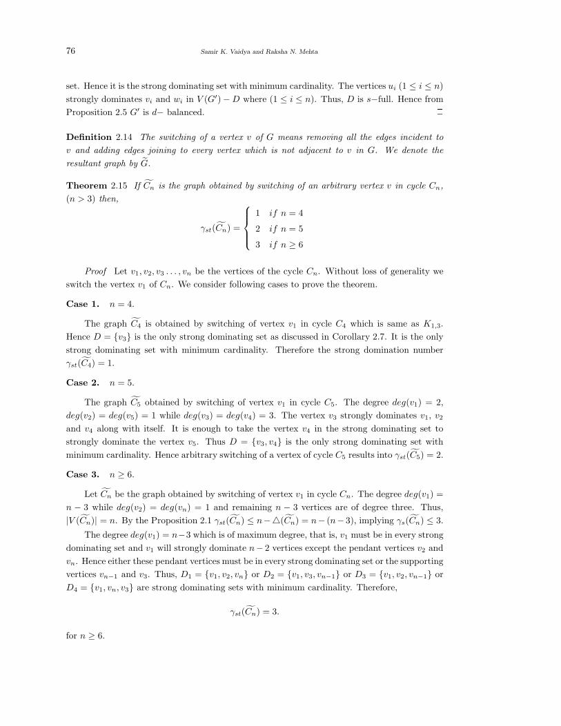
76 Samir K. Vaidya and Raksha N. Mehta
set. Hence it is the strong dominating set with minimum cardinality. The vertices ui (1 ≤ i ≤ n)
strongly dominates vi and wi in V (G′) − D where (1 ≤ i ≤ n). Thus, D is s−full. Hence from
Proposition 2.5 G′ is d− balanced. 2Definition 2.14 The switching of a vertex v of G means removing all the edges incident to
v and adding edges joining to every vertex which is not adjacent to v in G. We denote the
resultant graph by G.
Theorem 2.15 If Cn is the graph obtained by switching of an arbitrary vertex v in cycle Cn,
(n > 3) then,
γst(Cn) =
1 if n = 4
2 if n = 5
3 if n ≥ 6
Proof Let v1, v2, v3 . . . , vn be the vertices of the cycle Cn. Without loss of generality we
switch the vertex v1 of Cn. We consider following cases to prove the theorem.
Case 1. n = 4.
The graph C4 is obtained by switching of vertex v1 in cycle C4 which is same as K1,3.
Hence D = {v3} is the only strong dominating set as discussed in Corollary 2.7. It is the only
strong dominating set with minimum cardinality. Therefore the strong domination number
γst(C4) = 1.
Case 2. n = 5.
The graph C5 obtained by switching of vertex v1 in cycle C5. The degree deg(v1) = 2,
deg(v2) = deg(v5) = 1 while deg(v3) = deg(v4) = 3. The vertex v3 strongly dominates v1, v2
and v4 along with itself. It is enough to take the vertex v4 in the strong dominating set to
strongly dominate the vertex v5. Thus D = {v3, v4} is the only strong dominating set with
minimum cardinality. Hence arbitrary switching of a vertex of cycle C5 results into γst(C5) = 2.
Case 3. n ≥ 6.
Let Cn be the graph obtained by switching of vertex v1 in cycle Cn. The degree deg(v1) =
n − 3 while deg(v2) = deg(vn) = 1 and remaining n − 3 vertices are of degree three. Thus,
|V (Cn)| = n. By the Proposition 2.1 γst(Cn) ≤ n−△(Cn) = n− (n− 3), implying γs(Cn) ≤ 3.
The degree deg(v1) = n−3 which is of maximum degree, that is, v1 must be in every strong
dominating set and v1 will strongly dominate n− 2 vertices except the pendant vertices v2 and
vn. Hence either these pendant vertices must be in every strong dominating set or the supporting
vertices vn−1 and v3. Thus, D1 = {v1, v2, vn} or D2 = {v1, v3, vn−1} or D3 = {v1, v2, vn−1} or
D4 = {v1, vn, v3} are strong dominating sets with minimum cardinality. Therefore,
γst(Cn) = 3.
for n ≥ 6. 2
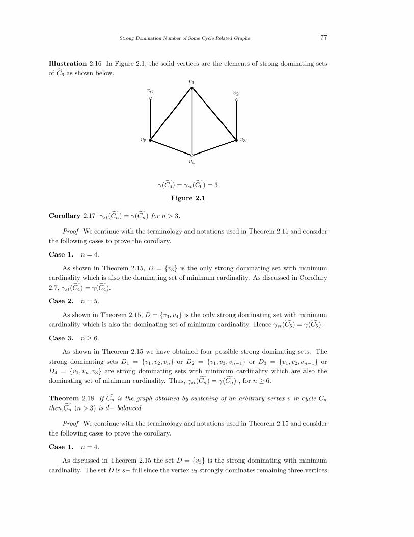
Strong Domination Number of Some Cycle Related Graphs 77
Illustration 2.16 In Figure 2.1, the solid vertices are the elements of strong dominating sets
of C6 as shown below.v1
v2
v3
v4
v6
v5
γ(C6) = γst(C6) = 3
Figure 2.1
Corollary 2.17 γst(Cn) = γ(Cn) for n > 3.
Proof We continue with the terminology and notations used in Theorem 2.15 and consider
the following cases to prove the corollary.
Case 1. n = 4.
As shown in Theorem 2.15, D = {v3} is the only strong dominating set with minimum
cardinality which is also the dominating set of minimum cardinality. As discussed in Corollary
2.7, γst(C4) = γ(C4).
Case 2. n = 5.
As shown in Theorem 2.15, D = {v3, v4} is the only strong dominating set with minimum
cardinality which is also the dominating set of minimum cardinality. Hence γst(C5) = γ(C5).
Case 3. n ≥ 6.
As shown in Theorem 2.15 we have obtained four possible strong dominating sets. The
strong dominating sets D1 = {v1, v2, vn} or D2 = {v1, v3, vn−1} or D3 = {v1, v2, vn−1} or
D4 = {v1, vn, v3} are strong dominating sets with minimum cardinality which are also the
dominating set of minimum cardinality. Thus, γst(Cn) = γ(Cn) , for n ≥ 6. 2Theorem 2.18 If Cn is the graph obtained by switching of an arbitrary vertex v in cycle Cn
then,Cn (n > 3) is d− balanced.
Proof We continue with the terminology and notations used in Theorem 2.15 and consider
the following cases to prove the corollary.
Case 1. n = 4.
As discussed in Theorem 2.15 the set D = {v3} is the strong dominating with minimum
cardinality. The set D is s− full since the vertex v3 strongly dominates remaining three vertices
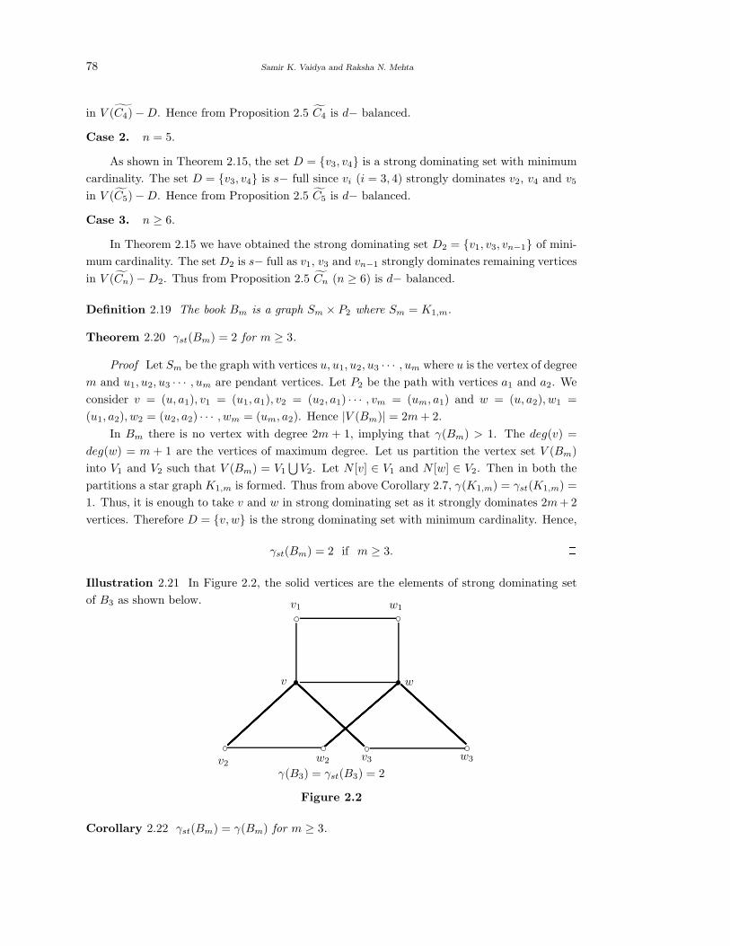
78 Samir K. Vaidya and Raksha N. Mehta
in V (C4) − D. Hence from Proposition 2.5 C4 is d− balanced.
Case 2. n = 5.
As shown in Theorem 2.15, the set D = {v3, v4} is a strong dominating set with minimum
cardinality. The set D = {v3, v4} is s− full since vi (i = 3, 4) strongly dominates v2, v4 and v5
in V (C5) − D. Hence from Proposition 2.5 C5 is d− balanced.
Case 3. n ≥ 6.
In Theorem 2.15 we have obtained the strong dominating set D2 = {v1, v3, vn−1} of mini-
mum cardinality. The set D2 is s− full as v1, v3 and vn−1 strongly dominates remaining vertices
in V (Cn) − D2. Thus from Proposition 2.5 Cn (n ≥ 6) is d− balanced. 2Definition 2.19 The book Bm is a graph Sm × P2 where Sm = K1,m.
Theorem 2.20 γst(Bm) = 2 for m ≥ 3.
Proof Let Sm be the graph with vertices u, u1, u2, u3 · · · , um where u is the vertex of degree
m and u1, u2, u3 · · · , um are pendant vertices. Let P2 be the path with vertices a1 and a2. We
consider v = (u, a1), v1 = (u1, a1), v2 = (u2, a1) · · · , vm = (um, a1) and w = (u, a2), w1 =
(u1, a2), w2 = (u2, a2) · · · , wm = (um, a2). Hence |V (Bm)| = 2m + 2.
In Bm there is no vertex with degree 2m + 1, implying that γ(Bm) > 1. The deg(v) =
deg(w) = m + 1 are the vertices of maximum degree. Let us partition the vertex set V (Bm)
into V1 and V2 such that V (Bm) = V1
⋃V2. Let N [v] ∈ V1 and N [w] ∈ V2. Then in both the
partitions a star graph K1,m is formed. Thus from above Corollary 2.7, γ(K1,m) = γst(K1,m) =
1. Thus, it is enough to take v and w in strong dominating set as it strongly dominates 2m + 2
vertices. Therefore D = {v, w} is the strong dominating set with minimum cardinality. Hence,
γst(Bm) = 2 if m ≥ 3. 2Illustration 2.21 In Figure 2.2, the solid vertices are the elements of strong dominating set
of B3 as shown below. v1
v
v2w2
w1
w
v3 w3
γ(B3) = γst(B3) = 2
Figure 2.2
Corollary 2.22 γst(Bm) = γ(Bm) for m ≥ 3.
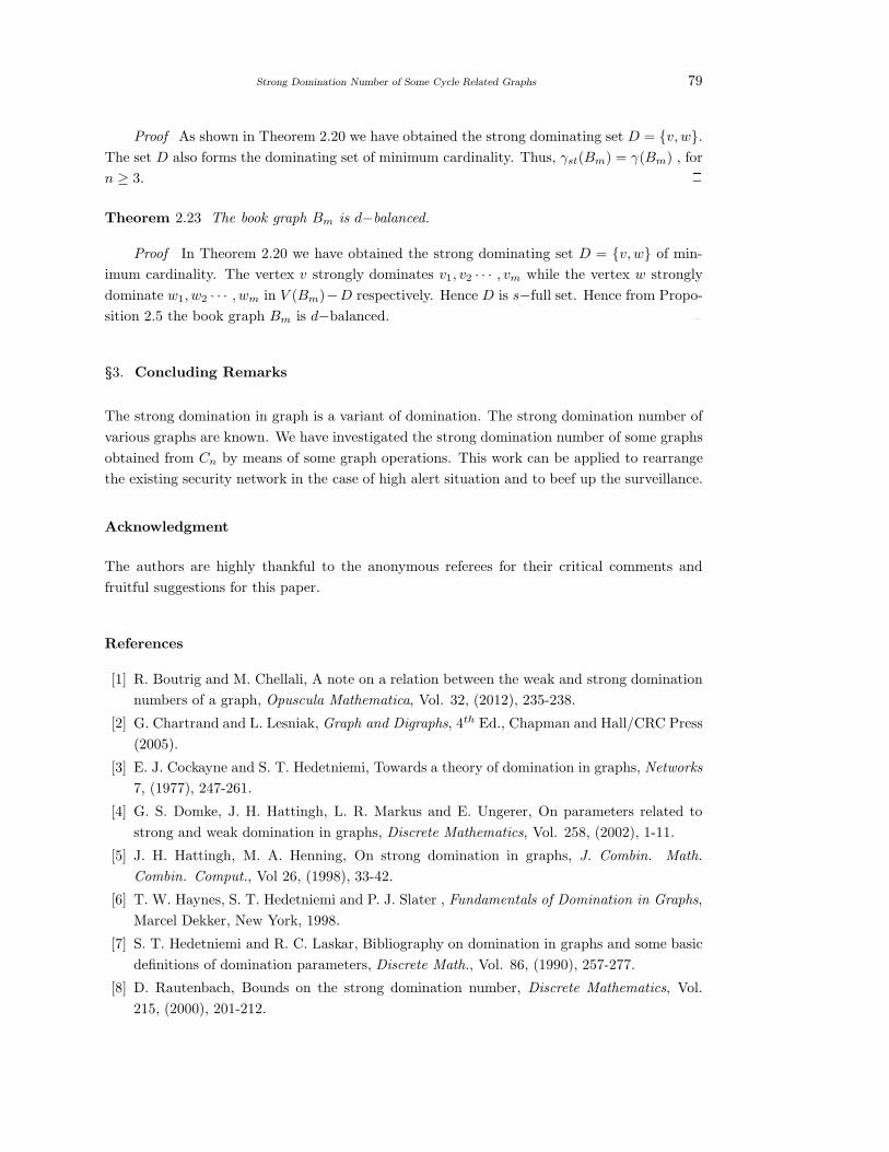
Strong Domination Number of Some Cycle Related Graphs 79
Proof As shown in Theorem 2.20 we have obtained the strong dominating set D = {v, w}.The set D also forms the dominating set of minimum cardinality. Thus, γst(Bm) = γ(Bm) , for
n ≥ 3. 2Theorem 2.23 The book graph Bm is d−balanced.
Proof In Theorem 2.20 we have obtained the strong dominating set D = {v, w} of min-
imum cardinality. The vertex v strongly dominates v1, v2 · · · , vm while the vertex w strongly
dominate w1, w2 · · · , wm in V (Bm)−D respectively. Hence D is s−full set. Hence from Propo-
sition 2.5 the book graph Bm is d−balanced. 2§3. Concluding Remarks
The strong domination in graph is a variant of domination. The strong domination number of
various graphs are known. We have investigated the strong domination number of some graphs
obtained from Cn by means of some graph operations. This work can be applied to rearrange
the existing security network in the case of high alert situation and to beef up the surveillance.
Acknowledgment
The authors are highly thankful to the anonymous referees for their critical comments and
fruitful suggestions for this paper.
References
[1] R. Boutrig and M. Chellali, A note on a relation between the weak and strong domination
numbers of a graph, Opuscula Mathematica, Vol. 32, (2012), 235-238.
[2] G. Chartrand and L. Lesniak, Graph and Digraphs, 4th Ed., Chapman and Hall/CRC Press
(2005).
[3] E. J. Cockayne and S. T. Hedetniemi, Towards a theory of domination in graphs, Networks
7, (1977), 247-261.
[4] G. S. Domke, J. H. Hattingh, L. R. Markus and E. Ungerer, On parameters related to
strong and weak domination in graphs, Discrete Mathematics, Vol. 258, (2002), 1-11.
[5] J. H. Hattingh, M. A. Henning, On strong domination in graphs, J. Combin. Math.
Combin. Comput., Vol 26, (1998), 33-42.
[6] T. W. Haynes, S. T. Hedetniemi and P. J. Slater , Fundamentals of Domination in Graphs,
Marcel Dekker, New York, 1998.
[7] S. T. Hedetniemi and R. C. Laskar, Bibliography on domination in graphs and some basic
definitions of domination parameters, Discrete Math., Vol. 86, (1990), 257-277.
[8] D. Rautenbach, Bounds on the strong domination number, Discrete Mathematics, Vol.
215, (2000), 201-212.
80 Samir K. Vaidya and Raksha N. Mehta
[9] D. Rautenbach, The influence of special vertices on strong domination, Discrete Mathe-
matics, Vol. 197/198, (1999), 683-690.
[10] E. Sampathkumar and L. Pushpa Latha, Strong weak domination and domination balance
in a graph, Discrete Mathematics, Vol. 161, (1996), 235-242.
[11] V. Swaminathan and P. Thangaraju, Strong and weak domination in graphs, Electronic
Notes in Discrete Mathematics, vol. 15, (2003), 213-215.
International J.Math. Combin. Vol.3(2017), 81-89
Minimum Equitable Dominating Randic Energy of a Graph
P.Siva Kota Reddy
(Department of Mathematics, Siddaganga Institute of Technology, B.H.Road, Tumkur-572103, India)
K. N. Prakasha
(Department of Mathematics, Vidyavardhaka College of Engineering, Mysuru- 570 002, India)
Gavirangaiah K
(Department of Mathematics, Government First Grade Collge, Tumkur-562 102, India)
E-mail: reddy [email protected], [email protected], [email protected]
Abstract: In this paper, we introduce the minimum equitable dominating Randic energy of
a graph and computed the minimum dominating Randic energy of graph. Also, established
the upper and lower bounds for the minimum equitable dominating Randic energy of a graph.
Key Words: Minimum equitable dominating set, Smarandachely equitable dominating set,
minimum equitable dominating Randic eigenvalues, minimum equitable dominating Randic
energy.
AMS(2010): 05C50.
§1. Introduction
Let G be a simple, finite, undirected graph, The energy E(G) is defined as the sum of the
absolute values of the eigenvalues of its adjacency matrix. For more details on energy of graph
see [5, 6].
The Randic matrix R(G) = (Rij)n×n is given by [1-3].
Rij =
1√didi
if vi ∼ vj ,
0 otherwise
We can see lower and upper bounds on Randic energy in [1,2]. Some sharp upper bounds
for Randic energy of graphs were obtain in [3].
§2. The Minimum Equitable Dominating Randic Energy of Graph
Let G be a simple graph of order n with vertex set V (G) = {v1, v2, v3, · · · , vn} and edge set E.
A subset U of V (G) is an equitable dominating set, if for every v ∈ V (G) − U there exists a
1Received December 19, 2016, Accepted August 22, 2017.
82 P.Siva Kota Reddy, K. N. Prakasha and Gavirangaiah K
vertex u ∈ U such that uv ∈ E(G) and |deg(u) − deg(v)| ≤ 1, and a Smarandachely equitable
dominating set is its contrary, i.e., |deg(u) − deg(v)| ≥ 1 for such an edge uv, where deg(x)
denotes the degree of vertex x in V (G). Any equitable dominating set with minimum cardinality
is called a minimum equitable dominating set. Let E be a minimum equitable dominating set
of a graph G. The minimum equitable dominating Randic matrix RE(G) = (REij)n×n is given
by
REij =
1√didi
if vi ∼ vj ,
1 if i = j and vi ∈ E,
0 otherwise
The characteristic polynomial of RE(G) is denoted by φER(G, λ) = det(λI −RE(G)). Since
the minimum equitable dominating Randic Matrix is real and symmetric, its eigenvalues are
real numbers and we label them in non-increasing order λ1 > λ2 > · · · λn. The minimum
equitable dominating Randic Energy is given by
REE(G) =
n∑
i=1
|λi|. (1)
Definition 2.1 The spectrum of a graph G is the list of distinct eigenvalues λ1 > λ2 > · · · λr,
with their multiplicities m1, m2, . . . , mr, and we write it as
Spec(G) =
λ1 λ2 · · · λr
m1 m2 · · · mr
.
This paper is organized as follows. In the Section 3, we get some basic properties of
minimum equitable dominating Randic energy of a graph. In the Section 4, minimum equitable
dominating Randic energy of some standard graphs are obtained.
§3. Some Basic Properties of Minimum Equitable Dominating Randic
Energy of a Graph
Let us consider
P =∑
i<j
1
didj,
where didj is the product of degrees of two vertices which are adjacent.
Proposition 3.1 The first three coefficients of φER(G, λ) are given as follows:
(i) a0 = 1;
(ii) a1 = −|E|;(iii) a2 = |E|C2 − P .
Minimum Equitable Dominating Randic Energy of a Graph 83
Proof (i) From the definition ΦER(G, λ) = det[λI − RE(G)], we get a0 = 1.
(ii) The sum of determinants of all 1 × 1 principal submatrices of RE(G) is equal to the
trace of RE(G) ⇒ a1 = (−1)1 trace of [RE(G)] = −|E|.(iii)
(−1)2a2 =∑
1≤i<j≤n
∣∣∣∣∣∣aii aij
aji ajj
∣∣∣∣∣∣
=∑
1≤i<j≤n
aiiajj − ajiaij
=∑
1≤i<j≤n
aiiajj −∑
1≤i<j≤n
ajiaij
= |E|C2 − P. 2Proposition 3.2 If λ1, λ2, . . . , λn are the minimum equitable dominating Randic eigenvalues
of RE(G), thenn∑
i=1
λi2 = |E| + 2P.
Proof We know that
n∑
i=1
λ2i =
n∑
i=1
n∑
j=1
aijaji
= 2∑
i<j
(aij)2 +
n∑
i=1
(aii)2
= 2∑
i<j
(aij)2 + |E|
= |E| + 2P. 2Theorem 3.3 Let G be a graph with n vertices and Then
REE(G) ≤√
n(|E| + 2[P ])
where
P =∑
i<j
1
didj
for which didj is the product of degrees of two vertices which are adjacent.
Proof Let λ1, λ2, · · · , λn be the eigenvalues of RE(G). Now by Cauchy - Schwartz inequal-
ity we have (n∑
i=1
aibi
)2
≤(
n∑
i=1
ai2
)(n∑
i=1
bi2
).
84 P.Siva Kota Reddy, K. N. Prakasha and Gavirangaiah K
Let ai = 1 , bi =| λi |. Then
(n∑
i=1
|λi|)2
≤(
n∑
i=1
1
)(n∑
i=1
|λi|2)
Thus,
[REE ]2 ≤ n(|E| + 2P ),
which implies that
[REE ] ≤√
n(|E| + 2P ),
i.e., the upper bound. 2Theorem 3.4 Let G be a graph with n vertices. If R= det RE(G), then
REE(G) ≥√
(|E| + 2P ) + n(n − 1)R2n .
Proof By definition,
(REE(G)
)2=
(n∑
i=1
| λi |)2
=
n∑
i=1
| λi |n∑
j=1
| λj |
=
(n∑
i=1
| λi |2)
+∑
i6=j
| λi || λj | .
Using arithmetic mean and geometric mean inequality, we have
1
n(n − 1)
∑
i6=j
| λi || λj | ≥
∏
i6=j
| λi || λj |
1n(n−1)
.
Therefore,
[REE(G)]2 ≥n∑
i=1
| λi |2 +n(n − 1)
∏
i6=j
| λi || λj |
1n(n−1)
≥n∑
i=1
| λi |2 +n(n − 1)
(n∏
i=1
| λi |2(n−1)
) 1n(n−1)
=
n∑
i=1
| λi |2 +n(n − 1)R2n
= (|E| + 2P ) + n(n − 1)R2n .
Minimum Equitable Dominating Randic Energy of a Graph 85
Thus,
REE(G) ≥√
(|E| + 2P ) + n(n − 1)R2n . 2
§4. Minimum Equitable Dominating Randic Energy of Some Standard Graphs
Theorem 4.1 The minimum equitable dominating Randic energy of a complete graph Kn is
REE(Kn) = 3n−5n−1 .
Proof Let Kn be the complete graph with vertex set V = {v1, v2, · · · , vn}. The minimum
equitable dominating set = E = {v1}. The minimum equitable dominating Randic matrix is
RE(Kn) =
1 1n−1
1n−1 . . . 1
n−11
n−1
1n−1 0 1
n−1 . . . 1n−1
1n−1
1n−1
1n−1 0 . . . 1
n−11
n−1
......
.... . .
......
1n−1
1n−1 . . . 1
n−1 0 1n−1
1n−1
1n−1 . . . 1
n−11
n−1 0
.
The characteristic equation is
(λ +
1
n − 1
)n−2(λ2 − 2n − 3
n − 1λ +
n − 3
n − 1
)= 0
and the spectrum is SpecER(Kn) =
(2n−3)+√
4n−32(n−1)
(2n−3)−√
4n−32(n−1)
−1n−1
1 1 n − 2
.
Therefore, REE(Kn) =3n − 5
n − 1. 2
Theorem 4.2 The minimum equitable dominating Randic energy of star graph K1,n−1 is
REE(K1,n−1) =√
5.
Proof Let K1,n−1 be the star graph with vertex set V = {v0, v1, · · · , vn−1}. Here v0 be
the center. The minimum equitable dominating set = E = V (G). The minimum equitable
86 P.Siva Kota Reddy, K. N. Prakasha and Gavirangaiah K
dominating Randic matrix is
RE(K1,n−1) =
1 1√n−1
1√n−1
. . . 1√n−1
1√n−1
1√n−1
1 0 . . . 0 0
1√n−1
0 1 . . . 0 0
......
.... . .
......
1√n−1
0 0 . . . 1 0
1√n−1
0 0 . . . 0 1
.
The characteristic equation is
λ(λ − 1)n−2[λ − 2] = 0
spectrum is SpecER(K1,n−1) =
2 1 0
1 n − 2 1
.
Therefore, REE(K1,n−1) = n. 2Theorem 4.3 The minimum equitable dominating Randic energy of Crown graph S0
n is
REE(S0n) =
(4n − 7) +√
4n2 − 8n + 5
n − 1.
Proof Let S0n be a crown graph of order 2n with vertex set {u1, u2, · · · , un, v1, v2, · · · , vn}
and minimum dominating set = E = {u1, v1}. The minimum equitable dominating Randic
matrix is
RE(S0n) =
1 0 0 . . . 0 0 1n−1 . . . 1
n−11
n−1
0 0 0 . . . 0 1n−1 0 . . . 1
n−11
n−1
0 0 0 . . . 0 1n−1 . . . 1
n−1 0 1n−1
......
.... . .
......
.... . .
......
0 0 0 . . . 0 1n−1 . . . 1
n−11
n−1 0
0 1n−1
1n−1 . . . 1
n−1 1 0 . . . 0 0
1n−1 0 1
n−1 . . . 1n−1 0 0 . . . 0 0
......
.... . .
......
.... . .
......
1n−1
1n−1 0 . . . 1
n−1 0 0 . . . 0 0
1n−1
1n−1
1n−1 . . . 0 0 0 . . . 0 0
.
Minimum Equitable Dominating Randic Energy of a Graph 87
The characteristic equation is
(λ +
1
n − 1
)n−2(λ − 1
n − 1
)n−2(λ2 − 1
n − 1λ − 1
)(λ2 − 2n − 3
n − 1λ +
n − 3
n − 1
)= 0
spectrum is SpecER(S0
n)
=
(2n−3)+√
4n−32(n−1)
1+√
4n2−8n+52(n−1)
(2n−3)−√
4n−32(n−1)
1n−1
−1n−1
1−√
4n2−8n+52(n−1)
1 1 1 n − 2 n − 2 1
.
Therefore, REE(S0n) =
(4n − 7) +√
4n2 − 8n + 5
n − 1. 2
Theorem 4.4 The minimum equitable dominating Randic energy of complete bipartite graph
Kn,nof order 2n with vertex set {u1, u2, · · · , un, v1, v2, · · · , vn} is
REE(Kn,n) =2√
n − 1√n
+ 2.
Proof Let Kn,n be the complete bipartite graph of order 2n with vertex set {u1, u2, · · · , un,
v1, v2, · · · , vn}. The minimum equitable dominating set = E = {u1, v1} with a minimum
equitable dominating Randic matrix
RE(Kn,n) =
1 0 0 0 . . . 1n
1n
1n
1n
0 0 0 0 . . . 1n
1n
1n
1n
0 0 0 0 . . . 1n
1n
1n
1n
0 0 0 0 . . . 1n
1n
1n
1n
......
......
. . ....
......
...
1n
1n
1n
1n . . . 1 0 0 0
1n
1n
1n
1n . . . 0 0 0 0
1n
1n
1n
1n . . . 0 0 0 0
1n
1n
1n
1n . . . 0 0 0 0
.
The characteristic equation is
λ2n−4(λ2 − n − 1
n)[λ2 − 2λ +
n − 1
n] = 0
Hence, spectrum is
SpecER(Kn,n) =
1 +
√1n
√n−1√
n1 −
√1n 0 −
√n−1√
n
1 1 1 2n− 4 1
.
Therefore, REE(Kn,n) =2√
n − 1√n
+ 2. 2
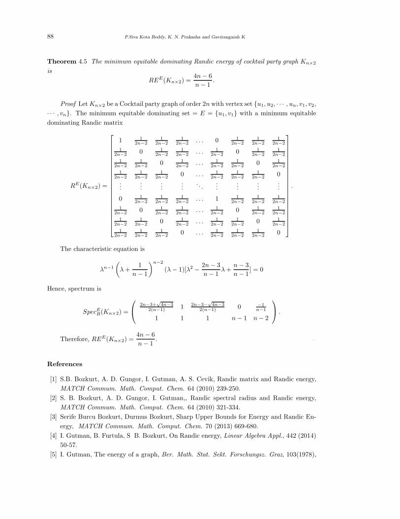
88 P.Siva Kota Reddy, K. N. Prakasha and Gavirangaiah K
Theorem 4.5 The minimum equitable dominating Randic energy of cocktail party graph Kn×2
is
REE(Kn×2) =4n − 6
n − 1.
Proof Let Kn×2 be a Cocktail party graph of order 2n with vertex set {u1, u2, · · · , un, v1, v2,
· · · , vn}. The minimum equitable dominating set = E = {u1, v1} with a minimum equitable
dominating Randic matrix
RE(Kn×2) =
1 12n−2
12n−2
12n−2 . . . 0 1
2n−21
2n−21
2n−2
12n−2 0 1
2n−21
2n−2 . . . 12n−2 0 1
2n−21
2n−2
12n−2
12n−2 0 1
2n−2 . . . 12n−2
12n−2 0 1
2n−2
12n−2
12n−2
12n−2 0 . . . 1
2n−21
2n−21
2n−2 0...
......
.... . .
......
......
0 12n−2
12n−2
12n−2 . . . 1 1
2n−21
2n−21
2n−2
12n−2 0 1
2n−21
2n−2 . . . 12n−2 0 1
2n−21
2n−2
12n−2
12n−2 0 1
2n−2 . . . 12n−2
12n−2 0 1
2n−2
12n−2
12n−2
12n−2 0 . . . 1
2n−21
2n−21
2n−2 0
.
The characteristic equation is
λn−1
(λ +
1
n − 1
)n−2
(λ − 1)[λ2 − 2n − 3
n − 1λ +
n − 3
n − 1] = 0
Hence, spectrum is
SpecER(Kn×2) =
2n−3+√
4n−32(n−1) 1 2n−3−
√4n−3
2(n−1) 0 −1n−1
1 1 1 n − 1 n − 2
.
Therefore, REE(Kn×2) =4n − 6
n − 1. 2
References
[1] S.B. Bozkurt, A. D. Gungor, I. Gutman, A. S. Cevik, Randic matrix and Randic energy,
MATCH Commum. Math. Comput. Chem. 64 (2010) 239-250.
[2] S. B. Bozkurt, A. D. Gungor, I. Gutman,, Randic spectral radius and Randic energy,
MATCH Commum. Math. Comput. Chem. 64 (2010) 321-334.
[3] Serife Burcu Bozkurt, Durmus Bozkurt, Sharp Upper Bounds for Energy and Randic En-
ergy, MATCH Commum. Math. Comput. Chem. 70 (2013) 669-680.
[4] I. Gutman, B. Furtula, S B. Bozkurt, On Randic energy, Linear Algebra Appl., 442 (2014)
50-57.
[5] I. Gutman, The energy of a graph, Ber. Math. Stat. Sekt. Forschungsz. Graz, 103(1978),
Minimum Equitable Dominating Randic Energy of a Graph 89
1-22.
[6] I. Gutman, The energy of a graph: old and new results, Combinatorics and applications, A.
Betten, A. Khoner, R. Laue and A. Wassermann, eds., Springer, Berlin, (2001), 196-211.
[7] G. Indulal, I. Gutman, A. Vijayakumar, On distance energy of graphs, Match Commun.
Math. Comput. Chem., 60(2008), 461-472.
International J.Math. Combin. Vol.3(2017), 90-105
Cordiality in the Context of Duplication in Web and Armed Helm
U M Prajapati
(St. Xavier’s College, Ahmedabad-380009, Gujarat, India)
R M Gajjar
(Department of Mathematics, School of Sciences, Gujarat University, Ahmedabad-380009, Gujarat, India)
E-mail: [email protected], [email protected]
Abstract: Let G = (V (G), E(G)) be a graph and let f : V (G) → {0, 1} be a mapping
from the set of vertices to {0,1} and for each edge uv ∈ E assign the label |f(u) − f(v)|.If the number of vertices labeled with 0 and the number of vertices labeled with 1 differ by
at most 1 and the number of edges labled with 0 and the number of edges labeled with 1
differ by at most 1, then f is called a cordial labeling. We discuss cordial labeling of graphs
obtained from duplication of certain graph elements in web and armed helm.
Key Words: Graph labeling, cordial labeling, cordial graph, Smarandachely cordial label-
ing, Smarandachely cordial graph.
AMS(2010): 05C78
§1. Introduction
We begin with simple, finite, undirected graph G = (V (G), E(G)) where V (G) and E(G)
denotes the vertex set and the edge set respectively. For all other terminology we follow West
[1]. We will give the brief summary of definitions which are useful for the present work.
Definition 1.1 The graph labeling is an assignment of numbers to the vertices or edges or both
subject to certain condition(s).
A detailed survey of various graph labeling is explained in Gallian [3].
Definition 1.2 For a graph G = (V (G), E(G)), a mapping f : V (G) → {0, 1} is called a
binary vertex labeling of G and f(v) is called the label of the vertex v of G under f . For an
edge e = uv, the induced edge labeling f∗ : E(G) → {0, 1} defined as f∗(uv) = |f(u) − f(v)|.
Let vf (0), vf (1) be the number of vertices of G having labels 0 and 1 respectively under f
and let ef (0), ef (1) be the number of edges having labels 0 and 1 respectively under f∗.
Definition 1.3 Duplication of a vertex v of a graph G produces a new graph G′ by adding a
new vertex v′ such that N(v′) = N(v). In other words a vertex v′ is said to be duplication of v
if all the vertices which are adjacent to v in G are also adjacent to v′ in G′.
Definition 1.4 Duplication of an edge e = uv of a graph G produces a new graph G′ by adding
1Received December 19, 2016, Accepted August 24, 2017.
Cordiality in the Context of Duplication in Web and Armed Helm 91
an edge e′ = u′v′ such that N(u′) = N(u) ∪ {v′} − {v} and N(v′) = N(v) ∪ {u′} − {u}.
Definition 1.5 The wheel Wn, is join of the graphs Cn and K1. i.e Wn = Cn + K1. Here
vertices corresponding to Cn are called rim vertices and Cn is called rim of Wn while, the vertex
corresponding to K1 is called the apex vertex, edges joining the apex vertex and a rim vertex is
called spoke.
Definition 1.6([3]) The helm Hn, is the graph obtained from the wheel Wn by adding a pendant
edge at each rim vertex.
Definition 1.7([3]) The web Wbn, is the graph obtained by joining the pendent points of a helm
to form a cycle and then adding a single pendent edge to each vertex of this outer cycle, here
vertices corresponding to this outer cycle are called outer rim vertices and vertices corresponding
to wheel except the apex vertex are called inner rim vertices.
We define one new graph family as follows:
Definition 1.8 An armed helm is a graph in which path P2 is attached at each vertex of wheel
Wn by an edge. It is denoted by AHn where n is the number of vertices in cycle Cn.
Definition 1.9 A binary vertex labeling f of a graph G is called a cordial labeling if |vf (1) −vf (0)| ≤ 1 and |ef(1) − ef(0)| ≤ 1, and a binary vertex labeling f of a graph G is called a
Smarandachely cordial labeling if |vf (1) − vf (0)| ≥ 1 or |ef (1) − ef(0)| ≥ 1.
A graph G is said to be cordial if it admits cordial labeling, and Smarandachely cordial if
it admits Smarandachely cordial labeling.
The concept of cordial labeling was introduced by Cahit [2] in which he proved that the
wheel Wn is cordial if and only if n 6≡ 3(mod4). Vaidya and Dani [4] proved that the graphs
obtained by duplication of an arbitrary edge of a cycle and a wheel admit a cordial labeling.
Prajapati and Gajjar [5] proved that complement of wheel graph and complement of cycle
graph are cordial if n 6≡ 4(mod8) or n 6≡ 7(mod8). Prajapati and Gajjar [6] proved that cordial
labeling in the context of duplication of cycle graph and path graph.
§2. Main Results
Theorem 2.1 The graph obtained by duplicating all the vertices of the web Wbn is cordial.
Proof Let V (Wbn) = {t}⋃{ui, vi, wi, /1 ≤ i ≤ n} and E(Wbn) = {tui, uivi, viwi/1 ≤ i ≤n}⋃{unu1, vnv1}
⋃{uiui+1, vivi+1/1 ≤ i ≤ n−1}. Let G be the graph obtained by duplicating
all the vertices in Wbn. Let t′, u′1, u
′2, · · · , u′
n, v′1, v′2, · · · , v′n, w′
1, w′2, · · · , w′
n be the new vertices
of G by duplicating t, u1, u2, · · · , un, v1, v2, · · · , vn, w1, w2, · · · , wn respectively. Then V (G) =
{t, t′}∪{ui, vi, wi, u′i, v
′i, w
′i/1 ≤ i ≤ n} and E(G) = {tui, uivi, viwi, wiv
′i, uiv
′i, u
′ivi, tu
′i, viw
′i, t
′ui
/1 ≤ i ≤ n}⋃{unu1, vnv1, v′nv1, vnv′1, u
′nu1, unu′
1}⋃{uiui+1, vivi+1, v
′ivi+1, viv
′i+1, u
′iui+1, uiu
′i+1
/1 ≤ i ≤ n − 1}. Therefore |V (G)| = 6n + 2 and |E(G)| = 15. Using parity of n, we have the
following cases:
Case 1. n is even.
92 U M Prajapati and R M Gajjar
Define a vertex labeling f : V (G) → {0, 1} as follows:
f(x) =
1 if x = t′;
1 if x = w′i, i ∈ {2, 4, . . . , n − 2, n};
1 if x = wi, i ∈ {1, 3, . . . , n − 3, n− 1};1 if x ∈ {ui, v
′i}, i ∈ {1, 2, . . . , n − 1, n};
0 if x = t;
0 if x ∈ {vi, u′i}, i ∈ {1, 2, . . . , n − 1, n};
0 if x = wi, i ∈ {2, 4, . . . , n − 2, n};0 if x = w′
i, i ∈ {1, 3, . . . , n − 3, n− 1}.
Thus vf (1) = 3n + 1 and vf (0) = 3n + 1. The induced edge labeling f∗ : E(G) → {0, 1} is
f∗(uv) = |f(u) − f(v)|, for every edge e = uv ∈ E. Therefore
f∗(e) =
1 if e ∈ {tui, uivi}, i ∈ {1, 2, . . . , n − 1, n};0 if e ∈ {uiui+1, vivi+1}, i ∈ {1, 2, . . . , n − 2, n− 1};1 if e ∈ {uiu
′i+1, u
′iui+1, viv
′i+1, v
′ivi+1}, i ∈ {1, 2, . . . , n − 2, n− 1};
0 if e ∈ {t′ui, tu′i, u
′ivi, uiv
′i}, i ∈ {1, 2, . . . , n − 1, n};
0 if e ∈ {viw′i, wiv
′i}, i ∈ {1, 3, . . . , n − 3, n − 1};
1 if e ∈ {viw′i, wiv
′i}, i ∈ {2, 4, . . . , n − 2, n};
1 if e = viwi, i ∈ {1, 3, . . . , n − 3, n− 1};0 if e = viwi, i ∈ {2, 4, . . . , n − 2, n};0 if e ∈ {unu1, vnv1};1 if e ∈ {u′
nu1, unu′1, v
′nv1, vnv′1}.
Thus ef (1) =15n
2and ef(0) =
15n
2.
Case 2 n is odd.
Define a vertex labeling f : V (G) → {0, 1} as follows:
f(x) =
1 if x = t′;
1 if x = w′i, i ∈ {2, 4, . . . , n − 3, n − 1};
1 if x = wi, i ∈ {1, 3, . . . , n − 2, n};1 if x ∈ {ui, v
′i}, i ∈ {1, 2, . . . , n − 1, n};
0 if x = t;
0 if x ∈ {vi, u′i}, i ∈ {1, 2, . . . , n − 1, n};
0 if x = wi, i ∈ {2, 4, . . . , n − 3, n− 1};0 if x = w′
i, i ∈ {1, 3, . . . , n − 2, n}.
Cordiality in the Context of Duplication in Web and Armed Helm 93
Thus vf (1) = 3n + 1 and vf (0) = 3n + 1. The induced edge labeling f∗ : E(G) → {0, 1} is
f∗(uv) = |f(u) − f(v)|, for every edge e = uv ∈ E. Therefore
f∗(e) =
1 if e ∈ {tui, uivi}, i ∈ {1, 2, . . . , n − 1, n};0 if e ∈ {uiui+1, vivi+1}, i ∈ {1, 2, . . . , n − 2, n− 1};1 if e ∈ {uiu
′i+1, u
′iui+1, viv
′i+1, v
′ivi+1}, i ∈ {1, 2, . . . , n − 2, n− 1};
0 if e ∈ {t′ui, tu′i, u
′ivi, uiv
′i}, i ∈ {1, 2, . . . , n − 1, n};
0 if e ∈ {viw′i, wiv
′i}, i ∈ {1, 3, . . . , n − 2, n};
1 if e ∈ {viw′i, wiv
′i}, i ∈ {2, 4, . . . , n − 3, n − 1};
1 if e = viwi, i ∈ {1, 3, . . . , n − 2, n};0 if e = viwi, i ∈ {2, 4, . . . , n − 3, n− 1};0 if e ∈ {unu1, vnv1};1 if e ∈ {u′
nu1, unu′1, v
′nv1, vnv′1}.
Thus ef (1) =15n− 1
2and ef(0) =
15n + 1
2.
From both the cases we can conclude |vf (1) − vf (0)| ≤ 1 and |ef(1) − ef (0)| ≤ 1. So, f
admits cordial labeling on G. Hence G is cordial. 2Theorem 2.2 The graph obtained by duplicating all the pendent vertices of the web Wbn is
cordial.
Proof Let V (Wbn) = {t}⋃{ui, vi, wi/1 ≤ i ≤ n} and E(Wbn) = {tui, uivi, viwi/1 ≤i ≤ n} ∪ {unu1, vnv1}
⋃{uiui+1, vivi+1/1 ≤ i ≤ n − 1}. Let G be the graph obtained by
duplicating all the pendent vertices in Wbn. Let w′1, w
′2, · · · , w′
n be the new vertices of G by
duplicating w1, w2, · · · , wn respectively. Then V (G) = {t} ∪ {ui, vi, wi, w′i/1 ≤ i ≤ n} and
E(G) = {tui, uivi, viwi, viw′i/1 ≤ i ≤ n} ∪ {unu1, vnv1}
⋃{uiui+1, vivi+1/1 ≤ i ≤ n − 1}.Therefore |V (G)| = 4n + 1 and |E(G)| = 6n. Define a vertex labeling f : V (G) → {0, 1} as
follows:
f(x) =
0 if x = t;
1 if x ∈ {wi, ui}, i ∈ {1, 2, . . . , n − 1, n};0 if x ∈ {vi, w
′i}, i ∈ {1, 2, . . . , n − 1, n}.
Thus vf (1) = 2n and vf (0) = 2n + 1. The induced edge labeling f∗ : E(G) → {0, 1} is
f∗(uv) = |f(u) − f(v)|, for every edge e = uv ∈ E. Therefore
f∗(e) =
1 if e ∈ {tui, uivi, viwi}, i ∈ {1, 2, . . . , n − 1, n};0 if e = viw
′i, i ∈ {1, 2, . . . , n − 1, n};
0 if e ∈ {uiui+1, vivi+1}, i ∈ {1, 2, . . . , n − 2, n− 1};0 if e ∈ {unu1, vnv1}.
Thus ef (1) = 3n and ef (0) = 3n. Therefore f satisfies the conditions |vf (1) − vf (0)| ≤ 1 and
94 U M Prajapati and R M Gajjar
|ef (1) − ef (0)| ≤ 1. So, f admits cordial labeling on G. Hence G is cordial. 2Theorem 2.3 The graph obtained by duplicating the outer rim vertices and the apex of the web
Wbn is cordial.
Proof Let V (Wbn) = {t}⋃{ui, vi, wi, /1 ≤ i ≤ n} and E(Wbn) = {tui, uivi, viwi/1 ≤ i ≤n}⋃{uiui+1, vivi+1/1 ≤ i ≤ n−1}⋃{unu1, vnv1}. Let G be the graph obtained by duplicating
the outer rim vertices and the apex in Wbn. Let t′, v′1, v′2, · · · , v′n be the new vertices of G
by duplicating t, v1, v2, · · · , vn respectively. Then V (G) = {t, t′}⋃{ui, vi, wi, v′i/1 ≤ i ≤ n}
and E(G) = {tui, uivi, viwi, wiv′i, uiv
′i, t
′ui/1 ≤ i ≤ n}⋃{uiui+1, vivi+1, v′ivi+1, viv
′i+1/1 ≤ i ≤
n−1}⋃{unu1, vnv1, v′nv1, vnv′1}. Therefore |V (G)| = 4n+2 and |E(G)| = 10n. Define a vertex
labeling f : V (G) → {0, 1} as follows:
f(x) =
0 if x = t;
1 if x ∈ {ui, wi}, i ∈ {1, 2, . . . , n − 1, n};0 if x ∈ {vi, v
′i}, i ∈ {1, 2, . . . , n − 1, n};
1 if x = t′.
Thus vf (1) = 2n + 1 and vf (0) = 2n + 1. The induced edge labeling f∗ : E(G) → {0, 1} is
f∗(uv) = |f(u) − f(v)|, for every edge e = uv ∈ E. Therefore
f∗(e) =
1 if e ∈ {tui, uivi, viwi, wiv′i, uiv
′i}, i ∈ {1, 2, . . . , n − 1, n};
0 if e ∈ {uiui+1, vivi+1, v′ivi+1, viv
′i+1}, i ∈ {1, 2, . . . , n − 2, n − 1};
0 if e = t′ui, i ∈ {1, 2, . . . , n − 1, n};0 if e ∈ {unu1, vnv1.v
′nv1, vnv′1}.
Thus ef (1) = 5n and ef (0) = 5n. Therefore f satisfies the conditions |vf (1) − vf (0)| ≤ 1 and
|ef (1) − ef (0)| ≤ 1. So, f admits cordial labeling on G. Hence G is cordial. 2Theorem 2.4 The graph obtained by duplicating all the vertices except the apex vertex of the
web Wbn is cordial.
Proof Let V (Wbn) = {t}⋃{ui, vi, wi/1 ≤ i ≤ n} and E(Wbn) = {tui, uivi, viwi/1 ≤ i ≤n}⋃{unu1, vnv1}
⋃{uiui+1, vivi+1/1 ≤ i ≤ n−1}. Let G be the graph obtained by duplicating
all the vertices except the apex vertex in Wbn. Let u′1, u
′2, · · · , u′
n, v′1, v′2, · · · , v′n, w′
1, w′2, · · · , w′
n
be the new vertices of G by duplicating u1, u2, · · · , un, v1, v2, · · · , vn, w1, w2, · · · , wn respec-
tively. Then V (G) = {t}⋃{ui, vi, wi, u′i, v
′i, w
′i/1 ≤ i ≤ n} and E(G) = {tui, uivi, viwi, wiv
′i, uiv
′i,
u′ivi, viw
′i, tu
′i/1 ≤ i ≤ n}⋃{unu1, vnv1, v
′nv1, vnv′1, u
′nu1, unu′
1}⋃{uiui+1, vivi+1, v
′ivi+1, viv
′i+1,
u′iui+1, uiu
′i+1/1 ≤ i ≤ n − 1}. Therefore |V (G)| = 6n + 1 and |E(G)| = 14n. Define a vertex
Cordiality in the Context of Duplication in Web and Armed Helm 95
labeling f : V (G) → {0, 1} as follows:
f(x) =
0 if x = t;
1 if x ∈ {wi, ui, u′i}, i ∈ {1, 2, . . . , n − 1, n};
0 if x ∈ {vi, w′i, v
′i}, i ∈ {1, 2, . . . , n − 1, n}.
Thus vf (1) = 3n and vf (0) = 3n + 1. The induced edge labeling f∗ : E(G) → {0, 1} is
f∗(uv) = |f(u) − f(v)|, for every edge e = uv ∈ E. Therefore
f∗(e) =
1 if e ∈ {tui, uivi, viwi, wiv′i, uiv
′i, u
′ivi, tu
′i}, i ∈ {1, 2, . . . , n − 1, n};
0 if e = viw′i, i ∈ {1, 2, . . . , n − 1, n};
0 if e ∈ {uiui+1, vivi+1, v′ivi+1, viv
′i+1, u
′iui+1, uiu
′i+1}, i ∈ {1, 2, . . . , n − 2, n− 1};
0 if e ∈ {unu1, vnv1.v′nv1, vnv′1, u
′nu1, unu′
1}.
Thus ef (1) = 7n and ef (0) = 7n. Therefore f satisfies the conditions |vf (1) − vf (0)| ≤ 1 and
|ef (1) − ef (0)| ≤ 1. So, f admits cordial labeling on G. Hence G is cordial. 2Theorem 2.5 The graph obtained by duplicating all the inner rim vertices and the apex vertex
of the web Wbn is cordial.
Proof Let V (Wbn) = {t}⋃{ui, vi, wi, /1 ≤ i ≤ n} and E(Wbn) = {tui, uivi, viwi/1 ≤ i ≤n}∪{unu1, vnv1}
⋃{uiui+1, vivi+1/1 ≤ i ≤ n−1}. Let G be the graph obtained by duplicating
all the inner rim vertices and the apex vertex in Wbn. Let t′, u′1, u
′2, · · · , u′
n be the new vertices
of G by duplicating t, u1, u2, · · · , un respectively. Then V (G) = {t, t′}∪{ui, vi, wi, u′i/1 ≤ i ≤ n}
and E(G) = {tui, uivi, viwi, u′ivi, tu
′i, t
′ui/1 ≤ i ≤ n} ∪ {uiui+1, vivi+1, u′iui+1, uiu
′i+1/1 ≤ i ≤
n − 1} ∪ {unu1, vnv1, u′nu1, unu′
1}. Therefore |V (G)| = 4n + 2 and |E(G)| = 10n. Define a
vertex labeling f : V (G) → {0, 1} as follows:
f(x) =
0 if x = t;
1 if x ∈ {wi, ui}, i ∈ {1, 2, . . . , n − 1, n};0 if x ∈ {vi, u
′i}, i ∈ {1, 2, . . . , n − 1, n};
1 if x = t′.
Thus vf (1) = 2n + 1 and vf (0) = 2n + 1. The induced edge labeling f∗ : E(G) → {0, 1} is
f∗(uv) = |f(u) − f(v)|, for every edge e = uv ∈ E. Therefore
f∗(e) =
1 if e ∈ {tui, uivi, viwi}, i ∈ {1, 2, . . . , n − 1, n};1 if e ∈ {u′
iui+1, uiu′i+1}, i ∈ {1, 2, . . . , n − 2, n − 1};
0 if e ∈ {uiui+1, vivi+1}, i ∈ {1, 2, . . . , n − 2, n − 1};0 if e ∈ {tu′
i, t′ui, u
′ivi}, i ∈ {1, 2, . . . , n − 1, n}
96 U M Prajapati and R M Gajjar
and
f∗(e) =
0 if e ∈ {unu1, vnv1};1 if e ∈ {u′
nu1, unu′1}.
Thus ef (1) = 5n and ef (0) = 5n. Therefore f satisfies the conditions |vf (1) − vf (0)| ≤ 1 and
|ef (1) − ef (0)| ≤ 1. So, f admits cordial labeling on G. Hence G is cordial. 2Theorem 2.6 The graph obtained by duplicating all the edges other than spoke edges of the
web Wbn is cordial.
Proof Let V (Wbn) = {t}⋃{ui, vi, wi/1 ≤ i ≤ n} and E(Wbn) = {ji = tui, li = uivi, oi =
viwi/1 ≤ i ≤ n}⋃{ki = uiui+1, mi = vivi+1/1 ≤ i ≤ n − 1}⋃{kn = unu1, mn = vnv1}. Let G
be the graph obtained by duplicating all the edges other than spoke edges in Wbn. For each i ∈1, 2, · · · , n, let k′
i = aibi, l′i = cidi, m
′i = eifi and o′i = gihi be the new edges of G by duplicating
ki, li, mi and oi respectively. Then V (G) = {t} ∪ {ui, vi, wi, ai, bi, ci, di, ei, fi, gi, hi/1 ≤ i ≤ n}and E(G) = {biui+2, vifi+2/1 ≤ i ≤ n− 2}⋃{tui, uivi, aibi, eifi, cidi, gihi, tci, tbi, giui, tai, aivi,
eiui, diwi, viwi, eiwi/1 ≤ i ≤ n}⋃{bivi+1, uiai+1, fiui+1, viei+1, uiui+1, vivi+1, divi+1, vidi+1,
ciui+1, uici+1, givi+1, vigi+1, fiwi+1/1 ≤ i ≤ n − 1}⋃{unu1, vnv1, dnv1, vnd1, cnu1, unc1, gnv1,
vng1, bn−1u1, bnu2, vn−1f1, fnv2, bnv1, una1, fnu1, vne1, fnw1}. Therefore |V (G)| = 11n+ 1 and
|E(G)| = 30n. Using parity of n, we have the following cases:
Case 1 n is even.
Define a vertex labeling f : V (G) → {0, 1} as follows:
f(x) =
0 if x = t;
0 if x ∈ {vi, ai, di, fi, gi}, i ∈ {1, 2, . . . , n − 1, n};1 if x ∈ {ui, bi, ci, ei, hi}, i ∈ {1, 2, . . . , n − 1, n};1 if x = wi, i ∈ {1, 3, . . . , n − 3, n − 1};0 if x = wi, i ∈ {2, 4, . . . , n − 2, n}.
Thus vf (1) =11n
2and vf (0) =
11n
2+ 1. The induced edge labeling f∗ : E(G) → {0, 1} is
f∗(uv) = |f(u) − f(v)|, for every edge e = uv ∈ E. Therefore
f∗(e) =
1 if e ∈ {tui, uivi, aibi, eifi, cidi, gihi, tci, tbi, giui}, i ∈ {1, 2, . . . , n − 1, n};0 if e ∈ {tai, aivi, eiui}, i ∈ {1, 2, . . . , n − 1, n};0 if e ∈ {uiui+1, vivi+1, divi+1, vidi+1, ciui+1, uici+1, givi+1, vigi+1}, 1 ≤ i ≤ n − 1;
1 if e ∈ {bivi+1, uiai+1, fiui+1, viei+1}, i ∈ {1, 2, . . . , n − 2, n − 1};0 if e ∈ {biui+2, vifi+2}, i ∈ {1, 2, . . . , n − 3, n − 2};1 if e ∈ {diwi, viwi}, i ∈ {1, 3, . . . , n − 3, n− 1}
Cordiality in the Context of Duplication in Web and Armed Helm 97
and
f∗(e) =
0 if e ∈ {diwi, viwi}, i ∈ {2, 4, . . . , n − 2, n};0 if e ∈ {eiwi, fiwi+1}, i ∈ {1, 3, . . . , n − 3, n − 1};1 if e = eiwi, i ∈ {2, 4, . . . , n − 2, n};1 if e = fiwi+1, i ∈ {2, 4, . . . , n − 4, n − 2};0 if e ∈ {unu1, vnv1, dnv1, vnd1, cnu1, unc1, gnv1, vng1, bn−1u1, bnu2, vn−1f1, fnv2};1 if e ∈ {bnv1, una1, fnu1, vne1, fnw1}.
Thus ef (1) = 15n and ef(0) = 15n.
Case 2 n is odd.
Define a vertex labeling f : V (G) → {0, 1} as follows:
f(x) =
0 if x = t;
0 if x ∈ {vi, ai, di, fi, gi}, i ∈ {1, 2, . . . , n − 1, n};1 if x ∈ {ui, bi, ci, ei, hi}, i ∈ {1, 2, . . . , n − 1, n};1 if x = wi, i ∈ {1, 3, . . . , n − 2, n};0 if x = wi, i ∈ {2, 4, . . . , n − 3, n − 1}.
Thus vf (1) =11n + 1
2and vf (0) =
11n + 1
2. The induced edge labeling f∗ : E(G) → {0, 1}
is f∗(uv) = |f(u) − f(v)|, for every edge e = uv ∈ E. Therefore
f∗(e) =
1 if e ∈ {tui, uivi, aibi, eifi, cidi, gihi, tci, tbi, giui}, i ∈ {1, 2, . . . , n − 1, n};0 if e ∈ {tai, aivi, eiui}, i ∈ {1, 2, . . . , n − 1, n};0 if e ∈ {uiui+1, vivi+1, divi+1, vidi+1, ciui+1, uici+1, givi+1, vigi+1}, 1 ≤ i ≤ n − 1;
1 if e ∈ {bivi+1, uiai+1, fiui+1, viei+1}, i ∈ {1, 2, . . . , n − 2, n − 1};0 if e ∈ {biui+2, vifi+2}, i ∈ {1, 2, . . . , n − 3, n − 2};1 if e ∈ {diwi, viwi}, i ∈ {1, 3, . . . , n − 2, n};0 if e ∈ {diwi, viwi}, i ∈ {2, 4, . . . , n − 3, n− 1};0 if e = eiwi, i ∈ {1, 3, . . . , n − 2, n};1 if e ∈ {eiwi, fiwi+1}, i ∈ {2, 4, . . . , n − 3, n− 1};0 if e = fiwi+1, i ∈ {1, 3, . . . , n − 4, n − 2};0 if e ∈ {unu1, vnv1, dnv1, vnd1, cnu1, unc1, gnv1, vng1, bn−1u1, bnu2, vn−1f1, fnv2, fnw1};1 if e ∈ {bnv1, una1, fnu1, vne1}.
Thus ef (1) = 15n and ef(0) = 15n.
Therefore f satisfies the conditions |vf (1) − vf (0)| ≤ 1 and |ef (1) − ef (0)| ≤ 1. So, f
admits cordial labeling on G. Hence G is cordial. 2
98 U M Prajapati and R M Gajjar
Theorem 2.7 The graph obtained by duplicating all the vertices of the armed helm AHn is
cordial.
Proof Let V (AHn) = {t}⋃{ui, vi, wi/1 ≤ i ≤ n} and E(AHn) = {tui, uivi, viwi/1 ≤i ≤ n}⋃{uiui+1; 1 ≤ i ≤ n − 1}⋃{unu1}. Let G be the graph obtained by duplicating all
the vertices in AHn. Let t′, u′1, u
′2, · · · , u′
n, v′1, v′2, · · · , v′n, w′
1, w′2, · · · , w′
n be the new vertices
of G by duplicating t, u1, u2, · · · , un, v1, v2, · · · , vn, w1, w2, · · · , wn respectively. Then V (G) =
{t, t′}⋃{ui, vi, wi, u′i, v
′i, w
′i/1 ≤ i ≤ n} and E(G) = {tui, uivi, viwi, w
′ivi, wiv
′i, uiv
′i, t
′ui, u′ivi, tu
′i;
1 ≤ i ≤ n}⋃{uiui+1, u′iui+1, uiu
′i+1; 1 ≤ i ≤ n − 1}⋃{unu1, u
′nu1, unu′
1}. Therefore |V (G)| =
6n + 2 and |E(G)| = 12n. Define a vertex labeling f : V (G) → {0, 1} as follows:
f(x) =
1 if x = t;
0 if x ∈ {ui, u′i, w
′i}, i ∈ {1, 2, . . . , n − 1, n};
1 if x ∈ {vi, wi, v′i}, i ∈ {1, 2, . . . , n − 1, n};
0 if x = t′.
Thus vf (1) = 3n + 1 and vf (0) = 3n + 1. The induced edge labeling f∗ : E(G) → {0, 1} is
f∗(uv) = |f(u) − f(v)|, for every edge e = uv ∈ E. Therefore
f∗(e) =
1 if e ∈ {tui, uivi, uiv′i, viw
′i, u
′ivi, tu
′i}, i ∈ {1, 2, . . . , n − 1, n};
0 if e ∈ {viwi, t′ui, wiv
′i}, i ∈ {1, 2, . . . , n − 1, n};
0 if e ∈ {uiui+1, u′iui+1, uiu
′i+1}, i ∈ {1, 2, . . . , n − 2, n − 1};
0 if e ∈ {unu1, u′nu1, unu′
1}.
Thus ef (1) = 6n and ef(0) = 6n. Therefore, f satisfies the conditions |vf (1) − vf (0)| ≤ 1 and
|ef (1) − ef (0)| ≤ 1. So, f admits cordial labeling on G. Hence G is cordial. 2Theorem 2.8 The graph obtained by duplicating all the vertices other than the rim vertices of
the armed helm AHn is cordial.
Proof Let V (AHn) = {t}⋃{ui, vi, wi/1 ≤ i ≤ n} and E(AHn) = {tui, uivi, viwi/1 ≤i ≤ n} ∪ {unu1}
⋃{uiui+1/1 ≤ i ≤ n − 1}. Let G be the graph obtained by duplicating all
the vertices other than the rim vertices in AHn. Let t′, v′1, v′2, · · · , v′n, w′
1, w′2, · · · , w′
n be the
new vertices of G by duplicating t, v1, v2, · · · , vn, w1, w2, · · · , wn respectively. Then V (G) =
{t, t′}⋃{ui, vi, wi, v′i, w
′i/1 ≤ i ≤ n} and E(G) = {tui, uivi, viwi, w
′ivi, wiv
′i, uiv
′i, t
′ui/1 ≤ i ≤n}⋃{uiui+1/1 ≤ i ≤ n − 1} ∪ {unu1}. Therefore |V (G)| = 5n + 2 and |E(G)| = 8n. Using
parity of n, we have the following cases:
Case 1 n is even.
Define a vertex labeling f : V (G) → {0, 1} as follows:
f(x) =
0 if x = t;
0 if x ∈ {ui, w′i}, i ∈ {1, 2, . . . , n − 1, n}
Cordiality in the Context of Duplication in Web and Armed Helm 99
and
f(x) =
1 if x ∈ {vi, wi}, i ∈ {1, 2, . . . , n − 1, n};1 if x = t′;
1 if x = v′i, i ∈ {1, 3, . . . , n − 3, n− 1};0 if x = v′i, i ∈ {2, 4, . . . , n − 2, n}.
Thus vf (1) =5n + 2
2and vf (0) =
5n + 2
2. The induced edge labeling f∗ : E(G) → {0, 1}
is f∗(uv) = |f(u) − f(v)|, for every edge e = uv ∈ E.
Therefore
f∗(e) =
1 if e ∈ {uivi, viw′i, t
′iui}, i ∈ {1, 2, . . . , n − 1, n};
1 if e = uiv′i, i ∈ {1, 3, . . . , n − 3, n− 1};
1 if e = wiv′i, i ∈ {2, 4, . . . , n − 2, n};
0 if e ∈ {tui, viwi}, i ∈ {1, 2, . . . , n − 1, n};0 if e = uiui+1, i ∈ {1, 2, . . . , n − 2, n − 1};0 if e = uiv
′i, i ∈ {2, 4, . . . , n − 2, n};
0 if e = wiv′i, i ∈ {1, 3, . . . , n − 3, n − 1};
0 if e ∈ {unu1}.
Thus ef (1) = 4n and ef (0) = 4n.
Case 2 n is odd.
Define a vertex labeling f : V (G) → {0, 1} as follows:
f(x) =
1 if x = t′;
1 if x ∈ {vi, wi}, i ∈ {1, 2, . . . , n − 1, n};1 if x = v′i, i ∈ {1, 3, . . . , n − 2, n};0 if x = t;
0 if x ∈ {ui, w′i}, i ∈ {1, 2, . . . , n − 1, n};
0 if x = v′i, i ∈ {2, 4, . . . , n − 3, n − 1}.
Thus vf (1) =5n + 3
2and vf (0) =
5n + 1
2. The induced edge labeling f∗ : E(G) → {0, 1}
is f∗(uv) = |f(u) − f(v)|, for every edge e = uv ∈ E. Therefore
f∗(e) =
1 if e ∈ {uivi, viw′i, t
′iui}, i ∈ {1, 2, . . . , n − 1, n};
1 if e = uiv′i, i ∈ {1, 3, . . . , n − 2, n};
1 if e = wiv′i, i ∈ {2, 4, . . . , n − 3, n − 1};
0 if e ∈ {tui, viwi}, i ∈ {1, 2, . . . , n − 1, n};0 if e = uiui+1, i ∈ {1, 2, . . . , n − 2, n − 1}
100 U M Prajapati and R M Gajjar
and
f∗(e) =
0 if e = uiv′i, i ∈ {2, 4, . . . , n − 3, n− 1};
0 if e = wiv′i, i ∈ {1, 3, . . . , n − 2, n};
0 if e ∈ {unu1}.
Thus ef (1) = 4n and ef (0) = 4n.
From both the cases we can conclude |vf (1) − vf (0)| ≤ 1 and |ef(1) − ef (0)| ≤ 1. So, f
admits cordial labeling on G. Hence G is cordial. 2Theorem 2.9 The graph obtained by duplicating all the rim vertices of the armed helm AHn
is cordial.
Proof Let V (AHn) = {t}⋃{ui, vi, wi/1 ≤ i ≤ n} and E(AHn) = {tui, uivi, viwi//1 ≤i ≤ n}⋃{unu1}
⋃{uiui+1/1 ≤ i ≤ n − 1}. Let G be the graph obtained by duplicat-
ing all the rim vertices in AHn. Let u′1, u
′2, · · · , u′
n be the new vertices of G by duplicat-
ing u1, u2, · · · , un respectively. Then V (G) = {t} ∪ {ui, vi, wi, u′i/1 ≤ i ≤ n} and E(G) =
{tui, uivi, viwi, u′ivi, tu
′i/1 ≤ i ≤ n}∪{uiui+1, u
′iui+1, uiu
′i+1/1 ≤ i ≤ n−1}∪{unu1, u
′nu1, unu′
1}.Therefore |V (G)| = 4n + 1 and |E(G)| = 8n. Define a vertex labeling f : V (G) → {0, 1} as
follows:
f(x) =
1 if x = t;
0 if x ∈ {ui, u′i}, i ∈ {1, 2, . . . , n − 1, n};
1 if x ∈ {vi, wi}, i ∈ {1, 2, . . . , n − 1, n}.
Thus vf (1) = 2n + 1 and vf (0) = 2n. The induced edge labeling f∗ : E(G) → {0, 1} is
f∗(uv) = |f(u) − f(v)|, for every edge e = uv ∈ E. Therefore
f∗(e) =
1 if e ∈ {tui, uivi, tu′i, u
′ivi}, i ∈ {1, 2, . . . , n − 1, n};
0 if e = viwi, i ∈ {1, 2, . . . , n − 1, n};0 if e ∈ {uiui+1, uiu
′i+1, u
′iui+1}, i ∈ {1, 2, . . . , n − 2, n− 1};
0 if e ∈ {unu1, u′nu1, unu′
1}.
Thus ef (1) = 4n and ef(0) = 4n. Therefore, f satisfies the conditions |vf (1) − vf (0)| ≤ 1 and
|ef (1) − ef (0)| ≤ 1. So, f admits cordial labeling on G. Hence G is cordial. 2Theorem 2.10 The graph obtained by duplicating all the vertices except the apex vertex of the
armed helm AHn is cordial.
Proof Let V (AHn) = {t}⋃{ui, vi, wi/1 ≤ i ≤ n} and E(AHn) = {tui, uivi, viwi/1 ≤i ≤ n}⋃{unu1}
⋃{uiui+1/1 ≤ i ≤ n − 1}. Let G be the graph obtained by duplicating all the
vertices except the apex vertex in AHn. Let u′1, u
′2, · · · , u′
n, v′1, v′2, · · · , v′n, w′
1, w′2, · · · , w′
n be the
new vertices of G by duplicating u1, u2, · · · , un, v1, v2, · · · , vn, w1, w2, · · · , wn respectively. Then
V (G) = {t}⋃{ui, vi, wi, u′i, v
′i, w
′i/1 ≤ i ≤ n} and E(G) = {tui, uivi, viwi, w
′ivi, wiv
′i, uiv
′i, u
′ivi,
tu′i/1 ≤ i ≤ n}⋃{uiui+1, u
′iui+1, uiu
′i+1/1 ≤ i ≤ n − 1}⋃{unu1, u
′nu1, unu′
1}. Therefore
Cordiality in the Context of Duplication in Web and Armed Helm 101
|V (G)| = 6n + 1 and |E(G)| = 11n. Using parity of n, we have the following cases:
Case 1. n is even.
Define a vertex labeling f : V (G) → {0, 1} as follows:
f(x) =
1 if x = t;
1 if x ∈ {vi, u′i}, i ∈ {1, 2, . . . , n − 1, n};
1 if x = wi, i ∈ {2, 4, . . . , n − 2, n};1 if x = w′
i, i ∈ {1, 3, . . . , n − 3, n− 1};0 if x ∈ {ui, v
′i}, i ∈ {1, 2, . . . , n − 1, n};
0 if x = wi, i ∈ {1, 3, . . . , n − 3, n − 1};0 if x = w′
i, i ∈ {2, 4, . . . , n − 2, n}.
Thus vf (1) = 3n + 1 and vf (0) = 3n. The induced edge labeling f∗ : E(G) → {0, 1} is
f∗(uv) = |f(u) − f(v)|, for every edge e = uv ∈ E. Therefore
f∗(e) =
1 if e ∈ {tui, uivi}, i ∈ {1, 2, . . . , n − 1, n};1 if e = viwi, i ∈ {1, 3, . . . , n − 3, n − 1};1 if e ∈ {wiv
′i, viw
′i}, i ∈ {2, 4, . . . , n − 2, n};
1 if e ∈ {u′iui+1, uiu
′i+1}, i ∈ {1, 2, . . . , n − 2, n − 1};
0 if e = viwi, i ∈ {2, 4, . . . , n − 2, n};0 if e = uiui+1, i ∈ {1, 2, . . . , n − 2, n − 1};0 if e = uiv
′i, i ∈ {1, 2, . . . , n − 1, n};
0 if e ∈ {wiv′i, viw
′i}, i ∈ {1, 3, . . . , n − 3, n − 1};
0 if e ∈ {u′ivi, tu
′i}, i ∈ {1, 2, . . . , n − 1, n};
0 if e = unu1;
1 if e ∈ {u′nu1, unu′
1}.
Thus ef (1) =11n
2and ef(0) =
11n
2.
Case 2. n is odd.
Define a vertex labeling f : V (G) → {0, 1} as follows:
f(x) =
1 if x = t;
1 if x = wi, i ∈ {2, 4, . . . , n − 3, n− 1};1 if x ∈ {u′
i, vi}, i ∈ {1, 2, . . . , n − 1, n};1 if x = w′
i, i ∈ {1, 3, . . . , n − 2, n}
102 U M Prajapati and R M Gajjar
and
f(x) =
0 if x ∈ {ui, v′i}, i ∈ {1, 2, . . . , n − 1, n};
0 if x = wi, i ∈ {1, 3, . . . , n − 2, n};0 if x = w′
i, i ∈ {2, 4, . . . , n − 3, n− 1}.
Thus vf (1) = 3n + 1 and vf (0) = 3n. The induced edge labeling f∗ : E(G) → {0, 1} is
f∗(uv) = |f(u) − f(v)|, for every edge e = uv ∈ E. Therefore
f∗(e) =
1 if e ∈ {tui, uivi}, i ∈ {1, 2, . . . , n − 1, n};1 if e = viwi, i ∈ {1, 3, . . . , n − 2, n};1 if e ∈ {wiv
′i, viw
′i}, i ∈ {2, 4, . . . , n − 3, n − 1};
1 if e ∈ {u′iui+1, uiu
′i+1}, i ∈ {1, 2, . . . , n − 2, n − 1};
0 if e = viwi, i ∈ {2, 4, . . . , n − 3, n − 1};0 if e = uiui+1, i ∈ {1, 2, . . . , n − 2, n − 1};0 if e = uiv
′i, i ∈ {1, 2, . . . , n − 1, n};
0 if e ∈ {wiv′i, viw
′i}, i ∈ {1, 3, . . . , n − 2, n};
0 if e ∈ {u′ivi, tu
′i}, i ∈ {1, 2, . . . , n − 1, n};
0 if e = unu1;
1 if e ∈ {u′nu1, unu′
1}.
Thus ef (1) =11n− 1
2and ef(0) =
11n + 1
2.
From both the cases we can conclude |vf (1) − vf (0)| ≤ 1 and |ef(1) − ef (0)| ≤ 1. So, f
admits cordial labeling on G. Hence G is cordial. 2Theorem 2.11 The graph obtained by duplicating all the edges other than spoke edges of of the
armed helm AHn is cordial.
Proof Let V (AHn) = {t}⋃{ui, vi, wi/1 ≤ i ≤ n} and E(AHn) = {ji = tui, li =
uivi, mi = uiwi/1 ≤ i ≤ n}⋃{ki = uiui+1/1 ≤ i ≤ n − 1}⋃{kn = unu1}. Let G be the
graph obtained by duplicating all the edges other than spoke edges in AHn. For each i ∈1, 2, · · · , n, let k′
i = aibi, l′i = cidi and m′
i = eifi be the new edges of G by duplicating ki, liand
mi respectively. Then V (G) = {t}⋃{ui, vi, wi, ai, bi, ci, di, ei, fi/1 ≤ i ≤ n} and E(G) =
{biui+2/1 ≤ i ≤ n − 2}⋃{tui, uivi, viwi, cidi, aibi, aivi, tai, tbi, tci, eifi, eiui, diwi/1 ≤ i ≤n}⋃{uiui+1, bivi+1, uiai+1, ciui+1, uici+1/1 ≤ i ≤ n−1}⋃{unu1, bnv1, una1, cnu1, unc1, bn−1u1,
bnu2}. Therefore |V (G)| = 9n + 1 and |E(G)| = 18n. Using parity of n, we have the following
cases:
Case 1. n is even.
Cordiality in the Context of Duplication in Web and Armed Helm 103
Define a vertex labeling f : V (G) → {0, 1} as follows:
f(x) =
1 if x = t;
0 if x ∈ {ui, vi, ci, di}, i ∈ {1, 2, . . . , n − 1, n}
and
f(x) =
1 if x ∈ {wi, ai, bi, fi}, i ∈ {1, 2, . . . , n − 1, n};0 if x = ei, i ∈ {1, 3, . . . , n − 3, n− 1};1 if x = ei, i ∈ {2, 4, . . . , n − 2, n}.
Thus vf (1) =9n
2+ 1 and vf (0) =
9n
2. The induced edge labeling f∗ : E(G) → {0, 1} is
f∗(uv) = |f(u) − f(v)|, for every edge e = uv ∈ E. Therefore
f∗(e) =
1 if e ∈ {tui, viwi, aivi, tci, diwi}, i ∈ {1, 2, . . . , n − 1, n};0 if e ∈ {uivi, , tai, tbi, aibi, cidi}, i ∈ {1, 2, . . . , n − 1, n};1 if e ∈ {bivi+1, uiai+1}, i ∈ {1, 2, . . . , n − 2, n − 1};1 if e = biui+2, i ∈ {1, 2, . . . , n − 3, n − 2};0 if e ∈ {uiui+1, ciui+1, uici+1}, i ∈ {1, 2, . . . , n − 2, n − 1};0 if e = uiei, i ∈ {1, 3, . . . , n − 3, n − 1};1 if e = uiei, i ∈ {2, 4, . . . , n − 2, n};1 if e = eifi, i ∈ {1, 3, . . . , n − 3, n − 1};0 if e = eifi, i ∈ {2, 4, . . . , n − 2, n};0 if e ∈ {unu1, cnu1, unc1};1 if e ∈ {bnv1, una1, bn − 1u1, bnu2}.
Thus ef (1) = 9n and ef (0) = 9n.
Case 2. n is odd.
Define a vertex labeling f : V (G) → {0, 1} as follows:
f(x) =
1 if x = t;
0 if x ∈ {ui, vi, ci, di}, i ∈ {1, 2, . . . , n − 1, n};1 if x ∈ {wi, ai, bi, fi}, i ∈ {1, 2, . . . , n − 1, n};0 if x = ei, i ∈ {1, 3, . . . , n − 2, n};1 if x = ei, i ∈ {2, 4, . . . , n − 3, n− 1}.
Thus vf (1) =9n + 1
2and vf (0) =
9n + 1
2. The induced edge labeling f∗ : E(G) → {0, 1}
104 U M Prajapati and R M Gajjar
is f∗(uv) = |f(u) − f(v)|, for every edge e = uv ∈ E. Therefore
f∗(e) =
1 if e ∈ {tui, viwi, aivi, tci, diwi}, i ∈ {1, 2, . . . , n − 1, n};0 if e ∈ {uivi, , tai, tbi, aibi, cidi}, i ∈ {1, 2, . . . , n − 1, n};1 if e ∈ {bivi+1, uiai+1}, i ∈ {1, 2, . . . , n − 2, n − 1};1 if e = biui+2, i ∈ {1, 2, . . . , n − 3, n − 2}
and
f∗(e) =
0 if e ∈ {uiui+1, ciui+1, uici+1}, i ∈ {1, 2, . . . , n − 2, n − 1};0 if e = uiei, i ∈ {1, 3, . . . , n − 2, n};1 if e = uiei, i ∈ {2, 4, . . . , n − 3, n − 1};1 if e = eifi, i ∈ {1, 3, . . . , n − 2, n};0 if e = eifi, i ∈ {2, 4, . . . , n − 3, n − 1};0 if e ∈ {unu1, cnu1, unc1};1 if e ∈ {bnv1, una1, bn−1u1, bnu2}.
Thus ef (1) = 9n and ef (0) = 9n.
From both the cases we can conclude |vf (1) − vf (0)| ≤ 1 and |ef(1) − ef (0)| ≤ 1. So, f
admits cordial labeling on G. Hence G is cordial. 2§3. Conclusion
we have derived eleven new results by investigating cordial labeling in the context of duplication
in Web and Armed Helm. More exploration is possible for other graph families and in the
context of different graph labeling problems.
Acknowledgement
The first author is thankful to the University Grant Commission, India for supporting him with
Minor Research Project under No. F. 47-903/14(WRO) dated 11th March, 2015.
References
[1] D. B. West, Introduction to Graph Theory, Prentice-Hall of India, New Delhi (2001).
[2] I. Cahit, On cordial and 3-equitable labellings of graphs, Util. Math., 37 (1990), 189-198.
[3] J. A. Gallian , A dynamic survey of graph labeling, The Electronic Journal of Combina-
torics, 17 (2015), #DS6. Available online: http://www.combinatorics.org.
[4] S. K. Vaidya and N. A. Dani, Cordial and 3-equitable graphs induced by duplication of
edge, Mathematics Today, 27 (2011), 71-82.
[5] U. M. Prajapati and R. M. Gajjar, Cordial labeling of complement of some graph, Mathe-
matics Today, 30 (2015), 99-118.
Cordiality in the Context of Duplication in Web and Armed Helm 105
[6] U. M. Prajapati and R. M. Gajjar, Cordial labeling in the context of duplication of some
graph elements, International Journal of Mathematics and Soft Computing, Vol. 6, No. 2
(2016), 65 - 73.
International J.Math. Combin. Vol.3(2017), 106-118
A Study on
Equitable Triple Connected Domination Number of a Graph
M. Subramanian
Department of Mathematics
Anna University Regional Campus - Tirunelveli, Tirunelveli - 627 007, India
T. Subramanian
Department of Mathematics, University Voc College of Engineering
Anna University:Thoothukudi Campus, Thoothukudi- 628008, India
E-mail: ms [email protected], [email protected]
Abstract: A graph G is said to be triple connected if any three vertices lie on a path in G.
A dominating set S of a connected graph G is said to be a triple connected dominating set
of G if the induced subgraph 〈S〉 is triple connected. The minimum cardinality taken over
all triple connected dominating sets is called the triple connected domination number and is
denoted by γtc. A triple connected dominating set S of V in G is said to be an equitable triple
connected dominating set if for every vertex u in V −S there exists a vertex v in S such that
uv is an edge of G and |deg(v)−deg(u)| ≤ 1.The minimum cardinality taken over all equitable
triple connected dominating sets is called the equitable triple connected domination number
and is denoted by γetc. In this paper we initiate a study on this parameter. In addition,
we discuss the related problem of finding the stability of γetc upon edge addition on some
classes of graphs.
Key Words: Connected domination, triple connected domination, equitable triple con-
nected dominating set, equitable triple connected domination number, Smarandachely equi-
table dominating set.
AMS(2010): 05C69.
§1. Introduction
By a graph, we mean a finite, simple, connected and undirected graph G(V, E), where V denotes
its vertex set and E its edge set. Unless otherwise stated, the graph G is connected and has p
vertices and q edges. For graph theoretic terminology, we refer to Harary [1].
Definition 1.1([2]) A subset S of V in G is called a dominating set of G if every vertex in
V −S is adjacent to at least one vertex in S. The domination number γ(G) of G is the minimum
cardinality taken over all dominating sets in G.
1Received January 05, 2017, Accepted August 25, 2017.
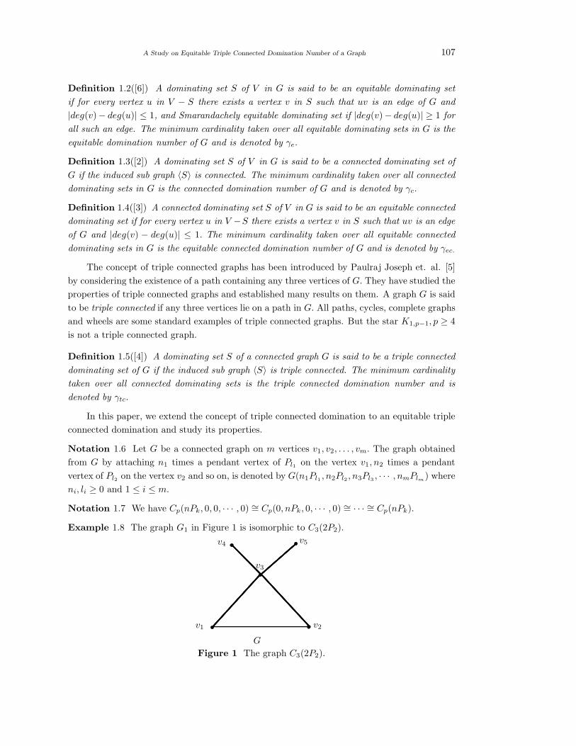
A Study on Equitable Triple Connected Domination Number of a Graph 107
Definition 1.2([6]) A dominating set S of V in G is said to be an equitable dominating set
if for every vertex u in V − S there exists a vertex v in S such that uv is an edge of G and
|deg(v)− deg(u)| ≤ 1, and Smarandachely equitable dominating set if |deg(v)− deg(u)| ≥ 1 for
all such an edge. The minimum cardinality taken over all equitable dominating sets in G is the
equitable domination number of G and is denoted by γe.
Definition 1.3([2]) A dominating set S of V in G is said to be a connected dominating set of
G if the induced sub graph 〈S〉 is connected. The minimum cardinality taken over all connected
dominating sets in G is the connected domination number of G and is denoted by γc.
Definition 1.4([3]) A connected dominating set S of V in G is said to be an equitable connected
dominating set if for every vertex u in V −S there exists a vertex v in S such that uv is an edge
of G and |deg(v) − deg(u)| ≤ 1. The minimum cardinality taken over all equitable connected
dominating sets in G is the equitable connected domination number of G and is denoted by γec.
The concept of triple connected graphs has been introduced by Paulraj Joseph et. al. [5]
by considering the existence of a path containing any three vertices of G. They have studied the
properties of triple connected graphs and established many results on them. A graph G is said
to be triple connected if any three vertices lie on a path in G. All paths, cycles, complete graphs
and wheels are some standard examples of triple connected graphs. But the star K1,p−1, p ≥ 4
is not a triple connected graph.
Definition 1.5([4]) A dominating set S of a connected graph G is said to be a triple connected
dominating set of G if the induced sub graph 〈S〉 is triple connected. The minimum cardinality
taken over all connected dominating sets is the triple connected domination number and is
denoted by γtc.
In this paper, we extend the concept of triple connected domination to an equitable triple
connected domination and study its properties.
Notation 1.6 Let G be a connected graph on m vertices v1, v2, . . . , vm. The graph obtained
from G by attaching n1 times a pendant vertex of Pl1 on the vertex v1, n2 times a pendant
vertex of Pl2 on the vertex v2 and so on, is denoted by G(n1Pl1 , n2Pl2 , n3Pl3 , · · · , nmPlm) where
ni, li ≥ 0 and 1 ≤ i ≤ m.
Notation 1.7 We have Cp(nPk, 0, 0, · · · , 0) ∼= Cp(0, nPk, 0, · · · , 0) ∼= · · · ∼= Cp(nPk).
Example 1.8 The graph G1 in Figure 1 is isomorphic to C3(2P2).
v1 v2
v3
v4 v5
G
Figure 1 The graph C3(2P2).
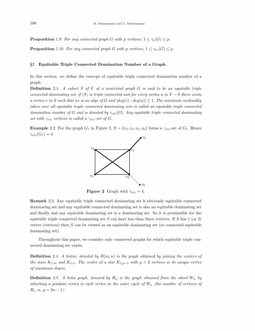
108 M. Subramanian and T. Subramanian
Proposition 1.9 For any connected graph G with p vertices, 1 ≤ γe(G) ≤ p.
Proposition 1.10 For any connected graph G with p vertices, 1 ≤ γec(G) ≤ p.
§2. Equitable Triple Connected Domination Number of a Graph
In this section, we define the concept of equitable triple connected domination number of a
graph.
Definition 2.1 A subset S of V of a nontrivial graph G is said to be an equitable triple
connected dominating set, if 〈S〉 is triple connected and for every vertex u in V −S there exists
a vertex v in S such that uv is an edge of G and |deg(v)−deg(u)| ≤ 1. The minimum cardinality
taken over all equitable triple connected dominating sets is called an equitable triple connected
domination number of G and is denoted by γetc(G). Any equitable triple connected dominating
set with γetc vertices is called a γetc-set of G.
Example 2.2 For the graph G1 in Figure 2, S = {v2, v3, v5, v6} forms a γetc-set of G1. Hence
γetc(G1) = 4.
v1 v2
v3v4
v5
v6
Figure 2 Graph with γetc = 4.
Remark 2.3 Any equitable triple connected dominating set is obviously equitable connected
dominating set and any equitable connected dominating set is also an equitable dominating set
and finally and any equitable dominating set is a dominating set. So it is permissible for the
equitable triple connected dominating set S can have less than three vertices. If S has 1 (or 2)
vertex (vertices) then S can be viewed as an equitable dominating set (or connected equitable
dominating set).
Throughout this paper, we consider only connected graphs for which equitable triple con-
nected dominating set exists.
Definition 2.4 A bistar, denoted by B(m, n) is the graph obtained by joining the centers of
the stars K1,m and K1,n. The center of a star K1,p−1 with p > 2 vertices is its unique vertex
of maximum degree.
Definition 2.5 A helm graph, denoted by Hn is the graph obtained from the wheel Wn by
attaching a pendant vertex to each vertex in the outer cycle of Wn (the number of vertices of
Hn is, p = 2n − 1).
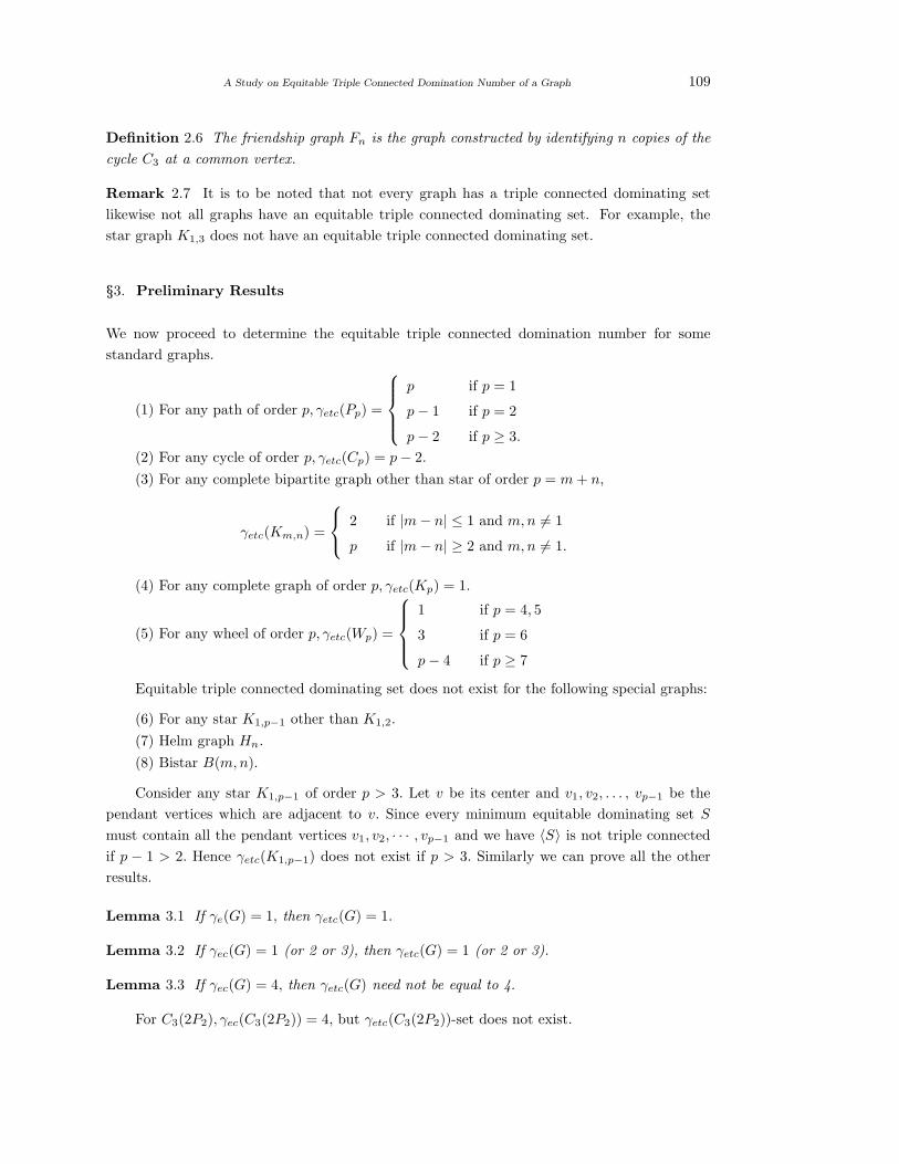
A Study on Equitable Triple Connected Domination Number of a Graph 109
Definition 2.6 The friendship graph Fn is the graph constructed by identifying n copies of the
cycle C3 at a common vertex.
Remark 2.7 It is to be noted that not every graph has a triple connected dominating set
likewise not all graphs have an equitable triple connected dominating set. For example, the
star graph K1,3 does not have an equitable triple connected dominating set.
§3. Preliminary Results
We now proceed to determine the equitable triple connected domination number for some
standard graphs.
(1) For any path of order p, γetc(Pp) =
p if p = 1
p − 1 if p = 2
p − 2 if p ≥ 3.
(2) For any cycle of order p, γetc(Cp) = p − 2.
(3) For any complete bipartite graph other than star of order p = m + n,
γetc(Km,n) =
2 if |m − n| ≤ 1 and m, n 6= 1
p if |m − n| ≥ 2 and m, n 6= 1.
(4) For any complete graph of order p, γetc(Kp) = 1.
(5) For any wheel of order p, γetc(Wp) =
1 if p = 4, 5
3 if p = 6
p − 4 if p ≥ 7
Equitable triple connected dominating set does not exist for the following special graphs:
(6) For any star K1,p−1 other than K1,2.
(7) Helm graph Hn.
(8) Bistar B(m, n).
Consider any star K1,p−1 of order p > 3. Let v be its center and v1, v2, . . . , vp−1 be the
pendant vertices which are adjacent to v. Since every minimum equitable dominating set S
must contain all the pendant vertices v1, v2, · · · , vp−1 and we have 〈S〉 is not triple connected
if p − 1 > 2. Hence γetc(K1,p−1) does not exist if p > 3. Similarly we can prove all the other
results.
Lemma 3.1 If γe(G) = 1, then γetc(G) = 1.
Lemma 3.2 If γec(G) = 1 (or 2 or 3), then γetc(G) = 1 (or 2 or 3).
Lemma 3.3 If γec(G) = 4, then γetc(G) need not be equal to 4.
For C3(2P2), γec(C3(2P2)) = 4, but γetc(C3(2P2))-set does not exist.
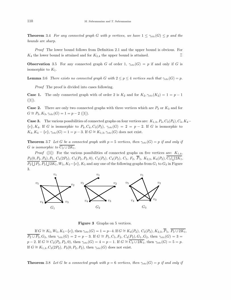
110 M. Subramanian and T. Subramanian
Theorem 3.4 For any connected graph G with p vertices, we have 1 ≤ γetc(G) ≤ p and the
bounds are sharp.
Proof The lower bound follows from Definition 2.1 and the upper bound is obvious. For
K4 the lower bound is attained and for K2,4 the upper bound is attained. 2Observation 3.5 For any connected graph G of order 1, γetc(G) = p if and only if G is
isomorphic to K1.
Lemma 3.6 There exists no connected graph G with 2 ≤ p ≤ 4 vertices such that γetc(G) = p.
Proof The proof is divided into cases following.
Case 1. The only connected graph with of order 2 is K2 and for K2, γetc(K2) = 1 = p − 1
([1]).
Case 2. There are only two connected graphs with three vertices which are P3 or K3 and for
G ∼= P3, K3, γetc(G) = 1 = p − 2 ([1]).
Case 3. The various possibilities of connected graphs on four vertices are: K1,3, P4, C3(P2), C4, K4−{e}, K4. If G is isomorphic to P4, C4, C3(P2), γetc(G) = 2 = p − 2. If G is isomorphic to
K4, K4 − {e}, γetc(G) = 1 = p − 3. If G ∼= K1,3, γetc(G) does not exist. 2Theorem 3.7 Let G be a connected graph with p = 5 vertices, then γetc(G) = p if and only if
G is isomorphic to C3 ∪ 2K1.
Proof ([1]) For the various possibilities of connected graphs on five vertices are: K1,4,
P3(0, P2, P2), P5, C3(2P2), C3(P2, P2, 0), C3(P3), C4(P2), C5, F2, P 5, K2,3, K4(P2), C3
⋃2K1,
P2
⋃P3, P3
⋃2K1, W5, K5−{e}, K5 and any one of the following graphs from G1 to G3 in Figure
3.
v1
v2
v3v4
v5
v1
v2
v3v4
v5
v1
v2
v3v4
v5
G1 G2 G3
Figure 3 Graphs on 5 vertices.
If G ∼= K5, W5, K5−{e}, then γetc(G) = 1 = p−4. If G ∼= K4(P2), C3(P3), K2,3, P 5, P3 ∪ 2K1,
P2 ∪ P3, G3, then γetc(G) = 2 = p − 3. If G ∼= P5, C5, F2, C4(P2), G1, G2, then γetc(G) = 3 =
p − 2. If G ∼= C3(P2, P2, 0), then γetc(G) = 4 = p − 1. If G ∼= C3 ∪ 2K1, then γetc(G) = 5 = p.
If G ∼= K1,4, C3(2P2), P3(0, P2, P2), then γetc(G) does not exist. 2Theorem 3.8 Let G be a connected graph with p = 6 vertices, then γetc(G) = p if and only if
A Study on Equitable Triple Connected Domination Number of a Graph 111
G is isomorphic to K2,4 or any one of the graphs: G1, G2, G3 in Figure 4.
v1 v2
v3 v4
v5 v6
v1 v2
v3 v4
v5 v6
v1 v2
v3v4
v5 v6
G1G2 G3
Figure 4 Graphs on 6 vertices with γetc(G) = 6.
Proof Let G be a connected graph with p = 6 vertices, and let γetc(G) = 6 ([1]). Among
all of the connected graphs on 6 vertices, it can be easily verified that G ∼= K2,4 or any one of
the graphs G1, G2, G3 in Figure 4.The converse part is obvious. 2Lemma 3.9 Let G be a connected graph of order 2 such that γ(G) = γetc(G). Then G ∼= K2.
Lemma 3.10 Let G be a connected graph of order 3 such that γ(G) = γetc(G). Then G ∼= K3, P3.
Lemma 3.11 Let G be a connected graph of order 4 such that γ(G) = γetc(G). Then G is
isomorphic to one of the following graphs: P4, C4, K4, K4 − {e}.
Proof For the various possibilities of connected graphs on four vertices are: K1,3, P4, C3(P2),
C4, K4 − {e}, K4. If G ∼= P4, C4, γ(G) = γetc(G) = 2. If G ∼= K4, K4 − {e}, γ(G) = γetc(G) = 1.
If G ∼= C3(P2), K1,3, γ(C3(P2)) = 1 but γetc(C3(P2)) = 2 and γ(K1,3) = 1 but γetc(K1,3) does
not exist. Hence the lemma. 2Theorem 3.12 Let G be a connected graph on order 5 such that γ(G) = γetc(G). Then G is
isomorphic to one of the following graphs: C3(P3), P 5, K2,3, P2 ∪ P3, W5, K5 − {e}, K5.
Proof For the various possibilities of connected graphs on five vertices are: K1,4, P3(0, P2, P2),
P5, C3(2P2), C3(P2, P2, 0), C3(P3), C4(P2), C5, F2, P 5, K2,3, K4(P2), C3 ∪ 2K1, P2 ∪ P3, P3 ∪ 2K1,
W5, K5−{e}, K5 and any one of the following graphs from G1 to G3 in Figure 3. Among all the
above possibilities it can be easily verified that γ(G) = γetc(G) only if G ∼= C3(P3), P 5, K2,3,
P2 ∪ P3, W5, K5 − {e}, K5. 2Theorem 3.13 Let G be a connected graph of order 6 such that γ(G) = γetc(G). Then G is iso-
morphic to K3,3, K6−{e}, K6, or any one of the graphs: G1, G2, G3, G4, G5, G6, G7, G8, G9, G10,
G11, G12 in Figure 5.
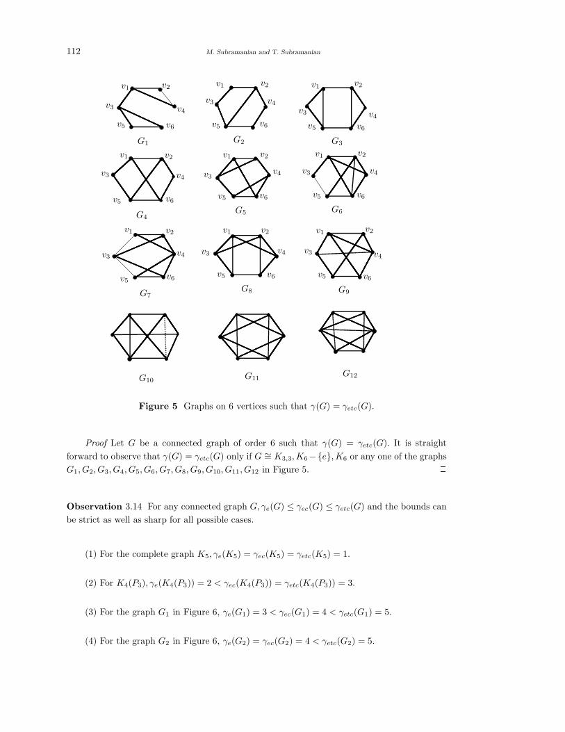
112 M. Subramanian and T. Subramanian
v1 v2
v3 v4
v5 v6
v1 v2
v3 v4
v5 v6
v1 v2
v3 v4
v5 v6
G1 G2 G3
v1 v2 v1 v2 v1 v2
v3 v4 v3v4 v3 v4
v5 v6v5 v6 v5 v6
G4G5 G6
v1 v2 v1 v2 v1 v2
v3 v4 v3 v4 v3 v4
v5v6
v5 v6 v5 v6
G7G8 G9
G10G11
G12
Figure 5 Graphs on 6 vertices such that γ(G) = γetc(G).
Proof Let G be a connected graph of order 6 such that γ(G) = γetc(G). It is straight
forward to observe that γ(G) = γetc(G) only if G ∼= K3,3, K6−{e}, K6 or any one of the graphs
G1, G2, G3, G4, G5, G6, G7, G8, G9, G10, G11, G12 in Figure 5. 2Observation 3.14 For any connected graph G, γe(G) ≤ γec(G) ≤ γetc(G) and the bounds can
be strict as well as sharp for all possible cases.
(1) For the complete graph K5, γe(K5) = γec(K5) = γetc(K5) = 1.
(2) For K4(P3), γe(K4(P3)) = 2 < γec(K4(P3)) = γetc(K4(P3)) = 3.
(3) For the graph G1 in Figure 6, γe(G1) = 3 < γec(G1) = 4 < γetc(G1) = 5.
(4) For the graph G2 in Figure 6, γe(G2) = γec(G2) = 4 < γetc(G2) = 5.
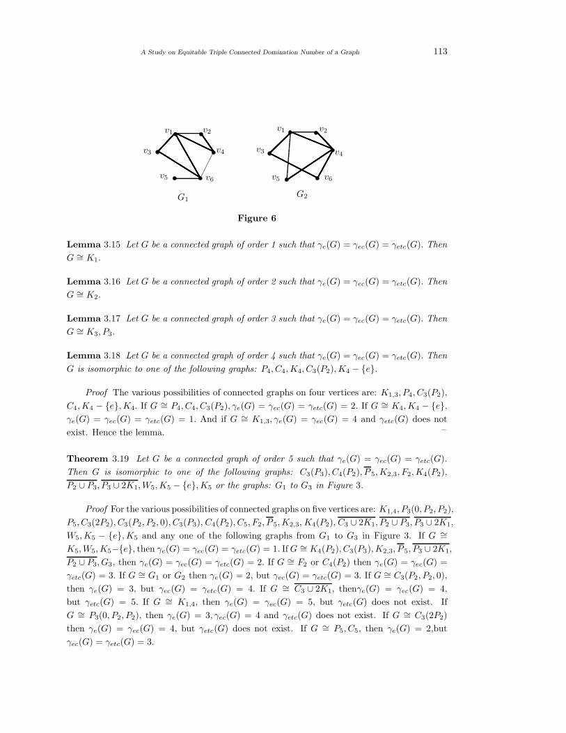
A Study on Equitable Triple Connected Domination Number of a Graph 113
v1 v2 v1 v2
v3 v4 v3 v4
v5 v6 v5 v6
G1G2
Figure 6
Lemma 3.15 Let G be a connected graph of order 1 such that γe(G) = γec(G) = γetc(G). Then
G ∼= K1.
Lemma 3.16 Let G be a connected graph of order 2 such that γe(G) = γec(G) = γetc(G). Then
G ∼= K2.
Lemma 3.17 Let G be a connected graph of order 3 such that γe(G) = γec(G) = γetc(G). Then
G ∼= K3, P3.
Lemma 3.18 Let G be a connected graph of order 4 such that γe(G) = γec(G) = γetc(G). Then
G is isomorphic to one of the following graphs: P4, C4, K4, C3(P2), K4 − {e}.
Proof The various possibilities of connected graphs on four vertices are: K1,3, P4, C3(P2),
C4, K4 − {e}, K4. If G ∼= P4, C4, C3(P2), γe(G) = γec(G) = γetc(G) = 2. If G ∼= K4, K4 − {e},γe(G) = γec(G) = γetc(G) = 1. And if G ∼= K1,3, γe(G) = γec(G) = 4 and γetc(G) does not
exist. Hence the lemma. 2Theorem 3.19 Let G be a connected graph of order 5 such that γe(G) = γec(G) = γetc(G).
Then G is isomorphic to one of the following graphs: C3(P3), C4(P2), P 5, K2,3, F2, K4(P2),
P2 ∪ P3, P3 ∪ 2K1, W5, K5 − {e}, K5 or the graphs: G1 to G3 in Figure 3.
Proof For the various possibilities of connected graphs on five vertices are: K1,4, P3(0, P2, P2),
P5, C3(2P2), C3(P2, P2, 0), C3(P3), C4(P2), C5, F2, P 5, K2,3, K4(P2), C3 ∪ 2K1, P2 ∪ P3, P3 ∪ 2K1,
W5, K5 − {e}, K5 and any one of the following graphs from G1 to G3 in Figure 3. If G ∼=K5, W5, K5−{e}, then γe(G) = γec(G) = γetc(G) = 1. If G ∼= K4(P2), C3(P3), K2,3, P 5, P3 ∪ 2K1,
P2 ∪ P3, G3, then γe(G) = γec(G) = γetc(G) = 2. If G ∼= F2 or C4(P2) then γe(G) = γec(G) =
γetc(G) = 3. If G ∼= G1 or G2 then γe(G) = 2, but γec(G) = γetc(G) = 3. If G ∼= C3(P2, P2, 0),
then γe(G) = 3, but γec(G) = γetc(G) = 4. If G ∼= C3 ∪ 2K1, thenγe(G) = γec(G) = 4,
but γetc(G) = 5. If G ∼= K1,4, then γe(G) = γec(G) = 5, but γetc(G) does not exist. If
G ∼= P3(0, P2, P2), then γe(G) = 3, γec(G) = 4 and γetc(G) does not exist. If G ∼= C3(2P2)
then γe(G) = γec(G) = 4, but γetc(G) does not exist. If G ∼= P5, C5, then γe(G) = 2,but
γec(G) = γetc(G) = 3. 2
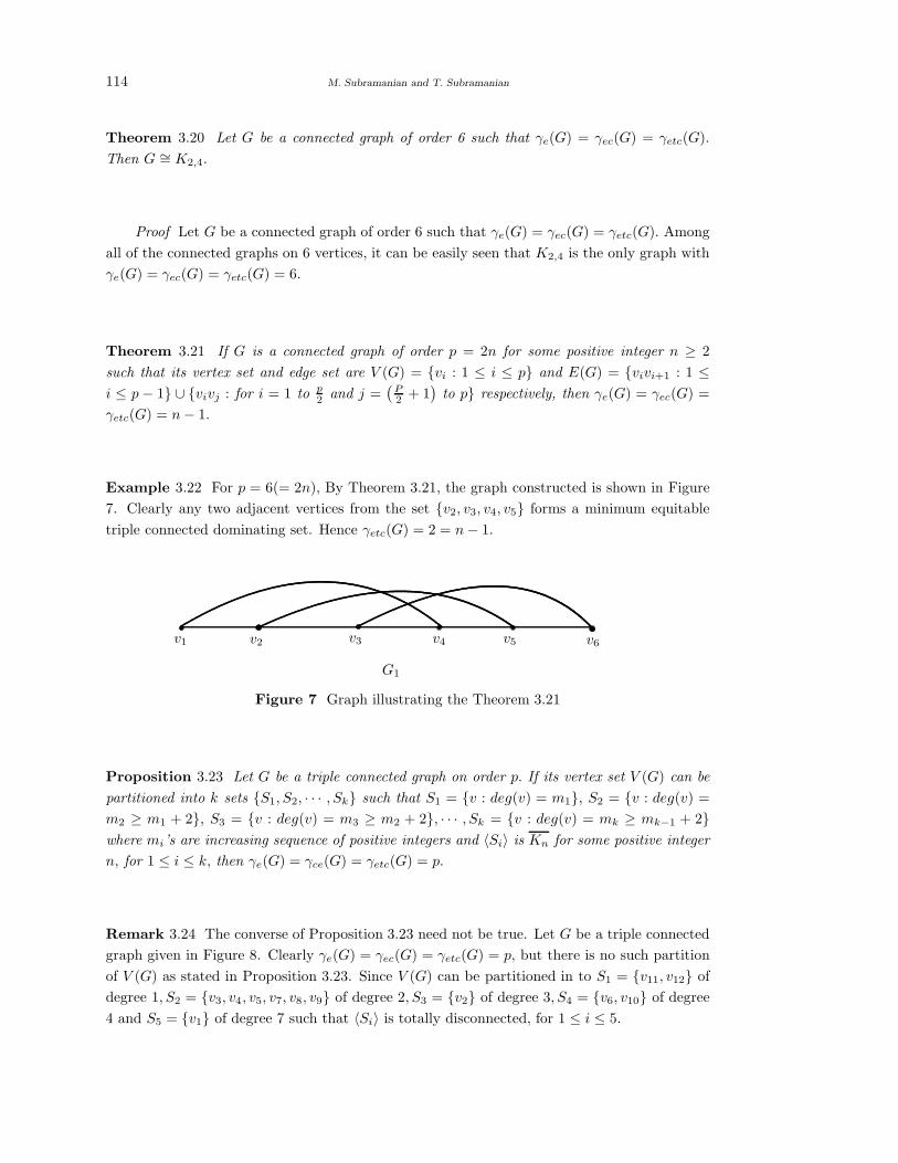
114 M. Subramanian and T. Subramanian
Theorem 3.20 Let G be a connected graph of order 6 such that γe(G) = γec(G) = γetc(G).
Then G ∼= K2,4.
Proof Let G be a connected graph of order 6 such that γe(G) = γec(G) = γetc(G). Among
all of the connected graphs on 6 vertices, it can be easily seen that K2,4 is the only graph with
γe(G) = γec(G) = γetc(G) = 6. 2Theorem 3.21 If G is a connected graph of order p = 2n for some positive integer n ≥ 2
such that its vertex set and edge set are V (G) = {vi : 1 ≤ i ≤ p} and E(G) = {vivi+1 : 1 ≤i ≤ p − 1} ∪ {vivj : for i = 1 to p
2 and j =(
P2 + 1
)to p} respectively, then γe(G) = γec(G) =
γetc(G) = n − 1.
Example 3.22 For p = 6(= 2n), By Theorem 3.21, the graph constructed is shown in Figure
7. Clearly any two adjacent vertices from the set {v2, v3, v4, v5} forms a minimum equitable
triple connected dominating set. Hence γetc(G) = 2 = n − 1.
v1 v2 v3 v4 v5 v6
G1
Figure 7 Graph illustrating the Theorem 3.21
Proposition 3.23 Let G be a triple connected graph on order p. If its vertex set V (G) can be
partitioned into k sets {S1, S2, · · · , Sk} such that S1 = {v : deg(v) = m1}, S2 = {v : deg(v) =
m2 ≥ m1 + 2}, S3 = {v : deg(v) = m3 ≥ m2 + 2}, · · · , Sk = {v : deg(v) = mk ≥ mk−1 + 2}where mi’s are increasing sequence of positive integers and 〈Si〉 is Kn for some positive integer
n, for 1 ≤ i ≤ k, then γe(G) = γce(G) = γetc(G) = p.
Remark 3.24 The converse of Proposition 3.23 need not be true. Let G be a triple connected
graph given in Figure 8. Clearly γe(G) = γec(G) = γetc(G) = p, but there is no such partition
of V (G) as stated in Proposition 3.23. Since V (G) can be partitioned in to S1 = {v11, v12} of
degree 1, S2 = {v3, v4, v5, v7, v8, v9} of degree 2, S3 = {v2} of degree 3, S4 = {v6, v10} of degree
4 and S5 = {v1} of degree 7 such that 〈Si〉 is totally disconnected, for 1 ≤ i ≤ 5.
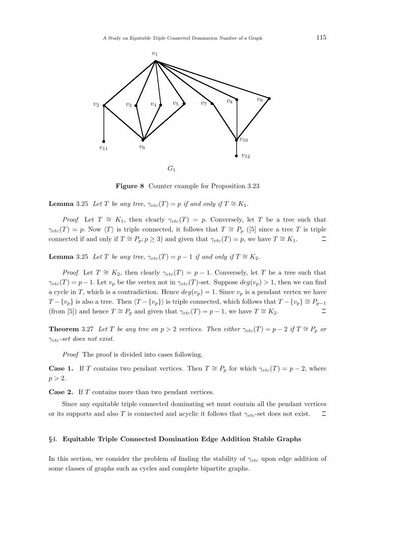
A Study on Equitable Triple Connected Domination Number of a Graph 115
v1
v2 v3 v4 v5
v6
v7v8
v9
v10
v11
v12
G1
Figure 8 Counter example for Proposition 3.23
Lemma 3.25 Let T be any tree, γetc(T ) = p if and only if T ∼= K1.
Proof Let T ∼= K1, then clearly γetc(T ) = p. Conversely, let T be a tree such that
γetc(T ) = p. Now 〈T 〉 is triple connected, it follows that T ∼= Pp ([5] since a tree T is triple
connected if and only if T ∼= Pp; p ≥ 3) and given that γetc(T ) = p, we have T ∼= K1. 2Lemma 3.25 Let T be any tree, γetc(T ) = p − 1 if and only if T ∼= K2.
Proof Let T ∼= K2, then clearly γetc(T ) = p − 1. Conversely, let T be a tree such that
γetc(T ) = p− 1. Let vp be the vertex not in γetc(T )-set. Suppose deg(vp) > 1, then we can find
a cycle in T, which is a contradiction. Hence deg(vp) = 1. Since vp is a pendant vertex we have
T −{vp} is also a tree. Then 〈T −{vp}〉 is triple connected, which follows that T −{vp} ∼= Pp−1
(from [5]) and hence T ∼= Pp and given that γetc(T ) = p − 1, we have T ∼= K2. 2Theorem 3.27 Let T be any tree on p > 2 vertices. Then either γetc(T ) = p − 2 if T ∼= Pp or
γetc-set does not exist.
Proof The proof is divided into cases following.
Case 1. If T contains two pendant vertices. Then T ∼= Pp for which γetc(T ) = p − 2, where
p > 2.
Case 2. If T contains more than two pendant vertices.
Since any equitable triple connected dominating set must contain all the pendant vertices
or its supports and also T is connected and acyclic it follows that γetc-set does not exist. 2§4. Equitable Triple Connected Domination Edge Addition Stable Graphs
In this section, we consider the problem of finding the stability of γetc upon edge addition of
some classes of graphs such as cycles and complete bipartite graphs.
116 M. Subramanian and T. Subramanian
Definition 4.1 A connected graph G is said to be an equitable triple connected domination
edge addition stable (γetc-stable), if both G and G + e have the same equitable triple connected
domination number, where G + e is a simple graph (i.e.) γetc(G) = γetc(G + e).
Definition 4.2 A connected graph G is said to be an equitable triple connected domination
edge addition positive critical (γ+etc- critical), if G + e has greater equitable triple connected
domination number than G, where G + e is a simple graph (i.e.) γetc(G) < γetc(G + e).
Definition 4.3 A connected graph G is said to be an equitable triple connected domination edge
addition negative critical (γ−etc-critical), if G has greater equitable triple connected domination
number than G + e, where G + e is a simple graph (i.e.) γetc(G) > γetc(G + e).
Theorem 4.4 The cycle Cp(p > 3), is γ−etc-critical.
Proof Let Cp = v1v2 · · · vpv1 be any cycle of length p, p > 3. Now S = {v2, v3, · · · , vp−1}is the minimum equitable triple connected dominating set, we have γetc(Cp) = p − 2. Consider
Cp + e, where e = vivj .
Case 1. Let Cp+e contain C3 = v1v2v3v1, where e = vivj = v3v1. Since S = {v3, v4, · · · , vp−1}forms a minimum equitable triple connected dominating set, we have γetc(Cp + e) = p − 3.
Case 2. Let Cp+e does not contain C3. Let e = vivj . Now S = V (Cp+e)−{vi+1, vi+2, vj+1, vj+2},where vi+2 = N(vi+1)−vi and vj+2 = N(vj+1)−vj forms a minimum equitable triple connected
dominating set. Hence γetc(Cp + e) = p − 4.
In both cases γetc(Cp + e) < γetc(Cp). Hence Cp(p > 3), is γ−etc-critical. 2
Lemma 4.5 The complete bipartite graph K1,2 is γetc-stable.
Lemma 4.6 The complete bipartite graph K2,2 is γ−etc-critical.
Lemma 4.7 The complete bipartite graph Kn,n, (n > 2, p = 2n) is γetc-stable.
Proof Let Kn,n, (n > 2) be a complete bipartite graph and its vertex partition is given by
V = V1∪V2 such that V1 = {u1, u2, · · · , un} and V2 = {v1, v2, · · · , vn}. Now S = {u1, v1} forms
a minimum equitable triple connected dominating set so that γetc(Kn,n) = 2. If we add any
edge to Kn,n there is no change in the equitable triple connected domination number. Hence
Kn,n, (n > 2) is γetc-stable. 2Lemma 4.8 If an edge e is added between the vertices of V1. Then the complete bipartite graph
K3,2, is γetc-stable, where V (K3,2) = V1 ∪ V2 such that V1 = {u1, u2, u3} and V2 = {v1, v2}.
Proof Here S = {u1, v1} forms a minimum equitable triple connected dominating set so
that γetc(K3,2) = 2. If we add an edge e is added between the vertices of V1 we see that there
is no change in the equitable triple connected domination number. 2Lemma 4.9 If an edge e is added between the vertices of V2. Then the complete bipartite graph
K3,2 is γ+etc-critical, where V (K3,2) = V1
⋃V2 such that V1 = {u1, u2, u3} and V2 = {v1, v2}.
A Study on Equitable Triple Connected Domination Number of a Graph 117
Proof Here S = {u1, v1} forms a minimum equitable triple connected dominating set so that
γetc(K3,2) = 2. By adding an edge between the vertices of V2, we see that S = {u1, u2, u3, v1, v2}is a minimum equitable triple connected dominating set so that γetc(K3,2) = 5. 2Lemma 4.10 If an edge e is added between the vertices of V1. Then the complete bipartite graph
Kn+1,n, (n > 2) is γetc-stable, where V (Kn+1,n) = V1 ∪ V2 such that V1 = {u1, u2, · · · , un+1}and V2 = {v1, v2, · · · , vn}.
Proof Here S = {u1, v1} forms a minimum equitable triple connected dominating set so
that γetc(Kn+1,n) = 2. If we add an edge e is added between the vertices of V1 we see that there
is no change in the equitable triple connected domination number. 2Lemma 4.11 If an edge e is added between the vertices of V2. Then the complete bipartite graph
Kn+1,n, (n > 2) is γ+etc-critical, where V (Kn+1,n) = V1 ∪ V2 such that V1 = {u1, u2, · · · , un+1}
and V2 = {v1, v2, · · · , vn}.
Proof Here S = {u1, v1} forms a minimum equitable triple connected dominating set so
that γetc(Kn+1,n) = 2. By adding an edge e between the vertices of V2 say e = v1v2, we see
that S = {v1, u1, vi} for i 6= 2 is a minimum equitable triple connected dominating set so that
γetc(Kn+1,n) = 3. 2Lemma 4.12 If an edge e is added between the vertices of V1. Then the complete bipartite graph
Kn+2,n, (n > 1) is γ−etc-critical, where V (Kn+2,n) = V1∪V2 such that V1 = {u1, u2, · · · , un+1, un+2}
and V2 = {v1, v2, · · · , vn}.
Proof Here S = {u1, u2, · · · , un+1, un+2, v1, v2, · · · , vn} forms a minimum equitable triple
connected dominating set so that γetc(Kn+2,n) = p. By adding an edge e between the vertices
of V1 say e = u1u2, we see that S = {u3, · · · , un+1, un+2, v1, v2, · · · , vn} forms a minimum
equitable triple connected dominating set so that γetc(Kn+2,n) = p − 2. 2Lemma 4.13 If an edge e is added between the vertices of V2. Then the complete bipartite graph
Kn+2,n, (n > 1) is γetc-stable, where V (Kn+2,n) = V1∪V2 such that V1 = {u1, u2, · · · , un+1, un+2}and V2 = {v1, v2, · · · , vn}.
Proof Here S = {u1, u2, · · · , un+1, un+2, v1, v2, · · · , vn} forms a minimum equitable triple
connected dominating set so that γetc(Kn+2,n) = p. By adding an edge e between the vertices
of V2 say e = v1v2, we see that there is no change in the equitable triple connected domination
number. 2Theorem 4.14 The complete bipartite graph Km,n, (m − n > 2 and m + n = p) is γetc-stable.
Proof Let Km,n, (m− n > 2 and m + n = p) be a complete bipartite graph and its vertex
partition is given by V = V1∪V2 such that V1 = {u1, u2, · · · , um} and V2 = {v1, v2, · · · , vn}. Now
S = {u1, u2, · · · , um, v1, v2, · · · , vn} forms a minimum equitable triple connected dominating set
so that γetc(Km,n) = p. If we add any edge to Km,n there is no change in the equitable triple
connected domination number. 2
118 M. Subramanian and T. Subramanian
§5. Conclusion
We conclude this paper by giving the following interesting open problems for further study:
(1) Characterize connected graphs of order p for which γetc = p.
(2) For which graphs, γe = γec = γetc = p.
References
[1] F. Harary, Graph Theory, Addison-Wesley, Reading Mass (1972).
[2] T. W. Haynes, S. T. Hedetniemi and P. J. Slater, Fundamentals of Domination in Graphs,
Marcel Dekker, New York (1998).
[3] K. Kavitha, and N. G. David, Equitable Total Domination Edge Addition Stable Graphs,
J. Combin. Math. Combin. Comput., 92 (2015), 185–194.
[4] G. Mahadevan, A. Selvam, J. Paulraj Joseph and T. Subramanian, Triple connected domi-
nation number of a graph, International Journal of Mathematical Combinatorics, 3 (2012),
93–104.
[5] J. Paulraj Joseph J, M. K. Angel Jebitha, P. Chithra Devi and G. Sudhana, Triple con-
nected graphs, Indian Journal of Mathematics and Mathematical Sciences, 8 (1) (2012),
61–75.
[6] E. Sampathkumar, Equitable Domination, Kragujevac Journal of Mathematics, 35(1) (2011),
191–197.
International J.Math. Combin. Vol.3(2017), 119-124
Path Related n-Cap Cordial Graphs
A. Nellai Murugan
(Department of Mathematics, V.O.Chidambaram College, Tamil Nadu, India)
P. Iyadurai Selvaraj
(Department of Computer Science, V.O.Chidambaram College, Tamil Nadu, India)
E-mail: [email protected], [email protected]
Abstract: Let G = (V,E) be a graph with p vertices and q edges. A n-cap (∧
) cordial
labeling of a graph G with vertex set V is a bijection from V to {0,1} such that if each edge
uv is assigned the label
f(uv) =
0, if f(u) = f(v) = 1
1, otherwise.
with the condition that the number of vertices labeled with 0 and the number of vertices
labeled with 1 differ by at most 1 and the number of edges labeled with 0 and the number
of edges labeled with 1 differ by at most 1. The graph that admits a∧
cordial labeling is
called a∧
cordial graph (nCCG). In this paper, we proved that Path Pn, Comb (Pn ⊙K1),
Pm ⊙ 2K1 and Fan (Fn = Pn + K1) are∧
cordial graphs.
Key Words:∧
cordial labeling, Smarandachely cordial labeling,∧
cordial labeling graph.
AMS(2010): 05C78.
§1. Introduction
A graph G is a finite non-empty set of objects called vertices together with a set of unordered
pairs of distinct vertices of G which is called edges. Each pair e = {uv} of vertices in E is called
an edge or a line of G. In this paper, we proved that Path Pn, Comb (Pn⊙1), Pm ⊙ 2K1 and
Fan (Fn = Pn + K1) are∧
cordial graphs.
§2. Preliminaries
Let G = (V, E) be a graph with p vertices and q edges. A n-cap (∧
) cordial labeling of a graph
G with vertex set V is a bijection from V to {0, 1} such that if each edge uv is assigned the
1Received September 30, 2016, Accepted August 26, 2017.
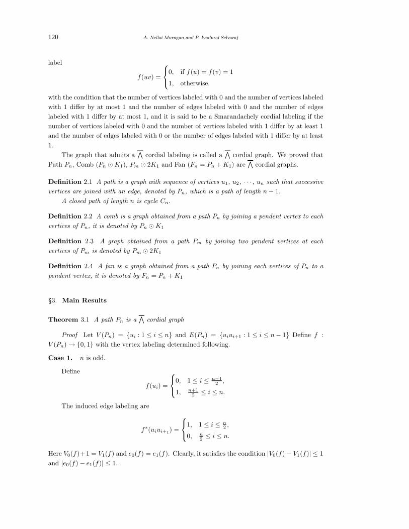
120 A. Nellai Murugan and P. Iyadurai Selvaraj
label
f(uv) =
0, if f(u) = f(v) = 1
1, otherwise.
with the condition that the number of vertices labeled with 0 and the number of vertices labeled
with 1 differ by at most 1 and the number of edges labeled with 0 and the number of edges
labeled with 1 differ by at most 1, and it is said to be a Smarandachely cordial labeling if the
number of vertices labeled with 0 and the number of vertices labeled with 1 differ by at least 1
and the number of edges labeled with 0 or the number of edges labeled with 1 differ by at least
1.
The graph that admits a∧
cordial labeling is called a∧
cordial graph. We proved that
Path Pn, Comb (Pn ⊙ K1), Pm ⊙ 2K1 and Fan (Fn = Pn + K1) are∧
cordial graphs.
Definition 2.1 A path is a graph with sequence of vertices u1, u2, · · · , un such that successive
vertices are joined with an edge, denoted by Pn, which is a path of length n − 1.
A closed path of length n is cycle Cn.
Definition 2.2 A comb is a graph obtained from a path Pn by joining a pendent vertex to each
vertices of Pn, it is denoted by Pn ⊙ K1
Definition 2.3 A graph obtained from a path Pm by joining two pendent vertices at each
vertices of Pm is denoted by Pm ⊙ 2K1
Definition 2.4 A fan is a graph obtained from a path Pn by joining each vertices of Pn to a
pendent vertex, it is denoted by Fn = Pn + K1
§3. Main Results
Theorem 3.1 A path Pn is a∧
cordial graph
Proof Let V (Pn) = {ui : 1 ≤ i ≤ n} and E(Pn) = {uiui+1 : 1 ≤ i ≤ n − 1} Define f :
V (Pn) → {0, 1} with the vertex labeling determined following.
Case 1. n is odd.
Define
f(ui) =
0, 1 ≤ i ≤ n−12 ,
1, n+12 ≤ i ≤ n.
The induced edge labeling are
f∗(uiui+1) =
1, 1 ≤ i ≤ n2 ,
0, n2 ≤ i ≤ n.
Here V0(f)+1 = V1(f) and e0(f) = e1(f). Clearly, it satisfies the condition |V0(f) − V1(f)| ≤ 1
and |e0(f) − e1(f)| ≤ 1.
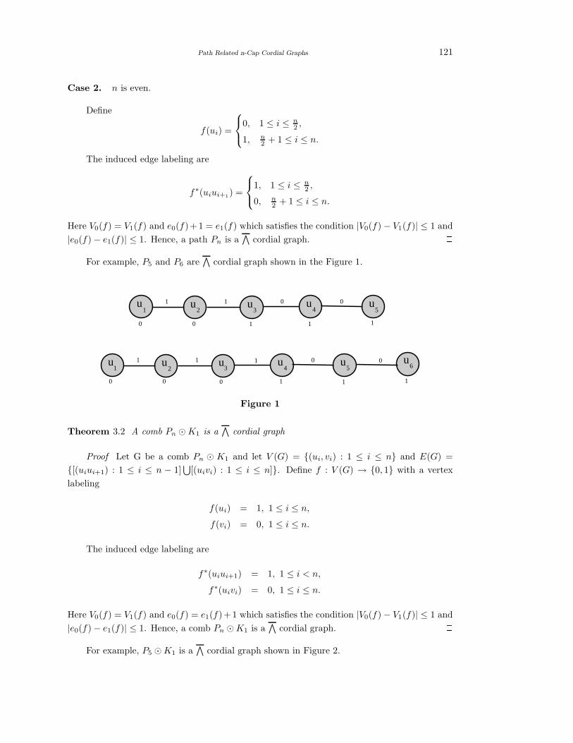
Path Related n-Cap Cordial Graphs 121
Case 2. n is even.
Define
f(ui) =
0, 1 ≤ i ≤ n2 ,
1, n2 + 1 ≤ i ≤ n.
The induced edge labeling are
f∗(uiui+1) =
1, 1 ≤ i ≤ n2 ,
0, n2 + 1 ≤ i ≤ n.
Here V0(f) = V1(f) and e0(f)+1 = e1(f) which satisfies the condition |V0(f) − V1(f)| ≤ 1 and
|e0(f) − e1(f)| ≤ 1. Hence, a path Pn is a∧
cordial graph. 2For example, P5 and P6 are
∧cordial graph shown in the Figure 1.
u1
u2
u3
u4
u5
1 1
1 1 10 0
0 0
u1
u2
u3
u4
u5
1 1
11 10 0
00 u6
1
0
Figure 1
Theorem 3.2 A comb Pn ⊙ K1 is a∧
cordial graph
Proof Let G be a comb Pn ⊙ K1 and let V (G) = {(ui, vi) : 1 ≤ i ≤ n} and E(G) =
{[(uiui+1) : 1 ≤ i ≤ n − 1]⋃
[(uivi) : 1 ≤ i ≤ n]}. Define f : V (G) → {0, 1} with a vertex
labeling
f(ui) = 1, 1 ≤ i ≤ n,
f(vi) = 0, 1 ≤ i ≤ n.
The induced edge labeling are
f∗(uiui+1) = 1, 1 ≤ i < n,
f∗(uivi) = 0, 1 ≤ i ≤ n.
Here V0(f) = V1(f) and e0(f) = e1(f)+1 which satisfies the condition |V0(f) − V1(f)| ≤ 1 and
|e0(f) − e1(f)| ≤ 1. Hence, a comb Pn ⊙ K1 is a∧
cordial graph. 2For example, P5 ⊙ K1 is a
∧cordial graph shown in Figure 2.
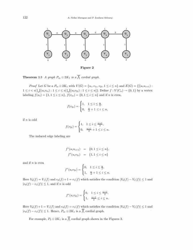
122 A. Nellai Murugan and P. Iyadurai Selvaraj
u1
u2
u3
u4
u5
1 1 1 1 1
0 0
v1
v2
v3
v4
v5
1 1
0 0 0
1
0
00
0
1 1
Figure 2
Theorem 3.3 A graph Pm ⊙ 2K1 is a∧
cordial graph.
Proof Let G be a Pm ⊙ 2K1 with V (G) = {ui, v1i, v2i, 1 ≤ i ≤ n} and E(G) = {[(uiui+1) :
1 ≤ i < n]⋃
[(uiv1i) : 1 ≤ i ≤ n]⋃
[(uiv2i) : 1 ≤ i ≤ n]}. Define f : V (Cn) → {0, 1} by a vertex
labeling f(ui) = {1, 1 ≤ i ≤ n}, f(v1i) = {0, 1 ≤ i ≤ n} and if n is even,
f(v2i) =
1, 1 ≤ i ≤ n2 ,
0, n2 + 1 ≤ i ≤ n,
if n is odd
f(v2i) =
1, 1 ≤ i ≤ n+12 ,
0, n+12 + 1 ≤ i ≤ n.
The induced edge labeling are
f∗(uiui+1) = {0, 1 ≤ i ≤ n},f∗(uiv1i) = {1, 1 ≤ i ≤ n}
and if n is even
f∗(uiv2i) =
0, 1 ≤ i ≤ n2 ,
1, n2 + 1 ≤ i ≤ n.
Here V0(f) = V1(f) and e0(f)+1 = e1(f) which satisfies the condition |V0(f) − V1(f)| ≤ 1 and
|e0(f) − e1(f)| ≤ 1, and if n is odd
f∗(uiv2i) =
0, 1 ≤ i ≤ n+12 ,
1, n+12 ≤ i ≤ n.
Here V0(f)+1 = V1(f) and e0(f) = e1(f) which satisfies the condition |V0(f) − V1(f)| ≤ 1 and
|e0(f) − e1(f)| ≤ 1. Hence, Pm ⊙ 2K1 is a∧
cordial graph. 2For example, P5 ⊙ 2K1 is a
∧cordial graph shown in the Figures 3.
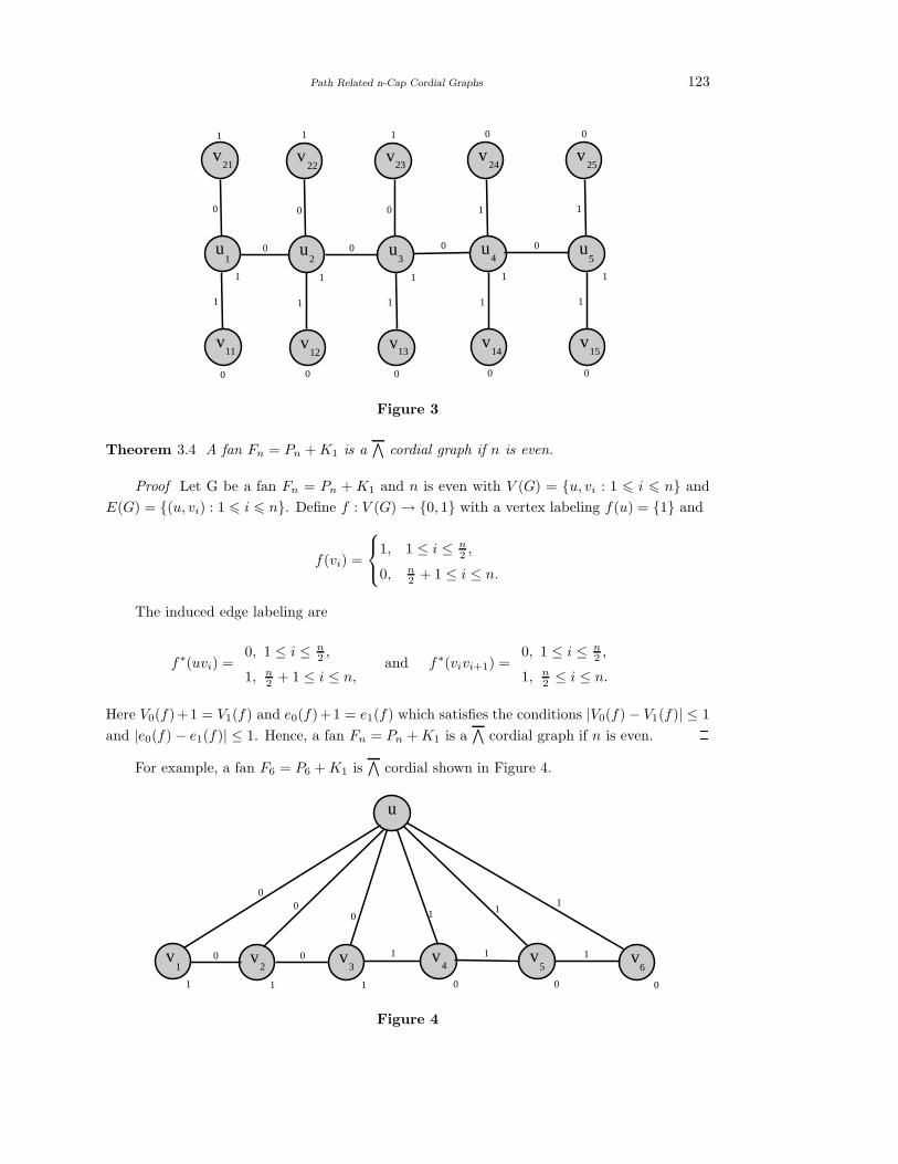
Path Related n-Cap Cordial Graphs 123
u1
u2
u3
u4
u5
1 1 1 1 1
0 0
v11
v12
v13
v14
v15
1 1
0 0 0
1
0
00
0
1 1
v21
v22
v23
v24
v25
0 0 0 1 1
1 1 01 0
Figure 3
Theorem 3.4 A fan Fn = Pn + K1 is a∧
cordial graph if n is even.
Proof Let G be a fan Fn = Pn + K1 and n is even with V (G) = {u, vi : 1 6 i 6 n} and
E(G) = {(u, vi) : 1 6 i 6 n}. Define f : V (G) → {0, 1} with a vertex labeling f(u) = {1} and
f(vi) =
1, 1 ≤ i ≤ n2 ,
0, n2 + 1 ≤ i ≤ n.
The induced edge labeling are
f∗(uvi) =0, 1 ≤ i ≤ n
2 ,
1, n2 + 1 ≤ i ≤ n,
and f∗(vivi+1) =0, 1 ≤ i ≤ n
2 ,
1, n2 ≤ i ≤ n.
Here V0(f)+1 = V1(f) and e0(f)+1 = e1(f) which satisfies the conditions |V0(f) − V1(f)| ≤ 1
and |e0(f) − e1(f)| ≤ 1. Hence, a fan Fn = Pn + K1 is a∧
cordial graph if n is even. 2For example, a fan F6 = P6 + K1 is
∧cordial shown in Figure 4.
v1
v2
v3
v4
v5
1 1 1 0 0
1 100
00
0 1 1
v6
0
1
1
u
Figure 4
124 A. Nellai Murugan and P. Iyadurai Selvaraj
References
[1] J. A. Gallian, A dynamic survey of graph labeling, The Electronic Journal of Combina-
torics, 6(2001), #DS6.
[2] F. Harary, Graph Theory, Addition - Wesley Publishing Company Inc, USA, 1969.
[3] A.Nellai Murugan and V.Baby Suganya, Cordial labeling of path related splitted graphs,
Indian Journal of Applied Research , Vol.4, 3(2014), 1-8.
[4] A.Nellai Murugan and M. Taj Nisha, A study on divisor cordial labelling of star attached
paths and cycles, Indian Journal of Research, Vol.3, 3(20140, 12-17.
[5] A.Nellai Murugan and V.Brinda Devi, A study on path related divisor cordial graphs,
International Journal of Scientific Research, Vol.3, 4(2014), 286 - 291.
[6] A.Nellai Murugan and A Meenakshi Sundari, On cordial graphs, International Journal of
Scientific Research, Vol.3, 7(20140, 54-55.
[7] A.Nellai Murugan and P. Iyadurai Selvaraj, Path related cup cordial graphs, Indian Journal
of Applied Research, Vol.4, 8(2014).
[8] A.Nellai Murugan and P. Iyadurai Selvaraj, Cycle and Armed Cap Cordial Graphs, Inter-
national Journal on Mathematical Combinatorics, Vol.2(2016), 144-152.
[9] A.Nellai Murugan and P. Iyadurai Selvaraj, Cycle and armed cup cordial graphs, Interna-
tional Journal of Innovative Science, Engineering and Technology, Vol. I, 5(2014), 478-485.
[10] A.Nellai Murugan and P. Iyadurai Selvaraj, Path related cap cordial graphs, OUTREACH,
Multidisciplinary Research Journal, Vol. VII (2015), 100-106.
[11] A.Nellai Murugan and P. Iyadurai Selvaraj, Additive square mean labeling of path related
graphs, OUTREACH, Multidisciplinary Research Journal, Vol. IX (2016), 168-174.
[12] A.Nellai Murugan and P. Iyadurai Selvaraj, Path related n-cup cordial craphs, ACTA
VELIT, Vol.3, 3, 12-17.
International J.Math. Combin. Vol.3(2017), 125-135
Some New Families of 4-Prime Cordial Graphs
R.Ponraj
(Department of Mathematics, Sri Paramakalyani College, Alwarkurichi-627412, India)
Rajpal Singh and R.Kala
(Department of Mathematics, Manonmaniam Sundaranar University, Tirunelveli-627012, India)
E-mail: [email protected], [email protected], [email protected]
Abstract: Let G be a (p, q) graph. Let f : V (G) → {1, 2, . . . , k} be a function. For
each edge uv, assign the label gcd (f(u), f(v)). f is called k-prime cordial labeling of G
if |vf (i) − vf (j)| ≤ 1, i, j ∈ {1, 2, . . . , k} and |ef (0) − ef (1)| ≤ 1 where vf (x) denotes the
number of vertices labeled with x, ef (1) and ef (0) respectively denote the number of edges
labeled with 1 and not labeled with 1. A graph with admits a k-prime cordial labeling is
called a k-prime cordial graph. In this paper we investigate 4-prime cordial labeling behavior
of shadow graph of a path, cycle, star, degree splitting graph of a bistar, jelly fish, splitting
graph of a path and star.
Key Words: Cordial labeling, Smarandachely cordial labeling, cycle, star, bistar, splitting
graph.
AMS(2010): 05C78.
§1. Introduction
In this paper graphs are finite, simple and undirected. Let G be a (p, q) graph where p is the
number of vertices of G and q is the number of edge of G. In 1987, Cahit introduced the concept
of cordial labeling of graphs [1]. Sundaram, Ponraj, Somasundaram [5] have been introduced
the notion of prime cordial labeling and discussed the prime cordial labeling behavior of various
graphs. Recently Ponraj et al. [7], introduced k-prime cordial labeling of graphs. A 2-prime
cordial labeling is a product cordial labeling [6]. In [8, 9] Ponraj et al. studied the 4-prime
cordial labeling behavior of complete graph, book, flower, mCn, wheel, gear, double cone, helm,
closed helm, butterfly graph, and friendship graph and some more graphs. Ponraj and Rajpal
singh have studied about the 4-prime cordiality of union of two bipartite graphs, union of trees,
durer graph, tietze graph, planar grid Pm ×Pn, subdivision of wheels and subdivision of helms,
lotus inside a circle, sunflower graph and they have obtained some 4-prime cordial graphs from
4-prime cordial graphs [10, 11, 12]. Let x be any real number. In this paper we have studied
about the 4-prime cordiality of shadow graph of a path, cycle, star, degree splitting graph of a
1Received November 12, 2016, Accepted August 28, 2017.
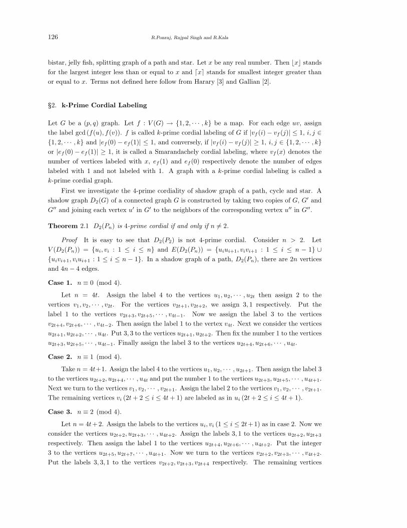
126 R.Ponraj, Rajpal Singh and R.Kala
bistar, jelly fish, splitting graph of a path and star. Let x be any real number. Then ⌊x⌋ stands
for the largest integer less than or equal to x and ⌈x⌉ stands for smallest integer greater than
or equal to x. Terms not defined here follow from Harary [3] and Gallian [2].
§2. k-Prime Cordial Labeling
Let G be a (p, q) graph. Let f : V (G) → {1, 2, · · · , k} be a map. For each edge uv, assign
the label gcd (f(u), f(v)). f is called k-prime cordial labeling of G if |vf (i) − vf (j)| ≤ 1, i, j ∈{1, 2, · · · , k} and |ef (0) − ef(1)| ≤ 1, and conversely, if |vf (i) − vf (j)| ≥ 1, i, j ∈ {1, 2, · · · , k}or |ef (0) − ef (1)| ≥ 1, it is called a Smarandachely cordial labeling, where vf (x) denotes the
number of vertices labeled with x, ef(1) and ef (0) respectively denote the number of edges
labeled with 1 and not labeled with 1. A graph with a k-prime cordial labeling is called a
k-prime cordial graph.
First we investigate the 4-prime cordiality of shadow graph of a path, cycle and star. A
shadow graph D2(G) of a connected graph G is constructed by taking two copies of G, G′ and
G′′ and joining each vertex u′ in G′ to the neighbors of the corresponding vertex u′′ in G′′.
Theorem 2.1 D2(Pn) is 4-prime cordial if and only if n 6= 2.
Proof It is easy to see that D2(P2) is not 4-prime cordial. Consider n > 2. Let
V (D2(Pn)) = {ui, vi : 1 ≤ i ≤ n} and E(D2(Pn)) = {uiui+1, vivi+1 : 1 ≤ i ≤ n − 1} ∪{uivi+1, viui+1 : 1 ≤ i ≤ n − 1}. In a shadow graph of a path, D2(Pn), there are 2n vertices
and 4n − 4 edges.
Case 1. n ≡ 0 (mod 4).
Let n = 4t. Assign the label 4 to the vertices u1, u2, · · · , u2t then assign 2 to the
vertices v1, v2, · · · , v2t. For the vertices v2t+1, v2t+2, we assign 3, 1 respectively. Put the
label 1 to the vertices v2t+3, v2t+5, · · · , v4t−1. Now we assign the label 3 to the vertices
v2t+4, v2t+6, · · · , v4t−2. Then assign the label 1 to the vertex v4t. Next we consider the vertices
u2t+1, u2t+2, · · · , u4t. Put 3, 3 to the vertices u2t+1, u2t+2. Then fix the number 1 to the vertices
u2t+3, u2t+5, · · · , u4t−1. Finally assign the label 3 to the vertices u2t+4, u2t+6, · · · , u4t.
Case 2. n ≡ 1 (mod 4).
Take n = 4t+1. Assign the label 4 to the vertices u1, u2, · · · , u2t+1. Then assign the label 3
to the vertices u2t+2, u2t+4, · · · , u4t and put the number 1 to the vertices u2t+3, u2t+5, · · · , u4t+1.
Next we turn to the vertices v1, v2, · · · , v2t+1. Assign the label 2 to the vertices v1, v2, · · · , v2t+1.
The remaining vertices vi (2t + 2 ≤ i ≤ 4t + 1) are labeled as in ui (2t + 2 ≤ i ≤ 4t + 1).
Case 3. n ≡ 2 (mod 4).
Let n = 4t+2. Assign the labels to the vertices ui, vi (1 ≤ i ≤ 2t+1) as in case 2. Now we
consider the vertices u2t+2, u2t+3, · · · , u4t+2. Assign the labels 3, 1 to the vertices u2t+2, u2t+3
respectively. Then assign the label 1 to the vertices u2t+4, u2t+6, · · · , u4t+2. Put the integer
3 to the vertices u2t+5, u2t+7, · · · , u4t+1. Now we turn to the vertices v2t+2, v2t+3, · · · , v4t+2.
Put the labels 3, 3, 1 to the vertices v2t+2, v2t+3, v2t+4 respectively. The remaining vertices
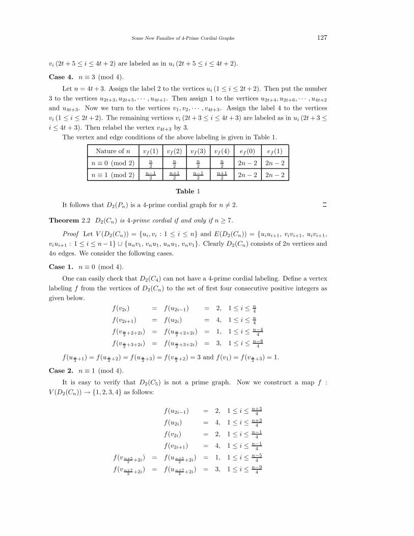
Some New Families of 4-Prime Cordial Graphs 127
vi (2t + 5 ≤ i ≤ 4t + 2) are labeled as in ui (2t + 5 ≤ i ≤ 4t + 2).
Case 4. n ≡ 3 (mod 4).
Let n = 4t+3. Assign the label 2 to the vertices ui (1 ≤ i ≤ 2t+2). Then put the number
3 to the vertices u2t+3, u2t+5, · · · , u4t+1. Then assign 1 to the vertices u2t+4, u2t+6, · · · , u4t+2
and u4t+3. Now we turn to the vertices v1, v2, · · · , v4t+3. Assign the label 4 to the vertices
vi (1 ≤ i ≤ 2t + 2). The remaining vertices vi (2t + 3 ≤ i ≤ 4t + 3) are labeled as in ui (2t + 3 ≤i ≤ 4t + 3). Then relabel the vertex v4t+3 by 3.
The vertex and edge conditions of the above labeling is given in Table 1.
Nature of n vf (1) vf (2) vf (3) vf (4) ef (0) ef (1)
n ≡ 0 (mod 2) n2
n2
n2
n2 2n − 2 2n − 2
n ≡ 1 (mod 2) n−12
n+12
n−12
n+12 2n − 2 2n − 2
Table 1
It follows that D2(Pn) is a 4-prime cordial graph for n 6= 2. 2Theorem 2.2 D2(Cn) is 4-prime cordial if and only if n ≥ 7.
Proof Let V (D2(Cn)) = {ui, vi : 1 ≤ i ≤ n} and E(D2(Cn)) = {uiui+1, vivi+1, uivi+1,
viui+1 : 1 ≤ i ≤ n− 1} ∪ {unv1, vnu1, unu1, vnv1}. Clearly D2(Cn) consists of 2n vertices and
4n edges. We consider the following cases.
Case 1. n ≡ 0 (mod 4).
One can easily check that D2(C4) can not have a 4-prime cordial labeling. Define a vertex
labeling f from the vertices of D2(Cn) to the set of first four consecutive positive integers as
given below.
f(v2i) = f(u2i−1) = 2, 1 ≤ i ≤ n4
f(v2i+1) = f(u2i) = 4, 1 ≤ i ≤ n4
f(vn2+2+2i) = f(u n
2+2+2i) = 1, 1 ≤ i ≤ n−4
4
f(vn2 +3+2i) = f(u n
2 +3+2i) = 3, 1 ≤ i ≤ n−84
f(u n2+1) = f(u n
2+2) = f(u n
2+3) = f(vn
2+2) = 3 and f(v1) = f(vn
2+3) = 1.
Case 2. n ≡ 1 (mod 4).
It is easy to verify that D2(C5) is not a prime graph. Now we construct a map f :
V (D2(Cn)) → {1, 2, 3, 4} as follows:
f(u2i−1) = 2, 1 ≤ i ≤ n+34
f(u2i) = 4, 1 ≤ i ≤ n+34
f(v2i) = 2, 1 ≤ i ≤ n−14
f(v2i+1) = 4, 1 ≤ i ≤ n−14
f(vn+52 +2i) = f(u n+5
2 +2i) = 1, 1 ≤ i ≤ n−54
f(vn+72 +2i) = f(u n+7
2 +2i) = 3, 1 ≤ i ≤ n−94
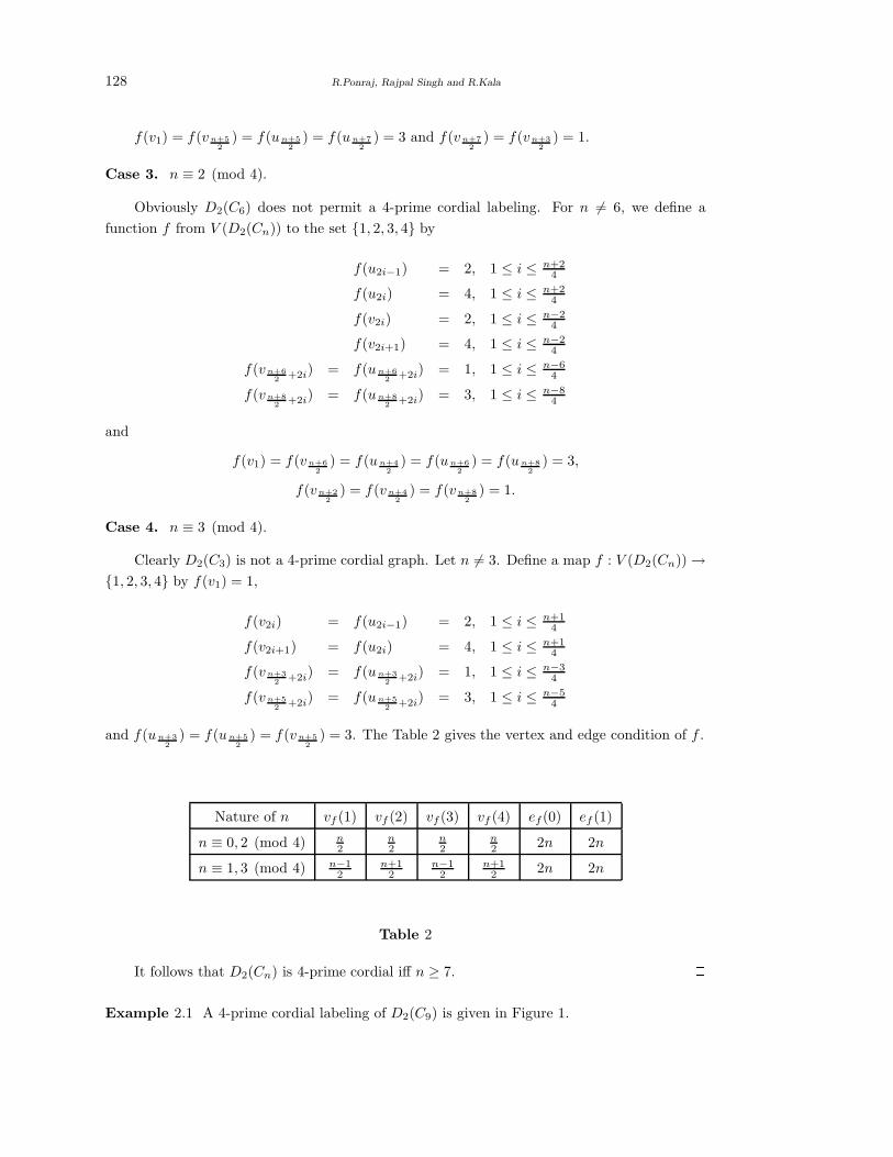
128 R.Ponraj, Rajpal Singh and R.Kala
f(v1) = f(vn+52
) = f(u n+52
) = f(u n+72
) = 3 and f(vn+72
) = f(vn+32
) = 1.
Case 3. n ≡ 2 (mod 4).
Obviously D2(C6) does not permit a 4-prime cordial labeling. For n 6= 6, we define a
function f from V (D2(Cn)) to the set {1, 2, 3, 4} by
f(u2i−1) = 2, 1 ≤ i ≤ n+24
f(u2i) = 4, 1 ≤ i ≤ n+24
f(v2i) = 2, 1 ≤ i ≤ n−24
f(v2i+1) = 4, 1 ≤ i ≤ n−24
f(vn+62 +2i) = f(u n+6
2 +2i) = 1, 1 ≤ i ≤ n−64
f(vn+82 +2i) = f(u n+8
2 +2i) = 3, 1 ≤ i ≤ n−84
and
f(v1) = f(vn+62
) = f(u n+42
) = f(u n+62
) = f(u n+82
) = 3,
f(vn+22
) = f(vn+42
) = f(vn+82
) = 1.
Case 4. n ≡ 3 (mod 4).
Clearly D2(C3) is not a 4-prime cordial graph. Let n 6= 3. Define a map f : V (D2(Cn)) →{1, 2, 3, 4} by f(v1) = 1,
f(v2i) = f(u2i−1) = 2, 1 ≤ i ≤ n+14
f(v2i+1) = f(u2i) = 4, 1 ≤ i ≤ n+14
f(vn+32 +2i) = f(u n+3
2 +2i) = 1, 1 ≤ i ≤ n−34
f(vn+52 +2i) = f(u n+5
2 +2i) = 3, 1 ≤ i ≤ n−54
and f(u n+32
) = f(u n+52
) = f(vn+52
) = 3. The Table 2 gives the vertex and edge condition of f .
Nature of n vf (1) vf (2) vf (3) vf (4) ef(0) ef (1)
n ≡ 0, 2 (mod 4) n2
n2
n2
n2 2n 2n
n ≡ 1, 3 (mod 4) n−12
n+12
n−12
n+12 2n 2n
Table 2
It follows that D2(Cn) is 4-prime cordial iff n ≥ 7. 2Example 2.1 A 4-prime cordial labeling of D2(C9) is given in Figure 1.
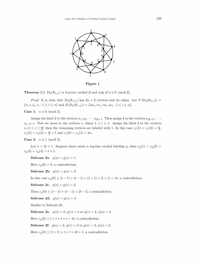
Some New Families of 4-Prime Cordial Graphs 129
b
b
b
b
b
b
b
b
b
b
b
b
b
b
b
b
b
b
2
2
2
22
4 4
4
4
4
3
3
3
3
1
1
1
1
Figure 1
Theorem 2.3 D2(K1,n) is 4-prime cordial if and only if n ≡ 0 (mod 2).
Proof It is clear that D2(K1,n) has 2n + 2 vertices and 4n edges. Let V (D2(K1,n)) =
{u, v, ui, vi : 1 ≤ i ≤ n} and E(D2(K1,n)) = {uui, vvi, vui, uvi : 1 ≤ i ≤ n}.
Case 1. n ≡ 0 (mod 2).
Assign the label 2 to the vertices u1, u2, · · · , u n2+1. Then assign 4 to the vertices u n
2+2, · · · ,
un, u, v. Now we move to the vertices vi where 1 ≤ i ≤ n. Assign the label 3 to the vertices
vi (1 ≤ i ≤ n2 ) then the remaining vertices are labeled with 1. In this case vf (1) = vf (3) = n
2 ,
vf (2) = vf (4) = n2 + 1 and ef (0) = ef(1) = 2n.
Case 2. n ≡ 1 (mod 2).
Let n = 2t + 1. Suppose there exists a 4-prime cordial labeling g, then vg(1) = vg(2) =
vg(3) = vg(4) = t + 1.
Subcase 2a. g(u) = g(v) = 1.
Here eg(0) = 0, a contradiction.
Subcase 2b. g(u) = g(v) = 2.
In this case eg(0) ≤ (t − 1) + (t − 1) + (t + 1) + (t + 1) = 4t, a contradiction.
Subcase 2c. g(u) = g(v) = 3.
Then eg(0) ≤ (t − 1) + (t − 1) = 2t − 2, a contradiction.
Subcase 2d. g(u) = g(v) = 4.
Similar to Subcase 2b.
Subcase 2e. g(u) = 2, g(v) = 4 or g(v) = 2, g(u) = 4.
Here eg(0) ≤ t + t + t + t = 4t, a contradiction.
Subcase 2f. g(u) = 2, g(v) = 3 or g(v) = 2, g(u) = 3.
Here eg(0) ≤ (t + 1) + t + t = 3t + 1, a contradiction.
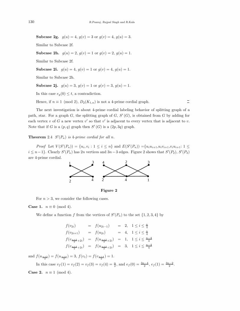
130 R.Ponraj, Rajpal Singh and R.Kala
Subcase 2g. g(u) = 4, g(v) = 3 or g(v) = 4, g(u) = 3.
Similar to Subcase 2f.
Subcase 2h. g(u) = 2, g(v) = 1 or g(v) = 2, g(u) = 1.
Similar to Subcase 2f.
Subcase 2i. g(u) = 4, g(v) = 1 or g(v) = 4, g(u) = 1.
Similar to Subcase 2h.
Subcase 2j. g(u) = 3, g(v) = 1 or g(v) = 3, g(u) = 1.
In this case eg(0) ≤ t, a contradiction.
Hence, if n ≡ 1 (mod 2), D2(K1,n) is not a 4-prime cordial graph. 2The next investigation is about 4-prime cordial labeling behavior of splitting graph of a
path, star. For a graph G, the splitting graph of G, S′ (G), is obtained from G by adding for
each vertex v of G a new vertex v′ so that v′ is adjacent to every vertex that is adjacent to v.
Note that if G is a (p, q) graph then S′ (G) is a (2p, 3q) graph.
Theorem 2.4 S′(Pn) is 4-prime cordial for all n.
Proof Let V (S′(Pn)) = {ui, vi : 1 ≤ i ≤ n} and E(S′(Pn)) ={uiui+1,uivi+1,viui+1: 1 ≤i ≤ n−1}. Clearly S′(Pn) has 2n vertices and 3n−3 edges. Figure 2 shows that S′(P2), S′(P3)
are 4-prime cordial.
bb
b b
b b b
bbb
2 2
2
4
4
4
331
1
Figure 2
For n > 3, we consider the following cases.
Case 1. n ≡ 0 (mod 4).
We define a function f from the vertices of S′(Pn) to the set {1, 2, 3, 4} by
f(v2i) = f(u2i−1) = 2, 1 ≤ i ≤ n4
f(v2i+1) = f(u2i) = 4, 1 ≤ i ≤ n4
f(vn+22 +2i) = f(u n+2
2 +2i) = 1, 1 ≤ i ≤ n−44
f(vn+42 +2i) = f(u n+4
2 +2i) = 3, 1 ≤ i ≤ n−44
and f(u n+22
) = f(u n+42
) = 3, f(v1) = f(vn+42
) = 1.
In this case vf (1) = vf (2) = vf (3) = vf (4) = n2 , and ef (0) = 3n−4
2 , ef (1) = 3n−22 .
Case 2. n ≡ 1 (mod 4).
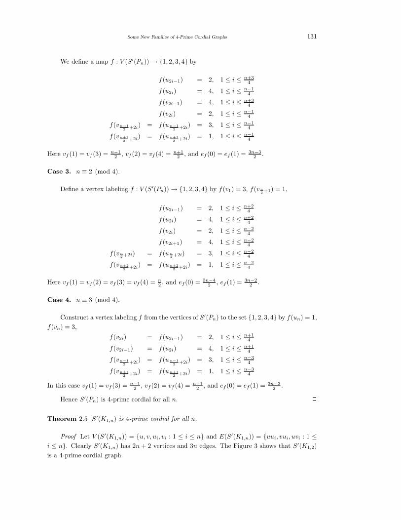
Some New Families of 4-Prime Cordial Graphs 131
We define a map f : V (S′(Pn)) → {1, 2, 3, 4} by
f(u2i−1) = 2, 1 ≤ i ≤ n+34
f(u2i) = 4, 1 ≤ i ≤ n−14
f(v2i−1) = 4, 1 ≤ i ≤ n+34
f(v2i) = 2, 1 ≤ i ≤ n−14
f(vn−12 +2i) = f(u n−1
2 +2i) = 3, 1 ≤ i ≤ n−14
f(vn+12 +2i) = f(u n+1
2 +2i) = 1, 1 ≤ i ≤ n−14
Here vf (1) = vf (3) = n−12 , vf (2) = vf (4) = n+1
2 , and ef (0) = ef (1) = 3n−32 .
Case 3. n ≡ 2 (mod 4).
Define a vertex labeling f : V (S′(Pn)) → {1, 2, 3, 4} by f(v1) = 3, f(vn2+1) = 1,
f(u2i−1) = 2, 1 ≤ i ≤ n+24
f(u2i) = 4, 1 ≤ i ≤ n+24
f(v2i) = 2, 1 ≤ i ≤ n−24
f(v2i+1) = 4, 1 ≤ i ≤ n−24
f(vn2 +2i) = f(u n
2 +2i) = 3, 1 ≤ i ≤ n−24
f(vn+22 +2i) = f(u n+2
2 +2i) = 1, 1 ≤ i ≤ n−24
Here vf (1) = vf (2) = vf (3) = vf (4) = n2 , and ef(0) = 3n−4
2 , ef (1) = 3n−22 .
Case 4. n ≡ 3 (mod 4).
Construct a vertex labeling f from the vertices of S′(Pn) to the set {1, 2, 3, 4} by f(un) = 1,
f(vn) = 3,
f(v2i) = f(u2i−1) = 2, 1 ≤ i ≤ n+14
f(v2i−1) = f(u2i) = 4, 1 ≤ i ≤ n+14
f(vn−12 +2i) = f(u n−1
2 +2i) = 3, 1 ≤ i ≤ n−34
f(vn+12 +2i) = f(u n+1
2 +2i) = 1, 1 ≤ i ≤ n−34
In this case vf (1) = vf (3) = n−12 , vf (2) = vf (4) = n+1
2 , and ef(0) = ef (1) = 3n−32 .
Hence S′(Pn) is 4-prime cordial for all n. 2Theorem 2.5 S′(K1,n) is 4-prime cordial for all n.
Proof Let V (S′(K1,n)) = {u, v, ui, vi : 1 ≤ i ≤ n} and E(S′(K1,n)) = {uui, vui, uvi : 1 ≤i ≤ n}. Clearly S′(K1,n) has 2n + 2 vertices and 3n edges. The Figure 3 shows that S′(K1,2)
is a 4-prime cordial graph.
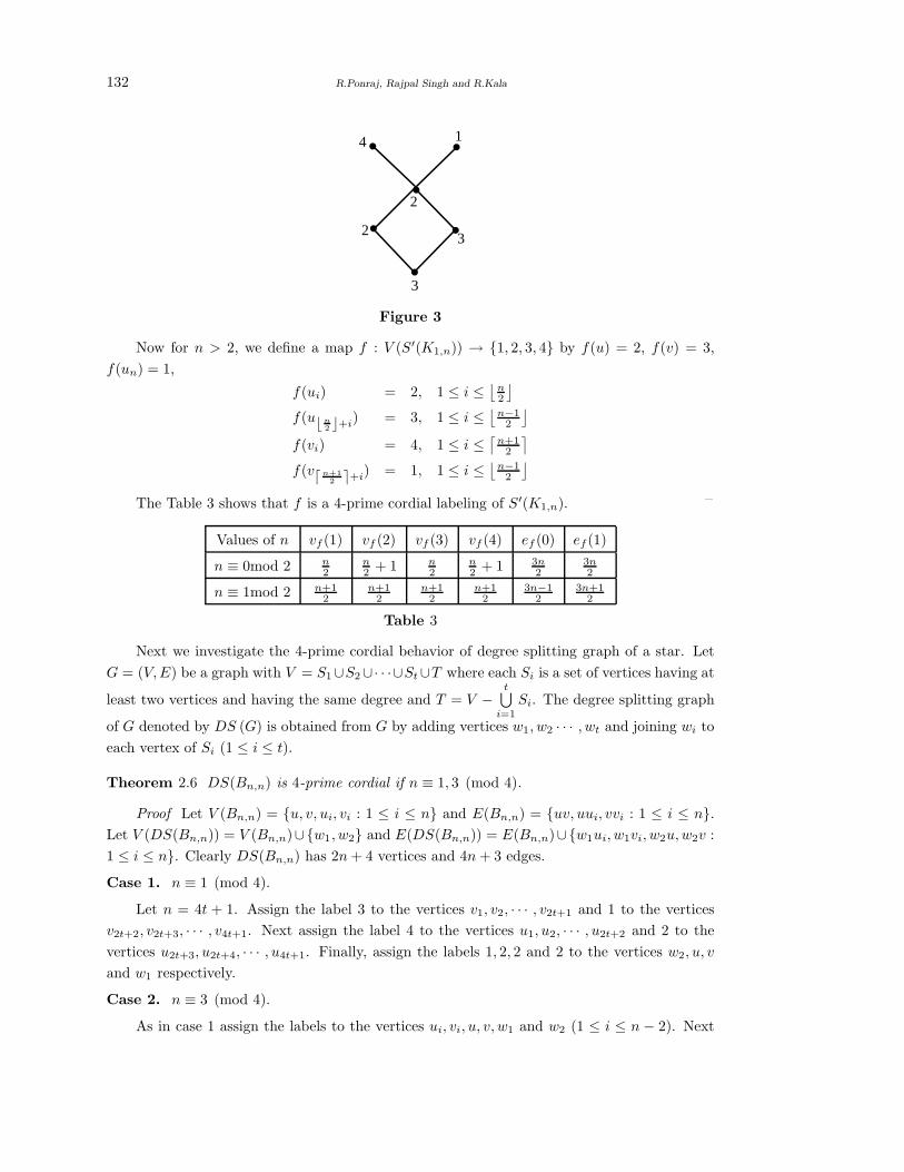
132 R.Ponraj, Rajpal Singh and R.Kala
b b
b
b b
b
2
2
4 1
3
3
Figure 3
Now for n > 2, we define a map f : V (S′(K1,n)) → {1, 2, 3, 4} by f(u) = 2, f(v) = 3,
f(un) = 1,
f(ui) = 2, 1 ≤ i ≤⌊
n2
⌋
f(u⌊n2 ⌋+i) = 3, 1 ≤ i ≤
⌊n−1
2
⌋
f(vi) = 4, 1 ≤ i ≤⌈
n+12
⌉
f(v⌈n+12 ⌉+i) = 1, 1 ≤ i ≤
⌊n−1
2
⌋
The Table 3 shows that f is a 4-prime cordial labeling of S′(K1,n). 2Values of n vf (1) vf (2) vf (3) vf (4) ef (0) ef (1)
n ≡ 0mod 2 n2
n2 + 1 n
2n2 + 1 3n
23n2
n ≡ 1mod 2 n+12
n+12
n+12
n+12
3n−12
3n+12
Table 3
Next we investigate the 4-prime cordial behavior of degree splitting graph of a star. Let
G = (V, E) be a graph with V = S1∪S2∪· · ·∪St∪T where each Si is a set of vertices having at
least two vertices and having the same degree and T = V −t⋃
i=1
Si. The degree splitting graph
of G denoted by DS (G) is obtained from G by adding vertices w1, w2 · · · , wt and joining wi to
each vertex of Si (1 ≤ i ≤ t).
Theorem 2.6 DS(Bn,n) is 4-prime cordial if n ≡ 1, 3 (mod 4).
Proof Let V (Bn,n) = {u, v, ui, vi : 1 ≤ i ≤ n} and E(Bn,n) = {uv, uui, vvi : 1 ≤ i ≤ n}.Let V (DS(Bn,n)) = V (Bn,n)∪{w1, w2} and E(DS(Bn,n)) = E(Bn,n)∪{w1ui, w1vi, w2u, w2v :
1 ≤ i ≤ n}. Clearly DS(Bn,n) has 2n + 4 vertices and 4n + 3 edges.
Case 1. n ≡ 1 (mod 4).
Let n = 4t + 1. Assign the label 3 to the vertices v1, v2, · · · , v2t+1 and 1 to the vertices
v2t+2, v2t+3, · · · , v4t+1. Next assign the label 4 to the vertices u1, u2, · · · , u2t+2 and 2 to the
vertices u2t+3, u2t+4, · · · , u4t+1. Finally, assign the labels 1, 2, 2 and 2 to the vertices w2, u, v
and w1 respectively.
Case 2. n ≡ 3 (mod 4).
As in case 1 assign the labels to the vertices ui, vi, u, v, w1 and w2 (1 ≤ i ≤ n − 2). Next
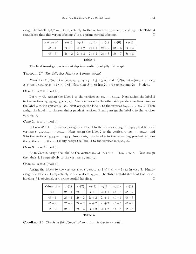
Some New Families of 4-Prime Cordial Graphs 133
assign the labels 1, 3, 2 and 4 respectively to the vertices vn−1, vn, un−1 and un. The Table 4
establishes that this vertex labeling f is a 4-prime cordial labeling. 2Nature of n vf (1) vf (2) vf (3) vf (4) ef (0) ef(1)
4t + 1 2t + 1 2t + 2 2t + 1 2t + 2 8t + 3 8t + 4
4t + 3 2t + 2 2t + 3 2t + 2 2t + 3 8t + 7 8t + 8
Table 4
The final investigation is about 4-prime cordiality of jelly fish graph.
Theorem 2.7 The Jelly fish J(n, n) is 4-prime cordial.
Proof Let V (J(n, n)) = {u, v, ui, vi, w1, w2 : 1 ≤ i ≤ n} and E(J(n, n)) ={uui, vui, uw1,
w1v, vw2, uw2, w1w2 : 1 ≤ i ≤ n}. Note that J(n, n) has 2n + 4 vertices and 2n + 5 edges.
Case 1. n ≡ 0 (mod 4).
Let n = 4t. Assign the label 1 to the vertices u1, u2, · · · , u2t+1. Next assign the label 3
to the vertices u2t+2, u2t+3, · · · , u4t. We now move to the other side pendent vertices. Assign
the label 3 to the vertices u1, u2. Next assign the label 2 to the vertices u3, u4, . . . , u2t+3. Then
assign the label 4 to the remaining pendent vertices. Finally assign the label 4 to the vertices
u, v, w1, w2.
Case 2. n ≡ 1 (mod 4).
Let n = 4t+ 1. In this case, assign the label 1 to the vertices v1, v2, · · · , v2t+1 and 3 to the
vertices v2t+1, v2t+3, · · · , v4t+1. Next assign the label 2 to the vertices u1, u2, · · · , u2t+2, and
3 to the vertices u2t+3 and u2t+4. Next assign the label 4 to the remaining pendent vertices
u2t+5, u2t+6, · · · , u4t+1. Finally assign the label 4 to the vertices u, v, w1, w2.
Case 3. n ≡ 2 (mod 4).
As in Case 2, assign the label to the vertices ui, vi(1 ≤ i ≤ n− 1), u, v, w1, w2. Next assign
the labels 1, 4 respectively to the vertices un and vn.
Case 4. n ≡ 3 (mod 4).
Assign the labels to the vertices u, v, w1, w2, ui, vi(1 ≤ i ≤ n − 1) as in case 3. Finally
assign the labels 2, 1 respectively to the vertices un, vn. The Table 5establishes that this vertex
labeling f is obviously a 4-prime cordial labeling. 2Values of n vf (1) vf (2) vf (3) vf (4) ef (0) ef(1)
4t 2t + 1 2t + 1 2t + 1 2t + 1 4t + 3 4t + 2
4t + 1 2t + 1 2t + 2 2t + 2 2t + 1 4t + 4 4t + 3
4t + 2 2t + 2 2t + 2 2t + 2 2t + 2 4t + 5 4t + 4
4t + 3 2t + 3 2t + 3 2t + 2 2t + 2 4t + 6 4t + 5
Table 5
Corollary 2.1 The Jelly fish J(m, n) where m ≥ n is 4-prime cordial.
134 R.Ponraj, Rajpal Singh and R.Kala
Proof Let m = n + r, r ≥ 0. Use of the labeling f given in theorem ?? assign the label to
the vertices u, v, w1, w2, ui, vi (1 ≤ i ≤ n).
Case 1. r ≡ 0 (mod 4).
Let r = 4k, k ∈ N . Assign the label 2 to the vertices un+1, un+2, · · · , un+k and to the ver-
tices un+k+1, un+k+2, · · · , un+2k. Then assign the label 1 to the vertices un+2k+1, un+2k+2, · · · , un+3k
and 3 to the vertices un+3k+1, un+3k+2, . . . , un+4k. Clearly this vertex labeling is a 4-prime
cordial labeling.
Case 2. r ≡ 1 (mod 4).
Let r = 4k + 1, k ∈ N . Assign the labels to the vertices un+i (1 ≤ i ≤ r − 1) as in case 1.
If n ≡ 0, 1, 2 (mod 4), then assign the label 1 to the vertex ur; otherwise assign the label 4 to
the vertex ur.
Case 3. r ≡ 2 (mod 4).
Let r = 4k + 2, k ∈ N . As in Case 2 assign the labels to the vertices un+i (1 ≤ i ≤ r − 1).
Then assign the label 4 to the vertex ur.
Case 4. r ≡ 3 (mod 4).
Let r = 4k + 3, k ∈ N . In this case assign the label 3 to the last vertex and assign the
label to the vertices un+i (1 ≤ i ≤ r − 1) as in Case 3. 2References
[1] I.Cahit, Cordial Graphs: A weaker version of Graceful and Harmonious graphs, Ars com-
bin., 23 (1987) 201-207.
[2] J.A.Gallian, A Dynamic survey of graph labeling, The Electronic Journal of Combinatorics,
17 (2015) #Ds6.
[3] F.Harary, Graph theory, Addision wesley, New Delhi (1969).
[4] M.A.Seoud and M.A.Salim, Two upper bounds of prime cordial graphs, JCMCC, 75(2010)
95-103.
[5] M.Sundaram, R.Ponraj and S.Somasundaram, Prime cordial labeling of graphs, J. Indian
Acad. Math., 27(2005) 373-390.
[6] M. Sundaram, R. Ponraj and S. Somasundaram, Product cordial labeling of graphs, Bull.
Pure and Appl. Sci. (Math. & Stat.), 23E (2004) 155-163.
[7] R.Ponraj, Rajpal singh, R.Kala and S. Sathish Narayanan, k-prime cordial graphs, J. Appl.
Math. & Informatics, 34 (3-4) (2016) 227 - 237.
[8] R.Ponraj, Rajpal singh and S. Sathish Narayanan, 4-prime cordiality of some classes of
graphs, Journal of Algorithms and Computation, 48(1)(2016), 69- 79.
[9] R.Ponraj, Rajpal singh and S. Sathish Narayanan, 4-prime cordiality of some cycle related
graphs, Applications and Applied Mathematics, 12(1)(2016), 230-240.
[10] R.Ponraj and Rajpal singh, 4-Prime cordial graphs obtained from 4-Prime cordial graphs,
Bulletin of International Mathematical Virtual Institute, 8(1)(2018), 1-9.

Some New Families of 4-Prime Cordial Graphs 135
[11] R.Ponraj, Rajpal singh and R.Kala, 4-Prime cordiality of some special graphs, Bulletin of
International Mathematical Virtual Institute, 8(1)(2018), 89-97.
[12] R.Ponraj, Rajpal singh and R.Kala, Some more 4-Prime cordial graphs, International
Journal of Mathematical Combinatorics, 2 (2017) 105-115.
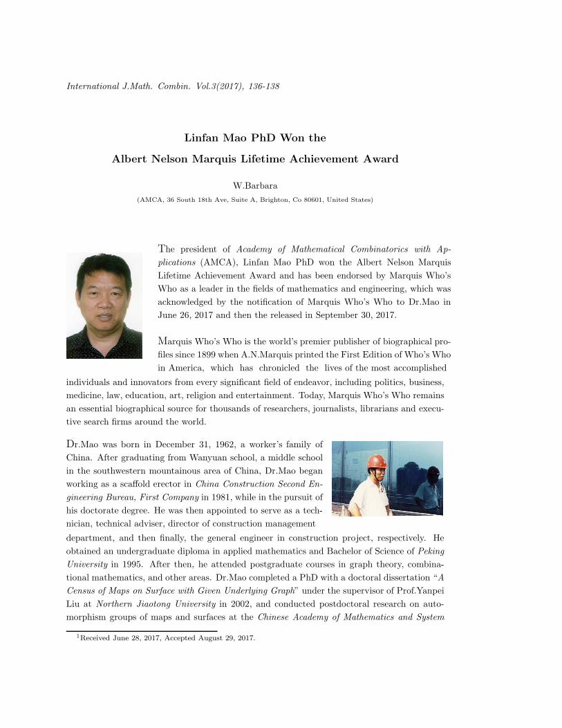
International J.Math. Combin. Vol.3(2017), 136-138
Linfan Mao PhD Won the
Albert Nelson Marquis Lifetime Achievement Award
W.Barbara
(AMCA, 36 South 18th Ave, Suite A, Brighton, Co 80601, United States)
The president of Academy of Mathematical Combinatorics with Ap-
plications (AMCA), Linfan Mao PhD won the Albert Nelson Marquis
Lifetime Achievement Award and has been endorsed by Marquis Who’s
Who as a leader in the fields of mathematics and engineering, which was
acknowledged by the notification of Marquis Who’s Who to Dr.Mao in
June 26, 2017 and then the released in September 30, 2017.
Marquis Who’s Who is the world’s premier publisher of biographical pro-
files since 1899 when A.N.Marquis printed the First Edition of Who’s Who
in America, which has chronicled the lives of the most accomplished
individuals and innovators from every significant field of endeavor, including politics, business,
medicine, law, education, art, religion and entertainment. Today, Marquis Who’s Who remains
an essential biographical source for thousands of researchers, journalists, librarians and execu-
tive search firms around the world.
Dr.Mao was born in December 31, 1962, a worker’s family of
China. After graduating from Wanyuan school, a middle school
in the southwestern mountainous area of China, Dr.Mao began
working as a scaffold erector in China Construction Second En-
gineering Bureau, First Company in 1981, while in the pursuit of
his doctorate degree. He was then appointed to serve as a tech-
nician, technical adviser, director of construction management
department, and then finally, the general engineer in construction project, respectively. He
obtained an undergraduate diploma in applied mathematics and Bachelor of Science of Peking
University in 1995. After then, he attended postgraduate courses in graph theory, combina-
tional mathematics, and other areas. Dr.Mao completed a PhD with a doctoral dissertation “A
Census of Maps on Surface with Given Underlying Graph” under the supervisor of Prof.Yanpei
Liu at Northern Jiaotong University in 2002, and conducted postdoctoral research on auto-
morphism groups of maps and surfaces at the Chinese Academy of Mathematics and System
1Received June 28, 2017, Accepted August 29, 2017.
Linfan Mao PhD Won the Albert Nelson Marquis Lifetime Achievement Award 137
Science, finished his postdoctoral report “On Automorphism Groups of Maps, Surfaces and
Smarandache Geometries” with co-advisor Prof.Feng Tian from 2003 to 2005.
In his postdoctoral report, Dr.Mao pointed
out that the motivation for developing mathe-
matics for understanding the reality of things
is a combinatorial notion, i.e., mathematical
combinatorics on Smarandache multispaces,
i.e., establishing an envelope mathematical
theory by combining different branches of clas-
sical mathematics into a union one such that
the classical branch is its special or local case,
or determining the combinatorial structure ofclassical mathematics and then extending clas-
sical mathematics under a given combinatorial
structure, characterizing and finding its invari-
ants today, which is in fact the global mathe-
matics for hold on the behavior of complex sys-
tems such as those of interaction system, biolog-
ical system or the adaptable system. Generally,
a thing is complex and hybrid with other things
but the understanding of human beings is limi-
tation, which results in the difficult to hold on
the true face of things in the world. However, there always exist universal connection between
things. By this philosophical principle, Dr.Mao has found a natural road from combinatorics
to topology, topology to geometry, and then from geometry to theoretical physics and other
sciences, i.e., his combinatorial notion, or Mathematical Combinatorics.
Dr.Mao’s combinatorial notion on things in the world was praised by many mathematicians
in the world. For example, Prof.L.Lovasz, the chairman of International Mathematical Union
(IMU) appraise it “an interesting paper”, and said “I agree that combinatorics, or rather the
interface of combinatorics with classical mathematics, is a major theme today and in the near
future” in 2007, and Prof.F.Smarandache of University of New Mexico presented a paper Math-
ematics for Everything with Combinatorics on Nature – A Report on the Promoter Dr.Linfan
Mao in 2016.
As a corresponding member of the Chinese Academy
of Mathematics and Systems, Dr.Mao is a mathemati-
cian, also a consultant with nearly 35 years of expe-
rience and research in applied mathematics and engi-
neering. His main interests is mainly on mathematical
combinatorics and Smarandache multi-spaces with ap-
plications to sciences, research fields including combi-
natorics, graph theory, algebra, topology, geometry,
138 W.Barbara
differential equations, complex network, biological mathematics, theoretical physics, parallel
universe, purchasing and circular economy. Now, he has published 9 books and more than 80
research papers on mathematics and engineering management for the guidance of young teach-
ers and post-graduate students.
Dr.Mao’s work on Florentin Smarandache’s notion, particularly, the Smarandache multispaces
applies mathematics to the understanding of natural phenomena. For example, Automorphism
Groups of Maps, Surfaces and Smarandache Geometries, Combinatorial Geometry with Appli-
cations to Field Theory and Smarandache Multi-Space Theory, 3 books on mathematics with
applications in 2011, The Foundation of Bidding Theory and The Provisions of Clauses of the
Law on Tendering and Bidding of P.R.China with Cases Analysis in 2013, and famous papers,
such as those of Combinatorial Speculation and Combinatorial Conjecture for Mathematics,
Mathematics on Non-mathematics on International J.Mathematical Combinatorics respectively
in 2007 and 2014, and Mathematics with Natural Reality – Action Flows on Bulletin of Calcutta
Mathematical Society in 2015, an established journal of more than 100 years.
Dr.Mao currently serves also as the vice president of the China Academy of Urban Gover-
nance, the chief advisor of China Purchasing Association, the editor-in-chief of the Interna-
tional Journal of Mathematical Combinatorics, and the editor of Mathematical Combinatorics,
an international book series since 2008 and also an honorary member of the Neutrosophic Sci-
ence International Associations since 2015. He was included in Who’s Who in Science and
Engineering and Who’s Who in the World beginning in 2006.
The Marquis Who’s Who announced in September 30,
2017:“an accomplished listee, Dr.Mao celebrates many
years’ experience in his professional network, and has
been noted for achievements, leadership qualities, and
the credentials and successes he has accrued in his field”
and also “In recognition of outstanding contributions to his profession and the Marquis Who’s
Who community, Linfan Mao, PhD, has been featured on the Albert Nelson Marquis Lifetime
Achievement ”.

Famous Words 139
I want to bring out the secrets of nature and apply them for the happiness of
man. I don’t know of any better service to offer for the short time we are in the
world.
By Thomas Edison, an American inventor.

Author Information
Submission: Papers only in electronic form are considered for possible publication. Papers
prepared in formats, viz., .tex, .dvi, .pdf, or.ps may be submitted electronically to one member
of the Editorial Board for consideration in the International Journal of Mathematical
Combinatorics (ISSN 1937-1055). An effort is made to publish a paper duly recommended
by a referee within a period of 3 − 4 months. Articles received are immediately put the ref-
erees/members of the Editorial Board for their opinion who generally pass on the same in six
week’s time or less. In case of clear recommendation for publication, the paper is accommo-
dated in an issue to appear next. Each submitted paper is not returned, hence we advise the
authors to keep a copy of their submitted papers for further processing.
Abstract: Authors are requested to provide an abstract of not more than 250 words, lat-
est Mathematics Subject Classification of the American Mathematical Society, Keywords and
phrases. Statements of Lemmas, Propositions and Theorems should be set in italics and ref-
erences should be arranged in alphabetical order by the surname of the first author in the
following style:
Books
[4]Linfan Mao, Combinatorial Geometry with Applications to Field Theory, InfoQuest Press,
2009.
[12]W.S.Massey, Algebraic topology: an introduction, Springer-Verlag, New York 1977.
Research papers
[6]Linfan Mao, Mathematics on non-mathematics - A combinatorial contribution, International
J.Math. Combin., Vol.3(2014), 1-34.
[9]Kavita Srivastava, On singular H-closed extensions, Proc. Amer. Math. Soc. (to appear).
Figures: Figures should be drawn by TEXCAD in text directly, or as EPS file. In addition,
all figures and tables should be numbered and the appropriate space reserved in the text, with
the insertion point clearly indicated.
Copyright: It is assumed that the submitted manuscript has not been published and will
not be simultaneously submitted or published elsewhere. By submitting a manuscript, the
authors agree that the copyright for their articles is transferred to the publisher, if and when,
the paper is accepted for publication. The publisher cannot take the responsibility of any loss
of manuscript. Therefore, authors are requested to maintain a copy at their end.
Proofs: One set of galley proofs of a paper will be sent to the author submitting the paper,
unless requested otherwise, without the original manuscript, for corrections after the paper is
accepted for publication on the basis of the recommendation of referees. Corrections should be
restricted to typesetting errors. Authors are advised to check their proofs very carefully before
return.
September 2017
Contents
Smarandache Curves of Curves lying on Lightlike Cone in R31
By Tanju Kahraman and Hasan Huseyin Ugurlu. . . . . . . . . . . . . . . . . . . . . . . . . . . . . . . . . . . . . . . . .01
On ((r1, r2), m, (c1, c2))-Regular Intuitionistic Fuzzy Graphs
By N.R.Santhi Maheswaria and C.Sekar . . . . . . . . . . . . . . . . . . . . . . . . . . . . . . . . . . . . . . . . . . . . . . . . . 10
Minimum Dominating Color Energy of a Graph
By P.S.K.Reddy, K.N.Prakasha and Gavirangaiah K. . . . . . . . . . . . . . . . . . . . . . . . . . . . . . . . . . . . .22
Cohen-Macaulay of Ideal I2(G) By Abbas Alilou . . . . . . . . . . . . . . . . . . . . . . . . . . . . . . . . . . 32
Slant Submanifolds of a Conformal (κ, µ)-Contact Manifold
By Siddesha M.S. and Bagewadi C.S.. . . . . . . . . . . . . . . . . . . . . . . . . . . . . . . . . . . . . . . . . . . . . . . . . . . .39
Operations of n-Wheel Graph via Topological Indices
By V. Lokesha and T. Deepika . . . . . . . . . . . . . . . . . . . . . . . . . . . . . . . . . . . . . . . . . . . . . . . . . . . . . . . . . . 51
Complexity of Linear and General Cyclic Snake Networks
By E. M. Badr and B. Mohamed . . . . . . . . . . . . . . . . . . . . . . . . . . . . . . . . . . . . . . . . . . . . . . . . . . . . . . . . 57
Strong Domination Number of Some Cycle Related Graphs
By Samir K. Vaidya and Raksha N. Mehta . . . . . . . . . . . . . . . . . . . . . . . . . . . . . . . . . . . . . . . . . . . . . . 72
Minimum Equitable Dominating Randic Energy of a Graph
By P. S. K. Reddy, K. N. Prakasha and Gavirangaiah K . . . . . . . . . . . . . . . . . . . . . . . . . . . . . . . . . 81
Cordiality in the Context of Duplication in Web and Armed Helm
By U M Prajapati and R M Gajjar . . . . . . . . . . . . . . . . . . . . . . . . . . . . . . . . . . . . . . . . . . . . . . . . . . . . . .90
A Study on Equitable Triple Connected Domination Number of a Graph
By M. Subramanian and T. Subramanian . . . . . . . . . . . . . . . . . . . . . . . . . . . . . . . . . . . . . . . . . . . . . . 106
Path Related n-Cap Cordial Graphs
By A. Nellai Murugan and P. Iyadurai Selvaraj . . . . . . . . . . . . . . . . . . . . . . . . . . . . . . . . . . . . . . . . 119
Some New Families of 4-Prime Cordial Graphs
By R.Ponraj, Rajpal Singh and R.Kala . . . . . . . . . . . . . . . . . . . . . . . . . . . . . . . . . . . . . . . . . . . . . . . . 125
Linfan Mao PhD Won the Albert Nelson Marquis Lifetime Achievement Award
By W.Barbara . . . . . . . . . . . . . . . . . . . . . . . . . . . . . . . . . . . . . . . . . . . . . . . . . . . . . . . . . . . . . . . . . . . . . . . . 136
An International Journal on Mathematical Combinatorics