Embed Size (px)
DESCRIPTION
combinatorics & probability
Citation preview
MathematicalProblems and Proofs
Combinatorics, Number Theory, and Geometry

This page intentionally left blank.
MathematicalProblems and Proofs
Combinatorics, Number Theory,and Geometry
Branislav Kisacanin∨
Delphi Delco Electronics Systems Kokomo, Indiana
Kluwer Academic PublishersNew York / Boston / Dordrecht / London / Moscow
eBook ISBN: 0-306-46963-4Print ISBN: 0-306-45967-1
©2002 Kluwer Academic PublishersNew York, Boston, Dordrecht, London, Moscow
All rights reserved
No part of this eBook may be reproduced or transmitted in any form or by any means, electronic,mechanical, recording, or otherwise, without written consent from the Publisher
Created in the United States of America
Visit Kluwer Online at: http://www.kluweronline.comand Kluwer's eBookstore at: http://www.ebooks.kluweronline.com

To my love Saska∨ and
my hometown Novi Sad

This page intentionally left blank.
Preface
For Whom Is this Book?
This book is written for those who enjoy seeing mathematical formulas and
ideas, interesting problems, and elegant solutions.
More specifically it is written for talented high-school students who are
hungry for more mathematics and undergraduates who would like to see illus-
trations of abstract mathematical concepts and to learn a bit about their historic
origin.
It is written with that hope that many readers will learn how to read math-
ematical literature in general.
How Do We Read Mathematics Books?
Mathematics books are read with pencil and paper at hand. The reader some-
times wishes to check a derivation, complete some missing steps, or try a
different solution.
It is often very useful to compare one book’s explanation to another. It is
also very useful to use the index and locate some other references to a theorem,
formula, or a name.
Many people do not know that mathematics books are read in more than
one way: The first reading is just browsing — the reader makes the first contact
with the book. At that time the reader forms a first impression about contents,
readability, and illustrations. At the second reading the reader identifies sections
or chapters to read. After such second readings the reader may find the entire
vii
viii Preface
book interesting and worth reading from cover to cover. Every author aspires
to be read in this way by more than just a few readers.
The reader should not expect to understand every proof or idea at once: It
may be necessary to skip some details until other theorems or examples show
the importance or further explain difficult parts. The reader will then discover
that the previously unclear concepts are much easier to understand. Even when
entire sections of a book are difficult to grasp, it is useful to skim them, so that
at the next reading this material will be easier to understand.
What Does this Book Contain?
Besides many basic and some advanced theorems from combinatorics and
number theory, this book contains more than 150 thoroughly solved exam-
ples and problems that illustrate theorems and ideas and develop the reader’s
problem-solving ability and sense for elegant solutions.
Historic notes and biographies of the four most important mathematicians
of all time — Archimedes, Newton, Euler, and Gauss — will spark the reader’s
imagination and interest for mathematics and its history.
The main contents of the book are as follows:
Chapter 1 defines and explains set theory terminology and concepts. Several
historically important examples are included.
Chapter 2 introduces the reader to elementary combinatorics. Before defin-
ing combinations and permutations, the reader is led through several examples
to stimulate interest. Several illustrative examples in a separate section explain
how to use the method of generating functions.
Chapter 3 introduces number theory, once the most theoretical of all math-
ematical disciplines and today the heart of cryptography. Among other topics
the reader can find the Euclidean algorithm, Lamé’s theorem, the Chinese
remainder theorem, and a few words about the Fermat’s last theorem.
Four appendixes at the end of the book provide additional information.
Appendix A explains mathematical induction, an important mathematical tool.
Appendix B provides many fascinating details and historic facts about four
important mathematical constants: π, e, γ, and φ. Appendix C presents brief
biographies of Archimedes, Newton, Euler, and Gauss, followed by a chrono-
logical list of many other important names from the history of mathematics.
Appendix D gives the Greek alphabet.
Extensive references and index are provided for the benefit of the reader.
Preface ix
Acknowledgments
I would like to thank many people who supported me and helped me while
I was writing this book. Above all my parents, Ljiljana and Miodrag; my
brother, Miroslav; the love of my life, Saska and my former and present∨
professors, in particular Prof. Rade Doroslovacki from the University of Novi∨
Sad, and Prof. Gyan C. Agarwal from the University of Illinois at Chicago.
Mrs. Apolonia Dugich and Dr. Miodrag Radulovacka were great friends, and∨
I wish to acknowledge their support, too. Finally I wish to thank Plenum and
its mathematics editor, Mr. Thomas Cohn, for their interest in publishing my
work, and their referees, whose names I will never know, for their comments
and suggestions. Ms. Marilyn Buckingham did a wonderful job copyediting
the manuscript. My wife, Saska, helped me compile the index.∨
Kokomo, IN Branislav Kisacanin∨

This page intentionally left blank.
Contents
Key to Symbols . . . . . . . . . . . . . . . . . . . . . . . . . . . . . . . . . . . . . . . xiii
. . . . . . . . . . . . . . . . . . . . . . . . . . . . . . . . . . . . . . . . 11 . Set Theory1.1. Sets and Elementary Set Operations . . . . . . . . . . . . . . . . . . . . 31.2. Cartesian Product and Relations . . . . . . . . . . . . . . . . . . . . . . 7
1.3. Functions and Operations . . . . . . . . . . . . . . . . . . . . . . . . . . 9
1.4. Cardinality . . . . . . . . . . . . . . . . . . . . . . . . . . . . . . . . . . . . . 11
1.5. Problems . . . . . . . . . . . . . . . . . . . . . . . . . . . . . . . . . . . . . . 14
2. Combinatorics . . . . . . . . . . . . . . . . . . . . . . . . . . . . . . . . . . . . . . 192.1. Four Enumeration Principles . . . . . . . . . . . . . . . . . . . . . . . . . 212.2. Introductory Problems . . . . . . . . . . . . . . . . . . . . . . . . . . . . . . 222.3. Basic Definitions . . . . . . . . . . . . . . . . . . . . . . . . . . . . . . . . . . 30
2.4. Generating Functions . . . . . . . . . . . . . . . . . . . . . . . . . . . . . . 452.5. Problems . . . . . . . . . . . . . . . . . . . . . . . . . . . . . . . . . . . . . . . 52
3 . Number Theory3.1. Divisibility of Numbers . . . . . . . . . . . . . . . . . . . . . . . . . . . . 75
3.2. Important Functions in Number Theory . . . . . . . . . . . . . . . . . 893.3. Congruences . . . . . . . . . . . . . . . . . . . . . . . . . . . . . . . . . . . . 923.4. Diophantine Equations . . . . . . . . . . . . . . . . . . . . . . . . . . . . . 1013.5. Problems . . . . . . . . . . . . . . . . . . . . . . . . . . . . . . . . . . . . . . . 110
4.1. Properties of Triangles . . . . . . . . . . . . . . . . . . . . . . . . . . . . . 119
. . . . . . . . . . . . . . . . . . . . . . . . . . . . . . . . . . . . 73
. . . . . . . . . . . . . . . . . . . . . . . . . . . . . . . . . . . . . . . . .4. Geometry 117
xi
xii Contents
4.2. Analogies in Geometry . . . . . . . . . . . . . . . . . . . . . . . . . . . . 140
4.3. Two Geometric Tricks . . . . . . . . . . . . . . . . . . . . . . . . . . . . 142
4.4. Problems . . . . . . . . . . . . . . . . . . . . . . . . . . . . . . . . . . . . . . 145
Appendixes
A. Mathematical Induction . . . . . . . . . . . . . . . . . . . . . . . . . . . 165A.1. Overview . . . . . . . . . . . . . . . . . . . . . . . . . . . . . . . . . . . . 167
A.2. Examples . . . . . . . . . . . . . . . . . . . . . . . . . . . . . . . . . . . 167
A.3. Problems . . . . . . . . . . . . . . . . . . . . . . . . . . . . . . . . . . . . 177
A.4. Hints and Notes . . . . . . . . . . . . . . . . . . . . . . . . . . . . . . 180
B. Important Mathematical Constants . . . . . . . . . . . . . . . . . . . . . 189
C. Great Mathematicians . . . . . . . . . . . . . . . . . . . . . . . . . . . . . 199
D. Greek Alphabet. . . . . . . . . . . . . . . . . . . . . . . . . . . . . . . . . . . 207
References . . . . . . . . . . . . . . . . . . . . . . . . . . . . . . . . . . . . . . . . . 211
Index . . . . . . . . . . . . . . . . . . . . . . . . . . . . . . . . . . . . . . . . . . . . . 215
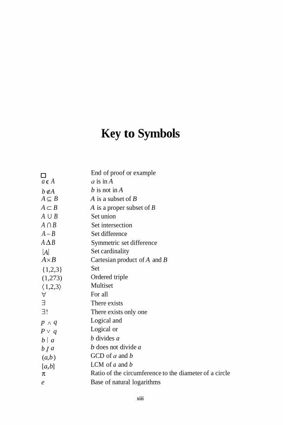
Key to Symbols
a ∋A
A ⊆ BA ⊂ BA
⊃
BA B
A ∆ B
A× B
b ∉ A
A – B
A
1,2,3
(1,273)
⟨1,2,3⟩∀∃∃!p > qP q
>
b aa/b
(a,b)
[a,b]
πe
End of proof or example
a is in Ab is not in AA is a subset of BA is a proper subset of BSet union
Set intersection
Set difference
Symmetric set difference
Set cardinality
Cartesian product of A and BSet
Ordered triple
Multiset
For all
There exists
There exists only one
Logical and
Logical or
b divides ab does not divide aGCD of a and bLCM of a and bRatio of the circumference to the diameter of a circle
Base of natural logarithms
xiii
⊃
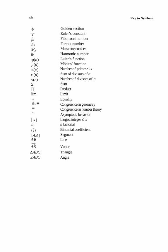
xiv
φ
fnFn
Mp
Hn
ϕ(n)
µ(n)
π(x)
σ(n)
τ(n)
Σ∏lim
γ
x
(nk)
[AB ]
n!
AB
AB∆ABC∠ABC
→
Golden section
Euler’s constant
Fibonacci number
Fermat number
Mersenne number
Harmonic number
Euler’s function
Möbius’ function
Number of primes ≤ xSum of divisors of nNumber of divisors of nSum
Product
Limit
Equality=, Congruence in geometry
≡≡~
Congruence in number theory
Asymptotic behavior
Largest integer ≤ xn factorial
~
Binomial coefficient
Segment
Line
Vector
Triangle
Angle
Key to Symbols
=
MathematicalProblems and Proofs
Combinatorics, Number Theory,and Geometry

This page intentionally left blank.
1
Set Theory

This page intentionally left blank.
Set Theory 3
Set theoretic terminology is used in all parts of mathematics, even in everyday
language and life. In Chapter 1 we introduce the notation and terminology
from set theory that are used in later chapters. We also show a few historically
important examples that had a large impact on the development of mathematics.
1.1. Sets and Elementary Set Operations
Set and set elements are basic mathematical notions.
If a , b , and c are elements of the set A , then we write
A = a,b,c
In this case the element a is in A , while the element d is not in A . We write
that as follows:
a
∋
A d∉ A
Instead of naming all elements of A by their names, it is often more conve-
nient to define a set in the following analytic way:
A =x|P(x)
which means that A is the set of all elements having the property P.
EXAMPLE 1.1. The set of natural numbers less than 9 can be written in several
equivalent ways, for example:
A = 1,2,3,4,5,6,7,8 A = 1,2,...,8
Some sets are used so often that there is a standard notation for them:
A = n |n ∈ N
<
n < 9
N Set of natural numbers
N0
Z Set of integers
Q Set of rational numbers
R Set of real numbers
C Set of complex numbers
NOTE: Authors often consider zero a natural number.
Set of natural numbers along with zero
4 Chapter I
DEFINITION 1.1 (SUBSET). If for every element of A it is true that it is in B, too,we say that A is a subset of B, and write A⊆B.
DEFINITION 1.2 (EQUALITY OF SETS). Sets A and B are equal if A ⊆B and B⊆A .Then we write A = B.
Many proofs of equality of two sets proceed just as in this definition: Firstwe prove that A⊆B, then that B ⊆A .
DEFINITION 1.3 (PROPER SUBSET). If A⊆ B and A ≠ B, we say that A is a proper subset of B, and write A⊆B.
EXAMPLE 1.2. If A = 1,2,3,4,5,6,7,8,9 and B = 1,3,5,7,9, then B ⊆ A.Since obviously A≠ B, we can also write A⊂B.
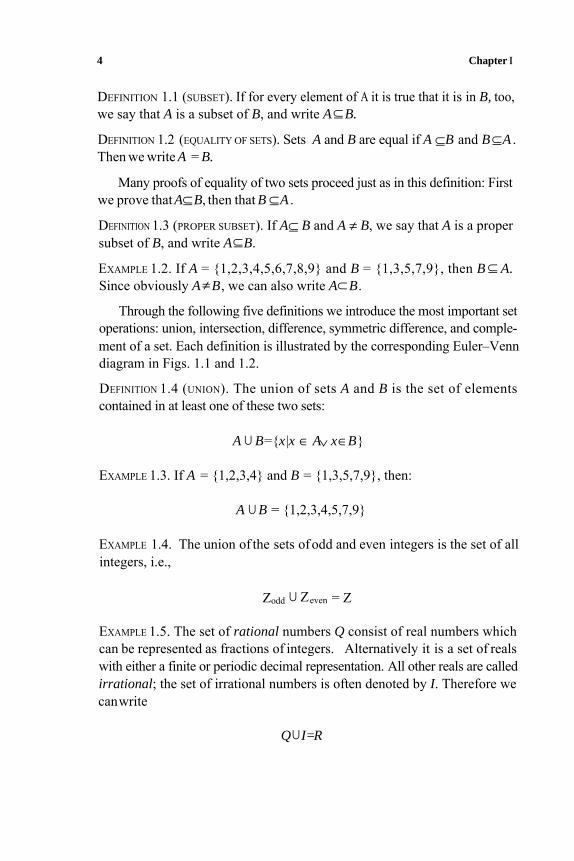
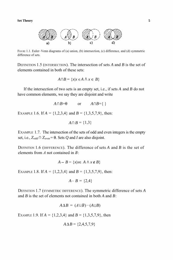
Through the following five definitions we introduce the most important setoperations: union, intersection, difference, symmetric difference, and comple-ment of a set. Each definition is illustrated by the corresponding Euler–Venndiagram in Figs. 1.1 and 1.2.
DEFINITION 1.4 (UNION). The union of sets A and B is the set of elements contained in at least one of these two sets:
A ⊂ B=x|x ∈ A x∈B
EXAMPLE 1.3. If A = 1,2,3,4 and B = 1,3,5,7,9, then:
∧
A
⊃
B = 1,2,3,4,5,7,9
EXAMPLE 1.4. The union of the sets of odd and even integers is the set of all integers, i.e.,
Zodd
⊃
Zeven = Z
EXAMPLE 1.5. The set of rational numbers Q consist of real numbers which can be represented as fractions of integers. Alternatively it is a set of reals with either a finite or periodic decimal representation. All other reals are calledirrational; the set of irrational numbers is often denoted by I. Therefore we can write
Q
⊃
I=R
Set Theory 5
FIGURE 1.1. EuIer–Venn diagrams of (a) union, (b) intersection, (c) difference, and (d) symmetric difference of sets.
DEFINITION 1.5 (INTERSECTION). The intersection of sets A and B is the set ofelements contained in both of these sets:
A ⊃B = x|x ∈A ∧ x ∈ B
If the intersection of two sets is an empty set, i.e., if sets A and B do nothave common elements, we say they are disjoint and write
A ⊃ B=θ or A ⊃B=
EXAMPLE 1.6. If A = 1,2,3,4 and B = 1,3,5,7,9, then:
A ⊃ B = 1,3
EXAMPLE 1.7. The intersection of the sets of odd and even integers is the empty set, i.e., Zodd ⊃ Zeven = θ. Sets Q and I are also disjoint.
DEFINITION 1.6 (DIFFERENCE). The difference of sets A and B is the set ofelements from A not contained in B:
A- B = x|x∈ A ∧ x ∉B
EXAMPLE 1.8. If A = 1,2,3,4 and B = 1,3,5,7,9, then:
A– B = 2,4
DEFINITION 1.7 (SYMMETRIC DIFFERENCE). The symmetric difference of sets A and B is the set of elements not contained in both A and B:
A∆B = (A ⊂B) (A ⊂B)
EXAMPLE 1.9. If A = 1,2,3,4 and B = 1,3,5,7,9, then
A ∆ B = 2,4,5,7,9
–
6 Chapter 1
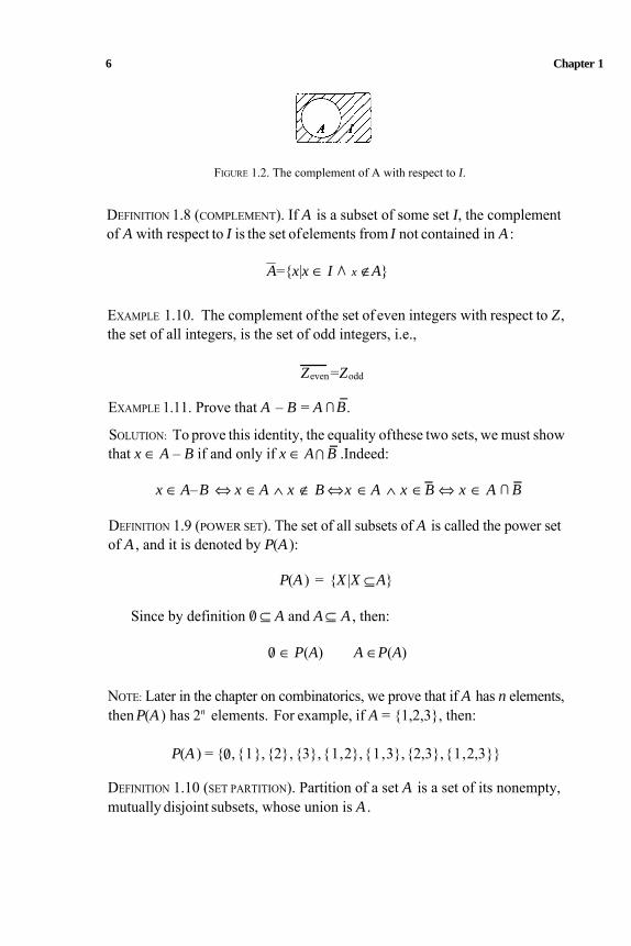
FIGURE 1.2. The complement of A with respect to I.
DEFINITION 1.8 (COMPLEMENT). If A is a subset of some set I, the complement of A with respect to I is the set ofelements from I not contained in A :
A=x|x ∈ I ∧ x ∉ A–
EXAMPLE 1.10. The complement of the set of even integers with respect to Z,the set of all integers, is the set of odd integers, i.e.,
Zeven=Zodd
EXAMPLE 1.11. Prove that A – B = A ⊃ B.-
SOLUTION: To prove this identity, the equality ofthese two sets, we must showthat x ∈ A – B if and only if x ∈ A ⊃ B .Indeed:-
x ∈ A–B ⇔ x ∈ A ∧ x ∉ B ⇔ x ∈ A ∧ x ∈ B ⇔ x ∈ A
⊂
B-
DEFINITION 1.9 (POWER SET). The set of all subsets of A is called the power set of A , and it is denoted by P(A ):
P(A ) = X |X ⊆A
Since by definition 0 ⊆ A and A ⊆ A , then:
0
/
∈ P(A) A ∈P(A)
NOTE: Later in the chapter on combinatorics, we prove that if A has n elements,then P(A ) has 2n elements. For example, if A = 1,2,3, then:
P(A ) = ,1,2, 3,1,2,1,3,2,3,1,2,3
DEFINITION 1.10 (SET PARTITION). Partition of a set A is a set of its nonempty, mutually disjoint subsets, whose union is A .
-
/
0/
Set Theory 7
EXAMPLE 1.12. If A = 1,2,3, then all partitions of A are 1,2,3,
When defining a set, the order of its elements is irrelevant. It also does not
1,2,3, 2,1,3, 3,1,2, and 1,2,3).
matter if we list some element more than once, for example:
1,2,3=1,3,2=1,1,1,2,3
If we do care about the order and repetition of elements, we use orderedpairs, triples, etc., for example:
(1,2) ≠ (2,1) (1,1,2) ≠ (1,2)
Here we define only the ordered pair because ordered triples, etc., are defined similarly.
DEFINITION 1.11 (ORDERED PAIR). The ordered pair (a,b) is defined as
(a,b) = a, a,b
The element a is its first component, while b is its second component.
EXAMPLE 1.13. The ordered pair (a, b) is equal to another ordered pair (c,d)if and only if a = c and b = d.
NOTE: In mathematics we often work with objects for which the order of their elements is irrelevant, but the repetition is not. To model such objects we usethe so-called multisets. There will be more about them in Chapter 2.
1.2. Cartesian Product and Relations
DEFINITION 1.12 (CARTESIAN PRODUCT). The Cartesian product of sets A and Bis the set of all ordered pairs in which the first component is from A and thesecond component is from B:
A xB =(a,b )| a ∈ A ∧ b ∈B
NOTE: The name Cartesian is derived from the Latin name of the Frenchmathematician and philosopher René Descartes — Renatus Cartesius.

8 Chapter 1
EXAMPLE 1.14. If A = 1,2,3 and B = 7,9, then:
A×B= (1,7),(1,9),(2,7),(2,9),(3,7),(3,9)
DEFINITION 1.13 (RELATION). The relation ρ on set A is a subset of A2 = A × A:
ρ⊆ A2
If (x,y ) ∈ρ, we say that x is in relation with y. We also write x ρy.
Relations can have many different properties. The following are the mostimportant.
DEFINITION 1.14 (REFLEXIVITY). The relationρ on A is reflexive if every elementof A is in relation with itself :
ρ is reflexive ⇔ (∀x ∈ A ) xρ x
DEFINITION 1-15 (SYMMETRY). The relation ρ on A is symmetric if for all x,y ∈ A , y is in relation with x whenever x is in relation with y:
ρ is symmetric ⇔ (∀x, y ∈ A) x ρ y ⇒ y ρ x
DEFINITION 1.16 (ANTISYMMETRY). The relation ρ on A is antisymmetric if forall x,y ∈ A, x ρ y and y ρ x only when x = y:
ρ is antisymmetric ⇔ (∀x,y ∈ A) (x ρ y ∧ y ρx) ⇒ x = y
NOTE: There are relations that are neither symmetric nor antisymmetric. Thereare also relations that are both symmetric and antisymmetric. See Examples 1.27, 1.28, and 2.67.
DEFINITION 1.17 (TRANSITIVITY). The relation ρ on A is transitive if for all x,y,and z ∈A, it follows from x ρ y and y ρ z that x ρ z:
ρ is transitive ⇔ (∀x,y,z ∈ A) (x ρ y ∧ y ρ z) ⇒ x ρ z
The following three definitions introduce three important types of relations,which satisfy some of the preceding properties:
Set Theory 9
DEFINITION 1.18 (EQUIVALENCE RELATION). The relation ρ on A that is reflexive,symmetric, and transitive is called the equivalence relation.
EXAMPLE 1.15. If A = 1,2,3 and ρ = (1,1), (2,2), (3,3), (1,2), (2,1),(2,3), (1,3), then ρ is an equivalence relation on A. If A is given as A = 1,2,3,4, then ρ is not reflexive, and therefore it is not an equivalence relation on A .
DEFINITION 1.19 (PARTIAL-ORDER RELATION). The relation ρ on A that is reflex-ive, antisymmetric, and transitive is called the partial-order relation.
DEFINITION 1.20 (SIMPLE-ORDER RELATION). The partial order relation ρ on Ais a simple-order relation if every two elements of A are comparable, i.e., for every x, y ∈A we have either x ρ y, or y ρ x.
Simple-order relations are also called linear-order relations, while the cor-responding sets are called simply ordered sets or linearly ordered sets.
EXAMPLE 1.16. If A =1,2,3 and ρ=(1,1), (2,2), (3,3), (1,2), (2,3), (1,3), then ρ is a partial-order relation on A. This particular relation is usually denoted by ≤ (less then or equal). In this case every two elements of A are comparable, therefore ≤ is also a simple-order relation.
EXAMPLE 1.17. If A = 1,2,3,4,5,6 and ρ = (1,1), (2,2), (3,3), (4,4),
partial-order relation on A. For example since 3 and 5 are not in relation (notcomparable), this relation is not a simple-order relation. The reader may haverecognized that this is the division relation.
(5,5), (6,6), (1,2), (1,3) (1,4), (1,5), (1,6), (2,4), (2,6), (3,6), then ρ is a
1.3. Functions and Operations
A function or mapping is one of the most important concepts in mathematics.
DEFINITION 1.21 (FUNCTION). The function f of set X into set Y is a subset of the Cartesian product X × Y such that every x ∈ X appears exactly once as thefirst component of the elements of f.
Symbolically we write
f : X → Y x | → f (x) or y = f (x)
Therefore a relation, i.e., a set of ordered pairs, is a function if and only
10 Chapter 1
if for no two ordered pairs their first components are equal and their second components differ.
EXAMPLE 1.18. If A = 1,2,3 and B = t,u,v,w, then f =(1,u), (2, w),(3,t) is a function, while g = (1,u), (2,w) and h = (1,u), (2,w), (3, t),(3,v) are not. Why? Because g does not specify the image for 3, while hspecifies two of them instead of just one.
If (x,y) ∈ f, we say that x is an original, while y is its image. Set X is called the domain, while the set of all images y = f (x),which is a subset of Y,is called the range or sometimes the codomain.
Functions f and g are equal if they have the same domain, and f (x) = g(x) for every element x from the domain. Then we write f = g.
DEFINITION 1.22 (SURJECTION). The function f mapping X into Y such that therange is the whole set Y is called “onto” or a surjection.
DEFINITION 1.23 (INJECTION). The function f mapping X into Y such that notwo originals have equal images is called “one-to-one” (1-1, for short) or an injection.
DEFINITION 1.24 (BIJECTION). The function f mapping X into Y that is botha surjection and an injection is called a “one-to-one correspondence” or a bijection.
Bijections have many important properties, and they are used very often. See the examples at the end of Chapter 1.
In the following we define binary operations and their properties.
DEFINITION 1.25 (BINARY OPERATION). The binary operation on the set A is a function of A 2 = A × A into A.
If a binary operation is denoted by *, then if (a, b) ∈A2 is mapped by * onc ∈ A , we write
a*b=c
We now define the three basic properties of binary operations.
DEFINITION 1.26 (COMMUTATIVITY). The binary operation * is commutative if:
(∀a, b ∈ A) a* b = b*a
SetTheory 11
DEFINITION 1.27 (ASSOCIATIVITY). The binary operation * is associative if:
(∀a,b,c ∈A) (a* b)* c = a*(b* c)
DEFINITION 1.28 (DISTRIBUTIVITY). The binary operation * is distributive withrespect to the binary operation o if
(∀a,b ,c ∈A ) (a o b)*c = (a * c) o (b *c)∧ c* (ao b) = (c*a) o (c*b)
1.4. Cardinality
DEFINITION 1.29 (INFINITE SET). A set is infinite if it can be bijectively mapped onto some of its proper subsets.
DEFINITION 1.30 (FINITE SET). A set is finite if it is not infinite.
EXAMPLE 1.19 (SET N IS INFINITE). The set of even natural numbers is a propersubset of the set of natural numbers N. Since f (n) = 2n is a bijection, the setN is infinite. The fact that there is a one-to one correspondence between thesetwo sets is an apparent paradox noted by Galileo in 1638.
EXAMPLE 1.20 (EUCLID’S THEOREM ON PRIMES). In the ninth book of his Ele-ments, Euclid gives the following proof of the infiniteness of the set of primes.
Assume there are only finitely many primes, p1,p2,...,pn and let pn be the greatest among them. Consider
P = p1 p2...pn+1
which is obviously P > Pn. There are two possibilities for P:
• P is a prime. This contradicts the assumption that pn is the greatestprime.
• P is a composite. This contradicts the assumption that p1 ,p2,. . . ,pn are all primes. Dividing P by any of these yields remainder 1; i.e., P has prime factors that differ from p1 ,p2,. . . ,pn.
This proves the infiniteness of the set of primes.
NOTE: Proofs by contradiction are very common in mathematics: We firstassume that a statement is true, then we show that this assumption leads to a contradiction.
12 Chapter 1
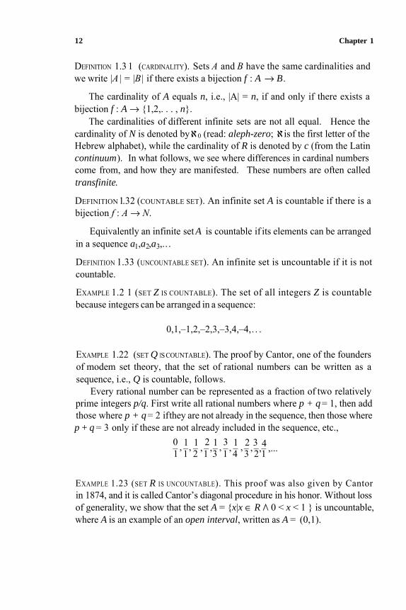
DEFINITION 1.3 1 (CARDINALITY). Sets A and B have the same cardinalities andwe write |A | = |B| if there exists a bijection f : A → B.
The cardinality of A equals n, i.e., |A| = n, if and only if there exists a bijection f : A → 1,2,. . . , n.
The cardinalities of different infinite sets are not all equal. Hence thecardinality of N is denoted byℵ0 (read: aleph-zero; ℵis the first letter of the Hebrew alphabet), while the cardinality of R is denoted by c (from the Latin continuum). In what follows, we see where differences in cardinal numbers come from, and how they are manifested. These numbers are often calledtransfinite.
DEFINITION1.32 (COUNTABLE SET). An infinite set A is countable if there is abijection f : A → N.
Equivalently an infinite set A is countable if its elements can be arrangedin a sequence a1,a2,a3,.. .
DEFINITION 1.33 (UNCOUNTABLE SET). An infinite set is uncountable if it is notcountable.
EXAMPLE 1.2 1 (SET Z IS COUNTABLE). The set of all integers Z is countablebecause integers can be arranged in a sequence:
0,1,–1,2,–2,3,–3,4,–4,. . .
EXAMPLE 1.22 (SET Q IS COUNTABLE). The proof by Cantor, one of the foundersof modem set theory, that the set of rational numbers can be written as a sequence, i.e., Q is countable, follows.
Every rational number can be represented as a fraction of two relatively prime integers p/q. First write all rational numbers where p + q = 1, then addthose where p + q = 2 ifthey are not already in the sequence, then those wherep + q = 3 only if these are not already included in the sequence, etc.,
0 1 1 2 1 3 1 2 3 4–1, 1
, 2 , 1 , 3
, 1 , 4
, 3 , 2 , 1 ,...
EXAMPLE 1.23 (SET R IS UNCOUNTABLE). This proof was also given by Cantorin 1874, and it is called Cantor’s diagonal procedure in his honor. Without lossof generality, we show that the set A = x|x ∈ R ∧ 0 < x < 1 is uncountable,where A is an example of an open interval, written as A = (0,1).
– –– –––– – –
Set Theory 13
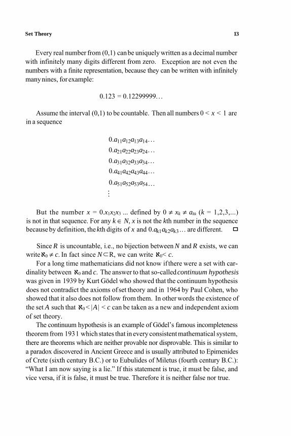
Every real number from (0,1) canbe uniquely written as a decimal numberwith infinitely many digits different from zero. Exception are not even the numbers with a finite representation, because they can be written with infinitelymany nines, for example:
0.123 = 0.12299999. . .
Assume the interval (0,1) to be countable. Then all numbers 0 < x < 1 arein a sequence
0.a11a12a13a14 . . .0.a21a22a23a24. . .0.a31a32a33a34. . .0.a41a42a43a44. . .
. . .0.a51a52a53a54
But the number x = 0.x1x2x3 ... defined by 0 ≠ xk ≠ akk (k = 1,2,3,...) is not in that sequence. For any k ∈ N, x is not the kth number in the sequence because by definition, the kth digits of x and 0.ak1ak2ak3 .. . are different.
Since R is uncountable, i.e., no bijection between N and R exists, we canwriteℵ0 ≠ c. In fact since N ⊂R, we can write ℵ0< c.
For a long time mathematicians did not know if there were a set with car-dinality between ℵ0 and c. The answer to that so-calledcontinuum hypothesiswas given in 1939 by Kurt Gödel who showed that the continuum hypothesisdoes not contradict the axioms of set theory and in 1964 by Paul Cohen, whoshowed that it also does not follow from them. In other words the existence of the set A such that ℵ0 < |A | < c can be taken as a new and independent axiomof set theory.
The continuum hypothesis is an example of Gödel’s famous incompletenesstheorem from 193 1 which states that in every consistent mathematical system, there are theorems which are neither provable nor disprovable. This is similar to a paradox discovered in Ancient Greece and is usually attributed to Epimenidesof Crete (sixth century B.C.) or to Eubulides of Miletus (fourth century B.C.):“What I am now saying is a lie.” If this statement is true, it must be false, andvice versa, if it is false, it must be true. Therefore it is neither false nor true.
...
14 Chapter 1
1.5. Problems
EXAMPLE 1.24 (PROPERTIES OF SET OPERATIONS). The following properties of
set operations are easy to prove. Let A, B, and C be arbitrary sets, then:
A ⊂ A=A Idempotency of union
A
⊂
A =A Idempotency of intersection
A ⊂B =B ⊂ A Commutativity of union
A
⊂
B =B
⊂
A Commutativity of intersection
(A
⊃
B)
⊃
C = A ⊂ (B ⊂C )
(A
⊂
B)
⊂
C = A
⊂
(B
⊂
C )
(A
⊂
B)
⊂
C=(A
⊂
C)
⊂
(B
⊂
C )
(A ⊂B) ⊂ C= (A ⊂ C) ⊂ (B ⊂
C )
A⊂B ⇒ A ⊂ B=BA⊂B ⇒ A
⊂
B=AA ⊂ (A ⊂ B) = AA
⊂
(A
⊂
B) =A
A=A Involutivity of complement
A ⊂B=A
⊂
B- -- -
De Morgan’s law
A
⊂
B=A ⊂B De Morgan’s law
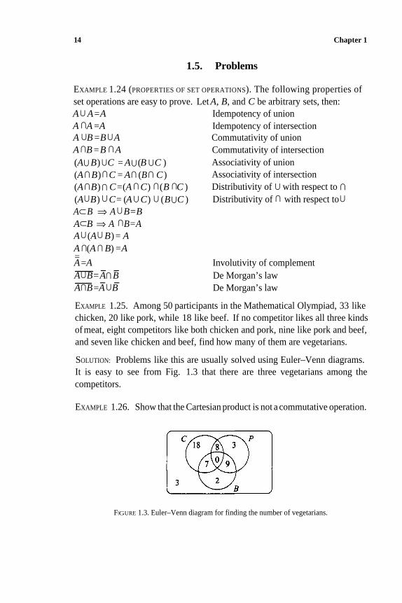
EXAMPLE 1.25. Among 50 participants in the Mathematical Olympiad, 33 like
chicken, 20 like pork, while 18 like beef. If no competitor likes all three kinds
of meat, eight competitors like both chicken and pork, nine like pork and beef,
and seven like chicken and beef, find how many of them are vegetarians.
SOLUTION: Problems like this are usually solved using Euler–Venn diagrams.
It is easy to see from Fig. 1.3 that there are three vegetarians among the
competitors.
EXAMPLE 1.26. Show that the Cartesian product is not a commutative operation.
Associativity of union
Associativity of intersection
Distributivity of
⊃
with respect to ⊃ Distributivity of
⊂
with respect to ⊂
FIGURE 1.3. Euler–Venn diagram for finding the number of vegetarians.
=
Set Theory 15
SOLUTION: It is enough to find a pair of sets A and B such that A × B ≠ B × A:
A=1,2, B=3 ⇒ A × B =(1,3),(2,3)≠(3,1),(3,2)=B × A
NOTE: This is a typical solution by finding a counterexample.
EXAMPLE 1.27. Show that the relation ρ = (1,1), (2,2) on A = 1,2,3 is
not reflexive but symmetric, antisymmetric, and transitive.
EXAMPLE 1.28. Show that ρ = (1,2), (1,3), (2, 1), (2,3) defined on A =
1,2,3 has none of the properties in Example 1.27.
EXAMPLE 1.29 (EQUIVALENCE CLASSES). Consider an equivalence relation on
A denoted by ~ (read: tilde). Denote by [x] a subset of A that contains all
elements from A in relation with x ∈ A and these elements only, i.e.,
[x] = y|y ∈ A ∧ x ~ y
The set [x] is called the equivalence class of x. Since ~ is an equivalence
relation, i.e., it is reflexive, symmetric, and transitive, we easily see that:
[x] = [y] ⇔ x ~ y
This implies that every two equivalence classes are either disjoint or equal to
each other. The union of all equivalence classes is obviously A. The set of
all equivalence classes is called the quotient set, and it is denoted by A/ ~ .
Since the equivalence classes are disjoint and their union is A ,each equivalence
relation describes one partition of A, and vice versa, every partition of A defines
one equivalence relation.
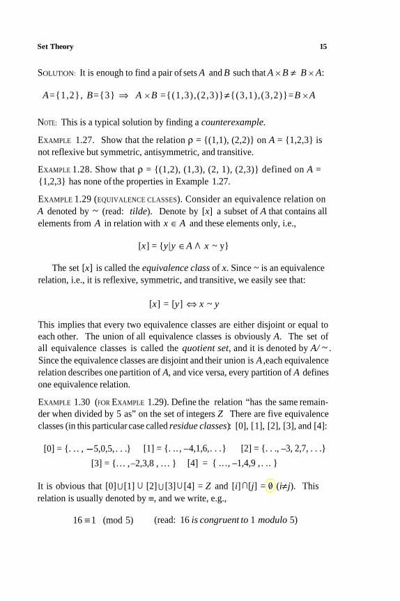
EXAMPLE 1.30 (FOR EXAMPLE 1.29). Define the relation “has the same remain-
der when divided by 5 as” on the set of integers Z. There are five equivalence
classes (in this particular case called residue classes): [0], [1], [2], [3], and [4]:
[0] = . . . , -5,0,5, . . . [1] = . .. , –4,1,6,. . . [2] = . . ., –3, 2,7, . . .
[3] = . . . ,–2,3,8 , . . . [4] = .. ., –1,4,9 , . ..
It is obvious that [0] ⊂ [1] ⊂ [2] ⊂ [3] ⊂ [4] = Z and [i]
⊂
[j] = 0 (i≠ j). This /
relation is usually denoted by ≡, and we write, e.g.,
16 ≡ 1 (mod 5) (read: 16 is congruent to 1 modulo 5)
16 Chapter 1
Thequotient setnow is (Z / ≡) = [0],[1],[2],[3],[4].
EXAMPLE 1.31 (IRRATIONAL NUMBERS). Until the Pythagoreans, students and
followers of Pythagoras, discovered that the diagonal of a square is not com-
mensurable to the side of the square or in other words that is not a rational
number, ancient mathematicians were content with rational numbers, i.e., num-
bers that can be written as integer fractions.
We prove here that is irrational as the Pythagoreans did by contradiction.
Suppose is rational; i.e., it can be written as a fraction of integers:
Assume also that a and b are such that they do not have common factors.
Assuming all this, and squaring the previous equality, we obtain
a2 = 2b2
This implies a is an even number, i.e., a = 2a1. But:
b2=2a21
This implies b is an even number, too, which contradicts our assumption that aand b have no common factors.
Therefore we find that it is impossible to write as a fraction of integers;
i.e., is irrational.
EXAMPLE 1.32 (TRANSCENDENTAL NUMBERS). Among irrationals, too, there are
different kinds of numbers. Irrationals that can be defined as the roots* of
polynomials with integer coefficients are called algebraic numbers. The golden
section φ is one of the solutions of x2 – x – 1 = 0, hence φ is an algebraic
number. Irrational numbers that are not algebraic are called transcendentalnumbers.
In 1873 Hermite proved that e is a transcendental number, and in 1882
Lindemann showed the same for π, thus also proving that, using only a ruler
and compass, it is impossible to construct the square whose area is the same
as the given circle. This is the so-called problem of squaring a circle, which
remained unsolved since antiquity. It is still not known whether some important
*The following are synonyms: the roots of the polynomial P(x), the zeros of the polynomial P(x),
and the solutions of the equation P(x) = 0.
Set Theory 17
mathematical constants are rational or irrational, let alone whether they are
algebraic or transcendental (if they are irrational). One such numbers is Euler’s
constant
See Appendix B for more about these important numbers.
EXAMPLE 1.33 (RATIONAL OR NOT?). If a and b are irrational, can ab be a rational
number?
SOLUTION: Yes! Consider If it is rational, then an effective example is
a = b = If it is irrational, then take a = and b = Then:
EXAMPLE 1.34 (ABORIGINAL ELECTIONS). The Aborigines of Australia pick for
their head the man with the largest flock of sheep. But since in their language
and culture there are no numbers larger than 20, they have an ingenious election
system: One sheep from each flock of the two finalists is taken through a gate,
until it is determined which man has the larger flock: Mapping at work!
EXAMPLE 1.35. Let A be a set with n elements; i.e., let |A| = n. Show that the
number of subsets of A having k (0 ≤ k ≤ n) elements is equal to the number
of subsets of A having (n – k) elements.
SOLUTION: To an arbitrary k-element set B ⊂ A we can uniquely ascribe the
(n – k)-element set A – B ⊂ A . This mapping is a bijection from the set of all
k-element subsets of A, Pk (A), onto the set of all (n – k)-element subsets of A,
Pn-k(A ). Hence we find
|Pk (A )|= |Pn-k (A )|
Also see Example 2.27.
EXAMPLE 1.36. Let a ∈ A . Are there more subsets of A containing a or those
not containing it?
SOLUTION: The function f that maps every subset B not containing a onto the
subset B ⊂ a is obviously a bijection; therefore the cardinalities of sets of
18 Chapter 1
these subsets are equal. This solution does not depend on whether or not A is
finite.
EXAMPLE 1.37. Let X ⊂A . Are there more subsets of A that contain X are
disjoint with it?
RESULT: The cardinalities are equal again; the whole problem is very similar
to the one in Example 1.36.
EXAMPLE 1.38. Let X be a subset of a finite set A and let |X| > 1. Are there
more subsets of A which contain X , or those which do not?
RESULT: Since not all subsets of A that do not contain X are disjoint with it,
more subsets do not contain X than do.
EXAMPLE 1.39. Show that for an arbitrary set A , the number of subsets with an
even number of elements equals the number of subsets with an odd number of
elements,
SOLUTION: Let us pick one element from A and denote it by a. Define a function
f from the set of even-numbered subsets onto the set of odd-numbered subsets
as follows: If an even-numbered subset B contains a, let f (B) = B – a, and if
a ∉ B, let f (B) = B ⊂ a. It is easy to see that f is a bijection. This completes
the proof.
Also see Example 2.54.

2
Combinatorics

This page intentionally left blank.
Combinatorics 21
Chapter 2 discusses the basic notions ofcombinatorics. At the beginning, our
main task is to solve enumeration problems without considering permutations,
combinations, etc. That is, we try to find the best way of enumerating objects
and their arrangements. Once we have a reasonable amount ofexperience with
such problems, we define and use combinatorial terminology. Even then we
sometimes find it easier to solve problems simply by counting.
2.1. Four Enumeration Principles
To answer such questions as How many ways are there to give 30 books toseven friends? as well as much more difficult questions, we use the following
enumeration rules andprinciples:
Let A and B be sets with m and n elements, respectively; i.e., let
|A | = m |B| = n
Rule of product. The number of ways of forming an ordered pair (a, b)
such that a ∈ A and b ∈ B; equals m . n. In other words:
|A × B| = m . n
Rule of sum. If sets A and B are disjoint, then the number of ways ofpicking one element from their union equals the sum m + n. In other words:
A
⊂
B = 0 ⇒ |A B|=m+n
Principle of inclusion–exclusion. In general when A and B are not nec- essarily disjoint, the following is true:
( A
⊂
B = C | C | = p ≥ 0 ) ⇒ | A ⊂ B | = m + n – p
/ ⊂
22 Chapter 2
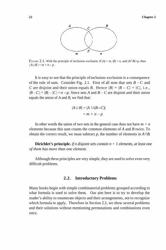
FIGURE 2.1. With the principle of inclusion–exclusion. If |A| = m, |B| = n, and |A
⊂
B|=p, then
| A ⊂ B | = m + n - p .
It is easy to see that the principle of inclusion–exclusion is a consequence
of the rule of sum. Consider Fig. 2.1. First of all note that sets B – C and
C are disjoint and their union equals B. Hence |B | = |B – C | + |C|, i.e.,
|B – C | = |B| – |C | = n -p. Since sets A and B – C are disjoint and their union
equals the union of A and B, we find that:
|A ⊂ B| = |A ⊂ (B-C)|
= m + n – p
In other words the union of two sets in the general case does not have m + n elements because this sum counts the common elements of A and B twice. To
obtain the correct result, we must subtract p, the number of elements in A
⊂
B.
Dirichlet’s principle. if n disjoint sets contain n + 1 elements, at least one of them has more than one element.
Although these principles are very simple, they are used to solve even very
difficult problems.
2.2. Introductory Problems
Many books begin with simple combinatorial problems grouped according to
what formula is used to solve them. Our aim here is to try to develop the
reader’s ability to enumerate objects and their arrangements, not to recognize
which formula to apply, Therefore in Section 2.2, we show several problems
and their solutions without mentioning permutations and combinations even
once.
Combinatorics 23
EXAMPLE 2.1. How many elements are there in the set given by A = n , n + 1,
. . . ,n2?
SOLUTION: It is obvious that |A|= n2 – n + 1, but let us try tojustify this answer.
What does it actually mean to enumerate the elements of a set? If A has r ∈ Nelements, then each element can be assigned an order, a number from the set
Nr = 1,2,3,. . . ,r ⊂ N .In our problem, we assign order 1 to n , order 2 to n + 1, and so on. The
question now is what is the order of n2? We notice that in this case, the
difference between the element of A and its order is always n – 1. Therefore
the order of n2 is n2 – (n– 1) = n2 – n + 1, which implies that | A | = n2 – n + 1.
EXAMPLE 2.2. A certain island is home to 510 seals. Suppose each seal has 10
or more mustaches, but not more than 30. Prove that among these 510 seals at
least 25 of them have an equal number of mustaches.
SOLUTION: If we divide the seals into 21 groups according to how many
mustaches they have (note that 21 is the cardinality of the set 10,11, .. . , 30)
and assume that each group has ≤ 24 seals, then there are ≤ 21 . 24 = 504 < 510
seals on the island. Hence, at least one group has 25 or more seals.
EXAMPLE 2.3. How many seven-digit phone numbers begin with 432 and end
with 3 or 5?
SOLUTION: The fourth digit can be selected from 10 possible choices:
0,1,2,. . . ,9. The same is true for the fifth and the sixth digit. The seventh digit
can be picked in two ways: it can be either 3 or 5. Therefore, according to the
rule of product, the number of such phone numbers is 10.10.10.2 = 2000.
EXAMPLE 2.4. There are n points given in a plane, and no three of these are
collinear, i.e., no three lie on the same line. How many lines are defined by
these n points?
SOLUTION: Since each pair of different points defines a line, in this problem
we are actually interested in counting all pairs of different points that can be
formed from the n given points. The first point can be picked in n different
ways, while the other can be picked in (n – 1) ways since it must differ from
the first. Hence the number ofpairs is n (n – 1).
Please note that every line formed in this way appears twice because, for
example, ordered pairs (A,B ) and (B,A ) define the same line: AB ≡ BA.Therefore the number of lines is twice as small as the number of ordered pairs;
it equals n(n – 1)/2.
24 Chapter 2
EXAMPLE 2.5. Similarly if n points are given in space and among them no fourcoplanar, i.e., no four lie in the same plane, there are n(n – 1)(n – 2)/6 planesdefined by these n points.
NOTE: In Examples 2.4 and 2.5 we reduced the problems to counting the two-or three-element subsets of the n-element sets. Since the order of the elements of a (sub)set is irrelevant, we can uniquely assign A,B to the line AB ≡ BAand A,B,C to the plane πABC ≡ πACB ≡ . . . ≡ πCBA.
EXAMPLE 2.6. How many seven-digit phone numbers begin with 215-2 if the last three digits must differ among themselves; they cannot be 0, 2, or 5; and the last digit cannot be 1?
SOLUTION 1: Let us try to solve this problem as follows: We cannot changethe first four digits; these are fixed. The fifth digit can be selected from the set 1,3,4,6,7,8,9, i.e., in seven different ways. The sixth digit must differfrom the fifth, so it can be picked in six ways. The last digit must be different from the fifth and the sixth, so without the last condition, we could pick it in five ways. Due to the last condition we cannot select the last digit in four ways, because if the fifth or sixth digit were 1, the last digit can be selected in five ways, not four.
Let us divide the set of all phone numbers satisfying these conditions intothree disjoint sets: the set of numbers having neither a fifth nor sixth digit equal to 1, the set of numbers having 1 at the fifth place, and the set of numbershaving 1 at the sixth place.
In the first set, there are 6 . 5 . 4 choices. In the second set the first five digits are fixed, so there are 6 . 5 choices. Similarly in the third set, there are 6 . 5choices. Therefore 6 . 5 . 4 + 1 . 6 . 5 + 6 . 1 . 5 = 180 phone numbers have the required properties.
SOLUTION 2: The solution can be obtained much more easily ifwe begin withthe last digit, which can be picked from 3,4,6,7,8,9, i.e., in 6 ways. Once itis selected, we can select the sixth digit in six ways, too, because although we cannot repeat the last digit, we can use digit 1. The fifth digit can be selected in five ways. The result is the same as before: 6 . 6 . 5 = 180.
SOLUTION 3: Let us consider the third way to solve this problem. From thetotal number ofphone numbers that can be formed using different digits from 1,3,4,6,7,8,9 at their last three places, we subtract the number of phonenumbers having 1 at the last place: 7 . 6 . 5 – 6 . 5 = 180.
Combinatorics 25
EXAMPLE 2.7. Fromthesetcontainingn arbitrarynatural numbers a1 , . . . ,anwe can select a subset in which the sum ofall elements is divisible by n. Provethis.
SOLUTION: Let us consider n subsets:
a1,a1,a2,...,a1,a2,...,an
First calculate the sums in each of these subsets and in the remainders after division by n. If some of these remainders is 0, we have the subset we seek.If none of these is 0 then, according to Dirichlet’s principle, among these nsubsets there are two with equal remainders. [Ifnone of these has remainder0, then n remainders are to be distributed in (n – 1) residue classes.] Let thesetwo subsets be a1 ,a2,. . . ,ar and a1 ,a2,. . . ,as, where, e.g., r < s. Then:
a1 +a2 +. . . +as – (a1 +a2 +. . .+ar.) = ar+1 +ar+2 +. . .+as
is divisible by n, and ar+1, ar+2,. . . ,as is the subset we seek.
EXAMPLE 2.8 (NUMBER OF DIVISORS). How many different divisors, includingitself and 1, does 2520 have?
SOLUTION: Canonical decomposition of 2520 is 2520 = 23 . 32 . 5 . 7, so alldivisors of 2520can be written as 2a . 3b . 5c . 7d, where a,b,c,d ≥ 0; each of these is less than or equal to the corresponding exponent in the decomposition of 2520. In other words, 0 ≤ a ≤ 3, 0 ≤ b ≤ 2, 0 ≤ c ≤ 1, 0 ≤ d ≤ 1. Hence acan be picked in four ways, b in three, c in two, and d in two. Therefore, thenumber of divisors of 2520 is 4.3.2.2 = 48.
NOTE: In number theory the number of divisors is denoted by τ(n) or sometimes by d(n). If p1 ,p2,. . . ,pr are the prime factors of n, then:
EXAMPLE 2.9. A code for a safe is a five-digit number that can have a 0 in thefirst place as well as in any other place. How many codes are there whose digits form an increasing sequence?
SOLUTION: Considercodes composed of different digits without the increasing order restriction. Suppose we select five out of ten possible digits to form these
26 Chapter2
codes. Among all 5 . 4 . 3 . 2 . 1 = 120 codes that can be formed using these five digits, only one code has its digits in increasing order.
This observation is already an important step toward the solution. Let Mbe the solution, the number of length-5 increasing sequences.
The total number of codes with different digits is 10. 9.8.7. 6 = 30240,but also 120M, hence:
10. 9. 8 .7. 6 302405. 4. 3 . 2 .1
=120
252=M =
EXAMPLE 2.10. A code for a safe is a five-digit number that can have a 0 at thefirst place. How many codes have exactly one digit 7?
SOLUTION: There are 5 . 94 = 52488 codes with exactly one digit 7. Actually,there are 9 . 9 . 9 . 9 = 94 codes with a digit 7 in the first place. The same is true for codes with 7 in the second, third, fourth, and fifth places. The total numberis therefore 5. 94. We obtain the same result if we say there are five choices for placing 7 and nine choices for each of the remaining four places.
EXAMPLE 2.11. A code for a safe is a five-digit number that can have a 0 at thefirst place. How many codes have at least one digit 7?
SOLUTION: There are 5 . 94 with exactly one 7. There are 10. 93 codes withexactly two digits 7 because two places containing 7 can be selected in ten ways. Similarly there are 10 . 92 codes with exactly three 7s, 5 .9 codes withexactly four 7s, and only one code with all five digits equal to 7. The total is
5 . 94 + 10 . 93 + 10 . 92 + 5 . 9+ 1 = 40951
The more elegant way of solving this problem involves subtracting thenumber of codes not having any digits equal to 7 from the total number of codes:
105 – 95 = 40951
NOTE: The following equality, obtained by comparison of the two solutions,
105 = 95 + 5 . 94 + 10 . 93 + 10 . 92 + 5 . 9+ 1
is a special case of Newton’s binomial expansion.
Combinatorics 21
EXAMPLE 2.12. A can of red paint is spilled over a white plane. Show that this red and white plane contains two points of the same color whose distance is exactly 1 cm. SOLUTION: Consider the vertices of an equilateral triangle whose side is 1 cm. Each of these three points is either red or white; hence two of them have the same color.
EXAMPLE 2.13. Let us consider a chess board with a knight moving on it. Can the knight start from the lower left comer (A-1), visit every field on the board exactly once, and end in the upper right corner (H-8)?
SOLUTION: The answer is no, and this is why. The first field (A-1) is black, the second, according to rules governing the knight’s motion, must be white, the third is then black, and so on. We thus observe that even fields must be white, including the last, sixty-fourth field. But H-8 is black, so it cannot be the last field.
From previous examples we see that parts, sometimes even an entire prob-lem, can be reduced to counting the number of subsets or ordered k-tuplesformed by elements of some set. For that reason mathematicians introduced terms like combinations and permutations. Before defining these, let us con-sider a few examples using only set-theoretic terminology.
EXAMPLE 2.14. How many subsets does A = a1,a2,. . . ,an have? SOLUTION: Consider an arbitrary subset of A. Each of n elements of A is either in that subset or not. Thus according to the rule of product, the number ofdifferent subsets of A is
EXAMPLE 2.15. How many ordered k-tuples can be formed from different ele-ments of A= a1,a2, .. ., an?SOLUTION: The first component of the ordered k-tuple can be filled by one ofn elements of A, the second by any of the remaining n – 1 elements, etc. The kth component can be picked from the last remaining n – k + 1 elements of A .Hence the total number of ordered k-tuples formed from different elements ofA is
n!n(n – 1)(n –2). . .(n –k+ 1) = (n – k)!
28 Chapter 2
where r! = r(r – 1). . . 1 is the factorial of r (read: r factorial). For this and similar formulas to be valid when n = k, the convention is that 0! = 1.
EXAMPLE 2.16. How many ordered k-tuples can be formed from the elementsof the set A = a1, a2, . . . , an if repetition is allowed?
SOLUTION: Since repetition is allowed, each component can be selected in anyof n ways; hence, the number of such ordered k-tuples is
EXAMPLE 2.17. How many k-element subsets does the n-element set A have ?
SOLUTION: Assume without any loss of generality that the set A is A = 1,2, . . . ,n. As in Example 2.9, there are as many k-element subsets ofA as there are increasing sequences made from its elements. Let the final answer be M. From each of M increasing length-k sequences, we can form k(k – 1). . . 1 = k! ordered k-tuples. Hence the number ofall ordered k-tupleswhose components are different elements of A equals k! . M. On the otherhand, as in Example 2.15, their number equals
Therefore:
We see later that instead of this clumsy quotient of factorials, we write
which reads n choose k.
coefficients, and we learn why very soon. It is not a coincidence that the same symbol is used for the binomial
Unlike with ordered k-tuples, the order of elements for sets is irrelevant,for example:
(1,2,3) ≠ (1,3,2) 1,2,3 = 1,3,2
Combinatorics 29
Besides 1,2,2 = 1,2. However in some cases we have objects whose order is irrelevant, but their
repetition may occur. In such cases we must be careful with the notation weuse or even better to introduce the multisets.
Unlike with ordered k-tuples, order is irrelevant for multisets. At the sametime, unlike with sets, repetition is allowed. We use ⟨a1 ,a2,. . . ,an⟩ to denote amultiset,forexample, ⟨1,2,2,3⟩ ≠ ⟨1,2,3⟩ and ⟨1,2,2,3⟩ = ⟨1,2,3,2⟩ . Henceinstead of asking the wrong question, How many k-element subsets can beformed from the elements of an n-element set A if repetition is allowed? we ask the following question in Example 2.18.
EXAMPLE 2.18. How many k-element multisets can be formed from the ele-ments of A = a1 ,a2, . . . ,an?
SOLUTION: Every k-element multiset consisting of elements from A can beuniquely represented as a sequence of k zeros and n – 1 vertical lines. Thenumber of zeros to the left from the first line represents the number of repetitions of a1, the number of zeros between the first and second lines represents thenumber of repetitions of a2, . . . ; the number of zeros to the right from the last vertical line represents the number of repetitions of an.
For example if n = 7 and k = 4, the multiset ⟨a1 ,a1 ,a3,a6⟩ can be repre-sented as 00||0|||0|.
If the zeros differ among themselves and the lines among themselves, thenumber of different sequences of zeros and lines would be (n – 1 + k)! But since the zeros are indistinguishable (as well as the lines) the number of differentsequences of zeros and lines is
EXAMPLE 2.19. Let us consider how many different ordered n-tuples can be formed from the elements of the multiset:
SOLUTION: If there were no repetitions, i.e., ifall elements were different, thesolution would be n!, but because of repetitions, the solution is
30 Chapter 2
2.3. Basic Definitions
In the introductory problems we saw that two questions were very important:
• Is there a repetition of objects to be arranged?
• Is their order important?
To emphasize and formalize the importance of these two questions, in this section we define combinations, permutations, etc. Because of the importance ofthe last few examples in Section 2.2, we repeat them here and later presentdifferent derivations of the same formulas.
DEFINITION 2.1 (k-PERMUTATIONS WITHOUT REPETITION). A k-permutation with-out repetition of the set A = a1 ,a2, . . . , an, (n ≥ k) is an arbitrary orderedk-tuple of different elements from that set.
How many different k-permutations of the set A are there? Denote thatnumber as Pn
k. Since | A| = n, the first component of the ordered k-tuple canbe selected in n different ways. Since the components must be different, the second component can be selected in (n – 1) ways, the third in (n – 2) ways,etc. Using the product rule, it is now obvious that:
Pnk = n . (n – 1) . (n –2). . . . .(n - k + 1)
DEFINITION 2.2 (PERMUTATIONS WITHOUT REPETITION). A permutation withoutrepetition of the set A with n elements is an arbitrary bijection of A onto itself.
It is easy to see that this definition is equivalent to saying that a permutationis just an n-permutation of a set with n elements. Hence, it is uniquelydetermined by an ordered n-tuple of different elements from A.
If we denote by Pn the number of permutations of the set A with n elements,
then:
Pn =Pnn = n . (n – 1) . (n –2) . . . . .(n –n + 1)
That is,
Pn = n!
Combinatorics 31
DEFINITION 2.3 (COMBINATIONS WITHOUT REPETITION). A k-combination without repetition of the set A with n elements is an arbitrary subset of A having kelements.
NOTE: The k-combinations are subsets, while k-permutations are ordered k-tuples.
Let Cnk be the numberof all k-combinations of a set with n elements. Since
we can form k! different ordered k-tuples from a subset with k elements, wecan write
Pnk =Cn
k .k!
That is,
where (nk) (read: n choose k) is the usual notation:
DEFINITION 2.4 (k-PERMUTATIONS WITH REPETITION). A k-permutation with rep-etition of the set A = a1,a2,.. .,an, (n ≥ k) is an arbitrary ordered k-tuple of (not necessarily different) elements from that set.
denoted by and it is easy to see that: The number of k-permutations with repetition of a set with n elements is
–kPn = nk
DEFINITION 2.5 (PERMUTATIONS WITH REPETITION). A permutation with repeti-tion of the type (n1 , . . . , nr) of the set A = a1,. . . ,ar, where n1 + . . . +nr = n,is an arbitrary ordered n-tuple, whose components are from A , such that n1
components equal a1, n2 components equal a2, .. . and nr components equal ar.
The number of permutations with repetition of the type (n1, . . . ,nr) isdenoted by and it equals (as in Example 2.19):
0 ≤ k ≤ nk < 0 or k >n .
32 Chapter2
DEFINITION 2.6 (COMBINATIONS WlTH REPETITION). A k-combination with rep-etition of the set A = a1 ,a2, . . . , an is an arbitrary k-element multiset ofelements from A.
The number of k-combinations with repetition of a set with n elements is denoted by –Cn
k, and it equals (as in Example 2.18):
EXAMPLE 2.20. Citizens of a certain town asked their telephone company for a special switchboard. They wanted their phone numbers to begin with 555-6and one ofthe following features, whichever is most profitable for the phonecompany:
1. The last three digits must differ, and all numbers having the same digits at these places, order being irrelevant, should activate the same phone, e.g., 555-6145, 555-6154, .. .
2. The last three digits are arbitrary, repetition is allowed. All numbers having the same sum of digits should activate the same phone line, e.g., 555-6249, 555-6555, 555-6366,. . .
3. The fifth digit must be 4, while the sixth and the seventh digits are arbitrary. All numbers with the same product of digits must activate the same phone, e.g., 555-6436, 555-6463, 555-6429, . . .
Which option was selected by the telephone company if its goal is to achieve the largest capacity, i.e., to have as many telephones as possible in this town?
SOLUTION: In the first case we want to see how many connections the switch-board can have if each connection is determined by three different digits no matter in what order. Let this number be M. If we select three digits from(0, 1, 2,. . . ,9, these three digits determine 3 . 2 . 1 = 6 different ordered triples.
These three digits can be selected inM different ways; therefore 6M is thenumber of all possible ordered triples composed of different digits. In otherwords 6M = 10.9 . 8 = 720; i.e., M = 120.
As soon as we notice that the order ofdigits is irrelevant and the digits mustbe different, we can say these are three-element subsets of the set of digits, i.e.,3-combinations without repetition: M = ( 10
3 ) = 120.
Combinatorics 33
In the second case we must know how many different sums can be formedusing three digits. On the lower side we have 0 + 0 + 0 = 0, while on the higher side we have 9 + 9 + 9 = 27. All numbers from 0-27 can be represented as sums of three digits, so the number of connections in this case is 28. Since 28 < 120, the first case is better than the second.
In the third case the number of connections is equal to the number of different products of two digits. This number can be found in many different ways, but we can avoid almost any calculations by noting that the number of different products is certainly not greater than 100, because there are exactly100 ordered couples, 10. 10 = 100. It can be shown that there are exactly 37 different products of two digits.
Finally the choice is clear: The type-1 switchboard will be used.
EXAMPLE 2.21. How many diagonals exist in a convex polygon with n sides?
SOLUTION: The points forming the polygon define the total of (n2)lines, because
every line is defined by a two-element subset of given points. Among these (n2)
lines, n are the sides of the polygon, so the number of diagonals is
EXAMPLE 2.22. How many intersections of diagonals of a convex polygon with n sides exist, if the n vertices of the polygon are not counted?
SOLUTION: Two intersecting diagonals must be defined by four different vertices of the polygon or their intersection is one of the vertices. Thus there are asmany intersections ofthe diagonals as there are quadrilaterals formed by the nvertices of the polygon, i.e., (n
4 ) .
EXAMPLE 2.23. We are given a rectangle divided by horizontal and verticallines into m × n squares 1 × 1. How many different rectangles are defined bythis grid?
SOLUTION: Every rectangle is defined by two horizontal and two vertical lines. There are m + 1 and n + 1 such lines, respectively. Since the horizontal linesare picked independently from the vertical lines, and the order in which the two horizontal and the two vertical lines are picked is irrelevant, and also repetition is not allowed (otherwise some of the rectangles would have area zero), the
.solution is (m+1 (n+12 ).2 )
34 Chapter 2
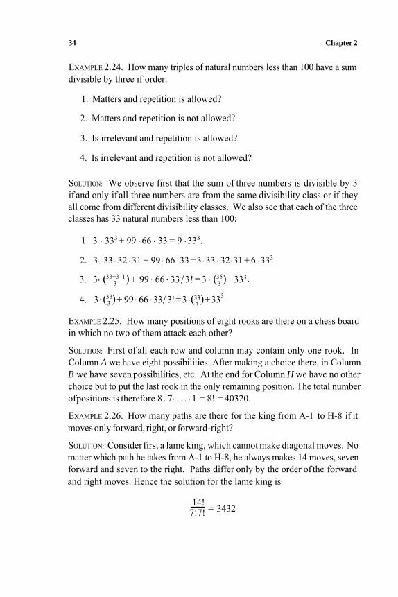
EXAMPLE 2.24. How many triples of natural numbers less than 100 have a sum divisible by three if order:
1. Matters and repetition is allowed?
2. Matters and repetition is not allowed?
3. Is irrelevant and repetition is allowed?
4. Is irrelevant and repetition is not allowed?
SOLUTION: We observe first that the sum of three numbers is divisible by 3if and only if all three numbers are from the same divisibility class or if they all come from different divisibility classes. We also see that each of the three classes has 33 natural numbers less than 100:
1. 3 . 333 + 99 . 66 . 33 = 9 .333.
2. 3. 33. 32. 31 + 99. 66 .33 =3. 33. 32.31 + 6 .333.
.33. 3. (33+3–13 ) + 99 . 66 . 33/3! = 3 . (35
3 )+ 33
4. 3. (333 )+ 99. 66 .33/ 3!=3.(33
3)+333.
EXAMPLE 2.25. How many positions of eight rooks are there on a chess board in which no two of them attack each other?
SOLUTION: First of all each row and column may contain only one rook. InColumn A we have eight possibilities. After making a choice there, in Column B we have seven possibilities, etc. At the end for Column H we have no otherchoice but to put the last rook in the only remaining position. The total numberofpositions is therefore 8 . 7. . . . . 1 = 8! = 40320.
EXAMPLE 2.26. How many paths are there for the king from A-1 to H-8 if itmoves only forward, right, or forward-right?
SOLUTION: Consider first a lame king, which cannot make diagonal moves. Nomatter which path he takes from A-1 to H-8, he always makes 14 moves, sevenforward and seven to the right. Paths differ only by the order of the forward and right moves. Hence the solution for the lame king is
14!7!7! = 3432
Combinatorics 35
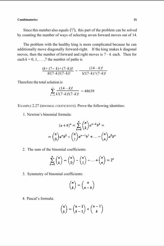
Since this number also equals (147 ), this part of the problem can be solved
by counting the number of ways of selecting seven forward moves out of 14.
The problem with the healthy king is more complicated because he can additionally move diagonally forward-right. If the king makes k diagonal moves, then the number of forward and right moves is 7 – k each. Then foreach k = 0, 1, . . . ,7 the number of paths is
(k+ (7- k)+ (7–k))! =(14 – k )!
k!(7–k )!(7–k)! k!(7–k) ! (7–k)!
Therefore the total solution is
EXAMPLE 2.27 (BINOMIAL COEFFICIENTS). Prove the following identities:
1. Newton’s binomial formula:
2. The sum of the binomial coefficients:
3. Symmetry of binomial coefficients:
4. Pascal’s formula:
(14 – k)!k!(7–k)!(7–k)!
= 48639 Σk = 0
7
36 Chapter 2
SOLUTION OF 1: Earlier we proved that the number of k-element subsets of an n-element set is
n!Cn
k = k! (n –k)!
We also mentioned that instead of the clumsy quotient of factorials, it ismore convenient to write
and that the numbers (nk) are called binomial coefficients. Now we see where
this name came from. Ifwe calculate (n
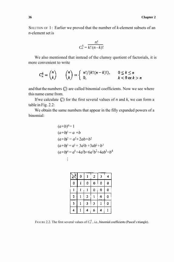
k) for the first several values of n and k, we can form a table in Fig. 2.2:
We obtain the same numbers that appear in the filly expanded powers of abinomial:
(a+b)0= 1(a+b)1 = a +b
(a+b)2 = a2+2ab+b2
(a+b)3 = a3 + 3a2b +3ab2 +b3
(a+b)4 = a4+4a3b+6a2b2+4ab3+b4
FIGURE 2.2. The first several values of Cnk , i.e., binomial coefficients (Pascal’s triangle).
.. .
Cornbinatorics 37
In general Newton’s binomial formula holds
This can be proved by mathematical induction (see Problem A.8, Appendix A) but also by using the following combinatorial thinking.
Expanding the expression (a + b)n yields a sum whose terms all have theform A kan–kbk, 0 ≤ k ≤ n, where the numbers Ak are called the binomialcoefficients. We next show that Ak equals the number of k-combinations of an n-element set.
In the equality:
the term an–kbk appears as many times as there are ways ofselecting k lettersb from n boxes. Also the order of boxes is not important because the order is irrelevant in multiplication; it always yields bk. Therefore the binomialcoefficients equal the number of k-combinations of an n-element set. In otherwords:
which justifies the name binomial coefficients.
SOLUTION OF 2: In Newton's binomial formula set a = b = 1 to obtain thedesired identity. Here is another, combinatorial proof: In Example 2.14 the total number of subsets ofan n-element set is 2n. We can enumerate them bycounting all k-element subsets for each k = 0,1 ,2, . . . , n, so we can write
SOLUTION OF 3: The symmetry of the binomial coefficients can be proved by algebraically manipulating the formulas. Here we prove it in a combinatorial manner: Every k-element subset is determined by the k elements it contains
38 Chapter 2
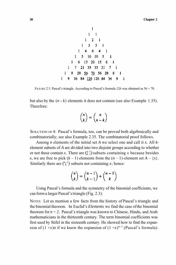
FIGURE 2.3. Pascal’s triangle. According to Pascal’s formula 126 was obtained as 56 + 70.
but also by the (n – k) elements it does not contain (see also Example 1.35).Therefore:
SOLUTION OF 4: Pascal’s formula, too, can be proved both algebraically and combinatorially; see also Example 2.35. The combinatorial proof follows.
Among n elements of the initial set A we select one and call it x. All k-element subsets of A are divided into two disjoint groups according to whetheror not these contain x. There are (n–1
k–1) subsets containing x because besides x, we are free to pick (k – 1) elements from the (n – 1)-element set A – x.Similarly there are (n–1
k ) subsets not containing x; hence:
Using Pascal’s formula and the symmetry of the binomial coefficients, we can form a larger Pascal’s triangle (Fig. 2.3):
NOTES: Let us mention a few facts from the history of Pascal’s triangle andthe binomial theorem. In Euclid’s Elements we find the case ofthe binomialtheorem for n = 2. Pascal’s triangle was known to Chinese, Hindu, and Arabmathematicians in the thirteenth century. The term binomial coefficients wasfirst used by Stifel in the sixteenth century. He showed how to find the expan-sion of (1 +x)n if we know the expansion of (1 +x)n–1 (Pascal’s formula).
Combinatorics 39
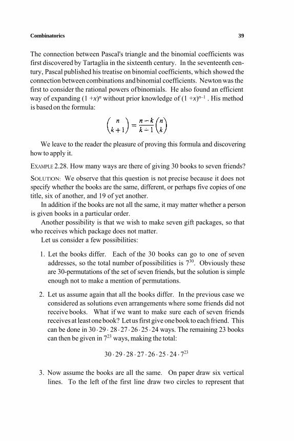
The connection between Pascal's triangle and the binomial coefficients was first discovered by Tartaglia in the sixteenth century. In the seventeenth cen-tury, Pascal published his treatise on binomial coefficients, which showed the connection between combinations and binomial coefficients. Newton was the first to consider the rational powers of binomials. He also found an efficient way of expanding (1 +x)n without prior knowledge of (1 +x)n–1 . His method is based on the formula:
We leave to the reader the pleasure of proving this formula and discovering how to apply it.
EXAMPLE 2.28. How many ways are there of giving 30 books to seven friends?
SOLUTION: We observe that this question is not precise because it does notspecify whether the books are the same, different, or perhaps five copies of onetitle, six of another, and 19 of yet another.
In addition if the books are not all the same, it may matter whether a person is given books in a particular order.
Another possibility is that we wish to make seven gift packages, so thatwho receives which package does not matter.
Let us consider a few possibilities:
1. Let the books differ. Each of the 30 books can go to one of seven addresses, so the total number of possibilities is 730. Obviously theseare 30-permutations of the set of seven friends, but the solution is simple enough not to make a mention of permutations.
2. Let us assume again that all the books differ. In the previous case we considered as solutions even arrangements where some friends did not receive books. What if we want to make sure each of seven friends receives at least one book? Let us first give one book to each friend. This can be done in 30 . 29 . 28 .27 .26 .25 . 24 ways. The remaining 23 books can then be given in 723 ways, making the total:
30 . 29 . 28 . 27 . 26 . 25 . 24 . 723
3. Now assume the books are all the same. On paper draw six verticallines. To the left of the first line draw two circles to represent that
40 Chapter 2
the first friend receives two copies. Draw five circles between the first and the second line to represent five copies given to the second friend. Continue like that, then finally draw one circle to the right of the last line for the one copy given to the seventh friend. There must be 30 circles. Every such arrangement of six lines and 30 circles uniquely represents one arrangement of the books. Note: Every book arrangement can beuniquely represented by one such diagram. The number of diagramswith lines and circles is 36!/(30!6!) = (36
30) = (366 ).
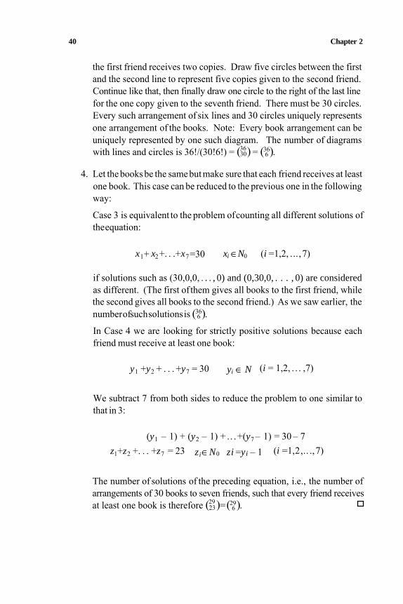
4. Let the books be the same but make sure that each friend receives at leastone book. This case can be reduced to the previous one in the following way:
Case 3 is equivalent to the problem of counting all different solutions of the equation:
x1+ x2+. . .+x7=30 xi ∈N0 (i = 1,2, . . . , 7)
if solutions such as (30,0,0, . . . , 0) and (0,30,0, . . . , 0) are considered
as different. (The first of them gives all books to the first friend, while the second gives all books to the second friend.) As we saw earlier, thenumberofsuchsolutionsis (36
6 ).In Case 4 we are looking for strictly positive solutions because each friend must receive at least one book:
y1 +y2 + . . . +y7 = 30 yi ∈ N (i = 1,2, . . . , 7)
We subtract 7 from both sides to reduce the problem to one similar to that in 3:
(y1 – 1) + (y2 – 1) + .. .+(y7 – 1) = 30 – 7z1+z2 +. . . +z7 = 23 zi∈N0 zi =yi – 1 (i =1, 2 , . . . , 7)
The number of solutions of the preceding equation, i.e., the number ofarrangements of 30 books to seven friends, such that every friend receivesat least one book is therefore (29
23)=(296 ).
Combinatorics 41
Among other things in Example 2.27 we saw that the equation:
x1+x2+... +xn = k xi ∈N0 (i = 1,2 , . . . ,n)
has (n+k–1k ) solutions. Among them some solutions can be considered equal,
e.g., (k, 0,0,. . . ,0) and (0,k, 0,. . . ,0), but in Example 2.27 we wanted to countthem as different.
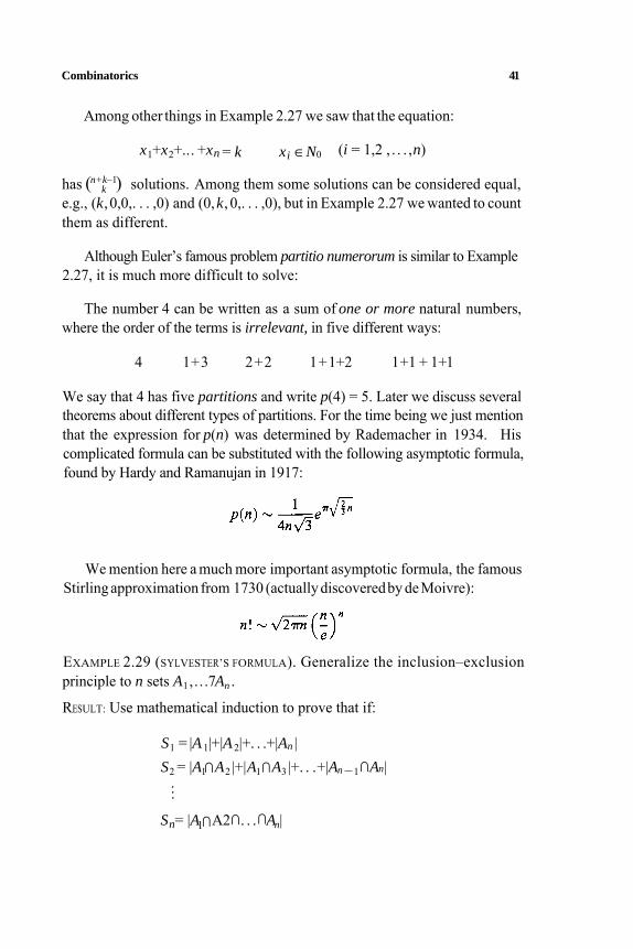
Although Euler’s famous problem partitio numerorum is similar to Example 2.27, it is much more difficult to solve:
The number 4 can be written as a sum of one or more natural numbers,where the order of the terms is irrelevant, in five different ways:
4 1+3 2+2 1+1+2 1+1 + 1+1
We say that 4 has five partitions and write p(4) = 5. Later we discuss several theorems about different types of partitions. For the time being we just mention that the expression for p(n) was determined by Rademacher in 1934. Hiscomplicated formula can be substituted with the following asymptotic formula,found by Hardy and Ramanujan in 1917:
We mention here a much more important asymptotic formula, the famous Stirling approximation from 1730 (actually discovered by de Moivre):
EXAMPLE 2.29 (SYLVESTER’S FORMULA). Generalize the inclusion–exclusion principle to n sets A1,. . .7An .
RESULT: Use mathematical induction to prove that if:
S1 = |A 1|+|A 2|+. . .+|An |S2 = |A1 ⊃ A2 |+|A1 ⊃ A3 |+. . .+|An –1 ⊃An|
..
.
Sn= |A1 ⊃A2 ⊃ . . . ⊃An|
42 Chapter 2
then:
|A1
⊃
A 2
⊃ . . . ⊃
An | = S1–S2+S3 – S4+. . . +(–1) n+1Sn =
This formula was also first discovered by de Moivre, but it bears Sylvester’sname because he often used it.
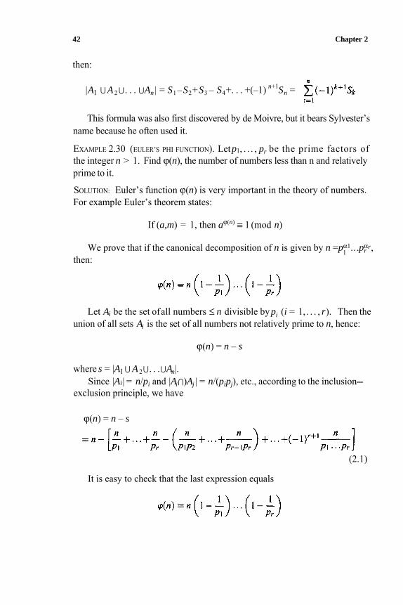
EXAMPLE 2.30 (EULER’S PHI FUNCTION). Letp1, . . . , pr be the prime factors ofthe integer n > 1. Find ϕ(n), the number of numbers less than n and relatively prime to it.
SOLUTION: Euler’s function ϕ(n) is very important in the theory of numbers. For example Euler’s theorem states:
If (a,m) = 1, then aϕ(n) ≡ 1 (mod n)
We prove that if the canonical decomposition of n is given by n =p1α1.. .pαr
r ,then:
Let Ai be the set ofall numbers ≤ n divisible bypi (i = 1, . . . , r). Then theunion of all sets Ai is the set of all numbers not relatively prime to n, hence:
ϕ(n) = n – s
where s = |A1
⊃
A 2
⊃ . . . ⊃ An|.
exclusion principle, we have Since |Ai| = n/pi and |Ai ⊃)Aj | = n/(pipj), etc., according to the inclusion-
ϕ(n) = n – s
(2.1)
It is easy to check that the last expression equals
Cornbinstorics 43
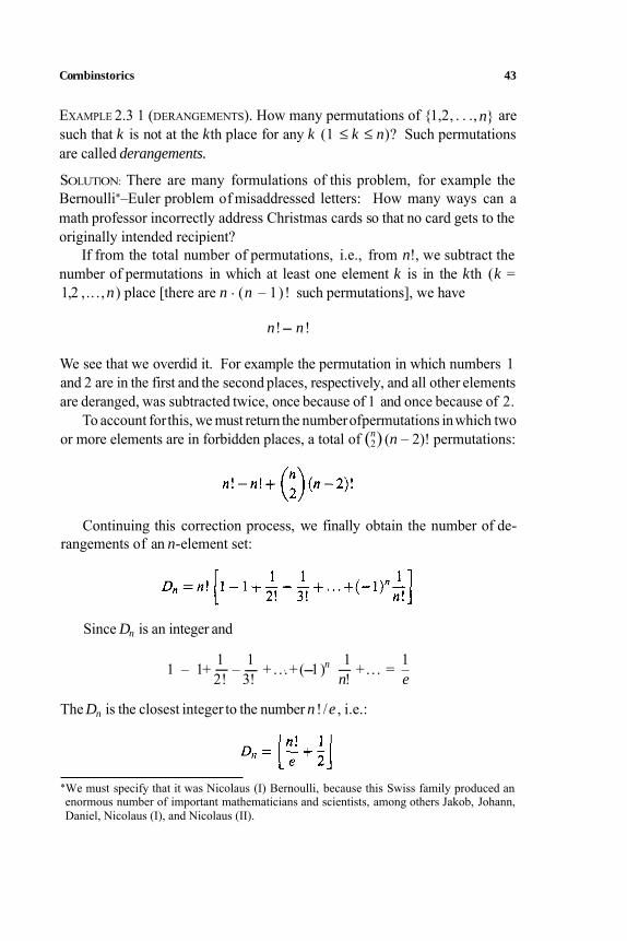
EXAMPLE 2.3 1 (DERANGEMENTS). How many permutations of 1,2, . . ., n aresuch that k is not at the kth place for any k (1 ≤ k ≤ n)? Such permutationsare called derangements.
SOLUTION: There are many formulations of this problem, for example theBernoulli*–Euler problem of misaddressed letters: How many ways can amath professor incorrectly address Christmas cards so that no card gets to theoriginally intended recipient?
If from the total number of permutations, i.e., from n!, we subtract the number of permutations in which at least one element k is in the kth (k =1,2 , .. . ,n) place [there are n . (n – 1)! such permutations], we have
n!- n!
We see that we overdid it. For example the permutation in which numbers 1and 2 are in the first and the second places, respectively, and all other elementsare deranged, was subtracted twice, once because of 1 and once because of 2.
To account forthis, we must return the numberofpermutations inwhich twoor more elements are in forbidden places, a total of (n
2) (n – 2)! permutations:
Continuing this correction process, we finally obtain the number of de-rangements of an n-element set:
Since Dn is an integer and
1 1 1 1n
2! 3! n! e1 – 1 + –- + -. . .+(-1) +. . . = –
The Dn is the closest integer to the number n ! /e , i.e.:
*We must specify that it was Nicolaus (I) Bernoulli, because this Swiss family produced anenormous number of important mathematicians and scientists, among others Jakob, Johann,Daniel, Nicolaus (I), and Nicolaus (II).
- -
44 Chapter2
where x is the first integer ≤ x.
We see that the probability of having all cards sent incorrectly is rather
large:
Dn 1— ≈ – = 0.36792 . . . n! e
The recursion for the number of derangements is Dn = (n – 1)(Dn –1 +
Dn–2), with D1 = 0 and D2 = 1. Other initial conditions give other solutions.
Fibonacci, better known among his contemporaries as Leonardo of Pisa or
Leonardo Pisano, is remembered today mostly for the sequence of numbers
appearing as a solution to his problem about rabbits. He published that problem
in his book Liber Abaci in 1202 (see Example 2.32). His contribution to
Western civilization however is much greater, for he insisted that Hindu-
Arabic numerals be used instead of Roman numerals. The change was difficult,
but succeeded because of the many advantages of Hindu–Arabic numerals in
calculating and accounting.
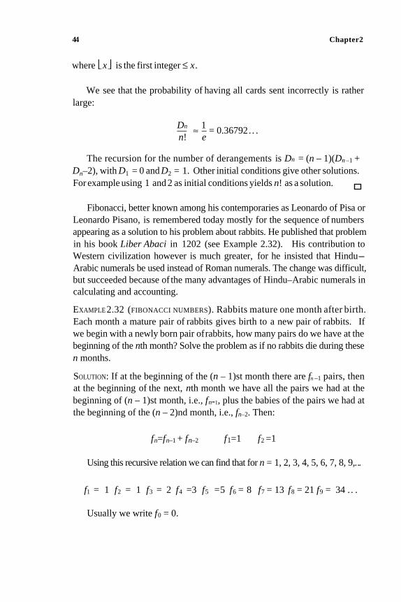
EXAMPLE 2.32 (FIBONACCI NUMBERS). Rabbits mature one month after birth.
Each month a mature pair of rabbits gives birth to a new pair of rabbits. If
we begin with a newly born pair of rabbits, how many pairs do we have at the
beginning of the nth month? Solve the problem as if no rabbits die during these
n months.
SOLUTION: If at the beginning of the (n – 1)st month there are fn –1 pairs, then
at the beginning of the next, nth month we have all the pairs we had at the
beginning of (n – 1)st month, i.e., fn-1, plus the babies of the pairs we had at
the beginning of the (n – 2)nd month, i.e., fn–2. Then:
For example using 1 and 2 as initial conditions yields n! as a solution.
fn=fn–1 + fn–2 f1=1 f2 =1
Using this recursive relation we can find that for n = 1, 2, 3, 4, 5, 6, 7, 8, 9, . . .
f1 = 1 f2 = 1 f3 = 2 f4 =3 f5 =5 f6 = 8 f7 = 13 f8 = 21 f9 = 34 . . .
Usually we write f0 = 0.
Combinatorics 45
NOTES: Fibonacci numbers posses a number of properties, which we investigat
to some extent here and in Appendix A. The recursion fn+1 =fn + fn–1 was
first used by Girard in 1634. Simson noted in 1753 that as n increases, the rati
fn+1/ fn converges to the golden section:
This ubiquitous sequence of numbers was given this name only in the
nineteenth century by the French mathematician Lucas.
Fibonacci numbers are often encountered in mathematical problems of
various kinds and in nature too. For example in a row of seeds in a sunflower
head, there is a Fibonacci number ofseeds, e.g., 55, even more but always one
Before we go on to generating functions, recall that Newton’s binomial
formula can be generalized using the Maclaurin series for (1 +x)α. According
to Maclaurin's formula and Abel’s convergence criterion, we find
of the numbers fn !!
α(α – 1.) . . . (α – k+ 1) xk+ . . . k!
α(α – 1) x2 +. . .+ 2
(1+x)α = 1+ αx +
(|x | < 1, α ∈ R)
When α = n, this expression has a finite number of terms, and it reduces
to Newton’s binomial formula.
2.4. Generating Functions
Besides the algebraic and combinatorial methods of proofs, there is the third
general method used in enumeration and to prove identities and properties of
binomial coefficients —the method of generating functions. Since many other
problems in mathematics can be solved by generating functions, we briefly
introduce this method, first used by de Moivre and later improved by Euler and
Laplace.
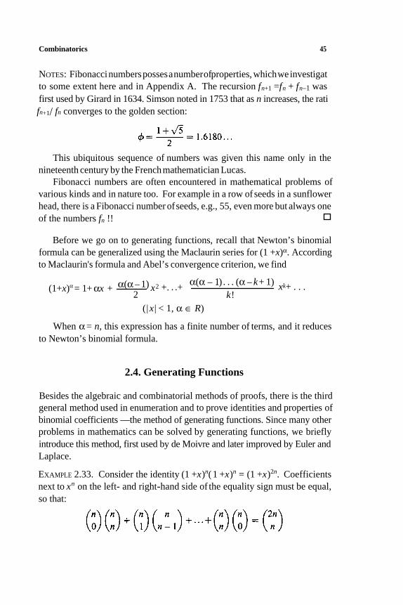
EXAMPLE 2.33. Consider the identity (1 +x)n( 1 +x)n = (1 +x)2n. Coefficients
next to xn on the left- and right-hand side of the equality sign must be equal,
so that:
46 Chapter 2
Since the binomial coefficients are symmetric, i.e., (nk) = ( n
n–k), we obtain the
identity:
That is,
Here we use the fact that in a power of a binomial all binomial coefficients
are hidden. We say that (1+ x)n generates the binomial coefficients or that it
is the generating function of the binomial coefficients. But before defining this
new terminology, let us consider a few more examples.
EXAMPLE 2.34. If we multiply three binomials:
(1 + ax) (1 + bx) (1 + cx) =1 + (a + b+ c)x + (ab+ac+bc)x2 + ab c x 3
next to xk (k = 0,1,2,3) we have all k-combinations of the set a,b,c.
Similarly in the product:
(1 + a1x) (1 + a2x). . .(1 + anx) =
= 1 + (a1 +. . . +an)x + (a1a2 + a1a3 +. . . +an –1an)x +. . . + a1. . . . anxn2
(2.2)
we find a list of all k-combinations of a1 ,a2 , . . . ,an next to xk (k = 0, 1, . . . , n).
To count them, we just set a1 = a2 = . . . = an = 1 and next to xk we can
find the number of k-combinations of an n-element set, a fact that we found
earlier from Newton’s binomial formula.
Thus we see that the function Cn(x) = (1 +x)n generates binomial coeffi-
cients (n0), (n
1), .. . , (nn) ; therefore it is called the generating function of binomial
coefficients.
EXAMPLE 2.35 (AGAIN PASCAL’S FORMULA). From Cn(x) = (1 +x)n it follows
that:
Cn(x) = (1+x)Cn–1 (x) = Cn–1(x) +xCn–1(x)
Combinatorics 47
Equating coefficients next to xk on the two sides, we obtain Pascal’s formula:
EXAMPLE 2.36. What happens if we multiply (1 +ax + a2x2) (1 + bx )(1 + cx)?
(1+ax+a2x 2)(1+bx )(1+cx ) =
= 1 + (a +b +c)x + (a2 +ab +ac + bc)x2 + (a2b +a2c +abc)x3 +a2bcx4
(2.3)
Coefficients next to xk list combinations neither with nor without repetition
in some kind of hybrid combinations in which the element a can be repeated at
most twice. To enumerate how many such combinations there are, it suffices
to set a = b = c= 1, then to examine the coefficient next to the corresponding
power xk.
EXAMPLE 2.37 (AGAIN COMBINATIONS WITH REPETITIONS). From the previous
example we can learn that to construct a generating function for combinations
with repetitions, we must allow every element to appear an arbitrary number of
times. Hence the generating function for combinations with repetition of the
seta,b ,c is
(1 +ax + a2x2 + . . . )( 1 + bx + b2x2 + . . .)( 1 + cx+ c2x2 +. . . )
To see their numbers, set a = b = c = 1 and observe the corresponding coeffi-
cients.
In general the generating function for the number of k-combinations with
repetition of an n-element set is
–= (1- x )nCf l ( x ) = ( l + x + x 2 + . . . )n =
– 1
(1 –x)n
As we mentioned earlier, according to Maclaurin’s formula, we have
That is,
48 Chapter2
We could have expected this result from our earlier derivations.
EXAMPLE 2.38. Let us try a small experiment again. What kinds of problems
can be solved by the following generating function:
(1 +x +x2 +x3 +x4 +x2 +x6 + . . . ) (1 +x2 +x4 +x6 +x8 +x10 +x12 + . . . )
= 1 + x +2x2 +ax3 + 3x4 + 3x5 +4x6 +. . .
The fact that the coefficient next to x5 equals 3, tells us that x5 was produced
in three different ways, namely:
x5 . 1 +x3x2 +xx 4
This reminds us that number 5 can be represented by using only numbers
1 and 2 in exactly three ways:
1 + 1+1 +1+1 1+ 1 +1 + 2 1 + 2 +2
Example 2.38 suggests a way of determining the generating function for
the number of partitions of the integer n. Recall that the partition of n is
any particular way of writing n as a sum of one or more positive integers. It
is important to emphasize that the order of terms is irrelevant, for example
1 + 3 +4 and 1 +4 + 3 represent the same partition of 8.
The generating function of the sequence p(n) is
P(x) = (1 + x + x2+. . . ) (1+x2+x4+. . .) (1+x 2 +x 6 + . . . ) ×× (1 + x 4 + x 8 +. . . ) . . .
That is,
1 1 11P(x) =
1– x 1– x 2 1 – x3 1 – x 4.. .
By expanding this formula and using number theory, Hardy and Ramanujan
derived their approximation.
Let us take a look at some other types of partitions.
Combinatorics 49
EXAMPLE 2.39. The generating function for partitions using numbers a, b, c,and d, such that a may be used an arbitrary number of times, b can be used at
most three times, c must be used at least twice, while d must be used an even
number of times is
(1 +xa +x2a + . . . )(1 +xb +x2b +x3b)(x2c +x3c + . . . ) (1 +x2d +x4d + . . . )
EXAMPLE 2.40 (CHANGE). The number of ways of making change for 1 dinar
using an arbitrary number of coins of 1, 2, 5, 10, 20, and 50 paras can be
calculated as the coefficient next to x100 in the expansion of the following
generating function:
(1+x + . . . ) ( 1 + x 2 + . . .) (1+x5+...) ×× (1 +x10+. . .)(1 +x20 +. . .)(1 +x50 +. . .)
Using polynomial multiplication, the computer gives us the solution of
4562 ways of making change for 1 dinar.
EXAMPLE 2.41 (EULER’S THEOREM ABOUT PARTITIONS). we prove that the num-
ber of partitions using different natural numbers, pr(n), equals the number
of partitions using (not necessarily different) odd numbers, pn(n). The proof
shows that two sequences pr(n) and Pn(n) have the same generating func-
tions. Indeed:
Pr(x ) = (1+x)(1+x2)(1+x3)(1+x4) . . .
while
1 1 1 1Pn(x)
(1–x) (1–x3) (1–x5) (1–x7). . .
Since
1-x2k1+x (k = 1,2, . . .)k
1- xk
after appropriate cancellations, we find Pr (x) = Pn (x), i.e., pr (n) = pn (n).
=
=
50 Chapter2
Definition 2.7 formally defines generating functions.
DEFINITION 2.7. Generating function of the sequence (a0,a1, . . . ,ak,. . . ) is the
power series:
kA (x) = a0 + a1x + . . . +akx +. . .
EXAMPLE 2.42. Examples follow of some sequences and their generating func-
tions:
(1,0,0,1,0,0 , . ..) ↔ 1+x3
(1,1,1,1,1,1,. ..) ↔ 1+x+x +x +. . . =
(1,0,1,0,1,0, ...) ↔ 1+x2+x4+x6+ . . . =
2 3 1
1 – x1
1–x2
1(1,2,3,4,5,6, ...) ↔ 1+2x+3x2+4x3+... =
(0,1,2,3,4,5, ...) ↔ x+2 x2+3 x3+4x4+. .. =
(1 – x)2
(1 –x)2
x
x2 x3 x4
2! 3! 4! 2! 3! 4!(l ,1,-,-,- )... ↔ l+x +-+-+ - + .. . = ex11
((n0), (
n1), (n
2), . . . , (nn))↔ (1+x)n
,
It is often useful to form the generating function of a sequence to see what
can be accomplished through its transformations. Examples 2.43 and 2.44 use
this approach to investigate Fibonacci numbers.
EXAMPLE 2.43. Generating function for the sequence of Fibonacci numbers is
F(x) =f0 +f1x +f2x2 + . . .
Since x F(x) = f0x +f1x2 +f2x3 +. . . and x2F(x) = f 0x2 +f1x3 +f2 x4 + . . .
while f0 = 0,f1 = 1, and for n ≥ 2 we have fn =fn–1 +fn –2, we find that:
F(x) – xF(x) – x2F(x) = x
That is,
xF(x ) =
1–x –x 2
1
Combinatorics 51
Reciprocals of roots of the trinomial in the denominator of F(x) are φ (the
golden section) and = – 1 /φ: φ∧
If F(x) is written in the form of partial fractions, we find that:
That is,
which finally yields
This implies
That is,
NOTES: This formula was derived by de Moivre in 1718. Historically this was
the first known use of generating functions. A different proof was given by
Nicolaus (I) Bernoulli in 1728, and it was first published by Euler in 1765.
The proof was later forgotten, then rediscovered by Binet in 1843. Today it is
called Binet’s formula. The number φ= 1.61803 . . . is called the golden section, and it is also
denoted as g or τ. The notation φ is used in honor of Phidias, the Ancient
Greek sculptor, who believed that objects having proportions dominated by
52 Chapter 2
the golden section were most pleasing to the eye. The number φ, just like
Fibonacci numbers, is encountered very often, not only in mathematics but
also in the natural sciences and the arts. See Appendix B for more about this
and some other important numbers.
we see that fn is the integer closest to i.e.,
Since Fibonacci numbers are integers, and for n ≥ 0 we have
EXAMPLE 2.44. If we write F(x) in the following form:
xF(x) = =x1 + [x(1 +x)] + [x(1 + x)]2 +. . .
x1 –x –x2
1 –x(1 +x)
we easily find that:
=
For example:
Generating functions have many other properties and applications, espe-
cially in probability theory, solving recursions, and such engineering disci-
plines, as communications and digital signal processing, where they are called
the z-transform.
2.5. Problems
EXAMPLE 2.45. There are 100 competitors in a tennis tournament. The com-
petition is organized as a cup, i.e., the competitor who looses a match must
leave the tournament. How many matches must be played before we know the
winner of the tournament?
SOLUTION: Instead of considering all possible ways of organizing matches
among competitors, it suffices to note that every match eliminates one player.
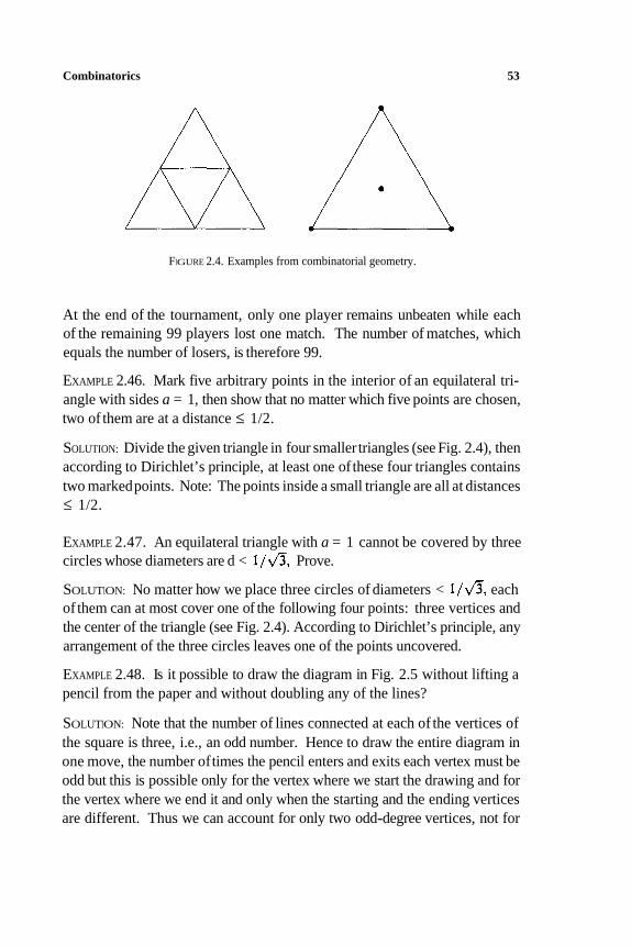
Combinatorics 53
FIGURE 2.4. Examples from combinatorial geometry.
At the end of the tournament, only one player remains unbeaten while each
of the remaining 99 players lost one match. The number of matches, which
equals the number of losers, is therefore 99.
EXAMPLE 2.46. Mark five arbitrary points in the interior of an equilateral tri-
angle with sides a = 1, then show that no matter which five points are chosen,
two of them are at a distance ≤ 1/2.
SOLUTION: Divide the given triangle in four smaller triangles (see Fig. 2.4), then
according to Dirichlet’s principle, at least one of these four triangles contains
two markedpoints. Note: The points inside a small triangle are all at distances
≤ 1/2.
EXAMPLE 2.47. An equilateral triangle with a = 1 cannot be covered by three
circles whose diameters are d < 1 Prove.
SOLUTION: No matter how we place three circles of diameters < each
of them can at most cover one of the following four points: three vertices and
the center of the triangle (see Fig. 2.4). According to Dirichlet’s principle, any
arrangement of the three circles leaves one of the points uncovered.
EXAMPLE 2.48. Is it possible to draw the diagram in Fig. 2.5 without lifting a
pencil from the paper and without doubling any of the lines?
SOLUTION: Note that the number of lines connected at each of the vertices of
the square is three, i.e., an odd number. Hence to draw the entire diagram in
one move, the number oftimes the pencil enters and exits each vertex must be
odd but this is possible only for the vertex where we start the drawing and for
the vertex where we end it and only when the starting and the ending vertices
are different. Thus we can account for only two odd-degree vertices, not for
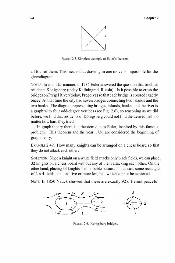
54 Chapter 2
FIGURE 2.5. Simplest example of Euler’s theorem.
all four of them. This means that drawing in one move is impossible for the given diagram.
NOTES: In a similar manner, in 1736 Euler answered the question that troubled residents Königsberg (today Kaliningrad, Russia): Is it possible to cross the bridges on Pregel River (today, Pregolya) so that each bridge is crossed exactly once? At that time the city had seven bridges connecting two islands and the two banks. The diagram representing bridges, islands, banks, and the river is a graph with four odd-degree vertices (see Fig. 2.6), so reasoning as we did before, we find that residents of Königsberg could not find the desired path no matter how hard they tried.
In graph theory there is a theorem due to Euler, inspired by this famous problem. This theorem and the year 1736 are considered the beginning of graph theory.
EXAMPLE 2.49. How many knights can be arranged on a chess board so thatthey do not attack each other?
SOLUTION: Since a knight on a white field attacks only black fields, we can place32 knights on a chess board without any of them attacking each other. On theother hand, placing 33 knights is impossible because in that case some rectangleof 2 × 4 fields contains five or more knights, which cannot be achieved.
NOTE: In 1850 Nauck showed that there are exactly 92 different peaceful
FIGURE 2.6. Königsberg bridges.
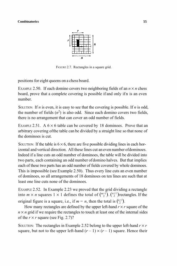
Combinatorics 55
FIGURE 2.7. Rectangles in a square grid.
positions for eight queens on a chess board.
EXAMPLE 2.50. If each domino covers two neighboring fields of an n × n chess board, prove that a complete covering is possible if and only if n is an even number.
SOLUTION: If n is even, it is easy to see that the covering is possible. If n is odd,the number of fields (n2) is also odd. Since each domino covers two fields,there is no arrangement that can cover an odd number of fields.
EXAMPLE 2.51. A 6 × 6 table can be covered by 18 dominoes. Prove that anarbitrary covering of the table can be divided by a straight line so that none of the dominoes is cut.
SOLUTION: If the table is 6 × 6, there are five possible dividing lines in each hor-izontal and vertical direction. All these lines cut an even number of dominoes. Indeed if a line cuts an odd number of dominoes, the table will be divided into two parts, each containing an odd number of domino halves. But that implies each of these two parts has an odd number of fields covered by whole dominoes. This is impossible (see Example 2.50). Thus every line cuts an even number of dominoes, so all arrangements of 18 dominoes on ten lines are such that at least one line cuts none of the dominoes.
EXAMPLE 2.52. In Example 2.23 we proved that the grid dividing a rectangle into m × n squares 1 × 1 defines the total of (m+1
2 ). (n+12 )rectangles. If the
original figure is a square, i.e., if m = n, then the total is (n+12 ).
How many rectangles are defined by the upper left-hand r × r square of then × n grid if we require the rectangles to touch at least one of the internal sidesof the r × r square (see Fig. 2.7)?
SOLUTION: The rectangles in Example 2.52 belong to the upper left-hand r × rsquare, but not to the upper left-hand (r – 1) × (r – 1) square. Hence their
56 Chapter 2
number is
NOTE: The total number of rectangles (n+12 )2 can be written as the sum of
numbers for upper left-hand r × r squares for all values of r (r = 1,2, . . . , n ).Thus we find that:
On the other hand since:
n(n + 1)1+2 +. . . + n =-2
we just found a combinatorial proof of an interesting identity:
(1 + 2 + . . . + n ) 2 = 13 + 23 + . . . + n 3
EXAMPLE 2.53. How many ways can eight rooks be placed on a chess boardso that they do not attack each other and none of them occupies a field on the main diagonal (the one connecting A-1 and H-8)?
RESULT: From the formula for derangements:
EXAMPLE 2.54. Prove that:
COMBINATORIAL PROOF: Earlier we showed that:
Combinatorics 57
In Example 1.39 we saw that the number of subsets of A = (a1 , . . . ,an witheven cardinalities equals the number of its subsets with odd cardinalities.
The number of even subsets is
The number of odd subsets is
Since these add up to 2n, there are 2n/2 = 2n–1 of each kind.
ALGEBRAIC PROOF: In Newton’s binomial formula, set a = b = 1 to find
while a = 1 and b = – 1 yields
Adding and subtracting these two identities yields
and
EXAMPLE 2.55. Show that:
58 Chapter 2
COMBINATORIAL PROOF:
= number of k-element subsets among which the smallest is 1
+number of k-element subsets among which the smallest is 2...
+number of k-element subsets among which the smallest is n – k + 1
ALGEBRAIC PROOF: This identity is easily proved by mathematical induction.For the first several cases:
Assume
Then using Pascal’s formula
ANOTHER PROOF: The third solution is based on the generating function for the
Combinatorics 59
sequence of binomial coefficients:
Equating the coefficients of xk we obtain
EXAMPLE 2.56 (LEIBNIZ’S FORMULA). If h(r)(x) denotes the rth derivative ofh(x), show that the nth derivative of the product of functions f (x) and g(x)(having all necessary derivatives) can be expressed using Leibniz’s formula:
HINT: Use mathematical induction.
EXAMPLE 2.57 (VANDERMONDE’S FORMULA). For an integer r > 0 the falling factorial of a real number a is
In addition:
ar = a(a – 1). . .(a – r + 1)-
a0– = 1
Prove Vandermonde’s formula:
HINT: Use mathematical induction.
60 Chapter 2
EXAMPLE 2.58 (FERMAT’S LESSER THEOREM). Assume a very large number ofballs are available, each of which is colored by one of n colors. Also let p be some prime number. Find the number of different circular arrangements of pballs except those where all balls are the same color.
SOLUTION: If the balls are arranged in a line, there will be np – n differentarrangements. Since p is a prime, exactly p different linear arrangementscorrespond to one circular arrangement; therefore the solution is
np – nP
NOTES: This is a combinatorial proof of Fermat’s lesser theorem from thenumber theory, which states that:
For n ∈ N and arbitrary prime p:
np ≡ n (mod p)
That is, the numbers np and n have the same remainder after division by p.
NOTES: Why is it important to consider only prime p? Does it follow from asimilar problem that does not exclude arrangements of equally colored balls that np is divisible byp? Let us also mention that Fermat’s lesser theorem isa special case of Euler’s theorem, already mentioned in Example 2.30. See Chapter 3 for more about these theorems.
EXAMPLE 2.59. How many ways are there of selecting two disjoint subsets ofthe n-element setA?
SOLUTION: Let the first subset have k elements, 0 ≤ k ≤ n. It can be chosen in (n
k ) ways. The second subset must be disjoint with the first; therefore itselements can be chosen from (n – k) remaining elements of A . The totalnumber of choices for the second set is then 2n–k. Hence if the first subsethas k elements, the total number of choices of two disjoint subsets of A is(n
k) .2n–k, When we sum the corresponding numbers for all allowable ks, i.e.,for k = 0,1, . . . , n we have
Combinatorics 61
The last equality was obtained from Newton’s binomial formula, with a = 2,b = 1.
We are not done yet, however. Except in the case when both sets are empty, we counted every other choice twice. Therefore the final solution is
3n+ 12
The following three examples show three important probability distribu-tions used in statistical physics. In all three examples we:
1. Start from simple physical models and assumptions.
2. Use combinatorics to find the numbers of different states of systems as functions of particular distributions of particles over the energies.
3. Find those distributions that maximize the numbers of possible states.
The distributions thus obtained are most often involved in macroscopic mea-surements. Equivalently these are distributions with maximum entropy.
EXAMPLE 2.60 (MAXWELL–BOLTZMANN STATISTICS). The following assump-tions form this model:
• The particles are distinguishable.
• There are ni particles with energy Ei, where i = 1,2,3, . . .
• Every energy level Ei has gi sublevels (phase cells).
• The number of particles that can be found at sublevels with energy Ei is limited by only the number of particles ni on that level.
• The following conditions are satisfied
nl +n2 +n3 + . . . = N n1E1 +n2E2 +n3E3 +. . . = Etot
According to these assumptions, if the distribution of particles over theenergies is known, i.e., if the numbers ni are known, the number of differentarrangements of the particles is
62 Chapter 2
To find the particular distribution that maximizes the number of statesPMB ,we introduce two approximations. We justify these by the fact that the system typically contains very large numbers of particles, e.g., N ≈ 1023, and everylevel has many sublevels, e.g., gi ≈ 108.
For large values of r, Stirling’s approximation for r!:
yields
lnr !≈ rln r - r
Later instead ofa discrete distribution ni over energies Ei (i = 1,2,3, . . , ),
Based on the preceding assumptions and using the method of Lagrange we use a continuous distribution n(E).
multipliers, we find that the number ofstates PMB is maximized by:
NkT
where N is the total number of particles in the system, k is Boltzmann’sconstant, and T is the absolute temperature of the system.
This distribution was first discovered by Boltzmann in 1896. Maxwell’sdistribution of particles over the velocities, first derived by Maxwell in 1860, can be derived from it.
EXAMPLE 2.6 1 (BOSE–EINSTEIN STATISTICS). This model is based on the follow-ing assumptions:
n(E) =-e-E/kT
• The particles are indistinguishable.
• There are ni particles with energy Ei, where i = 1 ,2,3,. . .
• Every energy-levelEi hasgi sublevels.
• The number ofparticles that can be found at sublevels with energy Ei islimited by only the number of particles ni on that level.
• The following conditions are satisfied
n1 + n 2 +n 3+. . . = N n1E1 + n 2 E 2 +n 3 E 3 +. . . = Etot
Combinatorics 63
From these assumptions we find
. . . . (n1 +g1 – 1)! . (n2+g2 – 1) ! . (n3 +g3 – 1)!n1!(g1 – 1)! n2!(g2– 1)! n3!(g3 – 1)!PBA (n1,n2 ,n3 ,. . .) =
This time the distribution n(E) maximizing the number of states PBA is
1n(E ) ~ e(E–EB)/kT – 1
where EB is the Bose energy (Bose level) and T is the absolute temperature. Particles obeying this statistic are called bosons. For example photons andatoms ofhelium He4 at low temperatures are bosons. At temperatures aboveseveral kelvins, the Bose–Einstein distribution for He4 atoms becomes practi-cally indistinguishable from the classical Maxwell–Boltzmann distribution.
This distribution was first found by Bose in 1924; it was published with help from Einstein.
EXAMPLE 2.62 (FERMI–DIRAC STATISTICS). This model is based on the fol-lowing assumptions:
• The particles are indistinguishable.
• There are ni particles with energy Ei, where i = 1,2,3, . . .
• Every energy level Ei has gi sublevels.
• The number of particles that can be found at sublevels with energy Ei
is limited by Pauli’s exclusion principle: Every sublevel may contain at most one particle. (The assumption about the indistinguishability of particles is actually the second part of Pauli’s principle.)
• The following conditions hold
n1 + n2 + n3 + . . . = N n1E1 +n2E2 + n3E3 + . . . = Etot
Based on the preceding we find
64 Chapter 2
The distribution that maximizes the number ofstates PFD is
1n(E) ~ e(E–EF)/kT +1
where EF is the so-called Fermi energy (Fermi level) and is the absoluteTtemperature. Particles obeying this distribution are called fermions. For
example electron gas in metals obeys it even at room temperatures. Only
at temperatures of 104 K does electron gas behave as an ideal gas, i.e.,
according to the Maxwell–Boltzmann distribution. Helium He3 atoms at
temperatures of a few kelvins are fermions, while at higher temperatures
differences between Fermi–Dirac and Maxwell–Boltzmann distributions dis-
appear.
This distribution was discovered by Fermi and Dirac in 1926.
EXAMPLE 2.63 (HAMMING’S FORMULA). Digital systems for handling informa-
tion have many advantages over analog systems. One such advantage is the
possibility of protection from damaging noise. A few instances where these
error-correcting systems are used include CD players, computer and commu-
nication networks, and interplanetary image and data transfer.
We consider here a very simple code capable of error detection and even
error correction.
Suppose we examine in detail information transfer conditions, then decide
to use the transmitter of a power sufficient to ensure that when any of 2n possible
length-n binary words is transmitted, there is a small probability that some
binary digits will be received incorrectly. Let us assume that the transmitter
power is chosen so that the probability of more than r errors happening is
practically zero.
If we choose to use only M length-n binary words out of 2n, then if at the
receiver we receive some words not in our vocabulary, we can be sure that an
error occurred. This is called error detection. We can do even more, however.
If we carefully pick the number M and words in the vocabulary, then we can
also correct the occurrence of r (or less) errors. For example let n = 8, and let
us find M such that our code can correct r = 2 errors. If one of the words is
00111100, then our system will operate so that if it receives some word from
the 2-neighborhood of 00111100, these all being words that differ from this
one at 0, 1, or 2 binary places, it recognizes that the originally transmitted word
was 00111100.
Combinatorics 65
Every r-neighborhood has the following number of words:
Hence M must satisfy the Hamming formula:
2n
(0n)+ (n
1)+ . . . + (nr )
M ≤
For the system in our example to correct r = 2 errors, among all
28 = 256 possible words, we can use at most M = 256/(1 + 8 + 28) = 6
binary words.
The problem of choosing those M words cannot be discussed here. Let
us just note that the number of binary digits that differ in two binary words
is called the Hamming distance of these two words.
EXAMPLE 2.64 (TOWERS OF HANOI). One of three vertical sticks has n disks, so
placed that the largest disk is at the bottom and remaining disks are stacked in
decreasing order. The problem is to move the disks to another stick in as few
moves as possible and with an additional requirement: At all times, each stick
must have disks stacked in decreasing order.
The story following this 1883 problem by Lucas relates that at the beginning
of time, God Brahma put 64 golden disks on one of three diamond needles, then
ordered his priests to move them to another needle and always to be careful not
to put larger disk above smaller. When the priests finish their job, Brahma's
tower will crumble, and the world will end.
SOLUTION: Let Tn denote the minimum number ofmoves needed to move ndisks according to the preceding rules. According to these rules, at the moment
we move the largest disk from Stick 1 to Stick 3, all other disks must be stacked
at Stick 2 in decreasing order. To accomplish this, we needed Tn–1 moves.
These must be followed by moving the largest disk and by additional Tn–1
moves to place (n – 1) smaller disks over it (see Fig. 2.8). Thus we obtain the
following recursion:
Tn= 2Tn –1+1 (n >1) T1 = 1
The solution ofthis recursion is Tn = 2n
– 1, which means that Brahma’s
priests can accomplish their task in 264 – 1 moves. If each move requires 1
second, the time needed is around 5.85.1011 years!
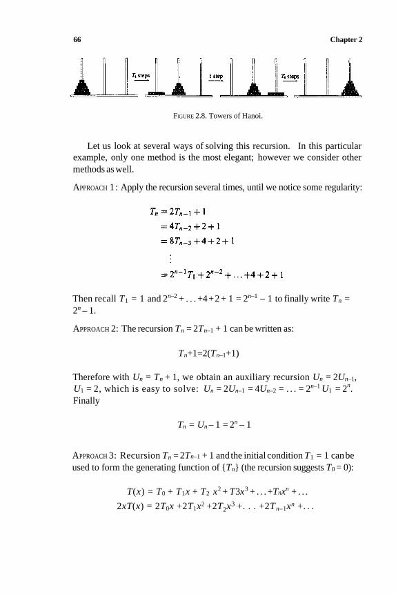
66 Chapter 2
FIGURE 2.8. Towers of Hanoi.
Let us look at several ways of solving this recursion. In this particular
example, only one method is the most elegant; however we consider other
methods as well.
APPROACH 1: Apply the recursion several times, until we notice some regularity:
Then recall T1 = 1 and 2n–2 + . . . +4+2 + 1 = 2n–1 – 1 to finally write Tn =
2n – 1.
APPROACH 2: The recursion Tn = 2Tn–1 + 1 can be written as:
Tn+1=2(Tn–1+1)
Therefore with Un = Tn + 1, we obtain an auxiliary recursion Un = 2Un–1,
U1 = 2, which is easy to solve: Un = 2Un–1 = 4Un–2 = . . . = 2n–1 U1 = 2n.
Finally
Tn = Un – 1 = 2n – 1
APPROACH 3: Recursion Tn = 2Tn–1 + 1 and the initial condition T1 = 1 canbe
used to form the generating function of Tn (the recursion suggests T0 = 0):
T(x) = T0 + T1x + T2 x2 + T3x3 + . . .+Tnxn + . . .
2xT(x) = 2T0x +2T1x2 +2T2x3 +. . . +2Tn–1xn +. . .
Combinatorics 67
Hence:
T(x) – 2xT (x) = T0 +x +x2 +x3 + . . . +xn + . . .
That is,
Since
we find
T(x) = (1 +2x + (2x)2
+ (2x)3 +. . .+(2x)n +. . .)
–(1 + x + x 2+ x 3 +. . . + xn + . . .)
Finally:
xT(x) =
(1 – 2 x ) (1 – x)
1 1 =x(1–2 x) (1–x) 1–2x 1– x
T(x) = (2-1)x + ( 22 –1) x 2 + (23– 1) x3 + . . . + ( 2n
–1)xn + . . .
which implies
Tn = 2n– 1
EXAMPLE 2.65 (POLYNOMIAL FORMULA). This example shows the combinatorial
derivation of the formula for the power of a polynomial:
(a1 +a2 +. . .+ar)n
A typical term in its full expansion has the following form:
where k1 +k2 + . . . +kr = n. The only remaining problem is to find how many
times each of these terms appears.
Term a1 can be selected k1 times from n boxes, i.e., in (nk1) ways. Then
term a2 can be selected k2 times from the remaining n – k1 boxes, i.e., in (n–k1k2 )
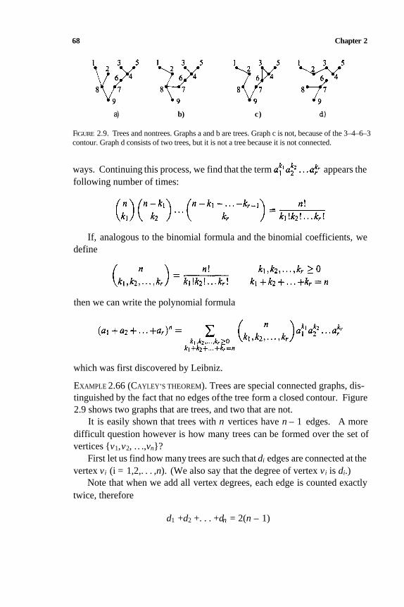
68 Chapter 2
a) b) c) d)
FIGURE 2.9. Trees and nontrees. Graphs a and b are trees. Graph c is not, because of the 3–4–6–3
contour. Graph d consists of two trees, but it is not a tree because it is not connected.
ways. Continuing this process, we find that the term appears the
following number of times:
If, analogous to the binomial formula and the binomial coefficients, we
define
then we can write the polynomial formula
which was first discovered by Leibniz.
EXAMPLE 2.66 (CAYLEY’S THEOREM). Trees are special connected graphs, dis-
tinguished by the fact that no edges of the tree form a closed contour. Figure
2.9 shows two graphs that are trees, and two that are not.
It is easily shown that trees with n vertices have n – 1 edges. A more
difficult question however is how many trees can be formed over the set of
vertices v1,v2, . . .,vn?
First let us find how many trees are such that di edges are connected at the
vertex vi (i = 1,2,. . . ,n). (We also say that the degree of vertex vi is di.)
Note that when we add all vertex degrees, each edge is counted exactly
twice, therefore
d1 +d2 +. . . +dn = 2(n – 1)
Combinatorics 69
The next step is the inductive proof (not quite trivial) that there are
trees whose vertex vi has degree di (i = 1,. . . ,n), so that the total number of
trees with n vertices is
This sum can be simplified if we write
ki =di –1 (i= 1,2, .. . , n)
then use the polynomial formula for a1 = . . . = an = 1:
This ends the proof of Cayley’s theorem.
NOTE: Enumerating all isomers of the saturated carbo-hydrates CnH2n+2 is a
much more difficult problem, and it requires using Polya’s theorem because
while Cayley’s theorem holds for graphs whose vertices are distinguishable
(labeled graph), carbon and hydrogen atoms are not distinguishable inside their
species (unlabeled graph).
EXAMPLE 2.67. 1. How many elements does P(A), the partitive set of the
n-element set A, have? How many elements are there in the Cartesian
product A × A? How many relations are there over the set A?
2. How many reflexive relations exist over an n-element set?
3. How many symmetric relations exist over an n-element set?
4. How many antisymmetric relations exist over an n-element set?
5. How many relations that are both symmetric and antisymmetric exist
over an n-element set?
70 Chapter 2
RESULTS:
1. 2n,n2,2n2=2n. 4 (
n2) .
2. 2n2–n= 4(n2).
3. 2n .2 (n2).
4. 2n.3(n2 ) .
5. 2n.
EXAMPLE 2.68. Let P(m,n) be the number of ways of obtaining m as the sum
after rolling n differently colored dice. Determine the generating function for
the sequence P(m,n).
SOLUTION: Since the dice are colored differently the following outcomes are
considered as different
1,1, . . . , 1, 2 2,1 , . . . ,1,1
With a little inspiration, we find the generating function:
G(x) = (x +x2+x3
+x4+x5
+x6)n
where the coefficient next toxm represents the number of outcomes having the
summ.
EXAMPLE 2.69. Assume we are rolling n mutually indistinguishable dice at
once.
1. How many different outcomes are possible?
2. How many ways are there of obtaining the outcome described by the
multiset ⟨1,1, . . . , 1,2⟩?
3. How many different sums are possible?
4. How many different outcomes give sum m? Which sum is produced by
the largest number of outcomes? Is that sum the most probable?
Combinatorics 71
SOLUTIONS:
1. Since the dice are indistinguishable and each can have an outcome
1, 2, 3, 4, 5, or 6, we are working with the n-combinations with repe-
titions of a six-element set, and the answer is (n+5
5 ).
2. This outcome is much more probable than the outcome where all dice
show 1, because all 1 scan be obtained in only one way. The outcome de-
scribedbythe multiset ⟨1, l, . . . , l,2⟩ canbe obtained inn ways, although
we cannot distinguish among them. (The dice are indistinguishable, and
they are rolled simultaneously).
3. All sums from 1 + 1 + ...+ 1 = n to 6+ 6 +. . .+6 = 6n are possible, so
the answer is 6n –n + 1 = 5n + 1.
4. If m < n, or m > 6n, none of the outcomes can have the sum m. Only
one outcome yields sum m = n; also only one yields the sum m = n+ 1,
although the latter is much more probable. Two outcomes produced
the sum m = n + 2. They are described by multisets ⟨1, 1, . . . ,1,3⟩and ⟨1,1, . . . ,2,2⟩. Thus while the sequence begins as the Fibonacci
sequence:
0 , . . ., 0, 1, 1, 2, 3, 5
that is where similarities stop, because the next numbers are 7, 10, 13,
18, 23, 29, 35, . . .
With a little luck and imagination we come up with the following generating
function:
G(x) = ( 1 +x +x2 + . . . ) ( 1 +x2 +x4 + . . . ) . . . (1 +x6 +x12+ . . . )
We see that next to xm it gives the number of all possible partitions of m using
an arbitrary number of terms 1,2,3, 4, 5, or 6. How do we extract the number
of partitions using exactly n terms 1,2, 3,4,5, or 6 from this number? The
solution is to introduce an additional variable:
G(x,y ) = (1+ xy+x2 y 2 +. . .) (1+x2y+ x4y2+. . . ) . . .
. . .( 1 +x6y +x12y2 + . . .)
72 Chapter2
Now the number of outcomes producing a sum m after rolling n identical
dice is the coefficient next toxmyn in the expansion:
1. . .
1 1 G(x,y ) =
1 –xy 1 –x2y 1–x6y
Using the Taylor expansion in two variables, we can write
However this formula is not very useful for determining numbers Bm,n.
Much more useful is the observation that just as polynomial multiplication is
easily performed as the convolution of sequences of polynomial coefficients,
multiplication of polynomials with two variables can be accomplished as the
convolution of matrices of corresponding coefficients. These calculations are
easily performed on a computer.
3
Number Theory

This page intentionally left blank.
Number Theory 75
Since antiquity, people have been interested in the properties of numbers. For
example in Babylon, a whole millennium before Pythagoras, mathematicians
knew how to determine Pythagorean numbers, i.e., the integers that repre-
sent the sides of a right-angled triangle. Theory of numbers answers many
other questions as well, yet there are many unsolved problems. The publicity
given to the successful collective attack by thousands of Internet users on the
Rivest–Shamir–Adleman (RSA) public coding system in spring 1994 shows
how important a part of mathematics number theory is.
3.1. Divisibility of Numbers
In this section we consider the divisibility of numbers, the division remainders,
and similar elementary number theory concepts.
Basic Notions and Theorems
DEFINITION 3.1 (DIVISIBILITY). Integer a is divisible by integer b ≠0 if there
exists integer q, such that a = bq.
If a is divisible by b, we write b | a (read: b divides a).
Definition 3.1 is written symbolically as:
(∀a,b ∈Z, b ≠ 0) b | a ⇔ ( ∃q ∈Z ) a =bq
Ifa is not divisible by b, we write b | a/ (b does not divide a), for example:
3 |15 6 |/15
We can prove the following properties of integers.
THEOREM 3.1. Let a, b, and c be any integers. Then:
a. b | a ⇒ (∀m ∈Z) b | am.
b. a | b ∧ b | c ⇒ a | c.
c. a | b ∧ a | c ⇒ (∀m,n ∈ Z ) a | ( mb + nc).
PROOF:
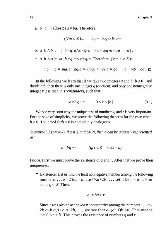
76 Chapter 3
a. b | a ⇒ (∃q∈Z) a = bq. Therefore:
(∀m ∈Z )am = bqm=bq1⇒ b |am
b. a | b ∧ b |c ⇒ b =q1 a∧c =q2 b ⇒ c= q1q 2a =qa ⇒ a | c.
C. a |b ∧ a |c ⇒ b =q1a ∧ c=q2a. Therefore (∀m,n ∈Z ):
mb + nc = mq1a +nq2a = (mq1 + nq2)a = qa ⇒ a | (mb + nc).
In the following we learn that if we take two integers a and b (b ≠ 0), and
divide a/b, then there is only one integer q (quotient) and only one nonnegative
integer r less than |b| (remainder), such that:
a=b q+ r 0≤ r < |b | (3.1)
We see very soon why the uniqueness of numbers q and r is very important.
For the sake of simplicity, we prove the following theorem for the case when
b > 0. The proof forb < 0 is completely analogous.
THEOREM 3.2 (DIVISION). If a ∈ Z and b∈ N, then a can be uniquely representedas:
a =bq + r (q, r ∈Z 0 ≤ r < b)
PROOF: First we must prove the existence of q and r. After that we prove their
uniqueness:
• Existence: Let us find the least nonnegative number among the following
numbers . . . , a – 2 b,a – b, a,a+b,a+2b , . . . Let it be r = a– q b for
some q ∈ Z. Then:
a = bq + r
Since r was picked as the least nonnegative among the numbers . . . ,a –
2b,a–b,a,a+b,a+2b, . . . , we see that a–(q+1)b <0. This means
that 0 ≤ r < b. This proves the existence of numbers q and r.
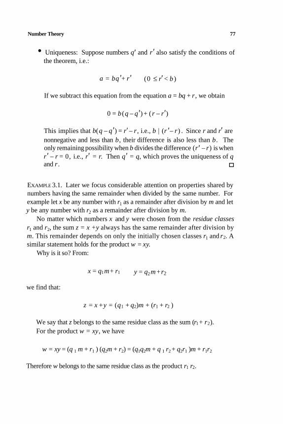
Number Theory 77
• Uniqueness: Suppose numbers q' and r' also satisfy the conditions of
the theorem, i.e.:
a = bq'+ r' (0 ≤ r' < b )
If we subtract this equation from the equation a = bq + r , we obtain
0 = b (q – q') + (r – r')
This implies that b(q – q') = r' – r , i.e., b | (r'– r) . Since r and r' are
nonnegative and less than b, their difference is also less than b. The
only remaining possibility when b divides the difference (r' – r) is when
r' – r = 0, i.e., r' = r. Then q' = q, which proves the uniqueness of qand r .
EXAMPLE 3.1. Later we focus considerable attention on properties shared by
numbers having the same remainder when divided by the same number. For
example let x be any number with r1 as a remainder after division by m and let
y be any number with r2 as a remainder after division by m.No matter which numbers x and y were chosen from the residue classes
r1 and r2, the sum z = x +y always has the same remainder after division by
m. This remainder depends on only the initially chosen classes r1 and r2. A
similar statement holds for the product w = x y. Why is it so? From:
x = q1m+ r1 y = q2 m +r 2
we find that:
z = x +y = (q1 + q2)m + (r1 + r2 )
We say that z belongs to the same residue class as the sum (r1+ r2).
For the product w = xy, we have
w = xy = (q 1 m + r1 ) (q2m + r2) = (q1q2m + q 1 r2 + q2r1 )m + r1r2
Therefore w belongs to the same residue class as the product r1 r2.
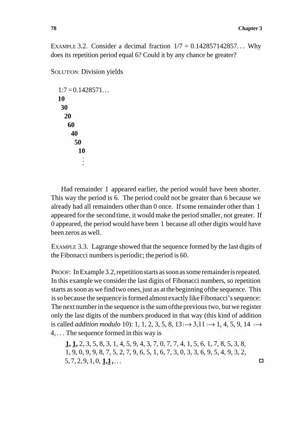
78 Chapter 3
EXAMPLE 3.2. Consider a decimal fraction 1/7 = 0.142857142857. . . Why
does its repetition period equal 6? Could it by any chance be greater?
SOLUTION: Division yields
1:7 = 0.1428571. . .
1030
206040
5010
.
.
.
Had remainder 1 appeared earlier, the period would have been shorter.
This way the period is 6. The period could not be greater than 6 because we
already had all remainders other than 0 once. If some remainder other than 1
appeared for the second time, it would make the period smaller, not greater. If
0 appeared, the period would have been 1 because all other digits would have
been zeros as well.
EXAMPLE 3.3. Lagrange showed that the sequence formed by the last digits of
the Fibonacci numbers is periodic; the period is 60.
PROOF: In Example 3.2, repetition starts as soon as some remainder is repeated.
In this example we consider the last digits of Fibonacci numbers, so repetition
starts as soon as we find two ones, just as at the beginning of the sequence. This
is so because the sequence is formed almost exactly like Fibonacci’s sequence:
The next number in the sequence is the sum ofthe previous two, but we register
only the last digits of the numbers produced in that way (this kind of addition
is called addition modulo 10): 1, 1, 2, 3, 5, 8, 13 | → 3,11 | → 1, 4, 5, 9, 14 | → 4, . . . The sequence formed in this way is
1, 1, 2, 3, 5, 8, 3, 1, 4, 5, 9, 4, 3, 7, 0, 7, 7, 4, 1, 5, 6, 1, 7, 8, 5, 3, 8,
1, 9, 0, 9, 9, 8, 7, 5, 2, 7, 9, 6, 5, 1, 6, 7, 3, 0, 3, 3, 6, 9, 5, 4, 9, 3, 2,
5, 7, 2, 9, 1, 0, --1,1, . . .
- -
Number Theory 79
Primes and Canonical Decomposition
DEFINITION 3.2 (PRIME NUMBERS). A prime is an integer greater than 1 divisible
only by itself and one. All other integers greater than 1 are called composite
integers.
NOTE: Number 1 is neither a prime nor a composite. This is due to its special
status as a neutral element (unit) in multiplication.
The sequence of primes begins as: 2, 3, 5, 7, 11, 13, 17, 19, . . . The
easiest way of continuing this sequence involves the ancient method known
as the sieve of Eratosthenes: To determine all primes < n, first list all natural
numbers from 2 to n – 1. Then eliminate all even numbers except 2, then all
numbers divisible by 3 except 3, and so on for 5, 7, 11, 13, etc., until we have
covered all prime numbers < Note: After eliminating even numbers, we
need not worry about numbers divisible by 4, 6, 8, etc., because these are even
numbers. Similarly after eliminating all numbers divisible by 3, we need not
worry about those divisible by 6, 9, 12, etc., because they have already been
eliminated. Thus to find all primes < n, we eliminate numbers divisible by
primes <
EXAMPLE 3.4 (PRIMES LESS THAN 100). To determine the primes less than 100,
we use the sieve of Eratosthenes to eliminate all numbers divisible by 2, 3, 5,
and 7. This procedure yields the following 25 numbers:
2, 3, 5, 7, 11, 13, 17, 19, 23, 29, 31, 37, 41, 43, 47, 53, 59,
61, 67, 71, 73, 79, 83, 89, 97
The answer to the question of how many primes exist was already known
to Greek mathematicians. In the ninth book of the Elements, Euclid gives the
following proof that the set of primes is infinite.
Suppose there are only finitely many primes. Denote these as p1 , p2 , . . . ,pn.
Let pn be the greatest among these. If we form the number:
P = p1p2 . . . pn + 1
we see that P > pn, so there are only two possibilities for P:
• P is a prime, which contradicts our assumption that pn is the greatest
prime.
80 Chapter 3
• P is a composite, which contradicts the assumption that p1,p2 , . . . ,pn are
the only primes, because when divided by any of them, P has remainder 1.
Thus since P is a composite number, there must exist other primes that
divide it.
This proves that there cannot be only finitely many primes:
THEOREM 3.3 (EUCLID'S THEOREM). The set of primes is infinite.
EXAMPLE 3.5 (ANOTHER PROOF). Euclid’s theorem can be proved in many dif-
ferent ways. Here we add only the proofgiven by Kummer in 1878:
Let p1,p2 ,...,pn be the only primes and let N =p1p2 ...pn > 2. The
number N – 1 has at least one prime factor, e.g., pk, for some 1 ≤ k ≤ n. Since
pk | N and pk | (N – 1), we see that pk divides the difference N – (N – 1) = 1,
which is impossible.
EXAMPLE 3.6 (EULER’S TRINOMIAL). In 1772 Euler gave the following quadratic
trinomial:
x2 + x + 41
which for x = 0, 1, 2, . . . , 39 produces different primes.
NOTE: A useful formula for generating all primes does not exist. Some formu-
las are true ifand only if their argument is prime; other formulas theoretically
generate all primes, but none of these can be used because they either in-
volve extremely complicated calculations or constants whose values depend on
knowing all primes in advance.
EXAMPLE 3.7 (FERMAT NUMBERS). If 2m + 1 is a prime, then m must be a power
of 2. Prove.
SOLUTION: Assume that m is not a power of 2 or in other words, that m = 2n . kfor some n ≥ 0 and odd k. Then:
2m + 1 = 22n.k + 1 = (22n)k + 1
Since for odd k we have ak + 1 = (a + 1)(ak–1- ak–2 + ak–3 – . . . +1),
we see that (22n+ 1) | [(22n
)k + 1]. Therefore if 2m
+ 1 is a prime, then k = 1;
i.e., m is a power of 2.
Number Theory 81
NOTES: The numbers Fn = 22n+ 1 are called the Fermat numbers. In 1640
Fermat conjectured that all of these numbers were prime, probably his only
incorrect conjecture. The first counterexample was identified by Euler, who
found that F5 = 4294967297 = 641 . 6700417. Since that time, a lot of effort
and in the last few decades, a lot of computer time has been dedicated to
factoring Fermat numbers. Although Fermat’s conjecture is known to be false,
it is not known whether there are any primes among the Fermat numbers except
F0, F1, F2, F3, and F4.
One of the many properties of Fermat numbers is the following formula:
Fn = F0F1 . . .Fn –1 +2, which implies that the only common factor that they
might have is 2. But since Fermat numbers are odd, this is not the case,
therefore they are all relatively prime. This observation is the basis of Polya’s
proof of the infiniteness of the set of primes.
Fermat numbers emerge in quite an unexpected place — Gauss’s theorem
about the constructibility ofregular polygons*: A regularpolygon with n sides can be constructed using a ruler and compass if and only if n= 2rp1. . .pm,
where r≥ 0, and p1 , . . . , pm are different Fermat primes or n= 2r, where r ≥ 2.
Among other things, this theorem shows that it is impossible to construct
a regular heptagon (n = 7), but constructing a regular heptadecagon (n =
17) is possible. The question of constructing regular polygons with a ruler
and compass was considered even by Ancient Greek mathematicians, who
constructed the regular pentagon but stopped there.
EXAMPLE 3.8. Prove that all Fermat numbers of order higher than 1 have 7 as
the last digit.
SOLUTION: All numbers ofthe form 22n, where n > 1, end in the digit 6 because
after 222= 16, all others are produced by squaring the previous number of that
form. This is the key observation here, because squaring a number ending in 6
again yields a number ending in 6:
(10k + 6)2 = 10( 10k2 + 12k) + 6
EXAMPLE 3.9. If p > 3 is a prime, then p2 – 1 is divisible by 24. Prove.
SOLUTION: Since p is an odd number, (p – 1) and (p + 1) are consecutive even
numbers. Thus one of these is divisible by 2 and the other by 4. Therefore
p2 – 1 = (p – 1)(p + 1) is a number divisible by 8. Similarly since (p – 1), p,
*Gauss made this discovery when he was only nineteen.
82 Chapter 3
and (p + 1) are consecutive numbers, one is divisible by 3, but it cannot be p,
because it is a prime greater than 3. This ends the proof.
We may think that the following theorem (Theorem 3.4) does not require
proof because our experience guarantees its correctness, but we must be careful,
since in mathematics experience is not a proof. Theorem 3.4 is so important
that it is often called the Fundamental Theorem of Arithmetic.
THEOREM 3.4 (FUNDAMENTAL THEOREM OF ARITHMETIC). Every integer greaterthan 1 has a unique representation as a product of prime factors. (Their order is considered to be irrelevant.)
PROOF: First we prove the existence of such a representation. By definition
all primes are represented in this way, and from experience we know that the
first several composites are similarly represented 4 = 22, 6 = 2 . 3, 8 = 23,
10 = 2 . 5, . . . Ifwe assume there are composites without such representation,
there must exist the smallest among them. Let us denote it by m. Since mis a composite, we can write m = m1m2, where 1 < m1,m2 < m. Since m is
assumed to be the least composite without factorization into primes, m1 and
m2 certainly have unique representation as a product of prime factors, but then
m, too, has it, which is a contradiction.
Now we prove the uniqueness of prime factorization. For all primes and
the first several composites, we know it is unique. Now suppose there are
composites with two or more prime factorizations. Denote the least such
composite by n. Then we can write
n = p1p2 . . .pr n = q1q2 . . .qs
wherep1 ≤ p2 ≤ . . . ≤pr and q1 ≤ q2 ≤ . . . ≤ qs. It is easy to see thatpi ≠qj,
because if these two factorizations had a common factorp, after cancellation
by p we would have two different factorizations for n/p, an integer less than n.
Hence we can take p1 < q1.
Consider now k = p1q2 . . .qs. We now show that if n has two different
factorizations, then n – k, too, has a nonunique factorization. This again
contradicts the assumed minimality of n.Indeed since both n and k are divisible by p1, so is n – k; hence there exists a
factorization n – k =p1f2 . . .fa. On the other hand, n – k = (q1 –p1)q2.. .qs =
g1 . . .gbq2. . .qs. Since p1 ≠ qj, these two factorizations differ because the
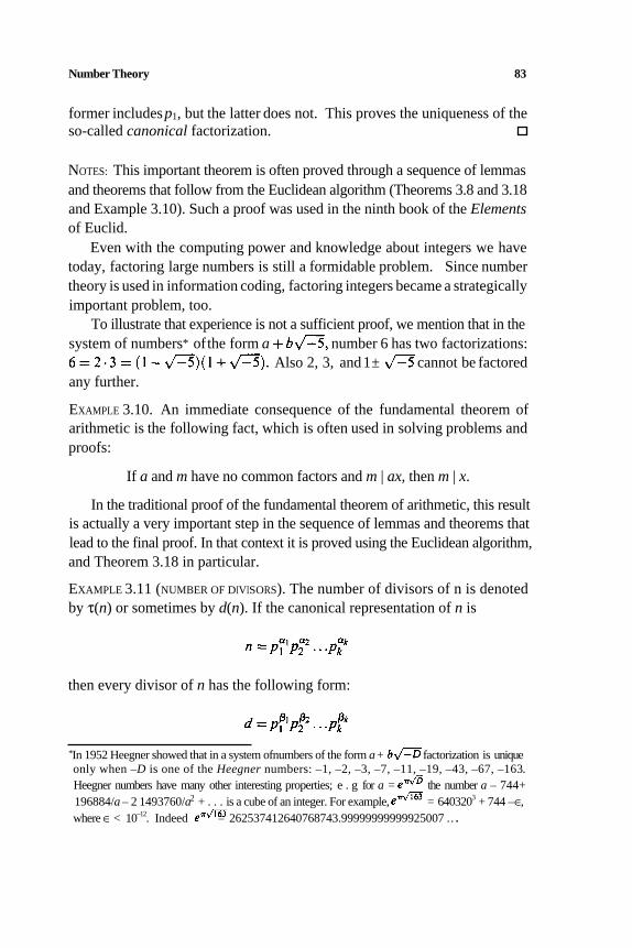
Number Theory 83
former includesp1, but the latter does not. This proves the uniqueness of the
so-called canonical factorization.
NOTES: This important theorem is often proved through a sequence of lemmas
and theorems that follow from the Euclidean algorithm (Theorems 3.8 and 3.18
and Example 3.10). Such a proof was used in the ninth book of the Elementsof Euclid.
Even with the computing power and knowledge about integers we have
today, factoring large numbers is still a formidable problem. Since number
theory is used in information coding, factoring integers became a strategically
important problem, too.
To illustrate that experience is not a sufficient proof, we mention that in the
system of numbers* ofthe form a number 6 has two factorizations:
Also 2, 3, and 1 ± cannot be factored
any further.
EXAMPLE 3.10. An immediate consequence of the fundamental theorem of
arithmetic is the following fact, which is often used in solving problems and
proofs:
If a and m have no common factors and m | ax, then m | x.
In the traditional proof of the fundamental theorem of arithmetic, this result
is actually a very important step in the sequence of lemmas and theorems that
lead to the final proof. In that context it is proved using the Euclidean algorithm,
and Theorem 3.18 in particular.
EXAMPLE 3.11 (NUMBER OF DIVISORS). The number of divisors of n is denoted
by τ(n) or sometimes by d(n). If the canonical representation of n is
then every divisor of n has the following form:
*In 1952 Heegner showed that in a system ofnumbers of the form a + factorization is unique
only when –D is one of the Heegner numbers: –1, –2, –3, –7, –11, –19, –43, –67, –163.
Heegner numbers have many other interesting properties; e . g for a = the number a – 744+
196884/a – 2 1493760/a2 + . . . is a cube of an integer. For example, = 6403203
+ 744 – ∈,
where ∈ < 10–12
. Indeed = 262537412640768743.99999999999925007 . . .
84 Chapter 3
where βi (i= 1,2, . . . , k) are such that:
0 ≤ βi ≤ αi (i = 1,2, . . ., k)
Because ofthe uniqueness ofthe canonical representation, which applies to das well, every divisor of n is uniquely determined by the choice of the exponentsβi (i = 1,2,. . . ,k). Since βi can be selected from (αi+ 1) different values, thetotal number of choices for d, i.e., the total number of divisors of n, is
GCD, LCM, and Euclidean Algorithm
DEFINITION 3.3 (COMMON DIVISOR). The integer d for which d | a and d | b is a common divisor of integers a and b.
Since a divisor of a number cannot be greater than the number itself, we see that among the common divisors of a and b there exists the greatest.
DEFINITION 3.4 (GREATEST COMMON DIVISOR — GCD). The greatest element inthe set of common divisors of integers a and b, where a ≠ 0 or b ≠ 0, is called the greatest common divisor of a and b, denoted GCD(a,b) or simply (a,b).
If a and b are relatively prime, i.e., if they do not have common factors, their GCD is 1, i.e., (a,b) = 1. For that reason to emphasize that a and b are relatively prime, we write (a,b) = 1.
EXAMPLE 3.12. For example the important result mentioned in Example 3.10,
If a and m have no common factors and m | ax, then m | x,
is written symbolically as:
(a,m)=1 ∧ m| ax ⇒ m|x
DEFINITION 3.5 (COMMON MULTIPLE). The integers for which a | s and b | s iscalled a common multiple of integers a and b.
A multiple of a number cannot be smaller than the number itself; therefore there exists the least among the common multiples of integers a and b.
DEFINITION 3.6 (LEAST COMMON MULTIPLE — LCM). The least element in theset of common multiples of integers a and b is called the least common multiple,denoted LCM[a,b] or simply [a,b].
τ(n) = (α1 + 1) (α2 + 1) ... (αk + 1)
Number Theory 85
If a and b are relatively prime, then their LCM equals their product, i.e.:
(a,b) = 1 ⇒ [a,b] =ab
In fact because of the fundamental theorem of arithmetic, the more general Theorem 3.5 is true.
THEOREM 3.5 (GCD AND LCM). If:
where among the exponents αi and βi there may be some zeros, then:
The consequence of Theorem 3.5 is Theorem 3.6.
THEOREM 3.6. The product of the GCD and LCM of two integers equals theabsolute value of the product of those two numbers, i.e.:
(a,b).[a,b] = |ab|
NOTE: Since factoring integers is a very difficult task, except when a and bare relatively small or easy to factor, we never use the results of Theorem 3.5to determine their GCD. Although the formula is simple, the calculations involved are more complicated than the Euclidean algorithm, probably theoldest nontrivial algorithm still in use. The Euclidean algorithm first appeared inTheorems VII-1 and VII-2 of Euclid’s Elements.
To prove and fully understand this algorithm we must examine the properties of GCD in an entirely different manner.
The key factor in the proof is Theorem 3.7.
THEOREM 3.7. If a = bq + r, then:
(a,b) = (br)
PROOF: The proof has two parts. If d = (a, b) and d' = (b,r), we first provethat d | d', then that d' | d, which when taken together imply d = d'.
86 Chapter 3
• If d = (a,b), then d | a and d | b, therefore d | r = a – bq. Thus, d | b,
• Using similar arguments, we find that d' | d.
and d | r, which implies d | d' = (b,r).
NOTE: In a special case when r = 0, i.e., when b | a, obviously (a, b) = b.
To find the GCD of two numbers denoted by a and b, with a > b, according to Theorem 3.7 the problem can be reduced to finding the GCD of another pairof numbers, b and r. We can choose q and r in infinitely many ways, but onlyone choice leads to an efficient algorithm. To reach the end of the algorithm as quickly as possible, we must choose r as small as possible. Thus the optimalchoice is r equal to the remainder of a when divided by b. We continue by applying the same procedure to finding (b,r), and so on.
We have just described the famous Euclidean algorithm. In the following, we write q1 and r1 instead of q and r:
a = bq1+ r1 0 < r1 < b
b =r1q2 + r2 0< r2 < r1
r l= r2q3+r3 0 < r3 < r 2
r2 =r3 q4+ r4 0< r4 < r3
We continue this process until we reach the first division whose remainder
...
is 0. Ifrn = 0, then the result we seek is rn–1, the last nonzero remainder in the Euclidean algorithm. Note: Such an n exists because a descending sequenceof positive integers, such as ri, has a finite number of elements.
THEOREM 3.8 (EUCLIDEAN ALGORITHM). In the Euclidean algorithm, the lastnonzero remainder equals the GCD of the input numbers.
PROOF: Ifrn = 0, then rn–2 is divisible by rn– 1. Therefore their GCD is rn–1.According to Theorem 3.7:
(a,b) = (b,r1) = (r1,r2) = (r2,r3) =. . . = (rn–2,rn–1) = rn–1
This completes the proof of correctness of the Euclidean algorithm.
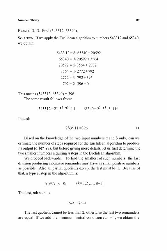
Number Theory 87
EXAMPLE 3.13. Find (543312, 65340).
SOLUTION: If we apply the Euclidean algorithm to numbers 543312 and 65340, we obtain
5433 12 = 8. 65340 + 2059265340 = 3. 20592 + 356420592 = 5. 3564 + 2772
3564 = 1. 2772 +7922772 = 3 . 792 + 396
792 = 2 . 396 + 0
This means (543312, 65340) = 396.The same result follows from:
543312 =24 .32 .73 . 11 65340 = 22 .33 . 5 .112
Indeed:
22.32.11 =396
Based on the knowledge of the two input numbers a and b only, can weestimate the number of steps required for the Euclidean algorithm to produceits output (a,b)? Yes, but before giving more details, let us first determine the two smallest numbers requiring n steps in the Euclidean algorithm.
We proceed backwards. To find the smallest of such numbers, the last division producing a nonzero remainder must have as small positive numbersas possible. Also all partial quotients except the last must be 1. Because of that, a typical step in the algorithm is:
rk–2=rk–1.1+rk (k= 1,2 ,. . . , n–1)
The last, nth step, is
rn–2 = 2rn–1
The last quotient cannot be less than 2, otherwise the last two remainders are equal. If we add the minimum initial condition rn–1 = 1, we obtain the
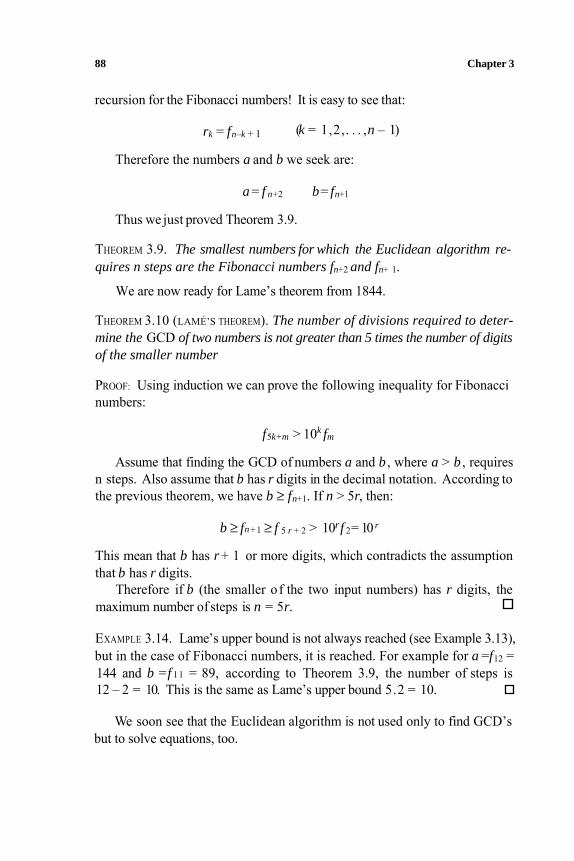
88 Chapter 3
recursion for the Fibonacci numbers! It is easy to see that:
rk = fn–k + 1
Therefore the numbers a and b we seek are:
(k = 1,2,. . . ,n – 1)
a = f n+2 b= fn+1
Thus we just proved Theorem 3.9.
THEOREM 3.9. The smallest numbers for which the Euclidean algorithm re-quires n steps are the Fibonacci numbers fn+2 and fn+ 1.
We are now ready for Lame’s theorem from 1844.
THEOREM 3.10 (LAMÉ’S THEOREM). The number of divisions required to deter- mine the GCD of two numbers is not greater than 5 times the number of digits of the smaller number
PROOF: Using induction we can prove the following inequality for Fibonaccinumbers:
f5k+m > 10k fm
Assume that finding the GCD of numbers a and b , where a > b , requiresn steps. Also assume that b has r digits in the decimal notation. According tothe previous theorem, we have b ≥ fn+1. If n > 5r, then:
b ≥ fn + 1 ≥ f 5 r + 2 > 10rf 2= 10 r
This mean that b has r + 1 or more digits, which contradicts the assumptionthat b has r digits.
Therefore if b (the smaller of the two input numbers) has r digits, the
EXAMPLE 3.14. Lame’s upper bound is not always reached (see Example 3.13), but in the case of Fibonacci numbers, it is reached. For example for a =f12 = 144 and b =f 11 = 89, according to Theorem 3.9, the number of steps is12 – 2 = 10. This is the same as Lame’s upper bound 5.2 = 10.
We soon see that the Euclidean algorithm is not used only to find GCD’s
maximum number of steps is n = 5r.
but to solve equations, too.
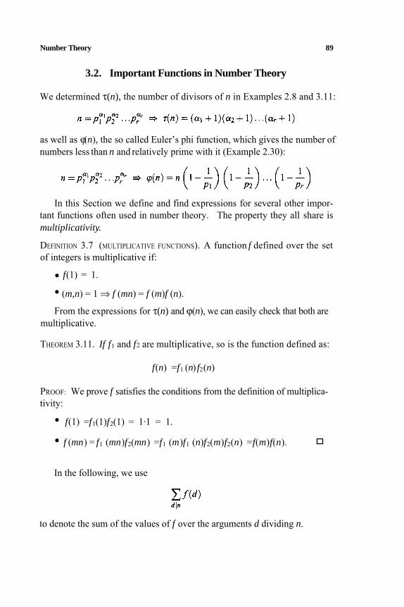
Number Theory 89
3.2. Important Functions in Number Theory
We determined τ(n), the number of divisors of n in Examples 2.8 and 3.11:
as well as ϕ(n), the so called Euler’s phi function, which gives the number ofnumbers less than n and relatively prime with it (Example 2.30):
In this Section we define and find expressions for several other impor-tant functions often used in number theory. The property they all share is multiplicativity..
DEFINITION 3.7 (MULTIPLICATIVE FUNCTIONS). A function f defined over the setof integers is multiplicative if:
f(1) = 1.
• (m,n) = 1 ⇒ f (mn) = f (m)f (n).
From the expressions for τ(n) and ϕ(n), we can easily check that both are multiplicative.
THEOREM 3.11. If f1 and f2 are multiplicative, so is the function defined as:
f(n) =f1 (n) f2(n)
PROOF: We prove f satisfies the conditions from the definition of multiplica-tivity:
• f(1) =f1(1)f2(1) = 1.1 = 1.
• f (mn) = f1 (mn)f2(mn) =f1 (m)f1 (n)f2(m)f2(n) =f(m)f(n).
In the following, we use
to denote the sum of the values of f over the arguments d dividing n.
•
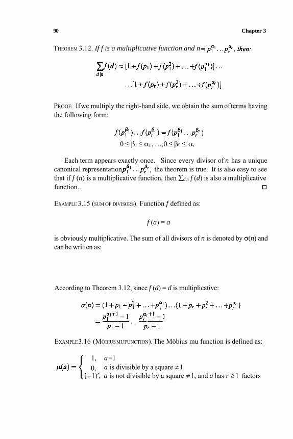
90 Chapter 3
THEOREM 3.12. If f is a multiplicative function and n
PROOF: Ifwe multiply the right-hand side, we obtain the sum ofterms havingthe following form:
0 ≤ βI ≤ α1 , . .., ≤0 βr ≤ αr
Each term appears exactly once. Since every divisor of n has a uniquecanonical representation the theorem is true. It is also easy to seethat if f (n) is a multiplicative function, then ∑d|n f (d) is also a multiplicative function.
EXAMPLE 3.15 (SUM OF DIVISORS). Function f defined as:
f (a) = a
is obviously multiplicative. The sum of all divisors of n is denoted by σ(n) andcan be written as:
According to Theorem 3.12, since f (d) = d is multiplicative:
EXAMPLE3.16 (MÖBIUS MUFUNCTION).The Möbius mu function is defined as:
1, a=10, a is divisible by a square ≠1
–1)r, a is not divisible by a square ≠ 1, and a has r ≥ 1 factors
Number Theory 91
It is straightforward to check that the Mobius mu function is multiplicative. According to Theorem 3.11, if f(a) is multiplicative, then µ(a)f(a) is also multiplicative. If n = then according to Theorem 3.12 and thedefinition of the Möbius mu function:
For example if f(a) = 1, we obtain the following identity:
This is often used as the definition of the Möbius mu function.If f(a) = 1/a:
It follows that:
EXAMPLE 3.17. The following identity is very interesting:
To prove it, consider and Theorem 3.12.
NOTE: The identities
are an example of the more general Möbius inversion rule:
92 Chapter 3
EXAMPLE 3.18. If n has an odd number of divisors, then n is a square. Prove.
SOLUTION: If n = then the number of its divisors is τ(n) =(α1 + 1)(α2+ 1). . .(αr+ 1). If τ(n) is odd, so is each of its factors (αk + 1)(k = 1,2, . . . ,r). Thus all exponents αk are even; i.e., we can write αk = 2βk.Now it is clear that n is a square, because:
3.3. Congruences
We mentioned earlier that numbers with equal remainders after dividing by theinteger m ≠ 0 have many properties in common. For that reason we introduce Definition 3.8 and the following notation.
DEFINITION 3.8 (CONGRUENCE). For integers a and b that have equal remainders after division by m, we write
a ≡ b (mod m)
We say that they are congruent modulo m.
This notation was introduced by Gauss in Disquisitiones Arithmeticae,which was published in 1801 when Gauss was only 24.
In the next few examples we examine some of the properties of numbers congruent modulo m.
EXAMPLE 3.19. If a and b are congruent modulo m, then their difference isdivisible by m:
a ≡ b (mod m) ⇒ a=q1 m +r ∧ b = q2 m+ r
Then a – b = (q1 – q2)m, therefore m | (a – b), i.e.:
a–b ≡ 0 (mod m)
Note the analogy with the equals sign:
a ≡ b (mod m) ⇔ a – b ≡ 0 (mod m)
Number Theory 93
We say that the difference (a – b) is congruent to zero modulo m, orshorter, that the difference (a – b) is zero modulo m. Almost always weconsider integers m > 0, i.e., m ∈ N.
EXAMPLE 3.20. If
a ≡ b (mod m)
then there exists q, an integer, such that:
a =mq +b
Indeed:
a ≡ b (mod m) ⇒ a=q1 m + r ∧ b = q2 m+r ⇒ ⇒a – b = (q1 – q2)m = qm
EXAMPLE 3.21. It is easy to verify that the relation ofcongruency modulo m isan equivalence relation:
• Reflexivity: Obviously a ≡ a.
• Symmetry: Also a ≡ b ⇒ b ≡ a.
• Transitivity: Ifa ≡ b and b ≡c, then the differences a – b and b – c aredivisible by m. Therefore (a – b) + (b – c) = a – c is also divisible bym, i.e., a ≡ c.
EXAMPLE 3.22. Let us use the new notation to express the fact that the value of the sum or product modulo m does not depend on the choice of numbers beingadded or multiplied but rather on their residues modulo m:
a ≡b (mod m) ∧ s≡ t (mod m)⇒ a +s ≡ b+ t (mod m) ∧ as ≡ bt (mod m)
More generally if P(x) is a polynomial in x with integer coefficients, then:
a ≡ b (mod m) ⇒ P(a) ≡ P(b) (mod m)
94 Chapter 3
EXAMPLE 3.23 (CANCELLATION). If (a, m) = 1, then:
ax≡ ay (mod m) ⇒ x ≡y (mod m)
Indeed:
ax ≡ ay (mod m) ⇒ m | a (x –y)
According to Example 3.10, since a and m are relatively prime, m | (x –y),i.e., x ≡y (mod m).
NOTE: If (a,m) > 1, cancellation is not permitted. For example, 5.4 ≡ 5.2
EXAMPLE 3.24. If (a,m) = d ≥ 1, then:
(mod 10), but4 (mod 10).
ax ≡ ay (mod m) ⇒ x ≡ y (mod )—md
As in Example 3.23:
ax ≡ ay (mod m) ⇒ m | a(x –y) ⇒ m– a (x –y)d |d
Finally:
EXAMPLE 3.25. If a ≡ b (mod qm), then a ≡b (mod m). Indeed:
a ≡ b (mod qm) ⇒ qm| ( a – b) ⇒ m | (a –b) ⇒ a ≡ b (mod m)
EXAMPLE 3.26. What can we conclude if we know that:
x ≡ y (mod m) x ≡ y (mod n)?
From m | (x –y) and n | (x –y), we find that (x –y) is a common multiple
From Example 3.25 we see that the converse is also true, so: of m and n;therefore [m,n] | (x–y), i.e., x ≡ y (mod [m,n]).
x ≡ y (mod m) ∧ x ≡ y (mod n) ⇔ x ≡ y (mod [m,n])
–
Number Theory 95
Since the congruence is an equivalence relation, the classes of congruence modulo m:
[0], [1], . . . , [m-1]
form a complete partition of the set of integers. In other words, the classes of residues modulo m are disjoint sets, and their union is the set of integers Z.
The set 0, 1, . . . , (m – 1) has a special name, the complete residue sys-tem modulo m. In fact any set in which every residue class has exactly onerepresentative is called a complete residue system modulo m.
To prove the next few theorems, we need another residue system, the socalled reducedresidue system modulo m. It is constructed from the completeresidue system modulo m by eliminating all numbers not relatively prime withm. Obviously the number of elements in the reduced residue system modulo m equals Euler’s phi function ϕ(m).
EXAMPLE 3.27. If m = 9, the most often used complete residue system is thefollowing set: (0, 1, 2, 3, 4, 5, 6, 7, 8. The most often used reduced residue system is 1, 2, 4, 5, 7, 8. The sets 0, 1, 2, 3, 4, 5, 6, 7, 17 and 1, 2, 4, 5, 7, 17 are also complete and reduced residue systems, respectively.
Let us consider Theorem 3.13, which we use to prove Euler’s and Wilson’s theorems.
THEOREM 3.13. If x1 ,x2, . . . , axϕ(m) is a reduced residue system modulo mand (a,m) = 1, then the set ax1 ,ax2 ,. . . , axϕ(m) is a reduced residue system modulo m, too. (Note: The order of the elements in a set is not important.)
PROOF: Suppose (ax1 , ax2,. . . ,axϕ(m) is not a reduced residue system modulo m. Then for some i ≠ j, axi ≡ ax j (mod m), or for some i, (ax i,m) ≠ 1.But since (a,m) = 1, in the former case xi ≡xj (mod m); in the latter case(axi,m) ≠1. Both cases imply that x1, x2 ,. . . , xϕ(m) is not a reduced residue system modulo m either. Note:
(a, m ) = 1∧ ( xi,m ) = 1(i = 0, 1, . . . , ϕ(m))
(a xi, m) = 1(i = 0,1, . . . ,ϕ(m))
⇒
This completes the proof.
The proof of Theorem 3.14 is completely analogous.
96 Chapter 3
THEOREM 3.14. Ifx1 ,x2, . . . , xm is a complete residue system modulo m and(a,m) = 1, then thesetax1 ,ax2, . . . ,axm is a complete residue system modulo m, too. (Note: The order of the elements in a set is not important.)
We are now ready to proceed with the proof of Euler’s theorem (Theorem3.15).
THEOREM 3.15 (EULER’S THEOREM). If (a,m) = 1, then:
aϕ(m)≡ 1 (mod m)
PROOF: According to Theorem 3.14, to every number from the reduced residue system x1,x2, . . . ,xϕ(m), there corresponds exactly one element of the reduced residue system ax1,ax2, . . . , axϕ(m) such that:
xi ≡ axj (mod m)
Therefore we can write
ax1ax2 . . . axϕ(m) ≡ x1x2. . . xϕ(m) (mod m)
Since (xi, m) = 1 [i = 0, 1, . . . , ϕ(m)], we are allowed to cancel the xis.Thus:
aϕ(m)≡1 (mod m).
Fermat’s lesser theorem from 1640 (Theorem 3.16) is a special case of Euler’s theorem.
THEOREM 3.16 (FERMAT’S LESSERTHEOREM). If p is a prime and a is an integer not divisible by p, then:
ap–1 ≡ 1 (mod p)
PROOF: The proof reduces to the observation that if p is a prime, then ϕ(p) =
NOTE: Around 500 B.C., Chinese mathematicians knew that if p is a prime, then 2p ≡2 (mod p). This is a special case of Fermat’s lesser theorem. But
p – 1. Two different proofs can be found in Examples 2.58 and 3.28.
Number Theory 97
they, and also Leibniz centuries after them, thought the converse was true too;i.e., if 2n ≡ 2 (mod n), then n must be prime. The smallest counterexampleto their belief is n = 341 = 11.3 1, for which:
342341≡(210) . 2 ≡ 134. 2≡ 2 (mod 341)
Such numbers as 341 are called pseudoprimes to the base 2. In Example3.45 we show that there are infinitely many pseudoprimes to the base 2; thereare pseudoprimes to other bases as well. Some numbers are pseudoprime forall bases. Such numbers are called absolute pseudoprimes, or Carmichaelnumbers. The smallest such number is 561.
Theorem 3.17 proves a formula that holds for all primes and only for primes. Unfortunately that formula is not very useful for primality testing, because it requires considerable computation. Theorem 3.17 was discovered by Leibnizin 1682, but it is better known today as Wilson’s theorem.
THEOREM 3.17 (WILSON’S THEOREM). Congruence:
(p – 1)! ≡ –1 (mod p)
is true if and only if p is a prime.
PROOF: If (p – 1)! ≡ – 1 (mod p), then if p is not a prime, there exists a prime q < p that divides p. But since q < p, q is a factor in (p – 1) !; therefore(p – 1) ! + 1 cannotbedivisible by p. Therefore p must be prime if (p – 1) ! ≡ – 1
(mod p) is true.On the other hand for p prime, consider
(p–1)! = 1. 2.3.. . .. (p –2) . (p –1)
Obviously 1 ≡ 1 (mod p) and (p – 1) ≡ – 1 (mod p). For the remainingterms in the product, for any r, 2 ≤ r ≤ (p – 2), there exists exactly one s ≠ r,2 ≤ s ≤ (p – 2), such that rs ≡ 1 (mod p).
Since 1,2 , . . . , (p – 1)) is a reduced residue system modulo p, so isr, 2r, . . . , (p – 1)r. Therefore exactly one element of the latter set is 1 mod-ulo p. Since 2 ≤ r ≤ (p – 2), it is not r. It is also not r(p – 1), becauser(p – 1) ≡rp – r ≡ –r (mod p). Furthermore it is not r . r, otherwise r2 ≡ 1
98 Chapter 3
(mod p), which implies (r – 1)(r + 1) ≡ 0 (mod p); i.e., r ≡ 1 (mod p) orr ≡ – 1 (mod p), which contradicts the initial assumption 2 ≤ r ≤ (p, – 2).This completes the proof.
EXAMPLE 3.28 (AGAIN FERMAT’S LESSER THEOREM). Prove the following:
1. Product of two consecutive integers is divisible by 2.
2. Product of three consecutive integers is divisible by 6.
3. Product n(n – 1)(n – 2). . .(n – k + 1) is divisible by k!
SOLUTION:
1. One of the two consecutive integers is even. Therefore their product is even too.
2. Among the three consecutive integers, one is divisible by 3. In addition at least one of these is even. Therefore their product is divisible by
3. In Chapter 2 we saw that the number of subsets with k elements picked
3 . 2 = 6.
out of an n-element set equals
n!n(n – 1)(n –2) . . .( n –k+1)k! k! (n – k)!
Therefore it must be an integer. Another way ofshowing that follows. First note that the exponent of an arbitrary prime number q in the canonical decomposition of m! is
m/q + m/q2 + m/q3 +. . .
because among the integers ≤ m, m/q are divisible by q, m/q2 aredivisible by q2, etc.To show that
n!k! (n – k)!
is an integer, we apply the previous finding to numbers n!, k!, and(n–k)!, noting that a+b ≥a+b .
Number Theory 99
NOTE: If n = p, where p is any prime number, then for 2 ≤ k ≤ (p – 1):
is divisible by p, because p is a prime and p > k, so p is not a factor in k!.Therefore the binomial theorem modulo a prime becomes
(a+ b)p= ap + bP (mod p)
The result can easily be extended to the powers of sums of three or more terms:
(mod p)
If we let a1 = a2 = . . . = ar = 1, we obtain Fermat’s lesser theorem:
rp ≡ r (mod p)
If Fermat’s lesser theorem is written in this form, it does not require thecondition (r, p) = 1.
EXAMPLE 3.29. If the number 1968 is written as a sum of several integers and these integers are cubed and added together, we obtain the number divisible by6. Prove.
SOLUTION: Instead of 1968, we write n to prove the more general statement that the sum of the cubes of any partition of n is congruent with n modulo 6. If n = n1+ . . . +nr , then:
= n1 (n1 – 1>(n1 + 1) + . . . +nr(nr – 1)(nr+ 1) +n
Since each of the numbers nk(nk – 1)(nk + 1) is divisible by 6:
n 31 +. . . +n3
r ≡ n (mod 6)
NOTE: r, the number of terms in the partition of n, does not play any role at all.
100 Chapter 3
EXAMPLE 3.30. Find the last digit of 777333.
SOLUTION: For any n the power nk ends with the same digit as rk, where r isthe last digit of n. Indeed if n = 10q
1
+ r , then:
nk = (10q+r)k = 10q +rk =rk (mod 10)
Thus we are interested in finding the last digit of 7333. Since:
70 ≡ 1 71 ≡ 7 72 ≡ 9 73 ≡ 3 74 ≡ 1 (mod 10) . . .
we see that the last digits are periodically repeated, with the period equal to 4.Since 333 ≡ 1 (mod 4), 777333 ≡ 7 (mod 10).
EXAMPLE 3.31. If n > 4 is a composite number, then n | (n – 1)! Prove.
SOLUTION: If n is a composite number, then there exist integers n1 and n2 suchthat n = n1n2 and n1 ,n2 > 1. Obviously n1, n2 < n. Two cases are possible:
• n1 ≠n2. Thenboth numbers enterthe product (n – 1)! = 1 .2. . . . .(n – 1)and obviously n | (n | 1)!
• n1 = n2. Then n = n21 , and since n > 4, n1 > 2. Hence n = n 2
1 > 2n1.This implies that n1 and 2n1 are less than n and thus enter the product(n–1) ! =1.2 . . . . . ( n–1). Therefore we find n | (n–1)!
EXAMPLE 3.32 (PASCAL’S CRITERION). If the digits of a are an,an–1 ,. . .,a1,anda0, or in other words if:
then it is straightforward to prove the general divisibility criterion, due to Pascal:
m | a ⇔ m | (rnan+rn–1an–1 +. . .+r1 a1 + r0 a0 )
(k = 0, 1, 2 , . . . , n).where 10k ≡ rk (mod m)
Using this criterion we can find the divisibility criteria for powers of 2 and 5 and for numbers 3, 9, 7, 11, and 13:
Number Theory 101
• Divisibility by 2r (r ∈N): A number is divisible by 2r if and only if the number formed from its last r digits is divisible by 2r.
• Divisibility by 5r (r ∈N): A number is divisible by 5r if and only if the number formed from its last r digits is divisible by 5r.
• Divisibility by 3: A number is divisible by 3 if and only if the sum of its digits is divisible by 3.
• Divisibility by 9: A number is divisible by 9 if and only if the sum of its digits is divisible by 9.
• Divisibility by 11: There are at least three criteria for 11:
• Divisibility by 7 and 13: Since 7. 11 . 13 = 1001, the criteria for 7 and13 are the same as the third criterion for 11.
3.4. Diophantine Equations
Any equation whose solutions are required to be integers or rational numbers is called a Diophantine equation. Only some of these equations can be solvedsystematically, i.e., using some algorithm. For others we usually need to know a lot of number theory and have a lot of ideas and imagination.
Linear Congruences with One Unknown
The simplest Diophantine equations are
ax ≡ c (mod m) (3.2)
That is:
ax+my = c (3.3)
According to Example 3.20, Eqs. (3.2) and (3.3) are equivalent.
102 Chapter 3
Let us first consider the existence of the solution of Eq. (3.2) or Eq. (3.3).Recall Euler’s theorem:
(a,m)= 1 ⇒ aϕ(m) ≡ 1 (mod m)
According to Euler’s theorem, if (a,m) = 1, the solution exists, and fur-thermore we can write the following explicit* formula for it:
x ≡ caϕ (m)–1 (mod m)
We see that there are infinitely many solutions — all numbers from the
In the case when (a, m) = d > 1, there are two possibilities. Case 1 : When d | c, we cancel d on both sides ofthe congruence to obtain
same residue class modulo m as caϕ(m)–1.
the new equation:
where:
Thus we reduced the problem to the previously encountered and solved case.
d | ( ax +my) =c.
EXAMPLE 3.33. The equation:
Case 2: When d /| c, there is no solution because if d | a and d | m, then
15x +25y= 14
does not have integer solutions because 14 is not divisible by 5. The equation:
15 x + 25y = 10
has solutions, which can be found from the simpler equation obtained bydividing by 5:
3x + 5y = 2*Unfortunately the application of this formula requires a lot of calculations. We soon learn how touse the Euclidean algorithm, which is computationally less involved.
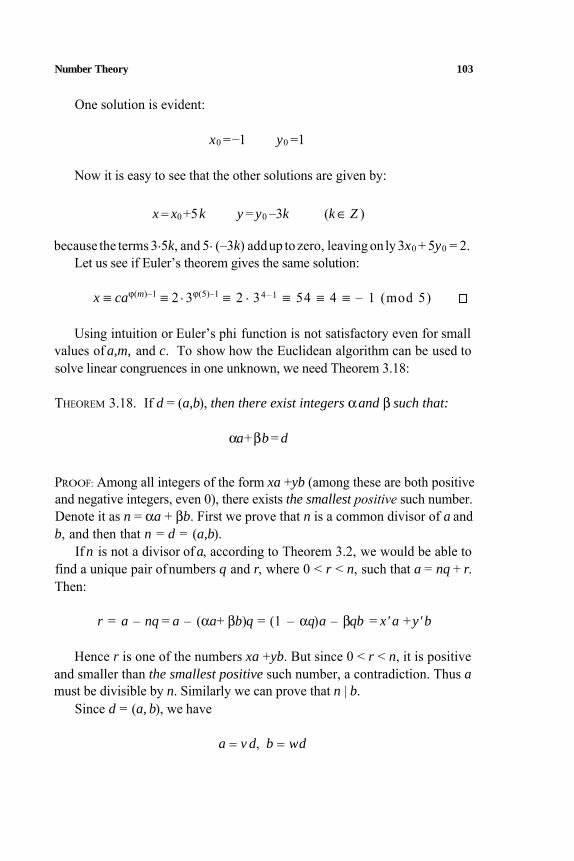
Number Theory 103
One solution is evident:
x0 =–1 y0 =1
Now it is easy to see that the other solutions are given by:
x = x0 +5k y = y0 –3k (k ∈ Z )
because the terms 3.5k, and 5. (–3k) addup to zero, leaving on ly 3x0 + 5y0 = 2.Let us see if Euler’s theorem gives the same solution:
x ≡ caϕ(m)–1 ≡ 2 . 3ϕ(5)–1 ≡ 2 . 34–1 ≡ 54 ≡ 4 ≡ – 1 (mod 5)
Using intuition or Euler’s phi function is not satisfactory even for smallvalues of a,m, and c. To show how the Euclidean algorithm can be used tosolve linear congruences in one unknown, we need Theorem 3.18:
THEOREM 3.18. If d = (a,b), then there exist integers αand β such that:
αa+βb = d
PROOF: Among all integers of the form xa +yb (among these are both positive and negative integers, even 0), there exists the smallest positive such number. Denote it as n = αa + βb. First we prove that n is a common divisor of a andb, and then that n = d = (a,b).
If n is not a divisor of a, according to Theorem 3.2, we would be able tofind a unique pair ofnumbers q and r, where 0 < r < n, such that a = nq + r.Then:
r = a – nq = a – (αa+ βb)q = (1 – αq)a – βqb = x' a +y' b
Hence r is one of the numbers xa +yb. But since 0 < r < n, it is positiveand smaller than the smallest positive such number, a contradiction. Thus amust be divisible by n. Similarly we can prove that n | b.
Since d = (a, b), we have
a = v d, b = wd
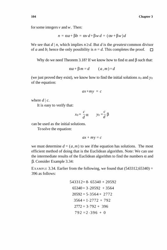
104 Chapter 3
for some integers v and w . Then:
n = αa+ βb = αv d + βw d = (αv +βw )d
We see that d | n, which implies n ≥ d. But d is the greatest common divisor
of a and b; hence the only possibility is n = d. This completes the proof.
Why do we need Theorem 3.18? If we know how to find α and β such that:
αa + β m = d ( a , m ) = d
(we just proved they exist), we know how to find the initial solutions x0 and y0
of the equation:
ax +my = c
where d | c.
It is easy to verify that:
cx0 = – α y0 =
c–d
βd
can be used as the initial solutions.
To solve the equation:
ax + my = c
we must determine d = (a,m ) to see if the equation has solutions. The most
efficient method of doing that is the Euclidean algorithm. Note: We can use
the intermediate results of the Euclidean algorithm to find the numbers α and
β. Consider Example 3.34:
EXAMPLE 3.34. Earlier from the following, we found that (543312,65340) =
396 as follows:
543312= 8. 65340 + 20592
65340 = 3 .20592 + 3564
20592 = 5.3564 + 2772
3564 = 1.2772 + 792
2772 = 3.792 + 396
7 9 2 = 2 . 3 9 6 + 0
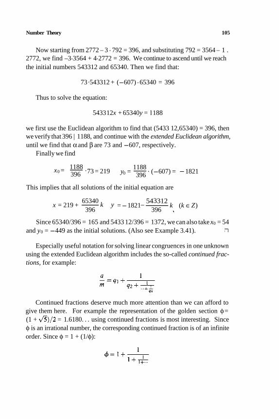
Number Theory 105
Now starting from 2772 – 3 . 792 = 396, and substituting 792 = 3564 – 1 .
2772, we find –3.3564 + 4.2772 = 396. We continue to ascend until we reach
the initial numbers 543312 and 65340. Then we find that:
73 .543312 + (-607) .65340 = 396
Thus to solve the equation:
543312x + 65340y = 1188
we first use the Euclidean algorithm to find that (5433 12,65340) = 396, then
we verify that 396 | 1188, and continue with the extended Euclidean algorithm, until we find that αand β are 73 and -607, respectively.
Finally we find
y0 = . (-607) = -182173 = 219x0 = . 11881188
396 396
This implies that all solutions of the initial equation are
y =-1821–543312
k (k ∈Z)65340
kx = 219 + 396 396
Since 65340/396 = 165 and 5433 12/396 = 1372, we can also take x0 = 54
Especially useful notation for solving linear congruences in one unknown
using the extended Euclidean algorithm includes the so-called continued frac- tions, for example:
and y0 = -449 as the initial solutions. (Also see Example 3.41).
Continued fractions deserve much more attention than we can afford to
give them here. For example the representation of the golden section φ=
(1 + = 1.6180. . . using continued fractions is most interesting. Since
φ is an irrational number, the corresponding continued fraction is of an infinite
order. Since φ = 1 + (1/φ):
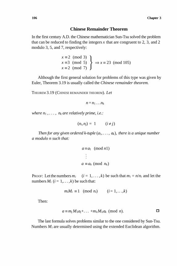
106 Chapter 3
Chinese Remainder Theorem
In the first century A.D. the Chinese mathematician Sun-Tsu solved the problem
that can be reduced to finding the integers x that are congruent to 2, 3, and 2
modulo 3, 5, and 7, respectively:
⇒ x ≡ 23 (mod 105)
x ≡ 2 (mod 3)
x ≡3 (mod 5)
x ≡ 2 (mod 7)
Although the first general solution for problems of this type was given by
Euler, Theorem 3.19 is usually called the Chinese remainder theorem.
THEOREM 3.19 (CHINESE REMAINDER THEOREM). Let
n = n1 . . .nk
where n1 , . . . , nk are relatively prime, i.e.:
(ni,nj) = 1 (i ≠ j)
Then for any given ordered k-tuple (a1, . . . , ak), there is a unique numbera modulo n such that:
a ≡a1 (mod n1)
. ..a ≡ ak (mod nk)
(i = 1, . . . ,k) be such that mi = n/ni and let thePROOF: Let the numbers mi
numbers Mi (i = 1,. . . ,k) be such that:
miMi ≡ 1 (mod ni) (i = 1, . . .,k)
Then:
a ≡ m1 M1a1+. . . +mkMkak (mod n).
The last formula solves problems similar to the one considered by Sun-Tsu.
Numbers Mi are usually determined using the extended Euclidean algorithm.
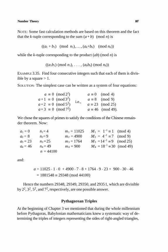
Number Theory 107
NOTE: Some fast calculation methods are based on this theorem and the fact
that the k-tuple corresponding to the sum (a+ b) (mod n) is
((a1 + b1) (mod n1), . . . , (ak+bk) (mod nk))
while the k-tuple corresponding to the product (ab) (mod n) is
((a1b1) (mod n1), . . . , (akbk) (mod nk))
EXAMPLE 3.35. Find four consecutive integers such that each of them is divis-
ible by a square > 1.
SOLUTION: The simplest case can be written as a system of four equations:
a ≡ 0 (mod 22) a ≡ 0 (mod 4)
a + 1 ≡ 0 (mod 32) a ≡ 8 (mod 9)i.e.,
a +2 ≡ 0 (mod 52)
a+ 3 ≡ 0 (mod 72)
a ≡ 23 (mod 25)
a ≡ 46 (mod 49).
We chose the squares of primes to satisfy the conditions of the Chinese remain-
der theorem. Now:
a1 = 0 n1= 4 m1 = 11025 M1 = 1–1 ≡ 1 (mod 4)
a2 = 8 n2= 9 m2 = 4900 M2 = 4–1 ≡ 7 (mod 9)
a3 = 23 n3 =25 m3 = 1764 M3 =14–1 ≡ 9 (mod 25)
a4 = 46 n4 = 49 m4 = 900 M4 = 18–1 ≡ 30 (mod 49)
n = 44100
and:
a = 11025 . 1 . 0 + 4900 . 7 . 8 + 1764 . 9 . 23 + 900 . 30 . 46
= 1881548 ≡ 29348 (mod 44100)
Hence the numbers 29348, 29349, 29350, and 29351, which are divisible
by 22, 32, 52, and 72, respectively, are one possible answer.
Pythagorean Triples
At the beginning of Chapter 3 we mentioned that during the whole millennium
before Pythagoras, Babylonian mathematicians knew a systematic way of de-
termining the triples of integers representing the sides of right-angled triangles,
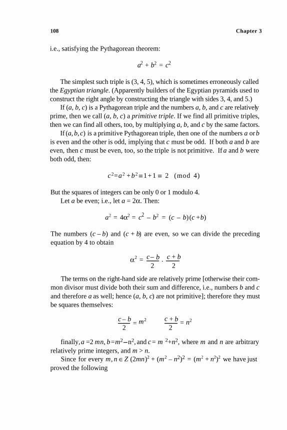
108 Chapter 3
i.e., satisfying the Pythagorean theorem:
a2 + b2 = c2
The simplest such triple is (3, 4, 5), which is sometimes erroneously called
the Egyptian triangle. (Apparently builders of the Egyptian pyramids used to
construct the right angle by constructing the triangle with sides 3, 4, and 5.)
If (a, b, c) is a Pythagorean triple and the numbers a, b, and c are relatively
prime, then we call (a, b, c) a primitive triple. If we find all primitive triples,
then we can find all others, too, by multiplying a, b, and c by the same factors.
If (a, b,c) is a primitive Pythagorean triple, then one of the numbers a or bis even and the other is odd, implying that c must be odd. If both a and b are
even, then c must be even, too, so the triple is not primitive. If a and b were
both odd, then:
c2=a2 + b2 ≡ 1 + 1 ≡ 2 (mod 4)
But the squares of integers can be only 0 or 1 modulo 4.
Let a be even; i.e., let a = 2α. Then:
a2 = 4α2 = c2– b2 = (c – b) (c +b)
The numbers (c – b) and (c + b) are even, so we can divide the preceding
equation by 4 to obtain
2 c– b c + bα = .2 2
The terms on the right-hand side are relatively prime [otherwise their com-
mon divisor must divide both their sum and difference, i.e., numbers b and cand therefore a as well; hence (a, b, c) are not primitive]; therefore they must
be squares themselves:
= n2c – b c + bm2
2 2
finally,a =2 mn, b=m2-n2, and c = m 2+n2, where m and n are arbitrary
Since for every m, n ∈Z (2mn)2 + (m2 – n2)2 = (m2 + n2)2 we have just
relatively prime integers, and m > n.
proved the following
=
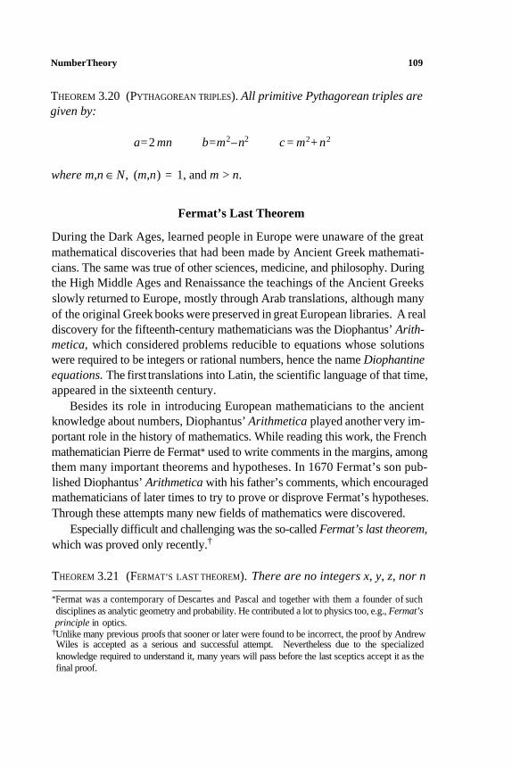
NumberTheory 109
THEOREM 3.20 (PYTHAGOREAN TRIPLES). All primitive Pythagorean triples are given by:
2 2a=2 mn b=m2–n2 c = m + n
where m,n ∈ N, (m,n) = 1, and m > n.
Fermat’s Last Theorem
During the Dark Ages, learned people in Europe were unaware of the great
mathematical discoveries that had been made by Ancient Greek mathemati-
cians. The same was true of other sciences, medicine, and philosophy. During
the High Middle Ages and Renaissance the teachings of the Ancient Greeks
slowly returned to Europe, mostly through Arab translations, although many
of the original Greek books were preserved in great European libraries. A real
discovery for the fifteenth-century mathematicians was the Diophantus’ Arith-metica, which considered problems reducible to equations whose solutions
were required to be integers or rational numbers, hence the name Diophantineequations. The first translations into Latin, the scientific language of that time,
appeared in the sixteenth century.
Besides its role in introducing European mathematicians to the ancient
knowledge about numbers, Diophantus’ Arithmetica played another very im-
portant role in the history of mathematics. While reading this work, the French
mathematician Pierre de Fermat* used to write comments in the margins, among
them many important theorems and hypotheses. In 1670 Fermat’s son pub-
lished Diophantus’ Arithmetica with his father’s comments, which encouraged
mathematicians of later times to try to prove or disprove Fermat’s hypotheses.
Through these attempts many new fields of mathematics were discovered.
Especially difficult and challenging was the so-called Fermat’s last theorem, which was proved only recently.†
THEOREM 3.21 (FERMAT’S LAST THEOREM). There are no integers x, y, z, nor n
*Fermat was a contemporary of Descartes and Pascal and together with them a founder of such
disciplines as analytic geometry and probability. He contributed a lot to physics too, e.g., Fermat’sprinciple in optics.
†Unlike many previous proofs that sooner or later were found to be incorrect, the proof by Andrew
Wiles is accepted as a serious and successful attempt. Nevertheless due to the specialized
knowledge required to understand it, many years will pass before the last sceptics accept it as the
final proof.
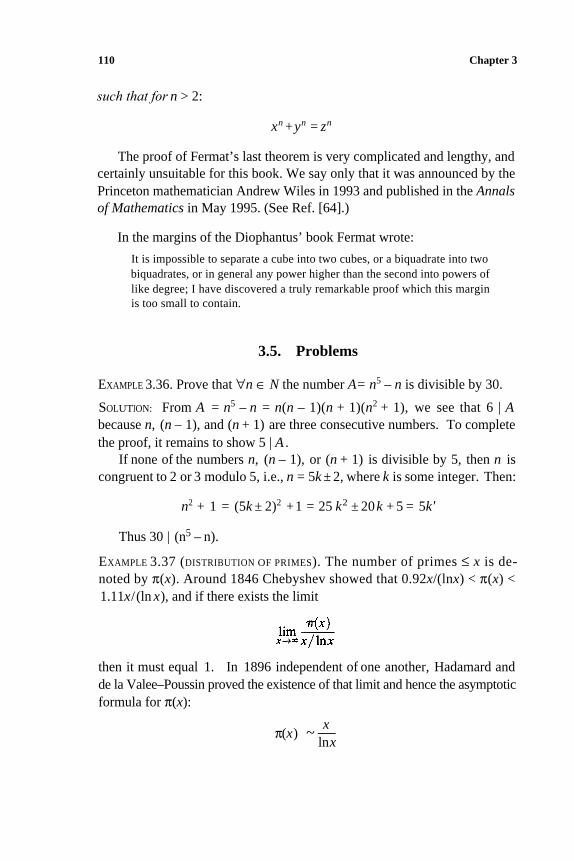
110 Chapter 3
such that for n > 2:
xn +yn = zn
The proof of Fermat’s last theorem is very complicated and lengthy, and
certainly unsuitable for this book. We say only that it was announced by the
Princeton mathematician Andrew Wiles in 1993 and published in the Annalsof Mathematics in May 1995. (See Ref. [64].)
In the margins of the Diophantus’ book Fermat wrote:
It is impossible to separate a cube into two cubes, or a biquadrate into two
biquadrates, or in general any power higher than the second into powers of
like degree; I have discovered a truly remarkable proof which this margin
is too small to contain.
3.5. Problems
EXAMPLE 3.36. Prove that ∀n ∈ N the number A= n5 – n is divisible by 30.
SOLUTION: From A = n5 – n = n(n – 1)(n + 1)(n2 + 1), we see that 6 | Abecause n, (n – 1), and (n + 1) are three consecutive numbers. To complete
the proof, it remains to show 5 | A .
If none of the numbers n, (n – 1), or (n + 1) is divisible by 5, then n is
congruent to 2 or 3 modulo 5, i.e., n = 5k ± 2, where k is some integer. Then:
n2 + 1 = (5k ± 2)2 + 1 = 25 k2 ± 20k + 5 = 5k'
Thus 30 | (n5 – n).
EXAMPLE 3.37 (DISTRIBUTION OF PRIMES). The number of primes ≤ x is de-
noted by π(x). Around 1846 Chebyshev showed that 0.92x/(lnx) < π(x) <
1.11x/(ln x), and if there exists the limit
then it must equal 1. In 1896 independent of one another, Hadamard and
de la Valee–Poussin proved the existence of that limit and hence the asymptotic
formula for π(x):
xπ(x) ~ —lnx
Number Theory
or, in other words:
EXAMPLE 3.38. Find all natural numbers a, b, and c satisfying:
1 1 1 -+-+- = 1 ab ac bc
SOLUTION: If the sum of three positive numbers is 1, then at least one of them
is ≥ 1/3, and all of them are < 1. Let
–1 1- ≥ab 3
Then 1 < ab ≤ 3. Ifwe check all possible cases, we find that all solutions
are permutations of the set 1, 2, 3.
EXAMPLE 3.39. Solve the following equation in the set of natural numbers:
1 ! + 2! + 3! + . . . +x ! =y2
SOLUTION: We prove that this equation has only two solutions:
x =1 y = 1 and x = 3 y = 3
It is easy to verify that for x = 1, 2, and 3 the only solutions are (1,1) and (3,3).
When x = 4 the equation does not have a solution because 33 is not a square.
When x≥ 5 the last digit of x! is 0, so the sum on the left-hand side always
ends in 3. On the other hand, squares of integers end in 0, 1, 4, 5, 6, 9, i.e., never
in 3.
EXAMPLE 3.40. Are there any solutions to:
x!y! = z!
if they are required to be integers > 5?
SOLUTION: This equation has infinitely many solutions of the following form:
x = n y = (n!–1) z = n!
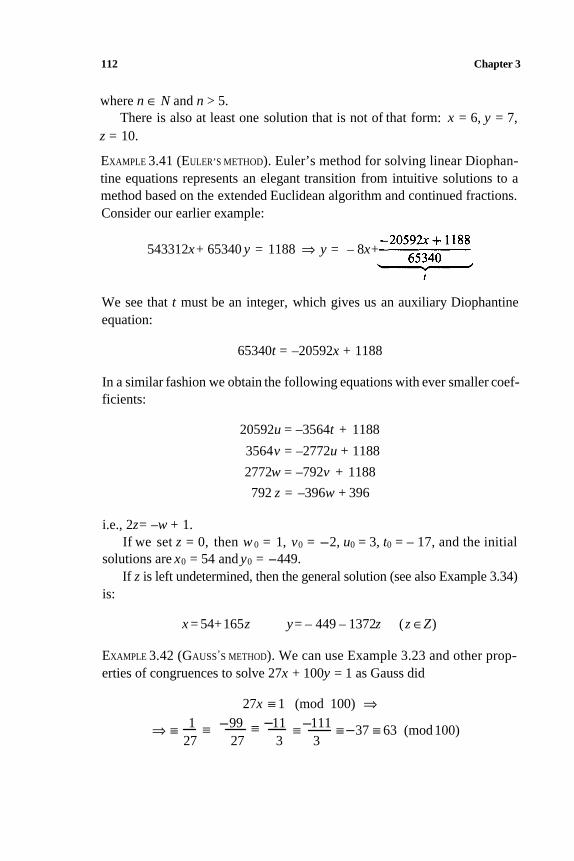
112 Chapter 3
where n ∈ N and n > 5.
z = 10.
EXAMPLE 3.41 (EULER’S METHOD). Euler’s method for solving linear Diophan-
tine equations represents an elegant transition from intuitive solutions to a
method based on the extended Euclidean algorithm and continued fractions.
Consider our earlier example:
There is also at least one solution that is not of that form: x = 6, y = 7,
543312x+ 65340 y = 1188 ⇒ y = – 8x+
We see that t must be an integer, which gives us an auxiliary Diophantine
equation:
65340t = –20592x + 1188
In a similar fashion we obtain the following equations with ever smaller coef-
ficients:
20592u = –3564t + 1188
3564v = –2772u + 1188
2772w = –792v + 1188
792 z = –396w + 396
i.e., 2z= –w + 1.
solutions are x0 = 54 and y0 = -449.
is:
If we set z = 0, then w 0 = 1, v0 = -2, u0 = 3, t0 = – 17, and the initial
If z is left undetermined, then the general solution (see also Example 3.34)
x = 54+165z y= – 449 – 1372z (z ∈Z)
EXAMPLE 3.42 (GAUSS’S METHOD). We can use Example 3.23 and other prop-
erties of congruences to solve 27x + 100y = 1 as Gauss did
27x ≡ 1 (mod 100) ⇒1 ≡ -99 ≡ 11 ≡ 111⇒ ≡ ≡ 37 ≡ 63 (mod 100)
27 27 3 3
--
-
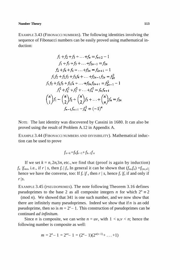
Number Theory 113
EXAMPLE 3.43 (FIBONACCI NUMBERS). The following identities involving the
sequence of Fibonacci numbers can be easily proved using mathematical in-
duction:
NOTE: The last identity was discovered by Cassini in 1680. It can also be
proved using the result of Problem A.12 in Appendix A.
EXAMPLE 3.44 (FIBONACCI NUMBERS AND DIVISIBILITY). Mathematical induc-
tion can be used to prove
fn+k =fk fn +1+ fk–1f n
If we set k = n, 2n,3n, etc., we find that (proof is again by induction)
fn |fmn, i.e., if r | s, then fr | fs. In general it can be shown that (fm,fn) =f(m,n);
hence we have the converse, too: If fr |f s then r | s, hence fr |fs if and only if
EXAMPLE 3.45 (PSEUDOPRIMES). The note following Theorem 3.16 defines
pseudoprimes to the base 2 as all composite integers n for which 2n ≡ 2(mod n). We showed that 341 is one such number, and we now show that
there are infinitely many pseudoprimes. Indeed we show that if n is an odd
pseudoprime, then so is m = 2n – 1. This construction of pseudoprimes can be
continued ad infinitum. Since n is composite, we can write n = uv, with 1 < u,v < n; hence the
following number is composite as well:
r | s.
m = 2n – 1 = 2uv– 1 = (2u– 1)(2u(v–1)+ . . . +1)
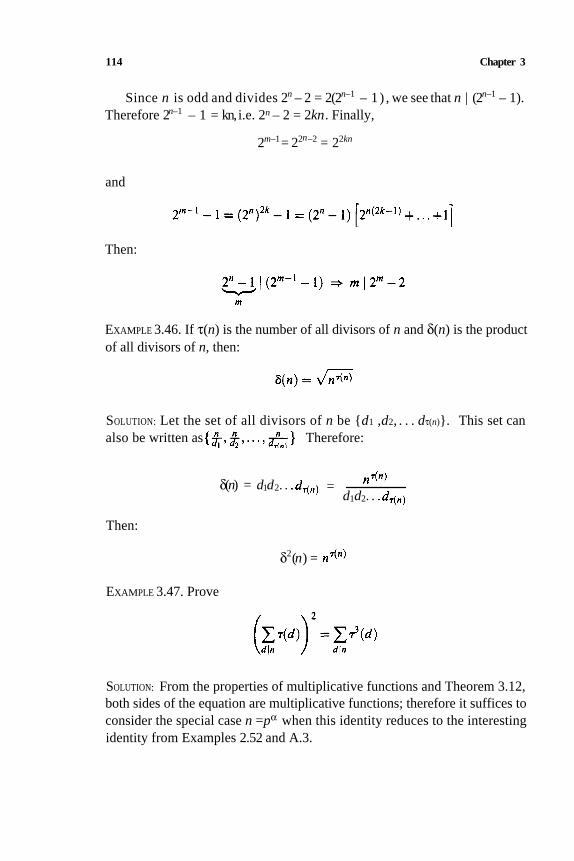
114 Chapter 3
Since n is odd and divides 2n – 2 = 2(2n–1 – 1) , we see that n | (2n–1 – 1).
Therefore 2n–1 – 1 = kn,i.e. 2n – 2 = 2kn. Finally,
2m–1 2n–2 22kn== 2
and
Then:
EXAMPLE 3.46. If τ(n) is the number of all divisors of n and δ(n) is the product
of all divisors of n, then:
SOLUTION: Let the set of all divisors of n be d1 ,d2, . . . dτ(n). This set can
also be written as Therefore:
d1d2. .δ(n) = d1d2. . =
Then:
δ2(n) =
EXAMPLE 3.47. Prove
SOLUTION: From the properties of multiplicative functions and Theorem 3.12,
both sides of the equation are multiplicative functions; therefore it suffices to
consider the special case n =pα when this identity reduces to the interesting
identity from Examples 2.52 and A.3.
Number Theory 115
EXAMPLE 3.48 (MERSENNE PRIMES). If 2m – 1 is a prime, then m must be a
prime too. Prove.
SOLUTION: If we assume m to be composite, i.e. m = ab, with a,b > 1, then:
i.e. 2m
– 1 is also composite.
NOTES: This is just a one-way implication because if m is prime, 2m – 1 may
be composite (for example, 211 – 1 = 2047 = 23 . 89).
For prime numbers p, numbers Mp = 2p – 1 are called Mersenne numbers.Some of these are primes (e.g., for p = 2, 3, 5, 7, 9), while some are composite
(e.g., p = 11). Due to their many interesting properties, it is much easier to
investigate the primality of Mersenne numbers Mp then of other integers of
comparable size. Hence it is not surprising that some of the largest known
primes are Mersenne primes. For example in 1968 the discovery of the then
largest prime 211213 – 1 at the University of Illinois at Urbana–Champaign was
celebrated by an appropriate postal stamp. Since then many more primes have
been found among the Mersenne numbers, for example 221701 – 1, found in
1978 by two high-school students in California.
EXAMPLE 3.49 (PERFECT NUMBERS). Many civilizations found the properties of
numbers not only interesting but also mystical. For example Ancient Greek
mathematicians defined and investigated properties of perfect numbers, integers
that equal the sum of their properdivisors. The first such number is 6, because:
6 = 1 + 2 + 3
The only perfect numbers < 10000 are 6, 28, 496, and 8128. It is a nice
programming exercise to determine other perfect numbers < 1000000.
Euclid knew that if 2n – 1 is a prime (then of course n must be prime, and
2n – 1 is a Mersenne prime), then:
2n –1 (2n – 1)
is perfect.
Euler showed that an even number is perfect if and only if it takes the form
2p–1Mp
116 Chapter 3
where Mp is a Mersenne prime (notjust any Mersenne number). To this day it
is not known whether or not there are odd perfect numbers.
EXAMPLE 3.50. Show that if n is a perfect number, then:
SOLUTION: The equivalent definition of perfect numbers is that the sum of
all of their divisors is twice the number itself (σ(n) = 2n). For example
1 + 2 + 3 + 6 = 2 . 6. With that in mind, consider
4
Geometry

This page intentionally left blank.
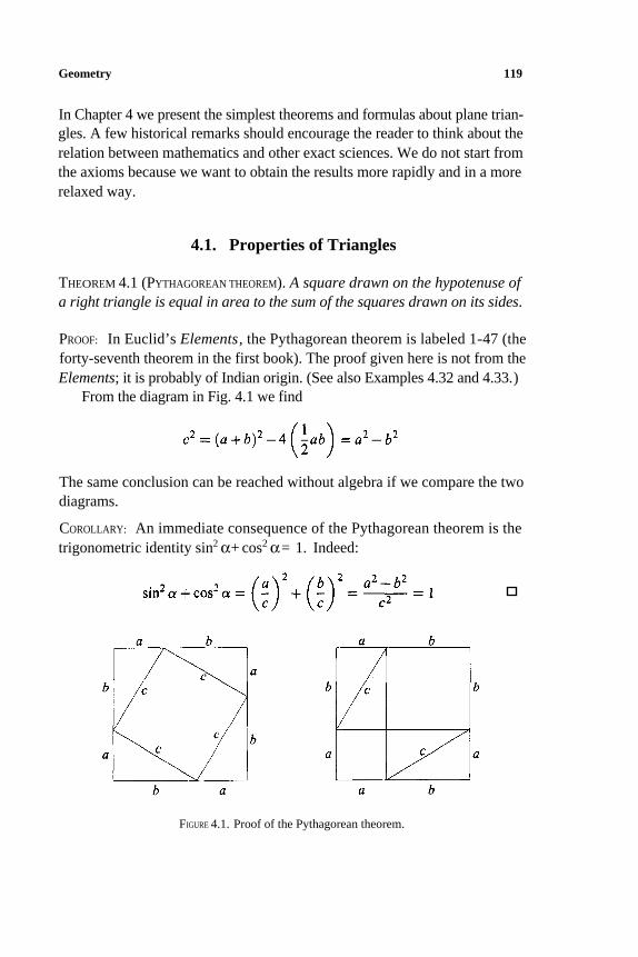
Geometry 119
In Chapter 4 we present the simplest theorems and formulas about plane trian-
gles. A few historical remarks should encourage the reader to think about the
relation between mathematics and other exact sciences. We do not start from
the axioms because we want to obtain the results more rapidly and in a more
relaxed way.
4.1. Properties of Triangles
THEOREM 4.1 (PYTHAGOREAN THEOREM). A square drawn on the hypotenuse ofa right triangle is equal in area to the sum of the squares drawn on its sides.
PROOF: In Euclid’s Elements, the Pythagorean theorem is labeled 1-47 (the
forty-seventh theorem in the first book). The proof given here is not from the
Elements; it is probably of Indian origin. (See also Examples 4.32 and 4.33.)
From the diagram in Fig. 4.1 we find
The same conclusion can be reached without algebra if we compare the two
diagrams.
COROLLARY: An immediate consequence of the Pythagorean theorem is the
trigonometric identity sin2 α+ cos2 α= 1. Indeed:
FIGURE 4.1. Proof of the Pythagorean theorem.
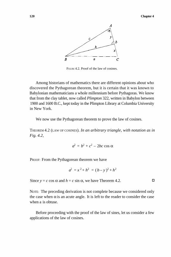
120 Chapter 4
FIGURE 4.2. Proof of the law of cosines.
Among historians of mathematics there are different opinions about who
discovered the Pythagorean theorem, but it is certain that it was known to
Babylonian mathematicians a whole millennium before Pythagoras. We know
that from the clay tablet, now called Plimpton 322, written in Babylon between
1900 and 1600 B.C., kept today in the Plimpton Library at Columbia University
in New York.
We now use the Pythagorean theorem to prove the law of cosines.
THEOREM 4.2 (LAW OF COSINES). In an arbitrary triangle, with notation as inFig. 4.2,
a2 = b2 + c2 – 2bc cos α
PROOF: From the Pythagorean theorem we have
a2 = x 2 + h2 = ( b – y )2 + h2
Since y = c cos α and h = c sin α, we have Theorem 4.2.
NOTE: The preceding derivation is not complete because we considered only
the case when α is an acute angle. It is left to the reader to consider the case
when a is obtuse.
Before proceeding with the proof of the law of sines, let us consider a few
applications of the law of cosines.
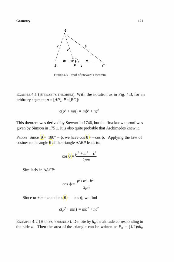
Geometry 121
FIGURE 4.3. Proof of Stewart’s theorem.
EXAMPLE 4.1 (STEWART’S THEOREM). With the notation as in Fig. 4.3, for an
arbitrary segment p = [AP], P∈ [BC]:
a(p2 + mn) = mb2 + nc2
This theorem was derived by Stewart in 1746, but the first known proof was
given by Simson in 175 1. It is also quite probable that Archimedes knew it.
PROOF: Since θ = 180° – φ, we have cos θ = – cos φ. Applying the law of
cosines to the angle θ of the triangle ∆ABP leads to:
p2 + m2 – c2
2pmcos θ =
Similarly in ∆ACP:
p2+n2– b2
cos φ =2pn
Since m + n = a and cos θ = – cos φ, we find
a(p2 + mn) = mb2 + nc2
EXAMPLE 4.2 (HERO’S FORMULA). Denote by ha the altitude corresponding to
the side a. Then the area of the triangle can be written as P∆ = (1/2)aha.
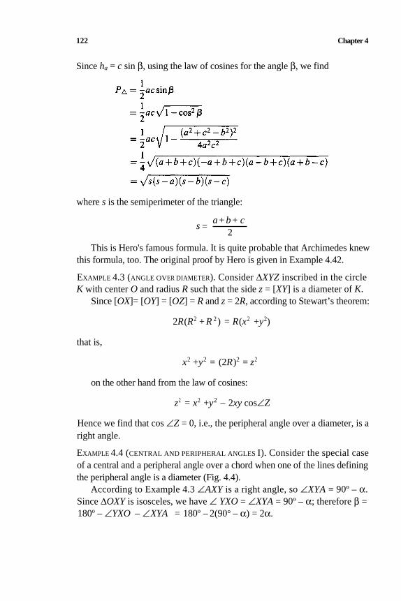
122 Chapter 4
Since ha = c sin β, using the law of cosines for the angle β, we find
where s is the semiperimeter of the triangle:
a + b + c2
This is Hero's famous formula. It is quite probable that Archimedes knew
s =
this formula, too. The original proof by Hero is given in Example 4.42.
EXAMPLE 4.3 (ANGLE OVER DIAMETER). Consider ∆XYZ inscribed in the circle
K with center O and radius R such that the side z = [XY] is a diameter of K.
Since [OX]= [OY] = [OZ] = R and z = 2R, according to Stewart’s theorem:
2R(R2 + R 2 ) = R(x2 +y2)
that is,
x2 +y2 = (2R)2 = z2
z2 = x2 +y2 – 2xy cos∠Z
on the other hand from the law of cosines:
Hence we find that cos ∠Z = 0, i.e., the peripheral angle over a diameter, is a
right angle.
EXAMPLE 4.4 (CENTRAL AND PERIPHERAL ANGLES I). Consider the special case
of a central and a peripheral angle over a chord when one of the lines defining
the peripheral angle is a diameter (Fig. 4.4).
According to Example 4.3 ∠AXY is a right angle, so ∠XYA = 90º – α.
Since ∆OXY is isosceles, we have ∠ YXO = ∠XYA = 90º – α; therefore β =
180º – ∠YXO – ∠XYA = 180º – 2(90° – α) = 2α.
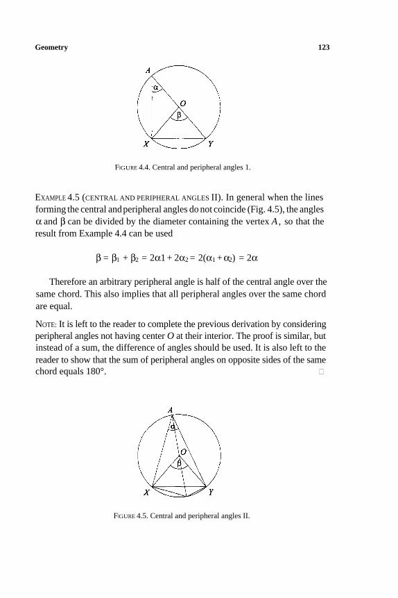
Geometry 123
FIGURE 4.4. Central and peripheral angles 1.
EXAMPLE 4.5 (CENTRAL AND PERIPHERAL ANGLES II). In general when the lines
forming the central and peripheral angles do not coincide (Fig. 4.5), the angles
α and β can be divided by the diameter containing the vertex A , so that the
result from Example 4.4 can be used
β = β1 + β2 = 2α1 + 2α2 = 2(α1 + α2) = 2α
Therefore an arbitrary peripheral angle is half of the central angle over the
same chord. This also implies that all peripheral angles over the same chord
are equal.
NOTE: It is left to the reader to complete the previous derivation by considering
peripheral angles not having center O at their interior. The proof is similar, but
instead of a sum, the difference of angles should be used. It is also left to the
reader to show that the sum of peripheral angles on opposite sides of the same
chord equals 180°.
FIGURE 4.5. Central and peripheral angles II.
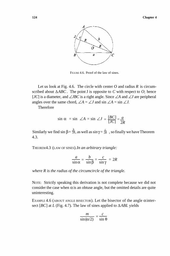
124 Chapter 4
FIGURE 4.6. Proof of the law of sines.
Let us look at Fig. 4.6. The circle with center O and radius R is circum-
scribed about ∆ABC . The point J is opposite to C with respect to O; hence
[JC] is a diameter, and ∠JBC is a right angle. Since ∠A and ∠J are peripheral
angles over the same chord, ∠A = ∠J and sin ∠A = sin ∠J.
Therefore
[BC] asin α = sin ∠A = sin ∠J = =[JC] 2R
bSimilarly we find sin β= 2R, as well as sinγ =
c2R , so finally we have Theorem
4.3.
THEOREM4.3 (LAW OF SINES).In an arbitrary triangle:
a c2R= = =
bsin α sin β sin γ
where R is the radius of the circumcircle of the triangle.
NOTE: Strictly speaking this derivation is not complete because we did not
consider the case when α is an obtuse angle, but the omitted details are quite
uninteresting.
EXAMPLE 4.6 (ABOUT ANGLE BISECTOR). Let the bisector of the angle α inter-
sect [BC] at L (Fig. 4.7). The law of sines applied to ∆ABL yields
m c=
sin(α/2) sin θ
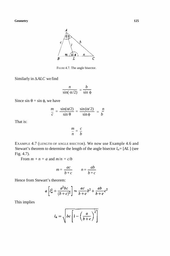
Geometry 125
FIGURE 4.7. The angle bisector.
Similarly in ∆ALC we find
b=
nsin( α /2) sin φ
Since sin θ = sin φ, we have
m sin(α/2) sin(α/2) n== -=
c sin sin φ b_
That is:
m c= ––
n b
EXAMPLE 4.7 (LENGTH OF ANGLE BISECTOR). We now use Example 4.6 and
Stewart’s theorem to determine the length of the angle bisector lα = [AL ] (see
Fig. 4.7).
From m + n = a and m/n = c/b
ac abb + c b + c
m = n =
Hence from Stewart’s theorem:
This implies
θ
126 Chapter 4
EXAMPLE 4.8 (LENGTH OF MEDIAN). From the definition of the median, we have
m = n = a/2, thus, according to Stewart’s theorem:
That is:
EXAMPLE 4.9 (LENGTH OF ALTITUDE). The length of the altitude ha can be found
using Stewart’s theorem, but the derivation from Hero’s formula is much sim-
pler:
EXAMPLE 4.10 (CIRCUMCENTER). The circumcenter of a triangle, i.e., the center
of the circumcircle (the circle circumscribed about the triangle), is found as the
intersection of the perpendicular bisectors of the sides (see Fig. 4.8). Why?
Because the circumcircle contains all three vertices of the triangle. This means
that the circumcenter O is at the same distance from all three vertices. Hence:
O ∈perp bis [AB ] O ∈perp bis [AC ] O ∈ perp bis [BC]
That is:
O = perp bis [AB] ⊃ perp bis [AC] ⊃ perp bis [BC ]
Of course when constructing the circumcenter O, it suffices to construct
only the perpendicular bisectors of any two sides.
EXAMPLE 4.11 (INCENTER). The incenter of a triangle, i.e., the center of the
incircle (the circle inscribed in the triangle), is found as the intersection of
the angle bisectors (see Fig. 4.9). The incircle touches all three sides of the
triangle. For a circle to touch both arms of the angle α, its center must lie on
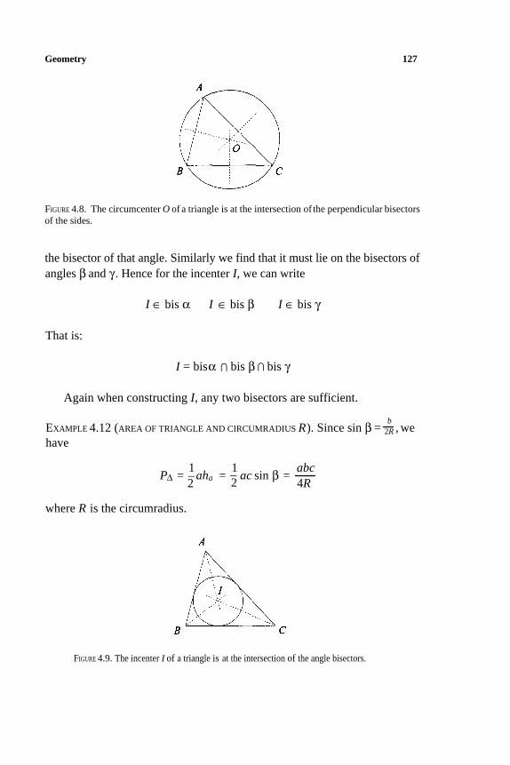
Geometry 127
FIGURE 4.8. The circumcenter O of a triangle is at the intersection of the perpendicular bisectors
of the sides.
the bisector of that angle. Similarly we find that it must lie on the bisectors of
angles β and γ . Hence for the incenter I, we can write
I ∈ bis α I ∈ bis β I ∈ bis γ
That is:
I = bisα ⊃ bis β ⊃ bis γ
Again when constructing I, any two bisectors are sufficient.
EXAMPLE 4.12 (AREA OF TRIANGLE AND CIRCUMRADIUS R). Since sin β =b
2R , we
have
1 1 abc––P∆ = aha = ac sin β =
2 2 4R
where R is the circumradius.
FIGURE 4.9. The incenter I of a triangle is at the intersection of the angle bisectors.
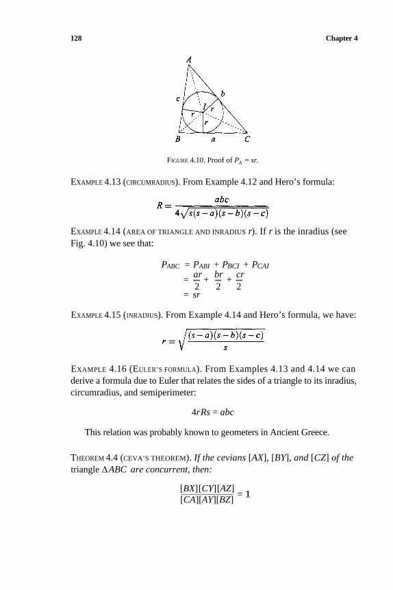
128 Chapter 4
FIGURE 4.10. Proof of P∆ = sr.
EXAMPLE 4.13 (CIRCUMRADIUS). From Example 4.12 and Hero’s formula:
EXAMPLE 4.14 (AREA OF TRIANGLE AND INRADIUS r). If r is the inradius (see
Fig. 4.10) we see that:
PABC = PABI + PBCI + PCAIar br cr
= - + -+-2 2 2
= sr
EXAMPLE 4.15 (INRADIUS). From Example 4.14 and Hero’s formula, we have:
EXAMPLE 4.16 (EULER’S FORMULA). From Examples 4.13 and 4.14 we can
derive a formula due to Euler that relates the sides of a triangle to its inradius,
circumradius, and semiperimeter:
4r Rs = abc
This relation was probably known to geometers in Ancient Greece.
THEOREM 4.4 (CEVA’S THEOREM). If the cevians [AX], [BY], and [CZ] of the triangle ∆ABC are concurrent, then:
[BX] [CY] [AZ]
[CA][AY][BZ]= 1
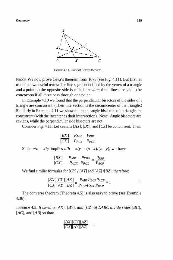
Geometry 129
FIGURE 4.11. Proof of Ceva’s theorem.
PROOF: We now prove Ceva’s theorem from 1678 (see Fig. 4.11). But first let
us define two useful terms: The line segment defined by the vertex of a triangle
and a point on the opposite side is called a cevian; three lines are said to be
concurrent if all three pass through one point.
In Example 4.10 we found that the perpendicular bisectors of the sides of a
triangle are concurrent. (Their intersection is the circumcenter of the triangle.)
Similarly in Example 4.11 we showed that the angle bisectors of a triangle are
concurrent (with the incenter as their intersection). Note: Angle bisectors are
cevians, while the perpendicular side bisectors are not.
Consider Fig. 4.11. Let cevians [AX], [BY], and [CZ] be concurrent. Then:
[BX ] PABX PPBX
[CX ] PACX PPCX= = -
Since a/b = x /y implies a/b = x /y = (a –x )/(b –y), we have
[BX ] PABX PPBX PABP–=
[CX ] PACX –PPCX PACP
We find similar formulas for [CY] / [AY] and [AZ] /[BZ]; therefore:
[BX ][CY ][AZ ] PABP PBCPPACP= = 1
[CX ][AY ][BZ ] PACPPABPPBCP
The converse theorem (Theorem 4.5) is also easy to prove (see Example
4.36):
THEOREM 4.5. If cevians [AX], [BY], and [CZ] of ∆ABC divide sides [BC],
[AC], and [AB] so that:
[BX] [CY] [AZ]
[CX][AY][BZ]= 1
130 Chapter 4
then they are concurrent.
EXAMPLE 4.17 (ANGLE BISECTORS ARE CONCURRENT). For the angle bisectors,
we have
[BX] [CY][AZ] c– a– b
= – 1=[CX][AY][BZ ] b c a
Therefore according to Theorem 4.5, they are concurrent. A different proof was
given in Example 4.11, where we saw that their intersection is at the incenterof the triangle.
EXAMPLE 4.18 (MEDIANS ARE CONCURRENT). The medians of a triangle divide
its sides so that [BX ] = [CX], [CY ] = [AY ], and [AZ ] = [BZ]; therefore:
[BX] [CY] [AZ]
[CX][AY][BZ]= 1
That is, the medians are concurrent. Their intersection is called the centroid of
the triangle.
EXAMPLE 4.19 (ALTITUDES ARE CONCURRENT). For the altitudes of a triangle,
we have
1[BX ] [CY ] [AZ ] ccosβ acosγ bcosα
==[CX ][AY ][BZ ] bcosγ ccosα acosβ
This proves that they are concurrent. Their intersection is called the orthocenterof the triangle.
If points A 1 , . . . , A n have masses m1 , . . . , mn, we have a system of material
A point T is the centroid of the system (m1, A 1), . . . , (mn, A n) of material
points, usually denoted by (m1, A1) , . . . , ( mn, An ).
points if the following is satisfied:
→ →m1A1T + . . . +mnAnT = 0 (4.1)
THEOREM 4.6. For an arbitrary system of material points
(m1, A1) ,. . . , (mn, An )
there is one and only one centroid.
Geometry 131
PROOF: Let the origin of the coordinate system be denoted by O. If both sides
of the defining equality (4.1) are augmented by m1OA1 + . . . + mn OAn , then: → →
→ → → (m1+ . . . + mn)OT=m1OA 1 + . . . + mnOAn
This implies
→ → → OT=
m1OA1 + . . . +mnOAn
m1 + . . . + mn
NOTE: The reader is probably familiar with the fact that if T is the centroid
of the system (m1,A 1 ), . . . , (mn,An ) and if we add another material point
to it, e.g., (mn+1, An+1), the centroid of the new system is the centroid of
(m, T ), (mn+1, An+1), where m = m1 +. . .+mn.
Indeed:
→ → →→ m1OA1 +. . . +mnOAn+mn+1OAn+1OT' =
m1+. . . + mn + mn+1
→ →mOT + mn+1 OAn+ 1
m + mn+1=
We see that T' lies on the segment [An+1T] and further:
[TA n+1] (4.2)mn+1
m+ mn+1
THEOREM 4.7 (ARCHIMEDES’ THEOREM). The medians of a triangle intersect at the centroid of a triangle, and they divide each other in 1 : 2 ratio.
PROOF: From Theorem 4.6, independent of Ceva’s theorem, we find that the
medians are concurrent and that they divide each other with the ratio 1 : 2. The
centroid T of the triangle ∆ABC is the centroid of the system:
[TT'] =
(m,A ), (m,B ), (m,C))
Hence as mentioned earlier, T is also the centroid of the following systems:
(2m,TAB),(m,C) (2m,TAC),(m,B) (2m,TBC),(m,A)
132 Chapter 4
where TAB , TAC , and TBC are centroids of the segments [AB], [AC], and [BC],
respectively.
Hence T ∈[CTAB ], T ∈[BTAC], and T ∈[AT BC]. This implies that the
medians are concurrent, since their intersection is the centroid T.
From Eq. (4.2) we find that the medians divide each other in a 1 : 2 ratio.
This proves Theorem 4.7.
Earlier we used Stewart’s theorem to find the length of the median ta:
We use this result in Examples 4.20 and 4.2 1.
EXAMPLE 4.20 (TWO SIMILAR TRIANGLES). Consider ∆ABC and use its medians
to form a new triangle ∆A1 B1 C1 . If ∆A2B2C2 is constructed from the medians
of ∆A1 B1 C1 , then triangles ∆ABC and ∆Α2B2C2 are similar.
The squares of the sides of ∆A1B1 C1 are given by:
The squares of the sides of ∆A2B2C2 are given by:
Hence we find that ∆ABC and ∆A2B2C2 are similar, with a factor of 3/4.
EXAMPLE 4.21 (LEIBNIZ’S THEOREM). Let T be the centroid of ∆ABC. Then
for an arbitrary point M, we have Leibniz’s theorem (see Fig. 4.12):
[M A]2 + [MB ]2 + [MC]2 = 3[MT ]2 + [AT ]2+ [BT ]2 + [CT]2
Let T1 be the center of [BC]. Then [MT1] is a median for ∆MBC; from
Example 4.8 we know that:
1[MT 1]
2 = –4
(2[MB ]2+2[MC]
2– [BC]
2)
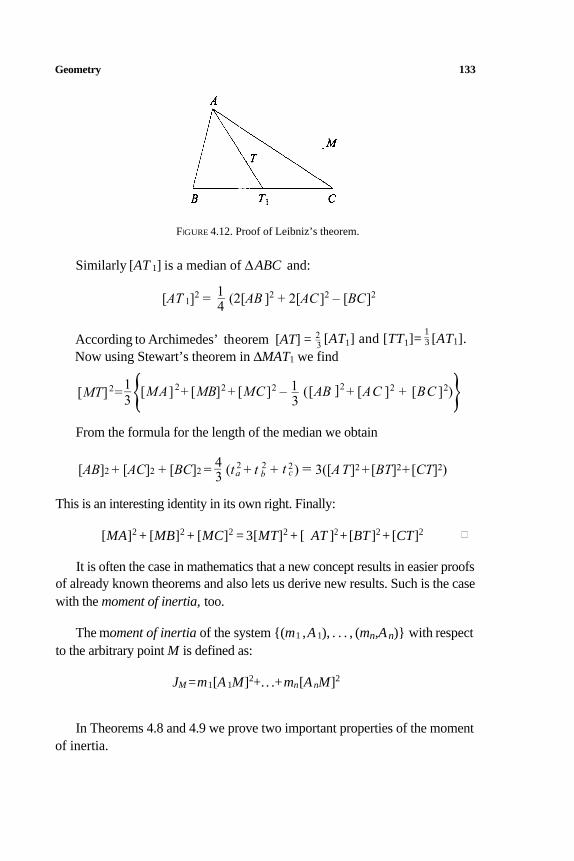
Geometry 133
FIGURE 4.12. Proof of Leibniz’s theorem.
Similarly [AT 1] is a median of ∆ABC and:
According to Archimedes’ theorem [AT] =2–3 [AT1] and [TT1]=
1
3 [AT1].–
Now using Stewart’s theorem in ∆MAT1 we find
From the formula for the length of the median we obtain
This is an interesting identity in its own right. Finally:
[MA]2 + [MB]2 + [MC]2 = 3[MT]2 + [ AT ]2 +[BT ]2 + [CT]2
It is often the case in mathematics that a new concept results in easier proofs
of already known theorems and also lets us derive new results. Such is the case
with the moment of inertia, too.
The moment of inertia of the system (m1 ,A 1), . . . , (mn,An) with respect
to the arbitrary point M is defined as:
JM =m1[A 1M]2+. . .+mn[A nM]2
In Theorems 4.8 and 4.9 we prove two important properties of the moment
of inertia.
[AT 1]2 = 14– (2[AB ]2 + 2[AC ]2 – [BC]2
[MT]2= 1–3[MA]2 + [MB]2 + [MC ]2 – –13
([AB ]2 + [AC ]2 + [BC ]2)[AB]2 + [AC]2 + [BC]2 = 4–3 (t 2
a + t 2b + t 2
c ) = 3([A T]2 +[BT]2+[CT]2)
134 Chapter 4
THEOREM 4.8 (LAW OF STEINER AND LAGRANGE). For the moment of inertia withrespect to the arbitrary point M, we have
JM = JT + m[MT ]2
where m = m1 + . . . + mn, while T is the centroid of the system.
PROOF: The following sequence of equalities leads us to the desired formula:
COROLLARY: An immediate consequence of the law of Steiner and Lagrange is that the moment of inertia is the least when taken with respect to the centroid. Indeed since m[MT]2 ≥ 0, the following inequality holds
JM ≥ JT
with the equality if and only if M = T.
THEOREM 4.9 (JACOBI’S THEOREM). The moment of inertia with respect to the centroid of a system is given by:
where rij = [AiAj ] and m = m1 + . . . + mn.
PROOF: Apply the law of Steiner and Lagrange to the special case when M = Ak ,where Ak is a point of the system, to obtain
JAk = JT + m[Ak T]2
Multiply both sides of this equality by mk , then sum both sides over k to obtain
Geometry 135
EXAMPLE 4.22 (MOMENT OF INERTIA OF TRIANGLE). Let us calculate the moment of inertia of ∆ABC with respect to its centroid T. If we substitute the unit masses for the vertices of the triangle, by definition we have
On the other hand from Jacobi’s theorem, we have
13JT = – (a2 + b2 + c2)
Thus we have another proof of the identity:
34t 2
a + t 2b + t 2
c = – (a2 + b2 + c2)
which we found earlier using the formula for the length of a median.
EXAMPLE 4.23 (LEIBNIZ’S THEOREM AGAIN). If we look at the moment of inertia of a triangle with respect to the arbitrary point M, from the law of Steiner andLagrange and the previous example we find
JM = JT + 3[MT ]2
= 3[MT ]2 + [AT ]2+ [BT ]2+ [CT]2
By definition:
JM = [MA ]2 + [MB ]2 + [MC]2
In a very simple and elegant manner we derived Leibniz’s theorem:
[M A]2+ [MB ]2+ [MC]2 = 3[MT ]2+ [AT ]2+ [BT ]2+ [CT]2
EXAMPLE 4.24 (STEWART’S THEOREM AGAIN). Let us consider how to use the concept of the moment of inertia to derive Stewart’s theorem. Instead of theunit or equal masses, we now need the masses proportional to segments n and m at points B and C, respectively. We do not need mass at the vertex A.
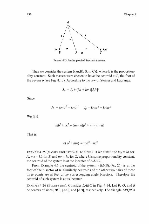
136 Chapter 4
FIGURE 4.13.Anotherproof of Stewart’s theorem.
Thus we consider the system (kn,B), (km, C), where k is the proportion- ality constant. Such masses were chosen to have the centroid at P, the foot ofthe cevian p (see Fig. 4.13). According to the law of Steiner and Lagrange:
JA = Jp + (kn + km )[AP]2
Since:
JA = kmb 2 + knc2 Jp = knm2 + kmn 2
We find
mb2+ nc2 = (m+ n)p2 + mn(m+n)
That is:
a( p2 + mn) = mb2 + nc2
EXAMPLE 4.25 (MASSES PROPORTIONAL TO SIDES). If we substitute mA = ka for A , mB = kb for B, and mC = kc for C, where k is some proportionality constant,the centroid of the system is at the incenter of ∆ABC.
From Example 4.6 the centroid of the system (kb,B), (kc, C) is at the foot of the bisector of α. Similarly centroids of the other two pairs of these three points are at feet of the corresponding angle bisectors. Therefore the centroid of such system is at its incenter.
EXAMPLE 4.26 (EULER’S LINE). Consider ∆ABC in Fig. 4.14. Let P, Q, and Rbe centers of sides [BC], [AC], and [AB], respectively. The triangle ∆PQR is
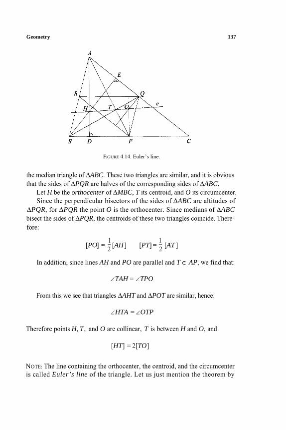
Geometry 137
FIGURE 4.14. Euler’s line.
the median triangle of ∆ABC. These two triangles are similar, and it is obviousthat the sides of ∆PQR are halves of the corresponding sides of ∆ABC.
Let H be the orthocenter of ∆MBC, T its centroid, and O its circumcenter.Since the perpendicular bisectors of the sides of ∆ABC are altitudes of
∆PQR, for ∆PQR the point O is the orthocenter. Since medians of ∆ABCbisect the sides of ∆PQR, the centroids of these two triangles coincide. There-fore:
1 12 2
In addition, since lines AH and PO are parallel and T ∈ AP, we find that:
[PO] = -[AH ] [PT] = - [AT ]
∠TAH = ∠TPO
From this we see that triangles ∆AHT and ∆POT are similar, hence:
∠HTA = ∠OTP
Therefore points H, T, and O are collinear, T is between H and O, and
[HT] = 2[TO]
NOTE: The line containing the orthocenter, the centroid, and the circumcenteris called Euler’s line of the triangle. Let us just mention the theorem by
138 Chapter 4
Brianchon and Poncelet from 1820, which states that the center of [OH] is thecenter of the nine-point circle, which contains feet of the altitudes, centers ofthe sides, and centers of the segments defined by the orthocenter and verticesof the triangle. The radius of the nine-point circle is 1–2 R . In 1822 Feuerbach showed that the nine-point circle touches the incircle and all three excircles* ofthe triangle. The nine-point circle is also called Euler’s circle (in France), andFeuerbach’s circle (in Germany). It can be proved that if R is the circumradius,r the inradius, and ra, rb, and rc the exradii, the following is true:
4R = ra + rb + rc – r
In addition:
1 1 1– – –+ + 1ra rb rc r= -
EXAMPLE 4.27 (HAMILTON–SYLVESTER’S THEOREM). This theorem states that: → → → →
OH = OA + OB + OC
→ → →To prove this, write the definition of the centroid AT + BT + CT = 0, then
observe that: → →
OH = 3OT→ → → → →
= OA +AT + OB + BT + OC+ CT→ → →
= OA + OB + OC
EXAMPLE 4.28 (SEGMENT [OT]). In this example we derive the expression for the segment [OT] in terms of the sides of the triangle only. If we substitute the unit masses in the vertices of the triangle, the law of Steiner and Lagrange applied to the circumcenter O yields
JO = JT + 3[OT]2
From the definition of the moment of inertia and Example 4.22, we know that:
JO =3R2 JT = – (a2 + b2 + c2)
*A circle touching one side of the triangle and the extensions of the other two sides is called theexcircle or the escribed circle of the triangle. There are three excircles; their radii (the exradii ofthe triangle) are ra =P∆ / (s – a), rb = P∆ / (s – b), and rc = P∆ / (s – c).
13
→
Geometry 139
Then:
1[OT]2 = R2 – – (a2 + b2 + c2 )9
NOTE: Earlier we found the expression for R in terms of a, b, and c; therefore the same can be done for [OT] and segments [OH] and [TH], too.
EXAMPLE 4.29 (SEGMENT [OI]). Let us determine the expression for [OI]. Asin Example 4.25 we substitute the masses ka, kb, and kc in the vertices A, B ,and C, respectively, so that the centroid of the system is at the incenter I.
The law of Steiner and Lagrange gives
JO = J1 + k(a + b + c ) [OI]2
Jacobi’s theorem yields
k2(abc2 +ab2c +a2bc)k(a + b + c)
JI = = kabc
From the definition of the moment of inertia it follows that:
JO = k(a + b + c)R2
Therefore:
JO – J1 = R2 –abc
[OI]2 = k(a + b + c) a + b + c
Observe that (see Examples 4.13 and 4.15):
= 2Rrabc
a + b + c
so finally:
[OI]2 = R(R – 2r)
This formula was first discovered by Euler. Since [OI]2 ≥0, it implies thatR ≥ 2r. In Example 4.47 we give another proof of this formula.
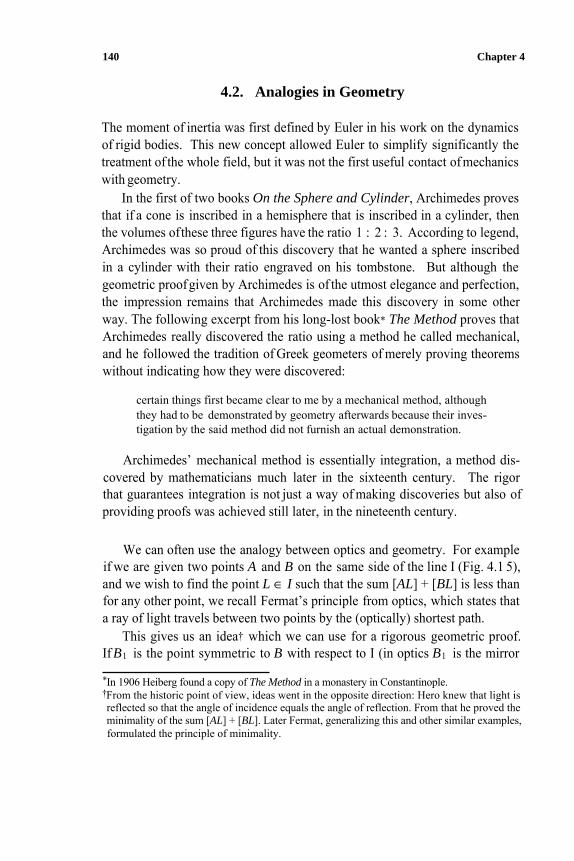
140 Chapter 4
4.2. Analogies in Geometry
The moment of inertia was first defined by Euler in his work on the dynamics of rigid bodies. This new concept allowed Euler to simplify significantly the treatment of the whole field, but it was not the first useful contact of mechanics with geometry.
In the first of two books On the Sphere and Cylinder, Archimedes proves that if a cone is inscribed in a hemisphere that is inscribed in a cylinder, then the volumes of these three figures have the ratio 1 : 2 : 3. According to legend, Archimedes was so proud of this discovery that he wanted a sphere inscribed in a cylinder with their ratio engraved on his tombstone. But although the geometric proof given by Archimedes is of the utmost elegance and perfection, the impression remains that Archimedes made this discovery in some other way. The following excerpt from his long-lost book* The Method proves thatArchimedes really discovered the ratio using a method he called mechanical, and he followed the tradition of Greek geometers of merely proving theorems without indicating how they were discovered:
certain things first became clear to me by a mechanical method, althoughthey had to be demonstrated by geometry afterwards because their inves-tigation by the said method did not furnish an actual demonstration.
Archimedes’ mechanical method is essentially integration, a method dis-covered by mathematicians much later in the sixteenth century. The rigor that guarantees integration is not just a way of making discoveries but also of providing proofs was achieved still later, in the nineteenth century.
We can often use the analogy between optics and geometry. For example if we are given two points A and B on the same side of the line I (Fig. 4.1 5),and we wish to find the point L ∈ I such that the sum [AL] + [BL] is less thanfor any other point, we recall Fermat’s principle from optics, which states that a ray of light travels between two points by the (optically) shortest path.
This gives us an idea† which we can use for a rigorous geometric proof.If B1 is the point symmetric to B with respect to I (in optics B1 is the mirror
*In 1906 Heiberg found a copy of The Method in a monastery in Constantinople.†From the historic point of view, ideas went in the opposite direction: Hero knew that light is reflected so that the angle of incidence equals the angle of reflection. From that he proved the minimality of the sum [AL] + [BL]. Later Fermat, generalizing this and other similar examples, formulated the principle of minimality.
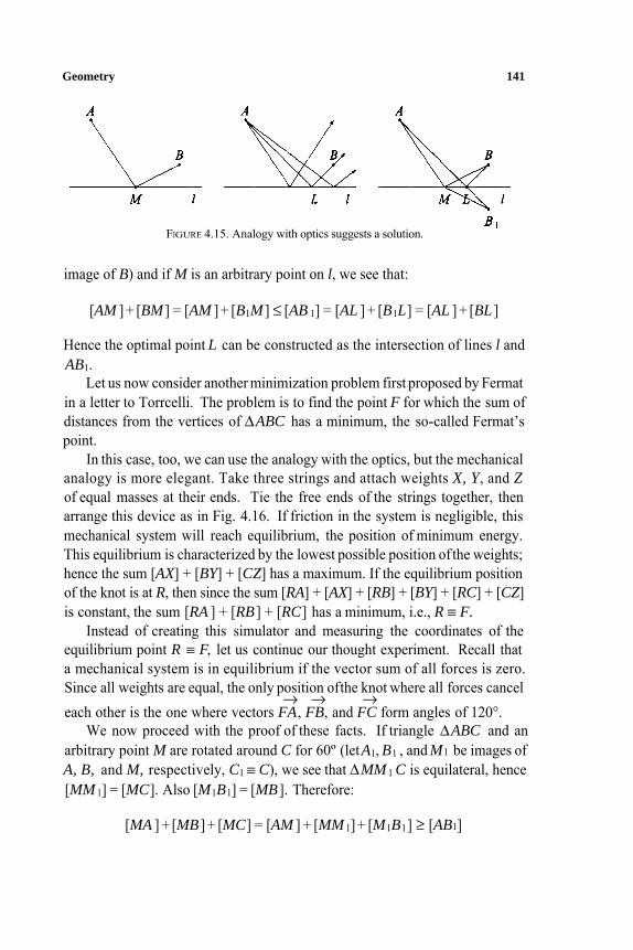
Geometry 141
FIGURE 4.15. Analogy with optics suggests a solution.
image of B) and if M is an arbitrary point on l, we see that:
[AM ] + [BM ] = [AM ] + [B1M ] ≤ [AB 1] = [AL ] + [B1L] = [AL ] + [BL ]
Hence the optimal point L can be constructed as the intersection of lines l and AB1.
Let us now consider another minimization problem first proposed by Fermat in a letter to Torrcelli. The problem is to find the point F for which the sum ofdistances from the vertices of ∆ABC has a minimum, the so-called Fermat’spoint.
In this case, too, we can use the analogy with the optics, but the mechanical analogy is more elegant. Take three strings and attach weights X, Y, and Zof equal masses at their ends. Tie the free ends of the strings together, then arrange this device as in Fig. 4.16. If friction in the system is negligible, this mechanical system will reach equilibrium, the position of minimum energy. This equilibrium is characterized by the lowest possible position of the weights; hence the sum [AX] + [BY] + [CZ] has a maximum. If the equilibrium positionof the knot is at R, then since the sum [RA] + [AX] + [RB] + [BY] + [RC] + [CZ]is constant, the sum [RA ] + [RB ] + [RC] has a minimum, i.e., R ≡ F.
Instead of creating this simulator and measuring the coordinates of theequilibrium point R ≡ F, let us continue our thought experiment. Recall thata mechanical system is in equilibrium if the vector sum of all forces is zero.Since all weights are equal, the only position ofthe knot where all forces canceleach other is the one where vectors FA, FB, and FC form angles of 120°.
We now proceed with the proof of these facts. If triangle ∆ABC and anarbitrary point M are rotated around C for 60º (letA1, B1 , and M1 be images ofA, B, and M, respectively, C1 ≡ C), we see that ∆MM 1 C is equilateral, hence[MM 1] = [MC]. Also [M1B1] = [MB ]. Therefore:
→ → →
[MA ] + [MB ] + [MC] = [AM ] + [MM 1]+ [M1B1] ≥ [AB1]
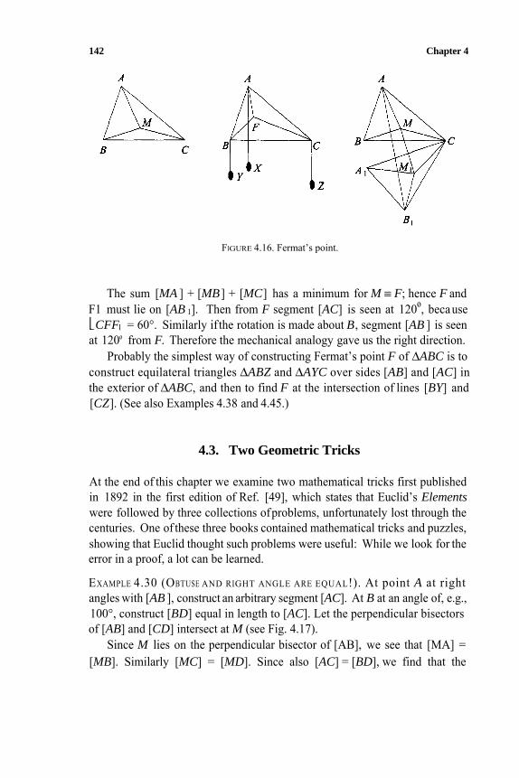
142 Chapter 4
FIGURE 4.16. Fermat’s point.
The sum [MA ] + [MB ] + [MC] has a minimum for M ≡ F; hence F and F1 must lie on [AB 1]. Then from F segment [AC] is seen at 120º, becauseCFF1 = 60°. Similarly if the rotation is made about B, segment [AB ] is seenat 120º from F. Therefore the mechanical analogy gave us the right direction.
Probably the simplest way of constructing Fermat’s point F of ∆ABC is to construct equilateral triangles ∆ABZ and ∆AYC over sides [AB] and [AC] in the exterior of ∆ABC, and then to find F at the intersection of lines [BY] and[CZ]. (See also Examples 4.38 and 4.45.)
4.3. Two Geometric Tricks
At the end of this chapter we examine two mathematical tricks first published in 1892 in the first edition of Ref. [49], which states that Euclid’s Elementswere followed by three collections of problems, unfortunately lost through the centuries. One of these three books contained mathematical tricks and puzzles,showing that Euclid thought such problems were useful: While we look for the error in a proof, a lot can be learned.
EXAMPLE 4.30 (OBTUSE AND RIGHT ANGLE ARE EQUAL!). At point A at rightangles with [AB ], construct an arbitrary segment [AC]. At B at an angle of, e.g.,100°, construct [BD] equal in length to [AC]. Let the perpendicular bisectors of [AB] and [CD] intersect at M (see Fig. 4.17).
Since M lies on the perpendicular bisector of [AB], we see that [MA] =[MB]. Similarly [MC] = [MD]. Since also [AC] = [BD], we find that the
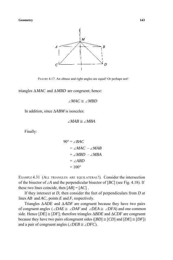
Geometry 143
FIGURE 4.17. An obtuse and right angles are equal! Or perhaps not!
triangles ∆MAC and ∆MBD are congruent; hence:
∠MAC ≅ ∠MBD
In addition, since ∆ABM is isosceles:
∠MAB ≅ ∠MBA
Finally:
90° = ∠BAC
= ∠MAC – ∠MAB
= ∠MBD – ∠MBA
= ∠ABD
= 100°
EXAMPLE 4.31 (ALL TRIANGLES ARE EQUILATERAL!). Consider the intersectionof the bisector of ∠A and the perpendicular bisector of [BC] (see Fig. 4.18). If these two lines coincide, then [AB] = [AC] .
If they intersect at D, then consider the feet of perpendiculars from D atlines AB and AC , points E and F, respectively.
Triangles ∆ADE and ∆ADF are congruent because they have two pairsof congruent angles ( ∠DAE ≅ ∠DAF and ∠DEA ≅ ∠DFA) and one commonside. Hence [DE] ≅ [DF]; therefore triangles ∆BDE and ∆CDF are congruent because they have two pairs ofcongruent sides ([BD] ≅ [CD] and [DE] ≅ [DF])and a pair of congruent angles (∠DEB ≅ ∠DFC).
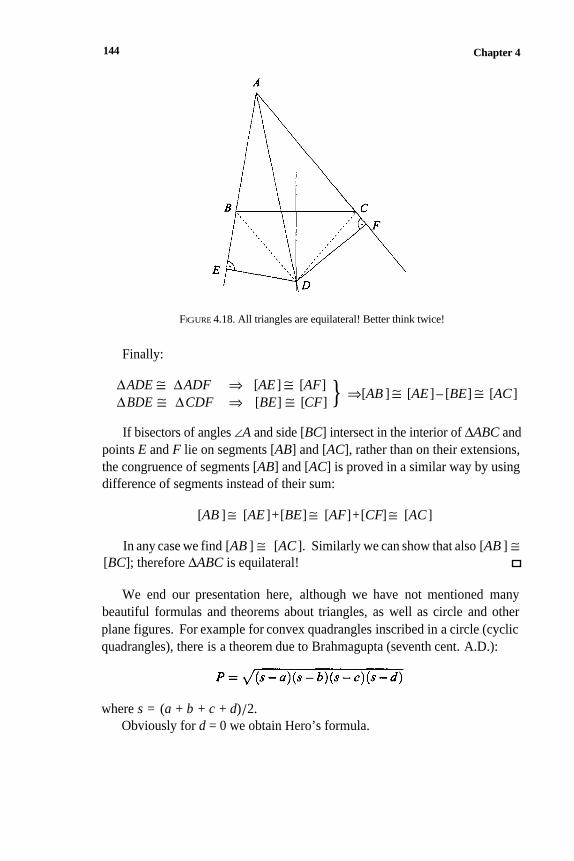
Chapter 4144
FIGURE 4.18. All triangles are equilateral! Better think twice!
Finally:
⇒[AB ] ≅ [AE ] – [BE] ≅ [AC ]∆ADE ≅ ∆ADF ⇒ [AE ] ≅ [AF]
∆BDE ≅ ∆CDF ⇒ [BE] ≅ [CF]
If bisectors of angles ∠A and side [BC] intersect in the interior of ∆ABC and
points E and F lie on segments [AB] and [AC], rather than on their extensions,
the congruence of segments [AB] and [AC] is proved in a similar way by using
difference of segments instead of their sum:
[AB ] ≅ [AE ]+[BE] ≅ [AF]+[CF] ≅ [AC ]
In any case we find [AB ] ≅ [AC ]. Similarly we can show that also [AB ] ≅
We end our presentation here, although we have not mentioned many
beautiful formulas and theorems about triangles, as well as circle and other
plane figures. For example for convex quadrangles inscribed in a circle (cyclic
quadrangles), there is a theorem due to Brahmagupta (seventh cent. A.D.):
[BC]; therefore ∆ABC is equilateral!
where s = (a + b + c + d)/2.
Obviously for d = 0 we obtain Hero’s formula.
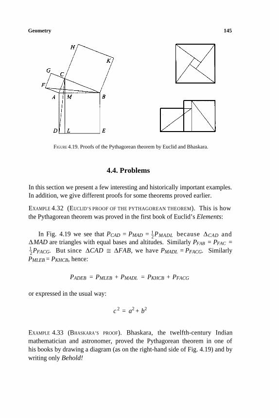
Geometry 145
FIGURE 4.19. Proofs of the Pythagorean theorem by Euclid and Bhaskara.
4.4. Problems
In this section we present a few interesting and historically important examples.
In addition, we give different proofs for some theorems proved earlier.
EXAMPLE 4.32 (EUCLID’S PROOF OF THE PYTHAGOREAN THEOREM). This is how
the Pythagorean theorem was proved in the first book of Euclid’s Elements:
In Fig. 4.19 we see that PCAD = PMAD = 1–2PMADL because ∆CAD and
∆MAD are triangles with equal bases and altitudes. Similarly PFAB = PFAC =1–2PFACG. But since ∆CAD ≅ ∆FAB, we have PMADL = PFACG. Similarly
PMLEB = PKHCB, hence:
PADEB = PMLEB + PMADL = PKHCB + PFACG
or expressed in the usual way:
c 2 = a2 + b2
EXAMPLE 4.33 (BHASKARA’S PROOF). Bhaskara, the twelfth-century Indian
mathematician and astronomer, proved the Pythagorean theorem in one of
his books by drawing a diagram (as on the right-hand side of Fig. 4.19) and by
writing only Behold!
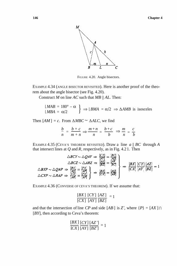
146 Chapter 4
FIGURE 4.20. Angle bisectors.
EXAMPLE 4.34 (ANGLE BISECTOR REVISITED). Here is another proof of the theo-
rem about the angle bisector (see Fig. 4.20).
Construct M on line AC such that MB || AL. Then:
⇒ BMA = α/2 ⇒ ∆AMB is isoscelesMAB = 180° – αMBA = α/2
Then [AM ] = c. From ∆MBC ~ ∆ALC, we find
b b + c m+n b+c m cn m + n n b n b
EXAMPLE 4.35 (CEVA’S THEOREM REVISITED). Draw a line a || BC through Athat intersect lines at Q and R, respectively, as in Fig. 4.2 1. Then
⇒⇒=–
EXAMPLE 4.36 (CONVERSE OF CEVA’S THEOREM). If we assume that:
---= 1[BX ] [CY ] [AZ ]
[CX ] [AY ] [BZ ]
and that the intersection of line CP and side [AB ] is Z', where P = [AX ] ⊃
[BY], then according to Ceva’s theorem:
[
[BX ] [CY ] [AZ ']= 1
] [AYCX ] [BZ']
= =
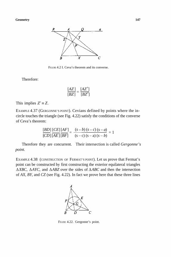
Geometry 147
FIGURE 4.2 I. Ceva’s theorem and its converse.
Therefore:
[AZ ]=
[AZ'][BZ ] [BZ']
This implies Z' ≡ Z.
EXAMPLE 4.37 (GERGONNE’S POINT). Cevians defined by points where the in-
circle touches the triangle (see Fig. 4.22) satisfy the conditions of the converse
of Ceva’s theorem:
[BD] [CE] [AF] (s – b) (s – c) (s – a)
[CD] [AE ] [BF] (s – c) (s – a) (s – b)= 1=
Therefore they are concurrent. Their intersection is called Gergonne’spoint.
EXAMPLE 4.38 (CONSTRUCTION OF FERMAT’S POINT). Let us prove that Fermat’s
point can be constructed by first constructing the exterior equilateral triangles
∆XBC, ∆AYC, and ∆ABZ over the sides of ∆ABC and then the intersection
of AX, BY, and CZ (see Fig. 4.22). In fact we prove here that these three lines
FIGURE 4.22. Gergonne’s point.
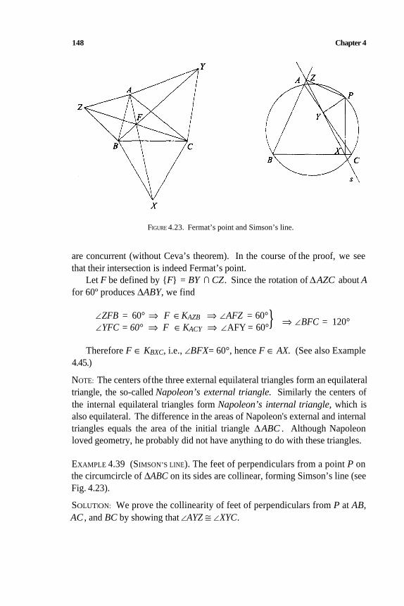
148 Chapter 4
FIGURE 4.23. Fermat’s point and Simson’s line.
are concurrent (without Ceva’s theorem). In the course of the proof, we see
that their intersection is indeed Fermat’s point.
Let F be defined by F = BY ⊃ CZ. Since the rotation of ∆AZC about Afor 60º produces ∆ABY, we find
⇒ ∠BFC = 120°∠ZFB = 60° ⇒ F ∈KAZB ⇒ ∠AFZ = 60°
∠YFC = 60° ⇒ F ∈ KACY ⇒ ∠AFY = 60°
Therefore F ∈ KBXC, i.e., ∠BFX= 60°, hence F ∈ AX. (See also Example
NOTE: The centers ofthe three external equilateral triangles form an equilateral
triangle, the so-called Napoleon’s external triangle. Similarly the centers of
the internal equilateral triangles form Napoleon’s internal triangle, which is
also equilateral. The difference in the areas of Napoleon's external and internal
triangles equals the area of the initial triangle ∆ABC . Although Napoleon
loved geometry, he probably did not have anything to do with these triangles.
EXAMPLE 4.39 (SIMSON’S LINE). The feet of perpendiculars from a point P on
the circumcircle of ∆ABC on its sides are collinear, forming Simson’s line (see
Fig. 4.23).
SOLUTION: We prove the collinearity of feet of perpendiculars from P at AB,
AC , and BC by showing that ∠AYZ ≅ ∠XYC.
4.45.)
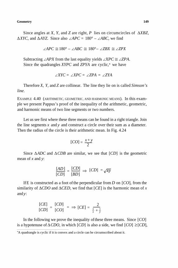
Geometry 149
Since angles at X, Y, and Z are right, P lies on circumcircles of ∆XBZ,∆XYC, and ∆AYZ. Since also ∠APC = 180° – ∠ABC, we find
∠APC ≅ 180° – ∠ABC ≅ 180°– ∠ZBX ≅ ∠ZPX
Subtracting ∠APX from the last equality yields ∠XPC ≅ ∠ZPA.
Since the quadrangles XYPC and ZPYA are cyclic,* we have
∠XYC = ∠XPC = ∠ZPA = ∠ZYA
Therefore X, Y, and Z are collinear. The line they lie on is called Simson’sline.
EXAMPLE 4.40 (ARITHMETIC, GEOMETRIC, AND HARMONIC MEANS). In this exam-
ple we present Pappus’s proof of the inequality of the arithmetic, geometric,
and harmonic means of two line segments or two numbers.
Let us see first where these three means can be found in a right triangle. Join
the line segments x and y and construct a circle over their sum as a diameter.
Then the radius of the circle is their arithmetic mean. In Fig. 4.24
x + y[CO]
2=
Since ∆ADC and ∆CDB are similar, we see that [CD] is the geometric
mean of x and y:
=[CD] ⇒ [CD] =[AD ]
[CD] [BD]
IfE is constructed as a foot of the perpendicular from D on [CO], from the
similarity of ∆CDO and ∆CED, we find that [CE] is the harmonic mean of xand y:
2=
[CE]=
[CD]⇒ [CE] =
[CD] [CO] 1–x +1y
In the following we prove the inequality of these three means. Since [CO]
is a hypotenuse of ∆CDO, in which [CD] is also a side, we find [CO] ≥ [CD],
*A quadrangle is cyclic if it is convex and a circle can be circumscribed about it.
–
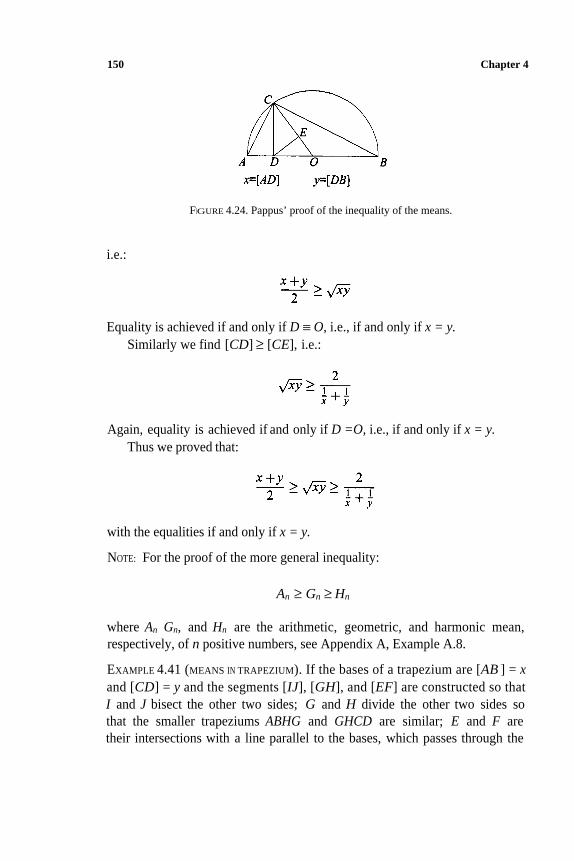
150 Chapter 4
FIGURE 4.24. Pappus’ proof of the inequality of the means.
i.e.:
Equality is achieved if and only if D ≡ O, i.e., if and only if x = y. Similarly we find [CD] ≥ [CE], i.e.:
Again, equality is achieved if and only if D =O, i.e., if and only if x = y. Thus we proved that:
with the equalities if and only if x = y.
NOTE: For the proof of the more general inequality:
An ≥ Gn ≥ Hn
where An Gn, and Hn are the arithmetic, geometric, and harmonic mean,
respectively, of n positive numbers, see Appendix A, Example A.8.
EXAMPLE 4.41 (MEANS IN TRAPEZIUM). If the bases of a trapezium are [AB ] = xand [CD] = y and the segments [IJ], [GH], and [EF] are constructed so that
I and J bisect the other two sides; G and H divide the other two sides so
that the smaller trapeziums ABHG and GHCD are similar; E and F are
their intersections with a line parallel to the bases, which passes through the
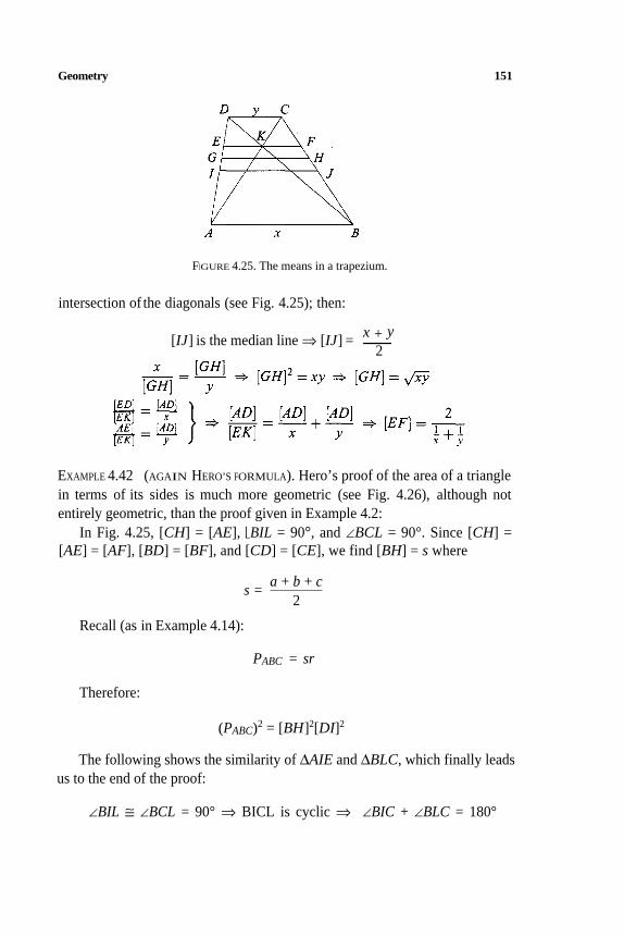
Geometry 151
FIGURE 4.25. The means in a trapezium.
intersection of the diagonals (see Fig. 4.25); then:
x + y[IJ] is the median line ⇒ [IJ] =
2
EXAMPLE 4.42 (AGAIN HERO’S FORMULA). Hero’s proof of the area of a triangle
in terms of its sides is much more geometric (see Fig. 4.26), although not
entirely geometric, than the proof given in Example 4.2:
In Fig. 4.25, [CH] = [AE], BIL = 90°, and ∠BCL = 90°. Since [CH] =
[AE] = [AF], [BD] = [BF], and [CD] = [CE], we find [BH] = s where
a + b + c 2
s =
Recall (as in Example 4.14):
PABC = sr
Therefore:
(PABC)2 = [BH]2[DI]2
The following shows the similarity of ∆AIE and ∆BLC, which finally leads
us to the end of the proof:
∠BIL ≅ ∠BCL = 90° ⇒ BICL is cyclic ⇒ ∠BIC + ∠BLC = 180°
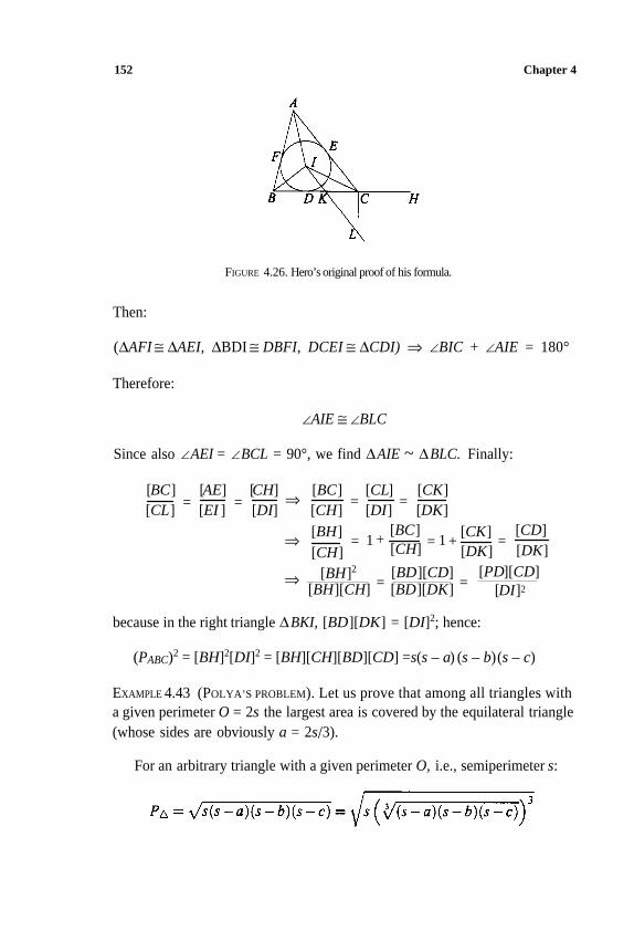
152 Chapter 4
FIGURE 4.26. Hero’s original proof of his formula.
Then:
(∆AFI ≅ ∆AEI, ∆BDI ≅ DBFI, DCEI ≅ ∆CDI) ⇒ ∠BIC + ∠AIE = 180°
Therefore:
∠AIE ≅ ∠BLC
Since also ∠AEI = ∠BCL = 90°, we find ∆AIE ~ ∆BLC. Finally:
[BC] [AE] [CH] ⇒ [BC] [CL] [CK]
[CL]=
[EI ]=
[DI] [CH]=
[DI]=
[DK]
[BH]+1+1
[BC] [CK] [CD]
[CH]
[BH]2
=
[BD][CD]
=
[PD][CD]
[CH] [DK] [DK]⇒ =
[BH][CH]=
[BD][DK]=
[DI]2⇒
because in the right triangle ∆BKI, [BD][DK] = [DI]2; hence:
(PABC)2 = [BH]2[DI]2 = [BH][CH][BD][CD] =s(s – a) (s – b)(s – c)
EXAMPLE 4.43 (POLYA’S PROBLEM). Let us prove that among all triangles with
a given perimeter O = 2s the largest area is covered by the equilateral triangle
(whose sides are obviously a = 2s/3).
For an arbitrary triangle with a given perimeter O, i.e., semiperimeter s:
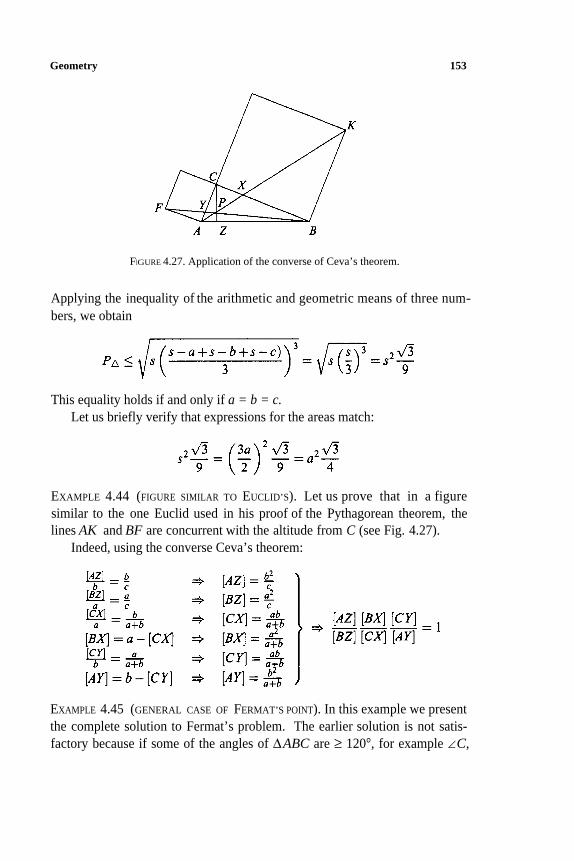
Geometry 153
FIGURE 4.27. Application of the converse of Ceva’s theorem.
Applying the inequality of the arithmetic and geometric means of three num-
bers, we obtain
This equality holds if and only if a = b = c. Let us briefly verify that expressions for the areas match:
EXAMPLE 4.44 (FIGURE SIMILAR TO EUCLID’S). Let us prove that in a figure
similar to the one Euclid used in his proof of the Pythagorean theorem, the
lines AK and BF are concurrent with the altitude from C (see Fig. 4.27).
Indeed, using the converse Ceva’s theorem:
EXAMPLE 4.45 (GENERAL CASE OF FERMAT’S POINT). In this example we present
the complete solution to Fermat’s problem. The earlier solution is not satis-
factory because if some of the angles of ∆ABC are ≥ 120°, for example ∠C,
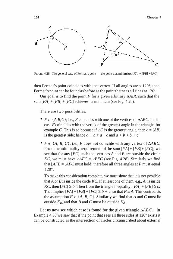
154 Chapter 4
FIGURE 4.28. The general case of Fermat’s point — the point that minimizes [FA] + [FB] + [FC].
then Fermat’s point coincides with that vertex. If all angles are < 120°, then
Fermat’s point can be found as before as the point that sees all sides at 120°.
Our goal is to find the point F for a given arbitrary ∆ABC such that the
sum [FA] + [FB] + [FC] achieves its minimum (see Fig. 4.28).
There are two possibilities:
• F ∈ A,B,C; i.e., F coincides with one of the vertices of ∆ABC. In that
case F coincides with the vertex of the greatest angle in the triangle, for
example C. This is so because if ∠C is the greatest angle, then c = [AB]
is the greatest side; hence a + b < a + c and a + b < b + c.
• F ∉ A, B, C, i.e., F does not coincide with any vertex of ∆ABC.From the minimality requirement of the sum [FA] + [FB]+ [FC], we
see that for any [FC] such that vertices A and B are outside the circle
KC, we must have ∠AFC = ∠BFC (see Fig. 4.28). Similarly we find
that AFB = AFC must hold; therefore all three angles at F must equal
120°.
To make this consideration complete, we must show that it is not possible
that A or B is inside the circle KC. If at least one of them, e.g., A, is inside
KC, then [FC] ≥ b. Then from the triangle inequality, [FA] + [FB] ≥ c.
That implies [FA] + [FB] + [FC] ≥ b + c, so that F ≡ A. This contradicts
the assumption F ∉ A, B, C. Similarly we find that A and C must lie
outside KB, and that B and C must lie outside KA.
Let us now see which case is found for the given triangle ∆ABC. In
Example 4.38 we saw that if the point that sees all three sides at 120° exists it
can be constructed as the intersection of circles circumscribed about external
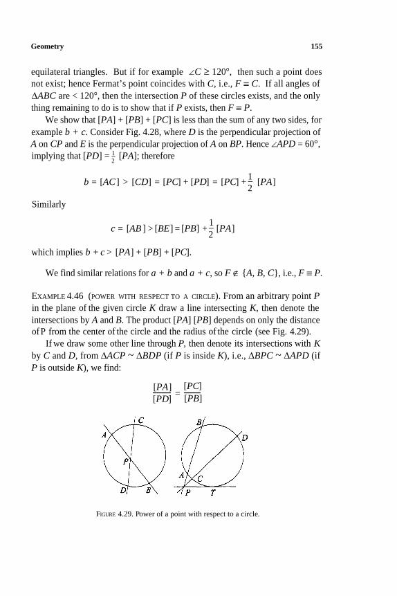
Geometry 155
equilateral triangles. But if for example ∠C ≥ 120°, then such a point does
not exist; hence Fermat’s point coincides with C, i.e., F ≡ C. If all angles of
∆ABC are < 120°, then the intersection P of these circles exists, and the only
thing remaining to do is to show that if P exists, then F ≡ P.
We show that [PA] + [PB] + [PC] is less than the sum of any two sides, for
example b + c. Consider Fig. 4.28, where D is the perpendicular projection of
A on CP and E is the perpendicular projection of A on BP. Hence ∠APD = 60°,
implying that [PD] = 1–2
[PA]; therefore
1
2b = [AC ] > [CD] = [PC] + [PD] = [PC] +- [PA]
Similarly
c = [AB ] > [BE] = [PB] +1
2– [PA]
which implies b + c > [PA] + [PB] + [PC].
We find similar relations for a + b and a + c, so F ∉ A, B, C, i.e., F ≡ P.
EXAMPLE 4.46 (POWER WITH RESPECT TO A CIRCLE). From an arbitrary point Pin the plane of the given circle K draw a line intersecting K, then denote the
intersections by A and B. The product [PA] [PB] depends on only the distance
of P from the center of the circle and the radius of the circle (see Fig. 4.29).
If we draw some other line through P, then denote its intersections with Kby C and D, from ∆ACP ~ ∆BDP (if P is inside K), i.e., ∆BPC ~ ∆APD (if
P is outside K), we find:
[PA] [PC]
[PD]=
[PB]
FIGURE 4.29. Power of a point with respect to a circle.
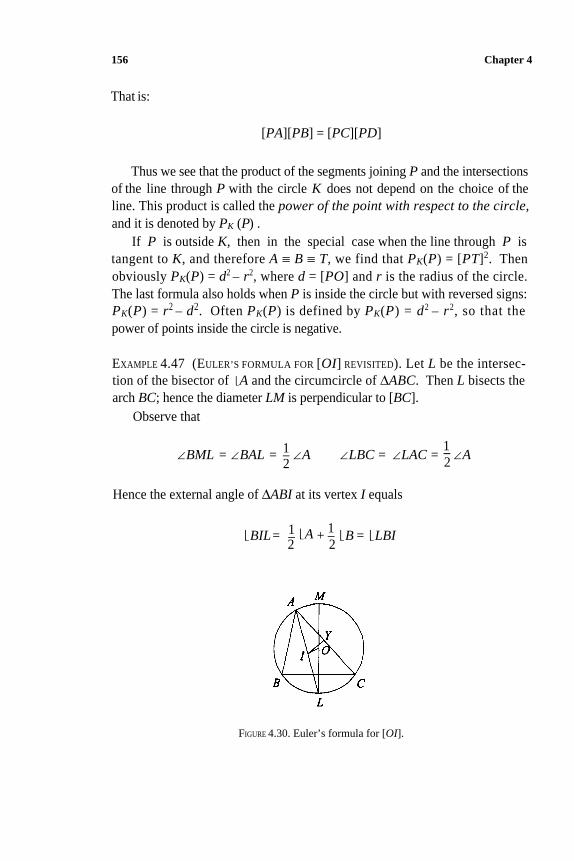
156 Chapter 4
That is:
[PA][PB] = [PC][PD]
Thus we see that the product of the segments joining P and the intersections
of the line through P with the circle K does not depend on the choice of the
line. This product is called the power of the point with respect to the circle,and it is denoted by PK (P) .
If P is outside K, then in the special case when the line through P is
tangent to K, and therefore A ≡ B ≡ T, we find that PK(P) = [PT]2. Then
obviously PK(P) = d2 – r2, where d = [PO] and r is the radius of the circle.
The last formula also holds when P is inside the circle but with reversed signs:
PK(P) = r2 – d2. Often PK(P) is defined by PK(P) = d2 – r2, so that the
power of points inside the circle is negative.
EXAMPLE 4.47 (EULER’S FORMULA FOR [OI] REVISITED). Let L be the intersec-
tion of the bisector of A and the circumcircle of ∆ABC. Then L bisects the
arch BC; hence the diameter LM is perpendicular to [BC].
Observe that
1 1
2 2∠BML = ∠BAL = – ∠A ∠LBC = ∠LAC = -∠A
Hence the external angle of ∆ABI at its vertex I equals
1 1
2 2BIL= – A + – B = LBI
FIGURE 4.30. Euler’s formula for [OI].
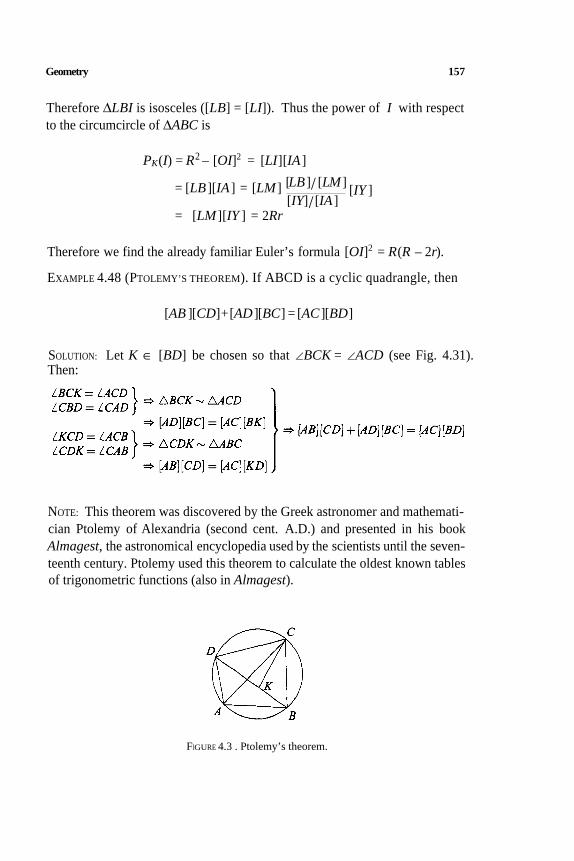
Geometry 157
Therefore ∆LBI is isosceles ([LB] = [LI]). Thus the power of I with respect
to the circumcircle of ∆ABC is
PK(I) = R2 – [OI]2 = [LI][IA ]
[LB ] / [LM ][IY ]
[IY]/ [IA ]= [LB ][IA ] = [LM ]
= [LM ][IY ] = 2Rr
Therefore we find the already familiar Euler’s formula [OI]2 = R(R – 2r).
EXAMPLE 4.48 (PTOLEMY’S THEOREM). If ABCD is a cyclic quadrangle, then
[AB ][CD]+[AD ][BC] = [AC ][BD]
SOLUTION: Let K ∈ [BD] be chosen so that ∠BCK = ∠ACD (see Fig. 4.31).
Then:
NOTE: This theorem was discovered by the Greek astronomer and mathemati-
cian Ptolemy of Alexandria (second cent. A.D.) and presented in his book
Almagest, the astronomical encyclopedia used by the scientists until the seven-
teenth century. Ptolemy used this theorem to calculate the oldest known tables
of trigonometric functions (also in Almagest).
FIGURE 4.3 . Ptolemy’s theorem.
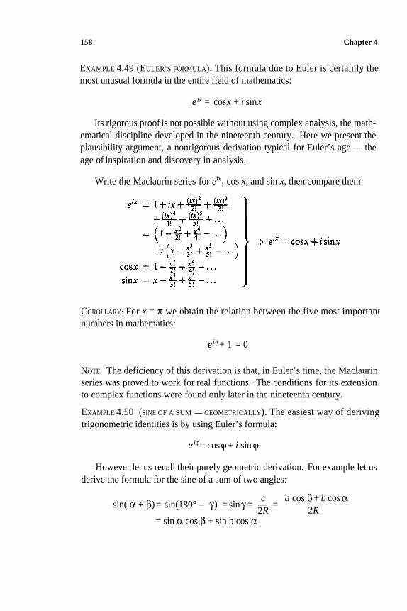
158 Chapter 4
EXAMPLE 4.49 (EULER’S FORMULA). This formula due to Euler is certainly the
most unusual formula in the entire field of mathematics:
eix = cosx + i sinx
Its rigorous proof is not possible without using complex analysis, the math-
ematical discipline developed in the nineteenth century. Here we present the
plausibility argument, a nonrigorous derivation typical for Euler’s age — the
age of inspiration and discovery in analysis.
Write the Maclaurin series for eix, cos x, and sin x, then compare them:
COROLLARY: For x = π we obtain the relation between the five most important
numbers in mathematics:
eiπ+ 1 = 0
NOTE: The deficiency of this derivation is that, in Euler’s time, the Maclaurin
series was proved to work for real functions. The conditions for its extension
to complex functions were found only later in the nineteenth century.
EXAMPLE 4.50 (SINE OF A SUM-GEOMETRICALLY). The easiest way of deriving
trigonometric identities is by using Euler’s formula:
e iϕ =cosϕ + i sin ϕ
However let us recall their purely geometric derivation. For example let us
derive the formula for the sine of a sum of two angles:
c a cos β + b cos α2R 2R
sin( α + β)= sin(180° – γ) = sin γ = — =
= sin α cos β + sin b cos α
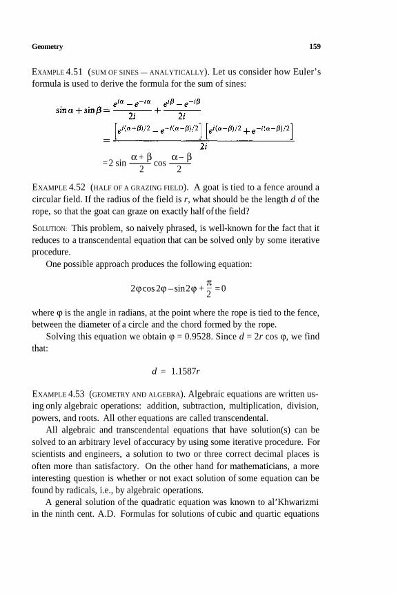
Geometry 159
EXAMPLE 4.51 (SUM OF SINES — ANALYTICALLY). Let us consider how Euler’s
formula is used to derive the formula for the sum of sines:
α + β α – β=2 sin-cos-
2 2
EXAMPLE 4.52 (HALF OF A GRAZING FIELD). A goat is tied to a fence around a
circular field. If the radius of the field is r, what should be the length d of the
rope, so that the goat can graze on exactly half of the field?
SOLUTION: This problem, so naively phrased, is well-known for the fact that it
reduces to a transcendental equation that can be solved only by some iterative
procedure.
One possible approach produces the following equation:
π2ϕcos 2ϕ – sin 2ϕ + – = 0
where ϕ is the angle in radians, at the point where the rope is tied to the fence,
between the diameter of a circle and the chord formed by the rope.
Solving this equation we obtain ϕ = 0.9528. Since d = 2r cos ϕ, we find
that:
2
d = 1.1587r
EXAMPLE 4.53 (GEOMETRY AND ALGEBRA). Algebraic equations are written us-
ing only algebraic operations: addition, subtraction, multiplication, division,
powers, and roots. All other equations are called transcendental.
All algebraic and transcendental equations that have solution(s) can be
solved to an arbitrary level of accuracy by using some iterative procedure. For
scientists and engineers, a solution to two or three correct decimal places is
often more than satisfactory. On the other hand for mathematicians, a more
interesting question is whether or not exact solution of some equation can be
found by radicals, i.e., by algebraic operations.
A general solution of the quadratic equation was known to al’Khwarizmi
in the ninth cent. A.D. Formulas for solutions of cubic and quartic equations
160 Chapter 4
were found by Tartaglia and Ferrari in the sixteenth century, and first published
by Cardano. All these formulas require only algebraic operations, so it was
expected that the quintic and other equations would have similar solutions by
radicals.
But although great effort was directed toward finding the solution for the
quintic equation, no results were found until Abel showed in 1824 that there
are quintics without a solution in radicals. The general criterion for solvability
in radicals was found by Galois* in 1829.
As in the theory of equations, geometry has two different goals: to solve a
problem in any way or to solve it using a ruler and compass only. The second
approach is not necessarily the fastest or the simplest, but it is especially
attractive because construction tools are so limited. Such solutions often have
many steps; hence they are not very precise and primarily of theoretical interest.
Several geometric problems have remained unsolved since antiquity. We
mention the four most famous: trisecting an angle,† doubling a cube,‡ squaring
a circle§ (these are the three so-called classical problems), and constructing a
regular heptagon.
Even ancient geometers knew how to solve some of these problems, but
besides the straightedge and compass, they needed some other instruments.
Hence the interest in such curves as the spiral of Archimedes, cissoid of Diocles,
quadratrix of Dinostratus, and conchoid of Nicomedes.
When only nineteen Gauss used the analogy between constructions by
straightedge and compass and the process of solving algebraic equations to
show that the regular n-gon can be constructed if n is a product of different
Fermat primes¶ or a unity with a nonnegative power of two. Therefore we can
construct regular polygons for
n = 2, 3, 4, 5, 6, 8, 10, 12, 15, 16, 17, 20 , . . .*Evarist Galois had a very tragic destiny — he was killed in a duel at twenty-one. Since he had
unsuccessfully tried to publish his results during the previous two years, and he was aware of the
impending tragedy, the night before the duel, he wrote a letter to his friend, Auguste Chevalier,
presenting the elements of his theory. His work was published 14 years after his death, in 1846.†The problem is to trisect an arbitrary angle.‡This problem is also known as the Delian problem, because, by the legend, the oracle at Delos
advised the Athenians to double the cubical altar of Apollo in order to stop the plague of 430 B.C.§The problem here is to construct the square of the area equal to the given circle.¶Ofall Fermat numbers Fk = 22k
+ 1 (k = 0,1,2, . . .) it is quite probable that only F0 = 3, F1 = 5,
F2 = 17, F3 = 257, and F4 = 65537 are prime, but that is still an unsolved problem.
Geometry 161
Although Gauss probably knew that this condition is not only sufficient but
also necessary, this part of the solution was published later. Thus construction
is impossible for
n = 7, 9, 11, 13, 14, 18, 19, 21, 22, 23, . . .
The other problems reduce to questions of the constructibility of the solu-
tion of a cubic equation (angle trisection and cube duplication), and the number
π (squaring the circle). In the seventeenth century Descartes observed that Eu-
clidean constructions (those using only the straightedge and compass) allow
us to construct only solutions of linear and quadratic equations; i.e., the con-
struction of rational numbers and the quadratic irrationals only. Hence square
roots can be constructed but third roots cannot; therefore angle trisection and
the Delian problem cannot be solved by Euclidean constructions. The im-
possibility to construct the number π followed from Lindemann’s proof of its
transcendence* in 1882.
*A number is transcendental if it is not a root of an algebraic equation.

This page intentionally left blank.
Appendixes

This page intentionally left blank.
Appendix A
Mathematical Induction

This page intentionally left blank.
Mathematical Induction 167
Appendix A presents an important mathematical tool, mathematical induction, primarily through examples.
A.1. Overview
In many mathematical problems we want to prove that the statementAn is true
for any value of the natural number n ≥ nmin. If the statement we are trying
to prove is indeed true, very often we can use the method of mathematical
induction to facilitate the proof. We need to show that:
1. The statement is true forn = nmin.
2. From the correctness of the statement for n = k (k ≥nmin), it follows
that the statement is true for n = k + 1.
Historians of mathematics have different opinions about who first formu-
lated the principle of mathematical induction. However it is certain that Ancient
Greek mathematicians used it. For example Theorem IX-20 in Euclid’s Ele-ments proves the infiniteness of the set of primes by showing that if there are nprimes, there must exist the (n + 1)th prime, too.
For the precise formulation of this theorem, we should probably credit
Jakob Bernoulli and Blaise Pascal. In 1889 Giuseppe Peano introduced the
principle of mathematical induction among the axioms of natural numbers.
A proof by mathematical induction can be imagined as a row of falling
dominoes. To ensure that all dominoes fall, first we verify that the first domino
can fall. After that if for every k ≥ 1 we can prove that the fall of the kth
domino produces the fall of the next, i.e., the (k + 1)th domino, we can be
certain that all dominoes will fall.
We continue with a few applications of the principle of mathematical in-
duction.
A.2. Examples
EXAMPLE A.1 (SUM OF FIRST n NATURAL NUMBERS). Let us prove that for all
n ∈N :
n(n + 1)
21 +2 + 3 + . . . + n = —
168 Appendix A
Step 1: Check for n = 1
1.21 =
2
Step 2: We assume that for n = k, k ≥ 1 the formula is true, then try to
prove that this implies its correctness for n = k + 1:
1 + 2+ 3 + . . . + k + (k + 1) =k( + 1)
+ (kk + 1)2
=(k + 1) (k + 2)
2
This completes the proof.
EXAMPLE A.2 (SUM OF FIRST n SQUARES). Here we prove that for all n ∈ N:
n(n + 1)(2n + 1)12 + 22 + 32 + . . . +n2 =
6
Step 1: Check for n = 1
1 .2 .312 =
6
Step 2: If the statement is true for n = k, k ≥ 1, then for n = k + 1 :
k (k + 1)(2k + 1)+(k + 1)2
612 +22 +3
2+. . .+k2 + (k + 1)
2=
(k + 1)(k + 2)(2k + 3)=
6
This completes the proof.
EXAMPLE A.3 (SUM OF FIRST n CUBES). Let us show that for all n ∈ N:
Step 1: Check for n = 1:
Mathematical Induction 169
Step 2: Let the formula be true for n = k, k ≥ 1. Then for n = k + 1:
This completes the proof.
NOTE: By combining this result and the identity 1 + 2 + 3 + . . . + n = n (n + 1) / 2,
we obtain:
(1 +2 + 3 + . . . +n)2 = 13 + 23 + 33 + . . . +n3
See Example 2.52 for the combinatorial proof of this identity.
Is there a simple method of finding sums similar to those in previous
examples or such sums as:
especially if we do not know (or forget) that:
Indeed when we know where to begin, using mathematical induction to
prove such identities is a routine matter.
The identity 1 + 2 + . . . + n = n(n + 1) / 2 can be found using the same idea
that Gauss had when he was only nine years old and impressed his teacher by
quickly summing 1 + 2 + . . . + 100 = 5050.
Indeed:
1 + 2 + . . . + 99 + 100 = (1 + 100) + (2 + 99) + . . . + (50 + 5 1)
=100 .1012
The solution to the sum of the first n odd numbers, i.e., 1 + 3 + 5 + . . . + (2n –
1) = n2, is clear if we draw a square 5 × 5 (Fig. A. 1), then note that it is made
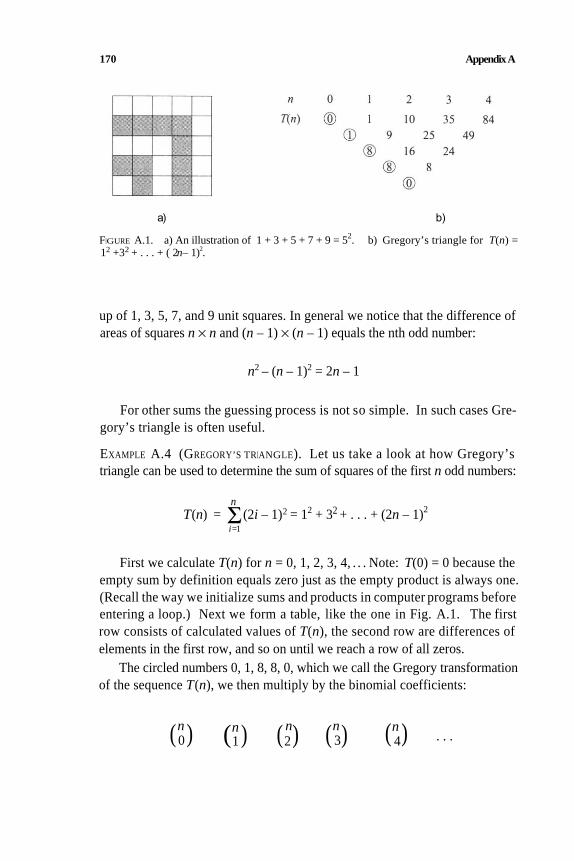
170 AppendixA
a) b)
FIGURE A.1. a) An illustration of 1 + 3 + 5 + 7 + 9 = 52. b) Gregory’s triangle for T(n) =
12 +32 + . . . + ( 2n– 1)
2.
up of 1, 3, 5, 7, and 9 unit squares. In general we notice that the difference of
areas of squares n × n and (n – 1) × (n – 1) equals the nth odd number:
n2 – (n – 1)2 = 2n – 1
For other sums the guessing process is not so simple. In such cases Gre-
gory’s triangle is often useful.
EXAMPLE A.4 (GREGORY’S TRIANGLE). Let us take a look at how Gregory’s
triangle can be used to determine the sum of squares of the first n odd numbers:
n
i=1
T(n) = Σ (2i – 1)2 = 12 + 32 + . . . + (2n – 1)
2
First we calculate T(n) for n = 0, 1, 2, 3, 4, . . . Note: T(0) = 0 because the
empty sum by definition equals zero just as the empty product is always one.
(Recall the way we initialize sums and products in computer programs before
entering a loop.) Next we form a table, like the one in Fig. A.1. The first
row consists of calculated values of T(n), the second row are differences of
elements in the first row, and so on until we reach a row of all zeros.
The circled numbers 0, 1, 8, 8, 0, which we call the Gregory transformation
of the sequence T(n), we then multiply by the binomial coefficients:
(n0) (
n1 ) (
n2) (
n3) (n
4) . . .
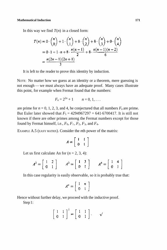
Mathematical Induction 171
In this way we find T(n) in a closed form:
It is left to the reader to prove this identity by induction.
NOTE: No matter how we guess at an identity or a theorem, mere guessing is
not enough — we must always have an adequate proof. Many cases illustrate
this point, for example when Fermat found that the numbers:
Fn = 22n + 1 n = 0, 1, . . .
are prime for n = 0, 1, 2, 3, and 4, he conjectured that all numbers Fn are prime.
But Euler later showed that F5 = 4294967297 = 641.6700417. It is still not
known if there are other primes among the Fermat numbers except for those
found by Fermat himself, i.e., F0, F1 , F2, F3, and F4.
EXAMPLE A.5 (EASY MATRIX). Consider the nth power of the matrix:
Let us first calculate An for (n = 2, 3, 4):
In this case regularity is easily observable, so it is probably true that:
Hence without further delay, we proceed with the inductive proof.
Step 1:
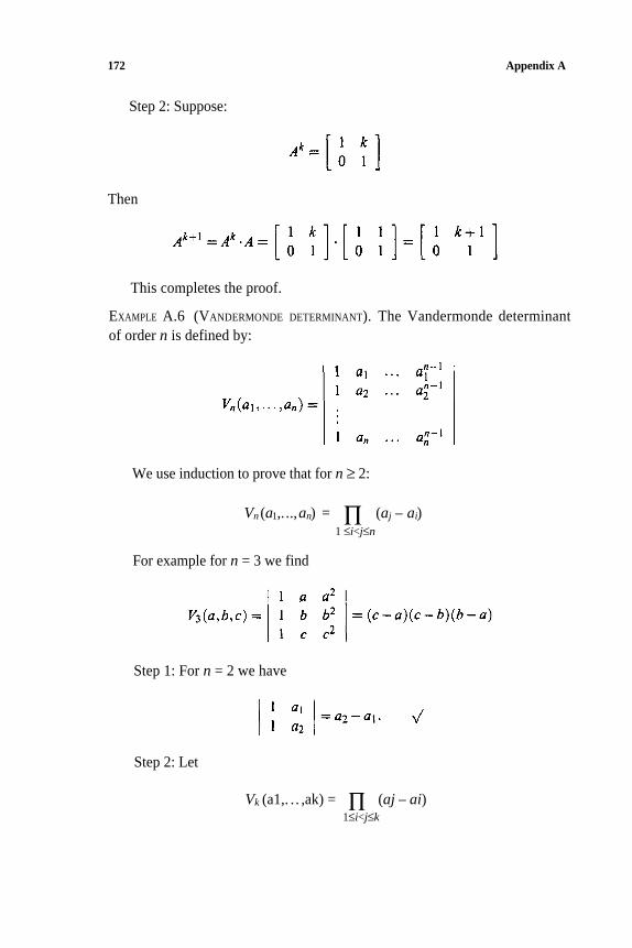
172 Appendix A
Step 2: Suppose:
Then
This completes the proof.
EXAMPLE A.6 (VANDERMONDE DETERMINANT). The Vandermonde determinant
of order n is defined by:
We use induction to prove that for n ≥ 2:
Vn (a1,. ..,an) = ∏ (aj – ai)
1 ≤i<j≤n
For example for n = 3 we find
Step 1: For n = 2 we have
Step 2: Let
Vk (a1,. . . ,ak) = ∏ (aj – ai)1≤i<j≤k
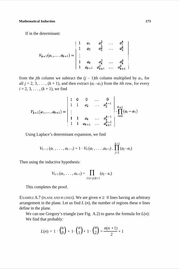
Mathematical Induction 173
If in the determinant:
from the jth column we subtract the (j – 1)th column multiplied by a1, for
all j = 2, 3, . . . , (k + 1), and then extract (ai –a1) from the ith row, for every
i = 2, 3, . . . , (k + 1), we find
Using Laplace’s determinant expansion, we find
k+1
j=2
Vk + 1 (a1 , . . . , ak + 1) = 1 . Vk (a2 , . . . ,ak+1) . ∏ (aj –a1)
Then using the inductive hypothesis:
Vk+1 (a1, . . . , ak+1) = ∏ (aj – ai)
1≤i<j≤k+1
This completes the proof.
EXAMPLE A.7 (PLANE AND n LINES). We are given n ≥ 0 lines having an arbitrary
arrangement in the plane. Let us find L (n), the number of regions these n lines
define in the plane.
We can use Gregory’s triangle (see Fig. A.2) to guess the formula for L(n):
We find that probably:
L(n) = 1 . (n0) + 1. (n
1)+ 1 . (n2) =
n(n +1)
2+ 1
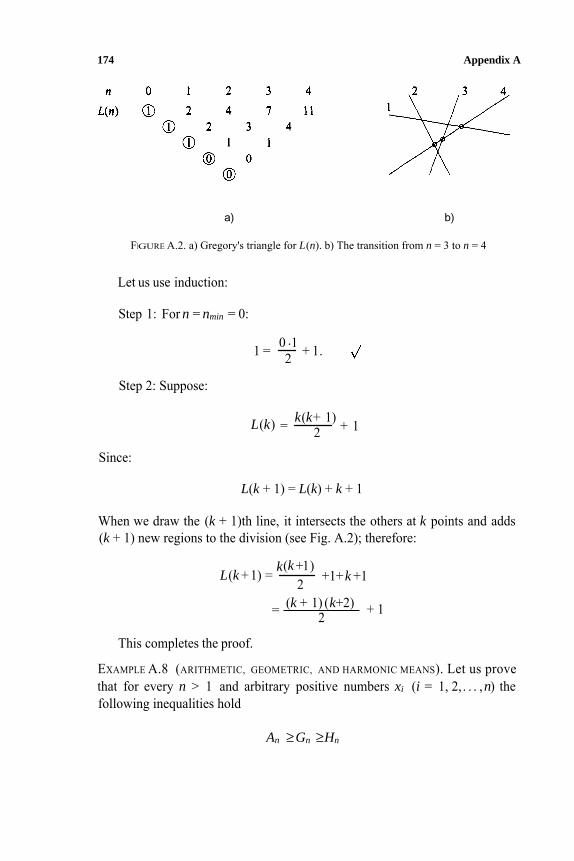
174 Appendix A
a) b)
FIGURE A.2. a) Gregory's triangle for L(n). b) The transition from n = 3 to n = 4
Let us use induction:
Step 1: For n = nmin = 0:
0 .11 = + 1 .2
Step 2: Suppose:
k(k+ 1) + 1L(k) = 2
Since:
L(k + 1) = L(k) + k + 1
When we draw the (k + 1)th line, it intersects the others at k points and adds(k + 1) new regions to the division (see Fig. A.2); therefore:
L(k + 1) =(k + )1k
+1+k +12(k + 1) (k+2) + 1= 2
This completes the proof.
EXAMPLE A.8 (ARITHMETIC, GEOMETRIC, AND HARMONIC MEANS). Let us prove that for every n > 1 and arbitrary positive numbers xi (i = 1, 2,. . . ,n) thefollowing inequalities hold
An ≥Gn ≥Hn
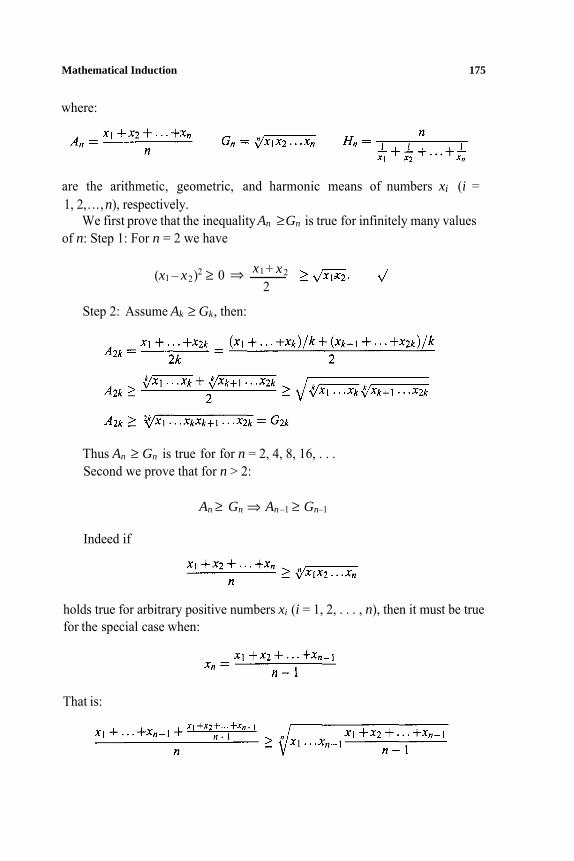
Mathematical Induction 175
where:
are the arithmetic, geometric, and harmonic means of numbers xi (i =1, 2,. ..,n), respectively.
We first prove that the inequality An ≥Gn is true for infinitely many valuesof n: Step 1: For n = 2 we have
(x1 – x2)2 ≥ 0 ⇒ x1 + x 2 -2
Step 2: Assume Ak ≥ Gk, then:
Thus An ≥ Gn is true for for n = 2, 4, 8, 16, . . . Second we prove that for n > 2:
An ≥ Gn ⇒ An –1 ≥ Gn–1
Indeed if
holds true for arbitrary positive numbers xi (i = 1, 2, . . . , n), then it must be true for the special case when:
That is:
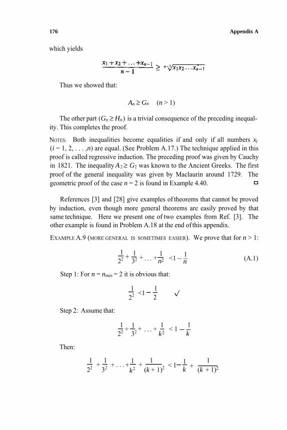
176 Appendix A
which yields
Thus we showed that:
An ≥ (n > 1) Gn
The other part (Gn ≥ Hn) is a trivial consequence of the preceding inequal-ity. This completes the proof.
NOTES: Both inequalities become equalities if and only if all numbers xi
(i = 1, 2, . . . ,n) are equal. (See Problem A.17.) The technique applied in thisproof is called regressive induction. The preceding proof was given by Cauchy in 1821. The inequality A 2 ≥ G2 was known to the Ancient Greeks. The first proof of the general inequality was given by Maclaurin around 1729. The geometric proof of the case n = 2 is found in Example 4.40.
References [3] and [28] give examples of theorems that cannot be proved by induction, even though more general theorems are easily proved by that same technique. Here we present one of two examples from Ref. [3]. The other example is found in Problem A.18 at the end of this appendix.
EXAMPLE A.9 (MORE GENERAL IS SOMETIMES EASIER). We prove that for n > 1:
1 1 1 122 32 n2 n
+ + . . . + <1 (A.1)
Step 1: For n = nmin = 2 it is obvious that:
1 1 <1
22 2
Step 2: Assume that:
1 1 1 1+ + . . . + - < 1--22 32 k2 k
Then:
1 1 1 1 1 1< 1 ++ + . . . + +
22 32 k2 (k + 1)2 k (k + 1)2
––
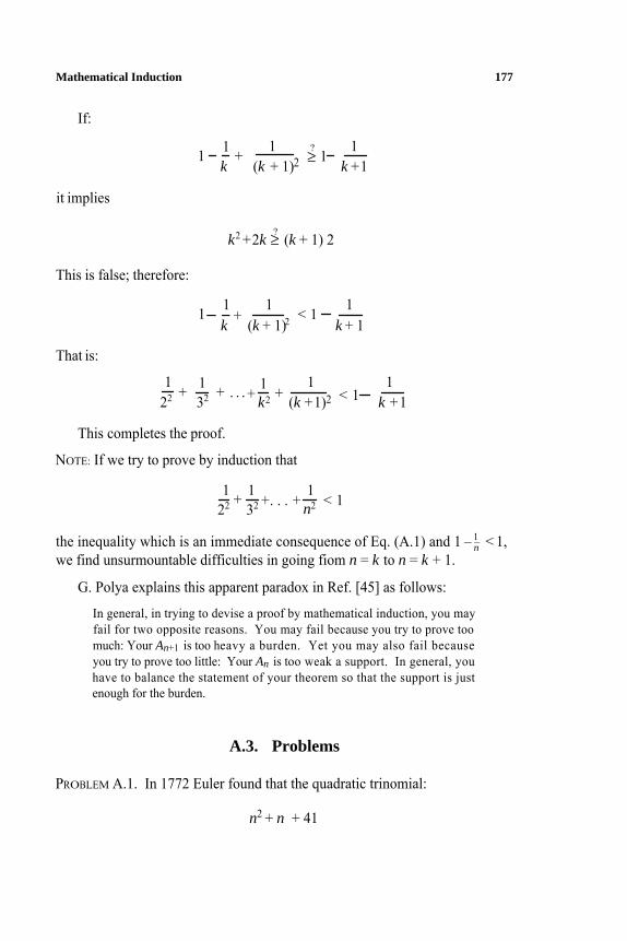
Mathematical Induction 177
If:
1 ? 1≥ 111 +
k (k + 1)2 k + 1
it implies
k2 +2k ≥ (k + 1) 2?
This is false; therefore:
1< 1 1 1 k + 1
1- -+k (k + 1)2
That is:
1 1 1 1 1+ + . . . + +22 32 k2 (k +1)2 < k +1 1
This completes the proof.
NOTE: If we try to prove by induction that
1 1 1+ + . . . + < 1 22 32 n2
the inequality which is an immediate consequence of Eq. (A.1) and 1 – 1–n < 1,we find unsurmountable difficulties in going fiom n = k to n = k + 1.
G. Polya explains this apparent paradox in Ref. [45] as follows:
In general, in trying to devise a proof by mathematical induction, you mayfail for two opposite reasons. You may fail because you try to prove toomuch: Your An+1 is too heavy a burden. Yet you may also fail becauseyou try to prove too little: Your An is too weak a support. In general, youhave to balance the statement of your theorem so that the support is justenough for the burden.
A.3. Problems
PROBLEM A.1. In 1772 Euler found that the quadratic trinomial:
n2 + n + 41
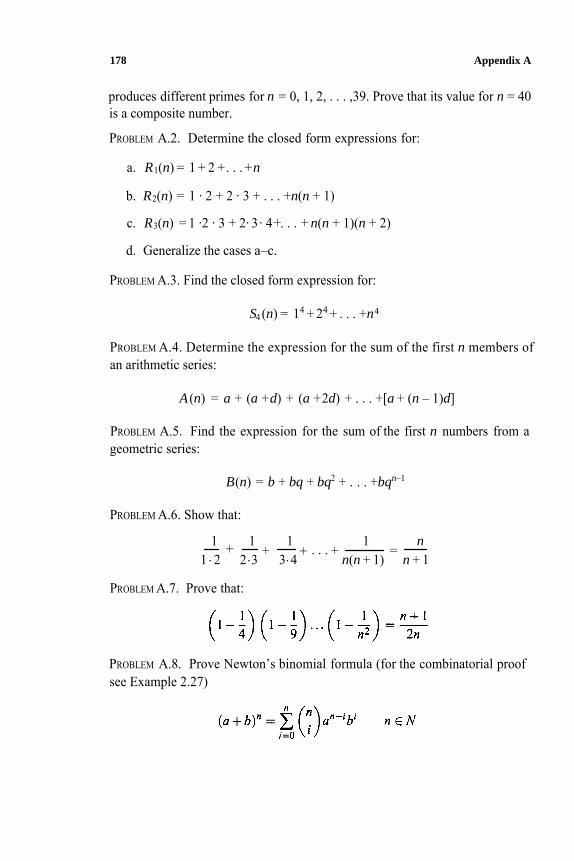
178 Appendix A
produces different primes for n = 0, 1, 2, . . . ,39. Prove that its value for n = 40 is a composite number.
PROBLEM A.2. Determine the closed form expressions for:
a. R1(n) = 1 + 2 + . . . + n
b. R2(n) = 1 . 2 + 2 . 3 + . . . +n(n + 1)
c. R3(n) = 1 .2 . 3 + 2. 3. 4 +. . . + n(n + 1)(n + 2)
d. Generalize the cases a–c.
PROBLEM A.3. Find the closed form expression for:
S4 (n) = 14 + 24 + . . . +n4
PROBLEM A.4. Determine the expression for the sum of the first n members of an arithmetic series:
A (n) = a + (a +d) + (a +2d) + . . . +[a + (n – 1)d]
PROBLEM A.5. Find the expression for the sum of the first n numbers from ageometric series:
B(n) = b + bq + bq2 + . . . +bqn–1
PROBLEM A.6. Show that:
1 1 1 1 n+ + + . . . + =1. 2 2.3 3.4 n(n + 1) n + 1
PROBLEM A.7. Prove that:
PROBLEM A.8. Prove Newton’s binomial formula (for the combinatorial proofsee Example 2.27)
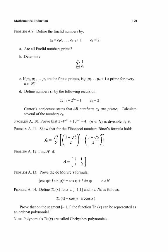
Mathematical Induction 179
PROBLEM A.9. Define the Euclid numbers by:
en = e1e2 . . . en–1 + 1 e1 = 2
a. Are all Euclid numbers prime?
b. Determine
i= 1 eiΣ 1n
–
c. If p1, p2 , . .. ,pn are the first n primes, is p1p2. . . pn + 1 a prime for every n ∈ N?
d. Define numbers cn by the following recursion:
cn + 1 = 2cn – 1 c0 = 2
Cantor’s conjecture states that All numbers cn are prime. Calculateseveral of the numbers cn.
PROBLEM A. 10. Prove that 3 . 4n+1 + 10n–1 – 4
PROBLEM A.11. Show that for the Fibonacci numbers Binet’s formula holds
(n ∈ N) is divisible by 9.
PROBLEM A. 12. Find An if:
PROBLEM A. 13. Prove the de Moivre’s formula:
(cos ϕ+ i sin ϕ)n = cos ϕ + i sin ϕ n ∈N
PROBLEM A. 14. Define Tn (x) for x ∈[– 1,1] and n ∈ N0 as follows:
Tn (x) = cos(n . arccos x )
Prove that on the segment [– 1,1] the function Tn (x) can be represented as an order-n polynomial.
NOTE: Polynomials Tn (x) are called Chebyshev polynomials.
180 Appendix A
PROBLEM A. 15. Prove that for any n ∈ N:
On the right-hand side, there are n nested square roots.
PROBLEM A. 16. Find the Maclaurin expansion of f (x) = In(1 + x). Recall that the Maclaurin series has the following form:
PROBLEM A.17. Use mathematical induction to prove that for arbitrary positive numbers a1, (a2 , . . . , an
a1a2 . . . an = 1 ⇒ a1 + a2 + . . . + an ≥ n
Use this inequality to prove the inequality of the arithmetic, geometric, andharmonic means.
PROBLEM A.18. Use the induction to prove that:
1 3 2n– 1 1<- . - . .
2 4 . . .2n
NOTE: In this case it is easier to prove a more restrictive inequality.
A.4. Hints and Notes
HINT A.1. Indeed, 402 + 40 + 41 = 412. Euler’s trinomial produces an incred-ibly long sequence of primes, which could make us think that all of its valuesare prime. The following anecdote from Ref. [45] depicts different inductivereasonings:
“Look at this mathematician,” said the logician. “He observes that thefirst ninety-nine numbers are less than hundred and infers hence, by whathe calls induction, that all numbers are less than a hundred.”
“A physicist believes,” said the mathematician, “that 60 is divisible by allnumbers. He observes that 60 is divisible by 1, 2, 3, 4, 5, and 6. He
Mathematical Induction 181
examines a few more cases, as 10, 20, and 30, taken at random as he says. Since 60 is divisible also by these, he considers the experimental evidence sufficient.”“Yes, but look at the engineers,” said the physicist. “An engineer suspected that all odd numbers are prime numbers. At any rate, 1 can be consideredas aprime number, he argued. Then there come 3, 5, and 7, all indubitably primes. Then there comes 9; an awkward case, it does not seem to be a prime number. Yet 11 and 13 are certainly primes. ‘Coming back to 9,’he said, ‘I conclude that 9 must be an experimental error.’”
HINT A.2. Cases a–c are special cases of case d.
d. Define
Rk(n) = 1 . 2. . . . . k + 2 . 3. . . . .( k + 1) + . . . + n(n + 1) . . .( n + k– 1)
Then show that:
1k + 1
Rk (n) = n(n + 1). . .(n + k)
HINT A.3. Gregory’s triangle gives
which after some effort yields
130S4(n) = n (n + 1) (2n + 1) (3n2 + 3n– 1)
In general the formula for Sk (n)can be derived if we know expressions for S1 (n), S2 (n), . . . ,Sk –1 (n), as illustrated by the following derivation for S5 (n).If in the identity:
(m + 1)6 = m6 + 6m5 + 15m4 + 20m3 + 15m2 + 6m + 1
We set m = 1,2 , . . . , n, then add all equalities obtained in this way; aftercanceling all sixth powers except 16 and (n + 1)6, we find
16
S5(n) = – [ (n + 1)6 – 1 – 15S4 (n) – 20S3 (n) – 15S2 (n) – 6S1 (n) – n]
182 Appendix A
That is:
1 n2S5(n) =12
(n + 1)2 (2n2 + 2n – 1)
A(n) = na + d = (a1 + an)–2
HINT A.4. This result should be familiar to all readers:
n(n – 1) n2
HINT A.5. For q = 1, obviously B(n) = n. For q ≠ 1, consider
B(n) = b + bq + . . . + bqn–1 qB(n) = bq + bq2 + . . . +bqn
then write
qB(n) – B(n) = bqn – bqp.
That is:
qn – 1q– 1B(n) = b-
NOTE: If |q| < 1 and n → ∞, the last identity gives us the formula for the sumof an infinite geometric series:
b
1– qb + bq + bq2 + . . . =
HINT A.6. The identity to be proved can be guessed after calculating n =1, 2, 3, . . , until regularity is observed. It can also be derived by using the partial fraction expansion of 1 / [k(k + 1)]:
1 1__1k(k +1) =
k k +1
Could we use Gregory’s triangle here?
HINT A.7. This identity can be derived from:
1 k – 1 k + 1 1k2 =
k k
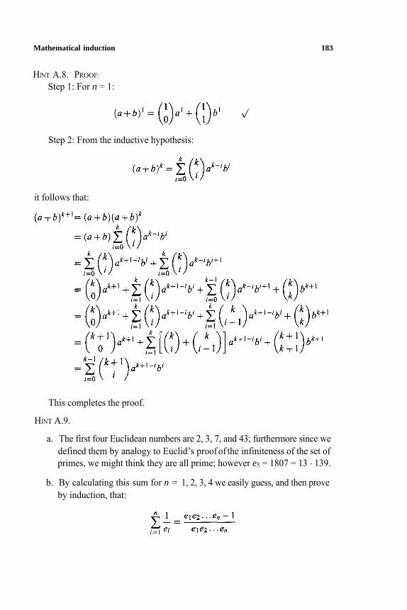
Mathematical induction 183
HINT A.8. PROOF:
Step 1: For n = 1:
Step 2: From the inductive hypothesis:
it follows that:
This completes the proof.
HINT A.9.
a. The first four Euclidean numbers are 2, 3, 7, and 43; furthermore since we defined them by analogy to Euclid’s proof of the infiniteness of the set of primes, we might think they are all prime; however e5 = 1807 = 13 . 139.
b. By calculating this sum for n = 1, 2, 3, 4 we easily guess, and then prove by induction, that:
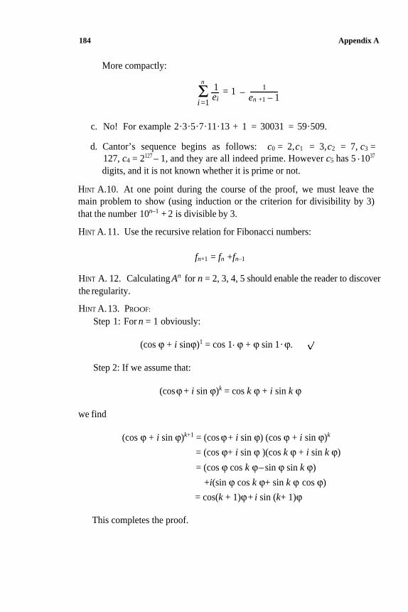
184 Appendix A
More compactly:
Σ = 1ei
– 1
i =1en +1 – 1
1n
c. No! For example 2.3.5.7.11.13 + 1 = 30031 = 59.509.
d. Cantor’s sequence begins as follows: c0 = 2,c1 = 3,c2 = 7, c3 =
127, c4 = 2127 – 1, and they are all indeed prime. However c5 has 5 . 1037
digits, and it is not known whether it is prime or not.
HINT A.10. At one point during the course of the proof, we must leave the
main problem to show (using induction or the criterion for divisibility by 3)
that the number 10n–1 + 2 is divisible by 3.
HINT A. 11. Use the recursive relation for Fibonacci numbers:
fn+1 = fn +fn–1
HINT A. 12. Calculating An for n = 2, 3, 4, 5 should enable the reader to discover
the regularity.
HINT A.13. PROOF:
Step 1: For n = 1 obviously:
(cos ϕ + i sinϕ)1 = cos 1. ϕ + ϕ sin 1 . ϕ.
Step 2: If we assume that:
(cos ϕ + i sin ϕ)k = cos k ϕ + i sin k ϕ
we find
(cos ϕ + i sin ϕ)k+1 = (cos ϕ+ i sin ϕ) (cos ϕ + i sin ϕ)k
= (cos ϕ+ i sin ϕ )(cos k ϕ + i sin k ϕ)
= (cos ϕ cos k ϕ– sin ϕ sin k ϕ)
+i(sin ϕ cos k ϕ+ sin k ϕ cos ϕ)
= cos(k + 1)ϕ+ i sin (k+ 1)ϕ
This completes the proof.
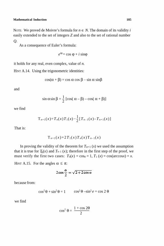
Mathematical Induction 185
NOTE: We proved de Moivre’s formula for n ∈ N. The domain of its validity ieasily extended to the set of integers Z and also to the set of rational number
Q.As a consequence of Euler’s formula:
eiϕ = cos ϕ + i sinϕ
it holds for any real, even complex, value of n.
HINT A.14. Using the trigonometric identities:
cos(α + β) = cos α cos β – sin α sinβ
and
1
2sin αsin β = – [cos( α – β) – cos( α + β)]
we find
1
2– –T n+1(x )=T n(x )T 1(x) [T n– 1 (x )–T n+1(x ) ]
That is:
T n + 1( x ) = 2 T 1( x ) T n( x ) T n – 1( x )
In proving the validity of the theorem for Tn+1 (x) we used the assumption
that it is true for Tn(x) and Tn–1 (x); therefore in the first step of the proof, we
must verify the first two cases: T0(x) = cos0 = 1, T1 (x) = cos(arccosx) = x.
HINT A.15. For the angles α ≤ π:
because from:
cos2 θ + sin2 θ = 1 cos2 θ –sin2 e = cos 2 θ
we find
1 + cos 2θ2
cos2 θ =
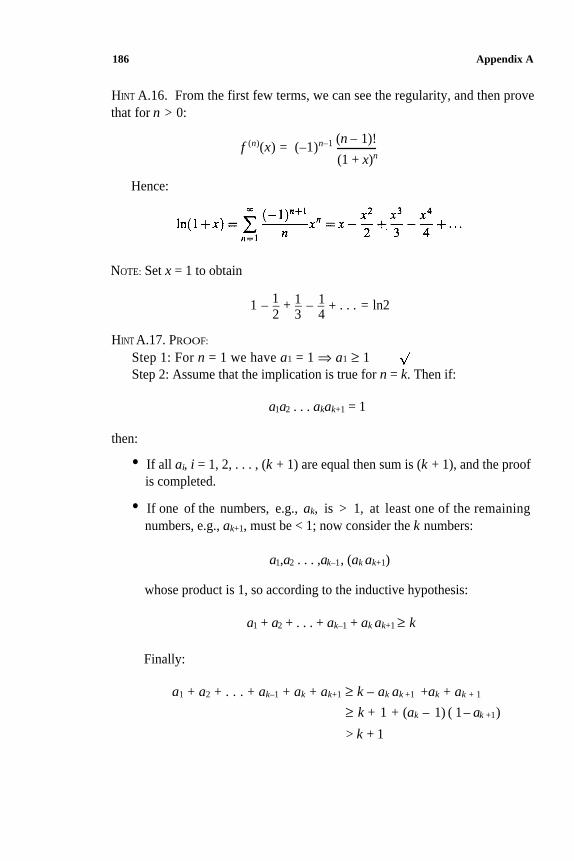
186 Appendix A
HINT A.16. From the first few terms, we can see the regularity, and then prove
that for n > 0:
(n – 1)!f (n)(x) = (–1)n–1
(1 + x)n
Hence:
NOTE: Set x = 1 to obtain
1 1 1
2 3 41 – – + – – – + . . . = ln2
HINT A.17. PROOF:
Step 1: For n = 1 we have a1 = 1 ⇒ a1 ≥ 1Step 2: Assume that the implication is true for n = k. Then if:
a1a2 . . . akak+1 = 1
then:
• If all ai, i = 1, 2, . . . , (k + 1) are equal then sum is (k + 1), and the proof
is completed.
• If one of the numbers, e.g., ak, is > 1, at least one of the remaining
numbers, e.g., ak+1, must be < 1; now consider the k numbers:
a1,a2 . . . ,ak–1, (ak ak+1)
whose product is 1, so according to the inductive hypothesis:
a1 + a2 + . . . + ak–1 + ak ak+1 ≥ k
Finally:
a1 + a2 + . . . + ak–1 + ak + ak+1 ≥ k – ak ak +1 +ak + ak + 1
≥ k + 1 + (ak – 1) ( 1– ak +1)
> k + 1
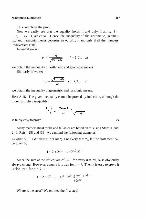
Mathematical Induction 187
This completes the proof.
Now we easily see that the equality holds if and only if all ai, i =
1, 2, . . . , (k + 1) are equal. Hence the inequality of the arithmetic, geomet-
ric, and harmonic means becomes an equality if and only if all the numbers
involved are equal.
Indeed if we set
we obtain the inequality of arithmetic and geometric means.
Similarly, if we set
we obtain the inequality of geometric and harmonic means.
HINT A.18. The given inequality cannot be proved by induction, although the
more restrictive inequality:
is fairly easy to prove.
Many mathematical tricks and fallacies are based on misusing Steps 1 and
2. In Refs. [28] and [39], we can find the following examples.
EXAMPLE A.10 (WHERE IS THE ERROR?). For every n ∈N0, let the statement An
be given by:
1 + 2 + 22 + . . . +2n =?
2n+1
Since the sum at the left equals 2n+1 – 1 for every n ∈ N0, An is obviously
always wrong. However, assume it is true for n = k. Then it is easy to prove it
is also true for n = k +1:
1 + 2 + 22 + . . . +2k +2k+1=? 2k+1 + 2k+1
?= 2k+ 2
Where is the error? We omitted the first step!
188 Appendix A
EXAMPLE A.11 (ALL HORSES ARE THE SAME COLOR!). All horses are the same
color! We prove that by induction on the number of horses: If we have only
one horse, the proposition is true because that horse is the same color as itself.
Assume now the proposition is true when we have k horses, then consider k + 1
horses. Let these horses be marked by numbers from 1 to k + 1. If we extract
the horses with numbers 1 through k, by the inductive hypothesis they are all
the same color. Similarly horses numbered 2 through k + 1 are the same color.
Finally since the relation “is the same color as” is transitive, we see that the
whole group of k + 1 horses is also the same color!
Where is the error now? This example was given in Ref. [28]. The first
example similar to this one was published in Ref. [45].
Appendix B
Important Mathema tical Constants

This page intentionally left blank.
Important Mathematical Constants 191
π = 3.14159 26535 89793 . . .
By definition the number π is the ratio of the circumference and the diameter
of a circle. Archimedes was the first to prove that the same proportionality
constant appears in expressions for the area of a circle, (r 2 π), area of a sphere
(4r2π), and the volume of a ball (4r3π/3), as well as in similar formulas for a
cylinder and a cone.
The number π is probably the most important mathematical constant be-
cause in addition geometry, it appears in number theory, analysis, probability
theory, and many other branches of mathematics.
In ancient times the Chinese thought this ratio equaled 3. The Rhindpapyrus* from Ancient Egypt (around 1650-1500 B.C.) says the area of a
circle equals the square of eight-ninths of its radius, which yields π ≈ 256/81 =
3.16049. . .
Archimedes estimated the value of π in several ways. For example by
calculating areas of regular 96-gons, one inscribed in the circle, the other
circumscribed around it, he found that:
310/71 < π < 310/70
The upper bound found by Archimedes is the popular approximation π ≈ 22/7. It is the best approximation by a fraction for integers less than 100.
Ptolemy of Alexandria (second cent. A.D.) used the fraction 377/ 120. Later
Tsu Chung-Chi in China (fifth cent. A.D.) used 355/ 113 = 3.1415929. . . This
fraction is the best among the fractions for integers less than 30000.
This approximation was the best until Arab mathematicians found better
values in the fifteenth century. At the same time, European mathematicians
were far behind. They took the lead only in the sixteenth century, thanks to
Ludolph van Ceulen, who determined π to 35 decimal places. In his honor π is
still sometimes called the Ludolphine number. Today the value of π is known
to several millions of decimal places.
The Greek letter π was first used as a symbol for this number by W. Jones
in 1707, but it was not widely used until Euler began using it in 1737. Why π?
Probably from the Greek words π∈ριµ∈τρον (perimetron = circumference) or
π∈ριφ∈ρ∈ια (periferia = periphery).
*This papyrus was bought in 1858 by a Scottish antiquary, A. H. Rhind, in Egypt. It is sometimes
called the Ahmes papyrus in honor of the scribe who wrote it.
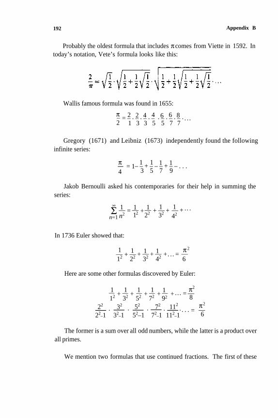
Appendix B
Probably the oldest formula that includes πcomes from Viette in 1592. In
192
today’s notation, Vete’s formula looks like this:
Wallis famous formula was found in 1655:
π2 1 3 3 5 5 7 7– . . .
2 2 4 4 6 6 8= – . – . – . – . – . – . – .
Gregory (1671) and Leibniz (1673) independently found the following
infinite series:
π 1 1 1 1- = 1– – + – – – + – – . . .4 3 5 7 9
Jakob Bernoulli asked his contemporaries for their help in summing the
series:
1 1 1 . . .∝
1— + + +n2 22 32
42+————
12Σ =1
n=1
In 1736 Euler showed that:
1 1 1 1 π 2
12 22 32 42 6. . . =++++ ——— — —
Here are some other formulas discovered by Euler:
1 1 1 1 1 π2
12 32 52 72 92 8————— — =+++++ . . .
π2
22–1 32
–1 52–1 72–1 112
–1. .——— — —
6—. . . =
22 32 52 72 112
. ..
The former is a sum over all odd numbers, while the latter is a product over
all primes.
We mention two formulas that use continued fractions. The first of these
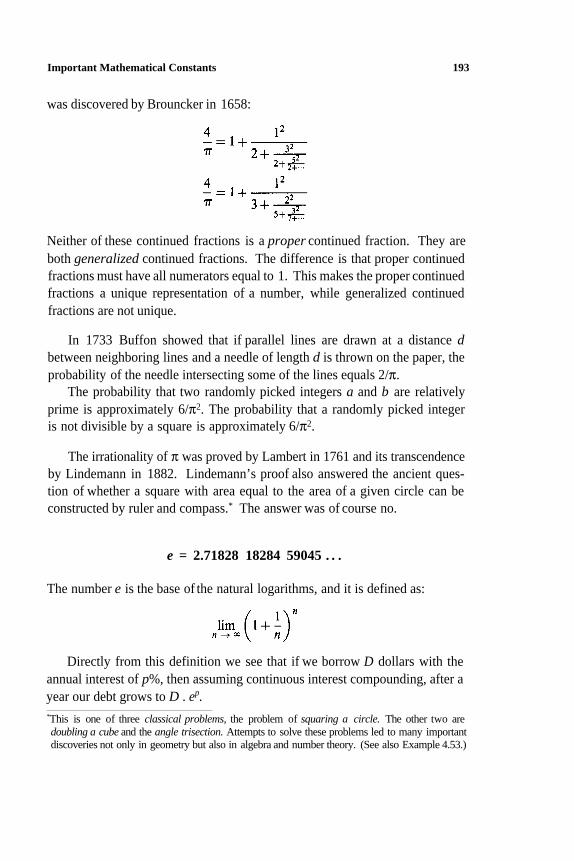
Important Mathematical Constants 193
was discovered by Brouncker in 1658:
Neither of these continued fractions is a proper continued fraction. They are
both generalized continued fractions. The difference is that proper continued
fractions must have all numerators equal to 1. This makes the proper continued
fractions a unique representation of a number, while generalized continued
fractions are not unique.
In 1733 Buffon showed that if parallel lines are drawn at a distance dbetween neighboring lines and a needle of length d is thrown on the paper, the
probability of the needle intersecting some of the lines equals 2/π.
The probability that two randomly picked integers a and b are relatively
prime is approximately 6/π2. The probability that a randomly picked integer
is not divisible by a square is approximately 6/π2.
The irrationality of π was proved by Lambert in 1761 and its transcendence
by Lindemann in 1882. Lindemann’s proof also answered the ancient ques-
tion of whether a square with area equal to the area of a given circle can be
constructed by ruler and compass.* The answer was of course no.
e = 2.71828 18284 59045 . . .
The number e is the base of the natural logarithms, and it is defined as:
Directly from this definition we see that if we borrow D dollars with the
annual interest of p%, then assuming continuous interest compounding, after a
year our debt grows to D . ep.*This is one of three classical problems, the problem of squaring a circle. The other two are
doubling a cube and the angle trisection. Attempts to solve these problems led to many important
discoveries not only in geometry but also in algebra and number theory. (See also Example 4.53.)
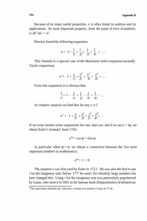
Appendix B
Because of its many useful properties, e is often found in analysis and its
applications. Its most important property, from the point of view of analysis,
is dex /dx = ex.
194
Newton found the following expansion:
1 1 1 1
1! 2! 3! 4!
This formula is a special case of the Maclaurin series expansion (actually
e = 1+ – + – + – + – + . . .
Taylor expansion):
x x2 x3 x4
1! 2! 3! 4!ex= 1 + – + – + – + – + . . .
From this expansion it is obvious that:
1 1 1 1 1– = 1 – – + – – – + – – . . .e 1! 2! 3! 4!
In complex analysis we find that for any z ∈C
z z2 z3 z4
1! 2! 3! 4!ez = 1 + – + – + – + – + . . .
If we write similar series expansions for sinz and cosz and if we set z = iϕ, we
obtain Euler’s formula* from 1743:
eiϕ = cos ϕ + isin ϕ
In particular when ϕ = π, we obtain a connection between the five most
important numbers in mathematics:
eiπ + 1 = 0
The notation e was first used by Euler in 173 1. He was also the first to use
i for the imaginary unit; before 1777 he used i for infinitely large numbers but
later changed this. Using i for the imaginary unit was particularly popularized
by Gauss, who used it in 1801 in his famous book Disquisitiones Arithmeticae.*The equivalent formula iϕ= In(cosϕ + isin ϕ) was used by Cotes in 1714.
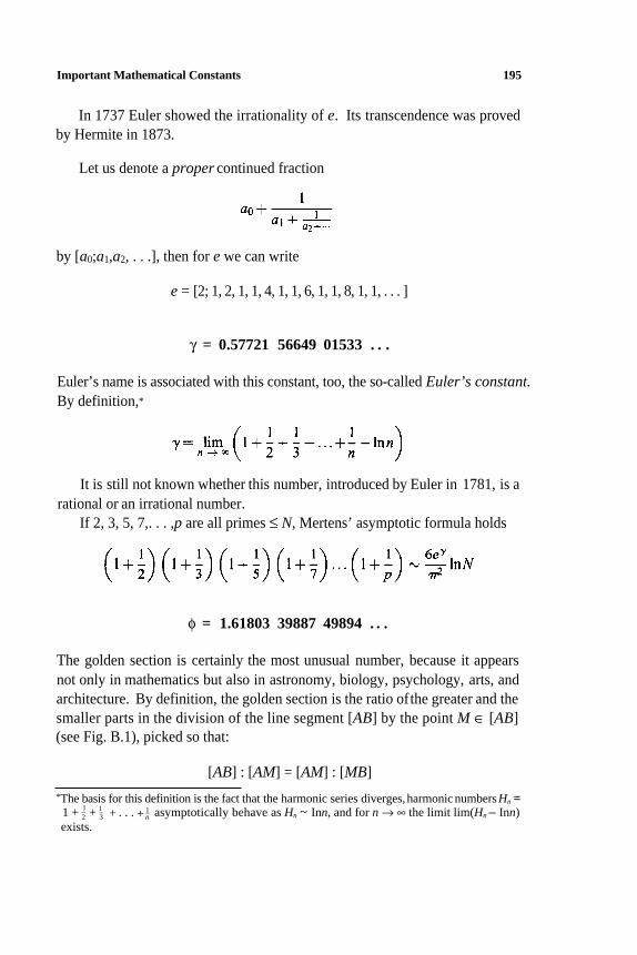
Important Mathematical Constants 195
In 1737 Euler showed the irrationality of e. Its transcendence was proved
by Hermite in 1873.
Let us denote a proper continued fraction
by [a0;a1,a2, . . .], then for e we can write
e = [2; 1, 2, 1, 1, 4, 1, 1, 6, 1, 1, 8, 1, 1, . . . ]
γ = 0.57721 56649 01533 . . .
Euler’s name is associated with this constant, too, the so-called Euler’s constant. By definition,*
It is still not known whether this number, introduced by Euler in 1781, is a
If 2, 3, 5, 7,. . . ,p are all primes ≤ N, Mertens’ asymptotic formula holds
rational or an irrational number.
φ = 1.61803 39887 49894 . . .
The golden section is certainly the most unusual number, because it appears
not only in mathematics but also in astronomy, biology, psychology, arts, and
architecture. By definition, the golden section is the ratio of the greater and the
smaller parts in the division of the line segment [AB] by the point M ∈ [AB]
(see Fig. B.1), picked so that:
[AB] : [AM] = [AM] : [MB]
*The basis for this definition is the fact that the harmonic series diverges,harmonic numbersHn =1 +
1–2
+1–3 + . . . +
1–n asymptotically behave as Hn ~ Inn, and for n → ∞ the limit lim(Hn – Inn)
exists.
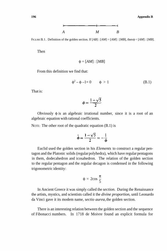
196 Appendix B
A M B
FIGUREB.1 . Definition of the golden section. If [AB] : [AM] = [AM] : [MB], then φ = [AM] : [MB].
Then
φ = [AM] : [MB]
From this definition we find that:
φ2 – φ –1= 0 φ > 1 (B.1)
That is:
Obviously φ is an algebraic irrational number, since it is a root of an
algebraic equation with rational coefficients.
NOTE: The other root of the quadratic equation (B.1) is
Euclid used the golden section in his Elements to construct a regular pen-
tagon and the Platonic solids (regular polyhedra), which have regular pentagons
in them, dodecahedron and icosahedron. The relation of the golden section
to the regular pentagon and the regular decagon is condensed in the following
trigonometric identity:
πφ = 2cos –
5
In Ancient Greece it was simply called the section. During the Renaissance
the artists, mystics, and scientists called it the divine proportion, until Leonardo
da Vinci gave it its modem name, sectio aurea, the golden section.
There is an interesting relation between the golden section and the sequence
of Fibonacci numbers. In 1718 de Moivre found an explicit formula for
Important Mathematical Constants 197
Fibonacci numbers, known today as Binet’s formula:
Thanks to this formula we see that ratios of consecutive Fibonacci numbers
tend to the golden section:
fn +1
n → ∞ fnlim — = φ
Until recently the golden section was denoted by τ, the first letter of its
Ancient Greek name τοµη (tome = section), or by g; today the most common
symbol is φ, in honor of the Ancient Greek sculptor Phidias, who thought
golden proportions are the most pleasing to the human eye. This notation was
introduced by Mark Barr and widely popularized by Donald Knuth.
From the quadratic equation x2 – x – 1 = 0, we easily find that
The golden section has a special place in the theory of continued fractions
because:
φ = [1; 1, 1, 1, 1, 1, 1, . . . ]
It is interesting that the approximation of φ by a continued fraction of order
n is equal to the ratio of consecutive Fibonacci numbers fn+2 and fn+1; for
example:
13 f7[1; 1, 1, 1, 1, 1] = – = –8 f6

This page intentionally left blank.
Appendix C
Great Mathematicians

This page intentionally left blank.
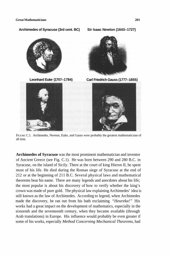
Great Mathematicians 201
Archimedes of Syracuse (3rd cent. BC) Sir Isaac Newton (1643-1727)
Leonhard Euler (1707-1784) Carl Friedrich Gauss (1777-1855)
FIGURE C.1. Archimedes, Newton, Euler, and Gauss were probably the greatest mathematicians of
all time.
Archimedes of Syracuse was the most prominent mathematician and inventor
of Ancient Greece (see Fig. C.1). He was born between 290 and 280 B.C. in
Syracuse, on the island of Sicily. There at the court of king Hieron II, he spent
most of his life. He died during the Roman siege of Syracuse at the end of
212 or at the beginning of 211 B.C. Several physical laws and mathematical
theorems bear his name. There are many legends and anecdotes about his life;
the most popular is about his discovery of how to verify whether the king’s
crown was made of pure gold. The physical law explaining Archimedes’ idea is
still known as the law of Archimedes. According to legend, when Archimedes
made the discovery, he ran out from his bath exclaiming “Heureka!” His
works had a great impact on the development of mathematics, especially in the
sixteenth and the seventeenth century, when they became available (through
Arab translations) in Europe. His influence would probably be even greater if
some of his works, especially Method Concerning Mechanical Theorems, had
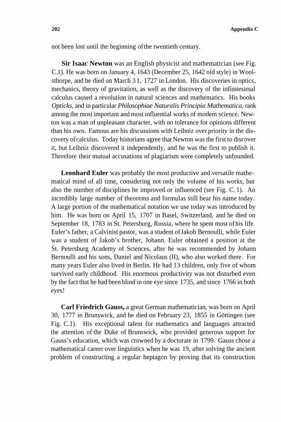
202 Appendix C
not been lost until the beginning of the twentieth century.
Sir Isaac Newton was an English physicist and mathematician (see Fig.
C.1). He was born on January 4, 1643 (December 25, 1642 old style) in Wool-
sthorpe, and he died on March 3 1, 1727 in London. His discoveries in optics,
mechanics, theory of gravitation, as well as the discovery of the infinitesimal
calculus caused a revolution in natural sciences and mathematics. His books
Opticks, and in particular Philosophiae Naturalis Principia Mathematica, rank
among the most important and most influential works of modem science. New-
ton was a man of unpleasant character, with no tolerance for opinions different
than his own. Famous are his discussions with Leibniz over priority in the dis-
covery of calculus. Today historians agree that Newton was the first to discover
it, but Leibniz discovered it independently, and he was the first to publish it.
Therefore their mutual accusations of plagiarism were completely unfounded.
Leonhard Euler was probably the most productive and versatile mathe-
matical mind of all time, considering not only the volume of his works, but
also the number of disciplines he improved or influenced (see Fig. C. 1). An
incredibly large number of theorems and formulas still bear his name today.
A large portion of the mathematical notation we use today was introduced by
him. He was born on April 15, 1707 in Basel, Switzerland, and he died on
September 18, 1783 in St. Petersburg, Russia, where he spent most of his life.
Euler’s father, a Calvinist pastor, was a student of Jakob Bernoulli, while Euler
was a student of Jakob’s brother, Johann. Euler obtained a position at the
St. Petersburg Academy of Sciences, after he was recommended by Johann
Bernoulli and his sons, Daniel and Nicolaus (II), who also worked there. For
many years Euler also lived in Berlin. He had 13 children, only five of whom
survived early childhood. His enormous productivity was not disturbed even
by the fact that he had been blind in one eye since 1735, and since 1766 in both
eyes!
Carl Friedrich Gauss, a great German mathematician, was born on April
30, 1777 in Brunswick, and he died on February 23, 1855 in Göttingen (see
Fig. C.1). His exceptional talent for mathematics and languages attracted
the attention of the Duke of Brunswick, who provided generous support for
Gauss’s education, which was crowned by a doctorate in 1799. Gauss chose a
mathematical career over linguistics when he was 19, after solving the ancient
problem of constructing a regular heptagon by proving that its construction
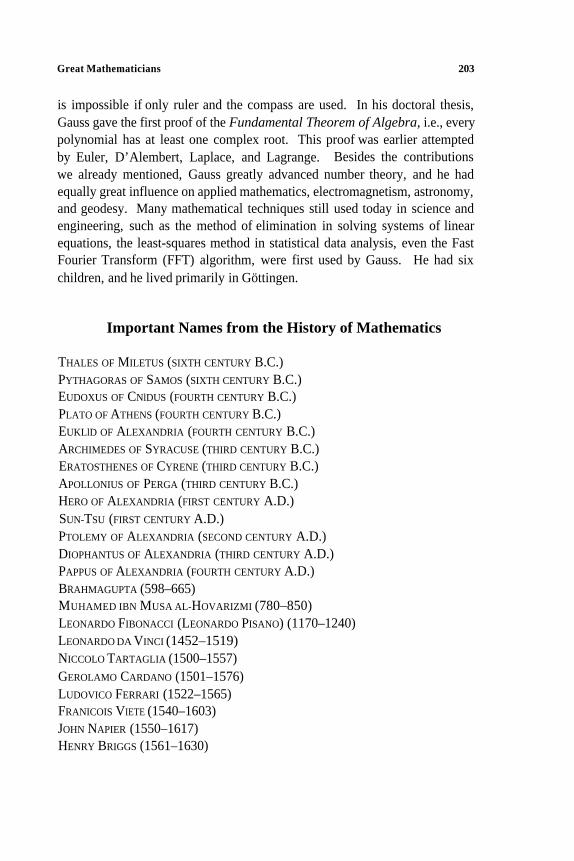
Great Mathematicians 203
is impossible if only ruler and the compass are used. In his doctoral thesis,
Gauss gave the first proof of the Fundamental Theorem of Algebra, i.e., every
polynomial has at least one complex root. This proof was earlier attempted
by Euler, D’ Alembert, Laplace, and Lagrange. Besides the contributions
we already mentioned, Gauss greatly advanced number theory, and he had
equally great influence on applied mathematics, electromagnetism, astronomy,
and geodesy. Many mathematical techniques still used today in science and
engineering, such as the method of elimination in solving systems of linear
equations, the least-squares method in statistical data analysis, even the Fast
Fourier Transform (FFT) algorithm, were first used by Gauss. He had six
children, and he lived primarily in Göttingen.
Important Names from the History of Mathematics
THALES OF MILETUS (SIXTH CENTURY B.C.)
PYTHAGORAS OF SAMOS (SIXTH CENTURY B.C.)
EUDOXUS OF CNlDUS (FOURTH CENTURY B.C.)
PLATO OF ATHENS (FOURTH CENTURY B.C.)
EUKLlD OF ALEXANDRIA (FOURTH CENTURY B.C.)
ARCHIMEDES OF SYRACUSE (THIRD CENTURY B.C.)
ERATOSTHENES OF CYRENE (THIRD CENTURY B.C.)
APOLLONIUS OF PERGA (THIRD CENTURY B.C.)
HERO OF ALEXANDRIA (FIRST CENTURY A.D.)
SUN-TSU (FIRST CENTURY A.D.)
PTOLEMY OF ALEXANDRIA (SECOND CENTURY A.D.)
DIOPHANTUS OF ALEXANDRIA (THIRD CENTURY A.D.)
PAPPUS OF ALEXANDRIA (FOURTH CENTURY A.D.)
BRAHMAGUPTA (598–665)
LEONARDO FIBONACCI (LEONARDO PISANO) (1170–1240)
NICCOLO TARTAGLIA (1500–1557)
GEROLAMO CARDANO (1501–1576)
LUDOVICO FERRARI (1522–1565)
FRANICOIS VIETE (1540–1603)
JOHN NAPIER (1550–1617)
HENRY BRIGGS (1561–1630)
MUHAMED IBN MUSA AL-HOVARIZMI (780–850)
LEONARDO DA VINCI (1452–1519)
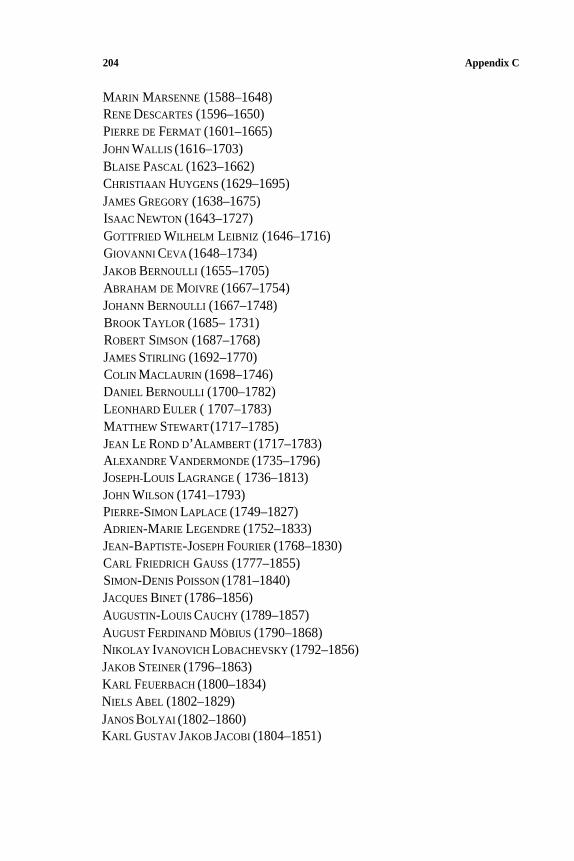
204 Appendix C
MARIN MARSENNE (1588–1648)
RENE DESCARTES (1596–1650)
JOHN WALLIS (1616–1703)
BLAISE PASCAL (1623–1662)
CHRISTIAAN HUYGENS (1629–1695)
JAMES GREGORY (1638–1675)
ISAAC NEWTON (1643–1727)
GOTTFRIED WILHELM LEIBNIZ (1646–1716)
GIOVANNI CEVA (1648–1734)
JAKOB BERNOULLI (1655–1705)
JOHANN BERNOULLI (1667–1748)
BROOK TAYLOR (1685– 1731)
ROBERT SIMSON (1687–1768)
JAMES STIRLING (1692–1770)
COLIN MACLAURIN (1698–1746)
DANIEL BERNOULLI (1700–1782)
LEONHARD EULER ( 1707–1783)
MATTHEW STEWART(1717–1785)
JEAN LE ROND D’ALAMBERT (1717–1783)
ALEXANDRE VANDERMONDE (1735–1796)
JOSEPH-LOUIS LAGRANGE ( 1736–1813)
JOHN WILSON (1741–1793)
PIERRE-SIMON LAPLACE (1749–1827)
ADRIEN-MARIE LEGENDRE (1752–1833)
JEAN-BAPTISTE-JOSEPH FOURIER (1768–1830)
CARL FRIEDRICH GAUSS (1777–1855)
JACQUES BINET (1786–1856)
AUGUSTIN-LOUIS CAUCHY (1789–1857)
AUGUST FERDINAND MÖBIUS (1790–1868)
NIKOLAY IVANOVICH LOBACHEVSKY (1792–1856)
JAKOB STEINER (1796–1863)
KARL FEUERBACH (1800–1834)
NIELS ABEL (1802–1829)
JANOS BOLYAI (1802–1860)
KARL GUSTAV JAKOB JACOBI (1804–1851)
PIERRE DE FERMAT (1601–1665)
ABRAHAM DE MOIVRE (1667–1754)
SIMON-DENIS POISSON (1781–1840)
Great Mathematicians 205
PETER GUSTAV LEJEUNE DIRICHLET (1805–1859)
WILLIAM ROWAN HAMILTON (1805–1865)
AUGUSTUS DE MORGAN (1806–1 871)
JOSEPH LIOUVILLE (1809–1882)
EVARISTE GALOIS (1811–1832)
JAMES SYLVESTER (1814–1897)
GEORGE BOOLE (1815–1864)
PAFNUTY LVOVICH CHEBYSHEV (1821–1894)
ARTHUR CAYLEY (1821–1895)
BERNHARD RIEMANN (1826–1866)
GEORG CANTOR (1845–1918)
FELIX KLEIN (1849–1925)
HENRI POINCARE (1854–1912)
ANDREY ANDREYEVICH MARKOV (1856–1922)
ALEKSANDR MIHAILOVICH LYAPUNOV (1857–1918)
GIUSEPPE PEANO (1858–1932)
DAVID HILBERT (1862–1943)
HERMANN MINKOWSKI (1864–1909)
BERTRAND RUSSEL (1872–1970)
GODFREY HAROLD HARDY (1877–1947)
SRINIVASA RAMANUJAN (1887–1920)
GEORGE POLYA (1887–1985)
NORBERT WIENER (1894–1964)
ANDREY NIKOLAYEVICH KOLMOGOROV (1903–1987)
KURT GÖDEL (1906–1978)
ALAN TURING (1912–1954)
JOHN VON NEUMANN (1903–1957)
Biographies of these and many other mathematicians can be found on
the internet, for example, at: www-groups .dcs.st-andrews.ac.uk/~history

This page intentionally left blank.
Appendix D
Greek Alphabet

This page intentionally left blank.
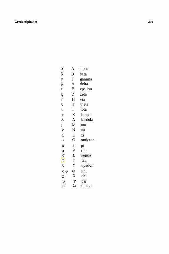
Greek Alphabet 209
α Α alpha
β Β beta
γ Γ gamma
δ ∆ delta
ε Ε epsilon
ζ Ζ zeta
η Η eta
θ Τ theta
ι Ι iota
κ Κ kappa
λ Λ lambda
µ Μ mu
ν Ν nu
ξ Ξ xi
ο Ο omicron
π Π pi
ρ P rho
σ Σ sigma
τ Τ tau
υ Υ upsilon
χ X chi
ψ Ψ psi
ω Ω omega
φ,ϕ Φ Phi

This page intentionally left blank.
References
1. Aaboe, A., Episodes from the Early History of Mathematics (Random House, New York,
1964).
2. Balk. M. B., and V. G. Boltijanskij, Geometriia mass (Bibliotechka Kvant, Nauka, Moskva,
1987).
3. Bashmakov, M. I., B. M. Bekker, and V. M. Goljhovoj, Zadachi po matematike (Bibliotechka
Kvant,Nauka, Moskva, 1982).
4. Bell, E. T., Men of Mathematics (Touchstone, New York, 1937).
5. Bold, B., Famous Problems of Geometry and How to Solve Them (Dover, New York, 1969).
6. Born, M., Atomic Physics, 8th ed. (Dover, New York, 1989).
7. Brualdi, R. A,, Introductory Combinatorics, 2nd ed. (Prentice Hall, Englewood Cliffs, 1992).
8. Bryant, V., Aspects of Combinarorics (Cambridge University Press, 1993).
9. Bullen, P. S., D. S. Mitrinovic, and P. M. Vasic, Means and their Inequalities (D.Reidel,
Dodrecht,1988).
''
10. Carroll, L., Lewis Carroll Picture Book (Tower Books, Detroit, 1971).
11. Cohen, D. I. A., Basic Techniques of Combinatorial Theory (Wiley, New York, 1978).
12. Collier’s Encyclopedia (Collier, New York, 1992).
13. Conway, J. H., and R. K. Guy, Book of Numbers (Copernicus, New York, 1995).
14. Cormen, T. H., C. E. Leiserson, and R. L. Rivest, Introduction to Algorithms (MIT Press,
Cambridge, MA, 1990).
15. Courant, R., and H. Robbins, What is Mathematics? 2nd ed. (Revised by I. Stewart) (Oxford
University Press, 1996).
16. Coxeter, H. S. M., and S. L. Greitzer, Geometry Revisited (Random House, New York, 1967).
17. Coxeter, H. S. M., Introduction to Geometry (Wiley, New York, 1969).
18. Cvetkovic, D., Teorija grafova i njene primene (Naucna knjiga, Belgrade, 1981).∨'
'19. Cvetkovic, D., and S. Simic, Diskretna matematika (Naucna knjiga, Belgrade, 1990).
20. Dörrie, H., 100 Great Problems of Elementary Mathema tics, Their History, and Solutions (Dover, New York, 1965).
211
' ∨
212 References
21. Davis, D. M., Nature and Power of Mathematics (Princeton University Press, Princeton, NJ,
1993).
22. Devlin, K., Mathematics: New Golden Age (Penguin, London, 1988).
23. Dijksterhuis, E. J., Archimedes (Princeton University Press, Princeton, NJ, 1987).
24. Doroslovacki, R., Algebra (Stylos, Novi Sad, 1995).
25. Euclid, Thirteen Books of Euclid’s Elements (T. L. Heath, ed., Dover, New York, 1956).
26. Eves, H., A Survey of Geomerty, Vol. 1 (Allyn and Bacon, Boston, 1965).
27. Gardner, M., My Best Mathematical and Logic Puzzles (Dover, New York, 1994).
28. Graham, R. L., D. E. Knuth, and O. Patashnik, Concrete Mathematics: A Foundation for Computer Science (Addison-Wesley, Reading, MA, 1989).
29. Heath, T. L., A Manual of Greek Mathematics (Dover, New York, 1963).
30. Hogben, L., Mathematics for the Million (Pan Books, London, 1978).
3 1. Hoggatt, V. E., Jr., Fibonacci and Lucas Numbers (Houghton Mifflin, Boston, 1969).
32. Huntley, H. E., Divine Proportion (Dover, New York, 1970).
33. Kac, M., and S. M. Ulam, Mathematics and Logic (Dover, New York, 1992).
34. Khintchine, A. Ya., Continued Fractions (Nordhoff, Groningen, 1964).
35. Klein, F., Famous Problems of Elementary Geometry (Hafner, New York, 1950).
36. Knuth, D. E., Art of Computer Programming, 2nd ed., Vol. 1, Fundamental Algorithms (Addison-Wesley,Reading,MA, 1973).
∨'37. M. Petkovic, Zanimljivi matematicki problemi (Naucna knjiga, Belgrade, 1988).
38. Micic, V., and Z. Kadelburg, Uvod u teoriju brojeva (DMSRS, Belgrade, 1983).'
'
'
39. Mitrinovic, D. S., Matematicka indukcija, binomna formula i kombinatorika (Gradevinska
knjiga,Belgrade, 1990).
'40. Mladenovic, P., Kombinatorika (Drugo izdanje, DMS, Belgrade, 1992).
41. Neugebauer, O., Exact Sciences in Antiquity (Princeton University Press, Princeton, NJ, 1952).
42. New Encyclopaedia Britannica, 15th ed. (Encyclopaedia Britannica, Chicago, 1991).
43. Ore, O., Number Theory and Its History (McGraw-Hill, New York, 1948).
44. Oxford English Dictionary, 2nd ed. (Clarendon Press, Oxford, 1989).
45. Polya, G., Induction and Analogy in Mathematics. Vol. 1 of Mathematics and Plausible Reasoning (Princeton University Press, Princeton, NJ, 1954).
46. Rademacher, H., and O. Toeplitz, Enjoyment of Math (Princeton University Press, Princeton,
NJ, 1957).
47. Ribenboim, P., Book of Prime Number Records (Springer-Verlag, Berlin, 1989).
48. Riordan, J., Generating Functions, in Applied Combinatorial Mathematics (E. F. Beckenbach,
ed., Wiley, New York, 1964).
49. Rouse Ball, W. W., and H. S. M. Coxeter, Mathematical Recreations and Essays (Macmillan,
New York, 1944).
50. Scharlau, W., and H. Opolka, From Fermat to Minkowski (Springer-Verlag, Berlin, 1985).
5 1. Schroeder, M. R., Number Theory in Science and Communication (Springer-Verlag, Berlin,
1986).
∨
∨
References 213
52. Sierpinski, W., Elementary Theory of Numbers (North-Holland, Amsterdam, 1988).
53. Slomson, A., An Introduction to Combinatorics (Chapman and Hall, London, 1991).
54. Smith, D. E., History of Mathematics, Vol. I (Ginn and Company, Boston, 1923).
55. Stewart, I., Galois Theory, 2nd ed. (Chapman & Hall, London, 1989).
56. Struik, D., A Concise History of Mathematics (Dover, New York, 1967).
∨
∨
57. Tosic, R., and V. Vukoslavcevic, Elementi teorije brojeva (Alef, Novi Sad, 1995).
58. Vajda, S., Fibonacci and Lucas Numbers, and the Golden Section (Ellis Horwood, Chichester,
UK,1989).
∨
59. van der Waerden, B. L., Science Awakening (Noordhoff, Groningen, 1954).
' '
60. Vaught, R. L., Set Theory: An Introduction, 2nd ed. (Birkhäuser, Boston, 1995).
61. Veljan, D., Kombinatorika s teorijom grafova (Skolska knjiga, Zagreb, 1989).
62. Wells, D., Penguin Dictionary of Curious and Interesting Numbers (Penguin Books, London,
1987).
63. Wells, D., Penguin Book of Curious and Interesting Puzzles (Penguin Books, London, 1992).
64. Wiles, A., Annals of Mathematics, 141, No. 3, pp. 443–551 (May 1995).
65. Yaglom, A. M., and I. M. Yaglom, Challenging Mathematical Problems with Elementary Solutions, Vol. 1 and 2 (Dover, New York, 1987).
66. Yakovlev, G. N., ed., High-School Mathematics (Translated from the Russian) (Mir Publishers,
Moscow,1984).

This page intentionally left blank.
Index
Abel, 160
Abel’s criterion, 45
Aborigines, 17
Ahmes,191nℵ 0(aleph-zero), 11, 13
AI’Khwarizmi, 159
Almagest, 157
Anecdote about logician, 180
Angle trisection, 160, 193n
Annals of Mathematics, 110
Apollo, 160nArchimedes, 121, 122, 140, 191, 201
Archimedes’ spiral, 160
Archimedes’ theorem, 13 I
Arithmetic mean, 149, 150, 174, 180, 187
Arithmetica, 109
Babylon, 75
Barr, 197
Bernoulli
Daniel, 43n, 202
Jakob,43n, 167, 192
Johann, 43n, 202
Nicolaus (I), 43n, 51
Nicolaus (II),43n,202
Bhaskara, 145
Bijection, 10
Binary operation, 10
Binet, 5 1
Binet’s formula, 5 1, 179, 197
Binomial coefficients, 28, 35-37, 52, 56-59,
64, 67, 113, 170
Binomial formula, 26, 35–39, 45, 46, 57, 60,
Boltzmann’s constant, 62
Bose–Einstein statistics, 62
Bosons, 62
Brahma, 65
Brahmagupta’s formula, 144
Brianchon, 138
Brouncker, 193
Buffon, 193
67, 99, 178
c, 11,13
Canonical factorization, 82, 83
Cantor, 12
Cardano, 160
Cardinality, 11
Carmichael numbers, 97
Cartesian product, 7, 14, 69
Cauchy, 176
Cayley’s theorem, 68
Centroid, 130-138
Ceva’s theorem, 128, 146
Cevian, 129
Change for one dinar, 49
Chebyshev, 1 10
Chebyshev polynomials, I79
Chess board, 27, 34, 55, 56
Chevalier,160nChinese remainder theorem, 106
215
216 Index
Circle
circumcircle, 126–128, 138
excircle, 138
incircle, 126–128, 138
nine-point (Feuerbach’s), 138
Classical constructions, 81, 160
Classical problems, 160, 193ndoubling a cube, 160, 193nsquaring acircle, 160, 193ntrisectingan angle, 160, 193n
Codomain, 10
Cohen, 13
Collinear points, 23
Combinations
hybrid, 47
with repetition, 33, 47
without repetition, 31
Complete residue system, 95, 96
Conchoid of Nicomedes, 160
Concurrent lines, 129
Congruences, 92
Continuum hypotheses, 13
Contradiction, 11, 16
Converse Ceva’s theorem, 129, I46
Coplanar points, 24
Cotes, 194nCountable set, 12
Counterexample, 14
Cubeduplication, 160, 193n
DelaValee–Poussin, 110
Delian problem, 160n, 193nDerangements, 43, 56
Descartes, 7, 109n, 16 1
Dinostratus’ quadratrix, 160
Diocles’ cissoid, 160
Diophantine equations, 101, 109, 112
Diophantus, 109
Dirichlet’s principle, 22, 53
Disjoint sets, 5
Disquisitiones Arithmeticae, 92, 194
Distribution of primes, 110
Divisibility criteria, 100, 101
Dodecahedron, 197
Domain, 10
Dominos, 55, 167
Doubling a cube, 160n, 193n
e, 16, 41, 43, 193, 194
Egyptian triangle, 108
Eight queens, 55
Electron, 63
Elements, 11, 38, 79, 83, 85, 119, 142, 167,
Energy levels, 61–63
Epimenides, 13
Eratosthenes, 79
Eubulides, I3
Euclid, 11, 38, 79, 85, 119, 167, 196
Euclid numbers, 179
Euclidean algorithm, 83–88, 102–106
I96
complexity of, 88
extended, 105
Euclid’s proof of Pythagorean theorem, 145
Euclid’s theorem on primes, 11, 80, 167
Euler, 43, 45, 49, 51, 80, 106, 140, 171, 192,
195, 202
Euler’s constant (γ), 17, 195
Euler’s formula, 128, 139, 156, 157, 185, 194
Euler’s line, 136
Euler’s method, 112
Euler’s partition theorem, 49
Euler’s phi function, 42, 89, 91, 95, 96, 102
Euler’s problem partitio numerorum, 41
Euler’s theorem in graph theory, 54
Euler’s theorem in number theory, 42, 96, 102
Euler’s trinomial, 80, 177, 180
Euler–Venn diagram, 4, 5, 14
Extended Euclidean algorithm, 105
Factorial, 28
falling factorial, 59
Stirling’s approximation for, 41, 61
Factorization of integers, 82, 83
Fermat, 80, 109, 141, 171
Fermat numbers, 80, 81, 160, 160n, 171
Fermat’s point, 140, 147, 153–155
Fermat’s principle, 109n, 140
Fermat’s theorem
last, 109
lesser, 60, 96, 99
Fermi–Dirac statistics, 63
Fermions, 63
Ferrari, 160
Feuerbach, 197
Feuerbach’s theorem, 197
Fibonacci (Leonardo Pisano), 44
Fibonacci’s numbers, 44, 45, 50, 51, 70, 78,
87, 113, 179, 197
Index 217
Fibonacci’s rabbits, 44
Finite set, 11
Five most important numbers, 158, 194
Formula
Binet’s, 51, 179, 197
binomial formula, 26, 35-39, 45, 46, 57,
60, 67, 99, 178
Brahmagupta’s, 144
Euler’s, 128, 139, 156, 157, 185, 194
Hadamard–de la Valee–Poussin’s, 110
Hamming’s, 64
Hardy–Ramanujan, 4 1, 48
Hero’s, 121, 126–128, 144, 151, 152
Leibniz’s, 59, I92
Maclaurin’s, 45, 47, 158, 180, 194
Mertens’, 195
de Moivre’s, I79
Newton’s: see Formula, binomial
Pascal’s, 35, 38, 47
polynomial, 67
for prime numbers, 80
Stirling’s, 41, 61
Sylvester’s, 41
Taylor’s, 7 1, 194
Vandermonde’s, 59
Viette’s, 192
Wallis’, 192
Function: see Multiplicative functions,
Fundamental Theorem of Algebra, 203
Fundamental Theorem of Arithmetic, 82
Galois, 160, 160nγ, 17, 195
Gauss, 8 I, 92, I 12, 160, 169, 194, 202
Gauss’ method, 112
Gauss’ theorem, 81
GCD (greatest common divisor), 84
Generating functions, 45
Geometric mean, 149, 150, 174, 180, 187
Gergonne’s point, 147
Girard, 45
Goat, 159
Golden section (φ), 16, 45, 51, 105, 195
Gödel’s theorem, 13
Graph theory, 54, 68
Gregory, 192
Gregory’s triangle, 170, 173, 182
Mappings, and Important functions
Hadamard, I 10
Hamilton–Sylvester’s theorem, 138
Hamming’s formula, 64
Hanoi towers, 65, 66
Hardy–Ramanujan’s formula, 41, 48
Harmonic mean, 149, 150, 174, 180, 187
Harmonic numbers, 19nHarmonic series, 195nHe
3, 63
He4, 63
Heegner, 83
Heiberg,140nHermite, 16, 195
Hero’s formula, 121, 126–128, 144, 151, 152
“Heureka!”, 201
Horses, 188
Hypotenuse, 1 19
i (imaginary unit), 194
Icosahedron, 196
Ideal gas, 63
Important functions
( nk ) binomial coefficient), 28, 35–37, 52.
(56–59, 64, 67, 113, 170
ϕ(n) (Euler’s f.), 42, 89, 91, 95, 96, 102
n! (factorial), 28, 41, 61
nr– (falling factorial), 59
x (floor), 43, 52, 98
δ(n) (product of divisors of n), 114
µ(n) (Möbius f.), 90
τ(n) (number of divisors of n), 25, 83, 89,
π(n) (number of primes ≤ n), 110
σ(n) (sum of divisors of n), 90
centroid (T), 130–138
circumcenter (O), 126, 129
Fermat’s point (F), 140, 147, 153-155
Gergonne’s point (G), 147
incenter (I), 126, 127, 130
orthocenter (H), 130, 137, 138
114
Important points
Induction, 37, 41, 58, 59, 167
Inequality of means, 149, 150, 174, 180, 187
Infinite set, 11
Injection, 10
Integers, 3, 75
Integration, 140
Internet, 75, 204
Isomers, 69
Jacobi’s theorem, 134, 139
Jones, 191
218 Index
Knuth, 196
Königsberg bridges, 54
Kummer, 80
Lagrange, 78
Lagrange’s method of multipliers, 62
Lambert, 193
Lame’s theorem, 88
Laplace, 45
Law of cosines, 120
Law of sines, 120
LCM (least common multiple), 84
Leibniz, 67, 97, 132, 135
Leibniz’s formula, 59, 192
Leibniz’s theorem, 132
Leonardo da Vinci, 196
Liber Abaci, 44
Lindemann, 16, 161, 193
Linear congruences with one unknown, 101
Lucas, 45, 65
Ludolph van Ceulen , 191
Ludolphine number, 191
Maclaurin series, 45, 47, 158, 180, 194
Mapping, 9
bijective, 10
injective, 10
surjective, 10
Math professor, 43
Mathematical induction, 37, 41, 58, 59, 167
Mathematical tricks and fallacies, 142–144,
Maxwel–Boltzmann’s statistics, 42, 43
Means, 149, 150, 174, 180, 187
Mechanical method, 140
Mersenne numbers, I I5
Mertens’ formula, 195
The Method, 140, 202
Mobius inversion rule, 91
µ(n) (Möbius mu function), 90
de Moivre, 45, 51, 179, 196
de Moivre’s formula, 179
Moment of inertia, 133, 140
Multiplicative functions, 89
Multiset, 7, 29
Napoleon’s triangles, 148
Nauck, 54
Newton, 35–39, 194, 202
Newton’s binomial formula, 26, 35–39, 45, 46,
187
57, 60, 67, 99, 178
Numbers
algebraic, 16
Carmichael, 97
Euclid, 179
Fermat,80, 81, 160, 160n, 171
Fibonacci, 44, 45, 50, 51, 70, 78, 87, 113,
179, 197
harmonic,195nHeegner,83nintegers, 3, 75
irrational, I6
Mersenne, 115
natural, 3
perfect, 115
prime, 11, 25, 79
pseudoprimes, 97, 1 13
Pythagorean, 75, 107, 108
rational, 3, I2
real, 3
transcendental, 16
transfinite, 12
Hindu-Arabic, 44
Roman, 44
Numerals
Opticks, 202
Oracle at Delos, 160nOrdered pair, 7
Orthocenter, 130, 137, 138
Pappus, 149
Papyrus, 191
Partition of an integer, 41
Partition of a set, 6, 15
Pascal, 109n, 167
Pascal’s criterion, 100
Pascal’s formula, 35, 38,47
Pascal’s triangle, 36, 38
Pauli’s principle, 63
Peano, 167
Perfect numbers, 115
Permutations
with repetition, 31
withoutrepetition, 31
ϕ(n) (Euler’s phi function), 42, 89, 91, 95, 96,
φ (golden section), 16, 45, 51, 105, 195
Phidias, 5 1, 197
Photons, 62
π, 16, 161, 191
Platonic solids, 196
102
Index 219
Plimpton 322, 120
Polya, 81, 177
Polya’s problem, 152
Polynomial formula, 67
Poncelet, 138
Power set, 6
Primes, 11, 25, 79
Pyramids, 108
Principia, 202
Principle
Dirichlet’s, 22, 53
Fermat’s, 109n, 140
inclusion–exclusion, 21, 41
Pauli’s, 63
Pseudoprimes, 97, 113
Ptolemy, 157
Ptolemy’s theorem, 157
Pythagoras, 16, 75, 107
Pythagorean numbers, 75, 107, 108
Pythagorean theorem, 107, I 19, 120, 145
Pythagoreans, 16
Quotient, 76
Rabbits, 44
Rademacher,41
Ramanujan, 41
Red paint, 27
Reduced residue system, 95, 96
Regular polygons, 81, 160
Regular polyhedra (Platonic solids), 196
Relation, 8, 69
equivalence, 8, 94
order, 9
Remainder, 76
Residue classes, 34, 77
Rhind papyrus, 191
Roots of a polynomial, 16nRSA code, 75
Seals, 23
Set, 3
complement, 5
countable, 12
difference, 5
elements, 3
finite, 1 1
infinite, 11
integers, 3, 12
intersection, 4
natural numbers, 3, 11
Set, continuedpower, 6
primes, 11
symmetric difference, 5
uncountable, 12
union, 4
Sieve of Eratosthenes, 79
Simson, 45, 121, 148
Simson’s line, 148
On the Sphere and Cylinder, 140
Squaring a circle, 160, 193nSteiner–Lagrange law,134–136
Stewart’s theorem, 121, 125, 126, 132, 135
Stifel, 38
Stirling’s formula, 41, 61
Subset, 3, 4
Sum of divisors (σ(n)): see Important
Sunflowers, 45
Sun-Tsu, 106
Surjection, 10
Sylvester, 41, 138
Sylvester’s formula, 41
τ(n) (number of divisors): see Important
Tartaglia, 39, 160
Taylor series, 71, 194
Theorem
functions
functions
Archimedes’, 13 1
binomial, 26, 35–39, 45, 46, 57, 60, 67,
99, 178
Brianchon-Poncelet’s, 9 1
Cayley’s, 68
Ceva’s, 128, 146
Chinese remainder, 106
converse Ceva’s, 129, 146
division, 76
Euclid’s on primes, 11, 80, 167
Euler’s, 17, 42, 49, 54, 96, 102, 128, 139,
Fermat’s last, 109
Fermat’s lesser, 60, 96, 99
Feuerbach’s, 197
Fundamental Th. of Algebra, 203
Fundamental Th. of Arithmetic, 82
Gauss’, 8 1
Gödel’s, 13
Hamilto–Sylvester’s, 138
Jacobi’s, 134, 139
Lame’s, 88
156, 157, 185, 194, 195
220 Index
Theorem, continuedlaw of cosines, 120
law of sines, 120
Leibniz’s, 132
polynomial, 67
Ptolemy’s, 157
Pythagorean, 107, 119, 120, 145
Steiner–Lagrange law, 134–436
Stewart’s, 121, 125, 126, 132, 135
Wilson’s, 97
Torricelli, 141
Towers of Hanoi, 65, 66
Transfinite numbers, 12
Trees, 68
Trisecting an angle, 160, 193nTsu Chung-Chi, 191
Uncountable set, 12
Vandermonde’s determinant, 111
Vandermonde’s formula, 172
Vegetarians, 14
Viete, 192
Wallis’ formula, 192
White plane, 27
Wiles, 110
Wilson’s theorem, 97
Zeros of a polynomial, 16