Embed Size (px)
Citation preview
Mathematics 195
MATHEMATICAL METHODS FOR
OPTIMIZATION
Dynamic Optimization
Spring 2021 version
Lawrence C. Evans
Department of Mathematics
University of California, Berkeley

Contents
PREFACE v
INTRODUCTION 1
Chapter 1. FIRST VARIATION 3
§1.1. The calculus of variations 3
§1.2. Computing the first variation 5
1.2.1. Euler-Lagrange equation 5
1.2.2. Alternative notation 9
1.2.3. Derivation 10
§1.3. Extensions and generalizations 13
1.3.1. Conservation laws 13
1.3.2. Transversality conditions 19
1.3.3. Integral constraints 22
1.3.4. Systems 27
1.3.5. Routh’s method 31
§1.4. Applications 32
1.4.1. Brachistochrone 32
1.4.2. Terrestrial brachistochrone 35
1.4.3. Lagrangian and Hamiltonian dynamics 38
1.4.4. Geodesics 41
1.4.5. Maxwell’s fisheye 47
Chapter 2. SECOND VARIATION 51
§2.1. Computing the second variation 51
2.1.1. Integral and pointwise versions 51
i
ii Contents
2.1.2. Weierstrass condition 53
§2.2. Positive second variation 55
2.2.1. Riccati equation 55
2.2.2. Conjugate points 56
§2.3. Strong local minimizers 58
2.3.1. Fields of extremals 59
2.3.2. More on conjugate points 62
§2.4. Existence of minimizers 63
2.4.1. Examples 63
2.4.2. Convexity and minimizers 65
Chapter 3. MULTIVARIABLE VARIATIONAL PROBLEMS 67
§3.1. Multivariable calculus of variations 67
§3.2. First variation 69
3.2.1. Euler-Lagrange equation 69
3.2.2. Derivation of Euler-Lagrange PDE 72
§3.3. Second variation 73
§3.4. Extensions and generalizations 75
3.4.1. Other boundary conditions 75
3.4.2. Integrating factors 77
3.4.3. Integral constraints 78
3.4.4. Systems 79
§3.5. Applications 80
3.5.1. Eigenvalues, eigenfunctions 80
3.5.2. Minimal surfaces 83
3.5.3. Harmonic maps 84
3.5.4. Gradient flows 86
Chapter 4. OPTIMAL CONTROL THEORY 89
§4.1. The basic problem 89
§4.2. Time optimal linear control 93
4.2.1. Linear systems of ODE 94
4.2.2. Reachable sets and convexity 94
§4.3. Pontryagin Maximum Principle 99
4.3.1. Fixed time, free endpoint problems 99
4.3.2. Other terminal conditions 101
§4.4. Applications 106
4.4.1. Simple linear-quadratic regulator 107
4.4.2. Production and consumption 108
Contents iii
4.4.3. Ramsey consumption model 110
4.4.4. Zermelo’s navigation problem 111
4.4.5. Chaplygin’s navigation problem 113
4.4.6. Optimal harvesting 115
§4.5. Proof of PMP 119
4.5.1. Simple control variations 119
4.5.2. Fixed time problem 121
4.5.3. Multiple control variations 125
4.5.4. Fixed endpoint problem 126
Chapter 5. DYNAMIC PROGRAMMING 131
§5.1. Hamilton-Jacobi-Bellman equation 131
5.1.1. Derivation 132
5.1.2. Optimality 135
§5.2. Applications 136
5.2.1. General linear-quadratic regulator 137
5.2.2. Rocket railway car 139
5.2.3. Fuller’s problem, chattering controls 141
APPENDIX 147
A. Notation 147
B. Linear algebra 147
C. Multivariable chain rule 148
D. Divergence Theorem 150
E. Implicit Function Theorem 150
F. Solving a nonlinear equation 151
EXERCISES 153
Bibliography 165

PREFACE
Last fall I taught a revised version of Math 170, primarily on finite di-
mensional optimization. This new spring class Math 195 discusses dynamic
optimization, mostly the calculus of variations and optimal control theory.
(However, Math 170 is not a prerequisite for Math 195, since we will be
developing quite different mathematical tools.)
We continue to be grateful to Kurt and Evelyn Riedel for their very gen-
erous contribution to the Berkeley Math Department, in financial support
of the redesign and expansion of our undergraduate classes in optimization
theory.
The texts Dynamic Optimization by Kamien and Schwartz [K-S] and
Introduction to Optimal Control Theory by Macki–Strauss [M-S] are good
overall references for this class, and I also strongly recommend Levi, Classical
Mechanics with Calculus of Variations and Optimal Control [L]. Part of the
content in Chapters 4 and 5 is reworked from my old online lecture notes
[E].
I have used Inkscape and SageMath for the illustrations. Thanks to
David Hoffman for the beautiful pictures of minimal surfaces. I am again
very thankful to have had Haotian Gu as my course assistant this term.
v

INTRODUCTION
Mathematical optimization theory comprises three major subareas:
A. Discrete optimization
B. Finite dimensional optimization
C. Infinite dimensional optimization.
This class covers several topics from infinite dimensional optimization the-
ory, mainly the rigorous mathematical theories for the calculus of variations
and optimal control theory. For these problems the unknowns are functions,
and our main mathematical tools will be calculus and differential equations
techniques. In most of our examples the unknowns will be functions of time,
whence the name dynamic optimization.
The big math ideas for this class are
(i) First variation, Euler-Lagrange equations
(ii) Hamiltonian dynamics
(iii) Second variation
(iv) Pontryagin maximum principle
(v) Dynamic programming
While reading these notes students should carefully distinguish between
the core mathematical theories and their applications. It is essential to un-
derstand how to write down for various problems the correct Euler-Lagrange
equations or the correct form of the Pontryagin maximum principle. But
these in turn may lead to problem-specific difficulties that can be quite hard.
1
2 INTRODUCTION
I have written up in detail a lot of tricky mathematics needed for particu-
lar problems; students should read the calculations but should not let these
particular issues deflect from their understanding of the larger mathematical
framework.
Chapter 1
FIRST VARIATION
1.1. The calculus of variations
We introduce a class of optimization problems for which the unknown is a
function.
DEFINITION. Assume a < b and the points y0, y1 ∈ R are given. The
corresponding set of admissible functions is
A = {y : [a, b]→ R | y(·) is continuous and piecewise
continuously differentiable, y(a) = y0, y(b) = y1}.
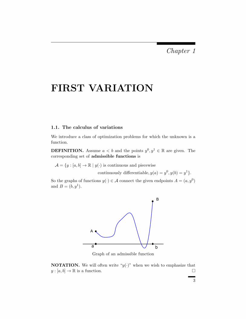
So the graphs of functions y(·) ∈ A connect the given endpoints A = (a, y0)
and B = (b, y1).
b
A
B
a
Graph of an admissible function
NOTATION. We will often write “y(·)” when we wish to emphasize that
y : [a, b]→ R is a function. �
3
4 1. FIRST VARIATION
DEFINITION. The Lagrangian is a given continuous function
L : [a, b]× R× R→ R,
written
L = L(x, y, z).
DEFINITION. If y(·) ∈ A and L is a Lagrangian, we define the corre-
sponding integral functional
(1.1) I[y(·)] =
∫ b
aL(x, y(x), y′(x)) dx,
where
y′ =dy
dx.
Note that we insert y(x) into the y-variable slot of L(x, y, z), and y′(x)
into the z-variable slot of L(x, y, z).
INTERPRETATION. We can informally think of the number I[y(·)] as
being some sort of “energy” associated with the function y(·) (but there can
be many other interesting interpretations). �
REMARK. To avoid various technical issues, we will usually suppress men-
tion of the precise degree of smoothness assumed for various functions that
we discuss. In particular, whenever we write down a derivative (or partial
derivative) of some function at some point, the reader should suppose that
the function is indeed differentiable there. �
The basic problem in the calculus of variations is to study func-
tions y0(·) ∈ A that satisfy
(COV) I[y0(·)] = miny(·)∈A
I[y(·)].
Does such a minimizer y0(·) exist? What are its properties?
Different choices of the Lagrangian L give us different sorts of problems:
EXAMPLE (Shortest path between two points). Consider first the
case that
L(x, y, z) = (1 + z2)1/2.
Then
I[y(·)] =
∫ b
a(1 + (y′)2)1/2 dx
= length of the graph of y(·).
1.2. Computing the first variation 5
So a minimizer y0 ∈ A will give the shortest path connecting the points
A = (a, y0) and B = (b, y1), at least among curves that can be written as
graphs of functions. The graph of the minimizer y0(·) is obviously a straight
line, but it will be interesting to see later what our general theory says even
for this simple problem. �
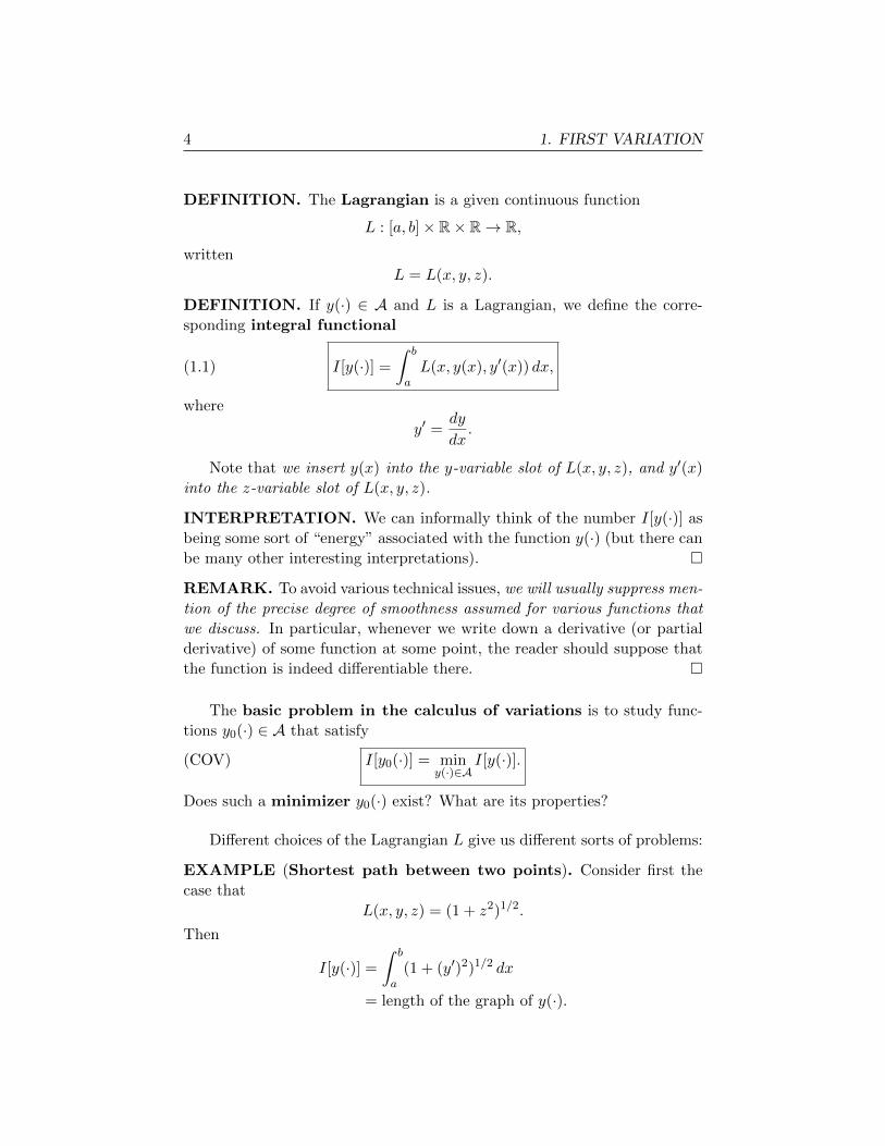
EXAMPLE (Minimal surfaces of revolution). As a second example,
take
L(x, y, z) = 2πy(1 + z2)1/2.
Then
I[y(·)] = 2π
∫ b
ay(1 + (y′)2
)1/2dx
= area of surface of revolution of the graph.
A surface of revolution
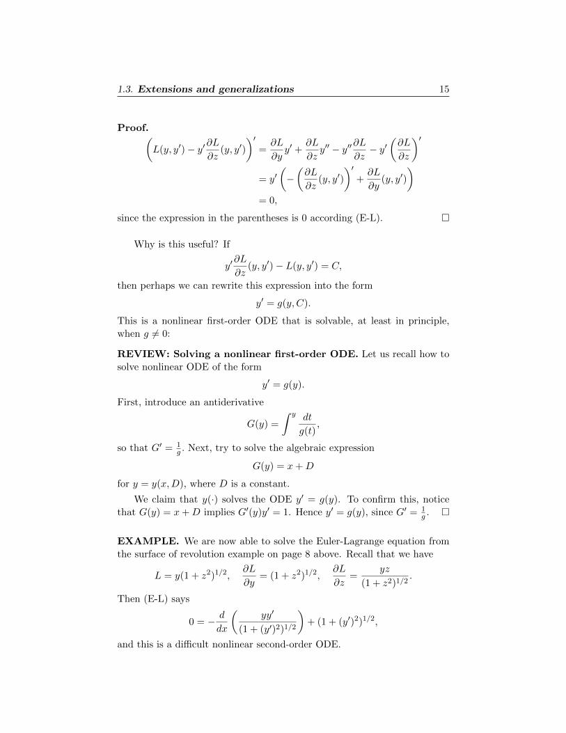
What curve y0(·) gives the surface of revolution of least surface area?
This is more difficult than the previous example, and we will only later have
the tools to handle this. �
1.2. Computing the first variation
1.2.1. Euler-Lagrange equation.
The most important insight of the calculus of variations is the next the-
orem. It says that a minimizer y0(·) ∈ A automatically solves a certain
ordinary differential equation (ODE). This equation appears when we com-
pute an appropriate first variation for our minimization problem (COV).
THEOREM 1.2.1. Assume y0(·) ∈ A solves (COV) and y0(·) is twice
continuously differentiable.
6 1. FIRST VARIATION
Then y0 solves the nonlinear ODE
(1.2) − d
dx
(∂L
∂z(x, y0(x), y′0(x))
)+∂L
∂y(x, y0(x), y′0(x)) = 0
for a ≤ x ≤ b.
DEFINITIONS. (i) We call
(E-L) − d
dx
(∂L
∂z(x, y, y′)
)+∂L
∂y(x, y, y′) = 0
the Euler-Lagrange equation corresponding to the Lagrangian L. This
is a second-order, and usually nonlinear, ODE for the function y = y(·).(ii) Solutions y(·) of the Euler-Lagrange equation are called extremals
(or critical points or stationary points) of I[ · ].(iii) Problems in mathematics or the sciences that lead to equations of
the form (E-L) are called variational. �
REMARKS.
(i) Theorem 1.2.1 says that any minimizer y0 solving (COV) satisfies the
Euler-Lagrange differential equation and thus is an extremal. But a given
extremal need not be a minimizer.
(ii) Remember that ′ = ddx . So it is also correct to write (E-L) as
−(∂L
∂z(x, y, y′)
)′+∂L
∂y(x, y, y′) = 0.
(iii) We could apply the chain rule to expand out the first term in (E-L),
but it is almost always best not to do so. �
HOW TO WRITE DOWN THE EULER-LAGRANGE EQUA-
TION FOR A SPECIFIC PROBLEM:
Step 1. Given L = L(x, y, z), compute
∂L
∂y(x, y, z) and
∂L
∂z(x, y, z).
Step 2. Plug in y(x) for the variable y and y′(x) for z, to obtain
∂L
∂y(x, y(x), y′(x)) and
∂L
∂z(x, y(x), y′(x)).
Step 3. Now write (E-L):
−ddx
(∂L
∂z(x, y(x), y′(x))
)+∂L
∂y(x, y(x), y′(x)) = 0.
1.2. Computing the first variation 7
WARNING ABOUT NOTATION. Most books write (E-L) as
− d
dx
(∂L
∂y′(x, y, y′)
)+∂L
∂y(x, y, y′) = 0.
This is very common, but bad, notation. Note carefully: L = L(x, y, z) is
a function of the three real variables x, y, z; it has nothing to do with the
derivative y′ of some other function y(·). So “ ∂L∂y′ ” has no meaning. �
The Euler-Lagrange equation is extremely important, since it provides
us with a procedure for finding candidates for minimizers y0(·) of (COV).
We do so by trying to solve the (E-L) differential equation.
EXAMPLE. In the first example from page 4, the function y0 minimizes
I[y] =∫ ba (1 + (y′)2)
12 dx (the length of graph of y) among functions y ∈ A.
The Euler-Lagrange equation is an ODE which provides useful informa-
tion about y0. For this example we have
L = (1 + z2)1/2,
and therefore∂L
∂y= 0,
∂L
∂z=
z
(1 + z2)1/2.
We insert y′ for z and then write down (E-L):
0 = −(
y′
(1 + (y′)2)1/2
)′= −y′′(1 + (y′)2)−1/2 − y′
(−1
2
)(1 + (y′)2
)−3/22y′y′′
= − y′′
(1 + (y′)2)3/2.
Consequently a minimizer y0 solvesy′′0
(1+(y′0)2)1/2 = 0, and this implies
y′′0 = 0 (a ≤ x ≤ b).
Hence the graph of y0 is indeed a straight line connecting A and B.
GEOMETRIC INTERPRETATION. This conclusion is of course ob-
vious, but our method suggests something interesting, namely that the ex-
pression (y′
(1 + (y′)2)1/2
)′=
y′′
(1 + (y′)2)3/2
8 1. FIRST VARIATION
may have a geometric meaning. It does. For any twice differentiable curve
y(·),
(1.3) κ =y′′
(1 + (y′)2)3/2
is the curvature of the graph of y(·) at the point (x, y(x)). The calculus
of variations has automatically produced this important expression for the
geometry of planar curves. And what (E-L) really says is that the graph of
our minimizer y0 has constant curvature κ = 0. �
EXAMPLE. Compute the Euler-Lagrange equation satisfied by minimiz-
ers of
I[y(·)] =
∫ b
a
(y′)2
2− fy dx
where f : [a, b]→ R is given.
In this case
L(x, y, z) =z2
2− f(x)y,
∂L
∂y= −f(x),
∂L
∂z= z.
So (E-L) is the simple linear ODE
−y′′ = f.
�
EXAMPLE. In the second example on page 5, we have
L(x, y, z) = 2πy(1 + z2)1/2.
Then∂L
∂y= 2π(1 + z2)1/2,
∂L
∂z=
2πyz
(1 + z2)1/2.
Consequently (E-L) reads
0 = −
(yy′
(1 + (y′)2)1/2
)′+(1 + (y′)2
)1/2.
Which functions y solve this nonlinear ODE? We do not yet have the
tools to answer this and so must return to this example later. �
EXAMPLE. Lagrangians of the form
(1.4) L = a(y)z
are called null Lagrangians, meaning that every function y : [a, b] → Rautomatically solves the associated Euler-Lagrange equation.
1.2. Computing the first variation 9
Indeed,
− d
dx
(∂L
∂z(y, y′)
)+∂L
∂y(y, y′) = − d
dx(a(y)) + a′(y)y′ = 0
for all functions y.
We will learn later that null Lagrangians, especially for more complicated
variational problems, can provide useful information. �
1.2.2. Alternative notation.
In the examples above the variable x denotes a spatial position, but for
many other applications the independent variable represents time t. In these
situations it is appropriate to use different notation.
For such problems we consider Lagrangians
L : [0, T ]× R× R→ R
that depend upon the variables t denoting time, x denoting position, and v
denoting velocity. So we will write
L = L(t, x, v).
The letter T gives a terminal time. We also redefine the admissible class to
be
A = {x : [0, T ]→ R | x(·) is continuous and piecewise
continuously differentiable, x(0) = x0, x(T ) = x1}
for given points x0, x1 ∈ R, and put
(1.5) I[x(·)] =
∫ T
0L(t, x(t), x(t)) dt.
Observe that when the independent variable is t, we usually write
˙ =d
dt.
Employing this new notation, we check that the Euler-Lagrange equation
for extremals x(·) now reads
(E-L) − d
dt
(∂L
∂v(t, x, x)
)+∂L
∂x(t, x, x) = 0
for 0 ≤ t ≤ T . There is no new mathematics here; we are simply changing
notation by renaming the variables.
10 1. FIRST VARIATION
EXAMPLE. Consider the following simple model for the motion of a par-
ticle along the real line, moving under the influence of a potential energy. In
this interpretation m denotes the mass, x(t) is the position of the particle
at time t, and x(t) is its velocity.
In addition,
m
2|x(t)|2 = kinetic energy at time t,
W (x(t)) = potential energy at time t,
where W : R→ R is given. The action of a path x : [0, T ]→ R is the time
integral of the difference between the kinetic and potential energies:
I[x(·)] =
∫ T
0
m
2|x|2 −W (x(t)) dt.
What is the corresponding Euler-Lagrange equation?
We have
L =mv2
2−W (x),
∂L
∂x= −W ′(x),
∂L
∂v= mv,
where ′ = ddx . So (E-L) is
− d
dt(mx)−W ′(x) = 0,
which is Newton’s law of motion:
mx = −W ′(x).
In other words, ma = f for the acceleration a = x and force f = −W ′. The
calculus of variations provides a systematic derivation for this fundamental
law of physics. �
1.2.3. Derivation.
In this section we prove that minimizers satisfy the Euler-Lagrange equa-
tion.
LEMMA 1.2.1. (i) If f, g : [a, b] → R are continuously differentiable, we
have the integration by parts formula
(1.6)
∫ b
af ′g dx = −
∫ b
afg′ dx+ f(b)g(b)− f(a)g(a).
(ii) Assume f : [a, b]→ R is continuous and
(1.7)
∫ b
afw dx = 0
1.2. Computing the first variation 11
for all continuously differentiable functions w : [a, b]→ R such that w(a) =
w(b) = 0. Then
f(x) = 0 for all a ≤ x ≤ b.
Proof. 1. Integrate (fg)′ = f ′g + fg′ from a to b.
2. A standard approximation argument shows if holds for all contin-
uously differentiable functions w, it is valid also for all merely continuous
functions w. Let φ : [a, b] → R be positive for a < x < b and zero at the
endpoints a, b. Put w(x) = φ(x)f(x) above, to find∫ b
aφf2 dx = 0.
Hence φ(x)f2(x) = 0 for all x ∈ [a, b], since the integrand is nonnegative.
Then since φ(x) > 0 for all x ∈ (a, b), we see that f(x) = 0 if x ∈ (a, b). �
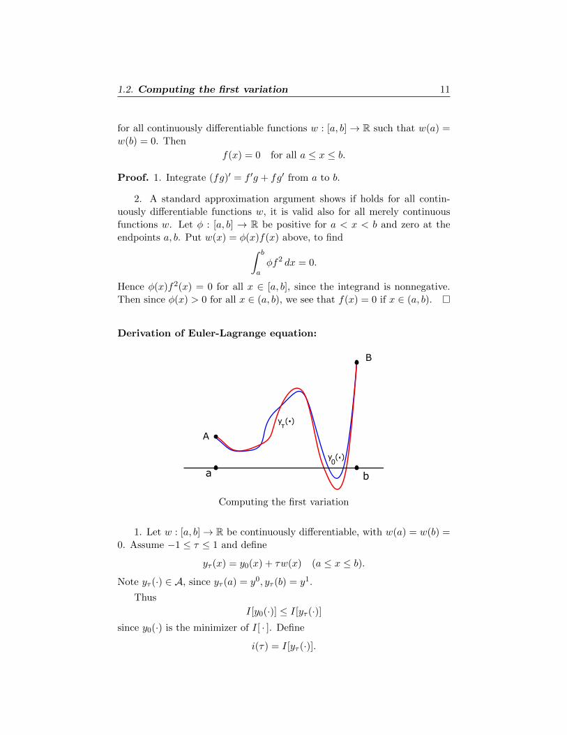
Derivation of Euler-Lagrange equation:
b
A
B
a
y ( )0
y ( )τ
Computing the first variation
1. Let w : [a, b]→ R be continuously differentiable, with w(a) = w(b) =
0. Assume −1 ≤ τ ≤ 1 and define
yτ (x) = y0(x) + τw(x) (a ≤ x ≤ b).
Note yτ (·) ∈ A, since yτ (a) = y0, yτ (b) = y1.
Thus
I[y0(·)] ≤ I[yτ (·)]since y0(·) is the minimizer of I[ · ]. Define
i(τ) = I[yτ (·)].
12 1. FIRST VARIATION
Then
i(0) ≤ i(τ).
So i(·) has a minimum at τ = 0 on the interval −1 ≤ τ ≤ 1, and therefore
di
dτ(0) = 0.
Our task now is to see what information we can extract from this simple
formula.
2. We have
i(τ) = I[yτ (·)]
=
∫ b
aL(x, yτ (x), (yτ )′(x)) dx
=
∫ b
aL(x, y0(x) + τw(x), y′0(x) + τw′(x)) dx.
Therefore
di
dτ(τ) =
∫ b
a
∂
∂τL(x, y0 + τw, y′0 + τw′) dx
=
∫ b
a
∂L
∂y(x, y0 + τw, y′0 + τw′)w +
∂L
∂z(x, y0 + τw, y′0 + τw′)w′ dx,
where we used the chain rule. Next, set τ = 0, to learn that
0 =di
dτ(0) =
∫ b
a
∂L
∂y(x, y0, y
′0)w +
∂L
∂z(x, y0, y
′0)w′ dx.
We now integrate by parts, to deduce∫ b
a
[∂L
∂y(x, y0, y
′0)− d
dx
(∂L
∂z(x, y0, y
′0)
)]w dx = 0.
This is valid for all functions w such that w(a) = w(b) = 0. According then
to the Lemma above, it follows that
∂L
∂y(x, y0, y
′0)− d
dx
(∂L
∂z(x, y0, y
′0)
)= 0
for all a ≤ x ≤ b. This is (E-L). �
REMARK. The procedure in this proof is called computing the first vari-
ation. �
1.3. Extensions and generalizations 13
1.3. Extensions and generalizations
In this section we discuss various extensions of the basic theory, focussing
in particular upon how to use the Euler-Lagrange equation (E-L) to extract
useful information. There are several general approaches for this:
(a) deriving exact formulas for extremals;
(b) calculating perturbative corrections from known solutions;
(c) applying rigorous ODE theory;
(d) introducing numerical methods.
In these notes we will stress (a) (although there is certainly no magic way
to exactly solve all (E-L) equations) and (c).
1.3.1. Conservation laws.
We introduce first some methods for actually finding solutions of Euler-
Lagrange equations in the various special cases. The idea is to try to reduce
(E-L) to a (much simpler) first-order equation.
• SPECIAL CASE 1: L = L(x, z) does not depend on y.
THEOREM 1.3.1. If L does not depend on y and the function y(·) solves
(E-L), then
(1.8)∂L
∂z(x, y′) is constant for a ≤ x ≤ b.
Proof. Since ∂L∂y = 0, (E-L) says
−(∂L
∂z(x, y′)
)′= 0;
and so ∂L∂z (x, y′) is a constant. �
REMARK. Why is this result useful? The point is that when
∂L
∂z(x, y′) = C
for some constant C, we can perhaps rewrite this to solve for y′:
y′ = f(x,C).
Then
y(x) =
∫ x
0f(t, C) dt+D
14 1. FIRST VARIATION
for constants C,D is a formula for general solution of (E-L). We can next
try to select C,D so that the boundary conditions y(a) = y0, y(b) = y1 hold;
in which case y(·) ∈ A. �
EXAMPLE. (a) Write down and then solve (E-L) for
I[y(·)] =
∫ b
ax3(y′)2 dx.
We have
L(x, y, z) = x3z2,∂L
∂y= 0,
∂L
∂z= 2x3z;
therefore∂L
∂z(x, y′(x)) = 2x3y′(x) = C.
Hence
y′(x) =C
2x3,
and so
y(x) =E
x2+ F
for constants E,F .
(b) Find a minimizer of I[ · ] from the admissible class
A = {y : [1, 2]→ R | y(1) = 3, y(2) = 4}.
We need to select the constants E,F above so that
3 = y(1) = E + F, 4 = y(2) =E
4+ F.
Solving, we find that E = −43 , F = 13
3 , and thus
y0(x) = − 4
3x2+
13
3.
Therefore if (COV) has a solution, it must be this. �
• SPECIAL CASE 2: L = L(y, z) does not depend on x.
THEOREM 1.3.2. If L does not depend on x and the function y(·) solves
(E-L), then
(1.9) y′∂L
∂z(y, y′)− L(y, y′) is constant for a ≤ x ≤ b.
REMARK. Conversely, we will see from the proof that if y′ ∂L∂z (y, y′) −L(y, y′) is constant, then y(·) solves the Euler-Lagrange equation on any
subinterval where y′ 6= 0. �
1.3. Extensions and generalizations 15
Proof.(L(y, y′)− y′∂L
∂z(y, y′)
)′=∂L
∂yy′ +
∂L
∂zy′′ − y′′∂L
∂z− y′
(∂L
∂z
)′= y′
(−(∂L
∂z(y, y′)
)′+∂L
∂y(y, y′)
)= 0,
since the expression in the parentheses is 0 according (E-L). �
Why is this useful? If
y′∂L
∂z(y, y′)− L(y, y′) = C,
then perhaps we can rewrite this expression into the form
y′ = g(y, C).
This is a nonlinear first-order ODE that is solvable, at least in principle,
when g 6= 0:
REVIEW: Solving a nonlinear first-order ODE. Let us recall how to
solve nonlinear ODE of the form
y′ = g(y).
First, introduce an antiderivative
G(y) =
∫ y dt
g(t),
so that G′ = 1g . Next, try to solve the algebraic expression
G(y) = x+D
for y = y(x,D), where D is a constant.
We claim that y(·) solves the ODE y′ = g(y). To confirm this, notice
that G(y) = x+D implies G′(y)y′ = 1. Hence y′ = g(y), since G′ = 1g . �
EXAMPLE. We are now able to solve the Euler-Lagrange equation from
the surface of revolution example on page 8 above. Recall that we have
L = y(1 + z2)1/2,∂L
∂y= (1 + z2)1/2,
∂L
∂z=
yz
(1 + z2)1/2.
Then (E-L) says
0 = − d
dx
(yy′
(1 + (y′)2)1/2
)+ (1 + (y′)2)1/2,
and this is a difficult nonlinear second-order ODE.
16 1. FIRST VARIATION
But since L does not depend on x, we can apply Theorem 1.3.2. Now
y′∂L
∂z− L = y′
yy′
(1 + (y′)2)1/2− y(1 + (y′)2)1/2
= − y
(1 + (y′)2)1/2.
Therefore Theorem 1.3.2 tells us that
y
(1 + (y′)2)1/2= C
for some constant C. We solve this expression for
y′ = ±(y2 − C2
C2
)1/2.
We take the positive sign and solve this ODE:
dy
dx=
(y2 − C2)1/2
Cdy
(y2 − C2)1/2=dx
C∫dy
(y2 − C2)1/2=
∫dx
C
cosh−1( yC
)=x
C+D.
(I looked up the expression for the y integral from a table of standard inte-
grals.)
Therefore the curve giving a surface of revolution of least area is
y0(x) = C cosh( xC
+D),
where we recall that cosh(x) = ex+e−x
2 . The graph for the y-curve is called
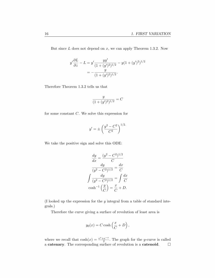
a catenary. The corresponding surface of revolution is a catenoid. �
1.3. Extensions and generalizations 17
A catenoid
REMARK. To fully resolve our problem we need try to adjust the con-
stants C and D so the solution passes through the given endpoints. This
however can be subtle and may not be possible: see Gilbert [G]. �
EXAMPLE. (Geometric optics) Suppose that the velocity of light v in
some two-dimensional translucent material depends only upon the vertical
coordinate y. Then the time for a light ray, moving along the path of the
function y(·), to travel between two given points is∫ b
a
ds
v(y)=
∫ b
a
(1 + (y′)2)12
v(y)dx,
where s denotes arclength along the curve. The Lagrangian
L = L(y, z) =(1 + z2)
12
v(y)
does not depend upon x. Consequently if the graph of the function y(·)describes the path along which light travels, we know that
L(y, y′)− y′∂L∂z
(y, y′) =1
v(y)(1 + (y′)2)12
=sin ξ
v,
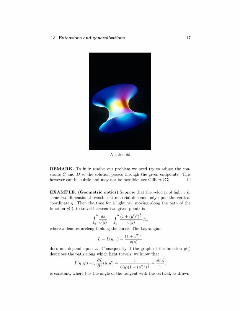
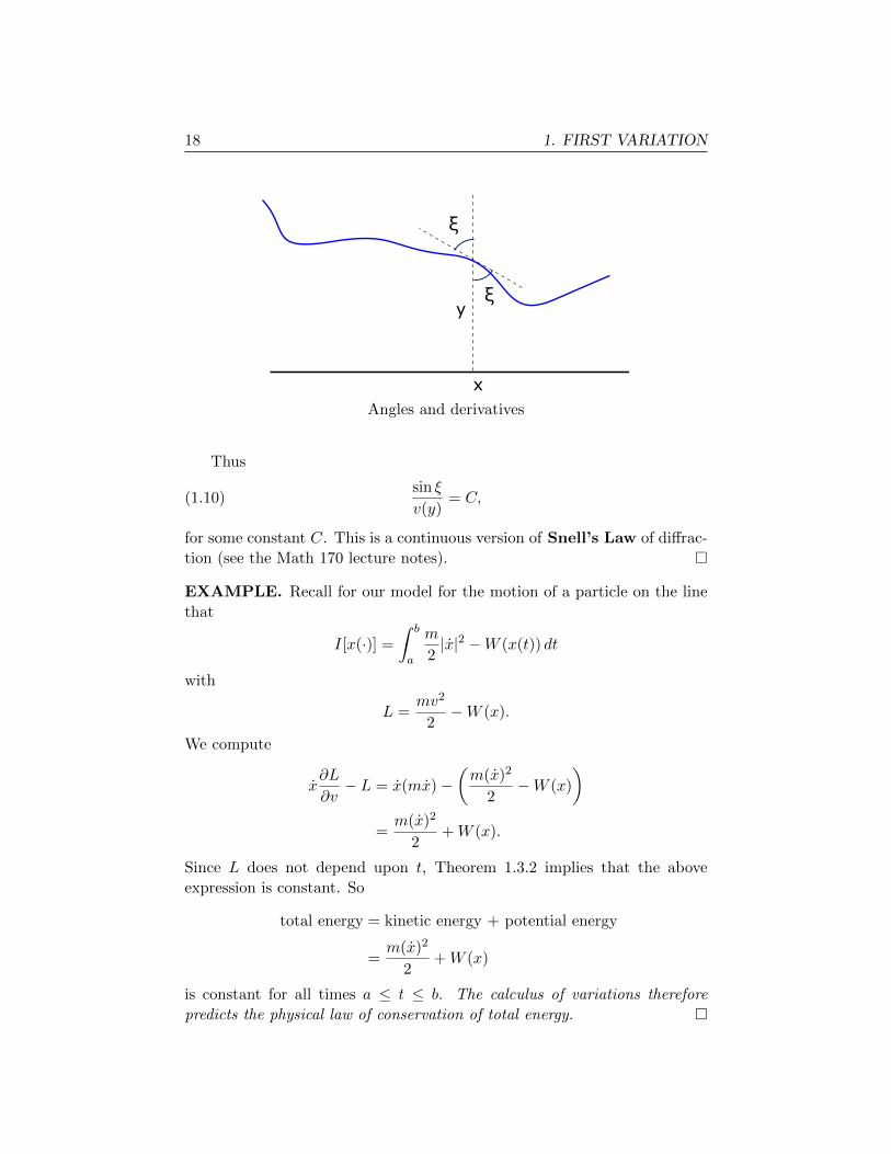
is constant, where ξ is the angle of the tangent with the vertical, as drawn.
18 1. FIRST VARIATION
ξ
ξ
x
y
Angles and derivatives
Thus
(1.10)sin ξ
v(y)= C,
for some constant C. This is a continuous version of Snell’s Law of diffrac-
tion (see the Math 170 lecture notes). �
EXAMPLE. Recall for our model for the motion of a particle on the line
that
I[x(·)] =
∫ b
a
m
2|x|2 −W (x(t)) dt
with
L =mv2
2−W (x).
We compute
x∂L
∂v− L = x(mx)−
(m(x)2
2−W (x)
)=m(x)2
2+W (x).
Since L does not depend upon t, Theorem 1.3.2 implies that the above
expression is constant. So
total energy = kinetic energy + potential energy
=m(x)2
2+W (x)
is constant for all times a ≤ t ≤ b. The calculus of variations therefore
predicts the physical law of conservation of total energy. �
1.3. Extensions and generalizations 19
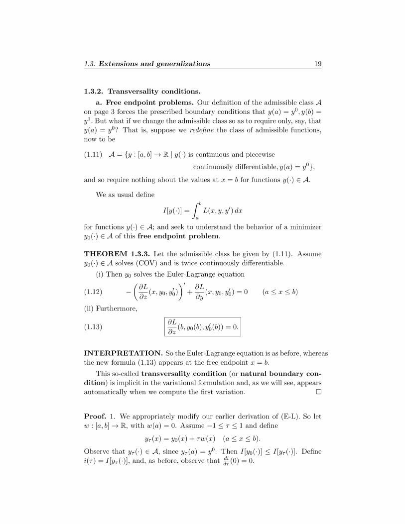
1.3.2. Transversality conditions.
a. Free endpoint problems. Our definition of the admissible class Aon page 3 forces the prescribed boundary conditions that y(a) = y0, y(b) =
y1. But what if we change the admissible class so as to require only, say, that
y(a) = y0? That is, suppose we redefine the class of admissible functions,
now to be
(1.11) A = {y : [a, b]→ R | y(·) is continuous and piecewise
continuously differentiable, y(a) = y0},
and so require nothing about the values at x = b for functions y(·) ∈ A.
We as usual define
I[y(·)] =
∫ b
aL(x, y, y′) dx
for functions y(·) ∈ A; and seek to understand the behavior of a minimizer
y0(·) ∈ A of this free endpoint problem.
THEOREM 1.3.3. Let the admissible class be given by (1.11). Assume
y0(·) ∈ A solves (COV) and is twice continuously differentiable.
(i) Then y0 solves the Euler-Lagrange equation
(1.12) −(∂L
∂z(x, y0, y
′0)
)′+∂L
∂y(x, y0, y
′0) = 0 (a ≤ x ≤ b)
(ii) Furthermore,
(1.13)∂L
∂z(b, y0(b), y′0(b)) = 0.
INTERPRETATION. So the Euler-Lagrange equation is as before, whereas
the new formula (1.13) appears at the free endpoint x = b.
This so-called transversality condition (or natural boundary con-
dition) is implicit in the variational formulation and, as we will see, appears
automatically when we compute the first variation. �
Proof. 1. We appropriately modify our earlier derivation of (E-L). So let
w : [a, b]→ R, with w(a) = 0. Assume −1 ≤ τ ≤ 1 and define
yτ (x) = y0(x) + τw(x) (a ≤ x ≤ b).
Observe that yτ (·) ∈ A, since yτ (a) = y0. Then I[y0(·)] ≤ I[yτ (·)]. Define
i(τ) = I[yτ (·)], and, as before, observe that didτ (0) = 0.
20 1. FIRST VARIATION
As in the earlier proof, we have
0 =di
dτ(0) =
∫ b
a
∂L
∂y(x, y0, y
′0)w +
∂L
∂z(x, y0, y
′0)w′ dx.
Integrate by parts in the second term, remembering that w(a) = 0, but that
w(b) need not necessarily vanish:∫ b
a
[∂L
∂y(x, y0, y
′0)−
(∂L
∂z(x, y0, y
′0)
)′]w dx
+∂L
∂z(b, y0(b), y′0(b))w(b) = 0.
(1.14)
2. If we now assume also that w(b) = 0, then (1.14) gives∫ b
a
[∂L
∂y(x, y0, y
′0)−
(∂L
∂z(x, y0, y
′0)
)′]w dx = 0.
That this integral identity holds for all variations w satisfying w(a) = w(b) =
0 implies the (E-L) equation (1.12).
Now, drop the assumption that w(b) = 0 and return to (1.14). Since we
now know that (1.12) holds, we deduce from (1.14) that
∂L
∂z(b, y0(b), y′0(b))w(b) = 0.
This is valid for all choices of w(b) and consequently the natural boundary
condition (1.13) holds. �
EXAMPLE. The minimizer y0(·) of
I[y(·)] =
∫ 1
0
(y′)2
2− fy dx,
subject to y(0) = 0, satisfies
−y′′0 = f (0 ≤ x ≤ 1), y0(0) = 0, y′0(1) = 0.
�
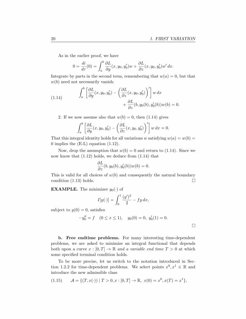
b. Free endtime problems. For many interesting time-dependent
problems, we are asked to minimize an integral functional that depends
both upon a curve x : [0, T ] → R and a variable end time T > 0 at which
some specified terminal condition holds.
To be more precise, let us switch to the notation introduced in Sec-
tion 1.2.2 for time-dependent problems. We select points x0, x1 ∈ R and
introduce the new admissible class
(1.15) A = {(T, x(·)) | T > 0, x : [0, T ]→ R, x(0) = x0, x(T ) = x1},
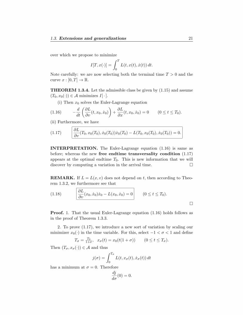
1.3. Extensions and generalizations 21
over which we propose to minimize
I[T, x(·)] =
∫ T
0L(t, x(t), x(t)) dt.
Note carefully: we are now selecting both the terminal time T > 0 and the
curve x : [0, T ]→ R.
THEOREM 1.3.4. Let the admissible class be given by (1.15) and assume
(T0, x0(·)) ∈ A minimizes I[ · ].(i) Then x0 solves the Euler-Lagrange equation
(1.16) − d
dt
(∂L
∂v(t, x0, x0)
)+∂L
∂x(t, x0, x0) = 0 (0 ≤ t ≤ T0).
(ii) Furthermore, we have
(1.17)∂L
∂v(T0, x0(T0), x0(T0))x0(T0)− L(T0, x0(T0), x0(T0)) = 0.
INTERPRETATION. The Euler-Lagrange equation (1.16) is same as
before; whereas the new free endtime transversality condition (1.17)
appears at the optimal endtime T0. This is new information that we will
discover by computing a variation in the arrival time. �
REMARK. If L = L(x, v) does not depend on t, then according to Theo-
rem 1.3.2, we furthermore see that
(1.18)∂L
∂v(x0, x0)x0 − L(x0, x0) = 0 (0 ≤ t ≤ T0).
�
Proof. 1. That the usual Euler-Lagrange equation (1.16) holds follows as
in the proof of Theorem 1.3.3.
2. To prove (1.17), we introduce a new sort of variation by scaling our
minimizer x0(·) in the time variable. For this, select −1 < σ < 1 and define
Tσ = T01+σ , xσ(t) = x0(t(1 + σ)) (0 ≤ t ≤ Tσ).
Then (Tσ, xσ(·)) ∈ A and thus
j(σ) =
∫ Tσ
0L(t, xσ(t), xσ(t)) dt
has a minimum at σ = 0. Thereforedj
dσ(0) = 0.
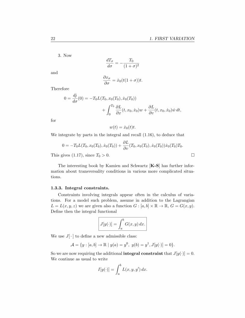
22 1. FIRST VARIATION
3. NowdTσdσ
= − T0
(1 + σ)2
and∂xσ∂σ
= x0(t(1 + σ))t.
Therefore
0 =dj
dσ(0) = −T0L(T0, x0(T0), x0(T0))
+
∫ T0
0
∂L
∂x(t, x0, x0)w +
∂L
∂v(t, x0, x0)w dt,
for
w(t) = x0(t)t.
We integrate by parts in the integral and recall (1.16), to deduce that
0 = −T0L(T0, x0(T0), x0(T0)) +∂L
∂v(T0, x0(T0), x0(T0))x0(T0)T0.
This gives (1.17), since T0 > 0. �
The interesting book by Kamien and Schwartz [K-S] has further infor-
mation about transversality conditions in various more complicated situa-
tions.
1.3.3. Integral constraints.
Constraints involving integrals appear often in the calculus of varia-
tions. For a model such problem, assume in addition to the Lagrangian
L = L(x, y, z) we are given also a function G : [a, b]× R→ R, G = G(x, y).
Define then the integral functional
J [y(·)] =
∫ b
aG(x, y) dx.
We use J [ · ] to define a new admissible class:
A = {y : [a, b]→ R | y(a) = y0, y(b) = y1, J [y(·)] = 0}.
So we are now requiring the additional integral constraint that J [y(·)] = 0.
We continue as usual to write
I[y(·)] =
∫ b
aL(x, y, y′) dx.
1.3. Extensions and generalizations 23
THEOREM 1.3.5. Assume that y0(·) ∈ A is a minimizer of I[ · ] over A.
Suppose also that
(1.19)∂G
∂y(x, y0) is not identically zero for all a ≤ x ≤ b.
Then there exists λ0 ∈ R such that
(1.20) −(∂L
∂z(x, y0, y
′0)
)′+∂L
∂y(x, y0, y
′0) + λ0
∂G
∂y(x, y0) = 0
for a ≤ x ≤ b.
INTERPRETATION. We understand λ0 as the Lagrange multiplier
corresponding to the integral equality constraint that J [x(·)] = 0. The
hypothesis (1.19) is a constraint qualification condition, ensuring the
existence of the Lagrange multiplier. See the Math 170 notes for lots more
about constraint qualification conditions in finite dimensional optimization.
�
Proof. 1. Select w : [a, b] → R with w(a) = w(b) = 0. We want to design
a variation involving w, but setting y0 + τw for small τ will not work, since
this function will probably not belong to A. We must build some sort of
correction, to restore the integral constraint.
Now the condition (1.19) implies that we can find a smooth function
v : [a, b]→ R, such that v(a) = v(b) = 0 and
(1.21)
∫ b
a
∂G
∂y(x, y0)v dx 6= 0.
Define
Φ(τ, σ) =
∫ b
aG(x, y0 + τw + σv) dx.
Then
Φ(0, 0) =
∫ b
aG(x, y0) dx = J [y0(·)] = 0
and∂Φ
∂σ(0, 0) =
∫ b
a
∂G
∂y(x, y0)v dx 6= 0.
Therefore the Implicit Function Theorem (see the Appendix) tells us
that for some small τ0 > there exists a function
φ : [−τ0, τ0]→ R
such that φ(0) = 0 and
Φ(τ, φ(τ)) = Φ(0, 0) = 0 (−τ0 ≤ τ ≤ τ0).
24 1. FIRST VARIATION
Let us differentiate this expression in τ , to learn that
∂Φ
∂τ(0, 0) +
∂Φ
∂σ(0, 0)φ′(0) = 0,
where φ′ = dφdτ . Since
∂Φ
∂τ(0, 0) =
∫ b
a
∂G
∂y(x, y0)w dx,
it follows that
(1.22)
∫ b
a
∂G
∂y(x, y0)w dx+ φ′(0)
∫ b
a
∂G
∂y(x, y0)v dx = 0.
2. Now define
yτ (x) = y0(x) + τw(x) + φ(τ)v(x) (−τ0 ≤ τ ≤ τ0).
Then yτ (a) = y0, yτ (b) = y1, and
J [yτ (·)] =
∫ b
aG(x, y0 + τw + φ(τ)v) dx = Φ(τ, φ(τ)) = 0;
therefore yτ (·) ∈ A. Hence i(τ) = I[yτ (·)] has a minimum at τ = 0, and
consequentlydi
dτ(0) = 0.
We will extract the Lagrange multiplier from this simple looking equality.
3. We compute
di
dτ(τ) =
∫ b
a
∂L
∂y(x, y0 + τw + φ(τ)v, y′0 + τw′ + φ(τ)v′)(w + φ′(τ)v)
+
∫ b
a
∂L
∂z(x, y0 + τw + φ(τ)v, y′0 + τw′ + φ(τ)v′)(w′ + φ′(τ)v′) dx.
Now put τ = 0 and then integrate by parts:
0 =di
dτ(0) =
∫ b
a
∂L
∂y(w + φ′(0)v) +
∂L
∂z(w′ + φ′(0)v′) dx
=
∫ b
a
[∂L
∂y−(∂L
∂z
)′](w + φ′(0)v) dx,(1.23)
where L is evaluated at (x, y0, y′0).
4. We next define the Lagrange multiplier to be
λ0 = −
∫ ba
[∂L∂y −
(∂L∂z
)′]v dx∫ b
a∂G∂y v dx
,
1.3. Extensions and generalizations 25
in which L is evaluated at (x, y0, y′0) and G is evaluated at (x, y0). Then
(1.22) implies
φ′(0)
∫ b
a
[∂L
∂y−(∂L
∂z
)′]v dx = −φ′(0)λ0
∫ b
a
∂G
∂yv dx = λ0
∫ b
a
∂G
∂y(x, y0)w dx.
We utilize this calculation in (1.23), to find that∫ b
a
[∂L
∂y−(∂L
∂z
)′+ λ0
∂G
∂y
]w dx = 0.
This identity is valid for all functions w as above, and therefore the ODE
(1.20) holds.
�
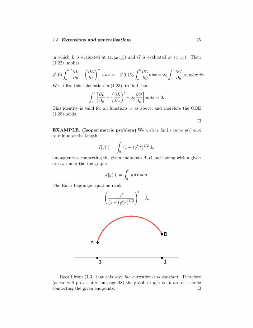
EXAMPLE. (Isoperimetric problem) We wish to find a curve y(·) ∈ Ato minimize the length
I[y(·)] =
∫ 1
0(1 + (y′)2)1/2 dx
among curves connecting the given endpoints A,B and having with a given
area a under the the graph:
J [y(·)] =
∫ 1
0y dx = a.
The Euler-Lagrange equation reads(y′
(1 + (y′)2)1/2
)′= λ.
0
A
B
1
Recall from (1.3) that this says the curvature κ is constant. Therefore
(as we will prove later, on page 48) the graph of y(·) is an arc of a circle
connecting the given endpoints. �
26 1. FIRST VARIATION
Generalization. We can extend the foregoing to handle more compli-
cated integral constraints having the form
J [y(·)] =
∫ b
aG(x, y(x), y′(x)) dx
where G : [a, b]× R× R→ R, G = G(x, y, z).
THEOREM 1.3.6. Assume that y0 ∈ A is a minimizer of I[ · ] over A.
Suppose also that
(1.24) −(∂G
∂z(x, y0, y
′0)
)′+∂G
∂y(x, y0, y
′0)
is not identically zero on the interval [a, b].
Then there exists λ0 ∈ R such that
(1.25) −(∂L
∂z(x, y0, y
′0) + λ0
∂G
∂z(x, y0, y
′0)
)′+
(∂L
∂y(x, y0, y
′0) + λ0
∂G
∂y(x, y0, y
′0)
)= 0
for a ≤ x ≤ b.
We omit the proof, which is similar to that for the previous theorem.
REMARKS. (i) The ODE (1.25) is of course the Euler-Lagrange equation
for the new Lagrangian K = L+ λoG.
(ii) It is not hard to see that the same Euler-Lagrange equation (1.25)
holds if we change the constraint to read J [y(·)] = C for any constant C. �
EXAMPLE. (Hanging chain) A chain of constant mass density and
length l hangs between the points A± = (±a, 0). What is its shape?
The problem is to minimize the gravitational potential energy
I[y(·)] =
∫ a
−ay(1 + (y′)2)
12 dx,
subject to y(±a) = 0 and the length constraint
J [y(·)] =
∫ a
−a(1 + (y′)2)
12 dx = l.
Here L = y(1 + z2)12 , G = (1 + z2)
12 . Since K = L + λG does not depend
on x, we see from the Euler-Lagrange equation (1.25) that
−y′(∂L
∂z+ λ
∂G
∂z
)(y, y′) + (L+ λG)(y, y′) =
y + λ
(1 + (y′)2)12
1.3. Extensions and generalizations 27
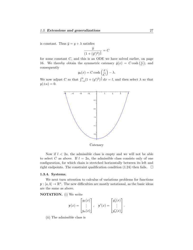
is constant. Thus y = y + λ satisfies
y
(1 + (y′)2)12
= C
for some constant C, and this is an ODE we have solved earlier, on page
16. We thereby obtain the symmetric catenary y(x) = C cosh(xC
); and
consequently
y0(x) = C cosh( xC
)− λ.
We now adjust C so that∫ a−a(1 + (y′)2)
12 dx = l, and then select λ so that
y(±a) = 0.
Catenary
Now if l < 2a, the admissible class is empty and we will not be able
to select C as above. If l = 2a, the admissible class consists only of one
configuration, for which chain is stretched horizontally between its left and
right endpoints. The constraint qualification condition (1.24) then fails. �
1.3.4. Systems.
We next turn attention to calculus of variations problems for functions
y : [a, b]→ Rn. The new difficulties are mostly notational, as the basic ideas
are the same as above.
NOTATION. (i) We write
y(x) =
y1(x)...
yn(x)
, y′(x) =
y′1(x)...
y′n(x)
.(ii) The admissible class is
28 1. FIRST VARIATION
A = {y : [a, b]→ Rn | y(·) is continuous and piecewise
continuously differentiable,y(a) = y0,y(b) = y1},
where y0, y1 ∈ Rn are given.
(iii) We are given a Lagrangian function L : [a, b]× Rn × Rn → R,
L = L(x, y, z) = L(x, y1, . . . , yn, z1, . . . , zn),
with
∇yL =
∂L∂y1...∂L∂yn
, ∇zL =
∂L∂z1...∂L∂zn
.(iv) We write
I[y(·)] =
∫ b
aL(x,y(x),y′(x)) dx.
Our problem now is to study functions y0(·) ∈ A that satisfy
(COV) I[y0(·)] = miny(·)∈A
I[y(·)].
THEOREM 1.3.7. Suppose y0(·) ∈ A solves (COV) and is twice contin-
uously differentiable. Then y0(·) solves the Euler-Lagrange system of ODE
(E-L) − d
dx
(∂L
∂zk(x,y,y′)
)+∂L
∂yk(x,y,y′) = 0 (k = 1, . . . , n).
REMARKS. (i) In vector notation (E-L) reads
−(∇zL(x,y,y′)
)′+∇yL(x,y,y′) = 0.
These comprise n coupled second-order ODE for the n unknown functions
y1(·), . . . , yn(·) that are the components of y(·)(ii) If time t is the independent variable and L = L(t, x, v), the Euler-
Lagrange system of ODE is written
(E-L) − d
dt
(∂L
∂vk(t,x, x)
)+∂L
∂xk(t,x, x) = 0
for k = 1, . . . , n. In vector form, this is
(1.26) − d
dt(∇vL(t,x, x)) +∇xL(t,x, x) = 0.
�
1.3. Extensions and generalizations 29
Proof. 1. We extend our previous derivation of the Euler-Lagrange equa-
tion to this vector case. Select w : [a, b]→ R, written
w =
w1...
wn
,such that w(a) = w(b) = 0. Then define
yτ (x) = y0(x) + τw(x) (a ≤ x ≤ b)
for −1 ≤ τ ≤ 1. We have yτ (·) ∈ A, and consequently
I[y0(·)] ≤ I[yτ (·)].
Define i(τ) = I[yτ (·)], so that i(·) has a minimum at τ = 0. Therefore
di
dτ(0) = 0.
2. Since
i(τ) =
∫ b
aL(x,y0(x) + τw(x),y′0(x) + τw′(x)) dx,
we can apply the chain rule to compute
di
dτ(τ) =
∫ b
a
n∑l=1
∂L
∂yl(x,y0 + τw,y′0 + τw′)wl
+n∑l=1
∂L
∂zl(x,y0 + τw,y′0 + τw′)w′l dx.
Thus
0 =di
dτ(0) =
∫ b
a
n∑l=1
∂L
∂yl(x,y0,y
′0)wl +
n∑l=1
∂L
∂zl(x,y0,y
′0)w′l dx.
Now fix some index k ∈ {1, . . . , n} and put
w = [0 . . . 0w 0 . . . 0]T ,
where the real-valued function w : [a, b]→ R appears in the k-th slot. Then
we have ∫U
∂L
∂yk(x,y0,y
′0)w +
∂L
∂zk(x,y0,y
′0)w′ dx = 0.
Upon integrating by parts, we deduce as usual that the k-th equation of the
stated Euler-Lagrange system (E-L) holds. �
30 1. FIRST VARIATION
EXAMPLE. (Motion of particle in space) For this example the inde-
pendent variable is t (for time) and if x : [a, b]→ Rn, we regard x(t) as the
position at time t of a particle with mass m moving in Rn. The action of
any such path is
I[x(·)] =
∫ b
a
m|x|2
2−W (x) dt.
So
L =m|v|2
2−W (x), ∇vL = mv, ∇xL = −∇W (x).
The Euler-Lagrange system of equations give Newton’s law
mx = −∇W (x)
for the motion of a particle in space governed by the potential energy W .
The path of the particle is thus an extremal of the action. It is sometimes
said that the path of the particle satisfies the principle of least action. But
this terminology is misleading: the path is an extremal of the action, but is
not necessarily a minimizer. �
THEOREM 1.3.8. Suppose y(·) is an extremal.
(i) If L = L(x, z) does not depend on y, then
∇zL(x,y′) is constant for a ≤ x ≤ b.
More generally, if L does not depend upon yk for some k ∈ {1, . . . , n}, then
(1.27)∂L
∂zk(x,y,y′) is constant for a ≤ x ≤ b.
(ii) If L = L(y, z) does not depend on x, then
(1.28) y′ · ∇zL(y,y′)− L(y,y′) is constant for a ≤ x ≤ b.
The proof of (1.27) is simple, and the proof of (1.28) is similar to that
for our earlier Theorem 1.3.2.
EXAMPLE. For the motion of a particle in space, the Lagrangian does
not depend upon t, and therefore the total energy
x · ∇L(x, x)− L(x, x) =m|x|2
2+W (x)
is conserved. �
1.3. Extensions and generalizations 31
1.3.5. Routh’s method. We explain next a technique that can sometimes
be invoked to reduce the number of unknowns in an Euler-Lagrange system
of ODE.
The simplest case is m = 2, for which the unknown is y = [y1 y2]T . The
basic idea is that if the Lagrangian
L = L(x, y, z) = L(x, y1, z1, z2)
does not depend upon y2, we can then convert the full (E-L) system
(1.29)
−(∂L∂z1
(x,y,y′))′
+ ∂L∂y1
(x,y,y′) = 0
−(∂L∂z2
(x,y,y′))′
= 0
into a single ODE for the single unknown y1.
To do this, first observe that the second Euler-Lagrange equation in
(1.29) implies
(1.30)∂L
∂z2(x, y1, y
′1, y′2) = C
for some constant C. We assume next that we can rewrite the algebraic
identity∂L
∂z2(x, y1, z1, z2) = C
to solve for z2:
z2 = φ(x, y1, z1, C).
Thus
(1.31) y′2 = φ(x, y1, y′1, C).
DEFINITION. Routh’s function is
(1.32) R(x, y1, z1) = L(x, y1, z1, φ(x, y1, z1, C))− Cφ(x, y1, z1, C).
THEOREM 1.3.9. Assume that y = [y1 y2]T solves the (E-L) system
(1.29) and that the conservation law (1.30) holds.
Then y1 solves the single (E-L) equation determined by Routh’s function:
(1.33) −(∂R
∂z1(x, y1, y
′1)
)′+∂R
∂y1(x, y1, y
′1) = 0.
REMARK. And so if we can solve the ODE (1.33) for the unknown func-
tion y1, we can then recover y2 by integrating (1.31). �
32 1. FIRST VARIATION
Proof. We calculate
∂R
∂x=∂L
∂x+
(∂L
∂z2− C
)∂φ
∂x
and∂R
∂z1=∂L
∂z1+
(∂L
∂z2− C
)∂φ
∂z1.
Hence (1.31) and (1.30) imply
∂R
∂x(x, y1, y
′1) =
∂L
∂x(x, y1, y
′1, y′2).
and∂R
∂z1(x, y1, y
′1) =
∂L
∂z1(x, y1, y
′1, y′2).
Then the first equation in (1.29) lets us compute that
−(∂R
∂z1(x, y1, y
′1)
)′+∂R
∂y1(x, y1, y
′1)
= −(∂L
∂z1(x,y,y′)
)′+∂L
∂y1(x,y,y′) = 0.
�
1.4. Applications
Following are some more substantial, and more interesting, applications of
our theory.
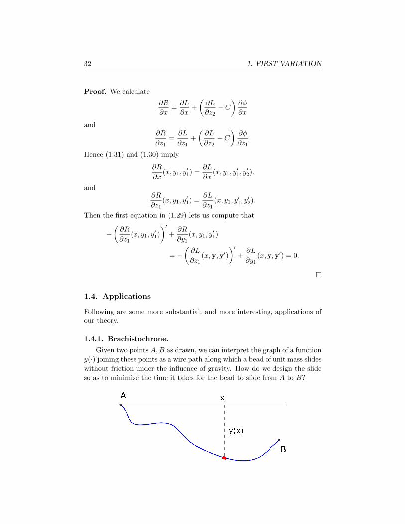
1.4.1. Brachistochrone.
Given two points A,B as drawn, we can interpret the graph of a function
y(·) joining these points as a wire path along which a bead of unit mass slides
without friction under the influence of gravity. How do we design the slide
so as to minimize the time it takes for the bead to slide from A to B?
xA
B
1.4. Applications 33
For simplicity, we assume that A = (0, 0) and that y(x) ≤ 0 for all
0 ≤ x ≤ b. As the particle slides its total energy (= kinetic energy +
potential energy) is constant. Therefore
v2
2+ gy = 0
on the interval [0, b], where v is the velocity and g is gravitational accelera-
tion. The constant is 0, since v(0) = y(0) = 0. Therefore
v = (−2gy)12 .
The time for the bead to slide from A to B is thus∫ b
0
ds
v=
∫ b
0
((1 + (y′)2)
−2gy
) 12
dx.
We therefore seek a path y0(·) from A to B that minimizes
I[y(·)] =
∫ b
0
((1 + (y′)2)
−y
) 12
dx.
Now
L =
((1 + z2)
−y
) 12
,∂L
∂z= −
((1 + z2)
−y
)− 12 z
y,
and consequently
y′∂L
∂z(y, y′)− L(y, y′) = −
((1 + (y′)2)
−y
)− 12 (y′)2
y−(
(1 + (y′)2)
−y
) 12
= (−y(1 + (y′)2))−12 .
Since L does not depend on x, it follows from Theorem 1.3.2 that
y′∂L
∂z(y, y′)− L(y, y′)
is constant. Therefore
(1.34) y(1 + (y′)2) = C
on the interval [0, b] for some (negative) constant C.
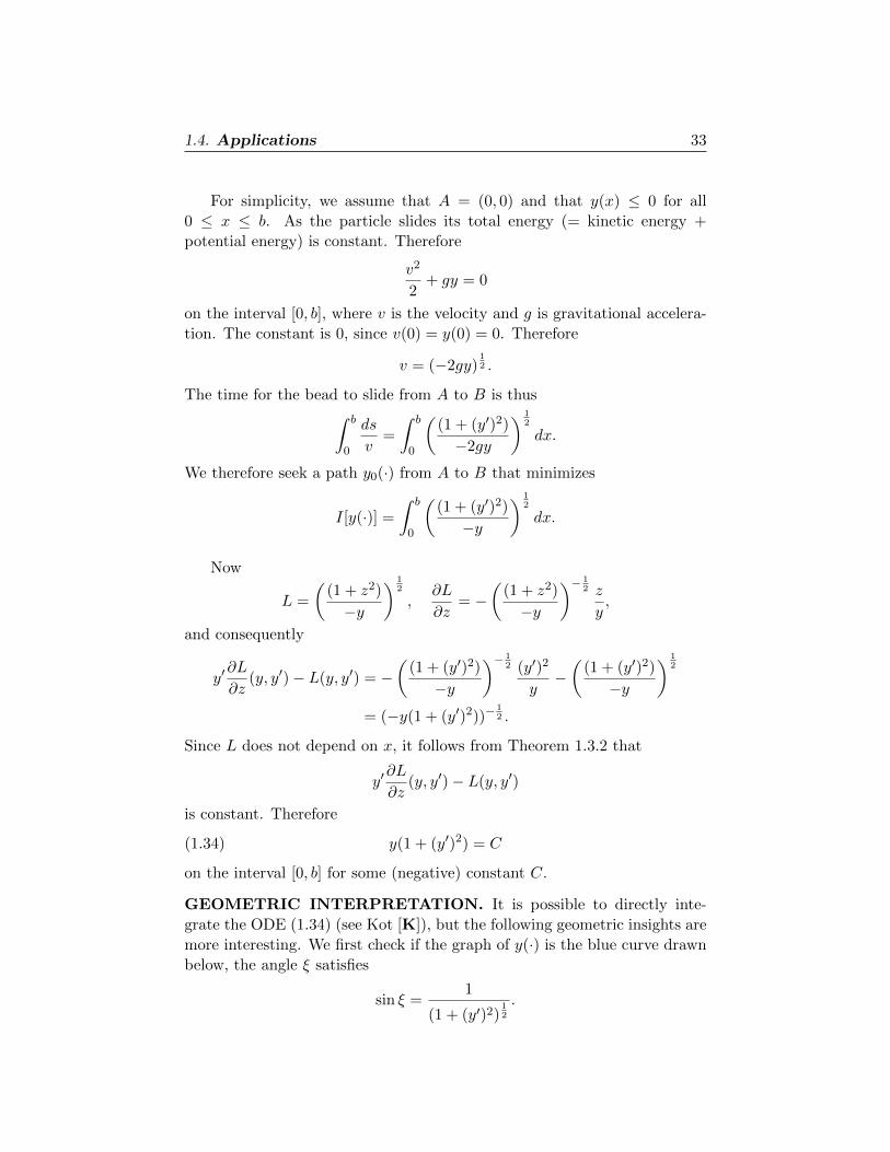
GEOMETRIC INTERPRETATION. It is possible to directly inte-
grate the ODE (1.34) (see Kot [K]), but the following geometric insights are
more interesting. We first check if the graph of y(·) is the blue curve drawn
below, the angle ξ satisfies
sin ξ =1
(1 + (y′)2)12
.
34 1. FIRST VARIATION
ξ
ξ
x
y
Angles and derivatives
Hence the ODE (1.34) says geometrically that
(1.35)sin ξ
(−y)12
is constant;
and, according to the Remark on page 14, this in turn implies y(·) solves the
full Euler-Lagrange equation. (Compare all this with the geometric optics
example on page 17.)
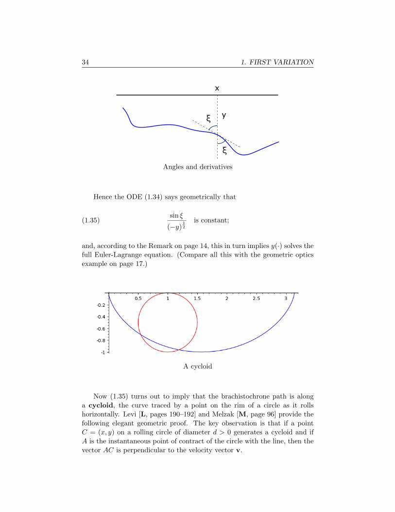
A cycloid
Now (1.35) turns out to imply that the brachistochrone path is along
a cycloid, the curve traced by a point on the rim of a circle as it rolls
horizontally. Levi [L, pages 190–192] and Melzak [M, page 96] provide the
following elegant geometric proof. The key observation is that if a point
C = (x, y) on a rolling circle of diameter d > 0 generates a cycloid and if
A is the instantaneous point of contract of the circle with the line, then the
vector AC is perpendicular to the velocity vector v.
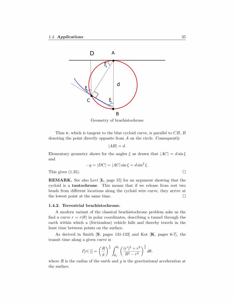
1.4. Applications 35
d
C
B
AD
Geometry of brachistochrone
Thus v, which is tangent to the blue cycloid curve, is parallel to CB, B
denoting the point directly opposite from A on the circle. Consequently
|AB| = d.
Elementary geometry shows for the angles ξ as drawn that |AC| = d sin ξ
and
−y = |DC| = |AC| sin ξ = d sin2 ξ.
This gives (1.35). �
REMARK. See also Levi [L, page 55] for an argument showing that the
cycloid is a tautochrone. This means that if we release from rest two
beads from different locations along the cycloid wire curve, they arrive at
the lowest point at the same time. �
1.4.2. Terrestrial brachistochrone.
A modern variant of the classical brachistochrone problem asks us the
find a curve r = r(θ) in polar coordinates, describing a tunnel through the
earth within which a (frictionless) vehicle falls and thereby travels in the
least time between points on the surface.
As derived in Smith [S, pages 131-133] and Kot [K, pages 6-7], the
transit time along a given curve is
I[r(·)] =
(R
g
) 12∫ θb
θa
((r′)2 + r2
R2 − r2
) 12
dθ,
where R is the radius of the earth and g is the gravitational acceleration at
the surface.
36 1. FIRST VARIATION
Since the Lagrangian
L(r, s) =
(s2 + r2
R2 − r2
) 12
does not depend on θ, we know that for any minimizing curve the expression
r′∂L
∂s(r, r′)− L(r, r′)
is constant. We compute this and simplify, to find for some constant C that
(1.36)
(r′
r
)2
+ 1 = Cr2
R2 − r2
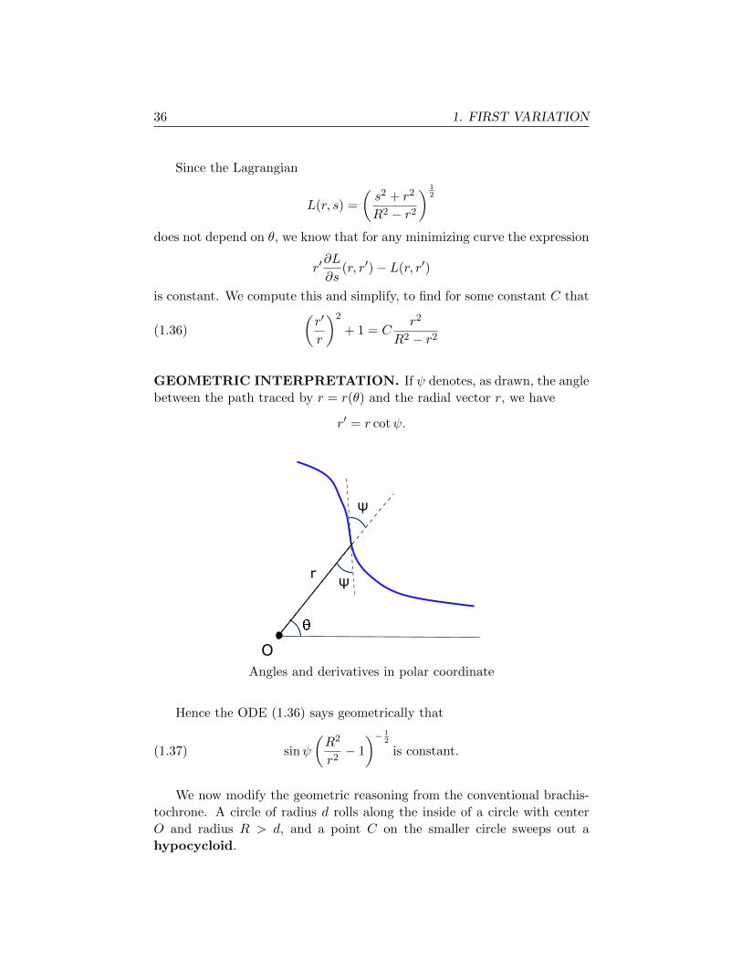
GEOMETRIC INTERPRETATION. If ψ denotes, as drawn, the angle
between the path traced by r = r(θ) and the radial vector r, we have
r′ = r cotψ.
O
ψ
rψ
Angles and derivatives in polar coordinate
Hence the ODE (1.36) says geometrically that
(1.37) sinψ
(R2
r2− 1
)− 12
is constant.
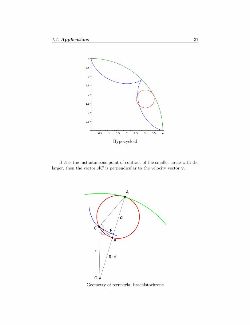
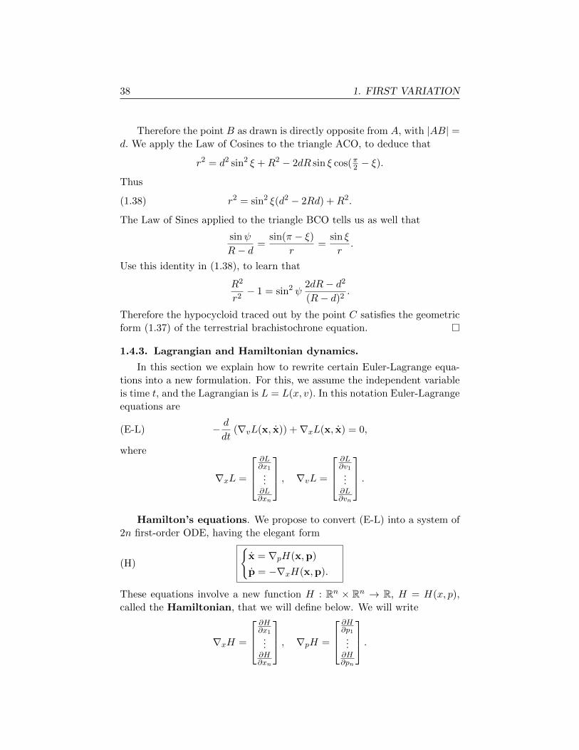
We now modify the geometric reasoning from the conventional brachis-
tochrone. A circle of radius d rolls along the inside of a circle with center
O and radius R > d, and a point C on the smaller circle sweeps out a
hypocycloid.
1.4. Applications 37
Hypocycloid
If A is the instantaneous point of contract of the smaller circle with the
larger, then the vector AC is perpendicular to the velocity vector v.
d
C
B
A
O
d
r
R-d
ψ
Geometry of terrestrial brachistochrone
38 1. FIRST VARIATION
Therefore the point B as drawn is directly opposite from A, with |AB| =d. We apply the Law of Cosines to the triangle ACO, to deduce that
r2 = d2 sin2 ξ +R2 − 2dR sin ξ cos(π2 − ξ).
Thus
(1.38) r2 = sin2 ξ(d2 − 2Rd) +R2.
The Law of Sines applied to the triangle BCO tells us as well that
sinψ
R− d=
sin(π − ξ)r
=sin ξ
r.
Use this identity in (1.38), to learn that
R2
r2− 1 = sin2 ψ
2dR− d2
(R− d)2.
Therefore the hypocycloid traced out by the point C satisfies the geometric
form (1.37) of the terrestrial brachistochrone equation. �
1.4.3. Lagrangian and Hamiltonian dynamics.
In this section we explain how to rewrite certain Euler-Lagrange equa-
tions into a new formulation. For this, we assume the independent variable
is time t, and the Lagrangian is L = L(x, v). In this notation Euler-Lagrange
equations are
(E-L) − d
dt(∇vL(x, x)) +∇xL(x, x) = 0,
where
∇xL =
∂L∂x1...∂L∂xn
, ∇vL =
∂L∂v1...∂L∂vn
.Hamilton’s equations. We propose to convert (E-L) into a system of
2n first-order ODE, having the elegant form
(H)
{x = ∇pH(x,p)
p = −∇xH(x,p).
These equations involve a new function H : Rn × Rn → R, H = H(x, p),
called the Hamiltonian, that we will define below. We will write
∇xH =
∂H∂x1...∂H∂xn
, ∇pH =
∂H∂p1...∂H∂pn
.
1.4. Applications 39
The unknowns in (H) are the two functions x,p : [0,∞)→ Rn, where
x =
x1...
xn
, p =
p1...
pn
.Assume hereafter that x(·) solves (E-L) for all times t ≥ 0.
DEFINITION. Set
p(t) = ∇vL(x(t), x(t)) (t ≥ 0).
We call p(·) the (generalized) momentum associated with x(·).
The Hamiltonian. We will need the following hypothesis:
(1.39)
Assume for all x, p ∈ Rn that the equation
p = ∇vL(x, v)
can be uniquely solved for v as a function of x and p:
v = φ(x, p).
We consequently have the identity
(1.40) ∇vL(x,φ(x, p)) = p (x, p ∈ Rn).
DEFINITION. The Hamiltonian H corresponding to the Lagrangian L
is
(1.41) H(x, p) = p · φ(x, p)− L(x,φ(x, p)) (x, p ∈ Rn).
THEOREM 1.4.1.
(i) The functions x,p : [0,∞)→ Rn solve Hamilton’s equations (H).
(ii) Furthermore,
(1.42) H(x,p) is constant on [0,∞).
Proof. 1. We compute using (1.41) and (1.40) that
(1.43)∇pH(x, p) = φ(x, p) + (∇pφ)T (x, p)(p−∇vL(x,φ(x, p)))
= φ(x, p)
and
(1.44)∇xH(x, p) = (∇xφ)T (x, p)(p−∇vL(x,φ(x, p)))−∇xL(x,φ(x, p))
= −∇xL(x,φ(x, p)).
40 1. FIRST VARIATION
Put x = x and p = p into these formulas, and note that (1.39) implies
x = φ(x,p).
From (1.43), it follows that ∇pH(x,p) = x. And (1.44) gives
∇xH(x,p) = −∇xL(x, x)
= − d
dt(∇vL(x, x)) according to (E-L)
= −p.
2. To see that H(x,p) is constant in time, compute
d
dtH(x,p) = ∇xH(x,p) · x +∇pH(x,p) · p
= ∇xH(x,p) · ∇pH(x,p)−∇pH(x,p) · ∇xH(x,p)
= 0.
�
REMARK. (Lagrangians, Hamiltonians and convex duality) If we
assume for each x ∈ Rn that
v 7→ L(x, v) is uniformly convex
and that the superlinear growth condition
lim|v|→∞
L(x, v)
|v|=∞
holds, then the Hamiltonian is the dual convex function
(1.45) H(x, p) = maxv∈Rn{x · v − L(x, v)},
the maximum occurring for v = φ(x, p). (See the Math 170 notes for more
about convex duality.) �
EXAMPLE. (Motion within a magnetic field) Let B : R3 → R3
denote a time-independent magnetic field. A charged particle within this
magnetic field moves according to the Lorentz equation
(1.46) mx = q(x×B(x)),
in which m is the mass of the particle and q is its charge.
We now show that this equation follows from Hamilton’s equations (H)
for
(1.47) H =1
2m|p− qA(x)|2,
1.4. Applications 41
where the magnetic potential field A satisfies
∇×A = B.
We compute
∇pH =p− qA(x)
m, ∇xH = −q(∇A(x))T (p− qA(x))
m,
since ∇(|A|2
)= 2(∇A)TA. So Hamilton’s equations read{
x = p−qA(x)m
p = q(∇A(x))T (p−qA(x))m .
We now show that these imply the Lorentz equation (1.46), by comput-
ing
mx = p− q∇Ax
=q(∇A)T (p− qA)
m− q∇A(x)x
= q((∇A)T −∇A)x
= q(x× (∇×A))
= q(x×B).
In this calculation we employed the vector calculus rule
(∇g − (∇g)T )y = (∇× g)× y
for y ∈ R3 and g : R3 → R3.
Taylor [T] is a good text for more on physical applications of variational
principles and Hamilton’s equations. �
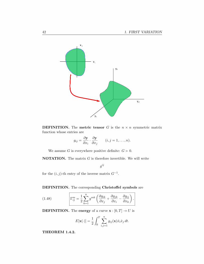
1.4.4. Geodesics.
Let U ⊆ Rn be an open region. Assume that we are given a function
y : U → Rl, which we write as
y =
y1...
yl
.We call y a coordinate patch.
42 1. FIRST VARIATION
x1
xn
DEFINITION. The metric tensor G is the n × n symmetric matrix
function whose entries are
gij =∂y
∂xi· ∂y
∂xj(i, j = 1, . . . , n).
We assume G is everywhere positive definite: G � 0.
NOTATION. The matrix G is therefore invertible. We will write
gij
for the (i, j)-th entry of the inverse matrix G−1.
DEFINITION. The corresponding Christoffel symbols are
(1.48) Γmij =1
2
n∑k=1
gmk(∂gik∂xj
+∂gjk∂xi
− ∂gij∂xk
).
DEFINITION. The energy of a curve x : [0, T ]→ U is
E[x(·)] =1
2
∫ T
0
n∑i,j=1
gij(x)xixj dt.
THEOREM 1.4.2.
1.4. Applications 43
(i) The Euler-Lagrange equations for the energy E[ · ] are
(1.49) xm +n∑
i,j=1
Γmij (x)xixj = 0 (m = 1, . . . , n).
(ii) If x solves (1.49), then
(1.50)
n∑i,j=1
gij(x)xixj is constant.
DEFINITION. A curve x(·) solving the system of ODE (1.49) is called a
geodesic. We will see later that (1.50) says geodesics have constant speed.
�
Proof. 1. The Lagrangian is
L = L(x, v) =1
2
n∑i,j=1
gij(x)vivj ,
with∂L
∂vk=
n∑i=1
gikvi,∂L
∂xk=
1
2
n∑i,j=1
∂gij∂xk
vivj .
We insert these into the Euler-Lagrange equation − ddt
(∂L∂vk
)+ ∂L
∂xk= 0, to
find
d
dt
(n∑i=1
gikxi
)− 1
2
n∑i,j=1
∂gij∂xk
xixj = 0.
Therefore
0 =
n∑i=1
gikxi +
n∑i,j=1
(∂gik∂xj
− 1
2
∂gij∂xk
)xixj
=
n∑i=1
gikxi +1
2
n∑i,j=1
(∂gik∂xj
+∂gjk∂xi
− ∂gij∂xk
)xixj .
Multiply by gmk, sum on m, and recall∑n
k=1 gmkgki = δmi, to deduce
xm +1
2
n∑i,j,k=1
gmk
∂gik∂xj
+∂gjk∂xi
−n∑
i,j=1
∂gij∂xk
xixj = 0.
We recall the definition (1.48) of the Christoffel symbols to complete the
derivation of (1.49).

44 1. FIRST VARIATION
2. Since the Lagrangian L does not depend upon the independent vari-
able t, Theorem 1.3.8 tells us that the expression
x · ∇zL(x, x)− L(x, x) =1
2
n∑i,j=1
gij(x)xixj
is constant for times 0 ≤ t ≤ T. �
Length and energy. We discuss next how minimizing the energy is
equivalent to minimizing length. We henceforth take T = 1 in the definiton
of the energy.
DEFINITIONS.
(i) The length of a curve x : [0, 1]→ U is
L[x(·)] =
∫ 1
0
( n∑i,j=1
gij(x)xixj
) 12dt.
(This is the Euclidean length of the image of x(·) under the coordinate chart
y(·).)(ii) The distance between two points A,B ∈ Rn in the metric deter-
mined by G is
dist(A,B) = min {L[x] | x : [0, 1]→ Rn,x(0) = A,x(1) = B} .
�
It turns out that minimizing energy is equivalent to minimizing length:
THEOREM 1.4.3. A curve that minimizes the energy among paths join-
ing A and B for 0 ≤ t ≤ 1 if and only if it also minimizes the length.
Furthermore
(1.51) min {E[x] | x : [0, 1]→ Rn,x(0) = A,x(1) = B} =dist(A,B)2
2.
Proof. Let us assume that a curve x = [x1 · · · xn]T joining A and B gives
the distance:
dist(A,B) =
∫ 1
0
( n∑i,j=1
gij(x)xixj
) 12dt.
We can if necessary reparameterize x(·) to have constant speed, so that
(1.52)( n∑i,j=1
gij(x)xixj
) 12
= dist(A,B) (0 ≤ t ≤ 1).
1.4. Applications 45
Next, assume that a curve y(·) minimizes the energy among paths connecting
A to B:
E[y] = min {E[w] | w : [0, 1]→ Rn,w(0) = A,w(1) = B} .
According to Theorem 1.4.2,
(1.53)1
2
n∑i,j=1
gij(y)yiyj = E
is constant in time. Then (1.52) implies
E = E[y] ≤ E[x] =1
2
∫ 1
0
n∑i,j=1
gij(x)xixj dt =dist(A,B)2
2.
But also
dist(A,B) = L[x] ≤ L[y] =
∫ 1
0
( n∑i,j=1
gij(y)yiyj
) 12dt
≤
∫ 1
0
n∑i,j=1
gij(y)yiyj dt
12
= (2E)12 ,
according to (1.53). Hence E = dist(A,B)2
2 ; and therefore L[x] = L[y], E[y] =
E[x]. �
EXAMPLE (Hyperbolic metric). A famous model in geometry is the
Poincare hyperbolic plane, for which n = 2 and
gij =1
(x2)2δij (i ≤ i, j ≤ 2)
in the region H = {−∞ < x1 <∞, 0 < x2 <∞}.We calculate using the definition (1.48) that
Γ112 = Γ1
21 = Γ222 = − 1
x2, Γ2
11 =1
x2,
and the remaining Christoffel symbols vanish. Employing these formulas in
(1.49) yields this system of geodesic ODE for the hyperbolic plane:
(1.54)
{x1 = 2x1x2
x2
x2 = (x2)2−(x1)2
x2.
We can extract geometric information from these equations:
THEOREM 1.4.4. The path of any trajectory solving (1.54) is either
along a vertical line or else along a circle centered on the x1-axis.
46 1. FIRST VARIATION
Proof. 1. Consider a solution of the ODE system (1.54) with x1 6= 0. Define
(1.55) a = x1 +x2x2
x1.
Then
a = x1 +x2x2 + x2x2
x1− x2x2x1
(x1)2
= x1 +(x2)2
x1+x2
x1
((x2)2 − (x1)2
x2
)− x2x2
(x1)2
(2x1x2
x2
)= 0;
consequently a is constant.
2. We claim that the motion of the point x = [x1 x2]T lies within a circle
with center (a, 0). To confirm this, let us use (1.55) to calculate that
d
ds
{(x1 − a)2 + (x2)2
2
}= (x1 − a)x1 + x2x2
=
(−x2x2
x1
)x1 + x2x2
= 0.
Therefore
(x1 − a)2 + x22 = r2
for some appropriate radius r > 0. �
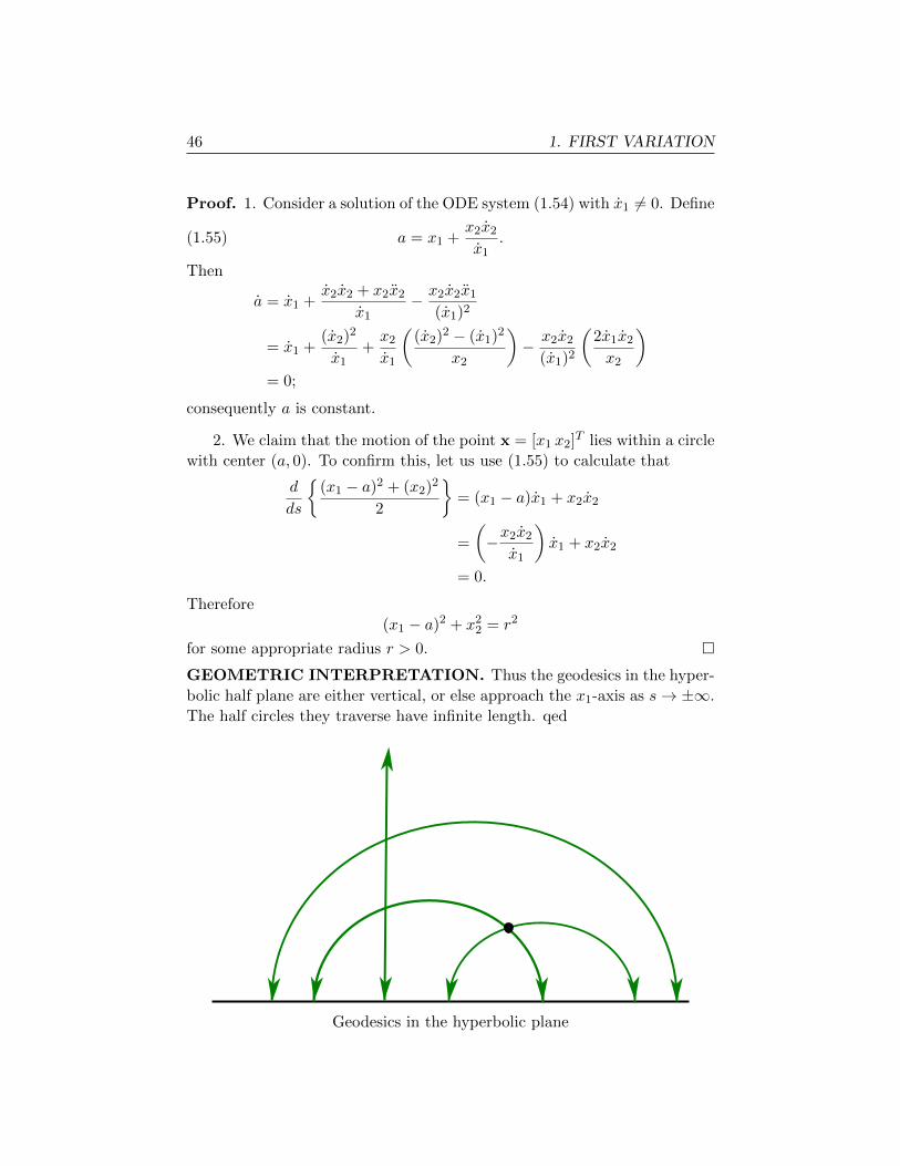
GEOMETRIC INTERPRETATION. Thus the geodesics in the hyper-
bolic half plane are either vertical, or else approach the x1-axis as s→ ±∞.
The half circles they traverse have infinite length. qed
Geodesics in the hyperbolic plane
1.4. Applications 47
�
1.4.5. Maxwell’s fisheye.
This example concerns curves x(·) taking values in R3 that are extremals
for the Lagrangian
(1.56) L(x, v) =|v|
1 + |x|2(x, v ∈ R3).
Then
∇vL =v
|v|(1 + |x|2), ∇xL = − 2|v|x
(1 + |x|2)2.
The (E-L) system is therefore
(1.57) − d
dt
(x
|x|(1 + |x|2)
)− 2|x|x
(1 + |x|2)2= 0.
where · = ddt . We reparameterize in terms of the arclength s = s(t), which
satisfiesds
dt= |x|.
Then (1.57) becomes
(1.58)
(x′
1 + |x|2
)′= − 2x
(1 + |x|2)2.
where ′ = dds .
We will now investigate properties of solutions of the system (1.58), with
|x′| ≡ 1.
THEOREM 1.4.5. Any trajectory solving (1.58) is either along a line
through the origin, or else along a circle in a plane passing through the
origin.
GEOMETRIC INTERPRETATION. The proof below shows how we
can sometimes deduce interesting geometric information about solutions of
a system of ODE.
In particular, the Lagrangian (1.56) has the remarkable property that
all solutions of the corresponding Euler-Lagrange system of ODE move in
circles (or along straight lines). And even though L is radial in x, the centers
of these circles need not be the origin.
�
Proof. 1. We compute using the cross product and the ODE (1.58) that(x′
1 + |x|2× x
)′=
(x′
1 + |x|2
)′× x +
(x′
1 + |x|2× x′
)
48 1. FIRST VARIATION
= − 2x
(1 + |x|2)2× x = 0.
Hencex′
1 + |x|2× x = b for some vector b ∈ R3.
If b 6= 0, then since x · b = 0, the trajectory lies in the plane through the
origin perpendicular to b. If b = 0, then x and x′ are everywhere parallel
and so the motion is along a line.
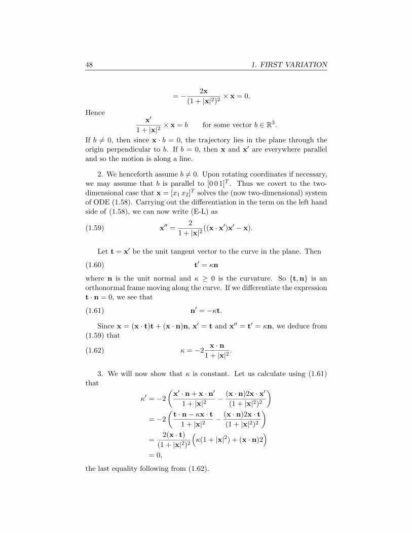
2. We henceforth assume b 6= 0. Upon rotating coordinates if necessary,
we may assume that b is parallel to [0 0 1]T . Thus we covert to the two-
dimensional case that x = [x1 x2]T solves the (now two-dimensional) system
of ODE (1.58). Carrying out the differentiation in the term on the left hand
side of (1.58), we can now write (E-L) as
(1.59) x′′ =2
1 + |x|2((x · x′)x′ − x).
Let t = x′ be the unit tangent vector to the curve in the plane. Then
(1.60) t′ = κn
where n is the unit normal and κ ≥ 0 is the curvature. So {t,n} is an
orthonormal frame moving along the curve. If we differentiate the expression
t · n = 0, we see that
(1.61) n′ = −κt.
Since x = (x · t)t + (x · n)n, x′ = t and x′′ = t′ = κn, we deduce from
(1.59) that
(1.62) κ = −2x · n
1 + |x|2.
3. We will now show that κ is constant. Let us calculate using (1.61)
that
κ′ = −2
(x′ · n + x · n′
1 + |x|2− (x · n)2x · x′
(1 + |x|2)2
)= −2
(t · n− κx · t
1 + |x|2− (x · n)2x · t
(1 + |x|2)2
)=
2(x · t)
(1 + |x|2)2
(κ(1 + |x|2) + (x · n)2
)= 0,
the last equality following from (1.62).
1.4. Applications 49
4. Finally we show that the trajectory lies on a circle if κ > 0. Define
c = x +1
κn.
Then
c′ = x′ + 1κn′ = t− 1
κκt = 0,
and hence c ≡ c for some point c ∈ R2. Furthermore,
(|x− c|2)′ = 2(x− c) · x′ = −2
κn · t = 0.
Consequently the trajectory moves along the circle of radius κ−1 and center
c. �
PHYSICAL INTERPRETATION. In the 19th century, there was inter-
est in the optical properties of the eyes of fishes, and in particular the ques-
tion as to how such eyes, which are often quite flat, focus images. Maxwell
had found the geometric properties of extremals for the Langrangian (1.56),
and there was some thought that these may explain the optics of fish eyes.
In the 20th century R. Luneburg generalized Maxwell’s ideas to design
lenses with various interesting properties, made from transparent materials
with radially varying refractive index. (The refractive index of an optical
medium is n = cv , where c is the speed of light in a vacuum and v is the
speed within the medium.) �

Chapter 2
SECONDVARIATION
2.1. Computing the second variation
We return to our standard calculus of variations problem of characterizing
minimizers y0(·) of the functional
I[y(·)] =
∫ b
aL(x, y, y′) dx
over the admissible class
A = {y : [a, b]→ R | y(a) = y0, y(b) = y1}.
We have so far examined in great detail the Euler-Lagrange equation, the
derivation of which corresponds to taking the first variation. This chapter
turns attention to the second variation.
2.1.1. Integral and pointwise versions.
THEOREM 2.1.1. Suppose y0(·) ∈ A is a minimizer.
(i) Then
(2.1)
∫ b
a
∂2L
∂z2(x, y0, y
′0)(w′)2
+ 2∂2L
∂y∂z(x, y0, y
′0)ww′ +
∂2L
∂y2(x, y0, y
′0)w2 dx ≥ 0
for all w : [a, b]→ R with w(a) = w(b) = 0.
51
52 2. SECOND VARIATION
(ii) Furthermore,
(2.2)∂2L
∂z2(x, y0(x), y′0(x)) ≥ 0 (a ≤ x ≤ b).
REMARKS.
(i) We call the left hand side of (2.1) the second variation of I[ · ]about y0(·), evaluated at w(·).
(ii) If the mapping
(2.3) z 7→ L(x, y0(x), z) is convex,
then (2.2) holds. This observation strongly suggests that the convexity of
the Lagrangian L in the variable z will be a useful hypothesis if we try to
find minimizers: see Section 2.4.2. �
Proof. 1. We extend our earlier first variation proof of the Euler-Lagrange
equation. Select w : [a, b] → R, with w(a) = w(b) = 0, and define yτ (x) =
y0(x) + τw(x) for −1 ≤ τ ≤ 1. Then yτ (·) ∈ A, and so τ 7→ i(τ) has a
minimum at τ = 0 on the interval −1 ≤ τ ≤ 1. Therefore
d2i
dτ2(0) ≥ 0.
2. Differentiating twice with respect to τ , we find
d2i
dτ2(τ) =
∫ b
a
∂2L
∂y2(x, y0 + τw, y′0 + τw′)w2
+ 2∂2L
∂y∂z(x, y0 + τw, y′0 + τw′)ww′ +
∂2L
∂z2(x, y0 + τw, y′0 + τw′)(w′)2 dx.
Put τ = 0 and recall d2idτ2
(0) ≥ 0, to prove (2.1).
3. We need to design appropriate functions w to extract pointwise in-
formation from (2.1). For this, define φ : R→ R by setting
φ(x) =
{x if 0 ≤ x ≤ 1
2− x if 1 ≤ x ≤ 2
on the interval [0, 2] and then extend φ to be 2-periodic on all of R. Thus φ
is a “sawtooth function” with corners at the integers and φ′ = ±1 elsewhere.
Next let ζ : [a.b] → R be any continuously differentiable function with
ζ(a) = ζ(b) = 0. Then for each ε > 0, define
wε(x) = εφ(xε )ζ(x).
2.1. Computing the second variation 53
Then for all but finitely many points, wε is differentiable:
w′ε(x) = φ′(xε )ζ(x) + εφ(xε )ζ ′(x).
Note that the second term on the right is less than or equal to Aε for some
appropriate constant A.
We now plug in wε in place of w in (2.1). Then upon making some
simple estimates, we learn that∫ b
a
∂2L
∂z2(x, y0, y
′0)(φ′(xε ))2ζ2 dx+Dε ≥ 0,
for some constant D. But (φ′(xε )
)2= 1
except at finitely many points (which have no effect on the integral). There-
fore upon sending ε→ 0, we deduce that∫ b
a
∂2L
∂z2(x, y0, y
′0)ζ2 dx ≥ 0
for all functions ζ as above. This implies (2.2). �
2.1.2. Weierstrass condition.
In this section we strengthen (2.2):
THEOREM 2.1.2. Suppose y0(·) ∈ A is a minimizer that is continuously
differentiable.
Then for all z ∈ R and all points a ≤ x ≤ b,
(2.4) L(x, y0(x), z) ≥ L(x, y0(x), y′0(x)) +∂L
∂z(x, y0(x), y′0(x))(z − y′0(x)).
This is the Weierstrass condition for a minimizer.
GEOMETRIC INTERPRETATION. This inequality says that for fixed
x and y0(x), the graph of the function
z 7→ L(x, y0(x), z)
lies above the tangent line at the point z = y′0(x). This of course is clear if
z 7→ L(x, y0(x), z) is convex.
Notice that (2.4) does not follow from any sort of local second varia-
tion argument, since z need not be close to y′0(x). Rather, the Weierstrass
condition is a consequence of the global minimality of y0(·). �
54 2. SECOND VARIATION
Proof. To simplify the exposition, we will assume for simplicity that L =
L(x, z) does not depend upon y.
1. Select any z ∈ R and 0 < δ < 1. Choose any point a < x0 < b and
select ε > 0 so small that the interval [x0− δε, x0 + ε] lies within [a, b]. Now
define
y(x) =
y0(x) (a ≤ x ≤ x0 − δε)l1(x) (x0 − δε ≤ x ≤ x0)
l2(x) (x0 ≤ x ≤ x0 + ε)
y0(x) (x0 + ε ≤ x ≤ b),where l1, l2 are linear functions selected so that y(·) is continuous and{
l′1(x) = z (x0 − δε ≤ x ≤ x0)
l′2(x) = y0(x0+ε)−y0(x0−δε)ε − δz (x0 ≤ x ≤ x0 + ε)
Then y(·) ∈ A and thus
I[y0(·)] ≤ I[y(·)]
Since y(·) = y0(·) outside the interval [x0 − δε, x0 + ε], it follows that∫ x0+ε
x0−δεL(x, y′0) dx ≤
∫ x0+ε
x0−δεL(x, y′) dx
=
∫ x0
x0−δεL(x, z) dx+
∫ x0+ε
x0
L(x, y0(x0+ε)−y0(x0−δε)
ε − δz)dx.
Then
(2.5)1
δε
∫ x0
x0−δεL(x, y′0) dx ≤ 1
δε
∫ x0
x0−δεL(x, z) dx
+1
δε
∫ x0+ε
x0
L(x, y0(x0+ε)−y0(x0−δε)
ε − δz)− L(x, y′0) dx.
2. We must examine carefully the integral on the right. Now
(2.6) L(x, y0(x0+ε)−y0(x0−δε)
ε − δz)− L(x, y′0) = ∂L
∂z (x, y′0)aε + rε,
for
aε =y0(x0 + ε)− y0(x0 − δε)
ε− δz − y′0(x),
where the remainder term rε satisfies the estimate
(2.7) |rε| ≤ Aa2ε.
According to L’Hospital’s Rule,
(2.8) limε→0
aε = (1 + δ)y′0(x0)− δz − y′0(x).
2.2. Positive second variation 55
Then (2.7) implies
(2.9) lim supε→0
|rε| ≤ B(δ2 + (y′0(x0)− y′0(x))2).
for a suitable constant B.
3. Now send ε→ 0 in (2.5), using (2.6),(2.8) and (2.9):
L(x0, y′0) ≤ L(x0, z) + ∂L
∂z (x0, y′0)(y′0(x0)− z) +Bδ.
Finally, let δ → 0, to deduce
L(x0, y′0) + ∂L
∂z (x0, y′0)(z − y′0(x0)) ≤ L(x0, z);
this is (2.4) for L = L(x, z). �
2.2. Positive second variation
Suppose now that y(·) ∈ A is an extremal, and consequently solves the
Euler-Lagrange equation
(E-L) −(∂L
∂z(x, y, y′)
)′+∂L
∂y(x, y, y′) = 0 (a ≤ x ≤ b).
We devote the rest of this chapter to the question:
When is y(·) in fact a local minimizer of I[ · ]?
2.2.1. Riccati equation.
NOTATION. Let us write
(2.10) A =∂2L
∂z2(x, y, y′), B =
∂2L
∂y∂z(x, y, y′), C =
∂2L
∂y2(x, y, y′).
Therefore the second variation of I[ · ] about y(·) is
(2.11)
∫ b
aA(w′)2 + 2Bww′ + Cw2 dx
for w : [a, b]→ R with w(a) = w(b) = 0. �
We assume hereafter that
(2.12) A > 0 on [a, b].
As a first approach towards understanding local minimizers, we intro-
duce a new nonlinear equation:
56 2. SECOND VARIATION
DEFINITION. The Riccati equation associated with (E-L) and the
extremal y(·) is the first-order ODE
(R) q′ = −(q −B)2
A+ C (a ≤ x ≤ b),
for the functions A,B,C defined by (2.10). �
A remarkable observation is that if (R) has a solution, then the second
variation is positive:
THEOREM 2.2.1. Assume that there exists a solution q(·) of the Riccati
equation (R).
Then the second variation of I[ · ] around y(·) is positive:
(2.13)
∫ b
aA(w′)2 + 2Bww′ + Cw2 dx > 0
for all nonzero w : [a, b]→ R with w(a) = w(b) = 0.
Proof. We calculate that∫ b
aA(w′)2+2Bww′ + Cw2 dx
=
∫ b
aA(w′)2 + 2Bww′ +
(q′ + (q−B)2
A
)w2 dx
=
∫ b
aA(w′)2 − 2(q −B)ww′ + (q−B)2
A w2 dx
=
∫ b
aA(w′ − q−B
A w)2
dt ≥ 0.
Furthermore, if w′ − q−BA w = 0 on the interval [a, b] and w(a) = 0, then
uniqueness of the solution of this ODE imples w = 0. �
2.2.2. Conjugate points.
We show next that we can construct a solution to (R) if we can find a
positive solution of a related linear ODE.
DEFINITIONS. (i) The linearization of the Euler-Lagrange equa-
tion (E-L) about the extremal y(·) is the linear operator
(2.14) Ju = −(Au′ +Bu)′ +Bu′ + Cu,
defined for twice continuously differentiable functions u : [a, b]→ R.
2.2. Positive second variation 57
(ii) We call the ODE
Ju = 0 (a ≤ x ≤ b)
Jacobi’s equation. �
We can construct solutions of the Riccati equation from positive solutions
of Jacobi’s equation:
THEOREM 2.2.2. Suppose that
(2.15)
{Ju = 0 (a ≤ x ≤ b)u > 0 (a ≤ x ≤ b).
Then
(2.16) q = Au′
u+B
solves the Riccati equation (R).
Proof. We calculate
0 = −(Au′ +Bu)′ +Bu′ + Cu
= −(qu)′ +Bu′ + Cu
= −q′u+ (B − q)u′ + Cu
= −q′u− (q −B)2
Au+ Cu.
Divide by u > 0 to derive (R). �
In light of the previous theorem, we need to understand when we can
find a positive solution of the Jacobi equation on a given interval [a, b]. This
depends upon whether or not the interval contains conjugate points:
DEFINITION. Select a ∈ R. We say that a point c > a is a conjugate
point with respect to a if there exists a function u : [a, c]→ R such that
(2.17)
Ju = 0 (a ≤ x ≤ c)u(a) = u(c) = 0
u 6= 0.
�
THEOREM 2.2.3. If there are no conjugate points within the interval
(a, b], then there exists a solution q(·) of the Riccati equation (R).
Consequently, the second variation of I[ · ] about y(·) is positive.
58 2. SECOND VARIATION
Proof. 1. It can be shown that if there are no conjugate points with respect
to a within (a, b], then in fact for some nearby point d < a there are no
conjugate points with respect to d within (d, b]. (The proof of this relies
upon some mathematical ideas a bit beyond the scope of these notes.)
2. Consider then the initial-value problem
(2.18)
{Ju = 0 (d ≤ x ≤ b)u(d) = 0, u′(d) = 1.
Standard ODE theory tells us that this problem has a unique solution. We
observe furthermore that
u(x) > 0 (d < x ≤ d+ ε)
for some sufficiently small ε > 0, since u′(d) = 1.
We claim that in fact
(2.19) u(x) > 0 (d < x ≤ b).
To see this, assume instead that d < c ≤ b is a point where u(c) = 0. Then
c would be a conjugate point with respect to d, and this is not possible.
Since by continuity u is strictly positive on the interval [a, b], it follows
from Theorem 2.2.2 that q = Au′
u +B solves (R). Theorem 2.2.1 now implies
that the second variation is positive. �
2.3. Strong local minimizers
We now build upon the ideas just developed. We next show that the absence
of conjugate points implies not only that the second variation is positive, but
also that y(·) is a local minimizer of I[ · ], in fact a strong local minimizer.
DEFINITION. We say y : [a, b] → R is a strong local minimizer of
I[ · ] if there exists δ > 0 such that
(2.20) max[a,b]|y − y| ≤ δ
implies
(2.21) I[y(·)] ≤ I[y(·)]
for all y : [a, b]→ R satisfying
y(a) = y(a), y(b) = y(b).
REMARK. We call such a local minimizer strong since we require only
that (2.20) be valid, and not necessarily also that
(2.22) max[a,b]|y′ − y′| ≤ δ.
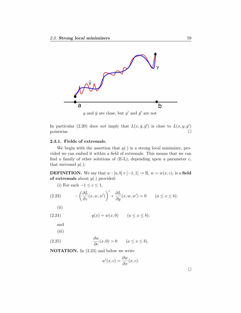
2.3. Strong local minimizers 59
ba
y
y
y and y are close, but y′ and y′ are not
In particular (2.20) does not imply that L(x, y, y′) is close to L(x, y, y′)
pointwise. �
2.3.1. Fields of extremals.
We begin with the assertion that y(·) is a strong local minimizer, pro-
vided we can embed it within a field of extremals. This means that we can
find a family of other solutions of (E-L), depending upon a parameter c,
that surround y(·):
DEFINITION. We say that w : [a, b]× [−1, 1]→ R, w = w(x, c), is a field
of extremals about y(·) provided:
(i) For each −1 ≤ c ≤ 1,
(2.23) −(∂L
∂z(x,w,w′)
)′+∂L
∂y(x,w,w′) = 0 (a ≤ x ≤ b);
(ii)
(2.24) y(x) = w(x, 0) (a ≤ x ≤ b);
and
(iii)
(2.25)∂w
∂c(x, 0) > 0 (a ≤ x ≤ b).
NOTATION. In (2.23) and below we write
w′(x, c) =∂w
∂x(x, c).
�
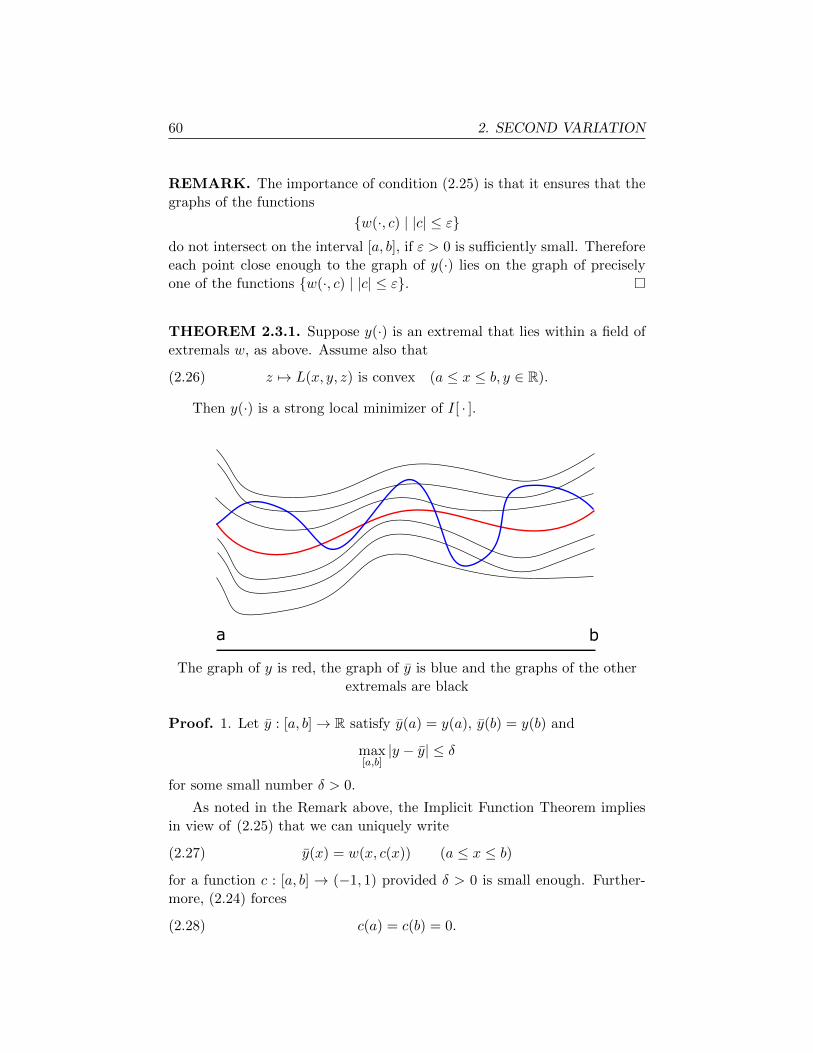
60 2. SECOND VARIATION
REMARK. The importance of condition (2.25) is that it ensures that the
graphs of the functions
{w(·, c) | |c| ≤ ε}do not intersect on the interval [a, b], if ε > 0 is sufficiently small. Therefore
each point close enough to the graph of y(·) lies on the graph of precisely
one of the functions {w(·, c) | |c| ≤ ε}. �
THEOREM 2.3.1. Suppose y(·) is an extremal that lies within a field of
extremals w, as above. Assume also that
(2.26) z 7→ L(x, y, z) is convex (a ≤ x ≤ b, y ∈ R).
Then y(·) is a strong local minimizer of I[ · ].
a b
The graph of y is red, the graph of y is blue and the graphs of the other
extremals are black
Proof. 1. Let y : [a, b]→ R satisfy y(a) = y(a), y(b) = y(b) and
max[a,b]|y − y| ≤ δ
for some small number δ > 0.
As noted in the Remark above, the Implicit Function Theorem implies
in view of (2.25) that we can uniquely write
(2.27) y(x) = w(x, c(x)) (a ≤ x ≤ b)
for a function c : [a, b] → (−1, 1) provided δ > 0 is small enough. Further-
more, (2.24) forces
(2.28) c(a) = c(b) = 0.
2.3. Strong local minimizers 61
2. According to (2.27) we have
y′(x) = w′(x, c(x)) +∂w
∂c(x, c(x))c′(x).
Therefore the convexity condition (2.26) implies
(2.29)L(x, y, y′) ≥ L(x, y, w′)
∣∣c=c(x)
+∂L
∂z(x, y, w′)
∂w
∂cc′∣∣c=c(x)
= L(x, y, y′) + E,
where
E = L(x,w,w′)∣∣c=c(x)
− L(x, y, y′) +∂L
∂z(x,w,w′)
∂w
∂cc′∣∣c=c(x)
.
3. We now show that E is the derivative of a function F that vanishes
at x = a, b. To see this, we compute using (2.23) that
E =
∫ c(x)
0
∂
∂cL(x,w(x, c), w′(x, c)) dc+
∂L
∂z(x,w,w′)
∂w
∂cc′∣∣c=c(x)
=
∫ c(x)
0
∂L
∂y
∂w
∂c+∂L
∂z
∂w′
∂cdc+
∂L
∂z(x,w,w′)
∂w
∂cc′∣∣c=c(x)
=
∫ c(x)
0
(∂L
∂z
)′ ∂w∂c
+∂L
∂z
∂w′
∂cdc+
∂L
∂z(x,w,w′)
∂w
∂cc′∣∣c=c(x)
= F ′
for
F (x) =
∫ c(x)
0
∂L
∂z(x,w,w′)
∂w
∂cdc.
We used here the calculus formula
d
dx
(∫ g(x)
af(x, t) dt
)=
∫ g(x)
a
∂f
∂x(x, t) dt+ f(x, g(x))g′(x).
Observe also that
(2.30) F (b) = F (a) = 0,
since c(a) = c(b) = 0, according to (2.28).
4. It now follows from (2.29) and (2.30) that∫ b
aL(x, y, y′) dx ≥
∫ b
aL(x, y, y′) + F ′ dx =
∫ b
aL(x, y, y′) dx.
Therefore
I[y(·)] ≤ I[y(·)].�
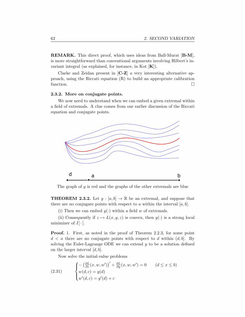
62 2. SECOND VARIATION
REMARK. This direct proof, which uses ideas from Ball-Murat [B-M],
is more straightforward than conventional arguments involving Hilbert’s in-
variant integral (as explained, for instance, in Kot [K]).
Clarke and Zeidan present in [C-Z] a very interesting alternative ap-
proach, using the Riccati equation (R) to build an appropriate calibration
function. �
2.3.2. More on conjugate points.
We now need to understand when we can embed a given extremal within
a field of extremals. A clue comes from our earlier discussion of the Riccati
equation and conjugate points.
a bd
The graph of y is red and the graphs of the other extremals are blue
THEOREM 2.3.2. Let y : [a, b] → R be an extremal, and suppose that
there are no conjugate points with respect to a within the interval [a, b].
(i) Then we can embed y(·) within a field w of extremals.
(ii) Consequently if z 7→ L(x, y, z) is convex, then y(·) is a strong local
minimizer of I[ · ].
Proof. 1. First, as noted in the proof of Theorem 2.2.3, for some point
d < a there are no conjugate points with respect to d within (d, b]. By
solving the Euler-Lagrange ODE we can extend y to be a solution defined
on the larger interval [d, b].
Now solve the initial-value problems
(2.31)
−(∂L∂z (x,w,w′)
)′+ ∂L
∂y (x,w,w′) = 0 (d ≤ x ≤ b)w(d, c) = y(d)
w′(d, c) = y′(d) + c
2.4. Existence of minimizers 63
for the functions w = w(x, c). By uniqueness of the solution to an initial-
value problem, we have y(x) = w(x, 0).
2. Define
(2.32) u(x) =∂w
∂c(x, 0).
We now differentiate the ODE in (2.31) with respect to the variable c. This
gives the identity
0 = −(∂2L
∂z∂y
∂w
∂c+∂2L
∂z2
∂w′
∂c
)′+∂2L
∂y2
∂w
∂c+
∂2L
∂y∂z
∂w′
∂c.
We now put c = 0 and recall the definitions (2.10) and (2.32):
0 = −(Bu+Au′)′ + Cu+Bu′ = Ju.
Upon differentiating as well the initial conditions in (2.31), we see that u
solves the initial-value problem
(2.33)
{Ju = 0 (d ≤ x ≤ b)u(d) = 0, u′(d) = 1.
3. As shown in the proof of Theorem 2.2.3, the hypothesis of no conju-
gate points implies that u = ∂w∂c (·, 0) is strictly positive on the interval [a, b].
Therefore w : [a, b]× [−1, 1]→ R is a field of extremals.
Now recall Theorem 2.3.1 to deduce that y(·) is a strong local minimizer,
provided we suppose also that z 7→ L is convex. �
REMARK. We are able to transform (2.31) into (2.33) by differentiating
in the parameter c, since the Jacobi differential operator
Ju = −(Au′ +Bu)′ +Bu′ + Cu
is the linearization of the Euler-Lagrange equation about y(·). �
2.4. Existence of minimizers
2.4.1. Examples.
We next build upon our insights from second variation calculations to
discuss the existence of minimizers.
We have thus far simply assumed for various variational problems that
minimizers exist, but in fact this issue can be quite complicated. Even quite
simple looking problems may have no solution:
64 2. SECOND VARIATION
EXAMPLE. For instance, the functional
I[y(·)] =
∫ 1
0y2 − (y′)2 dx
does not have a minimizer over the admissible set
A = {y : [a, b]→ R | y(0) = 0, y(1) = 0}.
This is clear from the second variation condition (2.2), which definitely fails
for all functions y0(·) ∈ A since
L = y2 − z2,∂2L
∂z2< 0.
In fact, we have
infAI[y(·)] = −∞.
To prove this, define for each integer k
yk(x) = sin(kπx) ∈ A
and observe that I[yk(·)]→ −∞ as k →∞. �
EXAMPLE. As an even easier example of nonexistence of minimizers con-
sider
I[y(·)] =
∫ 1
0y dx.
It is not hard to see that
(2.34) infy(·)∈A
I[y(·)] = −∞
for the admissible set A as above. �
EXAMPLE. This example illustrates a different mechanism for the failure
of minimizers to exist. We investigate
(2.35) I[y(·)] =
∫ 1
0x2(y′)2 dx,
over the admissible set A = {y : [0, 1]→ R | y(0) = 1, y(1) = 0}.Define
yk(x) =
{0 ( 1
k ≤ x ≤ 1)
1− kx (0 ≤ x ≤ 1k ).
Then
I[yk(·)] =
∫ 1k
0x2k2 dx =
1
3k→ 0 as k →∞,
2.4. Existence of minimizers 65
and consequently
infy(·)∈A
I[y(·)] = 0.
But the minimum is not attained, since∫ 1
0 x2(y′)2 dx > 0 for all y(·) ∈ A. �
EXAMPLE. We next show that the problem of minimizing
(2.36) I[y(·)] = −∫ 1
0xyy′ dx
over A = {y : [0, 1]→ R | y(0) = 0, y(1) = b} has a solution only if b = 0.
To see this, we first integrate by parts:
I[y(·)] = −1
2
∫ 1
0x(y2)′ dx = −b
2
2+
1
2
∫ 1
0y2 dx.
For any ε > 0 we can find a function y(·) ∈ A such that∫ 1
0 y2 dx < ε. Hence
infy(·)∈A
I[y(·)] = −b2
2.
But the minimum is not attained, because∫ 1
0 y2 dx > 0 for all y ∈ A (unless
b = 0). �
2.4.2. Convexity and minimizers.
The examples in the previous section illustrate that in general variational
problems need not have solutions. And even when we can show the existence
of minimizers, this theory depends upon the advanced mathematical topics
of measure theory and functional analysis, which are beyond the scope of
these notes. Instead, in this section we provide a brief discussion about the
key assumption for the existence theory for minimizers and mention some
typical theorems.
The primary requirement, strongly motivated by our earlier second vari-
ation necessary conditions (2.2) and (2.4), is that
(2.37) the mapping z 7→ L(x, y, z) is convex
for each (x, y).
This is the fundamental hypothesis for most existence theorems for mini-
mizers in the calculus of variations. Indeed, a basic existence theorem states
that if L satisfies (2.37) and also certain growth conditions, then there ex-
ists at least one minimizer y0(·) within some appropriate class of admissible
functions A.
66 2. SECOND VARIATION
REMARK. Modern existence theory in fact separates the questions of (i)
the existence of minimizers and (ii) their regularity (or smoothness) proper-
ties. The basic strategy is expand the admissible class A, to include various
functions that are less smooth than continuous and piecewise continuously
differentiable (as we have supposed throughout these notes). The precise
definition for this expanded admissible class is rather subtle, but the idea is
that the more functions we accept as belonging to A, the easier it will be to
find a minimizer.
And once we have resolved the problem (i) of existence of a minimizer,
we can then ask how smooth it is. A typical theorem concerning (ii) requires
that L be smooth and satisfies the strengthened convexity condition that
(2.38)∂2L
∂z2(x, y, z) ≥ γ > 0
for some constant γ. The regularity assertion is then that a minimizer y0(·)will be a smooth function of the variable x. �
Chapter 3
MULTIVARIABLEVARIATIONALPROBLEMS
3.1. Multivariable calculus of variations
In this chapter we extend the theory to variational problems for functions
of more than one variable. There will be few new mathematical ideas, and
so the only difficulties will be notational.
NOTATION. In the following U will always denote an open subset of Rn,
with smooth boundary ∂U . Its closure is U = U ∪ ∂U . �
DEFINITION. Assume g : ∂U → R is a given function. The correspond-
ing set of admissible functions is
A = {u : U → R | u(·) is continuously differentiable, u = g on ∂U}.
NOTATION. We will often write “u(·)” to emphasize that u : U → R is a
function. The gradient of a function u ∈ A is
∇u =
∂u∂x1...∂u∂xn
.�
Assume that in addition we are given a function L : U × R× Rn → R,
L = L(x, y, z),
67
68 3. MULTIVARIABLE VARIATIONAL PROBLEMS
called the Lagrangian. So L is a function of the 2n + 1 real variables
(x, y, z) = (x1, . . . , xn, y, z1, . . . , zn).
DEFINITION. If u(·) ∈ A, we define
I[u(·)] =
∫UL(x, u(x),∇u(x)) dx.
Note that we insert the number u(x) into the y-variable slot of L(x, y, z),
and the vector ∇u(x) into the z-variable slot of L(x, y, z).
The basic problem of the multivariable calculus of variations is
to characterize functions u0(·) ∈ A that satisfy
(COV) I[u0(·)] = minu(·)∈A
I[u(·)].
EXAMPLE (Dirichlet energy). As a first example, take
L(x, y, z) =|z|2
2=
1
2
n∑k=1
z2k.
Then
I[u(·)] =1
2
∫U|∇u(x)|2 dx,
an expression called the Dirichlet energy of u. What function u0(·) mini-
mizes this energy among all other candidates satisfying the given boundary
conditions that u = g on ∂U? �
EXAMPLE (Minimal surfaces). For a geometric example, we consider
now
L(x, y, z) = (1 + |z|2)1/2.
Then
I[u(·)] =
∫U
(1 + |∇u(x)|2
)1/2dx
= surface area of the graph of u.
Among all candidates that equal g on the boundary of U , which function
u0(·) gives the surface having the least area? �
3.2. First variation 69
3.2. First variation
3.2.1. Euler-Lagrange equation.
We show next that a minimizer u0(·) ∈ A of our multivariable vari-
ational problem automatically solves a certain partial differential equation
(PDE).
THEOREM 3.2.1. Assume u0(·) ∈ A is twice continuously differentiable
and solves (COV).
Then u0 satisfies the nonlinear PDE
(3.1) −n∑k=1
∂
∂xk
(∂L
∂zk(x, u0(x),∇u0(x))
)+∂L
∂y(x, u0(x),∇u0(x)) = 0
within the region U .
REMARKS.
(i) The Euler-Lagrange equation corresponding to L is the PDE
(E-L) −n∑k=1
∂
∂xk
(∂L
∂zk(x, u,∇u)
)+∂L
∂y(x, u,∇u) = 0.
Solutions u of the Euler-Lagrange equation are extremals (or critical
points or stationary points) of I[ · ]. Consequently, a minimizer u0(·)is an extremal, subject to the boundary conditions that u = g on ∂U .
(ii) Using vector calculus notation, we can also write (E-L) as
−div (∇zL(x, u,∇u)) +∂L
∂y(x, u,∇u) = 0.
Here “div” stands for divergence. �
WARNING ABOUT NOTATION. Most books write the (E-L) PDE
as
−n∑k=1
∂
∂xk
(∂L
∂uxk(x, u,∇u)
)+∂L
∂u(x, u,∇u) = 0
or, worse, as
−n∑k=1
∂
∂xk
(∂L
∂( ∂u∂xk )(x, u,∇u)
)+∂L
∂u(x, u,∇u) = 0.
This is spectacularly bad notation: the Lagrangian L = L(x, y, z) is a
function of the 2n+ 1 real variables (x, y, z) = (x1, . . . , xn, y, z1, . . . , zn). So
the expressions “∂L∂u” and “ ∂L∂uxk
” have no meaning. �
70 3. MULTIVARIABLE VARIATIONAL PROBLEMS
EXAMPLE. Let L(x, y, z) = |z|22 . Then
∂L
∂y= 0,
∂L
∂zk= zk.
Consequently the Euler-Lagrange equation is
n∑k=1
∂
∂xk
(∂u
∂xk
)= 0.
If we define the Laplacian
(3.2) ∆u =
n∑k=1
∂2u
∂x2k
,
then the Euler-Lagrange PDE is Laplace’s equation
∆u = 0 within U .
A function solving Laplace’s equation is called harmonic. Thus a minimizer
of Dirichlet’s energy functional is a harmonic function. �
WARNING ABOUT NOTATION. Many physics and engineering texts
use the symbol “∇2” for the Laplacian. In these and the Math 170 notes, we
instead employ ∇2 to denote the matrix of second derivatives: see Section
C in the Appendix. �
EXAMPLE. The Euler-Lagrange equation for the functional∫U
1
2|∇u|2 − uf dx
is Poisson’s equation
−∆u = f in U.
The Euler-Lagrange equation for the functional∫U
1
2|∇u|2 − F (u) dx
is the nonlinear Poisson equation
−∆u = f(u) in U,
where f = F ′. �
EXAMPLE. Assume L = (1 + |z|2)1/2. Then
∂L
∂y= 0,
∂L
∂zk=
zk(1 + |z|2)1/2
.
3.2. First variation 71
Consequently the Euler-Lagrange equation is
div
(∇u
(1 + |∇u|2)12
)=
n∑k=1
∂
∂xk
(∂u∂xk
(1 + |∇u|2)12
)= 0.
This is the minimal surface equation.
GEOMETRIC INTERPRETATION. The expression
H = div
(∇u
(1 + |∇u|2)12
)
has a geometric meaning; it is the mean curvature of the graph of u at
the point (x, u(x)). Therefore minimal surfaces have zero mean curvature
everywhere. �
EXAMPLE. If b : U → Rn and f : R→ R, the expression
L = z · b(x)f(y) + F (y) div b,
where F ′ = f , is a null Lagrangian. Recall from page 8 that this means
every function automatically solves the associated Euler-Lagrange PDE.
Indeed, for any function u : U → R we have
−div (∇zL) +∂L
∂y= −div (bf(u)) +∇u · bf ′(u) + f(u) div b = 0.
�
EXAMPLE. Let us for this example write points in Rn+1 as (x, t) with
x ∈ Rn denoting position and t ≥ 0 denoting time. We consider functions
u = u(x, t).
The Euler-Lagrange equation for the functional
I[u] =1
2
∫ T
0
∫Rn
(∂u
∂t
)2
− |∇xu|2 dxdt
is the wave equation
∂2u
∂t2−∆u = 0,
where the Laplacian ∆, defined as in (3.2), acts in the x-variables. However,
it is easy to see that the functional I[ · ] is unbounded from below on any
reasonable admissible class of functions. Consequently, solutions of the wave
equation correspond to extremals that are not minimizers. �
72 3. MULTIVARIABLE VARIATIONAL PROBLEMS
3.2.2. Derivation of Euler-Lagrange PDE.
NOTATION. We write
ν =
ν1...
νn
.for the outward pointing unit normal vector field along ∂U . �
LEMMA 3.2.1.
(i) For each k = 1, . . . , n we have the multivariable integration-by-
parts formula
(3.3)
∫U
∂f
∂xkg dx = −
∫Uf∂g
∂xkdx+
∫∂Ufgνk dS
for k = 1, . . . , n.
(ii) If f : U → R is continuous and∫Ufw dx = 0 for all continuous w : U → R
with w = 0 on ∂U , then f ≡ 0 within U .
Proof. 1.The Divergence Theorem says that∫U
div h dx =
∫∂U
h · ν dS.
Apply this to the vector field h = [0, . . . , 0, fg, 0, . . . , 0]T with the nonzero
term fg in the k-th slot.
2. Let φ : U → R be positive within U and equal to zero on ∂U . Let
w(x) = φ(x)f(x) above, to find∫Uφf2 dx = 0.
Hence φ(x)f2(x) = 0 for all x ∈ U as the integrand is positive. Then since
φ(x) > 0, we conclude that f(x) = 0 for all x ∈ U . �
Derivation of Euler-Lagrange equation:
1. Let w : U → R satisfy w = 0 on ∂U . Assume −1 ≤ τ ≤ 1 and define
uτ (x) = u0(x) + τw(x) (x ∈ U).
Note uτ (·) ∈ A, since w = 0 on ∂U .
Thus
I[u0(·)] ≤ I[uτ (·)],
3.3. Second variation 73
since u0 is the minimizer of I. Define i(τ) = I[uτ (·)]. Then
i(0) ≤ i(τ).
So τ 7→ i(τ) has a minimum at τ = 0 on the interval −1 ≤ τ ≤ 1, and
thereforedi
dτ(0) = 0.
2. Now
i(τ) =
∫UL(x, uτ ,∇uτ ) dx =
∫UL(x, u0 + τw,∇u0 + τ∇w) dx.
Therefore
di
dτ(τ) =
∫U
∂
∂τL(x, u0 + τw,∇u0 + τ∇w) dx.
=
∫U
∂L
∂y(x, u0 + τw,∇u0 + τ∇w)w
+n∑k=1
∂L
∂zk(x, u0 + τw,∇u0 + τ∇w)
∂w
∂xkdx.
Put τ = 0:
0 =di
dτ(0) =
∫U
∂L
∂y(x, u0,∇u0)w +
n∑k=1
∂L
∂zk(x, u0,∇u0)
∂w
∂xkdx.
We now integrate by parts, to deduce that∫U
[∂L
∂y(x, u0,∇u0)−
n∑k=1
∂
∂xk
(∂L
∂zk(x, u0,∇u0)
)]w dx = 0.
This is valid for all functions w such that w = 0 on ∂U . The lemma before
now implies that the (E-L) PDE holds everywhere in U . �
3.3. Second variation
THEOREM 3.3.1. Suppose u0(·) ∈ A is a minimizer and u0 is continu-
ously differentiable.
(i) Then
(3.4)
∫U
n∑k,l=1
∂2L
∂zk∂zl(x, u0,∇u0)
∂w
∂xk
∂w
∂xl
+ 2n∑k=1
∂2L
∂zk∂y(x, u0,∇u0)
∂w
∂xkw +
∂2L
∂y2(x, u0,∇u0)w2 dx ≥ 0
for all w : U → R with w = 0 on ∂U .
74 3. MULTIVARIABLE VARIATIONAL PROBLEMS
(ii) Furthermore,
(3.5) ∇2zL(x, u0(x),∇u0(x)) � 0 (x ∈ U).
DEFINITION. The expression on the left hand side of (3.4) the second
variation of I[ · ] about u0(·), evaluated at w(·). �
REMARK. The inequality (3.5) means that
n∑k,l=1
∂2L
∂zk∂zl(x, u0,∇u0)ykyl ≥ 0 (y ∈ Rn).
If the mapping
(3.6) z 7→ L(x, u0(x), z) is convex,
then (3.5) holds automatically. �
Proof. 1. Select w : U → R, with w = 0 on ∂U , and define uτ (x) =
u0(x) + τw(x) for −1 ≤ τ ≤ 1. Then uτ (·) ∈ A, and so τ 7→ i(τ) has a
minimum at τ = 0 and thus
d2i
dτ2(0) ≥ 0.
2. Differentiating twice with respect to τ , we find
d2i
dτ2(τ) =
∫U
∂2L
∂y2(x, u0 + τw,∇u0 + τ∇w)w2
+ 2
n∑k=1
∂2L
∂y∂zk(x, u0 + τw,∇u0 + τ∇w)w
∂w
∂xk
+
n∑k,l=1
∂2L
∂zk∂zl(x, u0 + τw,∇u0 + τ∇w)
∂w
∂xk
∂w
∂xldx.
Put τ = 0 and recall d2idτ2
(0) ≥ 0, to prove (3.4).
3. As in the second variation calculation for the scalar case, we define
φ(x) =
{x if 0 ≤ x ≤ 1
2− x if 1 ≤ x ≤ 2
and extend φ to be 2-periodic on R. Thus φ is a sawtooth function and
φ′ = ±1 except at the integers.

3.4. Extensions and generalizations 75
Next let ζ : U → R be any continuously differentiable function with
ζ = 0 on ∂U . Finally, choose any y ∈ Rn and write
wε(x) = εφ(x·yε )ζ(x).
for each ε > 0. Then wε is differentiable except along finitely many hyper-
planes that intersect U , with
∇wε(x) = φ′(x·yε )ζ(x)y + εφ(x·yε )∇ζ(x).
Note that the second term on the right is less than or equal to Aε for some
appropriate constant A.
Insert wε in place of w in (3.4). It follows that∫U
n∑k,l=1
∂2L
∂zk∂zl(x, u0,∇u0)ykylζ
2(φ′(x·yε )
)2dx+Bε ≥ 0
for some constant B. But (φ′(x·yε )
)2= 1
except along finitely many hyperplanes (which have no effect on the integral).
Therefore upon sending ε→ 0, we deduce that∫U
n∑k,l=1
∂2L
∂zk∂zl(x, u0,∇u0)ykylζ
2 dx ≥ 0
for all functions ζ as above. This implies (3.5). �
3.4. Extensions and generalizations
3.4.1. Other boundary conditions.
If we change the admissible class of functions and/or if we change the
energy functional I[ · ], new effects can appear.
For example, suppose we are additionally given a function B : ∂U×R→R, B = B(x, y). We then for this section redefine the energy by adding a
boundary integral term:
(3.7) I[u(·)] =
∫UL(x, u,∇u) dx+
∫∂UB(x, u) dS.
We also redefine
(3.8) A = {u : U → R | u is continuously differentiable},
so as now to require nothing about the boundary behavior of admissible
functions.
76 3. MULTIVARIABLE VARIATIONAL PROBLEMS
THEOREM 3.4.1. Let the energy be given by (3.7) and the admissible
class by (3.8). Assume u0(·) ∈ A is a twice continuously differentiable
minimizer
(i) Then u0 solves the usual Euler-Lagrange equation
(3.9) −n∑k=1
∂
∂xk
(∂L
∂zk(x, u0,∇u0)
)+∂L
∂y(x, u0,∇u0) = 0
within U .
(ii) Furthermore, we have the boundary condition
(3.10)
n∑k=1
∂L
∂zk(x, u0,∇u0)νk +
∂B
∂y(x, u0) = 0
on ∂U .
In vector notation, (3.10) reads
(3.11) ∇zL(x, u0,∇u0) · ν +∂B
∂y(x, u0) = 0 on ∂U.
INTERPRETATION. The identity (3.10) is the natural boundary
condition (or transversality condition) hidden in our new variational
problem. It appears automatically when we compute the first variation. �
Proof. 1. Select any w : U → R, but do not require that w vanishes on the
boundary. Define uτ (x) = u0(x) + τw(x) (x ∈ U), and observe uτ (·) ∈ A.
Thus i(τ) = I[uτ (·)] has a minimum at τ = 0 and therefore
di
dτ(0) = 0.
2. Now
i(τ) = I[uτ (·)]
=
∫UL(x, u0 + τw,∇u0 + τ∇w) dx+
∫∂UB(x, u0 + τw) dS.
Therefore
0 =di
dτ(0) =
∫U
∂L
∂y(x, u0,∇u0)w +
n∑k=1
∂L
∂zk(x, u0,∇u0)
∂w
∂xkdx
+
∫∂U
∂B
∂y(x, u0)w dS.
3.4. Extensions and generalizations 77
Integrate by parts, to deduce∫U
[∂L
∂y(x, u0(x),∇u0(x))−
n∑k=1
∂
∂xk
(∂L
∂zk(x, u0(x),∇u0(x))
)]w dx
+
∫∂U
n∑k=1
[∂L
∂zk(x, u0,∇u0)νk +
∂B
∂y(x, u0)
]w dS = 0.
This identity is valid for all functions w. If we restrict attention to
functions satisfying also w = 0 on ∂U , we as usual deduce that the Euler-
Lagrange PDE holds within U .
Knowing this, we can then rewrite the foregoing:∫∂U
n∑k=1
[∂L
∂zk(x, u0,∇u0)νk +
∂B
∂y(x, u0)
]w dS = 0.
As this identity is valid for all functions w, regardless of their behavior
on ∂U , it follows that the boundary condition (3.10) holds everywhere on
∂U . �
EXAMPLE. A minimizer u0(·) the functional
I[u(·)] =1
2
∫U|∇u|2dx+
∫∂UB(u) dS
over the admissible class (3.8) solves the nonlinear boundary-value problem{∆u0 = 0 in U
∂u0∂ν + b(u0) = 0 on ∂U,
where b = B′ and∂u
∂ν= ∇u · ν
is the outward normal derivative of u. �
3.4.2. Integrating factors.
It is often important to determine whether a given PDE (or ODE) prob-
lem is variational, meaning that it arises as the Euler-Lagrange equation
for an appropriate energy functional I[ · ].
Consider for instance the linear equation
(3.12) −∆u+ b · ∇u = f in U ,
where b : U → Rn is a given vector field, b = b(x). In general (3.12) is not
variational.
78 3. MULTIVARIABLE VARIATIONAL PROBLEMS
But for the special case that b = ∇φ is the gradient of a potential
function φ : U → R, let us consider the functional
(3.13) I[u(·)] =
∫Ue−φ
(1
2|∇u|2 − fu
)dx.
The Lagrangian function is
L = e−φ(x)
(1
2|z|2 − f(x)y
).
and the corresponding Euler-Lagrange equation for a minimizer u is
−div(e−φ∇u
)− e−φf = 0.
We simplify and cancel the term e−φ, to rewrite the foregoing as
(3.14) −∆u+∇φ · ∇u = f ;
this is (3.12) when b = ∇φ.
INTERPRETATION. We can regard e−φ as an integrating factor.
This means that if we multiply the PDE (3.14) by this expression, it then
becomes variational. �
3.4.3. Integral constraints.
In this section we for simplicity take L = 12 |z|
2; so that
I[u(·)] =1
2
∫U|∇u|2 dx.
Define also the functional
J [u(·)] =
∫UG(x, u(x)) dx,
where G : U × R→ R, G = G(x, y). The new admissible class will be
(3.15) A = {u : U → R | u = g on ∂U, J [u(·)] = 0}.
THEOREM 3.4.2. Assume that u0 ∈ A is a minimizer of I[ · ] over A.
Suppose also that
(3.16)∂G
∂y(x, u0) is not identically zero on U.
Then there exists λ0 ∈ R such that
(3.17) −∆u0 + λ0∂G
∂y(x, u0) = 0
within U .
3.4. Extensions and generalizations 79
We omit the proof, which is similar to that for Theorem 1.3.5. As in that
previous theorem, we interpret λ0 as the Lagrange multiplier for the integral
constraint J [u(·)] = 0. The requirement (3.16) is a constraint qualification
condition.
For an application, see Theorem 3.5.1 below.
3.4.4. Systems.
We can also extend our theory to handle systems. For this, we assume
g : ∂U → Rm is given, and redefine the class of admissible functions, now
to be
A = {u : U → Rm | u = g on ∂U}.
NOTATION. We write
u =
u1...
um
, ∇u =
(∇u1)T
...
(∇um)T
=
∂u1∂x1
. . . ∂u1∂xn
.... . .
...∂um∂x1
. . . ∂um∂xn
.�
Suppose next we have a Lagrangian function L : U ×Rm ×Mm×n → R,
L = L(x, y, Z),
where Mm×n denotes the space of real, m× n matrices.
NOTATION. In this section only, we will write a matrix Z ∈Mm×n as
Z =
z11 . . . z1
n...
. . ....
zm1 . . . zmn
.�
DEFINITION. If u(·) ∈ A, we define
I[u(·)] =
∫UL(x,u(x),∇u(x)) dx.
Note that we insert u(x) into the y-variables of L(x, y, Z), and ∇u(x) into
the Z-variables.
THEOREM 3.4.3. Assume u0(·) ∈ A minimizers I[ · ] and u0 is twice
continuously differentiable.
Then u0 solves within U the system of nonlinear PDE
(E-L) −n∑k=1
∂
∂xk
(∂L
∂zlk(x,u0(x),∇u0(x))
)+∂L
∂yl(x,u0(x),∇u0(x)) = 0
for l = 1, . . . ,m.
80 3. MULTIVARIABLE VARIATIONAL PROBLEMS
Proof. 1. Select w : U → R such that w = 0 on ∂U , and then define and
define
uτ (x) = u0(x) + τw(x) (x ∈ U).
for −1 ≤ τ ≤ 1 Then uτ (·) ∈ A, since w = 0 on ∂U . Hence
I[u0(·)] ≤ I[uτ (·)].
Define i(τ) = I[uτ (·)]. Then τ 7→ i(τ) has a minimum at τ = 0, and
thereforedi
dτ(0) = 0.
2. We have
i(τ) = I[uτ (·)] =
∫UL(x,u0(x) + τw(x),∇u0(x) + τ∇w(x)) dx.
Therefore
di
dτ(τ) =
∫U
m∑l=1
∂L
∂yl(x,u0 + τw,∇u0 + τ∇w)wl
+m∑l=1
n∑k=1
∂L
∂zlk(x,u0 + τw,∇u0 + τ∇w)
∂wl∂xk
dx;
and so
0 =di
dτ(0) =
∫U
m∑l=1
∂L
∂yl(x,u0,∇u0)wl +
m∑l=1
n∑k=1
∂L
∂zk(x,u0,∇u0)
∂wl∂xk
dx.
Now fix some index l ∈ {1, . . . ,m} and put
w = [0 . . . 0w 0 . . . 0]T ,
where the real-valued function w appears in the l-th slot. Then we have∫U
∂L
∂yl(x,u0,∇u0)w +
n∑k=1
∂L
∂zk(x,u0,∇u0)
∂w
∂xkdx = 0.
Upon integrating by parts, we deduce as usual that the l-th equation of the
(E-L) system of PDE holds. �
3.5. Applications
3.5.1. Eigenvalues, eigenfunctions.
Assume for this section that U ⊂ Rn is a connected, open set, with
smooth boundary ∂U .
3.5. Applications 81
THEOREM 3.5.1. (i) There exists a real number λ1 > 0 and a smooth
function w1 such that
(3.18)
−∆w1 = λ1w1 in U
w1 = 0 on ∂U
w1 > 0 in U,∫U w
21 dx = 1.
(ii) Furthermore,
(3.19) λ1 = min
{∫U|∇u|2 dx |
∫Uu2 dx = 1, u = 0 on ∂U
}.
DEFINITION. We call λ1 the principal eigenvalue for the Laplacian
with zero boundary conditions on ∂U . The function w1 is a principal eigen-
function.
REMARK. We can also write
(3.20) λ1 = minu=0 on ∂U,u6=0
∫U |∇u|
2 dx∫U u
2 dx.
This is Rayleigh’s principle. �
Proof. If w1 ∈ A is a minimizer for the constrained variational problem
(3.19), then∂G
∂y(w1) = 2w1 6≡ 0.
Therefore Theorem 3.4.2 tells us that the Euler-Lagrange equation is
−∆w1 + µw1 = 0,
where µ is the eigenvalue for the constraint. But then
µ = µ
∫Uw2
1 dx = −∫U|∇w1|2 dx = −λ1.
The existence of a smooth minimizer w1, with w1 > 0 within U , requires
graduate level mathematical ideas beyond the scope of these notes. �
THEOREM 3.5.2. (i) There exist real numbers 0 < λ1 < λ2 ≤ λ3 ≤ · · ·and smooth function w1, w2, w3, . . . such that
λk →∞
and
(3.21)
−∆wk = λkwk in U
wk = 0 on ∂U∫U w
2k dx = 1.
82 3. MULTIVARIABLE VARIATIONAL PROBLEMS
(ii) Furthermore,
(3.22) λk = min
{∫U|∇u|2 dx |
∫Uu2 dx = 1, u = 0 on ∂U,∫
Uwlu dx = 0 (l = 1, . . . , k − 1)
}.
DEFINITION. We call λk the k-th eigenvalue for the Laplacian with
zero boundary conditions on ∂U . The function wk is a corresponding eigen-
function. �
Proof. Assume that (3.21) holds for l = 1, . . . , k − 1. The Euler-Lagrange
PDE for the minimization problem (3.22) is
(3.23) −∆wk = λkwk +k−1∑l=1
µlwl,
where λk is the Lagrange multiplier for the constraint∫U w
2 dx = 1 and µl is
the Lagrange multiplier for the constraint∫U wlw dx = 0 for l = 1, . . . , k−1.
Let 1 ≤ m ≤ k − 1, multiply (3.23) by wm, and integrate:
−∫U
∆wkwm dx =
∫U
(λkwk +k−1∑l=1
µlwl)wm dx = µm.
Therefore
µm = −∫U
∆wkwm dx =
∫U∇wk · ∇wm dx
= −∫Uwk∆wm dx = λm
∫Uwkwm dx = 0.
Thus (3.23) becomes −∆wk = λkwk. �
REMARK. (Level curves for eigenfunctions) If U is connected, the
first eigenfunction w1 is positive; but the higher eigenfunctions wk for k =
2, . . . change sign within U .
Take a thin metal plate cut into the shape U ⊂ R2, sprinkle it with sand,
and then connect the plate to an audio speaker. If we we play appropriate
high frequencies over the speaker, the plate resonates according to the higher
eigenfunctions of the Laplacian (at least approximately) and so the sand
collects into the level sets {wk = 0}. At higher and higher frequencies,
complicated and beautiful structures appear, called Chladni patterns: see
www.youtube.com/watch?v=wvJAgrUBF4w. �
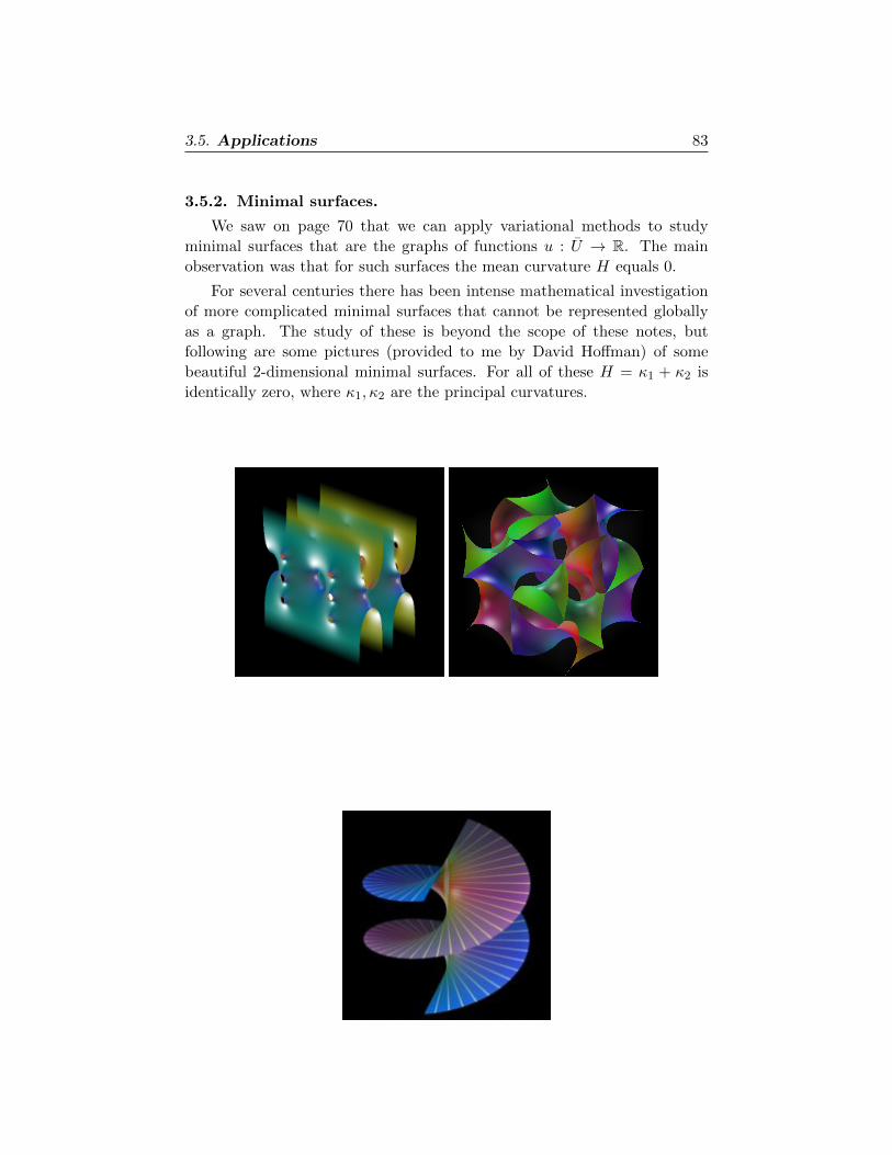
3.5. Applications 83
3.5.2. Minimal surfaces.
We saw on page 70 that we can apply variational methods to study
minimal surfaces that are the graphs of functions u : U → R. The main
observation was that for such surfaces the mean curvature H equals 0.
For several centuries there has been intense mathematical investigation
of more complicated minimal surfaces that cannot be represented globally
as a graph. The study of these is beyond the scope of these notes, but
following are some pictures (provided to me by David Hoffman) of some
beautiful 2-dimensional minimal surfaces. For all of these H = κ1 + κ2 is
identically zero, where κ1, κ2 are the principal curvatures.
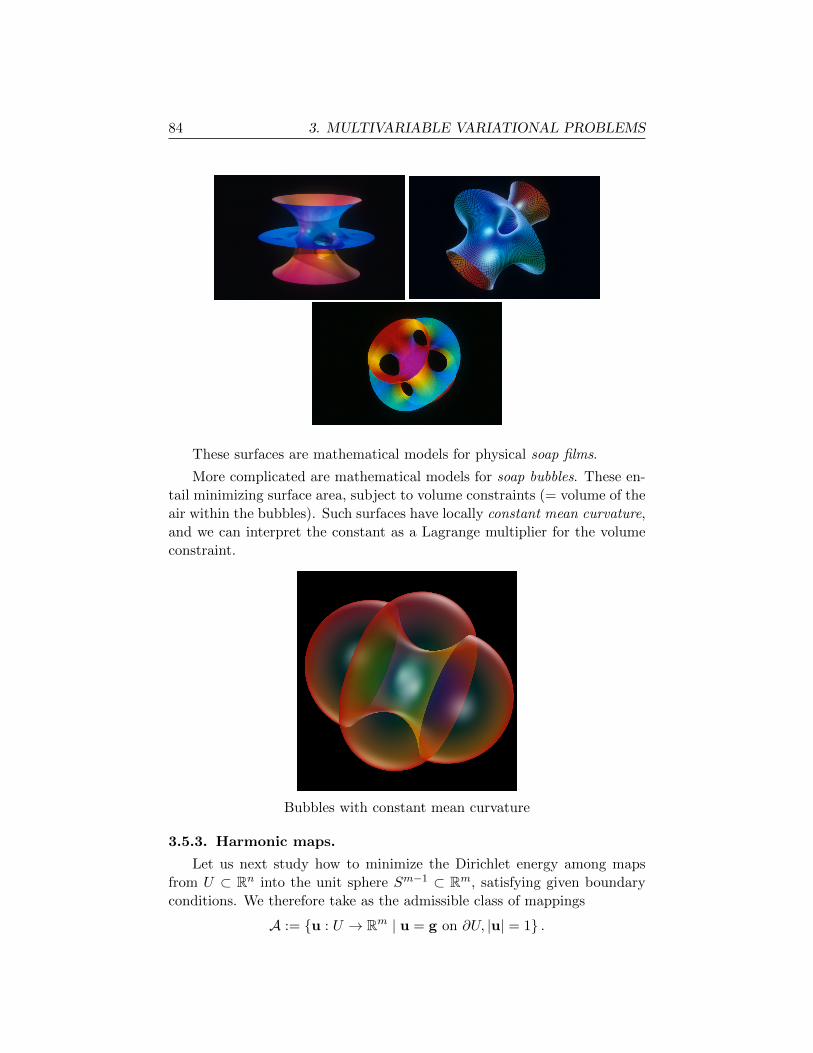
84 3. MULTIVARIABLE VARIATIONAL PROBLEMS
These surfaces are mathematical models for physical soap films.
More complicated are mathematical models for soap bubbles. These en-
tail minimizing surface area, subject to volume constraints (= volume of the
air within the bubbles). Such surfaces have locally constant mean curvature,
and we can interpret the constant as a Lagrange multiplier for the volume
constraint.
Bubbles with constant mean curvature
3.5.3. Harmonic maps.
Let us next study how to minimize the Dirichlet energy among maps
from U ⊂ Rn into the unit sphere Sm−1 ⊂ Rm, satisfying given boundary
conditions. We therefore take as the admissible class of mappings
A := {u : U → Rm | u = g on ∂U, |u| = 1} .
3.5. Applications 85
The corresponding energy is
I[u(·)] =1
2
∫U|∇u|2 dx
THEOREM 3.5.3. Let u0 ∈ A satisfy
I[u0] = minu∈A
I[u].
Then
(3.24)
{−∆u0 = |∇u0|2u0 in U
u0 = g on ∂U .
INTERPRETATION. The function λ0 = |∇u0|2 is the Lagrange multi-
plier corresponding to the pointwise constraint |u0| = 1. �
Proof. 1. Select w : U → Rm, with w = 0 on ∂U . Then since |u0| = 1, it
follows that |u0 + τw| 6= 0 for each sufficiently small τ . Consequently
(3.25) u(τ) :=u0 + τw
|u0 + τw|∈ A.
Thus
i(τ) := I[w(τ)]
has a minimum at τ = 0, and so, as usual,
di
dτ(0) = 0.
2. We have
(3.26) i′(0) =
∫U∇u · ∇u′(0) dx = 0.
where ′ = ddτ . But we compute directly from (3.25) that
u′(τ) =w
|u0 + τw|− [(u0 + τw) ·w](u0 + τw)
|u0 + τw|3.
So u′(0) = w − (u0 ·w)u0. Put this equality into (3.26):
(3.27) 0 =
∫U∇u0 · ∇w −∇u0 · ∇((u0 ·w)u0) dx.
We next differentiate the identity |u0|2 ≡ 1, to learn that
(∇u0)Tu0 = 0.
Using this fact, we then verify that
∇u0 · ∇((u0 ·w)u0) = |∇u0|2(u0 ·w)
86 3. MULTIVARIABLE VARIATIONAL PROBLEMS
in U . Inserting this into (3.27) gives
0 =
∫U∇u0 · ∇w − |∇u0|2(u0 ·w) dx.
This identity, valid for all functions w as above, implies the PDE in (3.24).
�
3.5.4. Gradient flows.
The Euler-Lagrange equation arising in PDE theory are mostly equilib-
rium equations that do not entail changes in time. But it is interesting also
to consider certain time-dependent equations that can be interpreted as gra-
dient flows. Recall that if we are given an “energy” function Φ : Rn → R,
the system of ODE
(3.28) x = −∇Φ(x),
describes a “downhill” gradient flow
We introduce next a PDE version, corresponding to the energy
I[u(·)] =
∫UL(x, u(x),∇u(x)) dx.
The corresponding time dependent gradient flow, generalizing (3.28), is the
PDE
(3.29)∂u
∂t=
n∑k=1
∂
∂xk
(∂L
∂zk(x, u,∇u)
)− ∂L
∂y(x, u,∇u).
We assume that u = u(x, t) solves this PDE, with the boundary condition
(3.30) u = 0 on ∂U.
THEOREM 3.5.4.
(i) The function
φ(t) = I[u(·, t)] (0 ≤ t <∞)
is nonincreasing on [0,∞).
(ii) Assume in addition that (y, z) 7→ L(x, y, z) is convex. Then φ is
convex on [0,∞).
Proof. 1. We differentiate in t, to see that
d
dtI[u(·, t)] =
d
dt
∫UL(x, u(x, t),∇xu(x, t)) dx
=
∫U
∂L
∂y(x, u,∇u)
∂u
∂t+∇zL(x, u,∇u) · ∇x
(∂u
∂t
)dx
3.5. Applications 87
=
∫U
[∂L
∂y(x, u,∇u)− div(∇zL(x, u,∇u))
]∂u
∂tdx
= −∫U
(∂u
∂t
)2
dx ≤ 0.
Observe that there is no boundary term when we integrate by parts, since
if (3.30) holds for all times t, then ∂u∂t = 0 on ∂U .
2. Differentiate again in t:
d2
dt2I[u(·, t)] = − d
dt
∫U
(∂u
∂t
)2
dx = −2
∫U
∂u
∂t
∂2u
∂t2dx.
We can also differentiate the PDE (3.29), to find
∂2u
∂t2=
n∑k=1
∂
∂xk
(∂2L
∂zk∂y
∂u
∂t+
n∑l=1
∂2L
∂zk∂zl
∂2u
∂xl∂t
)
− ∂2L
∂y2
∂u
∂t−
n∑l=1
∂2L
∂y∂zl
∂2u
∂xl∂t.
We insert this into the previous calculation, and integrate by parts:
d2
dt2I[u(·, t)] = 2
∫U
n∑k,l=1
∂2L
∂zk∂zl
∂2u
∂xk∂t
∂2u
∂xl∂t
+ 2
n∑k=1
∂2L
∂zk∂y
∂2u
∂xk∂t
∂u
∂t+∂2L
∂y2
(∂u
∂t
)2
dx ≥ 0,
the last inequality holding provided L is convex in the variables (y, z). �

Chapter 4
OPTIMAL CONTROLTHEORY
4.1. The basic problem
This section provides an informal introduction to optimal control theory,
and discusses three model problems. The basic issue is this: we are given
some system of interest, whose evolution in time is modeled by a differential
equation that depends upon certain parameters. We ask how to optimally
and continually adjust these parameters, so as to maximize a given payoff
functional.
To be more precise, assume that the state of our system at time t ≥ 0
is x(t), where
x : [0,∞)→ Rn
solves a system of differential equations having the form
(ODE)
{x(t) = f(x(t), α(t)) (t ≥ 0)
x(0) = x0,
x0 ∈ Rn denoting the initial state of the system. Here we are given
f : Rn ×A→ Rn,
where A ⊆ Rm is the set of control (or parameter) values. The (possibly
discontinuous) mapping
α : [0,∞)→ A
is an admissible control.
89
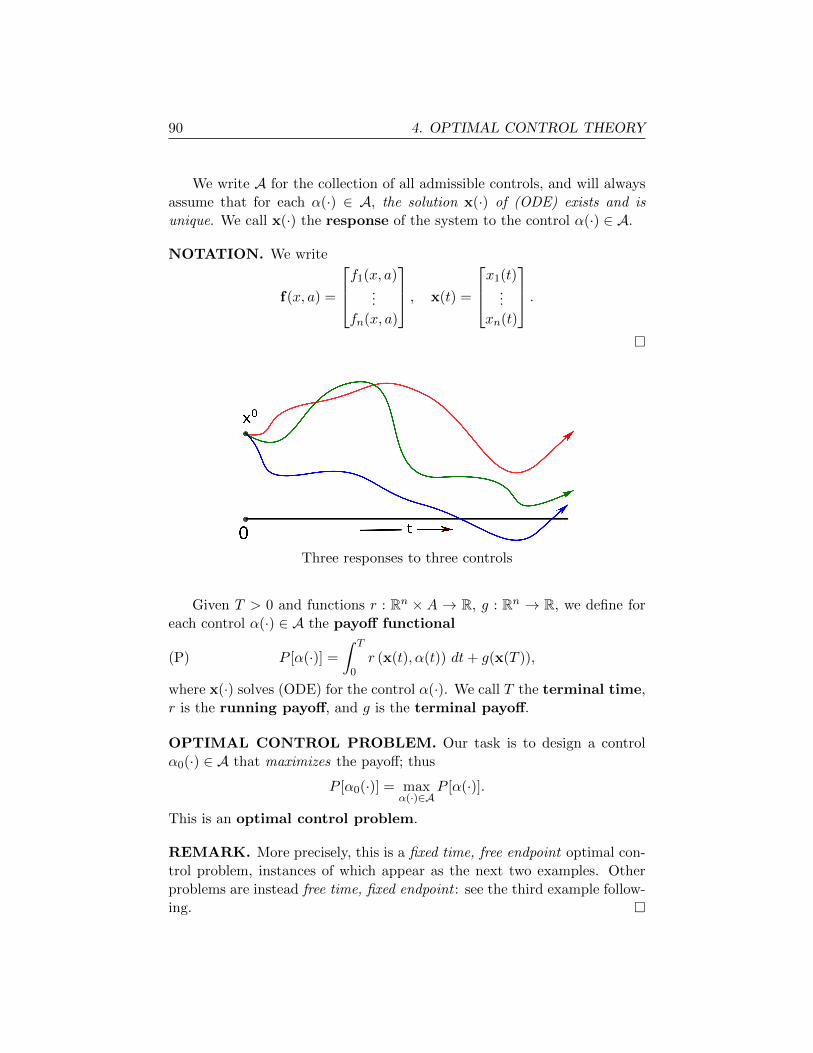
90 4. OPTIMAL CONTROL THEORY
We write A for the collection of all admissible controls, and will always
assume that for each α(·) ∈ A, the solution x(·) of (ODE) exists and is
unique. We call x(·) the response of the system to the control α(·) ∈ A.
NOTATION. We write
f(x, a) =
f1(x, a)...
fn(x, a)
, x(t) =
x1(t)...
xn(t)
.�
x0
Three responses to three controls
Given T > 0 and functions r : Rn × A → R, g : Rn → R, we define for
each control α(·) ∈ A the payoff functional
(P) P [α(·)] =
∫ T
0r (x(t), α(t)) dt+ g(x(T )),
where x(·) solves (ODE) for the control α(·). We call T the terminal time,
r is the running payoff, and g is the terminal payoff.
OPTIMAL CONTROL PROBLEM. Our task is to design a control
α0(·) ∈ A that maximizes the payoff; thus
P [α0(·)] = maxα(·)∈A
P [α(·)].
This is an optimal control problem.
REMARK. More precisely, this is a fixed time, free endpoint optimal con-
trol problem, instances of which appear as the next two examples. Other
problems are instead free time, fixed endpoint : see the third example follow-
ing. �
4.1. The basic problem 91
EXAMPLE. (A production and consumption model) Consider an
economic activity (such as running a company) that generates an output,
some fraction of which we can at each moment reinvest, while consuming
the rest. How should we plan our consumption/reinvestment strategy so as
to maximize our total consumption over a time period of given length T?
To write down a mathematical model, introduce
x(t) = output of company at time t
α(t) = fraction of output reinvested at time t.
Since the control α(·) represents a fraction of output, we have 0 ≤ α(t) ≤ 1
for times 0 ≤ t ≤ T . In other words,
α : [0, T ]→ A
where A denotes the interval [0, 1] ⊂ R.
Next we model the output of the company as a function of the reinvest-
ment strategy:
(ODE)
{x(t) = γα(t)x(t) (0 ≤ t ≤ T )
x(0) = x0.
Here γ > 0 is a known growth rate. Since (1 − α(t))x(t) is the amount of
the output consumed at time t, our total consumption will therefore be
(P) P [α(·)] =
∫ T
0(1− α(t))x(t) dt.
We wish to design an optimal reinvestment plan α0(·) that maximizes P [ · ].This fits into the fixed time, free endpoint control theory formulation
from above, with n = m = 1 and
f(x, a) = kax, r(x, a) = (1− a)x, g = 0.
�
EXAMPLE. (Linear-quadratic regulator) The linear-quadratic regu-
lator is a widely used model, since, as we will later see, it is solvable.
In the simplest case, we take n = m = 1 and introduce the system
dynamics
(ODE)
{x(t) = x(t) + α(t) (0 ≤ t ≤ T )
x(0) = x0.
We also assume A = R; so there is no constraint on the magnitude of control.
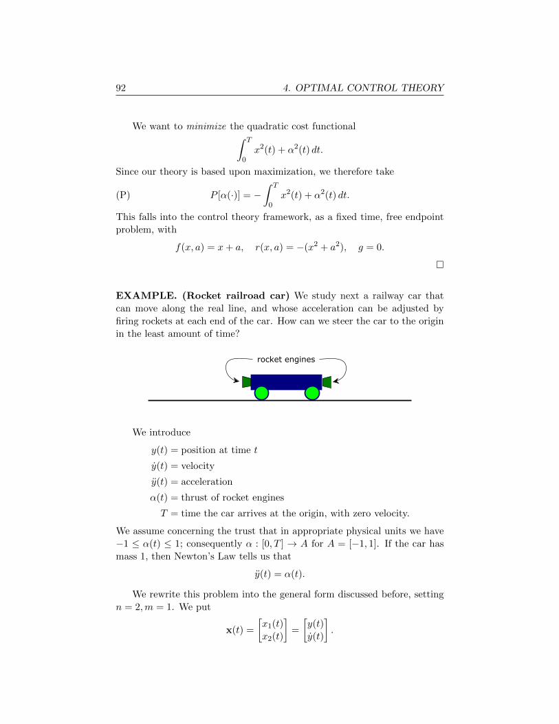
92 4. OPTIMAL CONTROL THEORY
We want to minimize the quadratic cost functional∫ T
0x2(t) + α2(t) dt.
Since our theory is based upon maximization, we therefore take
(P) P [α(·)] = −∫ T
0x2(t) + α2(t) dt.
This falls into the control theory framework, as a fixed time, free endpoint
problem, with
f(x, a) = x+ a, r(x, a) = −(x2 + a2), g = 0.
�
EXAMPLE. (Rocket railroad car) We study next a railway car that
can move along the real line, and whose acceleration can be adjusted by
firing rockets at each end of the car. How can we steer the car to the origin
in the least amount of time?
rocket engines
We introduce
y(t) = position at time t
y(t) = velocity
y(t) = acceleration
α(t) = thrust of rocket engines
T = time the car arrives at the origin, with zero velocity.
We assume concerning the trust that in appropriate physical units we have
−1 ≤ α(t) ≤ 1; consequently α : [0, T ] → A for A = [−1, 1]. If the car has
mass 1, then Newton’s Law tells us that
y(t) = α(t).
We rewrite this problem into the general form discussed before, setting
n = 2,m = 1. We put
x(t) =
[x1(t)
x2(t)
]=
[y(t)
y(t)
].
4.2. Time optimal linear control 93
Then our dynamics are
(ODE) x(t) =
[0 1
0 0
]x(t) +
[0
1
]α(t) (0 ≤ t ≤ T )
with x(0) = x0 = [y0 v0]T , where y0 is the initial position and v0 is the
initial velocity. Our goal is to steer the railway car to the origin at a time
T > 0 (so it arrives with zero velocity: x(T ) = [0 0]T ), and to do so in the
least time.
We consequently want to maximize
(P) P [α(·)] = −∫ T
01 dt = −T.
This is a free time, fixed endpoint problem, since the time T to reach the
origin is not prescribed. �
4.2. Time optimal linear control
When the dynamics are linear in both the state and the control, we can
use tools of linear and convex analysis to design explicit optimal controls
and/or to deduce detailed information. In this section we illustrate such an
approach. (However, our presentation will invoke ideas from measure theory
and functional analysis, and will also omit some details.)
Consider therefore the linear control system:
(ODE)
{x(t) = Mx(t) +Nα(t)
x(0) = x0,
for given matrices M ∈Mn×n and N ∈Mn×m. We will take
A = [−1, 1]m ⊂ Rm,
and consider the class of admissible controls
A = {α : [0,∞)→ A | α(·) is measurable} .
Define
(P) P [α(·)] = −T
where T = T (α(·)) denotes the first time the solution of our ODE hits
the origin 0: x(T ) = 0. (If the trajectory never reaches the origin, we set
T =∞.)
OPTIMAL TIME LINEAR PROBLEM. We are given the starting
point x0 ∈ Rn, and want to find an optimal control α0(·) such that
P [α0(·)] = maxα(·)∈A
P [α(·)].
94 4. OPTIMAL CONTROL THEORY
Then
T0 = −P[α0(·)] is the minimum time to steer to the origin.
4.2.1. Linear systems of ODE.
Let us first briefly recall some terminology and basic facts about linear
systems of ordinary differential equations.
DEFINITION. Assume M ∈ Mn×n. Let X(·) : [0,∞) → Mn×n be the
unique solution of the matrix ODE{X(t) = MX(t) (t ≥ 0)
X(0) = I.
We call X(·) the fundamental solution, and sometimes write
X(t) = etM =
∞∑k=0
tkMk
k!.
THEOREM 4.2.1. (Solving linear systems)
(i) The unique solution of the homogeneous initial-value problem
(4.1)
{x = Mx (t ≥ 0)
x(0) = x0
is
x(t) = X(t)x0.
(ii) Suppose that f : [0,∞) → Rn. Then the unique solution of the
nonhomogeneous initial-value problem
(4.2)
{x = Mx + f (t ≥ 0)
x(0) = x0.
is given by the variation of parameters formula
x(t) = X(t)x0 + X(t)
∫ t
0X−1(s)f(s) ds.
4.2.2. Reachable sets and convexity.
DEFINITION. We define the reachable set for time t > 0 to be
K(t, x0) = {x1 ∈ Rn | there exists α(·) ∈ A such that the
corresponding solution of (ODE) satisfies x(t) = x1}.
4.2. Time optimal linear control 95
In other words, x1 ∈ K(t, x0) provided there exists an admissible control
that steers the solution of (ODE) from x0 to x1 at time t. Using the variation
of parameters formula, we see that x1 ∈ K(t, x0) if and only if
(4.3) x1 = X(t)x0 + X(t)
∫ t
0X−1(s)Nα(s) ds
for some control α(·) ∈ A.
The geometry of the reachable set is important:
THEOREM 4.2.2. For each time t > 0, the reachable set K(t, x0) is
convex and closed.
Proof. 1. Let x1, x2 ∈ K(t, x0). Then there exist controls α1(·), α2(·) ∈ Asuch that
x1 = X(t)x0 + X(t)
∫ t
0X−1(s)Nα1(s) ds
x2 = X(t)x0 + X(t)
∫ t
0X−1(s)Nα2(s) ds.
Let 0 ≤ θ ≤ 1. Then
θx1 + (1− θ)x2 = X(t)x0 + X(t)
∫ t
0X−1(s)N(θα1(s) + (1− θ)α2(s)) ds.
Since θα1(·) + (1− θ)α2(·) ∈ A, we see that θx1 + (1− θ)x2 ∈ K(t, x0).
2. We omit the proof that K(t, x0) is closed, as this requires some
knowledge of functional analysis. �
We next exploit the convexity of reachable sets, to deduce nontrivial
information about the structure of an optimal control.
THEOREM 4.2.3. (Time optimal linear maximum principle) As-
sume that α0(·) is a piecewise continuous optimal control, which steers the
system from x0 to 0 in the least time T0.
Then there exists a nonzero vector h ∈ Rn such that
(M) h ·X−1(t)Nα0(t) = maxa∈A{h ·X−1(t)Na}
for each time 0 ≤ t ≤ T0 that is a point of continuity of α0(·).

96 4. OPTIMAL CONTROL THEORY
INTERPRETATION. Note that the maximum on the right hand side of
(M) is over the finite dimensional set A = [−1, 1]m of control values, and not
over the infinite dimensional set A of all admissible controls. And in fact,
since the expression h · X−1(t)Na is linear in a, the maximum will occur
among the finitely many corners of the cube A.
The significance is that if we know h, then the maximization principle
(M) provides us with a formula for computing α0(·), or at least for extracting
useful information. See the example below for how this works in practice.
We will see later that (M) is a special case of the general Pontryagin
Maximum Principle. �
Outline of proof 1. Since T0 denotes the minimum time it takes to steer
to 0, we have
0 /∈ K(t, x0) for all times 0 ≤ t < T0.
It follows that
(4.4) 0 ∈ ∂K(T0, x0).
Since K(T0, x0) is a nonempty closed convex set, there exists a support-
ing plane to K(T0, x0) at 0: see the Math 170 notes. This means that there
exists a nonzero vector g ∈ Rn, such that
(4.5) g · x ≤ 0 for all x ∈ K(T0, x0).
K(T0,x0)
2. Given any control α(·) ∈ A, define x ∈ K(T0, x0) by
x = X(T0)x0 + X(T0)
∫ T0
0X−1(s)Nα(s) ds.
4.2. Time optimal linear control 97
Note also that
0 = X(T0)x0 + X(T0)
∫ T0
0X−1(s)Nα0(s) ds.
Since g · x ≤ 0, we therefore have
g ·(
X(T0)x0 + X(T0)
∫ T0
0X−1(s)Nα(s) ds
)≤ 0 = g ·
(X(T0)x0 + X(T0)
∫ T0
0X−1(s)Nα0(s) ds
).
Define
h = XT (T0)g;
so that hT = gTX(T0). Then∫ T0
0hTX−1(s)Nα(s) ds ≤
∫ T0
0hTX−1(s)Nα0(s) ds,
and therefore
(4.6)
∫ T0
0h ·X−1(s)N(α0(s)− α(s)) ds ≥ 0
for all controls α(·) ∈ A.
3. Now select any time 0 < t < T0 and any value a ∈ A. We pick δ > 0
so small that the interval [t, t+ δ] lies in [0, T0]. Define
α(s) =
{a if t ≤ s ≤ t+ δ
α0(s) otherwise;
then (4.6) implies
(4.7)1
δ
∫ t+δ
th ·X−1(s)N(α0(s)− a) ds ≥ 0
We sent δ → 0, to deduce that if t is a point of continuity of α0(·), then
(4.8) h ·X−1(t)Nα0(t) ≥ h ·X−1(t)Na
for all a ∈ A. This implies the maximization assertion (M). �
REMARKS. (i) This outline of the proof needs more details, in particular
for the assertion (4.4) that 0 lies on the boundary of the reachable set.
(ii) If an optimal control α0(·) is measurable, but not necessarily piece-
wise continuous, the same proof shows that (M) holds for almost every point
time t in the interval [0, T0]. �
98 4. OPTIMAL CONTROL THEORY
EXAMPLE. (Rocket railway car) For this problem, introduced on page
92, we have
x(t) =
[0 1
0 0
]x(t) +
[0
1
]α(t)
for n = 2,m = 1 and
x(t) =
[x1(t)
x2(t)
], A = [−1, 1].
According to the maximum principle (M), there exists a nonzero vector
h ∈ R2 such that
(4.9) h ·X−1(t)Nα0(t) = max|a|≤1
{h ·X−1(t)Na
}for an optimal control α(·). We will now extract from this the useful in-
formation that an optimal control α0(·) takes on only the values ±1 and
switches between these values most once.
We must first compute X(t) = etM . To do so, we observe
M0 = I, M =
[0 1
0 0
], M2 =
[0 1
0 0
] [0 1
0 0
]= O;
and therefore Mk = O for all k ≥ 2, where O denotes the zero matrix.
Consequently,
etM = I + tM =
[1 t
0 1
].
Then
X−1(t) =
[1 −t0 1
];
h ·X−1(t)N = [h1 h2]
[−t1
]= −th1 + h2.
Thus (4.9) asserts
(4.10) (−th1 + h2)α0(t) = max|a|≤1{(−th1 + h2)a};
and this implies that
α0(t) = sgn(−th1 + h2)
for the sign function
sgnx =
1 (x > 0)
0 (x = 0)
−1 (x < 0).
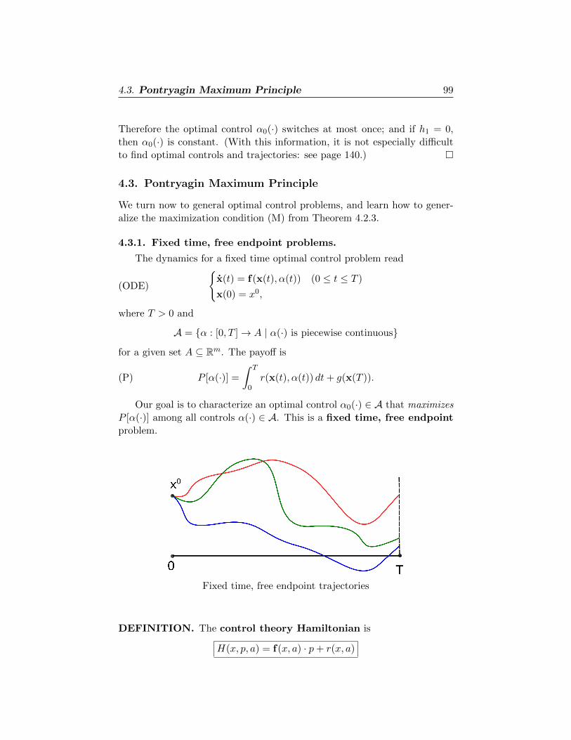
4.3. Pontryagin Maximum Principle 99
Therefore the optimal control α0(·) switches at most once; and if h1 = 0,
then α0(·) is constant. (With this information, it is not especially difficult
to find optimal controls and trajectories: see page 140.) �
4.3. Pontryagin Maximum Principle
We turn now to general optimal control problems, and learn how to gener-
alize the maximization condition (M) from Theorem 4.2.3.
4.3.1. Fixed time, free endpoint problems.
The dynamics for a fixed time optimal control problem read
(ODE)
{x(t) = f(x(t), α(t)) (0 ≤ t ≤ T )
x(0) = x0,
where T > 0 and
A = {α : [0, T ]→ A | α(·) is piecewise continuous}
for a given set A ⊆ Rm. The payoff is
(P) P [α(·)] =
∫ T
0r(x(t), α(t)) dt+ g(x(T )).
Our goal is to characterize an optimal control α0(·) ∈ A that maximizes
P [α(·)] among all controls α(·) ∈ A. This is a fixed time, free endpoint
problem.
x0
Fixed time, free endpoint trajectories
DEFINITION. The control theory Hamiltonian is
H(x, p, a) = f(x, a) · p+ r(x, a)
100 4. OPTIMAL CONTROL THEORY
for x, p ∈ Rn, a ∈ A. That is,
H(x, p, a) =n∑j=1
fj(x, a)pj + r(x, a).
NOTATION. (i) We write
p =
p1...
pn
, f =
f1...
fn
, ∇xf =
∂f1∂x1
. . . ∂f1∂xn
.... . .
...∂fn∂x1
. . . ∂fn∂xn
n×n
(ii) Since ∂H∂pi
= fi for i = 1, . . . , n, we have
(4.11) ∇pH = f .
Also, ∂H∂xi
=∑n
j=1∂fj∂xi
(x, a)pj + ∂r∂xi
(x, a) for i = 1, . . . , n. Consequently,
(4.12) ∇xH = (∇xf)T p+∇xr.
�
Next is our first version of the Pontryagin Maximum Principle.
THEOREM 4.3.1. (Fixed time, free endpoint PMP) Suppose α0(·)is an optimal control for the fixed time, free endpoint problem stated above,
and x0(·) is the corresponding solution to (ODE).
(i) Then there exists a function p0 : [0, T ] → Rn such that for times
0 ≤ t ≤ T we have
(ODE) x0(t) = ∇pH (x0(t),p0(t), α0(t)) ,
(ADJ) p0(t) = −∇xH (x0(t),p0(t), α0(t)) ,
(M) H (x0(t),p0(t), α0(t)) = maxa∈A
H(x0(t),p0(t), a),
and
(T) p0(T ) = ∇g (x0(T )) .
(ii) In addition,
(4.13) H (x0,p0, α0) is constant on [0, T ].
4.3. Pontryagin Maximum Principle 101
TERMINOLOGY. (i) We call
x0(t) =
x01(t)...
x0n(t)
, p0(t) =
p01(t)...
p0n(t)
the optimal state and costate at time t.
(ii) (ADJ) is the adjoint equation;
(iii) (M) is the maximization condition;
(iv) (T) is the terminal (or transversality) condition. �
REMARKS.
(i) To be more precise, (ODE), (ADJ) and (M) hold at times 0 < t < T
that are points of continuity of the optimal control α0(·).(ii) The most important assertion is (M). In practice, this usually allows
us to transform the infinite dimensional problem of finding an optimal con-
trol α0(·) ∈ A into a finite dimensional problem, at each time t, involving
maximization over A ⊆ Rm.
(iii) The costate equation (ADJ) and transversality condition (T) repre-
sent a sort of “back propagation” of information from the terminal time T .
We can also interpret the costate as a Lagrange multiplier corresponding to
the constraint that x0(·) solves (ODE).
Note that we specify the initial condition x0(0) = x0 for (ODE) and
the terminal condition p(T ) = ∇g(x0(T )) for (ADJ). Hence even if α0(·) is
known, solving this coupled system of equations can be tricky.
(iv) Remember from Section 1.4.3 that if H : Rn×Rn → R, H = H(x, p),
we call
(H)
{x = ∇pH(x,p)
p = −∇xH(x,p)
a Hamiltonian system of ODE. Notice that (ODE), (ADJ) are of this Hamil-
tonian form, except that now H = H(x, p, a) depends also on the control.
Observe furthermore that our assertion (4.13) is similar to (1.42) from The-
orem 1.4.1.
�
4.3.2. Other terminal conditions.
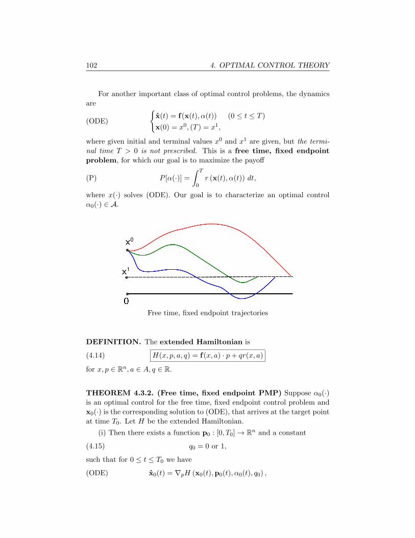
102 4. OPTIMAL CONTROL THEORY
For another important class of optimal control problems, the dynamics
are
(ODE)
{x(t) = f(x(t), α(t)) (0 ≤ t ≤ T )
x(0) = x0, (T ) = x1,
where given initial and terminal values x0 and x1 are given, but the termi-
nal time T > 0 is not prescribed. This is a free time, fixed endpoint
problem, for which our goal is to maximize the payoff
(P) P [α(·)] =
∫ T
0r (x(t), α(t)) dt,
where x(·) solves (ODE). Our goal is to characterize an optimal control
α0(·) ∈ A.
x0
Free time, fixed endpoint trajectories
DEFINITION. The extended Hamiltonian is
(4.14) H(x, p, a, q) = f(x, a) · p+ qr(x, a)
for x, p ∈ Rn, a ∈ A, q ∈ R.
THEOREM 4.3.2. (Free time, fixed endpoint PMP) Suppose α0(·)is an optimal control for the free time, fixed endpoint control problem and
x0(·) is the corresponding solution to (ODE), that arrives at the target point
at time T0. Let H be the extended Hamiltonian.
(i) Then there exists a function p0 : [0, T0]→ Rn and a constant
(4.15) q0 = 0 or 1,
such that for 0 ≤ t ≤ T0 we have
(ODE) x0(t) = ∇pH (x0(t),p0(t), α0(t), q0) ,
4.3. Pontryagin Maximum Principle 103
(ADJ) p0(t) = −∇xH (x0(t),p0(t), α0(t), q0) ,
and
(M) H (x0(t),p0(t), α0(t), q0) = maxa∈A
H(x0(t),p0(t), a, q0).
(ii) If q0 = 0, then
(4.16) p0(·) is not identically 0 on [0, T0].
(iii) Furthermore,
(T) H (x0,p0, α0, q0) = 0 on [0, T0].
REMARKS.
(i) So for the free time problem, we have the transversality condition
that H(x0,p0, α0, q0) = 0 at T0 and thus H(x0,p0, α0, q0) = 0 on the entire
interval [0, T0]. This generalization of our earlier Theorem 1.3.4 is stronger
than the corresponding assertion (4.13) for the fixed time problem.
(ii) But we for the free time problem, we must deal with an additional
Lagrange multiplier q0. We say the free time problem is normal if q0 = 1;
it is abnormal if q0 = 0. (The abnormal case is analogous to the existence
of the abnormal Lagrange multiplier γ0 = 0 in the F. John conditions for
finite dimensional optimization theory. See the Math 170 notes for more on
this.) �
Most free time problems are normal, and a simple assumption ensuring
this follows.
LEMMA 4.3.1. Suppose that the controllability assumption
(4.17) maxa∈A{f(x, a) · p} > 0 (x, p ∈ Rn, p 6= 0)
holds.
Then the associated free time, fixed endpoint control problem is normal.
Proof. If the problem were abnormal, then q0 = 0, p0 6≡ 0, and (T) would
assert
maxa∈A
H(x0(t),p0(t), a, q0) = maxa∈A{f(x0(t), a) · p0(t)} = 0
on [0, T0]. This however contradicts (4.17). �
104 4. OPTIMAL CONTROL THEORY
EXAMPLE. Here is an example of an abnormal problem with n = 2,
m = 1 and A = [−1, 1]. The dynamics are
(ODE)
{x1 = α2
x2 = 1
with the initial and terminal conditions
x(0) = x0 =
[0
0
], x(T ) = x1 =
[0
1
].
The goal is to maximize
P [α] =
∫ T
0αdt.
Now the only admissible control is α0(·) ≡ 0, which is therefore optimal,
and T0 = 1. The free time Hamiltonian is
H = p1a2 + p2 + qa.
Then (M) implies
0 =∂H
∂a= 2p0
1α0 + q0 = q0
and hence this problem is abnormal. Furthermore (ADJ) tells us that p0(·)is constant. If we take
p0 =
[−1
0
],
then p0 6= 0 and the conditions (M),(T) of Theorem 4.3.2 hold. This example
of course fails to satisfy (4.17). �
EXAMPLE. Let us check that Theorem 4.3.2 accords with our previous
maximum principle for the time optimal linear problem, as developed in
Section 4.2. We have
H(x, p, a, q) = (Mx+Na) · p− q (x, p ∈ Rn, a ∈ A, q ∈ R).
Select the vector h as in Theorem 4.2.3, and consider the system{p0(t) = −MTp0(t)
p0(0) = h,
the solution of which is
p0(t) = X−T (t)h.
We know from condition (M) in Theorem 4.2.3 that
h ·X−1(t)Nα0(t) = maxa∈A{h ·X−1(t)Na}.
4.3. Pontryagin Maximum Principle 105
But since p0(t)T = hTX−1(t), this says
p0(t) ·Nα0(t) = maxa∈A{p0(t) ·Na)},
Then
p0(t) · (Mx0(t) +Nα0(t))− q0 = maxa∈A{p0(t) · (Mx0(t) +Na)} − q0,
and this agrees with (M) from Theorem 4.3.2. �
Another sort of control problem has the dynamics
(ODE)
{x(t) = f(x(t), α(t)) (0 ≤ t ≤ T )
x(0) = x0, (T ) = x1
for fixed initial and terminal values x0 and x1 are given and a fixed terminal
time T > 0. This is a fixed time, fixed endpoint problem. The payoff
is again
(P) P [α(·)] =
∫ T
0r (x(t), α(t)) dt
THEOREM 4.3.3. (Fixed time, fixed endpoint PMP) Suppose α0(·)is an optimal control for the fixed time, fixed endpoint control problem and
x0(·) is the corresponding solution to (ODE). Let H be given by (4.14).
(i) Then there exists p0 : [0, T ]→ Rn and
(4.18) q0 = 0 or 1,
such that for all 0 ≤ t ≤ T :
x0(t) = ∇pH (x0(t),p0(t), α0(t), q0)(ODE)
p0(t) = −∇xH (x0(t),p0(t), α0(t), q0)(ADJ)
H (x0(t),p0(t), α0(t), q0) = maxa∈A
H(x0(t),p0(t), a, q0)(M)
(ii) Furthermore,
(4.19) H (x0,p0, α0, q0) is constant on [0, T ].
REMARKS.
(i) There is no transversality condition (T), since the fixed time, fixed
endpoint condition is too rigid to allow for any variations. As before, we
call the problem normal if q0 = 1 and abnormal if q0 = 0.
106 4. OPTIMAL CONTROL THEORY
(ii) We can deduce Theorem 4.3.3 from Theorem 4.3.2 by introducing a
new variable and rewriting the dynamics as{˙x(t) = f(x, α(t)) (0 ≤ t ≤ T )
x(0) = x0, x(T ) = x1,
for
x =
[x
xn+1
], f =
[f
1
], x0 =
[x0
0
], x1 =
[x1
T
].
This gives a free time, fixed endpoint problem. Consequently there exist
q0 and p0 : [0, T0]→ Rn+1 satisfying the conclusions of Theorem 4.3.2. We
write
p0 =
[p0
p0n+1
].
Then (ADJ) implies p0n+1 is constant on [0, T ]. Hence we may deduce from
(T) that H (x0,p0, α0, q0) = −p0n+1 is constant on [0, T ]. �
4.4. Applications
HOW TO USE THE PONTRYAGIN MAXIMUM PRINCIPLE
Step 1. Write down the Hamiltonian
H =
{f(x, a) · p+ r(x, a) for fixed time, free endpoint problems
f(x, a) · p+ qr(x, a) for fixed endpoint problems,
and calculate∂H
∂xi,∂H
∂pi(i = 1, . . . , n).
Step 2. Write down (ODE), (ADJ), (M) and, if appropriate, (T).
Step 3. Use the maximization condition (M) to compute, if possible,
α0(t) as a function of x0(t),p0(t).
Step 4. Now try to solve the coupled equations (ODE), (ADJ) and (T),
to find x0(·),p0(·) (and q0 for free time problems).
DEFINITION. If (M) does not uniquely determine α0(·) on some time
interval (where Step 3 therefore fails), we call that part of the trajectory of
x0(·) a singular arc. �
To simplify notation will mostly not write the subscripts “0” in the
following examples:
4.4. Applications 107
4.4.1. Simple linear-quadratic regulator.
The dynamics for the simplest version of the linear-quadratic regulator
read
(ODE)
{x = x+ α
x(0) = x0
for controls α : [0, T ]→ R. Here n = m = 1. The values of the controls are
unconstrained; that is, A = R. The payoff is quadratic in the state and the
control:
P [α(·)] = −∫ T
0x2 + α2 dt(P)
We therefore have a fixed time problem, for
f = x+ a, r = −x2 − a2, g = 0.
So the Hamiltonian is
H = f(x, a)p+ r(x, a) = (x+ a)p− x2 − a2.
Then∂H
∂p= x+ a,
∂H
∂x= p− 2x.
Consequently the equations for the PMP read
p = −∂H∂x
= 2x− p(ADJ)
H (x(t), p(t), α(t)) = maxa∈R{(x(t) + a)p(t)− x2(t)− a2}(M)
p(T ) = 0.(T)
We start with (M), and compute the value of α by noting the (uncon-
strained) maximum occurs where ∂H∂a = 0. Since ∂H
∂a = p− 2a, we see that
(4.20) α =p
2.
We use this information to rewrite (ODE), (ADJ):
(4.21)
{x = x+ p
2
p = 2x− p,
with the initial condition x(0) = x0 and the terminal condition p(T ) = 0.
To solve (4.21), let us suppose that we can write
(4.22) p(t) = d(t)x(t) (0 ≤ t ≤ T ),
108 4. OPTIMAL CONTROL THEORY
for some function d(·) that we must find. To find an equation for d(·), we
assume that (4.21) is valid and compute
p = dx+ dx
2x− p = dx+ d(x+
p
2
)(2− d)x = dx+ d
(x+
dx
2
).
Cancelling the x, we discover that we should select d(·) to solve the Riccati
equation
(4.23)
{d = 2− 2d− d2
2
d(T ) = 0.
Conversely, we check that if d(·) solves this Riccati equation and (4.22)
holds, then we have (4.21).
So we solve the terminal value problem for this nonlinear ODE, to get
the function d(·). Recalling then (4.22) and (4.20), we set
α0(t) =1
2d(t)x0(t) (0 ≤ t ≤ T ),
to synthesize an optimal feedback control, where x0(·) solves (ODE) for
this control: {x0 = x0 + 1
2dx0
x0(0) = x0.
REMARK. We can convert the Riccati equation (4.23) into a terminal
value problem for a linear second-order ODE, by writing
d =2b
b,
where {b = b− 2b
b(T ) = 1, b(T ) = 0.
�
4.4.2. Production and consumption.
Recall that for our production and consumption model on page 91, we
have the dynamics
(ODE)
{x = αx
x(0) = x0,
4.4. Applications 109
where the control α takes values in A = [0, 1]. We assume x0 > 0, and for
simplicity have taken the growth rate γ = 1. The payoff is
(P) P [α(·)] =
∫ T
0(1− α)x dt.
This fits within our fixed time PMP setting, for n = m = 1 and
f = ax, r = (1− a)x, g = 0.
Thus the Hamiltonian is
H = f(x, a)p+ r(x, a) = axp+ (1− a)x = x+ ax(p− 1);
and so∂H
∂p= ax,
∂H
∂x= 1 + a(p− 1).
Consequently,
(ADJ) p = −∂H∂x
= −1− α(p− 1).
Furthermore, we have
(M) H(x(t), p(t), α(t)) = max0≤a≤1
{x(t) + ax(t)(p(t)− 1)};
p(T ) = 0.(T)
We now carry out the maximization in (M), to learn how to compute an
optimal control α(·) in terms of the other functions:
(4.24) α(t) =
{1 if p(t) > 1
0 if p(t) < 1.
This follows since x(·) is positive on [0, T ].
We next use the above information to find x(·), p(·), and the idea is to
work backwards from the ending time. Since p(T ) = 0, it must be that
p(t) < 1 for some interval [t0, T ]. Thus (4.24) implies α = 0 for t0 ≤ t ≤ T .
We now analyze the various equations above on this interval (when α = 0):
x = 0,(ODE)
p = −1.(ADJ)
It follows that p(t) = T − t for t0 ≤ t ≤ T and p(t0) = 1 for
t0 = T − 1.
Next, we study the equations on the time interval 0 ≤ t ≤ t0:
x = αx,(ODE)
p = −1− α(p− 1).(ADJ)
110 4. OPTIMAL CONTROL THEORY
We see that p(t) > 1 if t1 ≤ t ≤ t0 for some time t1 < t0. But then (4.24)
says α = 1 for t1 ≤ t ≤ t0, and therefore
p = −1− (p− 1) = −p.
Since p(t0) = 1, it follows that p(t) = et0−t > 1 for t1 ≤ t < t0. Consequently
t1 = 0 and p(t) > 1 for 0 ≤ t < t0.
So the optimal control is
α0(t) =
{1 (0 ≤ t < T − 1)
0 (T − 1 < t ≤ T ).
This means that we should reinvest all of the output until the time t0 = T−1,
and thereafter consume all the output.
REMARK. The formulas (ODE) and (ADJ) from the PMP provide us
with explicit differential equations for the optimal states and costates, but we
do not in general have a differential equation for the corresponding optimal
control. Indeed, the production/consumption example above has a “bang-
bang” control, which is piecewise constant with a single jump, and so does
not solve any differential equation.
However the next two applications illustrate that we can sometimes es-
tablish ODE also for the controls. The idea will be to try to eliminate p(·)from the various equations. �
4.4.3. Ramsey consumption model.
For this example, x(t) ≥ 0 represents the capital at time t in some
economy and the control c(t) ≥ 0 is the consumption at time t. Given an
initial amount of capital x0, we want to maximize the utility of the total
consumption over a fixed time interval [0, T ], but are required to leave an
amount x1 of capital at time T .
We model the evolution of the economy by the equation
(ODE)
{x = f(x)− c (0 ≤ t ≤ T )
x(0) = x0, x(T ) = x1
for some appropriate function f : [0,∞) → [0,∞). So this is a fixed time,
fixed endpoint problem, which we assume is normal.
We wish to find an optimal consumption plan to maximize the payoff
(P) P [c(·)] =
∫ T
0ψ(c) dt,
where ψ : [0,∞)→ [0,∞), the consumption utility function, satisfies
ψ′ > 0, ψ′′ < 0.
4.4. Applications 111
We will not analyze this problem completely, but will show that we can
derive an ODE for an optimal consumption policy. The Hamiltonian is
H = (f(x)− c)p+ ψ(c),
and therefore
(ADJ) p = −f ′(x)p;
(M) H(x(t), p(t), c(t)) = maxc≥0{(f(x(t))− c)p(t) + ψ(c)}.
Now (M) implies for each time t that either
(4.25) c(t) = 0
or
(4.26) ψ′(c(t)) = p(t), c(t) > 0.
We ignore for the moment the first possibility and therefore suppose (4.26)
always holds. This and (ADJ) now imply
ψ′′(c)c = p = −f ′(x)p = −f ′(x)ψ′(c).
We thus obtain the Keynes-Ramsey consumption rule
(4.27) c = − ψ′(c)
ψ′′(c)f ′(x).
Then (ODE) and (4.27) provide us with a coupled system of equations for
an optimal control c0(·) and the corresponding state x0(·).
REMARKS. (i) Our analysis of this problem is however incomplete, since
we have ignored the state constraint that x(·) ≥ 0. If the consumption
plan c(·) computed above forces x(·) to start to go negative at some time t,
we are clearly in the case (4.25), rather than (4.26).
(ii) We have also not specified an initial condition for (4.27). This would
need to be selected so that x0(T ) = x1. �
4.4.4. Zermelo’s navigation problem.
Let x = [x1 x2]T denote the location of a boat moving at fixed speed V
through water that has a current (depending on position, but not changing
in time) given by the vector field v : R2 → R2, v = [v1 v2]T . We control the
boat by changing the direction in which it is pointing, determined by the
angle ξ from due east. The dynamics are therefore
(ODE)
{x1 = V cos ξ + v1(x1, x2)
x2 = V sin ξ + v2(x1, x2).
112 4. OPTIMAL CONTROL THEORY
How to we adjust the angle ξ(·) so as to steer the boat between two given
points x0, x1 in the least time?
This is a free time, fixed endpoint problem for which the control is ξ(·).We assume the problem is normal, and so the Hamiltonian is
H(x, p, ξ) = (V cos ξ + v1)p1 + (V sin ξ + v2)p2 − 1.
Consequently
(ADJ)
{p1 = −p1
∂v1∂x1− p2
∂v2∂x1
p2 = −p1∂v1∂x2− p2
∂v2∂x2
.
Furthermore, the maximization condition (M) implies
0 =∂H
∂ξ= V (−p1 sin ξ + p2 cos ξ).
Therefore
(4.28) ξ = arctanp2
p1,
(4.29) sin ξ =p2
(p21 + p2
2)12
, cos ξ =p1
(p21 + p2
2)12
.
For this problem, it turns out that we can eliminate the costates p1, p2
and so express the optimal dynamics in terms of x1, x2 and ξ. To do so, let
us use (4.28) and (ADJ) to compute
ξ =1
1 +(p2p1
)2
p2p1 − p2p1
p21
=p1
p21 + p2
2
(−p1
∂v1
∂x2− p2
∂v2
∂x2
)− p2
p21 + p2
2
(−p1
∂v1
∂x1− p2
∂v2
∂x1
).
Then (4.29) implies
(4.30) ξ = sin2 ξ∂v2
∂x1+ sin ξ cos ξ
(∂v1
∂x1− ∂v2
∂x2
)− cos2 ξ
∂v1
∂x2.
REMARK. The equations (ODE) and (4.30) provide us with a coupled
system for the optimal control ξ0(·) and optimal state x0(·). However we
do not have the initial condition for (4.30) and so must presumably rely
on numerical simulations to find a trajectory (if there is one) that passes
through the target point x1 at some time T0 > 0. �
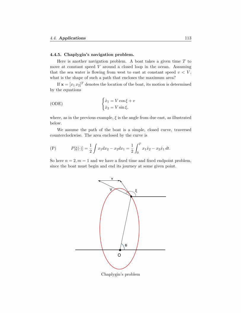
4.4. Applications 113
4.4.5. Chaplygin’s navigation problem.
Here is another navigation problem. A boat takes a given time T to
move at constant speed V around a closed loop in the ocean. Assuming
that the sea water is flowing from west to east at constant speed v < V ,
what is the shape of such a path that encloses the maximum area?
If x = [x1 x2]T denotes the location of the boat, its motion is determined
by the equations
(ODE)
{x1 = V cos ξ + v
x2 = V sin ξ,
where, as in the previous example, ξ is the angle from due east, as illustrated
below.
We assume the path of the boat is a simple, closed curve, traversed
counterclockwise. The area enclosed by the curve is
(P) P [ξ(·)] =1
2
∫x1dx2 − x2dx1 =
1
2
∫ T
0x1x2 − x2x1 dt.
So here n = 2,m = 1 and we have a fixed time and fixed endpoint problem,
since the boat must begin and end its journey at some given point.
O
ξV
Chaplygin’s problem
114 4. OPTIMAL CONTROL THEORY
Assuming the problem to be normal, we see that the Hamiltonian is
H = (V cos ξ + v)p1 + V sin ξ p2 +x1
2V sin ξ − x2
2(V cos ξ + v)
=(p1 −
x2
2
)(V cos ξ + v) +
(p2 +
x1
2
)V sin ξ.
Therefore the adjoint dynamics are
(ADJ)
{p1 = −V
2 sin ξ
p2 = 12(V cos ξ + v).
Using (ODE) and (ADJ), we see that
p1 +x2
2= 0, p2 −
x1
2= 0.
Consequently
p1 +x2
2= a, p2 −
x1
2= b
for appropriate constants a and b. Upon shifting coordinates if necessary,
we may assume a = b = 0; so that
(4.31) p1 +x2
2= 0, p2 −
x1
2= 0.
We next compute the optimal control angle from the maximization con-
dition (M), by setting
0 =∂H
∂ξ= −
(p1 −
x2
2
)V sin ξ +
(p2 +
x1
2
)V cos ξ.
Then (4.31) implies
(4.32) x1 cos ξ + x2 sin ξ = 0.
We now switch to polar coordinates, by writing
(4.33) x1 = r cos θ, x2 = r sin θ,
where θ is the polar angle, as drawn. Then (4.32) tells us that
0 = cos θ cos ξ + sin θ sin ξ = cos(ξ − θ).
Therefore ξ − θ is an odd multiple of π2 ; and so, from the picture,
(4.34) ξ = θ +π
2.
So the optimal control is to steer at right angles to the polar angle θ.
We show next that the optimal path is an ellipse. To do so, we first
differentiate (4.33):
x1 = r cos θ − rθ sin θ;
x2 = r sin θ + rθ cos θ.
4.4. Applications 115
This implies
r = x1 cos θ + x2 sin θ.
Now use (4.34) to compute
r − v
Vx2 = x1 cos θ + x2 sin θ − v
VV sin ξ
= (V cos ξ + v) cos θ + V sin ξ sin θ − v sin ξ
= (V cos ξ + v) sin ξ − V sin ξ cos ξ − v sin ξ
= 0.
Hence for some constant γ, we have
r − ex2 = γ,
where e = vV . Thus the motion lies on the projection into R2 of the inter-
section in R3 of the cone x3 = r with the plane x3 = ex2 + γ. This is an
ellipse, since e < 1.
REMARKS. If v = 0, the motion of the boat is a circle. We have thus
in particular shown that among smooth curves of fixed length, a circle en-
closes the maximum area. (More precisely, we have shown that if there
exists a smooth minimizer, it is a circle.) Compare this assertion with the
isoperimetric problem discussed on page 25. �
4.4.6. Optimal harvesting.
A simple ODE model for the population x of, say, fish in a lake is
x = γx(
1− x
k
),
where γ > 0 is the growth rate and k > 0 is the long term carrying capacity.
As t→∞ all positive solutions converge to the equilibrium level k.
Suppose now that we continually harvest the populations:
x = γx(
1− x
k
)− qαx,
where 0 ≤ α ≤ 1 represents our fishing effort and q > 0 its effectiveness.
Thus h = qαx is the harvest amount. The corresponding economic payoff
over a given time period [0, T ] is therefore
P [α(·)] =
∫ T
0ph− θα dt
where the constant p > 0 is the fixed price for fish and the constant θ > 0
represents a cost rate for our fishing efforts. We suppose the initial fish
population is x0, and we also require that after the fishing season is over,
the population of fish in the lake should be restored to a prescribed level x1.
116 4. OPTIMAL CONTROL THEORY
We rescale and make various simplifying choices of the parameters, to
reduce to the dynamics
(ODE)
{x = x(1− x)− qαxx(0) = x0, x(T ) = x1.
The payoff functional is
(P) P [α(·)] =
∫ T
0(x− θ)αdt.
We will assume
(4.35) 0 < θ < 1, q >1
2.
We say that a control α(·) is admissible if it satisfies the constraints 0 ≤α(·) ≤ 1 and the corresponding solution x(·) of the differential equation in
(ODE) with x(0) = x0 satisfies the terminal condition x(T ) = x1.
We wish to characterize an optimal fishing effort that maximizers the
payoff, subject to the dynamics (ODE). This is a fixed time, fixed endpoint
problem.
We assume our problem is normal, and consequently the Hamiltonian is
H = (x(1− x)− qax)p+ (x− θ)a.
Hence the adjoint dynamics are
(ADJ) p = −(1− 2x− qα)p− α
and the maximization condition is
(M) H(x(t), p(t), α(t)) = max0≤a≤1
{a(−qp(t)x(t) + x(t)− θ)}.
Equilibrium solutions. Let us first look for equilibrium solutions of
the above, that is, solutions of the form x(·) ≡ x∗, p(·) ≡ p∗, α(·) ≡ a∗ for
constants x∗, p∗, a∗ with 0 < a∗ < 1. This will be an algebra execise. In this
case, (ODE) and (ADJ) imply
(4.36) 1− x∗ − qa∗ = 0, (1− 2x∗ − qa∗)p∗ + a∗ = 0;
and, since 0 < a∗ < 1 solves (M), we must have
(4.37) −qp∗x∗ + x∗ − θ = 0.
The two equations (4.36) give a∗ = p∗x∗. Plugging this into (4.37) yields
a∗ = x∗−θq . Using this back in (4.36) and simplifying, we find
(4.38) x∗ =1 + θ
2, p∗ =
1− θq(1 + θ)
, a∗ =1− θ
2q.
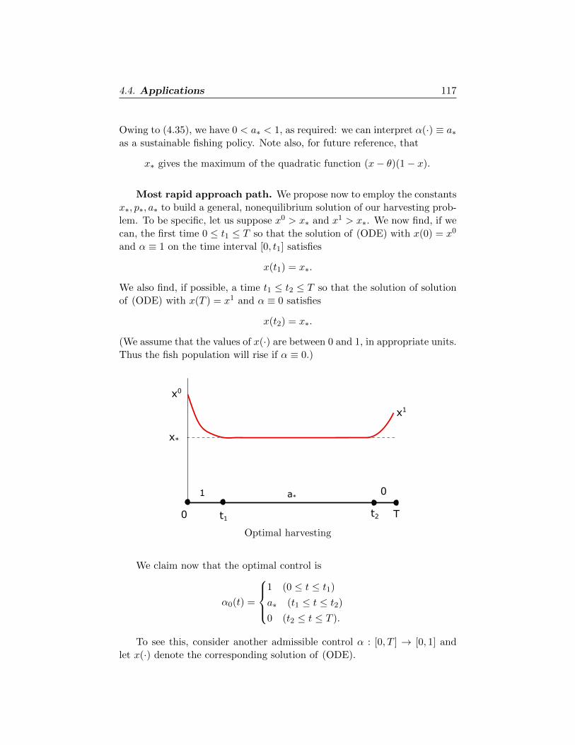
4.4. Applications 117
Owing to (4.35), we have 0 < a∗ < 1, as required: we can interpret α(·) ≡ a∗as a sustainable fishing policy. Note also, for future reference, that
x∗ gives the maximum of the quadratic function (x− θ)(1− x).
Most rapid approach path. We propose now to employ the constants
x∗, p∗, a∗ to build a general, nonequilibrium solution of our harvesting prob-
lem. To be specific, let us suppose x0 > x∗ and x1 > x∗. We now find, if we
can, the first time 0 ≤ t1 ≤ T so that the solution of (ODE) with x(0) = x0
and α ≡ 1 on the time interval [0, t1] satisfies
x(t1) = x∗.
We also find, if possible, a time t1 ≤ t2 ≤ T so that the solution of solution
of (ODE) with x(T ) = x1 and α ≡ 0 satisfies
x(t2) = x∗.
(We assume that the values of x(·) are between 0 and 1, in appropriate units.
Thus the fish population will rise if α ≡ 0.)
x*
x0
x1
t1t20 T
1 0a*
Optimal harvesting
We claim now that the optimal control is
α0(t) =
1 (0 ≤ t ≤ t1)
a∗ (t1 ≤ t ≤ t2)
0 (t2 ≤ t ≤ T ).
To see this, consider another admissible control α : [0, T ] → [0, 1] and
let x(·) denote the corresponding solution of (ODE).
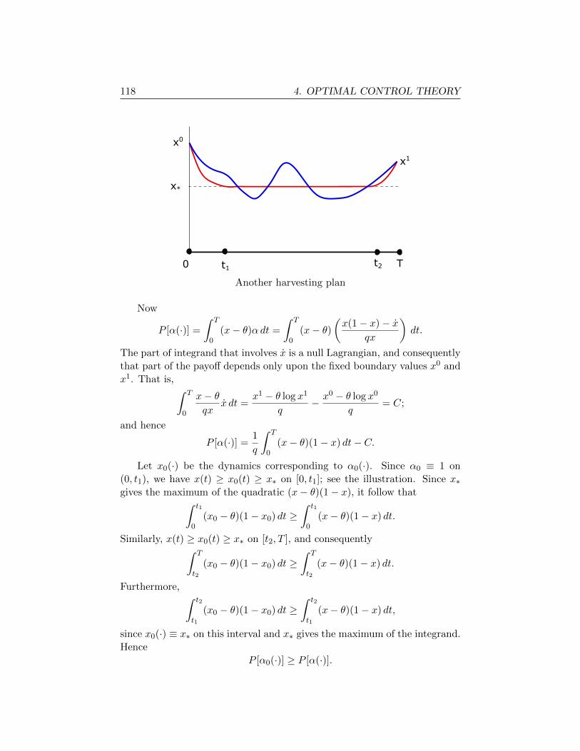
118 4. OPTIMAL CONTROL THEORY
x*
x0
x1
t1t20 T
Another harvesting plan
Now
P [α(·)] =
∫ T
0(x− θ)αdt =
∫ T
0(x− θ)
(x(1− x)− x
qx
)dt.
The part of integrand that involves x is a null Lagrangian, and consequently
that part of the payoff depends only upon the fixed boundary values x0 and
x1. That is, ∫ T
0
x− θqx
x dt =x1 − θ log x1
q− x0 − θ log x0
q= C;
and hence
P [α(·)] =1
q
∫ T
0(x− θ)(1− x) dt− C.
Let x0(·) be the dynamics corresponding to α0(·). Since α0 ≡ 1 on
(0, t1), we have x(t) ≥ x0(t) ≥ x∗ on [0, t1]; see the illustration. Since x∗gives the maximum of the quadratic (x− θ)(1− x), it follow that∫ t1
0(x0 − θ)(1− x0) dt ≥
∫ t1
0(x− θ)(1− x) dt.
Similarly, x(t) ≥ x0(t) ≥ x∗ on [t2, T ], and consequently∫ T
t2
(x0 − θ)(1− x0) dt ≥∫ T
t2
(x− θ)(1− x) dt.
Furthermore, ∫ t2
t1
(x0 − θ)(1− x0) dt ≥∫ t2
t1
(x− θ)(1− x) dt,
since x0(·) ≡ x∗ on this interval and x∗ gives the maximum of the integrand.
Hence
P [α0(·)] ≥ P [α(·)].
4.5. Proof of PMP 119
ECONOMIC INTERPRETATION. Observe that on [t1, t2] we have a
singular arc (see page 106), since the maximization condition (M) does not
determine there the value of the optimal control.
This example, adapted from Mesterton-Gibbons [MG], is an instance
of what economists call a most rapid approach path. It is optimal to
move as quickly as possible to where x = x∗ and then to stay on this path,
sometimes called a turnpike, as long as possible. �
REMARK. There are many more applications of the PMP discussed in
the texts listed in the References. See in particular Kamien–Schwartz [K-S],
Lee–Markus [L-M] and my old online lecture notes [E]. �
4.5. Proof of PMP
We present next a reasonably complete discussion of the ideas behind the
derivation of the Pontryagin Maximum Principle.
4.5.1. Simple control variations.
Recall that the response x(·) to a given control α(·) is the unique solution
of the system of differential equations:
(ODE)
{x(t) = f(x(t), α(t)) (t ≥ 0)
x(0) = x0.
We investigate in this section how certain simple changes in the control affect
the response.
DEFINITION. Fix a time s > 0 and a control parameter value a ∈ A.
Select 0 < ε < s and define then the modified control
αε(t) =
{a if s− ε < t < s
α(t) otherwise.
We call αε(·) a simple (or needle) variation of α(·).
Let xε(·) be the corresponding response to our system:
(ODEε)
{xε(t) = f(xε(t), αε(t)) (t > 0)
xε(0) = x0.
We want to understand how our choices of s and a cause xε(·) to differ from
x(·), for small ε > 0.
120 4. OPTIMAL CONTROL THEORY
NOTATION. Define the matrix-valued function A : [0,∞)→Mn×n by
A(t) = ∇xf(x(t), α(t)).
So the (i, j)-th entry of A(t) is
∂fi∂xj
(x(t), α(t)) (i, j = 1, . . . , n).
�
We first quote a standard perturbation assertion for ordinary differential
equations:
LEMMA 4.5.1. Let yε(·) solve the initial-value problem:{yε(t) = f(yε(t), α(t)) (t ≥ 0)
yε(0) = x0 + εy0 + o(ε).
Then
(4.39) yε(t) = x(t) + εy(t) + o(ε) as ε→ 0,
uniformly for t in compact subsets of [0,∞), where
(4.40)
{y(t) = A(t)y(t) (t ≥ 0)
y(0) = y0.
NOTATION. We write
o(ε)
to denote any expression gε such that
limε→0
gεε
= 0.
In words, if ε→ 0, then gε = o(ε) goes to zero “faster than ε”. �
Returning now to the dynamics (ODEε), we establish
LEMMA 4.5.2. Assume that s is a point of continuity for the control α(·).Then we have
(4.41) xε(t) = x(t) + εy(t) + o(ε) as ε→ 0,
uniformly for t in compact subsets of [0,∞), where
y(t) = 0 (0 ≤ t ≤ s)
and
(4.42)
{y(t) = A(t)y(t) (t ≥ s)y(s) = ys,
4.5. Proof of PMP 121
for
(4.43) ys = f(x(s), a)− f(x(s), α(s)).
NOTATION. We will sometimes write
y(t) = Y(t, s)ys (t ≥ s)
when (4.42) holds. �
Proof. Clearly xε(t) = x(t) for 0 ≤ t ≤ s− ε. For times s− ε ≤ t ≤ s, we
have
xε(t)− x(t) =
∫ t
s−εf(xε(r), a)− f(x(r), α(r)) dr.
Thus
xε(s)− x(s) = [f(x(s), a)− f(x(s), α(s))]ε+ o(ε).
On the time interval [s,∞), x(·) and xε(·) both solve the same ODE,
but with differing initial conditions given by
xε(s) = x(s) + εys + o(ε),
for ys defined by (4.43). According then to Lemma 4.5.1, we have
xε(t) = x(t) + εy(t) + o(ε) (t ≥ s),
the function y(·) solving (4.42). �
4.5.2. Fixed time problem.
Terminal payoff problem. We return to our usual dynamics
(ODE)
{x(t) = f(x(t), α(t)) (0 ≤ t ≤ T )
x(0) = x0,
and introduce the terminal payoff functional
(P) P [α(·)] = g(x(T )),
to be maximized. So for now we are taking the running payoff r ≡ 0.
We assume that α0(·) is an optimal control for this problem, correspond-
ing to the optimal response x0(·). The control theory Hamiltonian is
H(x, p, a) = f(x, a) · p,
and our task is find p0 : [0, T ]→ Rn such that (ADJ), (T) and (M) hold.
122 4. OPTIMAL CONTROL THEORY
We reintroduce the function A(·) = ∇xf(x0(·), α0(·)) and the control
variation αε(·), as in the previous section. We now define p0 : [0, T ]→ R to
be the unique solution of the terminal-value problem
(4.44)
{p0(t) = −AT (t)p0(t) (0 ≤ t ≤ T )
p0(T ) = ∇g(x0(T )).
This gives (ADJ) and (T), and so our goal is to establish the maximization
principle (M).
The main point is that p0(·) helps us calculate the variation of the
terminal payoff:
LEMMA 4.5.3. Assume 0 < s < T is a point of continuity for α0(·). Then
we have
(4.45)d
dεP [αε(·)]|ε=0 = [f(x0(s), a)− f(x0(s), α0(s))] · p0(s).
Proof. According to Lemma 4.5.2,
P [αε(·)] = g(xε(T )) = g(x0(T ) + εy(T ) + o(ε)),
where y(·) satisfies (4.42) for
ys = f(x0(s), a)− f(x0(s), α0(s)).
Thus
(4.46)d
dεP [αε(·)]|ε=0 = ∇g(x0(T )) · y(T ).
On the other hand, (4.42) and (4.44) imply
d
dt(p0(t) · y(t)) = p0(t) · y(t) + p0(t) · y(t)
= −AT (t)p0(t) · y(t) + p0(t) ·A(t)y(t)
= 0.
Hence
∇g(x0(T )) · y(T ) = p0(T ) · y(T ) = p0(s) · y(s) = p0(s) · ys.
Since ys = f(x0(s), a)−f(x0(s), α0(s)), this identity and (4.46) imply (4.45).
�
THEOREM 4.5.1. (PMP with no running costs) There exists a func-
tion p0 : [0, T ]→ Rn satisfying the adjoint dynamics (ADJ), the maximiza-
tion principle (M) and the terminal condition (T).
4.5. Proof of PMP 123
Proof. The adjoint dynamics and terminal condition are both in (4.44).
To confirm (M), fix 0 < s < T and a ∈ A, as above. Since the mapping
ε 7→ P [αε(·)] for 0 ≤ ε ≤ 1 has a maximum at ε = 0, we deduce from Lemma
4.5.3 that
0 ≥ d
dεP [αε(·)] = [f(x0(s), a)− f(x0(s), α0(s)] · p0(s).
Hence
H(x0(s),p0(s), a) = f(x0(s), a) · p0(s)
≤ f(x0(s), α0(s)) · p0(s) = H(x0(s),p0(s), α0(s))
for all a ∈ A and each time 0 < s < T that is a point of continuity for α0(·).This proves the maximization condition (M). �
General payoff problem. We next extend our analysis, to cover the
case that the payoff functional includes also a running payoff:
(P) P [α(·)] =
∫ T
0r(x(s), α(s)) ds+ g(x(T )).
The control theory Hamiltonian is now
H(x, p, a) = f(x, a) · p+ r(x, a)
and we must manufacture a costate function p0(·) satisfying (ADJ), (M)
and (T).
Adding a new variable. The trick is to introduce another variable
and thereby convert to the previous case. We consider the function xn+1 :
[0, T ]→ R given by
(4.47)
{xn+1(t) = r(x(t), α(t)) (0 ≤ t ≤ T )
xn+1(0) = 0,
where x(·) solves (ODE). It follows that
xn+1(T ) =
∫ T
0r(x(t), α(t)) dt.
Introduce next the new notation
x =
[x
xn+1
]=
x1...
xnxn+1
, x0 =
[x0
0
], p =
[p
pn+1
]=
p1...
pnpn+1
,
124 4. OPTIMAL CONTROL THEORY
(4.48) x(t) =
[x(t)
xn+1(t)
]=
x1(t)
...
xn(t)
xn+1(t)
, f(x, a) =
[f(x, a)
r(x, a)
]=
f1(x, a)
...
fn(x, a)
r(x, a)
and
(4.49) g(x) = g(x) + xn+1.
Then (ODE) and (4.47) produce the dynamics
(ODE)
{˙x(t) = f(x(t), α(t)) (0 ≤ t ≤ T )
x(0) = x0.
Consequently our control problem transforms into a new problem with no
running payoff and the terminal payoff functional
P [α(·)] = g(x(T )).
THEOREM 4.5.2. (PMP for fixed time, free endpoint problem)
There exists a function p0 : [0, T ] → Rn satisfying the adjoint dynamics
(ADJ), the maximization principle (M) and the terminal condition (T).
Proof. We apply Theorem 4.5.1, to obtain p0 : [0, T ] → Rn+1 satisfying
(M) for the Hamiltonian
H(x, p, a) = f(x, a) · p.
Also the adjoint equations (ADJ) hold, with the terminal transversality
condition
p0(T ) = ∇g(x0(T )).
But f does not depend upon the variable xn+1, and consequently the last
equation in (ADJ) reads
pn+10 (t) = − ∂H
∂xn+1= 0.
Since ∂g∂xn+1
= 1, we deduce that
p0n+1(t) ≡ 1.
As the last component of the vector function f is r, we then conclude from
(8.11) that
H(x, p, a) = f(x, a) · p+ r(x, a) = H(x, p, a).
Therefore
p0(t) =
p01(t)...
p0n(t)
4.5. Proof of PMP 125
satisfies (ADJ), (M) for the Hamiltonian H. �
4.5.3. Multiple control variations.
Proving the PMP for the free time, fixed endpoint problem is much
more difficult, since the result of a simple variation as above may produce
a response xε(·) that never hits the target point x1. We consequently need
to introduce more complicated control variations, discussed in this section.
DEFINITION. Let us select times 0 < s1 < s2 < · · · < sN , numbers
λ1, . . . , λN > 0, and also control parameters a1, a2, . . . , aN ∈ A. Write
(4.50) αε(t) =
{ak if sk − λkε ≤ t < sk (k = 1, . . . , N)
α(t) otherwise,
for ε > 0 taken so small that the intervals [sk − λkε, sk] do not overlap.
This is called a multiple variation of the control α(·).
We assume for this section that x(·) solves
(4.51)
{x(t) = f(x(t), α(t)) (0 ≤ t ≤ T )
x(0) = x0.
for some piecewise continuous control α(·), and that xε(·) is the response to
αε(·):
(4.52)
{xε(t) = f(xε(t), αε(t)) (0 ≤ t ≤ T )
xε(0) = x0.
NOTATION. (i) Define
ysk = f(x0(sk), ak))− f(x0(sk), α0(sk))
for k = 1, . . . , N .
(ii) As before, set A(·) = ∇xf(x0(·), α0(·)) and write
y(t) = Y(t, s)ys (t ≥ s)
to denote the solution of{y(t) = A(t)y(t) (t ≥ s)y(s) = ys,
where ys ∈ Rn is given.
Suitably modifying the proof of Lemma 4.5.2, we can establish
126 4. OPTIMAL CONTROL THEORY
LEMMA 4.5.4. We have
(4.53) xε(t) = x(t) + εy(t) + o(ε) as ε→ 0,
uniformly for t in compact subsets of [0,∞), wherey(t) = 0 (0 ≤ t ≤ s1)
y(t) =∑m
k=1 λkY(t, sk)ysk (sm ≤ t ≤ sm+1, m = 1, . . . , N − 1)
y(t) =∑N
k=1 λkY(t, sk)ysk (sN ≤ t).
DEFINITION. The cone of variations at time T is the set
K(T ) ={ N∑k=1
λkY(T, sk)ysk | N = 1, 2, . . . ,
λk > 0, ak ∈ A, 0 < s1 ≤ · · · ≤ sN < T}.
Observe that K(T ) is a convex cone in Rn, which according to Lemma
4.5.4 comprises all changes in the state x(T ), up to order ε, that we can
effect by multiple variations of the control α(·).
4.5.4. Fixed endpoint problem.
We turn now to the free time, fixed endpoint problem, characterized by
the constraint
x(T ) = x1,
where T = T [α(·)] is the first time that x(·) hits the given target point. The
payoff functional is
P [α(·)] =
∫ T
0r(x(s), α(s)) ds.
Adding a new variable. As before, we introduce the function xn+1 :
[0, T ]→ R defined by (4.47) and recall the notation (4.48), (4.49), with
g(x) = xn+1.
Our problem is therefore to find controlled dynamics satisfying
(ODE)
{˙x(t) = f(x(t), α(t)) (0 ≤ t ≤ T )
x(0) = x0,
and maximizing
(P) g(x(T )) = xn+1(T ),
T being the first time that x(T ) = x1. In other words, the first n components
of x(T ) are prescribed, and we want to maximize the (n+ 1)-th component.
4.5. Proof of PMP 127
We assume that α0(·) is an optimal control for this problem, corre-
sponding to the optimal trajectory x0(·) and the time T0; our task is to
construct the corresponding costate p0(·), satisfying (ADJ) and the maxi-
mization principle (M).
Using the cone of variations. Our program for building the costate
depends upon our taking multiple variations, as in the previous section, and
understanding the resulting cone of variations K = K(T0).
Let K0 denote the (perhaps empty) interior of K. Put
en+1 = [0 · · · 0 1]T ∈ Rn+1.
Here is the key observation:
LEMMA 4.5.5. We have
(4.54) en+1 /∈ K0.
Proof. 1. If (4.54) were false, there would exist n+ 1 linearly independent
vectors z1, . . . , zn+1 ∈ K such that
en+1 =n+1∑k=1
λkzk
with constants λk > 0 and
zk = Y(T0, sk)ysk
for appropriate times 0 < s1 < s1 < · · · < sn+1 < T0, where
ysk = f(x(sk), ak))− f(x(sk), α(sk)) (k = 1, . . . , n+ 1).
2. We will next construct a control αε(·), having the multiple variation
form (4.50), with corresponding response xε(·) = [xε(·)T xεn+1(·)]T satisfying
(4.55) xε(T0) = x1
and
(4.56) xεn+1(T0) > x0n+1(T0).
This will be a contradiction to the optimality of the control α0(·).
3. Introduce for small η > 0 the closed and convex set
C =
{z =
n+1∑k=1
λkzk | 0 ≤ λk ≤ η
}.
Since the vectors z1, . . . , zn+1 are independent, C has an interior.
128 4. OPTIMAL CONTROL THEORY
Now define for small ε > 0 the mapping
(4.57) Φε : C → Rn+1
by setting
Φε(z) = xε(T0)− x0(T0)
for z =∑n+1
k=1 λkzk, where xε(·) solves (4.52) for the control αε(·) defined by
(4.50).
We assert that if µ, η, ε > 0 are small enough, then we can solve the
nonlinear equation
(4.58) Φε(z) = µen+1 = [0 · · · 0µ]T
for some z ∈ C. To see this, note that
|Φε(z)− z| = |xε(T0)− x0(T0)− z|= o(|z|)
< |z − µen+1| for all z ∈ ∂C.
We now apply the topological theorem from Appendix F, to find a point
z ∈ C satisfying (4.58). Then
xε(T0) = x0(T0) + µen+1,
and hence (4.55), (4.56) hold. This gives the desired contradiction, provided
en+1 ∈ K0. �
Existence of the costate.
THEOREM 4.5.3. (PMP for free time, fixed endpoint problem)
There exists a function p0 : [0, T0]→ Rn and a number
q0 = 0 or 1
satisfying the statements (ADJ), (M) and (T) of the free time, fixed endpoint
PMP.
Proof. 1. Since en+1 /∈ K0 according to Lemma 4.5.5, there exists a nonzero
vector w ∈ Rn+1 such that
(4.59) w · z ≤ 0 for all z ∈ K
and
(4.60) w · en+1 = wn+1 ≥ 0.
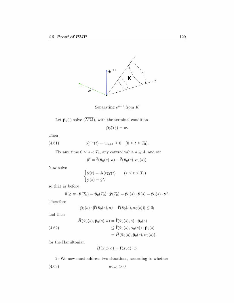
4.5. Proof of PMP 129
Separating en+1 from K
Let p0(·) solve (ADJ), with the terminal condition
p0(T0) = w.
Then
(4.61) pn+10 (t) = wn+1 ≥ 0 (0 ≤ t ≤ T0).
Fix any time 0 ≤ s < T0, any control value a ∈ A, and set
ys = f(x0(s), a)− f(x0(s), α0(s)).
Now solve {˙y(t) = A(t)y(t) (s ≤ t ≤ T0)
y(s) = ys;
so that as before
0 ≥ w · y(T0) = p0(T0) · y(T0) = p0(s) · y(s) = p0(s) · ys.
Therefore
p0(s) · [f(x0(s), a)− f(x0(s), α0(s))] ≤ 0;
and then
(4.62)
H(x0(s), p0(s), a) = f(x0(s), a) · p0(s)
≤ f(x0(s), α0(s)) · p0(s)
= H(x0(s), p0(s), α0(s)),
for the Hamiltonian
H(x, p, a) = f(x, a) · p.
2. We now must address two situations, according to whether
(4.63) wn+1 > 0
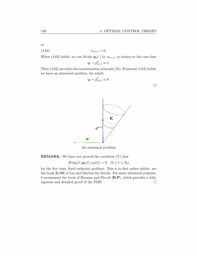
130 4. OPTIMAL CONTROL THEORY
or
(4.64) wn+1 = 0.
When (4.63) holds, we can divide p0(·) by wn+1, to reduce to the case that
q0 = p0n+1 ≡ 1.
Then (4.62) provides the maximization principle (M). If instead (4.64) holds,
we have an abnormal problem, for which
q0 = p0n+1 ≡ 0.
�
An abnormal problem
REMARK. We have not proved the condition (T) that
H(x0(t),p0(t), α0(t)) = 0 (0 ≤ t ≤ T0)
for the free time, fixed endpoint problem. This is in fact rather subtle: see
the book [L-M] of Lee and Markus for details. For more advanced students,
I recommend the book of Bressan and Piccoli [B-P], which provides a fully
rigorous and detailed proof of the PMP. �
Chapter 5
DYNAMICPROGRAMMING
5.1. Hamilton-Jacobi-Bellman equation
We next show how to use value functions in optimal control theory, within
the context of dynamic programming. This approach depends upon the
mathematical idea that it is sometimes easier to solve a given problem by
incorporating it within a larger class of problems.
We want to adapt some version of this insight to the vastly complicated
setting of control theory. For this, fix a terminal time T > 0 and then look
at the controlled dynamics{x(s) = f(x(s), α(s)) (0 < s < T )
x(0) = x0,
with the associated payoff functional
P [α(·)] =
∫ T
0r(x(s), α(s)) ds+ g(x(T ))
for the free endpoint problem.
The new idea is to embed this into a larger family of similar problems,
by varying the starting times and starting points:
(ODE)
{x(s) = f(x(s), α(s)) (t ≤ s ≤ T )
x(t) = x,
131
132 5. DYNAMIC PROGRAMMING
(P) Px,t[α(·)] =
∫ T
tr(x(s), α(s)) ds+ g(x(T )).
We will consider the above problems for all choices of starting times 0 ≤ t ≤T and all initial points x ∈ Rn.
5.1.1. Derivation.
DEFINITION. For x ∈ Rn, 0 ≤ t ≤ T , we define the value function
v : Rn × [0, T ] → R to be the greatest payoff possible if we start at x ∈ Rnat time t. In other words,
v(x, t) = supα(·)∈A
Px,t[α(·)]
for x ∈ Rn, 0 ≤ t ≤ T .
REMARK. Then
v(x, T ) = g(x) (x ∈ Rn),
since if we start at time T at the point x, we must immediately stop and so
collect the payoff g(x). �
Our task in this section is to show that the value function v so defined
satisfies a certain nonlinear partial differential equation. Our derivation will
be based upon the reasonable principle that it is better to act optimally from
the beginning, rather than to act arbitrarily for a while and then later act
optimally. We will convert this philosophy of life into mathematics.
To simplify, we hereafter suppose that the set A of control parameter
values is closed and bounded.
THEOREM 5.1.1. Assume that the value function v is a continuously
differentiable function of the variables (x, t). Then v solves the Hamilton–
Jacobi–Bellman partial differential equation
(HJB)∂v
∂t(x, t) + max
a∈A{f(x, a) · ∇xv(x, t) + r(x, a)} = 0
for x ∈ Rn, 0 ≤ t < T , with the terminal condition
(5.1) v(x, T ) = g(x) (x ∈ Rn).
DEFINITION. The PDE Hamiltonian is
H(x, p) = maxa∈A
H(x, p, a) = maxa∈A{f(x, a) · p+ r(x, a)}
5.1. Hamilton-Jacobi-Bellman equation 133
where x, p ∈ Rn. Hence we can write (HJB) as
∂v
∂t+H(x,∇xv) = 0 in Rn × [0, T ].
�
Proof. 1. Let x ∈ Rn, 0 ≤ t < T , and note that, as always in this course,
A = {α(·) : [0, T ]→ A | α(·) is piecewise continuous}.
Pick any parameter a ∈ A and let ε > 0 be so small that t+ε ≤ T . Suppose
we start at x at time t, and use the constant control
α(s) = a
for times t ≤ s ≤ t + ε. The dynamics then arrive at the point x(t + ε).
Suppose now that we switch to an optimal control (assuming it exists) and
employ it for the remaining times t+ ε ≤ s ≤ T .
What is the payoff of this procedure? Now for t ≤ s ≤ t+ ε, we have
(5.2)
{x(s) = f(x(s), a)
x(t) = x.
The payoff for this time period is∫ t+εt r(x(s), a) ds. Furthermore, the payoff
incurred from time t+ ε to T is v(x(t+ ε), t+ ε), according to the definition
of the payoff function v(·). Hence the total payoff is∫ t+ε
tr(x(s), a) ds+ v(x(t+ ε), t+ ε).
But the greatest possible payoff if we start from (x, t) is v(x, t). Therefore∫ t+ε
tr(x(s), a) ds+ v(x(t+ ε), t+ ε) ≤ v(x, t).
2. Next rearrange (5.5) and divide by ε > 0:
v(x(t+ ε), t+ ε)− v(x, t)
ε+
1
ε
∫ t+ε
tr(x(s), a) ds ≤ 0.
Hence∂v
∂t(x, t) +∇xv(x(t), t) · x(t) + r(x(t), a) ≤ o(1),
as ε→ 0. But recall that x(·) solves (5.2). We employ this above and send
ε→ 0, to discover
∂v
∂t(x, t) + f(x, a) · ∇xv(x, t) + r(x, a) ≤ 0.
134 5. DYNAMIC PROGRAMMING
This inequality holds for all control parameters a ∈ A, and consequently
(5.3) maxa∈A
{∂v
∂t(x, t) + f(x, a) · ∇xv(x, t) + r(x, a)
}≤ 0.
3. We next demonstrate that in fact the maximum above equals zero.
To see this, suppose α0(·), x0(·) are optimal for the problem above. Let us
utilize the optimal control α0(·) for t ≤ s ≤ t+ ε. The payoff is∫ t+ε
tr(x0(s), α0(s)) ds
and the remaining payoff is v(x0(t+ε), t+ε). Consequently, the total payoff
is ∫ t+ε
tr(x0(s), α0(s)) ds+ v(x0(t+ ε), t+ ε) = v(x, t).
Rearrange and divide by ε:
v(x0(t+ ε), t+ ε)− v(x, t)
ε+
1
ε
∫ t+ε
tr(x0(s), α0(s)) ds = 0.
Let ε→ 0 and suppose α0(t) = a0 ∈ A. Then
∂v
∂t(x, t) +∇xv(x, t) · f(x, a0) + r(x, a0) = 0.
This and (5.3) confirm that v solves the Hamilton-Jacobi-Bellman PDE. �
REMARK. Dynamic programming applies as well to free time, fixed end-
point optimal control problems. To be specific, let us suppose that we are
required to steer from a point x ∈ Rn to the origin under the dynamics
(ODE)
{x(s) = f(x(s), α(s)) (0 ≤ s ≤ T )
x(0) = x, x(T ) = 0,
so as to maximize the payoff
(P) Px[α(·)] =
∫ T
0r(x(s), α(s)) ds.
Here the terminal time T is free.
The corresponding value function is
v(x) = supα(·)∈A
Px[α(·)] (x ∈ Rn).
5.1. Hamilton-Jacobi-Bellman equation 135
Arguing as above, we discover that if the value function v is continuously dif-
ferentiable, it solves the (stationary) Hamilton-Jacobi-Bellman equa-
tion
(HJB) maxa∈A{f(x, a) · ∇v(x) + r(x, a)} = 0
for x ∈ Rn \ {0} and
v(0) = 0.
�
5.1.2. Optimality.
HOW TO USE DYNAMIC PROGRAMMING
For fixed time optimal control problems as in Section 5.1.1, we carry out
these steps to synthesize an optimal control:
Step 1: Try to solve the HJB equation, with the terminal condition
(5.1), and thereby find the value function v.
Step 2: Use the value function v and the Hamilton–Jacobi–Bellman
PDE to design an optimal control α0(·), as follows. Define for each point
y ∈ Rn and each time 0 ≤ s ≤ T ,
a(y, s) ∈ A
to be a parameter value where the maximum in HJB is attained at the point
(y, s). In other words, select a(y, s) ∈ A so that
(5.4)∂v
∂t(y, s) + f(y, a(y, s)) · ∇xv(y, s) + r(y, a(y, s)) = 0.
Step 3: Next, solve the following ODE, assuming a(·) is sufficiently
regular to do so:
(5.5)
{x0(s) = f(x0(s), a(x0(s), s)) (t ≤ s ≤ T )
x0(t) = x.
Step 4: Finally, define the optimal feedback control
(5.6) α0(s) = a(x0(s), s) (t ≤ s ≤ T ),
so that we can rewrite (5.5) as{x0(s) = f(x0(s), α0(s)) (t ≤ s ≤ T )
x0(t) = x.
In particular, if the state of system is y at time s, we use the control which
at time s takes on a parameter value a = a(y, s) ∈ A for which the maximum
in HJB is obtained.
136 5. DYNAMIC PROGRAMMING
THEOREM 5.1.2. For each starting time 0 ≤ t < T and initial point
x ∈ Rn, the control α0(·) defined by (5.5) and (5.6) is optimal.
Proof. We have
Px,t[α0(·)] =
∫ T
tr(x0(s), α0(s)) ds+ g(x0(T )).
Then (5.4) and (5.6) imply
Px,t[α0(·)] =
∫ T
t
(−∂v∂t
(x0(s), s)− f(x0(s), α0(s)) · ∇xv(x0(s), s)
)ds+ g(x0(T ))
= −∫ T
t
∂v
∂t(x0(s), s) +∇xv(x0(s), s) · x0(s) ds+ g(x0(T ))
= −∫ T
t
d
dsv(x0(s), s) ds+ g(x0(T ))
= −v(x0(T ), T ) + v(x0(t), t) + g(x0(T ))
= v(x, t)
= supα(·)∈A
Px,t[α(·)].
Hence α0(·) is optimal, as asserted. �
REMARKS.
(i) Notice that v acts here as a calibration function that we use to es-
tablish optimality.
(ii) We can similarly design optimal controls for free time problems by
solving the stationary HJB equation. �
5.2. Applications
Applying dynamic programming is usually quite tricky, as it requires us to
solve a nonlinear PDE and this is often very difficult. The main hope, as
we will see in the following examples, is to try to guess the form of v, to
plug this guess into the HJB equation and then to adjust various constants
and auxiliary functions, to ensure that we have an actual solution. (Alter-
natively, we could compute the solution of the terminal-value problem for
HJB numerically.)
To simplify notation will not write the subscripts “0” in the subsequent
examples.
5.2. Applications 137
5.2.1. General linear-quadratic regulator. For this important prob-
lem, we are given matrices M,B,D ∈ Mn×n, N ∈ Mn×m, C ∈ Mm×m; and
assume
B,C,D are symmetric,
with
B,D � 0, C � 0.
In particular, C is invertible.
We take the linear dynamics
(ODE)
{x(s) = Mx(s) +Nα(s) (t ≤ s ≤ T )
x(t) = x,
for which we want to minimize the quadratic cost functional∫ T
tx(s)TBx(s) + α(s)TCα(s) ds+ x(T )TDx(T ).
So we must maximize the payoff
(P) Px,t[α(·)] = −∫ T
tx(s)TBx(s) + α(s)TCα(s) ds− x(T )TDx(T ).
The control values are unconstrained, meaning that the control parameter
values can range over all of A = Rm.
We employ dynamic programming to design an optimal control. To
carry out this plan, we first figure out the structure of the HJB equation{∂v∂t + maxa∈Rm {f · ∇xv + r} = 0 in Rn × [0, T ]
v = g on Rn × {t = T},
for
f = Mx+Na, r = −xTBx− aTCa, g = −xTDx.We rewrite the PDE as
(5.7)∂v
∂t+ maxa∈Rm
{(∇v)TNa− aTCa}+ (∇v)TMx− xTBx = 0,
and note that we have the terminal condition
(5.8) v(x, T ) = −xTDx.
To compute the maximum above, define
Q(a) = (∇v)TNa− aTCa,
and solve∂Q
∂aj=
n∑i=1
vxinij − 2aicij = 0 (j = 1, . . . , n).
138 5. DYNAMIC PROGRAMMING
Then (∇xv)TN = 2aTC, and thus 2Ca = NT∇xv, since C is symmetric.
Therefore
(5.9) a =1
2C−1NT∇xv.
This is the point at which the maximum in HJB occurs, which we now insert
into (5.7):
(5.10)∂v
∂t+
1
4(∇v)TNC−1NT∇v + (∇v)TMx− xTBx = 0.
Solving the HJB equation. Our task now is to solve this nonlinear PDE,
with the terminal condition (5.8). We guess that our solution has the form
(5.11) v(x, t) = xTK(t)x
for some appropriate symmetric n×n-matrix valued function K(·) for which
(5.12) K(T ) = −D.
Let us compute
(5.13)∂v
∂t= xT K(t)x, ∇xv = 2K(t)x.
We now insert our guess v = xTK(t)x into (5.10), to discover that
xT {K(t) +K(t)NC−1NTK(t) + 2K(t)M −B}x = 0.
Since
2xTKMx = xTKMx+ [xTKMx]T
= xTKMx+ xTMTKx,
the foregoing becomes
xT {K +KNC−1NTK +KM +MTK −B}x = 0.
This identity will hold providedK(·) satisfies the matrix Riccati equa-
tion
(R) K(t) +K(t)NC−1NTK(t) +K(t)M +MTK(t) = B
on the interval [0, T ].
In summary, once we solve the Riccati equation (R) with the terminal
condition (5.12), we can then use (5.9) and (5.13) to construct the optimal
feedback control
α0(t) = C−1NTK(t)x0(t).
�
5.2. Applications 139
5.2.2. Rocket railway car. In view of our discussion on page 98, the
rocket railway problem is actually quite easy to solve. However it is also
instructive to see how dynamic programming applies.
The equations of motion are
x =
[0 1
0 0
]x +
[0
1
]α, −1 ≤ α ≤ 1
for n = 2, and
Px[α(·)] = − time to reach the origin = −∫ T
01 dt = −T.
Then the value function v(x) is minus the least time it takes to get to
the origin from the point x = [x1 x2]T ; and the corresponding stationary
HJB equation is
maxa∈A{f · ∇v + r} = 0
for
A = [−1, 1], f =
[x2
a
], r = −1.
Therefore
max|a|≤1
{x2
∂v
∂x1+ a
∂v
∂x2− 1
}= 0;
and consequently the Hamilton-Jacobi-Bellman equation is
(HJB)
{x2
∂v∂x1
+∣∣∣ ∂v∂x2 ∣∣∣ = 1 in R2 \ {0}
v(0) = 0.
Solution of HJB equation. We introduce the regions
I := {(x1, x2) | x1 > −12x2|x2|},
II := {(x1, x2) | x1 < −12x2|x2|},
and define
(5.14) v(x) =
−x2 − 2(x1 + 1
2x22
) 12 in Region I
x2 − 2(−x1 + 1
2x22
) 12 in Region II.
We could have derived this formula for v using the ideas in the next example,
but for now let us just show that v really solves HJB.
In Region I we compute
∂v
∂x1= −
(x1 +
x22
2
)− 12
,∂v
∂x2= −1−
(x1 +
x22
2
)− 12
x2;
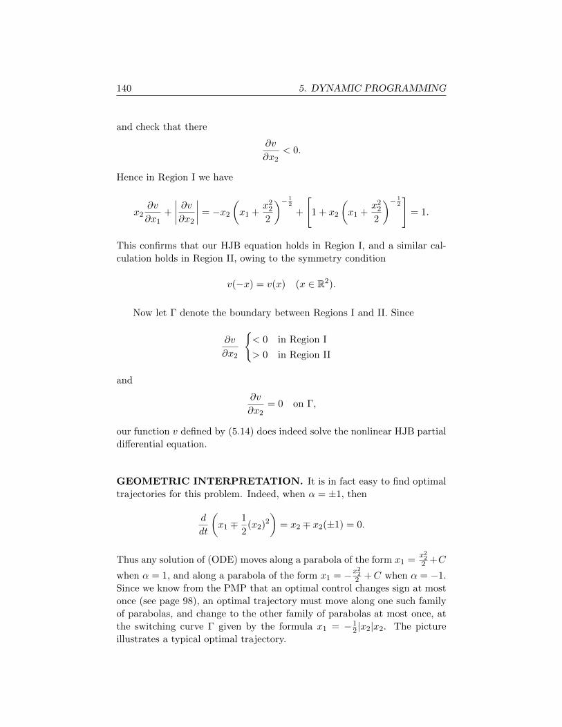
140 5. DYNAMIC PROGRAMMING
and check that there
∂v
∂x2< 0.
Hence in Region I we have
x2∂v
∂x1+
∣∣∣∣ ∂v∂x2
∣∣∣∣ = −x2
(x1 +
x22
2
)− 12
+
[1 + x2
(x1 +
x22
2
)− 12
]= 1.
This confirms that our HJB equation holds in Region I, and a similar cal-
culation holds in Region II, owing to the symmetry condition
v(−x) = v(x) (x ∈ R2).
Now let Γ denote the boundary between Regions I and II. Since
∂v
∂x2
{< 0 in Region I
> 0 in Region II
and
∂v
∂x2= 0 on Γ,
our function v defined by (5.14) does indeed solve the nonlinear HJB partial
differential equation.
GEOMETRIC INTERPRETATION. It is in fact easy to find optimal
trajectories for this problem. Indeed, when α = ±1, then
d
dt
(x1 ∓
1
2(x2)2
)= x2 ∓ x2(±1) = 0.
Thus any solution of (ODE) moves along a parabola of the form x1 =x222 +C
when α = 1, and along a parabola of the form x1 = −x222 +C when α = −1.
Since we know from the PMP that an optimal control changes sign at most
once (see page 98), an optimal trajectory must move along one such family
of parabolas, and change to the other family of parabolas at most once, at
the switching curve Γ given by the formula x1 = −12 |x2|x2. The picture
illustrates a typical optimal trajectory.
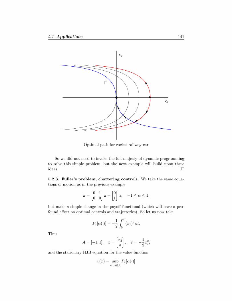
5.2. Applications 141
x1
x2
Γ
Optimal path for rocket railway car
So we did not need to invoke the full majesty of dynamic programming
to solve this simple problem, but the next example will build upon these
ideas. �
5.2.3. Fuller’s problem, chattering controls. We take the same equa-
tions of motion as in the previous example
x =
[0 1
0 0
]x +
[0
1
]α, −1 ≤ α ≤ 1,
but make a simple change in the payoff functional (which will have a pro-
found effect on optimal controls and trajectories). So let us now take
Px[α(·)] = −1
2
∫ T
0(x1)2 dt.
Thus
A = [−1, 1], f =
[x2
a
], r = −1
2x2
1;
and the stationary HJB equation for the value function
v(x) = supα(·)∈A
Px[α(·)]
142 5. DYNAMIC PROGRAMMING
is now
(HJB)
{x2
∂v∂x1
+∣∣∣ ∂v∂x2 ∣∣∣ = 1
2x21 in R2 \ {0}
v(0) = 0.
Solving the HJB equation. Using the definition of the value function,
we can check that it satisfies the two symmetry conditions:
(5.15) v(−x) = v(x) (x ∈ R2)
and
(5.16) v(λ2x1, λx2) = λ5v(x1, x2) (x ∈ R2, λ > 0).
To verify (5.16), suppose that x = [x1 x2]T is an optimal trajectory
starting at the point x0 = [x01 x
02]T , corresponding to an optimal control α.
Then if λ > 0 and we start instead at the point x0λ = [λ2x0
1 λx02]T , optimal
trajectories and control are
xλ(t) = [λ2x1( tλ)λx2( tλ)]T , αλ(t) = α( tλ).
Since
P [αλ(·)] = −1
2
∫ Tλ
0(x1λ)2dt = −λ
4
2
∫ Tλ
0(x1)2( tλ)dt = λ5P [α(·)],
the scaling identity (5.16) holds.
Now (5.16) and the previous example suggest that the optimal switching
should occur on the boundary Γ between two regions of the form
I := {(x1, x2) | x1 > −βx2|x2|},II := {(x1, x2) | x1 < −βx2|x2|},
for some as yet unknown constant β > 0.
Still motivated by the previous example, we look a function v for which
the scaling symmetry (5.16) holds,
(5.17)∂v
∂x2< 0 in Region I,
∂v
∂x2= 0 on Γ,
and v solves the linear PDE
(5.18) x2∂v
∂x1− ∂v
∂x2=
1
2(x1)2 in Region I.
In view (5.16), let us start by looking for a particular solution of (5.18)
having the polynomial form
v = Ax52 +Bx1x
32 + Cx2
1x2.
5.2. Applications 143
If we plug this guess into (5.18) and match coefficients, we discover that
v = − 1
15x5
2 −1
3x1x
32 −
1
2x2
1x2
is a solution. Now the general solution of the linear, homogeneous PDE
x2∂w
∂x1− ∂w
∂x2= 0
has the form
w = f
(x1 +
1
2x2
2
).
Hence the general solution of (5.18) is
v = − 1
15x5
2 −1
3x1x
32 −
1
2x2
1x2 + f
(x1 +
1
2x2
2
).
In order to satisfy the scaling condition (5.16), we take f to be homogeneous
and so have
(5.19) v = − 1
15x5
2 −1
3x1x
32 −
1
2x2
1x2 − γ(x1 +
1
2x2
2
) 52
for another as yet unknown constant γ > 0.
We want next to adjust the constants β, γ so that ∂v∂x2
= 0 on Γ. Now
(5.20)∂v
∂x2= −1
3x4
2 − x1x22 −
1
2x2
1 −5γ
2
(x1 +
1
2x2
2
) 32
x2.
Therefore on Γ+ = {x1 = −βx22, x2 > 0}, we have
(5.21)∂v
∂x2= x4
2
[−1
3+ β − 1
2β2 − 5γ
2
(−β +
1
2
) 32
];
and on Γ− = {x1 = βx22, x2 < 0}, we have
(5.22)∂v
∂x2= x4
2
[−1
3− β − 1
2β2 +
5γ
2
(β +
1
2
) 32
].
Consequently, we need to select β, γ so that
(5.23)
−13 + β − 1
2β2 − 5γ
2
(−β + 1
2
) 32 = 0
−13 − β −
12β
2 + 5γ2
(β + 1
2
) 32 = 0.
Solving each equation for γ, we see (5.23) implies
φ(β) =
(β +
1
2
) 32(−1
3+ β − 1
2β2
)−(−β +
1
2
) 32(
1
3+ β +
1
2β2
)= 0.
Since
φ(0) < 0, φ(12) > 0,
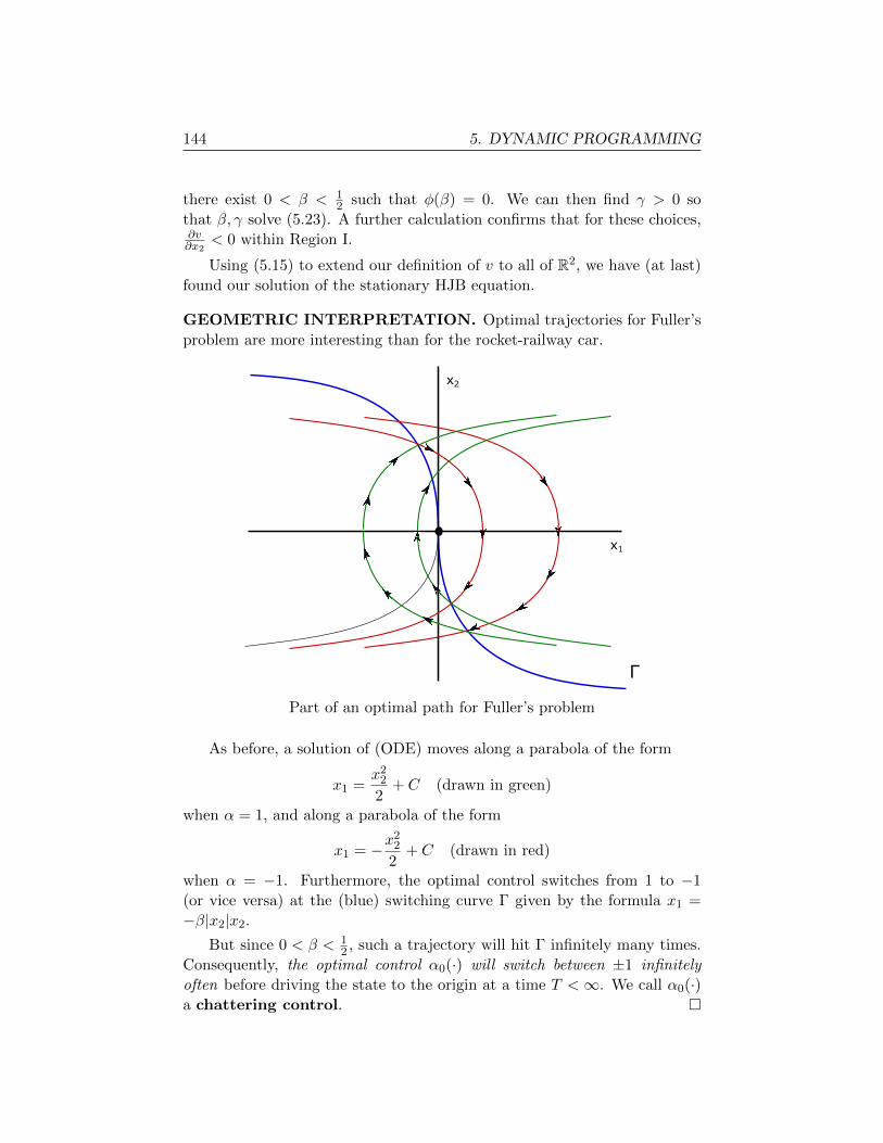
144 5. DYNAMIC PROGRAMMING
there exist 0 < β < 12 such that φ(β) = 0. We can then find γ > 0 so
that β, γ solve (5.23). A further calculation confirms that for these choices,∂v∂x2
< 0 within Region I.
Using (5.15) to extend our definition of v to all of R2, we have (at last)
found our solution of the stationary HJB equation.
GEOMETRIC INTERPRETATION. Optimal trajectories for Fuller’s
problem are more interesting than for the rocket-railway car.
x1
x2
Γ
Part of an optimal path for Fuller’s problem
As before, a solution of (ODE) moves along a parabola of the form
x1 =x2
2
2+ C (drawn in green)
when α = 1, and along a parabola of the form
x1 = −x22
2+ C (drawn in red)
when α = −1. Furthermore, the optimal control switches from 1 to −1
(or vice versa) at the (blue) switching curve Γ given by the formula x1 =
−β|x2|x2.
But since 0 < β < 12 , such a trajectory will hit Γ infinitely many times.
Consequently, the optimal control α0(·) will switch between ±1 infinitely
often before driving the state to the origin at a time T <∞. We call α0(·)a chattering control. �
5.2. Applications 145
CLOSING REMARKS. Our detailed discussion of Fuller’s problem illus-
trates how difficult it can be to find an explicit solution of an HJB equation,
if this is even possible.
In fact, there are not so many optimal control problems for which ex-
act formulas can be had, using either the Pontryagin maximum principle
or dynamic programming. (See the old book of Athans and Falb [A-F] for
an extensive discussion of various solvable engineering control problems.)
Designing optimal controls is an important, but highly nonlinear and infi-
nite dimensional undertaking, and it is not surprising that exactly solvable
problems have been named after the researchers who found them.
It is therefore essential to turn to computational methods for most op-
timal control problems, and indeed for optimization problems in general. I
therefore strongly recommend that students take subsequent classes (mostly
offered in engineering) on computational techniques for optimization, with
the hope that their understanding the optimization theory from Math 170
and 195 will make the algorithms and software packages from these courses
more understandable. �

APPENDIX
A. Notation
Rn denotes n-dimensional Euclidean space, a typical point of which is the
column vector
x =
x1...
xn
.To save space we will often write the corresponding row vector
x = [x1 · · · xn]T .
If x, y ∈ Rn, we define
x · y =
n∑i=1
xiyi = xT y, |x| = (x · x)12 =
(n∑i=1
x2i
)1/2
B. Linear algebra
Throughout these notes A denotes a real m× n matrix and AT denotes its
transpose:
A =
a11 . . . a1n...
. . ....
am1 . . . amn
AT =
a11 . . . am1...
. . ....
a1n . . . amn
.Recall the rule
(AB)T = BTAT .
147
148 APPENDIX
We write
Mn×m
for the space of all real m× n matrices.
An n × n matrix A is symmetric if A = AT , and a symmetric matrix
A is nonnegative definite if
yTAy =n∑
i,j=1
aijyiyj ≥ 0 for all y ∈ Rn.
We then write A � 0. We say A is positive definite if
yTAy =n∑
i,j=1
aijyiyj > 0 for all y ∈ Rn;
and write A � 0.
C. Multivariable chain rule
Let f : Rn → R, f = f(x) = f(x1, . . . , xn). Then we write
∂f
∂xk
for the k-th partial derivative, k = 1, . . . , n . We likewise write
∂2f
∂xk∂xl=
∂
∂xl
(∂f
∂xk
)(k, l = 1, . . . , n),
and recall that ∂2f∂xk∂xl
= ∂2f∂xl∂xk
if f is twice continuously differentiable.
The gradient ∇f is the vector
∇f =
∂f∂x1...∂f∂xn
and the Hessian matrix of second partial derivatives ∇2f is the symmetric
n× n matrix
∇2f =
∂2f
∂x21
. . .∂2f
∂x1∂xn...
. . ....
∂f
∂x1∂xn. . .
∂2f
∂x2n
.
C. Multivariable chain rule 149
The chain rule tells us how to compute the partial derivatives of com-
posite functions, made from simpler functions. For this, assume that we are
given a function
f : Rn → R,which we write as f(x) = f(x1, . . . , xn). Suppose also we have functions
g1, . . . , gn : Rm → R
so that gi(y) = gi(y1, . . . , ym) for i = 1, . . . , n.
NOTATION. We define g : Rm → Rn by
g =
g1...
gn
.The gradient matrix of g is
∇g =
(∇g1)T
...
(∇gn)T
=
∂g1∂y1
. . . ∂g1∂ym
.... . .
...∂gn∂y1
. . . ∂gn∂ym
.This is an n×m matrix-valued function. �
We now build the composite function h : Rm → R by setting xi = gi(y)
in the definition of f ; that is, we define
h(y) = f(g(y)) = f(g1(y), g2(y), . . . , gn(y)).
THEOREM. (Multivariable chain rule) We have
∂h
∂yk(y) =
n∑i=1
∂f
∂xi(g(y))
∂gi∂yk
(y) (k = 1, . . . ,m).
In matrix notation, this says
∇h = (∇g)T∇f.
EXAMPLE. We use the chain rule to prove the useful formula
∇(|g|2)
= 2(∇g)Tg
where g : Rn → Rn.
To prove this, we compute that
1
2
∂
∂xk|g|2 =
n∑i=1
gi∂gi∂xk
= k-th entry of (∇g)Tg.
�
150 APPENDIX
D. Divergence Theorem
If U ⊂ Rn is an open set, with smooth boundary ∂U , we let
ν =
ν1...
νn
.denote the outward pointing unit normal vector field along ∂U . Then |ν| = 1
along ∂U .
Assume also that h : U → Rn, written
h =
h1...
hn
,is a vector field. Its divergence is
div h = ∇ · h =
n∑i=1
∂hi∂xi
.
THEOREM. (Divergence Theorem) We have∫U
div h dx =
∫∂U
h · ν dS.
The expression on the right is an integral with respect to (n− 1 dimen-
sional) surface area over the boundary of U .
E. Implicit Function Theorem
Assume for this section that
f : R2 → R
is continuously differentiable. We will write f = f(x, y).
THEOREM. (Implicit Function Theorem) Assume that f(x0, y0) = 0
and∂f
∂y(x0, y0) 6= 0.
(i) Then there exist ε > 0 and a continuously differentiable function
g : (x0 − ε, x0 + ε)→ R
such that
f(x, g(x)) = 0 (x0 − ε < x < x0 + ε).
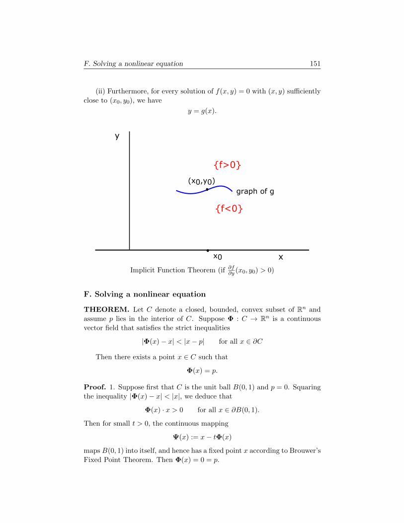
F. Solving a nonlinear equation 151
(ii) Furthermore, for every solution of f(x, y) = 0 with (x, y) sufficiently
close to (x0, y0), we have
y = g(x).
x
y
(x0,y0)
x0
graph of g
{f>0}
{f<0}
Implicit Function Theorem (if ∂f∂y (x0, y0) > 0)
F. Solving a nonlinear equation
THEOREM. Let C denote a closed, bounded, convex subset of Rn and
assume p lies in the interior of C. Suppose Φ : C → Rn is a continuous
vector field that satisfies the strict inequalities
|Φ(x)− x| < |x− p| for all x ∈ ∂C
Then there exists a point x ∈ C such that
Φ(x) = p.
Proof. 1. Suppose first that C is the unit ball B(0, 1) and p = 0. Squaring
the inequality |Φ(x)− x| < |x|, we deduce that
Φ(x) · x > 0 for all x ∈ ∂B(0, 1).
Then for small t > 0, the continuous mapping
Ψ(x) := x− tΦ(x)
maps B(0, 1) into itself, and hence has a fixed point x according to Brouwer’s
Fixed Point Theorem. Then Φ(x) = 0 = p.
152 APPENDIX
2. For the general case, we can always assume after a translation that
p = 0, so that 0 belongs to the interior of C. We introduce a nonnegative
gauge function ρ : Rn → [0,∞) such that ρ(λx) = λρ(x) for all λ ≥ 0 and
C = {x ∈ Rn | ρ(x) ≤ 1}.
We next map C onto B(0, 1) by the continuous function
a(x) =ρ(x)
|x|x = y.
Define
Ψ(y) =ρ(y)
|y|Φ
(|y|ρ(y)
y
).
Then the inequality |Φ(x)− x| < |x| implies
|Ψ(y)− y| < 1 for all y ∈ ∂B(0, 1).
Consequently the first part of the proof shows that there exits y ∈ B(0, 1)
such that Ψ(y) = 0. And then
x =|y|ρ(y)
y ∈ C
satisfies Φ(x) = 0 = p. �
EXERCISES
Some of these problems are from Kamien–Schwartz [K-S] and Bressan–
Piccoli [B-P].
1. This and the next few problems provide practice for solving certain
ODE. Find the general solution of
y′ = a(x)y + b(x).
(Hint: Multiply by eA(x) for an appropriate function A.)
2. (a) If y satisfies
y′ = a(x)y + b(x),
what ODE does z = yq solve?
(b) Use (a) to solve Bernoulli’s equation
y′ = a(x)y + b(x)yp.
3. Find an implicit formula for the general solution of the separable
ODE
y′ = a(x)b(y),
where b > 0.
4. Assume y1, y2 both solve the linear, second-order ODE
Ly = y′′ + b(x)y′ + c(x)y = 0.
Find the first-order ODE satisfied by the Wronskian w = y′2y1 −y′1y2.
153
154 EXERCISES
5. (a) Find two linearly independent solutions y1, y2 of the constant
coefficient ODE
Ly = ay′′ + by′ + cy = 0.
where a > 0. (Hint: Try y = eλx. What if λ is a repeated
root of the corresponding polynomial?)
(b) Find two linearly independent solutions y1, y2 of Euler’s equa-
tion
Ly = ax2y′′ + bxy′ + cy = 0.
6. If y1 solves
Ly = y′′ + b(x)y′ + c(x)y = 0,
find another, linearly independent solution of the form y2 = zy1.
(Hint: Show w = z′ satisfies a first-order linear ODE.)
7. Write down the Euler-Lagrange equations for the following La-
grangians:
(a) ez2
(b) z4 + y2
(c) sin(xyz)
(d) y3x4.
8. Give an alternate proof that
L = a(y)z
is a null Lagrangian, by observing I[y(·)] =∫ 1
0 L(y, y′) dx depends
only upon the values taken on by y(·) at the endpoints 0, 1.
9. Compute (E-L) for∫ 1
0a(x, y) + b(x, y)y′ dx
and show that it is not a differential equation, but rather an im-
plicit algebraic formula for y as a function of x.
10. (Discrete version of Euler-Lagrange equations) Let h > 0 and de-
fine xk = kh for k = 0, . . . , N +1. Consider the problem of finding
{yk}Nk=1 to minimize
N∑k=0
L(xk, yk,
yk+1−ykh
)h,
where y0 = y0, yN+1 = y1 are prescribed. What algebraic con-
ditions do minimizers satisfy? What is the connection with the
Euler-Lagrange equation?
EXERCISES 155
11. Assume
I[y(·)] =
∫ b
aL(x, y, y′, y′′) dx
for L = L(x, y, z, u). Derive the corresponding Euler-Lagrange
equation for extremals.
12. Show that the extremals of∫ b
a(y′)2e−y
′dx
are linear functions.
13. Find the extremals of∫ 1
0(y′)2 + 10xy dx,
subject to y(0) = 1, y(1) = 2.
14. Find the extremals of∫ T
0e−λt(a(x)2 + bx2) dt,
satisfying x(0) = 0, x(T ) = c.
15. Assume c > 0. Find the minimizer of∫ T
0e−λt(c(x)2 + dx) dt,
subject to x(0) = 0, x(T ) = b.
16. Find the minimizer of∫ 1
0
(y′)2
2− x2y dx,
where y(0) = 1 and y(1) is free.
17. Consider the free endpoint problem of minimizing
I[y(·)] =
∫ b
aL(x, y, y′) dx+ g(y(b))
subject to y(a) = y0, where g : R → R is a given function. What
is the transversality condition satisfied at x = b by a minimizer
y0(·)?18. Assume y0(·) minimizes the functional
I[y(·)] =1
2
∫ b
a(y′′)2 dx
over the admissible class
A = {y : [a, b]→ R | y(a) = 0, y(b) = 1}.
156 EXERCISES
What additional boundary conditions does y0(·) satisfy?
19. Give a different proof of Theorem 1.3.4 by rewriting
j(σ) =1
1 + σ
∫ T
0L(
s1+σ , x0(s), (1 + σ)x0(s)
)ds
and then computing djdσ (0).
20. Find the minimizer of ∫ 1
0(x)2 dt,
subject to x(0) = 0, x(1) = 2 and∫ 1
0 x dt = b.
21. Find a minimizer of I[y(·)] =∫ π
0 (y′)2 dx over the admissible class
A = {y : [0, π]→ R | y(0) = y(π) = 0,
∫ π
0y2 dx = 1}.
22. Suppose I[y(·)] =∫ ba L(x, y, y′) dx and the admissible class is
A = {y : [a, b]→ R | y(a) = 0, y(b) = 0, φ(x) ≤ y(x) (a ≤ x ≤ b)}
for some given function φ.
(a) Show that if y0(·) ∈ A is a minimizer, then
−(∂L
∂z(x, y0, y
′0)
)′+∂L
∂y(x, y0, y
′0) ≥ 0 (a ≤ x ≤ b).
(b) Show that
−(∂L
∂z(x, y0, y
′0)
)′+∂L
∂y(x, y0, y
′0) = 0
in the region {a ≤ x ≤ b | φ(x) < y0(x)} where y0(·) does not
hit the constraint.
23. Let I[x(·)] =∫ T
0 |x| dt for functions belonging to the admissible
class
A = {x : [0, T ]→ Rn | x(0) = A,x(T ) = B},
where A,B ∈ Rn are given. Show that the graph of a minimizer
x0(·) is a line segment from A to B.
24. For each Lagrangian L : Rn × Rn → R write out the Euler–
Lagrange equation, the Hamiltonian H and the Hamiltonian dif-
ferential equations:
(a) L = m2 |v|
2 −W (x)
(b) L = m2 |v|
2 + b(x) · v.
EXERCISES 157
25. Assume that the matrix function G, whose (i, j)-th entry is gij , is
symmetric and positive definite. What is the Hamiltonian corre-
sponding to the Lagrangian
L =1
2
n∑i,j=1
gij(x)vivj?
26. Show that
L =m
2|v|2 + qv ·A(x)
is the Lagrangian corresponding to the Hamiltonian
H =1
2m|p− qA(x)|2.
27. If x : [0, 1] → U is a curve and z = y(x) is its image under the
coordinate patch y : U → Rl, show that the length of the curve z
in Rl is ∫ 1
0
( n∑i,j=1
gij(x)xixj
) 12dt.
28. Compute explicitly the Christoffel symbols Γkij for the hyperbolic
plane. Check that the ODE given in the text for the geodesics is
correct.
29. Suppose ∫ b
a
∂2L
∂z2(x, y0, y
′0)ζ2 dx ≥ 0
for all functions ζ such that ζ(a) = ζ(b) = 0. Explain carefully
why this implies
∂2L
∂z2(x, y0, y
′0) ≥ 0 (a ≤ x ≤ b).
30. Assume y(·) > 0 solves the linear, second-order ODE
y′′ + b(x)y′ + c(x)y = 0.
Find the corresponding Riccati equation, which is the nonlinear,
first-order ODE that w = y′
y solves.
31. What does the Weierstrass condition say about the possible values
of y′0(·) for minimizers of
(a)∫ ba ((y′)2 − 1)2 dx
(b)∫ ba
11+(y′)2 dx
subject to given boundary conditions?
158 EXERCISES
32. Derive this useful calculus formula, which we used in the proof of
Theorem 2.3.1:
d
dx
(∫ g(x)
af(x, t) dt
)=
∫ g(x)
a
∂f
∂x(x, t) dt+ f(x, g(x))g′(x).
(Hint: Define F (x, y) =∫ ya f(x, t) dt; so that
∫ g(x)a f(x, t) dt =
F (x, g(x)). Apply the chain rule.)
33. Suppose that y(·) is an extremal of I[ · ], the second variation of
which satisfies for some constant γ > 0 the estimate∫ b
aA(w′)2 + 2Bww′ + Cw2 dx ≥ γ
∫ b
a(w′)2 + w2 dx
for all w : [a, b]→ R with w(a) = w(b) = 0. Use a Taylor expansion
to show directly that y(·) is a weak local minimizer; this means
that there exists δ > 0 such that
I[y] ≤ I[y]
for all admissible y satisfying max[a,b] {|y − y|+ |y′ − y′|} ≤ δ.34. Show that for each l > 0 the function y(·) = 0 is a strong local
minimizer of ∫ l
0
(y′)2
2+y2
2− y4
4dx
for
A = {y : [0, l]→ R | y(0) = y(l) = 0}.35. Assume that (y, z) 7→ L(x, y, z) is convex for each a ≤ x ≤ b.
Show that each extremal y(·) ∈ A is in fact a minimizer of I[ · ],for the admissible set
A = {y : [a, b]→ R | y(a) = y0, y(b) = y1}.
(Hint: Recall that if f : Rn → R is convex, then
f(x) ≥ f(x) +∇f(x) · (x− x)
for all x.)
36. A function f : Rn → R is strictly convex provided
f(θx+ (1− θ)x) < θf(x) + (1− θ)f(x)
if x 6= x and 0 < θ < 1.
Suppose that (y, z) 7→ L(x, y, z) is strictly convex for each
a ≤ x ≤ b. Show that there exists at most one minimizer y0(·) ∈ Aof I[ · ].
EXERCISES 159
37. Explain carefully why
I[y(·)] =
∫ 1
0y dx
does not have a minimizer over the admissible set
A = {y : [0, 1]→ R | y(·) is continuous, y ≥ 0, y(0) = 0, y(1) = 1}.
38. Write down the Euler-Lagrange PDE for the following Lagrangians:
(a) |z|2
2 + b(x) · z(b) |z|
p
p (1 ≤ p <∞)
(c)(1 + |z|2
) 12 + F (y).
39. Write down the Euler-Lagrange PDE for these functionals:
(a) I[u] =∫U|∇u|2
2 + F (x, u) dx
(b) I[u] = 12
∫U
∑nk,l=1 akl(x) ∂u∂xk
∂u∂xl
dx.
40. Use the Divergence Theorem to give another proof that
L = z · b(x)f(y) + F (y) div b,
is a null Lagrangian, where F ′ = f .
(Hint: L(x, u,∇u) = div(F (u)b).)
41. Derive the 4-th order Euler-Lagrange PDE satisfied by minimizers
of
I[u(·)] =1
2
∫U
(∆u)2 dx,
subject to the boundary conditions u = g on ∂U . What is the
transversality condition on ∂U for a minimizer?
42. Consider the system of PDE{−∆u1 = u2
−∆u2 = 2u1,
for the unknown u : R2 → R2, u =
[u1
u2
].
Show that this problem is variational. This means to find
a Lagrangian function L : R2 × R2 × M2×2 → R so that the
two PDE above are the Euler-Lagrange equations for I[u(·)] =∫R2 L(x,u,∇u) dx.
43. A system of two reaction-diffusion equations has the form{−a1∆u1 = f1(u1, u2)
−a2∆u2 = f2(u1, u2).
160 EXERCISES
Under what conditions on the functions f1, f2 : R2 → R is this
system variational?
44. Consider the dynamics{x(t) = α(t) (0 ≤ t ≤ 1)
x(0) = x0
and payoff functional
P [α(·)] =
∫ 1
0|x(t)| dt.
(a) Suppose A = {−1, 1}. If |x0| ≥ 1, describe an optimal control
that minimizes P [α(·)]. Explain why an optimal control does
not exist if |x0| < 1.
(b) Suppose instead that A = {−1, 0, 1}. Explain why an optimal
control exists.
45. Consider the problem of reaching the origin in least time, when
the dynamics are {x1 = x2
x2 = −x1 + α,
where |α| ≤ 1.
(a) Check that X(t) =
[cos t sin t
− sin t cos t
].
(b) Show that an optimal control α0(·) is periodic in time.
46. Use the maximum principle to find an optimal control for the linear
time optimal problem with dynamics{x1 = x2 + α1 |α1| ≤ 1
x2 = −x1 + α2 |α2| ≤ 1
47. Write down (ODE), (ADJ), (M) and (T) for the fixed time, free
endpoint problems with n = m = 1 and
(a) f = (x2 + a)2 − x4, A = [−1, 1], r = 2ax, g = sinx
(b) f = x2a,A = [0, 2], r = a2 + x2, g = 0.
48. Write down the equations (ADJ), (M) and (T) for the fixed time,
free endpoint problem corresponding to the dynamics{x1 = sin(x1 + αx2)
x2 = cos(αx1 + x2),
EXERCISES 161
where 0 ≤ α ≤ 1, with the payoff
P [α(·)] =
∫ T
0α4 + (x1x2)2 dt+ (x1(T ))4.
49. Consider the variational problem of minimizing
I[x(·)] =
∫ T
0L(x(t), x(t)) dt,
for L = L(x, v), over the admissible class
A = {x : [0, T ]→ Rn | x(·) is continuous and piecewise
continuously differentiable,x(0) = x0,x(T ) = x1}.
(a) Show how to interpret this as a fixed time, fixed endpoint
optimal control problem.
(b) If x0 is a minimizer, show that (M) implies p0 = ∇vL(x0, x0).
(c) Show that (ADJ) implies the Euler-Lagrange equations.
50. Use the free time, fixed endpoint PMP to give a new proof of
Theorem 1.3.4 for a Lagrangian L = L(x, v). In particular, explain
what condition (T) says for the variational problem.
51. Solve the linear-quadratic regulator problem of minimizing∫ T
0x2 + α2 dt+
x2(T )
2
for the dynamics {x = x+ α
x(0) = x0
with controls α : [0, T ]→ R.
52. Assume that a function z : [0, T ] → R is given and we wish to
minimize ∫ T
0(x− z)2 + α2 dt,
where A = R and {x = x+ α
x(0) = x0.
Show
α =1
2dx+
e
2
162 EXERCISES
is an optimal feedback control, where d(·) and e(·) solve{d = 2− 2d− 1
2d2, d(T ) = 0
e = −2z −(1 + d
2
)e, e(T ) = 0.
(Hint: Assume PMP applies and write down the equations for x
and p. Look for a solution of the form p = dx+ e.)
53. Find explicit formulas for the optimal state x0(·) and costate p0(·)for the production and consumption model discussed on page 108.
Show that H(x0, p0, α0) is constant on the interval [0, T ], as as-
serted by the PMP.
54. How does our analysis of the Ramsey consumption model break
down if we drop the requirement that x(T ) = x1?
55. Use the PMP to solve the problem of maximizing
P [α(·)] =
∫ 2
02x− 3α+ α2 dt,
where {x = x+ α, 0 ≤ α ≤ 2
x(0) = 0.
56. Use the PMP to find a control to minimize the payoff
P [α(·)] =1
4
∫ 1
0α4 dt,
for the dynamics{x = x+ α
x(0) = 1, x(1) = 0,
where A = R.
57. Assume that the matrices B,C,D are symmetric and that the
matrix Riccati equation{K +KNC−1NTK +KM +MTK = B (0 ≤ t ≤ T )
K(T ) = −D
has a unique solution K(·). Show that K(t) is symmetric for each
time 0 ≤ t ≤ T .
58. Apply the PMP to solve the general linear-quadratic regulator
problem, introduced on page 137. In particular, show how to solve
(ADJ) for the costate p0(·) in terms of the matrix Riccati equation.
EXERCISES 163
59. This exercise discusses the infinite horizon problem:{x = −x+ α (t ≥ 0)
x(0) = x,
where A = R and
Px[α(·)] =
∫ ∞0
x2 + α2 dt
Define
v(x) = infα(·)
Px[α(·)].
(a) Derive the HJB equation for v.
(b) Solve this equation and design an optimal feedback control.
60. Use dynamic programming to solve the tracking problem of mini-
mizing ∫ T
0|x(t)− z(t)|2 + |α(t)|2 dt
for the dynamics{x(t) = Mx(t) +Nα(t) (0 ≤ t ≤ T )
x(0) = 0,
where z : [0, T ]→ Rn is given. Here M ∈ Mn×n, N ∈ Mn×m, and
A = Rm.

Bibliography
[A-F] M. Athans and P. L. Falb, Optimal Control: An Introduction tothe Theory and its Applications, Dover, 2007
[B-M] J. Ball and F. Murat, Remarks on rank-one convexity and quasi-convexity, in Ordinary and Partial Differential Equations, B. D.Sleeman and R. J. Jarvis, eds., Pitman Research Notes, Pitman,1991.
[B-P] A. Bressan and B. Piccoli, Introduction to the Mathematical The-ory of Control, AIMS Series on Applied Math, Vol 2, AmericanInstitute of Mathematical Sciences, 2007
[C-Z] F. H. Clarke and V. Zeidan, Sufficiency and the Jacobi conditionin the calculus of variations, Canad. J. Math (38) 1986, 1199–1209.
[E] L. C. Evans, An Introduction to Mathematical Optimal ControlTheory, Version 0.2, lecture notes available at math.berkeley.
edu/~evans/control.course.pdf
[F-R] W. Fleming and R. Rishel, Deterministic and Stochastic OptimalControl, Springer, 1975
[G] T. Gilbert, Lost mail: the missing envelope in the problem of theminimal surface of revolution, American Math Monthly (119)2012, 359–372
[K-S] M. Kamien and N. Schwartz, Dynamic Optimization: The Cal-culus of Variations and Optimal Control in Economics and Man-agement, 2nd ed, Dover, 2012
165
166 Bibliography
[K] M. Kot, A First Course in the Calculus of Variations, StudentMathematical Library, Vol 72, American Math Society, 2014
[L-M] E. B. Lee and L. Markus, Foundations of Optimal Control The-ory, Wiley, 1967
[L] M. Levi, Classical Mechanics with Calculus of Variations andOptimal Control, Student Mathematical Library, Vol 69, Amer-ican Math Society, 2014
[M-S] J. Macki and A. Strauss, Introduction to Optimal Control The-ory, Springer, 1982
[M] Z. A. Melzak, Mathematical Ideas, Modeling & Applications,Wiley–Interscience, 1976
[MG] M. Mesterton-Gibbons, A Primer on the Calculus of Variationsand Optimal Control Theory, Student Mathematical Library, Vol50, American Math Society, 2009
[S] D. R. Smith, Variational Methods in Optimization, Prentice Hall,1974
[T] J. R. Taylor, Classical Mechanics, University Science Books,2005