MatLabin Biostatistica

Ing. Vincenzo Catrambonevincenzo.catrambone@ing.unipi.it

Generatore di numeri casuali

Y = random(name,A,B,C,D,[m,n,...]) returns an m-by-n-by... matrix

of random numbers for distributions that require four parameters.

name Distribution A B

'bino' or 'Binomial' Binomial Distribution n: number of trials p: probability of success for each trial

'chi2' or 'Chisquare' Chi-Square Distribution ν: degrees of freedom —

'exp' or 'Exponential' Exponential Distribution μ: mean —

'gam' or 'Gamma' Gamma Distribution a: shape parameter b: scale parameter

'logn' or 'Lognormal' Log-normal Distribution μ: mean σ: standard deviation

'norm' or 'Normal' Normal Distribution μ: mean σ: standard deviation

'poiss' or 'Poisson' Poisson Distribution λ: mean —

't' or 'T' Student’s Distribution ν: degrees of freedom —

Y = random(‘norm’,0,1,[m,n]) = randn(m,n)

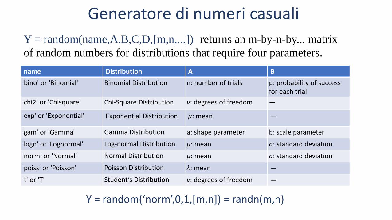
Rappresentazione grafica dei campioni

Campione proveniente da una distribuzione continua:

Istogramma: hist(x)

Campione appartenente a una distribuzione discreta:

Diagramma a bastoncini: stem(x)

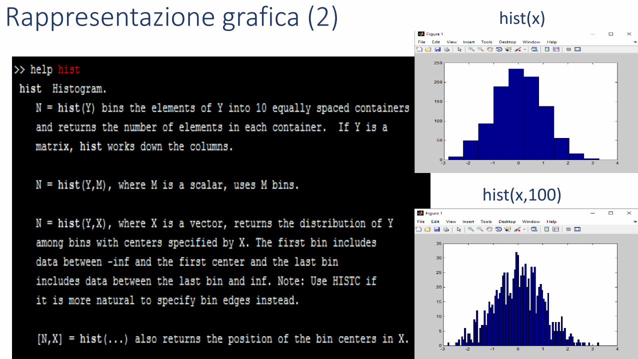
hist(x)

hist(x,100)

Rappresentazione grafica (2)

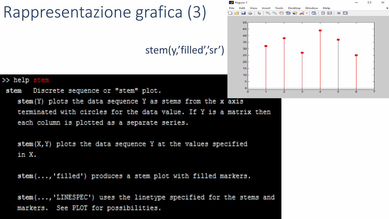
stem(y,’filled’,’sr’)

Rappresentazione grafica (3)

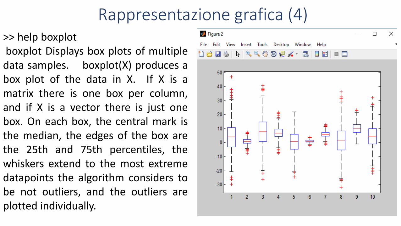
>> help boxplotboxplot Displays box plots of multiple

data samples. boxplot(X) produces abox plot of the data in X. If X is amatrix there is one box per column,and if X is a vector there is just onebox. On each box, the central mark isthe median, the edges of the box arethe 25th and 75th percentiles, thewhiskers extend to the most extremedatapoints the algorithm considers tobe not outliers, and the outliers areplotted individually.

Rappresentazione grafica (4)

Generatore di numeri casuali(2)

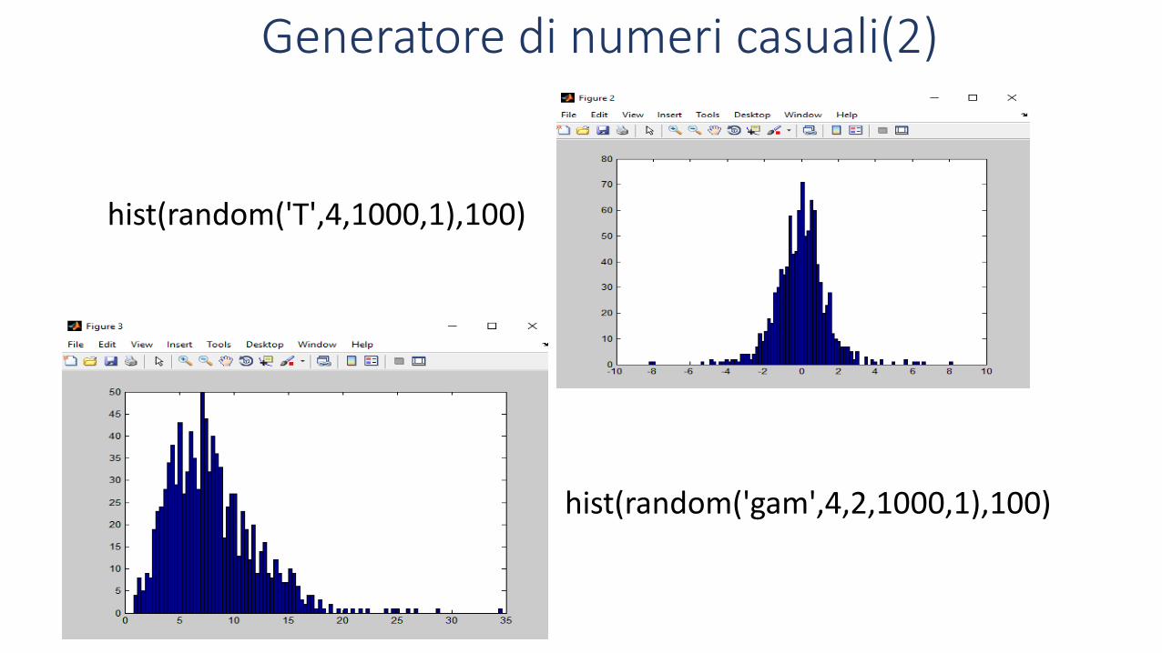
hist(random('T',4,1000,1),100)

hist(random('gam',4,2,1000,1),100)

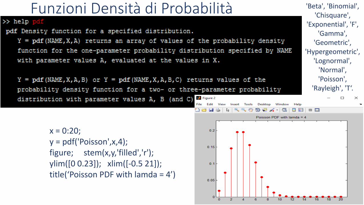
Funzioni Densità di Probabilità

x = 0:20;y = pdf('Poisson',x,4);figure; stem(x,y,'filled','r'); ylim([0 0.23]); xlim([-0.5 21]);title(‘Poisson PDF with lamda = 4’)

'Beta', 'Binomial', 'Chisquare',

'Exponential', 'F', 'Gamma',

'Geometric', 'Hypergeometric',

'Lognormal', 'Normal', 'Poisson',

'Rayleigh', 'T‘.

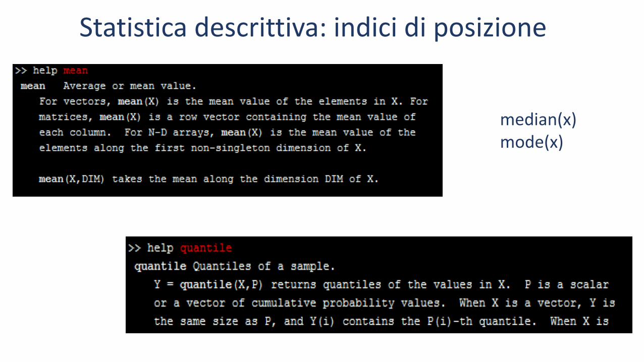
Statistica descrittiva: indici di posizione

median(x)mode(x)

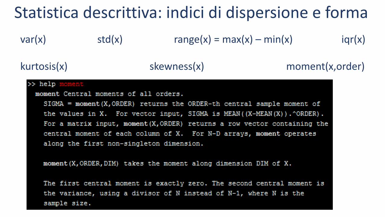
var(x) std(x) range(x) = max(x) – min(x) iqr(x)

kurtosis(x) skewness(x) moment(x,order)

Statistica descrittiva: indici di dispersione e forma

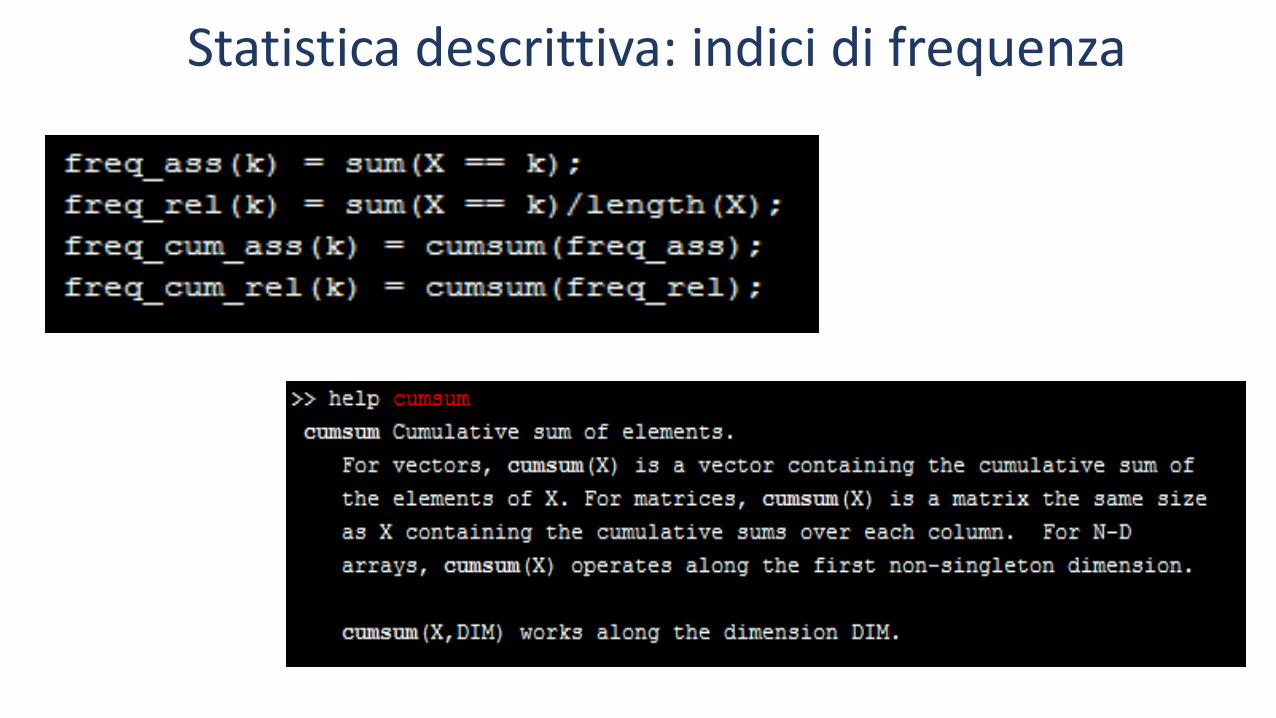
Statistica descrittiva: indici di frequenza

Esercizio:

• Costruire 1000 campioni di numerosità N=10000, appartenenti ad una distribuzione Gaussiana con media μ = 7 e deviazione standard σ = 2.3 .

• Valutare visivamente con un istogramma come si distribuiscono le variabili aleatorie media campionaria e varianza calcolate sui 100 campioni creati in precedenza e caratterizzarli statisticamente.

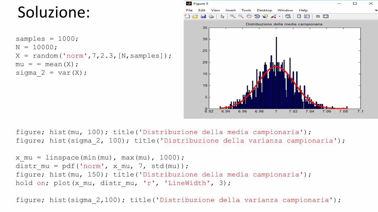
samples = 1000;

N = 10000;

X = random('norm',7,2.3,[N,samples]);

mu = = mean(X);

sigma_2 = var(X);

figure; hist(mu, 100); title('Distribuzione della media campionaria');

figure; hist(sigma_2, 100); title('Distribuzione della varianza campionaria');

x_mu = linspace(min(mu), max(mu), 1000);

distr_mu = pdf('norm', x_mu, 7, std(mu));

figure; hist(mu, 150); title('Distribuzione della media campionaria');

hold on; plot(x_mu, distr_mu, 'r', 'LineWidth', 3);

figure; hist(sigma_2,100); title('Distribuzione della varianza campionaria');

Soluzione: