U.S. Fish and Wildlife Service

Estimating Black Bear Density in New Mexico Using

Noninvasive Genetic Sampling Coupled with

Spatially Explicit Capture-Recapture Methods

Matthew J. Gould1

James W. Cain III2

Gary W. Roemer3

William R. Gould4

1 Department of Biology, New Mexico State University, Las Cruces, New Mexico 88003

2 U.S. Geological Survey, New Mexico Cooperative Fish and Wildlife

Research Unit, New Mexico State University, Las Cruces, New Mexico 88003

3 Department of Fish, Wildlife and Conservation Ecology,

New Mexico State University, Las Cruces, New Mexico 88003

4 College of Business, New Mexico State University, Las Cruces, New Mexico 88003

Cooperator Science Series # 120-2016 CO

OP

ER

AT

OR

SC

IEN

CE

SE

RIE

S

ii

About the Cooperator Science Series:

The Cooperator Science Series was initiated in 2013. Its purpose is to facilitate the archiving and

retrieval of research project reports resulting primarily from investigations supported by the U.S. Fish and Wildlife Service (FWS), particularly the Wildlife and Sport Fish Restoration Program. The online

format was selected to provide immediate access to science reports for FWS, state and tribal

management agencies, the conservation community, and the public at large.

All reports in this series have been subjected to a peer review process consistent with the agencies and entities conducting the research. For U.S. Geological Survey authors, the peer review process

(http://www.usgs.gov/usgs-manual/500/502-3.html) also includes review by a bureau approving official prior to dissemination. Authors and/or agencies/institutions providing these reports are solely

responsible for their content. The FWS does not provide editorial or technical review of these reports.

Comments and other correspondence on reports in this series should be directed to the report authors or agencies/institutions. In most cases, reports published in this series are preliminary to publication,

in the current or revised format, in peer reviewed scientific litera ture. Results and interpretation of data contained within reports may be revised following further peer review or availability of additional

data and/or analyses prior to publication in the scientific literature.

The Cooperator Science Series is supported and maintained by the FWS, National Conservation

Training Center at Shepherdstown, WV. The series is sequentially numbered with the publication year appended for reference and started with Report No. 101-2013. Various other numbering systems

have been used by the FWS for similar, but now discontinued report series. Starting with No. 101 for the current series is intended to avoid any confusion with earlier report numbers.

The use of contracted research agencies and institutions, trade, product, industry or firm names or products or software or models, whether commercially available or not, is for informative purposes

only and does not constitute an endorsement by the U.S. Government.

Contractual References: This document was developed in conjunction with the New Mexico Cooperative Fish and Wildlife

Research Unit to fulfill reporting requirements for Federal Aid in Wildlife Restoration Project W93 R56 2.0. Previously published documents that partially fulfilled any portion of this contract are referenced

within, when applicable. (USGS IPDS #: IP-074771). Recommended citation: Gould, M.J., J.W. Cain III, G.W. Roemer, and W.R. Gould. 2016. Estimating abundanc e and density of

American black bears (Ursus americanus) in New Mexico using noninvasive genetic sampling coupled

with spatially explicit capture-recapture methods. Report provided by the Cooperative Fish and Wildlife Research Unit Program under agreement with the U.S. Fish and Wildlife Service. U.S.

Department of Interior, Fish and Wildlife Service, Cooperator Science Series FWS/CSS -120-2016, National Conservation Training Center.

For additional copies or information, contact:

James W. Cain U.S. Geological Survey

New Mexico Cooperative Fish and Wildlife Research Unit New Mexico State University

Las Cruces, NM 88003

Phone: (575) 646-3382 E-mail: jwcain@usgs.gov

1

Estimating Black Bear Density in New Mexico Using Noninvasive Genetic Sampling

Coupled with Spatially Explicit Capture-Recapture Methods

Federal Aid in Wildlife Restoration Project W93 R56 2.0

Final Report to The New Mexico Department of Game and Fish

MATTHEW J. GOULD Department of Biology

New Mexico State University

P.O. Box 30003, MSC 4901

Las Cruces, New Mexico 88003

JAMES W. CAIN III U.S. Geological Survey,

New Mexico Cooperative Fish and Wildlife Research Unit

Department of Fish, Wildlife and Conservation Ecology

New Mexico State University

P.O. Box 30003, MSC 4901

Las Cruces, New Mexico 88003

GARY W. ROEMER Department of Fish, Wildlife and Conservation Ecology

New Mexico State University

PO Box 30003, MSC 4901

Las Cruces, New Mexico 88003

WILLIAM R. GOULD College of Business

New Mexico State University

PO Box 30001, MSC 3CQ

Las Cruces, New Mexico 88003

June 2016

2

EXECUTIVE SUMMARY

During the 2004–2005 to 2015–2016 hunting seasons, the New Mexico Department of

Game and Fish (NMDGF) estimated black bear abundance (Ursus americanus) across the state

by coupling density estimates with the distribution of primary habitat generated by Costello et al.

(2001). These estimates have been used to set harvest limits. For example, a density of 17

bears/100 km2 for the Sangre de Cristo and Sacramento Mountains and 13.2 bears/100 km

2 for

the Sandia Mountains were used to set harvest levels. The advancement and widespread

acceptance of non-invasive sampling and mark-recapture methods, prompted the NMDGF to

collaborate with the New Mexico Cooperative Fish and Wildlife Research Unit and New Mexico

State University to update their density estimates for black bear populations in select mountain

ranges across the state.

We established 5 study areas in 3 mountain ranges: the northern (NSC; sampled in 2012)

and southern Sangre de Cristo Mountains (SSC; sampled in 2013), the Sandia Mountains

(Sandias; sampled in 2014), and the northern (NSacs) and southern Sacramento Mountains

(SSacs; both sampled in 2014). We collected hair samples from black bears using two concurrent

non-invasive sampling methods, hair traps and bear rubs. We used a gender marker and a suite of

microsatellite loci to determine the individual identification of hair samples that were suitable for

genetic analysis. We used these data to generate mark-recapture encounter histories for each bear

and estimated density in a spatially explicit capture-recapture framework (SECR). We

constructed a suite of SECR candidate models using sex, elevation, land cover type, and time to

model heterogeneity in detection probability and the spatial scale over which detection

probability declines. We used Akaike’s Information Criterion corrected for small sample size

(AICc) to rank and select the most supported model from which we estimated density.

We set 554 hair traps, 117 bear rubs and collected 4,083 hair samples. We identified 725

(367 M, 358 F) individuals; the sex ratio for each study area was approximately equal. Our

density estimates varied within and among mountain ranges with an estimated density of 21.86

bears/100 km2

(95% CI: 17.83 – 26.80) for the NSC, 19.74 bears/100 km2 (95% CI: 13.77 –

28.30) in the SSC, 25.75 bears/100 km2 (95% CI: 13.22 – 50.14) in the Sandias, 21.86 bears/100

km2 (95% CI: 17.83 – 26.80) in the NSacs, and 16.55 bears/100 km

2 (95% CI: 11.64 – 23.53) in

the SSacs. Overall detection probability for hair traps and bear rubs, combined, was low across

all study areas and ranged from 0.00001 to 0.02. We speculate that detection probabilities were

affected by failure of some hair samples to produce a complete genotype due to UV degradation

of DNA, and our inability to set and check some sampling devices due to wildfires in the SSC.

Ultraviolet radiation levels are particularly high in New Mexico compared to other states where

NGS methods have been used because New Mexico receives substantial amounts of sunshine, is

relatively high in elevation (1,200 m – 4,000 m), and is at a lower latitude. Despite these

sampling difficulties, we were able to produce density estimates for New Mexico black bear

populations with levels of precision comparable to estimated black bear densities made

elsewhere in the U.S.

Our ability to generate reliable black bear density estimates for 3 New Mexico mountain

ranges is attributable to our use of a statistically robust study design and analytical method.

3

There are multiple factors that need to be considered when developing future SECR-based

density estimation projects. First, the spatial extent of the population of interest and the smallest

average home range size must be determined; these will dictate size of the trapping array and

spacing necessary between hair traps. The number of technicians needed and access to the study

areas will also influence configuration of the trapping array. We believe shorter sampling

occasions could be implemented to reduce degradation of DNA due to UV radiation; this might

help increase amplification rates and thereby increase both the number of unique individuals

identified and the number of recaptures, improving the precision of the density estimates. A pilot

study may be useful to determine the length of time hair samples can remain in the field prior to

collection. In addition, researchers may consider setting hair traps and bear rubs in more shaded

areas (e.g., north facing slopes) to help reduce exposure to UV radiation. To reduce the sampling

interval it will be necessary to either hire more field personnel or decrease the number of hair

traps per sampling session. Both of these will enhance detection of long-range movement events

by individual bears, increase initial capture and recapture rates, and improve precision of the

parameter estimates. We recognize that all studies are constrained by limited resources, however,

increasing field personnel would also allow a larger study area to be sampled or enable higher

trap density.

In conclusion, we estimated the density of black bears in 5 study areas within 3

mountains ranges of New Mexico. Our estimates will aid the NMDGF in setting sustainable

harvest limits. Along with estimates of density, information on additional demographic rates

(e.g., survival rates and reproduction) and the potential effects that climate change and future

land use may have on the demography of black bears may also help inform management of black

bears in New Mexico, and may be considered as future areas for research.

4

INTRODUCTION

Setting sustainable harvest limits for game species is one of the main duties of state

wildlife management agencies. To this end, state agencies spend a large portion of their annual

budget on population surveys to estimate abundance and population trends of game animals.

Survey methodologies for large ungulates are well developed and can provide relatively robust

estimates of common game species such as deer (Odocoileus spp.) and elk (Cervus canadensis).

In contrast, estimating the abundance or density of large carnivores like American black bears

(Ursus americanus), which are cryptic and occur at low densities is more difficult because their

behavior makes the survey methods used for ungulates ineffective, e.g., assuming perfect

detection probability (Miller 1990, Obbard et al. 2010). Historically, many state agencies set

harvest limits for carnivores based on harvest data (Hristienko and McDonald 2007), including

sex ratio and age structure of the harvested animals, which, along with other analytical

approaches, can be used to infer harvest effects on a population (Garshelis 1990). Yet, hunter

selectivity and sex-specific vulnerability may influence harvest composition (Miller 1990,

Beston and Mace 2012). Thus, additional information provided by abundance and density

estimates generated from robust statistical methods can aid in setting harvest limits for black bear

populations.

New Mexico’s most recent black bear density estimates were derived from a

comprehensive, decade-long study on black bear ecology in the 1990s in which researchers

estimated study area specific density using population reconstruction (Downing 1980), or

backdating, to estimate the minimum population size during the study and then divided that

estimate by the effective trapping area (ETA; Costello et al. 2001) to obtain a minimum density

estimate. The ETA is an estimate of the actual area used by identified individuals to account for

home ranges that straddle the study area boundary and may bias abundance estimates (Dice

1938, Wilson and Anderson 1985). Costello et al. (2001) estimated the ETA using the

distribution of live-capture trap sites buffered by the mean activity radius of adult bears. Their

minimum density estimate for the more northern, mesic, and presumably more productive Sangre

de Cristo Mountains was 17.0 bears/100 km2 (310 km

2 study area) while their estimate for the

more southern, xeric, and presumably less productive Mogollon Mountains was 9.4 bears/100

km2 (423 km

2 study area). It is important to note that backdating a population fails to account for

undetected individuals or provide measures of uncertainty in estimates, thereby producing only a

minimum population estimate. They extrapolated these minimum density estimates to similar

black bear habitat throughout New Mexico assigning areas with habitat conditions in between

the Sangre de Cristo Mountains and Mogollon Mountains a density equal to the mean of the two

minimum density estimates (i.e., 13.2 bears/100 km2). Costello et al. (2001) estimated the

statewide minimum population by multiplying minimum density by the area of statewide

primary habitat identified through their habitat suitability analysis, which introduces another

source of uncertainty that was not quantified. Along with the density estimates, Costello et al.

(2001) provided the NMDGF with a population model that incorporated the new density

estimates, harvest data, mast survey data, and the relationship between mast production and

reproductive success to model abundance and trend of black bear abundance in each Bear

Management Zone (BMZ). These model-based abundance estimates, coupled with yearly harvest

and mast survey data, have been the basis for establishing black bear harvest limits in New

Mexico (Rick Winslow, NMDGF, personal communication). Although live-capture provides a

wealth of information on age, dispersal, fecundity, health, home range size, and mortality rates, it

5

is still inferentially limited due to small sample sizes. While Costello et al. (2001) was a

progressive and highly informative study on New Mexico black bears, the capabilities of the

technology at that time limited their ability to estimate abundance and density.

Capture-recapture (CR) is a common method for estimating abundance and density of

animals and associated parameter uncertainty (Williams et al. 2002). Abundance estimates using

CR are determined by comparing the ratio of uniquely marked individuals to unmarked

individuals captured each sampling occasion in live capture studies (Pollock et al. 1990). Gould

and Kendall (2013) summarize CR methodology and recent advances. Low capture probabilities

and sample sizes inherent with species that typically reside at the low densities characteristic of

carnivore populations hinders management agencies from utilizing traditional CR techniques for

some species (Mills et al. 2000, Settlage et al. 2008). Noninvasive genetic sampling (NGS)

revolutionized CR research by providing the ability to use remotely collected DNA samples to

identify individuals (Waits and Paetkau 2005). Consequently, NGS enabled researchers to

estimate population parameters for carnivores by increasing detection probability, increasing

sample size of individuals detected, increasing the size of the study area, decreasing tag loss, and

decreasing invasiveness compared to live capture studies (Woods et al. 1999, Mills et al. 2000).

However, density estimators using traditional non-spatial CR methods are often less reliable

because of the ad hoc and arbitrary estimate of the ETA, which introduces an unquantifiable

error (Wilson and Anderson 1985, Parmenter et al. 2003).

Spatially explicit capture-recapture (SECR) models remedy this issue by estimating the

number of home range centers within the study area, and subsequently density, directly, using a

spatial point process (Efford 2004, Gopalaswamy 2013). By using SECR models, accounting for

edge effects has been rooted in statistical theory and incorporated into the modeling process

thereby eliminating the need to estimate ETA. Furthermore, integrating the distribution and

location of sampling devices into the model eliminates individual heterogeneity related to

unequal trap exposure (Borchers 2012). To date, SECR methods have shown improved

parameter estimation compared to non-spatial methods with simulated datasets (Ivan et al. 2013,

Whittington and Sawaya 2015) and similar or lower density estimates in empirical comparisons

(Obbard et al. 2010, Stetz et al. 2014, Whittington and Sawaya 2015), particularly when distance

to edge and sampling effort are not included in CR models. Although the accuracy of any density

estimate is unknown, use of statistically robust estimation methods yields greater confidence in a

management agency’s ability to set defensible management objectives that will help ensure the

long-term viability of harvested animal populations.

In light of advances in sampling (Woods et al. 1999) and statistical methods (Efford

2004), NMDGF began a collaborative project with the New Mexico Cooperative Fish and

Wildlife Research Unit (NMCFWRU) and New Mexico State University (NMSU) to update

their density estimates for New Mexico black bear populations. These estimates will then be

used by NMDGF to set harvest limits in the respective study areas. Our (NMCFWRU and

NMSU) objectives were to estimate the density of black bears ≥1 year of age in primary bear

habitat within 7 of the 14 BMZs located within the Sangre de Cristo (BMZs 3, 4, and 5), Sandia

(BMZ 8), and Sacramento Mountains (BMZs 11, 12, 13), New Mexico. We used non-invasive

genetic samples from hair traps and bear rubs in combination with SECR models to estimate

density for each study site.

6

STUDY AREA

We conducted our research in the Sangre de Cristo, Sandia, and Sacramento Mountains,

New Mexico constituting 5 study areas: northern (NSC; 6,400 km2) and southern Sangre de

Cristo Mountains (SSC; 3,525 km2), Sandia Mountains (300 km

2), and northern (NSacs; 925

km2) and southern Sacramento Mountains (SSacs; 2,775 km

2). Interstate 25 and Interstate 40

separated the 3-mountain ranges. The sampling area for each study area was limited to primary

habitat identified by Costello et al. (2001; Figure 1). Costello et al. (2001) used the New Mexico

Gap Analysis land cover map (NMGAP, Thompson et al. 1996) to classify primary habitat as all

closed-canopy forest and woodland types. All 5 study areas were managed as multiple-use

forests encompassing portions of 4 National Forests (Carson, Cibola, Lincoln, and Santa Fe), 6

wilderness areas (Columbine-Hondo, Latir Peak, Pecos, Sandia Mountain, Wheeler Peak, and

White Mountain), and 25 private landowners. Maximum elevation was 4,011 m, 3,254 m, and

3,649 m for the Sangre de Cristo, Sandia, and Sacramento Mountains and minimum elevations

were approximately 1,900 m, 1,700 m, and 1,500 m, respectively. The Southern Rocky

Mountains floristic district characterizes the Sangre de Cristo Mountains while the Sandia and

Sacramento Mountains are characterized by the Mogollon floristic district (McLaughlin 1992).

Dominant vegetation types in the study areas include: oak–mountain mahogany (Quercus spp. –

Cercocarpus spp.) scrublands; piñon pine (Pinus edulis) - juniper (Juniperus spp.) woodlands;

ponderosa pine (P. ponderosa), white pine (P. monticola), Douglas fir (Pseudotsuga menziesii),

aspen (Populus tremuloides), Engleman spruce (Picea engelmannii) and subalpine fir (Abies

lasiocarpa) mixed-forest, and bristlecone (P. aristata) and limber (P. flexilis) pine forests

(Costello et al. 2001). Important mast-producing species include oak, piñon pine, juniper,

algerita (Berberis haematocarpa), chokecherry (Prunus virginiana), gooseberry (Ribes spp.),

bear corn/squawroot (Conopholus alpina), cactus fruits (Opuntia spp.) and sumac (Rhus spp.;

Kaufmann et al. 1998, Costello et al 2001).

METHODS

Field Sampling

We used hair traps (Woods et al. 1999) and bear rubs (Kendall et al. 2008) concurrently

to sample black bear populations (Sawaya et al. 2012, Stetz et al. 2014). We sampled the black

bear populations by systematically distributing a grid of 5-km x 5-km cells, with a randomly

determined origin, across the landscape. A 5-km x 5-km cell size allowed us to place 4 hair traps

within the average fixed kernel female home range in the Sangre de Cristo Mountains (27.6 km2;

Costello et al. 2001). We then set hair traps across primary habitat in areas most likely to

encounter bears (Figure 2, 3, 4; Costello et al. 2001). We chose trap site locations based on

suspected travel routes, occurrence of seasonal forage (e.g., green grass and ripe soft and hard

mast), and presence of bear sign. We set hair traps and bear rubs across 4 sampling occasions in

the NSC (22 April – 5 September 2012) and SSC (29 April - 9 September 2013) and across 6

sampling occasions in the Sandias, NSacs, and SSacs (5 May – 6 August 2014). Due to logistical

constraints, a sampling occasion in the NSC and SSC lasted 4 weeks whereas the sampling

occasion for the Sandias, NSacs, and SSacs was 2 weeks.

A hair trap consisted of a single strand of barbed wire wrapped around ≥3 trees with a

lure pile constructed from woody debris, rocks, pine needles, and leaves at the center (Woods et

al. 1999). During each sampling occasion in the NSC and SSC, 1 of 4 non-consumable lures

(cow blood/fish emulsion mixture, anise oil, fatty acid scent tablet, or skunk tincture/lanolin

7

mixture) was randomly selected and applied to the lure pile to attract bears into the exclosure and

increase the novelty of hair traps to increase recapture rates. In the Sandias, NSacs, and SSacs we

randomly selected and applied 1 of 2 non-consumable lures (cow blood/fish emulsion mixture or

skunk tincture/lanolin mixture) each occasion. Based on our judgement in the field, we

eliminated anise oil and fatty acid scent tablets because their scent duration and dispersal

distance was inferior compared to the other two lures. Therefore, we believe the cow blood/ fish

emulsion and skunk tincture/lanolin mixtures provided a better opportunity to attract bears over a

longer period of time and greater distance. When a bear passed over or under the wire to

investigate the lure pile, a barb snagged a tuft of hair from the individual. We assumed that cubs

of the year were too small to be sampled by the barbed wire based on the size of cubs

photographed at hair traps by trail cameras. Thus, sub-adults and adults were our sampled

population. A sample consisted of all hair caught in one barb, and we used our best judgement to

define hair samples collected from the lure pile. We deposited each hair sample in a separate

paper coin envelope. We sterilized the barbed wire with a propane torch to ensure we removed

any remaining hair to prevent false recaptures during the next sampling occasion. Hair traps were

moved (100 m – 2.5 km) each occasion to help increase novelty and recapture rates (Boulanger

and McLellan 2001, Boulanger et al. 2004, Boulanger et al. 2008).

Bears rub on trees, power poles, barbed-wire fences, wooden signs, and road signposts

(Burst and Pelton 1983, Green and Mattson 2003). We opportunistically identified and collected

hair from bear rubs along trails used to navigate to hair traps. We identified bear rubs by

evidence of rubbing behavior such as a smoothed surface and snagged hair on the surface

(Kendall et al. 2008, 2009). We attached 3-short strands of barbed wire vertically to the rub

structure in order to collect discrete, higher quality hair samples (Kendall et al. 2008, 2009, Stetz

et al. 2014). Rubs were identified at varying time intervals across sampling occasions, however,

once established they were checked concurrently with nearby hair traps. We collected hair

samples only from the barbed wire to ensure that the samples collected were from individuals

that visited the rub during the sampling occasion and we sterilized the barbed wire to prevent

false recaptures (Kendall et al. 2009). All hair samples were stored in an airtight container on

silica desiccant at room temperature.

Genetic Analysis

We identified individuals by comparing multilocus genotypes generated for hair samples

using 8 polymorphic microsatellite loci (G1D, G10B, G10L, G10M [Paetkau et al. 1995]; G10H,

G10J, G10U [Paetkau et al. 1998]; MU59 [Taberlet et al. 1997]). We used the amelogenin or

ZFX/ZFY markers to identify the sex of the individual (Paetkau 2003, 2004; Yamamoto et al.

2002; Durin et al. 2007). We selected specific markers for individual identification by ensuring

that the mean expected heterozygosity for each marker was between 0.70 and 0.80 (Paetkau

2003, 2004). These markers were determined from an initial subsample from the NSC population

in 2012. Because NGS-collected samples may contain low quantity and quality DNA (e.g., hair

vs. tissue), genotyping errors may create or delete individuals, which may bias estimates (Mills

et al 2000, Lukacs and Burnham 2005). Paetkau (2003) suggested that the largest source of

genotyping error resulted from human error when identifying alleles at a locus, which only

training and experience could reduce. Therefore, we sent our genetic samples to Wildlife

Genetics International (WGI), which is a genetics laboratory that specializes in strict laboratory

and error-checking methods that reduce genotyping errors that may arise from poor quality or

small quantities of DNA (Paetkau 2003, Kendall et al. 2009). The laboratory has conducted over

8

2,000 projects including successfully identifying 653 samples without error during a blind

sample test (Kendall et al. 2009). Thus, WGI has established a reputation for integrity and high

quality work.

First, we eliminated samples that contained insufficient genetic material for analysis (no

root, ≤ 1 guard hair, or < 5 underfur hairs) or appeared to be from heterospecifics. Next, we used

either the G10J or ZFX/ZFY marker as a prescreen to remove low quality hair samples that were

likely to fail during the multilocus genotyping phase. After the prescreen, we amplified the 9

candidate markers for each sample. We eliminated samples that failed to amplify at ≥ 3 loci or

that amplified ≥ 3 alleles at 1 marker because they indicated a mixed sample from 2 individuals.

We reanalyzed the samples that failed at < 3 loci resulting in either a full 9-locus genotype or a

discarded sample. We examined pairs of samples that were mismatched at 1 or 2 markers (1MM

pairs or 2MM pairs) for evidence of amplification or human error. We then reamplified and

resequenced the mismatched pair for these samples under the assumption that genotyping error

may have created the similarity between the two samples (Paetkau 2003). If a 1MM or 2MM pair

remained between samples, then we considered the two samples to be from separate individuals,

otherwise, we identified and corrected the genotyping error and we concluded that the two

samples were from the same individual. We assigned individual ID to each sample with a unique

multilocus genotype based upon the first sample to identify the individual’s genotype. We

calculated the expected and observed heterozygosity for the Sangre de Cristo, Sandia, and

Sacramento Mountains using program GENEPOP (Genepop on the Web, Raymond and Rousset,

1995). Detailed laboratory methods may be found in Paetkau (2003, 2004).

Density Estimation

We used genotypes of individual samples to generate capture-recapture encounter

histories for each uniquely identified black bear. We then used these capture histories to estimate

density using spatially explicit capture-recapture (SECR) models (Efford 2004, Efford et al.

2009a, Efford et al. 2013) with the R package “secr” (Efford 2013). We used SECR to estimate 3

parameters: density (D), detection probability (g0), and the spatial scale over which the detection

probability declines (σ; Efford et al. 2004). We used a half-normal detection function for our

observation model, which represents the probability of detecting an individual as a function of

the individual’s home range location relative to the detection device (Efford et al. 2009a). We

then specified a homogeneous Poisson distribution as our state model to represent the spatial

distribution of animals across the sampling grid. We only included primary habitat as identified

by Costello et al. (2001) for black bears in New Mexico for our habitat mask. The habitat mask

identifies the area of habitat/non-habitat within and buffered around the trapping grid. We

estimated the state space (i.e., the trapping grid and all individuals potentially exposed to capture

outside the trapping grid) using the secr function suggest.buffer for each study area. However,

this buffer is not to be confused with the ad hoc method of identifying a buffer using the ETA.

Instead, the suggested buffer is the area of integration and includes all animals with a non-zero

probability of detection (Ivan et al. 2013). Habitat may extend beyond the mask but individuals

outside the buffer have a negligible probability of encounter (Borchers and Efford 2008, Royle et

al. 2014). Derived from the capture data using suggest.buffer, we set the habitat mask buffer for

the NSC, SSC, Sandias, NSacs, and SSacs as 18.75 km, 25.40 km, 13.23 km, 14.84 km, and

11.03 km, respectively. Variability in sampling effort may negatively bias density estimates and

reduce the ability to explain variation in detection probability (Efford et al. 2013). We accounted

9

for variable sampling effort by using the number of days each hair trap and bear rub was active

(Kendall et al 2009, Sawaya et al 2012, Efford et al. 2013).

We tested for variation due to time (t), sex, elevation (elev), detector type (type; hair trap

versus bear rub), and land cover classification (veg) as predictors of g0, and σ. Elevation was

standardized prior to analyses by subtracting the mean and dividing by the standard deviation

(Gelman and Hill 2007). We did not consider behavioral models because we did not provide a

food reward. We modeled D only using sex because we did not expect bear density to vary by

time, land cover type, or elevation. We entered sex into our models as a session covariate. We

modeled g0 and σ concurrently by fitting 4 models that varied by time, sex, land cover type, and

elevation. We also included models that varied by temporal variation for g0 and land cover for σ,

temporal variation for g0 and elevation for σ, land cover for g0 and temporal variation for σ, and

elevation for g0 and temporal variation for σ. We chose temporal variation and sex as covariates

because multiple studies have reported that detection probability and movement patterns

fluctuate over the course of the sampling period and differ between males and females (Kendall

et al. 2009, Sawaya et al. 2012, Stetz et al. 2014, Ciucci et al. 2015). We selected elevation and

land cover to represent the spatial heterogeneity of food resources exploited by black bears. We

hypothesized that this heterogeneity could influence g0 and σ depending on the presence or

absence and distribution of food on the landscape. However, we did not include both land cover

type and elevation in the same model due to concerns of multicollinearity. We also constructed

models with temporal variation for g0 and σ in addition to additive variation with either

elevation or land cover. We included additive effects because we hypothesized that g0 and σ are

likely to vary because of the black bear mating season, hyperphagic foraging behavior during

late summer and early fall, and the temporally variable distribution of food resources on the

landscape.

We extracted the elevation for each detector using the National Elevation Dataset 30 m

resolution digital elevation model. We extracted land cover using the Interagency Landfire

Project (www.landfire.gov; Rollins 2009) land cover classification at 30 m spatial resolution. We

combined 6 Landfire land cover classifications into 5 categories: aspen – conifer, mixed conifer

(combination of Douglas fir and white pine), piñon pine – juniper, ponderosa pine, and spruce –

fir. Variability in abundance and distribution of each land cover classification across study areas

resulted in a different number of categories and, consequently, number of parameters in each

model among study areas. Aspen-conifer and spruce-fir were only included in the NSC and SSC.

Mixed-conifer was included in all study areas except the Sandia Mountains. Piñon-juniper and

ponderosa pine were included in all study areas. We extracted elevation and assigned the

dominant land cover classification surrounding the location of each detector using ArcGIS 10.2.1

(Environmental Systems Research Institute, Inc. [ESRI], Redlands, California, USA). Each

model serves as a hypothesis modeling the heterogeneity in the data for each estimable

parameter. We used Akaike’s Information Criterion corrected for small sample size (AICc) to

rank our final model set (Akaike 1973, Hurvich and Tsai 1989). We used the difference in AICc

score (ΔAICc) between the top-ranked model and competing models to compare relative support,

and we provide the AICc weights (wi) to show the proportional support for each model (Burnham

and Anderson 2002). We used model averaging to account for model selection uncertainty when

the top ranked model in the final model set garnered less than 0.90 of the model weight

(Burnham and Anderson 2002).

10

We conducted our study with authorization under Convention on International Trade in

Endangered Species Export Permits 12US86417A/9, 13US19950B/9, and 14US43944B/9, and

New Mexico Department of Game and Fish Authorization for Taking Protected Wildlife for

Scientific and/or Education Purposes Permit 3504. All procedures were approved by the New

Mexico State University Institutional Animal Care and Use Committee (Protocol number 2011-

027).

RESULTS

Field Sampling

We set 557 hair traps that were open for 57,010 trap days and we collected 3,825 hair

samples. In addition, we identified and sampled 112 bear rubs, which yielded 258 hair samples

over 7,007 trap days (Figure 2, 3, and 4; Tables 1 and 2). Sampling effort varied across study

areas and was dependent on the number of hair traps and bear rubs set, the length of a sampling

occasion for each study area (4 weeks vs. 2 weeks), and the accessibility of areas due to

stochastic weather events and wildfire. The number of hair traps that collected ≥1 hair sample

ranged from 28% to 42% with most traps collecting a hair sample in 1 – 2 sampling occasions.

The number of hair samples collected during a particular occasion increased over the course of

the summer and decreased towards the conclusion of sampling with peak collection during June

and July (Table 2).

Genetic Analysis

The mean observed heterozygosity for our suite of genetic markers was 0.73 (Table 3).

The number of individuals that were mismatched at 1 or 2 markers was extremely low with 3, 0,

0, and 0 observed 1MM-pairs and 0, 4, 0, and 4 observed 2MM-pairs and 3, 0, 0, and 0 for the

NSC, SSC, Sandias, and Sacramento Mountains, respectively. Excluding the NSC, the observed

mismatched pairs fell within the expected mismatch distribution for each population (Paetkau

2003). The deviation from expectation observed in the NSC was likely due to chance (D.

Paetkau, WGI, personal communication). From the 4,083 total hair samples collected, we

eliminated 27.7% from the genotyping process. Reasons for excluding hair samples included: the

sample contained insufficient genetic material for analysis (26.1%), was not of black bear origin

(1.49%), or contained DNA from more than one individual (0.17%). We attempted to genotype

2,950 (72.3%) hair samples but were only able to generate a full 9-loci genotype for 49.6% of the

eligible samples and identified 726 (368 M: 358 F) individuals (Table 4). The observed sex ratio

for each study area was approximately equal. Genotyping success varied across study areas (43%

- 60%), but overall, our success rates were lower than the 75% success rate observed in similar

studies (D. Paetkau, WGI, personal communication). Contrary to our prediction, when we

shortened the length of the sampling occasion from 4 weeks (NSC and SSC) to 2 weeks

(Sandias, NSacs, and SSacs), we increased the percentage of successful genotypes by 4%.

Density Estimation

We detected the majority (61% – 85%) of individuals in each study area only once with

similar average number of detections of males (1.19 – 1.67) and females (1.14 – 1.56; Table 5).

The number of unique individuals detected during each occasion for the NSC, NSacs, and SSacs

increased over the course of sampling, peaking mid-summer, and subsequently decreasing

towards the end of the season (Figure 5); this pattern was similar to the total number of hair

11

samples collected per sampling occasion (Table 3). However, the number of unique individuals

detected continued to increase over the course of the summer reaching its highest point during

the last sampling occasion for both the SSC and the Sandias. Mean maximum recapture distance

for males ranged from 4.23 to 12.46 km with a maximum distance of 52 km by one individual in

the NSC (n = 3 – 33). Mean maximum recapture distance for females ranged from 0.38 to 4.59

km with a maximum distance of 47 km by one individual, also in the NSC (n = 4 - 23; Table 5).

Three individuals were detected in two study areas. The first two detections were males we

detected in the NSC in 2012 and then again in the SSC in 2013, and the third was a female we

detected in the SSC in 2013 and then again 90 km away in the Sandias in 2014.

The most supported model for the NSC received all model weight and suggested that

time and land cover type were important covariates explaining both g0 and σ (Table 6). The top

model (wi = 0.87) for the SSC included time and elevation, whereas the second highest-ranking

model (wi = 0.13) included time and land cover type (Table 7). The top model (wi = 0.96) for the

Sandias indicated that both g0 and σ varied by sex (Table 8). The highest-ranking model (wi =

0.96) for the NSacs included time and land cover type for both g0 and σ (Table 9). There was

higher model selection uncertainty for the SSacs than any other site, but the most supported

model (wi = 0.50) included land cover type for both g0 and σ (Table 10). The second and third

ranked models included time and land cover, and time and elevation, respectively; these three

top-ranked models contained all of the model weight (Table 15). For the NSC, we were able to

fit all models except when g0 and σ were modeled concurrently with elevation (i.e., g0 ~ elev, σ

~ elev), concurrently with time and elevation (i.e., g0 ~ t + elev, σ ~ t + elev), independently with

elevation (i.e., either g0 ~ elev, σ ~ constant; or g0 ~ constant, σ ~ elev), independently with time

and elevation (i.e., either g0 ~ t + elev, σ ~ constant; or g0 ~ constant, σ ~ t + elev), and with

time and elevation for different parameters (i.e., either g0 ~ t, σ ~ elev; or g0 ~ elev, σ ~ t)

because of computational limitations. For the NSacs, we did not fit a model using detector type

to predict g0 and σ concurrently because only one bear rub was set.

Detection probability (g0) was highest for the Sandias (g0 = 0.02), but overall, g0 was

low across all study areas (Table 11). The final model for all study areas, except the Sandias, did

not support a sex effect. Despite having the highest g0 relative to the other study areas, the

precision of the Sandias density estimate was the lowest; whereas, the NSC density estimate was

the most precise despite a low g0 (Table 11). Mean density estimates varied within and between

mountain ranges (range 16.55 to 21.86 bears/100 km2) and were model averaged for the SSC and

SSacs (Table 11).

DISCUSSION

Our study provided the most current density estimates for multiple New Mexico black

bear populations in over a decade (Costello et al. 2001). Our results suggest that densities are

similar (SSacs) to or higher (NSC, SSC, Sandia, and NSacs) than the previous estimates used by

NMDGF (17 bears/100 km2

and 13.2 bears/100 km2) to manage New Mexico black bear

populations. The differences in estimated density could be a result of an increasing black bear

population, simple variation in population density due to time, a difference in the state of

environmental conditions, or different sampling and analytical methods. For example, Costello et

al. (2001) did not account for uncollared individuals in their density estimation approach and

thus likely underestimated the density of the population by not accounting for imperfect

detection. Furthermore, their abundance and density estimates provided no measure of

12

uncertainty because their estimation technique was not statistically based and did not provide a

measure of uncertainty. As a result, Costello et al. (2001) used minimum abundance to derive

their density estimates, which may explain at least some of the difference in our density

estimates given we estimated mean density. Regardless, unless populations are extremely stable,

we would expect density of a population to vary across space and with time.

The relative importance of the covariates we selected for modeling parameters was

similar across study areas. The top model for all study areas held density constant suggesting an

equal sex ratio in each population. Time of the detection event and the land cover type or

elevation at which the detector was deployed were helpful covariates in modeling heterogeneity

in both g0 and σ for all study areas except the Sandia Mountains, which included sex of the

individual detected as an important explanatory variable. The importance of temporal variability

is likely a result of seasonal reproductive and foraging behaviors (Alt et al. 1980, Garshelis and

Pelton 1981, Costello et al. 2003). Black bear mating season begins with den emergence, which

can be as early as late March, peaks in June, and typically ends by July (Costello et al. 2001).

During this period, males move more as they traverse their home range searching for receptive

females (Young and Ruff 1982, Costello 2008, Lewis and Rachlow 2011). Mast season begins in

July, with peak masting occurring during late summer and early fall (Costello 2008). At this

time, bears begin to enter a hyperphagic state when they increase daily caloric intake from 8,000

kcal to 15,000 – 20,000 kcal to build up fat stores for hibernation and reproduction in females

(Nelson et al. 1980). Bear home range size and distance between sequentially recorded

movements increases as bears travel outside their core area to exploit the spatially and

temporally variable mast (Ostfeld et al. 1996, Costello 2008), which is an important food source

and highly correlated with black bear reproductive output in New Mexico (Costello et al. 2003).

Increased movement rates and enlarged home range size during mating and hyperphagia would

likely affect trap exposure rates on the landscape, thus affecting g0 and σ.

The influence of land cover and elevation is likely a function of black bears responding to

spatio-temporal changes in food abundance (Costello and Sage 1994, Costello et al. 2001, Mazur

et al. 2013, McCall et al. 2013). Using scat surveys, Costello et al. (2001) reported that grasses,

forbs, and ants tend to dominate bear diets during the pre-mast season (den emergence – 20

July). As the summer progresses, early mast season (21 July – 15 September) diets included soft

mast species including chokecherry, squawroot (Conopholis alpina), and gooseberry as well as

acorns (56% of scat volume). Diets during the late mast season (15 September – den entrance)

are dominated by acorns (87% of scat volume) and supplemented with juniper berries (Costello

et al. 2001). Mid-elevation land cover types (i.e., mixed conifer) are likely to contain a higher

abundance of pre-mast species (grass and forbs) due to earlier snowmelt (compared to higher

elevations) and moist conditions near riparian areas compared to dry, lower elevations. As snow

melts, grasses and forbs will increase in abundance and distribution. With the arrival of

monsoonal rains, soft mast will begin to ripen at lower elevations. Once oak acorns ripen in late

summer/early fall, black bears begin to shift their attention towards vegetation types containing

abundant acorns.

The main challenge we faced was genetic samples failing to produce a reliable genotype

(i.e., not generating an individual ID for a particular hair sample). The inability to assign a

reliable genotype to half of our genetic samples (44% - 61%) reduced the number of unique

individuals and spatial recaptures (i.e., recapture of individuals at different traps) available for

analysis. Consequently, this led to low detection probability and likely affected estimation of σ

13

inducing larger standard errors and less precise density estimates (Efford et al. 2004, Sollmann et

al. 2012, Sun et al. 2014). The relatively more precise NSC density estimate, despite a low g0,

may be a result of a greater number of unique individuals and recaptures, which provided

sufficient data for the model to predict unobserved movement distances (Table 5; Sollmann et al.

2012, Sun et al. 2014). Interestingly, despite having the highest estimated g0 among all study

areas, the density estimate for the Sandias was the least precise, which may have been influenced

by a low number of recaptures for both sexes, a low g0 for males, a large individual

heterogeneity in male movement patterns, and/or an over-partitioning in data due to estimating

sex specific detection parameters (i.e., g0 and σ). However, we believe the greatest factor

affecting the density estimate is the number of individuals detected. Detecting fewer individuals

results in less data to estimate the model parameters. Consequently, small sample size coupled

with few recaptures can result in wider confidence intervals (Sun et al. 2014), which is likely the

case for the Sandia density estimate. Our second highest-ranking model for the Sandias estimated

density as 18.4 bears/100 km2, which is still higher than the current density estimate used to

manage the population (13.2 bears/100 km2). Replicative sampling may help provide more

information on the density of the Sandias.

In the SSC, we likely lost hair samples due to two forest fires, the Tres Lagunas and

Jaroso Fires (Figure 6). The Tres Lagunas Fire started 30 May 2013 and burned 4,135 ha just

below the southern boundary of the Pecos Wilderness. The Jaroso Fire started 10 June 2013 and

burned 4,511 ha in the northwest corner of the Pecos Wilderness. We suspect these fires

contributed to a less precise density estimate for the SSC. These fires affected 450 km2 (12.7%)

of the trapping grid and prevented us from checking hair traps located in close proximity to the

fire primarily during the second and third sampling occasions (3–13% of total hair traps).

Moreover, many of the fire-affected traps were in relatively high quality bear habitat where we

would expect higher bear abundance. Anecdotally, post-fire these hair traps consistently yielded

more hair samples than hair traps located in some areas that were unaffected by the fires. The

inability to collect samples in this area may have reduced the number of new individuals

detected, and, more importantly, most likely reduced the number of recaptures necessary for

more precise parameter estimates. The limited access also prevented us from identifying more

bear rubs across the SSC, restricting our ability to utilize multiple sampling methods and

hindering our ability to minimize the impacts of capture heterogeneity (e.g., age, sex,

reproductive status) caused by any one survey method (Boulanger et al. 2008). The use of hair

traps and bears rubs concurrently has also been shown to increase the precision of parameter

estimates compared to those generate by hair traps alone (Sawaya et a. 2012, Stetz et al. 2014),

and likely aided our ability to generate more precise density estimates given our low

amplification rates. We also hypothesize that the presence of fire on the landscape increased

movements of individuals (Cunningham and Ballard 2004) as seen by our estimate of σ for the

SSC, which is 3x – 24x larger than the other study areas.

Overall, a net loss in sampling occasions and hair samples reduced the amount of data

available for the SSC analysis. The few individuals we recaptured in each occasion and the large

number of unique bears identified in the last occasion, after the fires were extinguished or

contained, support our argument that the fires in the SSC affected our model parameter

estimates. Ideally, as a population is sampled the number of unique individuals captured declines

14

over time (i.e., fewer unmarked individuals are encountered). Yet, in the SSC we captured 34%

of all unique individuals during the last sampling occasion. While the number of individuals

detected the last occasion in the NSC is still high (20%), it seems that the fires in the SSC

influenced our ability to detect bears in this area as compared to the NSacs and SSacs (both 10%;

Figure 5). Limited access to these hair traps during the fires led to longer sampling occasions and

greater exposure to environmental conditions (i.e., exposure increased from 4 weeks to ≥8

weeks), subjecting hair samples to longer periods of environmental exposure, particularly to

ultraviolet radiation (UV).

We suspect that for all study areas UV radiation is the main factor explaining failure of hair

samples to produce a complete genotype (Stetz et al. 2015). Ultraviolet radiation causes DNA

degradation by the formation of chemical compounds known as dimers. Dimers form by the

binding of two adjacent, pyrimidine-nucleotide bases (cytosine and thymine) on a single strand

of the double helix instead of binding between cross-strand partners (Jagger 1985). This fusion

forms a bulge in the chemical structure of the DNA preventing DNA polymerase from

progressing past the dimer and correctly duplicating the sequence, which prevents further

amplification of the DNA molecule resulting in an incomplete genotype. Consequently, we

suspect that the inability to assign an identity to a large portion of the genetic samples may have

reduced the number of unique individuals and recaptures across all study areas. Multiple factors

influence UV levels and, subsequently, its effects on DNA degradation including cloud cover,

elevation, latitude, time of day, time of year, length of exposure, season, ozone depletion, and

atmospheric turbidity (Piazena 1996, Stetz et al. 2015). For example, UV radiation increases

with decreasing cloud cover, increases with elevation (9.0% – 11.0% per 1,000 m), and increases

with lower latitude (Blumthaler et al. 1997). New Mexico receives substantial amounts of

sunshine (Albuquerque 76% vs. U.S 58% average annual possible sunshine; NOAA 2004), is

relatively high in elevation (1,200 m – 4,000 m), and is at a lower latitude than other geographic

areas where NGS methods have been used to estimate bear abundance and density. Collectively,

these factors result in UV radiation levels across much of New Mexico being higher than across

most of the U.S. Further, we would expect UV radiation levels to be 1% – 26% higher in our

study areas compared to those for Albuquerque, NM (Figure 7; NOAA 2015) because our study

areas were typically located at higher elevations. Reducing sampling interval length should

increase genotyping success, however, when we reduced our sampling interval from 4 to 2 weeks

(which is a common time frame used by similar NGS studies), in the Sandias, NSacs, and SSacs

we observed only a marginal improvement in genotyping success (4%). Surprisingly, the lowest

genotyping success rate was in the SSacs (44%) given sampling occasions in the SSacs were 2

weeks shorter than the NSC and SSC. Thus, we suggest researchers consider conducting a pilot

study to determine the optimal sampling interval for reducing UV degradation of DNA within

hair samples particularly for study areas in the southwestern U.S.

Despite these sampling difficulties, we were able to produce density estimates with

comparable levels of precision as those obtained in black bear studies conducted elsewhere in the

U.S. (Table 12). We believe these estimates were possible due to the large extent of our study

areas, which allowed us to detect a larger proportion of the population within each mountain

range, increased the potential number of recaptures, and buffered the data from the low

15

amplification success rates. In addition, we believe because there was no observable spatial

pattern in the collection locations of samples that failed to amplify we were still able to gather an

adequate representation of movement of individuals on the landscape due to our sampling

intensity and use of multiple survey methods. This allowed us to model unobserved movement

distances (Sollmann et al. 2012). However, a small data set affected the Sandias estimate

resulting in larger confidence intervals than the other study areas, particularly the NSC. It is

likely that precision for these two study areas was influenced by the number of individuals

detected (NSC: n = 379 vs. Sandias: n = 18).

Black bears are naturally difficult to sample due to their cryptic behavior and large home

ranges. Furthermore, spatially and temporally stochastic environmental (e.g., masting oak and

wildfire; Cunningham et al. 2003, Mazur et al. 2013) and anthropogenic (e.g., recreation and

roads; Boyle and Samson 1985, Kasworm and Manley 1988) factors confound black bear

detection by influencing the distribution of individuals across the landscape. In New Mexico, the

abundance and distribution of masting oak heavily influences black bear fitness and movement

patterns as they accrue adequate fat reserves for hibernation and reproduction for females

(Costello et al. 2001, Costello et al. 2003, Inman et al. 2007). Under the assumption of a count

index, multiple years of low black bear harvest may indicate a declining population while

multiple years of high black bear harvest may indicate an increasing population. While observed

harvest numbers may be a function of a changing population, the observed changes in harvest

could be a product of various factors unrelated to the number of animals harvested. In years with

average or above average precipitation levels, acorn and soft mast abundance increases. During

these times, black bear movement rates are smaller due to the high availability of food on the

landscape. Smaller movement rates reduce black bear exposure to hunters resulting in hunters

observing, and subsequently, harvesting fewer individuals (Costello et al. 2001, Fieberg et al.

2010). However, when food crops fail, particularly acorn crops, black bear home range size

increases, along with hunter harvest rates, due to the increased movements of black bears

searching for food (Costello et al. 2001, Fieberg et al. 2010).

In developing sampling designs for future SECR-based black bear density estimation

projects, there are multiple considerations. First, the spatial extent of the population must be

determined (Sun et al. 2014). Sollmann et al. (2012) suggested that trapping arrays could be

smaller than an average male home range but 1.5x larger than the average female home range.

Yet, they cautioned that a small trapping array might not provide an accurate representation of

movement patterns necessary to inform σ. A larger trapping array may buffer against stochastic

environmental events (e.g., mast crop failure) which may cause individuals to move larger

distances (McCall et al. 2013). If trapping arrays are large, there is a reduced chance that

individuals will move off of the study area and thus not be detected. Selecting study area

boundaries is an important aspect to consider when trying to avoid violating geographic closure

of the study area. The spacing between hair traps will also influence the spatial extent of the

trapping array. Non-spatial CR literature has suggested a trapping density of 4 traps per

individual home range, which we adhered to, however, recent simulation work has suggested

only 2 hair traps per individual home range may be required when using SECR models

(Sollmann et al. 2012, Sun et al. 2014). We stress that an accurate representation of the smallest

average home range size is necessary to prevent traps from being spaced too far apart. When

traps are spaced too widely, the number of unique individuals and recaptures declines causing a

decrease in the precision of the parameter estimates (Sun et al. 2014). If hair traps can be spaced

16

closer together, then a regular trapping array configuration may be used, however, if they cannot,

then a cluster configuration may be preferred with clusters wider than the spacing between hair

traps (Sun et al. 2014). Use of fewer traps has the benefit of decreasing the trapping array size,

reducing the sampling occasion length reducing environmental exposure, or reducing the number

of technicians required for the study potentially saving both time and money. However,

depending on the extent of the population, the size of the study area, and available resources it

may not be possible to sample all available black bear habitat. In that case, it may be more

appropriate to distribute multiple, smaller trapping arrays randomly across the available sampling

area instead of one large array (Wilton et al. 2014).

We suggest that future efforts to estimate the density of black bear populations in New

Mexico may need to shorten the length of the sampling occasion to reduce DNA degradation via

UV radiation, which will increase microsatellite amplification success helping to reduce

genotyping errors and increase the number of individual genotypes identified (Stetz et al. 2015).

When we decreased sampling occasion length from 4 weeks to 2 weeks the genotype success

rate increased by only 4% (Sandia and Sacramento Mountains: 52% vs. SSC: 48%). Thus, a pilot

study may be useful to determine the length of time hair samples can remain in the field prior to

collection. In addition, researchers may consider setting hair traps and bear rubs in more shaded

areas (e.g., north facing slopes) to help reduce exposure to UV radiation. This may help increase

the amplification success for hair samples. Increasing the number of personnel would be

preferable over fewer hair traps because it would allow for a larger study area or a denser

trapping array to be sampled, which should increase detection of long-range movements helping

to inform σ, increase recapture rates, and increase the precision of parameter estimates (Sollmann

et al. 2012). A larger study area will also place density estimates at the spatial scale at which

state agencies make management decisions (Dreher et al. 2007). Personnel should be able to

check and reset, on average, 3 – 5 hair traps per day depending on road density. For example, we

were able to check more traps in the Sacramento Mountains (n = 148) than the SSC (n = 141) in

half the time (2 weeks vs. 4 weeks, respectively) due to the higher road density in the

Sacramento Mountains. Increased seasonal personnel will certainly increase cost, but this cost

will be offset by a reduction in total sampling time per season. The other option is to reduce the

number of hair traps resulting in a smaller study area or an increased distance between hair traps.

A small study area, relative to home range size, will increase the probability that individuals

travel off the sampling grid and are unavailable for capture. Individuals will also be unavailable

for capture when traps are widely spaced relative to home range size causing some home ranges

to fall in between hair traps. Both scenarios will reduce the number of unique individuals

identified, the number of recaptures, and ultimately the precision of the parameter estimates

(Sollmann et al. 2012, Sun et al. 2014). Careful consideration of these factors must be taken into

account when reducing the number of hair traps to ensure a reasonable tradeoff between study

area size and the distance between hair traps.

To estimate density, we used SECR models. The SECR analysis may be performed using

inverse prediction (Efford 2004), maximum likelihood (ML; Borchers and Efford 2008), or

Bayesian based methods (Royle et al. 2009). Inverse prediction was the original constitution of

SECR models, but it is applied only to single catch traps (e.g. Sherman-live traps), due to the

lack of a ML based single-catch model. Inverse prediction is limited in regards to model

selection and the inclusion of parameter covariates (Borchers and Efford 2008). The two

prominent statistical paradigms in SECR-based analyses are ML and Bayesian with both

17

methods providing similar density estimates (Borchers and Efford 2008, Royle et al. 2009). The

ML framework is advantageous because these models require less computation time compared to

Bayesian methods (Noss et al. 2012). Although, we note that larger study areas and finer

discretization increases the necessary computation time for a model. Maximum likelihood

methods may require less user knowledge compared to the Bayesian because the latter requires a

prior distribution be specified and “model warnings” are often prompted if an error has occurred

during model fitting (Noss et al. 2012, Efford 2013). However, users should evaluate model

output carefully regardless of statistical paradigm chosen. Bayesian models may be preferred in

cases where data sets with small sample size are expected (Noss et al. 2012) because ML models

rely on asymptotic theory, which requires larger sample sizes in order to approach normality

(Gerber and Parmenter 2015). Model output generated by a Bayesian approach may be difficult

to decipher due to the mechanisms of the analysis. To interpret model output, a researcher must

be able to understand the influence of model priors, the distribution of the MCMC chains, the

posterior model output, and other results generated by the model (Noss et al. 2012). Inverse

prediction and ML based SECR models may be fitted in either program DENSITY, which offers

a Graphical User Interface (GUI), or the R package “secr” (Efford et al. 2004, Efford 2013). The

secr package allows a wider range of analyses including modeling density surfaces and

telemetry-integrated capture-recapture, and it provides the user greater flexibility in model

optimization and processing. Bayesian estimation may be conducted in either program

SPACECAP (Gopalaswamy et al. 2012), which offers a GUI, or in Program R using JAGS (Just

Another Gibbs Sampler) in the BUGS (Bayesian inference Using Gibbs Sampling) language

(Royle et al. 2014). For our study, we chose to estimate density using the ML based approach

because the statistical knowledge and expertise of our research laboratory is rooted in ML

theory.

In conclusion, we estimated the density of black bears in 5 study areas within 3

mountains ranges of New Mexico. Our estimates will aid the NMDGF in setting sustainable

harvest limits. In addition to density estimates, information on demographic rates (e.g., survival

rates and reproduction) and the potential effects that climate change and future land use may

have on the demography of black bears may also help inform management of black bears in New

Mexico, and may be considered as future areas for research.

ACKNOWLEDGMENTS

We thank our technicians and volunteers for their unwavering dedication even through

less than perfect weather conditions and equipment issues: Steve Allen, Casey Barela, Drew

Carter, Kerry Cobb, Billy Dooling, Jason Larson, Will Lubenau, Tim Melham, Clay Morrow,

Andy Orlando, Shelby Stroik, Trey Turnbull, and the Sandia Mountain Bear Collaborative. Also,

many thanks to Lief Ahlm, Nicole Carrier, Les Dhaseleer, Gus Holm, Sarah Holms, Sarah

Markert, Pat McGrew, and Bob Welch from Vermejo Park Ranch and Aaron Cook from Eastern

New Mexico State University for their sampling efforts. We thank the following private

landowners who graciously provided access to their property: Angel Fire Resort, Atmore

Express Ranch, Buena Vista Ranch, C.S. Cattle Company, Chase Ranch, Dawson Ranch,

Endless Blue Resort, Flying Horse Ranch, Fort Union, Gary Bates, G-F Ranch, I-X Ranch,

Jeannie Blattmon, National Rifle Association – Whittington Center, Ojo Feliz Ranch, Pecos

River Ranch, Perry Ranch Inc., Philmont Scout Ranch, Rio Costilla Cooperative Livestock

18

Association, Sandia Pueblo Bobcat Ranch, Torres Ranch, Wheaton Creek Ranch, Ute Creek

Ranch, UU Bar Express Ranch, Vista del Valle Ranch, and Vermejo Park Ranch.

We are grateful for the dedication and support from NMDGF biologists and conservation

officers Curtis Coburn, Elise Goldstein, Kyle Jackson, Ty Jackson, Jason Kline, Stewart Liley,

Chris Neary, Ryan McBee, Eric Nelson, Marcelino Peralta, Ryan Walker, Logan

Vanlandingham, and Rick Winslow. Also, thank you to Larry Cordova, Francisco Cortez, Sarah

Naegle, Esther Nelson, Mary Orr, and Todd Rawlinson from the U.S. Forest Service for their

logistical help. We are indebted to the numerous federal and state agencies and private entities

that provided invaluable in-kind and logistical support: Kit Carson Electric Cooperative Inc.,

Mora-San Miguel Electric Cooperative Inc., NMDGF regional offices, Otero County Electric

Cooperative Inc., U.S. Bureau of Land Management, and the U.S. Forest Service – Carson,

Lincoln, and Santa Fe National Forest offices.

Our project would not have been successful without the technical expertise provided by

Jeff Stetz and Wayne Simoneau, the invaluable knowledge Phil Howes and Huey Ley bestowed

in regards to the Pecos Wilderness, and the hospitality provided by the Smith Family as well as

Roger Smith and staff at CTG. Many thanks to the folks at Caviness Beef Packers for supplying

lure. We would like to thank Chuck Kennedy and the Mountain View Regional Medical Center

staff for saving saline bottles, which served as containers for our putrid smelling lure. We thank

the New Mexico Chapter of The Wildlife Society and New Mexico State University for

scholarship support. The New Mexico Department of Game and Fish, the New Mexico State

University Fish, Wildlife, and Conservation Ecology Department, the New Mexico State

University Agricultural Experiment Station, the United States Geological Survey-New Mexico

Cooperative Fish and Wildlife Research Unit, Vermejo Park Ranch, and T & E Inc provided

funding and support. Thank you to Tabitha Graves and Michael Sawaya for reviewing an earlier

draft of this report. Any use of trade, firm, or product names is for descriptive purposes only and

does not imply endorsement by the U.S. Government.

19

LITERATURE CITED

Akaike, H. 1973. Information theory as an extension of the maximum likelihood principle.

Pages. 267–281 in B. N. Petrov, F. Csaki, editors. Second International Symposium on

Information Theory. Akademiai Kiado, Budapest, Hungary.

Alt, G.L., G.J. Matula, Jr., F.W. Alt, and J.S. Lindzey. 1980. Dynamics of home range and

movements of adult black bears in northeastern Pennsylvania. Bears: Their Biology and

Management 4:131–136.

Apker, J.A., P. Lukacs, J. Broderick, B. Dreher, J. Nao, and A. Vitt. 2009. Non-invasive DNA-

based black bear density estimates in Colorado – 2009. Colorado Division of Wildlife,

Monte Vista, CO, USA.

Beston, J.A., and R.D. Mace. 2012. What can harvest data tell us about Montana’s black bears?

Ursus 23:30–41.

Blumthaler, M., W. Ambach, and R. Ellinger. 1997. Increase in solar UV radiation with altitude.

Journal of Photochemistry and Photobiology 39:130–134.

Borchers, D. 2012. A non-technical overview of spatially explicit capture recapture models.

Journal of Ornithology 152:435–444.

Borchers, D.L. and M.G. Efford. 2008. Spatially explicit maximum likelihood methods for

capture-recapture studies. Biometrics 64:377–385.

Boulanger, J. and B. McLellan. 2001. Closure violation in NDA-based mark-recapture

estimation of grizzly bear populations. Canadian Journal of Zoology 79:642–651.

Boulanger, J. B.N. McLellan, J.G. Woods, M.F. Proctor, and C. Strobeck. 2004. Sampling

design and bias in DNA-based capture-mark-recapture population and density estimates

of grizzly bears. Journal of Wildlife Management 68:457–469.

Boulanger, J., K.C. Kendall, J.B. Stetz, D.A. Roon, L.P. Waits, and D. Paetkau. 2008. Multiple

data sources improve DNA based mark-recapture population estimates of grizzly bears.

Ecological Applications 18:577–589.

Boyle, S.A., and F.B. Samson. 1985. Effects of nonconsumptive recreation on wildlife: a review.

Wildlife Society Bulletin 13:110–116.

Burnham, K.P., and D.R. Anderson. 2002. Model selection and multimodel inference: A

practical information-theoretic approach. Second addition. Springer, New York, USA.

Burst, T.L., and M.R. Pelton. 1983. Black bear mark trees in the Smoky Mountains. Ursus 5:45–

53.

Ciucci, P., V. Gervasi, L. Boitani, J. Boulanger, D. Paetkau, R. Prive, and E. Tosoni. Estimating

abundance of the remnant Apennine brown bear population using multiple noninvasive

genetic data sources. Journal of Mammalogy 96: 206–220.

Costello, C.M. 2008. The spatial ecology and mating system of black bears (Ursus americanus)

in New Mexico. Dissertation, Montana State University, Montana, USA.

Costello, C.M., and R.W. Sage Jr. 1994. Predicting black bear habitat selection from food

abundance under 3 forest management systems. Ursus 9:375–387.

Costello, C.M., D.E. Jones, K.A. Green-Hammond, R.M. Inman, K.H. Inman, B.C. Thompson,

R.A. Deitner, and H.B. Quigley. 2001. A study of black bear ecology in New Mexico

with models for population dynamics and habitat suitability. Final Report, Federal Aid in

Wildlife Restoration Project W-131-R, New Mexico Department of Game and Fish,

Santa Fe, New Mexico, USA.

20

Costello, C.M., D.E. Jones, R.M. Inman, K.H. Inman, B.C. Thompson, and H.B. Quigley. 2003.

Relationship of variable mast production to American black bear reproductive parameters

in New Mexico. Ursus 14:1–16.

Cunningham, S.C., and W.B. Ballard. 2004. Effects of wildfire on black bear demographics in

Central Arizona. Wildlife Society Bulletin 32:928-937.

Dice, L.R. 1938. Some census methods for mammals. Journal of Wildlife Management 2:119–

130.

Downing, R. L. 1980. Vital statistics of animal populations. Pages 247–267 in S.D. Schemnitz,

editor. Wildlife Techniques Manual. The Wildlife Society, Washington, D.C., USA.

Dreher, B.P., S.R. Winterstein, K.T. Scribner, P.M. Lukacs, D.R. Etter, G.J.M. Rosa, V.A.

Lopez, S. Libants, and K.B. Filcek. 2007. Noninvasive estimation of black bear

abundance incorporating genotyping errors and harvested bear. Journal of Wildlife

Management 71:2684-2693.

Drewry, J.M., F.T. Van Manen, and D.M. Ruth. 2013. Density of and genetic structure of black

bears in coastal South Carolina. Journal of Wildlife Management 77:153–164.

Durin, M.E., P.J. Palsboll, O.A. Ryder, D.R. McCullough. 2007. A reliable genetic technique for

sex determination of giant panda (Aliuropoda melanoleuca) from non-invasively

collected hair samples. Conservation Genetics 8:715–720.

Efford, M.G. 2004. Density estimation in live-trapping studies. Oikos 106:598 – 610.

Efford, M.G. 2013. secr: spatially explicit capture-recapture models. R package version 2.9.5.

http://CRAN.R-project.org/package=secr.

Efford, M.G., D.K. Dawson, and C.S. Robbins. 2004. DENSITY: software for analyzing

capture-recapture data from passive detector arrays. Animal Biodiversity and

Conservation 27: 217–228.

Efford, M.G., D.L. Borchers, and A.E. Byrom. 2009a. Density estimation by spatially explicit

capture-recapture: likelihood-based methods. Pages 255-269 in D.L. Thomson, E.G.

Cooch, and M.J. Conroy, editors. Modeling demographic processes in marked

populations. Springer, New York, New York, USA.

Efford, M.G., D.L. Borchers, and G. Mowat. 2013. Varying effort in capture-recapture studies.

Methods in Ecology and Evolution 4:629–636.

Fieberg, J.R., K.W. Shertzer, P.B. Conn, K.V. Noyce, and D.L. Garshelis. 2010. Integrated

population modeling of black bears in Minnesota: implications for monitoring and

management. PLoS ONE 5:e12114.

Gardner, B., J.A. Royle, M.T Wegan, R.E. Rainbold, and P.D. Curtis. 2010. Estimating black

bear density using DNA from hair snares. Journal of Wildlife Management 74:318–325.

Garshelis, D.L. 1990. Monitoring effects of harvest on black bear populations in North America:

a review and evaluation of techniques. Eastern Workshop on Black Bear research and

Management 10:120–144.

Garshelis, D.L. and M.R. Pelton. 1981. Movements of black bears in the Great Smoky National

Park. Journal of Wildlife Management 45:912–925.

Gelman, A., and J. Hill. 2007. Data analysis using regression and multilevel/hierarchical models.

Cambridge University Press, Cambridge, UK.

Gerber, B.D., and R.R. Parmenter. 2015. Spatial capture-recapture model performance with

known small-mammal densities. Ecological Applications 25:695–705.

21

Gopalaswamy, A.M. 2013. Spatially explicit capture-recapture models. Pages 1–11 in A. El-

Shaarawi and W.W. Piegorsch, editors. Encyclopedia of Environmetrics. Second edition.

John Wiley and Sons, Hoboken, New Jersey.

Gopalaswamy, A.M., Royle, J.A., Hines, J.E., Singh, P., Jathanna, D., Kumar, N.S. and Karanth,

K.U. 2012. Program SPACECAP: software for estimating animal density using spatially

explicit capture–recapture models. Methods in Ecology and Evolution 3:106–1072.

Gould, W.R. and W.L. Kendall. 2013. Capture-recapture methodology. Pages 1–6 in A. El-

Shaarawi and W.W. Piegorsch, editors. Encyclopedia of Environmetrics. Second edition.

John Wiley and Sons, Hoboken, New Jersey.

Green, G.I., and D.J. Mattson. 2003. Tree rubbing by Yellowstone grizzly bears Ursus arctos.

Wildlife Biology 9:1–10.

Hristienko, H., and J.E. McDonald Jr. 2007. Going into the 21st century: a perspective on trends

and controversies in the management of the American black bear. Ursus 18:72–88.

Hurvich, C.M., and C.L. Tsai. 1989. Regression and time series model selection in small

samples. Biometrika 76:297–307.

Inman, R.M., C.M. Costello, D.E. Jones, K.H. Inman, B.C. Thompson, and H.B. Quigley. 2007.

Denning chronology and design of effective bear management units. Journal of Wildlife

Management 71:1476–1483.

Ivan, J.S., G.C. White, and T.M. Shenk. 2013. Using simulation to compare methods for

estimating density from capture-recapture data. Ecology 94:817–826.

Jagger, J. 1985. Solar-UV actions on living cells. Praeger Publishers, New York, NY, USA.

Kasworm, W.F. and T.L. Manley. 1988. Grizzly bear and black bear ecology in the Cabinet

Mountains of Northwest Montana. Montana Department of Fish, Wildlife & Parks,

Helena, Montana, USA.

Kaufmann, M.R., L.S. Huckaby, C.M. Regan, J. Popp. 1998. Forest Reference Conditions for

Ecosystem Management in the Sacramento Mountains, New Mexico. U.S Forest Service,

Rocky Mountain Research Station, Fort Collins, Colorado, USA.

Kendall, K.C., J.B. Stetz, D.A. Roon, L.P. Waits, J.B. Boulanger, and D. Paetkau. 2008. Grizzly

bear density in Glacier National Park, Montana. Journal of Wildlife Management

72:1693–1705.

Kendall, K.C., J.B. Stetz, J. Boulanger, A.C. Macleod, D. Paetkau, and G.C. White. 2009.

Demography and genetic structure of a recovering grizzly bear population. Journal of

Wildlife Management 73:3–17.

Lewis, J.S., and J.L. Rachlow. 2011. Activity patterns of black bears in relation to sex, season,

and daily movement rates. Western North American Naturalist 71:388–395.

Lukacs, P.M. and K.P. Burnham 2005. Estimating population size from DNA-based closed

capture-recapture data incorporating genotyping error. Journal of Wildlife Management

69:396-403.

Mazur, R., A.P. Klimley, and K. Folger. 2013. Implications of the variable availability of

seasonal foods on the home ranges of black bears, Ursus americanus, in the Sierra

Nevada of California. Animal Biotelemetry 1:16.

McCall, B.S., M.S. Mitchell, M.K. Schwartz, J. Hayden, S.A. Cushman, P. Zager, and W.F.

Kasworm. 2013. Combined use of mark-recapture and genetic analyses reveals response

of a black bear population to changes in food productivity. Journal of Wildlife

Management 77:1572–1582.

22

McLaughlin, S.P. 1992. Are floristic areas hierarchically arranged? Journal of Biogeography

19:21–32.

Miller, S.D. 1990. Population management of bears in North American. International Conference

on Bear Research and Management 8:350–373.

Mills, L.S., J.J. Citta, K.P. Lair, M.K. Schwartz and D.A. Tallmon. 2000. Estimating animal

abundance using noninvasive DNA sampling: promise and pitfalls. Ecological

Applications 10:283–294.

National Oceanic and Atmospheric Administration [NOAA]. 2004. Ranking of cities based on %

annual possible sunshine in descending order from most to least average possible

sunshine. <http://www1.ncdc.noaa.gov/pub/data/ccd-data/pctposrank.txt>. Accessed 23

Aug 2015.

National Oceanic and Atmospheric Administration [NOAA]. 2015. UV Index: annual time series

<http://www.cpc.ncep.noaa.gov/products/stratosphere/uv_index/uv_annual.shtml>.

Accessed 11 Nov 2015.

Nelson, R.A., G.E. Folk, Jr, E.W. Pfeiffer, J.T. Craighead, C.J. Jonkel, and D.L. Steiger. 1980.

Behavior, biochemistry, and hibernation in black, grizzly, and polar bears. Pages 284–

290 in Proceedings of the Fifth International Conference on Bear Research and

Management, Madison, Wisconsin, USA.

Noss, A.J., B. Gardner, L. Maffei, E. Cuéllar, R. Montaño, A. Romero-Muñoz, R. Sollman, and

A.F. O’Connell. 2012. Comparison of density estimation methods for mammal

populations with camera traps in the Kaa-Iya del Gran Chaco landscape. Animal

Conservation 15:527–535.

Obbard, M., E.J. Howe, and C.J. Kyle. 2010. Empirical comparison of density estimators for

large carnivores. Journal of Applied Ecology 47:76–84.

Ostfeld, R.S., C.G. Jones, and J.O. Wolff. 1996. Of mice and mast. BioScience 46:323–330.

Paetkau, D. 2003. An empirical exploration of data quality in DNA-based population inventories.

Molecular Ecology 12:1375–1387.

Paetkau, D. 2004. The optimal number of markers in genetic capture-mark-recapture studies.

Ecological genetic studies of bears using microsatellite analysis. Journal of Wildlife

Management 68:449–452.

Paetkau, D., W. Calvert, I. Stirling, and C. Strobeck. 1995. Microsatellite analysis of population

structure in Canadian polar bears. Molecular Ecology 4:347–354.

Paetkau, D., G.F. Shileds, and C. Strobeck. 1998. Gene flow between insular, coastal, and

interior populations of brown bears in Alaska. Molecular Ecology 7:1283–1292.

Parmenter, R.R., T.L. Yates, D.R. Anderson, K.P. Burnham, J.L. Dunnum, A.B. Franklin, M.T.

Friggens, B.C. Lubow, M. Miller, G.S. Olson, C.A. Parmenter, J. Pollard, E. Rexstad,

T.M. Shenk, T.R. Stanley, and G.C. White. 2003. Small-mammal density estimation: a

field comparison of grid-based vs. web-based density estimators. Ecological Monographs

73: 1–26.

Piazena, H. 1996. The effect of altitude upon the solar UV-B and UV-A irradiance in the tropical

Chilean Andes. Solar Energy 57:133–140.

Pollock, K.H., J.D. Nichols, C. Brownie, and J.E. Hines. 1990. Statistical inference for capture-

recapture experiments. Wildlife Monographs 107:1–96.

Raymond, M., and F. Rousset .1995. GENEPOP (version 1.2): population genetics software for

exact tests and ecumenicism. Journal of Heredity 86:248–249.

23

Rollins, M.G. 2009. LANDFIRE: a nationally consistent vegetation, wildland fire, and fuel

assessment. International Journal of Wildland Fire 18: 235–249.

Royle, J.A., K.U. Karanth, A.M. Gopalaswamy, and N.S. Kumar. 2009. Bayesian inference in

camera trapping studies for a class of spatial capture-recapture models. Ecology 90:3233–

3244.

Royle, J.A., R.B. Chandler, R. Sollmann, and B.Gardner. 2014. Spatial Capture-Recapture.

Academic Press, Waltham, Massachusetts, USA.

Sawaya, M.A., J.B. Stetz, A.P. Clevenger, M.L. Gibeau, and S.T. Kainowski. 2012. Estimating

grizzly and black bear population abundance and trend in Banff National Park using

noninvasive genetic sampling. PLoS ONE 7:e34777.

Settlage, K.E., F.T. Van Manen, J.D. Clark, and T.L. King. 2008. Challenges of DNA-based

mark-recapture studies of American black bears. Journal of Wildlife Management

72:1035–1042.

Sollmann, R., B. Gardner, and J.L. Belant. 2012. How does spatial study design influence

density estimates from spatial capture recapture models? PLoS ONE 7:e34574.

Stetz, J.B., K.C. Kendall, and A.C. Macleod. 2014. Black bear density in Glacier National Park,

Montana. Wildlife Society Bulletin 38:60–70.

Stetz, J.B., T. Seitz, M.A. Sawaya. 2015. Effects of exposure on genotyping success rates of hair

samples from brown and American black bears. Journal of Fish and Wildlife

Management 6:191–198.

Sun, C.C., A.K. Fuller, and J.A. Royle. 2014. Trap configuration and spacing influences

parameter estimates in spatial capture-recapture models. PLoS ONE 9:e88025.

Taberlet, P., J.-J. Camarra, S. Griffin, O. Hanotte, L. P. Waits, C. Dubois- Paganon, T. Burke,

and T. Bouvet. 1997. Noninvasive genetic tracking of the endangered Pyrenean brown

bear population. Molecular Ecology 6:869–876.

Thompson, B.C., P.J. Crist, J.S. Prior-Magee, R.A. Deitner, D.L. Garber, and M.A. Hughes.

1996. Gap analysis of biological diversity conservation in New Mexico using geographic

information systems. Research completion report, New Mexico Cooperative Fish and

Wildlife Research Unit, Las Cruces.

Tredick, C.A., and M.R. Vaughn. 2009. DNA-based population demographics of black bears in

coastal North Carolina and Virginia. Journal of Wildlife Management 72:1031–1039.

Waits, L.P., and D. Paetkau. 2005. Noninvasive genetic sampling tools for wildlife biologists: a

review of applications and recommendations for accurate data collection. Journal of

Wildlife Management 69:1419–1433.

Whittington, J., M.A. Sawaya. 2015. A comparison of grizzly bear demographic parameters

estimated from non-spatial and spatial open population capture-recapture models. PLoS

ONE 10: e0134446.

Williams, B.K., J.D. Nichols, and M.J. Conroy. 2002. Analysis and management of animal

populations. Academic Press, New York.

Wilson, K.R., and D.R. Anderson. 1985. Evaluation of two density estimators of small mammal

population size. Journal of Mammalogy 66:13–21.

Wilton, C.M., E.E. Puckett, J. Beringer, B. Gardner, L.S. Eggert, and J.L. Belant. 2014. Trap

array configuration influences estimates and precision of black bear density and

abundance. PLoS ONE 9:e111257.

Woods, J.G., D. Paetkau, D. Lewis, B.N. McLellan, M. Proctor, and C. Strobeck. 1999. Genetic

tagging of free-ranging black and brown bears. Wildlife Society Bulletin 27:616–627.

24

Yamamoto, K., T. Tsubota, T. Komatsu, A. Katayama, T. Murase, I. Kita, and T. Kudo. 2002.

Sex identification of Japanese black bear, Ursus thibetanus japonicus, by PCR based on

amelogenin gene. Journal of Veterinary Medical Science 64:505–508.

Young, B.F. and R.L. Ruff. 1982. Population dynamics and movements of black bears in east

central Alberta. Journal of Wildlife Management 46:845–86.

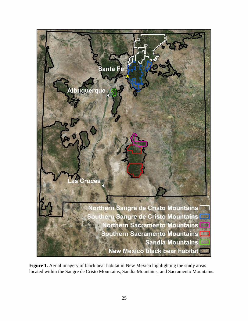
25

Figure 1. Aerial imagery of black bear habitat in New Mexico highlighting the study areas

located within the Sangre de Cristo Mountains, Sandia Mountains, and Sacramento Mountains.

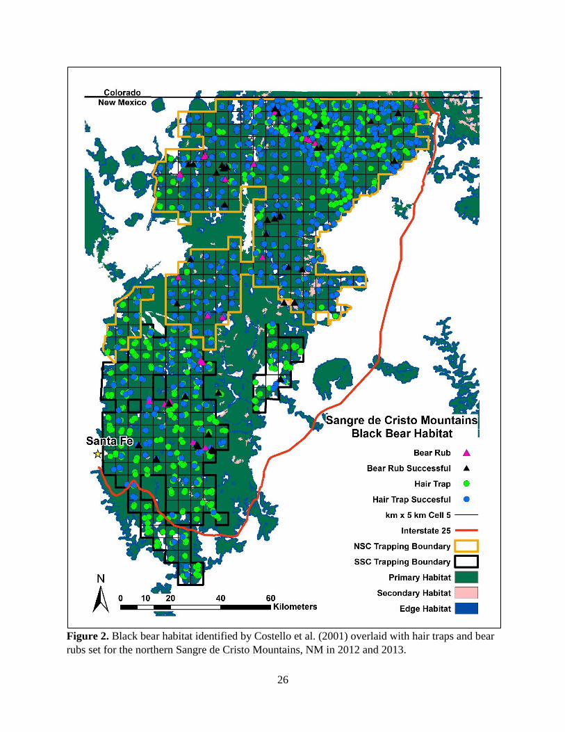
26

Figure 2. Black bear habitat identified by Costello et al. (2001) overlaid with hair traps and bear

rubs set for the northern Sangre de Cristo Mountains, NM in 2012 and 2013.

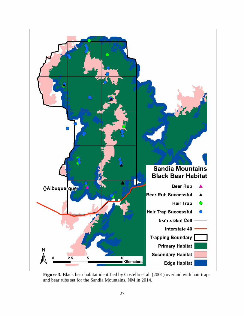
27

Figure 3. Black bear habitat identified by Costello et al. (2001) overlaid with hair traps

and bear rubs set for the Sandia Mountains, NM in 2014.

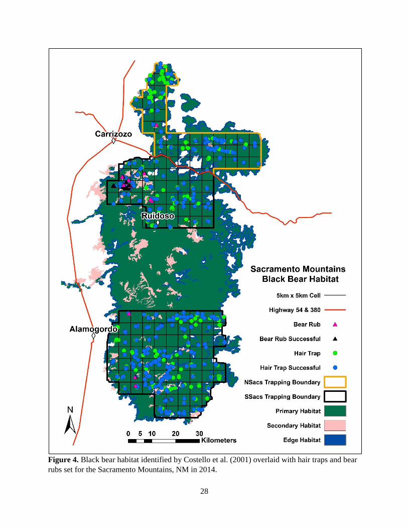
28

Figure 4. Black bear habitat identified by Costello et al. (2001) overlaid with hair traps and bear

rubs set for the Sacramento Mountains, NM in 2014.

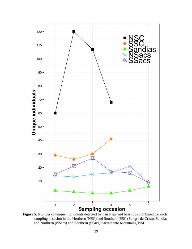
29

Figure 5. Number of unique individuals detected by hair traps and bear rubs combined for each

sampling occasion in the Northern (NSC) and Southern (SSC) Sangre de Cristo, Sandia,

and Northern (NSacs) and Southern (SSacs) Sacramento Mountains, NM.

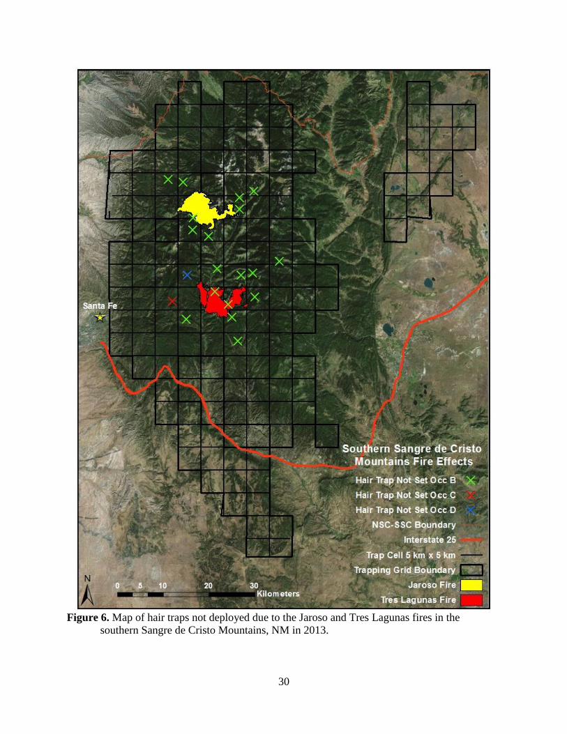
30

Figure 6. Map of hair traps not deployed due to the Jaroso and Tres Lagunas fires in the

southern Sangre de Cristo Mountains, NM in 2013.

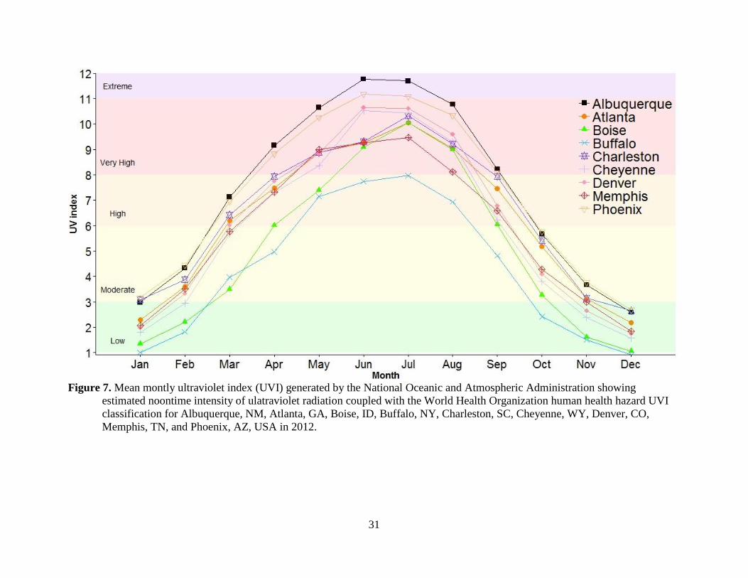
31

Figure 7. Mean montly ultraviolet index (UVI) generated by the National Oceanic and Atmospheric Administration showing

estimated noontime intensity of ulatraviolet radiation coupled with the World Health Organization human health hazard UVI

classification for Albuquerque, NM, Atlanta, GA, Boise, ID, Buffalo, NY, Charleston, SC, Cheyenne, WY, Denver, CO,

Memphis, TN, and Phoenix, AZ, USA in 2012.

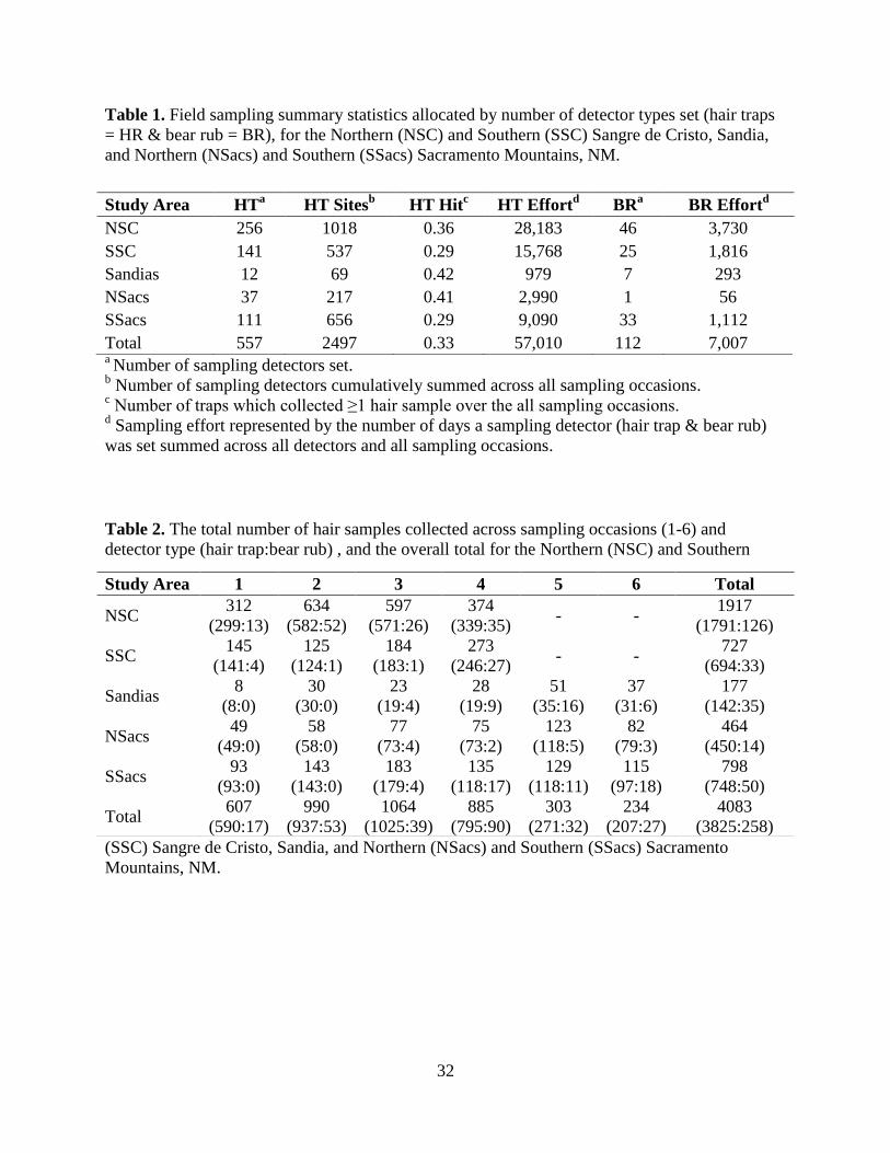
32

Table 1. Field sampling summary statistics allocated by number of detector types set (hair traps

= HR & bear rub = BR), for the Northern (NSC) and Southern (SSC) Sangre de Cristo, Sandia,

and Northern (NSacs) and Southern (SSacs) Sacramento Mountains, NM.

a Number of sampling detectors set.

b Number of sampling detectors cumulatively summed across all sampling occasions.

c Number of traps which collected ≥1 hair sample over the all sampling occasions.

d Sampling effort represented by the number of days a sampling detector (hair trap & bear rub)

was set summed across all detectors and all sampling occasions.

Table 2. The total number of hair samples collected across sampling occasions (1-6) and

detector type (hair trap:bear rub) , and the overall total for the Northern (NSC) and Southern

(SSC) Sangre de Cristo, Sandia, and Northern (NSacs) and Southern (SSacs) Sacramento

Mountains, NM.

Study Area HTa

HT Sitesb

HT Hitc HT Effort

d BR

a BR Effort

d

NSC 256 1018 0.36 28,183 46 3,730

SSC 141 537 0.29 15,768 25 1,816

Sandias 12 69 0.42 979 7 293

NSacs 37 217 0.41 2,990 1 56

SSacs 111 656 0.29 9,090 33 1,112

Total 557 2497 0.33 57,010 112 7,007

Study Area 1 2 3 4 5 6 Total

NSC 312

(299:13)

634

(582:52)

597

(571:26)

374

(339:35) - -

1917

(1791:126)

SSC 145

(141:4)

125

(124:1)

184

(183:1)

273

(246:27) - -

727

(694:33)

Sandias 8

(8:0)

30

(30:0)

23

(19:4)

28

(19:9)

51

(35:16)

37

(31:6)

177

(142:35)

NSacs 49

(49:0)

58

(58:0)

77

(73:4)

75

(73:2)

123

(118:5)

82

(79:3)

464

(450:14)

SSacs 93

(93:0)

143

(143:0)

183

(179:4)

135

(118:17)

129

(118:11)

115

(97:18)

798

(748:50)

Total 607

(590:17)

990

(937:53)

1064

(1025:39)

885

(795:90)

303

(271:32)

234

(207:27)

4083

(3825:258)

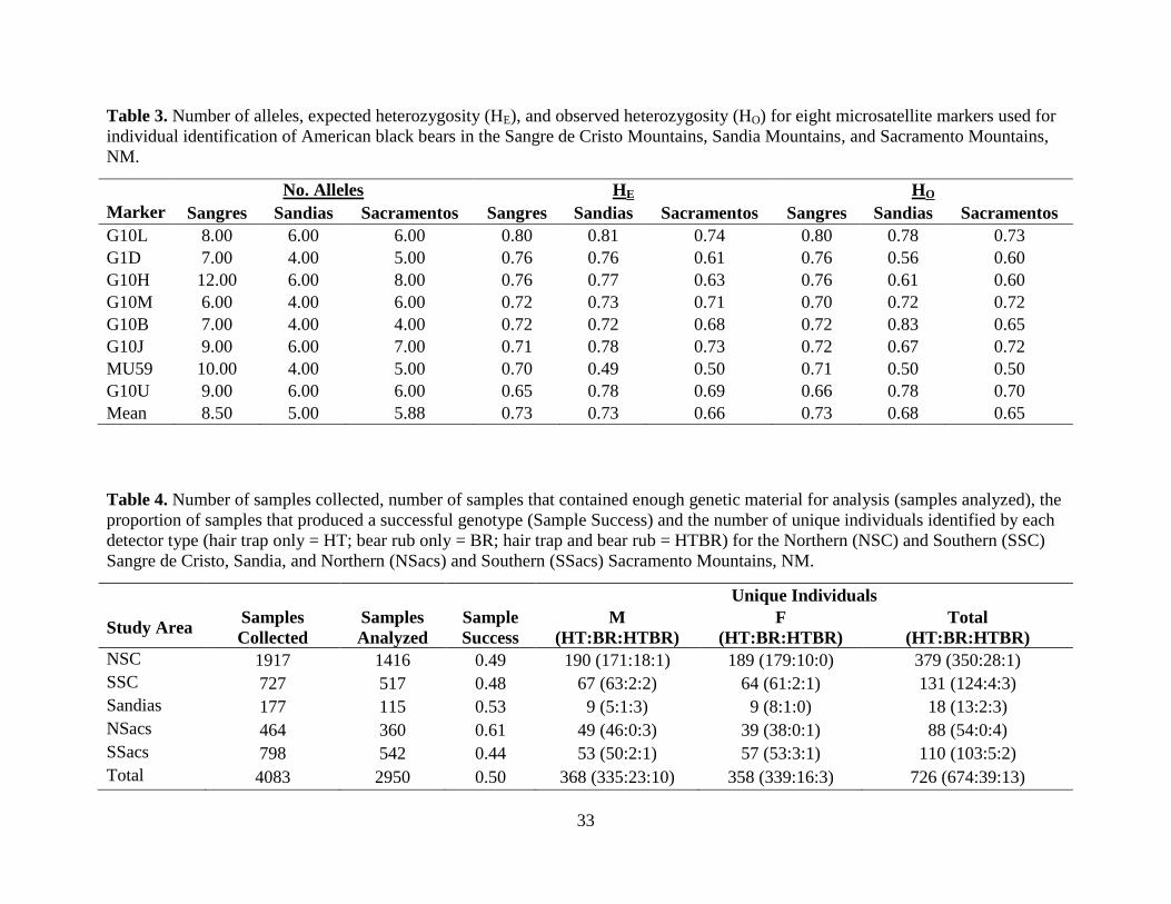
33

Table 3. Number of alleles, expected heterozygosity (HE), and observed heterozygosity (HO) for eight microsatellite markers used for

individual identification of American black bears in the Sangre de Cristo Mountains, Sandia Mountains, and Sacramento Mountains,

NM.

No. Alleles HE HO

Marker Sangres Sandias Sacramentos Sangres Sandias Sacramentos Sangres Sandias Sacramentos

G10L 8.00 6.00 6.00 0.80 0.81 0.74 0.80 0.78 0.73

G1D 7.00 4.00 5.00 0.76 0.76 0.61 0.76 0.56 0.60

G10H 12.00 6.00 8.00 0.76 0.77 0.63 0.76 0.61 0.60

G10M 6.00 4.00 6.00 0.72 0.73 0.71 0.70 0.72 0.72

G10B 7.00 4.00 4.00 0.72 0.72 0.68 0.72 0.83 0.65

G10J 9.00 6.00 7.00 0.71 0.78 0.73 0.72 0.67 0.72

MU59 10.00 4.00 5.00 0.70 0.49 0.50 0.71 0.50 0.50

G10U 9.00 6.00 6.00 0.65 0.78 0.69 0.66 0.78 0.70

Mean 8.50 5.00 5.88 0.73 0.73 0.66 0.73 0.68 0.65

Table 4. Number of samples collected, number of samples that contained enough genetic material for analysis (samples analyzed), the

proportion of samples that produced a successful genotype (Sample Success) and the number of unique individuals identified by each

detector type (hair trap only = HT; bear rub only = BR; hair trap and bear rub = HTBR) for the Northern (NSC) and Southern (SSC)

Sangre de Cristo, Sandia, and Northern (NSacs) and Southern (SSacs) Sacramento Mountains, NM.

Unique Individuals

Study Area Samples

Collected

Samples

Analyzed

Sample

Success

M

(HT:BR:HTBR)

F

(HT:BR:HTBR)

Total

(HT:BR:HTBR)

NSC 1917 1416 0.49 190 (171:18:1) 189 (179:10:0) 379 (350:28:1)

SSC 727 517 0.48 67 (63:2:2) 64 (61:2:1) 131 (124:4:3)

Sandias 177 115 0.53 9 (5:1:3) 9 (8:1:0) 18 (13:2:3)

NSacs 464 360 0.61 49 (46:0:3) 39 (38:0:1) 88 (54:0:4)

SSacs 798 542 0.44 53 (50:2:1) 57 (53:3:1) 110 (103:5:2)

Total 4083 2950 0.50 368 (335:23:10) 358 (339:16:3) 726 (674:39:13)

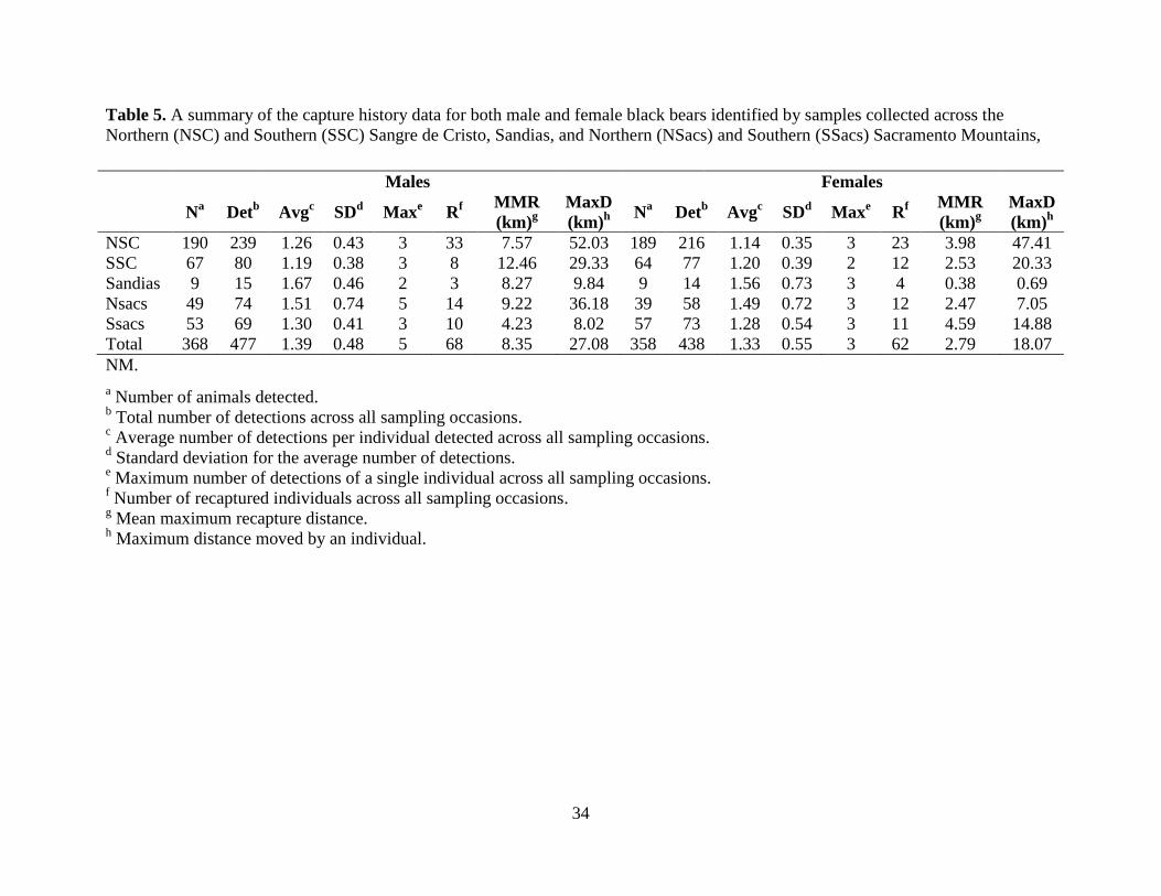
34

Table 5. A summary of the capture history data for both male and female black bears identified by samples collected across the

Northern (NSC) and Southern (SSC) Sangre de Cristo, Sandias, and Northern (NSacs) and Southern (SSacs) Sacramento Mountains,

NM.

a Number of animals detected.

b Total number of detections across all sampling occasions.

c Average number of detections per individual detected across all sampling occasions.

d Standard deviation for the average number of detections.

e Maximum number of detections of a single individual across all sampling occasions.

f Number of recaptured individuals across all sampling occasions.

g Mean maximum recapture distance.

h Maximum distance moved by an individual.

Males Females

N

a Det

b Avg

c SD

d Max

e R

f

MMR

(km)g

MaxD

(km)h N

a Det

b Avg

c SD

d Max

e R

f

MMR

(km)g

MaxD

(km)h

NSC 190 239 1.26 0.43 3 33 7.57 52.03 189 216 1.14 0.35 3 23 3.98 47.41

SSC 67 80 1.19 0.38 3 8 12.46 29.33 64 77 1.20 0.39 2 12 2.53 20.33

Sandias 9 15 1.67 0.46 2 3 8.27 9.84 9 14 1.56 0.73 3 4 0.38 0.69

Nsacs 49 74 1.51 0.74 5 14 9.22 36.18 39 58 1.49 0.72 3 12 2.47 7.05

Ssacs 53 69 1.30 0.41 3 10 4.23 8.02 57 73 1.28 0.54 3 11 4.59 14.88

Total 368 477 1.39 0.48 5 68 8.35 27.08 358 438 1.33 0.55 3 62 2.79 18.07

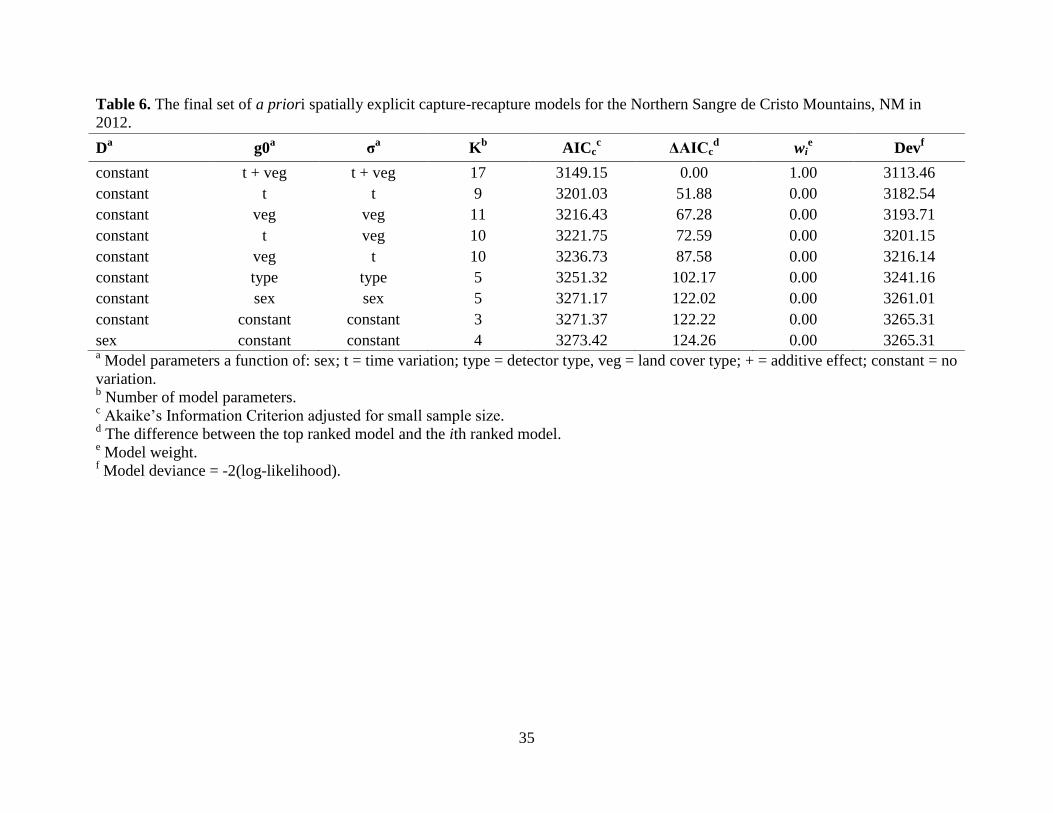
35

Table 6. The final set of a priori spatially explicit capture-recapture models for the Northern Sangre de Cristo Mountains, NM in

2012.

a Model parameters a function of: sex; t = time variation; type = detector type, veg = land cover type; + = additive effect; constant = no

variation. b Number of model parameters.

c Akaike’s Information Criterion adjusted for small sample size.

d The difference between the top ranked model and the ith ranked model.

e Model weight.

f Model deviance = -2(log-likelihood).

Da g0

a σ

a K

b AICc

c ΔAICc

d wi

e Dev

f

constant t + veg t + veg 17 3149.15 0.00 1.00 3113.46

constant t t 9 3201.03 51.88 0.00 3182.54

constant veg veg 11 3216.43 67.28 0.00 3193.71

constant t veg 10 3221.75 72.59 0.00 3201.15

constant veg t 10 3236.73 87.58 0.00 3216.14

constant type type 5 3251.32 102.17 0.00 3241.16

constant sex sex 5 3271.17 122.02 0.00 3261.01

constant constant constant 3 3271.37 122.22 0.00 3265.31

sex constant constant 4 3273.42 124.26 0.00 3265.31

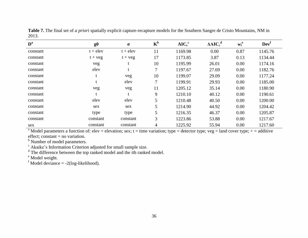
36

Table 7. The final set of a priori spatially explicit capture-recapture models for the Southern Sangre de Cristo Mountains, NM in

2013.

a Model parameters a function of: elev = elevation; sex; t = time variation; type = detector type; veg = land cover type; + = additive

effect; constant = no variation. b Number of model parameters.

c Akaike’s Information Criterion adjusted for small sample size.

d The difference between the top ranked model and the ith ranked model.

e Model weight.

f Model deviance = -2(log-likelihood).

Da g0 σ K

b AICc

c ΔAICc

d wi

e Dev

f

constant t + elev t + elev 11 1169.98 0.00 0.87 1145.76

constant t + veg t + veg 17 1173.85 3.87 0.13 1134.44

constant veg t 10 1195.99 26.01 0.00 1174.16

constant elev t 7 1197.67 27.69 0.00 1182.76

constant t veg 10 1199.07 29.09 0.00 1177.24

constant t elev 7 1199.91 29.93 0.00 1185.00

constant veg veg 11 1205.12 35.14 0.00 1180.90

constant t t 9 1210.10 40.12 0.00 1190.61

constant elev elev 5 1210.48 40.50 0.00 1200.00

constant sex sex 5 1214.90 44.92 0.00 1204.42

constant type type 5 1216.35 46.37 0.00 1205.87

constant constant constant 3 1223.86 53.88 0.00 1217.67

sex constant constant 4 1225.92 55.94 0.00 1217.60

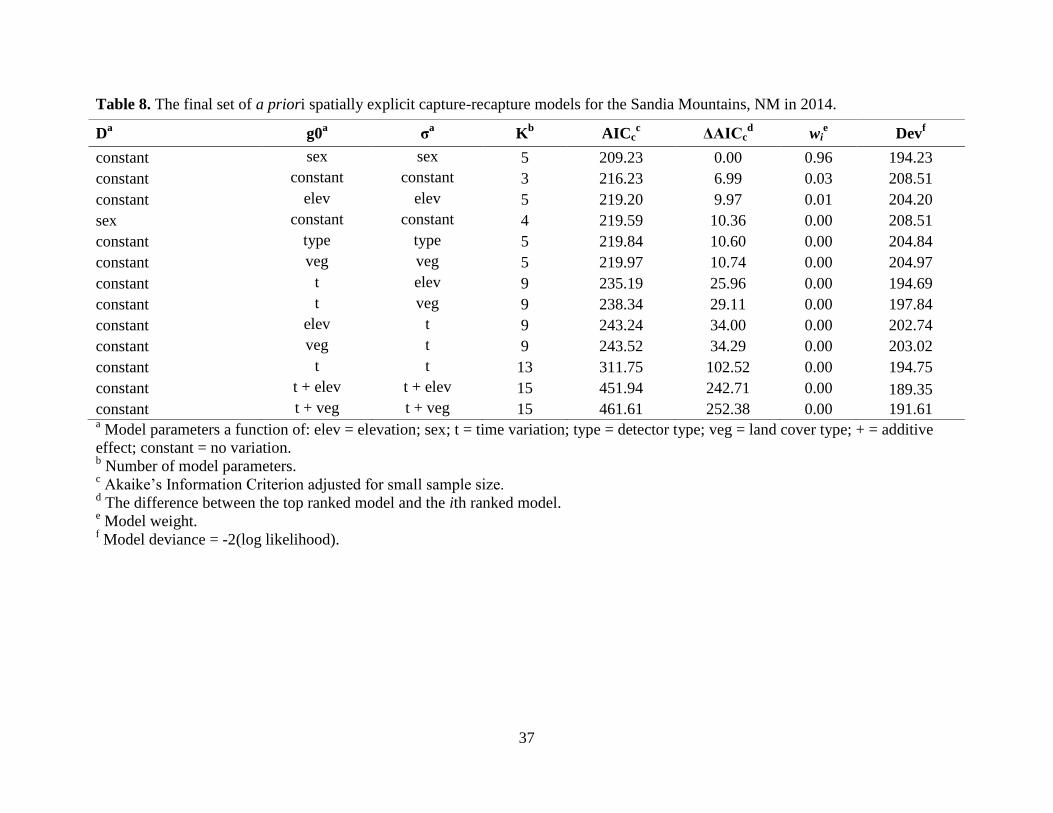
37

Table 8. The final set of a priori spatially explicit capture-recapture models for the Sandia Mountains, NM in 2014.

a Model parameters a function of: elev = elevation; sex; t = time variation; type = detector type; veg = land cover type; + = additive

effect; constant = no variation. b Number of model parameters.

c Akaike’s Information Criterion adjusted for small sample size.

d The difference between the top ranked model and the ith ranked model.

e Model weight.

f Model deviance = -2(log likelihood).

Da g0

a σ

a K

b AICc

c ΔAICc

d wi

e Dev

f

constant sex sex 5 209.23 0.00 0.96 194.23

constant constant constant 3 216.23 6.99 0.03 208.51

constant elev elev 5 219.20 9.97 0.01 204.20

sex constant constant 4 219.59 10.36 0.00 208.51

constant type type 5 219.84 10.60 0.00 204.84

constant veg veg 5 219.97 10.74 0.00 204.97

constant t elev 9 235.19 25.96 0.00 194.69

constant t veg 9 238.34 29.11 0.00 197.84

constant elev t 9 243.24 34.00 0.00 202.74

constant veg t 9 243.52 34.29 0.00 203.02

constant t t 13 311.75 102.52 0.00 194.75

constant t + elev t + elev 15 451.94 242.71 0.00 189.35

constant t + veg t + veg 15 461.61 252.38 0.00 191.61

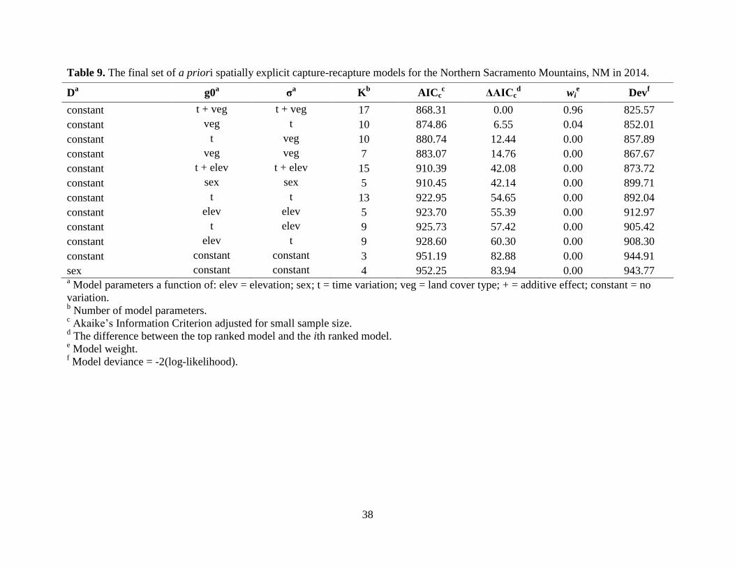
38

Table 9. The final set of a priori spatially explicit capture-recapture models for the Northern Sacramento Mountains, NM in 2014.

a Model parameters a function of: elev = elevation; sex; t = time variation; veg = land cover type; + = additive effect; constant = no

variation. b Number of model parameters.

c Akaike’s Information Criterion adjusted for small sample size.

d The difference between the top ranked model and the ith ranked model.

e Model weight.

f Model deviance = -2(log-likelihood).

Da g0

a σ

a K

b AICc

c ΔAICc

d wi

e Dev

f

constant t + veg t + veg 17 868.31 0.00 0.96 825.57

constant veg t 10 874.86 6.55 0.04 852.01

constant t veg 10 880.74 12.44 0.00 857.89

constant veg veg 7 883.07 14.76 0.00 867.67

constant t + elev t + elev 15 910.39 42.08 0.00 873.72

constant sex sex 5 910.45 42.14 0.00 899.71

constant t t 13 922.95 54.65 0.00 892.04

constant elev elev 5 923.70 55.39 0.00 912.97

constant t elev 9 925.73 57.42 0.00 905.42

constant elev t 9 928.60 60.30 0.00 908.30

constant constant constant 3 951.19 82.88 0.00 944.91

sex constant constant 4 952.25 83.94 0.00 943.77

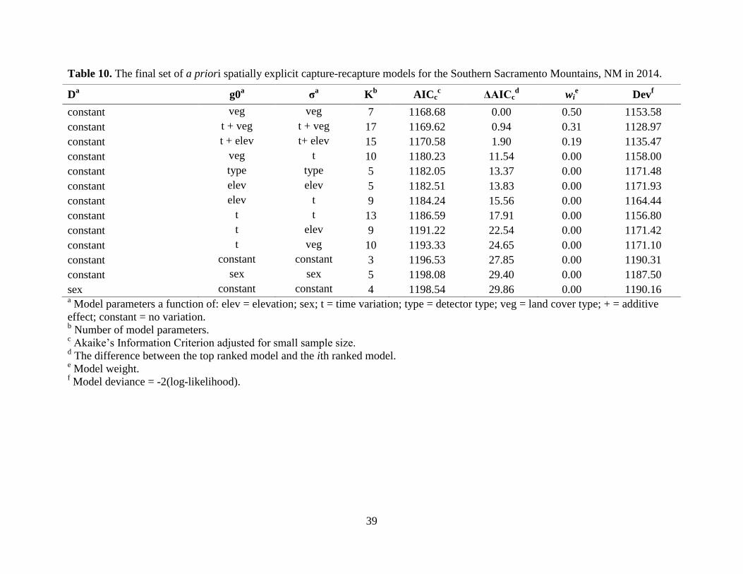
39

Table 10. The final set of a priori spatially explicit capture-recapture models for the Southern Sacramento Mountains, NM in 2014.

a Model parameters a function of: elev = elevation; sex; t = time variation; type = detector type; veg = land cover type; + = additive

effect; constant = no variation. b Number of model parameters.

c Akaike’s Information Criterion adjusted for small sample size.

d The difference between the top ranked model and the ith ranked model.

e Model weight.

f Model deviance = -2(log-likelihood).

Da g0

a σ

a K

b AICc

c ΔAICc

d wi

e Dev

f

constant veg veg 7 1168.68 0.00 0.50 1153.58

constant t + veg t + veg 17 1169.62 0.94 0.31 1128.97

constant t + elev t+ elev 15 1170.58 1.90 0.19 1135.47

constant veg t 10 1180.23 11.54 0.00 1158.00

constant type type 5 1182.05 13.37 0.00 1171.48

constant elev elev 5 1182.51 13.83 0.00 1171.93

constant elev t 9 1184.24 15.56 0.00 1164.44

constant t t 13 1186.59 17.91 0.00 1156.80

constant t elev 9 1191.22 22.54 0.00 1171.42

constant t veg 10 1193.33 24.65 0.00 1171.10

constant constant constant 3 1196.53 27.85 0.00 1190.31

constant sex sex 5 1198.08 29.40 0.00 1187.50

sex constant constant 4 1198.54 29.86 0.00 1190.16

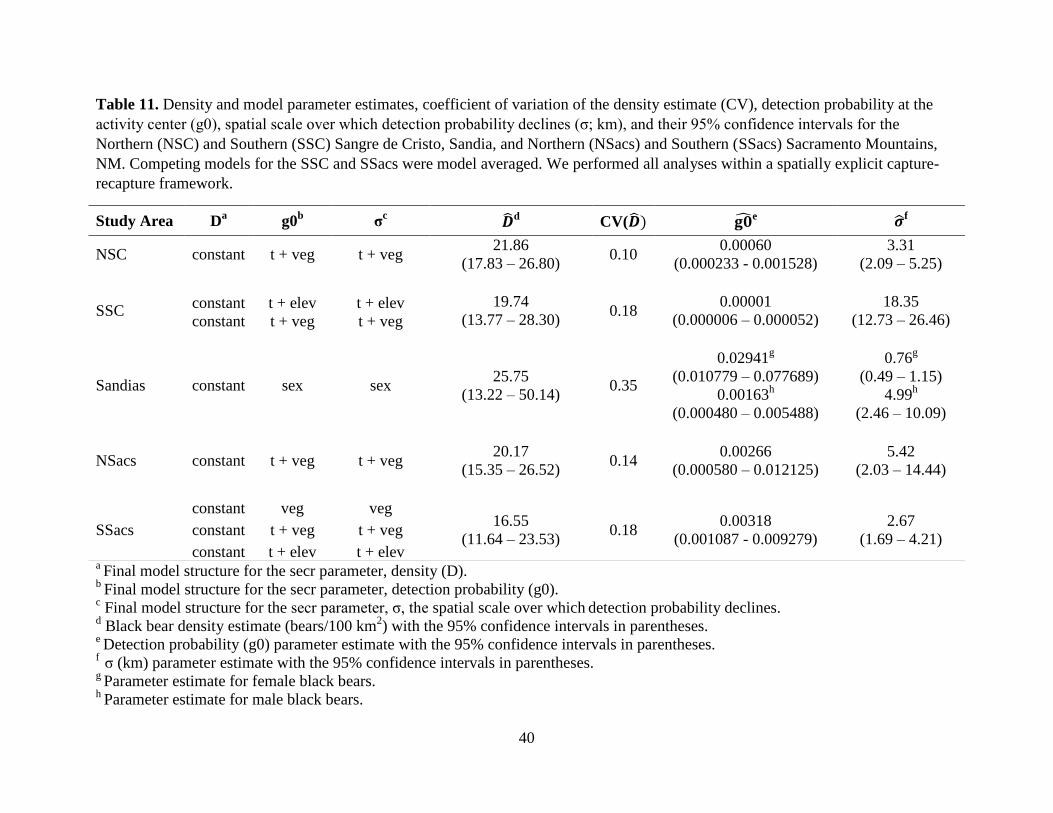
40

Table 11. Density and model parameter estimates, coefficient of variation of the density estimate (CV), detection probability at the

activity center (g0), spatial scale over which detection probability declines (σ; km), and their 95% confidence intervals for the

Northern (NSC) and Southern (SSC) Sangre de Cristo, Sandia, and Northern (NSacs) and Southern (SSacs) Sacramento Mountains,

NM. Competing models for the SSC and SSacs were model averaged. We performed all analyses within a spatially explicit capture-

recapture framework.

a Final model structure for the secr parameter, density (D).

b Final model structure for the secr parameter, detection probability (g0).

c Final model structure for the secr parameter, σ, the spatial scale over which

detection probability declines.

d Black bear density estimate (bears/100 km

2) with the 95% confidence intervals in parentheses.

e Detection probability (g0) parameter estimate with the 95% confidence intervals in parentheses.

f σ (km) parameter estimate with the 95% confidence intervals in parentheses.

g Parameter estimate for female black bears.

h Parameter estimate for male black bears.

Study Area Da

g0b

σc

�̂�d CV(�̂�) 𝐠�̂�e �̂�f

NSC

constant t + veg t + veg 21.86

(17.83 – 26.80) 0.10

0.00060

(0.000233 - 0.001528)

3.31

(2.09 – 5.25)

SSC constant t + elev t + elev 19.74

(13.77 – 28.30) 0.18

0.00001

(0.000006 – 0.000052)

18.35

(12.73 – 26.46) constant t + veg t + veg

Sandias constant sex sex 25.75

(13.22 – 50.14) 0.35

0.02941g

(0.010779 – 0.077689)

0.76g

(0.49 – 1.15)

0.00163h

(0.000480 – 0.005488)

4.99h

(2.46 – 10.09)

NSacs constant t + veg t + veg 20.17

(15.35 – 26.52) 0.14

0.00266

(0.000580 – 0.012125)

5.42

(2.03 – 14.44)

SSacs

constant veg veg 16.55

(11.64 – 23.53) 0.18

0.00318

(0.001087 - 0.009279)

2.67

(1.69 – 4.21) constant t + veg t + veg

constant t + elev t + elev

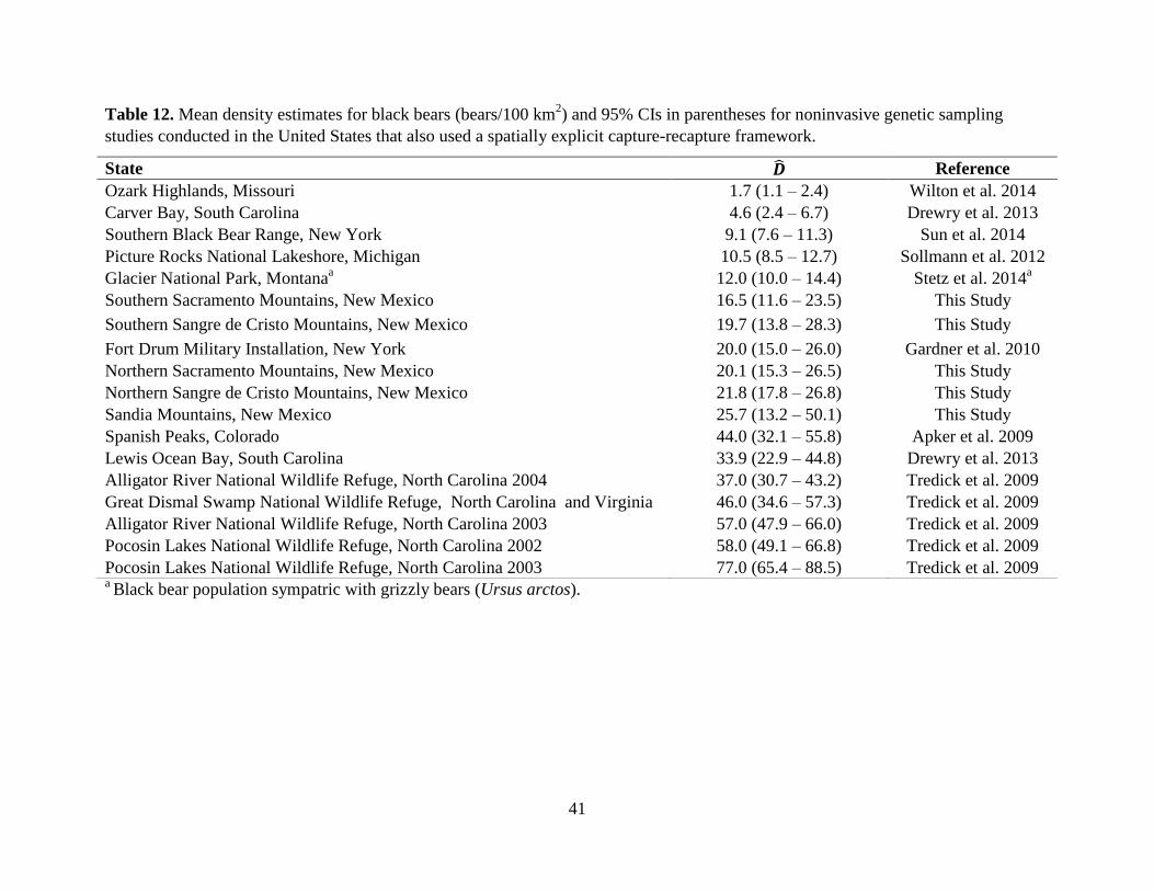
41

Table 12. Mean density estimates for black bears (bears/100 km2) and 95% CIs in parentheses for noninvasive genetic sampling

studies conducted in the United States that also used a spatially explicit capture-recapture framework.

a Black bear population sympatric with grizzly bears (Ursus arctos).

State �̂� Reference

Ozark Highlands, Missouri 1.7 (1.1 – 2.4) Wilton et al. 2014

Carver Bay, South Carolina 4.6 (2.4 – 6.7) Drewry et al. 2013

Southern Black Bear Range, New York 9.1 (7.6 – 11.3) Sun et al. 2014

Picture Rocks National Lakeshore, Michigan 10.5 (8.5 – 12.7) Sollmann et al. 2012

Glacier National Park, Montanaa

12.0 (10.0 – 14.4) Stetz et al. 2014a

Southern Sacramento Mountains, New Mexico 16.5 (11.6 – 23.5) This Study

Southern Sangre de Cristo Mountains, New Mexico 19.7 (13.8 – 28.3) This Study

Fort Drum Military Installation, New York 20.0 (15.0 – 26.0) Gardner et al. 2010

Northern Sacramento Mountains, New Mexico 20.1 (15.3 – 26.5) This Study

Northern Sangre de Cristo Mountains, New Mexico 21.8 (17.8 – 26.8) This Study

Sandia Mountains, New Mexico 25.7 (13.2 – 50.1) This Study

Spanish Peaks, Colorado 44.0 (32.1 – 55.8) Apker et al. 2009

Lewis Ocean Bay, South Carolina 33.9 (22.9 – 44.8) Drewry et al. 2013

Alligator River National Wildlife Refuge, North Carolina 2004 37.0 (30.7 – 43.2) Tredick et al. 2009

Great Dismal Swamp National Wildlife Refuge, North Carolina and Virginia 46.0 (34.6 – 57.3) Tredick et al. 2009

Alligator River National Wildlife Refuge, North Carolina 2003 57.0 (47.9 – 66.0) Tredick et al. 2009

Pocosin Lakes National Wildlife Refuge, North Carolina 2002 58.0 (49.1 – 66.8) Tredick et al. 2009

Pocosin Lakes National Wildlife Refuge, North Carolina 2003 77.0 (65.4 – 88.5) Tredick et al. 2009