Pergamon Mathl. Comput. Modelling Vol. 25, No. 10, pp. 57-62, 1997

Copyright@1997 Elsevier Science Ltd Printed in Great Britain. All rights reserved

PII: s0895-7177(97)00074-5 0895-7177197 $17.00 + 0.00

Maximizing the Weighted Number of On-Time Jobs in Single Machine

Scheduling with Time Windows

C. KOULAMAS Department of Decision Sciences and Information Systems Florida International University, Miami, FL 33199, U.S.A.

(Received August 1994; revised and accepted November 1996)

Abstract-The problem of maximizing the weighted number of on-time jobs on a single machine with time windows (STW) is shown to be strongly NP-hard. An efficient. heuristic is presented for STW. Computational experiments indicate that the performance of the heuristic is quite good.

Keywords-Single machine, Scheduling, Time windows.

1. INTRODUCTION

Single-machine scheduling with time windows (STW) has received relatively little attention in the

literature, although it has wide applicability in just-in-time manufacturing, chemical processing,

PERT/CPM scheduling, space station operations, etc. In this paper, we consider the following

static, deterministic, single-machine scheduling problem. There is a set of jobs Ji, i = 1,. . . , TX,

all available at time zero. Each job Ji has a known weight (value) ‘pi, a deterministic processing

time pi, and a time window (bi,&) with window length zi = di - bi, where bi is the earliest

desirable start time and di is the due date. For each job Ji, we define Vi = 1 if Ji is entirely

processed within its time window (Ji is on time), and Vi = 0 otherwise. The objective is to

determine a schedule so the weighted number of on-time jobs EYE1 WiUi is maximized. A schedule

is uniquely determined when the start times si are determined for all jobs Ji (i = 1, . . . , n). Each

job’s time window is longer than its processing time (Zi > pi) so it can be entirely processed

within its window if no other jobs are processed in its window. There are no other restrictions

imposed on time windows; windows may overlap and/or a window may be entirely contained

in another window. Preemption is not allowed and the machine is continuously available. Since

preemption is not allowed, a job’s completion time ci is uniquely determined from its start time si

&s Ci = Si + pi.

The STW problem has potential applications in scheduling chemical reactions on the same

equipment. Each completed reaction has a value and requires a catalyst. The catalyst’s incuba-

tion time determines the window start time for that reaction, and the catalyst’s useful life (after

its incubation is completed) determines the window length. The objective is to determine which

reactions to process on the equipment so the total value of all processed reactions during a finite

planning horizon is maximized.

Other potential applications include scheduling on a space station equipped with a camera to

photograph space objects. Based on a space object’s orbit, a time window is determined during

which the object is close enough to the space station so a photograph of acceptable quality can be

Typeset by A,#-w

57

58 C. KOULAMAS

taken. Each photograph has a given scientific value (weight). The time windows corresponding to different space objects may overlap, and the objective is to maximize the total scientific value of the photographs taken during a finite planning horizon.

The literature on single-machine time window scheduling (STW) is quite limited. Sidney [l] considered an STW problem with the objective of minimizing the maximum earliness/tardiness penalty. He also imposed the condition that no job’s window is allowed to contain the window of another job as a proper subset. This condition leads directly to an optimal sequence with jobs sequenced in ascending order of their target start times. Sidney then developed an optimal pro- cedure for determining the actual job start times to minimize the maximum earliness/tardiness penalty. Sidney’s procedure was further refined by Lakshminarayan et al. [2] so it can be imple- mented to run in O(n log n) time. The STW problem can be viewed as a generalization of the single machine early/tardy problem with distinct due dates. A recent survey of the literature for that problem can be found in [3].

The rest of the paper is organized as follows. In the next section, we show that STW is strongly NP-hard. In Section 3, we first derive some preliminary results. A problem specific heuristic is developed in Section 4, and its performance is tested in Section 5.

2. COMPLEXITY OF THE STW PROBLEM

In this section, we show that STW is strongly NP-hard by reducing the known unary NP-hard 3-partition problem to STW. Three-partition (see [4]) can be stated as follows: given 3n positive integers al, . . . , as,, and an integer q with C:z, al = nq and q/4 5 ai 5 q/2 for i = 1,. . . ,3n, does there exist a partition of (1,. . . ,3n} into n subsets Ii,. . . , I,, such that Cierj ai = q for j=l,...,n?

Prom an instance of bpartition, we construct the following instance of STW with 4n - 1 jobs:

Ji with bi = 0, pi = ai, di = nq + n - 1, wi = 1 for i = 1,. . . ,3n, Sr with 61 = q, pl = 1, dl = q + 1, WI = 1,

S,_r with b,.,_l = (n - 1)q + (n - 2)) p,_l = 1, d,_i = (n - 1)q + (n - 1)) w,+r = 1.

If Sr,..., S,_i are scheduled on time, there are n slots of size q left which must be filled to capacity if all 4n - 1 jobs are to be scheduled on time. Consequently, the instance of 3-partition has an affirmative answer if and only if all jobs in the STW problem can be scheduled on time. Notice that we proved the above complexity result by defining an instance of STW with equal weights for all jobs. This indicates that even the unweighted version of the problem is strongly NP-hard.

3. SOLUTION PRELIMINARIES

The first step in the solution procedure is to check if the problem decomposes into smaller independent subproblems. In order to do so, we initially sort all jobs in the data set according to earliest due date (EDD).

LEMMA 1. If there axe any two consecutive jobs Ji, Ji+l with di 5 bi+l, then the problem decomposes into two independent subproblems: one including jobs 51,. . . , Ji and one including jobs Ji+l,...,Jn.

PROOF. Assume that di 5 bi+l for some i = 1,. . . ,n. Any of the jobs Jl,. , . , J+ that are not on time, that is, they are not entirely processed within their respective windows (which are subsets of the {bl, di} interval), can be scheduled to start after d,, without affecting the value of the objective function. Consequently, the {bi+l, n d } interval can be dedicated to processing the optimal subset of on-time jobs from the {Ji+l, Jn} set.

Maximizing the Weighted Number 59

Similarly, any of the {&+I, 4,) jobs which are not on time can be processed outside the &+i,d,} interval without affecting the objective function value. Consequently, the two sub- problems can be solved separately and the resulting early/late jobs in each subproblem can be scheduled outside the {bi, &} interval in any order without affecting the objective function value.

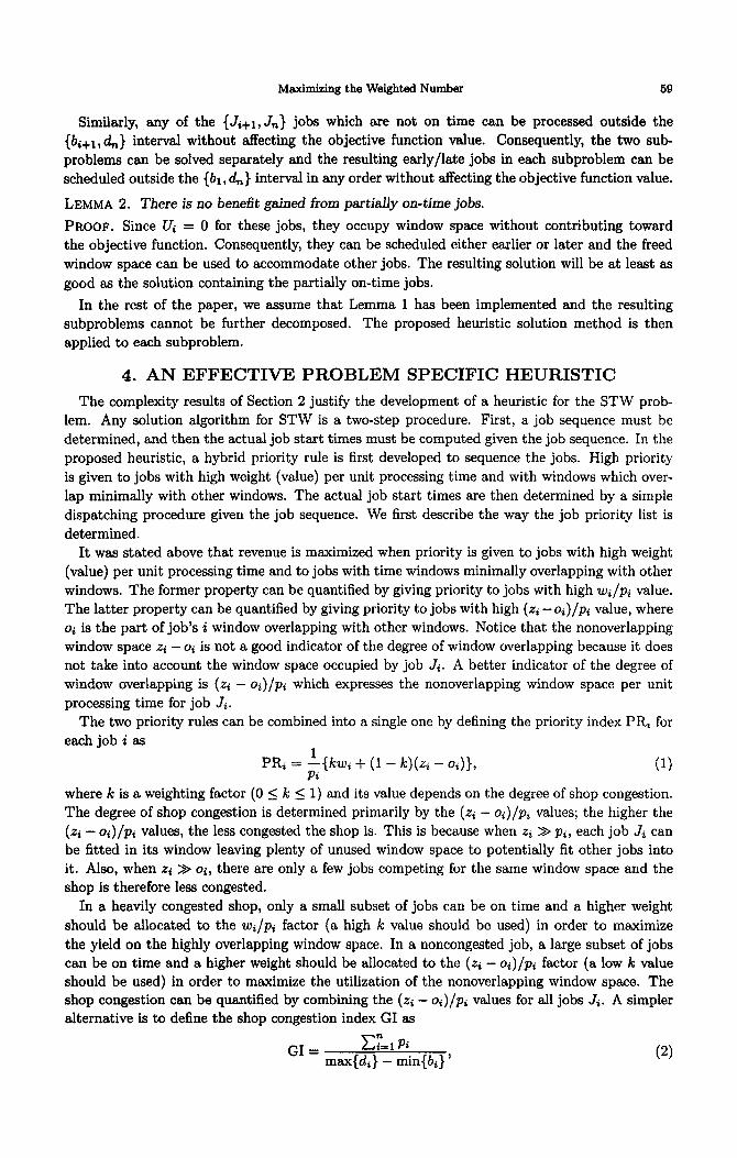
LEMMA 2. There is no benefit gained from partially on-time jobs.

PROOF. Since Vi = 0 for these jobs, they occupy window space without contributing toward the objective function. Consequently, they can be scheduled either earlier or later and the freed window space can be used to accommodate other jobs. The resulting solution will be at least as good as the solution containing the partially on-time jobs.

In the rest of the paper, we assume that Lemma 1 has been implemented and the resulting subproblems cannot be further decomposed. The proposed heuristic solution method is then applied to each subproblem.

4. AN EFFECTIVE PROBLEM SPECIFIC HEURISTIC

The complexity results of Section 2 justify the development of a heuristic for the STW prob- lem. Any solution algorithm for STW is a two-step procedure. First, a job sequence must be determined, and then the actual job start times must be computed given the job sequence. In the proposed heuristic, a hybrid priority rule is first developed to sequence the jobs. High priority is given to jobs with high weight (value) per unit processing time and with windows which over- lap minimally with other windows. The actual job start times are then determined by a simple dispatching procedure given the job sequence. We first describe the way the job priority list is determined.

It was stated above that revenue is maximized when priority is given to jobs with high weight (value) per unit processing time and to jobs with time windows minimally overlapping with other windows. The former property can be quantified by giving priority to jobs with high wi/pi value. The latter property can be quantified by giving priority to jobs with high (.ri - oi)/pi value, where oi is the part of job’s i window overlapping with other windows. Notice that the nonoverlapping window space .Zi - oi is not a good indicator of the degree of window overlapping because it does not take into account the window space occupied by job Ji. A better indicator of the degree of window overlapping is (t.i - oi)/pi which expresses the nonoverlapping window space per unit processing time for job Ji.

The two priority rules can be combined into a single one by defining the priority index PR, for each job i as

1 PRi = --(IFuJi + (1 - k)(& - Oi)}, (1)

where k is a weighting factor (0 5 k 5 1) and its value depends on the degree of shop congestion. The degree of shop congestion is determined primarily by the (pi - oi)/pi values; the higher the (,ri - oi)/pi values, the less congested the shop is. This is because when zZ~ >> pi, each job Ji can be fitted in its window leaving plenty of unused window space to potentially fit other jobs into it. Also, when pi >> oi, there are only a few jobs competing for the same window space and the shop is therefore less congested.

In a heavily congested shop, only a small subset of jobs can be on time and a higher weight should be allocated to the wi/pi factor (a high k value should be used) in order to maximize the yield on the highly overlapping window space. In a noncongested job, a large subset of jobs can be on time and a higher weight should be allocated to the (pi - oi)/pi factor (a low k value should be used) in order to maximize the utilization of the nonoverlapping window space. The shop congestion CEUI be quantified by combining the (Zi - oi)/pi values for all jobs Ji. A simpler alternative is to define the shop congestion index GI as

GI = cz, Pi msx{di} - min{bi} ’ (2)

60 C. KOULAMAS

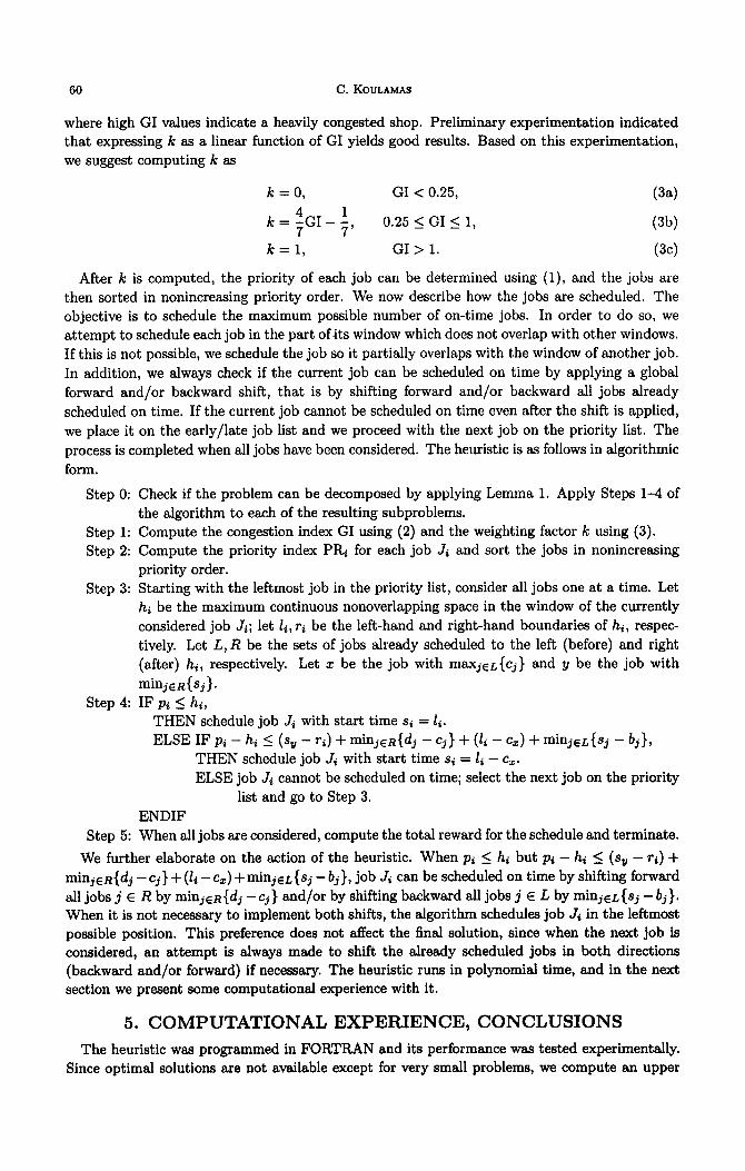
where high GI values indicate a heavily congested shop. Preliminary experimentation indicated that expressing Ic as a linear function of GI yields good results. Based on this experimentation, we suggest computing k as

k = 0, GI < 0.25,

k = ;GI - ;, 0.25 5 GI 5 1,

(3a)

Pb)

k = 1, GI> 1. (3c)

After k is computed, the priority of each job can be determined using (l), and the jobs are then sorted in nonincreasing priority order. We now describe how the jobs are scheduled. The objective is to schedule the maximum possible number of on-time jobs. In order to do so, we attempt to schedule each job in the part ofits window which does not overlap with other windows. If this is not possible, we schedule the job so it partially overlaps with the window of another job. In addition, we always check if the current job can be scheduled on time by applying a global forward and/or backward shift, that is by shifting forward and/or backward all jobs already scheduled on time. If the current job cannot be scheduled on time even after the shift is applied, we place it on the early/late job list and we proceed with the next job on the priority list. The process is completed when all jobs have been considered. The heuristic is as follows in algorithmic form.

Step 0: Check if the problem can be decomposed by applying Lemma 1. Apply Steps l-4 of the algorithm to each of the resulting subproblems.

Step 1: Compute the congestion index GI using (2) and the weighting factor k using (3). Step 2: Compute the priority index PR for each job Ji and sort the jobs in nonincreasing

priority order. Step 3: Starting with the leftmost job in the priority list, consider all jobs one at a time. Let

hi be the maximum continuous nonoverlapping space in the window of the currently considered job Ji; let li, ri be the left-hand and right-hand boundaries of hi, respec- tively. Let L, R be the sets of jobs already scheduled to the left (before) and right (after) hi, respectively. Let x be the job with maxjeL{cj} and y be the job with minjeR{sj}.

Step 4: IF pi I hi, THEN schedule job Ji with start time si = li. ELSE IF pi - hi 5 (sy - ~6) + minjeR{dj - cj} + (Zi - c,) + minjeL{sj - bj},

THEN schedule job Ji with start time si = li - c,. ELSE job Ji cannot be scheduled on time; select the next job on the priority

list and go to Step 3. ENDIF

Step 5: When all jobs are considered, compute the total reward for the schedule and terminate.

We further elaborate on the action of the heuristic. When pi 5 hi but pi - hi 5 (sa, - Ti) +

minjeR{dj - cj} + (li -c,) + minjeL{sj - bj}, job Ji can be scheduled on time by shifting forward all jobs j E R by minjeR{dj - cj) and/or by shifting backward all jobs j E L by minjeL{sj - bj}. When it is not necessary to implement both shifts, the algorithm schedules job Ji in the leftmost possible position. This preference does not affect the final solution, since when the next job is considered, an attempt is always made to shift the already scheduled jobs in both directions (backward and/or forward) if necessary. The heuristic runs in polynomial time, and in the next section we present some computational experience with it.

5. COMPUTATIONAL EXPERIENCE, CONCLUSIONS

The heuristic was programmed in FORTRAN and its performance was tested experimentally. Since optimal solutions are not available except for very small problems, we compute an upper

Maximizing the Weighted Number 61

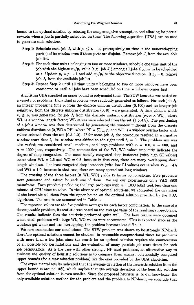
bound to the optimal solution by relaxing the nonpreemptive assumption and allowing for partial rewards when a job is partially scheduled on time. The following algorithm (UBA) can be used

to generate such solutions.

Step 1: Schedule each job Ji with pi I zi - oi preemptively on time in the nonoverlapping part(s) of its window even if these parts are disjoint. Remove job Ji from the available

job list. Step 2: For each time unit t belonging to two or more windows, schedule one time unit of the

job with the highest wj/pj value (e.g., job Jj) among all jobs eligible to be scheduled at t. Update pj = pj - 1 and add wj/pj to the objective function. If pj = 0, remove job Jj from the available job list.

Step 3: Repeat Step 2 until all time units t belonging to two or more windows have been considered or until all jobs have been scheduled on time, whichever comes first.

Algorithm UBA supplied an upper bound in polynomial time. The STW heuristic was tested on a variety of problems. Individual problems were randomly generated as follows. For each job Ji, an integer processing time pi from the discrete uniform distribution (0,100) and an integer job weight wi from the discrete uniform distribution (0,lO) were generated. A time window width Z~ > pi was generated for job Ji from the discrete uniform distribution [pi,pi x WL], where WL is a window length factor; WL values were selected from the set {1.5,4.5}. The positioning of a job’s window was then determined by generating the window midpoint from the discrete uniform distribution [0, WO x PP], where PP = x6, pi and WO is a window overlap factor with values selected from the set {0.5,1.0}. If for some job Ji the procedure resulted in a negative window start time bi, its window was shifted to the right until bi = 0. The problem size was also varied; we considered small, medium, and large problems with n = 100, n = 500, and n = 1000 jobs, respectively. The combination of the WL, WO values implicitly indicate the degree of shop congestion. The most heavily congested shop instances (with high GI values) occur when WL = 1.5 and WO = 0.5, because in that cese, there are many overlapping short length windows. The least congested shop instances (with low GI values) occur when WL = 4.5 and WO = 1.0, because in that case, there are many spread out long windows.

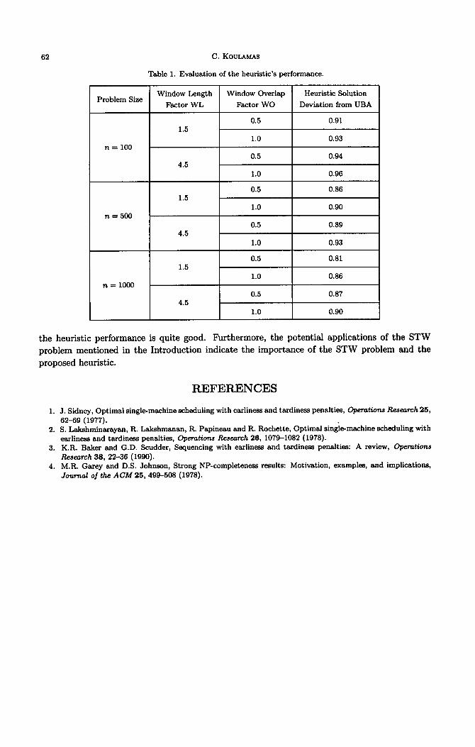
The crossing of the three factors (n, WL, WO) yields 12 factor combinations. Five problems were generated and solved for each one of them. We ran our experiments on a VAX 8800 mainframe. Each problem (including the large problems with n = 1000 jobs) took less than one minute of CPU time to solve. In the absence of optimal solutions, we computed the deviation of the heuristic solutions from the upper bound on the optimal solution provided by the UBA algorithm. The results are summarized in Table 1.

The reported values are the five problem averages for each factor combination. In the case of a decomposable problem, its statistic was baaed on the average value of the resulting subproblems. The results indicate that the heuristic performed quite well. The best results were obtained when small problems with large WL, WO values were encountered. This is expected since as the windows get wider and less overlapping, the problem becomes less difficult.

We now summarize our conclusions. The STW problem was shown to be strongly NP-hard, therefore optimal solutions cannot be obtained in reasonable computational times for problems with more than a few jobs, since the search for an optimal solution requires the enumeration of all possible job permutations and the evaluation of many possible job start times for each job permutation. As is the case with other strongly NP-hard problems, an alternative way to evaluate the quality of heuristic solutions is to compare them against polynomially computed upper bounds (for a maximization problem) like the ones provided by the UBA algorithm,

The experimental results indicated that the average deviation of the heuristic solution from the upper bound is around lo%, which implies that the average deviation of the heuristic solution from the optimal solution is even smaller. Since the proposed heuristic is, to our knowledge, the only available solution method for the problem and the problem is NP-hard, we conclude that

62 C. KOULAMAS

Table 1. Evaluation of the heuristic’s performance.

0.5 0.81 1.5

1.0 0.86 n = 1000

0.5 0.87 4.5

1.0 0.90

the heuristic performance is quite good. F’urthermore, the potential applications of the STW problem mentioned in the Introduction indicate the importance of the STW problem and the proposed heuristic.

REFERENCES

J. Sidney, Optimal single-machine scheduling with earliness and tardiness penalties, Cpemtiona Resee& 25, 62-69 (1977). S. Lakshminarayan, R. Lakshmanan, R. Papineau and R. Brochette, Optimal singlemachine scheduling with earliness and tardiness penalties, Operations Research 26, 1079-1082 (1978). K.R. Baker and G.D. Scudder, Sequencing with earliness and tardiness penalties: A review, Operations Research 58, 22-36 (1990). M.R. Garey and D.S. Johnson, Strong NP-completeness results: Motivation, examples, and implications, Journal of the ACM 25, 499-508 (1978).