Maximum likelihood estimates of North Pacific albacore tuna (Thunnus alalunga)

von Bertalanffy growth parameters using conditional-age-at-length data

Southwest Fisheries Science Center

CAPAM Workshop La Jolla, CA, November 4th, 2014

Yi Xu, Steven Teo, Kevin Piner, Hui-hua Lee, Kuo-shu Chen, and David Wells

Email: yi.xu@noaa.gov

Previous studies• Size at age: • Estimated size at age-1 in north Pacific albacore ranges from 45 to 64 cm (Clemens 1961; Wells

et al. 2011; Chen et al. 2011).• Albacore are ~ 60 cm FL at age 2 when they recruit into surface fisheries and growth slows to

about 10 cm per year for ages 2-4 and becomes even slower after 5-6 years of age when albacore are mature (Clemens 1961; Otsu and Uchida 1959; Yabuta and Yukinawa 1963; Wells et al. 2011; Chen et al. 2011).

• Maximum measured size of north Pacific albacore is 128 cm (Otsu and Uchida 1959; Clemens 1961) and the maximum recorded age is 15 years (Wells et al. 2013).

• Growth estimates (using von Bertalanffy growth model ):• Suda (1966) L1 = 40.2 cm, L∞ = 146.46 cm, and K = 0.149/yr. • Last assessment (2011) parameters were estimated inside SS3 as L1 = 44.4 cm, L∞ =

118.0 cm, K = 0.2495 yr-1, CV1 = 0.0599, and CV2 = 0.0339• Chen et al. (2012) otolith studies • Wellls et al., (2013) otolith studies

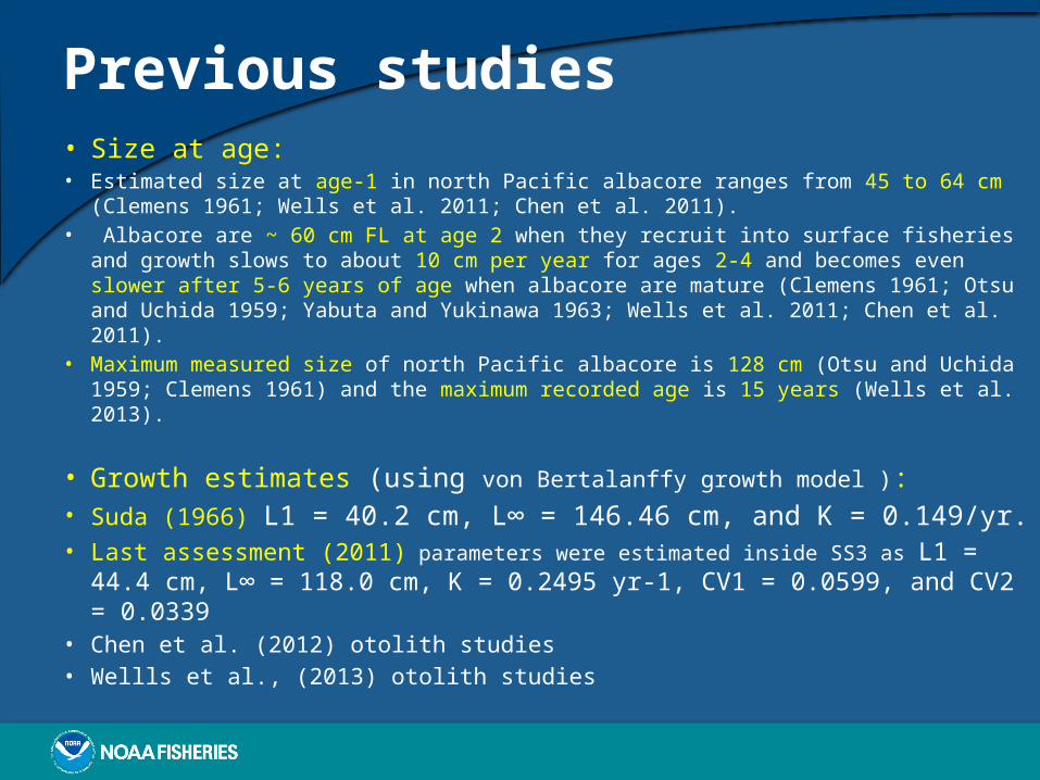
Wells1990-2012

CHN observer2011-2012

JP observer1987-2012

Chen2001-2006

Sampling Map

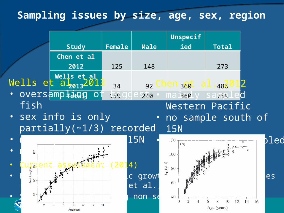
Sampling issues by size, age, sex, region

• Current assessment (2014)• Base case: Sex dimorphic growth with both data sources (Chen et al., 2012; Xu et al., 2014)• Sensitivity tests using non sex-specific growth, and using Chen’s data only

Study Female Male Unspecified Total

Chen et al 2012 125 148 273

Wells et al 2013 34 92 360 486

Total 159 240 360 759

Wells et al. 2013• oversampling of biggest fish• sex info is only partially(~1/3) recorded• no sample south of 15N• no big female sampled(<110cm)

Chen et al. 2012• mainly sampled Western Pacific• no sample south of 15N• no big female sampled (<110cm)

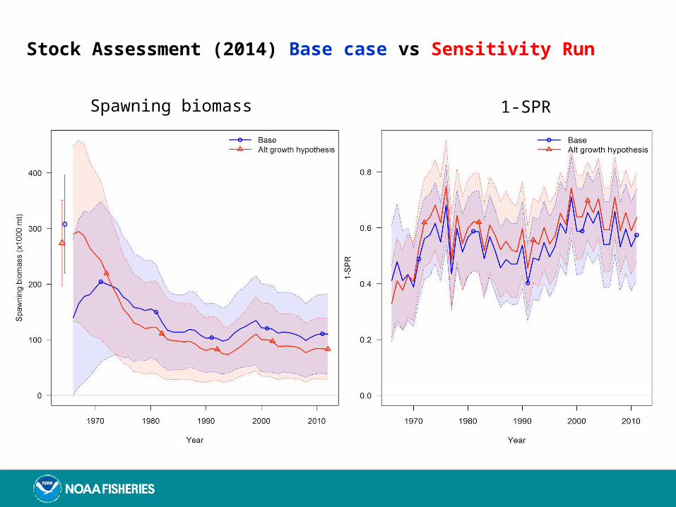
Stock Assessment (2014) Base case vs Sensitivity Run length

Spawning biomass 1-SPR

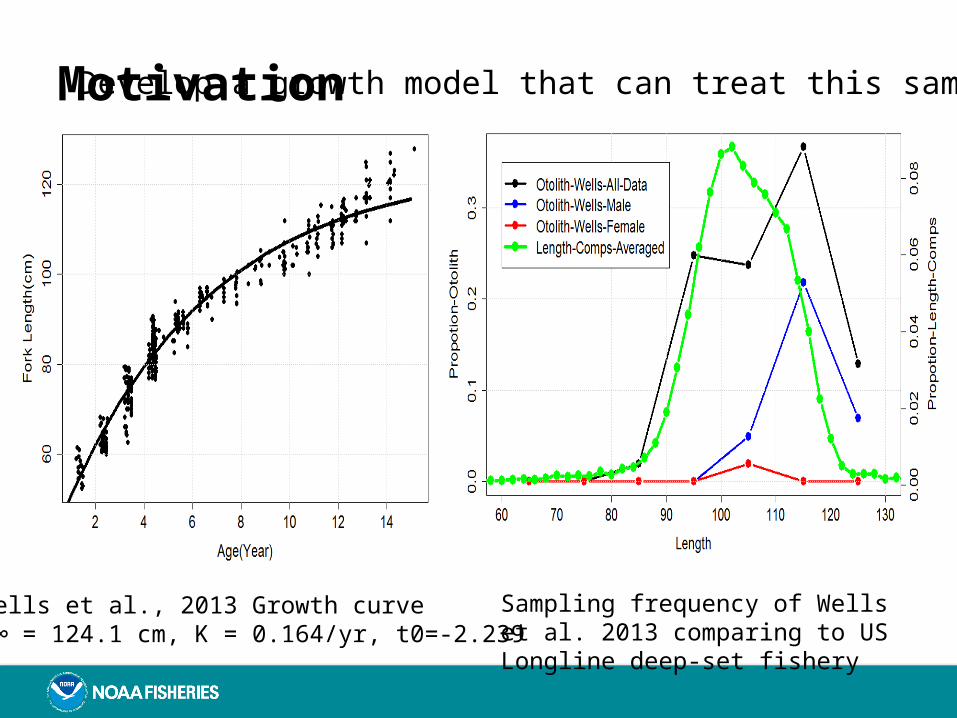
Motivationat length

Wells et al., 2013 Growth curveL∞ = 124.1 cm, K = 0.164/yr, t0=-2.239

Sampling frequency of Wells et al. 2013 comparing to US Longline deep-set fishery

Develop a growth model that can treat this sampling bias

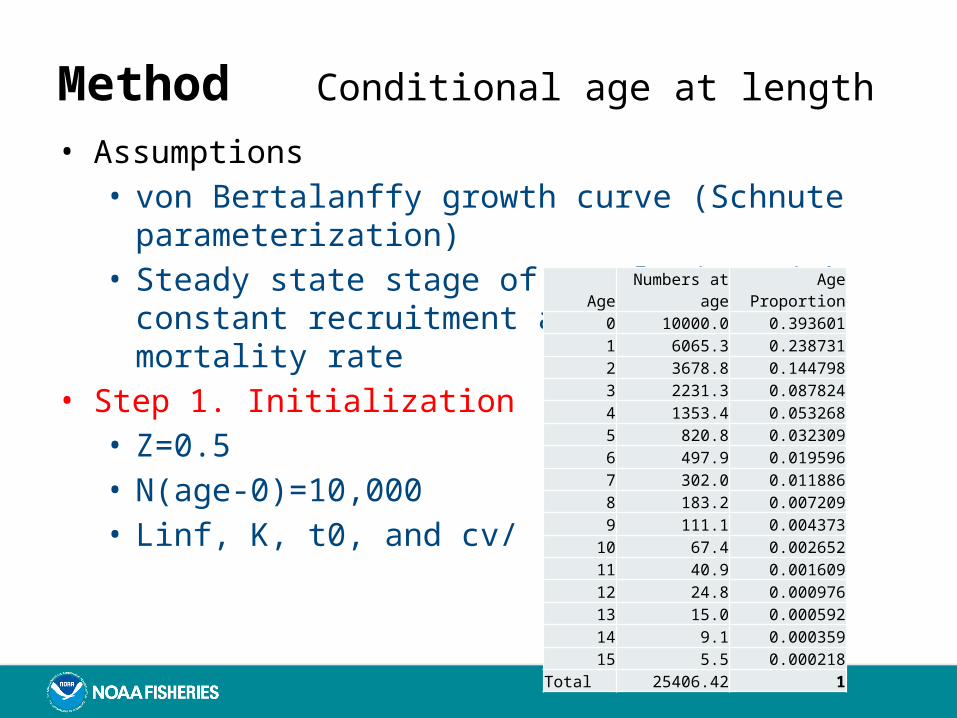
Method Conditional age at length

• Assumptions• von Bertalanffy growth curve (Schnute parameterization)• Steady state stage of population with constant recruitment and

constant mortality rate• Step 1. Initialization• Z=0.5• N(age-0)=10,000• Linf, K, t0, and cv/ (constant)

Age Numbers at age Age Proportion0 10000.0 0.3936011 6065.3 0.2387312 3678.8 0.1447983 2231.3 0.0878244 1353.4 0.0532685 820.8 0.0323096 497.9 0.0195967 302.0 0.0118868 183.2 0.0072099 111.1 0.004373

10 67.4 0.00265211 40.9 0.00160912 24.8 0.00097613 15.0 0.00059214 9.1 0.00035915 5.5 0.000218

Total 25406.42 1

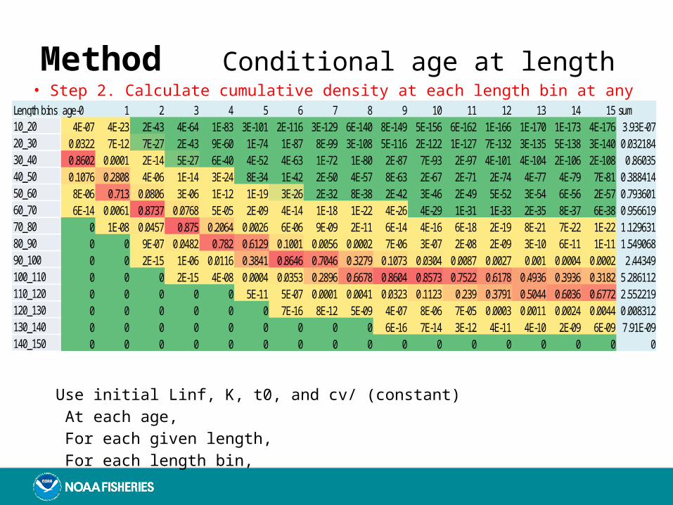
Method Conditional age at length• Step 2. Calculate cumulative density at each length bin at any age

Use initial Linf, K, t0, and cv/ (constant) At each age, For each given length, For each length bin,

Length bins age-0 1 2 3 4 5 6 7 8 9 10 11 12 13 14 15 sum10_20 4E-07 4E-23 2E-43 4E-64 1E-83 3E-101 2E-116 3E-129 6E-140 8E-149 5E-156 6E-162 1E-166 1E-170 1E-173 4E-176 3.93E-0720_30 0.0322 7E-12 7E-27 2E-43 9E-60 1E-74 1E-87 8E-99 3E-108 5E-116 2E-122 1E-127 7E-132 3E-135 5E-138 3E-140 0.03218430_40 0.8602 0.0001 2E-14 5E-27 6E-40 4E-52 4E-63 1E-72 1E-80 2E-87 7E-93 2E-97 4E-101 4E-104 2E-106 2E-108 0.8603540_50 0.1076 0.2808 4E-06 1E-14 3E-24 8E-34 1E-42 2E-50 4E-57 8E-63 2E-67 2E-71 2E-74 4E-77 4E-79 7E-81 0.38841450_60 8E-06 0.713 0.0806 3E-06 1E-12 1E-19 3E-26 2E-32 8E-38 2E-42 3E-46 2E-49 5E-52 3E-54 6E-56 2E-57 0.79360160_70 6E-14 0.0061 0.8737 0.0768 5E-05 2E-09 4E-14 1E-18 1E-22 4E-26 4E-29 1E-31 1E-33 2E-35 8E-37 6E-38 0.95661970_80 0 1E-08 0.0457 0.875 0.2064 0.0026 6E-06 9E-09 2E-11 6E-14 4E-16 6E-18 2E-19 8E-21 7E-22 1E-22 1.12963180_90 0 0 9E-07 0.0482 0.782 0.6129 0.1001 0.0056 0.0002 7E-06 3E-07 2E-08 2E-09 3E-10 6E-11 1E-11 1.54906890_100 0 0 2E-15 1E-06 0.0116 0.3841 0.8646 0.7046 0.3279 0.1073 0.0304 0.0087 0.0027 0.001 0.0004 0.0002 2.44349100_110 0 0 0 2E-15 4E-08 0.0004 0.0353 0.2896 0.6678 0.8604 0.8573 0.7522 0.6178 0.4936 0.3936 0.3182 5.286112110_120 0 0 0 0 0 5E-11 5E-07 0.0001 0.0041 0.0323 0.1123 0.239 0.3791 0.5044 0.6036 0.6772 2.552219120_130 0 0 0 0 0 0 7E-16 8E-12 5E-09 4E-07 8E-06 7E-05 0.0003 0.0011 0.0024 0.0044 0.008312130_140 0 0 0 0 0 0 0 0 0 6E-16 7E-14 3E-12 4E-11 4E-10 2E-09 6E-09 7.91E-09140_150 0 0 0 0 0 0 0 0 0 0 0 0 0 0 0 0 0

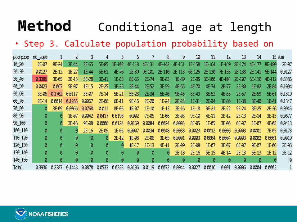
Method Conditional age at length• Step 3. Calculate population probability based on age proportion

pop.prop no_age0 1 2 3 4 5 6 7 8 9 10 11 12 13 14 15 sum10_20 2E-07 8E-24 3E-44 3E-65 5E-85 1E-102 4E-118 4E-131 4E-142 4E-151 1E-158 1E-164 1E-169 8E-174 4E-177 8E-180 2E-0720_30 0.0127 2E-12 1E-27 1E-44 5E-61 4E-76 2E-89 9E-101 2E-110 2E-118 6E-125 2E-130 7E-135 2E-138 2E-141 6E-144 0.012730_40 0.3386 3E-05 3E-15 5E-28 3E-41 1E-53 8E-65 2E-74 9E-83 1E-89 2E-95 3E-100 4E-104 2E-107 6E-110 4E-112 0.338640_50 0.0423 0.067 5E-07 1E-15 2E-25 3E-35 2E-44 2E-52 3E-59 4E-65 4E-70 4E-74 2E-77 2E-80 1E-82 2E-84 0.109450_60 3E-06 0.1702 0.0117 3E-07 7E-14 5E-21 5E-28 2E-34 6E-40 9E-45 8E-49 3E-52 4E-55 2E-57 2E-59 5E-61 0.181960_70 2E-14 0.0014 0.1265 0.0067 2E-06 6E-11 9E-16 2E-20 1E-24 2E-28 1E-31 2E-34 1E-36 1E-38 3E-40 1E-41 0.134770_80 0 3E-09 0.0066 0.0768 0.011 8E-05 1E-07 1E-10 1E-13 3E-16 1E-18 9E-21 2E-22 5E-24 3E-25 2E-26 0.094580_90 0 0 1E-07 0.0042 0.0417 0.0198 0.002 7E-05 1E-06 3E-08 9E-10 4E-11 2E-12 2E-13 2E-14 3E-15 0.067790_100 0 0 3E-16 9E-08 0.0006 0.0124 0.0169 0.0084 0.0024 0.0005 8E-05 1E-05 3E-06 6E-07 1E-07 4E-08 0.0413100_110 0 0 0 2E-16 2E-09 1E-05 0.0007 0.0034 0.0048 0.0038 0.0023 0.0012 0.0006 0.0003 0.0001 7E-05 0.0173110_120 0 0 0 0 0 2E-12 1E-08 2E-06 3E-05 0.0001 0.0003 0.0004 0.0004 0.0003 0.0002 0.0001 0.0019120_130 0 0 0 0 0 0 1E-17 1E-13 4E-11 2E-09 2E-08 1E-07 3E-07 6E-07 9E-07 1E-06 3E-06130_140 0 0 0 0 0 0 0 0 0 2E-18 2E-16 5E-15 4E-14 2E-13 6E-13 1E-12 2E-12140_150 0 0 0 0 0 0 0 0 0 0 0 0 0 0 0 0 0Total 0.3936 0.2387 0.1448 0.0878 0.0533 0.0323 0.0196 0.0119 0.0072 0.0044 0.0027 0.0016 0.001 0.0006 0.0004 0.0002 1

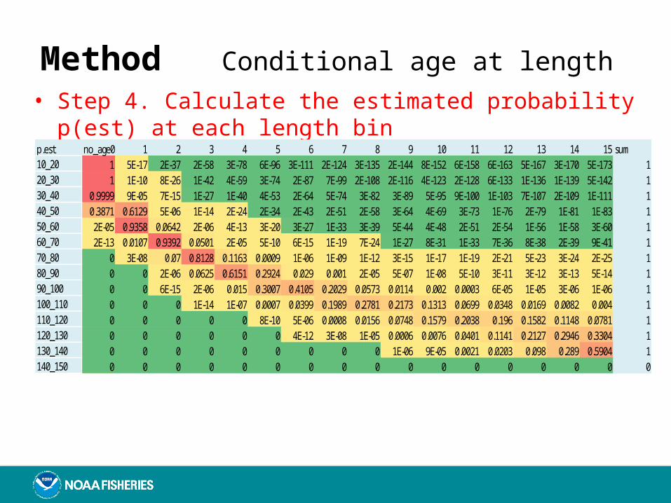
Method Conditional age at length• Step 4. Calculate the estimated probability p(est) at each length bin

p.est no_age0 1 2 3 4 5 6 7 8 9 10 11 12 13 14 15 sum10_20 1 5E-17 2E-37 2E-58 3E-78 6E-96 3E-111 2E-124 3E-135 2E-144 8E-152 6E-158 6E-163 5E-167 3E-170 5E-173 120_30 1 1E-10 8E-26 1E-42 4E-59 3E-74 2E-87 7E-99 2E-108 2E-116 4E-123 2E-128 6E-133 1E-136 1E-139 5E-142 130_40 0.9999 9E-05 7E-15 1E-27 1E-40 4E-53 2E-64 5E-74 3E-82 3E-89 5E-95 9E-100 1E-103 7E-107 2E-109 1E-111 140_50 0.3871 0.6129 5E-06 1E-14 2E-24 2E-34 2E-43 2E-51 2E-58 3E-64 4E-69 3E-73 1E-76 2E-79 1E-81 1E-83 150_60 2E-05 0.9358 0.0642 2E-06 4E-13 3E-20 3E-27 1E-33 3E-39 5E-44 4E-48 2E-51 2E-54 1E-56 1E-58 3E-60 160_70 2E-13 0.0107 0.9392 0.0501 2E-05 5E-10 6E-15 1E-19 7E-24 1E-27 8E-31 1E-33 7E-36 8E-38 2E-39 9E-41 170_80 0 3E-08 0.07 0.8128 0.1163 0.0009 1E-06 1E-09 1E-12 3E-15 1E-17 1E-19 2E-21 5E-23 3E-24 2E-25 180_90 0 0 2E-06 0.0625 0.6151 0.2924 0.029 0.001 2E-05 5E-07 1E-08 5E-10 3E-11 3E-12 3E-13 5E-14 190_100 0 0 6E-15 2E-06 0.015 0.3007 0.4105 0.2029 0.0573 0.0114 0.002 0.0003 6E-05 1E-05 3E-06 1E-06 1100_110 0 0 0 1E-14 1E-07 0.0007 0.0399 0.1989 0.2781 0.2173 0.1313 0.0699 0.0348 0.0169 0.0082 0.004 1110_120 0 0 0 0 0 8E-10 5E-06 0.0008 0.0156 0.0748 0.1579 0.2038 0.196 0.1582 0.1148 0.0781 1120_130 0 0 0 0 0 0 4E-12 3E-08 1E-05 0.0006 0.0076 0.0401 0.1141 0.2127 0.2946 0.3304 1130_140 0 0 0 0 0 0 0 0 0 1E-06 9E-05 0.0021 0.0203 0.098 0.289 0.5904 1140_150 0 0 0 0 0 0 0 0 0 0 0 0 0 0 0 0 0

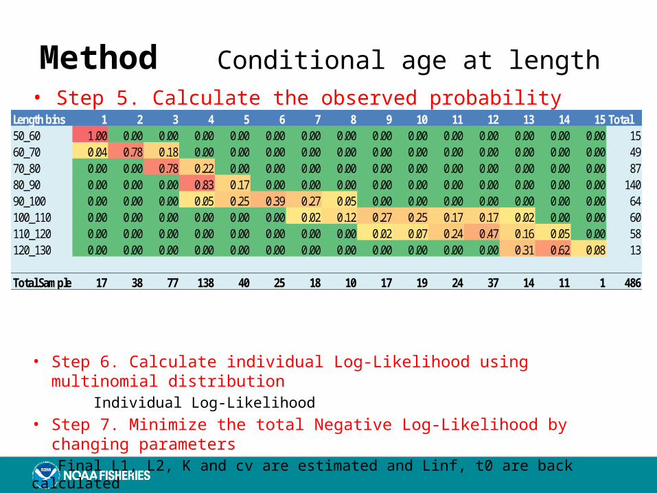
Method Conditional age at length• Step 5. Calculate the observed probability p(obs) at each length bin

Length bins 1 2 3 4 5 6 7 8 9 10 11 12 13 14 15 Total50_60 1.00 0.00 0.00 0.00 0.00 0.00 0.00 0.00 0.00 0.00 0.00 0.00 0.00 0.00 0.00 1560_70 0.04 0.78 0.18 0.00 0.00 0.00 0.00 0.00 0.00 0.00 0.00 0.00 0.00 0.00 0.00 4970_80 0.00 0.00 0.78 0.22 0.00 0.00 0.00 0.00 0.00 0.00 0.00 0.00 0.00 0.00 0.00 8780_90 0.00 0.00 0.00 0.83 0.17 0.00 0.00 0.00 0.00 0.00 0.00 0.00 0.00 0.00 0.00 14090_100 0.00 0.00 0.00 0.05 0.25 0.39 0.27 0.05 0.00 0.00 0.00 0.00 0.00 0.00 0.00 64100_110 0.00 0.00 0.00 0.00 0.00 0.00 0.02 0.12 0.27 0.25 0.17 0.17 0.02 0.00 0.00 60110_120 0.00 0.00 0.00 0.00 0.00 0.00 0.00 0.00 0.02 0.07 0.24 0.47 0.16 0.05 0.00 58120_130 0.00 0.00 0.00 0.00 0.00 0.00 0.00 0.00 0.00 0.00 0.00 0.00 0.31 0.62 0.08 13

Total Samples 17 38 77 138 40 25 18 10 17 19 24 37 14 11 1 486

• Step 6. Calculate individual Log-Likelihood using multinomial distribution Individual Log-Likelihood• Step 7. Minimize the total Negative Log-Likelihood by changing parameters

Final L1, L2, K and cv are estimated and Linf, t0 are back calculated

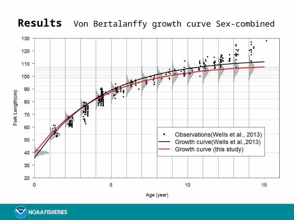
Results Von Bertalanffy growth curve Sex-combined

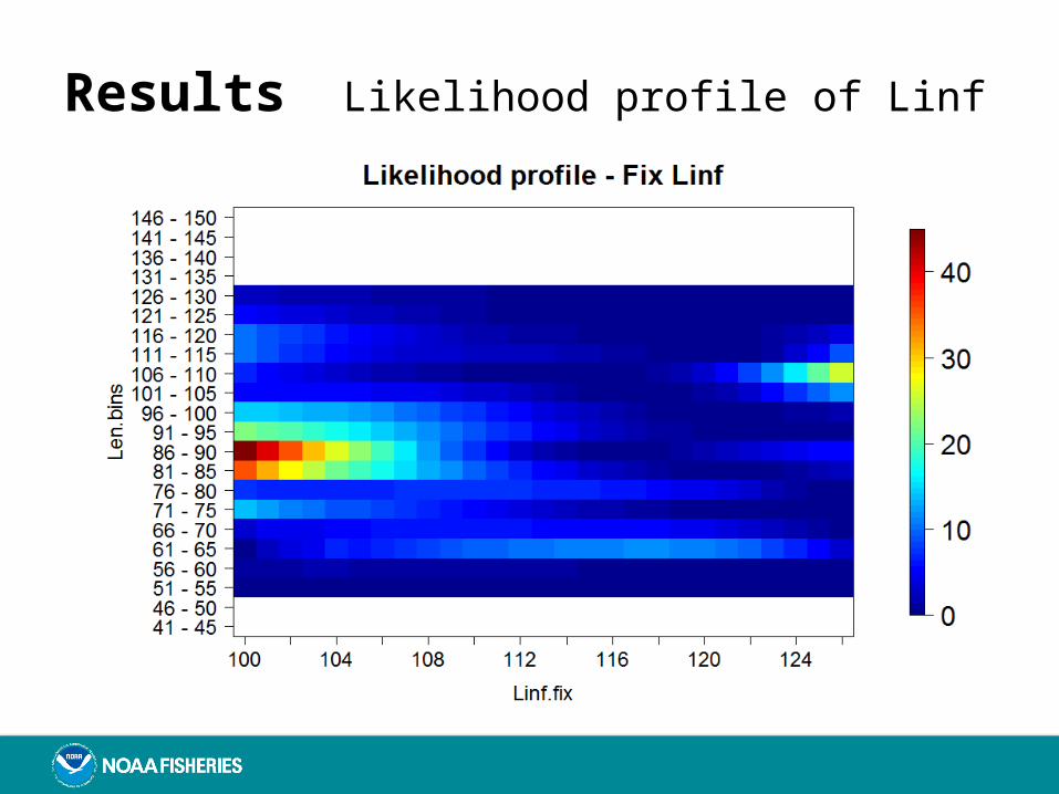
Results Likelihood profile of Linf

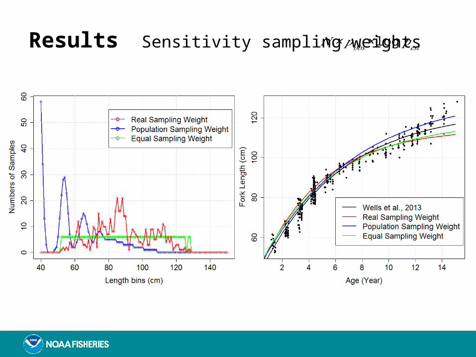
Results Sensitivity sampling weights 𝑁×𝑝𝑜𝑏𝑠× log𝑝𝑒𝑠𝑡

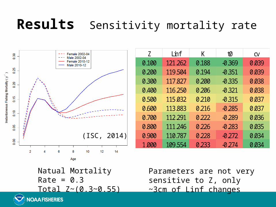
Results Sensitivity mortality rate

Z Linf K t0 cv0.100 121.262 0.188 -0.369 0.0390.200 119.504 0.194 -0.351 0.0390.300 117.827 0.200 -0.335 0.0380.400 116.250 0.206 -0.321 0.0380.500 115.032 0.210 -0.315 0.0370.600 113.883 0.216 -0.285 0.0370.700 112.291 0.222 -0.289 0.0360.800 111.246 0.226 -0.283 0.0350.900 110.787 0.228 -0.272 0.0341.000 109.554 0.233 -0.274 0.034

(ISC, 2014)

Natual Mortality Rate = 0.3Total Z~(0.3~0.55)

Parameters are not very sensitive to Z, only ~3cm of Linf changes

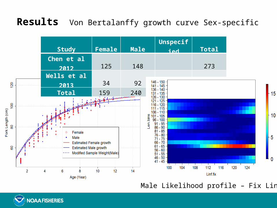
Results Von Bertalanffy growth curve Sex-specific

Male Likelihood profile – Fix Linf

Study Female Male Unspecified Total

Chen et al 2012 125 148 273

Wells et al 2013 34 92 360 486

Total 159 240 360 759

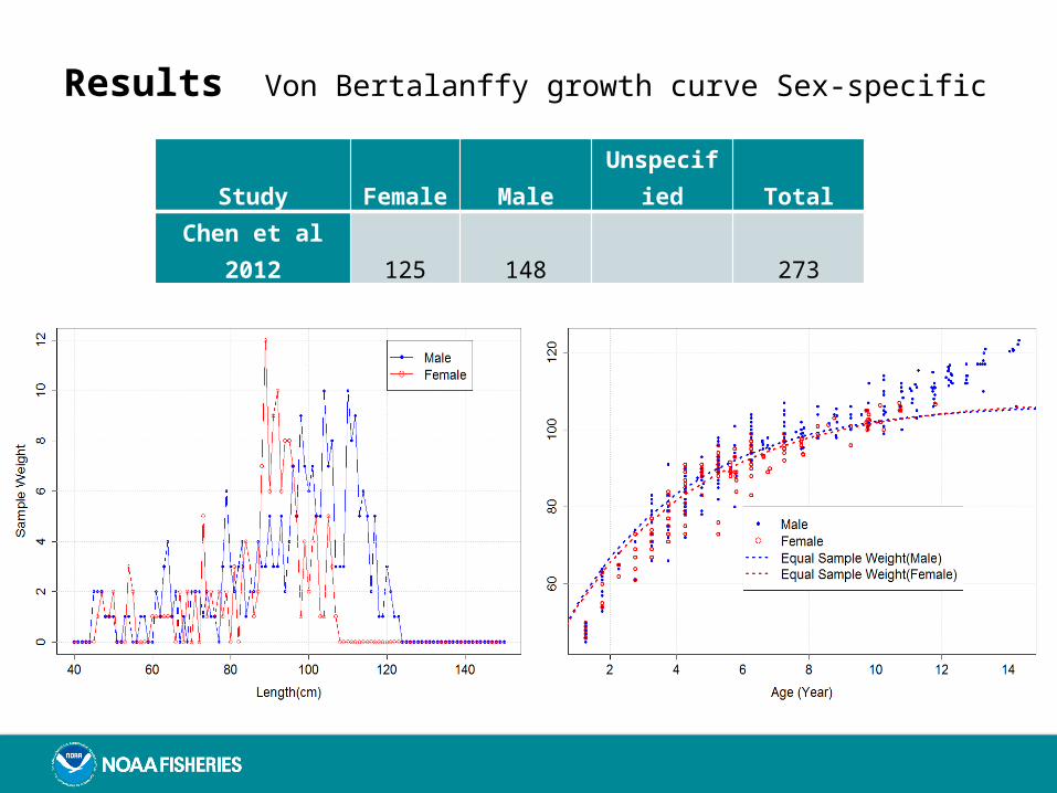
Results Von Bertalanffy growth curve Sex-specificStudy Female Male Unspecified Total

Chen et al 2012 125 148 273

Wells et al 2013 34 92 360 486

Total 159 240 360 759

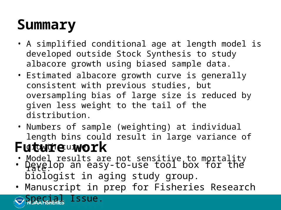
Summary• A simplified conditional age at length model is developed outside Stock

Synthesis to study albacore growth using biased sample data.• Estimated albacore growth curve is generally consistent with previous

studies, but oversampling bias of large size is reduced by given less weight to the tail of the distribution.

• Numbers of sample (weighting) at individual length bins could result in large variance of growth curve.

• Model results are not sensitive to mortality rate.

Future work• Develop an easy-to-use tool box for the biologist in aging study group.• Manuscript in prep for Fisheries Research Special Issue.

Discussion How to sample the fish?• Traditional way vs something new?• Complexity of nature

• Numbers of sample (weighting)• Age-specific mortality • Time-varying recruitment• Limited sample regions (HMS)• Spatial movement related to age/size/sex• Time-varying growth• Others

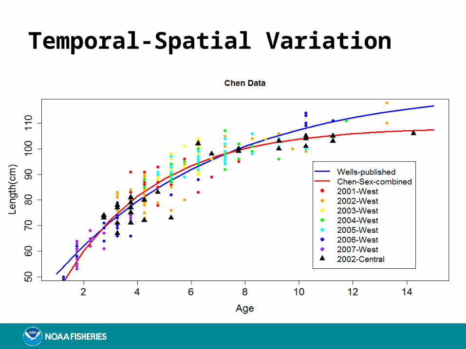
Temporal-Spatial Variation

Acknowledgement• Data provided by Dr. Chen Kuo-shu (National Taiwan University)

and Dr. David Wells (Texas A&M Univeristy at Galveston)• Dr. Tim Sippel, Dr. Suzanne Kohin, Dr. Kevin Hill, Dr. Paul Crone,

Yuhong Gu (SWFSC)• Dr. Mark Maunder, Dr. Carolina Minte-Vera, Dr. Alex Aires-de-

silva (IATTC)

Funded by NOAA-SWFSC-FRD

Email: yi.xu@noaa.gov CAPAM Workshop La Jolla, CA, November 4th, 2014