Maximum likelihood estimation of a log-concave density and ... · non-increasing density function f on ... The estimators and their basic properties Let X be a random variable with

arX

iv:0

709.

0334

v4 [

mat

h.ST

] 9

Feb

200

9

Bernoulli 15(1), 2009, 40–68DOI: 10.3150/08-BEJ141

Maximum likelihood estimation of a

log-concave density and its distribution

function: Basic properties and uniform

consistency

LUTZ DUMBGEN1 and KASPAR RUFIBACH2

1Institute of Mathematical Statistics and Actuarial Science, University of Bern, Sidlerstrasse 5,

CH-3012 Bern, Switzerland. E-mail: [email protected] Biostatistik, Institut fur Sozial- und Praventivmedizin, Universitat Zurich, Hirschen-

graben 84, CH-8001 Zurich, Switzerland. E-mail: [email protected]

We study nonparametric maximum likelihood estimation of a log-concave probability densityand its distribution and hazard function. Some general properties of these estimators are derivedfrom two characterizations. It is shown that the rate of convergence with respect to supremumnorm on a compact interval for the density and hazard rate estimator is at least (log(n)/n)1/3 andtypically (log(n)/n)2/5, whereas the difference between the empirical and estimated distributionfunction vanishes with rate op(n

−1/2) under certain regularity assumptions.

Keywords: adaptivity; bracketing; exponential inequality; gap problem; hazard function;method of caricatures; shape constraints

1. Introduction

Two common approaches to nonparametric density estimation are smoothing methodsand qualitative constraints. The former approach includes, among others, kernel densityestimators, estimators based on discrete wavelets or other series expansions and estima-tors based on roughness penalization. Good starting points for the vast literature in thisfield are Silverman (1982, 1986) and Donoho et al. (1996). A common feature of all ofthese methods is that they involve certain tuning parameters, for example, the order ofa kernel and the bandwidth. A proper choice of these parameters is far from trivial sinceoptimal values depend on unknown properties of the underlying density f . The secondapproach avoids such problems by imposing qualitative properties on f , for example,monotonicity or convexity on certain intervals in the univariate case. Such assumptionsare often plausible or even justified rigorously in specific applications.

This is an electronic reprint of the original article published by the ISI/BS in Bernoulli,2009, Vol. 15, No. 1, 40–68. This reprint differs from the original in pagination andtypographic detail.

1350-7265 c© 2009 ISI/BS

http://arxiv.org/abs/0709.0334v4

http://isi.cbs.nl/bernoulli/

http://dx.doi.org/10.3150/08-BEJ141

mailto:[email protected]

mailto:[email protected]

http://isi.cbs.nl/BS/bshome.htm

http://isi.cbs.nl/bernoulli/

http://dx.doi.org/10.3150/08-BEJ141

Estimating log-concave densities 41

Density estimation under shape constraints was first considered by Grenander (1956),

who found that the nonparametric maximum likelihood estimator (NPMLE) fmonn of a

non-increasing density function f on [0,∞) is given by the left derivative of the leastconcave majorant of the empirical cumulative distribution function on [0,∞). This workwas continued by Rao (1969) and Groeneboom (1985, 1988), who established asymptotic

distribution theory for n1/3(f − fmonn )(t) at a fixed point t > 0 under certain regular-

ity conditions and analyzed the non-Gaussian limit distribution. For various estimationproblems involving monotone functions, the typical rate of convergence is Op(n

−1/3)pointwise. The rate of convergence with respect to supremum norm is further deceler-ated by a factor of log(n)1/3 (Jonker and van der Vaart (2001)). For applications ofmonotone density estimation, consult, for example, Barlow et al. (1972) or Robertson etal. (1988).Monotone estimation can be extended to cover unimodal densities. Remember that a

density f on the real line is unimodal if there exists a number M =M(f) such that f isnon-decreasing on (−∞,M ] and non-increasing on [M,∞). If the true mode is known apriori, unimodal density estimation boils down to monotone estimation in a straightfor-ward manner, but the situation is different if M is unknown. In that case, the likelihoodis unbounded, problems being caused by observations too close to a hypothetical mode.Even if the mode was known, the density estimator is inconsistent at the mode, a phe-nomenon called “spiking”. Several methods were proposed to remedy this problem (seeWegman (1970), Woodroofe and Sun (1993), Meyer and Woodroofe (2004) or Kulikovand Lopuhaa (2006)), but all of them require additional constraints on f .The combination of shape constraints and smoothing was assessed by Eggermont and

La-Riccia (2000). To improve the slow rate of convergence of n−1/3 in the space L1(R)for arbitrary unimodal densities, they derived a Grenander-type estimator by takingthe derivative of the least concave majorant of an integrated kernel density estimatorrather than the empirical distribution function directly, yielding a rate of convergence ofOp(n

−2/5).Estimation of a convex decreasing density on [0,∞) was pioneered by Anevski (1994,

2003). The problem arose in a study of migrating birds discussed by Hampel (1987).Groeneboom et al. (2001) provide a characterization of the estimator, as well as con-sistency and limiting behavior at a fixed point of positive curvature of the function tobe estimated. They found that the estimator must be piecewise linear with knots be-tween the observation points. Under the additional assumption that the true densityf is twice continuously differentiable on [0,∞), they show that the MLE converges atrate Op(n

−2/5) pointwise, somewhat better than in the monotone case. Monotonicityand convexity constraints on densities on [0,∞) have been embedded into the generalframework of k–monotone densities by Balabdaoui and Wellner (2008). In a technicalreport, we provide a more thorough discussion of the similarities and differences betweenk-monotone density estimation and the present work (Dumbgen and Rufibach (2008)).In the present paper, we impose an alternative, and quite natural, shape constraint on

the density f , namely, log-concavity. That means

f(x) = expϕ(x)

42 L. Dumbgen and K. Rufibach

for some concave function ϕ :R→ [−∞,∞). This class is rather flexible, in that it gen-eralizes many common parametric densities. These include all non-degenerate normaldensities, all Gamma densities with shape parameter ≥ 1, all Weibull densities withexponent ≥ 1 and all beta densities with parameters ≥ 1. Further examples are thelogistic and Gumbel densities. Log-concave densities are of interest in econometrics;see Bagnoli and Bergstrom (2005) for a summary and further examples. Barlow andProschan (1975) describe advantageous properties of log-concave densities in reliabilitytheory, while Chang and Walther (2007) use log-concave densities as an ingredient innonparametric mixture models. In nonparametric Bayesian analysis, too, log-concavityis of certain relevance (Brooks (1998)).Note that log-concavity of a density implies that it is also unimodal. It will turn out

that by imposing log-concavity, one circumvents the spiking problem mentioned before,which yields a new approach to estimating a unimodal, possibly skewed density. Moreover,the log-concave density estimator is fully automatic, in the sense that there is no needto select any bandwidth, kernel function or other tuning parameters. Finally, simulatingdata from the estimated density is rather easy. All of these properties make the newestimator appealing for use in statistical applications.Little large sample theory is available for log-concave estimators thus far. Sengupta

and Paul (2005) considered testing for log-concavity of distribution functions on a com-pact interval. Walther (2002) introduced an extension of log-concavity in the contextof certain mixture models, but his theory does not cover asymptotic properties of thedensity estimators themselves. Pal et al. (2006) proved the log-concave NPMLE to beconsistent, but without rates of convergence.Concerning the computation of the log-concave NPMLE, Walther (2002) and Pal et al.

(2006) used a crude version of the iterative convex minorant (ICM) algorithm. A detaileddescription and comparison of several algorithms can be found in Rufibach (2007), whileDumbgen et al. (2007a) describe an active set algorithm, which is similar to the vertexreduction algorithms presented by Groeneboom et al. (2008) and seems to be the mostefficient one at present. The ICM and active set algorithms are implemented withinthe R package "logcondens" by Rufibach and Dumbgen (2006), accessible via "CRAN".Corresponding MATLAB code is available from the first author’s homepage.In Section 2, we introduce the log-concave maximum likelihood density estimator, dis-

cuss its basic properties and derive two characterizations. In Section 3, we illustrate thisestimator with a real data example and explain briefly how to simulate data from theestimated density. Consistency of this density estimator and the corresponding estima-tor of the distribution function are treated in Section 4. It is shown that the supremumnorm between estimated density, fn, and true density on compact subsets of the interiorof {f > 0} converges to zero at rate Op((log(n)/n)

γ), with γ ∈ [1/3,2/5] depending onf ’s smoothness. In particular, our estimator adapts to the unknown smoothness of f .Consistency of the density estimator entails consistency of the distribution function es-timator. In fact, under additional regularity conditions on f , the difference between theempirical c.d.f. and the estimated c.d.f. is of order op(n

−1/2) on compact subsets of theinterior of {f > 0}.


As a by-product of our estimator, note the following. Log-concavity of the densityfunction f also implies that the corresponding hazard function h = f/(1 − F ) is non-decreasing (cf. Barlow and Proschan (1975)). Hence, our estimators of f and its c.d.f.F entail a consistent and non-decreasing estimator of h, as pointed out at the end ofSection 4.Some auxiliary results, proofs and technical arguments are deferred to the Appendix.

2. The estimators and their basic properties

Let X be a random variable with distribution function F and Lebesgue density

f(x) = expϕ(x)

for some concave function ϕ :R→ [−∞,∞). Our goal is to estimate f based on a ran-dom sample of size n > 1 from F . Let X1 <X2 < · · ·<Xn be the corresponding orderstatistics. For any log-concave probability density f on R, the normalized log-likelihoodfunction at f is given by

∫logf dFn =

∫ϕdFn, (1)

where Fn stands for the empirical distribution function of the sample. In order to relaxthe constraint of f being a probability density and to get a criterion function to maximizeover the convex set of all concave functions ϕ, we employ the standard trick of adding aLagrange term to (1), leading to the functional

Ψn(ϕ) :=

∫ϕdFn −

∫expϕ(x) dx

(see Silverman (1982), Theorem 3.1). The nonparametric maximum likelihood estimatorof ϕ= logf is the maximizer of this functional over all concave functions,

ϕn := argmaxϕ concave

Ψn(ϕ)

and fn := exp ϕn.

Existence, uniqueness and shape of ϕn. One can easily show that Ψn(ϕ)>−∞ if andonly if ϕ is real-valued on [X1,Xn]. The following theorem was proven independently byPal et al. (2006) and Rufibach (2006). It also follows from more general considerationsin Dumbgen et al. (2007a), Section 2.

Theorem 2.1. The NPMLE ϕn exists and is unique. It is linear on all intervals[Xj ,Xj+1], 1≤ j < n. Moreover, ϕn =−∞ on R \ [X1,Xn].


Characterizations and further properties. We provide two characterizations of the es-timators ϕn, fn and the corresponding distribution function Fn, that is, Fn(x) =∫ x

−∞ fn(r) dr. The first characterization is in terms of ϕn and perturbation functions.

Theorem 2.2. Let ϕ be a concave function such that {x : ϕ(x)>−∞}= [X1,Xn]. Then,ϕ= ϕn if and only if

∫∆(x) dFn(x)≤

∫∆(x) exp ϕ(x) dx (2)

for any ∆:R→R such that ϕ+ λ∆ is concave for some λ> 0.

Plugging suitable perturbation functions ∆ in Theorem 2.2 yields valuable informationabout ϕn and Fn. For a first illustration, let µ(G) and Var(G) be the mean and variance,respectively, of a distribution (function) G on the real line with finite second moment.Setting ∆(x) :=±x or ∆(x) :=−x2 in Theorem 2.4 yields the following.

Corollary 2.3.

µ(Fn) = µ(Fn) and Var(Fn)≤Var(Fn).

Our second characterization is in terms of the empirical distribution function Fn andthe estimated distribution function Fn. For a continuous and piecewise linear functionh : [X1,Xn]→R, we define the set of its “knots” to be

Sn(h) := {t∈ (X1,Xn) :h′(t−) 6= h′(t+)} ∪ {X1,Xn}.

Recall that ϕn is an example of such a function h with Sn(ϕn)⊂ {X1,X2, . . . ,Xn}.

Theorem 2.4. Let ϕ be a concave function which is linear on all intervals [Xj ,Xj+1],

1≤ j < n, while ϕ=−∞ on R \ [X1,Xn]. Defining F (x) :=∫ x

−∞ exp ϕ(r) dr, we assume

further that F (Xn) = 1. Then, ϕ = ϕn and F = Fn if, and only if for arbitrary t ∈[X1,Xn],

∫ t

X1

F (r) dr ≤∫ t

X1

Fn(r) dr (3)

with equality in the case of t ∈ Sn(ϕ).

A particular consequence of Theorem 2.4 is that the distribution function estimatorFn is very close to the empirical distribution function Fn on Sn(ϕn).

Corollary 2.5.

Fn − n−1 ≤ Fn ≤ Fn on Sn(ϕn).


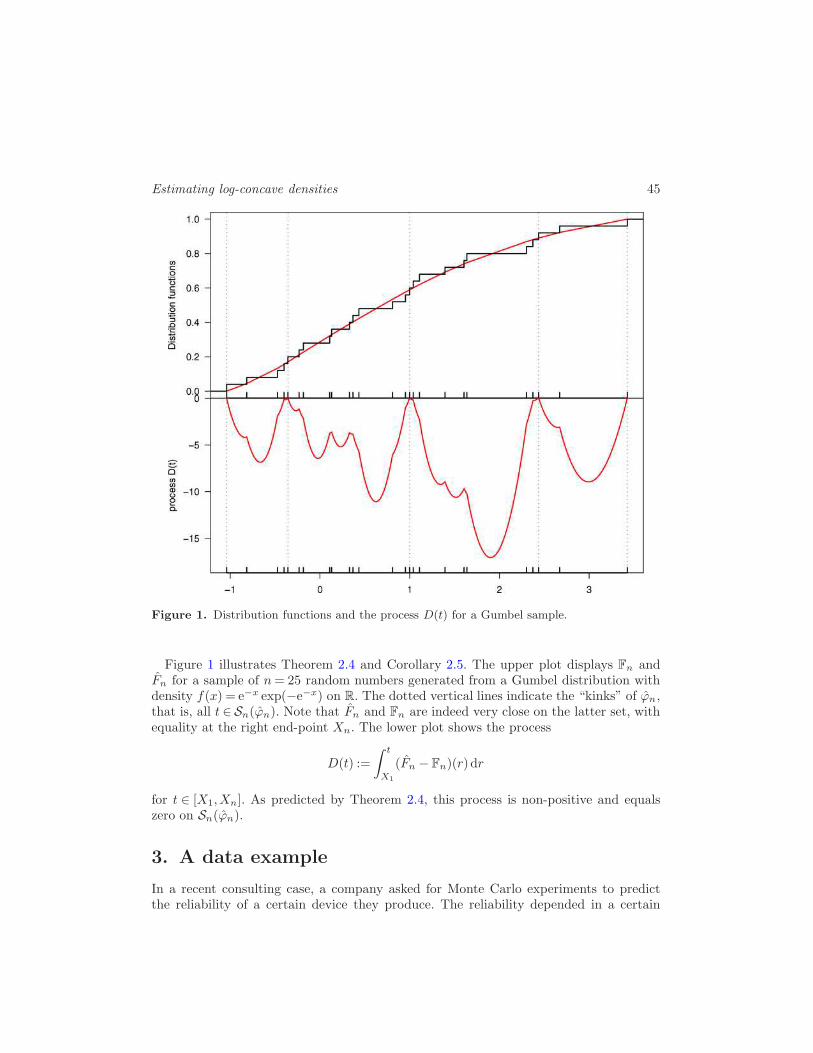
Figure 1. Distribution functions and the process D(t) for a Gumbel sample.

Figure 1 illustrates Theorem 2.4 and Corollary 2.5. The upper plot displays Fn andFn for a sample of n= 25 random numbers generated from a Gumbel distribution withdensity f(x) = e−x exp(−e−x) on R. The dotted vertical lines indicate the “kinks” of ϕn,that is, all t ∈ Sn(ϕn). Note that Fn and Fn are indeed very close on the latter set, withequality at the right end-point Xn. The lower plot shows the process

D(t) :=

∫ t

X1

(Fn − Fn)(r) dr

for t ∈ [X1,Xn]. As predicted by Theorem 2.4, this process is non-positive and equalszero on Sn(ϕn).

3. A data example

In a recent consulting case, a company asked for Monte Carlo experiments to predictthe reliability of a certain device they produce. The reliability depended in a certain


deterministic way on five different and independent random input parameters. For eachinput parameter, a sample was available and the goal was to fit a suitable distributionto simulate from. Here, we focus on just one of these input parameters.At first, we considered two standard approaches to estimate the unknown density f ,

namely, (i) fitting a Gaussian density fpar with mean µ(Fn) and variance σ2 := n(n−1)−1Var(Fn); (ii) the kernel density estimator

fker(x) :=

∫φσ/

√n(x− y) dFn(y),

where φσ denotes the density of N (0, σ2). This very small bandwidth σ/√n was chosen

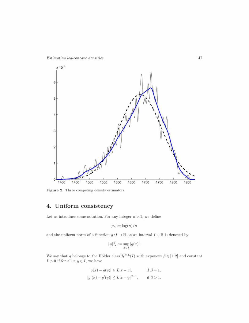
to obtain a density with variance σ2 and to avoid putting too much weight into the tails.Looking at the data, approach (i) is clearly inappropriate because our sample of size

n= 787 revealed a skewed and significantly non-Gaussian distribution. This can be seenin Figure 2, where the multimodal curve corresponds to fker, while the dashed line depictsfpar. Approach (ii) yielded Monte Carlo results agreeing well with measured reliabilities,

but the engineers questioned the multimodality of fker. Choosing a kernel estimator withlarger bandwidth would overestimate the variance and put too much weight into the tails.Thus, we agreed on a third approach and estimated f by a slightly smoothed version offn,

f∗n :=

∫φγ(x− y) dFn(y),

with γ2 := σ2−Var(Fn), so that the variance of f∗n coincides with σ2. Since log-concavity

is preserved under convolution (cf. Prekopa (1971)), f∗n is also log-concave. For the explicit

computation of Var(Fn), see Dumbgen et al. (2007a). By smoothing, we also avoid the

small discontinuities of fn at X1 and Xn. This density estimator is the skewed unimodalcurve in Figure 2. It also yielded convincing results in the Monte Carlo simulations.Note that both estimators fn and f∗

n are fully automatic. Moreover, it is very easy tosample from these densities: let Sn(ϕn) consist of x0 < x1 < · · ·< xm, and consider thedata Xi temporarily as fixed. Now,

(a) generate a random index J ∈ {1,2, . . . ,m} with P(J = j) = Fn(xj)− Fn(xj−1);(b) generate

X := xJ−1 + (xJ − xJ−1) ·{log(1 + (eΘ − 1)U)/Θ, if Θ 6= 0,U, if Θ = 0,

where Θ := ϕn(xJ )− ϕn(xJ−1) and U ∼Unif[0,1];(c) generate

X∗ :=X + γZ with Z ∼N (0,1),

where J , U and Z are independent. Then, X ∼ fn and X∗ ∼ f∗n .


Figure 2. Three competing density estimators.

4. Uniform consistency

Let us introduce some notation. For any integer n > 1, we define

ρn := log(n)/n

and the uniform norm of a function g : I →R on an interval I ⊂R is denoted by

‖g‖I∞ := supx∈I

|g(x)|.

We say that g belongs to the Holder class Hβ,L(I) with exponent β ∈ [1,2] and constantL> 0 if for all x, y ∈ I, we have

|g(x)− g(y)| ≤ L|x− y|, if β = 1,

|g′(x)− g′(y)| ≤ L|x− y|β−1, if β > 1.


Uniform consistency of ϕn. Our main result is the following theorem.

Theorem 4.1. Assume for the log-density ϕ= log f that ϕ ∈Hβ,L(T ) for some exponentβ ∈ [1,2], some constant L > 0 and a subinterval T = [A,B] of the interior of {f > 0}.Then,

maxt∈T

(ϕn − ϕ)(t) = Op(ρβ/(2β+1)n ),

maxt∈T (n,β)

(ϕ− ϕn)(t) = Op(ρβ/(2β+1)n ),

where T (n,β) := [A+ ρ1/(2β+1)n ,B− ρ

1/(2β+1)n ].

Note that the previous result remains true when we replace ϕn − ϕ with fn − f . Itis well known that the rates of convergence in Theorem 4.1 are optimal, even if β wasknown (cf. Khas’minskii (1978)). Thus, our estimators adapt to the unknown smoothnessof f in the range β ∈ [1,2].Also, note that concavity of ϕ implies that it is Lipschitz-continuous, that is, belongs to

H1,L(T ) for some L> 0 on any interval T = [A,B] with A> inf{f > 0} and B < sup{f >

0}. Hence, one can easily deduce from Theorem 4.1 that fn is consistent in L1(R) andthat Fn is uniformly consistent.

Corollary 4.2.

∫|fn(x)− f(x)|dx→p 0 and ‖Fn − F‖R∞ →p 0.

Distance of two consecutive knots and uniform consistency of Fn. By means of Theorem4.1, we can solve a “gap problem” for log-concave density estimation. The term “gapproblem” was first used by Balabdaoui and Wellner (2008) to describe the problem ofcomputing the distance between two consecutive knots of certain estimators.

Theorem 4.3. Suppose that the assumptions of Theorem 4.1 hold. Assume, further, thatϕ′(x) − ϕ′(y) ≥ C(y − x) for some constant C > 0 and arbitrary A≤ x < y ≤ B, whereϕ′ stands for ϕ′(·−) or ϕ′(·+). Then,

supx∈T

miny∈Sn(ϕn)

|x− y|=Op(ρβ/(4β+2)n ).

Theorems 4.1 and 4.3, combined with a result of Stute (1982) about the modulus ofcontinuity of empirical processes, yield a rate of convergence for the maximal differencebetween Fn and Fn on compact intervals.

Theorem 4.4. Under the assumptions of Theorem 4.3,

maxt∈T (n,β)

|Fn(t)− Fn(t)|=Op(ρ3β/(4β+2)n ).


In particular, if β > 1, then

maxt∈T (n,β)

|Fn(t)− Fn(t)|= op(n−1/2).

Thus, under certain regularity conditions, the estimators Fn and Fn are asymptoti-cally equivalent on compact sets. Conclusions of this type are known for the Grenanderestimator (cf. Kiefer and Wolfowitz (1976)) and the least squares estimator of a convexdensity on [0,∞) (cf. Balabdaoui and Wellner (2007)).The result of Theorem 4.4 is also related to recent results of Gine and Nickl (2007,

2008). In the latter paper, they devise kernel density estimators with data-driven band-widths which are also adaptive with respect to β in a certain range, while the integrateddensity estimator is asymptotically equivalent to Fn on the whole real line. However, ifβ ≥ 3/2, they must use kernel functions of higher order, that is, no longer non-negative,and simulating data from the resulting estimated density is not straightforward.

Example. Let us illustrate Theorems 4.1 and 4.4 with simulated data, again from theGumbel distribution with ϕ(x) =−x− e−x. Here, ϕ′′(x) =−e−x, so the assumptions ofour theorems are satisfied with β = 2 for any compact interval T . The upper panels ofFigure 3 show the true log-density ϕ (dashed line) and the estimator ϕn (line) for samplesof sizes n = 200 (left) and n = 2000 (right). The lower panels show the correspondingempirical processes n1/2(Fn − F ) (jagged curves) and n1/2(Fn − F ) (smooth curves).First, the quality of the estimator ϕn is quite good, even in the tails, and the qualityincreases with sample size, as expected. Looking at the empirical processes, the similaritybetween n1/2(Fn−F ) and n1/2(Fn−F ) increases with sample size, too, but rather slowly.Also, note that the estimator Fn outperforms Fn in terms of supremum distance fromF , which leads us to the next paragraph.

Marshall’s lemma. In all simulations we looked at, the estimator Fn satisfied the in-equality

‖Fn −F‖R∞ ≤ ‖Fn − F‖R∞, (4)

provided that f is indeed log-concave. Figure 3 shows two numerical examples of thisphenomenon. In view of such examples and Marshall’s (1970) lemma about the Grenanderestimator Fmon

n , we first tried to verify that (4) is correct almost surely and for anyn > 1. However, one can construct counterexamples showing that (4) may be violated,even if the right-hand side is multiplied with any fixed constant C > 1. Nevertheless, ourfirst attempts resulted in a version of Marshall’s lemma for convex density estimation;see Dumbgen et al. (2007). For the present setting, we conjecture that (4) is true withasymptotic probability one as n→∞, that is,

P(‖Fn − F‖R∞ ≤ ‖Fn − F‖R∞)→ 1.

A monotone hazard rate estimator. Estimation of a monotone hazard rate is described,for instance, in the book by Robertson et al. (1988). They directly solve an isotonic


Figure 3. Density functions and empirical processes for Gumbel samples of size n= 200 andn= 2000.

estimation problem similar to that for the Grenander density estimator. For this set-ting, Hall et al. (2001) and Hall and van Keilegom (2005) consider methods based uponsuitable modifications of kernel estimators. Alternatively, in our setting, it follows fromLemma A.2 in Section 5 that

hn(x) :=fn(x)

1− Fn(x)

defines a simple plug-in estimator of the hazard rate on (−∞,Xn) which is also non-decreasing. By virtue of Theorem 4.1 and Corollary 4.2, it is uniformly consistent on anycompact subinterval of the interior of {f > 0}. Theorems 4.1 and 4.4 even entail a rateof convergence, as follows.

Corollary 4.5. Under the assumptions of Theorem 4.3,

maxt∈T (n,β)

|hn(t)− h(t)|=Op(ρβ/(2β+1)n ).


5. Outlook

Starting from the results presented here, Balabdaoui et al. (2008) recently derived the

pointwise limiting distribution of fn. They also considered the limiting distribution ofargmaxx∈R

fn(x) as an estimator of the mode of f . Empirical findings of Muller and

Rufibach (2008) show that the estimator fn is even useful for extreme value statistics.Log-concave densities also have potential as building blocks in more complex models(e.g., regression or classification) or when handling censored data (cf. Dumbgen et al.(2007a)).Unfortunately, our proofs work only for fixed compact intervals, whereas simulations

suggest that the estimators perform well on the whole real line. Presently, the authorsare working on a different approach, where ϕn is represented locally as a parametricmaximum likelihood estimator of a log-linear density. Presumably, this will deepen ourunderstanding of the log-concave NPMLE’s consistency properties, particularly in thetails. For instance, we conjecture that Fn and Fn are asymptotically equivalent on anyinterval T on which ϕ′ is strictly decreasing.

Appendix: Auxiliary results and proofs

A.1. Two facts about log-concave densities

The following two results about a log-concave density f = expϕ and its distributionfunction F are of independent interest. The first result entails that the density f has atleast subexponential tails.

Lemma A.1. For arbitrary points x1 < x2,

√f(x1)f(x2)≤

F (x2)− F (x1)

x2 − x1.

Moreover, for xo ∈ {f > 0} and any real x 6= xo,

f(x)

f(xo)≤

(h(xo, x)

f(xo)|x− xo|

)2

,

exp

(1− f(xo)|x− xo|

h(xo, x)

)if f(xo)|x− xo| ≥ h(xo, x),

where

h(xo, x) := F (max(xo, x))−F (min(xo, x))≤{F (xo), if x < xo,1− F (xo), if x > xo.

A second well-known result (Barlow and Proschan (1975), Lemma 5.8) provides furtherconnections between the density f and the distribution function F . In particular, it entailsthat f/(F (1−F )) is bounded away from zero on {x : 0<F (x)< 1}.


Lemma A.2. The function f/F is non-increasing on {x : 0<F (x)≤ 1} and the functionf/(1−F ) is non-decreasing on {x : 0≤ F (x)< 1}.

Proof of Lemma A.1. To prove the first inequality, it suffices to consider the non-trivialcase of x1, x2 ∈ {f > 0}. Concavity of ϕ then entails that

F (x2)− F (x1) ≥∫ x2

x1

exp

(x2 − t

x2 − x1ϕ(x1) +

t− x1

x2 − x1ϕ(x2)

)dt

= (x2 − x1)

∫ 1

0

exp((1− u)ϕ(x1) + uϕ(x2)) du

≥ (x2 − x1) exp

(∫ 1

0

((1− u)ϕ(x1) + uϕ(x2)) du

)

= (x2 − x1) exp(ϕ(x1)/2+ ϕ(x2)/2)

= (x2 − x1)√

f(x1)f(x2),

where the second inequality follows from Jensen’s inequality.We prove the second asserted inequality only for x > xo, that is, h(xo, x) = F (x) −

F (xo), the other case being handled analogously. The first part entails that

f(x)

f(xo)≤(

h(xo, x)

f(xo)(x− xo)

)2

,

and the right-hand side is not greater than one if f(xo)(x− xo)≥ h(xo, x). In the lattercase, recall that

h(xo, x)≥ (x− xo)

∫ 1

0

exp((1− u)ϕ(xo) + uϕ(x)) du= f(xo)(x− xo)J(ϕ(x)− ϕ(xo))

with ϕ(x)− ϕ(xo)≤ 0, where J(y) :=∫ 1

0exp(uy) du. Elementary calculations show that

J(−r) = (1− e−r)/r ≥ 1/(1 + r) for arbitrary r > 0. Thus,

h(xo, x)≥f(xo)(x− xo)

1 + ϕ(xo)−ϕ(x),

which is equivalent to f(x)/f(xo)≤ exp(1− f(xo)(x− xo)/h(xo, x)). �

A.2. Proofs of the characterizations

Proof of Theorem 2.2. In view of Theorem 2.1, we may restrict our attention toconcave and real-valued functions ϕ on [X1,Xn] and set ϕ :=−∞ on R \ [X1,Xn]. Theset Cn of all such functions is a convex cone and for any function ∆ :R→ R and t > 0,concavity of ϕ+ t∆ on R is equivalent to its concavity on [X1,Xn].


One can easily verify that Ψn is a concave and real-valued functional on Cn. Hence, aswell known from convex analysis, a function ϕ ∈ Cn maximizes Ψn if and only if

limt↓0

Ψn(ϕ+ t(ϕ− ϕ))−Ψn(ϕ)

t≤ 0

for all ϕ ∈ Cn. But, this is equivalent to the requirement that

limt↓0

Ψn(ϕ+ t∆)−Ψn(ϕ)

t≤ 0

for any function ∆ :R→R such that ϕ+λ∆ is concave for some λ > 0. The assertion ofthe theorem now follows from

limt↓0

Ψn(ϕ+ t∆)−Ψn(ϕ)

t=

∫∆dFn −

∫∆(x) exp ϕ(x) dx.

�

Proof of Theorem 2.4. We start with a general observation. Let G be some distribution(function) with support [X1,Xn] and let ∆ : [X1,Xn]→R be absolutely continuous withL1-derivative ∆′. It then follows from Fubini’s theorem that

∫∆dG=∆(Xn)−

∫ Xn

X1

∆′(r)G(r) dr. (A.1)

Now, suppose that ϕ = ϕn and let t ∈ (X1,Xn]. Let ∆ be absolutely continuous on[X1,Xn] with L1–derivative ∆′(r) = 1{r ≤ t} and arbitrary value of ∆(Xn). Clearly,ϕ+∆ is concave, whence (2) and (A.1) entail that

∆(Xn)−∫ t

X1

Fn(r) dr ≤∆(Xn)−∫ t

X1

F (r) dr,

which is equivalent to inequality (3). In the case of t ∈ Sn(ϕ) \ {X1}, let ∆′(r) =−1{r≤t}. Then, ϕ+ λ∆ is concave for some λ > 0 so that

∆(Xn) +

∫ t

X1

Fn(r) dr ≤∆(Xn) +

∫ t

X1

F (r) dr,

which yields equality in (3).Now, suppose that ϕ satisfies inequality (3) for all t with equality if t ∈ Sn(ϕ). In view

of Theorem 2.1 and the proof of Theorem 2.2, it suffices to show that (2) holds for anyfunction ∆ defined on [X1,Xn] which is linear on each interval [Xj ,Xj+1], 1 ≤ j < n,while ϕ+ λ∆ is concave for some λ> 0. The latter requirement is equivalent to ∆ beingconcave between two consecutive knots of ϕ. Elementary considerations show that theL1-derivative of such a function ∆ may be written as

∆′(r) =n∑

j=2

βj1{r≤Xj},


with real numbers β2, . . . , βn such that

βj ≥ 0 if Xj /∈ Sn(ϕ).

Consequently, it follows from (A.1) and our assumptions on ϕ that

∫∆dFn = ∆(Xn)−

n∑

j=2

βj

∫ Xj

X1

Fn(r) dr

≤∆(Xn)−n∑

j=2

βj

∫ Xj

X1

F (r) dr

=

∫∆dF .

�

Proof of Corollary 2.5. For t ∈ Sn(ϕn) and s < t < u, it follows from Theorem 2.4that

1

u− t

∫ u

t

Fn(r) dr ≤1

u− t

∫ t

s

Fn(r) dr

and

1

t− s

∫ t

s

Fn(r) dr ≥1

t− s

∫ t

s

Fn(r) dr.

Letting u ↓ t and s ↑ t yields

Fn(t)≤ Fn(t) and Fn(t)≥ Fn(t−) = Fn(t)− n−1. �

A.3. Proof of ϕn’s consistency

Our proof of Theorem 4.1 involves a refinement and modification of methods introducedby Dumbgen et al. (2004). A first key ingredient is an inequality for concave functionsdue to Dumbgen (1998) (see also Dumbgen et al. (2004) or Rufibach (2006)).

Lemma A.3. For any β ∈ [1,2] and L> 0, there exists a constant K =K(β,L) ∈ (0,1]with the following property. Suppose that g and g are concave and real-valued functionson a compact interval T = [A,B], where g ∈Hβ,L(T ). Let ǫ > 0 and 0< δ ≤Kmin{B −A, ǫ1/β}. Then

supt∈T

(g − g)≥ ǫ or supt∈[A+δ,B−δ]

(g − g)≥ ǫ

implies that

inft∈[c,c+δ]

(g − g)(t)≥ ǫ/4 or inft∈[c,c+δ]

(g − g)(t)≥ ǫ/4

for some c ∈ [A,B − δ].


Starting from this lemma, let us first sketch the idea of our proof of Theorem 4.1.Suppose we had a family D of measurable functions ∆ with finite seminorm

σ(∆) :=

(∫∆2 dF

)1/2

,

such that

sup∆∈D

|∫∆d(Fn − F )|σ(∆)ρ

1/2n

≤C (A.2)

with asymptotic probability one, where C > 0 is some constant. If, in addition, ϕ− ϕn ∈Dand ϕ− ϕn ≤C with asymptotic probability one, then we could conclude that

∣∣∣∣∫(ϕ− ϕn) d(Fn −F )

∣∣∣∣≤Cσ(ϕ− ϕn)ρ1/2n ,

while Theorem 2.2, applied to ∆ := ϕ− ϕn, entails that

∫(ϕ− ϕn) d(Fn − F ) ≤

∫(ϕ− ϕn) d(F − F )

= −∫

∆(1− exp(−∆))dF

≤ −(1 +C)−1

∫∆2 dF

= −(1 +C)−1σ(ϕ− ϕn)2

because y(1− exp(−y))≥ (1+ y+)−1y2 for all real y, where y+ := max(y,0). Hence, with

asymptotic probability one,

σ(ϕ− ϕn)2 ≤C2(1 +C)2ρn.

Now, suppose that |ϕ − ϕn| ≥ ǫn on a subinterval of T = [A,B] of length ǫ1/βn , where

(ǫn)n is a fixed sequence of numbers ǫn > 0 tending to zero. Then, σ(ϕ − ϕn)2 ≥

ǫ(2β+1)/βn minT (f), so that

ǫn ≤ Cρ2β/(2β+1)n

with C = (C2(1 +C)2/minT (f))β/(2β+1).

The previous considerations will be modified in two aspects to get a rigorous proof

of Theorem 4.1. For technical reasons, we must replace the denominator σ(∆)ρ1/2n of

inequality (A.2) with σ(∆)ρ1/2n +W (∆)ρ

2/3n , where

W (∆) := supx∈R

|∆(x)|max(1, |ϕ(x)|) .


This is necessary to deal with functions ∆ with small values of F ({∆ 6= 0}). Moreover,we shall work with simple “caricatures” of ϕ− ϕn, namely, functions which are piecewiselinear with at most three knots. Throughout this section, piecewise linearity does notnecessarily imply continuity. A function being piecewise linear with at most m knotsmeans that the real line may be partitioned into m+1 non-degenerate intervals on eachof which the function is linear. Then, the m real boundary points of these intervals arethe knots.The next lemma extends inequality (2) to certain piecewise linear functions.

Lemma A.4. Let ∆:R→R be piecewise linear such that each knot q of ∆ satisfies oneof the following two properties:

q ∈ Sn(ϕn) and ∆(q) = lim infx→q

∆(x); (A.3)

∆(q) = limr→q

∆(r) and ∆′(q−)≥∆′(q+). (A.4)

Then,∫

∆dFn ≤∫

∆dFn. (A.5)

We can now specify the “caricatures” mentioned above.

Lemma A.5. Let T = [A,B] be a fixed subinterval of the interior of {f > 0}. Let ϕ−ϕn ≥ ǫ or ϕn − ϕ≥ ǫ on some interval [c, c+ δ]⊂ T with length δ > 0 and suppose thatX1 < c and Xn > c + δ. There then exists a piecewise linear function ∆ with at mostthree knots, each of which satisfies condition (A.3) or (A.4), and a positive constantK ′ =K ′(f,T ) such that

|ϕ− ϕn| ≥ ǫ|∆|, (A.6)

∆(ϕ− ϕn) ≥ 0, (A.7)

∆ ≤ 1, (A.8)∫ c+δ

c

∆2(x) dx ≥ δ/3, (A.9)

W (∆) ≤K ′δ−1/2σ(∆). (A.10)

Our last ingredient is a surrogate for (A.2).

Lemma A.6. Let Dm be the family of all piecewise linear functions on R with at mostm knots. There exists a constant K ′′ =K ′′(f) such that

supm≥1,∆∈Dm

|∫∆d(Fn −F )|

σ(∆)m1/2ρ1/2n +W (∆)mρ

2/3n

≤K ′′,


with probability tending to one as n→∞.

Before we verify all of these auxiliary results, let us proceed with the main proof.

Proof of Theorem 4.1. Suppose that

supt∈T

(ϕn − ϕ)(t) ≥ Cǫn

or

supt∈[A+δn,B−δn]

(ϕ− ϕn)(t) ≥ Cǫn

for some constant C > 0, where ǫn := ρβ/(2β+1)n and δn := ρ

1/(2β+1)n = ǫ

1/βn . It follows from

Lemma A.3 with ǫ :=Cǫn that in the case of C ≥K−β and for sufficiently large n, thereis a (random) interval [cn, cn + δn]⊂ T on which either ϕn − ϕ≥ (C/4)ǫn or ϕ− ϕn ≥(C/4)ǫn. But, then, there is a (random) function ∆n ∈D3 fulfilling the conditions statedin Lemma A.5. For this ∆n, it follows from (A.5) that

∫

R

∆n d(F − Fn)≥∫

R

∆n d(F − Fn) =

∫

R

∆n(1− exp[−(ϕ− ϕn)]) dF. (A.11)

With ∆n := (C/4)ǫn∆n, it follows from (A.6–A.7) that the right-hand side of (A.11) isnot smaller than

(4/C)ǫ−1n

∫∆n(1− exp(−∆n)) dF ≥ (4/C)ǫ−1

n

1+ (C/4)ǫnσ(∆n)

2 =(C/4)ǫn1 + o(1)

σ(∆n)2

because ∆n ≤ (C/4)ǫn, by (A.8). On the other hand, according to Lemma A.6, we mayassume that

∫

R

∆n d(F − Fn) ≤K ′′(31/2σ(∆n)ρ1/2n +3W (∆n)ρ

2/3n )

≤K ′′(31/2ρ1/2n + 3K ′δ−1/2n ρ2/3n )σ(∆n) (by (A.10))

≤K ′′(31/2ρ1/2n + 3K ′ρ2/3−1/(4β+2)n )σ(∆n)

≤ Gρ1/2n σ(∆n)

for some constant G=G(β,L, f, T ) because 2/3− 1/(4β+ 2)≥ 2/3− 1/6 = 1/2. Conse-quently,

C2 ≤ 16G2(1 + o(1))ǫ−2n ρn

σ(∆n)2=

16G2(1 + o(1))

δ−1n σ(∆n)2

≤ 48G2(1 + o(1))

minT (f),

where the last inequality follows from (A.9). �


Proof of Lemma A.4. There is a sequence of continuous, piecewise linear functions∆k converging pointwise isotonically to ∆ as k →∞ such that any knot q of ∆k eitherbelongs to Sn(ϕn) or ∆

′k(q−)>∆′

k(q+). Thus, ϕn+λ∆k is concave for sufficiently smallλ> 0. Consequently, since ∆1 ≤∆k ≤∆ for all k, it follows from dominated convergenceand (2) that

∫∆dFn = lim

k→∞

∫∆k dFn ≤ lim

k→∞

∫∆k dFn =

∫∆dFn. �

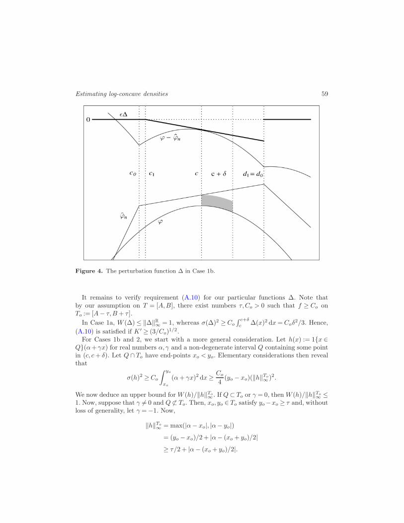
Proof of Lemma A.5. The crucial point in all the cases we must distinguish is toconstruct a ∆ ∈D3 satisfying the assumptions of Lemma A.4 and (A.6–A.9). Recall thatϕn is piecewise linear.Case 1a: ϕn − ϕ ≥ ǫ on [c, c + δ] and Sn(ϕn) ∩ (c, c + δ) 6= ∅. Here, we choose a

continuous function ∆ ∈D3 with knots c, c+ δ and xo ∈ Sn(ϕn)∩ (c, c+ δ), where ∆ := 0on (−∞, c] ∪ [c + δ,∞) and ∆(xo) := −1. Here, the assumptions of Lemma A.4 andrequirements (A.6–A.9) are easily verified.Case 1b: ϕn−ϕ≥ ǫ on [c, c+δ] and Sn(ϕn)∩(c, c+δ) =∅. Let [co, do]⊃ [c, c+δ] be the

maximal interval on which ϕ− ϕn is concave. There then exists a linear function ∆ suchthat ∆≥ ϕ− ϕn on [co, do] and ∆≤−ǫ on [c, c+δ]. Next, let (c1, d1) := {∆< 0}∩(co, do).We now define ∆ ∈D2 via

∆(x) :=

{0, if x ∈ (−∞, c1)∪ (d1,∞),

∆/ǫ, if x ∈ [c1, d1].

Again, the assumptions of Lemma A.4 and requirements (A.6–A.9) are easily verified;

this time, we even know that ∆ ≤−1 on [c, c+ δ], whence∫ c+δ

c ∆(x)2 dx≥ δ. Figure 4illustrates this construction.Case 2: ϕ− ϕn ≥ ǫ on [c, c+ δ]. Let [co, c] and [c+ δ, do] be maximal intervals on which

ϕn is linear. We then define

∆(x) :=

0, if x ∈ (−∞, co) ∪ (do,∞),1 + β1(x− xo), if x ∈ [co, xo],1 + β2(x− xo), if x ∈ [xo, do],

where xo := c+ δ/2 and β1 ≥ 0 is chosen such that either

∆(co) = 0 and (ϕ− ϕn)(co)≥ 0, or

(ϕ− ϕn)(co) < 0 and sign(∆) = sign(ϕ− ϕn) on [co, xo].

Analogously, β2 ≤ 0 is chosen such that

∆(do) = 0 and (ϕ− ϕn)(do)≥ 0, or

(ϕ− ϕn)(do) < 0 and sign(∆) = sign(ϕ− ϕn) on [xo, do].

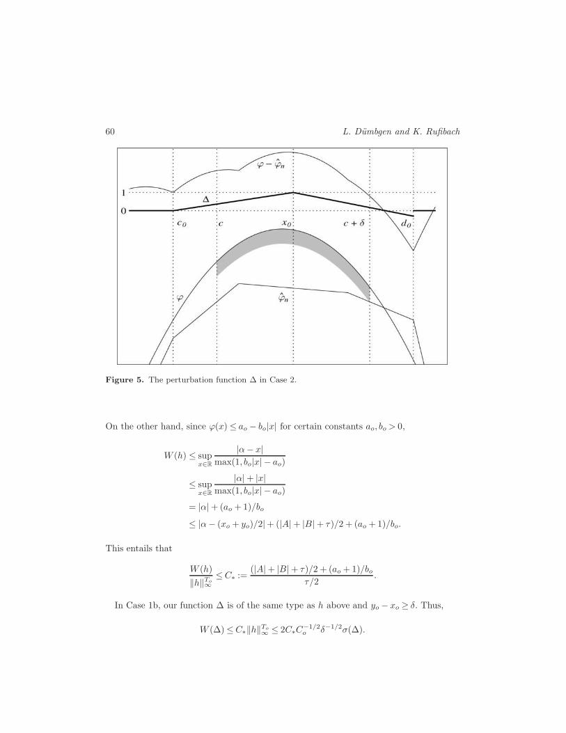
Again, the assumptions of Lemma A.4 and requirements (A.6–A.9) are easily verified.Figure 5 depicts an example.


Figure 4. The perturbation function ∆ in Case 1b.

It remains to verify requirement (A.10) for our particular functions ∆. Note thatby our assumption on T = [A,B], there exist numbers τ,Co > 0 such that f ≥ Co onTo := [A− τ,B+ τ ].

In Case 1a, W (∆)≤ ‖∆‖R∞ = 1, whereas σ(∆)2 ≥ Co

∫ c+δ

c ∆(x)2 dx= Coδ2/3. Hence,

(A.10) is satisfied if K ′ ≥ (3/Co)1/2.

For Cases 1b and 2, we start with a more general consideration. Let h(x) := 1{x ∈Q}(α+ γx) for real numbers α,γ and a non-degenerate interval Q containing some pointin (c, c+ δ). Let Q ∩ To have end-points xo < yo. Elementary considerations then revealthat

σ(h)2 ≥Co

∫ yo

xo

(α+ γx)2 dx≥ Co

4(yo − xo)(‖h‖To

∞ )2.

We now deduce an upper bound for W (h)/‖h‖To∞ . If Q⊂ To or γ = 0, then W (h)/‖h‖To∞ ≤1. Now, suppose that γ 6= 0 and Q 6⊂ To. Then, xo, yo ∈ To satisfy yo−xo ≥ τ and, withoutloss of generality, let γ =−1. Now,

‖h‖To

∞ = max(|α− xo|, |α− yo|)= (yo − xo)/2+ |α− (xo + yo)/2|≥ τ/2+ |α− (xo + yo)/2|.


Figure 5. The perturbation function ∆ in Case 2.

On the other hand, since ϕ(x)≤ ao − bo|x| for certain constants ao, bo > 0,

W (h) ≤ supx∈R

|α− x|max(1, bo|x| − ao)

≤ supx∈R

|α|+ |x|max(1, bo|x| − ao)

= |α|+ (ao +1)/bo

≤ |α− (xo + yo)/2|+ (|A|+ |B|+ τ)/2 + (ao +1)/bo.

This entails that

W (h)

‖h‖To∞≤C∗ :=

(|A|+ |B|+ τ)/2 + (ao + 1)/boτ/2

.

In Case 1b, our function ∆ is of the same type as h above and yo − xo ≥ δ. Thus,

W (∆)≤C∗‖h‖To

∞ ≤ 2C∗C−1/2o δ−1/2σ(∆).


In Case 2, ∆ may be written as h1 + h2, with two functions h1 and h2 of the same typeas h above having disjoint support and both satisfying yo − xo ≥ δ/2. Thus,

W (∆) = max(W (h1),W (h2))

≤ 23/2C∗C−1/2o δ−1/2max(σ(h1), σ(h2))

≤ 23/2C∗C−1/2o δ−1/2σ(∆). �

To prove Lemma A.6, we need a simple exponential inequality.

Lemma A.7. Let Y be a random variable such that E(Y ) = 0, E(Y 2) = σ2 and C :=E exp(|Y |)<∞. Then, for arbitrary t ∈R,

E exp(tY )≤ 1 +σ2t2

2+

C|t|3(1− |t|)+

.

Proof.

E exp(tY ) =

∞∑

k=0

tk

k!E(Y k)≤ 1 +

σ2t2

2+

∞∑

k=3

|t|kk!

E(|Y |k).

For any y ≥ 0 and integers k ≥ 3, yke−y ≤ kke−k. Thus, E(|Y |k) ≤ E exp(|Y |)kke−k =Ckke−k. Since kke−k ≤ k!, which can be verified easily via induction on k,

∞∑

k=3

|t|kk!

E(|Y |k)≤C

∞∑

k=3

|t|k = C|t|3(1− |t|)+

.�

Lemma A.7 entails the following result for finite families of functions.

Lemma A.8. Let Hn be a finite family of functions h with 0 < W (h) <∞ such that#Hn =O(np) for some p > 0. Then, for sufficiently large D,

limn→∞

P

(maxh∈Hn

|∫hd(Fn − F )|

σ(h)ρ1/2n +W (h)ρ

2/3n

≥D

)= 0.

Proof. Since W (ch) = cW (h) and σ(ch) = cσ(h) for any h ∈Hn and arbitrary constantsc > 0, we may assume, without loss of generality, that W (h) = 1 for all h ∈ Hn. Let Xbe a random variable with log-density ϕ. Since

limsup|x|→∞

ϕ(x)

|x| < 0

by Lemma A.1, the expectation of exp(tow(X)) is finite for any fixed to ∈ (0,1), wherew(x) := max(1, |ϕ(x)|). Hence,

E exp(to|h(X)−Eh(X)|)≤Co := exp(toEw(X))E exp(tow(X))<∞.


Lemma A.7, applied to Y := to(h(X)−Eh(X)), implies that

E exp[t(h(X)−Eh(X))] =E((t/to)Y )≤ 1 +σ(h)2t2

2+

C1|t|3(1−C2|t|)+

for arbitrary h ∈Hn, t ∈R and constants C1,C2 depending on to and Co. Consequently,

E exp

(t

∫hd(Fn − F )

)= E exp

((t/n)

n∑

i=1

(h(Xi)−Eh(X))

)

= (E exp((t/n)(h(X)−Eh(X))))n

≤(1 +

σ(h)2t2

2n2+

C1|t|3n3(1−C2|t|/n)+

)n

≤ exp

(σ(h)2t2

2n+

C1|t|3n2(1−C2|t|/n)+

).

It now follows from Markov’s inequality that

P

(∣∣∣∣∫

hd(Fn − F )

∣∣∣∣≥ η

)≤ 2 exp

(σ(h)2t2

2n+

C1t3

n2(1−C2t/n)+− tη

)(A.12)

for arbitrary t, η > 0. Specifically, let η =D(σ(h)ρ1/2n + ρ

2/3n ) and set

t :=nρ

1/2n

σ(h) + ρ1/6n

≤ nρ1/3n = o(n).

Then, the bound (A.12) is not greater than

2 exp

(σ(h)2 logn

2(σ(h) + ρ1/6n )2

+C1ρ

1/2n logn

(σ(h) + ρ1/6n )3(1−C2ρ

1/3n )+

−D logn

)

≤ 2 exp

[(1

2+

C1

(1−C2ρ1/3n )+

−D

)logn

]= 2exp((O(1)−D) logn).

Consequently, for sufficiently large D > 0,

P

(maxh∈Hn

|∫hd(Fn − F )|


2/3n

≥D

)

≤#Hn2 exp((O(1)−D) logn) =O(1) exp((O(1) + p−D) logn)→ 0. �

Proof of Lemma A.6. Let H be the family of all functions h of the form

h(x) = 1{x ∈Q}(c+dx),


with any interval Q⊂R and real constants c, d such that h is non-negative. Suppose thatthere exists a constant C =C(f) such that

P

(suph∈H

|∫hd(Fn − F )|


2/3n

≤C

)→ 1. (A.13)

For any m ∈N, an arbitrary function ∆ ∈Dm may be written as

∆ =

M∑

i=1

hi

with M = 2m+ 2 functions hi ∈H having pairwise disjoint supports. Consequently,

σ(∆) =

(M∑

i=1

σ(hi)2

)1/2

≥M−1/2M∑

i=1

σ(hi),

by the Cauchy–Schwarz inequality, while

W (∆) = maxi=1,...,M

W (hi)≥M−1M∑

i=1

W (hi).

Consequently, (A.13) entails that

∣∣∣∣∫

∆d(Fn −F )

∣∣∣∣ ≤M∑

i=1

∣∣∣∣∫

hi d(Fn − F )

∣∣∣∣

≤ C

(M∑

i=1

σ(hi)ρ1/2n +

M∑

i=1

W (hi)ρ2/3n

)

≤ 4C(σ(∆)m1/2ρ1/2n +W (∆)mρ2/3n )

uniformly in m ∈N and ∆ ∈Dm, with probability tending to one as n→∞.It remains to verify (A.13). To this end, we use a bracketing argument. With the

weight function w(x) = max(1, |ϕ(x)|), let −∞ = tn,0 < tn,1 < · · · < tn,N(n) = ∞ suchthat for In,j := (tn,j−1, tn,j],

(2n)−1 ≤∫

In,j

w(x)2f(x) dx≤ n−1 for 1≤ j ≤N(n),

with equality if j < N(n). Since 1 ≤∫exp(tow(x))f(x) dx <∞, such a partition exists

with N(n) =O(n). For any h ∈H, we define functions hn,ℓ, hn,u as follows. Let {j, . . . , k}be the set of all indices i∈ {1, . . . ,N(n)} such that {h > 0} ∩ In,i 6=∅. We then define

hn,ℓ(x) := 1{tn,j<x≤tn,k−1}h(x)


and

hn,u(x) := hn,ℓ(x) + 1{x ∈ In,j ∪ In,k}W (h)w(x).

Note that 0 ≤ hn,ℓ ≤ h ≤ hn,u ≤ W (h)w. Consequently, W (hn,ℓ) ≤ W (h) = W (hn,u).Suppose, for the moment, that the assertion is true for the (still infinite) familyHn := {hn,ℓ, hn,u :h ∈H} in place of H. It then follows from w ≥ 1 that

∫hd(Fn −F ) ≤

∫hn,u dFn −

∫hn,ℓ dF

=

∫hn,u d(Fn −F ) +

∫(hn,u − hn,ℓ) dF

≤∫

hn,u d(Fn −F ) +W (h)

∫

In,j∪In,k

w(x)2 dF

≤∫

hn,u d(Fn −F ) + 2W (h)n−1

≤ C(σ(hn,u)ρ1/2n + ρ2/3n ) + 2n−1

≤ C(σ(h)ρ1/2n + 21/2W (h)n−1/2ρ1/2n + ρ2/3n ) + 2W (h)n−1

≤ (C + o(1))(σ(h)ρ1/2n +W (h)ρ2/3n ),

uniformly in h ∈H with asymptotic probability one. Analogously,

∫hd(Fn − F ) ≥

∫hn,ℓ d(Fn − F )− 2W (h)n−1

≥ −C(σ(hn,ℓ)ρ1/2n +W (h)ρ2/3n )− 2W (h)n−1

≥ −(C + o(1))(σ(h)ρ1/2n +W (h)ρ2/3n ),

uniformly in h ∈H with asymptotic probability one.To accord with Lemma A.8, we must now deal with Hn. For any h ∈H, the function

hn,ℓ may be written as

h(tn,j)g(1)n,j,k + h(tn,k−1)g

(2)n,j,k,

with the “triangular functions”

g(1)n,j,k(x) :=

tn,k−1 − x

tn,k−1 − tn,j

and

g(2)n,j,k(x) :=

x− tn,jtn,k−1 − tn,j

for 1≤ j < k ≤N(n), k− j ≥ 2.


In case of k− j ≤ 1, we set g(1)n,j,k := g

(2)n,j,k := 0. Moreover,

hn,u = hn,ℓ +W (h)gn,j + 1{k > j}W (h)gn,k,

with gn,i(x) := 1{x ∈ In,i}w(x). Consequently, all functions in Hn are linear combinationswith non-negative coefficients of at most four functions in the finite family

Gn := {gn,i : 1≤ i≤N(n)} ∪ {g(1)n,j,k, g(2)n,j,k : 1≤ j < k ≤N(n)}.

Since Gn contains O(n2) functions, it follows from Lemma A.8 that for some constantD> 0,

∣∣∣∣∫

g d(Fn − F )

∣∣∣∣≤D(σ(g)ρ1/2n +W (g)ρ2/3n )

for all g ∈ Gn with asymptotic probability one. The assertion about Hn now followsfrom the basic observation that for h =

∑4i=1 αigi with non-negative functions gi and

coefficients αi ≥ 0,

σ(h) ≥(

4∑

i=1

α2i σ(gi)

2

)1/2

≥ 2−14∑

i=1

αiσ(gi),

W (h) ≥ maxi=1,...,4

αiW (gi)≥ 4−14∑

i=1

αiW (gi).�

A.4. Proofs for the gap problem and of Fn’s consistency

Proof of Theorem 4.3. Suppose that ϕn is linear on an interval [a, b]. Then, for x ∈[a, b] and λx := (x− a)/(b− a) ∈ [0,1],

ϕ(x)− (1− λx)ϕ(a)− λxϕ(b)

= (1− λx)(ϕ(x)− ϕ(a))− λx(ϕ(b)− ϕ(x))

= (1− λx)

∫ x

a

ϕ′(t) dt− λx

∫ b

x

ϕ′(t) dt

= (1− λx)

∫ x

a

(ϕ′(t)−ϕ′(x)) dt+ λx

∫ b

x

(ϕ′(x)− ϕ′(t)) dt

≥C(1− λx)

∫ x

a

(x− t) dt+Cλx

∫ b

x

(t− x) dt

=C(b− a)2λx(1− λx)/2

=C(b− a)2/8 if x= xo := (a+ b)/2.


This entails that sup[a,b] |ϕn −ϕ| ≥C(b− a)2/16. For if ϕn <ϕ+C(b− a)2/16 on {a, b},then

ϕ(xo)− ϕn(xo) = ϕ(xo)− (ϕn(a) + ϕn(b))/2

> ϕ(xo)− (ϕ(a) +ϕ(b))/2−C(b− a)2/16

≥ C(b− a)2/8−C(b− a)2/16 =C(b− a)2/16.

Consequently, if |ϕn − ϕ| ≤ Dnρβ/(2β+1)n on Tn := [A + ρ

1/(2β+1)n ,B − ρ

1/(2β+1)n ] with

Dn =Op(1), then the longest subinterval of Tn containing no points from Sn has length

at most 4D1/2n C−1/2ρ

β/(4β+2)n . Since Tn and T = [A,B] differ by two intervals of length

ρ1/(2β+1)n =O(ρ

β/(4β+2)n ), these considerations yield the assertion about Sn(ϕn). �

Proof of Theorem 4.4. Let δn := ρ1/(2β+1)n and rn := Dρ

β/(4β+2)n = Dδ

1/2n for some

constant D > 0. Since rn → 0 but nrn → ∞, it follows from boundedness of f and atheorem of Stute (1982) about the modulus of continuity of univariate empirical processesthat

ωn := supx,y∈R:|x−y|≤rn

|(Fn −F )(x)− (Fn −F )(y)|

= Op(n−1/2r1/2n log(1/rn)

1/2)

= Op(ρ(5β+2)/(8β+4)n ).

If D is sufficiently large, the asymptotic probability that for any point x ∈ [A+δn,B−δn],there exists a point y ∈ Sn(ϕn) ∩ [A+ δn,B − δn] with |x− y| ≤ rn, is equal to one. Inthat case, it follows from Corollary 2.5 and Theorem 4.1 that

|(Fn − Fn)(x)| ≤ |(Fn − Fn)(x)− (Fn − Fn)(y)|+ n−1

≤ |(Fn −F )(x)− (Fn −F )(y)|+ ωn + n−1

≤∫ max(x,y)

min(x,y)

|fn − f |(x) dx+ωn + n−1

≤ Op(rnρβ/(2β+1)n ) +ωn + n−1

= Op(ρ3β/(4β+2)n ). �

Acknowledgements

This work is part of the second author’s PhD dissertation, written at the University ofBern. The authors thank an anonymous referee for valuable remarks and some importantreferences. This work was supported by the Swiss National Science Foundation.


References

Anevski, D. (1994). Estimating the derivative of a convex density. Technical report, Dept. ofMathematical Statistics, Univ. Lund.

Anevski, D. (2003). Estimating the derivative of a convex density. Statist. Neerlandica 57 245–257. MR2028914

Bagnoli, M. and Bergstrom, T. (2005). Log-concave probability and its applications. Econ.

Theory 26 445–469. MR2213177Balabdaoui, F. and Wellner, J.A. (2007). A Kiefer–Wolfowitz theorem for convex densities. IMS

Lecture Notes Monograph Series 2007 55 1–31.Balabdaoui, F. and Wellner, J.A. (2008). Estimation of a k-monotone density: Limit distribution

theory and the spline connection. Ann. Statist. 35 2536–2564. MR2382657Balabdaoui, F., Rufibach, K. and Wellner, J.A. (2008). Limit distribution theory for maximum

likelihood estimation of a log-concave density. Ann. Statist. To appear.Barlow, E.B., Bartholomew, D.J., Bremner, J.M. and Brunk, H.D. (1972). Statistical Inference

under Order Restrictions. The Theory and Application of Isotonic Regression. New York:Wiley. MR0326887

Barlow, E.B. and Proschan, F. (1975). Statistical Theory of Reliability and Life Testing Proba-

bility Models. New York: Holt, Reinhart and Winston. MR0438625Brooks, S. (1998). MCMC convergence diagnosis via multivariate bounds on log-concave densi-

ties. Ann. Statist. 26 398–433. MR1608152Chang, G. and Walther, G. (2007). Clustering with mixtures of log-concave distributions. Comp.

Statist. Data Anal. 51 6242–6251.Donoho, D.L., Johnstone, I.M., Kerkyacharian, G. and Picard, D. (1996). Density estimation

by wavelet thresholding. Ann. Statist. 24 508–539. MR1394974Dumbgen, L. (1998). New goodness-of-fit tests and their application to nonparametric confidence

sets. Ann. Statist. 26 288–314. MR1611768Dumbgen, L., Freitag S. and Jongbloed, G. (2004). Consistency of concave regression, with an

application to current status data. Math. Methods Statist. 13 69–81. MR2078313Dumbgen, L., Husler, A. and Rufibach, K. (2007). Active set and EM algorithms for log-concave

densities based on complete and censored data. Technical Report 61, IMSV, Univ. Bern.arXiv:0707.4643.

Dumbgen, L., Rufibach, K. and Wellner, J.A. (2007). Marshall’s lemma for convex density esti-mation. In Asymptotics: Particles, Processes and Inverse Problems (E. Cator, G. Jongbloed,C. Kraaikamp, R. Lopuhaa and J.A. Wellner, eds.) 101–107. IMS Lecture Notes—Monograph

Series 55.Dumbgen, L. and Rufibach, K. (2008). Maximum likelihood estimation of a log-concave density

and its distribution function: Basic properties and uniform consistency. Technical Report 66,IMSV, Univ. Bern. arxiv:0709.0334.

Eggermont, P.P.B. and LaRiccia, V.N. (2000). Maximum likelihood estimation of smooth mono-tone and unimodal densities. Ann. Statist. 28 922–947. MR1792794

Gine, E. and Nickl, R. (2007). Uniform central limit theorems for kernel density estimators.Probab. Theory Related Fields 141 333–387. MR2391158

Gine, E. and Nickl, R. (2008). An exponential inequality for the distribution function of thekernel density estimator, with applications to adaptive estimation. Probab. Theory Related

Fields. To appear. MR2391158Grenander, U. (1956). On the theory of mortality measurement, part II. Skand. Aktuarietidskrift

39 125–153. MR0093415

http://www.ams.org/mathscinet-getitem?mr=2028914









http://arxiv.org/abs/math/0707.4643

http://arxiv.org/abs/math/0709.0334






Groeneboom, P. (1985). Estimating a monotone density. In Proc. Berkeley Conf. in Honor of

Jerzy Neyman and Jack Kiefer II (L.M. LeCam and R.A. Ohlsen, eds.) 539–555. MR0822052Groeneboom, P. (1988). Brownian motion with a parabolic drift and Airy functions. Probab.

Theory Related Fields 81 79–109. MR0981568Groeneboom, P., Jongbloed, G. and Wellner, J.A. (2001). Estimation of a convex function:

Characterization and asymptotic theory. Ann. Statist. 29 1653–1698. MR1891742Groeneboom, P., Jongbloed, G. and Wellner, J.A. (2008). The support reduction algorithm for

computing nonparametric function estimates in mixture models. Scand. J. Statist. To appear.Hall, P., Huang, L.S., Gifford, J.A. and Gijbels, I. (2001). Nonparametric estimation of hazard

rate under the constraint of monotonicity. J. Comput. Graph. Statist. 10 592–614. MR1939041Hall, P. and van Keilegom, I. (2005). Testing for monotone increasing hazard rate. Ann. Statist.

33 1109–1137. MR2195630Hampel, F.R. (1987). Design, modelling and analysis of some biological datasets. In Design,

Data and Analysis, By Some Friends of Cuthbert Daniel (C.L. Mallows, ed.). New York:Wiley.

Jonker, M. and van der Vaart, A. (2001). A semi-parametric model for censored and passivelyregistered data. Bernoulli 7 1–31. MR1811742

Khas’minskii, R.Z. (1978). A lower bound on the risks of nonparametric estimates of densitiesin the uniform metric. Theory Prob. Appl. 23 794–798. MR0516279

Kiefer, J. and Wolfowitz, J. (1976). Asymptotically minimax estimation of concave and convexdistribution functions. Z. Wahrsch. Verw. Gebiete 34 73–85. MR0397974

Kulikov, V.N. and Lopuhaa, H.P. (2006). The behavior of the NPMLE of a decreasing densitynear the boundaries of the support. Ann. Statist. 34 742–768. MR2283391

Marshall, A.W. (1970). Discussion of Barlow and van Zwet’s paper. In Nonparametric Techniques

in Statistical Inference. Proceedings of the First International Symposium on Nonparametric

Techniques held at Indiana University, June, 1969 (M.L. Puri, ed.) 174–176. Cambridge Univ.Press. MR0273755

Meyer, C.M. and Woodroofe, M. (2004). Consistent maximum likelihood estimation of a uni-modal density using shape restrictions. Canad. J. Statist. 32 85–100. MR2060547

Muller, S. and Rufibach, K. (2008). Smooth tail index estimation. J. Stat. Comput. Simul. Toappear.

Pal, J., Woodroofe, M. and Meyer, M. (2006). Estimating a Polya frequency function. In Complex

Datasets and Inverse problems: Tomography, Networks and Beyond (R. Liu, W. Strawdermanand C.-H. Zhang, eds.) 239–249. IMS Lecture Notes—Monograph Series 54.

Prekopa, A. (1971). Logarithmic concave measures with application to stochastic programming.Acta Sci. Math. 32 301–316. MR0315079

Rao, P. (1969). Estimation of a unimodal density. Sankhya Ser. A 31 23–36. MR0267677Robertson, T., Wright, F.T. and Dykstra, R.L. (1988). Order Restricted Statistical Inference.

Wiley, New York. MR0961262Rufibach, K. (2006). Log-concave density estimation and bump hunting for i.i.d. observations.

Ph.D. dissertation, Univ. Bern and Gottingen.Rufibach, K. (2007). Computing maximum likelihood estimators of a log-concave density func-

tion. J. Statist. Comput. Simul. 77 561–574.Rufibach, K. and Dumbgen, L. (2006). logcondens: Estimate a log-concave probability density

from i.i.d. observations. R package version 1.3.0.Sengupta, D. and Paul, D. (2005). Some tests for log-concavity of life distributions. Preprint.

Available at http://anson.ucdavis.edu/˜debashis/techrep/logconca.pdf.















http://anson.ucdavis.edu/~debashis/techrep/logconca.pdf


Silverman, B.W. (1982). On the estimation of a probability density function by the maximumpenalized likelihood method. Ann. Statist. 10 795–810. MR0663433

Stute, W. (1982). The oscillation behaviour of empirical processes. Ann. Probab. 10 86–107.MR0637378

Silverman, B.W. (1986). Density Estimation for Statistics and Data Analysis. London: Chapmanand Hall. MR0848134

Walther, G. (2002). Detecting the presence of mixing with multiscale maximum likelihood. J.Amer. Statist. Assoc. 97 508–514. MR1941467

Wegman, E.J. (1970). Maximum likelihood estimation of a unimodal density function. Ann.Math. Statist. 41 457–471. MR0254995

Woodroofe, M. and Sun, J. (1993). A penalized maximum likelihood estimate of f(0+) when fis non-increasing. Ann. Statist. 3 501–515. MR1243398

Received September 2007 and revised April 2008







Documents

Maximum likelihood estimation of a log-concave density and ... · non-increasing density function f on ... The estimators and their basic properties Let X be a random variable with