Embed Size (px)
Citation preview
Maximum Matchings in Bipartite Graphs via Strong Spanning Trees M. L. Balinski CNRS, Laboratoire d’Econometrie de I’Ecole Polytechnique, Paris, France
J. Gonzalez Departamento de Matematicas Aplicadas, U. de Chile, Casila 13017, Santiago, Chile
A new characterization of maximum matchings for bipartite graphs is presented. It is based on “strong spanning trees” and permits the development of a new algorithm that does not use the classical notion of augmenting paths and that runs in O(lVl [El) time for bipartite graphs with IVI nodes and IE( edges.
1. INTRODUCTION
Given an undirected finite graph G = (V, E ) with node set V and edge set E , a matching Z of G is a subset of E such that no node is incident with more than one edge in Z . The maximum matching problem is to find a matching having a maximum number of edges. This problem has long been studied, and most of the written work related to it is based on the classical notion of an augmenting path. The characterization of maximum matchings via augmenting paths in bipartite graphs appears implicitly in the Hungarian method developed by Kuhn [13], whose theoretical basis is derived from works of Konig [12] and Egervary [5]. Later, that characterization was proved explicitly for arbitrary graphs in independent papers of Berge [3] and Norman and Rabin [14]. The characterization gives the following procedure: Start with any matching (e.g., the empty one), and repeatedly conduct a search for an augmenting path. If the search finds one, the matching is augmented. Otherwise, there is no augment- ing path and the characterization ensures that the current matching is maxi- mum.
In the case when the graph is bipartite, the above procedure gives an algo- rithm that runs in O((V1 JEl) time. The best algorithm to find a maximum match-
NETWORKS, Vol. 21, (1991) 165-179 0 1991 by John Wiley & Sons, Inc. CCC 0028-3045/911020165-015$04.00
166 BALlNSKl AND GONZALEZ
ing in bipartite gra hs is due to Hopcroft and Karp [ 101, which has a running time of O(IEI / IVl). The fact that this algorithm is a special case of Dinic’s max-flow algorithm [3] applied to a simple network (associated with the graph) was first observed by Even and Tarjan [6]. All other algorithms for bipartite matchings (e.g., Hall [9], Ford and Fulkerson [7], Kuhn [13]) have a running time of O(lVl IEI).
In this article, a new approach to the maximum matching problem in bipartite graphs is presented. It is based on “strong spanning trees,” a concept that was introduced by Balinski [2]. This notion permits us to develop a new character- ization of maximum matchings in bipartite graphs as well as an algorithm that solves the problem without using augmenting paths. The worst time bound of the algorithm is O(lVl [El), competitive (in terms of worst case analysis) with all algorithms that use augmenting paths but the one due to Hopcroft and Karp. The algorithm constructs a finite sequence of strong spanning trees and termi- nates with one that contains a maximum matching of the graph.
The potential interest of this approach is due to three reasons: (i) a characterization is given independent of augmenting paths; (ii) an algorithm is given that uses only spanning trees, a structure that has
proven to be particularly convenient in computation; and (iii) of more importance, is the possibility that the underlying concept, so
different from the classical one, can be generalized to suggest a new approach based on spanning trees to solving maximum matching prob- lems on arbitrary graphs or to solving other problems.
2. MATCHINGS AND STRONG SPANNING TREES IN BIPARTITE GRAPHS
Let G = (M, N, E) be a finite connected undirected bipartite graph (without loops or multiple edges) with node set M U N and edge set E C M X N, where M = { 1,2, . . . , m} and N = { 1, 2, . . . , n}. The edges of G are not oriented, but we adopt the following convention; (i, j) E E means i E M a n d j E N. The elements of M and N are called row and column nodes, respectively (and in the figures they are drawn as circles and squares, respectively). It will be assumed that m 2 n.
The following definitions are relative to a given matching Z of G. A row or column node h isfree or unmatchedifh is incident with no edge of Z. Similarly, an edge is said to be matched if it belongs to 2 and unmatched otherwise. An augmenting path is a path of distinct nodes such that its edges are alternatively in E - Z and Z, and its endpoints are both free. The length (number of edges) of any augmenting path must be odd, and if one of its endpoints is a row node, the other one is a column node. If p is any augmenting path with respect to Z, then ZAp = (Z - p) U ( p - Z) is a matching and IZApI = IZI + 1. The following well-known result characterizes maximum matchings of G.
Lemma 1 ([3], [14]). Z is a maximum matching of G if and only if there is no augmenting path with respect to Z.
MAXIMUM MATCHINGS IN BIPARTITE GRAPHS 167
Every spanning tree Tof the bipartite graph G in this paper will be considered to be a tree rooted at a given row node. For h and k arbitrary nodes, let phk denote the unique path from h to k in T . Rooting T at r induces a direction on the edges of T All edges on paths prs are directed away from the root. If ( I ! , Z") is an edge in T directed from I ' to I " , then I ' is called the predecessor of 1" in T and I" is a successor of I ' in T. If (i, j ) E T , with i E M , j E N , is directed from row node i to column nodej, it is called odd; if f romj to i, it is said to be even. Furthermore, a node or an edge in T is said to be higher than a second node or edge in T (and the second is then lower) if the first is on the path that joins the root to the second one. The distance from the root to a (row or column) node s in T is the number of edges on prs. Given T, T(s) for any node s denotes the subtree of T containing s and all lower nodes and edges (than s) of T.
A spanning tree Tof G is a strong spanning tree (s.s.t.1 if every column node of degree 1 in T is joined to the root by an edge of T (i.e., terminal nodes in T whose distance to the root is greater than 1, are all row nodes). Q( T ) will denote the set of column nodes of degree 1 in a strong spanning tree T .
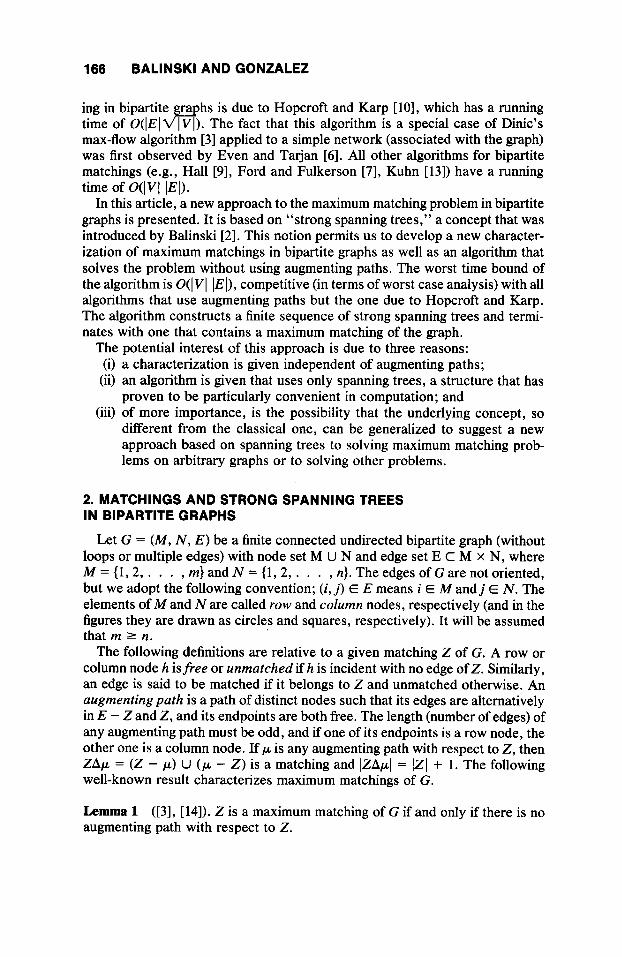
Since the concept of s.s.t. cannot be applied to every bipartite graph G (Fig. 1 shows one that contains no s.s.t.), an auxiliary graph associated with G is considered.
Given a bipartite graph G = (M, N , E), the auxiliary graph G" associated with G is the bipartite graph Ga = (Ma, N , E"), where M u = M U (0) and E" = E u { ( O , j ) : j E N } [0 is the auxiliary row node and (0, j ) with j E N denotes an auxiliary edge]. Every spanning tree T of G" is rooted at row node 0.
A column node h is called a candidate in the s.s.t. Tof G" if it is of degree at least 3 in Tand there exists a path p in G [i.e., excluding edges (0,j)l from h to a column node of degree 1 in T whose first edge ( f , g ) not in T(h) has row node f E T(h) and column node g @ T(h). The set ofcandidates is denoted by C ( T ) . By definition, if the set of degree 1 column nodes is empty, Q ( T ) = 0, then the set of candidates is empty, C(T) = 0.
Let Tbe an s.s.t. of G". For each column nodej @ Q(T) (i .e. , j is of degree at least 2 in T ) , let s ( j ) be some successor o f j in T . The set Z ( T ) = U { s ( j ) , j ) : j (Z Q(T)} is a matching of G , called the matching induced by T.
Figure 2(b) illustrates an s.s.t. T of the graph G" shown in Figure 2(a) (the broken lines denote edges in G" - T ) . Notice that the set of degree 1 column nodes is Q(T) = (2).
The set Z ( T ) = ((4, l ) , (6 , 4), (1, 5 ) , (2, 3)} is a matching of G induced by the s.s.t. Tof Figure 2(b). Column node 1 is a candidate because it is of degree 3 in
FIG. 1.
168 BALlNSKl AND GONZALEZ
FIG. 2.
T, and the edges (3, l), (3, 4), (6, 4), and (6, 2) form a path that joins column node 1 with column node 2, and the first edge (3, 4) $Z T( 1) joins row node 3 E T( 1) with column node 4 $Z T( 1). Column node 4 also is a candidate, whereas column node 5 is not [it is of degree 3 in T but no edge in G - Tjoins a row node in T(5) with a column node in T - T(5)I. Hence, the set of candidates of T is C(T) = (1, 4).
Ifj, , j 2 , . . . , j , are the indices of the column nodes of degree at least 2 in T, then the number of matchings induced by T is (bjl - l)(bj2 - 1) . . . (bj, - l) , where bj is the degree of column node j in T. In particular, and recalling that m 2 n, an s.s.t. T induces exactly one matching if and only if all column nodes are of degree 2 in T (and in such case m = n).
Theorem 1. If T is an s.s.t. of G" that has no candidates, then every matching induced by T is a maximum matching of G.
Pruof. Suppose T is an s.s.t. of G a having no candidates, C(T) = 0, and let
If there are no degree 1 column nodes, Q(T) = 0, then every column node is Z be a matching of G induced by T.
matched and Z is clearly a maximum matching, so assume Q(T> f 0.
MAXIMUM MATCHINGS IN BIPARTITE GRAPHS 169
Now suppose that Z is not a maximum matching. Then, by Lemma I , there exists an augmenting path plg in G joining a free row node 1 to a free column node g. By definition of Z , g free implies g E Q ( T ) and 1 free implies that its predecessor in T , call it column node h, is of degree at least 3 . We claim that h is a candidate.
If ( I , jl) denotes the first edge on pig, then plg without it may be written pjlE =
{(il id, (il A , . . . (&I &)}, where& = g, (i,,.h) E Z and G-1 ,A) P Z . Ifj, E T(h), then i, E T(h), so the first edge on the path not belonging to T(h) has ir-, E T(h) and j , $? T(h). Thus, h E C(T) , a contradiction that shows Z is a maximum matching. I
3. A NEW ALGORITHM FOR MAXIMUM MATCHINGS IN BIPARTITE GRAPHS
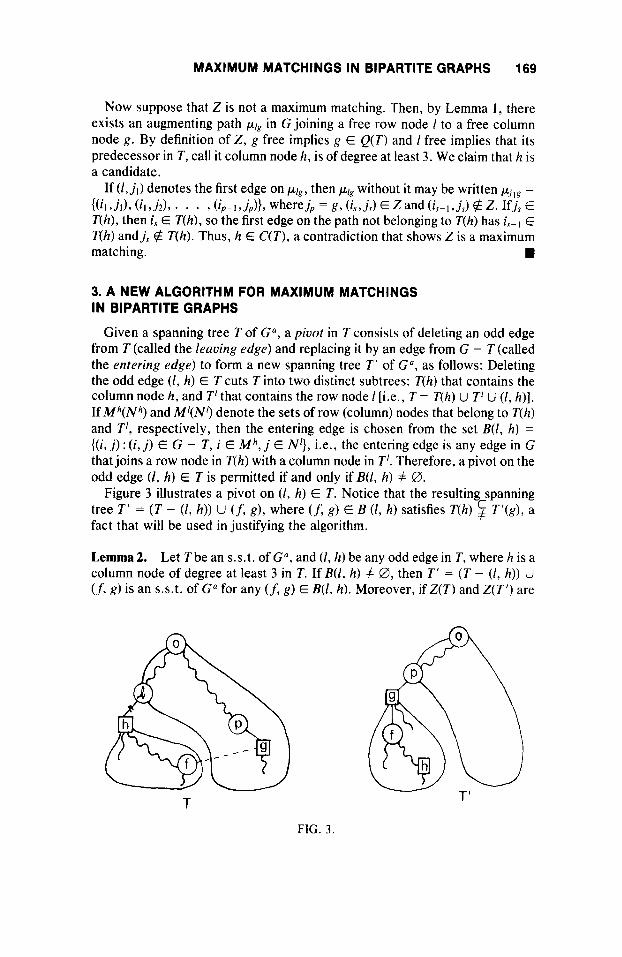
Given a spanning tree T of G", a pivot in T consists of deleting an odd edge from T (called the leaving edge) and replacing it by an edge from G - T (called the entering edge) to form a new spanning tree T ' of G", as follows: Deleting the odd edge ( I , h) E T cuts T into two distinct subtrees: T(h) that contains the column node h, and T' that contains the row node I [i.e., T = T(h) u T' LJ ( I , h ) ] . If Mh(Nh) and M'(N9 denote the sets of row (column) nodes that belong to T(h) and T', respectively, then the entering edge is chosen from the set B(I, h ) = {(i, j ) : (i, j) E G - T , i E M h , j E N'), i.e., the entering edge is any edge in G that joins a row node in T(h) with a column node in T'. Therefore, a pivot on the odd edge (2, h) E T is permitted if and only if B(I, h) f 0.
Figure 3 illustrates a pivot on ( I , h) E T . Notice that the resulting spanning tree T ' = ( T - ( I , h)) U (f, g), where (f, g) E B (1, h ) satisfies T(h) $ T ' ( g ) , a fact that will be used in justifying the algorithm.
Lemma 2. Let T be an s.s.t. of G", and (1, h) be any odd edge in T , where h is a column node of degree at least 3 in T. If B(1, h) f 0, then T' = ( T - ( I , h ) ) U (f, g) is an s.s.t. of G" for any (f, g) E B(1, h). Moreover, if Z(T) and Z(T' ) are
T 1
FIG. 3 .

170 BALlNSKl AND GONZALEZ
matchings of G induced by Tand T', then (Z(T')l = 1Z(T)( if g @ Q(T) and lZ(T)I + 1 if g E Q(T).
Proof. Since h is the only column node whose degree decreases (by 1) in pivoting on ( I , h) E T, no column node of degree 1 is created. Thus, T' is an s.s.t. of G". Further, g Q(T) implies that the column nodes of degree 1 remain the same, Q(T') = Q(T), whereas g E Q(T) implies that one column node of degree 1 is no longer of degree 1, so Q(T') = Q(T) - (8). From this and the definition of Z(T) , the lemma follows.
Let Tbe an s.s.t. of G a . A highest column node h in T having degree at least 3 is called dominant in T. This implies that column nodes in poh different from a dominant h are all of degree 2 in T. The set of dominants in T is denoted by D(Th
I fD(T) = 0, then every column node is of degree at most 2 in T. This implies IMI = IN[ (because of the assumption IM( 2 IN/) , and therefore every column node must be of degree 2 in T and the one induced matching is obviously a maximum matching.
The result of Theorem 1 is the motivation for the algorithm given below that seeks to produce an s.s.t. T that has no candidates. Another result is needed to make it efficient: It curtails the consideration of candidates that are of no use. Let T be an s.s.t. of G" and suppose D(T) # 0 and Q(T) # 0. Call all nodes that are below any h E D(T) and h itself dominated nodes at T, and designate the dominated row nodes by MD and the dominated column nodes by No. Say that T is closed if either D(T) = 0 or Q(T) = 0 or if i E MD and (i, j ) E G implies j E No.
Theorem 2. If T is a closed s.s.t. of G", then every matching induced by T is a maximum matching of G. Moreover, every Ga has a closed s.s.t. T.
Proof. Suppose T is closed. If either D(T) = 0 or Q(T) = 0, the result is immediate. So assume Q(T) # 0 and D(T) # 0. Let Z be any induced matching of T, and suppose it is not a maximum matching. Then, there exists an aug- menting path plg in G, with 1 a free row node and g a free column node. This means g 4 ND because g E Q(T), and 1 E MD because its predecessor in T is of degree at least 3. Suppose plg = {(il, jl), (i2, j , ) , . . . (i,, j , - A (i,, jJ}, with (is,js-l) E Z, ( i s , j s ) E G - Zand il = I andj, = g . Then, ip $Z M D , for otherwise since T is closed it would follow from (i,,j,,) E G thatj, = g E ND, a contradic- tion. But (i,,&l) E Z, sojp-, @ N D , which implies iPpl @ M D , and so forth, to il = 1 @ MD, a contradiction.
Thus, a closed s.s.t. Tprovides us with a maximum matching. The algorithm given below terminates with a closed s.s.t. T and so proves the second asser- tion of Theorem 2.

MAXIMUM MATCHINGS IN BIPARTITE GRAPHS 171
Row node i 1 2 3
Li 2 , 4 , 6 1 , 3 2 , 3 , 4
The Algorithm
4 5 6 7
l , 3 1 , 3 5 , 7 2 , 3 , 6
Input: a bipartite graph G = ( M , N , E ) . Output: a maximum matching Z* of G .
Step 0. Construct the initial s.s.t. of Ga
For each row node i E M , let j ( i ) be some column node adjacent to i in G . Define To = {(O,j) : j E N } U {(i,j(i)) : i E M } , and set R t 0 and S + 0 (R and S denote sets of row and column nodes that are “scanned” during the algo- rithm and may thereafter be ignored).
Step 1. Check optimality
Let T be the current s.s.t. of G ” , b the vector of the column node degrees in
If Q(T) = 0 or D ( T ) C S , set Z * to be any induced matching of T , stop. T, D ( T ) the set of its dominants, and Q ( T ) = { j E N : bj = l}.
Otherwise, let h E D ( T ) - S and go to step 2 .
Step 2. Pivot step
(a) Let 1 be the predecessor of h in T , and define M ’ = M h - R, N ’ = N h - S and N” = { j E N - N ” : ( i , j ) E G - T , some i E M’}.
(b) If N h (Z S , pivot on ( I , h) and choose any edge (f, g) E G - TwithfE M‘ and g E Nh - S, to be the entering edge. Go to step 3.
(c) Otherwise, set S t S U N ’ , R t R U M ‘ and go to step 1.
Step 3 . Update step
Set bh + bh - 1; b, t b, + 1, and T t ( T - (I, h ) U ( f , 8) . (a) If b, = 2 , set Q(T) t Q ( T ) - {g } and go to step 1. (b) Otherwise, let h’ E D(T) for h’ E peg. Set h t h‘ and go to step 2 .
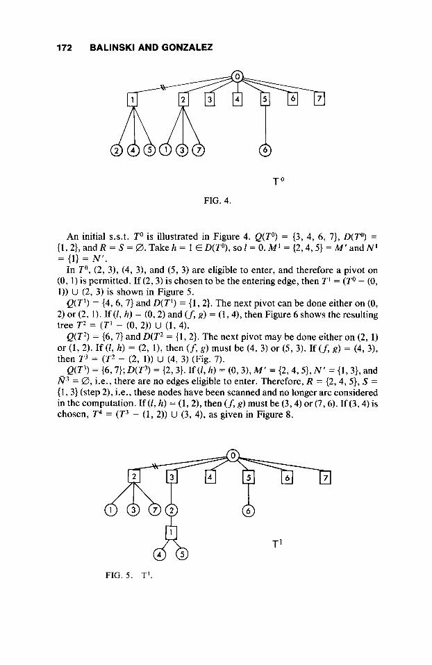
An example
Consider the bipartite graph defined by the following “dictionary”:
The list Li contains the indices of the column nodes that are adjacent to row node i, for i = I , 7.
172 BALlNSKl AND GONZALEZ
FIG. 4.
An initial s.s.t. T o is illustrated in Figure 4. Q(To) = (3, 4, 6, 7}, D(To) = { 1,2}, and R = S = 0. Take h = 1 E D(To), so I = 0. MI = {2,4,5} = M' and N' = (1) = N ' .
In To, (2, 3), (4, 3), and (5, 3) are eligible to enter, and therefore a pivot on (0,l) is permitted. If (2,3) is chosen to be the entering edge, then TI = (To - (0, 1)) U (2, 3) is shown in Figure 5.
Q(T1) = {4,6,7} and D(T') = {1,2}. The next pivot can be done either on (0, 2) or (2, 1). If (I, h) = (0,2) and (f, g) = (1,4), then Figure 6 shows the resulting tree T 2 = (TI - (0, 2)) U (1, 4).
Q(T2) = {6,7} and D(T2 = {I, 2). The next pivot may be done either on (2, 1) or (1, 2). If (I, h) = (2, l), then (f, g) must be (4, 3) or (5, 3). If (f, g) = (4, 3), then T 3 = (T2 - (2, 1)) U (4, 3) (Fig. 7).
Q(T3) = {6,7}; D(T3) = {2,3}. If (I, h) = (0,3), M' = {2,4,5}, N ' = {1,3}, and N 3 = 0, i.e., there are no edges eligible to enter. Therefore, R = (2, 4, 5}, S = {1,3} (step 2), i.e., these nodes have been scanned and no longer are considered in the computation. If (I, h ) = (1,2), then (f, g ) must be (3,4) or (7,6). If (3,4) is chosen, T4 = ( T 3 - (1, 2)) U (3, 4), as given in Figure 8.
T'
FIG. 5 . TI.
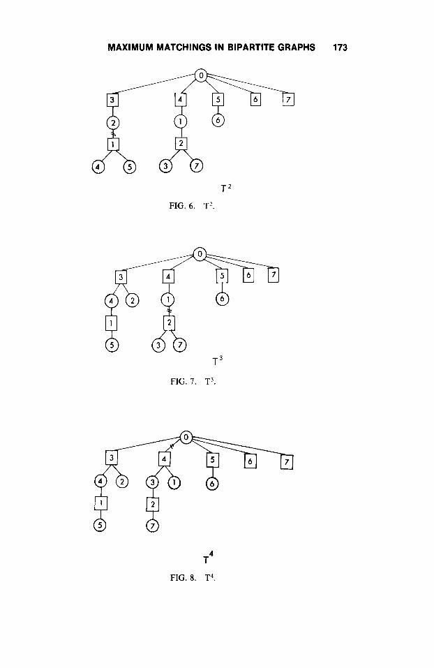
MAXIMUM MATCHINGS IN BIPARTITE GRAPHS 173
/
T 2
FIG. 6. T2.
T 3
FIG. 7. T3.
T4
FIG. 8. T4.
174 BALlNSKl AND GONZALEZ
8 T5
FIG. 9. T5.
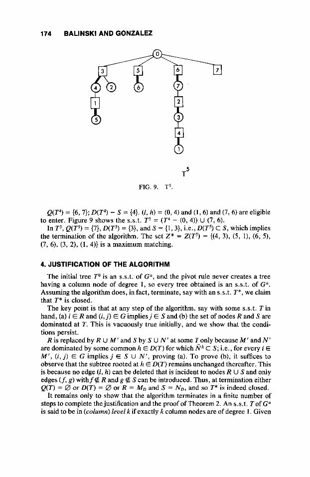
Q(T4) = {6,7}; D(T4) - S = (4). ( I , h) = (0,4) and (1, 6) and (7, 6) are eligible to enter. Figure 9 shows the s.s.t. T5 = (T4 - (0, 4)) U (7, 6).
In T5, Q(T5) = {7}, D(Ts) = {3}, and S = {1,3}, i.e., D(T5) C S , which implies the termination of the algorithm. The set Z* = Z(T5) = ((4, 3), (5, l), (6, 5 ) , (7, 6), (3, 2), (1, 4)) is a maximum matching.
4. JUSTIFICATION OF THE ALGORITHM
The initial tree To is an s.s.t. of G", and the pivot rule never creates a tree having a column node of degree 1, so every tree obtained is an s.s.t. of G". Assuming the algorithm does, in fact, terminate, say with an s.s.t. T*, we claim that T* is closed.
The key point is that at any step of the algorithm, say with some s.s.t. Tin hand, (a) i E R and ( i , j ) E G impliesj E S and (b) the set of nodes R and S are dominated at T. This is vacuously true initially, and we show that the condi- tions persist.
R is replaced by R U M ' and S by S U N ' at some T only because M ' and N ' are dominated by some common h E D(T) for which N h C S; i.e., for every i E M', (i, j ) E G implies j E S U N', proving (a). To prove (b), it suffices to observe that the subtree rooted at h E D(T) remains unchanged thereafter. This is because no edge ( I , h) can be deleted that is incident to nodes R U S and only edges (f, g) withfe R and g $2 S can be introduced. Thus, at termination either Q(T) = 0 or D(T) = 0 or R = MD and S = ND, and so T* is indeed closed.
It remains only to show that the algorithm terminates in a finite number of steps to complete the justification and the proof of Theorem 2. An s.s.t. T of G" is said to be in (column) level k if exactly k column nodes are of degree 1. Given

MAXIMUM MATCHINGS IN BIPARTITE GRAPHS 175
a tree of level k , a step of the algorithm in which a pivot is made yields either a tree of level k or one of level k - 1. Accordingly, say that stage k of the algorithm begins with the first s.s.t. that is of level k and ends when a tree of level k - 1 is found. The first s.s.t. T o is of level at most IN1 - 1 and since Q(T) = 0 means the algorithm ends, the lowest possible level is 0, so there can be at most IN/ - 1 stages. If, however, in a step of the algorithm no pivot is made, then IN1 - ISI, which we call the dimension, decreases strictly. Since the first s.s.t. To is of dimension IN/ , the number of dimension-reducing steps is at most PI.
Lemma 3. Suppose T is the first level k tree encountered and IN1 - IS1 is its dimension. Then, in at most IN1 - IS1 - k steps, a tree is obtained that either is in level k - 1 or is closed.
Proof. Suppose, first, that every step is a pivot, and let T ’ and T“ be two successive s.s.t. of level k . If the pivot on T f is made due to h’(h’ E D ( T ) - S chosen in step 1 or step 3) and the pivot on T” is made due to h” (chosen in step 3 ) , then T’(h’) 2 T”(h‘’) so that N” 2 N h ’ , meaning that the sets of column nodes eligible to increase in degree-which always include the column nodes of degree 1-are nested and strictly shrink. Therefore, if Tis the first tree of stage k , lNhl I IN1 - IS1 - 1, and since Q(T) C N h and lQ(T)I = k , there can be at most IN1 - IS1 - 1 - k pivots that do not yield a k - 1 level tree, and one more must terminate stage k .
Any one nonpivot step decreases the dimension by at least I , and so the set of column nodes eligible to increase in degree, Nh, decreases by at least 1 at every step, whether it is a pivot or a nonpivot step (indeed, p pivot steps in level k followed by one nonpivot step decreases the dimension by at least p + 1). I
This completes the proof of Theorem 2 . But notice that the worst case is when all steps are pivots in every stage S = 0 throughout and there are at most IN1 - k pivots in stage k , so at most 1 + 2 . . . + (IN1 - 1 ) steps in all. This establishes:
Theorem 3. The algorithm requires at most JNI(INI - 1)/2 steps.
It is now a relatively simple matter to prove a “converse” of Theorem 2 .
Theorem 4. If Z is a maximum matching of G , there exists a closed s.s.t. T of G“ with Z a matching induced by T .
Proof. Let 2 = { ( is , js)} be a maximum matching of G and construct an s.s.t. Tof G a as follows: ( 0 , j ) E Tfor dlj E N , ( i s , j s ) E Tfor all matching edges, and for each unmatched row node i, ( i , js ) E Tfor some s. We describe an iterative procedure to pass from one s.s.t. to another, each of which has Z as an induced matching, that terminates with a closed s.s.t. T*.

176 BALlNSKl AND GONZALEZ
If T is not closed, then for some h E D(T) there exists an edge (f, g ) , with f E T(h) and g $E No. It must be that g Q(T) , else Z would not be a maximum matching by Lemma 2. Therefore, g is of degree exactly 2 in T and is a neighbor of the root 0. Pivot by deleting (0, g ) and replacing it by (f, g), to obtain a new tree T‘ having Z as an induced matching. If T‘ is not closed, repeat. After at most IN1 - lQ(T)I - ID(T)( pivots of this type, the procedure terminates in a closed tree T* having Z as an induced matching.
5. THE COMPLEXITY OF THE ALGORITHM
In this section, an implementation is described that runs in at most O(lN1 IEI) time. The key point is to show that each stage of the algorithm requires at most O(IE() time.
A standard adjacency list [l] is used to represent the bipartite graph, and each tree is assumed to be represented by a “three-label’’ data structure [ l l ] that allows subsets of nodes to be obtained in work linear in their cardinalities.
Step 0 requires an amount of work proportional to IMI + IN[: The indexj(i), i E M, is the first element of the list Li of column nodes adjacent to row node i.
Step 1 is entered at the start and either after a pivot step when the level drops by 1 or when a nonpivot step is made and the dimension drops by at least 1. Since there can be at most IN/ decreases in dimension, step 1 is performed at most 21” times. Each step 1 requires O(lNI) work, so the total is bounded by
Next, consider the work required in steps 2 and 3. It will be shown that each edge is accessed at most once in each stage. All updating within a stage is postponed until the end of the stage when a “block pivot” is done in work of at most O(IMI + INI) (as suggested in [8]). Stars are used to indicate if a row node belongs to R or a column node belongs to S. Initially S = 0 = R, and if at some step a node is starred, it remains starred. Labels are used to indicate if a row node belongs to M‘ or a column node belongs to N’. They are assigned in step 2, and are all erased when a step 1 is entered.
Step 2 is done as follows: Call the tree Tat hand when step 1 was last entered and h E D(T) - S was chosen the “initial tree,” with (1, h) the first leaving edge. Label i E M’ with 6(i) = h a n d j E N ’ with 6 ( j ) = h. Thus, the set of nodes labeled h identifies the subtree T(h). Let i be a labeled row node, and consider each successive element j of Li: I f j E N ’ U S, that is, if j is labeled or starred, then declare the edge (i, j ) “scanned,” meaning it has been looked at once and will not be accessed again within the current stage. If every edge ( i , j ) f o r j E Li is scanned, then row node i is declared scanned and will not be accessed again in the current stage. Go to another labeled row node and con- tinue until either (i) every labeled row node is scanned or (ii) for some labeled row node f and g E Lf, g $Z N‘ U S.
In case (i), a nonpivot step is made. R U M’ replaces R and S U N ‘ replaces S. All labels are changed to stars.
O<l”’> 5 OClNI IEI).
MAXIMUM MATCHINGS IN BIPARTITE GRAPHS 177
In case (ii), a pivot step may be made with (f, g) the entering edge and (1, h ) the leaving edge. Maintain a list of entering edges and a list of leaving edges. The actual updating to store the new tree may be postponed. To see why, suppose the new tree after pivoting was T’ and th6 stage was not done, with the new leaving edge determined in step 3(b) ( l ’ , h’). Then, T(h) C T’(h’) , M ’ c M ” = Mh’ - R , and N ‘ C N “ = Nh’ - S, so M‘ and N ’ are enlarged to M‘land N ” , respectively, by assigning to row nodes i E M ” - M ’ the label 6( i ) = h’ and to column nodesj E N” - N ’ the label S ( j ) = h ’ . Any edges ( i , j ) , i E M ’ , already scanned remain scanned, and any row nodes i E M ’ already scanned remain scanned, too. These properties persist whatever number of repetitions of case (ii). Notice an additional property. Suppose that after several repetitions of case (ii) step 3(b) chooses ( l * , h*) as the leaving edge. If h* is of degree at least 3 in the initial tree T , then the nodes labeled h* are precisely the nodes of T(h*), whereas if h* is of degree 2 in T , then the nodes labeled h* belong to T(h*) and span a subtree of T rooted at h*. In either case, call this subtree Th*.
If the initial tree Tis of level t , then case (ii) can recur at most IN\ - t times before either case (i) occurs or the stage ends. If case (i) occurs, replace the labels by stars and go to step 1 . If the stage ends a block pivot is done to update T . A “complete” update would replace every leaving edge with the corre- sponding entering edge determined in case (ii) as prescribed by the algorithm. But doing a “complete” update is unnecessary: It suffices to obtain a new s.s.t. of G a of level t - 1. The labels are useful for this purpose.
The block pivot, which does the work of updating, is effected as follows: Suppose the entering edge with which the stage ends is (fi, gl) with S ( f i ) = g2. Then, T U (5, gI) contains a cycle that includes a unique edge (12 , gz) that is in the list of leaving edges. If g2 is of degree 2 in the initial tree T , then there is a unique entering edge ( f 2 , gz) with S(fi) = g3. T U (fi, gz) contains a cycle that includes a unique leaving edge ( 1 3 , g 3 ) . Continue identifying pairs of entering and leaving edges until an entering edge (J;., g;) is found with S ( J ) = g;+l, leaving edge (li+,, g,+l) and gi+l of degree at least 3 in T. Drop the edges (12 , gd, . . . , (1i+lT g;+d and enter (fi, gl) and Tqproperly oriented, (fi, gJ and 7’: properly oriented, . . . , and ( J , g;) and Tf+, properly oriented. This updat- ing may be done for each subtree and edge in work linear in the number of nodes, and so the entire update is bounded by OClMI + IMI).
This establishes the following statement.
Theorem 6. The algorithm requires O(lV( (El) work to find a maximum match- ing in a bipartite graph with IVI nodes and IEl edges.
Figure 10 gives an example of a block pivot. In Figure 10(a), the numbers within parentheses indicate the order in which the potential leaving and enter- ing edges are determined during the stage, the broken lines denote the entering edges, and the numbers associated with nodes are their labels. Starting with
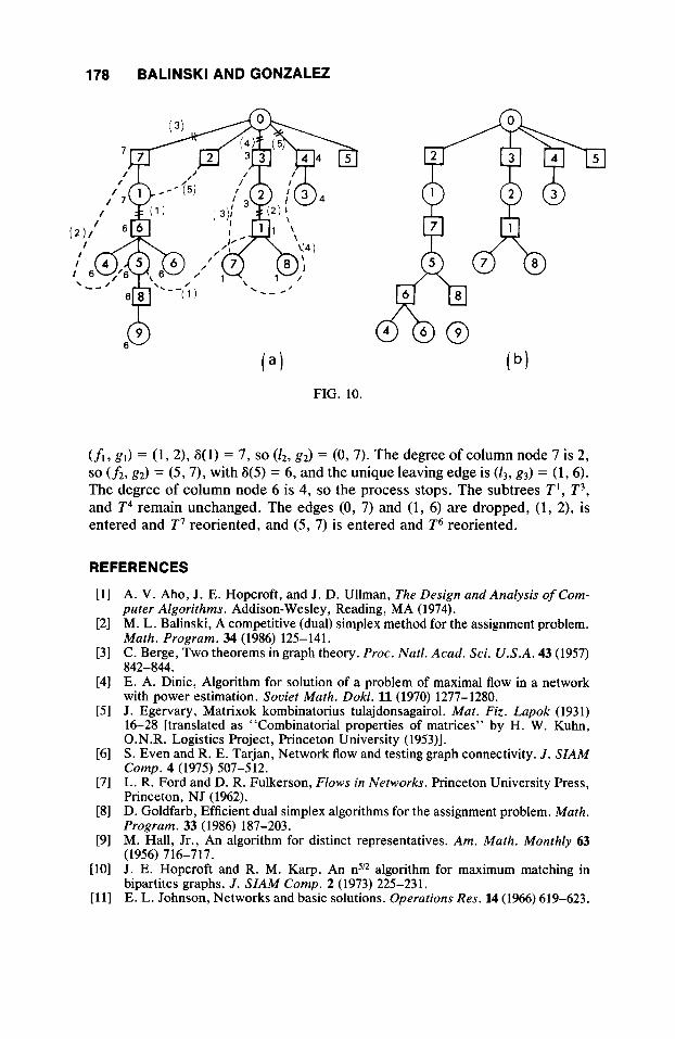
178 BALlNSKl AND GONZALEZ
a
6 6 FIG. 10.
(fi, gl) = ( 1 , 2), 6(1) = 7, so (i2, g 2 ) = (0, 7). The degree of column node 7 is 2, so (f2, g2) = (5,7), with 6(5) = 6, and the unique leaving edge is ( 1 3 , g3) = (1,6). The degree of column node 6 is 4, so the process stops. The subtrees TI, T 3 , and T4 remain unchanged. The edges (0, 7) and (1 , 6) are dropped, ( 1 , 2), is entered and T7 reoriented, and (5, 7) is entered and T6 reoriented.
REFERENCES
A. V. Aho, J. E. Hopcroft, and J. D. Ullman, The Design and Analysis of Com- puter Algorithms. Addison-Wesley, Reading, MA (1974). M. L. Balinski, A competitive (dual) simplex method for the assignment problem. Math. Program. 34 (1986) 125-141. C. Berge, Two theorems in graph theory. Proc. Natl. Acad. Sci. U.S.A. 43 (1957)
E. A. Dinic, Algorithm for solution of a problem of maximal flow in a network with power estimation. Soviet Math. Dokl. 11 (1970) 1277-1280. J. Egervary, Matrixok kombinatorius tulajdonsagairol. Mat. Fiz. Lapok (1931) 16-28 [translated as “Combinatorial properties of matrices” by H. W. Kuhn, O.N.R. Logistics Project, Princeton University (1953)l. S. Even and R. E. Tajan , Network flow and testing graph connectivity. J . SIAM Comp. 4 (1975) 507-512. L. R. Ford and D. R. Fulkerson, Flows in Networks. Princeton University Press, Princeton, NJ (1962). D. Goldfarb, Efficient dual simplex algorithms for the assignment problem. Math. Program. 33 (1986) 187-203. M. Hall, Jr., An algorithm for distinct representatives. Am. Math. Monthly 63
J. E. Hopcroft and R. M. Karp, An nS’* algorithm for maximum matching in bipartites graphs. J . SIAM Comp. 2 (1973) 225-231. E. L. Johnson, Networks and basic solutions. Operations Res. 14 (1966) 619-623.
842-844.
(1956) 716-717.

MAXIMUM MATCHINGS IN BIPARTITE GRAPHS 179
[I21 D. Konig, Uber graphen and ihre Anwendung auf Determinantentheorie und Mengenlehre. Math. Ann. 77 (1955) 83-97.
[13] H. W. Kuhn, The Hungarian method for the assignment problem. Naval Res.
[14] R. Z. Norman and M. 0. Rabin, An algorithm for a minimum cover of a graph. Proc. Am. Math. SOC. 10 (1959) 315-319.
Log. Q. 2 (1955) 83-97.
Received March 1988 Accepted June 1990


![Analysis of Stable Matchings in R: Package matchingMarkets · Analysis of Stable Matchings in R: ... 4 Analysis of Stable Matchings in R: Package matchingMarkets ... G = 1[V G 0]](https://img.pdfslide.net/doc/110x75/5b3cc11f7f8b9a9a098b5ae0/analysis-of-stable-matchings-in-r-package-matchingmarkets-analysis-of-stable.jpg)