Embed Size (px)
Citation preview
5MCMC Using Hamiltonian Dynamics
Radford M. Neal
5.1 Introduction
Markov chain Monte Carlo (MCMC) originated with the classic paper of Metropolis et al.(1953), where it was used to simulate the distribution of states for a system of idealizedmolecules. Not long after, another approach to molecular simulation was introduced (Alderand Wainwright, 1959), in which the motion of the molecules was deterministic, followingNewton’s laws of motion, which have an elegant formalization as Hamiltonian dynamics. Forfinding the properties of bulk materials, these approaches are asymptotically equivalent,since even in a deterministic simulation, each local region of the material experienceseffectively random influences from distant regions. Despite the large overlap in their appli-cation areas, the MCMC and molecular dynamics approaches have continued to coexist inthe following decades (see Frenkel and Smit, 1996).
In 1987, a landmark paper by Duane, Kennedy, Pendleton, and Roweth united theMCMC and molecular dynamics approaches. They called their method “hybrid MonteCarlo,” which abbreviates to “HMC,” but the phrase “Hamiltonian Monte Carlo,” retain-ing the abbreviation, is more specific and descriptive, and I will use it here. Duane et al.applied HMC not to molecular simulation, but to lattice field theory simulations of quan-tum chromodynamics. Statistical applications of HMC began with my use of it for neuralnetwork models (Neal, 1996a). I also provided a statistically-oriented tutorial on HMC in areview of MCMC methods (Neal, 1993, Chapter 5). There have been other applicationsof HMC to statistical problems (e.g. Ishwaran, 1999; Schmidt, 2009) and statistically-oriented reviews (e.g. Liu, 2001, Chapter 9), but HMC still seems to be underappreciatedby statisticians, and perhaps also by physicists outside the lattice field theory community.
This review begins by describing Hamiltonian dynamics. Despite terminology that maybe unfamiliar outside physics, the features of Hamiltonian dynamics that are needed forHMC are elementary. The differential equations of Hamiltonian dynamics must be dis-cretized for computer implementation. The “leapfrog” scheme that is typically used isquite simple.
Following this introduction to Hamiltonian dynamics, I describe how to use it to con-struct an MCMC method. The first step is to define a Hamiltonian function in terms of theprobability distribution we wish to sample from. In addition to the variables we are inter-ested in (the “position” variables), we must introduce auxiliary “momentum” variables,which typically have independent Gaussian distributions. The HMC method alternatessimple updates for these momentum variables with Metropolis updates in which a newstate is proposed by computing a trajectory according to Hamiltonian dynamics, imple-mented with the leapfrog method. A state proposed in this way can be distant from the
113
114 Handbook of Markov Chain Monte Carlo
current state but nevertheless have a high probability of acceptance. This bypasses the slowexploration of the state space that occurs when Metropolis updates are done using a simplerandom-walk proposal distribution. (An alternative way of avoiding random walks is to useshort trajectories but only partially replace the momentum variables between trajectories,so that successive trajectories tend to move in the same direction.)
After presenting the basic HMC method, I discuss practical issues of tuning the leapfrogstepsize and number of leapfrog steps, as well as theoretical results on the scaling of HMCwith dimensionality. I then present a number of variations on HMC. The acceptance ratefor HMC can be increased for many problems by looking at “windows” of states at thebeginning and end of the trajectory. For many statistical problems, approximate computa-tion of trajectories (e.g. using subsets of the data) may be beneficial. Tuning of HMC canbe made easier using a “short-cut” in which trajectories computed with a bad choice ofstepsize take little computation time. Finally, “tempering” methods may be useful whenmultiple isolated modes exist.
5.2 Hamiltonian Dynamics
Hamiltonian dynamics has a physical interpretation that can provide useful intuitions.In two dimensions, we can visualize the dynamics as that of a frictionless puck that slidesover a surface of varying height. The state of this system consists of the position of the puck,given by a two-dimensional vector q, and the momentum of the puck (its mass times itsvelocity), given by a two-dimensional vector p. The potential energy, U(q), of the puck isproportional to the height of the surface at its current position, and its kinetic energy, K(p),is equal to |p|2/(2m), where m is the mass of the puck. On a level part of the surface, thepuck moves at a constant velocity, equal to p/m. If it encounters a rising slope, the puck’smomentum allows it to continue, with its kinetic energy decreasing and its potential energyincreasing, until the kinetic energy (and hence p) is zero, at which point it will slide backdown (with kinetic energy increasing and potential energy decreasing).
In nonphysical MCMC applications of Hamiltonian dynamics, the position will cor-respond to the variables of interest. The potential energy will be minus the log of theprobability density for these variables. Momentum variables, one for each position variable,will be introduced artificially.
These interpretations may help motivate the exposition below, but if you find otherwise,the dynamics can also be understood as simply resulting from a certain set of differentialequations.
5.2.1 Hamilton’s Equations
Hamiltonian dynamics operates on a d-dimensional position vector, q, and a d-dimensionalmomentum vector, p, so that the full state space has 2d dimensions. The system is describedby a function of q and p known as the Hamiltonian, H(q, p).
5.2.1.1 Equations of Motion
The partial derivatives of the Hamiltonian determine how q and p change over time, t,according to Hamilton’s equations:
MCMC Using Hamiltonian Dynamics 115
dqi
dt= ∂H
∂pi, (5.1)
dpi
dt= −∂H
∂qi, (5.2)
for i = 1, . . ., d. For any time interval of duration s, these equations define a mapping, Ts,from the state at any time t to the state at time t+ s. (Here, H, and hence Ts, are assumed tonot depend on t.)
Alternatively, we can combine the vectors q and p into the vector z = (q, p) with 2ddimensions, and write Hamilton’s equations as
dzdt= J ∇H(z),
where ∇H is the gradient of H (i.e. [∇H]k = ∂H/∂zk), and
J =[
0d×d Id×d
−Id×d 0d×d
](5.3)
is a 2d× 2d matrix whose quadrants are defined above in terms of identity and zero matrices.
5.2.1.2 Potential and Kinetic Energy
For HMC we usually use Hamiltonian functions that can be written as
H(q, p) = U(q)+ K(p). (5.4)
Here U(q) is called the potential energy, and will be defined to be minus the log probabilitydensity of the distribution for q that we wish to sample, plus any constant that is convenient.K(p) is called the kinetic energy, and is usually defined as
K(p) = pTM−1p/2. (5.5)
Here M is a symmetric, positive-definite “mass matrix,” which is typically diagonal, andis often a scalar multiple of the identity matrix. This form for K(p) corresponds to minusthe log probability density (plus a constant) of the zero-mean Gaussian distribution withcovariance matrix M.
With these forms for H and K, Hamilton’s equations 5.1 and 5.2 can be written as follows,for i = 1, . . ., d:
dqi
dt= [M−1p]i, (5.6)
dpi
dt= −∂U
∂qi. (5.7)
116 Handbook of Markov Chain Monte Carlo
5.2.1.3 A One-Dimensional Example
Consider a simple example in one dimension (for which q and p are scalars and will bewritten without subscripts), in which the Hamiltonian is defined as follows:
H(q, p) = U(q)+ K(p), U(q) = q2
2, K(p) = p2
2. (5.8)
As we will see later in Section 5.3.1, this corresponds to a Gaussian distribution for q withmean zero and variance one. The dynamics resulting from this Hamiltonian (followingEquations 5.6 and 5.7) is
dqdt= p,
dpdt= −q.
Solutions have the following form, for some constants r and a:
q(t) = r cos(a+ t), p(t) = −r sin(a+ t). (5.9)
Hence, the mapping Ts is a rotation by s radians clockwise around the origin in the (q, p)
plane. In higher dimensions, Hamiltonian dynamics generally does not have such a simpleperiodic form, but this example does illustrate some important properties that we will lookat next.
5.2.2 Properties of Hamiltonian Dynamics
Several properties of Hamiltonian dynamics are crucial to its use in constructing MCMCupdates.
5.2.2.1 Reversibility
First, Hamiltonian dynamics is reversible—the mapping Ts from the state at time t, (q(t), p(t)),to the state at time t+ s, (q(t+ s), p(t+ s)), is one-to-one, and hence has an inverse, T−s.This inverse mapping is obtained by simply negating the time derivatives in Equations5.1 and 5.2. When the Hamiltonian has the form in Equation 5.4, and K(p) = K(−p), as inthe quadratic form for the kinetic energy of Equation 5.5, the inverse mapping can also beobtained by negating p, applying Ts, and then negating p again.
In the simple one-dimensional example of Equation 5.8, T−s is just a counterclockwiserotation by s radians, undoing the clockwise rotation of Ts.
The reversibility of Hamiltonian dynamics is important for showing that MCMC updatesthat use the dynamics leave the desired distribution invariant, since this is most eas-ily proved by showing reversibility of the Markov chain transitions, which requiresreversibility of the dynamics used to propose a state.
5.2.2.2 Conservation of the Hamiltonian
A second property of the dynamics is that it keeps the Hamiltonian invariant (i.e. conserved).This is easily seen from Equations 5.1 and 5.2 as follows:
dHdt=
d∑i=1
[dqi
dt∂H∂qi
+ dpi
dt∂H∂pi
]=
d∑i=1
[∂H∂pi
∂H∂qi
− ∂H∂qi
∂H∂pi
]= 0. (5.10)
MCMC Using Hamiltonian Dynamics 117
With the Hamiltonian of Equation 5.8, the value of the Hamiltonian is half the squareddistance from the origin, and the solutions (Equation 5.9) stay at a constant distance fromthe origin, keeping H constant.
For Metropolis updates using a proposal found by Hamiltonian dynamics, which formpart of the HMC method, the acceptance probability is one if H is kept invariant. We willsee later, however, that in practice we can only make H approximately invariant, and hencewe will not quite be able to achieve this.
5.2.2.3 Volume Preservation
A third fundamental property of Hamiltonian dynamics is that it preserves volume in (q, p)
space (a result known as Liouville’s theorem). If we apply the mapping Ts to the pointsin some region R of (q, p) space, with volume V, the image of R under Ts will also havevolume V.
With the Hamiltonian of Equation 5.8, the solutions (Equation 5.9) are rotations, whichobviously do not change the volume. Such rotations also do not change the shape of aregion, but this is not so in general—Hamiltonian dynamics might stretch a region in onedirection, as long as the region is squashed in some other direction so as to preserve volume.
The significance of volume preservation for MCMC is that we need not account for anychange in volume in the acceptance probability for Metropolis updates. If we proposednew states using some arbitrary, non-Hamiltonian, dynamics, we would need to computethe determinant of the Jacobian matrix for the mapping the dynamics defines, which mightwell be infeasible.
The preservation of volume by Hamiltonian dynamics can be proved in several ways.One is to note that the divergence of the vector field defined by Equations 5.1 and 5.2 iszero, which can be seen as follows:
d∑i=1
[∂
∂qi
dqi
dt+ ∂
∂pi
dpi
dt
]=
d∑i=1
[∂
∂qi
∂H∂pi
− ∂
∂pi
∂H∂qi
]=
d∑i=1
[∂2H
∂qi∂pi− ∂2H
∂pi∂qi
]= 0.
A vector field with zero divergence can be shown to preserve volume (Arnold, 1989).Here, I will show informally that Hamiltonian dynamics preserves volume more directly,
without presuming this property of the divergence. I will, however, take as given thatvolume preservation is equivalent to the determinant of the Jacobian matrix of Ts havingabsolute value one, which is related to the well-known role of this determinant in regardto the effect of transformations on definite integrals and on probability density functions.
The 2d× 2d Jacobian matrix of Ts, seen as a mapping of z = (q, p), will be written as Bs. Ingeneral, Bs will depend on the values of q and p before the mapping. When Bs is diagonal,it is easy to see that the absolute values of its diagonal elements are the factors by whichTs stretches or compresses a region in each dimension, so that the product of these factors,which is equal to the absolute value of det(Bs), is the factor by which the volume of theregion changes. I will not prove the general result here, but note that if we were to (say)rotate the coordinate system used, Bs would no longer be diagonal, but the determinantof Bs is invariant to such transformations, and so would still give the factor by which thevolume changes.
Let us first consider volume preservation for Hamiltonian dynamics in one dimension(i.e. with d = 1), for which we can drop the subscripts on p and q. We can approximate Tδ
118 Handbook of Markov Chain Monte Carlo
for δ near zero as follows:
Tδ(q, p) =[
q
p
]+ δ
[dq/dt
dp/dt
]+ terms of order δ2 or higher.
Taking the time derivatives from Equations 5.1 and 5.2, the Jacobian matrix can be written as
Bδ =
⎡⎢⎢⎢⎣
1+ δ ∂2H∂q∂p
δ∂2H∂p2
−δ∂2H
∂q2 1− δ ∂2H∂p∂q
⎤⎥⎥⎥⎦+ terms of order δ2 or higher. (5.11)
We can then write the determinant of this matrix as
det(Bδ) = 1+ δ ∂2H∂q∂p
− δ ∂2H∂p∂q
+ terms of order δ2 or higher
= 1+ terms of order δ2 or higher.
Since log(1+ x) ≈ x for x near zero, log det(Bδ) is zero, except perhaps for terms of orderδ2 or higher (though we will see later that it is exactly zero). Now consider log det(Bs) forsome time interval s that is not close to zero. Setting δ = s/n, for some integer n, we canwrite Ts as the composition of Tδ applied n times (from n points along the trajectory), sodet(Bs) is the n-fold product of det(Bδ) evaluated at these points. We then find that
log det(Bs) =n∑
i=1
log det(Bδ)
=n∑
i=1
{terms of order 1/n2 or smaller
}(5.12)
= terms of order 1/n or smaller.
Note that the value of Bδ in the sum in Equation 5.12 might perhaps vary with i, sincethe values of q and p vary along the trajectory that produces Ts. However, assuming thattrajectories are not singular, the variation in Bδ must be bounded along any particulartrajectory. Taking the limit as n →∞, we conclude that log det(Bs) = 0, so det(Bs) = 1, andhence Ts preserves volume.
When d > 1, the same argument applies. The Jacobian matrix will now have the followingform (compare Equation 5.11), where each entry shown below is a d× d submatrix, withrows indexed by i and columns by j:
Bδ=
⎡⎢⎢⎢⎢⎢⎢⎣
I + δ[
∂2H∂qj∂pi
]δ
[∂2H
∂pj∂pi
]
−δ[
∂2H∂qj∂qi
]I − δ
[∂2H
∂pj∂qi
]
⎤⎥⎥⎥⎥⎥⎥⎦+ terms of order δ2 or higher.
MCMC Using Hamiltonian Dynamics 119
As for d = 1, the determinant of this matrix will be one plus terms of order δ2 or higher,since all the terms of order δ cancel. The remainder of the argument above then applieswithout change.
5.2.2.4 Symplecticness
Volume preservation is also a consequence of Hamiltonian dynamics being symplectic. Let-ting z = (q, p), and defining J as in Equation 5.3, the symplecticness condition is that theJacobian matrix, Bs, of the mapping Ts satisfies
BTs J−1 Bs = J−1.
This implies volume conservation, since det(BTs ) det( J−1) det(Bs) = det( J−1) implies that
det(Bs)2 is one. When d > 1, the symplecticness condition is stronger than volume preserva-
tion. Hamiltonian dynamics and the symplecticness condition can be generalized to whereJ is any matrix for which JT = −J and det( J) = 0.
Crucially, reversibility, preservation of volume, and symplecticness can be maintainedexactly even when, as is necessary in practice, Hamiltonian dynamics is approximated, aswe will see next.
5.2.3 Discretizing Hamilton’s Equations—The Leapfrog Method
For computer implementation, Hamilton’s equations must be approximated by discretizingtime, using some small stepsize, ε. Starting with the state at time zero, we iteratively compute(approximately) the state at times ε, 2ε, 3ε, etc.
In discussing how to do this, I will assume that the Hamiltonian has the form H(q, p) =U(q)+ K(p), as in Equation 5.4. Although the methods below can be applied with any formfor the kinetic energy, I assume for simplicity that K(p) = pTM−1p/2, as in Equation 5.5, andfurthermore that M is diagonal, with diagonal elements m1, . . . , md, so that
K(p) =d∑
i=1
p2i
2mi. (5.13)
5.2.3.1 Euler’s Method
Perhaps the best-known way to approximate the solution to a system of differential equa-tions is Euler’s method. For Hamilton’s equations, this method performs the followingsteps, for each component of position and momentum, indexed by i = 1, . . ., d:
pi(t+ ε) = pi(t)+ ε dpi
dt(t) = pi(t)− ε ∂U
∂qi(q(t)), (5.14)
qi(t+ ε) = qi(t)+ ε dqi
dt(t) = qi(t)+ ε pi(t)
mi. (5.15)
The time derivatives in Equations 5.14 and 5.15 are from the form of Hamilton’s equa-tions given by Equations 5.6 and 5.7. If we start at t = 0 with given values for qi(0) andpi(0), we can iterate the steps above to get a trajectory of position and momentum values
120 Handbook of Markov Chain Monte Carlo
at times ε, 2ε, 3ε, . . . , and hence find (approximate) values for q(τ) and p(τ) after τ/ε steps(assuming τ/ε is an integer).
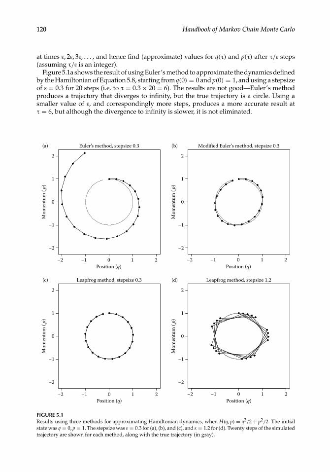
Figure 5.1a shows the result of using Euler’s method to approximate the dynamics definedby the Hamiltonian of Equation 5.8, starting from q(0) = 0 and p(0) = 1, and using a stepsizeof ε = 0.3 for 20 steps (i.e. to τ = 0.3× 20 = 6). The results are not good—Euler’s methodproduces a trajectory that diverges to infinity, but the true trajectory is a circle. Using asmaller value of ε, and correspondingly more steps, produces a more accurate result atτ = 6, but although the divergence to infinity is slower, it is not eliminated.
(a)
Mom
entu
m (
p)
Euler’s method, stepsize 0.3
−2
−1
0
1
2
−2
−1
0
1
2
(b) Modified Euler’s method, stepsize 0.3
Mom
entu
m (
p)
Mom
entu
m (
p)
−2
−1
0
1
2
−2
−1
0
1
2
Mom
entu
m (
p)
(c) (d)Leapfrog method, stepsize 0.3
Position (q)−2 −1 0 1 2
Position (q)−2 −1 0 1 2
Position (q)−2 −1 0 1 2
Position (q)−2 −1 0 1 2
Leapfrog method, stepsize 1.2
FIGURE 5.1Results using three methods for approximating Hamiltonian dynamics, when H(q, p) = q2/2+ p2/2. The initialstate was q = 0, p = 1. The stepsize was ε = 0.3 for (a), (b), and (c), and ε = 1.2 for (d). Twenty steps of the simulatedtrajectory are shown for each method, along with the true trajectory (in gray).
MCMC Using Hamiltonian Dynamics 121
5.2.3.2 A Modification of Euler’s Method
Much better results can be obtained by slightly modifying Euler’s method, as follows:
pi(t+ ε) = pi(t)− ε ∂U∂qi
(q(t)), (5.16)
qi(t+ ε) = qi(t)+ ε pi(t+ ε)mi
. (5.17)
We simply use the new value for the momentum variables, pi, when computing the newvalue for the position variables, qi. A method with similar performance can be obtained byinstead updating the qi first and using their new values to update the pi.
Figure 5.1b shows the results using this modification of Euler’s method with ε = 0.3.Though not perfect, the trajectory it produces is much closer to the true trajectory thanthat obtained using Euler’s method, with no tendency to diverge to infinity. This betterperformance is related to the modified method’s exact preservation of volume, which helpsavoid divergence to infinity or spiraling into the origin, since these would typically involvethe volume expanding to infinity or contracting to zero.
To see that this modification of Euler’s method preserves volume exactly despite thefinite discretization of time, note that both the transformation from (q(t), p(t)) to (q(t),p(t+ ε)) via Equation 5.16 and the transformation from (q(t), p(t+ ε)) to (q(t+ ε), p(t+ ε))via Equation 5.17 are “shear” transformations, in which only some of the variables change(either the pi or the qi), by amounts that depend only on the variables that do not change.Any shear transformation will preserve volume, since its Jacobian matrix will have deter-minant one (as the only nonzero term in the determinant will be the product of diagonalelements, which will all be one).
5.2.3.3 The Leapfrog Method
Even better results can be obtained with the leapfrog method, which works as follows:
pi (t+ ε/2) = pi(t)− (ε/2)∂U∂qi
(q(t)), (5.18)
qi(t+ ε) = qi(t)+ ε pi(t+ ε/2)
mi, (5.19)
pi(t+ ε) = pi (t+ ε/2)− (ε/2)∂U∂qi
(q(t+ ε)). (5.20)
We start with a half step for the momentum variables, then do a full step for the positionvariables, using the new values of the momentum variables, and finally do another half stepfor the momentum variables, using the new values for the position variables. An analogousscheme can be used with any kinetic energy function, with ∂K/∂pi replacing pi/mi above.
When we apply Equations 5.18 through 5.20 a second time to go from time t+ ε to t+ 2ε,we can combine the last half step of the first update, from pi(t+ ε/2) to pi(t+ ε), with thefirst half step of the second update, from pi(t+ ε) to pi(t+ ε+ ε/2). The leapfrog methodthen looks very similar to the modification of Euler’s method in Equations 5.17 and 5.16,except that leapfrog performs half steps for momentum at the very beginning and very endof the trajectory, and the time labels of the momentum values computed are shifted by ε/2.
122 Handbook of Markov Chain Monte Carlo
The leapfrog method preserves volume exactly, since Equations 5.18 through 5.20 areshear transformations. Due to its symmetry, it is also reversible by simply negating p,applying the same number of steps again, and then negating p again.
Figure 5.1c shows the results using the leapfrog method with a stepsize of ε = 0.3, whichare indistinguishable from the true trajectory, at the scale of this plot. In Figure 5.1d, theresults of using the leapfrog method with ε = 1.2 are shown (still with 20 steps, so almostfour cycles are seen, rather than almost one). With this larger stepsize, the approximationerror is clearly visible, but the trajectory still remains stable (and will stay stable indefinitely).Only when the stepsize approaches ε = 2 do the trajectories become unstable.
5.2.3.4 Local and Global Error of Discretization Methods
I will briefly discuss how the error from discretizing the dynamics behaves in the limit asthe stepsize, ε, goes to zero; Leimkuhler and Reich (2004) provide a much more detaileddiscussion. For useful methods, the error goes to zero as εgoes to zero, so that any upper limiton the error will apply (apart from a usually unknown constant factor) to any differentiablefunction of state—for example, if the error for (q, p) is no more than order ε2, the error forH(q, p) will also be no more than order ε2.
The local error is the error after one step, that moves from time t to time t+ ε. The globalerror is the error after simulating for some fixed time interval, s, which will require s/εsteps. If the local error is order εp, the global error will be order εp−1—the local errors oforder εp accumulate over the s/ε steps to give an error of order εp−1. If we instead fix εand consider increasing the time, s, for which the trajectory is simulated, the error can ingeneral increase exponentially with s. Interestingly, however, this is often not what hap-pens when simulating Hamiltonian dynamics with a symplectic method, as can be seen inFigure 5.1.
The Euler method and its modification above have order ε2 local error and order ε globalerror. The leapfrog method has order ε3 local error and order ε2 global error. As shown byLeimkuhler and Reich (2004, Section 4.3.3), this difference is a consequence of leapfrog beingreversible, since any reversible method must have global error that is of even order in ε.
5.3 MCMC from Hamiltonian Dynamics
Using Hamiltonian dynamics to sample from a distribution requires translating the densityfunction for this distribution to a potential energy function and introducing “momentum”variables to go with the original variables of interest (now seen as “position” variables). Wecan then simulate a Markov chain in which each iteration resamples the momentum andthen does a Metropolis update with a proposal found using Hamiltonian dynamics.
5.3.1 Probability and the Hamiltonian: Canonical Distributions
The distribution we wish to sample can be related to a potential energy function via theconcept of a canonical distribution from statistical mechanics. Given some energy function,E(x), for the state, x, of some physical system, the canonical distribution over states hasprobability or probability density function
P(x) = 1Z
exp(−E(x)
T
). (5.21)
MCMC Using Hamiltonian Dynamics 123
Here, T is the temperature of the system,∗ and Z is the normalizing constant needed forthis function to sum or integrate to one. Viewing this the opposite way, if we are interestedin some distribution with density function P(x), we can obtain it as a canonical distribu-tion with T = 1 by setting E(x) = − log P(x)− log Z, where Z is any convenient positiveconstant.
The Hamiltonian is an energy function for the joint state of “position,” q, and “momen-tum,” p, and so defines a joint distribution for them as follows:
P(q, p) = 1Z
exp(−H(q, p)
T
).
Note that the invariance of H under Hamiltonian dynamics means that a Hamiltoniantrajectory will (if simulated exactly) move within a hypersurface of constant probabilitydensity.
If H(q, p) = U(q)+ K(p), the joint density is
P(q, p) = 1Z
exp(−U(q)
T
)exp
(−K(p)
T
), (5.22)
and we see that q and p are independent, and each have canonical distributions, with energyfunctions U(q) and K(p). We will use q to represent the variables of interest, and introducep just to allow Hamiltonian dynamics to operate.
In Bayesian statistics, the posterior distribution for the model parameters is the usualfocus of interest, and hence these parameters will take the role of the position, q. We canexpress the posterior distribution as a canonical distribution (with T = 1) using a potentialenergy function defined as
U(q) = − log[π(q)L(q | D)
],
where π(q) is the prior density, and L(q|D) is the likelihood function given data D.
5.3.2 The Hamiltonian Monte Carlo Algorithm
We now have the background needed to present the Hamiltonian Monte Carlo algorithm.HMC can be used to sample only from continuous distributions on R
d for which the den-sity function can be evaluated (perhaps up to an unknown normalizing constant). For themoment, I will also assume that the density is nonzero everywhere (but this is relaxed inSection 5.5.1). We must also be able to compute the partial derivatives of the log of thedensity function. These derivatives must therefore exist, except perhaps on a set of pointswith probability zero, for which some arbitrary value could be returned.
HMC samples from the canonical distribution for q and p defined by Equation 5.22, inwhich q has the distribution of interest, as specified using the potential energy functionU(q). We can choose the distribution of the momentum variables, p, which are independentof q, as we wish, specifying the distribution via the kinetic energy function, K(p). Currentpractice with HMC is to use a quadratic kinetic energy, as in Equation 5.5, which leadsp to have a zero-mean multivariate Gaussian distribution. Most often, the components of
∗ Note to physicists: I assume here that temperature is measured in units that make Boltzmann’s constant unity.
124 Handbook of Markov Chain Monte Carlo
p are specified to be independent, with component i having variance mi. The kinetic energyfunction producing this distribution (setting T = 1) is
K(p) =d∑
i=1
p2i
2mi. (5.23)
We will see in Section 5.4 how the choice for the mi affects performance.
5.3.2.1 The Two Steps of the HMC Algorithm
Each iteration of the HMC algorithm has two steps. The first changes only the momentum;the second may change both position and momentum. Both steps leave the canonical jointdistribution of (q, p) invariant, and hence their combination also leaves this distributioninvariant.
In the first step, new values for the momentum variables are randomly drawn from theirGaussian distribution, independently of the current values of the position variables. For thekinetic energy of Equation 5.23, the d momentum variables are independent, with pi havingmean zero and variance mi. Since q is not changed, and p is drawn from its correct conditionaldistribution given q (the same as its marginal distribution, due to independence), this stepobviously leaves the canonical joint distribution invariant.
In the second step, a Metropolis update is performed, using Hamiltonian dynamics topropose a new state. Starting with the current state, (q, p), Hamiltonian dynamics is simu-lated for L steps using the leapfrog method (or some other reversible method that preservesvolume), with a stepsize of ε. Here, L and ε are parameters of the algorithm, which need tobe tuned to obtain good performance (as discussed below in Section 5.4.2). The momentumvariables at the end of this L-step trajectory are then negated, giving a proposed state (q∗, p∗).This proposed state is accepted as the next state of the Markov chain with probability
min[1, exp(−H(q∗, p∗)+H(q, p))
] = min[1, exp(−U(q∗)+U(q)− K(p∗)+ K(p))
].
If the proposed state is not accepted (i.e. it is rejected), the next state is the same as the currentstate (and is counted again when estimating the expectation of some function of state byits average over states of the Markov chain). The negation of the momentum variables atthe end of the trajectory makes the Metropolis proposal symmetrical, as needed for theacceptance probability above to be valid. This negation need not be done in practice, sinceK(p) = K(−p), and the momentum will be replaced before it is used again, in the first stepof the next iteration. (This assumes that these HMC updates are the only ones performed.)
If we look at HMC as sampling from the joint distribution of q and p, the Metropolis stepusing a proposal found by Hamiltonian dynamics leaves the probability density for (q, p)
unchanged or almost unchanged. Movement to (q, p) points with a different probabilitydensity is accomplished only by the first step in an HMC iteration, in which p is replacedby a new value. Fortunately, this replacement of p can change the probability density for(q, p) by a large amount, so movement to points with a different probability density isnot a problem (at least not for this reason). Looked at in terms of q only, Hamiltoniandynamics for (q, p) can produce a value for q with a much different probability density(equivalently, a much different potential energy, U(q)). However, the resampling of themomentum variables is still crucial to obtaining the proper distribution for q. Withoutresampling, H(q, p) = U(q)+ K(p) will be (nearly) constant, and since K(p) and U(q) are

MCMC Using Hamiltonian Dynamics 125
HMC = function (U, grad_U, epsilon, L, current_q){
q = current_qp = rnorm(length(q),0,1) # independent standard normal variatescurrent_p = p
# Make a half step for momentum at the beginningp = p - epsilon * grad_U(q) / 2
# Alternate full steps for position and momentum
for (i in 1:L){
# Make a full step for the positionq = q + epsilon * p# Make a full step for the momentum, except at end of trajectoryif (i!=L) p = p - epsilon * grad_U(q)
}
# Make a half step for momentum at the end.p = p - epsilon * grad_U(q) / 2# Negate momentum at end of trajectory to make the proposal symmetricp = -p
# Evaluate potential and kinetic energies at start and end of trajectory
current_U = U(current_q)current_K = sum(current_pˆ2) / 2proposed_U = U(q)proposed_K = sum(pˆ2) / 2
# Accept or reject the state at end of trajectory, returning either# the position at the end of the trajectory or the initial position
if (runif(1) < exp(current_U-proposed_U+current_K-proposed_K)){
return (q) # accept}else{
return (current_q) # reject}
}
FIGURE 5.2The Hamiltonian Monte Carlo algorithm.
nonnegative, U(q) could never exceed the initial value of H(q, p) if no resampling for pwere done.
A function that implements a single iteration of the HMC algorithm, written in the Rlanguage,∗ is shown in Figure 5.2. Its first two arguments are functions: U, which returns
∗ R is available for free from www.r-project.org
126 Handbook of Markov Chain Monte Carlo
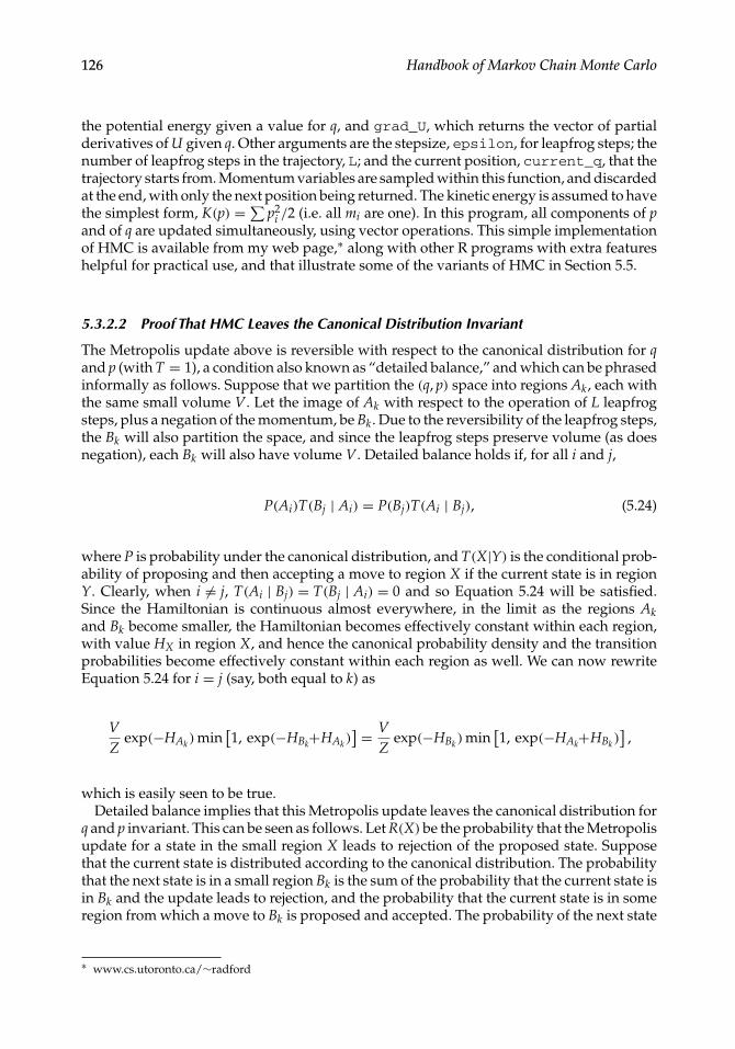
the potential energy given a value for q, and grad_U, which returns the vector of partialderivatives of U given q. Other arguments are the stepsize, epsilon, for leapfrog steps; thenumber of leapfrog steps in the trajectory, L; and the current position, current_q, that thetrajectory starts from. Momentum variables are sampled within this function, and discardedat the end, with only the next position being returned. The kinetic energy is assumed to havethe simplest form, K(p) =∑ p2
i /2 (i.e. all mi are one). In this program, all components of pand of q are updated simultaneously, using vector operations. This simple implementationof HMC is available from my web page,∗ along with other R programs with extra featureshelpful for practical use, and that illustrate some of the variants of HMC in Section 5.5.
5.3.2.2 Proof That HMC Leaves the Canonical Distribution Invariant
The Metropolis update above is reversible with respect to the canonical distribution for qand p (with T = 1), a condition also known as “detailed balance,” and which can be phrasedinformally as follows. Suppose that we partition the (q, p) space into regions Ak , each withthe same small volume V. Let the image of Ak with respect to the operation of L leapfrogsteps, plus a negation of the momentum, be Bk . Due to the reversibility of the leapfrog steps,the Bk will also partition the space, and since the leapfrog steps preserve volume (as doesnegation), each Bk will also have volume V. Detailed balance holds if, for all i and j,
P(Ai)T(Bj | Ai) = P(Bj)T(Ai | Bj), (5.24)
where P is probability under the canonical distribution, and T(X|Y) is the conditional prob-ability of proposing and then accepting a move to region X if the current state is in regionY. Clearly, when i = j, T(Ai | Bj) = T(Bj | Ai) = 0 and so Equation 5.24 will be satisfied.Since the Hamiltonian is continuous almost everywhere, in the limit as the regions Akand Bk become smaller, the Hamiltonian becomes effectively constant within each region,with value HX in region X, and hence the canonical probability density and the transitionprobabilities become effectively constant within each region as well. We can now rewriteEquation 5.24 for i = j (say, both equal to k) as
VZ
exp(−HAk ) min[1, exp(−HBk+HAk )
] = VZ
exp(−HBk ) min[1, exp(−HAk+HBk )
],
which is easily seen to be true.Detailed balance implies that this Metropolis update leaves the canonical distribution for
q and p invariant. This can be seen as follows. Let R(X) be the probability that the Metropolisupdate for a state in the small region X leads to rejection of the proposed state. Supposethat the current state is distributed according to the canonical distribution. The probabilitythat the next state is in a small region Bk is the sum of the probability that the current state isin Bk and the update leads to rejection, and the probability that the current state is in someregion from which a move to Bk is proposed and accepted. The probability of the next state
∗ www.cs.utoronto.ca/∼radford
MCMC Using Hamiltonian Dynamics 127
being in Bk can therefore be written as
P(Bk)R(Bk)+∑
i
P(Ai)T(Bk|Ai) = P(Bk)R(Bk)+∑
i
P(Bk)T(Ai|Bk)
= P(Bk)R(Bk)+ P(Bk)∑
i
T(Ai|Bk)
= P(Bk)R(Bk)+ P(Bk)(1− R(Bk))
= P(Bk).
The Metropolis update within HMC therefore leaves the canonical distribution invariant.Since both the sampling of momentum variables and the Metropolis update with a pro-
posal found by Hamiltonian dynamics leave the canonical distribution invariant, the HMCalgorithm as a whole does as well.
5.3.2.3 Ergodicity of HMC
Typically, the HMC algorithm will also be “ergodic”—it will not be trapped in some subset ofthe state space, and hence will asymptotically converge to its (unique) invariant distribution.In an HMC iteration, any value can be sampled for the momentum variables, which cantypically then affect the position variables in arbitrary ways. However, ergodicity can fail ifthe L leapfrog steps in a trajectory produce an exact periodicity for some function of state.For example, with the simple Hamiltonian of Equation 5.8, the exact solutions (given byEquation 5.9) are periodic with period 2π. Approximate trajectories found with L leapfrogsteps with stepsize εmay return to the same position coordinate when Lε is approximately2π. HMC with such values for L and εwill not be ergodic. For nearby values of L and ε, HMCmay be theoretically ergodic, but take a very long time to move about the full state space.
This potential problem of nonergodicity can be solved by randomly choosing ε or L(or both) from some fairly small interval (Mackenzie, 1989). Doing this routinely may beadvisable. Although in real problems interactions between variables typically prevent anyexact periodicities from occurring, near periodicities might still slow HMC considerably.
5.3.3 Illustrations of HMC and Its Benefits
I will now illustrate some practical issues with HMC, and demonstrate its potential tosample much more efficiently than simple methods such as random-walk Metropolis. I usesimple Gaussian distributions for these demonstrations, so that the results can be comparedwith known values, but of course HMC is typically used for more complex distributions.
5.3.3.1 Trajectories for a Two-Dimensional Problem
Consider sampling from a distribution for two variables that is bivariate Gaussian, withmeans of zero, standard deviations of one, and correlation 0.95. We regard these as“position” variables, and introduce two corresponding “momentum” variables, definedto have a Gaussian distribution with means of zero, standard deviations of one, and zerocorrelation. We then define the Hamiltonian as
H(q, p) = qTΣ−1q/2+ pTp/2, with Σ =[
1 0.950.95 1
].
128 Handbook of Markov Chain Monte Carlo
Position coordinates
−2 −1 0 1 2
−2
−1
0
1
2
−2
−1
0
1
2Momentum coordinates
−2 −1 0 1 2
Value of Hamiltonian
0 5 10 15 2520
2.2
2.3
2.4
2.5
2.6
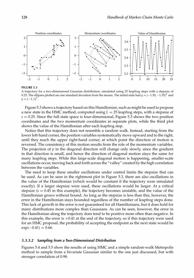
FIGURE 5.3A trajectory for a two-dimensional Gaussian distribution, simulated using 25 leapfrog steps with a stepsize of0.25. The ellipses plotted are one standard deviation from the means. The initial state had q = [−1.50,−1.55]T andp = [−1, 1]T .
Figure 5.3 shows a trajectory based on this Hamiltonian, such as might be used to proposea new state in the HMC method, computed using L = 25 leapfrog steps, with a stepsize ofε = 0.25. Since the full state space is four-dimensional, Figure 5.3 shows the two positioncoordinates and the two momentum coordinates in separate plots, while the third plotshows the value of the Hamiltonian after each leapfrog step.
Notice that this trajectory does not resemble a random walk. Instead, starting from thelower left-hand corner, the position variables systematically move upward and to the right,until they reach the upper right-hand corner, at which point the direction of motion isreversed. The consistency of this motion results from the role of the momentum variables.The projection of p in the diagonal direction will change only slowly, since the gradientin that direction is small, and hence the direction of diagonal motion stays the same formany leapfrog steps. While this large-scale diagonal motion is happening, smaller-scaleoscillations occur, moving back and forth across the “valley” created by the high correlationbetween the variables.
The need to keep these smaller oscillations under control limits the stepsize that canbe used. As can be seen in the rightmost plot in Figure 5.3, there are also oscillations inthe value of the Hamiltonian (which would be constant if the trajectory were simulatedexactly). If a larger stepsize were used, these oscillations would be larger. At a criticalstepsize (ε = 0.45 in this example), the trajectory becomes unstable, and the value of theHamiltonian grows without bound. As long as the stepsize is less than this, however, theerror in the Hamiltonian stays bounded regardless of the number of leapfrog steps done.This lack of growth in the error is not guaranteed for all Hamiltonians, but it does hold formany distributions more complex than Gaussians. As can be seen, however, the error inthe Hamiltonian along the trajectory does tend to be positive more often than negative. Inthis example, the error is +0.41 at the end of the trajectory, so if this trajectory were usedfor an HMC proposal, the probability of accepting the endpoint as the next state would beexp(−0.41) = 0.66.
5.3.3.2 Sampling from a Two-Dimensional Distribution
Figures 5.4 and 5.5 show the results of using HMC and a simple random-walk Metropolismethod to sample from a bivariate Gaussian similar to the one just discussed, but withstronger correlation of 0.98.
MCMC Using Hamiltonian Dynamics 129
Random−walk Metropolis
−2 −1 0 1 2
−2
−1
0
1
2
−2
−1
0
1
2
Hamiltonian Monte Carlo
−2 −1 0 1 2
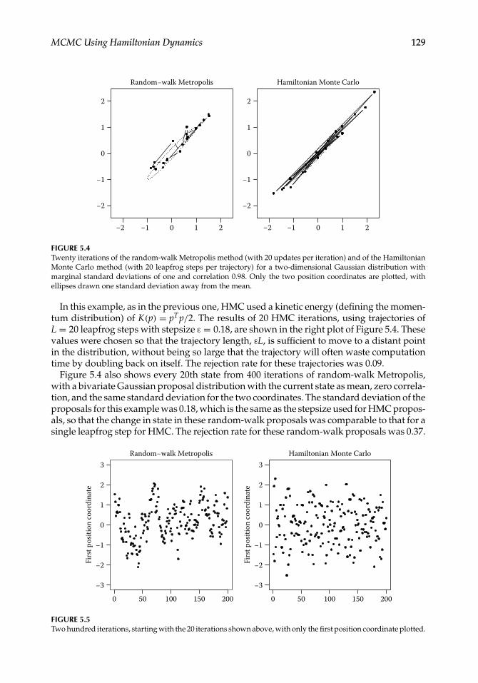
FIGURE 5.4Twenty iterations of the random-walk Metropolis method (with 20 updates per iteration) and of the HamiltonianMonte Carlo method (with 20 leapfrog steps per trajectory) for a two-dimensional Gaussian distribution withmarginal standard deviations of one and correlation 0.98. Only the two position coordinates are plotted, withellipses drawn one standard deviation away from the mean.
In this example, as in the previous one, HMC used a kinetic energy (defining the momen-tum distribution) of K(p) = pTp/2. The results of 20 HMC iterations, using trajectories ofL = 20 leapfrog steps with stepsize ε = 0.18, are shown in the right plot of Figure 5.4. Thesevalues were chosen so that the trajectory length, εL, is sufficient to move to a distant pointin the distribution, without being so large that the trajectory will often waste computationtime by doubling back on itself. The rejection rate for these trajectories was 0.09.
Figure 5.4 also shows every 20th state from 400 iterations of random-walk Metropolis,with a bivariate Gaussian proposal distribution with the current state as mean, zero correla-tion, and the same standard deviation for the two coordinates. The standard deviation of theproposals for this example was 0.18, which is the same as the stepsize used for HMC propos-als, so that the change in state in these random-walk proposals was comparable to that for asingle leapfrog step for HMC. The rejection rate for these random-walk proposals was 0.37.
Random−walk Metropolis
Firs
t pos
ition
coor
dina
te
0 50 100 150 200
−2
−3
−1
0
1
2
3
Firs
t pos
ition
coor
dina
te
−2
−3
−1
0
1
2
3Hamiltonian Monte Carlo
0 50 100 150 200
FIGURE 5.5Two hundred iterations, starting with the 20 iterations shown above, with only the first position coordinate plotted.
130 Handbook of Markov Chain Monte Carlo
One can see in Figure 5.4 how the systematic motion during an HMC trajectory (illustratedin Figure 5.3) produces larger changes in state than a corresponding number of random-walk Metropolis iterations. Figure 5.5 illustrates this difference for longer runs of 20× 200random-walk Metropolis iterations and of 200 HMC iterations.
5.3.3.3 The Benefit of Avoiding Random Walks
Avoidance of random-walk behavior, as illustrated above, is one major benefit of HMC. Inthis example, because of the high correlation between the two position variables, keepingthe acceptance probability for random-walk Metropolis reasonably high requires that thechanges proposed have a magnitude comparable to the standard deviation in the mostconstrained direction (0.14 in this example, the square root of the smallest eigenvalue ofthe covariance matrix). The changes produced using one Gibbs sampling scan would beof similar magnitude. The number of iterations needed to reach a state almost independentof the current state is mostly determined by how long it takes to explore the less constraineddirection, which for this example has standard deviation 1.41—about ten times greater thanthe standard deviation in the most constrained direction. We might therefore expect thatwe would need around 10 iterations of random-walk Metropolis in which the proposalwas accepted to move to a nearly independent state. But the number needed is actuallyroughly the square of this—around 100 iterations with accepted proposals—because therandom-walk Metropolis proposals have no tendency to move consistently in the samedirection.
To see this, note that the variance of the position after n iterations of random-walkMetropolis from some start state will grow in proportion to n (until this variance becomescomparable to the overall variance of the state), since the position is the sum of mostlyindependent movements for each iteration. The standard deviation of the amount moved(which gives the typical amount of movement) is therefore proportional to
√n.
The stepsize used for the leapfrog steps is similarly limited by the most constraineddirection, but the movement will be in the same direction for many steps. The distancemoved after n steps will therefore tend to be proportional to n, until the distance movedbecomes comparable to the overall width of the distribution. The advantage compared tomovement by a random walk will be a factor roughly equal to the ratio of the standarddeviations in the least confined direction and most confined direction—about 10 here.
Because avoiding a random walk is so beneficial, the optimal standard deviation forrandom-walk Metropolis proposals in this example is actually much larger than the valueof 0.18 used here. A proposal standard deviation of 2.0 gives a very low acceptance rate(0.06), but this is more than compensated for by the large movement (to a nearly independentpoint) on the rare occasions when a proposal is accepted, producing a method that is aboutas efficient as HMC. However, this strategy of making large changes with a small acceptancerate works only when, as here, the distribution is tightly constrained in only one direction.
5.3.3.4 Sampling from a 100-Dimensional Distribution
More typical behavior of HMC and random-walk Metropolis is illustrated by a 100-dimensional multivariate Gaussian distribution in which the variables are independent,with means of zero, and standard deviations of 0.01, 0.02, . . . , 0.99, 1.00. Suppose that wehave no knowledge of the details of this distribution, so we will use HMC with the samesimple, rotationally symmetric kinetic energy function as above, K(p) = pTp/2, and userandom-walk Metropolis proposals in which changes to each variable are independent, all
MCMC Using Hamiltonian Dynamics 131
with the same standard deviation. As discussed below in Section 5.4.1, the performance ofboth these sampling methods is invariant to rotation, so this example is illustrative of howthey perform on any multivariate Gaussian distribution in which the square roots of theeigenvalues of the covariance matrix are 0.01, 0.02, . . . , 0.99, 1.00.
For this problem, the position coordinates, qi, and corresponding momentum coordi-nates, pi, are all independent, so the leapfrog steps used to simulate a trajectory operateindependently for each (qi, pi) pair. However, whether the trajectory is accepted dependson the total error in the Hamiltonian due to the leapfrog discretization, which is a sum ofthe errors due to each (qi, pi) pair (for the terms in the Hamiltonian involving this pair).Keeping this error small requires limiting the leapfrog stepsize to a value roughly equal tothe smallest of the standard deviations (0.01), which implies that many leapfrog steps willbe needed to move a distance comparable to the largest of the standard deviations (1.00).
Consistent with this, I applied HMC to this distribution using trajectories with L = 150and with ε randomly selected for each iteration, uniformly from (0.0104, 0.0156), whichis 0.013± 20%. I used random-walk Metropolis with proposal standard deviation drawnuniformly from (0.0176, 0.0264), which is 0.022± 20%. These are close to optimal set-tings for both methods. The rejection rate was 0.13 for HMC and 0.75 for random-walkMetropolis.
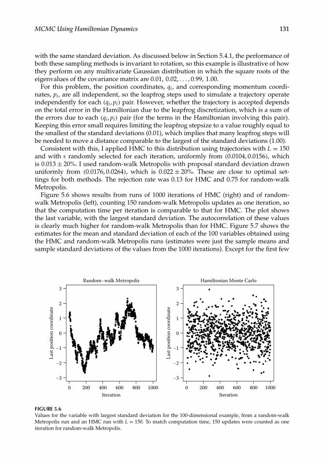
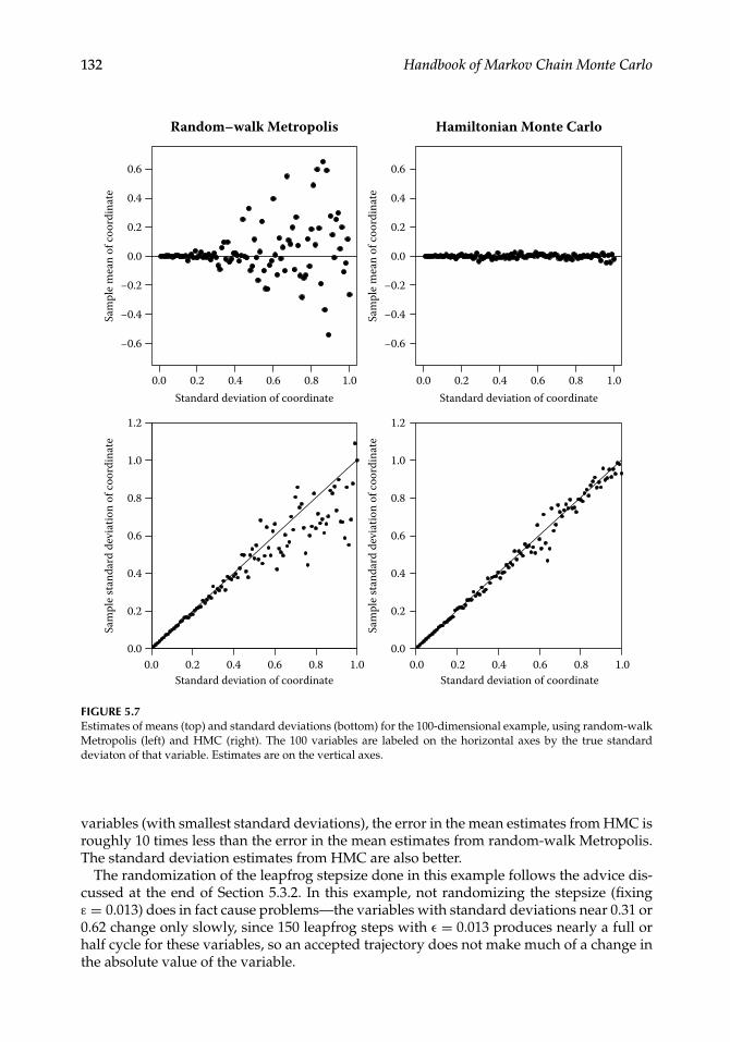
Figure 5.6 shows results from runs of 1000 iterations of HMC (right) and of random-walk Metropolis (left), counting 150 random-walk Metropolis updates as one iteration, sothat the computation time per iteration is comparable to that for HMC. The plot showsthe last variable, with the largest standard deviation. The autocorrelation of these valuesis clearly much higher for random-walk Metropolis than for HMC. Figure 5.7 shows theestimates for the mean and standard deviation of each of the 100 variables obtained usingthe HMC and random-walk Metropolis runs (estimates were just the sample means andsample standard deviations of the values from the 1000 iterations). Except for the first few
Random−walk Metropolis
Last
pos
ition
coor
dina
te
0 200 400Iteration
600 800 1000
−2
−3
−1
0
1
2
3
Last
pos
ition
coor
dina
te
−2
−3
−1
0
1
2
3Hamiltonian Monte Carlo
0 200 400Iteration
600 800 1000
FIGURE 5.6Values for the variable with largest standard deviation for the 100-dimensional example, from a random-walkMetropolis run and an HMC run with L = 150. To match computation time, 150 updates were counted as oneiteration for random-walk Metropolis.
132 Handbook of Markov Chain Monte Carlo
−0.6
−0.4
−0.2
0.0
0.2
0.4
0.6
Standard deviation of coordinate
Sam
ple m
ean
of co
ordi
nate
−0.6
−0.4
−0.2
0.0
0.2
0.4
0.6
Sam
ple m
ean
of co
ordi
nate
Random–walk Metropolis Hamiltonian Monte Carlo
0.0 0.2 0.4 0.6 0.8 1.0Standard deviation of coordinate
0.0 0.2 0.4 0.6 0.8 1.0
0.0 0.2 0.4 0.6 0.8 1.00.0
0.2
0.4
0.6
0.8
1.0
1.2
0.0
0.2
0.4
0.6
0.8
1.0
1.2
Standard deviation of coordinate
Sam
ple s
tand
ard
devi
atio
n of
coor
dina
te
0.0 0.2 0.4 0.6 0.8 1.0Standard deviation of coordinate
Sam
ple s
tand
ard
devi
atio
n of
coor
dina
te
FIGURE 5.7Estimates of means (top) and standard deviations (bottom) for the 100-dimensional example, using random-walkMetropolis (left) and HMC (right). The 100 variables are labeled on the horizontal axes by the true standarddeviaton of that variable. Estimates are on the vertical axes.
variables (with smallest standard deviations), the error in the mean estimates from HMC isroughly 10 times less than the error in the mean estimates from random-walk Metropolis.The standard deviation estimates from HMC are also better.
The randomization of the leapfrog stepsize done in this example follows the advice dis-cussed at the end of Section 5.3.2. In this example, not randomizing the stepsize (fixingε = 0.013) does in fact cause problems—the variables with standard deviations near 0.31 or0.62 change only slowly, since 150 leapfrog steps with ε = 0.013 produces nearly a full orhalf cycle for these variables, so an accepted trajectory does not make much of a change inthe absolute value of the variable.
MCMC Using Hamiltonian Dynamics 133
5.4 HMC in Practice and Theory
Obtaining the benefits from HMC illustrated in the previous section, including random-walk avoidance, requires proper tuning of L and ε. I discuss tuning of HMC below, andalso show how performance can be improved by using whatever knowledge is availableregarding the scales of variables and their correlations. After briefly discussing what to dowhen HMC alone is not enough, I discuss an additional benefit of HMC—its better scalingwith dimensionality than simple Metropolis methods.
5.4.1 Effect of Linear Transformations
Like all MCMC methods I am aware of, the performance of HMC may change if the variablesbeing sampled are transformed by multiplication by some nonsingular matrix, A. However,performance stays the same (except perhaps in terms of computation time per iteration) ifat the same time the corresponding momentum variables are multiplied by (AT)−1. Thesefacts provide insight into the operation of HMC, and can help us improve performancewhen we have some knowledge of the scales and correlations of the variables.
Let the new variables be q′ = Aq. The probability density for q′ will be given by P′(q′) =P(A−1q′)/|det(A)|, where P(q) is the density for q. If the distribution for q is the canoni-cal distribution for a potential energy function U(q) (see Section 5.3.1), we can obtain thedistribution for q′ as the canonical distribution for U′(q′) = U(A−1q′). (Since |det(A)| is aconstant, we need not include a log |det(A)| term in the potential energy.)
We can choose whatever distribution we wish for the corresponding momentum vari-ables, so we could decide to use the same kinetic energy as before. Alternatively, we canchoose to transform the momentum variables by p′ = (AT)−1p, and use a new kinetic energyof K′(p′) = K(ATp′). If we were using a quadratic kinetic energy, K(p) = pTM−1p/2 (seeEquation 5.5), the new kinetic energy will be
K′(p′) = (ATp′)TM−1(ATp′)/2 = (p′)T(A M−1AT) p′/2 = (p′)T(M′)−1p′/2, (5.25)
where M′ = (A M−1AT)−1 = (A−1)TMA−1.If we use momentum variables transformed in this way, the dynamics for the new vari-
ables, (q′, p′), essentially replicates the original dynamics for (q, p), so the performance ofHMC will be the same. To see this, note that if we follow Hamiltonian dynamics for (q′, p′),the result in terms of the original variables will be as follows (see Equations 5.6 and 5.7):
dqdt= A−1 dq′
dt= A−1(M′)−1 p′ = A−1(A M−1AT)(AT)−1 p = M−1 p,
dpdt= AT dp′
dt= −AT ∇U′(q′) = −AT (A−1)T ∇U(A−1q′) = −∇U(q),
which matches what would happen following Hamiltonian dynamics for (q, p).If A is an orthogonal matrix (such as a rotation matrix), for which A−1 = AT , the per-
formance of HMC is unchanged if we transform both q and p by multiplying by A (since(AT)−1 = A). If we chose a rotationally symmetric distribution for the momentum, with M =mI (i.e. the momentum variables are independent, each having variance m), such an ortho-gonal transformation will not change the kinetic energy function (and hence not change thedistribution of the momentum variables), since we will have M′ = (A (mI)−1AT)−1 = mI.
134 Handbook of Markov Chain Monte Carlo
Such an invariance to rotation holds also for a random-walk Metropolis method in whichthe proposal distribution is rotationally symmetric (e.g. Gaussian with covariance matrixmI). In contrast, Gibbs sampling is not rotationally invariant, nor is a scheme in which theMetropolis algorithm is used to update each variable in turn (with a proposal that changesonly that variable). However, Gibbs sampling is invariant to rescaling of the variables (trans-formation by a diagonal matrix), which is not true for HMC or random-walk Metropolis,unless the kinetic energy or proposal distribution is transformed in a corresponding way.
Suppose that we have an estimate,Σ, of the covariance matrix for q, and suppose also that qhas at least a roughly Gaussian distribution. How can we use this information to improve theperformance of HMC? One way is to transform the variables so that their covariance matrixis close to the identity, by finding the Cholesky decomposition,Σ = LLT , with L being lower-triangular, and letting q′ = L−1q. We then let our kinetic energy function be K(p) = pTp/2.Since the momentum variables are independent, and the position variables are close toindependent with variances close to one (if our estimate Σ and our assumption that qis close to Gaussian are good), HMC should perform well using trajectories with a smallnumber of leapfrog steps, which will move all variables to a nearly independent point. Morerealistically, the estimateΣmay not be very good, but this transformation could still improveperformance compared to using the same kinetic energy with the original q variables.
An equivalent way to make use of the estimated covariance Σ is to keep the original qvariables, but use the kinetic energy function K(p) = pTΣp/2—that is, we let the momentumvariables have covariance Σ−1. The equivalence can be seen by transforming this kineticenergy to correspond to a transformation to q′ = L−1q (see Equation 5.25), which givesK(p′) = (p′)TM′−1p′ with M′ = (L−1(LLT)(L−1)T)−1 = I.
Using such a kinetic energy function to compensate for correlations between positionvariables has a long history in molecular dynamics (Bennett, 1975). The usefulness of thistechnique is limited by the computational cost of matrix operations when the dimensionalityis high.
Using a diagonal Σ can be feasible even in high-dimensional problems. Of course, thisprovides information only about the different scales of the variables, not their correlation.Moreover, when the actual correlations are nonzero, it is not clear what scales to use. Makingan optimal choice is probably infeasible. Some approximation to the conditional standarddeviation of each variable given all the others may be possible—as I have done for Bayesianneural network models (Neal, 1996a). If this also is not feasible, using approximations tothe marginal standard deviations of the variables may be better than using the same scalefor them all.
5.4.2 Tuning HMC
One practical impediment to the use of Hamiltonian Monte Carlo is the need to selectsuitable values for the leapfrog stepsize, ε, and the number of leapfrog steps, L, whichtogether determine the length of the trajectory in fictitious time, εL. Most MCMC methodshave parameters that need to be tuned, with the notable exception of Gibbs sampling whenthe conditional distributions are amenable to direct sampling. However, tuning HMC ismore difficult in some respects than tuning a simple Metropolis method.
5.4.2.1 Preliminary Runs and Trace Plots
Tuning HMC will usually require preliminary runs with trial values for ε and L. In judg-ing how well these runs work, trace plots of quantities that are thought to be indicative
MCMC Using Hamiltonian Dynamics 135
of overall convergence should be examined. For Bayesian inference problems, high-levelhyperparameters are often among the slowest-moving quantities. The value of the potentialenergy function, U(q), is also usually of central significance. The autocorrelation for suchquantities indicates how well the Markov chain is exploring the state space. Ideally, wewould like the state after one HMC iteration to be nearly independent of the previous state.
Unfortunately, preliminary runs can be misleading, if they are not long enough to havereached equilibrium. It is possible that the best choices of ε and L for reaching equilibriumare different from the best choices once equilibrium is reached, and even at equilibrium, itis possible that the best choices vary from one place to another. If necessary, at each iterationof HMC, ε and L can be chosen randomly from a selection of values that are appropriatefor different parts of the state space (or these selections and can be used sequentially).
Doing several runs with different random starting states is advisable (for both preliminaryand final runs), so that problems with isolated modes can be detected. Note that HMC is noless (or more) vulnerable to problems with isolated modes than other MCMC methods thatmake local changes to the state. If isolated modes are found to exist, something needs to bedone to solve this problem—just combining runs that are each confined to a single mode isnot valid. A modification of HMC with “tempering” along a trajectory (Section 5.5.7) cansometimes help with multiple modes.
5.4.2.2 What Stepsize?
Selecting a suitable leapfrog stepsize, ε, is crucial. Too large a stepsize will result in a verylow acceptance rate for states proposed by simulating trajectories. Too small a stepsize willeither waste computation time, by the same factor as the stepsize is too small, or (worse)will lead to slow exploration by a random walk, if the trajectory length, εL, is then too short(i.e. L is not large enough; see below).
Fortunately, as illustrated in Figure 5.3, the choice of stepsize is almost independent ofhow many leapfrog steps are done. The error in the value of the Hamiltonian (which willdetermine the rejection rate) usually does not increase with the number of leapfrog steps,provided that the stepsize is small enough that the dynamics is stable.
The issue of stability can be seen in a simple one-dimensional problem in which thefollowing Hamiltonian is used:
H(q, p) = q2
2σ2 +p2
2.
The distribution for q that this defines is Gaussian with standard deviation σ. Aleapfrog stepfor this system (as for any quadratic Hamiltonian) will be a linear mapping from (q(t), p(t))to (q(t+ ε), p(t+ ε)). Referring to Equations 5.18 through 5.20, we see that this mapping canbe represented by a matrix multiplication as follows:[
q(t+ ε)p(t+ ε)
]=[
1− ε2/2σ2 ε
−ε/σ2 + ε3/4σ4 1− ε2/2σ2
][q(t)
p(t)
].
Whether iterating this mapping leads to a stable trajectory, or one that diverges to infinity,depends on the magnitudes of the eigenvalues of the above matrix, which are(
1− ε2
2σ2
)±( εσ
)√ε2/4σ2 − 1.
136 Handbook of Markov Chain Monte Carlo
When ε/σ > 2, these eigenvalues are real, and at least one will have absolute value greaterthan one. Trajectories computed using the leapfrog method with this ε will therefore beunstable. When ε/σ < 2, the eigenvalues are complex, and both have squared magnitude of
(1− ε2
2σ2
)2
+(ε2
σ2
)(1− ε2
4σ2
)= 1.
Trajectories computed with ε < 2σ are therefore stable.For multidimensional problems in which the kinetic energy used is K(p) = pTp/2 (as in the
example above), the stability limit for εwill be determined (roughly) by the width of the dis-tribution in the most constrained direction—for a Gaussian distribution, this would thesquare root of the smallest eigenvalue of the covariance matrix for q. Stability for moregeneral quadratic Hamiltonians with K(p) = pTM−1p/2 can be determined by applying alinear transformation that makes K(p′) = (p′)Tp′/2, as discussed above in Section 5.4.1.
When a stepsize, ε, that produces unstable trajectories is used, the value of H growsexponentially with L, and consequently the acceptance probability will be extremely small.For low-dimensional problems, using a value for ε that is just a little below the stability limitis sufficient to produce a good acceptance rate. For high-dimensional problems, however,the stepsize may need to be reduced further than this to keep the error in H to a level thatproduces a good acceptance probability. This is discussed further in Section 5.4.4.
Choosing too large a value of ε can have very bad effects on the performance of HMC.In this respect, HMC is more sensitive to tuning than random-walk Metropolis. A standarddeviation for proposals needs to be chosen for random-walk Metropolis, but performancedegrades smoothly as this choice is made too large, without the sharp degradation seenwith HMC when ε exceeds the stability limit. (However, in high-dimensional problems, thedegradation in random-walk Metropolis with too large a proposal standard deviation canalso be quite sharp, so this distinction becomes less clear.)
This sharp degradation in performance of HMC when the stepsize is too big would notbe a serious issue if the stability limit were constant—the problem would be obvious frompreliminary runs, and so could be fixed. The real danger is that the stability limit may differfor several regions of the state space that all have substantial probability. If the preliminaryruns are started in a region where the stability limit is large, a choice of ε a little less than thislimit might appear to be appropriate. However, if this ε is above the stability limit for someother region, the runs may never visit this region, even though it has substantial probability,producing a drastically wrong result. To see why this could happen, note that if the runever does visit the region where the chosen εwould produce instability, it will stay there fora very long time, since the acceptance probability with that ε will be very small. Since themethod nevertheless leaves the correct distribution invariant, it follows that the run onlyrarely moves to this region from a region where the chosen ε leads to stable trajectories.One simple context where this problem can arise is when sampling from a distribution withvery light tails (lighter than a Gaussian distribution), for which the log of the density willfall faster than quadratically. In the tails, the gradient of the log density will be large, and asmall stepsize will be needed for stability. See Roberts and Tweedie (1996) for a discussionof this in the context of the Langevin method (see Section 5.5.2).
This problem can be alleviated by choosing ε randomly from some distribution. Even if themean of this distribution is too large, suitably small values for εmay be chosen occasionally.(See Section 5.3.2 for another reason to randomly vary the stepsize.) The random choice ofε should be done once at the start of a trajectory, not for every leapfrog step, since even if
MCMC Using Hamiltonian Dynamics 137
all the choices are below the stability limit, random changes at each step lead to a randomwalk in the error for H, rather than the bounded error that is illustrated in Figure 5.3.
The “short-cut” procedures described in Section 5.5.6 can be seen as ways of savingcomputation time when a randomly chosen stepsize is inappropriate.
5.4.2.3 What Trajectory Length?
Choosing a suitable trajectory length is crucial if HMC is to explore the state space sys-tematically, rather than by a random walk. Many distributions are difficult to sample frombecause they are tightly constrained in some directions, but much less constrained in otherdirections. Exploring the less constrained directions is best done using trajectories that arelong enough to reach a point that is far from the current point in that direction. Trajectoriescan be too long, however, as is illustrated in Figure 5.3. The trajectory shown on the left ofthat figure is a bit too long, since it reverses direction and then ends at a point that mighthave been reached with a trajectory about half its length. If the trajectory were a little longer,the result could be even worse, since the trajectory would not only take longer to compute,but might also end near its starting point.
For more complex problems, one cannot expect to select a suitable trajectory length bylooking at plots like Figure 5.3. Finding the linear combination of variables that is leastconfined will be difficult, and will be impossible when, as is typical, the least confined“direction” is actually a nonlinear curve or surface.
Setting the trajectory length by trial and error therefore seems necessary. For a problemthought to be fairly difficult, a trajectory with L = 100 might be a suitable starting point.If preliminary runs (with a suitable ε; see above) show that HMC reaches a nearly inde-pendent point after only one iteration, a smaller value of L might be tried next. (Unlessthese “preliminary” runs are actually sufficient, in which case there is of course no need todo more runs.) If instead there is high autocorrelation in the run with L = 100, runs withL = 1000 might be tried next.
As discussed at the end of Sections 5.3.2 and 5.3.3, randomly varying the length of the tra-jectory (over a fairly small interval) may be desirable, to avoid choosing a trajectory lengththat happens to produce a near-periodicity for some variable or combination of variables.
5.4.2.4 Using Multiple Stepsizes
Using the results in Section 5.4.1, we can exploit information about the relative scales ofvariables to improve the performance of HMC. This can be done in two equivalent ways. Ifsi is a suitable scale for qi, we could transform q, by setting q′i = qi/si, or we could instead usea kinetic energy function of K(p) = pTM−1p, with M being a diagonal matrix with diagonalelements mi = 1/s2
i .A third equivalent way to exploit this information, which is often the most convenient,
is to use different stepsizes for different pairs of position and momentum variables. To seehow this works, consider a leapfrog update (following Equations 5.18 through 5.20) withmi = 1/s2
i :
pi (t+ ε/2) = pi(t)− (ε/2)∂U∂qi
(q(t)),
qi(t+ ε) = qi(t)+ ε s2i pi (t+ ε/2) ,
pi(t+ ε) = pi (t+ ε/2)− (ε/2)∂U∂qi
(q(t+ ε)).
138 Handbook of Markov Chain Monte Carlo
Define (q(0), p(0)) to be the state at the beginning of the leapfrog step (i.e. (q(t), p(t))),define (q(1), p(1)) to be the final state (i.e. (q(t+ ε), p(t+ ε))), and define p(1/2) to be half-waymomentum (i.e. p(t+ ε/2)). We can now rewrite the leapfrog step above as
p(1/2)
i = p(0)i − (ε/2)
∂U∂qi
(q(0)),
q(1)i = q(0)
i + ε s2i p(1/2)
i ,
p(1)i = p(1/2)
i − (ε/2)∂U∂qi
(q(1)).
If we now define rescaled momentum variables, p̃i = sipi, and stepsizes εi = siε, we canwrite the leapfrog update as
p̃(1/2)
i = p̃(0)i − (εi/2)
∂U∂qi
(q(0)),
q(1)i = q(0)
i + εi p̃(1/2)
i ,
p̃(1)i = p̃(1/2)
i − (εi/2)∂U∂qi
(q(1)).
This is just like a leapfrog update with all mi = 1, but with different stepsizes for different(qi, pi) pairs. Of course, the successive values for (q, p̃) can no longer be interpreted asfollowing Hamiltonian dynamics at consistent time points, but that is of no consequencefor the use of these trajectories in HMC. Note that when we sample for the momentumbefore each trajectory, each p̃i is drawn independently from a Gaussian distribution withmean zero and variance one, regardless of the value of si.
This multiple stepsize approach is often more convenient, especially when the estimatedscales, si, are not fixed, as discussed in Section 5.4.5, and the momentum is only partiallyrefreshed (Section 5.5.3).
5.4.3 Combining HMC with Other MCMC Updates
For some problems, MCMC using HMC alone will be impossible or undesirable. Twosituations where non-HMC updates will be necessary are when some of the variables arediscrete, and when the derivatives of the log probability density with respect to some ofthe variables are expensive or impossible to compute. HMC can then be feasibly appliedonly to the other variables. Another example is when special MCMC updates have beendevised that may help convergence in ways that HMC does not—for example, by movingbetween otherwise isolated modes—but which are not a complete replacement for HMC.As discussed in Section 5.4.5 below, Bayesian hierarchical models may also be best handledwith a combination of HMC and other methods such as Gibbs sampling.
In such circumstances, one or more HMC updates for all or a subset of the variables canbe alternated with one or more other updates that leave the desired joint distribution ofall variables invariant. The HMC updates can be viewed as either leaving this same jointdistribution invariant, or as leaving invariant the conditional distribution of the variablesthat HMC changes, given the current values of the variables that are fixed during the HMCupdate. These are equivalent views, since the joint density can be factored as this conditionaldensity times the marginal density of the variables that are fixed, which is just a constant
MCMC Using Hamiltonian Dynamics 139
from the point of view of a single HMC update, and hence can be left out of the potentialenergy function.
When both HMC and other updates are used, it may be best to use shorter trajectoriesfor HMC than would be used if only HMC were being done. This allows the other updatesto be done more often, which presumably helps sampling. Finding the optimal tradeoff islikely to be difficult, however. A variation on HMC that reduces the need for such a tradeoffis described below in Section 5.5.3.
5.4.4 Scaling with Dimensionality
In Section 5.3.3, one of the main benefits of HMC was illustrated—its ability to avoid theinefficient exploration of the state space via a random walk. This benefit is present (to atleast some degree) for most practical problems. For problems in which the dimensionality ismoderate to high, another benefit of HMC over simple random-walk Metropolis methodsis a slower increase in the computation time needed (for a given level of accuracy) as thedimensionality increases. (Note that here I will consider only sampling performance afterequilibrium is reached, not the time needed to approach equilibrium from some initial statenot typical of the distribution, which is harder to analyze.)
5.4.4.1 Creating Distributions of Increasing Dimensionality by Replication
To talk about how performance scales with dimensionality we need to assume somethingabout how the distribution changes with dimensionality, d.
I will assume that dimensionality increases by adding independent replicas of variables—that is, the potential energy function for q = (q1, . . . , qd) has the form U(q) = Σui(qi), forfunctions ui drawn independently from some distribution. Of course, this is not what anyreal practical problem is like, but it may be a reasonable model of the effect of increas-ing dimensionality for some problems—for instance, in statistical physics, distant regionsof large systems are often nearly independent. Note that the independence assumptionitself is not crucial since, as discussed in Section 5.4.1, the performance of HMC (and ofsimple random-walk Metropolis) does not change if independence is removed by rotat-ing the coordinate system, provided the kinetic energy function (or random-walk proposaldistribution) is rotationally symmetric.
For distributions of this form, in which the variables are independent, Gibbs samplingwill perform very well (assuming it is feasible), producing an independent point after eachscan of all variables.Applying Metropolis updates to each variable separately will also workwell, provided the time for a single-variable update does not grow with d. However, thesemethods are not invariant to rotation, so this good performance may not generalize to themore interesting distributions for which we hope to obtain insight with the analysis below.
5.4.4.2 Scaling of HMC and Random-Walk Metropolis
Here, I discuss informally how well HMC and random-walk Metropolis scale withdimension, loosely following Creutz (1988, Section III).
To begin, Cruetz notes that the following relationship holds when any Metropolis-stylealgorithm is used to sample a density P(x) = (1/Z) exp(−E(x)):
1 = E [P(x∗)/P(x)] = E [exp(−(E(x∗)− E(x)))] = E [exp(−Δ)], (5.26)
140 Handbook of Markov Chain Monte Carlo
where x is the current state, assumed to be distributed according to P(x), x∗ is the proposedstate, and Δ = E(x∗)− E(x). Jensen’s inequality then implies that the expectation of theenergy difference is nonnegative:
E [Δ] ≥ 0.
The inequality will usually be strict.When U(q) = Σui(qi), and proposals are produced independently for each i, we can apply
these relationships either to a single variable (or pair of variables) or to the entire state. For asingle variable (or pair), I will writeΔ1 for E(x∗)− E(x), with x = qi and E(x) = ui(qi), or x =(qi, pi) and E(x) = ui(qi)+ p2
i /2. For the entire state, I will writeΔd for E(x∗)− E(x), with x =q and E(x) = U(q), or x = (q, p) and E(x) = U(q)+ K(p). For both random-walk Metropolisand HMC, increasing dimension by replicating variables will lead to increasing energydifferences, sinceΔd is the sum ofΔ1 for each variable, each of which has positive mean. Thiswill lead to a decrease in the acceptance probability—equal to min(1, exp(−Δd))—unlessthe width of the proposal distribution or the leapfrog stepsize is decreased to compensate.
More specifically, for random-walk Metropolis with proposals that change each variableindependently, the difference in potential energy between a proposed state and the currentstate will be the sum of independent differences for each variable. If we fix the standarddeviation, ς, for each proposed change, the mean and the variance of this potential energydifference will both grow linearly with d, which will lead to a progressively lower accep-tance rate. To maintain reasonable performance, ς will have to decrease as d increases.Furthermore, the number of iterations needed to reach a nearly independent point will beproportional to ς−2, since exploration is via a random walk.
Similarly, when HMC is used to sample from a distribution in which the componentsof q are independent, using the kinetic energy K(p) = Σ p2
i /2, the different (qi, pi) pairs donot interact during the simulation of a trajectory—each (qi, pi) pair follows Hamiltoniandynamics according to just the one term in the potential energy involving qi and the oneterm in the kinetic energy involving pi. There is therefore no need for the length in fictitioustime of a trajectory to increase with dimensionality. However, acceptance of the endpoint ofthe trajectory is based on the error in H due to the leapfrog approximation, which is the sumof the errors pertaining to each (qi, pi) pair. For a fixed stepsize, ε, and fixed trajectory length,εL, both the mean and the variance of the error in H grow linearly with d. This will lead toa progressively lower acceptance rate as dimensionality increases, if it is not counteractedby a decrease in ε. The number of leapfrog steps needed to reach an independent point willbe proportional to ε−1.
To see which method scales better, we need to determine how rapidly we must reduceς and ε as d increases, in order to maintain a reasonable acceptance rate. As d increasesand ς or ε goes to zero, Δ1 will go to zero as well. Using a second-order approximation ofexp(−Δ1) as 1−Δ1 +Δ2
1/2, together with Equation 5.26, we find that
E [Δ1] ≈ E [Δ21]
2. (5.27)
It follows from this that the variance of Δ1 is twice the mean of Δ1 (when Δ1 is small),which implies that the variance ofΔd is twice the mean ofΔd (even whenΔd is not small).To achieve a good acceptance rate, we must therefore keep the mean ofΔd near one, since alarge mean will not be saved by a similarly large standard deviation (which would producefairly frequent acceptances as Δd occasionally takes on a negative value).
For random-walk Metropolis with a symmetric proposal distribution, we can see how ς
needs to scale by directly averaging Δ1 for a proposal and its inverse. Let the proposal for
MCMC Using Hamiltonian Dynamics 141
one variable be x∗ = x + c, and suppose that c = a and c = −a are equally likely. Approx-imating U(x∗) to second order as U(x)+ cU′(x)+ c2U′′(x)/2, we find that the average ofΔ1 = U(x∗)−U(x) over c = a and c = −a is a2U′′(x). Averaging this over the distributionof a, with standard deviation ς, and over the distribution of x, we see that E [Δ1] is propor-tional to ς2. It follows that E [Δd] is proportional to dς2, so we can maintain a reasonableacceptance rate by letting ς be proportional to d−1/2. The number of iterations needed toreach a nearly independent point will be proportional to ς−2, which will be proportionalto d. The amount of computation time needed will typically be proportional to d2.
As discussed at the end of Section 5.2.3, the error in H when using the leapfrog discretiza-tion to simulate a trajectory of a fixed length is proportional to ε2 (for sufficiently small ε).The error in H for a single (qi, pi) pair is the same as Δ1, so we see that Δ2
1 is proportionalto ε4. Equation 5.27 then implies that E [Δ1] is also proportional to ε4. The average totalerror in H for all variables, E [Δd], will be proportional to dε4, and hence we must make εbe proportional to d−1/4 to maintain a reasonable acceptance rate. The number of leapfrogupdates to reach a nearly independent point will therefore grow as d1/4, and the amount ofcomputation time will typically grow as d5/4, which is much better than the d2 growth forrandom-walk Metropolis.
5.4.4.3 Optimal Acceptance Rates
By extending the analysis above, we can determine what the acceptance rate of proposalsis when the optimal choice of ς or ε is used. This is helpful when tuning the algorithms—provided, of course, that the distribution sampled is high-dimensional, and has propertiesthat are adequately modeled by a distribution with replicated variables.
To find this acceptance rate, we first note that since Metropolis methods satisfy detailedbalance, the probability of an accepted proposal with Δd negative must be equal to theprobability of an accepted proposal with Δd positive. Since all proposals with negativeΔd are accepted, the acceptance rate is simply twice the probability that a proposal has anegative Δd. For large d, the central limit theorem implies that the distribution of Δd isGaussian, since it is a sum of d independent Δ1 values. (This assumes that the varianceof each Δ1 is finite.) We saw above that the variance of Δd is twice its mean, E [Δd] =μ. The acceptance probability can therefore be written as follows (Gupta et al., 1990),for large d:
P(accept) = 2Φ(
(0− μ)√2μ
)= 2Φ
(−√μ/2
)= a(μ), (5.28)
whereΦ(z) is the cumulative distribution function for a Gaussian variable with mean zeroand variance one.
For random-walk Metropolis, the cost of obtaining an independent point will be propor-tional to 1/(aς2), where a is the acceptance rate. We saw above thatμ = E [Δd] is proportionalto ς2, so the cost follows the proportionality
Crw ∝ 1(a(μ)μ)
.
Numerical calculation shows that this is minimized when μ = 2.8 and a(μ) = 0.23.
142 Handbook of Markov Chain Monte Carlo
For HMC, the cost of obtaining an independent point will be proportional to 1/(aε), andas we saw above, μ is proportional to ε4. From this we obtain
CHMC ∝ 1(a(μ)μ1/4)
.
Numerical calculation shows that the minimum is when μ = 0.41 and a(μ) = 0.65.The same optimal 23% acceptance rate for random-walk Metropolis was previously
obtained using a more formal analysis by Roberts et al. (1997). The optimal 65% accep-tance rate for HMC that I derive above is consistent with previous empirical results ondistributions following the model here (Neal, 1994, Figure 2), and on real high-dimensionalproblems (Creutz, 1988, Figures 2 and 3; Sexton and Weingarten, 1992, Table 1). Kennedyand Pendleton (1991) obtained explicit and rigorous results for HMC applied to multivariateGaussian distributions.
5.4.4.4 Exploring the Distribution of Potential Energy
The better scaling behavior of HMC seen above depends crucially on the resampling ofmomentum variables. We can see this by considering how well the methods explore thedistribution of the potential energy, U(q) = Σui(qi). Because U(q) is a sum of d independentterms, its standard deviation will grow in proportion to d1/2.
Following Caracciolo et al. (1994), we note that the expected change in potential energyfrom a single Metropolis update will be no more than order 1—intuitively, large upwardschanges are unlikely to be accepted, and since Metropolis updates satisfy detailed balance,large downward changes must also be rare (in equilibrium). Because changes in U willfollow a random walk (due again to detailed balance), it will take at least order (d1/2/ 1)2 = dMetropolis updates to explore the distribution of U.
In the first step of an HMC iteration, the resampling of momentum variables will typicallychange the kinetic energy by an amount that is proportional to d1/2, since the kinetic energyis also a sum of d independent terms, and hence has standard deviation that grows as d1/2
(more precisely, its standard deviation is d1/2/21/2). If the second step of HMC proposes adistant point, this change in kinetic energy (and hence in H) will tend, by the end of thetrajectory, to have become equally split between kinetic and potential energy. If the endpointof this trajectory is accepted, the change in potential energy from a single HMC iterationwill be proportional to d1/2, comparable to its overall range of variation. So, in contrast torandom-walk Metropolis, we may hope that only a few HMC iterations will be sufficientto move to a nearly independent point, even for high-dimensional distributions.
Analyzing how well methods explore the distribution of U can also provide insight intotheir performance on distributions that are not well modeled by replication of variables, aswe will see in the next section.
5.4.5 HMC for Hierarchical Models
Many Bayesian models are defined hierarchically. A large set of low-level parameters haveprior distributions that are determined by fewer higher-level “hyperparameters,” which inturn may have priors determined by yet-higher-level hyperparameters. For example, in aregression model with many predictor variables, the regression coefficients might be givenGaussian prior distributions, with a mean of zero and a variance that is a hyperparame-ter. This hyperparameter could be given a broad prior distribution, so that its posteriordistribution is determined mostly by the data.
MCMC Using Hamiltonian Dynamics 143
One could apply HMC to these models in an obvious way (after taking the logs of variancehyperparameters, so they will be unconstrained). However, it may be better to apply HMConly to the lower-level parameters, for reasons I will now discuss. (See Section 5.4.3 forgeneral discussion of applying HMC to a subset of variables.)
I will use my work on Bayesian neural network models (Neal, 1996a) as an exam-ple. Such models typically have several groups of low-level parameters, each with anassociated variance hyperparameter. The posterior distribution of these hyperparametersreflects important aspects of the data, such as which predictor variables are most rele-vant to the task. The efficiency with which values for these hyperparameters are sampledfrom the posterior distribution can often determine the overall efficiency of the MCMCmethod.
I use HMC only for the low-level parameters in Bayesian neural network models, withthe hyperparameters being fixed during an HMC update. These HMC updates alternatewith Gibbs sampling updates of the hyperparameters, which (in the simpler versions ofthe models) are independent given the low-level parameters, and have conditional distri-butions of standard form. By using HMC only for the low-level parameters, the leapfrogstepsizes used can be set using heuristics that are based on the current hyperparameter val-ues. (I use the multiple stepsize approach described at the end of Section 5.4.2, equivalentto using different mass values, mi, for different parameters.) For example, the size of thenetwork “weights” on connections out of a “hidden unit” determine how sensitive the like-lihood function is to changes in weights on connections into the hidden unit; the variance ofthe weights on these outgoing connections is therefore useful in setting the stepsize for theweights on the incoming connections. If the hyperparameters were changed by the sameHMC updates as change the lower-level parameters, using them to set stepsizes would notbe valid, since a reversed trajectory would use different stepsizes, and hence not retrace theoriginal trajectory. Without a good way to set stepsizes, HMC for the low-level parameterswould likely be much less efficient.
Choo (2000) bypassed this problem by using a modification of HMC in which trajec-tories are simulated by alternating leapfrog steps that update only the hyperparameterswith leapfrog steps that update only the low-level parameters. This procedure maintainsboth reversibility and volume-preservation (though not necessarily symplecticness), whileallowing the stepsizes for the low-level parameters to be set using the current values ofthe hyperparameters (and vice versa). However, performance did not improve as hopedbecause of a second issue with hierarchical models.
In these Bayesian neural network models, and many other hierarchical models, the jointdistribution of both low-level parameters and hyperparameters is highly skewed, withthe probability density varying hugely from one region of high posterior probability toanother. Unless the hyperparameters controlling the variances of low-level parametershave very narrow posterior distributions, the joint posterior density for hyperparame-ters and low-level parameters will vary greatly from when the variance is low to when itis high.
For instance, suppose that in its region of high posterior probability, a variance hyperpa-rameter varies by a factor of 4. If this hyperparameter controls 1000 low-level parameters,their typical prior probability density will vary by a factor of 21000 = 1.07 × 10301, corre-sponding to a potential energy range of log(21000) = 693, with a standard deviation of693/121/2 = 200 (since the variance of a uniform distribution is one twelfth of its range). Asdiscussed at the end of Section 5.4.4, one HMC iteration changes the energy only throughthe resampling of the momentum variables, which at best leads to a change in potentialenergy with standard deviation of about d1/2/23/2. For this example, with 1000 low-level
144 Handbook of Markov Chain Monte Carlo
parameters, this is 11.2, so about (200/11.2)2 = 319 HMC iterations will be needed to reachan independent point.
One might obtain similar performance for this example using Gibbs sampling. However,for neural network models, there is no feasible way of using Gibbs sampling for the pos-terior distribution of the low-level parameters, but HMC can be applied to the conditionaldistribution of the low-level parameters given the hyperparameters. Gibbs sampling canthen be used to update the hyperparameters. As we have seen, performance would not beimproved by trying to update the hyperparameters with HMC as well, and updating themby Gibbs sampling is easier.
Choo (2000) tried another approach that could potentially improve on this—reparameterizing low-level parameters θi, all with variance exp(κ), by letting θi =φi exp(κ/2), and then sampling for κ and the φi using HMC. The reparameterization elim-inates the extreme variation in probability density that HMC cannot efficiently sample.However, he found that it is difficult to set a suitable stepsize for κ, and that the error in Htended to grow with trajectory length, unlike the typical situation when HMC is used onlyfor the low-level parameters. Use of “tempering” techniques (see Section 5.5.7) is anotherpossibility.
Even though it does not eliminate all difficulties, HMC is very useful for Bayesian neuralnetwork models—indeed, without it, they might not be feasible for most applications. UsingHMC for at least the low-level parameter can produce similar benefits for other hierarchicalmodels (e.g. Ishwaran, 1999), especially when the posterior correlations of these low-levelparameters are high. As in any application of HMC, however, careful tuning of the stepsizeand trajectory length is generally necessary.
5.5 Extensions of and Variations on HMC
The basic HMC algorithm (Figure 5.2) can be modified in many ways, either to improve itsefficiency, or to make it useful for a wider range of distributions. In this section, I will startby discussing alternatives to the leapfrog discretization of Hamilton’s equations, and alsoshow how HMC can handle distributions with constraints on the variables (e.g. variablesthat must be positive). I will then discuss a special case of HMC—when only one leapfrogstep is done—and show how it can be extended to produce an alternative method of avoid-ing random walks, which may be useful when not all variables are updated by HMC.Most applications of HMC can benefit from using a variant in which “windows” of statesare used to increase the acceptance probability. Another widely applicable technique is touse approximations to the Hamiltonian to compute trajectories, while still obtaining correctresults by using the exact Hamiltonian when deciding whether to accept the endpoint of thetrajectory. Tuning of HMC may be assisted by using a “short-cut” method that avoids com-puting the whole trajectory when the stepsize is inappropriate. Tempering methods havepotential to help with distributions having multiple modes, or which are highly skewed.
There are many other variations that I will not be able to review here, such as the useof a “shadow Hamiltonian” that is exactly conserved by the inexact simulation of the realHamiltonian (Izagguirre and Hampton, 2004), and the use of symplectic integration meth-ods more sophisticated than the leapfrog method (e.g. Creutz and Gocksch, 1989), includinga recent proposal by Girolami et al. (2009) to use a symplectic integrator for a nonseparable
MCMC Using Hamiltonian Dynamics 145
Hamiltonian in which M in the kinetic energy of (Equation 5.5) depends on q, allowing for“adaptation” based on local information.
5.5.1 Discretization by Splitting: Handling Constraints and Other Applications
The leapfrog method is not the only discretization of Hamilton’s equations that is reversibleand volume-preserving, and hence can be used for HMC. Many “symplectic integrationmethods” have been devised, mostly for applications other than HMC (e.g. simulating thesolar system for millions of years to test its stability). It is possible to devise methods thathave a higher order of accuracy than the leapfrog method (see, e.g. McLachlan and Atela,1992). Using such a method for HMC will produce asymptotically better performance thanthe leapfrog method, as dimensionality increases. Experience has shown, however, that theleapfrog method is hard to beat in practice.
Nevertheless, it is worth taking a more general look at how Hamiltonian dynamics canbe simulated, since this also points to how constraints on the variables can be handled, aswell as possible improvements such as exploiting partial analytic solutions.
5.5.1.1 Splitting the Hamiltonian
Many symplectic discretizations of Hamiltonian dynamics can be derived by “splitting”the Hamiltonian into several terms, and then, for each term in succession, simulating thedynamics defined by that term for some small time step, then repeating this procedureuntil the desired total simulation time is reached. If the simulation for each term can bedone analytically, we obtain a symplectic approximation to the dynamics that is feasible toimplement.
This general scheme is described by Leimkuhler and Reich (2004, Section 4.2) and bySexton and Weingarten (1992). Suppose that the Hamiltonian can be written as a sum of kterms, as follows:
H(q, p) = H1(q, p)+H2(q, p)+ · · · +Hk−1(q, p)+Hk(q, p).
Suppose also that we can exactly implement Hamiltonian dynamics based on each Hi,for i = 1, . . ., k, with Ti,ε being the mapping defined by applying dynamics based on Hi fortime ε.As shown by Leimkuhler and Reich, if the Hi are twice differentiable, the compositionof these mappings, T1,ε ◦ T2,ε ◦ · · · ◦ Tk−1,ε ◦ Tk,ε, is a valid discretization of Hamiltoniandynamics based on H, which will reproduce the exact dynamics in the limit as ε goes tozero, with global error of order ε or less.
Furthermore, this discretization will preserve volume, and will be symplectic, since theseproperties are satisfied by each of the Ti,εmappings. The discretization will also be reversibleif the sequence of Hi is symmetrical—that is, Hi(q, p) = Hk−i+1(q, p).As mentioned at the endof Section 5.2.3, any reversible method must have global error of even order in ε (Leimkuhlerand Reich, 2004, Section 4.3.3), which means that the global error must be of order ε2 orbetter.
We can derive the leapfrog method from a symmetrical splitting of the Hamiltonian.If H(q, p) = U(q)+ K(p), we can write the Hamiltonian as
H(q, p) = U(q)2
+ K(p)+ U(q)2
,
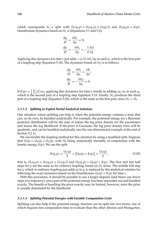
146 Handbook of Markov Chain Monte Carlo
which corresponds to a split with H1(q, p) = H3(q, p) = U(q)/2 and H2(q, p) = K(p).Hamiltonian dynamics based on H1 is (Equations 5.1 and 5.2):
dqi
dt= ∂H1
∂pi= 0,
dpi
dt= −∂H1
∂qi= −1
2∂U∂qi
.
Applying this dynamics for time ε just adds−(ε/2) ∂U/∂qi to each pi, which is the first partof a leapfrog step (Equation 5.18). The dynamics based on H2 is as follows:
dqi
dt= ∂H2
∂pi= ∂K
∂pi,
dpi
dt= −∂H2
∂qi= 0.
If K(p) = 12∑
p2i /mi, applying this dynamics for time ε results in adding εpi/mi to each qi,
which is the second part of a leapfrog step Equation 5.19. Finally, H3 produces the thirdpart of a leapfrog step (Equation 5.20), which is the same as the first part, since H3 = H1.
5.5.1.2 Splitting to Exploit Partial Analytical Solutions
One situation where splitting can help is when the potential energy contains a term thatcan, on its own, be handled analytically. For example, the potential energy for a Bayesianposterior distribution will be the sum of minus the log prior density for the parametersand minus the log likelihood. If the prior is Gaussian, the log prior density term will bequadratic, and can be handled analytically (see the one-dimensional example at the end ofSection 5.2.1).
We can modify the leapfrog method for this situation by using a modified split. Supposethat U(q) = U0(q)+U1(q), with U0 being analytically tractable, in conjunction with thekinetic energy, K(p). We use the split
H(q, p) = U1(q)2
+ [U0(q)+ K(p)]+ U1(q)
2, (5.29)
that is, H1(q, p) = H3(q, p) = U1(q)/2 and H2(q, p) = U0(q)+ K(p). The first and last halfsteps for p are the same as for ordinary leapfrog, based on U1 alone. The middle full stepfor q, which in ordinary leapfrog just adds εp to q, is replaced by the analytical solution forfollowing the exact dynamics based on the Hamiltonian U0(q)+ K(p) for time ε.
With this procedure, it should be possible to use a larger stepsize (and hence use fewersteps in a trajectory), since part of the potential energy has been separated out and handledexactly. The benefit of handling the prior exactly may be limited, however, since the prioris usually dominated by the likelihood.
5.5.1.3 Splitting Potential Energies with Variable Computation Costs
Splitting can also help if the potential energy function can be split into two terms, one ofwhich requires less computation time to evaluate than the other (Sexton and Weingarten,
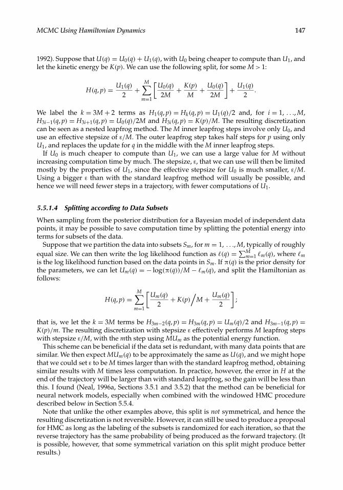
MCMC Using Hamiltonian Dynamics 147
1992). Suppose that U(q) = U0(q)+U1(q), with U0 being cheaper to compute than U1, andlet the kinetic energy be K(p). We can use the following split, for some M > 1:
H(q, p) = U1(q)2
+M∑
m=1
[U0(q)2M
+ K(p)
M+ U0(q)
2M
]+ U1(q)
2.
We label the k = 3M + 2 terms as H1(q, p) = Hk(q, p) = U1(q)/2 and, for i = 1, . . ., M,H3i−1(q, p) = H3i+1(q, p) = U0(q)/2M and H3i(q, p) = K(p)/M. The resulting discretizationcan be seen as a nested leapfrog method. The M inner leapfrog steps involve only U0, anduse an effective stepsize of ε/M. The outer leapfrog step takes half steps for p using onlyU1, and replaces the update for q in the middle with the M inner leapfrog steps.
If U0 is much cheaper to compute than U1, we can use a large value for M withoutincreasing computation time by much. The stepsize, ε, that we can use will then be limitedmostly by the properties of U1, since the effective stepsize for U0 is much smaller, ε/M.Using a bigger ε than with the standard leapfrog method will usually be possible, andhence we will need fewer steps in a trajectory, with fewer computations of U1.
5.5.1.4 Splitting according to Data Subsets
When sampling from the posterior distribution for a Bayesian model of independent datapoints, it may be possible to save computation time by splitting the potential energy intoterms for subsets of the data.
Suppose that we partition the data into subsets Sm, for m = 1, . . ., M, typically of roughlyequal size. We can then write the log likelihood function as �(q) =∑M
m=1 �m(q), where �mis the log likelihood function based on the data points in Sm. If π(q) is the prior density forthe parameters, we can let Um(q) = − log(π(q))/M − �m(q), and split the Hamiltonian asfollows:
H(q, p) =M∑
m=1
[Um(q)
2+ K(p)
/M + Um(q)
2
];
that is, we let the k = 3M terms be H3m−2(q, p) = H3m(q, p) = Um(q)/2 and H3m−1(q, p) =K(p)/m. The resulting discretization with stepsize ε effectively performs M leapfrog stepswith stepsize ε/M, with the mth step using MUm as the potential energy function.
This scheme can be beneficial if the data set is redundant, with many data points that aresimilar. We then expect MUm(q) to be approximately the same as U(q), and we might hopethat we could set ε to be M times larger than with the standard leapfrog method, obtainingsimilar results with M times less computation. In practice, however, the error in H at theend of the trajectory will be larger than with standard leapfrog, so the gain will be less thanthis. I found (Neal, 1996a, Sections 3.5.1 and 3.5.2) that the method can be beneficial forneural network models, especially when combined with the windowed HMC proceduredescribed below in Section 5.5.4.
Note that unlike the other examples above, this split is not symmetrical, and hence theresulting discretization is not reversible. However, it can still be used to produce a proposalfor HMC as long as the labeling of the subsets is randomized for each iteration, so that thereverse trajectory has the same probability of being produced as the forward trajectory. (Itis possible, however, that some symmetrical variation on this split might produce betterresults.)
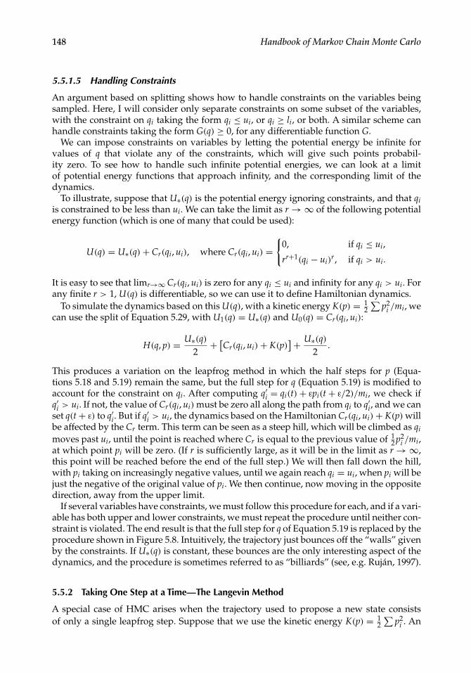
148 Handbook of Markov Chain Monte Carlo
5.5.1.5 Handling Constraints
An argument based on splitting shows how to handle constraints on the variables beingsampled. Here, I will consider only separate constraints on some subset of the variables,with the constraint on qi taking the form qi ≤ ui, or qi ≥ li, or both. A similar scheme canhandle constraints taking the form G(q) ≥ 0, for any differentiable function G.
We can impose constraints on variables by letting the potential energy be infinite forvalues of q that violate any of the constraints, which will give such points probabil-ity zero. To see how to handle such infinite potential energies, we can look at a limitof potential energy functions that approach infinity, and the corresponding limit of thedynamics.
To illustrate, suppose that U∗(q) is the potential energy ignoring constraints, and that qiis constrained to be less than ui. We can take the limit as r →∞ of the following potentialenergy function (which is one of many that could be used):
U(q) = U∗(q)+ Cr(qi, ui), where Cr(qi, ui) ={
0, if qi ≤ ui,
rr+1(qi − ui)r, if qi > ui.
It is easy to see that limr→∞ Cr(qi, ui) is zero for any qi ≤ ui and infinity for any qi > ui. Forany finite r > 1, U(q) is differentiable, so we can use it to define Hamiltonian dynamics.
To simulate the dynamics based on this U(q), with a kinetic energy K(p) = 12∑
p2i /mi, we
can use the split of Equation 5.29, with U1(q) = U∗(q) and U0(q) = Cr(qi, ui):
H(q, p) = U∗(q)2
+ [Cr(qi, ui)+ K(p)]+ U∗(q)
2.
This produces a variation on the leapfrog method in which the half steps for p (Equa-tions 5.18 and 5.19) remain the same, but the full step for q (Equation 5.19) is modified toaccount for the constraint on qi. After computing q′i = qi(t)+ εpi(t+ ε/2)/mi, we check ifq′i > ui. If not, the value of Cr(qi, ui) must be zero all along the path from qi to q′i, and we canset q(t+ ε) to q′i. But if q′i > ui, the dynamics based on the Hamiltonian Cr(qi, ui)+ K(p) willbe affected by the Cr term. This term can be seen as a steep hill, which will be climbed as qi
moves past ui, until the point is reached where Cr is equal to the previous value of 12 p2
i /mi,at which point pi will be zero. (If r is sufficiently large, as it will be in the limit as r →∞,this point will be reached before the end of the full step.) We will then fall down the hill,with pi taking on increasingly negative values, until we again reach qi = ui, when pi will bejust the negative of the original value of pi. We then continue, now moving in the oppositedirection, away from the upper limit.
If several variables have constraints, we must follow this procedure for each, and if a vari-able has both upper and lower constraints, we must repeat the procedure until neither con-straint is violated. The end result is that the full step for q of Equation 5.19 is replaced by theprocedure shown in Figure 5.8. Intuitively, the trajectory just bounces off the “walls” givenby the constraints. If U∗(q) is constant, these bounces are the only interesting aspect of thedynamics, and the procedure is sometimes referred to as “billiards” (see, e.g. Ruján, 1997).
5.5.2 Taking One Step at a Time—The Langevin Method
A special case of HMC arises when the trajectory used to propose a new state consistsof only a single leapfrog step. Suppose that we use the kinetic energy K(p) = 1
2∑
p2i . An
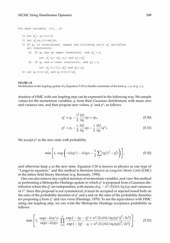
MCMC Using Hamiltonian Dynamics 149
For each variable, i=1, . . . ,d:
1) Let p′i= pi(t+ε/2)
2) Let q ′i=qi(t)+εp′i/mi
3) If qi is constrained, repeat the following until q ′i satisfiesall constraints:
a) If qi has an upper constraint, and q ′i > ui
Let q ′i=ui-(q ′i-ui) and p′i=-p′ib) If qi has a lower constraint, and q ′i < li
Let q ′i=li+(li-q ′i) and p′i=-p′i4) Let qi(t+ε)=q
′i and pi(t+ε/2)=p
′i
FIGURE 5.8Modification to the leapfrog update of q (Equation 5.19) to handle constraints of the form qi ≤ ui or qi ≤ li .
iteration of HMC with one leapfrog step can be expressed in the following way. We samplevalues for the momentum variables, p, from their Gaussian distributions with mean zeroand variance one, and then propose new values, q∗ and p∗, as follows:
q∗i = qi − ε2
2∂U∂qi
(q)+ εpi, (5.30)
p∗i = pi − ε2∂U∂qi
(q)− ε2
∂U∂qi
(q∗). (5.31)
We accept q∗ as the new state with probability
min
[1, exp
(−(U(q∗)−U(q))− 1
2
∑i
((p∗i )2 − p2
i )
)], (5.32)
and otherwise keep q as the new state. Equation 5.30 is known in physics as one type of“Langevin equation,” and this method is therefore known as Langevin Monte Carlo (LMC)in the lattice field theory literature (e.g. Kennedy, 1990).
One can also remove any explicit mention of momentum variables, and view this methodas performing a Metropolis–Hastings update in which q∗ is proposed from a Gaussian dis-tribution where the q∗i are independent, with means of qi − (ε2/2)[∂U/∂qi](q) and variancesof ε2. Since this proposal is not symmetrical, it must be accepted or rejected based both onthe ratio of the probability densities of q∗ and q and on the ratio of the probability densitiesfor proposing q from q∗ and vice versa (Hastings, 1970). To see the equivalence with HMCusing one leapfrog step, we can write the Metropolis–Hastings acceptance probability asfollows:
min
⎡⎣1,
exp(−U(q∗))exp(−U(q))
d∏i=1
exp(− (qi − q∗i + (ε2/2) [∂U/∂qi](q∗)
)2/ 2ε2
)exp
(− (q∗i − qi + (ε2/2) [∂U/∂qi](q))2
/ 2ε2)⎤⎦ . (5.33)
150 Handbook of Markov Chain Monte Carlo
To see that this is the same as Equation 5.32, note that using Equations 5.30 and 5.31, wecan write
p = 1ε
[q∗i − qi + ε
2
2∂U∂qi
(q)
],
p∗ = −1ε
[qi − q∗i +
ε2
2∂U∂qi
(q∗)]
.
After substituting these into Equation 5.32, it is straightforward to see the equivalenceto Equation 5.33.
In this Metropolis–Hastings form, the LMC method was first proposed by Rosskyet al. (1978) for use in physical simulations. Approximate Langevin methods without anaccept/reject step can also be used (for a discussion of this, see Neal, 1993, Section 5.3)—as,for instance, in a paper on statistical inference for complex models by Grenander and Miller(1990), where also an accept/reject step is proposed in the discussion by J. Besag (p. 591).
Although LMC can be seen as a special case of HMC, its properties are quite different.Since LMC updates are reversible, and generally make only small changes to the state (sinceε typically cannot be very large), LMC will explore the distribution via an inefficient randomwalk, just like random-walk Metropolis updates.
However, LMC has better scaling behavior than random-walk Metropolis as dimension-ality increases, as can be seen from an analysis paralleling that in Section 5.4.4 (Creutz, 1988;Kennedy, 1990). The local error of the leapfrog step is of order ε3, so E [Δ2
1], the averagesquared error in H from one variable, will be of order ε6. From Equation 5.27, E [Δ]will alsobe of order ε6, and with d independent variables, E [Δd]will be of order dε6, so that εmustscale as d−1/6 in order to maintain a reasonable acceptance rate. Since LMC explores the dis-tribution via a random walk, the number of iterations needed to reach a nearly independentpoint will be proportional to ε−2, which grows as d1/3, and the computation time to reacha nearly independent point grows as d4/3. This is better than the d2 growth in computationtime for random-walk Metropolis, but worse than the d5/4 growth when HMC is used withtrajectories that are long enough to reach a nearly independent point.
We can also find what the acceptance rate for LMC will be when the optimal ε is used, whensampling a distribution with independent variables replicated d times. As for random-walkMetropolis and HMC, the acceptance rate is given in terms of μ = E [Δd] by Equation 5.28.The cost of obtaining a nearly independent point using LMC is proportional to 1/(a(μ)ε2),and since μ is proportional to ε6, we can write the cost as
CLMC ∝ 1(a(μ)μ1/3)
.
Numerical calculation shows that this is minimized when a(μ) is 0.57, a result obtainedmore formally by Roberts and Rosenthal (1998). This may be useful for tuning, if the behav-ior of LMC for the distribution being sampled resembles its behavior when sampling forreplicated independent variables.
5.5.3 Partial Momentum Refreshment: Another Way to Avoid Random Walks
The single leapfrog step used in the LMC algorithm will usually not be sufficient to move toa nearly independent point, so LMC will explore the distribution via an inefficient random
MCMC Using Hamiltonian Dynamics 151
walk. This is why HMC is typically used with trajectories of many leapfrog steps. An alter-native that can suppress random-walk behavior even when trajectories consist of just oneleapfrog step is to only partially refresh the momentum between trajectories, as proposedby Horowitz (1991).
Suppose that the kinetic energy has the typical form K(p) = pTM−1p/2. The followingupdate for p will leave invariant the distribution for the momentum (Gaussian with meanzero and covariance M):
p′ = αp+ (1− α2)1/2n. (5.34)
Here, α is any constant in the interval [−1,+1], and n is a Gaussian random vector withmean zero and covariance matrix M. To see this, note that if p has the required Gaussiandistribution, the distribution of p′ will also be Gaussian (since it is a linear combination ofindependent Gaussians), with mean 0 and covariance α2M + (1− α2)M = M.
If α is only slightly less than one, p′ will be similar to p, but repeated updates of thissort will eventually produce a value for the momentum variables almost independent ofthe initial value. When α = 0, p′ is just set to a random value drawn from its Gaussiandistribution, independent of its previous value. Note that when M is diagonal, the updateof each momentum variable, pi, is independent of the updates of other momentum variables.
The partial momentum update of Equation 5.34 can be substituted for the full replacementof the momentum in the standard HMC algorithm. This gives a generalized HMC algorithmin which an iteration consists of three steps:
1. Update the momentum variables using Equation 5.34. Let the new momentumbe p′.
2. Propose a new state, (q∗, p∗), by applying L leapfrog steps with stepsize ε, startingat (q, p′), and then negating the momentum. Accept (q∗, p∗) with probability
min[1, exp
(−U(q∗)+U(q)− K(p∗)+ K(p′))]
.
If (q∗, p∗) is accepted, let (q′′, p′′) = (q∗, p∗); otherwise, let (q′′, p′′) = (q, p′).3. Negate the momentum, so that the new state is (q′′, −p′′).
The transitions in each of these steps—(q, p) → (q, p′), (q, p′) → (q′′, p′′), and (q′′, p′′) →(q′′, −p′′)—leave the canonical distribution for (q, p) invariant. The entire update there-fore also leaves the canonical distribution invariant. The three transitions also each satisfydetailed balance, but the sequential combination of the three does not satisfy detailed bal-ance (except when α = 0). This is crucial, since if the combination were reversible, it wouldstill result in random-walk behavior when L is small.
Note that omitting step (3) above would result in a valid algorithm, but then, far fromsuppressing random walks, the method (with α close to one) would produce nearly back-and-forth motion, since the direction of motion would reverse with every trajectory acceptedin step (2). With the reversal in step (3), motion continues in the same direction as long asthe trajectories in step (2) are accepted, since the two negations of p will cancel. Motionreverses whenever a trajectory is rejected, so if random-walk behavior is to be suppressed,the rejection rate must be kept small.
If α = 0, the above algorithm is the same as standard HMC, since step (1) will completelyreplace the momentum variables, step (2) is the same as for standard HMC, and step (3) will
152 Handbook of Markov Chain Monte Carlo
have no effect, since the momentum will be immediately replaced anyway, in step (1) ofthe next iteration.
Since this algorithm can be seen as a generalization of standard HMC, with an additionalα parameter, one might think it will offer an improvement, provided that α is tuned forbest performance. However, Kennedy and Pendleton (2001) show that when the method isapplied to high-dimensional multivariate Gaussian distributions only a small constant fac-tor improvement is obtained, with no better scaling with dimensionality. Best performanceis obtained using long trajectories (L large), and a value for α that is not very close to one(but not zero, so the optimum choice is not standard HMC). If L is small, the need to keepthe rejection rate very low (by using a small ε), as needed to suppress random walks, makesthe method less advantageous than standard HMC.
It is disappointing that only a small improvement is obtained with this generalizationwhen sampling a multivariate Gaussian, due to limitations that likely apply to other distri-butions as well. However, the method may be more useful than one would think from this.For reasons discussed in Sections 5.4.3 and 5.4.5, we will often combine HMC updates withother MCMC updates (perhaps for variables not changed by HMC). There may then be atradeoff between using long trajectories to make HMC more efficient, and using shortertrajectories so that the other MCMC updates can be done more often. If shorter-than-optimal trajectories are to be used for this reason, setting α greater than zero can reduce therandom-walk behavior that would otherwise result.
Furthermore, rejection rates can be reduced using the “window” method described next.An analysis of partial momentum refreshment combined with the window method mightfind that using trajectories of moderate length in conjunction with a value for α greater thanzero produces a more substantial improvement.
5.5.4 Acceptance Using Windows of States
Figure 5.3 (right plot) shows how the error in H varies along a typical trajectory computedwith the leapfrog method. Rapid oscillations occur, here with a period of between 2 and3 leapfrog steps, due to errors in simulating the motion in the most confined direction (ordirections, for higher-dimensional distributions). When a long trajectory is used to proposea state for HMC, it is essentially random whether the trajectory ends at a state where the errorin H is negative or close to zero, and hence will be accepted with probability close to one, orwhether it happens to end at a state with a large positive error in H, and a correspondinglylower acceptance probability. If somehow we could smooth out these oscillations, we mightobtain a high probability of acceptance for all trajectories.
I introduced a method for achieving this result that uses “windows” of states at thebeginning and end of the trajectory (Neal, 1994). Here, I will present the method as anapplication of a general technique in which we probabilistically map to a state in a differentspace, perform a Markov chain transition in this new space, and then probabilistically mapback to our original state space (Neal, 2006).
Our original state space consists of pairs, (q, p), of position and momentum variables. Wewill map to a sequence of W pairs, [(q0, p0), . . ., (qW−1, pW−1)], in which each (qi, pi) for i>0is the result of applying one leapfrog step (with some fixed stepsize, ε) to (qi−1, pi−1). Notethat even though a point in the new space seems to consist of W times as many numbersas a point in the original space, the real dimensionality of the new space is the same as theold, since the whole sequence of W pairs is determined by (q0, p0).
To probabilistically map from (q, p) to a sequence of pairs, [(q0, p0), . . ., (qW−1, pW−1)], weselect s uniformly from {0, . . ., W − 1}, and set (qs, ps) in the new state to our current state
MCMC Using Hamiltonian Dynamics 153
(q, p). The other (qi, pi) pairs in the new state are obtained using leapfrog steps from (qs, ps),for i>s, or backwards leapfrog steps (i.e. done with stepsize −ε) for i<s. It is easy to see,using the fact that leapfrog steps preserve volume, that if our original state is distributedwith probability density P(q, p), then the probability density of obtaining the sequence[(q0, p0), . . ., (qW−1, pW−1)] by this procedure is
P([(q0, p0), . . ., (qW−1, pW−1)]
) = 1W
W−1∑i=0
P(qi, pi), (5.35)
since we can obtain this sequence from a (q, p) pair that matches any pair in the sequence,and the probability is 1/W that we will produce the sequence starting from each of thesepairs (which happens only if the random selection of s puts the pair at the right place in thesequence).
Having mapped to a sequence of W pairs, we now perform a Metropolis update thatkeeps the sequence distribution defined by Equation 5.35 invariant, before mapping backto the original state space. To obtain a Metropolis proposal, we perform L−W + 1 leapfrogsteps (for some L ≥ W−1), starting from (qW−1, pW−1), producing pairs (qW , pW) to (qL, pL).We then propose the sequence [(qL,−pL), . . ., (qL−W+1,−pL−W+1)]. We accept or reject thisproposed sequence by the usual Metropolis criterion, with the acceptance probability being
min
⎡⎣1,
∑Li=L−W+1 P(qi, pi)∑W−1
i=0 P(qi, pi)
⎤⎦ , (5.36)
with P(q, p) ∝ exp(−H(q, p)). (Note here that H(q, p) = H(q,−p), and that starting from theproposed sequence would lead symmetrically to the original sequence being proposed.)
This Metropolis update leaves us with either the sequence [(qL, pL), . . ., (qL−W+1, pL−W+1)],called the “accept window,” or the sequence [(q0, p0), . . ., (qW−1, pW−1)], called the “rejectwindow.” (Note that these windows will overlap if L+ 1 < 2W.) We label the pairs inthe window chosen as [(q+0 , p+0 ), . . ., (q+W−1, p+W−1)]. We now produce a final state for thewindowed HMC update by probabilistically mapping from this sequence to a single pair,choosing (q+e , p+e ) with probability
P(q+e , p+e )∑W−1i=0 P(q+i , p+i )
.
If the sequence in the chosen window was distributed according to Equation 5.35, the pair(q+e , p+e ) chosen will be distributed according to P(q, p) ∝ exp(−H(q, p)), as desired. To seethis, let (q+e+n, p+e+n) be the result of applying n leapfrog steps (backward ones if n < 0)starting at (q+e , p+e ). The probability density that (q+e , p+e ) will result from mapping from asequence to a single pair can then be written as follows, considering all sequences that cancontain (q+e , p+e ) and their probabilities:
e∑k=e−W+1
⎡⎣ 1
W
k+W−1∑i=k
P(q+i , p+i )
⎤⎦ P(q+e , p+e )∑k+W−1
i=k P(q+i , p+i )
= P(q+e , p+e ).
The entire procedure therefore leaves the correct distribution invariant.When W > 1, the potential problem with ergodicity discussed at the end of Section 5.3.2
does not arise, since there is a nonzero probability of moving to a state only one leapfrogstep away, where q may differ arbitrarily from its value at the current state.
154 Handbook of Markov Chain Monte Carlo
It might appear that the windowed HMC procedure requires saving all 2W states in theaccept and reject windows, since any one of these states might become the new state when astate is selected from either the accept window or reject window. Actually, however, at mostthree states need to be saved—the start state, so that forward simulation can be resumedafter the initial backward simulation, plus one state from the reject window and one statefrom the accept window, one of which will become the new state after one of these windowsis chosen. As states in each window are produced in sequence, a decision is made whetherthe state just produced should replace the state presently saved for that window. Supposethat the sum of the probability densities of states seen so far is si = p1 + · · · + pi. If the statejust produced has probability density pi+1, it replaces the previous state saved from thiswindow with probability pi+1/(si + pi+1).
I showed (Neal, 1994) that, compared to standard HMC, using windows improves theperformance of HMC by a factor of 2 or more, on multivariate Gaussian distributions inwhich the standard deviation in some directions is much larger than in other directions.This is because the acceptance probability in Equation 5.36 uses an average of probabilitydensities over states in a window, smoothing out the oscillations in H from inexact sim-ulation of the trajectory. Empirically, the advantage of the windowed method was foundto increase with dimensionality. For high-dimensional distributions, the acceptance proba-bility when using the optimal stepsize was approximately 0.85, larger than the theoreticalvalue of 0.65 for HMC (see Section 5.4.4).
These results for multivariate Gaussian distributions were obtained with a window size,W, much less than the trajectory length, L. For less regular distributions, it may be advanta-geous to use a much larger window. When W = L/2, the acceptance test determines whetherthe new state is from the first half of the trajectory (which includes the current state) or thesecond half; the new state is then chosen from one half or the other with probabilitiesproportional to the probability densities of the states in that half. This choice of W guardsagainst the last few states of the trajectory having low probability density (high H), as mighthappen if the trajectory had by then entered a region where the stepsize used was too big.
The windowed variant of HMC may make other variants of HMC more attractive. Onesuch variant (Section 5.5.1) splits the Hamiltonian into many terms corresponding to subsetsof the data, which tends to make errors in H higher (while saving computation). Errors inH have less effect when averaged over windows. As discussed in Section 5.5.3, very lowrejection rates are desirable when using partial momentum refreshment. It is easier to obtaina low rejection probability using windows (i.e. a less drastic reduction in ε is needed), whichmakes partial momentum refreshment more attractive.
Qin and Liu (2001) introduced a variant on windowed HMC. In their version, L leapfrogsteps are done from the start state, with the accept window consisting of the states after thelast W of these steps. A state from the accept window is then selected with probabilitiesproportional to their probability densities. If the state selected is k states before the end, kbackwards leapfrog steps are done from the start state, and the states found by these stepsalong with those up to W − k − 1 steps forward of the start state form the reject window.The state selected from the accept window then becomes the next state with probabilitygiven by the analog of Equation 5.36; otherwise the state remains the same.
Qin and Liu’s procedure is quite similar to the original windowed HMC procedure. Onedisadvantage of Qin and Liu’s procedure is that the state is unchanged when the acceptwindow is rejected, whereas in the original procedure a state is selected from the rejectwindow (which might be the current state, but often will not be). The only other differenceis that the number of steps from the current state to an accepted state ranges from L−W + 1 to L (average L− (W + 1)/2) with Qin and Liu’s procedure, versus from L− 2W + 2
MCMC Using Hamiltonian Dynamics 155
to L (average L−W + 1) for the original windowed HMC procedure, while the numberof leapfrog steps computed varies from L to L+W − 1 with Qin and Liu’s procedure,and is fixed at L with the original procedure. These differences are slight if W � L. Qinand Lin claim that their procedure performs better than the original on high-dimensionalmultivariate Gaussian distributions, but their experiments are flawed.∗
Qin and Liu (2001) also introduce the more useful idea of weighting the states in theaccept and reject windows nonuniformly, which can be incorporated into the original pro-cedure as well. When mapping from the current state to a sequence of W weighted states,the position of the current state is chosen with probabilities equal to the weights, and whencomputing the acceptance probability or choosing a state from the accept or reject win-dow, the probability densities of states are multiplied by their weights. Qin and Liu useweights that favor states more distant from the current state, which could be useful byusually causing movement to a distant point, while allowing choice of a nearer point if thedistant points have low probability density. Alternatively, if one sees a window as a way ofsmoothing the errors in H, symmetrical weights that implement a better “low pass filter”would make sense.
5.5.5 Using Approximations to Compute the Trajectory
The validity of HMC does not depend on using the correct Hamiltonian when simulatingthe trajectory. We can instead use some approximate Hamiltonian, as long as we sim-ulate the dynamics based on it by a method that is reversible and volume-preserving.However, the exact Hamiltonian must be used when computing the probability of accept-ing the endpoint of the trajectory. There is no need to look for an approximation to thekinetic energy, when it is of a simple form such as Equation 5.13, but the potential energy isoften much more complex and costly to compute—for instance, it may involve the sum oflog likelihoods based on many data points, if the data cannot be summarized by a simplesufficient statistic. When using trajectories of many leapfrog steps, we can therefore savemuch computation time if a fast and accurate approximation to the potential energy is avail-able, while still obtaining exact results (apart from the usual sampling variation inherentin MCMC).
Many ways of approximating the potential energy might be useful. For example, if itsevaluation requires iterative numerical methods, fewer iterations might be done than arenecessary to get a result accurate to machine precision. In a Bayesian statistical application,a less costly approximation to the unnormalized posterior density (whose log gives thepotential energy) may be obtainable by simply looking at only a subset of the data. Thismay not be a good strategy in general, but I have found it useful for Gaussian processmodels (Neal, 1998; Rasmussen and Williams, 2006), for which computation time scalesas the cube of the number of data points, so that even a small reduction in the number ofpoints produces a useful speedup.
Rasmussen (2003) has proposed approximating the potential energy by modeling it as aGaussian process, inferred from values of the potential energy at positions selected duringan initial exploratory phase. This method assumes only a degree of smoothness of the poten-tial energy function, and so could be widely applied. It is limited, however, by the cost of
∗ In their first comparison, their method computes an average of 55 leapfrog steps per iteration, but the originalonly computes 50 steps, a difference in computation time which if properly accounted for negates the slightadvantage they see for their procedure. Their second comparison has a similar problem, and it is also clear froman examination of the results (in their Table I) that the sampling errors in their comparison are too large for anymeaningful conclusions to be drawn.
156 Handbook of Markov Chain Monte Carlo
Gaussian process inference, and so is most useful for problems of moderate dimensionalityfor which exact evaluation of the potential energy is very costly.
An interesting possibility, to my knowledge not yet explored, would be to expressthe exact potential energy as the sum of an approximate potential energy and the errorin this approximation, and to then apply one of the splitting techniques described inSection 5.5.1—exploiting either the approximation’s analytic tractability (e.g. for a Gaussianapproximation, with quadratic potential energy), or its low computational cost, so that itsdynamics can be accurately simulated at little cost using many small steps. This wouldreduce the number of evaluations of the gradient of the exact potential energy if the vari-ation in the potential energy removed by the approximation term permits a large stepsizefor the error term.
5.5.6 Short-Cut Trajectories: Adapting the Stepsize without Adaptation
One significant disadvantage of HMC is that, as discussed in Section 5.4.2, its performancedepends critically on the settings of its tuning parameters—which consist of at least theleapfrog stepsize, ε, and number of leapfrog steps, L, with variations such as windowedHMC having additional tuning parameters as well. The optimal choice of trajectory length(εL) depends on the global extent of the distribution, so finding a good trajectory lengthlikely requires examining a substantial number of HMC updates. In contrast, just a fewleapfrog steps can reveal whether some choice of stepsize is good or bad, which leads tothe possibility of trying to set the stepsize “adaptively” during an HMC run.
Recent work on adaptive MCMC methods is reviewed by Andrieu and Thoms (2008). Asthey explain, naively choosing a stepsize for each HMC update based on results of previ-ous updates—for example, reducing the stepsize by 20% if the previous 10 trajectories wereall rejected, and increasing it by 20% if less than two of the 10 previous trajectories wererejected—undermines proofs of correctness (in particular, the process is no longer a Markovchain), and will in general produce points from the wrong distribution. However, correctresults can be obtained if the degree of adaptation declines over time. Adaptive methodsof this sort could be used for HMC, in much the same way as for any other tunable MCMCmethod.
An alternative approach (Neal, 2005, 2007) is to perform MCMC updates with variousvalues of the tuning parameters, set according to a schedule that is predetermined or cho-sen randomly without reference to the realized states, so that the usual proofs of MCMCconvergence and error analysis apply, but to do this using MCMC updates that have beentweaked so that they require little computation time when the tuning parameters are notappropriate for the distribution. Most of the computation time will then be devoted toupdates with appropriate values for the tuning parameters. Effectively, the tuning param-eters are set adaptively from a computational point of view, but not from a mathematicalpoint of view.
For example, trajectories that are simulated with a stepsize that is much too large canbe rejected after only a few leapfrog steps, by rejecting whenever the change (either way)in the Hamiltonian due to a single step (or a short series of steps) is greater than somethreshold—that is, we reject if |H(q(t+ ε), p(t+ ε))−H(q(t), p(t))| is greater than the thresh-old. If this happens early in the trajectory, little computation time will have been wastedon this unsuitable stepsize. Such early termination of trajectories is valid, since any MCMCupdate that satisfies detailed balance will still satisfy detailed balance if it is modified toeliminate transitions either way between certain pairs of states.
MCMC Using Hamiltonian Dynamics 157
With this simple modification, we can randomly choose stepsizes from some distributionwithout wasting much time on those stepsizes that turn out to be much too large. However,if we set the threshold small enough to reject when the stepsize is only a little too large,we may terminate trajectories that would have been accepted, perhaps after a substantialamount of computation has already been done. Trying to terminate trajectories early whenthe stepsize is smaller than optimal carries a similar risk.
Aless drastic alternative to terminating trajectories when the stepsize seems inappropriateis to instead reverse the trajectory. Suppose that we perform leapfrog steps in groups of ksteps. Based on the changes in H over these k steps, we can test whether the stepsize isinappropriate—for example, the group may fail the test if the standard deviation of H overthe k + 1 states is greater than some upper threshold or less than some lower threshold(any criterion that would yield the same decision for the reversed sequence is valid). Whena group of k leapfrog steps fails this test, the trajectory stays at the state where this groupstarted, rather than moving k steps forward, and the momentum variables are negated. Thetrajectory will now exactly retrace states previously computed (and which therefore neednot be recomputed), until the initial state is reached, at which point new states will againbe computed. If another group of k steps fails the test, the trajectory will again reverse,after which the whole remainder of the trajectory will traverse states already computed,allowing its endpoint to be found immediately without further computation.
This scheme behaves the same as standard HMC if no group of k leapfrog steps fails thetest. If there are two failures early in the trajectory, little computation time will have beenwasted on this (most likely) inappropriate stepsize. Between these extremes, it is possiblethat one or two reversals will occur, but not early in the trajectory; the endpoint of thetrajectory will then usually not be close to the initial state, so the nonnegligible computationperformed will not be wasted (as it would be if the trajectory had been terminated).
Such short-cut schemes can be effective at finding good values for a small number oftuning parameters, for which good values will be picked reasonably often when drawingthem randomly. It will not be feasible for setting a large number of tuning parameters,such as the entries in the “mass matrix” of Equation 5.5 when dimensionality is high, sinceeven if two reversals happen early on, the cost of using inappropriate values of the tuningparameters will dominate when appropriate values are chosen only very rarely.
5.5.7 Tempering during a Trajectory
Standard HMC and the variations described so far have as much difficulty moving betweenmodes that are separated by regions of low probability as other local MCMC methods,such as random-walk Metropolis and Gibbs sampling. Several general schemes have beendevised for solving problems with such isolated modes that involve sampling from a seriesof distributions that are more diffuse than the distribution of interest. Such schemes includeparallel tempering (Geyer, 1991; Earl and Deem, 2005), simulated tempering (Marinariand Parisi, 1992), tempered transitions (Neal, 1996b), and annealed importance sampling(Neal, 2001). Most commonly, these distributions are obtained by varying a “temperature”parameter, T, as in Equation 5.21, with T = 1 corresponding to the distribution of interest,and larger values of T giving more diffuse distributions. Any of these “tempering” methodscould be used in conjunction with HMC. However, tempering-like behavior can also beincorporated directly into the trajectory used to propose a new state in the HMC procedure.
In the simplest version of such a “tempered trajectory” scheme (Neal, 1999, Section 6),each leapfrog step in the first half of the trajectory is combined with multiplication of themomentum variables by some factor α slightly greater than one, and each leapfrog step
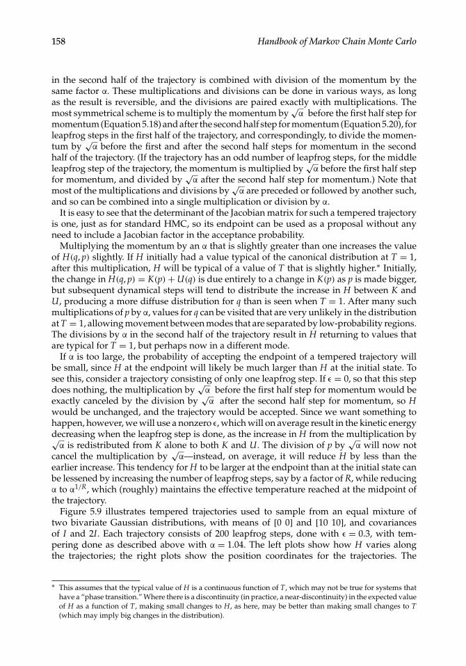
158 Handbook of Markov Chain Monte Carlo
in the second half of the trajectory is combined with division of the momentum by thesame factor α. These multiplications and divisions can be done in various ways, as longas the result is reversible, and the divisions are paired exactly with multiplications. Themost symmetrical scheme is to multiply the momentum by
√α before the first half step for
momentum (Equation 5.18) and after the second half step for momentum (Equation 5.20), forleapfrog steps in the first half of the trajectory, and correspondingly, to divide the momen-tum by
√α before the first and after the second half steps for momentum in the second
half of the trajectory. (If the trajectory has an odd number of leapfrog steps, for the middleleapfrog step of the trajectory, the momentum is multiplied by
√α before the first half step
for momentum, and divided by√α after the second half step for momentum.) Note that
most of the multiplications and divisions by√α are preceded or followed by another such,
and so can be combined into a single multiplication or division by α.It is easy to see that the determinant of the Jacobian matrix for such a tempered trajectory
is one, just as for standard HMC, so its endpoint can be used as a proposal without anyneed to include a Jacobian factor in the acceptance probability.
Multiplying the momentum by an α that is slightly greater than one increases the valueof H(q, p) slightly. If H initially had a value typical of the canonical distribution at T = 1,after this multiplication, H will be typical of a value of T that is slightly higher.∗ Initially,the change in H(q, p) = K(p)+U(q) is due entirely to a change in K(p) as p is made bigger,but subsequent dynamical steps will tend to distribute the increase in H between K andU, producing a more diffuse distribution for q than is seen when T = 1. After many suchmultiplications of p by α, values for q can be visited that are very unlikely in the distributionat T = 1, allowing movement between modes that are separated by low-probability regions.The divisions by α in the second half of the trajectory result in H returning to values thatare typical for T = 1, but perhaps now in a different mode.
If α is too large, the probability of accepting the endpoint of a tempered trajectory willbe small, since H at the endpoint will likely be much larger than H at the initial state. Tosee this, consider a trajectory consisting of only one leapfrog step. If ε = 0, so that this stepdoes nothing, the multiplication by
√α before the first half step for momentum would be
exactly canceled by the division by√α after the second half step for momentum, so H
would be unchanged, and the trajectory would be accepted. Since we want something tohappen, however, we will use a nonzero ε, which will on average result in the kinetic energydecreasing when the leapfrog step is done, as the increase in H from the multiplication by√α is redistributed from K alone to both K and U. The division of p by
√α will now not
cancel the multiplication by√α—instead, on average, it will reduce H by less than the
earlier increase. This tendency for H to be larger at the endpoint than at the initial state canbe lessened by increasing the number of leapfrog steps, say by a factor of R, while reducingα to α1/R, which (roughly) maintains the effective temperature reached at the midpoint ofthe trajectory.
Figure 5.9 illustrates tempered trajectories used to sample from an equal mixture oftwo bivariate Gaussian distributions, with means of [0 0] and [10 10], and covariancesof I and 2I. Each trajectory consists of 200 leapfrog steps, done with ε = 0.3, with tem-pering done as described above with α = 1.04. The left plots show how H varies alongthe trajectories; the right plots show the position coordinates for the trajectories. The
∗ This assumes that the typical value of H is a continuous function of T, which may not be true for systems thathave a “phase transition.” Where there is a discontinuity (in practice, a near-discontinuity) in the expected valueof H as a function of T, making small changes to H, as here, may be better than making small changes to T(which may imply big changes in the distribution).
MCMC Using Hamiltonian Dynamics 159
Leapfrog step number200150100500
0
10
20
30
40
50
60Va
lue o
f Ham
ilton
ian
–10
–5
0
5
10
15
20
25
Posit
ion
coor
dina
te 2
–10 –5 0 5 10 15 20 25Position coordinate 1
Leapfrog step number200150100500
0
10
20
30
40
50
60
Valu
e of H
amilt
onia
n
–10
–5
0
5
10
15
20
25
Posit
ion
coor
dina
te 2
–10 –5 0 5 10 15 20 25Position coordinate 1
FIGURE 5.9Illustration of tempered trajectories on a mixture of two Gaussians. The trajectory shown in the top plots movesbetween modes; the one shown in the bottom plots ends in the same mode.
top plots are for a trajectory starting at q = [−0.4 −0.9] and p = [0.7 −0.9], which hasan endpoint in the other mode around [10 10]. The bottom plots are for a trajectorystarting at q = [0.1 1.0] and p = [0.5 0.8], which ends in the same mode it begins in.The change in H for the top trajectory is 0.69, so it would be accepted with probabil-ity exp(−0.69) = 0.50. The change in H for the bottom trajectory is −0.15, so it would beaccepted with probability one.
By using such tempered trajectories, HMC is able to sample these two well-separatedmodes—11% of the trajectories move to the other mode and are accepted—whereas stan-dard HMC does very poorly, being trapped for a very long time in one of the modes.The parameters for the tempered trajectories in Figure 5.9 were chosen to produce easilyinterpreted pictures, and are not optimal. More efficient sampling is obtained with a muchsmaller number of leapfrog steps, larger stepsize, and largerα—for example, L = 20, ε = 0.6,and α = 1.5 give a 6% probability of moving between modes.
160 Handbook of Markov Chain Monte Carlo
Afundamental limitation of the tempering method described above is that (as for standardHMC) the endpoint of the tempered trajectory is unlikely to be accepted if the value for Hthere is much higher that for the initial state. This corresponds to the probability densityat the endpoint being much lower than at the current state. Consequently, the method willnot move well between two modes with equal total probability if one mode is high andnarrow and the other low and broad, especially when the dimensionality is high. (Sinceacceptance is based on the joint density for q and p, there is some slack for moving to apoint where the density for q alone is different, but not enough to eliminate this problem.)I have proposed (Neal, 1999) a modification that addresses this, in which the point movedto can come from anywhere along the tempered trajectory, not just the endpoint. Such apoint must be selected based both on its value for H and the accumulated Jacobian factorfor that point, which is easily calculated, since the determinant of the Jacobian matrix for amultiplication of p by α is simply αd, where d is the dimensionality. This modified temperingprocedure can not only move between modes of differing width, but also move back andforth between the tails and the central area of a heavy-tailed distribution.
More details on these variations on HMC can be found in the R implementations availablefrom my web page, at www.cs.utoronto.ca/∼radford
Acknowledgment
This work was supported by the Natural Sciences and Engineering Research Council ofCanada. The author holds a Canada Research Chair in Statistics and Machine Learning.
References
Alder, B. J. and Wainwright, T. E. 1959. Studies in molecular dynamics. I. General method. Journal ofChemical Physics, 31:459–466.
Andrieu, C. and Thoms, J. 2008. A tutorial on adaptive MCMC. Statistics and Computing, 18:343–373.Arnold, V. I. 1989. Mathematical Methods of Classical Mechanics, 2nd edn. Springer, New York.Bennett, C. H. 1975. Mass tensor molecular dynamics. Journal of Computational Physics, 19:267–279.Caracciolo, S., Pelissetto, A., and Sokal, A. D. 1994. A general limitation on Monte Carlo algorithms of
Metropolis type. Physical Review Letters, 72:179–182. Also available at http://arxiv.org/abs/hep-lat/9307021
Choo, K. 2000. Learning hyperparameters for neural network models using Hamiltoniandynamics. MSc thesis, Dept. of Computer Science, University of Toronto. Available athttp://www.cs.toronto.edu/∼radford/ftp/kiam-thesis.pdf
Creutz, M. 1988. Global Monte Carlo algorithms for many-fermion systems. Physical Review D,38:1228–1238.
Creutz, M. and Gocksch, A. 1989. Higher order hybrid Monte Carlo algorithms. Physical Review Letters,63:9–12.
Duane, S., Kennedy, A. D., Pendleton, B. J., and Roweth, D. 1987. Hybrid Monte Carlo. Physics LettersB, 195:216–222.
Earl, D. J. and Deem, M. W. 2005. Parallel tempering: Theory, applications, and new perspectives.Physical Chemistry Chemical Physics, 7:3910–3916.
Frenkel, D. and Smit, B. 1996. Understanding Molecular Simulation: From Algorithms to Applications.Academic Press, San Diego, CA.
MCMC Using Hamiltonian Dynamics 161
Geyer, C. J. 1991. Markov chain Monte Carlo maximum likelihood for dependent data. In E. M.Keramidas (ed.), Computing Science and Statistics: Proceedings of the 23rd Symposium on the Interface,pp. 156–163. American Statistical Association, New York.
Girolami, M., Calderhead, B., and Chin, S. A. 2009. Riemannian manifold Hamiltonian Monte Carlo.http://arxiv.org/abs/arxiv:0907.1100, 35 pp.
Grenander, U. and Miller, M. I. 1990. Representations of knowledge in complex systems. Physics LettersB, 242:437–443.
Gupta, S., Irbäck, A., Karsch, F., and Petersson, B. 1990. The acceptance probability in the hybridMonte Carlo method. Physics Letters B, 242:437–443.
Hastings, W. K. 1970. Monte Carlo sampling methods using Markov chains and their applications.Biometrika, 57:97–109.
Horowitz, A. M. 1991. A generalized guided Monte Carlo algorithm. Physics Letters B, 268:247–252.Ishwaran, H. 1999. Applications of hybrid Monte Carlo to generalized linear models: quasicomplete
separation and neural networks. Journal of Computational and Graphical Statistics, 8:779–799.Izagguirre, J. A. and Hampton, S. S. 2004. Shadow hybrid Monte Carlo: an efficient propagator in
phase space of macromolecules. Journal of Computational Physics, 200:581–604.Kennedy, A. D. 1990. The theory of hybrid stochastic algorithms. In P. H. Damgaard, H. Hüffel, and
A. Rosenblum (eds), Probabilistic Methods in Quantum Field Theory and Quantum Gravity, pp.209–223. Plenum Press, New York.
Kennedy, A. D. and Pendleton, B. 1991. Acceptances and autocorrelations in hybrid Monte Carlo.Nuclear Physics B (Proc. Suppl.), 20:118–121.
Kennedy, A. D. and Pendleton, B. 2001. Cost of the generalized hybrid Monte Carlo algorithm forfree field theory. Nuclear Physics B, 607:456–510. Also available at http://arxiv.org/abs/hep-lat/0008020
Leimkuhler, B. and Reich, S. 2004. Simulating Hamiltonian Dynamics. Cambridge University Press,Cambridge.
Liu, J. S. 2001. Monte Carlo Strategies in Scientific Computing. Springer, New York.Mackenzie, P. B. 1989. An improved hybrid Monte Carlo method. Physics Letters B, 226:369–371.Marinari, E. and Parisi, G. 1992. Simulated tempering: Anew Monte Carlo scheme. Europhysics Letters,
19:451–458.McLachlan, R. I. and Atela, P. 1992. The accuracy of symplectic integrators. Nonlinearity, 5:
541–562.Metropolis, N., Rosenbluth, A. W., Rosenbluth, M. N., Teller, A. H., and Teller, E. 1953. Equation of
state calculations by fast computing machines. Journal of Chemical Physics, 21:1087–1092.Neal, R. M. 1993. Probabilistic inference using Markov chain Monte Carlo methods. Technical Report
CRG-TR-93-1, Dept. of Computer Science, University of Toronto.Neal, R. M. 1994. An improved acceptance procedure for the hybrid Monte Carlo algorithm. Journal
of Computational Physics, 111:194–203.Neal, R. M. 1996a. Bayesian Learning for Neural Networks, Lecture Notes in Statistics, Vol. 118. Springer,
New York.Neal, R. M. 1996b. Sampling from multimodal distributions using tempered transitions. Statistics and
Computing, 6:353–356.Neal, R. M. 1998. Regression and classification using Gaussian process priors (with discussion). In J. M.
Bernardo, J. O. Berger, A. P. Dawid, and A. F. M. Smith (eds.), Bayesian Statistics 6, pp. 475–501.Oxford University Press, Oxford.
Neal, R. M. 1999. Markov chain sampling using Hamiltonian dynamics. Talk at the Joint Statisti-cal Meetings, Baltimore, MD, August. Slides are available at http://www.cs.utoronto.ca/∼radford/ftp/jsm99.pdf
Neal, R. M. 2001. Annealed importance sampling. Statistics and Computing, 11:125–139.Neal, R. M. 2005. The short-cut Metropolis method. Technical Report No. 0506, Department of
Statistics, University of Toronto, 28 pp. Available at http://arxiv.org/abs/math.ST/0508060Neal, R. M. 2006. Constructing efficient MCMC methods using temporary mapping and caching.
Talk at Columbia University, Dept. of Statistics, December 11. Slides are available athttp://www.cs.utoronto.ca/∼radford/ftp/cache-map.pdf
162 Handbook of Markov Chain Monte Carlo
Neal, R. M. 2007. Short-cut MCMC: An alternative to adaptation. Talk at the Third Workshopon Monte Carlo Methods, Harvard, May. Slides are available at http://www.cs.utoronto.ca/∼radford/ftp/short-mcmc-talk.pdf
Qin, Z. S. and Liu, J. S. (2001). Multipoint Metropolis method with application to hybrid Monte Carlo.Journal of Computational Physics, 172:827–840.
Rasmussen, C. E. 2003. Gaussian processes to speed up hybrid Monte Carlo for expensive Bayesianintegrals. In J. M. Bernardo, M. J. Bayarri, J. O. Berger, A. P. Dawid, D. Heckerman, A. F. M.Smith, and M. West, (eds.), Bayesian Statistics 7. Proceedings of the Seventh Valencia InternationalMeeting, pp. 651–659. Oxford University Press, Oxford.
Rasmussen, C. E. and Williams, C. K. I. 2006. Gaussian Processes for Machine Learning. MIT Press,Cambridge, MA.
Roberts, G. O., Gelman, A., and Gilks, W. R. 1997. Weak convergence and optimal scaling of randomwalk Metropolis algorithms. Annals of Applied Probability, 7:110–120.
Roberts, G. O. and Rosenthal, J. S. 1998. Optimal scaling of discrete approximations to Langevindiffusions. Journal of the Royal Statistical Society, Series B, 60:255–268.
Roberts, G. O. and Tweedie, R. L. 1996. Exponential convergence of Langevin distributions and theirdiscrete approximations. Bernoulli, 2:341–363.
Rossky, P. J., Doll, J. D., and Friedman, H. L. 1978. Brownian dynamics as smart Monte Carlosimulation. Journal of Chemical Physics, 69:4628–4633.
Ruján, P. 1997. Playing billiards in version space. Neural Computation, 9:99–122.Schmidt, M. N. 2009. Function factorization using warped Gaussian processes. In Proceedings of the
Twenty-Sixth International Conference on Machine Learning. ACM, New York.Sexton, J. C. and Weingarten, D. H. 1992. Hamiltonian evolution for the hybrid Monte Carlo method.
Nuclear Physics B, 380:665–677.


![MCMC using Hamiltonian dynamics arXiv:1206.1901v1 · PDF filearXiv:1206.1901v1 [stat.CO] 9 Jun 2012 Appears as Chapter 5 of the Handbook of Markov Chain Monte Carlo EditedbySteveBrooks,AndrewGelman,GalinJones,andXiao-LiMeng](https://img.pdfslide.net/doc/110x75/5a718b767f8b9a98538cfebf/mcmc-using-hamiltonian-dynamics-arxiv12061901v1-nbsppdf-filearxiv12061901v1.jpg)