Embed Size (px)
Citation preview
Measurement Driven Deployment of a Two-Tier UrbanMesh Access Network
Joseph Camp, Joshua Robinson, Christopher Steger, and Edward KnightlyDepartment of Electrical and Computer Engineering, Rice University, Houston, TX
{camp, jpr, cbs, knightly}@ece.rice.edu
ABSTRACTMultihop wireless mesh networks can provide Internet accessover a wide area with minimal infrastructure expenditure.In this work, we present a measurement driven deploymentstrategy and a data-driven model to study the impact ofdesign and topology decisions on network-wide performanceand cost. We perform extensive measurements in a two-tier urban scenario to characterize the propagation environ-ment and correlate received signal strength with applica-tion layer throughput. We find that well-known estimatesfor pathloss produce either heavily overprovisioned networksresulting in an order of magnitude increase in cost for highpathloss estimates or completely disconnected networks forlow pathloss estimates. Modeling throughput with wire-less interface manufacturer specifications similarly results inseverely underprovisioned networks. Further, we measurecompeting, multihop flow traffic matrices to empirically de-fine achievable throughputs of fully backlogged, rate limited,and web-emulated traffic. We find that while fully back-logged flows produce starving nodes, rate-controlling flowsto a fixed value yields fairness and high aggregate through-put. Likewise, transmission gaps occurring in statisticallymultiplexed web traffic, even under high offered load, re-move starvation and yield high performance. In comparison,we find that well-known noncompeting flow models for meshnetworks over-estimate network-wide throughput by a fac-tor of 2. Finally, our placement study shows that a regulargrid topology achieves up to 50 percent greater throughputthan random node placement.
Categories and Subject Descriptors: C.2.1 [Computer-Communication Networks]: Network Architecture and Design-Wireless Communication
General Terms: Measurement, Performance, Reliability,Experimentation, Design, Algorithms
Keywords: Mesh, Measurement-driven, Deployment, Wire-less, Access Network, Urban, Pathloss, Fairness, Placement,Two-tier Architecture
This research is supported by NSF ITR Grants ANI-0331620 and ANI-0325971, and by the Cisco ARTI program.
Permission to make digital or hard copies of all or part of this work forpersonal or classroom use is granted without fee provided that copies arenot made or distributed for profit or commercial advantage and that copiesbear this notice and the full citation on the first page. To copy otherwise, torepublish, to post on servers or to redistribute to lists, requires prior specificpermission and/or a fee.MobiSys’06, June 19–22, 2006, Uppsala, Sweden.Copyright 2006 ACM 1-59593-195-3/06/0006 ...$5.00.
1. INTRODUCTIONMesh networks provide high-bandwidth wireless access
over large coverage areas with substantially reduced deploy-ment cost as compared to fiber or wireline alternatives [1].In a mesh network, fixed mesh nodes are deployed through-out an area with a small fraction of the nodes featuring wiredconnections. In a two-tier mesh network, an access tier pro-vides a wireless connection between clients and mesh nodes,and a backhaul tier forwards traffic among mesh nodes tothe nearest wired Internet entry point.
In this paper, we present analysis of extensive field mea-surements of physical- and application-layer performance foraccess and backhaul links. We also present application-layerthroughput measurements of contending multihop backhaulflows driven by multiple traffic types. Using this data, wedevelop a measurement-driven deployment methodology fortwo-tier mesh access networks: We outline the key measure-ment steps required for mesh access network deploymentsand characterize the impact of design decisions on bothnetwork-wide performance (connectivity, achievable trafficmatrices, etc.) and cost (number of nodes and wires). We in-corporate inherent variability in factors that cannot be pre-cisely controlled such as the traffic matrix, link quality, andperturbations from ideal placement locations due to practi-cal constraints. We also include the impact of traffic controlstrategies such as rate limiting nodes to improve fairness.All measurements are obtained in a Houston urban networkthat we are deploying in partnership with Technology ForAll (TFA).1 The goal of the network is to provide affordablehigh-speed Internet access to low-income communities [2].
Our contributions are as follows. First, we use extensivemeasurements at various locations and distances to find ourenvironment’s pathloss exponent α = 3.3 and shadowingσe = 5.9 (variation in signal strength at a known pathloss).We use linear regression to find the mean throughput as apiecewise linear function of signal strength (in dBm). Wethen empirically validate determination of link reliability ata given distance for a given minimum throughput thresholdby using a Q-function to calculate the Gaussian tail proba-bility. We show that accurate baseline physical layer mea-surements are essential for an efficient deployment: Usingthe maximum pathloss exponent of 5 for 2.4 GHz urban en-vironments from [3] would yield networks that have a factorof over 9 times in overprovisioning (i.e., higher cost due toan increased number of nodes) whereas the minimum pathloss of 2 would yield a completely disconnected network.Even the average pathloss of 3.5 from [3] has an overprovi-
1http://www.techforall.org
96
sion factor of 55 percent and suggested urban pathloss of 4from [4] has an overprovision factor of over 330 percent. Wealso show that an accurate throughput-signal-strength char-acterization is critical: a network planned using the manu-facturer’s reported values overestimates the link range byapproximately three times the appropriate value, and wouldresult in a nearly completely disconnected network. Whileit is imperative to measure the pathloss of the particularpropagation environment, we find that in our case, just 15random measurement locations yield an average pathloss ex-ponent with a standard deviation of 3 percent about the truevalue, and 50 measurements reduce the standard deviationto 1.5 percent.
Next, we perform a broad set of application-layer through-put measurements for competing multihop flows. Exist-ing measurements of single (non-contending) flows capturethe basic effect of reduced throughput with increased pathlength. However, we show that application of such measure-ments to deployment decisions in a multi-flow environmentwould yield a large fraction of starving and disconnectednodes. In contrast, by driving the system with many con-current, fully backlogged flows and concurrent web-emulatedflows, we show that (i) starvation occurs for fully backlogged“upload” traffic due to the compounding effects of unequalflow collision probability and equal prioritization of each in-termediate node’s incoming traffic with all forwarded traffic;(ii) proper limiting of each mesh node’s maximum rate al-leviates starvation and provides near equal throughputs bymasking MAC-layer unfairness; and (iii) even under mod-est to high offered loads, web traffic leaves sufficient free airtime via statistical multiplexing and low activity factor toovercome the aforementioned starvation, even without ratelimiting. Thus, we use the achievable traffic matrices aboveto drive placement decisions and show that our empiricaldefinition of the multihop throughput distribution is essen-tial in planning high-performance and cost-effective meshnetworks.
Finally, we study node and wire placement and corre-sponding network topology issues with a novel mesh place-ment model. By using the single link and multihop mea-surement data, we incorporate effects of the physical layer,contention, MAC protocols, the hardware, etc. We exploresystem performance as a function of factors such as multi-hop traffic matrices, wire placement and density, mesh nodedensity, and randomness in mesh node placement. Exam-ple findings are (i) regular grid structures have an aver-age throughput up to 50% higher than randomly deployedtopologies, (ii) adding an additional wired location to ournetwork increases average throughput by a factor of up to2.75, and (iii) regular grid deployments have no performancedegradation with node perturbations up to 1
6the inter-node
spacing.Our work contrasts with existing mesh deployments in
the following ways. Philadelphia’s planned city-wide meshdeployment depends on exhaustive site surveys [5], and themeasurements are devoted exclusively to physical layer mea-surements of access links. The MIT Roofnet project alsoemploys multihop mesh forwarding [6]. In contrast to ournetwork, Roofnet has randomly placed nodes and a single-tier architecture, i.e., each node serves one in-building clientinstead of providing access to a large coverage area. More-over, Roofnet’s propagation environment is characterized byits strong Line-of-Sight (LOS) component whereas our links
InternetMeshNode
MeshNode
MeshNode
MeshNode
MeshNode
MeshNode
Gateway
AccessNode
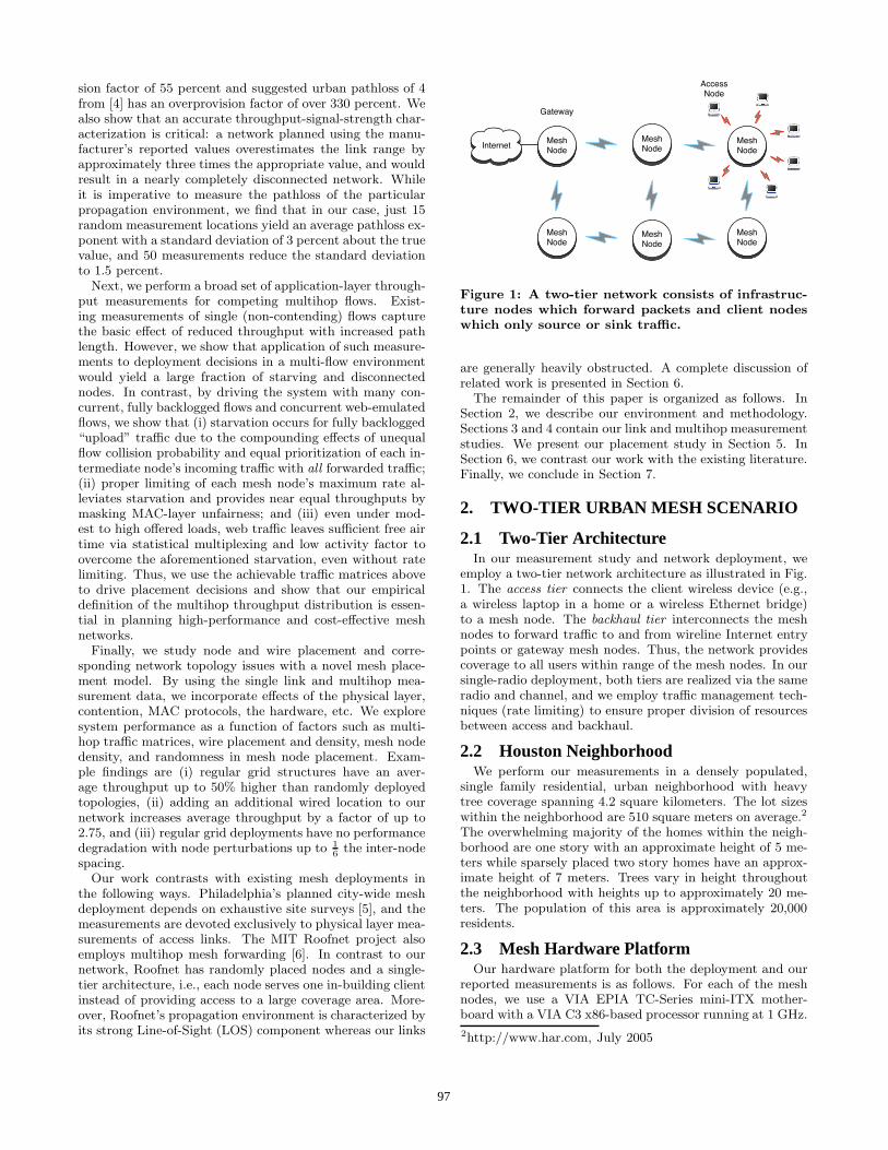
Figure 1: A two-tier network consists of infrastruc-ture nodes which forward packets and client nodeswhich only source or sink traffic.
are generally heavily obstructed. A complete discussion ofrelated work is presented in Section 6.
The remainder of this paper is organized as follows. InSection 2, we describe our environment and methodology.Sections 3 and 4 contain our link and multihop measurementstudies. We present our placement study in Section 5. InSection 6, we contrast our work with the existing literature.Finally, we conclude in Section 7.
2. TWO-TIER URBAN MESH SCENARIO
2.1 Two-Tier ArchitectureIn our measurement study and network deployment, we
employ a two-tier network architecture as illustrated in Fig.1. The access tier connects the client wireless device (e.g.,a wireless laptop in a home or a wireless Ethernet bridge)to a mesh node. The backhaul tier interconnects the meshnodes to forward traffic to and from wireline Internet entrypoints or gateway mesh nodes. Thus, the network providescoverage to all users within range of the mesh nodes. In oursingle-radio deployment, both tiers are realized via the sameradio and channel, and we employ traffic management tech-niques (rate limiting) to ensure proper division of resourcesbetween access and backhaul.
2.2 Houston NeighborhoodWe perform our measurements in a densely populated,
single family residential, urban neighborhood with heavytree coverage spanning 4.2 square kilometers. The lot sizeswithin the neighborhood are 510 square meters on average.2
The overwhelming majority of the homes within the neigh-borhood are one story with an approximate height of 5 me-ters while sparsely placed two story homes have an approx-imate height of 7 meters. Trees vary in height throughoutthe neighborhood with heights up to approximately 20 me-ters. The population of this area is approximately 20,000residents.
2.3 Mesh Hardware PlatformOur hardware platform for both the deployment and our
reported measurements is as follows. For each of the meshnodes, we use a VIA EPIA TC-Series mini-ITX mother-board with a VIA C3 x86-based processor running at 1 GHz.
2http://www.har.com, July 2005
97
In the PCMCIA type II slot, we use an SMC 2532-B 802.11bcard with 200 mW transmission power. The electrical hard-ware is housed in a NEMA 4 waterproof enclosure that canbe externally mounted on residences, schools, libraries, andother commercial property.
The mesh nodes run a minimal version of the Linux oper-ating system which fits in the on-board 32 MB memory chip.We use an open-source version of the LocustWorld3 meshnetworking software that uses AODV routing and HostAPdrivers. The client nodes within our network employ En-genius/Senao CB-3 Ethernet bridges which have 200 mWtransmission power and 3 dBi external omnidirectional an-tennas.
2.4 Mesh AntennaEach mesh node has a 15 dBi omnidirectional antenna
with an 8 degree vertical beamwidth. Selecting antennaheights represents a tradeoff that is affected by the each re-gion’s particular propagation environment. At one extreme,a very high antenna elevation that clears all rooftops andtrees has the advantage of providing strong Line-of-Sight(LOS) links for the backhaul tier. However, several prob-lems arise with high antenna elevations in urban scenarios:(i) high attenuation of access links due to tree canopies andbuildings, (ii) requirement of multiple antennas or anten-nas with substantial energy focused both downward (access)and horizontally (backhaul), and (iii) legal and practical re-strictions on maximum height. Likewise, while low antennaplacement reduces deployment costs, it yields poor propaga-tion paths for both access and backhaul. After completingexperiments to balance these issues (not presented here),we selected an antenna height of 10 meters for the deployednodes within the neighborhood.
3. LINK MEASUREMENTSIn this section, we present the results of our measurements
of single-link performance of mesh nodes in our neighbor-hood. The measurements represent both access and back-haul links and include received signal strength and through-put over a range of distances. We match our data to the-oretical models to find a pathloss exponent and shadowingstandard deviation so that we can accurately determine therange and reliability of the mesh links. As there are noaccepted theoretical models for throughput, we introducean empirical mapping between signal power and achievablethroughput. In Section 5, we discuss the impact of our mea-surements on the performance of a larger system.
3.1 Theoretical PredictionsThe multiplicative effects of the wireless channel are di-
vided into three categories: pathloss, shadowing, and mul-tipath fading [4]. In this work, we focus on pathloss andshadowing because they are the most measurable and pre-dictable effects. Multipath fading produces dramatic vari-ations in signal power, but the variations happen on suchsmall scales of time and space that predicting them is pro-hibitively complex.
Pathloss describes the attenuation experienced by a wire-less signal as a function of distance. Extensive prior empir-ical modeling indicates that signal power decays exponen-tially with distance according to a pathloss exponent that is
3http://www.locustworld.com
particular to the propagation scenario [3]. Pathloss expo-nents are dependent on the location and composition of ob-jects in the environment and therefore add site-specificity tochannel characterization. Pathloss is a very coarse descrip-tion of a propagation scenario that allows us to generalizebetween environments that are similar but not identical.
Shadowing describes the amount of variation in pathlossbetween similar propagation scenarios. For instance, withina single neighborhood, shadowing represents the differencebetween the signal power at different points with the sameestimated pathloss. Prior measurements show that shadow-ing manifests as a zero-mean Gaussian random variable withstandard deviation σε added to the average signal power indBm. The presence of shadowing makes any prediction ofreceived signal power inherently probabilistic. In the follow-ing equation, shadowing is represented by ε, α is the pathlossexponent, and d0 is a reference distance for which we havea measured power level [4].
PdBm(d) = PdBm(d0) − 10αlog10
„d
d0
«+ ε (1)
In the absence of scatterers or other attenuating media,the free space pathloss exponent is 2. With reflective andabsorbent materials in the propagation environment, thepathloss exponent will increase. Pathloss exponents in out-door environments range from 2 to 5 with a rough propor-tionality between the pathloss exponent and the amount ofobstruction between the transmitting and receiving anten-nas [3]. The expected shadowing standard deviation, σε, isapproximately 8 dB [3], [4].
3.2 Access Link Measurements
3.2.1 MethodologyThe following measurements characterize access links be-
tween clients (residences) and mesh nodes. The mesh nodeantennas are mounted at 10 meters while client nodes arefixed at a height of 1 meter. For a single fixed backbone nodeinstallation, we measure throughput and signal strength withthe access node at many representative locations in the sur-rounding neighborhood. We use iperf traffic generator tocreate a fully backlogged UDP flow by connecting a laptopto the access node via Ethernet. We record signal strengthmeasurements provided by the wireless interface in the meshnode. Both of the wireless interfaces have autorate enabledto determine the physical layer transmission rate.
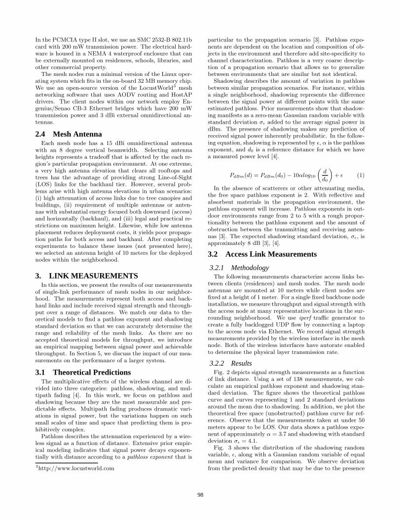
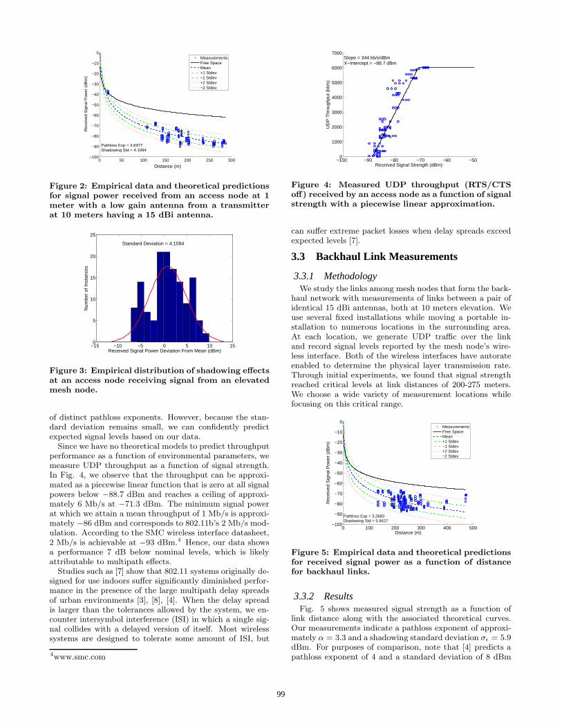
3.2.2 ResultsFig. 2 depicts signal strength measurements as a function
of link distance. Using a set of 138 measurements, we cal-culate an empirical pathloss exponent and shadowing stan-dard deviation. The figure shows the theoretical pathlosscurve and curves representing 1 and 2 standard deviationsaround the mean due to shadowing. In addition, we plot thetheoretical free space (unobstructed) pathloss curve for ref-erence. Observe that the measurements taken at under 50meters appear to be LOS. Our data shows a pathloss expo-nent of approximately α = 3.7 and shadowing with standarddeviation σε = 4.1.
Fig. 3 shows the distribution of the shadowing randomvariable, ε, along with a Gaussian random variable of equalmean and variance for comparison. We observe deviationfrom the predicted density that may be due to the presence
98
0 50 100 150 200 250 300−100
−90
−80
−70
−60
−50
−40
−30
−20
−10
0
Distance (m)
Rec
eive
d S
igna
l Pow
er (
dBm
)
Pathloss Exp = 3.6977Shadowing Std = 4.1094
MeasurementsFree SpaceMean+1 Stdev−1 Stdev+2 Stdev−2 Stdev
Figure 2: Empirical data and theoretical predictionsfor signal power received from an access node at 1meter with a low gain antenna from a transmitterat 10 meters having a 15 dBi antenna.
−15 −10 −5 0 5 10 150
5
10
15
20
25
Received Signal Power Deviation From Mean (dBm)
Num
ber
of In
stan
ces
Standard Deviation = 4.1094
Figure 3: Empirical distribution of shadowing effectsat an access node receiving signal from an elevatedmesh node.
of distinct pathloss exponents. However, because the stan-dard deviation remains small, we can confidently predictexpected signal levels based on our data.
Since we have no theoretical models to predict throughputperformance as a function of environmental parameters, wemeasure UDP throughput as a function of signal strength.In Fig. 4, we observe that the throughput can be approxi-mated as a piecewise linear function that is zero at all signalpowers below −88.7 dBm and reaches a ceiling of approxi-mately 6 Mb/s at −71.3 dBm. The minimum signal powerat which we attain a mean throughput of 1 Mb/s is approxi-mately −86 dBm and corresponds to 802.11b’s 2 Mb/s mod-ulation. According to the SMC wireless interface datasheet,2 Mb/s is achievable at −93 dBm.4 Hence, our data showsa performance 7 dB below nominal levels, which is likelyattributable to multipath effects.
Studies such as [7] show that 802.11 systems originally de-signed for use indoors suffer significantly diminished perfor-mance in the presence of the large multipath delay spreadsof urban environments [3], [8], [4]. When the delay spreadis larger than the tolerances allowed by the system, we en-counter intersymbol interference (ISI) in which a single sig-nal collides with a delayed version of itself. Most wirelesssystems are designed to tolerate some amount of ISI, but
4www.smc.com
−100 −90 −80 −70 −60 −500
1000
2000
3000
4000
5000
6000
7000
Received Signal Strength (dBm)
UD
P T
hrou
ghpu
t (kb
/s)
Slope = 344 kb/s/dBmX−Intercept = −88.7 dBm
Figure 4: Measured UDP throughput (RTS/CTSoff) received by an access node as a function of signalstrength with a piecewise linear approximation.
can suffer extreme packet losses when delay spreads exceedexpected levels [7].
3.3 Backhaul Link Measurements
3.3.1 MethodologyWe study the links among mesh nodes that form the back-
haul network with measurements of links between a pair ofidentical 15 dBi antennas, both at 10 meters elevation. Weuse several fixed installations while moving a portable in-stallation to numerous locations in the surrounding area.At each location, we generate UDP traffic over the linkand record signal levels reported by the mesh node’s wire-less interface. Both of the wireless interfaces have autorateenabled to determine the physical layer transmission rate.Through initial experiments, we found that signal strengthreached critical levels at link distances of 200-275 meters.We choose a wide variety of measurement locations whilefocusing on this critical range.
0 100 200 300 400 500−100
−90
−80
−70
−60
−50
−40
−30
−20
−10
0
Distance (m)
Rec
eive
d S
igna
l Pow
er (
dBm
)
Pathloss Exp = 3.2683Shadowing Std = 5.9427
MeasurementsFree SpaceMean+1 Stdev−1 Stdev+2 Stdev−2 Stdev
Figure 5: Empirical data and theoretical predictionsfor received signal power as a function of distancefor backhaul links.
3.3.2 ResultsFig. 5 shows measured signal strength as a function of
link distance along with the associated theoretical curves.Our measurements indicate a pathloss exponent of approxi-mately α = 3.3 and a shadowing standard deviation σε = 5.9dBm. For purposes of comparison, note that [4] predicts apathloss exponent of 4 and a standard deviation of 8 dBm
99
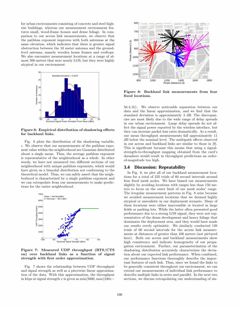
for urban environments consisting of concrete and steel high-rise buildings, whereas our measurement environment fea-tures small, wood-frame houses and dense foliage. In com-parison to our access link measurements, we observe thatthe pathloss exponent improves with both antennas at thesame elevation, which indicates that there is greater signalobstruction between the 10 meter antenna and the ground-level antenna, namely wooden house frames and rooftops.We also encounter measurement locations at a range of al-most 500 meters that were nearly LOS, but they were highlyatypical in our environment.
−20 −15 −10 −5 0 5 10 15 200
5
10
15
20
25
30
Received Signal Power Deviation From Mean (dBm)
Num
ber
of In
stan
ces
Standard Deviation = 5.9427
Figure 6: Empirical distribution of shadowing effectsfor backhaul links.
Fig. 6 plots the distribution of the shadowing variable,ε. We observe that our measurements of the pathloss expo-nent value within the neighborhood are Gaussian distributedabout a single mean. Thus, the average pathloss exponentis representative of the neighborhood as a whole. In otherwords, we have not measured two different sections of ourneighborhood with unique pathloss exponents, which wouldhave given us a bimodal distribution not conforming to thetheoretical model. Thus, we can safely assert that the neigh-borhood is characterized by a single pathloss exponent andwe can extrapolate from our measurements to make predic-tions for the entire neighborhood.
−100 −90 −80 −70 −60 −500
1000
2000
3000
4000
5000
6000
7000Slope = 240 kb/s/dBmX−Intercept = −86.4 dBm
Received Signal Strength (dBm)
UD
P T
hrou
ghpu
t (kb
/s)
Figure 7: Measured UDP throughput (RTS/CTSon) over backhaul links as a function of signalstrength with first order approximation.
Fig. 7 shows the relationship between UDP throughputand signal strength as well as a piecewise linear approxima-tion of the data. With this approximation, the throughputin kbps at signal strength x is given as min(5000, max(240x−
800 1000 1200 1400 1600 1800
600
700
800
900
1000
1100
1200
Pixels (Meters/1.9)
Pix
els
(Met
ers/
1.9)
Figure 8: Backhaul link measurements from fourfixed locations.
56.4, 0)). We observe noticeable separation between ourdata and the linear approximation, and we find that thestandard deviation is approximately 3 dB. The discrepan-cies are most likely due to the wide range of delay spreadsin our urban environment. Large delay spreads do not af-fect the signal power reported by the wireless interface, butthey can increase packet loss rates dramatically. As a result,our mean throughput measurements fall approximately 11dB below the nominal level. The multipath effects observedin our access and backhaul links are similar to those in [9].This is significant because this means that using a signal-strength-to-throughput mapping obtained from the card’sdatasheet would result in throughput predictions an order-of-magnitude too high.
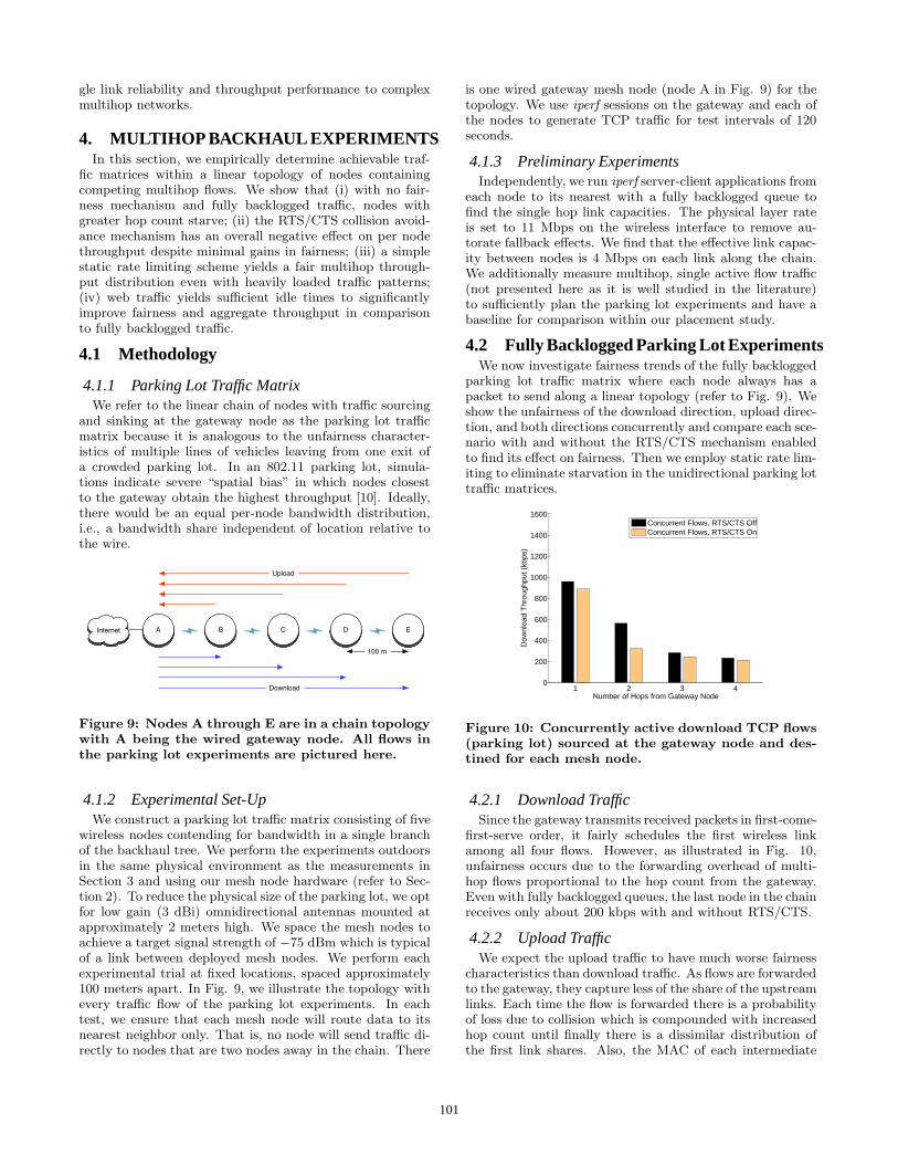
3.4 Discussion: RepeatabilityIn Fig. 8, we plot all of our backhaul measurement loca-
tions for a total of 235 trials of 60 second intervals aroundfour fixed mesh nodes. We have biased our measurementsslightly by avoiding locations with ranges less than 150 me-ters to focus on the outer limit of our mesh nodes’ range.The irregular measurement patterns in Fig. 8 arise becausewe avoided measurement locations that we deemed highlyatypical or unrealistic in our deployment scenario. Many ofthese locations were either inaccessible or located in largefields or parking lots. While the latter often presented goodperformance due to a strong LOS signal, they were not rep-resentative of the dense development and heavy foliage thatdominates the deployment area, and they would have madeour results overly optimistic. We similarly conducted 138trials of 60 second intervals for the access link measure-ments at distances of greater than 100 meters (not picturedhere). Both our access and backhaul measurements showhigh consistency and indicate homogeneity of our propa-gation environment. Further, our parameterization of theshadowing distribution accurately characterizes the devia-tion about our expected link performance. When combined,our performance functions thoroughly describe the impor-tant features of each link. Thus, since we found the links tobe generally consistent throughout our environment, we canextend our measurements of individual link performance todescribe multiple links in series and parallel. In the next twosections, we discuss extrapolating our understanding of sin-
100
gle link reliability and throughput performance to complexmultihop networks.
4. MULTIHOP BACKHAUL EXPERIMENTSIn this section, we empirically determine achievable traf-
fic matrices within a linear topology of nodes containingcompeting multihop flows. We show that (i) with no fair-ness mechanism and fully backlogged traffic, nodes withgreater hop count starve; (ii) the RTS/CTS collision avoid-ance mechanism has an overall negative effect on per nodethroughput despite minimal gains in fairness; (iii) a simplestatic rate limiting scheme yields a fair multihop through-put distribution even with heavily loaded traffic patterns;(iv) web traffic yields sufficient idle times to significantlyimprove fairness and aggregate throughput in comparisonto fully backlogged traffic.
4.1 Methodology
4.1.1 Parking Lot Traffic MatrixWe refer to the linear chain of nodes with traffic sourcing
and sinking at the gateway node as the parking lot trafficmatrix because it is analogous to the unfairness character-istics of multiple lines of vehicles leaving from one exit ofa crowded parking lot. In an 802.11 parking lot, simula-tions indicate severe “spatial bias” in which nodes closestto the gateway obtain the highest throughput [10]. Ideally,there would be an equal per-node bandwidth distribution,i.e., a bandwidth share independent of location relative tothe wire.
A B C D EInternet
Download
Upload
100 m
Figure 9: Nodes A through E are in a chain topologywith A being the wired gateway node. All flows inthe parking lot experiments are pictured here.
4.1.2 Experimental Set-UpWe construct a parking lot traffic matrix consisting of five
wireless nodes contending for bandwidth in a single branchof the backhaul tree. We perform the experiments outdoorsin the same physical environment as the measurements inSection 3 and using our mesh node hardware (refer to Sec-tion 2). To reduce the physical size of the parking lot, we optfor low gain (3 dBi) omnidirectional antennas mounted atapproximately 2 meters high. We space the mesh nodes toachieve a target signal strength of −75 dBm which is typicalof a link between deployed mesh nodes. We perform eachexperimental trial at fixed locations, spaced approximately100 meters apart. In Fig. 9, we illustrate the topology withevery traffic flow of the parking lot experiments. In eachtest, we ensure that each mesh node will route data to itsnearest neighbor only. That is, no node will send traffic di-rectly to nodes that are two nodes away in the chain. There
is one wired gateway mesh node (node A in Fig. 9) for thetopology. We use iperf sessions on the gateway and each ofthe nodes to generate TCP traffic for test intervals of 120seconds.
4.1.3 Preliminary ExperimentsIndependently, we run iperf server-client applications from
each node to its nearest with a fully backlogged queue tofind the single hop link capacities. The physical layer rateis set to 11 Mbps on the wireless interface to remove au-torate fallback effects. We find that the effective link capac-ity between nodes is 4 Mbps on each link along the chain.We additionally measure multihop, single active flow traffic(not presented here as it is well studied in the literature)to sufficiently plan the parking lot experiments and have abaseline for comparison within our placement study.
4.2 Fully Backlogged Parking Lot ExperimentsWe now investigate fairness trends of the fully backlogged
parking lot traffic matrix where each node always has apacket to send along a linear topology (refer to Fig. 9). Weshow the unfairness of the download direction, upload direc-tion, and both directions concurrently and compare each sce-nario with and without the RTS/CTS mechanism enabledto find its effect on fairness. Then we employ static rate lim-iting to eliminate starvation in the unidirectional parking lottraffic matrices.
1 2 3 40
200
400
600
800
1000
1200
1400
1600
Number of Hops from Gateway Node
Dow
nloa
d T
hrou
ghpu
t (kb
ps)
Concurrent Flows, RTS/CTS OffConcurrent Flows, RTS/CTS On
Figure 10: Concurrently active download TCP flows(parking lot) sourced at the gateway node and des-tined for each mesh node.
4.2.1 Download TrafficSince the gateway transmits received packets in first-come-
first-serve order, it fairly schedules the first wireless linkamong all four flows. However, as illustrated in Fig. 10,unfairness occurs due to the forwarding overhead of multi-hop flows proportional to the hop count from the gateway.Even with fully backlogged queues, the last node in the chainreceives only about 200 kbps with and without RTS/CTS.
4.2.2 Upload TrafficWe expect the upload traffic to have much worse fairness
characteristics than download traffic. As flows are forwardedto the gateway, they capture less of the share of the upstreamlinks. Each time the flow is forwarded there is a probabilityof loss due to collision which is compounded with increasedhop count until finally there is a dissimilar distribution ofthe first link shares. Also, the MAC of each intermediate
101
1 2 3 40
500
1000
1500
2000
2500
3000
Number of Hops from Gateway Node
Upl
oad
Thr
ough
put (
kbps
)
Concurrent Flows, RTS/CTS OffConcurrent Flows, RTS/CTS On
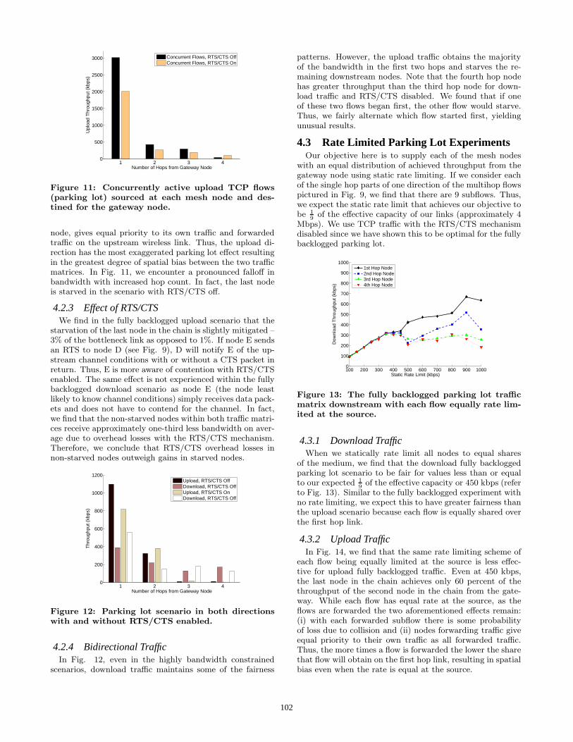
Figure 11: Concurrently active upload TCP flows(parking lot) sourced at each mesh node and des-tined for the gateway node.
node, gives equal priority to its own traffic and forwardedtraffic on the upstream wireless link. Thus, the upload di-rection has the most exaggerated parking lot effect resultingin the greatest degree of spatial bias between the two trafficmatrices. In Fig. 11, we encounter a pronounced falloff inbandwidth with increased hop count. In fact, the last nodeis starved in the scenario with RTS/CTS off.
4.2.3 Effect of RTS/CTSWe find in the fully backlogged upload scenario that the
starvation of the last node in the chain is slightly mitigated –3% of the bottleneck link as opposed to 1%. If node E sendsan RTS to node D (see Fig. 9), D will notify E of the up-stream channel conditions with or without a CTS packet inreturn. Thus, E is more aware of contention with RTS/CTSenabled. The same effect is not experienced within the fullybacklogged download scenario as node E (the node leastlikely to know channel conditions) simply receives data pack-ets and does not have to contend for the channel. In fact,we find that the non-starved nodes within both traffic matri-ces receive approximately one-third less bandwidth on aver-age due to overhead losses with the RTS/CTS mechanism.Therefore, we conclude that RTS/CTS overhead losses innon-starved nodes outweigh gains in starved nodes.
1 2 3 40
200
400
600
800
1000
1200
Number of Hops from Gateway Node
Thr
ough
put (
kbps
)
Upload, RTS/CTS OffDownload, RTS/CTS OffUpload, RTS/CTS OnDownload, RTS/CTS Off
Figure 12: Parking lot scenario in both directionswith and without RTS/CTS enabled.
4.2.4 Bidirectional TrafficIn Fig. 12, even in the highly bandwidth constrained
scenarios, download traffic maintains some of the fairness
patterns. However, the upload traffic obtains the majorityof the bandwidth in the first two hops and starves the re-maining downstream nodes. Note that the fourth hop nodehas greater throughput than the third hop node for down-load traffic and RTS/CTS disabled. We found that if oneof these two flows began first, the other flow would starve.Thus, we fairly alternate which flow started first, yieldingunusual results.
4.3 Rate Limited Parking Lot ExperimentsOur objective here is to supply each of the mesh nodes
with an equal distribution of achieved throughput from thegateway node using static rate limiting. If we consider eachof the single hop parts of one direction of the multihop flowspictured in Fig. 9, we find that there are 9 subflows. Thus,we expect the static rate limit that achieves our objective tobe 1
9of the effective capacity of our links (approximately 4
Mbps). We use TCP traffic with the RTS/CTS mechanismdisabled since we have shown this to be optimal for the fullybacklogged parking lot.
100 200 300 400 500 600 700 800 900 10000
100
200
300
400
500
600
700
800
900
1000
Static Rate Limit (kbps)
Dow
nloa
d T
hrou
ghpu
t (kb
ps)
1st Hop Node2nd Hop Node3rd Hop Node4th Hop Node
Figure 13: The fully backlogged parking lot trafficmatrix downstream with each flow equally rate lim-ited at the source.
4.3.1 Download TrafficWhen we statically rate limit all nodes to equal shares
of the medium, we find that the download fully backloggedparking lot scenario to be fair for values less than or equalto our expected 1
9of the effective capacity or 450 kbps (refer
to Fig. 13). Similar to the fully backlogged experiment withno rate limiting, we expect this to have greater fairness thanthe upload scenario because each flow is equally shared overthe first hop link.
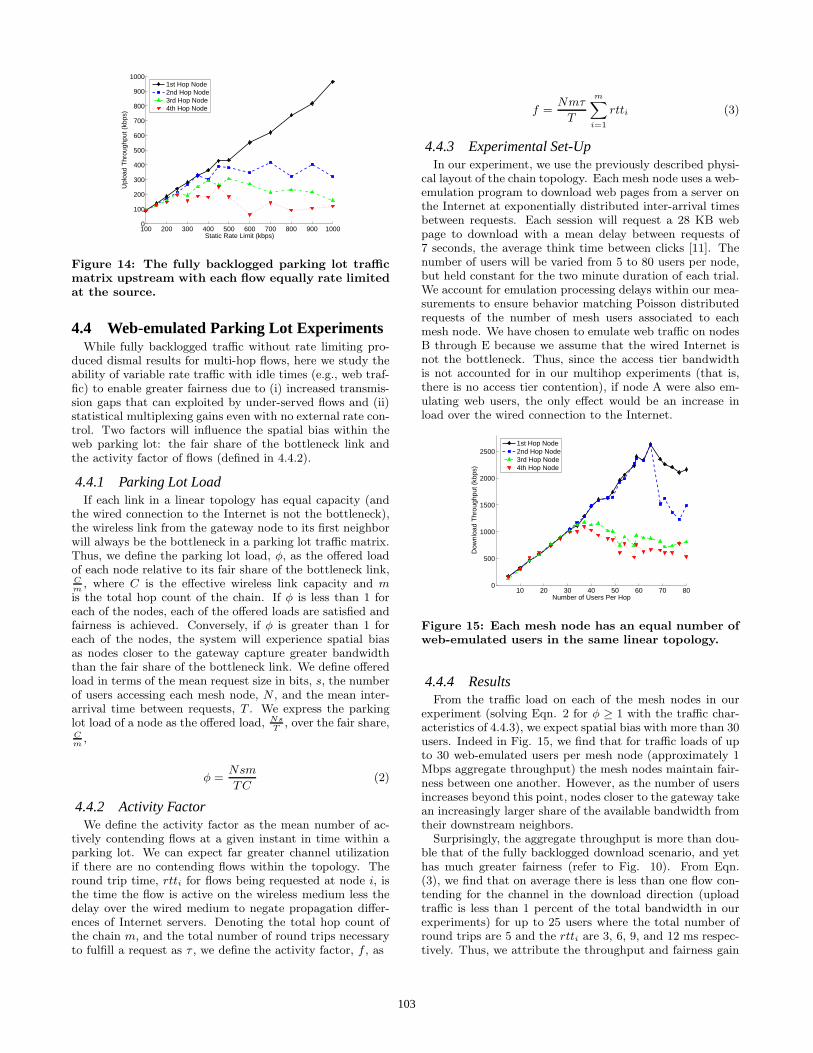
4.3.2 Upload TrafficIn Fig. 14, we find that the same rate limiting scheme of
each flow being equally limited at the source is less effec-tive for upload fully backlogged traffic. Even at 450 kbps,the last node in the chain achieves only 60 percent of thethroughput of the second node in the chain from the gate-way. While each flow has equal rate at the source, as theflows are forwarded the two aforementioned effects remain:(i) with each forwarded subflow there is some probabilityof loss due to collision and (ii) nodes forwarding traffic giveequal priority to their own traffic as all forwarded traffic.Thus, the more times a flow is forwarded the lower the sharethat flow will obtain on the first hop link, resulting in spatialbias even when the rate is equal at the source.
102
100 200 300 400 500 600 700 800 900 10000
100
200
300
400
500
600
700
800
900
1000
Static Rate Limit (kbps)
Upl
oad
Thr
ough
put (
kbps
)
1st Hop Node2nd Hop Node3rd Hop Node4th Hop Node
Figure 14: The fully backlogged parking lot trafficmatrix upstream with each flow equally rate limitedat the source.
4.4 Web-emulated Parking Lot ExperimentsWhile fully backlogged traffic without rate limiting pro-
duced dismal results for multi-hop flows, here we study theability of variable rate traffic with idle times (e.g., web traf-fic) to enable greater fairness due to (i) increased transmis-sion gaps that can exploited by under-served flows and (ii)statistical multiplexing gains even with no external rate con-trol. Two factors will influence the spatial bias within theweb parking lot: the fair share of the bottleneck link andthe activity factor of flows (defined in 4.4.2).
4.4.1 Parking Lot LoadIf each link in a linear topology has equal capacity (and
the wired connection to the Internet is not the bottleneck),the wireless link from the gateway node to its first neighborwill always be the bottleneck in a parking lot traffic matrix.Thus, we define the parking lot load, φ, as the offered loadof each node relative to its fair share of the bottleneck link,Cm
, where C is the effective wireless link capacity and mis the total hop count of the chain. If φ is less than 1 foreach of the nodes, each of the offered loads are satisfied andfairness is achieved. Conversely, if φ is greater than 1 foreach of the nodes, the system will experience spatial biasas nodes closer to the gateway capture greater bandwidththan the fair share of the bottleneck link. We define offeredload in terms of the mean request size in bits, s, the numberof users accessing each mesh node, N , and the mean inter-arrival time between requests, T . We express the parkinglot load of a node as the offered load, Ns
T, over the fair share,
Cm
,
φ =Nsm
TC(2)
4.4.2 Activity FactorWe define the activity factor as the mean number of ac-
tively contending flows at a given instant in time within aparking lot. We can expect far greater channel utilizationif there are no contending flows within the topology. Theround trip time, rtti for flows being requested at node i, isthe time the flow is active on the wireless medium less thedelay over the wired medium to negate propagation differ-ences of Internet servers. Denoting the total hop count ofthe chain m, and the total number of round trips necessaryto fulfill a request as τ , we define the activity factor, f , as
f =Nmτ
T
mXi=1
rtti (3)
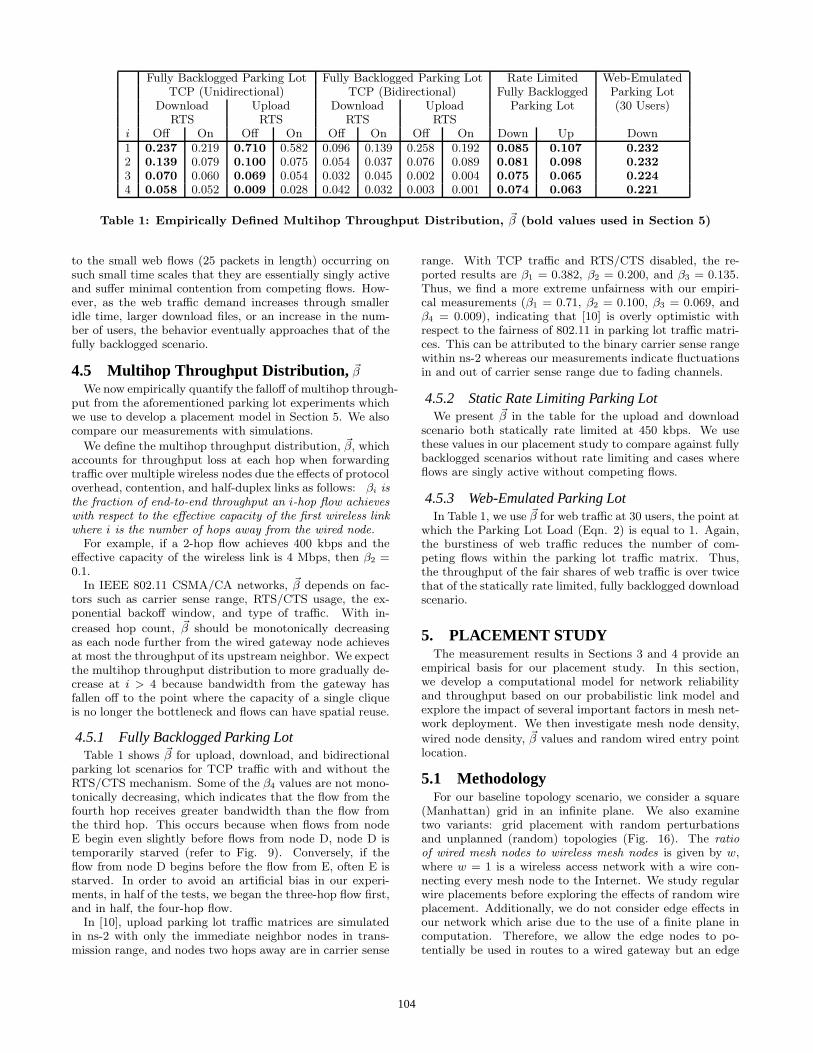
4.4.3 Experimental Set-UpIn our experiment, we use the previously described physi-
cal layout of the chain topology. Each mesh node uses a web-emulation program to download web pages from a server onthe Internet at exponentially distributed inter-arrival timesbetween requests. Each session will request a 28 KB webpage to download with a mean delay between requests of7 seconds, the average think time between clicks [11]. Thenumber of users will be varied from 5 to 80 users per node,but held constant for the two minute duration of each trial.We account for emulation processing delays within our mea-surements to ensure behavior matching Poisson distributedrequests of the number of mesh users associated to eachmesh node. We have chosen to emulate web traffic on nodesB through E because we assume that the wired Internet isnot the bottleneck. Thus, since the access tier bandwidthis not accounted for in our multihop experiments (that is,there is no access tier contention), if node A were also em-ulating web users, the only effect would be an increase inload over the wired connection to the Internet.
10 20 30 40 50 60 70 800
500
1000
1500
2000
2500
Number of Users Per Hop
Dow
nloa
d T
hrou
ghpu
t (kb
ps)
1st Hop Node2nd Hop Node3rd Hop Node4th Hop Node
Figure 15: Each mesh node has an equal number ofweb-emulated users in the same linear topology.
4.4.4 ResultsFrom the traffic load on each of the mesh nodes in our
experiment (solving Eqn. 2 for φ ≥ 1 with the traffic char-acteristics of 4.4.3), we expect spatial bias with more than 30users. Indeed in Fig. 15, we find that for traffic loads of upto 30 web-emulated users per mesh node (approximately 1Mbps aggregate throughput) the mesh nodes maintain fair-ness between one another. However, as the number of usersincreases beyond this point, nodes closer to the gateway takean increasingly larger share of the available bandwidth fromtheir downstream neighbors.
Surprisingly, the aggregate throughput is more than dou-ble that of the fully backlogged download scenario, and yethas much greater fairness (refer to Fig. 10). From Eqn.(3), we find that on average there is less than one flow con-tending for the channel in the download direction (uploadtraffic is less than 1 percent of the total bandwidth in ourexperiments) for up to 25 users where the total number ofround trips are 5 and the rtti are 3, 6, 9, and 12 ms respec-tively. Thus, we attribute the throughput and fairness gain
103
Fully Backlogged Parking Lot Fully Backlogged Parking Lot Rate Limited Web-EmulatedTCP (Unidirectional) TCP (Bidirectional) Fully Backlogged Parking Lot
Download Upload Download Upload Parking Lot (30 Users)RTS RTS RTS RTS
i Off On Off On Off On Off On Down Up Down1 0.237 0.219 0.710 0.582 0.096 0.139 0.258 0.192 0.085 0.107 0.2322 0.139 0.079 0.100 0.075 0.054 0.037 0.076 0.089 0.081 0.098 0.2323 0.070 0.060 0.069 0.054 0.032 0.045 0.002 0.004 0.075 0.065 0.2244 0.058 0.052 0.009 0.028 0.042 0.032 0.003 0.001 0.074 0.063 0.221
Table 1: Empirically Defined Multihop Throughput Distribution, �β (bold values used in Section 5)
to the small web flows (25 packets in length) occurring onsuch small time scales that they are essentially singly activeand suffer minimal contention from competing flows. How-ever, as the web traffic demand increases through smalleridle time, larger download files, or an increase in the num-ber of users, the behavior eventually approaches that of thefully backlogged scenario.
4.5 Multihop Throughput Distribution, �β
We now empirically quantify the falloff of multihop through-put from the aforementioned parking lot experiments whichwe use to develop a placement model in Section 5. We alsocompare our measurements with simulations.
We define the multihop throughput distribution, �β, whichaccounts for throughput loss at each hop when forwardingtraffic over multiple wireless nodes due the effects of protocoloverhead, contention, and half-duplex links as follows: βi isthe fraction of end-to-end throughput an i-hop flow achieveswith respect to the effective capacity of the first wireless linkwhere i is the number of hops away from the wired node.
For example, if a 2-hop flow achieves 400 kbps and theeffective capacity of the wireless link is 4 Mbps, then β2 =0.1.
In IEEE 802.11 CSMA/CA networks, �β depends on fac-tors such as carrier sense range, RTS/CTS usage, the ex-ponential backoff window, and type of traffic. With in-
creased hop count, �β should be monotonically decreasingas each node further from the wired gateway node achievesat most the throughput of its upstream neighbor. We expectthe multihop throughput distribution to more gradually de-crease at i > 4 because bandwidth from the gateway hasfallen off to the point where the capacity of a single cliqueis no longer the bottleneck and flows can have spatial reuse.
4.5.1 Fully Backlogged Parking LotTable 1 shows �β for upload, download, and bidirectional
parking lot scenarios for TCP traffic with and without theRTS/CTS mechanism. Some of the β4 values are not mono-tonically decreasing, which indicates that the flow from thefourth hop receives greater bandwidth than the flow fromthe third hop. This occurs because when flows from nodeE begin even slightly before flows from node D, node D istemporarily starved (refer to Fig. 9). Conversely, if theflow from node D begins before the flow from E, often E isstarved. In order to avoid an artificial bias in our experi-ments, in half of the tests, we began the three-hop flow first,and in half, the four-hop flow.
In [10], upload parking lot traffic matrices are simulatedin ns-2 with only the immediate neighbor nodes in trans-mission range, and nodes two hops away are in carrier sense
range. With TCP traffic and RTS/CTS disabled, the re-ported results are β1 = 0.382, β2 = 0.200, and β3 = 0.135.Thus, we find a more extreme unfairness with our empiri-cal measurements (β1 = 0.71, β2 = 0.100, β3 = 0.069, andβ4 = 0.009), indicating that [10] is overly optimistic withrespect to the fairness of 802.11 in parking lot traffic matri-ces. This can be attributed to the binary carrier sense rangewithin ns-2 whereas our measurements indicate fluctuationsin and out of carrier sense range due to fading channels.
4.5.2 Static Rate Limiting Parking LotWe present �β in the table for the upload and download
scenario both statically rate limited at 450 kbps. We usethese values in our placement study to compare against fullybacklogged scenarios without rate limiting and cases whereflows are singly active without competing flows.
4.5.3 Web-Emulated Parking LotIn Table 1, we use �β for web traffic at 30 users, the point at
which the Parking Lot Load (Eqn. 2) is equal to 1. Again,the burstiness of web traffic reduces the number of com-peting flows within the parking lot traffic matrix. Thus,the throughput of the fair shares of web traffic is over twicethat of the statically rate limited, fully backlogged downloadscenario.
5. PLACEMENT STUDYThe measurement results in Sections 3 and 4 provide an
empirical basis for our placement study. In this section,we develop a computational model for network reliabilityand throughput based on our probabilistic link model andexplore the impact of several important factors in mesh net-work deployment. We then investigate mesh node density,
wired node density, �β values and random wired entry pointlocation.
5.1 MethodologyFor our baseline topology scenario, we consider a square
(Manhattan) grid in an infinite plane. We also examinetwo variants: grid placement with random perturbationsand unplanned (random) topologies (Fig. 16). The ratioof wired mesh nodes to wireless mesh nodes is given by w,where w = 1 is a wireless access network with a wire con-necting every mesh node to the Internet. We study regularwire placements before exploring the effects of random wireplacement. Additionally, we do not consider edge effects inour network which arise due to the use of a finite plane incomputation. Therefore, we allow the edge nodes to po-tentially be used in routes to a wired gateway but an edge
104
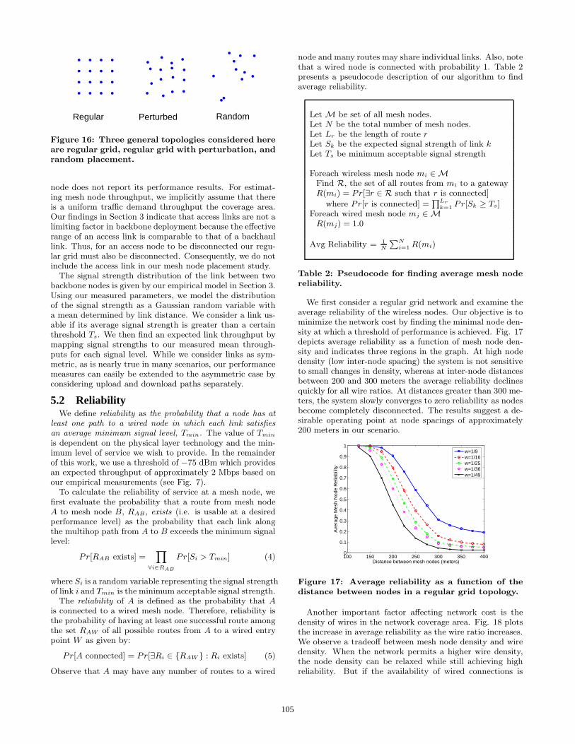
Regular Perturbed Random
Figure 16: Three general topologies considered hereare regular grid, regular grid with perturbation, andrandom placement.
node does not report its performance results. For estimat-ing mesh node throughput, we implicitly assume that thereis a uniform traffic demand throughput the coverage area.Our findings in Section 3 indicate that access links are not alimiting factor in backbone deployment because the effectiverange of an access link is comparable to that of a backhaullink. Thus, for an access node to be disconnected our regu-lar grid must also be disconnected. Consequently, we do notinclude the access link in our mesh node placement study.
The signal strength distribution of the link between twobackbone nodes is given by our empirical model in Section 3.Using our measured parameters, we model the distributionof the signal strength as a Gaussian random variable witha mean determined by link distance. We consider a link us-able if its average signal strength is greater than a certainthreshold Ts. We then find an expected link throughput bymapping signal strengths to our measured mean through-puts for each signal level. While we consider links as sym-metric, as is nearly true in many scenarios, our performancemeasures can easily be extended to the asymmetric case byconsidering upload and download paths separately.
5.2 ReliabilityWe define reliability as the probability that a node has at
least one path to a wired node in which each link satisfiesan average minimum signal level, Tmin. The value of Tmin
is dependent on the physical layer technology and the min-imum level of service we wish to provide. In the remainderof this work, we use a threshold of −75 dBm which providesan expected throughput of approximately 2 Mbps based onour empirical measurements (see Fig. 7).
To calculate the reliability of service at a mesh node, wefirst evaluate the probability that a route from mesh nodeA to mesh node B, RAB, exists (i.e. is usable at a desiredperformance level) as the probability that each link alongthe multihop path from A to B exceeds the minimum signallevel:
Pr[RAB exists] =Y
∀i∈RAB
Pr[Si > Tmin] (4)
where Si is a random variable representing the signal strengthof link i and Tmin is the minimum acceptable signal strength.
The reliability of A is defined as the probability that Ais connected to a wired mesh node. Therefore, reliability isthe probability of having at least one successful route amongthe set RAW of all possible routes from A to a wired entrypoint W as given by:
Pr[A connected] = Pr[∃Ri ∈ {RAW } : Ri exists] (5)
Observe that A may have any number of routes to a wired
node and many routes may share individual links. Also, notethat a wired node is connected with probability 1. Table 2presents a pseudocode description of our algorithm to findaverage reliability.
Let M be set of all mesh nodes.Let N be the total number of mesh nodes.Let Lr be the length of route rLet Sk be the expected signal strength of link kLet Ts be minimum acceptable signal strength
Foreach wireless mesh node mi ∈ MFind R, the set of all routes from mi to a gatewayR(mi) = Pr[∃r ∈ R such that r is connected]
where Pr[r is connected] =QLr
k=1 Pr[Sk ≥ Ts]Foreach wired mesh node mj ∈ M
R(mj) = 1.0
Avg Reliability = 1N
PNi=1 R(mi)
Table 2: Pseudocode for finding average mesh nodereliability.
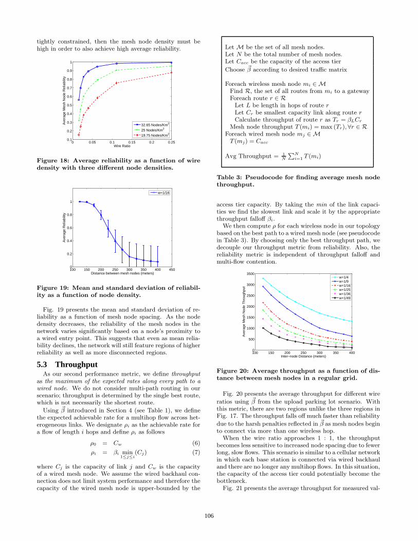
We first consider a regular grid network and examine theaverage reliability of the wireless nodes. Our objective is tominimize the network cost by finding the minimal node den-sity at which a threshold of performance is achieved. Fig. 17depicts average reliability as a function of mesh node den-sity and indicates three regions in the graph. At high nodedensity (low inter-node spacing) the system is not sensitiveto small changes in density, whereas at inter-node distancesbetween 200 and 300 meters the average reliability declinesquickly for all wire ratios. At distances greater than 300 me-ters, the system slowly converges to zero reliability as nodesbecome completely disconnected. The results suggest a de-sirable operating point at node spacings of approximately200 meters in our scenario.
100 150 200 250 300 350 4000
0.1
0.2
0.3
0.4
0.5
0.6
0.7
0.8
0.9
1
Distance between mesh nodes (meters)
Ave
rage
Mes
h N
ode
Rel
iabi
lity
w=1/9w=1/16w=1/25w=1/36w=1/49
Figure 17: Average reliability as a function of thedistance between nodes in a regular grid topology.
Another important factor affecting network cost is thedensity of wires in the network coverage area. Fig. 18 plotsthe increase in average reliability as the wire ratio increases.We observe a tradeoff between mesh node density and wiredensity. When the network permits a higher wire density,the node density can be relaxed while still achieving highreliability. But if the availability of wired connections is
105
tightly constrained, then the mesh node density must behigh in order to also achieve high average reliability.
0 0.05 0.1 0.15 0.2 0.250.1
0.2
0.3
0.4
0.5
0.6
0.7
0.8
0.9
1A
vera
ge M
esh
Nod
e R
elia
bilit
y
Wire Ratio
32.65 Nodes/Km2
25 Nodes/Km2
19.75 Nodes/Km2
Figure 18: Average reliability as a function of wiredensity with three different node densities.
100 150 200 250 300 350 400 4500
0.2
0.4
0.6
0.8
1
Distance between mesh nodes (meters)
Ave
rage
Rel
iabi
lity
w=1/16
Figure 19: Mean and standard deviation of reliabil-ity as a function of node density.
Fig. 19 presents the mean and standard deviation of re-liability as a function of mesh node spacing. As the nodedensity decreases, the reliability of the mesh nodes in thenetwork varies significantly based on a node’s proximity toa wired entry point. This suggests that even as mean relia-bility declines, the network will still feature regions of higherreliability as well as more disconnected regions.
5.3 ThroughputAs our second performance metric, we define throughput
as the maximum of the expected rates along every path to awired node. We do not consider multi-path routing in ourscenario; throughput is determined by the single best route,which is not necessarily the shortest route.
Using �β introduced in Section 4 (see Table 1), we definethe expected achievable rate for a multihop flow across het-erogeneous links. We designate ρi as the achievable rate fora flow of length i hops and define ρi as follows
ρ0 = Cw (6)
ρi = βi min1≤j≤i
(Cj) (7)
where Cj is the capacity of link j and Cw is the capacityof a wired mesh node. We assume the wired backhaul con-nection does not limit system performance and therefore thecapacity of the wired mesh node is upper-bounded by the
Let M be the set of all mesh nodes.Let N be the total number of mesh nodes.Let Cacc be the capacity of the access tier
Choose �β according to desired traffic matrix
Foreach wireless mesh node mi ∈ MFind R, the set of all routes from mi to a gatewayForeach route r ∈ R
Let L be length in hops of route rLet Cr be smallest capacity link along route rCalculate throughput of route r as Tr = βLCr
Mesh node throughput T (mi) = max (Tr),∀r ∈ RForeach wired mesh node mj ∈ M
T (mj) = Cacc
Avg Throughput = 1N
PNi=1 T (mi)
Table 3: Pseudocode for finding average mesh nodethroughput.
access tier capacity. By taking the min of the link capaci-ties we find the slowest link and scale it by the appropriatethroughput falloff βi.
We then compute ρ for each wireless node in our topologybased on the best path to a wired mesh node (see pseudocodein Table 3). By choosing only the best throughput path, wedecouple our throughput metric from reliability. Also, thereliability metric is independent of throughput falloff andmulti-flow contention.
100 150 200 250 300 350 4000
500
1000
1500
2000
2500
3000
3500
Inter−node Distance (meters)
Ave
rage
Mes
h N
ode
Thr
ough
put
w=1/4w=1/9w=1/16w=1/25w=1/36w=1/49
Figure 20: Average throughput as a function of dis-tance between mesh nodes in a regular grid.
Fig. 20 presents the average throughput for different wire
ratios using �β from the upload parking lot scenario. Withthis metric, there are two regions unlike the three regions inFig. 17. The throughput falls off much faster than reliability
due to the harsh penalties reflected in �β as mesh nodes beginto connect via more than one wireless hop.
When the wire ratio approaches 1 : 1, the throughputbecomes less sensitive to increased node spacing due to fewerlong, slow flows. This scenario is similar to a cellular networkin which each base station is connected via wired backhauland there are no longer any multihop flows. In this situation,the capacity of the access tier could potentially become thebottleneck.
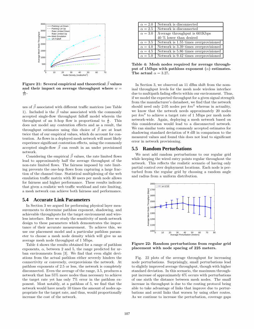
Fig. 21 presents the average throughput for measured val-
106
0 10 20 30 40 50 60 700
500
1000
1500
2000
2500
3000
3500
Node Density (nodes/km2)
Ave
rage
Mes
h N
ode
Thr
ough
put
Parking Lot DownParking Lot UpRate Limited DownRate Limited UpWeb Emulation1/h Falloff
Figure 21: Several empirical and theoretical �β valuesand their impact on average throughput where w =125
.
ues of �β associated with different traffic matrices (see Table
1). Included is the �β value associated with the commonlyaccepted single-flow throughput falloff model wherein thethroughput of an h-hop flow is proportional to 1
h. This
does not model any contention effects and as a result, the
throughput estimates using this choice of �β are at leasttwice that of our empirical values, which do account for con-tention. As flows in a deployed mesh network will most likelyexperience significant contention effects, using the commonly
accepted single-flow �β can result in an under provisionednetwork.
Considering the empirical �β values, the rate limited flowslead to approximately half the average throughput of thenon-rate limited flows. The fairness imposed by rate limit-ing prevents the one-hop flows from capturing a large frac-tion of the channel time. Statistical multiplexing of the webemulation traffic matrix with 30 users per mesh node allowsfor fairness and higher performance. These results indicatethat given a realistic web traffic workload and rate limiting,a mesh network can achieve both fairness and performance.
5.4 Accurate Link ParametersIn Section 3 we argued for performing physical layer mea-
surements to determine pathloss exponent, shadowing, andachievable throughputs for the target environment and wire-less interface. Here we study the sensitivity of mesh networkdesign to these parameters which demonstrates the impor-tance of their accurate measurement. To achieve this, weuse our placement model and a particular pathloss param-eter to choose a mesh node density which will give us anaverage mesh node throughput of 1 Mbps.
Table 4 shows the results obtained for a range of pathlossexponents, α, between 2 and 5, the range predicted for ur-ban environments from [3]. We find that even slight devi-ations from the actual pathloss either severely hinders theconnectivity or conversely, overprovisions the network. Atpathloss exponents of 2.5 or less, the network is completelydisconnected. Even the average of the range, 3.5, produces anetwork that has 55% more nodes than necessary to achievethe target rate yet has only 7% error in the pathloss ex-ponent. Most notably, at a pathloss of 5, we find that thenetwork would have nearly 10 times the amount of nodes ap-propriate for the target rate, and thus, would proportionallyincrease the cost of the network.
α = 2.0 Network is disconnectedα = 2.5 Network is disconnectedα = 3.0 Average throughput is 601Kbps
40 % lower than desiredα = 3.5 Network is 1.55 times overprovisionedα = 4.0 Network is 3.39 times overprovisionedα = 4.5 Network is 5.86 times overprovisionedα = 5.0 Network is 9.42 times overprovisioned
Table 4: Mesh nodes required for average through-put of 1Mbps with pathloss exponent (α) estimates.The actual α = 3.27.
In Section 3, we observed an 11 dBm shift from the nom-inal throughput levels for the mesh node wireless interfacedue to multipath fading effects within our environment. Thus,if we model the expected throughput for a given signal strengthfrom the manufacturer’s datasheet, we find that the networkshould need only 2.05 nodes per km2 whereas in actuality,we know that the network needs approximately 20 nodesper km2 to achieve a target rate of 1 Mbps per mesh nodenetwork-wide. Again, deploying a mesh network based onthis consideration would lead to a disconnected network.We ran similar tests using commonly accepted estimates forshadowing standard deviation of 8 dB in comparison to themeasured values and found this does not lead to significanterror in network provisioning.
5.5 Random PerturbationsWe next add random perturbations to our regular grid
while keeping the wired entry points regular throughout thenetwork. This reflects the realistic scenario of having onlypartial control over deployment locations. Each node is per-turbed from the regular grid by choosing a random angleand radius from a uniform distribution.
0 10 20 30 40 50 60 70 801000
1100
1200
1300
1400
1500
1600
1700
1800
Average Perturbation (meters)
Ave
rage
Mes
h N
ode
Thr
ough
put (
kbps
)
w=1/16
Figure 22: Random perturbations from regular gridplacement with node spacing of 225 meters.
Fig. 22 plots of the average throughput for increasingnode perturbations. Surprisingly, small perturbations leadto slightly improved average throughput, though with higherstandard deviation. In this scenario, the maximum through-put increase of approximately 6% occurs with perturbationsof one sixth the distance between mesh nodes. The smallincrease in throughput is due to the routing protocol beingable to take advantage of links that improve due to pertur-bations and avoid links that worsen by using other routes.As we continue to increase the perturbation, coverage gaps
107
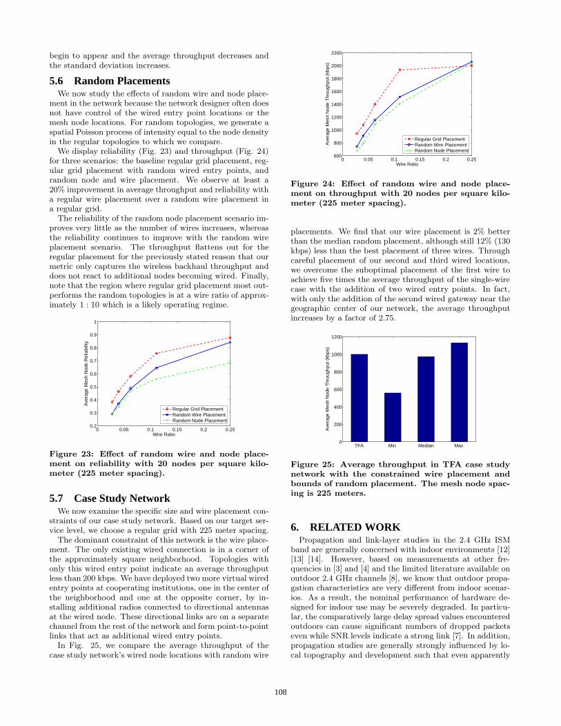
begin to appear and the average throughput decreases andthe standard deviation increases.
5.6 Random PlacementsWe now study the effects of random wire and node place-
ment in the network because the network designer often doesnot have control of the wired entry point locations or themesh node locations. For random topologies, we generate aspatial Poisson process of intensity equal to the node densityin the regular topologies to which we compare.
We display reliability (Fig. 23) and throughput (Fig. 24)for three scenarios: the baseline regular grid placement, reg-ular grid placement with random wired entry points, andrandom node and wire placement. We observe at least a20% improvement in average throughput and reliability witha regular wire placement over a random wire placement ina regular grid.
The reliability of the random node placement scenario im-proves very little as the number of wires increases, whereasthe reliability continues to improve with the random wireplacement scenario. The throughput flattens out for theregular placement for the previously stated reason that ourmetric only captures the wireless backhaul throughput anddoes not react to additional nodes becoming wired. Finally,note that the region where regular grid placement most out-performs the random topologies is at a wire ratio of approx-imately 1 : 10 which is a likely operating regime.
0 0.05 0.1 0.15 0.2 0.250.2
0.3
0.4
0.5
0.6
0.7
0.8
0.9
1
Wire Ratio
Ave
rage
Mes
h N
ode
Rel
iabi
lity
Regular Grid PlacementRandom Wire PlacementRandom Node Placement
Figure 23: Effect of random wire and node place-ment on reliability with 20 nodes per square kilo-meter (225 meter spacing).
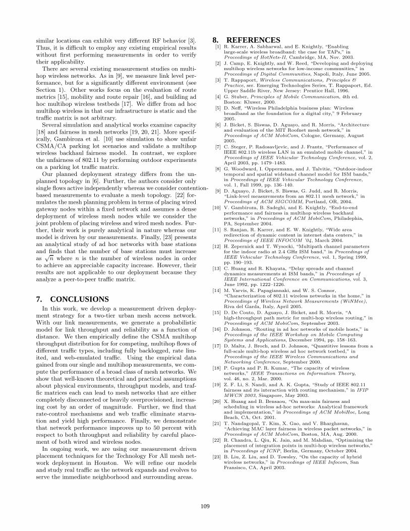
5.7 Case Study NetworkWe now examine the specific size and wire placement con-
straints of our case study network. Based on our target ser-vice level, we choose a regular grid with 225 meter spacing.
The dominant constraint of this network is the wire place-ment. The only existing wired connection is in a corner ofthe approximately square neighborhood. Topologies withonly this wired entry point indicate an average throughputless than 200 kbps. We have deployed two more virtual wiredentry points at cooperating institutions, one in the center ofthe neighborhood and one at the opposite corner, by in-stalling additional radios connected to directional antennasat the wired node. These directional links are on a separatechannel from the rest of the network and form point-to-pointlinks that act as additional wired entry points.
In Fig. 25, we compare the average throughput of thecase study network’s wired node locations with random wire
0 0.05 0.1 0.15 0.2 0.25600
800
1000
1200
1400
1600
1800
2000
2200
Wire Ratio
Ave
rage
Mes
h N
ode
Thr
ough
put (
kbps
)
Regular Grid PlacementRandom Wire PlacementRandom Node Placement
Figure 24: Effect of random wire and node place-ment on throughput with 20 nodes per square kilo-meter (225 meter spacing).
placements. We find that our wire placement is 2% betterthan the median random placement, although still 12% (130kbps) less than the best placement of three wires. Throughcareful placement of our second and third wired locations,we overcome the suboptimal placement of the first wire toachieve five times the average throughput of the single-wirecase with the addition of two wired entry points. In fact,with only the addition of the second wired gateway near thegeographic center of our network, the average throughputincreases by a factor of 2.75.
TFA Min Median Max 0
200
400
600
800
1000
1200
Ave
rage
Mes
h N
ode
Thr
ough
put (
kbps
)
Figure 25: Average throughput in TFA case studynetwork with the constrained wire placement andbounds of random placement. The mesh node spac-ing is 225 meters.
6. RELATED WORKPropagation and link-layer studies in the 2.4 GHz ISM
band are generally concerned with indoor environments [12][13] [14]. However, based on measurements at other fre-quencies in [3] and [4] and the limited literature available onoutdoor 2.4 GHz channels [8], we know that outdoor propa-gation characteristics are very different from indoor scenar-ios. As a result, the nominal performance of hardware de-signed for indoor use may be severely degraded. In particu-lar, the comparatively large delay spread values encounteredoutdoors can cause significant numbers of dropped packetseven while SNR levels indicate a strong link [7]. In addition,propagation studies are generally strongly influenced by lo-cal topography and development such that even apparently
108
similar locations can exhibit very different RF behavior [3].Thus, it is difficult to employ any existing empirical resultswithout first performing measurements in order to verifytheir applicability.
There are several existing measurement studies on multi-hop wireless networks. As in [9], we measure link level per-formance, but for a significantly different environment (seeSection 1). Other works focus on the evaluation of routemetrics [15], mobility and route repair [16], and building adhoc multihop wireless testbeds [17]. We differ from ad hocmultihop wireless in that our infrastructure is static and thetraffic matrix is not arbitrary.
Several simulation and analytical works examine capacity[18] and fairness in mesh networks [19, 20, 21]. More specif-ically, Gambiroza et al. [10] use simulation to show unfairCSMA/CA parking lot scenarios and validate a multihopwireless backhaul fairness model. In contrast, we explorethe unfairness of 802.11 by performing outdoor experimentson a parking lot traffic matrix.
Our planned deployment strategy differs from the un-planned topology in [6]. Further, the authors consider onlysingle flows active independently whereas we consider contention-based measurements to evaluate a mesh topology. [22] for-mulates the mesh planning problem in terms of placing wiredgateway nodes within a fixed network and assumes a densedeployment of wireless mesh nodes while we consider thejoint problem of placing wireless and wired mesh nodes. Fur-ther, their work is purely analytical in nature whereas ourmodel is driven by our measurements. Finally, [23] presentsan analytical study of ad hoc networks with base stationsand finds that the number of base stations must increaseas
√n where n is the number of wireless nodes in order
to achieve an appreciable capacity increase. However, theirresults are not applicable to our deployment because theyanalyze a peer-to-peer traffic matrix.
7. CONCLUSIONSIn this work, we develop a measurement driven deploy-
ment strategy for a two-tier urban mesh access network.With our link measurements, we generate a probabilisticmodel for link throughput and reliability as a function ofdistance. We then empirically define the CSMA multihopthroughput distribution for for competing, multihop flows ofdifferent traffic types, including fully backlogged, rate lim-ited, and web-emulated traffic. Using the empirical datagained from our single and multihop measurements, we com-pute the performance of a broad class of mesh networks. Weshow that well-known theoretical and practical assumptionsabout physical environments, throughput models, and traf-fic matrices each can lead to mesh networks that are eithercompletely disconnected or heavily overprovisioned, increas-ing cost by an order of magnitude. Further, we find thatrate-control mechanisms and web traffic eliminate starva-tion and yield high performance. Finally, we demonstratethat network performance improves up to 50 percent withrespect to both throughput and reliability by careful place-ment of both wired and wireless nodes.
In ongoing work, we are using our measurement drivenplacement techniques for the Technology For All mesh net-work deployment in Houston. We will refine our modelsand study real traffic as the network expands and evolves toserve the immediate neighborhood and surrounding areas.
8. REFERENCES[1] R. Karrer, A. Sabharwal, and E. Knightly, “Enabling
large-scale wireless broadband: the case for TAPs,” inProceedings of HotNets-II, Cambridge, MA, Nov. 2003.
[2] J. Camp, E. Knightly, and W. Reed, “Developing and deployingmultihop wireless networks for low-income communities,” inProceedings of Digital Communities, Napoli, Italy, June 2005.
[3] T. Rappaport, Wireless Communications, Principles &Practice, ser. Emerging Technologies Series, T. Rappaport, Ed.Upper Saddle River, New Jersey: Prentice Hall, 1996.
[4] G. Stuber, Principles of Mobile Communication, 4th ed.Boston: Kluwer, 2000.
[5] D. Neff, “Wireless Philadelphia business plan: Wirelessbroadband as the foundation for a digital city,” 9 February2005.
[6] J. Bicket, S. Biswas, D. Aguayo, and R. Morris, “Architectureand evaluation of the MIT Roofnet mesh network,” inProceedings of ACM MobiCom, Cologne, Germany, August2005.
[7] C. Steger, P. Radosavljevic, and J. Frantz, “Performance ofIEEE 802.11b wireless LAN in an emulated mobile channel,” inProceedings of IEEE Vehicular Technology Conference, vol. 2,April 2003, pp. 1479–1483.
[8] G. Woodward, I. Oppermann, and J. Talvitie, “Outdoor-indoortemporal and spatial wideband channel model for ISM bands,”in Proceedings of IEEE Vehicular Technology Conference,vol. 1, Fall 1999, pp. 136–140.
[9] D. Aguayo, J. Bicket, S. Biswas, G. Judd, and R. Morris,“Link-level measurements from an 802.11 mesh network,” inProceedings of ACM SIGCOMM, Portland, OR, 2004.
[10] V. Gambiroza, B. Sadeghi, and E. Knightly, “End-to-endperformance and fairness in multihop wireless backhaulnetworks,” in Proceedings of ACM MobiCom, Philadephia,PA, September 2004.
[11] S. Ranjan, R. Karrer, and E. W. Knightly, “Wide arearedirection of dynamic content in internet data centers,” inProceedings of IEEE INFOCOM ’04, March 2004.
[12] H. Zepernick and T. Wysocki, “Multipath channel parametersfor the indoor radio at 2.4 GHz ISM band,” in Proceedings ofIEEE Vehicular Technology Conference, vol. 1, Spring 1999,pp. 190–193.
[13] C. Huang and R. Khayata, “Delay spreads and channeldynamics measurements at ISM bands,” in Proceedings ofIEEE International Conference on Communications, vol. 3,June 1992, pp. 1222–1226.
[14] M. Yarvis, K. Papagiannaki, and W. S. Connor,“Characterization of 802.11 wireless networks in the home,” inProceedings of Wireless Network Measurements (WiNMee),Riva del Garda, Italy, April 2005.
[15] D. De Couto, D. Aguayo, J. Bicket, and R. Morris, “Ahigh-throughput path metric for multi-hop wireless routing,” inProceedings of ACM MobiCom, September 2003.
[16] D. Johnson, “Routing in ad hoc networks of mobile hosts,” inProceedings of the IEEE Workshop on Mobile ComputingSystems and Applications, December 1994, pp. 158–163.
[17] D. Maltz, J. Broch, and D. Johnson, “Quantitive lessons from afull-scale multi-hop wireless ad hoc network testbed,” inProceedings of the IEEE Wireless Communications andNetworking Conference, September 2000.
[18] P. Gupta and P. R. Kumar, “The capacity of wirelessnetworks,” IEEE Transactions on Information Theory,vol. 46, no. 2, Mar. 2000.
[19] Z. F. Li, S. Nandi, and A. K. Gupta, “Study of IEEE 802.11fairness and its interaction with routing mechanism,” in IFIPMWCN 2003, Singapore, May 2003.
[20] X. Huang and B. Bensaou, “On max-min fairness andscheduling in wireless ad-hoc networks: Analytical frameworkand implementation,” in Proceedings of ACM MobiHoc, LongBeach, CA, Oct. 2001.
[21] T. Nandagopal, T. Kim, X. Gao, and V. Bharghavan,“Achieving MAC layer fairness in wireless packet networks,” inProceedings of ACM MobiCom, Boston, MA, Aug. 2000.
[22] R. Chandra, L. Qiu, K. Jain, and M. Mahdian, “Optimizing theplacement of integration points in multi-hop wireless networks,”in Proceedings of ICNP, Berlin, Germany, October 2004.
[23] B. Liu, Z. Liu, and D. Towsley, “On the capacity of hybridwireless networks,” in Proceedings of IEEE Infocom, SanFransisco, CA, April 2003.
109