Embed Size (px)
Citation preview
Mechanics(draft)
by James Nearing
Physics Department
University of Miami
Copyright 2008, James Nearing
Permission to copy for
individual or classroom
use is granted.
Bibliography . . . . . . . . . . . iii
0 Mathematical Prependix . . . . . 1SeriesHyperbolic FunctionsCoordinate SystemsVectorsDifferentiationVelocity, AccelerationComplex AlgebraSeparation of variablesConstant Coefficient ODEsMatrices
1 Introduction . . . . . . . . . . 40Dimensions and UnitsTypes of MassConservation LawsAtwood’s Machine
2 One Dimensional Motion . . . . 58Solving F=ma: F(t)Solving F=ma: F(v)Solving F=ma: F(x)Falling with resistanceEquilibriumConservation of Energy
Interlude . . . . . . . . . . . 86
3 Simple Harmonic Motion . . . . 87Simplest CaseComplex ExponentialsDamped OscillatorsOther OscillatorsForced OscillationsStable MotionUnstable MotionCoupled OscillationsNormal ModesGreen’s Functions
Anharmonic Example: x4
4 Three Dimensional Motion . . . 139Projectile MotionGeneral ResultsE and B fieldsMagnetic MirrorsPendulum, large angles
5 Non-Inertial Systems . . . . . . 169Galilean TransformationRotating SystemCoriolis ForceFoucault PendulumCentrifugal ForceShape of the EarthTides
6 Orbits . . . . . . . . . . . . . 200Harmonic OscillatorPlanetary OrbitsKepler ProblemInsolationApproximate SolutionsSpherical PendulumCenter of Mass TransformationAnother OrbitHyperbolic OrbitsTime Dependence
7 Waves . . . . . . . . . . . . . 238A StringStatic caseThe Wave EquationEnergy and PowerReflectionsStanding WavesAn Algebraic AsidePerturbation TheoryStiffnessOther Waves
i
Other VelocitiesWaves and Tides
8 Rigid Body Motion . . . . . . . 276Center of MassAngular MomentumTensor ComponentsPrincipal AxesProperties of EigenvectorsDynamics
9 Special Relativity . . . . . . . . 310Time Dilation, Length ContractionExamplesSpace-Time DiagramsRelative VelocitySuperluminal SpeedsAccelerationRapidity
Energy and MomentumApplicationsYarkovsky EffectConservation Laws
10 Coupled Oscillators . . . . . . . 352Normal ModesScalar ProductsExamplePerturbation Theory
11 Nonlinear Oscillations . . . . . . 367A Method that FailsA KludgeWorkable, but Special MethodGeneral Approach
12 Statics and Bifurcations . . . . 371Bifurcations
ii
Bibliography
Analytical Mechanics by Grant R. Fowles. Brooks-Cole.
Analytical Mechanics by Fowles and Cassiday. A second author was added. I preferthe original.
Mechanics by Symon. Addison-Wesley The same subject as this text, at about thesame level. It’s been in print for almost 40 years, so it’s got to be pretty good.
Introduction to Classical Mechanics by Arya. Allyn and Bacon I think the recentedition is quite good.
Special Relativity by A.P. French. MIT Press I think this remains the best intro-duction to the subject.
Mathematical Methods for Physics and Engineering by Riley, Hobson, and Bence.Cambridge University Press For the quantity of well-written material here, it is sur-prisingly inexpensive in paperback.
Mathematical Methods in the Physical Sciences by Boas. John Wiley Publ Aboutthe right level and with a very useful selection of topics. If you know everything in here,you’ll find all your upper level courses much easier.
Schaum’s Outlines by various. There are many good and inexpensive books in thisseries: for example, “Complex Variables,” “Advanced Calculus,” ”German Grammar,”“Advanced Mathematics for Engineers and Scientists.” Amazon lists hundreds.
Mathematical Tools for Physics by Nearing. Dover Publ In my unbiased opinion,it’s pretty good.
A Brief on Tensor Analysis by James Simmonds. Springer This is the only text ontensors that I will recommend. To anyone. Under any circumstances.
Linear Algebra Done Right by Axler. Springer Don’t let the title turn you away.It’s pretty good.
iii
Mathematical PrependixThis preliminary chapter could as easily be an appendix to the text, but I prefer
to put it here. It is a collection of topics that you will need at many places later on, butthat you don’t have to study in detail now. In each section I will try to indicate wherethe material is used, and when you get to the chapter where you need it I will indicatethe reference here. You should at least skim the material now, so that you will haveseen where it is. If something catches your eye and you want to study it now, don’t letme stop you.
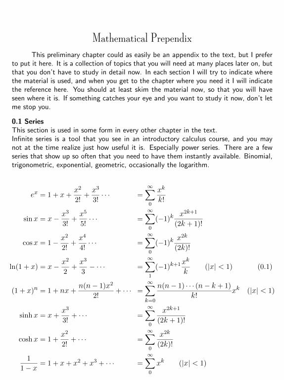
0.1 SeriesThis section is used in some form in every other chapter in the text.Infinite series is a tool that you see in an introductory calculus course, and you maynot at the time realize just how useful it is. Especially power series. There are a fewseries that show up so often that you need to have them instantly available. Binomial,trigonometric, exponential, geometric, occasionally the logarithm.
ex = 1 + x+x2
2!+x3
3!· · · =
∞∑0
xk
k!
sinx = x− x3
3!+x5
5!· · · =
∞∑0
(−1)kx2k+1
(2k + 1)!
cosx = 1− x2
2!+x4
4!· · · =
∞∑0
(−1)kx2k
(2k)!
ln(1 + x) = x− x2
2+x3
3− · · · =
∞∑1
(−1)k+1xk
k(|x| < 1) (0.1)
(1 + x)n = 1 + nx+n(n− 1)x2
2!+ · · · =
∞∑k=0
n(n− 1) · · · (n− k + 1)
k!xk (|x| < 1)
sinhx = x+x3
3!+ · · · =
∞∑0
x2k+1
(2k + 1)!
coshx = 1 +x2
2!+ · · · =
∞∑0
x2k
(2k)!
1
1− x= 1 + x+ x2 + x3 + · · · =
∞∑0
xk (|x| < 1)
1
Mathematical Prependix 2
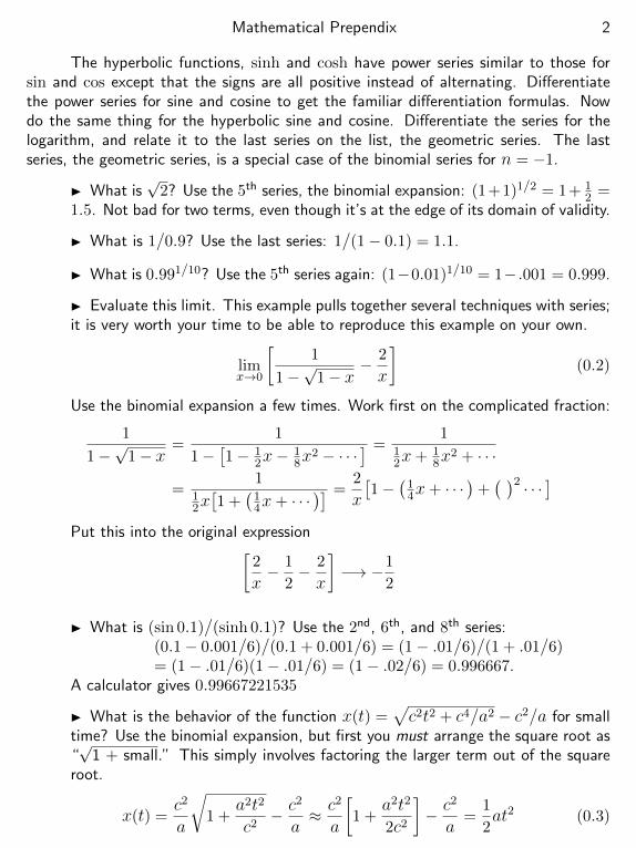
The hyperbolic functions, sinh and cosh have power series similar to those forsin and cos except that the signs are all positive instead of alternating. Differentiatethe power series for sine and cosine to get the familiar differentiation formulas. Nowdo the same thing for the hyperbolic sine and cosine. Differentiate the series for thelogarithm, and relate it to the last series on the list, the geometric series. The lastseries, the geometric series, is a special case of the binomial series for n = −1.
What is√
2? Use the 5th series, the binomial expansion: (1+1)1/2 = 1+ 12 =
1.5. Not bad for two terms, even though it’s at the edge of its domain of validity.
What is 1/0.9? Use the last series: 1/(1− 0.1) = 1.1.
What is 0.991/10? Use the 5th series again: (1−0.01)1/10 = 1− .001 = 0.999.
Evaluate this limit. This example pulls together several techniques with series;it is very worth your time to be able to reproduce this example on your own.
limx→0
[1
1−√
1− x− 2
x
](0.2)
Use the binomial expansion a few times. Work first on the complicated fraction:
1
1−√
1− x=
1
1−[1− 1
2x−18x
2 − · · ·] =
112x+ 1
8x2 + · · ·
=1
12x[1 +
(14x+ · · ·
)] =2
x
[1−
(14x+ · · ·
)+( )2 · · · ]
Put this into the original expression[2
x− 1
2− 2
x
]−→ −1
2
What is (sin 0.1)/(sinh 0.1)? Use the 2nd, 6th, and 8th series:(0.1− 0.001/6)/(0.1 + 0.001/6) = (1− .01/6)/(1 + .01/6)= (1− .01/6)(1− .01/6) = (1− .02/6) = 0.996667.
A calculator gives 0.99667221535
What is the behavior of the function x(t) =√c2t2 + c4/a2 − c2/a for small
time? Use the binomial expansion, but first you must arrange the square root as“√
1 + small.” This simply involves factoring the larger term out of the squareroot.
x(t) =c2
a
√1 +
a2t2
c2− c
2
a≈ c2
a
[1 +
a2t2
2c2
]− c
2
a=
1
2at2 (0.3)
Mathematical Prependix 3
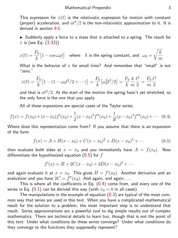
This expression for x(t) is the relativistic expression for motion with constant(proper) acceleration, and at2/2 is the non-relativistic approximation to it. It isderived in section 9.6.
Suddenly apply a force to a mass that is attached to a spring. The result forx is (see Eq. (3.33))
x(t) =F0
k
[1− cosω0t
]where k is the spring constant, and ω0 =
√km
What is the behavior of x for small time? And remember that “small” is not“zero.”
x(t) =F0
k
[1− (1− ω0t
2/2 + · · ·)]
=F0
k
[ω2
0t2/2]
=F0
kkmt2
2=F0
mt2
2
and that is at2/2. At the start of the motion the spring hasn’t yet stretched, sothe only force is the one that you apply.
All of these expansions are special cases of the Taylor series.
f(x) = f(x0)+(x−x0)f ′(x0)+1
2(x−x0)2f ′′(x0)+
1
3!(x−x0)3f ′′′(x0)+ · · · (0.4)
Where does this representation come from? If you assume that there is an expansionof the form
f(x) = A+B(x− x0) +C(x− x0)2 +D(x− x0)3 + · · · (0.5)
then evaluate both sides at x = x0 and you immediately have A = f(x0). Nowdifferentiate the hypothesized equation (0.5) for f
f ′(x) = B + 2C(x− x0) + 3D(x− x0)2 + · · ·
and again evaluate it at x = x0. This gives B = f ′(x0). Another derivative and anevaluation and you have 2C = f ′′(x0). And again, and again, . . .
This is where all the coefficients in Eq. (0.4) come from, and every one of theseries in Eq. (0.1) can be derived this way (with x0 = 0 in all cases).
The manipulations in the example of equation (0.3) are typical of the most com-mon way that series are used in this text. When you have a complicated mathematicalresult for the solution to a problem, the most important step is to understand thatresult. Series approximations are a powerful tool to dig simple results out of complexmathematics. There are technical details to learn too, though that is not the point ofthis text: Under what conditions do these series converge? Under what conditions dothey converge to the functions they supposedly represent?
Mathematical Prependix 4
0.2 Hyperbolic FunctionsThis section appears in chapters 3, 9, and 10.The circular trigonometric functions such as sine and cosine are familiar, but the hy-perbolic trigonometric functions may not be. These functions are defined in terms ofexponentials as
coshx =ex + e−x
2sinhx =
ex − e−x
2tanhx =
sinhxcoshx
(0.6)
Their reciprocals are sech, csch, coth in analogy with the definitions of the correspondingcircular functions.
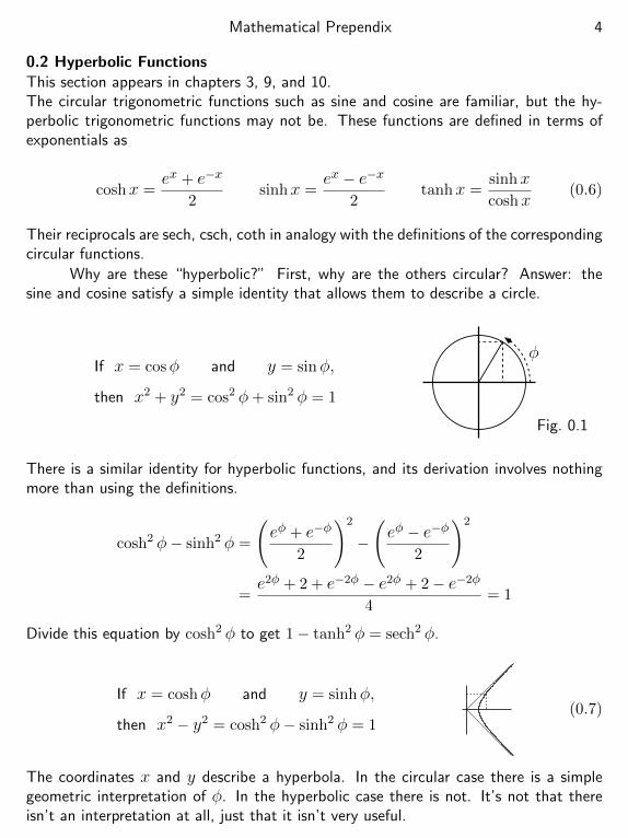
Why are these “hyperbolic?” First, why are the others circular? Answer: thesine and cosine satisfy a simple identity that allows them to describe a circle.
If x = cosφ and y = sinφ,
then x2 + y2 = cos2 φ+ sin2 φ = 1
φ
Fig. 0.1
There is a similar identity for hyperbolic functions, and its derivation involves nothingmore than using the definitions.
cosh2 φ− sinh2 φ =
(eφ + e−φ
2
)2
−
(eφ − e−φ
2
)2
=e2φ + 2 + e−2φ − e2φ + 2− e−2φ
4= 1
Divide this equation by cosh2 φ to get 1− tanh2 φ = sech2 φ.
If x = coshφ and y = sinhφ,
then x2 − y2 = cosh2 φ− sinh2 φ = 1(0.7)
The coordinates x and y describe a hyperbola. In the circular case there is a simplegeometric interpretation of φ. In the hyperbolic case there is not. It’s not that thereisn’t an interpretation at all, just that it isn’t very useful.
Mathematical Prependix 5
What are the derivatives of these functions? Differentiate the equations (0.6) orthe series in (0.1).
ddx
coshx = sinhxddx
sinhx = coshxddx
tanhx = sech2 x (0.8)
The hyperbolic functions involve exponentials, so it should not be too surprisingthat the inverse hyperbolic functions involve logarithms.
y = sinh−1 x means x = sinh y =1
2
(ey − e−y
)(0.9)
Multiply by 2ey and rearrange. The result is a quadratic equation.
e2y − 2xey − 1 =(ey)2 − 2xey − 1 = 0 which implies ey = x±
√x2 + 1
The exponential ey is positive, so that forces the + sign on the right. Now take thelogarithm.
y = sinh−1 x = ln(x+
√x2 + 1
)similarly, cosh−1 x = ln
(x±
√x2 − 1
)(x ≥ 1)
(0.10)
Common circular trigonometric identities have their parallel here. For example
cosh(x+ y) = coshx cosh y + sinhx sinh y
sinh(x+ y) = sinhx cosh y + coshx sinh y(0.11)
Use the series for the circular and the hyperbolic functions to see the relationsbetween the two sets of functions. For example, what is cos(ix)? Substitute ix intothe third series of Eq. (0.1). Similarly, substitute ix into the series for the sine to seeits relation to the hyperbolic sine.
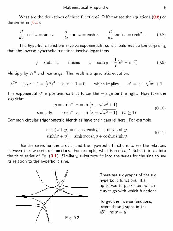
Fig. 0.2
These are six graphs of the sixhyperbolic functions. It’sup to you to puzzle out whichcurves go with which functions.
To get the inverse functions,invert these graphs in the45 line x = y.
Mathematical Prependix 6
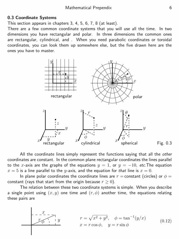
0.3 Coordinate SystemsThis section appears in chapters 3, 4, 5, 6, 7, 8 (at least).There are a few common coordinate systems that you will use all the time. In twodimensions you have rectangular and polar. In three dimensions the common onesare rectangular, cylindrical, and . When you need parabolic coordinates or toroidalcoordinates, you can look them up somewhere else, but the five drawn here are theones you have to master.
xy
x
y
r φ x
y
rectangular polar
xy
z
r
φ
z r
θ
φx
y
z
x
y
z
x
y
z
rectangular cylindrical spherical Fig. 0.3
All the coordinate lines simply represent the functions saying that all the othercoordinates are constant. In the common plane rectangular coordinates the lines parallelto the x-axis are the graphs of the equations y = 1, or y = −10, etc.The equationx = 5 is a line parallel to the y-axis, and the equation for that line is x = 0.
In plane polar coordinates the coordinate lines are r = constant (circles) or φ =constant (rays that start from the origin because r ≥ 0).
The relation between these two coordinate systems is simple. When you describea single point using (x, y) one time and (r, φ) another time, the equations relatingthese pairs are
x
yr φr =
√x2 + y2, φ = tan−1(y/x)
x = r cosφ, y = r sinφ(0.12)
Mathematical Prependix 7
The only place to stumble in this transformation is in computing φ from y and x. Youneed both numbers y and x to specify the quadrant for φ because the inverse tangentis multiple valued. The signs of y and x will however tell you that tan−1(1/1) = π/4and that tan−1(−1/− 1) = 3π/4, thereby removing the ambiguity.
In three dimensions, rectangular coordinates (x, y, z) are much like those in twodimensions, except that an equation such as y = 1 is now a plane perpendicular tothe y-axis as x and z vary from minus to plus infinity. To get a line you need twoequations. For example the pair x = 5 and z = 6 describes a line parallel to they-axis and puncturing the x-z plane at (5, 6). The z-axis itself is described by the twoequations x = 0 and y = 0.
Cylindrical coordinates (r, φ, z) are an extension of two-dimensional polar coor-dinates, simply stretched parallel to the z-axis. The z-coordinate is the same as therectangular z-coordinate, and the (r, φ) are the same as the two dimensional polarcoordinates. The equation z = constant is a plane parallel to the x-y plane as before,and the equation r = constant is now a cylinder centered along the z-axis. The thirdcoordinate φ = constant is a half-plane with one edge along the z-axis (0 < r < ∞and −∞ < z <∞).
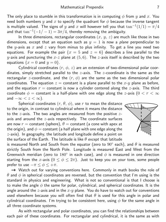
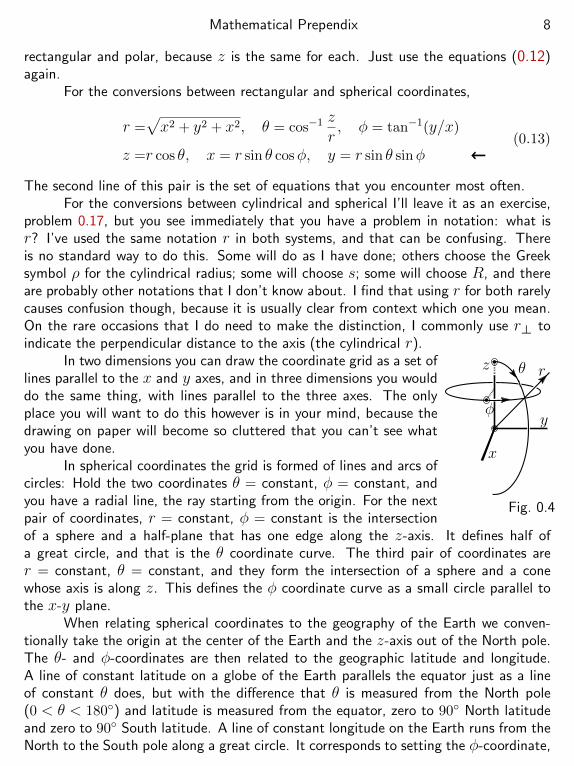
Spherical coordinates (r, θ, φ), use r to mean the distanceto the origin, in contrast to cylindrical where it means the distanceto the z-axis. The two angles are measured from the positive z-axis and around the z-axis respectively. The coordinate surfacesare now r = constant (sphere), θ = constant (a cone with apex atthe origin), and φ = constant (a half plane with one edge along thez-axis). In geography, the latitude and longitude define a point onthe surface of the Earth. The latitude is like θ except that latitudeis measured North and South from the equator (zero to 90 each), and θ is measuredstrictly South from the North Pole. Longitude is measured East and West from theGreenwich meridian (zero to 180 in each case), and φ is measured in one directionstarting from the x-axis (0 ≤ φ ≤ 2π). Just to keep you on your toes, some peopleprefer to use −π ≤ φ ≤ +π.→ Watch out for varying conventions here. Commonly in math books the role of
θ and φ in spherical coordinates are reversed, but the convention that I’m using is thestandard in physics and engineering. What is not so conventional is that I choose isto make the angle φ the same for polar, cylindrical, and spherical coordinates. It is theangle around the z-axis and in the x-y plane. You do have to watch out for conventionsused elsewhere because you will often find that θ is used for this angle in polar andcylindrical coordinates. I’m trying to be consistent here, using φ for the same angle inall three coordinate systems.
As with rectangular and polar coordinates, you can find the relationships betweeneach pair of these coordinates. For rectangular and cylindrical, it is the same as with
Mathematical Prependix 8
rectangular and polar, because z is the same for each. Just use the equations (0.12)again.
For the conversions between rectangular and spherical coordinates,
r =√x2 + y2 + x2, θ = cos−1 z
r, φ = tan−1(y/x)
z =r cos θ, x = r sin θ cosφ, y = r sin θ sinφ ←
(0.13)
The second line of this pair is the set of equations that you encounter most often.For the conversions between cylindrical and spherical I’ll leave it as an exercise,
problem 0.17, but you see immediately that you have a problem in notation: what isr? I’ve used the same notation r in both systems, and that can be confusing. Thereis no standard way to do this. Some will do as I have done; others choose the Greeksymbol ρ for the cylindrical radius; some will choose s; some will choose R, and thereare probably other notations that I don’t know about. I find that using r for both rarelycauses confusion though, because it is usually clear from context which one you mean.On the rare occasions that I do need to make the distinction, I commonly use r⊥ toindicate the perpendicular distance to the axis (the cylindrical r).
x
y
z r
φ
θ
Fig. 0.4
In two dimensions you can draw the coordinate grid as a set oflines parallel to the x and y axes, and in three dimensions you woulddo the same thing, with lines parallel to the three axes. The onlyplace you will want to do this however is in your mind, because thedrawing on paper will become so cluttered that you can’t see whatyou have done.
In spherical coordinates the grid is formed of lines and arcs ofcircles: Hold the two coordinates θ = constant, φ = constant, andyou have a radial line, the ray starting from the origin. For the nextpair of coordinates, r = constant, φ = constant is the intersectionof a sphere and a half-plane that has one edge along the z-axis. It defines half ofa great circle, and that is the θ coordinate curve. The third pair of coordinates arer = constant, θ = constant, and they form the intersection of a sphere and a conewhose axis is along z. This defines the φ coordinate curve as a small circle parallel tothe x-y plane.
When relating spherical coordinates to the geography of the Earth we conven-tionally take the origin at the center of the Earth and the z-axis out of the North pole.The θ- and φ-coordinates are then related to the geographic latitude and longitude.A line of constant latitude on a globe of the Earth parallels the equator just as a lineof constant θ does, but with the difference that θ is measured from the North pole(0 < θ < 180) and latitude is measured from the equator, zero to 90 North latitudeand zero to 90 South latitude. A line of constant longitude on the Earth runs from theNorth to the South pole along a great circle. It corresponds to setting the φ-coordinate,
Mathematical Prependix 9
and the difference this time is that longitude is measured zero to 180 East and Westfrom the line through Greenwich, England while φ is measured from the direction ofthe x-axis. Most commonly 0 < φ < 2π instead of −π to +π (but not always).
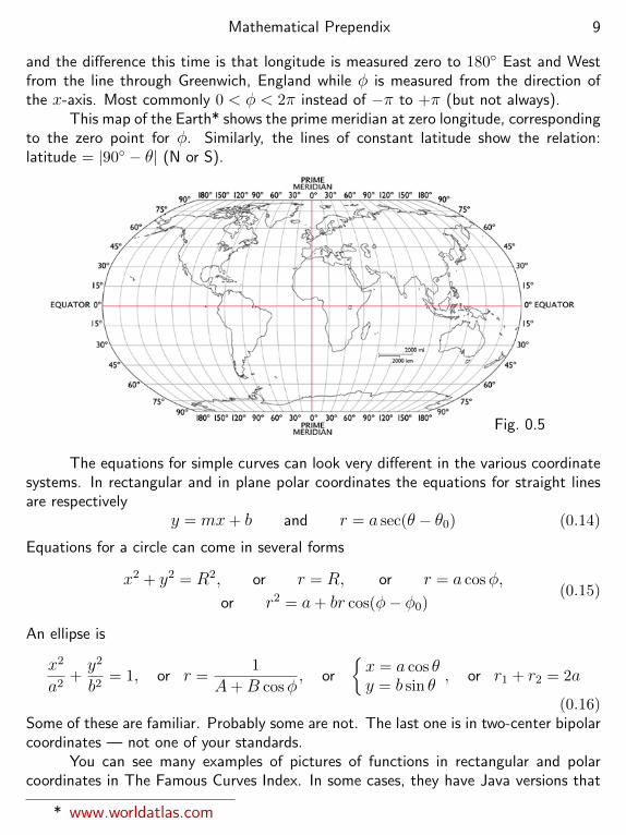
This map of the Earth* shows the prime meridian at zero longitude, correspondingto the zero point for φ. Similarly, the lines of constant latitude show the relation:latitude = |90 − θ| (N or S).
Fig. 0.5
The equations for simple curves can look very different in the various coordinatesystems. In rectangular and in plane polar coordinates the equations for straight linesare respectively
y = mx+ b and r = a sec(θ − θ0) (0.14)
Equations for a circle can come in several forms
x2 + y2 = R2, or r = R, or r = a cosφ,
or r2 = a+ br cos(φ− φ0)(0.15)
An ellipse is
x2
a2+y2
b2= 1, or r =
1
A+B cosφ, or
x = a cos θy = b sin θ
, or r1 + r2 = 2a
(0.16)Some of these are familiar. Probably some are not. The last one is in two-center bipolarcoordinates — not one of your standards.
You can see many examples of pictures of functions in rectangular and polarcoordinates in The Famous Curves Index. In some cases, they have Java versions that
* www.worldatlas.com
Mathematical Prependix 10
allow you to play with the parameters.www-groups.dcs.st-and.ac.uk/˜history/Curves/Curves.html
Areas and VolumesOne of the traditional uses for integration is to computes areas and volumes. Evenwhen that’s not the aim you still need to know how to set up such problems. Whenyou compute moments of inertia or a center of mass it’s a tool you will use.
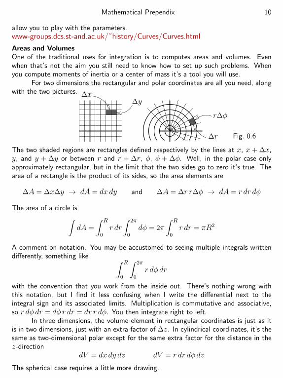
For two dimensions the rectangular and polar coordinates are all you need, alongwith the two pictures. ∆x
∆y
∆r
r∆φ
Fig. 0.6
The two shaded regions are rectangles defined respectively by the lines at x, x + ∆x,y, and y + ∆y or between r and r + ∆r, φ, φ + ∆φ. Well, in the polar case onlyapproximately rectangular, but in the limit that the two sides go to zero it’s true. Thearea of a rectangle is the product of its sides, so the area elements are
∆A = ∆x∆y → dA = dxdy and ∆A = ∆r r∆φ → dA = r dr dφ
The area of a circle is∫dA =
∫ R
0r dr
∫ 2π
0dφ = 2π
∫ R
0r dr = πR2
A comment on notation. You may be accustomed to seeing multiple integrals writtendifferently, something like ∫ R
0
∫ 2π
0r dφdr
with the convention that you work from the inside out. There’s nothing wrong withthis notation, but I find it less confusing when I write the differential next to theintegral sign and its associated limits. Multiplication is commutative and associative,so r dφdr = dφ r dr = dr r dφ. You then integrate right to left.
In three dimensions, the volume element in rectangular coordinates is just as itis in two dimensions, just with an extra factor of ∆z. In cylindrical coordinates, it’s thesame as two-dimensional polar except for the same extra factor for the distance in thez-direction
dV = dxdy dz dV = r dr dφdz
The spherical case requires a little more drawing.
Mathematical Prependix 11
x
y
z
φ
θ
r sin θ
r dθ
r sin θ dφ
Fig. 0.7
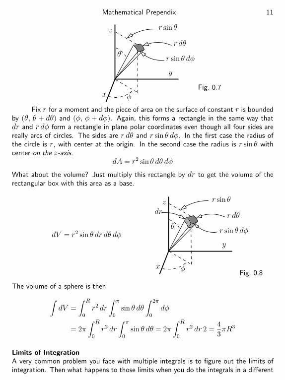
Fix r for a moment and the piece of area on the surface of constant r is boundedby (θ, θ + dθ) and (φ, φ + dφ). Again, this forms a rectangle in the same way thatdr and r dφ form a rectangle in plane polar coordinates even though all four sides arereally arcs of circles. The sides are r dθ and r sin θ dφ. In the first case the radius ofthe circle is r, with center at the origin. In the second case the radius is r sin θ withcenter on the z-axis.
dA = r2 sin θ dθ dφ
What about the volume? Just multiply this rectangle by dr to get the volume of therectangular box with this area as a base.
dV = r2 sin θ dr dθ dφ
x
y
z
φ
θ
r sin θ
r dθ
r sin θ dφ
dr
Fig. 0.8
The volume of a sphere is then∫dV =
∫ R
0r2 dr
∫ π
0sin θ dθ
∫ 2π
0dφ
= 2π∫ R
0r2 dr
∫ π
0sin θ dθ = 2π
∫ R
0r2 dr 2 =
4
3πR3
Limits of IntegrationA very common problem you face with multiple integrals is to figure out the limits ofintegration. Then what happens to those limits when you do the integrals in a different
Mathematical Prependix 12
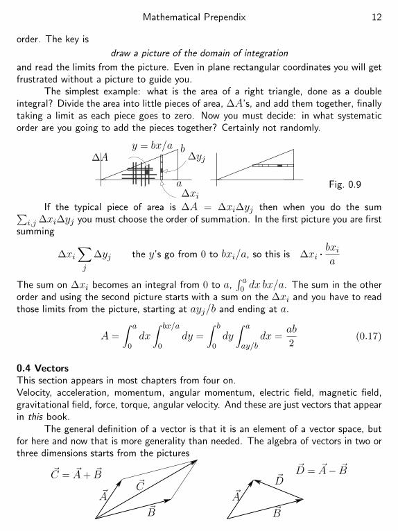
order. The key is
draw a picture of the domain of integration
and read the limits from the picture. Even in plane rectangular coordinates you will getfrustrated without a picture to guide you.
The simplest example: what is the area of a right triangle, done as a doubleintegral? Divide the area into little pieces of area, ∆A’s, and add them together, finallytaking a limit as each piece goes to zero. Now you must decide: in what systematicorder are you going to add the pieces together? Certainly not randomly.
∆A
∆xi
∆yj
a
by = bx/a
Fig. 0.9
If the typical piece of area is ∆A = ∆xi∆yj then when you do the sum∑i,j ∆xi∆yj you must choose the order of summation. In the first picture you are first
summing
∆xi∑j
∆yj the y’s go from 0 to bxi/a, so this is ∆xi . bxia
The sum on ∆xi becomes an integral from 0 to a,∫ a
0 dx bx/a. The sum in the otherorder and using the second picture starts with a sum on the ∆xi and you have to readthose limits from the picture, starting at ayj/b and ending at a.
A =
∫ a
0dx∫ bx/a
0dy =
∫ b
0dy∫ a
ay/bdx =
ab2
(0.17)
0.4 VectorsThis section appears in most chapters from four on.Velocity, acceleration, momentum, angular momentum, electric field, magnetic field,gravitational field, force, torque, angular velocity. And these are just vectors that appearin this book.
The general definition of a vector is that it is an element of a vector space, butfor here and now that is more generality than needed. The algebra of vectors in two orthree dimensions starts from the pictures
~A~B
~C~A
~B
~D~C = ~A+ ~B
~D = ~A− ~B
Mathematical Prependix 13
and these pictures apply whether you are talking about gravity or momentum or anyof the other vectors listed above. There is a mathematical theorem guaranteeing this,saying that once you know you are working with three dimensional vectors, then theyare all essentially the same. In mathematical jargon, “isomorphic.” The same for twodimensions (or seven). This means that you don’t have to learn everything differentlyfor different sorts of vectors — they all behave the same way.
Does a velocity vector look like a line with an arrowhead attached? Very few carstoday have arrows sticking out of the front end, designed to skewer pedestrians,* butthe import of this statement about vectors is that it doesn’t matter. You can use thesepictures to model velocity or magnetic fields or any other vector and you are guaranteedthat they all give the same results. This is why you study the geometry of vectors asa subject of its own. You don’t have to relearn it when you encounter the next sort ofvector.
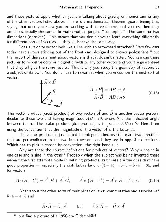
~A
~B
~A× ~B
θ
∣∣ ~A× ~B∣∣ = AB sin θ
~A . ~B = AB cos θ(0.18)
The vector product (cross product) of two vectors ~A and ~B is another vector perpen-dicular to these two and having magnitude AB sin θ, where θ is the indicated anglebetween them. The scalar product (dot product) is the scalar AB cos θ. Here I am
using the convention that the magnitude of the vector ~A is the letter A.The vector product as just stated is ambiguous because there are two directions
that are perpendicular to the two input vectors, and they are in opposite directions.Which one to pick is chosen by convention: the right-hand rule.
Why are these the correct definitions for products of vectors? Why a cosine inone case and a sine in the other? Probably when the subject was being invented theseweren’t the first attempts made in defining products, but these are the ones that havegood properties — especially the distributive law. 5 .(3 + 4) = 5 . 3 + 5 . 4 = 35, andfor vectors
~A .( ~B + ~C
)= ~A . ~B + ~A . ~C, ~A×
( ~B + ~C)
= ~A× ~B + ~A× ~C (0.19)
What about the other sorts of multiplication laws: commutative and associative?5 . 4 = 4 . 5 and
~A . ~B = ~B . ~A, but ~A× ~B = − ~B × ~A
* but find a picture of a 1950-era Oldsmobile!
Mathematical Prependix 14
so the commutative rule works for the dot product but not for the cross product. Itanti-commutes instead. For the associative law, 5 .(3 . 4) = (5 . 3) . 4 = 60, but
~A .( ~B . ~C) doesn’t make any sense. The dot product is between vectors.
For the cross product, ~A× ( ~B × ~C) makes sense, but it is not associative. The closestthat it comes is the Jacobi identity,
~A× ( ~B × ~C) + ~B × (~C × ~A) + ~C × ( ~A× ~B) = 0
This is useful elsewhere, but it won’t appear again in this text.
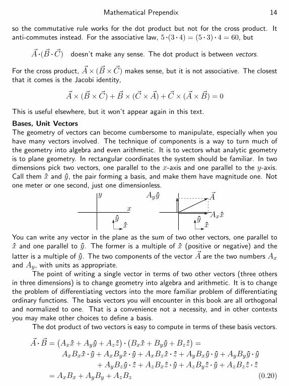
Bases, Unit VectorsThe geometry of vectors can become cumbersome to manipulate, especially when youhave many vectors involved. The technique of components is a way to turn much ofthe geometry into algebra and even arithmetic. It is to vectors what analytic geometryis to plane geometry. In rectangular coordinates the system should be familiar. In twodimensions pick two vectors, one parallel to the x-axis and one parallel to the y-axis.Call them x and y, the pair forming a basis, and make them have magnitude one. Notone meter or one second, just one dimensionless.
x
y
xy
xy
~A
Axx
Ayy
You can write any vector in the plane as the sum of two other vectors, one parallel tox and one parallel to y. The former is a multiple of x (positive or negative) and the
latter is a multiple of y. The two components of the vector ~A are the two numbers Axand Ay, with units as appropriate.
The point of writing a single vector in terms of two other vectors (three othersin three dimensions) is to change geometry into algebra and arithmetic. It is to changethe problem of differentiating vectors into the more familiar problem of differentiatingordinary functions. The basis vectors you will encounter in this book are all orthogonaland normalized to one. That is a convenience not a necessity, and in other contextsyou may make other choices to define a basis.
The dot product of two vectors is easy to compute in terms of these basis vectors.
~A . ~B =(Axx+Ayy +Az z
).(Bxx+Byy +Bz z
)=
AxBxx . y +AxByx . y +AxBzx . z +AyBxy . y +AyByy . y
+AyBz y . z +AzBxz . y +AzBy z . y +AzBz z . z
= AxBx +AyBy +AzBz (0.20)
Mathematical Prependix 15
The simplicity appears because the basis vectors are “orthonormal.” That is, each hasunit magnitude and they are mutually perpendicular.
Does the product rule for derivatives work for the product of vectors? Yes, andyou can see why by differentiating the component form:
ddt~A . ~B =
dAxdt
Bx +AxdBxdt
+ · · · = d ~Adt
. ~B + ~A . d~Bdt
The same analysis applies to the cross product.
Index NotationA convenient and powerful notation to manipulate the components of vectors: Denotethe basis vectors by a unified notation, ~e1, ~e2, and ~e3 instead of respectively x, y, andz. You then write the vectors as
~A = A1~e1 +A2~e2 +A3~e3 and ~B = B1~e1 +B2~e2 +B3~e3
That these vectors are orthogonal and unit vectors translates to
~e1 .~e2 = 0, ~e3 .~e3 = 1, and all the other combinations
Introduce a standard notation:
δij =
1 if i = j0 if i 6= j
then ~ei .~ej = δij (0.21)
where the indices i and j take on any and all of the values 1, 2, 3. This is called theKronecker delta symbol.
The dot product is exactly the same as in Eq. (0.20), only the final result justhas subscripts 1, 2, 3 instead of x, y, x. It doesn’t seem to be worth all the trouble doesit? It is. First a version of the calculation in this notation.
~A . ~B =∑i
Ai~ei .∑j
Bj~ej =∑i
∑j
AiBj~ei .~ej =∑i
∑j
AiBjδij
Now do the sum on j∑j
Bjδij = Bi Remember: δij = 0 for the two terms where j 6= i
The rest is∑iAiBi, exactly as in Eq. (0.20).
Mathematical Prependix 16
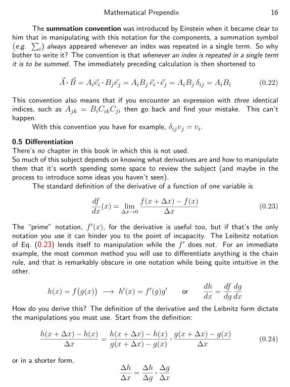
The summation convention was introduced by Einstein when it became clear tohim that in manipulating with this notation for the components, a summation symbol(
e.g.∑i) always appeared whenever an index was repeated in a single term. So why
bother to write it? The convention is that whenever an index is repeated in a single termit is to be summed. The immediately preceding calculation is then shortened to
~A . ~B = Ai~ei .Bj~ej = AiBj ~ei .~ej = AiBj δij = AiBi (0.22)
This convention also means that if you encounter an expression with three identicalindices, such as Ajk = BiCikCji then go back and find your mistake. This can’thappen.
With this convention you have for example, δijvj = vi.
0.5 DifferentiationThere’s no chapter in this book in which this is not used.So much of this subject depends on knowing what derivatives are and how to manipulatethem that it’s worth spending some space to review the subject (and maybe in theprocess to introduce some ideas you haven’t seen).
The standard definition of the derivative of a function of one variable is
dfdx
(x) = lim∆x→0
f(x+ ∆x)− f(x)
∆x(0.23)
The “prime” notation, f ′(x), for the derivative is useful too, but if that’s the onlynotation you use it can hinder you to the point of incapacity. The Leibnitz notationof Eq. (0.23) lends itself to manipulation while the f ′ does not. For an immediateexample, the most common method you will use to differentiate anything is the chainrule, and that is remarkably obscure in one notation while being quite intuitive in theother.
h(x) = f(g(x)
)−→ h′(x) = f ′(g)g′ or
dhdx
=dfdgdgdx
How do you derive this? The definition of the derivative and the Leibnitz form dictatethe manipulations you must use. Start from the definition:
h(x+ ∆x)− h(x)
∆x=h(x+ ∆x)− h(x)
g(x+ ∆x)− g(x). g(x+ ∆x)− g(x)
∆x(0.24)
or in a shorter form,∆h∆x
=∆h∆g
. ∆g∆x
Mathematical Prependix 17
As ∆x → 0, the increment in g must approach zero also, as otherwise its derivativewould not exist and the chain rule would not apply.* The second factor in Eq. (0.24)becomes, in the limit that ∆x → 0, the derivative dg/dx. Also, because in the samelimit ∆g = g(x+ ∆x)− g(x)→ 0, the first factor becomes df/dg, and that ends thederivation. A common way to write the composition of functions is to use, instead ofh(x) = f
(g(x)
), the notation h = f g.
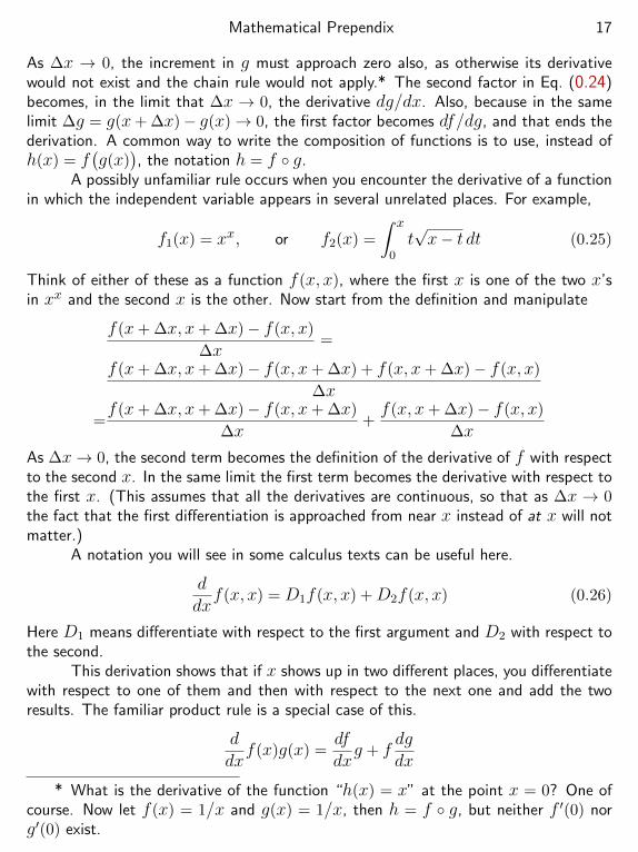
A possibly unfamiliar rule occurs when you encounter the derivative of a functionin which the independent variable appears in several unrelated places. For example,
f1(x) = xx, or f2(x) =
∫ x
0t√x− t dt (0.25)
Think of either of these as a function f(x, x), where the first x is one of the two x’sin xx and the second x is the other. Now start from the definition and manipulate
f(x+ ∆x, x+ ∆x)− f(x, x)
∆x=
f(x+ ∆x, x+ ∆x)− f(x, x+ ∆x) + f(x, x+ ∆x)− f(x, x)
∆x
=f(x+ ∆x, x+ ∆x)− f(x, x+ ∆x)
∆x+f(x, x+ ∆x)− f(x, x)
∆x
As ∆x→ 0, the second term becomes the definition of the derivative of f with respectto the second x. In the same limit the first term becomes the derivative with respect tothe first x. (This assumes that all the derivatives are continuous, so that as ∆x → 0the fact that the first differentiation is approached from near x instead of at x will notmatter.)
A notation you will see in some calculus texts can be useful here.
ddxf(x, x) = D1f(x, x) +D2f(x, x) (0.26)
Here D1 means differentiate with respect to the first argument and D2 with respect tothe second.
This derivation shows that if x shows up in two different places, you differentiatewith respect to one of them and then with respect to the next one and add the tworesults. The familiar product rule is a special case of this.
ddxf(x)g(x) =
dfdxg + f
dgdx
* What is the derivative of the function “h(x) = x” at the point x = 0? One ofcourse. Now let f(x) = 1/x and g(x) = 1/x, then h = f g, but neither f ′(0) norg′(0) exist.
Mathematical Prependix 18
In the less familiar cases,
df1
dx=
ddxxx = xxx−1 + lnxxx = xx(1 + lnx)
ordf2
dx= 0 +
1
2
∫ x
0
t√x− t
dt
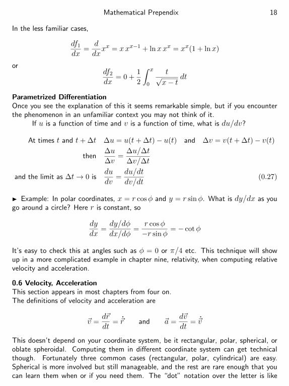
Parametrized DifferentiationOnce you see the explanation of this it seems remarkable simple, but if you encounterthe phenomenon in an unfamiliar context you may not think of it.
If u is a function of time and v is a function of time, what is du/dv?
At times t and t+ ∆t ∆u = u(t+ ∆t)− u(t) and ∆v = v(t+ ∆t)− v(t)
then∆u∆v
=∆u/∆t
∆v/∆t
and the limit as ∆t→ 0 isdudv
=du/dt
dv/dt(0.27)
Example: In polar coordinates, x = r cosφ and y = r sinφ. What is dy/dx as yougo around a circle? Here r is constant, so
dydx
=dy/dφ
dx/dφ=
r cosφ−r sinφ
= − cotφ
It’s easy to check this at angles such as φ = 0 or π/4 etc. This technique will showup in a more complicated example in chapter nine, relativity, when computing relativevelocity and acceleration.
0.6 Velocity, AccelerationThis section appears in most chapters from four on.The definitions of velocity and acceleration are
~v =d~rdt
= ~r and ~a =d~vdt
= ~v
This doesn’t depend on your coordinate system, be it rectangular, polar, spherical, oroblate spheroidal. Computing them in different coordinate system can get technicalthough. Fortunately three common cases (rectangular, polar, cylindrical) are easy.Spherical is more involved but still manageable, and the rest are rare enough that youcan learn them when or if you need them. The “dot” notation over the letter is like
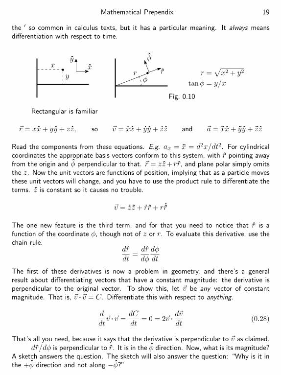
Mathematical Prependix 19
the ′ so common in calculus texts, but it has a particular meaning. It always meansdifferentiation with respect to time.
x
yx
y
rφ
r
φ
Fig. 0.10
r =√x2 + y2
tanφ = y/x
Rectangular is familiar
~r = xx+ yy + zz, so ~v = xx+ yy + zz and ~a = xx+ yy + zz
Read the components from these equations. E.g. ax = x = d2x/dt2. For cylindricalcoordinates the appropriate basis vectors conform to this system, with r pointing awayfrom the origin and φ perpendicular to that. ~r = zz+rr, and plane polar simply omitsthe z. Now the unit vectors are functions of position, implying that as a particle movesthese unit vectors will change, and you have to use the product rule to differentiate theterms. z is constant so it causes no trouble.
~v = zz + rr + r ˙r
The one new feature is the third term, and for that you need to notice that r is afunction of the coordinate φ, though not of z or r. To evaluate this derivative, use thechain rule.
drdt
=drdφ
dφdt
The first of these derivatives is now a problem in geometry, and there’s a generalresult about differentiating vectors that have a constant magnitude: the derivative isperpendicular to the original vector. To show this, let ~v be any vector of constantmagnitude. That is, ~v .~v = C. Differentiate this with respect to anything.
ddt~v .~v =
dCdt
= 0 = 2~v . d~vdt
(0.28)
That’s all you need, because it says that the derivative is perpendicular to ~v as claimed.dr/dφ is perpendicular to r. It is in the φ direction. Now, what is its magnitude?
A sketch answers the question. The sketch will also answer the question: “Why is it inthe +φ direction and not along −φ?”
Mathematical Prependix 20
φ r(φ)
r(φ+ ∆φ)
∆r
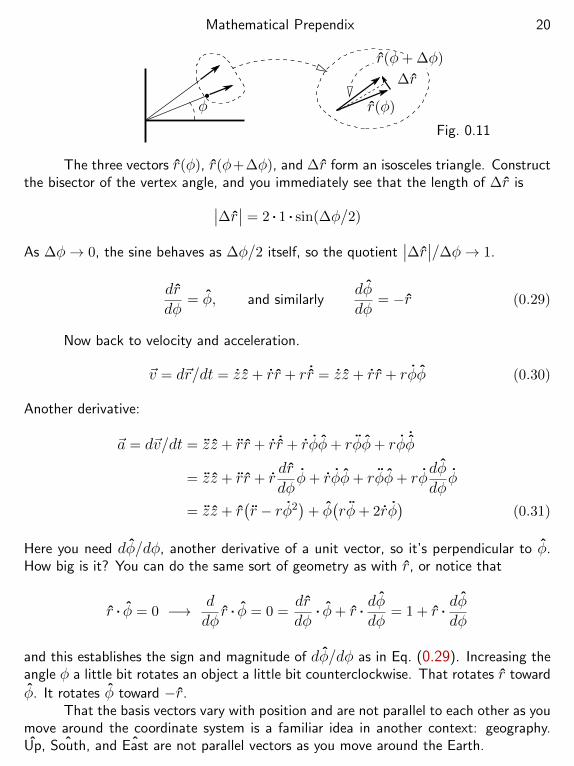
Fig. 0.11
The three vectors r(φ), r(φ+∆φ), and ∆r form an isosceles triangle. Constructthe bisector of the vertex angle, and you immediately see that the length of ∆r is∣∣∆r∣∣ = 2 . 1 . sin(∆φ/2)
As ∆φ→ 0, the sine behaves as ∆φ/2 itself, so the quotient∣∣∆r∣∣/∆φ→ 1.
drdφ
= φ, and similarlydφdφ
= −r (0.29)
Now back to velocity and acceleration.
~v = d~r/dt = zz + rr + r ˙r = zz + rr + rφφ (0.30)
Another derivative:
~a = d~v/dt = zz + rr + r ˙r + rφφ+ rφφ+ rφ ˙φ
= zz + rr + rdrdφφ+ rφφ+ rφφ+ rφ
dφdφφ
= zz + r(r − rφ2
)+ φ
(rφ+ 2rφ
)(0.31)
Here you need dφ/dφ, another derivative of a unit vector, so it’s perpendicular to φ.How big is it? You can do the same sort of geometry as with r, or notice that
r . φ = 0 −→ ddφr . φ = 0 =
drdφ
. φ+ r . dφdφ
= 1 + r . dφdφ
and this establishes the sign and magnitude of dφ/dφ as in Eq. (0.29). Increasing theangle φ a little bit rotates an object a little bit counterclockwise. That rotates r toward
φ. It rotates φ toward −r.That the basis vectors vary with position and are not parallel to each other as you
move around the coordinate system is a familiar idea in another context: geography.Up, ˆSouth, and ˆEast are not parallel vectors as you move around the Earth.
Mathematical Prependix 21
For spherical coordinates the derivations can be done along the same lines, butwith a whole lot more algebra. It’s not worth the trouble to go through it, and youdon’t need the results as often. The answer is (remember to distinguish the sphericalcoordinate r from the cylindrical one — they’re spelled the same).
~r = rr
~v = ~r = rr + rθθ + rφ sin θφ
~a =(r − rφ2 sin2 θ − rθ2
)r +
(rθ + 2rθ − rφ2 sin θ cos θ
)θ
+(rφ sin θ + 2rφ sin θ + 2rθφ cos θ
)φ
(0.32)
In geographical terms,
r ≡ Up θ ≡ South φ ≡ East
Examples Circular motion is a familiar example from introductory courses. If z = 0 and r = aconstant, the equations (0.30) and (0.31) are
~v = rφφ and ~a = −r rφ2 + φ rφ = −r v2
r+ φ
dvdt
(0.33)
The last form comes from using the magnitude of the first of these equations for ~v,that is v = rφ, and it reproduces the familiar inward radial acceleration for circular
motion (rφ2 = v2/r). The tangential component is rφ = d(rφ)/dt = dv/dt. Nowwait a minute! If you believe this manipulation, look again more critically. Is the motioncounterclockwise or clockwise and does it matter? Is φ positive or negative? Is themagnitude of a vector positive? When you express a vector in terms of components,is the coefficient of the unit vector the magnitude of the vector or a component of thevector? Answer: the correct equation is not v = rφ, but vφ = rφ, stating that the
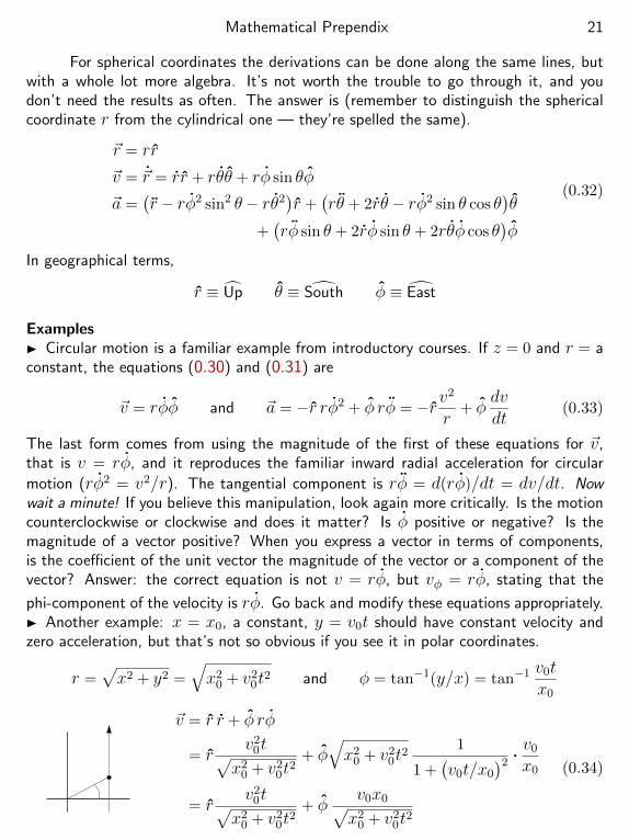
phi-component of the velocity is rφ. Go back and modify these equations appropriately. Another example: x = x0, a constant, y = v0t should have constant velocity andzero acceleration, but that’s not so obvious if you see it in polar coordinates.
r =√x2 + y2 =
√x2
0 + v20t
2 and φ = tan−1(y/x) = tan−1 v0tx0
~v = r r + φ rφ
= rv2
0t√x2
0 + v20t
2+ φ
√x2
0 + v20t
21
1 +(v0t/x0
)2 . v0
x0
= rv2
0t√x2
0 + v20t
2+ φ
v0x0√x2
0 + v20t
2
(0.34)
Mathematical Prependix 22
You can see that this has the correct behavior at t = 0 and as t → ∞. Does it havethe correct magnitude? And what is its derivative?
0.7 Complex Algebra
This section appears in chapters 3, 4, 6, and implicitly many other places.There are some standard manipulations with complex arithmetic that take some practice.Even the basic +, −, ×, and ÷ are not exactly what you learned in third grade, so I’llstart with those. The standard commutative, associative, and distributive laws apply tothe first three, so
(7 + 2i)(6 + 3i) = (6 + 3i)(7 + 2i) = 36 + 33i
(1 + 2i)[(3 + 4i)(5 + 6i)
]=[(1 + 2i)(3 + 4i)
](5 + 6i)
= (1 + 2i)(−9 + 38i) = −85 + 20i
(1 + 2i)[(3 + 4i) + (5 + 6i)
]= (1 + 2i)(3 + 4i) + (1 + 2i)(5 + 6i)
= (1 + 2i)(8 + 10i) = −12 + 26i
As for division, it’s no more commutative here than it is for real numbers, buta simple trick allows you to simplify some expressions. The complex conjugate of anumber is the number found by changing the sign of the imaginary part.
z = 5 + 7i =⇒ z∗ = 5− 7i
The ∗ notation is a common one for this operation, though z is another notation thatmany prefer. What is the product of a number and its complex conjugate?
z = 5 + 7i, z∗ = 5− 7i =⇒ z∗z = (5− 7i)(5 + 7i) = 25 + 49 + 35i− 35i = 74
z∗z is always real: (a + ib)(a − ib) = a2 + b2 is the square of the magnitude of thecomplex number, the square of
√a2 + b2. How do you use this to manipulate division?
Rationalize the denominator of a quotient.
1 + 2i3 + 4i
=(1 + 2i)(3− 4i)(3 + 4i)(3− 4i)
=11 + 2i
25(0.35)
Multiplying a number by its complex conjugate results in a real, so you can multiply thenumerator and denominator of a quotient by the complex conjugate of the denominatorin order to bring the result into a simpler form.
Mathematical Prependix 23
A few examples of such manipulation, simplifying complex expressions:
3− 4i2− i
=(3− 4i)(2 + i)(2− i)(2 + i)
=10− 5i
5= 2− i.
(3i+ 1)2
[1
2− i+
3i2 + i
]= (−8 + 6i)
[(2 + i) + 3i(2− i)
(2− i)(2 + i)
]= (−8 + 6i)
5 + 7i5
=2− 26i
5.
i3 + i10 + ii2 + i137 + 1
=(−i) + (−1) + i(−1) + (i) + (1)
=−1
i= i.
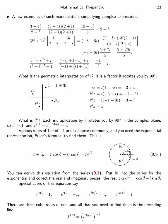
What is the geometric interpretation of i? It is a factor it rotates you by 90.
z = 1 + 3iiz
i2z i3z
iz = i(1 + 3i) = −3 + i
i2z = i(−3 + i) = −1− 3i
i3z = i(−1− 3i) = 3− ii4z = z
What is in? Each multiplication by i rotates you by 90 in the complex plane,so i4 = 1, and i217 = i4
. 54+1 = i.Various roots of 1 or of −1 or of i appear commonly, and you need the exponential
representation, Euler’s formula, to find them. This is
x+ iy = r cos θ + ir sin θ = reiθx
y
θ
(0.36)
You can derive this equation from the series (0.1). Put iθ into the series for theexponential and collect the real and imaginary pieces. the result is eiθ = cos θ+ i sin θ.
Special cases of this equation say
e2πi = 1, eπi = −1, eiπ/2 = i, e2nπi = 1
There are three cube roots of one, and all that you need to find them is the precedingline.
11/3 =(e2nπi
)1/3
Mathematical Prependix 24
Take n to be a succession of integers
n = 0 −→ 11/3 = 1
n = 1 −→(e2πi
)1/3= e2πi/3 = cos 2π/3 + i sin 2π/3 = (−1 + i
√3)/2
n = 2 −→(e4πi
)1/3= e4πi/3 = cos 4π/3 + i sin 4π/3 = (−1− i
√3)/2
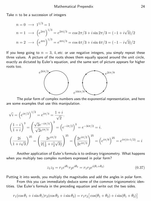
If you keep going to n = 3, 4, etc. or use negative integers, you simply repeat thesethree values. A picture of the roots shows them equally spaced around the unit circle,exactly as dictated by Euler’s equation, and the same sort of picture appears for higherroots too.
e2iπ/3e2iπ/8
e10iπ/8
The polar form of complex numbers uses the exponential representation, and hereare some examples that use this manipulation.
√i =
(eiπ/2
)1/2= eiπ/4 =
1 + i√2.(
1− i1 + i
)3
=
(√2e−iπ/4
√2eiπ/4
)3
=(e−iπ/2
)3= e−3iπ/2 = i.
(2i
1 + i√
3
)25
=
(2eiπ/2
2(
12 + i1
2
√3))25
=
(2eiπ/2
2eiπ/3
)25
=(eiπ/6
)25= eiπ(4+1/2) = i
Another application of Euler’s formula is to ordinary trigonometry. What happenswhen you multiply two complex numbers expressed in polar form?
z1z2 = r1eiθ1r2e
iθ2 = r1r2ei(θ1+θ2) (0.37)
Putting it into words, you multiply the magnitudes and add the angles in polar form.From this you can immediately deduce some of the common trigonometric iden-
tities. Use Euler’s formula in the preceding equation and write out the two sides.
r1(cos θ1 + i sin θ1)r2(cos θ2 + i sin θ2) = r1r2
[cos(θ1 + θ2) + i sin(θ1 + θ2)
]
Mathematical Prependix 25
The factors r1 and r2 cancel. Now multiply the two binomials on the left and matchthe real and the imaginary parts to the corresponding terms on the right. The result isthe pair of equations
cos(θ1 + θ2) = cos θ1 cos θ2 − sin θ1 sin θ2
sin(θ1 + θ2) = cos θ1 sin θ2 + sin θ1 cos θ2
(0.38)
and you have a much simpler than usual derivation of these common identities. Youcan do similar manipulations for other trigonometric identities, and in some cases youwill encounter relations for which there’s really no other way to get the result. Thatis why you will find that in physics applications where you might use sines or cosines(oscillations, waves) no one uses anything but complex exponentials. Get used to it.
The important applications of complex numbers in this text appear when youwant to differentiate complex functions, especially the exponential.
ddxeix = i eix =
ddx
(cosx+ i sinx
)= − sinx+ i cosx
and you can easily see that the second and the fourth forms agree. Do another derivativeand you get
d2
dx2eix = i2eix = −eix
so this function eix satisfies the harmonic oscillator equation, the subject of chapterthree.
0.8 Separation of variablesThis section appears in chapters 2, 3, 4, and in another version, in chapter 7.The subject of differential equations is large enough that you can make a profession of itand still not exhaust the subject, but in this text, when you solve differential equations,there are just two methods that show up with any regularity. “Separation of variables”is one. “Linear constant coefficient equations” is the other (next section). After thatthere are a few equations such as Eq. (6.8) that stand on their own, and you can waituntil you get there to find out about them.
A differential equation is an equation relating a function and one or more of its
derivatives, and ~F = m~a is this semester’s differential equation. The first tool in yourkit is separation of variables, and it is easiest to understand if you start with an exampleor two. Let c be a constant.
dxdt
= c2 + x2 −→ dxc2 + x2
= dt −→∫
dxc2 + x2
=
∫dt
Mathematical Prependix 26
The first of these is the differential equation to be solved. It is a first order equation,meaning that it is a relation between the function x and only the first derivative dx/dt.There are two variables here, the independent variable t, and the dependent variable x.You can’t simply integrate this with respect to t because the right side is a function ofx, and that is an (unknown) function of the variable t. To separate variables put allthe x’s on one side of the equation and all the t’s on the other. The second equationdoes this. It is now set up for integration.
Now do the integral, a trig substitution works: x = c tan θ.
dx = c sec2 θ dθ −→∫
c sec2 θ dθc2 + c2 tan2 θ
=
∫1
cdθ =
1
cθ =
1
ctan−1 x
c= t+D
and the solution is x(t) = c tan c(t+D). With an initial conditions such as x(0) = x0
you have
x(0) = x0 = c tan(cD) −→ D =1
ctan−1
(x0/c
)−→ x(t) = c tan
(ct+ tan−1(x0/c)
)Check the last expression: x(0) = c tan
(tan−1(x0/c)
)= x0. Never assume that you
haven’t made a mistake. As time increases, x(t) increases, so (c2 + x2) increases, sodx/dt increases, so the slope of the curve x versus t gets bigger and bigger — that’show the tangent of t behaves.
This method looks like such a special one; the combination of factors that willlet you do this seems so improbable that it can’t work very often. True. But, it works inenough important special cases that you have to know about it and learn to recognizewhen it can work.
1 : dN/dt = −λN, 2 :d2xdt2
= −ω2x, 3 : tdxdt
= αx+β, 4 : tdxdt
+αtx = βx
(0.39)Equations 1, 3, and 4 are separable, but not 2, though in chapters 2 and 3 you will seesome manipulations that will dig a separable equation out of even that one.
Wait, couldn’t you manipulate the second of these to be d2xx = −ω2 dt2 and
integrate? No! There’s no such mathematics as this, so don’t try.
0.9 Constant Coefficient ODEsThis sort of differential equation shows up often in this course, starting in chapter two,and commonly after that. It looks like
3d2xdt2− 4
dxdt
+ 7x = 0 or γd3xdt3
+ δd2xdt2
+ εdxdt
+ ζx = A cosωt
Mathematical Prependix 27
The dependent variable can have any number of derivatives, but it appears just to thefirst power, no x2 or xdxdt or sin(kx). That makes these equation “linear.” That thecoefficient of the x’s are constants make these “constant coefficient linear” equations.That the first one has only terms in x or its derivatives makes it “homogeneous” andthat the second one has an extra term with no x at all makes it “inhomogeneous.” Theprecise definition of this term is that if you multiply the variable x by a constant λ,then the whole expression is multiplied by some power of λ, i.e. λn. Here n = 1.
The first case, the linear constant coefficient homogeneous one, has a simplesolution. All you have to notice is that the derivative of an exponential is an exponential,and try a solution x(t) = Aeαt.
3d2xdt2− 4
dxdt
+ 7x = 0 −→ 3Aα2eαt − 4Aαeαt + 7Aeαt = 0
Aeαt[3α2 − 4α+ 7] = 0
Since neither A nor the exponential are zero, that leaves 3α2−4α+7 = 0, a polynomialequation with two roots, giving two solutions to the equation. Because you are tryingto undo two derivatives to get x you will somehow get two arbitrary constants. The keyproperty of linear homogeneous equations is that the sum of two solutions is a solution,so the full solution to this equation is
A1eα1t +A2e
α2t, where α1, 2 =(2± i
√17)/
3
How do you handle the inhomogeneous case example above? An exponentialwon’t work here. You will not get “A cosωt” out of it in order to match the right-handside. The sum of two solutions is no longer a solution. But, there is one simplification:If you (temporarily) throw away the inhomogeneous term (A cosωt), you can solve theremaining homogeneous part of the equation with a simple exponential. O.k. you get acubic equation, but at least it’s only a polynomial equation so there are ways to handleit. This partial solution will have three arbitrary constants. Now if somehow you canfind any one solution to the whole equation the trick is to add the two partial solutions.
γd3xhom
dt3+ δ
d2xhom
dt2+ ε
dxhom
dt+ ζxhom = 0, with three arbitrary constants
γd3xinh
dt3+ δ
d2xinh
dt2+ ε
dxinh
dt+ ζxinh = A cosωt, with none
Then x(t) = xinh(t)+xhom(t). How do you verify this? Plug in to the original equationand watch it work.
For the problems you encounter in this work, finding the special, inhomogeneoussolution will not be difficult, and later you will see some general methods for findingsuch solutions.
Mathematical Prependix 28
0.10 MatricesThis section appears in chapters 4, 8, 10.Just as you have components of vectors with respect to a basis you will have componentsof certain types of vector-valued functions. You have (vx, vy, vz) or (vr, vθ, vφ) withthree components for a vector. An important sort of function (a linear, vector-valuedfunction of a vector variable) appears in describing the angular momentum of a rigidbody. It also appears in describing dielectric properties of a crystal. And in describingrotations of vectors. And. . . . Anyway, it too has components (nine this time) and theseform matrices. The development of these ideas, showing the reason for the odd-lookingrules that matrices obey, can wait until they’re needed in section 8.2. For the momentthis will be a summary of some rules without any discussion of the reasons that theyare the way they are.
For the moment then a matrix is a square array of numbers. They can be rect-angular too, but not here. They can be added, multiplied, divided, even exponentiated.(
a bc d
)+
(e fg h
)=
(a+ e b+ fc+ g d+ h
)(0.40)
and of course subtraction just changes all the + signs to −. What matrix plays the roleof zero so that adding it changes nothing? An array of all zeroes.
I said that there are nine components and these objects have only four. If youknow everything about 2 × 2 arrays, the extension to 3 × 3 is easy. Just as with witheither mechanics or calculus, the step from one dimension to two is the big one. Afterthat the step to three dimensions or even N dimensions is relatively small. Besides,it’s easier to write these and they take only about 8/27 of the arithmetic to manipulatethem.
Multiplication obeys(a bc d
)(e fg h
)=
(ae+ bg af + bhce+ dg cf + dh
)(0.41)
You run across the rows of the first matrix and down the columns of the second matrixin order to construct the entries in the product. Just as there is a zero matrix foraddition, there is a unit matrix for multiplication. What is it? What entries in the firstfactor of (0.41) make the product equal the array of e, f, g, h, thereby reproducingthe second factor? For the top left entry of the product,
ae+ bg = e for all e and g =⇒ a = 1, b = 0
This makes the top right entry work too. Similarly for the bottom entries you need tohave c = 0 and d = 1. That makes the identity matrix
( I ) =
(1 00 1
)
Mathematical Prependix 29
The order of multiplication matters, and multiplication is not commutative. You canhowever check that this identity matrix works just as well as the right hand factor as itdoes on the left.
The inverse of a matrix is that matrix such that the product with the original isthe identity. Set the right side of Eq. (0.41) to the identity matrix and solve the fourequations in the four unknowns a, b, c, d. I’ll just write the answer, but you shouldcarry out the algebra so that the result is yours and not mine.(
e fg h
)−1
=1
eh− fg
(h −f−g e
)(0.42)
Multiply this by the original matrix and verify that you get the identity. It works ineither order, so check it both ways.
There is no common notation for a matrix as there is for vectors. In the latter caseyou see boldface type or an arrow or sometimes a squiggly underline, but for matricesthere are no standards. Sometimes a boldface sans serif font is chosen for this purpose,and it serves as well as anything else so that’s what I will use here.
A =
(a bc d
), B =
(e fg h
), then AB = C =
(ae+ bg af + bhce+ dg cf + dh
)The inverse matrix as in Eq. (0.42) obeys
BB−1 = B−1B = I
The statement that matrix multiplication is not commutative is AB 6= BA. You do havethe associative law though: A(BC) = (AB)C. Also the distributive law: A(B + C) =AB + AC.
Simultaneous equationsMatrices appear in many interesting and elegant contexts. They also appear in mundanesettings, but these are no less important. How do you solve two linear equations in twounknowns?
ax+ by = p, cx+ dy = q.
multiply the first by d and the second by b, then subtract
dax+ dby = dp, bcx+ bdy = bq −→ dax− bcx = dp− bq −→ x =dp− bqda− bc
multiply the first by c and the second by a, then subtract (0.43)
cax+ cby = cp, acx+ ady = aq −→ cby − ady = cp− aq −→ y =cp− aqbc− ad
Mathematical Prependix 30
This is matrix inversion in disguise.(a bc d
)(xy
)=
(pq
)or Mx = p
Multiply both sides of this matrix equation by the inverse of M from Eq. (0.42).
M−1Mx = x = M−1p =1
ad− bc
(d −b−c a
)(pq
)=
(xy
)This is exactly the same as the preceding explicit solution for x and y. In fact, thatexplicit solution is how the inverse matrix is derived, so this comparison is really circular.
Does this always work? No. You can’t divide by zero, and in Eq. (0.43) I ignoredthat important point.
dax− bcx = dp− bq −→ (da− bc)x = dp− bq also (da− bc)y = aq − cp
What if da − bc = 0? then the right sides of the equations must be zero, otherwisethere is no solution. You can have a solution if p and q are both zero or if a particularcombination of p, q, and the elements of the matrix conspire to make the right sidezero.
ad− bc = determinant of the matrix
The determinant determines the nature of the solutions (deterministically of course).1. If the determinant is non-zero then the solution exists and is unique.2. If the determinant is zero and p or q is non-zero there is no solution
unless special circumstances occur.3. If the determinant is zero and both p and q are zero there are an
infinite number of solutions.Case #1 is routine. You solve simultaneous equations and you expect to find a
solution. The second case is exceptional, and it can be used to determine properties ofthe right-hand side. It will show up (perhaps in disguise) in sections 7.8 and 10.4. Thethird case is the most common for the purposes of this book. It means that the twoequations you are solving are
ax+ by = 0, cx+ dy = 0 but ad− bc = 0 (0.44)
If for example d and b are 6= 0, multiply the first of these by d: dax+ dby = 0. Nowad = bc, so this equation is the same as bcx+bdy = 0 or cx+dy = 0. That means youreally have one equation for the two unknowns, not two. That in turn means that youhave an infinite number of solutions x and y for the answer. Once you have found one,
Mathematical Prependix 31
simply multiply x and y by any constant and you have another. You can understandthis most simply by a graphical interpretation.
ax+ by = 0 is a straight line through the origin.
and this graph represents an infinite number of possible solutions.And how do you write “boldface sans serif” on paper? Perhaps by using “Black-
board Bold” style: ABCDEFGHIJKLMNOPQRSTUVWXYZ. This is a way to fakeboldface type in writing.
Index NotationAij is the set of elements of the matrix A. The indices i and j run from one to whateverthe size of the matrix is (two in these examples). The first index specifies the row andthe second the column.
Arow, column = Aij ←→ A ←→(A11 A12
A21 A22
)← first row← second row
These are three notations for the same thing because you don’t have to think of thesubscripts i and j as particular values. It is like the common notation for a function,f(x). You are not supposed to think of this as some particular “x” but as a place-holder for any value that argument can take on.* In this notation matrix addition andmultiplication are
A + B = C ←→ Aij +Bij = Cij and AB = C ←→N∑j=1
AijBjk = Cik
A column matrix has a single index
xi ←→ x ←→(x1
x2
)and Ax = y ←→
∑k
Ajkxk = yj ←→(A11 A12
A21 A22
)(x1
x2
)=
(y1
y2
)
* Mathematicians will argue that this is bad notation, and that you should think off at the function and f(x) as the particular value of the function at the point x. Theyhave a point. That is technically the correct thing to do, and making that distinctioncan help keep you out of trouble, but it’s cumbersome, and this good advice is oftenignored. There is a case in chapter eight however, where I will raise this issue again,and there I will side with the mathematicians.
Mathematical Prependix 32
This sort of product-and-sum occurs so often that the conventional notation isagain to omit the summation symbol just as in Eq. (0.22). Whenever a product appearswith a repeated index summation is implied. The two sums just above then appear as
AijBjk = Cik and Ajkxk = yj (0.45)
In this kind of manipulation you will find that a repeated index always appears as a pair.If you find a combination such as AijBjkCjn then go back and find your mistake. Itshouldn’t happen.
Exercises
1 In Eq. (0.1) you have the series for 1/(1 − x). Differentiate it with respect to x.Next use the binomial expansion for n = −2 and expand 1/(1−x)2 to see if the resultsmatch.
2 Divide one of the two equations in Eq. (0.11) by the other and manipulate to obtainan identity for tanh(x+ y).
3 Verify that x2 + y2 + z2 = r2 in the second set of equations (0.13).
4 Either verify Eq. (0.33) or correct it if it’s wrong.
5 Verify that the result in Eq. (0.34) is right. Not that the derivation is right, that theresult is!. Also, what is it’s time-derivative?
6 Use the series in Eq. (0.1) to derive Eq. (0.36).
7 Set the right side of Eq. (0.41) equal to the unit matrix. If you know the numberse, f, g, h, then solve for a, b, c, d. For example, ae + bg = 1 is your first equation.Ans: Eq. (0.42)
8 Use the procedure starting at Eq. (0.5) to derive the power series for the sine andfor the cosine.
9 Compute the area of the triangle with vertices (0, 0), (a, 0), (a, b). Do it twice asa double integral dxdy, interchanging limits. Now integrate the function x over thesame area both ways and see if you again get the same answer both ways. Since you’vedone both integrals, divide the second by the first.
Mathematical Prependix 33
10 Verify that the spherical coordinate velocity and acceleration, Eq. (0.32), reduce tothe plane polar coordinate versions in the equatorial plane (θ = 90). Verify the samealong constant longitude (φ = constant).
11 In what states are the most Northern, Southern, Western, and Eastern points in theUnited States? Ans: You’re probably wrong. Look closely at the map on page 9.
12 Each day the Earth gains about 100 000 tons from space debris (rocks, dust, etc.)About what is the average daily change in the Earth’s radius from this bombardment?Express the result in atomic diameters. If you find yourself involved in a lot of arithmetic,re-read Eq. (0.23).
Mathematical Prependix 34
Problems
0.1 Find the next order correction to the series expansion for Eq. (0.3). Check theresult by a numerical comparison of the exact result versus your approximate result fora couple of modest sized values of at/c. Use a = g, but first convert g = 9.81 m/s2 tothe units light-years per year squared.
0.2 Write the power series expansion about t = 0 for 1/(1 + t), then evaluate theintegral
∫ x0 dt/(1 + t) by integrating this series. Ans: See table Eq. (0.1).
0.3 Use series expansions to find the limit as x→ 0 of
1
sin2 x− 1
x2
The series for the sine and for the binomial series are what you need. You can test yourresult experimentally by putting various values of x into a hand calculator.
0.4 Improve on the preceding calculation and find the behavior of that function for smallx. Find the results in a power series up through terms in x2. Check your approximateresult versus the exact one using a calculator for a couple of small x. Again you will usethe sine series and the binomial expansion, but keep the next order terms. Ans: 1
3 + 115x
2
0.5 The limit taken in Eq. (0.2) was simply the value as x→ 0. Improve it by keepingmore terms and finding the behavior for small x instead of just for zero x. Ans: −1
2−18x
0.6 The relativistic expression for the kinetic energy of a non-zero mass particle is
K = mc2
[1√
1− v2/c2− 1
]
For small speed (v c) expand this to terms in v4 at least.
0.7 The hyperbolic sine is an odd function, sinh(−x) = − sinhx, so the inverse hy-perbolic sine is odd too. Equation (0.10) doesn’t look odd, but prove that it is anyway.I.e. put in −x for x and manipulate.
0.8 Derive the equations (0.8).
0.9 From the definition of sinh, write sinh(2x) then factor the result and derive theidentity sinh(2x) = 2 sinhx coshx. Similarly, find cosh(2x) in terms of hyperbolicfunctions of x.
Mathematical Prependix 35
0.10 Derive the power series expansions of sinhx and coshx about x = 0. Ans: Seetable Eq. (0.1).
0.11 (a) y = sinh−1 x means x = sinh y. Differentiate the latter equation with respectto x, solve the result for dy/dx, use a simple identity to eliminate the cosh, and showthat the derivative of sinh−1 x is 1/
√1 + x2. (b) Repeat this calculation of the
derivative, but starting from Eq. (0.10).
0.12 Just after the equation (0.10) there is a set of graphs of the various hyperbolicfunctions. Sort out which graph is which.
0.13 In Eq. (0.7) you see how the hyperbolic functions produce a hyperbola for a graph.Now change variables (rotate coordinates) to x′ = (x+ y)/
√2, y′ = (x− y)/
√2 and
draw the corresponding graph for this.
0.14 Substitute ix into the power series for cosx to get cos(ix) and show that it iscoshx. Find an analogous relation for sin(ix).
0.15 From the preceding problem to get cos and sin of ix, show how to go from theknown identities for cos(x+ y) and sin(x+ y) to the corresponding ones for cosh andsinh.
0.16 From the equation cos2 x+ sin2 x = 1 you get a useful identity by dividing it bycos2 x. What is the analogous result starting from cosh2 x− sinh2 x = 1?
0.17 Similar to the relations in Eq. (0.13), find the relations between cylindrical andspherical coordinates.
0.18 Compute the area of the triangle in Eq. (0.17) using polar coordinates. The trian-gle has vertices at (0, 0), (a, 0), and (a, b). Consider carefully the order of integration,drawing enough pictures to allow you to make a considered choice.
0.19 Compute the volume of a sphere using (a) spherical coordinates, (b) cylindricalcoordinates.
0.20 Compute the area of a sphere using (a) spherical coordinates, (b) cylindricalcoordinates, (c) rectangular coordinates.
0.21 Compare the areas on the Earth between 10 and 11North latitude to the areabetween 79 and 80. Take the ratio. Can you do this by brute force by using acalculator that keeps a zillion digits? Yes, but don’t. Use algebra and some thoughtinstead before you grab the calculator.
Mathematical Prependix 36
0.22 A moment of area is∫r2 dA. Use the area of the triangle that led to Eq. (0.17)
with r measured from the origin, and evaluate this moment, doing the integral twice,once in each order shown.
0.23 Express the rectangular components x, y, z of a point in terms of its sphericalcoordinates. Verify x2 + y2 + z2.
0.24 (a) Compute the dot product of (3x+ 4y) and (4x+ 3y) two ways: once usingcomponents and once using the original definition of the dot product, Eq. (0.18).Equate the results and deduce the angle between the vectors. (b) Repeat the calculationto find the angle, but using the cross product instead — once with the definition andonce with basis vectors and components. What ambiguities appear in these results?Ans: in part 16.3
0.25 Obtain the law of cosines in trigonometry by interpreting the product( ~A −
~B)
.( ~A− ~B
). Let ~C = ~A− ~B. No components please.
0.26 (a) For a triangle with two sides being ~A and ~B, show that ~A× ~B has magnitude
twice the area of the triangle. (b) Make the third side of the triangle ~C and (having
chosen the directions appropriately) show that ~A× ~B = ~A× ~C. From there derive thelaw of sines. Again, no components please.
0.27 Show by drawing pictures and using the geometric definitions of the products that~A . ~B × ~C is (±) the volume of the parallelepiped spanned by the three vectors.
0.28˙ If ~A . ~B = 0 and ~A is not zero, show that the simultaneous equations ~V × ~A = ~Band ~V .A = p have the solution
~V =( ~A× ~B + p ~A
)/ ~A . ~A
0.29 Evaluate (remember the summation convention)
δijδjk, δiiδjj , δijδij , δiiδii, δiiδjk
0.30 Carry out the calculations of the derivatives from Eq. (0.25), with answers afew lines after that. Also compute the derivatives of f3 = df1/dx and of f4(x) =∫ x/2
0 t√x− t dt. In the case of f4, also evaluate the integral and differentiate the
result to see if the two ways to calculate the derivative give the same answer. To dothe integral, notice that the factor t can be written as
(− (x− t) + x
).
Mathematical Prependix 37
0.31 (a) Compute the derivative with respect to t of∫ 2tt dx e−tx
2. (b) Make a change
of integration variables so that the new limits are constants. Now compute the timederivative and compare the two answers.
0.32¨A tricky derivative. Try it the straight-forward way first and demonstrate all theways that it blows up on you. Next do a partial integration to put the integral into adifferent form and then do the derivative. f(t) an unspecified function of t.
ddx
∫ x
0dt
f(t)√x− t
Test your result on an explicit, non-constant, special f for which you can do the integral;then differentiate it.
0.33¨The preceding problem can also be done by going back to the ∆-definition ofa derivative and manipulating that. No partial integrations, just the definitions andmaybe a coordinate shift.
0.34 A function of x is defined to be∫∞
0 tx−1e−tdt. Call it Γ(x). Change variablesin the integral to t = αu. Differentiate the result with respect to α. Of course, theanswer has to be zero doesn’t it? Now set α = 1 and see what relation you get forΓ(x+ 1). (b) Evaluate Γ(1). Now what are Γ(2), (3), (4), (5)?
0.35 Computeddx
∫ 2x
xdt ext
3,
ddx
∫ x
−xdt ext
3,
without doing the integral (you won’t be able to anyway). Check one point of each ofyour results by asking what are these derivatives at x = 0. Compare your solutions tothis special case. Sketching a graph will be essential.
0.36 (a) Take the square of Eq. (0.36) and deduce two common identities concerningtrigonometric functions of double angles. (b) Take the cube of the same equation anddeduce two not-so-common trigonometric identities for triple angles.
0.37 Start from the equation (0.1) for the exponential and substitute x = iθ. Collectthe real and imaginary parts, and use other series from (0.1) to derive Euler’s formulafor eiθ.
0.38 Express in polar form, reiφ
1 + i1− i
,−1 + i
√3
+1 + i√
3, 1 + i, 14− 17i
Mathematical Prependix 38
0.39 Sketch the points in the complex plane: |z| < 1, |z − 2| > 1, z + z∗ = 5,z − z∗ = 5.
0.40 Show that cosx = 12(eix + e−ix) and that sinx = 1
2i(eix − e−ix).
0.41 Assume that the equations of problem 0.40 are valid for complex values of x,and use that to define cos(x + iy) and sin(x + iy). That is, start with cos(x + iy)defined by replacing x → x + iy in problem 0.40, then rearrange the result to showthat (a) sin(x + iy) = sinx cosh y + i cosx sinh y. (b) Find the analogous equationfor cos(x + iy). (c) And what are these when x = 0? (d) What is cos−1 2? What issin−1 2? Ans: in part: 1.570796− i1.316958
0.42 Differentiate eiθ with respect to θ to derive the differentiation formulas for sineand cosine.
0.43 Find the area of an ellipse. Doing the integral∫dA =
∫dxdy is easiest in
rectangular coordinates, with the equation Eq. (0.16). Ans: πab
0.44 In Eq. (0.28) there’s the derivative of a dot product. Can you really do this?Write ~v .~v in rectangular components, differentiate it, and re-assemble the results toshow that it works.
0.45 In Eq. (0.29) it says “and similarly,” leaving the rest of the derivation to you. Doit.
0.46 Fill in the steps leading to the example result, Eq. (0.34), and verify that theresult is plausible. Then compute its acceleration. Pictures of course. Lots of arrows.
0.47 A car starts from rest and moves along a circular track of radius R. It has constantforward acceleration, so the distance along the track is at2/2. Write its velocity and
acceleration in the r-φ basis and sketch the ~r, ~v, and ~a vectors at different times.
0.48 (a) Compute d~a/dt = d3~r/dt3 in plane polar coordinates. (b) What is this forcircular motion at constant speed?
0.49 In Eq. (0.35) it shows how to simplify a fraction by rationalizing the denominator.What do you get if you rationalize its numerator instead?
0.50 Use the identities in Eq. (0.38) or another way if you prefer, and derive theoccasionally useful identities
cosx+ cos y = 2 cos
(x+ y
2
)cos
(x− y
2
)cosx− cos y = 2 sin
(x+ y
2
)sin
(y − x
2
)
Mathematical Prependix 39
0.51 Solve by separation of variables dx/dt = a + x with the initial condition thatx(0) = b.
0.52 Solve the 1st, 3rd, and 4th of the equations in Eq. (0.39), finding the generalsolution.
IntroductionWhat are Newton’s laws of motion? For a caricature of them (don’t believe this)
you have
1. An object with no external forces on it will either remain atrest or stay moving at constant velocity.
2. ~F = m~a.
3. Action equal reaction.
Start with the last one. What in the world is “action”* let alone “reaction?” Theanswer is that you would never write this law in such a language today. A formulationin contemporary language is
3. If one object exerts a force on a second, then the second willexert on the first a force of the same magnitude but oppositedirection. In colloquial mathematics this is
~Fon 1 by 2 = −~Fon 2 by 1
Not obviously so, but another, better way to state the third lawis “momentum is conserved.”
For the first law, can’t you derive it from the second? Just set the total force onan object to zero, then ~a = 0 and the velocity is constant. Didn’t Newton notice this?
As stated, the first law is obviously false. The sun goes around the Earth daily.It’s moving on a circle and its velocity is certainly changing, but there’s no force causingit to do this. You say that this is because of the Earth’s rotation on its axis? Where, inthe first law as stated above, is this precluded? The last time that I was on a merry-go-round I saw people moving up and down and going in circles around me. They weren’tmoving at constant velocity even though there was no force to push them into this oddmotion. If you think that I’m wrong to say this, that I’m the one who’s moving, thenexplain why I can’t assume that I’m the center of the universe. What if I prefer to thinkthat the world moves around me and that I am forever standing still?
The answer is that I can do this. It is a question of complexity. Newton’s firstlaw is really a definition: that of an “inertial frame,” and it is only in inertial systemsthat the laws of nature take on an especially simple form.
* The Oxford English Dictionary says it is either momentum times time, or kineticenergy times time, or maybe closest of all, “The exertion of force by one body uponanother; influence.” And that doesn’t exhaust the possibilities.
40
1—Introduction 41
1. An inertial observer (or inertial frame or inertial coordinatesystem) is one for which IF no forces act on an object — thereare no discernible interactions with any other body — THEN thatobject will move with constant velocity. This is the definition ofan inertial system.
This doesn’t say that there’s anything wrong with a coordinate system that isnot inertial. It simply tells you what it means to be inertial. The Earth is not an inertialsystem. The merry-go-round isn’t either. Does that mean there’s anything wrong withsetting up a coordinate system centered on either of these? No, it simply means thatyou can’t use Newton’s laws in their simplest form.
For the second law,
2. IF you are in an inertial frame, THEN the acceleration of apoint mass is equal to the total force on it divided by its mass.
~a = ~F/m. More generally, ~F = d(m~v )/dt.
When you write the laws this way you can’t even ask that question about derivingthe first law from the second. You need the definition stated in the first law even tostate the second law. Do these restatements of the laws of mechanics clarify everything?No. There are still some ideas to resolve, some of them hard. What is acceleration?(easy) What is mass? (pretty easy) What is force? (tough)
Which is correct, ~F = m~a or ~F = d(m~v)/dt? That is an experimental question,and when the mass of an object is not constant, the two forms aren’t the same. Thesecond one is right, and that’s the one that is consistent with conservation of momen-tum. Of course the validity of that law is an experimental question too. Example: araindrop is falling and while falling it picks up more water from the surrounding moistair. Example: a rope is coiled on the table and you pick up one end, pulling it straightup at constant speed; only some of the mass is moving at any time. For most of thematerial in this text, the mass will be constant, so you can pull it out of the derivativeand use the simpler form. But,
In a non-inertial system ~F 6= m~a and it 6= d(m~v)
dteither.
What do you do if you really want to work in a non-inertial system? Read chapter five.This statement of Newton’s first law defines an inertial frame, but if you’re not
satisfied, you can look up plato.stanford.edu/entries/spacetime-iframes/ for a farmore detailed definition. It will tell you more than you want to know about the subject.Despite this snarky comment, it is very clear and readable.
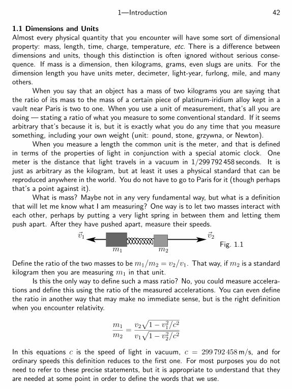
1—Introduction 42
1.1 Dimensions and UnitsAlmost every physical quantity that you encounter will have some sort of dimensionalproperty: mass, length, time, charge, temperature, etc. There is a difference betweendimensions and units, though this distinction is often ignored without serious conse-quence. If mass is a dimension, then kilograms, grams, even slugs are units. For thedimension length you have units meter, decimeter, light-year, furlong, mile, and manyothers.
When you say that an object has a mass of two kilograms you are saying thatthe ratio of its mass to the mass of a certain piece of platinum-iridium alloy kept in avault near Paris is two to one. When you use a unit of measurement, that’s all you aredoing — stating a ratio of what you measure to some conventional standard. If it seemsarbitrary that’s because it is, but it is exactly what you do any time that you measuresomething, including your own weight (unit: pound, stone, grzywna, or Newton).
When you measure a length the common unit is the meter, and that is definedin terms of the properties of light in conjunction with a special atomic clock. Onemeter is the distance that light travels in a vacuum in 1/299 792 458 seconds. It isjust as arbitrary as the kilogram, but at least it uses a physical standard that can bereproduced anywhere in the world. You do not have to go to Paris for it (though perhapsthat’s a point against it).
What is mass? Maybe not in any very fundamental way, but what is a definitionthat will let me know what I am measuring? One way is to let two masses interact witheach other, perhaps by putting a very light spring in between them and letting thempush apart. After they have pushed apart, measure their speeds.
m1 m2
~v1 ~v2
Fig. 1.1
Define the ratio of the two masses to be m1/m2 = v2/v1. That way, if m2 is a standardkilogram then you are measuring m1 in that unit.
Is this the only way to define such a mass ratio? No, you could measure accelera-tions and define this using the ratio of the measured accelerations. You can even definethe ratio in another way that may make no immediate sense, but is the right definitionwhen you encounter relativity.
m1
m2=v2
√1− v2
1/c2
v1
√1− v2
2/c2
In this equations c is the speed of light in vacuum, c = 299 792 458 m/s, and forordinary speeds this definition reduces to the first one. For most purposes you do notneed to refer to these precise statements, but it is appropriate to understand that theyare needed at some point in order to define the words that we use.
1—Introduction 43
At a fundamental level there are just a few types of forces. They are
1. gravity
2. electromagnetism
3. weak nuclear
4. strong nuclear
electroweak
standard model
?
At one time (before Maxwell in the 1860s) electricity and magnetism were two differentforces, but he found that they were just two different aspects of the same thing. Morerecently the electromagnetic force was united with the weak nuclear force (responsiblefor beta-decay). A little later these were combined with the strong nuclear force (reallythe interaction of quarks). Now we’re stuck.
In classical mechanics there are exactly two types of forces that you encounter:gravity and electromagnetism, and in the latter case the most common manifestationis the “contact force.” Two objects touch each other and exert forces on each other.Those are in fact molecule to molecule forces and those are electrical. Fortunately younever have to examine the problem at this level; you simply say that there is a force ofcontact between two objects and then let Newton’s equations figure out how big it is.That it involves interacting molecules is someone else’s business.
For this entire book the only forces are 1. gravity, 2. contact, 3. electric or mag-netic fields. Mostly numbers one and two. Are there exceptions? You could argue thatthe inertial forces in chapter five are different, but those are the result of a coordinatetransformation. Friction? That is just a contact force, so it is basically electromagnetic.
1.2 Types of MassMass is in some sense a resistance to acceleration. Any of the ways to define mass inthe preceding section came from this idea. When two masses push each other apart the
more massive one accelerates less. In the equation ~a = ~F/m, the bigger the mass theless the acceleration, other things being equal.
Mass appears in another basic physical law, gravity. The equation ~Fgrav = m~gsays that a gravitational field ~g pushes on an object in direct proportion to some specialproperty of the object, commonly called “mass.”
Look at the last two paragraphs. The same word, “mass,” appeared in twodifferent meanings. One involved resistance to acceleration and the other involved the
effect of a gravitational field. If I say that the electric field, ~E, caused a force m~Eon an object, you should object. Why is it that the effect by an electric field behavesso differently from the effect by a gravitational field? There are logically two differenttypes of mass. One is inertial mass, describing the resistance to acceleration; the otheris gravitational mass, describing the coupling to the gravitational field.
~a = ~Ftotal/mi, and ~Fgravitational = mg~g
1—Introduction 44
Who says that these two masses are the same?It’s an experimental question. Are they? The question was first asked by Newton,
but the real credit goes to Eotvos. In the late 1800’s and continuing into the first decadeof the 1900’s, he carried out some miraculously precise experiments to measure the ratioof the two masses, mi/mg. Is it the same for all materials? His conclusion was yes, toa precision of at least one part in 108. Later experiments, especially by Dicke and morerecently others, have improved this to one part in 1012. At this point it seems safe tosay that the two masses are the same.
1.3 Conservation LawsClassical mechanics is not just about forces and accelerations. Even if the problems youexamine are traditional ones with masses interacting — gravity, friction, magnetism,etc. There are other ways to approach those problems, and the conservation laws are
at least as fundamental as ~F = m~a. Conservation of energy, of momentum, of angularmomentum can all be derived from that equation, but did you know that you can derive~F = m~a from energy? If so, then which is more fundamental, F = ma or energy?
Work, EnergyIn one dimension with point masses, the work-energy theorem is very simple and is notat all difficult to derive from Newton’s equations. There are a couple of ways to doso, one involves the full power of calculus manipulations and a few lines of algebra; theother is more intuitive, but more tedious.
Start with the first way (and if you haven’t reviewed section 0.5 then go backand do it now).
Fx = max = mdvxdt
= mdvxdx
dxdt
= mvxdvxdx
(1.1)
This used the chain rule for differentiation and then it used the definition of velocity.Now integrate this equation with respect to x between some specified initial and finallimits.
W =
∫ xf
xi
Fx dx =
∫ xf
xi
mvxdvxdx
dx =
∫ x=xf
x=xi
mvx dvx
=m2v2x
∣∣∣∣x=xf
x=xi
=m2v2
f −m2v2
i = ∆K (1.2)
Strip the intervening material from this and you have the work-energy theorem:
W =
∫ xf
xi
Fx dx =m2v2
f −m2v2
i = ∆K (1.3)
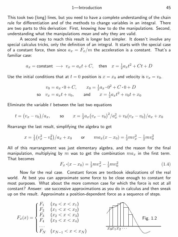
1—Introduction 45
This took two (long) lines, but you need to have a complete understanding of the chainrule for differentiation and of the methods to change variables in an integral. Thereare two parts to this derivation: First, knowing how to do the manipulations. Second,understanding what the manipulations mean and why they are valid.
A second way to reach this result is longer but simpler. It doesn’t involve anyspecial calculus tricks, only the definition of an integral. It starts with the special caseof a constant force, then since ax = Fx/m the acceleration is a constant. That’s afamiliar case:
ax = constant −→ vx = axt+C, then x = 12axt
2 +Ct+D
Use the initial conditions that at t = 0 position is x = x0 and velocity is vx = v0.
v0 = ax . 0 +C, x0 = 12ax
. 02 +C . 0 +D
so vx = axt+ v0, and x = 12axt
2 + v0t+ x0
Eliminate the variable t between the last two equations
t =(vx − v0
)/ax, so x = 1
2ax(vx − v0
)2/a2x + v0
(vx − v0
)/ax + x0
Rearrange the last result, simplifying the algebra to get
x = 12
(v2x − v2
0
)/ax + x0 or max(x− x0) = 1
2mv2x − 1
2mv20
All of this rearrangement was just elementary algebra, and the reason for the finalmanipulation, multiplying by m was to get the combination max in the first term.That becomes
Fx .(x− x0) = 12mv
2x − 1
2mv20 (1.4)
Now for the real case. Constant forces are textbook idealizations of the realworld. At best you can approximate some force to be close enough to constant formost purposes. What about the more common case for which the force is not at allconstant? Answer: use successive approximations as you do in calculus and then sneakup on the result. Approximate a position-dependent force as a sequence of steps.
Fx(x) =
F1 (x0 < x < x1)F2 (x1 < x < x2)F3 (x2 < x < x3)F4 (x3 < x < x4). . .FN (xN−1 < x < xN )
x0x1x2 · · ·
Fig. 1.2
1—Introduction 46
In each of these intervals, the equation (1.4) applies. At each point x0, x1,. . . the speedis v0, v1, etc.
F1(x1 − x0) = 12mv
21 − 1
2mv20
F2(x2 − x1) = 12mv
22 − 1
2mv21
F3(x3 − x2) = 12mv
23 − 1
2mv22
F4(x4 − x3) = 12mv
24 − 1
2mv23
F5(x5 − x4) = 12mv
25 − 1
2mv24
· · ·FN (xN − xN−1) = 1
2mv2N −
12mv
2N−1
The sum of all these equations is
F1(x1−x0) +F2(x2−x1) +F3(x3−x2) + · · ·+FN (xN −xN−1) = 12mv
2N −
12mv
20
because the terms on the right telescope. All the terms except the first and the lastcancel in pairs. In conventional notation this is
N∑k=1
Fk∆xk =
N∑k=1
Fx(xk) ∆xk = 12mv
2f − 1
2mv2i where
∆xk = xk − xk−1
xN = xf
x0 = xi
The limit of this equation as ∆xk → 0 is just the definition of the word “integral,” sothis reproduces Eq. (1.3).
These two derivations of the same equation, W = ∆K, look completely different,but they aren’t. When you look closely at them and compare them step by step theyare much more alike than you first think. The second derivation tells you that thecombination of force times distance is important — especially force times a little bit ofdistance: Fx dx. Write down this combination and manipulate it.
Fx dx = max dx = mdvxdtdx = m
dvxdtdx = mdvx
dxdt
= mvx dvx
However you do it, you get the work-energy relation stating that the work on a pointmass (
∫Fx dx) equals the change in its kinetic energy.
What happens if you don’t have a point mass? What if you aren’t working in onedimension? What if the force is not a function of position alone? All good questionsand all will have to be addressed in chapters 8, 4, and 2 respectively.
Mechanical EnergyFor this same simple case of a point mass in one dimension, and if the force is a functionof position only, you can rearrange the work-energy theorem to get a conservation law.
1—Introduction 47
The work is an integral of Fx(x) dx. When you evaluate integrals, the mostcommon way you use is to find an anti-derivative and then to evaluate it at the end-points of the integration interval, the fundamental theorem of calculus: If f has anantiderivative and if f is integrable then the two are related.
If f(x) = dF (x)/dx then
∫ b
af(x) dx = F (b)− F (a) (1.5)
In the present case the function you’re integrating is Fx(x) and I will denote its anti-derivative by −U(x). That is,
Fx(x) = −dU(x)
dx, then
∫ xf
xi
Fx(x) dx = −U(xf) + U(xi) (1.6)
Now apply this to the work-energy theorem, Eq. (1.3).
W = ∆K is
∫ xf
xi
Fx(x) dx = −U(xf) + U(xi) =m2v2
f −m2v2
i
which ism2v2
i + U(xi) =m2v2
f + U(xf) (1.7)
This is the reason for the minus sign in the definition of U in Eq. (1.6). If you don’tput the minus sign there you would not get a plus sign here, in this conservation ofenergy equation.
U is called the potential energy corresponding to the force Fx(x), and thisequation says that the sum of the kinetic and the potential energies has the samevalues throughout the motion; the sum is conserved.
Can’t you always do this manipulation to get conservation of mechanical energyout of the work-energy theorem? Can’t you always find an anti-derivative (maybe in abig table of integrals)? For example, what about common dry friction? Perhaps youremember an equation such as Ffr = −µkFN. The frictional force as an object slidesover a surface is the coefficient of (kinetic) friction times the normal component of theforce on the surface. It’s just a constant, so you can certainly integrate a constant andget a potential energy U and then get conservation of mechanical energy.
No.In this example of dry friction, the frictional force is velocity dependent even
though it doesn’t look like it — there’s no velocity in the expression −µkFN. True,but that’s because this expression is wrong. The frictional force is velocity dependentbecause it is always opposite the velocity. This commonly used expression for the forceis simply not right. A more correct way to write it is
~Ffr = −µkFNv (1.8)
1—Introduction 48
where v = ~v/v is the unit vector in the direction of the velocity of the sliding mass.If it slides in the reverse direction, the force from friction is reversed and you can havetwo opposite values of the force at the same value of the position. It is not a functionof x alone and no U exists. Why don’t people (including me) write this the correctway? Answer: It’s awkward and I’m lazy.
Notice that I keep using the clumsy phrase “conservation of mechanical energy”instead of “conservation of energy.” Why? That’s tied in to the fact that conservationof energy was one of the most difficult laws to sort out. Newton may have written hisbasic equations in the late 1600s, but conservation of energy did not become an acceptedlaw of physics until around 1850. These two expressions, kinetic energy and potentialenergy, seem easy to derive now, but historically even these were discovered throughtortuous and tortious routes.* The problem is that “energy” is not just “mechanicalenergy.”
Energy is an abstraction, a bookkeeping device much like money. It is a prescrip-tion saying that certain mathematically described properties of a system are to be addedtogether and if you do it right, you can come back later, redo the sum and you’re goingto get the same answer. The historical confusion arose in trying to figure out whatterms to include in this sum. It was resolved when heat was seen to be another form ofenergy (a term in the sum). Then light, sound, chemical energy, and eventually masswere added to the mix. Energy is not a thing, even though you can get that impressionif you read newspaper articles on the subject.
Did I just say that money is an abstraction? Isn’t it just the bills and coinsthat you carry with you? No. If you buy a car, do you pay for it with hundred dollarbills? Most people don’t, and bills and coins are nowhere near conserved. If you includewhat’s in your checking account, that’s not bills and coins stored in a vault. It is a setof bits stored on a computer disk. A savings account is more of the same. Then thereare whatever mysterious manipulations the Federal Reserve Board can implement. Thetotal “money” is a combination of many different things, of which just a tiny amountis in any sense concrete. If you ask five economists to define money you will likely getfive answers (M1, . . . , M5). The difference with the abstraction called energy is thatwe think we know what goes into it. Or do we? Cosmologists were surprised by thediscovery that the expansion of the universe is accelerating, caused by something called“dark energy” for lack of a better name. No one knows what it is.
Derive F = maA few paragraphs back I said that you can derive F = ma from energy. How? Takeconservation of mechanical energy and differentiate it:
E =1
2mv2
x + U(x) is conserved −→ dEdt
= 0
* but fortunately not torturous
1—Introduction 49
ddt
[1
2mv2
x + U(x)
]=
1
2m 2vx
dvxdt
+dUdx
dxdt
= vx
[mdvxdt
+dUdx
]= 0
or, mdvxdt
= −dUdx
and that is Fx = max. This is not just a pretty theorem, it is sometimes a usefulway to derive the equations of motion in specific cases. Often it involves much easiermanipulations to reach the answer, and I’ll use this method several places later in thetext.
MomentumThere are other ways to manipulate Newton’s equation. The first and least interestingway is to start from Newton’s equation for a single point mass and integrate it withrespect to time.
~F = m~a −→∫ t2
t1
~F dt =
∫ t2
t1m~adt = m~v(t2)−m~v(t1)
When you have at least two interacting masses, you get something more useful
~Fon 1 by 2 = m1~a1, ~Fon 2 by 1 = m2~a2 (1.9)
Add these, and the two forces cancel because of Newton’s third law, leaving
0 = m1d~v1
dt+m2
d~v2
dt=ddt
[m1~v1 +m2~v2
](1.10)
This is conservation of momentum. It doesn’t matter how complicated to two forcesare as long as the third law is satisfied.
If you have three or three million particles the result is the same, only the notationchanges. Put indices i and j on the masses instead of simple 1 and 2. The total forceon particle i is the sum of the forces from all the other particles
mi~ai =∑j 6=i
~Fon i by j
Now add this equation over all values of the index i.∑i
mi~ai =∑i
∑j 6=i
~Fon i by j = 0 Write this out for three masses! Really (1.11)
1—Introduction 50
Because acceleration is the time-derivative of velocity, this equation says that
ddt
∑i
mi~vi = 0, or∑i
mi~vi = a constant (1.12)
Can you really go from Eq. (1.9) to (1.10)? What if mass isn’t constant? Then~F 6= m~a anyway and you should have been using ~F = d~p/dt. That also makes thewhole process much more natural. (Go back and do it that way.)
Angular MomentumAnother manipulation of Newton’s equation uses the cross product. Pick an originand let ~r be the coordinate vector of a single point mass from that origin. Notice thedifference here: This result depends on having chosen an origin. It doesn’t matter whichorigin you pick, but you have to pick one.
~r × ~F = ~r × d~pdt
= ~r × d~pdt
+d~rdt× ~p =
ddt
(~r × ~p
)(1.13)
What was the trick that appears after the second equals sign? The terms that I addedis zero because it is simply ~v× ~p = ~v×m~v = 0. The final term is the ordinary productrule for derivatives, and the terms in this equation get names, torque and angularmomentum.
~τ =d~Ldt
is torque = time-derivative of angular momentum (1.14)
Again, when you have many particles, you put indices on the masses and sumover all the particles, but unlike the case of linear momentum the results are sufficientlycomplex that they deserve a complete chapter (eight) to themselves.
In the absence of external forces, you have the conservation law: ~Ltotal =constant. How to derive this? The force on a single particle, the ith one, is
~Fi = Fi, external +∑j 6=i
~Fon i by j
This represents the total force on a single particle as caused by everything else in theuniverse. The index j is for all the other particles in the body. In the present case,there is no external force, and
~τ =∑i
~ri × ~Fi =∑i
~ri ×∑j 6=i
~Fon i by j
1—Introduction 51
Look at one particular pair of terms in this sum, the ones for which i = 1, j = 2 andi = 2, j = 1. Those are
~r1 × ~Fon 1 by 2 + ~r2 × ~Fon 2 by 1
These two forces are opposite, so this is
~r1 × ~Fon 1 by 2 − ~r2 × ~Fon 1 by 2 =(~r1 − ~r2
)× ~Fon 1 by 2
If the forces acting between these masses act along the line between them then thiscross product is zero. The same will apply to all pair of forces.
MassMass is conserved. If two objects collide and they have masses m1 and m2, then afterthe collision the total mass will be the same.
m1 +m2 = m3 +m4
This doesn’t mean that m3 = m1 and m4 = m2. Mass can be moved from one objectto the other, perhaps by chipping off or because a loose part of one mass becomesattached to the other.
You can see why this is true if you assume that momentum conservation is valid.If you measure the velocity of some mass to be ~v and a friend of yours is moving byat velocity ~u then your friend will conclude that the velocity of the mass is ~v − ~u. Ifmomentum conservation holds for you then it should hold for your friend. The twoequations are
m1~v1 +m2~v2 = m3~v3 +m4~v4 and
m1(~v1 − ~u) +m2(~v2 − ~u) = m3(~v3 − ~u) +m4(~v4 − ~u)
Subtract these and you have (for all ~u )
m1~u+m2~u = m3~u+m4~u =⇒ m1 +m2 = m3 +m4 (1.15)
The idea here appears again in much more detail in chapter nine, especially section9.11. There, in the context of special relativity you will see that mass conservation isnot quite right after all.
This showed that if you start from momentum conservation and look at it fromanother point of view, you get a very interesting result. What if kinetic energy is
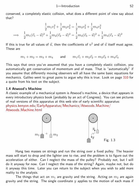
1—Introduction 52
conserved, a completely elastic collision, what does a different point of view say aboutthat?
1
2m1v
21 +
1
2m2v
22 =
1
2m3v
23 +
1
2m4v
24
=⇒ 1
2m1(~v1 − ~u)2 +
1
2m2(~v2 − ~u)2 =
1
2m3(~v3 − ~u)2 +
1
2m4(~v4 − ~u)2
If this is true for all values of ~u, then the coefficients of u2 and of ~u itself must agree.These are
m1 +m2 = m3 +m4 and m1~v1 +m2~v2 = m3~v3 +m4~v4
This says that once you’ve assumed that you have a completely elastic collision, youautomatically get conservation of momentum and of mass. That is “automatically” ifyou assume that differently moving observers will all have the same basic equations formechanics. Galileo went to great pains to argue why this is true. Look on page 310 fora quote from his text on the subject.
1.4 Atwood’s MachineA classic example of a mechanical system is Atwood’s machine, a device that appears inevery introductory physics book (probably by an act of Congress). You can see picturesof real versions of this apparatus at this web site of early scientific apparatus:physics.kenyon.edu/EarlyApparatus/Mechanics/Atwoods Machine/Atwoods Machine.html
m1 m2
y
yFig. 1.3
Hang two masses on strings and run the string over a fixed pulley. The heaviermass will start to drop and the lighter one to rise, and the problem is to figure out theacceleration of either. Can I neglect the mass of the pulley? Probably not, but I willdo it anyway for now. Can I neglect the mass of the string? Again, maybe not, but doit anyway this time. Later you can return to the subject when you wish to add morereality to the analysis.
The things that act on m1 are gravity and the string. Acting on m2 are againgravity and the string. The single coordinate y applies to the motion of each mass if
1—Introduction 53
you make the reasonable assumption that the string doesn’t stretch. (Conservation ofString?) Apply Newton’s law to each mass, treating the two masses as two separateproblems having nothing to do with each other.
(1) F1y = m1g − T1 = m1ay, (2) F2y = −m2g + T2 = m2ay (1.16)
These are two equations in the three unknowns (ay, T1, T2), so you need anotherequation. That is T1 = T2. Why is this so? It comes from a torque equation. Ifthe mass of the pulley is zero, any non-zero torque on it would give it infinite angularacceleration (Eq. (8.5)), and that can’t happen. With these three equations you cansolve for everything.
ay =m1 −m2
m1 +m2g, T1 = T2 =
2m1m2
m1 +m2g (1.17)
In analyzing this solution there are three cases that push it to its limit: m1 = m2,m1 m2, and m1 m2.
First: m1 = m2 : ay = 0, T =2mmm+m
g = mg
It balances, giving zero acceleration and with just enough tension in the string to makethe total force on each mass zero.
Second: m1 m2 : ay ≈m1
m1g = g, T ≈ 2m1m2
m1g = 2m2g
With m1 dominant, that mass accelerates at +g, causing the other mass to accelerateup at +g. As m2 experiences a downward force from gravity of m2g, this requires thestring to pull up with twice this force, and it does.
Third: m1 m2 : ay ≈ −m2
m2g = −g, T ≈ 2m1m2
m2g = 2m1g
Now m2 accelerates toward −y and pulls m1 up against gravity, requiring a tension of2m1g to do so.
Why did Atwood invent his machine and why is it important enough even to havea name? Perhaps he invented it as a way to harass physics students. Perhaps a betterreason is as a device to verify the then recently discovered Newton’s Laws. Also as adevice to measure g. In 1780, electronic timers hadn’t yet been invented, and this deviceslowed the motion enough to make measurements of acceleration easier. If you lookat the Kenyon historical link to early scientific apparatus, you will see that Atwood’s
1—Introduction 54
original machine does not look like the simple picture here; it has complications designedto reduce the effects of friction because good, low-friction bearings didn’t exist then.
What does this have to do with energy? In chapter two you will find much moreon the subject of energy, but for now I’ll assume that you have seen something of thesubject before and that the development of mechanical energy in the last section isfamiliar. You remember the gravitational potential energy to be mgh, and if you don’t,then the equation (1.6) tells you that
Fy = −mg = −dUdy, so U(y) = mgy
In the Atwood machine as drawn, I will assume that everything starts at rest when themasses have coordinates y = 0. Take the zero-point of potential energy to be zero atthat point too. Later the masses will have picked up speed and their positions will havechanged. Write down the total mechanical energy.
E =1
2m1v
2y +
1
2m2v
2y +m2gy −m1gy
The two kinetic energies are positive and (for positive y) the m2 gets positive potentialenergy and the potential energy for m1 is negative.
Energy is conserved. That means that the derivative of the total energy withrespect to time is zero.
dEdt
= 0 =ddt
[1
2m1v
2y +
1
2m2v
2y +m2gy −m1gy
]= m1vy
dvydt
+m2vydvydt
+m2gdydt−m1g
dvydt
= (m1 +m2)dvydt
+ (m2 −m1)g (1.18)
The second line used the chain rule for derivatives to differentiate v2y with respect to t.
The third line used the definition of velocity, vy = dy/dt, to cancel some factors. Solvethe final equation for the acceleration ay = dvy/dt and you have the result Eq. (1.17).Or at least part of it. Using energy methods is often an easier way to get to the resultyou want, but it does not always give you all the results you want. In this case it doesn’tprovide an equation for the tension in the string.
1—Introduction 55
Exercises
1 Verify the chain rule with an example constructed so that it has enough structure toshow something, but it is simple enough to work with easily.
h(t) = f(g(t)
)then
dhdt
=dfdgdgdt
Take g(t) = At2 and f(x) = Bx3 and evaluate dh/dt two ways. First use the chainrule. Next write h explicitly in terms of t and differentiate that.
1—Introduction 56
Problems
1.1 Derive Eq. (1.12) again, but starting from ~F = d~p/dt, so mass may or may notbe constant.
1.2 Write out Eq. (1.11) for the case of three masses.
1.3 In the deep oceans, the speed of a wave is expected to be a function of at mostthe gravitational field, g, the density of the water, ρ, and the wavelength of the waves,λ. Assume that the speed is given by an expression v = gaρbλc where a, b, and c areunknown numbers. You know the units of all the items, v, g, ρ, λ in the equation;determine the values of a, b, and c so that the equation is dimensionally consistent.
1.4 The speed of sound in a fluid such as air may depend on the pressure, the densityand the wavelength of the sound, as v = paρbλc where a, b, and c are unknownnumbers. Solve for the values of a, b, and c so that the equation is dimensionallyconsistent. In this case there is another parameter that can enter the equation: γ =cp/cv is the ratio of the specific heats, but it is dimensionless, so there’s no way bylooking at the dimensions to tell if or how it affects the results. In air at low frequenciesit enters as γ1/2, but at very high frequencies (megaHertz) it disappears.
1.5 A mass moves in a straight line and its velocity satisfies the equation vx = C/xfor some constant C. Find the force acting on this mass as a function of x > 0. Sketcha graph of this force.
1.6 A mass m2 is at rest. Another mass m1, having velocity v1x collides with it.Assume that all the motion is along a straight line and that both kinetic energy andmomentum are conserved. Find the velocities of m1 and m2 after the collision. Examinespecial cases to see if your result is plausible.
1.7 (a) The same as problem 1.6, except that mass is exchanged so that the finalmasses are m3 and m4. (b) Test the special case m1 = m2 in detail, looking at theeffect when the final masses are the same and when they are very different.
1.8 If two masses collide and in the process they break into three, must mass still beconserved?
1.9 You can sometimes find an amusement park ride called a Rotor. You walk into acylindrical room and stand against the wall. The room starts to rotate, and after it’scome to a sufficient rotation rate the floor drops by a few feet. If there is enough frictionwith the wall, you will not slide down. What is the relation between the radius R, ω,
1—Introduction 57
and the coefficient of static friction µk so that you stay up? Check the dimensions ofyour result and see if this minimum ω behaves in a plausible way as µk is changed.
1.10 A variation on a Rotor is a Gravitron. The difference is that the cylindrical wall isnot vertical. Analyze the problem assuming that the wall tilts out by an angle α. Whenyou look at the answer to examine if it behaves plausibly as you vary the governingparameters, also ask what happens if α is negative. That one is probably not going tomake a lot of money.
One Dimensional MotionThe simplest problems that you saw in a first introduction to mechanics start to
become harder as soon as you add some reality. Remembering some of the formulasfor constant acceleration will get you only so far and then you come up against variousforms of friction and against position or time dependent forces.
When you toss an object straight up, the simplest model of the force on it is toassume that only gravity acts and that the gravitational force is a constant in time andspace.
Fy = −mg = md2ydt2
The mass conveniently cancels and then you need to do a couple of integrals.
vy(t) =
∫ay dt = −gt+C, y(t) =
∫vy dt = −1
2gt2 +Ct+D
The two arbitrary constant C and D come from the integration and you need two moreequations to determine them. Boundary conditions are equations such as
y(0) = 0
vy(0) = v0
or
y(0) = 0
y(T ) = 0
or
y(0) = 0
vy(T ) = v1
(2.1)
In the first pair you specify the initial position and velocity. In the second pair youspecify the initial position and the time you want it to return. In the third pair youspecify the initial position and the velocity you desire at a later time.
What if you now remember that there’s an atmosphere on Earth. What effectwill that have on the motion? Usually lots. If the object is massive enough and movingslowly enough you can get away with ignoring such air resistance, but most of the timeyou can’t. Air resistance is complicated, and you will have to make some simplifyingmodel to describe it. There are a few commonly used mathematical models for airresistance, with varying simplicity and accuracy. More of the former typically meansless of the latter.
“Dry friction” is the sort that is typical of dry sliding surfaces at low speeds. Atypical equation is something like Ffriction = µkFN. This frictional force depends onthe velocity, but only through its direction and not its magnitude.
“Wet friction” is a model along the lines Fx = −bvx, so that it is explicitlydependent on the velocity, both in magnitude and direction. This sort of behavior ischaracteristic of lubricated surfaces or of objects moving at (very) low speed throughair.
58
2—One Dimensional Motion 59
A respectable model for air resistance is F = cv2. This applies to a broad rangeof objects as long as the speed isn’t too high.
Then there are the experimentally determined functions that you need for exactwork. Golf is big business, and the flight of golf balls is as well studied as the flight ofany spacecraft has ever been. I would try to refer you to the experimentally determinedair resistance functions for commercial golf balls, but you don’t think that Titleist isgoing to share their data with Callaway do you?
Don’t forget also that the gravitational field of the Earth decreases with altitude.Does that matter? Not for a golf ball, but does it make a difference when you fire aprojectile many kilometers? Yes, and we will examine that.
2.1 Solving F=ma: F(t)Time to get away from the generalities and to start solving some problems. To do that,stay in one dimension for a while so that the basic equation to solve for a single mass is
Fx(t, x, vx) = mdvxdt
= md2xdt2
Whether this is easy, hard, or nightmarish depends on the function Fx. Start with thesimplest case, for which Fx depends on t alone: you simply have to do a couple ofintegrals.
Fx(t) = md2xdt2
=⇒ vx(t) =
∫dt
1
mFx(t), =⇒ x(t) =
∫dt∫dt
1
mFx(t) (2.2)
Each integral has a constant of integration that must be determined, so this meansthat you need two more equations in order to find these two constants and to solve theproblem. Commonly these equations will come from specifying an initial position andan initial velocity, though not always. Take an example, Fx(t) = F0 sinωt (t > 0). Assume that the mass starts from theorigin and was at rest before time zero. Before doing the mathematics, what do youexpect the mass to do? You’re applying an oscillating force, as much positive as it isnegative, so will m wander around the origin or will it move away?
vx(t) =1
m
∫dtF0 sinωt = − F0
mωcosωt+C, then
x(t) =
∫dt vx(t) = − F0
mω2sinωt+Ct+D
Apply the initial conditions.
vx(0) = 0 = − F0
mω+C, so C =
F0
mω
2—One Dimensional Motion 60
x(0) = 0 = − F0
mω2. 0 +C . 0 +D, so D = 0
Put this together and you have
x(t) =F0
mωt− F0
mω2sinωt (2.3)
Does this make sense? First check the dimensions. F0 is (dimensionally) [F0] =ML/T2. This uses the notation that the heavy square brackets denote “the dimensionsof,” and the individual dimensions are
M = mass, L = length, T = time
The parameter ω has to be such that ωt is an angle, so [ω] = 1/T. This meansthat the two terms in Eq. (2.3) have the same dimensions, because dimensionally, t isthe same as 1/ω. Now, are they the correct dimensions?
[F0
/mω2] =
(ML/T2
)/(M/T2
)=(ML/T2
)(T2/M
)= L
and the dimensions pass their test. This bracket notation for the dimensions is acommon one.
What is the behavior of the solution for small time? Not zero time! For smalltime use the power series expansion of the sine. Remember the equations (0.1).
x(t) =F0
mωt− F0
mω2
[ωt− 1
6(ωt)3 + · · ·
]=F0
6mωt3 + · · ·
Check the dimensions again. You’d cannot change the dimensions by making an ap-proximation to the result, but you can always make a mistake. This starts off as t3.Can I understand why? For comparison I know that if it started as a0t2/2 then thiswould imply that there was a force ma0. This force function F0 sinωt however startsat zero force. That implies that it has to start more slowly than t2, and that’s t3.
What is the behavior for large time? The sine term oscillates and goes nowhere,but the t term means that it has an average drift velocity of F0/mω. It moves awaygradually. Compare problem 2.3 and then puzzle out the differences.
What if the time dependence of the force can’t be written in a single, simpleequation? What if Fx(t) is a sinωt on Monday and a cosωt on Tuesday and an eωt onWednesday? Answer: you notice that the end of Monday is the beginning of Tuesdayand the end of Tuesday is the beginning of Wednesday. The position and the velocity
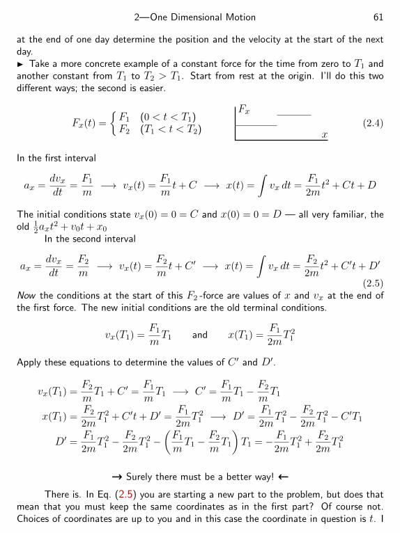
2—One Dimensional Motion 61
at the end of one day determine the position and the velocity at the start of the nextday. Take a more concrete example of a constant force for the time from zero to T1 andanother constant from T1 to T2 > T1. Start from rest at the origin. I’ll do this twodifferent ways; the second is easier.
Fx(t) =
F1 (0 < t < T1)F2 (T1 < t < T2)
Fx
x(2.4)
In the first interval
ax =dvxdt
=F1
m−→ vx(t) =
F1
mt+C −→ x(t) =
∫vx dt =
F1
2mt2 +Ct+D
The initial conditions state vx(0) = 0 = C and x(0) = 0 = D — all very familiar, theold 1
2axt2 + v0t+ x0
In the second interval
ax =dvxdt
=F2
m−→ vx(t) =
F2
mt+C ′ −→ x(t) =
∫vx dt =
F2
2mt2 +C ′t+D′
(2.5)Now the conditions at the start of this F2 -force are values of x and vx at the end ofthe first force. The new initial conditions are the old terminal conditions.
vx(T1) =F1
mT1 and x(T1) =
F1
2mT 2
1
Apply these equations to determine the values of C ′ and D′.
vx(T1) =F2
mT1 +C ′ =
F1
mT1 −→ C ′ =
F1
mT1 −
F2
mT1
x(T1) =F2
2mT 2
1 +C ′t+D′ =F1
2mT 2
1 −→ D′ =F1
2mT 2
1 −F2
2mT 2
1 −C ′T1
D′ =F1
2mT 2
1 −F2
2mT 2
1 −(F1
mT1 −
F2
mT1
)T1 = − F1
2mT 2
1 +F2
2mT 2
1
→ Surely there must be a better way! ←
There is. In Eq. (2.5) you are starting a new part to the problem, but does thatmean that you must keep the same coordinates as in the first part? Of course not.Choices of coordinates are up to you and in this case the coordinate in question is t. I
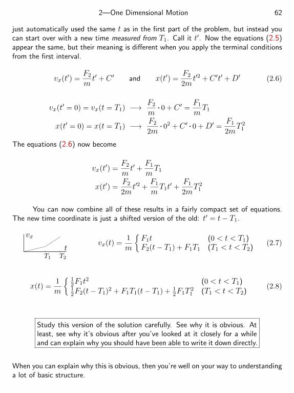
2—One Dimensional Motion 62
just automatically used the same t as in the first part of the problem, but instead youcan start over with a new time measured from T1. Call it t′. Now the equations (2.5)appear the same, but their meaning is different when you apply the terminal conditionsfrom the first interval.
vx(t′) =F2
mt′ +C ′ and x(t′) =
F2
2mt′2 +C ′t′ +D′ (2.6)
vx(t′ = 0) = vx(t = T1) −→ F2
m. 0 +C ′ =
F1
mT1
x(t′ = 0) = x(t = T1) −→ F2
2m. 02 +C ′ . 0 +D′ =
F1
2mT 2
1
The equations (2.6) now become
vx(t′) =F2
mt′ +
F1
mT1
x(t′) =F2
2mt′2 +
F1
mT1t′ +
F1
2mT 2
1
You can now combine all of these results in a fairly compact set of equations.The new time coordinate is just a shifted version of the old: t′ = t− T1.
vx
tT1 T2
vx(t) =1
m
F1t (0 < t < T1)F2(t− T1) + F1T1 (T1 < t < T2)
(2.7)
x(t) =1
m
12F1t2 (0 < t < T1)12F2(t− T1)2 + F1T1(t− T1) + 1
2F1T 21 (T1 < t < T2)
(2.8)
Study this version of the solution carefully. See why it is obvious. Atleast, see why it’s obvious after you’ve looked at it closely for a whileand can explain why you should have been able to write it down directly.
When you can explain why this is obvious, then you’re well on your way to understandinga lot of basic structure.
2—One Dimensional Motion 63
2.2 Solving F=ma: F(v)If the force is a function of the velocity alone,
Fx(vx) = mdvxdt
becomes dt = mdvx
Fx(vx)
This separation of variables method described in section 0.8 easily breaks the equationinto two parts, each of which can be integrated.
Slide an object along a tabletop. Give it an initial speed v0 and see how ittravels. What is the frictional force? Maybe it is common dry friction, for whichthe magnitude of the force is approximately independent of the sliding speed. If youlubricate the surface this won’t be a good approximation at all, and something suchas a force of magnitude Ffr = bv is a better approximation, with b a constant. Underother circumstances perhaps bv2 will be a better model. How do the results of theseassumptions vary? There is a qualitative difference in the behavior of these solutions,and the only way to understand these behaviors is to grasp the result of each problem,handle it, massage it, caress it, and feel how it responds.
(a) Constant friction:
md2xdt2
= −Ffr −→ vx(t) = v0 − Ffrt/m, x(t) = v0t− Ffrt2/2m (2.9)
This applies until the mass stops: vx(t) = 0 at time mv0/Ffr.(b) Friction proportional to speed:
mdvxdt
= −bvx −→dvxvx
= − bmdt −→
∫dvxvx
= − bm
∫dt −→ ln vx = − b
mt+C
This solution used separation of variables as in section 0.8. The initial condition thatvx(0) = v0 determines the constant C = ln v0, and you can combine that logarithmwith the one on the left side of the equation. Next, solve for vx = dx/dt and integrate.
lnvxv0
= − bmt −→ vx = v0e
−bt/m =dxdt
−→ x =
∫dt v0e
−bt/m = −mbv0e−bt/m +D (2.10)
With the same initial position as in the preceding case, x(0) = 0, this determinesD = mv0/b.
OR, you can do the same calculation more efficiently by using definite integralsto apply the initial conditions directly. When the two limits on an integral are equal,
2—One Dimensional Motion 64
so that the integration interval is zero, then the integral is zero. That’s such a simpleidea that you may not immediately see what good it is. Repeat the preceding lines asdefinite integrals:
mdvxdt
= −bvx −→∫ vx
v0
dvxvx
= −∫ t
0
bmdt
−→ ln vx − ln v0 = − bmt −→ vx(t) = v0e
−bt/m (2.11)
When t = 0 the dt integral vanishes, and this in turn requires the vx integral to vanish.That happens if the two limits there are equal, and you have then applied the initialconditions, vx(0) = v0. Next, the integral to get x, applying the limits the same way:
vx = v0e−bt/m =
dxdt−→
∫ x
0dx =
∫ t
0v0e−bt/mdt
−→ x(t) = −mbv0e−bt/m +
mv0
b(2.12)
(c) Friction proportional to speed squared:
mdvxdt
= −bv2x −→
∫ vx
v0
dvxv2x
= −∫ t
0
bmdt −→ − 1
vx+
1
v0= − b
mt (2.13)
Again, separation of variables handles this equation. This b is of course different fromthe one before. It doesn’t even have the same dimensions. Now for the position.
vx =dxdt
=v0
1 + bv0m t
−→∫ x
0dx =
∫ t
0
v0
1 + bv0m t
dt −→ x(t) =mb
ln
(1 +
bv0
mt
)(2.14)
Start the analysis at the start. How do these solutions behave for small time?The power series expansions of Eqs. (0.1) are again what you need for this.
ex = 1 + x+ x2/2! + x3/3! + · · ·, so Eqs. (2.12) are
vx = v0
[1− bt
m+
1
2
b2t2
m2− · · ·
]and
x(t) = −mbv0
[1− bt
m+
1
2
b2t2
m2− · · ·
]+mv0
b= v0t−
bv0
2mt2 + · · ·
The t2 term in this equation for x shows the familiar form axt2/2, so you can immedi-ately recognize that the initial acceleration ax = Fx/m = −bv0/m, and that says that
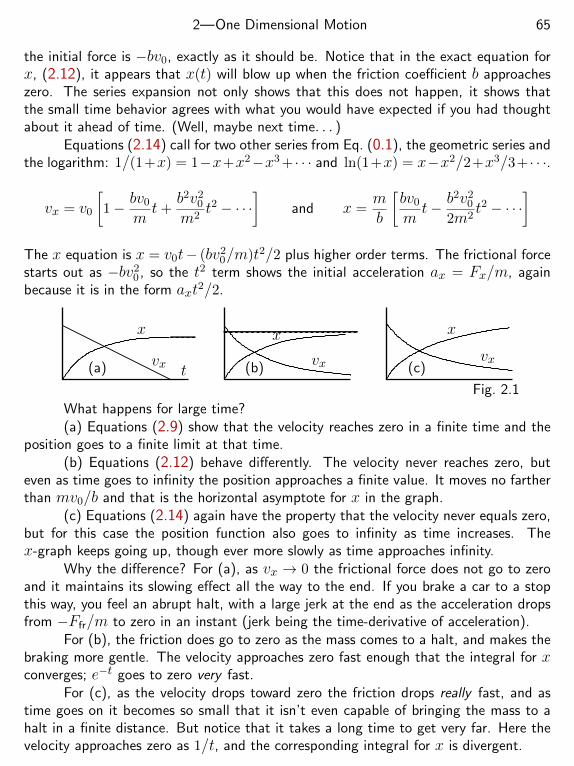
2—One Dimensional Motion 65
the initial force is −bv0, exactly as it should be. Notice that in the exact equation forx, (2.12), it appears that x(t) will blow up when the friction coefficient b approacheszero. The series expansion not only shows that this does not happen, it shows thatthe small time behavior agrees with what you would have expected if you had thoughtabout it ahead of time. (Well, maybe next time. . . )
Equations (2.14) call for two other series from Eq. (0.1), the geometric series andthe logarithm: 1/(1+x) = 1−x+x2−x3 + · · · and ln(1+x) = x−x2/2+x3/3+ · · ·.
vx = v0
[1− bv0
mt+
b2v20
m2t2 − · · ·
]and x =
mb
[bv0
mt− b
2v20
2m2t2 − · · ·
]The x equation is x = v0t− (bv2
0/m)t2/2 plus higher order terms. The frictional forcestarts out as −bv2
0 , so the t2 term shows the initial acceleration ax = Fx/m, againbecause it is in the form axt2/2.
x
vx
x
vx
x
vxt(a) (b) (c)
Fig. 2.1
What happens for large time?(a) Equations (2.9) show that the velocity reaches zero in a finite time and the
position goes to a finite limit at that time.(b) Equations (2.12) behave differently. The velocity never reaches zero, but
even as time goes to infinity the position approaches a finite value. It moves no fartherthan mv0/b and that is the horizontal asymptote for x in the graph.
(c) Equations (2.14) again have the property that the velocity never equals zero,but for this case the position function also goes to infinity as time increases. Thex-graph keeps going up, though ever more slowly as time approaches infinity.
Why the difference? For (a), as vx → 0 the frictional force does not go to zeroand it maintains its slowing effect all the way to the end. If you brake a car to a stopthis way, you feel an abrupt halt, with a large jerk at the end as the acceleration dropsfrom −Ffr/m to zero in an instant (jerk being the time-derivative of acceleration).
For (b), the friction does go to zero as the mass comes to a halt, and makes thebraking more gentle. The velocity approaches zero fast enough that the integral for xconverges; e−t goes to zero very fast.
For (c), as the velocity drops toward zero the friction drops really fast, and astime goes on it becomes so small that it isn’t even capable of bringing the mass to ahalt in a finite distance. But notice that it takes a long time to get very far. Here thevelocity approaches zero as 1/t, and the corresponding integral for x is divergent.
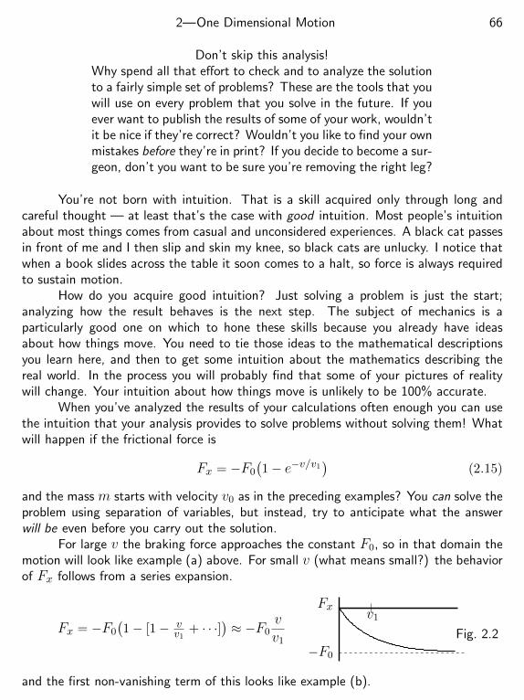
2—One Dimensional Motion 66
Don’t skip this analysis!Why spend all that effort to check and to analyze the solutionto a fairly simple set of problems? These are the tools that youwill use on every problem that you solve in the future. If youever want to publish the results of some of your work, wouldn’tit be nice if they’re correct? Wouldn’t you like to find your ownmistakes before they’re in print? If you decide to become a sur-geon, don’t you want to be sure you’re removing the right leg?
You’re not born with intuition. That is a skill acquired only through long andcareful thought — at least that’s the case with good intuition. Most people’s intuitionabout most things comes from casual and unconsidered experiences. A black cat passesin front of me and I then slip and skin my knee, so black cats are unlucky. I notice thatwhen a book slides across the table it soon comes to a halt, so force is always requiredto sustain motion.
How do you acquire good intuition? Just solving a problem is just the start;analyzing how the result behaves is the next step. The subject of mechanics is aparticularly good one on which to hone these skills because you already have ideasabout how things move. You need to tie those ideas to the mathematical descriptionsyou learn here, and then to get some intuition about the mathematics describing thereal world. In the process you will probably find that some of your pictures of realitywill change. Your intuition about how things move is unlikely to be 100% accurate.
When you’ve analyzed the results of your calculations often enough you can usethe intuition that your analysis provides to solve problems without solving them! Whatwill happen if the frictional force is
Fx = −F0
(1− e−v/v1
)(2.15)
and the mass m starts with velocity v0 as in the preceding examples? You can solve theproblem using separation of variables, but instead, try to anticipate what the answerwill be even before you carry out the solution.
For large v the braking force approaches the constant F0, so in that domain themotion will look like example (a) above. For small v (what means small?) the behaviorof Fx follows from a series expansion.
Fx = −F0
(1− [1− v
v1+ · · ·]
)≈ −F0
vv1
Fx
−F0
v1
Fig. 2.2
and the first non-vanishing term of this looks like example (b).
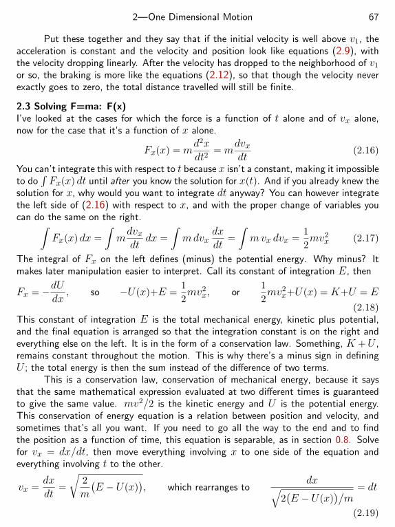
2—One Dimensional Motion 67
Put these together and they say that if the initial velocity is well above v1, theacceleration is constant and the velocity and position look like equations (2.9), withthe velocity dropping linearly. After the velocity has dropped to the neighborhood of v1
or so, the braking is more like the equations (2.12), so that though the velocity neverexactly goes to zero, the total distance travelled will still be finite.
2.3 Solving F=ma: F(x)I’ve looked at the cases for which the force is a function of t alone and of vx alone,now for the case that it’s a function of x alone.
Fx(x) = md2xdt2
= mdvxdt
(2.16)
You can’t integrate this with respect to t because x isn’t a constant, making it impossibleto do
∫Fx(x) dt until after you know the solution for x(t). And if you already knew the
solution for x, why would you want to integrate dt anyway? You can however integratethe left side of (2.16) with respect to x, and with the proper change of variables youcan do the same on the right.∫
Fx(x) dx =
∫mdvxdt
dx =
∫mdvx
dxdt
=
∫mvx dvx =
1
2mv2
x (2.17)
The integral of Fx on the left defines (minus) the potential energy. Why minus? Itmakes later manipulation easier to interpret. Call its constant of integration E, then
Fx = −dUdx, so −U(x)+E =
1
2mv2
x, or1
2mv2
x+U(x) = K+U = E
(2.18)This constant of integration E is the total mechanical energy, kinetic plus potential,and the final equation is arranged so that the integration constant is on the right andeverything else on the left. It is in the form of a conservation law. Something, K +U ,remains constant throughout the motion. This is why there’s a minus sign in definingU ; the total energy is then the sum instead of the difference of two terms.
This is a conservation law, conservation of mechanical energy, because it saysthat the same mathematical expression evaluated at two different times is guaranteedto give the same value. mv2/2 is the kinetic energy and U is the potential energy.This conservation of energy equation is a relation between position and velocity, andsometimes that’s all you want. If you need to go all the way to the end and to findthe position as a function of time, this equation is separable, as in section 0.8. Solvefor vx = dx/dt, then move everything involving x to one side of the equation andeverything involving t to the other.
vx =dxdt
=
√2
m
(E − U(x)
), which rearranges to
dx√2(E − U(x)
)/m
= dt
(2.19)
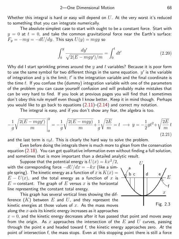
2—One Dimensional Motion 68
Whether this integral is hard or easy will depend on U . At the very worst it’s reducedto something that you can integrate numerically.
The absolute simplest case to start with ought to be a constant force. Start withy = 0 at t = 0, and take the common gravitational force near the Earth’s surface:Fy = −mg = −dU/dy. This says U(y) = mgy so∫ y
0
dy′√2(E −mgy′)/m
=
∫ t
0dt′ (2.20)
Why did I start sprinkling primes around the y and t variables? Because it is poor formto use the same symbol for two different things in the same equation. y′ is the variableof integration and y is the limit; t′ is the integration variable and the final coordinate isthe time t. If you confuse the (dummy) integration variable with one of the parametersof the problem you can cause yourself confusion and will probably make mistakes thatcan be very hard to find. If you look at previous pages you will find that I sometimesdon’t obey this rule myself even though I know better. Keep it in mind though. Perhapsyou would like to go back to equations (2.11)–(2.14) and correct my notation.
The integral is easy, and if you don’t show any fear, the algebra is too.
−1
g
√2(E −mgy′)
m
∣∣∣∣∣y
0
= −1
g
√2(E −mgy)
m+
1
g
√2Em
= t −→ y = −1
2gt2+
√2Em
t
(2.21)and the last term is v0t. This is clearly the hard way to solve the problem.
Even before doing the integrals there is much more to glean from the conservationequation (2.18). You can get qualitative information even without finding a full solution,and sometimes that is more important than a detailed analytic result.
U
x
E
a
b c d e
f
Fig. 2.3
Suppose that the potential energy is U(x) = kx2/2,with the corresponding force −dU/dx = −kx (like a sim-ple spring). The kinetic energy as a function of x isK(x) =E − U(x), and the total energy as a function of x isE = constant. The graph of E versus x is the horizontalline representing the constant total energy.
This graph has several vertical lines showing the dif-ference (K) between E and U , and they represent thekinetic energies at those values of x. As the mass movesalong the x-axis its kinetic energy increases as it approachesx = 0, and the kinetic energy decreases after it has passed that point and moves awayfrom the origin. As x approaches the intersection of the E and U curves, passingthrough the point e and headed toward f, the kinetic energy approaches zero. At thepoint of intersection f, the mass stops. Even at this stopping point there is still a force
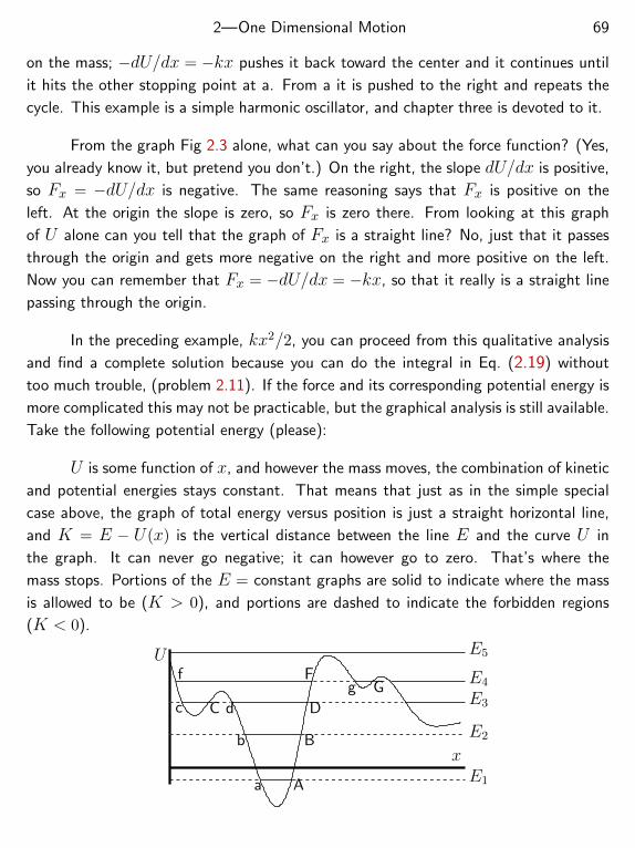
2—One Dimensional Motion 69
on the mass; −dU/dx = −kx pushes it back toward the center and it continues until
it hits the other stopping point at a. From a it is pushed to the right and repeats the
cycle. This example is a simple harmonic oscillator, and chapter three is devoted to it.
From the graph Fig 2.3 alone, what can you say about the force function? (Yes,
you already know it, but pretend you don’t.) On the right, the slope dU/dx is positive,
so Fx = −dU/dx is negative. The same reasoning says that Fx is positive on the
left. At the origin the slope is zero, so Fx is zero there. From looking at this graph
of U alone can you tell that the graph of Fx is a straight line? No, just that it passes
through the origin and gets more negative on the right and more positive on the left.
Now you can remember that Fx = −dU/dx = −kx, so that it really is a straight line
passing through the origin.
In the preceding example, kx2/2, you can proceed from this qualitative analysis
and find a complete solution because you can do the integral in Eq. (2.19) without
too much trouble, (problem 2.11). If the force and its corresponding potential energy is
more complicated this may not be practicable, but the graphical analysis is still available.
Take the following potential energy (please):
U is some function of x, and however the mass moves, the combination of kinetic
and potential energies stays constant. That means that just as in the simple special
case above, the graph of total energy versus position is just a straight horizontal line,
and K = E − U(x) is the vertical distance between the line E and the curve U in
the graph. It can never go negative; it can however go to zero. That’s where the
mass stops. Portions of the E = constant graphs are solid to indicate where the mass
is allowed to be (K > 0), and portions are dashed to indicate the forbidden regions
(K < 0).
U
xE1
E2
E3
E4
E5
a A
b B
c C d D
f Fg G
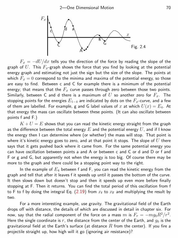
2—One Dimensional Motion 70
Fx
xc
C
d a
A
gG
Fig. 2.4
Fx = −dU/dx tells you the direction of the force by reading the slope of thegraph of U . This Fx-graph shows the force that you find by looking at the potentialenergy graph and estimating not just the sign but the size of the slope. The points atwhich Fx = 0 correspond to the minima and maxima of the potential energy, so thoseare easy to find. Between c and C for example there is a minimum of the potentialenergy; that means that the Fx curve passes through zero between those two points.Similarly, between C and d there is a maximum of U so another zero for Fx. Thestopping points for the energies E1−4 are indicated by dots on the Fx-curve, and a fewof them are labelled. For example, g and G label values of x at which U(x) = E4. Atthat energy the mass can oscillate between these points. (It can also oscillate betweenpoints f and F.)
K +U = E shows that you can read the kinetic energy straight from the graphas the difference between the total energy E and the potential energy U , and if I knowthe energy then I can determine where (or whether) the mass will stop. That point iswhere it’s kinetic energy goes to zero, and at that point it stops. The slope of U theresays that it gets pushed back where it came from. For the same potential energy youcan have oscillation between points a and A or between c and C or d and D or f andF or g and G, but apparently not when the energy is too big. Of course there may bemore to the graph and there could be a stopping point way to the right.
In the example of E4 between f and F, you can read the kinetic energy from thegraph and tell that after it leaves f it speeds up until it passes the bottom of the curve.It then slows down but doesn’t stop and then it speeds up even more before finallystopping at F. Then it returns. You can find the total period of this oscillation from fto F to f by doing the integral Eq. (2.19) from xf to xF and multiplying the result bytwo.
For a more interesting example, use gravity. The gravitational field of the Earthdrops off with distance, the details of which are discussed in detail in chapter six. Fornow, say that the radial component of the force on a mass m is Fr = −mg0R2/r2.Here the single coordinate is r, the distance from the center of the Earth, and g0 is thegravitational field at the Earth’s surface (at distance R from the center). If you fire aprojectile straight up, how high will it go (ignoring air resistance)?
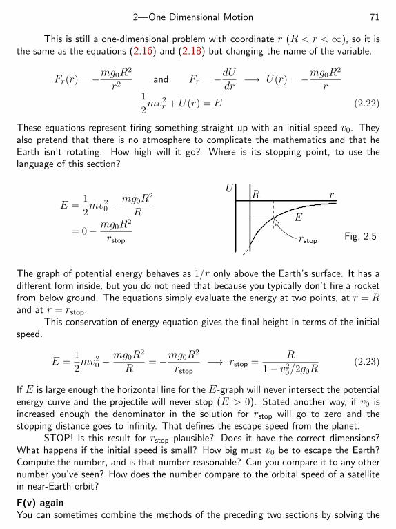
2—One Dimensional Motion 71
This is still a one-dimensional problem with coordinate r (R < r <∞), so it isthe same as the equations (2.16) and (2.18) but changing the name of the variable.
Fr(r) = −mg0R2
r2and Fr = −dU
dr−→ U(r) = −mg0R2
r1
2mv2
r + U(r) = E (2.22)
These equations represent firing something straight up with an initial speed v0. Theyalso pretend that there is no atmosphere to complicate the mathematics and that heEarth isn’t rotating. How high will it go? Where is its stopping point, to use thelanguage of this section?
E =1
2mv2
0 −mg0R2
R
= 0− mg0R2
rstop
UrR
E
rstop Fig. 2.5
The graph of potential energy behaves as 1/r only above the Earth’s surface. It has adifferent form inside, but you do not need that because you typically don’t fire a rocketfrom below ground. The equations simply evaluate the energy at two points, at r = Rand at r = rstop.
This conservation of energy equation gives the final height in terms of the initialspeed.
E =1
2mv2
0 −mg0R2
R= −mg0R2
rstop−→ rstop =
R
1− v20/2g0R
(2.23)
If E is large enough the horizontal line for the E-graph will never intersect the potentialenergy curve and the projectile will never stop (E > 0). Stated another way, if v0 isincreased enough the denominator in the solution for rstop will go to zero and thestopping distance goes to infinity. That defines the escape speed from the planet.
STOP! Is this result for rstop plausible? Does it have the correct dimensions?What happens if the initial speed is small? How big must v0 be to escape the Earth?Compute the number, and is that number reasonable? Can you compare it to any othernumber you’ve seen? How does the number compare to the orbital speed of a satellitein near-Earth orbit?
F(v) againYou can sometimes combine the methods of the preceding two sections by solving the
2—One Dimensional Motion 72
problems of a velocity-dependent force as a function of x instead of t. The same trickthat you saw in Eq. (2.17) to solve for forces depending on x alone also works for F (v).
Fx(vx) = mdvxdt
= mdvxdx
dxdt
= mvxdvxdx
−→ dx = mvx dvxF (vx)
(2.24)
Integrating this gives a relation between x and vx. Is this more useful than gettingvx(t)? Usually not, but it’s another tool in your utility belt.
2.4 Falling with resistance A plausible example comes by assuming that air resistance is proportional to velocity.It’s not all that accurate, but it is a fairly simple place to start. A more accurate modelwill assume that air resistance is proportional to v2, but this is easier to start with.
may = mdvydt
= md2ydt2
= −mg − bvy = −mg − bdydt
(2.25)
There are several ways to solve this equation. I’ll use separation of variables again,moving all the vys to one side of the equation and all the ts to the other.
mdvydt
= −mg − bvy −→ mdvy
mg + bvy= −dt
This is something that I can integrate. Use the same initial conditions as in the precedingexample, vy(0) = v0, and let u = bv′y
m∫ vy
v0
dv′ymg + bv′y
= −∫ t
0dt =
mb
∫ bvy
bv0
dumg + u
=mb
ln(mg + u)
∣∣∣∣bvybv0
=mb
lnmg + bvymg + bv0
= −t
Solve for the velocity.
mb
lnmg + bvymg + bv0
= −t −→ vy(t) = −mg/b+(v0 +mg/b
)e−bt/m (2.26)
Before proceeding, does this make sense? At time zero you have vy = v0 as required.At large time, vy approaches −mg/b, and from the original differential equation ofmotion, Eq. (2.25), this make the acceleration zero. That is the terminal velocity.
You can re-write Eq. (2.26) directly in terms of the terminal speed.;
vt =mgb, then vy(t) = −vt + (v0 + vt)e
−gt/vt (2.27)
2—One Dimensional Motion 73
To find y(t) you have a simple integral with respect to time. Use the boundarycondition that y(0) = 0 and
y(t) =
∫ t
0dt′[−mg/b+
(v0 +mg/b
)e−bt
′/m] = −mgbt′ −
(bv0 +mg
)mb2e−bt
′/m
∣∣∣∣t0
= −mgbt+
(bv0 +mg
)mb2
[1− e−bt/m
]= −vtt+ (v0 + vt)
vt
g
[1− e−gt/vt
](2.28)
Do these make sense? First, check the dimensions! Do not assume that you will nevermake a mistake. Notice that it’s easier to check dimensions now that everything isexpressed in terms of vt instead of m, b, and g. Next, see what the behavior of thesolution is in some special cases. Start with the small time behavior (not zero time).The initial velocity of the mass should be vy = v0, and its acceleration should be(−mg − bv0)/m. Why this last expression? Look at the original equation (2.25), andthat tells you the acceleration at all times, in particular the time t = 0. Now use apower series expansion on y(t) to find the small time behavior.
y(t) = −mgbt+ (bv0 +mg)
mb2
[1−
(1− bt
m+
(bt)2
2m2− (bt)3
6m3+ · · ·
)]≈ v0t− (bv0 +mg)
t2
2m+ (bv0 +mg)
b6m2
t3
= v0t−1
2m(mg + bv0)t2 + (bv0 +mg)
bt3
6m2
= v0t− gt2
2− v0
bt2
2m+ g
bt3
6m+ · · · (2.29)
• When I multiplied out the last equation, I was careful to keep terms to a consistentorder in b. That means that when I drop a b2 term in one place I should drop iteverywhere.• Some of the terms canceled: Those that involved 1/b. That’s an important checkon the algebra because if they don’t cancel then everything goes to infinity as the airresistance vanishes.• Some terms become independent of b as the viscosity approaches zero, and thoseare the ones that reproduce what you expect in the much simpler calculation for zeroviscosity.• The correction for small viscosity comes in the terms linear in b. These go beyond theelementary calculation, so look at the initial acceleration. That is in the t2 terms, theordinary at2/2, so you can recognize that the acceleration has the correct initial value,though it was hidden inside a more complicated exponential expression, waiting to bedug out. The initial force is the sum of gravity (down) and the friction (also down),producing initial acceleration ay0 = (−mg − bv0)/m.
2—One Dimensional Motion 74
The t3 term is starting to get harder to interpret, but at least the sign is under-standable. As the object start to rise, it starts to slow down (−gt). This in turn impliesthat the viscous force is not quite as big as it would have been without gravity, hencethis correction has a positive sign.
You’re not done. What happens in the opposite case, for which the viscosityis very large? Perhaps you’re firing a bullet into a barrel of honey. If b is large theexponential e−bt/m will go to zero very quickly. The viscous force will be much greaterthan the gravitational force: bv0 mg. In this case the solution (2.28) will beapproximately
y(t) ≈ mv0
b− mgt
b(2.30)
This means that it very quickly goes up a distance proportional to its initial momentum,stops at a height mv0/b, and then slowly drifts down at its constant terminal speedmg/b. Can I see why any of this is true independent of solving the whole equation?The terminal velocity is easy to see. Just go to the original equation Eq. (2.25) andask for the value of the velocity for which the acceleration is zero.
may = 0 = −mg − bvy −→ vy = −mg/b, the terminal velocity
For large times, the exponential e−bt/m dies out, and you are left with a constantvelocity,
y(t) ≈ −mgbt+
(v0 +mg/b
)mb
= −mgb
[t− m
b
(1 +
bv0
mg
)](2.31)
What can I say about the second term? It’s positive, and that’s correct, because theball has to spend some time going up before it starts down and eventually reaches itsterminal speed. The bigger the initial speed, the more time it spends going up. Did ithelp to rearrange the factors in the last expression and to put it in the form of somethinglike (t− t0)? Probably not, but you don’t know until you try.
Still another way to squeeze information out of this result: What if the airresistance is very small? Maybe even zero? One thing that I cannot do is to let b becomesmall in the last equations, because I was very careless in the preceding paragraph whenI said “For large times. . . ” What is large? That is meaningless because time is notdimensionless. Large compared to a femtosecond or large compared to a galactic year?What I should have said is that bt/m 1, making the exponential small comparedto one. Go back to the original equation (2.28), and look at that for small b. ThereI go again. What is “small b?” This time it is bt/m 1, and I essentially analyzedthis case in Eq. (2.29), where I said that t is small. If you set b = 0 there, you getv0t− gt2/2, and the correction is linear in the factor b.
Is there more that you can analyze in this simple-looking problem. Yes, seeproblem 2.10.
2—One Dimensional Motion 75
2.5 EquilibriumAt a point of equilibrium, the total force on the mass is zero, and in one dimensionthat’s all you need. Fx = −dU/dx, so a point of U at which the slope vanishes is anequilibrium point. Now, is it stable or unstable? Stable equilibrium means that if themass is disturbed slightly from the critical point, then the force pushes it back towardthe equilibrium position. If being a slight distance away from equilibrium causes it tobe pushed even farther away then it is an unstable equilibrium.
U
x (2.32)
The first of these curves has a potential maximum at dU/dx = 0, an unstableequilibrium. To the right of the maximum the force, −dU/dx, is positive — towardthe right; to its left it’s to the left. The second curve has a potential minimum as dU/dx = 0, a stable equilibriumbecause to the left the force is to the right and on the right it is to the left. The third has a potential minimum even though the derivative isn’t zero there. Infact it doesn’t even exist there. It is a stable point however. Just look at the directionsof the forces on the left and the right. The fourth graph has a point with zero derivative, but it is not a stable equilibriumwhen you consider motions in both directions. On the left the push is back to the right,but on the right the push is also to the right. And of course the x-axis itself graphs a potential function that has zero derivativeeverywhere. Neutral equilibrium.
The graph of U on page 69 shows several equilibria. Between c and C andbetween a and A and between g and G there are minimum points of U . Those are stableequilibrium points. Move to the right from any of them and dU/dx becomes positive,making Fx = −dU/dx negative. There are unstable equilibria between C and d andbetween F and g and just to the right of G. If the energy is just above that of a stableequilibrium, the motion near that point will be an oscillation around the equilibrium.The next chapter, on harmonic motion will look at that motion quantitatively.
When two atoms are bound into a diatomic molecule, the potential energy repre-senting the force binding the atoms together is a function of their separation distance.For the example of the molecule HCl the chlorine and hydrogen nuclei have an equilib-rium separation distance of about 1.3 A (0.13 nm). There is no simple exact expressionfor the potential energy of the molecule as a function of the atomic separation, butthere is a very good approximate one due to Morse. You can see from its graph thatwhen the distance between the atoms shrinks, the force pushing them apart becomesvery large. When they are farther apart than the equilibrium position the atoms are
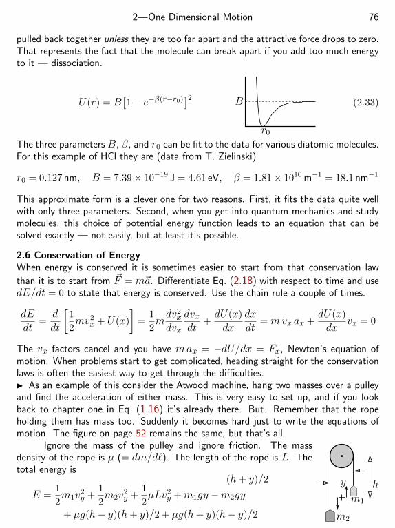
2—One Dimensional Motion 76
pulled back together unless they are too far apart and the attractive force drops to zero.That represents the fact that the molecule can break apart if you add too much energyto it — dissociation.
U(r) = B[1− e−β(r−r0)
]2 B
r0
(2.33)
The three parameters B, β, and r0 can be fit to the data for various diatomic molecules.For this example of HCl they are (data from T. Zielinski)
r0 = 0.127 nm, B = 7.39× 10⁻¹⁹ J = 4.61 eV, β = 1.81× 10¹⁰ m−1 = 18.1 nm−1
This approximate form is a clever one for two reasons. First, it fits the data quite wellwith only three parameters. Second, when you get into quantum mechanics and studymolecules, this choice of potential energy function leads to an equation that can besolved exactly — not easily, but at least it’s possible.
2.6 Conservation of EnergyWhen energy is conserved it is sometimes easier to start from that conservation law
than it is to start from ~F = m~a. Differentiate Eq. (2.18) with respect to time and usedE/dt = 0 to state that energy is conserved. Use the chain rule a couple of times.
dEdt
=ddt
[1
2mv2
x + U(x)
]=
1
2mdv2x
dvx
dvxdt
+dU(x)
dxdxdt
= mvx ax +dU(x)
dxvx = 0
The vx factors cancel and you have max = −dU/dx = Fx, Newton’s equation ofmotion. When problems start to get complicated, heading straight for the conservationlaws is often the easiest way to get through the difficulties. As an example of this consider the Atwood machine, hang two masses over a pulleyand find the acceleration of either mass. This is very easy to set up, and if you lookback to chapter one in Eq. (1.16) it’s already there. But. Remember that the ropeholding them has mass too. Suddenly it becomes hard just to write the equations ofmotion. The figure on page 52 remains the same, but that’s all.
hy
m1
(h+ y)/2
m2
Ignore the mass of the pulley and ignore friction. The massdensity of the rope is µ (= dm/d`). The length of the rope is L. Thetotal energy is
E =1
2m1v
2y +
1
2m2v
2y +
1
2µLv2
y +m1gy −m2gy
+ µg(h− y)(h+ y)/2 + µg(h+ y)(h− y)/2
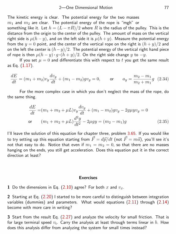
2—One Dimensional Motion 77
The kinetic energy is clear. The potential energy for the two massesm1 and m2 are clear. The potential energy of the rope is “mgh” orsomething like it. Let h = (L− πR)/2 where R is the radius of the pulley. This is thedistance from the origin to the center of the pulley. The amount of mass on the verticalright side is µ(h− y), and on the left side it is µ(h+ y). Measure the potential energyfrom the y = 0 point, and the center of the vertical rope on the right is (h+ y)/2 andon the left the center is (h−y)/2. The potential energy of the vertical right hand pieceof rope is then µ(h− y) . g .(h+ y)/2. On the right side change y to −y.
If you set µ = 0 and differentiate this with respect to t you get the same resultas Eq. (1.17).
dEdt
= (m1 +m2)vydvydt
+ (m1 −m2)gvy = 0, or ay =m2 −m1
m2 +m1g (2.34)
For the more complex case in which you don’t neglect the mass of the rope, dothe same thing.
dEdt
=(m1 +m2 + µL)vydvydt
+ (m1 −m2)gvy − 2gµyvy = 0
or (m1 +m2 + µL)d2ydt2− 2µgy = (m2 −m1)g (2.35)
I’ll leave the solution of this equation for chapter three, problem 3.65. If you would like
to try setting up this equation starting from ~F = d~p/dt (not ~F = m~a), you’ll see it’snot that easy to do. Notice that even if m1 = m2 = 0, so that there are no masseshanging on the ends, you still get acceleration. Does this equation put it in the correctdirection at least?
Exercises
1 Do the dimensions in Eq. (2.10) agree? For both x and vx.
2 Starting at Eq. (2.20) I started to be more careful to distinguish between integrationvariables (dummies) and parameters. What would equations (2.11) through (2.14)become with more care in writing?
3 Start from the result Eq. (2.27) and analyze the velocity for small friction. That isfor large terminal speed vt. Carry the analysis at least through terms linear in b. Howdoes this analysis differ from analyzing the system for small times instead?
2—One Dimensional Motion 78
4 In Eq. (2.22) the zero point of potential energy was at infinity; the constant ofintegration in finding U was zero. Instead, now assume that the potential energy iszero at the Earth’s surface, U(R) = 0. Re-do the calculation leading to Eq. (2.23) andcompare the answers.
5 A pendulum has a very light, rigid rod instead of a string to hold the mass at itsend. (a) What is the potential energy of the mass as a function of the angle from thevertical? And graph it of course. (b) Use this to describe all the qualitatively differentsorts of motion this mass can have.
6 Sketch a graph of the force function for the Morse potential energy, Eq. (2.33).
7 Write the total energy for a mass falling freely under gravity. Differentiate it withrespect to t.
8 In Eq. (2.35), what is the acceleration for µ = 0? More important: Analyze thisanswer for plausibility.
9 With the parameters stated, does the equation (2.33) really agree with the graphdrawn there? Check some numbers.
2—One Dimensional Motion 79
Problems
2.1 For the three sets of conditions specified in Eq. (2.1), solve for C and D and getthe corresponding y and vy. Ans: (2) y(t) = −1
2gt2 + 1
2gT t, vy(t) = −gt+ 12gT
2.2 ˙ The solution for a purely time-dependent force, Eq. (2.2), can be written as asingle integral.
x(t) = x0 + vx0t+1
m
∫ t
0dt′ (t− t′)Fx(t′)
Differentiate this twice to verify that it works. The general reason why this works andwhere it comes from can wait until section 3.10, though deriving this particular resultis problem 2.43. Read section 0.5.
2.3 Repeat the example leading to Eq. (2.3) but using a force proportional to cosineinstead of sine. Especially, repeat the analysis of the solution and compare the resultshere to those with the sine. Why the difference?
2.4 Repeat the example leading to Eq. (2.3) but using a force proportional to sinesquared instead of sine. Can you anticipate what at least some pieces of the solutionshould be even before you do an integral?
2.5˙ A force along the x-direction is given to be F0 for the time between zero and T . Itthen drops to zero in a straight line for the time from T to 2T . (a) Write this functionFx using the notation of Eqs. (0.21) and (2.4). Then graph it. (b) A mass m startsat the origin from rest and is subject to this force. Without solving any new equations,sketch a graph of what its velocity should be like as a function of time. (c) Solve forvx(t) and x(t). Look back at your graph and see how good it is, then draw a moreaccurate graph from the result.
2.6 For the constant force Fy = −mg, you already have the solution Eq. (2.21), but dothe qualitative and graphical analysis as in the example following it, where U = kx2/2.Do this as if you don’t already know the answer. Use all the tools in that second analysisto verify the plausibility of this solution. Stopping points, force, kinetic energy,. . . Fromthis, find the stopping point under the initial conditions vy(0) = v0.
2.7¨Instead of the specific functions of velocity as in Eq. (2.9) or (2.10), assume thefriction obeys Fx = −bvαx and find the velocity and position starting from x(0) = 0and vx(0) = v0. (Assume α 6= 1 for, I hope, obvious reasons.) Analyze the result forall (real) α.
2—One Dimensional Motion 80
2.8 ˙ A mass is initially moving at a velocity vx(0) = v0 > 0. The frictional force is−F0ekv (v > 0). Find the velocity and position as a function of time and of course,analyze the results (small time, large time, small and large k).
2.9 Start from the form of Eq. (2.22) and solve for dt. Set up the integral to find therelation between r and t, then carry out the integral in the special case that E = 0.The integrals aren’t so bad in this case and you can spend your time analyzing theresult.
2.10 You thought I spent enough time on analyzing the results of Eq. (2.26) and (2.28)but no. (a) Find the maximum height to which the projectile rises. (b) For small airresistance your result looks like it is going to infinity. Find its behavior for small b andsee if it is plausible. (c) Approximately what is this result for large air resistance? Thatis, what terms dominate?
Ans: ymax = −v2tg ln
(1 + v0
vt
)+ vtv0
g ≈ (v20/2g)− (bv3
0/3mg2) + · · ·
2.11 After Eq. (2.19) there is a qualitative analysis of the potential energy U(x) =kx2/2. Now do the integral in Eq. (2.19) to get t in terms of x (a trig substitution)and then solve for x(t). Compare your solution to the qualitative description in thetext.
2.12 (a) Analyze the preceding quadratic potential energy qualitatively as in the text,but turn it upside down first. Now U(x) = −kx2/2. (b) For the example in the text, Idid not consider the cases for which E < 0. Why not? What about this new potential?
2.13 Answer all the questions presented immediately after Eq. (2.23).
2.14˙ A particle of mass m is subject to the force as specified by the potential energyU(x) = U0|x|/a where a is a (constant) length and U0 is a constant energy. The masshas a total energy E. What is the period of oscillation? The amplitude? How does thisperiod vary with the amplitude of the oscillation? Sketch a graph of the dependence.Suggestion: Write |x| as two cases: x > 0 and x < 0.
2.15 A particle with mass m is subjected to a force Fx(x) = −F0x3/a3. At timet = 0 the particle is at rest at position x0 (a) Find vx(x), draw the potential energygraph in the process. (b) Set up the integral that you would have to do to go fromthe result in (a) to get the relation between x and t. If you find that you can do theintegral easily, go back and find your mistake.
2.16 When a mass m is oscillating within a potential energy function kx2/2, as on page68, you can try assuming the simplest functional form for the motion, x(t) = A cosωt.Do not assume that you have any knowledge of A or ω. Compute the total mechanical
2—One Dimensional Motion 81
energy mv2/2 + kx2/2 for this assumed x. This E(t) will be a function of time, butit’s not supposed to be. Find the value of ω so that E is independent of t.
2.17 If an elastic ball is bouncing on the floor, the potential energy curve is like thethird one at Eq. (2.32). A straight line mgy for y > 0 and jumping almost straight upat y = 0. Assume the ball’s total energy is E and use the methods of section 2.3 tofind the total time between bounces.
2.18 Find x(t) if Fx = F0ect, given x(0) = 0 and vx(0) = 0.
2.19 Derive the equation (2.8) using the result of problem 2.2.
2.20 In the problem leading to Eq. (2.8), the force F2 is turned off after time T2.What are vx and x for all times after that?
2.21˙ For the force in Eq. (2.15), with initial velocity v0, find the velocity and positionas a function of time. Analyze the results and compare this analysis to that done in theparagraphs just after that equation.
2.22 A mass m is subject to a frictional force Fx = −bvx, and x(0) = 0 with zerovelocity. Starting at time t = 0 there is an additional force Fx = ct, where c is aconstant. Find the motion as a function of time.
2.23 ˙ The assumption about air resistance made in Eq. (2.25) isn’t very good, as thedependence on velocity is more nearly quadratic than linear. Take the same initialconditions as there but assume the air resistance is −bv2
y on the way up, so may =
−mg− bv2y. Solve for vy(t) in this case, and express the result in terms of the terminal
speed, where mg = bv2t . Show that
vy(t) = vtv0 − vt tan(gt/vt)
vt + v0 tan(gt/vt)and that if vt = 100 m/s (typical for a 30 caliber bullet)
then no matter how big the initial speed is the mass will stop in less than about16 seconds. Did you sketch any graphs? Does the same statement apply to Eq. (2.26)?
2.24 A boat is slowed by a frictional force Fx(v). Its speed decreases according to theequation v(t) = c2(t− t1)2 where c is a constant and t1 is the time at which it stops.
Find the force Fx(v) as a function of v. (t < t1 of course.) Ans: −2mcv1/2
2.25˙ In problem 2.23, if the mass is moving down then the air resistance is Fy = +bv2y,
not minus. You have to handle this case separately because the form of the equationis different, and there’s not a neat analytical way to handle it. Solve for the velocity ifthe mass starts from rest and drops.
2.26 A force acts on m, with Fx = Av2/x. Find x(t) if x(0) = x0 > 0 and vx(0) =v0 > 0.
2—One Dimensional Motion 82
2.27 A particle of mass m is initially at rest at a coordinate x = x0. It is repelled fromthe origin by a force Fx = A/x3. Solve for x(t) and vx(t).
2.28˙ If a mass is bouncing up and down elastically on a rigid floor, the probabilityof seeing the mass within the interval y to y+ ∆y is proportional to the amount oftime it spends in that interval. (If you look at it only occasionally, the probabilityof seeing it somewhere is proportional to the time it spends within dy.) Statedmathematically, the probability dP to see it in the interval dy is C dt, wheredt is the time spent there and C is some constant. The probability density isdefined as dP/dy, so this is C dt/dy = C/v. (a) Compute this as a functionof y for a bouncing ball that has total energy E = mgymax, and the floor is aty = 0. The total probability must be one:
∫dP = 1. This lets you evaluate
C and then graph dP/dy versus y. Why does the graph have the shape thatit does, and does it make any sense? Do the dimensions of dP/dy make sense?Examine the simulation on the right. And when in doubt, remember that physicsis an experimental science so you may want to try bouncing a tennis ball yourself.(b) Just as the total probability is one,
∫dP = 1, the mean (or average) value of
the height is∫y dP =
∫∞0 y(dP/dy) dy. Evaluate this. Ans: 2
3y0
2.29˙ In the preceding problem, you have 100 balls all bouncing up and down ran-domly (but all with the same energy). (a) At any one time, if you take a photographof all of them at once, approximately how many of the balls would be at a heightfrom the ground up to one-half the maximum height? (b) The median height isthat height so that one-half the balls are below it and one-half are above. Whatis that median for these bouncing balls and how does it compare the mean valuefound in the preceding problem? There are 100 dots in the simulation on the right.
2.30 A mass m moves in one dimension and subject to a variety of forces and initialconditions. In each case, does the mass stop in a finite time or distance as the casemay be?[a] Fx = −α/t for t > 0. At time t = t0, the velocity is v = v0 > 0; find v(t).[b] Fx = −α/v for v > 0. At time t = t0, the velocity is v = v0 > 0; find v(t).[c] Fx = −α/x for x > 0. At position x = x0, the velocity is v = v0 > 0; find v(x).
2.31 The force on a mass m is Fx = kvxx where k is a positive constant. At timet = 0 the mass has x(0) = 0 and vx(0) = v0. Find x(t).
2.32 The coefficient of friction between a mass m and the horizontal table on whichit rests is µk. The air also provides a frictional force proportional to velocity. The massis given an initial velocity v0. Find vx(t). Find x(t).
2—One Dimensional Motion 83
2.33 A potential energy us given by U(x) = (a/x) − (b/x2), where a and b arepositive. Analyze the possible motions qualitatively. For what range of energy is themotion periodic? For what range is it not?
2.34 A wheel of radius R is rotating about a horizontal axis. The angle through whichit has rotated is φ(t) = At3 where A is a constant and φ is measured in radians fromthe bottom. When the point that was at the bottom at time t = 0 has gone around Ntimes and then comes up to the position directly to the right of the axis, a small pieceof the wheel at that point breaks off and flies straight up. Use the axis of the wheel asthe origin and find the displacement vector from the origin to the position of this pieceat the time it reaches its maximum height.
2.35 The more general form of Newton’s equation of motion is Fx = d(mvx)/dt, not= max. An open railroad car of mass M is traveling in a straight line, starting withan initial velocity v0. It rains, causing water to fill the car at a rate dm/dt = β. Findthe velocity and the position as a function of time. Assume no friction.
2.36¨A uniform chain is hung vertically with its bottom point just touching a table.Release the chain, letting it drop onto the table. Compute the force the chain exertson the table as this happens. Show that as the chain drops, this force is three timesthe weight of the chain that has already come to rest on the table. There are exactlytwo things acting on the chain: gravity and the table. On approach is to figure outwhat the motion will be and then take the time derivative of the chain’s momentum.Another approach is to draw careful pictures at the times t and t+ ∆t and to see what
has happened between the two times. Remember: ~F 6= m~a; it = d~p/dt.]
2.37 A mass m is dropped with initial velocity zero, and the forces on m are fromgravity and some form of air resistance. Measure the coordinate y positive downwardfrom the starting position. If you get the result
y(t) =v2
t
gln
[sinh
(gtvt
)](a) What is this position function for large time? Is the behavior correct? (b) Whatis this function for small time, keeping enough terms that you may be able to surmisewhat the assumed form for the air resistance force is? Are these results plausible?
2.38 Someone else got a different answer for the preceding problem:
y(t) =v2
t
gln
[cosh
(gtvt
)]
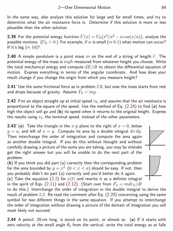
2—One Dimensional Motion 84
In the same way, also analyze this solution for large and for small times, and try todetermine what the air resistance force is. Determine if this solution is more or lessplausible than the other solution.
2.39 For the potential energy function U(x) = U0
(x2/a2 − α cos(x/a)
), analyze the
possible motions. (U0 > 0.) For example, if α is small (≈ 0.1) what motion can occur?If it’s big (≈ 10)?
2.40 A simple pendulum is a point mass m on the end of a string of length `. Thepotential energy of the mass is mgh measured from whatever height you choose. Writethe total mechanical energy and compute dE/dt to obtain the differential equation ofmotion. Express everything in terms of the angular coordinate. And how does yourresult change if you change the origin from which you measure height?
2.41˙ Use the same frictional force as in problem 2.8, but now the mass starts from restand drops because of gravity. Assume F0 < mg.
2.42 Fire an object straight up at initial speed v0, and assume that the air resistance isproportional to the square of the speed. Use the method of Eq. (2.24) to find (a) howhigh the object will go and (b) its speed when it returns to the original height. Expressthe results using vt, the terminal speed, instead of the other parameters.
2.43˙ (a) Take the triangle in the x-y plane to the right of x = 0, belowy = a, and left of x = y. Compute its area by a double integral dxdy.Then interchange the order of integration and compute the area againas another double integral. If you do this without thought and withoutcarefully drawing a picture of the sums you are taking, you may by mistakeget the right answer but you will be unable to do the next part of theproblem.(b) If you think you did part (a) correctly then the corresponding problemfor the area bounded by y = x2 (0 < x < a) should be easy. If not, thenyou probably didn’t do part (a) correctly and you’d better do it again.(c) Take the equation (2.2) for x(t) and rewrite it as a definite integralin the spirit of Eqs. (2.11) and (2.12). (Start over from Fx = mdvx/dtto do this.) Interchange the order of integration in the double integral to derive theresult of problem 2.2. Re-read the comment after Eq. (2.20) concerning using the samesymbol for two different things in the same equation. If you attempt to interchangethe order of integration without drawing a picture of the domain of integration you willmost likely not succeed.
2.44 A pencil, 20 cm long, is stood on its point, or almost so. (a) If it starts withzero velocity at the small angle θ0 from the vertical, write the total energy as at falls
2—One Dimensional Motion 85
over. Then separate variables to get a well-defined definite integral to determine howmuch time it will take to fall to the horizontal surface. (b) This is a hard integral, soto estimate it, assume that the angle θ as measured from the vertical is small all theway up to π/2, so that sin θ ≈ θ and cos θ ≈ 1 − θ2/2; evaluate the time to fall andevaluate it numerically for initial angles of 1, 10−3, and 10−6. Even though thisapproximation looks crude, it gives pretty good results. That’s because for most of theduration of the fall (i.e. when it’s just starting out), the angle is small.
2.45 The equation (2.19) lets you get time as a function of how far you’ve gone. Applythis to the potential energy U(x) = −kx2/2, starting at x = x0 > 0 with positivevelocity v0. (a) As x −→ ∞, does this converge? That is, does it take a finite timeto go an infinite distance? (b) More generally, for what values of the exponent inU(x) = −kxa/2 (a > 0) will that time be finite and for which is it infinite?
InterludeWhen solving problems, the goal is not an answer. The goal is understanding.
You will not get this understanding by checking whether your answer agrees with theback of the book or if it agrees with someone else, or if a teacher says it’s right. Doesyour solution make sense?
In the preceding chapter, section 2.2, what if Eqs. (2.13) and (2.14) had beendifferent, perhaps saying
vx =v0
1 +( bv0m t)2 ?
Would this make sense? It’s dimensionally correct; at least it has the same combinationof parameters bv0t/m that appeared in Eq. (2.14), so if it was correct there then it ishere too. As t→∞ this goes to zero faster than the other solution. Is that bad? Notobviously so. Before, the integral of vx dt went to infinity for large time because thevelocity went to zero so slowly. Does that happen here? No, because∫ ∞ dt
1 + t2converges to a finite value
That’s different, but again, not obviously wrong. What about small time?
vx ≈ v0
[1−
( bv0m t)2]
for small t
This implies that at time zero, the acceleration = −2b2v30t/m
2 = 0. Even with the airresistance, −mv2, assumed in deriving Eq. (2.13) this says that there is no decellerationat the beginning. That is clearly wrong because v 6= 0 at that time.
If you have a simple mechanical system with a mass hanging on a string that iswrapped around a pulley, what will the acceleration be? In chapter one the equation(1.18) said
dvydt
=m1 −m2
m1 +m2g
What if it had said
=m1 +m2
m1 −m2g or =
m1
m1 +m2g ?
In the first case, look at the expression for the special case that m1 = m2. Thedenominator vanishes, and that’s almost always a bad thing to happen. In the secondcase, notice that it is always positive. Even if m2 m1, this would be positive eventhough from the picture preceding Eq. (1.18) you see that ay would have to be negativein this case. Both of these are wrong, whether you know the correct solution or not.
86
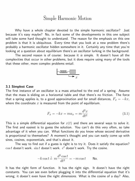
Simple Harmonic Motion
Why have a whole chapter devoted to the simple harmonic oscillator? Justbecause it’s easy maybe? No, in fact some of the developments in this one subjectwill take some hard thought to understand. The reason for the emphasis on this oneproblem is that it is ubiquitous. Every time that you look at a new problem there’sprobably a harmonic oscillator hidden somewhere in it. Certainly any time that you’relooking at a question about equilibrium there’s an oscillator lurking in the background.
The second reason is of course: because it is simple. It doesn’t have all thecomplexities that occur in other problems, but it does require using many of the toolsthat these other, more complex problems entail.
x
3.1 Simplest CaseThe first instance of an oscillator is a mass attached to the end of a spring. Assumethat the mass is sliding on a horizontal table and that there’s no friction. The forcethat a spring applies is, to a good approximation and for small distances, Fx = −kx,where the coordinate x is measured from the point of equilibrium.
Fx = −kx = max = md2xdt2
(3.1)
This is a simple differential equation for x(t) and there are several ways to solve it.The first and easiest is to guess the solution. You can’t do this very often, so takeadvantage of it when you can. What functions do you know whose second derivativeis proportional to themselves? A moment’s thought and you can easily come up withsines, cosines, exponentials, and that’s about it.
The way to find out if a guess is right is to try it. Does it satisfy the equation?cos t doesn’t work. sin t doesn’t work. et doesn’t work. Try the cosine.
−k cos t=? md2 cos tdt2
= −m cos t No.
It has the right form of function. It has the right sign. It doesn’t have the rightconstants. You can see even before plugging it into the differential equation that it’swrong; it doesn’t even have the right dimensions. What is the cosine of a day? Also,
87
3—Simple Harmonic Motion 88
the output of the cosine is dimensionless, but x(t) isn’t. You need to sprinkle someconstants around to take care of the units if nothing else.
Try x(t) = A cosω0t instead.
−kA cosω0t=? md2A cosω0t
dt2= −mAω2
0 cosω0t
The cosines match. The signs match. All that’s left are the constants, and A betternot be zero or you have a trivial solution, where nothing is happening.
kA = mAω20 implies ω2
0 = k/m or ω0 =√k/m
For this value of the constant ω0 you have a solution. It says nothing about A. Willx(t) = A sinω0t work too? Yes, just try it. How about x(t) = Aeαt? Try this andyou have
−kAeαt =? md2Aeαt
dt2= mAα2eαt, which implies
α2 = −k/m or α = ±√−k/m = ±i
√k/m = ±i ω0
All of these work.For a second order differential equation there are two arbitrary constants in the
complete solution. You’re undoing two derivatives and each gives a constant of inte-gration. Also, you need two constants in order to be able to specify an initial positionand an initial velocity. You can put the solutions in several different forms, notingspecifically that for this equation the sum of two solutions is a solution.
−k(x1(t) + x2(t)
)= m
d2(x1 + x2)
dt2
If x1 and x2 satisfy this equation separately then their sum does.
x(t) = A cosω0t+B sinω0t = Ceiω0t +De−iω0t (3.2)
Other equivalent forms are
x(t) = F cos(ω0t+ δ1) = G sin(ω0t+ δ2) (3.3)
These are all different forms of the solution and they all equal each other if the coef-ficients are arranged appropriately. This means that you can use whichever of these is
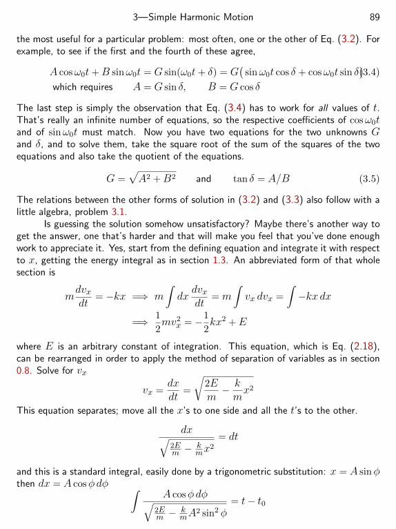
3—Simple Harmonic Motion 89
the most useful for a particular problem: most often, one or the other of Eq. (3.2). Forexample, to see if the first and the fourth of these agree,
A cosω0t+B sinω0t = G sin(ω0t+ δ) = G(
sinω0t cos δ + cosω0t sin δ)(3.4)
which requires A = G sin δ, B = G cos δ
The last step is simply the observation that Eq. (3.4) has to work for all values of t.That’s really an infinite number of equations, so the respective coefficients of cosω0tand of sinω0t must match. Now you have two equations for the two unknowns Gand δ, and to solve them, take the square root of the sum of the squares of the twoequations and also take the quotient of the equations.
G =√A2 +B2 and tan δ = A/B (3.5)
The relations between the other forms of solution in (3.2) and (3.3) also follow with alittle algebra, problem 3.1.
Is guessing the solution somehow unsatisfactory? Maybe there’s another way toget the answer, one that’s harder and that will make you feel that you’ve done enoughwork to appreciate it. Yes, start from the defining equation and integrate it with respectto x, getting the energy integral as in section 1.3. An abbreviated form of that wholesection is
mdvxdt
= −kx =⇒ m∫dx
dvxdt
= m∫vx dvx =
∫−kxdx
=⇒ 1
2mv2
x = −1
2kx2 +E
where E is an arbitrary constant of integration. This equation, which is Eq. (2.18),can be rearranged in order to apply the method of separation of variables as in section0.8. Solve for vx
vx =dxdt
=
√2Em− kmx2
This equation separates; move all the x’s to one side and all the t’s to the other.
dx√2Em −
kmx
2= dt
and this is a standard integral, easily done by a trigonometric substitution: x = A sinφthen dx = A cosφdφ ∫
A cosφdφ√2Em −
kmA
2 sin2 φ= t− t0
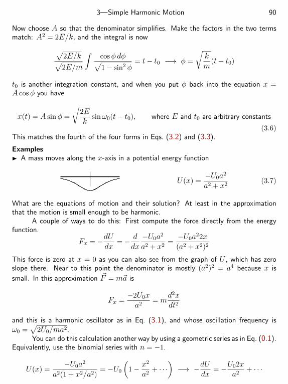
3—Simple Harmonic Motion 90
Now choose A so that the denominator simplifies. Make the factors in the two termsmatch: A2 = 2E/k, and the integral is now√
2E/k√2E/m
∫cosφdφ√1− sin2 φ
= t− t0 −→ φ =
√km
(t− t0)
t0 is another integration constant, and when you put φ back into the equation x =A cosφ you have
x(t) = A sinφ =
√2Ek
sinω0(t− t0), where E and t0 are arbitrary constants
(3.6)This matches the fourth of the four forms in Eqs. (3.2) and (3.3).
Examples A mass moves along the x-axis in a potential energy function
U(x) =−U0a2
a2 + x2(3.7)
What are the equations of motion and their solution? At least in the approximationthat the motion is small enough to be harmonic.
A couple of ways to do this: First compute the force directly from the energyfunction.
Fx = −dUdx
= − ddx−U0a2
a2 + x2=−U0a22x(a2 + x2)2
This force is zero at x = 0 as you can also see from the graph of U , which has zeroslope there. Near to this point the denominator is mostly (a2)2 = a4 because x is
small. In this approximation ~F = m~a is
Fx =−2U0xa2
= md2xdt2
and this is a harmonic oscillator as in Eq. (3.1), and whose oscillation frequency is
ω0 =√
2U0/ma2.You can do this calculation another way by using a geometric series as in Eq. (0.1).
Equivalently, use the binomial series with n = −1.
U(x) =−U0a2
a2(1 + x2/a2)= −U0
(1− x
2
a2+ · · ·
)−→ −dU
dx= −U02x
a2+ · · ·
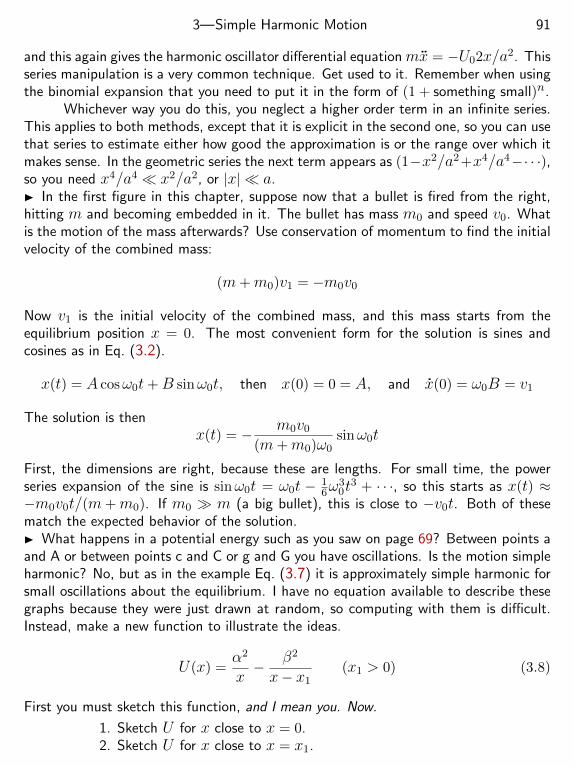
3—Simple Harmonic Motion 91
and this again gives the harmonic oscillator differential equation mx = −U02x/a2. Thisseries manipulation is a very common technique. Get used to it. Remember when usingthe binomial expansion that you need to put it in the form of (1 + something small)n.
Whichever way you do this, you neglect a higher order term in an infinite series.This applies to both methods, except that it is explicit in the second one, so you can usethat series to estimate either how good the approximation is or the range over which itmakes sense. In the geometric series the next term appears as (1−x2/a2+x4/a4−· · ·),so you need x4/a4 x2/a2, or |x| a. In the first figure in this chapter, suppose now that a bullet is fired from the right,hitting m and becoming embedded in it. The bullet has mass m0 and speed v0. Whatis the motion of the mass afterwards? Use conservation of momentum to find the initialvelocity of the combined mass:
(m+m0)v1 = −m0v0
Now v1 is the initial velocity of the combined mass, and this mass starts from theequilibrium position x = 0. The most convenient form for the solution is sines andcosines as in Eq. (3.2).
x(t) = A cosω0t+B sinω0t, then x(0) = 0 = A, and x(0) = ω0B = v1
The solution is thenx(t) = − m0v0
(m+m0)ω0sinω0t
First, the dimensions are right, because these are lengths. For small time, the powerseries expansion of the sine is sinω0t = ω0t − 1
6ω30t
3 + · · ·, so this starts as x(t) ≈−m0v0t/(m+m0). If m0 m (a big bullet), this is close to −v0t. Both of thesematch the expected behavior of the solution. What happens in a potential energy such as you saw on page 69? Between points aand A or between points c and C or g and G you have oscillations. Is the motion simpleharmonic? No, but as in the example Eq. (3.7) it is approximately simple harmonic forsmall oscillations about the equilibrium. I have no equation available to describe thesegraphs because they were just drawn at random, so computing with them is difficult.Instead, make a new function to illustrate the ideas.
U(x) =α2
x− β2
x− x1(x1 > 0) (3.8)
First you must sketch this function, and I mean you. Now.
1. Sketch U for x close to x = 0.2. Sketch U for x close to x = x1.
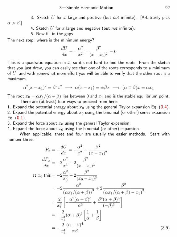
3—Simple Harmonic Motion 92
3. Sketch U for x large and positive (but not infinite). [Arbitrarily pickα > β.]
4. Sketch U for x large and negative (but not infinite).5. Now fill in the gaps.
The next step: where is the minimum energy?
dUdx
= −α2
x2+
β2
(x− x1)2= 0
This is a quadratic equation in x, so it’s not hard to find the roots. From the sketchthat you just drew, you can easily see that one of the roots corresponds to a minimumof U , and with somewhat more effort you will be able to verify that the other root is amaximum.
α2(x− x1)2 = β2x2 −→ α(x− x1) = ±βx −→ (α∓ β)x = αx1
The root x0 = αx1/(α+ β) lies between 0 and x1 and is the stable equilibrium point.There are (at least) four ways to proceed from here:
1. Expand the potential energy about x0 using the general Taylor expansion Eq. (0.4).2. Expand the potential energy about x0 using the binomial (or other) series expansionEq. (0.1).3. Expand the force about x0 using the general Taylor expansion.4. Expand the force about x0 using the binomial (or other) expansion.
When applicable, three and four are usually the easier methods. Start withnumber three:
Fx = −dUdx
= +α2
x2− β2
(x− x1)2
dFxdx
= −2α2
x3+ 2
β2
(x− x1)3
at x0 this = −2α2
x30
+ 2β2
(x0 − x1)3
= −2α2(
αx1/(α+ β))3 + 2
β2(αx1/(α+ β)− x1
)3=
2
x31
[−α
2(α+ β)3
α3+β2(α+ β)3
(−β)3
]= − 2
x31
(α+ β)3
[1
α+
1
β
]= − 2
x31
(α+ β)4
αβ(3.9)
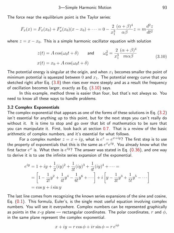
3—Simple Harmonic Motion 93
The force near the equilibrium point is the Taylor series:
Fx(x) = Fx(x0) + F ′x(x0)(x− x0) + · · · = 0− 2
x31
(α+ β)4
αβz = m
d2zdt2
where z = x− x0. This is a simple harmonic oscillator equation with solution
z(t) = A cos(ω0t+ δ) and ω20 =
2
x31
(α+ β)4
mαβ
x(t) = x0 +A cos(ω0t+ δ)
(3.10)
The potential energy is singular at the origin, and when x1 becomes smaller the point ofminimum potential is squeezed between 0 and x1. The potential energy curve that yousketched right after Eq. (3.8) then rises ever more steeply and as a result the frequencyof oscillation becomes larger, exactly as Eq. (3.10) says.
In this example, method three is easier than four, but that’s not always so. Youneed to know all these ways to handle problems.
3.2 Complex ExponentialsThe complex exponential that appears as one of the forms of these solutions in Eq. (3.2)isn’t essential for anything up to this point, but for the next steps you can’t really dowithout it. It is time to stop and go over that bit of mathematics to be sure thatyou can manipulate it. First, look back at section 0.7. That is a review of the basicarithmetic of complex numbers, and it’s essential for what follows.
For a complex number z = x+ iy, what is ez = ex+iy? The first step is to usethe property of exponentials that this is the same as exeiy. You already know what thefirst factor ex is. What then is eiy? The answer was stated in Eq. (0.36), and one wayto derive it is to use the infinite series expansion of the exponential.
eiy = 1 + iy +1
2(iy)2 +
1
3!(iy)3 +
1
4!(iy)4 + · · · =
=
[1− 1
2!y2 +
1
4!y4 − 1
6!y6 + · · ·
]+ i
[y − 1
3!y3 +
1
5!y5 − · · ·
]= cos y + i sin y
The last line comes from recognizing the known series expansions of the sine and cosine,Eq. (0.1). This formula, Euler’s, is the single most useful equation involving complexnumbers. You will see it everywhere. Complex numbers can be represented graphicallyas points in the x-y plane — rectangular coordinates. The polar coordinates, r and φ,in the same plane represent the complex exponential.
x+ iy = r cosφ+ ir sinφ = r eiφ
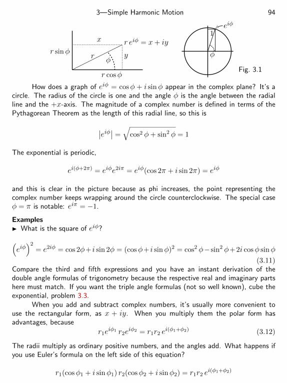
3—Simple Harmonic Motion 94
y
x
rφ
r cosφ
r sinφr eiφ = x+ iy
eiφ
1
φ
Fig. 3.1
How does a graph of eiφ = cosφ + i sinφ appear in the complex plane? It’s acircle. The radius of the circle is one and the angle φ is the angle between the radialline and the +x-axis. The magnitude of a complex number is defined in terms of thePythagorean Theorem as the length of this radial line, so this is
∣∣eiφ∣∣ =
√cos2 φ+ sin2 φ = 1
The exponential is periodic,
ei(φ+2π) = eiφe2iπ = eiφ(cos 2π + i sin 2π) = eiφ
and this is clear in the picture because as phi increases, the point representing thecomplex number keeps wrapping around the circle counterclockwise. The special caseφ = π is notable: eiπ = −1.
Examples What is the square of eiφ?(eiφ)2
= e2iφ = cos 2φ+ i sin 2φ = (cosφ+ i sinφ)2 = cos2 φ− sin2 φ+2i cosφ sinφ
(3.11)Compare the third and fifth expressions and you have an instant derivation of thedouble angle formulas of trigonometry because the respective real and imaginary partshere must match. If you want the triple angle formulas (not so well known), cube theexponential, problem 3.3.
When you add and subtract complex numbers, it’s usually more convenient touse the rectangular form, as x + iy. When you multiply them the polar form hasadvantages, because
r1eiφ1 r2e
iφ2 = r1r2 ei(φ1+φ2) (3.12)
The radii multiply as ordinary positive numbers, and the angles add. What happens ifyou use Euler’s formula on the left side of this equation?
r1(cosφ1 + i sinφ1) r2(cosφ2 + i sinφ2) = r1r2 ei(φ1+φ2)
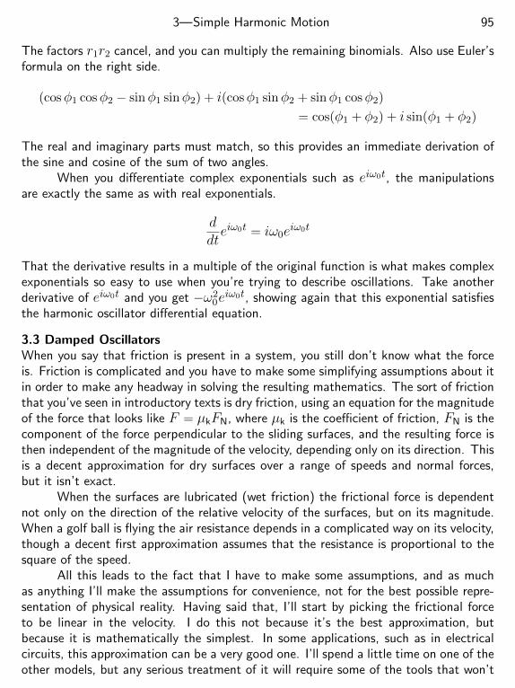
3—Simple Harmonic Motion 95
The factors r1r2 cancel, and you can multiply the remaining binomials. Also use Euler’sformula on the right side.
(cosφ1 cosφ2 − sinφ1 sinφ2) + i(cosφ1 sinφ2 + sinφ1 cosφ2)
= cos(φ1 + φ2) + i sin(φ1 + φ2)
The real and imaginary parts must match, so this provides an immediate derivation ofthe sine and cosine of the sum of two angles.
When you differentiate complex exponentials such as eiω0t, the manipulationsare exactly the same as with real exponentials.
ddteiω0t = iω0e
iω0t
That the derivative results in a multiple of the original function is what makes complexexponentials so easy to use when you’re trying to describe oscillations. Take anotherderivative of eiω0t and you get −ω2
0eiω0t, showing again that this exponential satisfies
the harmonic oscillator differential equation.
3.3 Damped OscillatorsWhen you say that friction is present in a system, you still don’t know what the forceis. Friction is complicated and you have to make some simplifying assumptions about itin order to make any headway in solving the resulting mathematics. The sort of frictionthat you’ve seen in introductory texts is dry friction, using an equation for the magnitudeof the force that looks like F = µkFN, where µk is the coefficient of friction, FN is thecomponent of the force perpendicular to the sliding surfaces, and the resulting force isthen independent of the magnitude of the velocity, depending only on its direction. Thisis a decent approximation for dry surfaces over a range of speeds and normal forces,but it isn’t exact.
When the surfaces are lubricated (wet friction) the frictional force is dependentnot only on the direction of the relative velocity of the surfaces, but on its magnitude.When a golf ball is flying the air resistance depends in a complicated way on its velocity,though a decent first approximation assumes that the resistance is proportional to thesquare of the speed.
All this leads to the fact that I have to make some assumptions, and as muchas anything I’ll make the assumptions for convenience, not for the best possible repre-sentation of physical reality. Having said that, I’ll start by picking the frictional forceto be linear in the velocity. I do this not because it’s the best approximation, butbecause it is mathematically the simplest. In some applications, such as in electricalcircuits, this approximation can be a very good one. I’ll spend a little time on one of theother models, but any serious treatment of it will require some of the tools that won’t
3—Simple Harmonic Motion 96
appear until another chapter, though this linear approximation is actually a pretty goodrepresentation for an object moving slowly through a fluid.
With this “viscous damping” the equation (3.1) become
Fx = −kx− bvx = −kx− bdxdt
= max = md2xdt2
(3.13)
Sines and cosines are not enough here, because the first derivative changes one into theother. This differential equation falls into a class of equations that appear repeatedly.They are
“linear, homogeneous, constant coefficient”
differential equations of the sort described in section 0.9. That is, The dependentvariable, x, or its derivatives appear just to the first power, and the coefficients areall constants. Such equations are easy to solve because of the special property ofexponentials. The derivative of an exponential is itself. That doesn’t mean that et is asolution (much less ex). It doesn’t even have the right dimensions.
Use x(t) = Aeαt, then md2xdt2
+ bdxdt
+ kx = 0 is
mα2Aeαt + bαAeαt + kAeαt = 0 = Aeαt[mα2 + bα+ k
]The exponential is not zero, and A 6= 0, so you’re left with a quadratic equation for α.
α =−b±
√b2 − 4km
2m= − b
2m±√
b2
4m2− km
(3.14)
The general solution to Fx = max is the sum,
x(t) = A1eα1t +A2e
α2t (3.15)
where A1 and A2 are arbitrary constants and the two α’s are the ones that I just found.In the common case that the damping is not too large (the underdamped case),
the argument of the square root is negative, so Eq. (3.14) becomes
α = − b2m± i√km− b2
4m2= −γ ± iω′, ω′ =
√ω2
0 − γ2 (3.16)
and this i is where the oscillations come from. Try initial conditions specifying that attime t = 0 the position is x = 0 and the velocity is vx = v0. The general solution inEq. (3.15) produces
x(0) = A1 +A2 = 0, and x(0) = α1A1 + α2A2 = v0
3—Simple Harmonic Motion 97
Solve these for the coefficients and put them into the equation for x(t).
x(t) =v0
α1 − α2
[eα1t − eα2t
](3.17)
In the underdamped case it’s easier to interpret if you switch to the explicitly complexform, in which α1,2 = −γ ± iω′.
x(t) =v0
−γ + iω′ − (−γ − iω′)e−γt
[eiω
′t − e−iω′t]
=v0
2iω′e−γt
[cosω′t+ i sinω′t− cosω′t+ i sinω′t
]=v0
ω′e−γt sinω′t (3.18)
In the end this is real, and it has to be because everything in the differential equationis real and the initial conditions are real, so if this hadn’t come out real I would thenhave to go back and find my mistake. The oscillation frequency ω′ is less than theundamped frequency ω0 =
√k/m. The damping slows the oscillations.
Does it make sense? First check the dimensions. [Do so.] What is the behavior forsmall time? The power series expansion for the exponential starts off as ex = 1+x+ · · ·and for the sine as sinx = x− x3/6 + · · ·. The first terms are then
x(t) =v0
ω′[1− γt+ · · ·][ω′t− ω′3t3/6 + · · ·] = v0t− bv0
t2
2m+ · · ·
and this is easy to interpret. The first term, v0t, says that the mass starts with velocityv0 as specified. The second terms is in the form at2/2, and shows the initial accelerationto be−bv0/m, which in turn says that the initial force is−bv0. That is the initial viscousforce because the spring hasn’t yet started to act (x = 0). At the other extreme, forlarge times the motion dies out exponentially as the damping removes the energy.
Overdamped OscillationsIf the damping is large, so that b2/4m2 > k/m, then the α’s are real and negative (theoverdamped case), and equation (3.17) is all you need to write. What sign do theseα’s have?
α1,2 = − b2m±√
b2
4m2− km
andb2
4m2− km<
b2
4m2
which makes the square root smaller in magnitude than the −b/2m term. This impliesthat both α’s are negative, and that both terms in the solution are decaying exponentials.If you put a mass on the end of a spring and then immerse everything in a vat of honeyyou don’t get any oscillations and in time the mass will approach x = 0.
3—Simple Harmonic Motion 98
If you start a mass at t = 0 at the origin with velocity vx = v0 you get preciselyEq. (3.17) for the answer. You don’t have to do it again. All that changes is that both
αs are now real. Take α1 as the α with the plus sign, then letting η =√
b24m2 − k
m
x(t) =v0
2√
b24m2 − k
m
e−bt/2m [eηt − e−ηt] =v0
ηe−bt/2m sinh ηt (3.19)
If the damping factor is large, b2/4m2 k/m, then η ≈ b/2m and
x(t) ≈ mv0
b
[1− e−bt/m
]t
x
(3.20)
Look at this closely. Is it really right? Does it really represent the motion when thedamping is very large? Answer: Yes and No, depending. In the exact equation, max =mx = −kx− bx. This approximate answer and graph imply that for large enough timethe velocity will go to zero even though x doesn’t go to zero. That would give thecontradictory equation max = 0 = −kx 6= 0. What’s wrong?
The answer is that this approximate result is good as long as the time is not toolarge. The problem is the first term, “1,” that keeps the graph from finally going tozero. Look back at where it came from. It is
e−bt/2meηt = e−bt/2me
√b2
4m2−km t
and this is not exactly one but it’s close, and when t becomes large that differencebecomes important. The exponent is really (here use the binomial series expansion)
− bt2m
+
√b2
4m2− kmt = − bt
2m+
b2m
√1− 4km
b2t
≈ − bt2m
+b
2m
[1− 2km
b2
]t = −k
bt
For this large damping case, the denominator b is large and this exponent dies off slowly,as e−kt/b. It changes the right side of the graph at Eq. (3.20) from a constant to acurve that slowly drops toward zero.
Critical DampingThere is one further case, though it’s sort of a special instance of either of the first two.What if the discriminant of the quadratic equation inside the square root in Eq. (3.14),
3—Simple Harmonic Motion 99
is zero? The two α’s are then the same and you have only one solution to the differentialequation. When you want to specify the two initial conditions, position and velocity,you don’t have enough arbitrary constants to go around and you cannot get a solution.The answer is that you already have the solution Eq. (3.17) in front of you for the casethat the damping does not have this special value. If the two α’s are almost, but notquite the same, maybe differing by one part in 1020 or so, then does it matter? Thesolution can’t change much by changing α by a tiny amount. In other words, startwith the solution for the under- or overdamped case and take the limit of Eq. (3.17) asα1 → α2.
x(t) = limα1→α2
v0
α1 − α2
[eα1t − eα2t
]= v0
ddαeαt = v0 te
αt = v0 te−bt/2m (3.21)
This limit is nothing more than the definition of the derivative* with respect to α. Onepoint that’s easy to miss is that in evaluating this special limiting case you must applythe initial conditions first and only after that can you take the limit. Just try it in theother order and you will see that nothing works. Is the small t behavior of Eq. (3.21)correct?
γ = 0
γ = 0.1ω0
γ = 0.25ω0 →critical, γ = ω0 →
x
t
Fig. 3.2
These four graphs show the motion for values of the damping from zero through criticaldamping, all with the same initial velocity: Eqs. (3.18) and (3.21).
The shock absorbers in an automobile are strongly damped because you do notwant the car to keep oscillating up and down after you go over a bump. (If that happens,then it’s time to replace them.) If the damping is too large however, the ride becomesuncomfortably stiff, so the standard choice it to make the damping parameter very closeto critical.
EnergyHow does the energy behave in a damped oscillator? Plausibly enough, you expect itto be dissipated by the friction, but it’s worth looking at the details to verify that itbehaves as you think it should. In the example leading to Eq. (3.18) the energy is
* These sort of limits are not always just a derivative. Usually you have to do alittle work, as in problem 3.10
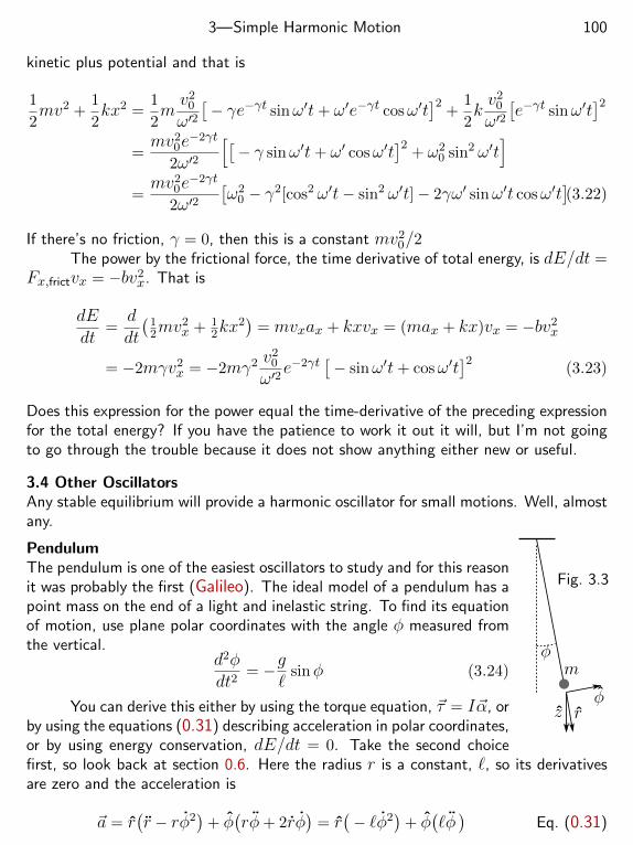
3—Simple Harmonic Motion 100
kinetic plus potential and that is
1
2mv2 +
1
2kx2 =
1
2mv2
0
ω′2[− γe−γt sinω′t+ ω′e−γt cosω′t
]2+
1
2kv2
0
ω′2[e−γt sinω′t
]2=mv2
0e−2γt
2ω′2
[[− γ sinω′t+ ω′ cosω′t
]2+ ω2
0 sin2 ω′t]
=mv2
0e−2γt
2ω′2[ω2
0 − γ2[cos2 ω′t− sin2 ω′t]− 2γω′ sinω′t cosω′t](3.22)
If there’s no friction, γ = 0, then this is a constant mv20/2
The power by the frictional force, the time derivative of total energy, is dE/dt =Fx,frictvx = −bv2
x. That is
dEdt
=ddt
(12mv
2x + 1
2kx2)
= mvxax + kxvx = (max + kx)vx = −bv2x
= −2mγv2x = −2mγ2 v
20
ω′2e−2γt [− sinω′t+ cosω′t
]2(3.23)
Does this expression for the power equal the time-derivative of the preceding expressionfor the total energy? If you have the patience to work it out it will, but I’m not goingto go through the trouble because it does not show anything either new or useful.
3.4 Other OscillatorsAny stable equilibrium will provide a harmonic oscillator for small motions. Well, almostany.
φm
z rφ
Fig. 3.3
PendulumThe pendulum is one of the easiest oscillators to study and for this reasonit was probably the first (Galileo). The ideal model of a pendulum has apoint mass on the end of a light and inelastic string. To find its equationof motion, use plane polar coordinates with the angle φ measured fromthe vertical.
d2φdt2
= −g`
sinφ (3.24)
You can derive this either by using the torque equation, ~τ = I~α, orby using the equations (0.31) describing acceleration in polar coordinates,or by using energy conservation, dE/dt = 0. Take the second choicefirst, so look back at section 0.6. Here the radius r is a constant, `, so its derivativesare zero and the acceleration is
~a = r(r − rφ2
)+ φ
(rφ+ 2rφ
)= r(− `φ2
)+ φ
(`φ)
Eq. (0.31)
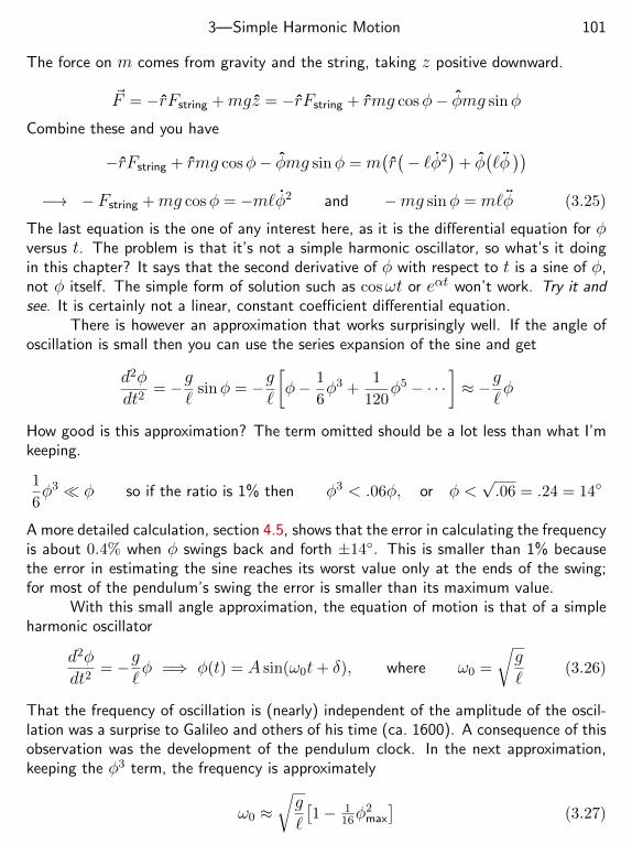
3—Simple Harmonic Motion 101
The force on m comes from gravity and the string, taking z positive downward.
~F = −rFstring +mgz = −rFstring + rmg cosφ− φmg sinφ
Combine these and you have
−rFstring + rmg cosφ− φmg sinφ = m(r(− `φ2
)+ φ
(`φ))
−→ − Fstring +mg cosφ = −m`φ2 and −mg sinφ = m`φ (3.25)
The last equation is the one of any interest here, as it is the differential equation for φversus t. The problem is that it’s not a simple harmonic oscillator, so what’s it doingin this chapter? It says that the second derivative of φ with respect to t is a sine of φ,not φ itself. The simple form of solution such as cosωt or eαt won’t work. Try it andsee. It is certainly not a linear, constant coefficient differential equation.
There is however an approximation that works surprisingly well. If the angle ofoscillation is small then you can use the series expansion of the sine and get
d2φdt2
= −g`
sinφ = −g`
[φ− 1
6φ3 +
1
120φ5 − · · ·
]≈ −g
`φ
How good is this approximation? The term omitted should be a lot less than what I’mkeeping.
1
6φ3 φ so if the ratio is 1% then φ3 < .06φ, or φ <
√.06 = .24 = 14
A more detailed calculation, section 4.5, shows that the error in calculating the frequencyis about 0.4% when φ swings back and forth ±14. This is smaller than 1% becausethe error in estimating the sine reaches its worst value only at the ends of the swing;for most of the pendulum’s swing the error is smaller than its maximum value.
With this small angle approximation, the equation of motion is that of a simpleharmonic oscillator
d2φdt2
= −g`φ =⇒ φ(t) = A sin(ω0t+ δ), where ω0 =
√g`
(3.26)
That the frequency of oscillation is (nearly) independent of the amplitude of the oscil-lation was a surprise to Galileo and others of his time (ca. 1600). A consequence of thisobservation was the development of the pendulum clock. In the next approximation,keeping the φ3 term, the frequency is approximately
ω0 ≈√g`
[1− 1
16φ2max
](3.27)
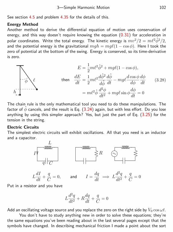
3—Simple Harmonic Motion 102
See section 4.5 and problem 4.35 for the details of this.
Energy MethodAnother method to derive the differential equation of motion uses conservation ofenergy, and this way doesn’t require knowing the equation (0.31) for acceleration in
polar coordinates. Write the total energy. The kinetic energy is mv2/2 = m`2φ2/2,and the potential energy is the gravitational mgh = mg`(1− cosφ). Here I took thezero of potential at the bottom of the swing. Energy is conserved, so its time-derivativeis zero.
`φ
h
E =1
2m`2φ2 +mg`(1− cosφ),
thendEdt
=1
2m`2dφ
2
dφ
dφdt−mg`d cosφ
dφdφdt
= m`2φd2φdt2
+mg` sinφdφdt
= 0
(3.28)
The chain rule is the only mathematical tool you need to do these manipulations. Thefactor of φ cancels, and the result is Eq. (3.24) again, but with less effort. Do you loseanything by using this simpler approach? Yes, but just the part of Eq. (3.25) for thetension in the string.
Electric CircuitsThe simplest electric circuits will exhibit oscillations. All that you need is an inductorand a capacitor.
I
L
q C
R
LdIdt
+qC
= 0, and I =dqdt
=⇒ Ld2qdt2
+qC
= 0
Put in a resistor and you have
Ld2qdt2
+Rdqdt
+qC
= 0
Add an oscillating voltage source and you replace the zero on the right side by V0 cosωt.You don’t have to study anything new in order to solve these equations; they’re
the same equations you’ve been reading about in the last several pages except that thesymbols have changed. In describing mechanical friction I made a point about the sort
3—Simple Harmonic Motion 103
of modelling that you have to do to describe it. The same question arises here too. Canyou really say that the electrical resistance is IR with a constant R? Sometimes and insome approximation you can, but not always. For an ordinary incandescent light bulbyou would probably expect this to be valid, but it too is just an approximation. Theresistance in the tungsten filament depends on its temperature, and that in turn dependson the size of the current going through it. That replaces the potential difference “IR”with a slightly nonlinear function of I . If you use a fluorescent bulb, the situation is noteven close to linear. The relation between current and voltage in that case is not evensingle-valued. It’s not a function, and the voltage-current relation even has a negativeslope (dI/dV < 0) in some regions. That’s the reason that fluorescent fixtures use a“ballast” to keep the system stable. That ballast could be just another resistor, but inpractice that would waste too much energy so other devices are used instead.
3.5 Forced OscillationsWhen you have any sort of harmonic oscillator you can also have other forces besidesthe spring and the damping (or the capacitance and the resistance). If the oscillatoris a child on a swing (a pendulum) you may be pushing periodically. If it’s a mass ona spring you may be pulling on the end of the spring, varying the force on the massby changing the length of the spring. In any case, the differential equation will besomething like
md2xdt2
= −bdxdt− kx+ Fexternal(t) (3.29)
This is not a linear, homogeneous, constant coefficient differential equation, and thesum of two of its solutions is not a solution, but it comes pretty close.
Terminology: “Homogeneous” means that if you multiply the dependent variablex by a constant then every term in the equation is multiplied by that constant.* Equa-tion (3.13) satisfies this, but (3.29) doesn’t. It is an inhomogeneous equation.“Linear” means that the dependent variable and its derivatives appear only to the firstor zeroth power. Both of these equations satisfy this.
There is a plan of attack for handling problems such as these.1. Toss out the inhomogeneous term and find the general solution of this homogeneouspart, complete with all the arbitrary constants.2. Find any one solution to the full, inhomogeneous equation, and it doesn’t need tohave any arbitrary constants.3. Add the results of steps 1 and 2.This will provide a solution to the full equation complete with the arbitrary constantsneeded to fit the initial conditions. To show that this is true, simply plug the result intothe original equation.
* or a power of that constant
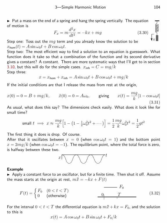
3—Simple Harmonic Motion 104
x
Put a mass on the end of a spring and hang the spring vertically. The equationof motion is
Fx = md2xdt2
= −kx+mg (3.30)
Step one: Toss out the mg term and you already know the solution to bexhom(t) = A sinω0t+B cosω0t.Step two: The most efficient way to find a solution to an equation is guesswork. Whatfunction does it take so that a combination of the function and its second derivativegives a constant? A constant. There are more systematic ways that I’ll get to in section3.10, but this will do for the simple cases. xinh = C = mg/kStep three:
x = xhom + xinh = A sinω0t+B cosω0t+mg/k
If the initial conditions are that I release the mass from rest at the origin,
x(0) = 0 = B +mg/k, x(0) = 0 = Aω0, giving x(t) =mgk
[1− cosω0t]
(3.31)As usual, what does this say? The dimensions check easily. What does it look like forsmall time?
small t =⇒ x ≈ mgk
[1−
(1− 1
2ω20t
2 + · · ·)]
=1
2
mgkω2
0t2 =
1
2gt2
The first thing it does is drop. Of course.After that it oscillates between x = 0 (when cosω0t = 1) and the bottom pointx = 2mg/k (when cosω0t = −1). The equilibrium point, where the total force is zero,is halfway between these two.
tx
Example Apply a constant force to an oscillator, but for a finite time. Then shut it off. Assumethe mass starts at the origin at rest, mx = −kx+ F (t)
F (t) =
F0 (0 < t < T )0 (otherwise) 0 T
F0
(3.32)
For the interval 0 < t < T the differential equation is mx+kx = F0, and the solutionto this is
x(t) = A cosω0t+B sinω0t+ F0/k
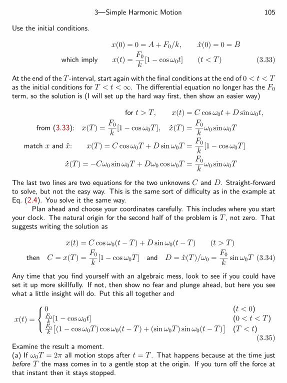
3—Simple Harmonic Motion 105
Use the initial conditions.
x(0) = 0 = A+ F0/k, x(0) = 0 = B
which imply x(t) =F0
k[1− cosω0t] (t < T ) (3.33)
At the end of the T -interval, start again with the final conditions at the end of 0 < t < Tas the initial conditions for T < t <∞. The differential equation no longer has the F0
term, so the solution is (I will set up the hard way first, then show an easier way)
for t > T, x(t) = C cosω0t+D sinω0t,
from (3.33): x(T ) =F0
k[1− cosω0T ], x(T ) =
F0
kω0 sinω0T
match x and x: x(T ) = C cosω0T +D sinω0T =F0
k[1− cosω0T ]
x(T ) = −Cω0 sinω0T +Dω0 cosω0T =F0
kω0 sinω0T
The last two lines are two equations for the two unknowns C and D. Straight-forwardto solve, but not the easy way. This is the same sort of difficulty as in the example atEq. (2.4). You solve it the same way.
Plan ahead and choose your coordinates carefully. This includes where you startyour clock. The natural origin for the second half of the problem is T , not zero. Thatsuggests writing the solution as
x(t) = C cosω0(t− T ) +D sinω0(t− T ) (t > T )
then C = x(T ) =F0
k[1− cosω0T ] and D = x(T )/ω0 =
F0
ksinω0T (3.34)
Any time that you find yourself with an algebraic mess, look to see if you could haveset it up more skillfully. If not, then show no fear and plunge ahead, but here you seewhat a little insight will do. Put this all together and
x(t) =
0 (t < 0)F0
k [1− cosω0t] (0 < t < T )F0
k
[(1− cosω0T ) cosω0(t− T ) + (sinω0T ) sinω0(t− T )
](T < t)
(3.35)Examine the result a moment.(a) If ω0T = 2π all motion stops after t = T . That happens because at the time justbefore T the mass comes in to a gentle stop at the origin. If you turn off the force atthat instant then it stays stopped.
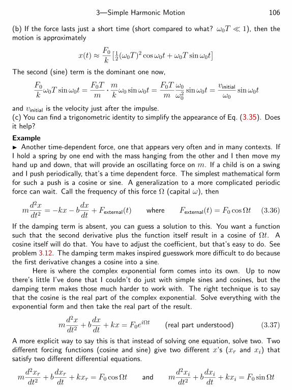
3—Simple Harmonic Motion 106
(b) If the force lasts just a short time (short compared to what? ω0T 1), then themotion is approximately
x(t) ≈ F0
k
[12(ω0T )2 cosω0t+ ω0T sinω0t
]The second (sine) term is the dominant one now,
F0
kω0T sinω0t =
F0Tm
. mkω0 sinω0t =
F0Tm
ω0
ω20
sinω0t =vinitial
ω0sinω0t
and vinitial is the velocity just after the impulse.(c) You can find a trigonometric identity to simplify the appearance of Eq. (3.35). Doesit help?
Example Another time-dependent force, one that appears very often and in many contexts. IfI hold a spring by one end with the mass hanging from the other and I then move myhand up and down, that will provide an oscillating force on m. If a child is on a swingand I push periodically, that’s a time dependent force. The simplest mathematical formfor such a push is a cosine or sine. A generalization to a more complicated periodicforce can wait. Call the frequency of this force Ω (capital ω), then
md2xdt2
= −kx− bdxdt
+ Fexternal(t) where Fexternal(t) = F0 cos Ωt (3.36)
If the damping term is absent, you can guess a solution to this. You want a functionsuch that the second derivative plus the function itself result in a cosine of Ωt. Acosine itself will do that. You have to adjust the coefficient, but that’s easy to do. Seeproblem 3.12. The damping term makes inspired guesswork more difficult to do becausethe first derivative changes a cosine into a sine.
Here is where the complex exponential form comes into its own. Up to nowthere’s little I’ve done that I couldn’t do just with simple sines and cosines, but thedamping term makes those much harder to work with. The right technique is to saythat the cosine is the real part of the complex exponential. Solve everything with theexponential form and then take the real part of the result.
md2xdt2
+ bdxdt
+ kx = F0eiΩt (real part understood) (3.37)
A more explicit way to say this is that instead of solving one equation, solve two. Twodifferent forcing functions (cosine and sine) give two different x’s (xr and xi) thatsatisfy two different differential equations.
md2xrdt2
+ bdxrdt
+ kxr = F0 cos Ωt and md2xidt2
+ bdxidt
+ kxi = F0 sin Ωt
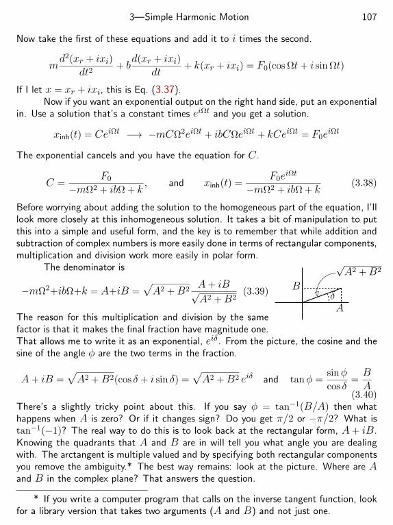
3—Simple Harmonic Motion 107
Now take the first of these equations and add it to i times the second.
md2(xr + ixi)
dt2+ b
d(xr + ixi)dt
+ k(xr + ixi) = F0(cos Ωt+ i sin Ωt)
If I let x = xr + ixi, this is Eq. (3.37).Now if you want an exponential output on the right hand side, put an exponential
in. Use a solution that’s a constant times eiΩt and you get a solution.
xinh(t) = CeiΩt −→ −mCΩ2eiΩt + ibCΩeiΩt + kCeiΩt = F0eiΩt
The exponential cancels and you have the equation for C.
C =F0
−mΩ2 + ibΩ + k, and xinh(t) =
F0eiΩt
−mΩ2 + ibΩ + k(3.38)
Before worrying about adding the solution to the homogeneous part of the equation, I’lllook more closely at this inhomogeneous solution. It takes a bit of manipulation to putthis into a simple and useful form, and the key is to remember that while addition andsubtraction of complex numbers is more easily done in terms of rectangular components,multiplication and division work more easily in polar form.
A
Bδ
√A2 +B2The denominator is
−mΩ2+ibΩ+k = A+iB =√A2 +B2
A+ iB√A2 +B2
(3.39)
The reason for this multiplication and division by the samefactor is that it makes the final fraction have magnitude one.That allows me to write it as an exponential, eiδ. From the picture, the cosine and thesine of the angle φ are the two terms in the fraction.
A+ iB =√A2 +B2(cos δ + i sin δ) =
√A2 +B2 eiδ and tanφ =
sinφcos δ
=BA
(3.40)There’s a slightly tricky point about this. If you say φ = tan−1(B/A) then whathappens when A is zero? Or if it changes sign? Do you get π/2 or −π/2? What istan−1(−1)? The real way to do this is to look back at the rectangular form, A+ iB.Knowing the quadrants that A and B are in will tell you what angle you are dealingwith. The arctangent is multiple valued and by specifying both rectangular componentsyou remove the ambiguity.* The best way remains: look at the picture. Where are Aand B in the complex plane? That answers the question.
* If you write a computer program that calls on the inverse tangent function, lookfor a library version that takes two arguments (A and B) and not just one.
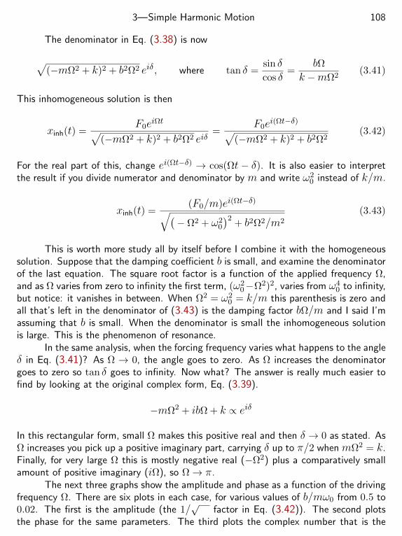
3—Simple Harmonic Motion 108
The denominator in Eq. (3.38) is now
√(−mΩ2 + k)2 + b2Ω2 eiδ, where tan δ =
sin δcos δ
=bΩ
k −mΩ2(3.41)
This inhomogeneous solution is then
xinh(t) =F0eiΩt√
(−mΩ2 + k)2 + b2Ω2 eiδ=
F0ei(Ωt−δ)√(−mΩ2 + k)2 + b2Ω2
(3.42)
For the real part of this, change ei(Ωt−δ) → cos(Ωt − δ). It is also easier to interpretthe result if you divide numerator and denominator by m and write ω2
0 instead of k/m.
xinh(t) =(F0/m)ei(Ωt−δ)√(
− Ω2 + ω20
)2+ b2Ω2/m2
(3.43)
This is worth more study all by itself before I combine it with the homogeneoussolution. Suppose that the damping coefficient b is small, and examine the denominatorof the last equation. The square root factor is a function of the applied frequency Ω,and as Ω varies from zero to infinity the first term, (ω2
0−Ω2)2, varies from ω40 to infinity,
but notice: it vanishes in between. When Ω2 = ω20 = k/m this parenthesis is zero and
all that’s left in the denominator of (3.43) is the damping factor bΩ/m and I said I’massuming that b is small. When the denominator is small the inhomogeneous solutionis large. This is the phenomenon of resonance.
In the same analysis, when the forcing frequency varies what happens to the angleδ in Eq. (3.41)? As Ω → 0, the angle goes to zero. As Ω increases the denominatorgoes to zero so tan δ goes to infinity. Now what? The answer is really much easier tofind by looking at the original complex form, Eq. (3.39).
−mΩ2 + ibΩ + k ∝ eiδ
In this rectangular form, small Ω makes this positive real and then δ → 0 as stated. AsΩ increases you pick up a positive imaginary part, carrying δ up to π/2 when mΩ2 = k.Finally, for very large Ω this is mostly negative real (−Ω2) plus a comparatively smallamount of positive imaginary (iΩ), so Ω→ π.
The next three graphs show the amplitude and phase as a function of the drivingfrequency Ω. There are six plots in each case, for various values of b/mω0 from 0.5 to0.02. The first is the amplitude (the 1/
√factor in Eq. (3.42)). The second plots
the phase for the same parameters. The third plots the complex number that is the
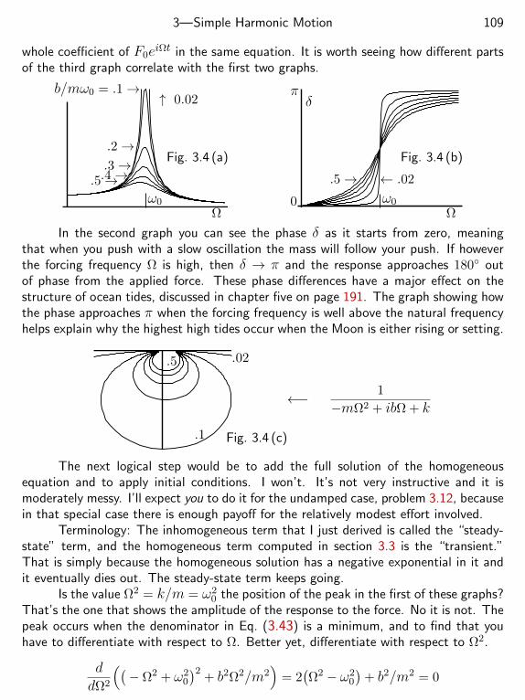
3—Simple Harmonic Motion 109
whole coefficient of F0eiΩt in the same equation. It is worth seeing how different partsof the third graph correlate with the first two graphs.
ω0
Ω
.5→.4→.3→.2→
b/mω0 = .1→↑ 0.02
Fig. 3.4 (a)
Ωω0
δ
0
π
.5→ ← .02
Fig. 3.4 (b)
In the second graph you can see the phase δ as it starts from zero, meaningthat when you push with a slow oscillation the mass will follow your push. If howeverthe forcing frequency Ω is high, then δ → π and the response approaches 180 outof phase from the applied force. These phase differences have a major effect on thestructure of ocean tides, discussed in chapter five on page 191. The graph showing howthe phase approaches π when the forcing frequency is well above the natural frequencyhelps explain why the highest high tides occur when the Moon is either rising or setting.
.5
.1
.02
Fig. 3.4 (c)
←− 1
−mΩ2 + ibΩ + k
The next logical step would be to add the full solution of the homogeneousequation and to apply initial conditions. I won’t. It’s not very instructive and it ismoderately messy. I’ll expect you to do it for the undamped case, problem 3.12, becausein that special case there is enough payoff for the relatively modest effort involved.
Terminology: The inhomogeneous term that I just derived is called the “steady-state” term, and the homogeneous term computed in section 3.3 is the “transient.”That is simply because the homogeneous solution has a negative exponential in it andit eventually dies out. The steady-state term keeps going.
Is the value Ω2 = k/m = ω20 the position of the peak in the first of these graphs?
That’s the one that shows the amplitude of the response to the force. No it is not. Thepeak occurs when the denominator in Eq. (3.43) is a minimum, and to find that youhave to differentiate with respect to Ω. Better yet, differentiate with respect to Ω2.
ddΩ2
((− Ω2 + ω2
0
)2+ b2Ω2/m2
)= 2(Ω2 − ω2
0
)+ b2/m2 = 0
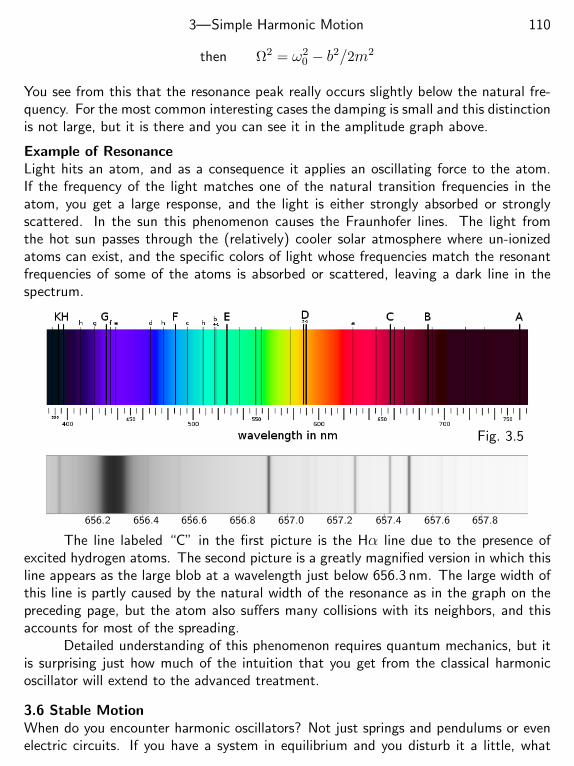
3—Simple Harmonic Motion 110
then Ω2 = ω20 − b2/2m2
You see from this that the resonance peak really occurs slightly below the natural fre-quency. For the most common interesting cases the damping is small and this distinctionis not large, but it is there and you can see it in the amplitude graph above.
Example of ResonanceLight hits an atom, and as a consequence it applies an oscillating force to the atom.If the frequency of the light matches one of the natural transition frequencies in theatom, you get a large response, and the light is either strongly absorbed or stronglyscattered. In the sun this phenomenon causes the Fraunhofer lines. The light fromthe hot sun passes through the (relatively) cooler solar atmosphere where un-ionizedatoms can exist, and the specific colors of light whose frequencies match the resonantfrequencies of some of the atoms is absorbed or scattered, leaving a dark line in thespectrum.
656.2 656.4 656.6 656.8 657.0 657.2 657.4 657.6 657.8
Fig. 3.5
The line labeled “C” in the first picture is the Hα line due to the presence ofexcited hydrogen atoms. The second picture is a greatly magnified version in which thisline appears as the large blob at a wavelength just below 656.3 nm. The large width ofthis line is partly caused by the natural width of the resonance as in the graph on thepreceding page, but the atom also suffers many collisions with its neighbors, and thisaccounts for most of the spreading.
Detailed understanding of this phenomenon requires quantum mechanics, but itis surprising just how much of the intuition that you get from the classical harmonicoscillator will extend to the advanced treatment.
3.6 Stable MotionWhen do you encounter harmonic oscillators? Not just springs and pendulums or evenelectric circuits. If you have a system in equilibrium and you disturb it a little, what
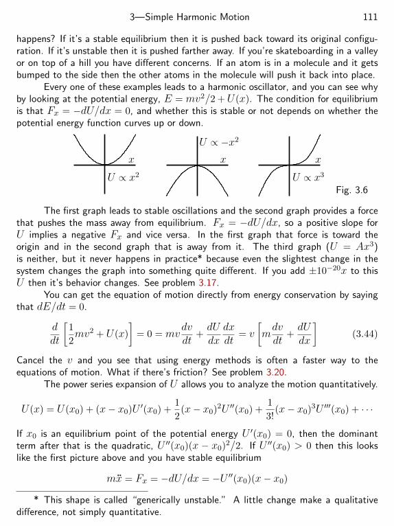
3—Simple Harmonic Motion 111
happens? If it’s a stable equilibrium then it is pushed back toward its original configu-ration. If it’s unstable then it is pushed farther away. If you’re skateboarding in a valleyor on top of a hill you have different concerns. If an atom is in a molecule and it getsbumped to the side then the other atoms in the molecule will push it back into place.
Every one of these examples leads to a harmonic oscillator, and you can see whyby looking at the potential energy, E = mv2/2 +U(x). The condition for equilibriumis that Fx = −dU/dx = 0, and whether this is stable or not depends on whether thepotential energy function curves up or down.
U ∝ x2
x
U ∝ −x2
x
U ∝ x3
x
Fig. 3.6
The first graph leads to stable oscillations and the second graph provides a forcethat pushes the mass away from equilibrium. Fx = −dU/dx, so a positive slope forU implies a negative Fx and vice versa. In the first graph that force is toward theorigin and in the second graph that is away from it. The third graph (U = Ax3)is neither, but it never happens in practice* because even the slightest change in thesystem changes the graph into something quite different. If you add ±10−20x to thisU then it’s behavior changes. See problem 3.17.
You can get the equation of motion directly from energy conservation by sayingthat dE/dt = 0.
ddt
[1
2mv2 + U(x)
]= 0 = mv
dvdt
+dUdx
dxdt
= v
[mdvdt
+dUdx
](3.44)
Cancel the v and you see that using energy methods is often a faster way to theequations of motion. What if there’s friction? See problem 3.20.
The power series expansion of U allows you to analyze the motion quantitatively.
U(x) = U(x0) + (x− x0)U ′(x0) +1
2(x− x0)2U ′′(x0) +
1
3!(x− x0)3U ′′′(x0) + · · ·
If x0 is an equilibrium point of the potential energy U ′(x0) = 0, then the dominantterm after that is the quadratic, U ′′(x0)(x − x0)2/2. If U ′′(x0) > 0 then this lookslike the first picture above and you have stable equilibrium
mx = Fx = −dU/dx = −U ′′(x0)(x− x0)
* This shape is called “generically unstable.” A little change make a qualitativedifference, not simply quantitative.
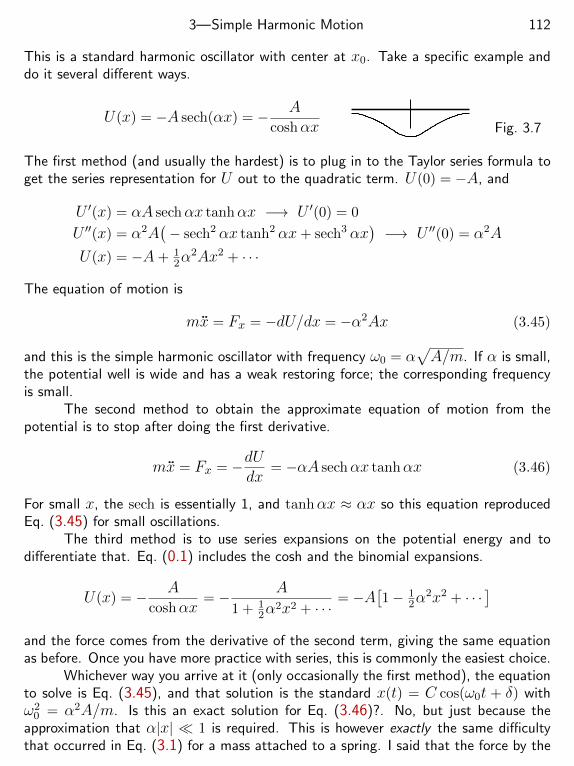
3—Simple Harmonic Motion 112
This is a standard harmonic oscillator with center at x0. Take a specific example anddo it several different ways.
U(x) = −A sech(αx) = − Acoshαx Fig. 3.7
The first method (and usually the hardest) is to plug in to the Taylor series formula toget the series representation for U out to the quadratic term. U(0) = −A, and
U ′(x) = αA sechαx tanhαx −→ U ′(0) = 0
U ′′(x) = α2A(− sech2 αx tanh2 αx+ sech3 αx
)−→ U ′′(0) = α2A
U(x) = −A+ 12α
2Ax2 + · · ·
The equation of motion is
mx = Fx = −dU/dx = −α2Ax (3.45)
and this is the simple harmonic oscillator with frequency ω0 = α√A/m. If α is small,
the potential well is wide and has a weak restoring force; the corresponding frequencyis small.
The second method to obtain the approximate equation of motion from thepotential is to stop after doing the first derivative.
mx = Fx = −dUdx
= −αA sechαx tanhαx (3.46)
For small x, the sech is essentially 1, and tanhαx ≈ αx so this equation reproducedEq. (3.45) for small oscillations.
The third method is to use series expansions on the potential energy and todifferentiate that. Eq. (0.1) includes the cosh and the binomial expansions.
U(x) = − Acoshαx
= − A
1 + 12α
2x2 + · · ·= −A
[1− 1
2α2x2 + · · ·
]and the force comes from the derivative of the second term, giving the same equationas before. Once you have more practice with series, this is commonly the easiest choice.
Whichever way you arrive at it (only occasionally the first method), the equationto solve is Eq. (3.45), and that solution is the standard x(t) = C cos(ω0t + δ) withω2
0 = α2A/m. Is this an exact solution for Eq. (3.46)?. No, but just because theapproximation that α|x| 1 is required. This is however exactly the same difficultythat occurred in Eq. (3.1) for a mass attached to a spring. I said that the force by the
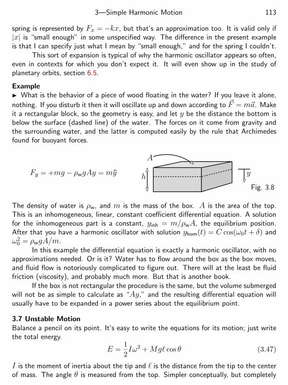
3—Simple Harmonic Motion 113
spring is represented by Fx = −kx, but that’s an approximation too. It is valid only if|x| is “small enough” in some unspecified way. The difference in the present exampleis that I can specify just what I mean by “small enough,” and for the spring I couldn’t.
This sort of expansion is typical of why the harmonic oscillator appears so often,even in contexts for which you don’t expect it. It will even show up in the study ofplanetary orbits, section 6.5.
Example What is the behavior of a piece of wood floating in the water? If you leave it alone,
nothing. If you disturb it then it will oscillate up and down according to ~F = m~a. Makeit a rectangular block, so the geometry is easy, and let y be the distance the bottom isbelow the surface (dashed line) of the water. The forces on it come from gravity andthe surrounding water, and the latter is computed easily by the rule that Archimedesfound for buoyant forces.
Fy = +mg − ρwgAy = myh
A
y
Fig. 3.8
The density of water is ρw, and m is the mass of the box. A is the area of the top.This is an inhomogeneous, linear, constant coefficient differential equation. A solutionfor the inhomogeneous part is a constant, yinh = m/ρwA, the equilibrium position.After that you have a harmonic oscillator with solution yhom(t) = C cos(ω0t + δ) andω2
0 = ρwgA/m.In this example the differential equation is exactly a harmonic oscillator, with no
approximations needed. Or is it? Water has to flow around the box as the box moves,and fluid flow is notoriously complicated to figure out. There will at the least be fluidfriction (viscosity), and probably much more. But that is another book.
If the box is not rectangular the procedure is the same, but the volume submergedwill not be as simple to calculate as “Ay,” and the resulting differential equation willusually have to be expanded in a power series about the equilibrium point.
3.7 Unstable MotionBalance a pencil on its point. It’s easy to write the equations for its motion; just writethe total energy.
E =1
2Iω2 +Mg` cos θ (3.47)
I is the moment of inertia about the tip and ` is the distance from the tip to the centerof mass. The angle θ is measured from the top. Simpler conceptually, but completely
3—Simple Harmonic Motion 114
equivalent mathematically: Put a point mass M on the top of a massless rod of length` and balance the rod on the other end. Then
E = 12Mv2 +Mgh = 1
2M`2θ2 +Mg` cos θ (3.48)
For the equation of motion, simply differentiate this with respect to time.
dEdt
= 0 = M`2θθ −Mg` sin θ θ
What is E? Cancel the θ factor and you have
`θ − g sin θ = 0
Just as with the standard pendulum, this inverted pendulum simplifies enormously ifyou make the small angle approximation, then
`θ − gθ = 0 (3.49)
and this linear equation is handled the same way as all the other linear equations in thischapter. Assume an exponential.
θ = Aeαt −→ `θ−gθ = `Aα2eαt−gAeαt = 0 −→ `α2−g = 0 −→ α = ±√g/`
(3.50)The general solution to the differential equation is now
θ(t) = Aeωt +Be−ωt, with ω =√g/`
This is like using the complex exponential solutions for the simple harmonicoscillator. It’s often more convenient to use sines and cosines directly in that case, andhere it is often more convenient to use hyperbolic sines and cosines as in section 0.2.
θ(t) = Aeωt +Be−ωt = C coshωt+D sinhωt (3.51)
A typical initial condition is to start at rest with initial angle from the vertical θ0, then
θ(0) = C = θ0 and θ(0) = ωD = 0
θ(t) = θ0 coshωt, and if ` = 20 cm = 0.2 m then ω =√
10/0.2 = 7.07 s−1
(3.52)
3—Simple Harmonic Motion 115
How much time would this take to hit the table starting with an initial angle of onedegree?
1 coshωt = 90 −→ t = ω−1 cosh−1 90 = 5.193/√
50 = 0.73 seconds
How much more time would it take to fall this far if the initial angle is smaller? Perhapsstarting at 0.1 or 0.01? Plug them in and find out just how little difference thischange makes: respectively 1.09 and 1.39 seconds.
Maybe the linear approximation made in Eq. (3.49) is not good enough. Howmuch difference would there be in the time it takes to hit the table? You have to goback to Eq. (3.48) and separate variables.
E = 12M`2θ2 +Mg` cos θ −→ dt =
dθ√2(E −Mg` cos θ)/M`2
Integrate this from θ0 to π/2 to get the time to fall. What is E? Assuming thateverything starts from rest that is E = Mg` cos θ0, making this∫
dt =
∫ π/2
θ0
dθ
ω√
2(cos θ0 − cos θ)(3.53)
This is not an integral that you’re likely to have seen before, and you cannot do it interms of the functions (polynomials, roots, trig functions, exponentials) that you arefamiliar with. It is an elliptic integral, and there will be a brief introduction to thesubject in section 4.5. For the three angles used one paragraph back, the results usingthis integral are respectively 0.742 s, 1.069 s, 1.379 s. See problem 3.64.
They are remarkable close to the numbers you get by using the linear approxi-mation in the second paragraph back, so that invites the question: Why? The linearapproximation to the sine function is good even at 30, but at 90, it’s terrible. Theexplanation of why it is so good is that as the mass falls it spends most of its timemoving slowly, when it is near the top. Most of its time is spent where the small angleapproximation is good, and is zips through the last part of its fall.
3.8 Coupled OscillationsOscillators don’t always come singly. You get a single oscillator when you have a stableequilibrium and you then examine small oscillations about that equilibrium point. Amolecule consists of several atoms, and each is in some sort of equilibrium. If they aredisturbed in any way they will oscillate about that point, but now each oscillator canaffect all the other oscillators. That’s the subject now.
As a prototype for all oscillators, I’ll use a mass on a spring again. Rather, twomasses on three springs. When you understand this example you can graduate to thevibrational properties of water and then to those of hemoglobin.
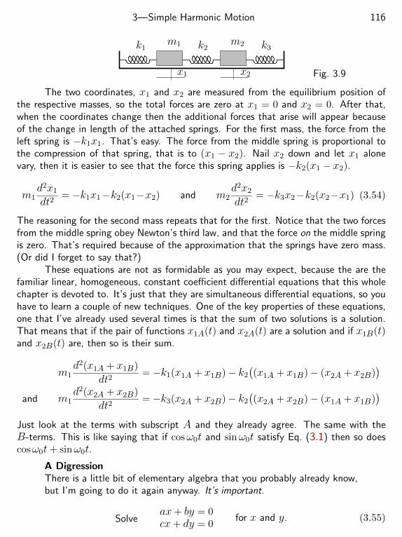
3—Simple Harmonic Motion 116
x1 x2
k1m1 k2
m2 k3
Fig. 3.9
The two coordinates, x1 and x2 are measured from the equilibrium position ofthe respective masses, so the total forces are zero at x1 = 0 and x2 = 0. After that,when the coordinates change then the additional forces that arise will appear becauseof the change in length of the attached springs. For the first mass, the force from theleft spring is −k1x1. That’s easy. The force from the middle spring is proportional tothe compression of that spring, that is to (x1 − x2). Nail x2 down and let x1 alonevary, then it is easier to see that the force this spring applies is −k2(x1 − x2).
m1d2x1
dt2= −k1x1−k2(x1−x2) and m2
d2x2
dt2= −k3x2−k2(x2−x1) (3.54)
The reasoning for the second mass repeats that for the first. Notice that the two forcesfrom the middle spring obey Newton’s third law, and that the force on the middle springis zero. That’s required because of the approximation that the springs have zero mass.(Or did I forget to say that?)
These equations are not as formidable as you may expect, because the are thefamiliar linear, homogeneous, constant coefficient differential equations that this wholechapter is devoted to. It’s just that they are simultaneous differential equations, so youhave to learn a couple of new techniques. One of the key properties of these equations,one that I’ve already used several times is that the sum of two solutions is a solution.That means that if the pair of functions x1A(t) and x2A(t) are a solution and if x1B(t)and x2B(t) are, then so is their sum.
m1d2(x1A + x1B)
dt2= −k1(x1A + x1B)− k2
((x1A + x1B)− (x2A + x2B)
)and m1
d2(x2A + x2B)
dt2= −k3(x2A + x2B)− k2
((x2A + x2B)− (x1A + x1B)
)Just look at the terms with subscript A and they already agree. The same with theB-terms. This is like saying that if cosω0t and sinω0t satisfy Eq. (3.1) then so doescosω0t+ sinω0t.
A DigressionThere is a little bit of elementary algebra that you probably already know,but I’m going to do it again anyway. It’s important.
Solveax+ by = 0cx+ dy = 0
for x and y. (3.55)
3—Simple Harmonic Motion 117
To solve for x, multiply the first equation by d and the second by b, thensubtract. Now start over and eliminate x by multiplying respectively by cand a and subtracting.
dax+ dby = 0bcx+ bdy = 0
=⇒ adx− bcx = 0
cax+ cby = 0acx+ ady = 0
=⇒ bcy − ady = 0
(3.56)
These are both in the form (ad− bc)× (x or y) = 0. If the product of twonumbers is zero then one or both of the numbers is zero, and this impliesthat if ad − bc 6= 0 then both x and y are zero. The only way to have anon-zero solution for x or y is to have ad− bc = 0. The quantity ad− bcis the determinant of these simultaneous equations.
A further point: If ad = bc then the two equations (3.55) are the sameequation. At least one of the numbers a and b is non-zero. (Otherwisewhy bother?) Say a 6= 0, then multiply the second of the pair of equationsby a to get acx + ady = 0 = acx + bcy = c(ax + by). The secondequation is a multiple of the first. (If c = 0, look at that case for yourselfand show that the result still holds.)
Now return to Eqs. (3.54) and solve them. These equations are linear, homoge-neous, constant coefficient equations, and an exponential solution works here just as itdid in the previous cases. Now however there are two functions, with two coefficients.
x1(t) = Aeαt, x2(t) = Beαt (3.57)
Plug in.
m1α2Aeαt = −k1Ae
αt − k2(Aeαt −Beαt)m2α
2Beαt = −k3Beαt − k2(Beαt −Aeαt) (3.58)
eαt is a common factor; that’s why this method works. Cancel it and rearrange.(m1α
2 + k1 + k2
)A− k2B = 0
−k2A+(m2α
2 + k3 + k2
)B = 0 (3.59)
These equations are in precisely the form of Eq. (3.55). If there is to be a non-zerosolution for A and B then the determinant of the coefficients must vanish. Thatdetermines α.
3—Simple Harmonic Motion 118
Instead of grinding through the rather messy algebra of this general problem,take a special and more symmetric case. Let the two masses be equal and let the twosprings on the ends be equal.
m1 = m2 = m and k1 = k3 = k =⇒(mα2 + k + k2
)A− k2B = 0
−k2A+(mα2 + k + k2
)B = 0
(3.60)The determinant of these equations must be zero.(
mα2 + k + k2
)2 − k22 = 0
This is the difference of squares, so it factors.(mα2 + k + k2 + k2
)(mα2 + k + k2 − k2
)= 0 =
(mα2 + k + 2k2
)(mα2 + k
)and the four roots for α are now
±i√km
= ±iω and ± i√k + 2k2
m= ±iω′
You’re not done. This tells only the frequencies of oscillation, now you need A and Bin order to get the functions x1 and x2.
In the equations (3.55), once you know that the determinant is zero, there isreally just one equation, as each is a multiple of the other. Pick one, whichever is moreconvenient, and solve for the ratio of x to y. Geometrically that determines a straightline through the origin in the x-y plane.
For the present application, pick one of the alphas, say α2 = −k/m and substi-tute is into the first of Eqs. (3.60).[
m
(− km
)+ k + k2
]A− k2B = 0, or A = B
The other choice for alpha with the same equation gives[m
(−k + 2k2
m
)+ k + k2
]A− k2B = 0 or A = −B
You now have four solutions to the original equations, and the general solution is alinear combination of all of them.
ω =√k/m, then x1(t) = A1e
iωt +A2e−iωt, with x2(t) = x1(t)
ω′ =√k + 2k2/m, then x1(t) = A3e
iω′t +A4e−iω′t, with x2(t) = −x1(t)
3—Simple Harmonic Motion 119
The total, general solution is now the sum of these.
x1(t) = A1eiωt +A2e
−iωt +A3eiω′t +A4e
−iω′t
x2(t) = A1eiωt +A2e
−iωt −A3eiω′t −A4e
−iω′t
OR, often easier to work with,
x1(t) = C1 cosωt+C2 sinωt+C3 cosω′t+C4 sinω′t
x2(t) = C1 cosωt+C2 sinωt−C3 cosω′t−C4 sinω′t
What do these solutions look like? Pick one: C1 6= 0, C2,3,4 = 0.
x1(t) = C1 cosωt, x2(t) = C1 cosωt (3.61)
The two masses are moving together, so as one moves to the right so does the other.The length of the middle spring does not change, and the (x1−x2) terms in Eq. (3.54)are identically zero. The solution behaves as if the middle spring is not there (leftpicture).
ω ω′Fig. 3.10
For the other form of solution, C3 6= 0, C1,2,4 = 0.
x1(t) = C3 cosω′t, x2(t) = −C3 cosω′t (3.62)
Here the two masses are oscillating in opposite directions, and the middle spring issqueezed from both sides. That’s why the frequency ω′ involves the combination k+2k3
(right picture). As the left mass moves by x1 to the right, the k3 spring is squeezed byx1−x2 = 2x1. This frequency is higher then the first one because there’s now a largerrestoring force applied to each mass. These solutions are the two modes of oscillationof the system.*
Example Take as initial conditions that you push the coordinate x1 to the value x0 whileholding x2 in place at zero. Then release everything from rest.
x1(0) = x0 = C1 +C3, x2(0) = 0 = C1 −C3
x1(0) = 0 = ωC2 + ω′C4, x2(0) = 0 = ωC2 − ω′C4
* If you want to see this normal mode problem fully worked out without makingassumptions of symmetry, so that k1 6= k3 and m1 6= m2, look up chapter four of thetext Mechanics by Keith Symon.
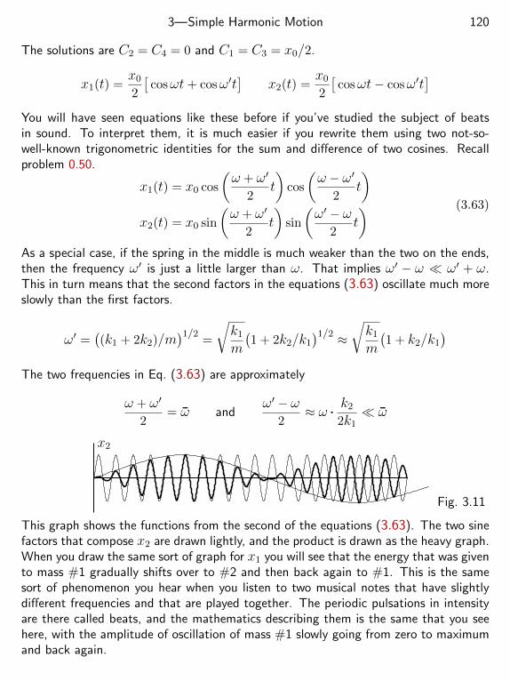
3—Simple Harmonic Motion 120
The solutions are C2 = C4 = 0 and C1 = C3 = x0/2.
x1(t) =x0
2
[cosωt+ cosω′t
]x2(t) =
x0
2
[cosωt− cosω′t
]You will have seen equations like these before if you’ve studied the subject of beatsin sound. To interpret them, it is much easier if you rewrite them using two not-so-well-known trigonometric identities for the sum and difference of two cosines. Recallproblem 0.50.
x1(t) = x0 cos
(ω + ω′
2t
)cos
(ω − ω′
2t
)x2(t) = x0 sin
(ω + ω′
2t
)sin
(ω′ − ω
2t
) (3.63)
As a special case, if the spring in the middle is much weaker than the two on the ends,then the frequency ω′ is just a little larger than ω. That implies ω′ − ω ω′ + ω.This in turn means that the second factors in the equations (3.63) oscillate much moreslowly than the first factors.
ω′ =((k1 + 2k2)/m
)1/2=
√k1
m
(1 + 2k2/k1
)1/2 ≈√k1
m
(1 + k2/k1
)The two frequencies in Eq. (3.63) are approximately
ω + ω′
2= ω and
ω′ − ω2
≈ ω . k2
2k1 ω
x2
Fig. 3.11
This graph shows the functions from the second of the equations (3.63). The two sinefactors that compose x2 are drawn lightly, and the product is drawn as the heavy graph.When you draw the same sort of graph for x1 you will see that the energy that was givento mass #1 gradually shifts over to #2 and then back again to #1. This is the samesort of phenomenon you hear when you listen to two musical notes that have slightlydifferent frequencies and that are played together. The periodic pulsations in intensityare there called beats, and the mathematics describing them is the same that you seehere, with the amplitude of oscillation of mass #1 slowly going from zero to maximumand back again.
3—Simple Harmonic Motion 121
3.9 Normal ModesThe two modes of oscillation represented by the equations (3.61) and (3.62) are called“normal modes” of oscillation. The reason for this is not that the word normal means“typical” or anything like it. It is used in the sense of “perpendicular” as when two linesintersect at right angles.
You can think of the components of a mode of oscillation as the coefficients inthe equation (3.61), so that the first (ω) mode is represented by the column matrix
M =
(C1
C1
)Similarly Eq. (3.62) states the components for the second (ω′) mode as
M ′ =
(C3
−C3
)These are orthogonal to each other in the sense of the scalar product
M
(m1 00 m2
)M ′ = (C1 C1 )
(m1 00 m2
)(C3
−C3
)= m1C1C3 −m2C1C3 = 0
(3.64)because m1 = m2, and where the tilde over the M means transpose. This is like thescalar product
~A . ~B = AB cos θ =(Axx+Ayy
).(Bxx+Byy
)= AxBx +AyBy
and the vectors ~A and ~B are perpendicular if ~A . ~B = 0. This example could bemisleading because the equal masses make the example so special. You might thinkthat you could simply omit the matrix in the middle of Eq. (3.64). Starting withEq. (3.60) the masses m1 and m2 were set equal, and if you go back to the equationpreceding it (3.59), carrying out all the calculations, you would find that the productin Eq. (3.64) would still be zero provided that you have the two masses m1 and m2 inthe product. The modes themselves will be more complicated, but the product
(C1 C ′1 )
(m1 00 m2
)(C3
C ′3
)will still be zero.
This redefinition of the scalar product may be unfamiliar, but it is part of a largerpicture that is explored in chapter ten, and it is a special case of Eq. (10.16). It canwait until then. It’s actually even a little more involved because when you deal withcomplex exponential solutions (eiωt) the coefficients can be complex. In that case thefirst factor is (C∗1 C ′∗1 ), in which there is a complex conjugation on each component.That conjugation should even be done in Eq. (3.64) too, but all this can wait until thatlater chapter.
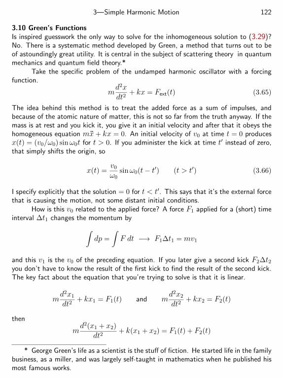
3—Simple Harmonic Motion 122
3.10 Green’s FunctionsIs inspired guesswork the only way to solve for the inhomogeneous solution to (3.29)?No. There is a systematic method developed by Green, a method that turns out to beof astoundingly great utility. It is central in the subject of scattering theory in quantummechanics and quantum field theory.*
Take the specific problem of the undamped harmonic oscillator with a forcingfunction.
md2xdt2
+ kx = Fext(t) (3.65)
The idea behind this method is to treat the added force as a sum of impulses, andbecause of the atomic nature of matter, this is not so far from the truth anyway. If themass is at rest and you kick it, you give it an initial velocity and after that it obeys thehomogeneous equation mx+ kx = 0. An initial velocity of v0 at time t = 0 producesx(t) = (v0/ω0) sinω0t for t > 0. If you administer the kick at time t′ instead of zero,that simply shifts the origin, so
x(t) =v0
ω0sinω0(t− t′) (t > t′) (3.66)
I specify explicitly that the solution = 0 for t < t′. This says that it’s the external forcethat is causing the motion, not some distant initial conditions.
How is this v0 related to the applied force? A force F1 applied for a (short) timeinterval ∆t1 changes the momentum by∫
dp =
∫F dt −→ F1∆t1 = mv1
and this v1 is the v0 of the preceding equation. If you later give a second kick F2∆t2you don’t have to know the result of the first kick to find the result of the second kick.The key fact about the equation that you’re trying to solve is that it is linear.
md2x1
dt2+ kx1 = F1(t) and m
d2x2
dt2+ kx2 = F2(t)
then
md2(x1 + x2)
dt2+ k(x1 + x2) = F1(t) + F2(t)
* George Green’s life as a scientist is the stuff of fiction. He started life in the familybusiness, as a miller, and was largely self-taught in mathematics when he published hismost famous works.
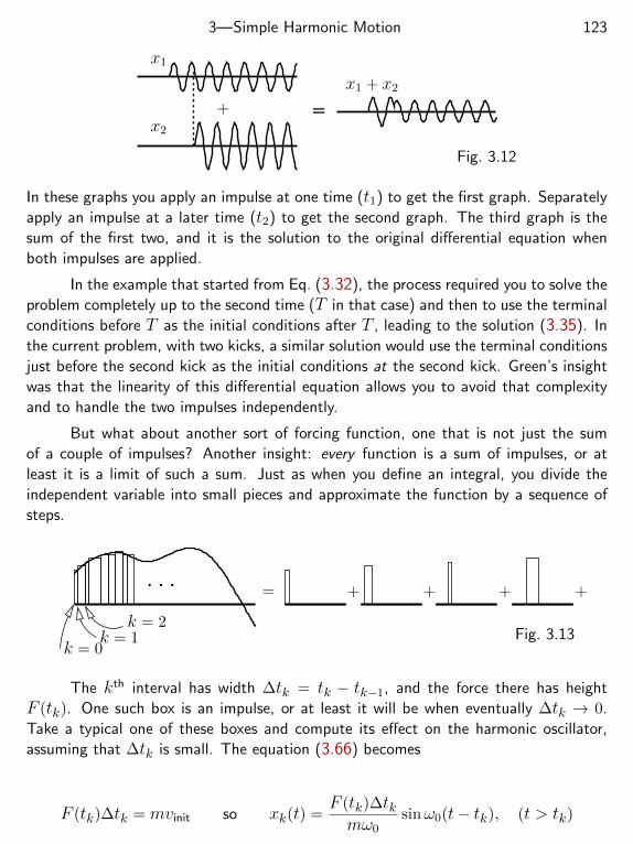
3—Simple Harmonic Motion 123
x1
x2
x1 + x2
+ =
Fig. 3.12
In these graphs you apply an impulse at one time (t1) to get the first graph. Separately
apply an impulse at a later time (t2) to get the second graph. The third graph is the
sum of the first two, and it is the solution to the original differential equation when
both impulses are applied.
In the example that started from Eq. (3.32), the process required you to solve the
problem completely up to the second time (T in that case) and then to use the terminal
conditions before T as the initial conditions after T , leading to the solution (3.35). In
the current problem, with two kicks, a similar solution would use the terminal conditions
just before the second kick as the initial conditions at the second kick. Green’s insight
was that the linearity of this differential equation allows you to avoid that complexity
and to handle the two impulses independently.
But what about another sort of forcing function, one that is not just the sum
of a couple of impulses? Another insight: every function is a sum of impulses, or at
least it is a limit of such a sum. Just as when you define an integral, you divide the
independent variable into small pieces and approximate the function by a sequence of
steps.
k = 0k = 1
k = 2
= + + + +
Fig. 3.13
The kth interval has width ∆tk = tk − tk−1, and the force there has height
F (tk). One such box is an impulse, or at least it will be when eventually ∆tk → 0.
Take a typical one of these boxes and compute its effect on the harmonic oscillator,
assuming that ∆tk is small. The equation (3.66) becomes
F (tk)∆tk = mvinit so xk(t) =F (tk)∆tkmω0
sinω0(t− tk), (t > tk)
3—Simple Harmonic Motion 124
As when there were just two impulses, you add the results of all these impulses to getthe (approximate) result for the motion of m.
x(t) ≈N∑k=1
F (tk)∆tkmω0
sinω0(t− tk) (t > tk)0 (t < tk)
As with any other integral, you improve the approximation by taking smaller timeintervals, and finally make it exact in the limit. That the response to the impulse iszero until the impulse happens dictates the limits of integration.
x(t) = lim∆tk→0
∑k
(tk<t)
1
mω0F (tk) ∆tk sinω0(t−tk) =
1
mω0
∫ t
−∞dt′ F (t′) sinω0(t−t′)
You see that you have to be careful to use different notations for the various time vari-ables, especially to distinguish the integration variable t′ from the independent variablet.
G(t− t′) =1
mω0
sinω0(t− t′) (t > t′)0 (t < t′)
so that x(t) =
∫ t
−∞dt′G(t− t′)F (t′)
(3.67)
and this function is called Green’s function for this differential equation. Because thisGreen’s function is defined to be zero for negative arguments t < t′, you could writethe limits on this integral as ±∞ without changing anything. I prefer the redundantform, using an explicit limit.
Does it Work?Apply this to the example Eq. (3.32). The solution is now a plug-in:
x(t) =
∫ t
−∞dt′G(t− t′)F (t′) =
1
mω0
∫ t
−∞dt′ sinω0(t− t′) .
F0 (0 < t′ < T )0 (otherwise)
This integral is ∫ t
−∞=
∫ 0
−∞+
∫ t
0
The first integral is zero, and the next has two cases: t < T and t > T .∫ t
0dt′ F (t′) sinω0(t− t′) =
∫ t0 dt
′ F0 sinω0(t− t′) (0 < t < T )∫ T0 dt′ F0 sinω0(t− t′) (T < t)
then x(t) =F0
mω20
1− cosω0t (0 < t < T )cosω0(t− T )− cosω0t (T < t)
3—Simple Harmonic Motion 125
This is identical to the solution Eq. (3.35), though you will have to do a small amountof algebra to verify that fact. Notice that this solution is continuous at t = T and ithas a continuous derivative there. This is so despite the fact that the Green’s functionhas a discontinuity in its derivative and the force function is discontinuous at 0 and T .You are integrating over these points, and that smooths the result.
Other Green’s FunctionsYou have seen Green’s functions before, though perhaps not under that name. Whatis the electrostatic potential produced by a point charge? That’s a Green’s function.The total potential produced by a lot of charges is the sum (integral?) over the poten-tials produced by the individual charges. Instead of an impulse in time to produce anoscillation, this is an analogous potential function of position produced from a point inspace.
The potential from a single point charge at the origin is φ(r) = q/4πε0r, andthe potential from several point charges is the sum over such contributions. For twocharges the potential is
q1
4πε0|~r − ~r1|+
q2
4πε0|~r − ~r2|For many charges, including a continuous distribution of them you have
G(~r − ~r ′) =1
4πε0|~r − ~r ′|−→ φ(~r ) =
∫dq′G(~r − ~r ′) =
∫d3r′ρ(~r ′)G(~r − ~r ′)
ρ is the volume charge density. and the Green’s function in this case is conventionallydefined without the q.
The analog of Eq. (3.67) for the damped harmonic oscillator is
G(t− t′) =1
mω′
e−γ(t−t′) sinω′(t− t′) (t > t′)0 (t < t′)
(3.68)
You can derive this yourself, problem 3.60.
3.11 Anharmonic Example: x4
What happens if the approximation of a linear harmonic oscillator isn’t even approxi-mately right? There are examples in problems 2.14 and 3.29, but the latter one is sortof extreme. The first really different potential energy after x2 that still gives oscillationsis x4. To solve that problem you can write the energy equation directly and separatevariables.
E =1
2mx2 + αx4 −→ x2 =
2Em− 2αmx4∫
dx√1− αx4/E
=
∫ √2E/mdt
U = αx4
E (3.69)
3—Simple Harmonic Motion 126
If you know about elliptic integrals and elliptic functions you can solve this for x(t)in terms of known functions. If you don’t know about them then they are unknownfunctions.
In any case, it’s sometimes easier to solve such problems numerically, and sincethere are some technical points about this example, I will proceed along this route fora while. The first thing to do is to change variables to get rid of a lot of parameters.Make all the E’s, m’s, and 2’s disappear.
LetαEx4 = y4 and
(αE
)1/4√
2E/mt = u then
∫ y
0
dy√1− y4
= u
(3.70)Here I chose the initial condition that x(0) = 0, so y = 0 when u = 0. It also sets thederivative dy/du = 1 at u = 0. This integral expresses time as a function of positioninstead of the reverse, but you take what you can get.
If you try a brute-force numerical integration of this equation (or let a computerdo the dirty work for you), you will run into trouble when you get near y = 1. That is aturning point, and the integrand blows up there. The integral is still finite, because thefunction you’re integrating goes to infinity only as one over a square root, and that’sintegrable, but it can still give a computer hiccups.
The trick to get around this annoyance is to make a change of variable. Factorout the bad behavior near y = 1.
1−y4 = (1−y)(1+y+y2 +y3), so letdy√1− y
= dz −→ z = 2−2√
1− y
You now have the integrals
u =
∫ z
0
dz√1 + y + y2 + y3
where y = z − z2/4 (0 < z < 2) (3.71)
The point z = 2 corresponds to the turning point of the oscillator. It comes to a stopthere and reverses direction. The original integral in terms of y worked only up to thatturning point, where it hit a singularity. This form in terms of z works all the way backto when the mass returns to the origin. That is, 0 < z < 4.
The procedure to compute this is1. Divide the interval 0 ≤ z ≤ 2 into N ≥ 1 pieces, ∆z = 2/N2. Choose your favorite integration method (midpoint, trapezoid, Simpson, . . . )3. Set k = 1 and z0 = 0 and z1 = ∆z and u0 = 04. Integrate from zk−1 to zk = zk−1 + ∆z5. uk = uk−1+ this integral.
3—Simple Harmonic Motion 127
6. Compute yk from zk.7. Increment k and unless you’re done, go back to 4.
This gives you two arrays: the uk (time) and the yk (position). Plot one versusthe other and then remember that the function is periodic so you can use the sameresults to plot the rest of the graph.
u
y
Fig. 3.14
The solid line is this quartic oscillator, and the dashed line is a pure harmonicoscillator having the same period and amplitude. They aren’t as different from eachother as you might have expected. The value of u when y = 1 (and z = 2) isu = 1.311029, and that corresponds to a quarter of a period.
Exercises
1 Where are the equilibrium points for the potential energy U(x) = A cos kx forA > 0.Which are stable and which are unstable?
2 Do the dimensions of Eq. (3.18) come out correctly?
3 Perhaps you’re more familiar with l’Hospital’s rule for evaluating certain types oflimits; apply it to Eq. (3.21) to see if you get the same answer as there.
4 For the equation Eq. (3.25), it says in that text that the solution φ(t) = A cosωtwon’t work. Try it and see.
5 Solve the problem Eq. (3.30) with x(0) = 0 = x(0). This time, use Green’s functionmethods.
6 Write in the form reiθ: (a) 1− i, (b) (1 + i)3, (c) 1/(−1− i). Pictures!
7 Write in rectangular form: (a) 5e−iπ/2, (b) e−1eiπ, (c) e137iπ/4.
8 In Eq. (3.51), what are C and D in terms of A and B?
9 Let α be an arbitrary complex number, then ddte
αt = αeαt. Write this out usingEuler’s formula and verify that the differentiation works as promised.
10 Let α be an arbitrary complex number, then ddte
iαt = iαeiαt. Write this out usingEuler’s formula and verify that the differentiation works as promised.
3—Simple Harmonic Motion 128
11 What is the general solution for md2x/dt2 − kx = 0? And sketch some of them.
12 A potential energy is given to be (in one dimension) U(x) = αx2 + βx4, whereα > 0 and β > 0, and a mass m moves in this potential.(a) Show graphically why there are oscillations.(b) For small motions about equilibrium, find the motion, x(t).
13 Two masses m1 and m2 are connected by a spring and there is no damping. Whenm1 is held fixed, m2 oscillates with a frequency ω0. Find the frequency of oscillationswhen m2 is held fixed instead.
14 Sketch the potential energy U(x) = U0a2 cos(αx)/(a2 +x2) and describe the sortof motions you will get. If there are oscillations, how do they behave?
15 What solutions do you get for mx+ bx− kx = 0 and for mx− bx+ kx = 0?
16 Just after Eq. (3.70) it states that dy/du = 1 at u = 0. Show why.
17 Use Eq. (3.67) to solve the problems presented in Eq. (3.30) with the initial con-dition that it is dropped from rest.
3—Simple Harmonic Motion 129
Problems
3.1 Work out the relations between the other forms of the solutions given in Eq. (3.4)
3.2 Find the general solution to
d2Λ
dℵ2= −ΞΛ, (Ξ > 0)
3.3 From the cube of eiφ, derive expressions for the sine and cosine of triple angles interms of single angles.
3.4 A particle of mass m is subject to a force computed from the potential energy:U(x) = −U0e−αx
2. Set up Fx = max for this mass and in the approximation that it
moves only a small distance from the origin find the general solution for the motion,x(t). At time t = 0 it is at the origin and you give it an initial velocity vx(0) = v0. Findthe later motion. How big can the “small distance” be? That is, for the approximatesolution to the equation to be good, how small must the oscillations be — and checkthe dimensions of your answer. Which of the methods on page 92 will you choose?
3.5 Express − cosωt− sinωt as D sin(ωt+ δ), finding D and δ. When you’re done,take some special cases for t (or ωt) and check that your result matches what youstarted with.
3.6 Derive the formulas for the sine and cosine of sums of angles. The derivation shouldoccupy not much more space than does Eq. (3.11).
3.7 Use Euler’s formula to evaluate√i, both of them, with a sketch in the complex
plane. Since you already have i expressed as a complex exponential, what is ii?
3.8 From eiφ you also have e−iφ = cosφ− i sinφ. Add and subtract these to expresscosφ and sinφ in terms of complex exponentials. From these, what are cos(iφ) andsin(iφ)? Use the standard equation for functions of sums of angles (from problem 3.6)to evaluate cos(x+iy) and sin(x+iy). Check your result numerically by trying cos(1+i)in Google.
3.9 Derive the critically damped solution for the harmonic oscillator starting from theunderdamped (oscillating) solution, Eq. (3.18).
3.10 In the damped harmonic oscillator specify the initial conditions that x(0) = x0
and vx(0) = 0. Evaluate the solution in the general case and finally take a limit to getthe critically damped solution.
3—Simple Harmonic Motion 130
3.11 If there is no damping in the harmonic oscillator and there is a forcing termF0 cos Ωt, you can easily guess a solution for the inhomogeneous equation. For fixedω0, plot the amplitude of this inhomogeneous solution versus Ω. Compare the result tothe graphs on page 108.
3.12 ˙ If the damping term is missing in Eq. (3.36) you easily guessed a solution forthe inhomogeneous equation in the preceding problem. Add the solution of the homo-geneous equation and then apply the initial conditions that x(0) = 0 and x(0) = 0.Analyze the resulting solution in detail, small t, large t, Ω ω0, Ω ω0.
3.13 In the preceding problem what happens to your solution if Ω = ω0? Take thelimit Ω→ ω0 and then analyze the result. Graphs of course!
3.14 In the paragraph following Eq. (3.43), it says “I’m assuming that b is small.”This really makes no sense, because b is not dimensionless. It has to be compared tosomething. What?
3.15 You can solve Eq. (3.36) without resorting to complex exponentials. You simplyassume a solution of the form x(t) = A cos(Ωt − δ) and plug it in to the differentialequation. On the left you get a combination of sines and cosines of (Ωt−δ) and on theright you have a cos Ωt. You can expand the left side using trigonometric identities andthen making the two sides match. It’s a lot of algebra. OR, you can write the right-handside as F0 cos
((Ωt − δ) + δ
)and expand that. It saves a lot of work. Compare the
result to the solution in the text.
3.16 (a) Write the potential energy for a simple pendulum as mgh and express it interms of the angle with respect to the vertical. Expand this for small angles about theequilibrium point at the bottom to show the shape of the energy function there. Do itagain for the equilibrium point at the top.(b) Express the kinetic energy in term of θ and compute dE/dt just as in Eq. (3.44)to get the equations of motion.(c) Assume that the position is near the top, and get the differential equation for smalldeviations from the vertical there. What is the solution to this equation for small anglesfrom the vertical, assuming initial conditions θ(0) = 0 and θ(0) = θ0.
3.17 The potential energy function U(x) = Ax3 has Fx = 0 at x = 0, but it doesn’tlook like either of the two parabolic potentials that I analyzed for stability or instability.What happens to the conditions for equilibrium (stable, unstable) if I add εx to thepotential energy, where ε is as small as I like, positive or negative. Describe the possiblemotions in all cases and if there is an equilibrium, find where it is.
3—Simple Harmonic Motion 131
3.18 What is the behavior of the damped harmonic oscillator if it starts at x = x0 andvx = 0 and is just slightly overdamped?
3.19 Using the equations (3.25), find the tension in the pendulum’s cord as a function
of time. Use φ = A sinω0t as the small angle solution to the second (φ) equation andkeep terms to a consistent order in the amplitude A. Examine various special cases ofyour result.
3.20 Derive the equation of motion for a simple harmonic oscillator directly from energyconsiderations as in Eq. (3.44), but now include friction. The time derivative of the totalmechanical energy is the power from other forces, and that is Fxx in one dimension.Here the Fx is specifically the frictional force. In the model used in Eq. (3.13) that is−bx.
3.21 What is the behavior of the solution Eq. (3.31) near the bottom of the oscillation.I.e. , do a series expansion about that point, near the time π/ω0. Can you anticipatethe answer before doing the expansion to derive it?
3.22˙ A mass m moves in one dimension in the potential energy U(x) = ax3− bx+ c,where a, b and c are positive constants. Find where the mass is in stable equilibriumand find the frequency of small oscillations about there.
3.23¨An undamped harmonic oscillator is subjected to a force Fx = α + βt2 startingwith the initial conditions x(0) = 0 and vx(0) = 0. Find the subsequent motion.
3.24 A particle of mass m moves in one dimension with an applied force Fx =−F0 sinhαx, where F0 and α are positive constants. Find the frequency of smalloscillations about the equilibrium position. Next, find the potential energy function andsketch it.
3.25˙ Another model for damping is one for which the damping force is proportional tothe amplitude (not velocity) but is 90 out of phase with it. You can model this asmx+hix+kx = 0, where i is the usual imaginary unit and h is a damping parameter.It would be wrong, but you could do it. Solve this equation with the usual exponentialsolutions and show why it doesn’t make much sense. [I did not make this up.]
3.26˙ In the calculations leading to the equations (3.10) I made some algebraic mistakse,resulting first in the expression (a) and later in expression (b) for the coefficient ofδ = x− x0.
(a) − 2(α+ β)4
βx31
, (b) − 2(α+ β)4
α2x31
3—Simple Harmonic Motion 132
I quickly realized that (a) was wrong and backtracked to find the source of the error.Why is (a) clearly wrong?After making another error to get (b) I realized that it too must be wrong. Why is (b)not possible as a solution? For this one look at the behavior of U(x) as the parametersα and β vary. Draw graphs!
3.27 An undamped harmonic oscillator has mass m and spring constant k. It is subjectto an additional force = ct for time t > 0, and it starts from the origin with zero velocity.Find its position as a function of time.
3.28˙ Do the problem that started at Eq. (3.8), but use either method one or twoinstead.
3.29 A mass m is moving under the force from a potential energy that is given by
U(x) = U0
(xa
)1000000
Carefully sketch U and analyze the motion qualitatively first! Find the period of oscil-lation for m if it has a total energy E. Compare how this period depends on E to howthe period depends on E in the case of a simple harmonic oscillator.
3.30 A critically damped simple harmonic oscillator starts at the origin at rest, and issubject to an additional force Fext = F0t/t0. Find the subsequent motion.
3.31 A mass m is moving in one dimension, and the potential energy associated withthe force on it is
U(x) = ax+bx, (a > 0 b > 0)
Sketch this and find the frequency for small oscillations about the equilibrium point.
3.32¨A piece of wood is floating in the water. Unlike the example of section3.6 however its shape is not rectangular. It is conical. The base of the coneis a circle of radius R and the height of the cone is h. Set it to float withthe base down and determine the frequency of vertical oscillations of thispiece of wood. A more difficult problem is to determine the circumstances(R, h) so that it will not tip over. I’m not asking that however.
3.33˙ Two point masses M are fixed on the x-axis at the coordinates x = ±a andy = 0. A third mass m is placed on the y-axis. Find the gravitational force exerted onm by the other two masses in terms of G and the given quantities. If |y| a, find the
differential equation from ~F = m~a and then the general solution y(t).
3—Simple Harmonic Motion 133
3.34 Same as the preceding problem except that the mass m is placed on the x-axisat |x| a. Find the solution of the equations of motion after it is released from rest(small x).
3.35 The equation (3.63) has two equations. The graph of the second one appears inthe text. Graph the first one and compare to two graphs to see how the energy movesfrom one mass to the other and back.
3.36 In (3.54), replace the spring in the middle with a viscous damper, so that theforce it applies is not ±k2(x1 − x2), but is proportional to the relative velocities of themasses, ±b(vx1 − vx2). Set up the general differential equations and then solve thespecial symmetric case as in the text.
3.37 The three springs for the system described by the equations (3.54) are replaceby viscous dampers. Each damper produces a force proportional the relative velocity ofits two ends, for example −b2(vx1 − vx2), or −b1vx1. Find the general motion of sucha system. Set up the equations assuming that the masses are different and the threedampers are different. To solve it, make it symmetric so that the masses are equal andthe two outside dampers are equal.
3.38 What is the solution to the equation mx + kx = F0 sinω0t? Assume that theforce starts as t = 0 and that the mass was not moving before then. Do this usingGreen’s function methods. ω0 =
√k/m.
3.39 Mimic the derivation starting with Eqs. (3.65) and (3.66) and culminating in(3.67), applying it to the equation md2x/dt2 = F (t). This will result in a singleintegral that undoes two derivatives. Verify by two differentiations that your answerproduces the correct result.
3.40 For the potential energy of the problem 3.4, assume now that U0 < 0. Start theparticle at the origin with the same small initial velocity and find (approximately) thefuture motion. For about what time interval will this solution be good?
3.41¨A mass M is on the end of a spring having spring constant k and with the springfixed at the other end. Take the fixed end as the origin, x = 0. The spring itself hasmass m. Assume that M is oscillating as x = L + A cos(ωt), but don’t assume youknow what ω is. L is the unstretched length of the spring. (It should cancel from thefinal result.) Each little piece of the spring will be moving at a speed proportional tothe distance from the fixed end, and getting to its maximum value at the end whereM is attached. At time t, what is the kinetic energy of each dm of the spring, andwhat then is the total kinetic energy in the spring? Use the usual k(x − L)2/2 forthe potential energy, and add this to the kinetic energy of the spring and of the mass
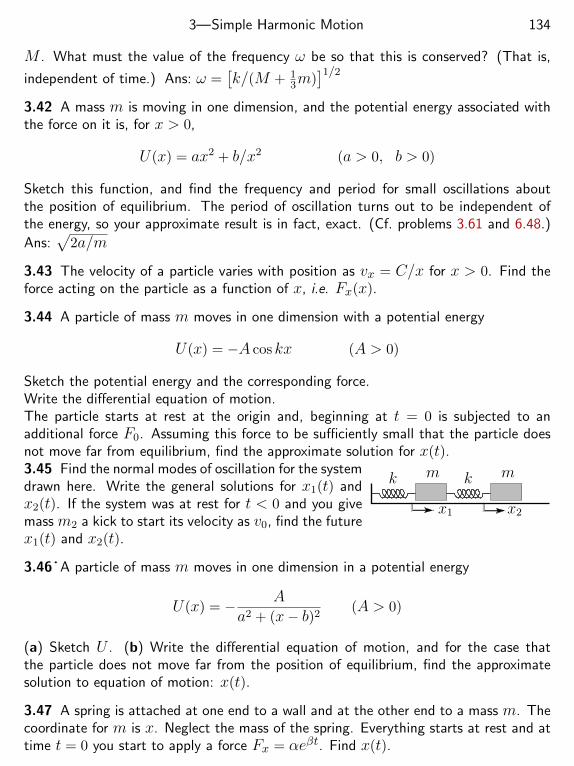
3—Simple Harmonic Motion 134
M . What must the value of the frequency ω be so that this is conserved? (That is,
independent of time.) Ans: ω =[k/(M + 1
3m)]1/2
3.42 A mass m is moving in one dimension, and the potential energy associated withthe force on it is, for x > 0,
U(x) = ax2 + b/x2 (a > 0, b > 0)
Sketch this function, and find the frequency and period for small oscillations aboutthe position of equilibrium. The period of oscillation turns out to be independent ofthe energy, so your approximate result is in fact, exact. (Cf. problems 3.61 and 6.48.)
Ans:√
2a/m
3.43 The velocity of a particle varies with position as vx = C/x for x > 0. Find theforce acting on the particle as a function of x, i.e. Fx(x).
3.44 A particle of mass m moves in one dimension with a potential energy
U(x) = −A cos kx (A > 0)
Sketch the potential energy and the corresponding force.Write the differential equation of motion.The particle starts at rest at the origin and, beginning at t = 0 is subjected to anadditional force F0. Assuming this force to be sufficiently small that the particle doesnot move far from equilibrium, find the approximate solution for x(t).
x1 x2
k m k m3.45 Find the normal modes of oscillation for the systemdrawn here. Write the general solutions for x1(t) andx2(t). If the system was at rest for t < 0 and you givemass m2 a kick to start its velocity as v0, find the futurex1(t) and x2(t).
3.46˙ A particle of mass m moves in one dimension in a potential energy
U(x) = − Aa2 + (x− b)2
(A > 0)
(a) Sketch U . (b) Write the differential equation of motion, and for the case thatthe particle does not move far from the position of equilibrium, find the approximatesolution to equation of motion: x(t).
3.47 A spring is attached at one end to a wall and at the other end to a mass m. Thecoordinate for m is x. Neglect the mass of the spring. Everything starts at rest and attime t = 0 you start to apply a force Fx = αeβt. Find x(t).
3—Simple Harmonic Motion 135
3.48 When a mass oscillates as x(t) = A sinω0t the velocity is dx/dt = Aω0 cosω0t.If you look at the mass at random times you will find it somewhere between ±A,what is the probability that you will find it at different places between those limits?In a little interval between x and x + dx the probability of seeing it is proportional tothe amount of time dt that it is in that interval. The probability per interval is thenproportional to dt/dx. Evaluate this probability density as a function of x and graphit. Is such behavior plausible? The total probability of being found somewhere is one,so the integral of this function with respect to x must be one. Use that to evaluate theproportionality constant and then graph the function. Cf. the plot immediately below.Ans: 1/π
√A2 − x2
3.49 In the spirit of the preceding problem, what is the probability density for themotion in problem 3.29?
3.50˙ Two springs having spring constants k1 and k2 are attached end-to-end (in series).Derive the effective spring constant of the whole combined spring. (What is the forceon the point of attachment?)
3.51¨The system described by Eqs. (3.54) now has an additional force F0 cos Ωt actingon mass m1. Write the differential equations for this case. Next take the symmetricspecial case of Eq. (3.60) and find a solution to these inhomogeneous equations. Itis just like the problem of Eq. (3.36), but without damping, or like the first part ofproblem 3.12. Get x1(t) and x2(t), and describe the behavior of this inhomogeneouspart of the solution (the steady-state part) as Ω varies. In particular, draw a graph ofthe amplitude of the x1 motion versus Ω and a graph of the amplitude of the x2 motionversus Ω. When you analyze your results, you will find it helpful to take the equationsfor x1 and for x2 and to break them up using partial fractions. You should find twodifferent resonances, at Ω2 = k/m and at Ω2 = (k + 2k2)/m.
3.52 A one dimensional potential energy is U(x) = −U0xae−x/a. Sketch it. What is
the position of equilibrium? What is the frequency of small oscillation about equilibrium?
3.53 A particle of mass m moves in a straight line with a potential energy given byU(x) = αx2−βx4, where α and β are positive constants. (a) Determine the range ofenergies for periodic motion. (b) What is the period of small oscillations?
3.54 The Morse potential, Eq. (2.33), has a stable equilibrium at r = r0. For smalloscillations about that point, find the frequency of oscillation of a mass m. Apply thisto the HCl molecule where m is the mass of the H-atom, assuming Cl is big enoughthat it doesn’t move much. Use the parameters stated there to compute the numericalvalue of this frequency. Assume that the molecule emits radiation at that frequency,
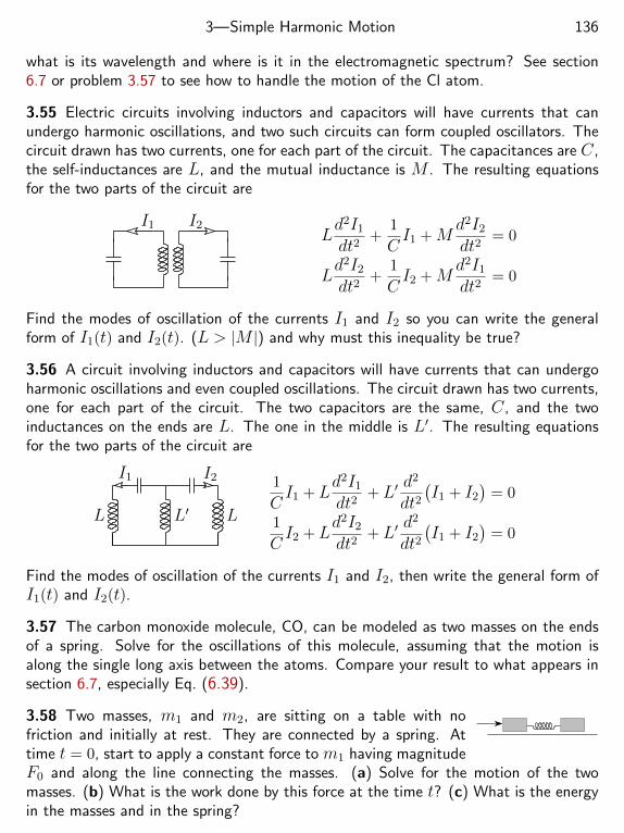
3—Simple Harmonic Motion 136
what is its wavelength and where is it in the electromagnetic spectrum? See section6.7 or problem 3.57 to see how to handle the motion of the Cl atom.
3.55 Electric circuits involving inductors and capacitors will have currents that canundergo harmonic oscillations, and two such circuits can form coupled oscillators. Thecircuit drawn has two currents, one for each part of the circuit. The capacitances are C,the self-inductances are L, and the mutual inductance is M . The resulting equationsfor the two parts of the circuit are
I1 I2Ld2I1
dt2+
1
CI1 +M
d2I2
dt2= 0
Ld2I2
dt2+
1
CI2 +M
d2I1
dt2= 0
Find the modes of oscillation of the currents I1 and I2 so you can write the generalform of I1(t) and I2(t). (L > |M |) and why must this inequality be true?
3.56 A circuit involving inductors and capacitors will have currents that can undergoharmonic oscillations and even coupled oscillations. The circuit drawn has two currents,one for each part of the circuit. The two capacitors are the same, C, and the twoinductances on the ends are L. The one in the middle is L′. The resulting equationsfor the two parts of the circuit are
L L′ L
I1 I2 1
CI1 + L
d2I1
dt2+ L′
d2
dt2(I1 + I2
)= 0
1
CI2 + L
d2I2
dt2+ L′
d2
dt2(I1 + I2
)= 0
Find the modes of oscillation of the currents I1 and I2, then write the general form ofI1(t) and I2(t).
3.57 The carbon monoxide molecule, CO, can be modeled as two masses on the endsof a spring. Solve for the oscillations of this molecule, assuming that the motion isalong the single long axis between the atoms. Compare your result to what appears insection 6.7, especially Eq. (6.39).
3.58 Two masses, m1 and m2, are sitting on a table with nofriction and initially at rest. They are connected by a spring. Attime t = 0, start to apply a constant force to m1 having magnitudeF0 and along the line connecting the masses. (a) Solve for the motion of the twomasses. (b) What is the work done by this force at the time t? (c) What is the energyin the masses and in the spring?
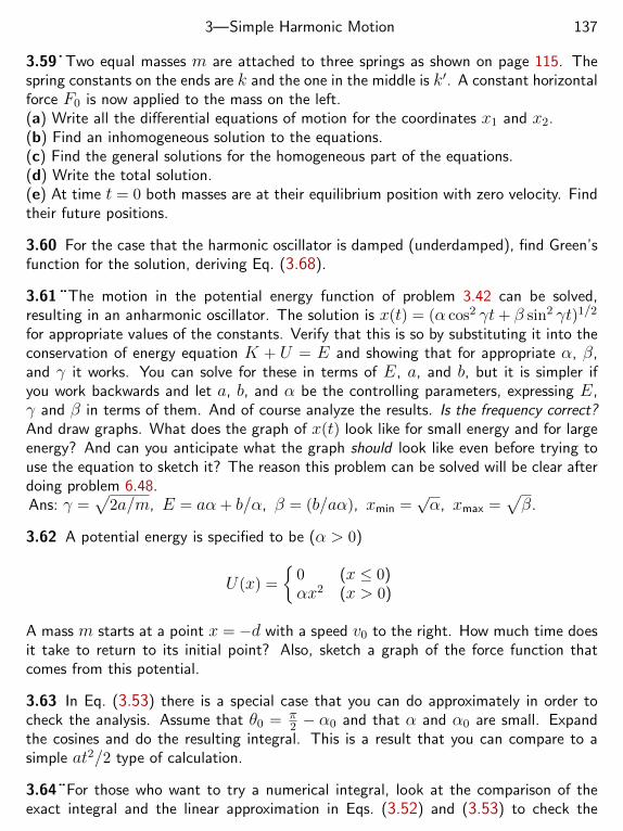
3—Simple Harmonic Motion 137
3.59˙ Two equal masses m are attached to three springs as shown on page 115. Thespring constants on the ends are k and the one in the middle is k′. A constant horizontalforce F0 is now applied to the mass on the left.(a) Write all the differential equations of motion for the coordinates x1 and x2.(b) Find an inhomogeneous solution to the equations.(c) Find the general solutions for the homogeneous part of the equations.(d) Write the total solution.(e) At time t = 0 both masses are at their equilibrium position with zero velocity. Findtheir future positions.
3.60 For the case that the harmonic oscillator is damped (underdamped), find Green’sfunction for the solution, deriving Eq. (3.68).
3.61 ¨The motion in the potential energy function of problem 3.42 can be solved,resulting in an anharmonic oscillator. The solution is x(t) = (α cos2 γt+ β sin2 γt)1/2
for appropriate values of the constants. Verify that this is so by substituting it into theconservation of energy equation K + U = E and showing that for appropriate α, β,and γ it works. You can solve for these in terms of E, a, and b, but it is simpler ifyou work backwards and let a, b, and α be the controlling parameters, expressing E,γ and β in terms of them. And of course analyze the results. Is the frequency correct?And draw graphs. What does the graph of x(t) look like for small energy and for largeenergy? And can you anticipate what the graph should look like even before trying touse the equation to sketch it? The reason this problem can be solved will be clear afterdoing problem 6.48.Ans: γ =
√2a/m, E = aα+ b/α, β = (b/aα), xmin =
√α, xmax =
√β.
3.62 A potential energy is specified to be (α > 0)
U(x) =
0 (x ≤ 0)αx2 (x > 0)
A mass m starts at a point x = −d with a speed v0 to the right. How much time doesit take to return to its initial point? Also, sketch a graph of the force function thatcomes from this potential.
3.63 In Eq. (3.53) there is a special case that you can do approximately in order tocheck the analysis. Assume that θ0 = π
2 − α0 and that α and α0 are small. Expandthe cosines and do the resulting integral. This is a result that you can compare to asimple at2/2 type of calculation.
3.64¨For those who want to try a numerical integral, look at the comparison of theexact integral and the linear approximation in Eqs. (3.52) and (3.53) to check the
3—Simple Harmonic Motion 138
numerical results stated there. To do this integral numerically you must first recognizethat the integrand is singular at θ = θ0. If you make the substitution θ− θ0 = x2, thenthe integrand in the x variable is no longer singular, but you must evaluate it as x→ 0in order to find its value at zero. Then integrate dx from x = 0 to where θ = π/2.
3.65 Solve the equation (2.35) for the motion of Atwood’s machine. Assume It startsfrom rest at initial y = y0. Many cases to analyze here: (a) µ = 0, (b) m1 = m2 = 0,(c) there’s an exponential in this solution. Can the acceleration ever be larger than g?The special case (b) will suffice for this one.
3.66 (a) Write the equation for conservation of energy for the potential functionU(x) = −kx2/2, and sketch the graph of U .(b)Separate variables to get dt and write the integral that will allow you to find t interms of x. (c) Evaluate the integral for the special case that E = 0 and apply theinitial condition that x(0) = x0 to solve for x(t).
3.67 Two masses, m1 and m2, are sitting on a table with no friction and initially atrest. They are connected by a spring. At time t = 0, start to apply a force F0 cosωtto m1 having magnitude F0 and along the line connecting the masses. Solve for themotion of the two masses.
3.68 For the simple harmonic oscillator, the period is independent of the energy. Forthe quartic potential, U ∝ x4, how does the period depend on the energy?
3.69 The manipulations that led from Eq. (3.69) to Eq. (3.71): do the same for thesimple harmonic oscillator.
3.70 Do the numerical integral, Eq. (3.71) from 0 to 2. Use the midpoint rule withN = 1 and with N = 2 (or Simpson — look it up). The more accurate answer for thisu when z = 2 is 1.311029.
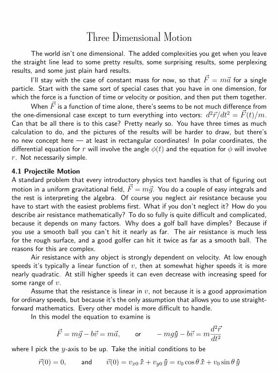
Three Dimensional MotionThe world isn’t one dimensional. The added complexities you get when you leave
the straight line lead to some pretty results, some surprising results, some perplexingresults, and some just plain hard results.
I’ll stay with the case of constant mass for now, so that ~F = m~a for a singleparticle. Start with the same sort of special cases that you have in one dimension, forwhich the force is a function of time or velocity or position, and then put them together.
When ~F is a function of time alone, there’s seems to be not much difference fromthe one-dimensional case except to turn everything into vectors: d2~r/dt2 = ~F (t)/m.Can that be all there is to this case? Pretty nearly so. You have three times as muchcalculation to do, and the pictures of the results will be harder to draw, but there’sno new concept here — at least in rectangular coordinates! In polar coordinates, thedifferential equation for r will involve the angle φ(t) and the equation for φ will involver. Not necessarily simple.
4.1 Projectile MotionA standard problem that every introductory physics text handles is that of figuring out
motion in a uniform gravitational field, ~F = m~g. You do a couple of easy integrals andthe rest is interpreting the algebra. Of course you neglect air resistance because youhave to start with the easiest problems first. What if you don’t neglect it? How do youdescribe air resistance mathematically? To do so fully is quite difficult and complicated,because it depends on many factors. Why does a golf ball have dimples? Because ifyou use a smooth ball you can’t hit it nearly as far. The air resistance is much lessfor the rough surface, and a good golfer can hit it twice as far as a smooth ball. Thereasons for this are complex.
Air resistance with any object is strongly dependent on velocity. At low enoughspeeds it’s typically a linear function of v, then at somewhat higher speeds it is morenearly quadratic. At still higher speeds it can even decrease with increasing speed forsome range of v.
Assume that the resistance is linear in v, not because it is a good approximationfor ordinary speeds, but because it’s the only assumption that allows you to use straight-forward mathematics. Every other model is more difficult to handle.
In this model the equation to examine is
~F = m~g − b~v = m~a, or −mgy − b~v = md2~rdt2
where I pick the y-axis to be up. Take the initial conditions to be
~r(0) = 0, and ~v(0) = vx0 x+ vy0 y = v0 cos θ x+ v0 sin θ y
139
4—Three Dimensional Motion 140
With these conditions the z-coordinate stays at zero.
md2xdt2
+ bdxdt
= 0, md2ydt2
+ bdydt
= −mg (4.1)
These are linear constant coefficient differential equations, one inhomogeneous. Youcan solve them in several different ways, and I choose to use the method of section 0.9.
Both of Eqs. (4.1) have the same homogeneous part, so do that first. Assumean exponential.
x = Aeαt =⇒ mAα2eαt + bAαeαt = 0, so α = 0 or α = −b/m
The homogeneous solution is then x(t) = A+Be−bt/m. The same for y. though withdifferent constants.
The inhomogeneous part of the differential equation is a constant, so try a con-stant times time for a solution:
y = Ct =⇒ m . 0 + bC = −mg, or C = −mg/b
Put these together and the total solution is
x(t) = A+Be−bt/m, y(t) = A′ +B′e−bt/m −mgt/b
Apply the initial conditions to evaluate the constants.
x(0) = 0 = A+B, y(0) = 0 = A′ +B′,
and vx(0) = v0 cos θ = − bmB, vy(0) = v0 sin θ = − b
mB′ − mg
b
x(t) =mbv0 cos θ
[1− e−bt/m
]y(t) =
mb
[v0 sin θ +
mgb
] [1− e−bt/m
]− mgt
b
(4.2)
Now comes the part that makes this worthwhile: analyzing the result. First checkthat the dimensions are correct. This has to be a reflex, so I’ll leave it to you. [Quickly:Look at the exponential and determine the units for m/b. The rest follows.] The nextstep is to check that it’s plausible. If there is no air resistance after all, then you knowthe answer. Does this give the right answer if b→ 0? You’ve got 0/0 and ∞−∞, souse power series expansions. The exponential is, from Eq. (0.1)
e−bt/m = 1− btm
+b2t2
2m2− b3t3
6m3+ · · ·
4—Three Dimensional Motion 141
Substitute into x(t) and you have
x(t) =mbv0 cos θ
[1−
(1− bt
m+b2t2
2m2− b3t3
6m3+ · · ·
)]=mbv0 cos θ
[btm− · · ·
]= v0 cos θ t+ · · ·
(4.3)
All the rest of the terms go to zero as b → 0, and this is the correct result for zeroresistance.
Next, y:
y(t) =mb
[v0 sin θ +
mgb
] [1−
(1− bt
m+b2t2
2m2− b3t3
6m3+ · · ·
)]− mgt
b
=mb
[v0 sin θ +
mgb
] [ btm− b2t2
2m2+b3t3
6m3+ · · ·
]− mgt
b
= v0 sin θ t− 1
2gt2 + · · ·
(4.4)
Again, the rest of the terms vanish as b → 0. These two limiting equations for x andy are what you must find or you have to go back and discover your mistake.
What about the opposite extreme, for which b is very large? What does “verylarge” mean? It has to be compared to something. Dimensionally you have few choices:
v0 +mg/b is dimensionally consistent, bt/m is dimensionless,
so I can say b mg/v0 or t m/b. The first of these says that the viscous drag ismuch bigger than the gravitational force; the second says that after a long enough timeviscosity dominates. In other words it’s not yet clear which one applies, so keep going.
In Eq. (4.2) the exponential terms will disappear if bt m, giving an approxi-mate solution after a long time:
x(t) ≈ mbv0 cos θ and y(t) ≈ m
b
[v0 sin θ +
mgb
]− mgt
b(4.5)
This says that eventually the mass is moving straight down with a constant veloc-ity vy = −mg/b, the terminal velocity. It’s off to the right a constant distance(mv0 cos θ)/b. This is not necessarily big viscosity, you just have to wait long enoughfor this approximation to be valid.
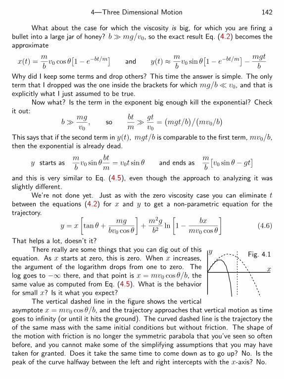
4—Three Dimensional Motion 142
What about the case for which the viscosity is big, for which you are firing abullet into a large jar of honey? bmg/v0, so the exact result Eq. (4.2) becomes theapproximate
x(t) =mbv0 cos θ
[1− e−bt/m
]and y(t) ≈ m
bv0 sin θ
[1− e−bt/m
]− mgt
b
Why did I keep some terms and drop others? This time the answer is simple. The onlyterm that I dropped was the one inside the brackets for which mg/b v0, and that isexplicitly what I just assumed to be true.
Now what? Is the term in the exponent big enough kill the exponential? Checkit out:
b mgv0, so
btm gtv0
=(mgt/b
)/(mv0/b
)This says that if the second term in y(t), mgt/b is comparable to the first term, mv0/b,then the exponential is already dead.
y starts asmbv0 sin θ
btm
= v0t sin θ and ends asmb
[v0 sin θ − gt
]and this is very similar to Eq. (4.5), even though the approach to analyzing it wasslightly different.
We’re not done yet. Just as with the zero viscosity case you can eliminate tbetween the equations (4.2) for x and y to get a non-parametric equation for thetrajectory.
y = x
[tan θ +
mgbv0 cos θ
]+m2gb2
ln
[1− bx
mv0 cos θ
](4.6)
That helps a lot, doesn’t it?
x
y Fig. 4.1There really are some things that you can dig out of this
equation. As x starts at zero, this is zero. When x increases,the argument of the logarithm drops from one to zero. Thelog goes to −∞ there, and that point is x = mv0 cos θ/b, thesame value as computed from Eq. (4.5). What is the behaviorfor small x? Is it what you expect?
The vertical dashed line in the figure shows the verticalasymptote x = mv0 cos θ/b, and the trajectory approaches that vertical motion as timegoes to infinity (or until it hits the ground). The curved dashed line is the trajectory theof the same mass with the same initial conditions but without friction. The shape ofthe motion with friction is no longer the symmetric parabola that you’ve seen so oftenbefore, and you cannot make some of the simplifying assumptions that you may havetaken for granted. Does it take the same time to come down as to go up? No. Is thepeak of the curve halfway between the left and right intercepts with the x-axis? No.
4—Three Dimensional Motion 143
4.2 General ResultsIf you read Newton’s Principia you will not find the equation ~F = m~a. You will not
even find the equation ~F = d~p/dt. His presentation of physics was nothing like themodern way to develop the subject, and it is close to unreadable today. The treatmentwe are accustomed to was mostly developed by Leonard Euler, and if you look up Euler’scollected works you will find the language and the notation remarkable modern. Thatis because we mostly use Euler’s notation.
Starting from the basic equation describing the motion of a particle, there aresome general results to derive. Start with one dimension.
Fx = mdvxdt−→ Fxvx = mvx
dvxdt−→ Fxvx =
m2
dv2x
dt
Reading from right to left, this says that the power, the rate of change of energy is
dWdt
=ddt
1
2mv2
x = Fxvx
Still another way to manipulate it is to integrate with respect to t.∫ tf
ti
Fxvx dt =
∫ tf
ti
m2
dv2x
dtdt =
∫ t=tf
t=ti
m2d(v2
x) =1
2mv2
f −1
2mv2
i (4.7)
This is the simplest form of the work-energy theorem,
Wtotal =
∫ tf
ti
Fxvx dt =
∫ xf
xi
Fx dx = ∆K = Kf −Ki (4.8)
Does this look familiar?In one dimension, Fxvx dt = Fx dx, and if the force Fx is a function of the
coordinate x alone, then the integral depends on the initial and final values of x andnot on how fast or how slowly you went from the start to the finish. Fx(x) has ananti-derivative, and the fundamental theorem of calculus says that you evaluate thisanti-derivative at the endpoints and subtract. Call this anti-derivative −U .
Fx(x) = −dUdx, then
∫ xf
xi
Fx(x) dx = −U(x)
∣∣∣∣xf
xi
= −U(xf) + U(xi) (4.9)
Put this into the preceding equation and rearrange it.
−U(xf) + U(xi) =1
2mv2
f −1
2mv2
i −→ 1
2mv2
i + U(xi) =1
2mv2
f + U(xf) (4.10)
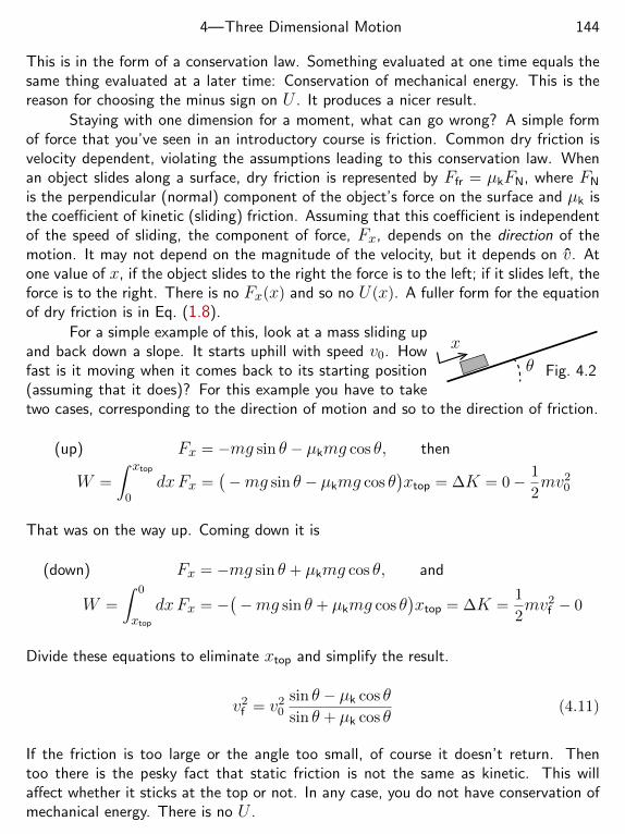
4—Three Dimensional Motion 144
This is in the form of a conservation law. Something evaluated at one time equals thesame thing evaluated at a later time: Conservation of mechanical energy. This is thereason for choosing the minus sign on U . It produces a nicer result.
Staying with one dimension for a moment, what can go wrong? A simple formof force that you’ve seen in an introductory course is friction. Common dry friction isvelocity dependent, violating the assumptions leading to this conservation law. Whenan object slides along a surface, dry friction is represented by Ffr = µkFN, where FN
is the perpendicular (normal) component of the object’s force on the surface and µk isthe coefficient of kinetic (sliding) friction. Assuming that this coefficient is independentof the speed of sliding, the component of force, Fx, depends on the direction of themotion. It may not depend on the magnitude of the velocity, but it depends on v. Atone value of x, if the object slides to the right the force is to the left; if it slides left, theforce is to the right. There is no Fx(x) and so no U(x). A fuller form for the equationof dry friction is in Eq. (1.8).
x
θ Fig. 4.2
For a simple example of this, look at a mass sliding upand back down a slope. It starts uphill with speed v0. Howfast is it moving when it comes back to its starting position(assuming that it does)? For this example you have to taketwo cases, corresponding to the direction of motion and so to the direction of friction.
(up) Fx = −mg sin θ − µkmg cos θ, then
W =
∫ xtop
0dxFx =
(−mg sin θ − µkmg cos θ
)xtop = ∆K = 0− 1
2mv2
0
That was on the way up. Coming down it is
(down) Fx = −mg sin θ + µkmg cos θ, and
W =
∫ 0
xtop
dxFx = −(−mg sin θ + µkmg cos θ
)xtop = ∆K =
1
2mv2
f − 0
Divide these equations to eliminate xtop and simplify the result.
v2f = v2
0
sin θ − µk cos θsin θ + µk cos θ
(4.11)
If the friction is too large or the angle too small, of course it doesn’t return. Thentoo there is the pesky fact that static friction is not the same as kinetic. This willaffect whether it sticks at the top or not. In any case, you do not have conservation ofmechanical energy. There is no U .
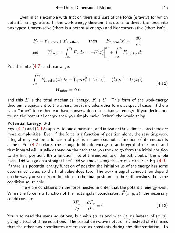
4—Three Dimensional Motion 145
Even in this example with friction there is a part of the force (gravity) for whichpotential energy exists. In the work-energy theorem it is useful to divide the force intotwo types: Conservative (there is a potential energy) and Nonconservative (there isn’t).
Fx = Fx, cons + Fx, other, then Fx, cons(x) = −dUdx
and Wtotal =
∫ xf
xi
Fx dx = −U(x)
∣∣∣∣xf
xi
+
∫ xf
xi
Fx, other dx
Put this into (4.7) and rearrange.∫ xf
xi
Fx, other(x) dx =(
12mv
2f + U(xf)
)−(
12mv
2i + U(xi)
)Wother = ∆E
(4.12)
and this E is the total mechanical energy, K + U . This form of the work-energytheorem is equivalent to the others, but it includes other forms as special cases. If thereis no “other” force then you have conservation of mechanical energy. If you decide notto use the potential energy then you simply make “other” the whole thing.
Potential Energy, 3-dEqs. (4.7) and (4.12) applies to one dimension, and in two or three dimensions there aremore complexities. Even if the force is a function of position alone, the resulting workintegral may not be a function of position alone (i.e. not a function of its endpointsalone). Eq. (4.7) relates the change in kinetic energy to an integral of the force, andthat integral will usually depend on the path that you took to go from the initial positionto the final position. It’s a function, not of the endpoints of the path, but of the wholepath. Did you go on a straight line? Did you move along the arc of a circle? In Eq. (4.9),if there is a potential energy function of position the initial value of the energy has somedetermined value, so the final value does too. The work integral cannot then dependon the way you went from the initial to the final position. In three dimensions the samecondition must hold.
There are conditions on the force needed in order that the potential energy exist.
When the force is a function of the rectangular coordinates, ~F (x, y, z), the necessaryconditions are
∂Fx∂y−∂Fy∂x
= 0 (4.13)
You also need the same equations, but with (y, z) and with (z, x) instead of (x, y),giving a total of three equations. The partial derivative notation (∂ instead of d) meansthat the other two coordinates are treated as constants during the differentiation. To
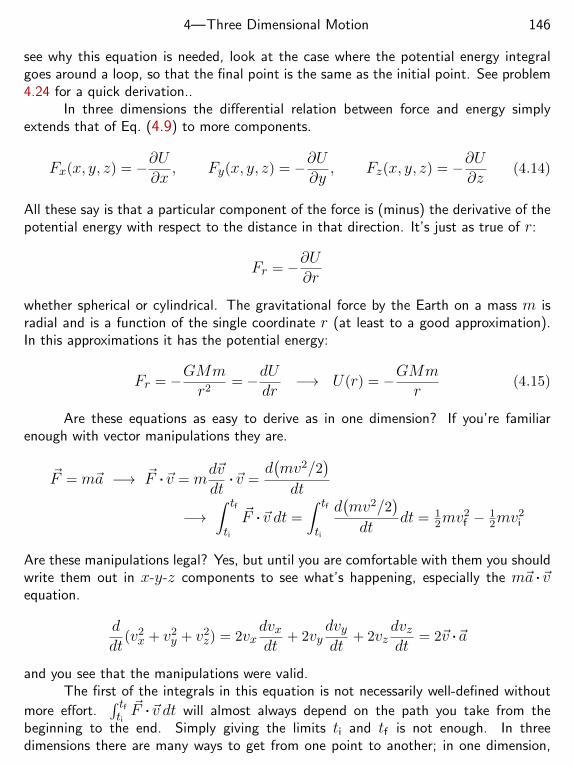
4—Three Dimensional Motion 146
see why this equation is needed, look at the case where the potential energy integralgoes around a loop, so that the final point is the same as the initial point. See problem4.24 for a quick derivation..
In three dimensions the differential relation between force and energy simplyextends that of Eq. (4.9) to more components.
Fx(x, y, z) = −∂U∂x
, Fy(x, y, z) = −∂U∂y
, Fz(x, y, z) = −∂U∂z
(4.14)
All these say is that a particular component of the force is (minus) the derivative of thepotential energy with respect to the distance in that direction. It’s just as true of r:
Fr = −∂U∂r
whether spherical or cylindrical. The gravitational force by the Earth on a mass m isradial and is a function of the single coordinate r (at least to a good approximation).In this approximations it has the potential energy:
Fr = −GMmr2
= −dUdr
−→ U(r) = −GMmr
(4.15)
Are these equations as easy to derive as in one dimension? If you’re familiarenough with vector manipulations they are.
~F = m~a −→ ~F .~v = md~vdt
.~v =d(mv2/2
)dt
−→∫ tf
ti
~F .~v dt =
∫ tf
ti
d(mv2/2
)dt
dt = 12mv
2f − 1
2mv2i
Are these manipulations legal? Yes, but until you are comfortable with them you shouldwrite them out in x-y-z components to see what’s happening, especially the m~a .~vequation.
ddt
(v2x + v2
y + v2z) = 2vx
dvxdt
+ 2vydvydt
+ 2vzdvzdt
= 2~v .~a
and you see that the manipulations were valid.The first of the integrals in this equation is not necessarily well-defined without
more effort.∫ tfti~F .~v dt will almost always depend on the path you take from the
beginning to the end. Simply giving the limits ti and tf is not enough. In threedimensions there are many ways to get from one point to another; in one dimension,
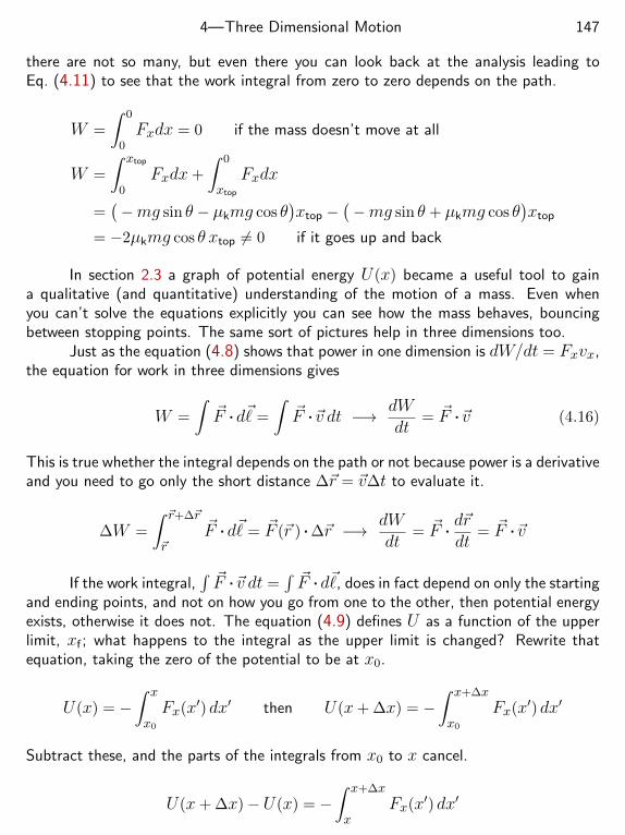
4—Three Dimensional Motion 147
there are not so many, but even there you can look back at the analysis leading toEq. (4.11) to see that the work integral from zero to zero depends on the path.
W =
∫ 0
0Fxdx = 0 if the mass doesn’t move at all
W =
∫ xtop
0Fxdx+
∫ 0
xtop
Fxdx
=(−mg sin θ − µkmg cos θ
)xtop −
(−mg sin θ + µkmg cos θ
)xtop
= −2µkmg cos θ xtop 6= 0 if it goes up and back
In section 2.3 a graph of potential energy U(x) became a useful tool to gaina qualitative (and quantitative) understanding of the motion of a mass. Even whenyou can’t solve the equations explicitly you can see how the mass behaves, bouncingbetween stopping points. The same sort of pictures help in three dimensions too.
Just as the equation (4.8) shows that power in one dimension is dW/dt = Fxvx,the equation for work in three dimensions gives
W =
∫~F . d~=
∫~F .~v dt −→ dW
dt= ~F .~v (4.16)
This is true whether the integral depends on the path or not because power is a derivativeand you need to go only the short distance ∆~r = ~v∆t to evaluate it.
∆W =
∫ ~r+∆~r
~r
~F . d~= ~F (~r ) . ∆~r −→ dWdt
= ~F . d~rdt
= ~F .~v
If the work integral,∫ ~F .~v dt =
∫ ~F . d~, does in fact depend on only the startingand ending points, and not on how you go from one to the other, then potential energyexists, otherwise it does not. The equation (4.9) defines U as a function of the upperlimit, xf ; what happens to the integral as the upper limit is changed? Rewrite thatequation, taking the zero of the potential to be at x0.
U(x) = −∫ x
x0Fx(x′) dx′ then U(x+ ∆x) = −
∫ x+∆x
x0Fx(x′) dx′
Subtract these, and the parts of the integrals from x0 to x cancel.
U(x+ ∆x)− U(x) = −∫ x+∆x
xFx(x′) dx′
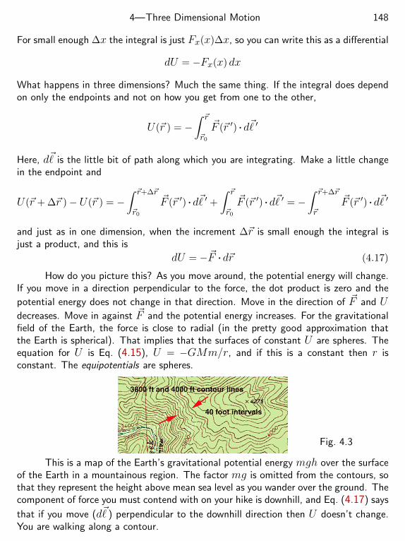
4—Three Dimensional Motion 148
For small enough ∆x the integral is just Fx(x)∆x, so you can write this as a differential
dU = −Fx(x) dx
What happens in three dimensions? Much the same thing. If the integral does dependon only the endpoints and not on how you get from one to the other,
U(~r ) = −∫ ~r
~r0
~F (~r ′) . d~ ′
Here, d~ is the little bit of path along which you are integrating. Make a little changein the endpoint and
U(~r + ∆~r )− U(~r ) = −∫ ~r+∆~r
~r0
~F (~r ′) . d~ ′ +∫ ~r
~r0
~F (~r ′) . d~ ′ = −∫ ~r+∆~r
~r
~F (~r ′) . d~ ′
and just as in one dimension, when the increment ∆~r is small enough the integral isjust a product, and this is
dU = −~F . d~r (4.17)
How do you picture this? As you move around, the potential energy will change.If you move in a direction perpendicular to the force, the dot product is zero and the
potential energy does not change in that direction. Move in the direction of ~F and Udecreases. Move in against ~F and the potential energy increases. For the gravitationalfield of the Earth, the force is close to radial (in the pretty good approximation thatthe Earth is spherical). That implies that the surfaces of constant U are spheres. Theequation for U is Eq. (4.15), U = −GMm/r, and if this is a constant then r isconstant. The equipotentials are spheres.
Fig. 4.3
This is a map of the Earth’s gravitational potential energy mgh over the surfaceof the Earth in a mountainous region. The factor mg is omitted from the contours, sothat they represent the height above mean sea level as you wander over the ground. Thecomponent of force you must contend with on your hike is downhill, and Eq. (4.17) says
that if you move (d~) perpendicular to the downhill direction then U doesn’t change.You are walking along a contour.
4—Three Dimensional Motion 149
ExampleIf in two dimensions (easier to draw) U = αy − βx2 where α and β are positiveconstants, the equipotentials are
αy − βx2 = C (4.18)
and Each C defines a different parabola as an equipotential. The force correspondingto this potential is everywhere perpendicular to these parabolas. What is the force?Equation (4.17) determines the answer. If you take d~r to be in the direction such thaty is a constant, then
d~= xdx, so dU = −~F . d~= −~F . xdx = −Fx dx
That just gives the first of the equations (4.14), Fx = −∂U/∂x = 2βx. For the othercomponent, just move in the y-direction to get Fy = −α
4.3 E and B fieldsHow does a charge behave in an electromagnetic field? The force law is
~F = q( ~E + ~v × ~B ) = md2~r/dt2 (4.19)
The values of the electric and magnetic fields have to be computed somewhere else,because that’s another subject. Suppose that someone works them out or measuresthem, the problem now is to determine their effect on charges. If it sounds straight-forward, that’s probably because you’ve looked at the cases of uniform fields when youtook a beginning course on the subject. Even there, you probably saw only the two fieldsseparately. When you put them together you already get some interesting and surprisingresults. When you allow the fields to be functions of position the mathematics escalatesdramatically, but there’s one important simplification that applies to all magnetic fields,uniform or not: a magnetic field does no work. Recall the expression (4.16) for power:~F .~v. If the force is magnetic then
power = ~F .~v = q~v × ~B .~v = 0 (4.20)
It’s the electric field alone that does work.Start with the case of uniform fields ~E = 0 and ~B = B0z. You’ve seen the
result. The charge will go in a circle. Well no, a helix is more likely. You should goback and look at what you’ve studied previously and review it to see that you can getthis simple answer by elementary means involving circular motion and a = v2/r. Here
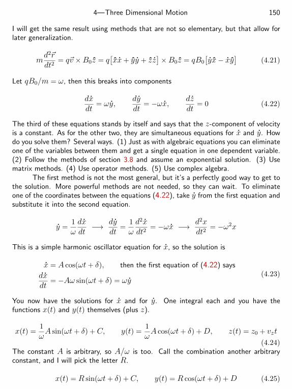
4—Three Dimensional Motion 150
I will get the same result using methods that are not so elementary, but that allow forlater generalization.
md2~rdt2
= q~v ×B0z = q[xx+ yy + zz
]×B0z = qB0
[yx− xy
](4.21)
Let qB0/m = ω, then this breaks into components
dxdt
= ωy,dydt
= −ωx, dzdt
= 0 (4.22)
The third of these equations stands by itself and says that the z-component of velocityis a constant. As for the other two, they are simultaneous equations for x and y. Howdo you solve them? Several ways. (1) Just as with algebraic equations you can eliminateone of the variables between them and get a single equation in one dependent variable.(2) Follow the methods of section 3.8 and assume an exponential solution. (3) Usematrix methods. (4) Use operator methods. (5) Use complex algebra.
The first method is not the most general, but it’s a perfectly good way to get tothe solution. More powerful methods are not needed, so they can wait. To eliminateone of the coordinates between the equations (4.22), take y from the first equation andsubstitute it into the second equation.
y =1
ωdxdt−→ dy
dt=
1
ωd2xdt2
= −ωx −→ d2xdt2
= −ω2x
This is a simple harmonic oscillator equation for x, so the solution is
x = A cos(ωt+ δ), then the first equation of (4.22) says
dxdt
= −Aω sin(ωt+ δ) = ωy(4.23)
You now have the solutions for x and for y. One integral each and you have thefunctions x(t) and y(t) themselves (plus z).
x(t) =1
ωA sin(ωt+ δ) +C, y(t) =
1
ωA cos(ωt+ δ) +D, z(t) = z0 + vzt
(4.24)The constant A is arbitrary, so A/ω is too. Call the combination another arbitraryconstant, and I will pick the letter R.
x(t) = R sin(ωt+ δ) +C, y(t) = R cos(ωt+ δ) +D (4.25)
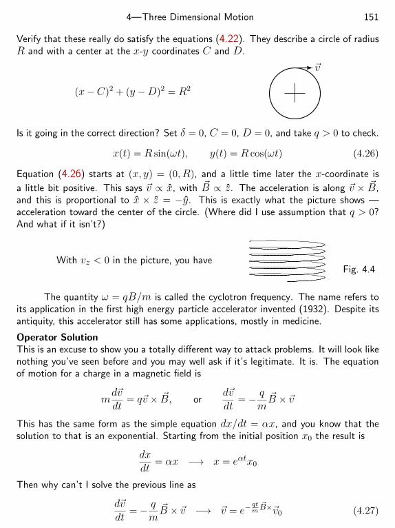
4—Three Dimensional Motion 151
Verify that these really do satisfy the equations (4.22). They describe a circle of radiusR and with a center at the x-y coordinates C and D.
(x−C)2 + (y −D)2 = R2
~v
Is it going in the correct direction? Set δ = 0, C = 0, D = 0, and take q > 0 to check.
x(t) = R sin(ωt), y(t) = R cos(ωt) (4.26)
Equation (4.26) starts at (x, y) = (0, R), and a little time later the x-coordinate is
a little bit positive. This says ~v ∝ x, with ~B ∝ z. The acceleration is along ~v × ~B,and this is proportional to x × z = −y. This is exactly what the picture shows —acceleration toward the center of the circle. (Where did I use assumption that q > 0?And what if it isn’t?)
With vz < 0 in the picture, you haveFig. 4.4
The quantity ω = qB/m is called the cyclotron frequency. The name refers toits application in the first high energy particle accelerator invented (1932). Despite itsantiquity, this accelerator still has some applications, mostly in medicine.
Operator SolutionThis is an excuse to show you a totally different way to attack problems. It will look likenothing you’ve seen before and you may well ask if it’s legitimate. It is. The equationof motion for a charge in a magnetic field is
md~vdt
= q~v × ~B, ord~vdt
= − qm~B × ~v
This has the same form as the simple equation dx/dt = αx, and you know that thesolution to that is an exponential. Starting from the initial position x0 the result is
dxdt
= αx −→ x = eαtx0
Then why can’t I solve the previous line as
d~vdt
= − qm~B × ~v −→ ~v = e−
qtm~B×~v0 (4.27)
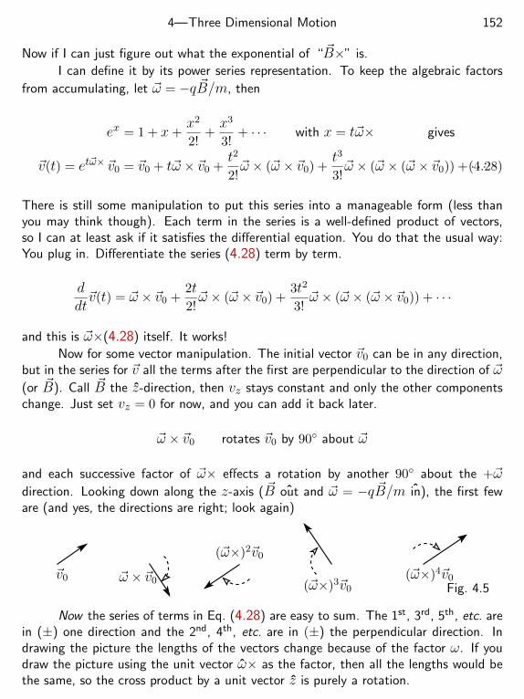
4—Three Dimensional Motion 152
Now if I can just figure out what the exponential of “ ~B×” is.
I can define it by its power series representation. To keep the algebraic factors
from accumulating, let ~ω = −q ~B/m, then
ex = 1 + x+x2
2!+x3
3!+ · · · with x = t~ω× gives
~v(t) = et~ω× ~v0 = ~v0 + t~ω × ~v0 +t2
2!~ω × (~ω × ~v0) +
t3
3!~ω × (~ω × (~ω × ~v0)) + · · ·(4.28)
There is still some manipulation to put this series into a manageable form (less thanyou may think though). Each term in the series is a well-defined product of vectors,so I can at least ask if it satisfies the differential equation. You do that the usual way:You plug in. Differentiate the series (4.28) term by term.
ddt~v(t) = ~ω × ~v0 +
2t2!~ω × (~ω × ~v0) +
3t2
3!~ω × (~ω × (~ω × ~v0)) + · · ·
and this is ~ω×(4.28) itself. It works!
Now for some vector manipulation. The initial vector ~v0 can be in any direction,but in the series for ~v all the terms after the first are perpendicular to the direction of ~ω(or ~B). Call ~B the z-direction, then vz stays constant and only the other componentschange. Just set vz = 0 for now, and you can add it back later.
~ω × ~v0 rotates ~v0 by 90 about ~ω
and each successive factor of ~ω× effects a rotation by another 90 about the +~ωdirection. Looking down along the z-axis ( ~B out and ~ω = −q ~B/m in), the first feware (and yes, the directions are right; look again)
~v0 ~ω × ~v0
(~ω×)2~v0
(~ω×)3~v0
(~ω×)4~v0Fig. 4.5
Now the series of terms in Eq. (4.28) are easy to sum. The 1st, 3rd, 5th, etc. arein (±) one direction and the 2nd, 4th, etc. are in (±) the perpendicular direction. Indrawing the picture the lengths of the vectors change because of the factor ω. If youdraw the picture using the unit vector ω× as the factor, then all the lengths would bethe same, so the cross product by a unit vector z is purely a rotation.
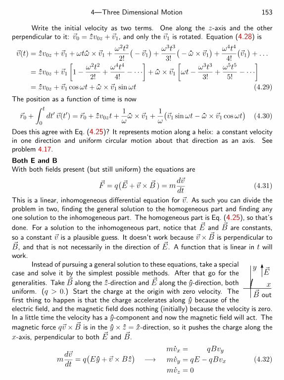
4—Three Dimensional Motion 153
Write the initial velocity as two terms. One along the z-axis and the otherperpendicular to it: ~v0 = zv0z + ~v1, and only the ~v1 is rotated. Equation (4.28) is
~v(t) = zv0z + ~v1 + ωtω × ~v1 +ω2t2
2!
(− ~v1
)+ω3t3
3!
(− ω × ~v1
)+ω4t4
4!
(~v1
)+ . . .
= zv0z + ~v1
[1− ω
2t2
2!+ω4t4
4!− · · ·
]+ ω × ~v1
[ωt− ω
3t3
3!+ω5t5
5!− · · ·
]= zv0z + ~v1 cosωt+ ω × ~v1 sinωt (4.29)
The position as a function of time is now
~r0 +
∫ t
0dt′ ~v(t′) = ~r0 + zv0zt+
1
ωω × ~v1 +
1
ω
(~v1 sinωt− ω × ~v1 cosωt
)(4.30)
Does this agree with Eq. (4.25)? It represents motion along a helix: a constant velocityin one direction and uniform circular motion about that direction as an axis. Seeproblem 4.17.
Both E and BWith both fields present (but still uniform) the equations are
~F = q( ~E + ~v × ~B ) = m
d~vdt
(4.31)
This is a linear, inhomogeneous differential equation for ~v. As such you can divide theproblem in two, finding the general solution to the homogeneous part and finding anyone solution to the inhomogeneous part. The homogeneous part is Eq. (4.25), so that’s
done. For a solution to the inhomogeneous part, notice that ~E and ~B are constants,
so a constant ~v is a plausible guess. It doesn’t work because ~v × ~B is perpendicular to~B, and that is not necessarily in the direction of ~E. A function that is linear in t willwork.
x
y ~E
~B out
Instead of pursuing a general solution to these equations, take a specialcase and solve it by the simplest possible methods. After that go for the
generalities. Take ~B along the z-direction and ~E along the y-direction, bothuniform. (q > 0.) Start the charge at the origin with zero velocity. Thefirst thing to happen is that the charge accelerates along y because of theelectric field, and the magnetic field does nothing (initially) because the velocity is zero.In a little time the velocity has a y-component and now the magnetic field will act. The
magnetic force q~v × ~B is in the y × z = x-direction, so it pushes the charge along the
x-axis, perpendicular to both ~E and ~B.
md~vdt
= q(Ey + ~v ×Bz
)−→
mvx = qBvymvy = qE − qBvxmvz = 0
(4.32)
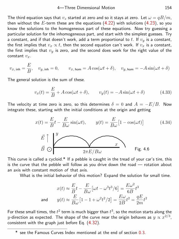
4—Three Dimensional Motion 154
The third equation says that vz started at zero and so it stays at zero. Let ω = qB/m,then without the E-term these are the equations (4.22) with solutions (4.23), so youknow the solutions to the homogeneous part of these equations. Now try guessing aparticular solution for the inhomogeneous part, and start with the simplest guesses. Trya constant, and if that doesn’t work, add a term proportional to t. If vy is a constant,the first implies that vx ∝ t, then the second equation can’t work. If vx is a constant,the first implies that vy is zero, and the second does work for the right value of theconstant vx.
vx, inh =EB, vy, inh = 0, vx, hom = A cos(ωt+ δ), vy, hom = −A sin(ωt+ δ)
The general solution is the sum of these.
vx(t) =EB
+A cos(ωt+ δ), vy(t) = −A sin(ωt+ δ) (4.33)
The velocity at time zero is zero, so this determines δ = 0 and A = −E/B. Nowintegrate these, starting with the initial conditions at the origin and getting
x(t) =EBt− E
Bωsin(ωt), y(t) =
EBω
[1− cos(ωt)
](4.34)
x
y
2πE/Bω
~Ex
~B⊙
Fig. 4.6
This curve is called a cycloid.* If a pebble is caught in the tread of your car’s tire, thisis the curve that the pebble will follow as you drive down the road — rotation aboutan axis with constant motion of that axis.
What is the initial behavior of this motion? Expand the solution for small time.
x(t) ≈ EBt− E
Bω
[ωt− ω3t3/6
]=Eω2
6Bt3
and y(t) ≈ EBω
[1− 1 + ω2t2/2
]=Eω2B
t2 =qE2m
t2
For these small times, the t2 term is much bigger than t3, so the motion starts along they-direction as expected. The shape of the curve near the origin behaves as y ∝ x2/3,consistent with the graph just before Eq. (4.32).
* see the Famous Curves Index mentioned at the end of section 0.3.
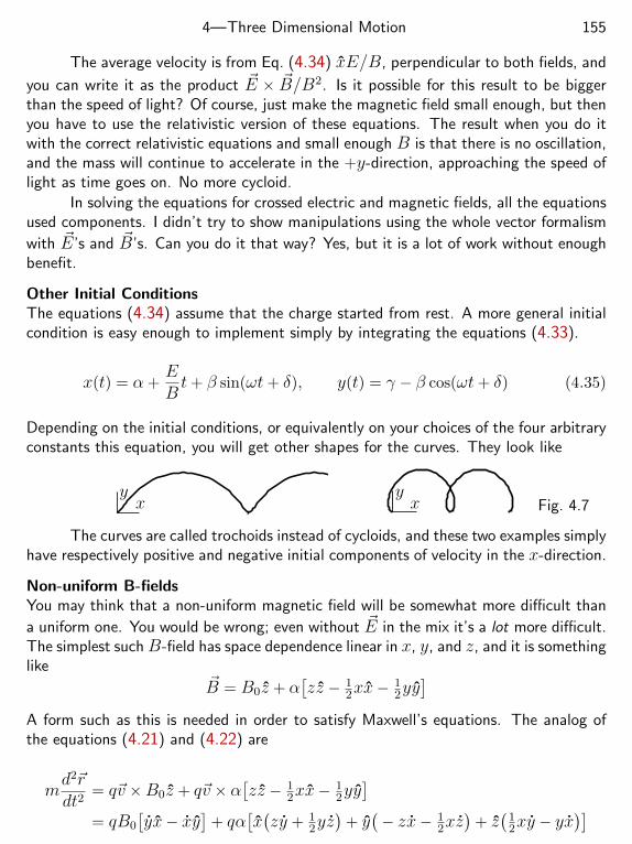
4—Three Dimensional Motion 155
The average velocity is from Eq. (4.34) xE/B, perpendicular to both fields, and
you can write it as the product ~E × ~B/B2. Is it possible for this result to be biggerthan the speed of light? Of course, just make the magnetic field small enough, but thenyou have to use the relativistic version of these equations. The result when you do itwith the correct relativistic equations and small enough B is that there is no oscillation,and the mass will continue to accelerate in the +y-direction, approaching the speed oflight as time goes on. No more cycloid.
In solving the equations for crossed electric and magnetic fields, all the equationsused components. I didn’t try to show manipulations using the whole vector formalism
with ~E’s and ~B’s. Can you do it that way? Yes, but it is a lot of work without enoughbenefit.
Other Initial ConditionsThe equations (4.34) assume that the charge started from rest. A more general initialcondition is easy enough to implement simply by integrating the equations (4.33).
x(t) = α+EBt+ β sin(ωt+ δ), y(t) = γ − β cos(ωt+ δ) (4.35)
Depending on the initial conditions, or equivalently on your choices of the four arbitraryconstants this equation, you will get other shapes for the curves. They look like
yx
yx Fig. 4.7
The curves are called trochoids instead of cycloids, and these two examples simplyhave respectively positive and negative initial components of velocity in the x-direction.
Non-uniform B-fieldsYou may think that a non-uniform magnetic field will be somewhat more difficult than
a uniform one. You would be wrong; even without ~E in the mix it’s a lot more difficult.The simplest such B-field has space dependence linear in x, y, and z, and it is somethinglike
~B = B0z + α[zz − 1
2xx−12yy
]A form such as this is needed in order to satisfy Maxwell’s equations. The analog ofthe equations (4.21) and (4.22) are
md2~rdt2
= q~v ×B0z + q~v × α[zz − 1
2xx−12yy
]= qB0
[yx− xy
]+ qα
[x(zy + 1
2yz)
+ y(− zx− 1
2xz)
+ z(
12xy − yx
)]
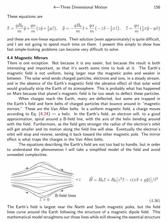
4—Three Dimensional Motion 156
These equations are
x =qB0
my+
qαm
(zy+ 1
2yz), y = −qB0
mx+
qαm
(−zx− 1
2xz), z =
qαm
(12xy−yx
)and these are non-linear equations. Their solution (even approximately) is quite difficult,and I am not going to spend much time on them. I present this simply to show howfast simple-looking problems can become very difficult to solve.
4.4 Magnetic MirrorsThere is one exception. Not because it is any easier, but because the result is bothinteresting and important, so that it’s worth some time to look at it. The Earth’smagnetic field is not uniform, being larger near the magnetic poles and weaker inbetween. The solar wind sends charged particles, electrons and ions, in a steady stream,and in the absence of the Earth’s magnetic field the abrasive effect of that solar windwould gradually strip the Earth of its atmosphere. This is probably what has happenedon Mars because that planet’s magnetic field is far too weak to deflect these particles.
When charges reach the Earth, many are deflected, but some are trapped inthe Earth’s field and form belts of charged particles that bounce around in “magneticmirrors.” These are the Van Allen belts. In a uniform magnetic field, a charge movesaccording to Eq. (4.24) — a helix. In the Earth’s field, an electron will, to a goodapproximation, spiral around a B-field line, with the axis of the helix bending aroundwith the field. Furthermore, as the field gets stronger the radius of the electron’s orbitwill get smaller and its motion along the field line will slow. Eventually the electron’sorbit will stop and reverse, sending it back toward the other magnetic pole. The mirroreffect is what traps the charges in the Van Allen belts.
The equations describing the Earth’s field are not too bad to handle, but in orderto understand the phenomenon I will take a simplified model of the field and avoidunneeded complexities.
+z
B-field linesz = 0
~B = B0z +B0
[z2z − z(xx+ yy)
]/`2
(4.36)
The Earth’s field is largest near the North and South magnetic poles, but the fieldlines curve around the Earth following the structure of a magnetic dipole field. Thismathematical model straightens out those lines while still showing the essential structure
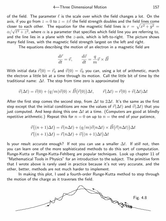
4—Three Dimensional Motion 157
of the field. The parameter ` is the scale over which the field changes a lot. On theaxis, if you go from z = 0 to z = ±` the field strength doubles and the field lines comecloser to each other. The equation for the magnetic field lines is r =
√x2 + y2 =
α/√`2 + z2, where α is a parameter that specifies which field line you are referring to,
and the line lies in a plane with the z-axis, which is left-to-right. The picture showsmany field lines, with the magnetic field strength largest on the left and right.
The equations describing the motion of an electron in a magnetic field are
d~rdt
= ~v,d~vdt
=qm~v × ~B
With initial data ~r(0) = ~r0 and ~v(0) = ~v0 you can, using a lot of arithmetic, marchthe electron a little bit at a time through its motion. Call the little bit of time by thetraditional name: ∆t. The step from time zero is approximated by
~v(∆t) = ~v(0) + (q/m)~v(0)× ~B(~r(0)
)∆t, ~r(∆t) = ~r(0) + ~v(∆t)∆t
After the first step comes the second step, from ∆t to 2∆t. It’s the same as the firststep except that the initial conditions are now the values of ~r(∆t) and ~v(∆t) that youjust computed. And keep doing this one ∆t at a time. (Computers are good at blindlyrepetitive arithmetic.) Repeat this for n = 0 on up to n = the end of your patience,
~v((n+ 1)∆t
)= ~v(n∆t) + (q/m)~v(n∆t)× ~B
(~r(n∆t)
)∆t
~r((n+ 1)∆t
)= ~r(n∆t) + ~v
((n+ 1)∆t
)∆t
Is your result accurate enough? If not you can use a smaller ∆t. If still not, thenyou can learn one of the more sophisticated methods to do this sort of computation.Runge-Kutta or Runge-Kutta-Fehlberg are popular techniques. Look up chapter 11 of“Mathematical Tools in Physics” for an introduction to the subject. The primitive formthat I wrote above is rarely used in practice because it’s not very accurate, and theother, better, methods are not much harder to implement.
In making this plot, I used a fourth-order Runge-Kutta method to step throughthe motion of the charge as it traverses the field.
Fig. 4.8
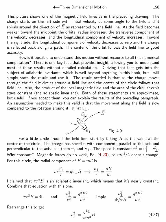
4—Three Dimensional Motion 158
This picture shows one of the magnetic field lines as in the preceding drawing. Thecharge starts on the left side with initial velocity at some angle to the field and it
spirals around the direction of ~B as represented by the field line. As the field becomesweaker toward the midpoint the orbital radius increases, the transverse component ofthe velocity decreases, and the longitudinal component of velocity increases. Towardthe right side, the longitudinal component of velocity decreases to zero and the chargeis reflected back along its path. The center of the orbit follows the field line to goodaccuracy.
How is it possible to understand this motion without recourse to all this numericalcomputation? There is one key fact that provides insight, allowing you to understandmost of these results without detailed calculation. Deriving that fact gets into thesubject of adiabatic invariants, which is well beyond anything in this book, but I willsimply state the result and use it. The result needed is that as the charge movesthrough the field it circles around a field line and the center of the circle follows thatfield line. Also, the product of the local magnetic field and the area of the circular orbitstays constant (the adiabatic invariant). Both of these statements are approximate,but useful. If you accept them, you can explain the results of the preceding paragraph.An assumption needed to make this valid is that the movement along the field is slowcompared to the rotation around it. v‖ v⊥.
~v‖
~v⊥
~B
r
Fig. 4.9
For a little circle around the field line, start by taking B as the value at thecenter of the circle. The charge has speed v with components parallel to the axis andperpendicular to the axis: call them v‖ and v⊥. The speed is constant v2 = v2
‖ + v2⊥.
Why constant? Magnetic forces do no work, Eq. (4.20), so mv2/2 doesn’t change.
For this circle, the radial component of ~F = m~a is
mv2⊥r
= qv⊥B −→ v⊥r
=qBm
I claimed that πr2B is an adiabatic invariant, which means that it’s nearly constant.Combine that equation with this one.
πr2B = Φ andv2⊥r2
=q2B2
m2imply
v2⊥
Φ/πB=q2B2
m2
Rearrange this to get
v2⊥ =
q2Φ
πm2B (4.37)
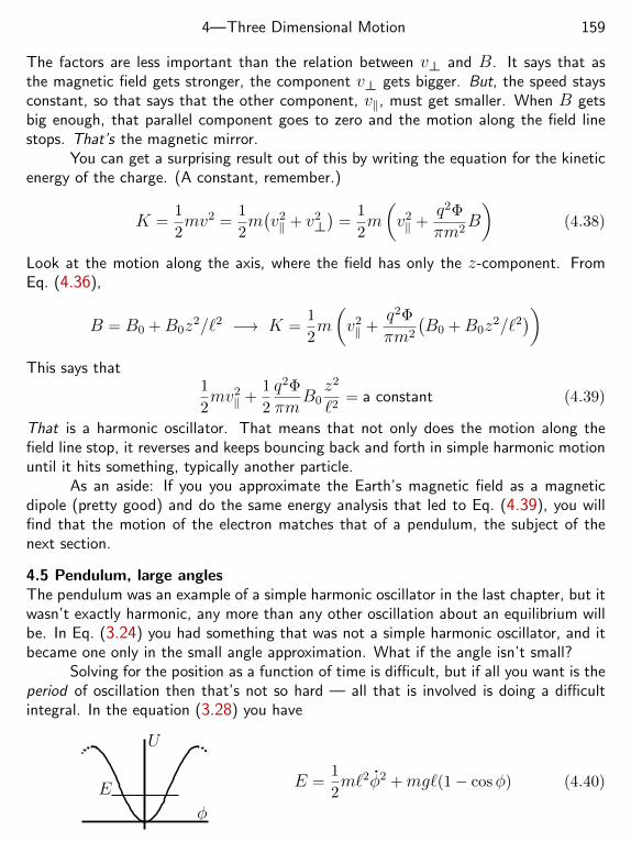
4—Three Dimensional Motion 159
The factors are less important than the relation between v⊥ and B. It says that asthe magnetic field gets stronger, the component v⊥ gets bigger. But, the speed staysconstant, so that says that the other component, v‖, must get smaller. When B getsbig enough, that parallel component goes to zero and the motion along the field linestops. That’s the magnetic mirror.
You can get a surprising result out of this by writing the equation for the kineticenergy of the charge. (A constant, remember.)
K =1
2mv2 =
1
2m(v2‖ + v2
⊥)
=1
2m
(v2‖ +
q2Φ
πm2B
)(4.38)
Look at the motion along the axis, where the field has only the z-component. FromEq. (4.36),
B = B0 +B0z2/`2 −→ K =
1
2m
(v2‖ +
q2Φ
πm2
(B0 +B0z
2/`2))
This says that1
2mv2‖ +
1
2
q2Φ
πmB0z2
`2= a constant (4.39)
That is a harmonic oscillator. That means that not only does the motion along thefield line stop, it reverses and keeps bouncing back and forth in simple harmonic motionuntil it hits something, typically another particle.
As an aside: If you you approximate the Earth’s magnetic field as a magneticdipole (pretty good) and do the same energy analysis that led to Eq. (4.39), you willfind that the motion of the electron matches that of a pendulum, the subject of thenext section.
4.5 Pendulum, large anglesThe pendulum was an example of a simple harmonic oscillator in the last chapter, but itwasn’t exactly harmonic, any more than any other oscillation about an equilibrium willbe. In Eq. (3.24) you had something that was not a simple harmonic oscillator, and itbecame one only in the small angle approximation. What if the angle isn’t small?
Solving for the position as a function of time is difficult, but if all you want is theperiod of oscillation then that’s not so hard — all that is involved is doing a difficultintegral. In the equation (3.28) you have
φ
U
E E =1
2m`2φ2 +mg`(1− cosφ) (4.40)
4—Three Dimensional Motion 160
In that chapter, I differentiated the energy, dE/dt = 0 and got the differential equationsof motion. Instead, solve this energy equation for dt directly.
2
m`2
[E −mg`(1− cosφ)
]=
(dφdt
)2
−→ dt =dφ√
(2E/m`2)− (2g/`)(1− cosφ)
This separates the equation, and all you have to do now is to integrate. It is a toughintegral but not impossible, and it helps to do a little manipulation first. Rememberthe trigonometric identity for half-angles?
sin2 φ2
=1
2(1− cosφ)
dt =dφ√
(2E/m`2)− (4g/`) sin2(φ/2)=
√`
4gdφ√
(E/2mg`)− sin2(φ/2)(4.41)
Why manipulate the expression in this way? It’s not obvious, and I’m sure that thefirst person to solve this problem did not find the right path through the maze with theinitial attack.
The motion of the pendulum is back and forth between the stopping points as insection 2.3. The stopping points occur when the kinetic energy drops to zero — whenthe line of constant E in the graph, Eq. (4.40), crosses the curve U(φ). That is when
φ = 0,
φ = 0 =⇒ E = mg`(1− cosφ) = 2mg` sin2(φ/2)
and that is the point where the denominator under dφ vanishes in Eq. (4.41).
Now you can try to do the integral of dt to get the period of the pendulum,and up to this point all the manipulations have been the same kind that you see in a“techniques of integration” chapter in your introductory calculus text. But now comesa clever trick. Again, it is nothing beyond what is done in beginning calculus (a changeof variables), but it is not an obvious change. As it stands the period of the pendulumis four times the time it takes to go from the center to the stopping point
T = 4
∫dt = 4
∫ φmax
0
√`
4gdφ√
(E/2mg`)− sin2(φ/2)
where φmax = 2 sin−1
√E
2mg`
4—Three Dimensional Motion 161
The integral goes from zero to a limit that depends on the energy. It would be mucheasier to handle if the limit is fixed. The trick: let√
E2mg`
sin θ = sinφ2
(4.42)
This is designed so that as θ goes from zero to π/2, the angle φ goes from zero toφmax. Why should this help? If it didn’t I would not be telling you about it. Executethe change of variables. √
E2mg`
cos θ dθ =1
2cos
φ2dφ
dφ√(E/2mg`)− sin2(φ/2)
=
√E
2mg`cos θ dθ
12 cos φ2
√(E/2mg`)− sin2(φ/2)
= 2cos θ dθ√
1− sin2(φ/2)√
1− sin2 θ
= 2dθ√
1− k2 sin2 θwhere k2 =
E2mg`
= sin2 φmax
2
(4.43)Assemble everything to get the period of oscillation
T = 4
∫dt = 4
√`
4g
∫ π/2
0dθ
2√1− k2 sin2 θ
= 4
√`g
∫ π/2
0dθ
1√1− k2 sin2 θ
(4.44)There are a lot of missing steps in this derivation, but not big ones. You should carryout these details for yourself. Why k2? That’s simply the most common conventionin the treatment of these “Elliptic Integrals,” though not the only one. In Abramowitzand Stegun they use the letter m instead of k2. The standard notation for this “ellipticintegral of the first kind” is
K =
∫ π/2
0dθ
1√1− k2 sin2 θ
, so T = 4K
√`g
(4.45)
Should I believe the answer? If the oscillations are small enough this must reduceto the solution of T for oscillations with small enough energy to allow small angle
4—Three Dimensional Motion 162
approximations. Small enough energy means that the parameter k2 =√E/mg` 1.
Start by making it zero.
T = 4
√`g
∫ π/2
0dθ
1
1= 4
√`gπ2
= 2π
√`g
and that is 2π/ω0 from Eq. (3.26), so it works.Now what if the energy is not so small? k2 can still be small but not negligible.
Do a power series expansion using the binomial expansion of Eq. (0.1).
(1 + x)n =1 + nx+n(n− 1)x2
2!+ · · · and for n = −1/2 this is
1− 1
2x+
1 . 3
22 . 2!x2 − 1 . 3 . 5
23 . 3!x3 + · · ·
T = 4
√`g
∫ π/2
0dθ
[1 +
1
2k2 sin2 θ +
1 . 3
22 . 2!k4 sin4 θ + · · ·
](4.46)
= 2π
√`g
[1 +
(1
2
)2
sin2 φmax
2+
(1 . 3
2 . 4
)2
sin4 φmax
2+
(1 . 3 . 5
2 . 4 . 6
)2
sin6 φmax
2+ · · ·
](4.47)
This requires another integral, that of sin2n θ dθ, and you can either learn how to do it(probably with complex variables) or have a big enough table of integrals such as thatby Gradshteyn and Ryzhik. The integral here is equation number 3.621.3 in their book:∫ π/2
0dθ sin2n θ =
(2n− 1)!!
(2n)!!
π2
The double factorial notation means the product of every other integer up to the givenone. For example 5!! = 15 and 6!! = 48.
For an angle of φmax = 30 this series is
2π
√`g
[1 + 0.01674 + 0.000005 + · · ·
],
[ ]= 1.017
For 90 it is
2π
√`g
[1 + 0.1250 + 0.0352 + 0.0122 + 0.0003 + · · ·
],
[ ]= 1.173
4—Three Dimensional Motion 163
You can see that even at 90 this series converges rapidly and changes the small angleresult by about 17%. If you want to try 179 you will quickly conclude that there’s gotto be a better way, because this time the sine of φmax/2 is close to one and the seriesconverges very slowly. At this point you can look up a reference on elliptic integrals tofind that the quantity in brackets is approximately 3.90, evaluated using Eq. (4.48).
k2 = sin2(179/2) = 0.9999238 −→ K ≈ 6.128 −→[ ]
= 2πK = 3.90
The defining equation for this elliptic integral can be evaluated by the series shownfor not too big values of k, and the equation following is an approximate expression thatis useful for larger k (near one). It is from Abramowitz and Stegun, equation (17.3.26).
K =
∫ π/2
0dθ
1√1− k2 sin2 θ
=π2
[1 +
(1
2
)2
k2 +
(1 . 3
2 . 4
)2
k4 +
(1 . 3 . 5
2 . 4 . 6
)2
k6 + · · ·
]
∼ 1
2ln
(16
1− k2
)as k → 1 (4.48)
Though this function approaches infinity as k → 1, it does so slowly. The logarithmhas a very mild sort of infinity.
Exercises
1 Apply Eq. (4.13) to Eq. (4.14).
2 Check the radial force function ~F (x, y) = (k/r2)r = (k/r3)~r against Eq. (4.13).
3 Using only the elementary methods (before you ever heard of a differential equation),Find the relations between speed, radius, angular frequency, and magnetic field strengthfor a charged particle moving in a uniform magnetic field.
4 Rearrange Eq. (4.39) in terms of the cyclotron frequency at z = 0, qB0/m, and theradius of the orbit at z = 0, r0.
4—Three Dimensional Motion 164
Problems
4.1 Fill in the missing steps in taking the limits, Eqs. (4.3) and (4.4). Also, find thenext order terms in b for these equations — the first non-vanishing correction.
4.2 Derive Eq. (4.6).
4.3 What is the maximum height as found from either Eq. (4.2) or (4.6).
4.4 Expand Eq. (4.6) for small b to find the equation for the trajectory as b→ 0.
4.5˙ Sometimes a quadratic equation is a linear equation in disguise.(a) Solve the equation 0.001x2 − x + 1 = 0 by noticing that it is almost linear, sox = 1 is almost right. Then x = 1+0.001x2 gives a correction to the first approximateanswer because you know the approximate value of x on the right (→ 1.001). Compareit to the traditional quadratic formula’s answer by using a series expansion on it.(b) A quadratic equation has two roots, and the other one is big. Assume that x is verybig in this quadratic equation and estimate its value as the root of a linear equation.(If x is big, which terms must nearly cancel each other?)
4.6 Expand Eq. (4.6) for small b, keeping terms up to those linear in b. What is therange of the projectile, assuming a level surface, and getting your answer correct toterms linear in b. Is your answer plausible?
4.7 A mass drops from rest without air resistance, starting from coordinates x = x0,y = y0, z = 0. Compute its angular momentum (Eq. (1.13)) about the origin at time t;compare it to the torque on the mass. Repeat this, but pick your origin for the angularmomentum and torque about the point (x, y, z) = (2x0, 0, 0).
4.8˙ The equation (4.6) will tell you where the projectile hits the ground, the range.The equation for the ground is y = 0 if you assume that the ground is level. First takethe case b = 0 and solve that for the range. Next expand Eq. (4.6) to the first order inb and find the first order correction to the range. If you haven’t done problem 4.5, nowwould be a good time.
4.9˙ If you fire a projectile up a hill and want to find its range, the equation for theground is no longer y = 0. Assume that the hill is represented by a straight line atan angle α from the horizontal and write its equation. Find the range of a projectilefired up such a hill. For this problem, assume zero air resistance. Do you measure theposition where it hits horizontally or along the hill? Your choice. At what angle do youfire it to get the maximum range? (And is this angle measured from the horizontal orfrom the hill itself? Again, your choice.) Do you choose your coordinate system x-y as
4—Three Dimensional Motion 165
horizontal and vertical or do you choose it parallel and perpendicular to the hill? Again,your choice, but I recommend the latter. Does your answer reduce to the correct valuesin all the special cases for which you can find the answer easily?
4.10 The projectile analyzed in section 4.1 now has a headwind; the air has a horizontalvelocity −vairx. Solve for the trajectory now and analyze the result. What wind will ittake to bring the mass back to its starting point?
4.11 Following the methods of section 3.10, find the Green’s function solution for
equations of the form Eq. (4.1), but for an arbitrary force on the right: md2ydt2 + bdydt =
F (t).
4.12˙ (a) Now use the formula from the preceding problem and apply it to Eq. (4.1).(b) The result doesn’t agree with the y part of Eq. (4.2) because the initial conditionvy(0) = v0 sin θ is not included. You can handle that if you remember that −mg isnot the only force that acts on the projectile. You had to apply a force to give it theinitial velocity; that is an impulse, a large force acting for a very short time, and it isFy(0) dt = mv0 sin θ. If you include this in the integral, so that the very first timeinterval contributes a large chunk to the whole integral, you add this to the result frompart (a) to get the full solution for y(t) in agreement with Eq. (4.2).
4.13˙ Start from ~r(t) = x r(t) cos(φ(t)
)+y r(t) sin
(φ(t)
)and differentiate it once and
twice. Rearrange the components and group the terms in order to derive the expressionfor acceleration found in Eq. (0.31). Here you are getting the same result by a differentmethod, and you will need this in chapter six.
4.14 Draw pictures of the equipotentials and of ~F for the example in Eq. (4.18).
4.15 Eq. (4.22) can be solved several different ways, as mentioned in thee paragraphright after it. Do it using method (2), assuming a solution x = A1eαt and y = A2eαt
just as in Eq. (3.57). Follow that method through to get a non-zero solution for A1
and A2 and then on to the complete solution.
4.16 As stated in the second paragraph of section 4.3, you can solve for the motionof a charge in a uniform magnetic field by elementary means, using such equations asa = v2/r. Do so. Is the result compatible with the expression ω = qB0/m as foundin the text?
4.17 Show that the solutions (4.30) and (4.25) agree.
4.18 For motion in uniform electric and magnetic fields, start a charge at the origin
with zero velocity and take ~E = E0x, with ~B = B0x. Find the motion of the charge.
4—Three Dimensional Motion 166
4.19 There is a lot of algebra between equations (4.40) and (4.47). (a) Fill in themissing steps. (b) Then evaluate the integrals for the first two terms in the seriesEqs. (4.46) and (4.47), through sin2.
4.20˙ There is one case for which the integral in Eq. (4.41) is possible in terms ofelementary functions: E = 2mg`. Start the pendulum at the bottom with exactly thiskinetic energy and solve for the angle as a function of time, graphing and interpretingthe result φ(t).
4.21 A particle of mass m can slide freely along a wire. The wire is straight andhorizontal, and is made to rotate in a horizontal plane about an axis perpendicular toone end at a fixed angular speed ω0. At time t = 0 the mass is at radius r0 and haszero radial velocity. Find the future motion of m. Assume zero friction. What is theforce that the wire exerts on m? Have you done problem 4.13 yet?
4.22˙ A particle of mass m is displaced slightly from its equilibrium position at the topof a smooth fixed sphere of radius R, and it slides because of gravity. Through whatangle does the particle move before it leaves the sphere?
4.23 A gravitational force is ~F = −GMmr/r2. Show that Fx = −GMmx/r3 andthat this force satisfies Eq. (4.13).
4.24 If the work integral in three dimensions is independent of path, then inparticular, the work going around a closed loop is zero. (One possible pathfrom a point to itself just sits still, going nowhere.) Apply this to a very tinyrectangular loop in the x-y plane, from y to y + ∆y and from x to x+ ∆x.Since this rectangle is so small, you can approximate the value of the integral along
each side by assuming that ~F has the constant value it attains at the midpoint of each
side. For example, on the right-hand side ~F = ~F (x + ∆x, y + 12∆y). For that side,
d~ → y∆y. The integral in this approximation is just the sum of four dot products.Divide by the area of the rectangle and take the limit as ∆x and ∆y → 0. Show thatthe result is Eq. (4.13).
4.25 In Eq. (2.23) you determine the escape speed from the Earth. That assumed thatthe planet is not rotating. At the equator you have the speed of the ground added tothe total velocity vector. Take that into account and determine the minimum speedthat you have to give the rocket relative to the ground so that it escapes. Put in thenumbers and compare the two speeds.
4.26 In Eq. (4.43) and those preceding it, what happens if E > 2mg`? And drawsome graphs.
4—Three Dimensional Motion 167
4.27 Using crossed electric and magnetic fields as in Eq. (4.32), find the initial condi-tions on the velocity so that the charge is unaccelerated.
4.28 To obtain Eq. (4.34) the charge started at rest. What is the shape of the pathof the charge if the initial velocity is in the −x direction? In the +x direction?
4.29 A charged particle has an initial velocity perpendicular to a uniform magnetic field
(no ~E ). Now there is friction with the air, assumed to be a force −b~v. Find (and ofcourse sketch) the charge’s subsequent motion. Note: This assumption −b~v is not agood one for this process. A constant magnitude force (like dry friction) is better, butthe mathematics is much harder in that case.
4.30 In the magnetic mirror of section 4.4, and for motion along the central axis,where is the stopping point? Did you do the exercise #4 to express this in terms of thecyclotron frequency?
4.31 For the same magnetic mirror, what is the frequency of oscillation determined byEq. (4.39)? Also get the numerical value for an electron in a field the size of Earth’s:0.5 Gauss = 0.5 × 10⁻⁴ T, with ` half the Earth’s radius. Pick radii for the electron’scircular motion of 1 mm and 1 cm.
4.32 In the same spirit as the operator solution in section 4.3, starting at Eq. (4.27),interpret this operator acting on functions of the real variable x.
ehddxf(x) (h is a constant)
4.33 An Atwood machine has two masses hung over a pulley, and idealized versionsuse massless strings and pulleys. In this otherwise ideal Atwood machine, submerge oneof the masses in water so that it feels a force −b~v. Now solve for the motion assumingthat you start the system from rest.
4.34¨There’s more to say about the coupled oscillators of section 3.8. Apply an oscillat-ing force to one of the masses: F0 cos Ωt. Write the equations of motion as done there,and now find the inhomogeneous solution to the equations. Do it in the symmetric casem1 = m2 and k1 = k3. It’s just like the forced simple harmonic oscillator except thatthe two functions x1(t) and x2(t) will have different amplitudes. Graph the two results(for just the inhomogeneous solution) for the two amplitudes versus Ω. Compare themto the results of problem 3.11. Why do the graphs behave this way?
4.35 In chapter three, Eq. (3.27), there is an approximate expression for the frequencyof a pendulum. Derive it from Eq. (4.47).
4—Three Dimensional Motion 168
4.36 In problem 3.36 one spring was replaced by a damper. What if all three springsare replaced by dampers? Again, make the problem symmetric so that the two on theend are the same.
4.37˙ The Earth’s gravity drops off with height. g(y) = −g0R2/r2 where R is theEarth’s radius; r = R+ y is the distance from its center; g0 is the gravitational field atthe surface. Expand this to the first order in y, getting the variation of g with altitudenear the surface. Fire a projectile from the surface at initial speed v0 and angle from
the horizontal θ. Set up and solve ~F = m~a for this case, neglecting air resistance thistime. Still assuming a flat Earth, find where it hits the ground and then the differencebetween this answer and the traditional one that assumes g has the constant value ithad at the surface. How large is this change if θ = 45 and v0 is large enough to getan uncorrected distance of 30 km? Ans: about 100 m.
4.38¨The electromagnetic force that one charged particle exerts on another starts withthe Coulomb law. The next approximation is that a moving charge creates a magneticfield that will affect the other charge if it too is moving. The total of these is
~Fon 2 by 1 =q1q2
4πε0
[r + 1
c2~v2 ×(~v1 × r
)]where r is the unit vector pointing from charge q1 toward charge q2.
What is the total force on the two particles, ~Fon 1 by 2 + ~Fon 2 by 1? To simplify theresult you will have to hunt up the “Jacobi Identity” involving cross products. Be sureto check some special cases to verify your result.
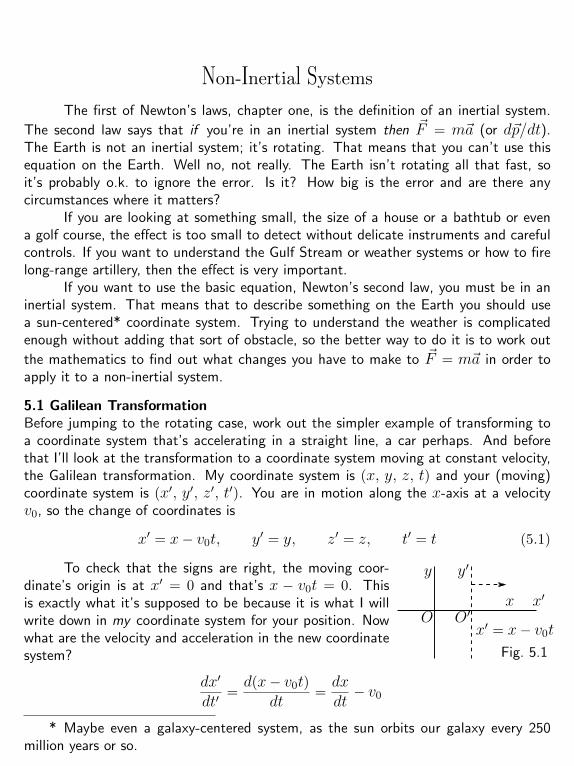
Non-Inertial SystemsThe first of Newton’s laws, chapter one, is the definition of an inertial system.
The second law says that if you’re in an inertial system then ~F = m~a (or d~p/dt).The Earth is not an inertial system; it’s rotating. That means that you can’t use thisequation on the Earth. Well no, not really. The Earth isn’t rotating all that fast, soit’s probably o.k. to ignore the error. Is it? How big is the error and are there anycircumstances where it matters?
If you are looking at something small, the size of a house or a bathtub or evena golf course, the effect is too small to detect without delicate instruments and carefulcontrols. If you want to understand the Gulf Stream or weather systems or how to firelong-range artillery, then the effect is very important.
If you want to use the basic equation, Newton’s second law, you must be in aninertial system. That means that to describe something on the Earth you should usea sun-centered* coordinate system. Trying to understand the weather is complicatedenough without adding that sort of obstacle, so the better way to do it is to work out
the mathematics to find out what changes you have to make to ~F = m~a in order toapply it to a non-inertial system.
5.1 Galilean TransformationBefore jumping to the rotating case, work out the simpler example of transforming toa coordinate system that’s accelerating in a straight line, a car perhaps. And beforethat I’ll look at the transformation to a coordinate system moving at constant velocity,the Galilean transformation. My coordinate system is (x, y, z, t) and your (moving)coordinate system is (x′, y′, z′, t′). You are in motion along the x-axis at a velocityv0, so the change of coordinates is
x′ = x− v0t, y′ = y, z′ = z, t′ = t (5.1)
y y′
O O′x x′
x′ = x− v0t
Fig. 5.1
To check that the signs are right, the moving coor-dinate’s origin is at x′ = 0 and that’s x − v0t = 0. Thisis exactly what it’s supposed to be because it is what I willwrite down in my coordinate system for your position. Nowwhat are the velocity and acceleration in the new coordinatesystem?
dx′
dt′=d(x− v0t)
dt=dxdt− v0
* Maybe even a galaxy-centered system, as the sun orbits our galaxy every 250million years or so.
169
5—Non-Inertial Systems 170
d2x′
dt2=ddt
(dxdt− v0
)=d2xdt2
(5.2)
Time is the same for each system, so it doesn’t matter whether you use t or t′. (Thatwill change when you get into special relativity, section 9.6.) Here the acceleration is
the same for both, so ~F = m~a is the same for both. Or is it? Suppose that the forceis velocity dependent; frictional forces commonly depend on velocity. Does that meanthat the force will be different in the two systems? No. All frictional forces depend onthe relative velocity of two things. A book sliding on a table, an airplane going throughthe air, a swimmer in water. When you transform the velocity of one object you haveto do it for all, and that means that the difference of two velocities will not change andthat the forces remain unaffected.
Accelerated SystemNow suppose that the moving coordinate system is accelerated at a constant rate.
x′ = x− v0t−1
2a0t
2, y′ = y, z′ = z, t′ = t (5.3)
The position x′ = 0 again defines the position of the moving observer. Repeat theprevious calculation:
dx′
dt′=d(x− v0t− a0t2/2)
dt=dxdt− v0 − a0t
d2x′
dt2=ddt
(dxdt− v0 − a0t
)=d2xdt2− a0
In the primed coordinate system Newton’s second law now becomes
Fx = md2xdt2
= m
(d2x′
dt2+ a0
)Rearrange this and make is look like the old F = ma.
Fx −ma0 = md2x′
dt2The y and z part are unchanged (5.4)
If you are in the accelerated system this looks like the normal ~F = m~a, but with anextra term that looks and behaves just like an extra force. It’s not one of the basicforces of nature (gravity, electromagnetism, etc.) but mathematically you can handle itas if it is. It is variously called an “inertial force” or a “fictitious force” and it appearssimply because of the transformation to a non-inertial system of coordinates.
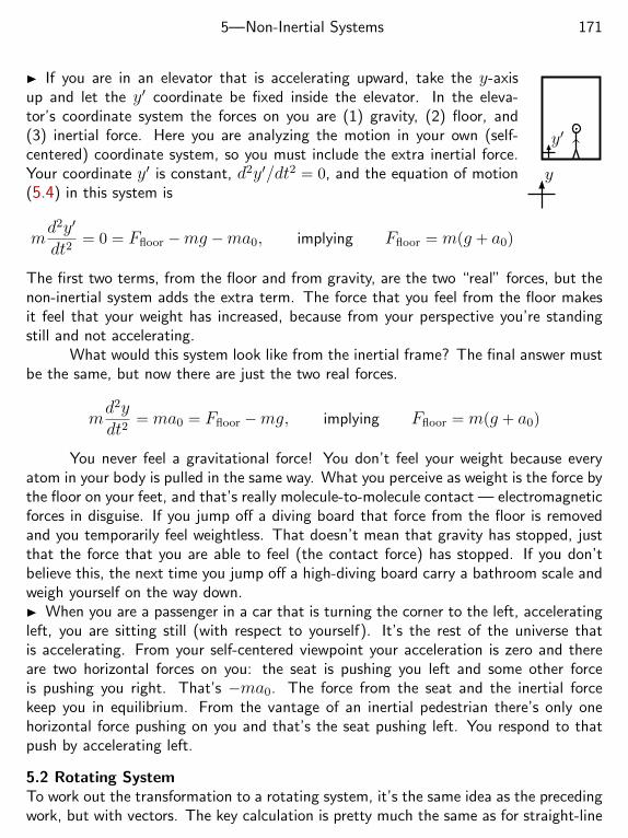
5—Non-Inertial Systems 171
y
y′
If you are in an elevator that is accelerating upward, take the y-axisup and let the y′ coordinate be fixed inside the elevator. In the eleva-tor’s coordinate system the forces on you are (1) gravity, (2) floor, and(3) inertial force. Here you are analyzing the motion in your own (self-centered) coordinate system, so you must include the extra inertial force.Your coordinate y′ is constant, d2y′/dt2 = 0, and the equation of motion(5.4) in this system is
md2y′
dt2= 0 = Ffloor −mg −ma0, implying Ffloor = m(g + a0)
The first two terms, from the floor and from gravity, are the two “real” forces, but thenon-inertial system adds the extra term. The force that you feel from the floor makesit feel that your weight has increased, because from your perspective you’re standingstill and not accelerating.
What would this system look like from the inertial frame? The final answer mustbe the same, but now there are just the two real forces.
md2ydt2
= ma0 = Ffloor −mg, implying Ffloor = m(g + a0)
You never feel a gravitational force! You don’t feel your weight because everyatom in your body is pulled in the same way. What you perceive as weight is the force bythe floor on your feet, and that’s really molecule-to-molecule contact — electromagneticforces in disguise. If you jump off a diving board that force from the floor is removedand you temporarily feel weightless. That doesn’t mean that gravity has stopped, justthat the force that you are able to feel (the contact force) has stopped. If you don’tbelieve this, the next time you jump off a high-diving board carry a bathroom scale andweigh yourself on the way down. When you are a passenger in a car that is turning the corner to the left, acceleratingleft, you are sitting still (with respect to yourself). It’s the rest of the universe thatis accelerating. From your self-centered viewpoint your acceleration is zero and thereare two horizontal forces on you: the seat is pushing you left and some other forceis pushing you right. That’s −ma0. The force from the seat and the inertial forcekeep you in equilibrium. From the vantage of an inertial pedestrian there’s only onehorizontal force pushing on you and that’s the seat pushing left. You respond to thatpush by accelerating left.
5.2 Rotating SystemTo work out the transformation to a rotating system, it’s the same idea as the precedingwork, but with vectors. The key calculation is pretty much the same as for straight-line
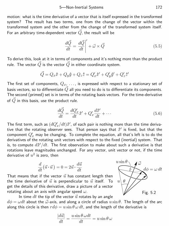
5—Non-Inertial Systems 172
motion: what is the time derivative of a vector that is itself expressed in the transformedsystem? The result has two terms, one from the change of the vector within thetransformed system and the other from the change of the transformed system itself.
For an arbitrary time-dependent vector ~Q, the result will be
d~Qdt
=d~Qdt
∣∣∣∣∣′
+ ~ω × ~Q (5.5)
To derive this, look at it in terms of components and it’s nothing more than the product
rule. The vector ~Q is the vector ~Q in either coordinate system.
~Q = Qxx+Qyy +Qz z = Q′xx′ +Q′yy
′ +Q′z z′
The first set of components, Qx, . . . , is expressed with respect to a stationary set of
basis vectors, so to differentiate ~Q all you need to do is to differentiate its components.The second (primed) set is in terms of the rotating basis vectors. For the time-derivative
of ~Q in this basis, use the product rule.
d~Qdt
=dQ′xdt
x′ +Q′xdx′
dt+ · · · (5.6)
The first term, such as (dQ′x/dt)x′, of each pair is nothing more than the time deriva-
tive that the rotating observer sees. That person says that x′ is fixed, but that thecomponent Q′x may be changing. To complete the equation, all that’s left is to do thederivatives of the rotating unit vectors with respect to the fixed (inertial) system. Thatis, to compute dx′/dt. The first observation to make about such a derivative is thatrotations leave magnitudes unchanged. For any vector, unit vector or not, if the timederivative of u2 is zero, then
u θ
u sin θ ~ωdφ = ω dt
Fig. 5.2
ddt
(~u .~u
)= 0 = 2~u . d~u
dt
That means that if the vector ~u has constant length thenthe time derivative of ~u is perpendicular to ~u itself. Toget the details of this derivative, draw a picture of a vectorrotating about an axis with angular speed ω.
In time dt the tip of the vector ~u rotates by an angledφ = ωdt about the ~ω-axis, and along a circle of radius u sin θ. The length of the arcalong this circle is then rdφ = u sin θ ω dt, and the length of the derivative is
|d~u|dt
=u sin θ ωdt
dt= u sin θ ω
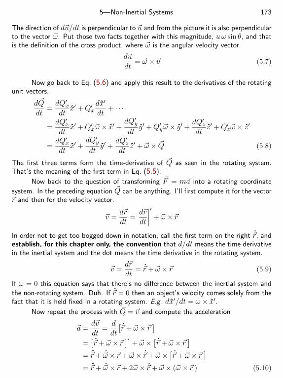
5—Non-Inertial Systems 173
The direction of d~u/dt is perpendicular to ~u and from the picture it is also perpendicularto the vector ~ω. Put those two facts together with this magnitude, uω sin θ, and thatis the definition of the cross product, where ~ω is the angular velocity vector.
d~udt
= ~ω × ~u (5.7)
Now go back to Eq. (5.6) and apply this result to the derivatives of the rotatingunit vectors.
d~Qdt
=dQ′xdt
x′ +Q′xdx′
dt+ · · ·
=dQ′xdt
x′ +Q′x~ω × x′ +dQ′ydt
y′ +Q′y~ω × y′ +dQ′zdt
z′ +Q′z~ω × z′
=dQ′xdt
x′ +dQ′ydt
y′ +dQ′zdt
z′ + ~ω × ~Q (5.8)
The first three terms form the time-derivative of ~Q as seen in the rotating system.That’s the meaning of the first term in Eq. (5.5).
Now back to the question of transforming ~F = m~a into a rotating coordinate
system. In the preceding equation ~Q can be anything. I’ll first compute it for the vector~r and then for the velocity vector.
~v =d~rdt
=d~rdt
∣∣∣∣′ + ~ω × ~r
In order not to get too bogged down in notation, call the first term on the right ~r, andestablish, for this chapter only, the convention that d/dt means the time derivativein the inertial system and the dot means the time derivative in the rotating system.
~v =d~rdt
= ~r + ~ω × ~r (5.9)
If ω = 0 this equation says that there’s no difference between the inertial system and
the non-rotating system. Duh. If ~r = 0 then an object’s velocity comes solely from thefact that it is held fixed in a rotating system. E.g. dx′/dt = ω × x′.
Now repeat the process with ~Q = ~v and compute the acceleration
~a =d~vdt
=ddt
[~r + ~ω × ~r
]=[~r + ~ω × ~r
].+ ~ω ×
[~r + ~ω × ~r
]= ~r + ~ω × ~r + ~ω × ~r + ~ω ×
[~r + ~ω × ~r
]= ~r + ~ω × ~r + 2~ω × ~r + ~ω × (~ω × ~r ) (5.10)
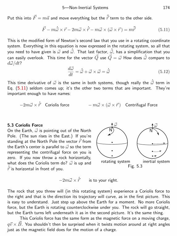
5—Non-Inertial Systems 174
Put this into ~F = m~a and move everything but the ~r term to the other side.
~F −m~ω × ~r − 2m~ω × ~r −m~ω × (~ω × ~r ) = m~r (5.11)
This is the modified form of Newton’s second law that you use in a rotating coordinatesystem. Everything in this equation is now expressed in the rotating system, so all that
you need to have given is ~ω and ~ω. That last factor, ~ω, has a simplification that you
can easily overlook. This time for the vector ~Q use ~Q = ~ω How does ~ω compare tod~ω/dt?
d~ωdt
= ~ω + ~ω × ~ω = ~ω (5.12)
This time derivative of ~ω is the same in both systems, though really the ~ω term inEq. (5.11) seldom comes up; it’s the other two terms that are important. They’reimportant enough to have names:
−2m~ω × ~r Coriolis force −m~ω × (~ω × ~r ) Centrifugal Force
rotating system inertial system
~ω ~ωN N
Fig. 5.3
5.3 Coriolis ForceOn the Earth, ~ω is pointing out of the NorthPole. (The sun rises in the East.) If you’restanding at the North Pole the vector ~r fromthe Earth’s center is parallel to ~ω so the termrepresenting the centrifugal force on you iszero. If you now throw a rock horizontally,what does the Coriolis term do? ~ω is up and
~r is horizontal in front of you.
−2m~ω × ~r is to your right.
The rock that you threw will (in this rotating system) experience a Coriolis force tothe right and that is the direction its trajectory will curve, as in the first picture. Thisis easy to understand. Just step up above the Earth for a moment. No more Coriolisforce, but the Earth is rotating counterclockwise under you. The rock will go straight,but the Earth turns left underneath it as in the second picture. It’s the same thing.
This Coriolis force has the same form as the magnetic force on a moving charge,
q~v × ~B. You shouldn’t then be surprised when it twists motion around at right anglesjust as the magnetic field does for the motion of a charge.
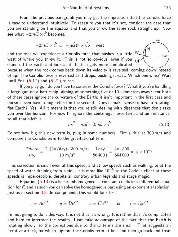
5—Non-Inertial Systems 175
From the previous paragraph you may get the impression that the Coriolis forceis easy to understand intuitively. To reassure you that it’s not, consider the case thatyou are standing on the equator and that you throw the same rock straight up. Now
see what −2m~ω × ~r becomes.
N
UP
W
~ω−2m~ω × ~r ∝ − ˆnorth× up = ˆwest
and the rock will experience a Coriolis force that pushes it a littlewest of where you threw it. This is not so obvious, even if youstand off the Earth and look at it. It then gets more complicatedbecause when the rock comes back down its velocity is reversed, coming down insteadof up. The Coriolis force is reversed as it drops, pushing it east. Which one wins? Waituntil Eqs. (5.17) and (5.21) to see.
If you play golf do you have to consider the Coriolis force? What if you’re handlinga large gun on a battleship, aiming at something five or 10 kilometers away? For bothof these cases ignore the curvature of the Earth; it isn’t important in the first case anddoesn’t even have a huge effect in the second. Does it make sense to have a rotating,flat Earth? Yes. All it means is that you’re still dealing with distances that don’t takeyou over the horizon. For now I’ll ignore the centrifugal force term and air resistance,so all that’s left is
m~r = m~g − 2m~ω × ~r (5.13)
To see how big this new term is, plug in some numbers. Fire a rifle at 300 m/s andcompare the Coriolis term to the gravitational term.
2mωvmg
=2 .(2π/day) .(300 m/s)
10 m/s2. 1 day
86 400 s=
4π . 300
864 000≈ 4× 10⁻³
This correction is small even at this speed, and at low speeds such as walking, or at thespeed of water draining from a sink, it is more like 10−5 so the Coriolis effect at thesespeeds is imperceptible, despite all contrary urban legends and stage magic.
Equation (5.13) is a linear, inhomogeneous, constant coefficient differential equa-tion for ~r, and as such you can solve the homogeneous part using an exponential solution,just as in section 3.8. In components this would look like
x = Aeαt, y = Beαt, z = Ceαt or ~r = ~r0eαt
I’m not going to do it this way. It is not that it’s wrong. It is rather that it’s complicatedand hard to interpret the results. I can take advantage of the fact that the Earth isrotating slowly, so the corrections due to the ω terms are small. That suggests aniterative attack, for which I ignore the Coriolis term at first and then go back and treat
5—Non-Inertial Systems 176
it as a correction. This is in the spirit of problem 4.5 — a good warmup if you haven’talready done it.
The lowest order approximation to Eq. (5.13) is
m~r = m~g (5.14)
This is pretty easy. Take initial conditions to start from the origin with velocity ~v0, then
~r0 = ~gt+ ~C = ~gt+ ~v0, and ~r0 = 12~gt
2 + ~Ct+ ~D = 12~gt
2 + ~v0t (5.15)
The subscript zero on r indicates that this is the lowest order approximation to the finalanswer, ignoring Coriolis effects. Use these equations as input to the right-hand side ofEq. (5.13), canceling the m’s. The improved approximation is ~r1, which now satisfies
~r1 = ~g − 2~ω × ~r0 = ~g − 2~ω ×(~gt+ ~v0
)(5.16)
Integrate this equation to get ~r1, including a couple of arbitrary constants, then reapply
the initial conditions to evaluate these constants. ~r1(0) = 0 and ~r1(0) = ~v0.
~r1 = 12~gt
2−2~ω×(
16~gt
3 + 12~v0t
2)+ ~Et+ ~F = 1
2~gt2−2~ω×
(16~gt
3 + 12~v0t
2)+~v0t (5.17)
If you need still higher order accuracy, put this into the right side of Eq. (5.13) and
repeat the process to get a still better result: ~r2 = ~g − 2~ω × ~r1.To understand this result, try some special cases.
1. At the North Pole firing straight up the ~g and ~v0 terms in Eq. (5.17) are along thevector ~ω, so the cross products vanish and the Coriolis force contributes nothing.
2. At the equator firing straight up ~ω × ~g is West, and ~ω × ~v0 is East. To find wherethe projectile hits the ground, note that neither of these two terms affects the amountof time that the projectile stays in the air because East and West are not up and down.The time aloft is governed solely by the old terms in ~r1(t): 1
2~gt2 + ~v0t = 0. At the
value of t that this determines, you compute the position of the projectile, ~r1, fromEq. (5.17).
−1
2gt2 + v0t = 0 ⇒ tf =
2v0
gthen the corrected term ~r1 back at ground level is
~r1(tf) = −2~ω ×(
16~g
2v0
g+ 1
2~v0
)(2v0
g
)2
= −2(− 1
3 + 12
)~ω × ~v0
(2v0
g
)2
=4ωv3
0
3g2West (5.18)
5—Non-Inertial Systems 177
For a speed of 300 m/s this is
4 .(2π/day) .(300 m/s)3
3 .(10 m/s2
)2 . 1 day
86 400 s= 26 m (5.19)
At least this answers the question raised a few paragraphs back: Which part of theCoriolis force wins? The one while the rock is going up or the one when it’s goingdown? Well, which is it?
Does this result of 26 m seem to be much larger than you would expect? To seehow reasonable this is, ask how much time the bullet is it in the air and how high doesit go? Answer:
tf =2 . v0
g=
2 . 300
10= 60 seconds, max height =
v20
2g=
2 . 3002
2 . 10= 4.5 km
(5.20)Will a bullet go that high? No, not even close. Air resistance is very important here,and it cuts these results by a big factor. Still, the Coriolis effect is significant.
To see how much air resistance can affect these results, go back to problem 2.23.For a 30 caliber bullet (not tumbling) the terminal speed is about 100 m/s, and if itis fired up at 300 or 400 m/s it comes to the maximum height in under 15 seconds.You can make a very crude estimate of the Coriolis effect in this case by assuming theextreme case that it reaches terminal speed very fast. Then replace the 300 m/s inEq. (5.19) by 100 m/s, changing the result from 26 m to 1 m. Reality is closer to thelatter number than the former, but working out the details requires a little effort. Asimpler version of this calculation appears in problem 5.11.
x
z↓
What is the trajectory of the bullet you just fired? It’s no longer astraight line up and down, but something described by Eq. (5.17). For this,use a coordinate system with x East, y North, and z Up — like the coordinatesystem sketched below, but on the equator. The motion described by thisequation is then all in the x-z plane.
~ω = ωy, ~g = −gz, ~v0 = v0z
~r1 = x1x+ z1z = −12gzt
2 − 2ωy ×(− 1
6gzt3 + 1
2v0zt2)
+ v0zt
x1 = 13ωgt
3 − ωv0t2, z1 = −1
2gt2 + v0t (5.21)
The scale on this graph is greatly exaggerated horizontally so that you can seethe effect.
3. For another example, fire a projectile and see where it lands, but this timestart from an arbitrary latitude. Again use coordinates x-East, y-North, z = x × y.
5—Non-Inertial Systems 178
The latitude is λ, so
~ω
λ
xy
~ω = ω(y cosλ+ z sinλ) (5.22)
The initial conditions are x0 = 0 and the other initial velocity components non-zero.Eq. (5.17) is
~r1 = 12~gt
2 + ~v0t− 2ω(y cosλ+ z sinλ)×(
16~gt
3 + 12~v0t
2)
~g = −gz, and ~v0 = y0y + z0z, so this is
~r1 = 12~gt
2 + ~v0t+ 13ωgt
3x cosλ+ ωt2x(y0 sinλ− z0 cosλ)
which says that the y and z-coordinates are not affected by ω (to this approximation),only x is. Where will it land? That is determined by z.
z1(t) = z0(t) = 0 = z0t− gt2/2 =⇒ tf = 2z0/g then y1 = y0tf = 2z0y0/g(5.23)
and x1 =1
3gω cosλ (2z0/g)3 + ω
(y0 sinλ− z0 cosλ
)(2z0/g)2
You can simplify this. Group terms and express the initial velocity in terms ofspeed v0 and the angle α above the horizontal.
x1 = −4
3ωz3
0
g2cosλ+ 4ω sinλ
y0z20
g2= ω
v30
g2
[−4
3sin3 α cosλ+ 4 sin2 α cosα sinλ
](5.24)
How big is this for a golf ball? Choose the latitude of Scotland, λ = 55, with sphericalcoordinate θ = 90 − λ, and hit the golf ball α = 45 above the horizontal. Youraverage world champion golfer can hit the ball about 300 meters, so from Eq. (5.23)
y1 = 2z0y0/g = 2v20 cosα sinα/g = v2
0 sin 2α/g = 300 m =⇒ v0 =√
3000 = 55 m/s
Then the deflection is
x1 =2πday
(55 m/s)3
(10 m/s2)2
[− 4
3. 1
23/2. 0.57 + 4 . 1
23/2. 0.82
](1 day
86 400 s
)= 0.11 m = 11 cm
5—Non-Inertial Systems 179
Compared to all the other variables, especially wind, this is not much, and I supposethat an expert golfer will have even this effect trained into the muscles. What happenswhen the tournament is in Southern Australia?
Take the same equations and fire a large artillery shell in the same way, but fastenough to go 30 km instead of 300 m. Everything else is the same, so all I have todo is see how the result scales with the range. The distance is 100 times greater, soEq. (5.23) for y1 says the speed is larger by 1001/2. Then Eq. (5.24) says that the
deviation, the value of x, varies as speed cubed, so 1003/2 = 1000 and the deviation is110 meters, which is not so small any more.
The result for x1 is positive, meaning that the deflection is toward the East.Stand off the Earth a moment and try to visualize the motion in an inertial coordinatesystem. Is that the direction it should move?
5.4 Foucault PendulumA classic experiment to give a decisive answer to the question: Does the Earth rotate?After all, just because such authorities as Galileo and Newton said it does, is thatenough? As late as the middle 1800’s this was an important question because peoplewanted to have some simple, easy-to-see evidence of the rotation, evidence not depend-ing on the motion of the stars. If you have a pendulum swinging at the South* Pole,what will the Earth’s rotation do to it? Stand off the Earth again and the pendulumwill be swinging back and forth in a plane while the Earth rotates underneath it. Tosomeone standing on the surface it will appear that the plane of the pendulum’s swingwill rotate counterclockwise once every 23 hours and 56 minutes, the time it takes theEarth to rotate once on its axis.www.phys.unsw.edu.au/PHYSICS_!/FOUCAULT_PENDULUM/foucault_pendulum
xy
z
θ
`
m
Fig. 5.4
To figure out what happens at any point on the Earth other thanthe poles takes some effort and the apparatus of rotating coordinate sys-tems developed in this chapter. To describe the mechanics, use the samecoordinate system as in Eq. (5.22), except that now there’s another forceon the mass, that of the cord that suspends the mass from the ceiling.These equations become
m~r = −mgz − Fcordr − 2m~ω × ~rm~r = −mgz + Fcord(z cos θ − x sin θ cosφ− y sin θ sinφ)− 2m~ω × ~r
(5.25)θ and φ are the spherical coordinates from the point of suspension onthe ceiling as in section 0.3, except that contrary to tradition the angle θ is measuredfrom the −z axis. The pendulum becomes a simple problem only if you make the
* Why not the North Pole? There’s an ocean there.
5—Non-Inertial Systems 180
approximation that it is oscillating through a small angle. That means that the cordis almost vertical. θ is small and the z-component of acceleration is small, so thez-component of the force is small too.
cos θ ≈ 1 and Fcord ≈mg (5.26)
The x and y-coordinates are related as in Eq. (0.13) to the spherical coordinates:
x = ` sin θ cosφ, and y = ` sin θ sinφ
Put these into the equation of motion and you have approximately
m~r =mg`
(−xx−yy)−2m~ω×~r =mg`
(−xx−yy)−2mω(y cosλ+z sinλ
)×~r (5.27)
Look at the components in the x-y plane, the plane parallel to the Earth’s surface.
x = −g`x+ 2ω sinλ y y = −g
`y − 2ω sinλ x (5.28)
To solve these, you can note that these are simultaneous, linear, constant coefficientequations and use an exponential solution. This is a perfectly correct method and itworks, but I’ll show two other methods to solve these equations more easily.
The use of complex algebra leads to much simpler equations. Take the first ofthe equations (5.28) and add i times the second equation.
x+ iy = −g`
(x+ iy) + 2ω sinλ(y − ix) = −g`
(x+ iy)− 2iω sinλ(x+ iy) (5.29)
Let q = x+ iy and this is
q = −g`q − 2iω sinλq
This is an ordinary constant coefficient equation with a solution
q(t) = Aeαt with α2 + 2iω sinλα+g`
= 0
α = −iω sinλ±√−ω2 sin2 λ− g/` = i
[− ω sinλ±
√ω2 sin2 λ+ g/`
]To interpret this, recall that the Earth is rotating slowly so that ω2 g/`. Use thisobservation to get a simpler approximate value of α by a series expansion. Let ω2
0 = g/`.
α = i[− ω sinλ± ω0
√1 + ω2 sin2 λ/ω2
0
]= i[− ω sinλ± ω0
(1 + ω2 sin2 λ/2ω2
0
)]= ±iω0 − iω sinλ
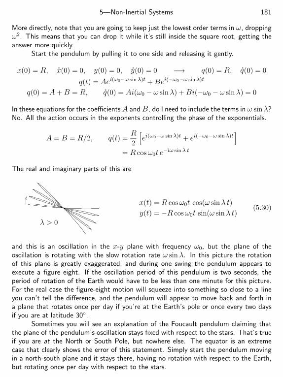
5—Non-Inertial Systems 181
More directly, note that you are going to keep just the lowest order terms in ω, droppingω2. This means that you can drop it while it’s still inside the square root, getting theanswer more quickly.
Start the pendulum by pulling it to one side and releasing it gently.
x(0) = R, x(0) = 0, y(0) = 0, y(0) = 0 −→ q(0) = R, q(0) = 0
q(t) = Aei(ω0−ω sinλ)t +Bei(−ω0−ω sinλ)t
q(0) = A+B = R, q(0) = Ai(ω0 − ω sinλ) +Bi(−ω0 − ω sinλ) = 0
In these equations for the coefficientsA andB, do I need to include the terms in ω sinλ?No. All the action occurs in the exponents controlling the phase of the exponentials.
A = B = R/2, q(t) =R2
[ei(ω0−ω sinλ)t + ei(−ω0−ω sinλ)t
]= R cosω0t e
−iω sinλ t
The real and imaginary parts of this are
λ > 0
x(t) = R cosω0t cos(ω sinλ t)
y(t) = −R cosω0t sin(ω sinλ t)(5.30)
and this is an oscillation in the x-y plane with frequency ω0, but the plane of theoscillation is rotating with the slow rotation rate ω sinλ. In this picture the rotationof this plane is greatly exaggerated, and during one swing the pendulum appears toexecute a figure eight. If the oscillation period of this pendulum is two seconds, theperiod of rotation of the Earth would have to be less than one minute for this picture.For the real case the figure-eight motion will squeeze into something so close to a lineyou can’t tell the difference, and the pendulum will appear to move back and forth ina plane that rotates once per day if you’re at the Earth’s pole or once every two daysif you are at latitude 30.
Sometimes you will see an explanation of the Foucault pendulum claiming thatthe plane of the pendulum’s oscillation stays fixed with respect to the stars. That’s trueif you are at the North or South Pole, but nowhere else. The equator is an extremecase that clearly shows the error of this statement. Simply start the pendulum movingin a north-south plane and it stays there, having no rotation with respect to the Earth,but rotating once per day with respect to the stars.
5—Non-Inertial Systems 182
The Slick WayAnd then there’s another, more clever way to solve this. Go back to the equations(5.28). Forget about the fact that these refer to a rotating coordinate system andpretend that someone handed them to you in an inertial system. These are now (except
for m’s) ~F = m~a in a (pretend) inertial system. Transform these x-y coordinates intoa new rotating system. If I do it right I can cancel the ω terms.
The new rotating system will have (unknown) angular velocity about the z-axis,~ω ′ = zω′. Equation (5.11) tells you how to modify the equations of motion by addingthe inertial forces. As before, don’t bother with the centrifugal force term and simply
add the Coriolis term to the forces, −2~ω ′ × ~r.
x = −g`x+ 2ω sinλ y
y = −g`y − 2ω sinλ x
−→x = −g
`x+ 2ω sinλ y + 2ω′y
y = −g`y − 2ω sinλ x− 2ω′x
If I choose ω′ = −ω sinλ the equations become two separate harmonic oscillators andin that system the pendulum does not rotate. Go back to the system fixed in the Earthand it says that the plane of oscillation of the pendulum will rotate at this rate ω′
and it even gets the direction right. If you’re at the North Pole it gives ω′ = −ω, or~ω ′ = −zω so that it’s rotating clockwise. Again step off the Earth for a moment toverify that this is correct. (I had to use dots for time derivatives in both systems. Whatelse can I do?)
In the next chapter, in section 6.6 you will see an analysis of the precession ofa pendulum even without a rotating Earth. The case examined there is quite a longway from the one here because it concerns a pendulum going around almost in a circle,but the basic ideas will still apply. If the pendulum is swinging back and forth butstarted with even a tiny amount of angular momentum about the vertical axis, so thatthe original motion is not a straight line but a very narrow ellipse, then there is aprecession that can easily be much larger than that caused by the Earth’s rotation. Itwill completely mask the Foucault effect. This is one reason it was so difficult to builda pendulum to measure the Earth’s rotation. Foucault’s achievement was not trivial!*
The Really Slick WayGo back to Eq. (5.25) and leave everything in vector form. After all isn’t the use ofvectors supposed to simplify the mathematics? Take the cross product of each side with~r.
m~r × ~r = −mg~r × z − ~r × Fcordr − 2m~r ×(~ω × ~r
)(5.31)
* The book ”Pendulum: Leon Foucault and the Triumph of Science” by Aczel is agood history of the subject.
5—Non-Inertial Systems 183
m(~r × ~r
).= −mg~r × z − 0− 2m
[~ω(~r . ~r )− ~r(~ω .~r )
]~L = −mg~r × z + 2m~r(~ω .~r )
= −mg~r × z − 2m~r ω` sinλ (5.32)
This is how you derive the angular momentum equation from ~F = m~a, as in section1.3. The right side is the torque: The first term is the vector version of mg` sin θ, andthe last term is the one that causes all the interesting problems.
As was done a couple of paragraphs back, pretend this is a stationary system andgo to a new system rotating with respect to it.
d~Ldt
= −mg~r × z − 2m~r ω` sinλ = ~L+ ~ω′ × ~L (5.33)
where this new unknown ~ω′ is the rotation with respect to the old coordinate system.
~L+ ~ω′ × ~L = ~L+m~ω′ ×(~r × ~r
)= ~L+m
[~r(~ω′ . ~r )− ~r(~ω′ .~r )
](5.34)
If the rotation of this system is about the vertical axis, the vector ~ω′ is perpendicular
to the velocity vector ~r. (Remember: small angle approximations here.) The equationis now
~L−m~r(~ω′ .~r ) = −mg~r × z − 2m~r ω` sinλ (5.35)
Now let ~ω′ = −2ω sinλz and the only term left is the mg` sin θ term that causesthe pendulum to swing back and forth. There’s no rotation left, so this defines thecoordinate system in which the pendulum does not precess. Notice: slicker does notmean easier.
5.5 Centrifugal ForceReturn to the general equation (5.11) and look closely at the other inertial force term,
−m~ω × (~ω × ~r ), and now ignore the Coriolis term. Use ~A× ( ~B × ~C ) = ~B( ~A . ~C )−~C( ~A . ~B )
−m~ω × (~ω × ~r ) = −m~ω(ω .~r ) +m~rω2
Choose the coordinate system so that z is along ~ω, and this is
−zmω(ωz) +m(xx+ yy + zz)ω2 = mω2(xx+ yy)
It points away from the axis of rotation. In this rotating system an extra force appears,pushing away from the axis.
There is a problem in notation here. The symbol ~r is overused. It is the vectorfrom the origin in spherical coordinates. It is the vector from the axis in cylindrical
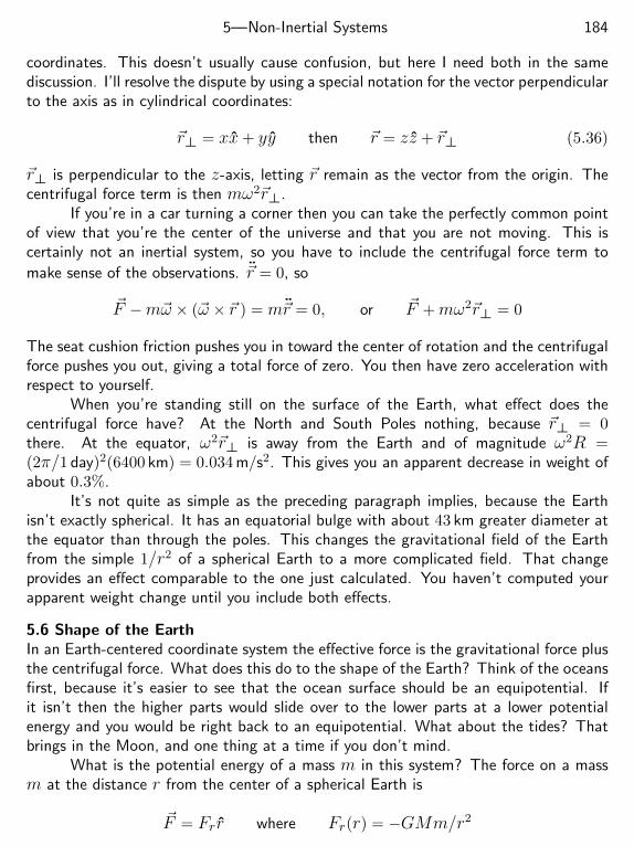
5—Non-Inertial Systems 184
coordinates. This doesn’t usually cause confusion, but here I need both in the samediscussion. I’ll resolve the dispute by using a special notation for the vector perpendicularto the axis as in cylindrical coordinates:
~r⊥ = xx+ yy then ~r = zz + ~r⊥ (5.36)
~r⊥ is perpendicular to the z-axis, letting ~r remain as the vector from the origin. Thecentrifugal force term is then mω2~r⊥.
If you’re in a car turning a corner then you can take the perfectly common pointof view that you’re the center of the universe and that you are not moving. This iscertainly not an inertial system, so you have to include the centrifugal force term to
make sense of the observations. ~r = 0, so
~F −m~ω × (~ω × ~r ) = m~r = 0, or ~F +mω2~r⊥ = 0
The seat cushion friction pushes you in toward the center of rotation and the centrifugalforce pushes you out, giving a total force of zero. You then have zero acceleration withrespect to yourself.
When you’re standing still on the surface of the Earth, what effect does thecentrifugal force have? At the North and South Poles nothing, because ~r⊥ = 0there. At the equator, ω2~r⊥ is away from the Earth and of magnitude ω2R =(2π/1 day)2(6400 km) = 0.034 m/s2. This gives you an apparent decrease in weight ofabout 0.3%.
It’s not quite as simple as the preceding paragraph implies, because the Earthisn’t exactly spherical. It has an equatorial bulge with about 43 km greater diameter atthe equator than through the poles. This changes the gravitational field of the Earthfrom the simple 1/r2 of a spherical Earth to a more complicated field. That changeprovides an effect comparable to the one just calculated. You haven’t computed yourapparent weight change until you include both effects.
5.6 Shape of the EarthIn an Earth-centered coordinate system the effective force is the gravitational force plusthe centrifugal force. What does this do to the shape of the Earth? Think of the oceansfirst, because it’s easier to see that the ocean surface should be an equipotential. Ifit isn’t then the higher parts would slide over to the lower parts at a lower potentialenergy and you would be right back to an equipotential. What about the tides? Thatbrings in the Moon, and one thing at a time if you don’t mind.
What is the potential energy of a mass m in this system? The force on a massm at the distance r from the center of a spherical Earth is
~F = Frr where Fr(r) = −GMm/r2
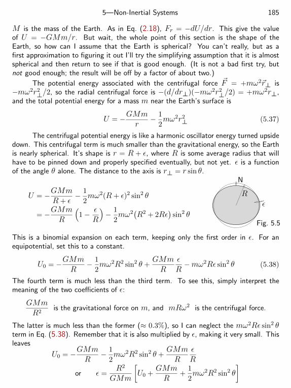
5—Non-Inertial Systems 185
M is the mass of the Earth. As in Eq. (2.18), Fr = −dU/dr. This give the valueof U = −GMm/r. But wait, the whole point of this section is the shape of theEarth, so how can I assume that the Earth is spherical? You can’t really, but as afirst approximation to figuring it out I’ll try the simplifying assumption that it is almostspherical and then return to see if that is good enough. (It is not a bad first try, butnot good enough; the result will be off by a factor of about two.)
The potential energy associated with the centrifugal force ~F = +mω2~r⊥ is−mω2r2
⊥/2, so the radial centrifugal force is −(d/dr⊥)(−mω2r2⊥/2) = +mω2r⊥,
and the total potential energy for a mass m near the Earth’s surface is
U = −GMmr
− 1
2mω2r2
⊥ (5.37)
The centrifugal potential energy is like a harmonic oscillator energy turned upsidedown. This centrifugal term is much smaller than the gravitational energy, so the Earthis nearly spherical. It’s shape is r = R + ε, where R is some average radius that willhave to be pinned down and properly specified eventually, but not yet. ε is a functionof the angle θ alone. The distance to the axis is r⊥ = r sin θ.
U = −GMmR+ ε
− 1
2mω2(R+ ε)2 sin2 θ
= −GMmR
(1− ε
R
)− 1
2mω2
(R2 + 2Rε
)sin2 θ
R
ε
N
Fig. 5.5
This is a binomial expansion on each term, keeping only the first order in ε. For anequipotential, set this to a constant.
U0 = −GMmR
− 1
2mω2R2 sin2 θ +
GMmR
εR−mω2Rε sin2 θ (5.38)
The fourth term is much less than the third term. To see this, simply interpret themeaning of the two coefficients of ε:
GMmR2
is the gravitational force on m, and mRω2 is the centrifugal force.
The latter is much less than the former (≈ 0.3%), so I can neglect the mω2Rε sin2 θterm in Eq. (5.38). Remember that it is also multiplied by ε, making it very small. Thisleaves
U0 = −GMmR
− 1
2mω2R2 sin2 θ +
GMmR
εR
or ε =R2
GMm
[U0 +
GMmR
+1
2mω2R2 sin2 θ
]
5—Non-Inertial Systems 186
The last expression is
ε = C +1
2
Rω2
GM/R2R sin2 θ = C +
1
2
acgR sin2 θ (5.39)
The last term involves the ratio of the centrifugal acceleration at the equator to thegravitational field there, and it is already enough to tell you the difference between thepolar diameter and the equatorial diameter. Just set θ = 0 and θ = π/2 to see theeffect. The diameter through the equator is Rac/g = R2ω2/g more than throughthe poles. The constant C is a combination of an already unknown constant U0 withanother term. Recall that I never precisely defined R, and until I do that the value ofε is ambiguous. (What does ε = 0 mean?) I will specify this so that the mean value ofε over the surface of the Earth is zero. That makes R the mean radius of the Earth.That is∫
dΩ
[C +
1
2
acgR sin2 θ
]=
∫ 2π
0dφ∫ π
0sin θ dθ
[C +
1
2
acgR sin2 θ
]= 0
This is
4πC +1
2
acgR . 8π
3= 0, C = −1
3
acgR, ε = −ac
3gR
[3
2cos2 θ − 1
2
]I wrote it in the final form because that is a Legendre polynomial in the brackets. Ifyou’re not already familiar with them you will be. What is ε at the equator and at thepoles?
εpoles = −acR3g
= −R2ω2
3gand εequator = +
R2ω2
6g
The difference in the equatorial and the polar diameters (not radii) is then
2εeq − 2εpol =R2ω2
g=
(6400 km)2(2π/day)2
10 m/s2.(
1 day
86 400s
)2
.(
1000 m
1 km
)= 22 km
You saw this faster directly from Eq. (5.39), but the expression in terms of a Legendrepolynomial is useful too. How accurate it this? Not very, as the measured value of thedifference in the diameters is closer to twice this. The major error in this calculation isin the assumption that the gravitational field is spherically symmetric. It’s a plausibleassumption, but it turns out to introduce an error that is about as big as the effectyou’re calculating, so it’s not good enough. Working out the more correct version wouldtake too much time and effort for this single result.
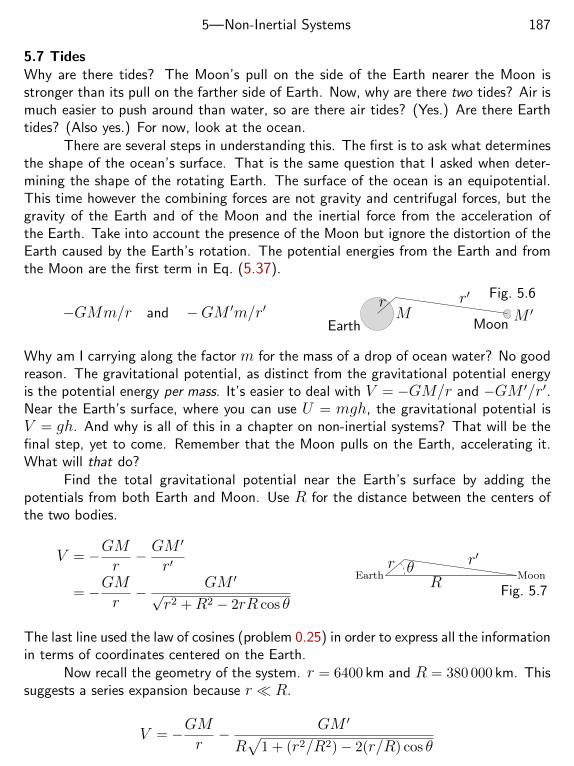
5—Non-Inertial Systems 187
5.7 TidesWhy are there tides? The Moon’s pull on the side of the Earth nearer the Moon isstronger than its pull on the farther side of Earth. Now, why are there two tides? Air ismuch easier to push around than water, so are there air tides? (Yes.) Are there Earthtides? (Also yes.) For now, look at the ocean.
There are several steps in understanding this. The first is to ask what determinesthe shape of the ocean’s surface. That is the same question that I asked when deter-mining the shape of the rotating Earth. The surface of the ocean is an equipotential.This time however the combining forces are not gravity and centrifugal forces, but thegravity of the Earth and of the Moon and the inertial force from the acceleration ofthe Earth. Take into account the presence of the Moon but ignore the distortion of theEarth caused by the Earth’s rotation. The potential energies from the Earth and fromthe Moon are the first term in Eq. (5.37).
−GMm/r and −GM ′m/r′Earth Moon
r r′
M M ′Fig. 5.6
Why am I carrying along the factor m for the mass of a drop of ocean water? No goodreason. The gravitational potential, as distinct from the gravitational potential energyis the potential energy per mass. It’s easier to deal with V = −GM/r and −GM ′/r′.Near the Earth’s surface, where you can use U = mgh, the gravitational potential isV = gh. And why is all of this in a chapter on non-inertial systems? That will be thefinal step, yet to come. Remember that the Moon pulls on the Earth, accelerating it.What will that do?
Find the total gravitational potential near the Earth’s surface by adding thepotentials from both Earth and Moon. Use R for the distance between the centers ofthe two bodies.
V = −GMr− GM
′
r′
= −GMr− GM ′√r2 +R2 − 2rR cos θ
Earthr r′
MoonR
θ
Fig. 5.7
The last line used the law of cosines (problem 0.25) in order to express all the informationin terms of coordinates centered on the Earth.
Now recall the geometry of the system. r = 6400 km and R = 380 000 km. Thissuggests a series expansion because r R.
V = −GMr− GM ′
R√
1 + (r2/R2)− 2(r/R) cos θ
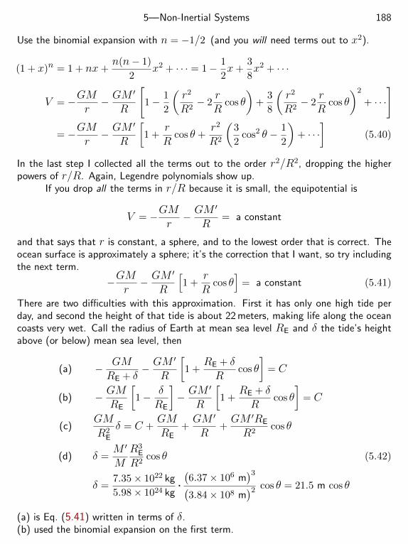
5—Non-Inertial Systems 188
Use the binomial expansion with n = −1/2 (and you will need terms out to x2).
(1 + x)n = 1 + nx+n(n− 1)
2x2 + · · · = 1− 1
2x+
3
8x2 + · · ·
V = −GMr− GM
′
R
[1− 1
2
(r2
R2− 2
rR
cos θ
)+
3
8
(r2
R2− 2
rR
cos θ
)2
+ · · ·
]
= −GMr− GM
′
R
[1 +
rR
cos θ +r2
R2
(3
2cos2 θ − 1
2
)+ · · ·
](5.40)
In the last step I collected all the terms out to the order r2/R2, dropping the higherpowers of r/R. Again, Legendre polynomials show up.
If you drop all the terms in r/R because it is small, the equipotential is
V = −GMr− GM
′
R= a constant
and that says that r is constant, a sphere, and to the lowest order that is correct. Theocean surface is approximately a sphere; it’s the correction that I want, so try includingthe next term.
−GMr− GM
′
R
[1 +
rR
cos θ]
= a constant (5.41)
There are two difficulties with this approximation. First it has only one high tide perday, and second the height of that tide is about 22 meters, making life along the oceancoasts very wet. Call the radius of Earth at mean sea level RE and δ the tide’s heightabove (or below) mean sea level, then
(a) − GMRE + δ
− GM′
R
[1 +
RE + δR
cos θ
]= C
(b) − GMRE
[1− δ
RE
]− GM
′
R
[1 +
RE + δR
cos θ
]= C
(c)GM
R2E
δ = C +GMRE
+GM ′
R+GM ′RE
R2cos θ
(d) δ =M ′
M
R3E
R2cos θ (5.42)
δ =7.35× 10²² kg
5.98× 1024 kg.
(6.37× 10⁶ m
)3(3.84× 10⁸ m
)2 cos θ = 21.5 m cos θ
(a) is Eq. (5.41) written in terms of δ.(b) used the binomial expansion on the first term.
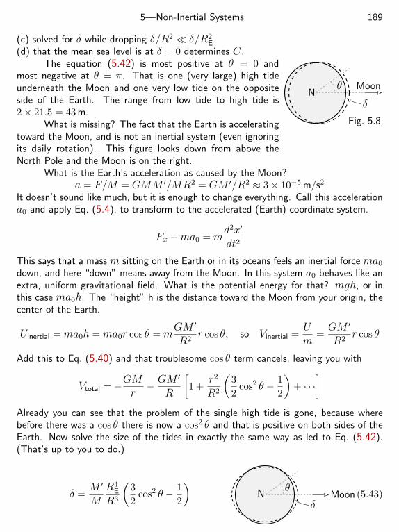
5—Non-Inertial Systems 189
(c) solved for δ while dropping δ/R2 δ/R2E.
(d) that the mean sea level is at δ = 0 determines C.
Nδ
θ Moon
Fig. 5.8
The equation (5.42) is most positive at θ = 0 andmost negative at θ = π. That is one (very large) high tideunderneath the Moon and one very low tide on the oppositeside of the Earth. The range from low tide to high tide is2× 21.5 = 43 m.
What is missing? The fact that the Earth is acceleratingtoward the Moon, and is not an inertial system (even ignoringits daily rotation). This figure looks down from above theNorth Pole and the Moon is on the right.
What is the Earth’s acceleration as caused by the Moon?a = F/M = GMM ′/MR2 = GM ′/R2 ≈ 3× 10⁻⁵ m/s2
It doesn’t sound like much, but it is enough to change everything. Call this accelerationa0 and apply Eq. (5.4), to transform to the accelerated (Earth) coordinate system.
Fx −ma0 = md2x′
dt2
This says that a mass m sitting on the Earth or in its oceans feels an inertial force ma0
down, and here “down” means away from the Moon. In this system a0 behaves like anextra, uniform gravitational field. What is the potential energy for that? mgh, or inthis case ma0h. The “height” h is the distance toward the Moon from your origin, thecenter of the Earth.
Uinertial = ma0h = ma0r cos θ = mGM ′
R2r cos θ, so Vinertial =
Um
=GM ′
R2r cos θ
Add this to Eq. (5.40) and that troublesome cos θ term cancels, leaving you with
Vtotal = −GMr− GM
′
R
[1 +
r2
R2
(3
2cos2 θ − 1
2
)+ · · ·
]Already you can see that the problem of the single high tide is gone, because wherebefore there was a cos θ there is now a cos2 θ and that is positive on both sides of theEarth. Now solve the size of the tides in exactly the same way as led to Eq. (5.42).(That’s up to you to do.)
δ =M ′
M
R4E
R3
(3
2cos2 θ − 1
2
)N
δ
θMoon (5.43)
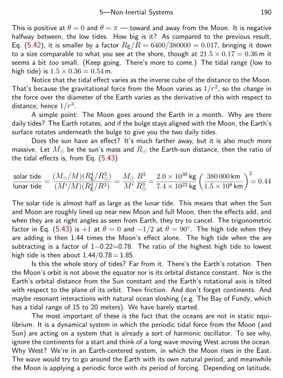
5—Non-Inertial Systems 190
This is positive at θ = 0 and θ = π — toward and away from the Moon. It is negativehalfway between, the low tides. How big is it? As compared to the previous result,Eq. (5.42), it is smaller by a factor RE/R = 6400/380000 = 0.017, bringing it downto a size comparable to what you see at the shore, though at 21.5 × 0.17 = 0.36 m itseems a bit too small. (Keep going. There’s more to come.) The tidal range (low tohigh tide) is 1.5× 0.36 = 0.54 m.
Notice that the tidal effect varies as the inverse cube of the distance to the Moon.That’s because the gravitational force from the Moon varies as 1/r2, so the change inthe force over the diameter of the Earth varies as the derivative of this with respect todistance; hence 1/r3.
A simple point: The Moon goes around the Earth in a month. Why are theredaily tides? The Earth rotates, and if the bulge stays aligned with the Moon, the Earth’ssurface rotates underneath the bulge to give you the two daily tides.
Does the sun have an effect? It’s much farther away, but it is also much moremassive. Let M be the sun’s mass and R the Earth-sun distance, then the ratio ofthe tidal effects is, from Eq. (5.43)
solar tide
lunar tide=
(M/M)(R4E/R
3)
(M ′/M)(R4E/R
3)=MM ′
R3
R3
=2.0× 1030 kg
7.4× 10²² kg
(380 000 km
1.5× 10⁸ km
)3
= 0.44
The solar tide is almost half as large as the lunar tide. This means that when the Sunand Moon are roughly lined up near new Moon and full Moon, then the effects add, andwhen they are at right angles as seen from Earth, they try to cancel. The trigonometricfactor in Eq. (5.43) is +1 at θ = 0 and −1/2 at θ = 90. The high tide when theyare adding is then 1.44 times the Moon’s effect alone. The high tide when the aresubtracting is a factor of 1−0.22=0.78. The ratio of the highest high tide to lowesthigh tide is then about 1.44/0.78 = 1.85.
Is this the whole story of tides? Far from it. There’s the Earth’s rotation. Thenthe Moon’s orbit is not above the equator nor is its orbital distance constant. Nor is theEarth’s orbital distance from the Sun constant and the Earth’s rotational axis is tiltedwith respect to the plane of its orbit. Then friction. And don’t forget continents. Andmaybe resonant interactions with natural ocean sloshing (e.g. The Bay of Fundy, whichhas a tidal range of 15 to 20 meters). We have barely started.
The most important of these is the fact that the oceans are not in static equi-librium. It is a dynamical system in which the periodic tidal force from the Moon (andSun) are acting on a system that is already a sort of harmonic oscillator. To see why,ignore the continents for a start and think of a long wave moving West across the ocean.Why West? We’re in an Earth-centered system, in which the Moon rises in the East.The wave would try to go around the Earth with its own natural period, and meanwhilethe Moon is applying a periodic force with its period of forcing. Depending on latitude,
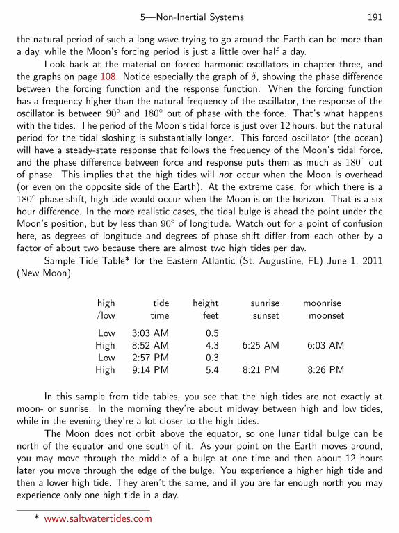
5—Non-Inertial Systems 191
the natural period of such a long wave trying to go around the Earth can be more thana day, while the Moon’s forcing period is just a little over half a day.
Look back at the material on forced harmonic oscillators in chapter three, andthe graphs on page 108. Notice especially the graph of δ, showing the phase differencebetween the forcing function and the response function. When the forcing functionhas a frequency higher than the natural frequency of the oscillator, the response of theoscillator is between 90 and 180 out of phase with the force. That’s what happenswith the tides. The period of the Moon’s tidal force is just over 12 hours, but the naturalperiod for the tidal sloshing is substantially longer. This forced oscillator (the ocean)will have a steady-state response that follows the frequency of the Moon’s tidal force,and the phase difference between force and response puts them as much as 180 outof phase. This implies that the high tides will not occur when the Moon is overhead(or even on the opposite side of the Earth). At the extreme case, for which there is a180 phase shift, high tide would occur when the Moon is on the horizon. That is a sixhour difference. In the more realistic cases, the tidal bulge is ahead the point under theMoon’s position, but by less than 90 of longitude. Watch out for a point of confusionhere, as degrees of longitude and degrees of phase shift differ from each other by afactor of about two because there are almost two high tides per day.
Sample Tide Table* for the Eastern Atlantic (St. Augustine, FL) June 1, 2011(New Moon)
high tide height sunrise moonrise/low time feet sunset moonset
Low 3:03 AM 0.5High 8:52 AM 4.3 6:25 AM 6:03 AMLow 2:57 PM 0.3
High 9:14 PM 5.4 8:21 PM 8:26 PM
In this sample from tide tables, you see that the high tides are not exactly atmoon- or sunrise. In the morning they’re about midway between high and low tides,while in the evening they’re a lot closer to the high tides.
The Moon does not orbit above the equator, so one lunar tidal bulge can benorth of the equator and one south of it. As your point on the Earth moves around,you may move through the middle of a bulge at one time and then about 12 hourslater you move through the edge of the bulge. You experience a higher high tide andthen a lower high tide. They aren’t the same, and if you are far enough north you mayexperience only one high tide in a day.
* www.saltwatertides.com
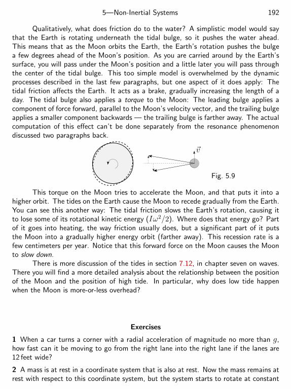
5—Non-Inertial Systems 192
Qualitatively, what does friction do to the water? A simplistic model would saythat the Earth is rotating underneath the tidal bulge, so it pushes the water ahead.This means that as the Moon orbits the Earth, the Earth’s rotation pushes the bulgea few degrees ahead of the Moon’s position. As you are carried around by the Earth’ssurface, you will pass under the Moon’s position and a little later you will pass throughthe center of the tidal bulge. This too simple model is overwhelmed by the dynamicprocesses described in the last few paragraphs, but one aspect of it does apply: Thetidal friction affects the Earth. It acts as a brake, gradually increasing the length of aday. The tidal bulge also applies a torque to the Moon: The leading bulge applies acomponent of force forward, parallel to the Moon’s velocity vector, and the trailing bulgeapplies a smaller component backwards — the trailing bulge is farther away. The actualcomputation of this effect can’t be done separately from the resonance phenomenondiscussed two paragraphs back.
~v
Fig. 5.9
This torque on the Moon tries to accelerate the Moon, and that puts it into ahigher orbit. The tides on the Earth cause the Moon to recede gradually from the Earth.You can see this another way: The tidal friction slows the Earth’s rotation, causing itto lose some of its rotational kinetic energy (Iω2/2). Where does that energy go? Partof it goes into heating, the way friction usually does, but a significant part of it putsthe Moon into a gradually higher energy orbit (farther away). This recession rate is afew centimeters per year. Notice that this forward force on the Moon causes the Moonto slow down.
There is more discussion of the tides in section 7.12, in chapter seven on waves.There you will find a more detailed analysis about the relationship between the positionof the Moon and the position of high tide. In particular, why does low tide happenwhen the Moon is more-or-less overhead?
Exercises
1 When a car turns a corner with a radial acceleration of magnitude no more than g,how fast can it be moving to go from the right lane into the right lane if the lanes are12 feet wide?
2 A mass is at rest in a coordinate system that is also at rest. Now the mass remains atrest with respect to this coordinate system, but the system starts to rotate at constant
5—Non-Inertial Systems 193
angular acceleration, so ω = αt. Just as the rotation starts, what does Eq. (5.10) tellyou about the mass, and what force does it take to hold it at rest in this system?
3 If a vector is stationary in an inertial system, what is its time derivative in a rotatingsystem?
4 If the Sun is compressed to a point, a black hole, and you are falling into it feet first,how far from the origin would you have to be so that the gravitational field on yourhead and on your feet differ by 10 m/s2 (the onset of spaghettification)? This is justan extreme version of a tide. [about 3700 km]
5—Non-Inertial Systems 194
Problems
5.1 Generalize the equations (5.3) to arbitrary straight-line motion: x′ = x − f(t)where f is any function. How are velocity and acceleration transformed?
5.2 If you are in a car that’s accelerating at a0, use Eqs. (5.4) to describe the totalforces that you perceive, assuming that you use the accelerated coordinate system inwhich you are at rest.A cord is hanging down from the roof inside the car. What angle does it make with thevertical in this case?
5.3 As in the preceding problem the cord is hanging down from the roof inside the car,but this time you are standing by the side of the road in an inertial coordinate system.Now figure out all the forces and deduce what angle the cord makes with the vertical.
5.4 A mass is hanging at the end of a one-meter length of light string, and it’s suspendedfrom the roof of the elevator that you are taking. You notice that the period of thependulum is 3 seconds. Are you in trouble? If so, how much?
5.5 Fill in the missing steps in Eqs. (5.13)–(5.24).
xy
x′y′
φ
5.6˙ In two dimensions, you have basis vectors x and y. Now take twoother unit vectors that are rotating so that φ = ωt. Write x′ and y′
in terms of x and y. A vector ~r is expressed in the rotating systemas x′(t)x′ + y′(t)y′. Express the rotating unit vectors in terms of thestationary x and y and from this compute d~r/dt. Compare this to thegeneral result in the text. Apply this to the particular example for whichx′(t) = x0 and y′(t) = v0t, drawing enough pictures to be sure that you understandwhat is happening.
5.7 For the golf ball and the artillery shell from Eq. (5.24) what result do you get ifyou aim south instead of north? What happens in the southern hemisphere at 55 southlatitude?
5.8˙ Stand in the center of a rotating platform and fire a bullet horizontally. Turn offgravity for a moment to make this a two-dimensional problem. What is the trajectoryof the bullet in your coordinate system? Express it in polar coordinates as an equationfor r in terms of φ. This problem is much easier to solve in an inertial system; you canthen transform the result into the rotating one and determine if your results satisfy theequations of motion in that system.
5.9 Analyze Eq. (5.24) for various special cases, e.g. equator, North or South pole,fired vertically, fired almost horizontally — all combinations. When is it zero?
5—Non-Inertial Systems 195
5.10¨There is a force in the x-y plane ~F0 = k~r⊥ = k(xx + yy) where k > 0. Amass m under this force will move rapidly away from the neighborhood of the origin.
(Show this.) The magnetic force on a charged particle is ~F1 = q~v × ~B. If ~B is alongthe z-axis, show that a sufficiently strong magnetic field will stabilize the motion of the(charged) mass, and that the motion of this mass will then be confined to some regionaround the origin. The Coriolis force has the same structure as this magnetic force,and in analyzing the motion of the Trojan asteroids the problem is quite similar to thisproblem (but with more algebra).
5.11˙ You can include air resistance in the calculations that started at Eq. (5.14): adda term −b~v. The solution for ~r0 is already done starting at Eq. (2.25), and you can usethat result here in order to improve the calculation leading to Eqs. (5.18) and (5.19).Assume that the projectile is fired straight up with the same initial speed 300 m/s andthat the terminal speed is 100 m/s. Now where will it land? A still better calculationwould be to use the added force ∝ v2 as in problem 2.23, but that would be cruel.
5.12 In the example #2 starting at Eq. (5.22) derive algebraically how the size of thedeflection depends on the initial speed of the golf ball.
5.13˙ Assume that Coriolis is the only force present. No gravity, no centrifugal, with~ω straight up and a flat Earth. Fire a rifle horizontally and get the trajectory. Userectangular coordinates to solve this problem, and don’t throw away any roots justbecause you expect them to be unimportant.
5.14˙ Add centrifugal force to the preceding problem and now find the trajectory.
5.15 (a) In the analysis of the trajectory of an object that you throw straight up fromthe equator, leading to Eq. (5.21), what is the horizontal velocity of the projectile whenit returns to the ground? (b) In trying to understand why the effect of the up and downmotion gives a net result to the West of the starting point, how does the answer to part(a) help?
5.16 If you didn’t do problem 5.5, then at least fill in the steps leading to Eq. (5.17).Then continue the process to find the next iteration.
5.17 At the start of section 5.4 it says that a rotation of the Earth occurs every 23 hours,56 minutes (and 4.1 seconds). Why not 24 hours? And are these numbers close toright?
5.18 In the equation (5.27) there is a z-component in the last term and it was veryconveniently ignored. What effect does it have?
5—Non-Inertial Systems 196
5.19 Drop a mass from a height h, initially at rest. Where does it land? You are atlatitude λ. Neglect air resistance.
5.20 Jump from a great height and you quickly reach terminal speed because of airresistance. Assume that you Jump from height h and reach terminal speed vt quickly(and there’s no wind), Where do you land? You are at latitude λ. Take terminal speedto be 60 m/s, λ = 30, and h = 2 km. Reaching terminal speed quickly — take it tomean that all the forces except Coriolis balance.
5.21 An insect is trying to walk on a rotating turntable, and with respect to theturntable its motion is a constant speed v0 directly away from the center. Find theforce (magnitude and direction) that the turntable must exert on the insect. Thecoefficient of static friction is µs. At what point will it start to slip?
5.22 Under what circumstances will the deviation of a golf ball as found in Eq. (5.24)be zero? For a reasonable choice of α, where is this?
5.23 If a bird is flying in level flight at speed v and desires to fly in a straight linedespite a horizontal component of Coriolis force, how much force must the bird exertto do so? Do this for a flight north and for flight west. Pick your favorite bird andlatitude and evaluate the size of this force.
5.24 Repeat problem 4.21 using the methods of this chapter.
5.25 In some oversimplified explanations of the Foucault pendulum you will read thestatement that with respect to the inertial system the plane in which the pendulumoscillates does not rotate. Show why this is false (with two exceptions). With respectto the inertial frame, what is the rotation rate of the plane of oscillation?
5.26 The differential equation for a charged particle in a magnetic field and an electricfield is
md2~rdt2
= q[~E +
d~rdt× ~B
]as in section 4.3. Write this equation in a coordinate system rotating with constant
angular velocity ~ω. Show that if ~B is a constant you can pick ~ω so as to eliminate ~B,at least if you neglect terms proportional to B2. What is the differential equation tosolve now? You may use components to solve this problem only if you want to do a lotof extra algebra and then get results that are difficult to interpret.
5.27 Leave the results for the Foucault pendulum, Eqs. (5.30), in terms of q = x+ iyas in the equation preceding it. What is the phase of q and what does that have to dowith interpreting the results?
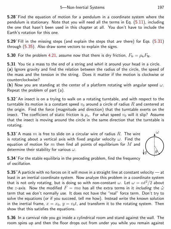
5—Non-Inertial Systems 197
5.28˙ Find the equation of motion for a pendulum in a coordinate system where thependulum is stationary. Note that you will need all the terms in Eq. (5.11), includingthe one that hasn’t been used in this chapter at all. You don’t have to include theEarth’s rotation for this one.
5.29˙ Fill in the missing steps (and explain the steps that are there) for Eqs. (5.31)through (5.35). Also draw some vectors to explain the signs.
5.30 For the problem 4.21, assume now that there is dry friction, Ffr = µkFN.
5.31 You tie a mass to the end of a string and whirl it around your head in a circle.(a) Ignore gravity and find the relation between the radius of the circle, the speed ofthe mass and the tension in the string. Does it matter if the motion is clockwise orcounterclockwise?(b) Now you are standing at the center of a platform rotating with angular speed ω.Repeat the problem of part (a).
5.32˙ An insect is on a trying to walk on a rotating turntable, and with respect to theturntable its motion is a constant speed v0 around a circle of radius R and centered atthe origin. Find the force (magnitude and direction) that the turntable exerts on theinsect. The coefficient of static friction is µs. For what speed v0 will it slip? Assumethat the insect is moving around the circle in the same direction that the turntable isrotating.
g
ω
θ
5.33˙ A mass m is free to slide on a circular wire of radius R. The wireis rotating about a vertical axis with fixed angular velocity ω. Find theequation of motion for m then find all points of equilibrium for M anddetermine their stability for various ω.
5.34˙ For the stable equilibria in the preceding problem, find the frequencyof oscillation.
5.35¨A particle with no forces on it will move in a straight line at constant velocity — atleast in an inertial coordinate system. Now analyze this problem in a coordinate systemthat is not only rotating, but is doing so with non-constant ω. Let ω = αt2/2 aboutthe z-axis. Now the modified F = ma has all the extra terms in it including the ωterm that we don’t normally use. It does not have the “real” force term. Don’t try tosolve the equations (or if you succeed, tell me how). Instead write the known solutionin the inertial frame, x = x0, y = v0t, and transform it to the rotating system. Thenshow that this satisfies the equations.
5.36 In a carnival ride you go inside a cylindrical room and stand against the wall. Theroom spins up and then the floor drops out from under you while you remain against
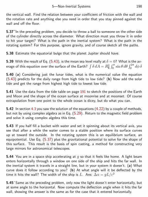
5—Non-Inertial Systems 198
the vertical wall. Find the relation between your coefficient of friction with the wall andthe rotation rate and anything else you need in order that you stay pinned against thewall and off the floor.
5.37¨In the preceding problem, you decide to throw a ball to someone on the other sideof the cylinder directly across the diameter. What direction must you throw it in orderto hit your target? What is the path in the inertial system? What is the path in therotating system? For this purpose, ignore gravity, and of course sketch all the paths.
5.38 Estimate the equatorial bulge that the planet Jupiter should have.
5.39 With the result of Eq. (5.43), is the mean sea level really at δ = 0? What is the av-
erage of this equation over the surface of the Earth?∫δ dA = R2
E
∫ π0 sin θ dθ
∫ 2π0 dφ δ
5.40 (a) Considering just the lunar tides, what is the numerical value the equation(5.43) predicts for the daily range from high tide to low tide? (b) Now add the solartide and get the range from highest high tide to lowest low tide.
5.41 Use the data from the tide table on page 191 to sketch the positions of the Earthand Moon and the shape of the ocean surface at moonrise and at moonset. Of courseextrapolation from one point to the whole ocean is dicey, but do what you can.
5.42 In section 4.3 you saw the solution of the equations (4.22) by a couple of methods,but not by using complex algebra as in Eq. (5.29). Return to the magnetic field problemand solve it using complex algebra this time.
5.43 If you half fill a bucket with water and set it spinning about its vertical axis, yousee that after a while the water comes to a stable position where its surface curvesup at toward the outside. In the rotating system this is an equilibrium surface, anequipotential. Use Eq. (5.37) plus the gravitational potential to solve for the shape ofthis surface. This result is the basis of spin casting, a method for constructing verylarge mirrors for astronomical telescopes.
5.44 You are in a space ship accelerating at g so that it feels like home. A light beamenters horizontally through a window on one side of the ship and hits the far wall. Inthe inertial system it travels in a straight line, but in your system it doesn’t. (a) Whatcurve does it follow according to you? (b) At what angle will it be deflected by thetime it hits the wall? The width of the ship is L. Ans: ∆α = gL/c2
5.45˙ Same as the preceding problem, only now the light doesn’t enter horizontally, butat some angle to the horizontal. Now compute the deflection angle when it hits the farwall, showing the answer is the same as for the case that it entered horizontally.
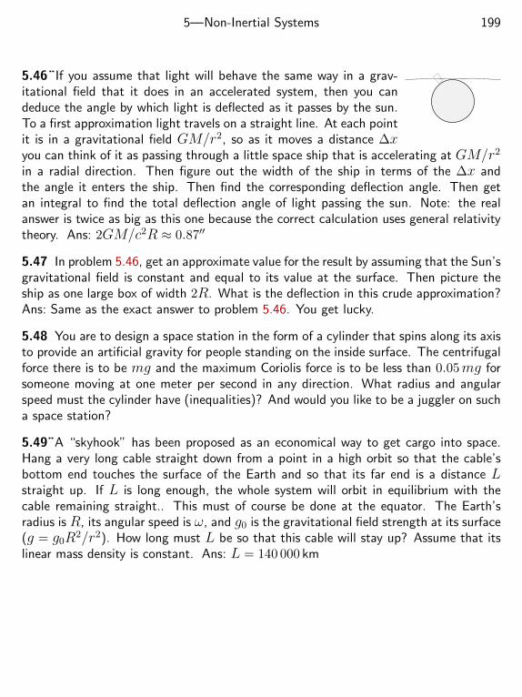
5—Non-Inertial Systems 199
5.46¨If you assume that light will behave the same way in a grav-itational field that it does in an accelerated system, then you candeduce the angle by which light is deflected as it passes by the sun.To a first approximation light travels on a straight line. At each pointit is in a gravitational field GM/r2, so as it moves a distance ∆xyou can think of it as passing through a little space ship that is accelerating at GM/r2
in a radial direction. Then figure out the width of the ship in terms of the ∆x andthe angle it enters the ship. Then find the corresponding deflection angle. Then getan integral to find the total deflection angle of light passing the sun. Note: the realanswer is twice as big as this one because the correct calculation uses general relativitytheory. Ans: 2GM/c2R ≈ 0.87′′
5.47 In problem 5.46, get an approximate value for the result by assuming that the Sun’sgravitational field is constant and equal to its value at the surface. Then picture theship as one large box of width 2R. What is the deflection in this crude approximation?Ans: Same as the exact answer to problem 5.46. You get lucky.
5.48 You are to design a space station in the form of a cylinder that spins along its axisto provide an artificial gravity for people standing on the inside surface. The centrifugalforce there is to be mg and the maximum Coriolis force is to be less than 0.05mg forsomeone moving at one meter per second in any direction. What radius and angularspeed must the cylinder have (inequalities)? And would you like to be a juggler on sucha space station?
5.49¨A “skyhook” has been proposed as an economical way to get cargo into space.Hang a very long cable straight down from a point in a high orbit so that the cable’sbottom end touches the surface of the Earth and so that its far end is a distance Lstraight up. If L is long enough, the whole system will orbit in equilibrium with thecable remaining straight.. This must of course be done at the equator. The Earth’sradius is R, its angular speed is ω, and g0 is the gravitational field strength at its surface(g = g0R2/r2). How long must L be so that this cable will stay up? Assume that itslinear mass density is constant. Ans: L = 140 000 km
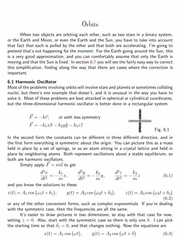
OrbitsWhen two objects are orbiting each other, such as two stars in a binary system,
or the Earth and Moon, or even the Earth and the Sun, you have to take into accountthat fact that each is pulled by the other and that both are accelerating. I’m going topretend that’s not happening for the moment. For the Earth going around the Sun, thisis a very good approximation, and you can comfortably assume that only the Earth ismoving and that the Sun is fixed. In section 6.7 you will see the fairly easy way to correctthis simplification, finding along the way that there are cases where the correction isimportant.
6.1 Harmonic OscillatorMost of the problems involving orbits will involve stars and planets or sometimes collidingnuclei, but there’s one example that doesn’t, and it is unusual in the way you have tosolve it. Most of these problems are best attacked in spherical or cylindrical coordinates,but the three-dimensional harmonic oscillator is better done in a rectangular system.
~F = −k~r, or with less symmetry
~F = −k1xx− k2yy − k3zzFig. 6.1
In the second form the constants can be different in three different direction, and inthe first form everything is symmetric about the origin. You can picture this as a massheld in place by a set of springs, or as an atom sitting in a crystal lattice and held inplace by neighboring atoms. Both represent oscillations about a stable equilibrium, soboth are harmonic oscillators.
Simply apply ~F = m~a to get
d2xdt2
= −k1
mx,
d2ydt2
= −k2
my,
d2zdt2
= −k3
mz (6.1)
and you know the solutions to these.
x(t) = A1 cos(ω1t+ δ1
), y(t) = A2 cos
(ω2t+ δ2
), z(t) = A3 cos
(ω3t+ δ3
)(6.2)
or any of the other convenient forms, such as complex exponentials. If you’re dealingwith the symmetric case, then the frequencies are all the same.
It’s easier to draw pictures in two dimensions, so stay with that case for now,setting z = 0. Also, start with the symmetric case so there is only one k. I can pickthe starting time so that δ1 = 0, and that changes nothing. Now the equations are
x(t) = A1 cos(ωt), y(t) = A2 cos
(ωt+ δ
)(6.3)
200
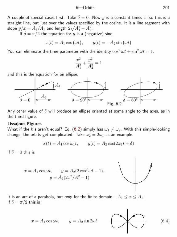
6—Orbits 201
A couple of special cases first. Take δ = 0. Now y is a constant times x, so this is astraight line, but just over the values specified by the cosine. It is a line segment withslope y/x = A2/A1 and length 2
√A2
1 +A22.
If δ = π/2 the equation for y is a (negative) sine.
x(t) = A1 cos(ωt), y(t) = −A2 sin
(ωt)
You can eliminate the time parameter with the identity cos2 ωt+ sin2 ωt = 1.
x2
A21
+y2
A22
= 1
and this is the equation for an ellipse.
δ = 0 δ = 90 δ = 60
A1
A2
Fig. 6.2
Any other value of δ will produce an ellipse oriented at some angle to the axes, as inthe third figure.
Lissajous FiguresWhat if the k’s aren’t equal? Eq. (6.2) simply has ω1 6= ω2. With this simple-lookingchange, the orbits get complicated. Take ω2 = 2ω1 as an example.
x(t) = A1 cosω1t, y(t) = A2 cos(2ω1t+ δ)
If δ = 0 this is
x = A1 cosωt, y = A2(2 cos2 ωt− 1),
y = A2(2x2/A21 − 1)
It is an arc of a parabola, but only for the finite domain −A1 ≤ x ≤ A1.If δ = π/2 this is
x = A1 cosωt, y = A2 sin 2ωt (6.4)
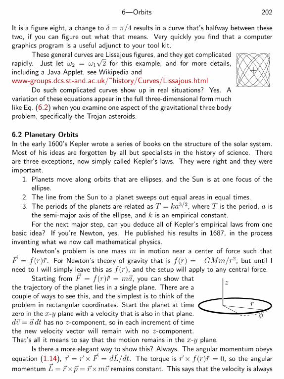
6—Orbits 202
It is a figure eight, a change to δ = π/4 results in a curve that’s halfway between thesetwo, if you can figure out what that means. Very quickly you find that a computergraphics program is a useful adjunct to your tool kit.
These general curves are Lissajous figures, and they get complicatedrapidly. Just let ω2 = ω1
√2 for this example, and for more details,
including a Java Applet, see Wikipedia andwww-groups.dcs.st-and.ac.uk/˜history/Curves/Lissajous.html
Do such complicated curves show up in real situations? Yes. Avariation of these equations appear in the full three-dimensional form muchlike Eq. (6.2) when you examine one aspect of the gravitational three bodyproblem, specifically the Trojan asteroids.
6.2 Planetary OrbitsIn the early 1600’s Kepler wrote a series of books on the structure of the solar system.Most of his ideas are forgotten by all but specialists in the history of science. Thereare three exceptions, now simply called Kepler’s laws. They were right and they wereimportant.
1. Planets move along orbits that are ellipses, and the Sun is at one focus of theellipse.
2. The line from the Sun to a planet sweeps out equal areas in equal times.
3. The periods of the planets are related as T = ka3/2, where T is the period, a isthe semi-major axis of the ellipse, and k is an empirical constant.
For the next major step, can you deduce all of Kepler’s empirical laws from onebasic idea? If you’re Newton, yes. He published his results in 1687, in the processinventing what we now call mathematical physics.
Newton’s problem is one mass m in motion near a center of force such that~F = f(r)r. For Newton’s theory of gravity that is f(r) = −GMm/r2, but until Ineed to I will simply leave this as f(r), and the setup will apply to any central force.
z
r
φ
Starting from ~F = f(r)r = m~a, you can show thatthe trajectory of the planet lies in a single plane. There are acouple of ways to see this, and the simplest is to think of theproblem in rectangular coordinates. Start the planet at timezero in the x-y plane with a velocity that is also in that plane.d~v = ~a dt has no z-component, so in each increment of timethe new velocity vector will remain with no z-component.That’s all it means to say that the motion remains in the x-y plane.
Is there a more elegant way to show this? Always. The angular momentum obeys
equation (1.14), ~τ = ~r × ~F = d~L/dt. The torque is ~r × f(r)r = 0, so the angular
momentum ~L = ~r×~p = ~r×m~v remains constant. This says that the velocity is always
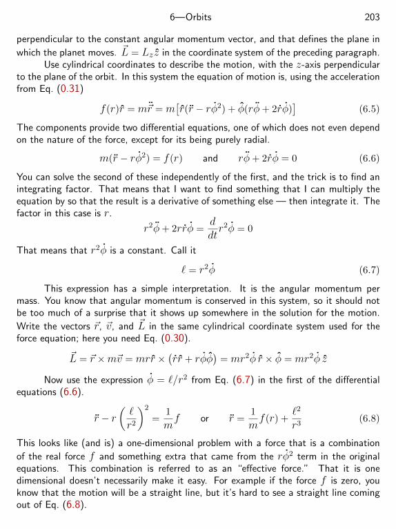
6—Orbits 203
perpendicular to the constant angular momentum vector, and that defines the plane in
which the planet moves. ~L = Lz z in the coordinate system of the preceding paragraph.Use cylindrical coordinates to describe the motion, with the z-axis perpendicular
to the plane of the orbit. In this system the equation of motion is, using the accelerationfrom Eq. (0.31)
f(r)r = m~r = m[r(r − rφ2) + φ(rφ+ 2rφ)
](6.5)
The components provide two differential equations, one of which does not even dependon the nature of the force, except for its being purely radial.
m(r − rφ2) = f(r) and rφ+ 2rφ = 0 (6.6)
You can solve the second of these independently of the first, and the trick is to find anintegrating factor. That means that I want to find something that I can multiply theequation by so that the result is a derivative of something else — then integrate it. Thefactor in this case is r.
r2φ+ 2rrφ =ddtr2φ = 0
That means that r2φ is a constant. Call it
` = r2φ (6.7)
This expression has a simple interpretation. It is the angular momentum permass. You know that angular momentum is conserved in this system, so it should notbe too much of a surprise that it shows up somewhere in the solution for the motion.
Write the vectors ~r, ~v, and ~L in the same cylindrical coordinate system used for theforce equation; here you need Eq. (0.30).
~L = ~r ×m~v = mrr ×(rr + rφφ
)= mr2φ r × φ = mr2φ z
Now use the expression φ = `/r2 from Eq. (6.7) in the first of the differentialequations (6.6).
r − r(`r2
)2
=1
mf or r =
1
mf(r) +
`2
r3(6.8)
This looks like (and is) a one-dimensional problem with a force that is a combination
of the real force f and something extra that came from the rφ2 term in the originalequations. This combination is referred to as an “effective force.” That it is onedimensional doesn’t necessarily make it easy. For example if the force f is zero, youknow that the motion will be a straight line, but it’s hard to see a straight line comingout of Eq. (6.8).
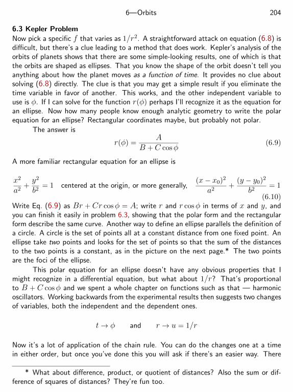
6—Orbits 204
6.3 Kepler Problem
Now pick a specific f that varies as 1/r2. A straightforward attack on equation (6.8) isdifficult, but there’s a clue leading to a method that does work. Kepler’s analysis of theorbits of planets shows that there are some simple-looking results, one of which is thatthe orbits are shaped as ellipses. That you know the shape of the orbit doesn’t tell youanything about how the planet moves as a function of time. It provides no clue aboutsolving (6.8) directly. The clue is that you may get a simple result if you eliminate thetime variable in favor of another. This works, and the other independent variable touse is φ. If I can solve for the function r(φ) perhaps I’ll recognize it as the equation foran ellipse. Now how many people know enough analytic geometry to write the polarequation for an ellipse? Rectangular coordinates maybe, but probably not polar.
The answer is
r(φ) =A
B +C cosφ(6.9)
A more familiar rectangular equation for an ellipse is
x2
a2+y2
b2= 1 centered at the origin, or more generally,
(x− x0)2
a2+
(y − y0)2
b2= 1
(6.10)Write Eq. (6.9) as Br + Cr cosφ = A; write r and r cosφ in terms of x and y, andyou can finish it easily in problem 6.3, showing that the polar form and the rectangularform describe the same curve. Another way to define an ellipse parallels the definition ofa circle. A circle is the set of points all at a constant distance from one fixed point. Anellipse take two points and looks for the set of points so that the sum of the distancesto the two points is a constant, as in the picture on the next page.* The two pointsare the foci of the ellipse.
This polar equation for an ellipse doesn’t have any obvious properties that Imight recognize in a differential equation, but what about 1/r? That’s proportionalto B + C cosφ and we spent a whole chapter on functions such as that — harmonicoscillators. Working backwards from the experimental results then suggests two changesof variables, both the independent and the dependent ones.
t→ φ and r → u = 1/r
Now it’s a lot of application of the chain rule. You can do the changes one at a timein either order, but once you’ve done this you will ask if there’s an easier way. There
* What about difference, product, or quotient of distances? Also the sum or dif-ference of squares of distances? They’re fun too.
6—Orbits 205
is: Do both at once.
Recall: ` = r2φ, so `u2 = φ
drdt
=drdu
dudφ
dφdt
= − 1
u2
dudφ`u2 = −`du
dφ
d2rdt2
= −`d2udφ2
dφdt
= −`2u2 d2udφ2
Put this change into Eq. (6.8) to get
−`2u2 d2udφ2
=1
mf( 1
u
)+ `2u3, or
d2udφ2
+ u = − 1
m`2u2f( 1
u
)(6.11)
This is starting to look like a harmonic oscillator. Can you solve it? Thatdepends on f , and for which functions f is it easy? If the right side is a constant or ifit’s proportional to u, then you can do it without difficulty, otherwise it’s hard. Whathappens with the Kepler problem?
f(r) = −GMmr2
=⇒ d2udφ2
+ u = − 1
m`2u2
[−GMmu2
]= +
GM`2
(6.12)
Leave the other easy case for later, section 6.8, because though the results are amusingthey’re not very important. (What f would that be?) Most of the rest of this chapterwill concern the exact solutions to the Kepler problem and approximate solutions to allthe others.
Equation (6.12) is easy.
u =GM`2
+C cos(φ− φ0), or1
u= r =
`2/GM1 + ε cos(φ− φ0)
(6.13)
C was an arbitrary constant so ε = C`2/GM is too, and it’s dimensionless. This isthe ellipse as stated in Kepler’s laws, at least as long as the parameter ε has magnitudeless than one. (More on that later, section 6.9.) The numerator of (6.13) is a length,and φ0 is an angle. I may as well assume that ε ≥ 0 because if not, then I can redefinethe parameter φ0 by adding π to it. That changes the sign in front of the cosine backto positive again. With this convention on ε, the angle φ0 is the direction in which thedenominator is largest. It points toward the smallest r in the orbit.
When you’re talking about planets going around the Sun, the orbital point nearestthe Sun is the perihelion, and the one farthest away is the aphelion. For objects orbitingthe Earth, the corresponding names are perigee and apogee, and the generic terms areperiapsis and apoapsis.
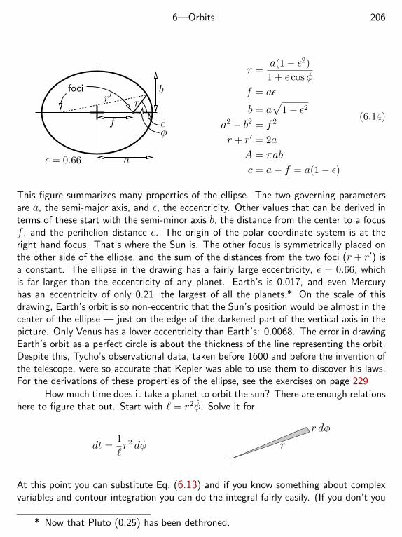
6—Orbits 206
ε = 0.66 a
b
f
r
cφ
r′foci
r =a(1− ε2)
1 + ε cosφ
f = aε
b = a√
1− ε2
a2 − b2 = f 2
r + r′ = 2a
A = πab
c = a− f = a(1− ε)
(6.14)
This figure summarizes many properties of the ellipse. The two governing parametersare a, the semi-major axis, and ε, the eccentricity. Other values that can be derived interms of these start with the semi-minor axis b, the distance from the center to a focusf , and the perihelion distance c. The origin of the polar coordinate system is at theright hand focus. That’s where the Sun is. The other focus is symmetrically placed onthe other side of the ellipse, and the sum of the distances from the two foci (r + r′) isa constant. The ellipse in the drawing has a fairly large eccentricity, ε = 0.66, whichis far larger than the eccentricity of any planet. Earth’s is 0.017, and even Mercuryhas an eccentricity of only 0.21, the largest of all the planets.* On the scale of thisdrawing, Earth’s orbit is so non-eccentric that the Sun’s position would be almost in thecenter of the ellipse — just on the edge of the darkened part of the vertical axis in thepicture. Only Venus has a lower eccentricity than Earth’s: 0.0068. The error in drawingEarth’s orbit as a perfect circle is about the thickness of the line representing the orbit.Despite this, Tycho’s observational data, taken before 1600 and before the invention ofthe telescope, were so accurate that Kepler was able to use them to discover his laws.For the derivations of these properties of the ellipse, see the exercises on page 229
How much time does it take a planet to orbit the sun? There are enough relationshere to figure that out. Start with ` = r2φ. Solve it for
dt =1
`r2 dφ r
r dφ
At this point you can substitute Eq. (6.13) and if you know something about complexvariables and contour integration you can do the integral fairly easily. (If you don’t you
* Now that Pluto (0.25) has been dethroned.
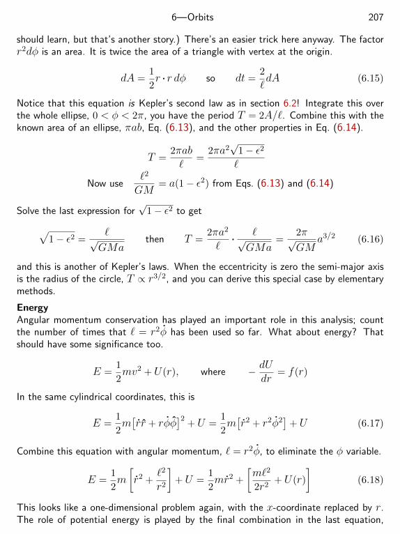
6—Orbits 207
should learn, but that’s another story.) There’s an easier trick here anyway. The factorr2dφ is an area. It is twice the area of a triangle with vertex at the origin.
dA =1
2r . r dφ so dt =
2
`dA (6.15)
Notice that this equation is Kepler’s second law as in section 6.2! Integrate this overthe whole ellipse, 0 < φ < 2π, you have the period T = 2A/`. Combine this with theknown area of an ellipse, πab, Eq. (6.13), and the other properties in Eq. (6.14).
T =2πab`
=2πa2
√1− ε2`
Now use`2
GM= a(1− ε2) from Eqs. (6.13) and (6.14)
Solve the last expression for√
1− ε2 to get√1− ε2 =
`√GMa
then T =2πa2
`. `√
GMa=
2π√GM
a3/2 (6.16)
and this is another of Kepler’s laws. When the eccentricity is zero the semi-major axisis the radius of the circle, T ∝ r3/2, and you can derive this special case by elementarymethods.
EnergyAngular momentum conservation has played an important role in this analysis; countthe number of times that ` = r2φ has been used so far. What about energy? Thatshould have some significance too.
E =1
2mv2 + U(r), where − dU
dr= f(r)
In the same cylindrical coordinates, this is
E =1
2m[rr + rφφ
]2+ U =
1
2m[r2 + r2φ2
]+ U (6.17)
Combine this equation with angular momentum, ` = r2φ, to eliminate the φ variable.
E =1
2m
[r2 +
`2
r2
]+ U =
1
2mr2 +
[m`2
2r2+ U(r)
](6.18)
This looks like a one-dimensional problem again, with the x-coordinate replaced by r.The role of potential energy is played by the final combination in the last equation,
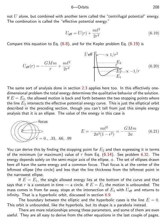
6—Orbits 208
not U alone, but combined with another term called the “centrifugal potential” energy.The combination is called the “effective potential energy.”
Ueff = U(r) +m`2
2r2(6.19)
Compare this equation to Eq. (6.8), and for the Kepler problem Eq. (6.19) is
Ueff(r) = −GMmr
+m`2
2r2
Ueff
r
E1
E2
E3
∝ 1/r2
∝ −1/r(6.20)
The same sort of analysis done in section 2.3 applies here too. In this effectively one-dimensional problem the total energy determines the qualitative behavior of the solution.If E = E2, the allowed motion is back and forth between the two stopping points wherethe line E2 intersects the effective potential energy curve. This is just the elliptical orbitdescribed in the preceding section, though you can’t tell from just this simple energyanalysis that it is an ellipse. The value of the energy in this case is
ε = 0., .33, .66, .99
focus
E = − m`2
2a2(1− ε2)= −GMm
2a(6.21)
You can derive this by finding the stopping point for E2 and then expressing it in termsof the minimum (or maximum) value of r from Eq. (6.14). See problem 6.32. Theenergy depends solely on the semi-major axis of the ellipse, a. The set of ellipses drawnhere all have the same energy and a common focus. That focus is at the center of theleftmost ellipse (the circle) and less that the line thickness from the leftmost point inthe narrowest ellipse.
If E = E1, the single allowed energy lies at the bottom of the curve and thatsays that r is a constant in time — a circle. If E = E3 the motion is unbounded. Themass comes in from far away, stops at the intersection of E3 with Ueff and returns toinfinity. That is a hyperbolic orbit, discussed in section 6.9.
The boundary between the elliptic and the hyperbolic cases is the line E = 0.This orbit is unbounded, like the hyperbola, but its shape is a parabola instead.
There are more relationships among these parameters, and some of them are evenuseful. They are all easy to derive from the other equations in the last couple of pages,
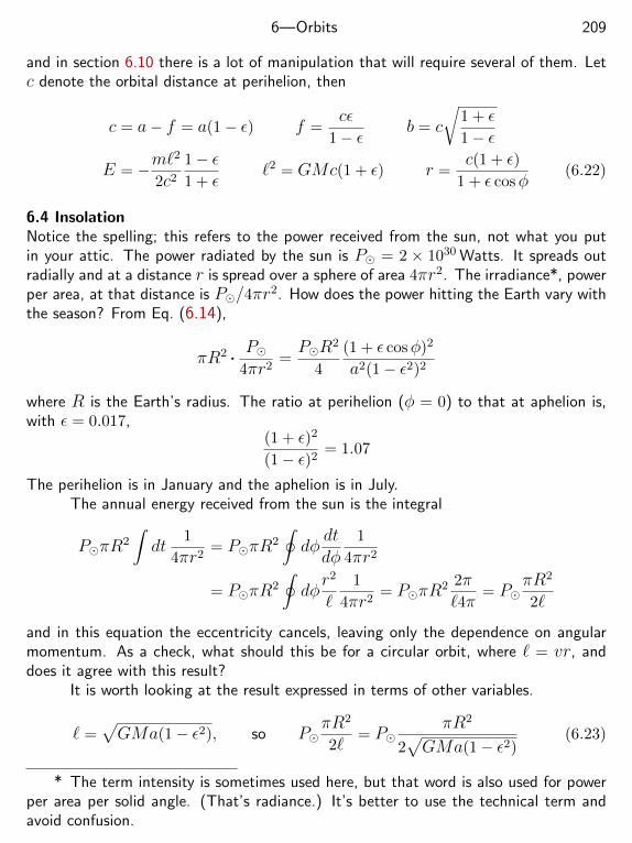
6—Orbits 209
and in section 6.10 there is a lot of manipulation that will require several of them. Letc denote the orbital distance at perihelion, then
c = a− f = a(1− ε) f =cε
1− εb = c
√1 + ε1− ε
E = −m`2
2c2
1− ε1 + ε
`2 = GMc(1 + ε) r =c(1 + ε)
1 + ε cosφ(6.22)
6.4 InsolationNotice the spelling; this refers to the power received from the sun, not what you putin your attic. The power radiated by the sun is P = 2 × 1030 Watts. It spreads outradially and at a distance r is spread over a sphere of area 4πr2. The irradiance*, powerper area, at that distance is P/4πr2. How does the power hitting the Earth vary withthe season? From Eq. (6.14),
πR2 . P4πr2
=PR2
4
(1 + ε cosφ)2
a2(1− ε2)2
where R is the Earth’s radius. The ratio at perihelion (φ = 0) to that at aphelion is,with ε = 0.017,
(1 + ε)2
(1− ε)2= 1.07
The perihelion is in January and the aphelion is in July.The annual energy received from the sun is the integral
PπR2
∫dt
1
4πr2= PπR
2
∮dφ
dtdφ
1
4πr2
= PπR2
∮dφr2
`1
4πr2= PπR
2 2π`4π
= PπR2
2`
and in this equation the eccentricity cancels, leaving only the dependence on angularmomentum. As a check, what should this be for a circular orbit, where ` = vr, anddoes it agree with this result?
It is worth looking at the result expressed in terms of other variables.
` =√GMa(1− ε2), so P
πR2
2`= P
πR2
2√GMa(1− ε2)
(6.23)
* The term intensity is sometimes used here, but that word is also used for powerper area per solid angle. (That’s radiance.) It’s better to use the technical term andavoid confusion.
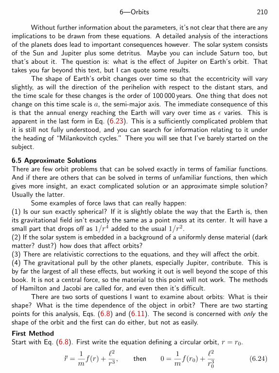
6—Orbits 210
Without further information about the parameters, it’s not clear that there are anyimplications to be drawn from these equations. A detailed analysis of the interactionsof the planets does lead to important consequences however. The solar system consistsof the Sun and Jupiter plus some detritus. Maybe you can include Saturn too, butthat’s about it. The question is: what is the effect of Jupiter on Earth’s orbit. Thattakes you far beyond this text, but I can quote some results.
The shape of Earth’s orbit changes over time so that the eccentricity will varyslightly, as will the direction of the perihelion with respect to the distant stars, andthe time scale for these changes is the order of 100 000 years. One thing that does notchange on this time scale is a, the semi-major axis. The immediate consequence of thisis that the annual energy reaching the Earth will vary over time as ε varies. This isapparent in the last form in Eq. (6.23). This is a sufficiently complicated problem thatit is still not fully understood, and you can search for information relating to it underthe heading of “Milankovitch cycles.” There you will see that I’ve barely started on thesubject.
6.5 Approximate SolutionsThere are few orbit problems that can be solved exactly in terms of familiar functions.And if there are others that can be solved in terms of unfamiliar functions, then whichgives more insight, an exact complicated solution or an approximate simple solution?Usually the latter.
Some examples of force laws that can really happen:(1) Is our sun exactly spherical? If it is slightly oblate the way that the Earth is, thenits gravitational field isn’t exactly the same as a point mass at its center. It will have asmall part that drops off as 1/r4 added to the usual 1/r2.(2) If the solar system is embedded in a background of a uniformly dense material (darkmatter? dust?) how does that affect orbits?(3) There are relativistic corrections to the equations, and they will affect the orbit.(4) The gravitational pull by the other planets, especially Jupiter, contribute. This isby far the largest of all these effects, but working it out is well beyond the scope of thisbook. It is not a central force, so the material to this point will not work. The methodsof Hamilton and Jacobi are called for, and even then it’s difficult.
There are two sorts of questions I want to examine about orbits: What is theirshape? What is the time dependence of the object in orbit? There are two startingpoints for this analysis, Eqs. (6.8) and (6.11). The second is concerned with only theshape of the orbit and the first can do either, but not as easily.
First MethodStart with Eq. (6.8). First write the equation defining a circular orbit, r = r0.
r =1
mf(r) +
`2
r3, then 0 =
1
mf(r0) +
`2
r30
(6.24)
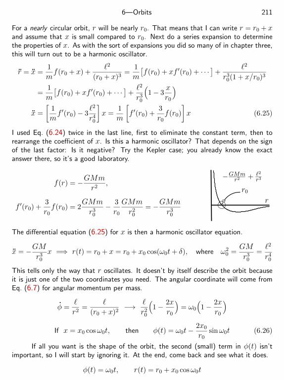
6—Orbits 211
For a nearly circular orbit, r will be nearly r0. That means that I can write r = r0 + xand assume that x is small compared to r0. Next do a series expansion to determinethe properties of x. As with the sort of expansions you did so many of in chapter three,this will turn out to be a harmonic oscillator.
r = x =1
mf(r0 + x) +
`2
(r0 + x)3=
1
m
[f(r0) + xf ′(r0) + · · ·
]+
`2
r30(1 + x/r0)3
=1
m
[f(r0) + xf ′(r0) + · · ·
]+`2
r30
(1− 3
xr0
)x =
[1
mf ′(r0)− 3
`2
r40
]x =
1
m
[f ′(r0) +
3
r0f(r0)
]x (6.25)
I used Eq. (6.24) twice in the last line, first to eliminate the constant term, then torearrange the coefficient of x. Is this a harmonic oscillator? That depends on the signof the last factor: Is it negative? Try the Kepler case; you already know the exactanswer there, so it’s a good laboratory.
f(r) = −GMmr2
,
f ′(r0) +3
r0f(r0) = 2
GMm
r30
− 3
r0
GMm
r20
= −GMm
r30
r0
−GMmr2 + `2
r3
r
The differential equation (6.25) for x is then a harmonic oscillator equation.
x = −GMr3
0
x =⇒ r(t) = r0 + x = r0 + x0 cos(ω0t+ δ), where ω20 =
GM
r30
=`2
r40
This tells only the way that r oscillates. It doesn’t by itself describe the orbit becauseit is just one of the two coordinates you need. The angular coordinate will come fromEq. (6.7) for angular momentum per mass.
φ =`r2
=`
(r0 + x)2−→ `
r20
(1− 2x
r0
)= ω0
(1− 2x
r0
)If x = x0 cosω0t, then φ(t) = ω0t−
2x0
r0sinω0t (6.26)
If all you want is the shape of the orbit, the second (small) term in φ(t) isn’timportant, so I will start by ignoring it. At the end, come back and see what it does.
φ(t) = ω0t, r(t) = r0 + x0 cosω0t
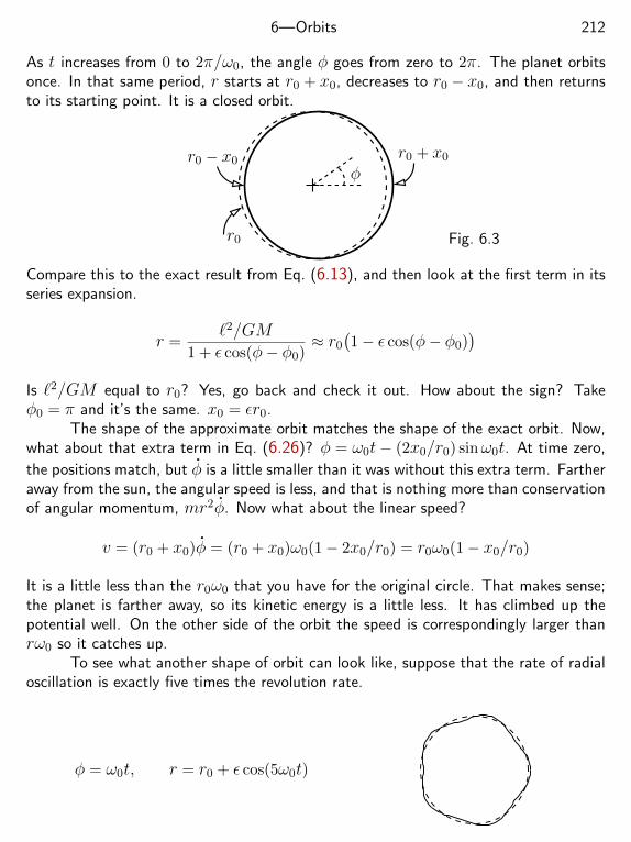
6—Orbits 212
As t increases from 0 to 2π/ω0, the angle φ goes from zero to 2π. The planet orbitsonce. In that same period, r starts at r0 + x0, decreases to r0 − x0, and then returnsto its starting point. It is a closed orbit.
r0
r0 − x0r0 + x0
φ
Fig. 6.3
Compare this to the exact result from Eq. (6.13), and then look at the first term in itsseries expansion.
r =`2/GM
1 + ε cos(φ− φ0)≈ r0
(1− ε cos(φ− φ0)
)Is `2/GM equal to r0? Yes, go back and check it out. How about the sign? Takeφ0 = π and it’s the same. x0 = εr0.
The shape of the approximate orbit matches the shape of the exact orbit. Now,what about that extra term in Eq. (6.26)? φ = ω0t− (2x0/r0) sinω0t. At time zero,
the positions match, but φ is a little smaller than it was without this extra term. Fartheraway from the sun, the angular speed is less, and that is nothing more than conservationof angular momentum, mr2φ. Now what about the linear speed?
v = (r0 + x0)φ = (r0 + x0)ω0(1− 2x0/r0) = r0ω0(1− x0/r0)
It is a little less than the r0ω0 that you have for the original circle. That makes sense;the planet is farther away, so its kinetic energy is a little less. It has climbed up thepotential well. On the other side of the orbit the speed is correspondingly larger thanrω0 so it catches up.
To see what another shape of orbit can look like, suppose that the rate of radialoscillation is exactly five times the revolution rate.
φ = ω0t, r = r0 + ε cos(5ω0t)
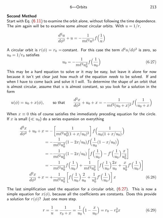
6—Orbits 213
Second MethodStart with Eq. (6.11) to examine the orbit alone, without following the time dependence.The aim again will be to examine some almost circular orbits. With u = 1/r,
d2udφ2
+ u = − 1
m`2u2f( 1
u
)A circular orbit is r(φ) = r0 = constant. For this case the term d2u/dφ2 is zero, sou0 = 1/r0 satisfies
u0 = − 1
m`2u20
f( 1
u0
)(6.27)
This may be a hard equation to solve or it may be easy, but leave it alone for nowbecause it isn’t yet clear just how much of the equation needs to be solved. If andwhen I have to come back and solve it I will. To determine the shape of an orbit thatis almost circular, assume that u is almost constant, so you look for a solution in theform
u(φ) = u0 + x(φ), so thatd2xdφ2
+ u0 + x = − 1
m`2(u0 + x)2f( 1
u0 + x
)When x ≡ 0 this of course satisfies the immediately preceding equation for the circle.If x is small ( u0) do a series expansion on everything
d2xdφ2
+ u0 + x = −[
1
m`2u20(1 + x/u0)2
]f( 1
u0(1 + x/u0)
)= − 1
m`2u20
(1− 2x/u0)f( 1
u0(1− x/u0)
)= − 1
m`2u20
(1− 2x/u0)
[f( 1
u0
)− f ′
( 1
u0
) xu2
0
]= − 1
m`2u20
f( 1
u0
)+
1
m`2u20
[f( 1
u0
)2xu0
+x
u20
f ′( 1
u0
)]d2xdφ2
+ x = +1
m`2u20
[f( 1
u0
) 2
u0+
1
u20
f ′( 1
u0
)]x (6.28)
The last simplification used the equation for a circular orbit, (6.27). This is now asimple equation for x(φ), because all the coefficients are constants. Does this providea solution for r(φ)? Just one more step.
r =1
u=
1
r0 + x=
1
u0
(1− x
u0
)= r0 − r2
0x (6.29)
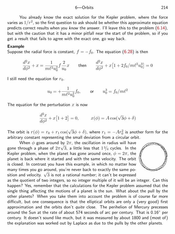
6—Orbits 214
You already know the exact solution for the Kepler problem, where the forcevaries as 1/r2, so the first question to ask should be whether this approximate equationpredicts correct results when you know the answer. I’ll leave this to the problem (6.14),but with the caution that it has a minor pitfall near the start of the problem, so if youget a result that fails to agree with the exact one, go way back.
ExampleSuppose the radial force is constant, f = −f0. The equation (6.28) is then
d2xdφ2
+ x =1
m`2u20
f2
u0x then
d2xdφ2
+ x[1 + 2f0/m`
2u30
]= 0
I still need the equation for r0.
u0 = +1
m`2u20
f0, or u30 = f0/m`
2
The equation for the perturbation x is now
d2xdφ2
+ x[1 + 2
]= 0, x(φ) = A cos(
√3φ+ δ)
The orbit is r(φ) = r0 + r1 cos(√
3φ + δ), where r1 = −Ar20 is another form for the
arbitrary constant representing the small deviation from a circular orbit.When φ goes around by 2π, the oscillation in radius will have
gone through a phase of 2π√
3, a little less that 13/4 cycles. In theKepler problem, when the planet has gone around once, φ = 2π, theplanet is back where it started and with the same velocity. The orbitis closed. In contrast you have this example, in which no matter howmany times you go around, you’re never back to exactly the same po-sition and velocity.
√3 is not a rational number; it can’t be expressed
as the quotient of two integers, so no integer multiple of it will be an integer. Can thishappen? Yes, remember that the calculations for the Kepler problem assumed that thesingle thing affecting the motions of a planet is the sun. What about the pull by theother planets? When you take them into account the problem is of course far moredifficult, but one consequence is that the elliptical orbits are only a (very good) firstapproximation and the orbits don’t quite close. The perihelion of Mercury precessesaround the Sun at the rate of about 574 seconds of arc per century. That is 0.16 percentury. It doesn’t sound like much, but it was measured by about 1800 and (most of)the explanation was worked out by Laplace as due to the pulls by the other planets.
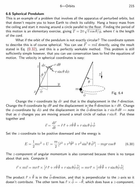
6—Orbits 215
6.6 Spherical PendulumThis is an example of a problem that involves all the apparatus of perturbed orbits, butthat doesn’t require you to leave Earth to check its validity. Hang a heavy mass fromthe ceiling and start it moving around a circle parallel to the floor. Finding the period ofthis motion is an elementary exercise, giving T = 2π
√` cos θ/g, where ` is the length
of the cord.
What if the orbit of the pendulum is not exactly circular? The coordinate system
to describe this is of course spherical. You can use ~F = m~a directly, using the resultstated in Eq. (0.32), and this is a perfectly workable method. This problem is stillsufficiently simple however, that you can use conservation laws to find the equations ofmotion. The velocity in spherical coordinates is easy:
x
y
z
rθ
φ
dr r dθ
r sin θ dφ
θ
φ
z
mFig. 6.4
Change the r-coordinate by dr and that is the displacement in the r-direction.Change the θ-coordinate by dθ and the displacement in the θ-direction is r dθ. Changethe φ-coordinate by dφ and the displacement in the φ-direction is r sin θ dθ — notethat as φ changes you are moving around a small circle of radius r sin θ. Put thesetogether and
~v =d~rdt
= r r + rθ θ + r sin θ φ φ
Set the z-coordinate to be positive downward and the energy is
E =1
2mv2 + U =
m2
[r2 + r2θ2 + r2 sin2 θ φ2
]−mgr cos θ (6.30)
The z-component of angular momentum is also conserved because there is no torqueabout that axis. Compute it
~r ×m~v = mrr ×[r r + rθ θ + r sin θφ φ
]= mrr ×
[rθ θ + r sin θφ φ
]The product r × θ is in the φ-direction, and that is perpendicular to the z-axis so it
doesn’t contribute. The other term has r × φ = −θ, which does have a z-component.
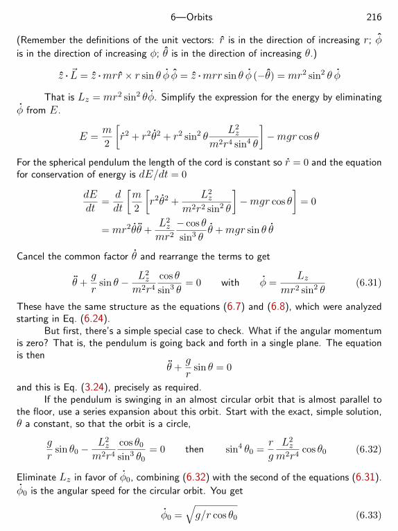
6—Orbits 216
(Remember the definitions of the unit vectors: r is in the direction of increasing r; φis in the direction of increasing φ; θ is in the direction of increasing θ.)
z . ~L = z .mrr × r sin θ φ φ = z .mrr sin θ φ (−θ) = mr2 sin2 θ φ
That is Lz = mr2 sin2 θφ. Simplify the expression for the energy by eliminating
φ from E.
E =m2
[r2 + r2θ2 + r2 sin2 θ
L2z
m2r4 sin4 θ
]−mgr cos θ
For the spherical pendulum the length of the cord is constant so r = 0 and the equationfor conservation of energy is dE/dt = 0
dEdt
=ddt
[m2
[r2θ2 +
L2z
m2r2 sin2 θ
]−mgr cos θ
]= 0
= mr2θθ +L2z
mr2
− cos θ
sin3 θθ +mgr sin θ θ
Cancel the common factor θ and rearrange the terms to get
θ +gr
sin θ − L2z
m2r4
cos θ
sin3 θ= 0 with φ =
Lzmr2 sin2 θ
(6.31)
These have the same structure as the equations (6.7) and (6.8), which were analyzedstarting in Eq. (6.24).
But first, there’s a simple special case to check. What if the angular momentumis zero? That is, the pendulum is going back and forth in a single plane. The equationis then
θ +gr
sin θ = 0
and this is Eq. (3.24), precisely as required.If the pendulum is swinging in an almost circular orbit that is almost parallel to
the floor, use a series expansion about this orbit. Start with the exact, simple solution,θ a constant, so that the orbit is a circle,
gr
sin θ0 −L2z
m2r4
cos θ0
sin3 θ0= 0 then sin4 θ0 =
rgL2z
m2r4cos θ0 (6.32)
Eliminate Lz in favor of φ0, combining (6.32) with the second of the equations (6.31).
φ0 is the angular speed for the circular orbit. You get
φ0 =√g/r cos θ0 (6.33)
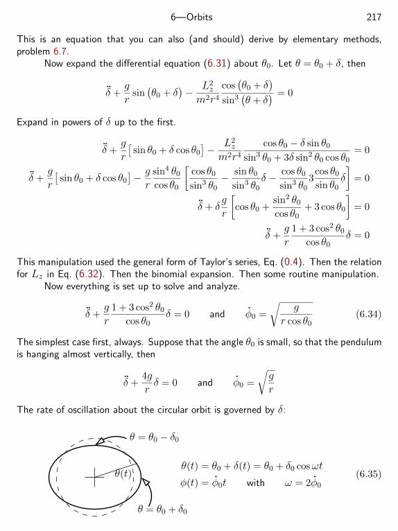
6—Orbits 217
This is an equation that you can also (and should) derive by elementary methods,problem 6.7.
Now expand the differential equation (6.31) about θ0. Let θ = θ0 + δ, then
δ +gr
sin(θ0 + δ
)− L2
z
m2r4
cos(θ0 + δ
)sin3
(θ + δ
) = 0
Expand in powers of δ up to the first.
δ +gr
[sin θ0 + δ cos θ0
]− L2
z
m2r4
cos θ0 − δ sin θ0
sin3 θ0 + 3δ sin2 θ0 cos θ0= 0
δ +gr
[sin θ0 + δ cos θ0
]− gr
sin4 θ0
cos θ0
[cos θ0
sin3 θ0− sin θ0
sin3 θ0δ − cos θ0
sin3 θ03
cos θ0
sin θ0δ
]= 0
δ + δgr
[cos θ0 +
sin2 θ0
cos θ0+ 3 cos θ0
]= 0
δ +gr
1 + 3 cos2 θ0
cos θ0δ = 0
This manipulation used the general form of Taylor’s series, Eq. (0.4). Then the relationfor Lz in Eq. (6.32). Then the binomial expansion. Then some routine manipulation.
Now everything is set up to solve and analyze.
δ +gr
1 + 3 cos2 θ0
cos θ0δ = 0 and φ0 =
√g
r cos θ0(6.34)
The simplest case first, always. Suppose that the angle θ0 is small, so that the pendulumis hanging almost vertically, then
δ +4grδ = 0 and φ0 =
√gr
The rate of oscillation about the circular orbit is governed by δ:
θ = θ0 − δ0
θ = θ0 + δ0
θ(t)θ(t) = θ0 + δ(t) = θ0 + δ0 cosωt
φ(t) = φ0t with ω = 2φ0
(6.35)
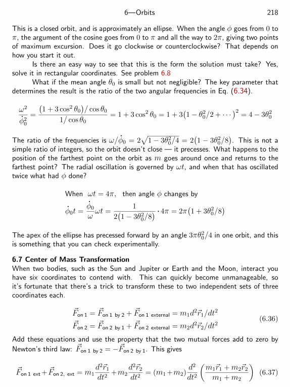
6—Orbits 218
This is a closed orbit, and is approximately an ellipse. When the angle φ goes from 0 toπ, the argument of the cosine goes from 0 to π and all the way to 2π, giving two pointsof maximum excursion. Does it go clockwise or counterclockwise? That depends onhow you start it out.
Is there an easy way to see that this is the form the solution must take? Yes,solve it in rectangular coordinates. See problem 6.8
What if the mean angle θ0 is small but not negligible? The key parameter thatdetermines the result is the ratio of the two angular frequencies in Eq. (6.34).
ω2
φ20
=
(1 + 3 cos2 θ0
)/ cos θ0
1/ cos θ0= 1 + 3 cos2 θ0 = 1 + 3
(1− θ2
0/2 + · · ·)2
= 4− 3θ20
The ratio of the frequencies is ω/φ0 = 2√
1− 3θ20/4 = 2
(1 − 3θ2
0/8). This is not a
simple ratio of integers, so the orbit doesn’t close — it precesses. What happens to theposition of the farthest point on the orbit as m goes around once and returns to thefarthest point? The radial oscillation is governed by ωt, and when that has oscillatedtwice what had φ done?
When ωt = 4π, then angle φ changes by
φ0t =φ0
ωωt =
1
2(1− 3θ2
0/8) . 4π = 2π
(1 + 3θ2
0/8)
The apex of the ellipse has precessed forward by an angle 3πθ20/4 in one orbit, and this
is something that you can check experimentally.
6.7 Center of Mass TransformationWhen two bodies, such as the Sun and Jupiter or Earth and the Moon, interact youhave six coordinates to contend with. This can quickly become unmanageable, soit’s fortunate that there’s a trick to transform these to two independent sets of threecoordinates each.
~Fon 1 = ~Fon 1 by 2 + ~Fon 1 external = m1d2~r1/dt
2
~Fon 2 = ~Fon 2 by 1 + ~Fon 2 external = m2d2~r2/dt
2(6.36)
Add these equations and use the property that the two mutual forces add to zero by
Newton’s third law: ~Fon 1 by 2 = −~Fon 2 by 1. This gives
~Fon 1 ext + ~Fon 2, ext = m1d2~r1
dt2+m2
d2~r2
dt2= (m1 +m2)
d2
dt2
(m1~r1 +m2~r2
m1 +m2
)(6.37)
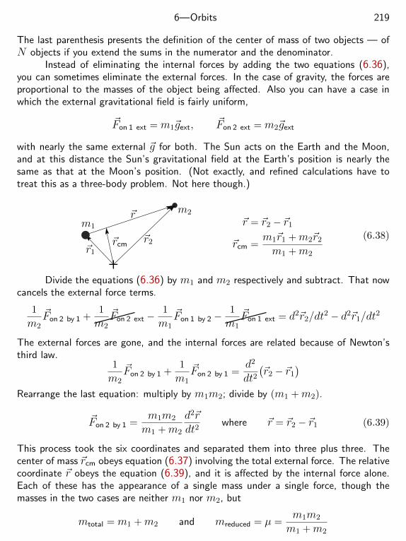
6—Orbits 219
The last parenthesis presents the definition of the center of mass of two objects — ofN objects if you extend the sums in the numerator and the denominator.
Instead of eliminating the internal forces by adding the two equations (6.36),you can sometimes eliminate the external forces. In the case of gravity, the forces areproportional to the masses of the object being affected. Also you can have a case inwhich the external gravitational field is fairly uniform,
~Fon 1 ext = m1~gext, ~Fon 2 ext = m2~gext
with nearly the same external ~g for both. The Sun acts on the Earth and the Moon,and at this distance the Sun’s gravitational field at the Earth’s position is nearly thesame as that at the Moon’s position. (Not exactly, and refined calculations have totreat this as a three-body problem. Not here though.)
~r1
~r2~rcm
~rm1
m2
~r = ~r2 − ~r1
~rcm =m1~r1 +m2~r2
m1 +m2
(6.38)
Divide the equations (6.36) by m1 and m2 respectively and subtract. That nowcancels the external force terms.
1
m2
~Fon 2 by 1 +1
m2
~Fon 2 ext −1
m1
~Fon 1 by 2 −1
m1
~Fon 1 ext = d2~r2/dt2 − d2~r1/dt
2
The external forces are gone, and the internal forces are related because of Newton’sthird law.
1
m2
~Fon 2 by 1 +1
m1
~Fon 2 by 1 =d2
dt2(~r2 − ~r1
)Rearrange the last equation: multiply by m1m2; divide by (m1 +m2).
~Fon 2 by 1 =m1m2
m1 +m2
d2~rdt2
where ~r = ~r2 − ~r1 (6.39)
This process took the six coordinates and separated them into three plus three. Thecenter of mass ~rcm obeys equation (6.37) involving the total external force. The relativecoordinate ~r obeys the equation (6.39), and it is affected by the internal force alone.Each of these has the appearance of a single mass under a single force, though themasses in the two cases are neither m1 nor m2, but
mtotal = m1 +m2 and mreduced = µ =m1m2
m1 +m2
6—Orbits 220
The “reduced mass” is the combination that takes the place of the ordinary mass inthe transformed equation. These two equations are
~Ftot,ext = Mtotd2~rcm
dt2and ~Fon 2 by 1 = µ
d2~rdt2
(6.40)
where µ is a common notation for the reduced mass. Some people use mr. If the massm1 is much larger than m2, this reduced mass is close to m2 and the correction fromtreating m1 as fixed is small. All the mathematics done in solving the gravitationalorbit problem is now the same except for some changes in the symbols. For example,Eq. (6.16) becomes
T =2π√
G(M +m)a3/2 (6.41)
As this transformation to center of mass and relative coordinates applies only un-der the assumption that the external force is uniform, the first equation, the one for theacceleration of the center of mass, is trivial. All the action is in the relative coordinate.There are still other circumstances in which the external forces are not gravitational,but are negligible anyway. Then you still have the center of mass transformation to therelative coordinate ~r. For example the hydrogen atom has a nucleus and an electron,and in the hydrogen gas the distance to neighboring atoms is typically large enough thatthe interactions are negligible. When you study some quantum theory, enough to beable to work out the structure of the hydrogen atom, the reduced mass of the nucleusand the electron is what appears in the energy calculations. It is a small correctionbecause the proton’s mass is 1836 times that of the electron. If you replace the protonby a deuteron (twice the mass) the energies will change but slightly, though still enoughto be detected.
For the Earth-Moon system, mEarth = 81mMoon, so the reduced mass µ =(81/82)mMoon. The center of mass is about 1000 km below the Earth’s surface. In abinary star system, two stars orbit each other. If their masses are the same, then thereduced mass is µ = m2/2m = m/2.
Extrasolar PlanetsIt is now possible to find planets around other stars, and the first method that borefruit in this search was an extension of this analysis of the center of mass. To see aplanet of another star directly you have to be very lucky, and only this year (2008) wasthere an instance of this. You can however detect the motion of the star itself. Whatis that? Solve for ~rst and ~rpl.
~rcm =mst~rst +mpl~rpl
mst +mpland ~r = ~rpl − ~rst
=⇒ ~rst = ~rcm −mpl
mst +mpl~r and ~rpl = ~rcm +
mst
mst +mpl~r
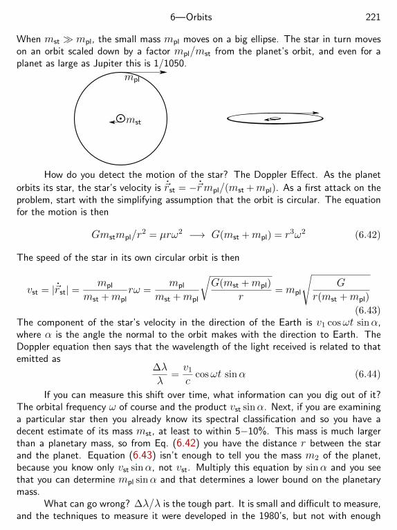
6—Orbits 221
When mst mpl, the small mass mpl moves on a big ellipse. The star in turn moveson an orbit scaled down by a factor mpl/mst from the planet’s orbit, and even for aplanet as large as Jupiter this is 1/1050.
mst
mpl
How do you detect the motion of the star? The Doppler Effect. As the planet
orbits its star, the star’s velocity is ~rst = −~rmpl/(mst +mpl). As a first attack on theproblem, start with the simplifying assumption that the orbit is circular. The equationfor the motion is then
Gmstmpl/r2 = µrω2 −→ G(mst +mpl) = r3ω2 (6.42)
The speed of the star in its own circular orbit is then
vst = |~rst| =mpl
mst +mplrω =
mpl
mst +mpl
√G(mst +mpl)
r= mpl
√G
r(mst +mpl)
(6.43)The component of the star’s velocity in the direction of the Earth is v1 cosωt sinα,where α is the angle the normal to the orbit makes with the direction to Earth. TheDoppler equation then says that the wavelength of the light received is related to thatemitted as
∆λλ
=v1
ccosωt sinα (6.44)
If you can measure this shift over time, what information can you dig out of it?The orbital frequency ω of course and the product vst sinα. Next, if you are examininga particular star then you already know its spectral classification and so you have adecent estimate of its mass mst, at least to within 5−10%. This mass is much largerthan a planetary mass, so from Eq. (6.42) you have the distance r between the starand the planet. Equation (6.43) isn’t enough to tell you the mass m2 of the planet,because you know only vst sinα, not vst. Multiply this equation by sinα and you seethat you can determine mpl sinα and that determines a lower bound on the planetarymass.
What can go wrong? ∆λ/λ is the tough part. It is small and difficult to measure,and the techniques to measure it were developed in the 1980’s, but not with enough
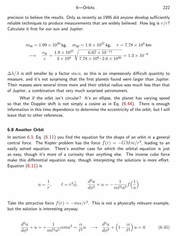
6—Orbits 222
precision to believe the results. Only as recently as 1995 did anyone develop sufficiently
reliable techniques to produce measurements that are widely believed. How big is v/c?Calculate it first for our sun and Jupiter:
mst = 1.99× 1030 kg, mpl = 1.9× 1027 kg, r = 7.78× 10⁸ km
−→ vst
c=
1.9× 1027
3× 10⁸
√6.67× 10⁻¹¹
7.78× 10⁸ . 2.0× 1030= 1.3× 10⁻⁶
∆λ/λ is still smaller by a factor sinα, so this is an impressively difficult quantity to
measure, and it’s not surprising that the first planets found were larger than Jupiter.
Their masses were several times more and their orbital radius was much less than that
of Jupiter, a combination that very much surprised astronomers.
What if the orbit isn’t circular? It’s an ellipse, the planet has varying speed
so that the Doppler shift is not simply a cosine as in Eq. (6.44). There is enough
information in this time dependence to determine the eccentricity of the orbit, but I will
leave that to other references.
6.8 Another Orbit
In section 6.3, Eq. (6.11) you find the equation for the shape of an orbit in a general
central force. The Kepler problem has the force f(r) = −GMm/r2, leading to an
easily solved equation. There’s another case for which the orbital equation is just
as easy, though it’s more of a curiosity than anything else. The inverse cube force
make this differential equation easy, though interpreting the solutions is more effort.
Equation (6.11) is
u =1
r, ` = r2φ,
d2udφ2
+ u = − 1
m`2u2f( 1
u
)
Take the attractive force f(r) = −mα/r3. This is not a physically relevant example,
but the solution is interesting anyway.
d2udφ2
+ u = +1
m`2u2αmu3 =
α`2u −→ d2u
dφ2+(
1− α`2
)u = 0 (6.45)
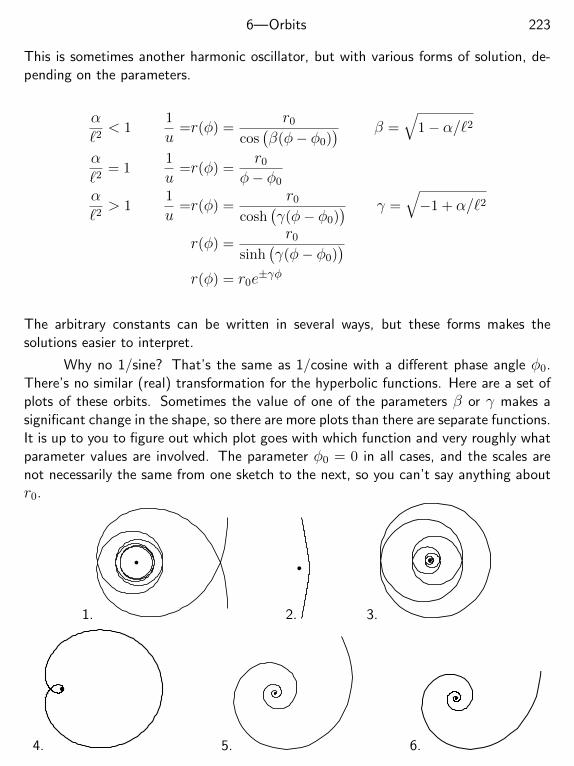
6—Orbits 223
This is sometimes another harmonic oscillator, but with various forms of solution, de-pending on the parameters.
α`2< 1
1
u=r(φ) =
r0
cos(β(φ− φ0)
) β =√
1− α/`2
α`2
= 11
u=r(φ) =
r0
φ− φ0
α`2> 1
1
u=r(φ) =
r0
cosh(γ(φ− φ0)
) γ =√−1 + α/`2
r(φ) =r0
sinh(γ(φ− φ0)
)r(φ) = r0e
±γφ
The arbitrary constants can be written in several ways, but these forms makes thesolutions easier to interpret.
Why no 1/sine? That’s the same as 1/cosine with a different phase angle φ0.There’s no similar (real) transformation for the hyperbolic functions. Here are a set ofplots of these orbits. Sometimes the value of one of the parameters β or γ makes asignificant change in the shape, so there are more plots than there are separate functions.It is up to you to figure out which plot goes with which function and very roughly whatparameter values are involved. The parameter φ0 = 0 in all cases, and the scales arenot necessarily the same from one sketch to the next, so you can’t say anything aboutr0.
1. 2. 3.
4. 5. 6.
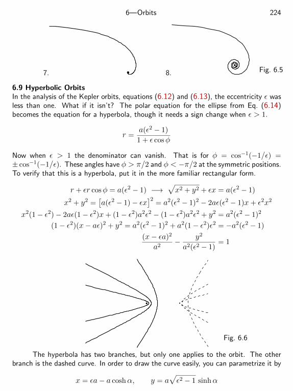
6—Orbits 224
7. 8. Fig. 6.5
6.9 Hyperbolic OrbitsIn the analysis of the Kepler orbits, equations (6.12) and (6.13), the eccentricity ε wasless than one. What if it isn’t? The polar equation for the ellipse from Eq. (6.14)becomes the equation for a hyperbola, though it needs a sign change when ε > 1.
r =a(ε2 − 1)
1 + ε cosφ
Now when ε > 1 the denominator can vanish. That is for φ = cos−1(−1/ε) =± cos−1(−1/ε). These angles have φ > π/2 and φ < −π/2 at the symmetric positions.To verify that this is a hyperbola, put it in the more familiar rectangular form.
r + εr cosφ = a(ε2 − 1) −→√x2 + y2 + εx = a(ε2 − 1)
x2 + y2 =[a(ε2 − 1)− εx
]2= a2(ε2 − 1)2 − 2aε(ε2 − 1)x+ ε2x2
x2(1− ε2)− 2aε(1− ε2)x+ (1− ε2)a2ε2 − (1− ε2)a2ε2 + y2 = a2(ε2 − 1)2
(1− ε2)(x− aε)2 + y2 = a2(ε2 − 1)2 + a2(1− ε2)ε2 = −a2(ε2 − 1)
(x− εa)2
a2− y2
a2(ε2 − 1)= 1
Fig. 6.6
The hyperbola has two branches, but only one applies to the orbit. The otherbranch is the dashed curve. In order to draw the curve easily, you can parametrize it by
x = εa− a coshα, y = a√ε2 − 1 sinhα
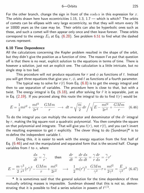
6—Orbits 225
For the other branch, change the sign in front of the coshα in this expression for x.The orbits drawn here have eccentricities 1.15, 1.3, 1.7 — which is which? The orbitsof comets can be ellipses with very large eccentricity, so that they will return every 76or 10000 years as the case may be. Their orbits can also be hyperbolic ones such asthese, and such a comet will then appear only once and then leave forever. These orbitscorrespond to the energy E3 at Eq. (6.20). See problem 6.51 to find what the dashedcurves represent.
6.10 Time DependenceAll the calculations concerning the Kepler problem resulted in the shape of the orbit,but they didn’t give the position as a function of time. The reason I’ve put that questionoff is that there is no neat, explicit solution to the equations in terms of time. There ishowever a solution, just not an explicit one. The calculation is a little intricate, but nosingle step is too bad.
This procedure will not produce equations for r and φ as functions of t. Insteadyou will get three equations that give you r, φ, and t as functions of a fourth parameter.
The typical way to solve for r(t) from Eq. (6.8) is to get the energy integral andthen to use separation of variables. The procedure here is close to that, but with atwist. The energy integral is Eq. (6.18), and after solving for r it is separable, just asin Eq. (2.19). If you proceed along this route the integral to do to find t(r) would be
E =1
2mr2 +
m`2
2r2− GMm
r−→ dt =
√m2dr
/√E − m`
2
2r2+GMmr
(6.46)
To do the integral you can multiply the numerator and denominator of the dr integralby r, making the big square root a quadratic polynomial. You then complete the squareon that polynomial and integrate. That will give you t(r), not r(t), and you can’t invertthe resulting expression to get r explicitly. The clever thing to do (Sundman)* is tore-define the independent variable t.
Doing this, it is easier to work with the energy equation from the first half ofEq. (6.46) and not the manipulated and separated form that is the second half. Changevariables from t to s, where
dsdt
=γr, then
drdt
=drdsdsdt
=γrdrds
=γrr′
E =m2
γ2
r2
(r′)2−GMm
r+m`2
2r2−→ 1
2m(r′)2−GMm
γ2r+
m`2
2γ2=Eγ2r2 (6.47)
* It is sometimes said that the general solution for the time dependence of threemutually orbiting masses is impossible. Sundman showed that this is not so, demon-strating that it is possible to find a series solution in powers of t1/3.
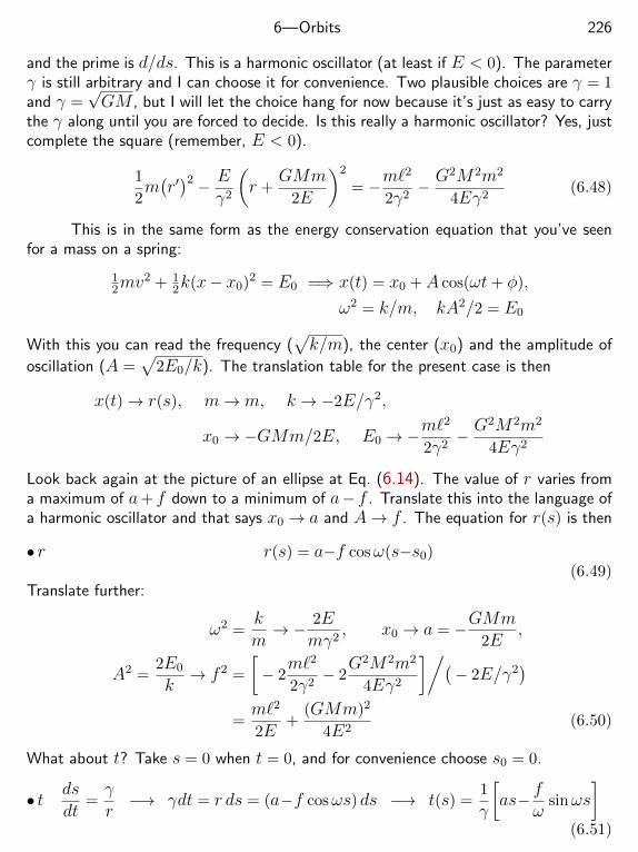
6—Orbits 226
and the prime is d/ds. This is a harmonic oscillator (at least if E < 0). The parameterγ is still arbitrary and I can choose it for convenience. Two plausible choices are γ = 1and γ =
√GM , but I will let the choice hang for now because it’s just as easy to carry
the γ along until you are forced to decide. Is this really a harmonic oscillator? Yes, justcomplete the square (remember, E < 0).
1
2m(r′)2 − E
γ2
(r +
GMm2E
)2
= −m`2
2γ2− G
2M2m2
4Eγ2(6.48)
This is in the same form as the energy conservation equation that you’ve seenfor a mass on a spring:
12mv
2 + 12k(x− x0)2 = E0 =⇒ x(t) = x0 +A cos(ωt+ φ),
ω2 = k/m, kA2/2 = E0
With this you can read the frequency (√k/m), the center (x0) and the amplitude of
oscillation (A =√
2E0/k). The translation table for the present case is then
x(t)→ r(s), m→m, k → −2E/γ2,
x0 → −GMm/2E, E0 → −m`2
2γ2− G
2M2m2
4Eγ2
Look back again at the picture of an ellipse at Eq. (6.14). The value of r varies froma maximum of a+ f down to a minimum of a− f . Translate this into the language ofa harmonic oscillator and that says x0 → a and A→ f . The equation for r(s) is then
• r r(s) = a−f cosω(s−s0)(6.49)
Translate further:
ω2 =km→ − 2E
mγ2, x0 → a = −GMm
2E,
A2 =2E0
k→ f 2 =
[− 2
m`2
2γ2− 2
G2M2m2
4Eγ2
]/(− 2E/γ2
)=m`2
2E+
(GMm)2
4E2(6.50)
What about t? Take s = 0 when t = 0, and for convenience choose s0 = 0.
• t dsdt
=γr−→ γdt = r ds = (a−f cosωs) ds −→ t(s) =
1
γ
[as− f
ωsinωs
](6.51)
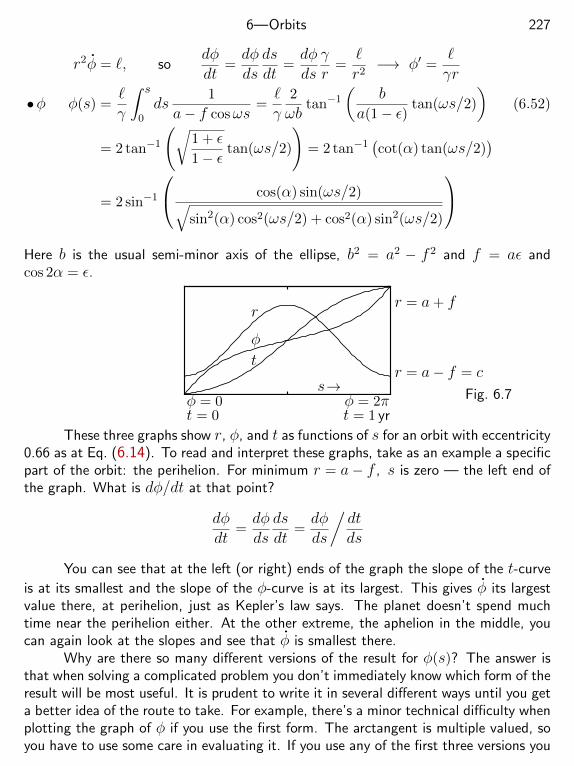
6—Orbits 227
r2φ = `, sodφdt
=dφdsdsdt
=dφdsγr
=`r2−→ φ′ =
`γr
•φ φ(s) =`γ
∫ s
0ds
1
a− f cosωs=`γ
2
ωbtan−1
(b
a(1− ε)tan(ωs/2)
)(6.52)
= 2 tan−1
(√1 + ε1− ε
tan(ωs/2)
)= 2 tan−1
(cot(α) tan(ωs/2)
)= 2 sin−1
cos(α) sin(ωs/2)√sin2(α) cos2(ωs/2) + cos2(α) sin2(ωs/2)
Here b is the usual semi-minor axis of the ellipse, b2 = a2 − f 2 and f = aε andcos 2α = ε.
r
t
φ
s→
r = a+ f
r = a− f = c
φ = 0 φ = 2πt = 0 t = 1 yr
Fig. 6.7
These three graphs show r, φ, and t as functions of s for an orbit with eccentricity0.66 as at Eq. (6.14). To read and interpret these graphs, take as an example a specificpart of the orbit: the perihelion. For minimum r = a− f , s is zero — the left end ofthe graph. What is dφ/dt at that point?
dφdt
=dφdsdsdt
=dφds
/dtds
You can see that at the left (or right) ends of the graph the slope of the t-curve
is at its smallest and the slope of the φ-curve is at its largest. This gives φ its largestvalue there, at perihelion, just as Kepler’s law says. The planet doesn’t spend muchtime near the perihelion either. At the other extreme, the aphelion in the middle, youcan again look at the slopes and see that φ is smallest there.
Why are there so many different versions of the result for φ(s)? The answer isthat when solving a complicated problem you don’t immediately know which form of theresult will be most useful. It is prudent to write it in several different ways until you geta better idea of the route to take. For example, there’s a minor technical difficulty whenplotting the graph of φ if you use the first form. The arctangent is multiple valued, soyou have to use some care in evaluating it. If you use any of the first three versions you
6—Orbits 228
may need to write the tangent as (sine over cosine) and then to treat the arctangentas a function of two variables. That will let you keep track of which quadrant you arein. The fourth version doesn’t have this difficulty. The third version however will haveadvantages when you are start to look at unbound (E > 0) orbits.
Does this complicated looking set of equations reduce to the correct results whenthe orbit is a circle? ε = 0, b = a, f = 0, so
r(s) = −GMm2E
= a, t(s) =1
γas, φ(s) =
`γ
2
ωatan−1 tan(ωs/2) =
`γas
The statement that A = 0 (no variation in r) determines `.
A2 =m`2
2E+
(GMm)2
4E2= 0 −→ `2 = −G
2M2m2E
−→ ` =GM√−2E/m
dφdt
=(`/γa)ds
(a/γ)ds=
`a2
and that is (r2φ/r2) as it should be.
Exercises
1 Sketch a Lissajous figure for the case ω2 = 10ω1.
2 What is the ratio of the solar power reaching Earth at its perihelion (January) to thatat its aphelion (July)? Now what about Mercury and Mars?
3 What figure do you get if the sum of the squares of the distances from two pointsadd to a constant?
4 Communications satellites are placed in orbits above the Earth’s equator so thatrelative to the Earth, they stay in a fixed position. How far are they from the Earth’scenter and from the Earth’s surface?
5 A mass is in orbit about a fixed center, and the attractive force law is such that it canorbit in a circle at radius r0 from that center. The angular speed is φ0 = ω0. The orbitis slightly perturbed, so that the mass orbits in a nearly circular orbit and the radiusoscillates about the circle with frequency 3ω0/2. Draw the resulting orbit and explainthe reasons that your drawing appears as it does.
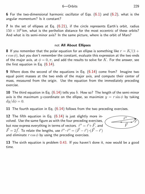
6—Orbits 229
6 For the two-dimensional harmonic oscillator of Eqs. (6.1) and (6.2), what is theangular momentum? Is it constant?
7 In the set of ellipses at Eq. (6.21), if the circle represents Earth’s orbit, radius150 × 106 km, what is the perihelion distance for the most eccentric of these orbits?And what is its semi-minor axis? In the same picture, where is the orbit of Mars?
not All About Ellipses
8 If you remember that the polar equation for an ellipse is something like r = K/(1 +ε cosφ), but you don’t remember the constant, evaluate this expression at the two endsof the major axis, at φ = 0, π, and add the results to solve for K. For the answer, seethe first equation in Eq. (6.14).
9 Where does the second of the equations in Eq. (6.14) come from? Imagine twoequal point masses at the two ends of the major axis, and compute their center ofmass, measured from the origin. Use the equation from the immediately precedingexercise.
10 The third equation in Eq. (6.14) tells you b. How so? The length of the semi-minoraxis is the maximum y-coordinate on the ellipse, so maximize y = r sinφ by takingdy/dφ = 0.
11 The fourth equation in Eq. (6.14) follows from the two preceding exercises.
~r~r ′
~F
12 The fifth equation in Eq. (6.14) is just slightly more in-volved. Use the same figure as with the four preceding exercises,
but now express everything in terms of vectors. ~r ′ = ~r+ ~F , and~F = 2~f . To relate the lengths, use ~r ′ .~r ′ = (~F − ~r ) .(~F − ~r )and eliminate r cosφ by using the preceding exercises.
13 The sixth equation is problem 0.43. If you haven’t done it, now would be a goodtime.
6—Orbits 230
Problems
6.1 In Eq. (6.8), if the force f is zero, the motion should somehow represent a straightline. Take the case as represented in rectangular coordinates by x = x0 and y = v0t;translate it into an expression for r(t), and show that it works.
6.2 The Lissajous curve in Eq. (6.4) can be expressed as a polynomial equation in xand y. Do so.
6.3 Transform Eq. (6.9) into the form Eq. (6.10) to show that this is the polar form ofan ellipse. Not really. Find the conditions on A, B, and C so that it is an ellipse. Whatshapes do you get if these conditions are violated? Catalog and sketch the possibilities,including B = C.
6.4 For a planet in circular orbit around the sun, what is the planet’s speed as a functionof distance from the sun?
6.5 In Eq. (6.11), let the force be zero. Solve, and show what the shape of the orbitis.
6.6 If r1 and r2 are the distances of perihelion and aphelion, what are their arithmeticand their geometric means?
6.7 Use elementary methods of the sort that you’ve seen in a previous course (a = v2/rand the like), and derive the period of a conical pendulum. This is another name for thespherical pendulum in the simple special case that the mass moves on a circle parallelto the floor.
6.8˙ For the spherical pendulum that is oscillating through small angles, show that thepotential energy in Eq. (6.30) can be written in the form U = A + B(x2 + y2) forappropriate A and B. Then find the force from this potential energy as Fx = −∂U/∂xand similarly for y. Now ~F = m~a gives two separate equations for x and y. Solvethem and show that the solution agrees with Eq. (6.35)
6.9˙ Start from ~r(t) = xr(t) cos(φ(t)
)+ yr(t) sin
(φ(t)
)and differentiate once and
twice. Rearrange into radial and tangential components to derive the equation foracceleration in terms of r and φ.
6.10˙ For the spherical pendulum with an almost circular orbit, what is the shape ofthe orbit if you have set it moving so fast that the cord holding the mass is almosthorizontal?
6—Orbits 231
6.11 The Earth-Sun distance is 150 Gm. Start from elementary principles, known data,and the value of G to deduce the mass of the Sun.
6.12 If the solar system is embedded in a uniform dust cloud of density ρ, find theforce on a planet as a function of r. Evaluate the effect on the planet’s orbit caused bythe dust.
6.13 A particle in a central force moves in a spiral orbit given by r = aφ. Find theforce and find the time dependence of φ, i.e. , φ(t).
6.14 Start from Eq. (6.28) and examine the case of the Kepler problem. Plot the polarcoordinate orbit r(φ) and compare the result to the exact solution.
6.15 The force on an orbiting planet of mass m is given as the sum of two terms: Oneis a central force; the other is a velocity dependent friction term.
~F1 = −F0 sech3(αr)K3(βr)r, ~F2 = −γ~v
where sech is the hyperbolic secant and K3 is the Bessel function of the third kind withimaginary argument. The angular momentum about the origin is given at time t = 0
to be ~L0. Find the angular momentum at later times.
6.16 The force on a mass m is given to be ~F = kr/r3. The mass is given an initialspeed v0 and is aimed so that in the absence of forces, it will miss the center of therepulsive force by a distance b (the impact parameter). Find the distance of closestapproach to the origin and what is its speed when it reaches that point? (Don’t solvefor the orbit unless you need the extra work.
6.17 ˙ If the Earth stopped still with respect to the sun, how much time would it taketo fall into the sun? Set up the equation of motion for straight line radial motion, getthe conservation of energy equation and rearrange to get dt in terms of dr. Set up awell-defined definite integral for the final answer, then evaluate it. Unless you’re cleverwith integrals, expect to look up this integral in a table. How many days? And sinceyou’ve done the work already, go back to the exercise #4 on page 193 to find how muchtime it takes from the onset of spaghettification.
6.18˙ A central attractive force is given by the equation ~F = −αrβ r. Here α > 0,but β can have either sign. (a) Assume that the orbit is almost circular and find thevalues of β for which the orbit is stable. (b) Find the values of β for which the orbit isclosed — at least in the perturbation approximation used in this chapter.
6.19 A particle in a central force moves in a spiral orbit given by r = a/φ. Find theforce that does this. And sketch this orbit.
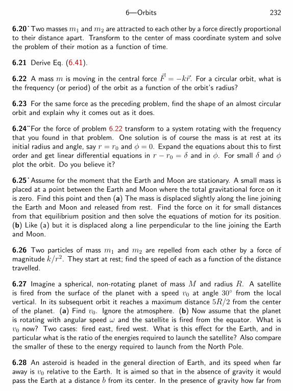
6—Orbits 232
6.20˙ Two massesm1 andm2 are attracted to each other by a force directly proportionalto their distance apart. Transform to the center of mass coordinate system and solvethe problem of their motion as a function of time.
6.21 Derive Eq. (6.41).
6.22 A mass m is moving in the central force ~F = −k~r. For a circular orbit, what isthe frequency (or period) of the orbit as a function of the orbit’s radius?
6.23 For the same force as the preceding problem, find the shape of an almost circularorbit and explain why it comes out as it does.
6.24¨For the force of problem 6.22 transform to a system rotating with the frequencythat you found in that problem. One solution is of course the mass is at rest at itsinitial radius and angle, say r = r0 and φ = 0. Expand the equations about this to firstorder and get linear differential equations in r − r0 = δ and in φ. For small δ and φplot the orbit. Do you believe it?
6.25˙ Assume for the moment that the Earth and Moon are stationary. A small mass isplaced at a point between the Earth and Moon where the total gravitational force on itis zero. Find this point and then (a) The mass is displaced slightly along the line joiningthe Earth and Moon and released from rest. Find the force on it for small distancesfrom that equilibrium position and then solve the equations of motion for its position.(b) Like (a) but it is displaced along a line perpendicular to the line joining the Earthand Moon.
6.26 Two particles of mass m1 and m2 are repelled from each other by a force ofmagnitude k/r2. They start at rest; find the speed of each as a function of the distancetravelled.
6.27 Imagine a spherical, non-rotating planet of mass M and radius R. A satelliteis fired from the surface of the planet with a speed v0 at angle 30 from the localvertical. In its subsequent orbit it reaches a maximum distance 5R/2 from the centerof the planet. (a) Find v0. Ignore the atmosphere. (b) Now assume that the planetis rotating with angular speed ω and the satellite is fired from the equator. What isv0 now? Two cases: fired east, fired west. What is this effect for the Earth, and inparticular what is the ratio of the energies required to launch the satellite? Also comparethe smaller of these to the energy required to launch from the North Pole.
6.28 An asteroid is headed in the general direction of Earth, and its speed when faraway is v0 relative to the Earth. It is aimed so that in the absence of gravity it wouldpass the Earth at a distance b from its center. In the presence of gravity how far from
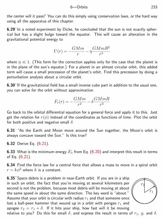
6—Orbits 233
the center will it pass? You can do this simply using conservation laws, or the hard wayusing all the apparatus of this chapter.
6.29˙ In a noted experiment by Dicke, he concluded that the sun is not exactly spher-ical but has a slight bulge toward the equator. This will cause an alteration in thegravitational potential energy to
U(r) = −GMmr
− ηGMmR2
r3
where η 1. (This form for the correction applies only for the case that the planet isin the plane of the sun’s equator.) For a planet in an almost circular orbit, this addedterm will cause a small precession of the planet’s orbit. Find this precession by doing aperturbation analysis about a circular orbit.
6.30˙ If the gravitational field has a small inverse cube part in addition to the usual one,you can solve for the orbit without approximation.
Fr(r) = −GMmr2
− δGMmRr3
Go back to the orbital differential equation for a general force and apply it to this. Justget the relation for r(φ) instead of the coordinates as functions of time. Plot the orbitfor both positive and negative small δ.
6.31 “As the Earth and Moon move around the Sun together, the Moon’s orbit isalways concave toward the Sun.” Is this true?
6.32 Derive Eq. (6.21).
6.33 What is the minimum energy E1 from Eq. (6.20) and interpret this result in termsof Eq. (6.21).
6.34 Find the force law for a central force that allows a mass to move in a spiral orbitr = kφ2 where k is a constant.
r2
r1
6.35˙ Space debris is a problem in near-Earth orbit. If you are in a shipin such an orbit, the fact that you’re moving at several kilometers persecond is not the problem, because most debris will be moving at aboutthe same speed in about the same direction. The key word is “about.”Assume that your orbit is circular with radius r1 and that someone oncelost a ball-peen hammer that wound up in a orbit with perigee r1 andapogee r2 = r1 + δ. If it hits your ship, how fast will it be movingrelative to you? Do this for small δ, and express the result in terms of r1, g, and δ.
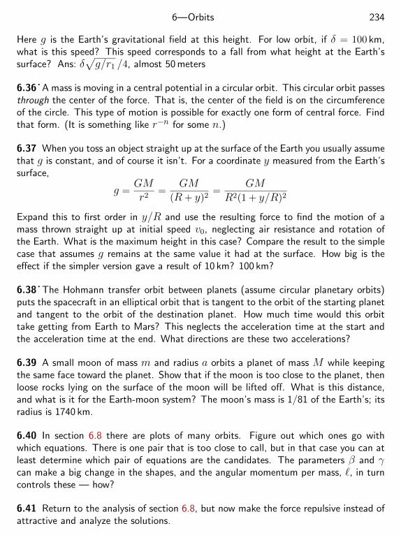
6—Orbits 234
Here g is the Earth’s gravitational field at this height. For low orbit, if δ = 100 km,what is this speed? This speed corresponds to a fall from what height at the Earth’ssurface? Ans: δ
√g/r1 /4, almost 50 meters
6.36˙ A mass is moving in a central potential in a circular orbit. This circular orbit passesthrough the center of the force. That is, the center of the field is on the circumferenceof the circle. This type of motion is possible for exactly one form of central force. Findthat form. (It is something like r−n for some n.)
6.37 When you toss an object straight up at the surface of the Earth you usually assumethat g is constant, and of course it isn’t. For a coordinate y measured from the Earth’ssurface,
g =GMr2
=GM
(R+ y)2=
GM
R2(1 + y/R)2
Expand this to first order in y/R and use the resulting force to find the motion of amass thrown straight up at initial speed v0, neglecting air resistance and rotation ofthe Earth. What is the maximum height in this case? Compare the result to the simplecase that assumes g remains at the same value it had at the surface. How big is theeffect if the simpler version gave a result of 10 km? 100 km?
6.38˙ The Hohmann transfer orbit between planets (assume circular planetary orbits)puts the spacecraft in an elliptical orbit that is tangent to the orbit of the starting planetand tangent to the orbit of the destination planet. How much time would this orbittake getting from Earth to Mars? This neglects the acceleration time at the start andthe acceleration time at the end. What directions are these two accelerations?
6.39 A small moon of mass m and radius a orbits a planet of mass M while keepingthe same face toward the planet. Show that if the moon is too close to the planet, thenloose rocks lying on the surface of the moon will be lifted off. What is this distance,and what is it for the Earth-moon system? The moon’s mass is 1/81 of the Earth’s; itsradius is 1740 km.
6.40 In section 6.8 there are plots of many orbits. Figure out which ones go withwhich equations. There is one pair that is too close to call, but in that case you can atleast determine which pair of equations are the candidates. The parameters β and γcan make a big change in the shapes, and the angular momentum per mass, `, in turncontrols these — how?
6.41 Return to the analysis of section 6.8, but now make the force repulsive instead ofattractive and analyze the solutions.
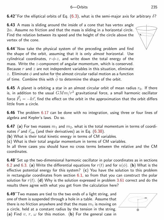
6—Orbits 235
6.42¨For the elliptical orbits of Eq. (6.3), what is the semi-major axis for arbitrary δ?
6.43 A mass is sliding around the inside of a cone that has vertex angle2α. Assume no friction and that the mass is sliding in a horizontal circle.Find the relation between its speed and the height of the circle above thevertex of the cone.
6.44˙ Now take the physical system of the preceding problem and findthe shape of the orbit, assuming that it is only almost horizontal. Usecylindrical coordinates, r-φ-z, and write down the total energy of themass. Write the z-component of angular momentum, which is conserved.Because r and z are not independent variables in this situation, eliminatez. Eliminate φ and solve for the almost circular radial motion as a function
of time. Combine this with φ to determine the shape of the orbit.
6.45 A planet is orbiting a star in an almost circular orbit of mean radius r0. If thereis, in addition to the usual GMm/r2 gravitational force, a small harmonic oscillator
force ~F1 = −k~r, find the effect on the orbit in the approximation that the orbit differslittle from a circle.
6.46 The problem 6.17 can be done with no integration, using three or four lines ofalgebra and Kepler’s laws. Do so.
6.47 (a) For two masses m1 and m2, what is the total momentum in terms of coordi-nates ~r and ~rcm (and their derivatives) as in Eq. (6.38).(b) What is their total kinetic energy in terms of CM variables.(c) What is their total angular momentum in terms of CM variables.In all three cases you should have no cross terms between the relative and the CMcoordinates.
6.48˙ Set up the two-dimensional harmonic oscillator in polar coordinates as in sections6.2 and 6.3. (a) Write the differential equations for r(t) and for u(φ). (b) What is theeffective potential energy for this system? (c) You have the solution to this problemin rectangular coordinates from section 6.1, so from that you can construct the polarsolution for r(t). (d) Why is the solution expressed in problem 3.61 correct and do theresults there agree with what you get from the calculation here?
6.49¨Two masses are tied to the two ends of a light string, andone of them is suspended through a hole in a table. Assume thatthere is no friction anywhere and that the mass m1 is moving ona circle, held at a constant radius by the tension in the string.(a) Find v, r, ω for this motion. (b) For the general case in
6—Orbits 236
which m1 has arbitrary motion in r and φ, write the total energy and the angularmomentum and use that to find the orbit of m1 if it is almost circular.Ans: φ2
0/ω20 = (m1 +m2)/3m1.
6.50˙ A satellite is in a circular orbit of radius r0 above the Earth. What is its total(kinetic plus potential) energy? If the orbit is low enough (say 200-300 km or so) therewill be some very small friction with the atmosphere, applying force of magnitude Ffr
to the satellite. In one orbit, what is the change in energy of the satellite? In that orbit,what will be the change in r? What then is the change in r per time for the satellite,dr/dt? If you make the implausible assumption that the frictional force is a constantall the way down to the Earth’s surface, how much time will it be before the satellitehits the ground? How does the speed of the satellite vary over time because of thisfrictional force?
6.51 The hyperbolic orbits in section 6.9 led to a picture in which only one half thehyperbola was the orbit. The other half (the dashed lines) didn’t seem to correspond toanything. Show that they represent the solution if the inverse square force is repulsiveinstead of attractive.
6.52¨Start from dt = r2 dφ/` and (6.13), and use contour integration to derive Ke-pler’s law Eq. (6.16).
6.53 For the orbits in section 6.8 the parameter α was positive. What orbits are thereif it is negative? Sketch the possible orbits.
6.54 For the orbital equation (6.11), what is the equation if the force has two terms,the usual Newtonian gravity plus a 1/r4 term.
f(r) = −GMmr2
− 3GMm`2
c2r4
Here, c is the speed of light. Does this even have correct dimensions? This is the orbitalequation derived from Einstein’s theory of gravity, the General Theory of relativity. Usethe methods starting with equation (6.27) to find the angle by which the ellipticalorbit described by the first term alone will precess in each orbit. Look up the orbitalparameters for the planet Mercury to get the numerical value for this result and thenconvert it into the conventionally reported value of the precession per Earth century.(43’’ per century)
6.55¨Add a uniform magnetic field to the spring force of Eq. (6.1), assuming that allthe spring constants are equal, and that the mass has a charge q. Choose the z-axisalong the direction of the magnetic field. Solve for the motion of the mass and sketchsome solutions, especially for weak fields.
6—Orbits 237
6.56 The carbon monoxide molecule, CO, can be modeled as two masses on the endsof a spring. Solve for the oscillations of this molecule, the normal modes, assumingthat the motion is along the single long axis between the atoms. Compare your resultto what appears in section 6.7, especially Eq. (6.39).
6.57 What is the period for the close orbit of a pebble around a rock? Some asteroidshave been observed with such satellites.
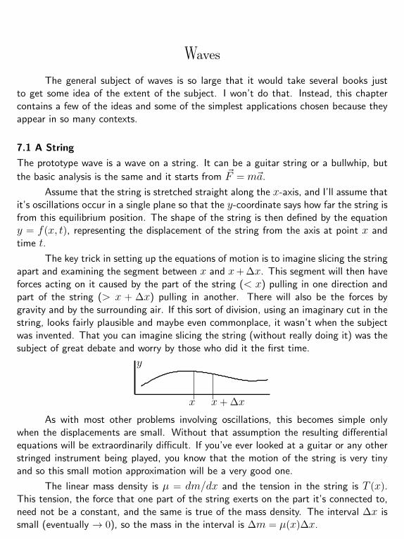
WavesThe general subject of waves is so large that it would take several books just
to get some idea of the extent of the subject. I won’t do that. Instead, this chaptercontains a few of the ideas and some of the simplest applications chosen because theyappear in so many contexts.
7.1 A String
The prototype wave is a wave on a string. It can be a guitar string or a bullwhip, but
the basic analysis is the same and it starts from ~F = m~a.
Assume that the string is stretched straight along the x-axis, and I’ll assume thatit’s oscillations occur in a single plane so that the y-coordinate says how far the string isfrom this equilibrium position. The shape of the string is then defined by the equationy = f(x, t), representing the displacement of the string from the axis at point x andtime t.
The key trick in setting up the equations of motion is to imagine slicing the stringapart and examining the segment between x and x+ ∆x. This segment will then haveforces acting on it caused by the part of the string (< x) pulling in one direction andpart of the string (> x + ∆x) pulling in another. There will also be the forces bygravity and by the surrounding air. If this sort of division, using an imaginary cut in thestring, looks fairly plausible and maybe even commonplace, it wasn’t when the subjectwas invented. That you can imagine slicing the string (without really doing it) was thesubject of great debate and worry by those who did it the first time.
y
x x+ ∆x
As with most other problems involving oscillations, this becomes simple onlywhen the displacements are small. Without that assumption the resulting differentialequations will be extraordinarily difficult. If you’ve ever looked at a guitar or any otherstringed instrument being played, you know that the motion of the string is very tinyand so this small motion approximation will be a very good one.
The linear mass density is µ = dm/dx and the tension in the string is T (x).This tension, the force that one part of the string exerts on the part it’s connected to,need not be a constant, and the same is true of the mass density. The interval ∆x issmall (eventually → 0), so the mass in the interval is ∆m = µ(x)∆x.
238
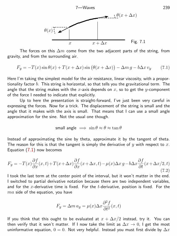
7—Waves 239
x x+ ∆x
θ(x)
θ(x+ ∆x)
Fig. 7.1
The forces on this ∆m come from the two adjacent parts of the string, fromgravity, and from the surrounding air.
Fy = −T (x) sin θ(x) + T (x+ ∆x) sin(θ(x+ ∆x)
)−∆mg − b∆xvy (7.1)
Here I’m taking the simplest model for the air resistance, linear viscosity, with a propor-tionality factor b. This string is horizontal, so that tells you the gravitational term. Theangle that the string makes with the x-axis depends on x, so to get the y-componentof the force I needed to indicate that explicitly.
Up to here the presentation is straight-forward, I’ve just been very careful inexpressing the forces. Now for a trick. The displacement of the string is small and theangle that it makes with the axis is small. That means that I can use a small angleapproximation for the sine. Not the usual one though.
small angle =⇒ sin θ ≈ θ ≈ tan θ
Instead of approximating the sine by theta, approximate it by the tangent of theta.The reason for this is that the tangent is simply the derivative of y with respect to x.Equation (7.1) now becomes
Fy = −T (x)∂f∂x
(x, t)+T (x+∆x)∂f∂x
(x+∆x, t)−µ(x)∆xg−b∆x∂f∂t
(x+∆x/2, t)
(7.2)I took the last term at the center point of the interval, but it won’t matter in the end.I switched to partial derivative notation because there are two independent variables,and for the x-derivative time is fixed. For the t-derivative, position is fixed. For thema side of the equation, you have
Fy = ∆may = µ(x)∆x∂2f∂t2
(x, t)
If you think that this ought to be evaluated at x + ∆x/2 instead, try it. You canthen verify that it won’t matter. If I now take the limit as ∆x → 0, I get the mostuninformative equation, 0 = 0. Not very helpful. Instead you must first divide by ∆x
7—Waves 240
and then take the limit.
1
∆x
[−T (x)
∂f∂x
(x, t) + T (x+ ∆x)∂f∂x
(x+ ∆x, t)
]−µ(x)g − b∂f
∂t(x+ ∆x/2, t)
= µ(x)∂2f∂t2
(x, t)
Now take the limit, and in most of the terms the limit simply evaluates the functionat x. The first term is different however, and it −→ 0/0. It is nothing more than thedefinition of a derivative. [something(x + ∆x) − something(x) divided by ∆x] Thelimit is
∂∂x
(T∂f∂x
)− µg − b∂f
∂t= µ
∂2f∂t2
(7.3)
Have I left out any physics? Yes. A thin string is easy to bend, but a thickerone resists deformation. It’s stiff and I’ve ignored this property. Is that important? It isif you are a professional piano tuner and have a demanding client. One aspect of thisproblem will appear in section 7.9.
What about Fx on the mass ∆m? Go back to the equation (7.1) and the picturethat accompanies it.
Fx = −T (x) cos θ(x) + T (x+ ∆x) cos(θ(x+ ∆x)
)In this example, because the string is horizontal there is no component from gravity.Of course if it’s vertical there is a term in ∆mg in this equation but it’s not in theFy equation. For small angles and for motion in the y-direction, Fx = ∆max is zeroand the tension is constant. I will leave the T factor as is anyway, allowing that it mayvary with x, not because it’s needed for this problem with the string but because it’sharmless, not causing any extra work. Also there are plenty of wave problems wheresomething analogous to this factor will show up and you may as well get used to it here.In most cases where I’m really solving something it will be constant.
7.2 Static caseStart with the simplest case. Nothing is moving. A string is stretched taut betweentwo posts and it sags. Let the tension and the mass density be constant here.
The equation (7.1) for the shape of the string is now
T∂2f∂x2
− µg = 0 (7.4)
This is easy to integrate. (Drop the t from f(x, t).)
f(x) = µgx2/2T +Ax+B
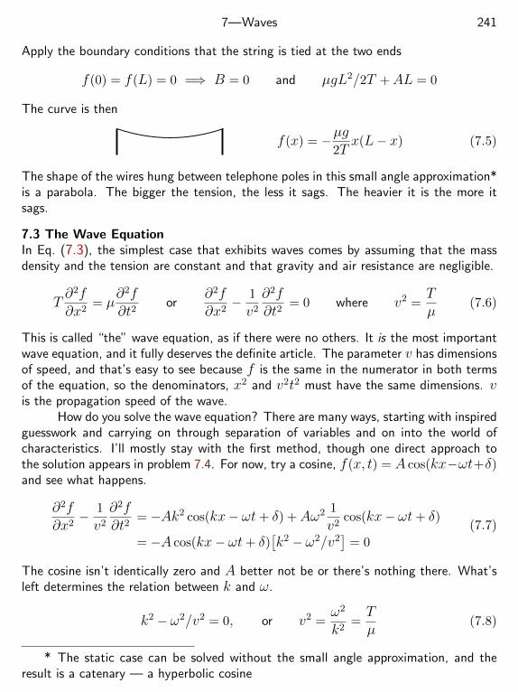
7—Waves 241
Apply the boundary conditions that the string is tied at the two ends
f(0) = f(L) = 0 =⇒ B = 0 and µgL2/2T +AL = 0
The curve is then
f(x) = −µg2Tx(L− x) (7.5)
The shape of the wires hung between telephone poles in this small angle approximation*is a parabola. The bigger the tension, the less it sags. The heavier it is the more itsags.
7.3 The Wave EquationIn Eq. (7.3), the simplest case that exhibits waves comes by assuming that the massdensity and the tension are constant and that gravity and air resistance are negligible.
T∂2f∂x2
= µ∂2f∂t2
or∂2f∂x2
− 1
v2
∂2f∂t2
= 0 where v2 =Tµ
(7.6)
This is called “the” wave equation, as if there were no others. It is the most importantwave equation, and it fully deserves the definite article. The parameter v has dimensionsof speed, and that’s easy to see because f is the same in the numerator in both termsof the equation, so the denominators, x2 and v2t2 must have the same dimensions. vis the propagation speed of the wave.
How do you solve the wave equation? There are many ways, starting with inspiredguesswork and carrying on through separation of variables and on into the world ofcharacteristics. I’ll mostly stay with the first method, though one direct approach tothe solution appears in problem 7.4. For now, try a cosine, f(x, t) = A cos(kx−ωt+δ)and see what happens.
∂2f∂x2
− 1
v2
∂2f∂t2
= −Ak2 cos(kx− ωt+ δ) +Aω2 1
v2cos(kx− ωt+ δ)
= −A cos(kx− ωt+ δ)[k2 − ω2/v2
]= 0
(7.7)
The cosine isn’t identically zero and A better not be or there’s nothing there. What’sleft determines the relation between k and ω.
k2 − ω2/v2 = 0, or v2 =ω2
k2=Tµ
(7.8)
* The static case can be solved without the small angle approximation, and theresult is a catenary — a hyperbolic cosine
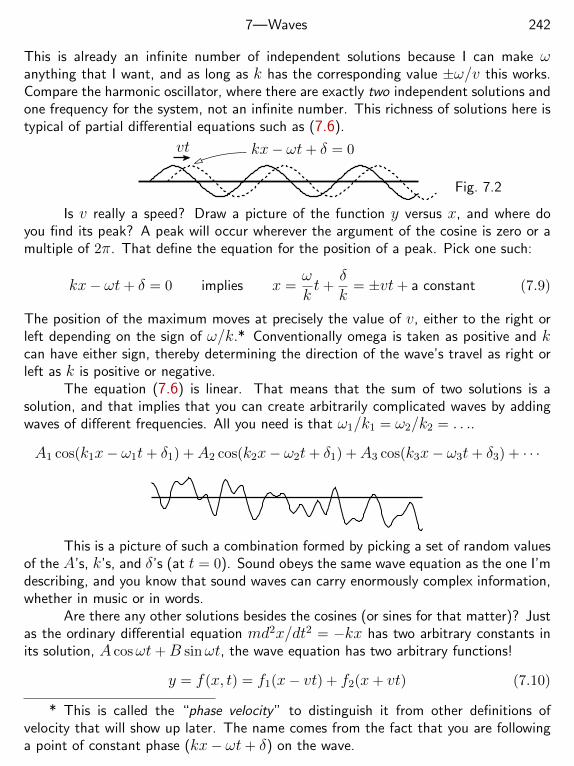
7—Waves 242
This is already an infinite number of independent solutions because I can make ωanything that I want, and as long as k has the corresponding value ±ω/v this works.Compare the harmonic oscillator, where there are exactly two independent solutions andone frequency for the system, not an infinite number. This richness of solutions here istypical of partial differential equations such as (7.6).
vt kx− ωt+ δ = 0
Fig. 7.2
Is v really a speed? Draw a picture of the function y versus x, and where doyou find its peak? A peak will occur wherever the argument of the cosine is zero or amultiple of 2π. That define the equation for the position of a peak. Pick one such:
kx− ωt+ δ = 0 implies x =ωkt+
δk
= ±vt+ a constant (7.9)
The position of the maximum moves at precisely the value of v, either to the right orleft depending on the sign of ω/k.* Conventionally omega is taken as positive and kcan have either sign, thereby determining the direction of the wave’s travel as right orleft as k is positive or negative.
The equation (7.6) is linear. That means that the sum of two solutions is asolution, and that implies that you can create arbitrarily complicated waves by addingwaves of different frequencies. All you need is that ω1/k1 = ω2/k2 = . . ..
A1 cos(k1x− ω1t+ δ1) +A2 cos(k2x− ω2t+ δ1) +A3 cos(k3x− ω3t+ δ3) + · · ·
This is a picture of such a combination formed by picking a set of random valuesof the A’s, k’s, and δ’s (at t = 0). Sound obeys the same wave equation as the one I’mdescribing, and you know that sound waves can carry enormously complex information,whether in music or in words.
Are there any other solutions besides the cosines (or sines for that matter)? Justas the ordinary differential equation md2x/dt2 = −kx has two arbitrary constants inits solution, A cosωt+B sinωt, the wave equation has two arbitrary functions!
y = f(x, t) = f1(x− vt) + f2(x+ vt) (7.10)
* This is called the “phase velocity” to distinguish it from other definitions ofvelocity that will show up later. The name comes from the fact that you are followinga point of constant phase (kx− ωt+ δ) on the wave.
7—Waves 243
The demonstration of this fact is no more than plugging in to the equation and usingthe chain rule.
∂f1
∂x= f ′1(x− vt), ∂2f1
∂x2= f ′′1 (x− vt),
∂f1
∂t= −vf ′1(x− vt), ∂2f1
∂t2= (−v)2f ′′1 (x− vt)
Substitute these into Eq. (7.6) and it works. Note: the “prime” notation is the derivativeof f with respect to its argument, not the derivative with respect to x, so that sin′ = cos.The same calculation works for f2(x+ vt). This means that any wave form will movealong the string. All that you have to do is to get it started. The cosine solution that Istarted with is simply a special case of this general solution. And yes, Eq. (7.10) is themost general solution for the wave equation. The proof is not difficult, involving only achange of variables. See problem 7.4.
Any function (well, any function with two derivatives) will provide a solution,and that is why waves can carry so much information. To find the behavior of a singlemass, you need to specify its initial position and velocity, and essentially the same thinghappens here. Specify the initial position and initial velocity at each point on the string.Assume
f(x, 0) = F (x),∂f∂t
(x, 0) = G(x) (7.11)
Apply Eq. (7.10) for the general solution, then
f1(x)+f2(x) = F (x) −→ f ′1(x)+f ′2(x) = F ′(x), and −vf ′1(x)+vf ′2(x) = G(x)
Solve for f ′1 and f ′2.
f ′1(x) = 12F′(x)− 1
2vG(x), f ′2(x) = 12F′(x) + 1
2vG(x)
And now do two integrals. These are all functions of a single variable, so nothingunusual happens. You have constants of integration, but they’re easy to handle.
f1(x) =1
2F (x)− 1
2v
∫ x
0G(x′) dx′ f2(x) =
1
2F (x) +
1
2v
∫ x
0G(x′) dx′
y = f(x, t) =1
2F (x− vt)− 1
2v
∫ x−vt
0G(x′) dx′ +
1
2F (x+ vt) +
1
2v
∫ x+vt
0G(x′) dx′
=1
2
[F (x− vt) + F (x+ vt)
]+
1
2v
∫ x+vt
x−vtG(x′) dx′ (7.12)
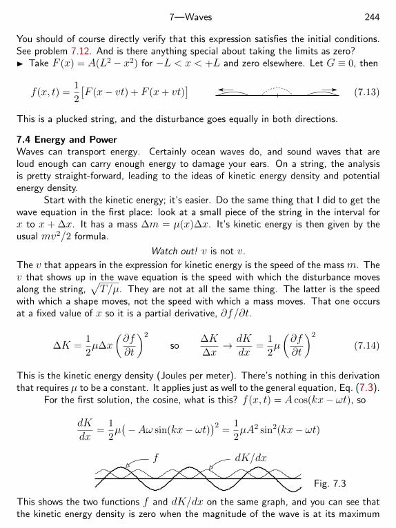
7—Waves 244
You should of course directly verify that this expression satisfies the initial conditions.See problem 7.12. And is there anything special about taking the limits as zero? Take F (x) = A(L2 − x2) for −L < x < +L and zero elsewhere. Let G ≡ 0, then
f(x, t) =1
2
[F (x− vt) + F (x+ vt)
](7.13)
This is a plucked string, and the disturbance goes equally in both directions.
7.4 Energy and PowerWaves can transport energy. Certainly ocean waves do, and sound waves that areloud enough can carry enough energy to damage your ears. On a string, the analysisis pretty straight-forward, leading to the ideas of kinetic energy density and potentialenergy density.
Start with the kinetic energy; it’s easier. Do the same thing that I did to get thewave equation in the first place: look at a small piece of the string in the interval forx to x + ∆x. It has a mass ∆m = µ(x)∆x. It’s kinetic energy is then given by theusual mv2/2 formula.
Watch out! v is not v.
The v that appears in the expression for kinetic energy is the speed of the mass m. Thev that shows up in the wave equation is the speed with which the disturbance movesalong the string,
√T/µ. They are not at all the same thing. The latter is the speed
with which a shape moves, not the speed with which a mass moves. That one occursat a fixed value of x so it is a partial derivative, ∂f/∂t.
∆K =1
2µ∆x
(∂f∂t
)2
so∆K∆x
→ dKdx
=1
2µ
(∂f∂t
)2
(7.14)
This is the kinetic energy density (Joules per meter). There’s nothing in this derivationthat requires µ to be a constant. It applies just as well to the general equation, Eq. (7.3).
For the first solution, the cosine, what is this? f(x, t) = A cos(kx− ωt), so
dKdx
=1
2µ(−Aω sin(kx− ωt)
)2=
1
2µA2 sin2(kx− ωt)
f dK/dx
Fig. 7.3
This shows the two functions f and dK/dx on the same graph, and you can see thatthe kinetic energy density is zero when the magnitude of the wave is at its maximum
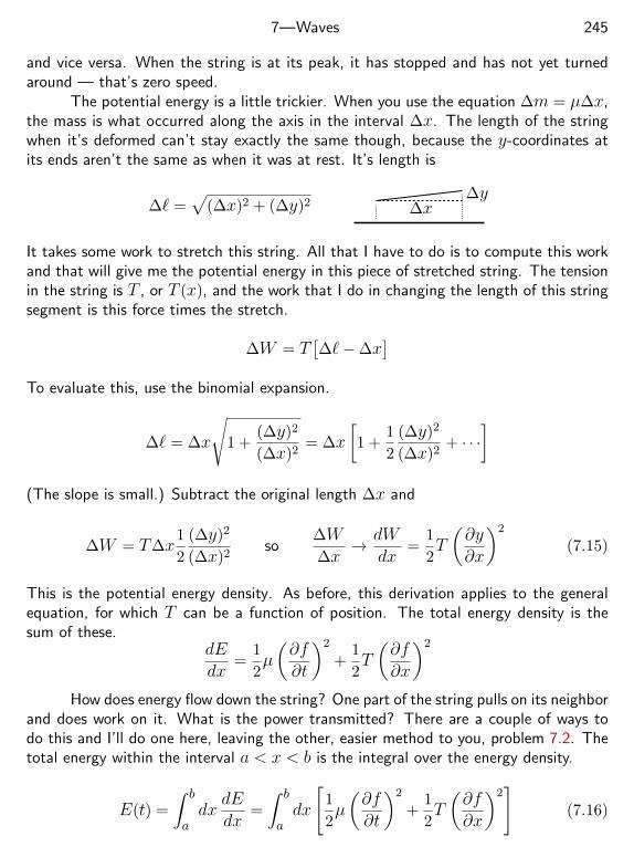
7—Waves 245
and vice versa. When the string is at its peak, it has stopped and has not yet turnedaround — that’s zero speed.
The potential energy is a little trickier. When you use the equation ∆m = µ∆x,the mass is what occurred along the axis in the interval ∆x. The length of the stringwhen it’s deformed can’t stay exactly the same though, because the y-coordinates atits ends aren’t the same as when it was at rest. It’s length is
∆` =√
(∆x)2 + (∆y)2 ∆x∆y
It takes some work to stretch this string. All that I have to do is to compute this workand that will give me the potential energy in this piece of stretched string. The tensionin the string is T , or T (x), and the work that I do in changing the length of this stringsegment is this force times the stretch.
∆W = T[∆`−∆x
]To evaluate this, use the binomial expansion.
∆` = ∆x
√1 +
(∆y)2
(∆x)2= ∆x
[1 +
1
2
(∆y)2
(∆x)2+ · · ·
](The slope is small.) Subtract the original length ∆x and
∆W = T∆x1
2
(∆y)2
(∆x)2so
∆W∆x
→ dWdx
=1
2T
(∂y∂x
)2
(7.15)
This is the potential energy density. As before, this derivation applies to the generalequation, for which T can be a function of position. The total energy density is thesum of these.
dEdx
=1
2µ
(∂f∂t
)2
+1
2T
(∂f∂x
)2
How does energy flow down the string? One part of the string pulls on its neighborand does work on it. What is the power transmitted? There are a couple of ways todo this and I’ll do one here, leaving the other, easier method to you, problem 7.2. Thetotal energy within the interval a < x < b is the integral over the energy density.
E(t) =
∫ b
adx
dEdx
=
∫ b
adx
[1
2µ
(∂f∂t
)2
+1
2T
(∂f∂x
)2]
(7.16)
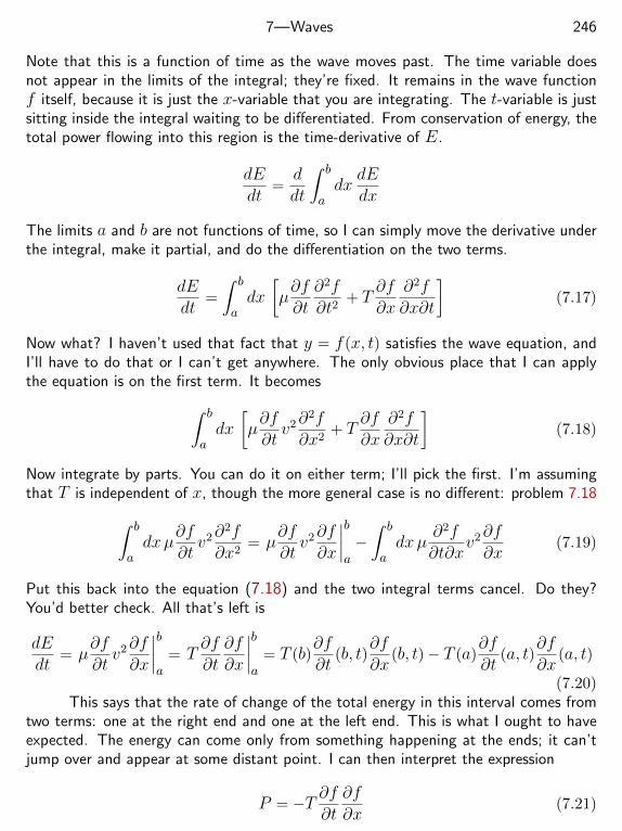
7—Waves 246
Note that this is a function of time as the wave moves past. The time variable doesnot appear in the limits of the integral; they’re fixed. It remains in the wave functionf itself, because it is just the x-variable that you are integrating. The t-variable is justsitting inside the integral waiting to be differentiated. From conservation of energy, thetotal power flowing into this region is the time-derivative of E.
dEdt
=ddt
∫ b
adx
dEdx
The limits a and b are not functions of time, so I can simply move the derivative underthe integral, make it partial, and do the differentiation on the two terms.
dEdt
=
∫ b
adx
[µ∂f∂t∂2f∂t2
+ T∂f∂x
∂2f∂x∂t
](7.17)
Now what? I haven’t used that fact that y = f(x, t) satisfies the wave equation, andI’ll have to do that or I can’t get anywhere. The only obvious place that I can applythe equation is on the first term. It becomes∫ b
adx
[µ∂f∂tv2∂
2f∂x2
+ T∂f∂x
∂2f∂x∂t
](7.18)
Now integrate by parts. You can do it on either term; I’ll pick the first. I’m assumingthat T is independent of x, though the more general case is no different: problem 7.18∫ b
adxµ
∂f∂tv2∂
2f∂x2
= µ∂f∂tv2∂f∂x
∣∣∣∣ba−∫ b
adxµ
∂2f∂t∂x
v2∂f∂x
(7.19)
Put this back into the equation (7.18) and the two integral terms cancel. Do they?You’d better check. All that’s left is
dEdt
= µ∂f∂tv2∂f∂x
∣∣∣∣ba
= T∂f∂t∂f∂x
∣∣∣∣ba
= T (b)∂f∂t
(b, t)∂f∂x
(b, t)− T (a)∂f∂t
(a, t)∂f∂x
(a, t)
(7.20)This says that the rate of change of the total energy in this interval comes from
two terms: one at the right end and one at the left end. This is what I ought to haveexpected. The energy can come only from something happening at the ends; it can’tjump over and appear at some distant point. I can then interpret the expression
P = −T ∂f∂t∂f∂x
(7.21)
7—Waves 247
as the power moving (to the right) past the point x. Why the minus sign? Look atthe term in Eq. (7.20) at the point a. If that term (with its minus sign) is positive, itrepresents energy coming into the interval from the left. Having gone through this, youwill better appreciate the simplicity of problem 7.2.
ExampleTake the cosine wave solution from Eq. (7.7), setting δ = 0 for convenience (f =A cos(kx− ωt)), and see what the total energy in an interval is.
dEdx
=1
2µ
(∂f∂t
)2
+1
2T
(∂f∂x
)2
, and f(x, t) = A cos(kx− ωt)
E =
∫ b
adx
1
2A2[µω2 sin2() + Tk2 sin2()
]= A2Tk2
∫ b
adx sin2(kx− ωt)
= A2Tk2
∫ b
adx[1− cos
(2(kx− ωt)
)]= A2Tk2
[(b− a)− 1
2k
(sin(2(kb− ωt))− sin(2(ka− ωt))
)](7.22)
(Remember Eq. (7.8).) The first term in the result represents the average energy inthe interval, and the other terms represent the fluctuations in total energy as the waveenters at a and leaves at b.
The power itself in this example is
P = −T ∂f∂t∂f∂x
= −T(
+Aω sin(kx− ωt))(−Ak sin(kx− ωt)
)= +A2Tkω sin2(kx− ωt) = A2µω2v sin2(kx− ωt) (7.23)
Notice that the power is zero where the wave is a maximum and vice versa. Or isit? And what is the time derivative of the energy computed in Eq. (7.22) and do youbelieve it?
7.5 ReflectionsWaves often meet barriers. Light waves hit glass. Ocean waves hit a reef. Soundwaves hit a wall. The analysis of all these is similar, so spending some time looking atreflections on a string will not be wasted.
Construct an example that typifies the process by tying two strings together, onethicker and heavier than the other. You know that light is partially reflected when ithits glass (just look in a window), so it is not surprising when the same thing happenshere. Let the mass density be µ1 to the left of the origin and µ2 to the right. A wavecomes in from the left and some of it gets through the boundary, but not all. Some isreflected. What equation do you have to solve? The same equation that started this
7—Waves 248
chapter, Eq. (7.3). After dropping the µg term, I assumed that T and µ were constantin order to produce “the” wave equation. Now µ isn’t constant, but I will assume thatT is.
T∂2f∂x2
= µ(x)∂2f∂t2
−→ ∂2f∂x2
=1
v2(x)
∂2f∂t2
(7.24)
The mass density is constant in two domains, µ = µ1 for x < 0 and µ2 for x > 0. Ineach region there are the corresponding (constant) wave speeds.
v(x) = v1 =√T/µ1, (x < 0) and = v2 =
√T/µ2, (x > 0)
This equation is exactly the same equation that you have to solve when light hits asheet of glass. The speed of the light wave in air decreases in glass by a factor of n, theindex of refraction. The function f is an electric field instead of the lateral displacementof a string. The mathematics is the same.
If you look only at the left part of the string or only at the right part, you alreadyknow the solutions. They are waves such as A cos(kx − ωt) or B cos(kx + ωt), andall you need is that the functions satisfy the wave equation, which means ω/k = v1 or= v2 in the two halves. If they have the same frequency then*
k1 = ω/v1
k2 = ω/v2
f(x, t) =
A cos(k1x− ωt) +B cos(k1x+ ωt) (x < 0)C cos(k2x− ωt) +D cos(k2x+ ωt) (x > 0)
(7.25)
There’s something missing. This works for x < 0 and for x > 0, but what aboutx = 0? It does not work there, at least not automatically, and this leads to the subjectof boundary conditions. You do not have a solution to the differential equation if youdon’t have it everywhere. If it misses a point, then it’s not a solution.
Boundary ConditionsFor the particular problem of a string with two mass densities, the boundary conditionsare
f is continuous, ∂f/∂x is continuous (7.26)
and where do these come from? I will show two different ways to get the answer. Oneby physical reasoning, the other mathematical. Fortunately they give the same answer.
The string hasn’t broken. That is the first condition, the continuity of f .Next, look at the point of attachment; did you tie a knot to attach the strings
together? If so that knot has a mass and you must apply ~F = m~a to it. In specifyingthe mass density µ(x) I tacitly assumed that there is no knot at x = 0, just somesort of massless attachment. The force Fy on that zero-mass connection must be zero:
* Do they have the same frequency? This is addressed at the end of this section.
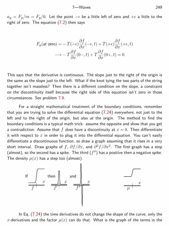
7—Waves 249
ay = Fy/m = Fy/0. Let the point −ε be a little left of zero and +ε a little to the
right of zero. The equation (7.2) then says
Fy(at zero) =− T (−ε)∂f∂x
(−ε, t) + T (+ε)∂f∂x
(+ε, t)
−→− T ∂f∂x
(0−, t) + T∂f∂x
(0+, t) = 0
This says that the derivative is continuous. The slope just to the right of the origin is
the same as the slope just to the left. What if the knot tying the two parts of the string
together isn’t massless? Then there is a different condition on the slope, a constraint
on the discontinuity itself because the right side of this equation isn’t zero in those
circumstances. See problem 7.9.
For a straight mathematical treatment of the boundary conditions, remember
that you are trying to solve the differential equation (7.24) everywhere, not just to the
left and to the right of the origin, but also at the origin. The method to find the
boundary conditions is a typical math trick: assume the opposite and show that you get
a contradiction. Assume that f does have a discontinuity at x = 0. Then differentiate
it with respect to x in order to plug it into the differential equation. You can’t easily
differentiate a discontinuous function, so draw a graph assuming that it rises in a very
short interval. Draw graphs of f , ∂f/∂x, and ∂2f/∂x2. The first graph has a step
(almost), so the second has a spike. The third (f ′′) has a positive then a negative spike.
The density µ(x) has a step too (almost).
x x x
f f ′ f ′′
If then and
xµ
In Eq. (7.24) the time derivatives do not change the shape of the curve; only the
x-derivatives and the factor µ(x) can do that. What is the graph of the terms in the
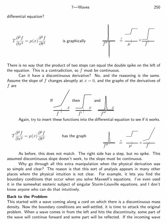
7—Waves 250
differential equation?
T∂2f∂x2
= µ(x)∂2f∂t2
is graphicallyf ′′
=?µ
×f
There is no way that the product of two steps can equal the double spike on the left ofthe equation. This is a contradiction, so f must be continuous.
Can it have a discontinuous derivative? No, and the reasoning is the same.Assume the slope of f changes abruptly at x = 0, and the graphs of the derivatives off are
x x x
f f ′ f ′′
If then and
Again, try to insert these functions into the differential equation to see if it works.
T∂2f∂x2
= µ(x)∂2f∂t2
has the graph
f ′′ µ f=? ×
As before, this does not match. The right side has a step, but no spike. Thisassumed discontinuous slope doesn’t work, to the slope must be continuous.
Why go through all this extra manipulation when the physical derivation wasso simple and clear? The reason is that this sort of analysis appears in many otherplaces where the physical intuition is not clear. For example, it lets you find theboundary conditions that occur when you solve Maxwell’s equations. I’ve even usedit in the somewhat esoteric subject of singular Sturm-Liouville equations, and I don’tknow anyone who can do that intuitively.
Back to the ProblemThis started with a wave coming along a cord on which there is a discontinuous massdensity. Now the boundary conditions are well-settled, it is time to attack the originalproblem. When a wave comes in from the left and hits the discontinuity, some part ofthe wave will continue forward and some part will be reflected. If the incoming wave
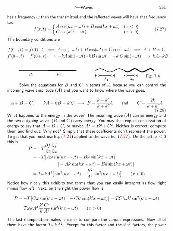
7—Waves 251
has a frequency ω then the transmitted and the reflected waves will have that frequencytoo.
f(x, t) =
A cos(kx− ωt) +B cos(kx+ ωt) (x < 0)C cos(k′x− ωt) (x > 0)
(7.27)
The boundary conditions are
f(0−, t) = f(0+, t) =⇒ A cos(−ωt) +B cos(ωt) = C cos(−ωt) =⇒ A+B = C
f ′(0−, t) = f ′(0+, t) =⇒ −kA sin(−ωt)−kB sinωt = −k′C sin(−ωt) =⇒ kA−kB = k′C
µ1 µ2
λ1 λ2Fig. 7.4
Solve the equations for B and C in terms of A because you can control theincoming wave amplitude (A) and you want to know where the wave goes.
A+B = C, kA− kB = k′C −→ B =k − k′
k + k′A and C =
2kk + k′
A
(7.28)What happens to the energy in the wave? The incoming wave (A) carries energy andthe two outgoing waves (B and C) carry energy. You may then expect conservation ofenergy to say that A = B +C, or maybe A2 = B2 +C2. Neither is correct; computethem and find out. Why not? Simply that these coefficients don’t represent the power.To get that you must use Eq. (7.21) applied to the wave Eq. (7.27). On the left, x < 0this is
P = −T ∂f∂t∂f∂x
= −T[Aω sin(kx− ωt)−Bω sin(kx+ ωt)
].[−Ak sin(kx− ωt)−Bk sin(kx+ ωt)
]= TωkA2
[sin2(kx− ωt)− B
2
A2sin2(kx+ ωt)
](x < 0)
Notice how nicely this exhibits two terms that you can easily interpret as flow rightminus flow left. Next, on the right the power flow is
P = −T[Cω sin(k′x− ωt)
][−Ck′ sin(k′x− ωt)
]= TC2ωk′ sin2(k′x− ωt)
= TωkA2 k′
kC2
A2sin2(k′x− ωt) (x > 0)
The last manipulation makes it easier to compare the various expressions. Now all ofthem have the factor TωkA2. Except for this factor and the sin2 factors, the power
7—Waves 252
flow is
1 (incoming from the left),B2
A2=
(k − k′
k + k′
)2
(outgoing to the left),
k′
kC2
A2=k′
k
(2k
k + k′
)2
(outgoing to the right)
(7.29)The two outgoing power factors add to(
k − k′
k + k′
)2
+k′
k
(2k
k + k′
)2
=k2 − 2kk′ + k′2 + 4kk′
(k + k′)2= 1
and energy is conserved.When you try to understand why light is reflected at a window, you are solving
Maxwell’s equations involving electric and magnetic fields. The details of the solutionare different, but for the case that the light is coming in perpendicular to the surface,the resulting equations (7.29) are identical. If the light hits the glass at an angleother than along the normal, then the equations are more complicated and depend onthe polarization of the light. (Look up the Fresnel equations.) For light you usuallysee the equations (7.29) expressed in terms of the index of refraction, so that thereflected and transmitted intensities for light going from vacuum or air to glass withindex n = c/v = k′/k are
1 (incoming to the surface),B2
A2=
(1− n1 + n
)2
(reflected from the glass),
k′
kC2
A2= n
(2
1 + n
)2
(transmitted into the glass)
(7.30)
Conservation of FrequencyIn the equations (7.25) I assumed that the frequency is the same on both sides of theboundary. It’s easy to believe, but shouldn’t it be possible to prove it? Assume thatthey are not the same and discover the consequences:
k1 = ω1/v1
k2 = ω2/v2
f(x, t) =
A cos(k1x− ω1t) +B cos(k1x+ ω1t) (x < 0)C cos(k2x− ω2t) +D cos(k2x+ ω2t) (x > 0)
What happens at the boundary? The wave is supposed to be continuous, so this is
f(0−, t) = f(0+, t)
A cos(−ω1t) +B cos(ω1t) = C cos(−ω2t) +D cos(ω2t)
(A+B) cos(ω1t) = (C +D) cos(ω2t)
7—Waves 253
If either one of (A + B) or (C + D) is non-zero, this is a contradiction. The twocosines are linearly independent. Specifically, take the case t = 0 then take the caset = π/(2ω2) for which the right side is zero but not the left. What else is needed?Don’t forget that the slope is continuous too. That gives still another equation involvingk1(A−B) and k2(C−D). They have to vanish also and that makes the whole solutionidentically zero. This nails down the intuitively plausible statement that the transmittedfrequency is the same as for incoming frequency.
7.6 Standing WavesA guitar string doesn’t have a wave moving toward plus or minus infinity. The wavestops at the end of the string, so I need different kinds of solutions for this case. I willconsider the case for which T and µ are constants, Eq. (7.6), but I’ll use a methodfor solving it that is common in these contexts: separation of variables. I could simplyguess the solution, as I did in Eq. (7.7), but this method is almost as easy and it is ofgreat general utility. It is in an extension of the ideas in section 0.8 about the separationof ordinary differential equations.
Assume a solution in the form of a product of functions, one of x and one of t.
f(x, t) = F (x)G(t)
Not all solutions will be like this, but the important result is that all solutions are sumsof solutions like this. That means that if I can find all the solutions that are productsthen I can add them and get all the other solutions that aren’t. To see if it works, plugin.
∂2f∂x2
− 1
v2
∂2f∂t2
= 0 =d2F (x)
dx2G(t)− 1
v2F (x)
d2G(t)dt2
Now move one term to the other side of the equation and divide by the product FG.
1
F (x)
d2F (x)
dx2=
1
v2G(t)d2G(t)dt2
The left side depends solely on the independent variable x. The right side depends solelyon the independent variable t. I can change x any way that I want without changingt, and in doing so the right side stays constant. That means that the left side mustbe constant. A similar argument holds for the right side, allowing t to vary. And theconstants have to be the same.
1
F (x)
d2F (x)
dx2= C,
1
G(t)d2G(t)dt2
= Cv2 (7.31)
These are ordinary differential equations, and they’re the same equation that I spent awhole chapter on: the harmonic oscillator. Or are they? Harmonic motion requires that
7—Waves 254
C is negative and how do I know that? At this point you don’t. C can be anything,even complex, and it provides a valid solution to the wave equation. The equationdoesn’t know that the string is tied down at its ends — that fact presents you with aset of boundary conditions that will determine the details of the solution.
In order to represent a system that’s tied at the two ends I have to specify thefunction at those points. Pick the coordinate x to be zero at the left and L at theright. The y-value is zero where the string is at rest.
y = f(0, t) = 0 and y = f(L, t) = 0
Apply this to the separated solution F (x)G(t) and it says that F (0) = 0 and F (L) = 0.The equation that F satisfies is F ′′ = CF , and if C is a positive number its solutionsare real exponentials. A hyperbolic sine vanishes at one point, but only at one point,so you can’t make it match these boundary conditions at both ends. If C is negativeyou have sinusoidal solutions, and these vanish at many places, allowing the possibilityof matching the boundary conditions at both places.
If C is negative, denote it by C = −k2, then
d2F (x)
dx2= −k2F =⇒ F (x) = A sin(kx+ δ)
You have to use the same constant for the G equation,
G = Cv2G = −k2v2G =⇒ G(t) = B sin(ωt+ δ) where ω2 = k2v2 (7.32)
Now apply the boundary conditions.
f(0, t) = F (0)G(t) = 0, so F (0) = A sin δ = 0 and δ = 0
You can pick another δ, such as π or −9π, but that just changes everything by anoverall minus sign and you can absorb that into A.
Next the other end of the string:
f(L, t) = F (L)G(t) = 0 =⇒ F (L) = A sinkL = 0 so kL = nπ
for integer n. Now put them together.
f(x, t) = A sin(nπxL
)sin(ωnt+ δn) where ωn =
nπvL
, n = 1, 2, 3, . . .
(7.33)You don’t need negative n here because they would just reproduce the same functionsas does the positive n.
7—Waves 255
Some pictures of these waves at maximum displacement, i.e. when sin(ωnt +δn) = 1:
n = 4n = 1 n = 2 n = 3
Stroboscopic pictures of the motionFig. 7.5
The first set of graphs show the waves at one instant, the peak displacement for eachmode. The second set shows the waves at eleven instants, equally spaced in time frompeak positive to peak negative amplitude, i.e. over half a period of oscillation.
The respective frequencies are ω1 = πv/L, ω2 = 2πv/L, etc., and they are thesequence of harmonics that you hear when you pluck the string on a musical instrument.
The lowest frequency, the fundamental, is ω1 = π√T/µ
/L. It says that the
greater the tension in the string, the higher the frequency. The same happens if themass density of the string is less. Tuning such a musical instrument means adjustingthe tension. Could you change the mass density instead? Actually yes. Look inside apiano and compare the strings for low frequencies and those for high frequencies. Theformer have much higher linear mass density.
You can hear the separate harmonics from a guitar string if you pluck it properly.Touch the tip of your finger to the midpoint of the string and pluck the string withyour thumb, immediately releasing contact from your finger. You will hear the upperharmonic (n = 2) because your finger damped out the n = 1 motion without affectingthe n = 2 component. Similarly place your finger at the 1/3 or 1/4 point to hear stillhigher harmonics. An expert musician can use this technique to good effect.
OrthogonalityThese standing wave solutions have a special property that won’t appear particularlyimportant now, but it will later. The idea of orthogonal vectors is one that you’re
familiar with: ~A . ~B = 0. There is a similar concept for waves. For each positiveinteger n, the equation (7.33) provides a mode of oscillation shaped as
un(x) = sin(nπx/L), n = 1, 2, 3, . . .
Take two different such modes and evaluate this integral
I =
∫ L
0dx sin
(nπxL
)sin(mπx
L
)for n 6= m (7.34)
You simply need the right trigonometric identity, and that is
sinx sin y = 12
[cos(x+ y)− cos(x− y)
]
7—Waves 256
I =
∫ L
0dx
1
2
[cos
((n+m)πx
L
)− cos
((n−m)πx
L
)]=
1
2
[L
(n+m)πsin
((n+m)πx
L
)− L
(n−m)πsin
((n−m)πx
L
)]L0
= 0
These functions un and um are said to be orthogonal to each other because of thisintegration. For an analogy, you can compute the common three-dimensional scalarproduct as AxBx+AyBy +AzBz, a sum over three indices running from x to z. Theintegral Eq. (7.34) is like a sum over a continuous index that runs from zero to L.
In what will probably seem like very different sorts of problems, essentially thesame idea will appear in the equations (8.37) and (10.15).
7.7 An Algebraic AsideHow do you solve a cubic equation? (And what does this have to do with waves?Patience.) That depends on the cubic. Try to solve
x− 1− 0.01x3 = 0
If you’ve solved problem 4.5 you may think that you have done this before and you have,but not this way. What follows is a different approach to the same problem, one thatclosely parallels what I will do for the wave equation. Just notice that 0.01 1. Thereis a solution near x = 1, and I can use the equation itself to find a series expansionfor the root near that point. The idea is that you assume the form of the series eventhough you do not know any of its coefficients. Then use the equation you’re solvingto determine those coefficients. Let ε = 0.01 be the expansion parameter.
x− 1− εx3 = 0, and x = x0 + εx1 + ε2x2 + ε3x3 + · · · (7.35)
You don’t know any of the coefficients x0 or x1, but plug the assumed solution intothe equation anyway.
x0 + εx1 + ε2x2 + · · · − 1− ε(x0 + εx1 + ε2x2 + · · ·
)3= 0
x0 + εx1 + ε2x2 + · · · − 1
−ε(x3
0 + 3x20
(εx1 + ε2x2 + · · ·
)+ 3x0
(εx1 + · · ·
)2+(εx1 + · · ·
)3)= 0
Expand everything and collect terms in powers of ε, multiplying out the square and cubeof the parenthesized expressions and carefully getting all the terms with like powers ofε.
x0 + εx1 + ε2x2 + · · · − 1− ε(x3
0 + 3εx20x1 + 3ε2x2
0x2 + 3ε2x0x21 + · · ·
)= 0
7—Waves 257
For this to be a valid series expansion in ε, all the like coefficients of powers of ε mustmatch.
ε0 : x0 − 1 = 0
ε1 : x1 − x30 = 0
ε2 : x2 − 3x20x1 = 0 (7.36)
ε3 : x3 − 3x20x2 − 3x0x
21 = 0
Solve these equations in sequence and you get
x0 = 1, x1 = 1, x2 = 3, x3 = 12, · · ·
The value of the root is x = 1 + .01 + .012 . 3 + .013 . 12 + · · · = 1.010312 Putthis into the original cubic and the value is x − 1 − .01x3 = −5.61 × 10⁻⁷. Forcomparison, if you put x = 1 into the equation, the error is 10−2. The next term in theseries for x is ε4x4 = 10−8x4. This example shows the essential idea of perturbationtheory. Continuing this to higher orders in ε produces 1.01031257881011 as a betterapproximation to the exact solution.
The spirit of this approximation is that you start with an easy solution to a sim-plified form of the problem and then you improve the solution by using the complicatedpart to generate the correction. Are there ways other then series expansions to do this?Yes, the subject of numerical analysis and of perturbation theory is well-developed andyou will find many variations on this theme, which brings me to. . .
7.8 Perturbation TheoryIf the mass density of the string isn’t constant, Eq. (7.3) is more complicated than thesimple wave equation. The same is true if the tension isn’t constant throughout. Howcan this happen? The non-uniform density is easy: place a wad of chewing gum on thestring. Or maybe use a bullwhip for the string. To get non-constant tension, simplyhold the string vertically. The part of the string at the top has to support everythingbelow, so the tension at the top will be greater than that at the bottom. Will this be abig effect in a musical instrument? No. The tension in that case is always far greaterthan the weight of the string, so this effect is not important, but if the string is notunder great tension then this will alter the harmonic structure substantially. There areother examples of physical systems where the same equation appears and for which theeffects of variable T (or its analog) are important.
There are a few special cases for which you can solve the equations exactly whenT or µ are not constant, but instead of spending time on those, I’ll show a generalprocedure that’s valid for any T or µ as long as they are almost constant.
The technique, “perturbation theory,” parallels the series solution for the cubicequation in the preceding section, and it starts from what you already know, the solution
7—Waves 258
for the uniform string. In this case the solution for the non-uniform case should be veryclose to the known, simple solution.
Take the case for which T is constant and µ is almost constant.
µ(x) = µ0 + µ1(x), |µ1| µ0
If µ1 is absent, I know how to solve the problem for which the string is tied down at twoends; that’s section 7.6 and Eq. (7.33). I said that the idea is to expand everything inpower series, but what is the variable to use? I’ll make one up. Change the precedingequation to
µ(x) = µ0 + εµ1(x)
and use ε as a dimensionless parameter for the series. This allows me to keep track ofthe terms easily.
To be certain that I’m not missing anything, I will return to the original waveequation (7.3), but with T = a constant and no gravity and no friction.
T∂2f∂x2
= µ(x)∂2f∂t2
The technique of separation of variables still works, even when µ (or T ) depends on x.
f(x, t) = F (x)G(t), then Td2F (x)
dx2G(t) = µ(x)F (x)
d2G(t)dt2
To separate variables now you have to divide by FGµ.
TµF
d2Fdx2
=1
Gd2G(t)dt2
and again the equation is separated, with all the x’s on one side and all the t’s on theother. They must therefore be (the same) constant. Back in Eq. (7.31) I called it C,but in the end it turned out to be proportional to ω2, so I’ll use that notation from theoutset.
1
Gd2G(t)dt2
= −ω2,TµF
d2Fdx2
= −ω2 (7.37)
The time equation is unchanged, so the solution is the familiar sine, cosine, orexponential: eiωt or sin(ωt+δ). The difference is in the equation for F , and that’s wherethe action occurs. I take the same boundary conditions as before, F (0) = F (L) = 0,so that the string is tied down.
Td2Fdx2
= −µω2F (7.38)
7—Waves 259
Now however µ, F , and ω2 are different, though they should be close to the unperturbedcase. Write all of them in terms of a power series in ε. The density µ of course hasonly two terms, so it hardly warrants the name power series.
µ = µ0 + εµ1
F = F0 + εF1 + ε2F2 + ε3F3 + · · · (7.39)
ω2 = ω20 + εω2
1 + ε2ω22 + · · ·
The coefficients F0, F1, ω22 , etc. are unknowns to be determined. The expansion for ω
may look a little odd, but it’s ω2 that shows up as the natural parameter, not ω itself,so this is the way to write it. It would probably be more consistent notation to call thecoefficients (ω2)0, (ω2)1, . . . , but that is being unnecessarily fussy and it is too clumsy,so I won’t. Now plug in.
T[F ′′0 +εF ′′1 +ε2F ′′2 +· · ·
]= −
[µ0+εµ1
][ω2
0 +εω21 +ε2ω2
2 +· · ·][F0+εF1+ε2F2+· · ·
]This looks like I’m taking a difficult problem and turning it into an impossible one. NowI have an infinite number of unknowns. But,
The left side is a power series in ε. The right side is a power series in ε. They’resupposed to agree no matter what ε is. For that to happen all the coefficients of likepowers have to match. The coefficient of ε0, the coefficient of ε1, etc.
TF ′′0 = −µ0ω20F0
TF ′′1 = −µ0ω20F1 − µ1ω
20F0 − µ0ω
21F0
TF ′′2 = −µ0ω20F2 − µ2ω
20F0 − µ0ω
22F0 − µ1ω
21F0 − µ1ω
20F1 − µ0ω
21F1
(7.40)
This is now an infinite number of equations for an infinite number of unknowns. Itdoesn’t look promising. First, some reassurance: I’m going to go just as far as the firsttwo of these equations. F2 will have to find itself.
Rearrange them.
TF ′′0 + µ0ω20F0 = 0 (a)
TF ′′1 + µ0ω20F1 = −µ1ω
20F0 − µ0ω
21F0 (b)
TF ′′2 + µ0ω20F2 = −µ2ω
20F0 − µ0ω
22F0 − µ1ω
21F0 − µ1ω
20F1 − µ0ω
21F1 (c)
(7.41)The systematic procedure to solve these:
1. Solve the 1st, easy equation.2. Use the F0 from step one to find the frequency correction ω2
1 from the 2nd
equation.3. Solve the 2nd equation for F1.
7—Waves 260
4. Use the F1 from step two to find the frequency correction ω22 from the 3nd
equation.5. Solve for F2 etc.(I’m not going past step three anyway.)
I haven’t been very specific about the problem that I want to solve, trying to leavethe setup general. Now to be specific, I have to set down the boundary conditions, andthe ones I choose are the same ones that I used before. Tie the string down at twoends. This says that f(0, t) = f(L, t) = 0 as before. Eq. (7.41)(a) is the same asEq. (7.32), so it has the same solution, Eq. (7.33).
TF ′′0 + µ0ω20F0 −→ F0(x) = A sin
(nπxL
), with T
n2π2
L2= µ0ω
20
Now comes the key observation that breaks open this complicated looking set ofequations.
If you take the unperturbed solution, F0(x), multiply the left-hand side of theequation (7.41)(b) by F0, and integrate from 0 to L with respect to x, you get zero.Stated in the language of vectors,
F0 is orthogonal to TF ′′1 + µ0ω20F1 (7.42)
whatever F1 is (as long as it satisfies the same boundary conditions and vanishes at 0and L).
The proof of this involves nothing more than a couple of partial integrations. Ihave to compute the following integral, showing that it is zero.∫ L
0dxF0(x)
[TF ′′1 + µ0ω
20F1
]=? 0 (7.43)
Work on the first term by itself, recalling that T and µ0 are constants.∫ L
0dxF0(x)TF ′′1 = TF0(x)F ′1(x)
∣∣∣L0− T
∫ L
0dxF ′0(x)F ′1(x)
= TF0(x)F ′1(x)∣∣∣L0− TF ′0(x)F1(x)
∣∣∣L0
+ T∫ L
0dxF ′′0 (x)F1(x)
Put this into the integral (7.43).
TF0(x)F1(x)∣∣∣L0−TF ′0(x)F1(x)
∣∣∣L0
+
∫ L
0dx[TF ′′0 (x)+F0(x)µ0ω
20
]F1(x) = 0 (7.44)
This last integral is zero because by assumption F0 satisfies the original, unperturbedequation (7.41)(a), and that is precisely what appears in brackets as the coefficient of
7—Waves 261
F1 inside the integral. The other terms are evaluated at the boundaries, 0 and L, andthe boundary conditions that I placed on the problem, that F (0) = 0 = F (L), makethis zero because F0 and F1 will vanish at these points. This result parallels those inEqs. (8.35) and (10.14).
Now multiply Eq. (7.41)(b) by F0 and integrate the whole equation from 0 toL. The left side is now zero.∫ L
0dxF0(x)
[TF ′′1 + µ0ω
20F1
]= 0 =
∫ L
0dx[− µ1ω
20F
20 − µ0ω
21F
20
](7.45)
The single unknown here is ω21 , the first correction for the frequency-squared.
ω21 = − ω2
0
∫ L
0dxµ1(x)F0(x)2
/µ0
∫ L
0dxF0(x)2 (7.46)
The denominator is easy, and the numerator’s complexity depends on µ1. I didn’t haveto solve any complicated differential equations to get this result, I have only to do twointegrals.
As an example, what if the string is tapered slightly, so that the mass densityvaries linearly from one end to the other? Take µ1(x) = αx, making the string slightlythicker toward x = L.
F0(x) = sin(nπx/L), and ω20 = n2π2T/µ0L
2
The integrals are∫ L
0dx sin2(nπx/L) = L/2, and∫ L
0dxx sin2(nπx/L) =
∫ L
0dx[(x− L/2) + L/2
]sin2(nπx/L) = L2/4 (7.47)
The correction to the frequency is then to this order
ω21 = −ω
20αL
2/4
µ0L/2= −ω2
0
αL2µ0
so that ω2 = ω20
[1− αL
2µ0
](7.48)
Is this plausible? If α is positive this is a decrease in the frequency, and that’s just whatyou should expect because it represents an increase in the linear mass density over theµ0 that I started with, and the density appears in the denominator of
√T/µ. And what
about the frequency itself, not just the squared frequency? See problem 7.19. Are thedimensions of (7.48) right?
7—Waves 262
How is the frequency altered if a small mass is added at one point along thestring? Perhaps a tenacious fly lands on it. In this case the perturbing mass densityµ1 is zero every place except very near the one point. Specifically a small mass m isadded at the point x = d. In the numerator of Eq. (7.46) the integrand is then zeroeverywhere except very close to the point d.∫ L
0dxµ1(x)F0(x)2 =
∫ d+ε
d−εdxµ1(x)F 2
0 (x)
where 2ε is the tiny width of the mass. As F0 is a smooth function it won’t changesignificantly over this small range of x and I can approximate the integral by evaluatingF0 at x = d.
≈∫ d+ε
d−εdxµ1(x)F 2
0 (d) = mF 20 (d) = m sin2(nπd/L)
The denominator in the frequency correction is µ0L/2, so the whole correction is
ω21 = −ω2
0
m sin2(nπd/L)
µ0L/2
Notice how this varies with d. Take the case n = 2 for example. There are two humpson either side and a node at the center, L/2. If the mass is placed exactly at thenode, then sin2(2πL/2L) = 0 and there is no shift in the frequency. This makes sensebecause the center point on the string isn’t moving anyway, so it doesn’t matter if thereis a extra mass there or not. In the same n = 2 mode, if you put the extra mass atL/4 or 3L/4 then the effect is maximum. It is negative; it has the correct dimensions.
Finding F1
All the preceding calculation did was to get the lowest order correction for the frequency,and that’s often all that you want. But what about the wave itself? Sometimes youneed more than the frequency. That’s Eq. (7.41)(b). Now you know the right sideof the equation because you’ve found ω2
1 and you already knew ω20 and F0. This is
an inhomogeneous linear differential equation for F1, and you have seen examples ofexactly this equation in chapter three. The sections 3.5 and 3.10 were devoted to it.The independent variable was t instead of x, but that makes no difference because theequations are the same. The only difference between this calculation and those is theextra use of boundary conditions.
Why would you need F1? One reason is that the equation for the second ordercorrection to ω2 uses it. That is in the third of the equations (7.41), and you need F1
to determine the right side of that equation. You do the same thing as in equations(7.41)(b) and (7.45) and suddenly you have ω2
2 . For here and now, it is not worthpursuing this matter, but precisely this sort of calculation appears in quantum mechanicsand the higher order corrections can be important in that context.
7—Waves 263
7.9 StiffnessIn the first section of this chapter I mentioned that I had left out some physics, thestiffness of the string. If you look inside a piano you will see that the low pitched noteshave heavy, wire-wound strings and they are stiff and hard to bend. How does thisaffect the frequencies you hear when the piano is played? The tools in the precedingsection on perturbation theory apply here too.
The first question, how do you describe stiffness mathematically? For a wire ofcircular cross section the extra force comes from a combination of Young’s modulus(Y ), the cross-sectional area (S), and a dimensionless factor (α = 1/4π).
µ∂2f∂t2
= T∂2f∂x2
− αY S2∂4f∂x4
I won’t attempt to derive this here, I will simply use it. Does it at least have the correctdimensions?
What does this do to the frequency of standing waves? You can solve thisparticular problem without using approximations, but treating the added term as a per-turbation is enough for many circumstances. Start from the same solution as Eq. (7.33)and introduce a dimensionless expansion parameter in front of the new term: ε. Usethe same sort of expansion as in Eq. (7.39) though now there is no change in the massdensity, no µ1. The x and t variables separate just as in Eq. (7.37), so that the equation(7.38) is
Td2Fdx2
− εαY S2d4Fdx4
= −µω2F (7.49)
Use Eqs. (7.39) for F and ω2, and collect the terms in ε0 and ε1. I won’t go beyondthis.
Td2F0
dx2= −µω2
0F0
Td2F1
dx2− αY S2d
4F0
dx4= −µω2
0F1 − µω21F0
Rearrange this to put it in the form of Eqs. (7.40).
Td2F0
dx2+ µω2
0F0 = 0
Td2F1
dx2+ µω2
0F1 = αY S2d4F0
dx4− µω2
1F0
The first of these gives the same standing wave as before,
F0(x) = A sin(nπxL
), with T
n2π2
L2= µω2
0
7—Waves 264
Now you are set to use the same equation (7.43) as before. Multiply the second ofthese equations by F0 and integrate from 0 to L.∫ L
0dxF0(x)
[Td2F1
dx2+ µω2
0F1
]= 0 =
∫ L
0dxF0(x)
[αY S2d
4F0
dx4− µω2
1F0
]This determines the correction ω2
1 for the frequency.
ω21 =
αY S2
µ
∫ L0 dxF0(x)F ′′′′0 (x)∫ L
0 dxF0(x)2=αY S2
µn4π4
L4
The total frequency squared to this order is then
ω2 =Tµn2π2
L2+αY S2
µn4π4
L4
This says that the overtones of the string are not quite in a simple harmonic sequence,ω ∝ n, but are stretched to slightly higher values. Can you hear this? I can’t, but agood piano tuner can.
7.10 Other WavesThe structure of waves on a string with constant tension and constant mass densityis so simple that is is misleading. Studying this is like studying electromagnetic wavesin a vacuum. They are important, but as soon as you encounter matter they becomecomplicated. The speed of light is a function of the wavelength (rainbows); the speedof light depends on the polarization of the wave (birefringence, optical activity); thespeed of the wave by the definition of speed that you’ve seen in this chapter so far can begreater than c, its speed in vacuum. In other words it is a lot more complicated thanyou may think.
What about the most commonly observed wave in nature, surface waves on theocean. People saw these long before anyone knew that sound is a wave, much lessthat light is. Oddly enough, these ocean waves are some of the more complicated sortsof waves to analyze mathematically. For example, the wave speed is v =
√gλ/2π
for deep water. This means that long wavelength waves travel much faster than shortwavelength waves. A little ripple in a pond can travel at walking speed or less. A tsunamican travel at hundreds of kilometers per hour. That you can listen to music at all tellsyou that for sound within the range of human hearing this dependence of the speedon wavelength must be very slight. The speed does change at ultrasonic frequenciesbecause at those very short wavelengths heat can flow quickly from a compression region
7—Waves 265
to a rarefaction region and make the process nearly isothermal. At low frequencies andlong wavelengths the distance is too great for this process to occur in the short timebetween wave crests. In that case the process is nearly adiabatic and the speed changesby a factor
√γ between the two cases, where γ is the ratio of specific heats discussed
so thoroughly in thermodynamics.Earthquake waves have speeds that depend on whether they are longitudinally
or transversely polarized. And then there are torsional waves in which the rocks aretwisted instead of being pushed forward and backward or side to side. This differencein the speed of different types of earthquake waves allows geologists to get informationabout what’s under the ground. It also allows them to determine the distance to anearthquake that occurs a thousand kilometers away — without receiving a phone callfrom someone in the middle of the quake itself.
7.11 Other VelocitiesI have alluded to that fact that the definition of the velocity of a wave is more com-plicated than what you saw in Eq. (7.9), v = ω/k. That is called the phase velocitybecause it describes the motion of a point having constant phase, but it is not the wholestory. There are at least four different definitions for the velocity of a wave:
phase velocity, group velocity, information (or signal) velocity, energy velocity
The first two are all that I will describe here, as the other two get very technical veryfast. They were described by Sommerfeld and Brillouin.*
If a wave has the property that its phase velocity ω/k is itself independent offrequency, that’s all there is. It’s the end of the subject because all these four sortsof wave velocity are then identical. A light wave in a vacuum is like this. The moreinteresting case is the one for which the phase velocity is not independent of frequency.The most visible example is that of light when it is passing through a medium such aswater or glass or even air, because in those cases the index of refraction, n = c/vphase,depends on the frequency of the light, and this is the reason that there are rainbows.This is “dispersion.”
Any real wave has a beginning and an end, and contains a mixture of frequencies.If these frequencies travel at different speeds, the wave cannot maintain the exact sameshape that it did at the beginning. It will deform, typically spreading its width. It canin some circumstances have some truly odd behavior.
Analyzing this in detail takes Fourier analysis, but I will take an easier route andanalyze the simplest possible case to show how the concept of group velocity arises.Any real wave is a mixture of many frequencies, and the simplest case to deal withis two. What happens when you have two waves moving in the same direction, and
* Leon Brillouin: Wave Propagation and Group Velocity, Academic Press 1960,still a standard reference.
7—Waves 266
one has a frequency slightly different from the other? Assume that they have thesame amplitude and have frequencies ω and ω′. The two waves will then have (phase)velocities v = ω/k and v′ = ω′/k′, but you cannot simply say that “the velocity” ofthe wave is the average of these two numbers. Notice that the wave numbers k and k′
aren’t the same either.The total wave is
f(x, t) = A cos(kx− ωt) +A cos(k′x− ω′t) (7.50)
You need a trig identity here, problem 0.50, in order to add these two cosines.
cosx+ cos y = 2 cos(x+ y
2
)cos(x− y
2
)f(x, t) = 2A cos
(k + k′
2x− ω + ω′
2t)
cos(k − k′
2x− ω − ω
′
2t)
(7.51)
Picture this wave at time zero, and assume that the frequencies are close, so thewave numbers k and k′ are close also. That means that the (k − k′) in the secondfactor is much smaller than the (k + k′) in the first, so the first cosine factor oscillatesin space much more rapidly than the second. The whole function at this instant is theproduct of two spatial oscillations: one with a short wavelength and one with a longwavelength: f(x, 0) = 2A cos
((k + k′)x/2
)cos((k − k′)x/2
).
cos kx
cos k′x
cos kx+ cos k′x
Fig. 7.6
The outline of the sum follows the ± cos((k − k′)x/2
)factor, and that is shown with
the lighter lines. When this envelope drops to zero, you can see that the two componentwaves in the upper two graphs are 180 out of phase. Follow the dotted line.
The velocity of one of these waves alone is ω/k = vk, and that of the otherwave is ω′/k′ = vk′ . The combined wave does not have a single velocity, so examinethe two factors in Eq. (7.51). Each factor has its own phase velocity.
cos(k + k′
2x− ω + ω′
2t)
has phase velocityω + ω′
k + k′
cos(k − k′
2x− ω − ω
′
2t)
has phase velocityω − ω′
k − k′
7—Waves 267
Unless the ratios ω/k and ω′/k′ are the same, these two velocities can be quite differenteven if the two frequencies are very close! If the two frequencies are close, the first ofthese velocities is near to both vk and vk′ ; all three are about the same. The secondequation however has a velocity that is essentially a derivative, and there’s no reasonto expect this to be close to any of the other velocities. That would be like saying thatthe slope of a function, f ′(x), is the same as f(x)/x.
ω − ω′
k − k′−→ dω
dk= vgroup (7.52)
This is called the group velocity. It is the velocity of the dashed curve above. Theshorter waves within the outline moves at the different velocity (ω+ω′)/(k+k′). Theenvelope of the wave (the dashed line) moves at the group velocity while the individualpeaks of the wave move at the phase velocity. The still image on the previous page isanimated at the linkwww.physics.miami.edu/nearing/mathmethods/groupvelocity.html
How different can these velocities be? In quantum mechanics you will see arelation between ω and k that follows ω = hk2/2m, so
vphase =ωk
=hk2m
, while vgroup =dωdk
=hkm
This group velocity is twice the phase velocity. For ocean waves, see problem 7.29
7.12 Waves and Tides
In chapter five there was a discussion about ocean tides and some of the probablyconfusing and certainly counter-intuitive aspects of the subject. In particular, how isit that a high tide can occur when the Moon is near the horizon? Shouldn’t the hightide be more-or-less underneath the Moon (or at the antipode) as in the picture ofEq. (5.43)? In describing the phenomena involved I did a lot of hand-waving and mademany qualitative statements. Here I propose to present some quantitative analysis toback up the previous work.
A simplified model that shows the phenomena uses a wave on a string. This timehowever, wrap the string around in a circle and set it spinning they way some people canspin a lasso. The rope forms a circle and is rotating about the central axis perpendicularto the plane of the circle. To simplify the problem, let it be rotating in empty space,and the only tension in the rope is there because it is spinning. The rope is still a rope,
so the basic equation is ~F = m~a and that in turn implies the wave equation Eq. (7.3)but without the µg or b∂f/∂t terms.
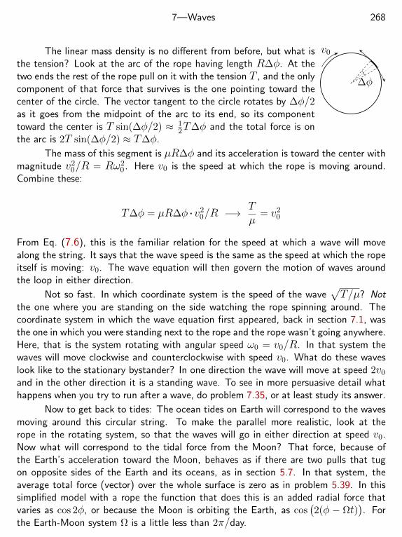
7—Waves 268
v0
∆φ
The linear mass density is no different from before, but what isthe tension? Look at the arc of the rope having length R∆φ. At thetwo ends the rest of the rope pull on it with the tension T , and the onlycomponent of that force that survives is the one pointing toward thecenter of the circle. The vector tangent to the circle rotates by ∆φ/2as it goes from the midpoint of the arc to its end, so its componenttoward the center is T sin(∆φ/2) ≈ 1
2T∆φ and the total force is onthe arc is 2T sin(∆φ/2) ≈ T∆φ.
The mass of this segment is µR∆φ and its acceleration is toward the center withmagnitude v2
0/R = Rω20 . Here v0 is the speed at which the rope is moving around.
Combine these:
T∆φ = µR∆φ . v20/R −→ T
µ= v2
0
From Eq. (7.6), this is the familiar relation for the speed at which a wave will movealong the string. It says that the wave speed is the same as the speed at which the ropeitself is moving: v0. The wave equation will then govern the motion of waves aroundthe loop in either direction.
Not so fast. In which coordinate system is the speed of the wave√T/µ? Not
the one where you are standing on the side watching the rope spinning around. Thecoordinate system in which the wave equation first appeared, back in section 7.1, wasthe one in which you were standing next to the rope and the rope wasn’t going anywhere.Here, that is the system rotating with angular speed ω0 = v0/R. In that system thewaves will move clockwise and counterclockwise with speed v0. What do these waveslook like to the stationary bystander? In one direction the wave will move at speed 2v0
and in the other direction it is a standing wave. To see in more persuasive detail whathappens when you try to run after a wave, do problem 7.35, or at least study its answer.
Now to get back to tides: The ocean tides on Earth will correspond to the wavesmoving around this circular string. To make the parallel more realistic, look at therope in the rotating system, so that the waves will go in either direction at speed v0.Now what will correspond to the tidal force from the Moon? That force, because ofthe Earth’s acceleration toward the Moon, behaves as if there are two pulls that tugon opposite sides of the Earth and its oceans, as in section 5.7. In that system, theaverage total force (vector) over the whole surface is zero as in problem 5.39. In thissimplified model with a rope the function that does this is an added radial force thatvaries as cos 2φ, or because the Moon is orbiting the Earth, as cos
(2(φ − Ωt)
). For
the Earth-Moon system Ω is a little less than 2π/day.
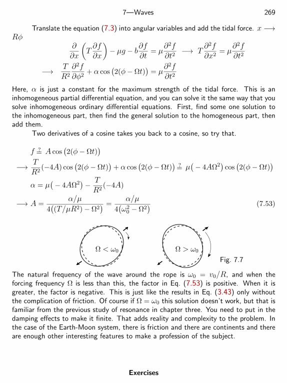
7—Waves 269
Translate the equation (7.3) into angular variables and add the tidal force. x −→Rφ
∂∂x
(T∂f∂x
)− µg − b∂f
∂t= µ
∂2f∂t2
−→ T∂2f∂x2
= µ∂2f∂t2
−→ TR2
∂2f∂φ2
+ α cos(2(φ− Ωt)
)= µ
∂2f∂t2
Here, α is just a constant for the maximum strength of the tidal force. This is aninhomogeneous partial differential equation, and you can solve it the same way that yousolve inhomogeneous ordinary differential equations. First, find some one solution tothe inhomogeneous part, then find the general solution to the homogeneous part, thenadd them.
Two derivatives of a cosine takes you back to a cosine, so try that.
f =? A cos(2(φ− Ωt)
)−→ T
R2(−4A) cos
(2(φ− Ωt)
)+ α cos
(2(φ− Ωt)
)=? µ
(− 4AΩ2
)cos(2(φ− Ωt)
)α = µ
(− 4AΩ2
)− TR2
(−4A)
−→ A =α/µ
4((T/µR2)− Ω2
) =α/µ
4(ω2
0 − Ω2) (7.53)
Ω < ω0 Ω > ω0
Fig. 7.7
The natural frequency of the wave around the rope is ω0 = v0/R, and when theforcing frequency Ω is less than this, the factor in Eq. (7.53) is positive. When it isgreater, the factor is negative. This is just like the results in Eq. (3.43) only withoutthe complication of friction. Of course if Ω = ω0 this solution doesn’t work, but that isfamiliar from the previous study of resonance in chapter three. You need to put in thedamping effects to make it finite. That adds reality and complexity to the problem. Inthe case of the Earth-Moon system, there is friction and there are continents and thereare enough other interesting features to make a profession of the subject.
Exercises
7—Waves 270
1 Do the algebra to get the equations Eq. (7.28).
2 Solve x− 1 + .01x4 = 0 to ±10−4.
3 What is f if f ′(x) = f(x)/x? And what does this have to do with group velocity?
4 Apply the equations for reflection (7.30) and determine the fraction of the light powerreflected from ordinary window glass.
5 For light travelling through a dilute gas such as air, and in the visible part of thespectrum, the relation between ω and k is, to a good approximation ω = αk + βk2.Here the constant α is close to c and the other term is small over the visible range.The index of refraction for blue light is larger than that for red light. Is β positive ornegative?
6 In Eq. (7.47) I used the manipulation x =[(x− L/2) + L/2
]. Why does this help
you to do the problem in your head?
7 In deriving Eq. (7.26) by physical reasoning, I tacitly assumed that the tension, T ,is continuous. Why is that correct?
7—Waves 271
Problems
7.1 For the wave on a uniform string, A cos(kx−ωt), compute the kinetic and potentialenergy densities and show that they are the same. Does this work for the more generalfunction f(x− vt)?
7.2 You can derive Eq. (7.21) directly from the expression ~F .~v for power in a simplemechanical system. Do so.
7.3 A string can be tapered, as with a bullwhip. Stretch it between two posts anddetermine how much it sags, assuming the static case. What is the shape of the stringin this case? Assume that the linear mass density is µ(x) = A +Bx for x < x < L.Does it matter if A = 0? And does your result reduce to the original case for which thedensity is constant? Where is the lowest point and where is the center of mass of thestring? For computing the center of mass, assume that the string is almost straight.
7.4 ˙ In the wave equation (7.6) you can solve for the most general solution directly ifyou make the right change of variables. Let z = x− vt and w = x+ vt. Use the chainrule four times to evaluate the derivatives ∂2y/∂x2 and ∂2y/∂t2 in terms of derivativeswith respect to z and w. For example,
∂y∂x
∣∣∣∣t
=∂y∂z
∣∣∣∣w
∂z∂x
∣∣∣∣t
+∂y∂w
∣∣∣∣z
∂w∂x
∣∣∣∣t
where the sub-w or -t etc. indicate which variable is held constant. Show that the waveequation in the variables z-w is
4∂2y∂z∂w
= 0 or with more explicit notation, 4∂∂z
∣∣∣∣w
∂∂w
∣∣∣∣zy = 0
Now do two integrals to get the answer for y in terms of z and w. When you integrate apartial derivative, note that you don’t get an arbitrary constant, but an arbitrary functionof the other variable. When you are done, replace z and w by their values in terms ofx and t, you will have actually solved the wave equation by straight integration insteadof just guessing the answer.
7.5 In the footnote to Eq. (7.5) it says that the static case has an exact solution hasan exact solution as a hyperbolic cosine: f(x) = A cosh
(B(x + C)
). What must A,
B, and C be in order to match the approximate solution?
7.6 Start from Eq. (7.18) again and do the partial integration on the second terminstead, showing that you get the same result Eq. (7.21) this way too.
7—Waves 272
7.7 Show that the two equations (7.14) and (7.15) remain valid even if T and µ arefunctions of x. Then show that the equations for power, (7.20) and (7.21) are alsovalid in this case.
7.8 The wave speed for water waves in very deep water depends at most on the density,ρ, the wavelength, λ, and g. (a) Use dimensional analysis to determine the only possibleform for the wave speed in terms of these. (b) For shallow water or long wavelengththe speed depends on ρ, g, and the depth d. What is the form for the speed now?
(c) A general expression for wave speed is v =[(gλ/2π) tanh(2πd/λ)
]1/2. Show that
this reproduces the first two results.
7.9 ˙ (a) When two parts of a string are tied together with a knot of mass M atcoordinate x = 0, show that the boundary conditions Eq. (7.26) are replaced by
f is continuous, i.e., f(0−, t) = f(0+, t),
T
(∂f∂x
(0+, t)− ∂f∂x
(0−, t))
= M∂2f∂t2
(0, t)
The derivative is not continuous in this case.(b) Assume that the two parts of the string have the same mass density and tensionand find the reflection and transmission amplitudes in terms of the incoming amplitude.Is energy conserved? And what happens to the result when M → 0 or M →∞?
7.10˙ In the immediately preceding problem, you assumed that the string was horizontal.Now hang it vertically and find the boundary conditions. Notice that the tension in thestring is not continuous in this case.
7.11 A cord is hanging vertically. (a) Find the tension in the cord as a function of thedistance from the bottom. (b) What is the speed of a wave as a function of position onthe cord? (c) Compute the acceleration, dv/dt, of a wave pulse moving up the cord.
7.12 (a) Verify that the solution presented in Eq. (7.12) does satisfy both of theinitial conditions on f as given by Eq. (7.11). (b) What happens if the two limits ofintegration were not taken to be 0 and 0, but two other numbers: either the same aseach other or different?
7.13 What initial conditions on the wave function will guarantee that the wave ismoving to the right only. I suggest that you don’t start with the final formula to answerthis. For the simple initial pulse in the example of Eq. (7.13), sketch and interpret theF and G that do this.
7.14 What would the resulting wave be if in the example at Eq. (7.13) you have F ≡ 0and G(x) = A(L2 − x2) for −L < x < L? Sketches please.
7—Waves 273
7.15 For the wave f = A cos(kx−ωt), explicitly evaluate the integral Eq. (7.16) andthen differentiate the result with respect to time, interpreting the result.
7.16 (a) Find the kinetic energy density and the potential energy density in a standingwave between two fixed points. (b) What is the total kinetic and total potential energyand is the sum constant?
7.17 Find the ε4 term for the solution of the cubic equation (7.35). Put the resultingnumber into the original equation and examine the accuracy of the total.
7.18 In Eq. (7.19) the factor v2 was treated as a constant, as if T and µ are independentof x. Go back to the calculation and repeat it, but allowing T and µ to depend on x.You should get the same answer.
7.19 In the perturbation calculation for standing waves, it was not the frequency thatwas easy to calculate but the square of the frequency. Show that to first order in ε, thecorrection to the frequency produces
ω =√ω2
0
[1 +
ε2
ω21
ω20
+ · · ·]
7.20 Starting from the modes of oscillation of a string of uniform tension and massdensity held at points x = 0 and x = L, change the mass density by the small amountµ1(x) = µA sin(Nπx/L), whereN is a given integer. Find the effect on the frequenciesof the oscillation modes of the string assuming that µA µ0. How does the effect ofthis perturbation depend on which mode of oscillation you are dealing with? Sketch aplot of the size of the correction versus n, the mode number.
7.21¨For a string stretched between the points x = 0 and x = L, the linear massdensity is a constant µ0 and the tension is the constant T . Write the solutions for thenormal modes of this system. Now the part of the string L/2 < x < L has mass densityµ0 + µ1 for a small constant µ1. Find the first order correction to the frequencies ofthese modes. Are the frequencies still integer multiples of a fundamental frequency tothis approximation?
7.22 In the calculation leading up to Eq. (7.48), in which the string is tapered slightlyby µ1 = αx, there is another way to arrange the calculation. Let the original µ0 bereplaced by µ0 + αL/2 with µ1 = α(x − L/2). Recompute ω2
0 and ω21 using these
definitions. Show that the final answer agrees with the old one, at least to first orderin α. That is, you may have to do a power series expansion to see if they agree.
7—Waves 274
7.23 Follow the method of problem 7.22 and apply it to problem 7.21. Show that tothis order the two solutions to 7.21 agree.
7.24 For a uniform string tied between two fixed walls, find the effect on the frequency2
for each mode when you add a set of N − 1 small masses equally spaced between 0and L, at xk = kL/N .
7.25 Sketch the wave Eq. (7.13) when the two parts have moved only partway fromeach other. vt = L/4 perhaps.
7.26˙ A uniform string is stretched between two walls and allowed to oscillate. Nowattach a set of small, evenly spaced masses to the string and to lowest order, find theeffect on the frequency of oscillation. The string has length L. The N − 1 masses mare placed a distance a apart so that Na = L. Under which circumstances is the effectbiggest and when is it smallest?
7.27 ˙ Three strings are attached to walls as shown and they vibrate onlyperpendicular to the plane of equilibrium (in and out in the drawing). Findthe lowest frequency normal mode. The strings are initially horizontal andare tied at the middle with a massless knot. They are at 120 from eachother.
7.28 In the equations (7.50) and (7.51), suppose that they describe sound within thefrequency range of human hearing. In this case the two velocities ω/k and ω′/k′ arethe same. In this simpler case, determine what these equations and the following graphstell you about what you will hear.
7.29 The phase velocity of deep water ocean waves is vphase =√gλ/2π. Express this
as a relation between ω and k, then compute the group velocity and compare it to thephase velocity. How large is this phase velocity for wavelengths of 1 cm and 1 km?
7.30 A string is tied down at one end, and the other end is attachedto a very light ring that is free to move without friction on a rod. Takethe mass of the ring to be zero and find the boundary conditions thatmust be satisfied at the two ends of the string. Find the modes andfrequencies of oscillation of the string.
7.31˙ Take the system defined in the preceding problem, but instead of letting the ringslide up and down freely, grab hold of it and force it to move as y = A cosωt. Afterthe string has settled into its steady-state motion so that it too is oscillating with afrequency ω, what is the motion of the string? Explain the singularities you (should)find.
7—Waves 275
7.32˙ Modify the preceding problem so that the other end of the string (at x = 0) isalso attached to a zero mass ring that is free to slide up and down.
7.33¨Return to problem 7.27 and find the next lowest frequency mode of oscillation.Again, look at vibrations perpendicular to the plane of equilibrium.
7.34¨A string of length L is made of two parts: mass density µ1 for 0 < x < L anddensity µ2 for L/2 < x < L. The string is fixed at x = 0 and x = L. Show that amode of oscillation, y = f(x, t) = F (x)G(t), will have the form
F (x) = A sin k1x (0 < x < L/2), F (x) = B sink2(L− x) (L/2 < x < L)
where k1 and k2 can, when needed, be expressed in terms of the tension, the frequency,and the respective mass densities. Use the fact that F and F ′ are continuous to getequations to determine the mode, and find the condition for a non-trivial solution toexist (a mode of oscillation). Check this by showing that it gives the right result whenthe two mass densities happen to be equal. Also, what happens if the mass densityµ2 = 0 or if µ2 →∞?
7.35¨(a) For those who want to demonstrate their mastery of the multivariable chainrule, what is the wave equation as seen by someone who is moving parallel to the x-axiswith velocity u? That is, show that the change from variables (x, t) to variables (x′, t)where x′ = x− ut changes the wave equation from
∂2f∂x2
− 1
v2
∂2f∂t2
= 0 to∂2f∂x′2
− 1
v2
[∂2f∂t2− 2u
∂2f∂x′∂t
+ u2 ∂2f
∂x′2
]= 0
(b) Show that the general solution to the original equation, Eq. (7.10), is now the sumof the two terms
y(x′, t) = f(x′ − ct) where c = −u± v
7.36 (b′) Someone else got a different answer for the preceding equation, getting thefinal solution to be
y(x′, t) = f(x′ − ct) where c = u± v
Analyze the proposed solutions to explain what they look like to the moving observerand decide which, if either, may be right. (c′) Describe the solutions in the special casethat u = v.
7.37˙ Solve for the modes of a string governed by Eq. (7.49) and fixed at the ends,but now do it exactly. Expand your answer for small corrections and compare it to theapproximate result in the text.
Rigid Body MotionThere’s no such thing as a rigid body of course, because everything is at least
slightly flexible. No matter. To a good approximation a lot of objects are reasonablyrigid, meaning that in the course of their motions the distances between all the pointsin the body are nearly constant. d|~ri − ~rj |/dt = 0, where the ~r’s are coordinates ofdifferent atoms.
Unless you live on the Pacific Rim, it’s a useful approximation to say that theEarth is rigid. The tire of a car flexes under the car’s weight, but you can still treat it asrigid for many purposes. A satellite in orbit around the Earth and having only electroniccomponents is a rigid body — or is it? At least one early Earth-orbital satellite was lostby making this approximation; it wasn’t quite rigid enough. See the end of section 8.6.
When you describe rotations, there are a couple of ideas that may seem fairlyintuitive, but I want to state them explicitly.1. Any motion (except pure translation) of a rigid body is a pure rotation about someaxis.2. Any motion of a rigid body is a translation of the center of mass plus rotation aboutthe center of mass.These are basically geometric theorems and their proofs aren’t very enlightening, so Iwon’t go through them.
8.1 Center of MassNewton’s equation, ~F = m~a applies to a point mass. Except maybe for an electron,there are no point masses, so how is it that you can get away with treating things as ifthey are? Is the Earth a point mass? It is if you’re discussing stellar astronomy; it isn’tif you’re discussing the weather.
Any real object is made of many others — atoms at least, and the total force onit is the sum of all the forces on the individual pieces. In this calculation, I will assumethat each mass remains constant, so I can move masses inside and outside of derivativesat will. The idea of the center of mass came up in section 6.7, but in that context Iwas trying to introduce a change of variables to simplify an orbit problem. The purposenow is different, so I’ll repeat the calculation in a form that is more useful here.
The point masses are mk, k = 1, 2, . . ., and the force on one such mass is~Fk.
~Fk = mkd~vkdt
=⇒∑k
~Fk =∑k
mkd~vkdt
276
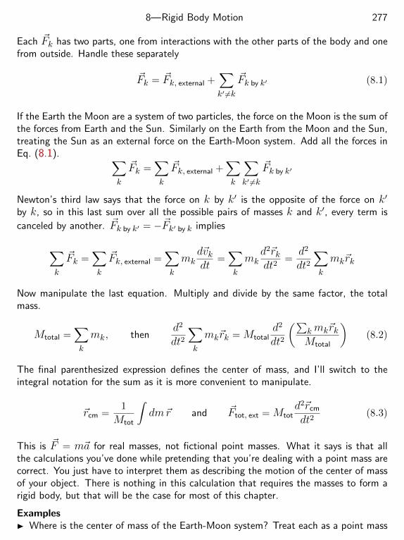
8—Rigid Body Motion 277
Each ~Fk has two parts, one from interactions with the other parts of the body and onefrom outside. Handle these separately
~Fk = ~Fk, external +∑k′ 6=k
~Fk by k′ (8.1)
If the Earth the Moon are a system of two particles, the force on the Moon is the sum ofthe forces from Earth and the Sun. Similarly on the Earth from the Moon and the Sun,treating the Sun as an external force on the Earth-Moon system. Add all the forces inEq. (8.1). ∑
k
~Fk =∑k
~Fk, external +∑k
∑k′ 6=k
~Fk by k′
Newton’s third law says that the force on k by k′ is the opposite of the force on k′
by k, so in this last sum over all the possible pairs of masses k and k′, every term is
canceled by another. ~Fk by k′ = −~Fk′ by k implies
∑k
~Fk =∑k
~Fk, external =∑k
mkd~vkdt
=∑k
mkd2~rkdt2
=d2
dt2∑k
mk~rk
Now manipulate the last equation. Multiply and divide by the same factor, the totalmass.
Mtotal =∑k
mk, thend2
dt2∑k
mk~rk = Mtotald2
dt2
(∑kmk~rkMtotal
)(8.2)
The final parenthesized expression defines the center of mass, and I’ll switch to theintegral notation for the sum as it is more convenient to manipulate.
~rcm =1
Mtot
∫dm~r and ~Ftot, ext = Mtot
d2~rcm
dt2(8.3)
This is ~F = m~a for real masses, not fictional point masses. What it says is that allthe calculations you’ve done while pretending that you’re dealing with a point mass arecorrect. You just have to interpret them as describing the motion of the center of massof your object. There is nothing in this calculation that requires the masses to form arigid body, but that will be the case for most of this chapter.
Examples Where is the center of mass of the Earth-Moon system? Treat each as a point mass
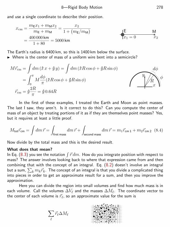
8—Rigid Body Motion 278
and use a single coordinate to describe their position.
xcm =mEx1 +mMx2
mE +mM=
x2
1 +(mE/mM
)=
400 000 km
1 + 80= 5000 km
x1 = 0 x2
E M
The Earth’s radius is 6400 km, so this is 1400 km below the surface. Where is the center of mass of a uniform wire bent into a semicircle?
M~rcm =
∫dm (x x+ y y) =
∫dm (xR cosφ+ yR sinφ)
=
∫ π
0Mdφπ
(xR cosφ+ yR sinφ)
~rcm = y2Rπ
= y 0.64R
φ
dφ
Rx
y
In the first of these examples, I treated the Earth and Moon as point masses.The last I saw, they aren’t. Is it correct to do this? Can you compute the center ofmass of an object by treating portions of it as if they are themselves point masses? Yes,but it requires at least a little proof.
Mtot~rcm =
∫dm~r =
∫first mass
dm~r +
∫second mass
dm~r = m1~rcm 1 +m2~rcm 2 (8.4)
Now divide by the total mass and this is the desired result.
What does that mean?In Eq. (8.3) you see the notation
∫~r dm. How do you integrate position with respect to
mass? The answer involves looking back to where that expression came from and thencombining that with the concept of an integral. Eq. (8.2) doesn’t involve an integralbut a sum,
∑kmk~rk. The concept of an integral is that you divide a complicated thing
into pieces in order to get an approximate result for a sum, and then you improve theapproximation.
Here you can divide the region into small volumes and find how much mass is ineach volume. Call the volumes ∆V` and the masses ∆M`. The coordinate vector tothe center of each volume is ~r`, so an approximate value for the sum is
∑`
~r`∆M`
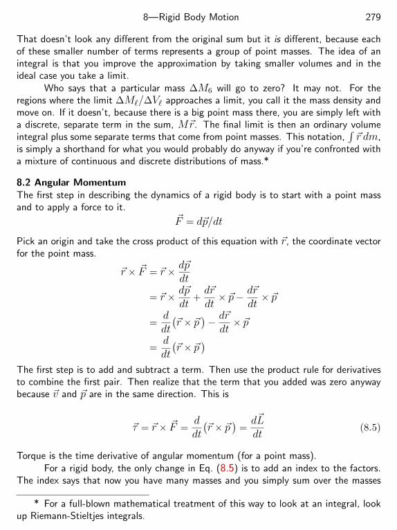
8—Rigid Body Motion 279
That doesn’t look any different from the original sum but it is different, because eachof these smaller number of terms represents a group of point masses. The idea of anintegral is that you improve the approximation by taking smaller volumes and in theideal case you take a limit.
Who says that a particular mass ∆M6 will go to zero? It may not. For theregions where the limit ∆M`/∆V` approaches a limit, you call it the mass density andmove on. If it doesn’t, because there is a big point mass there, you are simply left witha discrete, separate term in the sum, M~r. The final limit is then an ordinary volumeintegral plus some separate terms that come from point masses. This notation,
∫~r dm,
is simply a shorthand for what you would probably do anyway if you’re confronted witha mixture of continuous and discrete distributions of mass.*
8.2 Angular MomentumThe first step in describing the dynamics of a rigid body is to start with a point massand to apply a force to it.
~F = d~p/dt
Pick an origin and take the cross product of this equation with ~r, the coordinate vectorfor the point mass.
~r × ~F = ~r × d~pdt
= ~r × d~pdt
+d~rdt× ~p− d~r
dt× ~p
=ddt
(~r × ~p
)− d~rdt× ~p
=ddt
(~r × ~p
)The first step is to add and subtract a term. Then use the product rule for derivativesto combine the first pair. Then realize that the term that you added was zero anywaybecause ~v and ~p are in the same direction. This is
~τ = ~r × ~F =ddt
(~r × ~p
)=d~Ldt
(8.5)
Torque is the time derivative of angular momentum (for a point mass).For a rigid body, the only change in Eq. (8.5) is to add an index to the factors.
The index says that now you have many masses and you simply sum over the masses
* For a full-blown mathematical treatment of this way to look at an integral, lookup Riemann-Stieltjes integrals.
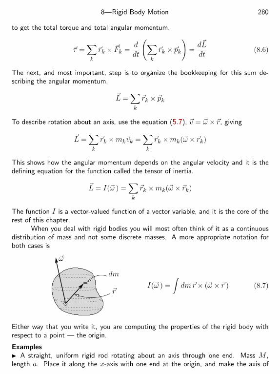
8—Rigid Body Motion 280
to get the total torque and total angular momentum.
~τ =∑k
~rk × ~Fk =ddt
(∑k
~rk × ~pk
)=d~Ldt
(8.6)
The next, and most important, step is to organize the bookkeeping for this sum de-scribing the angular momentum.
~L =∑k
~rk × ~pk
To describe rotation about an axis, use the equation (5.7), ~v = ~ω × ~r, giving
~L =∑k
~rk ×mk~vk =∑k
~rk ×mk(~ω × ~rk)
This shows how the angular momentum depends on the angular velocity and it is thedefining equation for the function called the tensor of inertia.
~L = I(~ω ) =∑k
~rk ×mk(~ω × ~rk)
The function I is a vector-valued function of a vector variable, and it is the core of therest of this chapter.
When you deal with rigid bodies you will most often think of it as a continuousdistribution of mass and not some discrete masses. A more appropriate notation forboth cases is
~ω
dm
~rI(~ω ) =
∫dm~r × (~ω × ~r ) (8.7)
Either way that you write it, you are computing the properties of the rigid body withrespect to a point — the origin.
Examples A straight, uniform rigid rod rotating about an axis through one end. Mass M ,length a. Place it along the x-axis with one end at the origin, and make the axis of
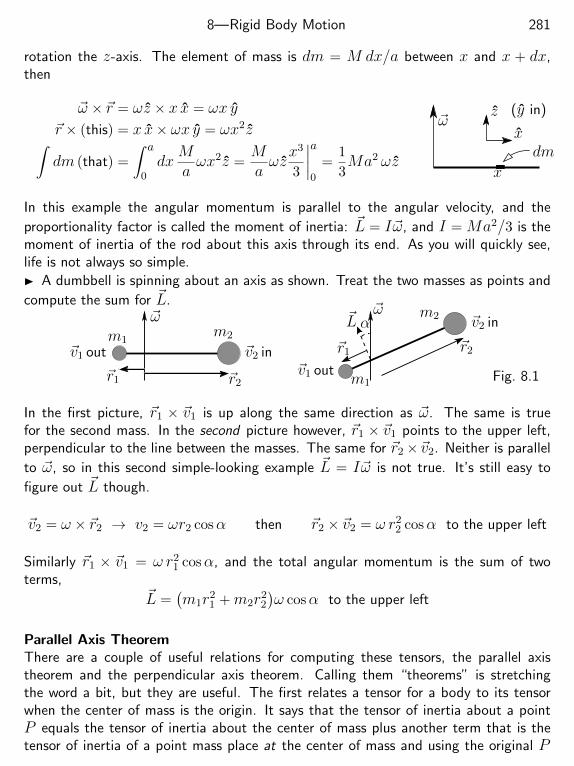
8—Rigid Body Motion 281
rotation the z-axis. The element of mass is dm = M dx/a between x and x + dx,then
~ω × ~r = ωz × x x = ωx y
~r × (this) = x x× ωx y = ωx2z∫dm (that) =
∫ a
0dx
Maωx2z =
Maωzx3
3
∣∣∣∣a0
=1
3Ma2 ωz
x
z~ω
x
dm
(y in)
In this example the angular momentum is parallel to the angular velocity, and the
proportionality factor is called the moment of inertia: ~L = I~ω, and I = Ma2/3 is themoment of inertia of the rod about this axis through its end. As you will quickly see,life is not always so simple.
A dumbbell is spinning about an axis as shown. Treat the two masses as points and
compute the sum for ~L.
~r1 ~r2
m1m2
~ω
~v1 out ~v2 in ~r1 ~r2
m1
m2~ωα
~v1 out
~v2 in~L
Fig. 8.1
In the first picture, ~r1 × ~v1 is up along the same direction as ~ω. The same is truefor the second mass. In the second picture however, ~r1 × ~v1 points to the upper left,perpendicular to the line between the masses. The same for ~r2×~v2. Neither is parallel
to ~ω, so in this second simple-looking example ~L = I~ω is not true. It’s still easy to
figure out ~L though.
~v2 = ω × ~r2 → v2 = ωr2 cosα then ~r2 × ~v2 = ω r22 cosα to the upper left
Similarly ~r1 × ~v1 = ω r21 cosα, and the total angular momentum is the sum of two
terms,~L =
(m1r
21 +m2r
22
)ω cosα to the upper left
Parallel Axis TheoremThere are a couple of useful relations for computing these tensors, the parallel axistheorem and the perpendicular axis theorem. Calling them “theorems” is stretchingthe word a bit, but they are useful. The first relates a tensor for a body to its tensorwhen the center of mass is the origin. It says that the tensor of inertia about a pointP equals the tensor of inertia about the center of mass plus another term that is thetensor of inertia of a point mass place at the center of mass and using the original P
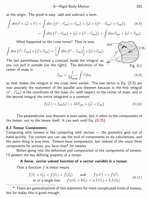
8—Rigid Body Motion 282
as the origin. The proof is easy: add and subtract a term.∫dm~r × (~ω × ~r ) =
∫dm
((~r − ~rcm) + ~rcm
)×(~ω ×
((~r − ~rcm) + ~rcm
))(8.8)
=
∫dm
(~r − ~rcm
)×(~ω ×
(~r − ~rcm
))+
∫dm~rcm ×
(~ω × ~rcm
)dm
c.m.~r
~rcm
Fig. 8.2
What happened to the cross terms? They’re zero.∫dm
(~r−~rcm
)×(~ω×~rcm
)=
[∫dm
(~r − ~rcm
)]×(~ω×~rcm
)The last parentheses formed a constant inside the integral, soyou can pull it outside (on the right). The definition of thecenter of mass is
~rcm =1
Mtotal
∫~r dm (8.9)
so that makes the integral in the cross term vanish. The two terms in Eq. (8.8) arenow precisely the statement of the parallel axis theorem because in the first integral(~r − ~rcm
)is the coordinate of the mass dm with respect to the center of mass, and in
the second integral the entire integrand is a constant.
I(~ω ) = Icm(~ω ) +M~rcm ×(~ω × ~rcm
)(8.10)
The perpendicular axis theorem is even easier, but it refers to the components ofthe tensor, not to the tensor itself. It can wait until Eq. (8.25).
8.3 Tensor ComponentsComputing with tensors is like computing with vectors — the geometry gets out ofhand quickly. For vectors you can use the tool of components to do calculations, andthe same thing is true here. Tensors have components, but instead of the usual threecomponents for vectors, you have nine* for tensors.
Before going into the definition and computation of the components of tensors,I’ll present the key defining property of a tensor.
A linear, vector-valued function of a vector variable is a tensor.
That a function f is linear means
f(~v1 + ~v2) = f(~v1) + f(~v2) and f(c~v ) = c f(~v )
or in a single line: f(a~v1 + b~v2) = a f(~v1) + b f(~v2)(8.11)
* There are generalizations of this statement for more complicated kinds of tensors,but for today this is good enough.
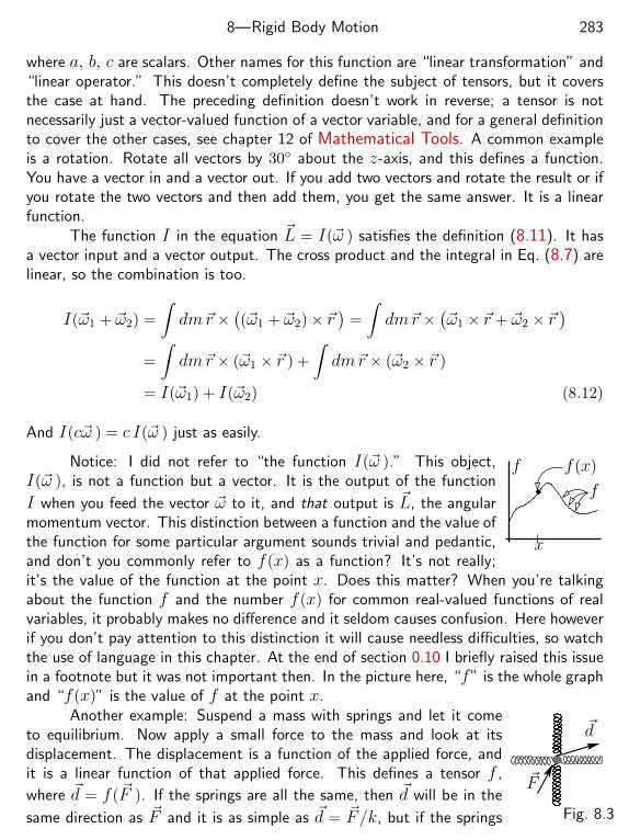
8—Rigid Body Motion 283
where a, b, c are scalars. Other names for this function are “linear transformation” and“linear operator.” This doesn’t completely define the subject of tensors, but it coversthe case at hand. The preceding definition doesn’t work in reverse; a tensor is notnecessarily just a vector-valued function of a vector variable, and for a general definitionto cover the other cases, see chapter 12 of Mathematical Tools. A common exampleis a rotation. Rotate all vectors by 30 about the z-axis, and this defines a function.You have a vector in and a vector out. If you add two vectors and rotate the result or ifyou rotate the two vectors and then add them, you get the same answer. It is a linearfunction.
The function I in the equation ~L = I(~ω ) satisfies the definition (8.11). It hasa vector input and a vector output. The cross product and the integral in Eq. (8.7) arelinear, so the combination is too.
I(~ω1 + ~ω2) =
∫dm~r ×
((~ω1 + ~ω2)× ~r
)=
∫dm~r ×
(~ω1 × ~r + ~ω2 × ~r
)=
∫dm~r × (~ω1 × ~r ) +
∫dm~r × (~ω2 × ~r )
= I(~ω1) + I(~ω2) (8.12)
And I(c~ω ) = c I(~ω ) just as easily.
f(x)f
f
x
Notice: I did not refer to “the function I(~ω ).” This object,I(~ω ), is not a function but a vector. It is the output of the function
I when you feed the vector ~ω to it, and that output is ~L, the angularmomentum vector. This distinction between a function and the value ofthe function for some particular argument sounds trivial and pedantic,and don’t you commonly refer to f(x) as a function? It’s not really;it’s the value of the function at the point x. Does this matter? When you’re talkingabout the function f and the number f(x) for common real-valued functions of realvariables, it probably makes no difference and it seldom causes confusion. Here howeverif you don’t pay attention to this distinction it will cause needless difficulties, so watchthe use of language in this chapter. At the end of section 0.10 I briefly raised this issuein a footnote but it was not important then. In the picture here, “f” is the whole graphand “f(x)” is the value of f at the point x.
~F
~d
Fig. 8.3
Another example: Suspend a mass with springs and let it cometo equilibrium. Now apply a small force to the mass and look at itsdisplacement. The displacement is a function of the applied force, andit is a linear function of that applied force. This defines a tensor f ,
where ~d = f(~F ). If the springs are all the same, then ~d will be in the
same direction as ~F and it is as simple as ~d = ~F/k, but if the springs
8—Rigid Body Motion 284
on the left and right are weaker than the others then this displacement won’t even be in
the same direction as ~F . Push in a direction between the springs and the displacementwill be more toward the weaker springs then the stronger.
Now for the components of the tensor: Start with the vectors ~ω and ~L, whichhave components with respect to a basis you’ve chosen
~ω = ωxx+ ωyy + ωz z and ~L = Lxx+ Lyy + Lz z
Now relate them with the function I .
~L = I(~ω ) is Lxx+ Lyy + Lz z = I(ωxx+ ωyy + ωz z) (8.13)
Use the linearity property of Eq. (8.11), which is the defining property of a tensor.
I(ωxx+ ωyy + ωz z ) = ωxI(x) + ωyI(y) + ωzI(z) (8.14)
The expression I(x) is a vector. As such it has three components. Denote these as
I(x) = Ixxx+ Iyxy + Izxz (8.15)
In the same way, the other terms are
I(y) = Ixyx+ Iyyy + Izy z and I(z) = Ixzx+ Iyz y + Izz z (8.16)
An abbreviated form for these equations is easier to write if you use a unified notationfor the basis vectors, ~ei, with the index i running over the set x, y, z (or more often 1,2, 3 once you get used to it).
I(~ei) =∑j
Iji~ej (8.17)
The indices denote which output basis vector and which input basis vector you arereferring to, and the order of the indices is carefully chosen for later convenience. Thesenine numbers are the components of the tensor I . Insert equations (8.14), (8.15), and(8.16) into equation (8.13) to get
Lxx+ Lyy + Lz z = ωx[Ixxx+ Iyxy + Izxz
]+ωy
[Ixyx+ Iyyy + Izy z
]+ωz
[Ixzx+ Iyz y + Izz z
]For these vectors to be equal, their respective components must match. Match thecoefficient of x on the left to the similar coefficient on the right. Now repeat the
8—Rigid Body Motion 285
process for y and z. This expresses the components of ~L in terms of the componentsof ~ω.
Lx = Ixxωx + Ixyωy + IxzωzLy = Iyxωx + Iyyωy + Iyzωz (8.18)
Lz = Izxωx + Izyωy + Izzωz
In matrix notation this isLxLyLz
=
Ixx Ixy IxzIyx Iyy IyzIzx Izy Izz
ωxωyωz
(8.19)
and this is the reason for the peculiar-looking way that you are told to multiply matrices,across the row of the first factor and down the columns of the second. It all comesfrom the equation (8.17), defining the components of a tensor. The meaning of theexpression (8.19) is the set of equations (8.18). The matrix indices are arranged asI(which row), (which column). Compare the placement of the indices in Eq. (8.18) and inEq. (8.16). The notation is designed to come out in the way conventionally used withmatrices.
The manipulations that took you from equation (8.13) through (8.19) becomefar more compact if you use the notation of Eq. (8.17).
~L =∑i
Li~ei = I(~ω) = I(∑
j
ωj~ej)
=∑j
ωjI(~ej) =∑j
ωj∑i
Iij~ei (8.20)
The basis vectors ~ei are independent, so the coefficients of ~ei must agree on the twosides of the equation. That is,
Li =∑j
Iijωj (8.21)
These two lines are so much more compact that you should compare their contentline-by-line with the preceding equations to verify that they are what they claim to be.
To compute these components, go back to the definition of the inertia tensor,Eq. (8.7). You need a vector identity to manipulate this:
~A× ( ~B × ~C ) = ~B( ~A . ~B )− ~C( ~A . ~B ) =⇒
I(~ω ) =
∫dm~r × (~ω × ~r ) =
∫dm
[r2~ω − ~r (~ω .~r )
]
8—Rigid Body Motion 286
Now compute I(x).
I(x) =
∫dm
[r2x− ~r (x .~r )
]=
∫dm
[(x2 + y2 + z2)x− (xx+ yy + zz)x
]=
∫dm
[(y2 + z2)x− yxy − zxz
]= Ixxx+ Iyxy + Izxz
The last line is the defining equation (8.15). Now all that you have to do is to read offthe coefficients of x, y, and z to get the first column of the matrix of components.
Ixx =
∫dm (y2 + z2), Iyx = −
∫dmyx, Izx = −
∫dmzx
The calculations for the other six components are identical, giving the next twocolumns of the matrix.
Ixy = −∫dmxy, Ixz = −
∫dmxz
Iyy =
∫dm (x2 + z2), Iyz = −
∫dmyz
Izy = −∫dmzy, Izz =
∫dm (x2 + y2)
The three diagonal components, Ixx, Iyy, and Izz, are the moments of inertia,and the other components are called the products of inertia. There’s some symmetryamong the nine components, as Ixy = Iyx etc, making the matrix in Eq. (8.19)symmetric. This is a special property of the inertia tensor, and it is not true for alltensors. You can write this matrix as
(I) =
∫dm
y2 + z2 −xy −xz−xy x2 + z2 −yz−xz −yz x2 + y2
(8.22)
In the spirit of Eq. (8.20) can these calculations of the components of the inertiatensor be made compact? Yes. Use x1, x2, and x3 for the coordinates instead of x, y,and z, then apply the summation convention as in Eq. (0.22), and
Li~ei = I(~ω) =
∫dm[xjxjωi~ei − xi~eiωjxj
]Li =
∫dm[xjxjωi − xiωjxj
]=
∫dm[xjxjδik − xixk
]ωk
~L~ω
α
yz
x out
1
2
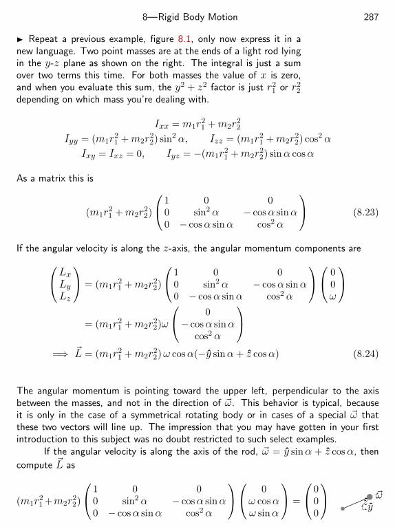
8—Rigid Body Motion 287
Repeat a previous example, figure 8.1, only now express it in anew language. Two point masses are at the ends of a light rod lyingin the y-z plane as shown on the right. The integral is just a sumover two terms this time. For both masses the value of x is zero,and when you evaluate this sum, the y2 + z2 factor is just r2
1 or r22
depending on which mass you’re dealing with.
Ixx = m1r21 +m2r
22
Iyy = (m1r21 +m2r
22) sin2 α, Izz = (m1r
21 +m2r
22) cos2 α
Ixy = Ixz = 0, Iyz = −(m1r21 +m2r
22) sinα cosα
As a matrix this is
(m1r21 +m2r
22)
1 0 00 sin2 α − cosα sinα0 − cosα sinα cos2 α
(8.23)
If the angular velocity is along the z-axis, the angular momentum components areLxLyLz
= (m1r21 +m2r
22)
1 0 00 sin2 α − cosα sinα0 − cosα sinα cos2 α
00ω
= (m1r
21 +m2r
22)ω
0− cosα sinα
cos2 α
=⇒ ~L = (m1r
21 +m2r
22)ω cosα(−y sinα+ z cosα) (8.24)
The angular momentum is pointing toward the upper left, perpendicular to the axisbetween the masses, and not in the direction of ~ω. This behavior is typical, becauseit is only in the case of a symmetrical rotating body or in cases of a special ~ω thatthese two vectors will line up. The impression that you may have gotten in your firstintroduction to this subject was no doubt restricted to such select examples.
If the angular velocity is along the axis of the rod, ~ω = y sinα + z cosα, then
compute ~L as
(m1r21 +m2r
22)
1 0 00 sin2 α − cosα sinα0 − cosα sinα cos2 α
0ω cosαω sinα
=
000
~ωzy
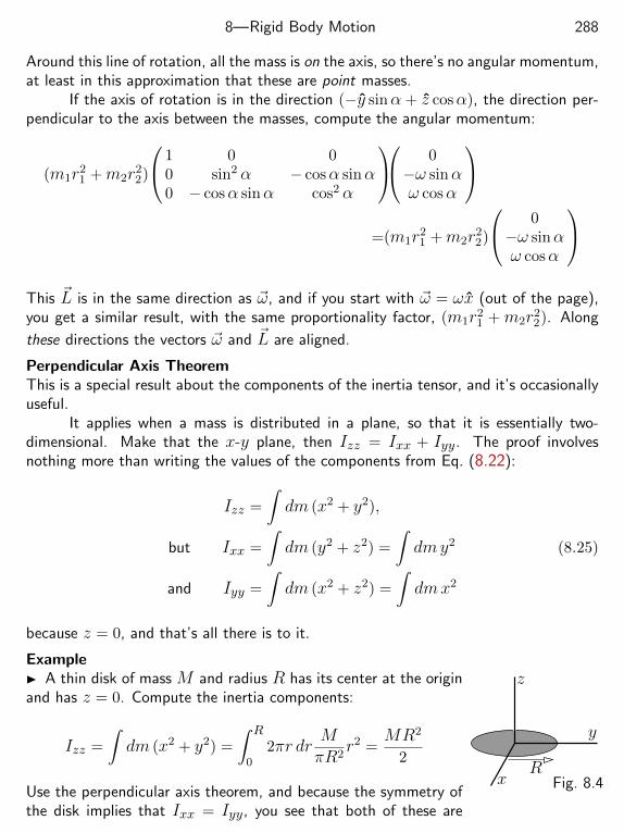
8—Rigid Body Motion 288
Around this line of rotation, all the mass is on the axis, so there’s no angular momentum,at least in this approximation that these are point masses.
If the axis of rotation is in the direction (−y sinα + z cosα), the direction per-pendicular to the axis between the masses, compute the angular momentum:
(m1r21 +m2r
22)
1 0 00 sin2 α − cosα sinα0 − cosα sinα cos2 α
0−ω sinαω cosα
=(m1r
21 +m2r
22)
0−ω sinαω cosα
This ~L is in the same direction as ~ω, and if you start with ~ω = ωx (out of the page),you get a similar result, with the same proportionality factor, (m1r2
1 + m2r22). Along
these directions the vectors ~ω and ~L are aligned.
Perpendicular Axis TheoremThis is a special result about the components of the inertia tensor, and it’s occasionallyuseful.
It applies when a mass is distributed in a plane, so that it is essentially two-dimensional. Make that the x-y plane, then Izz = Ixx + Iyy. The proof involvesnothing more than writing the values of the components from Eq. (8.22):
Izz =
∫dm (x2 + y2),
but Ixx =
∫dm (y2 + z2) =
∫dmy2
and Iyy =
∫dm (x2 + z2) =
∫dmx2
(8.25)
because z = 0, and that’s all there is to it.
Example
x
y
z
RFig. 8.4
A thin disk of mass M and radius R has its center at the originand has z = 0. Compute the inertia components:
Izz =
∫dm (x2 + y2) =
∫ R
02πr dr
MπR2
r2 =MR2
2
Use the perpendicular axis theorem, and because the symmetry ofthe disk implies that Ixx = Iyy, you see that both of these are
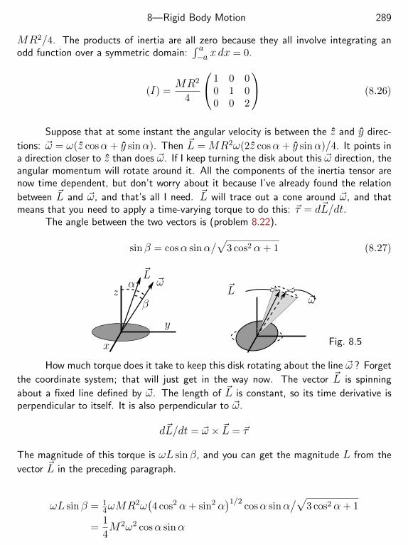
8—Rigid Body Motion 289
MR2/4. The products of inertia are all zero because they all involve integrating anodd function over a symmetric domain:
∫ a−a xdx = 0.
(I) =MR2
4
1 0 00 1 00 0 2
(8.26)
Suppose that at some instant the angular velocity is between the z and y direc-
tions: ~ω = ω(z cosα+ y sinα). Then ~L = MR2ω(2z cosα+ y sinα)/4. It points ina direction closer to z than does ~ω. If I keep turning the disk about this ~ω direction, theangular momentum will rotate around it. All the components of the inertia tensor arenow time dependent, but don’t worry about it because I’ve already found the relation
between ~L and ~ω, and that’s all I need. ~L will trace out a cone around ~ω, and thatmeans that you need to apply a time-varying torque to do this: ~τ = d~L/dt.
The angle between the two vectors is (problem 8.22).
sinβ = cosα sinα/√
3 cos2 α+ 1 (8.27)
α
β
~L~ω
z
y
x
~L~ω
Fig. 8.5
How much torque does it take to keep this disk rotating about the line ~ω ? Forget
the coordinate system; that will just get in the way now. The vector ~L is spinning
about a fixed line defined by ~ω. The length of ~L is constant, so its time derivative isperpendicular to itself. It is also perpendicular to ~ω.
d~L/dt = ~ω × ~L = ~τ
The magnitude of this torque is ωL sinβ, and you can get the magnitude L from the
vector ~L in the preceding paragraph.
ωL sinβ = 14ωMR2ω
(4 cos2 α+ sin2 α
)1/2cosα sinα
/√3 cos2 α+ 1
=1
4M2ω2 cosα sinα
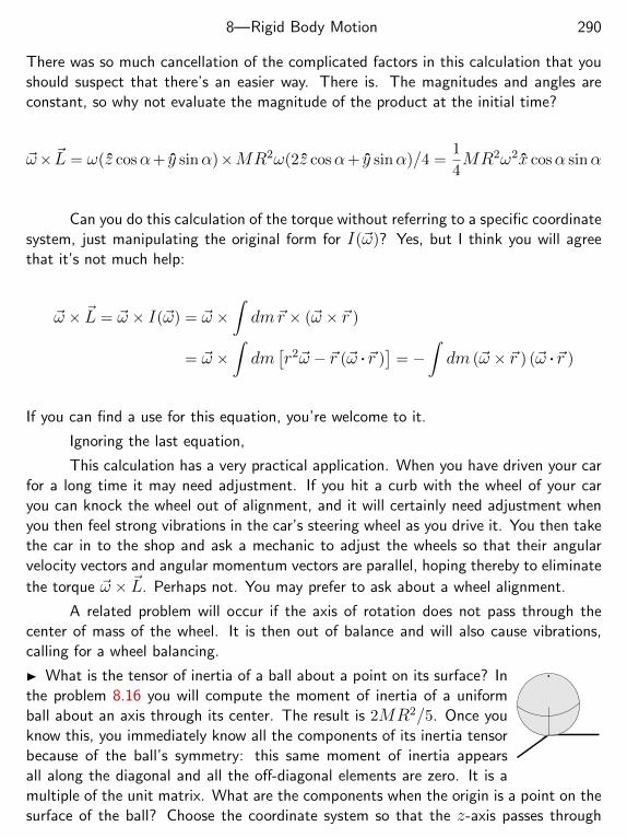
8—Rigid Body Motion 290
There was so much cancellation of the complicated factors in this calculation that youshould suspect that there’s an easier way. There is. The magnitudes and angles areconstant, so why not evaluate the magnitude of the product at the initial time?
~ω× ~L = ω(z cosα+ y sinα)×MR2ω(2z cosα+ y sinα)/4 =1
4MR2ω2x cosα sinα
Can you do this calculation of the torque without referring to a specific coordinatesystem, just manipulating the original form for I(~ω)? Yes, but I think you will agreethat it’s not much help:
~ω × ~L = ~ω × I(~ω) = ~ω ×∫dm~r × (~ω × ~r )
= ~ω ×∫dm
[r2~ω − ~r (~ω .~r )
]= −
∫dm (~ω × ~r ) (~ω .~r )
If you can find a use for this equation, you’re welcome to it.
Ignoring the last equation,
This calculation has a very practical application. When you have driven your carfor a long time it may need adjustment. If you hit a curb with the wheel of your caryou can knock the wheel out of alignment, and it will certainly need adjustment whenyou then feel strong vibrations in the car’s steering wheel as you drive it. You then takethe car in to the shop and ask a mechanic to adjust the wheels so that their angularvelocity vectors and angular momentum vectors are parallel, hoping thereby to eliminate
the torque ~ω × ~L. Perhaps not. You may prefer to ask about a wheel alignment.
A related problem will occur if the axis of rotation does not pass through thecenter of mass of the wheel. It is then out of balance and will also cause vibrations,calling for a wheel balancing.
What is the tensor of inertia of a ball about a point on its surface? Inthe problem 8.16 you will compute the moment of inertia of a uniformball about an axis through its center. The result is 2MR2/5. Once youknow this, you immediately know all the components of its inertia tensorbecause of the ball’s symmetry: this same moment of inertia appearsall along the diagonal and all the off-diagonal elements are zero. It is amultiple of the unit matrix. What are the components when the origin is a point on thesurface of the ball? Choose the coordinate system so that the z-axis passes through
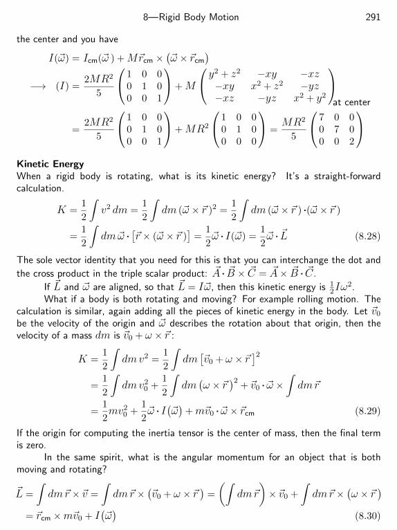
8—Rigid Body Motion 291
the center and you have
I(~ω) = Icm(~ω ) +M~rcm ×(~ω × ~rcm
)−→ (I) =
2MR2
5
1 0 00 1 00 0 1
+M
y2 + z2 −xy −xz−xy x2 + z2 −yz−xz −yz x2 + y2
at center
=2MR2
5
1 0 00 1 00 0 1
+MR2
1 0 00 1 00 0 0
=MR2
5
7 0 00 7 00 0 2
Kinetic EnergyWhen a rigid body is rotating, what is its kinetic energy? It’s a straight-forwardcalculation.
K =1
2
∫v2 dm =
1
2
∫dm (~ω × ~r )2 =
1
2
∫dm (~ω × ~r ) .(~ω × ~r )
=1
2
∫dm~ω .
[~r × (~ω × ~r )
]=
1
2~ω . I(~ω) =
1
2~ω . ~L (8.28)
The sole vector identity that you need for this is that you can interchange the dot and
the cross product in the triple scalar product: ~A . ~B × ~C = ~A× ~B . ~C.
If ~L and ~ω are aligned, so that ~L = I~ω, then this kinetic energy is 12Iω
2.What if a body is both rotating and moving? For example rolling motion. The
calculation is similar, again adding all the pieces of kinetic energy in the body. Let ~v0
be the velocity of the origin and ~ω describes the rotation about that origin, then thevelocity of a mass dm is ~v0 + ω × ~r :
K =1
2
∫dmv2 =
1
2
∫dm
[~v0 + ω × ~r
]2=
1
2
∫dmv2
0 +1
2
∫dm
(ω × ~r
)2+ ~v0 . ~ω ×
∫dm~r
=1
2mv2
0 +1
2~ω . I
(~ω)
+m~v0 . ~ω × ~rcm (8.29)
If the origin for computing the inertia tensor is the center of mass, then the final termis zero.
In the same spirit, what is the angular momentum for an object that is bothmoving and rotating?
~L =
∫dm~r × ~v =
∫dm~r ×
(~v0 + ω × ~r
)=
(∫dm~r
)× ~v0 +
∫dm~r ×
(ω × ~r
)= ~rcm ×m~v0 + I
(~ω)
(8.30)
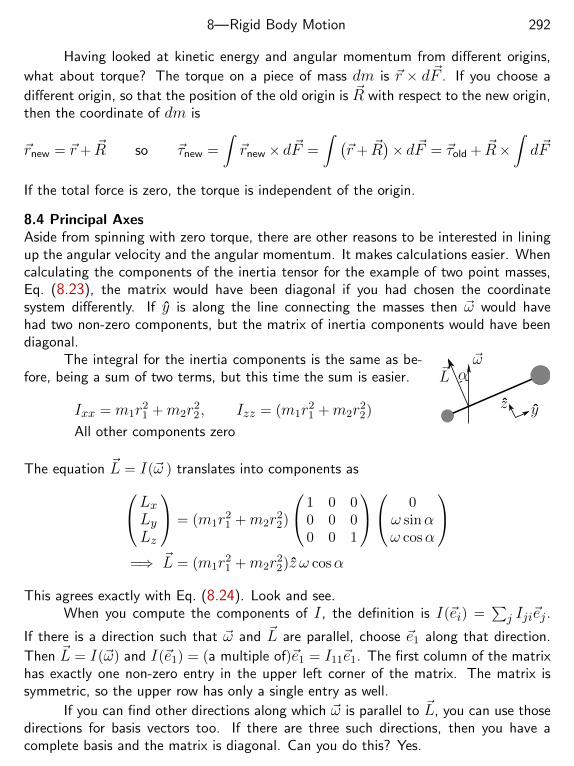
8—Rigid Body Motion 292
Having looked at kinetic energy and angular momentum from different origins,
what about torque? The torque on a piece of mass dm is ~r × d~F . If you choose a
different origin, so that the position of the old origin is ~R with respect to the new origin,then the coordinate of dm is
~rnew = ~r+ ~R so ~τnew =
∫~rnew × d~F =
∫ (~r+ ~R
)× d~F = ~τold + ~R×
∫d~F
If the total force is zero, the torque is independent of the origin.
8.4 Principal AxesAside from spinning with zero torque, there are other reasons to be interested in liningup the angular velocity and the angular momentum. It makes calculations easier. Whencalculating the components of the inertia tensor for the example of two point masses,Eq. (8.23), the matrix would have been diagonal if you had chosen the coordinatesystem differently. If y is along the line connecting the masses then ~ω would havehad two non-zero components, but the matrix of inertia components would have beendiagonal.
~L~ω
α
yz
The integral for the inertia components is the same as be-fore, being a sum of two terms, but this time the sum is easier.
Ixx = m1r21 +m2r
22, Izz = (m1r
21 +m2r
22)
All other components zero
The equation ~L = I(~ω ) translates into components asLxLyLz
= (m1r21 +m2r
22)
1 0 00 0 00 0 1
0ω sinαω cosα
=⇒ ~L = (m1r
21 +m2r
22)z ω cosα
This agrees exactly with Eq. (8.24). Look and see.When you compute the components of I , the definition is I(~ei) =
∑j Iji~ej .
If there is a direction such that ~ω and ~L are parallel, choose ~e1 along that direction.
Then ~L = I(~ω) and I(~e1) = (a multiple of)~e1 = I11~e1. The first column of the matrixhas exactly one non-zero entry in the upper left corner of the matrix. The matrix issymmetric, so the upper row has only a single entry as well.
If you can find other directions along which ~ω is parallel to ~L, you can use thosedirections for basis vectors too. If there are three such directions, then you have acomplete basis and the matrix is diagonal. Can you do this? Yes.
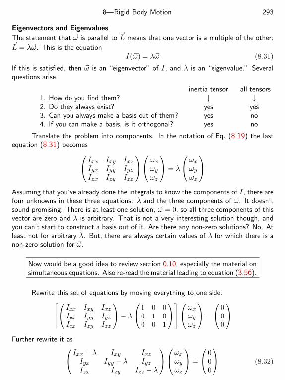
8—Rigid Body Motion 293
Eigenvectors and Eigenvalues
The statement that ~ω is parallel to ~L means that one vector is a multiple of the other:~L = λ~ω. This is the equation
I(~ω) = λ~ω (8.31)
If this is satisfied, then ~ω is an “eigenvector” of I , and λ is an “eigenvalue.” Severalquestions arise.
inertia tensor all tensors1. How do you find them? ↓ ↓2. Do they always exist? yes yes3. Can you always make a basis out of them? yes no4. If you can make a basis, is it orthogonal? yes no
Translate the problem into components. In the notation of Eq. (8.19) the lastequation (8.31) becomes Ixx Ixy Ixz
Iyx Iyy IyzIzx Izy Izz
ωxωyωz
= λ
ωxωyωz
Assuming that you’ve already done the integrals to know the components of I , there arefour unknowns in these three equations: λ and the three components of ~ω. It doesn’tsound promising. There is at least one solution, ~ω = 0, so all three components of thisvector are zero and λ is arbitrary. That is not a very interesting solution though, andyou can’t start to construct a basis out of it. Are there any non-zero solutions? No. Atleast not for arbitrary λ. But, there are always certain values of λ for which there is anon-zero solution for ~ω.
Now would be a good idea to review section 0.10, especially the material onsimultaneous equations. Also re-read the material leading to equation (3.56).
Rewrite this set of equations by moving everything to one side. Ixx Ixy IxzIyx Iyy IyzIzx Izy Izz
− λ 1 0 0
0 1 00 0 1
ωxωyωz
=
000
Further rewrite it as Ixx − λ Ixy Ixz
Iyx Iyy − λ IyzIzx Izy Izz − λ
ωxωyωz
=
000
(8.32)
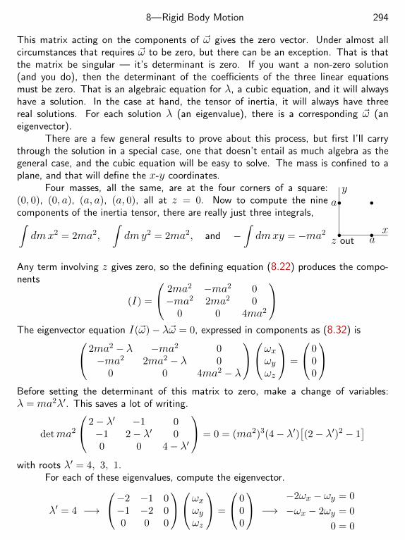
8—Rigid Body Motion 294
This matrix acting on the components of ~ω gives the zero vector. Under almost allcircumstances that requires ~ω to be zero, but there can be an exception. That is thatthe matrix be singular — it’s determinant is zero. If you want a non-zero solution(and you do), then the determinant of the coefficients of the three linear equationsmust be zero. That is an algebraic equation for λ, a cubic equation, and it will alwayshave a solution. In the case at hand, the tensor of inertia, it will always have threereal solutions. For each solution λ (an eigenvalue), there is a corresponding ~ω (aneigenvector).
There are a few general results to prove about this process, but first I’ll carrythrough the solution in a special case, one that doesn’t entail as much algebra as thegeneral case, and the cubic equation will be easy to solve. The mass is confined to aplane, and that will define the x-y coordinates.
x
y
a
a
z out
Four masses, all the same, are at the four corners of a square:(0, 0), (0, a), (a, a), (a, 0), all at z = 0. Now to compute the ninecomponents of the inertia tensor, there are really just three integrals,∫dmx2 = 2ma2,
∫dmy2 = 2ma2, and −
∫dmxy = −ma2
Any term involving z gives zero, so the defining equation (8.22) produces the compo-nents
(I) =
2ma2 −ma2 0−ma2 2ma2 0
0 0 4ma2
The eigenvector equation I(~ω)− λ~ω = 0, expressed in components as (8.32) is 2ma2 − λ −ma2 0
−ma2 2ma2 − λ 00 0 4ma2 − λ
ωxωyωz
=
000
Before setting the determinant of this matrix to zero, make a change of variables:λ = ma2λ′. This saves a lot of writing.
detma2
2− λ′ −1 0−1 2− λ′ 00 0 4− λ′
= 0 = (ma2)3(4− λ′)[(2− λ′)2 − 1
]with roots λ′ = 4, 3, 1.
For each of these eigenvalues, compute the eigenvector.
λ′ = 4 −→
−2 −1 0−1 −2 00 0 0
ωxωyωz
=
000
−→−2ωx − ωy = 0
−ωx − 2ωy = 0
0 = 0
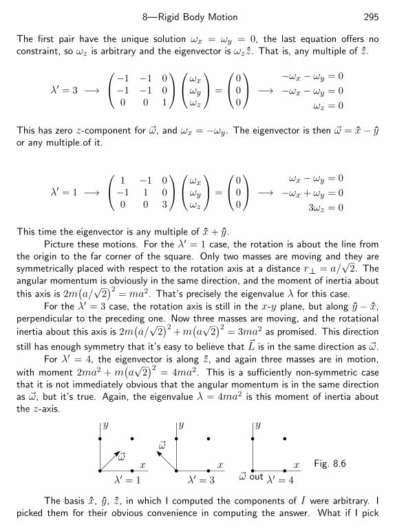
8—Rigid Body Motion 295
The first pair have the unique solution ωx = ωy = 0, the last equation offers noconstraint, so ωz is arbitrary and the eigenvector is ωz z. That is, any multiple of z.
λ′ = 3 −→
−1 −1 0−1 −1 00 0 1
ωxωyωz
=
000
−→−ωx − ωy = 0
−ωx − ωy = 0
ωz = 0
This has zero z-component for ~ω, and ωx = −ωy. The eigenvector is then ~ω = x− yor any multiple of it.
λ′ = 1 −→
1 −1 0−1 1 00 0 3
ωxωyωz
=
000
−→ωx − ωy = 0
−ωx + ωy = 0
3ωz = 0
This time the eigenvector is any multiple of x+ y.Picture these motions. For the λ′ = 1 case, the rotation is about the line from
the origin to the far corner of the square. Only two masses are moving and they aresymmetrically placed with respect to the rotation axis at a distance r⊥ = a/
√2. The
angular momentum is obviously in the same direction, and the moment of inertia about
this axis is 2m(a/√
2)2
= ma2. That’s precisely the eigenvalue λ for this case.For the λ′ = 3 case, the rotation axis is still in the x-y plane, but along y − x,
perpendicular to the preceding one. Now three masses are moving, and the rotational
inertia about this axis is 2m(a/√
2)2
+m(a√
2)2
= 3ma2 as promised. This direction
still has enough symmetry that it’s easy to believe that ~L is in the same direction as ~ω.For λ′ = 4, the eigenvector is along z, and again three masses are in motion,
with moment 2ma2 + m(a√
2)2
= 4ma2. This is a sufficiently non-symmetric casethat it is not immediately obvious that the angular momentum is in the same directionas ~ω, but it’s true. Again, the eigenvalue λ = 4ma2 is this moment of inertia aboutthe z-axis.
x
y
x
y
x
y
~ω~ω
~ω outλ′ = 1 λ′ = 3 λ′ = 4
Fig. 8.6
The basis x, y, z, in which I computed the components of I were arbitrary. Ipicked them for their obvious convenience in computing the answer. What if I pick
8—Rigid Body Motion 296
another basis, one consisting of these three orthogonal eigenvectors? I’ll call them ~e1,~e2, and ~e3 as a common notation used for basis vectors.
~e1 =(x+ y
)/√
2, ~e2 =(y − x
)/√
2, ~e3 = z (8.33)
Does it matter that these are unit vectors? No, as long as they are independent thatis good enough. You could drop the
√2 and compute the matrix for I , but for other
manipulations you should be consistent. In keeping with the change I will use subscripts1, 2, 3 instead of x, y, z on the components
I(~e1) =∑j
Ij1~ej = I11~e1 + I21~e2 + I31~e3 = λ1~e1
This determines the first column of the matrix for I in this basis. The other columnsare found the same way.
I(~e2) =∑j
Ij2~ej = I12~e1 + I22~e2 + I32~e3 = λ2~e2
I(~e3) =∑j
Ij3~ej = I13~e1 + I23~e2 + I33~e3 = λ3~e3
The matrix for I is now
(I) =
λ1 0 00 λ2 00 0 λ3
=
ma2 0 00 3ma2 00 0 4ma2
and you see that in this basis the matrix is diagonal. That can provide significantadvantages in manipulation for further calculations. Notice that you would get thesame matrix even if you do not put in the
√2 factors in Eq. (8.33).
Is it always easy to find the eigenvectors? No, this example is very easy and youdidn’t really have to confront a cubic equation to solve for the eigenvalues. Alas, it isnot typical.
8.5 Properties of EigenvectorsThere are some general results to be proved about these eigenvectors and eigenvalues,and the methods of proof used here will show up in several other important contexts,so they are worth learning. First an identity about the inertia tensor.
I(~ω ) =
∫dm~r × (~ω × ~r ) =
∫dm
[r2~ω − ~r(~ω .~r )
]~ω*
1. I(~ω2) = ~ω*
1.∫dm
[r2~ω2 − ~r(~ω2 .~r )
]=
∫dm
[r2~ω*
1. ~ω2 − ~ω*
1.~r(~ω2 .~r )
]= I(~ω*
1) . ~ω2 (8.34)
8—Rigid Body Motion 297
What is a complex conjugation doing here when all these vectors are supposed to bereal? And what does it mean anyway? Here I am allowing for the possibility that thesemay be complex in order to prove that they aren’t. How can a vector be complex? Inthe usual basis, just allow the components to be complex numbers. You won’t representit by a single arrow any more, but that’s not a requirement.
This symmetry property of the inertia tensor,
~ω*1
. I(~ω2) = I(~ω*1) . ~ω2 (8.35)
plays a key role in much of this analysis. Very similar identities appear in very different-looking contexts such as differential equations, and there they will lead to results muchlike the ones here. A tensor satisfying this equation is called “Hermitian” or “symmetric”depending on whether a physicist or a mathematician respectively is talking. It parallelsthe results in the equations (7.42) to (7.44).
In the calculation of eigenvalues and eigenvectors in the example of the precedingsection, the eigenvalues (roots of a cubic) were real and the eigenvectors are orthogonal.Is that a general property? For tensors that satisfy the identity derived in Eq. (8.35) itis. To prove this the manipulations are simple but not obvious. Assume that you havetwo eigenvectors:
I(~ω1) = λ1 ~ω1 and I(~ω2) = λ2 ~ω2
Take the scalar product of the first with ~ω*2 and the second with ω*
1.
~ω*2
. I(~ω1) = λ1 ~ω*2
. ~ω1 and ~ω*1
. I(~ω2) = λ2 ~ω*1
. ~ω2
Take the complex conjugate of the second equation:
~ω1 . I(~ω*2) = λ*
2 ~ω1 . ~ω*2
Subtract this from the first of the preceding equations.
~ω*2
. I(~ω1)− ~ω1 . I(~ω*2) = (λ1 − λ*
2)~ω1 . ~ω*2
The identity Eq. (8.35) says that the left side of this equation is zero, and the rightside is
0 =(λ1 − λ*
2
)~ω*
2. ~ω1 (8.36)
Now take the special case that ~ω1 = ~ω2. These two vectors are the same vector, sonecessarily the two eigenvalues are the same also
0 =(λ1 − λ*
1
)~ω*
1. ~ω1
8—Rigid Body Motion 298
The second factor is not zero, and this implies that the first factor must be. That inturn says that λ is real. With real λ and real components of the inertia tensor, all thecomponents of ~ω are real too.
Now Eq. (8.36) is0 =
(λ1 − λ2
)~ω2 . ~ω1 (8.37)
and this implies that for two different eigenvalues, i.e. λ1 6= λ2, the correspondingeigenvectors are orthogonal, as exemplified in the preceding example: z⊥ (y−x)⊥ (x+y).
These eigenvalues are the moments of inertia about the axis defined by theeigenvector, and they are of course non-negative. Of course? For an eigenvector,
λω2 = ~ω . I(~ω ) =
∫dm
[r2ω2 − (~r . ~ω )2
]= ω2
∫dmr2
⊥
where r⊥ is the perpendicular distance from dm to the axis defined by ~ω. This integralwill be zero only in the special case that all the mass is on the axis — when the bodyis a line. In all other cases it is positive.
8.6 DynamicsThe basic equation for rotating objects is ~τ = d~L/dt. Now ~L is nothing more than atensor expression involving ~ω.
~τ =ddtI(~ω) = I
(d~ωdt
)+dIdt
(~ω)
Written this way all the components of the inertia tensor are time-dependent, and that’snot a fruitful approach. The trick is to transform to the rotating coordinate system inwhich the body is at rest. Then I is a constant. From the equation (5.5),
~τ =d~Ldt
= ~L+ ~ω × ~L = I(~ω)
+ ~ω × I(~ω)
and this again uses the chapter five convention that the dot now refers to the timederivative in the rotating system. In this rotating system, you can pick the coordinatesso that the components of I are a diagonal matrix — the basis using eigenvectors ofI .dot convention
~τ = I(~ω)
+(xωx+yωy + zωz
)×(Ixxxωx + Iyyyωy + Izz zωz
)τx = Ixxωx + ωyωz(Izz − Iyy)
τy = Iyyωy + ωzωx(Ixx − Izz) (8.38)
τz = Izzωz + ωxωy(Iyy − Ixx)
8—Rigid Body Motion 299
These are the Euler equations. (As if he didn’t have enough things named for him.)If your automobile tire is misaligned, its axis of rotation doesn’t line up with its
axis of symmetry. Call the z-axis the symmetry axis of the tire, then Ixx = Iyy. Asyou drive at constant velocity what torque does this cause on your tire? In the inertialsystem ~ω is a constant because it is defined by the axle of the car. What happens to ~ωin the rotating system? Again, Eqs. (5.5) and (5.12):
~ωα
z-axisx-axis
~τ
d~ωdt
= ~ω + ~ω × ~ω = ~ω = 0 (8.39)
and this means that it is constant in the rotating system too. The equations (8.38) arenow
τx = ωyωz(Izz − Iyy), τy = ωzωx(Ixx − Izz), τz = 0
If the misalignment between ~ω and the axis of the tire is the angle α then pick the x-ycoordinates (rotating) so that ~ω = ωz cosα− ωx sinα.
τx = 0, τy = ω2 cosα sinα(Izz − Ixx), τz = 0
This is a constant torque about the y-axis, so why does it cause the wheel to shake?This is the rotating system remember. In the inertial system (the driver) this torquevector, τyy, is spinning about the axle at a rate ω, and the size of this torque varies asthe square of ω.
How can you picture this? Imagine yourself standing on this disk(tire?) and hanging on to the z-axis as hard as you can. Your feet arestraddling the x-axis, which is stationary between your legs. If you lookstraight ahead you see the angular velocity vector standing still in front
of you (~ω = 0). But if you look in the distance you may get dizzy fromwatching the world spinning around. If you look down and to your right youwill see the torque vector at your feet, pointing along the y-axis. (Notice
that Izz > Ixx.) And where is ~L?
~L = I(~ω) = I(ωz cosα− ωx sinα) = ω(Izz z cosα− Ixxx sinα
)This points in a direction closer to the z-axis than the ~ω vector does. Asyou look straight ahead you can see it fixed in front of you on the near
side of ~ω. Remember, ~L = 0.
8—Rigid Body Motion 300
Free RotationWhat if there is no torque, and the object is free to rotate in space. The equations(8.38) (with ~τ = 0) are differential equations for ~ω. They can be solved, but exceptfor the case of a symmetric rigid body the solution is non-linear and tough. For thatreason pick Ixx = Iyy.
0 = Ixxωx + ωyωz(Izz − Ixx)
0 = Ixxωy + ωzωx(Ixx − Izz) (8.40)
0 = Izzωz + 0
The last line says that ωz is a constant. That in turn makes the first two equationslinear equations for ωx and ωy. You know how to solve those: eαt.
ωx(t) = Aeαt, ωy(t) = Beαt
0 = IxxαA+ ωz(Izz − Ixx)B
0 = IxxαB − ωz(Izz − Ixx)A
A non-zero solution for A and B requires that the determinant vanish.
I2xxα
2 + ω2z(Izz − Ixx)2 = 0 −→ α = ±i ωz
Izz − IxxIxx
= ±i ω′ (8.41)
Put these back into one of the equations for A and B to get
0 = IxxA
(±i ωz
Izz − IxxIxx
)+ ωz(Izz − Ixx)B −→ ±iA+B = 0
A solution is now
ωx = Aeiω′t +A′e−iω
′t, ωy = −iAeiω′t + iA′e−iω′t
Chose some initial conditions:
ωx(0) = ω0, ωy(0) = 0 then ωx(t) = ω0 cosω′t, ωy(t) = ω0 sinω′t(8.42)
The rotation axis precesses about the z-axis at an angular velocity ω′.An example: Earth. It’s freely spinning in space and it is slightly ellipsoidal so
that the moments of inertia aren’t the same about all axes. The equatorial bulge makesIzz > Ixx = Iyy. If the angular velocity of the planet exactly lined up with its axisof symmetry, the constant ω0 in Eq. (8.42) would be zero. It would be too much of a
8—Rigid Body Motion 301
coincidence for the alignment to be perfect and it isn’t. It misses by an amount suchthat if you go to the North pole and look for the angular velocity vector you will find itseveral meters away. Then it wanders around the pole at a rate ω′ ≈ 2π/400 days. Itsmotion is not as regular as this rigid body analysis would lead you to believe, but theEarth isn’t perfectly rigid either.
That the Earth isn’t rigid should lead to damping of this oscillation within yearsor centuries, but it’s still here. It has been a puzzle what keeps this “Chandler Wobble”going, but recent analysis points to fluctuating pressure on the bottom of the ocean asthe largest source of the excitation.
This precession can give geologists information about the interior of the planet.Equation (8.41) tells you about Izz − Ixx and that gives some constraints on thedistribution of mass within the Earth. And not just Earth; Mars too. One of themeasuring devices sent to Mars looked at that planet’s wobble, and that says somethingabout the interior structure of Mars. Why hasn’t the wobble been completely dampedin the case of Mars? After all, it has no oceans to excite the oscillation. Unknown. Youwill have to do a search of the current literature on the subject to get some ideas ofthe complexity of the problem.
Stability of RotationsWhat happens when you toss a hammer or a tennis racket up and set it spinning? Theanswer depends very much on how you do it, and the motion can be very smooth orvery wild. If you don’t have either a hammer or a racket handy, perhaps you have aheavy rubber band. Then you can wrap it around a book so that the pages don’t openup when you toss it up and spinning. Depending on the axis about which it’s spinningyou will get very different results.
To analyze this, start again from Euler’s equations (8.38). This time assume thatthe three moments of inertia are different from each other, but assume that the angularvelocity vector is almost along one of the principle axes. This will be a perturbationexpansion and a linearization. Assume that the rotation is almost along the z-axis. Thetorque is zero because you have tossed the object up and it is then free to rotate as itwill.
~ω(t) = ω0z +~ε (t), with ε ω0
Start from the equations (8.38) with ~τ = 0, and as usual with these expansions, keeponly the first order terms in ε.
0 = Ixxεx + εyω0(Izz − Iyy)
0 = Iyy εy + εxω0(Ixx − Izz)0 = Izz εz
Every place that an ε2 appeared I dropped it, and the resulting equations are linear. Inthe third equation, both ωx and ωy are first order in ε so that killed its final term.
8—Rigid Body Motion 302
The third equation says that εz is a constant, and I may as well take it to bezero because a non-zero value would just be a redefinition of the original rotation rateω0 about the z-axis. The other two equations are linear differential equations for εxand εy. You know how to handle those: an exponential.
εx = Aeαt, εy = Beαt
then
(00
)=
(Ixxα ω0(Izz − Iyy)
ω0(Ixx − Izz) Iyyα
)(AB
)To get a non-zero solution the determinant must vanish.
IxxIyyα2 − ω2
0(Ixx − Izz)(Izz − Iyy) = 0 (8.43)
The nature of these solutions depends on the sign of α2. If it’s negative then α isimaginary and you have oscillations about the z direction; if α2 is positive then αis real and you have exponential movement away from there the z-axis: an unstablerotation.
α2 ∝ (Ixx − Izz)(Izz − Iyy)
If z has the largest moment, Izz > Ixx and Izz > Iyy, then α2 < 0
and this says that α is imaginary and that the motion is stable. If Izz is the smallest ofthe three moments you have the same result: α is imaginary and the motion is stable.It is only in the third case, when Izz is intermediate between the other two moments ofinertia, that α comes out to be real. That motion is unstable. Take a book and wrap aheavy rubber band about it. Now toss it in the air, spinning about one of the three axesof symmetry. Do it for each axis, and the difference in the results will be very obvious.
There is more to learn about the stability of these rotations. What is the kinetic
energy of rotation about each axis? Use Eq. (8.28) about each axis: K = 12~ω
. ~L.
~ω = ω0x −→ K =1
2Ixxω
20, ω0y −→
1
2Iyyω
20, ω0z −→
1
2Izzω
20
The angular momentum in each case is easy because these are eigenvectors of the inertiatensor and are respectively
Lx = Ixxω0, Ly = Iyyω0, Lz = Izzω0
Write the energy in terms of these angular momenta.
~ω = ω0x −→ K =L2
2Ixx, ω0y −→
L2
2Iyy, ω0z −→
L2
2Izz
8—Rigid Body Motion 303
This assumes the same angular momentum for every case, and these equations say thatfor a given angular momentum the rotation about the axis with the largest moment ofinertia has the smallest kinetic energy.
Whether this object is a rigid body or not, if there are no torques on it the angularmomentum is conserved. If you have a truly rigid body, then both angular momentumand mechanical energy are conserved, but completely rigid bodies are a mathematicalfiction. Any real object will flex slightly, and this has an important consequence. Ifa satellite is set to rotating about one of its principle axes and if that is one of thetwo stable axes then you might expect the rotation to remain about that axis forever.But. . . A tiny flexibility will cause a tiny friction — a way to dissipate energy. Theonly truly stable rotation in this case will be about the axis with the largest moment ofinertia and so the smallest kinetic energy for the given angular momentum.
~ω
Early in the space program the satellite Explorer-1 was placed in orbit around Earth andset spinning about the axis having the smallest moment, supposedly a stable rotation.The satellite however, had whip antennas and they had more than enough flexibility todestabilize this rotation and to set it to tumbling about its really stable axis — end overend — much to the embarrassment of the engineers and physicists involved.
If you have seen the motion pictures 2001 and its sequel 2010, a space ship wasleft in orbit around Jupiter’s moon Io at the end of the first picture, and when theyreturned in the sequel it was tumbling end-over-end. They made no comment in themovie, but they got the physics right.
Exercises
1 Three equal point masses m are at the corners of the right triangle (x, y) = (0, 0),(a, 0), (0, b). Where is the center of mass?
2 Remove the masses from the preceding triangle and replace the sides with thin rodsof constant linear mass density λ. Where is the center of mass?
3 Remove the rods from the preceding triangle and replace the area with a uniformsheet of constant area mass density σ. Where is the center of mass?
4 A vector-valued function F acts on vectors in the plane, reversing the direction ofeach. Compute the components of this function, a 2× 2 matrix.
8—Rigid Body Motion 304
5 With respect to the origin, what are the components of the tensor of inertia for apoint mass m at the point (x, y, z) = (a, 0, 0)?
6 With respect to the origin, what are the components of the tensor of inertia fora point mass m at the point (x, y, z) = (a, a, 0)? and what if its coordinates are(a, a, a)?
7 Use the summation convention and notation of Eq. (0.45) to write the equations(8.17), (8.20), (8.21).
8 For the springs that appear just before Eq. (8.13), call them k1 left and right and k2
top and bottom. What are the components of the f in ~d = f(~F )?
9 What are the dimensions of I(x)?
10 Starting at Eq. (8.33), drop the denominators√
2 from the basis vectors, so that~e1 = x+ y etc. Now compute the components of the same inertia tensor as done there.
11 Compute the moment of inertia of a thin spherical shell, mass m and radius R,about an axis through its center. Note: you must do this in your head! No complicatedintegrals allowed.
12 If a rigid body is both spinning and moving with no external forces, you expect itskinetic energy to stay constant. In Eq. (8.29) however the first two terms are constant,but the center of mass is moving, so the last term is always changing. What’s wrong?
8—Rigid Body Motion 305
Problems
8.1 Explicitly write out the derivation leading to Eqs. (8.2) and (8.3) for the case oftwo masses.
8.2 Compute the volume of a solid hemisphere of radius R. (a) cylindrical coordinates.(b) spherical coordinates. (c) Find the center of mass of a solid hemisphere with uniformmass density.
8.3 Write out the proof in Eq. (8.4) for the special case of 4 = 2 + 2 masses to verifythe calculation.
8.4 Find the center of mass of the parabolic-shaped plane object in problem 2.43.
8.5 Does f(~v ) = ~v + ~c define a tensor f , where ~c is a constant vector?What about f(~v ) = ~c .~v ?What about f(~v ) = z × ~v ?What about f(~v ) = c~v ?What about f(~v ) = x x .~v ?What about f(~v ) = y x .~v ?What about f(~v ) = v2~v ?In each case, draw pictures that explain what the function does.
8.6 The force on a charge moving in a magnetic field depends on its velocity as ~F =
q ~v× ~B. Show that this function of velocity, f(~v ) = ~v× ~B, defines a tensor and compute
its components in terms of the components of ~B. Write the result as a matrix.
8.7 In two dimensions rotating vectors by a fixed angle α defines a tensor. Use theusual x-y basis to compute the components of this tensor: ~u = f(~v ). Ans: in part,f21 = + sinα.
8.8 If an object is pivoted about some point and the only other forces on it are from auniform gravitational field, show that the torque about the pivot is the same as if all themass were concentrated at the center of mass. If the gravitational field is not uniform,show by a counterexample that this is false.
8.9 A meter stick is pivoted about its end, and you start it at rest horizontally. Findthe initial angular acceleration and find the initial linear acceleration of the end of thestick.
8.10˙ From the identity derived in Eq. (8.34), examine the special case that ~ω1 = xand ~ω2 = y. Generalize and determine what it says about all the components of thetensor of inertia.
8—Rigid Body Motion 306
8.11 Derive all the components in the equation (8.23).
8.12˙ For a uniform rigid rod rotating about an axis perpendicular to the rod, computethe rotational kinetic energy. The rotation axis can intersect the rod anywhere. Forfixed ω, find the position of this axis for which this kinetic energy is a minimum.
8.13˙ Generalize the preceding problem to an arbitrary body rotating about an arbitraryaxis. Among the set of all axes parallel to the given one, derive the axis that presentsthe smallest kinetic energy for a fixed ~ω.
8.14 Derive the component Ixx =∫dmy2 in Eq. (8.26) by direct integration.
8.15 For the functions in problem 8.5 that do define tensors, which ones are symmetricas defined in Eq. (8.34)? I.e. ~v∗1 . f(~v2) =
(f(~v1)
)∗ .~v2.
8.16 Compute the moment of inertia of a ball of uniform volume mass density aboutan axis through its center. Mass = M and radius = R. Do this two ways.(a) Straight-forward integration of
∫dmr2
⊥ =∫dm (x2 + y2) in your choice of coor-
dinates, probably cylindrical but maybe rectangular or spherical.(b) Compute
∫dmr2, where this r is the spherical coordinate. Then use this result to
get the moment of inertia of part (a).
8.17˙ A uniform sphere is rolling downhill without slipping. (a) Compute its kineticenergy by using the result of Eq. (8.29). (b) Compute its kinetic energy by noting thatthe point of contact is not moving, so that it is at any instant moving with pure rotationabout that point. Find the moment of inertia about this new axis of rotation in orderto get the kinetic energy this way.
8.18 At what point in the development from Eq. (8.13) to (8.19) did I use the factthat x, etc. are orthonormal?
8.19 Two equal masses are placed at coordinates (a, 0, a) and (0, a, a). Find thecomponents of the tensor of inertia about the origin in terms of the basis x, y, z in thiscoordinate system.
8—Rigid Body Motion 307
x
y
za
a8.20 Find the components of the inertia tensor for a triangular plate asshown in the sketch. The plate is in the x-y plane. Find the eigenvectorsand eigenvalues of the tensor.
8.21˙ Evaluate the components of the tensor of inertia of a uniform cube
of mass m and side `. The origin is at one corner. What is ~L if ~ω isthrough the origin and along the main diagonal of the cube? What is the moment ofinertia of the cube about the main diagonal?
8.22 Derive the angle between ~L and ~ω for the spinning disk, Eq. (8.27). The picture
there implies that ~L is closer to the z-axis than ~ω. Show that this equation agrees withthat statement.
8.23˙ A solid, uniform, rectangular block of mass m has sides a, b, c. Find its momentof inertia about the longest axis from one corner to the opposite.
8.24¨A disk is tossed into the air, spinning about its axis as it flies. Not exactly onaxis though because you see that it wobbles. Find the rate of wobbling and compare itto the rate of rotation of the disk itself. First, what is the relationship between ωz andω′? Which rotates faster, the plate or the wobble? That is, interpret the equations anddescribe exactly what you will see when you watch such a thin plate tossed into the airand wobbling about its axis. Perhaps even try it.
8.25 Generalize the parallel axis theorem to find a relationship between two inertiatensors, neither of which is about the center of mass. This theorem is not so useful.
a
a
b
b
8.26˙ This figure is a plane sheet of metal of mass M and di-mensions as shown. A coordinate system is set up in the lowerleft corner. (a) Compute the components of the tensor of inertiain this coordinate system. Find the eigenvectors of this tensor.(b) By how much would the coordinate system as given have tobe rotated in order that the matrix of components be in diagonalform? Ans: Izz = 2
3M[b3 + ba2 − a3
]/(2b− a)
8.27 Find the components of the inertia tensor for a thin rod of mass m and length `.One end is at the origin and the other is at the point (`, θ, φ) of the spherical coordinatesystem.
8.28 A thin, uniform rectangular plate has mass m, sides 2a and 2b. Take the originat the center of the plate.(a) Find the components of the inertia tensor of the plate.
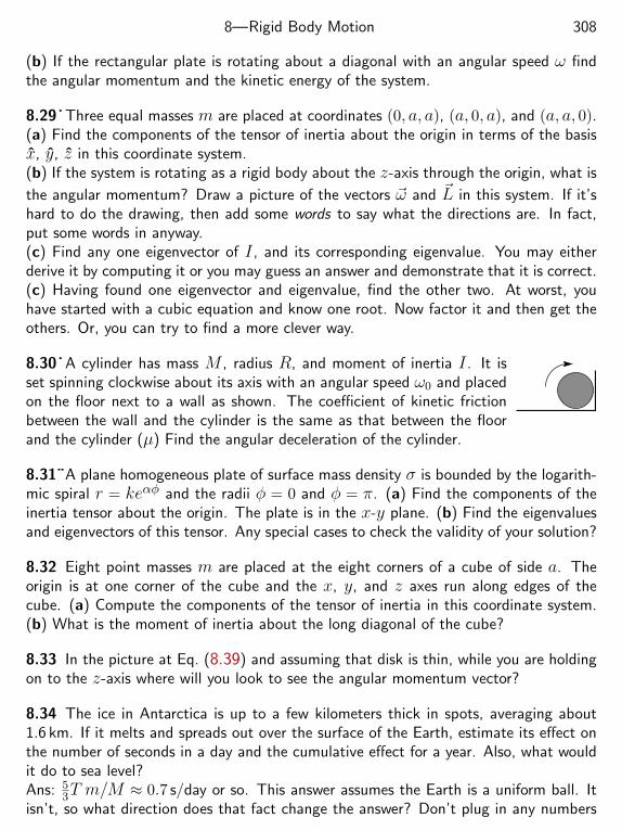
8—Rigid Body Motion 308
(b) If the rectangular plate is rotating about a diagonal with an angular speed ω findthe angular momentum and the kinetic energy of the system.
8.29˙ Three equal masses m are placed at coordinates (0, a, a), (a, 0, a), and (a, a, 0).(a) Find the components of the tensor of inertia about the origin in terms of the basisx, y, z in this coordinate system.(b) If the system is rotating as a rigid body about the z-axis through the origin, what is
the angular momentum? Draw a picture of the vectors ~ω and ~L in this system. If it’shard to do the drawing, then add some words to say what the directions are. In fact,put some words in anyway.(c) Find any one eigenvector of I , and its corresponding eigenvalue. You may eitherderive it by computing it or you may guess an answer and demonstrate that it is correct.(c) Having found one eigenvector and eigenvalue, find the other two. At worst, youhave started with a cubic equation and know one root. Now factor it and then get theothers. Or, you can try to find a more clever way.
8.30˙ A cylinder has mass M , radius R, and moment of inertia I . It isset spinning clockwise about its axis with an angular speed ω0 and placedon the floor next to a wall as shown. The coefficient of kinetic frictionbetween the wall and the cylinder is the same as that between the floorand the cylinder (µ) Find the angular deceleration of the cylinder.
8.31¨A plane homogeneous plate of surface mass density σ is bounded by the logarith-mic spiral r = keαφ and the radii φ = 0 and φ = π. (a) Find the components of theinertia tensor about the origin. The plate is in the x-y plane. (b) Find the eigenvaluesand eigenvectors of this tensor. Any special cases to check the validity of your solution?
8.32 Eight point masses m are placed at the eight corners of a cube of side a. Theorigin is at one corner of the cube and the x, y, and z axes run along edges of thecube. (a) Compute the components of the tensor of inertia in this coordinate system.(b) What is the moment of inertia about the long diagonal of the cube?
8.33 In the picture at Eq. (8.39) and assuming that disk is thin, while you are holdingon to the z-axis where will you look to see the angular momentum vector?
8.34 The ice in Antarctica is up to a few kilometers thick in spots, averaging about1.6 km. If it melts and spreads out over the surface of the Earth, estimate its effect onthe number of seconds in a day and the cumulative effect for a year. Also, what wouldit do to sea level?Ans: 5
3T m/M ≈ 0.7 s/day or so. This answer assumes the Earth is a uniform ball. Itisn’t, so what direction does that fact change the answer? Don’t plug in any numbers
8—Rigid Body Motion 309
until you’ve simplified all the algebra and so that you aren’t subtracting two largenumbers to get a small number.
8.35 The Sun rotates once in a little less that one Earth month. If the Sun collapsesto a radius of 10 km, what would its rotation period be? This is about the size of aneutron star, the remnant of an explosive stellar collapse. What would the speed of apoint on its equator be? What would the collapsed star’s density be? And of coursenot just a number. Find something to compare it to.
8.36 Compute the components of the inertia tensor for a solid cone of uniform massdensity. The origin is the vertex. Mass: M , height: h, radius of base, R. What is itskinetic energy if it is rotating about its axis of symmetry with angular speed ω?
8.37˙ The cone in the preceding problem is lying on a table and free to roll; its vertexstays fixed. (a) It takes a time T to roll all the way around; what is its angular velocityvector? Note: The line of contact with the table is instantaneously at rest, so thatdefines the axis of rotation. (b) What is its kinetic energy?
Special RelativityThe history of special relativity is fascinating: filled with partial answers, clever
ideas, false starts, intellectual barriers, and some smart people who, given enough ad-ditional time, would have figured it all out. Einstein got there first. He cut throughthe complexities that had slowed or stalled other work and he found the underlyingsimplicity. That is where I will start.
Galileo was really the first to articulate one of the foundational concepts, and hedid it three and a half centuries before Einstein was born. In his Dialog on the TwoChief World Systems he made the idea concrete by describing what you would see if youare in the main cabin below decks on some large ship, first when it is standing still, andthen when you
...have the ship proceed with any speed you like, so long as themotion is uniform and not fluctuating this way and that. Youwill discover not the least change in all the effects named, norcould you tell from any of them whether the ship was moving orstanding still.*
Put in modern terms,
1. Without looking outside the room, you can’t tell how fast you’removing.
or 2. Only relative velocities are measurable, not absolute velocities.or 3. The Results of Measurement depend only upon the relative veloc-
ity of observer and observed and not upon their absolute velocities.(And the third one is also Galileo’s phrasing — surprisingly mod-ern.)
Chapter five started with the Galilean transformation, which is the mathematicalcodification of the change to a moving coordinate system.
x′ = x− v0t, y′ = y, z′ = z, t′ = t Eq. (5.1)
As you saw there, as long as forces depend on at most the relative velocity of interactingobjects, Newton’s equations remain the same when switching to a moving observer.~F = d~p/dt no matter how fast you move. The problem is that Newtonian Mechanicsis not all. Maxwell has a set of equations that describe electromagnetism extraordinarily
* Translation: Stillman Drake
310
9—Special Relativity 311
well, and they do not transform properly under the Galilean transformation. That meansthat something has to give: Newton, Galileo, or Maxwell.
When these difficulties arose in the late 1800’s the natural response was to gowith the familiar, keeping Newton and Galileo, but modifying Maxwell. The mostfamous approach was to say that Maxwell’s electromagnetic equations are valid in onlyone coordinate system and no other: the “ether” theory.
That didn’t work, and Einstein’s approach kept Galileo and Maxwell, while forcingNewton to change. It all sounds so simple doesn’t it? When one choice doesn’t work,try another. This caricature of the history as I’ve sketched it in these few paragraphshas filled, and will further fill, whole books putting flesh on the details.
What is it about Maxwell’s theory that caused a problem? The simple and mostprofound fact is that it produces a unique value for the speed of light in a vacuum. Notspeed relative to something, just speed. The simplicity of the theory of special relativityis that you start from two assumptions:
1. Only relative velocities are measurable
2. The speed of light in a vacuum is the same for everyone.
This assumes that Maxwell is right and that Galileo’s verbal statement of theprinciple of relativity is right, but not the transformation equations written above. Inparticular the fourth one, t′ = t, will be sacrificed, and that is the most startling andperplexing aspect of this theory. The concepts “simultaneity,” or “at the same time,”or “now” will become puzzles to be sorted out. In Galileo’s day, or Maxwell’s, and allthe way up to Einstein’s, this equation stating that time is the same for everyone wasso obvious that it wasn’t even stated. It was just wrong.
What will replace the Galilean transformation of Eq. (5.1)? The answer is
x′ =x− v0t√1− v2
0/c2, y′ = y, z′ = z, t′ =
t− v0x/c2√1− v2
0/c2
These are called the Lorentz transformation, but developing them will take some effort,concluding at Eq. (9.9).
A matter of notation: Most of the time I have tried to be careful about it,sometimes probably to the point of being annoying. In this chapter there are so manyvelocities that I won’t bother with the distinctions such as those between v and vx. Iwill leave it to you to figure out which is which from context, otherwise there would betoo many sub-x’s filling the pages.
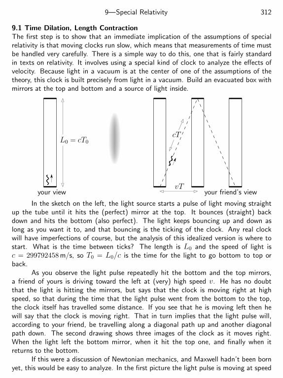
9—Special Relativity 312
9.1 Time Dilation, Length ContractionThe first step is to show that an immediate implication of the assumptions of specialrelativity is that moving clocks run slow, which means that measurements of time mustbe handled very carefully. There is a simple way to do this, one that is fairly standardin texts on relativity. It involves using a special kind of clock to analyze the effects ofvelocity. Because light in a vacuum is at the center of one of the assumptions of thetheory, this clock is built precisely from light in a vacuum. Build an evacuated box withmirrors at the top and bottom and a source of light inside.
L0 = cT0
your viewvT
cT
your friend’s view
In the sketch on the left, the light source starts a pulse of light moving straightup the tube until it hits the (perfect) mirror at the top. It bounces (straight) backdown and hits the bottom (also perfect). The light keeps bouncing up and down aslong as you want it to, and that bouncing is the ticking of the clock. Any real clockwill have imperfections of course, but the analysis of this idealized version is where tostart. What is the time between ticks? The length is L0 and the speed of light isc = 299792458 m/s, so T0 = L0/c is the time for the light to go bottom to top orback.
As you observe the light pulse repeatedly hit the bottom and the top mirrors,a friend of yours is driving toward the left at (very) high speed v. He has no doubtthat the light is hitting the mirrors, but says that the clock is moving right at highspeed, so that during the time that the light pulse went from the bottom to the top,the clock itself has travelled some distance. If you see that he is moving left then hewill say that the clock is moving right. That in turn implies that the light pulse will,according to your friend, be travelling along a diagonal path up and another diagonalpath down. The second drawing shows three images of the clock as it moves right.When the light left the bottom mirror, when it hit the top one, and finally when itreturns to the bottom.
If this were a discussion of Newtonian mechanics, and Maxwell hadn’t been bornyet, this would be easy to analyze. In the first picture the light pulse is moving at speed
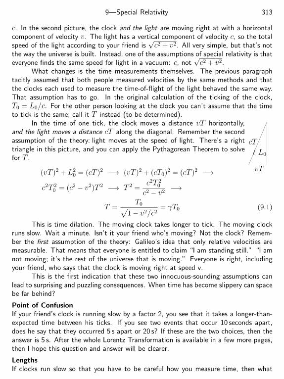
9—Special Relativity 313
c. In the second picture, the clock and the light are moving right at with a horizontalcomponent of velocity v. The light has a vertical component of velocity c, so the totalspeed of the light according to your friend is
√c2 + v2. All very simple, but that’s not
the way the universe is built. Instead, one of the assumptions of special relativity is thateveryone finds the same speed for light in a vacuum: c, not
√c2 + v2.
What changes is the time measurements themselves. The previous paragraphtacitly assumed that both people measured velocities by the same methods and thatthe clocks each used to measure the time-of-flight of the light behaved the same way.That assumption has to go. In the original calculation of the ticking of the clock,T0 = L0/c. For the other person looking at the clock you can’t assume that the timeto tick is the same; call it T instead (to be determined).
cT
vT
L0
In the time of one tick, the clock moves a distance vT horizontally,and the light moves a distance cT along the diagonal. Remember the secondassumption of the theory: light moves at the speed of light. There’s a righttriangle in this picture, and you can apply the Pythagorean Theorem to solvefor T .
(vT )2 + L20 = (cT )2 −→ (vT )2 + (cT0)2 = (cT )2 −→
c2T 20 = (c2 − v2)T 2 −→ T 2 =
c2T 20
c2 − v2−→
T =T0√
1− v2/c2= γT0 (9.1)
This is time dilation. The moving clock takes longer to tick. The moving clockruns slow. Wait a minute. Isn’t it your friend who’s moving? Not the clock? Remem-ber the first assumption of the theory: Galileo’s idea that only relative velocities aremeasurable. That means that everyone is entitled to claim “I am standing still.” “I amnot moving; it’s the rest of the universe that is moving.” Everyone is right, includingyour friend, who says that the clock is moving right at speed v.
This is the first indication that these two innocuous-sounding assumptions canlead to surprising and puzzling consequences. When time has become slippery can spacebe far behind?
Point of ConfusionIf your friend’s clock is running slow by a factor 2, you see that it takes a longer-than-expected time between his ticks. If you see two events that occur 10 seconds apart,does he say that they occurred 5 s apart or 20 s? If these are the two choices, then theanswer is 5 s. After the whole Lorentz Transformation is available in a few more pages,then I hope this question and answer will be clearer.
LengthsIf clocks run slow so that you have to be careful how you measure time, then what
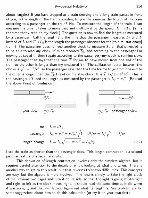
9—Special Relativity 314
about lengths? If you have stopped at a train crossing and a long train passes in frontof you, is the length of the train according to you the same as the length of the trainaccording to a passenger on the train? No. To measure the length of the train, I canmeasure the time it takes to move past and multiply it by the speed: L = vT0. (T0 isthe time that I read on my clock.) The question is now to find the length as measuredby a passenger. Call the length and the time that the passenger measures L0 and Tinstead of L and T . (L0 is the length the passenger observes for the [to him, stationary]train.) The passenger doesn’t need another clock to measure T , all that’s needed isto be able to read my clock. If mine recorded T0, and according to the passenger I’mmoving at speed v, then (again according to the passenger) my clock is running slow.The passenger then says that the time T for me to have moved from one end of thetrain to the other is longer than my measured T0. The calibration factor between theclocks is
√1− v2/c2, so the passenger says that the time for me to go from one end to
the other is longer than the T0 I read on my slow clock. It is T0/√
1− v2/c2. This isthe passenger’s T and the length as measured by the passenger is L0 = vT . (Re-readthe above Point of Confusion.)
your view
v
T0 passenger’s view
v
T0
me: L = vT0
passenger: L0 = vT = vT0
/√1− v2/c2 = L
/√1− v2/c2
length change: L = L0
√1− v2/c2 = L0/γ (9.2)
I see the train as shorter than the passenger does. This length contraction is a secondpeculiar feature of special relativity.
This derivation of length contraction involves only the simplest algebra, but itrequires careful attention to the details of who’s looking at what and when. There isanother way to get to this result, but that reverses these two difficulties. This conceptsare easy, but the algebra is more involved. The idea is simply to take the light clockof the previous two pages and turn it on its side, so that the light is going left-to-rightand right-to-left as the clock moves right. It should read the same time as it did whenit was upright, and that will let you figure out what its length is. See problem 9.7 forsome suggestions about how to do this calculation (or try it on your own first).
9—Special Relativity 315
It’s easy to mix up the applications of these dilation and contraction equations,so before applying either of Eqs. (9.1) or (9.2) you should think about the qualitativebehavior of the time and distance measurements. If a clock takes two seconds to markoff a second, its owner will think that someone just did the 100 yard dash in five seconds.This means that you can’t simply plug into formulas. The qualitative analysis shouldcome first.
A moving clock runs slow.The calibration factor between clocks is
√1− v2/c2.
That factor is less than one.So, does the factor go in the numerator or in the denominator?
Terminology: “Proper length” is the length of an object as measured by someonewho says it is not moving. “Proper time” is the time interval between two events asmeasured by someone who says the occurred at the same place — the clock is standingstill. For the train example, L0 is the proper length of the train, and T0 is the propertime on my clock. There is no universal convention about how you place subscriptshere, so don’t assume and a sub-0 will always be proper. For “proper acceleration” seeequation (9.21).*
If length contracts, shouldn’t the L0 in the original clock contract? Should theL0 in Eq. (9.1) be a variable too? No, but it’s not only a legitimate question, it’s animportant one.
Start with the length used in the calculation of time dilation: L0. I assumedthat both you and your friend used the same value for that number. Is that valid? Theanswer is yes, but now you have to test it to be certain.
The proof is by contradiction. Assume it’s false and show that it doesn’t work.Take the light clock, supposedly length L0. Your friend wants to measure it to see ifit remains L0 even when it moves past, so he uses a ruler of length L0 and holds it upso the ruler and the clock just miss each other. To be certain of his measurement heattaches a pair of paint brushes to the two tips of the ruler, set so that they will markthe ends of the clock as it passes. If the clock shrinks because of its motion then thepaint brush on one end of the ruler will mark the clock while the other end misses. Thetrouble is that paint leaves a permanent mark on the clock. You and your friend canget together over a beer after the experiment in order to compare data. If your clockhas only one paint mark, then there is a lateral length contraction and you were moving.If it has two paint marks that are not at the ends, then he was moving. Either way youhave violated the first axiom of the theory, that only relative velocities can be measured.What if lateral lengths expanded instead of contracting? You get into exactly the samecontradiction, but interchanging who is moving.
* What would “proper velocity” be?
9—Special Relativity 316
Another way to picture this: If a railroad train is entering a tunnel through amountain, and if the tunnel is just barely large enough to accommodate the width ofthe train when the train is moving slowly, what will happen when the train is movingrapidly? If there is either a lateral contraction or expansion because of the speed thensomeone, either the train engineer or the person who built the tunnel, will think thatthe train will still fit while the other will expect a crash. They can’t both be right.
ParadoxesUnder normal circumstances, i.e. before you started to study relativity, you may havean occasion to think that your watch keeps good time and that your friend’s is runningslow. Your friend, who thinks just as highly of his timepiece, would think that yourwatch is running fast. The calculation of time dilation leading to Eq. (9.1) says thatyour friend’s clock runs slow because it’s moving. If the first assumption of relativity iscorrect, that you can’t tell which of you is moving, then both of you will believe thatthe other’s clock is running slow — and be right. How can that be?
The same paradox applies to lengths. If the moving train contracts, a passengeron that train can look out and say that another train you think to be standing still hasshrunk. How can both be true? Resolving both of these problems will wait a few pagesuntil the Lorentz transformation is worked out.
If you drive a long car and have a short garage, can you fit your car within thegarage by driving extra fast? Someone standing outside and watching you try to dothis would say yes; your car has shrunk, so it now fits inside. You, as the driver, seethe garage approaching you, only it’s now even shorter than it was before. You’re nevergoing to fit inside now. Who’s right?
If two people are approaching each other, one at 34c from the left and the other
at 34c from the right, and you ask one of them how fast the other is moving, the answer
will not be 32c, but 24
25c. A derivation of this will appear in Eq. (9.13).
9.2 Examples
Before going into some more analytical problems with relativity, a few elementaryexamples are useful. Cosmic rays are (mostly) very high energy protons that come fromouter space and hit the Earth’s atmosphere. When one collides with an oxygen or nitro-gen nucleus it is so energetic that it simply blasts the nucleus apart and in the processcreates many thousands or millions of other new particles. A major component of theresulting debris is the muon. These are particles that are basically heavy, but unstable,electrons; mµ = 207me, and the mean lifetime of these particles is 2.2 microseconds.In this short time, even moving at nearly the speed of light, the mean distance such aparticle goes before decaying is about
cτ = (3× 10⁸ m/s)(2.2µs) = (300 m/µs)(2.2µs) = 660 m = 0.66 km
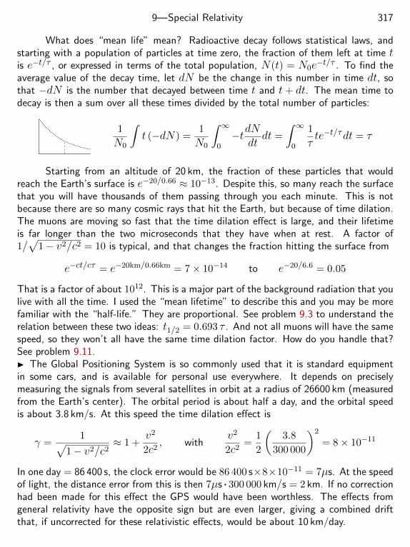
9—Special Relativity 317
What does “mean life” mean? Radioactive decay follows statistical laws, andstarting with a population of particles at time zero, the fraction of them left at time tis e−t/τ , or expressed in terms of the total population, N(t) = N0e−t/τ . To find theaverage value of the decay time, let dN be the change in this number in time dt, sothat −dN is the number that decayed between time t and t + dt. The mean time todecay is then a sum over all these times divided by the total number of particles:
1
N0
∫t (−dN) =
1
N0
∫ ∞0−tdN
dtdt =
∫ ∞0
1
τte−t/τdt = τ
Starting from an altitude of 20 km, the fraction of these particles that wouldreach the Earth’s surface is e−20/0.66 ≈ 10−13. Despite this, so many reach the surfacethat you will have thousands of them passing through you each minute. This is notbecause there are so many cosmic rays that hit the Earth, but because of time dilation.The muons are moving so fast that the time dilation effect is large, and their lifetimeis far longer than the two microseconds that they have when at rest. A factor of1/√
1− v2/c2 = 10 is typical, and that changes the fraction hitting the surface from
e−ct/cτ = e−20km/0.66km = 7× 10⁻¹⁴ to e−20/6.6 = 0.05
That is a factor of about 1012. This is a major part of the background radiation that youlive with all the time. I used the “mean lifetime” to describe this and you may be morefamiliar with the “half-life.” They are proportional. See problem 9.3 to understand therelation between these two ideas: t1/2 = 0.693 τ . And not all muons will have the samespeed, so they won’t all have the same time dilation factor. How do you handle that?See problem 9.11. The Global Positioning System is so commonly used that it is standard equipmentin some cars, and is available for personal use everywhere. It depends on preciselymeasuring the signals from several satellites in orbit at a radius of 26600 km (measuredfrom the Earth’s center). The orbital period is about half a day, and the orbital speedis about 3.8 km/s. At this speed the time dilation effect is
γ =1√
1− v2/c2≈ 1 +
v2
2c2, with
v2
2c2=
1
2
(3.8
300 000
)2
= 8× 10⁻¹¹
In one day = 86 400 s, the clock error would be 86 400 s×8×10−11 = 7µs. At the speedof light, the distance error from this is then 7µs . 300 000 km/s = 2 km. If no correctionhad been made for this effect the GPS would have been worthless. The effects fromgeneral relativity have the opposite sign but are even larger, giving a combined driftthat, if uncorrected for these relativistic effects, would be about 10 km/day.
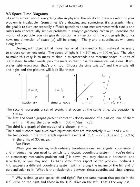
9—Special Relativity 318
9.3 Space-Time DiagramsAs with almost about everything else in physics, the ability to draw a sketch of your
problem is invaluable. Sometimes it’s a drawing and sometimes it’s a graph. Here,the goal is to turn conceptually difficult questions about measurements with clocks andrulers into conceptually simpler problems in analytic geometry. When you describe themotion of a particle, you can give its position as a function of time and graph that. Fornow, one dimension of space (x) will be enough. The y and z coordinates will comealong later.
Dealing with objects that move near or at the speed of light makes it necessaryto choose convenient units. The speed of light is 3× 10⁸ m/s = 300m/µs. The trickto make this easy is to measure time in microseconds and measure space in units of300 meters. In other words, pick the units so that c has the numerical value one. If youprefer light-years/year, that’s o.k. too. Choose the time axis up* and the x-axis leftand right and the pictures will look like these:
t
x
t
x
t
x
t
x
stationary
x = x0
simultaneous
t = t0
x = ct x = vt, v < c
The second represents a set of events that occur at the same time, the equation ist = t0.
The first and fourth graphs present constant velocity motion of a particle, one of themwith v = 0 and the other with v = 300 m/4µs = c/4.
The third is a graph of the motion of a photon, v = c.The t and x coordinate axes have equations that are respectively x = 0 and t = 0.The two points in the third graph represent events at (x, t) = (2.5, 0.5) and (1.5, 2.5)
in the units of 300 m, µs.But First:When you are dealing with ordinary two-dimensional rectangular coordinate x
and y, sometimes you need to switch to a rotated coordinate system. If you’re doingan elementary mechanics problem and ~g is down, you may choose x horizontal andy vertical, or you may not. Perhaps some other aspect of the problem, perhaps ahill, suggests a different coordinate system with x′ along the incline of the hill and y′
perpendicular to it. What it the relationship between these coordinates? Just express
* Why is time up and space left and right? For the same reason that people in theU.S. drive on the right and those in the U.K. drive on the left. That’s the way it is.
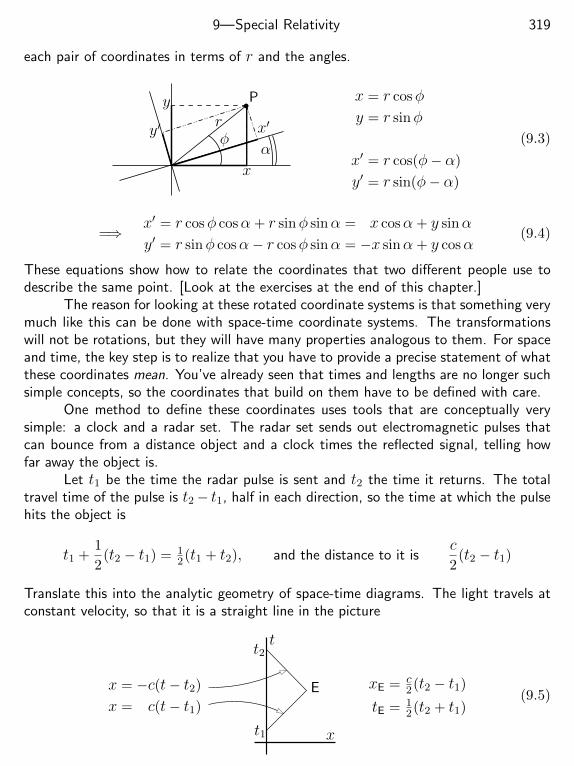
9—Special Relativity 319
each pair of coordinates in terms of r and the angles.
x
x′
y
y′rφ
α
P x = r cosφ
y = r sinφ
x′ = r cos(φ− α)
y′ = r sin(φ− α)
(9.3)
=⇒x′ = r cosφ cosα+ r sinφ sinα = x cosα+ y sinα
y′ = r sinφ cosα− r cosφ sinα = −x sinα+ y cosα(9.4)
These equations show how to relate the coordinates that two different people use todescribe the same point. [Look at the exercises at the end of this chapter.]
The reason for looking at these rotated coordinate systems is that something verymuch like this can be done with space-time coordinate systems. The transformationswill not be rotations, but they will have many properties analogous to them. For spaceand time, the key step is to realize that you have to provide a precise statement of whatthese coordinates mean. You’ve already seen that times and lengths are no longer suchsimple concepts, so the coordinates that build on them have to be defined with care.
One method to define these coordinates uses tools that are conceptually verysimple: a clock and a radar set. The radar set sends out electromagnetic pulses thatcan bounce from a distance object and a clock times the reflected signal, telling howfar away the object is.
Let t1 be the time the radar pulse is sent and t2 the time it returns. The totaltravel time of the pulse is t2− t1, half in each direction, so the time at which the pulsehits the object is
t1 +1
2(t2 − t1) = 1
2(t1 + t2), and the distance to it isc2
(t2 − t1)
Translate this into the analytic geometry of space-time diagrams. The light travels atconstant velocity, so that it is a straight line in the picture
x = −c(t− t2)
x = c(t− t1)
t
xt1
t2
E xE = c2(t2 − t1)
tE = 12(t2 + t1)
(9.5)
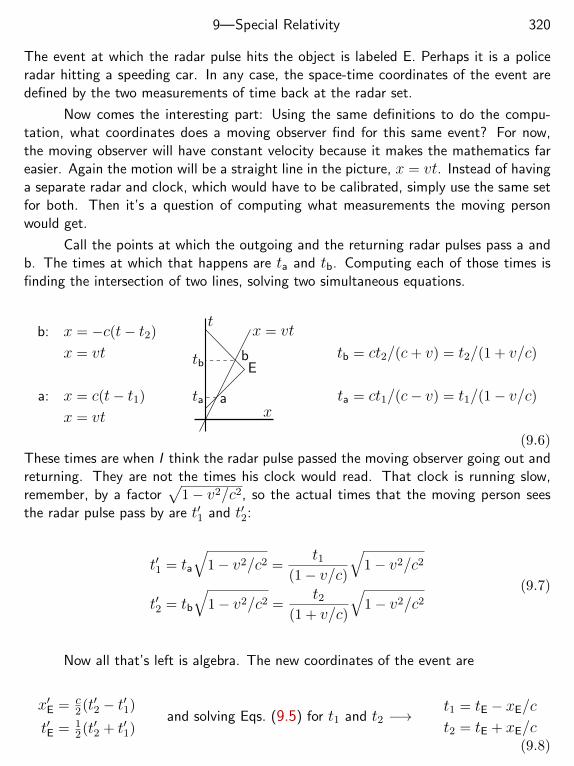
9—Special Relativity 320
The event at which the radar pulse hits the object is labeled E. Perhaps it is a policeradar hitting a speeding car. In any case, the space-time coordinates of the event aredefined by the two measurements of time back at the radar set.
Now comes the interesting part: Using the same definitions to do the compu-tation, what coordinates does a moving observer find for this same event? For now,the moving observer will have constant velocity because it makes the mathematics fareasier. Again the motion will be a straight line in the picture, x = vt. Instead of havinga separate radar and clock, which would have to be calibrated, simply use the same setfor both. Then it’s a question of computing what measurements the moving personwould get.
Call the points at which the outgoing and the returning radar pulses pass a andb. The times at which that happens are ta and tb. Computing each of those times isfinding the intersection of two lines, solving two simultaneous equations.
b: x = −c(t− t2)
x = vt
a: x = c(t− t1)
x = vt
t
xa
b
ta
tb
x = vt
Etb = ct2/(c+ v) = t2/(1 + v/c)
ta = ct1/(c− v) = t1/(1− v/c)
(9.6)These times are when I think the radar pulse passed the moving observer going out andreturning. They are not the times his clock would read. That clock is running slow,remember, by a factor
√1− v2/c2, so the actual times that the moving person sees
the radar pulse pass by are t′1 and t′2:
t′1 = ta
√1− v2/c2 =
t1(1− v/c)
√1− v2/c2
t′2 = tb
√1− v2/c2 =
t2(1 + v/c)
√1− v2/c2
(9.7)
Now all that’s left is algebra. The new coordinates of the event are
x′E = c2(t′2 − t′1)
t′E = 12(t′2 + t′1)
and solving Eqs. (9.5) for t1 and t2 −→t1 = tE − xE/c
t2 = tE + xE/c(9.8)
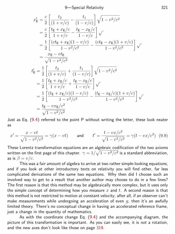
9—Special Relativity 321
x′E =c2
[t2
(1 + v/c)− t1
(1− v/c)
]√1− v2/c2
=c2
[tE + xE/c
1 + v/c− tE − xE/c
1− v/c
]√
=1
2
[(ctE + xE)(1− v/c)
1− v2/c2− (ctE − xE)(1 + v/c)
1− v2/c2
]√
=xE − vtE√1− v2/c2
t′E =1
2
[t2
(1 + v/c)+
t1(1− v/c)
]√1− v2/c2
=1
2
[tE + xE/c
1 + v/c+tE − xE/c
1− v/c
]√
=1
2
[(tE + xE/c)(1− v/c)
1− v2/c2− (tE − xE/c)(1 + v/c)
1− v2/c2
]√
=tE − vxE/c2√
1− v2/c2
Just as Eq. (9.4) referred to the point P without writing the letter, these look neateras
x′ =x− vt√1− v2/c2
= γ(x− vt) and t′ =t− vx/c2√1− v2/c2
= γ(t− vx/c2) (9.9)
These Lorentz transformation equations are an algebraic codification of the two axiomswritten on the first page of this chapter. γ = 1/
√1− v2/c2 is a standard abbreviation,
as is β = v/c.This was a fair amount of algebra to arrive at two rather simple-looking equations,
and if you look at other introductory texts on relativity you will find other, far lesscomplicated derivations of the same two equations. Why then did I choose such aninvolved way to get to a result that another author may choose to do in a few lines?The first reason is that this method may be algebraically more complex, but it uses onlythe simple concept of determining how you measure x and t. A second reason is thatthis method is not restricted to motion at constant velocity; after all, if an observer can’tmake measurements while undergoing an acceleration of even g, then it’s an awfullylimited theory. There’s no conceptual change in having an accelerated reference frame,just a change in the quantity of mathematics.
As with the coordinate change Eq. (9.4) and the accompanying diagram, thepicture of this transformation is important. As you can easily see, it is not a rotation,and the new axes don’t look like those on page 319.
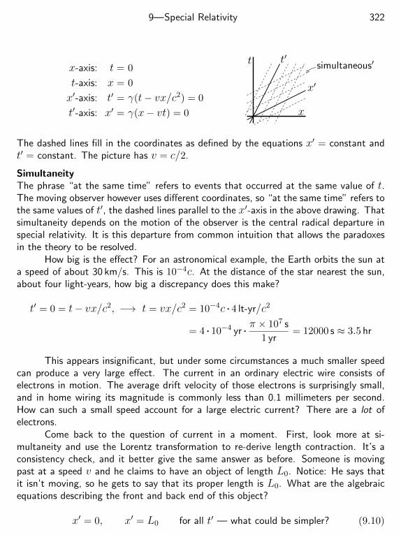
9—Special Relativity 322
x-axis: t = 0
t-axis: x = 0
x′-axis: t′ = γ(t− vx/c2) = 0
t′-axis: x′ = γ(x− vt) = 0 x
t
x′
t′simultaneous′
The dashed lines fill in the coordinates as defined by the equations x′ = constant andt′ = constant. The picture has v = c/2.
SimultaneityThe phrase “at the same time” refers to events that occurred at the same value of t.The moving observer however uses different coordinates, so “at the same time” refers tothe same values of t′, the dashed lines parallel to the x′-axis in the above drawing. Thatsimultaneity depends on the motion of the observer is the central radical departure inspecial relativity. It is this departure from common intuition that allows the paradoxesin the theory to be resolved.
How big is the effect? For an astronomical example, the Earth orbits the sun ata speed of about 30 km/s. This is 10−4c. At the distance of the star nearest the sun,about four light-years, how big a discrepancy does this make?
t′ = 0 = t− vx/c2, −→ t = vx/c2 = 10−4c . 4 lt-yr/c2
= 4 . 10−4 yr . π × 107 s
1 yr= 12000 s ≈ 3.5 hr
This appears insignificant, but under some circumstances a much smaller speedcan produce a very large effect. The current in an ordinary electric wire consists ofelectrons in motion. The average drift velocity of those electrons is surprisingly small,and in home wiring its magnitude is commonly less than 0.1 millimeters per second.How can such a small speed account for a large electric current? There are a lot ofelectrons.
Come back to the question of current in a moment. First, look more at si-multaneity and use the Lorentz transformation to re-derive length contraction. It’s aconsistency check, and it better give the same answer as before. Someone is movingpast at a speed v and he claims to have an object of length L0. Notice: He says thatit isn’t moving, so he gets to say that its proper length is L0. What are the algebraicequations describing the front and back end of this object?
x′ = 0, x′ = L0 for all t′ — what could be simpler? (9.10)
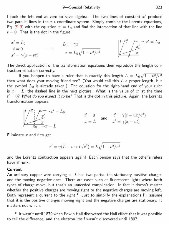
9—Special Relativity 323
I took the left end at zero to save algebra. The two lines of constant x′ producetwo parallel lines in the x-t coordinate system. Simply combine the Lorentz equations,Eq. (9.9) with the equation x′ = L0 and find the intersection of that line with the linet = 0. That is the dot in the figure.
x′ = L0
t = 0
x′ = γ(x− vt)−→
L0 = γx
x = L0
√1− v2/c2 x
t t′
x′x′ = L0
The direct application of the transformation equations then reproduce the length con-traction equation correctly.
If you happen to have a ruler that is exactly this length L = L0
√1− v2/c2
then what does your moving friend see? (You would call this L a proper length, butthe symbol L0 is already taken.) The equation for the right-hand end of your ruleris x = L, the dashed line in the next picture. What is the value of x′ at the timet′ = 0? What do you expect it to be? That is the dot in this picture. Again, the Lorentztransformation appears.
x
t t′
x′x′ = L0
x = L
t′ = 0
x = Land
t′ = γ(t− vx/c2)
x′ = γ(x− vt)
Eliminate x and t to get
x′ = γ(L− v . vL/c2) = L√
1− v2/c2
and the Lorentz contraction appears again! Each person says that the other’s rulershave shrunk.
CurrentAn ordinary copper wire carrying a I has two parts: the stationary positive chargesand the moving negative ones. There are cases such as fluorescent lights where bothtypes of charge move, but that’s an unneeded complication. In fact it doesn’t matterwhether the positive charges are moving right or the negative charges are moving left.Both represent a current to the right.* Just to simplify the explanations I’ll assumethat it is the positive charges moving right and the negative charges are stationary. Itmatters not which.
* It wasn’t until 1879 when Edwin Hall discovered the Hall effect that it was possibleto tell the difference, and the electron itself wasn’t discovered until 1897.
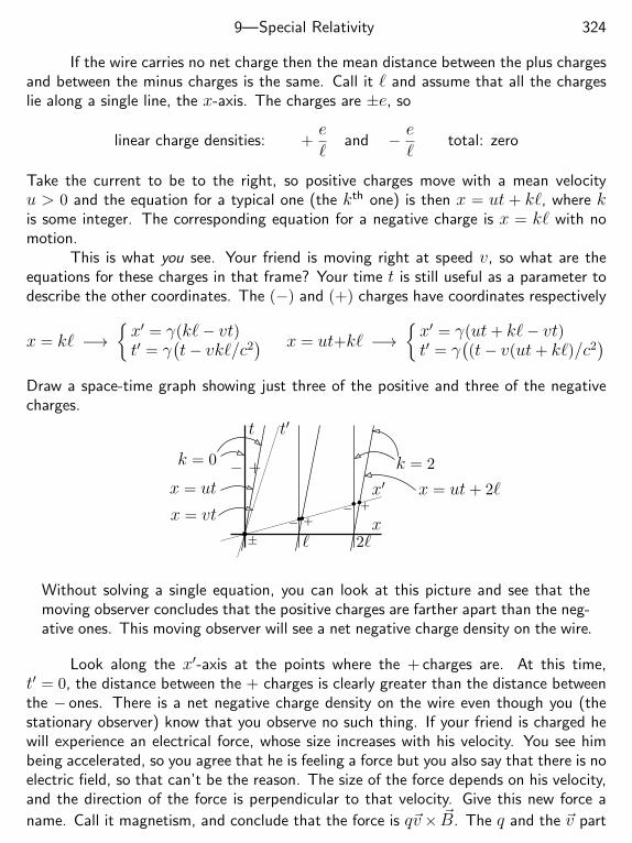
9—Special Relativity 324
If the wire carries no net charge then the mean distance between the plus chargesand between the minus charges is the same. Call it ` and assume that all the chargeslie along a single line, the x-axis. The charges are ±e, so
linear charge densities: +e`
and − e`
total: zero
Take the current to be to the right, so positive charges move with a mean velocityu > 0 and the equation for a typical one (the kth one) is then x = ut + k`, where kis some integer. The corresponding equation for a negative charge is x = k` with nomotion.
This is what you see. Your friend is moving right at speed v, so what are theequations for these charges in that frame? Your time t is still useful as a parameter todescribe the other coordinates. The (−) and (+) charges have coordinates respectively
x = k` −→x′ = γ(k`− vt)t′ = γ
(t− vk`/c2
) x = ut+k` −→x′ = γ(ut+ k`− vt)t′ = γ
((t− v(ut+ k`)/c2
)Draw a space-time graph showing just three of the positive and three of the negativecharges.
x
t
x′
t′
k = 2k = 0
x = ut
x = vt
x = ut+ 2`
− +
− +− +
± ` 2`
Without solving a single equation, you can look at this picture and see that themoving observer concludes that the positive charges are farther apart than the neg-ative ones. This moving observer will see a net negative charge density on the wire.
Look along the x′-axis at the points where the + charges are. At this time,t′ = 0, the distance between the + charges is clearly greater than the distance betweenthe − ones. There is a net negative charge density on the wire even though you (thestationary observer) know that you observe no such thing. If your friend is charged hewill experience an electrical force, whose size increases with his velocity. You see himbeing accelerated, so you agree that he is feeling a force but you also say that there is noelectric field, so that can’t be the reason. The size of the force depends on his velocity,and the direction of the force is perpendicular to that velocity. Give this new force a
name. Call it magnetism, and conclude that the force is q~v× ~B. The q and the ~v part
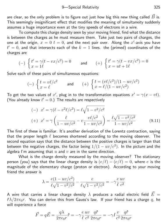
9—Special Relativity 325
are clear, so the only problem is to figure out just how big this new thing called ~B is.This seemingly insignificant effect that modifies the meaning of simultaneity suddenlyassumes a huge importance even at the tiny speeds of electrons in a wire.
To compute this charge density seen by your moving friend, find what the distanceis between the charges as he must measure them. Take just two pairs of charges, theone at the origin, x = 0 t = 0, and the next pair over. Along the x′-axis you havet′ = 0, and that intersects each of the k = 1 lines. the (primed) coordinates of thecharges are
(−)
t′ = γ(t− vx/c2) = 0x = 1`
and (+)
t′ = γ(t− vx/c2) = 0x = ut+ 1`
Solve each of these pairs of simultaneous equations:
(−)
t = v`/c2
x = `and (+)
t = (v`/c2)/(1− uv/c2)x = `/(1− uv/c2)
To get the two values of x′, plug in to the transformation equations x′ = γ(x − vt).(You already know t′ = 0.) The results are respectively
(−) x′ = γ(`− v2`/c2) = `√
1− v2/c2
(+) x′ = γ
(`
1− uv/c2− v v`/c2
1− uv/c2
)=`√
1− v2/c2
1− uv/c2(9.11)
The first of these is familiar. It’s another derivation of the Lorentz contraction, sayingthat the proper length ` becomes shortened according to the moving observer. Thesecond equation says that the distance between the positive charges is larger than thatbetween the negative charges, the factor being 1/(1 − uv/c2). In the picture and thealgebra I’m assuming that u and v are in the same direction.
What is the charge density measured by the moving observer? The stationaryperson (you) says that the linear charge density is (e/`) − (e/`) = 0, where e is themagnitude of the elementary charge (proton or electron). According to your movingfriend the answer is
λ =e(1− uv/c2)
`√
1− v2/c2− e
`√
1− v2/c2= −γ e
`uvc2
A wire that carries a linear charge density λ produces a radial electric field ~E =rλ/2πε0r. You can derive this from Gauss’s law. If your friend has a charge q, hewill experience a force
~F = q ~E =qλ
2πε0rr = −γ e
`uvc2
qr2πε0r
= −γI vc2
qr2πε0r
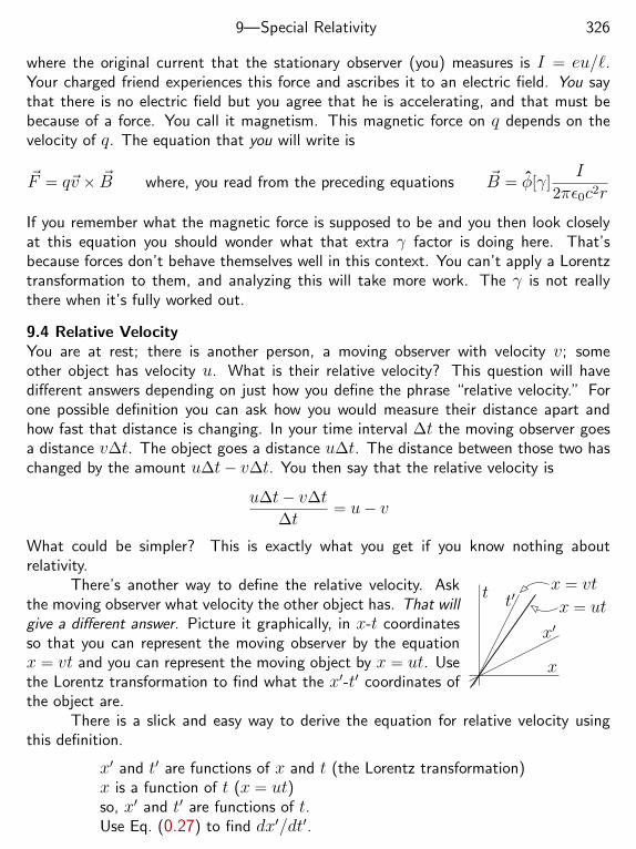
9—Special Relativity 326
where the original current that the stationary observer (you) measures is I = eu/`.Your charged friend experiences this force and ascribes it to an electric field. You saythat there is no electric field but you agree that he is accelerating, and that must bebecause of a force. You call it magnetism. This magnetic force on q depends on thevelocity of q. The equation that you will write is
~F = q~v × ~B where, you read from the preceding equations ~B = φ[γ]I
2πε0c2r
If you remember what the magnetic force is supposed to be and you then look closelyat this equation you should wonder what that extra γ factor is doing here. That’sbecause forces don’t behave themselves well in this context. You can’t apply a Lorentztransformation to them, and analyzing this will take more work. The γ is not reallythere when it’s fully worked out.
9.4 Relative VelocityYou are at rest; there is another person, a moving observer with velocity v; someother object has velocity u. What is their relative velocity? This question will havedifferent answers depending on just how you define the phrase “relative velocity.” Forone possible definition you can ask how you would measure their distance apart andhow fast that distance is changing. In your time interval ∆t the moving observer goesa distance v∆t. The object goes a distance u∆t. The distance between those two haschanged by the amount u∆t− v∆t. You then say that the relative velocity is
u∆t− v∆t∆t
= u− v
What could be simpler? This is exactly what you get if you know nothing aboutrelativity.
t
x
x′
t′x = vt
x = ut
There’s another way to define the relative velocity. Askthe moving observer what velocity the other object has. That willgive a different answer. Picture it graphically, in x-t coordinatesso that you can represent the moving observer by the equationx = vt and you can represent the moving object by x = ut. Usethe Lorentz transformation to find what the x′-t′ coordinates ofthe object are.
There is a slick and easy way to derive the equation for relative velocity usingthis definition.
x′ and t′ are functions of x and t (the Lorentz transformation)x is a function of t (x = ut)so, x′ and t′ are functions of t.Use Eq. (0.27) to find dx′/dt′.
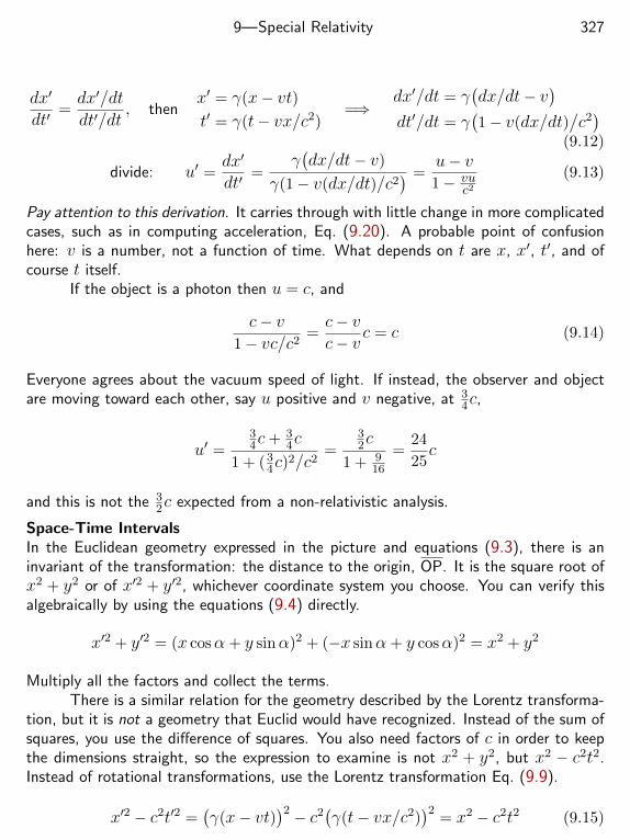
9—Special Relativity 327
dx′
dt′=dx′/dt
dt′/dt, then
x′ = γ(x− vt)t′ = γ(t− vx/c2)
=⇒dx′/dt = γ
(dx/dt− v
)dt′/dt = γ
(1− v(dx/dt)
/c2)
(9.12)
divide: u′ =dx′
dt′=
γ(dx/dt− v)
γ(1− v(dx/dt)/c2) =
u− v1− vu
c2(9.13)
Pay attention to this derivation. It carries through with little change in more complicatedcases, such as in computing acceleration, Eq. (9.20). A probable point of confusionhere: v is a number, not a function of time. What depends on t are x, x′, t′, and ofcourse t itself.
If the object is a photon then u = c, and
c− v1− vc/c2
=c− vc− v
c = c (9.14)
Everyone agrees about the vacuum speed of light. If instead, the observer and objectare moving toward each other, say u positive and v negative, at 3
4c,
u′ =34c+ 3
4c
1 + (34c)
2/c2=
32c
1 + 916
=24
25c
and this is not the 32c expected from a non-relativistic analysis.
Space-Time IntervalsIn the Euclidean geometry expressed in the picture and equations (9.3), there is aninvariant of the transformation: the distance to the origin, OP. It is the square root ofx2 + y2 or of x′2 + y′2, whichever coordinate system you choose. You can verify thisalgebraically by using the equations (9.4) directly.
x′2 + y′2 = (x cosα+ y sinα)2 + (−x sinα+ y cosα)2 = x2 + y2
Multiply all the factors and collect the terms.There is a similar relation for the geometry described by the Lorentz transforma-
tion, but it is not a geometry that Euclid would have recognized. Instead of the sum ofsquares, you use the difference of squares. You also need factors of c in order to keepthe dimensions straight, so the expression to examine is not x2 + y2, but x2 − c2t2.Instead of rotational transformations, use the Lorentz transformation Eq. (9.9).
x′2 − c2t′2 =(γ(x− vt)
)2 − c2(γ(t− vx/c2)
)2= x2 − c2t2 (9.15)
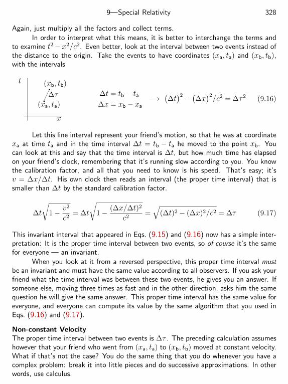
9—Special Relativity 328
Again, just multiply all the factors and collect terms.
In order to interpret what this means, it is better to interchange the terms andto examine t2−x2/c2. Even better, look at the interval between two events instead ofthe distance to the origin. Take the events to have coordinates (xa, ta) and (xb, tb),with the intervals
t
x
(xa, ta)
(xb, tb)
∆τ ∆t = tb − ta∆x = xb − xa
−→(∆t)2 − (∆x)2/c2 = ∆τ 2 (9.16)
Let this line interval represent your friend’s motion, so that he was at coordinatexa at time ta and in the time interval ∆t = tb − ta he moved to the point xb. Youcan look at this and say that the time interval is ∆t, but how much time has elapsedon your friend’s clock, remembering that it’s running slow according to you. You knowthe calibration factor, and all that you need to know is his speed. That’s easy; it’sv = ∆x/∆t. His own clock then reads an interval (the proper time interval) that issmaller than ∆t by the standard calibration factor.
∆t
√1− v
2
c2= ∆t
√1− (∆x/∆t)2
c2=√
(∆t)2 − (∆x)2/c2 = ∆τ (9.17)
This invariant interval that appeared in Eqs. (9.15) and (9.16) now has a simple inter-pretation: It is the proper time interval between two events, so of course it’s the samefor everyone — an invariant.
When you look at it from a reversed perspective, this proper time interval mustbe an invariant and must have the same value according to all observers. If you ask yourfriend what the time interval was between these two events, he gives you an answer. Ifsomeone else, moving three times as fast and in the other direction, asks him the samequestion he will give the same answer. This proper time interval has the same value foreveryone, and everyone can compute its value by the same algorithm that you used inEqs. (9.16) and (9.17).
Non-constant VelocityThe proper time interval between two events is ∆τ . The preceding calculation assumeshowever that your friend who went from (xa, ta) to (xb, tb) moved at constant velocity.What if that’s not the case? You do the same thing that you do whenever you have acomplex problem: break it into little pieces and do successive approximations. In otherwords, use calculus.
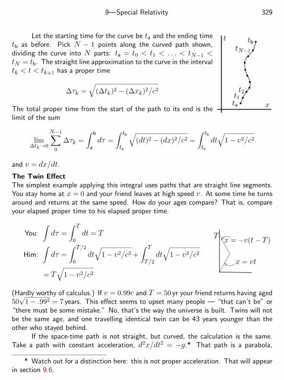
9—Special Relativity 329
x
t
tat1t2
tbtN−1
Let the starting time for the curve be ta and the ending timetb as before. Pick N − 1 points along the curved path shown,dividing the curve into N parts: ta = t0 < t1 < . . . < tN−1 <tN = tb. The straight line approximation to the curve in the intervaltk < t < tk+1 has a proper time
∆τk =√
(∆tk)2 − (∆xk)2/c2
The total proper time from the start of the path to its end is thelimit of the sum
lim∆tk→0
N−1∑0
∆τk =
∫ b
adτ =
∫ tb
ta
√(dt)2 − (dx)2/c2 =
∫ tb
tadt√
1− v2/c2
and v = dx/dt.
The Twin EffectThe simplest example applying this integral uses paths that are straight line segments.You stay home at x = 0 and your friend leaves at high speed v. At some time he turnsaround and returns at the same speed. How do your ages compare? That is, compareyour elapsed proper time to his elapsed proper time.
You:
∫dτ =
∫ T
0dt = T
Him:
∫dτ =
∫ T/2
0dt√
1− v2/c2 +
∫ T
T/2dt√
1− v2/c2
= T√
1− v2/c2
Tx = −v(t− T )
x = vt
(Hardly worthy of calculus.) If v = 0.99c and T = 50 yr your friend returns having aged50√
1− .992 = 7 years. This effect seems to upset many people — “that can’t be” or“there must be some mistake.” No, that’s the way the universe is built. Twins will notbe the same age, and one travelling identical twin can be 43 years younger than theother who stayed behind.
If the space-time path is not straight, but curved, the calculation is the same.Take a path with constant acceleration, d2x/dt2 = −g.* That path is a parabola,
* Watch out for a distinction here: this is not proper acceleration. That will appearin section 9.6.
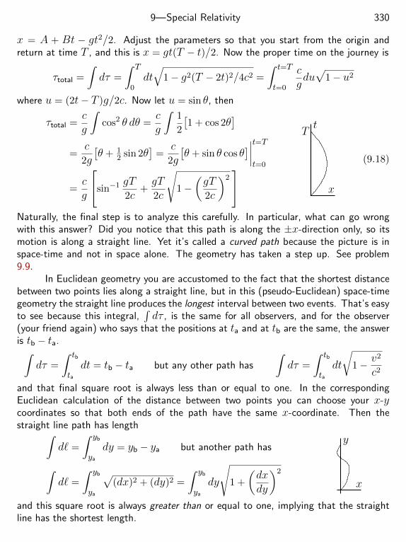
9—Special Relativity 330
x = A + Bt − gt2/2. Adjust the parameters so that you start from the origin andreturn at time T , and this is x = gt(T − t)/2. Now the proper time on the journey is
τtotal =
∫dτ =
∫ T
0dt√
1− g2(T − 2t)2/4c2 =
∫ t=T
t=0
cgdu√
1− u2
where u = (2t− T )g/2c. Now let u = sin θ, then
τtotal =cg
∫cos2 θ dθ =
cg
∫1
2
[1 + cos 2θ
]=
c2g
[θ + 1
2 sin 2θ]
=c
2g
[θ + sin θ cos θ
]∣∣∣∣t=Tt=0
=cg
sin−1 gT2c
+gT2c
√1−
(gT2c
)2
T
x
t
(9.18)
Naturally, the final step is to analyze this carefully. In particular, what can go wrongwith this answer? Did you notice that this path is along the ±x-direction only, so itsmotion is along a straight line. Yet it’s called a curved path because the picture is inspace-time and not in space alone. The geometry has taken a step up. See problem9.9.
In Euclidean geometry you are accustomed to the fact that the shortest distancebetween two points lies along a straight line, but in this (pseudo-Euclidean) space-timegeometry the straight line produces the longest interval between two events. That’s easyto see because this integral,
∫dτ , is the same for all observers, and for the observer
(your friend again) who says that the positions at ta and at tb are the same, the answeris tb − ta.∫
dτ =
∫ tb
tadt = tb − ta but any other path has
∫dτ =
∫ tb
tadt
√1− v
2
c2
and that final square root is always less than or equal to one. In the correspondingEuclidean calculation of the distance between two points you can choose your x-ycoordinates so that both ends of the path have the same x-coordinate. Then thestraight line path has length∫
d` =
∫ yb
ya
dy = yb − ya but another path has
∫d` =
∫ yb
ya
√(dx)2 + (dy)2 =
∫ yb
ya
dy
√1 +
(dxdy
)2
x
y
and this square root is always greater than or equal to one, implying that the straightline has the shortest length.
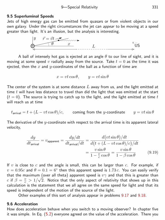
9—Special Relativity 331
9.5 Superluminal SpeedsJets of high energy gas can be emitted from quasars or from violent objects in ourown galaxy. Under the right circumstances the jet can appear to be moving at a speedgreater than light. It’s an illusion, but the analysis is interesting.
x
y ~r = ~vt
USLθ
A ball of intensely hot gas is ejected at an angle θ to our line of sight, and it ismoving at some speed v radially away from the source. Take t = 0 as the time it wasejected, then the x and y-coordinates of the ball as a function of time are
x = vt cos θ, y = vt sin θ
The center of the system is at some distance L away from us, and the light emitted attime t will have less distance to travel than did the light that was emitted at the start(t = 0). The source is trying to catch up to the light, and the light emitted at time twill reach us at time
tarrival = t+ (L− vt cos θ)/c, coming from the y-coordinate y = vt sin θ
The derivative of the y-coordinate with respect to the arrival time is its apparent lateralvelocity,
dydtarrival
= vapparent =dy/dt
dtarrival/dt=
d(vt sin θ
)/dt
d(t+ (L− vt cos θ)/c
)/dt
=v sin θ
1− vc cos θ
=v sin θ
1− β cos θ(9.19)
If v is close to c and the angle is small, this can be larger than c. For example, ifv = 0.95c and θ = 0.1 = 6 then this apparent speed is 1.73 c. You can easily verifythat the maximum (over all theta) apparent speed is vγ and that this is greater thanc if β = v
c > 1/√
2. Notice that the only aspect of relativity that shows up in thiscalculation is the statement that we all agree on the same speed for light and that itsspeed is independent of the motion of the source of the light.
Other examples of this sort of analysis appear in problems 9.17 and 9.18.
9.6 AccelerationHow does acceleration behave when you switch to a moving observer? In chapter fiveit was simple. In Eq. (5.2) everyone agreed on the value of the acceleration. There you
9—Special Relativity 332
had d2x′/dt′2 = d2x/dt2, but that no longer holds because the equation relating timesfor the two observers is no longer t′ = t.
When an object has an acceleration that is d2x/dt2 = du/dt according to you,what is it according to someone moving at velocity v? Look back carefully at thederivation of relative velocity in Eq. (9.12). Understand it there and the following willbe just some more algebra, but without any new conceptual complications. As in thatprevious derivation v is a constant. Here u = du/dt:
du′
dt′=du′/dt
dt′/dt
du′
dt=ddt
u− v1− uv/c2
=u
1− uv/c2− u− v
(1− uv/c2)2.(−vuc2
)= u
1− v2/c2
(1− uv/c2)2
dt′
dt=ddtγ(t− vx/c2) = γ(1− vu/c2)
du′
dt′=u(1− v2/c2)
/(1− uv/c2
)2γ(1− uv/c2
) =u(1− v2/c2)3/2(1− uv/c2
)3 (9.20)
At least if v = 0 then this reduces to u, as it must. Also look at what happens as vbecomes close to +c. In that case, unless u is also close to +c, the moving observersays that the object is already moving at very close to the speed of light, so it can’tspeed up much. It’s acceleration must be small and that is exactly what this equationsays. The numerator is (1− v2/c2)3/2.
For an important special case of this equation, take v = u. That means that thenew acceleration, du′/dt′, is being computed by the person who says that the object is(momentarily) at rest. That is the definition of proper acceleration.
aproper =u(1− u2/c2)3/2(1− uu/c2
)3 =u(
1− u2/c2)3/2
(9.21)
If you are taking an interstellar journey in a ship accelerating at what you perceive tobe a constant a, then what does someone remaining behind on Earth say about yourmotion? In other words, what is the equation to describe constant proper acceleration;what replaces at2/2? For a more realistic example, the acceleration of a charged particlein a uniform electric field will be described by constant proper acceleration. If you thinkthat’s not obvious, you’re right.
This is a differential equation, and for a constant proper a, and recalling section0.2 and problem 0.16
a =u(
1− u2/c2)3/2
−→ adt =du(
1− u2/c2)3/2
−→ at =
∫ u
0
du(1− u2/c2
)3/2
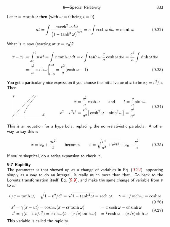
9—Special Relativity 333
Let u = c tanhω then (with ω = 0 being t = 0)
at =
∫c sech2 ω dω(
1− tanh2 ω)3/2
= c∫
coshω dω = c sinhω (9.22)
What is x now (starting at x = x0)?
x− x0 =
∫ t
0udt =
∫c tanhω dt = c
∫tanhω
ca
coshω dω =c2
a
∫sinhω dω
=c2
acoshω
∣∣∣∣t=tt=0
=c2
a(coshω − 1) (9.23)
You get a particularly nice expression if you choose the initial value of x to be x0 = c2/a.Then
x
tx =
c2
acoshω and t =
ca
sinhω
x2 − c2t2 =c4
a2
[cosh2 ω − sinh2 ω
]=c4
a2
(9.24)
This is an equation for a hyperbola, replacing the non-relativistic parabola. Anotherway to say this is
x = x0 +at2
2becomes x =
√c4
a2+ c2t2 + x0 −
c2
a(9.25)
If you’re skeptical, do a series expansion to check it.
9.7 RapidityThe parameter ω that showed up as a change of variables in Eq. (9.22), appearingsimply as a way to do an integral, is really much more than that. Go back to theLorentz transformation itself, Eq. (9.9), and make the same change of variable from vto ω.
v/c = tanhω,√
1− v2/c2 =√
1− tanh2 ω = sech ω, γ = 1/ sechω = coshω
(9.26)x′ = γ(x− vt) = coshω(x− ct tanhω)
t′ = γ(t− vx/c2) = coshω(t− (x/c) tanhω)
= x coshω − ct sinhω
= t coshω − (x/c) sinhω(9.27)
This variable is called the rapidity.
9—Special Relativity 334
What does velocity addition look like in terms of this variable?
tanh
v1 + v2
1 + v1v2/c2= c
tanhω1 + tanhω2
1 + tanhω1 tanhω2= c tanh(ω1 + ω2)
−→ ωtotal = ω1 + ω2
(9.28)If you’re not sure about this identity for the hyperbolic tangent of a sum, multiply nu-merator and denominator by coshω1 coshω2 and refer to section 0.2 and problem 0.15.These equations (9.27) look much more like the equations for rotations, Eq. (9.4), thandoes the previous way of writing the Lorentz transformation in terms of v. The rapidityvariable behaves the same way that the angle variable does in rotations. It is a naturaland far more convenient way to work.
9.8 Energy and MomentumIt should be no surprise that energy and momentum do not behave the same way thatyou remember from Newtonian mechanics. First, the results, and the derivation canwait until section 9.11, after you’ve used them for a while.
E2 = p2c2 +m2c4, ~p =Ec2~v (9.29)
These are the exact, no approximation, cover-all-cases equations relating energy, mo-mentum, and mass. Anything else is either a special case or an approximation. Thisenergy E is not the kinetic energy, but it now includes mass as another form of energy.To see this, look at what happens for zero velocity.
~v = 0 −→ ~p = 0 −→ E2 = 02c2 +m2c4 −→ E0 = mc2
Here E0 is a common notation for the value of the energy when the velocity is zero —the rest energy.
Instead, what if the speed is small? In this case E is still close to the rest value,mc2, so the momentum is
~p ≈ mc2
c2~v = m~v
and this reduces to the ordinary classical result. Now what about the kinetic energy?That’s the difference between the energy E and the rest energy E0 = mc2. For smallspeeds, the momentum is small, so this lets you do a series expansion. Rearrange theterms into the form (1 + small)n.
K = E −E0 =√p2c2 +m2c4 −mc2 = mc2
(1 + p2/m2c2
)1/2 −mc2
= mc2
(1 +
1
2
p2
m2c2+ · · ·
)−mc2 =
p2
2m+ · · · (9.30)
9—Special Relativity 335
In this small speed approximation, ~p = m~v, then p2/2m = (mv)2/2m = mv2/2 andyou have the familiar result. You also see what the word “small” means in order toallow this approximation: pmc, and that in turn is equivalent to v c.
These manipulations assumed that the mass is non-zero. What happens if m =0? The first of the equations (9.29) is then
E2 = p2c2 + 0 −→ E = cp (9.31)
That in turn makes the second of those equations
~p =Ec2~v =
cpc2~v = p
~vc
The magnitude of this equation is |~p | = p = pv/c, and that implies v = c. Amass zero particle must move at the speed of light. (For example, light.) That themass of a particle is zero does not imply that its energy or momentum is zero. That’s amisconception carried over from Newtonian mechanics, and it does not apply here. Thatlight, a particle of zero mass, carries energy is clear enough — just step outside and intothe sunshine. That it carries momentum is not so obvious because from Eq. (9.31) themomentum is p = E/c, and on a human scale that’s not much. For an electron howeverit can be a lot, and the force light exerts on that scale can be significant. Light fromthe sun pushes electrons and ions and even particles of dust outward. Radiation caneven measurably affect the motion of small asteroids — the Yarkovsky effect, discussedin section 9.10. At high intensity the force exerted by light can be used to compressmatter by huge factors. This has been used in the hope that it can lead to controllednuclear fusion, with release of enough energy to create a commercially feasible sourceof power. (Well, maybe someday.)
You’ve usually seen kinetic energy and momentum expressed in terms of velocity,and you can do that here simply by algebraic manipulation of the equations (9.29).Eliminate p between the two equations and for m 6= 0 you get
E =mc2√
1− v2/c2= mc2γ, p =
mv√1− v2/c2
= mvγ (9.32)
As in Eq. (9.30) you can expand this energy expression to get
E = mc2 +1
2mv2 + · · ·
What are energy and momentum expressed in terms of rapidity? As with theLorentz transformation and the velocity addition formula, the energy and momentumbecome especially simple in terms of ω. From Eq. (9.26) you have
E = mc2γ = mc2 coshω, p = mcvcγ = mc tanhω coshω = mc sinhω (9.33)
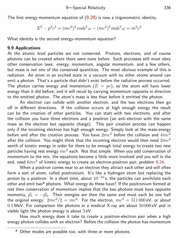
9—Special Relativity 336
The first energy-momentum equation of (9.29) is now a trigonometric identity.
E2 − p2c2 = (mc2)2 cosh2 ω − (mc2)2 sinh2 ω = m2c4
What identity is the second energy-momentum equation?
9.9 ApplicationsAt the atomic level particles are not conserved. Protons, electrons, and of coursephotons can be created where there were none before. Such processes still must obeyother conservation laws: energy, momentum, angular momentum, and a few others,but mass is not one of the conserved quantities. The most obvious example of this isradiation. An atom in an excited state in a vacuum with no other atoms around canemit a photon. That’s a particle that didn’t exist before the radiative process occurred.The photon carries energy and momentum (E = pc), so the atom will have lowerenergy than it did before, and it will recoil by carrying momentum opposite in directionto the emitted photon. The atom’s mass is less than before it emitted the photon.
An electron can collide with another electron, and the two electrons then gooff in different directions. If the collision occurs at high enough energy the resultcan be the creation of other particles. You can start with two electrons, and afterthe collision you have three electrons and a positron (an anti-electron with the samemass as the electron but opposite charge). This pair creation process can happenonly if the incoming electron has high enough energy. Simply look at the mass-energybefore and after the creation process: You have 2mc2 before the collision and 4mc2
after the collision. You might think that the incoming electron would then need 2mc2
worth of kinetic energy in order for there to be enough total energy to create two newparticles having rest energy mc2 each. Not that simple. When you add conservation ofmomentum to the mix, the equations become a little more involved and you will in theend, need 6mc2 of kinetic energy to create an electron-positron pair, problem 9.24.
When a positron comes near to an electron they attract each other and will oftenform a sort of atom, called positronium. It’s like a hydrogen atom but replacing theproton by a positron. In a short time, about 10−10 s, the particles can annihilate eachother and emit two* photons. What energy do these have? If the positronium formed atrest then conservation of momentum implies that the two photons must have oppositemomenta, ~p1 = −~p2. Their energies are then the same and must each be one halfthe original energy: 2mc2/2 = mc2. For the electron, mc2 = 511 000 eV, or about0.5 MeV. For comparison the photons in a medical X-ray are about 50 000 eV and invisible light the photon energy is about 2 eV.
How much energy does it take to create a positron-electron pair when a highenergy photon collides with an electron? Before the collision the photon has momentum
* Other modes are possible too, with three or more photons.
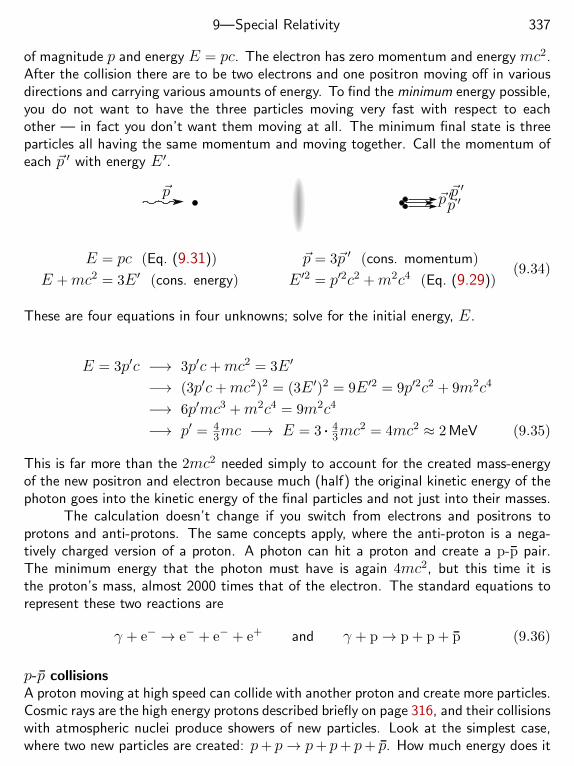
9—Special Relativity 337
of magnitude p and energy E = pc. The electron has zero momentum and energy mc2.After the collision there are to be two electrons and one positron moving off in variousdirections and carrying various amounts of energy. To find the minimum energy possible,you do not want to have the three particles moving very fast with respect to eachother — in fact you don’t want them moving at all. The minimum final state is threeparticles all having the same momentum and moving together. Call the momentum ofeach ~p ′ with energy E ′.
~p ~p ′~p ′~p ′
E = pc (Eq. (9.31))
E +mc2 = 3E ′ (cons. energy)
~p = 3~p ′ (cons. momentum)
E ′2 = p′2c2 +m2c4 (Eq. (9.29))(9.34)
These are four equations in four unknowns; solve for the initial energy, E.
E = 3p′c −→ 3p′c+mc2 = 3E ′
−→ (3p′c+mc2)2 = (3E ′)2 = 9E ′2 = 9p′2c2 + 9m2c4
−→ 6p′mc3 +m2c4 = 9m2c4
−→ p′ = 43mc −→ E = 3 . 4
3mc2 = 4mc2 ≈ 2 MeV (9.35)
This is far more than the 2mc2 needed simply to account for the created mass-energyof the new positron and electron because much (half) the original kinetic energy of thephoton goes into the kinetic energy of the final particles and not just into their masses.
The calculation doesn’t change if you switch from electrons and positrons toprotons and anti-protons. The same concepts apply, where the anti-proton is a nega-tively charged version of a proton. A photon can hit a proton and create a p-p pair.The minimum energy that the photon must have is again 4mc2, but this time it isthe proton’s mass, almost 2000 times that of the electron. The standard equations torepresent these two reactions are
γ + e− → e− + e− + e+ and γ + p→ p + p + p (9.36)
p-p collisionsA proton moving at high speed can collide with another proton and create more particles.Cosmic rays are the high energy protons described briefly on page 316, and their collisionswith atmospheric nuclei produce showers of new particles. Look at the simplest case,where two new particles are created: p+ p→ p+ p+ p+ p. How much energy does it
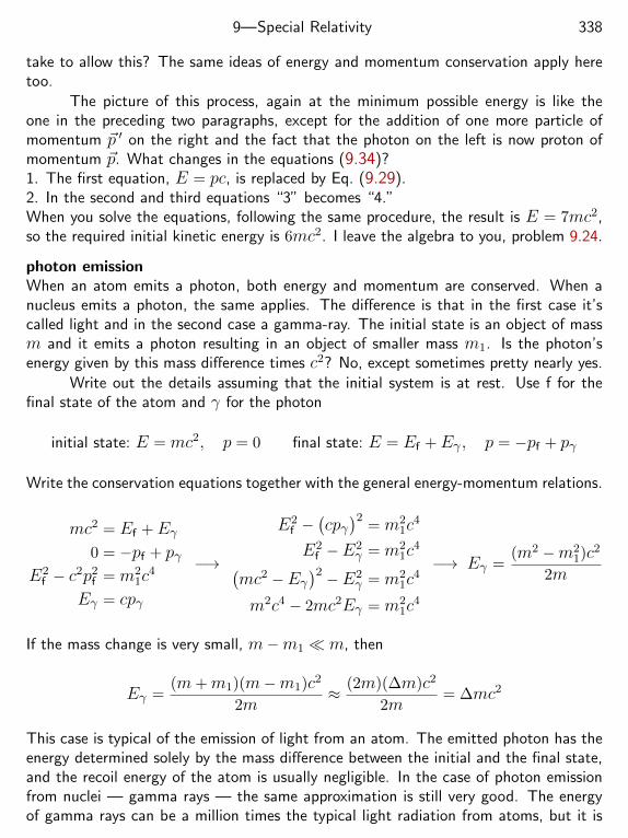
9—Special Relativity 338
take to allow this? The same ideas of energy and momentum conservation apply heretoo.
The picture of this process, again at the minimum possible energy is like theone in the preceding two paragraphs, except for the addition of one more particle ofmomentum ~p ′ on the right and the fact that the photon on the left is now proton ofmomentum ~p. What changes in the equations (9.34)?1. The first equation, E = pc, is replaced by Eq. (9.29).2. In the second and third equations “3” becomes “4.”When you solve the equations, following the same procedure, the result is E = 7mc2,so the required initial kinetic energy is 6mc2. I leave the algebra to you, problem 9.24.
photon emissionWhen an atom emits a photon, both energy and momentum are conserved. When anucleus emits a photon, the same applies. The difference is that in the first case it’scalled light and in the second case a gamma-ray. The initial state is an object of massm and it emits a photon resulting in an object of smaller mass m1. Is the photon’senergy given by this mass difference times c2? No, except sometimes pretty nearly yes.
Write out the details assuming that the initial system is at rest. Use f for thefinal state of the atom and γ for the photon
initial state: E = mc2, p = 0 final state: E = Ef +Eγ , p = −pf + pγ
Write the conservation equations together with the general energy-momentum relations.
mc2 = Ef +Eγ0 = −pf + pγ
E2f − c2p2
f = m21c
4
Eγ = cpγ
−→
E2f −
(cpγ)2
= m21c
4
E2f −E2
γ = m21c
4(mc2 −Eγ
)2 −E2γ = m2
1c4
m2c4 − 2mc2Eγ = m21c
4
−→ Eγ =(m2 −m2
1)c2
2m
If the mass change is very small, m−m1 m, then
Eγ =(m+m1)(m−m1)c2
2m≈ (2m)(∆m)c2
2m= ∆mc2
This case is typical of the emission of light from an atom. The emitted photon has theenergy determined solely by the mass difference between the initial and the final state,and the recoil energy of the atom is usually negligible. In the case of photon emissionfrom nuclei — gamma rays — the same approximation is still very good. The energyof gamma rays can be a million times the typical light radiation from atoms, but it is
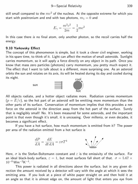
9—Special Relativity 339
still small compared to the mc2 of the nucleus. At the opposite extreme for which youstart with positronium and end with two photons, m1 = 0 and
Eγ =m2c2
2m=
1
2mc2
In this case there is no final atom, only another photon, so the recoil carries half theenergy.
9.10 Yarkovsky EffectThe concept of this phenomenon is simple, but it took a clever civil engineer, workingin his spare time, to think of it. Light can affect the motion of small asteroids. Sunlightcarries momentum, so it will apply a force directly on any object in its path. Once youknow that mass zero particles (photons) carry momentum, you pretty much expect it.The effect that I want to talk about is a different, more surprising one. As an asteroidorbits the sun and rotates on its axis, its will be heated during its day and cooled duringits night.
hot
cool
sun
All objects radiate, and a hotter object radiates more. Radiation carries momentum(p = E/c), so the hot part of an asteroid will be emitting more momentum than theother parts of its surface. Conservation of momentum implies that this provides a netforce on the asteroid in the direction away from the hot part of the surface. Surelythat is negligibly small! No. It’s been measured for some asteroids, and the importantpoint is that even though it’s small, it is unceasing. Over millenia, or even decades, itbecomes a significant effect.
If you have a hot surface, how much momentum is emitted from it? The powerper area of the radiation emitted from a hot surface is
dPdA
=dEdt dA
= εσT 4
Here, σ is the Stefan-Boltzmann constant and ε is the emissivity of the surface. Foran ideal black-body surface, ε = 1, but most surfaces fall short of that. σ = 5.67 ×10⁻⁸ Wm−2K−4.
This power is radiated in all directions above the surface, but in any given di-rection the amount received by a detector will vary with the angle at which it sees theemitting area. If you look at a piece of white paper straight on and then hold it atan angle so that it is almost edge on, the amount of light that enters you eye from
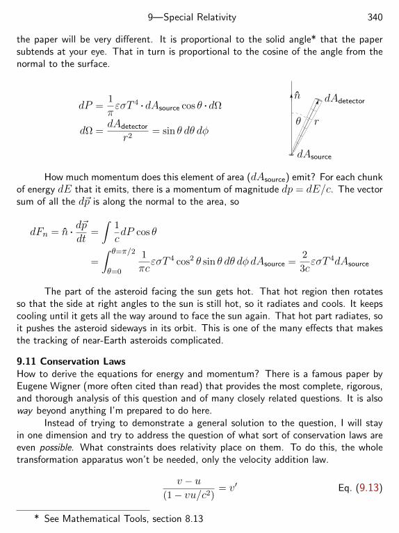
9—Special Relativity 340
the paper will be very different. It is proportional to the solid angle* that the papersubtends at your eye. That in turn is proportional to the cosine of the angle from thenormal to the surface.
dP =1
πεσT 4 . dAsource cos θ . dΩ
dΩ =dAdetector
r2= sin θ dθ dφ
dAsource
dAdetector
rθ
n
How much momentum does this element of area (dAsource) emit? For each chunkof energy dE that it emits, there is a momentum of magnitude dp = dE/c. The vectorsum of all the d~p is along the normal to the area, so
dFn = n . d~pdt
=
∫1
cdP cos θ
=
∫ θ=π/2
θ=0
1
πcεσT 4 cos2 θ sin θ dθ dφdAsource =
2
3cεσT 4dAsource
The part of the asteroid facing the sun gets hot. That hot region then rotatesso that the side at right angles to the sun is still hot, so it radiates and cools. It keepscooling until it gets all the way around to face the sun again. That hot part radiates, soit pushes the asteroid sideways in its orbit. This is one of the many effects that makesthe tracking of near-Earth asteroids complicated.
9.11 Conservation LawsHow to derive the equations for energy and momentum? There is a famous paper byEugene Wigner (more often cited than read) that provides the most complete, rigorous,and thorough analysis of this question and of many closely related questions. It is alsoway beyond anything I’m prepared to do here.
Instead of trying to demonstrate a general solution to the question, I will stayin one dimension and try to address the question of what sort of conservation laws areeven possible. What constraints does relativity place on them. To do this, the wholetransformation apparatus won’t be needed, only the velocity addition law.
v − u(1− vu/c2)
= v′ Eq. (9.13)
* See Mathematical Tools, section 8.13
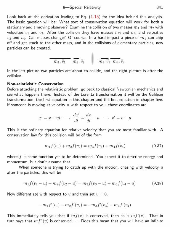
9—Special Relativity 341
Look back at the derivation leading to Eq. (1.15) for the idea behind this analysis.The basic question will be: What sort of conservation equation will work for both astationary and a moving observer? Examine the collision of two masses m1 and m2 withvelocities v1 and v2. After the collision they have masses m3 and m4 and velocitiesv3 and v4. Can masses change? Of course. In a hard impact a piece of m1 can chipoff and get stuck to the other mass, and in the collisions of elementary particles, newparticles can be created.
m1,~v1 m2,~v2 m3,~v3 m4,~v4
In the left picture two particles are about to collide, and the right picture is after thecollision.
Non-relativistic ConservationBefore attacking the relativistic problem, go back to classical Newtonian mechanics andsee what happens there. Instead of the Lorentz transformation it will be the Galileantransformation, the first equation in this chapter and the first equation in chapter five.If someone is moving at velocity u with respect to you, those coordinates are
x′ = x− ut −→ dx′
dt=dxdt− u −→ v′ = v − u
This is the ordinary equation for relative velocity that you are most familiar with. Aconservation law for this collision will be of the form
m1f(v1) +m2f(v2) = m3f(v3) +m4f(v4) (9.37)
where f is some function yet to be determined. You expect it to describe energy andmomentum, but don’t assume that.
When someone is trying to catch up with the motion, chasing with velocity uafter the particles, this will be
m1f(v1 − u) +m2f(v2 − u) = m3f(v3 − u) +m4f(v4 − u) (9.38)
Now differentiate with respect to u and then set u = 0.
−m1f′(v1)−m2f
′(v2) = −m3f′(v3)−m4f
′(v4)
This immediately tells you that if mf(v) is conserved, then so is mf ′(v). That inturn says that mf ′′(v) is conserved. . . . Does this mean that you will have an infinite
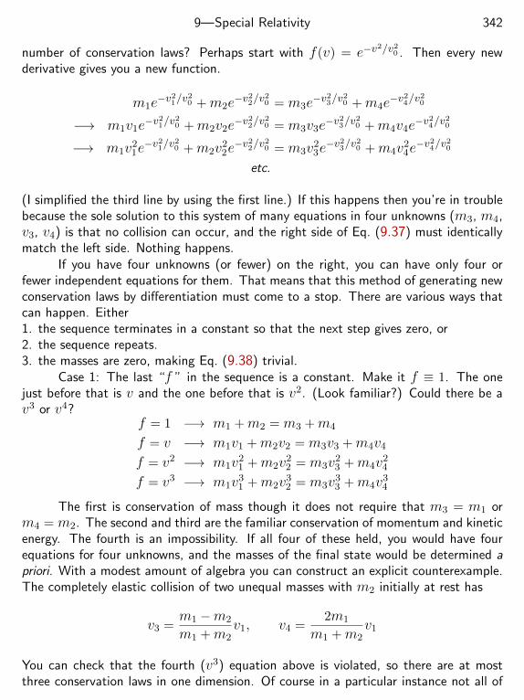
9—Special Relativity 342
number of conservation laws? Perhaps start with f(v) = e−v2/v20 . Then every new
derivative gives you a new function.
m1e−v21/v
20 +m2e
−v22/v20 = m3e
−v23/v20 +m4e
−v24/v20
−→ m1v1e−v21/v
20 +m2v2e
−v22/v20 = m3v3e
−v23/v20 +m4v4e
−v24/v20
−→ m1v21e−v21/v
20 +m2v
22e−v22/v
20 = m3v
23e−v23/v
20 +m4v
24e−v24/v
20
etc.
(I simplified the third line by using the first line.) If this happens then you’re in troublebecause the sole solution to this system of many equations in four unknowns (m3, m4,v3, v4) is that no collision can occur, and the right side of Eq. (9.37) must identicallymatch the left side. Nothing happens.
If you have four unknowns (or fewer) on the right, you can have only four orfewer independent equations for them. That means that this method of generating newconservation laws by differentiation must come to a stop. There are various ways thatcan happen. Either1. the sequence terminates in a constant so that the next step gives zero, or2. the sequence repeats.3. the masses are zero, making Eq. (9.38) trivial.
Case 1: The last “f ” in the sequence is a constant. Make it f ≡ 1. The onejust before that is v and the one before that is v2. (Look familiar?) Could there be av3 or v4?
f = 1 −→ m1 +m2 = m3 +m4
f = v −→ m1v1 +m2v2 = m3v3 +m4v4
f = v2 −→ m1v21 +m2v
22 = m3v
23 +m4v
24
f = v3 −→ m1v31 +m2v
32 = m3v
33 +m4v
34
The first is conservation of mass though it does not require that m3 = m1 orm4 = m2. The second and third are the familiar conservation of momentum and kineticenergy. The fourth is an impossibility. If all four of these held, you would have fourequations for four unknowns, and the masses of the final state would be determined apriori. With a modest amount of algebra you can construct an explicit counterexample.The completely elastic collision of two unequal masses with m2 initially at rest has
v3 =m1 −m2
m1 +m2v1, v4 =
2m1
m1 +m2v1
You can check that the fourth (v3) equation above is violated, so there are at mostthree conservation laws in one dimension. Of course in a particular instance not all of
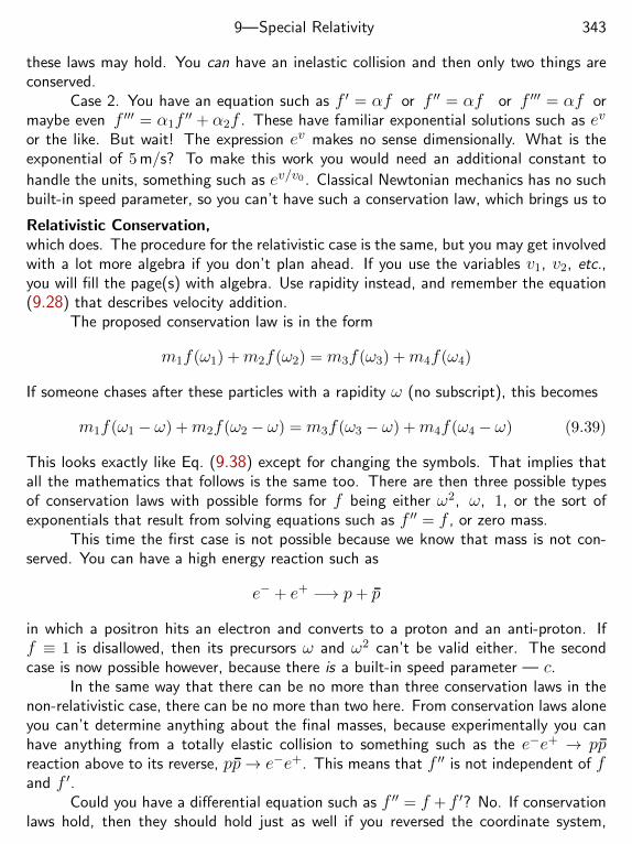
9—Special Relativity 343
these laws may hold. You can have an inelastic collision and then only two things areconserved.
Case 2. You have an equation such as f ′ = αf or f ′′ = αf or f ′′′ = αf ormaybe even f ′′′ = α1f ′′ + α2f . These have familiar exponential solutions such as ev
or the like. But wait! The expression ev makes no sense dimensionally. What is theexponential of 5 m/s? To make this work you would need an additional constant to
handle the units, something such as ev/v0 . Classical Newtonian mechanics has no suchbuilt-in speed parameter, so you can’t have such a conservation law, which brings us to
Relativistic Conservation,which does. The procedure for the relativistic case is the same, but you may get involvedwith a lot more algebra if you don’t plan ahead. If you use the variables v1, v2, etc.,you will fill the page(s) with algebra. Use rapidity instead, and remember the equation(9.28) that describes velocity addition.
The proposed conservation law is in the form
m1f(ω1) +m2f(ω2) = m3f(ω3) +m4f(ω4)
If someone chases after these particles with a rapidity ω (no subscript), this becomes
m1f(ω1 − ω) +m2f(ω2 − ω) = m3f(ω3 − ω) +m4f(ω4 − ω) (9.39)
This looks exactly like Eq. (9.38) except for changing the symbols. That implies thatall the mathematics that follows is the same too. There are then three possible typesof conservation laws with possible forms for f being either ω2, ω, 1, or the sort ofexponentials that result from solving equations such as f ′′ = f , or zero mass.
This time the first case is not possible because we know that mass is not con-served. You can have a high energy reaction such as
e− + e+ −→ p+ p
in which a positron hits an electron and converts to a proton and an anti-proton. Iff ≡ 1 is disallowed, then its precursors ω and ω2 can’t be valid either. The secondcase is now possible however, because there is a built-in speed parameter — c.
In the same way that there can be no more than three conservation laws in thenon-relativistic case, there can be no more than two here. From conservation laws aloneyou can’t determine anything about the final masses, because experimentally you canhave anything from a totally elastic collision to something such as the e−e+ → ppreaction above to its reverse, pp→ e−e+. This means that f ′′ is not independent of fand f ′.
Could you have a differential equation such as f ′′ = f + f ′? No. If conservationlaws hold, then they should hold just as well if you reversed the coordinate system,
9—Special Relativity 344
changing every ω to −ω. This differential equation doesn’t satisfy that criterion. Thef ′ term behaves oppositely from the other two. The only linear, constant coefficient,second order differential equation that works is f ′′ = ±α2f for some α. The solutionsare then respectively even and odd. Why not first order? You expect two conservationlaws not one, because in the non-relativistic limit that is what you have.
f ′′ = ±α2f −→(+) f(ω) = coshαω, f ′(ω) = α sinhαω
(−) f(ω) = cosαω, f ′(ω) = α sinαω
The circular functions are unexpected; are they possible? They would have the featurethat as one increases the other decreases, and in the non-relativistic limit nothing likethat occurs. On that basis alone, look at the other equations.
Are there any restrictions on α? No, it’s completely arbitrary and I can makeit anything that I want. Back when the rapidity ω appeared in the equations (9.23)and (9.26) it could just as easily have been v/c = tanh 2ω and nothing would havechanged. In the former instance ω was a change of variable in an integral, and theresult of an integration can’t depend on your choice how you do it. In the secondinstance a change of ω to αω would just be carried through the next few equationsintact, accomplishing nothing. So, just make it α = 1 and be done with it. This is sortof like choosing to work in radians when you use circular functions. You could work indegrees, but why carry along the extra factor of π/180?
One constraint is the non-relativistic limit. If p = A sinhω and E = B coshω,then for small ω ≈ v/c,
p ≈ Aω = Av/c and E ≈ B[1 + ω2/2
]These should match mv and mv2/2, so
A/c = m and m = B/c2 −→ p = mc sinhω, E = mc2 coshω
These are precisely the equations (9.33).The quotient of these equations relates E to p without m:
pE
=mc sinhωmc2 coshω
=1
ctanhω
For a photon, moving at the speed of light (ω →∞), this says that E = cp, and thatis just that third allowed way to have a consistent conservation law. There is no massin the equation. Of course, it’s an experimental question whether the photon has zeromass or not. The experimental upper limit on its mass is something like 10−20 electronmasses, and some claim even tighter bounds.
9—Special Relativity 345
Does this analysis show that anything is conserved? No. It does show that youdon’t have very much choice in the form of conservation laws if they do exist. Thereare other ways to obtain these results, but the real one, the derivation that nails it downso it is inescapable, is the 1939 paper by Wigner. (Good luck!)
Energy-Momentum transformationsWhat happens to energy and momentum when you switch to a moving observer? An-swer: They transform using the Lorentz transformation, just as x and t do. You canshow this using the same method as in Eq. (9.39), changing the rapidity and using thetrigonometric identities in Eq. (0.11).
A mass m has rapidity ω1, so its energy and momentum are
E = mc2 coshω1, p = mc sinhω1
Someone is chasing it with rapidity ω, so that person will see that the mass has rapidityω1 − ω and that the energy is (problem 0.15)
E ′ = mc2 cosh(ω1 − ω) = mc2[
coshω1 coshω − sinhω1 sinhω]
= E coshω − pc sinhω
Similarly he sees that its momentum is
p′ = mc sinh(ω1 − ω) = mc[
sinhω1 coshω − coshω1 sinhω]
= p coshω − 1cE sinhω
These are identical to the Lorentz transformation equations (9.27), and you shouldcompare this derivation to the derivation of coordinate rotations in Eq. (9.3).
x′ = x coshω − ct sinhω
ct′ = ct coshω − x sinhω
x←→ cp
ct←→ E
cp′ = cp coshω −E sinhω
E ′ = E coshω − pc sinhω(9.40)
The invariant interval t2−x2/c2 from Eqs. (9.15) and (9.16) is precisely reflectedin the equation E2 − p2c2 = m2c4 from Eq. (9.29). With more coordinates, y and zbehave just as py and pz do. (They’re unchanged by a Lorentz transformation along x.
9—Special Relativity 346
Exercises
1 Check special cases of Eqs. (9.4) to verify they they work: 0, ±π/4, ±π/2, π.Various points.
2 In Eqs. (9.4), solve for x and y.
3 Using the picture above Eqs. (9.4) and taking α = 45, graph the curve x′y′ = 1.Then express the equation in terms of x and y.
4 The Earth’s gravitational field is g. Express it in the units light-years/year2.
5 Two events occur at the space-time coordinates
x1 = 0, t1 = 0 and x2 = 2400 m, t2 = 5µs
Use the Lorentz transformation to determine a speed v such that either (a) the twoevents are simultaneous or (b) the two events occurred at the same position. Solve forv in each case and show that one solution is possible and the other is not. Recall: thespeed of light is c = 300 m/µs.
6 Can positronium decay by emitting a single photon? e−e+ → γ. Write the equationsfor conservation of energy and of momentum and verify that this is impossible, showingthat they have no solution.
7 The π+ meson, an unstable particle, lives on the average, about 2.6× 10⁻⁸ s (mea-sured in its own frame of reference) before decaying.(a) If such a particle is moving with respect to the laboratory with a speed of 0.8c,what lifetime is measured in the laboratory?(b) What average distance, measured in the laboratory, does the particle move beforedecaying?
8 A photon of energy E is emitted by an atom of mass m, which recoils in the oppositedirection. Assuming the atom can be treated nonrelativistically, compute the recoilvelocity of the atom. Hence, show that the recoil speed is much smaller than c wheneverE is much smaller than the rest energy mc2 of the atom.
9 At what speed is the momentum of a particle twice as great as the result obtainedfrom the nonrelativistic expression mv?
10 A particle is observed to go (on average) 6,000 meters in 100µs before decaying.If its mean life at rest is 80 millisec, what was v/c? (assume no acceleration).
9—Special Relativity 347
11 At what speed is the rest energy of a particle equal to its kinetic energy?
12 In Eq. (9.20), look more closely at the case for which the moving observer “v” hasvelocity very close to +c and then again when it is close to −c. For both of these, whatdoes the equation say if u is close to +c and to −c? (Four cases)
13 Expand Eqs. (9.22) and (9.23) to get t and x for small times. Eliminate ω betweenthem to get x(t) for small times.
14 Derive Eqs. (9.32) from Eqs. (9.29).
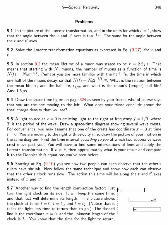
9—Special Relativity 348
Problems
9.1 In the picture of the Lorentz transformation, and in the units for which c = 1, showthat the angle between the x and x′ axes is tan−1 v. The same for the angle betweenthe t and t′ axes.
9.2 Solve the Lorentz transformation equations as expressed in Eq. (9.27), for x andt.
9.3 In section 9.2 the mean lifetime of a muon was stated to be τ = 2.2µs. Thatmeans that starting with N0 muons, the number of muons as a function of time isN(t) = N0e−t/τ . Perhaps you are more familiar with the half life, the time in which
one-half of the muons decay, so that N(t) = N02−t/t1/2 . What is the relation betweenthe mean life, τ , and the half life, t1/2, and what is the muon’s (proper) half life?Ans: 1.5µs
9.4 Draw the space-time figure on page 324 as seen by your friend, who of course saysthat you are the one moving to the left. What does your friend conclude about thetotal charge density that you see?
9.5˙ A light source at x = 0 is emitting light to the right at frequency f = 1/T whereT is the period of the wave. Draw a space-time diagram showing several wave crests.For convenience, you may assume that one of the crests has coordinate x = 0 at timet = 0. You are moving to the right with velocity v, so draw the picture of your motion inthe same diagram. Find the time interval according to you at which two successive wavecrest move past you. You will have to find some intersections of lines and apply theLorentz transformation. If v c, then approximately what is your result and compareit to the Doppler shift equations you’ve seen before.
9.6 Starting at Eq. (9.10) you see how two people can each observe that the other’srulers have shrunk. Now follow the same technique and show how each can observethat the other’s clock runs slow. The action this time will be along the t and t′ axesinstead of x and x′.
9.7 ˙ Another way to find the length contraction factor: justturn the light clock on its side. It will keep the same time,and that fact will determine its length. The picture showsthe clock at times t = 0, t = t1, and t = t2. (Notice that ittakes the light less time to return than to go.) The dashedline is the coordinate x = 0, and the unknown length of theclock is L. You know that the time for the light to return,
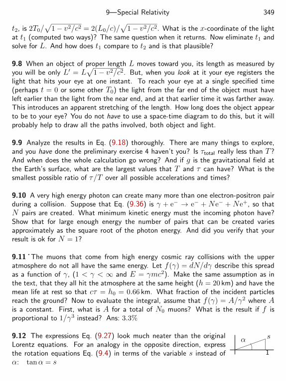
9—Special Relativity 349
t2, is 2T0/√
1− v2/c2 = 2(L0/c)/√
1− v2/c2. What is the x-coordinate of the lightat t1 (computed two ways)? The same question when it returns. Now eliminate t1 andsolve for L. And how does t1 compare to t2 and is that plausible?
9.8 When an object of proper length L moves toward you, its length as measured byyou will be only L′ = L
√1− v2/c2. But, when you look at it your eye registers the
light that hits your eye at one instant. To reach your eye at a single specified time(perhaps t = 0 or some other T0) the light from the far end of the object must haveleft earlier than the light from the near end, and at that earlier time it was farther away.This introduces an apparent stretching of the length. How long does the object appearto be to your eye? You do not have to use a space-time diagram to do this, but it willprobably help to draw all the paths involved, both object and light.
9.9 Analyze the results in Eq. (9.18) thoroughly. There are many things to explore,and you have done the preliminary exercise 4 haven’t you? Is τtotal really less than T ?And when does the whole calculation go wrong? And if g is the gravitational field atthe Earth’s surface, what are the largest values that T and τ can have? What is thesmallest possible ratio of τ/T over all possible accelerations and times?
9.10 A very high energy photon can create many more than one electron-positron pairduring a collision. Suppose that Eq. (9.36) is γ + e− → e− + Ne− + Ne+, so thatN pairs are created. What minimum kinetic energy must the incoming photon have?Show that for large enough energy the number of pairs that can be created variesapproximately as the square root of the photon energy. And did you verify that yourresult is ok for N = 1?
9.11 ˙ The muons that come from high energy cosmic ray collisions with the upperatmosphere do not all have the same energy. Let f(γ) = dN/dγ describe this spreadas a function of γ, (1 < γ < ∞ and E = γmc2). Make the same assumption as inthe text, that they all hit the atmosphere at the same height (h = 20 km) and have themean life at rest so that cτ = h0 = 0.66 km. What fraction of the incident particlesreach the ground? Now to evaluate the integral, assume that f(γ) = A/γ2 where Ais a constant. First, what is A for a total of N0 muons? What is the result if f isproportional to 1/γ3 instead? Ans: 3.3%
α s
1
9.12 The expressions Eq. (9.27) look much neater than the originalLorentz equations. For an analogy in the opposite direction, expressthe rotation equations Eq. (9.4) in terms of the variable s instead ofα: tanα = s
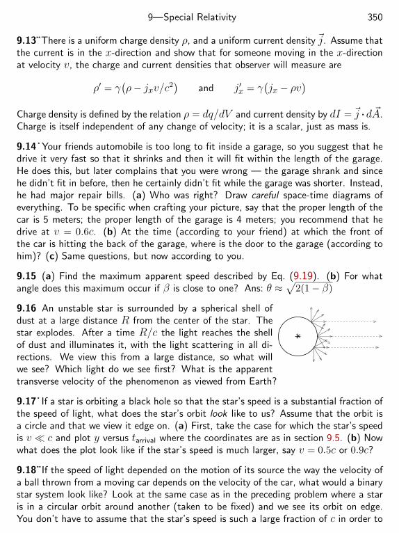
9—Special Relativity 350
9.13¨There is a uniform charge density ρ, and a uniform current density ~j. Assume thatthe current is in the x-direction and show that for someone moving in the x-directionat velocity v, the charge and current densities that observer will measure are
ρ′ = γ(ρ− jxv/c2
)and j′x = γ
(jx − ρv
)Charge density is defined by the relation ρ = dq/dV and current density by dI = ~j . d ~A.Charge is itself independent of any change of velocity; it is a scalar, just as mass is.
9.14˙ Your friends automobile is too long to fit inside a garage, so you suggest that hedrive it very fast so that it shrinks and then it will fit within the length of the garage.He does this, but later complains that you were wrong — the garage shrank and sincehe didn’t fit in before, then he certainly didn’t fit while the garage was shorter. Instead,he had major repair bills. (a) Who was right? Draw careful space-time diagrams ofeverything. To be specific when crafting your picture, say that the proper length of thecar is 5 meters; the proper length of the garage is 4 meters; you recommend that hedrive at v = 0.6c. (b) At the time (according to your friend) at which the front ofthe car is hitting the back of the garage, where is the door to the garage (according tohim)? (c) Same questions, but now according to you.
9.15 (a) Find the maximum apparent speed described by Eq. (9.19). (b) For whatangle does this maximum occur if β is close to one? Ans: θ ≈
√2(1− β)
9.16 An unstable star is surrounded by a spherical shell ofdust at a large distance R from the center of the star. Thestar explodes. After a time R/c the light reaches the shellof dust and illuminates it, with the light scattering in all di-rections. We view this from a large distance, so what willwe see? Which light do we see first? What is the apparenttransverse velocity of the phenomenon as viewed from Earth?
9.17˙ If a star is orbiting a black hole so that the star’s speed is a substantial fraction ofthe speed of light, what does the star’s orbit look like to us? Assume that the orbit isa circle and that we view it edge on. (a) First, take the case for which the star’s speedis v c and plot y versus tarrival where the coordinates are as in section 9.5. (b) Nowwhat does the plot look like if the star’s speed is much larger, say v = 0.5c or 0.9c?
9.18¨If the speed of light depended on the motion of its source the way the velocity ofa ball thrown from a moving car depends on the velocity of the car, what would a binarystar system look like? Look at the same case as in the preceding problem where a staris in a circular orbit around another (taken to be fixed) and we see its orbit on edge.You don’t have to assume that the star’s speed is such a large fraction of c in order to
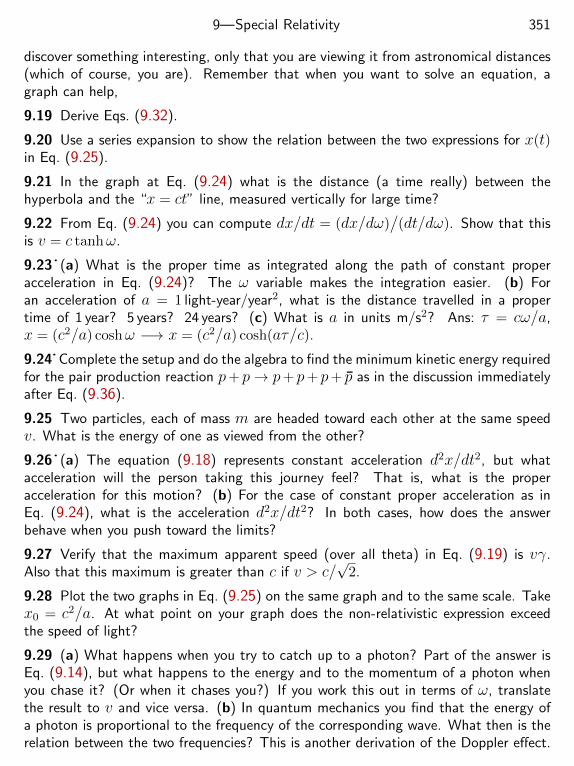
9—Special Relativity 351
discover something interesting, only that you are viewing it from astronomical distances(which of course, you are). Remember that when you want to solve an equation, agraph can help,
9.19 Derive Eqs. (9.32).
9.20 Use a series expansion to show the relation between the two expressions for x(t)in Eq. (9.25).
9.21 In the graph at Eq. (9.24) what is the distance (a time really) between thehyperbola and the “x = ct” line, measured vertically for large time?
9.22 From Eq. (9.24) you can compute dx/dt = (dx/dω)/
(dt/dω). Show that thisis v = c tanhω.
9.23˙ (a) What is the proper time as integrated along the path of constant properacceleration in Eq. (9.24)? The ω variable makes the integration easier. (b) Foran acceleration of a = 1 light-year/year2, what is the distance travelled in a propertime of 1 year? 5 years? 24 years? (c) What is a in units m/s2? Ans: τ = cω/a,x = (c2/a) coshω −→ x = (c2/a) cosh(aτ/c).
9.24˙ Complete the setup and do the algebra to find the minimum kinetic energy requiredfor the pair production reaction p+ p→ p+ p+ p+ p as in the discussion immediatelyafter Eq. (9.36).
9.25 Two particles, each of mass m are headed toward each other at the same speedv. What is the energy of one as viewed from the other?
9.26˙ (a) The equation (9.18) represents constant acceleration d2x/dt2, but whatacceleration will the person taking this journey feel? That is, what is the properacceleration for this motion? (b) For the case of constant proper acceleration as inEq. (9.24), what is the acceleration d2x/dt2? In both cases, how does the answerbehave when you push toward the limits?
9.27 Verify that the maximum apparent speed (over all theta) in Eq. (9.19) is vγ.Also that this maximum is greater than c if v > c/
√2.
9.28 Plot the two graphs in Eq. (9.25) on the same graph and to the same scale. Takex0 = c2/a. At what point on your graph does the non-relativistic expression exceedthe speed of light?
9.29 (a) What happens when you try to catch up to a photon? Part of the answer isEq. (9.14), but what happens to the energy and to the momentum of a photon whenyou chase it? (Or when it chases you?) If you work this out in terms of ω, translatethe result to v and vice versa. (b) In quantum mechanics you find that the energy ofa photon is proportional to the frequency of the corresponding wave. What then is therelation between the two frequencies? This is another derivation of the Doppler effect.
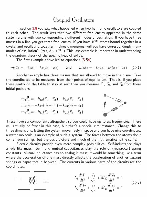
Coupled OscillatorsIn section 3.8 you saw what happened when two harmonic oscillators are coupled
to each other. The result was that two different frequencies appeared in the samesystem along with two correspondingly different modes of oscillation. If you have threemasses in a line you get three frequencies. If you have 1023 atoms bound together in acrystal and oscillating together in three dimensions, will you have correspondingly manymodes of oscillation? (Yes, 3× 10²³.) This last example is important in understandingthe quantum theory of the specific heat of solids.
The first example above led to equations (3.54).
m1x1 = −k1x1 − k2(x1 − x2) and m2x2 = −k3x2 − k2(x2 − x1) (10.1)
Another example has three masses that are allowed to move in the plane. Takethe coordinates to be measured from their points of equilibrium. That is, if you placethese gently on the table to stay at rest then you measure ~r1, ~r2, and ~r3 from theseinitial positions
m1~r1 = −k12
(~r1 − ~r2
)− k13
(~r1 − ~r3
)m2~r2 = −k12
(~r2 − ~r1
)− k23
(~r2 − ~r3
)m3~r3 = −k13
(~r3 − ~r1
)− k23
(~r3 − ~r2
)These have six components altogether, so you could have up to six frequencies. Therewill actually be fewer in this case, but that’s a special circumstance. Change this tothree dimensions, letting the system move freely in space and you have nine coordinates:a water molecule is an example of such a system. The forces between the atoms don’tcome from springs, but the basic picture and much of the mathematics is the same.
Electric circuits provide even more complex possibilities. Self-inductance playsa role like mass. Self- and mutual-capacitances play the role of (reciprocal) springconstants. Mutual inductance has no analog in mass; it would be something like a termwhere the acceleration of one mass directly affects the acceleration of another withoutsprings or capacitors in between. The currents in various parts of the circuits are thecoordinates.
L1d2I1
dt2+I1
C1+M12
d2I2
dt2= 0
L2d2I2
dt2+I2
C2+M21
d2I1
dt2= 0
(10.2)
352
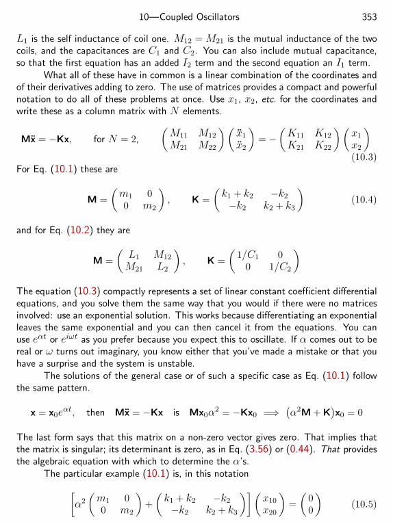
10—Coupled Oscillators 353
L1 is the self inductance of coil one. M12 = M21 is the mutual inductance of the twocoils, and the capacitances are C1 and C2. You can also include mutual capacitance,so that the first equation has an added I2 term and the second equation an I1 term.
What all of these have in common is a linear combination of the coordinates andof their derivatives adding to zero. The use of matrices provides a compact and powerfulnotation to do all of these problems at once. Use x1, x2, etc. for the coordinates andwrite these as a column matrix with N elements.
Mx = −Kx, for N = 2,
(M11 M12
M21 M22
)(x1
x2
)= −
(K11 K12
K21 K22
)(x1
x2
)(10.3)
For Eq. (10.1) these are
M =
(m1 00 m2
), K =
(k1 + k2 −k2
−k2 k2 + k3
)(10.4)
and for Eq. (10.2) they are
M =
(L1 M12
M21 L2
), K =
(1/C1 0
0 1/C2
)The equation (10.3) compactly represents a set of linear constant coefficient differentialequations, and you solve them the same way that you would if there were no matricesinvolved: use an exponential solution. This works because differentiating an exponentialleaves the same exponential and you can then cancel it from the equations. You canuse eαt or eiωt as you prefer because you expect this to oscillate. If α comes out to bereal or ω turns out imaginary, you know either that you’ve made a mistake or that youhave a surprise and the system is unstable.
The solutions of the general case or of such a specific case as Eq. (10.1) followthe same pattern.
x = x0eαt, then Mx = −Kx is Mx0α
2 = −Kx0 =⇒(α2M + K
)x0 = 0
The last form says that this matrix on a non-zero vector gives zero. That implies thatthe matrix is singular; its determinant is zero, as in Eq. (3.56) or (0.44). That providesthe algebraic equation with which to determine the α’s.
The particular example (10.1) is, in this notation[α2
(m1 00 m2
)+
(k1 + k2 −k2
−k2 k2 + k3
)](x10
x20
)=
(00
)(10.5)
10—Coupled Oscillators 354
This is the same as the equations (3.59), and the statement that the determinant iszero is
det(α2M + K
)=(α2m1 + k1 + k2
)(α2m2 + k2 + k3
)− k2
2 = 0 (10.6)
This is a quadratic equation in α2, but it’s messy. You can see that if you have threemasses instead of two, even if they’re oscillating along a straight line as these are, youwill get a cubic equation instead. Unless there’s some special symmetry that allows youto simplify the system, these problems rapidly becomes intractable. Fortunately, thereoften are such symmetries.
There are some general theorems about these equations that will apply to anysuch system, and they provide a guide about where to look for a solution. First thoughI’ll require that the matrices M and K satisfy certain properties:
M and K are real and symmetric, Mij = Mji, Kij = Kji
M and K are positive definite: x∗Mx > 0 and x∗Kx > 0 for all non-zero x(10.7)
You can check in the special case coming from Eq. (10.1) that the symmetry propertiesare satisfied. The “positive definite” requirement is needed to be sure that both thekinetic energy and the potential energy are positive. If you don’t have this, then theoscillator is unstable. Of course if you’re trying to stand a pencil on its tip, thatinstability is exactly what you expect and it isn’t wrong. Just don’t expect to use theresults of this chapter without modification.
10.1 Normal ModesThe different frequencies of oscillation corresponding to different shapes for the waythat the masses move. These are called “normal modes” of oscillation. What’s normalabout them and are other oscillations abnormal? Here, normal means perpendicular.The different oscillations are normal to each other, and normal means that the scalarproduct of one mode of oscillation with another mode will be zero. Which scalarproduct? Probably not the one you are thinking of.
The basic results come without solving a single differential equation or algebraicequation. It involves only some matrix manipulation, so first a quick review of thenotation and the pertinent parts of the subject. Look back at section 0.10 for a runningstart.*
M is the transpose of M. (M)ij = Mji M =
(a bc d
)=⇒ M =
(a cb d
)* Use M for the whole matrix; use Mij or (M)ij for the single number sitting in
the i-j position.
10—Coupled Oscillators 355
M∗ is the complex conjugate of each element, and M∗
= M† is the adjoint
MN = NM and (MN)† = N†M†
To prove the first of these equations just write out the meaning of each side.(MN
)ij =
∑k
MikNkj and the transpose of this interchanges i and j, so
(MN
)ij =
∑k
MjkNki =∑k
NkiMjk =∑k
(N)ik
(M)kj =
(NM
)ij (10.8)
The corresponding equation for the adjoint adds some complex conjugations amongEqs. (10.8).
If x =
(x1
x2
), then x† = (x∗1 x∗2 )
(Mx)†
= x†M† (10.9)
and x†My is a number whose complex conjugate is y†M†x (10.10)
How do you derive these equations? The same way as in Eq. (10.8).Now to derive the basic theorem about normal modes. For the equation
(α2M+
K)x = 0, let x1 and x2 be two non-zero solutions for two values of α. For now I don’t
need the values of the roots α, just that they exist.(α2
1M + K)x1 = 0
(α2
2M + K)x2 = 0
Multiply the first of these by x†2 and the second by x†1.
x†2(α2
1M + K)x1 = 0 x†1
(α2
2M + K)x2 = 0 (10.11)
Both of these are numbers. Take the complex conjugate of the second one and useEq. (10.10). [
x†1(α2
2M + K)x2
]∗= x†2
(α∗22 M† + K†
)x1 = 0 (10.12)
Recall the assumption that both M and K are real and symmetric, so M† = M andK† = K. That means that I can write Eqs. (10.11) and (10.12) as
x†2(α2
1M + K)x1 = 0 and x†2
(α∗22 M + K
)x1 = 0 (10.13)
Now subtract these equations and the K terms cancel.(α2
1 − α∗22
)x†2Mx1 = 0 (10.14)
10—Coupled Oscillators 356
This is the result I was aiming for. From this equation I can deduce two useful conse-quences, all without solving a complicated polynomial equation.
For the first result take the special case in which the two solutions are the samesolution. x1 = x2 and α1 = α2. (
α21 − α∗21
)x†1Mx1 = 0
One of my assumptions (and here’s why) was that the product x†1Mx1 > 0. M ispositive definite. This number can’t vanish unless the x itself is zero. The only waythat the product of two numbers can be zero is if one of the two numbers is itself zero.This implies that the other factor (
α21 − α∗21
)= 0
That is, α2 is real. It doesn’t say if it’s positive or negative, but at least it’s not complex.Now go back to the general case(
α21 − α2
2
)x†2Mx1 = 0 (10.15)
The α2’s are real now so I can drop a complex conjugation. If the two α2’s are differentthen this time the first factor cannot be zero and that means that the second factormust be zero.
If α21 6= α2
2, then x†2Mx1 = 0 (10.16)
This is a scalar product. This is the sense in which the modes are “normal.” Theirscalar product vanishes. The mass matrix defines a way to multiply the two vectors, x1
and x2, and it is by using this particular definition of scalar product that you get the nicetheorem. Go back to the material on waves and look closely at the equations (7.42)-(7.44). In a seeming distant context you are doing essentially the same manipulationsthere as here. In those equations you used partial integration. Here you used matrixtransposition, but there are close parallels.
10.2 Scalar ProductsCan you do this with a scalar product? Is it legitimate to call x†2Mx1 a scalar product?Yes. To see why, it’s necessary to understand what a scalar product is.
The fundamental definition of a scalar product is that it is a scalar-valued functionof two vector variables and that it must satisfy a certain set of requirements. Call thefunction f for now, so f(~v1,~v2) is a scalar and it must have these four properties:
1. f(~v1,~v2 + ~v3) = f(~v1,~v2) + f(~v1,~v3)2. f(~v1, α~v2) = αf (~v1,~v2)3. f(~v1,~v2) = f(~v2,~v1)∗
10—Coupled Oscillators 357
4. f(~v,~v ) ≥ 0, and f(~v,~v ) = 0 if and only if the vector ~v is itself thezero vector.
Any function that satisfies these requirements is called a scalar product. If youare using only real numbers then the complex conjugation in the third requirement isunnecessary. Does the familiar dot product satisfy them?
f( ~A, ~B ) = ~A . ~B = AB cos θ is certainly a scalar.
2. ~A .(α~B ) = α( ~A . ~B ) If α < 0 remember that cos(θ + π) = − cos θ.
3. ~A . ~B = ~B . ~A4. ~A . ~A ≥ 0 and it’s never zero except when ~A is itself zero.
1. This is the only part that takes any effort. Draw the picture of ~A .( ~B+ ~C ) assumingthat everything is in a single plane. That one is not so hard to prove — simply writeout the meaning of each term. With a little more thought the same picture works forthe three dimensional case too.
~B
~C
~AB cos θ1 C cos θ2
~A .( ~B + ~C
)=? ~A .B + ~A . ~C∣∣ ~B + ~C
∣∣ cos θ3 = B cos θ1 +C cos θ2
The projections of ~B and of ~C on ~A add to the projection of ~B + ~C on ~A. I didn’tdraw the angles explicitly because it would make the sketch too cluttered, and you caneasily figure out which angle is which anyway.
If you express displacement vectors in the plane in terms of rectangular coor-dinates, so that ~r1 = x1x + y1y and similarly for ~r2, the standard scalar product is~r1 .~r2 = x1x2 + y1y2. Suppose however that you decide to measure x in meters andy in centimeters. This product would have to be modified to account for this, lookingsomething like ~r1 .~r2 = x1x2 + ky1y2, where k = 10−4 m2/cm2.
The example Eq. (10.16) is like this, although the mass matrix came naturallyout of the computation instead of being an artifice of changing units. That (10.16)satisfies the requirements to be a scalar product is easy to check, and is essentially atranslation of the assumptions that I made about M in Eq. (10.7).
10.3 ExampleReturn to Eq. (10.1) and (10.6) and carry it out in this language. Just to keep thealgebra from getting completely out of hand, I’ll take k1 = k3, but let the masses bedifferent.
det(α2M + K
)=(α2m1 + k1 + k2
)(α2m2 + k2 + k1
)− k2
2 = 0
m1m2α4 + (m1 +m2)(k1 + k2)α2 + (k1 + k2)2 − k2
2 = 0 (10.17)
10—Coupled Oscillators 358
α2 =1
2m1m2
[− (m1 +m2)(k1 + k2) (10.18)
±√
(m1 +m2)2(k1 + k2)2 − 4m1m2
[(k1 + k2)2 − k2
2
]]=
1
2m1m2
[−(m1 +m2)(k1 + k2)±
√(m1 −m2)2(k1 + k2)2 + 4m1m2k2
2
]At least it came out real. If m1 = m2 this simplifies, but I don’t want to restrict myselfto that case because it doesn’t show enough about the nature of “normal” modes.
The modes themselves require solving the matrix equations (10.5). That thedeterminant is zero assures you that there is a non-trivial solution, and without thatrequirement on the determinant the only solution for x is identically zero. When thedeterminant is zero, the two simultaneous equations are really one equation. Pick either.(α2m1 + k1 + k2
)x10 − k2x20 = 0, x20 =
1
k2
(α2m1 + k1 + k2
)x10 (10.19)
The special case for which m1 = m2 gives
α2 =[− 2m(k1 + k2)± 2mk2
]/2m2, then α2
1 = −k1
m, α2
2 = −k1 + 2k2
m(10.20)
The solutions for the components are in this case
α21 =⇒ x20 = x10 and α2
2 =⇒ x20 = −x10
and the scalar product of these two vectors is
( 1 −1 )
(m 00 m
)(11
)= 0
If the masses aren’t equal there is more algebra, but not an impossible amount.I want to show that this really works, so evaluate the factor in Eq. (10.19) using thetwo values of α2 in (10.18).
1
k2
(α2m1 + k1 + k2
)=
1
k2
[[− (m1 +m2)(k1 + k2)±√
] 1
2m1m2m1 + k1 + k2
]=
1
2m2k2
[(m2 −m1)(k1 + k2)±√
]The scalar product is now(
1 12m2k2
[(m2 −m1)(k1 + k2)−√
] )(m1 00 m2
)(1
12m2k2
[(m2 −m1)(k1 + k2) +
√ ])= m1 +
m2
4m22k
22
[(m2 −m1)2(k1 + k2)2 −
[(m1 −m2)2(k1 + k2)2 + 4m1m2k
22
]]= 0
10—Coupled Oscillators 359
The two modes are orthogonal as promised. And yes, you do have to check the algebra.
What if one of the two masses is a lot bigger then the other? Let m1 m2,then look at the square root in Eq. (10.18). The first term has an m2
1 and the secondterm has only an m1. The first term wins. The α with the minus sign in front of thesquare root is
α22 ≈
[−m1(k1 + k2)−m1(k1 + k2)
]/2m1m2 = −(k1 + k2)/m2
For the other α, if you use the same approximation then the two terms cancel, leavingyou with nothing. That throws everything away, so it’s not good enough. You can doa series expansion in m2, but this time there’s an easier way. Both these α’s are rootsof the same quadratic equation, and perhaps you remember something about the rootsof polynomial equations.
(x− r1)(x− r2) = x2 − (r1 + r2)x+ r1r2
When a polynomial of any order (n) is written with its first coefficient one, the nextterm is (−) the sum of the roots, and the constant is (−1)n times the product of theroots. For Eq. (10.17) the product of the roots is
α21α
22 =
(k1 + k2)2 − k22
m1m2
I already know α22, so this implies
α21 =
(k1 + k2)2 − k22
m1m2
−m2
k1 + k2= −(k1 + k2)2 − k2
2
m1(k1 + k2)
If m1 m2 then∣∣α2
1
∣∣ ∣∣α22
∣∣. Now for the modes themselves, use Eq. (10.19) again.
x20 =1
k2
(α2m1 + k1 + k2
)x10
For the α21 case, the m1 cancels and you have
x20 ≈1
k2
(−(k1 + k2)2 − k2
2
(k1 + k2)+ k1 + k2
)x10 =
k2
k1 + k2x10
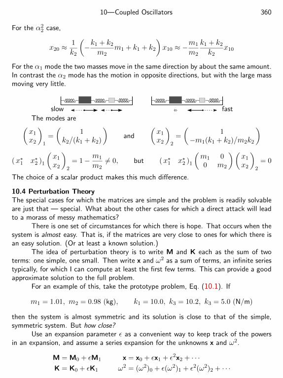
10—Coupled Oscillators 360
For the α22 case,
x20 ≈1
k2
(−k1 + k2
m2m1 + k1 + k2
)x10 ≈ −
m1
m2
k1 + k2
k2x10
For the α1 mode the two masses move in the same direction by about the same amount.In contrast the α2 mode has the motion in opposite directions, but with the large massmoving very little.
slow fast
The modes are(x1
x2
)1
=
(1
k2/(k1 + k2)
)and
(x1
x2
)2
=
(1
−m1(k1 + k2)/m2k2
)
(x∗1 x∗2 )1
(x1
x2
)2
= 1− m1
m26= 0, but (x∗1 x∗2 )1
(m1 00 m2
)(x1
x2
)2
= 0
The choice of a scalar product makes this much difference.
10.4 Perturbation TheoryThe special cases for which the matrices are simple and the problem is readily solvableare just that — special. What about the other cases for which a direct attack will leadto a morass of messy mathematics?
There is one set of circumstances for which there is hope. That occurs when thesystem is almost easy. That is, if the matrices are very close to ones for which there isan easy solution. (Or at least a known solution.)
The idea of perturbation theory is to write M and K each as the sum of twoterms: one simple, one small. Then write x and ω2 as a sum of terms, an infinite seriestypically, for which I can compute at least the first few terms. This can provide a goodapproximate solution to the full problem.
For an example of this, take the prototype problem, Eq. (10.1). If
m1 = 1.01, m2 = 0.98 (kg), k1 = 10.0, k3 = 10.2, k3 = 5.0 (N/m)
then the system is almost symmetric and its solution is close to that of the simple,symmetric system. But how close?
Use an expansion parameter ε as a convenient way to keep track of the powersin an expansion, and assume a series expansion for the unknowns x and ω2.
M = M0 + εM1
K = K0 + εK1
x = x0 + εx1 + ε2x2 + · · ·ω2 = (ω2)0 + ε(ω2)1 + ε2(ω2)2 + · · ·
10—Coupled Oscillators 361
Substitute these into the equations that I want to solve.
−ω2Mx + Kx = 0
−[(ω2)0 + ε(ω2)1 + ε2(ω2)2 + · · ·
][M0 + εM1
][x0 + εx1 + ε2x2 + · · ·
]+[K0 + εK1
][x0 + εx1 + ε2x2 + · · ·
]= 0
The only way that this can be valid for arbitrary ε is for the respective coefficients ofthe powers of ε to agree.
(ε0)
(ε1)
(ε2)
−(ω2)0M0x0 + K0x0 = 0
−(ω2)0M0x1 − (ω2)0M1x0 − (ω2)1M0x0 + K0x1 + K1x0 = 0
−(ω2)0M0x2 − (ω2)0M1x1 − (ω2)1M0x1−(ω2)1M1x0 − (ω2)2M0x0 + K0x2 + K1x1 = 0
It appears that I’ve made the problem worse, not better. I’ve replaced one difficultequation by an infinite number of difficult equations. But no. In what looks to be ahopeless tangle, there’s some simplicity hidden. Besides, I’m never going to get aroundto using the third of these equations, only the first two. And why the frequency squaredinstead of the frequency? That’s the way it works, but see problem 10.6. Writing thefrequency this way is unnecessarily cumbersome, so I will stop doing it. Instead of (ω2)1
I will write ω21 .
Equation (ε0) is the equation that I’ve already solved. It’s the one that is sup-posedly simple. The first new equation that I have to examine is (ε1).
−ω20M0x1 + K0x1 = +ω2
0M1x0 + ω21M0x0 −K1x0 (10.21)
Look at the way that I rearranged this equation and you see that on the right-hand sidethe only thing that is unknown is ω2
1 , the term that gives the first order correction to thefrequency. On the left side you have something that looks like the simple, unperturbedequation. At this point I have to stop and present a theorem. It’s such an easy theoremthat you may wonder why I’d bother calling it such, but it is the key to solving all theseequations. It breaks open the entire structure and makes it manageable.
Theorem: If (1) H is a matrix that satisfies H† = H∗
= H,(Hermitian)(2) H has a null eigenvector — there is an x such that Hx = 0then for any column matrix y,
x†Hy = 0 (10.22)
10—Coupled Oscillators 362
That is, if x is an eigenvector with zero eigenvalue then x is orthogonal to theoutput of H for any input.
The proof involves writing it out.
x†Hy =(Hx)†
y = 0
It’s as simple as that. If you want to see it written in terms of components I can dothat too.
x†Hy =∑i,j
x∗iHijyj =∑i,j
(H∗ijxi
)∗yj =
∑i,j
(H∗jixi
)∗yj
=∑i,j
(Hjixi
)∗yj =
(Hx)†
y (10.23)
The matrix on the left side of Eq. (10.21) and that acts on x1 is precisely sucha matrix. The (ε0) equation says that x0 is a null eigenvector. That means that if I
multiply the equation (ε1) by x†0 then I must get zero.
x†0(− ω2
0M0x1 + K0x1
)= 0 = x†0
[ω2
0M1x0 + ω21M0x0 −K1x0
]There’s no matrix inversion to do here, just a scalar product, and the result is that itdetermines the first order correction to the frequency, ω2
1 .
0 = ω21x†0M0x0 + x†0
(ω2
0M1x0 −K1x0
)so
ω21 = x†0
(− ω2
0M1x0 + K1x0
)/x†0M0x0 (10.24)
Computing the lowest order correction to the frequency (squared) is now just somematrix multiplication. Notice that what shows up in the denominator is the same scalarproduct as in Eq. (10.16).
Does all of this material seem familiar, as if you’ve seen it somewhere before?Possibly in a previous life? Not so far back: try section 7.8.
ExampleTake the case of two masses and three springs, Eq. (10.1). If you restrict yourself tothe special symmetric case of Eq. (10.20) for which k1 = k3 and m1 = m2 then themodes and the frequencies are simple.
ω20 =
k1
m, x0 =
(11
)and ω2
0 =k1 + 2k2
m, x0 =
(1−1
)(10.25)
What happens if I stick a small wad of chewing gum on one of the masses? Now it’s notsuch a symmetric system and the result is more complicated. In this case I’ve actually
10—Coupled Oscillators 363
solved for the frequencies, Eq. (10.18) so that I can test this perturbation method onsomething that I already know. Let m2 = m1 = m be changed to m2 = m + mg.What does the perturbation method say about the modified frequency?
M0 =
(m 00 m
), M1 =
(0 00 mg
), K1 =
(0 00 0
)(10.26)
The equation (10.24) now tells you the correction to the frequency for each mode ofoscillation.
x0 =
(11
)−→ ω2
1 =
( 1 1 )
[−k1
m
(0 00 mg
)(11
)]/( 1 1 )
(m 00 m
)(11
)= −k1
m
mg
2m
x0 =
(1−1
)−→ ω2
1 =
( 1 −1 )
[−k1 + 2k2
m
(0 00 mg
)(1−1
)]/2m = −k1 + 2k2
m
mg
2m
Both frequencies are lowered, and if you add some mass that is what you should expect.In this example you have the exact solution, so you can compare the two to see
if this procedure is working. Eq. (10.18) says for this case
α2 =[−(2m+mg)(k1 + k2)±
√m2
g(k1 + k2)2 + 4m(m+mg)k22
] /2m(m+mg)
To see what this says about the first order correction in mg, use series expansions. Firstnote the simplification that I can drop the m2
g term inside the square root because I’mkeeping terms only to the first power in the perturbing mass, not the second. Thesquare root is√
4m(m+mg)k22 =
√4m .m
(1 +
mg
m
)k2
2
= 2mk2
(1 +
mg
m
)1/2= 2mk2
(1 +
1
2
mm
m+ · · ·
)The denominator becomes
1
2m(m+mg)=
1
2m2(1 +mg/m)=
1
2m2(1 +mg/m)−1 =
1
2m2
(1− mg
m+ · · ·
)
10—Coupled Oscillators 364
Put these together and simplify.
α2 ≈[−2m
(1 +
mg
2m
)(k1 + k2)± 2mk2
(1 +
1
2
mg
m
)]. 1
2m2
(1− mg
m
)=
1
2m2
[− 2m(k1 + k2)± 2mk2
]+mg
m1
2m2
[−m(k1 + k2)±mk2 − [−2m(k1 + k2)± 2mk2]
]For the + sign this is
1
2m2
[− 2m(k1 + k2) + 2mk2
]+mg
m1
2m2
[−m(k1 + k2) +mk2 − [−2m(k1 + k2) + 2mk2]
]= −k1
m+mg
mk1
2m
And for the − sign,
1
2m2
[− 2m(k1 + k2)− 2mk2
]+mg
m1
2m2
[−m(k1 + k2)−mk2 − [−2m(k1 + k2)− 2mk2]
]= −k1 + 2k2
m+mg
mk1 + 2k2
2m
And this agrees exactly with the result from the perturbation calculation. (It doesdoesn’t it?)
10—Coupled Oscillators 365
Problems
10.1 Derive the equations (10.9) and (10.10). Also, explicitly write out each of themterm-by-term for the 2×2 matrix case.
10.2 For the special case Eq. (10.4), explicitly write out the equations (10.11), (10.12),(10.13), and (10.14)
10.3 If the mass matrix is proportional to
(1 23 4
), and the scalar product of two
column matrices is defined as in Eq. (10.16), which of the four requirements for ascalar product are violated? Which of the properties of Eq. (10.7) are violated?
10.4 Set up the equations for the frequencies of oscillation of the coupled circuits,Eq. (10.2), and(a) find the frequencies of oscillation.(b) In the special case that the mutual inductance is zero, do your results reduce to thecorrect values?(c) If the two capacitances have the equal values and the self-inductances do too, findthe frequencies and modes of oscillation.
10.5 Write out the manipulations of Eq. (10.23) explicitly for the two by two case,
with H =
(a bc d
).
10.6 In the perturbation calculation for normal modes, it was not the frequency thatwas easy to calculate but the square of the frequency. Show that to first order in ε, thecorrection to the frequency produces
ω =√
(ω2)0
[1 +
ε2
(ω2)1
(ω2)0+ · · ·
]
10.7 Verify that Eq. (10.16) satisfies the requirements for a scalar product.
10.8 You can do the example in equations (10.25) and (10.26) another way. Rewritethe matrices in a more symmetric form before doing the perturbation calculation.
M0 =
(m+ 1
2mg 0
0 m+ 12mg
), M1 =
1
2
(−mg 0
0 mg
), K1 =
(0 00 0
)The says that the perturbation involves subtracting some mass from one and adding itto the other. Now repeat the perturbation analysis. Show that to first order in mg thetwo results agree.
10—Coupled Oscillators 366
10.9 A string of N equal masses, m, are connected along a straight line by equalsprings, k. The last springs on each end are attached to walls. Write down the M andK matrices for this system. If instead of being attached to walls, the system is pulledaround into a large circle so that the masses are free to move only along the circle. Thelast spring is then attached to the first mass, making a system with circular symmetry.Write M and K now.
Nonlinear OscillationsThe simple harmonic oscillator provides an excellent model for oscillations about
equilibrium. A mass on a spring, a pendulum, a planet in an almost circular orbit, anatom vibrating in a crystal. . . . Even with the pendulum however, it is apparent thatwe are omitting something. In that case more than any of the others I was explicit inapproximating the sine by its argument. In the series expansion sin θ = θ − θ3/6 + · · ·I dropped everything but the first term and I didn’t look back. Is this approximationgood? How good? In such an approximation are there qualitatively different phenomenathat I am ignoring or are the errors only those of the next decimal place?
Regarding the last question, there are some of each. For the pendulum, as longas the oscillations don’t take it near the top, there are only quantitative differences. Ifyou apply an oscillating force to it however there are other, very different, things thatcan happen.
11.1 A Method that FailsStart with the example of the pendulum. The techniques to solve it more completelyare illustrative of the more general methods.
d2θdt2
= −g`
sin θ ≈ −ω20
[θ − 1
6θ3 + · · ·
](11.1)
If I drop the θ3 and higher terms, this is a simple harmonic oscillator and the solutionis θ0 sinω0t. I’ll first show you what does not work. If the maximum angle θ0 is small,then the exact solution ought to be close to the first one that I wrote. I’ll treat it as acorrection and try to solve for it.
θ(t) = θ0 sinω0t+ u(t) (11.2)
This function u ought to be small, so I will try to get at least an approximate equationfor it. Substitute into Eq. (11.1), and I’ll keep terms up to θ3.
d2θdt2
= −ω20θ0 sinω0t+
d2udt2
= −ω20
[θ0 sinω0t+ u(t)− 1
6
[θ0 sinω0t+ u(t)
]3]Cancel what I can and get
d2udt2
= −ω20u+
1
6ω2
0θ30 sin3 ω0t+
1
2ω2
0θ20 sin2 ω0t u+ · · ·
367
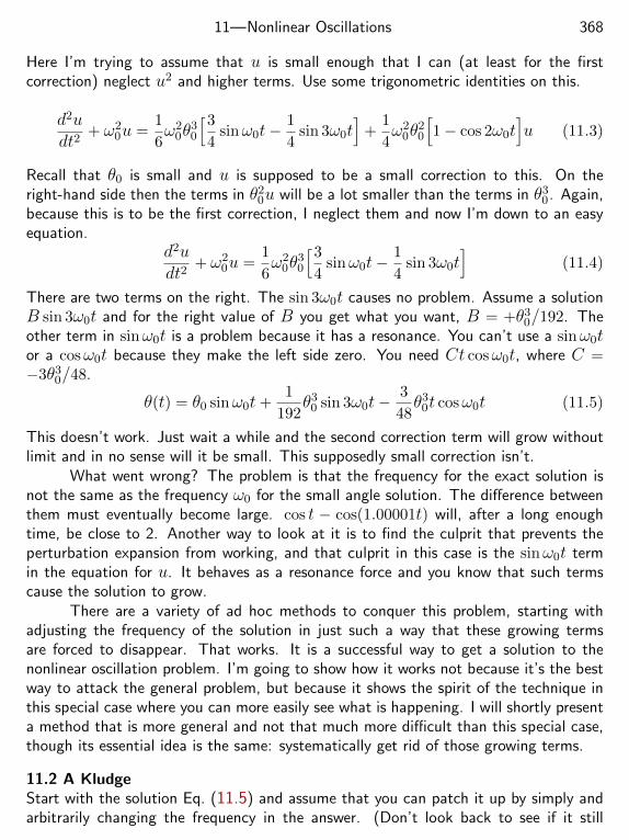
11—Nonlinear Oscillations 368
Here I’m trying to assume that u is small enough that I can (at least for the firstcorrection) neglect u2 and higher terms. Use some trigonometric identities on this.
d2udt2
+ ω20u =
1
6ω2
0θ30
[3
4sinω0t−
1
4sin 3ω0t
]+
1
4ω2
0θ20
[1− cos 2ω0t
]u (11.3)
Recall that θ0 is small and u is supposed to be a small correction to this. On theright-hand side then the terms in θ2
0u will be a lot smaller than the terms in θ30. Again,
because this is to be the first correction, I neglect them and now I’m down to an easyequation.
d2udt2
+ ω20u =
1
6ω2
0θ30
[3
4sinω0t−
1
4sin 3ω0t
](11.4)
There are two terms on the right. The sin 3ω0t causes no problem. Assume a solutionB sin 3ω0t and for the right value of B you get what you want, B = +θ3
0/192. Theother term in sinω0t is a problem because it has a resonance. You can’t use a sinω0tor a cosω0t because they make the left side zero. You need Ct cosω0t, where C =−3θ3
0/48.
θ(t) = θ0 sinω0t+1
192θ3
0 sin 3ω0t−3
48θ3
0t cosω0t (11.5)
This doesn’t work. Just wait a while and the second correction term will grow withoutlimit and in no sense will it be small. This supposedly small correction isn’t.
What went wrong? The problem is that the frequency for the exact solution isnot the same as the frequency ω0 for the small angle solution. The difference betweenthem must eventually become large. cos t − cos(1.00001t) will, after a long enoughtime, be close to 2. Another way to look at it is to find the culprit that prevents theperturbation expansion from working, and that culprit in this case is the sinω0t termin the equation for u. It behaves as a resonance force and you know that such termscause the solution to grow.
There are a variety of ad hoc methods to conquer this problem, starting withadjusting the frequency of the solution in just such a way that these growing termsare forced to disappear. That works. It is a successful way to get a solution to thenonlinear oscillation problem. I’m going to show how it works not because it’s the bestway to attack the general problem, but because it shows the spirit of the technique inthis special case where you can more easily see what is happening. I will shortly presenta method that is more general and not that much more difficult than this special case,though its essential idea is the same: systematically get rid of those growing terms.
11.2 A KludgeStart with the solution Eq. (11.5) and assume that you can patch it up by simply andarbitrarily changing the frequency in the answer. (Don’t look back to see if it still
11—Nonlinear Oscillations 369
satisfies the desired equation.) Just change ω0 to ω = ω0 + ε, where the last term issmall. Plug in.
θ(t) = θ0 sin(ω0 + ε)t+1
192θ3
0 sin 3(ω0 + ε)t− 3
48θ3
0t cos(ω0 + ε)t
What value of ε will kill the undesirable linear growth term when I do a series expansion?
θ(t) = θ0
[sin(ω0t)+cos(ω0t)εt
]− 1
192θ3
0
[sin(3ω0t)+cos(3ω0t)3εt
]− 3
48θ3
0t cos(ω0t)
To get the desired result, make the coefficient of t cosω0t be zero.
θ0ε−3
48θ3
0 = 0 −→ ε =3
48θ2
0xxxxxxxxxxx
11.3 Workable, but Special MethodThe idea of writing the solution as a sinusoidal oscillation plus a correction is essentiallyright. Just modify it a bit. Change one letter in Eq. (11.2) and it is
θ(t) = θ0 sinωt+ u(t) (11.6)
The next equation is then
d2θdt2
= −ω2θ0 sinωt+d2udt2
= −ω20
[θ0 sinωt+ u(t)− 1
6
[θ0 sinωt+ u(t)
]3]Rearrange it to get a differential equation for u and you have the new version ofEq. (11.3),
d2udt2
+ω20u =
[ω2−ω2
0
]θ0 sinωt+
1
6ω2
0θ30
[3
4sinωt− 1
4sin 3ωt
]+
1
4ω2
0θ20
[1−cos 2ωt
]u
Or,
d2udt2
+ω20
[1− θ
20
4
]u =
[ω2−ω2
0 +1
8ω2
0θ20
]θ0 sinωt− 1
24ω2
0θ30 sin 3ωt− 1
4ω2
0θ20 cos 2ωtu
As before, I neglect the smallest terms, the ones in θ20u.
d2udt2
+ ω20u =
[ω2 − ω2
0
]θ0 sinωt+
1
6ω2
0θ30
[3
4sinωt− 1
4sin 3ωt
]It was the sin
11.4 General Approach
x+ ω2x = εf(τ, x, x), where τ = εt
This is approximately a harmonic oscillator, but the term on the right can be anyfunction of x, x, and it can even be a slowly varying function of time.*
* This treatment is based on the work by Bogoliubov and Mitropolsky: AsymptoticMethods in the Theory of Nonlinear Oscillations.
11—Nonlinear Oscillations 370
Problems
11.1 Fill in the details in solving Eq. (11.4).
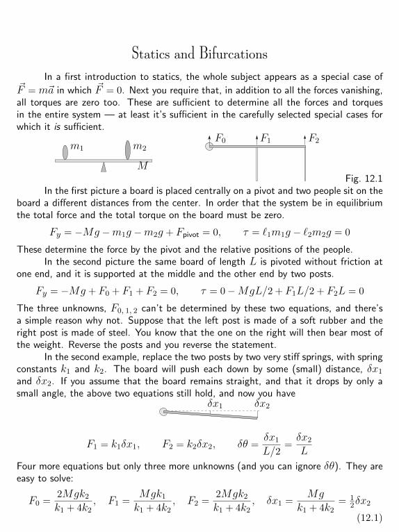
Statics and BifurcationsIn a first introduction to statics, the whole subject appears as a special case of
~F = m~a in which ~F = 0. Next you require that, in addition to all the forces vanishing,all torques are zero too. These are sufficient to determine all the forces and torquesin the entire system — at least it’s sufficient in the carefully selected special cases forwhich it is sufficient.
m1 m2
M
F0 F1 F2
Fig. 12.1In the first picture a board is placed centrally on a pivot and two people sit on the
board a different distances from the center. In order that the system be in equilibriumthe total force and the total torque on the board must be zero.
Fy = −Mg −m1g −m2g + Fpivot = 0, τ = `1m1g − `2m2g = 0
These determine the force by the pivot and the relative positions of the people.In the second picture the same board of length L is pivoted without friction at
one end, and it is supported at the middle and the other end by two posts.
Fy = −Mg + F0 + F1 + F2 = 0, τ = 0−MgL/2 + F1L/2 + F2L = 0
The three unknowns, F0, 1, 2 can’t be determined by these two equations, and there’sa simple reason why not. Suppose that the left post is made of a soft rubber and theright post is made of steel. You know that the one on the right will then bear most ofthe weight. Reverse the posts and you reverse the statement.
In the second example, replace the two posts by two very stiff springs, with springconstants k1 and k2. The board will push each down by some (small) distance, δx1
and δx2. If you assume that the board remains straight, and that it drops by only asmall angle, the above two equations still hold, and now you have
δx1 δx2
F1 = k1δx1, F2 = k2δx2, δθ =δx1
L/2=δx2
L
Four more equations but only three more unknowns (and you can ignore δθ). They areeasy to solve:
F0 =2Mgk2
k1 + 4k2, F1 =
Mgk1
k1 + 4k2, F2 =
2Mgk2
k1 + 4k2, δx1 =
Mgk1 + 4k2
= 12δx2
(12.1)
371
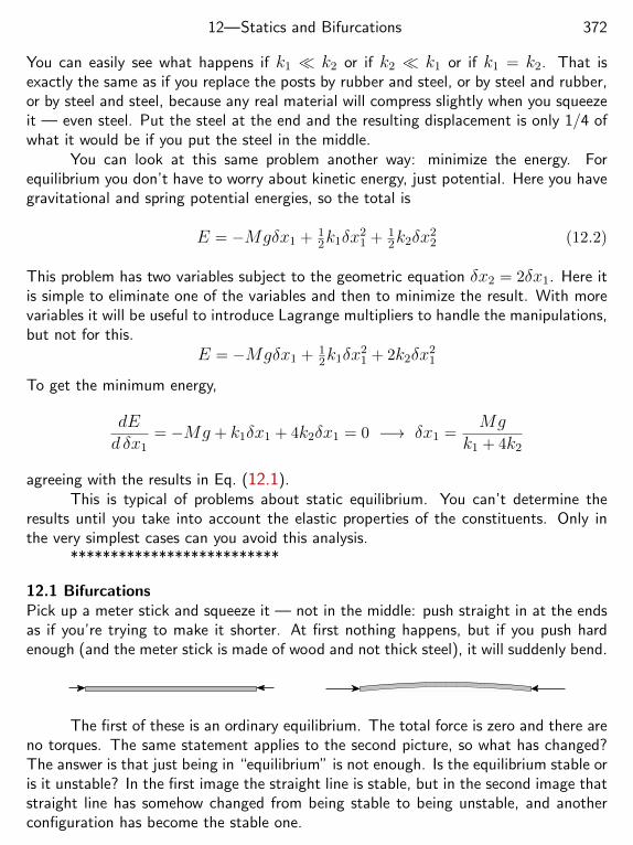
12—Statics and Bifurcations 372
You can easily see what happens if k1 k2 or if k2 k1 or if k1 = k2. That isexactly the same as if you replace the posts by rubber and steel, or by steel and rubber,or by steel and steel, because any real material will compress slightly when you squeezeit — even steel. Put the steel at the end and the resulting displacement is only 1/4 ofwhat it would be if you put the steel in the middle.
You can look at this same problem another way: minimize the energy. Forequilibrium you don’t have to worry about kinetic energy, just potential. Here you havegravitational and spring potential energies, so the total is
E = −Mgδx1 + 12k1δx
21 + 1
2k2δx22 (12.2)
This problem has two variables subject to the geometric equation δx2 = 2δx1. Here itis simple to eliminate one of the variables and then to minimize the result. With morevariables it will be useful to introduce Lagrange multipliers to handle the manipulations,but not for this.
E = −Mgδx1 + 12k1δx
21 + 2k2δx
21
To get the minimum energy,
dEd δx1
= −Mg + k1δx1 + 4k2δx1 = 0 −→ δx1 =Mg
k1 + 4k2
agreeing with the results in Eq. (12.1).This is typical of problems about static equilibrium. You can’t determine the
results until you take into account the elastic properties of the constituents. Only inthe very simplest cases can you avoid this analysis.
**************************
12.1 BifurcationsPick up a meter stick and squeeze it — not in the middle: push straight in at the endsas if you’re trying to make it shorter. At first nothing happens, but if you push hardenough (and the meter stick is made of wood and not thick steel), it will suddenly bend.
The first of these is an ordinary equilibrium. The total force is zero and there areno torques. The same statement applies to the second picture, so what has changed?The answer is that just being in “equilibrium” is not enough. Is the equilibrium stable oris it unstable? In the first image the straight line is stable, but in the second image thatstraight line has somehow changed from being stable to being unstable, and anotherconfiguration has become the stable one.
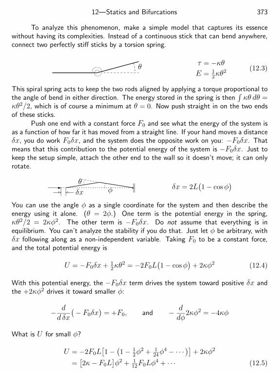
12—Statics and Bifurcations 373
To analyze this phenomenon, make a simple model that captures its essencewithout having its complexities. Instead of a continuous stick that can bend anywhere,connect two perfectly stiff sticks by a torsion spring.
θτ = −κθE = 1
2κθ2 (12.3)
This spiral spring acts to keep the two rods aligned by applying a torque proportional tothe angle of bend in either direction. The energy stored in the spring is then
∫κθ dθ =
κθ2/2, which is of course a minimum at θ = 0. Now push straight in on the two endsof these sticks.
Push one end with a constant force F0 and see what the energy of the system isas a function of how far it has moved from a straight line. If your hand moves a distanceδx, you do work F0δx, and the system does the opposite work on you: −F0δx. Thatmeans that this contribution to the potential energy of the system is −F0δx. Just tokeep the setup simple, attach the other end to the wall so it doesn’t move; it can onlyrotate.
δx
θφ δx = 2L
(1− cosφ
)You can use the angle φ as a single coordinate for the system and then describe theenergy using it alone. (θ = 2φ.) One term is the potential energy in the spring,κθ2/2 = 2κφ2. The other term is −F0δx. Do not assume that everything is inequilibrium. You can’t analyze the stability if you do that. Just let φ be arbitrary, withδx following along as a non-independent variable. Taking F0 to be a constant force,and the total potential energy is
U = −F0δx+ 12κθ
2 = −2F0L(1− cosφ
)+ 2κφ2 (12.4)
With this potential energy, the −F0δx term drives the system toward positive δx andthe +2κφ2 drives it toward smaller φ:
− dd δx
(− F0δx
)= +F0, and − d
dφ2κφ2 = −4κφ
What is U for small φ?
U = −2F0L[1−
(1− 1
2φ2 + 1
24φ4 − · · ·
)]+ 2κφ2
=[2κ− F0L
]φ2 + 1
12F0Lφ4 + · · · (12.5)
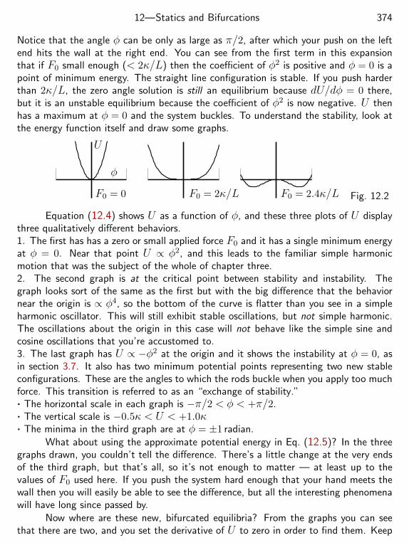
12—Statics and Bifurcations 374
Notice that the angle φ can be only as large as π/2, after which your push on the leftend hits the wall at the right end. You can see from the first term in this expansionthat if F0 small enough (< 2κ/L) then the coefficient of φ2 is positive and φ = 0 is apoint of minimum energy. The straight line configuration is stable. If you push harderthan 2κ/L, the zero angle solution is still an equilibrium because dU/dφ = 0 there,but it is an unstable equilibrium because the coefficient of φ2 is now negative. U thenhas a maximum at φ = 0 and the system buckles. To understand the stability, look atthe energy function itself and draw some graphs.
φ
U
F0 = 0 F0 = 2κ/L F0 = 2.4κ/L Fig. 12.2
Equation (12.4) shows U as a function of φ, and these three plots of U displaythree qualitatively different behaviors.1. The first has has a zero or small applied force F0 and it has a single minimum energyat φ = 0. Near that point U ∝ φ2, and this leads to the familiar simple harmonicmotion that was the subject of the whole of chapter three.2. The second graph is at the critical point between stability and instability. Thegraph looks sort of the same as the first but with the big difference that the behaviornear the origin is ∝ φ4, so the bottom of the curve is flatter than you see in a simpleharmonic oscillator. This will still exhibit stable oscillations, but not simple harmonic.The oscillations about the origin in this case will not behave like the simple sine andcosine oscillations that you’re accustomed to.3. The last graph has U ∝ −φ2 at the origin and it shows the instability at φ = 0, asin section 3.7. It also has two minimum potential points representing two new stableconfigurations. These are the angles to which the rods buckle when you apply too muchforce. This transition is referred to as an “exchange of stability.”. The horizontal scale in each graph is −π/2 < φ < +π/2.. The vertical scale is −0.5κ < U < +1.0κ. The minima in the third graph are at φ = ±1 radian.
What about using the approximate potential energy in Eq. (12.5)? In the threegraphs drawn, you couldn’t tell the difference. There’s a little change at the very endsof the third graph, but that’s all, so it’s not enough to matter — at least up to thevalues of F0 used here. If you push the system hard enough that your hand meets thewall then you will easily be able to see the difference, but all the interesting phenomenawill have long since passed by.
Now where are these new, bifurcated equilibria? From the graphs you can seethat there are two, and you set the derivative of U to zero in order to find them. Keep
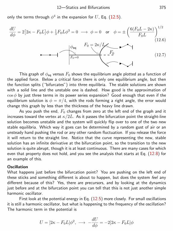
12—Statics and Bifurcations 375
only the terms through φ4 in the expansion for U , Eq. (12.5).
dUdφ
= 2[2κ− F0L
]φ+ 1
3F0Lφ3 = 0 −→ φ = 0 or φ = ±
(6(F0L− 2κ)
F0L
)1/2
(12.6)
F0
φeqF0 = 2κ/L
F0=0(12.7)
This graph of φeq versus F0 shows the equilibrium angle plotted as a function ofthe applied force. Below a critical force there is only one equilibrium angle, but thenthe function splits (“bifurcates”) into three equilibria. The stable solutions are shownwith a solid line and the unstable one is dashed. How good is the approximation ofcosφ by just three terms in its power series expansion? Good enough that even if theequilibrium solution is φ = π/4, with the rods forming a right angle, the error wouldchange this graph by less than the thickness of the heavy line drawn.
As you push the end, F0 changes from zero at the left end of the graph and itincreases toward the vertex at κ/2L. As it passes the bifurcation point the straight-linesolution becomes unstable and the system will quickly flip over to one of the two newstable equilibria. Which way it goes can be determined by a random gust of air or anunsteady hand pushing the rod or any other random fluctuation. If you release the forceit will return to the straight line. Notice that the curve representing the new, stablesolution has an infinite derivative at the bifurcation point, so the transition to the newsolution is quite abrupt, though it is at least continuous. There are many cases for whicheven that property does not hold, and you see the analysis that starts at Eq. (12.8) foran example of this.
OscillationWhat happens just before the bifurcation point? You are pushing on the left end ofthese sticks and something different is about to happen, but does the system feel anydifferent because of this? Yes, there are precursors, and by looking at the dynamicsjust before and at the bifurcation point you can tell that this is not just another simpleharmonic oscillator.
First look at the potential energy in Eq. (12.5) more closely. For small oscillationsit is still a harmonic oscillator, but what is happening to the frequency of the oscillation?The harmonic term in the potential is
U = [2κ− F0L]φ2, −→ −dUdφ
= −2[2κ− F0L]φ
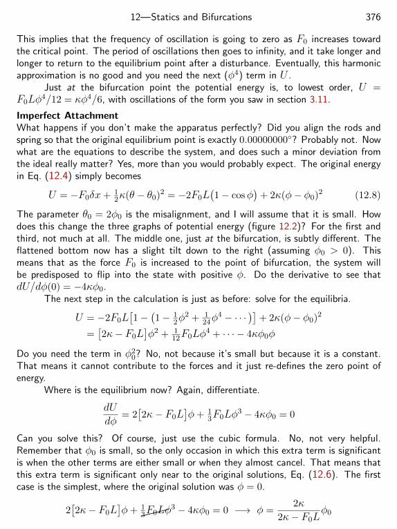
12—Statics and Bifurcations 376
This implies that the frequency of oscillation is going to zero as F0 increases towardthe critical point. The period of oscillations then goes to infinity, and it take longer andlonger to return to the equilibrium point after a disturbance. Eventually, this harmonicapproximation is no good and you need the next (φ4) term in U .
Just at the bifurcation point the potential energy is, to lowest order, U =F0Lφ4/12 = κφ4/6, with oscillations of the form you saw in section 3.11.
Imperfect AttachmentWhat happens if you don’t make the apparatus perfectly? Did you align the rods andspring so that the original equilibrium point is exactly 0.00000000? Probably not. Nowwhat are the equations to describe the system, and does such a minor deviation fromthe ideal really matter? Yes, more than you would probably expect. The original energyin Eq. (12.4) simply becomes
U = −F0δx+ 12κ(θ − θ0)2 = −2F0L
(1− cosφ
)+ 2κ(φ− φ0)2 (12.8)
The parameter θ0 = 2φ0 is the misalignment, and I will assume that it is small. Howdoes this change the three graphs of potential energy (figure 12.2)? For the first andthird, not much at all. The middle one, just at the bifurcation, is subtly different. Theflattened bottom now has a slight tilt down to the right (assuming φ0 > 0). Thismeans that as the force F0 is increased to the point of bifurcation, the system willbe predisposed to flip into the state with positive φ. Do the derivative to see thatdU/dφ(0) = −4κφ0.
The next step in the calculation is just as before: solve for the equilibria.
U = −2F0L[1−
(1− 1
2φ2 + 1
24φ4 − · · ·
)]+ 2κ(φ− φ0)2
=[2κ− F0L
]φ2 + 1
12F0Lφ4 + · · · − 4κφ0φ
Do you need the term in φ20? No, not because it’s small but because it is a constant.
That means it cannot contribute to the forces and it just re-defines the zero point ofenergy.
Where is the equilibrium now? Again, differentiate.
dUdφ
= 2[2κ− F0L
]φ+ 1
3F0Lφ3 − 4κφ0 = 0
Can you solve this? Of course, just use the cubic formula. No, not very helpful.Remember that φ0 is small, so the only occasion in which this extra term is significantis when the other terms are either small or when they almost cancel. That means thatthis extra term is significant only near to the original solutions, Eq. (12.6). The firstcase is the simplest, where the original solution was φ = 0.
2[2κ− F0L
]φ+ 1
3F0Lφ3 − 4κφ0 = 0 −→ φ =
2κ2κ− F0L
φ0
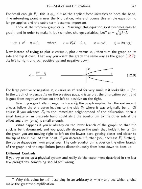
12—Statics and Bifurcations 377
For small enough F0, this is φ0, but as the applied force increases so does the bend.The interesting point is near the bifurcation, where of course this simple equation nolonger applies and the cubic term becomes important.
Look at the problem graphically. Rearrange this equation so it becomes easy to
graph, and in order to make it look simpler, change variables. Let* α =√
16F0L
−εx+ x3 − η = 0, where ε = F0L− 2κ, x = αφ, η = 2ακφ0
Now instead of trying to plot x versus ε, plot ε versus x, , then turn the graph on itsside and flip it over. That way you orient the graph the same way as the graph (12.7):F0 left to right and φeq positive up and negative down.
ε =x3 − ηx
εx
(12.9)
For large positive or negative x, ε varies as x2 and for very small x it looks like −1/x.In the graph of φ versus F0 on the previous page, ε is zero at the bifurcation point andit goes from negative values on the left to positive on the right.
Now if you gradually change the force F0 this graph implies that the system willalways follow the one curve leading to the side θ0 where it was originally bent. Ofcourse if you advance F0 to the immediate neighborhood of the bifurcation, then asmall breeze or an unsteady hand could shift the equilibrium to the other side if theoffset angle φ0 (or η) is small enough.
What happens if you’re already on the lower branch of the graph, so that thestick is bent downward, and you gradually decrease the push that holds it bent? Onthe graph you are moving right to left on the lowest part, getting closer and closer tothe tip of the curve. At that point, if you decrease ε further (you decrease F0 further),the curve disappears from under you. The only equilibrium is over on the other branchof the graph and the equilibrium jumps discontinuously from bent down to bent up.
Different ControlsIf you try to set up a physical system and really do the experiment described in the lastfew paragraphs, something should feel wrong.
* Why this value for α? Just plug in an arbitrary x = αφ and see which choicemake the greatest simplification.
12—Statics and Bifurcations 378
Exercises
1 In the equations (12.8) and following, what is the position of the angle for minimumU when the applied force is exactly at 2κ/L? What is this if φ0 = 0.01 radians = 0.6?Ans: 22

2001, 303•Abramowitz and Stegun, 161accelerated reference frame, 170,
321acceleration, 18, 38, 41
proper 332transformation 332
action, 40adiabatic, 265adiabatic invariant, 158adjoint, 355air resistance, 58, 139, 239amplitude, 108, 251analyzing results, 65, 140angular momentum, 50, 202, 231,
279, 303angular velocity, 173, 280, 289,
299Antarctica, 308anti-proton, 337, 343aphelion, 205, 209apparent weight, 184approximate orbits, 210arbitrary functions, 242Archimedes, 113artillery, 179associative, 13, 22asteroid, 232, 335, 339atmosphere, 58, 156, 349Atwood, 52, 76, 167•ballast, 103basis, 14, 19, 28, 284, 292, 296Bay of Fundy, 190beats, 120β, 321bifurcate, 375
binary star, 220, 350binomial series, 2birefringence, 264black hole, 193, 350blackboard bold, 31boundary condition, 58, 248, 250,
254, 262, 272Brillouin, 265buckle, 374bullwhip, 238, 257, 271•Callaway, 59capacitance, 102, 136, 352carbon monoxide, 136, 237center of mass, 218, 276, 281centrifugal force, 186centrifugal:
acceleration, 186force 174, 183–195, 199potential 185, 208
chain rule, 16, 45, 54, 102Chandler Wobble, 301charge, 125, 149, 151, 156, 195,
323–326charge density, 325clock, 312–323comet, 225commutative, 13, 22, 29complex:
algebra, 22–25, 180, 198conjugate 22, 297, 355exponential 23, 93, 106magnitude 22, 94plane 23, 38, 94, 107
component:gradient, 146index notation 15inertia 285–298matrix 28tangential 21tensor 282–284, 285vector 14, 28
379
Statics and Bifurcations 380
conservation:angular momentum, 203–212energy 47, 67, 76, 100, 111,
137, 216, 226, 231, 246, 251frequency 252laws 44, 144, 336, 340mass 51, 342momentum 41, 49, 51, 91,
336string 53
conservative, 145constant coefficient, 27, 96, 116constant of integration, 88contact force, 43contour map, 148converge, 3, 65, 163coordinate, 35, 318
accelerated 170center of mass 218, 220cylindrical 6, 7, 8polar 6, 204relative 220rotated 318rotating 182space-time 320spherical 6, 7, 179, 215
Coriolis force, 174–183cosmic rays, 316, 349coupled oscillators, 115–121, 136,
167critical damping, 98cross product, 13, 50, 152, 173,
291crystal, 200cubic equation, 256, 294current, 323–326
oscillations 136curved path, 330cycloid, 154cyclotron frequency, 151, 163•
damped oscillators, 95–100damping, 108dE/dt = 0, 100, 111definite integral, 64determinant, 30, 117, 294, 300,
353, 358deuteron, 220diagonal components, 286, 292diagonal matrix, 292, 296, 298Dialog, 310diatomic molecule, 75Dicke, 44, 233differential equation, 25, 88
constant coefficient 26, 175,353Green 122–125nonlinear 101separation 25simultaneous 116, 353types 96
differentiation, 16–18digression, 116dimensions, 42, 60, 73, 88discriminant, 98dispersion, 265distributive, 13, 22Doppler, 221dot convention, 173, 298dot product, 357double angle formula, 94double factorial, 162dry friction, 95, 144dumbbell, 281•~ei, 284Earth, 8, 9, 20, 41
acceleration 189eccentricity 206magnetic field 156, 159orbit 205, 210potential 146rotation 174–186shape 184, 300
Statics and Bifurcations 381
earthquake waves, 265eccentricity, 206effective force, 203effective potential, 208eigenvalue, 293, 296eigenvector, 293, 296, 361
orthogonal 297Einstein, 310electric circuit, 102, 352electric force, 43electromagnetic field, 149electron, 336electrostatic potential, 125elementary charge, 325elevator, 171ellipse, 9, 38, 204, 206, 229ellipsoid, 300elliptic integral, 161energy, 102, 244, 251, 334, 345
density 244flow 245integral 67, 89kinetic 334mechanical 67potential 67, 71qualitative 68relativistic 334velocity 265
Eotvos, 44equatorial bulge, 184equatorial diameter, 186equilibrium, 75, 111, 116equipotential, 149, 184, 187escape speed, 71Euclid, 327Euclidean geometry, 327, 330Euler, 143
equations 299, 301formula 23, 24, 37, 93, 127
eV, 336
event, 320exchange of stability, 374expansion, 360Explorer-1, 303exponential of a vector, 152external force, 219extrasolar, 220•factorial, 162falling, 72Famous Curves, 9, 10femtosecond, 74fictitious force, 170field line, 157flex, 303flexibility, 303focus, 206force, 326forcing frequency, 108, 109Foucault pendulum, 179Fourier, 265Fraunhofer, 110free rotation, 300frequency, 101, 252, 265Fresnel equations, 252friction, 47, 58, 63, 73, 95, 102,
144function, 280, 283fundamental theorem of calculus:,
47•Galilean transformation, 169, 310,
341Galileo, 100, 179, 310, 311γ, 321Gauss’s law, 325general relativity, 317generically unstable, 111geography, 21geometric series, 90geometry, 327, 330
Statics and Bifurcations 382
Get used to it., 25Global Positioning System, 317golf, 59, 175, 178golf ball, 139Gradshteyn and Ryzhik, 162gravitational field, 70gravitational potential, 148, 187Gravitron, 57gravity, 43Green’s function, 122–125Green, George, 122Greenwich, 7, 9group velocity, 265, 267Gulf Stream, 169•half-life, 317Hall effect, 323harmonic oscillator, 25, 87–125,
150, 159, 190, 205, 211, 226,235, 242, 253, 352damped 95–100forced 103non-simple 101three-dimensional 200
HCl, 75helix, 149, 153, 156Hermitian, 297, 361homogeneous, 27, 96, 103, 116honey, 74hydrogen, 336hydrogen atom, 220hyperbola, 4, 224, 333hyperbolic function, 2, 4•impulse, 122index notation, 15, 31index of refraction, 248, 252, 265indices, 284inductance, 352inductor, 102
inertia tensor, 280, 285inertial force, 170inertial system, 40, 169information velocity, 265inhomogeneous, 27, 103initial conditions, 99insolation, 209integral, 279integrating factor, 203intensity, 209internal force, 219interval, 328, 345intuition, 66inverse, 29inverse cube force, 222Io, 303irradiance, 209isomorphic, 13isothermal, 265iteration, 176•Jacobi identity, 14jerk, 65Jupiter, 210, 222, 303•Kenyon College, 52Kepler, 202, 204, 211kick, 122kinetic energy, 67, 291, 302kinetic energy density, 244Kronecker delta, 15•lasso, 267latitude, 7, 8Legendre polynomial, 186, 188length contraction, 314light, 265light bulb, 103light clock, 312light-year, 34
Statics and Bifurcations 383
linear, 96, 103, 116, 242, 282linear homogeneous, 27Lissajous figures, 202longitude, 7, 8Lorentz contraction, 325Lorentz transformation, 311, 321,
327, 333, 345lunar tides, 190•magnetic field, 305magnetic force, 43, 174magnetic mirror, 156magnetism, 324, 326Mars, 156, 301mass, 336mass density, 238, 255mass matrix, 357mass zero, 335matrix, 28–32, 121, 285, 353
adjoint 355index notation 31inertia 286inversion 30positive definite 354singular 294, 353symmetric 354transpose 354
Maxwell, 43, 311mean lifetime, 316mechanical energy, 48, 67, 145median, 82Mercury, 214merry-go-round, 40meter, 42MeV, 336Milankovitch, 210misaligned, 299modes, 119, 352, 358moment of inertia, 281, 286, 298momentum, 334, 345
money, 48Moon, 190, 267, 277, 278Morse potential, 76, 135muon, 316•neutron star, 309Newton, 179, 311Newton’s:
laws, 40second law 170third law 218, 277
Newtonian mechanics, 335non-inertial system, 169, 170nonconservative, 145normal mode, 355normal modes, 121, 354North Pole, 174, 176now, 311•ocean wave, 56Oldsmobile, 13~ω, 172, 173, 280ω/k, 242operator, 283operator solution, 151optical activity, 264orbits, 200orthogonal, 260, 298orthonormal, 15overdamped oscillation, 97•pair creation, 336, 337parabola, 333paradox, 316parallel axis theorem, 281Paris, 42partial differential equation, 242partial integration, 260pedestrians, 13
Statics and Bifurcations 384
pendulum, 100–102, 159Foucault 179–183inverted 114period 160spherical 215
perihelion, 205, 209perpendicular axis theorem, 288perturbation theory, 256–264, 360perturbed orbit, 211phase, 108, 109, 242phase velocity, 242, 265photon, 336, 344piano, 255point mass, 278polar coordinates, 100polar diameter, 186polynomial, 359poor form, 68positive definite, 354, 356positron, 336, 343positron-electron pair, 336positronium, 336potential energy, 67, 111,
145–148, 184potential energy density, 245power, 143, 247, 251power series, 64, 111precession, 218, 300, 301pretend inertial, 182principal axis, 292probability, 82product of inertia, 286proper:
acceleration, 2, 332length 315, 325, 350time 315, 328, 330, 351velocity 315
proton, 336pseudo-Euclidean, 330Pythagorean Theorem, 94, 313•
quantum mechanics, 267quasar, 331•r⊥, 8radar, 319radial acceleration, 21radian, 344radiance, 209radiation, 336, 339radical departure, 322rainbow, 264, 265random wave, 242rapidity, 333, 343, 344reduced mass, 220reflection, 247, 252relative velocity, 170, 311, 326relativistic, 155resistance, 103resistor, 102resonance, 108, 269resonance peak, 110rest energy, 334Riemann-Stieltjes, 279Arigid body, 276roots of one, 23rotated coordinate, 318rotating system, 171, 174, 298rotation, 152, 283rotational dynamics, 298Rotor, 56Runge-Kutta, 157•satellite, 303scalar product, 13, 121, 356Scotland, 178separation of variables, 25, 63,
67, 89, 241, 253, 258series, 1, 65, 256shock absorber, 99simultaneity, 311, 322
Statics and Bifurcations 385
simultaneous equations, 29small oscillations, 90snarky comment, 41solar tides, 190solar wind, 156Sommerfeld, 265space-time, 329space-time diagram, 318spaghettification, 193, 231special relativity, 310speed of light, 311spherical coordinates, 179spike, 249spring, 68, 87, 283stability, 301stable, 75, 111standing waves, 253steady-state, 109, 191Stefan-Boltzmann, 339stiffness, 263stopping point, 69, 70, 71stroboscopic, 255Sturm-Liouville, 250summation convention, 16Sun, 190Sundman, 225superluminal, 331surface wave, 264symmetric, 286, 292, 297symmetry, 286, 297syncopated clock, 349•Taylor series, 3, 217tennis ball, 82tension, 238tensor, 282–303
components 282, 284of inertia 280, 282symmetry 297
terminal speed, 72
terminal velocity, 74, 141thermodynamics, 265thin string, 240three body problem, 202tidal friction, 192tide table, 191tides, 109, 184, 187–192, 267time dilation, 312, 313, 317Titleist, 59torque, 50, 202, 279, 289, 292,
299torsional waves, 265transformation, 283transient, 109trigonometric identities, 24, 25triple angle formula, 94trochoid, 155Trojan asteroids, 195, 202tsunami, 264twin effect, 329Tycho, 206•underdamped, 96uninformative, 239unit matrix, 290unit vector, 172units, 42unstable, 75, 111, 302urban legend, 175•Van Allen, 156vector, 12vector product, 13velocity, 18velocity addition, 334viscosity, 73, 113, 142viscous damping, 96volume element, 10•wave equation, 241, 246, 275
Statics and Bifurcations 386
waves, 238weight, 171wet friction, 58, 95wheel alignment, 290Wigner, Eugene, 340wood floating, 113work, 147
magnetic field 149work-energy theorem, 44, 143,
145worldatlas.com, 9•Yarkovsky, 335, 339Young’s modulus, 263•Zielinski, 76