"Mental Accounting, Loss Aversion, and Individual Stock ...faculty.som.yale.edu/nicholasbarberis/ma_jnl.pdf · Mental Accounting, Loss Aversion, and Individual Stock Returns NICHOLAS

Mental Accounting, Loss Aversion,and Individual Stock Returns

NICHOLAS BARBERIS and MING HUANG*

ABSTRACT

We study equilibrium firm-level stock returns in two economies: one in which in-vestors are loss averse over the f luctuations of their stock portfolio, and another inwhich they are loss averse over the f luctuations of individual stocks that they own.Both approaches can shed light on empirical phenomena, but we find the secondapproach to be more successful: In that economy, the typical individual stock re-turn has a high mean and excess volatility, and there is a large value premium inthe cross section which can, to some extent, be captured by a commonly used multi-factor model.

OVER THE PAST TWO DECADES, researchers analyzing the structure of individualstock returns have uncovered a wide range of phenomena, both in the timeseries and the cross section. In the time series, the returns of a typical in-dividual stock have a high mean, are excessively volatile, and are slightlypredictable using lagged variables. In the cross section, there is a substan-tial “value” premium, in that stocks with low ratios of price to fundamentalshave higher average returns, and this premium can to some extent be cap-tured by certain empirically motivated multifactor models.1 These findingshave attracted a good deal of attention from finance theorists. It has provedsomething of a challenge, though, to explain both the time series and cross-sectional effects in the context of an equilibrium model where investors max-imize a clearly specified utility function.

In this paper, we argue that it may be possible to improve our under-standing of firm-level stock returns by refining the way we model investorpreferences. For guidance as to what kind of refinements might be impor-tant, we turn to the experimental evidence that has been accumulated onhow people choose among risky gambles. Many of the studies in this liter-ature suggest that loss aversion and narrow framing play an important

* University of Chicago Graduate School of Business and NBER, and Stanford University,Graduate School of Business, respectively. We are grateful to Michael Brennan, John Campbell,John Heaton, and Richard Thaler for discussing this paper at various conferences. We have alsobenefited from conversations with David Hirshleifer, Tano Santos, Andrei Shleifer, Jeremy Stein,and seminar participants at the University of Chicago, Harvard University, Yale University,and the NBER.

1 The value premium was originally noted by Basu ~1983! and Rosenberg, Reid, and Lan-stein ~1985!; Fama and French ~1992! provide more recent evidence. Fama and French ~1993!show that a specific three-factor model can capture much of the value premium. Vuolteenaho~1999! documents the excess volatility and time series predictability of firm level stock returns.

THE JOURNAL OF FINANCE • VOL. LVI, NO. 4 • AUGUST 2001

1247

role in determining attitudes towards risk. Financial economists do nottypically incorporate these ideas into their models of asset prices. We in-vestigate whether doing so can shed light on the behavior of individualstock returns.

Loss aversion is a feature of Kahneman and Tversky’s ~1979! descriptivemodel of decision making under risk, prospect theory, which uses experi-mental evidence to argue that people get utility from gains and losses inwealth, rather than from absolute levels. The specific finding known as lossaversion is that people are more sensitive to losses than to gains. Since ourframework is intertemporal, we also make use of more recent evidence ondynamic aspects of loss aversion. This evidence suggests that the degree ofloss aversion depends on prior gains and losses: A loss that comes after priorgains is less painful than usual, because it is cushioned by those earliergains. On the other hand, a loss that comes after other losses is more painfulthan usual: After being burned by the first loss, people become more sensi-tive to additional setbacks.

A crucial question that arises in applying this evidence on loss aversion tothe context of investing is: Over which gains and losses is the investor lossaverse? Is he loss averse over changes in total wealth? Or is he loss averseover changes in the value of his portfolio of stocks or even over changes inthe value of individual stocks that he owns? When gains and losses aretaken to be changes in total wealth, we say that they are defined “broadly.”When they refer to changes in the value of isolated components of wealth—the investor ’s stock portfolio or individual stocks that he owns—we say thatthey are defined “narrowly.” Which gains and losses the investor pays at-tention to is a question about mental accounting, a term coined by Thaler~1980! to refer to the process by which people think about and evaluate theirfinancial transactions.

Numerous experimental studies suggest that when doing their mental ac-counting, people engage in narrow framing, that is, they often appear to payattention to narrowly defined gains and losses. This may ref lect a concernfor non-consumption sources of utility, such as regret, which are often morenaturally experienced over narrowly framed gains and losses. If one of aninvestor ’s many stocks performs poorly, the investor may experience a senseof regret over the specific decision to buy that stock. In other words, indi-vidual stock gains and losses can be carriers of utility in their own right, andthe investor may take this into account when making decisions.

In our analysis, we study the equilibrium behavior of firm-level stock re-turns when investors are loss averse and exhibit narrow framing in theirmental accounting. We consider two kinds of narrow framing, one narrowerthan the other, and investigate whether either of them is helpful for under-standing the data.

In the first economy we consider, investors get direct utility not only fromconsumption, but also from gains and losses in the value of individual stocksthat they own. The evidence on loss aversion described above is applied tothese narrowly defined gains and losses: The investor is loss averse over

1248 The Journal of Finance

individual stock f luctuations, and how painful a loss on a particular stock isdepends on that stock’s prior performance. We refer to this as “individualstock accounting.”

In the second economy, investors get direct utility not only from consump-tion, but also from gains and losses in the value of their overall portfolio ofstocks. The evidence on loss aversion is now applied to these gains and losses:The investor is loss averse over portfolio f luctuations, and how painful adrop in portfolio value is depends on the portfolio’s prior performance. Wecall this “portfolio accounting,” a form of narrow framing, although not asextreme as individual stock accounting.

In our first set of results, we show that for all its severity, individual stockaccounting can be a helpful ingredient for understanding a wide range ofempirical phenomena. In equilibrium, under this form of mental accounting,individual stock returns have a high mean, are more volatile than theirunderlying cash f lows, and are slightly predictable in the time series. In thecross section, there is a large value premium: Stocks with low price–dividend ratios have higher average returns than stocks with high price–dividend ratios. Moreover, the same kinds of multifactor models that havebeen shown to capture the value premium in actual data can also do so inour simulated economy. At the same time, the model matches empirical fea-tures of aggregate asset returns. In equilibrium, aggregate stock returnshave a high mean, excess volatility, and are moderately predictable in thetime series, while the risk-free rate is constant and low.

Second, we find that the investor ’s system of mental accounting affectsasset prices in a significant way. As we broaden the investor ’s decision framefrom individual stock accounting to portfolio accounting, the equilibriumbehavior of individual stock returns changes considerably: Their mean valuefalls, they become less volatile, and they also become more correlated witheach other. Moreover, the value premium in the cross section disappears.Overall, portfolio accounting can explain some features of the data, but isless successful than individual stock accounting.

To understand where our results come from, consider first the case ofindividual stock accounting. Many of the effects here derive from a singlesource, namely a discount rate for individual stocks that changes as a func-tion of the stock’s past performance. If a stock has had good recent perfor-mance, the investor gets utility from this gain, and becomes less concernedabout future losses on the stock because any losses will be cushioned by theprior gains. In effect, the investor perceives the stock to be less risky thanbefore and discounts its future cash f lows at a lower rate. Conversely, if oneof his stocks performs dismally, he finds this painful and becomes more sen-sitive to the possibility of further losses on the stock. In effect, he views thestock as riskier than before and raises its discount rate.

This changing discount rate makes firm-level stock returns more volatilethan underlying cash f lows: A high cash f low pushes the stock price up, butthis prior gain also lowers the discount rate on the stock, pushing the stockprice still higher. It also generates a value premium in the cross section: In

Mental Accounting, Loss Aversion, and Individual Stock Returns 1249

this economy, a stock with a high price–dividend ratio ~a growth stock! isoften one that has done well in the past, accumulating prior gains for theinvestor, who then views it as less risky and requires a lower average re-turn. A stock with a low price–dividend ratio ~a value stock! has often haddismal prior performance, burning the investor, who now views it as riskier,and requires a higher average return. Finally, since the investor is lossaverse over individual stock f luctuations, he dislikes the frequent losses thatindividual stocks often produce, and charges a high average return ascompensation.

The reason the results are different under portfolio accounting is that inthis case, changes in discount rates on stocks are driven by f luctuations inthe value of the overall portfolio: When the portfolio does well, the investoris less concerned about losses on any of the stocks that he holds, since theprior portfolio gain will cushion any such losses. Effectively, he views allstocks as less risky. Discount rates on all stocks therefore go down simulta-neously. Conversely, discount rates on all stocks go up after a prior portfolioloss.

This discount rate behavior is the key to many of the portfolio accountingresults. Stock returns are less volatile here than under individual stock ac-counting. In the latter case, stocks are highly volatile because good cash-f low news is always accompanied by a lower discount rate, pushing the priceup even more. Under portfolio accounting, good cash-f low news on a partic-ular stock will only coincide with a lower discount rate on the stock if theportfolio as a whole does well. There is no guarantee of this, and so volatilityis not amplified by as much. Since shocks to discount rates are perfectlycorrelated across stocks, individual stock returns are highly correlated withone another. Moreover, the value premium largely disappears since a stock’spast performance no longer affects its discount rate, which is now deter-mined at the portfolio level. Finally, while there is a substantial equity pre-mium, it is not as large as under individual stock accounting. The investoris loss averse over portfolio level f luctuations, which are sizable but not assevere as the swings on individual stocks. The compensation for risk is there-fore more moderate.

While individual stock accounting can potentially be a helpful way of think-ing about the data, we emphasize that it is only a potential ingredient in anequilibrium model, and by no means a complete description of the facts. Forone thing, we show that it underpredicts the correlation of stocks with eachother, and argue that a model that combines individual stock accountingwith broader forms of accounting is likely to be superior to a model that usesindividual stock accounting alone.

The fact that we study equilibrium returns under both individual stockaccounting and portfolio accounting is also useful for making additional pre-dictions for future testing. If individual stock accounting is relatively moreprevalent among individual investors as opposed to institutional investors,we would expect to see stocks held primarily by individuals—small stocks,for example—exhibit more of the features associated with individual stock


accounting. Other predictions arise, if, over time, investors change the waythey do their mental accounting. For example, the increased availability ofmutual funds since the early 1980s may have caused a shift away fromindividual stock accounting towards portfolio accounting, since funds auto-matically prevent investors from worrying about individual stock f luctua-tions. Our analysis predicts that stocks that were once held directly but arenow held indirectly through mutual funds should exhibit specific changes inpricing behavior. Among other predictions, such stocks should have higherprice-to-fundamentals ratios and exhibit a lower cross-sectional value premium.

Loss aversion and narrow framing have already been applied with somesuccess to understanding the aggregate stock market. Benartzi and Thaler~1995! analyze the static portfolio problem of an investor who is loss averseover changes in his financial wealth and who is trying to allocate his wealthbetween T-bills and the stock market. They find that the investor is reluc-tant to allocate much to stocks, even if the expected return on the stockmarket is set equal to its high historical value. Motivated by this finding,Barberis, Huang, and Santos ~2001! introduce loss aversion over financialwealth f luctuations into a dynamic equilibrium model and find that it cap-tures a number of aggregate market phenomena. They do not address thetime series or cross-sectional behavior of individual stocks. Moreover, sincethey consider only one risky asset, they cannot investigate the impact ofdifferent forms of mental accounting, which is our main focus in this paper.

Ours is not the only paper to address empirical phenomena like time se-ries predictability and the cross-sectional value premium. Other promisingapproaches include models based on irrationality or bounded rationality, suchas Barberis, Shleifer, and Vishny ~1998!, Daniel, Hirshleifer, and Subrah-manyam ~2001!, and Hong and Stein ~1999!; models based on learning, suchas Brennan and Xia ~2001!; and models based on corporate growth optionssuch as Berk, Green, and Naik ~1999! and Gomes, Kogan, and Zhang ~2001!.

The rest of the paper is organized as follows. In Section I, we propose twodifferent specifications for investor preferences: In one case, the investor isloss averse over f luctuations in the value of individual stocks in his portfo-lio; in the other case, he is loss averse only over f luctuations in overall port-folio value. Section II derives the conditions that govern equilibrium pricesin economies with investors of each type. In Section III, we use simulateddata to analyze equilibrium stock returns under each of the two kinds ofmental accounting. Section IV discusses the results further and in particu-lar, argues that they may be robust to generalizations that allow for hetero-geneity across investors. Section V concludes.

I. Two Forms of Mental Accounting

Extensive experimental work suggests that loss aversion and narrow fram-ing are important features of the way people evaluate risky gambles. In thissection, we construct preferences that incorporate these two ideas.


Loss aversion is a central feature of Kahneman and Tversky’s ~1979! pros-pect theory, a descriptive model of decision making under risk, which arguesthat people derive utility from changes in wealth, rather than from absolutelevels. The specific finding known as loss aversion is that people are moresensitive to reductions in wealth than to increases, in the sense that there isa kink in the utility function. A simple functional form that captures lossaversion is

w~X ! � � X for X � 0

2X for X � 0, ~1!

where X is the individual’s gain or loss, and w~X ! is the utility of that gainor loss.

Kahneman and Tversky ~1979! introduce loss aversion as a way of explain-ing why people tend to reject small-scale gambles of the form2

G � ~110,21�;�100,2

1�!.

Most utility functions used by financial economists are not able to explainthese risk attitudes because they are differentiable everywhere, making theinvestor risk-neutral over small gambles.3

To incorporate loss aversion into an intertemporal framework, we need totake account of its dynamic aspects. Tversky and Kahneman ~1981! notethat their prospect theory was originally developed only for one-shot gamblesand that any application to a dynamic context must await further evidenceon how people think about sequences of gains and losses.

A number of papers have taken up this challenge, conducting experimentson how people evaluate sequences of gambles. In particular, Thaler and John-son ~1990! find that after a gain on a prior gamble, people are more riskseeking than usual, while after a prior loss, they become more risk averse.The result that risk aversion goes down after a prior gain, confirmed inother studies, has been labeled the “house money” effect, ref lecting gam-blers’ increased willingness to bet when ahead.4 Thaler and Johnson ~1990!

2 This should be read as: “receive $110 with probability 12_ , and lose $100 with probability 1

2_ .”

3 One exception is first-order risk aversion preferences, studied by Epstein and Zin ~1990!,Segal and Spivak ~1990!, Gul ~1991!, and others. However, this specification does not allow fornarrow framing, which is central in our analysis. Of course, even if a utility function is differ-entiable, one can explain aversion to small-scale risks by increasing the function’s curvature.However, this immediately runs into other difficulties. Rabin ~2000! shows that if an increas-ing, concave, and differentiable utility function is calibrated so as to reject G at all wealthlevels, then that utility function will also reject extremely attractive large-scale gambles, atroubling prediction.

4 It is important to distinguish Thaler and Johnson’s ~1990! evidence from other evidencepresented by Kahneman and Tversky ~1979! showing that people are risk averse over gains andrisk seeking over losses; indeed this evidence motivates a feature of prospect theory that we donot consider here, namely the concavity ~convexity! of the value function in the domain of gains


interpret these findings as evidence that the degree of loss aversion dependson prior gains and losses: A loss that comes after prior gains is less painfulthan usual, because it is cushioned by those earlier gains. A loss that comesafter other losses, however, is more painful than usual: After being burnedby the first loss, people become more sensitive to additional setbacks.

An important modeling issue that remains is: Which gains and losses shouldthis evidence on loss aversion be applied to? Are investors only loss averseover “broadly” defined gains and losses, by which we mean changes in totalwealth, or are they also loss averse over “narrowly” defined gains and losses,namely changes in the value of isolated components of their wealth, such astheir stock portfolio or even individual stocks that they own? Which gainsand losses people focus on is a question about what Thaler ~1980! calls mentalaccounting, the process people use to think about and evaluate their finan-cial transactions.

To see why mental accounting matters, consider the following simple ex-ample. An investor is thinking about buying a portfolio of two stocks—oneshare of each, say. The shares of both stocks are currently trading at $100,and after careful thought, the investor decides that for both stocks, the sharevalue a year from now will be distributed as

~150,21�;70,2

1�!, ~1!

independently across the two stocks.Suppose that the investor ’s loss aversion is captured by the functional

form in equation ~1!. If he is loss averse over portfolio f luctuations, the ex-pected utility of the investment is5

41�w~100!� 2

1�w~20!� 41�w~�60! � 5,

while if he is loss averse over individual stock f luctuations, it is6

2@21�w~50!� 2

1�w~�30!# � �10,

which is not as attractive.

~losses!. One set of evidence pertains to one-shot gambles, the other to sequences of gambles.Kahneman and Tversky’s ~1979! evidence suggests that people are willing to take risks in orderto avoid a loss; Thaler and Johnson’s ~1990! evidence suggests that if these efforts are unsuc-cessful and the investor suffers an unpleasant loss, he will subsequently act in a more risk-averse manner.

5 This calculation says: with probability 14_ , both stocks will gain $50, for a total gain of $100;

with probability 12_ , one stock will gain $50, the other will lose $30, for a total gain of $20; and

with probability 14_ , both stocks will lose $30, for a total loss of $60.

6 This calculation says: for each stock, there is an equal chance of a gain of $50 and a loss of$30.


Which form of mental accounting is a better description of individual be-havior? Traditional asset-pricing models usually assume as broad a form ofaccounting as possible: Utility is typically specified only over total wealth orover consumption, and not over individual stock f luctuations. A substantialbody of experimental work, however, suggests that when doing their mentalaccounting, people engage in narrow framing, that is, they often do appearto focus on narrowly defined gains and losses.

The studies in this literature typically ask subjects who are already fac-ing some kind of financial risk whether they would be willing to accept anadditional, uncorrelated gamble. This gamble is designed to be unattrac-tive when viewed in isolation: anyone focusing on the gains and losses ofthe gamble itself would tend to reject it. On the other hand, the gamble isdesigned to be attractive when viewed as part of the subjects’ broaderportfolio of gambles: subjects who are able to focus on portfolio gains andlosses would tend to accept the gamble. Typically, these studies find thatthe additional gamble is rejected, suggesting that subjects do frame nar-rowly to some extent.7

The absence of narrow framing from standard asset-pricing models is prob-ably due to doubts about its normative acceptability. These doubts may beunwarranted: Narrow framing can be defended on normative grounds be-cause it may simply ref lect a concern for non-consumption sources of utility,which are often naturally experienced over narrowly defined gains and losses.Regret is one example of such utility: A loss is more painful to us if it islinked to an action we took than if it simply befalls us through no fault ofour own. If one of an investor ’s many stocks performs poorly, the investormay experience a sense of regret over the specific decision to buy that stock.Since each stock is associated with a distinct decision, namely the decisionto buy that particular stock, each stock’s gains and losses can give rise to adistinct source of utility, based on regret or euphoria about the initial buyingdecision.

In other situations, narrow framing is less acceptable from a normativeperspective. These are situations where it arises because of cognitive limi-tations: Even though we know that gains and losses in total wealth are morerelevant for our consumption decisions, we may focus too much on gains andlosses in one part of our wealth—in our stock portfolio—simply because in-formation about those gains and losses is more readily available.

In what follows, we study asset prices in economies where investors areloss averse and exhibit narrow framing in their mental accounting. In thefirst economy we consider, investors get direct utility from consumption, butalso from gains and losses in the value of individual stocks that they own.The evidence on loss aversion is applied to these narrowly defined gains and

7 Redelmeier and Tversky ~1992!, Kahneman and Lovallo ~1993!, Gneezy and Potters ~1997!,Thaler et al. ~1997!, Benartzi and Thaler ~1999!, and Rabin and Thaler ~2000! present evidenceof various kinds of narrow framing. Read, Loewenstein, and Rabin ~1999! review some of theevidence and discuss possible explanations of why people frame decisions the way they do.


losses: The investor is loss averse over individual stock f luctuations, andhow painful a loss on a particular stock is depends on that stock’s priorperformance. We refer to this as “individual stock accounting.”8

In our second piece of analysis, we consider an economy where investorsget direct utility from consumption, but also from gains and losses in thevalue of their overall portfolio of stocks. The evidence on loss aversion is nowapplied to these gains and losses: The investor is loss averse over portfoliof luctuations, and how painful a drop in portfolio value is depends on theportfolio’s prior performance. We call this “portfolio accounting.” While thisis a broader form of mental accounting than individual stock accounting, itstill represents narrow framing: The investor is segregating his stock port-folio from his other forms of wealth such as human capital, and is focusingon its f luctuations separately.

It is worth noting one alternative interpretation of individual stock ac-counting. Until the advent of mutual funds, individuals with holdings in thestock market typically owned only a very small number of stocks. As a re-sult, even if these investors engaged in portfolio accounting—a weak form ofnarrow framing—the effect on prices may be more accurately captured byour model of individual stock accounting. In other words, individual stockaccounting may be primarily a consequence of the highly undiversified port-folios held by many investors, and not necessarily the result of excessivelynarrow framing.

We now show how these two forms of mental accounting can be incorpo-rated into a traditional asset-pricing framework, starting with individualstock accounting in Section I.A and then moving to portfolio accounting inSection I.B. In both cases, there are two kinds of assets: a risk-free asset inzero net supply, paying a gross interest rate of Rf, t between time t andt � 1; and n risky assets—“stocks”—each with a total supply of one unit. Thegross return on stock i between time t and t � 1 is Ri, t�1.

A. Individual Stock Accounting

When the investor is loss averse over individual stock f luctuations, hechooses consumption Ct and an allocation Si, t to stock i to maximize

E(t�0

` �r tCt

1�g

1 � g� b0 OCt

�g r t�1(i�1

n

v~Xi,t�1,Si,t ,zi,t!�. ~2!

8 A skeptic could argue that an investor who does individual stock accounting will be reluc-tant to take on blatantly attractive opportunities, such as exploiting a relative mispricing be-tween two stocks by going long one and short the other. Even if he is sure to make $5 on thelong position and to lose only $3 on the short, he may code this as 5 � 2~3!, which does not lookattractive. However, since the long and short positions are really components of a single tradingidea, it is more likely that the investor will evaluate the strategy as a single entity: he will codea gain of 5 � 3 � 2, and will be keen to take on the opportunity.


The first term in this preference specification, utility over consumptionCt , is a standard feature of asset-pricing models. Although the frameworkdoes not require it, we specialize to power utility, the benchmark case stud-ied in the literature. The parameter r is the time discount factor, and g � 0controls the curvature of utility over consumption.9

The second term models the idea that the investor is loss averse overchanges in the value of individual stocks that he owns. The variable Xi, t�1measures the gain or loss on stock i between time t and time t � 1, a positivevalue indicating a gain and a negative value, a loss. The utility the investorreceives from this gain or loss is given by the function v, and it is added upacross all stocks owned by the investor. It is a function not only of the gainor loss itself, but also of Si, t , the value of the investor ’s holdings of stock i attime t, and of a state variable zi, t , which measures the investor ’s gains orlosses on the stock prior to time t as a fraction of Si, t . By including Si, t andzi, t as arguments of v, we allow the investor ’s prior investment performanceto affect the way subsequent losses are experienced.

As discussed earlier, we think of v as capturing utility unrelated to con-sumption. Regret is one example of this, but there may also be other kindsof non-consumption utility at work here. An investor may interpret a big losson a stock as a sign that he is a second-rate investor, thus dealing his ego apainful blow, and he may feel humiliation in front of friends and familywhen word about the failed investment leaks out.

The b0 OCt�g coefficient on the loss aversion terms is a scaling factor that

ensures that risk premia in the economy remain stationary even as aggre-gate wealth increases over time. It involves per capita consumption OCtthat is exogeneous to the investor, and so does not affect the intuitionof the model. The constant b0 controls the importance of the loss aver-sion terms in the investor ’s preferences; setting b0 � 0 reduces our-framework to the much studied consumption-based model with powerutility.

Barberis et al. ~2001! have already formalized the notion of loss aversionin a model of the aggregate stock market. We borrow their specification,which we summarize in the remainder of this section. We limit ourselves todescribing the essential structure; Barberis et al. ~2001! provide more sup-porting detail.

The gain or loss on stock i between time t and t � 1 is measured as

Xi, t�1 � Si, t Ri, t�1 � Si, t Rf, t . ~3!

In words, the gain is the value of stock i at time t � 1 minus its value at timet multiplied by the risk-free rate. Multiplying by the risk-free rate modelsthe idea that investors may only view the return on a stock as a gain if itexceeds the risk-free rate. The unit of time is a year, so that gains and losses

9 For g � 1, we replace Ct1�g0~1 � g! with log Ct .


are measured annually. While the investor may check his holdings muchmore often than that, even several times a day, we assume that it is onlyonce a year, perhaps at tax time, that he confronts his past performance ina serious way.

The variable zi, t tracks prior gains and losses on stock i. It is the ratioof another variable, Zi, t , to Si, t , so that zi, t � Zi, t 0Si, t . Barberis et al.~2001! call Zi, t the “historical benchmark level” for stock i, to be thought ofas the investor ’s memory of an earlier price level at which the stock usedto trade. When Si, t � Zi, t , or zi, t � 1, the stock price today is higher thanwhat the investor remembers it to be, making him feel as though hehas accumulated prior gains on the stock, to the tune of Si, t � Zi, t .When Si, t � Zi, t , or zi, t � 1, the current stock price is lower than itused to be, so that the investor feels that he has had past losses, again ofSi, t � Zi, t .

The point of introducing zi, t is to allow v to capture experimental evidencesuggesting that the pain of a loss depends on prior outcomes. This is done bydefining v in the following way. When zi, t � 1,

v~Xi, t�1,Si, t ,1! � � Xi, t�1 for Xi, t�1 � 0

lXi, t�1 for Xi, t�1 � 0, ~4!

with l � 1. For zi, t � 1,

v~Xi, t�1,Si, t , zi, t !

� � Si, t Ri, t�1 � Si, t Rf, t for Ri, t�1 � zi, t Rf, t

Si, t ~zi, t Rf, t � Rf, t !� lSi, t ~Ri, t�1 � zi, t Rf, t ! for Ri, t�1 � zi, t Rf, t

, ~5!

and for zi, t � 1,

v~Xi, t�1,Si, t , zi, t ! � � Xi, t�1 for Xi, t�1 � 0

l~zi, t !Xi, t�1 for Xi, t�1 � 0, ~6!

with

l~zi, t ! � l� k~zi, t � 1!, ~7!

and k � 0.It is easiest to understand these equations graphically. Figure 1 shows the

form of v: the solid line for zi, t � 1, the dash-dot line for zi, t � 1, and thedashed line for zi, t � 1. When zi, t � 1, the case where the investor hasneither prior gains nor prior losses on stock i, v is a piecewise linear function


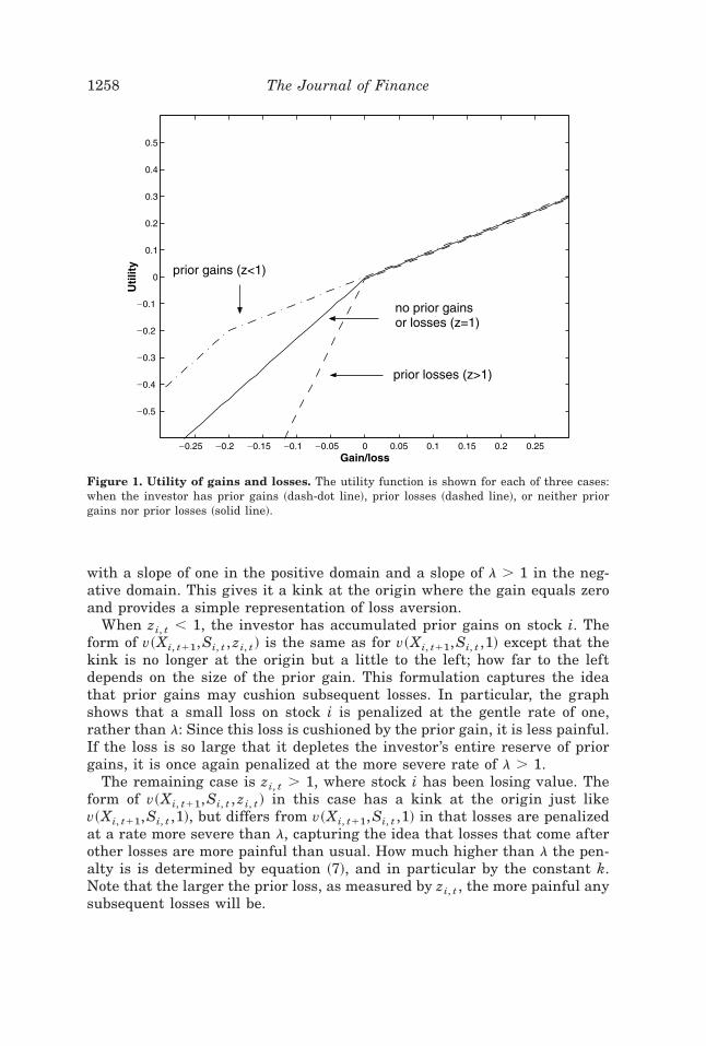
with a slope of one in the positive domain and a slope of l � 1 in the neg-ative domain. This gives it a kink at the origin where the gain equals zeroand provides a simple representation of loss aversion.

When zi, t � 1, the investor has accumulated prior gains on stock i. Theform of v~Xi, t�1,Si, t , zi, t ! is the same as for v~Xi, t�1,Si, t ,1! except that thekink is no longer at the origin but a little to the left; how far to the leftdepends on the size of the prior gain. This formulation captures the ideathat prior gains may cushion subsequent losses. In particular, the graphshows that a small loss on stock i is penalized at the gentle rate of one,rather than l: Since this loss is cushioned by the prior gain, it is less painful.If the loss is so large that it depletes the investor ’s entire reserve of priorgains, it is once again penalized at the more severe rate of l � 1.

The remaining case is zi, t � 1, where stock i has been losing value. Theform of v~Xi, t�1,Si, t , zi, t ! in this case has a kink at the origin just likev~Xi, t�1,Si, t ,1!, but differs from v~Xi, t�1,Si, t ,1! in that losses are penalizedat a rate more severe than l, capturing the idea that losses that come afterother losses are more painful than usual. How much higher than l the pen-alty is is determined by equation ~7!, and in particular by the constant k.Note that the larger the prior loss, as measured by zi, t , the more painful anysubsequent losses will be.

Figure 1. Utility of gains and losses. The utility function is shown for each of three cases:when the investor has prior gains ~dash-dot line!, prior losses ~dashed line!, or neither priorgains nor prior losses ~solid line!.


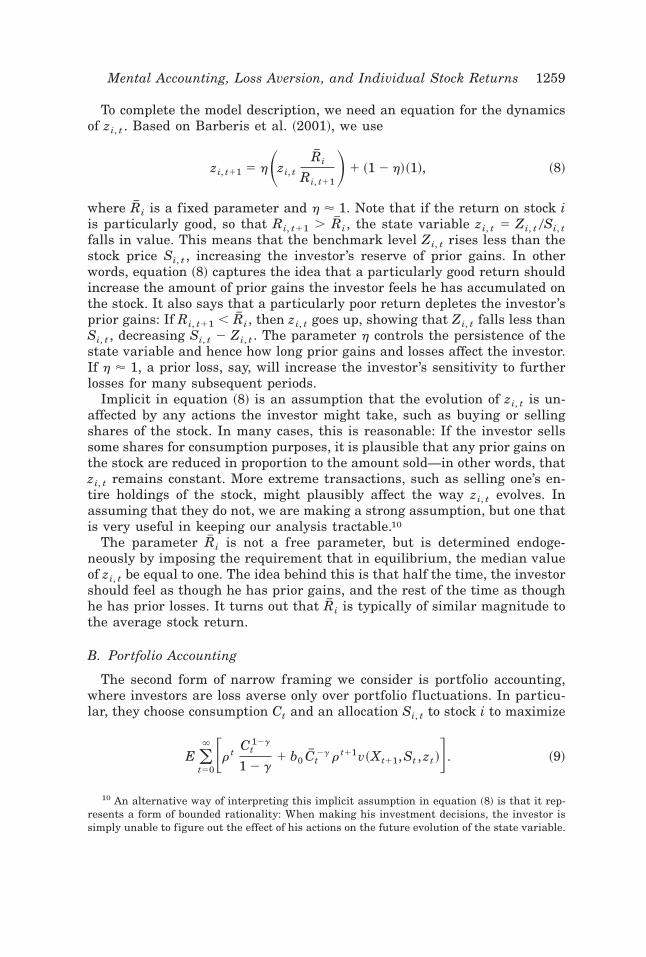
To complete the model description, we need an equation for the dynamicsof zi, t . Based on Barberis et al. ~2001!, we use

zi, t�1 � h�zi, t

ORi

Ri, t�1� � ~1 � h!~1!, ~8!

where ORi is a fixed parameter and h � 1. Note that if the return on stock iis particularly good, so that Ri, t�1 � ORi , the state variable zi, t � Zi, t 0Si, tfalls in value. This means that the benchmark level Zi, t rises less than thestock price Si, t , increasing the investor ’s reserve of prior gains. In otherwords, equation ~8! captures the idea that a particularly good return shouldincrease the amount of prior gains the investor feels he has accumulated onthe stock. It also says that a particularly poor return depletes the investor ’sprior gains: If Ri, t�1 � ORi , then zi, t goes up, showing that Zi, t falls less thanSi, t , decreasing Si, t � Zi, t . The parameter h controls the persistence of thestate variable and hence how long prior gains and losses affect the investor.If h � 1, a prior loss, say, will increase the investor’s sensitivity to furtherlosses for many subsequent periods.

Implicit in equation ~8! is an assumption that the evolution of zi, t is un-affected by any actions the investor might take, such as buying or sellingshares of the stock. In many cases, this is reasonable: If the investor sellssome shares for consumption purposes, it is plausible that any prior gains onthe stock are reduced in proportion to the amount sold—in other words, thatzi, t remains constant. More extreme transactions, such as selling one’s en-tire holdings of the stock, might plausibly affect the way zi, t evolves. Inassuming that they do not, we are making a strong assumption, but one thatis very useful in keeping our analysis tractable.10

The parameter ORi is not a free parameter, but is determined endoge-neously by imposing the requirement that in equilibrium, the median valueof zi, t be equal to one. The idea behind this is that half the time, the investorshould feel as though he has prior gains, and the rest of the time as thoughhe has prior losses. It turns out that ORi is typically of similar magnitude tothe average stock return.

B. Portfolio Accounting

The second form of narrow framing we consider is portfolio accounting,where investors are loss averse only over portfolio f luctuations. In particu-lar, they choose consumption Ct and an allocation Si, t to stock i to maximize

E(t�0

` �r tCt

1�g

1 � g� b0 OCt

�g r t�1v~Xt�1,St , zt !�. ~9!

10 An alternative way of interpreting this implicit assumption in equation ~8! is that it rep-resents a form of bounded rationality: When making his investment decisions, the investor issimply unable to figure out the effect of his actions on the future evolution of the state variable.


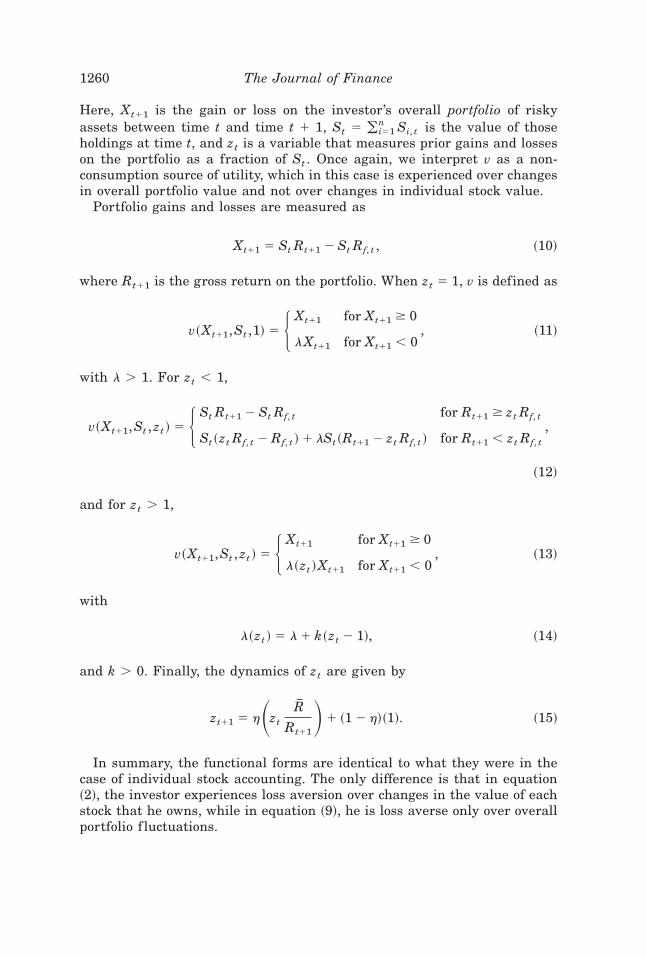
Here, Xt�1 is the gain or loss on the investor ’s overall portfolio of riskyassets between time t and time t � 1, St � (i�1

n Si, t is the value of thoseholdings at time t, and zt is a variable that measures prior gains and losseson the portfolio as a fraction of St . Once again, we interpret v as a non-consumption source of utility, which in this case is experienced over changesin overall portfolio value and not over changes in individual stock value.

Portfolio gains and losses are measured as

Xt�1 � St Rt�1 � St Rf, t , ~10!

where Rt�1 is the gross return on the portfolio. When zt � 1, v is defined as

v~Xt�1,St ,1! � � Xt�1 for Xt�1 � 0

lXt�1 for Xt�1 � 0, ~11!

with l � 1. For zt � 1,

v~Xt�1,St , zt ! � � St Rt�1 � St Rf, t for Rt�1 � zt Rf, t

St ~zt Rf, t � Rf, t !� lSt ~Rt�1 � zt Rf, t ! for Rt�1 � zt Rf, t

,

~12!

and for zt � 1,

v~Xt�1,St , zt ! � � Xt�1 for Xt�1 � 0

l~zt !Xt�1 for Xt�1 � 0, ~13!

with

l~zt ! � l� k~zt � 1!, ~14!

and k � 0. Finally, the dynamics of zt are given by

zt�1 � h�zt

OR

Rt�1� � ~1 � h!~1!. ~15!

In summary, the functional forms are identical to what they were in thecase of individual stock accounting. The only difference is that in equation~2!, the investor experiences loss aversion over changes in the value of eachstock that he owns, while in equation ~9!, he is loss averse only over overallportfolio f luctuations.


II. Equilibrium Prices

We now derive the conditions that govern equilibrium prices in two dif-ferent economies. The first economy is populated by investors who do indi-vidual stock accounting and have the preferences laid out in equations ~2!through ~8!. Investors in the second economy do portfolio accounting, andhave the preferences in equations ~9! through ~15!. In both cases, there is acontinuum of investors, with a total “mass” of one.

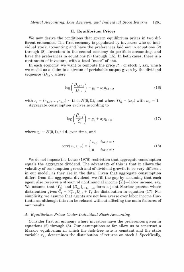
In each economy, we want to compute the price Pi, t of stock i, say, whichwe model as a claim to a stream of perishable output given by the dividendsequence $Di, t % , where

log�Di, t�1

Di, t� � gi � si «i, t�1, ~16!

with «t � ~«1, t , . . . ,«n, t ! ; i.i.d. N~0, �!, and where �ij � ~vij! with vii � 1.Aggregate consumption evolves according to

log� OCt�1

OCt� � gc � scht�1, ~17!

where ht ; N~0,1!, i.i.d. over time, and

corr~ht ,«i, t ' ! � � vci for t � t

0 for t � t '. ~18!

We do not impose the Lucas ~1978! restriction that aggregate consumptionequals the aggregate dividend. The advantage of this is that it allows thevolatility of consumption growth and of dividend growth to be very differentin our model, as they are in the data. Given that aggregate consumptiondiffers from the aggregate dividend, we fill the gap by assuming that eachagent also receives a stream of nonfinancial income $Yt %—labor income, say.We assume that $Yt % and $Di, t %i�1, . . . , n form a joint Markov process whosedistribution gives OCt [ (i�1

n Di, t � Yt the distribution in equation ~17!. Forsimplicity, we assume that agents are not loss averse over labor income f luc-tuations, although this can be relaxed without affecting the main features ofour results.

A. Equilibrium Prices Under Individual Stock Accounting

Consider first an economy where investors have the preferences given inequations ~2! through ~8!. Our assumptions so far allow us to construct aMarkov equilibrium in which the risk-free rate is constant and the statevariable zi, t determines the distribution of returns on stock i. Specifically,


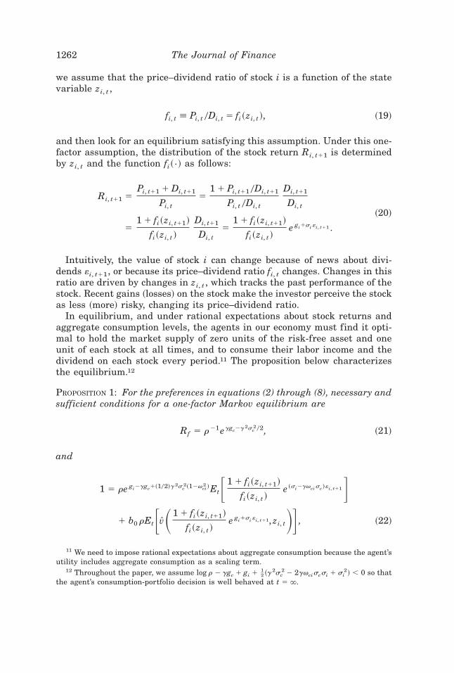
we assume that the price–dividend ratio of stock i is a function of the statevariable zi, t ,

fi, t [ Pi, t 0Di, t � fi ~zi, t !, ~19!

and then look for an equilibrium satisfying this assumption. Under this one-factor assumption, the distribution of the stock return Ri, t�1 is determinedby zi, t and the function fi~{! as follows:

Ri, t�1 �Pi, t�1 � Di, t�1

Pi, t�

1 � Pi, t�1 0Di, t�1

Pi, t 0Di, t

Di, t�1

Di, t

�1 � fi ~zi, t�1!

fi ~zi, t !

Di, t�1

Di, t�

1 � fi ~zi, t�1!

fi ~zi, t !e gi�si «i, t�1 .

~20!

Intuitively, the value of stock i can change because of news about divi-dends «i, t�1, or because its price–dividend ratio fi, t changes. Changes in thisratio are driven by changes in zi, t , which tracks the past performance of thestock. Recent gains ~losses! on the stock make the investor perceive the stockas less ~more! risky, changing its price–dividend ratio.

In equilibrium, and under rational expectations about stock returns andaggregate consumption levels, the agents in our economy must find it opti-mal to hold the market supply of zero units of the risk-free asset and oneunit of each stock at all times, and to consume their labor income and thedividend on each stock every period.11 The proposition below characterizesthe equilibrium.12

PROPOSITION 1: For the preferences in equations (2) through (8), necessary andsufficient conditions for a one-factor Markov equilibrium are

Rf � r�1eggc�g2sc

202, ~21!

and

1 � re gi�ggc�~102!g2sc

2~1�vci2 !Et� 1 � fi ~zi, t�1!

fi ~zi, t !e ~si�gvcisc!«i, t�1�

� b0 rEt� [v�1 � fi ~zi, t�1!

fi ~zi, t !e gi�si «i, t�1, zi, t�� , ~22!

11 We need to impose rational expectations about aggregate consumption because the agent’sutility includes aggregate consumption as a scaling term.

12 Throughout the paper, we assume log r � ggc � gi � 12_ ~g2sc

2 � 2gvciscsi � si2! � 0 so that

the agent’s consumption-portfolio decision is well behaved at t � `.


where for zi, t � 1,

[v~Ri, t�1, zi, t ! � � Ri, t�1 � Rf, t for Ri, t�1 � zi, t Rf, t

~zi, t Rf, t � Rf, t !� l~Ri, t�1 � zi, t Rf, t ! for Ri, t�1 � zi, t Rf, t

,

~23!

and for zi, t � 1,

[v~Ri, t�1, zi, t ! � � Ri, t�1 � Rf, t for Ri, t�1 � Rf, t

l~zi, t !~Ri, t�1 � Rf, t ! for Ri, t�1 � Rf, t

. ~24!

We prove this formally in the Appendix. At a less formal level, equation~22! follows directly from the agent’s Euler equation for optimality at equi-librium, derived using standard perturbation arguments,

1 � rEt�Ri, t�1� OCt�1

OCt��g�� b0 rEt @ [v~Ri, t�1, zi, t !# , ∀i. ~25!

The first term is the standard one that obtains in an economy where in-vestors have power utility over consumption. However, there is now an ad-ditional term. Consuming less today and investing the proceeds in stock iexposes the investor to the risk of greater losses on that stock. Just howpainful this might be is determined by the state variable zi, t .

B. Equilibrium Prices Under Portfolio Accounting

We now compute the price Pi, t of stock i in a second economy where in-vestors have the preferences described in equations ~9! through ~15!.

In the case of portfolio accounting, we need to price the portfolio of allstocks in the economy before we can price any one stock. This portfolio is aclaim to the aggregate dividend, which follows the process

log�Dt�1

Dt� � gp � sp«t�1, ~26!

with «t�1 ; N~0,1!, i.i.d. over time, and

corr~ht ,«t ' ! � � vcp for t � t

0 for t � t '~27!

corr~«i, t ,«t' ! � �

vip for t � t

0 for t � t '. ~28!


The dividend processes for stocks 1 through n in equation ~16! will not ingeneral “add up” to the aggregate dividend process in equation ~26!. Withoutadditional structure, we cannot think of the n stocks as a complete list of allstocks in the portfolio. We therefore imagine that there are some other se-curities in the economy whose dividends are distributed in such a way thatthe total dividend does add up to the aggregate dividend in equation ~26!.For the purpose of choosing parameters, it is helpful to have a setup wherethe dividends of the n original stocks alone do add up, and we present thisspecial case in Section III.

Our assumptions allow us to construct a Markov equilibrium in which therisk-free rate is constant and the portfolio-level state variable zt determinesthe distribution of returns on all stocks. Specifically, we assume that stocki ’s price–dividend ratio is a function of zt ,

fi, t [ Pi, t 0Di, t � fi ~zt !, ~29!

and then look for an equilibrium satisfying this assumption. Given this one-factor assumption, the distribution of the stock return Ri, t�1 is determinedby zt and the function fi~{! as follows:

Ri, t�1 �Pi, t�1 � Di, t�1

Pi, t�

1 � Pi, t�1 0Di, t�1

Pi, t 0Di, t

Di, t�1

Di, t

�1 � fi ~zt�1!

fi ~zt !

Di, t�1

Di, t�

1 � fi ~zt�1!

fi ~zt !e gi�si «i, t�1 .

~30!

As in the first economy, the price of stock i can change because of dividendnews «i, t�1 or because its price–dividend ratio fi, t changes. The key differ-ence is that changes in this ratio are not driven by a stock-level state vari-able zi, t , but by the portfolio-level state variable zt , which tracks prior gainsand losses on the overall portfolio. Recent gains ~losses! on the portfoliomake the investor perceive the entire portfolio as less ~more! risky, changingthe price–dividend ratio of every stock in the portfolio simultaneously.

In equilibrium, and under rational expectations about stock returns andaggregate consumption levels, the agents in our economy must find it opti-mal to hold the market supply of zero units of the risk-free asset and oneunit of each stock at all times, and to consume their labor income and theaggregate dividend stream every period. The proposition below character-izes the equilibrium.

PROPOSITION 2: For the preferences in equations (9) through (15), necessaryand sufficient conditions for a one-factor Markov equilibrium are

Rf � r�1eggc�g2sc

202, ~31!


and


2~1�vcp2 !�~102!si

2~1�vip2 !�gscsi ~vci�vcpvip!

Et� 1 � fi ~zt�1!

fi ~zt !e ~sivip�gscvcp!«t�1�

� b0 rEt� Iv�1 � fi ~zt�1!

fi ~zt !e gi�sivip«t�1�~102!si

2~1�vip2 !, Rt�1, zt��,

~32!

where for zt � 1,

Iv~Ri, t�1, Rt�1, zt !

� � Ri, t�1 � Rf, t for Rt�1 � zt Rf, t

~zt Rf, t � Rf, t !� l~Ri, t�1 � zt Rf, t ! for Rt�1 � zt Rf, t

, ~33!

and for zt � 1,

Iv~Ri, t�1, Rt�1, zt ! � � Ri, t�1 � Rf, t for Rt�1 � Rf, t

l~zt !~Ri, t�1 � Rf, t ! for Rt�1 � Rf, t

. ~34!

The gross return Rt�1 on the overall portfolio is given by

Rt�1 �1 � f ~zt�1!

f ~zt !e gp�sp«t�1, ~35!

where f ~{! satisfies

1 � re gp-ggc�~102!g2sc

2~1-vcp2 !Et� 1 � f ~zt�1!

f ~zt !e ~sp�gvcpsc!«t�1 �

� b0 rEt� [v�1 � f ~zt�1!

f ~zt !e gp�sp«t�1, zt�� ,

~36!

and where [v is defined in Proposition 1. Moreover, f ~{! and fi~{! must beself-consistent:

f ~zt ! �(i

Di, t

Dtfi ~zt !. ~37!


We prove this formally in the Appendix. At a less formal level, equation~32! follows from the agent’s Euler equation for optimality,


OCt��g� � b0 rEt @ Iv~Ri, t�1, Rt�1, zt !# , ∀i. ~38!

The first term is standard. The second term ref lects the fact that consum-ing less today and investing the proceeds in stock i exposes the investor tothe risk of greater losses on that stock. How painful this is is now deter-mined by the portfolio-level state variable zt .

Note that there is now an extra step in computing the price–dividend ratioof an individual stock. Under portfolio accounting, the price behavior of in-dividual stocks depends on the behavior of the overall portfolio. This meansthat we first need to calculate the equilibrium portfolio return Rt�1 in equa-tions ~35! and ~36!, and then use this in equation ~32! governing the indi-vidual stock return.

III. Numerical Results and Intuition

In this section, we solve equations ~22! and ~32! for the price–dividendratio of an individual stock fi~{! under individual stock accounting and port-folio accounting, respectively, and then use simulated data to study the prop-erties of equilibrium stock returns in each case.

A. Parameter Values

Table I summarizes our choice of parameters. We divide the table into twopanels to separate the two types of parameters: those that determine thedistributions of consumption and dividend growth, and those that determineinvestor preferences.

For the mean gc and standard deviation sc of log consumption growth, wefollow Ceccheti, Lam, and Mark ~1990!, who obtain gc � 1.84 percent andsc � 3.79 percent from a time series of annual data from 1889 to 1985.

In principle, specifying parameters for individual stock and aggregate div-idend growth is a daunting task. Equations ~16! and ~26! show that we needgi , si , vci , and vip for each stock, vij for each pair of stocks, and gp, sp, andvcp for the aggregate portfolio, a total of ~n202! � ~7n02! � 3 parameters.Fortunately, it turns out that with two simplifying assumptions, we canspecify the dividend processes with just four parameters, and yet still con-vey most of the important economics. Essentially, we take dividend growthto be identically distributed across all stocks, a restriction that we relax inSection III.E.

Our first assumption is that the mean and standard deviation of log div-idend growth is the same for all stocks:

gi � g, si � s, ∀i. ~39!


Second, we assume a simple factor structure for individual stock dividendgrowth innovations:

«i, t � vp«t � [«i, t!1 � vp2. ~40!

In words, the cash-f low shock to stock i has one component due to the ag-gregate dividend innovation «t introduced in equation ~26!, and one idiosyn-cratic component, [«i, t ; i.i.d. N~0,1!. The relative importance of the twocomponents is controlled by a new parameter, vp. The idiosyncratic compo-nent is orthogonal to consumption growth shocks, aggregate dividend growthshocks, and the idiosyncratic shocks on other stocks:

corr~ [«i, t ,ht ! � corr~ [«i, t ,«t !� corr~ [«i, t , [«j, t !� 0, ∀i, j. ~41!

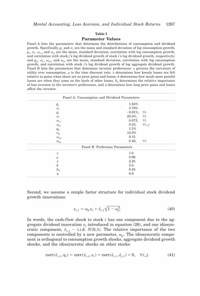
Table I

Parameter ValuesPanel A lists the parameters that determine the distributions of consumption and dividendgrowth. Specifically, gc and sc are the mean and standard deviation of log consumption growth;gi , si , vci , and vij are the mean, standard deviation, correlation with log consumption growth,and correlation with stock j ’s log dividend growth of stock i ’s log dividend growth, respectively;and gp, sp, vcp, and vip are the mean, standard deviation, correlation with log consumptiongrowth, and correlation with stock i ’s log dividend growth of log aggregate dividend growth.Panel B lists the parameters that determine investor preferences: g governs the curvature ofutility over consumption, r is the time discount rate, l determines how keenly losses are feltrelative to gains when there are no prior gains and losses, k determines how much more painfullosses are when they come on the heels of other losses, b0 determines the relative importanceof loss aversion in the investor ’s preferences, and h determines how long prior gains and lossesaffect the investor.

Panel A: Consumption and Dividend Parameters

gc 1.84%sc 3.79%gi �0.91%, ∀isi 25.0%, ∀ivci 0.072, ∀ivij 0.23, ∀i, jgp 1.5%sp 12.0%vcp 0.15vip 0.48, ∀i

Panel B: Preference Parameters

g 1.0r 0.98l 2.25k 3.0b0 0.45h 0.9


This immediately implies

vci � vpvcp , ∀i, ~42!

vij � vp2, ∀i, j, ~43!

vip � vp , ∀i. ~44!

Another attractive feature of this simple factor structure is that in thelimit, as we add more and more stocks, the growth of their total dividend isalso i.i.d lognormal:13

limnr`

(i�1

n

Di, t�1

(i�1

n

Di, t

r e g�~102!s2~1�vp2!�svp«t�1. ~45!

This means that we can think of the n stocks as being an exhaustive listof all securities, with their total dividend equaling the aggregate dividend in~26!, Dt �(i�1

n Di, t . Comparing equation ~45! with equation ~26!, we obtain14

gp � g �1

2s2~1 � vp

2!, ~46!

sp � svp . ~47!

Equations ~39!, ~42! through ~44!, and ~46! through ~47! show that theentire structure of dividend growth can be determined from gp, sp, s, andvcp alone. We choose these four quantities as the basis variables rather thanany other four because they can be estimated in a relatively straightforwardmanner. First, we estimate the mean and standard deviation of aggregatedividend growth using NYSE data from 1925 to 1995 from CRSP, which

13 For an economy with a finite horizon from t � �T to t � T, this limiting behavior is basedon an argument similar to the law of large numbers. Anderson ~1991! and Green ~1989! providetechnical details. Our stationary economy can then be thought of as the limit as the timehorizon goes to infinity.

14 The assumptions in this section also allow us to satisfy the self-consistency condition inProposition 2. Under our assumptions, if f ~{! solves equation ~36!, then it also solves equation~32! for all i. Therefore fi~{! � f ~{!, ∀i, and so the self-consistency condition is satisfied.


gives gp � 0.015 and sp � 0.12. The correlation between shocks to consump-tion growth and dividend growth, vcp, we take from Campbell ~2000!, whoestimates it in the neighborhood of 0.15.

We set the volatility s of individual stock dividend growth to 0.25. A directcalculation of the value-weighted average volatility of real dividend growthfor firms in the COMPUSTAT database suggests that this is a reasonablebenchmark level.15 Further confirmation comes from Vuolteenaho ~1999!,who estimates the cash-f low news volatility of an individual stock, equalweighted across stocks, to be 32 percent. Since smaller firms have morevolatile cash f lows, 25 percent may be a better estimate of value-weightedcash-f low volatility.

Panel A in Table I shows what these values imply for the remaining pa-rameters governing the dividend processes.16 The preference parameters aresummarized in Panel B of the table. We choose the curvature g of utilityover consumption and the time discount factor r so as to produce a sensiblylow value for the risk-free rate. Given the values of gc and sc, equation ~21!shows that g � 1.0 and r � 0.98 set the risk-free interest rate to Rf � 1 �3.86 percent.

The value of l determines how keenly losses are felt relative to gains inthe case where the investor has no prior gains or losses. We take l � 2.25,the value Tversky and Kahneman ~1992! estimate by offering subjects iso-lated gambles in experimental settings.

The parameter k determines how much more painful losses are when theycome on the heels of other losses. We choose k � 3. To interpret this, supposethat the state variable zi, t is initially equal to one, and that stock i thenexperiences a sharp fall of 10 percent. From equation ~8! with h � 1, thismeans that zi, t goes up by about 0.1, to 1.1. From equation ~7!, any addi-tional losses will now be penalized at 2.25 � 3~0.1! � 2.55, a slightly moresevere penalty.

The parameter b0 determines the relative importance of the loss aversionterm in the investor ’s preferences. We set b0 � 0.45. One way to think aboutb0 is to compare the disutility of losing a dollar on a stock investment withthe disutility of having to consume a dollar less. When computed at equilib-rium, the ratio of these two quantities equals b0rl. Our parameter choicestherefore make the psychological disutility of losing the $1 roughly equal inmagnitude to the consumption disutility.

Finally, h arises in the definition of the state variable dynamics. It con-trols the persistence of the state variable zi, t , which in turn controls theautocorrelation of price–dividend ratios. We find that h � 0.9 brings thisautocorrelation close to its empirical value.

15 More precisely, we take all stocks in the annual COMPUSTAT database for which at least11 consecutive years of dividend data are recorded, compute real dividend growth volatility foreach, and then calculate the average volatility, weighted by firm size.

16 Note that while the mean log dividend growth gi is negative, mean simple dividend growthequals exp@�0.0091 � ~0.25202!# � 1 � 2.24 percent, a positive number.


B. Methodology

For the case of individual stock accounting, we use an iterative tech-nique to solve equation ~22! for the price–dividend ratio fi~{! of an individ-ual stock. The only difficulty is that the state variable zi, t is endogenous:It tracks prior gains and losses which depend on past returns, them-selves endogenous. To deal with this, we use the following procedure. Weguess a solution to equation ~22!, fi

~0! say, and then construct a functionzi, t�1 � hi

~0!~zi, t ,«i, t�1! that solves

Ri, t�1 �1 � fi ~zi, t�1!

fi ~zi, t !e gi�si «i, t�1 ~48!

and

zi, t�1 � h�zi, t

OR

Ri, t�1� � ~1 � h!~1! ~49!

simultaneously for this particular fi � fi~0!. Given hi

~0! , we get a new candi-date solution fi

~1! through the recursion


2~1�vci2 !Et� 1 � fi

~ j !~zi, t�1!

fi~ j�1!~zi, t !

e ~si�gvcisc!«i, t�1�� b0 rEt� [v�1 � fi

~ j !~zi, t�1!

fi~ j�1!~zi, t !

e gi�si «i, t�1, zi, t��.

~50!

With fi~1! in hand, we calculate a new hi � hi

~1! that solves equations ~48!and ~49! for fi � fi

~1!. This hi~1! gives us a new candidate fi � fi

~2! from equa-tion ~50!. We continue this process until we obtain convergence, fi

~ j !r fi ,

hi~ j !r hi . Figure 2 shows the price–dividend ratio fi~{! that corresponds to

the parameter values in Table I. Its precise shape will be explained in moredetail later.

With the price–dividend ratio fi~{! in hand, we use simulated data to seehow returns behave in equilibrium. We simulate dividend shocks $«i, t % forn � 500 stocks and for 10,000 time periods subject to the specification inequation ~16! and the parameters in Table I. We then apply the price–dividend function fi~{! to this dividend data to see what realized returns looklike. More precisely, we use the zi, t�1 � hi~zi, t ,«i, t�1! function describedabove to generate the series of zi, t implied by the dividend shocks and thenset the return of stock i between time t and t � 1 equal to

Ri, t�1 �1 � fi ~zi, t�1!

fi ~zi, t !e gi�si «i, t�1 . ~51!


This gives n time series of individual stock returns. We can then computemoments—standard deviation, say—for each stock, and then average thesemoments across different stocks. This provides a sense of how the “typical”stock behaves, and we report the results of such calculations later inSection III.

We can also use our n time series of individual stock returns to computean equal-weighted average

Rp, t�1 �1

n (i�1

n

Ri, t�1, ~52!

which can be interpreted as the aggregate stock return.17

17 The aggregate return Rp, t�1 differs from the aggregate return Rt�1 described earlier onlyin that it is equal-weighted rather than value-weighted.

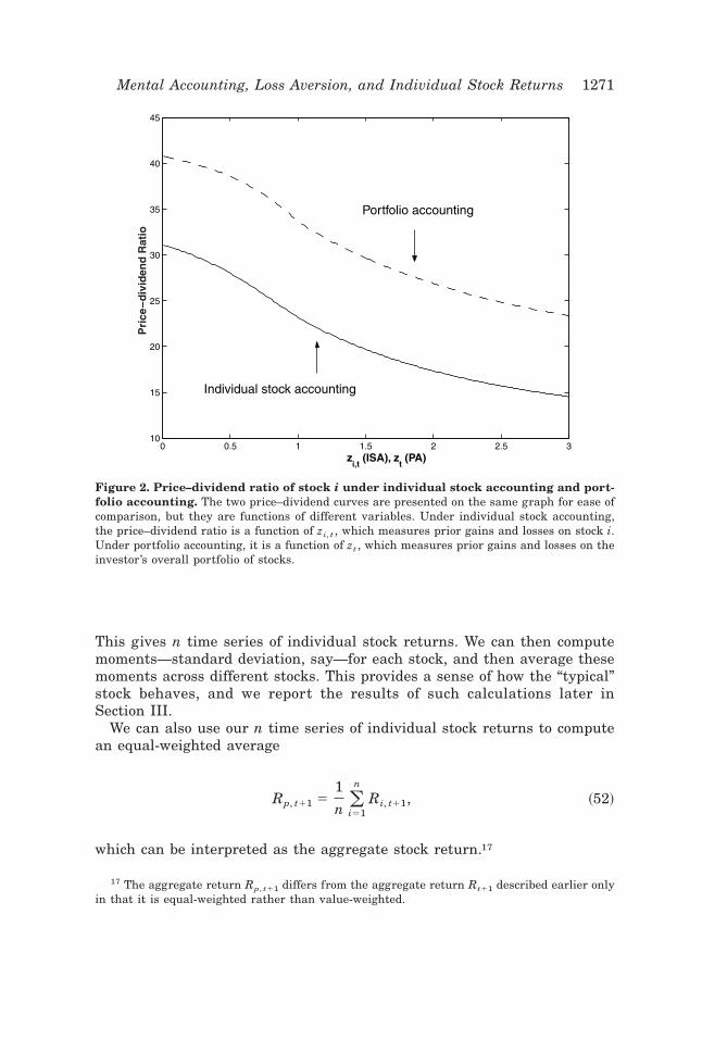
Figure 2. Price–dividend ratio of stock i under individual stock accounting and port-folio accounting. The two price–dividend curves are presented on the same graph for ease ofcomparison, but they are functions of different variables. Under individual stock accounting,the price–dividend ratio is a function of zi, t , which measures prior gains and losses on stock i.Under portfolio accounting, it is a function of zt , which measures prior gains and losses on theinvestor ’s overall portfolio of stocks.


For the case of portfolio accounting, we start out by using iteration inequation ~36! to compute the aggregate price–dividend ratio. As before, weiterate between guesses f � f ~ j ! and functions zt�1 � h~ j !~zt ,«t�1! that solve

Rt�1 �1 � f ~zt�1!

f ~zt !e gp�sp«t�1 ~53!

and

zt�1 � h�zt

OR

Rt�1� � ~1 � h!~1! ~54!

simultaneously for f � f ~ j !. Once this process converges with f ~ j ! r f andh~ j ! r h, we take the resulting functions f ~{! and zt�1 � h~zt ,«t�1! anditerate in equation ~32! over guesses fi

~ j !~{! for stock i ’s price–dividend ratio,converging eventually to the solution fi~{!.18 Figure 2 shows the price–dividend ratio fi~{! that we obtain for the parameter values in Table I. Wedisplay it on the same graph as the price–dividend ratio obtained earlier inthe individual stock accounting case, but it is important to note that the twocurves are plotted against different state variables: against zi, t for individ-ual stock accounting, and against zt for portfolio accounting.

Simulation then illustrates the behavior of individual stock returns. Weagain generate dividend shocks $«i, t % for n � 500 stocks and for the portfolio,$«t %, over 10,000 time periods. The function zt�1 � h~zt ,«t�1! generates thetime series for the aggregate state variable zt implied by these $«t % . Thetime series of returns for stock i is then given by

Ri, t�1 �1 � fi ~zt�1!

fi ~zt !e gi�si «i, t�1 , ~55!

while the aggregate return is measured by

Rp, t�1 �1

n (i�1

n

Ri, t�1. ~56!

C. Equilibrium Returns Under Individual Stock Accounting

Table II summarizes the properties of individual and aggregate stock re-turns in simulated data from three economies: one in which investors useindividual stock accounting, another in which they use portfolio accounting,and for comparison, a third economy in which investors experience no loss

18 The way f ~{! enters equation ~32! is through the portfolio return Rt�1 in equations ~33!and ~34!. Note that Rt�1 depends on f ~{! as shown in equation ~35!.


aversion at all. Specifically, in this third economy, investors have the pref-erences in equation ~2! but with b0 � 0; in other words, they have powerutility over consumption with g � 1 and r � 0.98.

Panel A in Table II reports time series properties of individual stock re-turns; Panel B describes the time series properties of aggregate returns;finally, Panel C summarizes the cross-sectional patterns in average returns.As described in Section III.B, the time series results for individual stockscome from computing the relevant moment for each stock in the simulated

Table II

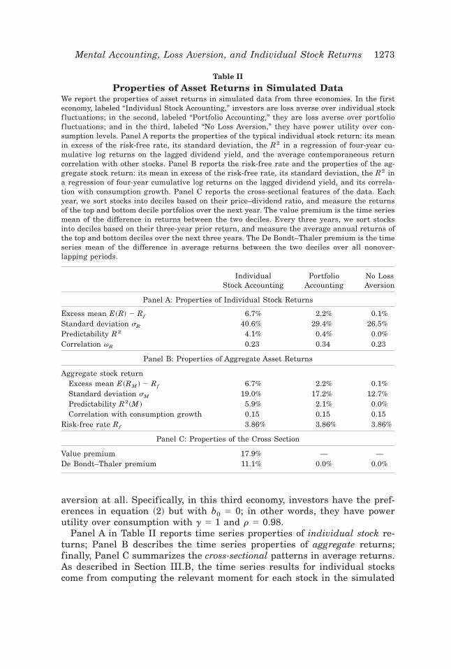
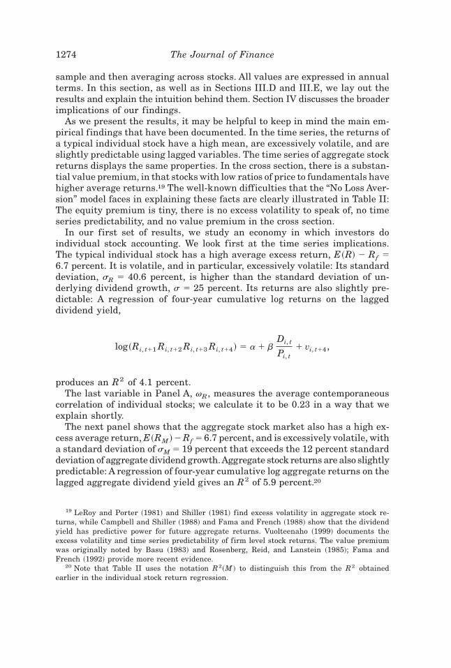
Properties of Asset Returns in Simulated DataWe report the properties of asset returns in simulated data from three economies. In the firsteconomy, labeled “Individual Stock Accounting,” investors are loss averse over individual stockf luctuations; in the second, labeled “Portfolio Accounting,” they are loss averse over portfoliof luctuations; and in the third, labeled “No Loss Aversion,” they have power utility over con-sumption levels. Panel A reports the properties of the typical individual stock return: its meanin excess of the risk-free rate, its standard deviation, the R2 in a regression of four-year cu-mulative log returns on the lagged dividend yield, and the average contemporaneous returncorrelation with other stocks. Panel B reports the risk-free rate and the properties of the ag-gregate stock return: its mean in excess of the risk-free rate, its standard deviation, the R2 ina regression of four-year cumulative log returns on the lagged dividend yield, and its correla-tion with consumption growth. Panel C reports the cross-sectional features of the data. Eachyear, we sort stocks into deciles based on their price–dividend ratio, and measure the returnsof the top and bottom decile portfolios over the next year. The value premium is the time seriesmean of the difference in returns between the two deciles. Every three years, we sort stocksinto deciles based on their three-year prior return, and measure the average annual returns ofthe top and bottom deciles over the next three years. The De Bondt–Thaler premium is the timeseries mean of the difference in average returns between the two deciles over all nonover-lapping periods.

IndividualStock Accounting

PortfolioAccounting

No LossAversion

Panel A: Properties of Individual Stock Returns

Excess mean E~R! � Rf 6.7% 2.2% 0.1%Standard deviation sR 40.6% 29.4% 26.5%Predictability R2 4.1% 0.4% 0.0%Correlation vR 0.23 0.34 0.23

Panel B: Properties of Aggregate Asset Returns

Aggregate stock returnExcess mean E~RM ! � Rf 6.7% 2.2% 0.1%Standard deviation sM 19.0% 17.2% 12.7%Predictability R2~M ! 5.9% 2.1% 0.0%Correlation with consumption growth 0.15 0.15 0.15

Risk-free rate Rf 3.86% 3.86% 3.86%

Panel C: Properties of the Cross Section

Value premium 17.9% — —De Bondt–Thaler premium 11.1% 0.0% 0.0%


sample and then averaging across stocks. All values are expressed in annualterms. In this section, as well as in Sections III.D and III.E, we lay out theresults and explain the intuition behind them. Section IV discusses the broaderimplications of our findings.

As we present the results, it may be helpful to keep in mind the main em-pirical findings that have been documented. In the time series, the returns ofa typical individual stock have a high mean, are excessively volatile, and areslightly predictable using lagged variables. The time series of aggregate stockreturns displays the same properties. In the cross section, there is a substan-tial value premium, in that stocks with low ratios of price to fundamentals havehigher average returns.19 The well-known difficulties that the “No Loss Aver-sion” model faces in explaining these facts are clearly illustrated in Table II:The equity premium is tiny, there is no excess volatility to speak of, no timeseries predictability, and no value premium in the cross section.

In our first set of results, we study an economy in which investors doindividual stock accounting. We look first at the time series implications.The typical individual stock has a high average excess return, E~R! � Rf �6.7 percent. It is volatile, and in particular, excessively volatile: Its standarddeviation, sR � 40.6 percent, is higher than the standard deviation of un-derlying dividend growth, s � 25 percent. Its returns are also slightly pre-dictable: A regression of four-year cumulative log returns on the laggeddividend yield,

log~Ri, t�1 Ri, t�2 Ri, t�3 Ri, t�4! � a� bDi, t

Pi, t� vi, t�4,

produces an R2 of 4.1 percent.The last variable in Panel A, vR, measures the average contemporaneous

correlation of individual stocks; we calculate it to be 0.23 in a way that weexplain shortly.

The next panel shows that the aggregate stock market also has a high ex-cess average return, E~RM !� Rf � 6.7 percent, and is excessively volatile, witha standard deviation of sM � 19 percent that exceeds the 12 percent standarddeviation of aggregate dividend growth.Aggregate stock returns are also slightlypredictable: A regression of four-year cumulative log aggregate returns on thelagged aggregate dividend yield gives an R2 of 5.9 percent.20

19 LeRoy and Porter ~1981! and Shiller ~1981! find excess volatility in aggregate stock re-turns, while Campbell and Shiller ~1988! and Fama and French ~1988! show that the dividendyield has predictive power for future aggregate returns. Vuolteenaho ~1999! documents theexcess volatility and time series predictability of firm level stock returns. The value premiumwas originally noted by Basu ~1983! and Rosenberg, Reid, and Lanstein ~1985!; Fama andFrench ~1992! provide more recent evidence.

20 Note that Table II uses the notation R2~M ! to distinguish this from the R2 obtainedearlier in the individual stock return regression.


The market standard deviation sM helps us measure the average correla-tion vR between stocks that we reported earlier: We compute it as ~sM 0sR!

2.This calculation is exact in the limit as the number of stocks n r `, if allstocks have the same standard deviation and correlation with one another,as they do in our simple economy. This follows because

sM2 � lim

nr`Var� R1, t�1 � . . . � Rn, t�1

n � � limnr`

�sR2

n� �1 �

1

n�sR2vR�� sR

2vR .

Panel C in Table II describes the cross-sectional features of individualstock returns. Our simulated data produces a value premium: A scaled-pricevariable—in our case, the price–dividend ratio—has predictive power for thecross section of average returns. Each year, we sort stocks into deciles basedon this ratio, and measure the returns of the top and bottom decile portfoliosover the next year. The time series mean of the difference in returns be-tween the two deciles is a very substantial 17.9 percent.

Our data also replicates a well-known study of De Bondt and Thaler ~1985!,which finds that long-term prior losing stocks on average outperform long-term prior winning stocks. Every three years, we sort stocks into decilesbased on their three-year prior return, and measure the average annualreturns of the top and bottom deciles over the next three years. The timeseries mean of the difference in average returns between the two decilesover all nonoverlapping periods in our simulated data is 11.1 percent.

Many of the effects we obtain under individual stock accounting derivefrom a single source, namely a discount rate for individual stocks that changesas a function of the stock’s past performance. If a stock has had good recentperformance, the investor gets utility from this gain, and becomes less con-cerned about future losses on the stock because any losses will be cushionedby the prior gains. In effect, the investor perceives the stock to be less riskythan before and discounts its future cash f lows at a lower rate. Conversely,if one of his stocks performs dismally, he finds this painful and becomesmore sensitive to the possibility of further losses on the stock. In effect, heviews the stock as riskier than before and raises its discount rate.

This changing discount rate has many implications. It gives individualstocks some time series predictability: A lower discount rate pushes up theprice–dividend ratio and leads to lower subsequent returns, which meansthat the lagged price–dividend ratio can predict returns. It makes stock re-turns more volatile than underlying cash f lows: A high cash f low pushes thestock price up, but this prior gain also lowers the discount rate on the stock,pushing the stock price still higher. It also generates a value premium in thecross section: In our economy, a stock with a high price–dividend ratio ~agrowth stock! is often one that has done well in the past, accumulating priorgains for the investor who then views it as less risky and requires a loweraverage return. A stock with a low price–dividend ratio ~a value stock! hasoften had dismal prior performance, burning the investor, who now views itas riskier, and requires a higher average return.


The high equity premia we obtain under individual stock accounting derivefrom a different source: Since the investor is loss averse over individual stockf luctuations, he dislikes the frequent losses that individual stocks often pro-duce, and charges a high average return as compensation. Other papers, suchas Benartzi and Thaler ~1995! and Barberis et al. ~2001! have also suggestedloss aversion as a way of understanding a high equity premium. The effect weobtain here, though, is one level stronger than in those earlier papers, since theinvestor is now loss averse over individual stock f luctuations rather than overthe less dramatic f luctuations in the diversified aggregate market.

This intuition also explains why the price–dividend function in Figure 2 isdownward sloping. A lower value of zi, t means that the investor has accu-mulated prior gains on stock i. Since he is now less concerned about futurelosses on this stock, he perceives it to be less risky and is therefore willingto pay a higher price for it per unit of cash f low.

D. Equilibrium Returns Under Portfolio Accounting

Our next set of results shows that the investor ’s system of mental account-ing matters a great deal for the behavior of asset prices. As we broaden theinvestor ’s frame from individual stock accounting to portfolio accounting,individual stock returns exhibit quite different features in equilibrium.

Table II shows that under portfolio accounting, the average excess returnon a typical individual stock is 2.2 percent—not insubstantial, but ratherlower than under individual stock accounting. At 29.4 percent, individualstock volatility is also lower than under individual stock accounting. In par-ticular, excess volatility of returns over dividend growth is much smaller.Individual stock returns are predictable in the time series, but only slightly.

The average excess return on the aggregate market is 2.2 percent. Inter-estingly, aggregate returns are roughly as volatile here as they are underindividual stock accounting. Since individual stocks are much less volatilehere than under individual stock accounting, this must mean that stocks aremore highly correlated than before, and indeed, vR � 0.34. Finally, aggre-gate stock returns are slightly predictable.

We now turn to the cross section. One disadvantage of our assumptionthat stock-specific parameters—dividend growth mean gi , standard devia-tion si , and correlations with the overall portfolio vip and with consumptionvci—are the same for all stocks is that there is no cross-sectional dispersionin price–dividend ratios in the case of portfolio accounting. This assumptionwill be relaxed in Section III.E. For now, the lack of dispersion means thatwe cannot check for a value premium in the simulated data.

We can, however, still look to see if there is a De Bondt–Thaler premiumto prior losers. As Table II shows, this effect is no longer present underportfolio accounting.

The reason the results are different under portfolio accounting is that in thiscase, changes in discount rates on stocks are driven by f luctuations in the valueof the overall portfolio. When the portfolio does well, the investor is less concerned


about losses on any of the stocks that he holds, since the prior portfolio gainwill cushion any such losses. Effectively, he views all stocks as less risky. Dis-count rates on all stocks therefore go down simultaneously. Conversely, dis-count rates on all stocks go up after a prior portfolio loss.

This discount rate behavior is the key to many of the portfolio accountingresults. Stock returns are less volatile here than under individual stock ac-counting. In the latter case, stocks are highly volatile because good cash-f low news is always accompanied by a lower discount rate, pushing the priceup even more. Under portfolio accounting, good cash-f low news on a partic-ular stock will only coincide with a lower discount rate on the stock if theportfolio as a whole does well. There is no guarantee of this, and so volatilityis not amplified by as much. Since shocks to discount rates are perfectlycorrelated across stocks, individual stock returns are highly correlated withone another. Moreover, the De Bondt–Thaler premium disappears because astock’s past performance no longer affects its discount rate, which is nowdetermined at the portfolio level.

Finally, while there is a substantial equity premium, it is not as large asunder individual stock accounting. The investor is loss averse over portfoliolevel f luctuations, which are sizable but not as severe as the swings on in-dividual stocks. The compensation for risk is therefore more moderate.

This intuition also clarifies why the price–dividend function in Figure 2 isdownward sloping. A lower value of zt means that the investor has accumu-lated prior gains on his portfolio. Since he is now less concerned about fu-ture losses on stock i—or indeed, on any stock—he perceives stock i to beless risky and is therefore willing to pay a higher price for it per unit of cashf low. Since he is loss averse only over portfolio f luctuations and not overindividual stock f luctuations, he on average perceives stocks to be less risky,which is why the overall level of the price–dividend function is higher herethan under individual stock accounting.

E. Further Cross-sectional Results

Our analysis so far has assumed that mean log dividend growth rates giand log dividend growth volatilities si are equal across stocks. In particular,Table I shows that we have assumed gi � �0.0091 and si � 0.25, ∀i. Notethat for the mean simple dividend growth rate Gi , this implies

Gi [ E�Di, t�1

Di, t� � 1 � e gi�si

202 � 1 � 0.0224, ∀i

ln~1 � Gi ! � 0.0222, ∀i.

We now relax these restrictive parameter choices. This should allow for amore realistic comparison of the cross-sectional features of the actual datawith those of the simulated data.


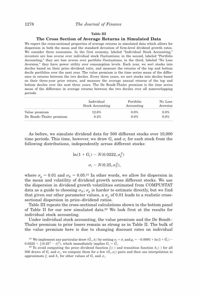
As before, we simulate dividend data for 500 different stocks over 10,000time periods. This time, however, we draw Gi and si for each stock from thefollowing distributions, independently across different stocks:

ln~1 � Gi ! ; N~0.0222,sg2!

si ; N~0.25,sS2!,

where sg � 0.01 and sS � 0.05.21 In other words, we allow for dispersion inthe mean and volatility of dividend growth across different stocks. We usethe dispersion in dividend growth volatilities estimated from COMPUSTATdata as a guide to choosing sS ; sg is harder to estimate directly, but we findthat given our other parameter values, a sg of 0.01 leads to a realistic cross-sectional dispersion in price–dividend ratios.

Table III repeats the cross-sectional calculations shown in the bottom panelof Table II for our new simulated data.22 We look first at the results forindividual stock accounting.

Under individual stock accounting, the value premium and the De Bondt–Thaler premium to prior losers remain as strong as in Table II. The bulk ofthe value premium here is due to changing discount rates on individual

21 We implement any particular draw ~ ZGi , [si! by setting si � [si and gi � �0.0091 � ln~1 � ZGi!�0.0222 � 1

2_ ~0.252 � [si

2!, which immediately implies Gi � ZGi .22 To avoid computing the price–dividend function fi~{! and transition function hi~{! for all

500 draws of Gi and si , we compute them for a few ~Gi ,si! pairs and then use interpolation toapproximate fi and hi for other values of Gi and si .

Table III

The Cross Section of Average Returns in Simulated DataWe report the cross-sectional properties of average returns in simulated data which allows fordispersion in both the mean and the standard deviation of firm-level dividend growth rates.We consider three economies. In the first economy, labeled “Individual Stock Accounting,”investors are loss averse over individual stock f luctuations; in the second, labeled “PortfolioAccounting,” they are loss averse over portfolio f luctuations; in the third, labeled “No LossAversion,” they have power utility over consumption levels. Each year, we sort stocks intodeciles based on their price–dividend ratio, and measure the returns of the top and bottomdecile portfolios over the next year. The value premium is the time series mean of the differ-ence in returns between the two deciles. Every three years, we sort stocks into deciles basedon their three-year prior return, and measure the average annual returns of the top andbottom deciles over the next three years. The De Bondt-Thaler premium is the time seriesmean of the difference in average returns between the two deciles over all nonoverlappingperiods.

IndividualStock Accounting

PortfolioAccounting

No LossAversion

Value premium 12.6% 0.0% 0.0%De Bondt–Thaler premium 8.2% 0.0% 0.0%


stocks, exactly as described earlier. Now that we have allowed for cross-sectional dispersion in the volatility of dividend growth, there is an addi-tional mechanism contributing to the value premium. A firm with more volatilecash-f low growth has more volatile returns, which scares the loss-averseinvestor into charging a higher risk premium. Since the investor is applyinga high discount rate to future cash f lows, the firm will have a low price–dividend ratio, thus generating a cross-sectional link between price–dividend ratios and average returns.23

The value premium in Table III is lower than the premium in Table II.The reason for this is the following. In the Table II simulations, a stock onlyhas a low price–dividend ratio if investors decide to assign it a high discountrate. Portfolios of low price–dividend stocks therefore earn high returns onaverage. In the more realistic simulations we do in Table III, a low price–dividend ratio can be a sign of a high discount rate, but it can also mean thatthe stock has a low gi , in other words, that investors expect low cash-f lowgrowth on the stock. Portfolios of low price–dividend stocks still have highreturns, but the effect is diluted since the portfolio now includes stocks withlow expected growth rates and only average discount rates.

Table III also presents results for the portfolio accounting case.24 There isnow dispersion in price–dividend ratios, which means that we can examinewhether price–dividend ratios have any predictive power in the cross sec-tion. They do not; in other words, there is no value premium. The attempt toreplicate De Bondt and Thaler ’s ~1985! findings is also a failure, as it was inTable II.

Given the ability of individual stock accounting to generate a value pre-mium, it is natural to ask whether we are also able to replicate the findingof Fama and French ~1993!, namely that the value premium can be capturedby a multifactor model that includes as a factor a portfolio formed by rank-ing stocks on their scaled-price ratios—the so-called HML portfolio.

To study this, we simplify the cash-f low structure by once again equatingthe mean and volatility of dividend growth across all stocks, but also enrichit by allowing firm level cash f lows to be driven not just by one factor, but bymany factors. These additional factors can be thought of as industry shocks.Suppose that each of the n stocks falls into one of a small number of indus-try sectors, labelled s � 1, . . . ,S. Suppose that the cash-f low shock to stock inow has the structure

«i, t�1 � vp«t�1 � vs«s, t�1 � [«i, t�1!1 � vp2 � vs

2. ~57!

23 Our claim that the bulk of the value premium is due to changing discount rates is basedon a comparison of the results in Table III to those for an economy in which there is dispersiononly in the mean dividend growth rate across firms and not in the volatility of dividend growth.These results are not shown here but are available from the authors on request.

24 Now that we have allowed for dispersion in gi and si , we cannot be certain that theself-consistency condition in Proposition 2 is satisfied. The portfolio accounting results in Table IIIshould therefore be viewed as approximate.


In addition to the market-wide shock «t�1 and the idiosyncratic shock [«i, t�1,there is sector-level cash-f low shock «s, t�1, where s is the sector to whichstock i belongs. All shocks are distributed N~0,1!, i.i.d. over time, and theirrelative importance is determined by vp and vs. If we assume for simplicitythat these shocks are orthogonal to one another, the correlation vij betweenthe cash-f low shocks on stock i and j will satisfy

vij � vp2, for i � j and i, j in different sectors,

vij � vp2 � vs

2, for i � j and i, j in the same sector,

vij � 1, for i � j.

We simulate dividend data on 500 stocks over 10,000 time periods using thiscorrelation structure, and then compute the resulting stock prices in an econ-omy where investors do individual stock accounting. We take vp � 0.48 asbefore, and vs � 0.5.

To investigate Fama and French’s ~1993! finding, we split our simulateddata into two equal subsamples. In the first subsample, we create theportfolios whose average returns we want to explain. Each year, we sortstocks into quintiles based on their price–dividend ratio and record theequal-weighted return Rj, t

P0D , j � 1, . . . ,5, of each quintile over the next year;in particular, R1, t

P0D is the return on the first quintile, containing stockswith the lowest price–dividend ratios. Repeating this each period produceslong time series of returns on the five portfolios. Table IV reports eachportfolio’s average return over time, ORj

P0D. Of course, the dispersion in theaverage returns across the five portfolios is what we refer to as the valuepremium.

Table IV shows the results of time series regressions of the excess returnson these five portfolios on the excess market return,

Rj, tP0D � Rf � aj � bj,1~Rp, t � Rf !� uj, t . ~58!

The intercepts are large, replicating Fama and French’s ~1993! finding thatthe CAPM is not able to explain the average returns on portfolios sorted byscaled-price ratios.

In our second subsample, we construct a counterpart to Fama and French’s~1993! HML factor: Each year, we compute the return on the portfolio ofstocks with price–dividend ratios in the lowest quartile that period minusthe return on the portfolio of stocks with price–dividend ratios in the highestquartile that period. We denote this difference Ft .25

25 The reason we split the data into two subsamples is so that Rj, tP0D and Ft can be computed

in different samples, thus ensuring that our regressions do not pick up any spurious correlation.


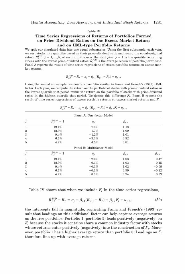
Table IV shows that when we include Ft in the time series regressions,

Rj, tP0D � Rf � aj � bj,1~Rp, t � Rf !� bj,2 Ft � uj, t , ~59!

the intercepts fall in magnitude, replicating Fama and French’s ~1993! re-sult that loadings on this additional factor can help capture average returnson the five portfolios. Portfolio 1 ~portfolio 5! loads positively ~negatively! onFt because the stocks it contains share a common industry factor with stockswhose returns enter positively ~negatively! into the construction of Ft . More-over, portfolio 1 has a higher average return than portfolio 5. Loadings on Fttherefore line up with average returns.

Table IV

Time Series Regressions of Returns of Portfolios Formedon Price–Dividend Ratios on the Excess Market Return

and on HML-type Portfolio ReturnsWe split our simulated data into two equal subsamples. Using the first subsample, each year,we sort stocks into quintiles based on their price–dividend ratio and record the equal-weightedreturn Rj, t

P0D , j � 1, . . . ,5, of each quintile over the next year; j � 1 is the quintile containingstocks with the lowest price–dividend ratios. ORj

P0D is the average return of portfolio j over time.Panel A reports the result of time series regressions of excess portfolio returns on excess mar-ket returns,

Rj, tP0D � Rf � aj � bj,1~Rp, t � Rf !� uj, t .

Using the second subsample, we create a portfolio similar to Fama and French’s ~1993! HMLfactor. Each year, we compute the return on the portfolio of stocks with price–dividend ratios inthe lowest quartile that period minus the return on the portfolio of stocks with price–dividendratios in the highest quartile that period. We denote this difference Ft . Panel B reports theresult of time series regressions of excess portfolio returns on excess market returns and Ft ,

Rj, tP0D � Rf � aj � bj,1~Rp, t � Rf !� bj,2 Ft � uj, t .

Panel A: One-factor Model

j ORjP0D � 1 aj bj,1

1 19.1% 7.3% 1.182 12.9% 1.7% 1.093 9.4% �1.2% 1.014 6.7% �3.3% 0.925 4.7% �4.5% 0.81

Panel B: Multifactor Model

j ORjP0D � 1 aj bj,1 bj,2

1 19.1% 2.2% 1.03 0.472 12.9% 0.1% 1.03 0.153 9.4% �0.1% 1.02 �0.054 6.7% �0.1% 0.99 �0.225 4.7% �0.3% 0.94 �0.39


IV. Discussion

We draw a number of conclusions from the results in Tables II, III, and IV.First, both kinds of narrow framing may shed light on certain aspects of thedata. Under both individual stock accounting and portfolio accounting, firmlevel returns have a high mean, are excessively volatile, and are predictablein the time series using lagged variables. In both cases, aggregate stockreturns inherit a high mean, excess volatility and some time series predict-ability, again in line with the available evidence. Moreover, the risk-free rateis constant and low.

Another attractive feature of both narrow framing models is that theyare able to generate excess volatility in the time series while still keepingthe correlation of aggregate stock returns and consumption growth—anumber that we also report in Table II—at realistically low levels. Someconsumption-based models, such as Campbell and Cochrane ~1999!, arealso able to generate excess volatility in aggregate returns. However, theextra volatility is driven by shocks to consumption growth, a mechanismthat inevitably gives consumption growth and stock returns a counter-factually high correlation.

Of the two models, individual stock accounting may be the more successfulone. Not only can it reproduce time series facts, but also a number of puz-zling cross-sectional features of the data: the premium to value stocks and tostocks with poor prior returns, as well as the ability of certain multifactormodels to capture the value premium. Portfolio accounting fails on the cross-sectional facts, and this is not simply a consequence of the particular pa-rameter values we have used. The way the cross-sectional facts emerge underindividual stock accounting is through a discount rate that is a function of astock’s own past performance. This is simply not a feature of portfolio ac-counting, whatever the parameters.

While individual stock accounting can be a useful device for understand-ing certain features of asset prices, we emphasize that it is at most a po-tential ingredient in an equilibrium model, and not a complete description ofthe facts. There are a number of dimensions on which it too, fails. For ex-ample, it predicts that the correlation between returns on different stocks isthe same as the correlation between their cash f lows. This can be seen inTable II, which reports the typical correlation between stocks to be vR �0.23, identical to the correlation between cash-f low shocks, vij � 0.23, listedin Table I. However, Vuolteenaho ~1999! finds that shocks to expected re-turns on different stocks are actually much more correlated than cash-f lowshocks, which immediately implies that stocks are more correlated with eachother than are their underlying cash f lows.26

26 Equivalently, the individual stock accounting model predicts that individual stock returnsand aggregate stock returns will exhibit the same amount of excess volatility, while Vuol-teenaho ~1999! finds there to be much less excess volatility in individual stocks than in theaggregate stock market.


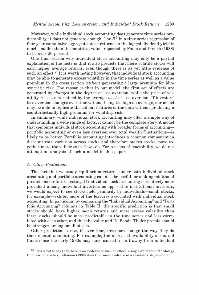
Moreover, while individual stock accounting does generate time series pre-dictability, it does not generate enough: The R2 in a time series regression offour-year cumulative aggregate stock returns on the lagged dividend yield ismuch smaller than the empirical value, reported by Fama and French ~1988!to be over 20 percent.

One final reason why individual stock accounting may only be a partialexplanation of the facts is that it also predicts that more volatile stocks willearn higher average returns, even though there is as yet little evidence ofsuch an effect.27 It is worth noting however, that individual stock accountingmay be able to generate excess volatility in the time series as well as a valuepremium in the cross section without generating a large premium for idio-syncratic risk. The reason is that in our model, the first set of effects aregenerated by changes in the degree of loss aversion, while the price of vol-atility risk is determined by the average level of loss aversion. If investors’loss aversion changes over time without being too high on average, our modelmay be able to replicate the salient features of the data without producing acounterfactually high premium for volatility risk.

In summary, while individual stock accounting may offer a simple way ofunderstanding a wide range of facts, it cannot be the complete story. A modelthat combines individual stock accounting with broader forms of accounting—portfolio accounting or even loss aversion over total wealth f luctuations—islikely to be better. Portfolio accounting introduces a common component indiscount rate variation across stocks and therefore makes stocks move to-gether more than their cash f lows do. For reasons of tractability, we do notattempt an analysis of such a model in this paper.

A. Other Predictions

The fact that we study equilibrium returns under both individual stockaccounting and portfolio accounting can also be useful for making additionalpredictions for future testing. If individual stock accounting is relatively moreprevalent among individual investors as opposed to institutional investors,we would expect to see stocks held primarily by individuals—small stocks,for example—exhibit more of the features associated with individual stockaccounting. In particular, by comparing the “Individual Accounting” and “Port-folio Accounting” columns in Table II, the specific prediction is that smallstocks should have higher mean returns and more excess volatility thanlarge stocks, should be more predictable in the time series and less corre-lated with each other, and that the value and De Bondt–Thaler premia shouldbe stronger among small stocks.

Other predictions arise, if, over time, investors change the way they dotheir mental accounting. For example, the increased availability of mutualfunds since the early 1980s may have caused a shift away from individual

27 This is not to say that there is no evidence of such an effect: Using a different methodologyfrom earlier studies, Lehmann ~1990! does find some evidence of a residual risk premium.


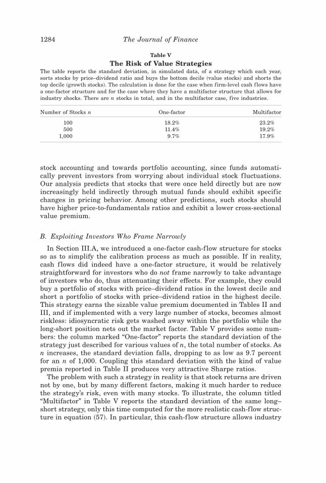
stock accounting and towards portfolio accounting, since funds automati-cally prevent investors from worrying about individual stock f luctuations.Our analysis predicts that stocks that were once held directly but are nowincreasingly held indirectly through mutual funds should exhibit specificchanges in pricing behavior. Among other predictions, such stocks shouldhave higher price-to-fundamentals ratios and exhibit a lower cross-sectionalvalue premium.

B. Exploiting Investors Who Frame Narrowly

In Section III.A, we introduced a one-factor cash-f low structure for stocksso as to simplify the calibration process as much as possible. If in reality,cash f lows did indeed have a one-factor structure, it would be relativelystraightforward for investors who do not frame narrowly to take advantageof investors who do, thus attenuating their effects. For example, they couldbuy a portfolio of stocks with price–dividend ratios in the lowest decile andshort a portfolio of stocks with price–dividend ratios in the highest decile.This strategy earns the sizable value premium documented in Tables II andIII, and if implemented with a very large number of stocks, becomes almostriskless: idiosyncratic risk gets washed away within the portfolio while thelong-short position nets out the market factor. Table V provides some num-bers: the column marked “One-factor” reports the standard deviation of thestrategy just described for various values of n, the total number of stocks. Asn increases, the standard deviation falls, dropping to as low as 9.7 percentfor an n of 1,000. Coupling this standard deviation with the kind of valuepremia reported in Table II produces very attractive Sharpe ratios.

The problem with such a strategy in reality is that stock returns are drivennot by one, but by many different factors, making it much harder to reducethe strategy’s risk, even with many stocks. To illustrate, the column titled“Multifactor” in Table V reports the standard deviation of the same long–short strategy, only this time computed for the more realistic cash-f low struc-ture in equation ~57!. In particular, this cash-f low structure allows industry

Table V

The Risk of Value StrategiesThe table reports the standard deviation, in simulated data, of a strategy which each year,sorts stocks by price–dividend ratio and buys the bottom decile ~value stocks! and shorts thetop decile ~growth stocks!. The calculation is done for the case when firm-level cash f lows havea one-factor structure and for the case where they have a multifactor structure that allows forindustry shocks. There are n stocks in total, and in the multifactor case, five industries.

Number of Stocks n One-factor Multifactor

100 18.2% 23.2%500 11.4% 19.2%

1,000 9.7% 17.9%


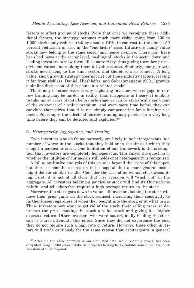
factors to affect groups of stocks. Note that once we recognize these addi-tional factors, the strategy becomes much more risky: going from 100 to1,000 stocks only reduces risk by about a fifth, in contrast to the almost 50percent reduction in risk in the “one-factor” case. Intuitively, many valuestocks now belong to the same sector and hence co-move: There may havebeen bad news at the sector level, pushing all stocks in the sector down andleading investors to view them all as more risky, thus giving them low price–dividend ratios and making them all value stocks. Similarly, many growthstocks now belong to the same sector, and therefore also co-move. A longvalue, short growth strategy does not net out these industry factors, leavingit far from riskless. Daniel, Hirshleifer, and Subrahmanyam ~2001! providea similar discussion of this point in a related model.

There may be other reasons why exploiting investors who engage in nar-row framing may be harder in reality than it appears in theory. It is likelyto take many years of data before arbitrageurs can be statistically confidentof the existence of a value premium, and even more time before they canconvince themselves that it is not simply compensation for a lurking riskfactor. Put simply, the effects of narrow framing may persist for a very longtime before they can be detected and exploited.28

C. Heterogeneity, Aggregation, and Trading

Even investors who do frame narrowly are likely to be heterogeneous in anumber of ways: in the stocks that they hold or in the time at which theybought a particular stock. One limitation of our framework is the assump-tion that investors are completely homogeneous. This raises the question ofwhether the intuition of our models still holds once heterogeneity is recognized.

A full quantitative analysis of this issue is beyond the scope of this paper,but there is nonetheless reason to be hopeful that a more general modelmight deliver similar results. Consider the case of individual stock account-ing. First, it is not at all clear that loss aversion will “wash out” in theaggregate. All investors holding a particular stock will find its f luctuationspainful and will therefore require a high average return on the stock.

Moreover, if a stock goes down in value, all investors holding the stock willhave their prior gains on the stock reduced, increasing their sensitivity tofurther losses regardless of when they bought into the stock or at what price.These investors now want to get rid of the stock: their selling pressure de-presses the price, making the stock a value stock and giving it a higherexpected return. Other investors who were not originally holding the stockcan of course attenuate this effect: Since they did not experience the loss,they do not require such a high rate of return. However, these other inves-tors will trade cautiously for the same reason that arbitrageurs in general

28 After all, the value premium in our simulated data, while certainly strong, has beencomputed using 10,000 years of data. Arbitrageurs looking for exploitable anomalies have muchless data at their disposal.


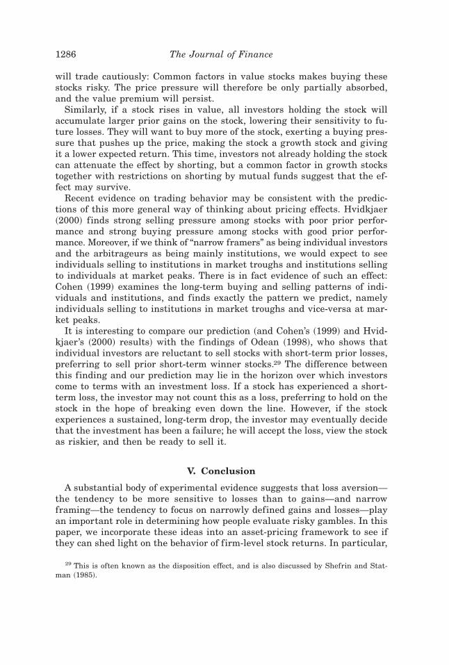
will trade cautiously: Common factors in value stocks makes buying thesestocks risky. The price pressure will therefore be only partially absorbed,and the value premium will persist.

Similarly, if a stock rises in value, all investors holding the stock willaccumulate larger prior gains on the stock, lowering their sensitivity to fu-ture losses. They will want to buy more of the stock, exerting a buying pres-sure that pushes up the price, making the stock a growth stock and givingit a lower expected return. This time, investors not already holding the stockcan attenuate the effect by shorting, but a common factor in growth stockstogether with restrictions on shorting by mutual funds suggest that the ef-fect may survive.

Recent evidence on trading behavior may be consistent with the predic-tions of this more general way of thinking about pricing effects. Hvidkjaer~2000! finds strong selling pressure among stocks with poor prior perfor-mance and strong buying pressure among stocks with good prior perfor-mance. Moreover, if we think of “narrow framers” as being individual investorsand the arbitrageurs as being mainly institutions, we would expect to seeindividuals selling to institutions in market troughs and institutions sellingto individuals at market peaks. There is in fact evidence of such an effect:Cohen ~1999! examines the long-term buying and selling patterns of indi-viduals and institutions, and finds exactly the pattern we predict, namelyindividuals selling to institutions in market troughs and vice-versa at mar-ket peaks.

It is interesting to compare our prediction ~and Cohen’s ~1999! and Hvid-kjaer ’s ~2000! results! with the findings of Odean ~1998!, who shows thatindividual investors are reluctant to sell stocks with short-term prior losses,preferring to sell prior short-term winner stocks.29 The difference betweenthis finding and our prediction may lie in the horizon over which investorscome to terms with an investment loss. If a stock has experienced a short-term loss, the investor may not count this as a loss, preferring to hold on thestock in the hope of breaking even down the line. However, if the stockexperiences a sustained, long-term drop, the investor may eventually decidethat the investment has been a failure; he will accept the loss, view the stockas riskier, and then be ready to sell it.

V. Conclusion

A substantial body of experimental evidence suggests that loss aversion—the tendency to be more sensitive to losses than to gains—and narrowframing—the tendency to focus on narrowly defined gains and losses—playan important role in determining how people evaluate risky gambles. In thispaper, we incorporate these ideas into an asset-pricing framework to see ifthey can shed light on the behavior of firm-level stock returns. In particular,

29 This is often known as the disposition effect, and is also discussed by Shefrin and Stat-man ~1985!.


we consider two economies: one, labeled “individual stock accounting,” inwhich investors are loss averse over individual stock f luctuations, and an-other, labeled “portfolio accounting,” in which investors are loss averse onlyover portfolio f luctuations.

We find that both forms of narrow framing can explain certain aspects ofthe data. In both cases, the typical individual stock has a high mean, isexcessively volatile, and is predictable in the time series. The aggregate stockreturn inherits these properties and is also only weakly correlated with con-sumption growth, while the risk-free rate is constant and low. Moreover,under individual stock accounting, there is a substantial value premium inthe cross section, and this premium can to some extent be captured by thesame kinds of multifactor models that have been successful in actual data.

Our paper suggests that using experimental evidence to refine the way wemodel investor preferences may be a promising avenue for further research.Nonetheless, there are alternative explanations under development for someof the phenomena discussed here, ranging from models firmly rooted in theconsumption-based paradigm to models of learning and models of irrationalbeliefs. An important topic for further study is to clarify the distinct predic-tions of these various explanations so that additional testing might tell themapart.

Appendix

Proof of Proposition 1: Each agent’s optimization problem is

maxCt , $Si, t %

E(t�0

` �r tCt

1�g

1 � g� b0 OCt

�g r t�1 (i�1

n

v~Xi, t�1,Si, t , zi, t !�, ~A1!

subject to the standard budget constraint

Wt�1 � ~Wt � Ct !Rf � (i�1

n

Si, t ~Ri, t�1 � Rf !, ~A2!

where Wt denotes the agent’s preconsumption wealth at t.The Euler equations for the optimization problem are

1 � rRf Et�� OCt�1

OCt��g�, ~A3!


OCt��g� � b0 rEt @ [v~Ri, t�1, zi, t !# , ∀i. ~A4!

These Euler equations are necessary conditions of optimality for the indi-vidual’s intertemporal problem. We now show that they are sufficient con-ditions, using a technique developed by Duffie and Skiadas ~1994!.


To simplify notation, let ut ~Ct ! � r tCt1�g0~1 � g! and Nbt � r t�1b0 OCt

�g.Assume that the strategy ~C *, $Si

*%! satisfies the Euler equations

ut'~Ct

*! � Rf Et @ut�1' ~Ct�1

* !# , ~A5!

ut'~Ct

*! � Et @Ri, t�1 ut�1' ~Ct�1

* !#� Nbt Et @ [v~Ri, t�1, zi, t !# . ~A6!

Consider any alternative strategy ~C * � dC, $Si* � dSi%! that satisfies the

budget constraint

dWt�1 � ~dWt � dCt !Rf � (i�1

n

dSi, t ~Ri, t�1 � Rf !. ~A7!

The increase in expected utility from using the alternative strategy is

E�(t�0

` �ut ~Ct*� dCt !� ut ~Ct

*!� Nbt (i�1

n

dSi, t [v~Ri, t�1, zi, t !�� [ E�(

t�0

` �ut'~Ct

*!dCt � Nbt (i�1

n

dSi, t [v~Ri, t�1, zi, t !��,

~A8!

where we have made use of the concavity of ut ~{! and the linearity of theprospect utility term with respect to Si, t . It is therefore enough to show that � 0 under budget constraint ~A7!.

Multiplying equation ~A7! by ut�1' ~Ct�1

* ! and applying Euler equations~A5! and ~A6!, we have

Et�ut'~Ct

*!dCt � Nbt (i�1

n

dSi, t [v~Ri, t�1, zi, t !�� ut

'~Ct*!dWt � Et @ut�1

' ~Ct�1* !dWt�1# .

~A9!

Summing up equation ~A9! for all t and taking expectations, we have

� u0~C0*!dW0 � lim

Tr`E @uT

' ~CT* !dWT # . ~A10!

The budget constraint implies that dW0 � 0. By requiring feasible strategiesto use bounded units of financial securities, and with a unit of the risk-freesecurity priced at one, we can show that the limiting term also goes to zeroif our model parameters satisfy log r � ggc � gi � 102~g2sc

2 � 2gvciscsi �si

2! � 0, a condition that we already noted in footnote 12.30 So � 0 for anyfeasible alternative to ~C *, $Si

*%!.

30 The proof of this is available upon request.


We have therefore shown that any other budget feasible strategy cannotincrease utility. The Euler equations are therefore necessary and sufficientconditions of optimality.

To close the proof, we show that if the risk-free gross interest rate is con-stant at Rf given by equation ~21! and if the returns on any stock have aone-factor Markov structure given by equations ~8!, ~19!, and ~20!, with fi~{!satisfying equation ~22! for all zi, t , then the agent’s strategy of consuminghis labor income and the dividend of each stock and holding the total supplyof assets at each time t indeed satisfies the Euler equations.

The choice of risk-free rate in equation ~21! allows us to satisfy Eulerequation ~A3!, given equation ~17!. Given the assumed Markov structure ofstock i ’s returns, zi, t�1 is determined by zi, t and «i, t�1. So we have

Et�Ri, t�1� OCt�1

OCt��g� � Et� 1 � fi ~zi, t�1!

fi ~zi, t !e gi�si «i, t�1e�g~gc�scht�1!�

� e gi�ggcEt�E @e�gscht�1 6«i, t�1#esi «i, t�1

1 � fi ~zi, t�1!

fi ~zi, t !�

� e gi�ggc�~102!g2sc

2~1�vci2 !Et� 1 � fi ~zi, t�1!

fi ~zi, t !e ~si�gvcisc!«i, t�1�.

~A11!

Applying this, we find that the strategy of consuming OCt and holding thesupply of all securities satisfies Euler equation ~A4! for all i. Q.E.D.

Proof of Proposition 2: Each agent’s optimization problem is

maxCt , $Si, t %

E(t�0

` �r tCt

1�g

1 � g� b0 OCt

�g r t�1v~Xt�1,St , zt !�, ~A12!

subject to the standard budget constraint

Wt�1 � ~Wt � Ct !Rf � (i�1

n

Si, t ~Ri, t�1 � Rf !, ~A13!

where Wt denotes the agent’s pre-consumption wealth at t.The Euler equations for the optimization problem are

1 � rRf Et�� OCt�1

OCt��g�, ~A14!


OCt��g�� b0 rEt @ Iv~Ri, t�1, Rt�1, zt !# , ∀i. ~A15!


These Euler equations are necessary conditions of optimality for the indi-vidual’s intertemporal problem. One can also show that they are sufficientconditions, using an identical argument to the one in the proof of Proposi-tion 1. Summing up equation ~A15! for all the stocks in the economy, weobtain the Euler equation for the market portfolio,

1 � rEt�Rt�1� OCt�1

OCt��g� � b0 rEt @ [v~Rt�1, zt !# . ~A16!

To close the proof, we show that if the risk-free gross interest rate is con-stant at Rf given by equation ~31!, and if the returns on any stock have aone-factor Markov structure given by equations ~15!, ~29!, and ~30!, with fi~{!satisfying equation ~32! for all zi, t , and if aggregate stock returns are givenby equation ~35! with f ~{! satisfying equation ~36! for all zt , then the agent’sstrategy of consuming his labor income and the dividend of each stock andholding the total supply of assets at each time t indeed satisfies the Eulerequations.

The choice of risk-free rate in equation ~31! allows us to satisfy Eulerequation ~A14!, given equation ~17!. A similar procedure to that used in theproof of Proposition 1 can be used to prove that the strategy of consuming OCtand holding the supply of all securities satisfies Euler equation ~A16! underthe conjectured Markov structure of market returns.

Turning now to Euler equation ~A15!, note that

Et @egi�si «i, t�1 6«t�1# � e gi�~102!si

2~1�vip2 !�sivip«t�1,

and

E @e�g~gc�scht�1!e gi�si «i, t�1 6«t�1#

� e gi�ggc�~102!g2sc

2~1�vcp2 !�~102!si

2~1�vip2 !�gscsi ~vci�vcpvip!e ~sivip�gscvcp!«t�1 .

By iterated expectations, and using the above two equations and observingthat zt�1 is determined by zt and «t�1 given the conjectured Markov struc-ture of stock returns, we see that Euler equation ~A15! reduces to equation~32! and is therefore satisfied by the strategy of consuming OCt and holdingthe supply of all stocks. Q.E.D.

REFERENCES

Anderson, Robert, 1991, Nonstandard methods with applications in economics, in Werner Hilden-brand and Hugo Sonnenschein, eds.: Handbook of Mathematical Economics ~North Hol-land, Amsterdam!.

Barberis, Nicholas, Ming Huang, and Tano Santos, 2001, Prospect theory and asset prices,Quarterly Journal of Economics 116, 1–53.

Barberis, Nicholas, Andrei Shleifer, and Robert Vishny, 1998, A model of investor sentiment,Journal of Financial Economics 49, 307–343.


Basu, Sanjoy, 1983, The relationship between earnings yield, market value and return forNYSE common stocks: Further evidence, Journal of Financial Economics 12, 129–156.

Benartzi, Shlomo, and Richard Thaler, 1995, Myopic loss aversion and the equity premiumpuzzle, Quarterly Journal of Economics 110, 73–92.

Benartzi, Shlomo, and Richard Thaler, 1999, Risk aversion or myopia? Choices in repeatedgambles and retirement investments, Management Science 45, 364–381.

Berk, Jonathan, Richard Green, and Vasant Naik, 1999, Optimal investment, growth options,and security returns, Journal of Finance 54, 1553–1607.

Brennan, Michael, and Yihong Xia, 2001, Stock price volatility and the equity premium, Jour-nal of Monetary Economics, forthcoming.

Campbell, John Y., 2000, Asset prices, consumption and the business cycle, in John Taylor andMichael Woodford, eds.: Handbook of Macroeconomics ~North Holland, Amsterdam!.

Campbell, John Y., and John Cochrane, 1999, By force of habit: A consumption-based ex-planation of aggregate stock market behavior, Journal of Political Economy 107, 205–251.

Campbell, John Y., and Robert Shiller, 1988, Stock prices, earnings, and expected dividends,Journal of Finance 43, 661–676.

Ceccheti, Stephen, Pok-sang Lam, and Nelson Mark, 1990, Mean reversion in equilibrium assetprices, American Economic Review 80, 398–418.

Cohen, Randolph, 1999, Asset allocation decisions of individuals and institutions, Working pa-per, Harvard Business School.

Daniel, Kent, David Hirshleifer, and Avanidhar Subrahmanyam, 2001, Covariance risk, mis-pricing, and the cross section of security returns, Journal of Finance, forthcoming.

De Bondt, Werner, and Richard Thaler, 1985, Does the stock market overreact? Journal ofFinance 40, 793–805.

Duffie, Darrell, and Costis Skiadas, 1994, Continuous-time security pricing: A utility gradientapproach, Journal of Mathematical Economics 23, 107–131.

Epstein, Larry, and Stanley Zin, 1990, First-order risk aversion and the equity premium puzzle,Journal of Monetary Economics 26, 387–407.

Fama, Eugene, and Kenneth French, 1988, Dividend yields and expected stock returns, Journalof Financial Economics 22, 3–27.

Fama, Eugene, and Kenneth French, 1992, The cross section of expected stock returns, Journalof Finance 47, 427–465.

Fama, Eugene, and Kenneth French, 1993, Common risk factors in the returns on stocks andbonds, Journal of Financial Economics 33, 3–56.

Gneezy, Uri, and Jan Potters, 1997, An experiment on risk taking and evaluation periods,Quarterly Journal of Economics 112, 631–645.

Gomes, Joao, Leonid Kogan, and Lu Zhang, 2001, Equilibrium cross-section of returns, Workingpaper, University of Pennsylvania.

Green, Edward, 1989, Individual-level randomness in a nonatomic population, Working paper,University of Pittsburgh.

Gul, Faruk, 1991, A theory of disappointment aversion, Econometrica 59, 667–686.Hong, Harrison, and Jeremy Stein, 1999, A unified theory of underreaction, momentum trad-

ing, and overreaction in asset markets, Journal of Finance 54, 2143–2184.Hvidkjaer, Soeren, 2000, A trade-based analysis of momentum, Working paper, Cornell University.Kahneman, Daniel, and Dan Lovallo, 1993, Timid choices and bold forecasts: A cognitive per-

spective on risk taking, Management Science 39, 17–31.Kahneman, Daniel, and Amos Tversky, 1979, Prospect theory: An analysis of decision under

risk, Econometrica 47, 263–291.Lehmann, Bruce, 1990, Residual risk revisited, Journal of Econometrics 45, 71–97.LeRoy, Stephen, and Richard Porter, 1981, The present value relation: Tests based on variance

bounds, Econometrica 49, 555–577.Lucas, Robert, 1978, Asset prices in an exchange economy, Econometrica 46, 1419–1446.Odean, Terrance, 1998, Are investors reluctant to realize their losses? Journal of Finance 53,

1775–1798.


Rabin, Matthew, 2000, Risk aversion and expected utility theory: A calibration theorem, Econ-ometrica 68, 1281–1292.

Rabin, Matthew, and Richard Thaler, 2000, Anomalies: Risk aversion, Working paper, Univer-sity of Chicago.

Read, Daniel, George Loewenstein, and Matthew Rabin, 1999, Choice bracketing, Journal ofRisk and Uncertainty 19, 171–197.

Redelmeier, Daniel, and Amos Tversky, 1992, On the framing of multiple prospects, Psycholog-ical Science 3, 191–193.

Rosenberg, Barr, Kenneth Reid, and Ronald Lanstein, 1985, Persuasive evidence of marketinefficiency, Journal of Portfolio Management 11, 9–17.

Segal, Uzi, and Avia Spivak, 1990, First-order versus second-order risk aversion, Journal ofEconomic Theory 51, 111–125.

Shefrin, Hersh, and Meir Statman, 1985, The disposition to sell winners too early and ridelosers too long: Theory and evidence, Journal of Finance 40, 777–790.

Shiller, Robert, 1981, Do stock prices move too much to be justified by subsequent changes individends? American Economic Review 71, 421–436.

Thaler, Richard, 1980, Toward a positive theory of consumer choice, Journal of Economic Be-havior and Organization 1, 39–60.

Thaler, Richard, and Eric Johnson, 1990, Gambling with the house money and trying to breakeven: The effects of prior outcomes on risky choice, Management Science 36, 643–660.

Thaler, Richard, Amos Tversky, Daniel Kahneman, and Alan Schwarz, 1997, The effect of my-opia and loss aversion on risk taking: An experimental test, Quarterly Journal of Econom-ics 112, 647–661.

Tversky, Amos, and Daniel Kahneman, 1981, The framing of decisions and the psychology ofchoice, Science 211, 453–458.

Tversky, Amos, and Daniel Kahneman, 1992, Advances in prospect theory: Cumulative repre-sentation of uncertainty, Journal of Risk and Uncertainty 5, 297–323.

Vuolteenaho, Tuomo, 1999, What drives firm level stock returns?, Working paper, University ofChicago.


Documents

"Mental Accounting, Loss Aversion, and Individual Stock ...faculty.som.yale.edu/nicholasbarberis/ma_jnl.pdf · Mental Accounting, Loss Aversion, and Individual Stock Returns NICHOLAS