Embed Size (px)
Citation preview

c© 2011 Craig G. Merrett
AERO-SERVO-VISCOELASTICITY THEORY: LIFTING SURFACES,PLATES, VELOCITY TRANSIENTS, FLUTTER, AND INSTABILITY
BY
CRAIG G. MERRETT
DISSERTATION
Submitted in partial fulfillment of the requirementsfor the degree of Doctor of Philosophy in Aerospace Engineering
in the Graduate College of theUniversity of Illinois at Urbana-Champaign, 2011
Urbana, Illinois
Doctoral Committee:
Professor Emeritus Harry H. Hilton, ChairProfessor Michael B. BraggAssistant Professor Daniel J. BodonyProfessor Martin Ostoja-Starzewski
ABSTRACT
Modern flight vehicles are fabricated from composite materials resulting in
flexible structures that behave differently from the more traditional elastic
metal structures. Composite materials offer a number of advantages com-
pared to metals, such as improved strength to mass ratio, and intentional ma-
terial property anisotropy. Flexible aircraft structures date from the Wright
brothers’ first aircraft with fabric covered wooden frames. The flexibility of
the structure was used to warp the lifting surface for flight control, a concept
that has reappeared as aircraft morphing. These early structures occasion-
ally exhibited undesirable characteristics during flight such as interactions
between the empennage and the aft fuselage, or control problems with the
elevators. The research to discover the cause and correction of these unde-
sirable characteristics formed the first foray into the field of aeroelasticity.
Aeroelasticity is the intersection and interaction between aerodynamics, elas-
ticity, and inertia or dynamics.
Aeroelasticity is well suited for metal aircraft, but requires expansion to
improve its applicability to composite vehicles. The first is a change from
elasticity to viscoelasticity to more accurately capture the solid mechanics
of the composite material. The second change is to include control systems.
While the inclusion of control systems in aeroelasticity lead to aero-servo-
elasticity, more control possibilities exist for a viscoelastic composite mate-
rial. As an example, during the lay-up of carbon-epoxy plies, piezoelectric
control patches are inserted between different plies to give a variety of control
options. The expanded field is called aero-servo-viscoelasticity.
The phenomena of interest in aero-servo-viscoelasticity are best classified
according to the type of structure considered, either a lifting surface or a
panel, and the type of dynamic stability present. For both types of struc-
tures, the governing equations are integral-partial differential equations. The
spatial component of the governing equations is eliminated using a series
ii
expansion of basis functions and by applying Galerkin’s method. The num-
ber of terms in the series expansion affects the convergence of the spatial
component, and convergence is best determined by the von Koch rules that
previously appeared for column buckling problems. After elimination of the
spatial component, an ordinary integral-differential equation in time remains.
The dynamic stability of elastic and viscoelastic problems is assessed using
the determinant of the governing system of equations and the time component
of the solution in the form exp (λt). The determinant is in terms of λ where
the values of λ are the latent roots of the aero-servo-viscoelastic system.
The real component of λ dictates the stability of the system. If all the real
components are negative, the system is stable. If at least one real component
is zero and all others are negative, the system is neutrally stable. If one or
more real components are positive, the system is unstable. In aero-servo-
viscoelasticity, the neutrally stable condition is termed flutter. For an aero-
servo-viscoelastic lifting surface, the unstable condition is historically termed
torsional divergence.
The more general aero-servo-viscoelastic theory has produced a number of
important results, enumerated in the following list:
1. Subsonic panel flutter can occur before panel instability. This result
overturned a long held assumption in aeroelasticity, and was produced
by the novel application of the von Koch rules for convergence. Further,
experimental results from the 1950s by the Air Force were retrieved to
provide additional proof.
2. An expanded definition for flutter of a lifting surface. The legacy defi-
nition is that flutter is the first occurrence of simple harmonic motion
of a structure, and the flight velocity at which this motion occurs is
taken as the flutter speed. The expanded definition indicates that the
flutter condition should be taken when simple harmonic motion occurs
and certain additional velocity derivatives are satisfied.
3. The viscoelastic material behavior imposes a flutter time indicating
that the presence of flutter should be verified for the entire life time of
a flight vehicle.
4. An expanded definition for instability of a lifting surface or panel. Tra-
ditionally, instability is treated as a static phenomenon. The static case
iii
is only a limiting case of dynamic instability for a viscoelastic structure.
Instability occurs when a particular combination of flight velocity and
time are reached leading to growing displacements of the structure.
5. The inclusion of flight velocity transients that occur during maneuvers.
Two- and three-dimensional unsteady incompressible and compressible
aerodynamics were reformulated for a time dependent velocity. The
inclusion of flight velocity transients do affect the flutter and instability
conditions for a lifting surface and a panel.
The applications of aero-servo-viscoelasticity are to aircraft design, wind
turbine blades, submarine’s stealth coatings and hulls, and land transporta-
tion to name a few examples. One caveat regarding this field of research
is that general predictions for an application are not always possible as the
stability of a structure depends on the phase relations between the various
parameters such as mass, stiffness, damping, and the aerodynamic loads.
The viscoelastic material parameters in particular alter the system parame-
ters in directions that are difficult to predict. The inclusion of servo controls
permits an additional design factor and can improve the performance of a
structure beyond the native performance; however over-control is possible so
a maximum limit to useful control does exist. Lastly, the number of material
and control parameters present in aero-servo-viscoelasticity are amenable to
optimization protocols to produce the optimal structure for a given mission.
iv

To my family
v
ACKNOWLEDGMENTS
The author gratefully acknowledges the financial support for his research
from the Natural Sciences and Engineering Research Council of Canada
(NSERC). Equal to the financial support is the support and encouragement
from the author’s family and friends on this endeavor. The necessary paper-
work and degree requirements in this endeavor could not have been completed
without the help of the wonderful staff of the Department of Aerospace En-
gineering. The author also thanks his PhD Committee for their time and
effort. Finally, many thanks to his mentor and advisor for all the guidance
and help over the past years. Thank you.
vi
TABLE OF CONTENTS
LIST OF TABLES . . . . . . . . . . . . . . . . . . . . . . . . . . . . . ix
LIST OF FIGURES . . . . . . . . . . . . . . . . . . . . . . . . . . . . xi
LIST OF SYMBOLS . . . . . . . . . . . . . . . . . . . . . . . . . . . . xiii
CHAPTER 1 INTRODUCTION . . . . . . . . . . . . . . . . . . . . 1
CHAPTER 2 AERODYNAMICS . . . . . . . . . . . . . . . . . . . . 62.1 Preliminaries . . . . . . . . . . . . . . . . . . . . . . . . . . . 72.2 2-D Incompressible Flow . . . . . . . . . . . . . . . . . . . . . 112.3 Solution to Poisson Equation . . . . . . . . . . . . . . . . . . 112.4 2-D Compressible Potential Flow . . . . . . . . . . . . . . . . 262.5 3-D Potential Flow for Wings . . . . . . . . . . . . . . . . . . 322.6 3-D Potential Flow for Plates . . . . . . . . . . . . . . . . . . 45
CHAPTER 3 CONTROL THEORY . . . . . . . . . . . . . . . . . . 47
CHAPTER 4 DYNAMICS . . . . . . . . . . . . . . . . . . . . . . . . 504.1 2-D Beam Dynamics . . . . . . . . . . . . . . . . . . . . . . . 504.2 Plate Dynamics . . . . . . . . . . . . . . . . . . . . . . . . . . 544.3 3-D Beam Dynamics . . . . . . . . . . . . . . . . . . . . . . . 604.4 Galerkin’s Method . . . . . . . . . . . . . . . . . . . . . . . . 624.5 The λ-Matrix . . . . . . . . . . . . . . . . . . . . . . . . . . . 664.6 Stability Definitions . . . . . . . . . . . . . . . . . . . . . . . . 714.7 Phase Relations . . . . . . . . . . . . . . . . . . . . . . . . . . 72
CHAPTER 5 VISCOELASTICITY THEORY . . . . . . . . . . . . . 74
CHAPTER 6 DYNAMIC STABILITY OF ELASTIC ANDVISCOELASTIC WINGS . . . . . . . . . . . . . . . . . . . . . . . 856.1 Introduction . . . . . . . . . . . . . . . . . . . . . . . . . . . . 856.2 Example Problem Description . . . . . . . . . . . . . . . . . . 926.3 Viscoelastic Torsional Divergence Definition . . . . . . . . . . 946.4 Further Discussion of Viscoelastic Torsional Divergence . . . . 1016.5 Wing Flutter . . . . . . . . . . . . . . . . . . . . . . . . . . . 1076.6 Chordwise and Asymmetric Bending . . . . . . . . . . . . . . 116
vii
CHAPTER 7 ELASTIC AND VISCOELASTIC PANELINSTABILITY . . . . . . . . . . . . . . . . . . . . . . . . . . . . . 1237.1 Introduction . . . . . . . . . . . . . . . . . . . . . . . . . . . . 1237.2 Aero-viscoelastic Panel Governing Equations . . . . . . . . . . 1247.3 Aero-viscoelastic Panel Instability Definitions . . . . . . . . . 1267.4 Solution Procedure for Panels . . . . . . . . . . . . . . . . . . 1287.5 Some Mathematical Proofs Regarding Subsonic Panel Di-
vergence and Flutter Using Galerkin’s Method . . . . . . . . . 1297.6 General Considerations for Panel Instability and Flutter . . . 1317.7 Illustrative Examples . . . . . . . . . . . . . . . . . . . . . . . 1327.8 Low and High Speed Elastic Panel Flutter . . . . . . . . . . . 1367.9 Low and High Speed Viscoelastic Panel Flutter . . . . . . . . 136
CHAPTER 8 FLIGHT VELOCITY TRANSIENT RESPONSE . . . 1398.1 Introduction . . . . . . . . . . . . . . . . . . . . . . . . . . . . 1398.2 Illustrative Examples . . . . . . . . . . . . . . . . . . . . . . . 141
CHAPTER 9 CONCLUSIONS . . . . . . . . . . . . . . . . . . . . . 151
APPENDIX A . . . . . . . . . . . . . . . . . . . . . . . . . . . . . . 157
REFERENCES . . . . . . . . . . . . . . . . . . . . . . . . . . . . . . . 164
viii
LIST OF TABLES
1.1 Aeroelastic and Aeroviscoelastic Phenomena . . . . . . . . . . 4
6.1 Wing Stability Definitions . . . . . . . . . . . . . . . . . . . . 926.2 Goland Wing Parameters . . . . . . . . . . . . . . . . . . . . . 1116.3 Viscoelastic Parameters . . . . . . . . . . . . . . . . . . . . . . 1116.4 Flutter and Instability Results without Controllers . . . . . . 1126.5 Elastic Flutter and Torsional Divergence . . . . . . . . . . . . 1196.6 Viscoelastic Flutter and Torsional Divergence for mass/area
= 1.35 and AR = 4 . . . . . . . . . . . . . . . . . . . . . . . . 1206.7 Viscoelastic Flutter and Torsional Divergence for mass/area
= 27 and AR = 4 . . . . . . . . . . . . . . . . . . . . . . . . . 1206.8 Viscoelastic Flutter and Torsional Divergence for mass/area
= 27 and AR = 20 . . . . . . . . . . . . . . . . . . . . . . . . 121
7.1 Panel Stability Definitions . . . . . . . . . . . . . . . . . . . . 1277.2 Panel Parameters for Both 4 s.s.s. and 4 s.c . . . . . . . . . . 1327.3 Galerkin Approach Results for an Elastic 4 S.S.S. Panel
Exposed to Subsonic Potential Flow with x1 Derivatives . . . 1327.4 Galerkin Approach Results for an Elastic 4 S.S.S. Panel
Exposed to Subsonic Potential Flow without x1 Derivatives . . 1337.5 Galerkin Approach Results for an Elastic 4 S.S.S. Panel
Exposed to Supersonic Potential Flow with x1 Derivatives . . 1337.6 Galerkin Approach Results for an Elastic 4 S.S.S. Panel
Exposed to Supersonic Potential Flow without x1 Deriva-tives . . . . . . . . . . . . . . . . . . . . . . . . . . . . . . . . 134
7.7 Panel Flutter Conditions . . . . . . . . . . . . . . . . . . . . . 138
8.1 Square Plate Parameters . . . . . . . . . . . . . . . . . . . . . 1438.2 Subsonic Transient Flight Velocity Flutter for Panels with
4 s.s.s. . . . . . . . . . . . . . . . . . . . . . . . . . . . . . . . 1458.3 Subsonic Transient Flight Velocity Flutter for Panels with
4 s.s.s. Continued . . . . . . . . . . . . . . . . . . . . . . . . . 1468.4 Subsonic Transient Flight Velocity Flutter for Panels with
4 s.c. . . . . . . . . . . . . . . . . . . . . . . . . . . . . . . . . 148
ix
8.5 Subsonic Transient Flight Velocity Flutter for Panels with4 s.c. Continued . . . . . . . . . . . . . . . . . . . . . . . . . . 149
9.1 New and Legacy Panel Stability Definitions . . . . . . . . . . 155
A.1 Summary of Aeroelastic References . . . . . . . . . . . . . . . 158A.2 Summary of Aeroelastic References (Continued) . . . . . . . . 159A.3 Summary of Aeroelastic References (Continued) . . . . . . . . 160A.4 Summary of Aero-viscoelastic References . . . . . . . . . . . . 161A.5 Summary of Aero-viscoelastic References (Continued) . . . . . 162A.6 Summary of Aero-viscoelastic References (Continued) . . . . . 163
x
LIST OF FIGURES
1.1 Collar’s aeroelastic triangle [1] . . . . . . . . . . . . . . . . . . 11.2 Aero-servo-viscoelastic square . . . . . . . . . . . . . . . . . . 21.3 Aeroelastic phenomena [1] . . . . . . . . . . . . . . . . . . . . 31.4 Aero-servo-viscoelastic phenomena . . . . . . . . . . . . . . . 3
2.1 Two-dimensional flow control volume . . . . . . . . . . . . . . 72.2 Two-dimensional airfoil with streamlines - 1: leading edge
stagnation point, 2: trailing edge stagnation point [2, p. 291] . 82.3 Upper half plane for Green’s function [3] . . . . . . . . . . . . 122.4 Sources and sinks to represent upper surface flow . . . . . . . 132.5 Chordwise rigid, two-dimensional airfoil . . . . . . . . . . . . . 162.6 Geometric interpretation of source and sink field of influence . 172.7 Vortex elements and geometry with respect to point P in
the field . . . . . . . . . . . . . . . . . . . . . . . . . . . . . . 25
3.1 Block diagram of feedback control . . . . . . . . . . . . . . . . 47
4.1 Cantilever model of a wing. Wing root is at the origin ofthe coordinate system. . . . . . . . . . . . . . . . . . . . . . . 51
4.2 Front and side views of cantilever wing model . . . . . . . . . 514.3 Force equilibrium for the cantilever wing . . . . . . . . . . . . 524.4 Moment equilibrium for the cantilever wing . . . . . . . . . . 524.5 Forces on a plate element where x = x1, y = x2, and z = x3
[4, p. 332] . . . . . . . . . . . . . . . . . . . . . . . . . . . . . 544.6 Moments on a plate element [4, p. 332] . . . . . . . . . . . . . 554.7 Deformed middle surface of element with slopes [4, p. 333] . . 554.8 Kinematics of the midplane [4, p. 334] . . . . . . . . . . . . . 584.9 Types of chordwise bending for a lifting surface . . . . . . . . 61
5.1 Infinitesimal volume with normal vectors and tension andtorsion loads . . . . . . . . . . . . . . . . . . . . . . . . . . . . 75
5.2 Spring, Kelvin, and Maxwell mechanical models . . . . . . . . 775.3 Viscoelastic relaxation curve . . . . . . . . . . . . . . . . . . . 785.4 Tensile load on a composite block . . . . . . . . . . . . . . . . 82
6.1 Aero-viscoelastic triangle and phenomena . . . . . . . . . . . . 85
xi
6.2 Aero-servo-viscoelastic square and phenomena . . . . . . . . . 866.3 Wing schematic . . . . . . . . . . . . . . . . . . . . . . . . . . 876.4 Solution process for stability . . . . . . . . . . . . . . . . . . . 896.5 Viscoelastic relaxation curve . . . . . . . . . . . . . . . . . . . 916.6 Mechanical model of an airfoil [5] . . . . . . . . . . . . . . . . 996.7 Proportional controller with log (C2P ) = 0 . . . . . . . . . . . 1026.8 Proportional controller with log (C2P ) = 2 . . . . . . . . . . . 1036.9 Proportional controller with log (C2P ) = 4 . . . . . . . . . . . 1036.10 Integral controller with log (CII) = 0 . . . . . . . . . . . . . . 1046.11 Integral controller with log (CII) = 2 . . . . . . . . . . . . . . 1046.12 Integral controller with log (CII) = 4 . . . . . . . . . . . . . . 1056.13 Differential controller with log (C3D) = 0 . . . . . . . . . . . . 1056.14 Differential controller with log (C3D) = 2 . . . . . . . . . . . . 1066.15 Differential controller with log (C3D) = 4 . . . . . . . . . . . . 1066.16 Schematic representation of multiple flutter points . . . . . . . 1086.17 Variation on a Bisplinghoff example . . . . . . . . . . . . . . . 1106.18 Early experimental and theoretical result by Duncan and
Frazer [6] . . . . . . . . . . . . . . . . . . . . . . . . . . . . . 1106.19 Flutter velocities for C3t = 0.1 . . . . . . . . . . . . . . . . . . 1146.20 Flutter velocities for C3t = 0.5 . . . . . . . . . . . . . . . . . . 1146.21 Example wing for chordwise and asymmetric bending . . . . . 117
7.1 Aero-servo-viscoelastic square and phenomena . . . . . . . . . 1237.2 Wing schematic . . . . . . . . . . . . . . . . . . . . . . . . . . 1247.3 Panel free body diagram . . . . . . . . . . . . . . . . . . . . . 1257.4 Subsonic Panel Flutter Velocity . . . . . . . . . . . . . . . . . 1357.5 Supersonic Panel Flutter Velocity . . . . . . . . . . . . . . . . 1357.6 Galerkin Series Convergence . . . . . . . . . . . . . . . . . . . 137
8.1 Flight velocity transient with respect to viscoelastic relaxation 1408.2 Flutter velocities for 4 s.s.s. and E∞/E0 = 0.5 . . . . . . . . . 1448.3 Flutter velocities for 4 s.s.s. and E∞/E0 = 0.1 . . . . . . . . . 1448.4 Flutter velocities for 4 s.c. and E∞/E0 = 0.5 . . . . . . . . . . 1478.5 Flutter velocities for 4 s.c. and E∞/E0 = 0.1 . . . . . . . . . 1478.6 Convergence of Galerkin series . . . . . . . . . . . . . . . . . . 150
9.1 Aero-servo-viscoelastic square and phenomena . . . . . . . . . 152
xii
LIST OF SYMBOLS
Aij Matrix coefficient in a system of equations
Ai Matrix of polynomial coefficients
AR Aspect ratio
Ciβ Servo controller gain, i = 0, 1, 2, 3, β = P, I,D
E Material stiffness
E∞ Modulus at infinity
ER Viscoelastic moduli ratio
F Force
FSCP Servo control force - proportional
FSCI Servo control force - integral
FSCD Servo control force - differential
G Material torsional stiffness
Gf Green’s function
Hν (z) Hankel function of order ν
I Identity matrix
Iν (z) Modified Bessel function of order ν
Iy Mass moment of inertia
J Polar moment of inertia
Kν (z) Modified Bessel function of order ν
KP Proportional controller gain
xiii
KI Integral controller gain
KD Differential controller gain
LC Circulatory lift
LNC Noncirculatory lift
M Mach number
Mij Plate moment
MyC Circulatory moment
MNC Noncirculatory moment
Nij Plate force
PR Poisson ratio
R Residual
Ra Projected lifting surface planform on x1x2-plane
Rw Wake region
Sy Static mass moment
T Temperature
U Freestream air velocity in direction x1
Us Strength of surface discontinuity
X Separable solution in space
Xi Dimensional position coordinates according to Reissner
ZU Airfoil chordline
a Position of airfoil’s elastic axis with respect to the midpoint
a∞ Speed of sound
ap Panel length in x1 direction
bp Panel length in x2 direction
b Half-chord length
c Initial conditions vector
d Real component of λ signifying damped motion
xiv
d Non-dimensional damping term, real component of λ
e Control error
h Vertical displacement of an airfoil
hp Plate thickness
i Imaginary number,√−1
k Positive constant for wavelength, non-dimensional frequency term
m Mass
n Normal vector
p Pressure
p∞ Freestream pressure
pU Pressure on upper surface of airfoil
pL Pressure on lower surface of airfoil
p Vector of displacements, right latent vector
ql Left latent vector
q Velocity vector
qii Applied plate load in direction i
s Distance of first vortex element from airfoil
t Time
t Traction vector
uactual Output control signal
uinput Input control signal
u Cartesian velocity component in direction x1
v Cartesian velocity component in direction x2
vf Fiber volume fraction
vm Matrix volume fraction
w Cartesian velocity component in direction x3
w Vertical plate displacement
xv
x0 Non-dimensional distance of a vortex element from the airfoil trail-ing edge
xi Cartesian position using Einstein notation, i = 1, 2, 3
z Airfoil surface
α Angle of attack
β Root multiplicity
Γ Gamma function
Γ0 Vortex strength
Γk Circulation function in Reissner
γw Wake circulation
ε Strain
η Local x2 coordinate
θ Conformal mapping variable
λ Latent root, complex number
µ Eigenvalues
Ξ Nonhomogenity function
ξ Local x1 coordinate
ρ Air density
ρp Plate density
σ Stress
τ Relaxation time
Υ Separable solution in time
φ Velocity potential
ϕ Field function or orthogonal basis functions
φ′ Disturbance velocity potential
ψ Acceleration potential
ω Fourier transform variable
xvi
ω Imaginary component of λ signifying circular frequency of motion
D
DtMaterial derivative
P P operator in viscoelasticity
Q Q operator in viscoelasticity
f Fourier transform
∇ Gradient operator
˙ Time derivative
xvii
CHAPTER 1
INTRODUCTION
Modern flight vehicles are fabricated from composite materials resulting in
flexible structures that behave differently from the more traditional elastic
metal structures. Composite materials offer a number of advantages com-
pared to metals, such as improved strength to mass ratio, and intentional
anisotropy of material properties. Before describing how to fully exploit these
advantages for modern flight vehicles, some historical context is necessary.
Flexible aircraft structures date from the Wright brothers’ first aircraft
with fabric covered wooden frames. These structures occasionally exhibited
undesirable characteristics during flight such as interactions between the em-
pennage and the aft fuselage, or control problems with the elevators [6]. The
research to discover the cause and correction of these undesirable character-
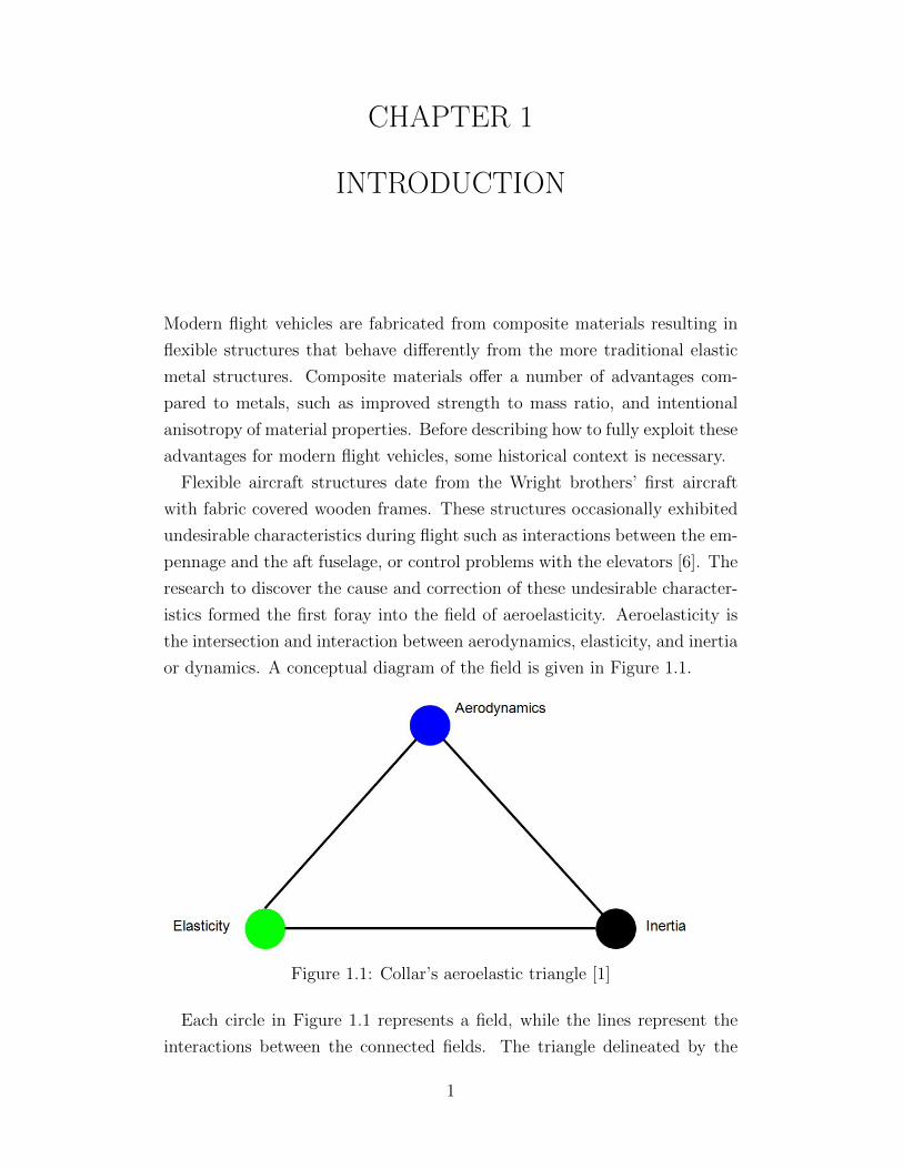
istics formed the first foray into the field of aeroelasticity. Aeroelasticity is
the intersection and interaction between aerodynamics, elasticity, and inertia
or dynamics. A conceptual diagram of the field is given in Figure 1.1.
Figure 1.1: Collar’s aeroelastic triangle [1]
Each circle in Figure 1.1 represents a field, while the lines represent the
interactions between the connected fields. The triangle delineated by the
1
interaction lines is the surface that represents aeroelasticity.
Aeroelasticity is well suited for metal aircraft, but requires several expan-
sions to improve its applicability to composite vehicles. The first is a change
from elasticity to viscoelasticity to more accurately capture the solid me-
chanics of the composite material. The second change is to include control
systems. While the inclusion of control systems in aeroelasticity lead to aero-
servo-elasticity [7], more control possibilities exist for a composite material.
As an example, during the lay-up of carbon-epoxy plies, piezoelectric con-
trol patches are inserted between different plies to give a variety of control
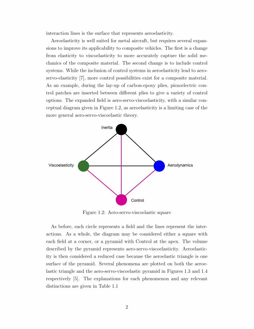
options. The expanded field is aero-servo-viscoelasticity, with a similar con-
ceptual diagram given in Figure 1.2, as aeroelasticity is a limiting case of the
more general aero-servo-viscoelastic theory.
Figure 1.2: Aero-servo-viscoelastic square
As before, each circle represents a field and the lines represent the inter-
actions. As a whole, the diagram may be considered either a square with
each field at a corner, or a pyramid with Control at the apex. The volume
described by the pyramid represents aero-servo-viscoelasticity. Aeroelastic-
ity is then considered a reduced case because the aeroelastic triangle is one
surface of the pyramid. Several phenomena are plotted on both the aeroe-
lastic triangle and the aero-servo-viscoelastic pyramid in Figures 1.3 and 1.4
respectively [5]. The explanations for each phenomenon and any relevant
distinctions are given in Table 1.1
2
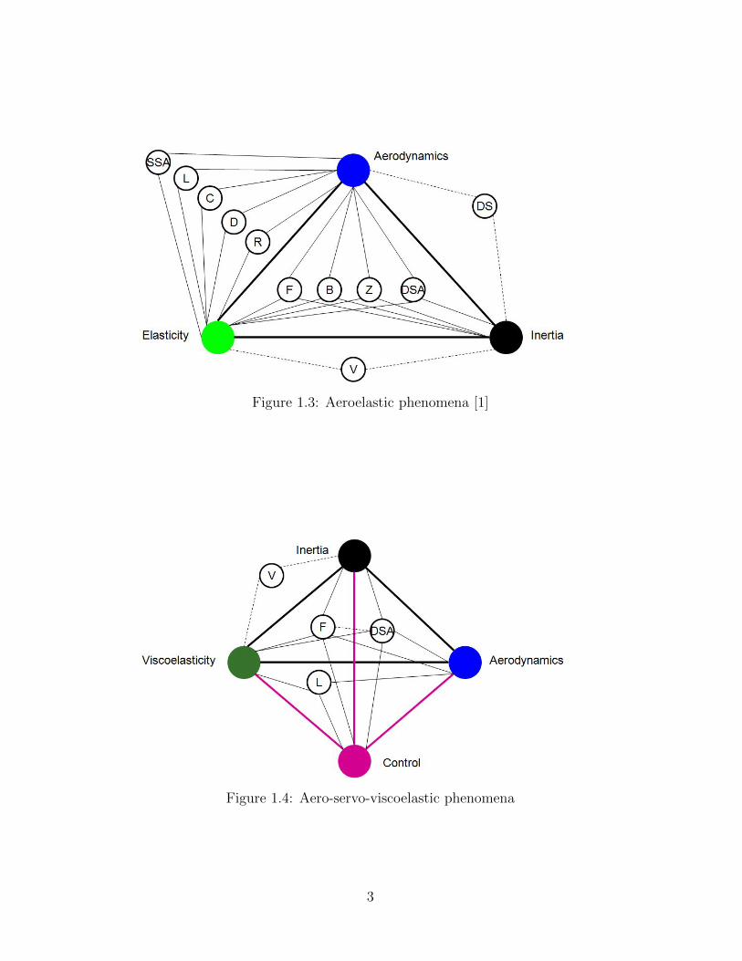
Figure 1.3: Aeroelastic phenomena [1]
Figure 1.4: Aero-servo-viscoelastic phenomena
3
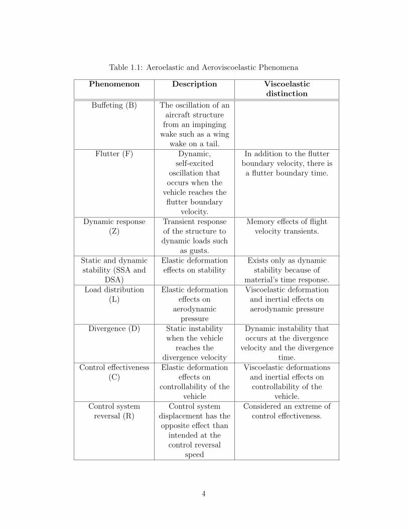
Table 1.1: Aeroelastic and Aeroviscoelastic Phenomena
Phenomenon Description Viscoelasticdistinction
Buffeting (B) The oscillation of anaircraft structure
from an impingingwake such as a wing
wake on a tail.Flutter (F) Dynamic,
self-excitedoscillation thatoccurs when the
vehicle reaches theflutter boundary
velocity.
In addition to the flutterboundary velocity, there isa flutter boundary time.
Dynamic response(Z)
Transient responseof the structure todynamic loads such
as gusts.
Memory effects of flightvelocity transients.
Static and dynamicstability (SSA and
DSA)
Elastic deformationeffects on stability
Exists only as dynamicstability because of
material’s time response.Load distribution
(L)Elastic deformation
effects onaerodynamic
pressure
Viscoelastic deformationand inertial effects onaerodynamic pressure
Divergence (D) Static instabilitywhen the vehicle
reaches thedivergence velocity
Dynamic instability thatoccurs at the divergence
velocity and the divergencetime.
Control effectiveness(C)
Elastic deformationeffects on
controllability of thevehicle
Viscoelastic deformationsand inertial effects oncontrollability of the
vehicle.Control system
reversal (R)Control system
displacement has theopposite effect than
intended at thecontrol reversal
speed
Considered an extreme ofcontrol effectiveness.
4
The additions to aerospace knowledge by aero-servo-viscoelasticity are
highlighted by demonstrating that the limiting cases of the theory are identi-
cal to aeroelasticity. Further, the relevant aeroelastic research produced over
the past decades is referenced in each section so that specific areas of growth
are identified.
The organization of this dissertation is into seven chapters: aerodynamics,
control theory, dynamics, viscoelasticity, dynamic stability of wings, panel
instability, and flight velocity transient response. The first four chapters
build the necessary background theory from the four fields that contribute
to aero-servo-viscoelasticity. The last three chapters are classes of problems
that appear in aerospace engineering and can benefit from an aero-servo-
viscoelastic approach. Each chapter incorporates a review of pertinent liter-
ature to provide context.
The most important contributions from this work are found in the aerody-
namics, two-dimensional wings, three-dimensional plates, and flight velocity
transients chapters. A number of novel expansions to unsteady aerodynamics
are required to solve the wing and plate problems. The expansions include
changes to Theodorsen’s function to accommodate damped motion, and flight
velocity transients.
5
CHAPTER 2
AERODYNAMICS
For an aero-servo-viscoelastic problem, unsteady aerodynamics analyses are
required to account for the motion of the structure and the influence of the
wake. The two- and three-dimensional problems in Chapters 6 and 7 require
subsonic and supersonic aerodynamic formulations; therefore 2-D subsonic,
2-D supersonic, 3-D subsonic, and 3-D supersonic unsteady aerodynamics
will be formulated in the following sections. The subsonic formulations in-
clude incompressible and compressible versions. All the formulations will
begin at the fundamentals using Green’s functions. The focus of this chapter
is on unsteady aerodynamics. A concise summary of aerodynamics for wings
and bodies is given in [8]. For purposes here, an isolated lifting surface or
panel is considered to avoid the complication of interactions between bod-
ies in an airflow [9]. Introductory resources on unsteady aerodynamics are
available by Stannard [10], Vel [11], Bland [12], Burggraf [13], Cebeci et al
[14], Wright and Cooper [15], and Botez et al [16]. Other approaches for the
derivation of unsteady aerodynamics are described by Jones [17, 18], Postel
and Leppert [19], Goland [20], Kurzin [21], Fromme and Halstead [22], Rowe
et al [23], Kemp and Homicz [24], Hemdan [25], Strganac [26], and Gulyaev
et al [27]. There is some overlap in applications of unsteady aerodynam-
ics between aero-servo-viscoelasticity and flapping flight. Two investigations
into flapping flight aerodynamics are by Ol [28] and Robertson et al [29].
A further overlap is with rotary aircraft where earlier research into variable
velocity effects on unsteady aerodynamics for rotor blades was conducted by
Isaacs [30] and Greenberg [31].
6
2.1 Preliminaries
To begin, consider a control volume that contains a two-dimensional flow as
shown in Figure 2.1.
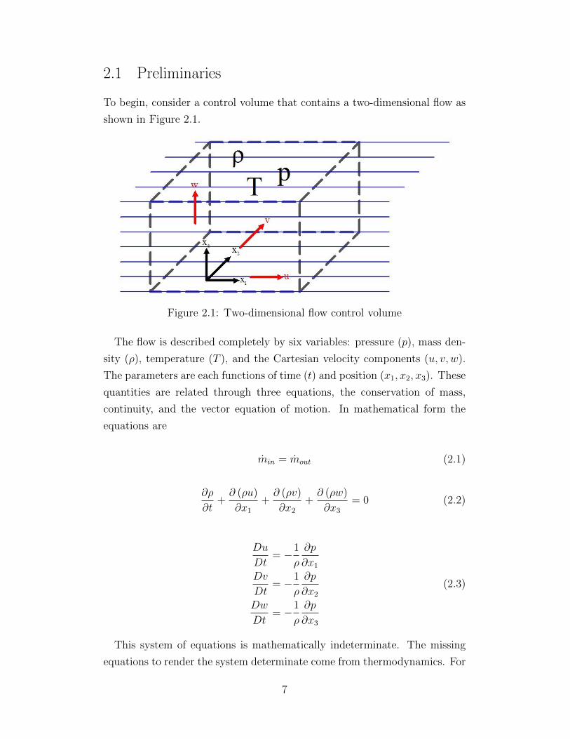
Figure 2.1: Two-dimensional flow control volume
The flow is described completely by six variables: pressure (p), mass den-
sity (ρ), temperature (T ), and the Cartesian velocity components (u, v, w).
The parameters are each functions of time (t) and position (x1, x2, x3). These
quantities are related through three equations, the conservation of mass,
continuity, and the vector equation of motion. In mathematical form the
equations are
min = mout (2.1)
∂ρ
∂t+∂ (ρu)
∂x1
+∂ (ρv)
∂x2
+∂ (ρw)
∂x3
= 0 (2.2)
Du
Dt= −1
ρ
∂p
∂x1
Dv
Dt= −1
ρ
∂p
∂x2
(2.3)
Dw
Dt= −1
ρ
∂p
∂x3
This system of equations is mathematically indeterminate. The missing
equations to render the system determinate come from thermodynamics. For
7
aeroelastic purposes, the thermodynamic equations are not necessary as the
state of the fluid is represented by a disturbance pressure. The disturbance
pressure is related to a velocity potential, φ (x1, x2, x3, t), that removes a
number of dependent variables from the problem. Use of the velocity poten-
tial relies on the assumption of irrotationality of the flow.
The relationship between the velocity potential and the pressure is given
by Kelvin’s equation:
∇2φ− 1
a2
[∂2φ
∂t2+∂q2
∂t+ q · grad
(q2
2
)]= 0 (2.4)
where
q = ui+ vj + wk = gradφ (2.5)
and a is the speed of sound.
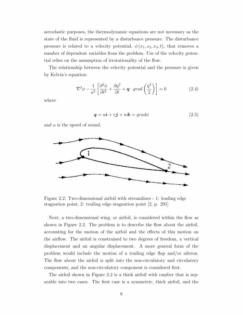
Figure 2.2: Two-dimensional airfoil with streamlines - 1: leading edgestagnation point, 2: trailing edge stagnation point [2, p. 291]
Next, a two-dimensional wing, or airfoil, is considered within the flow as
shown in Figure 2.2. The problem is to describe the flow about the airfoil,
accounting for the motion of the airfoil and the effects of this motion on
the airflow. The airfoil is constrained to two degrees of freedom, a vertical
displacement and an angular displacement. A more general form of the
problem would include the motion of a trailing edge flap and/or aileron.
The flow about the airfoil is split into the non-circulatory and circulatory
components, and the non-circulatory component is considered first.
The airfoil shown in Figure 2.2 is a thick airfoil with camber that is sep-
arable into two cases. The first case is a symmetric, thick airfoil, and the
8
second case is a curved plate at an angle of attack α. By separating the
airfoil into two cases, the effects of thickness, and angle of attack and airfoil
camber are considered separately assuming the problem remains linear. The
symmetric, thick airfoil does not contribute to lift within the constraints of
potential flow theory. The angle of attack and camber effects are considered
in the following.
The airfoil imposes boundary conditions on the flow in addition to bound-
ary conditions at infinity. The surface boundary condition is that the fluid
particles adjacent to the surface must have a perpendicular velocity that
matches the surface velocity. Neglecting this boundary condition would im-
ply the formation of fluid voids along the surface. If zU and zL define the
upper and lower surfaces of the airfoil respectively, then the vertical velocity,
w, over the surface is
w =∂zU∂t
+ u∂zU∂x1
+∂zU∂x2
; for x3 = zU , (x1, x2) ∈ Ra (2.6)
w =∂zL∂t
+ u∂zL∂x1
+∂zL∂x2
; for x3 = zL, (x1, x2) ∈ Ra (2.7)
where Ra is the projected planform of the entire wing on to the x1x2-plane;
a valid projection because the camber of the airfoil is small. Further simplifi-
cations are possible using the geometry of the wing. The slopes∂x3
∂x1
and∂x3
∂x2indicate the curvature of the wing in the chordwise and spanwise directions.
The wing is assumed to be straight; therefore, the spanwise curvature is zero.
The fluid vector q resulting from the presence of the airfoil is only slightly
different than the freestream velocity vector, U (t) i, so a disturbance velocity
potential, φ′is defined as
φ = φ′ + U (t)x1 (2.8)
that implies that u = U (t)+u′. Of particular note here is the introduction of
a time varying freestream velocity. In Bisplinghoff [5, p. 197], and most other
aeroelastic analyses, the freestream velocity is assumed to be constant. The
present inclusion of the time varying freestream velocity is representative of
changes in the flight velocity of an aircraft. Further, a time varying freestream
velocity reveals some interesting effects as will be shown.
Substitution of Equation 2.8 into Equation 2.6 results in a u′∂x3
∂x1
term that
9

is considered negligible because u′ U (t) for the linear case.
With the disturbance velocity potential defined, the boundary condition
is stated as
w(x1, 0
±, t)
=∂φ′
∂x3
(x1, 0
±, t)
(2.9)
where the airfoil is replaced with an infinitesimally thin distribution of sources
and sinks on the x1x2-plane that produce the flow about the airfoil. The
vertical velocity is then
w (t) =∂zU∂t
+ U (t)∂zU∂x1
; for x3 = 0+, (x1, x2) ∈ Ra (2.10)
w (t) =∂zU∂t
+ U (t)∂zL∂x1
; for x3 = 0−, (x1, x2) ∈ Ra (2.11)
Using Equation 2.8 and applying the boundary condition to the terms
within the square bracket in Equation 2.4 gives
∂2φ
∂t2+∂q2
∂t+q·grad
(q2
2
)=∂2φ′
∂t2+2 [U (t) i+ gradφ′]· ∂
∂t[U (t) i+ gradφ′] +
+ [U (t) i+ gradφ′] · grad
[U(t)2
2+ U (t) i · gradφ′ + 1
2|gradφ′|2
]∼=∂2φ′
∂t2+ 2U (t)
∂U (t)
∂t+ 2
∂U (t)
∂t
∂φ′
∂x1
+ 2U (t)∂2φ′
∂x1∂t+ U(t)2 ∂
2φ′
∂x12
(2.12)
If the freestream velocity is constant, then the second and third terms
in Equation 2.12 disappear and the equation reduces to the form given in
Bisplinghoff [5]. Substituting the result of Equation 2.12 into Equation 2.4
gives the linearized partial differential equation for time-varying, unsteady,
compressible flow:
∇2φ′ − 1
a2∞
[∂2φ′
∂t2+ 2U (t)
∂U (t)
∂t+
2∂U (t)
∂t
∂φ′
∂x1
+ 2U (t)∂2φ′
∂x1∂t+ U(t)2 ∂
2φ′
∂x12
]= 0 (2.13)
with the boundary conditions as given in Equations 2.10 and 2.11.
10
2.2 2-D Incompressible Flow
If the mass density (ρ) of the flow is constant, then the flow is considered in-
compressible. The stipulation of constant density has the implication that the
speed of sound (a∞) is very large compared to the small disturbance veloci-
ties; rendering their effects negligible. In the classic derivation by Theodorsen
[32] using a constant freestream velocity, the governing partial differential
equation reduces to a Laplace equation
∇2φ′ = 0 (2.14)
With a time-varying freestream velocity, the Poisson equation
∇2φ′ =2
a2∞U (t)
∂U (t)
∂t(2.15)
is the result, because the freestream velocity is not negligible compared to
the speed of sound.
The next step is to solve the Poisson equation subject to the two boundary
conditions. In effect, two problems are considered: the non-circulatory flow
above the airfoil, and the non-circulatory flow below the airfoil. The problem
is linearized so superposition of the two solutions is permissible in order to
give the final solution.
2.3 Solution to Poisson Equation
There are several approaches to solving the Poisson equation. One method
is by separation of variables in the form
φ′ = X1 (x1)X2 (x2) Υ (t) (2.16)
The time component of velocity potential is directly known because the
flow oscillations are required to match the structural oscillations. This leads
to a general solution of the form
Υ (t) = exp (λt) (2.17)
where
11
λ = d+ iω (2.18)
The physical meaning of d is a damped motion and ω is the circular fre-
quency of the motion, with both terms having units of1
Time. The spatial
solutions for X1 (x1) and X2 (x2) could be solved using Fourier transforms,
but an easier method is to use Green’s functions.
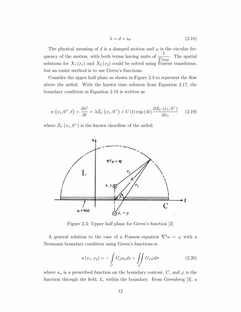
Consider the upper half plane as shown in Figure 2.3 to represent the flow
above the airfoil. With the known time solution from Equation 2.17, the
boundary condition in Equation 2.10 is written as
w(x1, 0
+, t)
=∂φ′
∂t= λZU
(x1, 0
+)
+ U (t) exp (λt)∂ZU (x1, 0
+)
∂x1
(2.19)
where ZU (x1, 0+) is the known chordline of the airfoil.
Figure 2.3: Upper half plane for Green’s function [3]
A general solution to the case of a Poisson equation ∇2u = ϕ with a
Neumann boundary condition using Green’s functions is
u (x1, x2) = −∫C
Gfunds+
∫∫L
Gfϕdσ (2.20)
where un is a prescribed function on the boundary contour, C, and ϕ is the
function through the field, L, within the boundary. From Greenberg [3], a
12
Poisson equation of the form ∇2u = ϕ on the half-plane with a Neumann
boundary condition ux3 = h (x1) on x3 = 0 has the known solution
u (x1, x3) = − 1
2π
∞∫−∞
ln[(ξ − x1)2 + x3
2]h (ξ) dξ+
+1
4π
∞∫−∞
∞∫−∞
ln[
(ξ − x1)2 + (η − x3)2] ·[(ξ − x1)2 + (η + x3)2]ϕ (ξ, η) dξdη (2.21)
subject to the additional restrictions of∫∫L
ϕdσ = 0 (2.22)
and
∞∫−∞
hdξ = 0 (2.23)
Before continuing, some comments about the physical meaning of Equation
2.21 are necessary so that the solution has a meaning in the context of the
flow field problem.
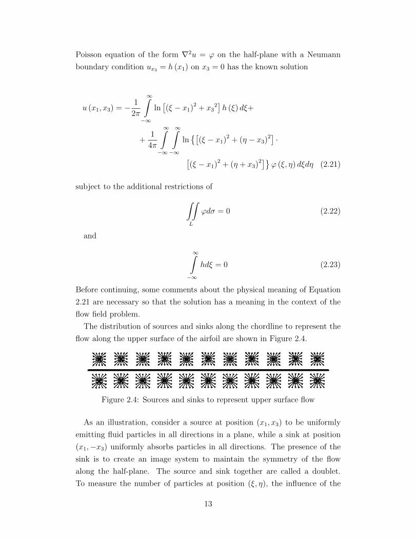
The distribution of sources and sinks along the chordline to represent the
flow along the upper surface of the airfoil are shown in Figure 2.4.
Figure 2.4: Sources and sinks to represent upper surface flow
As an illustration, consider a source at position (x1, x3) to be uniformly
emitting fluid particles in all directions in a plane, while a sink at position
(x1,−x3) uniformly absorbs particles in all directions. The presence of the
sink is to create an image system to maintain the symmetry of the flow
along the half-plane. The source and sink together are called a doublet.
To measure the number of particles at position (ξ, η), the influence of the
13
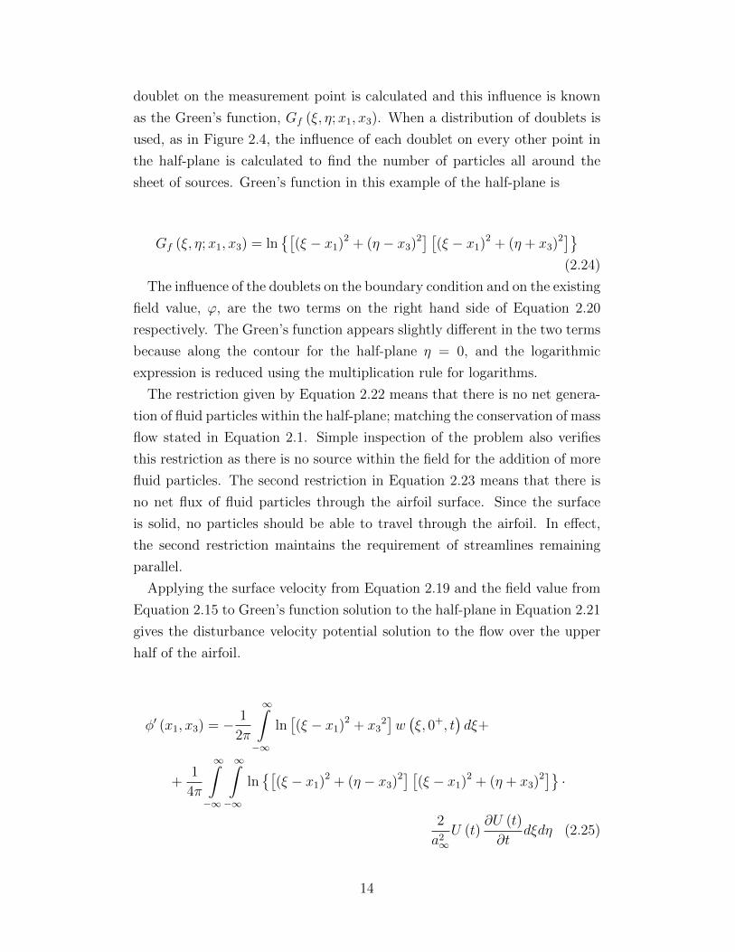
doublet on the measurement point is calculated and this influence is known
as the Green’s function, Gf (ξ, η;x1, x3). When a distribution of doublets is
used, as in Figure 2.4, the influence of each doublet on every other point in
the half-plane is calculated to find the number of particles all around the
sheet of sources. Green’s function in this example of the half-plane is
Gf (ξ, η;x1, x3) = ln[
(ξ − x1)2 + (η − x3)2] [(ξ − x1)2 + (η + x3)2](2.24)
The influence of the doublets on the boundary condition and on the existing
field value, ϕ, are the two terms on the right hand side of Equation 2.20
respectively. The Green’s function appears slightly different in the two terms
because along the contour for the half-plane η = 0, and the logarithmic
expression is reduced using the multiplication rule for logarithms.
The restriction given by Equation 2.22 means that there is no net genera-
tion of fluid particles within the half-plane; matching the conservation of mass
flow stated in Equation 2.1. Simple inspection of the problem also verifies
this restriction as there is no source within the field for the addition of more
fluid particles. The second restriction in Equation 2.23 means that there is
no net flux of fluid particles through the airfoil surface. Since the surface
is solid, no particles should be able to travel through the airfoil. In effect,
the second restriction maintains the requirement of streamlines remaining
parallel.
Applying the surface velocity from Equation 2.19 and the field value from
Equation 2.15 to Green’s function solution to the half-plane in Equation 2.21
gives the disturbance velocity potential solution to the flow over the upper
half of the airfoil.
φ′ (x1, x3) = − 1
2π
∞∫−∞
ln[(ξ − x1)2 + x3
2]w(ξ, 0+, t
)dξ+
+1
4π
∞∫−∞
∞∫−∞
ln[
(ξ − x1)2 + (η − x3)2] [(ξ − x1)2 + (η + x3)2] ·2
a2∞U (t)
∂U (t)
∂tdξdη (2.25)
14

The disturbance velocity potential is a helpful tool for calculating the flow,
but needs to be related to a physical property of the flow. The most direct re-
lationship is to the pressure through a manipulation of the unsteady Bernoulli
equation:
p− p∞ = −ρ[U (t)
∂φ′
∂x1
+∂φ′
∂t
](2.26)
where p∞ is the ambient pressure. The net pressure on the airfoil is the
difference between the pressures on the upper and lower surfaces. Therefore
pU − pL = −ρ[U (t)
(∂φ′U∂x1
− ∂φ′L∂x1
)+
(∂φ′U∂t− ∂φ′L
∂t
)](2.27)
The expressions for the disturbance velocity potentials are from Equation
2.25; however, only the first integral is relevant. The second integral that
includes the time-varying velocity is the same above and below the airfoil. In
the pressure difference equation, the time-varying velocity does not provide
any contribution. The first integral is different by a negative sign between
the upper and the lower potentials because of the surface velocity. The result
is
pU − pL = −2ρ
[U (t)
(∂φ′U∂x1
)+
(∂φ′U∂t
)](2.28)
The non-circulatory lift and moment of the airfoil are then easily found
using the known pressure equation and the expressions
LNC = −b∫
−b
(pU − pL) dx1 (2.29)
and
MyNC =
b∫−b
(pU − pL) (x1 − ba) dx1 (2.30)
where b is the half-chord length of the airfoil, and a is the nondimensional
location of a reference axis as a percentage of the half-chord.
The next step is to find the pressure, lift, and moment for a given airfoil
15

chordline. Of interest is to find a result that corresponds to Theodorsen’s
derivation for a constant freestream velocity. For this case, the airfoil is
chordwise rigid and Figure 2.5 gives a schematic of the problem:
Figure 2.5: Chordwise rigid, two-dimensional airfoil
The equation for the chordline of this flat plate airfoil is
za (x1, t) = −h− α (x1 − ba) (2.31)
where the vertical displacement or plunge is given by h and the angular
displacement or pitch is given by α. Substitution into Equation 2.10 gives
wa (x1, t) = −h− U (t)α− α (x1 − ba) (2.32)
Subsequent substitution into the first integral of the disturbance velocity
potential gives
φ′U (x1, x3) = − 1
2π
∞∫−∞
ln[(ξ − x1)2 + x3
2]·
[−h− U (t)α− α (ξ − ba)
]dξ (2.33)
Rearranging
16
φ′U (x1, x3) =
[h+ U (t)α
]2π
∞∫−∞
ln[(ξ − x1)2 + x3
2]dξ+
+1
2π
∞∫−∞
ln[(ξ − x1)2 + x3
2]
[α (ξ − ba)] dξ (2.34)
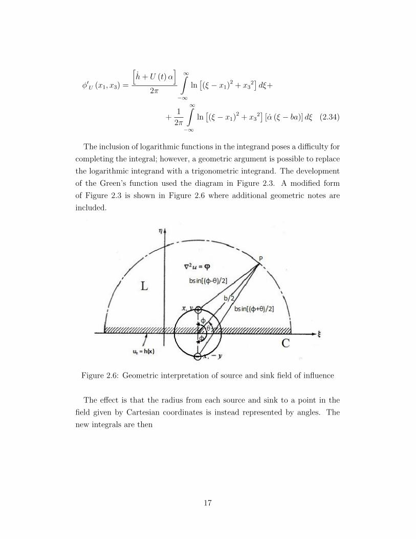
The inclusion of logarithmic functions in the integrand poses a difficulty for
completing the integral; however, a geometric argument is possible to replace
the logarithmic integrand with a trigonometric integrand. The development
of the Green’s function used the diagram in Figure 2.3. A modified form
of Figure 2.3 is shown in Figure 2.6 where additional geometric notes are
included.
Figure 2.6: Geometric interpretation of source and sink field of influence
The effect is that the radius from each source and sink to a point in the
field given by Cartesian coordinates is instead represented by angles. The
new integrals are then
17
φ′U (x1, x3) =b[h+ U (t)α
]π
π∫θ
π∫0
sin2φdφdθ
(cosφ− cos θ)
+b2α
π
π∫θ
π∫0
sin2φ [cosφ− a] dφdθ
(cosφ− cos θ)(2.35)
Evaluating the integrals gives a disturbance velocity potential of
φ′U (θ, t) = b[h+ U (t)α
]sin θ + b2α sin θ
[1
2cos θ − a
](2.36)
The potential is consistent with the results of Bisplinghoff and Theodorsen
other than a variable change of x1 = cos θ. The consistency is to be expected
as the only modification at this point is the inclusion of a time-varying free-
stream velocity. Applying the geometry modifications to the pressure equa-
tion in Equation 2.28 gives
(pU − pL)NC = −2ρ
[∂φ′U∂t− U (t)
b sin θ
∂φ′U∂θ
](2.37)
Substituting the potential gives a pressure distribution of
(pU − pL)NC = −2ρ
[bh sin θ + b
∂U (t)
∂tα sin θ + bU (t) α sin θ+
b2α sin θ
[1
2cos θ − a
]]+ 2ρ
[U (t)
b sin θ
[b[h+ U (t)α
]cos θ+
b2α cos θ
[1
2cos θ − a
]+ b2α sin θ
(−1
2sin θ
)]](2.38)
Grouping by the derivative orders of the displacements provides a more com-
pact expression
18
(pU − pL)NC = −2ρ
[b sin θ] h+
[−U (t) cot θ] h+
[b∂U (t)
∂tsin θ − U(t)2 cot θ
]α+
+
[sin θ − cot θ
(1
2cos θ − a
)+
1
2sin θ
]bU (t) α+
+
[1
2cos θ − a
]b2 sin θα
(2.39)
The non-circulatory lift is then
LNC = πρb2[h+ U (t)α + U (t) α− baα
](2.40)
and the non-circulatory moment is
MyNC = πρb2[U (t) h+ bah+
(U2 (t) + baU (t)
)α−
b2
(1
8+ a2
)α
](2.41)
Compared to Theodorsen’s derivation, these results are almost identical save
for the appearance of an extra term involving the first derivative of the
freestream velocity.
As mentioned earlier, the problem of the air flow around the airfoil was
separated into the non-circulatory and circulatory components. The lift and
moment of the non-circulatory component are now known for a time-varying
freestream velocity. What remains is to find the circulatory component.
By inspection of Theodorsen’s derivation, the presence of the time-varying
freestream velocity will not have an effect as there are no time derivatives in
the calculations. A modification is required because in Theodorsen’s original
work he assumed simple harmonic motion in the derivation of his eponymous
function [32]. Theodorsen wrote
“There is presumably no necessity of solving a general case of
damped or divergent motion, but only the border case of a pure
sinusoidal motion, applying to the case of unstable equilibrium
[32, p.291].”
19
Theodorsen’s derivation has not been revisited often to extended his results
to the case of damped motion. A generalization was implied by S’ohngen [33]
and a procedure given by Fraeys de Veubeke [34]. Extensions were completed
by Sears [35], Edwards and Ashley [36] using Laplace transforms, Bagley et al
using fractional calculus [37], and Tomonari [38]. Damped motion included
in the unsteady aerodynamics is necessary to investigate the possibility of
multiple stability points in aero-viscoelasticity. The starting assumption in
extending Theodorsen’s derivation to damped motion is that Theodorsen’s
derivation of the non-circulatory component is valid for the damped motion
case. The derivation is valid as seen earlier because the model for the motion
of the airfoil does not have a significant effect on the non-circulatory potential
flow model. Indeed, the airfoil motion only appears as the velocity wa that
acts as the boundary condition to the problem. An independent derivation
of unsteady motion with a constant freestream velocity by von Karman and
Sears confirms this assumption [39].
In Theodorsen’s derivation he sets Us = f (vt− x0) where Us is the strength
of a surface of discontinuity extending from the wing to infinity to describe
the circulatory flow, t is time, and v is freestream velocity. The x0 term is
a non-dimensional distance of a vortex element in the wake relative to the
wing in a conformal mapping space. The function U appears in the general
form of Theodorsen’s function which is
C =
∞∫1
x0√x2
0 − 1Usdx0
∞∫1
x0 + 1√x2
0 − 1Usdx0
(2.42)
Theodorsen’s assumption of simple harmonic motion appears when he as-
sumes the following
Us = U0 expi[k(sb− x0
)+ ϕ
](2.43)
where s = vt is the distance from the first vortex element to the airfoil, b is
the half-chord length, and k is a positive constant for the wavelength. The
integrals in Equation 2.42 are re-expressed using Hankel functions to give
20
C (k) =H
(2)1 (k)
H(2)1 (k) + iH
(2)0 (k)
(2.44)
The damped motion version or generalized Theodorsen function starts from
Theodorsen’s general, integral version of his function. Assume U is of the
following form:
Us = U0 expd(sb− x0
)+ i[k(sb− x0
)+ ϕ
](2.45)
where d is either a positive or negative constant that acts as the real com-
ponent to the imaginary component represented by k. Similar to k, d is
non-dimensional. Substitution of Equation 2.45 into Equation 2.42 and ex-
panding the exponential gives
C =
∞∫1
x0√x2
0 − 1
U0 exp
[d(sb− x0
)]exp
[ik(sb− x0
)]exp [iϕ]
dx0
∞∫1
x0 + 1√x2
0 − 1
U0 exp
[d(sb− x0
)]exp
[ik(sb− x0
)]exp [iϕ]
dx0
(2.46)
The U0, exp(ds
b
), exp
(iks
b
), and exp (iϕ) terms cancel out in both the
numerator and denominator because they are constants with respect to the
integration variable x0. The remaining exponential expressions are grouped
together as follows
(d+ ik
)(−x0) = λ (−x0) (2.47)
In the above, d, k, and λ are all non-dimensional terms. The notation is
intentionally similar to Equation 2.18 because there is a connection between
λ and λ. Typically, k is referred to as the reduced frequency and defined as
k =ωb
U[40]. Using the same non-dimensionalization, d and d are related by
d =db
U. This non-dimensionalization works for a constant flight velocity, but
for a time-varying flight velocity a different definition is required for d, k or
their combined form λ. The presence of a time varying flight velocity alters
the value of s = vt to s =t∫
0
v (τ) dτ ; however, as s→∞ the influence of the
flight velocity transient will become negligible on the total distance travelled
21
so the first equation for s and the non-dimensionalized frequency remain
valid. For short time periods, the non-dimensionalization using velocity is
no longer valid, but Theodorsen’s function of a constant is valid.
Using the λ grouping, Equation 2.46 becomes
C =
∞∫1
x0√x2
0 − 1
exp
[−λx0
]dx0
∞∫1
x0 + 1√x2
0 − 1
exp
[−λx0
]dx0
(2.48)
To convert the above integrals into Bessel function form, the table of integrals
from Abramowitz and Stegun is used [41]. Equation 9.6.23 from Abramowitz
and Stegun is
Kυ (z) =
√π
(1
2z
)υΓ
(υ +
1
2
) ∞∫1
exp [−zt](t2 − 1
)υ−1/2dt (2.49)
where z is a complex number and the following restrictions exist <υ > −1
2and |arg z| < π
2. The K Bessel functions are known as the modified Bessel
functions.
Setting υ in Equations 2.49 to 0 and 1 respectively gives
K0 (z) =
√π
Γ(
12
) ∞∫1
exp [−zt](t2 − 1
)−12 dt (2.50)
K1 (z) =
√π(
12z)
Γ(
32
) ∞∫1
exp [−zt](t2 − 1
) 12dt (2.51)
Starting with the numerator of 2.48 and integrating by parts gives
∞∫1
x0√x2
0 − 1exp
(−λx0
)dx0 = λ
∞∫1
√x2
0 − 1 exp(−λx0
)dx0 (2.52)
Substituting Equation 2.50 into Equation 2.52
22
∞∫1
x0√x2
0 − 1exp
(−λx0
)dx0 =
2Γ
(3
2
)√π
K1
(λ)
(2.53)
The denominator of Equation 2.48 is split into two parts. The first part
is identical to the numerator and has the same Bessel function substitution.
The second part is directly identifiable with the K0 Bessel function form.
∞∫1
1√x2
0 − 1exp
(−λx0
)dx0 =
Γ
(1
2
)√π
K0
(λ)
(2.54)
Therefore the intermediate general Theodorsen function is
C(λ)
=
2Γ
(3
2
)K1
(λ)
2Γ
(3
2
)K1
(λ)
+ Γ
(1
2
)K0
(λ) (2.55)
The Γ function values are known to be Γ
(1
2
)=√π and Γ
(3
2
)=
√π
2so
the final, general Theodorsen function is
C(λ)
=K1
(λ)
K1
(λ)
+K0
(λ) (2.56)
A check that the general Theodorsen function is correct is that the func-
tion should provide the classic function when simple harmonic motion is ap-
plied. To complete this check, two Bessel function relations are used. From
Abramowitz and Stegun’s Equation 9.6.4:
K0
(λ)
= −1
2πiH
(2)0
(λexp
(−πi
2
))(2.57)
K1
(λ)
= −1
2πi exp
(−πi
2
)H
(2)1
(λexp
(−πi
2
))(2.58)
Substituting Equations 2.57 and 2.58 into Equation 2.56 gives
23
C(λ)
=exp
(−πi2
)H
(2)1
(λexp
(−πi2
))exp
(−πi2
)H
(2)1
(λexp
(−πi2
))+H
(2)0
(λexp
(−πi2
)) (2.59)
By Euler’s formula
exp
(−iπ
2
)= −i (2.60)
So
C(λ)
=−iH(2)
1
(−iλ
)H
(2)1
(−iλ
)+ iH
(2)0
(−iλ
) (2.61)
Multiplying through by i, and setting d = 0 for simple harmonic motion,
λ = ik then gives
C (ik) =H
(2)1 (k)
H(2)1 (k) + iH
(2)0 (k)
(2.62)
which is the traditional Theodorsen’s function.
A necessary comment here regards Section 5-7 of Bisplinghoff because the
section implies that negative values of d within Theodorsen’s functions are
not possible. The basis for this conclusion is work by W.P.Jones [18], partic-
ularly the appendix to Jones’ paper. There is a slight error in the appendix in
the application of the Bessel functions leading to the conclusion that decay-
ing oscillations cause the integrals in Equation 2.48 to diverge. Sears proves
however by analytic continuation that the decaying oscillations are feasible
within the generalized Theodorsen’s function [35].
The circulatory component of the lift and moment is now possible to ex-
press using Theodorsen’s function to account for the unsteadiness. Further,
the circulatory component satisfies the Kutta condition at the trailing edge
of the airfoil; unlike the non-circulatory component. Similar to the sources
and sinks used for the non-circulatory component, a sheet of vortex elements
is postulated to represent the wake from the airfoil. Graphically, the vortex
elements and their induced velocities are shown in Figure 2.7.
After some geometrical manipulation, the induced velocity qθ becomes
24
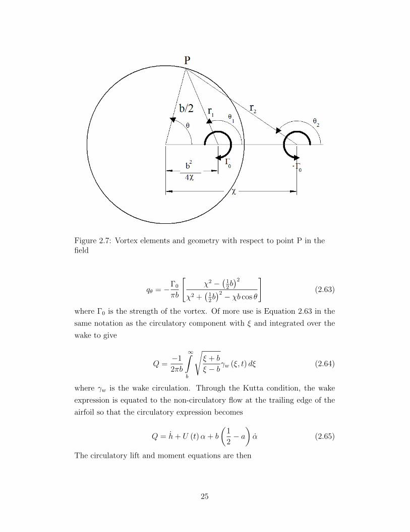
Figure 2.7: Vortex elements and geometry with respect to point P in thefield
qθ = −Γ0
πb
[χ2 −
(12b)2
χ2 +(
12b)2 − χb cos θ
](2.63)
where Γ0 is the strength of the vortex. Of more use is Equation 2.63 in the
same notation as the circulatory component with ξ and integrated over the
wake to give
Q =−1
2πb
∞∫b
√ξ + b
ξ − bγw (ξ, t) dξ (2.64)
where γw is the wake circulation. Through the Kutta condition, the wake
expression is equated to the non-circulatory flow at the trailing edge of the
airfoil so that the circulatory expression becomes
Q = h+ U (t)α + b
(1
2− a)α (2.65)
The circulatory lift and moment equations are then
25
LC = 2πρU (t) bQC(λ)
(2.66)
and
MyC = 2πρU (t) b2
(a+
1
2
)QC
(λ)
(2.67)
Summing Equations 2.66 and 2.67 with Equations 2.40 and 2.41 respectively
gives the complete lift and moment equations.
2.4 2-D Compressible Potential Flow
As before in the two-dimensional incompressible potential flow problem, con-
sider a control volume within a flow. The compressible case with a time-
varying freestream velocity is the complete Equation 2.13, repeated below
for ease of reference:
∇2φ′ − 1
a2∞
[∂2φ′
∂t2+ 2U (t)
∂U (t)
∂t+ 2
∂U (t)
∂t
∂φ′
∂x1
+
2U (t)∂2φ′
∂x1∂t+ U(t)2 ∂
2φ′
∂x12
]= 0 (2.68)
The boundary conditions are the following
1. Neumann type boundary condition on the surface of the airfoil:
∂
∂x3
φ′ (x1, x3, t)|x3=0 = wa (x1, t) (2.69)
2. Kutta-Joukowski condition at the trailing edge, that stipulates that
the pressure goes to zero and that the flow leaves the airfoil smoothly.
Mathematically, the condition may be defined used the acceleration
potential, ψ
ψ (x1, x3, t) =∂φ′
∂t+ U
∂φ′
∂x1
(2.70)
and the Kutta-Joukowski condition is
limx1→b
ψ (x1, 0, t) = 0 (2.71)
26
A weaker, but more tractable formulation is that the limit exists.
3. In the far-field the disturbance velocity potential goes to zero.
For the case of a constant free-stream velocity, there is a solution to Equa-
tion 2.68 using function space formulations, devised by Balakrishnan [42].
The solution uses a Laplace transform in time, and Fourier transforms in
space. The resulting transformed expression can be worked back to a time-
domain solution, but Balakrishnan leaves the formulation in the Laplace-
Fourier transformed version for aeroelastic problems. A thorough quanti-
tative study on unsteady, compressible flow for oscillating airfoils was con-
ducted by Carr et al [43] prior to Balakrishnan’s work. A solution approach
for the Possio integral was described even earlier by Miles [44].
For a time-varying free-stream velocity, the Laplace transform is not ap-
plicable for a general velocity function. The Fourier transforms remain ap-
plicable for the spatial component. The first Fourier transform is on x2 to
eliminate that derivative. The transformed equation is
∂2φ
∂x12
√2πδ (ω)− ω2φ− 1
a2∞
[√
2πδ (ω)∂2φ
∂t2+ 2√
2πU (t)∂U (t)
∂tδ (ω)
]
− 1
a2∞
[2√
2πδ (ω)∂U (t)
∂t
∂φ
∂x1
+ 2√
2πδ (ω)U (t)∂2φ
∂x1∂t+
√2πδ (ω)U(t)2 ∂
2φ
∂x12
]= 0 (2.72)
where the Fourier transform used is
f (ω) =1√2π
∫f (x2) exp (−iωx2)dy (2.73)
Using Fourier transform on ξ gives
27
−[(
1−M(t)2) δ (ω)µ2 + δ (µ)ω2] ˜φ−
1
a2∞
2∂U (t)
∂t˜φ+ 2U (t)
∂˜φ
∂t
δ (ω) iµ
− 1
a2∞
∂2˜φ∂t2
√2πδ (ω, µ) = 2
√2πM (t)
∂M (t)
∂tδ (ω, µ) (2.74)
Rearranging the left-hand side by order of the time derivatives:
−√
2πδ (ω, µ)
a2∞
∂2˜φ∂t2− 2U (t) δ (ω) iµ
a2∞
∂˜φ
∂t
−[(
1−M(t)2) δ (ω)µ2 + δ (µ)ω2 − 2δ (ω) iµ
a2∞
∂U (t)
∂t
] ˜φ =
2√
2πM (t)∂M (t)
∂tδ (ω, µ) (2.75)
The remaining time variable is more difficult to handle. In Balakrishnan’s
constant freestream velocity case, a Laplace transform was used. For a time-
varying freestream velocity Equation 2.75 is a second-order non-homogeneous
linear differential equation with variable coefficients. The solution to a vari-
able coefficient differential equation is approximate. The method by Kulikov
[45] will be used here to solve for the homogeneous component of the differ-
ential equation. The particular solution is solved by inspection because for a
smooth change in freestream velocity, the function is likely a trigonometric
function.
The general equation considered by Kulikov [45] is
αx2′′ + f (x1)x2
′ + F (x1)x2 = 0 (2.76)
that has the solution
x2 =1
F (x1)[p− (f (x1)−m) r1]A1exp r1x1+
[p− (f (x1)−m) r2]A2exp r2x1 (2.77)
28
where r1 and r2 are the roots of the characteristic equation
r2 +mr + p = 0 (2.78)
Comparing Equation 2.76 to the homogeneous component of Equation 2.75
gives
α = −2πδ (ω, µ)
a2∞
f (τ) = 2U (t) δ (ω)
a2∞
iµ (2.79)
F (τ) = −(1−M(τ)2) δ (ω)µ2 +
2δ (ω)
a2∞
∂U (t)
∂tiµ− δ (µ)ω2
All that remains is to find m, p, A1, A2, r1, and r2. The roots are related
to the coefficients of the characteristic equation by
r1 = −1
2m+ k
r2 = −1
2m− k (2.80)
k =
√1
4m2 − p
The expressions for m and p are
m =1
t− t0
t∫t0
f (t) dt− α
t− t0ln
F (t)
F (t0)(2.81)
and
p =f (t)− f (t0)
t− t0+
1
t− t0
t∫t0
[F (t)− F ′ (t) f (t)
F (t)
]dt (2.82)
The expressions for A1 and A2 are
A1 = A10 −r2
r1 − r2
t∫t0
ςexp (−r1t)dt (2.83)
29
and
A2 = A20 +r2
r1 − r2
t∫t0
ςexp (−r2t)dt (2.84)
This leaves the terms A10, A20 and ς as the only unknowns. Their expres-
sions are as follows
A10 =
˜φt (t0)− ψ0r2
r1 − r2
exp (−r1t0), (2.85)
A20 =
ψ0r1 −˜φt (t0)
r1 − r2
exp (−r2t0) (2.86)
where
ψ0 =[f (t0)−m] z0 + F (t0)
˜φ (t0)
p(2.87)
and
ς =
[f (t)−m
p− αFt (t)
pF (t)
] ˜φtt +
[ft (t) + F (t)− p
p− Ft (t) f (t)
pF (t)
] ˜φt (2.88)
The equation for ς is problematic because the equation relies on the un-
known function˜φ. It is at this point that the solution becomes an approxi-
mation. Successive approximations starting from the initial conditions may
be used to find the solution. The equation for the zeroth approximation is
˜φ =
1
F (t)exp
(−1
2m (t− t0)
)[(ab− cd) cosh (k (t− t0)) +(
bd− ack2
k
)sinh (k (t− t0))
](2.89)
In the foregoing, k was assumed to be real, implying that the roots of
the characteristic equation are distinct. If the roots are instead complex
conjugates of each other, only the following changes are necessary:
30
r1 = −1
2m+ qi
r2 = −1
2m− qi (2.90)
q =
√p− 1
4m2
and
˜φ =
1
F (t)exp
(−1
2(t− t0)
)[(ab− cd) cos (q (t− t0)) +(
bd+ acq2
q
)sin (q (t− t0))
](2.91)
In both Equations 2.89 and 2.91, there are four additional formulae that
are required
a =F (t0)
˜φ (t0) + [f (t0)−m]
˜φt (t0)
p
b = p+1
2m [f (t)−m] (2.92)
c = f (t)−m
d =˜φt (t0) +
1
2am
To fully solve for the transformed homogeneous solution of the potential
function˜φ, the initial conditions for
˜φ and
˜φt are required. The conditions
may not both be zero, otherwise Equation 2.89 will be zero.
With the time solution known, the inverse Fourier transform on µ would
ordinarily be taken to find the spatial solution in terms of ξ. The natural
logarithm that appears in Equation 2.81 is problematic to invert. Instead,
similar to Balakrishnan, the solution is to remain in the Fourier transform
space with the boundary conditions in Equations 2.69 and 2.71 converted to
the Fourier transform space. This is not an issue because the lift and moment
equations may also be transformed and the entire aeroelastic problem solved
in the Fourier transform space.
The particular solution to Equation 2.75 is not specified here because the
31
solution is dependent on the function used to describe the variations in the
freestream velocity. This step is completed when a specific problem is con-
sidered with a prescribed freestream velocity function. As noted earlier, the
particular solution is solved by inspection because of the presence of trigono-
metric functions in the freestream velocity function.
2.5 3-D Potential Flow for Wings
The imposition of potential flow for a three-dimensional finite wing is the
most general formulation for describing the aerodynamics of an aero-viscoelastic
wing. The formulation also requires the most numerical solution, compared
to the one- and two-dimensional cases, to account for the influence of the
flow at every point on the wing. Some papers for three dimensional flow are
by Jones [46], Reissner [47], Ashley et al [48], Landahl and Stark [49], Morino
[50], and Dusto and Epton [51]. The derivation presented here is by Reissner
and originally reported in five NACA technical notes [47], [52], [53], [54],
[55]. A summarized version of Reissner’s work is reported in Bisplinghoff
[5]. Technical note 946 is the first description of an integral-surface theory
for a finite wing in unsteady motion in an incompressible flow. The specific
example used by Reissner is a rectangular wing.
Reissner subsequently generalized his theory to any wing planform in an
incompressible flow in note 1194. Numerical examples appeared in the com-
plimentary note 1195. Compressible flow was elaborated in note 1953 with
note 2274 completing the compressible flow development. The derivation
is internally consistent because removing the compressibility correction from
note 2274 produces the results of note 1194. Further removal of the span com-
ponent of the flow reduces the theory in note 1194 to the two-dimensional, in-
compressible work of Theodorsen. The compressible three-dimensional flow
in note 2274 reduced to two-dimensions gives the Possio integral equation
which is solved by Balakrishnan [42].
In all cases Reissner used simple harmonic motion and a constant freestream
velocity. The modifications here are to include general motion through the
use of the λ notation introduced in Equation 2.47, and the time-varying
freestream velocity. The derivation will cover all the points up to the govern-
ing equation of the flow that is subsequently solved by numerical methods.
32
The inclusion of general motion will be shown first.
The first step is to non-dimensionalize the units of space and time. The
dimensional units are X1, X2, X3, and T . Using the half-chord length b to
non-dimensionalize the spatial units, and λ for the time unit gives
x1 =X1
b
x2 =X2
b(2.93)
x3 =X3
b
t = λT
The displacement H of the wing, freestream velocity U , and pressure p be-
come
h =H
b
u =U
U∞(2.94)
p =P
12ρ∞U2
∞
The vertical velocity of the wing in dimensional form is
W =∂H
∂T+ U∞
∂H
∂X1
(2.95)
Non-dimensionalizing gives
w = λ∂h
∂t+
∂h
∂x1
(2.96)
where
λ =λb
U∞(2.97)
The non-dimensional governing equations are the Euler and continuity equa-
tions:
33
λ∂u
∂t+∂u
∂x1
= −1
2∇p (2.98)
M2
2
(λ∂p
∂t+
∂p
∂x1
)+∇ · u = 0 (2.99)
The boundary conditions are applied on the projected planform of the
wing. Similar to the two-dimensional case, the wing is represented by a
sheet of sources and sinks that exist in a plane at x3 = 0. For points within
the project planform of the wing, Ra:
w = λ∂h
∂t+
∂h
∂x1
(2.100)
Along the trailing edge of the wing, x1 = xt (x2) the Kutta condition applies
so the velocity u is finite. At points beyond the projected planform, the
pressure of the flow is zero. Upstream of the wing at x1 = −∞ the velocity
and pressure are both zero.
In undisturbed flow, the curl or rotation of the flow is zero providing a
relationship between the velocity and a velocity potential:
u = ∇φ (2.101)
Substituting the expression for the velocity potential into the continuity equa-
tion and the Euler equation of motion:
∇2φ+1
2M2
(λ∂p
∂t+
∂p
∂x1
)= 0 (2.102)
∇(λ∂φ
∂t+∂φ
∂x1
)= −1
2∇p (2.103)
Rearranging Equation 2.103 for the pressure gives
−1
2p = λ
∂φ
∂t+∂φ
∂x1
(2.104)
The pressure equation is applied to the continuity equation to change the
continuity equation into a function of the velocity potential only.
∇2φ−M2
(λ∂
∂t+
∂
∂x1
)2
φ = 0 (2.105)
34
The boundary conditions in Equation 2.100 and the subsequent paragraph
are changed to use the velocity potential. The new boundary conditions are
∂φ
∂x3
= λ∂h
∂t+
∂h
∂x1
x3 = 0; x1, x2 ∈ Ra
∇φ finite x3 = 0; x = xt (x2) (2.106)
φ = 0 x3 = 0; x1 = −∞
λ∂φ
∂t+∂φ
∂x1
= 0 x3 = 0; x1, x2 /∈ Ra
Next, consider the displacement to have the form
h (x1, x2, x3, t) = hk (x1, x2, x3) exp (t) (2.107)
Recall that the non-dimensionalized time includes the λ term. The first
boundary condition implies that the velocity potential should have the same
form so
φ (x1, x2, x3, t) = φk (x1, x2, x3) exp (t) (2.108)
With this form for the velocity potential, the continuity equation becomes
∇2φk −M2
(λ+
∂
∂x1
)2
φk = 0 (2.109)
The motion equation likewise becomes
−1
2pk = λφk +
∂φk∂x1
(2.110)
The boundary conditions are
∂φk∂x3
= λhk +∂hk∂x1
x3 = 0; x1, x2 ∈ Ra
∇φk finite x3 = 0; x1 = xt (x2) (2.111)
φk = 0 x3 = 0; x1 = −∞
λφk +∂φk∂x1
= 0 x3 = 0; x1, x2 /∈ Ra
The fourth boundary condition equation is integrated for the region outside
35
the planform to give
φk (x1, x2, 0) = c (x2) exp(−λx1
)(2.112)
The third boundary condition applied to Equation 2.112 provides some ad-
ditional details to specify c (x2); however, another region in the flow is defined
first. The region from the trailing edge of the planform to infinity is termed
the wake region, Rw. The remaining region is termed Rr. For streamlines
within Rr, the coefficient in Equation 2.112 is zero. The boundary conditions
are then
φk = 0 x3 = 0; x1, x2 ∈ Rr
φk =1
2Γk (x2) exp
(−λ [x1 − xt (x2)]
)x3 = 0; x1, x2 ∈ Rw (2.113)
where
1
2Γk = φk (xt, x2,+0) =
xt∫xl
∂φk∂x1
(x1, x2,+0) dx1 (2.114)
The function Γ is the circulation function, and in the two-dimensional case
was treated as the strength of a vortex in the wake. The vortex had a
matching image within the airfoil; hence the connection between Equation
2.114 and Equation 2.5. The integral is between the leading and trailing
edge of the planform and represents the image vortex. While the boundary
condition contains the vortex in the trailing wake. The circulation function
is given as
Γ = Γkexp (t) (2.115)
The continuity equation must be solved for x3 > 0 and the appropriate
boundary conditions. The circulation function Γk is also unknown and must
satisfy the Kutta condition at the trailing edge of the planform. For the
remainder of this derivation the subscript k is dropped.
The boundary of x3 > 0 imposes that∂φ
∂x1
may be represented in terms of
the chordwise velocity component u0 through
36
∂φ
∂x1
=1
2π
∫∫u0 (ξ, η)x3[
(x1 − ξ)2 + (x2 − η)2 + x32] 3
2
dξdη (2.116)
In the two-dimensional flow case, Green’s functions were used to deter-
mine the flow. While a different approach has been used here for the three-
dimensional flow, there is a commonality between the two approaches. Equa-
tion 2.116 is very similar to the influence function that appears in Equation
2.25 if an additional derivative is taken. Similar to a Green’s function acting
as a kernel for an operator, Equation 2.116 provides the kernel
K =1
2π
x3[(x1 − ξ)2 + (x2 − η)2 + x3
2] 3
2
(2.117)
After a series of steps identical to those of Reissner [52], the vertical velocity
in terms of a derivative of the velocity potential is
∂φ
∂x3
= − 1
2π
∫∫Ra+Rw
u0x1 − ξ[
(x1 − ξ)2 + (x2 − η)2 + x32] 3
2
dξdη
− 1
2π
∫∫Ra+Rw
∂u0
∂x3
x2 − η(x2 − η)2 + x3
2 x1 − ξ[(x1 − ξ)2 + (x2 − η)2 + x3
2] 1
2
+ 1
dξdη (2.118)
Next, substitute the first boundary condition in Equation 2.5 and the second
boundary condition in Equation 2.5 to give
37
w0 (x1, x2) = − 1
2πlimx3→0
∫∫Ra
u0(x1 − ξ)
(x1 − ξ)2 + (x2 − η)2 + x32 3
2
dξdη
+
∫∫Ra
∂u0
∂x3
x2 − η(x2 − η)2 + x3
2
x1 − ξ[(x1 − ξ)2 + (x2 − η)2 + x3
2] 1
2
+ 1
dξdη−1
2λ
∫∫Rw
Γ (η)exp
(−λ [ξ − xt (η)]
)(x1 − ξ)
(x1 − ξ)2 + (x2 − η)2 + x32 3
2
+exp
(−λξ
)ddη
[Γ (η) exp
(λxt
)](x2 − η)
(x2 − η)2 + x32
· x1 − ξ[(x1 − ξ)2 + (x2 − η)2 + x3
2] 1
2
+ 1
dξdη (2.119)
Equation 2.119 is only valid for straight leading edges such as a rectangular
planform. Equation 66 in Reference [47] has the appropriate modification to
generalize Equation 2.119 for any curved leading edge. Only a rectangular
planform will be considered here.
The circulation and chordwise velocity are now
1
2Γ (η) =
xt∫xl
u0 (ξ, η) dξ (2.120)
and
u0 (ξt, η) finite (2.121)
Using gap symmetry in the ξ and η directions, Equation 2.119 is rewritten.
The purpose of the gap symmetry is to remove possible singularity points that
represent locations where the coordinates of a source overlap the coordinates
of an influence point. A further modification is possible by assuming a rect-
angular planform with the leading and trailing edges at x1 = ±1 and the
wing tips at x2 = ±s. Equation 2.119 is then
38
w0 (x1, x2) = − 1
2π
1∫−1
s∫−s
u0 (ξ, η) (x1 − ξ)(x1 − ξ)2 + (x2 − η)2 3
2
+∂u0
∂η
1
(x2 − η)
x1 − ξ[(x1 − ξ)2 + (x2 − η)2] 1
2
+ 1
dξdη
+λexp
(λ)
4π
∞∫1
s∫−s
exp(−λξ
) Γ (η) (x1 − ξ)(x1 − ξ)2 + (x2 − η)2 3
2
+
dΓdη
(x2 − η)
x1 − ξ[(x1 − ξ)2 + (x2 − η)2] 1
2
+ 1
dξdη (2.122)
and the boundary conditions on the wing are
1
2Γ (η) =
1∫−1
u0 (ξ, η) dξ (2.123)
u0 (1, η) finite (2.124)
A more compact notation for Equation 2.122 is
w0 = I1 + I2 (2.125)
where I1 is the airfoil integral and I2 is the wake integral. A stationary airfoil
provides an approximation for the airfoil integral; where the two-dimensional
result is used with a three-dimensional correction term. Thus,
I1 ≈ −1
π
1∫−1
u0 (ξ, η)
x1 − ξdξ − 1
4π
s∫−s
dΓ
dη
1
x2 − ηdη (2.126)
where the first integral is the two-dimensional flow, and the second integral
is a three-dimensional correction. The wake integral is also split into two
parts with the two-dimensional wake as
I3 =λexp
(λ)
2πΓ (x2)
∞∫1
exp(−λξ
)x1 − ξ
dξ (2.127)
39
The circulation term is
Γ (x2) =1
2
s∫−s
Γ′ (η)|x2 − η|x2 − η
dη (2.128)
Applying Equations 2.127 and 2.128 to the wake integral, followed by an
integration by parts and some combining of terms leads to
I2 = I3 +λexp
(λ)
4π
∞∫1
s∫−s
exp(−λξ
)Γ′ (η)
x2 − η1− |x2 − η|x1 − ξ
+
(x1 − ξ)2 + (x2 − η)2 1
2
x1 − ξ
dξdη (2.129)
The integral in Equation 2.129 is split into two integrals to produce further
simplifications. The split is
∞∫1
=
∞∫x1
−1∫
x1
(2.130)
so that
I2 = I3 + I4 + I5 (2.131)
The integral I4 is simplified by introducing
τ = λ (ξ − x1) (2.132)
This change of variable includes an alteration of the bounds of the integrals.
The resulting integral is
40
I4 =exp
(λ (1− x1)
)4π
s∫−s
Γ′ (η)
x2 − η
∞∫0
exp (−τ)
1 +λ |x2 − η|
τ−
τ 2 + λ2(x2 − η)2
12
τ
dτ dη (2.133)
The approximations for the wake appear in integral I5 and hold when
|x2 − η| > |x1 − ξ|. The integral is
I5 ≈ −λexp
(λ)
4π
1∫x1
s∫−s
exp(−λξ
) Γ′ (η)
x2 − ηdηdξ
−λexp
(λ)
4πΓ′ (x2)
1∫x1
∞∫−∞
exp(−λξ
)x2 − η
[(x1 − ξ)2 + (x2 − η)2] 1
2
x1 − ξ− |x2 − η|
x1 − ξ
dηdξ (2.134)
After some integration and cancellation a simplified expression is
I5 ≈1− exp
(λ (1− x1)
)4π
s∫−s
Γ′ (η)
x2 − ηdη (2.135)
Substituting Equations 2.127, 2.133 and 2.135 into the equation for the
vertical velocity, Equation 2.122 gives an approximate form of
w0 ≈ −1
π
1∫−1
u0 (ξ, x2)
x1 − ξdξ +
λexp(λ)
2πΓ (x2)
∞∫1
exp(−λξ
)x1 − ξ
dξ
−exp
(λ (1− x1)
)4π
s∫−s
Γ′ (η)
x2 − η
1− S
(λ |x2 − η|
)dη (2.136)
where
41
S(λ |x2 − η|
)=
∞∫0
exp (−τ)
1 +λ |x2 − η| −
τ 2 + λ2(x2 − η)2
12
τ
(2.137)
Of particular note is the first integral in Equation 2.136 that involves the
chordwise flow velocity component. This integral indicates that the induced
velocity due to the finite-span effect varies across the chord.
Combining the two-dimensional theory and three-dimensional steady flow
theory provides an approach to solve for circulation Γ by numerical meth-
ods. Section lift and moment are known once the circulation is known. In
Equation 2.136 the chordwise velocity component is the unknown because
the out of plane velocity component is dictated by the structure of the wing.
The chordwise velocity component is found by using the Sohngen inversion
formulae [47]. If
g (x1) = − 1
π
1∫−1
f (ξ)
x1 − ξdξ (2.138)
f (1) finite
then
f (x1) =1
π
√1− x1
1 + x1
1∫−1
√1 + ξ
1− ξg (ξ)
x1 − ξdξ (2.139)
Applying the Sohngen inversion formulae to Equation 2.136 gives
42
u0 (x1, x2) =1
π
√1− x1
1 + x1
1∫−1
√1 + ξ
1− ξw0 (ξ, x2)−
λexp(λ)
2πΓ (x2)
∞∫1
exp(−λτ
)ξ − τ
dτ+
+exp λ (1− ξ)
4πQ (x2)
dξ
x1 − ξ(2.140)
where
Q (x2) =
s∫−s
Γ′ (η)
x2 − η1− S dη (2.141)
After some manipulations, Equation 2.140 leads to an integral equation
for the circulation:
1
2Γ (x2)−
[I0
(λ)− I1
(λ)]
4λ[K0
(λ)−K1
(λ)] s∫−s
Γ′ (η)
x2 − η
1− S
(λ |x2 − η|
)dη
= −exp
(−λ)
λ[K0
(λ)
+K1
(λ)] 1∫−1
√1 + ξ
1− ξw0 (ξ, x2) dξ (2.142)
where In
(λ)
and Kn
(λ)
are the modified Bessel functions.
The lift is given by
lk = λ
xt∫xl
(xt − x1)u0dx1 +
xt∫xl
u0dx1 (2.143)
Applying the non-dimensionalized leading and trailing edges and Equation
2.120 provides the non-dimensional lift equation:
lk = λ
1∫−1
(1− x1)u0dx1 +1
2Γ (x2) (2.144)
43
From Equation 2.140 u0 is known and after some substitution, equation
manipulation, and application of Bessel function relations from Abramowitz
and Stegun [41, p. 376] the lift equation is
lk = −λ1∫
−1
√1− ξ2w0 (ξ, x2) dξ +
λexp(λ)
2K1
(λ)
Γ (x2)−
exp(λ)
4I1
(λ)Q (x2) (2.145)
The corresponding section moment, in a general form, is
mk (x0) = λ
xt∫xl
(xt − x1)
(xt + x1
2− x0
)u0dx1+
xt∫xl
(x1 − x0)u0dx1 (2.146)
For the rectangular wing, the semi-chord point is taken as the moment center
to give
mk (0) =λ
2
1∫−1
(1− x1
2)u0dx1 +
1∫−1
x1u0dx1 (2.147)
After more derivation involving Equation 2.140 and the Bessel functions, the
final form is
mk (0) =
1∫−1
√1− ξ2w0dξ −
λ
2
1∫−1
ξ√
1− ξ2w0dξ +λ
4exp
((λ)K2
(λ)
Γ
−exp
(λ)
2K1
(λ)
Γ +exp
(λ)Q
4
I1
(λ)
λ−I2
(λ)
2
(2.148)
There are four steps to solve for the lift and moment in Equations 2.145
and 2.148:
44
1. Calculate w0 using Equation 2.100 and Equation 2.107.
2. Solve Equation 2.142 for Γ.
3. Solve Equation 2.145 for lk.
4. Solve Equation 2.148 for mk (0).
A remaining point to consider is the time-varying freestream velocity that
was discussed in the two-dimensional flow problem. Given that the three-
dimensional flow problem requires a numeric solution, the derivation of Reiss-
ner’s three-dimensional flow solution to incorporate a time-varying freestream
velocity is not strictly necessary. Instead, the freestream velocity is adjusted
in Equation 2.5 as appropriate for each time step.
2.6 3-D Potential Flow for Plates
There are two approaches for the three-dimensional potential flow for plates.
If the plate is part of a wing, the formulation presented in the previous
section may be used to calculate the pressure over the plate. The advantage
of this method is that the influence of the flexibility of the wing on the
local pressure distribution is included. The disadvantage is the extensive
numerical calculations required. A simpler approach uses one-dimensional
approximations of the flow over the plate. This approach has been used
by Dowell [56], Hedgepeth [57], and Zeydel [58]. The disadvantage of the
simpler approach is an implicit assumption that the flexible plate is mounted
in an infinite, rigid baffle. The effect of this assumption is that any gross
movement by the overall structure is neglected. If all deflections are assumed
small, then the assumption is suitable.
The one-dimensional incompressible, subsonic equation by Dowell [56] is
∆pM ∼= A0ρ∞U2∞
[∂2h
∂x12
+2
U∞
∂2h
∂x1∂t+
1
U2∞
∂2h
∂t2
](2.149)
where
A0 =1
π
1−x1a∫
−x1a
ln |η| dη (2.150)
45
Of note in Equation 2.149 is the lack of a wake influence term such as the
Theodorsen function. The wake term is missing because of the assumption of
a flexible plate mounted in an infinite baffle. The second term in the equation
is the curvature of the plate. The freestream velocity is readily modified to
accommodate a time varying function.
The corresponding supersonic equation for a one-dimensional flow is
∆pM ∼=ρ∞U
2∞
(M2 − 1)12
[∂h
∂x1
+M2 − 2
M2 − 1
1
U∞
∂h
∂t
](2.151)
As in the incompressible case, the wake influence is missing. Both equa-
tions accept any form for the vertical displacement h. The compressible
subsonic case is missing because there is no simple one-dimensional approx-
imation to the flow. The full solution as described in the two-dimensional
compressible case is required.
46
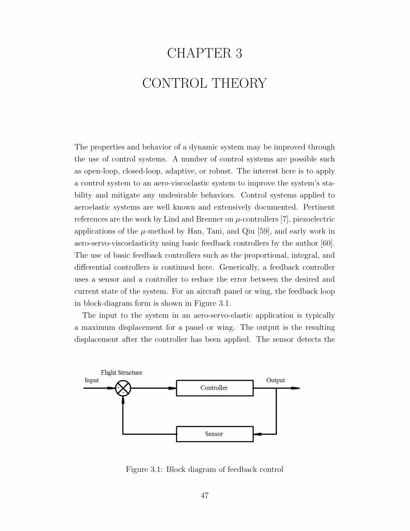
CHAPTER 3
CONTROL THEORY
The properties and behavior of a dynamic system may be improved through
the use of control systems. A number of control systems are possible such
as open-loop, closed-loop, adaptive, or robust. The interest here is to apply
a control system to an aero-viscoelastic system to improve the system’s sta-
bility and mitigate any undesirable behaviors. Control systems applied to
aeroelastic systems are well known and extensively documented. Pertinent
references are the work by Lind and Brenner on µ-controllers [7], piezoelectric
applications of the µ-method by Han, Tani, and Qiu [59], and early work in
aero-servo-viscoelasticity using basic feedback controllers by the author [60].
The use of basic feedback controllers such as the proportional, integral, and
differential controllers is continued here. Generically, a feedback controller
uses a sensor and a controller to reduce the error between the desired and
current state of the system. For an aircraft panel or wing, the feedback loop
in block-diagram form is shown in Figure 3.1.
The input to the system in an aero-servo-elastic application is typically
a maximum displacement for a panel or wing. The output is the resulting
displacement after the controller has been applied. The sensor detects the
Figure 3.1: Block diagram of feedback control
47
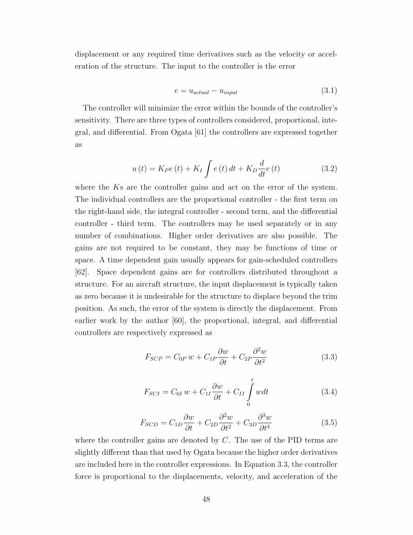
displacement or any required time derivatives such as the velocity or accel-
eration of the structure. The input to the controller is the error
e = uactual − uinput (3.1)
The controller will minimize the error within the bounds of the controller’s
sensitivity. There are three types of controllers considered, proportional, inte-
gral, and differential. From Ogata [61] the controllers are expressed together
as
u (t) = KP e (t) +KI
∫e (t) dt+KD
d
dte (t) (3.2)
where the Ks are the controller gains and act on the error of the system.
The individual controllers are the proportional controller - the first term on
the right-hand side, the integral controller - second term, and the differential
controller - third term. The controllers may be used separately or in any
number of combinations. Higher order derivatives are also possible. The
gains are not required to be constant, they may be functions of time or
space. A time dependent gain usually appears for gain-scheduled controllers
[62]. Space dependent gains are for controllers distributed throughout a
structure. For an aircraft structure, the input displacement is typically taken
as zero because it is undesirable for the structure to displace beyond the trim
position. As such, the error of the system is directly the displacement. From
earlier work by the author [60], the proportional, integral, and differential
controllers are respectively expressed as
FSCP = C0P w + C1P∂w
∂t+ C2P
∂2w
∂t2(3.3)
FSCI = C0I w + C1I∂w
∂t+ CII
t∫0
wdt (3.4)
FSCD = C1D∂w
∂t+ C2D
∂2w
∂t2+ C3D
∂3w
∂t3(3.5)
where the controller gains are denoted by C. The use of the PID terms are
slightly different than that used by Ogata because the higher order derivatives
are included here in the controller expressions. In Equation 3.3, the controller
force is proportional to the displacements, velocity, and acceleration of the
48
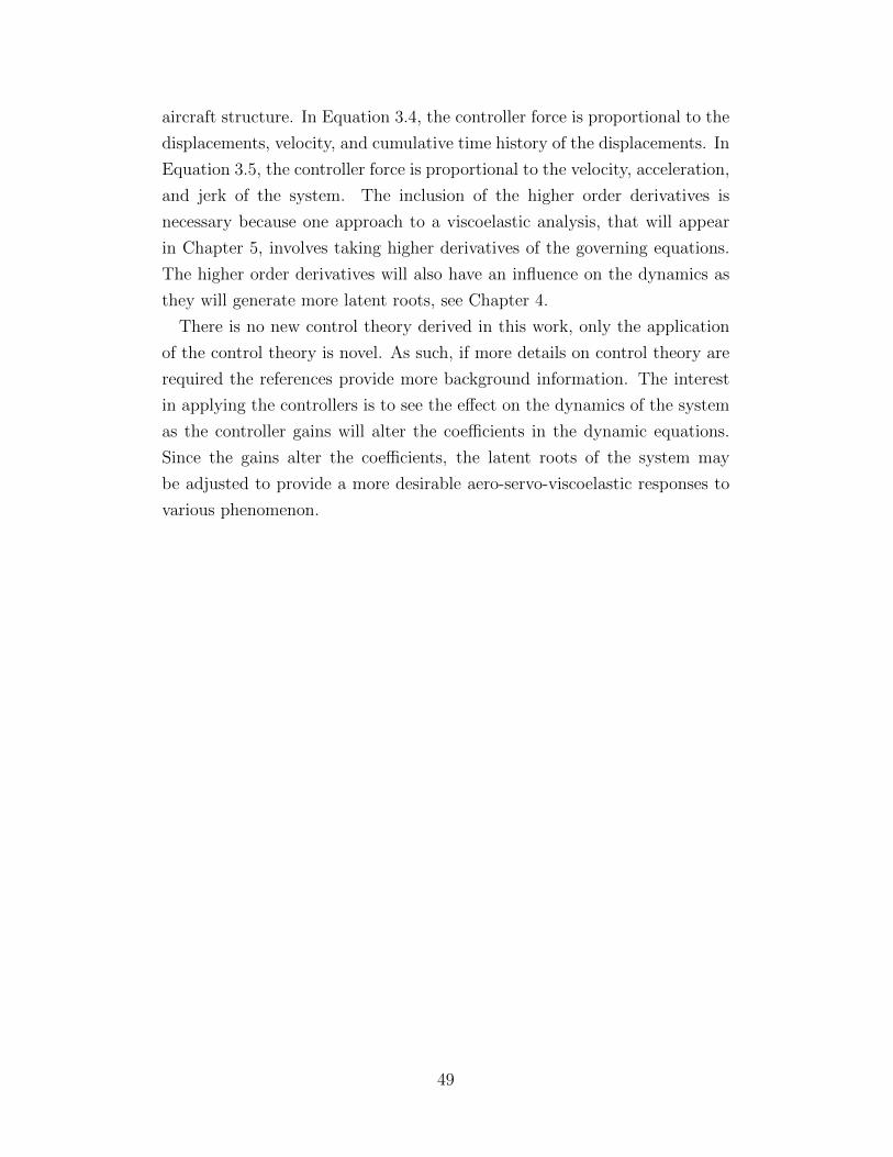
aircraft structure. In Equation 3.4, the controller force is proportional to the
displacements, velocity, and cumulative time history of the displacements. In
Equation 3.5, the controller force is proportional to the velocity, acceleration,
and jerk of the system. The inclusion of the higher order derivatives is
necessary because one approach to a viscoelastic analysis, that will appear
in Chapter 5, involves taking higher derivatives of the governing equations.
The higher order derivatives will also have an influence on the dynamics as
they will generate more latent roots, see Chapter 4.
There is no new control theory derived in this work, only the application
of the control theory is novel. As such, if more details on control theory are
required the references provide more background information. The interest
in applying the controllers is to see the effect on the dynamics of the system
as the controller gains will alter the coefficients in the dynamic equations.
Since the gains alter the coefficients, the latent roots of the system may
be adjusted to provide a more desirable aero-servo-viscoelastic responses to
various phenomenon.
49
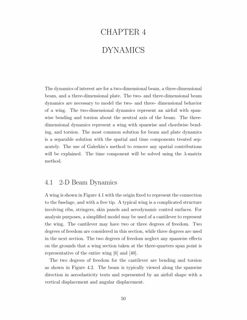
CHAPTER 4
DYNAMICS
The dynamics of interest are for a two-dimensional beam, a three-dimensional
beam, and a three-dimensional plate. The two- and three-dimensional beam
dynamics are necessary to model the two- and three- dimensional behavior
of a wing. The two-dimensional dynamics represent an airfoil with span-
wise bending and torsion about the neutral axis of the beam. The three-
dimensional dynamics represent a wing with spanwise and chordwise bend-
ing, and torsion. The most common solution for beam and plate dynamics
is a separable solution with the spatial and time components treated sep-
arately. The use of Galerkin’s method to remove any spatial contributions
will be explained. The time component will be solved using the λ-matrix
method.
4.1 2-D Beam Dynamics
A wing is shown in Figure 4.1 with the origin fixed to represent the connection
to the fuselage, and with a free tip. A typical wing is a complicated structure
involving ribs, stringers, skin panels and aerodynamic control surfaces. For
analysis purposes, a simplified model may be used of a cantilever to represent
the wing. The cantilever may have two or three degrees of freedom. Two
degrees of freedom are considered in this section, while three degrees are used
in the next section. The two degrees of freedom neglect any spanwise effects
on the grounds that a wing section taken at the three-quarters span point is
representative of the entire wing [6] and [40].
The two degrees of freedom for the cantilever are bending and torsion
as shown in Figure 4.2. The beam is typically viewed along the spanwise
direction in aeroelasticity texts and represented by an airfoil shape with a
vertical displacement and angular displacement.
50
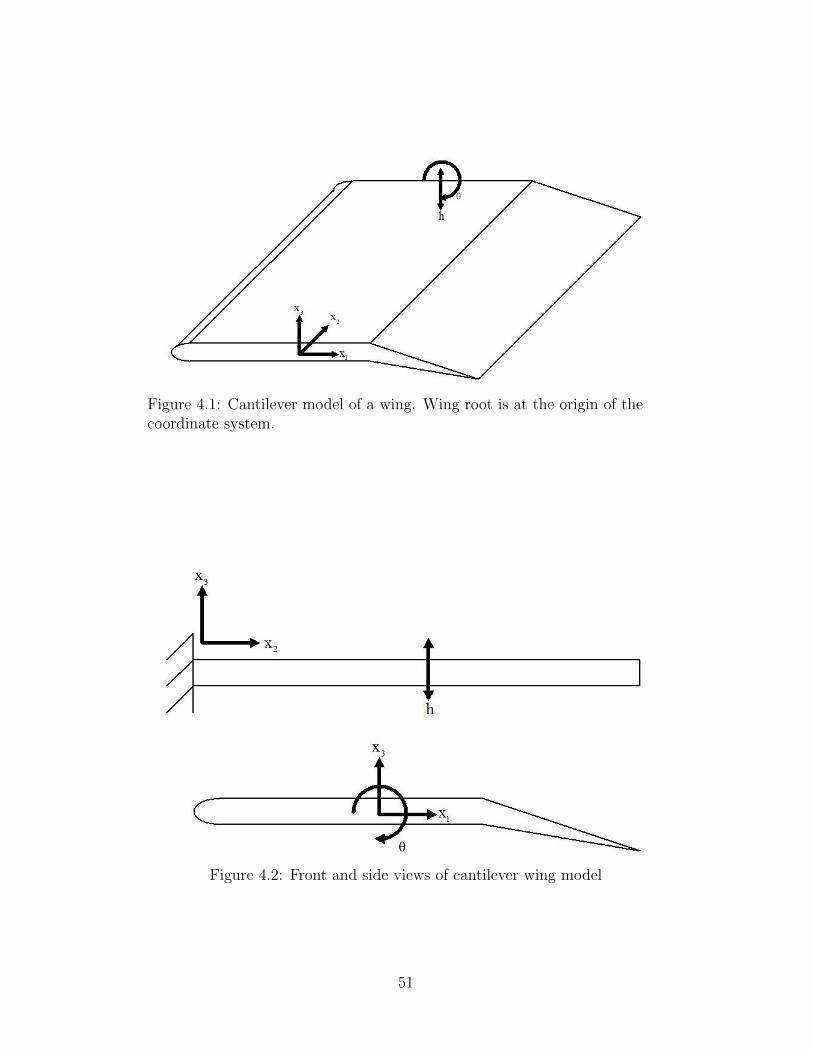
Figure 4.1: Cantilever model of a wing. Wing root is at the origin of thecoordinate system.
Figure 4.2: Front and side views of cantilever wing model
51
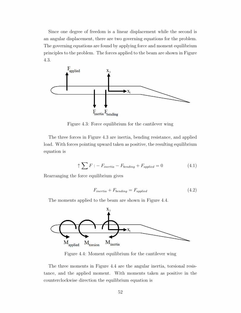
Since one degree of freedom is a linear displacement while the second is
an angular displacement, there are two governing equations for the problem.
The governing equations are found by applying force and moment equilibrium
principles to the problem. The forces applied to the beam are shown in Figure
4.3.
Figure 4.3: Force equilibrium for the cantilever wing
The three forces in Figure 4.3 are inertia, bending resistance, and applied
load. With forces pointing upward taken as positive, the resulting equilibrium
equation is
↑∑
F :− Finertia − Fbending + Fapplied = 0 (4.1)
Rearranging the force equilibrium gives
Finertia + Fbending = Fapplied (4.2)
The moments applied to the beam are shown in Figure 4.4.
Figure 4.4: Moment equilibrium for the cantilever wing
The three moments in Figure 4.4 are the angular inertia, torsional resis-
tance, and the applied moment. With moments taken as positive in the
counterclockwise direction the equilibrium equation is
52
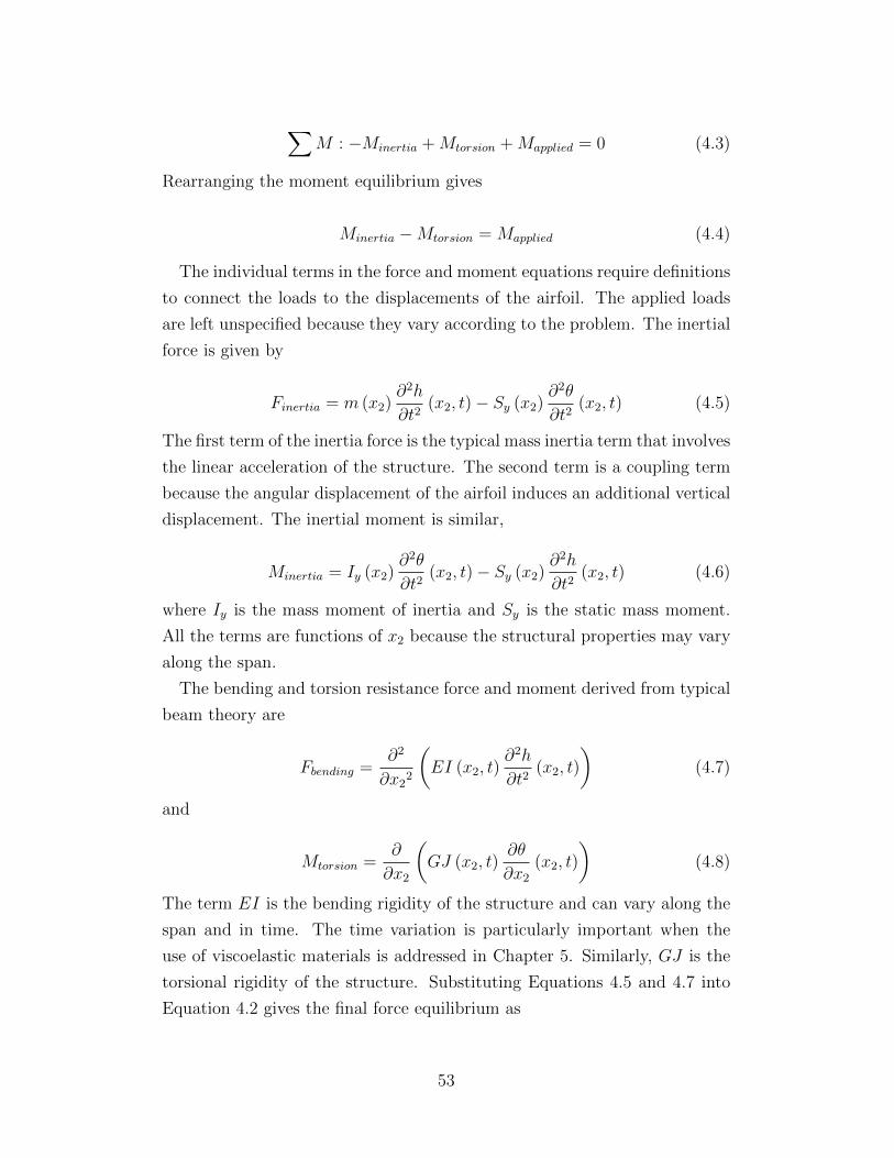
∑M : −Minertia +Mtorsion +Mapplied = 0 (4.3)
Rearranging the moment equilibrium gives
Minertia −Mtorsion = Mapplied (4.4)
The individual terms in the force and moment equations require definitions
to connect the loads to the displacements of the airfoil. The applied loads
are left unspecified because they vary according to the problem. The inertial
force is given by
Finertia = m (x2)∂2h
∂t2(x2, t)− Sy (x2)
∂2θ
∂t2(x2, t) (4.5)
The first term of the inertia force is the typical mass inertia term that involves
the linear acceleration of the structure. The second term is a coupling term
because the angular displacement of the airfoil induces an additional vertical
displacement. The inertial moment is similar,
Minertia = Iy (x2)∂2θ
∂t2(x2, t)− Sy (x2)
∂2h
∂t2(x2, t) (4.6)
where Iy is the mass moment of inertia and Sy is the static mass moment.
All the terms are functions of x2 because the structural properties may vary
along the span.
The bending and torsion resistance force and moment derived from typical
beam theory are
Fbending =∂2
∂x22
(EI (x2, t)
∂2h
∂t2(x2, t)
)(4.7)
and
Mtorsion =∂
∂x2
(GJ (x2, t)
∂θ
∂x2
(x2, t)
)(4.8)
The term EI is the bending rigidity of the structure and can vary along the
span and in time. The time variation is particularly important when the
use of viscoelastic materials is addressed in Chapter 5. Similarly, GJ is the
torsional rigidity of the structure. Substituting Equations 4.5 and 4.7 into
Equation 4.2 gives the final force equilibrium as
53
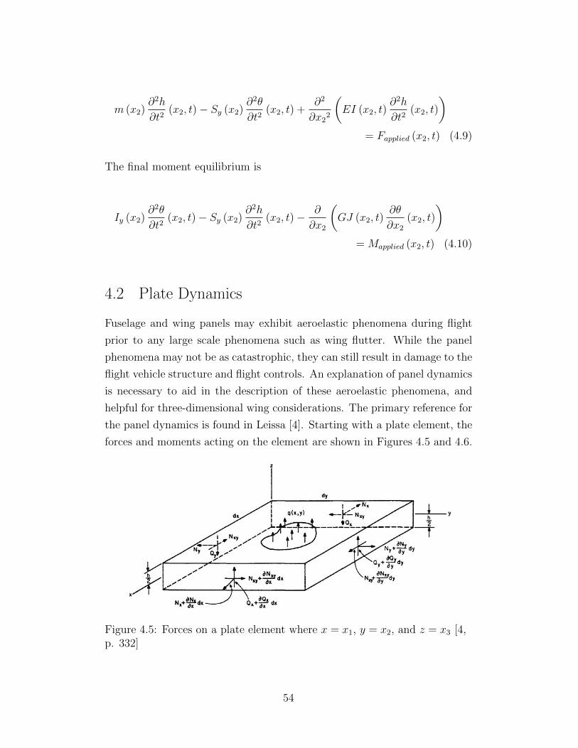
m (x2)∂2h
∂t2(x2, t)− Sy (x2)
∂2θ
∂t2(x2, t) +
∂2
∂x22
(EI (x2, t)
∂2h
∂t2(x2, t)
)= Fapplied (x2, t) (4.9)
The final moment equilibrium is
Iy (x2)∂2θ
∂t2(x2, t)− Sy (x2)
∂2h
∂t2(x2, t)−
∂
∂x2
(GJ (x2, t)
∂θ
∂x2
(x2, t)
)= Mapplied (x2, t) (4.10)
4.2 Plate Dynamics
Fuselage and wing panels may exhibit aeroelastic phenomena during flight
prior to any large scale phenomena such as wing flutter. While the panel
phenomena may not be as catastrophic, they can still result in damage to the
flight vehicle structure and flight controls. An explanation of panel dynamics
is necessary to aid in the description of these aeroelastic phenomena, and
helpful for three-dimensional wing considerations. The primary reference for
the panel dynamics is found in Leissa [4]. Starting with a plate element, the
forces and moments acting on the element are shown in Figures 4.5 and 4.6.
Figure 4.5: Forces on a plate element where x = x1, y = x2, and z = x3 [4,p. 332]
54
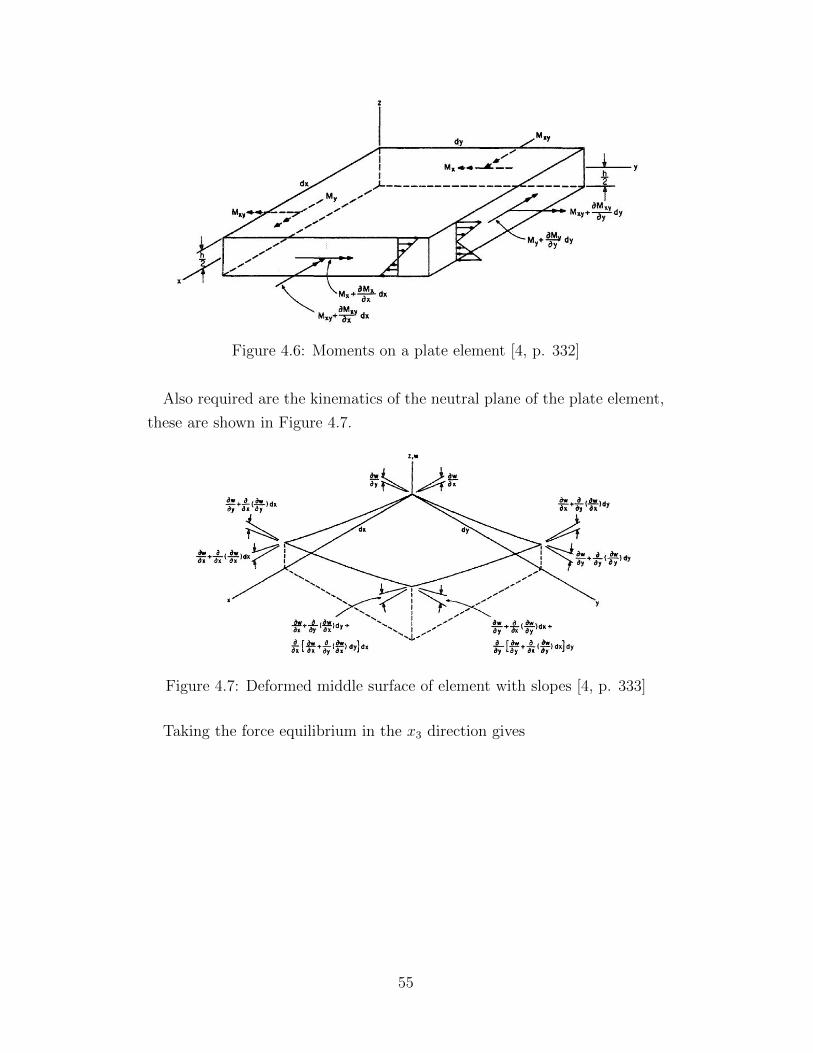
Figure 4.6: Moments on a plate element [4, p. 332]
Also required are the kinematics of the neutral plane of the plate element,
these are shown in Figure 4.7.
Figure 4.7: Deformed middle surface of element with slopes [4, p. 333]
Taking the force equilibrium in the x3 direction gives
55
∂N13
∂x1
dx1dx2 +∂N23
∂x2
dx2dx1 −N11dx2∂w
∂x1
+(N11 +
∂N11
∂x1
dx1
)dx2
(∂w
∂x1
+∂2w
∂x21
dx1
)−
−N22dx1∂w
∂x2
+
(N22 +
∂N22
∂x2
dx2
)dx1
(∂w
∂x2
+∂2w
∂x22
dx2
)−
N12dx1∂w
∂x1
+
(N12 +
∂N12
∂x2
dx2
)dx1
(∂w
∂x1
+∂2w
∂x1∂x2
dx2
)−
N12dx2∂w
∂x2
+
(N12 +
∂N12
∂x1
dx1
)dx2
(∂w
∂x2
+∂2w
∂x1∂x2
dx1
)+ q33 (x) dx1dx2 = ρ (x) dx1dx2
∂2w
∂t2(4.11)
where w is the vertical displacement of the plate, q33 is the applied vertical
load, and ρ is the density of the plate.
If Equation 4.11 is expanded, third order terms discarded, and the product
rule applied the equilibrium equation becomes
∂N13
∂x1
+∂N23
∂x2
+∂
∂x1
(N11
∂w
∂x1
)+
∂
∂x2
(N22
∂w
∂x2
)+
∂
∂x2
(N12
∂w
∂x1
)+
∂
∂x1
(N12
∂w
∂x2
)+ q33 (x) = ρ (x)
∂2w
∂t2(4.12)
Repeating the same procedure to find the force equilibriums in the x1 and
x2 directions respectively gives
∂N11
∂x1
+∂N12
∂x2
− ∂
∂x1
(N13
∂w
∂x1
)− ∂
∂x2
(N23
∂w
∂x1
)+ q31 (x)
= ρ (x)∂2u
∂t2(4.13)
∂N12
∂x1
+∂N22
∂x2
− ∂
∂x1
(N13
∂w
∂x2
)− ∂
∂x2
(N23
∂w
∂x2
)+q32 (x) = ρ (x)
∂2v
∂t2(4.14)
The q terms in Equations 4.13 and 4.14 represent any applied shear forces
to the plate. The terms u and v are the displacements in the x1 and x2
directions respectively. Typically the inertia terms in the above two equations
56
are considered negligible and are set to zero.
The moment equilibrium equations include high order derivatives. If those
derivatives are neglected, the equilibrium equations about the x1 and x2 axes
are
N13 −∂M11
∂x1
− ∂M12
∂x2
=ρ (x)h2
12
∂3w
∂x1∂t2(4.15)
N23 −∂M12
∂x1
− ∂M22
∂x2
=ρ (x)h2
12
∂3w
∂x2∂t2(4.16)
where h is the thickness of the plate element. The right hand sides of the
two equations represent the rotary inertia, but these are typically considered
to be small.
The forces and moments given in Equations 4.11 to 4.16 are related to the
stresses on the element through integral expressions. These integrals are
N11 =
h2∫
−h2
σ11dx3 (4.17)
N22 =
h2∫
−h2
σ22dx3 (4.18)
N12 =
h2∫
−h2
σ12dx3 (4.19)
M11 =
h2∫
−h2
σ11x3dx3 (4.20)
M22 =
h2∫
−h2
σ22x3dx3 (4.21)
M12 =
h2∫
−h2
σ12x3dx3 (4.22)
57
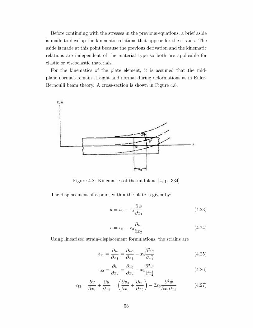
Before continuing with the stresses in the previous equations, a brief aside
is made to develop the kinematic relations that appear for the strains. The
aside is made at this point because the previous derivation and the kinematic
relations are independent of the material type so both are applicable for
elastic or viscoelastic materials.
For the kinematics of the plate element, it is assumed that the mid-
plane normals remain straight and normal during deformations as in Euler-
Bernoulli beam theory. A cross-section is shown in Figure 4.8.
Figure 4.8: Kinematics of the midplane [4, p. 334]
The displacement of a point within the plate is given by:
u = u0 − x3∂w
∂x1
(4.23)
v = v0 − x3∂w
∂x2
(4.24)
Using linearized strain-displacement formulations, the strains are
ε11 =∂u
∂x1
=∂u0
∂x1
− x3∂2w
∂x21
(4.25)
ε22 =∂v
∂x2
=∂v0
∂x2
− x3∂2w
∂x22
(4.26)
ε12 =∂v
∂x1
+∂u
∂x2
=
(∂v0
∂x1
+∂u0
∂x2
)− 2x3
∂2w
∂x1∂x2
(4.27)
58
The constitutive equations are where the viscoelastic contribution of the
derivation appears. This modification is the primary difference from the
derivation done by Leissa. The viscoelastic details appear in Chapter 5.
For a rectangular fuselage or wing panel the useful boundary conditions
are four sides simply-supported, four sides clamped, and two sides simply-
supported and two sides clamped. For panels, the easiest solution is a series
expansion to approximate the deflections. The panel length in the x1 direc-
tion is a and in the x2 direction is b. The series expansions for each set of
boundary conditions are as follows.
Four sides simply-supported:
X (x1) = sin
((m− 1)πx1
a
)Y (x2) = sin
((n− 1) πx2
b
)(4.28)
where m,n = 2, 3, 4, ...
Four sides clamped:
X (x1) = cos
(γ1
(x1
a− 1
2
))+
sin(γ1
2
)sinh
(γ1
2
) cosh
(γ1
(x1
a− 1
2
))
Y (x2) = cos
(γ1
(x2
b− 1
2
))+
sin(γ1
2
)sinh
(γ1
2
) cosh
(γ1
(x2
b− 1
2
))(4.29)
where m,n = 2, 4, 6, ... and γ1 is a root of
tan(γ1
2
)+ tanh
(γ1
2
)= 0 (4.30)
The odd numbered modes are given by
59
X (x1) = sin
(γ2
(x1
a− 1
2
))−
sin(γ2
2
)sinh
(γ2
2
) sinh
(γ2
(x1
a− 1
2
))
Y (x2) = sin
(γ2
(x2
b− 1
2
))−
sin(γ1
2
)sinh
(γ1
2
) sinh
(γ2
(x2
b− 1
2
))(4.31)
where m,n = 3, 5, 7, ... and γ2 is a root of
tan(γ2
2
)− tanh
(γ2
2
)= 0 (4.32)
The last set of boundary conditions, two sides simply-supported and two
sides clamped is assembled from the previous two sets of boundary conditions.
4.3 3-D Beam Dynamics
The three-dimensional beam dynamics are required if the movement of the
wing is in all directions. These movements may include spanwise bending
and torsion as before in the two-dimensional case, and chordwise bending.
There are two types of chordwise bending that are possible depending on
the scale considered. For the entire wing, the wing may bend forward or
backward similar to the vertical deflections. This type of bending is common
for helicopter rotor blades where the movement is known as lead-lag [63].
The second type of chordwise bending is a change in the camber of the wing.
The two movements are shown in Figure 4.9.
The change in camber will be considered chordwise bending as the change
in camber may have an effect on the air flow over the airfoil. The camber
change is also important for any panels on the wing, as the camber may
influence the panel’s curvature and pressure distribution. From a mechanics
perspective, this definition of chordwise bending means that a wing is treated
as a cantilevered plate. Therefore, the derivation from the previous section
is applicable. The difference between the plate dynamics section and the
three-dimensional wing is in the boundary conditions. The wing is treated
as a cantilevered plate with one side is clamped while the other three sides
are free. The appropriate equations, with x2 as the spanwise coordinate, are
60
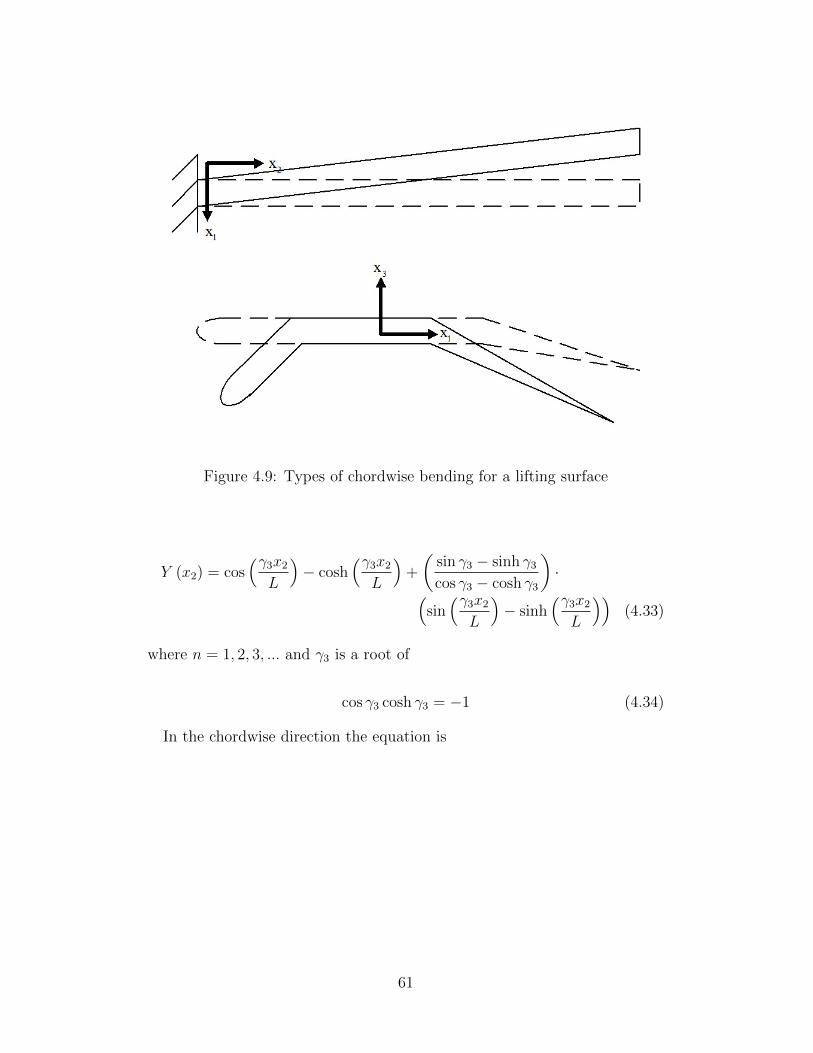
Figure 4.9: Types of chordwise bending for a lifting surface
Y (x2) = cos(γ3x2
L
)− cosh
(γ3x2
L
)+
(sin γ3 − sinh γ3
cos γ3 − cosh γ3
)·(
sin(γ3x2
L
)− sinh
(γ3x2
L
))(4.33)
where n = 1, 2, 3, ... and γ3 is a root of
cos γ3 cosh γ3 = −1 (4.34)
In the chordwise direction the equation is
61
X (x1) = 1 m = 0
X (x1) = 1− 2x1
cm = 1
X (x1) = cos
(γ1
(x1
c− 1
2
))−
sin(γ12
)sinh
(γ12
) cosh
(γ1
(x1
c− 1
2
))(4.35)
m = 2, 4, . . . (4.36)
X (x1) = sin
(γ2
(x1
c− 1
2
))+
sin(γ22
)sinh
(γ22
) sinh
(γ2
(x1
c− 1
2
))m = 3, 5, . . .
where γ1 and γ2 are defined by Equations 4.30 and 4.32.
4.4 Galerkin’s Method
The series solutions given in the plate dynamics and three-dimensional beam
subsections determine the spatial component of the dynamics problem. The
time component solution will be developed later in Section 4.5; however,
to help in solving the time component, eliminating the spatial component
variables is useful. The spatial component depends on the x1 and x2 vari-
ables. The conventional method for eliminating the spatial component is the
Galerkin method.
The Galerkin method begins by postulating the existence of an approxi-
mation solution that is expressible as a series such that
R = Wexact −Wapprox (4.37)
where R is the residual or error between the exact solution, Wexact, and
the approximate solution, Wapprox [64]. If there are N terms in the series
approximation, then in the limit it is desirable to have
limN→∞
R = 0 (4.38)
so that
62
limN→∞
Wapprox = Wexact (4.39)
Let the approximate solution take the form:
Wapprox =N∑i=1
aiϕi (4.40)
where the ϕi, or basis functions, are required to be orthogonal functions such
that the inner product space
〈ϕi, ϕj〉 =
b∫a
ϕi (t)ϕj (t) dt = δij (4.41)
is satisfied. Satisfying the inner product space is advantageous because the
weights, ai, are easily isolated. The methodology is to substitute the ap-
proximation solution in Equation 4.40 for the displacements in a governing
relation, then multiply the resulting equation by each basis function. Each
of the resulting equations is then integrated so that the inner product space
is applied to isolate the weights. As an example, consider a vibrating beam
simply supported at each end. The governing equation is
mh+ EIhIV = 0 (4.42)
The solution for the beam displacement is of the form:
h = W (x) Υ (t) (4.43)
While the separation of variables is one approach to solving the example
equation for both spatial and time components, Galerkin’s method will be
used instead for the spatial component. The time component will not be
considered here. The spatial component, for a simply supported beam, has
the form:
W (x) =N∑m=2
am−1 sin
((m− 1) πx2
L
)(4.44)
where L is taken as the length of the beam. For demonstration purposes,
only two modes will be taken so
63
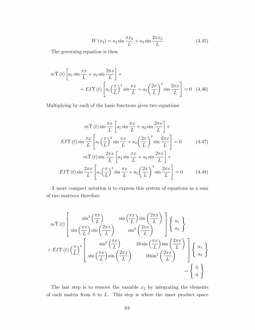
W (x2) = a1 sinπx2
L+ a2 sin
2πx2
L(4.45)
The governing equation is then
mΥ (t)
[a1 sin
πx
L+ a2 sin
2πx
L
]+
+ EIΥ (t)
[a1
(πL
)4
sinπx
L+ a2
(2π
L
)4
sin2πx
L
]= 0 (4.46)
Multiplying by each of the basis functions gives two equations
mΥ (t) sinπx
L
[a1 sin
πx
L+ a2 sin
2πx
L
]+
EIΥ (t) sinπx
L
[a1
(πL
)4
sinπx
L+ a2
(2π
L
)4
sin2πx
L
]= 0 (4.47)
mΥ (t) sin2πx
L
[a1 sin
πx
L+ a2 sin
2πx
L
]+
EIΥ (t) sin2πx
L
[a1
(πL
)4
sinπx
L+ a2
(2π
L
)4
sin2πx
L
]= 0 (4.48)
A more compact notation is to express this system of equations as a sum
of two matrices therefore
mΥ (t)
sin2(πxL
)sin(πxL
)sin
(2πx
L
)sin(πxL
)sin
(2πx
L
)sin2
(2πx
L
)a1
a2
+EIΥ (t)(πL
)4
sin2(πxL
)16 sin
(πxL
)sin
(2πx
L
)sin(πxL
)sin
(2πx
L
)16sin2
(2πx
L
)a1
a2
=
0
0
The last step is to remove the variable x2 by integrating the elements
of each matrix from 0 to L. This step is where the inner product space
64
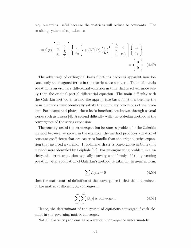
requirement is useful because the matrices will reduce to constants. The
resulting system of equations is
mΥ (t)
L
20
0L
2
a1
a2
+ EIΥ (t)
(πL
)4
L
20
0 8L
a1
a2
=
0
0
(4.49)
The advantage of orthogonal basis functions becomes apparent now be-
cause only the diagonal terms in the matrices are non-zero. The final matrix
equation is an ordinary differential equation in time that is solved more eas-
ily than the original partial differential equation. The main difficulty with
the Galerkin method is to find the appropriate basis functions because the
basis functions must identically satisfy the boundary conditions of the prob-
lem. For beams and plates, these basis functions are known through several
works such as Leissa [4]. A second difficulty with the Galerkin method is the
convergence of the series expansion.
The convergence of the series expansion becomes a problem for the Galerkin
method because, as shown in the example, the method produces a matrix of
constant coefficients that are easier to handle than the original series expan-
sion that involved a variable. Problems with series convergence in Galerkin’s
method were identified by Leipholz [65]. For an engineering problem in elas-
ticity, the series expansion typically converges uniformly. If the governing
equation, after application of Galerkin’s method, is taken in the general form,
∑Aijxi = 0 (4.50)
then the mathematical definition of the convergence is that the determinant
of the matrix coefficient, A, converges if
∞∑i=1
∞∑j=1
|Aij| is convergent (4.51)
Hence, the determinant of the system of equations converges if each ele-
ment in the governing matrix converges.
Not all elasticity problems have a uniform convergence unfortunately.
65
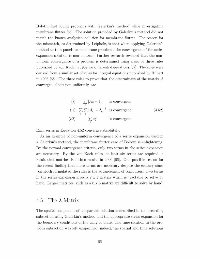
Bolotin first found problems with Galerkin’s method while investigating
membrane flutter [66]. The solution provided by Galerkin’s method did not
match the known analytical solution for membrane flutter. The reason for
the mismatch, as determined by Leipholz, is that when applying Galerkin’s
method to thin panels or membrane problems, the convergence of the series
expansion solution is non-uniform. Further research revealed that the non-
uniform convergence of a problem is determined using a set of three rules
published by von Koch in 1909 for differential equations [67]. The rules were
derived from a similar set of rules for integral equations published by Hilbert
in 1906 [68]. The three rules to prove that the determinant of the matrix A
converges, albeit non-uniformly, are
(i)∑i
|Aii − 1| is convergent
(ii)∑i
∑j
|Aij − δij|2 is convergent (4.52)
(iii)∑i
x2i is convergent
Each series in Equation 4.52 converges absolutely.
As an example of non-uniform convergence of a series expansion used in
a Galerkin’s method, the membrane flutter case of Bolotin is enlightening.
By the normal convergence criteria, only two terms in the series expansion
are necessary. By the von Koch rules, at least six terms are required, a
result that matches Bolotin’s results in 2000 [66]. One possible reason for
the recent finding that more terms are necessary despite the century since
von Koch formulated the rules is the advancement of computers. Two terms
in the series expansion gives a 2 x 2 matrix which is tractable to solve by
hand. Larger matrices, such as a 6 x 6 matrix are difficult to solve by hand.
4.5 The λ-Matrix
The spatial component of a separable solution is described in the preceding
subsection using Galerkin’s method and the appropriate series expansion for
the boundary conditions of the wing or plate. The time solution in the pre-
vious subsection was left unspecified; indeed, the spatial and time solutions
66
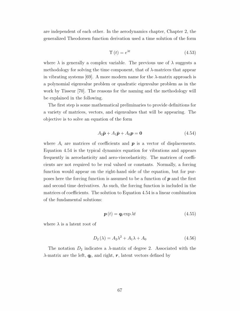
are independent of each other. In the aerodynamics chapter, Chapter 2, the
generalized Theodorsen function derivation used a time solution of the form
Υ (t) = eλt (4.53)
where λ is generally a complex variable. The previous use of λ suggests a
methodology for solving the time component, that of λ-matrices that appear
in vibrating systems [69]. A more modern name for the λ-matrix approach is
a polynomial eigenvalue problem or quadratic eigenvalue problem as in the
work by Tisseur [70]. The reasons for the naming and the methodology will
be explained in the following.
The first step is some mathematical preliminaries to provide definitions for
a variety of matrices, vectors, and eigenvalues that will be appearing. The
objective is to solve an equation of the form
A2p+ A1p+ A0p = 0 (4.54)
where Ai are matrices of coefficients and p is a vector of displacements.
Equation 4.54 is the typical dynamics equation for vibrations and appears
frequently in aeroelasticity and aero-viscoelasticity. The matrices of coeffi-
cients are not required to be real valued or constants. Normally, a forcing
function would appear on the right-hand side of the equation, but for pur-
poses here the forcing function is assumed to be a function of p and the first
and second time derivatives. As such, the forcing function is included in the
matrices of coefficients. The solution to Equation 4.54 is a linear combination
of the fundamental solutions:
p (t) = ql expλt (4.55)
where λ is a latent root of
D2 (λ) = A2λ2 + A1λ+ A0 (4.56)
The notation D2 indicates a λ-matrix of degree 2. Associated with the
λ-matrix are the left, ql, and right, r, latent vectors defined by
67
D2 (λi) qli = 0 (4.57)
r′iD2 (λi) = 0′ (4.58)
where the prime denotes the vector transpose. The left and right latent
vectors have a correspondence with the left and right eigenvectors that will
be shown shortly. Most of the theory for λ-matrices require the matrix to be
simple. There are two requirements for a matrix to be simple:
1. The matrix is regular
2. The matrix has rank n− β when λ = λi and λi has multiplicity β
A regular λ-matrix is a square matrix and matrix A2 in Equation 4.56 is
non-singular. The multiplicity, β, of a latent root is the number of times that
root appears and the value n is the size of the coefficient matrix. The last
definition is for the latent equation of a λ-matrix . The equation is given by
the determinant of the λ-matrix :
∆ (λ) = |D2 (λ)| = 0 (4.59)
The connection between latent roots and eigenvalues appears when an
equation of the form
A (λi) ql = 0 (4.60)
is considered. This equation is similar to Equation 4.57. If matrix A is taken
as a square matrix and I as the identity matrix of the same order then the
eigenvalues µ of matrix A are the zeros of
|A− µI| = 0 (4.61)
The associated left and right eigenvectors are
(A− µiI)x = 0 (4.62)
y′ (A− µiI) = 0′ (4.63)
68
If the matrix A is constant then the latent roots and eigenvalues, and the
latent vectors and eigenvectors are the same. However, if the matrix A is a
function of the scalar λ then the eigenvalues and eigenvectors are also func-
tions of λ. The reason for the pedantic definition is that MATLABTMprovides
a function called polyeig for solving polynomial eigenvalue problems derived
from the work by Tisseur [70] where the eigenvalues are defined as the roots
of a polynomial equation similar to Equation 4.56. Tisseur defines the latent
root as an eigenvalue because of a more flexible definition for the eigenprob-
lem.
A conventional eigenproblem is expressed as
Ax = µx (4.64)
or after some rearrangement
(A− µI)x = 0 (4.65)
However, if an eigenproblem is not restricted to having the identity matrix
as the eigenvalue multiplier then a second form is equally valid:
Ax = µBx (4.66)
Repetitive use of the second form converts a latent root polynomial equa-
tion into an eigenproblem form. This form is called the quadratic or polyno-
mial eigenvalue problem, and the equation A− λB is a matrix pencil.
The latent equation is easily solved using a root finder. Lancaster does
provide several algorithms to solve for the latent roots, but they are not the
most efficient methods for modern computers [69]. The algorithm by Tisseur
that is used in MATLAB TM’s polyeig function does work but the output
can be unclear. A preferred method is to repeatedly apply the matrix pencil
form and use MATLAB TM’s eig function.
If a forcing function is used that is a function of time, but not a function of
the displacements or the displacement derivatives, then a non-homogeneous
equation results
A2p+ A1p+ A0p = f (t) (4.67)
This equation may occur in aero-servo-viscoelastic problems with an imping-
69
ing acoustic pressure or an open loop control system. There are two ap-
proaches to solve the non-homogeneous problem depending on the λ-matrix,
each approach depends on a mathematical theorem. For the first approach,
the mathematical theorem is
“Let λi be a latent root of multiplicity βi (1 ≤ βi ≤ n) of the sim-
ple λ-matrix D2 (λ); then basis vectors can be found in the sub-
spaces of left and right latent vectors of λi which are biorthogonal
with respect to D(1)2 (λi). That is, there exist right latent vectors
qlυ and left latent vectors rµ (µ, υ = 1, 2, . . . , βi) associated with
λi such that
r′µD(1)2 (λi) qlυ = δµυ
is satisfied [69, p. 65].”
The key part of that theorem is if the λ-matrix has latent roots with the
appropriate multiplicity, then the basis vectors do exist. Since the basis
vectors exist, then the following solution for Equation 4.67 is possible:
(d
dt
)rp (t) =
2n∑j=1
λrjexp (λjt) cj + ϕj (t) qlj (4.68)
where r = 0, 1 to correspond to the displacements and first derivative of the
displacements. The vector c is the initial conditions and ϕj is given by
ϕj (t) =
t∫0
exp (−λjτ)r′jf (τ) dτ (4.69)
The second approach for a solution to the non-homogeneous equation is
used when the λ-matrix does not satisfy the theorem used in the first ap-
proach. The mathematical theorem used in the second approach is
“Let D2 (λ) be a regular λ-matrix. Assume that the 2n latent
roots of D2 (λ) can be split into two disjoint sets
λ1, λ2, . . . , λn and λn+1, λn+2, . . . , λ2n,
and that there are n linearly independent right latent vectors
ql1, ql2, . . . , qln associated with λ1, λ2, . . . , λn and n linearly in-
70
dependent left latent vectors rn+1, rn+2, . . . , r2n associated with
the second set.
If we write
Q1 = [ql1, ql2, . . . , qln], R2 = [rn+1, rn+2, . . . , r2n]
and Λ1,Λ2 for the associated diagonal matrices of latent roots,
then
D2 (λ) =(Iλ−
(R2Λ2R
−12
)′)A2
(Iλ−
(Q1Λ1Q
−11
))[69, p. 50].”
What the second theorem means is that if the conditions are satisfied then
the extra work of normalizing the latent vectors or creating a biorthogonal
system are avoided. The solution for Equation 4.67 is then
p (t) = Q1
t∫0
Ωexp (Λ2 (t− υ))− exp (Λ1 (t− υ))ΩR′2f (υ) dυ (4.70)
where
Ω =tjk
λn+k − λj, j, k = 1, 2, . . . , n
and tjk are the elements of
Υ = (R′2A2Q1)−1
4.6 Stability Definitions
The main intent of the dynamics is to assess the stability of a given aeroelastic
or aero-viscoelastic system. Stability using the λ-matrix method is defined
by the real component of the latent roots:
λj = dj + i ωj (4.71)
ergo
<λj = dj (4.72)
71
A general solution to Equation 4.54 or Equation 4.67 has three possibili-
ties, stable, neutrally stable, or unstable. A stable solution has all the real
components of the latent roots, all the dj, as negative. A neutrally stable
solution has one or more real components as zero while the remainder are neg-
ative. An unstable solution has at least one real component that is positive.
Stable or neutrally stable solutions are quickly determined by inspection of
matrices A1 and A0. If both matrices are positive definite then the solutions
are stable or neutrally stable.
A matrix, M , is positive definite if
z′Mz > 0 (4.73)
for all non-zero, real vectors z where the prime denotes the transpose. The
matrix must be symmetric and real. The more general case of complex
numbers require that the matrix be Hermitian and allows the vectors to be
complex. The corresponding mathematical definition is
z∗Mz > 0 (4.74)
where the asterisk denotes a conjugate transpose [64]. A Hermitian matrix
is square and equal to its own conjugate transpose. If this requirement is not
met, then the matrix is a non-self-adjoint operator.
4.7 Phase Relations
A final point to consider for the dynamics of a vibrating system that involves
several degrees of freedom is the phase relationship between the degrees or
displacements. In the previous subsections, the general form of the displace-
ment solution was given as
Υ = expλt (4.75)
however, the more accurate solution form is
Υ = expλt+ φ (4.76)
where φ is the phase angle. Duncan and Frazer in RM1155 propose finding
72
the phase angle between the displacements by direct comparison of the results
for each displacement [6]. The phase angle may be found graphically using
phasors as explained in any intermediate dynamics textbook [71].
73
CHAPTER 5
VISCOELASTICITY THEORY
To model aero-servo-viscoelasticity requires aerodynamics to represent the
air flow, control theory for the actuators, dynamics for the displacements
of the structures, and viscoelasticity theory for the constitutive equations
to link the structural dynamics to the material behavior. The structural
dynamics are divided into two sections, two-dimensional airfoil dynamics
and three-dimensional wing and plate dynamics. The viscoelasticity section
has a similar division so that the connections between the constitutive model
and the dynamics are more obvious. Some preliminaries for viscoelasticity
are necessary before describing the connections to dynamics. The elasticity
equivalents are explained simultaneously as elasticity is more common and
well known than viscoelasticity. For aircraft, particular interest is in high
polymer composite materials. These materials are explained in Reference
[72].
Consider a block of material, as in Figure 5.1, with normal vectors on each
face. A normal vector is defined as positive when pointing outward from the
face. Forces and moments are applied to two opposing faces of the block to
create tension and torsion. The forces and moments are known collectively as
tractions. The block is considered an infinitesimally small volume of a larger
body; therefore, the results for the block apply throughout the continuum of
the body.
The connection between the tractions, t, and the Cauchy stress, σ, inside
the material is
t = σ · n (5.1)
where n is the normal vector for the face considered. While the traction
and normal are vectors, the stresses are a second order tensor. Cauchy stress
represents one means to represent forces acting on an element of area in a
74
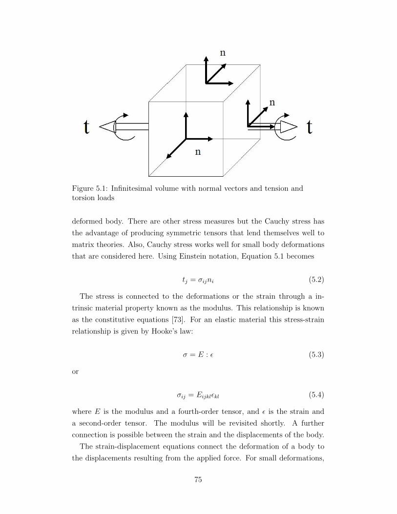
Figure 5.1: Infinitesimal volume with normal vectors and tension andtorsion loads
deformed body. There are other stress measures but the Cauchy stress has
the advantage of producing symmetric tensors that lend themselves well to
matrix theories. Also, Cauchy stress works well for small body deformations
that are considered here. Using Einstein notation, Equation 5.1 becomes
tj = σijni (5.2)
The stress is connected to the deformations or the strain through a in-
trinsic material property known as the modulus. This relationship is known
as the constitutive equations [73]. For an elastic material this stress-strain
relationship is given by Hooke’s law:
σ = E : ε (5.3)
or
σij = Eijklεkl (5.4)
where E is the modulus and a fourth-order tensor, and ε is the strain and
a second-order tensor. The modulus will be revisited shortly. A further
connection is possible between the strain and the displacements of the body.
The strain-displacement equations connect the deformation of a body to
the displacements resulting from the applied force. For small deformations,
75
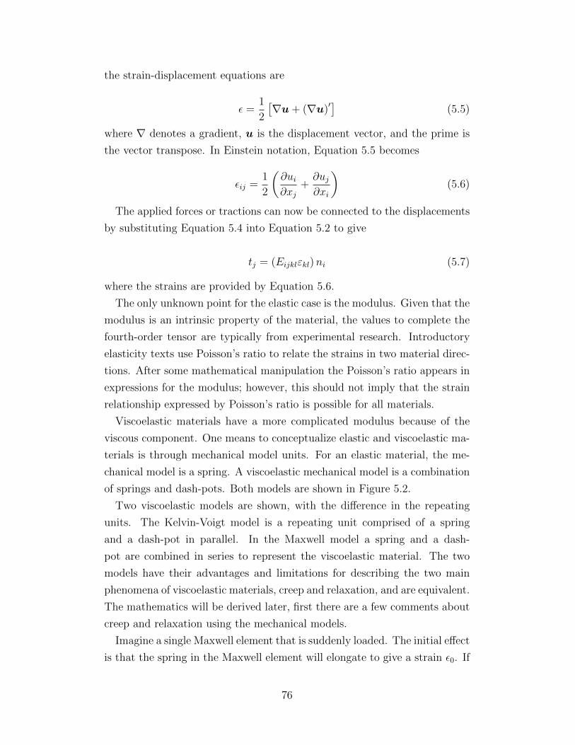
the strain-displacement equations are
ε =1
2
[∇u+ (∇u)′
](5.5)
where ∇ denotes a gradient, u is the displacement vector, and the prime is
the vector transpose. In Einstein notation, Equation 5.5 becomes
εij =1
2
(∂ui∂xj
+∂uj∂xi
)(5.6)
The applied forces or tractions can now be connected to the displacements
by substituting Equation 5.4 into Equation 5.2 to give
tj = (Eijklεkl)ni (5.7)
where the strains are provided by Equation 5.6.
The only unknown point for the elastic case is the modulus. Given that the
modulus is an intrinsic property of the material, the values to complete the
fourth-order tensor are typically from experimental research. Introductory
elasticity texts use Poisson’s ratio to relate the strains in two material direc-
tions. After some mathematical manipulation the Poisson’s ratio appears in
expressions for the modulus; however, this should not imply that the strain
relationship expressed by Poisson’s ratio is possible for all materials.
Viscoelastic materials have a more complicated modulus because of the
viscous component. One means to conceptualize elastic and viscoelastic ma-
terials is through mechanical model units. For an elastic material, the me-
chanical model is a spring. A viscoelastic mechanical model is a combination
of springs and dash-pots. Both models are shown in Figure 5.2.
Two viscoelastic models are shown, with the difference in the repeating
units. The Kelvin-Voigt model is a repeating unit comprised of a spring
and a dash-pot in parallel. In the Maxwell model a spring and a dash-
pot are combined in series to represent the viscoelastic material. The two
models have their advantages and limitations for describing the two main
phenomena of viscoelastic materials, creep and relaxation, and are equivalent.
The mathematics will be derived later, first there are a few comments about
creep and relaxation using the mechanical models.
Imagine a single Maxwell element that is suddenly loaded. The initial effect
is that the spring in the Maxwell element will elongate to give a strain ε0. If
76
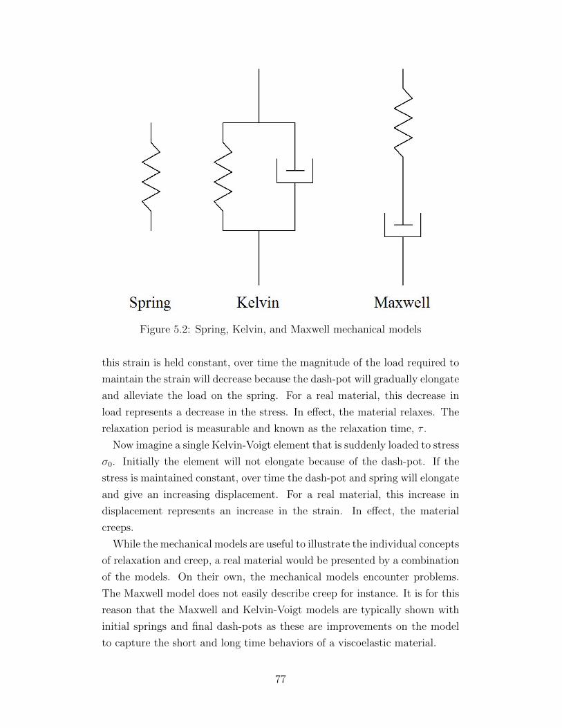
Figure 5.2: Spring, Kelvin, and Maxwell mechanical models
this strain is held constant, over time the magnitude of the load required to
maintain the strain will decrease because the dash-pot will gradually elongate
and alleviate the load on the spring. For a real material, this decrease in
load represents a decrease in the stress. In effect, the material relaxes. The
relaxation period is measurable and known as the relaxation time, τ .
Now imagine a single Kelvin-Voigt element that is suddenly loaded to stress
σ0. Initially the element will not elongate because of the dash-pot. If the
stress is maintained constant, over time the dash-pot and spring will elongate
and give an increasing displacement. For a real material, this increase in
displacement represents an increase in the strain. In effect, the material
creeps.
While the mechanical models are useful to illustrate the individual concepts
of relaxation and creep, a real material would be presented by a combination
of the models. On their own, the mechanical models encounter problems.
The Maxwell model does not easily describe creep for instance. It is for this
reason that the Maxwell and Kelvin-Voigt models are typically shown with
initial springs and final dash-pots as these are improvements on the model
to capture the short and long time behaviors of a viscoelastic material.
77
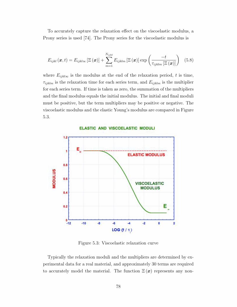
To accurately capture the relaxation effect on the viscoelastic modulus, a
Prony series is used [74]. The Prony series for the viscoelastic modulus is
Eijkl (x, t) = Eijkl∞ [Ξ (x)] +
Nijkl∑m=1
Eijklm [Ξ (x)] exp
(−t
τijklm [Ξ (x)]
)(5.8)
where Eijkl∞ is the modulus at the end of the relaxation period, t is time,
τijklm is the relaxation time for each series term, and Eijklm is the multiplier
for each series term. If time is taken as zero, the summation of the multipliers
and the final modulus equals the initial modulus. The initial and final moduli
must be positive, but the term multipliers may be positive or negative. The
viscoelastic modulus and the elastic Young’s modulus are compared in Figure
5.3.
Figure 5.3: Viscoelastic relaxation curve
Typically the relaxation moduli and the multipliers are determined by ex-
perimental data for a real material, and approximately 30 terms are required
to accurately model the material. The function Ξ (x) represents any non-
78
homogeneous distribution function of the modulus through the body. This
function is necessary to model any functionally graded materials.
The next step is to assemble the constitutive equation for a viscoelastic
material similar to Hooke’s law for elastic materials. [73, 75]. Since the
modulus has an exponential relaxation function a loading event at time ζ
on the material will have a decaying effect on all later times. Similar to the
Green’s function method applied in the aerodynamics development, Chapter
2, the constitutive equation is expressed as an influence function:
σ =
b∫a
E (t− ζ) f (ε (ζ)) dζ (5.9)
The bounds of the integral are determined through physical reasoning.
The time period where an event may influence the viscoelastic material is
from when the material is first created to the present time. These bounds
are then −∞ to the present time t. The function of the strain, f (ε (t)), is a
generic placeholder function. By dimensional analysis, the time rate of strain
satisfies the equation and makes conceptual sense because of the dash-pots
in the mechanical model. The constitutive equation is then
σ =
t∫−∞
E (t− ζ)∂ε (ζ)
∂ζdζ (5.10)
The constitutive equation may also be expressed in terms of the strain
directly as
σ =
t∫−∞
E∗ (t− ζ) ε (ζ) dζ (5.11)
where the asterisk denotes a different function involving the modulus and
the Prony series. Both forms of the constitutive equation are considered
hereditary integrals because of their form and the inclusion of events to the
beginning of time.
An important point about the hereditary integrals and the bounds occurs
during the solution of a governing equation involving a viscoelastic material.
The constitutive equations appear similar to a convolution integral so the
use of Laplace transforms is tempting. However, the Laplace transform uses
79
bounds of 0 to∞. The upper bound is not problematic, but the lower bound
of 0 implies that the history of the viscoelastic material begins at the start
of the particular application. Further, initial conditions at 0 must then be
specified. For engineering applications with long life spans, such as the 20
to 30 years of an aircraft, the influence of events from previous flights may
become important and affect the predicted life span of an aircraft fabricated
from composite materials.
While on the topic of the constitutive equations, some note should be made
of the Poisson ratio. The ratio appears frequently in elasticity and provides
a convenient mathematical shortcut in relating the stress and strain in one
direction to the stress and strain in another direction inside a solid body. The
Poisson ratio has appeared in viscoelasticity throughout its history; however,
in 2001 Hilton demonstrated that the ratio is flawed for a viscoelastic ma-
terial and instead the constitutive equations must be used directly for each
direction [76].
As mentioned earlier, a temptation in solving a governing equation for a
viscoelastic material is to use a Laplace transform because of the similarity of
the convolution transform to the hereditary integral. The more appropriate
operators to use to solve a viscoelastic governing equation are the P and Q
operators. The operators are defined as
Pij σij (x, t) = Qijkl εkl (x, t) (5.12)
indicating that the P operator is applied to stress terms, while the Q operator
is applied to strain terms. In applications to governing equations, the P
operator is typically applied to all the terms save the hereditary integral
term. The Q operator is applied to the hereditary integral. The P operator
is
Pij =s∑
n=0
aijn
(∂
∂t
)n(5.13)
and the Q operator is
Qijkl =s∑
n=0
bijkln
(∂
∂t
)n(5.14)
The coefficients aij and bijkl are material property parameters and are
80
found through experiment. The number of terms taken in the series expan-
sion match the number of terms used for the Prony series. Earlier it was
mentioned that the constitutive equation is similar to a Green’s function
solution. In fact, the constitutive equation given by Equation 5.10 is the
Green’s function solution to the differential equation resulting from the P
and Q operators.
The isotropic, elastic Hooke’s law is produced through the P and Q oper-
ators by setting s = 0 and
PEij = aij0 = 1 (5.15)
QEijkl = bijkl0 = Eijkl0 (5.16)
While the P and Q operator do have their uses, calculating the coefficients
is tedious for an accurate representation with 30 terms. The integral rela-
tionships are much preferred for viscoelastic analyses; however, when used in
the governing equations that appeared in Chapter 4, the result is an integro-
differential equation of the form
A2w + A1w +
t∫−∞
A0 (t− ζ) ε (w, ζ) dζ = 0 (5.17)
The solution for this equation varies depending on the details of the A0
and ε functions, and the solution form for w (t). The solution method for an
integro-differential equation will be elaborated upon in Chapters 6 to 8. The
λ-matrix method used in the dynamics section will appear frequently.
Viscoelasticity is suggested for use in high-polymer composite materials
rather than the existing elasticity theory that normally appears in the mi-
cromechanics of composite materials. As a demonstration of the difference
between elasticity and viscoelasticity consider the stress in a fiber reinforced
matrix from a tensile load along a principal axis as shown in Figure 5.4.
The total volume of the block is the sum of the fibers, Vf , and the matrix,
Vm:
V = Vf + Vm (5.18)
The average stress of the block is
81
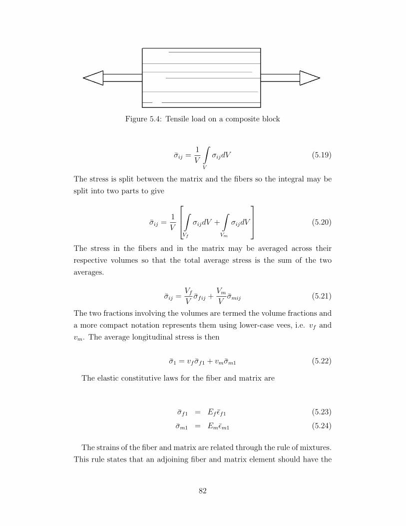
Figure 5.4: Tensile load on a composite block
σij =1
V
∫V
σijdV (5.19)
The stress is split between the matrix and the fibers so the integral may be
split into two parts to give
σij =1
V
∫Vf
σijdV +
∫Vm
σijdV
(5.20)
The stress in the fibers and in the matrix may be averaged across their
respective volumes so that the total average stress is the sum of the two
averages.
σij =VfVσfij +
VmVσmij (5.21)
The two fractions involving the volumes are termed the volume fractions and
a more compact notation represents them using lower-case vees, i.e. vf and
vm. The average longitudinal stress is then
σ1 = vf σf1 + vmσm1 (5.22)
The elastic constitutive laws for the fiber and matrix are
σf1 = Ef εf1 (5.23)
σm1 = Emεm1 (5.24)
The strains of the fiber and matrix are related through the rule of mixtures.
This rule states that an adjoining fiber and matrix element should have the
82
same strain so
εf1 = εm1 = ε1 (5.25)
Applying the rule of mixtures and Equation 5.23 to Equation 5.22 gives
the elastic stress as
σ1 = vfEf ε1 + vmEmε1 (5.26)
In the viscoelastic application, only the matrix is considered a viscoelastic
material because a polymer matrix is fairly typical. The constitutive law for
the matrix is then
σm1 =
t∫−∞
Em (t− ζ) ˙ε1 (ζ) dζ (5.27)
Using the following Prony series for the modulus
Em (t) = E∞ +N∑n=1
En exp−tτn
(5.28)
leads to
σm1 =
t∫−∞
[E∞ +
N∑n=1
En exp−t+ ζ
τn
]˙ε1 (ζ) dζ
= E∞ε1 (t) +
t∫−∞
[N∑n=1
En exp−t+ ζ
τn
]˙ε1 (ζ) dζ (5.29)
If the displacement of the body has a time solution of the form exp (λt) as
discussed in Chapter 4, then the strain has the form
ε1 (t) = B0exp (λt) (5.30)
The integral is easily evaluated and the resulting matrix stress is
83
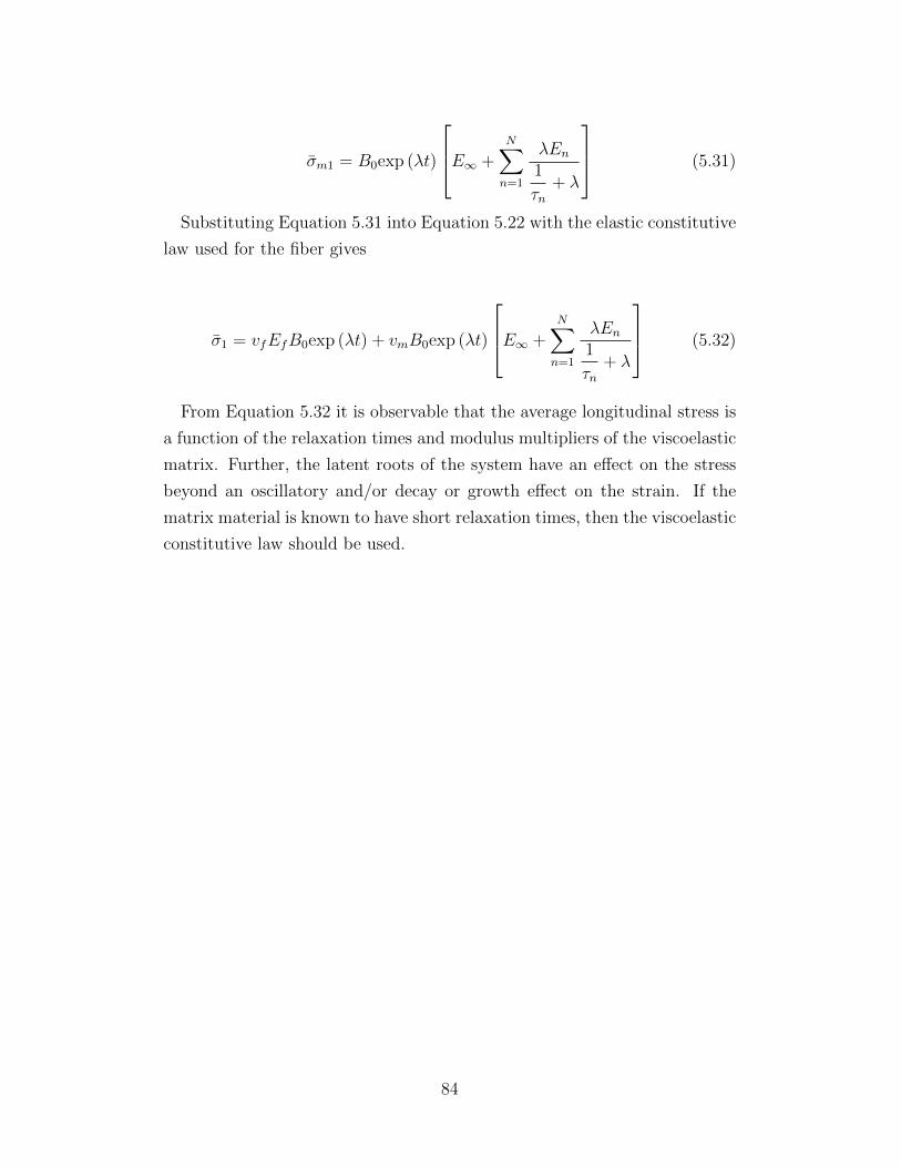
σm1 = B0exp (λt)
E∞ +N∑n=1
λEn1
τn+ λ
(5.31)
Substituting Equation 5.31 into Equation 5.22 with the elastic constitutive
law used for the fiber gives
σ1 = vfEfB0exp (λt) + vmB0exp (λt)
E∞ +N∑n=1
λEn1
τn+ λ
(5.32)
From Equation 5.32 it is observable that the average longitudinal stress is
a function of the relaxation times and modulus multipliers of the viscoelastic
matrix. Further, the latent roots of the system have an effect on the stress
beyond an oscillatory and/or decay or growth effect on the strain. If the
matrix material is known to have short relaxation times, then the viscoelastic
constitutive law should be used.
84
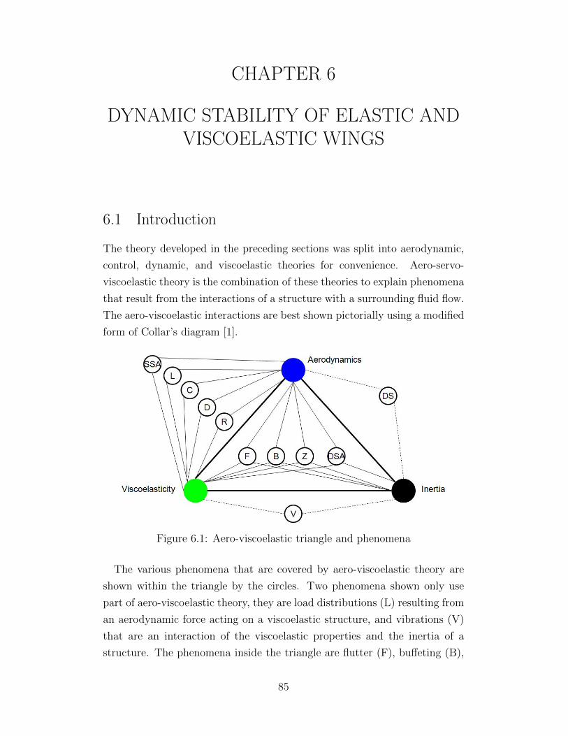
CHAPTER 6
DYNAMIC STABILITY OF ELASTIC ANDVISCOELASTIC WINGS
6.1 Introduction
The theory developed in the preceding sections was split into aerodynamic,
control, dynamic, and viscoelastic theories for convenience. Aero-servo-
viscoelastic theory is the combination of these theories to explain phenomena
that result from the interactions of a structure with a surrounding fluid flow.
The aero-viscoelastic interactions are best shown pictorially using a modified
form of Collar’s diagram [1].
Figure 6.1: Aero-viscoelastic triangle and phenomena
The various phenomena that are covered by aero-viscoelastic theory are
shown within the triangle by the circles. Two phenomena shown only use
part of aero-viscoelastic theory, they are load distributions (L) resulting from
an aerodynamic force acting on a viscoelastic structure, and vibrations (V)
that are an interaction of the viscoelastic properties and the inertia of a
structure. The phenomena inside the triangle are flutter (F), buffeting (B),
85
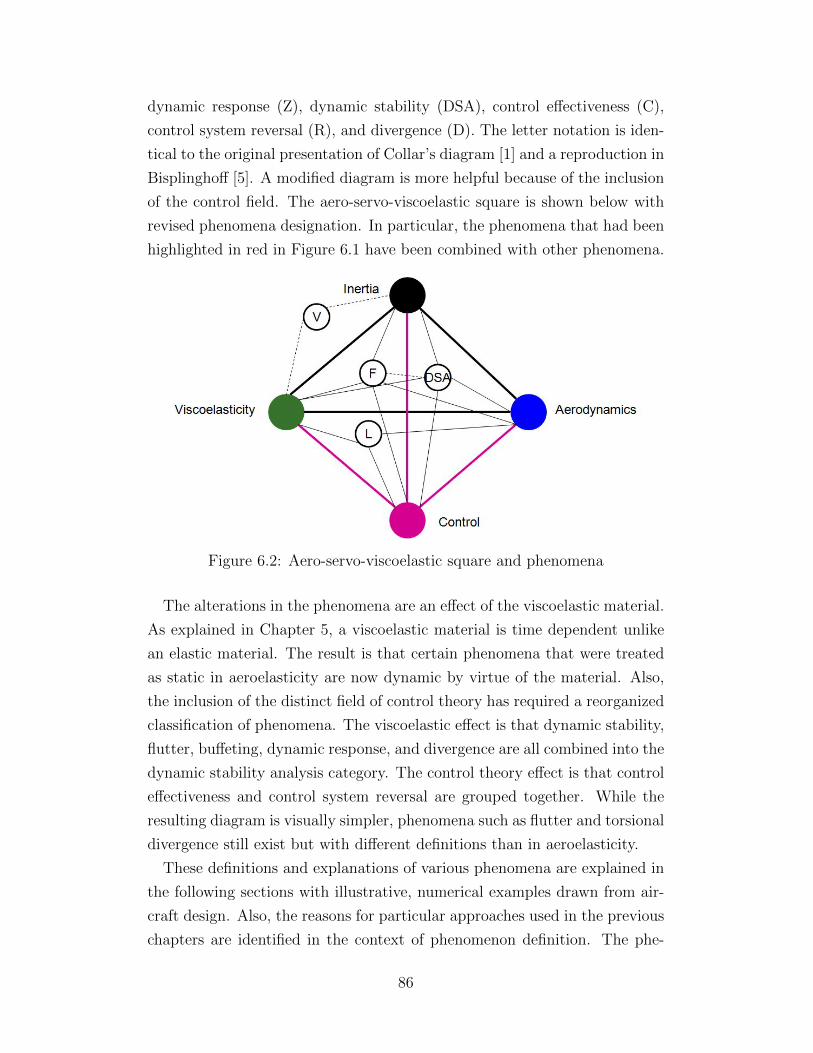
dynamic response (Z), dynamic stability (DSA), control effectiveness (C),
control system reversal (R), and divergence (D). The letter notation is iden-
tical to the original presentation of Collar’s diagram [1] and a reproduction in
Bisplinghoff [5]. A modified diagram is more helpful because of the inclusion
of the control field. The aero-servo-viscoelastic square is shown below with
revised phenomena designation. In particular, the phenomena that had been
highlighted in red in Figure 6.1 have been combined with other phenomena.
Figure 6.2: Aero-servo-viscoelastic square and phenomena
The alterations in the phenomena are an effect of the viscoelastic material.
As explained in Chapter 5, a viscoelastic material is time dependent unlike
an elastic material. The result is that certain phenomena that were treated
as static in aeroelasticity are now dynamic by virtue of the material. Also,
the inclusion of the distinct field of control theory has required a reorganized
classification of phenomena. The viscoelastic effect is that dynamic stability,
flutter, buffeting, dynamic response, and divergence are all combined into the
dynamic stability analysis category. The control theory effect is that control
effectiveness and control system reversal are grouped together. While the
resulting diagram is visually simpler, phenomena such as flutter and torsional
divergence still exist but with different definitions than in aeroelasticity.
These definitions and explanations of various phenomena are explained in
the following sections with illustrative, numerical examples drawn from air-
craft design. Also, the reasons for particular approaches used in the previous
chapters are identified in the context of phenomenon definition. The phe-
86
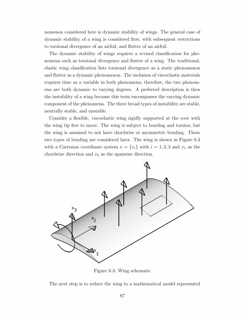
nomenon considered here is dynamic stability of wings. The general case of
dynamic stability of a wing is considered first, with subsequent restrictions
to torsional divergence of an airfoil, and flutter of an airfoil.
The dynamic stability of wings requires a revised classification for phe-
nomena such as torsional divergence and flutter of a wing. The traditional,
elastic wing classification lists torsional divergence as a static phenomenon
and flutter as a dynamic phenomenon. The inclusion of viscoelastic materials
requires time as a variable in both phenomena; therefore, the two phenom-
ena are both dynamic to varying degrees. A preferred description is then
the instability of a wing because this term encompasses the varying dynamic
component of the phenomena. The three broad types of instability are stable,
neutrally stable, and unstable.
Consider a flexible, viscoelastic wing rigidly supported at the root with
the wing tip free to move. The wing is subject to bending and torsion, but
the wing is assumed to not have chordwise or asymmetric bending. Those
two types of bending are considered later. The wing is shown in Figure 6.3
with a Cartesian coordinate system x = xi with i = 1, 2, 3 and x1 as the
chordwise direction and x2 as the spanwise direction.
Figure 6.3: Wing schematic
The next step is to reduce the wing to a mathematical model represented
87
by a system of equations. The necessary properties to include in the model
are the inertia, stiffness, aerodynamic loads, and control loads. These loads
are represented schematically in Figure 6.3. Taking the force equilibrium
about the x3 direction gives the bending equation
LBending w (x2, t) , θ (x2, t) = Iw (x2)∂2w (x2, t)
∂t2−
Iwθ (x2)∂2θ (x2, t)
∂t2+
∂2
∂x22
(∫ t
−∞E∗ (x2, t− s) I (x2)
∂2w (x2, s)
∂x22
ds
)−
− Lrigid (x2, V )− Lflexible (x2, V, t)− FASC (x2, t) = 0 (6.1)
while taking the moment equilibrium about the x2 direction gives the torsion
equation
LTorsion w (x2, t) , θ (x2, t) = Iθ (x2)∂2θ (x2, t)
∂t2−
Iwθ (x2)∂2w (x2, t)
∂t2− ∂
∂x2
(∫ t
−∞G∗ (x2, t− s) J (x2)
∂θ (x2, s)
∂x2
ds
)−
−Mrigid (x2, V )−Mflexible (x2, V, t)−MASC (x2, t) = 0 (6.2)
where θ is the flexible angle of attack, w is the vertical displacement of
the lifting surface, and E∗ and G∗ are the viscoelastic material properties.
The aerodynamic loads, L and M , are divided into the rigid and flexible
components. The rigid components are typically functions of the lifting sur-
face’s geometry, while the flexible components are functions of time and the
displacements w and θ. The details for the aerodynamics are available in
Chapter 2. The existence of the rigid components of the aerodynamic loads
imposes a particular solution on the system of equations that will vary ac-
cording to the fixed geometry of the lifting surface for each problem. Further,
the particular solution means that there exists stable displacements of the
lifting surface prior to the divergence time occurring.
The control forces and moments are the terms FASC and MASC , with ex-
pressions given by Equations 3.3 to 3.5 in Chapter 3. The inputs that the
controllers act on are the displacements, either vertical or angular, of the
lifting surface and any associated time derivatives that are detected by the
88
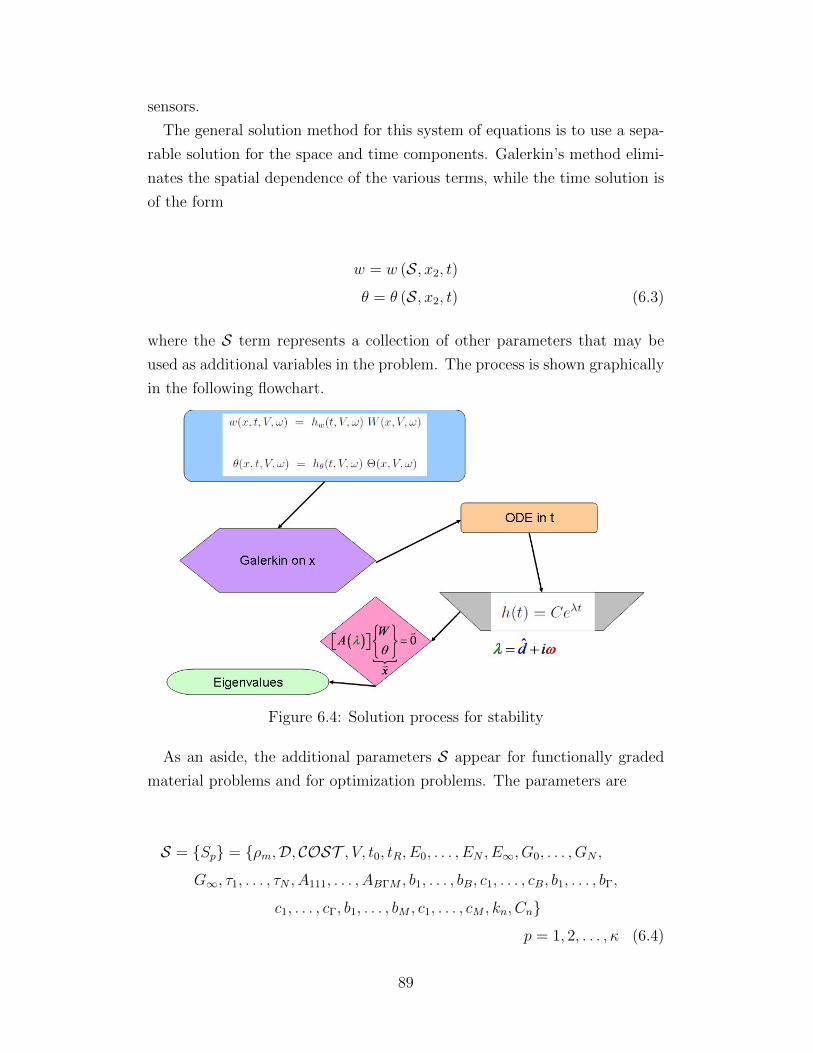
sensors.
The general solution method for this system of equations is to use a sepa-
rable solution for the space and time components. Galerkin’s method elimi-
nates the spatial dependence of the various terms, while the time solution is
of the form
w = w (S, x2, t)
θ = θ (S, x2, t) (6.3)
where the S term represents a collection of other parameters that may be
used as additional variables in the problem. The process is shown graphically
in the following flowchart.
Figure 6.4: Solution process for stability
As an aside, the additional parameters S appear for functionally graded
material problems and for optimization problems. The parameters are
S = Sp = ρm,D, COST , V, t0, tR, E0, . . . , EN , E∞, G0, . . . , GN ,
G∞, τ1, . . . , τN , A111, . . . , ABΓM , b1, . . . , bB, c1, . . . , cB, b1, . . . , bΓ,
c1, . . . , cΓ, b1, . . . , bM , c1, . . . , cM , kn, Cn
p = 1, 2, . . . , κ (6.4)
89
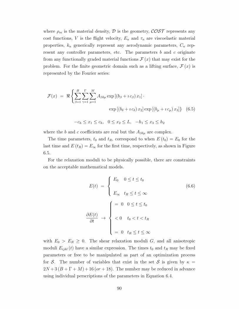
where ρm is the material density, D is the geometry, COST represents any
cost functions, V is the flight velocity, En and τn are viscoelastic material
properties, kn generically represent any aerodynamic parameters, Cn rep-
resent any controller parameters, etc. The parameters b and c originate
from any functionally graded material functions F (x) that may exist for the
problem. For the finite geometric domain such as a lifting surface, F (x) is
represented by the Fourier series:
F(x) = <
B∑β=1
Γ∑γ=1
M∑µ=1
Aβδµ exp [(bβ + ı cβ)x1] ·
exp [(bδ + ı cδ)x2] exp [(bµ + ı cµ)x3] (6.5)
−ch ≤ x1 ≤ ch, 0 ≤ x2 ≤ L, −h1 ≤ x3 ≤ h2
where the b and c coefficients are real but the Aβδµ are complex.
The time parameters, t0 and tR, correspond to when E (t0) = E0 for the
last time and E (tR) = E∞ for the first time, respectively, as shown in Figure
6.5.
For the relaxation moduli to be physically possible, there are constraints
on the acceptable mathematical models.
E(t) =
E0 0 ≤ t ≤ t0
E∞ tR ≤ t ≤ ∞(6.6)
∂E(t)
∂t→
= 0 0 ≤ t ≤ t0
< 0 t0 < t < tR
= 0 tR ≤ t ≤ ∞
with E0 > ER ≥ 0. The shear relaxation moduli G, and all anisotropic
moduli Eijkl (t) have a similar expression. The times t0 and tR may be fixed
parameters or free to be manipulated as part of an optimization process
for S. The number of variables that exist in the set S is given by κ =
2N + 3 (B + Γ +M) + 16 (or + 18). The number may be reduced in advance
using individual perscriptions of the parameters in Equation 6.4.
90
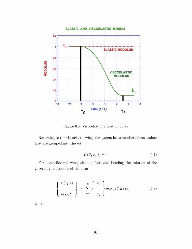
Figure 6.5: Viscoelastic relaxation curve
Returning to the viscoelastic wing, the system has a number of constraints
that are grouped into the set:
C (S, x2, t) = 0 (6.7)
For a cantilevered wing without chordwise bending the solution of the
governing relations is of the form
w(x2, t)
θ(x2, t)
=K∑n=1
wn
θn
exp (λ t) Ξ (x2) (6.8)
where
91
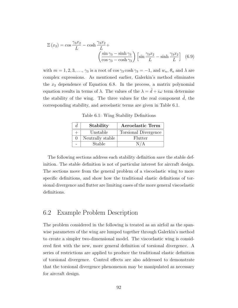
Ξ (x2) = cosγ3x2
L− cosh
γ3x2
L+(
sin γ3 − sinh γ3
cos γ3 − cosh γ3
)[sin
γ3x2
L− sinh
γ3x2
L
](6.9)
with m = 1, 2, 3, . . ., γ3 is a root of cos γ3 cosh γ3 = −1, and wn, θn and λ are
complex expressions. As mentioned earlier, Galerkin’s method eliminates
the x2 dependence of Equation 6.8. In the process, a matrix polynomial
equation results in terms of λ. The values of the λ = d+ iω term determine
the stability of the wing. The three values for the real component d, the
corresponding stability, and aeroelastic terms are given in Table 6.1.
Table 6.1: Wing Stability Definitions
d Stability Aeroelastic Term
+ Unstable Torsional Divergence0 Neutrally stable Flutter- Stable N/A
The following sections address each stability definition save the stable def-
inition. The stable definition is not of particular interest for aircraft design.
The sections move from the general problem of a viscoelastic wing to more
specific definitions, and show how the traditional elastic definitions of tor-
sional divergence and flutter are limiting cases of the more general viscoelastic
definitions.
6.2 Example Problem Description
The problem considered in the following is treated as an airfoil as the span-
wise parameters of the wing are lumped together through Galerkin’s method
to create a simpler two-dimensional model. The viscoelastic wing is consid-
ered first with the new, more general definition of torsional divergence. A
series of restrictions are applied to produce the traditional elastic definition
of torsional divergence. Control effects are also addressed to demonstrate
that the torsional divergence phenomenon may be manipulated as necessary
for aircraft design.
92
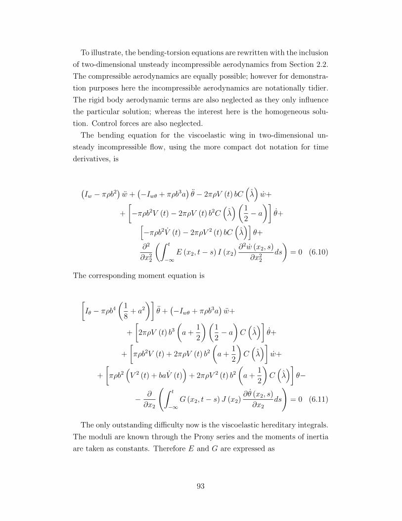
To illustrate, the bending-torsion equations are rewritten with the inclusion
of two-dimensional unsteady incompressible aerodynamics from Section 2.2.
The compressible aerodynamics are equally possible; however for demonstra-
tion purposes here the incompressible aerodynamics are notationally tidier.
The rigid body aerodynamic terms are also neglected as they only influence
the particular solution; whereas the interest here is the homogeneous solu-
tion. Control forces are also neglected.
The bending equation for the viscoelastic wing in two-dimensional un-
steady incompressible flow, using the more compact dot notation for time
derivatives, is
(Iw − πρb2
)w +
(−Iwθ + πρb3a
)θ − 2πρV (t) bC
(λ)w+
+
[−πρb2V (t)− 2πρV (t) b2C
(λ)(1
2− a)]
θ+[−πρb2V (t)− 2πρV 2 (t) bC
(λ)]θ+
∂2
∂x22
(∫ t
−∞E (x2, t− s) I (x2)
∂2w (x2, s)
∂x22
ds
)= 0 (6.10)
The corresponding moment equation is
[Iθ − πρb4
(1
8+ a2
)]θ +
(−Iwθ + πρb3a
)w+
+
[2πρV (t) b3
(a+
1
2
)(1
2− a)C(λ)]
θ+
+
[πρb2V (t) + 2πρV (t) b2
(a+
1
2
)C(λ)]
w+
+
[πρb2
(V 2 (t) + baV (t)
)+ 2πρV 2 (t) b2
(a+
1
2
)C(λ)]
θ−
− ∂
∂x2
(∫ t
−∞G (x2, t− s) J (x2)
∂θ (x2, s)
∂x2
ds
)= 0 (6.11)
The only outstanding difficulty now is the viscoelastic hereditary integrals.
The moduli are known through the Prony series and the moments of inertia
are taken as constants. Therefore E and G are expressed as
93
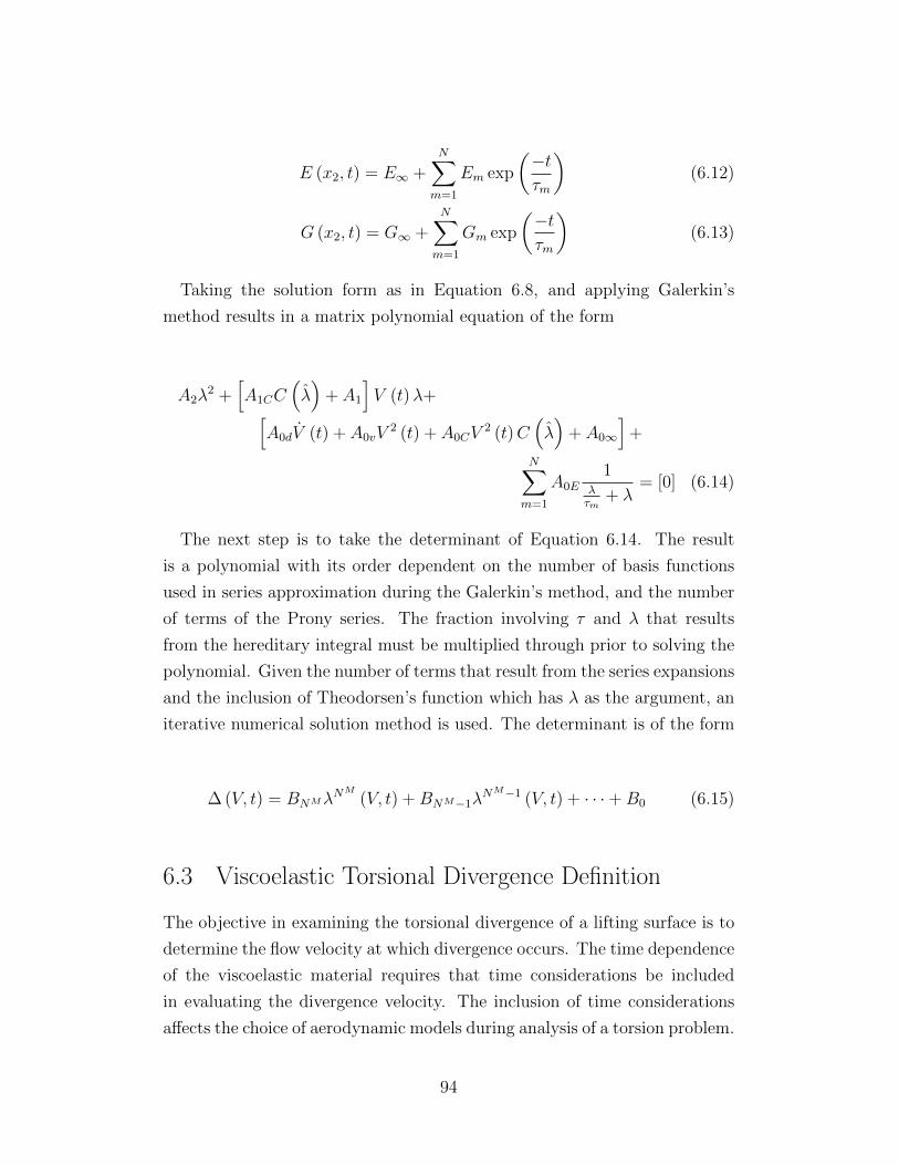
E (x2, t) = E∞ +N∑m=1
Em exp
(−tτm
)(6.12)
G (x2, t) = G∞ +N∑m=1
Gm exp
(−tτm
)(6.13)
Taking the solution form as in Equation 6.8, and applying Galerkin’s
method results in a matrix polynomial equation of the form
A2λ2 +
[A1CC
(λ)
+ A1
]V (t)λ+[
A0dV (t) + A0vV2 (t) + A0CV
2 (t)C(λ)
+ A0∞
]+
N∑m=1
A0E1
λτm
+ λ= [0] (6.14)
The next step is to take the determinant of Equation 6.14. The result
is a polynomial with its order dependent on the number of basis functions
used in series approximation during the Galerkin’s method, and the number
of terms of the Prony series. The fraction involving τ and λ that results
from the hereditary integral must be multiplied through prior to solving the
polynomial. Given the number of terms that result from the series expansions
and the inclusion of Theodorsen’s function which has λ as the argument, an
iterative numerical solution method is used. The determinant is of the form
∆ (V, t) = BNMλNM
(V, t) +BNM−1λNM−1 (V, t) + · · ·+B0 (6.15)
6.3 Viscoelastic Torsional Divergence Definition
The objective in examining the torsional divergence of a lifting surface is to
determine the flow velocity at which divergence occurs. The time dependence
of the viscoelastic material requires that time considerations be included
in evaluating the divergence velocity. The inclusion of time considerations
affects the choice of aerodynamic models during analysis of a torsion problem.
94
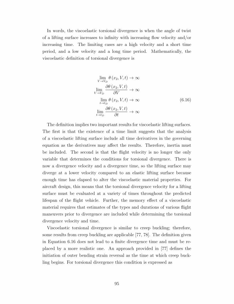
In words, the viscoelastic torsional divergence is when the angle of twist
of a lifting surface increases to infinity with increasing flow velocity and/or
increasing time. The limiting cases are a high velocity and a short time
period, and a low velocity and a long time period. Mathematically, the
viscoelastic definition of torsional divergence is
limV→VD
θ (x2, V, t)→∞
limV→VD
∂θ (x2, V, t)
∂V→∞
limt→tD
θ (x2, V, t)→∞ (6.16)
limt→tD
∂θ (x2, V, t)
∂t→∞
The definition implies two important results for viscoelastic lifting surfaces.
The first is that the existence of a time limit suggests that the analysis
of a viscoelastic lifting surface include all time derivatives in the governing
equation as the derivatives may affect the results. Therefore, inertia must
be included. The second is that the flight velocity is no longer the only
variable that determines the conditions for torsional divergence. There is
now a divergence velocity and a divergence time, so the lifting surface may
diverge at a lower velocity compared to an elastic lifting surface because
enough time has elapsed to alter the viscoelastic material properties. For
aircraft design, this means that the torsional divergence velocity for a lifting
surface must be evaluated at a variety of times throughout the predicted
lifespan of the flight vehicle. Further, the memory effect of a viscoelastic
material requires that estimates of the types and durations of various flight
maneuvers prior to divergence are included while determining the torsional
divergence velocity and time.
Viscoelastic torsional divergence is similar to creep buckling; therefore,
some results from creep buckling are applicable [77, 78]. The definition given
in Equation 6.16 does not lead to a finite divergence time and must be re-
placed by a more realistic one. An approach provided in [77] defines the
initiation of outer bending strain reversal as the time at which creep buck-
ling begins. For torsional divergence this condition is expressed as
95
limt→tD
∂εmax22 (h, t, V )
∂t→ 0
0 < V < VD and 0 < t0 < tD <∞ (6.17)
The connection between the torsional divergence definition and the λ def-
inition in Table 6.1 is through the solution form in Equation 6.15. For θ
to go to infinity, the real part of λ must be positive. The imaginary part
of λ is not restricted in any way and may be zero for some combinations of
parameters. The calculation of the torsional divergence speed and time for
a specific example occurs simultaneously. The aerodynamics of the problem
include the flight velocity which is left as a free variable during the calcula-
tions. The time is also a free variable as it appears as the upper bound in
the viscoelastic integral.
To calculate the torsional divergence speed and time, all that is necessary
is to solve Equation 6.15 and find the combinations of velocity and time that
result in at least one root λ having a positive real component.
6.3.1 Limiting cases of viscoelastic torsional divergence
There are three limiting cases of viscoelastic torsional divergence to consider,
each successively more restrictive:
Case 1 Torsion equation only with unsteady aerodynamics
Case 2 Torsion equation only with quasi-steady aerodynamics
Case 3 Torsion equation only with elastic material and quasi-steady aero-
dynamics
The reasons for the limiting cases is that they are easier to calculate for
quick design checks, and the successive cases demonstrate the connection be-
tween the new bending-torsion viscoelastic definition of torsional divergence
and the legacy elastic definition.
Case 1: The first case uses a modified form of the torsion equation that
appears as part of the bending-torsion model. The torsion equation with
unsteady aerodynamics is
96
[Iθ − πρb4
(1
8+ a2
)]θ+
+
[2πρV (t) b3
(a+
1
2
)(1
2− a)C(λ)]
θ+
+
[πρb2
(V 2 (t) + baV (t)
)+ 2πρV 2 (t) b2
(a+
1
2
)C(λ)]
θ−
− ∂
∂x2
(∫ t
−∞G (x2, t− s) J (x2)
∂θ (x2, s)
∂x2
ds
)= 0 (6.18)
As before, Galerkin’s method is necessary to eliminate the x2 component
of the problem, and the same solution form for θ is used. The result is
a polynomial equation that is similar to the determinant required for the
bending-torsion equation. The polynomial is only of the order N + 2.
∆ (V, t) = BN+2λN+2 (V, t) +BN+1λ
N+1 (V, t) + · · ·+B0 (6.19)
A similar iterative root finder to the bending-torsion case is used to solve
for the combinations of velocity and time that result in at least one positive
real component of λ.
Case 2: A further restriction is implemented by the use of quasi-steady
aerodynamics. The modification is simple in that the Theodorsen’s function,
C(λ)
is set to 1. The resulting equation is
[Iθ − πρb4
(1
8+ a2
)]θ+
+
[2πρV (t) b3
(a+
1
2
)(1
2− a)]
θ+
+
[πρb2
(V 2 (t) + baV (t)
)+ 2πρV 2 (t) b2
(a+
1
2
)]θ−
− ∂
∂x2
(∫ t
−∞G (x2, t− s) J (x2)
∂θ (x2, s)
∂x2
ds
)= 0 (6.20)
The polynomial equation after application of Galerkin’s method and the
θ solution form is nearly identical to Equation 6.19. The only change is
that the elimination of Theodorsen’s function allows a direct root solver
97
such as MATLABTM’s roots subroutine. The iteration was only necessary
in the previous two cases because of the implicit situation created by the
Theodorsen’s function.
Case 3: Elastic torsional divergence with quasi-steady aerodynamics. The
time dependence of the material is removed thus creating a static problem.
Torsional divergence for an elastic wing is defined as the flight velocity at
which the angle of twist of the wing, θE, and/or its velocity derivative in-
creases to infinity. Conceptually, torsional divergence of an elastic wing is
similar to column buckling. Mathematically, the definition is
limV→VD
θE (x2, V )→∞
limV→VD
∂θE (x2, V )
∂V→∞ (6.21)
Starting from first principles, a cross-section of the wing is shown in Figure
6.6 with the stiffness of the wing represented as an angular spring. The lift
and moment are also depicted. Torsional divergence is conventionally treated
as a static equilibrium problem because it is assumed that there are no oscil-
latory motions of the wing as the flight speed gradually increases. Another
way to depict the situation is to envision an aircraft gradually increasing its
flight speed with long pauses for any transitory motion to disappear. After
each pause, the angle of twist of the wing is measured.
The moment equilibrium about the x2 axis is given as
∑M : My −Mresistance = 0 (6.22)
where My is the moment resulting from the aerodynamic loads taken about
the elastic axis of the wing and Mresistance is the resisting moment of the
material. For static equilibrium, the associated aerodynamics are steady
because there are no changes in the wake from oscillatory movements of the
airfoil. As such, the aerodynamics may be expressed as
My = Mac + Le (6.23)
where Mac is the moment about the aerodynamic center, L is the lift, and
e is the distance from the aerodynamic center to the elastic axis [79]. The
98
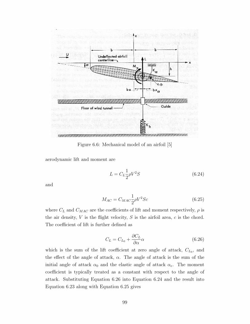
Figure 6.6: Mechanical model of an airfoil [5]
aerodynamic lift and moment are
L = CL1
2ρV 2S (6.24)
and
MAC = CMAC1
2ρV 2Sc (6.25)
where CL and CMAC are the coefficients of lift and moment respectively, ρ is
the air density, V is the flight velocity, S is the airfoil area, c is the chord.
The coefficient of lift is further defined as
CL = CL0 +∂CL∂α
α (6.26)
which is the sum of the lift coefficient at zero angle of attack, CL0 , and
the effect of the angle of attack, α. The angle of attack is the sum of the
initial angle of attack α0 and the elastic angle of attack αe. The moment
coefficient is typically treated as a constant with respect to the angle of
attack. Substituting Equation 6.26 into Equation 6.24 and the result into
Equation 6.23 along with Equation 6.25 gives
99
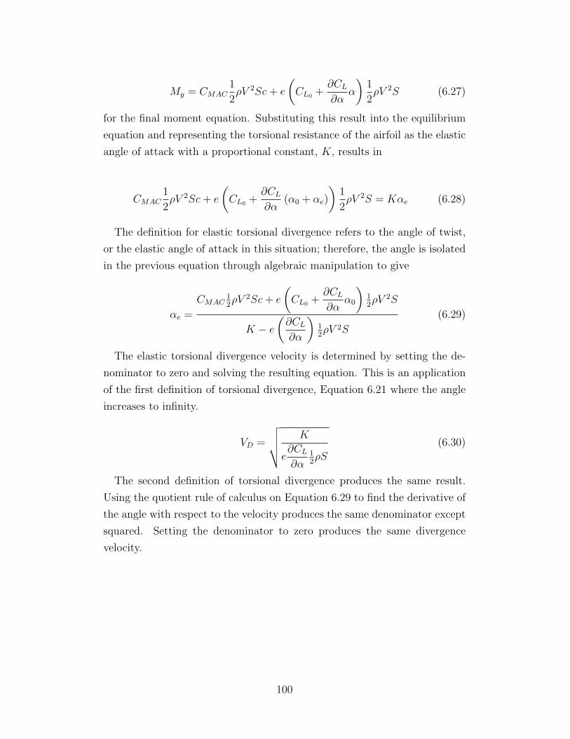
My = CMAC1
2ρV 2Sc+ e
(CL0 +
∂CL∂α
α
)1
2ρV 2S (6.27)
for the final moment equation. Substituting this result into the equilibrium
equation and representing the torsional resistance of the airfoil as the elastic
angle of attack with a proportional constant, K, results in
CMAC1
2ρV 2Sc+ e
(CL0 +
∂CL∂α
(α0 + αe)
)1
2ρV 2S = Kαe (6.28)
The definition for elastic torsional divergence refers to the angle of twist,
or the elastic angle of attack in this situation; therefore, the angle is isolated
in the previous equation through algebraic manipulation to give
αe =
CMAC12ρV 2Sc+ e
(CL0 +
∂CL∂α
α0
)12ρV 2S
K − e(∂CL∂α
)12ρV 2S
(6.29)
The elastic torsional divergence velocity is determined by setting the de-
nominator to zero and solving the resulting equation. This is an application
of the first definition of torsional divergence, Equation 6.21 where the angle
increases to infinity.
VD =
√√√√ K
e∂CL∂α
12ρS
(6.30)
The second definition of torsional divergence produces the same result.
Using the quotient rule of calculus on Equation 6.29 to find the derivative of
the angle with respect to the velocity produces the same denominator except
squared. Setting the denominator to zero produces the same divergence
velocity.
100
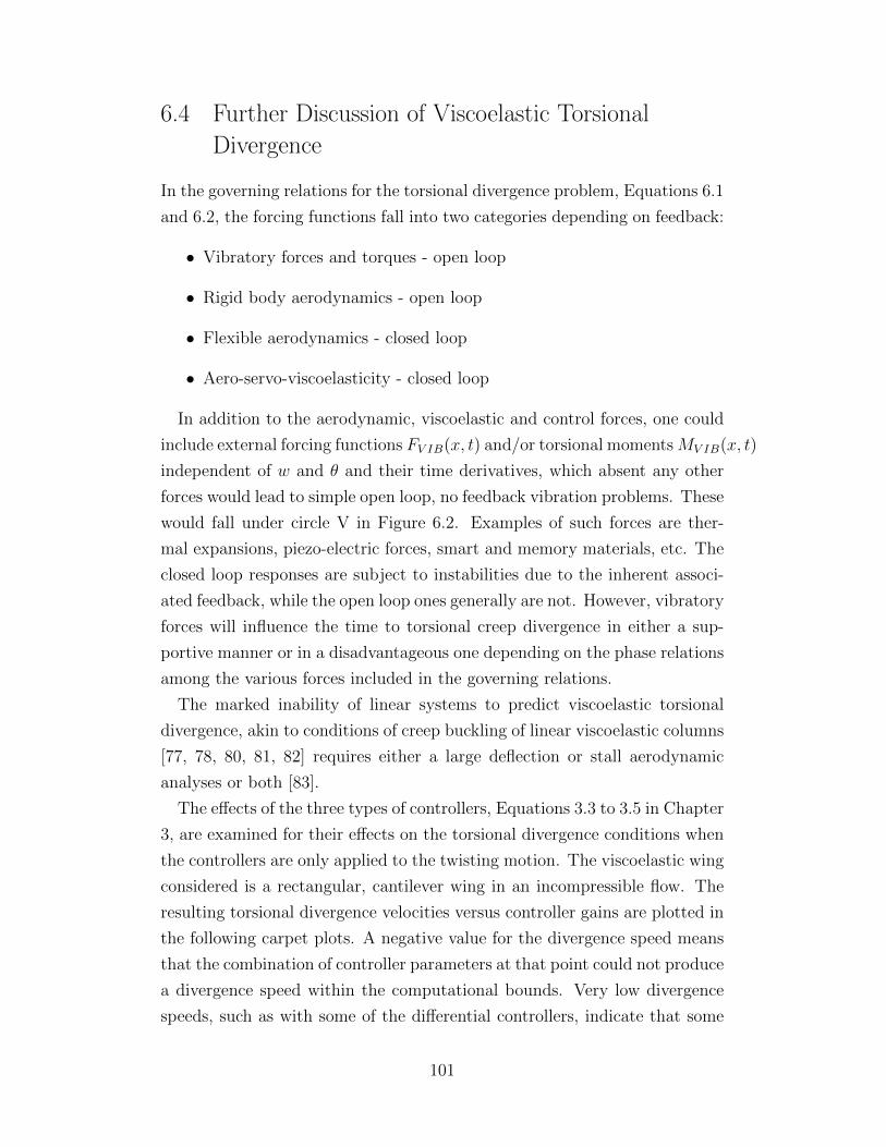
6.4 Further Discussion of Viscoelastic Torsional
Divergence
In the governing relations for the torsional divergence problem, Equations 6.1
and 6.2, the forcing functions fall into two categories depending on feedback:
• Vibratory forces and torques - open loop
• Rigid body aerodynamics - open loop
• Flexible aerodynamics - closed loop
• Aero-servo-viscoelasticity - closed loop
In addition to the aerodynamic, viscoelastic and control forces, one could
include external forcing functions FV IB(x, t) and/or torsional momentsMV IB(x, t)
independent of w and θ and their time derivatives, which absent any other
forces would lead to simple open loop, no feedback vibration problems. These
would fall under circle V in Figure 6.2. Examples of such forces are ther-
mal expansions, piezo-electric forces, smart and memory materials, etc. The
closed loop responses are subject to instabilities due to the inherent associ-
ated feedback, while the open loop ones generally are not. However, vibratory
forces will influence the time to torsional creep divergence in either a sup-
portive manner or in a disadvantageous one depending on the phase relations
among the various forces included in the governing relations.
The marked inability of linear systems to predict viscoelastic torsional
divergence, akin to conditions of creep buckling of linear viscoelastic columns
[77, 78, 80, 81, 82] requires either a large deflection or stall aerodynamic
analyses or both [83].
The effects of the three types of controllers, Equations 3.3 to 3.5 in Chapter
3, are examined for their effects on the torsional divergence conditions when
the controllers are only applied to the twisting motion. The viscoelastic wing
considered is a rectangular, cantilever wing in an incompressible flow. The
resulting torsional divergence velocities versus controller gains are plotted in
the following carpet plots. A negative value for the divergence speed means
that the combination of controller parameters at that point could not produce
a divergence speed within the computational bounds. Very low divergence
speeds, such as with some of the differential controllers, indicate that some
101
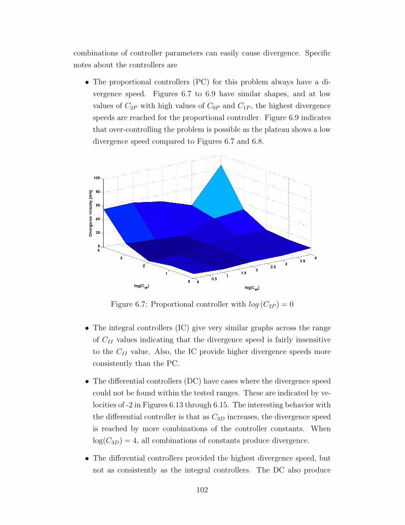
combinations of controller parameters can easily cause divergence. Specific
notes about the controllers are
• The proportional controllers (PC) for this problem always have a di-
vergence speed. Figures 6.7 to 6.9 have similar shapes, and at low
values of C2P with high values of C0P and C1P , the highest divergence
speeds are reached for the proportional controller. Figure 6.9 indicates
that over-controlling the problem is possible as the plateau shows a low
divergence speed compared to Figures 6.7 and 6.8.
Figure 6.7: Proportional controller with log (C2P ) = 0
• The integral controllers (IC) give very similar graphs across the range
of CII values indicating that the divergence speed is fairly insensitive
to the CII value. Also, the IC provide higher divergence speeds more
consistently than the PC.
• The differential controllers (DC) have cases where the divergence speed
could not be found within the tested ranges. These are indicated by ve-
locities of -2 in Figures 6.13 through 6.15. The interesting behavior with
the differential controller is that as C3D increases, the divergence speed
is reached by more combinations of the controller constants. When
log(C3D) = 4, all combinations of constants produce divergence.
• The differential controllers provided the highest divergence speed, but
not as consistently as the integral controllers. The DC also produce
102
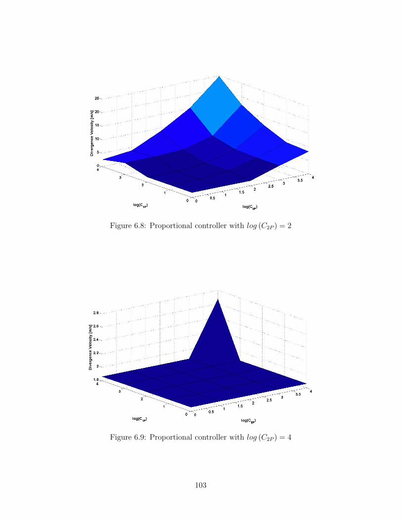
Figure 6.8: Proportional controller with log (C2P ) = 2
Figure 6.9: Proportional controller with log (C2P ) = 4
103
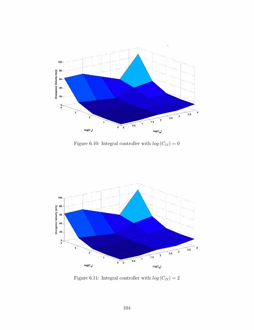
Figure 6.10: Integral controller with log (CII) = 0
Figure 6.11: Integral controller with log (CII) = 2
104
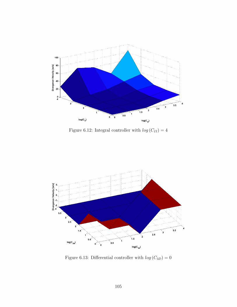
Figure 6.12: Integral controller with log (CII) = 4
Figure 6.13: Differential controller with log (C3D) = 0
105
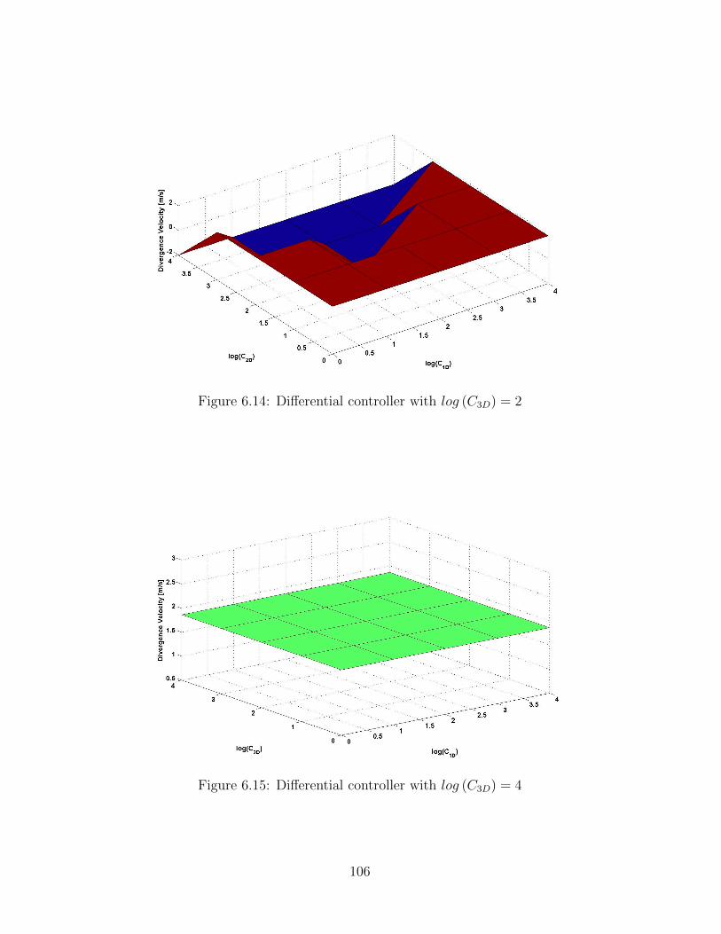
Figure 6.14: Differential controller with log (C3D) = 2
Figure 6.15: Differential controller with log (C3D) = 4
106
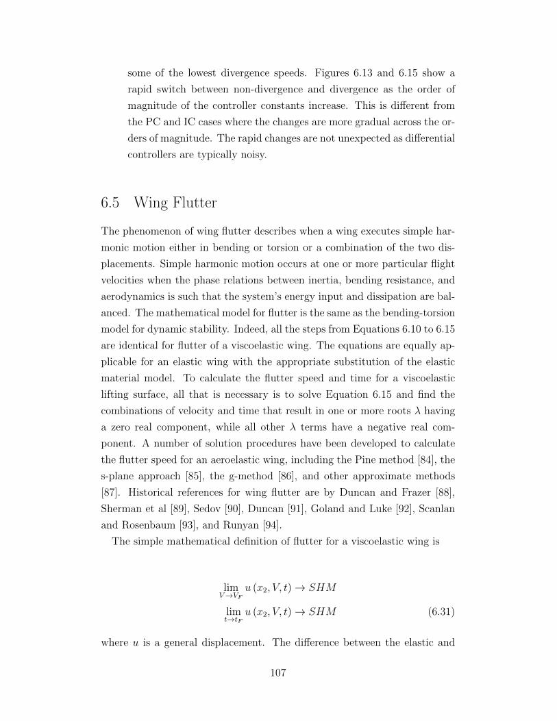
some of the lowest divergence speeds. Figures 6.13 and 6.15 show a
rapid switch between non-divergence and divergence as the order of
magnitude of the controller constants increase. This is different from
the PC and IC cases where the changes are more gradual across the or-
ders of magnitude. The rapid changes are not unexpected as differential
controllers are typically noisy.
6.5 Wing Flutter
The phenomenon of wing flutter describes when a wing executes simple har-
monic motion either in bending or torsion or a combination of the two dis-
placements. Simple harmonic motion occurs at one or more particular flight
velocities when the phase relations between inertia, bending resistance, and
aerodynamics is such that the system’s energy input and dissipation are bal-
anced. The mathematical model for flutter is the same as the bending-torsion
model for dynamic stability. Indeed, all the steps from Equations 6.10 to 6.15
are identical for flutter of a viscoelastic wing. The equations are equally ap-
plicable for an elastic wing with the appropriate substitution of the elastic
material model. To calculate the flutter speed and time for a viscoelastic
lifting surface, all that is necessary is to solve Equation 6.15 and find the
combinations of velocity and time that result in one or more roots λ having
a zero real component, while all other λ terms have a negative real com-
ponent. A number of solution procedures have been developed to calculate
the flutter speed for an aeroelastic wing, including the Pine method [84], the
s-plane approach [85], the g-method [86], and other approximate methods
[87]. Historical references for wing flutter are by Duncan and Frazer [88],
Sherman et al [89], Sedov [90], Duncan [91], Goland and Luke [92], Scanlan
and Rosenbaum [93], and Runyan [94].
The simple mathematical definition of flutter for a viscoelastic wing is
limV→VF
u (x2, V, t)→ SHM
limt→tF
u (x2, V, t)→ SHM (6.31)
where u is a general displacement. The difference between the elastic and
107
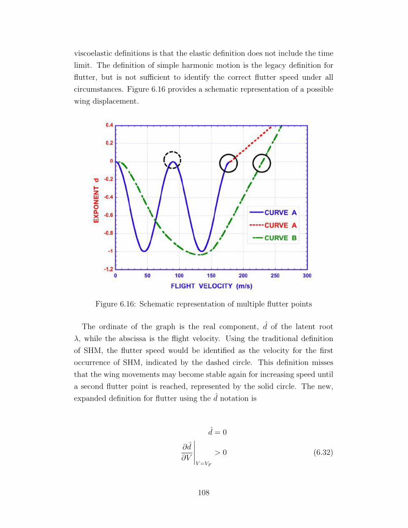
viscoelastic definitions is that the elastic definition does not include the time
limit. The definition of simple harmonic motion is the legacy definition for
flutter, but is not sufficient to identify the correct flutter speed under all
circumstances. Figure 6.16 provides a schematic representation of a possible
wing displacement.
Figure 6.16: Schematic representation of multiple flutter points
The ordinate of the graph is the real component, d of the latent root
λ, while the abscissa is the flight velocity. Using the traditional definition
of SHM, the flutter speed would be identified as the velocity for the first
occurrence of SHM, indicated by the dashed circle. This definition misses
that the wing movements may become stable again for increasing speed until
a second flutter point is reached, represented by the solid circle. The new,
expanded definition for flutter using the d notation is
d = 0
∂d
∂V
∣∣∣∣∣V=VF
> 0 (6.32)
108
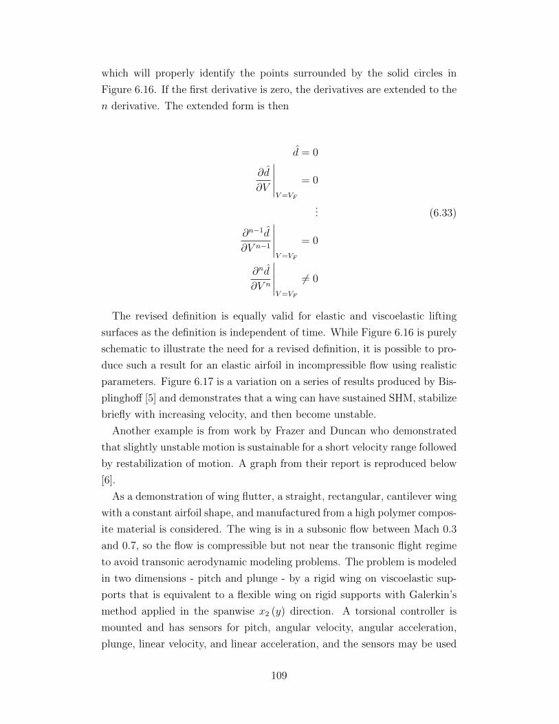
which will properly identify the points surrounded by the solid circles in
Figure 6.16. If the first derivative is zero, the derivatives are extended to the
n derivative. The extended form is then
d = 0
∂d
∂V
∣∣∣∣∣V=VF
= 0
... (6.33)
∂n−1d
∂V n−1
∣∣∣∣∣V=VF
= 0
∂nd
∂V n
∣∣∣∣∣V=VF
6= 0
The revised definition is equally valid for elastic and viscoelastic lifting
surfaces as the definition is independent of time. While Figure 6.16 is purely
schematic to illustrate the need for a revised definition, it is possible to pro-
duce such a result for an elastic airfoil in incompressible flow using realistic
parameters. Figure 6.17 is a variation on a series of results produced by Bis-
plinghoff [5] and demonstrates that a wing can have sustained SHM, stabilize
briefly with increasing velocity, and then become unstable.
Another example is from work by Frazer and Duncan who demonstrated
that slightly unstable motion is sustainable for a short velocity range followed
by restabilization of motion. A graph from their report is reproduced below
[6].
As a demonstration of wing flutter, a straight, rectangular, cantilever wing
with a constant airfoil shape, and manufactured from a high polymer compos-
ite material is considered. The wing is in a subsonic flow between Mach 0.3
and 0.7, so the flow is compressible but not near the transonic flight regime
to avoid transonic aerodynamic modeling problems. The problem is modeled
in two dimensions - pitch and plunge - by a rigid wing on viscoelastic sup-
ports that is equivalent to a flexible wing on rigid supports with Galerkin’s
method applied in the spanwise x2 (y) direction. A torsional controller is
mounted and has sensors for pitch, angular velocity, angular acceleration,
plunge, linear velocity, and linear acceleration, and the sensors may be used
109
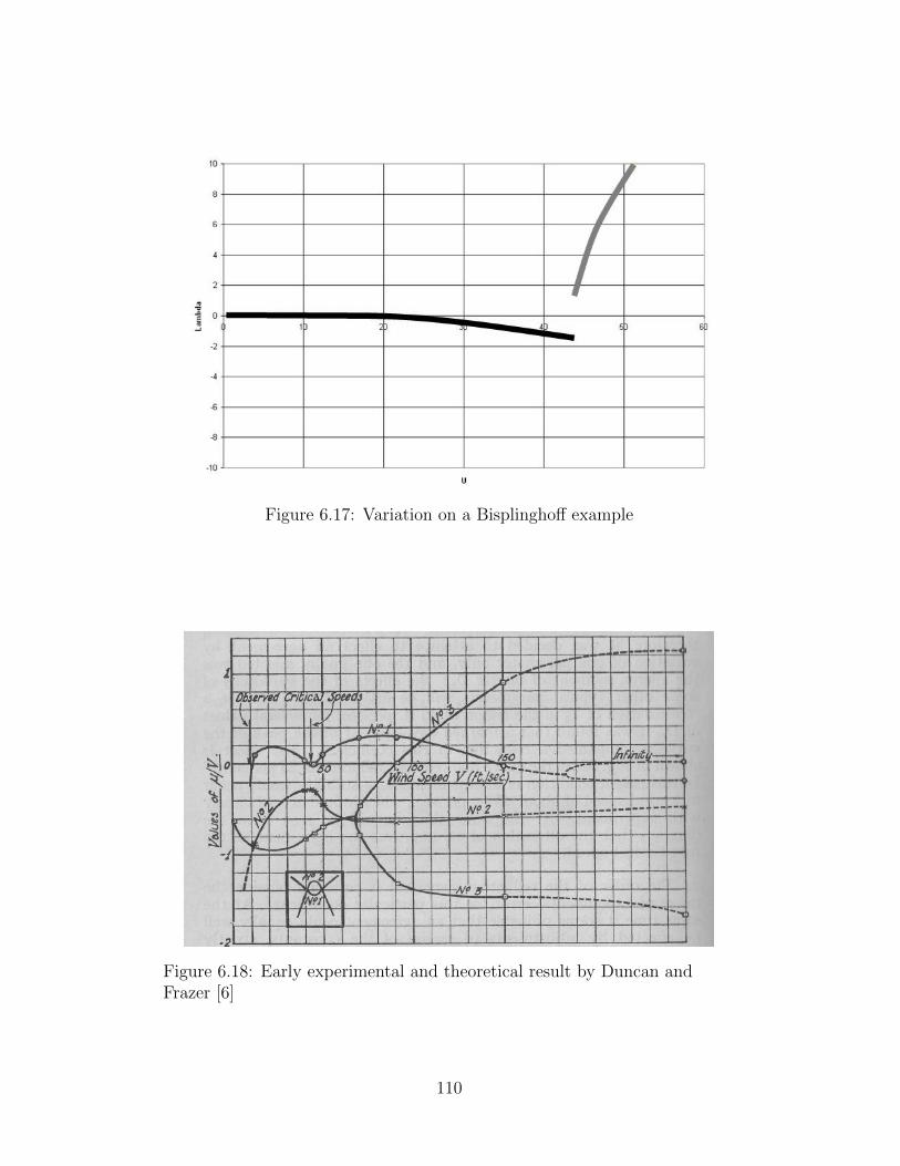
Figure 6.17: Variation on a Bisplinghoff example
Figure 6.18: Early experimental and theoretical result by Duncan andFrazer [6]
110
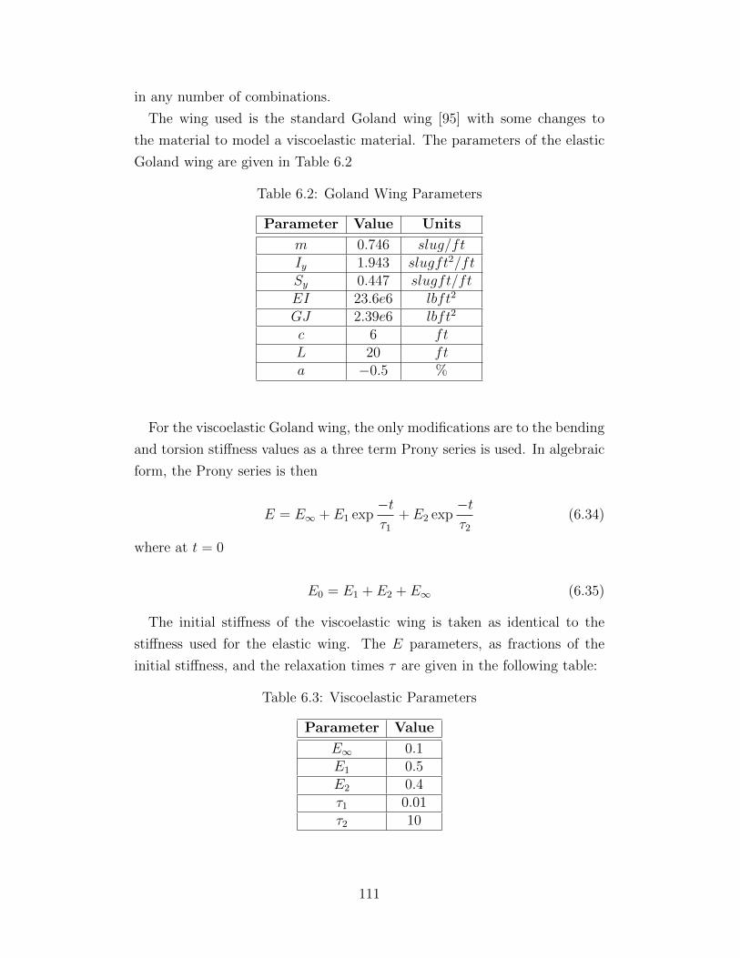
in any number of combinations.
The wing used is the standard Goland wing [95] with some changes to
the material to model a viscoelastic material. The parameters of the elastic
Goland wing are given in Table 6.2
Table 6.2: Goland Wing Parameters
Parameter Value Units
m 0.746 slug/ftIy 1.943 slugft2/ftSy 0.447 slugft/ftEI 23.6e6 lbft2
GJ 2.39e6 lbft2
c 6 ftL 20 fta −0.5 %
For the viscoelastic Goland wing, the only modifications are to the bending
and torsion stiffness values as a three term Prony series is used. In algebraic
form, the Prony series is then
E = E∞ + E1 exp−tτ1
+ E2 exp−tτ2
(6.34)
where at t = 0
E0 = E1 + E2 + E∞ (6.35)
The initial stiffness of the viscoelastic wing is taken as identical to the
stiffness used for the elastic wing. The E parameters, as fractions of the
initial stiffness, and the relaxation times τ are given in the following table:
Table 6.3: Viscoelastic Parameters
Parameter Value
E∞ 0.1E1 0.5E2 0.4τ1 0.01τ2 10
111
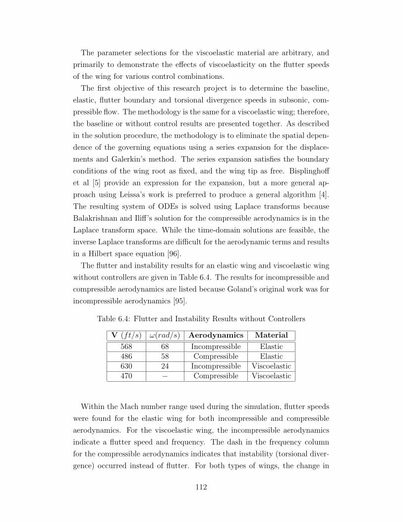
The parameter selections for the viscoelastic material are arbitrary, and
primarily to demonstrate the effects of viscoelasticity on the flutter speeds
of the wing for various control combinations.
The first objective of this research project is to determine the baseline,
elastic, flutter boundary and torsional divergence speeds in subsonic, com-
pressible flow. The methodology is the same for a viscoelastic wing; therefore,
the baseline or without control results are presented together. As described
in the solution procedure, the methodology is to eliminate the spatial depen-
dence of the governing equations using a series expansion for the displace-
ments and Galerkin’s method. The series expansion satisfies the boundary
conditions of the wing root as fixed, and the wing tip as free. Bisplinghoff
et al [5] provide an expression for the expansion, but a more general ap-
proach using Leissa’s work is preferred to produce a general algorithm [4].
The resulting system of ODEs is solved using Laplace transforms because
Balakrishnan and Iliff’s solution for the compressible aerodynamics is in the
Laplace transform space. While the time-domain solutions are feasible, the
inverse Laplace transforms are difficult for the aerodynamic terms and results
in a Hilbert space equation [96].
The flutter and instability results for an elastic wing and viscoelastic wing
without controllers are given in Table 6.4. The results for incompressible and
compressible aerodynamics are listed because Goland’s original work was for
incompressible aerodynamics [95].
Table 6.4: Flutter and Instability Results without Controllers
V (ft/s) ω(rad/s) Aerodynamics Material
568 68 Incompressible Elastic486 58 Compressible Elastic630 24 Incompressible Viscoelastic470 − Compressible Viscoelastic
Within the Mach number range used during the simulation, flutter speeds
were found for the elastic wing for both incompressible and compressible
aerodynamics. For the viscoelastic wing, the incompressible aerodynamics
indicate a flutter speed and frequency. The dash in the frequency column
for the compressible aerodynamics indicates that instability (torsional diver-
gence) occurred instead of flutter. For both types of wings, the change in
112
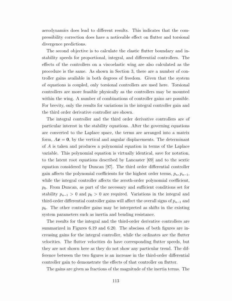
aerodynamics does lead to different results. This indicates that the com-
pressibility correction does have a noticeable effect on flutter and torsional
divergence predictions.
The second objective is to calculate the elastic flutter boundary and in-
stability speeds for proportional, integral, and differential controllers. The
effects of the controllers on a viscoelastic wing are also calculated as the
procedure is the same. As shown in Section 3, there are a number of con-
troller gains available in both degrees of freedom. Given that the system
of equations is coupled, only torsional controllers are used here. Torsional
controllers are more feasible physically as the controllers may be mounted
within the wing. A number of combinations of controller gains are possible.
For brevity, only the results for variations in the integral controller gain and
the third order derivative controller are shown.
The integral controller and the third order derivative controllers are of
particular interest in the stability equations. After the governing equations
are converted to the Laplace space, the terms are arranged into a matrix
form, Ax = 0, by the vertical and angular displacements. The determinant
of A is taken and produces a polynomial equation in terms of the Laplace
variable. This polynomial equation is virtually identical, save for notation,
to the latent root equations described by Lancaster [69] and to the sextic
equation considered by Duncan [97]. The third order differential controller
gain affects the polynomial coefficients for the highest order terms, pn, pn−1,
while the integral controller affects the zeroth-order polynomial coefficient,
p0. From Duncan, as part of the necessary and sufficient conditions set for
stability pn−1 > 0 and p0 > 0 are required. Variations in the integral and
third-order differential controller gains will affect the overall signs of pn−1 and
p0. The other controller gains may be interpreted as shifts in the existing
system parameters such as inertia and bending resistance.
The results for the integral and the third-order derivative controllers are
summarized in Figures 6.19 and 6.20. The abscissa of both figures are in-
creasing gains for the integral controller, while the ordinates are the flutter
velocities. The flutter velocities do have corresponding flutter speeds, but
they are not shown here as they do not show any particular trend. The dif-
ference between the two figures is an increase in the third-order differential
controller gain to demonstrate the effects of that controller on flutter.
The gains are given as fractions of the magnitude of the inertia terms. The
113
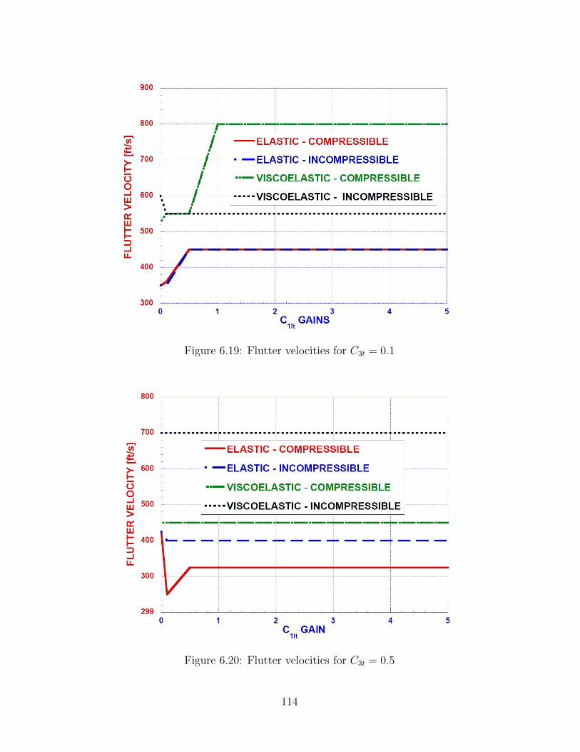
Figure 6.19: Flutter velocities for C3t = 0.1
Figure 6.20: Flutter velocities for C3t = 0.5
114
inertia terms are of the order 1 therefore the controller gains range from 0.1
to 5. Higher order gains are possible; however, larger gains will dominate the
system and are less feasible to implement.
For the elastic wing with C3t = 0.1, the results for incompressible and com-
pressible flow are identical. There is a noticeable increase in flutter speed
when the gain CIIt is increased from 0 to 0.5; but no further increase oc-
curs with increasing gain. For C3t = 0.5, the compressible flutter boundary
speeds are lower than the incompressible flutter boundary speeds for all in-
tegral controller gains. The elastic wing flutter speeds are also lower for
C3t = 0.5 compared to the results for C3t = 0.1. This suggests that increas-
ing the third-order differential controller gain decreases the stability of the
wing. The result is expected as the controller gain in the polynomial stability
equation is negative and affects the pn−1 term. As per Duncan, pn−1 > 0 is
part of the necessary and sufficient conditions for stability. The difference
in compressible and incompressible flutter boundary speeds when C3t = 0.5
for elastic wings is related to the aerodynamics as increasing integral con-
troller gain does not change the flutter speed. As for the no-controller case,
the incompressible aerodynamics over-estimate the flutter speeds. No over-
estimate exists for C3t = 0.1 which suggests that the differential controller
minimizes the mathematical effects of the compressibility correction.
For the viscoelastic wing with C3t = 0.1, the flutter speeds for increasing
integral controller gains are significantly higher for the compressible aerody-
namics model. For gains greater than 1, the flutter speeds are beyond the
parameters of the simulation. The incompressible aerodynamics model has a
relatively lower flutter speed that is insensitive to increasing controller gain.
For C3t = 0.5, the flutter boundary speeds of the viscoelastic wing are higher
for the incompressible aerodynamics than the compressible aerodynamics.
The flutter speeds for the incompressible aerodynamics are at the top of the
plot. Compared to the results for C3t = 0.1 the flutter speeds for the higher
gain are lower by over 100ft/s. The difference between the C3t = 0.1 and
C3t = 0.5 viscoelastic flutter boundary speeds is consistent with the elastic
flutter boundary speeds, suggesting that the higher differential controller gain
destabilizes both systems. The effect of the compressibility correction on the
viscoelastic wing is less obvious compared to the elastic wing. Without con-
trollers, the compressible aerodynamics predicted a lower flutter speed than
the incompressible aerodynamics. With controllers, there is no discernible
115
trend for the effects of compressibility. The lack of a trend is not unexpected
as, in other papers, it has been demonstrated that the results of a viscoelastic
system are highly dependent on the parameter values [60].
The lack of an effect for the viscoelastic wing with increasing integral
controller gain is similar to that of the elastic wing. Much larger controller
gains may be necessary to observe drastic changes in flutter boundary speeds;
however, larger gains are more difficult to implement physically. Of note
though, is even for small integral controller gains, there is an improvement
over the no-controller scenario. This suggests that even a simple integral
controller acting on the angular displacement of the wing would provide an
improved flutter boundary speed.
The effect of the viscoelastic material is noticeable for identical wing ge-
ometries. Improvements in flutter boundary speed of up to 200ft/s are pos-
sible. A viscoelastic material, as mentioned earlier, dissipates energy and has
a memory. Energy is supplied to the wing by the airflow and is proportional
to the velocity. With increasing flow velocity, an increasing amount of energy
is provided to the wing. The dissipation effect of the material would remove
the accumulated energy thus delaying the flutter boundary. The memory
effect is also, potentially, beneficial as controller forces will linger after the
control force is initially applied.
Torsional divergence speeds do not appear in the graphs explicitly. For
most cases, the numerical simulations indicate that the neutral stability of
the wing is immediately followed by instability if the flight velocity is in-
creased. For the elastic wing, if the flight velocity is held at the flutter
boundary speed, the neutral stability will persist indefinitely. For the vis-
coelastic wing, neutral stability will not persist indefinitely because of the
material’s time dependence. Depending on the viscoelastic parameters, sta-
bility or instability are possible. The viscoelastic wing with C3t = 0.5 and
CIIt = 0.1 becomes stable with increasing flight speed beyond the flutter
boundary.
6.6 Chordwise and Asymmetric Bending
Chordwise and asymmetric bending were neglected in the governing bending-
torsion equations described in the introduction of this chapter. The inclusion
116
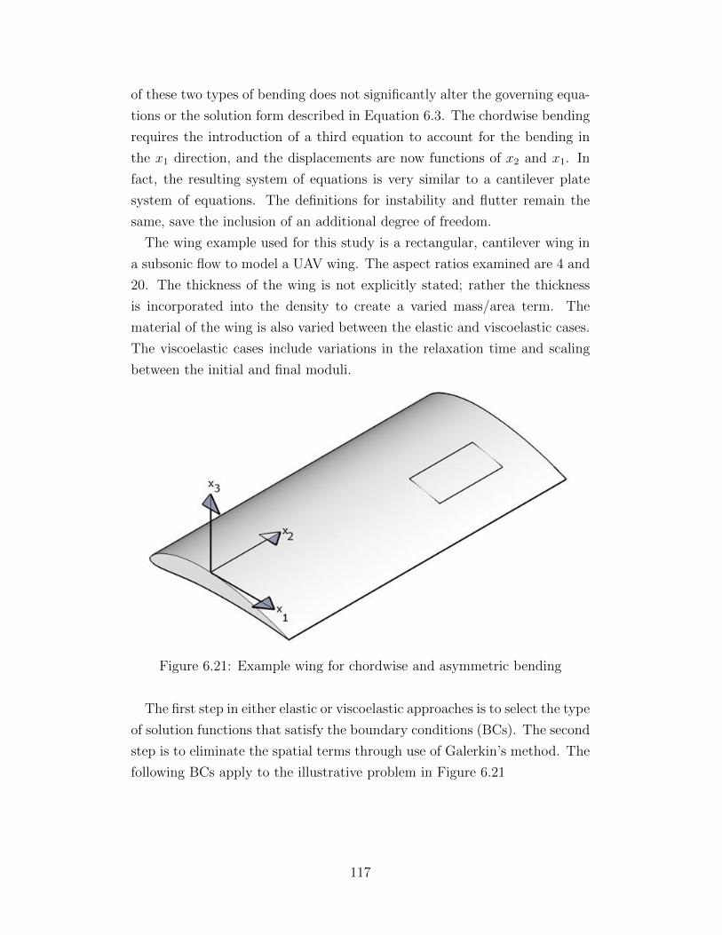
of these two types of bending does not significantly alter the governing equa-
tions or the solution form described in Equation 6.3. The chordwise bending
requires the introduction of a third equation to account for the bending in
the x1 direction, and the displacements are now functions of x2 and x1. In
fact, the resulting system of equations is very similar to a cantilever plate
system of equations. The definitions for instability and flutter remain the
same, save the inclusion of an additional degree of freedom.
The wing example used for this study is a rectangular, cantilever wing in
a subsonic flow to model a UAV wing. The aspect ratios examined are 4 and
20. The thickness of the wing is not explicitly stated; rather the thickness
is incorporated into the density to create a varied mass/area term. The
material of the wing is also varied between the elastic and viscoelastic cases.
The viscoelastic cases include variations in the relaxation time and scaling
between the initial and final moduli.
Figure 6.21: Example wing for chordwise and asymmetric bending
The first step in either elastic or viscoelastic approaches is to select the type
of solution functions that satisfy the boundary conditions (BCs). The second
step is to eliminate the spatial terms through use of Galerkin’s method. The
following BCs apply to the illustrative problem in Figure 6.21
117
x1 = −b free
x1 = b free
x2 = 0 clamped
x2 = L free
(6.36)
At this point, depending on the form of the constitutive relations, a sys-
tem of ordinary differential equations (ODE) or ordinary integral differential
equations (OIDE) remain after the spatial components are eliminated by ap-
plication of Galerkin’s method. The third step is to select a time solution of
the form:
h(t) = Ceλt (6.37)
where
λ = d+ iω (6.38)
The real parameter d is a function of the flight velocity, V, while ω is the
frequency. The constant C is a vector of scalars representing the amplitudes
of the modes used in the Galerkin method. These amplitudes are a function
of the flight velocity as well.
Substituting the time solution into the differential equations results in a
latent root problem as before in terms of the λ. As a demonstration of the
generalized eigenvalue method described by Tisseur and Meerbergen [70],
and its equivalence to the λ-matrix method, the following example is solved
using their approach. Given that the problem is of order two or three, a
change of variables is required. Assuming the governing equation is of the
form:
A3 λ3 q + A2 λ
2 q + A1 λ q + A0 q = 0 (6.39)
where all the An terms are matrices in the general case, and q is the eigen-
118
vector. Using the following changes of variable
r = λq (6.40)
s = λr (6.41)
u = λs (6.42)
Equation 6.39 is transformed into the generalized form
[A] x = λ [B] x (6.43)
by a procedure described in detail in [70]. The resulting eigenvalue problem
is solvable in MATLABTM using the eig or polyeig functions. This method
produces all the eigenvalues, λ, of the problem. As in Sections 6.1 and 6.5
the real component of λ, denoted as d, indicates stability.
Using the above procedure and definitions for flutter and instability, a flex-
ible wing with combined chordwise and asymmetric bending, and torsion is
examined. Two mass/area values, two aspect ratios, five viscoelastic relax-
ation times, and two viscoelastic ratios
(E∞E0
)were considered for the wing.
The elastic results are given in Table 6.5, while the viscoelastic results are in
Tables 6.6 to 6.8. Some cells of the tables contain a dash (-), which means
that a value for that entry was not found within the bounds of the subsonic
flight profile used during the computations. All results are taken using four
modes in the Galerkin’s method.
Table 6.5: Elastic Flutter and Torsional Divergence
Mass/area Aspect VF ωF VD(kg/m2) ratio (m/s) (Hz) (m/s)
1.35 4 80 5 -27 4 60 2.5 -27 20 - - 50
For the elastic wing, Table 6.5, increasing the mass/area ratio has the
effect of decreasing the flutter speed. The effect is not unexpected because
increasing the mass/area ratio increases the inertia term in the governing
equations, thus changing the phase relationships between the terms. The
change in aspect ratio is more difficult to quantify. Within the simulation
parameters, the higher aspect ratio produced a divergence velocity that is
119
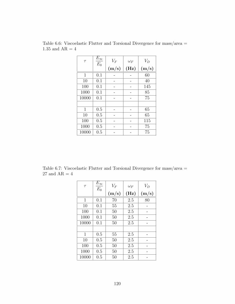
Table 6.6: Viscoelastic Flutter and Torsional Divergence for mass/area =1.35 and AR = 4
τE∞E0
VF ωF VD
(m/s) (Hz) (m/s)
1 0.1 - - 6010 0.1 - - 40100 0.1 - - 1451000 0.1 - - 8510000 0.1 - - 75
1 0.5 - - 6510 0.5 - - 65100 0.5 - - 1151000 0.5 - - 7510000 0.5 - - 75
Table 6.7: Viscoelastic Flutter and Torsional Divergence for mass/area =27 and AR = 4
τE∞E0
VF ωF VD
(m/s) (Hz) (m/s)
1 0.1 70 2.5 8010 0.1 55 2.5 -100 0.1 50 2.5 -1000 0.1 50 2.5 -10000 0.1 50 2.5 -
1 0.5 55 2.5 -10 0.5 50 2.5 -100 0.5 50 2.5 -1000 0.5 50 2.5 -10000 0.5 50 2.5 -
120
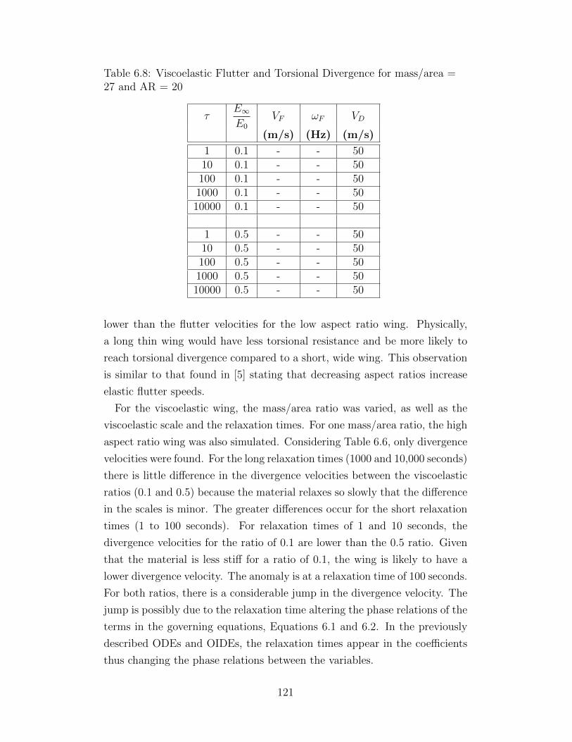
Table 6.8: Viscoelastic Flutter and Torsional Divergence for mass/area =27 and AR = 20
τE∞E0
VF ωF VD
(m/s) (Hz) (m/s)
1 0.1 - - 5010 0.1 - - 50100 0.1 - - 501000 0.1 - - 5010000 0.1 - - 50
1 0.5 - - 5010 0.5 - - 50100 0.5 - - 501000 0.5 - - 5010000 0.5 - - 50
lower than the flutter velocities for the low aspect ratio wing. Physically,
a long thin wing would have less torsional resistance and be more likely to
reach torsional divergence compared to a short, wide wing. This observation
is similar to that found in [5] stating that decreasing aspect ratios increase
elastic flutter speeds.
For the viscoelastic wing, the mass/area ratio was varied, as well as the
viscoelastic scale and the relaxation times. For one mass/area ratio, the high
aspect ratio wing was also simulated. Considering Table 6.6, only divergence
velocities were found. For the long relaxation times (1000 and 10,000 seconds)
there is little difference in the divergence velocities between the viscoelastic
ratios (0.1 and 0.5) because the material relaxes so slowly that the difference
in the scales is minor. The greater differences occur for the short relaxation
times (1 to 100 seconds). For relaxation times of 1 and 10 seconds, the
divergence velocities for the ratio of 0.1 are lower than the 0.5 ratio. Given
that the material is less stiff for a ratio of 0.1, the wing is likely to have a
lower divergence velocity. The anomaly is at a relaxation time of 100 seconds.
For both ratios, there is a considerable jump in the divergence velocity. The
jump is possibly due to the relaxation time altering the phase relations of the
terms in the governing equations, Equations 6.1 and 6.2. In the previously
described ODEs and OIDEs, the relaxation times appear in the coefficients
thus changing the phase relations between the variables.
121
Table 6.7 is for the same viscoelastic wing except at a higher mass/area
ratio. The increase in the mass/area is sufficient to produce flutter velocities
for all the combinations of viscoelastic scale and relaxation times. Similar
to Table 6.6, the longer relaxation times show little difference in the flutter
velocities between the two viscoelastic scales. Even the short relaxation times
are not excessively different. The only anomalous data point is the flutter
speed of 70 m/s for a relaxation time of 1 second and a ratio of 0.1, that
value is higher than the flutter velocities for the longer relaxation times. The
discrepancy can also be related to the phase relations. The relaxation in
viscoelastic modulus may be sufficiently quick that the change in modulus
has little effect on the system.
Last, Table 6.8 considers the higher mass/area ratio for a high aspect
ratio wing. Once again only torsional divergence velocities were found for this
scenario. The velocities are consistently the same and suggest that the inertia
component of the system is highly dominate in relation to the aerodynamic
and stiffness components.
Chordwise bending and asymmetric bending were both included in the
simulations for all cases studied. The effects of these dynamics are diffi-
cult to extract from the simulations because of the simultaneous viscoelastic
effects. The variations in aspect ratio and mass/area ratio were attempts
to exaggerate the effects of both because the chordwise bending should be
less influential for a narrow wing, while the asymmetric bending would be-
come apparent for a wider wing. For this simulation example, it was found
that removing chordwise bending from the example would result in a wing
that did not flutter or diverge within the parameter set. This result would
suggest that neglecting chordwise bending effects could lead to erroneous
performance estimates for the wing.
122
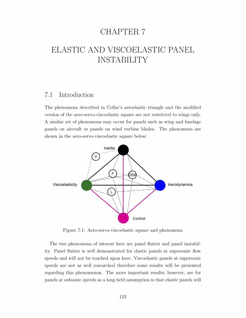
CHAPTER 7
ELASTIC AND VISCOELASTIC PANELINSTABILITY
7.1 Introduction
The phenomena described in Collar’s aeroelastic triangle and the modified
version of the aero-servo-viscoelastic square are not restricted to wings only.
A similar set of phenomena may occur for panels such as wing and fuselage
panels on aircraft or panels on wind turbine blades. The phenomena are
shown in the aero-servo-viscoelastic square below:
Figure 7.1: Aero-servo-viscoelastic square and phenomena
The two phenomena of interest here are panel flutter and panel instabil-
ity. Panel flutter is well demonstrated for elastic panels at supersonic flow
speeds and will not be touched upon here. Viscoelastic panels at supersonic
speeds are not as well researched therefore some results will be presented
regarding this phenomenon. The more important results; however, are for
panels at subsonic speeds as a long held assumption is that elastic panels will
123
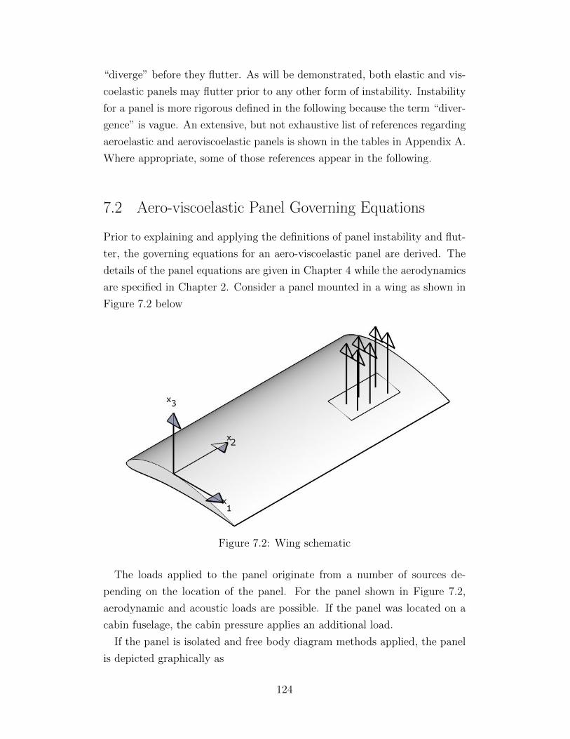
“diverge” before they flutter. As will be demonstrated, both elastic and vis-
coelastic panels may flutter prior to any other form of instability. Instability
for a panel is more rigorous defined in the following because the term “diver-
gence” is vague. An extensive, but not exhaustive list of references regarding
aeroelastic and aeroviscoelastic panels is shown in the tables in Appendix A.
Where appropriate, some of those references appear in the following.
7.2 Aero-viscoelastic Panel Governing Equations
Prior to explaining and applying the definitions of panel instability and flut-
ter, the governing equations for an aero-viscoelastic panel are derived. The
details of the panel equations are given in Chapter 4 while the aerodynamics
are specified in Chapter 2. Consider a panel mounted in a wing as shown in
Figure 7.2 below
Figure 7.2: Wing schematic
The loads applied to the panel originate from a number of sources de-
pending on the location of the panel. For the panel shown in Figure 7.2,
aerodynamic and acoustic loads are possible. If the panel was located on a
cabin fuselage, the cabin pressure applies an additional load.
If the panel is isolated and free body diagram methods applied, the panel
is depicted graphically as
124
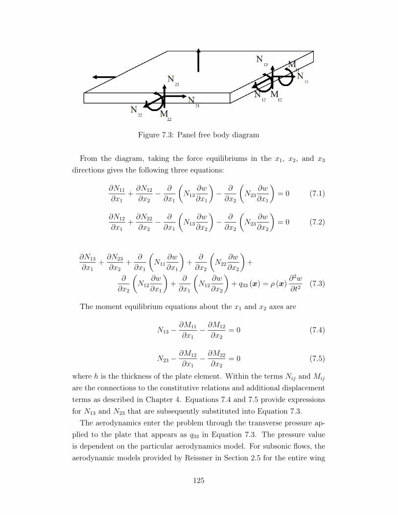
Figure 7.3: Panel free body diagram
From the diagram, taking the force equilibriums in the x1, x2, and x3
directions gives the following three equations:
∂N11
∂x1
+∂N12
∂x2
− ∂
∂x1
(N13
∂w
∂x1
)− ∂
∂x2
(N23
∂w
∂x1
)= 0 (7.1)
∂N12
∂x1
+∂N22
∂x2
− ∂
∂x1
(N13
∂w
∂x2
)− ∂
∂x2
(N23
∂w
∂x2
)= 0 (7.2)
∂N13
∂x1
+∂N23
∂x2
+∂
∂x1
(N11
∂w
∂x1
)+
∂
∂x2
(N22
∂w
∂x2
)+
∂
∂x2
(N12
∂w
∂x1
)+
∂
∂x1
(N12
∂w
∂x2
)+ q33 (x) = ρ (x)
∂2w
∂t2(7.3)
The moment equilibrium equations about the x1 and x2 axes are
N13 −∂M11
∂x1
− ∂M12
∂x2
= 0 (7.4)
N23 −∂M12
∂x1
− ∂M22
∂x2
= 0 (7.5)
where h is the thickness of the plate element. Within the terms Nij and Mij
are the connections to the constitutive relations and additional displacement
terms as described in Chapter 4. Equations 7.4 and 7.5 provide expressions
for N13 and N23 that are subsequently substituted into Equation 7.3.
The aerodynamics enter the problem through the transverse pressure ap-
plied to the plate that appears as q33 in Equation 7.3. The pressure value
is dependent on the particular aerodynamics model. For subsonic flows, the
aerodynamic models provided by Reissner in Section 2.5 for the entire wing
125
or the panel specific aerodynamics provided by Dowell in Section 2.6 are
both applicable and only differ in the details. The general form of the aero-
dynamics is of more note as the form affects the stability equation. Most
aerodynamics may be represented generally as
q33 = A1w + A2∂w
∂x1
+ A3∂w
∂t+ A4
∂2w
∂t∂x1
+ A5∂2w
∂t2+ A6
∂2w
∂x21
(7.6)
To solve for the stability of the plate the transverse governing equation,
Equation 7.3, is the equation of use. The equilibrium equations in the other
two directions are not applicable as in-plane displacements are assumed to
be negligible.
The solution procedure for the plate is similar to that of the wing. A solu-
tion form is selected that is separable in space and time, Galerkin’s method is
applied to eliminate the space components, and the resulting ODE or OIDE
in time is solved through an exponential time solution. The solution form for
the space component is dictated by the boundary conditions of the panel.
7.2.1 Panel solution forms
The solution of the homogeneous part of Equation 7.3 is of the form
w(x, t) =N∑m=1
Wm (x) exp (λt) (7.7)
where λ = d+ iω and the Wm(x) function satisfies the boundary conditions.
The boundary conditions of interest here are four sides simply supported (4
s.s.s), four sides clamped (4 s.c), and two sides simply supported and two sides
clamped (2 s.s.s.c). The functions that satisfy these boundary conditions are
given in Section 4.2.
7.3 Aero-viscoelastic Panel Instability Definitions
Panel stability, in the context of an aeroviscoelastic panel, refers to the sta-
bility of the self-excited system of aerodynamics, dynamics, and material.
Within solid mechanics, “panel stability” refers to panel buckling which is a
126
distinct and separate phenomenon from what is discussed here. The stability
of the plate is defined by the parameter d that appears in Equation 7.7. The
values of d and their corresponding stabilities are
Table 7.1: Panel Stability Definitions
d Stability Aeroelastic Term
+ Unstable “Divergence”0 Neutrally stable Flutter- Stable N/A
The mathematical definitions for each stability condition, including the
effects of viscoelasticity and the associated time dependence are shown in
the following limit criteria.
For panel instability
limV→VD
w (x, V, t)→∞ (7.8)
limV→VD
∂w (x, V, t)
∂V→∞ (7.9)
limt→tD
w (x, V, t)→∞ (7.10)
limt→VD
∂w (x, V, t)
∂t→∞ (7.11)
(7.12)
which implies that d must be positive as stated in Table 7.1 and ω is free.
For panel flutter
limV→VF
w (x, V, t)→ SHM (7.13)
limt→tF
w (x, V, t)→ SHM (7.14)
(7.15)
which implies that d must be zero and ω 6= 0. Some additional restrictions
on the flutter condition are necessary as explained in Section 6.5 so that the
true flutter point is found. These restrictions for d are
127
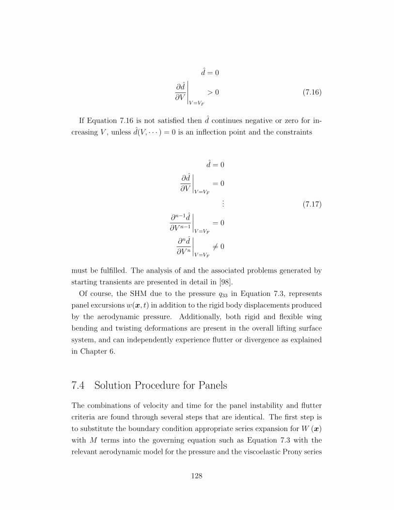
d = 0
∂d
∂V
∣∣∣∣∣V=VF
> 0 (7.16)
If Equation 7.16 is not satisfied then d continues negative or zero for in-
creasing V , unless d(V, · · · ) = 0 is an inflection point and the constraints
d = 0
∂d
∂V
∣∣∣∣V=VF
= 0
... (7.17)
∂n−1d
∂V n−1
∣∣∣∣V=VF
= 0
∂nd
∂V n
∣∣∣∣V=VF
6= 0
must be fulfilled. The analysis of and the associated problems generated by
starting transients are presented in detail in [98].
Of course, the SHM due to the pressure q33 in Equation 7.3, represents
panel excursions w(x, t) in addition to the rigid body displacements produced
by the aerodynamic pressure. Additionally, both rigid and flexible wing
bending and twisting deformations are present in the overall lifting surface
system, and can independently experience flutter or divergence as explained
in Chapter 6.
7.4 Solution Procedure for Panels
The combinations of velocity and time for the panel instability and flutter
criteria are found through several steps that are identical. The first step is
to substitute the boundary condition appropriate series expansion for W (x)
with M terms into the governing equation such as Equation 7.3 with the
relevant aerodynamic model for the pressure and the viscoelastic Prony series
128
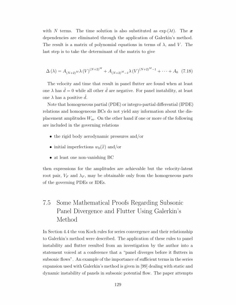
with N terms. The time solution is also substituted as exp (λt). The x
dependencies are eliminated through the application of Galerkin’s method.
The result is a matrix of polynomial equations in terms of λ, and V . The
last step is to take the determinant of the matrix to give
∆ (λ) = A(N+2)Mλ (V )(N+2)M + A(N+2)M−1λ (V )(N+2)M−1 + · · ·+ A0 (7.18)
The velocity and time that result in panel flutter are found when at least
one λ has d = 0 while all other d are negative. For panel instability, at least
one λ has a positive d.
Note that homogeneous partial (PDE) or integro-partial differential (IPDE)
relations and homogeneous BCs do not yield any information about the dis-
placement amplitudes Wm. On the other hand if one or more of the following
are included in the governing relations
• the rigid body aerodynamic pressures and/or
• initial imperfections w0(x) and/or
• at least one non-vanishing BC
then expressions for the amplitudes are achievable but the velocity-latent
root pair, VF and λF , may be obtainable only from the homogeneous parts
of the governing PDEs or IDEs.
7.5 Some Mathematical Proofs Regarding Subsonic
Panel Divergence and Flutter Using Galerkin’s
Method
In Section 4.4 the von Koch rules for series convergence and their relationship
to Galerkin’s method were described. The application of these rules to panel
instability and flutter resulted from an investigation by the author into a
statement voiced at a conference that a “panel diverges before it flutters in
subsonic flows”. An example of the importance of sufficient terms in the series
expansion used with Galerkin’s method is given in [99] dealing with static and
dynamic instability of panels in subsonic potential flow. The paper attempts
129
to prove that panels will only diverge at subsonic speeds and that flutter will
not occur prior to divergence. The mathematical analysis is entirely correct
and does demonstrate that subsonic divergence occurs before flutter, but one
of the starting assumptions is problematic. In [99] it is mentioned that the
series approximation is an infinite series “but by virtue of the convergence
of Galerkin’s method (e.g. see [100]) this can be ignored and the discussion
confined to j,m = 1, 2 only.” In the quotation j and m are the indices for the
series expansion and, therefore, the referenced expansion is limited to only
two terms. By limiting the expansion to two terms, the assumption is made
that the results from a two term expansion are representative of the results
from larger expansions.
Unfortunately, the above assumption is not correct, and it has been demon-
strated in [65] that, for some cases, Galerkin’s method has a non-uniform con-
vergence. In [65] two situations are examined, namely supersonic membrane
flutter and a clamped-clamped rod with a follower force. The membrane flut-
ter example originated in [101] where a paradox is identified, which states
that Galerkin’s method would produce a supersonic flutter velocity while the
exact solution would not.
This discrepancy is explained by demonstrating that membranes do not
have a normal determinant, as defined in Section 4.4. A typical plate problem
in solid mechanics does have a normal determinant and, therefore, Galerkin’s
method produces reliable results. Reference [66] suggests that as a plate ap-
proaches a membrane, the convergence of Galerkin’s method becomes slower
to the point of failure when a membrane is actually reached. In [65] it is
demonstrated that the discrepancy is the result of using normal determinants
in the analysis of [101]. If the more general conditions for the convergence
of an infinite series by von Koch [67] are used, then Galerkin’s method is
shown to converge for the membrane flutter; however, the convergence is
non-uniform in general.
The non-uniform convergence of Galerkin’s method is numerically demon-
strated in the second example of a clamped-clamped rod with a follower force
in [65]. In [100] it was shown earlier that the rod diverged (buckled) with
a two term expansion in the Galerkin method. However, if the expansion is
taken to four terms, the rod is no longer buckled. In [66] it was demonstrated
that a similar result is obtained for supersonic membrane flutter where eight
terms are required to demonstrate flutter.
130
While the membrane paradox originated with supersonic membranes, the
subsequent non-uniform convergence of Galerkin’s method shown in [65] ap-
pears to hold for subsonic panel flutter cases. It is suggested that to correctly
use Galerkin’s method for any panel flutter case that the von Koch conditions
[67] are used to estimate the number of terms required for convergence.
7.6 General Considerations for Panel Instability and
Flutter
Circumstances leading to panel flutter are found in self-excited closed loop
systems and are due to the interdependence between aerodynamic and in-
ertia forces and structural deflections as well as their spatial and temporal
derivatives. The two open flutter driver parameters in flight vehicles are
their velocity and time. Consequently, for other fixed conditions1 the lowest
velocity, i. e. the flutter velocity, needs to be established for entire vehicles
and for their components such as outer skin panels. In the present linear
formulation, the existence of SHM is controlled by the relative values of the
coefficients of displacements and their derivatives in Equation 7.3 which in
turn are governed by the interrelations between inertia, elastic/viscoelastic,
aerodynamic, thermal, in-plane and control forces. Additionally, the BCs di-
rectly affect the matrix of the coefficients of the Wm amplitudes of Equation
7.7. All of the above conditions coalesce to determine the eigenvalues and
hence the flutter conditions VF and λF .
The presence of viscoelastic material damping, or for that matter exter-
nal and/or structural damping offers no guarantees that viscoelastic flutter
speeds VF will be higher or lower than the corresponding elastic V EF . The
values of these VF s move in either direction depending again on the charac-
ter of the phase relationships between aerodynamic, elastic/viscoelastic and
inertia forces. Similar comments are made regarding the contributions made
by changes in mass and aerodynamic forces. However, since Equation 7.7 is a
transcendental relation in the eigenvalues VF and λF no analytical solutions
are attainable and hence no general conclusions about the interrelations, if
any, between elastic and viscoelastic panel flutter velocities are drawn.
1aerodynamic shapes, mass distributions, material properties, controls, trim angles ofattack, etc.
131
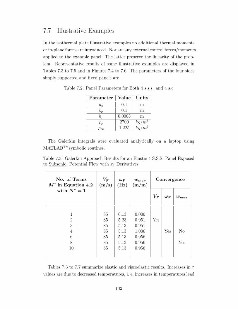
7.7 Illustrative Examples
In the isothermal plate illustrative examples no additional thermal moments
or in-plane forces are introduced. Nor are any external control forces/moments
applied to the example panel. The latter preserve the linearity of the prob-
lem. Representative results of some illustrative examples are displayed in
Tables 7.3 to 7.5 and in Figures 7.4 to 7.6. The parameters of the four sides
simply supported and fixed panels are
Table 7.2: Panel Parameters for Both 4 s.s.s. and 4 s.c
Parameter Value Units
ap 0.1 mbp 0.1 mhp 0.0005 mρp 2700 kg/m3
ρ∞ 1.225 kg/m3
The Galerkin integrals were evaluated analytically on a laptop using
MATLABTMsymbolic routines.
Table 7.3: Galerkin Approach Results for an Elastic 4 S.S.S. Panel Exposedto Subsonic Potential Flow with x1 Derivatives
No. of Terms VF ωF wmax ConvergenceM ∗ in Equation 4.2 (m/s) (Hz) (m/m)
with N∗ = 1VF ωF wmax
1 85 6.13 0.0002 85 5.23 0.951 Yes3 85 5.13 0.9514 85 5.13 1.006 Yes No6 85 5.13 0.9568 85 5.13 0.956 Yes10 85 5.13 0.956
Tables 7.3 to 7.7 summarize elastic and viscoelastic results. Increases in τ
values are due to decreased temperatures, i. e. increases in temperatures lead
132
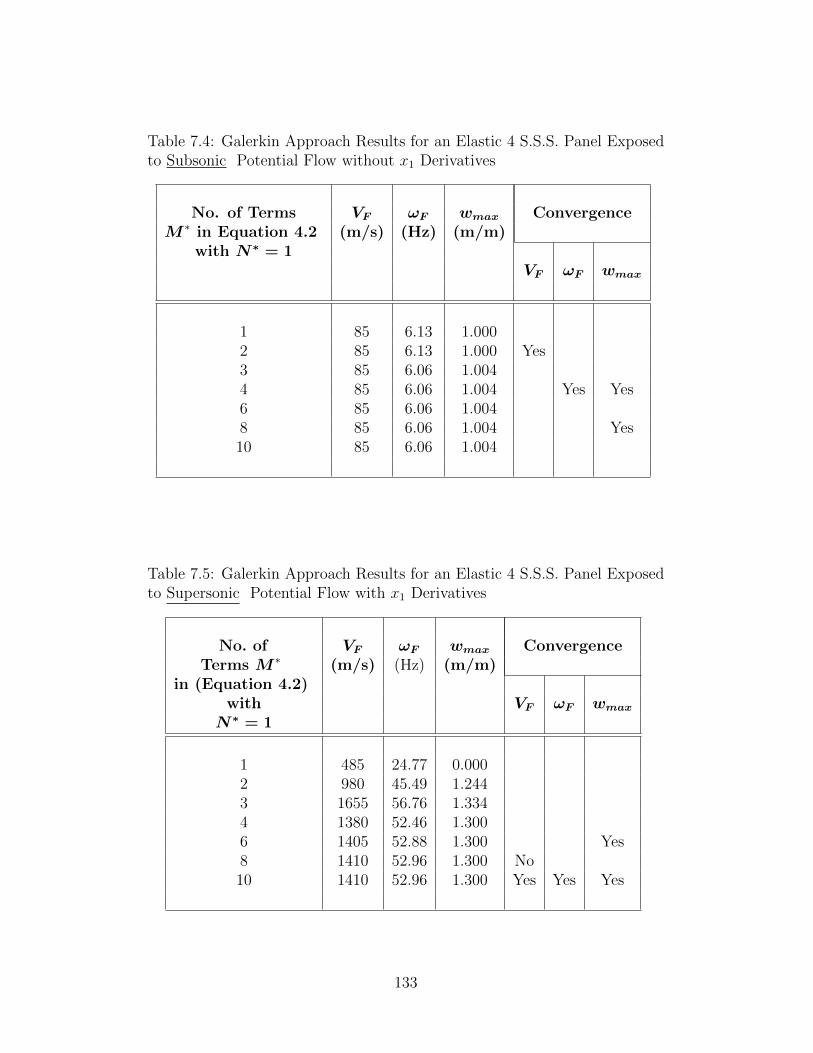
Table 7.4: Galerkin Approach Results for an Elastic 4 S.S.S. Panel Exposedto Subsonic Potential Flow without x1 Derivatives
No. of Terms VF ωF wmax ConvergenceM ∗ in Equation 4.2 (m/s) (Hz) (m/m)
with N∗ = 1VF ωF wmax
1 85 6.13 1.0002 85 6.13 1.000 Yes3 85 6.06 1.0044 85 6.06 1.004 Yes Yes6 85 6.06 1.0048 85 6.06 1.004 Yes10 85 6.06 1.004
Table 7.5: Galerkin Approach Results for an Elastic 4 S.S.S. Panel Exposedto Supersonic Potential Flow with x1 Derivatives
No. of VF ωF wmax ConvergenceTerms M ∗ (m/s) (Hz) (m/m)
in (Equation 4.2)with VF ωF wmax
N∗ = 1
1 485 24.77 0.0002 980 45.49 1.2443 1655 56.76 1.3344 1380 52.46 1.3006 1405 52.88 1.300 Yes8 1410 52.96 1.300 No10 1410 52.96 1.300 Yes Yes Yes
133
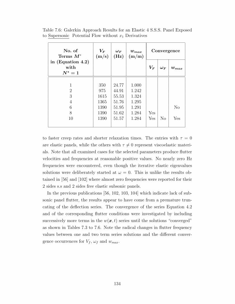
Table 7.6: Galerkin Approach Results for an Elastic 4 S.S.S. Panel Exposedto Supersonic Potential Flow without x1 Derivatives
No. of VF ωF wmax ConvergenceTerms M ∗ (m/s) (Hz) (m/m)
in (Equation 4.2)with VF ωF wmax
N∗ = 1
1 350 24.77 1.0002 975 44.91 1.2423 1615 55.53 1.3244 1365 51.76 1.2956 1390 51.95 1.291 No8 1390 51.62 1.284 Yes10 1390 51.57 1.284 Yes No Yes
to faster creep rates and shorter relaxation times. The entries with τ = 0
are elastic panels, while the others with τ 6= 0 represent viscoelastic materi-
als. Note that all examined cases for the selected parameters produce flutter
velocities and frequencies at reasonable positive values. No nearly zero Hz
frequencies were encountered, even though the iterative elastic eigenvalues
solutions were deliberately started at ω = 0. This is unlike the results ob-
tained in [56] and [102] where almost zero frequencies were reported for their
2 sides s.s and 2 sides free elastic subsonic panels.
In the previous publications [56, 102, 103, 104] which indicate lack of sub-
sonic panel flutter, the results appear to have come from a premature trun-
cating of the deflection series. The convergence of the series Equation 4.2
and of the corresponding flutter conditions were investigated by including
successively more terms in the w(x, t) series until the solutions “converged”
as shown in Tables 7.3 to 7.6. Note the radical changes in flutter frequency
values between one and two term series solutions and the different conver-
gence occurrences for Vf , ωf and wmax.
134
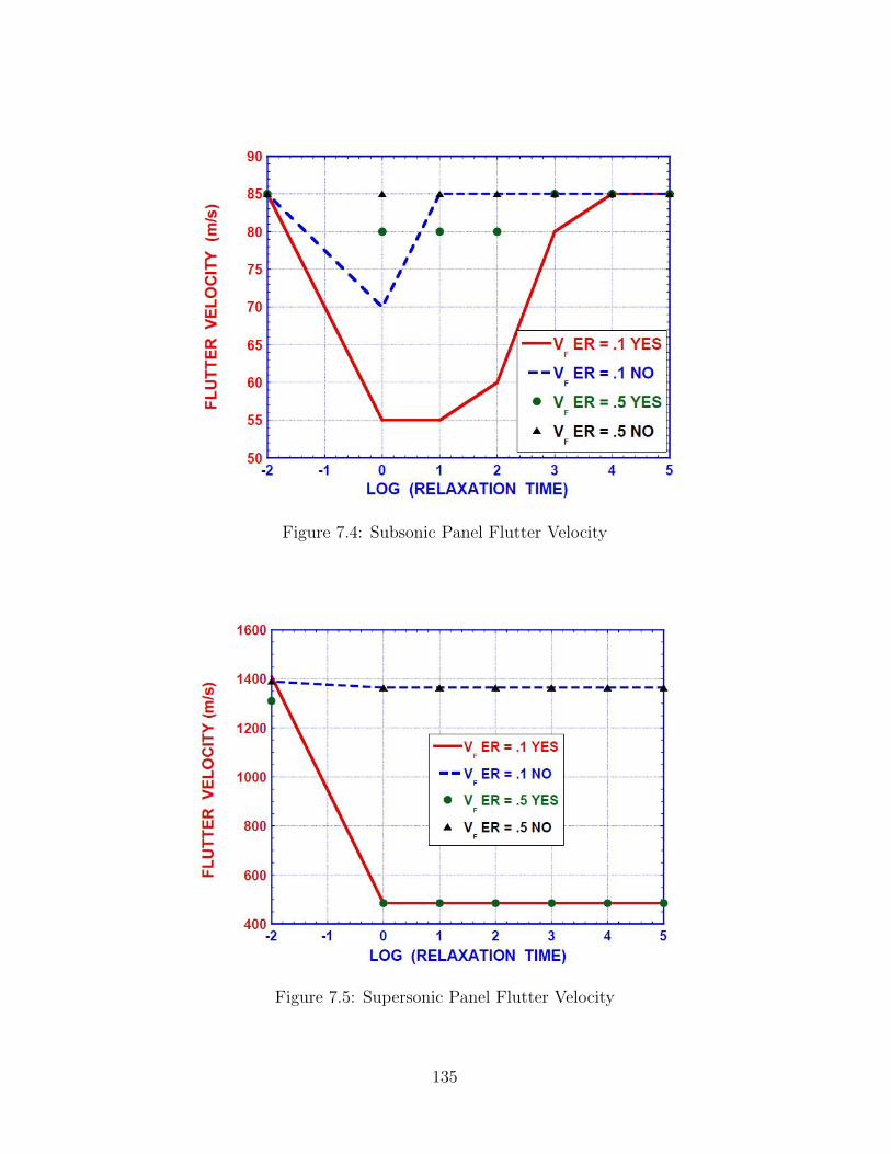
Figure 7.4: Subsonic Panel Flutter Velocity
Figure 7.5: Supersonic Panel Flutter Velocity
135
7.8 Low and High Speed Elastic Panel Flutter
Tables 7.3 to 7.6 display results for sub- and super- sonic illustrative examples
with typical ordinary properties. Both cases with x1 derivatives present and
absent in the aerodynamic force definition of Equation 2.149 are considered.
The possible presence of these first spatial derivatives in some of the aero-
dynamic force definitions radically alters the character of the plate governing
relations, Equation 7.3. Without either or both of these terms, in addition to
time derivatives, only derivatives of even orders in x1 and the function itself
are present in the governing relations. For instance, the illustrative example
of 4 s.s.s. requires only sine terms in the series for the deflection w(x, t),
Equations 7.7 and 4.2, to satisfy the BCs.
Normal to the airflow, the curvature in the x2-direction is of limited sig-
nificance since its presence with or without the use of the Galerkin protocol
only changes the values of the coefficients in the governing relations. Similar
or equal changes in these coefficients are produced through normal variations
of standard parameters, such as stiffness, inertia, aerodynamics, etc. For the
simply supported edges parallel to the x1-axis only a single half sine wave
(sin πx2b
) is required to satisfy the BCs along those plate edges.
As a check on possible divergence occurrences, attempts were made to
find values of V E > 0 by setting d = ω = 0. No divergence occurrences
were found indicating that the elastic eigenvalues VF and ωF represent panel
flutter. These results are, of course, predicated on the use of a sufficient
number of terms in the truncated deflection series Equation 4.2 to assure
proper convergence.
7.9 Low and High Speed Viscoelastic Panel Flutter
Table 7.7 depicts combined (converged) results for identical elastic or vis-
coelastic panels subjected to subsonic or supersonic aerodynamic pressures.
These results are, of course, strongly influenced by the choice of parameters
and their interaction of the various forces, i.e. their phase relations, with
each other. Consequently, any conclusions must be considered specific to
only the present parameter set and do not lead to any further possible gen-
eralizations. Similar conditions were noted for the viscoelastic instabilities
136
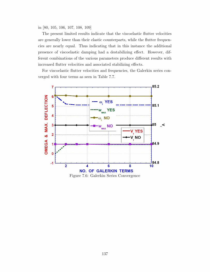
in [80, 105, 106, 107, 108, 109]
The present limited results indicate that the viscoelastic flutter velocities
are generally lower than their elastic counterparts, while the flutter frequen-
cies are nearly equal. Thus indicating that in this instance the additional
presence of viscoelastic damping had a destabilizing effect. However, dif-
ferent combinations of the various parameters produce different results with
increased flutter velocities and associated stabilizing effects.
For viscoelastic flutter velocities and frequencies, the Galerkin series con-
verged with four terms as seen in Table 7.7.
Figure 7.6: Galerkin Series Convergence
137
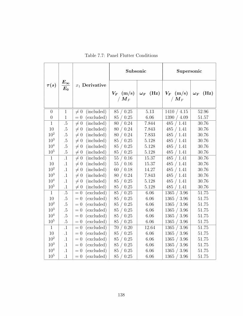
Table 7.7: Panel Flutter Conditions
Subsonic Supersonic
τ (s)E∞E0
x1 Derivative
VF (m/s) ωF (Hz) VF (m/s) ωF (Hz)/ MF / MF
0 1 6= 0 (included) 85 / 0.25 5.13 1410 / 4.15 52.960 1 = 0 (excluded) 85 / 0.25 6.06 1390 / 4.09 51.571 .5 6= 0 (included) 80 / 0.24 7.844 485 / 1.41 30.7610 .5 6= 0 (included) 80 / 0.24 7.843 485 / 1.41 30.76102 .5 6= 0 (included) 80 / 0.24 7.833 485 / 1.41 30.76103 .5 6= 0 (included) 85 / 0.25 5.128 485 / 1.41 30.76104 .5 6= 0 (included) 85 / 0.25 5.128 485 / 1.41 30.76105 .5 6= 0 (included) 85 / 0.25 5.128 485 / 1.41 30.761 .1 6= 0 (included) 55 / 0.16 15.37 485 / 1.41 30.7610 .1 6= 0 (included) 55 / 0.16 15.37 485 / 1.41 30.76102 .1 6= 0 (included) 60 / 0.18 14.27 485 / 1.41 30.76103 .1 6= 0 (included) 80 / 0.24 7.843 485 / 1.41 30.76104 .1 6= 0 (included) 85 / 0.25 5.128 485 / 1.41 30.76105 .1 6= 0 (included) 85 / 0.25 5.128 485 / 1.41 30.761 .5 = 0 (excluded) 85 / 0.25 6.06 1365 / 3.96 51.7510 .5 = 0 (excluded) 85 / 0.25 6.06 1365 / 3.96 51.75102 .5 = 0 (excluded) 85 / 0.25 6.06 1365 / 3.96 51.75103 .5 = 0 (excluded) 85 / 0.25 6.06 1365 / 3.96 51.75104 .5 = 0 (excluded) 85 / 0.25 6.06 1365 / 3.96 51.75105 .5 = 0 (excluded) 85 / 0.25 6.06 1365 / 3.96 51.751 .1 = 0 (excluded) 70 / 0.20 12.64 1365 / 3.96 51.7510 .1 = 0 (excluded) 85 / 0.25 6.06 1365 / 3.96 51.75102 .1 = 0 (excluded) 85 / 0.25 6.06 1365 / 3.96 51.75103 .1 = 0 (excluded) 85 / 0.25 6.06 1365 / 3.96 51.75104 .1 = 0 (excluded) 85 / 0.25 6.06 1365 / 3.96 51.75105 .1 = 0 (excluded) 85 / 0.25 6.06 1365 / 3.96 51.75
138
CHAPTER 8
FLIGHT VELOCITY TRANSIENTRESPONSE
8.1 Introduction
In past and present elastic and viscoelastic analyses, the flight velocity tran-
sients contributions to the deformations remain unresolved. One attempt at
modeling transitional flow in unsteady aerodynamics was made by Ohgami
and Akamatsu [110]. The important influence of flight velocity transients
is due to the inherent memory and energy dissipation associated with vis-
coelastic material behavior. In the mathematical models for aero-viscoelastic
structures, it is acceptable for simple harmonic motion (SHM) of the struc-
ture to occur instantaneously as a Heaviside input function is valid. Re-
alistically, there is a velocity transient as the flight speed of the structure
approaches SHM, and the memory effect of a viscoelastic material will retain
this transient input unlike an elastic material.
From a realistic physical point of view, the SHM deflections must be pre-
ceded by a build-up during a preferably short time interval 0 ≤ t ≤ t1 where
t1 < t0, d < 0 and V < VF . The time t0 is the time when the modulus E(t0)
begins to relax. Thus the buildup and possible short time resultant tran-
sient responses are contained in the elastic portion of the relaxation modulus
curve at 0 ≤ t ≤ t0 (see Figure 8.1) and no additional memory effects will be
imposed on the SHM portion, provided any transient responses die out be-
fore t0 is reached. While these conditions are not mathematically mandated,
their imposition yields more meaningful comparisons relative to the identical
elastic reference base.
The initial conditions then become
139
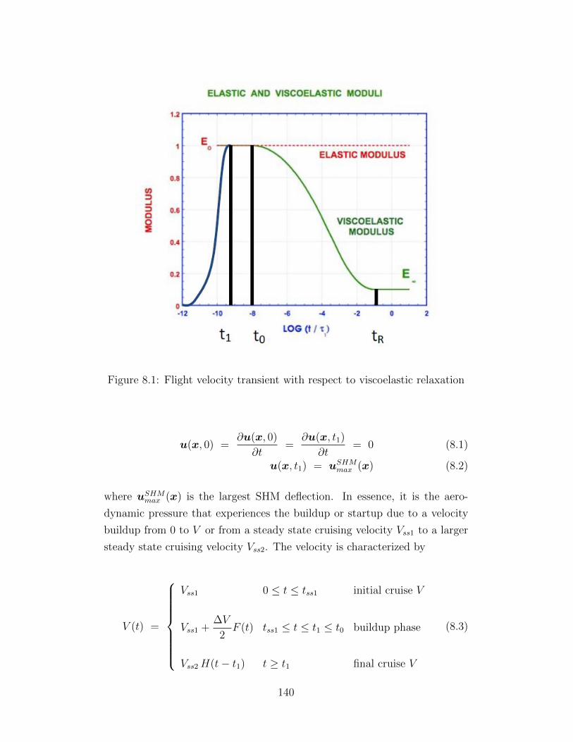
Figure 8.1: Flight velocity transient with respect to viscoelastic relaxation
u(x, 0) =∂u(x, 0)
∂t=
∂u(x, t1)
∂t= 0 (8.1)
u(x, t1) = uSHMmax (x) (8.2)
where uSHMmax (x) is the largest SHM deflection. In essence, it is the aero-
dynamic pressure that experiences the buildup or startup due to a velocity
buildup from 0 to V or from a steady state cruising velocity Vss1 to a larger
steady state cruising velocity Vss2. The velocity is characterized by
V (t) =
Vss1 0 ≤ t ≤ tss1 initial cruise V
Vss1 +∆V
2F (t) tss1 ≤ t ≤ t1 ≤ t0 buildup phase
Vss2H(t− t1) t ≥ t1 final cruise V
(8.3)
140
where
F (t) = 1− cos
[π (t− tss1)
t1 − tss1
](8.4)
with
F (0) =∂F (0)
∂t=
∂F (t1)
∂t= 0 and V (t1) = Vss2 = Vss1 +∆V (8.5)
where t = 0 represents the relative time when the flight or maneuver is
initiated. This analysis applies to both positive and negative ∆V s and any
change in velocity directly influences lift and drag values.
The approach consist of specifying the velocity growth function that will
satisfy the initial conditions of Equation 8.1 but may produce transient start
up oscillations in u(x, t) prior to t = t1 and possibly thereafter.
A typical elastic flutter frequency has a high end value of some 50 Hz.
If the startup time t1 is say 0.01 secs1 and the beginning relaxation time
t0 is 0.1 secs, then the initial elastic SHM may undergo some 5 cycles or
less. Generally in that short time frame the deflections w would not develop
large destructive amplitudes even if d were slightly positive, since high flutter
frequencies would be required. After t > t0 the viscoelastic effects take over
and the flutter velocity VF will adjust itself accordingly to acquire a value
distinct from the elastic V EF , such that VF ≤ V E
F or VF ≥ V EF .
8.1.1 Flutter and Instability
The definitions for flutter and instability are not altered by the inclusion
of a flight velocity transient for either a wing or a plate. The definitions
appearing in Sections 6.5 and 7.3 are still valid.
8.2 Illustrative Examples
The inclusion of flight velocity transients does not alter the governing equa-
tions for the dynamics of a wing or panel. Instead, the only alteration is
1This implies that in such short time intervals, the elastic terms predominate over theviscoelastic ones.
141
to the aerodynamics. For this reason, velocity was left as a variable during
the derivations given in Chapter 2. The variable velocity does alter the gen-
eral form of the resulting aero-viscoelastic equations because the coefficients
of the equations are now functions of time, as are the displacements. One
solution method is to use Kulikov’s approach as described in Chapter 2 for
second order ordinary differential equations. The hereditary integral that
appears for the viscoelastic material and the ordinary integral that appears
for the integral controller do pose a problem in the solution method.
In the following illustrative examples, a panel identical to that used in
Chapter 7 is considered with the only change being a flight velocity tran-
sient. To avoid some of the computational difficulties, the transient velocity
and loading is restricted to occur during the initial elastic portion of the vis-
coelastic relaxation curve. The stability evaluation occurs after the elastic
portion. This arrangement avoids the variable coefficients, but the transient
effect influences the panel through the viscoelastic memory. The more general
case is that the velocity transient occurs at any time, but a variable coef-
ficient partial differential - integral equation solver is required in that case.
All formal symbolic evaluations and numerical calculations have been carried
out in MATLABTM on a desktop PC. Convergence questions are treated in
Subsection 8.2.3.
8.2.1 Contributions of Spatial Derivatives to AerodynamicForces
The “YES/NO“ and “Include/Excluded” notations in the figures and tables
refer to the derivatives with respect to the air flow direction, x1, in Equation
2.149. These are the slopes indicating panel curvature and their aerodynamic
effects. It is readily seen in Figures 8.2 to 8.5 and Tables 8.2 and 8.4 that their
presence or absence significantly alters the values of the flutter velocities and
frequencies. However, the pattern is illusive and far from obvious. Therefore,
no specific conclusions are drawn except that their inclusion in determining
panel flutter is mandatory.
142
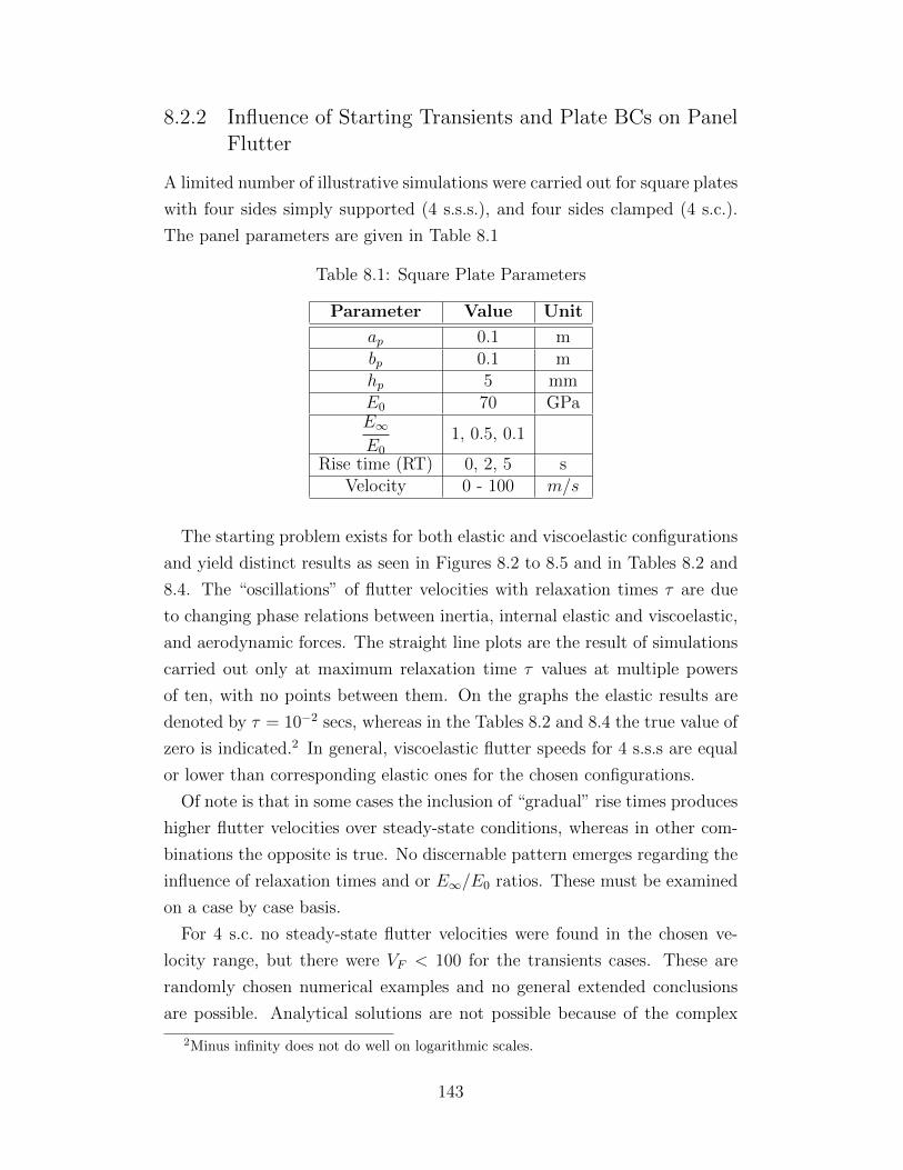
8.2.2 Influence of Starting Transients and Plate BCs on PanelFlutter
A limited number of illustrative simulations were carried out for square plates
with four sides simply supported (4 s.s.s.), and four sides clamped (4 s.c.).
The panel parameters are given in Table 8.1
Table 8.1: Square Plate Parameters
Parameter Value Unit
ap 0.1 mbp 0.1 mhp 5 mmE0 70 GPaE∞E0
1, 0.5, 0.1
Rise time (RT) 0, 2, 5 sVelocity 0 - 100 m/s
The starting problem exists for both elastic and viscoelastic configurations
and yield distinct results as seen in Figures 8.2 to 8.5 and in Tables 8.2 and
8.4. The “oscillations” of flutter velocities with relaxation times τ are due
to changing phase relations between inertia, internal elastic and viscoelastic,
and aerodynamic forces. The straight line plots are the result of simulations
carried out only at maximum relaxation time τ values at multiple powers
of ten, with no points between them. On the graphs the elastic results are
denoted by τ = 10−2 secs, whereas in the Tables 8.2 and 8.4 the true value of
zero is indicated.2 In general, viscoelastic flutter speeds for 4 s.s.s are equal
or lower than corresponding elastic ones for the chosen configurations.
Of note is that in some cases the inclusion of “gradual” rise times produces
higher flutter velocities over steady-state conditions, whereas in other com-
binations the opposite is true. No discernable pattern emerges regarding the
influence of relaxation times and or E∞/E0 ratios. These must be examined
on a case by case basis.
For 4 s.c. no steady-state flutter velocities were found in the chosen ve-
locity range, but there were VF < 100 for the transients cases. These are
randomly chosen numerical examples and no general extended conclusions
are possible. Analytical solutions are not possible because of the complex
2Minus infinity does not do well on logarithmic scales.
143
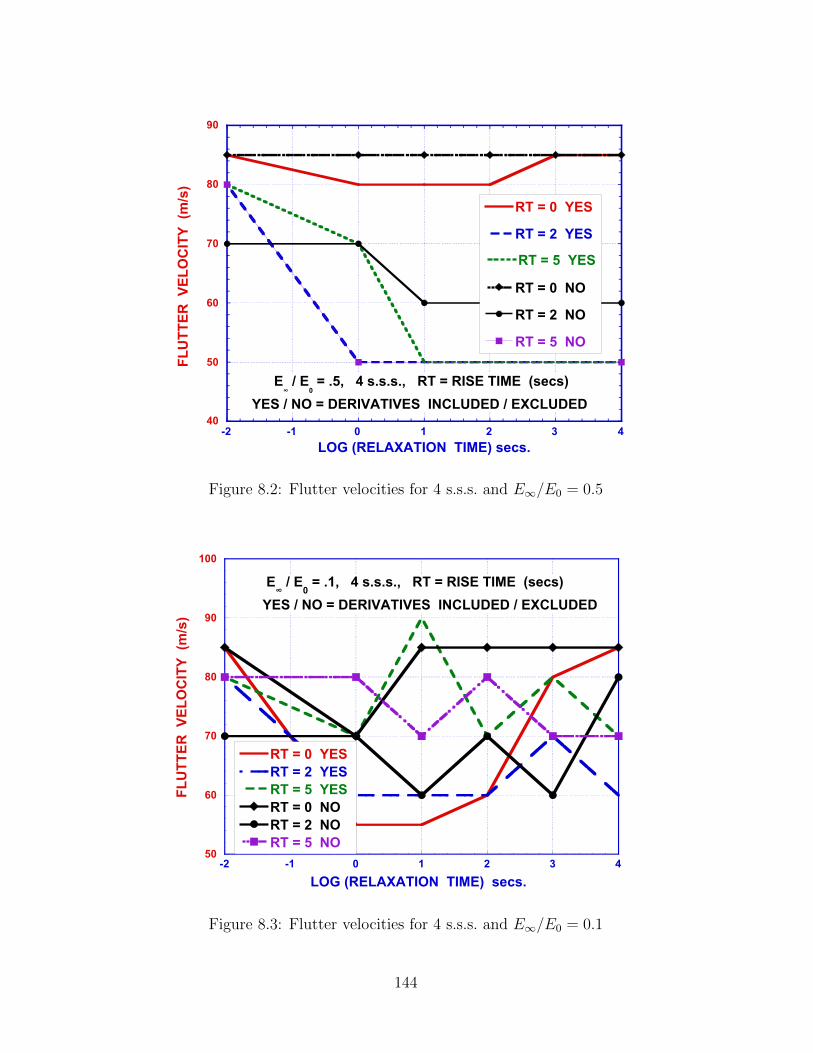
40
50
60
70
80
90
-2 -1 0 1 2 3 4
RT = 0 YES
RT = 2 YES
RT = 5 YES
RT = 0 NO
RT = 2 NO
RT = 5 NO
FLU
TTER
VEL
OC
ITY
(m/s
)
LOG (RELAXATION TIME) secs.
E! / E
0 = .5, 4 s.s.s., RT = RISE TIME (secs)
YES / NO = DERIVATIVES INCLUDED / EXCLUDED
Figure 8.2: Flutter velocities for 4 s.s.s. and E∞/E0 = 0.5
50
60
70
80
90
100
-2 -1 0 1 2 3 4
RT = 0 YESRT = 2 YES RT = 5 YESRT = 0 NORT = 2 NORT = 5 NO
FLU
TTER
VEL
OC
ITY
(m/s
)
LOG (RELAXATION TIME) secs.
E! / E
0 = .1, 4 s.s.s., RT = RISE TIME (secs)
YES / NO = DERIVATIVES INCLUDED / EXCLUDED
Figure 8.3: Flutter velocities for 4 s.s.s. and E∞/E0 = 0.1
144
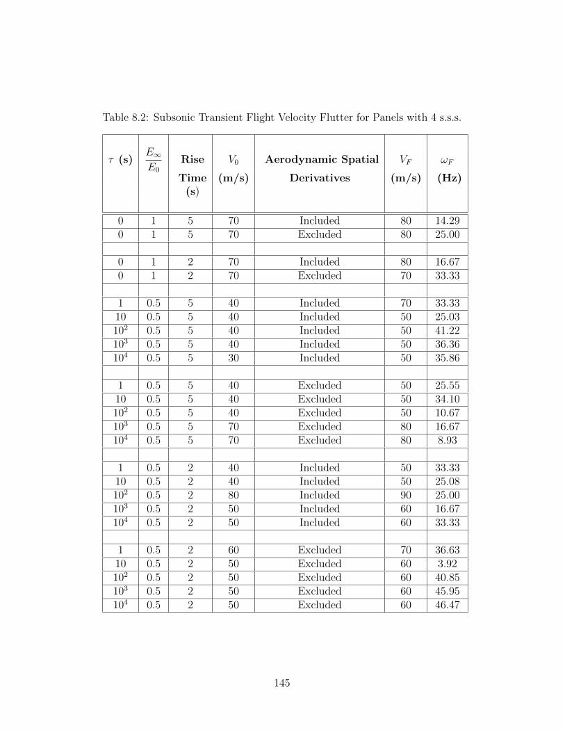
Table 8.2: Subsonic Transient Flight Velocity Flutter for Panels with 4 s.s.s.
τ (s)E∞E0
Rise V0 Aerodynamic Spatial VF ωF
Time (m/s) Derivatives (m/s) (Hz)(s)
0 1 5 70 Included 80 14.290 1 5 70 Excluded 80 25.00
0 1 2 70 Included 80 16.670 1 2 70 Excluded 70 33.33
1 0.5 5 40 Included 70 33.3310 0.5 5 40 Included 50 25.03102 0.5 5 40 Included 50 41.22103 0.5 5 40 Included 50 36.36104 0.5 5 30 Included 50 35.86
1 0.5 5 40 Excluded 50 25.5510 0.5 5 40 Excluded 50 34.10102 0.5 5 40 Excluded 50 10.67103 0.5 5 70 Excluded 80 16.67104 0.5 5 70 Excluded 80 8.93
1 0.5 2 40 Included 50 33.3310 0.5 2 40 Included 50 25.08102 0.5 2 80 Included 90 25.00103 0.5 2 50 Included 60 16.67104 0.5 2 50 Included 60 33.33
1 0.5 2 60 Excluded 70 36.6310 0.5 2 50 Excluded 60 3.92102 0.5 2 50 Excluded 60 40.85103 0.5 2 50 Excluded 60 45.95104 0.5 2 50 Excluded 60 46.47
145
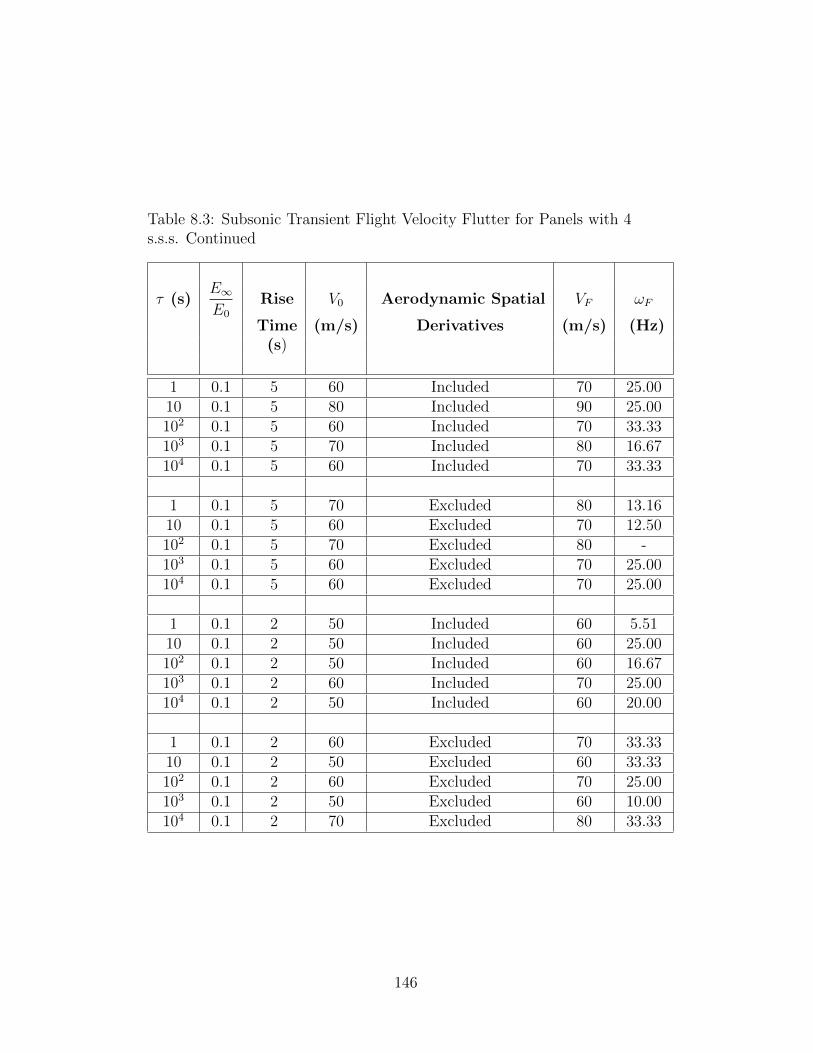
Table 8.3: Subsonic Transient Flight Velocity Flutter for Panels with 4s.s.s. Continued
τ (s)E∞E0
Rise V0 Aerodynamic Spatial VF ωF
Time (m/s) Derivatives (m/s) (Hz)(s)
1 0.1 5 60 Included 70 25.0010 0.1 5 80 Included 90 25.00102 0.1 5 60 Included 70 33.33103 0.1 5 70 Included 80 16.67104 0.1 5 60 Included 70 33.33
1 0.1 5 70 Excluded 80 13.1610 0.1 5 60 Excluded 70 12.50102 0.1 5 70 Excluded 80 -103 0.1 5 60 Excluded 70 25.00104 0.1 5 60 Excluded 70 25.00
1 0.1 2 50 Included 60 5.5110 0.1 2 50 Included 60 25.00102 0.1 2 50 Included 60 16.67103 0.1 2 60 Included 70 25.00104 0.1 2 50 Included 60 20.00
1 0.1 2 60 Excluded 70 33.3310 0.1 2 50 Excluded 60 33.33102 0.1 2 60 Excluded 70 25.00103 0.1 2 50 Excluded 60 10.00104 0.1 2 70 Excluded 80 33.33
146
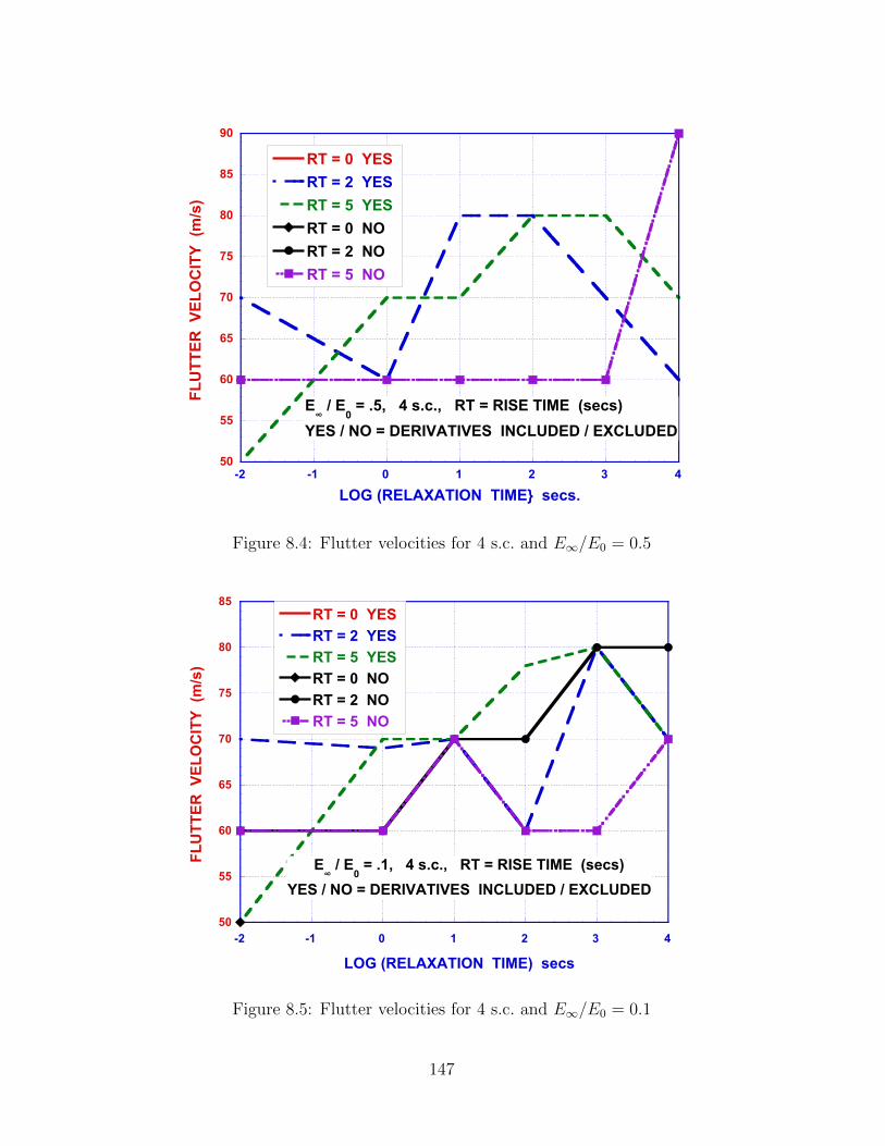
50
55
60
65
70
75
80
85
90
-2 -1 0 1 2 3 4
RT = 0 YESRT = 2 YES RT = 5 YESRT = 0 NORT = 2 NO RT = 5 NO
FLU
TTER
VEL
OC
ITY
(m/s
)
LOG (RELAXATION TIME secs.
E! / E
0 = .5, 4 s.c., RT = RISE TIME (secs)
YES / NO = DERIVATIVES INCLUDED / EXCLUDED
Figure 8.4: Flutter velocities for 4 s.c. and E∞/E0 = 0.5
50
55
60
65
70
75
80
85
-2 -1 0 1 2 3 4
RT = 0 YESRT = 2 YES RT = 5 YESRT = 0 NORT = 2 NORT = 5 NO
FLU
TTER
VEL
OC
ITY
(m/s
)
E! / E
0 = .1, 4 s.c., RT = RISE TIME (secs)
YES / NO = DERIVATIVES INCLUDED / EXCLUDED
LOG (RELAXATION TIME) secs
Figure 8.5: Flutter velocities for 4 s.c. and E∞/E0 = 0.1
147

Table 8.4: Subsonic Transient Flight Velocity Flutter for Panels with 4 s.c.
τ (s)E∞E0
Rise V0 Aerodynamic Spatial VF ωF
Time (m/s) Derivatives (m/s) (Hz)(s)
0 1 2 70 Included 80 33.330 1 2 60 Excluded 70 33.33
0 1 5 70 Included 80 14.290 1 5 70 Excluded 80 25.00
1 0.5 5 60 Included 70 6.2510 0.5 5 60 Included 70 33.33102 0.5 5 70 Included 80 33.33103 0.5 5 70 Included 80 33.33104 0.5 5 60 Included 70 25.00
1 0.5 5 50 Excluded 60 10.0010 0.5 5 50 Excluded 60 33.33102 0.5 5 50 Excluded 60 25.00103 0.5 5 50 Excluded 60 14.29104 0.5 5 80 Excluded 90 33.33
1 0.5 2 50 Included 60 7.5410 0.5 2 70 Included 80 33.33102 0.5 2 70 Included 80 33.33103 0.5 2 60 Included 70 25.00104 0.5 2 50 Included 60 33.33
1 0.5 2 50 Excluded 60 9.0910 0.5 2 60 Excluded 70 16.67102 0.5 2 60 Excluded 70 33.33103 0.5 2 70 Excluded 80 33.33104 0.5 2 70 Excluded 80 40.00
148
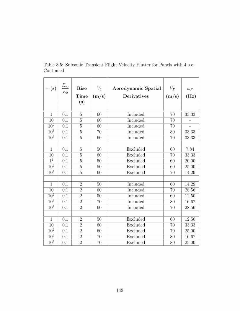
Table 8.5: Subsonic Transient Flight Velocity Flutter for Panels with 4 s.c.Continued
τ (s)E∞E0
Rise V0 Aerodynamic Spatial VF ωF
Time (m/s) Derivatives (m/s) (Hz)(s)
1 0.1 5 60 Included 70 33.3310 0.1 5 60 Included 70 -102 0.1 5 60 Included 70 -103 0.1 5 70 Included 80 33.33104 0.1 5 60 Included 70 33.33
1 0.1 5 50 Excluded 60 7.8410 0.1 5 60 Excluded 70 33.3312 0.1 5 50 Excluded 60 20.00103 0.1 5 50 Excluded 60 25.00104 0.1 5 60 Excluded 70 14.29
1 0.1 2 50 Included 60 14.2910 0.1 2 60 Included 70 28.56102 0.1 2 50 Included 60 12.50103 0.1 2 70 Included 80 16.67104 0.1 2 60 Included 70 28.56
1 0.1 2 50 Excluded 60 12.5010 0.1 2 60 Excluded 70 33.33102 0.1 2 60 Excluded 70 25.00103 0.1 2 70 Excluded 80 16.67104 0.1 2 70 Excluded 80 25.00
149
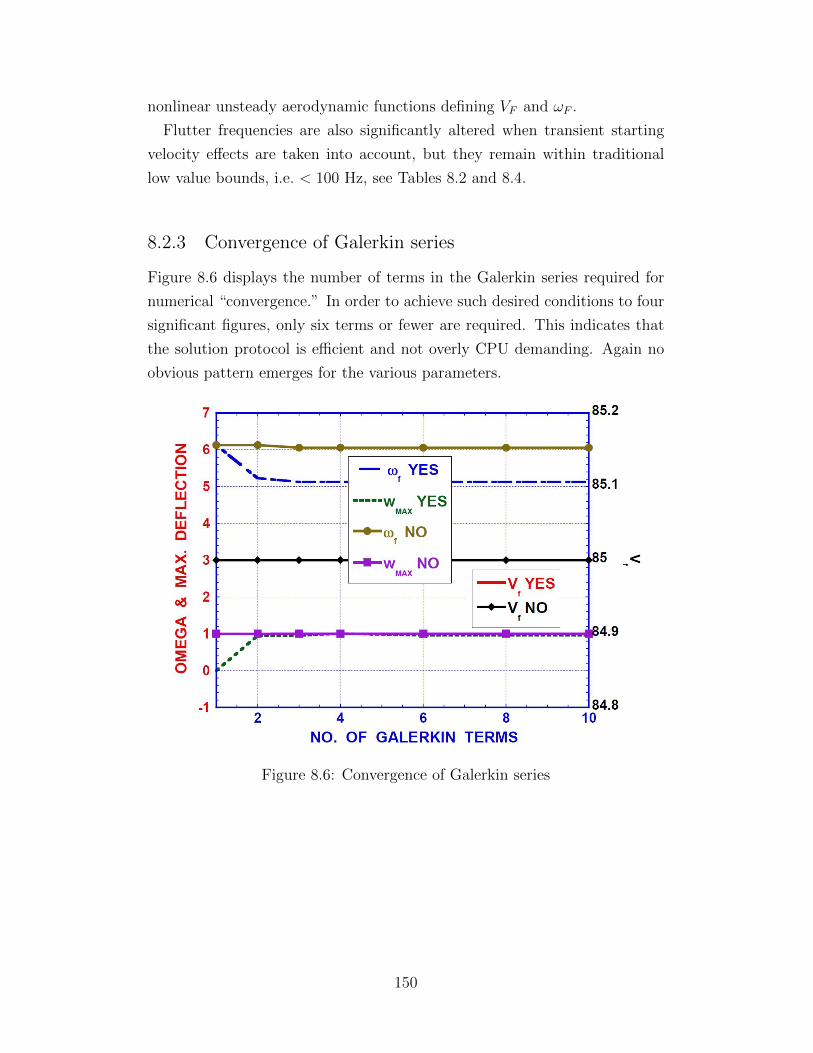
nonlinear unsteady aerodynamic functions defining VF and ωF .
Flutter frequencies are also significantly altered when transient starting
velocity effects are taken into account, but they remain within traditional
low value bounds, i.e. < 100 Hz, see Tables 8.2 and 8.4.
8.2.3 Convergence of Galerkin series
Figure 8.6 displays the number of terms in the Galerkin series required for
numerical “convergence.” In order to achieve such desired conditions to four
significant figures, only six terms or fewer are required. This indicates that
the solution protocol is efficient and not overly CPU demanding. Again no
obvious pattern emerges for the various parameters.
Figure 8.6: Convergence of Galerkin series
150
CHAPTER 9
CONCLUSIONS
Aero-servo-viscoelasticity is the intersection of aerodynamics, viscoelasticity,
dynamics, and controls to model the behavior of flexible structures in an
air flow. This theory is a recent development, growing out of earlier research
on aeroviscoelasticity, and generalizes existing aeroelastic theory by including
the effects of controls and viscoelastic materials. The advantages of including
controls and viscoelasticity are improved aircraft design incorporating the use
of controls and time dependent materials for enhanced vehicle performance,
and to correctly predict the limits of the vehicle. The increasing use of
composite materials in aircraft requires a change from elastic material models
to viscoelastic models to accurately characterize the long time behavior of the
material. These materials change their properties in time and have a memory
of previous load conditions that may influence the material response at any
time.
The phenomena of particular interest here are the aeroviscoelastic phe-
nomena of flutter and instability for both lifting surfaces such as wings, and
for panels. Flutter is defined as the simple harmonic motion of a wing or
panel at a particular flight velocity, while instability is the increasing motion
of a wing or panel. These definitions require improvement when a viscoelastic
material is used because of the time dependency of the material. The con-
nection of these phenomena to the components of aero-servo-viscoelasticity
are shown graphically in the aero-servo-viscoelastic square in Figure 9.1.
If the vector u represents the displacements of a structure, t is time, and
V is the flight velocity, the old and new definitions for flutter are
Old definition
limV→VF
u (V, t)→ SHM (9.1)
151
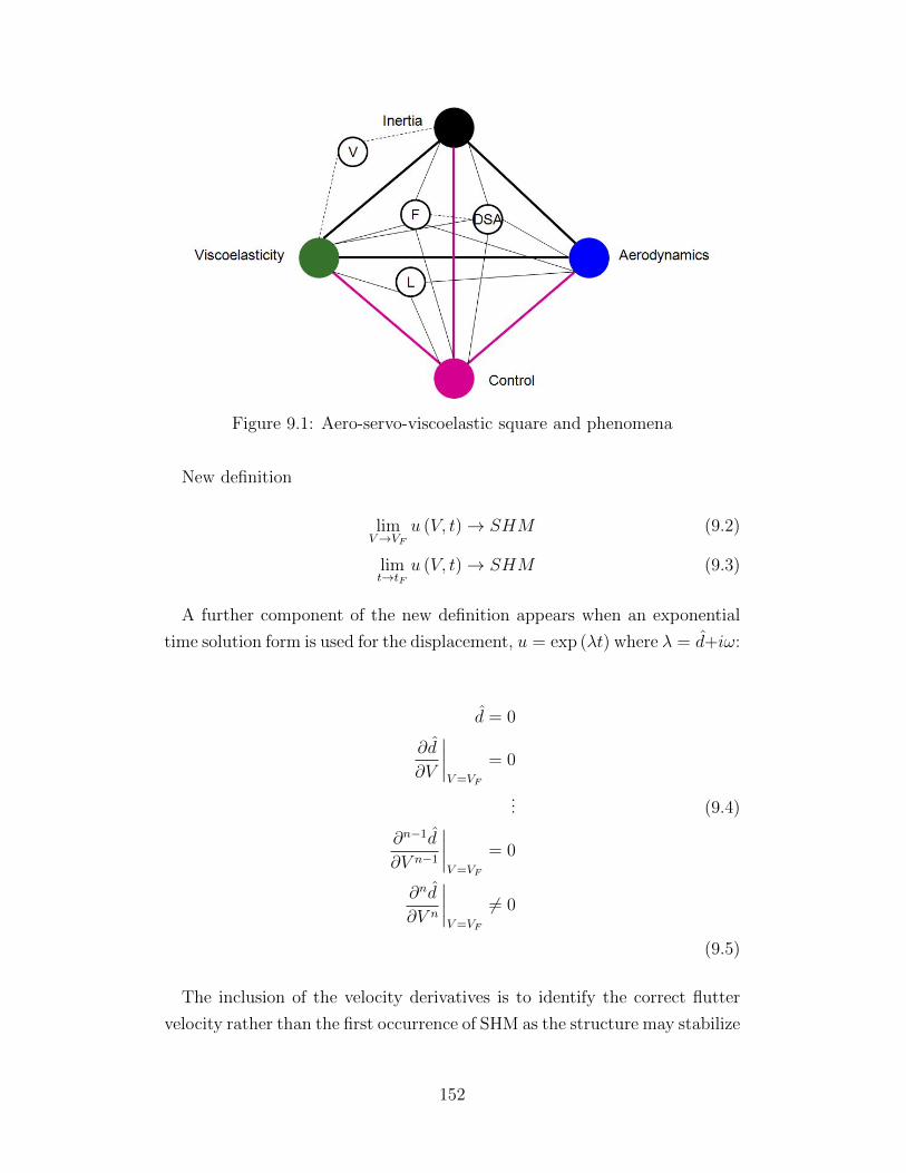
Figure 9.1: Aero-servo-viscoelastic square and phenomena
New definition
limV→VF
u (V, t)→ SHM (9.2)
limt→tF
u (V, t)→ SHM (9.3)
A further component of the new definition appears when an exponential
time solution form is used for the displacement, u = exp (λt) where λ = d+iω:
d = 0
∂d
∂V
∣∣∣∣V=VF
= 0
... (9.4)
∂n−1d
∂V n−1
∣∣∣∣V=VF
= 0
∂nd
∂V n
∣∣∣∣V=VF
6= 0
(9.5)
The inclusion of the velocity derivatives is to identify the correct flutter
velocity rather than the first occurrence of SHM as the structure may stabilize
152
with an increase in velocity. The old and new definitions for instability of a
wing, using the same notation as flutter are
Old definition
limV→VD
θ (V, t)→∞ (9.6)
New definition
limV→VD
θ (x2, V, t)→∞
limV→VD
∂θ (x2, V, t)
∂V→∞
limt→tD
θ (x2, V, t)→∞ (9.7)
limt→tD
∂θ (x2, V, t)
∂t→∞
Of particular note is the introduction of the λ notation that is consis-
tent with other dynamic stability problems that occur in engineering. The
advantage of the λ notation is that flutter and instability are treated as a con-
tinuum of dynamic phenomena rather than the traditional definition which
restricts instability of a wing to a static problem called torsional divergence,
and flutter as a dynamic problem. For this reason, flutter and instability of a
viscoelastic lifting surface are reclassified as dynamic wing stability problems.
The inclusion of controls in the instability of a viscoelastic wing has led to
some interesting results. The effects of proportional, integral, and differential
controllers were examined for the instability conditions when the controllers
are only applied to the twisting motion. The wing considered was a simple
cantilever wing without chordwise or spanwise bending. Very low instability
speeds, such as with some of the differential controllers, indicate that some
combinations of controller parameters easily cause instability. Specific notes
about the controllers are
• The proportional controllers for this problem always have a instability
speed and delay instability to significantly higher speeds. However,
over-control is possible.
• The integral controllers give very similar results across the range of
gain values indicating that the instability speed is fairly insensitive to
153
the gain value. Also, the integral controller provides higher instability
speeds more consistently than the proportional controller.
• The differential controllers have cases where the instability speed could
not be found within the tested ranges. The differential controllers pro-
vided the highest instability speed, but not as consistently as the inte-
gral controllers. The controllers also produce some of the lowest insta-
bility speeds. Rapid switching between stability and instability as the
order of magnitude of the controller gains increase is an issue particular
to differential controllers and suggest that the practical use of differ-
ential controllers is limited. The rapid changes are not unexpected as
differential controllers are typically noisy.
The effects of including chordwise and unsymmetrical bending and twisting
for an aero-viscoelastic lifting surface were examined using an example case
of a rectangular, cantilever wing in subsonic flow. A range of parameters were
studied including aspect ratios, viscoelastic relaxation times and viscoelastic
scaling factors. The most noticeable result was the removal of chordwise
bending effects from the simulation example resulted in a wing that did
not flutter or diverge. This would suggest that including chordwise bending
is necessary to accurately predict the behavior of a wing. The effects of
the unsymmetrical bending were less obvious, likely because of the chosen
parameter set. Further analyses of unsymmetrical bending are necessary.
The λ notation is also advantageous for the more challenging problem of
viscoelastic panels and the occurrence of flutter and panel instability. In
aeroelasticity, panel instability is referred to as divergence which unfortu-
nately is a vague term as it may imply panel buckling rather than a phe-
menon parallel to torsional divergence of a wing. Further, past analytical
proofs of subsonic panel flutter indicated that panel “divergence” will occur
before panel flutter. This proof became accepted wisdom in the aeroelastic
field for a number of decades. First, the revised definitions for panel flutter
and instability using the λ notation are
The issue of panel “divergence” before flutter at subsonic speeds was re-
solved by the author through the identification of a non-uniform convergence
of a series approximation that is applied during the use of Galerkin’s method.
The earlier proof terminated that series prematurely resulting in an incorrect
154
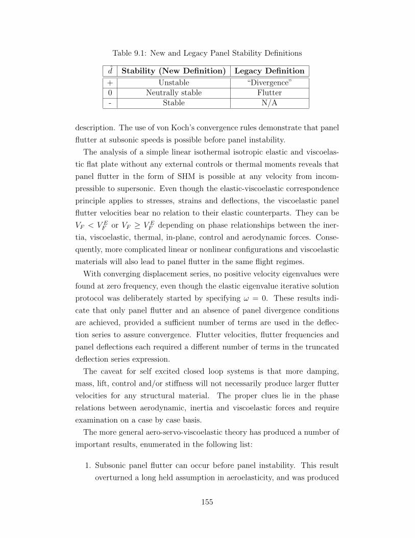
Table 9.1: New and Legacy Panel Stability Definitions
d Stability (New Definition) Legacy Definition
+ Unstable “Divergence”0 Neutrally stable Flutter- Stable N/A
description. The use of von Koch’s convergence rules demonstrate that panel
flutter at subsonic speeds is possible before panel instability.
The analysis of a simple linear isothermal isotropic elastic and viscoelas-
tic flat plate without any external controls or thermal moments reveals that
panel flutter in the form of SHM is possible at any velocity from incom-
pressible to supersonic. Even though the elastic-viscoelastic correspondence
principle applies to stresses, strains and deflections, the viscoelastic panel
flutter velocities bear no relation to their elastic counterparts. They can be
VF < V EF or VF ≥ V E
F depending on phase relationships between the iner-
tia, viscoelastic, thermal, in-plane, control and aerodynamic forces. Conse-
quently, more complicated linear or nonlinear configurations and viscoelastic
materials will also lead to panel flutter in the same flight regimes.
With converging displacement series, no positive velocity eigenvalues were
found at zero frequency, even though the elastic eigenvalue iterative solution
protocol was deliberately started by specifying ω = 0. These results indi-
cate that only panel flutter and an absence of panel divergence conditions
are achieved, provided a sufficient number of terms are used in the deflec-
tion series to assure convergence. Flutter velocities, flutter frequencies and
panel deflections each required a different number of terms in the truncated
deflection series expression.
The caveat for self excited closed loop systems is that more damping,
mass, lift, control and/or stiffness will not necessarily produce larger flutter
velocities for any structural material. The proper clues lie in the phase
relations between aerodynamic, inertia and viscoelastic forces and require
examination on a case by case basis.
The more general aero-servo-viscoelastic theory has produced a number of
important results, enumerated in the following list:
1. Subsonic panel flutter can occur before panel instability. This result
overturned a long held assumption in aeroelasticity, and was produced
155
by the novel application of the von Koch rules for convergence. Further,
experimental results from the 1950s by the Air Force were retrieved to
provide additional proof.
2. An expanded definition for flutter of a lifting surface. The legacy defi-
nition is that flutter is the first occurrence of simple harmonic motion
of a structure, and the flight velocity at which this motion occurs is
taken as the flutter speed. The expanded definition indicates that the
flutter condition should be taken when simple harmonic motion occurs
and additional velocity derivatives are zero.
3. The viscoelastic material behavior imposes a flutter time indicating
that the presence of flutter should be verified for the entire life time of
a flight vehicle.
4. An expanded definition for instability of a lifting surface or panel. Tra-
ditionally, instability is treated as a static phenomenon. The static case
is only a limiting case of dynamic instability for a viscoelastic structure.
Instability occurs when a particular combination of flight velocity and
time are reached leading to growing displacements of the structure.
5. The inclusion of flight velocity transients that occur during maneuvers.
Two- and three-dimensional unsteady incompressible and compressible
aerodynamics were reformulated for a time dependent velocity. The
inclusion of flight velocity transients do affect the flutter and instability
conditions for a lifting surface and a panel.
6. Viscoelastic materials are applicable to
• Airplanes, missiles, space vehicles, UAVs, MAVs, satellites, gos-
samer structures, antenna dishes, space suits, body armor, solar
sails, circuit boards, etc.
• Ground transportation: automotive, tanks, railroads, cargo con-
tainers
• Submarines and other navy ships
156
APPENDIX A
As a note, a number of papers that were produced from this dissertation are
referenced in the following tables. The tables list publicly available publica-
tions on aeroelasticity and aero-viscoelasticity.
157
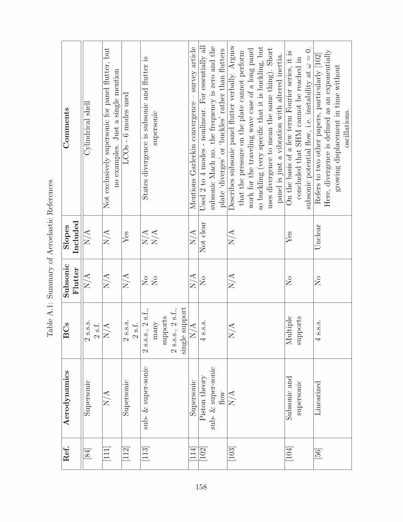
Tab
leA
.1:
Sum
mar
yof
Aer
oel
asti
cR
efer
ence
s
Ref.
Aero
dyn
am
ics
BC
sSubso
nic
Flu
tter
Slo
pes
Incl
uded
Com
ments
[84]
Sup
erso
nic
2s.
s.s.
2s.
f.N
/AN
/AC
ylindri
cal
shel
l
[111
]N
/AN
/AN
/AN
/AN
otex
clusi
vely
sup
erso
nic
for
pan
elflutt
er,
but
no
exam
ple
s.Just
asi
ngl
em
enti
on[1
12]
Sup
erso
nic
2s.
s.s.
2s.
f.N
/AY
esL
CO
s-
6m
odes
use
d
[113
]su
b-
&su
per
-son
ic2
s.s.
s.,
2s.
f.,
man
ysu
pp
orts
2s.
s.s.
,2
s.f.
,si
ngl
esu
pp
ort
No
No
N/A
N/A
Sta
tes
div
erge
nce
issu
bso
nic
and
flutt
eris
sup
erso
nic
[114
]Sup
erso
nic
N/A
N/A
N/A
Men
tion
sG
arle
rkin
conve
rgen
ce–
surv
eyar
ticl
e[1
02]
Pis
ton
theo
rysu
b-
&su
per
-son
icflow
4s.
s.s.
No
Not
clea
rU
sed
2to
4m
odes
-non
linea
r.F
ores
senti
ally
all
subso
nic
Mac
hno.
the
freq
uen
cyis
zero
and
the
pla
te‘d
iver
ges’
or‘b
uck
les’
rath
erth
anflutt
ers
[103
]N
/AN
/AN
/AN
/AD
escr
ibes
subso
nic
pan
elflutt
erve
rbal
ly.
Arg
ues
that
the
pre
ssure
onth
epla
teca
nnot
per
form
wor
kfo
rth
etr
avel
ing
wav
eca
seof
alo
ng
pan
elso
buck
ling
(ver
ysp
ecifi
cth
atit
isbuck
ling,
but
use
sdiv
erge
nce
tom
ean
the
sam
eth
ing)
.Shor
tpan
elis
just
avib
rati
onw
ith
alte
red
iner
tia.
[104
]Subso
nic
and
sup
erso
nic
Mult
iple
supp
orts
No
Yes
On
the
bas
isof
afe
wte
rmF
ouri
erse
ries
,it
isco
ncl
uded
that
SH
Mca
nnot
be
reac
hed
insu
bso
nic
pot
enti
alflow
,i.e.
inst
abilit
yatω
=0.
[56]
Lin
eari
zed
4s.
s.s.
No
Uncl
ear
Ref
ers
totw
oot
her
pap
ers,
par
ticu
larl
y[1
02]
Her
e,div
erge
nce
isdefi
ned
asan
exp
onen
tial
lygr
owin
gdis
pla
cem
ent
inti
me
wit
hou
tos
cillat
ions.
158
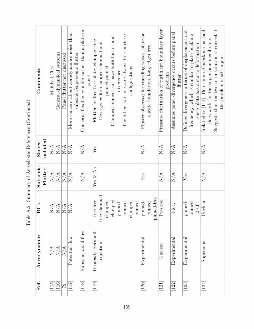
Tab
leA
.2:
Sum
mar
yof
Aer
oel
asti
cR
efer
ence
s(C
onti
nued
)
Ref.
Aero
dyn
am
ics
BC
sSubso
nic
Flu
tter
Slo
pes
Incl
uded
Com
ments
[115
]N
/AN
/AN
/AN
/AM
ainly
LC
Os
[116
]N
/AN
/AN
/AN
/AG
ener
aldynam
ical
syst
ems
[79]
N/A
N/A
N/A
N/A
Pan
elflutt
ernot
dis
cuss
ed[1
17]
Pot
enti
alflow
N/A
N/A
N/A
Mor
eco
nce
rnab
out
aero
dynam
ics
noi
seth
ansu
bso
nic
/sup
erso
nic
flutt
er[1
18]
Subso
nic
axia
lflow
N/A
N/A
Con
cern
sflex
ible
cylinder
rath
erth
ana
pla
teor
pan
el[1
19]
Unst
eady
Ber
nou
lli
equat
ion
free
-fre
efr
ee-c
lam
ped
clam
ped
-cl
amp
edpin
ned
-pin
ned
clam
ped
-pin
ned
Yes
&N
oY
esF
lutt
erfo
rfr
ee-f
ree
pla
te,
clam
ped
-fre
eD
iver
gence
for
clam
ped
-cla
mp
edan
dpin
ned
-pin
ned
Cla
mp
ed-p
inned
can
hav
eb
oth
flutt
eran
ddiv
erge
nce
The
other
two
sides
are
alw
ays
free
inth
ese
configu
rati
ons
[120
]E
xp
erim
enta
lpin
ned
-pin
ned
pin
ned
-fre
e
Yes
N/A
Flu
tter
obse
rved
for
trav
elin
gw
aves
,pla
teon
elas
tic
foundat
ion,
long
edge
sfr
ee
[121
]U
ncl
ear
Tw
oro
dN
/AN
/AP
ress
ure
fluct
uat
ion
oftu
rbule
nt
bou
ndar
yla
yer
pro
ble
m[1
22]
Exp
erim
enta
l4
s.c.
N/A
N/A
Ass
um
espan
eldiv
erge
nce
occ
urs
bef
ore
pan
elflutt
er[1
23]
Exp
erim
enta
lpin
ned
-pin
ned
2s.
f.
Yes
N/A
Defi
nes
div
erge
nce
inte
rms
ofdis
pla
cem
ent
not
freq
uen
cy,
whic
his
sim
ilar
topla
tebuck
ling
since
pla
tehas
ast
atic
def
orm
atio
n[1
24]
Sup
erso
nic
Uncl
ear
N/A
N/A
Rel
ated
to[1
14].
Det
erm
ines
Gal
erkin
’sm
ethod
does
wor
kfo
rth
esu
per
sonic
mem
bra
ne.
Sugg
ests
that
the
two
term
solu
tion
isco
rrec
tif
the
pro
ble
mis
self
-adjo
int.
159
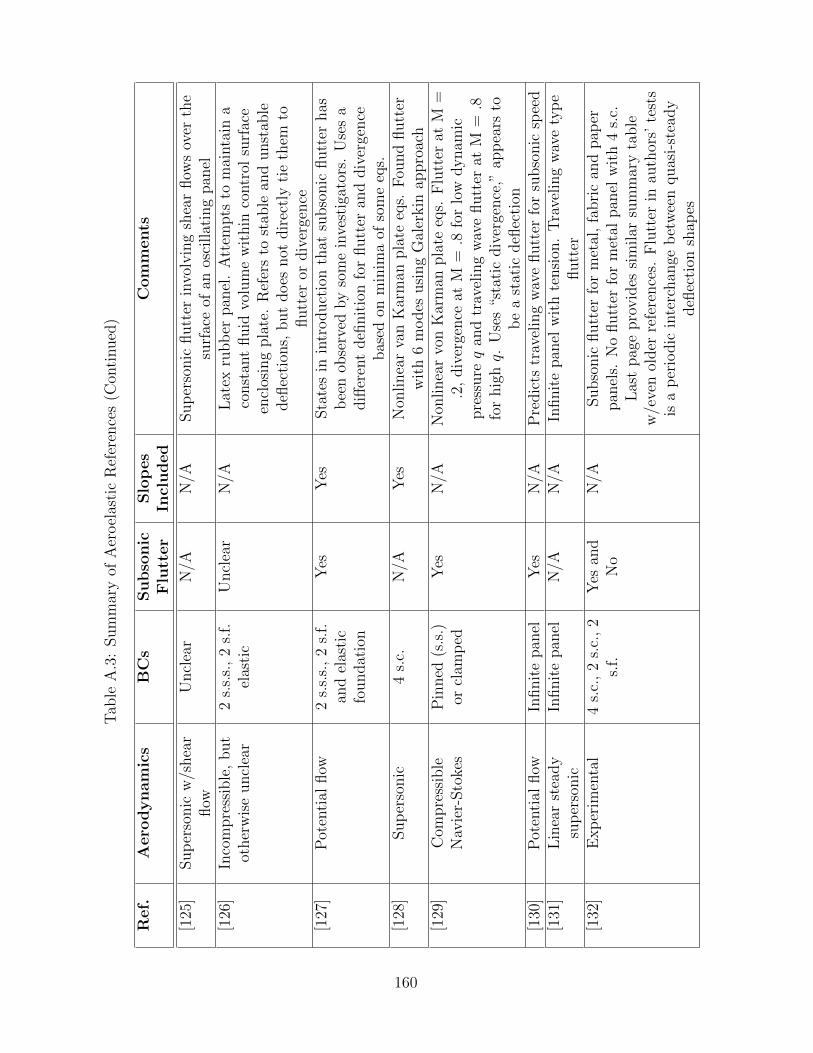
Tab
leA
.3:
Sum
mar
yof
Aer
oel
asti
cR
efer
ence
s(C
onti
nued
)
Ref.
Aero
dyn
am
ics
BC
sSubso
nic
Flu
tter
Slo
pes
Incl
uded
Com
ments
[125
]Sup
erso
nic
w/s
hea
rflow
Uncl
ear
N/A
N/A
Sup
erso
nic
flutt
erin
volv
ing
shea
rflow
sov
erth
esu
rfac
eof
anos
cillat
ing
pan
el[1
26]
Inco
mpre
ssib
le,
but
other
wis
euncl
ear
2s.
s.s.
,2
s.f.
elas
tic
Uncl
ear
N/A
Lat
exru
bb
erpan
el.
Att
empts
tom
ainta
ina
const
ant
fluid
volu
me
wit
hin
contr
olsu
rfac
een
clos
ing
pla
te.
Ref
ers
tost
able
and
unst
able
defl
ecti
ons,
but
does
not
dir
ectl
yti
eth
emto
flutt
eror
div
erge
nce
[127
]P
oten
tial
flow
2s.
s.s.
,2
s.f.
and
elas
tic
foundat
ion
Yes
Yes
Sta
tes
inin
troduct
ion
that
subso
nic
flutt
erhas
bee
nob
serv
edby
som
ein
vest
igat
ors.
Use
sa
diff
eren
tdefi
nit
ion
for
flutt
eran
ddiv
erge
nce
bas
edon
min
ima
ofso
me
eqs.
[128
]Sup
erso
nic
4s.
c.N
/AY
esN
onlinea
rva
nK
arm
anpla
teeq
s.F
ound
flutt
erw
ith
6m
odes
usi
ng
Gal
erkin
appro
ach
[129
]C
ompre
ssib
leN
avie
r-Sto
kes
Pin
ned
(s.s
.)or
clam
ped
Yes
N/A
Non
linea
rvo
nK
arm
anpla
teeq
s.F
lutt
erat
M=
.2,
div
erge
nce
atM
=.8
for
low
dynam
icpre
ssureq
and
trav
elin
gw
ave
flutt
erat
M=
.8fo
rhig
hq.
Use
s“s
tati
cdiv
erge
nce
,”ap
pea
rsto
be
ast
atic
defl
ecti
on[1
30]
Pot
enti
alflow
Infinit
epan
elY
esN
/AP
redic
tstr
avel
ing
wav
eflutt
erfo
rsu
bso
nic
spee
d[1
31]
Lin
ear
stea
dy
sup
erso
nic
Infinit
epan
elN
/AN
/AIn
finit
epan
elw
ith
tensi
on.
Tra
veling
wav
ety
pe
flutt
er[1
32]
Exp
erim
enta
l4
s.c.
,2
s.c.
,2
s.f.
Yes
and
No
N/A
Subso
nic
flutt
erfo
rm
etal
,fa
bri
can
dpap
erpan
els.
No
flutt
erfo
rm
etal
pan
elw
ith
4s.
c.L
ast
pag
epro
vid
essi
milar
sum
mar
yta
ble
w/e
ven
older
refe
rence
s.F
lutt
erin
auth
ors’
test
sis
ap
erio
dic
inte
rchan
geb
etw
een
quas
i-st
eady
defl
ecti
onsh
apes
160
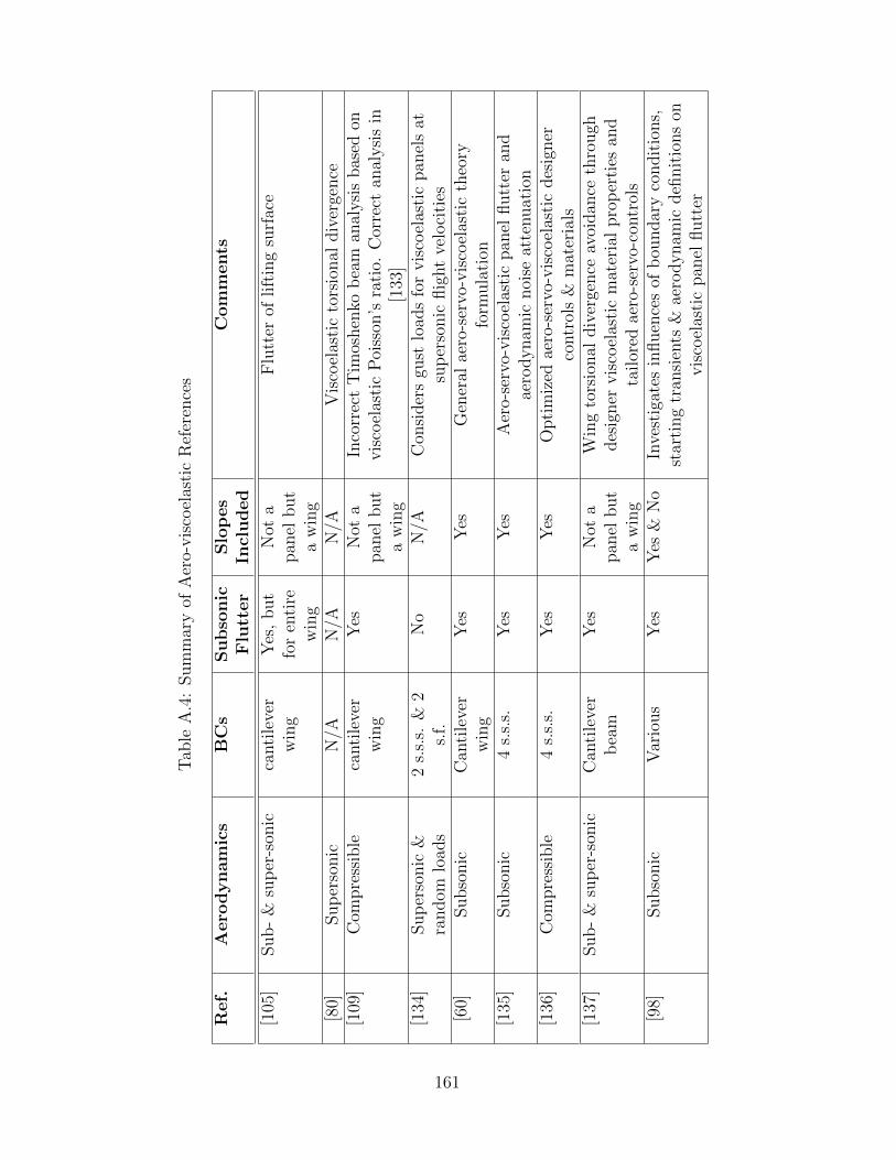
Tab
leA
.4:
Sum
mar
yof
Aer
o-vis
coel
asti
cR
efer
ence
s
Ref.
Aero
dyn
am
ics
BC
sSubso
nic
Flu
tter
Slo
pes
Incl
uded
Com
ments
[105
]Sub-
&su
per
-son
icca
nti
leve
rw
ing
Yes
,but
for
enti
rew
ing
Not
apan
elbut
aw
ing
Flu
tter
oflift
ing
surf
ace
[80]
Sup
erso
nic
N/A
N/A
N/A
Vis
coel
asti
cto
rsio
nal
div
erge
nce
[109
]C
ompre
ssib
leca
nti
leve
rw
ing
Yes
Not
apan
elbut
aw
ing
Inco
rrec
tT
imos
hen
kob
eam
anal
ysi
sbas
edon
vis
coel
asti
cP
oiss
on’s
rati
o.C
orre
ctan
alysi
sin
[133
][1
34]
Sup
erso
nic
&ra
ndom
load
s2
s.s.
s.&
2s.
f.N
oN
/AC
onsi
der
sgu
stlo
ads
for
vis
coel
asti
cpan
els
atsu
per
sonic
flig
ht
velo
citi
es[6
0]Subso
nic
Can
tile
ver
win
gY
esY
esG
ener
alae
ro-s
ervo
-vis
coel
asti
cth
eory
form
ula
tion
[135
]Subso
nic
4s.
s.s.
Yes
Yes
Aer
o-se
rvo-
vis
coel
asti
cpan
elflutt
eran
dae
rodynam
icnoi
seat
tenuat
ion
[136
]C
ompre
ssib
le4
s.s.
s.Y
esY
esO
pti
miz
edae
ro-s
ervo
-vis
coel
asti
cdes
igner
contr
ols
&m
ater
ials
[137
]Sub-
&su
per
-son
icC
anti
leve
rb
eam
Yes
Not
apan
elbut
aw
ing
Win
gto
rsio
nal
div
erge
nce
avoi
dan
ceth
rough
des
igner
vis
coel
asti
cm
ater
ial
pro
per
ties
and
tailor
edae
ro-s
ervo
-con
trol
s[9
8]Subso
nic
Var
ious
Yes
Yes
&N
oIn
vest
igat
esin
fluen
ces
ofb
oundar
yco
ndit
ions,
star
ting
tran
sien
ts&
aero
dynam
icdefi
nit
ions
onvis
coel
asti
cpan
elflutt
er
161
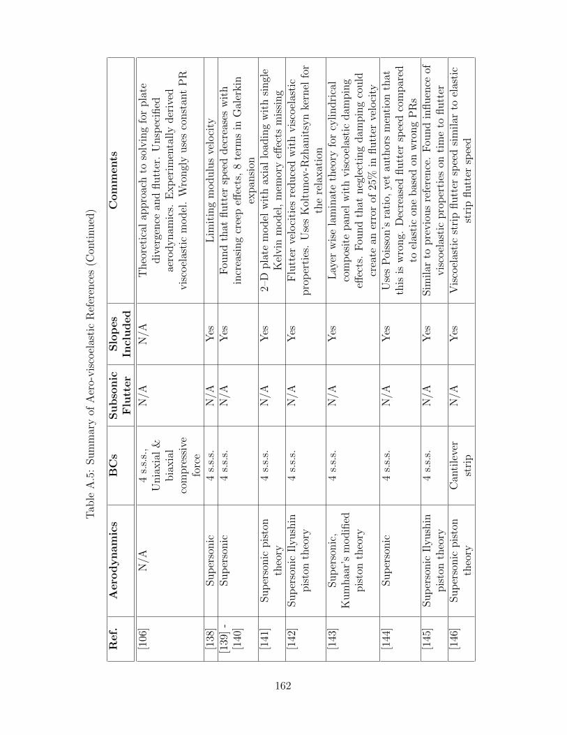
Tab
leA
.5:
Sum
mar
yof
Aer
o-vis
coel
asti
cR
efer
ence
s(C
onti
nued
)
Ref.
Aero
dyn
am
ics
BC
sSubso
nic
Flu
tter
Slo
pes
Incl
uded
Com
ments
[106
]N
/A4
s.s.
s.,
Unia
xia
l&
bia
xia
lco
mpre
ssiv
efo
rce
N/A
N/A
Theo
reti
cal
appro
ach
toso
lvin
gfo
rpla
tediv
erge
nce
and
flutt
er.
Unsp
ecifi
edae
rodynam
ics.
Exp
erim
enta
lly
der
ived
vis
coel
asti
cm
odel
.W
rongl
yuse
sco
nst
ant
PR
[138
]Sup
erso
nic
4s.
s.s.
N/A
Yes
Lim
itin
gm
odulu
sve
loci
ty[1
39]
-[1
40]
Sup
erso
nic
4s.
s.s.
N/A
Yes
Fou
nd
that
flutt
ersp
eed
dec
reas
esw
ith
incr
easi
ng
cree
peff
ects
,8
term
sin
Gal
erkin
expan
sion
[141
]Sup
erso
nic
pis
ton
theo
ry4
s.s.
s.N
/AY
es2–
Dpla
tem
odel
wit
hax
ial
load
ing
wit
hsi
ngl
eK
elvin
model
,m
emor
yeff
ects
mis
sing
[142
]Sup
erso
nic
Ilyush
inpis
ton
theo
ry4
s.s.
s.N
/AY
esF
lutt
erve
loci
ties
reduce
dw
ith
vis
coel
asti
cpro
per
ties
.U
ses
Kol
tunov
-Rzh
anit
syn
kern
elfo
rth
ere
laxat
ion
[143
]Sup
erso
nic
,K
um
haa
r’s
modifi
edpis
ton
theo
ry
4s.
s.s.
N/A
Yes
Lay
erw
ise
lam
inat
eth
eory
for
cylindri
cal
com
pos
ite
pan
elw
ith
vis
coel
asti
cdam
pin
geff
ects
.F
ound
that
neg
lect
ing
dam
pin
gco
uld
crea
tean
erro
rof
25%
influtt
erve
loci
ty[1
44]
Sup
erso
nic
4s.
s.s.
N/A
Yes
Use
sP
oiss
on’s
rati
o,ye
tau
thor
sm
enti
onth
atth
isis
wro
ng.
Dec
reas
edflutt
ersp
eed
com
par
edto
elas
tic
one
bas
edon
wro
ng
PR
s[1
45]
Sup
erso
nic
Ilyush
inpis
ton
theo
ry4
s.s.
s.N
/AY
esSim
ilar
topre
vio
us
refe
rence
.F
ound
influen
ceof
vis
coel
asti
cpro
per
ties
onti
me
toflutt
er[1
46]
Sup
erso
nic
pis
ton
theo
ryC
anti
leve
rst
rip
N/A
Yes
Vis
coel
asti
cst
rip
flutt
ersp
eed
sim
ilar
toel
asti
cst
rip
flutt
ersp
eed
162
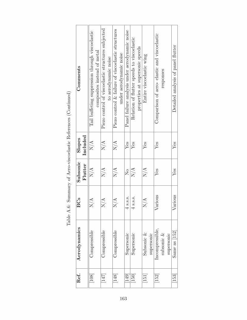
Tab
leA
.6:
Sum
mar
yof
Aer
o-vis
coel
asti
cR
efer
ence
s(C
onti
nued
)
Ref.
Aero
dyn
am
ics
BC
sSubso
nic
Flu
tter
Slo
pes
Incl
uded
Com
ments
[108
]C
ompre
ssib
leN
/AN
/AN
/AT
ail
buff
etin
gsu
ppre
ssio
nth
rough
vis
coel
asti
cco
mp
osit
esin
stea
dof
met
al[1
47]
Com
pre
ssib
leN
/AN
/AN
/AP
iezo
contr
olof
vis
coel
asti
cst
ruct
ure
ssu
bje
cted
toae
rodynam
icnoi
se[1
48]
Com
pre
ssib
leN
/AN
/AN
/AP
iezo
contr
ol&
failure
ofvis
coel
asti
cst
ruct
ure
sunder
aero
dynam
icnoi
se[1
49]
Sup
erso
nic
4s.
s.s.
No
Yes
Pan
elfa
ilure
anal
ysi
sunder
aero
dynam
icnoi
se[1
50]
Sup
erso
nic
4s.
s.s.
N/A
Yes
Rel
atio
nof
flutt
ersp
eeds
tovis
coel
asti
cpro
per
ties
atsu
per
sonic
spee
ds
[151
]Subso
nic
&su
per
sonic
N/A
N/A
Yes
Enti
revis
coel
asti
cw
ing
[152
]In
com
pre
ssib
le,
subso
nic
&su
per
sonic
Var
ious
Yes
Yes
Com
par
ison
ofae
ro-
elas
tic
and
vis
coel
asti
cre
spon
ses
[153
]Sam
eas
[152
]V
ario
us
Yes
Yes
Det
aile
dan
alysi
sof
pan
elflutt
er
163
REFERENCES
[1] A. Collar, “The expanding domain of aeroelasticity,” The Royal Aero-nautical Society, vol. 50, pp. 613–636, August 1946.
[2] J. Anderson, Fundamentals of Aerodynamics, 3rd ed. McGraw-HillBook Co, 2001.
[3] M. Greenberg, Application of Green’s Functions in Science and Engi-neering. Englewood Cliffs, NJ: Prentice Hall, 1971.
[4] A. Leissa, “Vibration of plates,” NASA, Washington DC, TechnicalReport SP-160, 1969.
[5] R. L. Bisplinghoff, H. Ashley, and R. L. Halfman, Aeroelasticity. NewYork: Dover Publications, 1980.
[6] R. Frazer and W. Duncan, “The flutter of aeroplane wings,” BritishAeronautical Research Council, Reports and memoranda 1155, August1928.
[7] R. Lind and M. Brenner, Robust Aeroservoelastic Stability Analysis:Flight Test Applications, ser. Advances in Industrial Control. Springer,1999.
[8] H. Ashley and M. Landahl, Aerodynamics of Wings and Bodies. DoverPublications, 1985.
[9] H. Ashley and W. Rodden, “Wing-body aerodynamic interaction,” An-nual Review of Fluid Mechanics, vol. 4, pp. 431–472, 1972.
[10] E. Stannard, “Summary of the fundamentals of incompressible un-steady aerodynamics,” M.S. thesis, University of Illinois at Urbana-Champaign, 1957.
[11] H. Vel, “Unsteady profile theory in incompressible flow,” Ph.D. disser-tation, Rijksuniversiteit te Groningen, 1964.
[12] S. Bland, “Recent advances and concepts in unsteady aerodynamictheory,” NASA Langley Research Center, Tech. Rep. 46, 1975, p. 1305-1326.
164
[13] O. Burggraf, “Notes on unsteady aerodynamics.”
[14] T. Cebeci, M. Platzer, H. Chen, K. Chang, and J. Shao, Analysis ofLow Speed Unsteady Airfoil Flows. Long Beach, California: Horizons,2005.
[15] J. R. Wright and J. E. Cooper, Introduction to Aircraft Aeroelasticityand Loads. Hoboken NJ: John Wiley, 2007.
[16] R. Botez, A. Dinu, I. Cotoi, N. Strathopoulos, S. Therien, M. Dick-inson, and A. Rathe, “Improved method for creating time-domainunsteady aerodynamic models,” Journal of Aerospace Engineering,vol. 20, no. 3, pp. 204–208, 2007.
[17] R. Jones, “Operational treatment of the nonuniform-lift theory in air-plane dynamics,” NACA, Technical Note 667, 1938.
[18] W. Jones, “Aerodynamic forces on wings in nonuniform motion,” Br.A.R.C., Reports and Memoranda 2117, 1945.
[19] E. Postel and E. Leppert, “Theoretical pressure distributions for a thinairfoil oscillating in incompressible flow,” Journal of the AeronauticalSciences, vol. 15, pp. 486–492, August 1948.
[20] M. Goland, “The quasi-steady air forces for use in low-frequency stabil-ity calculations,” Journal of the Aeronautical Sciences, vol. 17, no. 10,pp. 601–608,672, October 1950.
[21] V. Kurzin, “Aerodynamic disturbances of profiles in subsonic unsteadyflow,” NASA, TTF 10,293, September 1966, translation.
[22] J. Fromme and D. Halstead, “Solutions to Kussner’s integral equationin unsteady flow using local basis functions,” NASA, CR 137719, 1975.
[23] W. Rowe, M. Redman, F. Ehlers, and J. Sebastian, “Prediction ofunsteady aerodynamic loadings caused by leading edge and trailingedge control surface motions in subsonic compressible flow - analysisand results,” NASA, CR 2543, 1975.
[24] N. Kemp and G. Homicz, “Approximate unsteady thin-airfoil theoryfor subsonic flow,” AIAA Journal, vol. 14, no. 8, pp. 1083–1089, 1976.
[25] H. Hemdan, “Unsteady Newtonian flow over two-dimensional airfoils,”Trans. Japan Soc. Aero. Space Sci, vol. 30, no. 88, pp. 65–79, August1987.
[26] T. Strganac, “A numerical model of unsteady subsonic aeroelastic be-havior,” PhD Thesis, Virigina Polytechnic Institute and State Univer-sity, August 1987, NASA-TM-101126.
165
[27] V. Gulyaev, M. Nisht, and V. Popov, “Linear mathematical modes forthe aerodynamics of three-dimensional lifting systems in an unsteadysubsonic gas flow,” Fluid Dynamics, vol. 35, no. 6, pp. 933–944, 2000.
[28] M. Ol, “The high-frequency, high-amplitude pitch problem: Airfoils,plates and wings,” in 39th AIAA Fluid Dynamics Conference, 2009,aIAA Paper 2009-3686.
[29] D. Robertson, J. Joo, and G. Reich, “Vortex particle aerodynamicmodelling of perching manoeuvres with micro aerial vehicles,” in 51stAIAA/ASME/ASCE/AHS/ASC Structures, Structural Dynamics andMaterials Conference, 2010, aIAA Paper 2010-2825.
[30] R. Isaacs, “Airfoil theory for flows of variable velocity,” Journal ofAeronautical Sciences, vol. 12, no. 1, pp. 113–118, January 1945.
[31] J. M. Greenberg, “Airfoil in sinusoidal motion in a pulsating stream,”NACA, Technical Note 1326, June 1947.
[32] T. Theodorsen, “General theory of aerodynamic instability and themechanism of flutter,” NACA, Technical Report 496, 1934.
[33] H. Sohngen, “Bestimmung der auftriebsvertelinug fur beliebige insta-tionare bewegungen (Ebenes problem),” Luftfahrtforschung, vol. 17,no. 11, pp. 401–420, December 1940.
[34] B. F. de Veubeke, “Aerodynamique instationnaire des profils mincesdeformables,” Brussels, Belgium, Bulletin du Service Technique del’Aeronautique 25, November 1953.
[35] W. Sears, “Operational methods in the theory of airfoils in non-uniformmotion,” Journal of the Franklin Institute, vol. 230, pp. 95–111, 1940.
[36] J. Edwards, H. Ashley, and J. Breakwell, “Unsteady aerodynamic mod-eling for arbitrary motions,” AIAA Journal, vol. 17, no. 4, pp. 365–374,April 1979.
[37] R. Bagley, D. Swinney, and K. Griffin, “Fractional order calculus modelof the generalized Theodorsen function,” Journal of Aircraft, vol. 30,no. 6, pp. 1003–1005, 1992.
[38] Y. Tomonari, “Extended Theodorsen function for an airfoil with awake,” Transactions of the Japan Society for Aero. Space Science,vol. 45, no. 150, pp. 229–235, 2003.
[39] T. von Karman and W. Sears, “Airfoil theory for non-uniform mo-tion,” Journal of the Aeronautical Sciences, vol. 5, no. 10, pp. 379–390,August 1938.
166
[40] B. Smilg and L. Wasserman, “Application of three-dimensional fluttertheory to aircraft structures,” Army Air Corps, Technical Report 4798,July 1942.
[41] M. Abramowitz and I. Stegun, Eds., Handbook of Mathematical Func-tions with Formulas, Graphs, and Mathematical Tables, 4th ed., ser.Applied Mathematics Series. National Bureau of Standards, 1965,no. 55.
[42] A. Balakrishnan, “Possio integral equation of aeroelasticity theory,”Journal of Aerospace Engineering, vol. 16, no. 4, pp. 139–154, October2003.
[43] L. Carr, M. Chandrasekhara, and N. Brock, “Quantitative study of un-steady compressible flow on an oscillating airfoil,” Journal of Aircraft,vol. 31, no. 4, pp. 892–898, July 1994.
[44] J. Miles, “A note on a solution to Possio’s integral equation for anoscillating airfoil in subsonic flow,” Quarterly of Applied Mathematics,vol. 7, pp. 213–216, 1949.
[45] N. Kulikov, “Approximate solution of a second-order linear differentialequation with variable coefficients,” Journal of Applied Mathematicsand Mechanics, vol. 24, no. 4, pp. 1135–1143, 1960.
[46] R. Jones, “The unsteady lift of a finite wing,” NACA, Technical Note682, 1939.
[47] E. Reissner, “On the general theory of thin airfoils for nonuniformmotion,” N.A.C.A, Technical Note 946, 1944.
[48] H. Ashley, S. Windall, and M. Landahl, “New directions in lifting sur-face theory,” AIAA Journal, vol. 3, no. 1, pp. 3–16, January 1965.
[49] M. Landahl and V. Stark, “Numerical lifting-surface theory - problemsand progress,” AIAA Journal, vol. 6, no. 11, pp. 2049–2060, November1968.
[50] L. Morino, “A general theory of unsteady compressible potential aero-dynamics,” NASA, CR 2464, 1974.
[51] A. Dusto and M. Epton, “An advanced panel method for analysis ofarbitrary configurations in unsteady subsonic flow,” NASA, CR 152323,1980.
[52] E. Reissner, “Effect of finite span on the airload distributions for oscil-lating wings I - aerodynamic theory of oscillating wings of finite span,”N.A.C.A., Technical Note 1194, 1947.
167
[53] E. Reissner, “Effect of finite span on the airload distributions for oscil-lating wings. II - methods of calculation and examples of application,”N.A.C.A., Technical Note 1195, 1947.
[54] E. Reissner, “On the theory of oscillating airfoils of finite span in sub-sonic compressible flow,” N.A.C.A., Technical Note 1953, 1949.
[55] E. Reissner, “Extension of the theory of oscillating airfoils of finite spanin subsonic compressible flow,” N.A.C.A., Technical Note 2274, 1951.
[56] E. H. Dowell, Aeroelasticity of Plates and Shells. Leyden: NoordhoffInternational Publishing, 1975.
[57] J. Hedgepeth, “Flutter of rectangular simply supported panels at highsupersonic speeds,” Journal of the Aeronautical Sciences, vol. 24, pp.563–573, 1957.
[58] E. Zeydel, “Research study on panel flutter aerodynamics final report,apr. 5, 1965 - nov. 4, 1966,” NASA, Contractor Report 83826, 1967.
[59] J.-H. Han, J. Tani, and J. Qiu, “Active flutter suppression of a lift-ing surface using piezoelectric actuation and modern control theory,”Journal of Sound and Vibration, vol. 291, pp. 706–722, 2006.
[60] C. G. Merrett and H. H. Hilton, “Generalized linear aero-servo-viscoelasticity: Theory and applications,” in Proceedings 49thAIAA/ASME/ASCE/AHS Structures, Structural Dynamics and Ma-terials Conference, Schaumburg, IL, 2008, AIAA Paper 2008-1997.
[61] K. Ogata, Modern Control Engineering, 4th ed. Upper Saddle River,New Jersey: Prentice Hall, 2002.
[62] M. Dahleh and I. Diaz-Bobillo, Control of Uncertain Systems. UpperSaddle River: Prentice Hall, 1995.
[63] W. Johnson, Helicopter Theory. New York: Dover Publications, 1980.
[64] J. P. Keener, Principles of Applied Mathematics: Transformation andApproximation. Cambridge MA: Westview, 2000.
[65] H. Leipholz and R. Mandadi, “On the non-uniform convergence ofGalerkin’s method,” Journal of Sound and Vibration, vol. 57, pp. 483–498, 1978.
[66] V. Bolotin, A. Grishko, J. Roberts, A. Kounadis, and C. Gantes, “Thefluttering panel as a continuous nonlinear nonconservative system,”Journal of Vibration and Control, vol. 7, pp. 233–247, 2001.
168
[67] H. von Koch, “Sur la convergence des determinants infinis,” Rendicontidel Circolo Mathematico di Palermo, vol. XXVIII, pp. 255–266, 1909.
[68] D. Hilbert, “Grundzuge einer allgemeinen theorie der linearen in-tegralgleichungen,” Nachrichten von der Kgl. Gesellschaft der Wis-senschaften zu Gottingen, Mathematisch-physikalische Klasse, pp. 439–480, 1906.
[69] P. Lancaster, Lambda-matrices and Vibrating Systems. PergamonPress, 1966.
[70] F. Tisseur and K. Meerbergen, “The quadratic eigenvalue problem,”SIAM Review, vol. 43, no. 2, pp. 235–286, 2001.
[71] J. Uicker, G. Pennock, and J. Shigley, Theory of Machines and Mech-anisms, 3rd ed. New York: Oxford University Press, 2003.
[72] H. F. Brinson and L. C. Brinson, Polymer engineering science andviscoelasticity: an introduction. New York: Springer, 2008.
[73] C. Truesdell and W. Noll, The Non-linear Field Theories of Mechanics,3rd ed., S. Antman, Ed. New York: Springer, 2003.
[74] G. C. B. de Prony, “Essai experimental et analytique,” Journal del’Ecole Polytechnique de Paris, vol. 1, pp. 24–76, 1795.
[75] R. M. Christensen, Theory of Viscoelasticity - An Introduction, 2nd ed.New York: Academic Press, 1982.
[76] H. H. Hilton, “Implications and constraints of time independent Pois-son ratios in linear isotropic and anisotropic viscoelasticity,” Journalof Elasticity, vol. 63, pp. 221–251, 2001.
[77] H. H. Hilton, “Dynamic thermal stress creep buckling, probabilisticfailures and survival times of viscoelastic columns with follower loads,”in Collected papers in structural mechanics honoring Dr. James H.Starnes, Jr, Special NASA/TM 2006-214276, N. Knight, N. Nemeth,and J. Malone, Eds. VA: NASA Langley Research Center, 2006, pp.469–487.
[78] H. H. Hilton, “On the nonexistence of finite critical times for gen-eralized linear viscoelastic columns with arbitrary initial curvatures,”Journal of the Aero/Space Sciences, vol. 28, pp. 655–656, 1961.
[79] E. H. Dowell, E. F. Crawley, H. C. C. Jr., D. A. Peters, R. H. Scanlan,and F. Sisto, A Modern Course in Aeroelasticity. Boston: KluwerAcademic Publishers, 2004.
169
[80] H. H. Hilton, “The divergence of supersonic, linear viscoelastic lift-ing surfaces, including chordwise bending,” Journal of the Aero/SpaceSciences, vol. 27, pp. 926–934, 1960.
[81] H. H. Hilton, “Dynamic creep buckling of linear viscoelastic columnsincluding failure probabilities and survival times,” University of IllinoisUIUC, Technical Report UILU ENG 20-0503, 2002.
[82] H. H. Hilton, “Creep collapse of viscoelastic columns with initial cur-vatures,” Journal of the Aeronautical Sciences, vol. 19, pp. 844–846,1952.
[83] H. H. Hilton and S. Yi, “Creep divergence of nonlinear viscoelasticlifting surfaces with piezoelectric control,” in Proceedings of the Sec-ond International Conference on Nonlinear Problems in Aviation andAerospace, S. Sivasundaram, Ed., vol. 1. Cambridge, UK: EuropeanConference Publications, 1999, pp. 271–280.
[84] Y. Fung, An Introduction to the Theory of Aeroelasticity. New York:John Wiley & Sons, 1955.
[85] H. Cunningham and R. Desmarais, “Generalization of the subsonickernel function in the s-plane, with applications to flutter analysis,”NASA, Technical Paper 2292, March 1984.
[86] P. Chen, “Damping perturbation method for flutter solution: The g-method,” AIAA Journal, vol. 38, no. 9, pp. 1519–1524, 2000.
[87] C. Pak and W.Li, “Application of approximate unsteady aerodynam-ics for flutter analysis,” in Proceedings 51st AIAA/ASME/ASCE/AHSSDM Conference, Orlando, FL, 2010, aIAA 2010-3085-839.
[88] R. Frazer and W. Duncan, “The flutter of monoplanes, biplanes and tailunits,” Aeronautical Research Committee, Reports and Memoranda1255, January 1931.
[89] S. Sherman, J. DiPaola, and H. Frissel, “The simplification of fluttercalculations by use of an extended form of the Routh-Hurwitz dis-criminant,” Journal of the Aeronautical Sciences, vol. 12, pp. 385–392,October 1945.
[90] L. Sedov, “On the theory of unsteady motion of an airfoil,” NACA,TM 1156, 1947.
[91] W. Duncan, “The fundamentals of flutter,” Aeronautical ResearchCouncil, Reports and Memoranda 2417, November 1948.
170
[92] M. Goland and Y. Luke, “A study of the bending-torsion aeroelasticmodes for aircraft wings,” Journal of the Aeronautical Sciences, vol. 16,no. 7, pp. 389–396, July 1949.
[93] R. H. Scanlan and R. Rosenbaum, Introduction to the Theory of Air-craft Vibration and Flutter. New York: MacMillan Company, 1951.
[94] H. L. Runyan, “Single-degree-of-freedom-flutter calculations for a wingin subsonic potential flow and comparison with an experiment,” NACA,Technical Note 2396, July 1951.
[95] M. Goland, “The flutter of a uniform cantilever wing,” Journal of Ap-plied Mechanics, vol. 12, no. 4, pp. 197–208, December 1945.
[96] A. Balakrishnan and K. Iliff, “Continuum aeroelastic model for inviscidsubsonic bending-torsion wing flutter,” Journal of Aerospace Engineer-ing, vol. 20, no. 3, pp. 152–164, July 2007.
[97] W. Duncan, “Stability criteria, with special reference to the sexticequation,” Journal of the Royal Aeronautical Society, vol. 58, pp. 431–433, June 1954.
[98] C. G. Merrett and H. H. Hilton, “The influence of starting transients,aerodynamic definitions, and boundary conditions on elastic and vis-coelastic flutter,” in ICNPAA 2010: mathematical problems in engi-neering, aerospace and sciences, 2010.
[99] A. Kornecki, “Static and dynamic instability of panels and cylindricalshells in subsonic potential flow,” Journal of Sound and Vibration,vol. 32, pp. 251–263, 1994.
[100] H. Leipholz, Stability Theory: An Introduction to the Stability of Dy-namic Systems and Rigid Bodies. New York: Academic Press, 1970.
[101] V. Bolotin, Nonconservative problems of the theory of elastic stability.Pergamon Press, 1963.
[102] E. H. Dowell, “Nonlinear oscillations of a fluttering plate II,” AIAAJournal, vol. 5, pp. 1856–1862, 1967.
[103] H. Ashley, “Vibrations of plate and shell structures in the presence offlow,” in Aero-hydro-elasticite: recherches actuelle et application indus-trielles. Eyorolles, Paris: L’Ecole d’Ete de Mechanique des Fluides,1972.
[104] J. Hedgepeth, B. Budiansky, and R. Leonard, “Analysis of flutter incompressible flow of a panel on many supports,” Journal of the Aero-nautical Sciences, vol. 21, pp. 475–486, 1954.
171
[105] H. H. Hilton, “Pitching instability of rigid lifting surfaces on viscoelas-tic supports in subsonic or supersonic potential flow,” in Advances inSolid Mechanics. Ann Arbor: Edward Bros, 1957, pp. 1–19.
[106] N. Chandiramani and L. Librescu, “The theory of orthotropic viscoelas-tic shear deformable composite flat panels and their dynamic stability,”International Journal of Solids and Structures, vol. 25, pp. 465–482,1989.
[107] N. Zimmerman, M. Ferman, R. Yurkorvich, and G. Korn, “Predic-tion of tail buffet loads for design applications,” in AIAA/ASME/AHS30th Structures, Structural Dynamics, and Materials Conference, 1989,AIAA Paper 89-1378.
[108] S. Liguore, M. Ferman, and R. Yurkorvich, “Integral damping treat-ment for primary aircraft structures,” in Proceedings Damping 91 Con-ference, 1991, also MCAIR 91-004, McDonnell Aircraft Co. St. Louis,Mo.
[109] H. H. Hilton and C. F. Vail, “Bending-torsion flutter of linearviscoelastic wings including structural damping,” in ProceedingsAIAA/ASME/ASCE/AHS/ASC 33rd Structures, Structural Dynam-ics and Materials Conference, vol. 3, 1993, AIAA Paper 93-1475. pp.1461–1481.
[110] Y. Ohgami and T. Akamatsu, “Characteristics of unsteady lift in tran-sitional accelerated flow,” Trans. Japan Society of Mechanical Engi-neers Part B, vol. 53, no. 488, pp. 1224–1231, 1987.
[111] E. H. Dowell, “Panel flutter,” NASA Langley Research Center, Tech.Rep., 1972, NASA SP-8004.
[112] E. H. Dowell, “Nonlinear oscillations of a fluttering plate I,” AIAAJournal, vol. 4, pp. 1267–1275, 1966.
[113] D. Johns, “Panel flutter and divergence criteria design guide for flatunbuckled sheets,” Aircraft Engineering and Aerospace Technology,vol. 32, pp. 203–204, 1960.
[114] D. Johns, “A survey on panel flutter,” NATO, Brussels, Tech. Rep.,1965, AGARD Advisory Report No. 1.
[115] C. Nam, P. Chen, D. Liu, J. Urnes, R. Yurkorvich, and Y. Kim, “Adap-tive reconfigurable control based on a reduced order system identifica-tion for flutter and aeroservoelastic instability suppression,” in Proceed-ings AIAA/ASME/ASCE/AHS/ASC Structures, Structural Dynamicsand Materials Conference, Seattle, WA, 2001, AIAA Paper 2001-1523.
172
[116] E. H. Dowell and D. Tang, Dynamics of Very High Dimensional Sys-tems. River Edge NJ: World Scientific, 2003.
[117] E. H. Dowell, “Noise or flutter or both?” Journal of Sound and Vibra-tions, vol. 11, pp. 159–180, 1970.
[118] M. P. Paidoussis and M. Ostoja-Starzewski, “Dynamics of a flexiblecylinder in subsonic axial flow,” AIAA Journal, vol. 19, pp. 1467–1475,1981.
[119] C. Guo and M. P. Paidoussis, “Stability of rectangular plates with freeside-edges in two dimensional inviscid channel flow,” ASME Journal ofApplied Mechanics, vol. 67, pp. 171–176, 2000.
[120] J. Dugundji, E. H. Dowell, and B. Perkin, “Subsonic flutter of panels oncontinous elastic foundations,” AIAA Journal, vol. 1, pp. 1146–1154,1963.
[121] L. R. Sinay and E. L. Reiss, “Perturbed panel flutter: a simple model,”AIAA Journal, vol. 19, pp. 1476–1483, 1981.
[122] T. Gislason, “Experimental investigation of panel divergence at sub-sonic speeds,” AIAA Journal, vol. 9, no. 11, pp. 2252–2258, November1971.
[123] T. Ishii, “Aeroelastic instabilities of simply supported panels in sub-sonic flow,” in AIAA/RAeS/JSASS Aircraft Design and TechnologyMeeting, Los Angeles, CA, November 15-18 1965, AIAA Paper 65-772.
[124] C. Ellen, “Approximate solutions of the membrane flutter problem,”AIAA Journal, vol. 3, no. 6, pp. 1186–1187, 1965.
[125] E. Dowell, “Generalized aerodynamic forces on a flexible plate under-going transient motion in a shear flow with an application to panelfluttter,” AIAA Journal, vol. 9, no. 5, pp. 834–841, May 1971.
[126] Y. Matsuzaki, “Reexamination of stability of a two-dimensional finitepanel exposed to an incompressible flow,” Transactions of the ASME,vol. 48, pp. 472–478, September 1981.
[127] G. A. Oyibo, “Unified aeroelastic flutter theory for very low aspectratio panels,” AIAA Journal, vol. 21, no. 11, pp. 1581–1587, November1983.
[128] C. Ventres and E. Dowell, “Comparison of theory and experiment fornonlinear flutter of loaded plates,” AIAA Journal, vol. 8, no. 11, pp.2022–2030, November 1970.
173
[129] M. Visbal and R. Gordnier, “Numerical simulation of the interaction ofa transitional boundary layer with a 2-d flexible panel in the subsonicregime,” Journal of Fluids and Structures, vol. 19, pp. 881–903, 2004.
[130] J. W. Miles, “On the aerodynamic instability of thin panels,” Journalof Aeronautical Sciences, vol. 23, pp. 771–780, August 1956.
[131] P. Jordan, “The physical nature of panel flutter,” Aero Digest, vol. 72,pp. 34–38, 1956.
[132] J. Greenspon and R. Goldman, “Flutter of thin panels at subsonic andsupersonic speeds,” Martin Company, Tech. Rep., 1957.
[133] H. Hilton, “Viscoelastic Timoshenko beam theory,” Mechanics ofTime-Dependent Materials, vol. 13, pp. 1–10, 2009.
[134] V. D. Potapov, “Stability of viscoelastic plates in supersonic flow underrandom loading,” AIAA Journal, vol. 33, pp. 712–715, 1995.
[135] C. G. Merrett and H. H. Hilton, “Panel flutter and aerodynamic noiseattenuation through aero-servo-viscoelastic controls,” in Proceedings50th AIAA/ASME/ASCE/AHS Structures, Structural Dynamics andMaterials Conference, Palm Springs, CA, 2009, AIAA Paper 2009-2512.
[136] H. H. Hilton, D. H. Lee, and C. G. Merrett, “Novel protocols of match-ing optimized designer aero-servo-controls with engineered viscoelas-tic materials,” in Proceedings IV ECCOMAS Thematic Conference onSmart Structures and Materials, SMART-09, Porto, Portugal, 2009,paper CD131 CD-ROM:1-10.
[137] H. H. Hilton, D. H. Lee, and C. G. Merrett, “Wing torsional di-vergence avoidance through designer viscoelastic materials propertiesand tailored aero-servo-controls,” in Proceedings International Forumon Aeroelasticity and Structural Dynamics, Seattle, WA, 2009, paperIFASD 2009-146.
[138] I. Kiiko, “Flutter of a viscoelastic plate,” Journal of Applied Mathe-matics and Mechanics, vol. 60, pp. 167–170, 1996.
[139] A. Drozdov, “Lyapunov stability of a class of operator integro-differential equations with applications to viscoelasticity,” Mathemati-cal Methods in the Applied Sciences, vol. 19, pp. 341–361, 1996.
[140] A. Drozdov, “Explicit stability conditions for integro-differential equa-tions with operator coefficients,” Quarterly Journal of Mechanics andApplied Mathematics, vol. 50, pp. 261–277, 1997.
174
[141] S. Pourtakdoust and S. Fazelzadeh, “Chaotic analysis of nonlinear vis-coelastic panel flutter in supersonic flow,” Nonlinear Dynamics, vol. 32,pp. 387–404, 2003.
[142] B. Khudayarov, “Numerical analysis of the nonlinear flutter of vis-coelastic plates,” International Applied Mechanics, vol. 41, pp. 538–542, 2005.
[143] W.-H. Shin, I.-K. Oh, J.-H. Han, and I. Lee, “Aeroelastic characteris-tics of cylindrical hybrid composite panels with viscoelastic dampingtreatments,” Journal of Sound and Vibration, vol. 296, pp. 99–116,2006.
[144] M. Ilyasov and N. Ilyasova, “Flutter of viscoelastic strips,” Mechanicsof Time-Dependent Materials, vol. 10, pp. 201–213, 2006.
[145] B. Khudayarov, “Numerical study of the dependence of the critical flut-ter speed and time of a plate on rheological parameters,” InternationalApplied Mechanics, vol. 44, pp. 676–682, 2008.
[146] V. Pokazeyev, “Flutter of a cantilevered elastic and viscoelastic strip,”Journal of Applied Mathematics and Mechanics, vol. 72, pp. 446–451,2008.
[147] C. Beldica, H. Hilton, and S. Yi, “Viscoelastic damping and piezo-electric control of structures subjected to aerodynamic noise,” in Pro-ceedings of the 4th AIAA/CEAS Aeroacoustics Conference, vol. 2,Toulouse, France, 1998, AIAA Paper 98-2343. pp. 805–815.
[148] C. Beldica and H. Hilton, “Piezoelectric and viscoelastic control of lift-ing surface aerodynamic derivatives and aileron reversal,” in Proceed-ings of the 40th AIAA/ASME/AHS/ASC Structures, Structural Dy-namics and Materials Conference, vol. 3, 1999, AIAA Paper 99-1423.pp. 1869–1879.
[149] H. Hilton, M. Achour, and C. Greffe, “Failure probabilities and survivaltimes of light weight viscoelastic sandwich panels due to aerodynamicnoise and piezoelectric control,” in Proceedings of the InternationalWorkshop on High Speed Transport Noise and Environmental Acous-tics (HSTNEA). Moscow, Russia: Computer Center of the RussianAcademy of Sciences, 2003, pp. 68–78.
[150] C. Beldica, H. Hilton, and S. Yi, “Viscoelastic damping and piezo-electric control of structures subjected to aerodynamic noise,” Journalof Technical Acoustics, vol. 18, pp. 1–14, 2006, www.ejta.org.
175
[151] C. Merrett and H. Hilton, “Influence of aero-viscoelastic chordwisebending and unsymmetric lifting surface bending and twisting ontorsional divergence and flutter,” in 51th AIAA/ASME/ASCE/AHSStructures, Structural Dynamics and Materials Conference, Orlando,FL, 2010, AIAA Paper 2010-2553.
[152] H. Hilton, “Aeroelasticity and aero-viscoelasticity: a critical ap-preciation of similarities and differences,” in Proceedings 51stAIAA/ASME/ASCE/AHS/ASC Structures, Structural Dynamics andMaterials Conference, Orlando, FL, 2010, AIAA Paper 2010-2702.
[153] C. G. Merrett and H. H. Hilton, “Flutter of elastic and viscoelasticpanels in incompressible, subsonic and supersonic flows,” in 10th In-ternational Conference on Recent Advances in Structural Dynamics,Southampton, UK, 2010.
176


![Henderson v Merrett Syndicates [1994] 3 WLR 761](https://img.pdfslide.net/doc/110x75/577cc1781a28aba711932aad/henderson-v-merrett-syndicates-1994-3-wlr-761.jpg)