Embed Size (px)
Citation preview
Méthode “logique” multivaluée
de René Thomas
et logique temporelle
Gilles Bernot
University of Nice sophia antipolis, I3S laboratory, France
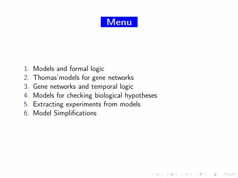
Menu
1. Models and formal logic2. Thomas’models for gene networks3. Gene networks and temporal logic4. Models for checking biological hypotheses5. Extracting experiments from models6. Model Simplifications
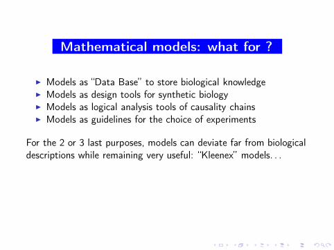
Mathematical models: what for ?
◮ Models as “Data Base” to store biological knowledge◮ Models as design tools for synthetic biology◮ Models as logical analysis tools of causality chains◮ Models as guidelines for the choice of experiments
For the 2 or 3 last purposes, models can deviate far from biologicaldescriptions while remaining very useful: “Kleenex” models. . .
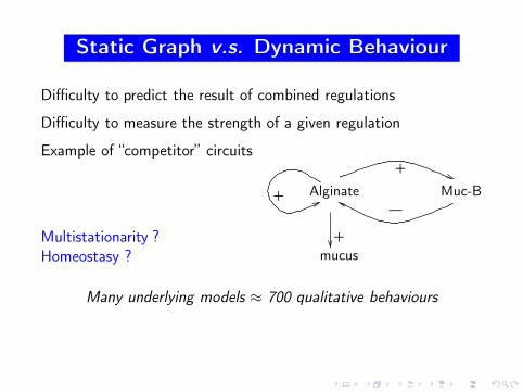
Static Graph v.s. Dynamic Behaviour
Difficulty to predict the result of combined regulations
Difficulty to measure the strength of a given regulation
Example of “competitor” circuits
Multistationarity ?Homeostasy ?
—
+
+
mucus
+ Alginate Muc-B
Many underlying models ≈ 700 qualitative behaviours
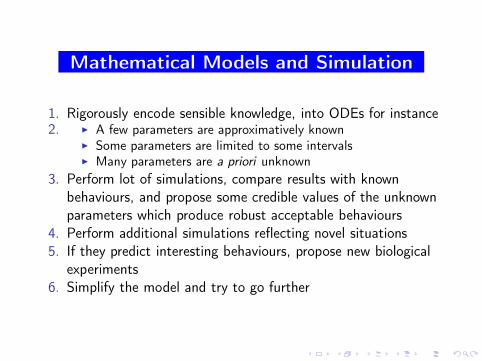
Mathematical Models and Simulation
1. Rigorously encode sensible knowledge, into ODEs for instance2. ◮ A few parameters are approximatively known
◮ Some parameters are limited to some intervals◮ Many parameters are a priori unknown
3. Perform lot of simulations, compare results with knownbehaviours, and propose some credible values of the unknownparameters which produce robust acceptable behaviours
4. Perform additional simulations reflecting novel situations5. If they predict interesting behaviours, propose new biological
experiments6. Simplify the model and try to go further
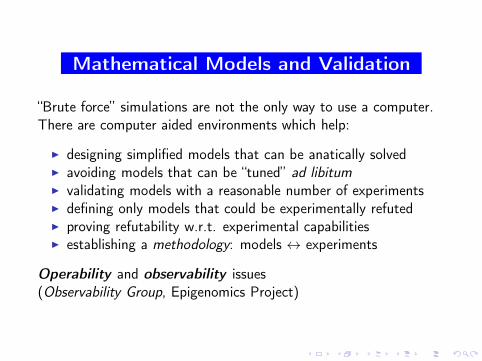
Mathematical Models and Validation
“Brute force” simulations are not the only way to use a computer.There are computer aided environments which help:
◮ designing simplified models that can be anatically solved◮ avoiding models that can be “tuned” ad libitum◮ validating models with a reasonable number of experiments◮ defining only models that could be experimentally refuted◮ proving refutability w.r.t. experimental capabilities◮ establishing a methodology: models ↔ experiments
Operability and observability issues(Observability Group, Epigenomics Project)
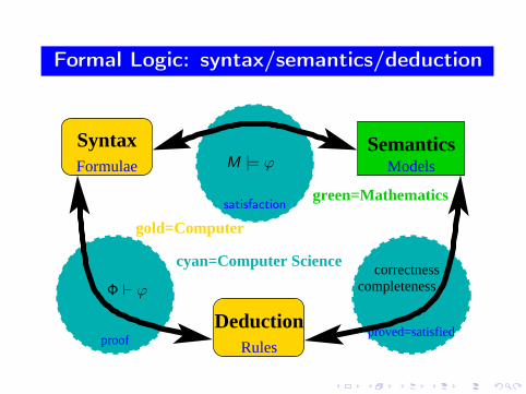
Formal Logic: syntax/semantics/deduction
gold=Computer
green=Mathematics
correctness
Rulesproof
SemanticsModels
Syntax
Deductionproved=satisfied
completeness
Formulae
cyan=Computer Science
M |= ϕ
Φ ⊢ ϕ
satisfaction
Menu
1. Models and formal logic2. Thomas’models for gene networks3. Gene networks and temporal logic4. Models for checking biological hypotheses5. Extracting experiments from models6. Model Simplifications
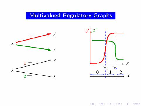
Multivalued Regulatory Graphs
x
x
y
z
y
z2
1
—
—
+
+ x
z’
x
y’
τ20 1 2
τ1
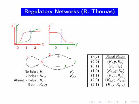
Regulatory Networks (R. Thomas)
y0 1
x′
x1 20
x′y′
Ky
12
—
x y
+
1
No help : Kx
x helps : Kx,x Ky ,x
Absent y helps : Kx,y
Both : Kx,xy
+
(x,y) Focal Point
(0,0) (Kx,y ,Ky )(0,1) (Kx ,Ky )(1,0) (Kx,xy ,Ky )(1,1) (Kx,x ,Ky )(2,0) (Kx,xy ,Ky ,x)(2,1) (Kx,x ,Ky ,x)
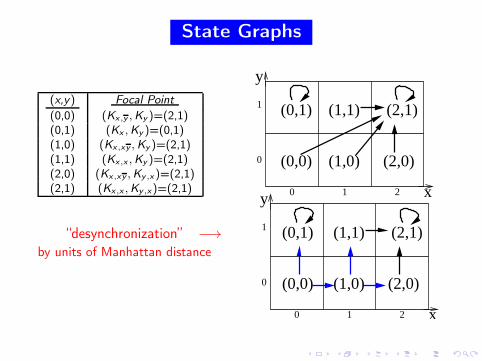
State Graphs
(x,y) Focal Point
(0,0) (Kx,y ,Ky )=(2,1)(0,1) (Kx ,Ky )=(0,1)(1,0) (Kx,xy ,Ky )=(2,1)(1,1) (Kx,x ,Ky )=(2,1)(2,0) (Kx,xy ,Ky ,x )=(2,1)(2,1) (Kx,x ,Ky ,x)=(2,1)
y
x
0
1 (1,1)(0,1)
(0,0) (1,0) (2,0)
(2,1)
0 1 2
“desynchronization” −→by units of Manhattan distance
y
x
0
1 (1,1)
(1,0) (2,0)
(2,1)
(0,0)
(0,1)
0 1 2

Do it by yourselves !
Example on paper sheets. . .
Menu
1. Models and formal logic2. Thomas’models for gene networks3. Gene networks and temporal logic4. Models for checking biological hypotheses5. Extracting experiments from models6. Model Simplifications
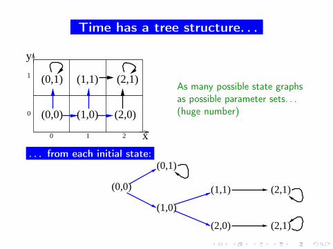
Time has a tree structure. . .
y
x
0
1 (1,1)
(1,0) (2,0)
(2,1)
(0,0)
(0,1)
0 1 2
As many possible state graphsas possible parameter sets. . .(huge number)
. . . from each initial state:
(2,1)
(2,1)(1,1)
(2,0)
(1,0)
(0,1)
(0,0)
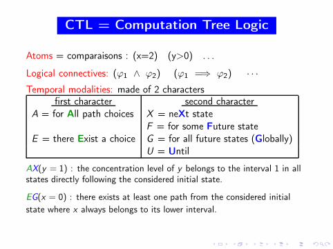
CTL = Computation Tree Logic
Atoms = comparaisons : (x=2) (y>0) . . .
Logical connectives: (ϕ1 ∧ ϕ2) (ϕ1 =⇒ ϕ2) · · ·
Temporal modalities: made of 2 charactersfirst character second character
A = for All path choices X = neXt stateF = for some Future state
E = there Exist a choice G = for all future states (Globally)U = Until
AX(y = 1) : the concentration level of y belongs to the interval 1 in allstates directly following the considered initial state.
EG(x = 0) : there exists at least one path from the considered initial
state where x always belongs to its lower interval.
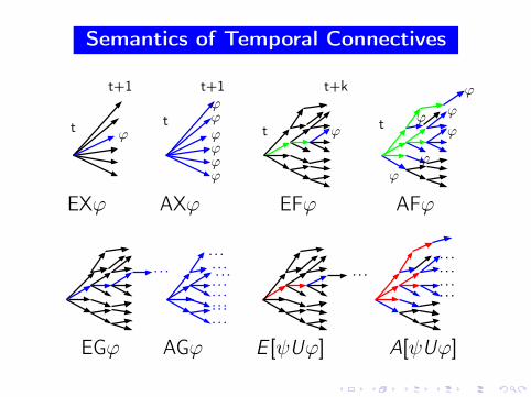
Semantics of Temporal Connectives
t+1
ϕ
AXϕ
ϕϕ
ϕϕϕ
ϕt+1
ϕ
EXϕ
t tt ϕ
t
t+k
EFϕ
........................
AGϕ
...
EGϕ
...
AFϕ
ϕ
ϕ
ϕ
ϕϕ
E [ψUϕ] A[ψUϕ]
...
...
...
...
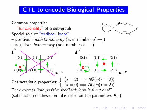
CTL to encode Biological Properties
Common properties:“functionality” of a sub-graph
Special role of “feedback loops”—
y+
+ x1 2
1
– positive: multistationnarity (even number of — )– negative: homeostasy (odd number of — )
y
x
y
x
(0,1) (2,1)(1,1)
(2,0)(0,0) (1,0) (0,0) (1,0) (2,0)
(2,1)(1,1)(0,1)
Characteristic properties:
{
(x = 2) =⇒ AG (¬(x = 0))(x = 0) =⇒ AG (¬(x = 2))
They express “the positive feedback loop is functional”(satisfaction of these formulas relies on the parameters K...)
Model Checking
Efficiently computes all the states of a state graph which satisfy agiven formula: { η | M |=η ϕ }.
Efficiently select the models which globally satisfy a given formula.
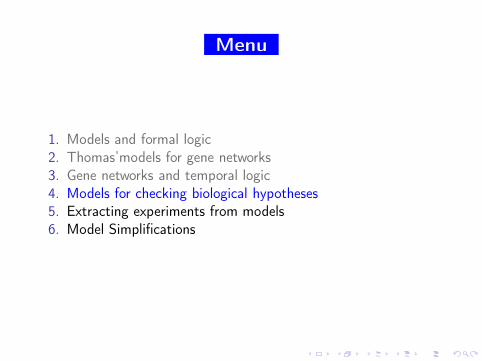
Menu
1. Models and formal logic2. Thomas’models for gene networks3. Gene networks and temporal logic4. Models for checking biological hypotheses5. Extracting experiments from models6. Model Simplifications
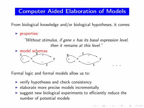
Computer Aided Elaboration of Models
From biological knowledge and/or biological hypotheses, it comes:
◮ properties:
“Without stimulus, if gene x has its basal expression level,then it remains at this level.”
◮ model schemas:
—
y+
+ x1 2
1—
x y+
+
21
1 . . .
Formal logic and formal models allow us to:
◮ verify hypotheses and check consistency◮ elaborate more precise models incrementally◮ suggest new biological experiments to efficiently reduce the
number of potential models
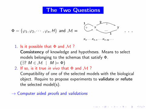
The Two Questions
Φ = {ϕ1, ϕ2, · · · , ϕn,H} and M = —
y+
+ x1 2
1
Kx · · ·Kx,x · · ·Kx,xy · · ·
. . .
1. Is it possible that Φ and M ?Consistency of knowledge and hypotheses. Means to selectmodels belonging to the schemas that satisfy Φ.(∃? M ∈ M | M |= Φ)
2. If so, is it true in vivo that Φ and M ?Compatibility of one of the selected models with the biologicalobject. Require to propose experiments to validate or refute
the selected model(s).
→ Computer aided proofs and validations
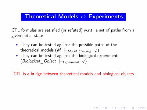
Theoretical Models ↔ Experiments
CTL formulas are satisfied (or refuted) w.r.t. a set of paths from agiven initial state
◮ They can be tested against the possible paths of thetheoretical models (M |=Model Checking ϕ)
◮ They can be tested against the biological experiments(Biological_Object |=Experiment ϕ)
CTL is a bridge between theoretical models and biological objects
Menu
1. Models and formal logic2. Thomas’models for gene networks3. Gene networks and temporal logic4. Models for checking biological hypotheses5. Extracting experiments from models6. Model Simplifications
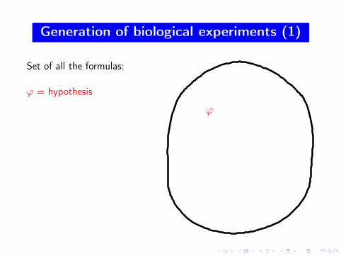
Generation of biological experiments (1)
Set of all the formulas:
ϕ = hypothesis
ϕ
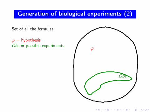
Generation of biological experiments (2)
Set of all the formulas:
ϕ = hypothesisObs = possible experiments
Obs
ϕ
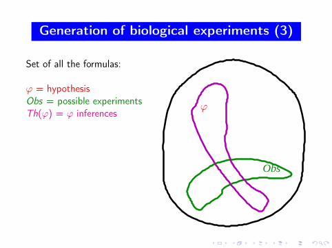
Generation of biological experiments (3)
Set of all the formulas:
ϕ = hypothesisObs = possible experimentsTh(ϕ) = ϕ inferences
Obs
ϕ
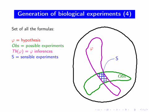
Generation of biological experiments (4)
Set of all the formulas:
ϕ = hypothesisObs = possible experimentsTh(ϕ) = ϕ inferencesS = sensible experiments
Obs
ϕ
S
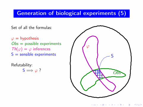
Generation of biological experiments (5)
Set of all the formulas:
ϕ = hypothesisObs = possible experimentsTh(ϕ) = ϕ inferencesS = sensible experiments
Refutability:S =⇒ ϕ ? Obs
ϕ
S
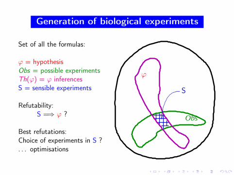
Generation of biological experiments
Set of all the formulas:
ϕ = hypothesisObs = possible experimentsTh(ϕ) = ϕ inferencesS = sensible experiments
Refutability:S =⇒ ϕ ?
Best refutations:Choice of experiments in S ?. . . optimisations
Obs
ϕ
S
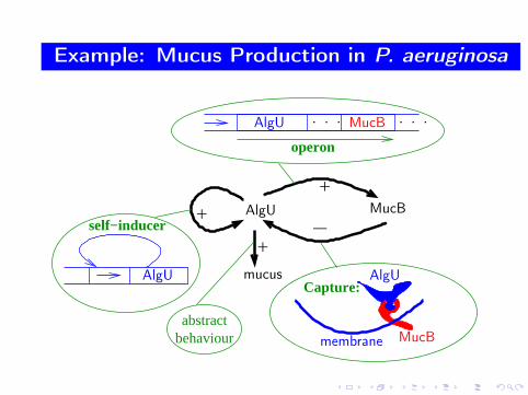
Example: Mucus Production in P. aeruginosa
Capture:
operon
self−inducer
abstractbehaviour
—
+
AlgU MucB
mucus
+
+
membrane
AlgU
MucB
AlgU
AlgU
MucB. . . . . .
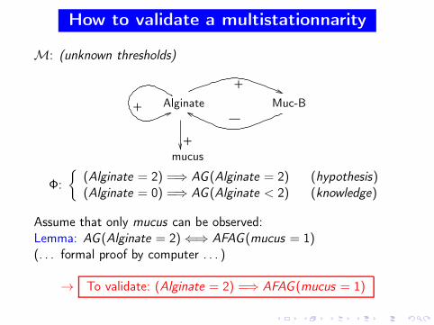
How to validate a multistationnarity
M: (unknown thresholds)
—
+
+
mucus
+ Alginate Muc-B
Φ:
{
(Alginate = 2) =⇒ AG (Alginate = 2) (hypothesis)(Alginate = 0) =⇒ AG (Alginate < 2) (knowledge)
Assume that only mucus can be observed:Lemma: AG (Alginate = 2) ⇐⇒ AFAG (mucus = 1)(. . . formal proof by computer . . . )
→ To validate: (Alginate = 2) =⇒ AFAG (mucus = 1)
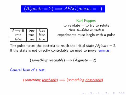
(Alginate = 2) =⇒ AFAG (mucus = 1)
A =⇒ B true false
true true falsefalse true true
Karl Popper:to validate = to try to refute
thus A=false is uselessexperiments must begin with a pulse
The pulse forces the bacteria to reach the initial state Alginate = 2.If the state is not directly controlable we need to prove lemmas:
(something reachable) =⇒ (Alginate = 2)
General form of a test:
(something reachable) =⇒ (something observable)

Menu
1. Models and formal logic2. Thomas’models for gene networks3. Gene networks and temporal logic4. Models for checking biological hypotheses5. Extracting experiments from models6. Model Simplifications
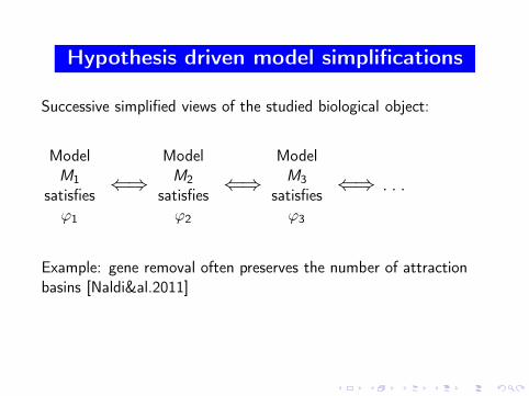
Hypothesis driven model simplifications
Successive simplified views of the studied biological object:
ModelM1
satisfiesϕ1
⇐⇒
ModelM2
satisfiesϕ2
⇐⇒
ModelM3
satisfiesϕ3
⇐⇒ . . .
Example: gene removal often preserves the number of attractionbasins [Naldi&al.2011]
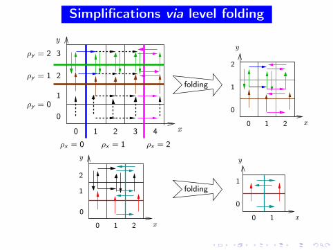
Simplifications via level folding
folding
0
0 1 2 x
1
2
y
folding1
0
0 1
y
x
0
0 1 2 x
2
1
3
3 4
ρx = 0 ρx = 2ρx = 1
ρy = 0
ρy = 1
ρy = 2
2
1
0
0 1 2 x
y
y
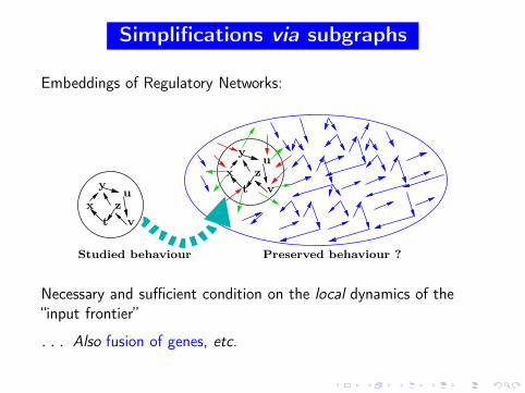
Simplifications via subgraphs
Embeddings of Regulatory Networks:
x
y
z
t
u
v
x
y
z
t
u
v
Preserved behaviour ?Studied behaviour
Necessary and sufficient condition on the local dynamics of the“input frontier”
. . . Also fusion of genes, etc.
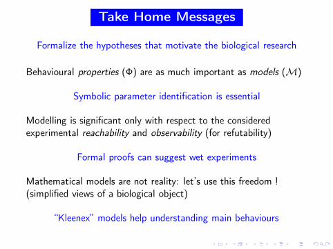
Take Home Messages
Formalize the hypotheses that motivate the biological research
Behavioural properties (Φ) are as much important as models (M)
Symbolic parameter identification is essential
Modelling is significant only with respect to the consideredexperimental reachability and observability (for refutability)
Formal proofs can suggest wet experiments
Mathematical models are not reality: let’s use this freedom !(simplified views of a biological object)
“Kleenex” models help understanding main behaviours