www.iap.uni-jena.de

Metrology and Sensing

Lecture 7: Wavefront sensors

2017-11-30

Herbert Gross

Winter term 2017

2

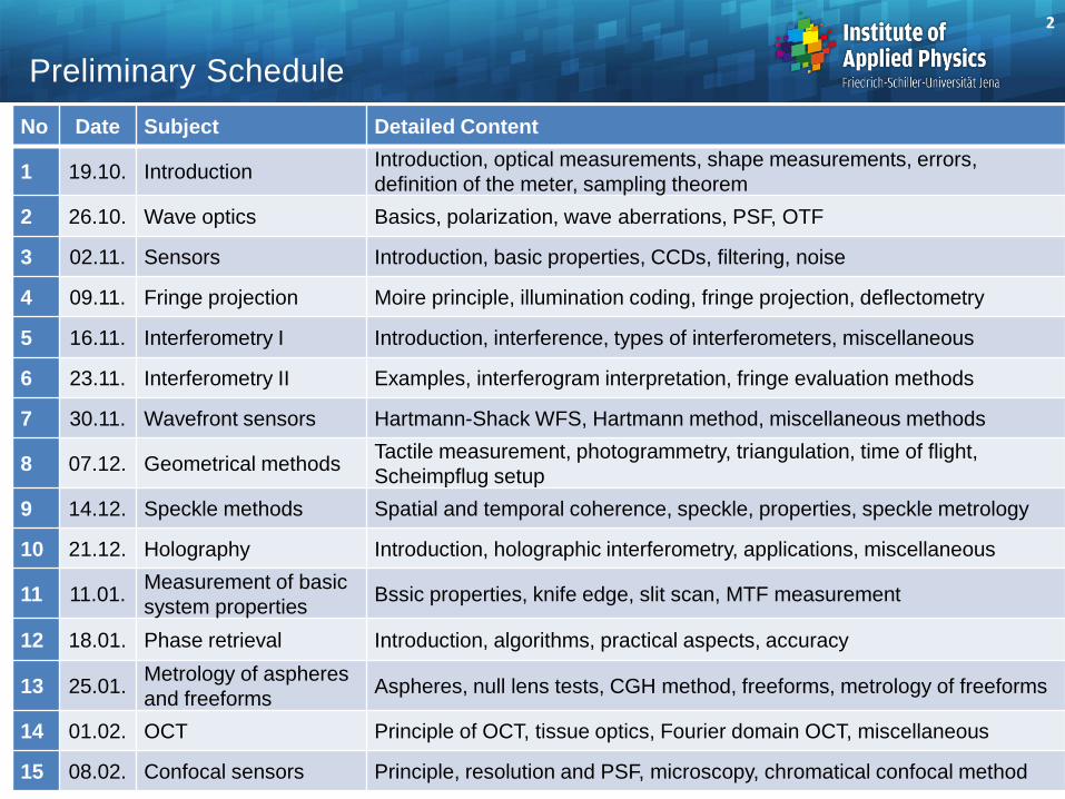
Preliminary Schedule

No Date Subject Detailed Content

1 19.10. Introduction Introduction, optical measurements, shape measurements, errors,

definition of the meter, sampling theorem

2 26.10. Wave optics Basics, polarization, wave aberrations, PSF, OTF

3 02.11. Sensors Introduction, basic properties, CCDs, filtering, noise

4 09.11. Fringe projection Moire principle, illumination coding, fringe projection, deflectometry

5 16.11. Interferometry I Introduction, interference, types of interferometers, miscellaneous

6 23.11. Interferometry II Examples, interferogram interpretation, fringe evaluation methods

7 30.11. Wavefront sensors Hartmann-Shack WFS, Hartmann method, miscellaneous methods

8 07.12. Geometrical methods Tactile measurement, photogrammetry, triangulation, time of flight,

Scheimpflug setup

9 14.12. Speckle methods Spatial and temporal coherence, speckle, properties, speckle metrology

10 21.12. Holography Introduction, holographic interferometry, applications, miscellaneous

11 11.01. Measurement of basic

system properties Bssic properties, knife edge, slit scan, MTF measurement

12 18.01. Phase retrieval Introduction, algorithms, practical aspects, accuracy

13 25.01. Metrology of aspheres

and freeforms Aspheres, null lens tests, CGH method, freeforms, metrology of freeforms

14 01.02. OCT Principle of OCT, tissue optics, Fourier domain OCT, miscellaneous

15 08.02. Confocal sensors Principle, resolution and PSF, microscopy, chromatical confocal method

3

Content

Hartmann-Shack WFS

Hartmann method

Miscellaneous methods

4

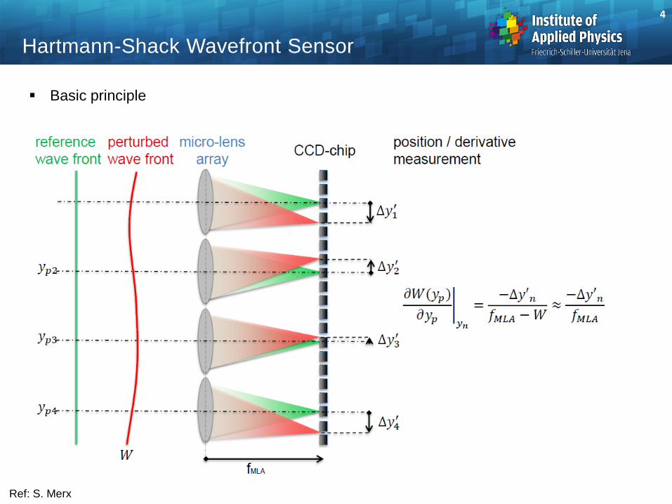
Hartmann-Shack Wavefront Sensor

Basic principle

Ref: S. Merx

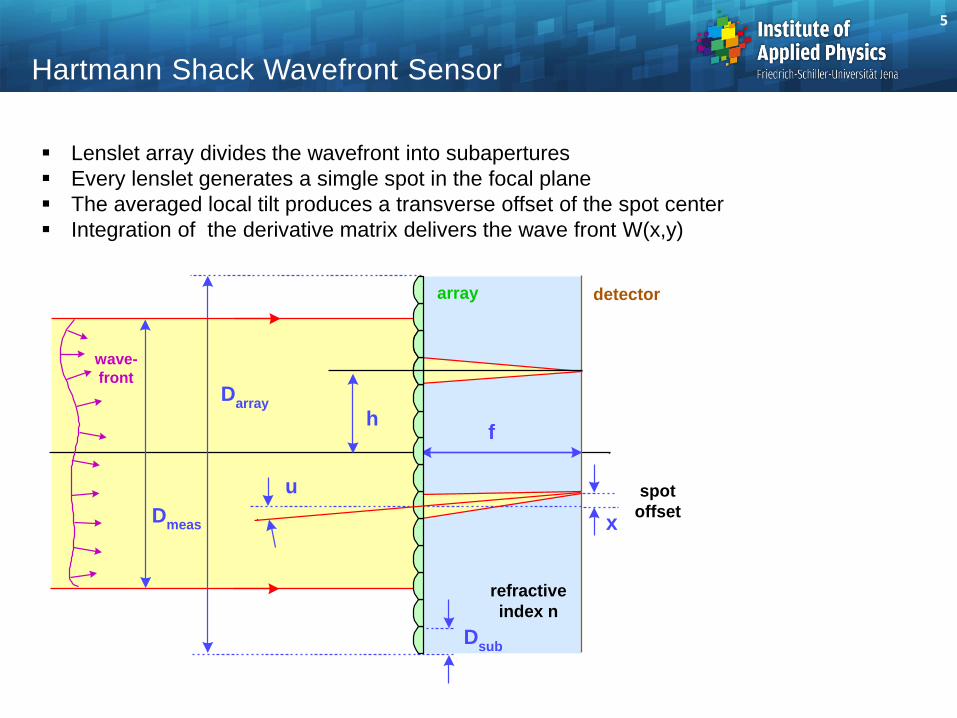
Hartmann Shack Wavefront Sensor

detector

xDmeas

u

hf

array

spot

offset

Darray

Dsub

refractive

index n

wave-

front

Lenslet array divides the wavefront into subapertures

Every lenslet generates a simgle spot in the focal plane

The averaged local tilt produces a transverse offset of the spot center

Integration of the derivative matrix delivers the wave front W(x,y)

5

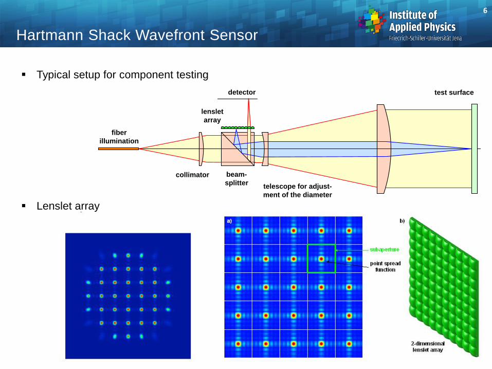
Typical setup for component testing

Lenslet array

Hartmann Shack Wavefront Sensor

6

test surface

telescope for adjust-

ment of the diameter

detector

collimator

lenslet

array

fiber

illumination

beam-

splitter

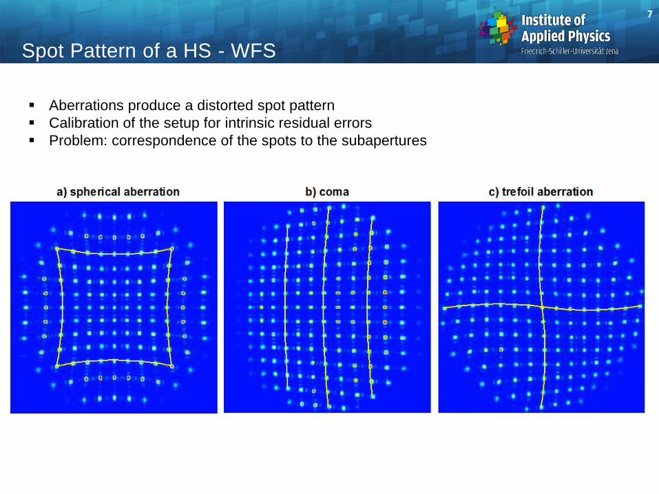
Spot Pattern of a HS - WFS

Aberrations produce a distorted spot pattern

Calibration of the setup for intrinsic residual errors

Problem: correspondence of the spots to the subapertures

7

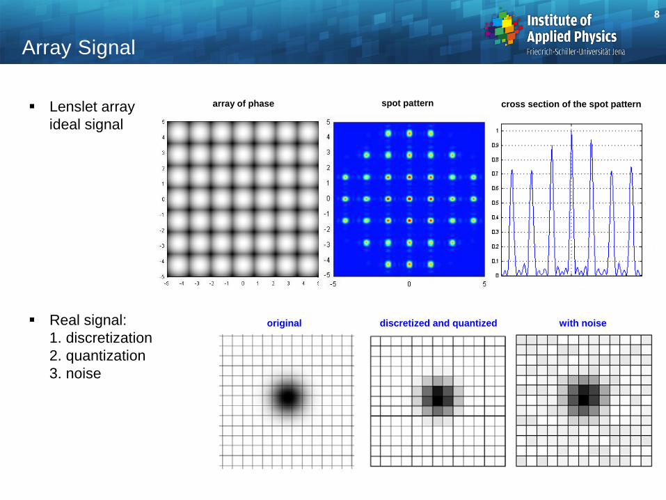
Array Signal

array of phase spot pattern cross section of the spot pattern

original discretized and quantized with noise

Lenslet array

ideal signal

Real signal:

1. discretization

2. quantization

3. noise

8

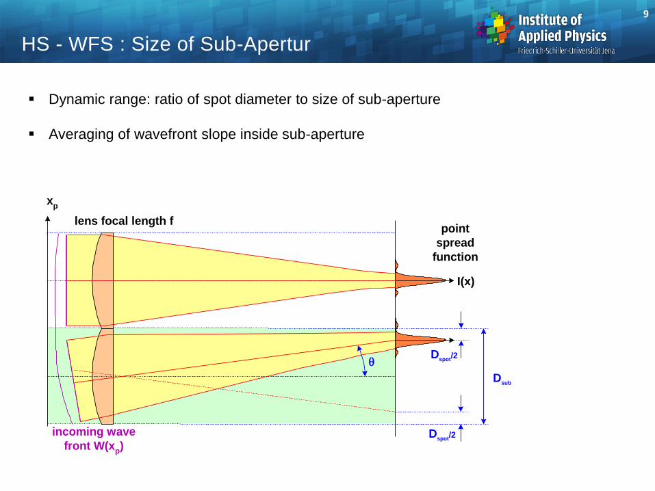
Dynamic range: ratio of spot diameter to size of sub-aperture

Averaging of wavefront slope inside sub-aperture

HS - WFS : Size of Sub-Apertur

I(x)

xp

lens focal length f

Dsub

Dspot

/2

point

spread

function

Dspot

/2incoming wave

front W(xp)

9

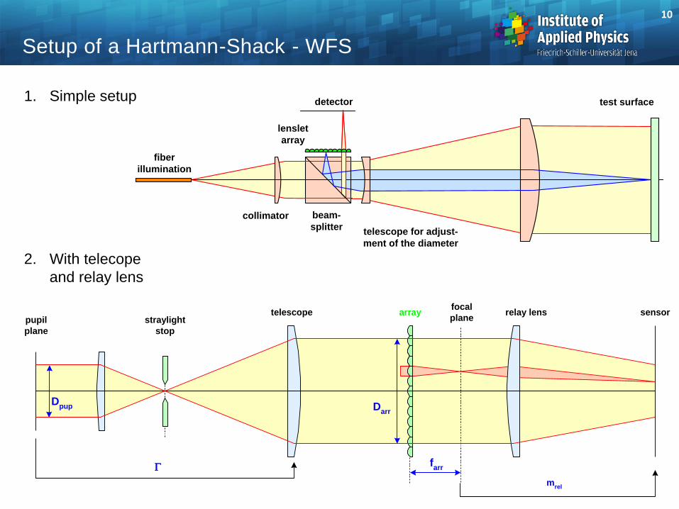
Setup of a Hartmann-Shack - WFS

pupil

plane

straylight

stop

Dpup D

arr

sensor

farr

array relay lenstelescopefocal

plane

mrel

1. Simple setup

2. With telecope

and relay lens

10

test surface

telescope for adjust-

ment of the diameter

detector

collimator

lenslet

array

fiber

illumination

beam-

splitter

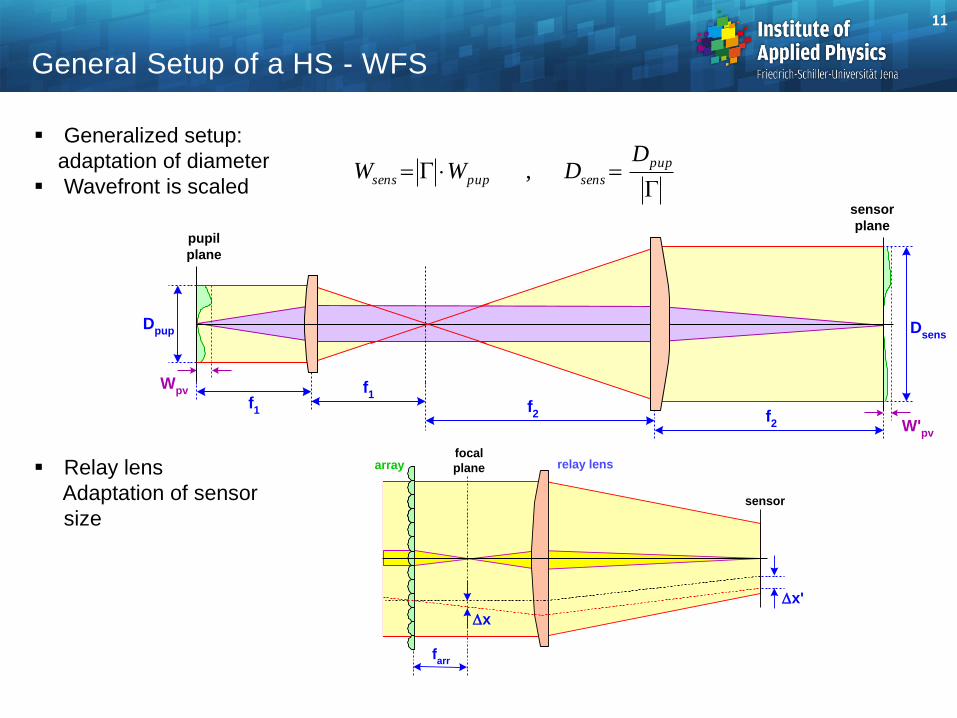
General Setup of a HS - WFS

Generalized setup:

adaptation of diameter

Wavefront is scaled

Relay lens

Adaptation of sensor

size

f2

f1

f1

f2

pupil

plane

sensor

plane

Dpup D

sens

Wpv

W'pv

pup

senspupsens

DDWW ,

focal

plane

x'

farr

array relay lens

x

sensor

11

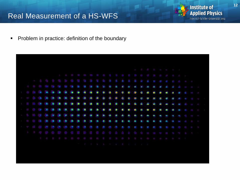
Real Measurement of a HS-WFS

Problem in practice: definition of the boundary

12

Real Measurement of a HS-WFS

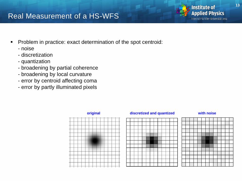
Problem in practice: exact determination of the spot centroid:

- noise

- discretization

- quantization

- broadening by partial coherence

- broadening by local curvature

- error by centroid affecting coma

- error by partly illuminated pixels

original discretized and quantized with noise

13

Parametrization of a HS-WFS

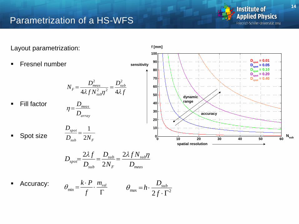
Layout parametrization:

Fresnel number

Fill factor

Spot size

Accuracy:

f [mm]

Nsub

0 10 20 30 40 50 600

10

20

30

40

50

60

70

80

90

100

Dspot

= 0.01

Dspot

= 0.05

Dspot

= 0.10

Dspot

= 0.20

Dspot

= 0.40

sensitivity

spatial resolution

accuracy

dynamic

range

f

D

Nf

DN sub

sub

measF

44

2

22

2

array

meas

D

D

meas

sub

F

sub

sub

spotD

Nf

N

D

D

fD

2

2

2

Fsub

spot

ND

D

2

1

relm

f

Pkmin

2max2

f

Dh sub

14

Parametrization of a HS-WFS

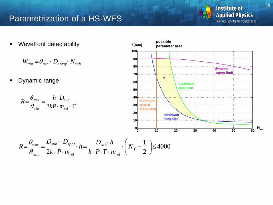
Wavefront detectability

Dynamic range

f [mm]

Nsub

0 10 20 30 40 50 600

10

20

30

40

50

60

70

80

90

100

minimum

spot size

maximum

spot size

minimum

spatial

resolution

possible

parameter area

dynamic

range limit

rel

sub

mkP

DhR

2min

max

subarray NDW minmin

40002

1

2min

max

f

rel

sub

rel

spotsubN

mPk

hDh

mPk

DDR

15

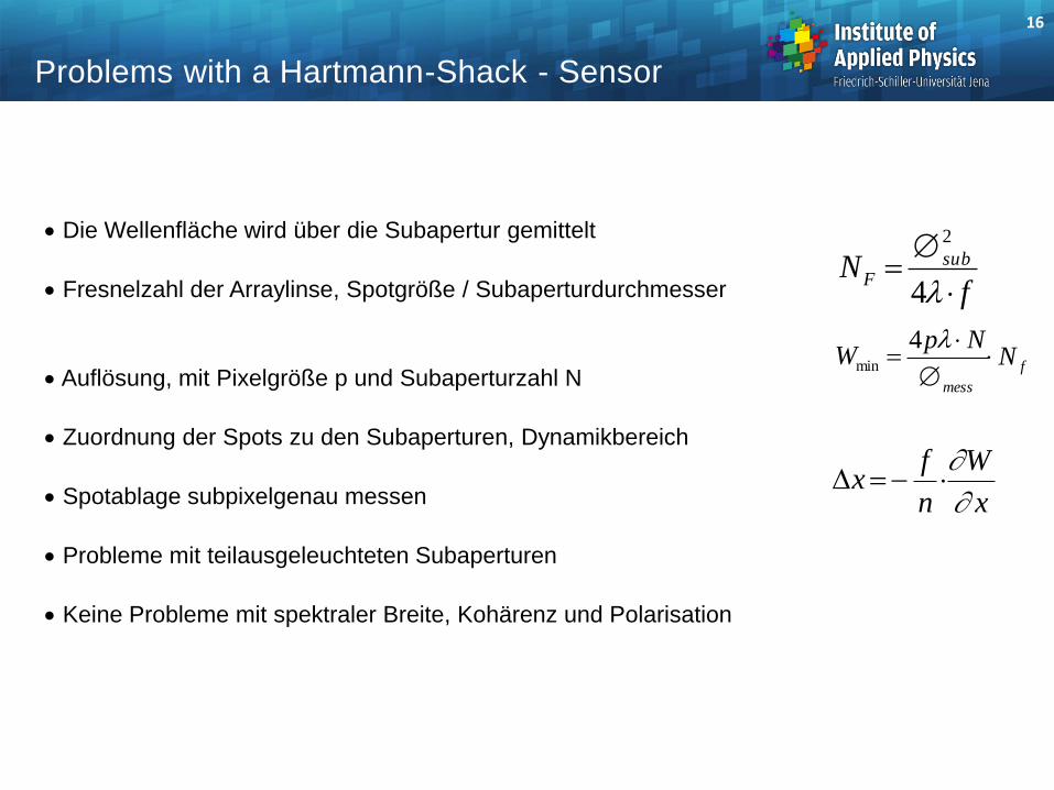
Die Wellenfläche wird über die Subapertur gemittelt

Fresnelzahl der Arraylinse, Spotgröße / Subaperturdurchmesser

Auflösung, mit Pixelgröße p und Subaperturzahl N

Zuordnung der Spots zu den Subaperturen, Dynamikbereich

Spotablage subpixelgenau messen

Probleme mit teilausgeleuchteten Subaperturen

Keine Probleme mit spektraler Breite, Kohärenz und Polarisation

x

W

n

fx

fN sub

F

4

2

f

mess

NNp

W

4min

Problems with a Hartmann-Shack - Sensor

16

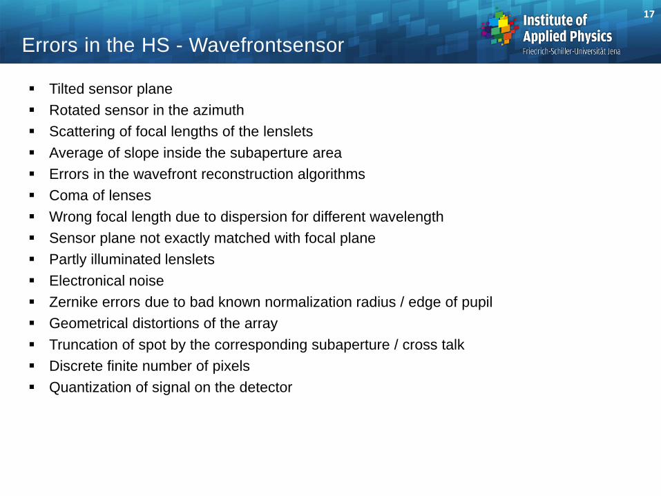
Tilted sensor plane

Rotated sensor in the azimuth

Scattering of focal lengths of the lenslets

Average of slope inside the subaperture area

Errors in the wavefront reconstruction algorithms

Coma of lenses

Wrong focal length due to dispersion for different wavelength

Sensor plane not exactly matched with focal plane

Partly illuminated lenslets

Electronical noise

Zernike errors due to bad known normalization radius / edge of pupil

Geometrical distortions of the array

Truncation of spot by the corresponding subaperture / cross talk

Discrete finite number of pixels

Quantization of signal on the detector

Errors in the HS - Wavefrontsensor

17

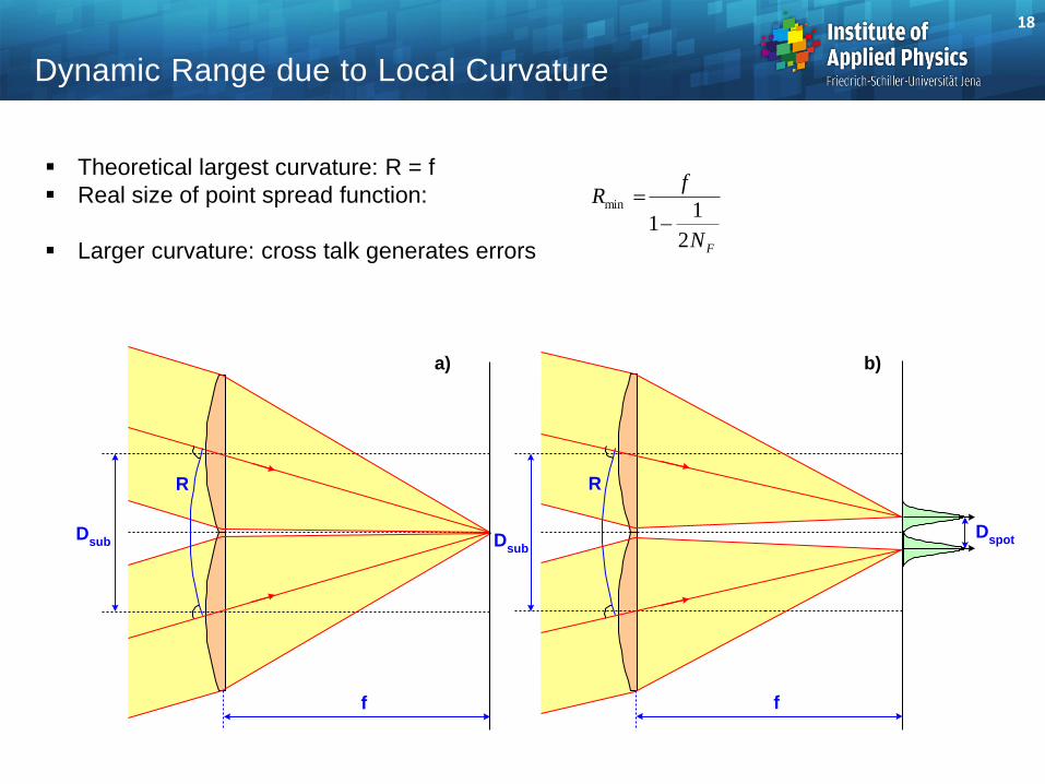
Theoretical largest curvature: R = f

Real size of point spread function:

Larger curvature: cross talk generates errors

Dynamic Range due to Local Curvature

R

f

Dsub

R

f

Dsub

Dspot

a) b)

FN

fR

2

11

min

18

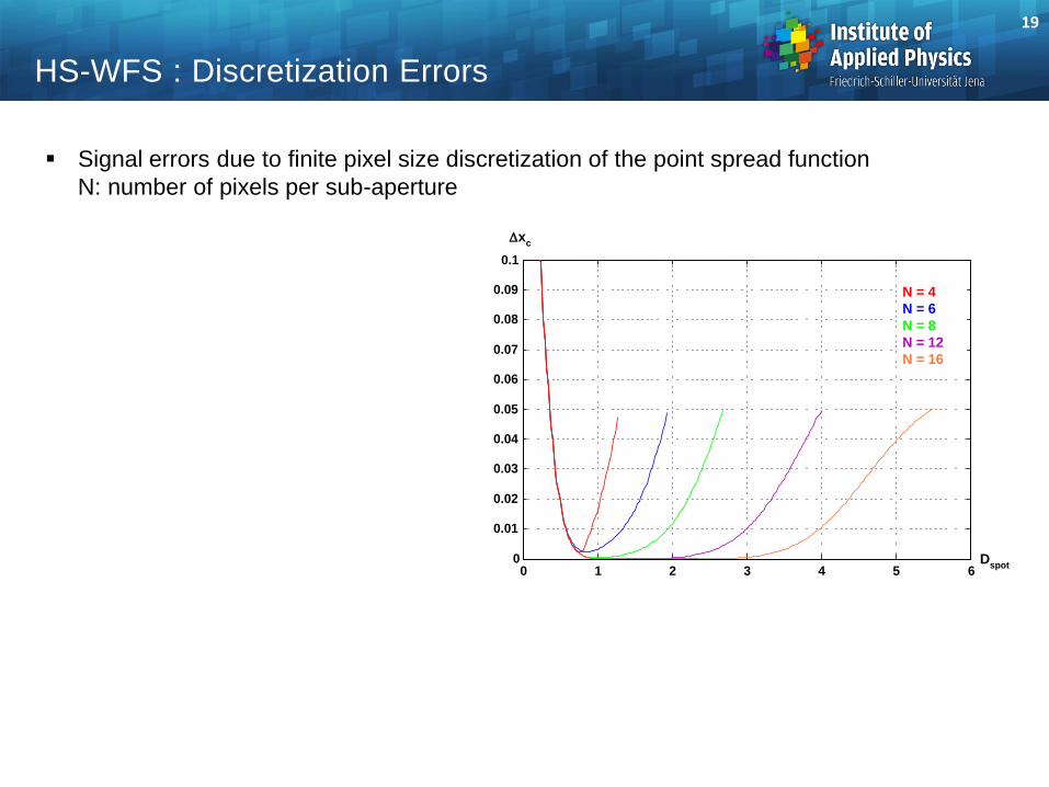
HS-WFS : Discretization Errors

Signal errors due to finite pixel size discretization of the point spread function

N: number of pixels per sub-aperture

N = 4

N = 6

N = 8

N = 12

N = 16

xc

Dspot

0

0.01

0.02

0.03

0.04

0.05

0.06

0.07

0.08

0.09

0.1

0 1 2 3 4 5 6

19

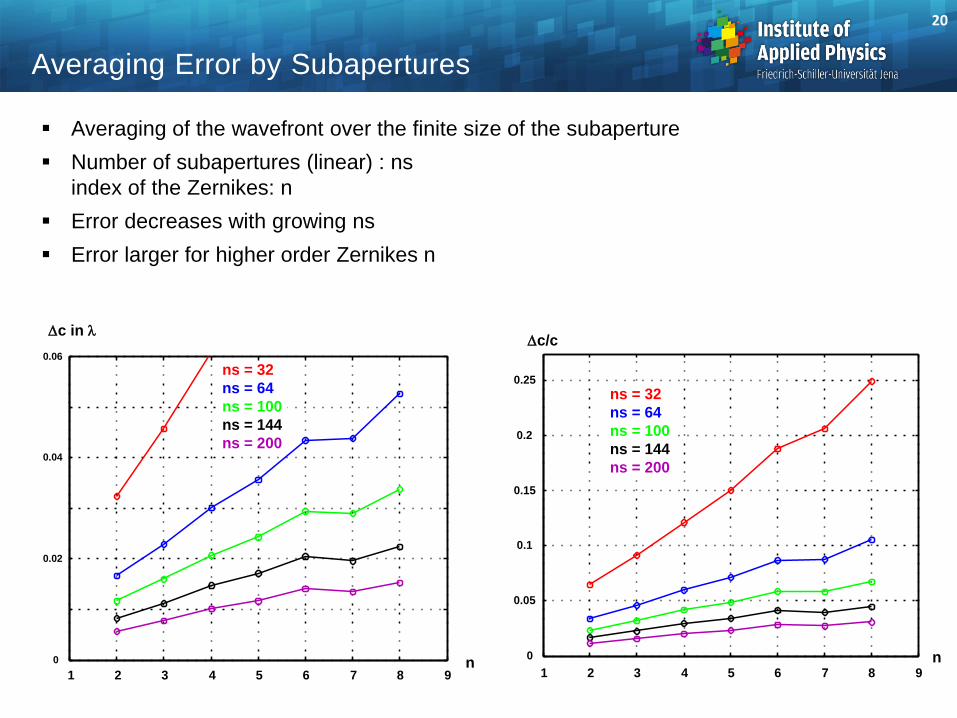
Averaging of the wavefront over the finite size of the subaperture

Number of subapertures (linear) : ns

index of the Zernikes: n

Error decreases with growing ns

Error larger for higher order Zernikes n

Averaging Error by Subapertures

n

c/c

1 2 3 4 5 6 7 8 9

Wrms Wpv

n

c in

1 2 3 4 5 6 7 8 9

0

0.02

0.04

0.06

ns = 32

ns = 64

ns = 100

ns = 144

ns = 200

0

0.05

0.1

0.15

0.2

0.25

ns = 32

ns = 64

ns = 100

ns = 144

ns = 200

nn1 2 3 4 5 6 7 8 9

0

0.005

0.01

0.015

0.02

0.025

0.03

ns = 32

ns = 64

ns = 100

ns = 144

ns = 200

1 2 3 4 5 6 7 8 90

0.05

0.1

0.15

0.2

0.25

0.3ns = 32

ns = 64

ns = 100

ns = 144

ns = 200

20

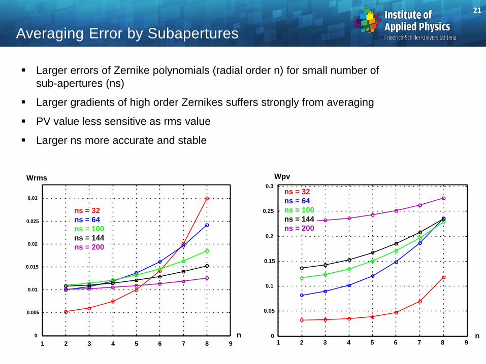
Larger errors of Zernike polynomials (radial order n) for small number of

sub-apertures (ns)

Larger gradients of high order Zernikes suffers strongly from averaging

PV value less sensitive as rms value

Larger ns more accurate and stable

Averaging Error by Subapertures

n

c/c

1 2 3 4 5 6 7 8 9

Wrms Wpv

n

c in

1 2 3 4 5 6 7 8 9

0

0.02

0.04

0.06

ns = 32

ns = 64

ns = 100

ns = 144

ns = 200

0

0.05

0.1

0.15

0.2

0.25

ns = 32

ns = 64

ns = 100

ns = 144

ns = 200

nn1 2 3 4 5 6 7 8 9

0

0.005

0.01

0.015

0.02

0.025

0.03

ns = 32

ns = 64

ns = 100

ns = 144

ns = 200

1 2 3 4 5 6 7 8 90

0.05

0.1

0.15

0.2

0.25

0.3ns = 32

ns = 64

ns = 100

ns = 144

ns = 200

21

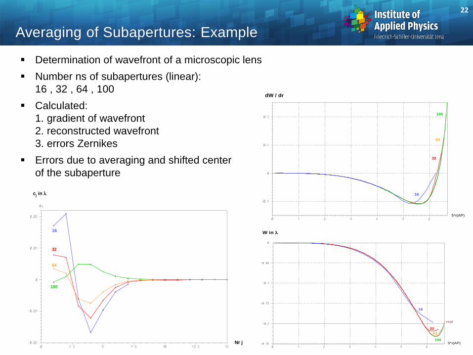
Determination of wavefront of a microscopic lens

Number ns of subapertures (linear):

16 , 32 , 64 , 100

Calculated:

1. gradient of wavefront

2. reconstructed wavefront

3. errors Zernikes

Errors due to averaging and shifted center

of the subaperture

16

32

64

100

5*r(AP)

dW / dr

W in

16

32

64

100

real

5*r(AP)

cj in

16

32

64

100

Nr j

Averaging of Subapertures: Example

22

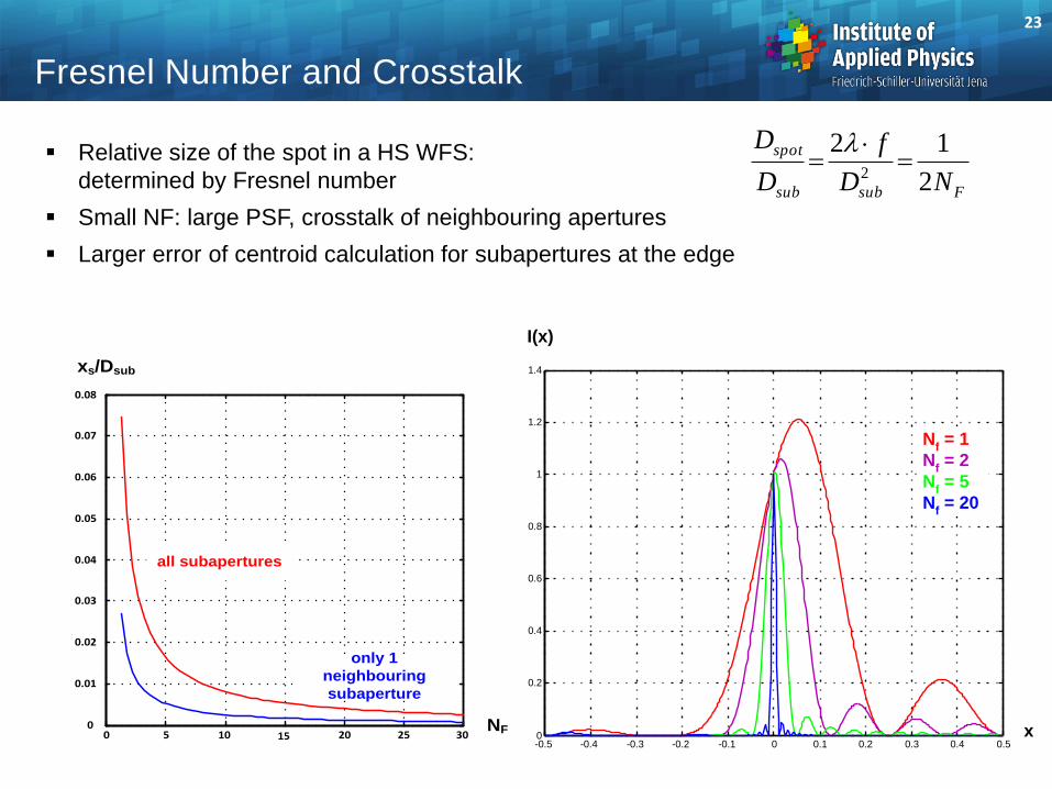
Relative size of the spot in a HS WFS:

determined by Fresnel number

Small NF: large PSF, crosstalk of neighbouring apertures

Larger error of centroid calculation for subapertures at the edge

Fresnel Number and Crosstalk

Fsubsub

spot

ND

f

D

D

2

122

I(x)

-0.5 -0.4 -0.3 -0.2 -0.1 0 0.1 0.2 0.3 0.4 0.50

0.2

0.4

0.6

0.8

1

1.2

1.4

x

Nf = 1

Nf = 2

Nf = 5

Nf = 20

xs/Dsub

0 5 10 15 20 25 300

0.01

0.02

0.03

0.04

0.05

0.06

0.07

0.08

NF

all subapertures

only 1

neighbouring

subaperture

23

HS-WFS : Partly Illuminated Sub-Apertures

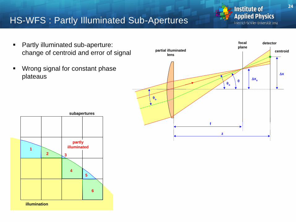
Partly illuminated sub-aperture:

change of centroid and error of signal

Wrong signal for constant phase

plateaus

subapertures

illumination

12 3

45

6

partly

illuminated

focal

plane

f

z

detector

centroidpartial illuminated

lens

xo

x

o

o

24

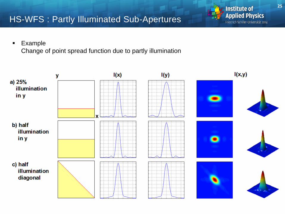
HS-WFS : Partly Illuminated Sub-Apertures

Example

Change of point spread function due to partly illumination

25

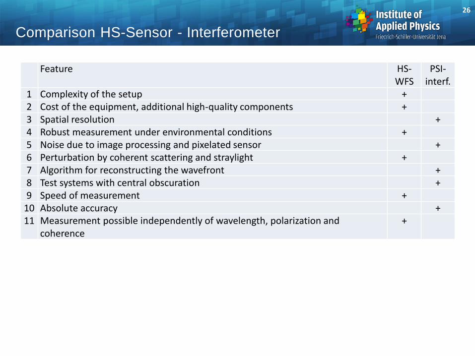
Comparison HS-Sensor - Interferometer

Feature HS-WFS

PSI-interf.

1 Complexity of the setup + 2 Cost of the equipment, additional high-quality components + 3 Spatial resolution +

4 Robust measurement under environmental conditions + 5 Noise due to image processing and pixelated sensor +

6 Perturbation by coherent scattering and straylight + 7 Algorithm for reconstructing the wavefront +

8 Test systems with central obscuration +

9 Speed of measurement + 10 Absolute accuracy +

11 Measurement possible independently of wavelength, polarization and coherence

+

26

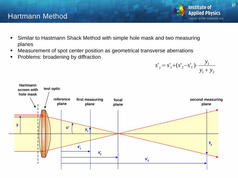
21

1121 )''(''

yy

yssss y

Hartmann Method

Similar to Hastmann Shack Method with simple hole mask and two measuring

planes

Measurement of spot center position as geometrical transverse aberrations

Problems: broadening by diffraction

Hartmann

screen with

hole mask

test optic

y

focal

plane

first measuring

plane

second measuring

plane

reference

plane

s'1

y

2

s'

s'

y1

y2

u'

27

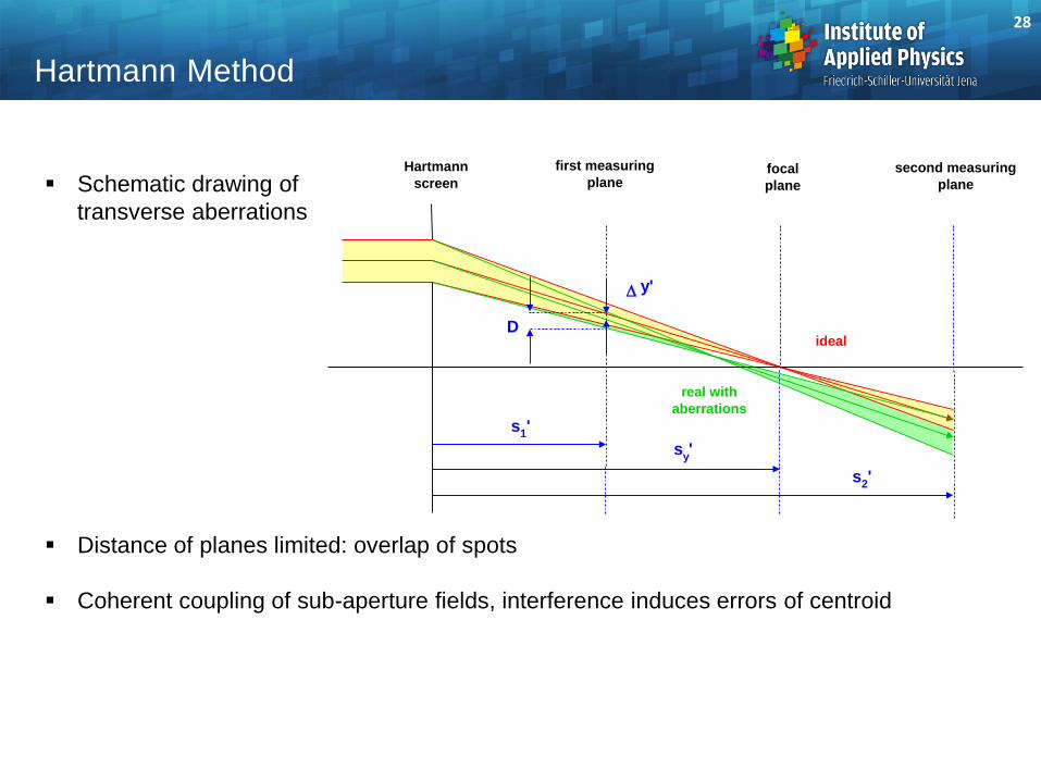
Schematic drawing of

transverse aberrations

Distance of planes limited: overlap of spots

Coherent coupling of sub-aperture fields, interference induces errors of centroid

Hartmann Method

Hartmann

screenfocal

plane

first measuring

planesecond measuring

plane

y'

D

s1'

sy'

s2'

ideal

real with

aberrations

28

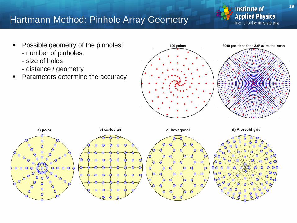
Possible geometry of the pinholes:

- number of pinholes,

- size of holes

- distance / geometry

Parameters determine the accuracy

Hartmann Method: Pinhole Array Geometry

c) hexagonalb) cartesiana) polar d) Albrecht grid

120 points 3000 positions for a 3.6° azimuthal scan

29

Hartmann Method Properties

z-positions critical for large spots diameters

No dependence on spectral range and polarization

Coherence is critical, interference for overlapping pinhole images

Apodization not critical

Averaging gives stable data evaluation

30

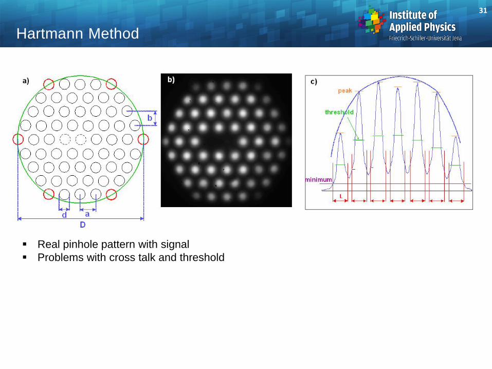
Hartmann Method

Real pinhole pattern with signal

Problems with cross talk and threshold

31

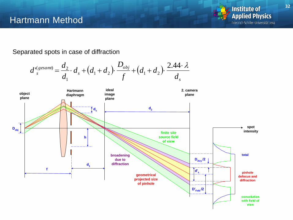
Separated spots in case of diffraction

s

obj

s

gesamt

sd

ddf

Dddd

d

dd

44.2' 2121

1

2)(

Hartmann Method

Hartmann

diaphragm

ideal

image

plane

2. camera

planeobject

plane

geometrical

projected size

of pinhole

finite site

source field

of view

broadening

due to

diffraction

spot

intensity

pinhole

defocus and

diffraction

convolution

with field of

view

total

d1

f

Dobj

d's

DAiry

/2

D'Feld

/2

ds

h

d2

32

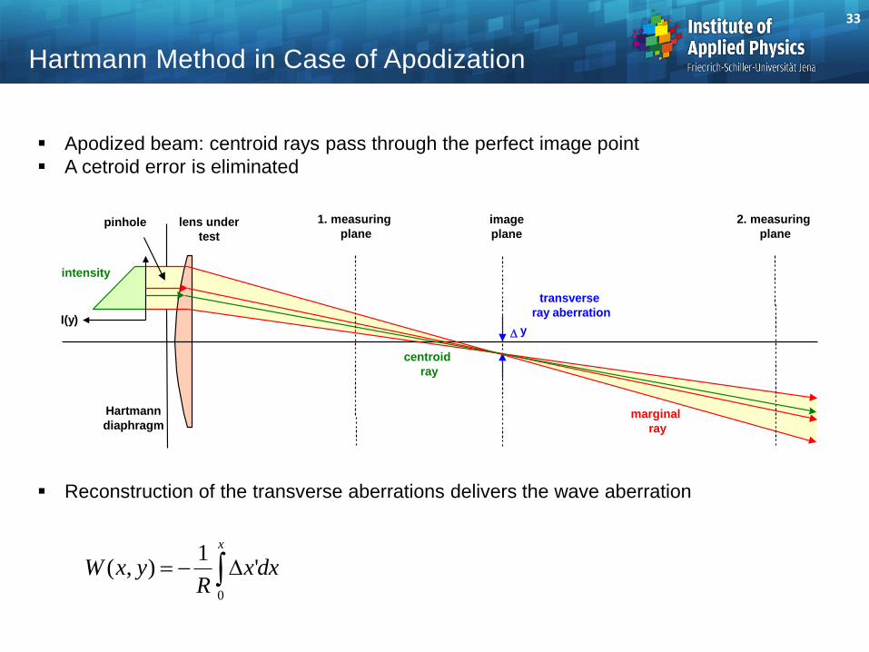
Apodized beam: centroid rays pass through the perfect image point

A cetroid error is eliminated

Reconstruction of the transverse aberrations delivers the wave aberration

x

dxxR

yxW0

'1

),(

Hartmann Method in Case of Apodization

Hartmann

diaphragm

I(y)

image

plane

1. measuring

plane

y

marginal

ray

centroid

ray

transverse

ray aberration

intensity

2. measuring

planepinhole lens under

test

33

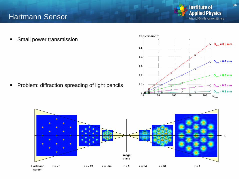
Hartmann Sensor

Small power transmission

Problem: diffraction spreading of light pencils

z

z = 0 z = f/4 z = fz = f/2z = - f z = - f/2 z = - f/4

image

plane

Hartmann

screen

transmission T

0 50 100 150 2000

0.1

0.2

0.3

0.4

0.5

Nsub

Dsub

= 0.5 mm

Dsub

= 0.4 mm

Dsub

= 0.3 mm

Dsub

= 0.2 mm

Dsub

= 0.1 mm

34

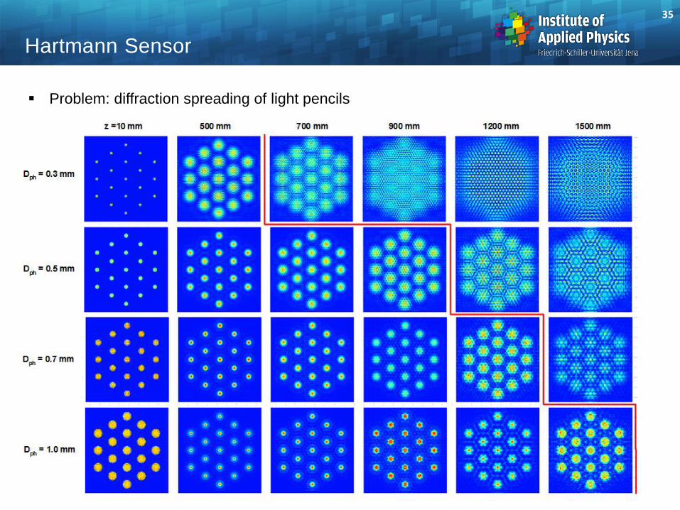
Hartmann Sensor

Problem: diffraction spreading of light pencils

35

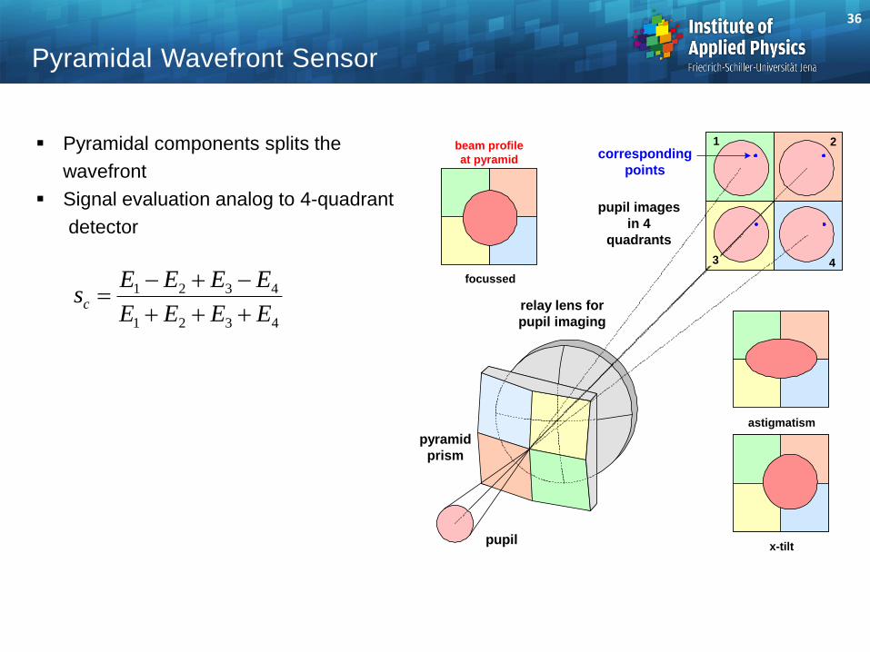
Pyramidal Wavefront Sensor

Pyramidal components splits the

wavefront

Signal evaluation analog to 4-quadrant

detector

pupil

pyramid

prism

pupil images

in 4

quadrants

relay lens for

pupil imaging

astigmatism

x-tilt

focussed

beam profile

at pyramid

1

43

2corresponding

points

4321

4321

EEEE

EEEEsc

36

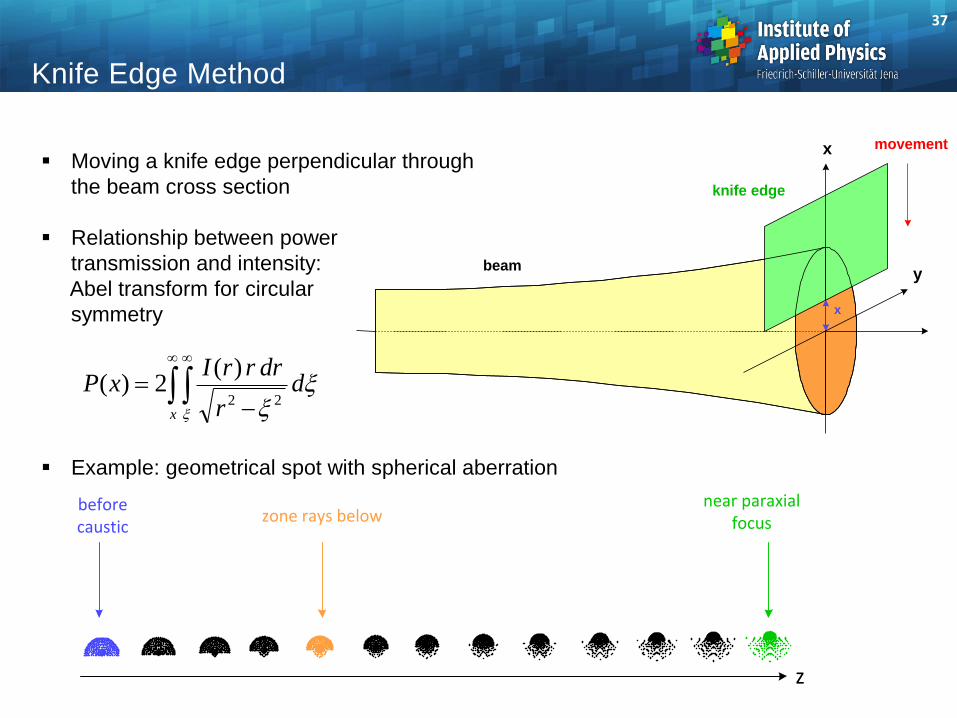
Moving a knife edge perpendicular through

the beam cross section

Relationship between power

transmission and intensity:

Abel transform for circular

symmetry

Example: geometrical spot with spherical aberration

dr

drrrIxP

x

22

)(2)(

z

beforecaustic

zone rays belownear paraxial

focus

Knife Edge Method

y

x

beam

x

knife edge

movement

37

38

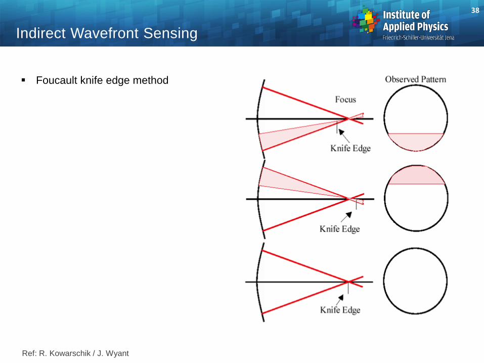
Indirect Wavefront Sensing

Foucault knife edge method

Ref: R. Kowarschik / J. Wyant

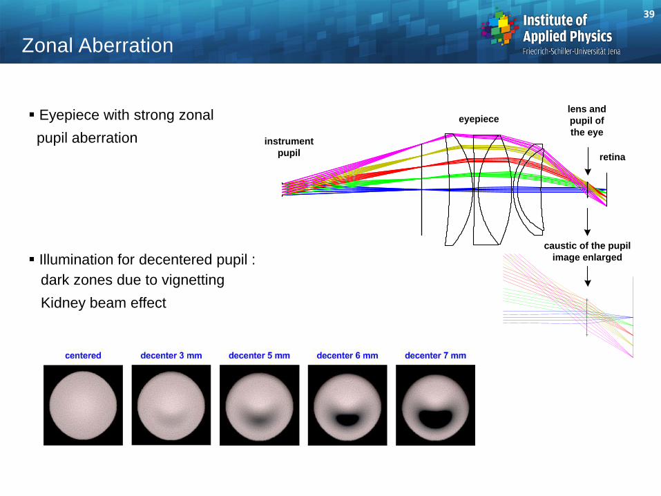
Eyepiece with strong zonal pupil aberration

Illumination for decentered pupil :

dark zones due to vignetting Kidney beam effect

Zonal Aberration

eyepiecelens and

pupil of

the eye

retina

caustic of the pupil

image enlarged

instrument

pupil

39

40

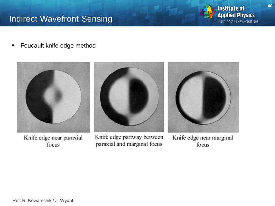
Indirect Wavefront Sensing

Foucault knife edge method

Ref: R. Kowarschik / J. Wyant

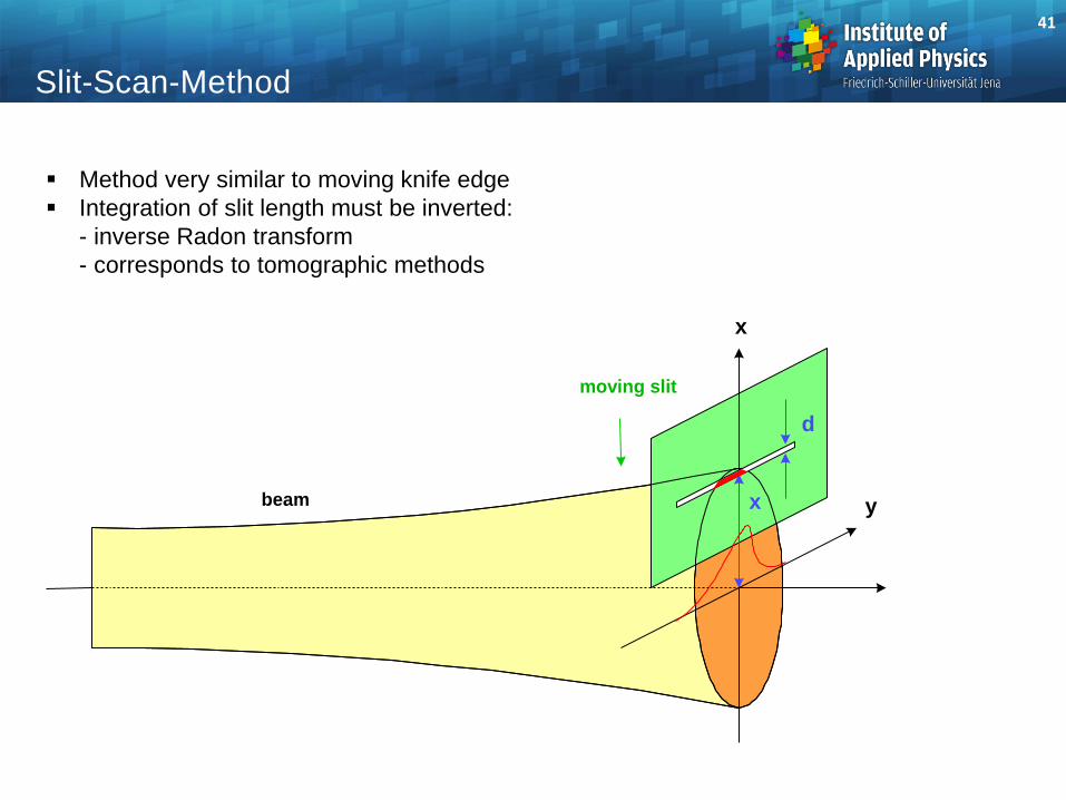
Method very similar to moving knife edge

Integration of slit length must be inverted:

- inverse Radon transform

- corresponds to tomographic methods

Slit-Scan-Method

y

x

beam x

moving slit

d

41

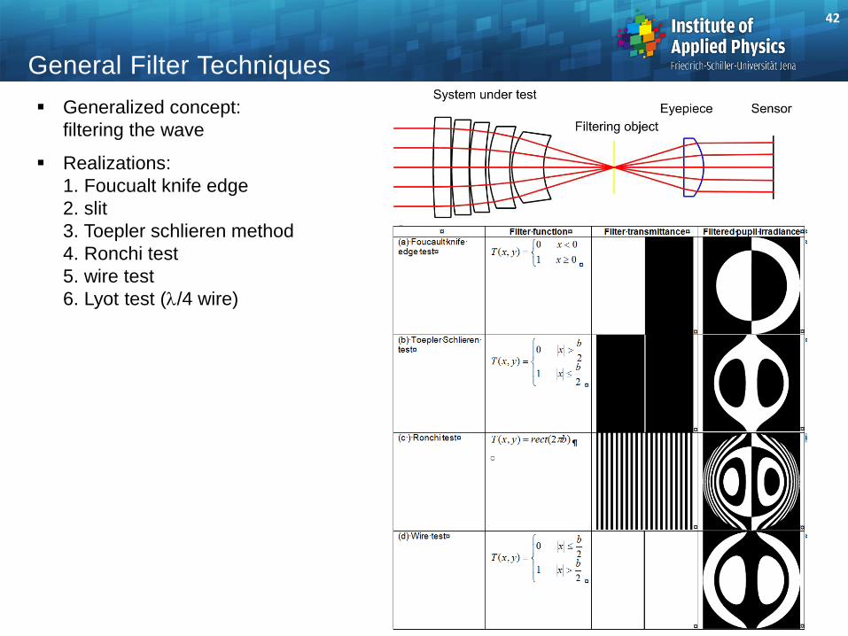
Generalized concept:

filtering the wave

Realizations:

1. Foucualt knife edge

2. slit

3. Toepler schlieren method

4. Ronchi test

5. wire test

6. Lyot test (/4 wire)

General Filter Techniques

42

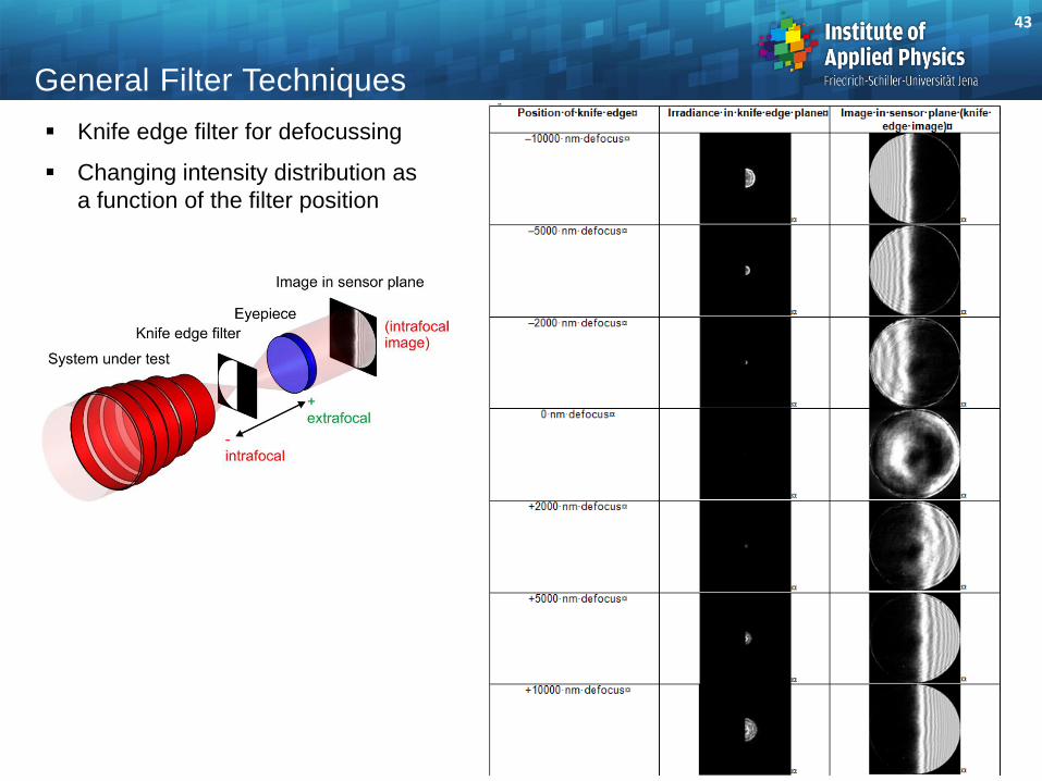
Knife edge filter for defocussing

Changing intensity distribution as

a function of the filter position

General Filter Techniques

43

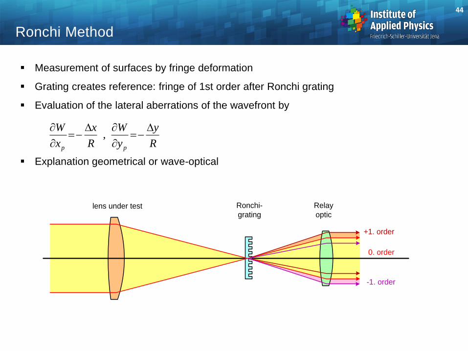
Measurement of surfaces by fringe deformation

Grating creates reference: fringe of 1st order after Ronchi grating

Evaluation of the lateral aberrations of the wavefront by

Explanation geometrical or wave-optical

Ronchi Method

lens under test Ronchi-

grating

Relay

optic

0. order

-1. order

+1. order

R

y

y

W

R

x

x

W

pp

,

44

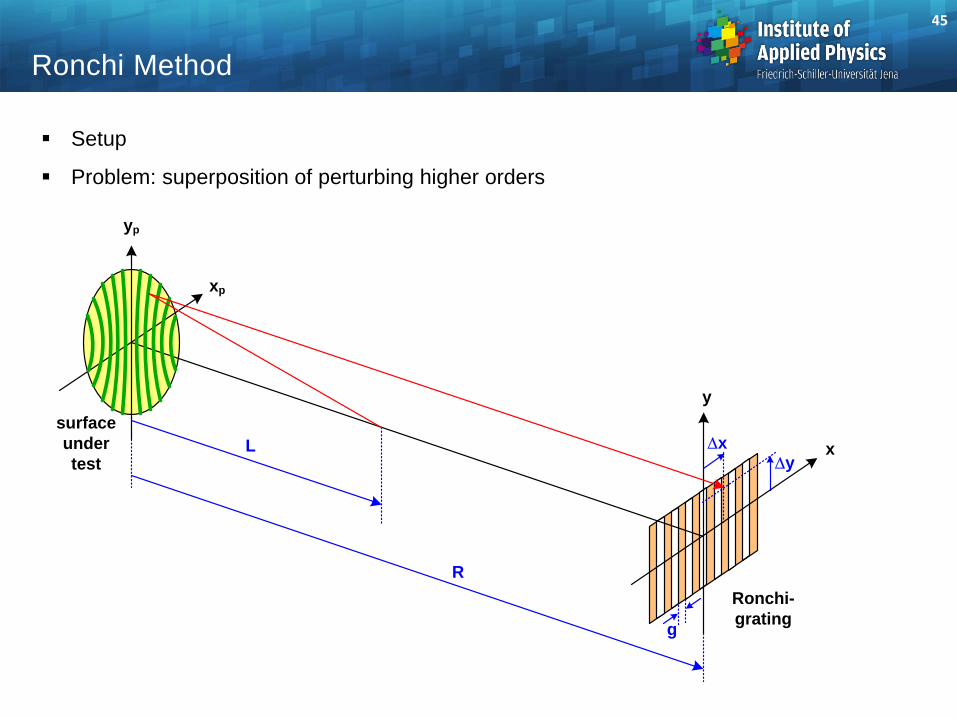
Setup

Problem: superposition of perturbing higher orders

Ronchi Method

xp

yp

y

x

Ronchi-

grating

R

L xy

g

surface

under

test

45

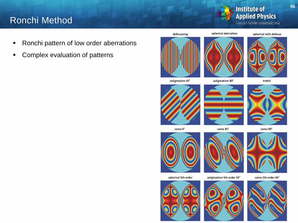
Ronchi pattern of low order aberrations

Complex evaluation of patterns

Ronchi Method

46

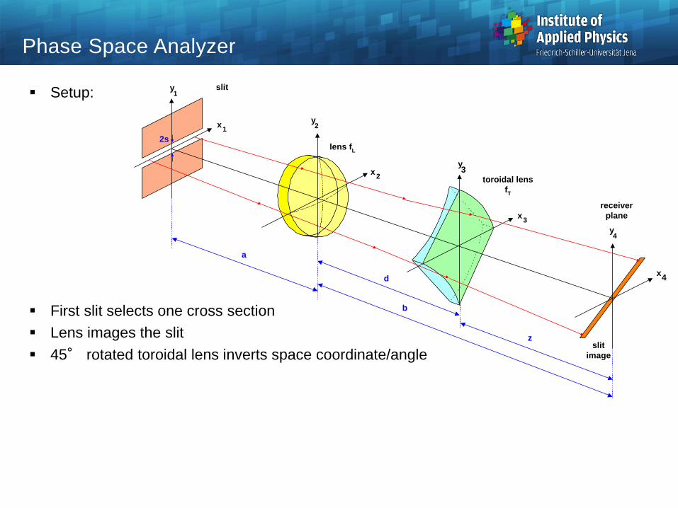
Setup:

First slit selects one cross section

Lens images the slit

45° rotated toroidal lens inverts space coordinate/angle

Phase Space Analyzer

d

toroidal lens

fT

y

x

1

1

y

x

4

4

y

x

3

3

a

z

lens fL

slit

2s

receiver

plane

y

x

2

2

b

slit

image

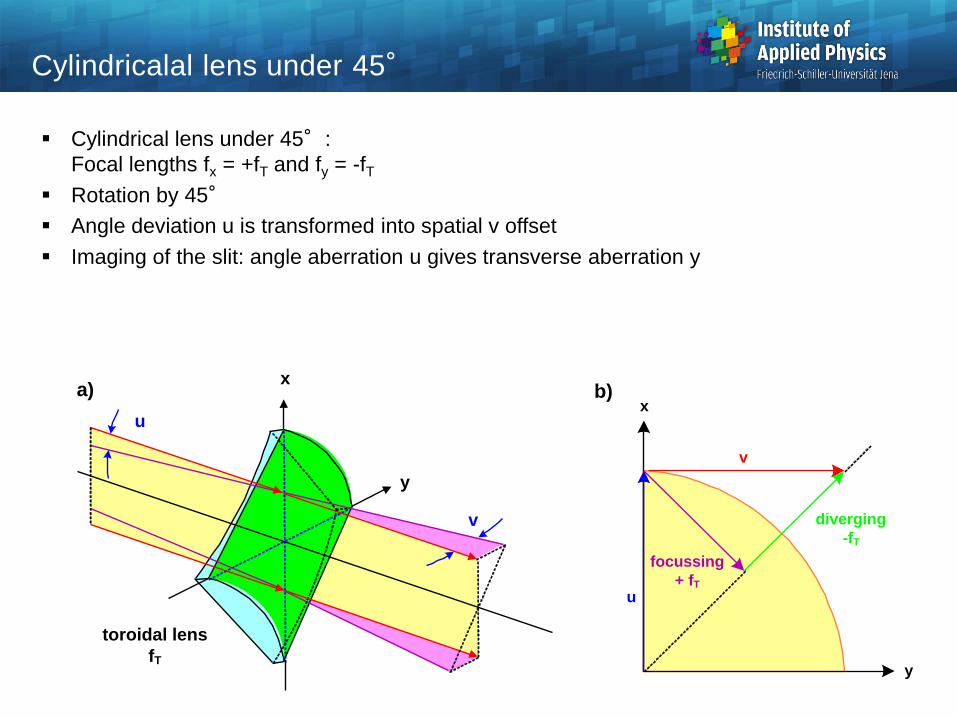
Cylindrical lens under 45°:

Focal lengths fx = +fT and fy = -fT

Rotation by 45°

Angle deviation u is transformed into spatial v offset

Imaging of the slit: angle aberration u gives transverse aberration y

Cylindricalal lens under 45°

diverging

-fT

y

u

v

x

focussing

+ fT

toroidal lens

fT

x

y

u

v

a) b)

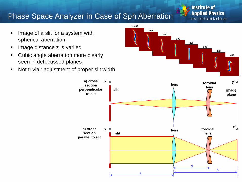
Phase Space Analyzer in Case of Sph Aberration z = 50

100

150

200

250

300

350

400

Image of a slit for a system with

spherical aberration

Image distance z is variied

Cubic angle aberration more clearly

seen in defocussed planes

Not trivial: adjustment of proper slit width

y y'

slit

toroidal

lenslens

x'

slit

toroidal

lenslensx

a

db

image

plane

a) cross

section

perpendicular

to slit

b) cross

section

parallel to slit

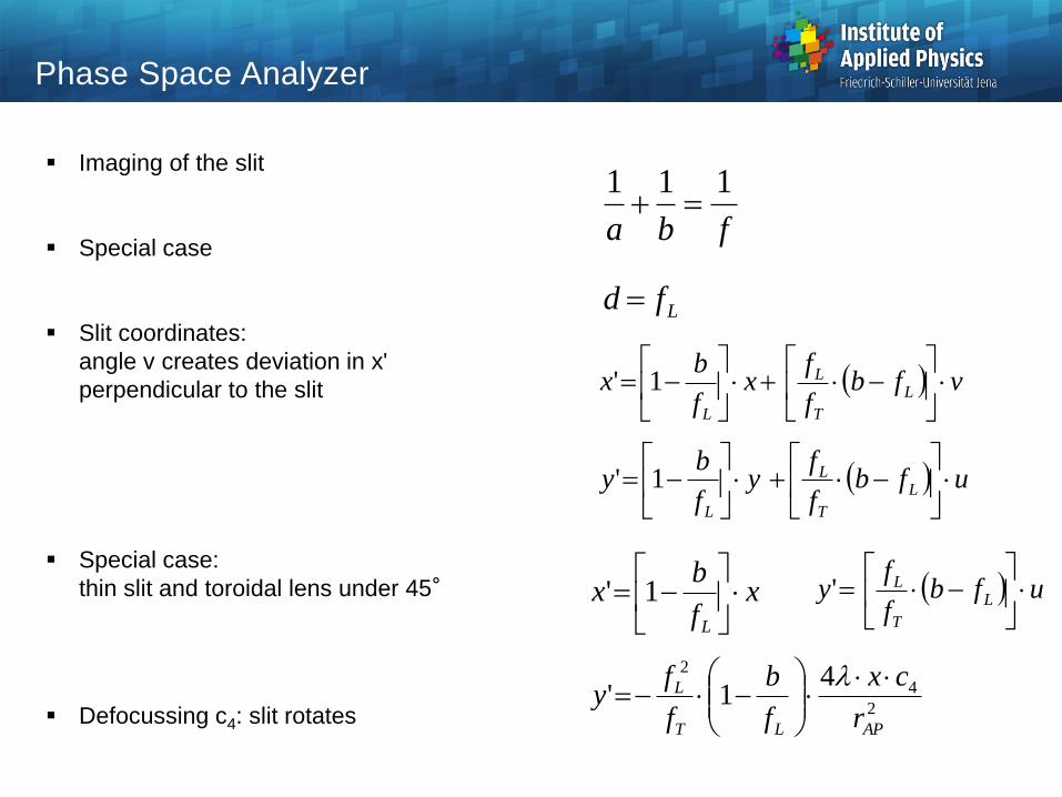
Imaging of the slit

Special case

Slit coordinates:

angle v creates deviation in x'

perpendicular to the slit

Special case:

thin slit and toroidal lens under 45°

Defocussing c4: slit rotates

fba

111

Lfd

vfbf

fx

f

bx L

T

L

L

1'

ufbf

fy

f

by L

T

L

L

1'

xf

bx

L

1' ufb

f

fy L

T

L

'

2

4

2 41'

APLT

L

r

cx

f

b

f

fy

Phase Space Analyzer

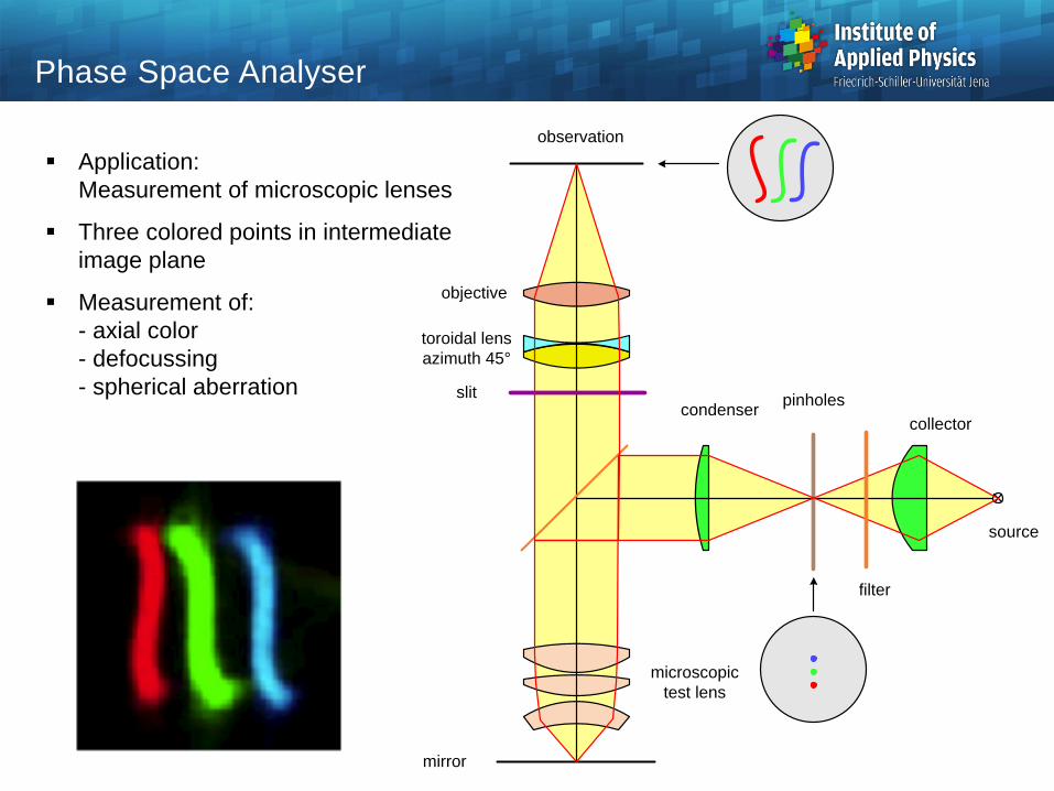
Application:

Measurement of microscopic lenses

Three colored points in intermediate

image plane

Measurement of:

- axial color

- defocussing

- spherical aberration

Phase Space Analyser

source

collectorcondenser

microscopic

test lens

mirror

objective

observation

pinholesslit

toroidal lens

azimuth 45°

filter