Microgenetic Algorithm

DRAFT MANUSCRIPT, AUGUST 2000

NUMERICAL OPTIMIZATION USING THE GEN4 MICRO-GENETIC ALGORITHM CODE

PETER KELLY SENECAL

ENGINE RESEARCH CENTER

UNIVERSITY OF WISCONSIN-MADISON

Peter Kelly Senecal, August 2000.


INTRODUCTION

The micro-Genetic Algorithm (µGA) is a “small population” Genetic Algorithm (GA) that operates on the principles of natural selection or “survival of the fittest” to evolve the best potential solution (i.e., design) over a number of generations to the most-fit, or optimal, solution. In contrast to the more classical Simple Genetic Algorithm (SGA), which requires a large number of individuals in each population (i.e., 30 – 200), the µGA uses a µ−population of five individuals (Krishnakumar 1989). This is very convenient for three-dimensional engine simulations, for example, which require a large amount of computational time. The small population size allows for entire generations to be run in parallel with five (or four, as will be discussed later) CPUs. This feature significantly reduces the amount of elapsed time required to achieve the most-fit solution. In addition, Krishnakumar (1989) and Senecal (2000) have shown that the µGA requires a fewer number of total function evaluations compared to SGAs for their test problems. The present document provides a simple description of the µGA optimization technique. Details of the key features of the strategy are presented and illustrated through an example two-dimensional, multi-modal optimization problem.

GENETIC ALGORITHM OVERVIEW

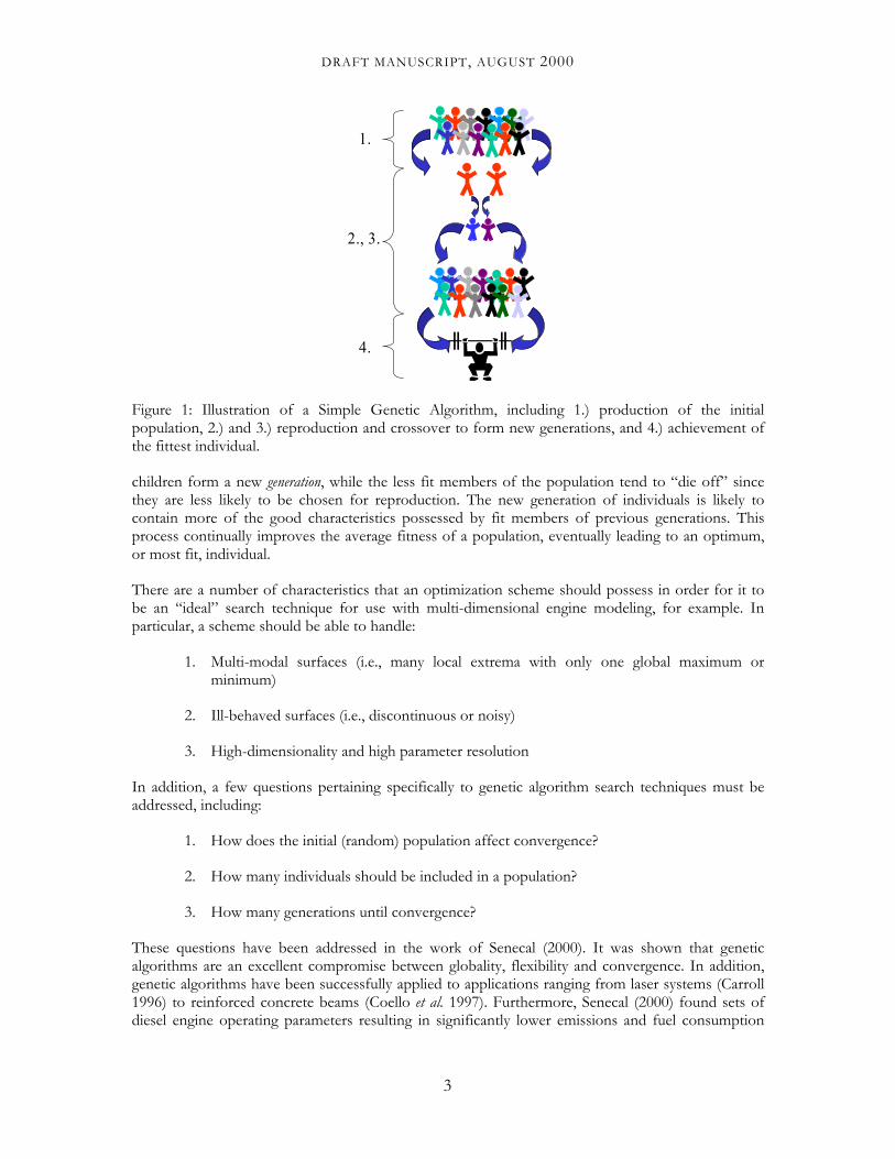
Genetic algorithms are search techniques based on the mechanics of natural selection which combine a “survival of the fittest” approach with some randomization and/or mutation. The technique can be summarized as follows (Pilley et al. 1994):

1. “Individuals” are generated through random selection of the parameter space for each control factor, and a “population” is then produced from the set of individuals.

2. A model (which may be analytical or multi-dimensional) is used to evaluate the fitness of each individual.

3. The fittest individuals are allowed to “reproduce,” resulting in a new “generation” through combining the characteristics from two sets of individuals. “Mutations” are also allowed through random changes to a small set of the population.

4. The fitness criteria thin out the population by “killing off” less suitable solutions. The characteristics of the individuals tend to converge to the most fit solution over successive generations.

A pictorial description of the above four steps is presented in Fig. 1.

As described above, GAs are search techniques based on the concepts of natural evolution and thus their principles are directly analogous to natural behavior. GAs work with a population of individuals, each of which represents a candidate solution to a given optimization problem. Just as organisms in nature compete for resources, a population’s individuals are assigned a fitness based on a defined objective, or merit, function. Individuals with higher fitness prove to be more effective, and hence have a higher probability of survival and reproduction. Thus, the most fit parents produce new individuals, or children, which share some of their features with each of the parents. The set of

2


1.

2., 3.

4.

Figure 1: Illustration of a Simple Genetic Algorithm, including 1.) production of the initial population, 2.) and 3.) reproduction and crossover to form new generations, and 4.) achievement of the fittest individual.

children form a new generation, while the less fit members of the population tend to “die off” since they are less likely to be chosen for reproduction. The new generation of individuals is likely to contain more of the good characteristics possessed by fit members of previous generations. This process continually improves the average fitness of a population, eventually leading to an optimum, or most fit, individual.

There are a number of characteristics that an optimization scheme should possess in order for it to be an “ideal” search technique for use with multi-dimensional engine modeling, for example. In particular, a scheme should be able to handle:

1. Multi-modal surfaces (i.e., many local extrema with only one global maximum or minimum)

2. Ill-behaved surfaces (i.e., discontinuous or noisy)

3. High-dimensionality and high parameter resolution

In addition, a few questions pertaining specifically to genetic algorithm search techniques must be addressed, including:

1. How does the initial (random) population affect convergence?

2. How many individuals should be included in a population?

3. How many generations until convergence?

These questions have been addressed in the work of Senecal (2000). It was shown that genetic algorithms are an excellent compromise between globality, flexibility and convergence. In addition, genetic algorithms have been successfully applied to applications ranging from laser systems (Carroll 1996) to reinforced concrete beams (Coello et al. 1997). Furthermore, Senecal (2000) found sets of diesel engine operating parameters resulting in significantly lower emissions and fuel consumption

3


compared to a baseline case using a µGA search technique. This technique is described in the following section.

THE MICRO-GENETIC ALGORITHM (µGA)

As explained above, the µGA operates on a family, or population, of designs similar to the SGA. However, unlike the SGA, the mechanics of the µGA allow for a very small population size, npop. This is especially important for studies where the function evaluation consists of CPU-intensive three-dimensional calculations. The µGA can be outlined in the following way:

1. A µ-population of five designs is generated randomly. 2. The fitness of each design is determined and the fittest individual is carried to the next

generation (elitist strategy).

3. The parents of the remaining four individuals are determined using a tournament selection strategy. In this strategy, designs are paired randomly and adjacent pairs compete to become parents of the remaining four individuals in the following generation (Krishnakumar 1989).

4. Convergence of the µ-population is checked. If the population is converged, go to step

1, keeping the best individual and generating the other four randomly. If the population has not converged, go to step 2.

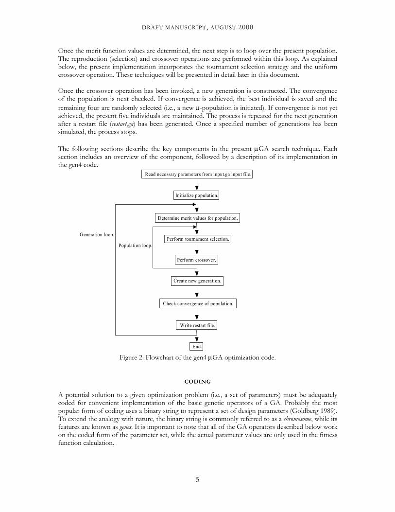
Note that mutations are not applied in the µGA since enough diversity is introduced after convergence of a µ-population. In addition, Krishnakumar (1989), Carroll (1996) and Senecal (2000) have shown that µGAs reach the optimum in fewer function evaluations compared to an SGA for their test functions. A summary of the gen4 µGA code is presented in Fig. 2. As shown in the figure, the process begins by reading in the input parameters specified in the input.ga file. A detailed description of this input file will be given below. The next step is to initialize the population of five individuals. In the present code, the user is allowed to initialize one individual as the present baseline design, while randomly sampling the parameter space to determine the other four. As illustrated in Fig. 2, the third step is to begin the generation loop. A number of steps are included in this loop. First of all, the merit function for each of the population members is determined. As described below, the present code can be run in either “serial” or “parallel” mode, depending on the scope of the optimization problem. In serial mode, a function routine (which can range from a simple subroutine consisting of an analytic function to a full-blown CFD code) is called within a loop over the population. On the other hand, the parallel mode takes advantage of multiple processors through the use of a Unix shell script. This will be explained in detail in a following section. In the present discussion, however, it is sufficient to think of the merit function evaluation as a “black box” operation.

4


Once the merit function values are determined, the next step is to loop over the present population. The reproduction (selection) and crossover operations are performed within this loop. As explained below, the present implementation incorporates the tournament selection strategy and the uniform crossover operation. These techniques will be presented in detail later in this document. Once the crossover operation has been invoked, a new generation is constructed. The convergence of the population is next checked. If convergence is achieved, the best individual is saved and the remaining four are randomly selected (i.e., a new µ-population is initiated). If convergence is not yet achieved, the present five individuals are maintained. The process is repeated for the next generation after a restart file (restart.ga) has been generated. Once a specified number of generations has been simulated, the process stops. The following sections describe the key components in the present µGA search technique. Each section includes an overview of the component, followed by a description of its implementation in the gen4 code.

Read necessary parameters from input.ga input file.

Initialize population.

Generation loop.

Determine merit values for population.

Population loop.Perform tournament selection.

Perform crossover.

Create new generation.

Check convergence of population.

Write restart file.

End. Figure 2: Flowchart of the gen4 µGA optimization code.

CODING

A potential solution to a given optimization problem (i.e., a set of parameters) must be adequately coded for convenient implementation of the basic genetic operators of a GA. Probably the most popular form of coding uses a binary string to represent a set of design parameters (Goldberg 1989). To extend the analogy with nature, the binary string is commonly referred to as a chromosome, while its features are known as genes. It is important to note that all of the GA operators described below work on the coded form of the parameter set, while the actual parameter values are only used in the fitness function calculation.

5


The precision of each of the design parameters included in a chromosome is based on the desired range of the parameter (i.e., its minimum and maximum values) and how many bits are used in its representation. Thus, the precision π of a parameter Xi is given by (Homaifar et al. 1994):

12min,max.

−−

=i

ii XXλπ

where λi is the number of bits in its representation. Thus if m possible values of a parameter are desired, its binary representation will include λi=ln(m)/ln(2) bits.

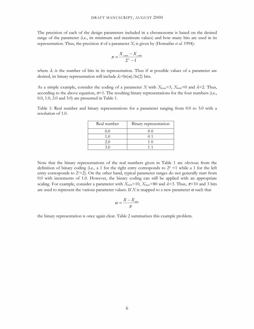
As a simple example, consider the coding of a parameter X with Xmax=3, Xmin=0 and λ=2. Thus, according to the above equation, π=1. The resulting binary representations for the four numbers (i.e., 0.0, 1.0, 2.0 and 3.0) are presented in Table 1.

Table 1: Real number and binary representations for a parameter ranging from 0.0 to 3.0 with a resolution of 1.0.

Real number Binary representation

0.0 0 0 1.0 0 1 2.0 1 0 3.0 1 1

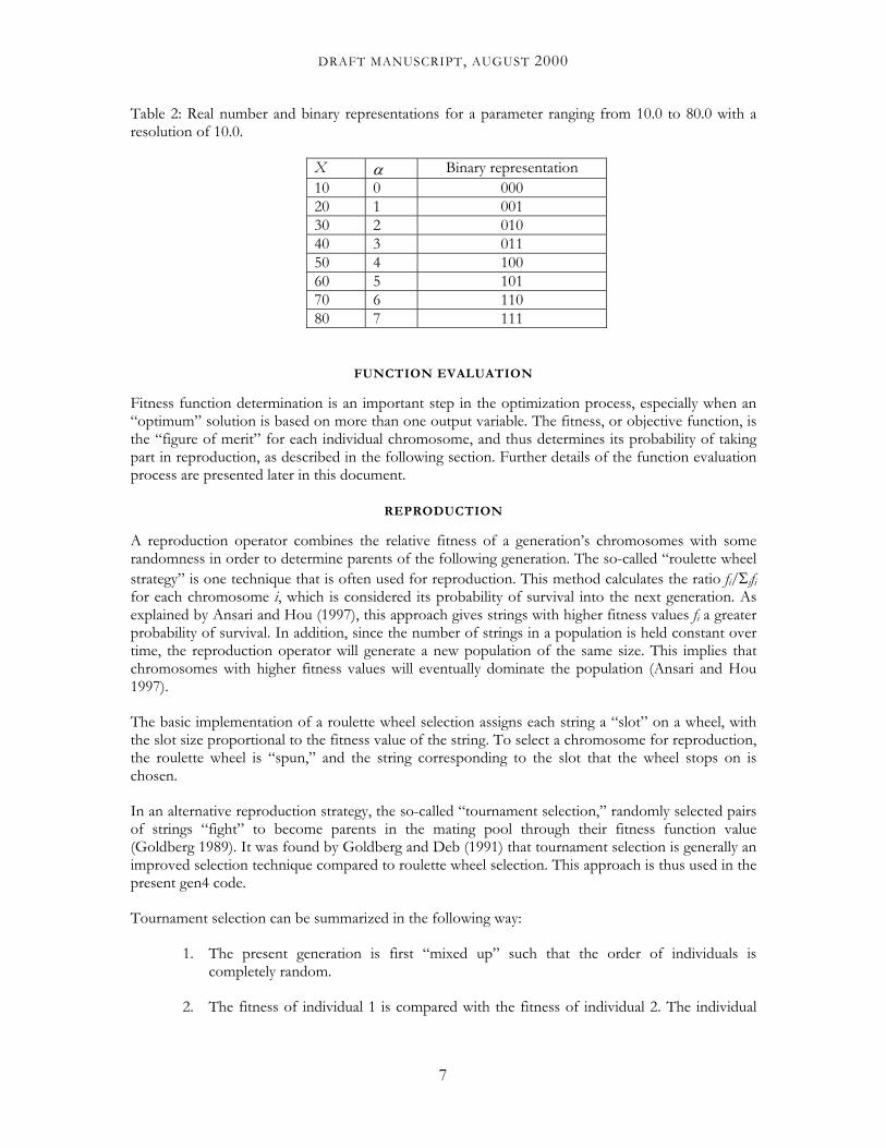
Note that the binary representations of the real numbers given in Table 1 are obvious from the definition of binary coding (i.e., a 1 for the right entry corresponds to 20 =1 while a 1 for the left entry corresponds to 21=2). On the other hand, typical parameter ranges do not generally start from 0.0 with increments of 1.0. However, the binary coding can still be applied with an appropriate scaling. For example, consider a parameter with Xmin=10, Xmax=80 and λ=3. Thus, π=10 and 3 bits are used to represent the various parameter values. If X is mapped to a new parameter α such that

πα minXX −=

the binary representation is once again clear. Table 2 summarizes this example problem.

6


Table 2: Real number and binary representations for a parameter ranging from 10.0 to 80.0 with a resolution of 10.0.

X α Binary representation 10 0 000 20 1 001 30 2 010 40 3 011 50 4 100 60 5 101 70 6 110 80 7 111

FUNCTION EVALUATION

Fitness function determination is an important step in the optimization process, especially when an “optimum” solution is based on more than one output variable. The fitness, or objective function, is the “figure of merit” for each individual chromosome, and thus determines its probability of taking part in reproduction, as described in the following section. Further details of the function evaluation process are presented later in this document.

REPRODUCTION

A reproduction operator combines the relative fitness of a generation’s chromosomes with some randomness in order to determine parents of the following generation. The so-called “roulette wheel strategy” is one technique that is often used for reproduction. This method calculates the ratio fi/Σifi for each chromosome i, which is considered its probability of survival into the next generation. As explained by Ansari and Hou (1997), this approach gives strings with higher fitness values fi a greater probability of survival. In addition, since the number of strings in a population is held constant over time, the reproduction operator will generate a new population of the same size. This implies that chromosomes with higher fitness values will eventually dominate the population (Ansari and Hou 1997).

The basic implementation of a roulette wheel selection assigns each string a “slot” on a wheel, with the slot size proportional to the fitness value of the string. To select a chromosome for reproduction, the roulette wheel is “spun,” and the string corresponding to the slot that the wheel stops on is chosen.

In an alternative reproduction strategy, the so-called “tournament selection,” randomly selected pairs of strings “fight” to become parents in the mating pool through their fitness function value (Goldberg 1989). It was found by Goldberg and Deb (1991) that tournament selection is generally an improved selection technique compared to roulette wheel selection. This approach is thus used in the present gen4 code.

Tournament selection can be summarized in the following way:

1. The present generation is first “mixed up” such that the order of individuals is completely random.

2. The fitness of individual 1 is compared with the fitness of individual 2. The individual

7


with the higher fitness is chosen as “parent 1.”

3. The fitness of individual 3 is compared with the fitness of individual 4. The individual with the higher fitness is chosen as “parent 2.”

4. Parents 1 and 2 are used in the crossover operation described below.

The above process is repeated until the desired number of children is produced.

Another strategy sometimes used in conjunction with either the roulette wheel or tournament selection strategies, is the so-called “elitist approach” (Goldberg 1989). Elitism automatically forms a child in the new generation with the exact qualities of the parent with the highest merit (i.e., a “clone” of the parent is produced). This approach guarantees that the highest fitness in a given generation will be at least as high as in the previous generation. It is important to note that the “best” string is still included in either of the reproduction strategies described above. It was shown by Carroll (1996) that elitism significantly improved the GA performance for his chemical laser application.

Further note that the use of elitism in the present code allows for a reduced number of total function evaluations (and hence fewer CPUs if run in parallel), since the merit of the “best” individual from the previous generation is already known and can be saved. As a result, only four function evaluations are required per generation instead of five.

CROSSOVER

The crossover operation is the process of mating the selected strings in the reproduction phase in order to form the individuals of a new generation. The main idea is that combining “good” genes from two strings will lead to an even better string. Of course, this is not always the case, but in general this method works over successive generations.

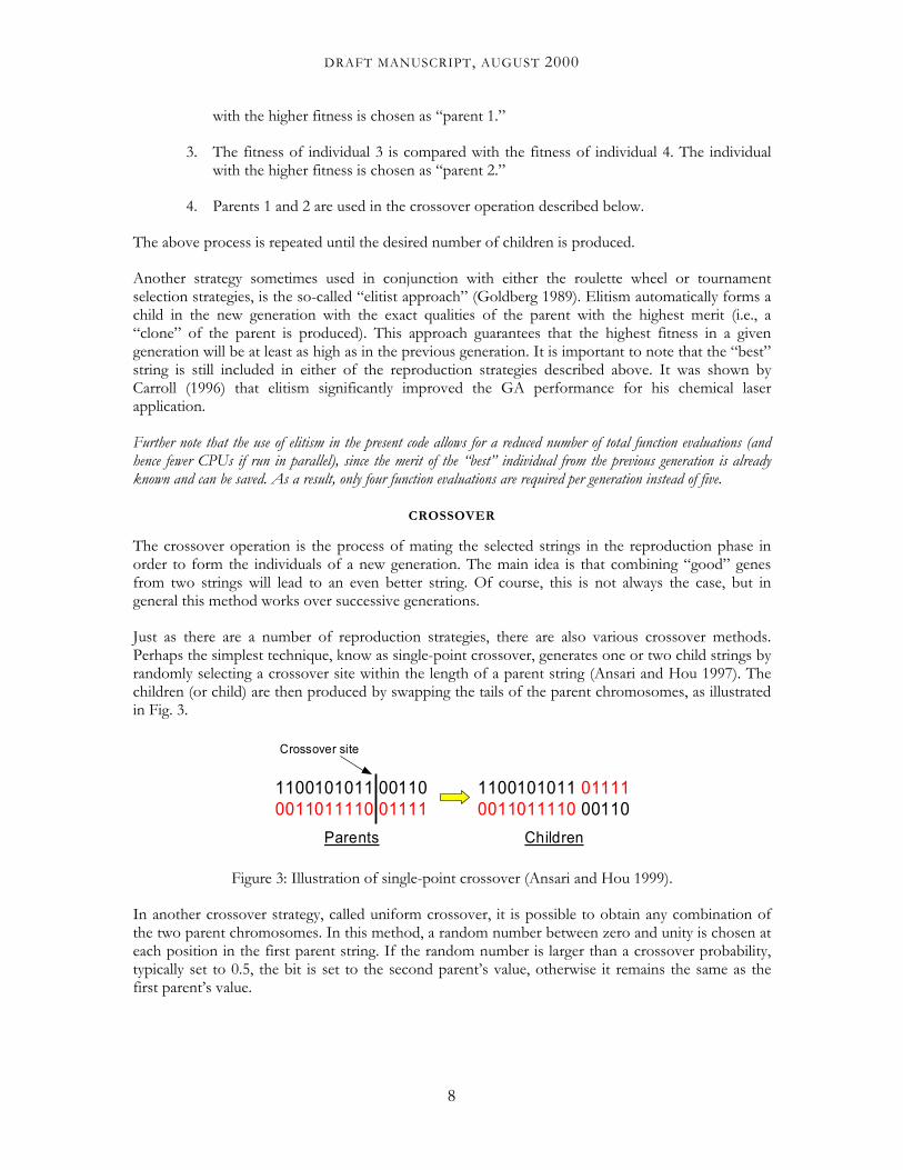
Just as there are a number of reproduction strategies, there are also various crossover methods. Perhaps the simplest technique, know as single-point crossover, generates one or two child strings by randomly selecting a crossover site within the length of a parent string (Ansari and Hou 1997). The children (or child) are then produced by swapping the tails of the parent chromosomes, as illustrated in Fig. 3.

1100101011 00110 1100101011 110

Parents Children

Crossover site

0011011110 0111101111

0011011110 00

Figure 3: Illustration of single-point crossover (Ansari and Hou 1999).

In another crossover strategy, called uniform crossover, it is possible to obtain any combination of the two parent chromosomes. In this method, a random number between zero and unity is chosen at each position in the first parent string. If the random number is larger than a crossover probability, typically set to 0.5, the bit is set to the second parent’s value, otherwise it remains the same as the first parent’s value.

8


CONVERGENCE AND RESTARTING

As explained by Goldberg (1989), the optimal solution is not guaranteed with genetic algorithms for arbitrary problems, and GAs are thus sometimes called weak methods. However, the same characteristics which make GAs weak methods also enhance their utility for global optimization. As described by Goldberg (1989), more convergent methods sacrifice globality and flexibility for their convergence, and are also typically limited to a narrow class of problems. On the other hand, genetic algorithms are very global both in their applicability and in their method of search.

While global optimality is not guaranteed with genetic algorithms (i.e., the author is not aware of a mathematical proof of their convergence), the population of solutions will evolve over successive generations so that the fitness of the best individual increases toward the global optimum. In this context, convergence should be defined as the progression towards chromosome uniformity. Thus, for the genetic algorithm operators described above, a gene may be considered to be converged, for example, when 95% of that particular gene in the entire population shares the same value. A population is then converged when all of the genes are converged. Recall that a µGA search potentially includes many µ-populations in the optimization process. As a result, the 95% convergence criterion is only used to determine when a µ-population is converged; the µGA is constantly looking for better designs and must be stopped by the user. This is not an issue for analytic functions since the optima are typically known a priori and the function evaluations require very little CPU time. A maximum number of generations can thus be defined, and the µGA will typically find an optimum within this specified number. On the other hand, multi-dimensional engine simulations, for example, require a large amount of CPU time and a method is thus needed to stop the search process.

A method to stop the µGA is described by Senecal (2000). In that work, engine optimization studies were set up to initially run for 50 generations. Two methods were then used to determine if the search had run for a sufficient amount of time. First of all, the maximum merit function curve (i.e., a plot of maximum merit as a function of generation number – see Fig. 7 below) was examined. If the “best” solution did not change for a sufficient number of generations (i.e., if a number of µ-populations converge to the same result), an optimal, or near-optimal design is indicated. In addition, output specific to the problem of interest can be used to monitor the convergence of the optimization scheme. For example, in the work of Senecal (2000), a “lowest” soot-NOx tradeoff curve was typically formed, and the optimum was determined visually to be the best compromise between soot and NOx along this curve.

The present code includes a “restart” feature, as described below. Thus, if the search has not found an optimum within the specified maximum number of generations, the process can be restarted without any loss of information.

SERIAL VS . PARALLEL

As described above, the gen4 code can be run in either serial or parallel mode. If the serial option is chosen, each member of a population will be run one after the other (i.e., in series). This option is recommended for functions that take only seconds or minutes to evaluate since it requires only one CPU. On the other hand, the parallel option allows for much more rapid population evaluation since each generation is run in “parallel” on four CPUs (recall that although the µGA includes five individuals per generation, the present implementation only requires four to be calculated). As a result, this option is recommended for functions that take hours or days to calculate. The use of each

9


of these options is described in the context of the example problem in a following section.

FILE DESCRIPTIONS

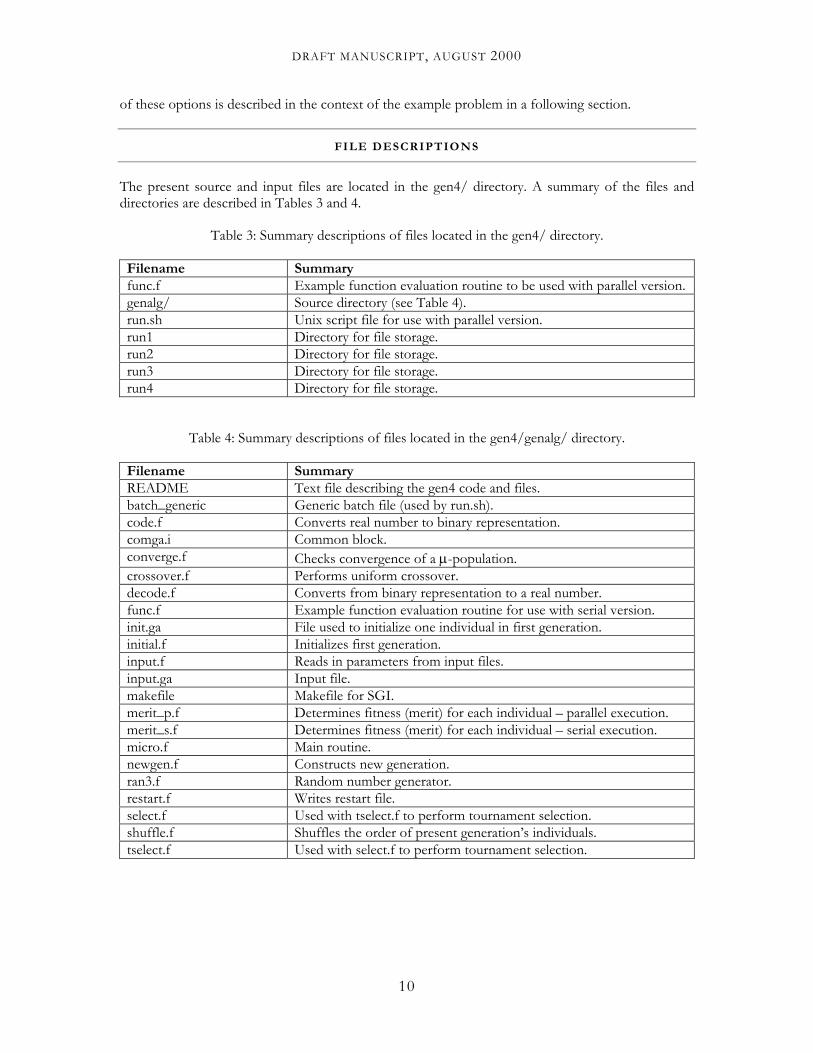
The present source and input files are located in the gen4/ directory. A summary of the files and directories are described in Tables 3 and 4.

Table 3: Summary descriptions of files located in the gen4/ directory.

Filename Summary func.f Example function evaluation routine to be used with parallel version.genalg/ Source directory (see Table 4). run.sh Unix script file for use with parallel version. run1 Directory for file storage. run2 Directory for file storage. run3 Directory for file storage. run4 Directory for file storage.

Table 4: Summary descriptions of files located in the gen4/genalg/ directory.

Filename Summary README Text file describing the gen4 code and files. batch_generic Generic batch file (used by run.sh). code.f Converts real number to binary representation. comga.i Common block. converge.f Checks convergence of a µ-population. crossover.f Performs uniform crossover. decode.f Converts from binary representation to a real number. func.f Example function evaluation routine for use with serial version. init.ga File used to initialize one individual in first generation. initial.f Initializes first generation. input.f Reads in parameters from input files. input.ga Input file. makefile Makefile for SGI. merit_p.f Determines fitness (merit) for each individual – parallel execution. merit_s.f Determines fitness (merit) for each individual – serial execution. micro.f Main routine. newgen.f Constructs new generation. ran3.f Random number generator. restart.f Writes restart file. select.f Used with tselect.f to perform tournament selection. shuffle.f Shuffles the order of present generation’s individuals. tselect.f Used with select.f to perform tournament selection.

10


EXAMPLE PROBLEM

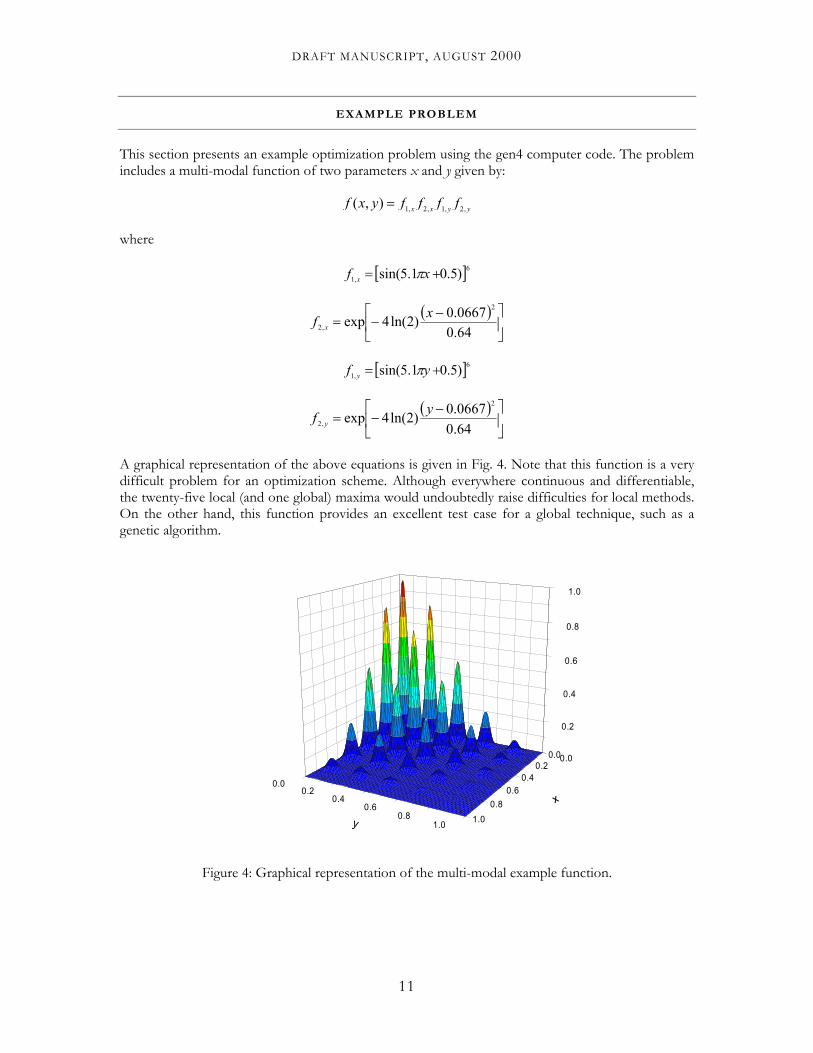
This section presents an example optimization problem using the gen4 computer code. The problem includes a multi-modal function of two parameters x and y given by:

yyxx ffffyxf ,2,1,2,1),( =

where

[ ]6,1 )5.01.5sin( += xf x π

( )

−−=

64.00667.0)2ln(4exp

2

,2

xf x

[ ]6,1 )5.01.5sin( += yf y π

( )

−−=

64.00667.0)2ln(4exp

2

,2

yf y

A graphical representation of the above equations is given in Fig. 4. Note that this function is a very difficult problem for an optimization scheme. Although everywhere continuous and differentiable, the twenty-five local (and one global) maxima would undoubtedly raise difficulties for local methods. On the other hand, this function provides an excellent test case for a global technique, such as a genetic algorithm.

0.00.2

0.40.6

0.81.0

0.00.2

0.40.6

0.81.0

0.0

0.2

0.4

0.6

0.8

1.0

x

y

Figure 4: Graphical representation of the multi-modal example function.

11


SETTING UP THE PROBLEM

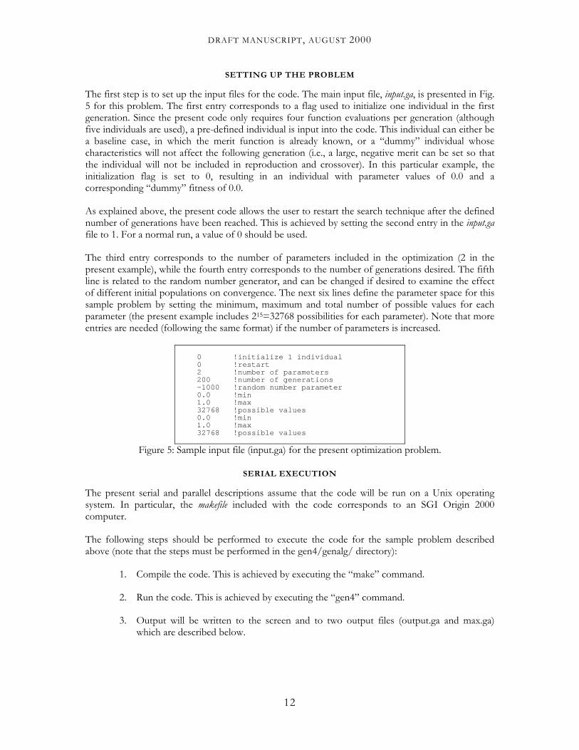
The first step is to set up the input files for the code. The main input file, input.ga, is presented in Fig. 5 for this problem. The first entry corresponds to a flag used to initialize one individual in the first generation. Since the present code only requires four function evaluations per generation (although five individuals are used), a pre-defined individual is input into the code. This individual can either be a baseline case, in which the merit function is already known, or a “dummy” individual whose characteristics will not affect the following generation (i.e., a large, negative merit can be set so that the individual will not be included in reproduction and crossover). In this particular example, the initialization flag is set to 0, resulting in an individual with parameter values of 0.0 and a corresponding “dummy” fitness of 0.0.

As explained above, the present code allows the user to restart the search technique after the defined number of generations have been reached. This is achieved by setting the second entry in the input.ga file to 1. For a normal run, a value of 0 should be used.

The third entry corresponds to the number of parameters included in the optimization (2 in the present example), while the fourth entry corresponds to the number of generations desired. The fifth line is related to the random number generator, and can be changed if desired to examine the effect of different initial populations on convergence. The next six lines define the parameter space for this sample problem by setting the minimum, maximum and total number of possible values for each parameter (the present example includes 215=32768 possibilities for each parameter). Note that more entries are needed (following the same format) if the number of parameters is increased.

0 !initialize 1 individual 0 !restart 2 !number of parameters 200 !number of generations -1000 !random number parameter 0.0 !min 1.0 !max 32768 !possible values 0.0 !min 1.0 !max 32768 !possible values

Figure 5: Sample input file (input.ga) for the present optimization problem.

SERIAL EXECUTION

The present serial and parallel descriptions assume that the code will be run on a Unix operating system. In particular, the makefile included with the code corresponds to an SGI Origin 2000 computer.

The following steps should be performed to execute the code for the sample problem described above (note that the steps must be performed in the gen4/genalg/ directory):

1. Compile the code. This is achieved by executing the “make” command.

2. Run the code. This is achieved by executing the “gen4” command.

3. Output will be written to the screen and to two output files (output.ga and max.ga) which are described below.

12


PARALLEL EXECUTION

Parallel execution is more complicated due to the extra files and directories involved. It essentially involves a Unix script (called here run.sh) and four “run” directories (called here run1, run2, run3 and run4) for file storage.

The following steps should be performed to execute the code for the sample problem:

1. Compile the function routine in the gen4/ directory. This is achieved with the command: f77 –o func func.f

2. Compile the gen4 code in the gen4/genalg/ directory. This step is not necessary if the code has already been compiled for serial execution.

3. Run the code. This is achieved by executing the run.sh script from the gen4/ directory. A file called parallel.ga is created (in gen4/genalg/) which “tells” gen4 to run in parallel mode. The command “run.sh > filename &” can alternatively be used to run in the background.

4. In addition to the output.ga and max.ga output files, a file called output.dat will be generated (see the following section).

Note that while the merit function routine is included in the gen4 source for serial execution, a separate “stand alone” merit function code is required for parallel execution (i.e., func.f in step 1 above). This allows for relatively easy interfacing with existing codes. In addition, input and output files for each run are stored in the four output directories (run1-run4).

ANALYZING THE RESULTS

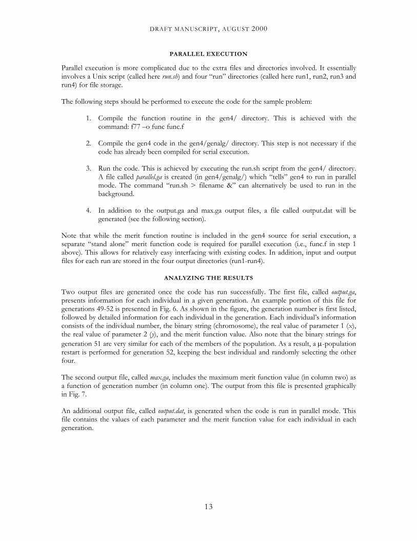
Two output files are generated once the code has run successfully. The first file, called output.ga, presents information for each individual in a given generation. An example portion of this file for generations 49-52 is presented in Fig. 6. As shown in the figure, the generation number is first listed, followed by detailed information for each individual in the generation. Each individual’s information consists of the individual number, the binary string (chromosome), the real value of parameter 1 (x), the real value of parameter 2 (y), and the merit function value. Also note that the binary strings for generation 51 are very similar for each of the members of the population. As a result, a µ-population restart is performed for generation 52, keeping the best individual and randomly selecting the other four.

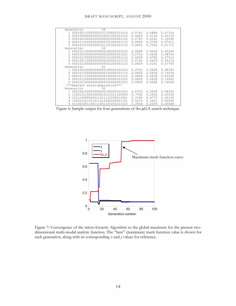
The second output file, called max.ga, includes the maximum merit function value (in column two) as a function of generation number (in column one). The output from this file is presented graphically in Fig. 7.

An additional output file, called output.dat, is generated when the code is run in parallel mode. This file contains the values of each parameter and the merit function value for each individual in each generation.

13


Generation 49 1 000100110000000101100000101010 0.0742 0.6888 0.07124 2 000100000000000100001000001010 0.0625 0.5159 0.02154 3 000100100000000000001000001110 0.0703 0.0161 0.10290 4 000101100000000000101000001110 0.0859 0.0786 0.67412 5 000101010000000101101000101110 0.0820 0.7046 0.01712 Generation 50 1 000101110000000000100000101010 0.0898 0.0638 0.65246 2 000100100000000000100000101010 0.0703 0.0638 0.98354 3 000101100000000000101000001110 0.0859 0.0786 0.67412 4 000100110000000000100000101110 0.0742 0.0639 0.95216 5 000101100000000000001000001110 0.0859 0.0161 0.07793 Generation 51 1 000100100000000000100000101010 0.0703 0.0638 0.98354 2 000101100000000000100000101110 0.0859 0.0639 0.74534 3 000101110000000000100000101010 0.0898 0.0638 0.65246 4 000101100000000000100000101010 0.0859 0.0638 0.74492 5 000101100000000000100000001010 0.0859 0.0628 0.74094 ***Restart micro-population*** Generation 52 1 000100100000000000100000101010 0.0703 0.0638 0.98354 2 110010110001000010111011100000 0.7932 0.3662 0.00000 3 101110000000011011110100011001 0.7189 0.4773 0.00118 4 100010101011011011000100001101 0.5419 0.3832 0.00000 5 011001001100111001101001011010 0.3938 0.2059 0.00048

Figure 6: Sample output for four generations of the µGA search technique.

0

0.2

0.4

0.6

0.8

1

0 20 40 60

xyf(x,y)

Generation num

e

Figure 7: Convergence of the micro-Genetic Algorithm tdimensional multi-modal analytic function. The “best” (meach generation, along with its corresponding x and y valu

14

Maximum merit function curv

80 100ber

o the global maximum for the present two-aximum) merit function value is shown for es for reference.


INTERFACING WITH GEN4

Now that the example problem has been successfully executed, the user will likely wish to use the present methodology for his or her own optimization problem. The present section describes how to interface an existing code with the gen4 µGA code for both serial and parallel mode execution.

SERIAL MODE

Interfacing with the gen4 code in serial mode is very straightforward, and essentially only requires the user to replace the func.f subroutine with his or her own subroutine(s). The func.f subroutine uses an individual’s parameter values (taken from the “parent” array in the code) to calculate its merit function value (called “funcval” in the code). The value of funcval is then passed back to the merit_s.f subroutine. The example func.f subroutine also requires the values of “j” (the present individual number) and “nparam” (the total number of parameters) to access the appropriate parameter values in the parent array.

If an existing code consisting of several subroutines is to be interfaced with gen4, the main routine must be converted to a subroutine of gen4. In addition, the function evaluation code’s routines can be added to the included makefile for compilation.

As an example, consider a code (called here “engine”) for calculating power based on a set of input parameters. The user wishes to examine the effects of start-of-injection timing (variable name “soi”), injection duration (variable name “dur_inj”) and exhaust gas recirculation (variable name “egr”) on performance (i.e., find the set of values to maximize power). The following modifications would be made to the routines merit_s.f and engine.f (the main routine of the engine code):

merit_s.f:

Replace: call func(j,funcval,nparam,parent)

With: call engine(j,funcval,nparam,parent)

engine.f:

Replace: program engine

With: subroutine engine(j,funcval,nparam,parent)

. . .

soi=parent(1,j)

dur_inj=parent(2,j)

egr=parent(3,j)

. . . funcval=power

15


Note that the above coding assumes that power is calculated somewhere in the engine code above the “funcval=power” statement. In addition, appropriate parameter ranges and resolutions would be defined in the input.ga input file.

PARALLEL MODE

As for the serial mode interface described above, the main task for the parallel mode interface is to “pass” the parameter values to the function evaluation code and to return the function (merit) value. This is more complicated in parallel mode, since each function evaluation is its own process, independent of the others. In other words, the gen4 code does not simply call the function evaluator in a loop, as in the serial mode. Instead input/output files are used to interface the two codes. This is achieved through the run.sh script file (located in gen4/), the merit_p.f subroutine (located in gen4/genalg/), and the func.f program (located in gen4/).

First of all, “param” files are written by the gen4 code (from subroutine merit_p.f) for each member of the population. These files are named param.j-i where “j” is the individual number and “i” is the generation number. Each of these files has the following format:

generation number (i), individual number (j), value of parameter 1, value of parameter 2, …

Each of the param files are copied into one of the four run directories. The run.sh script file creates a batch file for each of the four runs. For the sample problem, for example, the batch file executes the command:

func param.1-20

for the first individual in the twentieth generation. The necessary logic to read in the param file must thus exist in the function evaluation code. In FORTRAN this is accomplished with the “getarg” command. The following lines are included in the sample func.f program for this purpose:

call getarg(1,fname)

open(111,file=fname,status=’unknown’)

read(111,*)i,j,pp1,pp2

where “fname” has been declared as a character string, “i” is the generation number, “j” is the individual number, “pp1” is the value of parameter 1 and “pp2” is the value of parameter 2. The values of pp1 and pp2 are then used to calculate the merit function, or funcval, parameter.

Once funcval is computed, its value must be “passed back” to the gen4 code. This is accomplished by writing an “outdata” file using the following coding (see func.f program):

outname=’outdata. ‘

write(outname(9:9),’(i1)’)j

.

.

.

open(unit=j,file=outname,status=’unknown’)

write(j,*)1,funcval

The above will create four different outdata files including function values for each case. Once all four files have been created (indicating that all of the present individuals have been evaluated), the gen4 code will read in the outdata files and continue until the next generation is created. Note that

16


the above steps (reading/writing files, submitting runs, etc.) are all automated with the run.sh script. However, the user must modify the above code in order to adapt the methodology to his or her problem.

To summarize, the main tasks are:

1. Read in the parameter values appropriately in the function evaluator from the param files.

2. Write the outdata files from the function evaluator.

3. In addition, the user must be careful to modify path names, etc. in the batch_generic file (used for creating batch files) as necessary.

ENGINE OPTIMIZATION USING THE µGA

The following papers illustrate the use of the µGA and multi-dimensional modeling applied to diesel engine optimization:

• Senecal, P. K. and Reitz, R. D., “Optimization of Diesel Engine Emissions and Fuel Efficiency using Genetic Algorithms and Computational Fluid Dynamics,” International Conference on Liquid Atomization and Spray Systems, Pasadena, CA, 2000.

• Senecal, P. K. and Reitz, R. D., “Simultaneous Reduction of Diesel Engine Emissions and Fuel Consumption using Genetic Algorithms and Multi-Dimensional Spray and Combustion Modeling,” Society of Automotive Engineers Paper 2000-01-1890, 2000.

• Senecal, P. K., Montgomery, D. T. and Reitz, R. D., “A Methodology for Engine Design using Multi-Dimensional Modeling and Genetic Algorithms with Validation Through Experiments,” accepted to International Journal of Engine Research.

• Senecal, P. K., Montgomery, D. T. and Reitz, R. D., “Diesel Engine Optimization Using Multi-Dimensional Modeling and Genetic Algorithms Applied to a Medium Speed, High Load Operating Condition,” accepted to American Society of Mechanical Engineers, ICE Division, Peoria, IL, 2000.

• Wickman, D. D., Senecal, P. K. and Reitz, R. D., “Diesel Engine Combustion Chamber Geometry Optimization using Genetic Algorithms and Multi-Dimensional Modeling,” in preparation.

NOTE

Although no bugs are believed to exist, this code is not guaranteed to be “bug free.” Please send comments, suggestions, etc. to the author at [email protected].

17

mailto:[email protected]


18

REFERENCES

Ansari, N. and Hou, E., Computational Intelligence for Optimization, Kluwer Academic, Boston, MA, 1999. Carroll, D. L., “Genetic Algorithms and Optimizing Chemical Oxygen-Iodine Lasers,” Developments in Theoretical and Applied Mechanics, 18, 1996. Coello Coello, C. A., Christiansen, A. D. and Santos Hernandez, F., “A Simple Genetic Algorithm for the Design of Reinforced Concrete Beams,” Engineering with Computers, 13, 1997 Goldberg, D. E., Genetic Algorithms in Search, Optimization and Machine Learning, Addison-Wesley, Reading, MA, 1989. Goldberg, D. E. and Deb, K., “A Comparative Analysis of Selection Schemes used in Genetic Algorithms,” in: Foundations of Genetic Algorithms, Morgan Kauffmann Publishers, San Mateo, CA, 1991. Homaifar, A., Lai H. Y. and McCormick, E., “System Optimization of Turbofan Engines using Genetic Algorithms,” Appl. Math. Modelling, 18, 1994. Krishnakumar, K., “Micro-Genetic Algorithms for Stationary and Non-Stationary Function Optimization,” SPIE 1196, Intelligent Control and Adaptive Systems, 1989. Pilley, A. D., Beaumont, A. J., Robinson, D. R. and Mowll, D., “Design of Experiments for Optimization of Engines to Meet Future Emissions Targets,” 27th Int. Symposium on Automotive Technology and Automation, ISATA Paper 94EN014, 1994. Senecal P. K., “Development of a Methodology for Internal Combustion Engine Design Using Multi-Dimensional Modeling with Validation Through Experiments,” Ph.D. Dissertation, University of Wisconsin-Madison, 2000.

Documents

Microgenetic Algorithm