Embed Size (px)
Citation preview
June 6, 2012 15:43 WSPC - Proceedings Trim Size: 9in x 6in microLecture
1
MICROMEGAS a package for calculation of of Dark Matter
properties in generic model of particle interaction.
G. Belanger and F. Boudjema
LAPTH,University de Savoie,CNRS,B.P.110,
F-74941 Annecy-le-Vieux Cedex, France
E-mail: [email protected], [email protected]
lapth.in2p3.fr
A. Pukhov ∗
Skobeltsyn Institute of Nuclear Physics, Lomonosov Moscow State University,
Leninskie gory, GSP-1, Moscow, 119991, Russia∗E-mail: [email protected]
www.sinp.msu.ru
These lecture notes describe the micrOMEGAs package for the calculation of
Dark Matter observables in extensions of the standard model.
Keywords: Dark Matter; Relic density; Direct detection; Indirect detection;
Solar neutrinos
1. Introduction
Since the 1930’s, with the pioneering work of Zwicky1 on the dynamics
of the Coma galaxy and the observation2 thirty years later of the flat-
ness of the rotation curves of spiral galaxies, evidence for the existence of
some missing non luminous matter has been steadily gathering. The last
two decades or so have witnessed spectacular advances in cosmology and
astrophysics confirming that ordinary matter is a minute part of what con-
stitutes the Universe at large. Most spectacular has been the study of the
Cosmic Microwave Background (CMB), in particular combining the results
of the 7-year WMAP data3 on the 6-parameter ΛCDM model, the baryon
acoustic oscillations from SDSS4 and the most recent determination of the
Hubble constant5 one6 arrives at a measurement of the relic density to bet-
ter than 3%. Yet the exact nature of this dark matter and its microscopic
properties remain mysterious. At the same time the field of high energy
June 6, 2012 15:43 WSPC - Proceedings Trim Size: 9in x 6in microLecture
2
physics has been rich in discoveries of a large number of particles. All these
particles can in fact fit very neatly with a modicum of elementary building
blocks within the much successful standard model (SM). Were it not for the
masses of these particles the dynamics of the standard model would require
less than a handful of parameters which makes the theory very predictive.
Yet, none of the particles of the SM contributes much to the weight of the
Universe, therefore Dark Matter (DM) is certainly New Physics. Moreover,
the problem of mass in the SM is also still mysterious. Electroweak sym-
metry breaking and the mechanism behind the generation of mass need
elucidation. The SM description poses serious conceptual problems having
to do with the missing scalar particle of the SM: the Higgs particle. At the
heart of the problem, the naturalness problem, is the observation that there
is no symmetry to protect the mass of a lone elementary scalar like the SM
Higgs. This fact has been behind the intense activity in the construction of
New Physics models. Until a few years ago, the epitome of this New Physics
has been supersymmetry which when endowed with a discrete symmetry,
called R-parity, furnishes a good dark matter candidate. Recently, a few
alternatives for the New Physics have been put forward. Originally, they
were confined to solving the Higgs problem, but it has been discovered that,
generically, their most viable implementation (in accord with electroweak
precision data, proton decay, etc.) fares far better if a discrete symmetry is
embedded in the model. The discrete symmetry is behind the existence of
a possible dark matter candidate. We will call even the particles which are
neutral with respect to the symmetry and odd the ones which get non-trivial
factorsa. All the SM particles share the same quantum number (even) which
sets them apart from most of the New Physics particles which have a non
even quantum number. This makes the lightest New Physics particle with
this non even quantum number a stable particle which is, beside its electri-
cally neutral character, a potentially good dark matter candidate. Among
the most popular possibilities, let us mention some of the candidates and
the discrete symmetry behind each of these candidates.
• R-parity (a Z2 symmetry)7 with the DM in Supersymmetry which is a
Majorana fermion
• KK parity (a Z2 symmetry with x5 → −x5)8 and the DM in Universal
Extra Dimension which is a gauge boson
• T-parity (a Z2 symmetry)9 in Little Higgs model with the DM which is
a gauge boson
aThis terminology comes from the widely used Z2 case
June 6, 2012 15:43 WSPC - Proceedings Trim Size: 9in x 6in microLecture
3
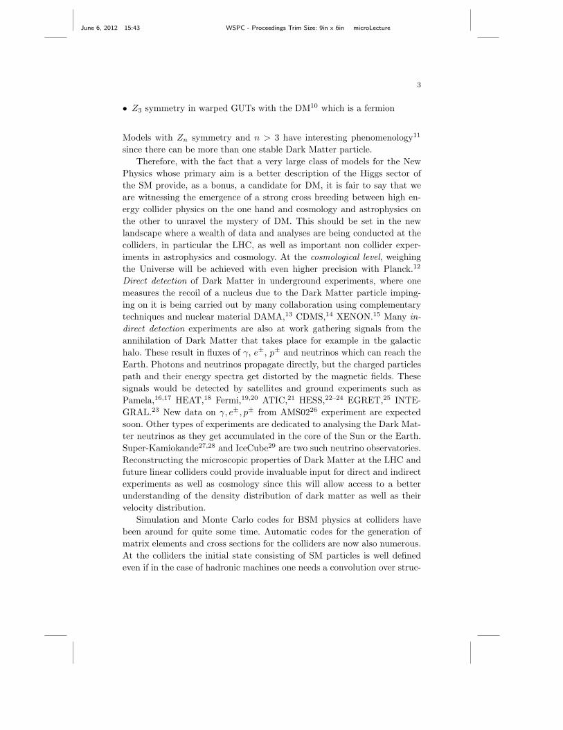
• Z3 symmetry in warped GUTs with the DM10 which is a fermion
Models with Zn symmetry and n > 3 have interesting phenomenology11
since there can be more than one stable Dark Matter particle.
Therefore, with the fact that a very large class of models for the New
Physics whose primary aim is a better description of the Higgs sector of
the SM provide, as a bonus, a candidate for DM, it is fair to say that we
are witnessing the emergence of a strong cross breeding between high en-
ergy collider physics on the one hand and cosmology and astrophysics on
the other to unravel the mystery of DM. This should be set in the new
landscape where a wealth of data and analyses are being conducted at the
colliders, in particular the LHC, as well as important non collider exper-
iments in astrophysics and cosmology. At the cosmological level, weighing
the Universe will be achieved with even higher precision with Planck.12
Direct detection of Dark Matter in underground experiments, where one
measures the recoil of a nucleus due to the Dark Matter particle imping-
ing on it is being carried out by many collaboration using complementary
techniques and nuclear material DAMA,13 CDMS,14 XENON.15 Many in-
direct detection experiments are also at work gathering signals from the
annihilation of Dark Matter that takes place for example in the galactic
halo. These result in fluxes of γ, e±, p± and neutrinos which can reach the
Earth. Photons and neutrinos propagate directly, but the charged particles
path and their energy spectra get distorted by the magnetic fields. These
signals would be detected by satellites and ground experiments such as
Pamela,16,17 HEAT,18 Fermi,19,20 ATIC,21 HESS,22–24 EGRET,25 INTE-
GRAL.23 New data on γ, e±, p± from AMS0226 experiment are expected
soon. Other types of experiments are dedicated to analysing the Dark Mat-
ter neutrinos as they get accumulated in the core of the Sun or the Earth.
Super-Kamiokande27,28 and IceCube29 are two such neutrino observatories.
Reconstructing the microscopic properties of Dark Matter at the LHC and
future linear colliders could provide invaluable input for direct and indirect
experiments as well as cosmology since this will allow access to a better
understanding of the density distribution of dark matter as well as their
velocity distribution.
Simulation and Monte Carlo codes for BSM physics at colliders have
been around for quite some time. Automatic codes for the generation of
matrix elements and cross sections for the colliders are now also numerous.
At the colliders the initial state consisting of SM particles is well defined
even if in the case of hadronic machines one needs a convolution over struc-
June 6, 2012 15:43 WSPC - Proceedings Trim Size: 9in x 6in microLecture
4
ture functions. Predictions are then made for a specific channel or a BSM
particle in the final state. The task of a DM code that returns the value of
the relic density requires the calculation of a very large number of channels
and processes. First of all one needs to identify what could be a potentially
valid DM candidate (neutrality and stability are a first requirement). Once
this is set one generally needs to calculate a large number of processes cor-
responding to the annihilation of this candidate to all possible SM final
states. In general, since the BSM model has not been constrained and its
parameters not measured one has to allow for the calculation of a very
large number of processes depending on the properties of the DM particle.
In the MSSM for example, one has to be ready to calculate the rates for
some 3000 processes. Early codes for the calculations of the relic density
listed only a few processes that were, at some stage, of a particular inter-
est. Whenever a new mechanism was deemed interesting new calculations
were added. Indirect detection codes require the decay and fragmentation
products of the SM produced in annihilation of DM particles. Furthermore
sophisticated modeling of the propagation of charged particles is needed.
In direct detection the rates have to be parametrized and evaluated at very
small recoil energy, interaction with nuclei require elements from nuclear
physics for instance (form factors,..). All these different observables need
to be “convoluted” with different DM density distributions and call for a
knowledge of the velocity distribution. For the relic density a model of cos-
mology has to be invoked to take into account the evolution of the Universe,
the dilution of the DM and its decoupling.
micrOMEGAs has been developed with the aim of providing the value the
relic density, the fluxes of photons, antiprotons, and positrons for indirect
DM searches; cross sections of DM interactions with nuclei and energy dis-
tribution of recoil nuclei; neutrino and the corresponding muon flux from
DM particles captured by the Sun; collider cross sections and partial decay
widths of particles within a BSM that provides a possible WIMP (weakly
Interacting Massive Particle) DM candidate. What sets micrOMEGAs apart
from other codes is its ability, once given a Model File that encodes a
BSM model, to output, for any set of parameters of the model, all the
observables we have just listed. All the needed cross sections are built up
on the fly. There are several packages which calculate different properties
of DM within the very popular minimal supersymmetric standard model
(MSSM): DarkSUSY30 SuperIso31 and Isared.32 The modular structure of
micrOMEGAs with the (self) automatic generation of all the needed ma-
June 6, 2012 15:43 WSPC - Proceedings Trim Size: 9in x 6in microLecture
5
trix elements and cross sections allows micrOMEGAs to tackle practically
any model. The package has been developed within a French-Russian col-
laboration by G.Belanger, F.Boudjema (LAPTh), A. Pukhov (SINP), and
A.Semenov (JINR). The various features of the micrOMEGAs code are de-
scribed in a series of papers.33–37 In these lectures we describe the mi-
crOMEGAs package, give the main formulas related to the calculation of
DM relic density and DM signals and present some examples of micrOMEGAs
output. The micrOMEGAs package is accompanied with an on-line manual
which provides a detailed description of all functions included in the pack-
age. The user can refer to this manual for a complete specification of the
functions and more detailed information on the program.
For a review on Dark Matter see.38–40
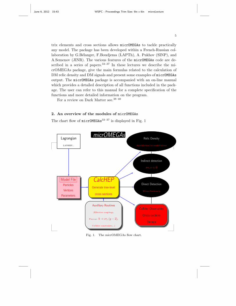
2. An overview of the modules of micrOMEGAs
The chart flow of micrOMEGAs33–37 is displayed in Fig. 1
micrOMEGAsLagrangian
LANHEP,..
Relic Density
Annihilation/co-annihilations
Indirect detection
σv, v = 0
Model File
Particles
Vertices
Parameters
CalcHEP
Generate tree-level
cross sections
Direct Detection
Wimp-Nucleon/q
Auxilliary Routines
(Effective couplings,
Flavour: b → sγ, (g − 2),
Collider constraints,..)
Collider Observables
Cross sections
Decays
Fig. 1. The micrOMEGAs flow chart.
June 6, 2012 15:43 WSPC - Proceedings Trim Size: 9in x 6in microLecture
6
All the observables we have pointed at require the computation of inter-
action rates. The calculation of the cross sections in different kinematical
regimes is at the heart of the system. We rely on CalcHEP41,42 for the gen-
eration of all tree-level cross sections. Naturally a model must be defined.
CalcHEP requires therefore a model file which defines the nature of all par-
ticles in the model (spin, charges,..), parameters (masses, couplings) as well
as the interaction vertices or in other words the Feynman rules. Once this
is specified in the proper format, CalcHEP proceeds to the identification
of the DM particle. The Zn assignment is therefore crucial as is of course
the mass ordering and the electric neutral character of the WIMP candi-
date. The current public version of micrOMEGAs can only treat models
with Z2 and Z3 discrete symmetries. The code is then ready to process any
needed cross section. For some models, for example the MSSM, deriving
the Feynman rules is a horrendous task. Traditionally micrOMEGAs has re-
lied on LanHEP43 which is a code that outputs the model file once given
the Lagrangian. FEYNRULES44 is another recent code that can achieve the
same effect. From the cross sections which are model specific, the code calls
different shared libraries (common to all models) to output the value of
• the relic density
• the rates for indirect detection of e+, p, γ, ν. For the case of ν this includes
capture by the Sun and the Earth.
• direct detection for specific targets in large-scale underground experi-
ments.
• cross sections at colliders and branching ratios for various particles of the
model.
This sequence of calls and computations is automated. The code includes
also many auxiliary routines which are model specific. Since CalcHEP is
a tree level cross section generator some important radiative corrections
must be introduced through the auxiliary routines. This is the case of the
MSSM where the mass of the lightest Higgs must be corrected in a coher-
ent way through an effective Lagrangian that can be interfaced to some
spectrum calculator, for example FeynHiggs45 or corrections to Higgs cou-
plings (HDECAY46). Input of the MSSM mass spectrum is also implemented
through SLHA.47,48 Other routines include computations such as (g − 2),
b → sγ, Bs → µ + µ−,..Bounds on some masses and parameters can be
easily input by the user with sometimes the help of external codes such
as HiggsBounds.49,50 The code is “open source” and allows to add a large
number of models and also different external codes for some of the auxiliary
June 6, 2012 15:43 WSPC - Proceedings Trim Size: 9in x 6in microLecture
7
routines.
3. Downloading and compilation of micrOMEGAs.
To download micrOMEGAs, go to
http://lapth.in2p3.fr/micromegas
and unpack the file received, micromegas_2.6.X.tgz, with the command
tar -xvzf micromegas_2.6.X.tgz
This should create the directory micromegas_2.6.X/ which occupies about
40 Mb of disk space. You will need more disk space after compilation of
specific models and generation of matrix elements. In case of problems and
questions
email: [email protected]
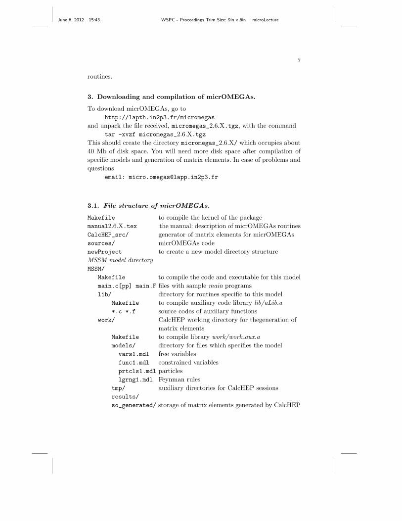
3.1. File structure of micrOMEGAs.
Makefile to compile the kernel of the package
manual2.6.X.tex the manual: description of micrOMEGAs routines
CalcHEP_src/ generator of matrix elements for micrOMEGAs
sources/ micrOMEGAs code
newProject to create a new model directory structure
MSSM model directory
MSSM/
Makefile to compile the code and executable for this model
main.c[pp] main.F files with sample main programs
lib/ directory for routines specific to this model
Makefile to compile auxiliary code library lib/aLib.a
*.c *.f source codes of auxiliary functions
work/ CalcHEP working directory for thegeneration of
matrix elements
Makefile to compile library work/work aux.a
models/ directory for files which specifies the model
vars1.mdl free variables
func1.mdl constrained variables
prtcls1.mdl particles
lgrng1.mdl Feynman rules
tmp/ auxiliary directories for CalcHEP sessions
results/
so_generated/ storage of matrix elements generated by CalcHEP
June 6, 2012 15:43 WSPC - Proceedings Trim Size: 9in x 6in microLecture
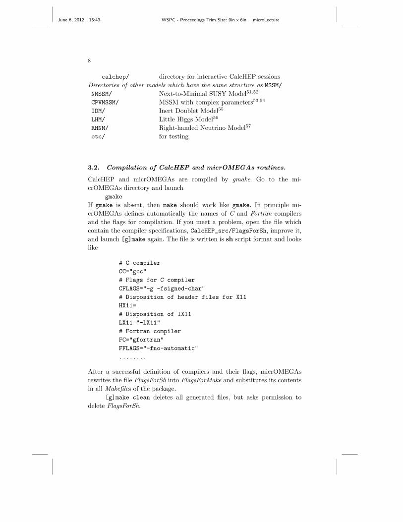
8
calchep/ directory for interactive CalcHEP sessions
Directories of other models which have the same structure as MSSM/
NMSSM/ Next-to-Minimal SUSY Model51,52
CPVMSSM/ MSSM with complex parameters53,54
IDM/ Inert Doublet Model55
LHM/ Little Higgs Model56
RHNM/ Right-handed Neutrino Model57
etc/ for testing
3.2. Compilation of CalcHEP and micrOMEGAs routines.
CalcHEP and micrOMEGAs are compiled by gmake. Go to the mi-
crOMEGAs directory and launch
gmake
If gmake is absent, then make should work like gmake. In principle mi-
crOMEGAs defines automatically the names of C and Fortran compilers
and the flags for compilation. If you meet a problem, open the file which
contain the compiler specifications, CalcHEP_src/FlagsForSh, improve it,
and launch [g]make again. The file is written is sh script format and looks
like
# C compiler
CC="gcc"
# Flags for C compiler
CFLAGS="-g -fsigned-char"
# Disposition of header files for X11
HX11=
# Disposition of lX11
LX11="-lX11"
# Fortran compiler
FC="gfortran"
FFLAGS="-fno-automatic"
........
After a successful definition of compilers and their flags, micrOMEGAs
rewrites the file FlagsForSh into FlagsForMake and substitutes its contents
in all Makefiles of the package.
[g]make clean deletes all generated files, but asks permission to
delete FlagsForSh.
June 6, 2012 15:43 WSPC - Proceedings Trim Size: 9in x 6in microLecture
9
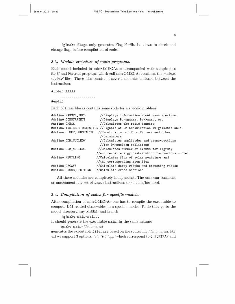
[g]make flags only generates FlagsForSh. It allows to check and
change flags before compilation of codes.
3.3. Module structure of main programs.
Each model included in micrOMEGAs is accompanied with sample files
for C and Fortran programs which call micrOMEGAs routines, the main.c,
main.F files. These files consist of several modules enclosed between the
instructions
#ifdef XXXXX
....................
#endif
Each of these blocks contains some code for a specific problem
#define MASSES_INFO //Displays information about mass spectrum
#define CONSTRAINTS //Displays B_>sgamma, Bs->mumu, etc
#define OMEGA //Calculates the relic density
#define INDIRECT_DETECTION //Signals of DM annihilation in galactic halo
#define RESET_FORMFACTORS //Redefinition of Form Factors and other
//parameters
#define CDM_NUCLEON //Calculates amplitudes and cross-sections
//for DM-nucleon collisions
#define CDM_NUCLEUS //Calculates number of events for 1kg*day
//and recoil energy distribution for various nuclei
#define NEUTRINO //Calculates flux of solar neutrinos and
//the corresponding muon flux
#define DECAYS //Calculate decay widths and branching ratios
#define CROSS_SECTIONS //Calculate cross sections
All these modules are completely independent. The user can comment
or uncomment any set of define instructions to suit his/her need.
3.4. Compilation of codes for specific models.
After compilation of micrOMEGAs one has to compile the executable to
compute DM related observables in a specific model. To do this, go to the
model directory, say MSSM, and launch
[g]make main=main.c
It should generate the executable main. In the same manner
gmake main=filename.ext
generates the executable filename based on the source file filename.ext. For
ext we support 3 options: ’c’ , ’F’, ’cpp’ which correspond to C, FORTRAN and
June 6, 2012 15:43 WSPC - Proceedings Trim Size: 9in x 6in microLecture
10
C++ sources. [g]make called in the model directory automatically launches
[g]make in subdirectories lib and work to compile
lib/aLib.a - library of auxiliary model functions, e.g. constraints,
work/work_aux.a - library of model particles, free and dependent
parameters.
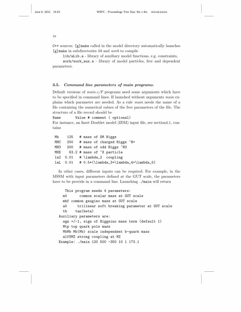
3.5. Command line parameters of main programs.
Default versions of main.c/F programs need some arguments which have
to be specified in command lines. If launched without arguments main ex-
plains which parameter are needed. As a rule main needs the name of a
file containing the numerical values of the free parameters of the file. The
structure of a file record should be
Name Value # comment ( optional)
For instance, an Inert Doublet model (IDM) input file, see section4.1, con-
tains
Mh 125 # mass of SM Higgs
MHC 200 # mass of charged Higgs ~H+
MH3 200 # mass of odd Higgs ~H3
MHX 63.2 # mass of ~X particle
la2 0.01 # \lambda_2 coupling
laL 0.01 # 0.5*(\lambda_3+\lambda_4+\lambda_5)
In other cases, different inputs can be required. For example, in the
MSSM with input parameters defined at the GUT scale, the parameters
have to be provide in a command line. Launching ./main will return
This program needs 4 parameters:
m0 common scalar mass at GUT scale
mhf common gaugino mass at GUT scale
a0 trilinear soft breaking parameter at GUT scale
tb tan(beta)
Auxiliary parameters are:
sgn +/-1, sign of Higgsino mass term (default 1)
Mtp top quark pole mass
MbMb Mb(Mb) scale independent b-quark mass
alfSMZ strong coupling at MZ
Example: ./main 120 500 -350 10 1 173.1
June 6, 2012 15:43 WSPC - Proceedings Trim Size: 9in x 6in microLecture
11
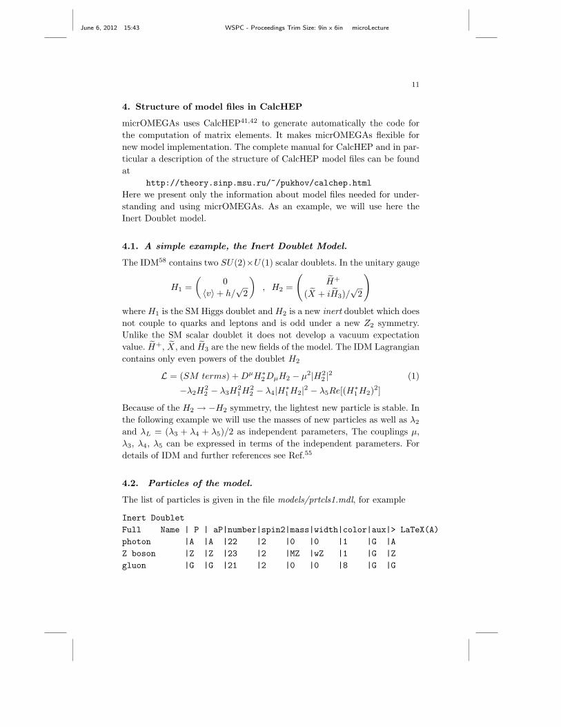
4. Structure of model files in CalcHEP
micrOMEGAs uses CalcHEP41,42 to generate automatically the code for
the computation of matrix elements. It makes micrOMEGAs flexible for
new model implementation. The complete manual for CalcHEP and in par-
ticular a description of the structure of CalcHEP model files can be found
at
http://theory.sinp.msu.ru/~/pukhov/calchep.html
Here we present only the information about model files needed for under-
standing and using micrOMEGAs. As an example, we will use here the
Inert Doublet model.
4.1. A simple example, the Inert Doublet Model.
The IDM58 contains two SU(2)×U(1) scalar doublets. In the unitary gauge
H1 =
(0
〈v〉 + h/√
2
), H2 =
(H+
(X + iH3)/√
2
)
where H1 is the SM Higgs doublet and H2 is a new inert doublet which does
not couple to quarks and leptons and is odd under a new Z2 symmetry.
Unlike the SM scalar doublet it does not develop a vacuum expectation
value. H+, X, and H3 are the new fields of the model. The IDM Lagrangian
contains only even powers of the doublet H2
L = (SM terms) + DµH∗2DµH2 − µ2|H2
2 |2 (1)
−λ2H22 − λ3H
21H2
2 − λ4|H∗1H2|2 − λ5Re[(H∗
1H2)2]
Because of the H2 → −H2 symmetry, the lightest new particle is stable. In
the following example we will use the masses of new particles as well as λ2
and λL = (λ3 + λ4 + λ5)/2 as independent parameters, The couplings µ,
λ3, λ4, λ5 can be expressed in terms of the independent parameters. For
details of IDM and further references see Ref.55
4.2. Particles of the model.
The list of particles is given in the file models/prtcls1.mdl, for example
Inert Doublet
Full Name | P | aP|number|spin2|mass|width|color|aux|> LaTeX(A)
photon |A |A |22 |2 |0 |0 |1 |G |A
Z boson |Z |Z |23 |2 |MZ |wZ |1 |G |Z
gluon |G |G |21 |2 |0 |0 |8 |G |G
June 6, 2012 15:43 WSPC - Proceedings Trim Size: 9in x 6in microLecture
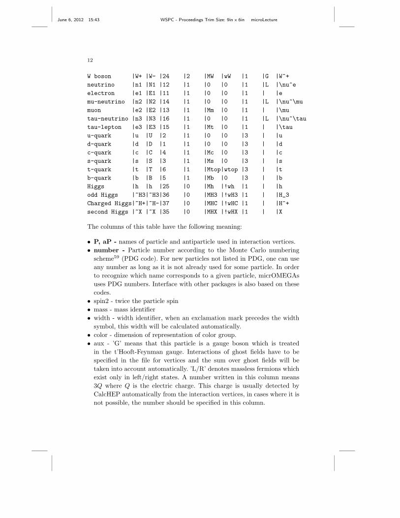
12
W boson |W+ |W- |24 |2 |MW |wW |1 |G |W^+
neutrino |n1 |N1 |12 |1 |0 |0 |1 |L |\nu^e
electron |e1 |E1 |11 |1 |0 |0 |1 | |e
mu-neutrino |n2 |N2 |14 |1 |0 |0 |1 |L |\nu^\mu
muon |e2 |E2 |13 |1 |Mm |0 |1 | |\mu
tau-neutrino |n3 |N3 |16 |1 |0 |0 |1 |L |\nu^\tau
tau-lepton |e3 |E3 |15 |1 |Mt |0 |1 | |\tau
u-quark |u |U |2 |1 |0 |0 |3 | |u
d-quark |d |D |1 |1 |0 |0 |3 | |d
c-quark |c |C |4 |1 |Mc |0 |3 | |c
s-quark |s |S |3 |1 |Ms |0 |3 | |s
t-quark |t |T |6 |1 |Mtop|wtop |3 | |t
b-quark |b |B |5 |1 |Mb |0 |3 | |b
Higgs |h |h |25 |0 |Mh |!wh |1 | |h
odd Higgs |~H3|~H3|36 |0 |MH3 |!wH3 |1 | |H_3
Charged Higgs|~H+|~H-|37 |0 |MHC |!wHC |1 | |H^+
second Higgs |~X |~X |35 |0 |MHX |!wHX |1 | |X
The columns of this table have the following meaning:
• P, aP - names of particle and antiparticle used in interaction vertices.
• number - Particle number according to the Monte Carlo numbering
scheme59 (PDG code). For new particles not listed in PDG, one can use
any number as long as it is not already used for some particle. In order
to recognize which name corresponds to a given particle, micrOMEGAs
uses PDG numbers. Interface with other packages is also based on these
codes.
• spin2 - twice the particle spin
• mass - mass identifier
• width - width identifier, when an exclamation mark precedes the width
symbol, this width will be calculated automatically.
• color - dimension of representation of color group.
• aux - ’G’ means that this particle is a gauge boson which is treated
in the t’Hooft-Feynman gauge. Interactions of ghost fields have to be
specified in the file for vertices and the sum over ghost fields will be
taken into account automatically. ’L/R’ denotes massless fermions which
exist only in left/right states. A number written in this column means
3Q where Q is the electric charge. This charge is usually detected by
CalcHEP automatically from the interaction vertices, in cases where it is
not possible, the number should be specified in this column.
June 6, 2012 15:43 WSPC - Proceedings Trim Size: 9in x 6in microLecture
13
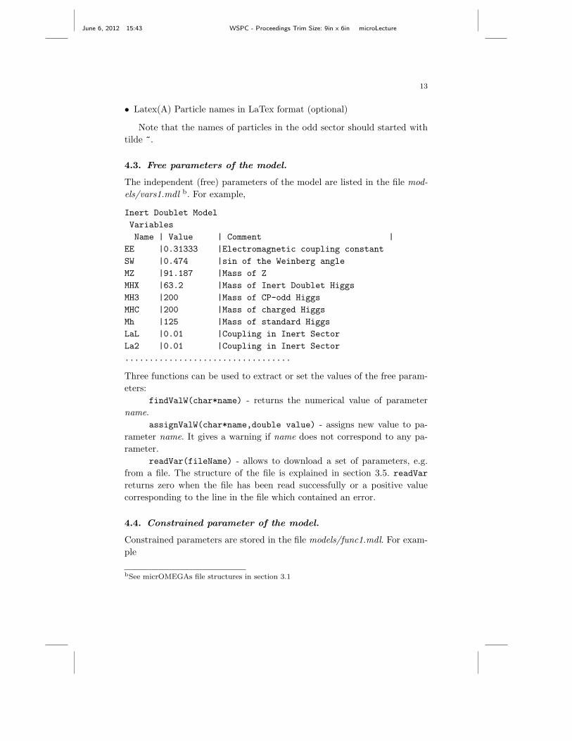
• Latex(A) Particle names in LaTex format (optional)
Note that the names of particles in the odd sector should started with
tilde ~.
4.3. Free parameters of the model.
The independent (free) parameters of the model are listed in the file mod-
els/vars1.mdl b. For example,
Inert Doublet Model
Variables
Name | Value | Comment |
EE |0.31333 |Electromagnetic coupling constant
SW |0.474 |sin of the Weinberg angle
MZ |91.187 |Mass of Z
MHX |63.2 |Mass of Inert Doublet Higgs
MH3 |200 |Mass of CP-odd Higgs
MHC |200 |Mass of charged Higgs
Mh |125 |Mass of standard Higgs
LaL |0.01 |Coupling in Inert Sector
La2 |0.01 |Coupling in Inert Sector
..................................
Three functions can be used to extract or set the values of the free param-
eters:
findValW(char*name) - returns the numerical value of parameter
name.
assignValW(char*name,double value) - assigns new value to pa-
rameter name. It gives a warning if name does not correspond to any pa-
rameter.
readVar(fileName) - allows to download a set of parameters, e.g.
from a file. The structure of the file is explained in section 3.5. readVar
returns zero when the file has been read successfully or a positive value
corresponding to the line in the file which contained an error.
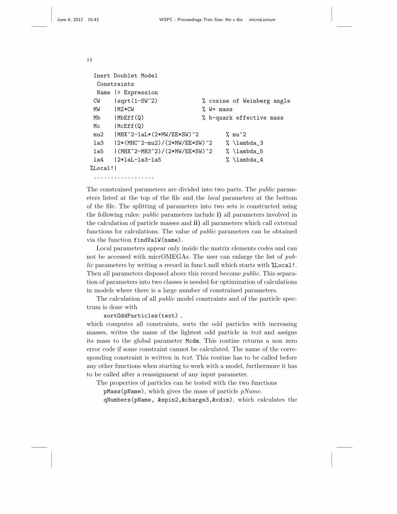
4.4. Constrained parameter of the model.
Constrained parameters are stored in the file models/func1.mdl. For exam-
ple
bSee micrOMEGAs file structures in section 3.1
June 6, 2012 15:43 WSPC - Proceedings Trim Size: 9in x 6in microLecture
14
Inert Doublet Model
Constraints
Name |> Expression
CW |sqrt(1-SW^2) % cosine of Weinberg angle
MW |MZ*CW % W+ mass
Mb |MbEff(Q) % b-quark effective mass
Mc |McEff(Q)
mu2 |MHX^2-laL*(2*MW/EE*SW)^2 % mu^2
la3 |2*(MHC^2-mu2)/(2*MW/EE*SW)^2 % \lambda_3
la5 |(MHX^2-MH3^2)/(2*MW/EE*SW)^2 % \lambda_5
la4 |2*laL-la3-la5 % \lambda_4
%Local!|
..................
The constrained parameters are divided into two parts. The public param-
eters listed at the top of the file and the local parameters at the bottom
of the file. The splitting of parameters into two sets is constructed using
the following rules: public parameters include i) all parameters involved in
the calculation of particle masses and ii) all parameters which call external
functions for calculations. The value of public parameters can be obtained
via the function findValW(name).
Local parameters appear only inside the matrix elements codes and can
not be accessed with micrOMEGAs. The user can enlarge the list of pub-
lic parameters by writing a record in func1.mdl which starts with %Local!.
Then all parameters disposed above this record become public. This separa-
tion of parameters into two classes is needed for optimization of calculations
in models where there is a large number of constrained parameters.
The calculation of all public model constraints and of the particle spec-
trum is done with
sortOddParticles(text) ,
which computes all constraints, sorts the odd particles with increasing
masses, writes the name of the lightest odd particle in text and assigns
its mass to the global parameter Mcdm. This routine returns a non zero
error code if some constraint cannot be calculated. The name of the corre-
sponding constraint is written in text. This routine has to be called before
any other functions when starting to work with a model, furthermore it has
to be called after a reassignment of any input parameter.
The properties of particles can be tested with the two functions
pMass(pName), which gives the mass of particle pName.
qNumbers(pName, &spin2,&charge3,&cdim), which calculates the
June 6, 2012 15:43 WSPC - Proceedings Trim Size: 9in x 6in microLecture
15
quantum numbers of a particle and returns directly its PDG code. This
function allows to check that the Dark Matter candidate has no electric or
color charges.
The table of Feynman rules for each model is rather long. For ex-
ample, one can check the IDM/work/models/lgrng1.mdl file to see how
the interactions of SM and Inert doublet particles are presented in
CalcHEP/micrOMEGAs.
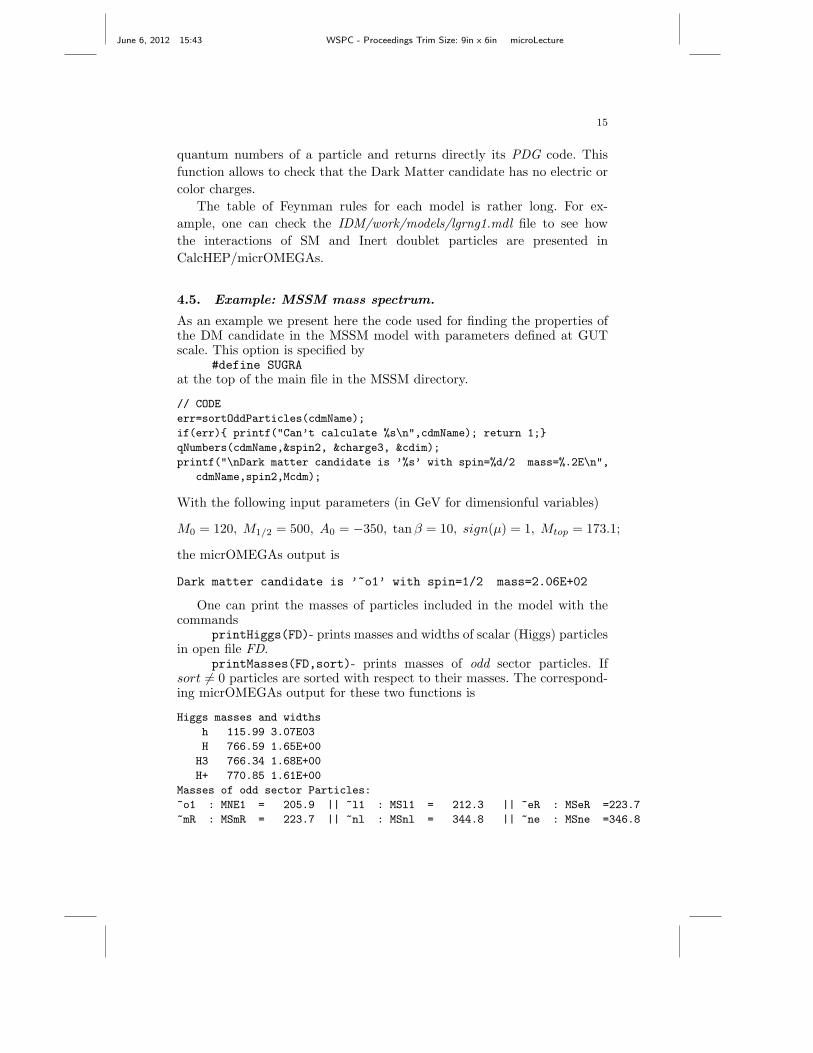
4.5. Example: MSSM mass spectrum.
As an example we present here the code used for finding the properties ofthe DM candidate in the MSSM model with parameters defined at GUTscale. This option is specified by
#define SUGRAat the top of the main file in the MSSM directory.
// CODE
err=sortOddParticles(cdmName);
if(err) printf("Can’t calculate %s\n",cdmName); return 1;
qNumbers(cdmName,&spin2, &charge3, &cdim);
printf("\nDark matter candidate is ’%s’ with spin=%d/2 mass=%.2E\n",
cdmName,spin2,Mcdm);
With the following input parameters (in GeV for dimensionful variables)
M0 = 120, M1/2 = 500, A0 = −350, tan β = 10, sign(µ) = 1, Mtop = 173.1;
the micrOMEGAs output is
Dark matter candidate is ’~o1’ with spin=1/2 mass=2.06E+02
One can print the masses of particles included in the model with thecommands
printHiggs(FD)- prints masses and widths of scalar (Higgs) particlesin open file FD.
printMasses(FD,sort)- prints masses of odd sector particles. Ifsort 6= 0 particles are sorted with respect to their masses. The correspond-ing micrOMEGAs output for these two functions is
Higgs masses and widths
h 115.99 3.07E03
H 766.59 1.65E+00
H3 766.34 1.68E+00
H+ 770.85 1.61E+00
Masses of odd sector Particles:
~o1 : MNE1 = 205.9 || ~l1 : MSl1 = 212.3 || ~eR : MSeR =223.7
~mR : MSmR = 223.7 || ~nl : MSnl = 344.8 || ~ne : MSne =346.8
June 6, 2012 15:43 WSPC - Proceedings Trim Size: 9in x 6in microLecture
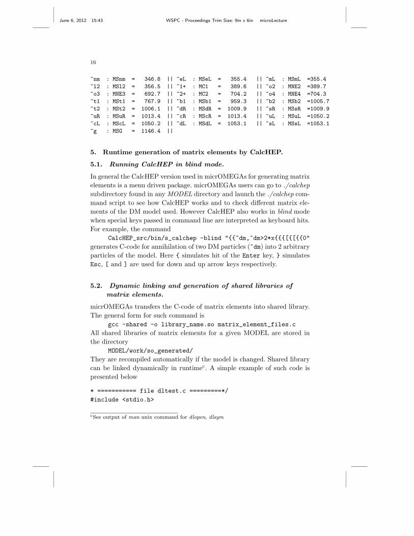
16
~nm : MSnm = 346.8 || ~eL : MSeL = 355.4 || ~mL : MSmL =355.4
~l2 : MSl2 = 356.5 || ~1+ : MC1 = 389.6 || ~o2 : MNE2 =389.7
~o3 : MNE3 = 692.7 || ~2+ : MC2 = 704.2 || ~o4 : MNE4 =704.3
~t1 : MSt1 = 767.9 || ~b1 : MSb1 = 959.3 || ~b2 : MSb2 =1005.7
~t2 : MSt2 = 1006.1 || ~dR : MSdR = 1009.9 || ~sR : MSsR =1009.9
~uR : MSuR = 1013.4 || ~cR : MScR = 1013.4 || ~uL : MSuL =1050.2
~cL : MScL = 1050.2 || ~dL : MSdL = 1053.1 || ~sL : MSsL =1053.1
~g : MSG = 1146.4 ||
5. Runtime generation of matrix elements by CalcHEP.
5.1. Running CalcHEP in blind mode.
In general the CalcHEP version used in micrOMEGAs for generating matrix
elements is a menu driven package. micrOMEGAs users can go to ./calchep
subdirectory found in any MODEL directory and launch the ./calchep com-
mand script to see how CalcHEP works and to check different matrix ele-
ments of the DM model used. However CalcHEP also works in blind mode
when special keys passed in command line are interpreted as keyboard hits.
For example, the command
CalcHEP_src/bin/s_calchep -blind "~dm,~dm>2*x[[0"
generates C-code for annihilation of two DM particles (~dm) into 2 arbitrary
particles of the model. Here simulates hit of the Enter key, simulates
Esc, [ and ] are used for down and up arrow keys respectively.
5.2. Dynamic linking and generation of shared libraries of
matrix elements.
micrOMEGAs transfers the C-code of matrix elements into shared library.
The general form for such command is
gcc -shared -o library_name.so matrix_element_files.c
All shared libraries of matrix elements for a given MODEL are stored in
the directory
MODEL/work/so_generated/
They are recompiled automatically if the model is changed. Shared library
can be linked dynamically in runtimec. A simple example of such code is
presented below
* =========== file dltest.c =========*/
#include <stdio.h>
cSee output of man unix command for dlopen, dlsym
June 6, 2012 15:43 WSPC - Proceedings Trim Size: 9in x 6in microLecture
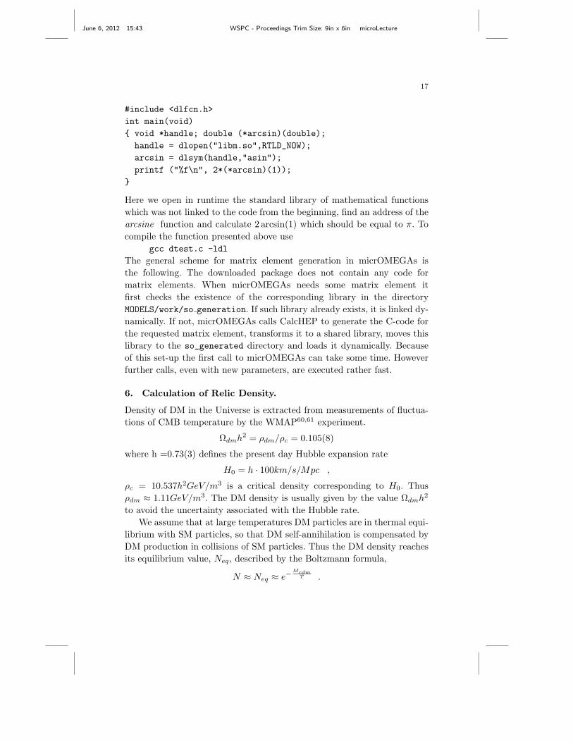
17
#include <dlfcn.h>
int main(void)
void *handle; double (*arcsin)(double);
handle = dlopen("libm.so",RTLD_NOW);
arcsin = dlsym(handle,"asin");
printf ("%f\n", 2*(*arcsin)(1));
Here we open in runtime the standard library of mathematical functions
which was not linked to the code from the beginning, find an address of the
arcsine function and calculate 2 arcsin(1) which should be equal to π. To
compile the function presented above use
gcc dtest.c -ldl
The general scheme for matrix element generation in micrOMEGAs is
the following. The downloaded package does not contain any code for
matrix elements. When micrOMEGAs needs some matrix element it
first checks the existence of the corresponding library in the directory
MODELS/work/so generation. If such library already exists, it is linked dy-
namically. If not, micrOMEGAs calls CalcHEP to generate the C-code for
the requested matrix element, transforms it to a shared library, moves this
library to the so_generated directory and loads it dynamically. Because
of this set-up the first call to micrOMEGAs can take some time. However
further calls, even with new parameters, are executed rather fast.
6. Calculation of Relic Density.
Density of DM in the Universe is extracted from measurements of fluctua-
tions of CMB temperature by the WMAP60,61 experiment.
Ωdmh2 = ρdm/ρc = 0.105(8)
where h =0.73(3) defines the present day Hubble expansion rate
H0 = h · 100km/s/Mpc ,
ρc = 10.537h2GeV/m3 is a critical density corresponding to H0. Thus
ρdm ≈ 1.11GeV/m3. The DM density is usually given by the value Ωdmh2
to avoid the uncertainty associated with the Hubble rate.
We assume that at large temperatures DM particles are in thermal equi-
librium with SM particles, so that DM self-annihilation is compensated by
DM production in collisions of SM particles. Thus the DM density reaches
its equilibrium value, Neq, described by the Boltzmann formula,
N ≈ Neq ≈ e−Mcdm
T .
June 6, 2012 15:43 WSPC - Proceedings Trim Size: 9in x 6in microLecture
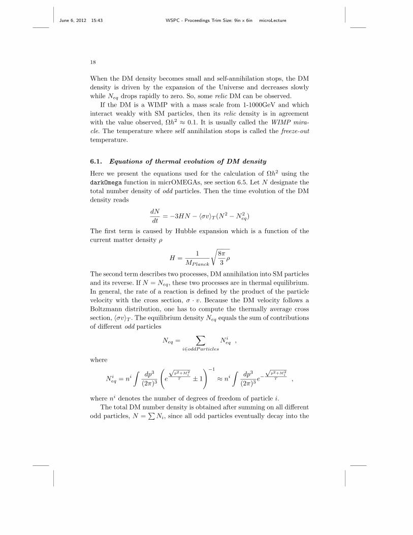
18
When the DM density becomes small and self-annihilation stops, the DM
density is driven by the expansion of the Universe and decreases slowly
while Neq drops rapidly to zero. So, some relic DM can be observed.
If the DM is a WIMP with a mass scale from 1-1000GeV and which
interact weakly with SM particles, then its relic density is in agreement
with the value observed, Ωh2 ≈ 0.1. It is usually called the WIMP mira-
cle. The temperature where self annihilation stops is called the freeze-out
temperature.
6.1. Equations of thermal evolution of DM density
Here we present the equations used for the calculation of Ωh2 using the
darkOmega function in micrOMEGAs, see section 6.5. Let N designate the
total number density of odd particles. Then the time evolution of the DM
density reads
dN
dt= −3HN − 〈σv〉T (N2 − N2
eq)
The first term is caused by Hubble expansion which is a function of the
current matter density ρ
H =1
MPlanck
√8π
3ρ
The second term describes two processes, DM annihilation into SM particles
and its reverse. If N = Neq, these two processes are in thermal equilibrium.
In general, the rate of a reaction is defined by the product of the particle
velocity with the cross section, σ · v. Because the DM velocity follows a
Boltzmann distribution, one has to compute the thermally average cross
section, 〈σv〉T . The equilibrium density Neq equals the sum of contributions
of different odd particles
Neq =∑
i∈oddParticles
N ieq ,
where
N ieq = ni
∫dp3
(2π)3
(e
√p2+M2
iT ± 1
)−1
≈ ni
∫dp3
(2π)3e−
√p2+M2
iT ,
where ni denotes the number of degrees of freedom of particle i.
The total DM number density is obtained after summing on all different
odd particles, N =∑
Ni, since all odd particles eventually decay into the
June 6, 2012 15:43 WSPC - Proceedings Trim Size: 9in x 6in microLecture
19
DM. One can assume a chemical equilibrium between different components
Ni because of the decays of all odd particles into the lightest one. Thus,
Ni(T )/Nj(T ) = N ieq(T )/N j
eq(T ) ≈ e−Mi−Mj
T
Consequently the formula for 〈σv〉T should contain averaging over different
particle of the odd sector. One can find explicit formulas for 〈σv〉T in the
papers.35,62
Let us define s as the entropy density. Because of entropy conservation
ds
dt= −3H · s
and we can replace the equation for the number density by a simpler equa-
tion for the abundance Y = N/s
dY
ds=
1
3H〈σv〉T (Y 2 − Yeq(T )2) =
MPlanck√24πρ
〈σv〉T (Y 2 − Yeq(T )2) (2)
6.2. Thermodynamics of Universe
The formulas that give the contribution of one relativistic degree of freedom
to the entropy density and energy density of the Universe are rather simple.
For bosons
ρb =π2
30T 4 , sb =
2π2
45T 3 (3)
The corresponding functions for fermions have an additional factor 78 . In
the generic case one can write
ρ(T ) =π2
30T 4geff (T ) , s(T ) =
2π2
45T 3heff (T ) (4)
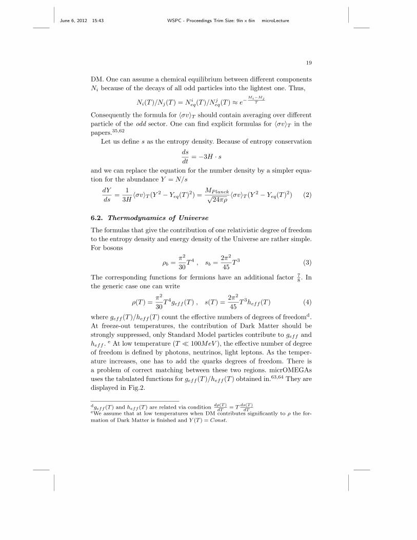
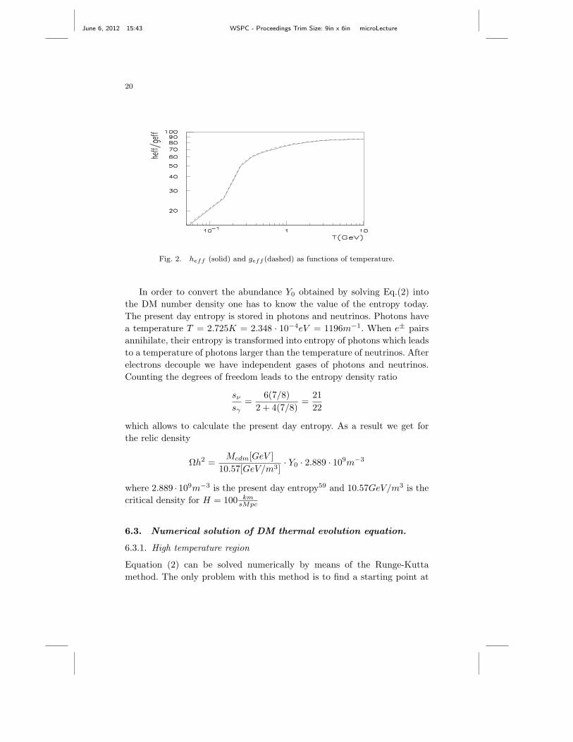
where geff (T )/heff (T ) count the effective numbers of degrees of freedomd.
At freeze-out temperatures, the contribution of Dark Matter should be
strongly suppressed, only Standard Model particles contribute to geff and
heff . e At low temperature (T ≪ 100MeV ), the effective number of degree
of freedom is defined by photons, neutrinos, light leptons. As the temper-
ature increases, one has to add the quarks degrees of freedom. There is
a problem of correct matching between these two regions. micrOMEGAs
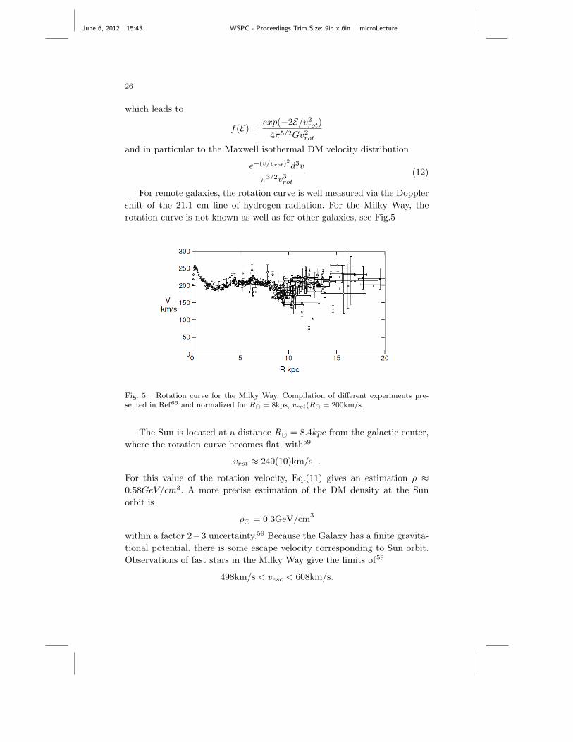
uses the tabulated functions for geff (T )/heff (T ) obtained in.63,64 They are
displayed in Fig.2.
dgeff (T ) and heff (T ) are related via conditiondρ(T )
dT= T
ds(T )dT
eWe assume that at low temperatures when DM contributes significantly to ρ the for-mation of Dark Matter is finished and Y (T ) = Const.
June 6, 2012 15:43 WSPC - Proceedings Trim Size: 9in x 6in microLecture
20
Fig. 2. heff (solid) and geff (dashed) as functions of temperature.
In order to convert the abundance Y0 obtained by solving Eq.(2) into
the DM number density one has to know the value of the entropy today.
The present day entropy is stored in photons and neutrinos. Photons have
a temperature T = 2.725K = 2.348 · 10−4eV = 1196m−1. When e± pairs
annihilate, their entropy is transformed into entropy of photons which leads
to a temperature of photons larger than the temperature of neutrinos. After
electrons decouple we have independent gases of photons and neutrinos.
Counting the degrees of freedom leads to the entropy density ratio
sν
sγ=
6(7/8)
2 + 4(7/8)=
21
22
which allows to calculate the present day entropy. As a result we get for
the relic density
Ωh2 =Mcdm[GeV ]
10.57[GeV/m3]· Y0 · 2.889 · 109m−3
where 2.889 · 109m−3 is the present day entropy59 and 10.57GeV/m3 is the
critical density for H = 100 kmsMpc
6.3. Numerical solution of DM thermal evolution equation.
6.3.1. High temperature region
Equation (2) can be solved numerically by means of the Runge-Kutta
method. The only problem with this method is to find a starting point at
June 6, 2012 15:43 WSPC - Proceedings Trim Size: 9in x 6in microLecture
21
high temperature. Let ∆Y = Y − Yeq. Assuming that at high temperature
∆Y ≪ Yeq ,d∆Y
ds≪ dYeq
ds(5)
we estimate
∆Y =d log Yeq(s)
ds
√6πρ
MPlanck〈σv〉T. (6)
The function Yeq drops rapidly, nevertheless our initial assumption (5) is
satisfied because the dependence on Yeq is only logarithmic. This gives us a
rather simple picture of freeze-out. We have an almost constant ∆Y on the
background of a fast dropping Yeq as the temperature decreases. At some
temperature ∆Y becomes comparable with Yeq and we have the freezing-
out of Y ≈ ∆Y .
micrOMEGAs uses Eq.(6) to find the starting point for the Runge-Kutta
procedure looking for a point where ∆Y ≈ 0.1Yeq.
6.3.2. Freeze-out approximation
One can use Eq.(6) to find sf ( or the corresponding Tf ) where Y (Tf ) ≫Yeq(T ). micrOMEGAs defines Tf by condition
Y (Tf ) = 2.5Yeq(Tf ) . (7)
Below Tf one can neglect the Y 2eq term in Eq.(2) and get the explicit solution
1
Y (s0)=
1
2.5Yeq(sf )+
∫ sf
s0
dsMPlanck〈σv〉T√
24πρ(8)
This solution is called freeze-out approximation and as a rule works with
≈ 2% accuracy.
One can make further approximations and discard the first term in the
right side of (8). This approximation corresponds to an infinite DM density
at Tf and works with ≈ 20% accuracy
1
Y (s0)=
∫ sf
s0
dsMPlanck〈σv〉T√
24πρ(9)
micrOMEGAs uses this to calculate the relative contributions of different
channels to Ω−1. It gives an understanding of the physical reactions respon-
sible for relic DM formation.
June 6, 2012 15:43 WSPC - Proceedings Trim Size: 9in x 6in microLecture
22
6.4. The Z3 case.
The Z3 internal charge of particles can be zero, 1, or −1, which corresponds
to phases 0, 2π3 , −2π
3 . The lightest particle with non-zero charge has to be
stable. Particles with charge −1 are the antiparticles of those with charge
1. Thus, only one DM candidate is expected. We have 2 types of reactions
which change the DM density
X, Y → SM,SM X, Y → Z, SM (10)
The second type of reactions modify the abundance equation, Eq.(2),
dY
ds=
MPlanck√24πρ
(〈σv〉11→00T (Y 2 − Yeq(T )2) + 0.5〈σv〉11→10
T Y · (Y − Yeq(T ))
where 〈σv〉11→00T , 〈σv〉11→10
T define the thermally average cross section for 2
particles with charge ±1 annihilating into particles with charge 0 and into a
charge 1 and a charge 0 respectively. The modified abundance equation can
be solved by the same method as Eq.(2) and is included in micrOMEGAs.
The case of Z4 discrete symmetry which leads to two stable particles with
Z4 charges 1,-1 and 2,-2 is not treated in the current version of mi-
crOMEGAs, however see Ref.11 for an application.
6.5. The micrOMEGAs routines.
Ωh2 can be calculated by the function
omega= darkOmega(&Xf, fast,Beps);
where fast and Beps are input parameters. fast 6= 0 leads to an opti-
mized fast calculation. The parameter Besp allows to change the number of
channels taken into account for the evaluation of Ωh2. The contribution of
channels for which the sum of the mass of incoming or outgoing particles,
Ms, is large is suppressed by the Boltzmann factor
e2Mcdm−Ms
Tf
where Tf is the freeze-out temperature (7). micrOMEGAs discards all
channels for which this factor is smaller then Beps. The default value
Beps = 10−4 leads to a robust evaluation of the relic density. In some
special cases, for example, in models with extra dimensions, there are too
many co-annihilation channels and it is reasonable to set Beps = 10−2 to
have a fast calculation. The output parameter
Xf = Mcdm/Tf
June 6, 2012 15:43 WSPC - Proceedings Trim Size: 9in x 6in microLecture
23
characterizes the freeze-out temperature Tf . To get a reasonable value of
the DM density, the parameter Xf should be about 25.
The micrOMEGAs package contains two routines which are useful for
understanding of relic density formation.
• printChannels(Xf,cut,Beps,prcnt,FD)
writes into opened file FD the contributions of different channels to (Ωh2)−1.
Here Xf is an input parameter which should be first evaluated in darkOmega.
Only the channels whose relative contribution is larger than cut will be dis-
played. Beps plays the same role as the darkOmega routine. If prcnt 6= 0
the contributions are given in percent. Note that for this specific purpose
we use the freeze-out approximation (9).
• vSigma(T,Beps,fast)
calculates the thermally averaged cross section for DM annihilation times
velocity at a temperature T [GeV], see formula (2.6) in Ref.33 The value for
σv is expressed in [pb]. The parameters Beps and fast work in the same
way as in the darkOmega function. In the Z3 case, vSigma returns
〈σv〉DM,DM−>SM,SMT + 0.5〈σv〉DM,DM−>DM,SM
T
The micrOMEGAs code contains the obsolete darkOmegaFO function
which calculates Ωh2 in freeze-out approximation (8).
6.6. Example of output
The output of darkOmega, vSigma and printChannels commands for the
MSSM point of section 4.5 is presented below,
==== Calculation of relic density =====
Xf=2.65e+01 Omega=1.10e01
Channels which contribute to 1/(omega) more than 1%.
Relative contributions in % are displyed
29% ~o1 ~l1 >A l
21% ~l1 ~l1 >l l
8% ~o1 ~l1 >Z l
6% ~l1 ~L1 >A A
4% ~o1 ~o1 >l L
3% ~o1 ~o1 >m M
3% ~o1 ~o1 >e E
3% ~o1 ~eR >A e
June 6, 2012 15:43 WSPC - Proceedings Trim Size: 9in x 6in microLecture
24
3% ~o1 ~mR >A m
3% ~l1 ~L1 >A Z
3% ~eR ~l1 >e l
3% ~mR ~l1 >m l
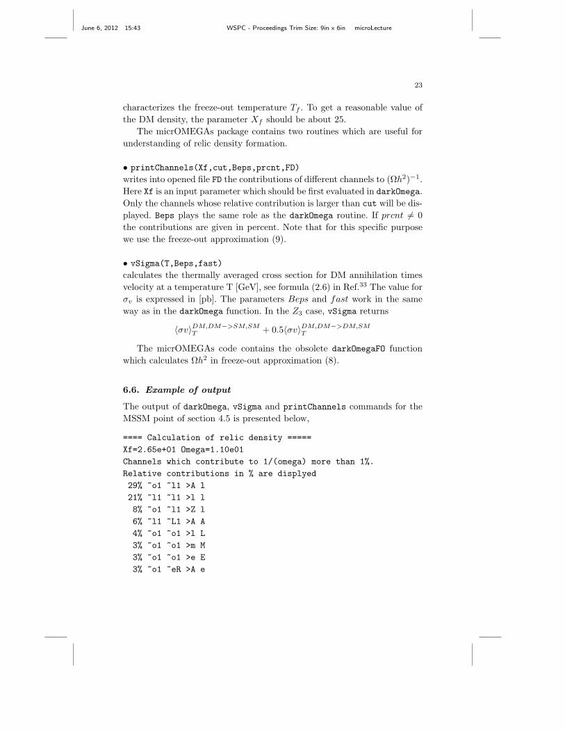
One can use the vSigma function to study the dependence of 〈σv〉 on
the temperature, see Fig.3.
Fig. 3. σv(T ) for the MSSM point of section 4.5 including all coannihilation
channes(solid) and the same for only neutralino self-annihilation(dashed).
For this test point, the contribution of DM (the neutralino - ~o1 ) self-
annihilation to Ω−1 is about 10%. The spectrum also contains the stau
particle (~l1 - superpartner of τ) which has a large self-annihilation cross
section as well as a large annihilation cross section with DM. Furthermore
the stau has a small mass difference with the DM (≈ 6 GeV). At the freeze-
out temperature (Tf ≈ 8GeV) the stau density is hardly suppressed by
the Boltzmann factor, therefore this particle give a large contribution to
〈σv〉T . Fig.3 shows that at low temperatures where the stau contribution is
suppressed, the total cross section is small, but at T = Tf it increases to
the [pb] level, this is sufficient to get a reasonable value for the relic density.
7. Dark Matter distribution in Milky Way.
Fluctuations of CMB temperatures provide crucial information about DM
in the early Universe before recombination. Other observables are related
to DM in the galaxies. To make predictions for these observables, one has to
June 6, 2012 15:43 WSPC - Proceedings Trim Size: 9in x 6in microLecture
25
know the DM density in the region of our Galaxy where the Sun is located
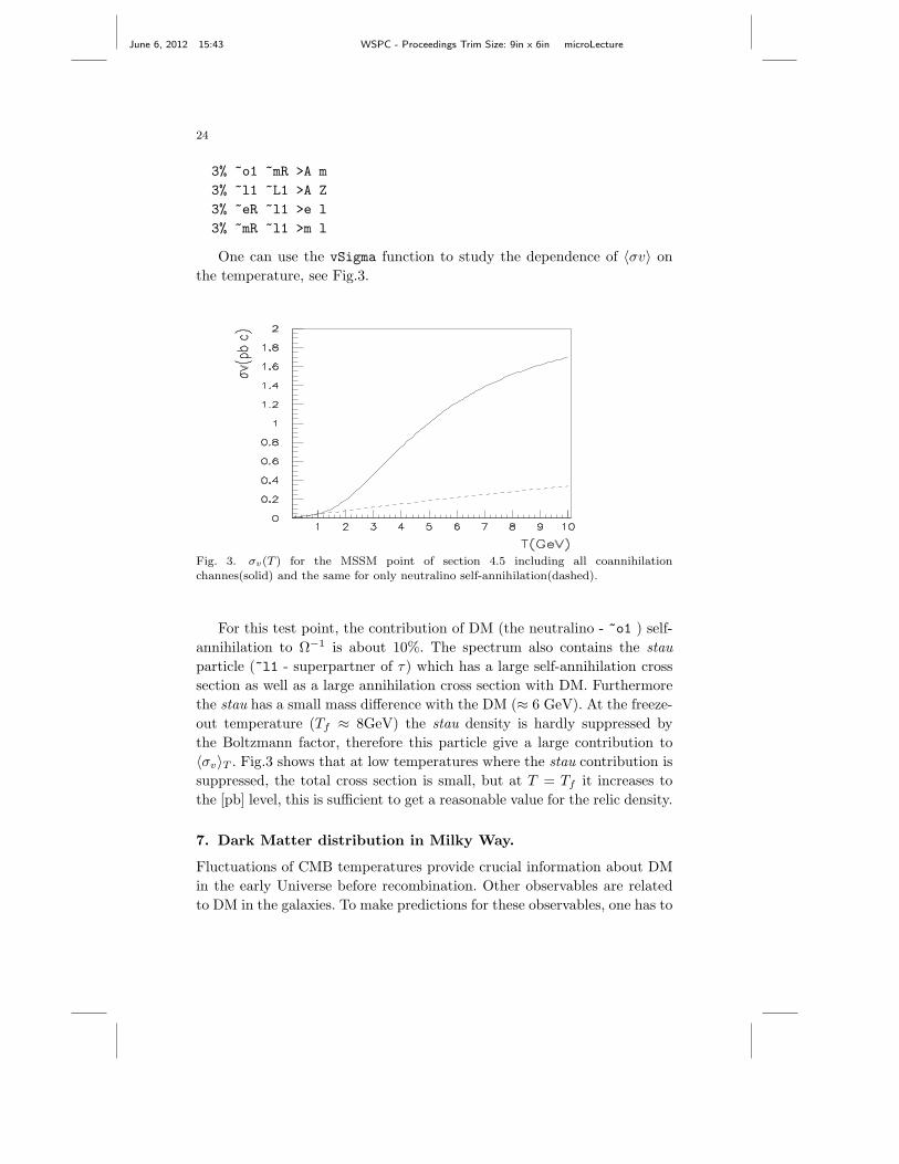
as well as the velocity distribution for DM particles. The more impressive
evidence of DM is the flatness of galactic rotation curves at large distances
r from the galactic center
v(r) ≈ Const
which is established from observations of a large set of spiral galaxies. See,
for instance, Fig.4.
Fig. 4. Rotation curve for spiral galaxy NGC 3198.65
For the rotation velocity to be constant at all distances, assuming that
the DM contribution dominates, the density has to be
ρ(r) =v2
rot
4πGr2, (11)
where G is the gravitational constant. DM velocity distribution is related
to the spatial distribution. In the simplest case one can assume the micro-
canonical DM phase space distributionf
f(Etot/Mcdm)d3vd3x = f(v2/2 − v2rotlog(r))d3vd3x ,
where v2rotlog(r) is the gravitational potential of unit mass. This phase space
distribution has to reproduce the DM density Eq.(11)∫
f(v2/2 − v2rotlog(r))d3v =
v2rot
4πGr2
fIn general, the equilibrium phase space distribution could also depend on angular mo-mentum.
June 6, 2012 15:43 WSPC - Proceedings Trim Size: 9in x 6in microLecture
26
which leads to
f(E) =exp(−2E/v2
rot)
4π5/2Gv2rot
and in particular to the Maxwell isothermal DM velocity distribution
e−(v/vrot)2
d3v
π3/2v3rot
(12)
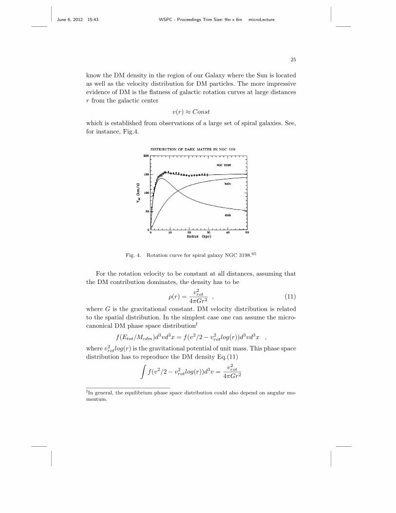
For remote galaxies, the rotation curve is well measured via the Doppler
shift of the 21.1 cm line of hydrogen radiation. For the Milky Way, the
rotation curve is not known as well as for other galaxies, see Fig.5
Fig. 5. Rotation curve for the Milky Way. Compilation of different experiments pre-
sented in Ref66 and normalized for R⊙ = 8kps, vrot(R⊙ = 200km/s.
The Sun is located at a distance R⊙ = 8.4kpc from the galactic center,
where the rotation curve becomes flat, with59
vrot ≈ 240(10)km/s .
For this value of the rotation velocity, Eq.(11) gives an estimation ρ ≈0.58GeV/cm3. A more precise estimation of the DM density at the Sun
orbit is
ρ⊙ = 0.3GeV/cm3
within a factor 2−3 uncertainty.59 Because the Galaxy has a finite gravita-
tional potential, there is some escape velocity corresponding to Sun orbit.
Observations of fast stars in the Milky Way give the limits of59
498km/s < vesc < 608km/s.
June 6, 2012 15:43 WSPC - Proceedings Trim Size: 9in x 6in microLecture
27
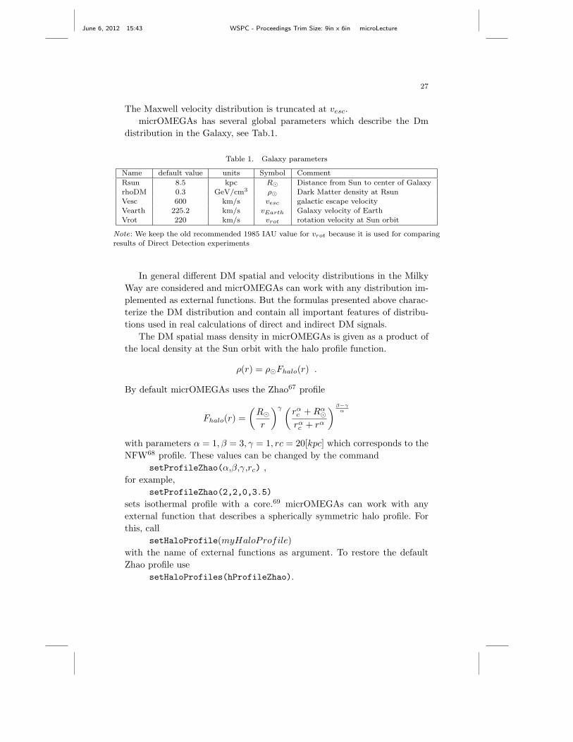
The Maxwell velocity distribution is truncated at vesc.
micrOMEGAs has several global parameters which describe the Dm
distribution in the Galaxy, see Tab.1.
Table 1. Galaxy parameters
Name default value units Symbol Comment
Rsun 8.5 kpc R⊙ Distance from Sun to center of Galaxy
rhoDM 0.3 GeV/cm3 ρ⊙ Dark Matter density at Rsun
Vesc 600 km/s vesc galactic escape velocityVearth 225.2 km/s vEarth Galaxy velocity of Earth
Vrot 220 km/s vrot rotation velocity at Sun orbit
Note: We keep the old recommended 1985 IAU value for vrot because it is used for comparingresults of Direct Detection experiments
In general different DM spatial and velocity distributions in the Milky
Way are considered and micrOMEGAs can work with any distribution im-
plemented as external functions. But the formulas presented above charac-
terize the DM distribution and contain all important features of distribu-
tions used in real calculations of direct and indirect DM signals.
The DM spatial mass density in micrOMEGAs is given as a product of
the local density at the Sun orbit with the halo profile function.
ρ(r) = ρ⊙Fhalo(r) .
By default micrOMEGAs uses the Zhao67 profile
Fhalo(r) =
(R⊙
r
)γ (rαc + Rα
⊙
rαc + rα
) β−γα
with parameters α = 1, β = 3, γ = 1, rc = 20[kpc] which corresponds to the
NFW68 profile. These values can be changed by the command
setProfileZhao(α,β,γ,rc) ,
for example,
setProfileZhao(2,2,0,3.5)
sets isothermal profile with a core.69 micrOMEGAs can work with any
external function that describes a spherically symmetric halo profile. For
this, call
setHaloProfile(myHaloProfile)
with the name of external functions as argument. To restore the default
Zhao profile use
setHaloProfiles(hProfileZhao).
June 6, 2012 15:43 WSPC - Proceedings Trim Size: 9in x 6in microLecture
28
8. Direct Detection in micrOMEGAs.
8.1. Amplitudes in the v = 0 limit.
To predict the Direct Detection rate one has to calculate the differential
cross section for elastic scattering of a DM particle on atomic nuclei. The
velocities of DM particles near the Earth are close to the orbital velocity of
the Sun, v ≈ 0.001c. Since elastic cross sections are finite in the v → 0 limit,
we can compute the DM nucleon cross sections in this limit thus simplifying
the computation. However the transfer momenta are large as compared
with the inverse size of a nucleus, so nuclei elastic form factors have to
be taken into account. In the non-relativistic limit the DM-nucleon elastic
amplitudes can be divided into two classes, the scalar or spin independent
(SI) interaction and the axial-vector or spin dependent (SD) interaction.
For a spin 1/2 nucleon interactions corresponding to higher spin exchange
will clearly vanish in the zero momentum limit. When the DM particle is
not self-conjugate the amplitudes can be further divided in two classes even
and odd with respect to swapping DM ↔ DM .
DM-nucleon amplitudes are related to the DM-quark amplitudes after
introducing form factors that describe the quark content of the nucleon.
These form factors are different for different quark current. The general
scheme for calculating DM nuclei cross sections is the following:
(i) we expand the DM-quark amplitudes over basic operators in the v = 0
limit;
(ii) using information about nucleon quark form factors we transform
DM-quark amplitudes into DM-nucleon amplitudes;
(iii) we use the nucleon form factors in nuclei to calculate the DM-nuclei
differential cross sections.
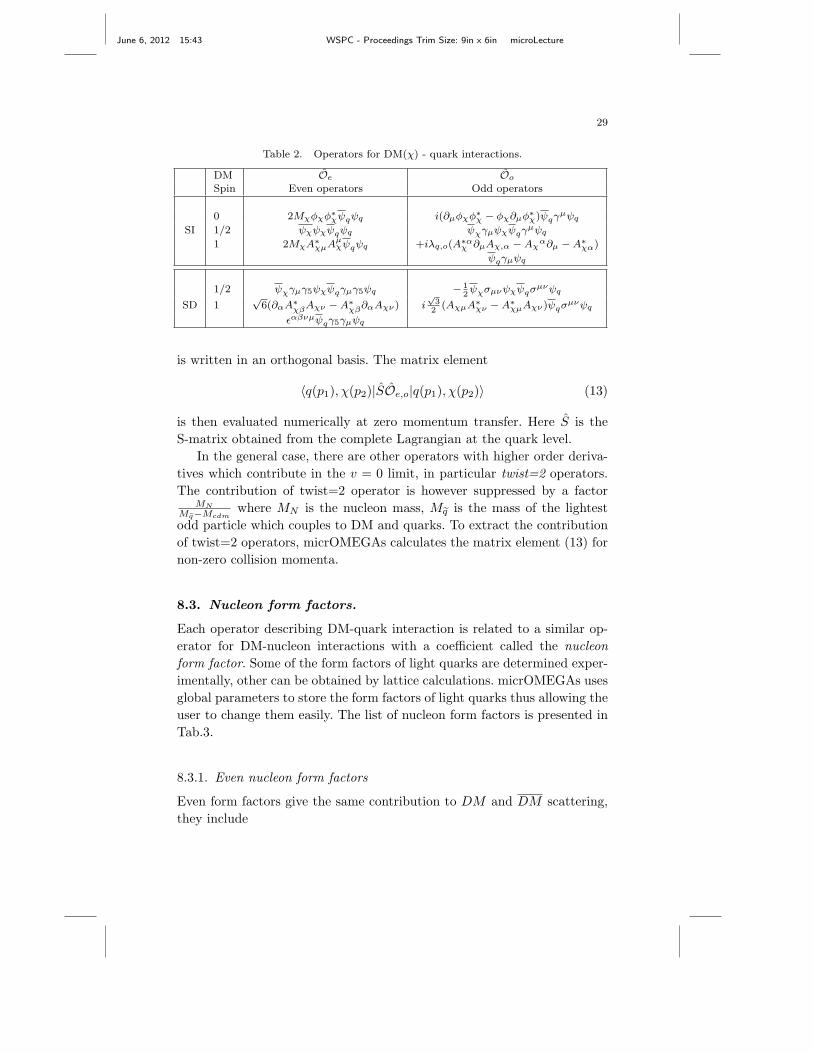
8.2. DM-quark operators.
The independent set of DM-quark operators in the v = 0 limit are presented
in Tab.2,
To compute the amplitudes for DM -quark scattering at low energy,
micrOMEGAs expands the Lagrangian of the model in terms of local op-
erators and extracts the coefficients of the low energy effective DM quark
Lagrangian numerically. To do this we need to add to the model Lagrangian
the projection operators defined in Table 1. The interference between one
projection operator and the effective vertices will single out either the spin
dependent or spin independent contribution, since the effective Lagrangian
June 6, 2012 15:43 WSPC - Proceedings Trim Size: 9in x 6in microLecture
29
Table 2. Operators for DM(χ) - quark interactions.
DM Oe Oo
Spin Even operators Odd operators
0 2Mχφχφ∗χψqψq i(∂µφχφ∗
χ − φχ∂µφ∗χ)ψqγµψq
SI 1/2 ψχψχψqψq ψχγµψχψqγµψq
1 2MχA∗χµAµ
χψqψq +iλq,o(A∗αχ ∂µAχ,α − Aχ
α∂µ − A∗χα)
ψqγµψq
1/2 ψχγµγ5ψχψqγµγ5ψq − 12ψχσµνψχψqσµνψq
SD 1√
6(∂αA∗χβ
Aχν − A∗χβ
∂αAχν) i√
32
(AχµA∗χν − A∗
χµAχν)ψqσµνψq
ǫαβνµψqγ5γµψq
is written in an orthogonal basis. The matrix element
〈q(p1), χ(p2)|SOe,o|q(p1), χ(p2)〉 (13)
is then evaluated numerically at zero momentum transfer. Here S is the
S-matrix obtained from the complete Lagrangian at the quark level.
In the general case, there are other operators with higher order deriva-
tives which contribute in the v = 0 limit, in particular twist=2 operators.
The contribution of twist=2 operator is however suppressed by a factorMN
Meq−Mcdmwhere MN is the nucleon mass, Meq is the mass of the lightest
odd particle which couples to DM and quarks. To extract the contribution
of twist=2 operators, micrOMEGAs calculates the matrix element (13) for
non-zero collision momenta.
8.3. Nucleon form factors.
Each operator describing DM-quark interaction is related to a similar op-
erator for DM-nucleon interactions with a coefficient called the nucleon
form factor. Some of the form factors of light quarks are determined exper-
imentally, other can be obtained by lattice calculations. micrOMEGAs uses
global parameters to store the form factors of light quarks thus allowing the
user to change them easily. The list of nucleon form factors is presented in
Tab.3.
8.3.1. Even nucleon form factors
Even form factors give the same contribution to DM and DM scattering,
they include
June 6, 2012 15:43 WSPC - Proceedings Trim Size: 9in x 6in microLecture
30
• Scalar (SI) even form factor for light quarks. These form factors,
fNq , which relate quark and nucleon operators are defined by
〈N |mqψqψq|N〉 = fNq MN (14)
where N means nucleon and MN its mass. The scalar form factor actually
counts the contribution of each quark to the nucleon mass. If, for instance,
the DM interacts with light quarks via Higgs exchange, then the matrix
element will contain a quark mass. This mass will cancel with the quark
mass in the scalar form factor so that the final answer will be independent
of the quark mass, a quantity which depends strongly on the QCD scale.
This also means that despite the very small coupling of light quarks with
the Higgs, they give a finite contribution to DM-nucleon scattering.
Scalar form factors are known from hadron spectroscopy, data of πN
scattering70 and lattice calculations of s quark contribution to the nucleon
mass. Still there is some uncertainty in the form factors especially for the
s-quark contribution.
• Axial-vector(SD) even form factors. The axial-vector current
ψqγµγ5ψq counts the total spin of quarks and anti-quarks q in the nu-
cleon. The axial-vector interactions in the nucleon are related to those
involving quarks, with
2sµ∆qN = 〈N |ψqγµγ5ψq|N〉 (15)
where sµ is the nucleon spin. The coefficients ∆qN are extracted
from HERMES71 and COMPASS72 experiments, they are defined as
pVectorFFPq in micrOMEGAs, see Tab.3.
• Form factors for heavy quarks.
The nucleon consists of light quarks and gluons, nevertheless one can
also consider interactions of DM with heavy quarks inside the nucleon.
These effectively come into play since heavy quark loops contribute to
the interactions of DM with gluons, see for example the diagrams in Fig.
6. Heavy quarks, Q, give a large contribution to the SI amplitude. Their
form factor can be calculated in QCD.
When the contribution of the triangle diagram in Fig.6 is dominant one
can use the anomaly of the trace of the QCD energy-momentum tensor73
to calculate the heavy quark form factor. The leading order result is
fQ =2
27(16)
which is about twice as large than the form factor of light quarks. If the
mass of q, the new particle that couples to the DM and a quark, is not
June 6, 2012 15:43 WSPC - Proceedings Trim Size: 9in x 6in microLecture
31
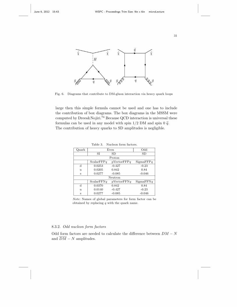
Fig. 6. Diagrams that contribute to DM-gluon interaction via heavy quark loops
large then this simple formula cannot be used and one has to include
the contribution of box diagrams. The box diagrams in the MSSM were
computed by Drees&Nojiri.74 Because QCD interaction is universal these
formulas can be used in any model with spin 1/2 DM and spin 0 q.
The contribution of heavy quarks to SD amplitudes is negligible.
Table 3. Nucleon form factors.
Quark Even Odd
SI SD SD
Proton
ScalarFFPq pVectorFFPq SigmaFFPq
d 0.0253 -0.427 -0.23u 0.0205 0.842 0.84
s 0.0277 -0.085 -0.046
Neutron
ScalarFFNq pVectorFFNq SigmaFFNq
d 0.0370 0.842 0.84
u 0.0140 -0.427 -0.23s 0.0277 -0.085 -0.046
Note: Names of global parameters for form factor can beobtained by replacing q with the quark name.
8.3.2. Odd nucleon form factors
Odd form factors are needed to calculate the difference between DM − N
and DM − N amplitudes.
June 6, 2012 15:43 WSPC - Proceedings Trim Size: 9in x 6in microLecture
32
• Scalar (SI) odd form factors. The ψqγµψq quark current gives rise to
scalar interactions. Since the vector current is conserved, the associated
nucleon form factor just counts the number of quark minus the number
of antiquarks in the nucleon. Thus the u ,d quarks have form factors
2,1 in proton and 1,2 in neutron while the form factor is zero for
heavy quarks .
• Pseudo-vector (SD) odd form factors. The 〈N |ψσµνψ|N〉 current
can be interpreted as the difference between the spin of quarks and the
spin of anti-quarks in nucleons. Measurements by COMPASS and HER-
MES indicate that the antiquark contribution to nucleon spin is com-
patible with zero. Thus these form factors should be close to the even
SD axial-vector form factors. QCD lattice calculations75,76 confirm this
expectation, the lattice results are used as default values for the form
factors SigmaFFPq listed in Tab.3.
Form factors for twist=2 operators are calculated via parton dis-
tribution functions
f twist=2q =
1
2
∫ 1
0
dxxfpdfq (x,Q = Mq)
8.4. Nucleon amplitudes: example.
In micrOMEGAs the amplitudes for DM-nucleon scattering at rest can be
computed using the routine
nucleonAmplitudes(qBOX,pAsi,pAsd,nAsi,nAsd)
where pAsi, pAsd, nAsi, nAsd are output parameters which contain pro-
ton/neutron SI/SD amplitudes. Each of these parameters is a two dimen-
sional array which contains amplitudes for DM and DM scattering. Am-
plitudes are normalized so that the total cross section for DM -nucleon
scattering reads
σtot =4M2
cdmM2N
π(Mcdm + MN )2(|pAsi[0]|2 + 3|pAsd[0]|2)
The parameter qBOX specifies the name of the function which calculates
the box diagram of Fig.6. The option qBOX=FeScLoop includes the calcula-
tion of the box diagram with a spin 1/2 DM and a scalar q particle. When
qBOX=NULL, the form factors for heavy quarks (6) with QCD NLO correc-
tion are used. This approximation works well when the masses of q particles
included in vertices DM · q · q are large.
For the MSSM test point of section 4.5 we have
June 6, 2012 15:43 WSPC - Proceedings Trim Size: 9in x 6in microLecture
33
// CODE OUTPUT
nucleonAmplitudes(FeScLoop, pA0,pA5,nA0,nA5); |
printf("CDM-nucleon micrOMEGAs amplitudes:\n"); |CDM-nucleon micrOMEGAs amplitudes:
printf("proton: SI=%.2E SD=%.2E\n",pA0[0],pA5[0]); |proton: SI=-1.33E-09 SD=-1.58E-08
printf("neutron:SI=%.2E SD=%.2E\n",nA0[0],nA5[0]); |neutron:SI=-1.33E-09 SD= 1.98E-08
|
coef=4/M_PI*3.8938E8*pow(Nmass*Mcdm/(Nmass+Mcdm),2);|
printf("CDM-nucleon cross sections[pb]:\n"); |CDM-nucleon cross sections[pb]:
printf(" proton SI %.3E SD%.3E\n", |
coeff*pA0[0]*pA0[0],3*SCcoeff*pA5[0]*pA5[0]); |proton SI 2.177E-10 SD 3.223E-07
printf(" neutron SI %.3E SD %.3E\n", |
coeff*nA0[0]*nA0[0],3*SCcoeff*nA5[0]*nA5[0]); |neutron SI 2.696E-10 SD 5.113E-07
[A The cross section for SI interactions on protons in this example,
σSI ≈ 2.2 · 10−10[pb] = 2.2 · 10−46[cm2]
is well below the current Xenon10015 upper limit σSI < 2 · 10−44[cm2], but
within reach of the next generation of direct detection experiments such as
Xenon1T.
8.5. Dark matter nucleus scattering.
For zero DM velocity, the cross section for DM-nucleus SI interaction reads
σSI0 =
4µ2
π(λpZ + λn(A − Z))
2, µ =
McdmMA
Mcdm + MA(17)
where λp, λn are amplitudes for DM scattering on nucleons; MA, Z, A are
the nucleus mass, charge, and atomic number respectively. For a small DM
velocity, v ≈ 10−3c, we neglect the dependence on the small momentum
transfer in the cross section but include this dependence in the nucleus
form factor, the differential cross section is
dσSI
dE=
σSI0
EmaxF 2
A(q) , 0 < E < Emax = 2
(v2µ2
MA
)(18)
where E is the nucleus recoil energy and q =√
2EMA the transfer mo-
mentum. The form factors FA(q) are well known from experiments of µ
scattering on atomic nuclei. Note that Eq. 18 predicts an A2 enhancement
of the SI cross section at large A. Such enhancement does not occur for
SD interactions due to a strong compensation of the proton/neutron spins
with the same orbital state.
For SD scattering on nucleus, three form factors are introduced
dσSDA
dE=
16πµ2
(2JA + 1)Emax(S00(q)a
20 + S01(q)a0a1 − S11(q)a
21) (19)
June 6, 2012 15:43 WSPC - Proceedings Trim Size: 9in x 6in microLecture
34
where a0 = ξp + ξn, a1 = ξp − ξn, ξp, ξn are proton and neutron SD
amplitudes, JA is a total angular momentum of nucleus. The Sij form
factors are obtained by computation. The list of available form factors is
presented in the review.77,78
8.6. Calculation of Direct Detection signal in
micrOMEGAs.
The distribution of the number of events over the recoil energy is obtained
after integrating Eq. (18, 19) over the DM velocity distribution. In the
resulting formulas, the DM local density enters as a total factor. In the
micrOMEGAs package this density is a global parameter rhoDM whose de-
fault value is 0.3GeV/cm3. The recoil energy distribution is calculated by
the routine
nucleusRecoil(f,A,Z,J,Sxx,qBOX,dNdE)
Here the input parameters are
⋄ f - the DM velocity distribution normalized such that
∫ ∞
0
vf(v)dv = 1 (20)
The units are km/s for v and s2/km2 for f(v).
⋄ A - atomic number of nucleus;
⋄ Z - number of protons in the nucleus;
⋄ J - nucleus spin;
⋄ Sxx - routine which calculates SD nucleus form factors, Eq.(19), for spin-
dependent interactions.
⋄ qBOX - a parameter needed by nucleonAmplitudes, see the description
above.
The micrOMEGAs package contains the predefined constants Z Name,J Nameatomic number for the electric charges and spins for a large
set of isotopes, for instance, Z_Xe, J_Xe129, J_Xe131. Furthermore all
SD form factors presented in the Review77,78 are included. Their generic
name is Sxx Nameatomic number, for instance SxxXe129. The iso-
topes whose charges, spins and form factors are included in micrOMEGAs
are
F19 Na23 Na23A Al27 Si29 K39 Ge73 Ge73A Nb92 Te125 I127 Xe129 Xe131
For the velocity distribution, the user can substitute any function. The
June 6, 2012 15:43 WSPC - Proceedings Trim Size: 9in x 6in microLecture
35
default function included in micrOMEGAs is
Maxwell(v) =cnorm
v
∫
|~v|<vesc
d3~v exp
(− (~v − VEarth)2
v2rot
)δ(v − |~v|)
which corresponds to the velocity distribution of the isothermal model. Here
VEarth, vrot, and vesc a global parameter presented in Tab.1.
nucleusRecoil returns the total number of events per day and per
kilogram of detector material. In general the result is averaged over DM
and DM . The energy spectrum of recoil nuclei is stored in dNdE array which
contains 200 elements. The value in the ith element corresponds to
dNdE[i] =dN
dE|E=i∗keV
in units of (1/keV/kg/day). The recoil energy distribution can be displayed
on the screen with
displayRecoilPlot(dNdE,title,E1,E2)
where title is a character string specifying the title of the plot and E1,E2
are minimal and maximal values for the displayed energy in keV. The func-
tion
cutRecoilResult(dNdE,E1,E2) calculates the number of events in
an energy interval defined by the values E1,E2 in keV, each experiment
normally gives an energy interval for their result.
8.7. Example.
For the MSSM test point of section 4.5, to obtain the recoil energy corre-
sponding to the Xenon100 experiment, we call
double E1=8.4 /*KeV*/, E2=44.6/*KeV*/, Exposure=1471/*day*kg*/;
double nEvents, dNdE[200]; /* output */
int i;
nucleusRecoil(Maxwell,131,Z_Xe,J_Xe131,SxxXe131,FeScLoop,dNdE);
nEvent=Exposur*cutRecoilResult(dNdE,E1,E2);
printf("Expected number of events %.2E\n",nEvents);
for(i=0;i<200;i++) dNdE[i]*=Exposure;
displayRecoilPlot(dNdE,"Recoil energy distribution for Xe",E1,E2);
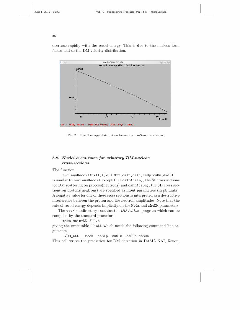
The number of events given in output is 0.07, this means that this point
can be tested by XENON if one increases the exposure by roughly a factor
50, in agreement with the estimate obtained in section 8.4. The resulting
distribution is displayed in Fig.7. Here we see that the number of events
June 6, 2012 15:43 WSPC - Proceedings Trim Size: 9in x 6in microLecture
36
decrease rapidly with the recoil energy. This is due to the nucleus form
factor and to the DM velocity distribution.
Fig. 7. Recoil energy distribution for neutralino-Xenon collisions.
8.8. Nuclei event rates for arbitrary DM-nucleon
cross-sections.
The function
nucleusRecoilAux(f,A,Z,J,Sxx,csIp,csIn,csDp,csDn,dNdE)
is similar to nucleusRecoil except that csIp(csIn), the SI cross sections
for DM scattering on protons(neutrons) and csDp(csDn), the SD cross sec-
tions on protons(neutrons) are specified as input parameters (in pb units).
A negative value for one of these cross sections is interpreted as a destructive
interference between the proton and the neutron amplitudes. Note that the
rate of recoil energy depends implicitly on the Mcdm and rhoDM parameters.
The etc/ subdirectory contains the DD ALL.c program which can be
compiled by the standard procedure
make main=DD_ALL.c
giving the executable DD ALL which needs the following command line ar-
guments
./DD_ALL Mcdm csSIp csSIn csSDp csSDn
This call writes the prediction for DM detection in DAMA NAI, Xenon,
June 6, 2012 15:43 WSPC - Proceedings Trim Size: 9in x 6in microLecture
37
CDMS, CoGent and COUPP. Some experimental input data used in this
program (exposures, energy cuts, efficiency) can be obsolete. The user can
improve this code easily to take into account new experimental data.
9. Neutrino signals of DM captured by Sun and Earth.
9.1. Neutrino fluxes
Dark Matter particles captured by the Sun/Earth accumulate in the center
of the Sun/Earth and annihilate into standard model particles. The neu-
trinos that escape the Sun/Earth can then be detected. When the capture
and annihilation rates reach an equilibrium (we assume that equilibrium
can be reached within the lifetime of the Sun/Earth), the rate of DM an-
nihilation is defined by the capture rate. This rate depends on the cross
sections for elastic scattering of DM on nuclei in the Sun/Earth. The larger
the atomic weight, the larger the DM energy loss. Knowing the chemical
contents of the Sun/Earth is important for the calculation of the capture
rate. The DM(DM) capture rates Cχ (Cχ) depend also on the DM density
and velocity distribution at the Sun galactic orbit. To calculate the capture
rate we use the simplified formula found in the review of Jungman et.al.40
Cχ = 4.8 × 1028 s−1
(ρχ
0.3GeV/cm3
) (270 km/s
v
)
×∑
i
(σχi
pb
)fiφi
mχmNi
Fi(mχ)S(mχ/mNi)
where mNi, the mass of the nuclear specie i, and mχ are given in GeV. v is
the DM velocity dispersion, fi is the mass fraction of element i in the Sun,
and φi its distribution. Fi(m) is a form factor suppression and S a kinetic
suppression factor.
Let Γχχ, Γχχ and Γχχ be the annihilation rates for DM(DM) processes
in the Sun/Earth and Nχ/Nχ the DM/DM densities in the Sun/Earth.
For a self-conjugate DM,
Cχ = 2Γχχ,
June 6, 2012 15:43 WSPC - Proceedings Trim Size: 9in x 6in microLecture
38
while in general we have the following equations
Cχ = 2Γχχ + Γχχ
Cχ = 2Γχχ + Γχχ
Γχχ
Γχχ=
〈σχχv 〉
〈σχχv 〉
(Nχ
Nχ
)2
Γχχ
Γχχ=
〈σχχv 〉/2
〈σχχv 〉
(Nχ
Nχ
)
which can be solved to obtain the annihilation rates Γχχ, Γχχ , Γχχ.
The neutrino spectrum that result from DM annihilation inside the Sun
is different from annihilation in the vacuum because some long-lived par-
ticles can interact with the Sun medium before decaying. Furthermore the
neutrino spectrum is deformed by attenuation and oscillation processes that
occur during propagation inside the Sun/Earth. In Ref79 all these factors
where taken into account and the neutrino spectra after propagation were
tabulated for different DM masses. To get the neutrino flux at the surface
of the Earth micrOMEGAs calculates for each SM final state the relative
contribution of the χχ → SMSM channel and multiplies this by the anni-
hilation rate Γχχ and the tabulated neutrino spectra functions79 prepared
for this channel for the relevant Mcdm.
neutrinoFlux(forSun,nu_flux, Nu_flux)
calculates νµ and νµ fluxes close to the Earth surface. If forSun==0 then
the flux of neutrinos from the Earth is calculated, otherwise this function
computes the flux of neutrinos from the Sun. The velocity distribution is as-
sumed to be Maxwellian and its parameters can be changed by SetfMaxwell
function. The calculated fluxes are stored in nu_flux, Nu_flux arrays of
dimension NZ=250. For neutrino fluxes we use units [1/Year/km2].
9.2. micrOMEGAs tools to work with particle spectra.
Various particle spectra and fluxes relevant to neutrino signals and to in-
direct detection ones (see next section) are stored in arrays with NZ=250
elements. The ith element of an array corresponds to dN/dzi where zi =
log(Ei/Mcdm)g. Spectra interpolation can be done by one of the two func-
tions
zInterp(z,flux) which returns d(flux)/dz and
SpectdNdE(E,flux) which returns d(flux)/dE[GeV]
gThe zi grid can be obtained with the function Zi(i).
June 6, 2012 15:43 WSPC - Proceedings Trim Size: 9in x 6in microLecture
39
where flux means the array where tabulated data are stored. To display
the function on the screen one can use
displaySpectrum(flux,title,Emin,Emax,Units) ,
where title is a text string which gives a title to the plot. Emin and
Emax define plot limits. If Units=0 the flux is displayed as a function of
z10 = log10(E/Mcdm) otherwise one gets the dN/dE plot as a function of
the energy E in GeV units.
The integrated spectra/fluxes can be obtained by
spectrInfo(Xmin,flux,&Ntot,&Xtot) where Xmin = Emin/Mcdm
and
Ntot =
∫ 1
Xmin
d(flux)
dxdx
Xtot =
∫ 1
Xmin
xd(flux)
dxdx
.
9.3. Muon fluxes
A detector measures the muon flux that results from interactions of neu-
trinos with rocks below the detector or water within the detector. The
routines which calculate such µ fluxes are based on the formulas of Ref.80
muonUpward(nu_flux,Nu_flux, mu)
calculates the muon flux which result from interactions of neu-
trinos with rocks. Here nu_flux and Nu_flux are input parame-
ters which designate the neutrino/anti-neutrino fluxes calculated by
neutrinoFlux. mu is an array which stores the sum of µ+ and µ− fluxes.
muonContained(nu,Nu,rho, mu) calculates the flux of muon which
are produced in a given (detector) volume. It has the same parameters as
the function for the calculation of upward events. rho is the density of de-
tector material in g/cm3 units. For instance, rho=1 for water. The array
mu gives the muon flux in 1/Year/km3 units representing the number of
neutrinos converted to muons in a km3 volume.
9.4. Example
As an example we calculate the muon flux for the CMSSM with parameters
M0 = 3200, M1/2 = 315, A0 = 0, tan β = 10, sign(µ) = 1, Mtop = 173.2;
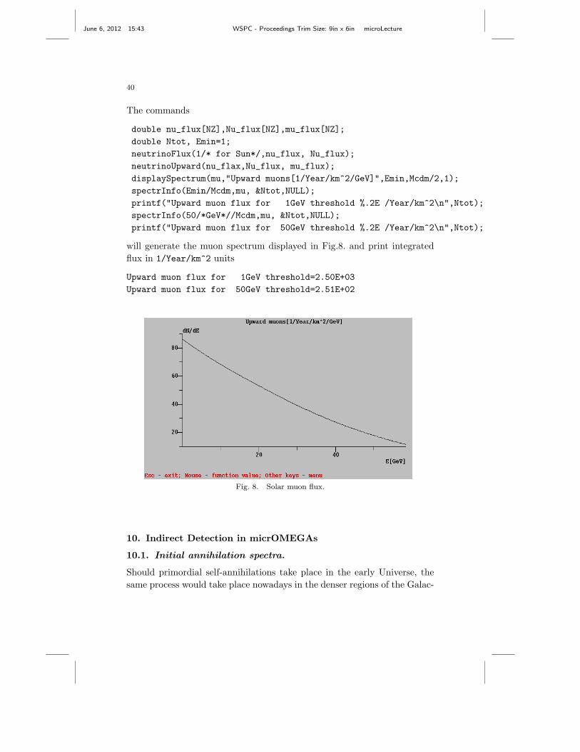
June 6, 2012 15:43 WSPC - Proceedings Trim Size: 9in x 6in microLecture
40
The commands
double nu_flux[NZ],Nu_flux[NZ],mu_flux[NZ];
double Ntot, Emin=1;
neutrinoFlux(1/* for Sun*/,nu_flux, Nu_flux);
neutrinoUpward(nu_flax,Nu_flux, mu_flux);
displaySpectrum(mu,"Upward muons[1/Year/km^2/GeV]",Emin,Mcdm/2,1);
spectrInfo(Emin/Mcdm,mu, &Ntot,NULL);
printf("Upward muon flux for 1GeV threshold %.2E /Year/km^2\n",Ntot);
spectrInfo(50/*GeV*//Mcdm,mu, &Ntot,NULL);
printf("Upward muon flux for 50GeV threshold %.2E /Year/km^2\n",Ntot);
will generate the muon spectrum displayed in Fig.8. and print integrated
flux in 1/Year/km^2 units
Upward muon flux for 1GeV threshold=2.50E+03
Upward muon flux for 50GeV threshold=2.51E+02
Fig. 8. Solar muon flux.
10. Indirect Detection in micrOMEGAs
10.1. Initial annihilation spectra.
Should primordial self-annihilations take place in the early Universe, the
same process would take place nowadays in the denser regions of the Galac-
June 6, 2012 15:43 WSPC - Proceedings Trim Size: 9in x 6in microLecture
41
tic DM halo. DM annihilation in the Galactic halo produces pairs of Stan-
dard Model particles that hadronize and decay into stable particles. The
final states with γ, e+, p, and νµ are particularly interesting as they are
the subject of indirect searches. The production rate of particles from DM
annihilation at location x reads
Qa(x, E) =1
2〈σv〉 〈ρ(x)2〉
M2cdm
fa(E) , (21)
where 〈σv〉 is the annihilation cross-section times the relative velocity of
incoming DM particles which we evaluate in the limit v = 0 (this is a good
approximation since v = 10−3c). Note that 〈σv〉 includes averaging over
incoming particles/antiparticles. Thus, for a Dirac DM particle χ for which
σχχ = 0, 〈σv〉 = 1/2〈σχχv〉. ρ(x) is the DM mass density at the location x
and fa(E) = dNa/dE is the energy distribution of the particle a produced
in one reaction. micrOMEGAs first calculates the cross sections for all basic
processes with two body final states. The tabulated fragmentation functions
obtained by Pythia are then used to generate spectra for each final stable
particle. The routine to compute the spectra fa and 〈σv〉 is
calcSpectrum(key,Sg,Se,Sp,Sne,Snm,Snl,&err)
which returns 〈σv〉 in cm3/s units. The calculated spectra for γ, e+, p,
and neutrinos, are stored in arrays Sg, Se, Sp, Sne, Snm, Snl of dimension
NZ(See section 9.2). Note that the spectra of particles and anti-particles
are identical. key is a switch, depending on its value micrOMEGAs
1 takes into account the polarization of W,Z bosons. It can be important
for MSSM-like models where W,Z are transversely polarized;
2 calculates 2 → 2 + γ processes to improve spectrum of high energy pho-
tons.
4 prints on the screen the calculated cross sections.
More than one option can be switched on simultaneously by adding the
corresponding values for key. A problem in the spectrum calculation will
produce a non zero error code, err 6= 0.
The annihilation processes DM,DM → 2γ and DM,DM → γ, Z are
loop suppressed but lead to a very distinctive signature, a monochromatic
gamma-ray line. micrOMEGAs can calculate the corresponding cross sec-
tion only for specific models, for example the MSSM. The routine to do
this is
loopGamma(&vcs_gz,&vcs_gg) which calculates 〈σv〉 for γγ and γZ
processes in cm3/s units.
June 6, 2012 15:43 WSPC - Proceedings Trim Size: 9in x 6in microLecture
42
10.2. Propagation of photons and neutrinos
The flux of photons (neutrinos) can be evaluated as
Φγ(E, φ) =〈σv〉M2
cdm
fγ(E)H(φ) (22)
where the factor H includes the integral over the line of sight,
H(φ) =1
8π
∫ ∞
0
drρ2
(√r2 + r2
⊙ − 2rr⊙ cos φ
)(23)
and φ is the angle in the direction of observation. This flux can be calculated
by the routine
gammaFluxTab(fi,dfi,sigmav,Sg,Sobs)
where fi is the angle between the line of sight and the center of the galaxy,
dfi is half the cone angle which characterizes the detector resolution (the
solid angle is 2π(1 − cos(dfi)), sigmav and Sg are the annihilation cross
section and the photon spectrum calculated previously by calcSpectrum.
Sobs is the flux observed in [(cm2s)−1]units.
Note that the neutrino spectra obtained by calcSpectrum do not take
into account neutrino oscillation. One expects the muon neutrino flux at
the Earth
fEarthνµ
= 0.22f0νe
+ 0.39(f0νµ
+ f0ντ
) ,
where numerical coefficients are defined by neutrino flavour mixing29 and
f0ν fluxes are calculated by calcSpectrum.
10.3. Propagation of charged particles
The propagation of charged particles depends on the structure of the galac-
tic magnetic field and is characterized by the diffusion equations. We assume
that the region of diffusion of cosmic rays is represented by a thick disk of
thickness 2L and radius R ≈ 20 kpc, with a thin galactic disk in the mid-
dle of the thick disk. The parameters entering this equation are not well
known, but they are constrained by observations of the B/C ratio in cosmic
rays.81 Table 4 lists the default values for the propagation parameters, to-
gether with the MIN/MAX variations which are compatible with the B/C
observations.
The energy spectrum of positrons is obtained by solving the diffusion-
loss equation keeping only the two dominant contributions: space diffusion
and energy losses,
−∇ · (K(E)∇ψe+) − ∂
∂E(b(E)ψe+) = Qe+(x, E) (24)
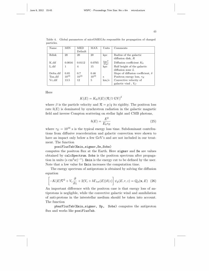
June 6, 2012 15:43 WSPC - Proceedings Trim Size: 9in x 6in microLecture
43
Table 4. Global parameters of micrOMEGAs responsible for propagation of chargedparticles.
Name MIN MED MAX Units Comments
Default
Rdisk 20 20 20 kpc Radius of the galacticdiffusion disk, R
K dif 0.0016 0.0112 0.0765 kpc2
MyrDiffusion coefficient K0
L dif 1 4 15 kpc Half height of the galactic
diffusion zone L
Delta dif 0.85 0.7 0.46 Slope of diffusion coefficient, δ
Tau dif 1016 1016 1016 s Positron energy loss, τE
Vc dif 13.5 12 5 km/s Convective velocity of
galactic vind , VC
Here
K(E) = K0β(E) (R/1 GV)δ
where β is the particle velocity and R = p/q its rigidity. The positron loss
rate b(E) is dominated by synchrotron radiation in the galactic magnetic
field and inverse Compton scattering on stellar light and CMB photons,
b(E) =E2
E0τE(25)
where τE = 1016 s is the typical energy loss time. Subdominant contribu-
tions from diffusive reacceleration and galactic convection were shown to
have an impact only below a few GeV’s and are not included in our treat-
ment. The function
posiFluxTab(Emin,sigmav,Se,Sobs)
computes the positron flux at the Earth. Here sigmav and Se are values
obtained by calcSpectrum. Sobs is the positron spectrum after propaga-
tion in units (s cm2sr)−1). Emin is the energy cut to be defined by the user.
Note that a low value for Emin increases the computation time.
The energy spectrum of antiprotons is obtained by solving the diffusion
equation[−K(E)∇2 + Vc
∂
∂z+ 2(Vc + hΓtot(E))δ(z)
]ψp(E, r, z) = Qp(x, E) (26)
An important difference with the positron case is that energy loss of an-
tiprotons is negligible, while the convective galactic wind and annihilation
of anti-protons in the interstellar medium should be taken into account.
The function
pbarFluxTab(Emin,sigmav, Sp, Sobs) computes the antiproton
flux and works like posiFluxTab.
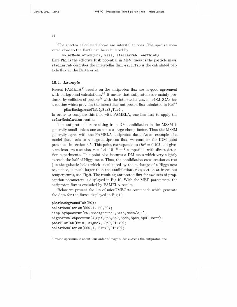
June 6, 2012 15:43 WSPC - Proceedings Trim Size: 9in x 6in microLecture
44
The spectra calculated above are interstellar ones. The spectra mea-
sured close to the Earth can be calculated by
solarModulation(Phi, mass, stellarTab, earthTab)
Here Phi is the effective Fisk potential in MeV, mass is the particle mass,
stellarTab describes the interstellar flux, earthTab is the calculated par-
ticle flux at the Earth orbit.
10.4. Example
Recent PAMELA82 results on the antiproton flux are in good agreement
with background calculations.83 It means that antiprotons are mainly pro-
duced by collision of protonsh with the interstellar gas. micrOMEGAs has
a routine which provides the interstellar antiproton flux tabulated in Ref84
pBarBackgroundTab(pBarBgTab) .
In order to compare this flux with PAMELA, one has first to apply the
solarModulation routine.
The antiproton flux resulting from DM annihilation in the MSSM is
generally small unless one assumes a large clump factor. Thus the MSSM
generally agree with the PAMELA antiproton data. As an example of a
model that leads to a large antiproton flux, we consider the IDM point
presented in section 3.5. This point corresponds to Ωh2 = 0.102 and gives
a nucleon cross section σ = 1.4 · 10−45cm2 compatible with direct detec-
tion experiments. This point also features a DM mass which very slightly
exceeds the half of Higgs mass. Thus, the annihilation cross section at rest
( in the galactic halo) which is enhanced by the exchange of a Higgs near
resonance, is much larger than the annihilation cross section at freeze-out
temperatures, see Fig.9. The resulting antiproton flux for two sets of prop-
agation parameters is displayed in Fig.10. With the MED parameters, the
antiproton flux is excluded by PAMELA results.
Below we present the list of micrOMEGAs commands which generate
the data for the fluxes displayed in Fig.10
pBarBackgroundTab(BG);
solarModulation(560,1, BG,BG);
displaySpectrum(BG,"Background",Emin,Mcdm/2,1);
sigmaV=calcSpectrum(4,SpA,SpE,SpP,SpNe,SpNm,SpNl,&err);
pbarFluxTab(Emin, sigmaV, SpP,FluxP);
solarModulation(560,1, FluxP,FluxP);
hProton spectrum is about four order of magnitudes exceeds the antiproton one.
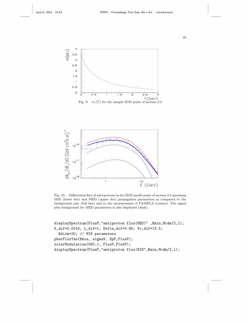
June 6, 2012 15:43 WSPC - Proceedings Trim Size: 9in x 6in microLecture
45
Fig. 9. σv(T ) for the sample IDM point of section 4.3
Fig. 10. Differential flux of anti-protons in the IDM model point of section 3.5 assuming
MIN (lower dot) and MED (upper dot) propagation parameters as compared to thebackground only (full line) and to the measurement of PAMELA (crosses). The signalplus background for MED parameters is also displayed (dash).
displaySpectrum(FluxP,"antiproton flux(MED)" ,Emin,Mcdm/2,1);
K_dif=0.0016; L_dif=1; Delta_dif=0.85; Vc_dif=13.5;
Rdisk=20; // MIN parameters
pbarFluxTab(Emin, sigmaV, SpP,FluxP);
solarModulation(560,1, FluxP,FluxP);
displaySpectrum(FluxP,"antiproton flux(MIN",Emin,Mcdm/2,1);
June 6, 2012 15:43 WSPC - Proceedings Trim Size: 9in x 6in microLecture
46
11. Calculation of cross sections in micrOMEGAs.
The functions presented in this section are activated in micrOMEGAs tem-
plate files main.c[F] by uncommenting the instruction
#define CROSS_SECTIONS
micrOMEGAS uses the function
numout*cc=newProcess(ProcessName);
for generating codes of matrix elements for processes defined by the textual
variable ProcessesName. numout is a special type to store process code and
auxiliary information. The variable cc contains the computer address of the
corresponding code. For instance
cc = newProcess("e,E->2*x");
returns a code for the matrix elements of all processes with e+e− annihi-
lation into two arbitrary particles. newProcess can generate the code for
processes with more than two particles in the final state, however the cur-
rent version of micrOMEGAs contains integration tools only for 2 → 2
processes. The function:
cs22(cc,L,Pcm,cos_min,cos_max,&err);
calculates the cross section for Lth subprocess where
Pcm - momentum in center of Mass reference frame;
cos min, cos max - cuts for cosine of scattering angle in the same frame;
L numerates subprocesses. 1 ≤ L ≤ ntot, the total number of subprocess.
The number of the subprocess as well as the numbers of incoming (nin)
and outgoing (nout) particles for the compiled set of processes cc can be
obtained by
procInfo1(cc,&ntot,&nin,&nout)
The names of incoming/outgoing particles of a given process and their
masses can be obtained by the function
procInfo2(cc,L,Names,Masses);
where the variable char**Names is an output parameter used for the array
of particle names, and the variable double*Masses is an array of numerical
values for masses.
For proton-[anti]proton collisions we have to apply convolution of ma-
trix element with structure functions and perform summation over all types
on incoming partons. This calculation can be performed with the function
hCollider( Pcm, pp, scale, pName1, pName2)
which compiles the needed matrix elements and calculates the cross sec-
tion for production of two heavy particles at a hadron collider. Here Pcm
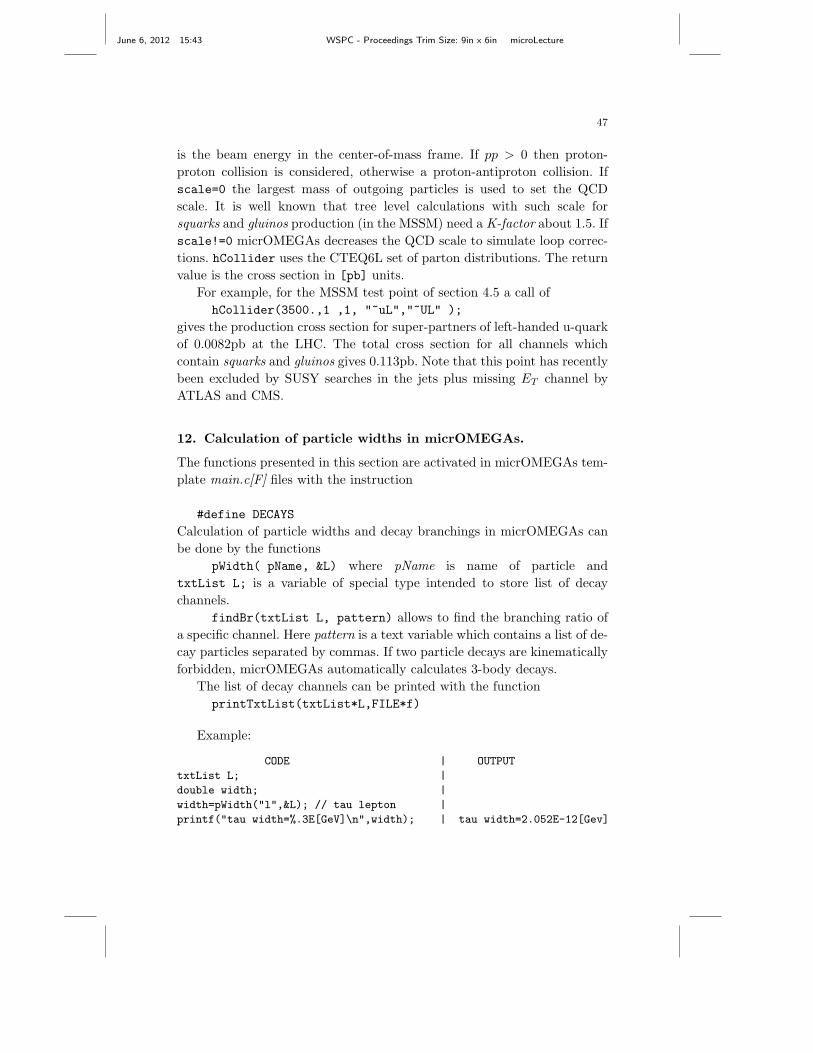
June 6, 2012 15:43 WSPC - Proceedings Trim Size: 9in x 6in microLecture
47
is the beam energy in the center-of-mass frame. If pp > 0 then proton-
proton collision is considered, otherwise a proton-antiproton collision. If
scale=0 the largest mass of outgoing particles is used to set the QCD
scale. It is well known that tree level calculations with such scale for
squarks and gluinos production (in the MSSM) need a K-factor about 1.5. If
scale!=0 micrOMEGAs decreases the QCD scale to simulate loop correc-
tions. hCollider uses the CTEQ6L set of parton distributions. The return
value is the cross section in [pb] units.
For example, for the MSSM test point of section 4.5 a call of
hCollider(3500.,1 ,1, "~uL","~UL" );
gives the production cross section for super-partners of left-handed u-quark
of 0.0082pb at the LHC. The total cross section for all channels which
contain squarks and gluinos gives 0.113pb. Note that this point has recently
been excluded by SUSY searches in the jets plus missing ET channel by
ATLAS and CMS.
12. Calculation of particle widths in micrOMEGAs.
The functions presented in this section are activated in micrOMEGAs tem-
plate main.c[F] files with the instruction
#define DECAYS
Calculation of particle widths and decay branchings in micrOMEGAs can
be done by the functions
pWidth( pName, &L) where pName is name of particle and
txtList L; is a variable of special type intended to store list of decay
channels.
findBr(txtList L, pattern) allows to find the branching ratio of
a specific channel. Here pattern is a text variable which contains a list of de-
cay particles separated by commas. If two particle decays are kinematically
forbidden, micrOMEGAs automatically calculates 3-body decays.
The list of decay channels can be printed with the function
printTxtList(txtList*L,FILE*f)
Example:
CODE | OUTPUT
txtList L; |
double width; |
width=pWidth("l",&L); // tau lepton |
printf("tau width=%.3E[GeV]\n",width); | tau width=2.052E-12[Gev]
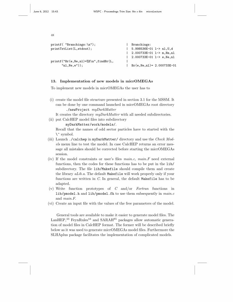
June 6, 2012 15:43 WSPC - Proceedings Trim Size: 9in x 6in microLecture
48
printf( "Branchings:\n"); | Branchings:
printTxtList(L,stdout); | 5.998536E-01 l-> nl,U,d
| 2.000733E-01 l-> m,Nm,nl
| 2.000733E-01 l-> e,Ne,nl
printf("Br(e,Ne,nl)=%E\n",findBr(L, |
"nl,Ne,e")); | Br(e,Ne,nl)= 2.000733E-01
13. Implementation of new models in micrOMEGAs
To implement new models in micrOMEGAs the user has to
(i) create the model file structure presented in section 3.1 for the MSSM. It
can be done by one command launched in micrOMEGAs root directory
./newProject myDarkMatter
It creates the directory myDarkMatter with all needed subdirectories.
(ii) put CalcHEP model files into subdirectory
myDarkMatter/work/models/.
Recall that the names of odd sector particles have to started with the
\~ symbol.
(iii) Launch ./calchep in myDarkMatter/ directory and use the Check Mod-
els menu line to test the model. In case CalcHEP returns an error mes-
sage all mistakes should be corrected before starting the micrOMEGAs
session.
(iv) If the model constraints or user’s files main.c, main.F need external
functions, then the codes for these functions has to be put in the lib/
subdirectory. The file lib/Makefile should compile them and create
the library aLib.a. The default Makefile will work properly only if your
functions are written in C. In general, the default Makefile has to be
adapted.
(v) Write function prototypes of C and/or Fortran functions in
lib/pmodel.h and lib/pmodel.fh to use them subsequently in main.c
and main.F.
(vi) Create an input file with the values of the free parameters of the model.
General tools are available to make it easier to generate model files. The
LanHEP,43 FeynRules44 and SARAH85 packages allow automatic genera-
tion of model files in CalcHEP format. The former will be described briefly
below as it was used to generate micrOMEGAs model files. Furthermore the
SLHAplus package facilitates the implementation of complicated models.
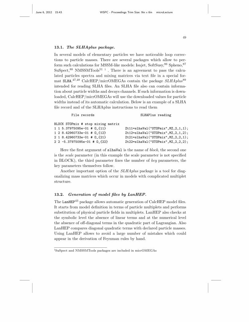
June 6, 2012 15:43 WSPC - Proceedings Trim Size: 9in x 6in microLecture
49
13.1. The SLHAplus package.
In several models of elementary particles we have noticeable loop correc-
tions to particle masses. There are several packages which allow to per-
form such calculations for MSSM-like models: Isajet, SoftSusy,86 Spheno,87
SuSpect,88 NMSSMTools51 i . There is an agreement to pass the calcu-
lated particles spectra and mixing matrices via text file in a special for-
mat SLHA.47,48 CalcHEP/micrOMEGAs contain the package SLHAplus89
intended for reading SLHA files. An SLHA file also can contain informa-
tion about particle widths and decays channels. If such information is down-
loaded, CalcHEP/micrOMEGAs will use the downloaded values for particle
widths instead of its automatic calculation. Below is an example of a SLHA
file record and of the SLHAplus instructions to read them
File records SLHAPlus reading
BLOCK STOPmix # stop mixing matrix
1 1 5.37975095e-01 # O_11 Zt11=slhaVal("STOPmix",MZ,2,1,1);
1 2 8.42960733e-01 # O_12 Zt12=slhaVal("STOPmix",MZ,2,1,2);
2 1 8.42960733e-01 # O_21 Zt21=slhaVal("STOPmix",MZ,2,2,1);
2 2 -5.37975095e-01 # O_22 Zt22=slhaVal("STOPmix",MZ,2,2,2);
Here the first argument of slhaVal is the name of block, the second one
is the scale parameter (in this example the scale parameter is not specified
in BLOCK), the third parameter fixes the number of key parameters, the
key parameters themselves follow.
Another important option of the SLHAplus package is a tool for diag-
onalizing mass matrices which occur in models with complicated multiplet
structure.
13.2. Generation of model files by LanHEP.
The LanHEP43 package allows automatic generation of CalcHEP model files.
It starts from model definition in terms of particle multiplets and performs
substitution of physical particle fields in multiplets. LanHEP also checks at
the symbolic level the absence of linear terms and at the numerical level
the absence of off-diagonal terms in the quadratic part of Lagrangian. Also
LanHEP compares diagonal quadratic terms with declared particle masses.
Using LanHEP allows to avoid a large number of mistakes which could
appear in the derivation of Feynman rules by hand.
iSuSpect and NMSSMTools packages are included in micrOMEGAs
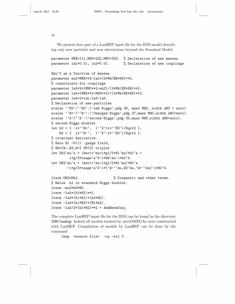
June 6, 2012 15:43 WSPC - Proceedings Trim Size: 9in x 6in microLecture
50
We present here part of a LanHEP input file for the IDM model describ-
ing only new particles and new interactions beyond the Standard Model.
parameter MHX=111,MH3=222,MHC=333. % Declaration of new masses
parameter laL=0.01, la2=0.01. % Declaration of new couplings
%mu^2 as a function of masses
parameter mu2=MHX**2-laL*(2*MW/EE*SW)**2.
% constraints for couplings
parameter la3=2*(MHC**2-mu2)/(2*MW/EE*SW)**2.
parameter la5=(MHX**2-MH3**2)/(2*MW/EE*SW)**2.
parameter la4=2*laL-la3-la5.
% Declaration of new particles
scalar ’~H3’/’~H3’:(’odd Higgs’,pdg 36, mass MH3, width wH3 = auto).
scalar ’~H+’/’~H-’:(’Charged Higgs’,pdg 37,mass MHC,width wHC=auto).
scalar ’~X’/’~X’:(’second Higgs’,pdg 35,mass MHX,width wHX=auto).
% second Higgs doublet
let h2 = -i*’~H+’, (’~X’+i*’~H3’)/Sqrt2 ,
H2 = i*’~H-’, (’~X’-i*’~H3’)/Sqrt2 .
% covariant derivative.
% Here B1 -U(1) gauge field,
% WW=W-,W3,W+ SU(2) triplet
let Dh2^mu^a = (deriv^mu+i*g1/2*B1^mu)*h2^a +
i*g/2*taupm^a^b^c*WW^mu^c*h2^b.
let DH2^mu^a = (deriv^mu-i*g1/2*B1^mu)*H2^a
-i*g/2*taupm^a^b^c*’W-’^mu,W3^mu,’W+’^mu^c*H2^b.
lterm DH2*Dh2. % Kinematic and other terms.
% Below h1 is standard Higgs doublet.
lterm -mu2*h2*H2.
lterm -la2*(h2*H2)**2.
lterm -la3*(h1*H1)*(h2*H2).
lterm -la4*(h1*H2)*(H1*h2).
lterm -la5/2*(h1*H2)**2 + AddHermConj.
The complete LanHEP input file for the IDM can be found in the directory
IDM/lanhep. Indeed all models treated by micrOMEGAs were constructed
with LanHEP. Compilation of models by LanHEP can be done by the
command
lhep <source file> -ca -evl 2
June 6, 2012 15:43 WSPC - Proceedings Trim Size: 9in x 6in microLecture
51
References
1. F. Zwicky, Astrophys.J. 86, 217 (1937).2. V. C. Rubin and J. Ford, W. Kent, Astrophys.J. 159, 379 (1970).3. N. Jarosik, C. Bennett, J. Dunkley, B. Gold, M. Greason et al., Astro-
phys.J.Suppl. 192, p. 14 (2011).4. W. J. Percival et al., Mon.Not.Roy.Astron.Soc. 401, 2148 (2010).5. A. G. Riess, L. Macri, S. Casertano, M. Sosey, H. Lampeitl et al., Astrophys.J.
699, 539 (2009).6. E. Komatsu et al., Astrophys.J.Suppl. 192, p. 18 (2011).7. S. P. Martin, A Supersymmetry primer, hep-ph/9709356, (1997).8. H.-C. Cheng, K. T. Matchev and M. Schmaltz, Phys.Rev. D66, p. 056006
(2002).9. H.-C. Cheng and I. Low, JHEP 0408, p. 061 (2004).
10. K. Agashe and G. Servant, Phys.Rev.Lett. 93, p. 231805 (2004).11. G. Belanger, K. Kannike, A. Pukhov and M. Raidal, JCAP 04, p. 010 (2012).12. P. Ade et al., Planck Early Results: The Planck mission, arXiv:1101.2022,
(2011).13. R. Bernabei et al., Eur. Phys. J. C67, 39 (2010).14. Z. Ahmed et al., Phys. Rev. Lett. 106, p. 131302 (2011).15. E. Aprile et al., Phys.Rev.Lett. 107, p. 131302 (2011).16. O. Adriani et al., Nature 458, 607 (2009).17. O. Adriani et al., Phys. Rev. Lett. 102, p. 051101 (2009).18. J. J. Beatty et al., Phys. Rev. Lett. 93, p. 241102 (2004).19. A. A. Abdo et al., Phys. Rev. Lett. 102, p. 181101 (2009).20. C. Meurer and f. t. F. L. collaboration, AIP Conf. Proc. 719, p. 1085 (2009).21. J. Chang et al., Nature 456, 362 (2008).22. F. Aharonian et al., Astron. Astrophys. 508, p. 561 (2009).23. A. W. Strong et al., Astron. Astrophys. 444, p. 495 (2005).24. F. Aharonian et al., Nature 439, 695 (2006).25. D. J. Thompson, Rept. Prog. Phys. 71, p. 116901 (2008).26. M. Aguilar et al., Phys.Rept. 366, 331 (2002).27. J. L. Feng, J. Kumar, J. Learned and L. E. Strigari, JCAP 0901, p. 032
(2009).28. S. Desai et al., Phys. Rev. D70, p. 083523 (2004).29. R. Abbasi et al., Phys. Rev. D84, p. 022004 (2011).30. P. Gondolo et al., JCAP 0407, p. 008 (2004).31. A. Arbey and F. Mahmoudi, Comput. Phys. Commun. 182, 1582 (2011).32. H. Baer, A. Belyaev, T. Krupovnickas and J. O’Farrill, JCAP 0408, p. 005
(2004).33. G. Belanger, F. Boudjema, A. Pukhov and A. Semenov, Comput. Phys. Com-
mun. 149, 103 (2002).34. G. Belanger, F. Boudjema, A. Pukhov and A. Semenov, Comput. Phys. Com-
mun. 174, 577 (2006).35. G. Belanger, F. Boudjema, A. Pukhov and A. Semenov, Comput. Phys. Com-
mun. 176, 367 (2007).36. G. Belanger, F. Boudjema, A. Pukhov and A. Semenov, Comput. Phys. Com-
June 6, 2012 15:43 WSPC - Proceedings Trim Size: 9in x 6in microLecture
52
mun. 180, 747 (2009).37. G. Belanger et al., Comput. Phys. Commun. 182, 842 (2011).38. e. Bertone, Gianfranco, Particle dark matter: Observations, models and
searches 2010.39. G. Bertone, D. Hooper and J. Silk, Phys. Rept. 405, 279 (2005).40. G. Jungman, M. Kamionkowski and K. Griest, Phys. Rept. 267, 195 (1996).41. A. Pukhov, CalcHEP 2.3: MSSM, structure functions, event generation,
batchs, and generation of matrix elements for other packages, arXiv:0412191,(2004).
42. A. Belyaev, N. Christensen and P. A., CalcHEP, Calculator for High Energy
Physics. A package for the evaluation of Feynman diagrams, integration over
multi-particle phase space, and event generation., (2012). http://theory.
sinp.msu.ru/~pukhov/calchep.html.43. A. Semenov, Comput. Phys. Commun. 180, 431 (2009).44. N. D. Christensen and C. Duhr, Comput.Phys.Commun. 180, 1614 (2009).45. S. Heinemeyer, W. Hollik and G. Weiglein, Comput.Phys.Commun. 124, 76
(2000).46. A. Djouadi, J. Kalinowski and M. Spira, Comput.Phys.Commun. 108, 56
(1998).47. P. Z. Skands et al., JHEP 07, p. 036 (2004).48. B. C. Allanach et al., Comp. Phys. Commun. 180, 8 (2009).49. P. Bechtle, O. Brein, S. Heinemeyer, G. Weiglein and K. E. Williams, Com-
put.Phys.Commun. 181, 138 (2010), 64 pages, 15 tables, 8 figures/ threetypos which made it to the published version corrected/ the code (cur-rently version 3.0.0beta including LHC Higgs search results) is available via:http://projects.hepforge.org/higgsbounds/.
50. P. Bechtle, O. Brein, S. Heinemeyer, G. Weiglein and K. E. Williams, Com-
put.Phys.Commun. 182, 2605 (2011).51. U. Ellwanger and C. Hugonie, Comput. Phys. Commun. 177, 399 (2007).52. G. Belanger, F. Boudjema, C. Hugonie, A. Pukhov and A. Semenov, JCAP
0509, p. 001 (2005).53. J. S. Lee et al., Comput. Phys. Commun. 156, 283 (2004).54. G. Belanger, F. Boudjema, S. Kraml, A. Pukhov and A. Semenov, Phys. Rev.
D73, p. 115007 (2006).55. L. Lopez Honorez and C. E. Yaguna, JHEP 09, p. 046 (2010).56. A. Belyaev, C.-R. Chen, K. Tobe and C. P. Yuan, Phys. Rev. D74, p. 115020
(2006).57. G. Belanger, A. Pukhov and G. Servant, JCAP 0801, p. 009 (2008).58. R. Barbieri, L. J. Hall and V. S. Rychkov, Phys.Rev. D74, p. 015007 (2006).59. K. Nakamura et al., J. Phys. G37, p. 075021 (2010).60. C. L. Bennett et al., Astrophys. J. Suppl. 148, p. 1 (2003).61. D. N. Spergel et al., Astrophys. J. Suppl. 148, 175 (2003).62. J. Edsjo and P. Gondolo, Phys. Rev. D56, 1879 (1997).63. K. A. Olive, D. N. Schramm and G. Steigman, Nucl. Phys. B180, p. 497
(1981).64. M. Srednicki, R. Watkins and K. A. Olive, Nucl. Phys. B310, p. 693 (1988).
June 6, 2012 15:43 WSPC - Proceedings Trim Size: 9in x 6in microLecture
53
65. T. van Albada, J. N. Bahcall, K. Begeman and R. Sancisi, Astrophys.J. 295,305 (1985).
66. Y. Sofue, M. Honma and T. Omodaka, Unified Rotation Curve of the Galaxy– Decomposition into de Vaucouleurs Bulge, Disk, Dark Halo, and the 9-kpcRotation Dip –, arXiv:0811.0859, (2008).
67. H. Zhao, Mon. Not. Roy. Astron. Soc. 278, 488 (1996).68. J. F. Navarro, C. S. Frenk and S. D. M. White, Astrophys. J. 490, 493 (1997).69. L. Bergstrom, P. Ullio and J. H. Buckley, Astropart. Phys. 9, 137 (1998).70. M. M. Pavan, I. I. Strakovsky, R. L. Workman and R. A. Arndt, PiN Newslett.
16, 110 (2002).71. A. Airapetian et al., Phys. Rev. D75, p. 012007 (2007).72. E. S. Ageev et al., Phys. Lett. B647, 330 (2007).73. M. A. Shifman, A. I. Vainshtein and V. I. Zakharov, Phys. Lett. B78, p. 443
(1978).74. M. Drees and M. Nojiri, Phys. Rev. D48, 3483 (1993).75. S. Aoki, M. Doui, T. Hatsuda and Y. Kuramashi, Phys. Rev. D56, 433 (1997).76. D. Dolgov et al., Phys. Rev. D66, p. 034506 (2002).77. V. A. Bednyakov and F. Simkovic, Phys. Part. Nucl. 36, 131 (2005).78. V. A. Bednyakov and F. Simkovic, Phys. Part. Nucl. 37, S106 (2006).79. M. Cirelli et al., Nucl. Phys. B727, 99 (2005).80. A. E. Erkoca, M. H. Reno and I. Sarcevic, Phys. Rev. D80, p. 043514 (2009).81. D. Maurin, F. Donato, R. Taillet and P. Salati, Astrophys. J. 555, 585 (2001).82. O. Adriani et al., Phys.Rev.Lett. 105, p. 121101 (2010).83. F. Donato et al., Astrophys. J. 563, 172 (2001).84. D. Maurin, R. Taillet and C. Combet, Approximate formulae for exotic GCR
anti-p and anti-d: Fluxes and astrophysical uncertainties, astro-ph/0609522,(2006).
85. F. Staub, arXiv:0806.0538 [hep-ph] (2008).86. B. C. Allanach, Comput. Phys. Commun. 143, 305 (2002).87. W. Porod, Comput. Phys. Commun. 153, 275 (2003).88. A. Djouadi, J.-L. Kneur and G. Moultaka, Comput. Phys. Commun. 176,
426 (2007).89. G. Belanger, N. D. Christensen, A. Pukhov and A. Semenov, Comput. Phys.
Commun. 182, 763 (2011).
![arXiv:1402.0787v1 [hep-ph] 4 Feb 2014arXiv:1402.0787v1 [hep-ph] 4 Feb 2014 February 5,2014 1:22 WSPC -ProceedingsTrimSize:9inx6in microLecture 1 micrOMEGAs : a code for the calculation](https://img.pdfslide.net/doc/110x75/60c8ddbc1496c5419c45ca9b/arxiv14020787v1-hep-ph-4-feb-2014-arxiv14020787v1-hep-ph-4-feb-2014-february.jpg)