Embed Size (px)
Citation preview
Microwave Radiometry of Vegetated Surfaces in Different
Environments
by Yogesh Kumar Singh
Dipartimento di Ingegneria Civile e Ingegneria Informatica (DICII)
University of Rome Tor Vergata, Italy
Submitted in total fulfillment of the requirements of the degree of
Doctor of Philosophy
Date: 30th
Nov 2013

II
Supervisor: Prof. Paolo ferrazzoli
Thesis committee: Prof. Domenico Solimini
Prof. Schiavon Giovanni
Dr.
Dr.
Day of the defense: 14th
Jan 2014
Signature from head of PhD committee:
III
To my family
Jai Sai Nath

IV
When I started writing my PhD thesis,
I began to wonder what would make the best opening lines.
I got many suggestions from my friends and colleagues (many thanks to all of them).
I analyzed that the whole duration of PhD was an amalgamation of different emotions,
tension, worries, happiness and most of all, confusion.
But the most overwhelming of all was the overall satisfaction of completing the task
I had undertaken.
So I choose to start my preface on a lighter note, with all the
enthralling memories of my unforgettable experience.
I could not think of one unique event because there were numerous episodes that put my mind in impasse.
I could tell you about the time I felt like almost drown in River Brahmaputra
Or losing my way in thick American forests.
Or, I could try to describe the first reprimand; I received from the director of my hostel
for not keeping the room clean.
Or perhaps, I could tell about my first conference/seminar, when my friends described me as ‘‘more of
teacher than student’’ to illustrate the work carried out, but when in fact All
I was trying was to fight the feeling of running away howling.
The truth is that I found all the processes of research to be an incredibly fascinating game.
Sometimes you win and feel like you deserve the Nobel Prize for a silly calculation that a fresher could
have done, and sometimes you lose and you cannot stop thinking about the return match
and a new strategy that will get you to the laurels.
With the impossibility of finding a single episode, I cannot do more than just say that all the words,
electromagnetic theory and algorithms, the reader will find in the thesis are the result of a game that I
enjoyed a lot to play both while winning or while trying to win.
My ultimate hope is that the reader will enjoy the content as well. But now I am too tempted to lay bare
the content of this thesis!

V
Contents
Contents .......................................................................................................................................... V
Preface ......................................................................................................................................... VIII
Acknowledgement ......................................................................................................................... XI
List of Figures ............................................................................................................................... XIII
List of Tables ............................................................................................................................... XVII
List of Tables ............................................................................................................................... XVII
Glossary ...................................................................................................................................... XVIII
1. Introduction ................................................................................................................................ 2
1.1 Basic Concepts ................................................................................................................ 2
1.1.1 Brightness and power collected by an antenna ........................................................ 2
1.1.2 Blackbody radiation .................................................................................................. 2
1.1.3 Gray body radiation ................................................................................................... 4
1.1.4 Power-temperature correspondence ....................................................................... 5
1.1.5 Measuring brightness temperatures from space and concerns ............................... 6
1.1.6 Polarization and Stokes parameters .......................................................................... 9
1.1.7 Microwave electromagnetic spectrum ................................................................... 10
1.1.8 Microwave Radiometers ......................................................................................... 11
1.2 Applications ................................................................................................................... 14
1.2.1 Soil Moisture Monitoring ........................................................................................ 14
1.2.2 Floods and Methods of its monitoring: .................................................................. 16
1.2.3 Forest monitoring .................................................................................................... 21
1.3 Historical notes about Microwave Passive Systems ...................................................... 23
1.4 Recent Satellite Missions .............................................................................................. 24
1.4.1 Advanced Microwave Scanning Radiometer (AMSR-E) .......................................... 24
1.4.2 Soil Moisture and Ocean Salinity (SMOS) Mission: ................................................. 30
1.5 Research objectives: ...................................................................................................... 36
1.6 Organization of the Thesis............................................................................................. 37
VI
2 Microwave Emission of Land covers ..................................................................................... 38
2.1 Bare Soils ....................................................................................................................... 38
2.1.1 Physical properties of soils ...................................................................................... 38
2.1.2 Dielectric constant of soils ...................................................................................... 42
2.1.3 Soil surface roughness ............................................................................................ 46
2.1.4 Soil effective temperature ...................................................................................... 47
2.1.5 Microwave Emission Models .................................................................................. 48
2.2 Vegetative Soil ............................................................................................................... 51
2.3 Soil moisture retrieval algorithms ................................................................................. 51
3 Flood Monitoring using Microwave Passive Remote Sensing (AMSR-E) in part of
Brahmaputra basin, India.............................................................................................................. 53
3.1 Introduction .................................................................................................................. 53
3.2 Study Area ..................................................................................................................... 54
3.2.1 General properties .................................................................................................. 54
3.2.2 Regional Hydrology ................................................................................................. 55
3.3 AMSR-E Observations ................................................................................................... 56
3.3.1 Dynamic ranges of emissivity at vertical and horizontal polarization ................... 56
3.3.2 Polarization Index .................................................................................................... 58
3.3.3 Fractional Water Surface ......................................................................................... 60
3.4 Correlations with ground truth ..................................................................................... 61
3.4.1 General considerations ........................................................................................... 61
3.4.2 Fractional Water Surface FWS vs Water Level WL .................................................. 61
3.4.3 Polarization Index (PI) vs Water Level (WL) ............................................................ 62
3.5 Effect of falling raindrops ............................................................................................. 63
3.6 Rain pixels elimination .................................................................................................. 63
3.7 Possible use of PI to generate flood maps .................................................................... 66
3.8 Conclusion ..................................................................................................................... 68
4 Retrieving soil moisture over Forests : SMOS results and comparison with ground
observation, other algorithms and independent observations ................................................... 70
VII
4.1 Introduction .................................................................................................................. 70
4.2 SMOS Algorithm ............................................................................................................ 72
4.2.1 General properties of SMOS Algorithm over forests .............................................. 72
4.3 AMSRE Algorithm .......................................................................................................... 76
4.4 Test Sites ........................................................................................................................ 76
4.4.1 SCAN/SNOTEL Nodes .............................................................................................. 76
4.4.2 BERMS (CANADA).................................................................................................... 77
4.4.3 Indian sites .............................................................................................................. 79
4.5 Results and Analysis ...................................................................................................... 81
4.5.1 Retrieved Optical Depth .......................................................................................... 81
4.5.2 Retrieved Soil Moisture ........................................................................................... 84
4.6 Conclusion ..................................................................................................................... 99
Publications: ................................................................................................................................ 100
Paper ....................................................................................................................................... 100
Conference Proceedings ......................................................................................................... 100
Bibliography ................................................................................................................................ 101
Appendix A .................................................................................................................................. 117
Radiative Transfer Equation (RTE) .......................................................................................... 117
Appendix B .................................................................................................................................. 120
Taylor Diagrams ....................................................................................................................... 120

VIII
Preface Earth functions as a system – a large, complex and dynamic one, but a system nonetheless. It is affected
in measurable ways by external forces such as sun and its variability, and by the internal forces that are
shaped by variations in the atmosphere, oceans, continents, life, and the complex web of interactions
among them. According to Thermodynamics, the Earth can be defined as a closed system; In fact, it can
only exchange energy, not matter, with its surroundings (asteroid penetrations and satellite remnants can
be definitely neglected). Global water content on Earth, as any other matter, doesn't change; nevertheless
water doesn't stand steady, but it is in continuous movement.
Water relentlessly changes in position and state, moving throughout the whole planet in liquid, gaseous,
and solid states; this process is called the Water Cycle (Figure I). The Water Cycle affects, and is studied
by, several disciplines, among them Oceanography, Meteorology, Hydrology, Agronomy etc.
Figure I : The water cycle (from http:ga.water.usgs.gov)
“Water is at the heart of climate change and the impacts of climate variability.
Any assessment of climate change, its causes and impacts, must be based on significantly better
observations of the water cycle.”
(National Research Council 1999)
It is obvious that water is crucial for human life in the day-by-day needs, and it has the same importance
in large-scale dynamics. The water cycle is, in fact, responsible for mitigating climate variations and
homogenizing Earth's temperature, being at the same time a good tracer and forcer of climate changes.
Among the variables mirroring the water cycle, soil moisture is probably the most important one, or at
least, it is the one whose knowledge would improve most of the characterization of the large-scale water
dynamics. Measurements of soil moisture, both its global distribution and temporal variations, are
required to study the water and carbon cycles. Soil moisture is fundamental to land surface hydrology,
IX
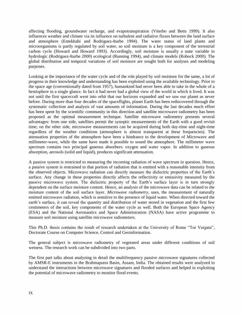
affecting flooding, groundwater recharge, and evapotranspiration (Viterbo and Betts 1999). It also
influences weather and climate via its influence on turbulent and radiative fluxes between the land surface
and atmosphere (Entekhabi and Rodriguez-Iturbe 1994). The water status of land plants and
microorganisms is partly regulated by soil water, so soil moisture is a key component of the terrestrial
carbon cycle (Howard and Howard 1993). Accordingly, soil moisture is usually a state variable in
hydrologic (Rodriguez-Iturbe 2000) ecological (Running 1994), and climate models (Robock 2000). The
global distribution and temporal variations of soil moisture are sought both for analyses and modeling
purposes.
Looking at the importance of the water cycle and of the role played by soil moisture for the same, a lot of
progress in their knowledge and understanding has been exploited using the available technology. Prior to
the space age (conventionally dated from 1957), humankind had never been able to take in the whole of a
hemisphere in a single glance. In fact it had never had a global view of the world in which it lived. It was
not until the first spacecraft went into orbit that our horizons expanded and we saw our planet as never
before. During more than four decades of the spaceflights, planet Earth has been rediscovered through the
systematic collection and analysis of vast amounts of information. During the last decades much effort
has been spent by the scientific community in this direction and satellite microwave radiometry has been
proposed as the optimal measurement technique. Satellite microwave radiometry presents several
advantages: from one side, satellites permit the synoptic measurements of the Earth with a good revisit
time; on the other side, microwave measurements can be acquired during both day-time and night-time
regardless of the weather conditions (atmosphere is almost transparent at these frequencies). The
attenuation properties of the atmosphere have been a hindrance to the development of Microwave and
millimeter-wave, while the same have made it possible to sound the atmosphere. The millimeter wave
spectrum contains two principal gaseous absorbers: oxygen and water vapor. In addition to gaseous
absorption, aerosols (solid and liquid), produces significant attenuation.
A passive system is restricted to measuring the incoming radiation of wave spectrum in question. Hence,
a passive system is restrained to that portion of radiation that is emitted with a reasonable intensity from
the observed objects. Microwave radiation can directly measure the dielectric properties of the Earth’s
surface. Any change in these properties directly affects the reflectivity or emissivity measured by the
passive microwave system. The dielectric property of the Earth’s surface layer is in turn strongly
dependent on the surface moisture content. Hence, an analysis of the microwave data can be related to the
moisture content of the soil surface layer. Microwave radiometry, uses, the measurement of naturally
emitted microwave radiation, which is sensitive to the presence of liquid water. When directed toward the
earth’s surface, it can reveal the quantity and distribution of water stored in vegetation and the first few
centimeters of the soil, key components of the water cycle as well. Both the European Space Agency
(ESA) and the National Aeronautics and Space Administration (NASA) have active programme to
measure soil moisture using satellite microwave radiometers.
This Ph.D. thesis contains the result of research undertaken at the University of Rome “Tor Vergata”,
Doctorate Course on Computer Science, Control and Geoinformation.
The general subject is microwave radiometry of vegetated areas under different conditions of soil
wetness. The research work can be subdivided into two parts.
The first part talks about analyzing in detail the multifrequency passive microwave signatures collected
by AMSR-E instruments in the Brahmaputra Basin, Assam, India. The obtained results were analyzed to
understand the interactions between microwave signatures and flooded surfaces and helped in exploiting
the potential of microwave radiometry to monitor flood events.

X
The second part of the research involves refining, exploiting and testing the soil moisture retrieval
algorithm of the SMOS mission, particularly over forests. The SMOS mission is a strategic program of
the European Space Agency, aimed at monitoring soil moisture over land and ocean salinity using an L
band radiometer.

XI
Acknowledgement Though only my name appears on the cover of this thesis, a great many people have contributed to its
production. I owe my gratitude to all those people who have made this thesis possible and because of
whom my experience at Rome has been one that I will cherish forever.
First and foremost I want to thank my advisor Prof. Paolo Ferrazzoli. It has been an honor to be his Ph.D.
student. He has taught me, both consciously and un- consciously, not just about remote sensing but many
others facets of life. I appreciate all his contributions of time, ideas, and funding to make my Ph.D.
experience productive and stimulating. The joy and enthusiasm he has for his research was very
motivational for me, even during tough times in the Ph.D. pursuit. I am also thankful for the excellent
example he has provided as a dedicated, hardworking, unbiased and honest professor. I am grateful to him
for holding me to a high research standard and enforcing strict validations for each research result, and
thus teaching me how to do best research.
It is with immense gratitude that I acknowledge the support and help of Dr. Rachid Rahmoune. His
insightful comments and constructive criticism at different stages of my research were thought-provoking
and they helped me focus my ideas. I am indebted to him for his continuous encouragement and guidance.
I will forever be thankful to Prof Domenico Solimini. He is one of the best teachers that I have had in my
life. He sets high standards for his students and he encourages and guides them to meet those standards.
His enthusiasm and love for teaching is contagious. His lectures on Understanding Earth Observation,
The Electromagnetic Foundations of Satellite Remote Sensing, have helped me a lot to understand the
basic concepts of Remote Sensing and understanding its implementation in the research work.
I acknowledge the support of the Doctorate School of Tor Vergata University, Rome, Italy, for giving me
the opportunity to carry out my doctoral research with the scholarship and LAZIODISU, for providing me
accommodation. I cannot find words to express my gratitude for Sharon, Daya Singh, Mrs Bartolini, Lui
Chi and all the staff of the International office of the University for providing all the administrative help
during my stay in Rome.
I am thankful to Antonio Perrone, Prof Leila Guerriero, Prof Elisabetta Marino and all the former as well
as the current PhD students for their constant help and support.
Most of the results described in this thesis would not have been obtained without a close collaboration
with few laboratories. I owe a great deal of appreciation and gratitude to Dr. Y. Kerr and Dr. P. Richaume,
CESBIO, Toulouse, France and Dr. R. Magagi, University of Sherbrooke, Canada. Thanks are also due to,
ESA (Euopean Space Agency) for giving me opportunity to work on SMOS data, IMD, India, and State
Water Resource Department, Lakhimpur, Assam, India for providing the daily rainfall and water level
data, respectively, for the research.
I take this opportunity to owe my deepest gratitude to, Centre for Development of Advanced Computing
(C-DAC), Pune, India, for allowing me to avail my study leave to peruse my PhD. I would like to thank
Mrs Upasana Dutta, Dr. Medha Dhurandhar, Sandeep Srivastava, Dr. Manoj Khare, Late Dr. V.
Sundarajan and Sunil Misar for all the support and encouragement both at personal and professional level.
Few people support you directly and few support you indirectly to achieve your goals in life. My deepest gratitude goes to my Brother in law Ashutosh Singh for his unflagging love and support

XII
throughout my professional carrier.
I also thank my friends Mrs. Anjali Sharma, Saikat Sen Gupta, Deepak Nair, Raja Chakraborty, Cristina
Vittucci (too many to list all here but you know who you are!) for providing support and friendship that I
needed. Their support and care helped me overcome setbacks and stay focused on my study. I greatly
value their friendship and I deeply appreciate their belief in me.
I would like to thank my family for all their love and encouragement. For my parents who raised me,
supported me and did so many untold sacrifices for me in all my pursuits.
The acknowledgement will be incomplete, if I miss to thank my loving son, Achintya, whose eyes always
inspired me to be through with this research work quickly.
A journey is easier when you travel together. Interdependence is certainly more valuable than
independence. A very special thanks to my loving, supportive, encouraging, and patient wife, Aastha,
whose faithful support during all the stages of this Ph.D. is so appreciated.
Above all, I owe it all to the Almighty God for granting me the wisdom, health and strength to undertake
this research task and enabling me to its completion.
Thank you.
XIII
List of Figures
Figure I : The water cycle (from http:ga.water.usgs.gov) ......................................................... VIII
Figure 1.1 : Geometry of the incident radiation from an extended source on an antenna, from
(Ulaby et al. 1981) ....................................................................................................... 2
Figure 1.2 : Comparision of Plank radiation law with its low-frequency approximation
(Rayleigh-Jeans law) for T = 300K and T = 6000K ...................................................... 3
Figure 1.3: Radiation incident upon an Earth-looking radiometer. relationship between the
antenna temperature TA, apparanet temperature TAP and brightness temperature
TB, from Ulaby et al., (1981) ] ...................................................................................... 5
Figure 1.4: Atmospheric attenuation by absorption at different frequencies (Solimini 2013) ..... 7
Figure 1.5: Typical values of Faraday rotation angle as a function of TEC and frequency, from
(P.531-6 et al. 2001) ..................................................................................................... 8
Figure 1.6: A Total Power radiometer block diagram. from [(Ulaby et al. 1982)] ......................... 11
Figure 1.7: (a) total power, (b) Dicke, and (c) noise injection radiometer schematic [Skou, 1989]
................................................................................................................................... 13
Figure1.8: Cause of floods (http://drace-project.org/index.php/floods/human factor) ............. 16
Figure 1.9: Photo of AMSR-E sensor unit during deployment testing at NASDA Tsukuba
Space Center .............................................................................................................. 25
Figure 1.10 : Overview of AMSR-E sensor unit ............................................................................. 26
Figure 1.11: AMSR-E scanning geometry ...................................................................................... 27
Figure 1.12 : Schematic diagram of 89 GHz scan geometry. Beam centers of three successive
scans are shown by solid (N), dotted (N+1), and thick-solid (N+2) lines. .................. 28
Figure 1.13 : MIRAS arm and LICEF details. Courtesy ESA ............................................................ 31
Figure 1.14 : Geometric concentions for the definition of the (ξ, η) coordinates. ....................... 32
Figure 1.15 : SMOS (a) AF and (b) EAF-FOV in the cosine domain: (black) unit circle, (red)
SMOS aliased zone borders, and (green) SMOS (a) AF-FOV and (b) EAF-FOV .......... 32
XIV
Figure 1.16: (a) Radiometric Radiometric (blue) Accuracy and (red) Sensitivity, and (b) (blue)
Incidence Angle and (red) Spatial Resolution [calculated using SEPS]. ..................... 33
Figure 1.17: (a) Stereo pairs of a regular icosahedron., (b) Subdividing the faces of a regular
icosahedron: Gray and black regions represent the central hexagons for resolutions
1 and 2, respectively. ................................................................................................. 34
Figure 2.1 : USDA Soil classification triangle ……………………………….………………………………………….39
Figure 2.2 : Relative real (upper curves) and imaginary (lower curves) parts of permittivity of
two different soil types at f = 1.4GHz (left) and f = 5.0 GHz (right) vs. volumetric
water content mv (m3/m3). (Solimini 2013) .............................................................. 42
Figure 2.3 : Microwave emissivity of a fresh water at surface at L- (left), C- (middle)
and X-band (right). ..................................................................................................... 48
Figure 2.4: C-band emissivity of ideal flat-surface terrain: top left, dry (mv = 12%); top right,
moist (mv = 21%); bottom left, wet (mv = 31%); bottom right, very wet (mv = 35%).
Red curves refer to v polarization and the blue curves to h polarization. ................ 49
Figure 2.5: L-band emissivity of ideal at-surface terrain: top left, dry (mv = 12%); top right,
moist (mv = 21%); bottom left, wet (mv = 31%); bottom right, very wet (mv = 35%).
Red curves refer to vertical polarization, the blue curves to horizontal polarization.
Note that ev < 1 at the pseudo-Brewster angle ........................................................ .49
Figure 3.1: Study area:Lakhimpur District, Assam, India .............................................................. 55
Figure 3.2: Relationship between emissivities at H(eH) and V(eV) polarization at 10.65, 18.7
and 36.5 GHz for Dhalghat Site (2007) ...................................................................... 57
Figure 3.3: Upper figures: PI (C, X and Ka band) vs Julian Date of 2007 for Dhalgat, Ghansari
and Jamugurihat sites. Lower figures: corresponding trends of Water Level (WL). . 59
Figure 3.4: Temporal trend of FWS at H and V Polarization as a function of Julian Date of 2007.
Left: X band. Right: Ka band. ...................................................................................... 61
Figure 3.5: Scatterplots of Polarization Index (PI) vs. Water Level (WL) for Dhalgat, Ghansari
and Jamugurihat sites. Left: 10 GHz. Right: 36 GHz. ................................................. 62
XV
Figure 3.6: Multitemporal trends. a) PI at 36 Ghz, b) PI at 10 Ghz and c) Water Level. Rainfall
measurements are reported for comparison. ........................................................... 64
Figure 3.7: (a) Maps of FWSH, FWSV and PI at 10 GHz and 36 GHz on 29/06/2007, without rain
(b): Maps of FWSH, FWSV and PI at 10 GHz and 36 GHz on 15/07/2007 with rain .......... 65
Figure 3.8: Scatterplots of TBV at 89.0 GHz vs. the difference TBV (23 GHz – 89.0 GHz).
Left: June 29 (no rain). Right: July 15 (rain) ............................................................... 66
Figure 3.9: Scatterplots of Polarization Index (PI) at X band vs. Water Level for Dhalgat,
Ghansari ..................................................................................................................... 67
Figure 3.10: Maps of PI at X band of Lakhimpur District and neighboring areas, in 2007.
Left hand side, top to bottom: March 18th (before flood), September 10th
(during flood) and difference image. Right had side, top to bottom: September 10th
(during flood), November 13th (after flood) and the difference image. White
squares indicate the locations of water level stations and the blue line represents
the main rivers. .......................................................................................................... 68
Figure 4.1: Trends of fitted radiative transfer parameters τF and ωF as a function of
maximum yearly value of forest LAI, for broadleaf forests (Rahmoune 2013)……… 74
Figure 4.2: SCAN/SNOTEL network ....…………………………………………………………………. ………………… 77
Figure 4.3: CanEx-SM10 study area over BERMS ……………………………………………………… …………….78
Figure 4.4: RFI map over India ...................................................................................................... 80
Figure 4.5: RFI issues over forests (Western Ghats) in India (a) RFI maps at X and Y pol
(b) TB at V and Ho pol. vs Julian Days ....................................................................... 81
Figure 4.6: Global Map of Retreived optical depth ....................................................................... 82
Figure 4.7: Optical Depth Maps obtained from SMOS (1-4 July 2011) (a) and ............................ 83
Figure 4.8: Retrieved optical depth vs. forest height (m) reported in (Masson et al. 2003a) ...... 84
Figure 4.9: Tailor Diagram of S6 and S8 Model for 80% (a) & 40% (b) Forest Cover .................... 87
Figure .4.10: Correlation coefficient and Root Mean Square Error S6 Model .............................. 88
Figure 4.11: Taylor Diagram for S6 and S8 model SMOS retrieved SM vs BERMS
ground observed SM at OJP (a) and OBS (b) sites. .................................................... 89
XVI
Figure 4.12: Scatterplot of All the SMOS retrieved SM and SCAN node SM obtained
from case 1…......………………………………………………………………………………………………… 91
Figure 4.13: Bar charts showing CC, RMSE, Ba and % of samples obatined for each case for
40 % FFO and 80 % FFO ......................................................................................... 93
Figure 4.14: Scatterplot of all the SMOS retrieved SM vs BERMS Ground observed SM obtained
from case 1. .............................................................................................................. 94
Figure 4.15: Comparison of Soil Moisture Retrieved from different algorithms vs.
SCAN/SNOTEL Ground Observation over different forest land covers
(80% forest (a), 40% forest (b) and low vegetation (c)). Results are given
in form of a global scatterplot, including all nodes. .................................................. 96
XVII
List of Tables
Table 1.1: Microwave Electromagnetic Spectrum ........................................................................ 10
Table 1.2: Summary of Major Performance and Characteristic of AMSR-E .................................. 25
Table 2.1: Classification of soil particles as a function of their diameter (in mm) ....................... .39
Table 2.2: Properties of Soil as a function of Texture………………………………………………………………..39
Table 2.3 : Details of parameters emperically determined by Dobson et., al. (1985) .................. 44
Table 3.1: Minimum and maximum values of emissivities, and average PI values, on selected
dates at X and Ka Bands……………………………………………………………………… ………………….. 59
Table 3.2: Cumulative distribution of FWS calculated at specific days using X band TB values
and surface temperature data provided by IMD. .......................................................... 60
Table 4.1: Correlation coefficient (CC), Root Mean Square Error (RMSE) and Bais (BA) for
different SCAN nodes with respect to SMOS nodes averaged over 15Km buffer
(with 80% forest) fraction for S6 and S8 algorithm ……………………………………………………86
Table 4.2: Correlation coefficient (CC), Root Mean Square Error (RMSE) and Bais (BA) for
different SCAN nodes with respect to SMOS nodes averaged over 15Km buffer
(with 40% forest) fraction for S6 and S8 algorithm ……………………………………………………87
Table 4.3: CC, RMSE and Bais for the case 1 for 80% and 40% forest fraction……………………………90
Table 4.4: CC, RMSE and Bais for the case 2 of 80 % and 40% forest fraction……………………………91
Table 4.5: CC, RMSE and Bais for the case 3 for 80% and 40% forest fraction …………………………..92
Table 4.6: CC, RMSE and Bais for all the cases for OBS and OJP sites…………………………………………94
Table 4.7: Correlation coefficient (CC) and Root Mean Square Error (RMSE) for each node of
SMOS node under different forest fractions covered area with respect to the ground
observed SM……………………………………………………….………………………….…………………………97
Table 4.8: Correlation coefficient (CC) and Root Mean Square Error (RMSE) for each node of
LPRM node under different forest fractions covered area with respect to the ground
observed SM……………………………………………………….…………………………………………………….98

XVIII
Glossary
AMSR-E Advanced Microwave Scanning
Radiometer - Earth Observing System
ATBD Algorithm Theoretical Baseline
Document
DFFG Discrete Flexible Fine Grid
DFG Discrete Fine Grid
DGG Discrete Global Grid: the SMOS grid
ECMWF European Centre for Medium-range
Weather Forecasting
ESA European Space Agency
FOV SMOS alias-free Field of View
L1c SMOS Level 1c processor or Data Products
L2 SMOS Level 2 processor or Data Products
LAI Leaf Area Index
LAIMax Maximum value of the LAI over one
year for a forest stand
RFI Radio Frequency Interference
RMSE Root Mean Square Error
RTE RT Radiative Transfer Equation, Radiative
Transfer
SM Soil volumetric Moisture content
TEC Total Electron Content
IEEE Institute of Electrical and Electronics
Engineers
TPR Total Power Radiometer
NIR Noise Injection Radiometer
TDR Time Domain Reflectometry
NP Neutron Probe
AVHRR Advanced Very High Resolution
Radiometer
TRMM Tropical Rainfall Measuring Mission
TB Brightness Temperatures
SMOS Soil Moisture and Ocean Salinity
ISEA – Grid - Inverse Snyder Icosahedral equal
area projection
BSW Bound Soil Water
FSW Free Soil Water
RMDM refractive mixing dielectric model
VMC Volumetric Water Content
PI Polarization Index
WL Water Level
FWS Fractional Water Surface
2
1. Introduction
1.1 Basic Concepts
The Earth continuously receives electromagnetic radiation coming mainly from the Sun. Part of it is
scattered and/or absorbed by the atmosphere, and the other part is transmitted to the Earth’s surface. At
the Earth’s surface, part of this energy is absorbed, and part is scattered outwards. The energy absorbed is
then transformed into thermal energy, which leads to a temperature increase until the thermodynamic
equilibrium is reached. At this state, according to Thermodynamics, all media (gases, liquids, solids and
plasma) radiate energy to keep the energy balance. Radiometry is the field of science that studies the
thermal electromagnetic energy radiated by the bodies. Radiometers are instruments capable of measuring
the power emitted by a body with high accuracy. A microwave radiometer is a passive sensor that simply
measures electromagnetic energy radiated towards it from some target or area. As a passive sensor, it is
related more to the classical optical and IR sensors than to radar, its companion active microwave sensor.
The energy detected by a radiometer at microwave frequencies is the thermal emission from the target
itself as well as thermal emission from the sky that arrives at the radiometer after reflection from the
target.
The basic concepts of microwave radiometry are reviewed in this section.
1.1.1 Brightness and power collected by an antenna
Brightness, is defined as the power emitted by a source in a solid angle per unit area of the emitting
surface B (θ, ϕ) [Wsr−1
m−2
]. Although the proper SI term for this quantity is actually radiance, but the
term brightness is still commonly used in radiometry, photonics and laser work. Since the word
“brightness” conveys a more intuitive understanding of its meaning than the technical term radiance,
brightness is more commonly used.
Brightness depends on the source’s normalized radiation pattern Ft (θ, ϕ) (power density per unit solid
angle) and the total radiating area At.
( , )
( , ) t
t
FB
A
(1.1)
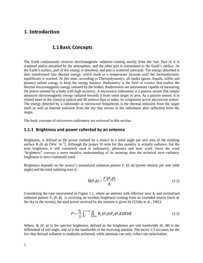
Considering the case represented in Figure 1.1, where an antenna with effective area Ar and normalized
radiation pattern Fn (θ, ϕ) is receiving an incident brightness coming from an extended source (such as
the sky or the terrain), the total power received by the antenna is given by (Ulaby et al., 1981):
4
( , ) ( , )2
f fr
f nf
AP B F d df
(1.2)
Where, Bf (θ, ϕ) is the spectral brightness, defined as the brightness per unit bandwidth df, dΩ is the
differential of soil angle, and ∆f is the bandwidth of the receiving antenna. The factor 1/2 accounts for the
fact that thermal radiation is randomly polarized, while antennas can only collect one polarization.
2
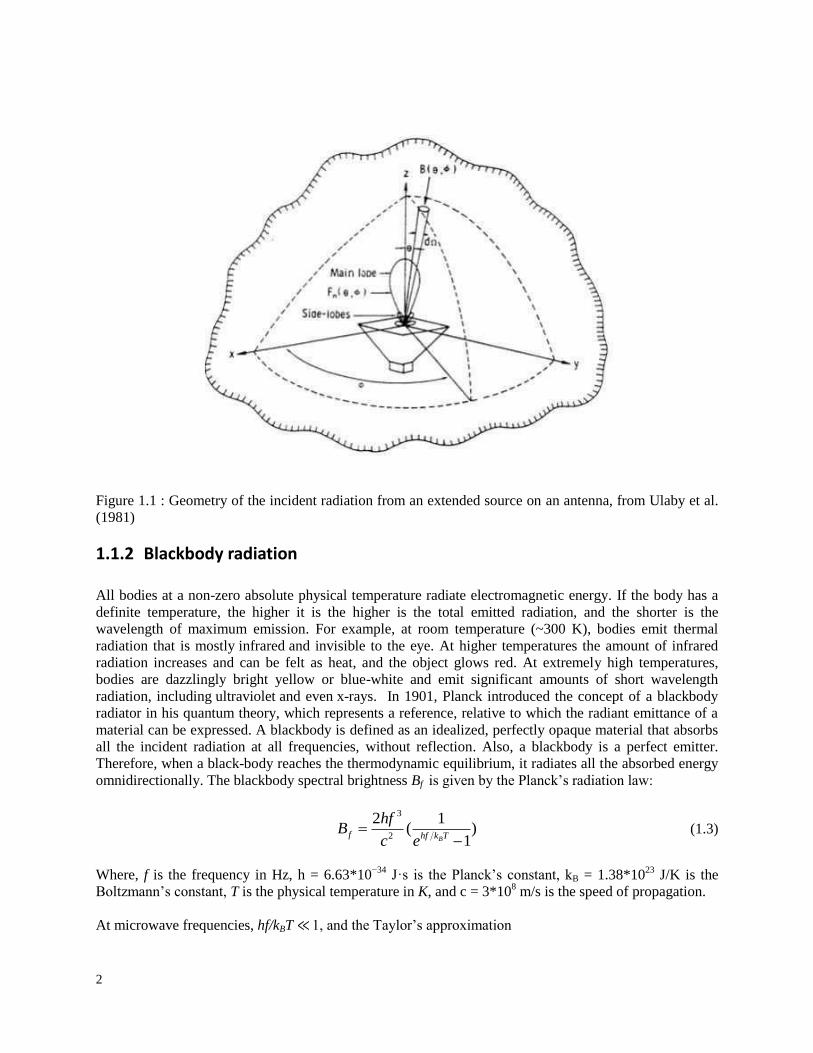
Figure 1.1 : Geometry of the incident radiation from an extended source on an antenna, from Ulaby et al.
(1981)
1.1.2 Blackbody radiation
All bodies at a non-zero absolute physical temperature radiate electromagnetic energy. If the body has a
definite temperature, the higher it is the higher is the total emitted radiation, and the shorter is the
wavelength of maximum emission. For example, at room temperature (~300 K), bodies emit thermal
radiation that is mostly infrared and invisible to the eye. At higher temperatures the amount of infrared
radiation increases and can be felt as heat, and the object glows red. At extremely high temperatures,
bodies are dazzlingly bright yellow or blue-white and emit significant amounts of short wavelength
radiation, including ultraviolet and even x-rays. In 1901, Planck introduced the concept of a blackbody
radiator in his quantum theory, which represents a reference, relative to which the radiant emittance of a
material can be expressed. A blackbody is defined as an idealized, perfectly opaque material that absorbs
all the incident radiation at all frequencies, without reflection. Also, a blackbody is a perfect emitter.
Therefore, when a black-body reaches the thermodynamic equilibrium, it radiates all the absorbed energy
omnidirectionally. The blackbody spectral brightness Bf is given by the Planck’s radiation law:
3
2
2 1( )
1Bf hf k T
hfB
c e
(1.3)
Where, f is the frequency in Hz, h = 6.63*10−34
J·s is the Planck’s constant, kB = 1.38*1023
J/K is the
Boltzmann’s constant, T is the physical temperature in K, and c = 3*108 m/s is the speed of propagation.
At microwave frequencies, hf/kBT ≪ 1, and the Taylor’s approximation
3
2
1 (1 ......) 1 , 12
x xe x x forx (1.4)
can be used to simplify (1.3) into a simple linear law such as:
2
2 2
2 2B Bf
f k T k TB
c (1.5)
where λ = c/f is the wavelength. This is the Rayleigh-Jeans law, a low-frequency approximation of the
Planck’s radiation law. The Rayleigh-Jeans law is widely used in microwave radiometry since it is
mathematically simpler than the Planck law and has a deviation error smaller than 1% for f < 117 GHz
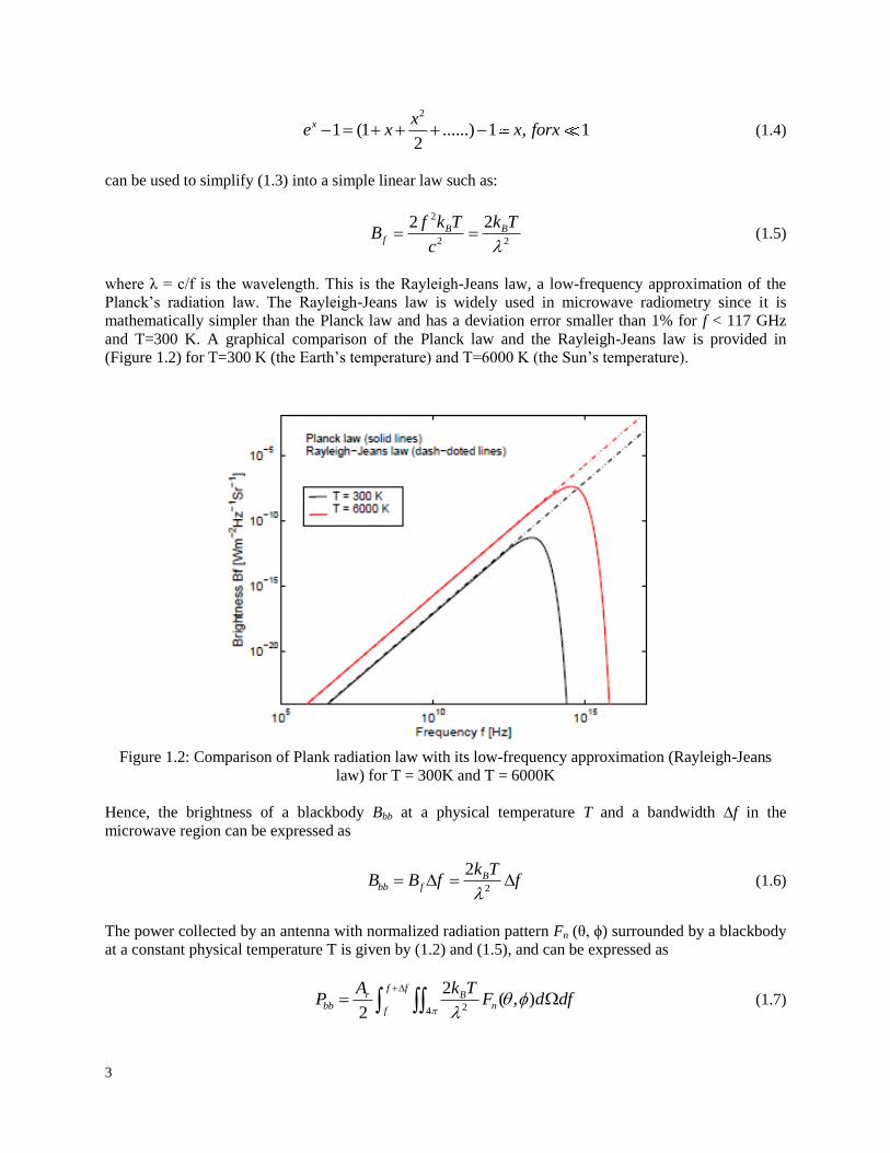
and T=300 K. A graphical comparison of the Planck law and the Rayleigh-Jeans law is provided in
(Figure 1.2) for T=300 K (the Earth’s temperature) and T=6000 K (the Sun’s temperature).
Figure 1.2: Comparison of Plank radiation law with its low-frequency approximation (Rayleigh-Jeans
law) for T = 300K and T = 6000K
Hence, the brightness of a blackbody Bbb at a physical temperature T and a bandwidth ∆f in the
microwave region can be expressed as
2
2 Bbb f
k TB B f f
(1.6)
The power collected by an antenna with normalized radiation pattern Fn (θ, ϕ) surrounded by a blackbody
at a constant physical temperature T is given by (1.2) and (1.5), and can be expressed as
24
2( , )
2
f fr B
bb nf
A k TP F d df
(1.7)
4
The solid angle Ω is the 2-Dimension analog of the conventional 1-Dimension angle. Just as the 1-D
angle is defined as the distance along a circle divided by the radius of that circle, so the solid angle Ω is
analogously defined as the area on the surface of a sphere divided by the radius squared of that sphere.
The unit for Ω is steradians (sr), although it should be noted that both of these measures of angle (1-D and
2-D) have no actual dimensions. Since the total surface area of a sphere is 4πR2, the total solid angle in
one sphere is 4π sr.
In case of the antenna, solid angle can be expressed as a function of its effective area
2
4( , )p n
r
F dA
(1.8)
Hence, assuming the system bandwidth ∆f small enough so that Bf can be considered constant over the
frequency range, equation (1.7), becomes
bb BP k T f (1.9)
This direct linear relationship between power and temperature is of fundamental importance in
microwave remote sensing, where the power received by an antenna is commonly given in units of
temperature (see Section 1.1.4).
1.1.3 Gray body radiation
A blackbody is a useful theoretical concept for describing radiation principles, but real materials or gray
bodies do not behave like blackbodies: they do not absorb the entire energy incident upon them and their
emission is lower than that of perfect blackbodies. It is therefore convenient to define a microwave
brightness temperature TB (θ, ϕ), so that the brightness of a gray body can be expressed, similarly to
equation (1.6) as,
2
2( , ) ( , )B
B
kB T f
(1.10)
TB (θ, ϕ) is the temperature that a blackbody would have to produce the observed brightness B (θ, ϕ); it is
not the real temperature of the object, but an effective temperature. The brightness of gray bodies relative
to that of blackbodies at the same physical temperature is called the emissivity e (θ, ϕ).
( , )( , )
( , ) B
bb
TBe
B T
(1.11)
Note that, since real materials emit less than a blackbody, B (θ, ϕ) ≤ Bbb, and therefore 0 ≤ e (θ, ϕ) ≤ 1.
The emissivity equals 0 in the case of a perfect reflector (e.g. a lossless metal), and 1 in the case of a
perfect absorber, a blackbody. Thus, the brightness temperature TB (θ, ϕ) of a material is always smaller
than, or equal to, its physical temperature T.
5
1.1.4 Power-temperature correspondence
In the microwave region, since the radiance emitted by an object is proportional to its physical
temperature (1.5), it is convenient to express the radiance in units of temperature. Hence, the brightness
temperature TB (θ, ϕ) is used to characterize the radiation of an object (equation 1.10). Similarly, an
apparent temperature TAP is defined to characterize the total brightness incident over a radiometer antenna
Bi (θ, ϕ), as
2
2( , ) ( , )B
i AP
kB T f
(1.12)
Therefore, the power collected by an antenna with normalized radiation pattern Fn (θ, ϕ) receiving a non-
blackbody incidence brightness is given by (1.2) and (1.12),
24
2( , ) ( , )
2
f fr B
bb AP nf
A k TP T F d df
(1.13)
It is convenient to define an antenna temperature TA as the temperature equivalent of the power received
with an antenna, so that (1.9) holds as P = kBTA∆f for gray bodies. Hence, TA can be expressed as
2 4
( , ) ( , )rA AP n
AT T F d
(1.14)
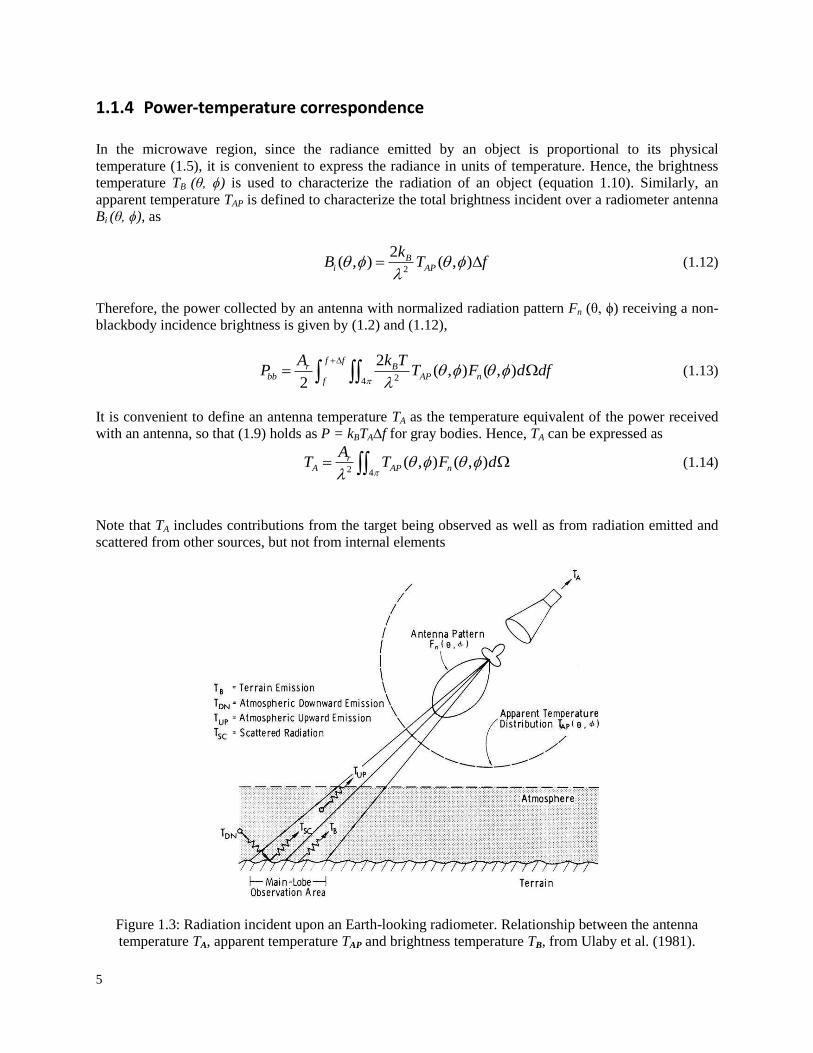
Note that TA includes contributions from the target being observed as well as from radiation emitted and
scattered from other sources, but not from internal elements
Figure 1.3: Radiation incident upon an Earth-looking radiometer. Relationship between the antenna
temperature TA, apparent temperature TAP and brightness temperature TB, from Ulaby et al. (1981).
6
The case of prime interest in passive remote sensing is that of an Earth-looking radiometer, as illustrated
in (Figure 1.3). In this case, the radiation incident upon the antenna is a function of both the land surface
and the atmosphere, and may be expressed as
1
( , ) ( )AP UP S SC
a
T T T TL
(1.15)
where TS is the brightness temperature of the land surface, TUP is the atmospheric upward radiation, TSC is
the downward atmospheric radiation scattered by the Earth’s surface in the direction of the antenna, and
La represents the attenuation of the atmosphere. At the lower microwave frequencies used in soil moisture
sensing, the atmospheric effects are small and may be safely neglected in most cases.
1.1.5 Measuring brightness temperatures from space and concerns Space-borne radiometers are very sensitive receivers capable of measuring the radiance emitted by the
Earth’s surface with high accuracy. They are designed to transform the radiation collected by an antenna
into mapable electric signals, and its performance is usually characterized by its radiometric resolution,
accuracy, and spatial resolution (Randa 2008):
The radiometric resolution (sometimes called sensitivity) is computed as the smallest change in
input brightness temperature or radiance that can be detected in the system output.
The radiometric accuracy represents the closeness of the agreement between the measured
antenna temperature and its true value (systematic error). Because the true value cannot be
determined exactly, the measured or calculated value of highest available accuracy is typically
taken to be the true value.
The spatial resolution is the ability of the sensor to separate two closely spaced identical point
sources.
In a remote sensing mission, in addition to instrumental errors, other phenomena can degrade the
radiometric resolution and must be corrected (compensated for). At lower frequencies, the atmosphere is
almost transparent, and the main error sources are the Faraday rotation and the space radiation, which are
described hereafter.
1.1.5.1 The atmosphere:
The atmosphere plays an obvious crucial role in Earth observation from space, since the electromagnetic
field has to cross it. The damping of the field caused by the atmosphere affects the performance of the
observing systems. Atmospheric attenuation caused by absorption from the constituent gases is strongly
dependent on the frequency. The atmosphere essentially consists of nitrogen (78.1%) and oxygen
(20.9%), a small amount of water vapor and minor quantities of other gases(carbon dioxide, methane,
ozone etc.). Because of the low activity of nitrogen, permittivity of the atmosphere mainly results from
the polarization of the other molecule species of which water vapor, being polar, is particularly active. At
radio frequency (i.e., microwave), main interactive gases are oxygen and especially water vapor, which
determine the dominant trend with frequency of real and imaginary parts of atmospheric permittivity. As
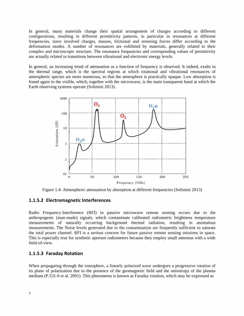
indicated by the diagram in Figure 1.4, the overall attenuation by absorption show peaks at the resonance
frequencies of water vapor and oxygen.
7
In general, many materials change their spatial arrangement of charges according to different
configurations, resulting in different permittivity patterns, in particular in resonances at different
frequencies, since involved charges, masses, frictional and restoring forces differ according to the
deformation modes. A number of resonances are exhibited by materials, generally related to their
complex and microscopic structure. The resonance frequencies and corresponding values of permittivity
are actually related to transitions between vibrational and electronic energy levels.
In general, an increasing trend of attenuation as a function of frequency is observed. It indeed, exalts in
the thermal range, which is the spectral regions at which rotational and vibrational resonances of
atmospheric species are more numerous, so that the atmosphere is practically opaque. Low absorption is
found again in the visible, which, together with the microwave, is the main transparent band at which the
Earth observing systems operate (Solimini 2013) .
Figure 1.4: Atmospheric attenuation by absorption at different frequencies (Solimini 2013)
1.1.5.2 Electromagnetic Interferences
Radio Frequency Interference (RFI) in passive microwave remote sensing occurs due to the
anthropogenic (man-made) signals, which contaminate calibrated radiometric brightness temperature
measurements of naturally occurring background thermal radiation, resulting in anomalous
measurements. The Noise levels generated due to the contamination are frequently sufficient to saturate
the total power channel. RFI is a serious concern for future passive remote sensing missions in space.
This is especially true for synthetic aperture radiometers because they employ small antennas with a wide
field-of-view.
1.1.5.3 Faraday Rotation
When propagating through the ionosphere, a linearly polarized wave undergoes a progressive rotation of
its plane of polarization due to the presence of the geomagnetic field and the anisotropy of the plasma
medium (P.531-6 et al. 2001). This phenomena is known as Faraday rotation, which may be expressed as
8
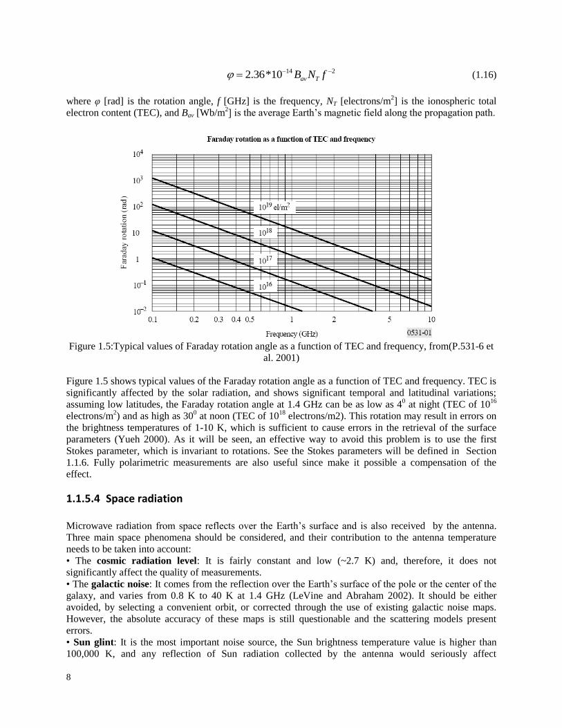
14 22.36*10 av TB N f (1.16)
where φ [rad] is the rotation angle, f [GHz] is the frequency, NT [electrons/m2] is the ionospheric total
electron content (TEC), and Bav [Wb/m2] is the average Earth’s magnetic field along the propagation path.
Figure 1.5:Typical values of Faraday rotation angle as a function of TEC and frequency, from(P.531-6 et
al. 2001)
Figure 1.5 shows typical values of the Faraday rotation angle as a function of TEC and frequency. TEC is
significantly affected by the solar radiation, and shows significant temporal and latitudinal variations;
assuming low latitudes, the Faraday rotation angle at 1.4 GHz can be as low as 40 at night (TEC of 10
16
electrons/m2) and as high as 30
0 at noon (TEC of 10
18 electrons/m2). This rotation may result in errors on
the brightness temperatures of 1-10 K, which is sufficient to cause errors in the retrieval of the surface
parameters (Yueh 2000). As it will be seen, an effective way to avoid this problem is to use the first
Stokes parameter, which is invariant to rotations. See the Stokes parameters will be defined in Section
1.1.6. Fully polarimetric measurements are also useful since make it possible a compensation of the
effect.
1.1.5.4 Space radiation
Microwave radiation from space reflects over the Earth’s surface and is also received by the antenna.
Three main space phenomena should be considered, and their contribution to the antenna temperature
needs to be taken into account:
• The cosmic radiation level: It is fairly constant and low (~2.7 K) and, therefore, it does not
significantly affect the quality of measurements.
• The galactic noise: It comes from the reflection over the Earth’s surface of the pole or the center of the
galaxy, and varies from 0.8 K to 40 K at 1.4 GHz (LeVine and Abraham 2002). It should be either
avoided, by selecting a convenient orbit, or corrected through the use of existing galactic noise maps.
However, the absolute accuracy of these maps is still questionable and the scattering models present
errors.
• Sun glint: It is the most important noise source, the Sun brightness temperature value is higher than
100,000 K, and any reflection of Sun radiation collected by the antenna would seriously affect
9
measurements. Hence, direct reflections should be avoided by pointing the instrument to the shadow zone
of a polar sun-synchronous orbit.
1.1.6 Polarization and Stokes parameters
The received field of an antenna is composed of electric and magnetic lines of forces. These lines of
forces are always at right angle to each other. The electric field determines the direction of polarization of
the wave.
The polarization of an electromagnetic wave can be completely described by the four Stokes parameters I,
Q, U, V. The first Stokes parameter (I) describes the total intensity of electromagnetic emission and the
second Stokes parameter (Q) is the difference between the intensity in two orthogonal directions in a
given polarization frame, i.e. vertical and horizontal polarizations. The third (U) and fourth (V) Stokes
parameters, respectively, represent the real and imaginary parts of the cross-correlation between these
orthogonal polarizations (Randa 2008)
2 2
0
2 2
0
*
0
*
0
| | | |,
| | | |,
2,
2,
v h
v h
e v h
m v h
E EI
E EQ
R E EU
I E EV
(1.17)
Where, Ev and Eh are the electric field components at vertical and horizontal polarizations, respectively,
and ηo is the electromagnetic wave impedance of the medium (120π Ω in vacuum). In polarimetric remote
sensing radiometry the Stokes parameters are conventionally expressed in terms of brightness temperature
2
2
2
45 45
2
. ,.
. ,.
. ,.
. ,.
I v h
B w
Q v h
B w
U
B w
V lc rc
B w
T T T Ik B
T T T Qk B
T T T Uk B
T T T Vk B
(1.18)
where λ is the wavelength, and Bw is the noise-equivalent bandwidth. Tv and Th are the vertical and
horizontal brightness temperatures, T45 and T−45 represent orthogonal measurements skewed ±45 with
respect to normal, and Tlc and Trc refer to left-hand and right-hand circular polarized quantities.
10
Generally, the energy emitted from the Earth’s surface is partly polarized, meaning that the vertical
brightness temperature is different from the horizontal. Whereas conventional dual-polarization
radiometers only measure vertical and horizontal polarized brightness temperatures, a polarimetric
radiometer is capable of directly or indirectly measuring all four Stokes parameters, which provides a full
characterization of the polarization properties of the emitted energy. Note that the Faraday rotation ϕ
mixes the polarization as follows
cos sin ,
sin cos
Faraday
v v h
Faraday
h v h
E E E
E E E
(1.19)
Hence, the first and fourth Stokes parameter are invariant to rotations, whereas the second and third
Stokes parameter are not. In remote sensing, third and fourth Stokes parameters are primarily used for
correcting polarization rotation (Yueh et al. 1995), (Mart´ın-Neira et al. 2002) or, in the case of the ocean
for instance, to infer wind direction information (Brown et al. 2006).
1.1.7 Microwave electromagnetic spectrum Electromagnetic waves are originator and carrier of information in earth observation. The information
content of products delivered by a given type of system is essentially related to electromagnetic
parameters (mainly frequency/ wavelength) and to the properties of the observed medium. . Frequency or
wavelength of operation is mainly selected considering the kind, intensity and effectiveness of the
interaction with the material to be observed and on the transmission of the atmosphere interposed between
the sensor and the observed object. The wave interacts with different variety of materials, including
natural or man-made solid, liquid and gaseous media. Because of the variety of obtainable information
and the exploitability of various atmospheric windows, the portion of the electromagnetic spectrum over
which the earth observation missions operate is wide, from low microwave frequency to the ultraviolet
wavelengths. The choice of sensor, of frequency band is essentially driven by the kind of object user wish
to observe and the type of parameters to be retrieved.
Microwaves are waves with wavelengths ranging from about one meter to about one millimeter, or
equivalently, with frequencies between 300 MHz (0.3 GHz) and 300 GHz. The microwave spectrum is
subdivided into bans, according to the IEEE definitions recalled in (Table 1.1)
Table 1.1: Microwave Electromagnetic Spectrum
IEEE Band Frequency range (GHz)
P (UHF) 0.3 – 1.0
L 1.0 – 2.0
S 2.0 – 4.0
C 4.0 – 8.0
X 8.0 – 12.0
Ku 12.0 – 18.0
K 18.0 – 27.0
Ka 27.0 – 40.0
11
1.1.8 Microwave Radiometers
A radiometer is a receiver that measures the electromagnetic radiation emitted by an object in a given
frequency band. This radiation, being basically thermal noise, has generally very low power.
1.1.8.1 Real Aperture Radiometers
Real aperture radiometers scan across the field of view to measure the TB. Moreover, if they are flying at
a height h the antenna size D required for a footprint d is D = ¸λh/d. For low-Earth orbit satellites
operating at L-band, such as SMOS, an adequate ground resolution using real aperture radiometer implies
an antenna size of several metres. This is impossible to implement for in-orbit sensors, but these
radiometers are still being used (AMSR-E). The configurations and main characteristics of real aperture
radiometers are briefly described hereafter. Further information may be found in ((Skou 1989) and
(Ulaby et al. 1986b).
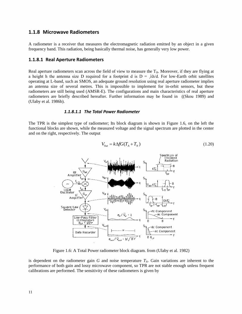
1.1.8.1.1 The Total Power Radiometer
The TPR is the simplest type of radiometer; Its block diagram is shown in Figure 1.6, on the left the
functional blocks are shown, while the measured voltage and the signal spectrum are plotted in the center
and on the right, respectively. The output
0 ( )ut A NV k fG T T (1.20)
Figure 1.6: A Total Power radiometer block diagram. from (Ulaby et al. 1982)
is dependent on the radiometer gain G and noise temperature TN. Gain variations are inherent to the
performance of both gain and lossy microwave component, so TPR are not stable enough unless frequent
calibrations are performed. The sensitivity of these radiometers is given by
12
A N
r
T TT
f
(1.21)
being r the integration time. It is the maximum than can be achieved if gain variations are neglected.
1.1.8.1.2 Dicke radiometer
The Dicke radiometer was proposed to solve the stability problems of total power radiometers. A Dicke
radiometer views the scene during half the cycle and a matched load during the other half of the cycle. In
this case, instead of the antenna temperature the difference between the antenna temperature and a known
reference value TR is measured:
( )out A RV c T T G (1.22)
Note that this radiometer is more stable than TPR since the output does not depend on TN and the weight
of G can be diminished by choosing TR values in the range of TN. However, neglecting the gain
fluctuations, the sensitivity of this configuration is:
2 A R
r
T TT
f
(1.23)
It is degraded by a factor of 2 as compared to total power radiometers. The 2 factor arises from the fact
that the scene is measured only half of the time.
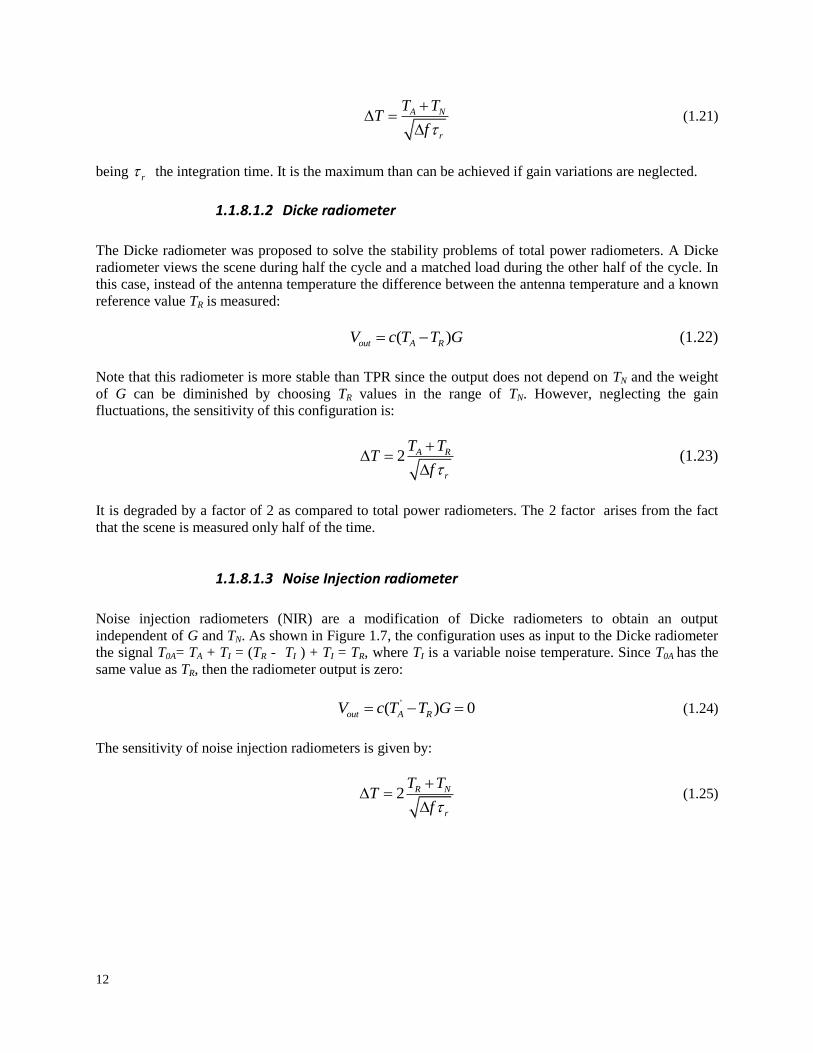
1.1.8.1.3 Noise Injection radiometer
Noise injection radiometers (NIR) are a modification of Dicke radiometers to obtain an output
independent of G and TN. As shown in Figure 1.7, the configuration uses as input to the Dicke radiometer
the signal T0A= TA + TI = (TR - TI ) + TI = TR, where TI is a variable noise temperature. Since T0A has the
same value as TR, then the radiometer output is zero:
'( ) 0out A RV c T T G (1.24)
The sensitivity of noise injection radiometers is given by:
2 R N
r
T TT
f
(1.25)
13
Figure 1.7: (a) total power, (b) Dicke, and (c) noise injection radiometer schematic (Skou 1989)
1.1.8.2 Synthetic Aperture Radiometers
Synthetic aperture technology was proposed to solve the antenna size problem of real aperture
radiometers commented on the previous section (LeVine and Good 1983). The basic concept of
interferometric radiometry is to synthesize a large aperture using a number of small antennas. A two-
dimensional image of the observed scenario is obtained by the cross-correlation of every pair of antenna
having an overlapping field of view. The output voltages of a pair of antennas (e.g. located at (X1, Y1) and
(X2, Y2)) are cross-correlated to obtain the so- called “visibility samples", as expressed by the following
equation
*
1 2
1 2 1 2
1 1( , ) ( ) ( )
2B
V u v b t b tk B B G G
(1.26)
where u and v are the spatial frequencies of visibility sample: (u, v) = (X2 - X1, Y2 - Y1) / λ = (∆x, ∆y) / λ,
kB is the Boltzmann constant, B1 and B2 the receivers' noise bandwidths, G1 and G2 the avail- able power
gains, b1(t) and b2(t) the complex signals measured by elements 1 and 2, respectively, and * is the
complex conjugate operation. The complete set of the visibility samples is called a visibility map, and it is
approximately the Fourier transform of the brightness temperature distribution of the scene.
To invert this process the inverse Fourier transform can be applied as a first approximation (Camps et al.
1997) or a more sophisticated G-matrix inversion (Anterrieu and Camps 2008), (Camps et al. 2008a)can
be used. The result is a potential degradation of the radiometric sensitivity in terms of a higher rms noise,
on the other hand a complete image is acquired in one snapshot, permitting to increase the integration
time and improve the measurement sensitivity. Nevertheless, a further advantage of interferometric
radiometry can be the multi-angular measurement: the output of an IFR is, in fact, an image; this permits
having several views under different incidence angles of the same point on the Earth before it exits from
the Field of View. For these reasons, interferometric radiometry has been preferred by ESA over real
aperture radiometers, leading to the design and implementation of the MIRAS instrument aboard the
SMOS mission. Details can be found in SMOS mission section (1.4.2). Further information may be found
in (Camps 1996).
14
1.2 Applications
1.2.1 Soil Moisture Monitoring
Soil moisture patterns, both spatial and temporal, are the key to understand the spatial variability and
scale problems that are of paramount importance in scientific hydrological, meteorological and
climatological studies. Soil moisture not only controls the ratio of runoff and infiltration (Delworth and
Manabe 1988; Wagner et al. 2003), decides the energy fluxes (Entekhabi and Rodriguez-Iturbe 1996;
Prigent et al. 2005) but also influences vegetation development and through that the carbon cycle. It
controls the exchange of water and heat energy between the land surface and the atmosphere through
evaporation and plant transpiration. As a result, soil moisture plays an important role in the development
of weather patterns and the production of precipitation. Simulations with numerical weather prediction
models have shown that improved characterization of surface soil moisture, vegetation, and temperature
can lead to significant forecast improvements. Soil moisture also strongly affects the amount of
precipitation that runs off into nearby streams and rivers.
A long term soil moisture data set on a region scale therefore could provide valuable information for
researches such as climate change and global warming (Seneviratne et al. 2006), and also improve the
weather forecasting (Beljaars et al. 1996; Schar et al. 1999) and water resources management in more
methodical manner.
Understanding of soil moisture is different in different disciplines. Soil Moisture for a farmer is different
from that of a water resource manager or a weather forecaster. Generally, soil moisture is the water that is
held in the spaces between soil particles. Usually surface soil moisture is the water that is in the upper 10
cm of soil, whereas root zone soil moisture is the water that is available to plants, which is generally
considered to be in the upper 200 cm of soil.
Soil moisture profile can be observed at point scale by using gravimetric sampling or some automatic
probes, such as Time Domain Reflectometry (TDR), Neutron Probe (NP), etc. These methods are
commonly used to provide accurate and continuous soil moisture information and adopted by the
meteorology, hydrology and agriculture stations. But these point information are not enough for the
regional research and application, and are also not available in the remote areas where it is difficult to
access and to maintain such stations. On the other hand, satellite remote sensing offers a possibility to
measure surface soil moisture at regional, continental and even global scales.
Remote sensing of soil moisture from the vantage point of space is advantageous because of its spatial
coverage and temporal continuity. Research in soil moisture remote sensing began in the mid 1970's
shortly after the surge in satellite development. Although surface soil moisture can be estimated indirectly
from visible/infrared remote sensing data (Verstraeten et al. 2006), it failed to produce routinely soil
moisture map mainly due to factors inherent in optical remote sensing, such as atmosphere effects, cloud
masking effects and vegetation cover masking effects. Subsequent research has occurred along many
diverse paths. In general, quantitative measurements of soil moisture in the surface layer of soil have been
most successful using passive remote sensing in the microwave region. It is so because, microwave
remote sensing offers a possibility to observe area-averaged surface soil moisture regularly in the global
scale, by directly measuring to the soil dielectric properties which are strongly related to the liquid
moisture content (Hipp 1974).Moreover, extra advantages of microwave remote sensing include: (1) long
wavelength in microwave region which enable the low frequency microwave signals to penetrate clouds
15
and to provide physical information of the land surface; and (2) independent of illumination source which
enables the spaceborne sensors to observe earth all-day with all-weather coverage.
Many studies have shown the success of using passive microwave remote sensors to monitor surface soil
moisture over land surfaces (Eagleman and Lin 1976; Ulaby et al. 1986b and Schmugge et al. 1994). As
the moisture increases, the dielectric constant of the soil-water mixture increases and this change is
detectable by microwave sensors (Njoku and Kong 1977). These sensors measure the intensity of
microwave emission from the soil, which is proportional to the brightness temperature, a product of the
surface temperature and emissivity. This observed emission is related to its moisture content, due to the
large differences in the dielectric constant of dry soil and water (Moran et al. 2004)
Soil moisture remote sensing is fraught with challenges. Only the moisture in the top few centimeters of
soil can be detected. Algorithm development is complicated by the need for surface roughness and
vegetation corrections, which are based on empirical and model based relationships, but still of limited
breadth. Extending ground-based techniques to space-based systems requires innovative antenna
technology. In spite of these challenges, recent advances in aperture synthesis and thinned array
technology applied at L band (section 1.4.2) have shown great promise for soil moisture mapping. The
potential exists today to retrieve soil moisture estimates from space-based instruments at frequencies
ranging from 36 GHz (Ka band) to the observations at frequencies between 1 and 3 GHz (L band) for
detection of soil moisture from a deeper soil layer, even in presence vegetation.
16
1.2.2 Floods and Methods of its monitoring:
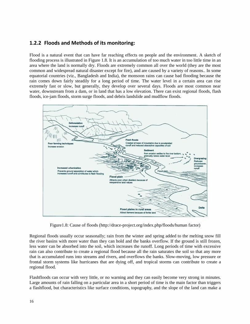
Flood is a natural event that can have far reaching effects on people and the environment. A sketch of
flooding process is illustrated in Figure 1.8. It is an accumulation of too much water in too little time in an
area where the land is normally dry. Floods are extremely common all over the world (they are the most
common and widespread natural disaster except for fire), and are caused by a variety of reasons.. In some
equatorial countries (viz., Bangladesh and India), the monsoon rains can cause bad flooding because the
rain comes down fairly steadily for a long period of time. The water level in a certain area can rise
extremely fast or slow, but generally, they develop over several days. Floods are most common near
water, downstream from a dam, or in land that has a low elevation. There can exist regional floods, flash
floods, ice-jam floods, storm surge floods, and debris landslide and mudflow floods.
Figure1.8: Cause of floods (http://drace-project.org/index.php/floods/human factor)
Regional floods usually occur seasonally; rain from the winter and spring added to the melting snow fill
the river basins with more water than they can hold and the banks overflow. If the ground is still frozen,
less water can be absorbed into the soil, which increases the runoff. Long periods of time with excessive
rain can also contribute to create a regional flood because all the rain saturates the soil so that any more
that is accumulated runs into streams and rivers, and overflows the banks. Slow-moving, low pressure or
frontal storm systems like hurricanes that are dying off, and tropical storms can contribute to create a
regional flood.
Flashfloods can occur with very little, or no warning and they can easily become very strong in minutes.
Large amounts of rain falling on a particular area in a short period of time is the main factor than triggers
a flashflood, but characteristics like surface conditions, topography, and the slope of the land can make a
17
flashflood more likely in a certain area. Urban areas have a larger risk than other places because streets,
roofs, and parking lots are a good place for water to runoff and gather. Mountainous areas also have a
larger risk because the ground has a steep slope, and runoff water can go into a narrow canyon, and then
the canyon can overflow. If you are standing below a flashflood when it starts, it will look like a wall of
water is descending upon you.
Ice jam floods occur on rivers that are at least partially frozen. If the water level rises, the ice will break
up and then pile together in shallow places to block other things that might be coming downstream, like
logs. The combination of the ice, logs, and other debris will block the river and keep the water from
flowing by. Eventually the natural dam will break and the water behind it will be released. With all this
water being released at the same time, the flood becomes a flashflood with large ice chunks in it that can
badly hurt people or other objects.
Storm surge flooding is caused by water pushed up on land that is usually dry by a storm surge. Dam and
Levee (An embankment raised to prevent a river from overflowing) failure floods occur if more water
piles up behind the dam or levee than the structure is built to hold. The water will spill over the dam, and
most likely, the force of the water will break the dam, letting all the water inside pour out. In this case, the
flood becomes a flash flood. Debris and landslide floods are created when debris, mud, rocks and maybe
logs pile up over a river and form a temporary dam. As the water gathers behind the debris, a flood
begins, and when the dam breaks and the water is released, it becomes a flashflood.
The use of remote sensing within the domain of natural hazards and disasters has become increasingly
common, due in part to increased awareness of environmental issues such as climate change, but also to
the increase in geospatial technologies and the ability to provide up-to-date imagery to the public through
the media and internet. They enable the collection and monitoring of data about atmospheric conditions
and characteristics of the Earth’s surface leading to processes, which may bring about floods. Such
information can be used to help determine appropriate actions to reduce the disastrous effects of these
processes. It has been demonstrated that using satellite data for flood mapping becomes economically
advantageous with respect to ground survey for areas larger than a couple of ten square kilometers.
Since the year 2000 there have been a number of space borne satellites and sensors that have changed the
approach to managing the natural disasters. The increase in the satellite data acquisition rates, sensor
resolution, improvement of change detection algorithms and integration of remote sensing systems has
significantly improved the real-time assessment and management of natural hazards (Gillespie et al.
2007).
Earth observation satellite systems provide a high degree of detail and a wealth of information at a global
level for early warning activities. This information includes two categories of data: first, numerical values
of detected geophysical parameters or related measurements, and second, imaging data sensed in various
electromagnetic bands. Many different space systems, with different characteristics related to Spatial
distribution, Spatial resolution, Temporal resolution, Spectral resolution and Radiometric resolution,
provide valuable data.
Both optical/infrared and microwave remote sensing instruments have been used for mapping surface
water through time. Optical imagery operates in the visible portion of the wavelength spectrum, but also
includes the infrared and thermal regions. Microwave imagery operates in the longer wavelengths from
less than a centimeter up to a meter (or frequencies from 89 GHz to 0.3 GHz respectively).
Different wavelengths have different responses to water in the landscape. Much of the literature shows
that for optical imagery the infrared wavelength, particularly around 1.5-1.7 micrometers performs well
18
for separating water from land (Overton et al. 2006) Instruments such as Landsat have a relatively high
spatial resolution (30m pixels) allowing for the detection of fine water bodies. However such imagery is
not routinely collected on a global scale through time, making regular monitoring of flooding events
difficult.
Instruments such as the Advanced Very High Resolution Radiometer (AVHRR) and the more recent
MODIS do collect data at daily/sub-daily intervals. Even with a poorer spatial resolution (1 km pixels),
the AVHRR has been used to map water with reasonable success (Tanaka et al. 2003). The utility of
AVHRR sensor was also realized by (Sandholt et al. 2003), who state that although the spatial resolution
is coarser than many other satellite sensors the frequent revisit time offers a greater probability of
obtaining cloud-free imagery. They used linear spectral unmixing with thermal imagery to determine
inundated areas, but were faced with the difficulty of selecting pure end members. Alternatively, they also
tested supervised maximum likelihood and ISODATA clustering classifications with the higher spatial
resolution Landsat ETM+, concluding that no technique is necessarily better than the other, rather that
each has its advantages and disadvantages depending on the flooding extent, cloud cover and temporal
variability. The MODIS sensors have a higher spatial resolution ranging from 250m up to 1km with a
twice daily overpass through much of the world, which has also been used to map surface water
(Sakamoto et al. 2007). Potentially one of the most useful studies for rapid-response flood mapping was
conducted to create on-board satellite processing algorithms for Hyperion imagery (Ip et al. 2006). The
algorithm utilizes three narrow spectral bands for a classification and is then compared to a base scene to
extract flood detail rather than just wet regions (eg, rivers, lakes). However, Hyperion has limited global
coverage, and obtains imagery in relatively small segments that would be useful for localized flooding but
not necessarily large events.
The extreme flooding events associated with several tropical storms in recent years (Hurricane Katrina,
Cyclone Nargis) have been successfully and rapidly mapped using a variety of sensors to take advantage
of differences in spatial and temporal resolution. Geoscience Australia is actively acquiring imagery of
flooding events in Australia and attempting to develop semi-automated techniques for extracting
inundated areas (Lymburner et al. 2008 and Thankappan et al. 2008)]. Flooding events of 2007 and 2008
were successfully mapped using Landsat-5 TM and ALOS AVNIR-2.
A major disadvantage in using optical imagery for flood mapping is that flood events are often associated
with cloud cover. This is the main reason that scientists across the world started exploring microwave
sensors for their potential to map surface water. For the active microwave case, the overall backscattering
coefficient is essentially influenced by three processes: surface direct contribution, vegetation
contribution and surface-vegetation double bounce. At lower frequencies (L, C and X Band) and angles
higher than about 300, the three contributions behave and interact in a complex way. Surface
backscattering increases with moisture and roughness. Vegetation attenuates surface backscattering and
produces its own contribution, as well as double bounce. Flooding reduces the surface contribution, due
to the decrease of roughness, and increases the double bounce effect in vegetated areas. At C Band, the
overall effect produced by a moderate flooding is an increase of the backscattering coefficient due to an
increase of the double bounce contribution. However, if the increase of water level submerges most of the
vegetation cover, the overall effect is a decrease of backscattering coefficient. Therefore, the trend of the
backscattering coefficient as a function of water level is not monotonic. These properties have been
investigated for some cases of agricultural and natural vegetation, mostly at C and X Band, also with the
aid of models (Le Toan et al. 1989; Caizzone et al. 2009 and Grings et al. 2005) The increase of the
backscattering coefficient during flooding, related to double bounce, was detected also in forest cover
areas, using L Band signatures (Wang et al. 1995) Synthetic Aperture Radar sensors have proven useful in
mapping floods since the backscatter signature of water is so distinctive compared with that of vegetation
(Alsdorf et al. 2007 and Lewis et al. 1998) but they are not routinely available at regional scales. (Smith
19
1997) suggested the use of Multi-frequency polarimetric SAR to classify different types of inundated
terrain to an extent not possible with single-frequency SARs and visible/infrared sensors.
The use of passive microwave remote sensing data to monitor soil moisture, vegetation and in turn the
flood events, has been the subject of several studies in recent decades. Passive microwave sensors acquire
data at a high temporal frequency (1-2 times daily) on a near-global scale in comparison to active sensors.
Several theoretical and experimental investigations has proved the sensitivity of passive microwave
remote sensing measurements to soil and vegetation properties from the physical perspective. Researchers
tried to exploit the polarization effect on the emissivity on different surfaces. For bare soil, the emissivity
at vertical (V) polarization is higher than the one at horizontal (H) polarization. An increase of soil
moisture produces a decrease of emissivity at both polarizations, and at all microwave frequencies.
However, the effect is more important at H polarization and at the lower frequencies (Ulaby et al. 1986a;
Paloscia et al. 1993; Kerr and Njoku 1990). On the other hand, a decrease of roughness produces effects
which are similar to the ones produced by an increase of moisture. If the soil becomes smoother, a
decrease of emissivity, which is more evident at polarization and at lower frequencies, is observed
(Paloscia et al. 1993). In the presence of flooding events and/or strong rainstorms, the two effects can
couple together to reduce the emissivity, since the soil becomes wet and smoother at the same time.
Though on average, the vegetation growth produces a decrease of the difference between vertically
polarized and horizontally polarized emission. Studies were also aimed at singling out vegetation effects
from soil effects and it was found that the polarization difference at high frequencies (Ka band) was
mostly related to vegetation emission, and showed a good correlation with vegetation indexes derived by
optical instruments (Choudhury and Tucker 1987) further studies adopted lower frequencies, typically X
band In order to eliminate the dependence on surface temperature, a normalized polarization index
(Paloscia and Pampaloni 1988) was defined (details mentioned in section). A further parametric study,
carried out by means of a discrete physical model, confirmed the main finding of experimental studies
and pointed out that the same polarization index is also sensitive to soil moisture, at least at frequencies
lower than 10 GHz (Ferrazzoli et al. 1992). In (Choudhury 1989), the absolute polarization difference at
37 GHz proved to be correlated to vegetation density and was sensitive to flooding effects occurred in the
Amazon River. This last application was further exploited in (Sippel et al. 1994 and Sippel et al. 1998)
and (Hamilton et al. 2002). A simple algorithm, based on the polarization difference at 37 GHz measured
by SMMR, was adopted to estimate the fraction of flooded area during several events occurred in the
Amazon river and in other large South American rivers floodplains.
The availability AMSR-E signatures offered new opportunities (Kawanishi et al. 2003) to understand soil
moisture at different frequencies. This sensor spans a wide range of frequencies, from 6.925 GHz to 89.0
GHz, and the spatial resolution is substantially improved with respect to previous ones (details in section
1.4.1). Based on AMSR-E data, useful algorithms have been developed to retrieve soil moisture (Njoku et
al. 2003 and Paloscia et al. 2006) and vegetation variables (Njoku and Chan 2006). In more recent
studies, (Ferrazzoli et al. 2010) found that increase in the water level are associated with the increase in
the polarization index. (Singh et al. 2012; Singh et al. 2012a and Singh et al. 2013) also found that At the
X band, the water level was better correlated with the PI than with emissivity and fractional water surface.
The correlation was good in cases of slow variation in WL. In cases of sudden variation in the river, the PI
followed the variations with some time delay related to the propagation of water within the covered
AMSR-E pixel.
One of the large challenges in using passive microwave to map surface water is its large spatial footprint
(5km up to 70km). Mixed pixel analysis is often used to determine the proportion of water within each
flooded pixel based on theoretical or empirical estimates of the proportion of wet and dry surfaces
(Mialon et al. 2005). Daily river stage or discharge has been correlated to inundation area as derived from
regularly acquired remote sensing imagery. Even without ground data, these correlations can still show
the shape and timing of seasonal hydrographs, and with ground measurements the absolute discharge can
20
be estimated to within a factor of two (Smith 1997). For microwave data, (Choudhury 1989) achieved a
linear correlation of R =0.8 while (Brakenridge et al. 2007a) used a fourth order polynomial with an
AMSR-E 36.5 GHz horizontal ratio achieving good results. (Sippel et al. 1998) found mapped flooded
area was correlated with river stage, using it to develop a predictive relationship for inundation patterns
with historical stage records. Work by (Bindlish 2009) also demonstrated the role of passive microwave
data for flood forecasting. Most of the work, however, has demonstrated the increased skill in
runoff/rainfall partition modeling by using remotely sensed surface soil moisture (Pauwels et al. 2002;
Jacobs et al. 2003 and Crow et al. 2005) as a tool for flood monitoring and assessment instead of for
forecasting (Alsdorf et al. 2000; Brivio et al. 2002; Freeman et al. 2002 and Scofield et al. 1994). Making
the transition between monitoring and forecasting requires direct observations of the hydrologic
precursors to flooding events (e.g., elevated soil moisture conditions) and not simply the manifestation of
the flood itself.
Many researchers also worked to combine of various data sources (optical, active and passive microwave
data) for flood mapping. (Ticehurst et al. 2009) developed different ways of using optical (MODIS) and
passive microwave remote sensing imagery (TRMM) for mapping floods to help reduce the effects of
cloud contamination, and optimize the data’s spatial resolution and temporal frequency to suit the size and
duration of the flood events. (Salvia et al. 2011) presented a methodology to estimate the fraction of
flooded area and the mean water level inside a wetland using both active and passive microwave orbital
systems. The methodology is based on the quasi-simultaneous measurements of the radiometric
polarization difference and the differences of the backscattering coefficient with respect to a reference
image.
21
1.2.3 Forest monitoring
Forests cover about a third of the Earth's land surface, and they influence the exchange of gases and
energy between the atmosphere and the surface. About 80% of the global biomass is contained in forests,
and this forms the central component of the stocks and acquisition of carbon in the biosphere. The growth
and distribution of forests has a critical impact on atmospheric carbon dioxide concentrations, a central
issue in global change research. To meet the various information requirements in forest studies different
data sources, like field survey, aerial photography and satellite imagery is used, depending on the level of
detail required and the extension of the area under study.
Ground-based measurements allow us to evaluate in detail the influence of variables depending markedly
on time, such as soil moisture and Leaf Area Index (LAI), but they cover only small forest plots. For the
purpose of consistently and repeatedly monitor forests and their parameters over larger areas, it is
preferable to use remote sensing data. Several types of remote sensing data, including aerial photography,
multi-spectral scanner (MSS), Lidar (Light Detection and Ranging) laser, Active-Passive Microwave data
and Videography data have been used by forest agencies to detect, identify, classify, evaluate and
measure various forest cover types and their changes.
Over the past decades tremendous progress has been made in demonstrating the potentials and limitations
for identifying and mapping various forest surface features using optical remote sensing data. Optical
systems, although proved their effectiveness in sensing leaf parameters, are not able to sense the woody
biomass. At microwave frequencies, remote-sensing research was mostly based on active systems.
Radiometric forestry has received a much lower attention than radar forestry mainly due to poor spatial
resolution of spaceborne radiometers. Nevertheless, important experiments about forest emissivity took
place using ground-based, airborne, and spaceborne radiometers (Shutko and Chukhlantsev 1982b;
Matzler 1994a; Wigneron et al. 1997; Kruopis et al. 1999; Hallikainen et al. 1988; Lang et al. 2000; Lang
et al. 2001 and Macelloni et al. 2001). A review was given in (Pampaloni 2004).
Particularly, the capability of microwave radiometers to monitor soil moisture is a subject receiving
attention Experiments using both ground based and airborne radiometers have provided an insight into the
problem but only a limited number of forests have been observed. Some experimental investigations,
carried out over coniferous forests, or deciduous forests in cold climates, indicate that the effects of soil
moisture variations on radiometric signatures are very low, even at L band (Guglielmetti et al. 2008),
(Grant et al. 2007). Other experiments in temperate climates indicate that a moderate sensitivity to
variations of soil moisture exists, at least at L band (Rahmoune et al. 2010). These experimental efforts
were aimed at evaluating the overall emissivity and appreciate the sensitivity of the emission process to
forest variables, such as branch volume, LAI, and soil-moisture content (SMC).
More recently, studies about forest emission have been stimulated by the development of space projects,
such as the Soil Moisture and Ocean Salinity of the European Space Agency, using lower microwave
frequencies (L-band) for soil-moisture monitoring (Berger et al. 2003). Although field experiments are
fundamental to investigate the potential of radiometers, theoretical simulations carried out using physical
models, also add important information. Models allow us to extend the estimates to several cases of
possible forest variables, single out all the contributions of forest components, and carry out parametric
studies at various frequencies, angles, and polarizations. Theoretical efforts aimed at simulating the
electromagnetic behavior of forests were mostly focused on radar applications (Ulaby et al. 1990;
Chauhan et al. 1991; Karam 1997; Ferrazzoli and Guerriero 1995). However, physical models of forest
emission are also available (Ferrazzoli and Guerriero 1996 and Karam 1997) The basic modeling
approach is discrete and based on the radiative-transfer theory (τ – ω model). At higher frequencies (C
22
band and above) there is a strong contribution of leaves to crown attenuation, but at lower frequency (L-
band and below), leaves are almost transparent, attenuation is mostly due to branches, and soil
contribution can be still appreciable, unless if the forest is dense.
It was found that a simple empirical approach, based on τ and ω parameters fitted over experimental data
is not appropriate in the case of forests, due to very limited amount of experimental brightness data
presently available at L band and the complexity of the emission/scattering processes, since trunks and
branches are not small when compared to sensing wavelength. Therefore, in the algorithm developed to
explit SMOS data over land, forests are modeled using a simple zero order RT model, but with τ and ω
obtained by fitting the outputs of a theoretical discrete model developed at Tor Vergata University
(Rahmoune et al. 2013). τ and ω represent, respectively, the vegetation attenuation properties and the
scattering effects within the canopy layer. The algorithm compares the brightness temperatures measured
by SMOS with those simulated by a zero order forward model, and starts an iterative procedure which
minimizes the “cost function”. Further using allometric equations and auxiliary information, the inputs
required by the model are related to the maximum yearly value of Leaf Area Index (LAI). The retrieval
algorithm estimates soil moisture and optical depth as outputs of the retrieval process. Several more
efforts have been done to improve the performance of the forward model and the retrieval algorithm to
improve the soil moisture retrieval performance, at least under moderately developed forests (Ferrazzoli
et al. 2013 and Rahmoune et al. 2013a).
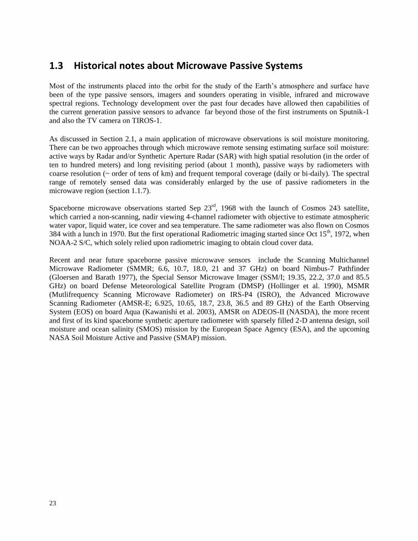
23
1.3 Historical notes about Microwave Passive Systems
Most of the instruments placed into the orbit for the study of the Earth’s atmosphere and surface have
been of the type passive sensors, imagers and sounders operating in visible, infrared and microwave
spectral regions. Technology development over the past four decades have allowed then capabilities of
the current generation passive sensors to advance far beyond those of the first instruments on Sputnik-1
and also the TV camera on TIROS-1.
As discussed in Section 2.1, a main application of microwave observations is soil moisture monitoring.
There can be two approaches through which microwave remote sensing estimating surface soil moisture:
active ways by Radar and/or Synthetic Aperture Radar (SAR) with high spatial resolution (in the order of
ten to hundred meters) and long revisiting period (about 1 month), passive ways by radiometers with
coarse resolution (~ order of tens of km) and frequent temporal coverage (daily or bi-daily). The spectral
range of remotely sensed data was considerably enlarged by the use of passive radiometers in the
microwave region (section 1.1.7).
Spaceborne microwave observations started Sep 23rd
, 1968 with the launch of Cosmos 243 satellite,
which carried a non-scanning, nadir viewing 4-channel radiometer with objective to estimate atmospheric
water vapor, liquid water, ice cover and sea temperature. The same radiometer was also flown on Cosmos
384 with a lunch in 1970. But the first operational Radiometric imaging started since Oct 15th, 1972, when
NOAA-2 S/C, which solely relied upon radiometric imaging to obtain cloud cover data.
Recent and near future spaceborne passive microwave sensors include the Scanning Multichannel
Microwave Radiometer (SMMR; 6.6, 10.7, 18.0, 21 and 37 GHz) on board Nimbus-7 Pathfinder
(Gloersen and Barath 1977), the Special Sensor Microwave Imager (SSM/I; 19.35, 22.2, 37.0 and 85.5
GHz) on board Defense Meteorological Satellite Program (DMSP) (Hollinger et al. 1990), MSMR
(Mutlifrequency Scanning Microwave Radiometer) on IRS-P4 (ISRO), the Advanced Microwave
Scanning Radiometer (AMSR-E; 6.925, 10.65, 18.7, 23.8, 36.5 and 89 GHz) of the Earth Observing
System (EOS) on board Aqua (Kawanishi et al. 2003), AMSR on ADEOS-II (NASDA), the more recent
and first of its kind spaceborne synthetic aperture radiometer with sparsely filled 2-D antenna design, soil
moisture and ocean salinity (SMOS) mission by the European Space Agency (ESA), and the upcoming
NASA Soil Moisture Active and Passive (SMAP) mission.
24
1.4 Recent Satellite Missions
1.4.1 Advanced Microwave Scanning Radiometer (AMSR-E)
The Advanced Microwave Scanning Radiometer for the Earth Observing System (AMSR-E) was
developed and provided to the National Aeronautics and Space Administration’s (NASA) EOS Aqua
satellite by the National Space Development Agency of Japan (NASDA), as one of the indispensable
instruments for Aqua’s mission. AMSR-E is a modified version of AMSR. AMSR-E was launched
December 2002 aboard the Advanced Earth Observing Satellite-II (ADEOS-II) (Nakajima et al. 1994),
(Imaoka et al. 2002). It is a multichannel microwave radiometer that observes hydrological and
geophysical parameters to understand the mechanism of global water and energy circulation. It uses one
of the largest microwave radiometer antennas to observe global and continuous phenomena with finer
spatial resolution, with respect to previous radiometers. In addition to the time-proven capabilities for
observing such variables as water vapor, precipitation, and sea surface wind speed, novel geophysical
parameters, including sea surface temperature (SST) and soil moisture, are retrieved by using microwave
frequency channels. Near-real-time products are further used to investigate satellite data assimilation into
weather forecasting models and to contribute to improved forecasting accuracy. AMSR-E aboard Aqua is
a joint project between Japan and United States as well as an international activity in which scientists
worldwide collaborate in algorithm development, data validation, and scientific research.
The mission aims at exploring the global hydrologic cycle and its role in the earth’s climate system.
AMSR-E plays an important role in the Aqua mission, by measuring geophysical parameters supporting
several global change sciences and monitoring efforts, including precipitation, oceanic water vapor and
cloud liquid water, sea surface wind speed, sea surface temperature, soil moisture, snow cover, and sea
ice parameters.
In the AMSR-E instrument design, there are two major improvements over previous spaceborne
microwave radiometers for earth imaging: the addition of 6.925-GHz channels and the largest main
reflector of its kind, providing higher spatial resolution. The 6.925-GHz channels enable us to observe
SST over the global oceans, while the TMI 10-GHz channels only appear to be sensitive to warmer SST
above 100 C (Shibata et al. 1999). These channels are also useful to investigate soil moisture content.
Although TMI realized the higher spatial resolution thanks to the lower orbit altitude of the TRMM,
AMSR-E essentially improves the solution and extends its capability to global measurements.
On the afternoon orbit of the Aqua satellite, AMSR-E provides measurement at approximately 1:30 A.M.
and 1:30 P.M. This observing local time is not covered by the previous measurements of SSM/I. Having
AMSR-E therefore also helps in filling this gap of local observing time. More important is the
combination of AMSR-E and AMSR onboard ADEOS-II. This system, combining microwave
radiometers of the latest design in morning and afternoon orbits, helps in providing information on
diurnal variability of most geophysical parameters necessary for process studies and frequent sampling of
transient phenomena like severe tropical storms essential for improving data assimilation techniques.
1.4.1.1 Instrument design and performance
1.4.1.1.1 Overview
AMSR-E is a six-frequency total-power microwave radiometer system with dual polarization capability
for all frequency bands. The frequency bands include 6.925, 10.65, 18.7, 23.8, 36.5, and 89.0 GHz.
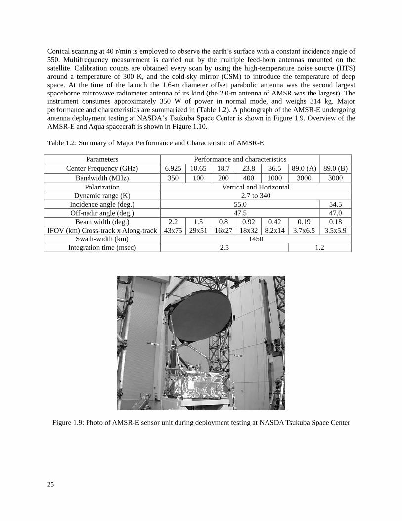
25
Conical scanning at 40 r/min is employed to observe the earth’s surface with a constant incidence angle of
550. Multifrequency measurement is carried out by the multiple feed-horn antennas mounted on the
satellite. Calibration counts are obtained every scan by using the high-temperature noise source (HTS)
around a temperature of 300 K, and the cold-sky mirror (CSM) to introduce the temperature of deep
space. At the time of the launch the 1.6-m diameter offset parabolic antenna was the second largest
spaceborne microwave radiometer antenna of its kind (the 2.0-m antenna of AMSR was the largest). The
instrument consumes approximately 350 W of power in normal mode, and weighs 314 kg. Major
performance and characteristics are summarized in (Table 1.2). A photograph of the AMSR-E undergoing
antenna deployment testing at NASDA’s Tsukuba Space Center is shown in Figure 1.9. Overview of the
AMSR-E and Aqua spacecraft is shown in Figure 1.10.
Table 1.2: Summary of Major Performance and Characteristic of AMSR-E
Parameters Performance and characteristics
Center Frequency (GHz) 6.925 10.65 18.7 23.8 36.5 89.0 (A) 89.0 (B)
Bandwidth (MHz) 350 100 200 400 1000 3000 3000
Polarization Vertical and Horizontal
Dynamic range (K) 2.7 to 340
Incidence angle (deg.) 55.0 54.5
Off-nadir angle (deg.) 47.5 47.0
Beam width (deg.) 2.2 1.5 0.8 0.92 0.42 0.19 0.18
IFOV (km) Cross-track x Along-track 43x75 29x51 16x27 18x32 8.2x14 3.7x6.5 3.5x5.9
Swath-width (km) 1450
Integration time (msec) 2.5 1.2
Figure 1.9: Photo of AMSR-E sensor unit during deployment testing at NASDA Tsukuba Space Center
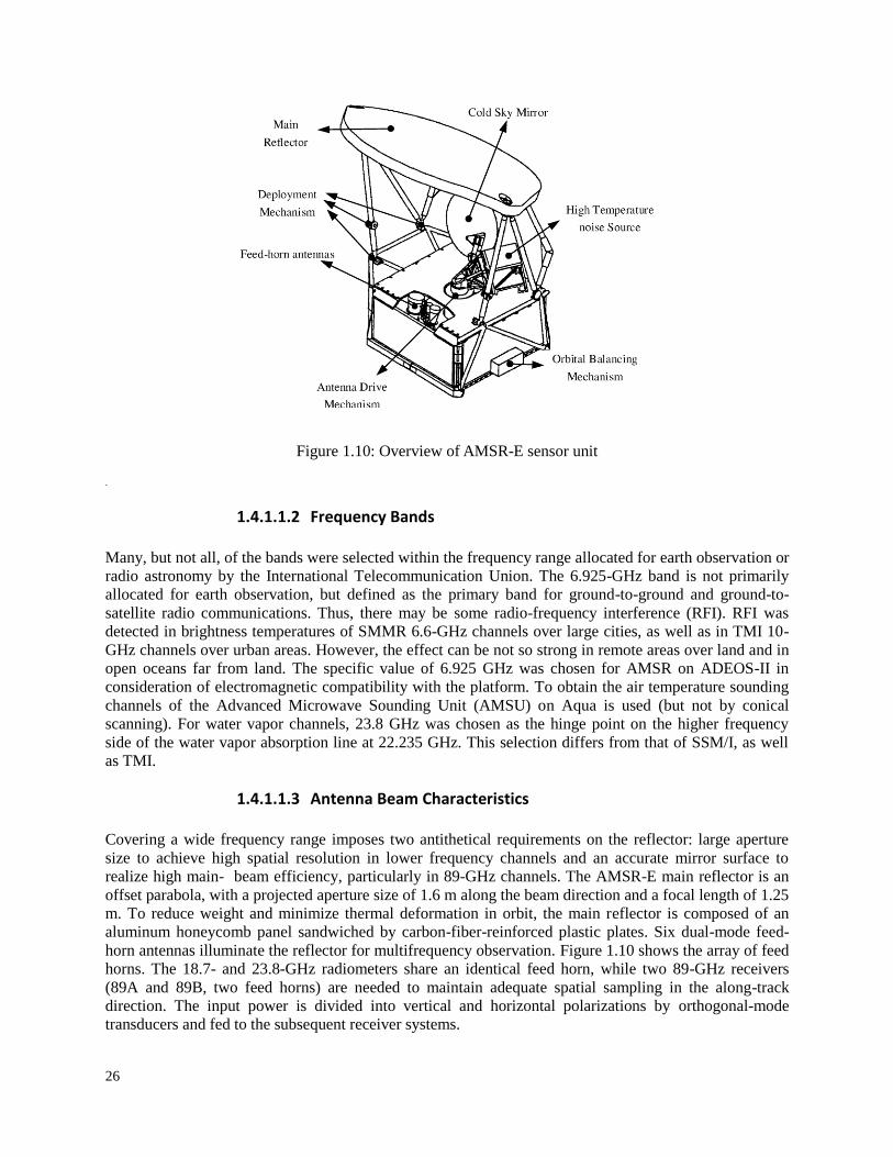
26
Figure 1.10: Overview of AMSR-E sensor unit .
1.4.1.1.2 Frequency Bands
Many, but not all, of the bands were selected within the frequency range allocated for earth observation or
radio astronomy by the International Telecommunication Union. The 6.925-GHz band is not primarily
allocated for earth observation, but defined as the primary band for ground-to-ground and ground-to-
satellite radio communications. Thus, there may be some radio-frequency interference (RFI). RFI was
detected in brightness temperatures of SMMR 6.6-GHz channels over large cities, as well as in TMI 10-
GHz channels over urban areas. However, the effect can be not so strong in remote areas over land and in
open oceans far from land. The specific value of 6.925 GHz was chosen for AMSR on ADEOS-II in
consideration of electromagnetic compatibility with the platform. To obtain the air temperature sounding
channels of the Advanced Microwave Sounding Unit (AMSU) on Aqua is used (but not by conical
scanning). For water vapor channels, 23.8 GHz was chosen as the hinge point on the higher frequency
side of the water vapor absorption line at 22.235 GHz. This selection differs from that of SSM/I, as well
as TMI.
1.4.1.1.3 Antenna Beam Characteristics
Covering a wide frequency range imposes two antithetical requirements on the reflector: large aperture
size to achieve high spatial resolution in lower frequency channels and an accurate mirror surface to
realize high main- beam efficiency, particularly in 89-GHz channels. The AMSR-E main reflector is an
offset parabola, with a projected aperture size of 1.6 m along the beam direction and a focal length of 1.25
m. To reduce weight and minimize thermal deformation in orbit, the main reflector is composed of an
aluminum honeycomb panel sandwiched by carbon-fiber-reinforced plastic plates. Six dual-mode feed-
horn antennas illuminate the reflector for multifrequency observation. Figure 1.10 shows the array of feed
horns. The 18.7- and 23.8-GHz radiometers share an identical feed horn, while two 89-GHz receivers
(89A and 89B, two feed horns) are needed to maintain adequate spatial sampling in the along-track
direction. The input power is divided into vertical and horizontal polarizations by orthogonal-mode
transducers and fed to the subsequent receiver systems.
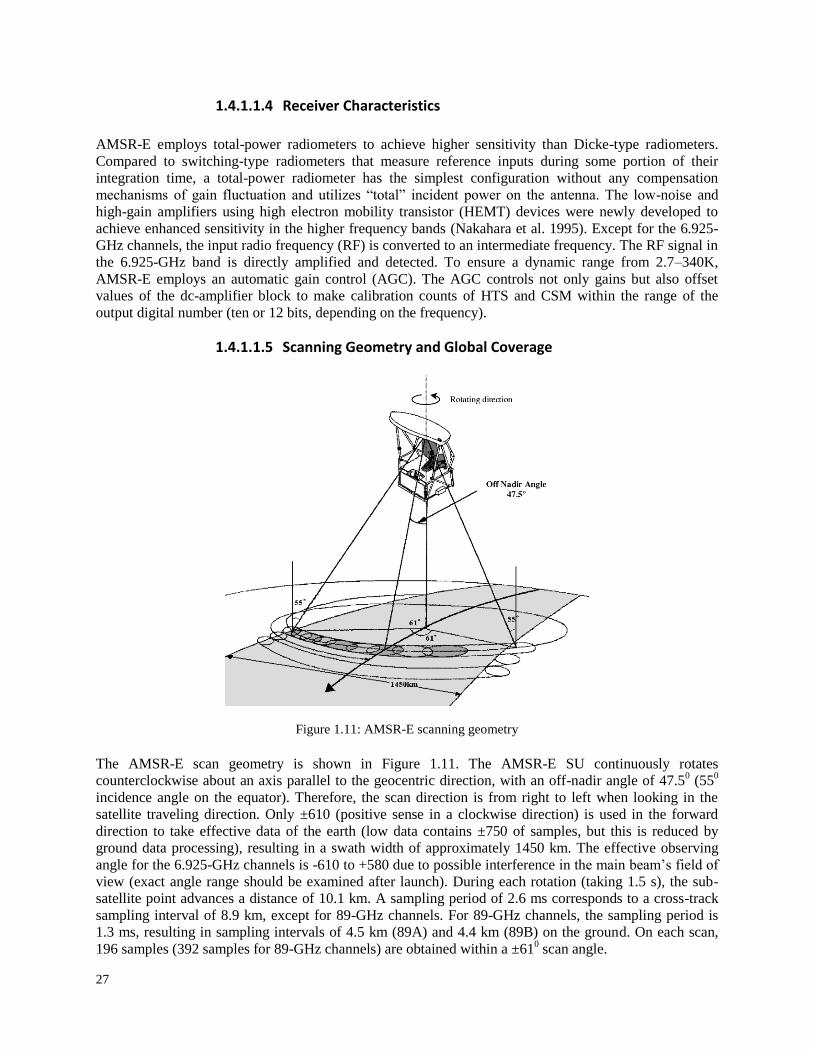
27
1.4.1.1.4 Receiver Characteristics
AMSR-E employs total-power radiometers to achieve higher sensitivity than Dicke-type radiometers.
Compared to switching-type radiometers that measure reference inputs during some portion of their
integration time, a total-power radiometer has the simplest configuration without any compensation
mechanisms of gain fluctuation and utilizes “total” incident power on the antenna. The low-noise and
high-gain amplifiers using high electron mobility transistor (HEMT) devices were newly developed to
achieve enhanced sensitivity in the higher frequency bands (Nakahara et al. 1995). Except for the 6.925-
GHz channels, the input radio frequency (RF) is converted to an intermediate frequency. The RF signal in
the 6.925-GHz band is directly amplified and detected. To ensure a dynamic range from 2.7–340K,
AMSR-E employs an automatic gain control (AGC). The AGC controls not only gains but also offset
values of the dc-amplifier block to make calibration counts of HTS and CSM within the range of the
output digital number (ten or 12 bits, depending on the frequency).
1.4.1.1.5 Scanning Geometry and Global Coverage
Figure 1.11: AMSR-E scanning geometry
The AMSR-E scan geometry is shown in Figure 1.11. The AMSR-E SU continuously rotates
counterclockwise about an axis parallel to the geocentric direction, with an off-nadir angle of 47.50 (55
0
incidence angle on the equator). Therefore, the scan direction is from right to left when looking in the
satellite traveling direction. Only ±610 (positive sense in a clockwise direction) is used in the forward
direction to take effective data of the earth (low data contains ±750 of samples, but this is reduced by
ground data processing), resulting in a swath width of approximately 1450 km. The effective observing
angle for the 6.925-GHz channels is -610 to +580 due to possible interference in the main beam’s field of
view (exact angle range should be examined after launch). During each rotation (taking 1.5 s), the sub-
satellite point advances a distance of 10.1 km. A sampling period of 2.6 ms corresponds to a cross-track
sampling interval of 8.9 km, except for 89-GHz channels. For 89-GHz channels, the sampling period is
1.3 ms, resulting in sampling intervals of 4.5 km (89A) and 4.4 km (89B) on the ground. On each scan,
196 samples (392 samples for 89-GHz channels) are obtained within a ±610 scan angle.
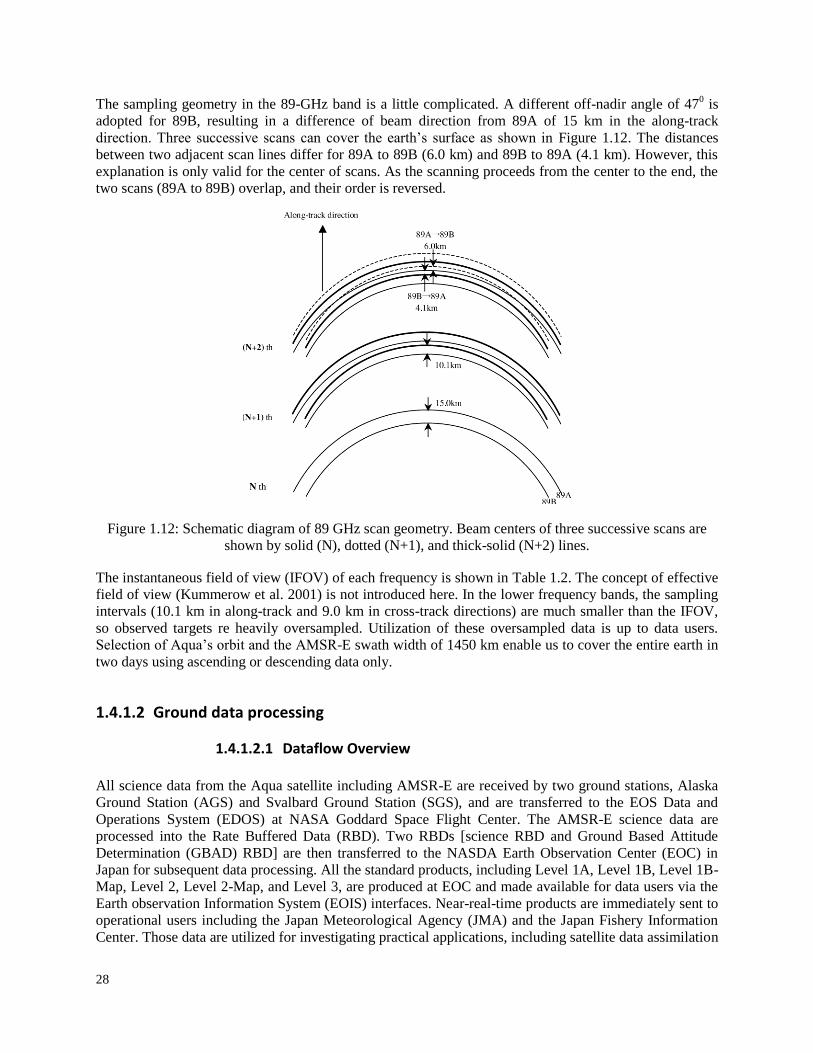
28
The sampling geometry in the 89-GHz band is a little complicated. A different off-nadir angle of 470 is
adopted for 89B, resulting in a difference of beam direction from 89A of 15 km in the along-track
direction. Three successive scans can cover the earth’s surface as shown in Figure 1.12. The distances
between two adjacent scan lines differ for 89A to 89B (6.0 km) and 89B to 89A (4.1 km). However, this
explanation is only valid for the center of scans. As the scanning proceeds from the center to the end, the
two scans (89A to 89B) overlap, and their order is reversed.
Figure 1.12: Schematic diagram of 89 GHz scan geometry. Beam centers of three successive scans are
shown by solid (N), dotted (N+1), and thick-solid (N+2) lines.
The instantaneous field of view (IFOV) of each frequency is shown in Table 1.2. The concept of effective
field of view (Kummerow et al. 2001) is not introduced here. In the lower frequency bands, the sampling
intervals (10.1 km in along-track and 9.0 km in cross-track directions) are much smaller than the IFOV,
so observed targets re heavily oversampled. Utilization of these oversampled data is up to data users.
Selection of Aqua’s orbit and the AMSR-E swath width of 1450 km enable us to cover the entire earth in
two days using ascending or descending data only.
1.4.1.2 Ground data processing
1.4.1.2.1 Dataflow Overview
All science data from the Aqua satellite including AMSR-E are received by two ground stations, Alaska
Ground Station (AGS) and Svalbard Ground Station (SGS), and are transferred to the EOS Data and
Operations System (EDOS) at NASA Goddard Space Flight Center. The AMSR-E science data are
processed into the Rate Buffered Data (RBD). Two RBDs [science RBD and Ground Based Attitude
Determination (GBAD) RBD] are then transferred to the NASDA Earth Observation Center (EOC) in
Japan for subsequent data processing. All the standard products, including Level 1A, Level 1B, Level 1B-
Map, Level 2, Level 2-Map, and Level 3, are produced at EOC and made available for data users via the
Earth observation Information System (EOIS) interfaces. Near-real-time products are immediately sent to
operational users including the Japan Meteorological Agency (JMA) and the Japan Fishery Information
Center. Those data are utilized for investigating practical applications, including satellite data assimilation
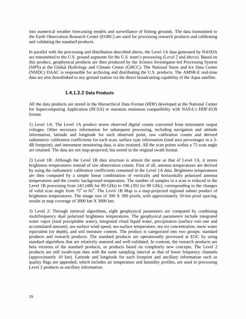
29
into numerical weather forecasting models and surveillance of fishing grounds. The data transmitted to
the Earth Observation Research Center (EORC) are used for processing research products and calibrating
and validating the standard products.
In parallel with the processing and distribution described above, the Level 1A data generated by NASDA
are transmitted to the U.S. ground segments for the U.S. team’s processing (Level 2 and above). Based on
this product, geophysical products are then produced by the Science Investigator-led Processing System
(SIPS) at the Global Hydrology and Climate Center (GHCC). The National Snow and Ice Data Center
(NSIDC) DAAC is responsible for archiving and distributing the U.S. products. The AMSR-E real-time
data are also downlinked to any ground station via the direct broadcasting capability of the Aqua satellite.
1.4.1.2.2 Data Products
All the data products are stored in the Hierarchical Data Format (HDF) developed at the National Center
for Supercomputing Application (NCSA) to maintain minimum compatibility with NASA’s HDF-EOS
format.
1) Level 1A: The Level 1A product stores observed digital counts converted from instrument output
voltages. Other necessary information for subsequent processing, including navigation and attitude
information, latitude and longitude for each observed point, raw calibration counts and derived
radiometric calibration coefficients for each scan, surface type information (land area percentages in a 3-
dB footprint), and instrument monitoring data, is also retained. All the scan points within a 75 scan angle
are retained. The data are not map-projected, but stored in the original swath format.
2) Level 1B: Although the Level 1B data structure is almost the same as that of Level 1A, it stores
brightness temperatures instead of raw observation counts. First of all, antenna temperatures are derived
by using the radiometric calibration coefficients contained in the Level 1A data. Brightness temperatures
are then computed by a simple linear combination of vertically and horizontally polarized antenna
temperatures and the cosmic background temperature. The number of samples in a scan is reduced in the
Level 1B processing from 243 (486 for 89 GHz) to 196 (392 for 89 GHz), corresponding to the changes
of valid scan angle from 750 to 61
0. The Level 1B Map is a map-projected regional subset product of
brightness temperatures. The image size of 300 X 300 pixels, with approximately 10-km pixel spacing,
results in map coverage of 3000 km X 3000 km.
3) Level 2: Through retrieval algorithms, eight geophysical parameters are computed by combining
multifrequency dual polarized brightness temperatures. The geophysical parameters include integrated
water vapor (total precipitable water), integrated cloud liquid water, precipitation (surface rain rate and
accumulated amount), sea surface wind speed, sea surface temperature, sea ice concentration, snow water
equivalent (or depth), and soil moisture content. The product is categorized into two groups: standard
products and research products. The standard products are operationally processed at EOC by using
standard algorithms that are relatively matured and well-validated. In contrast, the research products are
beta versions of the standard products, or products based on completely new concepts. The Level 2
products are still swath-type data with the same sampling interval as that of lower frequency channels
(approximately 10 km). Latitude and longitude for each footprint and ancillary information such as
quality flags are appended, which includes air temperature and humidity profiles, are used in processing
Level 2 products as ancillary information.

30
4) Level 3: The Level 3 products are daily and monthly grids of Level 1B and Level 2 products.
Depending on the products, 0.25 X 0.25 grids and/or polar stereographic grids with 25-km resolution are
used.
For the current study, we have used brightness temperature values, provided by level 2 product
(AE_L2A.2 - AMSR-E/Aqua) global swath brightness temperatures, resampled at resolutions of 56 km,
38 km, 21 km, 12 km, and 5.4 km. Level 3 (AE_Land3.2 - AMSR-E/Aqua) level 3 global daily surface
soil moisture with vegetation water content, surface temperature, & brightness temperature are generated
on a nominal 25-km equal area earth grid by time-compositing the level 2B parameters separately for
ascending and descending passes. This product was used to compare AMSR-E global soil moisture map
with soil moisture obtained from other data products (SMOS).
1.4.2 Soil Moisture and Ocean Salinity (SMOS) Mission:
1.4.2.1 Mission objective and characteristics
The SMOS (Soil Moisture and Ocean Salinity) mission was approved by the European Space Agency
(ESA) in May 1999. Its objective is to provide frequent global Soil Moisture and Sea Surface Salinity
(SSS) maps. SMOS was launched on November 2, 2009, and after the first calibration and checkout
period (the so-called Commissioning Phase), processed products started to be distributed.
The SMOS satellite, launched with a ROCKOT Breeze KM, is on a low Earth polar Sun- synchronous
dawn-dusk orbit, at 763 km of altitude, covering a complete orbit around the Earth in approximately 100
minutes. It is characterized by a 3-day revisit time at the Equator and a spatial resolution ranging between
32 and 100 km.
The single payload of the SMOS mission is the Microwave Imaging Radiometer by Aperture Synthesis
(MIRAS,(McMullan et al. 2008)); MIRAS is a 2D interferometric radiometer operating in the protected
L-band with a nominal frequency of 1413.5 MHz and a bandwidth of 27 MHz. It consists of three
deployable arms connected to a central hub (8-m diameter radiometer when completely deployed). The
arms are equally spaced with an angular separation of 1200. Each arm encompasses three segments, each
one containing six L-band radiometers (Light-weight Cost-Effective Front-end, LICEF). Four more
radiometers are situated in the central hub, for a total of 66 radiometers. In addition to that, there are three
Noise Injection Radiometers (NIRs) located in the central hub, each of which consists of two LICEF
receivers coupled to a single antenna. The total number of elements is therefore 69 antennas and 72
receivers, arranged as shown in Figure 1.13.
The integration time used in MIRAS is 0.158 s, with an interval between snapshots of 1.2 s, allowing a
snapshot radiometric sensitivity of 3.5 - 5.8 K over land and 2.5 - 4.1 K over ocean. Every 1.2 seconds
data provided by the Control and Monitoring Network (CMN), by the Noise Injection Radiometer (NIR),
by the LICEF units, plus additional information from the platform (attitude information) are recorded in
the Raw-Data product. Raw Data are downloaded through the X-band channel when a ground contact
is established. MIRAS can operate according to two different observation modes:
Dual-Polarization mode: Brightness temperatures are alternately measured in each polarization every 1.2
s, and all the LICEFs measure the same polarization.
Full-Polarization mode: Brightness temperatures in H and V polarization as well as the third and fourth
Stokes parameters are measured. Four consecutive integration times are used for each measurement.
31
During the first integration time, all receivers measure the X polarization and during the third integration
time, the Y polarization. In the other two integration times the polarization of one arm is the opposite of
the other two arms to perform measurements of the cross-polarization terms T (XY/YX).The arm in the
alternative polarization rotates in a clockwise direction completing 4 rounds in each integration time.
Figure 1.13: MIRAS arm and LICEF details. Courtesy ESA
Brightness temperatures are reconstructed in the director cosine domain (ξ, η) :
( , ) (sin( )cos( ),sin( )sin( )) (1.27)
where θ is the angle from the normal to the instrument plane (0 ≤ θ ≤ π/2 ) and ϕ is the angle in the
instrument plane (0 ≤ ϕ ≤ 2π). Theoretically, the maximum visible space is the area inside the unit circle
(ξ2 + η
2 = 1) even though non-zero antenna pattern backlobes also contribute to the TB image in the unit
circle. Geometric conventions are sketched in Figure 1.14.
visibility samples are measured and plotted as a function of the distance between antennas in the
horizontal (u) and vertical (v) components;
the visibility map is properly repeated to compute the Inverse Fourier Transformation (F-1
)
leading to the brightness temperatures map (TB ) in the cosine domain, and finally
the periodic extension is removed from the brightness temperature map.
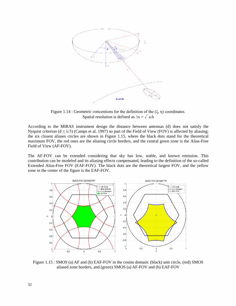
32
Figure 1.14 : Geometric concentions for the definition of the (ξ, η) coordinates.
Spatial resolution is defined as ∆x = √a.b
According to the MIRAS instrument design the distance between antennas (d) does not satisfy the
Nyquist criterion (d ≤ λ/3) (Camps et al. 1997) so part of the Field of View (FOV) is affected by aliasing;
the six closest aliases circles are shown in Figure 1.15, where the black dots stand for the theoretical
maximum FOV, the red ones are the aliasing circle borders, and the central green zone is the Alias-Free
Field of View (AF-FOV).
The AF-FOV can be extended considering that sky has low, stable, and known emission. This
contribution can be modeled and its aliasing effects compensated, leading to the definition of the so-called
Extended Alias-Free FOV (EAF-FOV). The black dots are the theoretical largest FOV, and the yellow
zone in the center of the figure is the EAF-FOV.
Figure 1.15 : SMOS (a) AF and (b) EAF-FOV in the cosine domain: (black) unit circle, (red) SMOS
aliased zone borders, and (green) SMOS (a) AF-FOV and (b) EAF-FOV
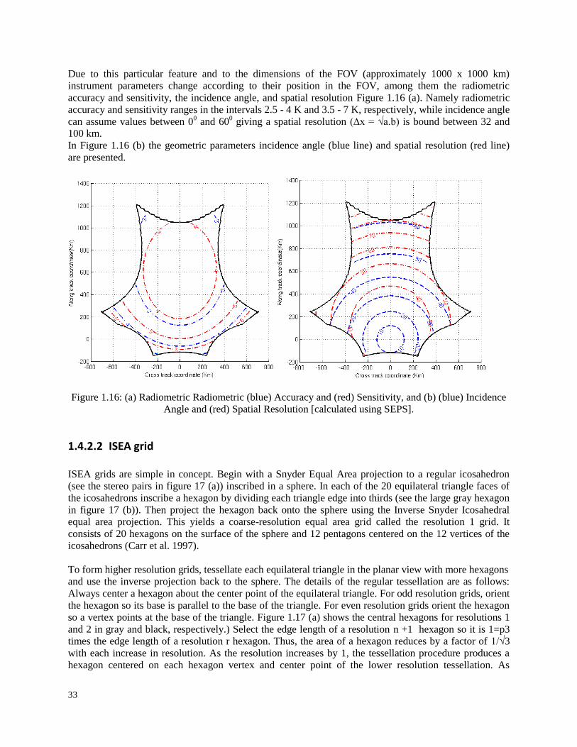
33
Due to this particular feature and to the dimensions of the FOV (approximately 1000 x 1000 km)
instrument parameters change according to their position in the FOV, among them the radiometric
accuracy and sensitivity, the incidence angle, and spatial resolution Figure 1.16 (a). Namely radiometric
accuracy and sensitivity ranges in the intervals 2.5 - 4 K and 3.5 - 7 K, respectively, while incidence angle
can assume values between 00 and 60
0 giving a spatial resolution (∆x = √a.b) is bound between 32 and
100 km.
In Figure 1.16 (b) the geometric parameters incidence angle (blue line) and spatial resolution (red line)
are presented.
Figure 1.16: (a) Radiometric Radiometric (blue) Accuracy and (red) Sensitivity, and (b) (blue) Incidence
Angle and (red) Spatial Resolution [calculated using SEPS].
1.4.2.2 ISEA grid
ISEA grids are simple in concept. Begin with a Snyder Equal Area projection to a regular icosahedron
(see the stereo pairs in figure 17 (a)) inscribed in a sphere. In each of the 20 equilateral triangle faces of
the icosahedrons inscribe a hexagon by dividing each triangle edge into thirds (see the large gray hexagon
in figure 17 (b)). Then project the hexagon back onto the sphere using the Inverse Snyder Icosahedral
equal area projection. This yields a coarse-resolution equal area grid called the resolution 1 grid. It
consists of 20 hexagons on the surface of the sphere and 12 pentagons centered on the 12 vertices of the
icosahedrons (Carr et al. 1997).
To form higher resolution grids, tessellate each equilateral triangle in the planar view with more hexagons
and use the inverse projection back to the sphere. The details of the regular tessellation are as follows:
Always center a hexagon about the center point of the equilateral triangle. For odd resolution grids, orient
the hexagon so its base is parallel to the base of the triangle. For even resolution grids orient the hexagon
so a vertex points at the base of the triangle. Figure 1.17 (a) shows the central hexagons for resolutions 1
and 2 in gray and black, respectively.) Select the edge length of a resolution n +1 hexagon so it is 1=p3
times the edge length of a resolution r hexagon. Thus, the area of a hexagon reduces by a factor of 1/√3
with each increase in resolution. As the resolution increases by 1, the tessellation procedure produces a
hexagon centered on each hexagon vertex and center point of the lower resolution tessellation. As
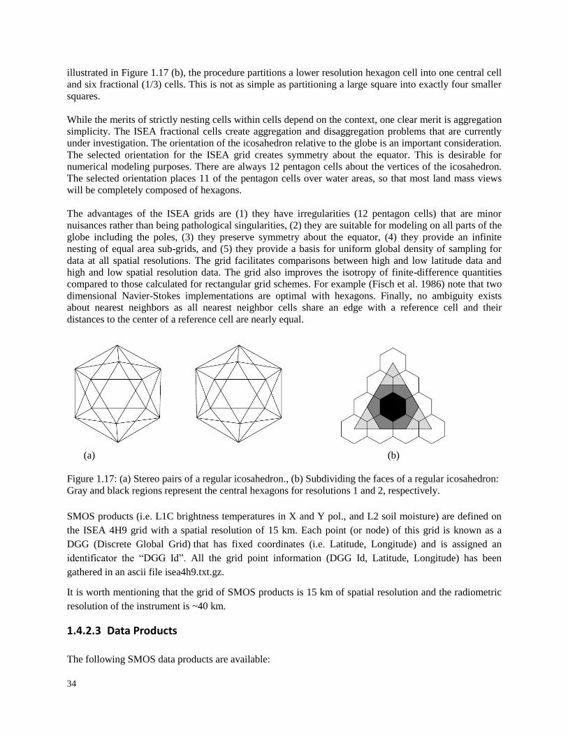
34
illustrated in Figure 1.17 (b), the procedure partitions a lower resolution hexagon cell into one central cell
and six fractional (1/3) cells. This is not as simple as partitioning a large square into exactly four smaller
squares.
While the merits of strictly nesting cells within cells depend on the context, one clear merit is aggregation
simplicity. The ISEA fractional cells create aggregation and disaggregation problems that are currently
under investigation. The orientation of the icosahedron relative to the globe is an important consideration.
The selected orientation for the ISEA grid creates symmetry about the equator. This is desirable for
numerical modeling purposes. There are always 12 pentagon cells about the vertices of the icosahedron.
The selected orientation places 11 of the pentagon cells over water areas, so that most land mass views
will be completely composed of hexagons.
The advantages of the ISEA grids are (1) they have irregularities (12 pentagon cells) that are minor
nuisances rather than being pathological singularities, (2) they are suitable for modeling on all parts of the
globe including the poles, (3) they preserve symmetry about the equator, (4) they provide an infinite
nesting of equal area sub-grids, and (5) they provide a basis for uniform global density of sampling for
data at all spatial resolutions. The grid facilitates comparisons between high and low latitude data and
high and low spatial resolution data. The grid also improves the isotropy of finite-difference quantities
compared to those calculated for rectangular grid schemes. For example (Fisch et al. 1986) note that two
dimensional Navier-Stokes implementations are optimal with hexagons. Finally, no ambiguity exists
about nearest neighbors as all nearest neighbor cells share an edge with a reference cell and their
distances to the center of a reference cell are nearly equal.
(a) (b)
Figure 1.17: (a) Stereo pairs of a regular icosahedron., (b) Subdividing the faces of a regular icosahedron:
Gray and black regions represent the central hexagons for resolutions 1 and 2, respectively.
SMOS products (i.e. L1C brightness temperatures in X and Y pol., and L2 soil moisture) are defined on
the ISEA 4H9 grid with a spatial resolution of 15 km. Each point (or node) of this grid is known as a
DGG (Discrete Global Grid) that has fixed coordinates (i.e. Latitude, Longitude) and is assigned an
identificator the “DGG Id”. All the grid point information (DGG Id, Latitude, Longitude) has been
gathered in an ascii file isea4h9.txt.gz.
It is worth mentioning that the grid of SMOS products is 15 km of spatial resolution and the radiometric
resolution of the instrument is ~40 km.
1.4.2.3 Data Products
The following SMOS data products are available:
35
Level 1A product: calibrated visibilities between receivers prior to applying image reconstruction.
Level 1B product: output of the image reconstruction of the observations and comprising the
Fourier component of the brightness temperature in the antenna polarization reference frame.
Level 1C product: multi-angular brightness temperatures at the top of the atmosphere, geolocated
in an equal-area grid system. Two different Level 1C products are generated according to the
surface type: one containing only sea and the other only containing land pixels. Two sets of
information are available: pixel-wise and snapshot-wise. For each Level 1C product there is also
a browse product containing brightness temperatures for an incidence angle of 42.5°.
Level 2 soil moisture product: containing not only the soil moisture retrieved, but also a series of
ancillary data derived from the processing (nadir optical thickness, surface temperature,
roughness parameter, dielectric constant and brightness temperature retrieved at top of
atmosphere and on the surface) with the corresponding uncertainties.
Level 2 ocean salinity product: containing three different ocean salinity values derived from
retrieval algorithms using different assumptions for the surface roughness correction and the
brightness temperature retrieved at the top of atmosphere and on the sea surface (with the
corresponding uncertainties).
Near-real time product: similar to the Level 1C product but adjusted to requirements of
operational meteorological agencies such as ECMWF and Météo France, available 3 hours from
sensing. It will contain brightness temperatures at the top of the atmosphere on an ISEA grid with
reduced spatial resolution.
For the current study,L2 soil moisture data were used. The focus was on the forested area. The L2 SM
retrieval algorithm used two types of auxiliary data files: static and dynamic. The static data do not vary
over time or have slowly varying quantities. They include the soil texture maps from FAO (FAO 1988),
the land use maps from ECOCLIMAP (Masson et al. 2003b) and MODIS, and the topography index
(Mialon et al. 2008). The dynamic data provided time varying quantities (snow, freeze defreeze, rain,
temperature) obtained from the European Centre for Medium Range Weather Forecasts (ECMWF)
forecasts.
The algorithm is based on two main components. The first consists of a forward model, which estimates
the brightness temperature emitted by land nodes of SMOS using a priori information (auxiliary data)
about land cover, surface temperature, Leaf Area Index (LAI), etc., and initial estimates of soil moisture
taken by the data base of the ECMWF data. The second consists of an inversion process, which estimates
the actual soil moisture and optical depth by using Level 1C multiangular measurements, forward model
outputs and a Cost Function. The radiative transfer parameters τ (optical depth) and ω (albedo) are
estimated using the synthetic outputs of the theoretical model, according to the procedure which was
further developed and described in further sections of the thesis.
36
1.5 Research objectives:
Estimation of soil moisture from radiometric measurements is not simple and direct since there are many
soil and vegetation parameters affecting the land emission. The development of algorithms to compute
bio/geophysical variables from brightness temperature measurements and the assessment of the impact of
each of the involved parameters is crucial to have accurate soil moisture estimations. The radiometric
measurements vary drastically over vegetative surfaces in different environments. An attempt is made to
understand the behavior of soil moisture on different land surfaces when studied through radiometer at
different frequencies.
The subject of the thesis is “MICROWAVE RADIOMETRY OF VEGETATED SURFACES IN
DIFFERENT ENIRONMENTS “, with first part investigating flooding events in short vegetation at
higher frequencies (C-band and above) and second part exploiting lower frequency (L-Band) over forests.
The first part of the PhD work discusses the use of multifrequency AMSR-E signatures in floods
monitoring and shows tests over the part of Indian Brahmaputra basin (test sites at North Lakimpur
district). The temporal evolution of parameters defined in the literature, such as FWS, and PI is analyzed,
and results are compared against available ground measurements of river water level. Techniques aimed
at eliminating images affected by heavy rainfalls are also investigated. Radiometric signatures of L-band
could not be used in this area due to high Radio Frequency Interference (RFI) in Asian regions.
The second part of the research was carried out as part of the background research for the SMOS mission.
At the spatial resolution of SMOS (~40Km), many pixels over land contain a certain percentage of forest
cover. Forests usually consist of rather thick and dense vegetation layers. However modelling studies
have shown that it might be possible to monitor soil moisture in moderately dense forests if forest
emission can be modeled correctly. In this thesis, last results about the retrieved soil moisture are
presented using both the presently available algorithm and a refined one, based on a revised forward
model, which will be implemented in the next version of the processor.
Retrieved values of optical depth τ have been compared against tree height made available by NASA
Earth Observatory. For both configurations, the retrieved soil moistures were compared against IN-SITU
measurements of the SCAN/SNOTEL network which includes several forest sites in the US, for which
multitemporal measurements of soil moisture and other environmental variables are available and RFI
problems were moderate. By considering the multitemporal series, for each node we have compared the
retrieved and the measured values of soil moisture for the various cases mentioned above. A further
analysis using the soil moisture retrieved by the different algorithms exploiting the Advanced Microwave
Scanning Radiometer for the Earth (AMSR-E) is also carried out and results were compared against the
ones obtained by SMOS.

37
1.6 Organization of the Thesis
This Ph.D. Thesis focuses on understanding of microwave radiometer observations user different
environmental conditions, and it is organized as follows:
Chapter 2 describes the variables influencing the microwave emission of land covers, as well as the basic
models adopted to estimate the dielectric constant of soils, and revises the land emission models
(including radiative transfer principles) which are used at present in soil moisture retrieval algorithms.
Chapter 3 describes the results of the tests performed using selected AMSR-E channels on the parts of
Brahmaputra Basin, India for analyzing the inundated areas in both bare and vegetated land.
Chapter 4 investigates the capability of SMOS MIRAS radiometer to monitor soil moisture over forests
of North America.
38
2 Microwave Emission of Land covers
Although there have been a number of space borne microwave instruments since the late 1970's, antenna
technology and the need to accommodate requirements of the atmospheric and ocean sciences have
resulted in these sensors operating at frequencies higher than what is deemed optimal for soil moisture
estimation (6.9, 10, 19, 37, and 85 GHz). Research in soil moisture remote sensing began in the mid
1970's shortly after the surge in satellite development (Barton 1978; Eagleman and Lin 1976; Idso et al.
1975; Njoku and Kong 1977 and Schmugge et al. 1977). Theoretical and empirical evidence suggest that
the 1400-1427 MHz region (L-band) is most suitable for soil moisture radiometry because long
wavelengths penetrate soil and vegetation to a greater extent than higher frequencies (Jackson et al. 1993
and Njoku and Entekhabi 1996) and transmission is prohibited in the band by the Federal
Communications Commission so that it remains suitable for radioastronomy observations (cosmic
hydrogen absorption occurs at 1420 MHz).
At 1400 MHz, there is a large contrast between the dielectric properties of liquid water (~80) and dry
soil (< 4). Several investigators (Wang and Schmugge 1980; Dobson et al. 1985 and Ulaby et al. 1986b)
studied the dielectric properties of wet soil. As the moisture increases, the dielectric constant of the soil-
water mixture increases and this change is detectable by microwave sensors (Njoku and Kong et al.
1977). The microwave brightness temperature of an emitter of microwave radiation is related to the
physical temperature of the source through the emissivity as mentioned in section (1.1.3). The depth
through which energy is emitted and sensed by microwave radiometers has been the subject of research
and discussion for many years, but it varies, depending on the frequencies we are studying, viz., for L-
Band, it is on the order of about 5 cm.
This chapter describes the properties of soils and vegetation, and revises the land emission models which
are used at present in soil moisture retrieval algorithms from microwave remote sensing data.
2.1 Bare Soils
2.1.1 Physical properties of soils
An accurate estimation of spatially variable soil media properties is necessary to develop reliable models
of flow and transport throughout the soil-plant-atmosphere continuum, for efficient management of
resources, and for maintenance of environmental quality. Soils consist of a mix of air, water, organic
matter, and mineral particles. According to (Jenny 1994), soils result from the combination of climate,
organisms, relief, parent material, and time. Further information on soil properties is reported, among
others, in (Brady and Weil 2003 and Behari 2005). Next sections briefly summarize the main soil physical
properties.
2.1.1.1 Texture
The size distribution of primary mineral particles, called soil texture, has a strong influence on the
properties of a soil. It usually ranges from below 0.002 mm to above 2 mm in diameter. The fraction
above 2 mm is classed as gravel, and the fractions below 2 mm are classed as clay, silt, or sand as is
indicated in Table 2.1. The relative proportions of clay, silt, and sand determine the soil texture. The three
fundamental groups of soil are sands, loams, and clays, but there are many other types named according
to the USDA soil classification triangle shown in Figure 2.1.
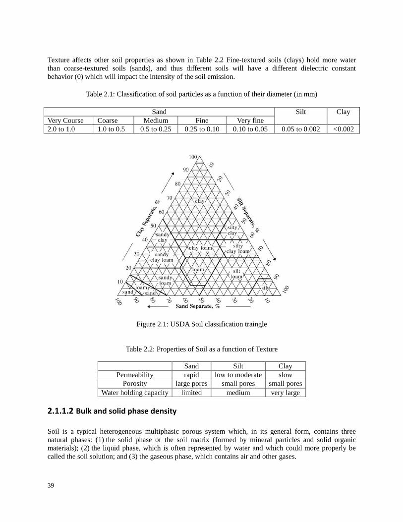
39
Texture affects other soil properties as shown in Table 2.2 Fine-textured soils (clays) hold more water
than coarse-textured soils (sands), and thus different soils will have a different dielectric constant
behavior (0) which will impact the intensity of the soil emission.
Table 2.1: Classification of soil particles as a function of their diameter (in mm)
Sand Silt Clay
Very Course Coarse Medium Fine Very fine
2.0 to 1.0 1.0 to 0.5 0.5 to 0.25 0.25 to 0.10 0.10 to 0.05 0.05 to 0.002 <0.002
Figure 2.1: USDA Soil classification traingle
Table 2.2: Properties of Soil as a function of Texture
Sand Silt Clay
Permeability rapid low to moderate slow
Porosity large pores small pores small pores
Water holding capacity limited medium very large
2.1.1.2 Bulk and solid phase density
Soil is a typical heterogeneous multiphasic porous system which, in its general form, contains three
natural phases: (1) the solid phase or the soil matrix (formed by mineral particles and solid organic
materials); (2) the liquid phase, which is often represented by water and which could more properly be
called the soil solution; and (3) the gaseous phase, which contains air and other gases.

40
Soil bulk density ρb [g/cm3] is defined as the ratio of the mass of dry solids to the bulk volume of the soil
occupied by those dry solids:
s s sb p p
s s s
c A cMassofdrysoil
Volumeofbulksoil D A D (2.1)
being ρp the soil phase density, As the area, cs the equivalent depth filled with solid, and Ds the total
equivalent density of the soil made up of solids, water, and air. The density of the solid phase is constant
for a soil type, and varies from 1.3 to 2.1 g/cm3 in sands, from 1.2 to 2.6 g/cm3 in clays, and from 0.8 to
1.6 g/cm3 in loams (Chukhlantsev 2006). On the contrary, the bulk density has not a unique value since
depends on compaction, swelling, etc. Porous soils have low ρb and those compact have higher values.
The range of possible values varies from 1 to 1.6 g/cm3 for clay, clay loam, and silt loam soils, and from
1.2 to 1.8 g/cm3 in sands and sandy loams.
2.1.1.3 Pore space or porosity
Pores are the void spaces between soil particles. Pore spaces of dry soils are mostly filled with air, while
water fills the pores of wet soils. Processes such as infiltration, ground-water movement, and storage
occur in these void spaces. Porosity is in turn affected by texture, soil structure, compaction, and organic
matter. The porosity is determined from the bulk density ρb and particle density ρp (see section 2.1.1.2) as,
1 bs
p
P
(2.2)
Pores in a soil have a large variability in arrangement, size, and shape. Sands have very few small pores
which hold water, while clays have many large pores which are needed for the rapid water intake and
distribution of water. Typical values of the porosity range from 25-50% in sands, from 35-50% in loams,
and from 33-60% in clays (Fetter 2001).
2.1.1.4 Permeability and water holding capacity
Permeability is the rate at which fluid can flow through the soil pores, while water-holding capacity is the
ability of soils to hold water for plant use. Both parameters are a function of soil structure, porosity, and
texture as summarized in Table 2.2.
2.1.1.5 Structure
Soil structure refers to the way sand, silt, and clay particles are arranged into clumps or aggregates. The
aggregates are bound together by clay and organic matter. Structure affects drainage, root growth,
infiltration, germination, and aeration.
2.1.1.6 Temperature
Soil temperature determines the chemical reaction within a soil and, thus, plants growth, water movement
and availability of nutrients. Soil temperature depends on meteorological and physical soil properties such
as color, surface roughness, and water content. For instance, dark soils absorb more heat than smooth
light-colored ones and thus warm faster. On its part, soil moisture affects the rate of temperature change:
41
more heat is needed to warm a wet soil than a dry one. The temperature of soils follows the temperature
of the air, but with a time lag. This effect diminishes with soil depth.
2.1.1.7 Water in soils
Water content is one of the most variable characteristics of soil. Although there is not a unique
classification of water in soils, the common classification divides it into bound and free water. Bound
water is the water adsorbed by the surface of soil particles, while free water is the liquid water located in
the pore spaces. Bound water depends on soil texture and takes the minimum values (2-3%) in sands, and
the maximum (20-40%) in clays. The soil moisture, or water in a soil, is usually determined in two ways:
Gravimetric soil moisture wg, which depends on the wet and dry weights of the soil sample (ww and wd
respectively),
w dg
d
w ww
w
(2.3)
Volumetric soil moisture mv, which depends on the volume of water Vw, the volume of the soil sample Vs,
the soil bulk density ρb, and the density of wet soil ρws and water ρw,
w ws bs g
s w w
Vw w m
V
(2.4)
The field capacity and wilting pointing are, among other hydrological parameters, involved in the
dielectric constant models. The field capacity (FC) is the maximum amount of water held in a soil against
gravity or amount of water held in soil after excess water has drained away. Physically, it is the water held
at a soil at a tension of 1/3 bar. The field capacity can be estimated from the volumetric soil moisture and
the weight fractions (in %) of sand S and clay C as (Wang and Schmugge 1980)
0.3 0.25 0.5FC S C (2.5)
The wilting point (WP) is the level of soil moisture below which plants wilt, and is usually taken as the
soil moisture at a tension of 15 bar. The wilting point is estimated from the textural composition as (Wang
and Schmugge 1980),
0.06774 0.00064 0.00478WP S C (2.6)
The difference between field capacity and wilting point is the available water content.
Last but not least, organic litter layers on top of soils as well as the organic matter content intermixed in
mineral soils are very important properties (Bot and Bernites 2005): Plant residues that cover the soil
surface protect the soil from sealing and crusting by raindrop impact, thereby enhancing rainwater
infiltration and reducing runoff. Organic matter affects both the chemical and physical properties of the
soil and its overall health. It influences soil structure by an enhanced stability of soil aggregates and pores
through bonding/adhesion of particles and increases diversity and activity of soil organisms, and nutrient
availability. Furthermore, and very importantly, organic matter increases the soil moisture holding
capacity by increasing the soil porosity as well as (like in case of clay minerals) through high water-
binding capacities of humic substances. (Miller 1977) stated that typically 1-3 kg/m2 of liquid water are
stored in a medium dense forest vegetation, and a like amount can be retained on the forest floor. Helvey
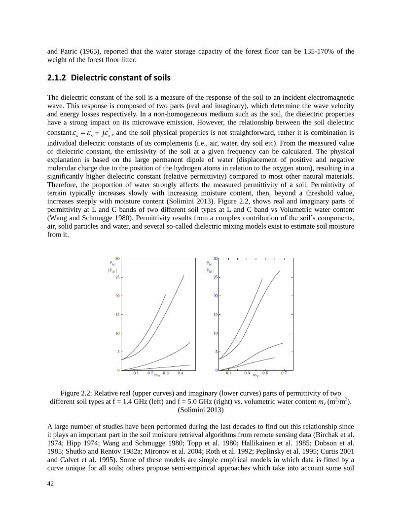
42
and Patric (1965), reported that the water storage capacity of the forest floor can be 135-170% of the
weight of the forest floor litter.
2.1.2 Dielectric constant of soils
The dielectric constant of the soil is a measure of the response of the soil to an incident electromagnetic
wave. This response is composed of two parts (real and imaginary), which determine the wave velocity
and energy losses respectively. In a non-homogeneous medium such as the soil, the dielectric properties
have a strong impact on its microwave emission. However, the relationship between the soil dielectric
constant' ''
s s sj , and the soil physical properties is not straightforward, rather it is combination is
individual dielectric constants of its complements (i.e., air, water, dry soil etc). From the measured value
of dielectric constant, the emissivity of the soil at a given frequency can be calculated. The physical
explanation is based on the large permanent dipole of water (displacement of positive and negative
molecular charge due to the position of the hydrogen atoms in relation to the oxygen atom), resulting in a
significantly higher dielectric constant (relative permittivity) compared to most other natural materials.
Therefore, the proportion of water strongly affects the measured permittivity of a soil. Permittivity of
terrain typically increases slowly with increasing moisture content, then, beyond a threshold value,
increases steeply with moisture content (Solimini 2013). Figure 2.2, shows real and imaginary parts of
permittivity at L and C bands of two different soil types at L and C band vs Volumetric water content
(Wang and Schmugge 1980). Permittivity results from a complex contribution of the soil’s components,
air, solid particles and water, and several so-called dielectric mixing models exist to estimate soil moisture
from it.
Figure 2.2: Relative real (upper curves) and imaginary (lower curves) parts of permittivity of two
different soil types at f = 1.4 GHz (left) and f = 5.0 GHz (right) vs. volumetric water content mv (m3/m
3).
(Solimini 2013)
A large number of studies have been performed during the last decades to find out this relationship since
it plays an important part in the soil moisture retrieval algorithms from remote sensing data (Birchak et al.
1974; Hipp 1974; Wang and Schmugge 1980; Topp et al. 1980; Hallikainen et al. 1985; Dobson et al.
1985; Shutko and Rentov 1982a; Mironov et al. 2004; Roth et al. 1992; Peplinsky et al. 1995; Curtis 2001
and Calvet et al. 1995). Some of these models are simple empirical models in which data is fitted by a
curve unique for all soils; others propose semi-empirical approaches which take into account some soil
43
physical properties. The dielectric constant of dry soils is almost independent of temperature (Topp et al.
1980) and frequency. On the contrary, wet soils show a complex behavior depending on the interaction
between soil, water, and air particles. (Hallikainen et al. 1985) performed a series of dielectric constant
measurements of five soils with different texture composition at frequencies between 1.4 and 18 GHz and
found out that texture has a strong effect on the dielectric behavior which is especially pronounced at
frequencies below 5 GHz. In the dielectric-mixing model by (Roth et al. 1992), differences in soil texture
and bound water and free water are ignored altogether. Next sections review some of the most commonly
used dielectric constant models relevant to the thesis work. More information can be found in (Behari
2005 and Chukhlantsev 2006). A thorough review on soil moisture measurements is presented by
(Robinson et al. 2008).
2.1.2.1 Empirical approach
In this approach, mathematical expressions are simply fitted to the observed data. This approach does not
take soil physics into account. This is, for instance, the approach followed by in (Topp et al. 1980), where
the dielectric constant of mineral soils ε is related to the volumetric moisture content measured using TDR
techniques ws by a third order polynomial:
6 3 4 2 2 24.3.10 5.5.10 2.92.10 5.3.10s s s sw (2.7)
This equation has been successfully used by many authors over different soils and even ice, although
others have found out that soil moisture content was under- or overestimated. (Ledieu et al. 1986)
presented an even simpler empirical relation, by fitting a linear relation between dielectric constant and
volumetric moisture content. (Noboroi et al. 2001) offers a complete reference of these studies.
2.1.2.2 Semi-empirical approach
Other models use a semi-empirical (SEM) approach that contains a model of the complex dielectric
constant and the volume fraction of each of the soil components. This kind of approach was used by
(Wang and Schmugge 1980; Dobson et al. 1985 and Roth et al. 1992). In most cases, the starting point is
the dielectric mixing model by (Birchak et al. 1974):
s sp sp a a fw fw bw bwV V V V (2.8)
Where, Vsp (εsp), Va (εa), Vfw (εfw) and Vbw (εbw) are the volume fraction (dielectric constant) of solid phase,
air, free water, and bound water in the soil, respectively. The expression in (2.8) can be rewritten as a
function of the bulk density and the volumetric moisture as
1 ( 1)bs sp fw fw bw bw s
s
V V w
(2.9)
If α = 0.5 the model in equation 2.9 is known as refractive model.
The Wang and Schmugge model and the Mironov model consider the effect of bound water on the
dielectric constant. They are limited to rather short frequencies of 1-5 GHz and 1-10 GHz, respectively.
The Dobson model is valid for a larger range of frequency (1-18 GHz) but it does not differentiate
between bound water and free water.
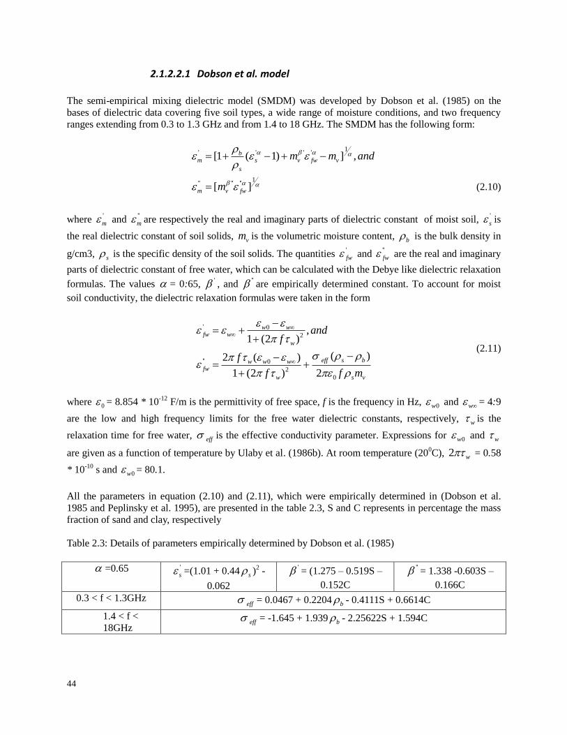
44
2.1.2.2.1 Dobson et al. model
The semi-empirical mixing dielectric model (SMDM) was developed by Dobson et al. (1985) on the
bases of dielectric data covering five soil types, a wide range of moisture conditions, and two frequency
ranges extending from 0.3 to 1.3 GHz and from 1.4 to 18 GHz. The SMDM has the following form:
1' ' ' '
1'' '' ''
[1 ( 1) ] ,
[ ]
bm s v fw v
s
m v fw
m m and
m
(2.10)
where '
m and ''
m are respectively the real and imaginary parts of dielectric constant of moist soil, '
s is
the real dielectric constant of soil solids, vm is the volumetric moisture content, b is the bulk density in
g/cm3, s is the specific density of the soil solids. The quantities '
fw and ''
fw are the real and imaginary
parts of dielectric constant of free water, which can be calculated with the Debye like dielectric relaxation
formulas. The values = 0:65, ' , and
'' are empirically determined constant. To account for moist
soil conductivity, the dielectric relaxation formulas were taken in the form
' 0
2
'' 0
2
0
,1 (2 )
( )2 ( )
1 (2 ) 2
w wfw w
w
eff s bw w wfw
w s v
andf
f
f f m
(2.11)
where 0 = 8.854 * 10-12
F/m is the permittivity of free space, f is the frequency in Hz, 0w and w = 4:9
are the low and high frequency limits for the free water dielectric constants, respectively, w is the
relaxation time for free water, eff is the effective conductivity parameter. Expressions for 0w and w
are given as a function of temperature by Ulaby et al. (1986b). At room temperature (200C), 2 w = 0.58
* 10-10
s and 0w = 80.1.
All the parameters in equation (2.10) and (2.11), which were empirically determined in (Dobson et al.
1985 and Peplinsky et al. 1995), are presented in the table 2.3, S and C represents in percentage the mass
fraction of sand and clay, respectively
Table 2.3: Details of parameters empirically determined by Dobson et al. (1985)
=0.65 '
s =(1.01 + 0.44 s )2 -
0.062
' = (1.275 – 0.519S –
0.152C
'' = 1.338 -0.603S –
0.166C
0.3 < f < 1.3GHz eff = 0.0467 + 0.2204 b - 0.4111S + 0.6614C
1.4 < f <
18GHz eff = -1.645 + 1.939 b - 2.25622S + 1.594C
45
It is worth noticing that all the SMDM input parameters relating to a given soil type are available from the
soil granulometric mineralogy data, which can be borrowed from soil databases. This is a major
advantage of the SMDM over many other models, resulting in a wide employment of this model in
microwave remote sensing.
2.1.2.2.2 Mironov et al. model
The SEM proposed by (Dobson et al. 1985) has become an effective means to relate soil moisture and
microwave dielectric properties (De Roo et al. 2001; Galantowicz et al. 2000 and Jackson et al. 1999). In
order to provide for frequency dispersion of the soil dielectric properties, the Debye relaxation formula
for the complex dielectric constant (CDC) related to the out-of-soil water is extensively employed in the
SEM. At the same time, soil moisture is known to have biphasic dielectric properties (Ulaby et al. 1986b),
which usually are correlated to the bound soil water (BSW) and free soil water (FSW). Apparently, the
SEM does not account for the dielectric dissimilarities between the BSW and FSW components.
Therefore, it appeared not to be applicable to the soils studied in (Sabburg et al. 1997) and (Or and Wraith
1999)1, and the problem of determination of the BSW dielectric properties is still important for the
development of moist soil dielectric models.
The first study of the BSW dielectric properties was undertaken in (Wang and Schmugge 1980).
Subsequently, CDCs of the BSW and FSW fractions as the separate components of moist soil were
obtained in (Mironov et al. 1995 and Mironov et al. 1997). The approach employed was based on the
refractive mixing dielectric model (RMDM), initially proposed and validated in (Birchak et al. 1974). At
the same time, the RMDM is only capable of making prediction of the soil CDC as a function of moisture
for the frequency, for which soil dielectric measurements were carried out.
In contrast to the SMDM, exclusively employing dielectric relaxation spectrum valid for the water located
out of soil, the GRMDM suggested in (Mironov et al. 2004) employs the dielectric spectra explicitly
related to either bound or free soil water. The description of this concept is given below.
The real and imaginary parts, '
m ''
m , as a function of volumetric moisture vm , can be represented in the
form of RMDM:
' 2 2 ', 2m m m m m mn n
(2.12)
( 1) ,
( 1) ( 1)( ),
,
( ),
m d b v v vt
m d b vt u v vt v vt
m d b v v vt
m b vt u v vt v vt
n n n m m m
n n n m n m m m m
and
m m m
m m m m m
(2.13)
Where mn , dn , bn , un and m , d , b , u are the values of refractive index and normalized
attenuation coefficient, which is understood here as a proportion of the standard attenuation coefficient to
the free space propagation constant. The subscripts m, d, b and u in (2.12), (2.13) and further on stand for
moist soil, dry soil, bound soil water (BSW), and free soil water (FSW), respectively, and vtm is a value
of the maximum bound water fraction (MBWF) in a given type of the soil. The latter depends on the soil
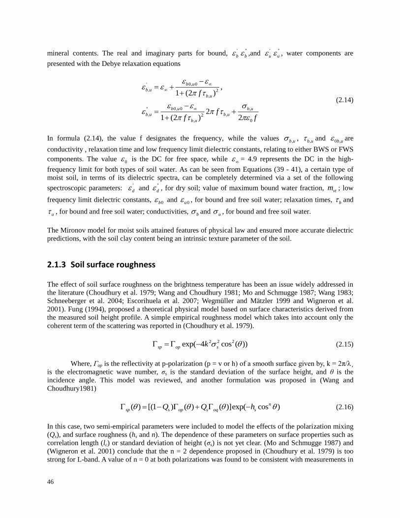
46
mineral contents. The real and imaginary parts for bound, '
b''
b ,and '
u''
u , water components are
presented with the Debye relaxation equations
0, 0'
, 2
,
0, 0 ,''
, ,2
, 0
,1 (2 )
21 (2 ) 2
b u
b u
b u
b u b u
b u b u
b u
f
ff f
(2.14)
In formula (2.14), the value f designates the frequency, while the values ,b u , ,b u and 0 ,b u are
conductivity , relaxation time and low frequency limit dielectric constants, relating to either BWS or FWS
components. The value 0 is the DC for free space, while = 4.9 represents the DC in the high-
frequency limit for both types of soil water. As can be seen from Equations (39 - 41), a certain type of
moist soil, in terms of its dielectric spectra, can be completely determined via a set of the following
spectroscopic parameters: '
d and ''
d , for dry soil; value of maximum bound water fraction, vtm ; low
frequency limit dielectric constants, 0b and 0u , for bound and free soil water; relaxation times, b and
u , for bound and free soil water; conductivities, b and u , for bound and free soil water.
The Mironov model for moist soils attained features of physical law and ensured more accurate dielectric
predictions, with the soil clay content being an intrinsic texture parameter of the soil.
2.1.3 Soil surface roughness
The effect of soil surface roughness on the brightness temperature has been an issue widely addressed in
the literature (Choudhury et al. 1979; Wang and Choudhury 1981; Mo and Schmugge 1987; Wang 1983;
Schneeberger et al. 2004; Escorihuela et al. 2007; Wegmüller and Mätzler 1999 and Wigneron et al.
2001). Fung (1994), proposed a theoretical physical model based on surface characteristics derived from
the measured soil height profile. A simple empirical roughness model which takes into account only the
coherent term of the scattering was reported in (Choudhury et al. 1979).
2 2 2exp( 4 cos ( ))sp op sk (2.15)
Where, Гop is the reflectivity at p-polarization (p = v or h) of a smooth surface given by, k = 2π/λ¸
is the electromagnetic wave number, σs is the standard deviation of the surface height, and θ is the
incidence angle. This model was reviewed, and another formulation was proposed in (Wang and
Choudhury1981)
( ) [(1 ) ( ) ( )]exp( cos )n
sp s op s oq sQ Q h (2.16)
In this case, two semi-empirical parameters were included to model the effects of the polarization mixing
(Qs), and surface roughness (hs and n). The dependence of these parameters on surface properties such as
correlation length (lc) or standard deviation of height (σs) is not yet clear. (Mo and Schmugge 1987) and
(Wigneron et al. 2001) conclude that the n = 2 dependence proposed in (Choudhury et al. 1979) is too
strong for L-band. A value of n = 0 at both polarizations was found to be consistent with measurements in
47
(Wigneron et al. 2001), while Escorihuela et al. (2007) distinguishes n values for both polarizations (1 at
horizontal and -1 at vertical).
Similarly, there are discrepancies on the value of the roughness parameter hs. Some authors obtain hs from
experimental data by best-fit (Wigneron et al. 2001) while others propose expressions for hs as a function
of geophysical parameters. Mo and Schmugge (1987) obtained good results with two parameterizations of
hs as a function of σs and lc.
Finally, there is a general agreement on the value of the cross-polarization parameter Qs, which has been
found to be very small (0 to 0.12) at L-band (Mo and Schmugge 1987 and Wigneron et al. 2001). Apart
from these considerations, the effects of frequency and incidence angle on the roughness parameters have
not been studied thoroughly. Mo and Schmugge (1987) and Shi et al. (2002) pointed out that the
roughness effects depend on both of the frequency and the incidence angle.
Shi et al. (2002) suggested a parameterization of the surface reflectivity derived from data simulated for a
wide range of soil water content and roughness properties using the integral equation model (Fung 1994).
The surface reflectivity model of Shi et al. (2002) was tested in Schneeberger et al. (2004) and found, not
capable of explaining discrepancies between the ground truth and remotely sensed data.
2.1.4 Soil effective temperature
Soil microwave brightness temperature depends on soil emission and on the soil effective temperature, Teff
(Ulaby et al. 1986b). The theoretical effective temperature of a soil profile can be estimated as,
0 0
( ) ( )exp[ ( ') ']x
effT T z z z dz dz
(2.17)
Where, T is the thermodynamic temperature, and α is the attenuation coefficient at a depth z. The
attenuation is a function of the soil dielectric constant (0), and of the microwave emission wavelength :
''
'
( )4( )
2 ( )
s
s
zz
z
(2.18)
Several simple formulations have been developed to estimate the soil effective temperature from soil
properties, and soil moisture and temperature profiles. Choudhury et al. (1982) proposed a
parameterization of Teff based on the soil temperature at deep soil (T∞) corresponding to a depth between
50 cm and 1 m, and on a ‘’surface" temperature (Tsurf) corresponding to a depth of 0-5 cm:
( )eff s surfT T C T T (2.19)
The coefficient Cs was considered constant for a given frequency, and equal to 0.246 at L-band. On the
other hand, Chanzy et al. (1997) presented a model for the soil effective temperature at L- and C-bands
based on the air temperature, a deep soil temperature, and the brightness temperature measured at X-band
and V-pol.
Wigneron et al. (2001) proposed a parameterization based on equation 2.19, but with a coefficient Cs
dependent on the volumetric water content ws, and two semi-empirical parameters (w0 and bw0):
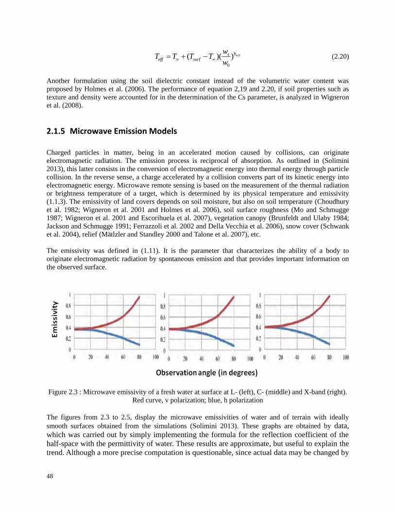
48
0
0
( )( ) wbseff surf
wT T T T
w (2.20)
Another formulation using the soil dielectric constant instead of the volumetric water content was
proposed by Holmes et al. (2006). The performance of equation 2,19 and 2.20, if soil properties such as
texture and density were accounted for in the determination of the Cs parameter, is analyzed in Wigneron
et al. (2008).
2.1.5 Microwave Emission Models
Charged particles in matter, being in an accelerated motion caused by collisions, can originate
electromagnetic radiation. The emission process is reciprocal of absorption. As outlined in (Solimini
2013), this latter consists in the conversion of electromagnetic energy into thermal energy through particle
collision. In the reverse sense, a charge accelerated by a collision converts part of its kinetic energy into
electromagnetic energy. Microwave remote sensing is based on the measurement of the thermal radiation
or brightness temperature of a target, which is determined by its physical temperature and emissivity
(1.1.3). The emissivity of land covers depends on soil moisture, but also on soil temperature (Choudhury
et al. 1982; Wigneron et al. 2001 and Holmes et al. 2006), soil surface roughness (Mo and Schmugge
1987; Wigneron et al. 2001 and Escorihuela et al. 2007), vegetation canopy (Brunfeldt and Ulaby 1984;
Jackson and Schmugge 1991; Ferrazzoli et al. 2002 and Della Vecchia et al. 2006), snow cover (Schwank
et al. 2004), relief (Mätlzler and Standley 2000 and Talone et al. 2007), etc.
The emissivity was defined in (1.11). It is the parameter that characterizes the ability of a body to
originate electromagnetic radiation by spontaneous emission and that provides important information on
the observed surface.
Figure 2.3 : Microwave emissivity of a fresh water at surface at L- (left), C- (middle) and X-band (right).
Red curve, v polarization; blue, h polarization
The figures from 2.3 to 2.5, display the microwave emissivities of water and of terrain with ideally
smooth surfaces obtained from the simulations (Solimini 2013). These graphs are obtained by data,
which was carried out by simply implementing the formula for the reflection coefficient of the
half-space with the permittivity of water. These results are approximate, but useful to explain the
trend. Although a more precise computation is questionable, since actual data may be changed by
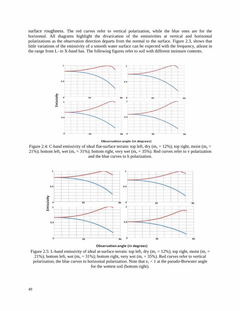
49
surface roughness. The red curves refer to vertical polarization, while the blue ones are for the
horizontal. All diagrams highlight the divarication of the emissivities at vertical and horizontal
polarizations as the observation direction departs from the normal to the surface. Figure 2.3, shows that
little variations of the emissivity of a smooth water surface can be expected with the frequency, atleast in
the range from L- to X-band has. The following figures refer to soil with different moisture contents.
Figure 2.4: C-band emissivity of ideal flat-surface terrain: top left, dry (mv = 12%); top right, moist (mv =
21%); bottom left, wet (mv = 31%); bottom right, very wet (mv = 35%). Red curves refer to v polarization
and the blue curves to h polarization.
Figure 2.5: L-band emissivity of ideal at-surface terrain: top left, dry (mv = 12%); top right, moist (mv =
21%); bottom left, wet (mv = 31%); bottom right, very wet (mv = 35%). Red curves refer to vertical
polarization, the blue curves to horizontal polarization. Note that ev < 1 at the pseudo-Brewster angle
for the wettest soil (bottom right).
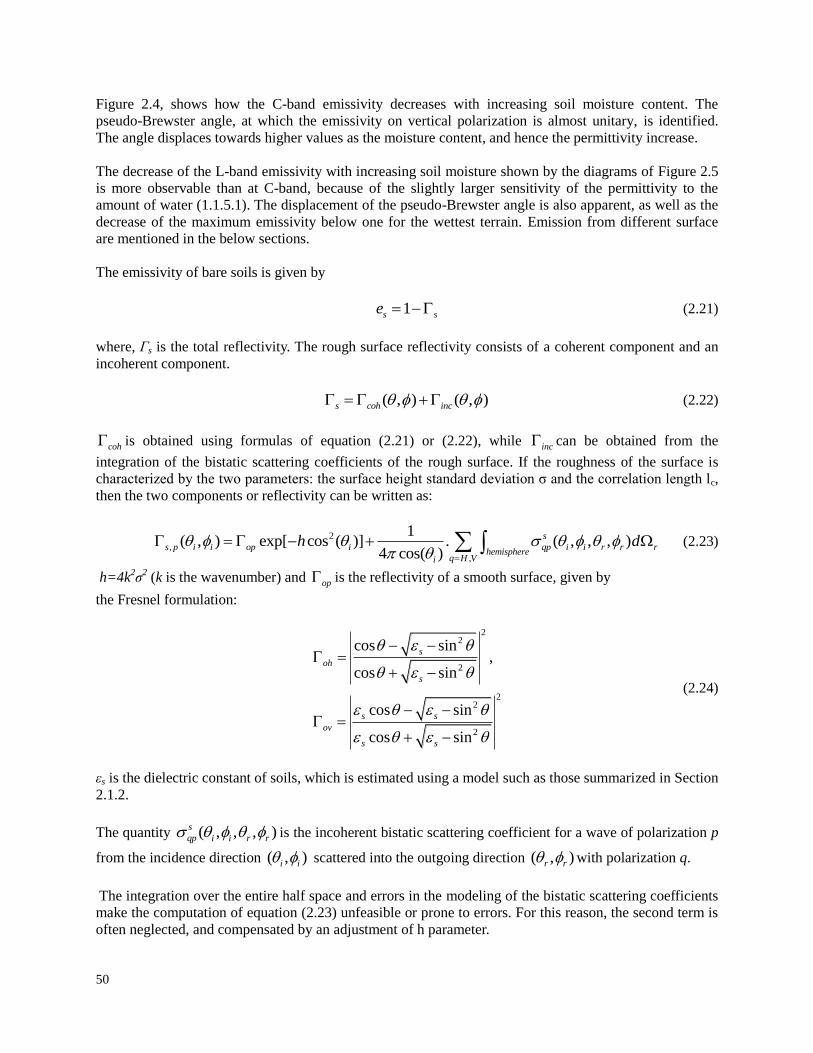
50
Figure 2.4, shows how the C-band emissivity decreases with increasing soil moisture content. The
pseudo-Brewster angle, at which the emissivity on vertical polarization is almost unitary, is identified.
The angle displaces towards higher values as the moisture content, and hence the permittivity increase.
The decrease of the L-band emissivity with increasing soil moisture shown by the diagrams of Figure 2.5
is more observable than at C-band, because of the slightly larger sensitivity of the permittivity to the
amount of water (1.1.5.1). The displacement of the pseudo-Brewster angle is also apparent, as well as the
decrease of the maximum emissivity below one for the wettest terrain. Emission from different surface
are mentioned in the below sections.
The emissivity of bare soils is given by
1s se (2.21)
where, Гs is the total reflectivity. The rough surface reflectivity consists of a coherent component and an
incoherent component.
( , ) ( , )s coh inc (2.22)
coh is obtained using formulas of equation (2.21) or (2.22), while inc can be obtained from the
integration of the bistatic scattering coefficients of the rough surface. If the roughness of the surface is
characterized by the two parameters: the surface height standard deviation σ and the correlation length lc,
then the two components or reflectivity can be written as:
2
,
,
1( , ) exp[ cos ( )] . ( , , , )
4 cos( )
s
s p i i op i qp i i r r rhemisphere
q H Vi
h d
(2.23)
h=4k2σ
2 (k is the wavenumber) and op is the reflectivity of a smooth surface, given by
the Fresnel formulation:
22
2
22
2
cos sin,
cos sin
cos sin
cos sin
s
oh
s
s s
ov
s s
(2.24)
εs is the dielectric constant of soils, which is estimated using a model such as those summarized in Section
2.1.2.
The quantity ( , , , )s
qp i i r r is the incoherent bistatic scattering coefficient for a wave of polarization p
from the incidence direction ( , )i i scattered into the outgoing direction ( , )r r with polarization q.
The integration over the entire half space and errors in the modeling of the bistatic scattering coefficients
make the computation of equation (2.23) unfeasible or prone to errors. For this reason, the second term is
often neglected, and compensated by an adjustment of h parameter.
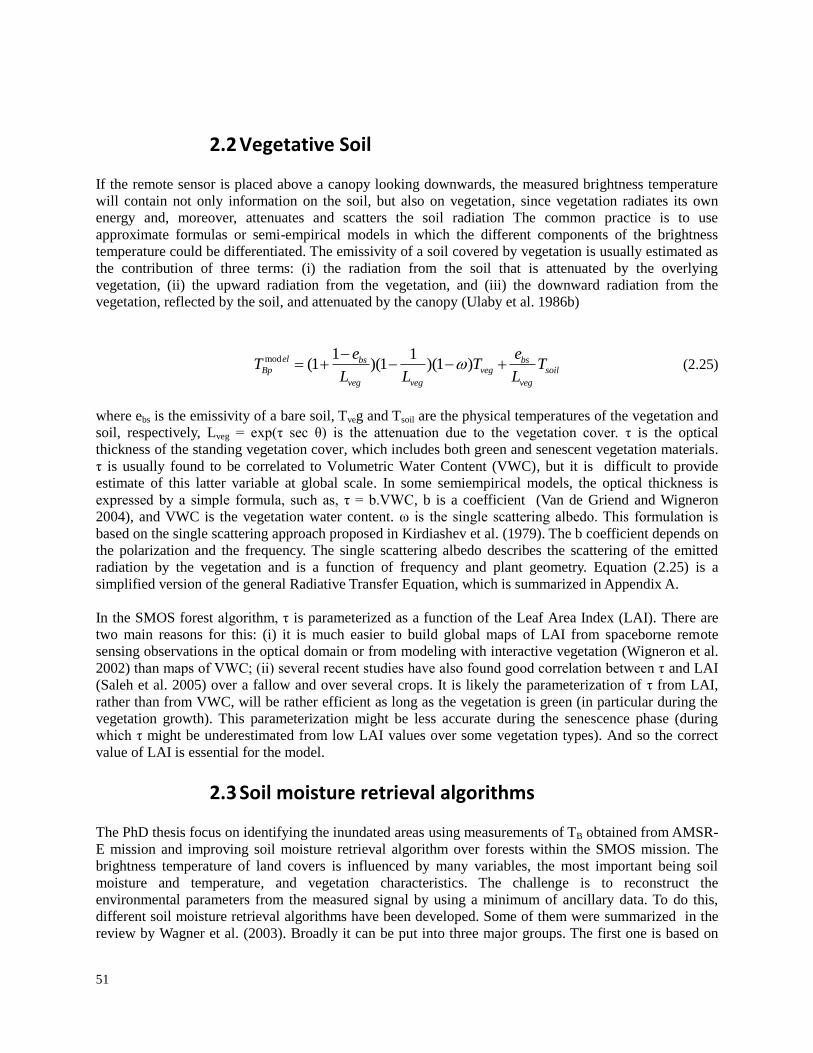
51
2.2 Vegetative Soil
If the remote sensor is placed above a canopy looking downwards, the measured brightness temperature
will contain not only information on the soil, but also on vegetation, since vegetation radiates its own
energy and, moreover, attenuates and scatters the soil radiation The common practice is to use
approximate formulas or semi-empirical models in which the different components of the brightness
temperature could be differentiated. The emissivity of a soil covered by vegetation is usually estimated as
the contribution of three terms: (i) the radiation from the soil that is attenuated by the overlying
vegetation, (ii) the upward radiation from the vegetation, and (iii) the downward radiation from the
vegetation, reflected by the soil, and attenuated by the canopy (Ulaby et al. 1986b)
mod 1 1
(1 )(1 )(1 )el bs bsBp veg soil
veg veg veg
e eT T T
L L L
(2.25)
where ebs is the emissivity of a bare soil, Tveg and Tsoil are the physical temperatures of the vegetation and
soil, respectively, Lveg = exp(τ sec θ) is the attenuation due to the vegetation cover. τ is the optical
thickness of the standing vegetation cover, which includes both green and senescent vegetation materials.
τ is usually found to be correlated to Volumetric Water Content (VWC), but it is difficult to provide
estimate of this latter variable at global scale. In some semiempirical models, the optical thickness is
expressed by a simple formula, such as, τ = b.VWC, b is a coefficient (Van de Griend and Wigneron
2004), and VWC is the vegetation water content. ω is the single scattering albedo. This formulation is
based on the single scattering approach proposed in Kirdiashev et al. (1979). The b coefficient depends on
the polarization and the frequency. The single scattering albedo describes the scattering of the emitted
radiation by the vegetation and is a function of frequency and plant geometry. Equation (2.25) is a
simplified version of the general Radiative Transfer Equation, which is summarized in Appendix A.
In the SMOS forest algorithm, τ is parameterized as a function of the Leaf Area Index (LAI). There are
two main reasons for this: (i) it is much easier to build global maps of LAI from spaceborne remote
sensing observations in the optical domain or from modeling with interactive vegetation (Wigneron et al.
2002) than maps of VWC; (ii) several recent studies have also found good correlation between τ and LAI
(Saleh et al. 2005) over a fallow and over several crops. It is likely the parameterization of τ from LAI,
rather than from VWC, will be rather efficient as long as the vegetation is green (in particular during the
vegetation growth). This parameterization might be less accurate during the senescence phase (during
which τ might be underestimated from low LAI values over some vegetation types). And so the correct
value of LAI is essential for the model.
2.3 Soil moisture retrieval algorithms
The PhD thesis focus on identifying the inundated areas using measurements of TB obtained from AMSR-
E mission and improving soil moisture retrieval algorithm over forests within the SMOS mission. The
brightness temperature of land covers is influenced by many variables, the most important being soil
moisture and temperature, and vegetation characteristics. The challenge is to reconstruct the
environmental parameters from the measured signal by using a minimum of ancillary data. To do this,
different soil moisture retrieval algorithms have been developed. Some of them were summarized in the
review by Wagner et al. (2003). Broadly it can be put into three major groups. The first one is based on
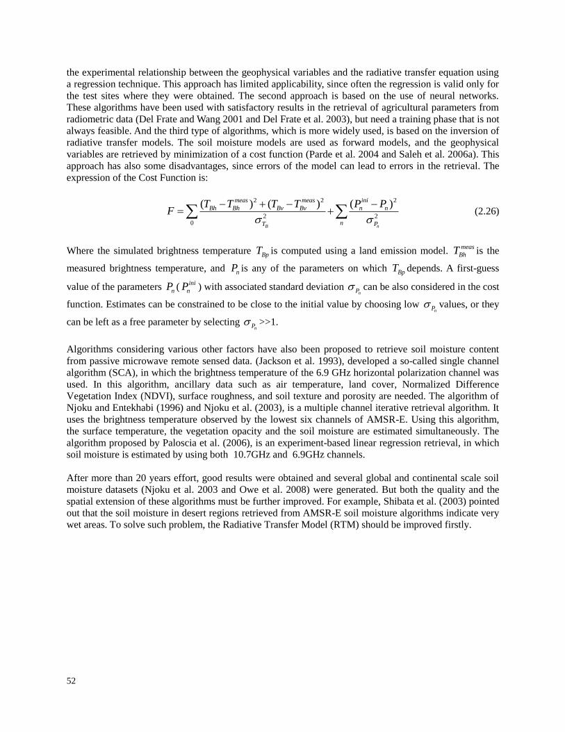
52
the experimental relationship between the geophysical variables and the radiative transfer equation using
a regression technique. This approach has limited applicability, since often the regression is valid only for
the test sites where they were obtained. The second approach is based on the use of neural networks.
These algorithms have been used with satisfactory results in the retrieval of agricultural parameters from
radiometric data (Del Frate and Wang 2001 and Del Frate et al. 2003), but need a training phase that is not
always feasible. And the third type of algorithms, which is more widely used, is based on the inversion of
radiative transfer models. The soil moisture models are used as forward models, and the geophysical
variables are retrieved by minimization of a cost function (Parde et al. 2004 and Saleh et al. 2006a). This
approach has also some disadvantages, since errors of the model can lead to errors in the retrieval. The
expression of the Cost Function is:
2 2 2
2 20
( ) ( ) ( )
B n
meas meas ini
Bh Bh Bv Bv n n
nT P
T T T T P PF
(2.26)
Where the simulated brightness temperature BpT is computed using a land emission model. meas
BhT is the
measured brightness temperature, and nP is any of the parameters on which BpT depends. A first-guess
value of the parameters nP (ini
nP ) with associated standard deviation nP can be also considered in the cost
function. Estimates can be constrained to be close to the initial value by choosing low nP values, or they
can be left as a free parameter by selecting nP >>1.
Algorithms considering various other factors have also been proposed to retrieve soil moisture content
from passive microwave remote sensed data. (Jackson et al. 1993), developed a so-called single channel
algorithm (SCA), in which the brightness temperature of the 6.9 GHz horizontal polarization channel was
used. In this algorithm, ancillary data such as air temperature, land cover, Normalized Difference
Vegetation Index (NDVI), surface roughness, and soil texture and porosity are needed. The algorithm of
Njoku and Entekhabi (1996) and Njoku et al. (2003), is a multiple channel iterative retrieval algorithm. It
uses the brightness temperature observed by the lowest six channels of AMSR-E. Using this algorithm,
the surface temperature, the vegetation opacity and the soil moisture are estimated simultaneously. The
algorithm proposed by Paloscia et al. (2006), is an experiment-based linear regression retrieval, in which
soil moisture is estimated by using both 10.7GHz and 6.9GHz channels.
After more than 20 years effort, good results were obtained and several global and continental scale soil
moisture datasets (Njoku et al. 2003 and Owe et al. 2008) were generated. But both the quality and the
spatial extension of these algorithms must be further improved. For example, Shibata et al. (2003) pointed
out that the soil moisture in desert regions retrieved from AMSR-E soil moisture algorithms indicate very
wet areas. To solve such problem, the Radiative Transfer Model (RTM) should be improved firstly.
53
3 Flood Monitoring using Microwave Passive Remote Sensing (AMSR-E) in part of Brahmaputra basin, India
3.1 Introduction
Floods are one of the most recurring, widespread and disastrous hazards of the world, both natural and
man-made in origin. On the world flood map, India is only preceded by Bangladesh and among the major
rivers basins of India, Brahmaputra basin and floods are almost synonymous to the world. Every year
thousands of acres of land remain under water for most part of the year in this region. One of the
important causes for frequent occurrence of flood in this region is the extremely dynamic monsoon
rainfall regime in the backdrop of the unique physiographic setting. Also, the water yield of the
Brahmaputra is among the highest in the world. These factors, together with high sediment yield, limited
width of the valley and the abruptly flattened gradient, leads to tremendous drainage congestion and
resultant flooding. The scenario is further exacerbated by a myriad of social, economic and environmental
factors causing increased vulnerability of people to the flood hazard
Monitoring of global phenomenon such as flood using satellite data is important for assessing the damage
caused by flood. Also it can lead to a better understanding of the global water cycle and its role in climate
change. Over the past decade, several flood monitoring/forecast methodologies, based on remote sensing
data, have been proposed as described in Section 1.2.2. Among them, the ones based on microwave
observations have a better success rate since large flood events and intense cloud covers are often
encountered simultaneously. Furthermore, since flood events are dynamic processes, higher temporal
resolutions are required even if this leads to lower spatial resolutions. Therefore, passive microwaves are
often exploited. This is particularly true in the case of large river basins, where extreme flood events
compromise thousands of square kilometres in a matter of few hours.
Earlier work carried out by Singh et al. (2008) and Dutta et al. (2010) has also discussed the necessity of
flood mapping and a detailed hydrodynamic investigation to simulate the flood behaviour and the flood
propagation in the low lying flood plain in the proposed study area.
Rainfall measurement over land is another crucial element for understanding the water cycle exchange
between land and atmosphere. Precipitation has a very high correlation with the soil moisture. However it
is very difficult to find a direct way to study these two variables with respect to each other as rainfall is
the main source of uncertainty in retrieval of soil moisture (Jin et al. 2006). In fact, the microwave signals
gets highly affected when they pass through a raining atmosphere, which results in incorrect estimation of
soil moisture in the footprint of the satellite. For global rain identification, (Grody 1991) developed a set
of rules to separate rain from snow and deserts. Ferraro and Marks (1994) expanded on those ideas and
developed a more expansive set of screens to be used for rainfall retrievals that included separate indices
for land and ocean, improved screens for semi-arid land, coastlines, and sea ice, as well as some
discussion on the uncertainties related to each screen.
As stated in Section 1.4.1, the Advanced Microwave Scanning Radiometer (AMSR-E) of the Earth
Observing System (EOS), developed by the National Space Development Agency of Japan (NASDA) and
provided to the U.S. National Aeronautics and Space Administration (NASA) for launch on its Aqua
satellite, can be a valid instrument for flood monitoring. The AMSR-E instrument operates at multiple
frequencies, ranging from 6.9 GHz – 89.0 GHz. The antenna scans conically at a fixed incidence angle of
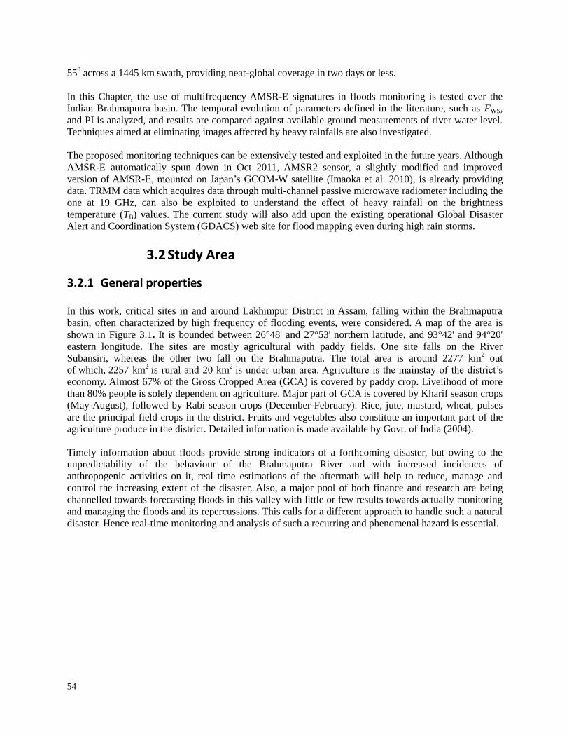
54
550 across a 1445 km swath, providing near-global coverage in two days or less.
In this Chapter, the use of multifrequency AMSR-E signatures in floods monitoring is tested over the
Indian Brahmaputra basin. The temporal evolution of parameters defined in the literature, such as FWS,
and PI is analyzed, and results are compared against available ground measurements of river water level.
Techniques aimed at eliminating images affected by heavy rainfalls are also investigated.
The proposed monitoring techniques can be extensively tested and exploited in the future years. Although
AMSR-E automatically spun down in Oct 2011, AMSR2 sensor, a slightly modified and improved
version of AMSR-E, mounted on Japan’s GCOM-W satellite (Imaoka et al. 2010), is already providing
data. TRMM data which acquires data through multi-channel passive microwave radiometer including the
one at 19 GHz, can also be exploited to understand the effect of heavy rainfall on the brightness
temperature (TB) values. The current study will also add upon the existing operational Global Disaster
Alert and Coordination System (GDACS) web site for flood mapping even during high rain storms.
3.2 Study Area
3.2.1 General properties
In this work, critical sites in and around Lakhimpur District in Assam, falling within the Brahmaputra
basin, often characterized by high frequency of flooding events, were considered. A map of the area is
shown in Figure 3.1. It is bounded between 26°48' and 27°53' northern latitude, and 93°42' and 94°20'
eastern longitude. The sites are mostly agricultural with paddy fields. One site falls on the River
Subansiri, whereas the other two fall on the Brahmaputra. The total area is around 2277 km2 out
of which, 2257 km2 is rural and 20 km
2 is under urban area. Agriculture is the mainstay of the district’s
economy. Almost 67% of the Gross Cropped Area (GCA) is covered by paddy crop. Livelihood of more
than 80% people is solely dependent on agriculture. Major part of GCA is covered by Kharif season crops
(May-August), followed by Rabi season crops (December-February). Rice, jute, mustard, wheat, pulses
are the principal field crops in the district. Fruits and vegetables also constitute an important part of the
agriculture produce in the district. Detailed information is made available by Govt. of India (2004).
Timely information about floods provide strong indicators of a forthcoming disaster, but owing to the
unpredictability of the behaviour of the Brahmaputra River and with increased incidences of
anthropogenic activities on it, real time estimations of the aftermath will help to reduce, manage and
control the increasing extent of the disaster. Also, a major pool of both finance and research are being
channelled towards forecasting floods in this valley with little or few results towards actually monitoring
and managing the floods and its repercussions. This calls for a different approach to handle such a natural
disaster. Hence real-time monitoring and analysis of such a recurring and phenomenal hazard is essential.
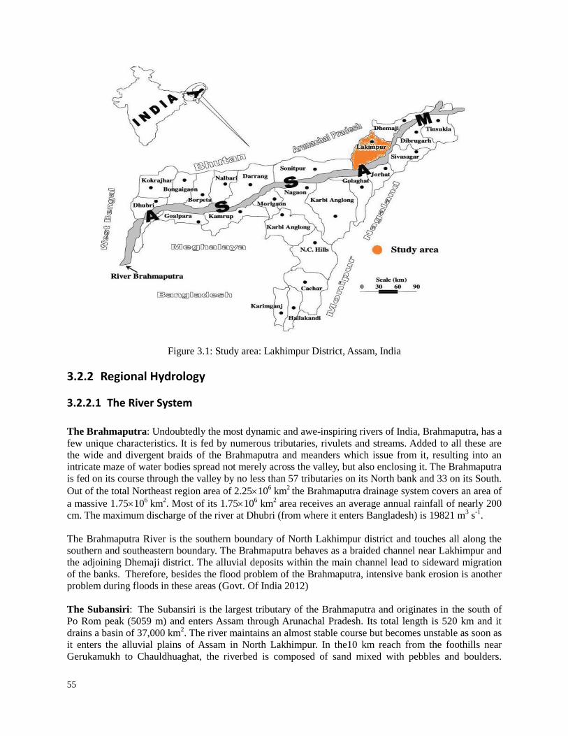
55
Figure 3.1: Study area: Lakhimpur District, Assam, India
3.2.2 Regional Hydrology
3.2.2.1 The River System
The Brahmaputra: Undoubtedly the most dynamic and awe-inspiring rivers of India, Brahmaputra, has a
few unique characteristics. It is fed by numerous tributaries, rivulets and streams. Added to all these are
the wide and divergent braids of the Brahmaputra and meanders which issue from it, resulting into an
intricate maze of water bodies spread not merely across the valley, but also enclosing it. The Brahmaputra
is fed on its course through the valley by no less than 57 tributaries on its North bank and 33 on its South.
Out of the total Northeast region area of 2.25106 km
2 the Brahmaputra drainage system covers an area of
a massive 1.75106 km
2. Most of its 1.7510
6 km
2 area receives an average annual rainfall of nearly 200
cm. The maximum discharge of the river at Dhubri (from where it enters Bangladesh) is 19821 m3 s
-1.
The Brahmaputra River is the southern boundary of North Lakhimpur district and touches all along the
southern and southeastern boundary. The Brahmaputra behaves as a braided channel near Lakhimpur and
the adjoining Dhemaji district. The alluvial deposits within the main channel lead to sideward migration
of the banks. Therefore, besides the flood problem of the Brahmaputra, intensive bank erosion is another
problem during floods in these areas (Govt. Of India 2012)
The Subansiri: The Subansiri is the largest tributary of the Brahmaputra and originates in the south of
Po Rom peak (5059 m) and enters Assam through Arunachal Pradesh. Its total length is 520 km and it
drains a basin of 37,000 km2. The river maintains an almost stable course but becomes unstable as soon as
it enters the alluvial plains of Assam in North Lakhimpur. In the10 km reach from the foothills near
Gerukamukh to Chauldhuaghat, the riverbed is composed of sand mixed with pebbles and boulders.
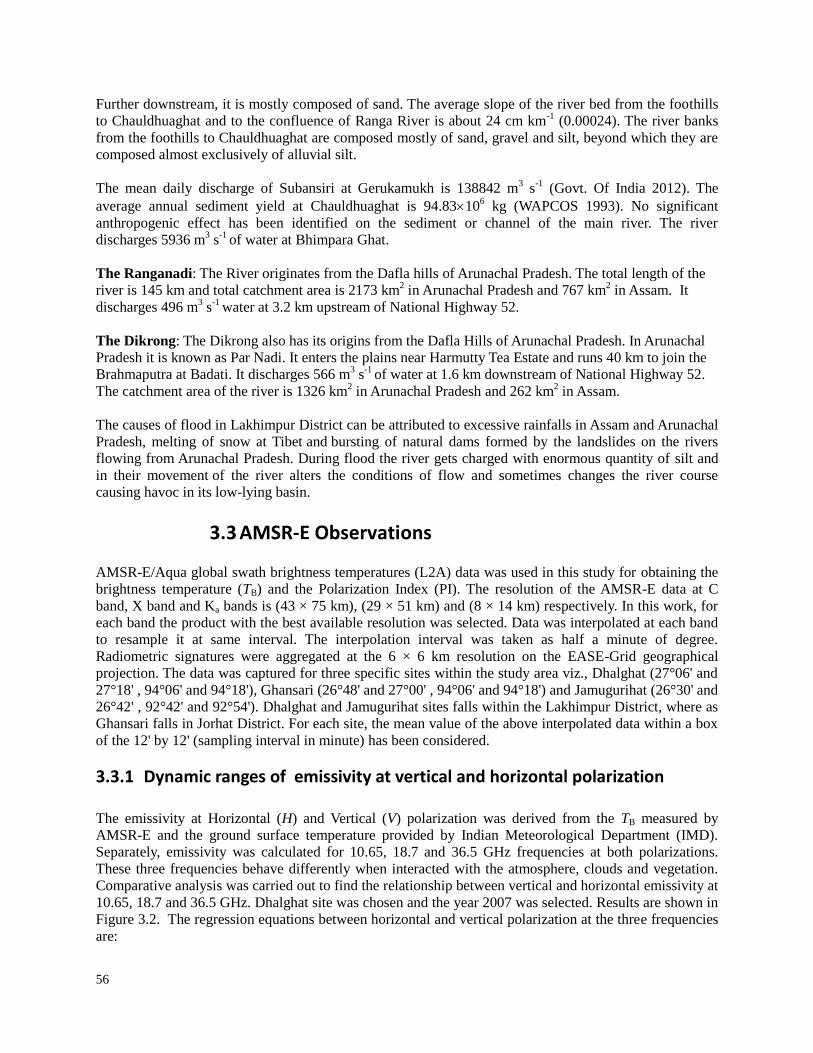
56
Further downstream, it is mostly composed of sand. The average slope of the river bed from the foothills
to Chauldhuaghat and to the confluence of Ranga River is about 24 cm km-1
(0.00024). The river banks
from the foothills to Chauldhuaghat are composed mostly of sand, gravel and silt, beyond which they are
composed almost exclusively of alluvial silt.
The mean daily discharge of Subansiri at Gerukamukh is 138842 m3 s
-1 (Govt. Of India 2012). The
average annual sediment yield at Chauldhuaghat is 94.83106 kg (WAPCOS 1993). No significant
anthropogenic effect has been identified on the sediment or channel of the main river. The river
discharges 5936 m3 s
-1 of water at Bhimpara Ghat.
The Ranganadi: The River originates from the Dafla hills of Arunachal Pradesh. The total length of the
river is 145 km and total catchment area is 2173 km2 in Arunachal Pradesh and 767 km
2 in Assam. It
discharges 496 m3 s
-1 water at 3.2 km upstream of National Highway 52.
The Dikrong: The Dikrong also has its origins from the Dafla Hills of Arunachal Pradesh. In Arunachal
Pradesh it is known as Par Nadi. It enters the plains near Harmutty Tea Estate and runs 40 km to join the
Brahmaputra at Badati. It discharges 566 m3 s
-1 of water at 1.6 km downstream of National Highway 52.
The catchment area of the river is 1326 km2 in Arunachal Pradesh and 262 km
2 in Assam.
The causes of flood in Lakhimpur District can be attributed to excessive rainfalls in Assam and Arunachal
Pradesh, melting of snow at Tibet and bursting of natural dams formed by the landslides on the rivers
flowing from Arunachal Pradesh. During flood the river gets charged with enormous quantity of silt and
in their movement of the river alters the conditions of flow and sometimes changes the river course
causing havoc in its low-lying basin.
3.3 AMSR-E Observations
AMSR-E/Aqua global swath brightness temperatures (L2A) data was used in this study for obtaining the
brightness temperature (TB) and the Polarization Index (PI). The resolution of the AMSR-E data at C
band, X band and Ka bands is (43 × 75 km), (29 × 51 km) and (8 × 14 km) respectively. In this work, for
each band the product with the best available resolution was selected. Data was interpolated at each band
to resample it at same interval. The interpolation interval was taken as half a minute of degree.
Radiometric signatures were aggregated at the 6 × 6 km resolution on the EASE-Grid geographical
projection. The data was captured for three specific sites within the study area viz., Dhalghat (27°06' and
27°18' , 94°06' and 94°18'), Ghansari (26°48' and 27°00' , 94°06' and 94°18') and Jamugurihat (26°30' and
26°42' , 92°42' and 92°54'). Dhalghat and Jamugurihat sites falls within the Lakhimpur District, where as
Ghansari falls in Jorhat District. For each site, the mean value of the above interpolated data within a box
of the 12' by 12' (sampling interval in minute) has been considered.
3.3.1 Dynamic ranges of emissivity at vertical and horizontal polarization
The emissivity at Horizontal (H) and Vertical (V) polarization was derived from the TB measured by
AMSR-E and the ground surface temperature provided by Indian Meteorological Department (IMD).
Separately, emissivity was calculated for 10.65, 18.7 and 36.5 GHz frequencies at both polarizations.
These three frequencies behave differently when interacted with the atmosphere, clouds and vegetation.
Comparative analysis was carried out to find the relationship between vertical and horizontal emissivity at
10.65, 18.7 and 36.5 GHz. Dhalghat site was chosen and the year 2007 was selected. Results are shown in
Figure 3.2. The regression equations between horizontal and vertical polarization at the three frequencies
are:
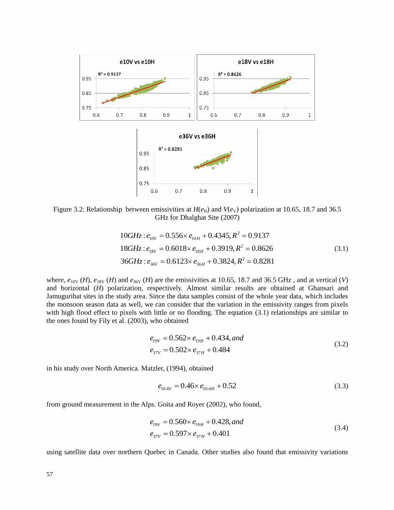
57
Figure 3.2: Relationship between emissivities at H(eH) and V(eV) polarization at 10.65, 18.7 and 36.5
GHz for Dhalghat Site (2007)
2
10 10
2
18 18
2
36 36
10 : 0.556 0.4345, 0.9137
18 : 0.6018 0.3919, 0.8626
36 : 0.6123 0.3824, 0.8281
V H
V H
V H
GHz e e R
GHz e e R
GHz e e R
(3.1)
where, e10V (H), e18V (H) and e36V (H) are the emissivities at 10.65, 18.7 and 36.5 GHz , and at vertical (V)
and horizontal (H) polarization, respectively. Almost similar results are obtained at Ghansari and
Jamugurihat sites in the study area. Since the data samples consist of the whole year data, which includes
the monsoon season data as well, we can consider that the variation in the emissivity ranges from pixels
with high flood effect to pixels with little or no flooding. The equation (3.1) relationships are similar to
the ones found by Fily et al. (2003), who obtained
19 19
37 37
0.562 0.434,
0.502 0.484
V H
V H
e e and
e e
(3.2)
in his study over North America. Matzler, (1994), obtained
10.4 10.40.46 0.52V He e (3.3)
from ground measurement in the Alps. Goita and Royer (2002), who found,
19 19
37 37
0.560 0.428,
0.597 0.401
V H
V H
e e and
e e
(3.4)
using satellite data over northern Quebec in Canada. Other studies also found that emissivity variations
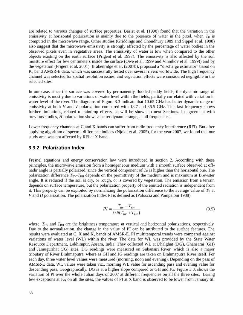
58
are related to various changes of surface properties. Basist et al. (1998) found that the variation in the
emissivity at horizontal polarization is mainly due to the presence of water in the pixel, when TB is
computed in the microwave range. Other studies (Griddings and Choudhury 1989 and Sippel et al. 1998)
also suggest that the microwave emissivity is strongly affected by the percentage of water bodies in the
observed pixels even in vegetative areas. The emissivity of water is low when compared to the other
objects existing on the earth surface (Prigent et al. 1997). The emissivity is also affected by the soil
moisture effect for few centimeters inside the surface (Owe et al. 1999 and Vinnikov et al. 1999)) and by
the vegetation (Prigent et al. 2001). Brakenridge et al. (2007b), proposed a “discharge estimator” based on
Ka band AMSR-E data, which was successfully tested over several rivers worldwide. The high frequency
channel was selected for spatial resolution issues, and vegetation effects were considered negligible in the
selected sites.
In our case, since the surface was covered by permanently flooded paddy fields, the dynamic range of
emissivity is mostly due to variations of water level within the fields, partially correlated with variation in
water level of the river. The diagrams of Figure 3.3 indicate that 10.65 GHz has better dynamic range of
emissivity at both H and V polarization compared with 18.7 and 36.5 GHz. This last frequency shows
further limitations, related to raindrop effects, as will be shown in next Sections. In agreement with
previous studies, H polarization shows a better dynamic range, at all frequencies.
Lower frequency channels at C and X bands can suffer from radio frequency interference (RFI). But after
applying algorithm of spectral difference indices (Njoku et al. 2005), for the year 2007, we found that our
study area was not affected by RFI at X band.
3.3.2 Polarization Index
Fresnel equations and energy conservation law were introduced in section 2. According with these
principles, the microwave emission from a homogeneous medium with a smooth surface observed at off-
nadir angle is partially polarized, since the vertical component of TB is higher than the horizontal one. The
polarization difference TBV-TBH depends on the permittivity of the medium and is maximum at Brewster
angle. It is reduced if the soil is dry, or rough, or is covered by vegetation. The emission from a terrain
depends on surface temperature, but the polarization property of the emitted radiation is independent from
it. This property can be exploited by normalizing the polarization difference to the average value of TB at
V and H polarization. The polarization Index PI is defined as (Paloscia and Pampaloni 1988):
0.5( )
BV BH
BV BH
T TPI
T T
(3.5)
where, TBV and TBH are the brightness temperature at vertical and horizontal polarizations, respectively.
Due to the normalization, the change in the value of PI can be attributed to the surface features. The
results were evaluated at C, X and Ka bands of AMSR-E. PI multitemporal trends were compared against
variations of water level (WL) within the river. The data for WL was provided by the State Water
Resource Department, Lakhimpur, Assam, India. They collected WL at Dhalghat (DG), Ghansarai (GH)
and Jamugurihat (JG) sites. DG readings were measured on Subansiri River, which is also a major
tributary of River Brahmaputra, where as GH and JG readings are taken on Brahmaputra River itself. For
each day, three water level values were measured (morning, noon and evening). Depending on the pass of
AMSR-E data, WL values were taken viz., morning WL value for ascending pass and evening value for
descending pass. Geographically, DG is at a higher slope compared to GH and JG. Figure 3.3, shows the
variation of PI over the whole Julian days of 2007 at different frequencies on all the three sites. Baring
few exceptions at JG, on all the sites, the values of PI at X band is observed to be lower from January till
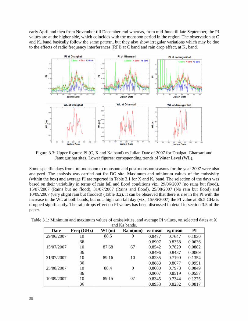
59
early April and then from November till December end whereas, from mid June till late September, the PI
values are at the higher side, which coincides with the monsoon period in the region. The observation at C
and Ka band basically follow the same pattern, but they also show irregular variations which may be due
to the effects of radio frequency interferences (RFI) at C band and rain drop effect, at Ka band.
Figure 3.3: Upper figures: PI (C, X and Ka band) vs Julian Date of 2007 for Dhalgat, Ghansari and
Jamugurihat sites. Lower figures: corresponding trends of Water Level (WL).
Some specific days from pre-monsoon to monsoon and post-monsoon seasons for the year 2007 were also
analyzed. The analysis was carried out for DG site. Maximum and minimum values of the emissivity
(within the box) and average PI are reported in Table 3.1 for X and Ka band. The selection of the days was
based on their variability in terms of rain fall and flood conditions viz., 29/06/2007 (no rains but flood),
15/07/2007 (Rains but no flood), 31/07/2007 (Rains and flood), 25/08/2007 (No rain but flood) and
10/09/2007 (very slight rain but flooded) (Table 3.2). It can be observed that there is rise in the PI with the
increase in the WL at both bands, but on a high rain fall day (viz., 15/06/2007) the PI value at 36.5 GHz is
dropped significantly. The rain drops effect on PI values has been discussed in detail in section 3.5 of the
paper.
Table 3.1: Minimum and maximum values of emissivities, and average PI values, on selected dates at X
and Ka bands.
Date Freq (GHz) WL(m) Rain(mm) eV mean eH mean PI
29/06/2007 10 88.5 0 0.8477 0.7647 0.1030
36 0.8907 0.8358 0.0636
15/07/2007 10 87.68 67 0.8542 0.7820 0.0882
36 0.8496 0.8437 0.0069
31/07/2007 10 89.16 10 0.8235 0.7190 0.1354
36 0.8883 0.8077 0.0951
25/08/2007 10 88.4 0 0.8680 0.7973 0.0849
36 0.9007 0.8519 0.0557
10/09/2007 10 89.15 07 0.8345 0.7344 0.1275
36 0.8933 0.8232 0.0817
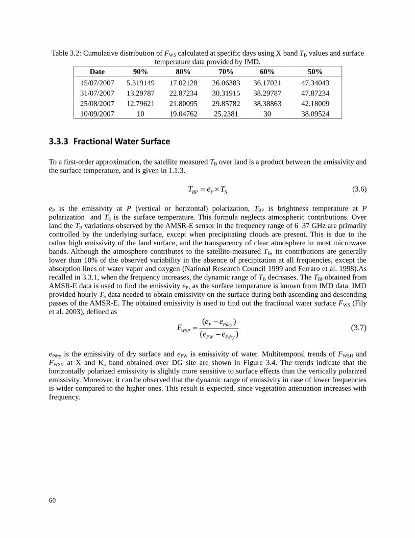
60
Table 3.2: Cumulative distribution of FWS calculated at specific days using X band TB values and surface
temperature data provided by IMD.
Date 90% 80% 70% 60% 50%
15/07/2007 5.319149 17.02128 26.06383 36.17021 47.34043
31/07/2007 13.29787 22.87234 30.31915 38.29787 47.87234
25/08/2007 12.79621 21.80095 29.85782 38.38863 42.18009
10/09/2007 10 19.04762 25.2381 30 38.09524
3.3.3 Fractional Water Surface
To a first-order approximation, the satellite measured TB over land is a product between the emissivity and
the surface temperature, and is given in 1.1.3.
BP P ST e T (3.6)
eP is the emissivity at P (vertical or horizontal) polarization, TBP is brightness temperature at P
polarization and TS is the surface temperature. This formula neglects atmospheric contributions. Over
land the TB variations observed by the AMSR-E sensor in the frequency range of 6–37 GHz are primarily
controlled by the underlying surface, except when precipitating clouds are present. This is due to the
rather high emissivity of the land surface, and the transparency of clear atmosphere in most microwave
bands. Although the atmosphere contributes to the satellite-measured TB, its contributions are generally
lower than 10% of the observed variability in the absence of precipitation at all frequencies, except the
absorption lines of water vapor and oxygen (National Research Council 1999 and Ferraro et al. 1998).As
recalled in 3.3.1, when the frequency increases, the dynamic range of TB decreases. The TBP obtained from
AMSR-E data is used to find the emissivity eP, as the surface temperature is known from IMD data. IMD
provided hourly TS data needed to obtain emissivity on the surface during both ascending and descending
passes of the AMSR-E. The obtained emissivity is used to find out the fractional water surface FWS (Fily
et al. 2003), defined as
( )
( )
P Pdry
WSP
PW Pdry
e eF
e e
(3.7)
ePdry is the emissivity of dry surface and ePW is emissivity of water. Multitemporal trends of FWSH and
FWSV at X and Ka band obtained over DG site are shown in Figure 3.4. The trends indicate that the
horizontally polarized emissivity is slightly more sensitive to surface effects than the vertically polarized
emissivity. Moreover, it can be observed that the dynamic range of emissivity in case of lower frequencies
is wider compared to the higher ones. This result is expected, since vegetation attenuation increases with
frequency.
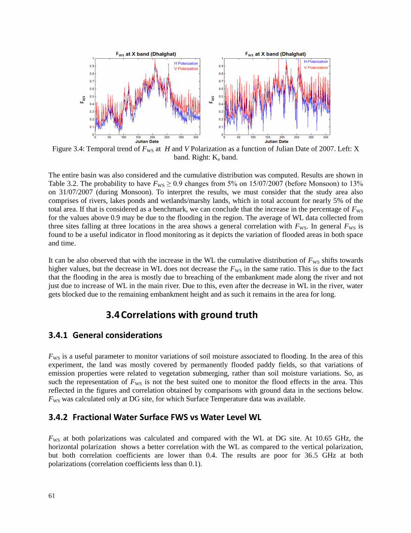
61
Figure 3.4: Temporal trend of FWS at H and V Polarization as a function of Julian Date of 2007. Left: X
band. Right: Ka band.
The entire basin was also considered and the cumulative distribution was computed. Results are shown in
Table 3.2. The probability to have FWS ≥ 0.9 changes from 5% on 15/07/2007 (before Monsoon) to 13%
on 31/07/2007 (during Monsoon). To interpret the results, we must consider that the study area also
comprises of rivers, lakes ponds and wetlands/marshy lands, which in total account for nearly 5% of the
total area. If that is considered as a benchmark, we can conclude that the increase in the percentage of FWS
for the values above 0.9 may be due to the flooding in the region. The average of WL data collected from
three sites falling at three locations in the area shows a general correlation with FWS. In general FWS is
found to be a useful indicator in flood monitoring as it depicts the variation of flooded areas in both space
and time.
It can be also observed that with the increase in the WL the cumulative distribution of FWS shifts towards
higher values, but the decrease in WL does not decrease the FWS in the same ratio. This is due to the fact
that the flooding in the area is mostly due to breaching of the embankment made along the river and not
just due to increase of WL in the main river. Due to this, even after the decrease in WL in the river, water
gets blocked due to the remaining embankment height and as such it remains in the area for long.
3.4 Correlations with ground truth
3.4.1 General considerations FWS is a useful parameter to monitor variations of soil moisture associated to flooding. In the area of this
experiment, the land was mostly covered by permanently flooded paddy fields, so that variations of
emission properties were related to vegetation submerging, rather than soil moisture variations. So, as
such the representation of FWS is not the best suited one to monitor the flood effects in the area. This
reflected in the figures and correlation obtained by comparisons with ground data in the sections below.
FWS was calculated only at DG site, for which Surface Temperature data was available.
3.4.2 Fractional Water Surface FWS vs Water Level WL FWS at both polarizations was calculated and compared with the WL at DG site. At 10.65 GHz, the
horizontal polarization shows a better correlation with the WL as compared to the vertical polarization,
but both correlation coefficients are lower than 0.4. The results are poor for 36.5 GHz at both
polarizations (correlation coefficients less than 0.1).
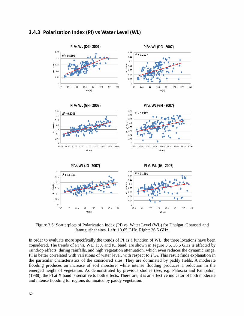
62
3.4.3 Polarization Index (PI) vs Water Level (WL)
Figure 3.5: Scatterplots of Polarization Index (PI) vs. Water Level (WL) for Dhalgat, Ghansari and
Jamugurihat sites. Left: 10.65 GHz. Right: 36.5 GHz.
In order to evaluate more specifically the trends of PI as a function of WL, the three locations have been
considered. The trends of PI vs. WL, at X and Ka band, are shown in Figure 3.5. 36.5 GHz is affected by
raindrop effects, during rainfalls, and high vegetation attenuation, which even reduces the dynamic range.
PI is better correlated with variations of water level, with respect to FWS. This result finds explanation in
the particular characteristics of the considered sites. They are dominated by paddy fields. A moderate
flooding produces an increase of soil moisture, while intense flooding produces a reduction in the
emerged height of vegetation. As demonstrated by previous studies (see, e.g. Paloscia and Pampaloni
(1988), the PI at X band is sensitive to both effects. Therefore, it is an effective indicator of both moderate
and intense flooding for regions dominated by paddy vegetation.
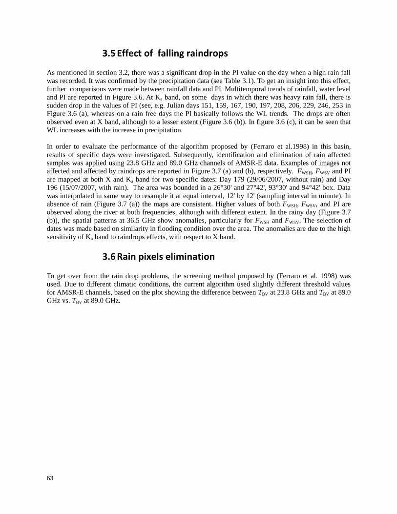
63
3.5 Effect of falling raindrops
As mentioned in section 3.2, there was a significant drop in the PI value on the day when a high rain fall
was recorded. It was confirmed by the precipitation data (see Table 3.1). To get an insight into this effect,
further comparisons were made between rainfall data and PI. Multitemporal trends of rainfall, water level
and PI are reported in Figure 3.6. At Ka band, on some days in which there was heavy rain fall, there is
sudden drop in the values of PI (see, e.g. Julian days 151, 159, 167, 190, 197, 208, 206, 229, 246, 253 in
Figure 3.6 (a), whereas on a rain free days the PI basically follows the WL trends. The drops are often
observed even at X band, although to a lesser extent (Figure 3.6 (b)). In figure 3.6 (c), it can be seen that
WL increases with the increase in precipitation.
In order to evaluate the performance of the algorithm proposed by (Ferraro et al.1998) in this basin,
results of specific days were investigated. Subsequently, identification and elimination of rain affected
samples was applied using 23.8 GHz and 89.0 GHz channels of AMSR-E data. Examples of images not
affected and affected by raindrops are reported in Figure 3.7 (a) and (b), respectively. FWSH, FWSV and PI
are mapped at both X and Ka band for two specific dates: Day 179 (29/06/2007, without rain) and Day
196 (15/07/2007, with rain). The area was bounded in a 26°30' and 27°42', 93°30' and 94°42' box. Data
was interpolated in same way to resample it at equal interval, 12' by 12' (sampling interval in minute). In
absence of rain (Figure 3.7 (a)) the maps are consistent. Higher values of both FWSH, FWSV, and PI are
observed along the river at both frequencies, although with different extent. In the rainy day (Figure 3.7
(b)), the spatial patterns at 36.5 GHz show anomalies, particularly for FWSH and FWSV. The selection of
dates was made based on similarity in flooding condition over the area. The anomalies are due to the high
sensitivity of Ka band to raindrops effects, with respect to X band.
3.6 Rain pixels elimination
To get over from the rain drop problems, the screening method proposed by (Ferraro et al. 1998) was
used. Due to different climatic conditions, the current algorithm used slightly different threshold values
for AMSR-E channels, based on the plot showing the difference between TBV at 23.8 GHz and TBV at 89.0
GHz vs. TBV at 89.0 GHz.
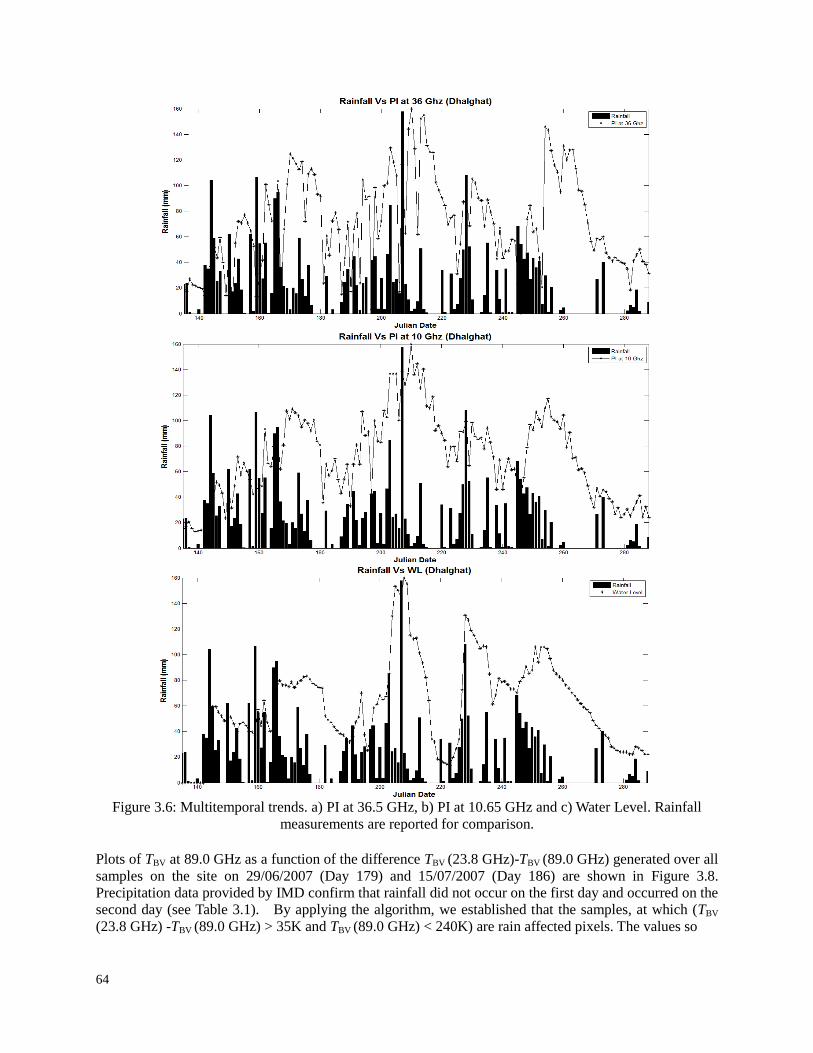
64
Figure 3.6: Multitemporal trends. a) PI at 36.5 GHz, b) PI at 10.65 GHz and c) Water Level. Rainfall
measurements are reported for comparison.
Plots of TBV at 89.0 GHz as a function of the difference TBV (23.8 GHz)-TBV (89.0 GHz) generated over all
samples on the site on 29/06/2007 (Day 179) and 15/07/2007 (Day 186) are shown in Figure 3.8.
Precipitation data provided by IMD confirm that rainfall did not occur on the first day and occurred on the
second day (see Table 3.1). By applying the algorithm, we established that the samples, at which (TBV
(23.8 GHz) -TBV (89.0 GHz) > 35K and TBV (89.0 GHz) < 240K) are rain affected pixels. The values so
65
(a)
(b)
Figure.3.7: (a) Maps of FWSH, FWSV and PI at 10.65 GHz and 36.5 GHz on 29/06/2007, without rain (b):
Maps of FWSH, FWSV and PI at 10.65 GHz and 36.5 GHz on 15/07/2007 with rain
Obtained for threshold however, were slightly different from the one obtained by Jin et al. (2006), mainly
due to the fact that here the study area is not that dry as in west central Africa. Data were analyzed for two
dates and the threshold was decided based on the scatter plot obtained.
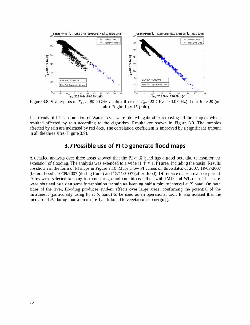
66
Figure 3.8: Scatterplots of TBV at 89.0 GHz vs. the difference TBV (23 GHz – 89.0 GHz). Left: June 29 (no
rain). Right: July 15 (rain)
The trends of PI as a function of Water Level were plotted again after removing all the samples which
resulted affected by rain according to the algorithm. Results are shown in Figure 3.9. The samples
affected by rain are indicated by red dots. The correlation coefficient is improved by a significant amount
in all the three sites (Figure 3.9).
3.7 Possible use of PI to generate flood maps
A detailed analysis over three areas showed that the PI at X band has a good potential to monitor the
extension of flooding. The analysis was extended to a wide (1.40 × 1.4
0) area, including the basin. Results
are shown in the form of PI maps in Figure 3.10. Maps show PI values on three dates of 2007: 18/03/2007
(before flood), 10/09/2007 (during flood) and 13/11/2007 (after flood). Difference maps are also reported.
Dates were selected keeping in mind the ground conditions tallied with IMD and WL data. The maps
were obtained by using same interpolation techniques keeping half a minute interval at X band. On both
sides of the river, flooding produces evident effects over large areas, confirming the potential of the
instrument (particularly using PI at X band) to be used as an operational tool. It was noticed that the
increase of PI during monsoon is mostly attributed to vegetation submerging.
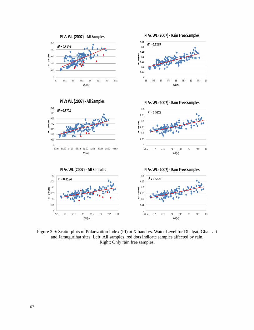
67
Figure 3.9: Scatterplots of Polarization Index (PI) at X band vs. Water Level for Dhalgat, Ghansari
and Jamugurihat sites. Left: All samples, red dots indicate samples affected by rain.
Right: Only rain free samples.
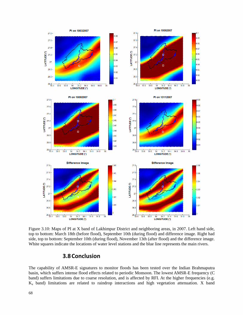
68
Figure 3.10: Maps of PI at X band of Lakhimpur District and neighboring areas, in 2007. Left hand side,
top to bottom: March 18th (before flood), September 10th (during flood) and difference image. Right had
side, top to bottom: September 10th (during flood), November 13th (after flood) and the difference image.
White squares indicate the locations of water level stations and the blue line represents the main rivers.
3.8 Conclusion
The capability of AMSR-E signatures to monitor floods has been tested over the Indian Brahmaputra
basin, which suffers intense flood effects related to periodic Monsoon. The lowest AMSR-E frequency (C
band) suffers limitations due to coarse resolution, and is affected by RFI. At the higher frequencies (e.g.
Ka band) limitations are related to raindrop interactions and high vegetation attenuation. X band
69
demonstrated to have a good trade-off between spatial resolution and sensitivity requirements. Therefore,
it proves to be particularly useful when the site is characterized by wide vegetation covers and high
recurrence of rainstorms. The performances of different parameters defined in the literature, such as
Polarization Index (PI) and Fractional Water Surface (FWS) have been investigated. PI proved to have the
best correlation with water level measurements in the river. This result is related to the particular
properties of the site, which is mostly covered by paddy fields. Flooding effects on PI are related both to
an increase of soil moisture and to a decrease of emerged vegetation height. While correlation between PI
and WL is good when WL increases, it is reduced when it decreases, since the water remains in the large
AMSR-E pixels, and subsides with some delay with respect to the river. At X band, a significant
improvement in the correlation between PI and WL is obtained after eliminating samples affected by
raindrop interactions. To this aim, a technique based on AMSR-E data collected at 23.8 GHz and 89.0
GHz, was applied. The PhD work proposal also included development of a flood response system. The
plan was to generate a network-enabled GIS based solution, to be developed using open source tools, to
assess post flood damage with the help of query based modules, with outputs in the form of both maps
and statistical database. This resultant data and information generated would have been useful for
planning, designing and executing the emergency response measures in an effective manner. But the
resolution of AMSRE data was not optimum to map the accurate extent of flood for a better post-flood
disaster management analysis at smaller scales. Due to this reason, this implementation could not be
attempted. But such system could be of great benefit to the society, even if it just displays the flood maps
derived from AMSRE data (without details query) on GIS background (village boundary), for a operators
to assess the condition of a village during flood.
70
4 Retrieving soil moisture over Forests : SMOS results and comparison with ground observation, other algorithms and independent observations
4.1 Introduction
As discussed in chapter 1.2.1, soil moisture (SM) is an important parameter in weather, hydrologic,
climatologic and atmospheric models because of its influence on evaporation, infiltration, runoff and
uptake of water by vegetation. Because of its variability in time and place, however, creating a database
of the entire earth based on field measurements would be extremely time- and labor-intensive. A solution
to this is satellite imagery. Satellite imagery can give information on SM on a global scale, potentially at
intervals of at most a couple of days.
For this purpose, the European Space Agency (ESA) has developed the Soil Moisture and Ocean Salinity
(SMOS) satellite to retrieve soil moisture over several kinds of land cover, including low vegetation and
forests (see section 1.4.2). This satellite measures brightness temperature (TB) at L-band. From these
measurements SM in the top five centimeters of the soil can be determined. The resolution is in a range of
30-50Km but, the data grid is approximately 15 by 15 km.
It is well established that soil moisture retrieval is difficult under forest cover (Grant et al. 2007;
Guglielmetti et al. 2008 and Kurum et al. 2012). In fact the attenuation related to the high wood biomass
reduces the contribution of the soil surface to the overall emission, thus reducing the sensitivity to
variations of soil moisture. A further reduction of sensitivity is associated to litter cover (Grant et al.
2007; Kurum et al. 2012 and Grant et al. 2009). At C band and higher frequencies, crown attenuation
makes soil moisture retrieval very difficult in most of the cases. At L band some sensitivity to soil
moisture is expected, since crown attenuation is lower than that at the higher frequencies, however
establishing quantitative models is not that simple.
Hence taking the above factors into consideration, developing a reliable forward model and a valid
retrieval algorithm for forests is essential to analyze SMOS data more efficiently.
First of all, forest cover dominates several SMOS pixels. Moreover there are mixed pixels, and even when
other land covers (e.g. agricultural fields, grass) are dominant, a correct characterization of forest
emission improves the retrieval accuracy (Van de Griend et al. 2003).
To provide an insight into this problem important ground-based and airborne experiments have been
undertaken over the years. Multitemporal measurements of brightness temperature were carried out over
coniferous and broadleaf forests using L-band radiometers mounted on a tower (Grant et al. 2007;
Guglielmetti et al. 2008; Kurum et al. 2012; Grant et al. 2008; Guglielmetti et al. 2007; Santi et al. 2009
and Kurum et al. 2011), and were accompanied by detailed measurements of ground variables, such as
soil moisture, wood biomass, and forest geometrical properties. In some cases, outputs were used to test
theoretical models (Kurum et al. 2011 and Kurum et al. 2012), or fit the parameters of semi-empirical
models (Grant et al. 2008 and Santi et al. 2009). Upward looking radiometric data were also collected in
some forests (Grant et al. 2008 and Santi et al. 2009). Moreover, airborne campaigns have provided useful
data for investigating the relationship between emissivity and forest biomass (Lang et al. 2000; Saleh et
al. 2004 and Macelloni et al. 2001), and soil conditions (Grant et al. 2010). Although these efforts are
71
very important, they are not yet sufficient to reach a complete understanding of the forest emission
problem, and to draw conclusive considerations. While some studies indicate the radiometric sensitivity
to variations of soil moisture to be poor in developed forests (Grant et al. 2007; Guglielmetti et al. 2008
and Kurum et al. 2012), others over moderately dense forests with thin litter show the sensitivity to be
appreciable (Guglielmetti et al. 2007; Santi et al. 2009 and Grant et al. 2010), although still lower than
over low vegetation. Moreover, further efforts are required to establish if the sensitivity to soil moisture is
mostly reduced by crown attenuation or by litter cover. Spaceborne monitoring can substantially help to
investigate these problems.
Details about SMOS measurements have been given in Section 1.4.2 and the basic concepts underlying
the algorithms adopted to retrieve soil moisture have been given in Section 2. The SMOS retrieval
algorithm (Kerr et al., 2012) is based on two main components. The first consists of a forward model,
which estimates the TB emitted by land nodes of SMOS using a priori information (from auxiliary data)
about land cover, surface temperature, Leaf Area Index (LAI), and initial estimates of soil moisture taken
by the data base of the European Centre for Medium-Range Weather Forecasts (ECMWF). The second
consists of an inversion process, which estimates the actual soil moisture and optical depth by using
multiangular measurements, forward model outputs and a Cost Function (Kerr et al. 2012). The algorithm
follows an iterative approach which aims at minimizing a cost function whose main component is the sum
of the squared weighted differences between measured and modeled TB data, for a collection of incidence
angles. This is achieved by finding the best-suited set of parameters, which drive the direct TB model,
e.g., SM and vegetation characteristics.
For all SMOS nodes classified as soil covered by vegetation, the TB is estimated by a simple first order
radiative transfer model (Grant et al. 2007) as described in section 2.2. At the SMOS scale, pixels are not
uniform and may have a variety of surface types. In such cases, the total TB comes from several classes of
emitters. This composite TB is obtained through an aggregated forward model which combines each class
of emitting sources weighted by their intra-pixel cover fractions. In order to keep the algorithm consistent,
and to consider the case of mixed pixels, the same approach is kept for both low vegetation and forests
(Kerr et al. 2012). For the case of forests, the radiative transfer parameters τ (optical depth) and ω
(albedo) are estimated using the synthetic outputs of the theoretical model described in Ferrazzoli and
Guerriero (1996), according to the procedure which was further developed in Ferrazzoli et al. (2002). The
theoretical model was tested and revised using sets of ground based and airborne measurements carried
out over various forests in different environments (Della Vecchia et al. 2007; Della Vecchia et al. 2010
and Rahmoune et al. 2010).
The choice of the operating wavelength for SMOS is determined by the increase in sensitivity of the
brightness temperature to soil moisture (ground) with the decrease in the observation frequency. The
1400–1427 MHz band (L-Band) is used because it is the lowest passive frequency band allocated to the
Earth Exploration Satellite Service (EESS) (Kerr 2001). But the microwave radiometers receive
emissions at very low levels compared to those generally handled by other radio communications
services; these sensors are therefore generally more susceptible to Radio Frequency Interference (RFI)
originated from man-made emitters on the ground, on aircraft or space borne systems.
The issue of RFI within this passive band, especially due to the presence of long-range air surveillance
radar systems in nearby bands, has been identified as a key concern by Committee On Scientific Use Of
The Radio Spectrum (2010). Observations already performed using airborne campaigns have shown clear
instances of RFI signals (Zribi 2011). Unwanted emissions arising from radars within the adjacent Earth
Exploration-Satellite Service (EESS) band within the radiometer antenna footprint can easily exceed the
maximum emission level allowed. The experience obtained during the operations of SMOS satellite is
also showing that the presence of radio-links in nearby bands and unauthorized transmissions within
passive band are also a common source of interference for the radiometer (Daganzo 2010).
72
The RFI problem is not due to inadequate filtering in the SMOS receiver (which is using less than the
allocated frequency band and which boasts of very high performance), but is due to two specific
problems: i) Unauthorized emissions within the protected passive band coming from active sources, ii)
Unwanted emissions from active services operating in neighboring bands.
In this chapter results obtained by a prototype version of SMOS SM retrieval algorithm are shown. The
basic algorithm is described in the Algorithm Theoretical Baseline Document (ATBD) (Kerr et al. 2010
and Kerr et al. 2012), while details about forest cover are given by Rahmoune et al. (2013). The prototype
version of the algorithm here adopted is flexible and it can run with different sources of auxiliary data. In
particular the Leaf Area Index, which is an input to the forward model, can be extracted by the
ECOCLIMAP database (Masson et al. 2003b) or by the MODIS database (Knyazikhin et al. 1998a).
In this chapter, first of all, the specific aspects of the algorithm for forests will be described, followed
with the details about the selected test sites used for validation of the results. Then some results about
retrieved optical depth will be discussed..This is an important aspect, since a correct retrieval of optical
depth is fundamental in order to correctly retrieve soil moisture. Finally, soil moisture retrieval results
will be presented. Different approaches to make comparisons with available ground measurements and
filtered data were used, and relevant results were presented. Initially, for the selected nodes of the
available ground networks, averaging was done among SM outputs obtained by the retrieval algorithm in
all SMOS nodes with a center falling within the buffer of 15 Km distance from the ground observation.
This first analysis was done by using both ECOCLIMAP and MODIS as input data sets for the LAI of the
forward model, and results were presented. Then, other comparisons with ground measurements were
shown, done using ECOCLIMAP as input data set, and taking just the SMOS node with a center having
the closest position with respect to the considered network node. This analysis was repeated under
different conditions imposed to RFI filtering and location of SMOS nodes with respect to the swath axis.
Finally, SM data obtained by SMOS and results obtained by the Advanced Microwave Scanning
Radiometer - Earth Observing System (AMSR-E) were compared with respect to the ground observation
to analyze the SM output derived from different data products. In this study, two algorithms were
considered, which were developed to determine SM from AMSR-E measurements, namely that of the
National Snow and Ice Data Centre (NSIDC) and the Vrije Universiteit Amsterdam (VUA) in
combination with NASA.
4.2 SMOS Algorithm
4.2.1 General properties of SMOS Algorithm over forests
4.2.1.1 The forward model
As stated in Section 4.1, a simple radiative transfer equation of zero order RT0 (see Sections 2.1.5 and
2.2) is used as forward model in order to estimate the brightness temperatures which are compared against
SMOS measurements. For forests, the initial values of ω and τ (see equation 2.25) were estimated by
fitting the outputs of a theoretical model, which is based on the radiative transfer theory and adopts a
discrete approach (Ferrazzoli and Guerriero 1996). In that model, trunks and branches are represented as
dielectric objects with the shape of cylinders, while leaves are represented as needles or disks. The bistatic
scattering cross sections and extinction cross sections are computed by using suitable electromagnetic
approximations. The bistatic scattering coefficient of the soil is computed by using the Integral Equation
Model, in its bistatic version (Fung 1994). Single contributions are combined by using the matrix
doubling algorithm, which allows us to compute the overall bistatic scattering coefficient in all directions,
73
including multiple scattering effects. The overall reflectivity is computed using formulas of Section 2.1.5,
where the incoherent component is obtained by integration over the upper half space and the emissivity is
finally obtained by the energy conservation law. Details about the electromagnetic model are given in
Ferrazzoli and Guerriero (1996). For litter, the model published in Della Vecchia et al. (2007), which
considers the litter as a dielectric layer over the soil, was applied.
This theoretical forest model was previously tested against ground based and airborne measurements
(Della Vecchia et al., 2007; Della Vecchia et al., 2010; Rahmoune et al., 2010). RMS errors were in the
range of 2.5 K – 4.0 K.
As discussed in (Rahmoune et al., 2013), for estimating the input variables and parameters, the procedure
assumes to know, besides soil variables, the following inputs:
Leaf Area Index contributed by forest leaves LAIF
Leaf Area Index contributed by herbaceous vegetation LAIV
Distribution of trunk diameters at breast height dbh [cm]: p(dbh)
Moisture [g/g] and dry matter density ρD [g/cm3] of trunks, branches and leaves.
Using allometric equations, simplifying approximations and the theoretical model, the emissivity was
computed at both V and H polarizations, at all angles in the range of 20°-50° and for soil moisture values
in a range of 0.05-04.
The simulation outputs were used to fit the equivalent parameters τF (forest optical depth) and ωF (forest
albedo), contributed by arboreous vegetation and assumed to be independent of polarization, of the RT0
forest model. The RT0 model was run for the same conditions as the theoretical model, and ωF and τF
were selected in order to yield the minimum root mean square (rms) difference between TB (K) outputs of
the two models.
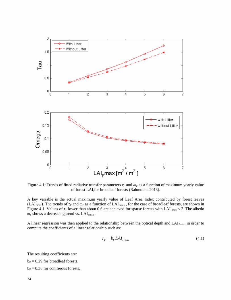
74
Figure 4.1: Trends of fitted radiative transfer parameters τF and ωF as a function of maximum yearly value
of forest LAI,for broadleaf forests (Rahmoune 2013).
A key variable is the actual maximum yearly value of Leaf Area Index contributed by forest leaves
(LAIFmax). The trends of τF and ωF as a function of LAIFmax , for the case of broadleaf forests, are shown in
Figure 4.1. Values of τF lower than about 0.6 are achieved for sparse forests with LAIFmax < 2. The albedo
ωF shows a decreasing trend vs. LAIFmax .
A linear regression was then applied to the relationship between the optical depth and LAIFmax, in order to
compute the coefficients of a linear relationship such as:
maxF F Fb LAI (4.1)
The resulting coefficients are:
bF = 0.29 for broadleaf forests.
bF = 0.36 for coniferous forests.
75
Equation (4.1) gives the maximum yearly value of τF, which is achieved in full leaf development. If the
forest is deciduous, τF decreases in late autumn and winter due to the absence of leaves. Further model
simulations, not shown here, indicated that the corresponding decrease of bF coefficient is 0.03 units.
Therefore, a general expression is:
max max0.03( )F F F F Fb LAI LAI LAI (4.2)
The total optical depth, including contributions of both forest vegetation and herbaceous vegetation is
given by:
F V Vb LAI (4.3)
The bV coefficient is set equal to 0.06, which is the value adopted by the ATBD for low vegetation (Kerr
et al., 2010).
Then, we assumed:
LAIF = fF LAI
LAIV = fV LAI
LAI is the total Leaf Area Index, available by ECOCLIMAP data base (Masson et al., 2003b).
fF and fV represented the fractions of LAI contributed by arboreous leaves and herbaceous vegetation,
respectively. Some data are available in the literature, showing some dispersion. In order to simplify the
initial guess of τ we made an assumption which was verified in some broadleaf and coniferous forests
(Peduzzi et al., 2010 and Blanken et al., 1997). : fF = 0.6, fV = 0.4
For the albedo, the value achieved fitting the outputs of the theoretical model (as described above) for the
dense forest (higher values of LAIFmax in Figure 4.1) is used:
ωF = 0.08
This value represented a good fit for both broadleaf and coniferous forests.
The roughness parameter h of Equation (2.23) has been set equal to 0.3. This value corresponds to a
height standard.of about 1.0 cm, which is quite realistic.
The procedure described in this Section leads to compution of the optical depth and the albedo of the RT0
forest model
4.2.1.2 The retrieval procedure
Using brightness temperatures simulated by the forward model and measured over SMOS grid nodes, SM
and optical depth are determined. The calculated TB is used in an iterative procedure which minimizes a
“cost function” in order to get the retrieved SM and τ. The cost function subtracts measured multiangular
brightness temperatures (L1C data), measured by the satellite to the TB’s simulated by the model. SM
and τ , which are parameters in the equations for TB (see Section 2, eq. 2.25), are kept free in the function
in order to determine the best fit of measured and theoretical TB.
76
In this process, the algorithm uses initial values of soil moisture predicted by ECMWF and the optical
depth predicted by the procedure illustrated in section 4.2.1.1.
4.3 AMSRE Algorithm
As specified in Section 4.1, soil moistures retrieved by SMOS will be compared with the outputs of two
algorithms exploiting AMSR-E data. Some information about the two algorithms is summarized here.
The AMSR-E satellite has a morning (descending) and evening (ascending) overpass (see Section 1.4.1).
Two different SM datasets derived from the AMSR-E satellite, NSIDC and VUA, have been considered.
The difference between NSIDC and UVA SM product lies in the algorithm used. The details are
explained in the next paragraph. For both the cases, SM is determined for approximately the first
centimeter of soil. Both datasets have a resolution of 0.25 by 0.25 decimal degrees.
NSIDC SM data is determined using X-band (10.65 GHz) and Ku-band (18.7 GHz) channels. The
algorithm uses two low frequency dual polarized channels to optimize SM, vegetation optical depth and
effective soil temperature simultaneously. The SM algorithm uses the Polarization ratio (PR). PR is the
difference between the vertical and horizontal TB at a given frequency divided by their sum. This
effectively eliminates or reduces surface temperature effects, which is necessary since no dynamic
ancillary surface temperature is used as input to the algorithm. The algorithm first calculates a
vegetation/roughness parameter, g using PR at 10.7 GHz and PR at 18.7 GHz, plus three empirical
coefficients. SM is then computed using departures of PR at 10.7 GHz from a baseline value, plus four
additional coefficients. The baseline values for PR at 10.7 GHz are based on monthly minima at each grid
cell over annual cycle. The parameter g incorporates effects of vegetation and roughness together and is
interpreted as an equivalent vegetation water content. It uses average values of optical depth and temporal
variations for calculating SM. The input TB data corresponds to 38 Km mean spatial resolution, and are
resampled to a global cylindrical 25 km EASE- Grid cell spacing. The effective spatial resolution is thus
slightly higher than the inherent 38 km resolution.
VUA data is derived according to the Land Surface Parameter Model (LPRM) (Owe et al. 2007). The
LPRM is a three-parameter retrieval model for passive microwave data and is based on a microwave
radiative transfer model that links surface geophysical variables (i.e., SM, optical depth, and soil/canopy
temperature). The model uses dual polarized channel (either 6.925 or 10.65 GHz) and retrieves both SM
and optical depth. The SM retrieval methodology uses a nonlinear iterative procedure in a forward
modeling approach, into its primary source components, i.e. the soil emission and the canopy emission,
and then optimizes on the canopy optical depth and the soil dielectric constant. Once convergence
between the calculated and observed TB is achieved, the model uses global database of physical properties
(Rodell et al. 2004) together with a soil dielectric mixing model (Wang and Schmugge 1980) to derive
surface SM. The model is largely physically-based with no regional dependence since no field
observations of SM, canopy biophysical properties, or other observations are used for calibration
purposes.
For both the products, descending data was used, as it was falling close to the timing of SMOS SM
measurement and Ground SM observations.
4.4 Test Sites
4.4.1 SCAN/SNOTEL Nodes

77
The SCAN from the National Soil Survey Center (NRCS), USDA, gives free access near real time (NRT)
with hourly sampling access to climatic station data across the U.S. (http://www.wcc.nrcs.usda.gov)
(Schaefer et al. 2007). The stations are equipped with a multitude of sensors (air temperature, relative
humidity, soil moisture at different depths, soil temperature at different depths, solar radiation, wind
speed, precipitation, etc.). The most important sensors for this study are the soil moisture at 2 in (~5 cm),
soil temperature at 2 in, and precipitation. The soil moisture instrument is the Hydra Probe (Stevens). The
original objective of the SCAN network was to improve decision making in agriculture, but the network
has been extensively used in research activities. Several investigations (Sahoo et al. 2008; De Lannoy et
al. 2007; Jackson et al. 2010 and De Lannoy et al. 2011) used the SCAN site data combined with other
data sources for validation of soil moisture products.
Figure 4.2: SCAN network
The network has a low density compared to the heterogeneity of soil moisture over the SMOS footprint
but covers a wide variety of soil types and climates over continental U.S. (See map in Figure 4.2). The
NRT data are provided after screened sensor limits, and no additional processing or quality check is
provided.
The NRCS also gives NRT access to the SNOTEL network. This network covers the Western U.S. and
Alaska. SNOTEL stations are, in majority, installed over mountainous regions (Rocky Mountains,
Colorado) with forests. In many SNOTEL sites, a soil moisture Hydra Probe is installed. Both SNOTEL
and SCAN data collection systems use meteor burst communication techniques to obtain near real-time
data from remote sites (http://www.wcc.nrcs.usda.gov/ftpref/downloads/factpub/soils/SNOTEL-
SCAN.pdf).
4.4.2 BERMS (CANADA)
BERMS is located in the southern boreal forest in north central Saskatchewan, Canada. The BERMS
research effort is a collaborative project with EC and other government agencies and universities
(http://berms.ccrp.ec.gc.ca/Overview/e-overview-brochure.htm). The project began in 1996 following the
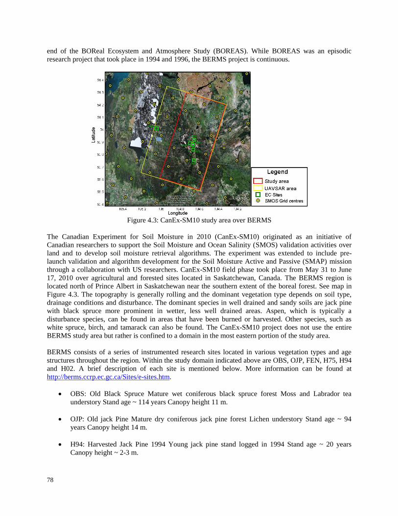
78
end of the BOReal Ecosystem and Atmosphere Study (BOREAS). While BOREAS was an episodic
research project that took place in 1994 and 1996, the BERMS project is continuous.
Figure 4.3: CanEx-SM10 study area over BERMS
The Canadian Experiment for Soil Moisture in 2010 (CanEx-SM10) originated as an initiative of
Canadian researchers to support the Soil Moisture and Ocean Salinity (SMOS) validation activities over
land and to develop soil moisture retrieval algorithms. The experiment was extended to include pre-
launch validation and algorithm development for the Soil Moisture Active and Passive (SMAP) mission
through a collaboration with US researchers. CanEx-SM10 field phase took place from May 31 to June
17, 2010 over agricultural and forested sites located in Saskatchewan, Canada. The BERMS region is
located north of Prince Albert in Saskatchewan near the southern extent of the boreal forest. See map in
Figure 4.3. The topography is generally rolling and the dominant vegetation type depends on soil type,
drainage conditions and disturbance. The dominant species in well drained and sandy soils are jack pine
with black spruce more prominent in wetter, less well drained areas. Aspen, which is typically a
disturbance species, can be found in areas that have been burned or harvested. Other species, such as
white spruce, birch, and tamarack can also be found. The CanEx-SM10 project does not use the entire
BERMS study area but rather is confined to a domain in the most eastern portion of the study area.
BERMS consists of a series of instrumented research sites located in various vegetation types and age
structures throughout the region. Within the study domain indicated above are OBS, OJP, FEN, H75, H94
and H02. A brief description of each site is mentioned below. More information can be found at
http://berms.ccrp.ec.gc.ca/Sites/e-sites.htm.
OBS: Old Black Spruce Mature wet coniferous black spruce forest Moss and Labrador tea
understory Stand age ~ 114 years Canopy height 11 m.
OJP: Old jack Pine Mature dry coniferous jack pine forest Lichen understory Stand age ~ 94
years Canopy height 14 m.
H94: Harvested Jack Pine 1994 Young jack pine stand logged in 1994 Stand age ~ 20 years
Canopy height ~ 2-3 m.
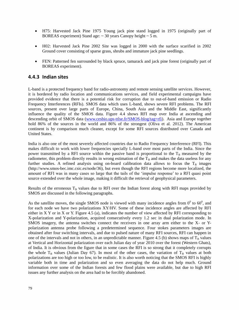
79
H75: Harvested Jack Pine 1975 Young jack pine stand logged in 1975 (originally part of
BOREAS experiment) Stand age: ~ 30 years Canopy height ~ 5 m.
H02: Harvested Jack Pine 2002 Site was logged in 2000 with the surface scarified in 2002
Ground cover consisting of sparse grass, shrubs and immature jack pine seedlings.
FEN: Patterned fen surrounded by black spruce, tamarack and jack pine forest (originally part of
BOREAS experiment).
4.4.3 Indian sites L-band is a protected frequency band for radio-astronomy and remote sensing satellite services. However,
it is bordered by radio location and communications services, and field experimental campaigns have
provided evidence that there is a potential risk for corruption due to out-of-band emission or Radio
Frequency Interferences (RFIs). SMOS data which uses L-band, shows severe RFI problems. The RFI
sources, present over large parts of Europe, China, South Asia and the Middle East, significantly
influence the quality of the SMOS data. Figure 4.4 shows RFI map over India at ascending and
descending orbit of SMOS data (www.cesbio.ups-ttlse.fr/SMOS-blog/tag=rfi). Asia and Europe together
hold 86% of the sources in the world and 86% of the strongest (Oliva et al. 2012). The American
continent is by comparison much cleaner, except for some RFI sources distributed over Canada and
United States.
India is also one of the most severely affected countries due to Radio Frequency Interference (RFI). This
makes difficult to work with lower frequencies specially L-band over most parts of the India. Since the
power transmitted by a RFI source within the passive band is proportional to the TB measured by the
radiometer, this problem directly results in wrong estimation of the TB and makes the data useless for any
further studies. A refined analysis using on-board calibration data allows to focus the TB images
(http://www.smos-bec.imc.csic.es/node/36), but even though the RFI regions become more localized, the
amount of RFI was in many cases so large that the tails of the ‘impulse response’ to a RFI quasi point
source extended over the whole image, making it difficult the retrieval of geophysical parameters.
Results of the erroneous TB values due to RFI over the Indian forest along with RFI maps provided by
SMOS are discussed in the following paragraphs.
As the satellite moves, the single SMOS node is viewed with many incidence angles from 00 to 60
0, and
for each node we have two polarizations XY/HV. Some of these incidence angles are affected by RFI
either in X Y or in X or Y. Figure 4.5 (a), indicates the number of view affected by RFI corresponding to
X-polarization and Y-polarization, acquired consecutively every 1.2 sec in dual polarization mode. In
SMOS imagery, the antenna switches connect the receivers in one array arm either to the X- or Y-
polarization antenna probe following a predetermined sequence. Four stokes parameters images are
obtained after four switching intervals, and due to pulsed nature of many RFI sources, RFI can happen in
one of the intervals and not in others, in an unpredictable manner. Figure 4.5 (b) shows maps of TB values
at Vertical and Horizontal polarization over each Julian day of year 2010 over the forest (Western Ghats),
of India. It is obvious from the figure that in some cases the RFI is so strong that it completely corrupts
the whole TB values (Julian Day 67). In most of the other cases, the variation of TB values at both
polarizations are too high or too low, to be realistic. It is also worth noticing that the SMOS RFI is highly
variable both in time and polarization and so even averaging the data do not help much. Ground
information over some of the Indian forests and few flood plains were available, but due to high RFI
issues any further analysis on the area had to be forcibly abandoned.
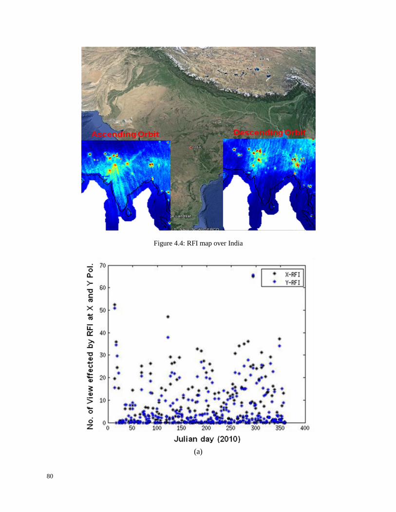
80
Figure 4.4: RFI map over India
(a)
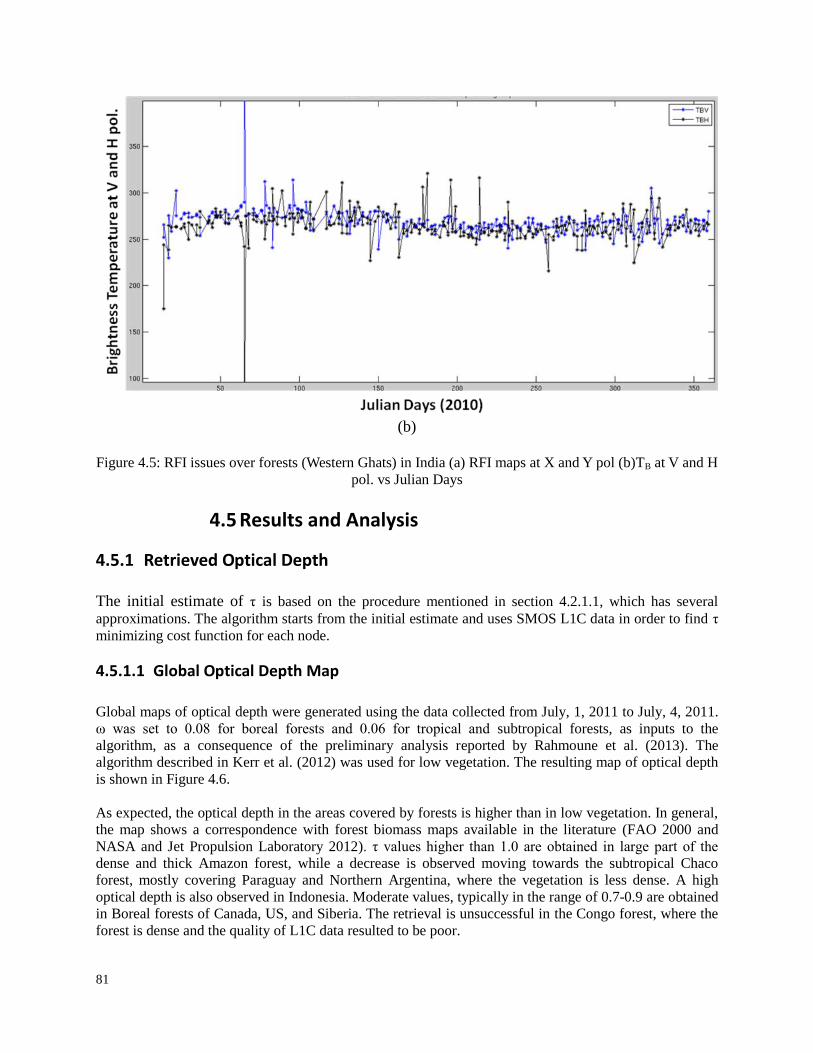
81
(b)
Figure 4.5: RFI issues over forests (Western Ghats) in India (a) RFI maps at X and Y pol (b)TB at V and H
pol. vs Julian Days
4.5 Results and Analysis
4.5.1 Retrieved Optical Depth
The initial estimate of τ is based on the procedure mentioned in section 4.2.1.1, which has several
approximations. The algorithm starts from the initial estimate and uses SMOS L1C data in order to find τ
minimizing cost function for each node.
4.5.1.1 Global Optical Depth Map
Global maps of optical depth were generated using the data collected from July, 1, 2011 to July, 4, 2011.
ω was set to 0.08 for boreal forests and 0.06 for tropical and subtropical forests, as inputs to the
algorithm, as a consequence of the preliminary analysis reported by Rahmoune et al. (2013). The
algorithm described in Kerr et al. (2012) was used for low vegetation. The resulting map of optical depth
is shown in Figure 4.6.
As expected, the optical depth in the areas covered by forests is higher than in low vegetation. In general,
the map shows a correspondence with forest biomass maps available in the literature (FAO 2000 and
NASA and Jet Propulsion Laboratory 2012). τ values higher than 1.0 are obtained in large part of the
dense and thick Amazon forest, while a decrease is observed moving towards the subtropical Chaco
forest, mostly covering Paraguay and Northern Argentina, where the vegetation is less dense. A high
optical depth is also observed in Indonesia. Moderate values, typically in the range of 0.7-0.9 are obtained
in Boreal forests of Canada, US, and Siberia. The retrieval is unsuccessful in the Congo forest, where the
forest is dense and the quality of L1C data resulted to be poor.
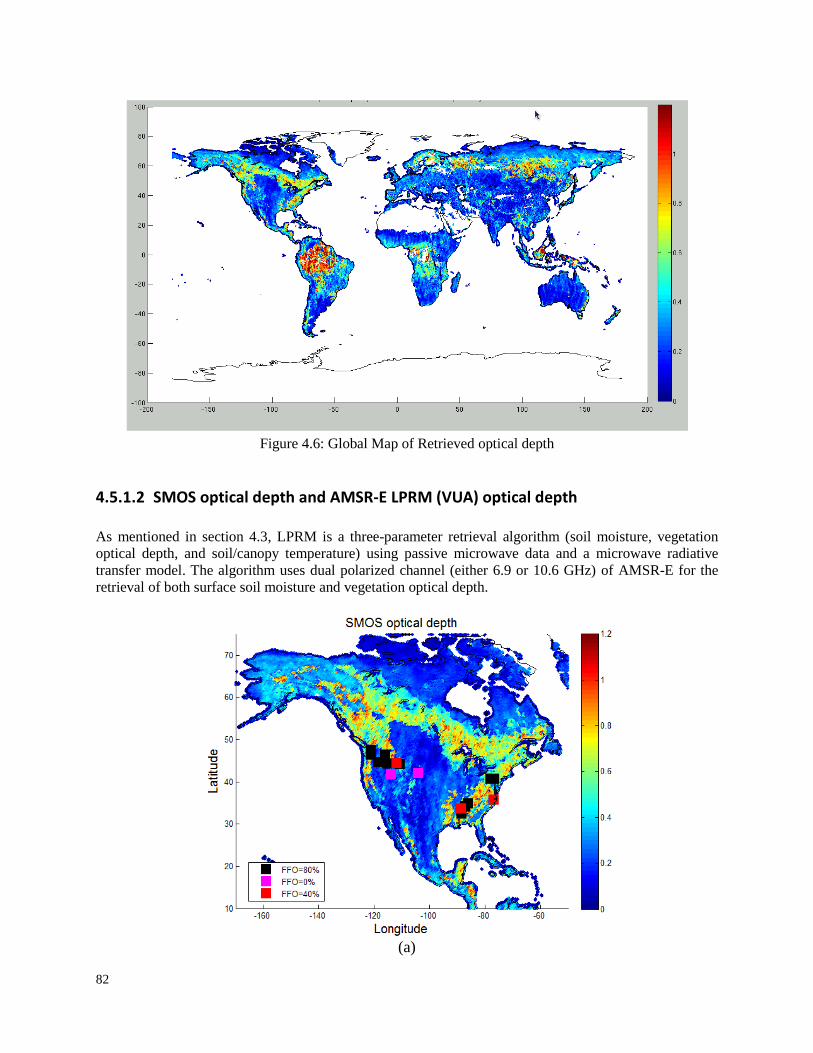
82
Figure 4.6: Global Map of Retrieved optical depth
4.5.1.2 SMOS optical depth and AMSR-E LPRM (VUA) optical depth
As mentioned in section 4.3, LPRM is a three-parameter retrieval algorithm (soil moisture, vegetation
optical depth, and soil/canopy temperature) using passive microwave data and a microwave radiative
transfer model. The algorithm uses dual polarized channel (either 6.9 or 10.6 GHz) of AMSR-E for the
retrieval of both surface soil moisture and vegetation optical depth.
(a)

83
(b)
Figure 4.7: Optical Depth Maps obtained from (a) SMOS (1-4 July 2011) and
LPRM (VUA) (1-2 July 2011) algorithms. Colored boxes indicate sites selected for SM retrieval.
Comparison was done between the SMOS retrieved optical depth and LPRM optical depth map under
different forest fraction (FFO=80%, 40% and 0%). Figure 4.7 (a) and (b), shows the optical depth map
retrieved from SMOS algorithm and the vegetation optical depth retrieved by the LPRM algorithm (and
averaged for the period 1st July 2011 and 2nd July 2011).
In general, SMOS retrieval is more sensitive to the presence of forest cover, in comparison to LPRM.
While L band signatures are fundamentally influenced by branch attenuation, C band signatures are also
strongly affected by low vegetation or other factors. It is also worth noticing that, although noisy, SMOS
vegetation optical thickness contains useful information regarding forest cover.
4.5.1.3 Comparison with an independent data source
Retrieved values of optical depth τ have been compared against tree height estimates obtained by the
algorithm described in Simard et al. (2011), and made available by NASA Earth Observatory. The
algorithm used data collected by the Geoscience Laser Altimeter System (GLAS) of ICESAT satellite,
with information from MODIS, additional elevation data from the Shuttle Radar Topography Mission
(STRM), and climatology information from both the Tropical Rainfall Measuring Mission (TRMM) and
the http://www.worldclim.org/Worldclim database (Simard et al. 2011). GLAS data, which originally had
1 km resolution, were re-sampled at ISEA4H9 grid (1.4.2.2).
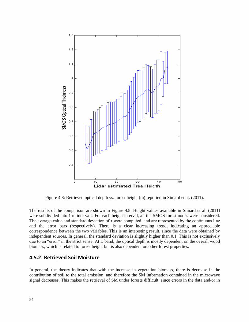
84
Figure 4.8: Retrieved optical depth vs. forest height (m) reported in Simard et al. (2011).
The results of the comparison are shown in Figure 4.8. Height values available in Simard et al. (2011)
were subdivided into 1 m intervals. For each height interval, all the SMOS forest nodes were considered.
The average value and standard deviation of τ were computed, and are represented by the continuous line
and the error bars (respectively). There is a clear increasing trend, indicating an appreciable
correspondence between the two variables. This is an interesting result, since the data were obtained by
independent sources. In general, the standard deviation is slightly higher than 0.1. This is not exclusively
due to an “error” in the strict sense. At L band, the optical depth is mostly dependent on the overall wood
biomass, which is related to forest height but is also dependent on other forest properties.
4.5.2 Retrieved Soil Moisture
In general, the theory indicates that with the increase in vegetation biomass, there is decrease in the
contribution of soil to the total emission, and therefore the SM information contained in the microwave
signal decreases. This makes the retrieval of SM under forests difficult, since errors in the data and/or in
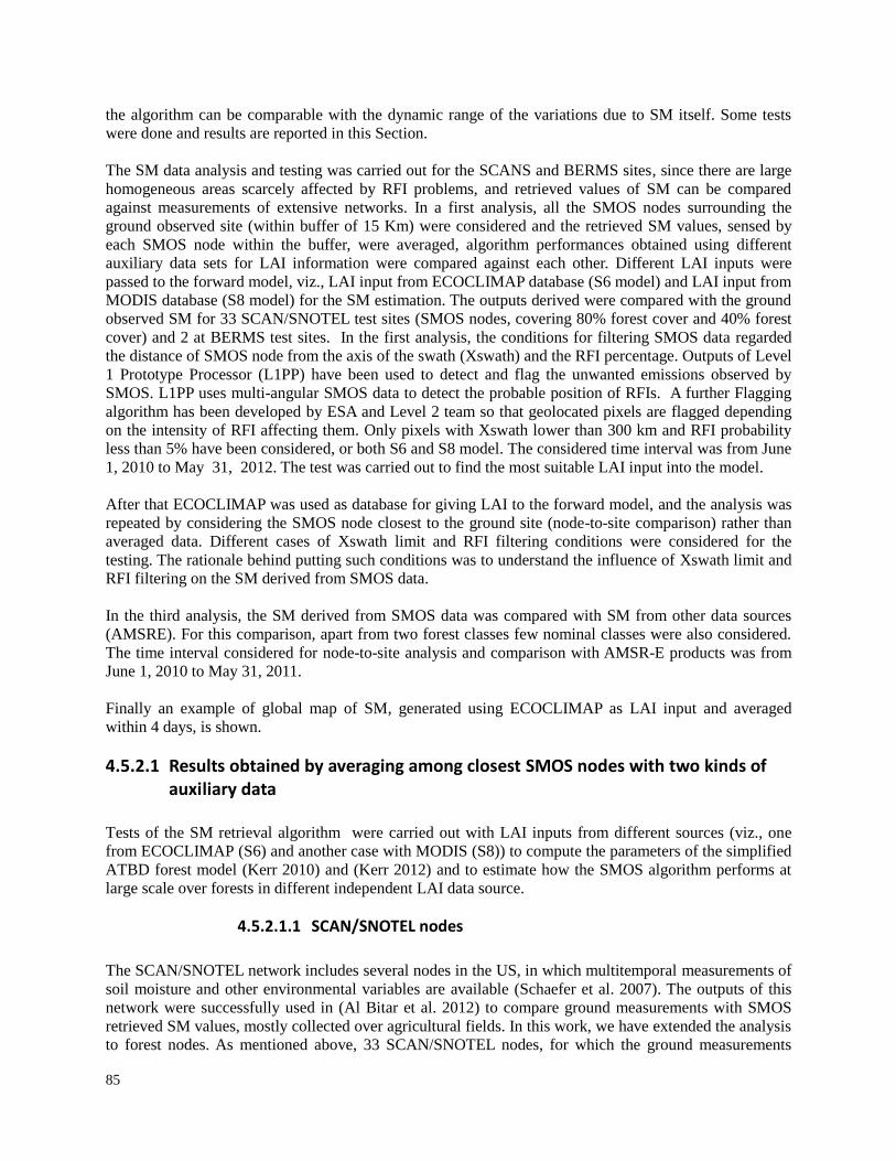
85
the algorithm can be comparable with the dynamic range of the variations due to SM itself. Some tests
were done and results are reported in this Section.
The SM data analysis and testing was carried out for the SCANS and BERMS sites, since there are large
homogeneous areas scarcely affected by RFI problems, and retrieved values of SM can be compared
against measurements of extensive networks. In a first analysis, all the SMOS nodes surrounding the
ground observed site (within buffer of 15 Km) were considered and the retrieved SM values, sensed by
each SMOS node within the buffer, were averaged, algorithm performances obtained using different
auxiliary data sets for LAI information were compared against each other. Different LAI inputs were
passed to the forward model, viz., LAI input from ECOCLIMAP database (S6 model) and LAI input from
MODIS database (S8 model) for the SM estimation. The outputs derived were compared with the ground
observed SM for 33 SCAN/SNOTEL test sites (SMOS nodes, covering 80% forest cover and 40% forest
cover) and 2 at BERMS test sites. In the first analysis, the conditions for filtering SMOS data regarded
the distance of SMOS node from the axis of the swath (Xswath) and the RFI percentage. Outputs of Level
1 Prototype Processor (L1PP) have been used to detect and flag the unwanted emissions observed by
SMOS. L1PP uses multi-angular SMOS data to detect the probable position of RFIs. A further Flagging
algorithm has been developed by ESA and Level 2 team so that geolocated pixels are flagged depending
on the intensity of RFI affecting them. Only pixels with Xswath lower than 300 km and RFI probability
less than 5% have been considered, or both S6 and S8 model. The considered time interval was from June
1, 2010 to May 31, 2012. The test was carried out to find the most suitable LAI input into the model.
After that ECOCLIMAP was used as database for giving LAI to the forward model, and the analysis was
repeated by considering the SMOS node closest to the ground site (node-to-site comparison) rather than
averaged data. Different cases of Xswath limit and RFI filtering conditions were considered for the
testing. The rationale behind putting such conditions was to understand the influence of Xswath limit and
RFI filtering on the SM derived from SMOS data.
In the third analysis, the SM derived from SMOS data was compared with SM from other data sources
(AMSRE). For this comparison, apart from two forest classes few nominal classes were also considered.
The time interval considered for node-to-site analysis and comparison with AMSR-E products was from
June 1, 2010 to May 31, 2011.
Finally an example of global map of SM, generated using ECOCLIMAP as LAI input and averaged
within 4 days, is shown.
4.5.2.1 Results obtained by averaging among closest SMOS nodes with two kinds of auxiliary data
Tests of the SM retrieval algorithm were carried out with LAI inputs from different sources (viz., one
from ECOCLIMAP (S6) and another case with MODIS (S8)) to compute the parameters of the simplified
ATBD forest model (Kerr 2010) and (Kerr 2012) and to estimate how the SMOS algorithm performs at
large scale over forests in different independent LAI data source.
4.5.2.1.1 SCAN/SNOTEL nodes
The SCAN/SNOTEL network includes several nodes in the US, in which multitemporal measurements of
soil moisture and other environmental variables are available (Schaefer et al. 2007). The outputs of this
network were successfully used in (Al Bitar et al. 2012) to compare ground measurements with SMOS
retrieved SM values, mostly collected over agricultural fields. In this work, we have extended the analysis
to forest nodes. As mentioned above, 33 SCAN/SNOTEL nodes, for which the ground measurements
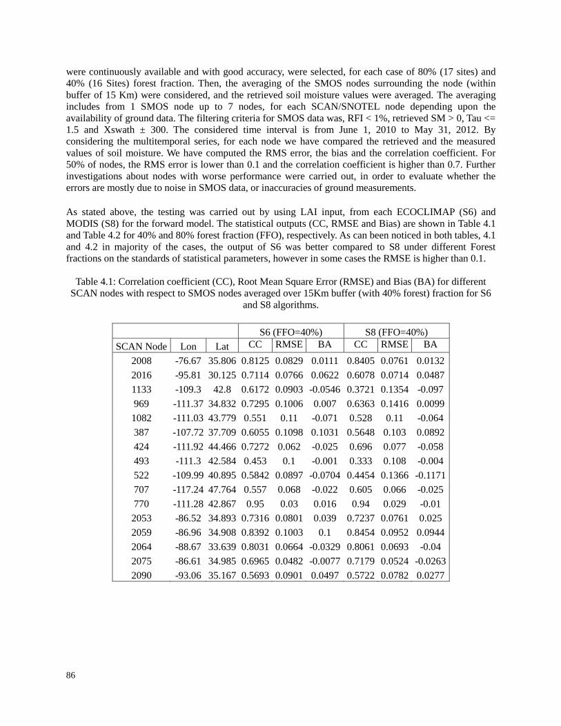
86
were continuously available and with good accuracy, were selected, for each case of 80% (17 sites) and
40% (16 Sites) forest fraction. Then, the averaging of the SMOS nodes surrounding the node (within
buffer of 15 Km) were considered, and the retrieved soil moisture values were averaged. The averaging
includes from 1 SMOS node up to 7 nodes, for each SCAN/SNOTEL node depending upon the
availability of ground data. The filtering criteria for SMOS data was, RFI < 1%, retrieved SM > 0, Tau <=
1.5 and Xswath ± 300. The considered time interval is from June 1, 2010 to May 31, 2012. By
considering the multitemporal series, for each node we have compared the retrieved and the measured
values of soil moisture. We have computed the RMS error, the bias and the correlation coefficient. For
50% of nodes, the RMS error is lower than 0.1 and the correlation coefficient is higher than 0.7. Further
investigations about nodes with worse performance were carried out, in order to evaluate whether the
errors are mostly due to noise in SMOS data, or inaccuracies of ground measurements.
As stated above, the testing was carried out by using LAI input, from each ECOCLIMAP (S6) and
MODIS (S8) for the forward model. The statistical outputs (CC, RMSE and Bias) are shown in Table 4.1
and Table 4.2 for 40% and 80% forest fraction (FFO), respectively. As can been noticed in both tables, 4.1
and 4.2 in majority of the cases, the output of S6 was better compared to S8 under different Forest
fractions on the standards of statistical parameters, however in some cases the RMSE is higher than 0.1.
Table 4.1: Correlation coefficient (CC), Root Mean Square Error (RMSE) and Bias (BA) for different
SCAN nodes with respect to SMOS nodes averaged over 15Km buffer (with 40% forest) fraction for S6
and S8 algorithms.
S6 (FFO=40%) S8 (FFO=40%)
SCAN Node Lon Lat CC RMSE BA CC RMSE BA
2008 -76.67 35.806 0.8125 0.0829 0.0111 0.8405 0.0761 0.0132
2016 -95.81 30.125 0.7114 0.0766 0.0622 0.6078 0.0714 0.0487
1133 -109.3 42.8 0.6172 0.0903 -0.0546 0.3721 0.1354 -0.097
969 -111.37 34.832 0.7295 0.1006 0.007 0.6363 0.1416 0.0099
1082 -111.03 43.779 0.551 0.11 -0.071 0.528 0.11 -0.064
387 -107.72 37.709 0.6055 0.1098 0.1031 0.5648 0.103 0.0892
424 -111.92 44.466 0.7272 0.062 -0.025 0.696 0.077 -0.058
493 -111.3 42.584 0.453 0.1 -0.001 0.333 0.108 -0.004
522 -109.99 40.895 0.5842 0.0897 -0.0704 0.4454 0.1366 -0.1171
707 -117.24 47.764 0.557 0.068 -0.022 0.605 0.066 -0.025
770 -111.28 42.867 0.95 0.03 0.016 0.94 0.029 -0.01
2053 -86.52 34.893 0.7316 0.0801 0.039 0.7237 0.0761 0.025
2059 -86.96 34.908 0.8392 0.1003 0.1 0.8454 0.0952 0.0944
2064 -88.67 33.639 0.8031 0.0664 -0.0329 0.8061 0.0693 -0.04
2075 -86.61 34.985 0.6965 0.0482 -0.0077 0.7179 0.0524 -0.0263
2090 -93.06 35.167 0.5693 0.0901 0.0497 0.5722 0.0782 0.0277
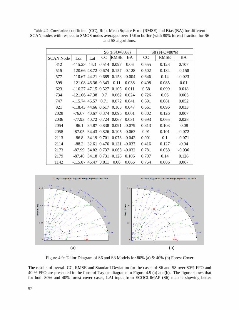
87
Table 4.2: Correlation coefficient (CC), Root Mean Square Error (RMSE) and Bias (BA) for different
SCAN nodes with respect to SMOS nodes averaged over 15Km buffer (with 80% forest) fraction for S6
and S8 algorithms.
S6 (FFO=80%) S8 (FFO=80%)
SCAN Node Lon Lat CC RMSE BA CC RMSE BA
312 -115.23 44.3 0.514 0.097 0.06 0.555 0.123 0.107
515 -120.66 48.72 0.674 0.157 -0.128 0.502 0.184 -0.158
577 -110.67 44.21 0.689 0.153 -0.004 0.646 0.14 -0.023
599 -121.08 46.36 0.343 0.11 0.038 0.408 0.085 0.01
623 -116.27 47.15 0.527 0.105 0.011 0.58 0.099 0.018
734 -121.06 47.38 0.7 0.062 0.024 0.726 0.05 0.005
747 -115.74 46.57 0.71 0.072 0.041 0.691 0.081 0.052
821 -118.43 44.66 0.617 0.105 0.047 0.661 0.096 0.033
2028 -76.67 40.67 0.374 0.095 0.001 0.302 0.126 0.007
2036 -77.93 40.72 0.724 0.067 0.031 0.693 0.065 0.028
2054 -86.1 34.87 0.838 0.091 -0.079 0.813 0.103 -0.08
2058 -87.05 34.43 0.826 0.105 -0.063 0.91 0.101 -0.072
2113 -86.8 34.19 0.701 0.073 -0.042 0.901 0.1 -0.071
2114 -88.2 32.61 0.476 0.121 -0.037 0.416 0.127 -0.04
2173 -87.99 34.82 0.737 0.063 -0.032 0.781 0.058 -0.036
2179 -87.46 34.18 0.731 0.126 0.106 0.797 0.14 0.126
1142 -115.87 46.47 0.811 0.08 0.066 0.754 0.086 0.067
(a) (b)
Figure 4.9: Tailor Diagram of S6 and S8 Models for 80% (a) & 40% (b) Forest Cover
The results of overall CC, RMSE and Standard Deviation for the cases of S6 and S8 over 80% FFO and
40 % FFO are presented in the form of Taylor diagrams in Figure 4.9 (a) and(b). The figure shows that
for both 80% and 40% forest cover cases, LAI input from ECOCLIMAP (S6) map is showing better
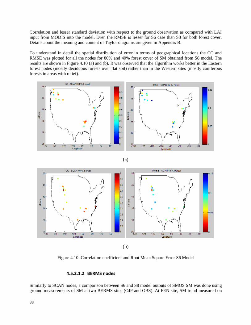
88
Correlation and lesser standard deviation with respect to the ground observation as compared with LAI
input from MODIS into the model. Even the RMSE is lesser for S6 case than S8 for both forest cover.
Details about the meaning and content of Taylor diagrams are given in Appendix B.
To understand in detail the spatial distribution of error in terms of geographical locations the CC and
RMSE was plotted for all the nodes for 80% and 40% forest cover of SM obtained from S6 model. The
results are shown in Figure 4.10 (a) and (b). It was observed that the algorithm works better in the Eastern
forest nodes (mostly deciduous forests over flat soil) rather than in the Western sites (mostly coniferous
forests in areas with relief).
(a)
(b)
Figure 4.10: Correlation coefficient and Root Mean Square Error S6 Model
4.5.2.1.2 BERMS nodes
Similarly to SCAN nodes, a comparison between S6 and S8 model outputs of SMOS SM was done using
ground measurements of SM at two BERMS sites (OJP and OBS). At FEN site, SM trend measured on
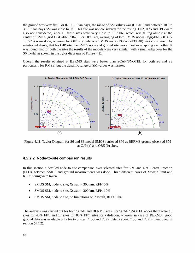
89
the ground was very flat: For 0-100 Julian days, the range of SM values was 0.06-0.1 and between 101 to
365 Julian days SM was close to 0.9. This site was not considered for the testing. H02, H75 and H95 were
also not considered, since all these sites were very close to OJP site, which was falling almost at the
center of SMOS grid DGG-Id-139040. For OBS site, averaging of two SMOS nodes (Dgg-Id-138014 &
138526) were done, whereas for OJP site only one SMOS node (DGG-Id-139040) was considered. As
mentioned above, that for OJP site, the SMOS node and ground site was almost overlapping each other. It
was found that for both the sites the results of the models were very similar, with a small edge over for the
S6 model as shown in the Tylor diagrams of Figure 4.11.
Overall the results obtained at BERMS sites were better than SCAN/SNOTEL for both S6 and S8
particularly for RMSE, but the dynamic range of SM values was narrow.
(a) (b)
Figure 4.11: Taylor Diagram for S6 and S8 model SMOS retrieved SM vs BERMS ground observed SM
at OJP (a) and OBS (b) sites.
4.5.2.2 Node-to-site comparison results
In this section a detailed node to site comparison over selected sites for 80% and 40% Forest Fraction
(FFO), between SMOS and ground measurements was done. Three different cases of Xswath limit and
RFI filtering were taken.
SMOS SM, node to site, Xswath< 300 km, RFI< 5%
SMOS SM, node to site, Xswath< 300 km, RFI< 10%
SMOS SM, node to site, no limitations on Xswath, RFI< 10%
The analysis was carried out for both SCAN and BERMS sites. For SCAN/SNOTEL nodes there were 16
sites for 40% FFO and 17 sites for 80% FFO sites for validation, whereas in case of BERMS, good
ground data was available only for two sites (OBS and OJP) (details about OBS and OJP is mentioned in
section (4.4.2).
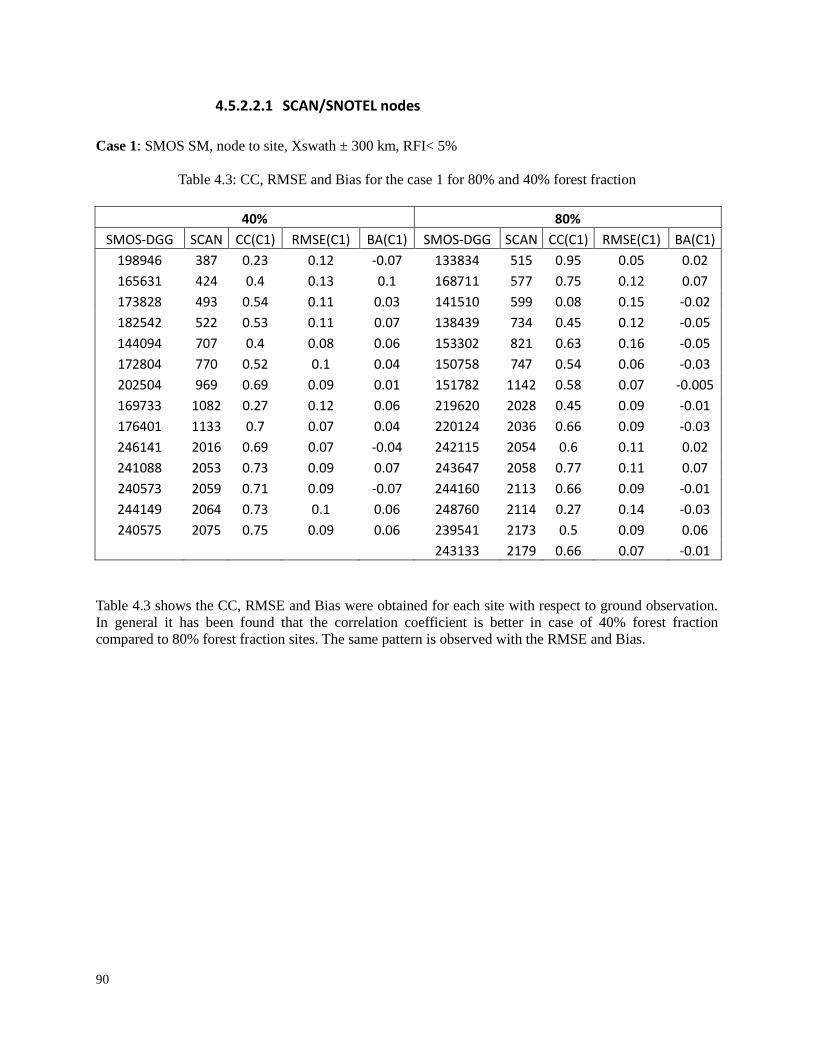
90
4.5.2.2.1 SCAN/SNOTEL nodes
Case 1: SMOS SM, node to site, Xswath ± 300 km, RFI< 5%
Table 4.3: CC, RMSE and Bias for the case 1 for 80% and 40% forest fraction
40% 80%
SMOS-DGG SCAN CC(C1) RMSE(C1) BA(C1) SMOS-DGG SCAN CC(C1) RMSE(C1) BA(C1)
198946 387 0.23 0.12 -0.07 133834 515 0.95 0.05 0.02
165631 424 0.4 0.13 0.1 168711 577 0.75 0.12 0.07
173828 493 0.54 0.11 0.03 141510 599 0.08 0.15 -0.02
182542 522 0.53 0.11 0.07 138439 734 0.45 0.12 -0.05
144094 707 0.4 0.08 0.06 153302 821 0.63 0.16 -0.05
172804 770 0.52 0.1 0.04 150758 747 0.54 0.06 -0.03
202504 969 0.69 0.09 0.01 151782 1142 0.58 0.07 -0.005
169733 1082 0.27 0.12 0.06 219620 2028 0.45 0.09 -0.01
176401 1133 0.7 0.07 0.04 220124 2036 0.66 0.09 -0.03
246141 2016 0.69 0.07 -0.04 242115 2054 0.6 0.11 0.02
241088 2053 0.73 0.09 0.07 243647 2058 0.77 0.11 0.07
240573 2059 0.71 0.09 -0.07 244160 2113 0.66 0.09 -0.01
244149 2064 0.73 0.1 0.06 248760 2114 0.27 0.14 -0.03
240575 2075 0.75 0.09 0.06 239541 2173 0.5 0.09 0.06
243133 2179 0.66 0.07 -0.01
Table 4.3 shows the CC, RMSE and Bias were obtained for each site with respect to ground observation.
In general it has been found that the correlation coefficient is better in case of 40% forest fraction
compared to 80% forest fraction sites. The same pattern is observed with the RMSE and Bias.
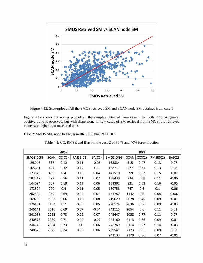
91
Figure 4.12: Scatterplot of All the SMOS retrieved SM and SCAN node SM obtained from case 1
Figure 4.12 shows the scatter plot of all the samples obtained from case 1 for both FFO. A general
positive trend is observed, but with dispersion. In few cases of SM retrieval from SMOS, the retrieved
values are higher than measured ones.
Case 2: SMOS SM, node to site, Xswath ± 300 km, RFI< 10%
Table 4.4: CC, RMSE and Bias for the case 2 of 80 % and 40% forest fraction
40% 80%
SMOS-DGG SCAN CC(C2) RMSE(C2) BA(C2) SMOS-DGG SCAN CC(C2) RMSE(C2) BA(C2)
198946 387 0.12 0.11 -0.06 133834 515 0.47 0.13 0.07
165631 424 0.32 0.14 0.1 168711 577 0.71 0.13 0.08
173828 493 0.4 0.13 0.04 141510 599 0.07 0.15 -0.01
182542 522 0.56 0.11 0.07 138439 734 0.58 0.11 -0.06
144094 707 0.19 0.12 0.06 153302 821 0.63 0.16 -0.05
172804 770 0.4 0.11 0.05 150758 747 0.6 0.1 -0.06
202504 969 0.69 0.09 0.01 151782 1142 0.6 0.08 -0.002
169733 1082 0.06 0.15 0.08 219620 2028 0.45 0.09 -0.01
176401 1133 0.7 0.08 0.05 220124 2036 0.66 0.09 -0.03
246141 2016 0.69 0.07 -0.04 242115 2054 0.6 0.11 0.02
241088 2053 0.73 0.09 0.07 243647 2058 0.77 0.11 0.07
240573 2059 0.71 0.09 -0.07 244160 2113 0.66 0.09 -0.01
244149 2064 0.73 0.1 0.06 248760 2114 0.27 0.14 -0.03
240575 2075 0.74 0.09 0.06 239541 2173 0.5 0.09 0.07
243133 2179 0.66 0.07 -0.01
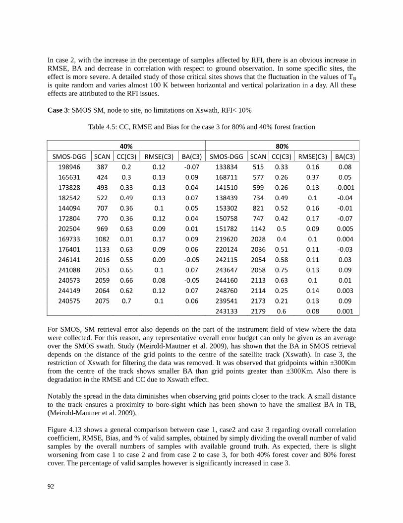
92
In case 2, with the increase in the percentage of samples affected by RFI, there is an obvious increase in
RMSE, BA and decrease in correlation with respect to ground observation. In some specific sites, the
effect is more severe. A detailed study of those critical sites shows that the fluctuation in the values of TB
is quite random and varies almost 100 K between horizontal and vertical polarization in a day. All these
effects are attributed to the RFI issues.
Case 3: SMOS SM, node to site, no limitations on Xswath, RFI< 10%
Table 4.5: CC, RMSE and Bias for the case 3 for 80% and 40% forest fraction
40% 80%
SMOS-DGG SCAN CC(C3) RMSE(C3) BA(C3) SMOS-DGG SCAN CC(C3) RMSE(C3) BA(C3)
198946 387 0.2 0.12 -0.07 133834 515 0.33 0.16 0.08
165631 424 0.3 0.13 0.09 168711 577 0.26 0.37 0.05
173828 493 0.33 0.13 0.04 141510 599 0.26 0.13 -0.001
182542 522 0.49 0.13 0.07 138439 734 0.49 0.1 -0.04
144094 707 0.36 0.1 0.05 153302 821 0.52 0.16 -0.01
172804 770 0.36 0.12 0.04 150758 747 0.42 0.17 -0.07
202504 969 0.63 0.09 0.01 151782 1142 0.5 0.09 0.005
169733 1082 0.01 0.17 0.09 219620 2028 0.4 0.1 0.004
176401 1133 0.63 0.09 0.06 220124 2036 0.51 0.11 -0.03
246141 2016 0.55 0.09 -0.05 242115 2054 0.58 0.11 0.03
241088 2053 0.65 0.1 0.07 243647 2058 0.75 0.13 0.09
240573 2059 0.66 0.08 -0.05 244160 2113 0.63 0.1 0.01
244149 2064 0.62 0.12 0.07 248760 2114 0.25 0.14 0.003
240575 2075 0.7 0.1 0.06 239541 2173 0.21 0.13 0.09
243133 2179 0.6 0.08 0.001
For SMOS, SM retrieval error also depends on the part of the instrument field of view where the data
were collected. For this reason, any representative overall error budget can only be given as an average
over the SMOS swath. Study (Meirold-Mautner et al. 2009), has shown that the BA in SMOS retrieval
depends on the distance of the grid points to the centre of the satellite track (Xswath). In case 3, the
restriction of Xswath for filtering the data was removed. It was observed that gridpoints within ±300Km
from the centre of the track shows smaller BA than grid points greater than ±300Km. Also there is
degradation in the RMSE and CC due to Xswath effect.
Notably the spread in the data diminishes when observing grid points closer to the track. A small distance
to the track ensures a proximity to bore-sight which has been shown to have the smallest BA in TBs
(Meirold-Mautner et al. 2009),
Figure 4.13 shows a general comparison between case 1, case2 and case 3 regarding overall correlation
coefficient, RMSE, Bias, and % of valid samples, obtained by simply dividing the overall number of valid
samples by the overall numbers of samples with available ground truth. As expected, there is slight
worsening from case 1 to case 2 and from case 2 to case 3, for both 40% forest cover and 80% forest
cover. The percentage of valid samples however is significantly increased in case 3.
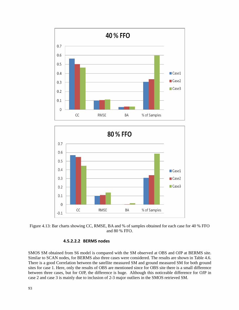
93
Figure 4.13: Bar charts showing CC, RMSE, BA and % of samples obtained for each case for 40 % FFO
and 80 % FFO.
4.5.2.2.2 BERMS nodes
SMOS SM obtained from S6 model is compared with the SM observed at OBS and OJP at BERMS site.
Similar to SCAN nodes, for BERMS also three cases were considered. The results are shown in Table 4.6.
There is a good Correlation between the satellite measured SM and ground measured SM for both ground
sites for case 1. Here, only the results of OBS are mentioned since for OBS site there is a small difference
between three cases, but for OJP, the difference is huge. Although this noticeable difference for OJP in
case 2 and case 3 is mainly due to inclusion of 2-3 major outliers in the SMOS retrieved SM.
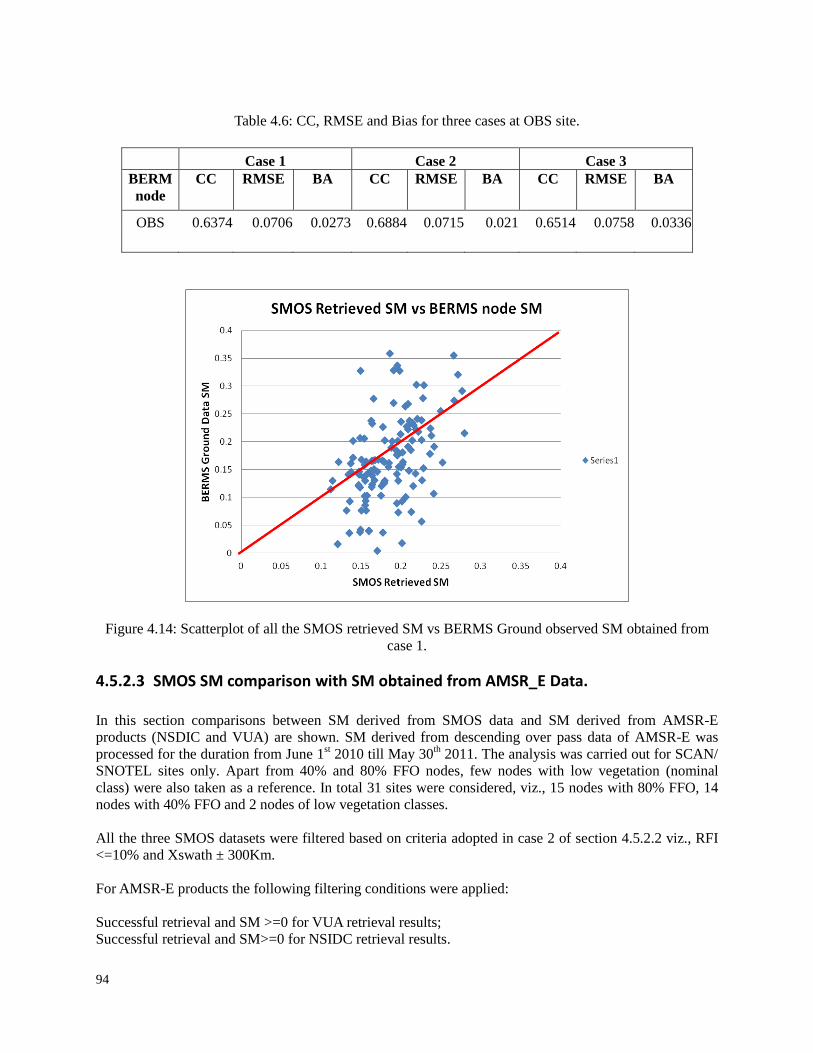
94
Table 4.6: CC, RMSE and Bias for three cases at OBS site.
Case 1 Case 2 Case 3
BERM
node
CC RMSE BA CC RMSE BA CC RMSE BA
OBS 0.6374 0.0706 0.0273 0.6884 0.0715 0.021 0.6514 0.0758 0.0336
Figure 4.14: Scatterplot of all the SMOS retrieved SM vs BERMS Ground observed SM obtained from
case 1.
4.5.2.3 SMOS SM comparison with SM obtained from AMSR_E Data.
In this section comparisons between SM derived from SMOS data and SM derived from AMSR-E
products (NSDIC and VUA) are shown. SM derived from descending over pass data of AMSR-E was
processed for the duration from June 1st 2010 till May 30
th 2011. The analysis was carried out for SCAN/
SNOTEL sites only. Apart from 40% and 80% FFO nodes, few nodes with low vegetation (nominal
class) were also taken as a reference. In total 31 sites were considered, viz., 15 nodes with 80% FFO, 14
nodes with 40% FFO and 2 nodes of low vegetation classes.
All the three SMOS datasets were filtered based on criteria adopted in case 2 of section 4.5.2.2 viz., RFI
<=10% and Xswath ± 300Km.
For AMSR-E products the following filtering conditions were applied:
Successful retrieval and SM >=0 for VUA retrieval results;
Successful retrieval and SM>=0 for NSIDC retrieval results.
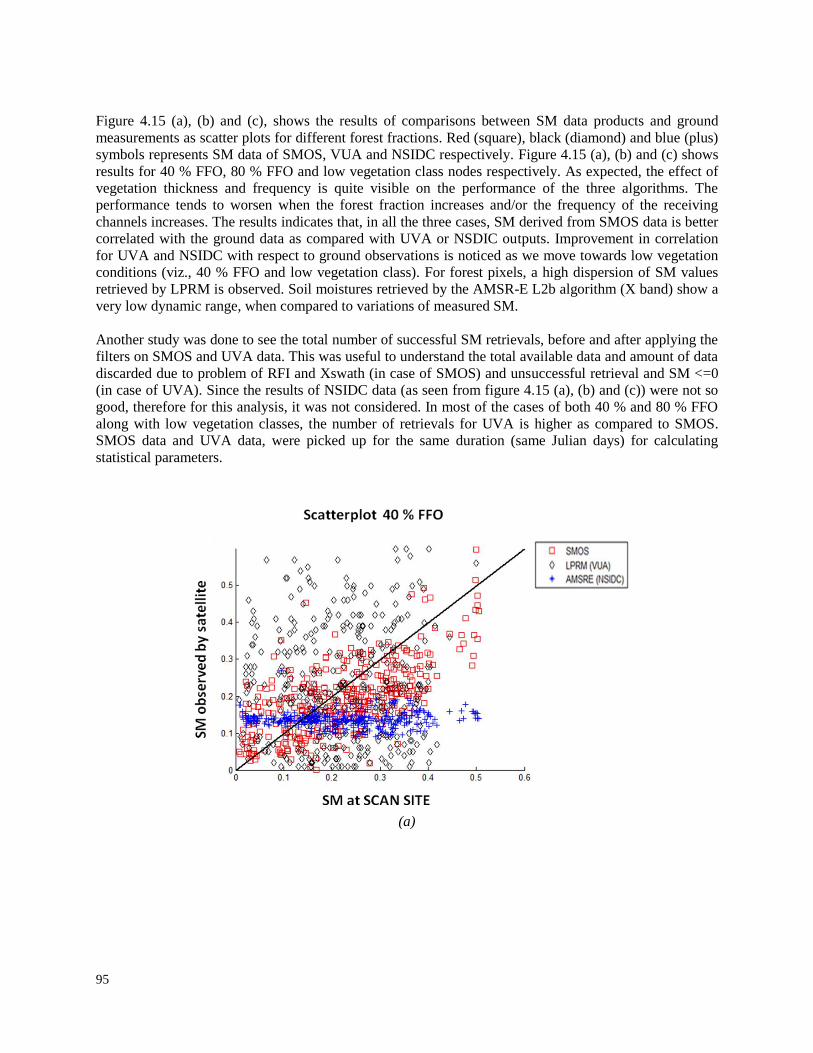
95
Figure 4.15 (a), (b) and (c), shows the results of comparisons between SM data products and ground
measurements as scatter plots for different forest fractions. Red (square), black (diamond) and blue (plus)
symbols represents SM data of SMOS, VUA and NSIDC respectively. Figure 4.15 (a), (b) and (c) shows
results for 40 % FFO, 80 % FFO and low vegetation class nodes respectively. As expected, the effect of
vegetation thickness and frequency is quite visible on the performance of the three algorithms. The
performance tends to worsen when the forest fraction increases and/or the frequency of the receiving
channels increases. The results indicates that, in all the three cases, SM derived from SMOS data is better
correlated with the ground data as compared with UVA or NSDIC outputs. Improvement in correlation
for UVA and NSIDC with respect to ground observations is noticed as we move towards low vegetation
conditions (viz., 40 % FFO and low vegetation class). For forest pixels, a high dispersion of SM values
retrieved by LPRM is observed. Soil moistures retrieved by the AMSR-E L2b algorithm (X band) show a
very low dynamic range, when compared to variations of measured SM.
Another study was done to see the total number of successful SM retrievals, before and after applying the
filters on SMOS and UVA data. This was useful to understand the total available data and amount of data
discarded due to problem of RFI and Xswath (in case of SMOS) and unsuccessful retrieval and SM <=0
(in case of UVA). Since the results of NSIDC data (as seen from figure 4.15 (a), (b) and (c)) were not so
good, therefore for this analysis, it was not considered. In most of the cases of both 40 % and 80 % FFO
along with low vegetation classes, the number of retrievals for UVA is higher as compared to SMOS.
SMOS data and UVA data, were picked up for the same duration (same Julian days) for calculating
statistical parameters.
(a)
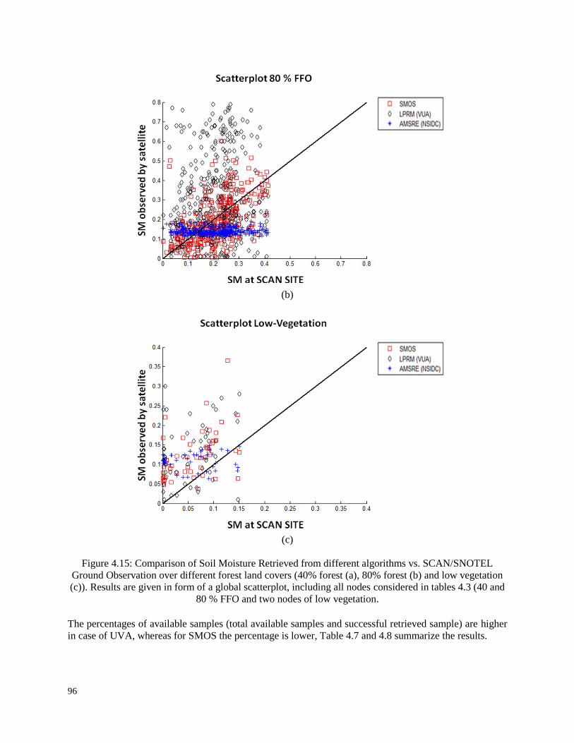
96
(b)
(c)
Figure 4.15: Comparison of Soil Moisture Retrieved from different algorithms vs. SCAN/SNOTEL
Ground Observation over different forest land covers (40% forest (a), 80% forest (b) and low vegetation
(c)). Results are given in form of a global scatterplot, including all nodes considered in tables 4.3 (40 and
80 % FFO and two nodes of low vegetation.
The percentages of available samples (total available samples and successful retrieved sample) are higher
in case of UVA, whereas for SMOS the percentage is lower, Table 4.7 and 4.8 summarize the results.
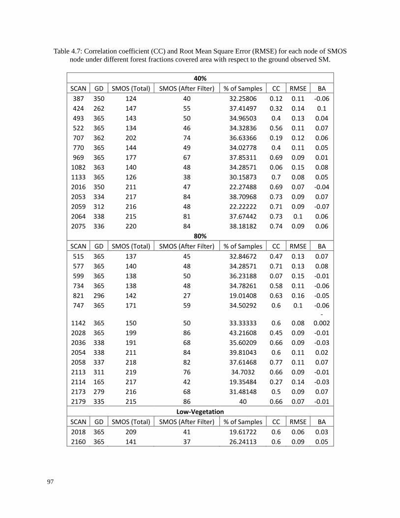
97
Table 4.7: Correlation coefficient (CC) and Root Mean Square Error (RMSE) for each node of SMOS
node under different forest fractions covered area with respect to the ground observed SM.
40%
SCAN GD SMOS (Total) SMOS (After Filter) % of Samples CC RMSE BA
387 350 124 40 32.25806 0.12 0.11 -0.06
424 262 147 55 37.41497 0.32 0.14 0.1
493 365 143 50 34.96503 0.4 0.13 0.04
522 365 134 46 34.32836 0.56 0.11 0.07
707 362 202 74 36.63366 0.19 0.12 0.06
770 365 144 49 34.02778 0.4 0.11 0.05
969 365 177 67 37.85311 0.69 0.09 0.01
1082 363 140 48 34.28571 0.06 0.15 0.08
1133 365 126 38 30.15873 0.7 0.08 0.05
2016 350 211 47 22.27488 0.69 0.07 -0.04
2053 334 217 84 38.70968 0.73 0.09 0.07
2059 312 216 48 22.22222 0.71 0.09 -0.07
2064 338 215 81 37.67442 0.73 0.1 0.06
2075 336 220 84 38.18182 0.74 0.09 0.06
80%
SCAN GD SMOS (Total) SMOS (After Filter) % of Samples CC RMSE BA
515 365 137 45 32.84672 0.47 0.13 0.07
577 365 140 48 34.28571 0.71 0.13 0.08
599 365 138 50 36.23188 0.07 0.15 -0.01
734 365 138 48 34.78261 0.58 0.11 -0.06
821 296 142 27 19.01408 0.63 0.16 -0.05
747 365 171 59 34.50292 0.6 0.1 -0.06
1142 365 150 50 33.33333 0.6 0.08 -
0.002
2028 365 199 86 43.21608 0.45 0.09 -0.01
2036 338 191 68 35.60209 0.66 0.09 -0.03
2054 338 211 84 39.81043 0.6 0.11 0.02
2058 337 218 82 37.61468 0.77 0.11 0.07
2113 311 219 76 34.7032 0.66 0.09 -0.01
2114 165 217 42 19.35484 0.27 0.14 -0.03
2173 279 216 68 31.48148 0.5 0.09 0.07
2179 335 215 86 40 0.66 0.07 -0.01
Low-Vegetation
SCAN GD SMOS (Total) SMOS (After Filter) % of Samples CC RMSE BA
2018 365 209 41 19.61722 0.6 0.06 0.03
2160 365 141 37 26.24113 0.6 0.09 0.05
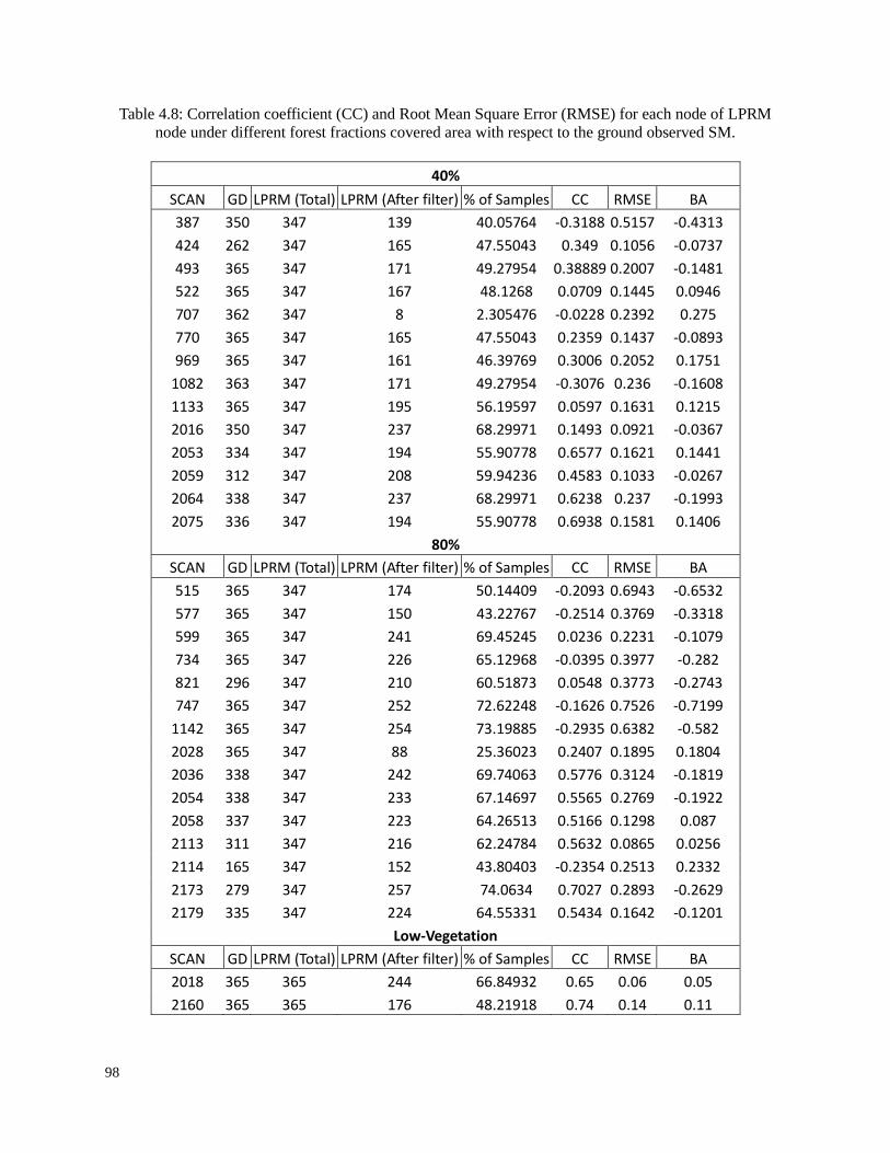
98
Table 4.8: Correlation coefficient (CC) and Root Mean Square Error (RMSE) for each node of LPRM
node under different forest fractions covered area with respect to the ground observed SM.
40%
SCAN GD LPRM (Total) LPRM (After filter) % of Samples CC RMSE BA
387 350 347 139 40.05764 -0.3188 0.5157 -0.4313
424 262 347 165 47.55043 0.349 0.1056 -0.0737
493 365 347 171 49.27954 0.38889 0.2007 -0.1481
522 365 347 167 48.1268 0.0709 0.1445 0.0946
707 362 347 8 2.305476 -0.0228 0.2392 0.275
770 365 347 165 47.55043 0.2359 0.1437 -0.0893
969 365 347 161 46.39769 0.3006 0.2052 0.1751
1082 363 347 171 49.27954 -0.3076 0.236 -0.1608
1133 365 347 195 56.19597 0.0597 0.1631 0.1215
2016 350 347 237 68.29971 0.1493 0.0921 -0.0367
2053 334 347 194 55.90778 0.6577 0.1621 0.1441
2059 312 347 208 59.94236 0.4583 0.1033 -0.0267
2064 338 347 237 68.29971 0.6238 0.237 -0.1993
2075 336 347 194 55.90778 0.6938 0.1581 0.1406
80%
SCAN GD LPRM (Total) LPRM (After filter) % of Samples CC RMSE BA
515 365 347 174 50.14409 -0.2093 0.6943 -0.6532
577 365 347 150 43.22767 -0.2514 0.3769 -0.3318
599 365 347 241 69.45245 0.0236 0.2231 -0.1079
734 365 347 226 65.12968 -0.0395 0.3977 -0.282
821 296 347 210 60.51873 0.0548 0.3773 -0.2743
747 365 347 252 72.62248 -0.1626 0.7526 -0.7199
1142 365 347 254 73.19885 -0.2935 0.6382 -0.582
2028 365 347 88 25.36023 0.2407 0.1895 0.1804
2036 338 347 242 69.74063 0.5776 0.3124 -0.1819
2054 338 347 233 67.14697 0.5565 0.2769 -0.1922
2058 337 347 223 64.26513 0.5166 0.1298 0.087
2113 311 347 216 62.24784 0.5632 0.0865 0.0256
2114 165 347 152 43.80403 -0.2354 0.2513 0.2332
2173 279 347 257 74.0634 0.7027 0.2893 -0.2629
2179 335 347 224 64.55331 0.5434 0.1642 -0.1201
Low-Vegetation
SCAN GD LPRM (Total) LPRM (After filter) % of Samples CC RMSE BA
2018 365 365 244 66.84932 0.65 0.06 0.05
2160 365 365 176 48.21918 0.74 0.14 0.11
99
4.6 Conclusion
Results obtained using the prototype SMOS L2 algorithm have been described. Two algorithms were
tested, one with the input of LAI from ECOCLIMAP (S6) and the other from MODIS (S8). S6 algorithm
was found to work slightly better with respect to S8 algorithm in more than 80% of the total samples
selected for the tests at SCANS (US) and BERMS (Canada). For 50% of nodes, the RMS error is lower
than 0.09 and the correlation coefficient is higher than 0.7. It was observed that the algorithm works better
in the Eastern forest nodes (mostly deciduous forests over flat soil) rather than in the Western sites
(mostly coniferous forests in areas with relief) over the forests in US. However the interpretation of this
result needs further investigations.
The optical depth map obtained from SMOS data processing are compared with optical depth map
provided by LPRM (VUA). Differences are important, since SMOS is mostly sensitive to forest cover,
while AMSR-E is also influenced by low vegetation.
The global map of optical depth has been compared with the tree height using LIDAR data shows a clear
increasing trend, indicating an appreciable correspondence between the two variables.
Finally the results of SM obtained from SMOS are compared with LPRM and NDICS SM. The
performance of LPRM algorithm (C and X band) is inferior with respect to SMOS one (L band) over
most of the pixels. The worsening however is moderate over low vegetation, and becomes strong when
the forest fraction increases. For forest pixels, a high dispersion of SM values retrieved by LPRM is
observed. Soil moistures retrieved by the AMSR-E L2b algorithm (X band) show a very low dynamic
range, when compared to variations of measured SM. This problem is observed for all forest fractions.
100
Publications:
Paper
Y. Singh, P. Ferrazzoli, R. Rahmoune, Flood Monitoring using Microwave Passive Remote
Sensing (AMSR-E) in part of Brahmaputra basin, India’. International Journal of Remote
Sensing, 2013 Vol. 34, No. 14, 4967–4985, http://dx.doi.org/10.1080/01431161.2013.786194
R. Rahmoune, P. Ferrazzoli, Y. Singh, Y. Kerr, P. Richaume, A. Albitar, ‘SMOS retrieval results
over forests: Comparisons with independent measurements’. (submitted in IEEE-JSTARS)
Conference Proceedings
P. Ferrazzoli, R. Rahmoune, Y. Singh, Y. Kerr, P. Richaume, A. Al Bitar, C. Moisy, ‘SMOS L2
Retrieval Results Over Forests And Tests’, at ESA Living Planet Symposium 9 - 13 September,
2013 Edinburgh, United Kingdom.
R. Rahmoune, Y. Singh, P. Ferrazzoli, Y. Kerr, P. Richaume, A. Albitar, C. Moisy, ‘SMOS L2
Retrieval Results Over the American Continent And Comparisons With Independent Data
Sources’ , at IGARSS-2013, 21-26 July, Melborne, Australia .
R. Rahmoune, Y. Singh, P. Ferrazzoli, Y. Kerr, P. Richaume, A.Albitar, C. Moisy, Retrieving
Soil Moisture over North American Forests: SMOS results and comparisons with previous
algorithms, , at SMOS Land Application Workshop-2013, 1-3 July, Frascati(Rome), Italy.
R. Rahmoune, Y. Singh, P. Ferrazzoli, Y. Kerr, P. Richaume, A.Albitar, R. Magagi, C. Moisy,
‘Improved SMOS Soil Moisture Algorithm & Validation over North America Forests’ , at SMOS
Land Application Workshop-2013, 25-27 Feburary, Frascati(Rome), Italy.
P. Ferrazzoli, R. Rahmoune, Y. Singh, Y. Kerr, P. Richaume, A. Al Bitar, C. Moisy, "Estimate of
forest parameters and comparisons with independent measurements“,at SMOS Land Application
Workshop-2013, 25-27 Feburary, Frascati(Rome), Italy.
Y. Singh, P. Ferrazzoli, R. Rahmoune ‘Flood Monitoring using Microwave Passive Remote
Sensing (AMSR-E) in part of Brahmaputra basin, India ' at IGARSS-2012, 22-27 July, Munich,
Germany
Y. Singh, R. Chakraborty, P. Ferrazzoli, Testing flood monitoring methods using AMSR-E in
Indian sites MICRORAD – 2012, 5-9 March.
101
Bibliography
Al Bitar, A., Leroux, D., Kerr, Y. H., Merlin, O., Richaume, P., Sahoo, A. and Wood, E. F., 2012,
Evaluation of SMOS Soil Moisture Products Over Continental U.S. Using the SCAN/SNOTEL
Network: IEEE Trans. on Geosci. and Remote Sens., v. 50, p. 1572-1586.
Alsdorf, D. E., Bates, P., Melack, J., Wilson, M. and Dunne, T. , 2007, Spatial and temporal complexity
of the Amazon flood measured from space: Geophysical Research Letters, v. 34, p. L08402.
Alsdorf, D. E., Melack, J. M., Dunne, T., Mertes, L. A. K., Hess, L. L. and Smith, L. C. , 2000,
Interferometric radar measurements of water level changes on the Amazon flood plain: Nature, v.
404, p. 174-177.
Anterrieu, E. and Camps, A., 2008, On the reduction of the systematic error in imaging radiometry by
aperture synthesis: a new approach for the smos space mission, IEEE MicroRad.
Barton, I. J., 1978, A case study of microwave radiometer measurements over bare and vegetated
surfaces: Journal of Geophysical Research, v. 83, p. 3515-3517.
Behari, J., 2005, Microwave Dielectric Behavior of Wet Soils: Remote Sensing and Digital Image
Processing.
Beljaars, C. M., Viterbo, P., Miller, M. J. and Betts, A. J., 1996, The anomalous rainfall over the United
States during July 1993: sensitivity to land surface parameterization and soil moisture anomalies,
Monthly Weather Review, p. 362-383.
Berger, M., Kerr, Y., Font, J., Wigneron, J.-P., Calvet, J.-C., Saleh, K., Lopez-Baeza, E., Simmonds, L.,
Ferrazzoli, P., Van de Hurk, B., Viterbo, P., Waldteufel, P., Petitcolin, F., Van de Griend, A.,
Attema, E. and Rast, M., 2003, Measuring the moisture in the earth’s soil—Advancing the
science with ESA’s SMOS mission, ESA Bulleteen, p. 41-45.
Bindlish, R., 2009, Role of Passive Microwave Remote Sensing in Improving Flood Forecasts: IEEE
Journal iof Selected Topics in Applied Eart6h Observation and Remote Sens., v. 6, p. 112-116.
Birchak, J. R., Gardner, C.G., Hipp, J.E. and Victor, J.M, 1974, High dielectric constant microwave
probes for sensing soil moisture: IEEE Proceedings, v. 62, p. 92-98.
Bot, A. and Benites, J., 2005, The importance of soil organic matter. Key to drought resistant soil and
sustained food production, FAO Soils Bulletin 80, Rome, Italy, FAO.
Brady, N. C. and Weil, R.R., 2003, Elements of the Nature and Properties of Soils, v. 2nd edn.: NJ,
Prentice Hall.
Brakenridge, G. R., Nghiem, S.V., Anderson, E. and Mic, R., 2007a, Orbital microwave measurement of
river discharge and ice status: Water Resource Research, v. 43.
Brakenridge, G. R., Nghiem, S. V., Anderson, E. and Mic, R., 2007b, Orbital Microwave Measurement of
River Discharge and Ice Status: Water Resources Research, v. W04405, p. 5238.
Brivio, P. A., Colombo, R., Maggi, M. and Tomasoni, R., 2002, Integration of remote sensing data and
102
GIS for accurate mapping of flooded areas: International Journal of Remote Sensing, v. 23, p.
429-441.
Brown, S., Ruf, C. and Lyzenga, D., 2006, An emissivity-based wind vector retrieval algorithm for the
WindSat polarimetric radiometer: IEEE Transactions on Geoscience and Remote Sensing, v. 44,
p. 611-621.
Brunfeldt, D. R. and Ulaby, F. T., 1984, Measured microwave emission and scattering in vegetation
canopies: IEEE Trans. on Geosci. and Remote Sens., v. GE-22, p. 520-524.
Caizzone, S., Ferrazzoli, P., Guerriero, L. and Pierdicca, N., 2009, Modeling backscattering variations
due to flooding over vegetated surfaces: Italian Journal of Remote Sensing, v. 3, p. 2537-2549.
Calvet, J. C., Wigneron, J.P., Chanzy, A., Raju, S. and Laguerre, L. , 1995, Microwave dielectric
properties of a silt-loam at high frequencies: IEEE Trans. on Geosci. and Remote Sens., v. 33, p.
634-642.
Camps, A., 1996, Application of interferometric radiometry to Earth observation., Universitat
Politµecnica de Catalunya.
Camps, A., Bara, J., Corbella, I. and Torres, F., 1997, The processing of hexagonally sampled signals
with standard rectangular techniques: Application to 2-d large aperture syn- thesis interferometric
radiometer: IEEE Trans. on Geosci. and Remote Sens., v. 35(1), p. 183-190.
Camps, A., Vall-llossera, M., Corbella, I., Du_o, N. and Torres, F., 2008a, Improved image
reconstruction algorithm for aperture synthesis radiometers: IEEE Trans. on Geosci. and Remote
Sens., v. 46(1), p. 146-158.
Carr, D., Kahn, R., Sahr, K. and Olsen, T., 1997, ISEA Discrete Global Grids: Statistical Computing &
Statistical Graphics Newsletter, v. 8, p. 31-39.
Chanzy, A., Raju, S. and Wigneron, J.-P. , 1997, Estimation of soil microwave effective temperature at L
and C bands: IEEE Trans. on Geosci. and Remote Sens., v. 35, p. 570-580.
Chauhan, N. S., Lang, R. H. and Ranson, K. J., 1991, Radar modeling of a boreal forest: IEEE Journal iof
Selected Topics in Applied Eart6h Observation and Remote Sens., v. 29, p. 627-638.
Choudhury B. J. and Jackson, T. C., 1987, Monitoring global vegetation using Nimbus-7 37 GHz data:
Some empirical relations: International Journal of Remote Sensing, v. 8, p. 1085-1090.
Choudhury, B. J., 1989, Monitoring global land surface using nimbus-7 37GHz data, Theory and
examples: International Journal of Remote Sensing, v. 10, p. 1579-1605.
Choudhury, B. J., Schmugge, T.J. and Mo, T., 1982, A simple parameterization of e®ective soil
temperature for microwave emission: Journal of Geophysical Research, p. 1301-1304.
Choudhury, B. J., Schmugge, T.J., Chang, A.T.C. and Newton, R.W. , 1979, Effect of surface roughness
on the microwave emission of soils: Journal of Geophysical Research, v. 84, p. 5699-5705.
Chukhlantsev, A. A., 2006, Microwave radiometry of vegetation canopies. , v. Advances in Global
Change Research, Springer.

103
Crow, W. T., Bindlish, R. and Jackson T. J. , 2005, The added value of spaceborne passive microwave
soil moisture retrievals for forecasting rainfall–runoff partitioning: Geophysical Research Letters,
v. 32.
Curtis, J. O., 2001, Moisture effect on the dielectric properties of soils: IEEE Trans. on Geosci. and
Remote Sens., v. 39, p. 125-128.
De Lannoy, G. J. M., Houser, P. R., Verhoest, N. E. C., Pauwels, V. R. N. and Gish, T. J. , 2007,
Upscaling of point soil moisture measurements to field averages at the OPE3 test site: Journal of
Hydrology, v. 343, p. 1-11.
De Lannoy, G. J. M., Ufford, J., Sahoo, A. K., Dirmeyer, P. and Houser, P. R., 2011, Observed and
simulated water and energy budget components at SCAN sites in the lower Mississippi Basin:
Hydrological Processes, v. 25, p. 634-649.
De Roo, R. D., Du, Y., Ulaby, F. T. and Dobson, M. C., 2001, A semi-empirical backscattering model at
L-band and C-band for a soybean canopy with soil moisture inversion: IEEE Trans. on Geosci.
and Remote Sens., v. 39, p. 864-872.
Del Frate, F., and Wang, L., 2001, Sunflower biomass estimation using a scattering model and a neural
network algorithm: International Journal of Remote Sensing, v. 22, p. 1235-1244.
Del Frate, F., Ferrazzoli, P., & Schiavon, G. , 2003, Retrieving soil moisture and agricultural variables by
microwave radiometry using neural networks: Remote Sens. Environ, v. 84, p. 174-183.
Della Vecchia, A., Ferrazzoli, P., Guerriero, L., Rahmoune, R., Paloscia, S., Pettinato, S. and Santi, E.,
2010, Modeling the Multifrequency Emission of Broadleaf Forests and Their Components: IEEE
Trans. on Geosci. and Remote Sens., v. 48.
Della Vecchia, A., Ferrazzoli, P., Wigneron, J.-P. and Grant, J., 2007, Modeling forest emissivity at L
band and a comparison with multitemporal measurements: ieee Geosciences Remote Letters, v. 4,
p. 508-512.
Della Vecchia, A., Saleh, K., Ferrazzoli, P., Guerriero, L., & Wigneron, J.-P., 2006, Simulating L-band
emission of coniferous forests using a discrete model and a detailed geometrical representation:
IEEE Trans. on Geosci. and Remote Sens., v. 3, p. 364-368.
Delworth, T., and Manabe, S., 1988, The influence of potential evaporation on the variability of simulated
soil wetness and climate: Journal of Climate, v. 13, p. 2900-2922.
Dobson, M. C., Ulaby, F.T., Hallikainen, M.T. and El-Rayes, M.A., 1985, Microwave Dielectric
Behaviour of Wet Soil Part II: Dielectric Mixing Models: IEEE Trans. on Geosci. and Remote
Sens., v. 23, p. 35-46.
Dutta, S., Medhi, H., Karmaker, T., Singh, Y., Prabu I. and Dutta, U., 2010, Probabilistic Flood Hazard
Mapping For Embankment Breaching: ISH Journal of Hydraulic Engineering, v. 16, p. 15-25.
Eagleman, J. R., and Lin, W.C., 1976, Remote sensing of soil moisture by a 21-cm passive radiometer:
Journal of Geophysical Research Oceans and Atmospheres, v. 82, p. 3108-3118.
Entekhabi, D., and I. Rodriguez-Iturbe 1994, Analytical framework for the characterization of the space-
104
time variability of soil moisture: Advance Water Research, v. 17, p. 35-45.
Entekhabi, D., Rodrigues-Iturbe, I., and Castelli, F., 1996, Mutual interaction of soil moisture state and
atmospheric processes: Journal of Hydrology, v. 184, p. 3-17.
Escorihuela, M. J., Kerr, Y. H., de Rosnay, P., Wigneron, J.-P., Calvet, J.-C., and Lemaitre, F., 2007, A
simple model of the bare soil microwave emission at L-band: IEEE Trans. on Geosci. and
Remote Sens., v. 45, p. 1978-1987.
FAO, 1988, UNESCO Soil Map of the World, UNESCO, Rome World Soil Resources
FAO, 2000, The status of forests: the Global Forest Resources Assessment 2000.
Ferraro, R. R., and Marks, G. F., 1994 Effects of Surface Conditions on Rain Identification Using the
SSM/I: Remote Sensing Reviews, v. 11, p. 195-209.
Ferraro, R. R., Smith, E. A., Berg, W., and Huffman, G. J., 1998, Screening Methodology for Passive
Microwave Precipitation Retrieval Algorithms: Journal of Atmospheric Sciences, v. 55, p. 1583-
1600.
Ferrazzoli, P. and Guerriero, L., 1995, Radar sensitivity to tree geometry and woody volume: A model
analysis: IEEE Trans. on Geosci. and Remote Sens., v. 33, p. 360-371.
Ferrazzoli, P. and Guerriero, L., 1996, Passive microwave remote sensing of forests: A model
investigation: IEEE Trans. on Geosci. and Remote Sens., v. 34, p. 433-443.
Ferrazzoli, P., Guerriero, L. and Wigneron, J.-P. , 2002, Simulating L-band emission of forests in view of
future satellite applications: IEEE Trans. on Geosci. and Remote Sens., v. 40.
Ferrazzoli, P., Guerriero, L., Paloscia, S., Pampaloni, P. and Solimini, D. 1992, Modelling
polarizationproperties of emission from soil covered with vegetation: IEEE Trans. on Geosci. and
Remote Sens., v. 30, p. 157-165.
Ferrazzoli, P., Rahmoune, R., Moccia, F., Grings, F., Salvia, M., Douna, M. B., V., Karszenbaum, H.,
Soldano, A., Goniadzki, D., Parmuchi, G., Montenegro, C., Kandus, P. and Borro, M. 2010, The
Effect of Rain and Flooding Events on AMSR-E Signatures of La Plata Basin, Argentina: IEEE
Journal iof Selected Topics in Applied Eart6h Observation and Remote Sens., v. 3, p. 81-90.
Ferrazzoli, P., Rahmoune, R., Singh,Y., Kerr, Y., Richaume, P., Al Bitar, A., Magagi, R. and Moisy, C. ,
2013, Estimate of forest parameters and comparisons with independent measurements: SMOS-
workshop.
Fily, M., Royer, A., Goita, K. and Prigent., C., 2003, A Simple Retrieval Method for Land Surface
Temperature and Fraction of Water Surface Determination from Satellite Microwave Brightness
Temperature in Sub-Arctic Area: Remote Sens. Environ, v. 85, p. 328-338.
Fisch, U., Hasslacher, B. and Pomeau, Y., 1986, Lattice-Gas Automata for the Navier Stokes equation:
Physical Review Letters, v. 56, p. 1505-1508.
Freeman, A., Chapman, B. and Siqueira, P., 2002, The JERS-1 Amazon Multi-season Mapping Study
(JAMMS): Science objectives and implications for future missions: International Journal of
105
Remote Sensing, v. 23, p. 1447-1460.
Fung, A. K., 1994, Microwave Scattering and Emission. Models and their applications, Artech House.
Galantowicz, J. F., Entekhabi, D..and Njoku, I. G., 2000, Estimation of soil-type heterogeneity effects in
the retrieval of soil moisture from radio brightness: IEEE Trans. on Geosci. and Remote Sens., v.
38, p. 312-316.
Gillespie, T. W., Chu, J., Frankenberg, E. and Thomas, D. , 2007, Assessment and prediction of natural
hazards from satellite imagery: Progress in Physical Geography v. 31, p. 459-470.
Gloersen, P. and Barath, F. T., 1977, Scanning multichannel microwave radiometer for Nimbus-G and
Seasat-A: IEEE Journal of Ocean Engineering, v. OE(2), p. 172-178.
Goita, K. and Royer, A., 2002, Combination of Passive Microwave and Thermal Infrared for the Retrieval
and Analysis of Microwave Emissivities and Temperature: IGRSS (IEEE).
Govt. Of India, 2012, Official Website of Dhemaji District.
Grant, J. P., Saleh, K., Wigneron, J.P., Guglielmetti, M., Kerr, Y.H., Schwank, M., Skou, N. and Van de
Griend, A. A., 2008, Calibration of the L-MEB Model Over a Coniferous and a Deciduous
Forest: IEEE Trans. on Geosci. and Remote Sens., v. 46, p. 808-818.
Grant, J. P., Van de Griend, A. A., Schwank, M. and Wigneron, J.P., 2009, Observations and modeling of
a pine forest floor at L-band: IEEE Trans. on Geosci. and Remote Sens., v. 47.
Grant, J. P., Van de Griend, A. A., Wigneron, J.-P., Saleh, K., Panciera, K. and Walker J. P., 2010, On
the Influence of Forest Cover Fraction on L-band Soil Moisture Retrievals from Heterogeneous
Pixels using Multi-Angular Observations: Remote Sens. Environ, v. 114, p. 1026-1037.
Grant, J. P., Wigneron, J.-P., Van de Griend, A.A., Kruszewski, A., Schmidl Sbjrg, S. and Skou,, 2007, A
field experiment on microwave forest radiometry: L-band signal behaviour for varying conditions
of surface wetness: Remote Sens. Environ, v. 109, p. 10-19.
Griddings, L. and Choudhury, B. J., 1989, Observation of Hydrological Features with Nimbus-7 37 Ghz
Data, Applied to South America: International Journal of Remote Sensing, v. 10, p. 1673-1686.
Grings, F., Ferrazzoli, P., Karszenbaum, H., Tiffenberg, J., Kandus, P., Guerriero, L. and Jacobo-Berrles,
J., 2005, Modeling temporal evolution of junco marshes radar signatures: IEEE Trans. on Geosci.
and Remote Sens., v. 43, p. 2238-2245.
Grody, N. C., 1991, Classification of Snow Cover and Precipitation Using the Special Sensor
Microwave/Imager (SSM/I): journal of Geophysical Research, v. 96, p. 7423-7435.
Guglielmetti, M., Schwank, M., Mätzler, C., Oberdörster, C., Vanderborght, J. and Flühler, H., 2007,
Measured microwave radiative transfer properties of a deciduous forest canopy: Remote Sens.
Environ, v. 109, p. 523-532.
Guglielmetti, M., Schwank, M., Mtzler, C., Oberdrster, C., Vanderborght, J. and Flhler, H., 2008,
FOSMEX: Forest Soil Moisture Experiments with Microwave Radiometry: IEEE Trans. on
Geosci. and Remote Sens., v. 46, p. 727-735.
106
Hallikainen, M. T., Jolma, P. A. and Hyyppa, J. M., 1988, Satellite microwave radiometry of forest and
surface types in Finland: IEEE Trans. on Geosci. and Remote Sens., v. 26, p. 622-628.
Hallikainen, M. T., Ulaby, F.T., Dobson, M.C., El-Rayes, M.A. and L-Wu., 1985, Microwave Dielectric
Behavior of Wet Soil-Part 1: Empirical Models and Experimental Observations: IEEE Trans. on
Geosci. and Remote Sens., v. 23, p. 25-34.
Hamilton, S. K., Sippel, S. J. and Melack, J. M., 2002, Comparison of inundation patterns among major
South American floodplains: Journal of Geophysical Research, v. 107 D20, p. 8038.
Helvey, J. D. and Patric, J. H. 1965, Canopy and litter interception of rainfall by hardwoods of eastern
United States: Water Resource Research, v. 1(2), p. 193-206.
Hipp, J. E., 1974, Soil electromagnetic parameters as functions of frequency, soil density, and soil
moisture: Proceesings of IEEE, v. 62, p. 98-103.
Hollinger, J. P., Pierce, J. L. and Poe, G. A., 1990, SSM/I instrument evaluation: IEEE Trans. on Geosci.
and Remote Sens., v. 28, p. 781-790.
Holmes, T., de Rosnay, P., de Jeu, R., Wigneron, J.-P., Kerr, Y., Calvet, J.-C., Escorihuela, M. J., Saleh,
K. and Lematre, F., 2006, A new parameterization of the effective temperature for L- band
radiometry: Geophysical Research Letters, v. 33, p. 7405.
Howard, D. and Howard, P. 1993, Relationships between CO2 evolution, moisture content and
temperature for a range of soil types: Soil Biology Biochemistry, v. 25, p. 1537-1546.
Idso, S. B., Jackson, R.D. and Reginato, R.J., 1975, Detection of soil moisture by remote surveillance:
American Science, v. 63, p. 549-557.
Imaoka, K., Kachi, M., Kasahara, M., Itoa, N., Nakagawa, N. and Oki. T., 2010, Instrument Performance
and Calibration of AMSR-E and AMSR2: International Archives of the Photogrammetry, Remote
Sensing and Spatial Information Science.
Imaoka, K., Sezai, T., Takeshima, T., Kawanishi, T. and Shibata, A. 2002, Instrument characteristics and
calibration of AMSR and AMSR-E: Proc. IGARSS, p. 18-20.
Ip, F., Dohm, J.M., Baker, V.R., Doggett, T., Davies, A.G., Castano, R., Chien, S., Cichy, B., Greeley, R.,
Sherwood, R., Tran, D. and Rabideau, G. , 2006, Flood detection and monitoring with the
autonomous sciencecraft experiment onboard EO-1: Remote Sens. Environ, v. 101, p. 463-481.
Jackson, T. J. and Schmugge, T. J. , 1991, Vegetation effects on the microwave emission from soils:
Remote Sens. Environ, v. 36.
Jackson, T. J., Cosh, M. H., Bindlish, R., Starks, P. J., Bosch, D. D., Seyfried, M., Goodrich, D. C.,
Moran, M. S. and Du, J., 2010, Validation of Advanced Microwave Scanning Radiometer soil
moisture products: IEEE Trans. on Geosci. and Remote Sens., v. 48, p. 4256-4272.
Jackson, T. J., Le Vine, D. M., Hsu, A. Y., Oldak, A., Starks, P. J., Sift, C. T., Isham, J. D. and Haken,
M., 1999, Soil moisture mapping at Regional Scales using microwave radiometry: The Southern
Great Plains hydrology experiment: IEEE Trans. on Geosci. and Remote Sens., v. 37, p. 2136-
2151.
107
Jackson, T. J., Levine, D.M., Griffis, A.J., Goodrich, D.C., Schmugge, T.J., Swift, C.T. and O.Neill, P.E.,
1993, Soil moisture and rainfall estimation over a semi-arid environment with the ESTAR
microwave radiometer: IEEE Trans. on Geosci. and Remote Sens., v. 31, p. 836-841.
Jacobs, J. M., Myers, D. A. and Whitfield, B. M. , 2003, Improved rainfall/runoff estimates using
remotely sensed soil moisture: J. Amer. Water Resour. Assoc., v. 39, p. 313-324.
Jenny, H., 1994, Factors of Soil Formation. A System of Quantitative Pedology: New York, Mcgraw-hill
Jin, K.-W., Njoku, E. G. and Chan, S. 2006, Impact of Rainfall on the Retrieval of Soil Moisture using
AMSR-E Data: IGARSS.
Karam, M. A., 1997, A physical model for microwave radiometry of vegetation: IEEE Trans. on Geosci.
and Remote Sens., v. 35, p. 1045-1058.
Kawanishi, T., Sezai, T., Ito, Y., Imaoka, K., Takeshima, T., Ishido, Y., Shibata, A., Miura, M., Inahata,
H. and Spencer, R., 2003, “The advanced microwave scanning radiometer for the earth observing
system (AMSR-E) NASDA’s contribution to the EOS for global energy and water cycles studies,:
IEEE Trans. on Geosci. and Remote Sens., v. 41, p. 184-194.
Kerr, Y. H., Waldteufel, P., Richaume, P., Wigneron, J. P., Ferrazzoli, P., Mahmoodi, A., Al Bitar, A.,
Cabot, F., Gruhier, C., Juglea, S. E., Leroux, D., Mialon, A. and Delwart, S., 2012, The SMOS
Soil Moisture Retrieval Algorithm: IEEE Trans. on Geosci. and Remote Sens., v. 50, p. 1367-
1383.
Kerr, Y. H., Waldteufel, P., Richaume, P., Davenport, I., Ferrazzoli, P. and Wigneron, J.-P., 2010, SMOS
level 2 processor for soil moisture, algorithm theoretical based document (ATBD), CESBIO,
IPSL-Service d'Aéronomie, INRA-EPHYSE, Reading University, Tor Vergata University. SO-
TN-ESL-SM-GS-0001.
Kerr, Y. K. and Njoku, E. G. , 1990, A semiempirical model for interpreting microwave emission from
semiarid land surfaces as seen from space: IEEE Trans. on Geosci. and Remote Sens., v. 28, p.
384-393.
Kirdiashev, K. P., Chukhlantsev, A.A. and Shutko, A.M., 1979, Microwave radiation of the Earth's
surface in the presence of vegetation cover: Radio Eng. Eletron Physics, v. 2, p. 37-56.
Kruopis, N., Praks, J., Arslan, A. N., Alasalmi, H. M., Koskinen, J. T. and Hallikainen, M. T., 1999,
Passive microwave measurements of snow-covered forest areas in EMAC’95: IEEE Trans. on
Geosci. and Remote Sens., v. 37, p. 2699-2705.
Kummerow, C., Barnes, W., Kozu, T., Shiue, J. and Simpson, J., 2001, The Tropical Rainfall Measuring
Mission (TRMM) sensor package: Journal of Atmospheric Oceanic Technology, v. 15.
Kurum, M., Lang, R., O’Neill, P., Joseph, A., Jackson, T. and Cosh, M., 2011, A First-Order Radiative
Transfer Model for Microwave Radiometry of Forest Canopies at L-band: IEEE Trans. on
Geosci. and Remote Sens., v. 49, p. 3167-3179.
Kurum, M., O’Neill, P., Lang, R., Cosh, M., Joseph, A. and Jackson, T., 2012, Impact of Conifer Forest
Litter on Microwave Emission at L-Band: IEEE Trans. on Geosci. and Remote Sens., v. 47, p.
2024-2034.
108
Lang, R. H., Utku, C., de Matthaeis, P., Chauhan, N. and LeVine, D. M., 2001, ESTAR and model
brightness temperatures over forests: Effects of soil moisture: IGRSS, p. 1300-1302.
Lang, R. H., de Matthaeis, P., LeVine, D. M., Bidwell, S., Haken, M. and Chauhan, N., 2000, L-band
radiometer measurements of coniferous forests: IGRSS, p. 1930-1932.
Le Toan, T., Laur, H., Mougin, E. and Lopes, A., 1989, Multitemporal and dual-polarization
observationsof agricultural vegetation covers by X-band SAR images: IEEE Trans. on Geosci.
and Remote Sens., v. 27, p. 709-718.
Ledieu, J., DeRidder, P., DeClerck, P. and Dautreband, S. , 1986, A method of measuring soil moisture
by time-domain reflectometry: Journal of Hydrology, v. 88, p. 319-328.
LeVine, D. M. and Good, J.C. , 1983, Aperture synthesis for microwave radiometry in space, NASA
Technical Memorandum.
LeVine, D. M. and Abraham, S., 2002, The effect of the ionosphere on remote sensing of the sea surface
salinity from space: absorption and emission at L-band: IEEE Transactions on Geoscience and
Remote Sensing, v. 40, p. 771-782.
Lewis, A. J., Henderson, F.M. and Holcomb, D.W. , 1998, Radar fundamentals: the geosciences
perspective. : Principles and applications of imaging radar: New York, , Wiley.
Lymburner, L., Mueller, N. and Islam, A. , 2008, Assessing the accuracy of fl ood mapping techniques
using coincident MODIS and Landsat TM scenes: 14th Australasian Remote Sensing and
Photogrammetry Conference.
MÄatlzler, C. and Standley, A. , 2000, Relief effects for passive microwave remote sensing: journal of
Geophysical Research, v. 21, p. 2403-2412.
Macelloni, G., Paloscia, S., Pampaloni, P. and Ruisi, R., 2001, Airborne multifrequency L- to Ka-band
radiometric measurements over forests: IEEE Trans. on Geosci. and Remote Sens., v. 39, p.
2507-2513.
Mart´ın-Neira, M., Rib´o, S. and Mart´ın-Polegre, A. J., 2002, Polarimetric mode of MIRAS: IEEE
Transactions on Geoscience and Remote Sensing, v. 40, p. 1755-1768.
Masson, V., Champeau, J.-L.,Chauvin, F., Meriguet, C. and Lacaze R., 2003a, A global data base of land
surface parameters at 1 km resolution in meteorological and climate models: Journal of Climate,
v. 16, p. 1261-1282.
Masson, V., Champeau, J.-L., Chauvin, F., Meriguet, C. and Lacaze, R., 2003b, A global data base of
land surface parameters at 1 km resolution in meteorological and climate models: Journal of
Climate, v. 16, p. 1261-1282.
Matzler, C., 1994a, Microwave transmissivity of a forest canopy: Experiments made with a beech:
Remote Sens. Environ, v. 48, p. 172-180.
Matzler, C., 1994b, Passive Microwave Signatures of Landscape in Winter: Materological Atmospheric
Physics, v. 54, p. 241-260.
109
McMullan, K. D., Brown, M., Martin-Neira, M., Rits, W., Ekhlom, S., Marti, J. and Lemanczyk, J., 2008,
SMOS: The payload: IEEE Trans. on Geosci. and Remote Sens., v. 46, p. 594-605.
Meirold-Mautner, I., Mugerin, C., Vergely, J.-L.,Spurgeon, P., Rouffi, F. and Meskini, N., 2009, SMOS
ocean salinity performance and TB bias correction: EGU.
Mialon, A., Royer, A. and Fily, M., 2005, Wetland seasonal dynamics and interannual variability over
northern high latitudes, derived from microwave satellite data: Journal of Geophysical Research,
v. 110.
Mialon, A., Coret, L., Kerr, Y. H., Sécherre, F. and Wigneron, J.-P., 2008, Flagging the topographic
impact on the SMOS signal: IEEE Geosciences Remote Sensing, v. 46, p. 689-694.
Miller, D. H., 1977, Water at the Surface of the Earth: An Introduction to Ecosystem Hydrodynamics, v. 2
ed.: NY, USA, Academic Press.
Mironov, V. L., Dobson, M.C., Kaupp, V.H., Komarov, S.A. and Kleshchenko, V.N. , 2004, Generalized
refractive mixing dielectric model for moist soils: IEEE Trans. on Geosci. and Remote Sens., v.
42, p. 773-785.
Mironov, V. L., Komarov, S. A. and Kleshchenko, V. N., 1997, Effect of bound water on the dielectric
properties of wet frozen soils: Earth Observation Remote Sensing, v. 13, p. 347-356.
Mironov, V. L., Komarov, S. A., Rychkova, N. V. and Kleshchenko, V. N., 1995, Study of the dielectric
properties of wet grounds at microwave frequencies: Earth Observation Remote Sensing, v. 12, p.
495-504.
Mo, T. and Schmugge, T.J. , 1987, A parameterization ot the effect of surface roughness on microwave
emission: IEEE Trans. on Geosci. and Remote Sens., v. 25, p. 47-54.
Moran, M. S., Peters-Lidard, C. D. and McElroy, S. A., 2004, Estimating soil moisture at the watershed
scale with satellite-based radar and land surface models: Canadian journal of Remote Sensing, v.
30, p. 805-826.
Nakahara, K., Itoh, Y., Horiie, Y., Sakura, T., Yoshida, N., Katoh, T., Takagi, T. and Mitsui, Y., 1995,
Millimeter-wave monolithic AlGaAs/In-GaAs/GaAs pseudomorphic HEMT low noise amplifier
modules for advanced microwave scanning radiometer: IEICE Trans. Electron, v. E78-C, p.
1210-1215.
Nakajima, M., Ito, Y., Maejima, H. and Kojima, Y., 1994, The development of AMSR and GLI for
ADEOS-II: 45th Congress of the International Astronautical Federation.
NASA and Jet Propulsion Laboratory, 2012, NASA Map Sees Earth’s Trees in New Light.
Njoku, E. G. and Chan, T.K., 2006, Vegetation and surface roughness effects on AMSR-E land
observations: Remote Sens. Environ, v. 100, p. 190-199.
Njoku, E. G. and Entekhabi, D., 1996, Passive microwave remote sensing of soil moisture: Journal of
Hydrology, v. 184, p. 101-129.
Njoku, E. G. and Kong, J. A., 1977, Theory for passive microwave remote sensing of near-surface soil
110
moisture: Journal of Geophysical Research Solid Earth and Planets, v. 82, p. 3108-3118.
Njoku, E. G., Ashcroft, P., Chan, T. K. and Li. L., 2005, Global Survey and Statistics of Radio-Frequency
Interference in AMSR-E Land Observations: IEEE Trans. on Geosci. and Remote Sens., v. 43, p.
938-947.
Njoku, E. G., Jackson, T., Lakshmi, V., Chan, T. and Nghiem, S. V., 2003, Soil moisture retrieval from
AMSR-E: IEEE Trans. on Geosci. and Remote Sens., v. 41, p. 215-229.
Noboroi, K., 2001, Measurement of soil water content and electrical conductivity by time domain
reflectometry: a review: Computer and Electronics in Agriculture, v. 31, p. 213-237.
Or, D. and Wraith, J. M. 1999, Temperature effects on soil bulk dielectric permittivity measured by time
domain reflectometry: A physical model: Water Resource Research, v. 35, p. 371-383.
Overton, I. C., McEwan, K., Gabrovsek, C. and Sherrah, J.R. , 2006, The River Murray Floodplain
Inundation Model – Hume Dam to Lower Lakes, CSIRO Water for a Healthy Country Technical
Report, CSIRO, Canberra.
Owe, M., Van De Griend, A. A.,.De Jeu, R., De Vries, J. J., Seyhan, E. and Engman, E. T., 1999,
Estimating Soil Moisture from Satellite Microwave Observations: Past and Ongoing Projects, and
Relevance to GCIP: Journal of Geophysical Research, v. 104, p. 19735-19742.
Owe M., Ram, D. J. and Holmes, T. R. H., 2008, Multi-Sensor Historical Climatology of Satellite-
Derived Global Land Surface Moisture: Journal of Geophysical Research, v. 113.
P.531-6, I.-R., 2001, Ionospheric propagation data and prediction methods required for the design of
satellite services and systems, Tech. rep., ITU. (document), 2.1.5.
Paloscia, S. and Pampaloni, P., 1988, Microwave polarization index for monitoring vegetation growth:
IEEE Trans. on Geosci. and Remote Sens., v. 26, p. 617-621.
Paloscia, S., Macelloni, G. and Santi, E., 2006, Soil moisture estimates from AMSR-E brightness
temperatures by using a dual-frequency algorithm: IEEE Trans. on Geosci. and Remote Sens., v.
44, p. 3135-3144.
Paloscia, S., Pampaloni, P., Chiarantini, L., Coppo, P., Gagliani, S. and Luzi, G., 1993, Multifrequency
passive microwave remote sensing of soil misture and roughness: International Journal of Remote
Sensing, v. 14, p. 467-483.
Pampaloni, P., 2004, Microwave radiometry of forests: Wave Random Media, v. 14, p. S275-S298.
Parde, M., Wigneron, J.-P., Waldteufel, P., Kerr, Y.H., Chanzy, A., Sobjaerg, S.S. and Skou, N., 2004, N-
parameter retrievals from L-band microwave observations acquired over a variety of crop fields:
IEEE Trans. on Geosci. and Remote Sens., v. 42, p. 1168-1178.
Pauwels, R. N., Hoeben, R., Verhoest, N. E. C., De Troch, F. R. and Troch, P. A. , 2002, Improvement
of TOPLATS-based discharge predictions through assimilation of ERS-based remotely sensed
soil moisture values: Hydrological Processes, v. 16, p. 995-1014.
Peplinsky, N. R., Ulaby, F.T. and Dobson, M.C, 1995, Dielectric properties of soils in the 0.3-1.3 GHz
111
range. : IEEE Trans. on Geosci. and Remote Sens., v. 33, p. 803-807 (correction: IEEE Trans. on
Geosci. and Remote Sens. 1995 33:1349).
Prigent, C., Aires, F., Rossow, W. B. and Robock, A., 2005, Sensitivity of satellite microwave and
infrared observations to soil moisture at a global scale: Relationship of satellite observations to in
situ soil moisture measurements: Journal of Geophysical Research, v. 110, D07110.
Prigent, C., Aires, F.,. Rossow, W. B. and Matthews, E., 2001, Joint Characterization of Vegetation by
Satellite Observations from Visible to Microwave Wavelength: A Sensitivity Analysis: Journal of
Geophysical Research, v. 106, p. 20665-20685.
Prigent, C., Rossow, W. B. and Matthews, E., 1997, Microwave Land Surface Emissivities Estimated
from SSM/I Observations: Journal of Geophysical Research, v. 102, p. 21867-21890.
Rahmoune, R., Ferrazzoli, P., Kerr, Y. and Richaume, P., 2013, SMOS L2 algorithm over forests:
Description and generation of global maps: IEEE Journal of Selected Topics in Applied Eart6h
Observation and Remote Sens (in press).
Rahmoune, R., Ferrazzoli, P., Walker, J. P. and Grant, J. P, 2010, L-band emission from a Eucalyptus
forest in various soil conditions during the NAFE campaign: MICRORAD.
Rahmoune, R., Singh, Y., Ferrazzoli, P., Kerr, Y., Richaume, P., Al Bitar, A. and Moisy, C., 2013a,
SMOS L2 Retrival Results over the American continents and comparison with independent data
sources: IGARSS.
Randa, J., 2008, Recommended terminology for microwave radiometry, Tech. rep., National Institution of
Standards and Tecnology.
Robinson, D. A., Campbell, C. S., Hopmans, J. W., Hornbuckle, B. K., Jones, S. B., Knight, R., Ogden,
F., Selker, J. and Wendroth, O., 2008, Soil moisture measurement for ecological and hydrological
watershed-scale observatories : A review: Vadose Zome Journal, v. 7, p. 358-389.
Robock, A., 2000, The Global Soil Moisture Data Bank: Bull Atmospheric Meterological Society, v. 81,
p. 1281-1299.
Rodell, M., Houser, P. R., Jambor. U., Gottschalck, J., Mitchell, K., Meng, C.J., Arsenault, K., Cosgrove,
B., Radakovich, J., Bosilovich, M., Entin, J. K., Walker, J. P., Lohmann, D. and Toll, D., 2004,
The global Land Data Assimilation System: Bulleten American Meterological Society, v. 85(3),
p. 381-394.
Rodriguez-Iturbe, I., 2000, Ecohydrology : A hydrologic perspective of climate-soil-vegetation dynamics:
Water Resource Research, v. 36, p. 3-9.
Roth, C. H., Malicki, M.A. and Plagge, R. , 1992, Empirical evaluation of the relationship between soil
dielectric constant and volumetric water content as the basis for calibrating soil moisture
measurements by TDR: Journal of Soil Science, v. 43, p. 1-3.
Running, S. W., 1994, Testing FOREST-BGC ecosystem process simulations across a climatic gradient
in Oregon: Ecological Applications, v. 4, p. 238-247.
Sabburg, J., Ball, J. A. R. and Hancock, N. H., 1997, Dielectric behavior of moist swelling clay soils at
112
microwave frequencies: IEEE Trans. on Geosci. and Remote Sens., v. 35, p. 784-787.
Sahoo, A. K., Houser, P. R., Ferguson, C., Wood, E. F., Dirmeyer, P. A. and Kafatos, M., 2008,
Evaluation of AMSR-E soil moisture results using the insitu data over the Little River
Experimental Watershed, Georgia: Remote Sens. Environ, v. 112, p. 3142-3152.
Sakamoto, T., Nguyen, N.V., Kotera, A., Ohno, H., Ishitsuka, N. and Yokozawa, M. , 2007, Detecting
temporal changes in the extent of annual flooding within the Cambodia and the Vietnamese
Mekong Delta from MODIS time-series imagery: Remote Sensing of Environment, v. 109, p.
295-313.
Saleh, K., Wigneron, J.-P., de Rosnay, P., Calvet, J.-C., Escorihuela, M. J., Kerr, Y. and Waldteufel,
P., 2005, Impact of rain interception by vegetation and litter on the L-band emission of natural
grasslands (SMOSREX Experiment): Journal of Geophysical Research.
Saleh, K., Wigneron, J.-P., de Rosnay, P., Calvet, J.-C., Escorihuela, M.J., Kerr, Y. and Waldteufel, P.,
2006a, Impact of rain interception by vegetation and mulch on the L-band emission of natural
grass: Remote Sens. Environ, v. 101, p. 127-139.
Saleh, K., Wigneron, J. P., Calvet, J. C., Lopez-Baeza, E., Ferrazzoli, P., Berger, M., Wursteisen, P.,
Simmonds, L. and Miller, J., 2004, The EuroSTARRS airborne campaign in support of the
SMOS mission: first results over land surfaces: International Journal of Remote Sensing, v. 25, p.
177-194.
Salvia, M., Grings, F., Ferrazzoli, P., Barraza, V., Douna, V., Perna, P. and Karszenbaum, H., 2011,
Estimating flooded area and mean water level using active and passive microwaves: the example
of Paran´a River Delta floodplain: Hydrological Earth System Science Discussion, v. 8, p. 2895-
2928.
Sandholt, I., Nyborg, L., Fog, B., Lo, M., Bocoum, O. and Rasmussen, K, 2003, Remote sensing
techniques for flood monitoring in the Senegal River Valley: Danish Journal of Geography, v.
103, p. 71-81.
Santi, E., Paloscia, S., Pampaloni, P. and Pettinato, S., 2009, Ground-based microwave investigations of
forest plots in Italy: IEEE Trans. on Geosci. and Remote Sens., v. 47, p. 3016-3025.
Schaefer, G. L., Cosh, M. H. and Jackson, T. J., 2007, USDA natural resources conservation service Soil
Climate Analysis Network (SCAN): Journal Atmos. Ocean Technology, v. 24, p. 2073-2077.
Schar, C., Luthi, D., Beyerle, U. and Heise, E., 1999, The soil-precipitation feedback: A process study
with a regional climate model: Journal of Climate, v. 12, p. 722-741.
Schmugge, T., Jackson, T. J., Kustas, W. P., Roberts, R., Parry, R., Goodrich, D. C., Amer, S. A. and
Weltz, M. A.,1994, Push broom microwave radiometer observations of surface soil moisture in
Monsoon '90: Water Resource Research, v. 30, p. 1321-1327.
Schmugge, T. J., Menennly, J.M., Rango, A. and Neff, R., 1977, Satellite microwave observations of soil
moisture variations: Water Resource Bull., v. 13, p. 265-281.
Schneeberger, K., Schwank, M., Stamm, Ch., de Rosnay, P., MÄatzler, C. and FlÄuhler, H. , 2004,
Topsoil Structure Influencing Soil Water Retrieval by Microwave Radiometry: Vadose Zome
113
Journal, v. 3, p. 1169-1179.
Schwank, M., StÄahli, M., Wydler, H., Leuenberger, J., MÄatzler, C. and FlÄuhler, H. , 2004,
Microwave L-band emission of freezing soil: IEEE Trans. on Geosci. and Remote Sens., v. 42, p.
1252-1261.
Scofield, R., LaDue, J. G., Scofield, R., Grody, N. and Ferraro, R., 1994, A soil wetness index for
monitoring the great flood of 1993: 7th Conf. Satellite Meteorol. Oceanography, p. 580-583.
Seneviratne, S. I., Luthi, D., Litschi, M. and Schar, C., 2006, Land-atmosphere coupling and climate
change in Europe: Nature, v. 443(7108), p. 205-209.
Shi, J., Chen, K.S., Qin, L., Jackson, T.J., O'Neill, P.E. and Leung, T. , 2002, A parameterized surface
reflectivity model and estimation of bare-surface soil moisture with L-band radiometer: IEEE
Trans. on Geosci. and Remote Sens., v. 40, p. 2674-2686.
Shibata, A., Imaoka, K. and Koike, T., 2003, AMSR/AMSR-E level 2 and 3 algorithm developments and
data validation plans of NASDA: IEEE Trans. on Geosci. and Remote Sens., v. 41, p. 195-203.
Shibata, K. I., Kachi, M. and Murakami, H., 1999, SST observation by TRMM microwave imager aboard
tropical rainfall measuring mission: Umi no Kenkyu, v. 8, p. 135-139.
Shutko, A. M. and Reutov, E.M. , 1982a, Mixture formulae applied in estimation of dielectric and
radiative characteristics of soils and grounds at microwave frequencies: IEEE Trans. on Geosci.
and Remote Sens., v. GE-20, p. 29-32.
Shutko, A. M. and Chukhlantsev, A. A., 1982b, Microwave radiation peculiarities of vegetative covers:
IEEE Trans. on Geosci. and Remote Sens., v. GRS-20, p. 27-29.
Simard, M., Pinto, N., Fisher, J. B. and Baccini, A., 2011, Mapping forest canopy height globally with
spaceborne lidar”, Journal of Biophysical Research: Biophysical Research v. 116.
Singh, Y., Dutta U. and Prabhu I., 2008, Multi-variate Segmentation Approach for Flood Monitoring
using Microwave Data: PORSEC 2008.
Singh, Y., Ferrazzoli, P. and Rahmoune, R., 2012, Testing flood monitoring methods using AMSR-E in
Indian sites: MICRORAD.
Singh, Y., Ferrazzoli, P and Rahmoune, R., 2012(a), Flood monotoring using Passive Remote Sensing
(AMSR-E) over a part of Brahmaputra Basin, India: IGARSS.
Singh, Y., Ferrazzoli, P. and Rahmoune, R., 2013, Flood monitoring using microwave passive remote
sensing (AMSR-E) in part of the Brahmaputra basin, India: International Journal of Remote
Sensing, v. 34, p. 4967-4985.
Sippel, S. J., Hamilton, S. K., Melack, J. M., and Novo, E. M. M., 1998, Passive microwave observations
of inundation area and the area/stage relation in the Amazon River floodplain: International
Journal of Remote Sensing, v. 19, p. 3055-3074.
Sippel, S. K., Hamilton, S. K., Melack, J. M. and Choudhury, B. J., 1994, Determination of inundation
area in the Amazon River floodplain using the SMMR 37 GHz polarization difference: Remote
114
Sens. Environ, v. 48, p. 70-76.
Skou, N., 1989, Microwave radiometer systems: Design and analysis, Artech House.
Smith, L. C., 1997, Satellite remote sensing of river inundation area, stage, and discharge, A review:
Hydrological Processes, v. 11, p. 1427-1439.
Solimini, D., 2013, Understanding Earth Observation, v. Draft Ver. 2.1: Rome, Italy.
Talone, M., Camps, A., Monerris, A., Vall-llossera, M., Ferrazzoli, P. and Piles, M., 2007, Surface
topography and mixed pixel effects on the simulated L-band brightness temperatures: IEEE
Trans. on Geosci. and Remote Sens., v. 42, p. 786-794.
Tanaka, M., Sugimura, T., Tanaka, S. and Tamai, N. , 2003, Flood-drought cycle of Tonle Sap and
Mekong Delta area observed by DMSP-SSM/I: International Journal of Remote Sensing, v.
24(7), p. 1487-1504.
Thankappan, M., Reddy, S., Ackerly, S. and Forghani, A., 2008, Sentinel floods prototype: a system for
rapid dissemination of satellite derived information on flooding: 14th Australasian Remote
Sensing and Photogrammetry Conference.
Ticehurst, C. J., Dyce, P. and Guerschman, J.P., 2009, Using passive microwave and optical remote
sensing to monitor flood inundation in support of hydrologic modelling 18th World IMACS /
MODSIM Congress, Crains, Australia.
Topp, G. C., Davies, J.L. and Annan, A.P. , 1980, Electromagnetic determination of soil water content:
Measurements in coaxial transmission lines: Water Resource Research, v. 16, p. 574-582.
Ulaby, F., Moore, R. and Fung, A., 1981, Microwave remote sensing active and passive, v. 1 & 2, Artech
House.
Ulaby, F., Moore, R. and Fung, A. K., 1982, Microwave Remote Sensing: Active and Passive v. volume
II: Radar remote sensing and surface scattering and emission theory, Addison-Wesley Publishing
Company.
Ulaby, F. T., Sarabandi, K., McDonald, K., Whitt, M. and Dobson, M. C., 1990, Michigan microwave
canopy scattering model: International Journal of Remote Sensing, v. 11, p. 1223-1253.
Ulaby, F. T., Moore, R. K. and Fung, A. K. , 1986a.
Ulaby, F. T., Moore, R. K. and Fung, A. K. , 1986b, Microwave Remote Sensing: Active and Passive.
Vol. II, Radar remote sensing and surface scattering and emission theory: Reading,Massachusetts,
Addison-Wesley.
Van de Griend, A. A. and Wigneron, J. P, 2004, The b-factor as a function of frequency and canopy type
at H-polarization: IEEE Trans. on Geosci. and Remote Sens., v. 42, p. 786-794.
Van de Griend, A. A., Wigneron, J. P. and Waldteufel, P., 2003, Consequences of Surface Heterogeneity
for Parameter Retrieval from 1.4 GHz Multiangle SMOS Observations: IEEE Trans. on Geosci.
and Remote Sens., v. 41, p. 803-811.
Verstraeten, W. W., Veroustraete, F., van der Sande, C. J., Grootaers, I. and Feyen, J., 2006, Soil moisture
115
retrieval using thermal inertia, determined with visible and thermal spaceborne data, validated for
European forests: Remote Sens. Environ, v. 101, p. 299-314.
Vinnikov, K. Y., Robock, A., Qiu, A. S., Entin, J. K., Owe, M., Choudhury, B. J., Hollinger, S. E. and
Njoku., E. G., 1999, Satellite Remote Sensing of Soil Moisture in Illinois, United States: journal
of Geophysical Research, v. 104, p. 4145-4168.
Viterbo, P. and Betts, A. K., 1999, Impact of the ECMWF reanalysis soil water on forecasts of the July
1993 Mississippi flood: Journal of Geophysics Research, v. 104, p. 19361-19366.
Wagner, W., Scipal, K., Pathe, C., Gerten, D., Lucht, W. and Rudolf, B., 2003, Evaluation of the
agreement between the first global remotely sensed soil moisture data with model and
precipitation data: Journal of Geophysical Research, v. 108(D19), p. 4611.
Wang, J. R., 1983, Passive microwave sensng of soil moisture content: The effects of soil bulk density
and surface roughness: Remote Sens. Environ, v. 13, p. 329-344.
Wang, J. R. and Choudhury, B.J. , 1981, Remote sensing of soil moisture content over bare field at 1.4
GHz frequency: Journal of Geophysical Research, v. 86, p. 5277-5282.
Wang, J. R. and Schmugge, T. J. , 1980, An empirical model for the complex dielectric permittivity of
soils as a function of water content: IEEE Trans. on Geosci. and Remote Sens., v. 18, p. 288-295.
Wang, Y., Hess, L., Filoso, S. and Melack, J., 1995, Understanding the radar backscattering from flooded
and nonflooded Amazonian Forests: results from canopy backscatter modeling: Remote Sens.
Environ, v. 54, p. 324-332.
WegmÄuller, U. and MÄatzler, C. , 1999, Rough bare soil reflectivity model: IEEE Trans. on Geosci. and
Remote Sens., v. 37, p. 1391-1395.
Wigneron, J.-P., Chanzy, A., Calvet, J.-C. Olioso, A. and Kerr, Y., 2002, Modeling approaches to
assimilating LBand passive microwave observations over land surfaces: Journal of Geophysical
Research, v. 107.
Wigneron, J.-P., Chanzy, A., de Rosnay, P., RÄudiger, C. and Calvet, J.-C., 2008, Estimating the
effective soil temperature at L-band as a function of soil properties: IEEE Trans. on Geosci. and
Remote Sens., v. 46, p. 797-807.
Wigneron, J.-P., Guyon, D., Calvet, J.-C., Courrier, G. and Bruguier, N., 1997, Monitoring coniferous
forest characteristics using a multifrequency (5–90 GHz) microwave radiometer: Remote Sens.
Environ, v. 60, p. 299-310.
Wigneron, J.-P., Laguerre, L. and Kerr, Y.H. , 2001, A simple parameterization of the L-band microwave
emission from rough agricultural soils: IEEE Trans. on Geosci. and Remote Sens., v. 39, p. 1697-
1707.
Yueh, S., 2000, Estimates of Faraday rotation with passive microwave polarimetry for microwave remote
sensing of Earth surfaces: IEEE Transactions on Geoscience and remote Sensing, v. 38, p. 2434–
2438. .
Yueh, S., Wilson, W., Li, F., Nghiem, S. and Ricketts, W., 1995, Polarimetric measurements of sea

116
surface brightness temperatures using an aircraft K-band radiometer: IEEE Transactions on
Geoscience and Remote Sensing, v. 33, p. 86-92.
117
Appendix A
Radiative Transfer Equation (RTE)
The specific intensity of radiation is the energy flux per unit time, unit frequency, unit solid angle and unit
area normal to the direction of propagation.
The radiative transfer equation states that the specific intensity of radiation I during its propagation in a
medium is subject to losses due to extinction and to gains due to emission:
. .x
dII j
d
(A.1)
Where, x is the co-ordinate along the optical path, is the extinction coefficient, ρ is the mass density
j is the emission coefficient per unit mass. First to understand the simple case of the radiative transfer
equation where there is no scattering effect, local thermodynamic equilibrium and the medium is
homogeneous. In general, the extinction coefficient includes both the absorption coefficient and
the scattering coefficient s , of both the gas and the aerosols present in the gas:
gas gas aerosol aerosols s (A.2)
In case of of a pure gas atmosphere with no-scattering a simple expression is obtained:
gas
(A.3)
In absence of scattering and for local thermodynamic equilibrium (LTE), the source function is equal to :
. ( )j B T (A.4)
where is the absorption coefficient (equal to the emission coefficient for the Kirchhoff's law) and
( )B T is the Plank function at frequency σ and temperature T.
So, for an atmosphere with no scattering and in LTE the radiative transfer equation is reduced to:
. . ( )dI
I B Tdx
(A.5)
Losses and gains must obey the second law of thermodynamics. For any term that introduces a loss there
must be a term that introduces a gain. In the propagating beam a change of intensity is caused by the
difference between the intensity of the source I that is being attenuated and the intensity of the local
118
source ( )B T . An analytical integral expression of the differential equation of radiative transfer can be
obtained for a homogeneous medium.
The differential equation is at point x and we want to obtain the integral from x1 and x2 .
This can be formally obtained by multiplying both terms of the differential equation by (i.e. the
attenuation from x1 to x
1 1
1 1 1
1 1
( ) ( )
( ) ( ) ( )
( ) ( )
. . .[ . ( )]
. . . . . ( )
[ . ] [ ]. ( )
x x x x
x x x x x x
x x x x
dIe e I B T
dx
dIe e I e B T
dx
d de I e B T
dx dx
(A.6)
An expression is obtained that can be integrated from x1 to x2.
2 1 1 1 2 1 1 1
2 1 2 1
2 1 2 1
( ) ( ) ( ) ( )
2 1
( ) ( )
2 1
( ) ( )
2 1
. ( ) . ( ) ( ). ( )
. ( ) ( ) ( ).( 1)
( ) ( ). ( ).(1 )
x x x x x x x x
x x x x
x x x x
e I x e I x e e B T
e I x I x B T e
I x I x e B T e
(A.7)
In the integral expression of radiative transfer
2 1 2 1( ) ( )
2 1( ) ( ). ( ).(1 )x x x x
I x I x e B T e
(A.8)
the first term is the Lambert-Beer law which gives the attenuation of the external source and the second
term gives the emission of the local source.
The modelling of radiative transfer is made more complicated by, scattering, non-LTE and variable
medium. In presence of scattering (2.27) becomes s and the differential equation equals to
. . . ( ) .dI
I s I B T s Jdx
(A.9)
Where, .s I is the loss and .s J is the gain due to scattering and the and the solution over an
homogeneous path from x1 to x2 is equal to:
2 1 2 1( ).( ) ( ).( )
2 1
. ( ) .( ) ( ). .(1 )
( )
s x x s x xB T s JI x I x e e
s
(A.10)
Radiative transfer is an exchange of energy between the radiation field and the energy levels of molecules
and atoms (which are defined by the Boltzman temperature). We are in local thermodynamic equilibrium
119
(LTE) when the Boltzman temperature is in equilibrium with the kinetic temperature. Of course LTE does
not imply a complete equilibrium that includes the radiation field. When an equilibrium exists between
the radiation field and the local black-body emission no energy exchange and no radiative transfer occur.
The Boltzman temperature is controlled by chemical reaction, radiation absorption and thermal collisions.
When the collisions are not frequent enough the Boltzman temperature can be different from the kinetic
temperature and we are in non-LTE conditions. When in non-LTE conditions we must consider the
different components of the medium and define for each of them their individual temperature T(i) and
absorption coefficient ασ (i). In the case of non-LTE conditions, the differential equation of radiative
transfer equation is :
( ) ( )2 1 2 1
( ) ( ) ( )
1 2
( ) ( )
( ) ( )
2 2 ( )
. . ( )
and the solution over a path from x to x is equal to
( )
I ( ) I ( ). .(1 )
i i
i i
i i i
i i
i i
x x x xi
i
i
dII B T
dx
B T
x x e e
(A.11)
When the optical and physical properties of the medium are not constant along the optical path, the
absorption coefficient ασ (x) and the local temperature T(x) depend on the variable of integration x. In
general, for a non-homogeneous medium the differential equation cannot be analytically integrated. The
general integrated radiative transfer equation for non-homogeneous medium is
(0, )(0, ) ( , )
0
' '
( ) (0) ( ( ))
,
( , ) ( )
LL x L
L
x
I L I e B T x e d
where
x L x dx
(A.12)
( )I L is the spectral intensity observed at L, (0, )L
e is the transmittance between 0 and L.
(0, )(0)
LI e
represents the absorption term and
(0, )( , )
0( ( ))
Lx L
B T x e d
represents the emission
component.
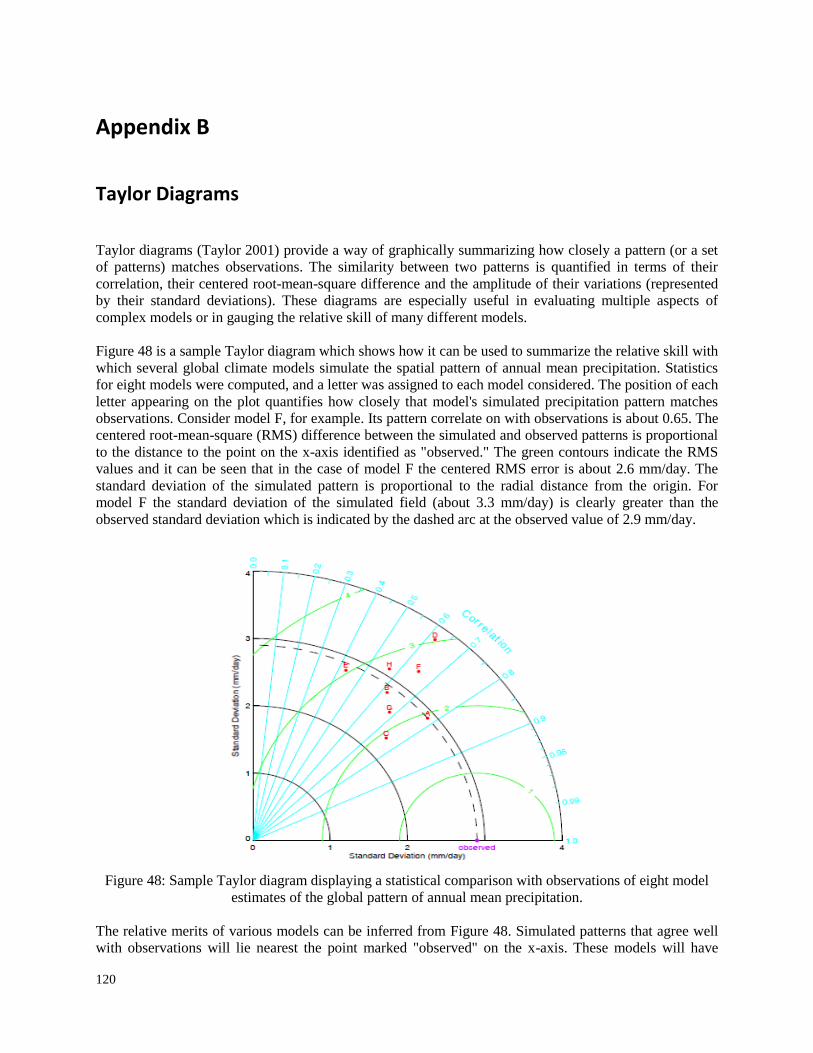
120
Appendix B
Taylor Diagrams
Taylor diagrams (Taylor 2001) provide a way of graphically summarizing how closely a pattern (or a set
of patterns) matches observations. The similarity between two patterns is quantified in terms of their
correlation, their centered root-mean-square difference and the amplitude of their variations (represented
by their standard deviations). These diagrams are especially useful in evaluating multiple aspects of
complex models or in gauging the relative skill of many different models.
Figure 48 is a sample Taylor diagram which shows how it can be used to summarize the relative skill with
which several global climate models simulate the spatial pattern of annual mean precipitation. Statistics
for eight models were computed, and a letter was assigned to each model considered. The position of each
letter appearing on the plot quantifies how closely that model's simulated precipitation pattern matches
observations. Consider model F, for example. Its pattern correlate on with observations is about 0.65. The
centered root-mean-square (RMS) difference between the simulated and observed patterns is proportional
to the distance to the point on the x-axis identified as "observed." The green contours indicate the RMS
values and it can be seen that in the case of model F the centered RMS error is about 2.6 mm/day. The
standard deviation of the simulated pattern is proportional to the radial distance from the origin. For
model F the standard deviation of the simulated field (about 3.3 mm/day) is clearly greater than the
observed standard deviation which is indicated by the dashed arc at the observed value of 2.9 mm/day.
Figure 48: Sample Taylor diagram displaying a statistical comparison with observations of eight model
estimates of the global pattern of annual mean precipitation.
The relative merits of various models can be inferred from Figure 48. Simulated patterns that agree well
with observations will lie nearest the point marked "observed" on the x-axis. These models will have

121
relatively high correlation and low RMS errors. Models lying on the dashed arc will have the correct
standard deviation (which indicates that the pattern variations are of the right amplitude). In Figure 48, it
can be seen that models A and C generally agree best with observations, each with about the same RMS
error. Model A, however, has a slightly higher correlation with observations and has the same standard
deviation as the observed, whereas model C has too little spatial variability (with a standard deviation of
2.3 mm/day compared to the observed value of 2.9 mm/day). Of the poorer performing models, model E
has a low pattern correlation, while model D has variations that are much larger than observed, in both
cases resulting in a relatively large (~3 mm/day) centered RMS error in the precipitation fields. Note also
that although models D and B have about the same correlation with observations, model B simulates the
amplitude of the variations (i.e., the standard deviation) much better than model D, and this results in a
smaller RMS error.
In summary, the Taylor diagram characterizes the statistical relationship between two fields, a "test" field
(often representing a field simulated by a model) and a "reference" field (usually representing “truth”,
based on observations). Note that the means of the fields are subtracted out before computing their
second-order statistics, so the diagram does not provide information about overall biases, but solely
characterizes the centered pattern error.

122
Declaration
I herewith declare that I have produced this paper without the prohibited assistance of third
parties and without making use of aids other than those specified; notions taken over directly or indirectly
from other sources have been identified as such. This paper has not previously been presented in identical
or similar form to any other Italian or foreign examination board.
The thesis work was conducted from November 2010 to November 2013 under the supervision of
Professor Paolo Ferrazzoli at the Dipartimento di Ingegneria Civile e Ingegneria Informatica (DICII),
University of Rome Tor Vergata, Italy
ROME,


![Quantum Microwave Radiometry with a Superconducting Qubit · 2019-09-30 · A classical microwave radiometer [11] typically consists of a radio receiver followed by a square-law detector](https://img.pdfslide.net/doc/110x75/5f35d9f5da760769e114f3fc/quantum-microwave-radiometry-with-a-superconducting-qubit-2019-09-30-a-classical.jpg)