Embed Size (px)
Citation preview
Millimeter-wave Mobile Broadband:
Unleashing 3-300GHz Spectrum
Farooq Khan & Jerry Pi
Samsung
March 28, 2011
1Copyright 2011 by the authors. All rights reserved.
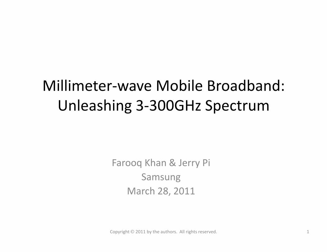
Outline• Introduction
– Mobile broadband growth
– The myth of traffic and revenue gap
– The national broadband plan
• mmW spectrum
– History of millimeter wave communications
– Unleashing 3-300GHz spectrum
– LMDS and 70/80/90 GHz bands
• mmW Propagation characteristics
– Free Space Propagation
• MMB air-interface design
– Duplex and multiple access schemes
– Frame Structure
– Channel coding and modulation
• Dynamic beamforming with miniature antennas
– Beamforming fundamentals
– Baseband beamforming
– Analog beamforming
– RF beamforming
– Beamforming in fading channels– Free Space Propagation
– Material penetration loss
– Oxygen and water absorption
– Foliage absorption
– Rain absorption
– Diffraction
– Ground reflection
• mmW Mobile Broadband (MMB) network
architecture
– Stand-alone MMB system
– MMB base station grid
– Hybrid MMB + 4G systems
– Deployment and antenna configuration
– Beamforming in fading channels
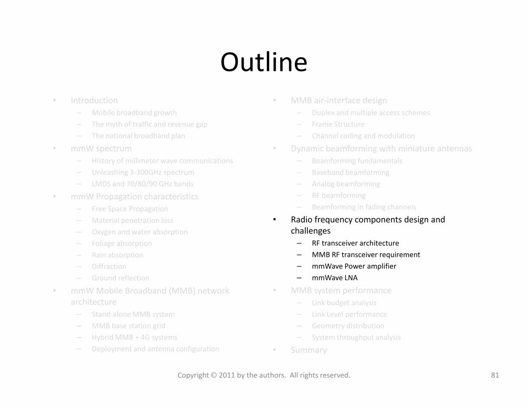
• Radio frequency components design and
challenges
– RF transceiver architecture
– MMB RF transceiver requirement
– mmWave Power amplifier
– mmWave LNA
• MMB system performance
– Link budget analysis
– Link Level performance
– Geometry distribution
– System throughput analysis
• Summary
2Copyright 2011 by the authors. All rights reserved.
Outline• Introduction
– Mobile broadband growth
– The myth of traffic and revenue gap
– The national broadband plan
• mmW spectrum
– History of millimeter wave communications
– Unleashing 3-300GHz spectrum
– LMDS and 70/80/90 GHz bands
• mmW Propagation characteristics
– Free Space Propagation
• MMB air-interface design
– Duplex and multiple access schemes
– Frame Structure
– Channel coding and modulation
• Dynamic beamforming with miniature antennas
– Beamforming fundamentals
– Baseband beamforming
– Analog beamforming
– RF beamforming
– Beamforming in fading channels– Free Space Propagation
– Material penetration loss
– Oxygen and water absorption
– Foliage absorption
– Rain absorption
– Diffraction
– Ground reflection
• mmW Mobile Broadband (MMB) network
architecture
– Stand-alone MMB system
– MMB base station grid
– Hybrid MMB + 4G systems
– Deployment and antenna configuration
– Beamforming in fading channels
• Radio frequency components design and
challenges
– RF transceiver architecture
– MMB RF transceiver requirement
– mmWave Power amplifier
– mmWave LNA
• MMB system performance
– Link budget analysis
– Link Level performance
– Geometry distribution
– System throughput analysis
• Summary
3Copyright 2011 by the authors. All rights reserved.
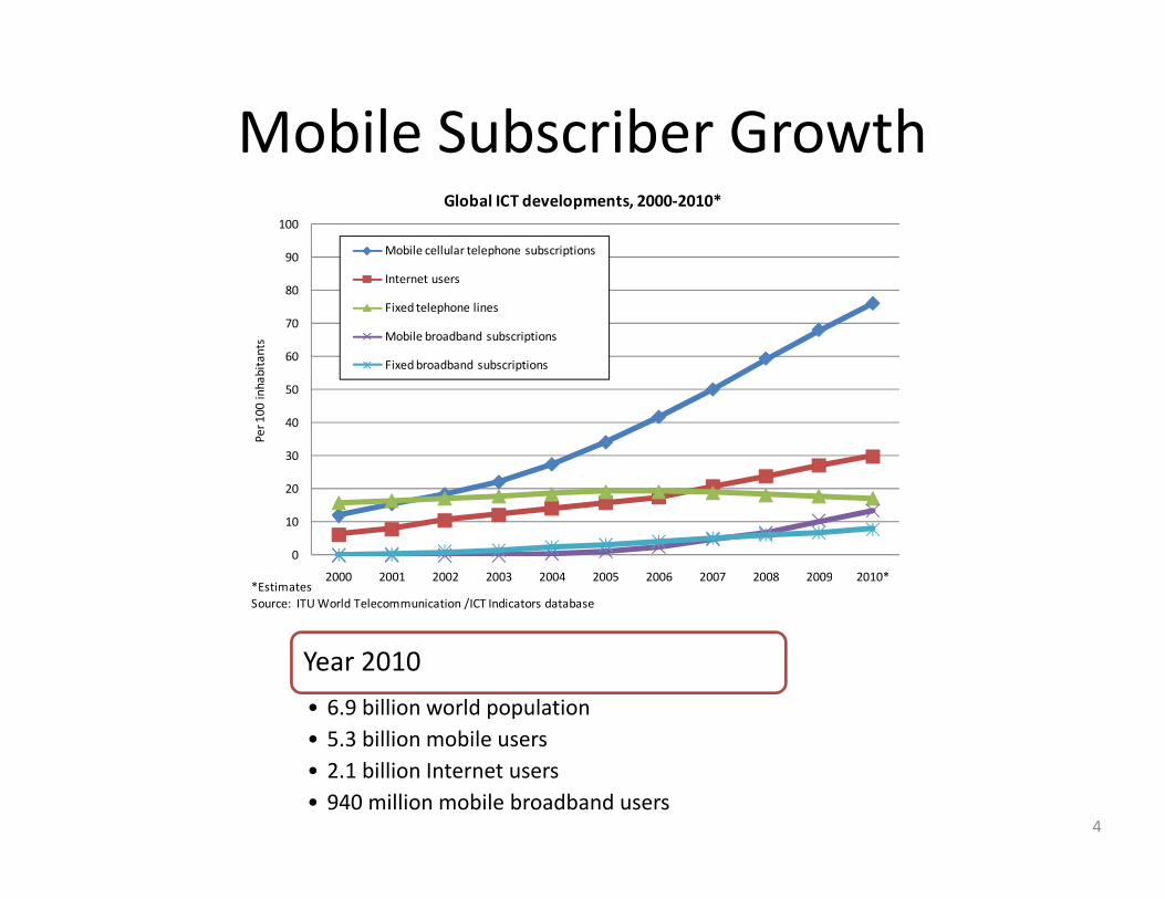
Mobile Subscriber Growth
30
40
50
60
70
80
90
100
Pe
r 1
00
in
ha
bit
an
ts
Global ICT developments, 2000-2010*
Mobile cellular telephone subscriptions
Internet users
Fixed telephone lines
Mobile broadband subscriptions
Fixed broadband subscriptions
Year 2010
• 6.9 billion world population
• 5.3 billion mobile users
• 2.1 billion Internet users
• 940 million mobile broadband users
0
10
20
30
2000 2001 2002 2003 2004 2005 2006 2007 2008 2009 2010**Estimates
Source: ITU World Telecommunication /ICT Indicators database
4
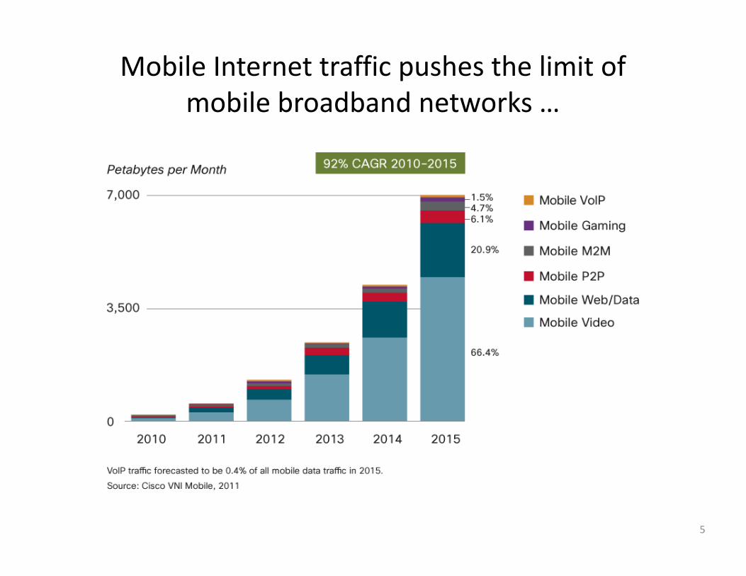
Mobile Internet traffic pushes the limit of
mobile broadband networks …
5
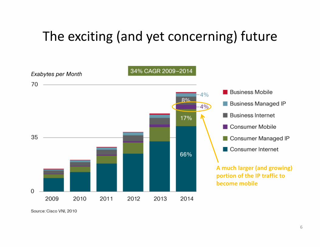
The exciting (and yet concerning) future
A much larger (and growing)
portion of the IP traffic to
become mobile
6
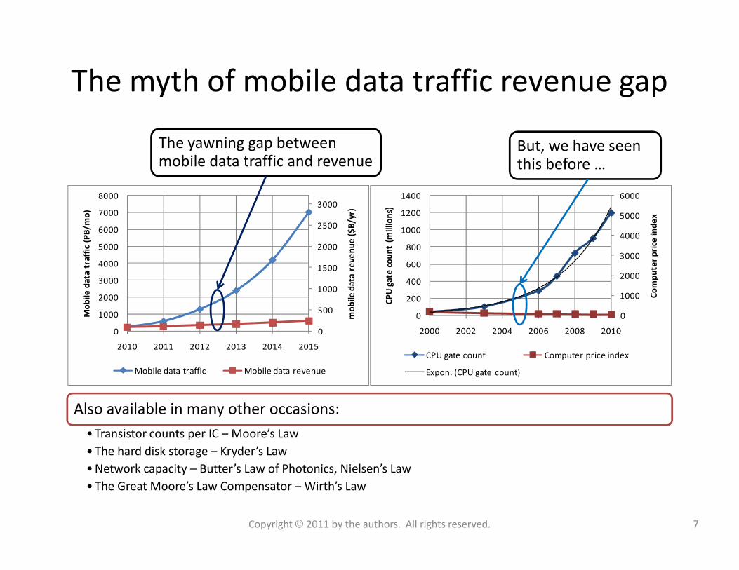
The myth of mobile data traffic revenue gap
1000
1500
2000
2500
3000
3000
4000
5000
6000
7000
8000
mo
bile
da
ta r
eve
nu
e (
$B
/yr)
Mo
bile
dat
a tr
affi
c (P
B/m
o)
2000
3000
4000
5000
6000
400
600
800
1000
1200
1400
Co
mp
ute
r p
rice
ind
ex
CP
U g
ate
co
un
t (m
illio
ns)
The yawning gap between mobile data traffic and revenue
But, we have seen this before …
0
500
1000
0
1000
2000
3000
2010 2011 2012 2013 2014 2015m
ob
ile d
ata
re
ven
ue
($
B/y
r)
Mo
bile
dat
a tr
affi
c (P
B/m
o)
Mobile data traffic Mobile data revenue
0
1000
0
200
400
2000 2002 2004 2006 2008 2010
Co
mp
ute
r p
rice
ind
ex
CP
U g
ate
co
un
t (m
illio
ns)
CPU gate count Computer price index
Expon. (CPU gate count)
Also available in many other occasions:
• Transistor counts per IC – Moore’s Law
• The hard disk storage – Kryder’s Law
• Network capacity – Butter’s Law of Photonics, Nielsen’s Law
• The Great Moore’s Law Compensator – Wirth’s Law
7Copyright 2011 by the authors. All rights reserved.
1000
1000
10000
mo
bile
da
ta r
eve
nu
e (
$B
/yr)
Mo
bile
dat
a tr
affi
c (P
B/m
o)
100
1000
100
1000
10000
Co
mp
ute
r p
rice
ind
ex
CP
U g
ate
co
un
t (m
illio
ns)
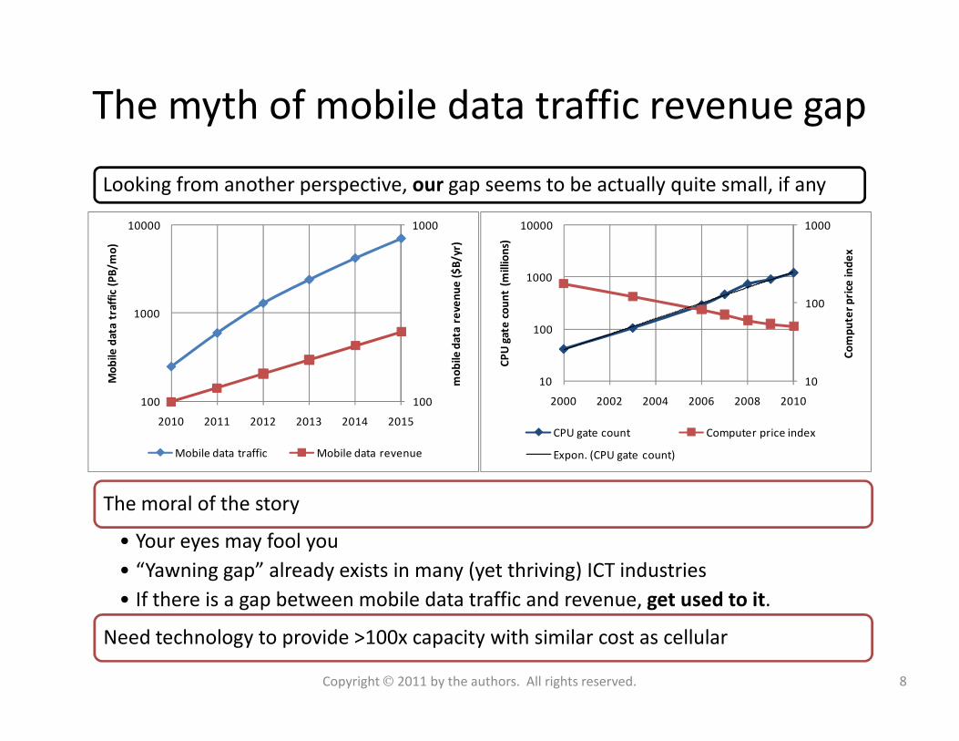
Looking from another perspective, our gap seems to be actually quite small, if any
The myth of mobile data traffic revenue gap
100100
2010 2011 2012 2013 2014 2015
mo
bile
da
ta r
eve
nu
e (
$B
/yr)
Mo
bile
dat
a tr
affi
c (P
B/m
o)
Mobile data traffic Mobile data revenue
1010
2000 2002 2004 2006 2008 2010
CPU gate count Computer price index
Expon. (CPU gate count)
The moral of the story
• Your eyes may fool you
• “Yawning gap” already exists in many (yet thriving) ICT industries
• If there is a gap between mobile data traffic and revenue, get used to it.
Need technology to provide >100x capacity with similar cost as cellular
8Copyright 2011 by the authors. All rights reserved.
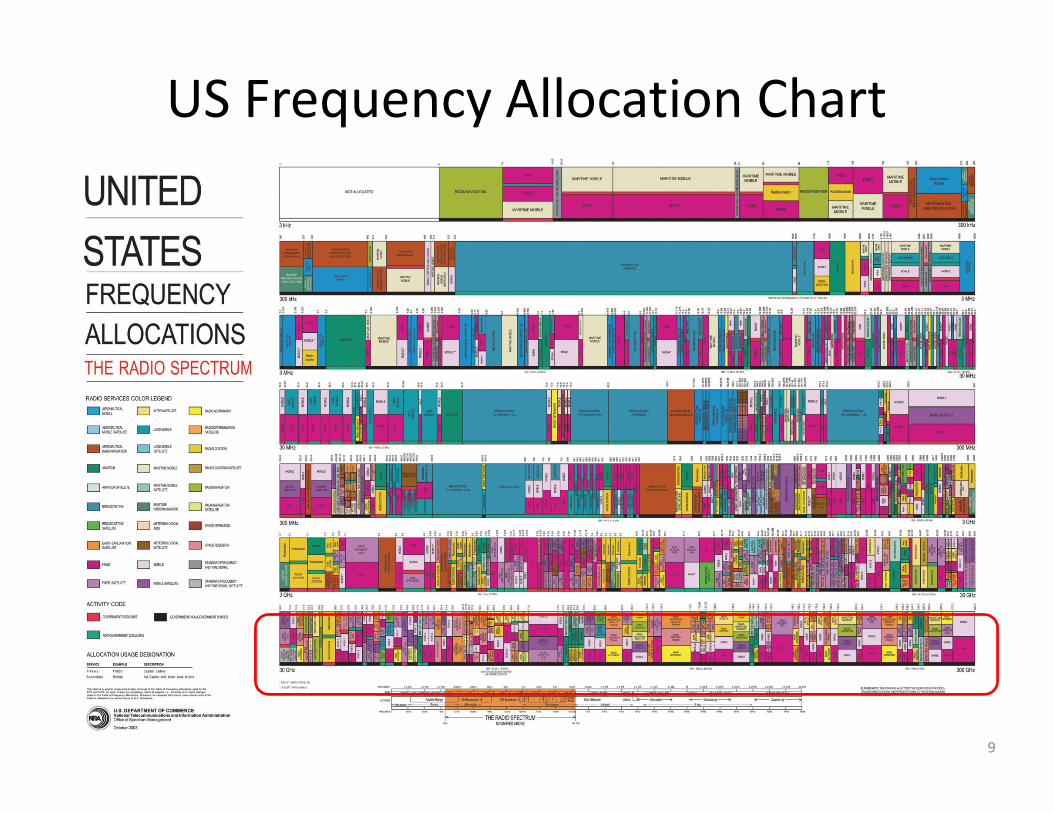
US Frequency Allocation Chart
9
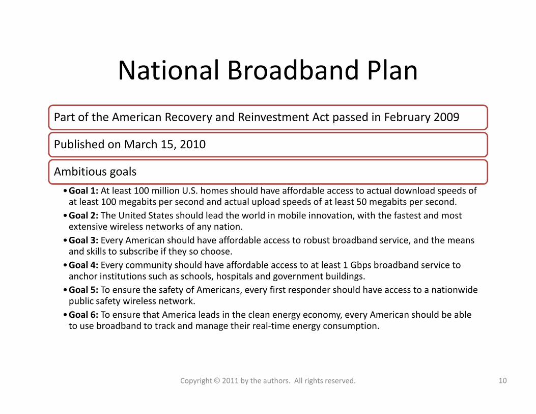
National Broadband Plan
Part of the American Recovery and Reinvestment Act passed in February 2009
Published on March 15, 2010
Ambitious goals
•Goal 1: At least 100 million U.S. homes should have affordable access to actual download speeds of at least 100 megabits per second and actual upload speeds of at least 50 megabits per second.
•Goal 2: The United States should lead the world in mobile innovation, with the fastest and most extensive wireless networks of any nation.
•Goal 3: Every American should have affordable access to robust broadband service, and the means and skills to subscribe if they so choose.
•Goal 4: Every community should have affordable access to at least 1 Gbps broadband service to anchor institutions such as schools, hospitals and government buildings.
•Goal 5: To ensure the safety of Americans, every first responder should have access to a nationwide public safety wireless network.
•Goal 6: To ensure that America leads in the clean energy economy, every American should be able to use broadband to track and manage their real-time energy consumption.
10Copyright 2011 by the authors. All rights reserved.
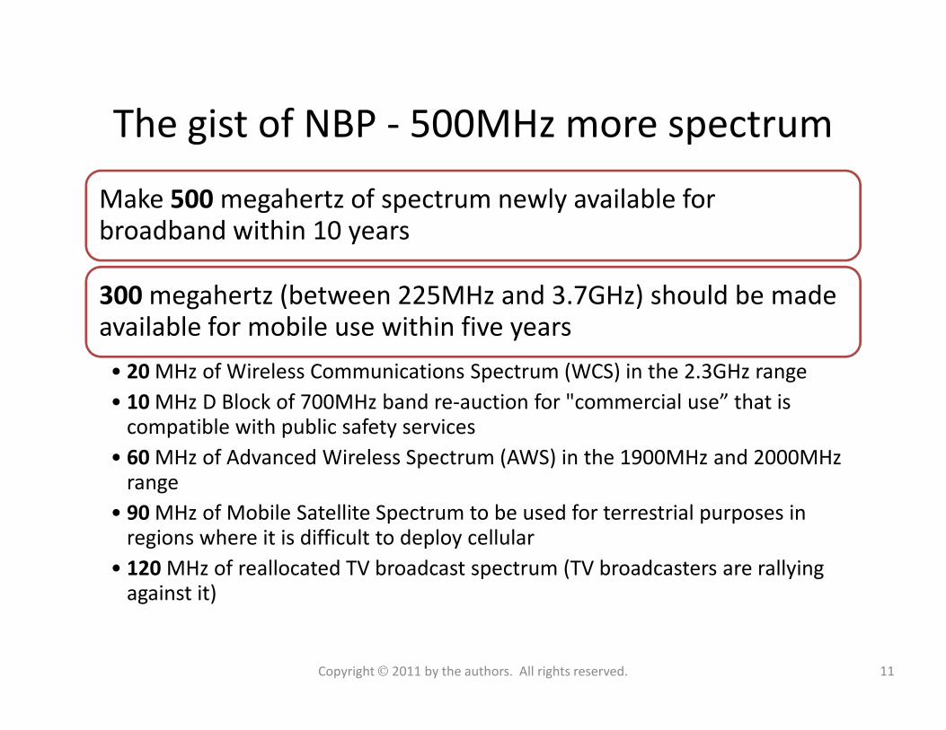
The gist of NBP - 500MHz more spectrum
Make 500 megahertz of spectrum newly available for broadband within 10 years
300 megahertz (between 225MHz and 3.7GHz) should be made available for mobile use within five years
• 20 MHz of Wireless Communications Spectrum (WCS) in the 2.3GHz range• 20 MHz of Wireless Communications Spectrum (WCS) in the 2.3GHz range
• 10 MHz D Block of 700MHz band re-auction for "commercial use” that is compatible with public safety services
• 60 MHz of Advanced Wireless Spectrum (AWS) in the 1900MHz and 2000MHz range
• 90 MHz of Mobile Satellite Spectrum to be used for terrestrial purposes in regions where it is difficult to deploy cellular
• 120 MHz of reallocated TV broadcast spectrum (TV broadcasters are rallying against it)
11Copyright 2011 by the authors. All rights reserved.
Outline• Introduction
– Mobile broadband growth
– The myth of traffic and revenue gap
– The national broadband plan
• mmW spectrum
– History of millimeter wave communications
– Unleashing 3-300GHz spectrum
– LMDS and 70/80/90 GHz bands
• mmW Propagation characteristics
– Free Space Propagation
• MMB air-interface design
– Duplex and multiple access schemes
– Frame Structure
– Channel coding and modulation
• Dynamic beamforming with miniature antennas
– Beamforming fundamentals
– Baseband beamforming
– Analog beamforming
– RF beamforming
– Beamforming in fading channels– Free Space Propagation
– Material penetration loss
– Oxygen and water absorption
– Foliage absorption
– Rain absorption
– Diffraction
– Ground reflection
• mmW Mobile Broadband (MMB) network
architecture
– Stand-alone MMB system
– MMB base station grid
– Hybrid MMB + 4G systems
– Deployment and antenna configuration
– Beamforming in fading channels
• Radio frequency components design and
challenges
– RF transceiver architecture
– MMB RF transceiver requirement
– mmWave Power amplifier
– mmWave LNA
• MMB system performance
– Link budget analysis
– Link Level performance
– Geometry distribution
– System throughput analysis
• Summary
12Copyright 2011 by the authors. All rights reserved.
Wavepropagation
Eletric field
Magnetic field
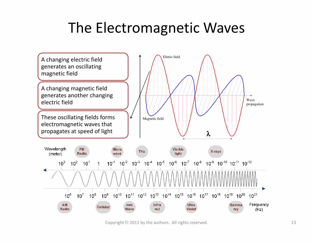
The Electromagnetic Waves
A changing electric field generates an oscillating magnetic field
A changing magnetic field generates another changing electric field
These oscillating fields forms electromagnetic waves that
λλλλ
electromagnetic waves that propagates at speed of light
13Copyright 2011 by the authors. All rights reserved.
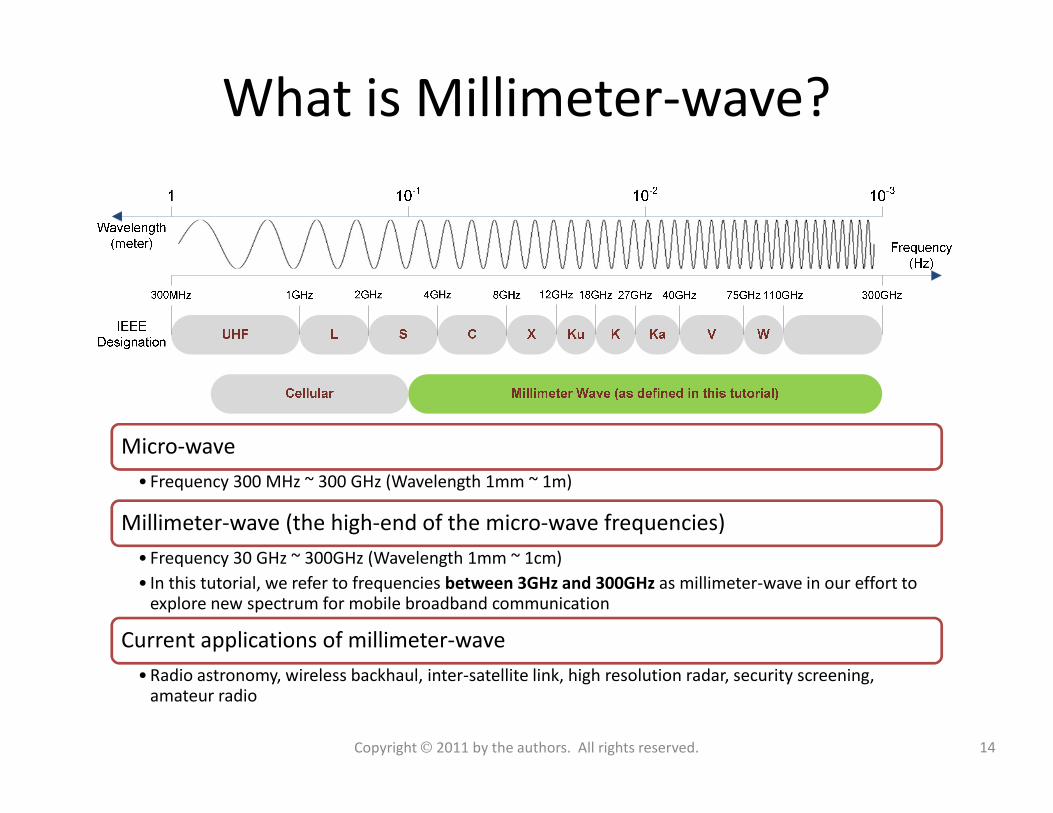
What is Millimeter-wave?
Micro-wave
• Frequency 300 MHz ~ 300 GHz (Wavelength 1mm ~ 1m)
Millimeter-wave (the high-end of the micro-wave frequencies)
• Frequency 30 GHz ~ 300GHz (Wavelength 1mm ~ 1cm)
• In this tutorial, we refer to frequencies between 3GHz and 300GHz as millimeter-wave in our effort to explore new spectrum for mobile broadband communication
Current applications of millimeter-wave
• Radio astronomy, wireless backhaul, inter-satellite link, high resolution radar, security screening, amateur radio
14Copyright 2011 by the authors. All rights reserved.
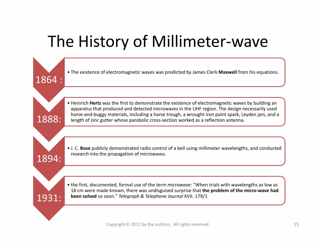
The History of Millimeter-wave
1864 :• The existence of electromagnetic waves was predicted by James Clerk Maxwell from his equations.
1888:
• Heinrich Hertz was the first to demonstrate the existence of electromagnetic waves by building an apparatus that produced and detected microwaves in the UHF region. The design necessarily used horse-and-buggy materials, including a horse trough, a wrought iron point spark, Leyden jars, and a length of zinc gutter whose parabolic cross-section worked as a reflection antenna. 1888: length of zinc gutter whose parabolic cross-section worked as a reflection antenna.
1894:• J. C. Bose publicly demonstrated radio control of a bell using millimeter wavelengths, and conducted
research into the propagation of microwaves.
1931:
• the first, documented, formal use of the term microwave: "When trials with wavelengths as low as 18 cm were made known, there was undisguised surprise that the problem of the micro-wave had been solved so soon." Telegraph & Telephone Journal XVII. 179/1
15Copyright 2011 by the authors. All rights reserved.

Unleashing the 3-300GHz Spectrum
With a reasonable assumption that about 40% of the spectrum in the mmW bands can be made available over time, we open the door for possible 100GHz new spectrum for mobile broadband
• More than 200 times the spectrum currently allocated for this purpose below 3GHz.
16Copyright 2011 by the authors. All rights reserved.
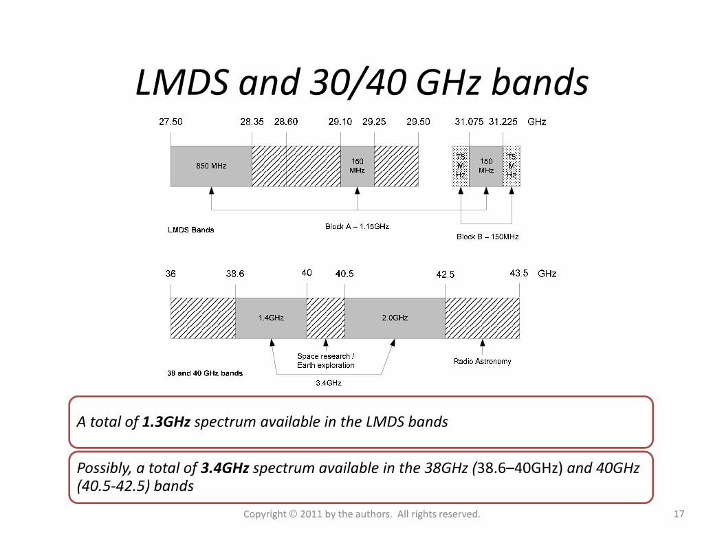
LMDS and 30/40 GHz bands
A total of 1.3GHz spectrum available in the LMDS bands
Possibly, a total of 3.4GHz spectrum available in the 38GHz (38.6–40GHz) and 40GHz (40.5-42.5) bands
17Copyright 2011 by the authors. All rights reserved.
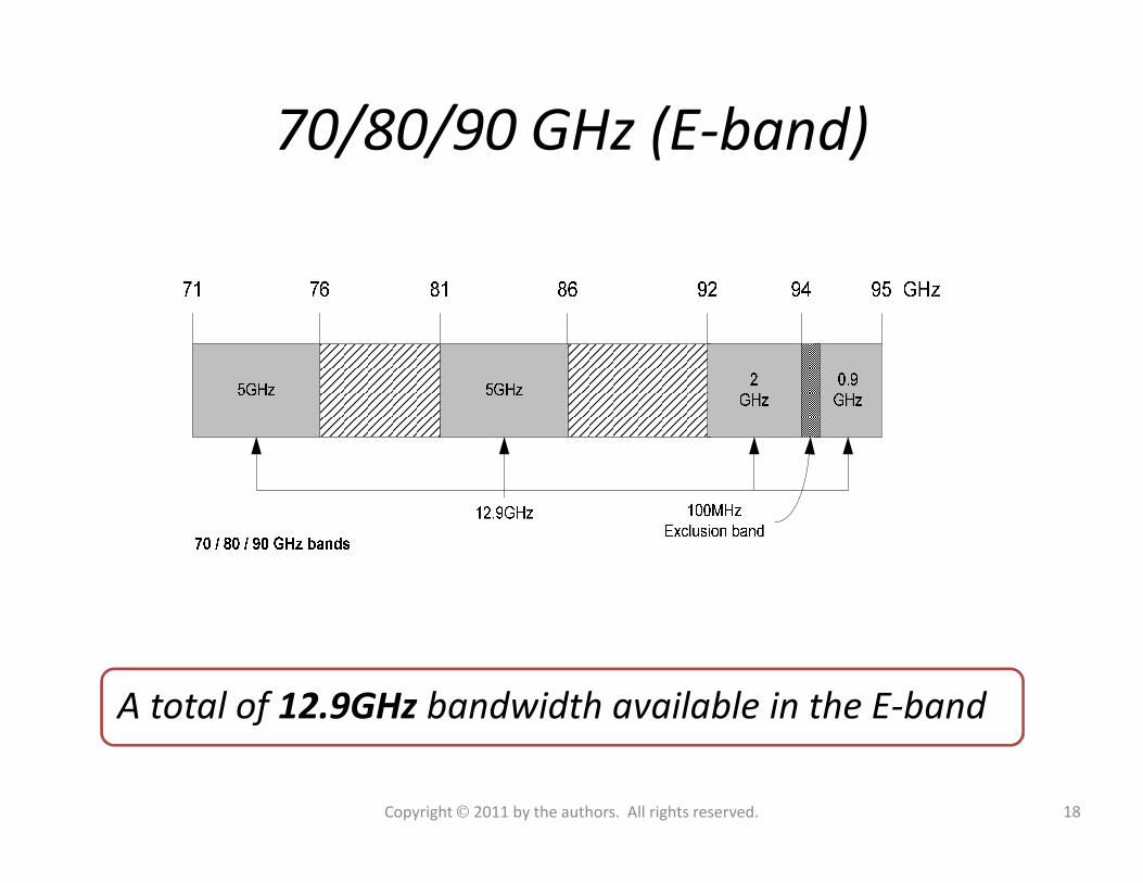
70/80/90 GHz (E-band)
A total of 12.9GHz bandwidth available in the E-band
18Copyright 2011 by the authors. All rights reserved.
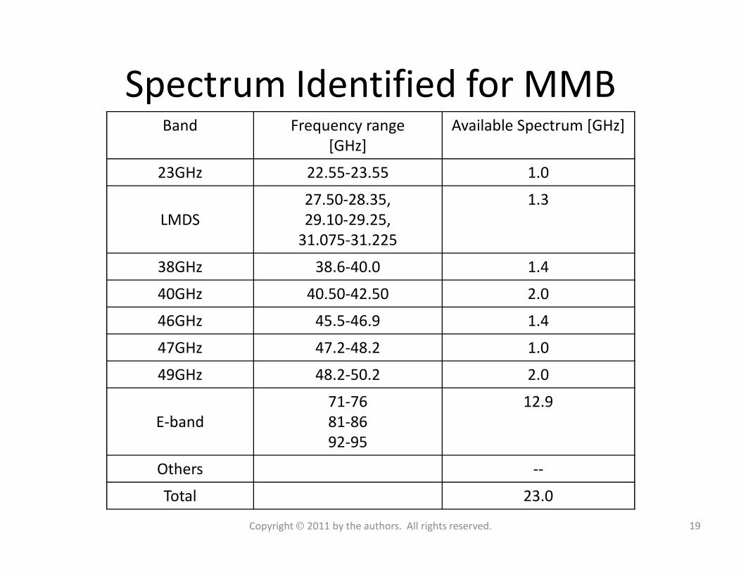
Spectrum Identified for MMBBand Frequency range
[GHz]
Available Spectrum [GHz]
23GHz 22.55-23.55 1.0
LMDS
27.50-28.35,
29.10-29.25,
31.075-31.225
1.3
38GHz 38.6-40.0 1.4
40GHz 40.50-42.50 2.040GHz 40.50-42.50 2.0
46GHz 45.5-46.9 1.4
47GHz 47.2-48.2 1.0
49GHz 48.2-50.2 2.0
E-band
71-76
81-86
92-95
12.9
Others --
Total 23.0
19Copyright 2011 by the authors. All rights reserved.
Outline• Introduction
– Mobile broadband growth
– The myth of traffic and revenue gap
– The national broadband plan
• mmW spectrum
– History of millimeter wave communications
– Unleashing 3-300GHz spectrum
– LMDS and 70/80/90 GHz bands
• mmW Propagation characteristics
– Free Space Propagation
• MMB air-interface design
– Duplex and multiple access schemes
– Frame Structure
– Channel coding and modulation
• Dynamic beamforming with miniature antennas
– Beamforming fundamentals
– Baseband beamforming
– Analog beamforming
– RF beamforming
– Beamforming in fading channels– Free Space Propagation
– Material penetration loss
– Oxygen and water absorption
– Foliage absorption
– Rain absorption
– Diffraction
– Ground reflection
• mmW Mobile Broadband (MMB) network
architecture
– Stand-alone MMB system
– MMB base station grid
– Hybrid MMB + 4G systems
– Deployment and antenna configuration
– Beamforming in fading channels
• Radio frequency components design and
challenges
– RF transceiver architecture
– MMB RF transceiver requirement
– mmWave Power amplifier
– mmWave LNA
• MMB system performance
– Link budget analysis
– Link Level performance
– Geometry distribution
– System throughput analysis
• Summary
20Copyright 2011 by the authors. All rights reserved.
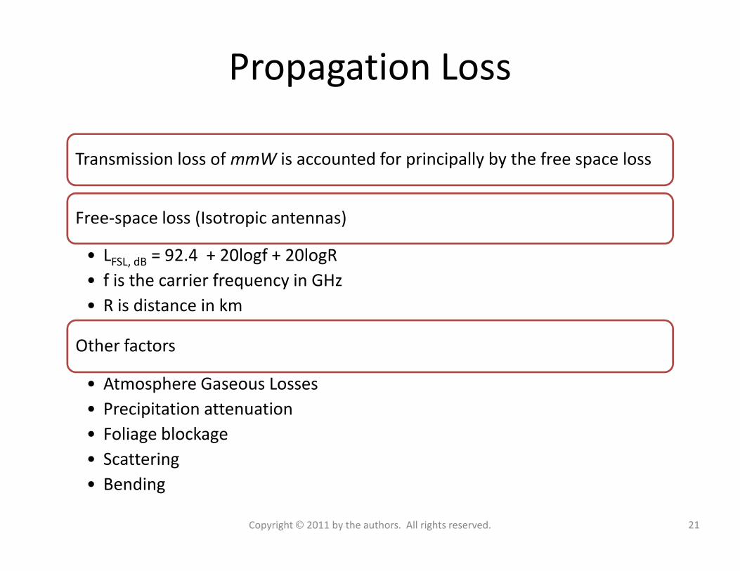
Propagation Loss
Transmission loss of mmW is accounted for principally by the free space loss
Free-space loss (Isotropic antennas)
• LFSL, dB = 92.4 + 20logf + 20logR
• f is the carrier frequency in GHz• f is the carrier frequency in GHz
• R is distance in km
Other factors
• Atmosphere Gaseous Losses
• Precipitation attenuation
• Foliage blockage
• Scattering
• Bending
21Copyright 2011 by the authors. All rights reserved.
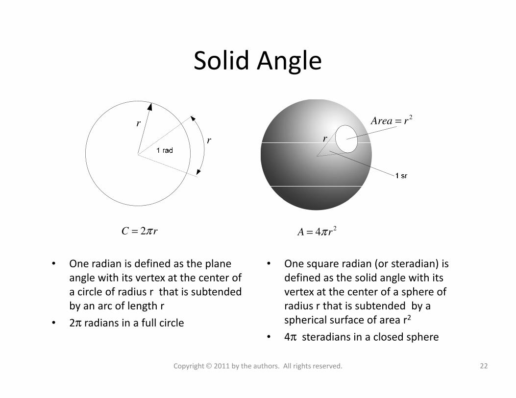
Solid Angle
2Area r=
rr
r
• One radian is defined as the plane
angle with its vertex at the center of
a circle of radius r that is subtended
by an arc of length r
• 2π radians in a full circle
• One square radian (or steradian) is
defined as the solid angle with its
vertex at the center of a sphere of
radius r that is subtended by a
spherical surface of area r2
• 4π steradians in a closed sphere
Copyright 2011 by the authors. All rights reserved. 22
24A rπ=2C rπ=
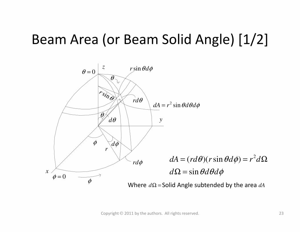
Beam Area (or Beam Solid Angle) [1/2]
z0θ =
θ
θ
sinr
θ
sinr dθ φ
rdθ2 sindA r d dθ θ φ=
θ
x
y
φ
0φ =φ
dφr
rdφ
θdθ
2( )( sin )
sin
dA rd r d r d
d d d
θ θ φ
θ θ φ
= = Ω
Ω =
Where Solid Angle subtended by the areadΩ = dA
23Copyright 2011 by the authors. All rights reserved.
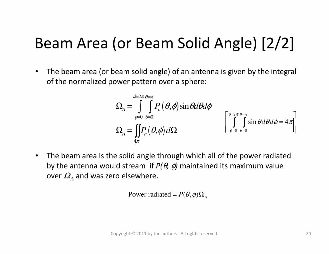
Beam Area (or Beam Solid Angle) [2/2]
• The beam area (or beam solid angle) of an antenna is given by the integral
of the normalized power pattern over a sphere:
( )
( )
2
0 0
, sin
,
A nP d d
P d
φ π θ π
φ θ
θ φ θ θ φ
θ φ
= =
= =
Ω =
Ω = Ω
∫ ∫
∫∫
2
sin 4d d
φ π θ π
θ θ φ π= =
= ∫ ∫
• The beam area is the solid angle through which all of the power radiated
by the antenna would stream if P(θ, φ) maintained its maximum value
over ΩΑ and was zero elsewhere.
( )4
,A n
P dπ
θ φΩ = Ω∫∫ 0 0φ θ= = ∫ ∫
Power radiated = ( , ) AP θ φ Ω
24Copyright 2011 by the authors. All rights reserved.
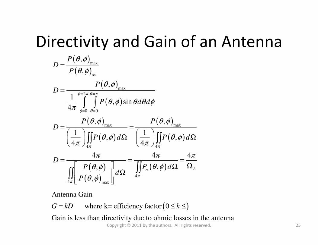
Directivity and Gain of an Antenna( )( )
( )
( )
( ) ( )
max
max
2
0 0
max max
,
,
,
1, sin
4
, ,
av
PD
P
PD
P d d
P PD
φ π θ π
φ θ
θ φ
θ φ
θ φ
θ φ θ θ φπ
θ φ θ φ
= =
= =
=
=
= =
∫ ∫
( )
( )
( )
( )
( )( )
( )
max max
4 4
4
4 max
, ,
1 1, ,
4 4
4 4 4
,,
,
An
P PD
P d P d
DP dP
dP
π π
π
π
θ φ θ φ
θ φ θ φπ π
π π π
θ φθ φ
θ φ
= =
Ω Ω
= = =Ω Ω
Ω
∫∫ ∫∫
∫∫∫∫
( )
Antenna Gain
where k= efficiency factor 0
Gain is less than directivity due to ohmic losses in the antenna
G kD k= ≤ ≤
25Copyright 2011 by the authors. All rights reserved.
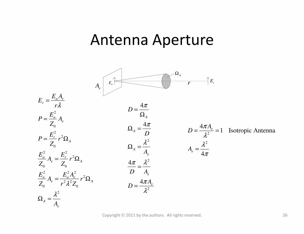
Antenna Aperture
AΩ
aE rE
eA
r
2
a er
a
E AE
r
EP A
λ=
=
4
A
Dπ
=Ω
0
22
0
2 22
0 0
2 2 22
2 2
0 0
2
ae
rA
a re A
a a ee A
A
e
EP A
Z
EP r
Z
E EA r
Z Z
E E AA r
Z r Z
A
λ
λ
=
= Ω
= Ω
= Ω
Ω =
2
2
2
4
4
4
A
A
A
e
e
e
D
A
D A
AD
π
λ
π λ
π
λ
Ω
Ω =
Ω =
=
=
2
2
41 Isotropic Antenna
4
e
e
AD
A
π
λ
λ
π
= =
=
26Copyright 2011 by the authors. All rights reserved.
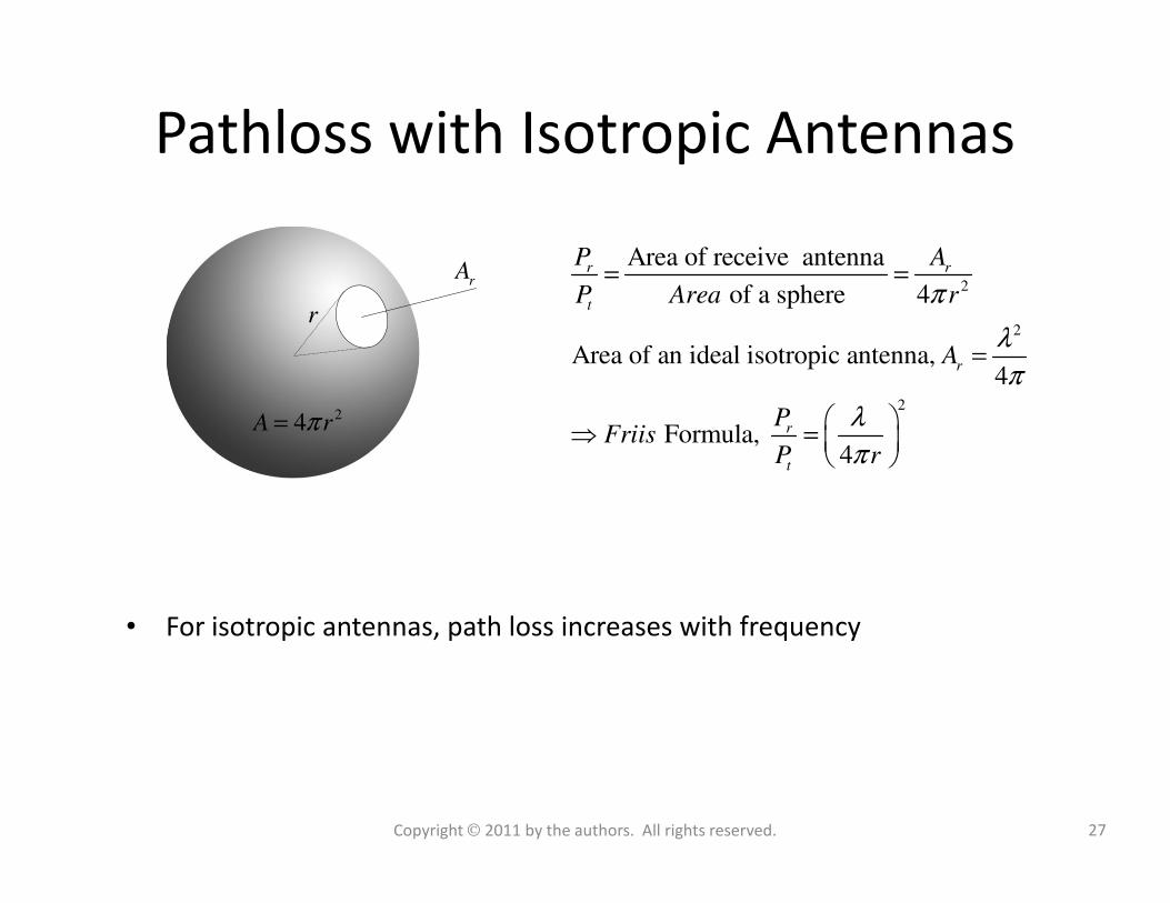
Pathloss with Isotropic Antennas
2
2
2
Area of receive antenna
of a sphere 4
Area of an ideal isotropic antenna, 4
Formula, 4
r r
t
r
r
P A
P Area r
A
PFriis
P r
π
λ
π
λ
π
= =
=
⇒ =
rA
r
24A rπ=
4t
P rπ
• For isotropic antennas, path loss increases with frequency
27Copyright 2011 by the authors. All rights reserved.
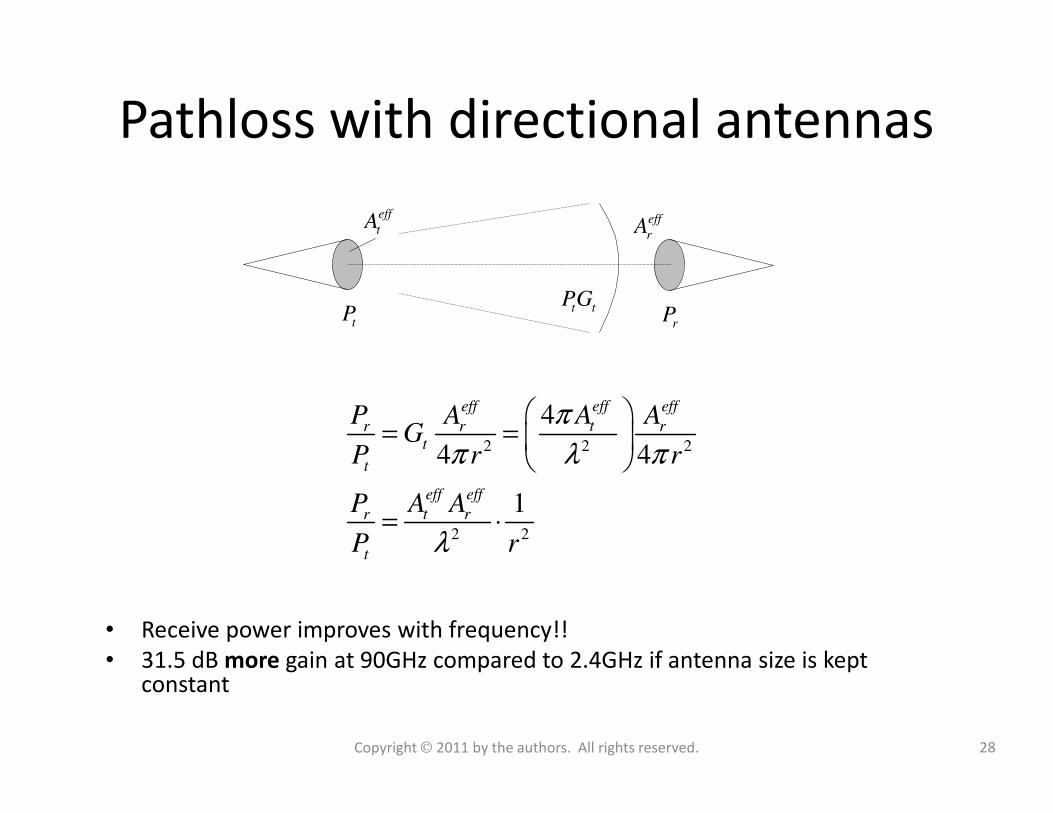
Pathloss with directional antennas
4 effeff effAP A Aπ
eff
tA eff
rA
tP
rPt t
PG
2 2 2
2 2
4
4 4
1
effeff eff
tr r rt
t
eff eff
t rr
t
AP A AG
P r r
A AP
P r
π
π λ π
λ
= =
= ⋅
• Receive power improves with frequency!!
• 31.5 dB more gain at 90GHz compared to 2.4GHz if antenna size is kept constant
28Copyright 2011 by the authors. All rights reserved.
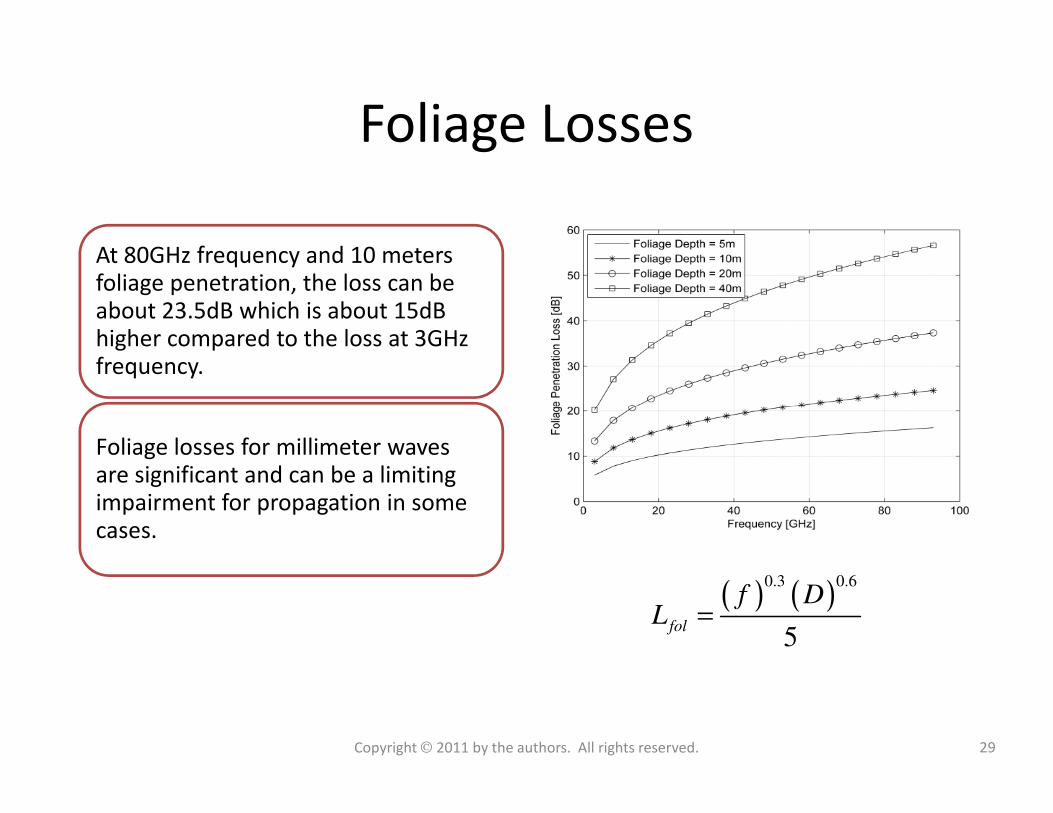
Foliage Losses
At 80GHz frequency and 10 meters foliage penetration, the loss can be about 23.5dB which is about 15dB higher compared to the loss at 3GHz frequency.
Foliage losses for millimeter waves are significant and can be a limiting impairment for propagation in some cases.
( ) ( )0.3 0.6
5fol
f DL =
29Copyright 2011 by the authors. All rights reserved.
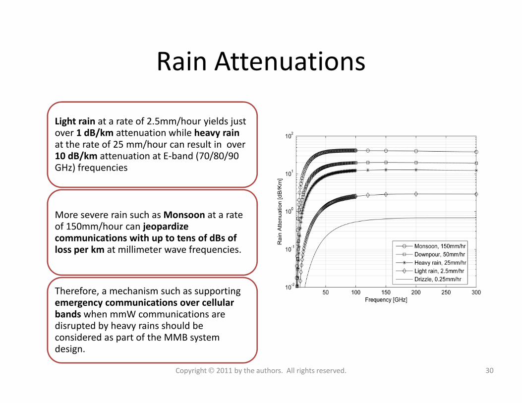
Rain Attenuations
Light rain at a rate of 2.5mm/hour yields just over 1 dB/km attenuation while heavy rain at the rate of 25 mm/hour can result in over 10 dB/km attenuation at E-band (70/80/90 GHz) frequencies
More severe rain such as Monsoon at a rate of 150mm/hour can jeopardize communications with up to tens of dBs of loss per km at millimeter wave frequencies.
Therefore, a mechanism such as supporting emergency communications over cellular bands when mmW communications are disrupted by heavy rains should be considered as part of the MMB system design.
30Copyright 2011 by the authors. All rights reserved.
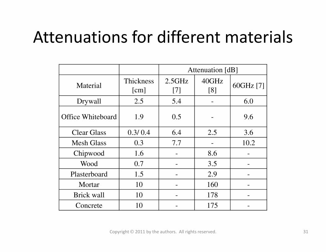
Attenuations for different materials
Attenuation [dB]
MaterialThickness
[cm]
2.5GHz
[7]
40GHz
[8]60GHz [7]
Drywall 2.5 5.4 - 6.0
Office Whiteboard 1.9 0.5 - 9.6
Clear Glass 0.3/ 0.4 6.4 2.5 3.6
Mesh Glass 0.3 7.7 - 10.2
Chipwood 1.6 - 8.6 -
Wood 0.7 - 3.5 -
Plasterboard 1.5 - 2.9 -
Mortar 10 - 160 -
Brick wall 10 - 178 -
Concrete 10 - 175 -
31Copyright 2011 by the authors. All rights reserved.
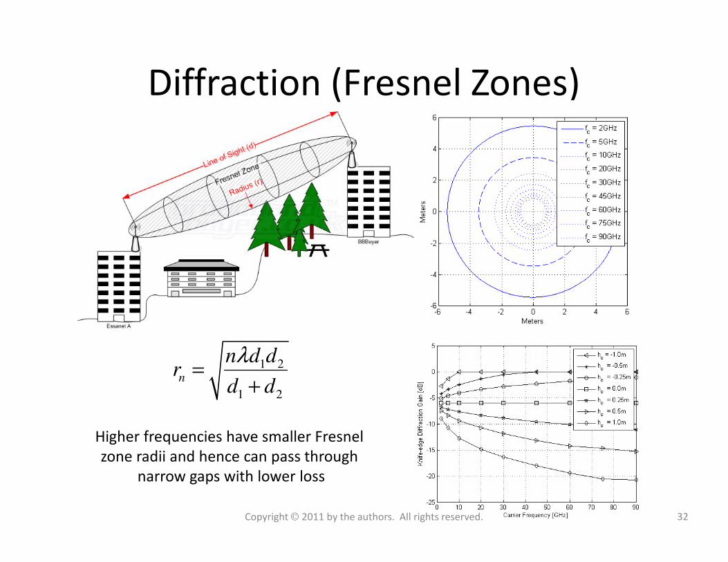
Diffraction (Fresnel Zones)
1 2
1 2
n
n d dr
d d
λ=
+
Higher frequencies have smaller Fresnel
zone radii and hence can pass through
narrow gaps with lower loss
32Copyright 2011 by the authors. All rights reserved.
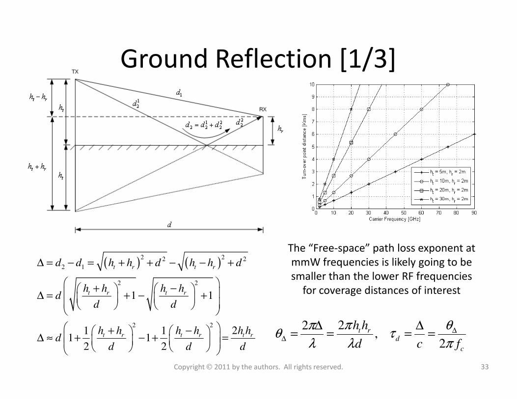
Ground Reflection [1/3]
( ) ( )2 22 2
2 1
2 2
2 2
1 1
21 11 1
2 2
t r t r
t r t r
t r t r t r
d d h h d h h d
h h h hd
d d
h h h h h hd
d d d
∆ = − = + + − − +
+ − ∆ = + − +
+ − ∆ ≈ + − + =
22,
2
t rd
c
h h
d c f
π θπθ τ
λ λ π∆
∆
∆ ∆= = = =
The “Free-space” path loss exponent at
mmW frequencies is likely going to be
smaller than the lower RF frequencies
for coverage distances of interest
33Copyright 2011 by the authors. All rights reserved.
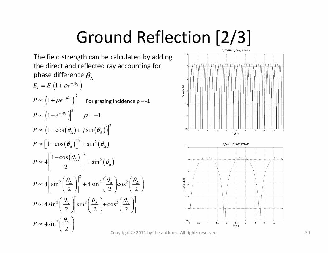
Ground Reflection [2/3]The field strength can be calculated by adding
the direct and reflected ray accounting for
phase difference θ∆
( )
( )
( )
( ) ( )( )
2
2
2
1
1
1 1
1 cos sin
j
T i
j
j
E E e
P e
P e
P j
θ
θ
θ
ρ
ρ
ρ
θ θ
∆
∆
∆
−
−
−
= +
∝ +
∝ − = −
∝ − +
For grazing incidence ρ = -1
( ) ( )( )
( ) ( )
( )( )
2
2 2
2
2
2
2 2 2
2 2 2
1 cos sin
1 cos sin
1 cos4 sin
2
4 sin 4sin cos2 2 2
4sin sin cos2 2 2
P j
P
P
P
P
θ θ
θ θ
θθ
θ θ θ
θ θ θ
∆ ∆
∆ ∆
∆
∆
∆ ∆ ∆
∆ ∆ ∆
∝ − +
∝ − +
−∝ +
∝ +
∝ +
24sin2
Pθ∆
∝
34Copyright 2011 by the authors. All rights reserved.
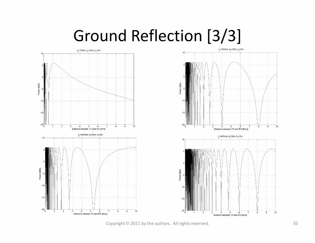
Ground Reflection [3/3]
35Copyright 2011 by the authors. All rights reserved.
Outline• Introduction
– Mobile broadband growth
– The myth of traffic and revenue gap
– The national broadband plan
• mmW spectrum
– History of millimeter wave communications
– Unleashing 3-300GHz spectrum
– LMDS and 70/80/90 GHz bands
• mmW Propagation characteristics
– Free Space Propagation
• MMB air-interface design
– Duplex and multiple access schemes
– Frame Structure
– Channel coding and modulation
• Dynamic beamforming with miniature antennas
– Beamforming fundamentals
– Baseband beamforming
– Analog beamforming
– RF beamforming
– Beamforming in fading channels– Free Space Propagation
– Material penetration loss
– Oxygen and water absorption
– Foliage absorption
– Rain absorption
– Diffraction
– Ground reflection
• mmW Mobile Broadband (MMB) network
architecture
– Stand-alone MMB system
– MMB base station grid
– Hybrid MMB + 4G systems
– Deployment and antenna configuration
– Beamforming in fading channels
• Radio frequency components design and
challenges
– RF transceiver architecture
– MMB RF transceiver requirement
– mmWave Power amplifier
– mmWave LNA
• MMB system performance
– Link budget analysis
– Link Level performance
– Geometry distribution
– System throughput analysis
• Summary
36Copyright 2011 by the authors. All rights reserved.
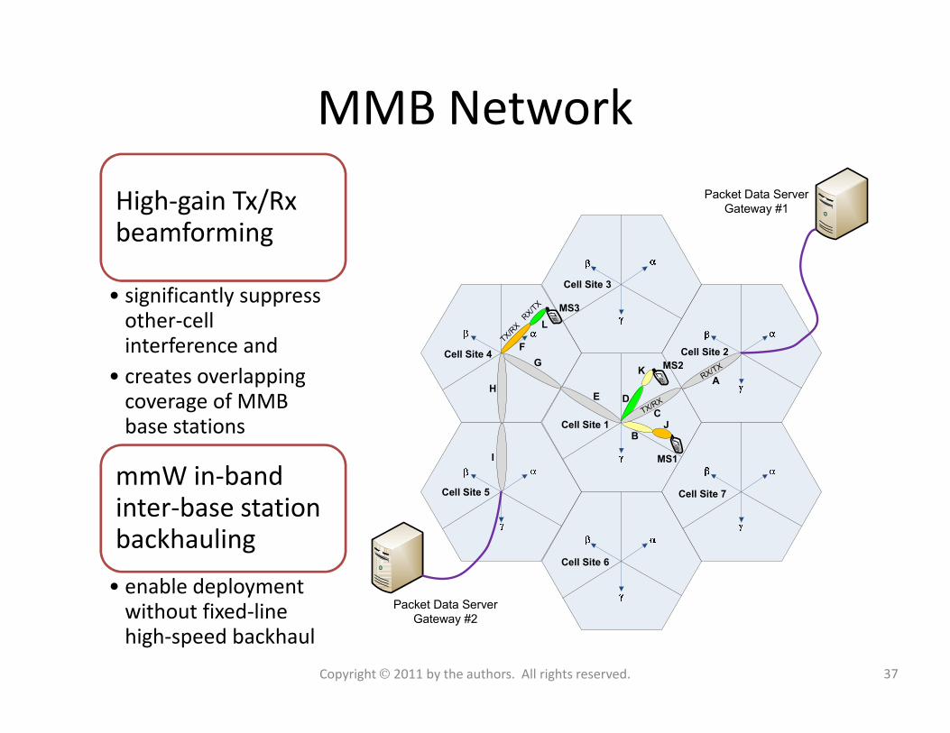
MMB Network
Packet Data Server
Gateway #1
F
GK
L
Cell Site 2
Cell Site 3
Cell Site 4
MS3
MS2
TX/R
XRX/
TX
TX
High-gain Tx/Rx beamforming
• significantly suppress other-cell interference and
• creates overlapping
Packet Data Server
Gateway #2
B
C
DE
AH
I
J
K
Cell Site 1
Cell Site 5
Cell Site 6
Cell Site 7
MS1
MS2
TX/RX
RX/TX• creates overlapping
coverage of MMB base stations
mmW in-band inter-base station backhauling
• enable deployment without fixed-line high-speed backhaul
37Copyright 2011 by the authors. All rights reserved.
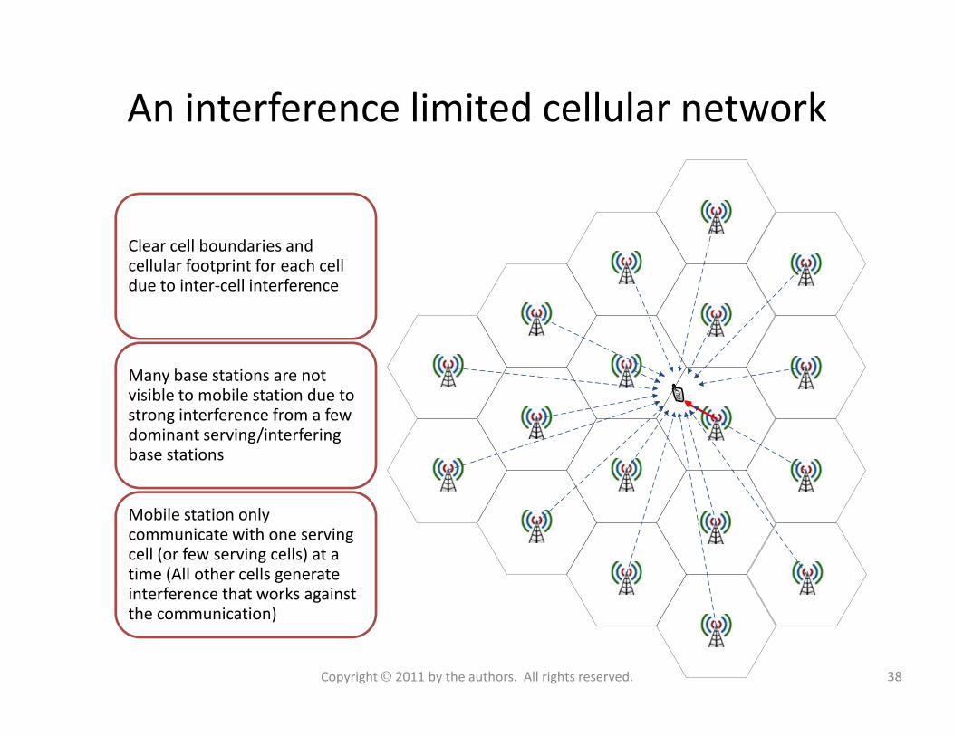
An interference limited cellular network
Clear cell boundaries and cellular footprint for each cell due to inter-cell interference
Many base stations are not Many base stations are not visible to mobile station due to strong interference from a few dominant serving/interfering base stations
Mobile station only communicate with one serving cell (or few serving cells) at a time (All other cells generate interference that works against the communication)
38Copyright 2011 by the authors. All rights reserved.
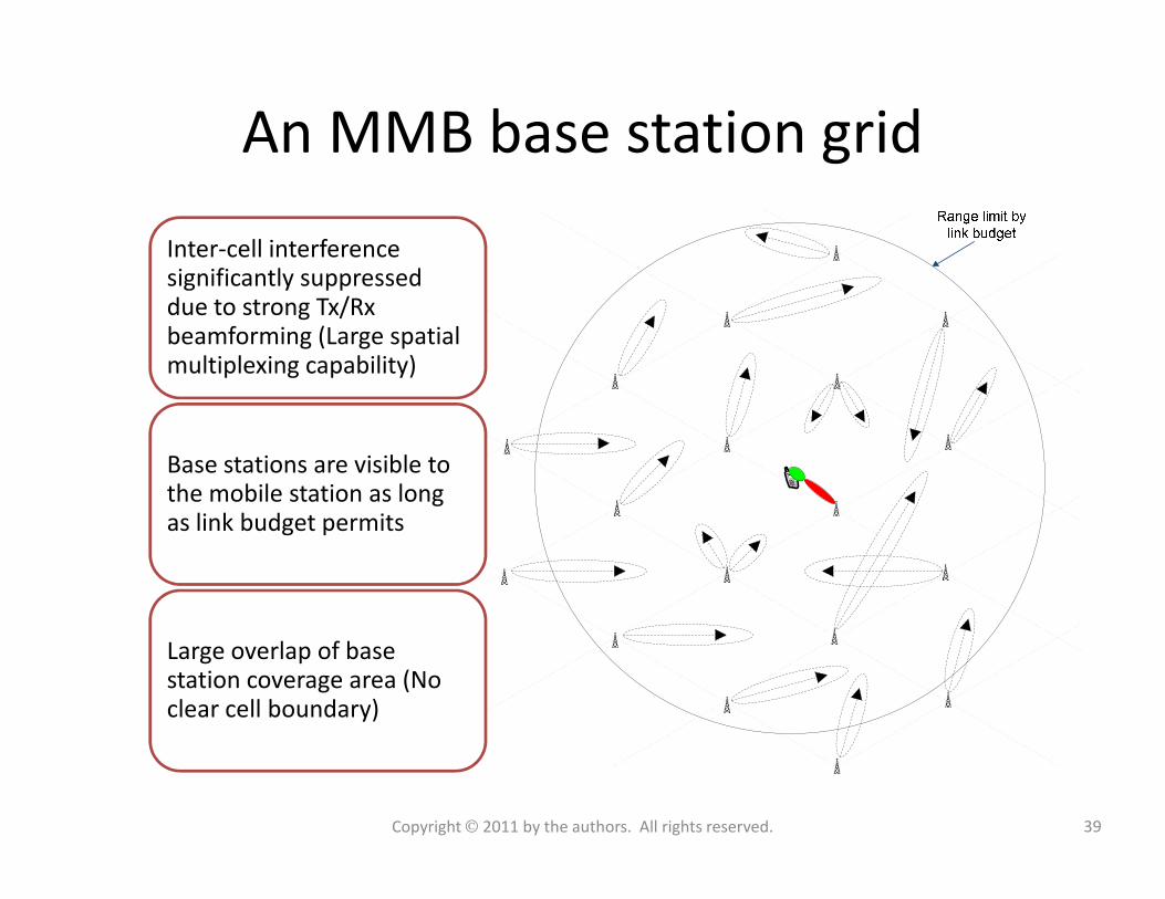
An MMB base station grid
Inter-cell interference significantly suppressed due to strong Tx/Rx beamforming (Large spatial multiplexing capability)
Base stations are visible to Base stations are visible to the mobile station as long as link budget permits
Large overlap of base station coverage area (No clear cell boundary)
39Copyright 2011 by the authors. All rights reserved.
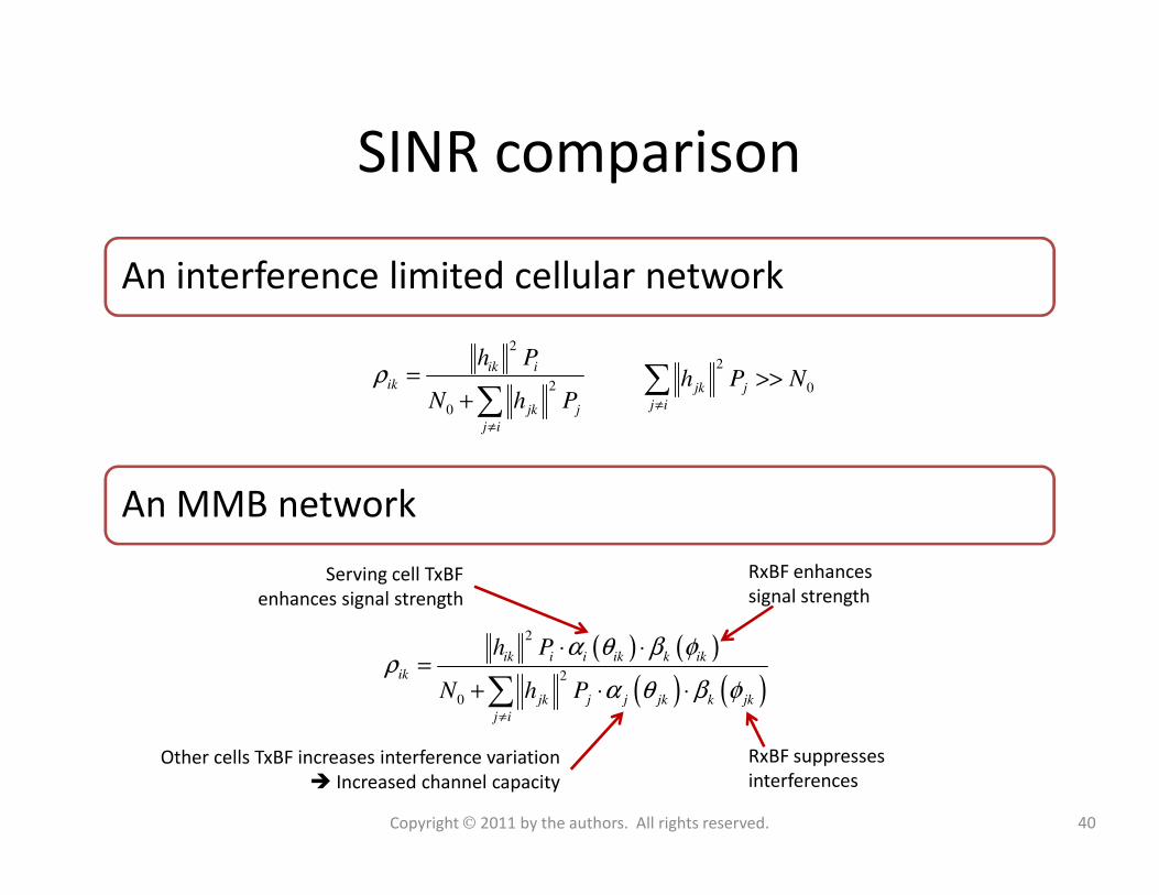
SINR comparison
An interference limited cellular network
2
2
0
ik i
ik
jk j
j i
h P
N h Pρ
≠
=+∑
2
0jk j
j i
h P N≠
>>∑
Copyright 2011 by the authors. All rights reserved. 40
An MMB network
( ) ( )
( ) ( )
2
2
0
ik i i ik k ik
ik
jk j j jk k jk
j i
h P
N h P
α θ β φρ
α θ β φ≠
⋅ ⋅=
+ ⋅ ⋅∑
Serving cell TxBF
enhances signal strength
RxBF enhances
signal strength
RxBF suppresses
interferencesOther cells TxBF increases interference variation
Increased channel capacity
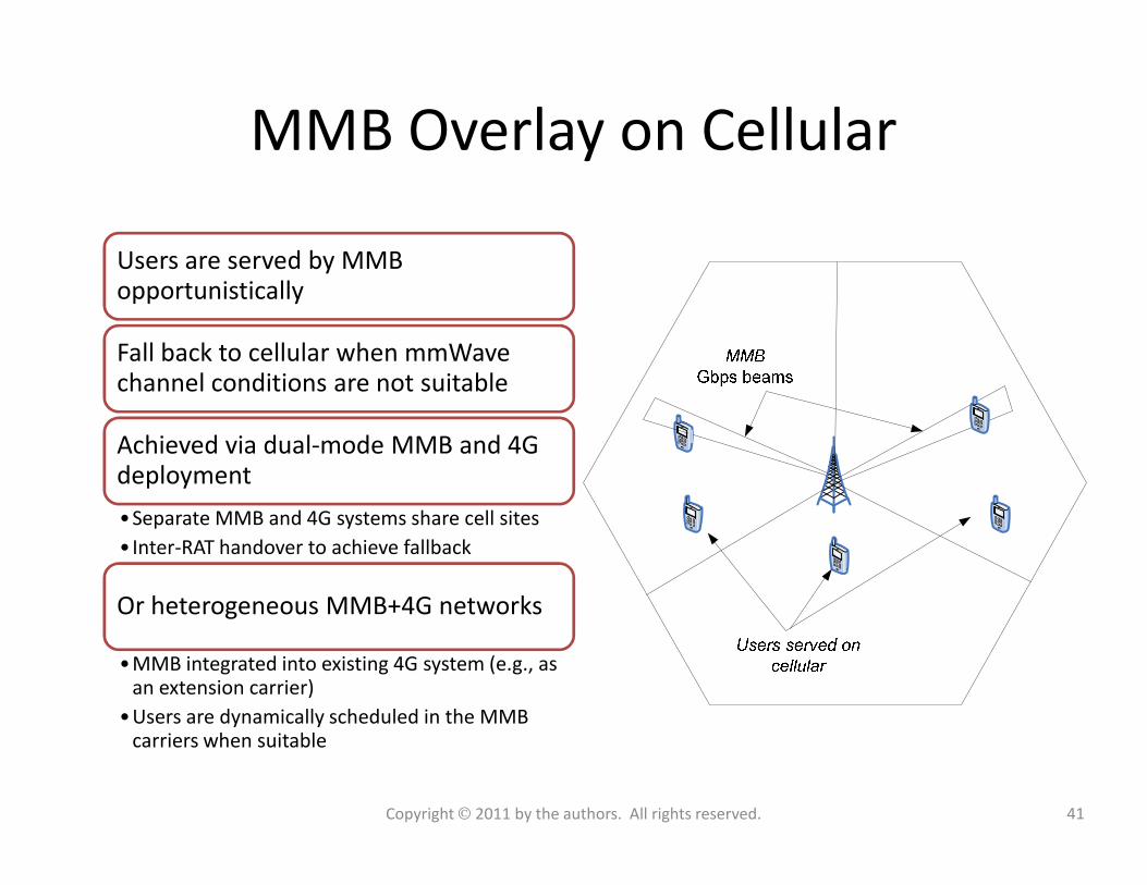
MMB Overlay on Cellular
Users are served by MMB opportunistically
Fall back to cellular when mmWavechannel conditions are not suitable
Achieved via dual-mode MMB and 4G Achieved via dual-mode MMB and 4G deployment
•Separate MMB and 4G systems share cell sites
•Inter-RAT handover to achieve fallback
Or heterogeneous MMB+4G networks
•MMB integrated into existing 4G system (e.g., as an extension carrier)
•Users are dynamically scheduled in the MMB carriers when suitable
41Copyright 2011 by the authors. All rights reserved.
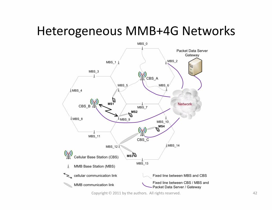
Heterogeneous MMB+4G Networks
Packet Data Server
Gateway
MS1
MBS_0
MBS_1 MBS_2
MBS_3
MBS_4
MBS_5 MBS_6
CBS_A
CBS B
42Copyright 2011 by the authors. All rights reserved.
MS2
MS3
MBS_9
MBS_7
MBS_8MBS_10
MBS_11
MBS_12
MBS_13
MBS_14
Cellular Base Station (CBS)
MMB Base Station (MBS)
MMB communication link
cellular communication link
CBS_B
CBS_C
Fixed line between MBS and CBS
Fixed line between CBS / MBS and
Packet Data Server / Gateway
MS4
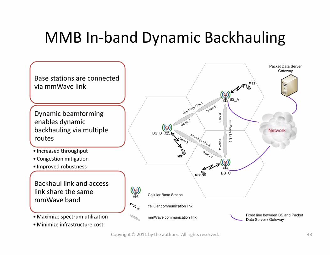
MMB In-band Dynamic Backhauling
Packet Data Server
Gateway
MS2
BS_A
mmWave L
ink 1
mmWBe
am 1
Beam
0Beam 5
Base stations are connected via mmWave link
Dynamic beamformingenables dynamic backhauling via multiple
MS1
MS3
Cellular Base Station
mmWave communication link
cellular communication link
BS_B
BS_C
Fixed line between BS and Packet
Data Server / Gateway
mmWave Link 2
Wave Link 3
Beam 2
Beam 3
Beam 4
43Copyright 2011 by the authors. All rights reserved.
backhauling via multiple routes
• Increased throughput
• Congestion mitigation
• Improved robustness
Backhaul link and access link share the same mmWave band
• Maximize spectrum utilization
• Minimize infrastructure cost
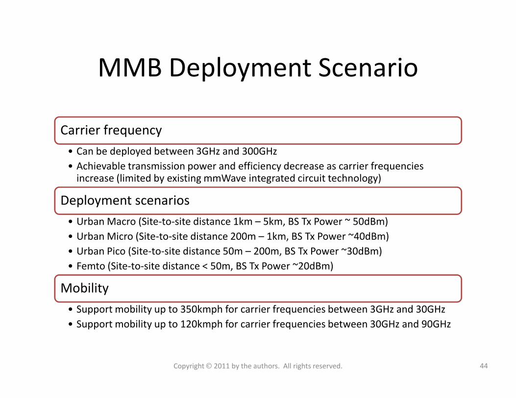
MMB Deployment Scenario
Carrier frequency
• Can be deployed between 3GHz and 300GHz
• Achievable transmission power and efficiency decrease as carrier frequencies increase (limited by existing mmWave integrated circuit technology)
Deployment scenariosDeployment scenarios
• Urban Macro (Site-to-site distance 1km – 5km, BS Tx Power ~ 50dBm)
• Urban Micro (Site-to-site distance 200m – 1km, BS Tx Power ~40dBm)
• Urban Pico (Site-to-site distance 50m – 200m, BS Tx Power ~30dBm)
• Femto (Site-to-site distance < 50m, BS Tx Power ~20dBm)
Mobility
• Support mobility up to 350kmph for carrier frequencies between 3GHz and 30GHz
• Support mobility up to 120kmph for carrier frequencies between 30GHz and 90GHz
44Copyright 2011 by the authors. All rights reserved.
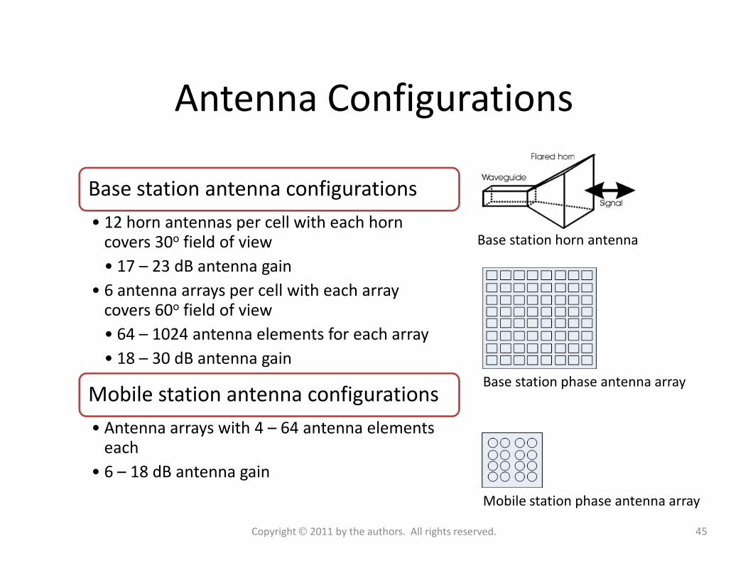
Antenna Configurations
Base station antenna configurations
• 12 horn antennas per cell with each horn covers 30o field of view
• 17 – 23 dB antenna gain
• 6 antenna arrays per cell with each array
Base station horn antenna
• 6 antenna arrays per cell with each array covers 60o field of view
• 64 – 1024 antenna elements for each array
• 18 – 30 dB antenna gain
Mobile station antenna configurations
• Antenna arrays with 4 – 64 antenna elements each
• 6 – 18 dB antenna gain
Mobile station phase antenna array
Base station phase antenna array
45Copyright 2011 by the authors. All rights reserved.
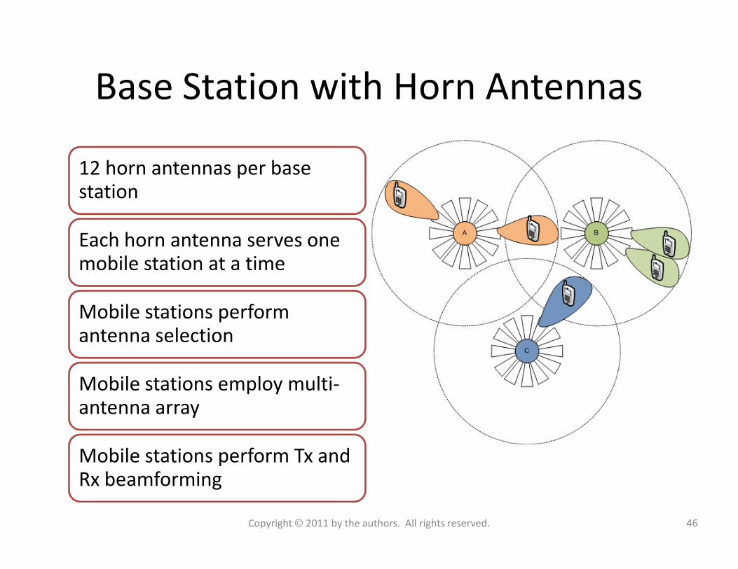
Base Station with Horn Antennas
12 horn antennas per base station
Each horn antenna serves one mobile station at a time
Mobile stations perform antenna selection
Mobile stations employ multi-antenna array
Mobile stations perform Tx and Rx beamforming
46Copyright 2011 by the authors. All rights reserved.
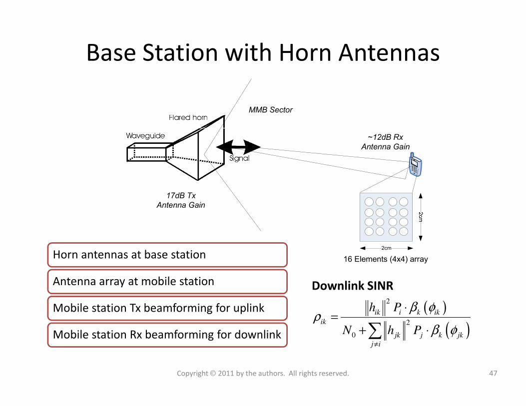
Base Station with Horn Antennas
17dB Tx
Antenna Gain
~12dB Rx
Antenna Gain
MMB Sector
Antenna Gain
16 Elements (4x4) array
2cm
47Copyright 2011 by the authors. All rights reserved.
Horn antennas at base station
Antenna array at mobile station
Mobile station Tx beamforming for uplink
Mobile station Rx beamforming for downlink
( )
( )
2
2
0
ik i k ik
ik
jk j k jk
j i
h P
N h P
β φρ
β φ≠
⋅=
+ ⋅∑
Downlink SINR
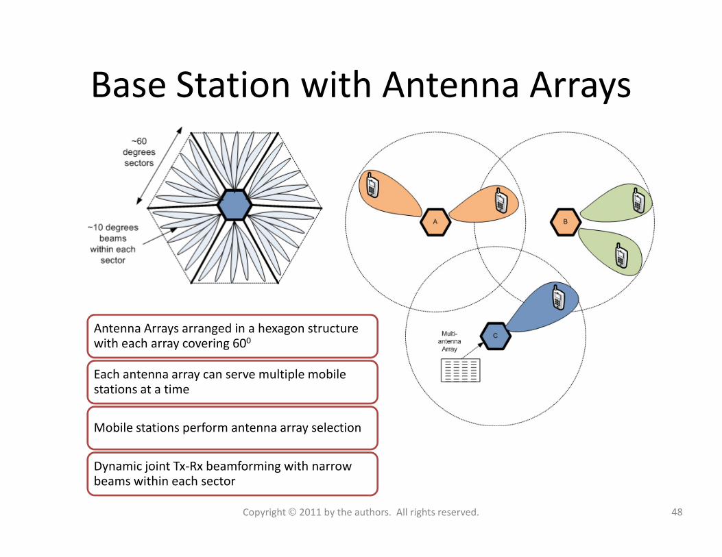
Base Station with Antenna Arrays
Antenna Arrays arranged in a hexagon structure with each array covering 600
Each antenna array can serve multiple mobile stations at a time
Mobile stations perform antenna array selection
Dynamic joint Tx-Rx beamforming with narrow beams within each sector
48Copyright 2011 by the authors. All rights reserved.
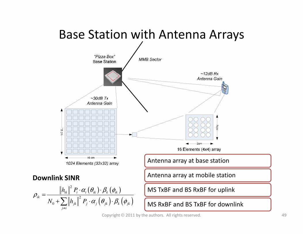
Base Station with Antenna Arrays
49Copyright 2011 by the authors. All rights reserved.
Antenna array at base station
Antenna array at mobile station
MS TxBF and BS RxBF for uplink
MS RxBF and BS TxBF for downlink
Downlink SINR
( ) ( )
( ) ( )
2
2
0
ik i i ik k ik
ik
jk j j jk k jk
j i
h P
N h P
α θ β φρ
α θ β φ≠
⋅ ⋅=
+ ⋅ ⋅∑
Outline• Introduction
– Mobile broadband growth
– The myth of traffic and revenue gap
– The national broadband plan
• mmW spectrum
– History of millimeter wave communications
– Unleashing 3-300GHz spectrum
– LMDS and 70/80/90 GHz bands
• mmW Propagation characteristics
– Free Space Propagation
• MMB air-interface design
– Duplex and multiple access schemes
– Frame Structure
– Channel coding and modulation
• Dynamic beamforming with miniature antennas
– Beamforming fundamentals
– Baseband beamforming
– Analog beamforming
– RF beamforming
– Beamforming in fading channels– Free Space Propagation
– Material penetration loss
– Oxygen and water absorption
– Foliage absorption
– Rain absorption
– Diffraction
– Ground reflection
• mmW Mobile Broadband (MMB) network
architecture
– Stand-alone MMB system
– MMB base station grid
– Hybrid MMB + 4G systems
– Deployment and antenna configuration
– Beamforming in fading channels
• Radio frequency components design and
challenges
– RF transceiver architecture
– MMB RF transceiver requirement
– mmWave Power amplifier
– mmWave LNA
• MMB system performance
– Link budget analysis
– Link Level performance
– Geometry distribution
– System throughput analysis
• Summary
50Copyright 2011 by the authors. All rights reserved.
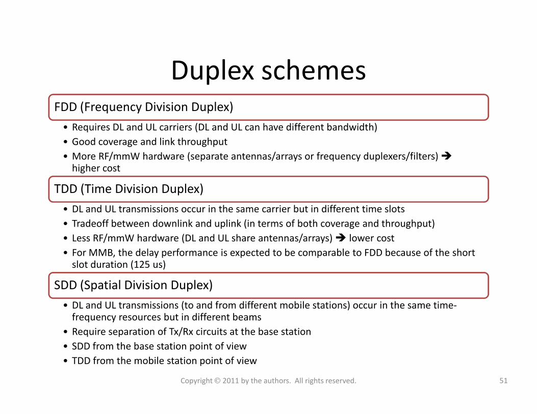
Duplex schemesFDD (Frequency Division Duplex)
• Requires DL and UL carriers (DL and UL can have different bandwidth)
• Good coverage and link throughput
• More RF/mmW hardware (separate antennas/arrays or frequency duplexers/filters) higher cost
TDD (Time Division Duplex)
• DL and UL transmissions occur in the same carrier but in different time slots• DL and UL transmissions occur in the same carrier but in different time slots
• Tradeoff between downlink and uplink (in terms of both coverage and throughput)
• Less RF/mmW hardware (DL and UL share antennas/arrays) lower cost
• For MMB, the delay performance is expected to be comparable to FDD because of the short slot duration (125 us)
SDD (Spatial Division Duplex)
• DL and UL transmissions (to and from different mobile stations) occur in the same time-frequency resources but in different beams
• Require separation of Tx/Rx circuits at the base station
• SDD from the base station point of view
• TDD from the mobile station point of view
51Copyright 2011 by the authors. All rights reserved.
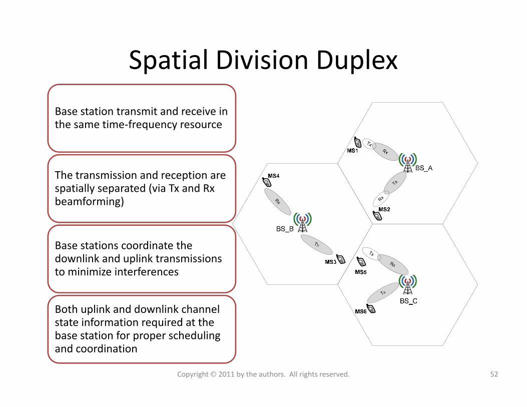
Spatial Division Duplex
Tx
RxR
x
Base station transmit and receive in the same time-frequency resource
The transmission and reception are spatially separated (via Tx and Rx beamforming) R
x
52Copyright 2011 by the authors. All rights reserved.
beamforming)
Base stations coordinate the downlink and uplink transmissions to minimize interferences
Both uplink and downlink channel state information required at the base station for proper scheduling and coordination
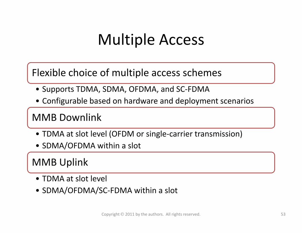
Multiple Access
Flexible choice of multiple access schemes
• Supports TDMA, SDMA, OFDMA, and SC-FDMA
• Configurable based on hardware and deployment scenarios
MMB DownlinkMMB Downlink
• TDMA at slot level (OFDM or single-carrier transmission)
• SDMA/OFDMA within a slot
MMB Uplink
• TDMA at slot level
• SDMA/OFDMA/SC-FDMA within a slot
53Copyright 2011 by the authors. All rights reserved.
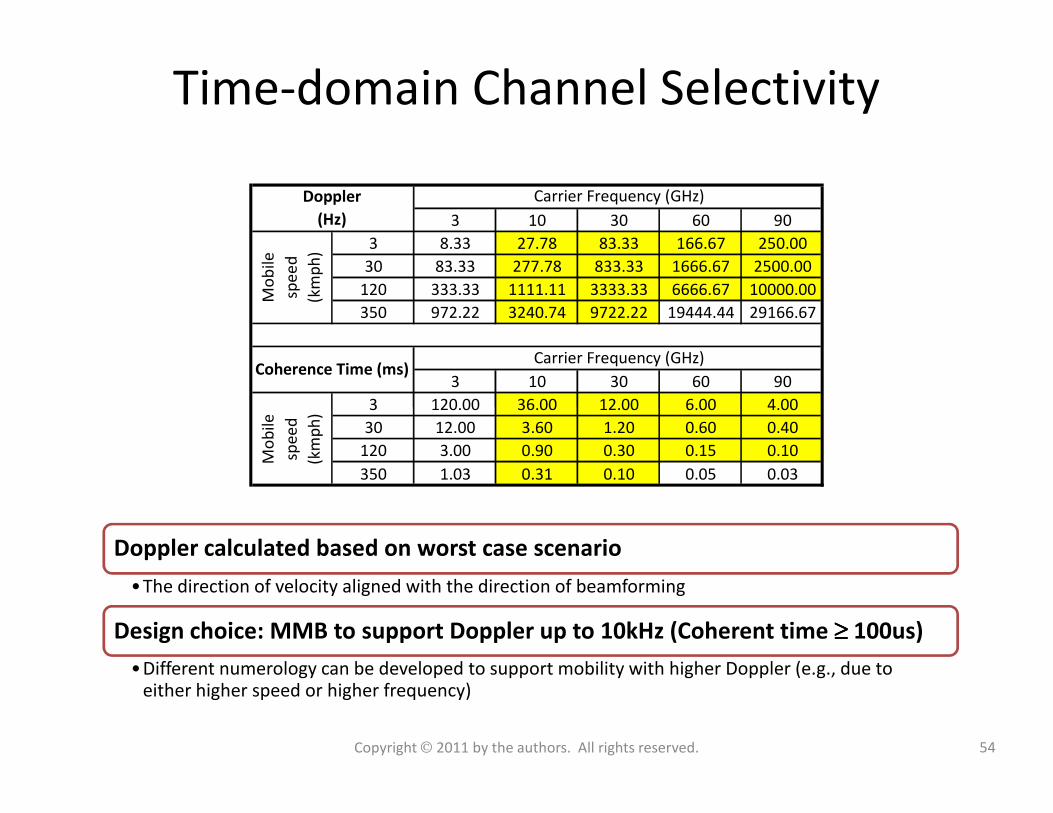
Time-domain Channel Selectivity
3 10 30 60 90
3 8.33 27.78 83.33 166.67 250.00
30 83.33 277.78 833.33 1666.67 2500.00
120 333.33 1111.11 3333.33 6666.67 10000.00
350 972.22 3240.74 9722.22 19444.44 29166.67
3 10 30 60 90
3 120.00 36.00 12.00 6.00 4.00
Doppler
(Hz)
Carrier Frequency (GHz)
Mo
bile
spe
ed
(km
ph
)
Coherence Time (ms)Carrier Frequency (GHz)
Doppler calculated based on worst case scenario
•The direction of velocity aligned with the direction of beamforming
Design choice: MMB to support Doppler up to 10kHz (Coherent time ≥≥≥≥ 100us)
•Different numerology can be developed to support mobility with higher Doppler (e.g., due to either higher speed or higher frequency)
3 120.00 36.00 12.00 6.00 4.00
30 12.00 3.60 1.20 0.60 0.40
120 3.00 0.90 0.30 0.15 0.10
350 1.03 0.31 0.10 0.05 0.03
Mo
bile
spe
ed
(km
ph
)
54Copyright 2011 by the authors. All rights reserved.
Frequency-domain Channel Selectivity
Millimeter wave propagation characteristics in a mobile communication environment is not well understood
• Most literature reports RMS delay ~ 10ns and maximum delay spread ~ 100ns
• For cellular waves in a 1km cell, the maximum delay spread should mostly be within a few microseconds (1km ~ 3.3us)
• High gain antennas and beamforming of mmW should significantly reduce the delay spread
• As the cell size gets smaller, LOS will occur more frequently, which also reduce the delay • As the cell size gets smaller, LOS will occur more frequently, which also reduce the delay spread and frequency selectivity
Best guesstimate (at this point) is the maximum delay spread of mmW in a mobile environment should mostly be less than 1us for cell radius < 1km
• Equivalent to 333-meter difference among the travel distance of the rays that arrive at the receiver via the narrow beams formed by the transmitter antennas and receiver antennas
Design choice: MMB to support delay spread up to 1us (Coherent bandwidth ≥ 1MHz)
55Copyright 2011 by the authors. All rights reserved.
OFDM/Single-Carrier numerology
Subcarrier spacing and Cyclic Prefix
• Two important design parameters that pertain to many issues
• Wide subcarrier spacing leads to sensitivity to frequency selectivity, and high CP overhead
• Narrow subcarrier spacing leads to sensitivity to Doppler, frequency offset, and require more expensive VCOs and VCXOs
• Larger CP provides protection against inter-symbol-interference due to multipath channel
• Shorter CP incurs less overhead and leads to a more efficient system design• Shorter CP incurs less overhead and leads to a more efficient system design
Subcarrier spacing = 270 kHz
• OFDM/SC symbol length is ~3.7 us
• Possible to support a coherence time of 100 us (350kmph @ 30 GHz, 120kmph @ 90 GHz)
1/8 and 1/4 CP
• Both 1/8 and 1/4 CP are supported
• 1/8 CP = 463 ns, low overhead
• 1/4 CP = 926 ns, ensure good performance in deployment with larger cells (1~5 km)
56Copyright 2011 by the authors. All rights reserved.
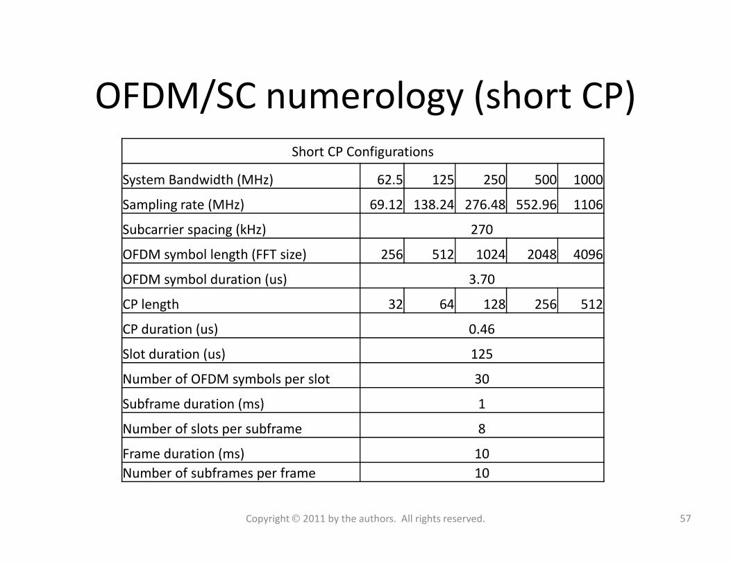
OFDM/SC numerology (short CP)
Short CP Configurations
System Bandwidth (MHz) 62.5 125 250 500 1000
Sampling rate (MHz) 69.12 138.24 276.48 552.96 1106
Subcarrier spacing (kHz) 270
OFDM symbol length (FFT size) 256 512 1024 2048 4096
OFDM symbol duration (us) 3.70OFDM symbol duration (us) 3.70
CP length 32 64 128 256 512
CP duration (us) 0.46
Slot duration (us) 125
Number of OFDM symbols per slot 30
Subframe duration (ms) 1
Number of slots per subframe 8
Frame duration (ms) 10
Number of subframes per frame 10
57Copyright 2011 by the authors. All rights reserved.
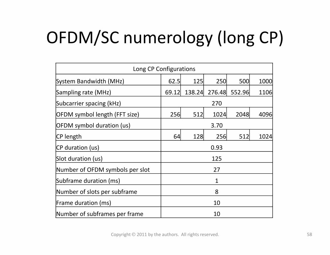
OFDM/SC numerology (long CP)
Long CP Configurations
System Bandwidth (MHz) 62.5 125 250 500 1000
Sampling rate (MHz) 69.12 138.24 276.48 552.96 1106
Subcarrier spacing (kHz) 270
OFDM symbol length (FFT size) 256 512 1024 2048 4096
OFDM symbol duration (us) 3.70OFDM symbol duration (us) 3.70
CP length 64 128 256 512 1024
CP duration (us) 0.93
Slot duration (us) 125
Number of OFDM symbols per slot 27
Subframe duration (ms) 1
Number of slots per subframe 8
Frame duration (ms) 10
Number of subframes per frame 10
58Copyright 2011 by the authors. All rights reserved.
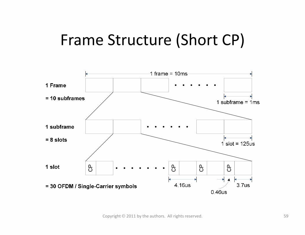
Frame Structure (Short CP)
CP
CP
CP
CP
59Copyright 2011 by the authors. All rights reserved.
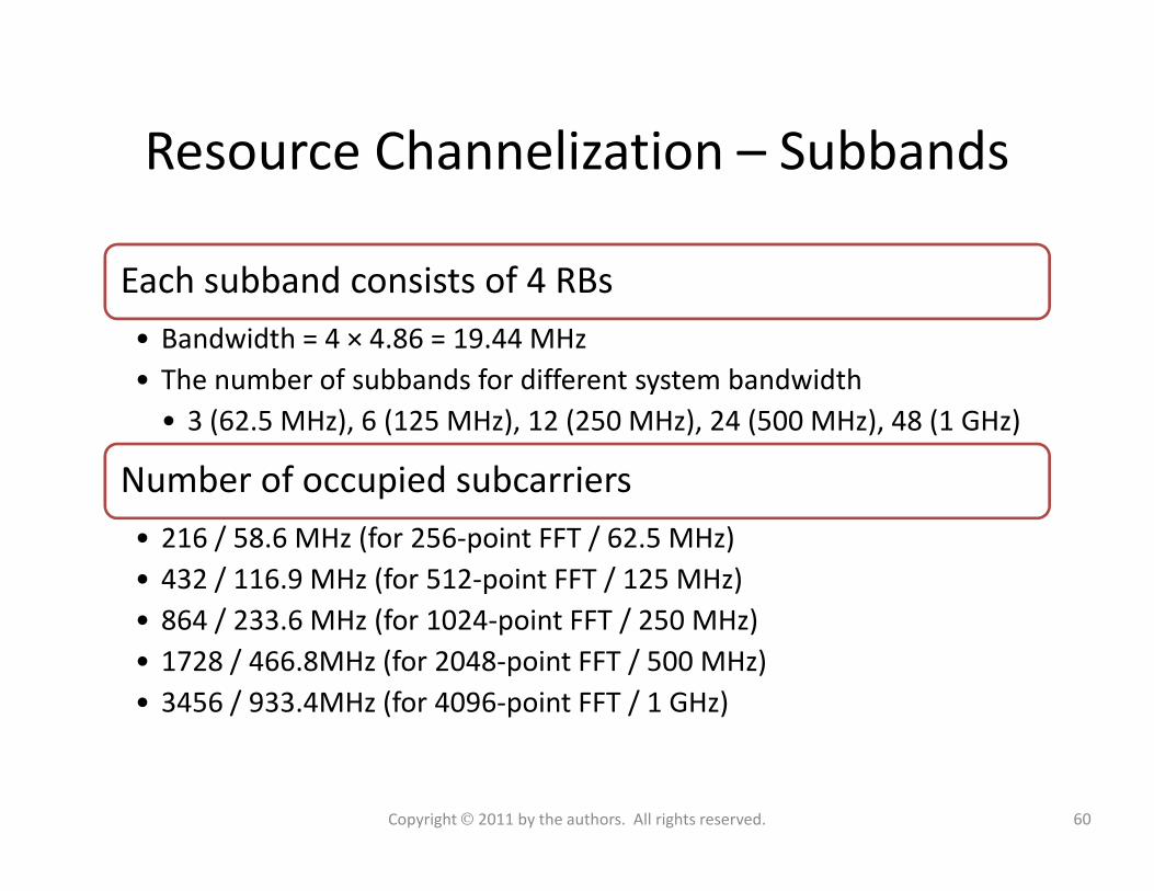
Resource Channelization – Subbands
Each subband consists of 4 RBs
• Bandwidth = 4 × 4.86 = 19.44 MHz
• The number of subbands for different system bandwidth
• 3 (62.5 MHz), 6 (125 MHz), 12 (250 MHz), 24 (500 MHz), 48 (1 GHz)
Number of occupied subcarriers
• 216 / 58.6 MHz (for 256-point FFT / 62.5 MHz)
• 432 / 116.9 MHz (for 512-point FFT / 125 MHz)
• 864 / 233.6 MHz (for 1024-point FFT / 250 MHz)
• 1728 / 466.8MHz (for 2048-point FFT / 500 MHz)
• 3456 / 933.4MHz (for 4096-point FFT / 1 GHz)
60Copyright 2011 by the authors. All rights reserved.
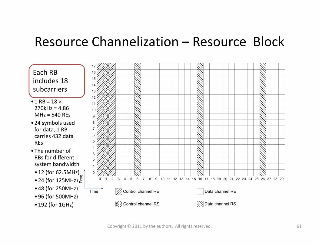
Resource Channelization – Resource Block
8
9
10
11
12
13
14
15
16
17
Each RB includes 18 subcarriers
•1 RB = 18 ×270kHz = 4.86 MHz = 540 REs
•24 symbols used
Time
Freq
0 1 2 3 4 5 6 7 8 9 10 11 12 13 14 15 16 17 18 19 20 21 22 23 24 25 26 27 28 29
0
1
2
3
4
5
6
7
8
Control channel RE
Control channel RS
Data channel RE
Data channel RS
•24 symbols used for data, 1 RB carries 432 data REs
•The number of RBs for different system bandwidth
•12 (for 62.5MHz)
•24 (for 125MHz)
•48 (for 250MHz)
•96 (for 500MHz)
•192 (for 1GHz)
61Copyright 2011 by the authors. All rights reserved.
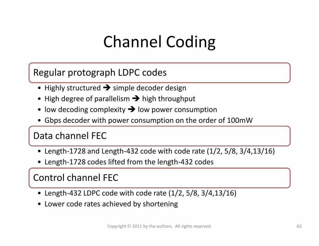
Channel Coding
Regular protograph LDPC codes
• Highly structured simple decoder design
• High degree of parallelism high throughput
• low decoding complexity low power consumption
• Gbps decoder with power consumption on the order of 100mW• Gbps decoder with power consumption on the order of 100mW
Data channel FEC
• Length-1728 and Length-432 code with code rate (1/2, 5/8, 3/4,13/16)
• Length-1728 codes lifted from the length-432 codes
Control channel FEC
• Length-432 LDPC code with code rate (1/2, 5/8, 3/4,13/16)
• Lower code rates achieved by shortening
62Copyright 2011 by the authors. All rights reserved.
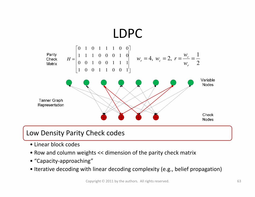
LDPC0 1 0 1 1 1 0 0
1 1 1 0 0 0 1 0
0 0 1 0 0 1 1 1
1 0 0 1 1 0 0 1
H
=
14, 2,
2
cr c
r
ww w r
w= = = =
Low Density Parity Check codes
• Linear block codes
• Row and column weights << dimension of the parity check matrix
• “Capacity-approaching”
• Iterative decoding with linear decoding complexity (e.g., belief propagation)
63Copyright 2011 by the authors. All rights reserved.
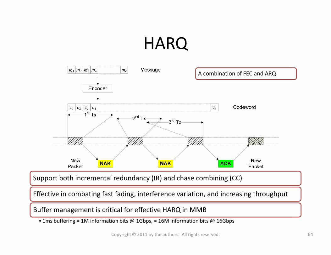
HARQ
A combination of FEC and ARQ
Support both incremental redundancy (IR) and chase combining (CC)
Effective in combating fast fading, interference variation, and increasing throughput
Buffer management is critical for effective HARQ in MMB
• 1ms buffering = 1M information bits @ 1Gbps, = 16M information bits @ 16Gbps
64Copyright 2011 by the authors. All rights reserved.
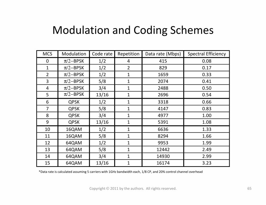
Modulation and Coding Schemes
MCS Modulation Code rate Repetition Data rate (Mbps) Spectral Efficiency
0 π/2−BPSK 1/2 4 415 0.08
1 π/2−BPSK 1/2 2 829 0.17
2 π/2−BPSK 1/2 1 1659 0.33
3 π/2−BPSK 5/8 1 2074 0.41
4 π/2−BPSK 3/4 1 2488 0.50
5 π/2−BPSK 13/16 1 2696 0.54
6 QPSK 1/2 1 3318 0.66
*Data rate is calculated assuming 5 carriers with 1GHz bandwidth each, 1/8 CP, and 20% control channel overhead
6 QPSK 1/2 1 3318 0.66
7 QPSK 5/8 1 4147 0.83
8 QPSK 3/4 1 4977 1.00
9 QPSK 13/16 1 5391 1.08
10 16QAM 1/2 1 6636 1.33
11 16QAM 5/8 1 8294 1.66
12 64QAM 1/2 1 9953 1.99
13 64QAM 5/8 1 12442 2.49
14 64QAM 3/4 1 14930 2.99
15 64QAM 13/16 1 16174 3.23
65Copyright 2011 by the authors. All rights reserved.
Outline• Introduction
– Mobile broadband growth
– The myth of traffic and revenue gap
– The national broadband plan
• mmW spectrum
– History of millimeter wave communications
– Unleashing 3-300GHz spectrum
– LMDS and 70/80/90 GHz bands
• mmW Propagation characteristics
– Free Space Propagation
• MMB air-interface design
– Duplex and multiple access schemes
– Frame Structure
– Channel coding and modulation
• Dynamic beamforming with miniature antennas
– Beamforming fundamentals
– Baseband beamforming
– Analog beamforming
– RF beamforming
– Beamforming in fading channels– Free Space Propagation
– Material penetration loss
– Oxygen and water absorption
– Foliage absorption
– Rain absorption
– Diffraction
– Ground reflection
• mmW Mobile Broadband (MMB) network
architecture
– Stand-alone MMB system
– MMB base station grid
– Hybrid MMB + 4G systems
– Deployment and antenna configuration
– Beamforming in fading channels
• Radio frequency components design and
challenges
– RF transceiver architecture
– MMB RF transceiver requirement
– mmWave Power amplifier
– mmWave LNA
• MMB system performance
– Link budget analysis
– Link Level performance
– Geometry distribution
– System throughput analysis
• Summary
66Copyright 2011 by the authors. All rights reserved.
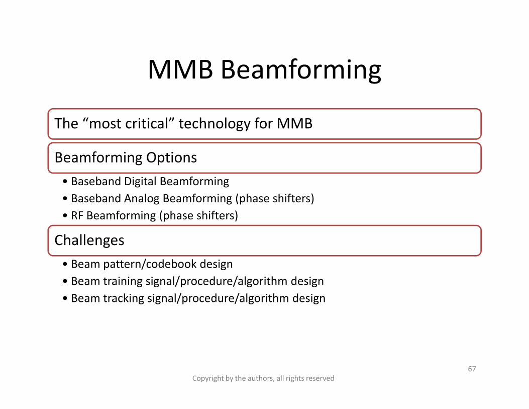
MMB Beamforming
The “most critical” technology for MMB
Beamforming Options
• Baseband Digital Beamforming
• Baseband Analog Beamforming (phase shifters)• Baseband Analog Beamforming (phase shifters)
• RF Beamforming (phase shifters)
Challenges
• Beam pattern/codebook design
• Beam training signal/procedure/algorithm design
• Beam tracking signal/procedure/algorithm design
67
Copyright by the authors, all rights reserved
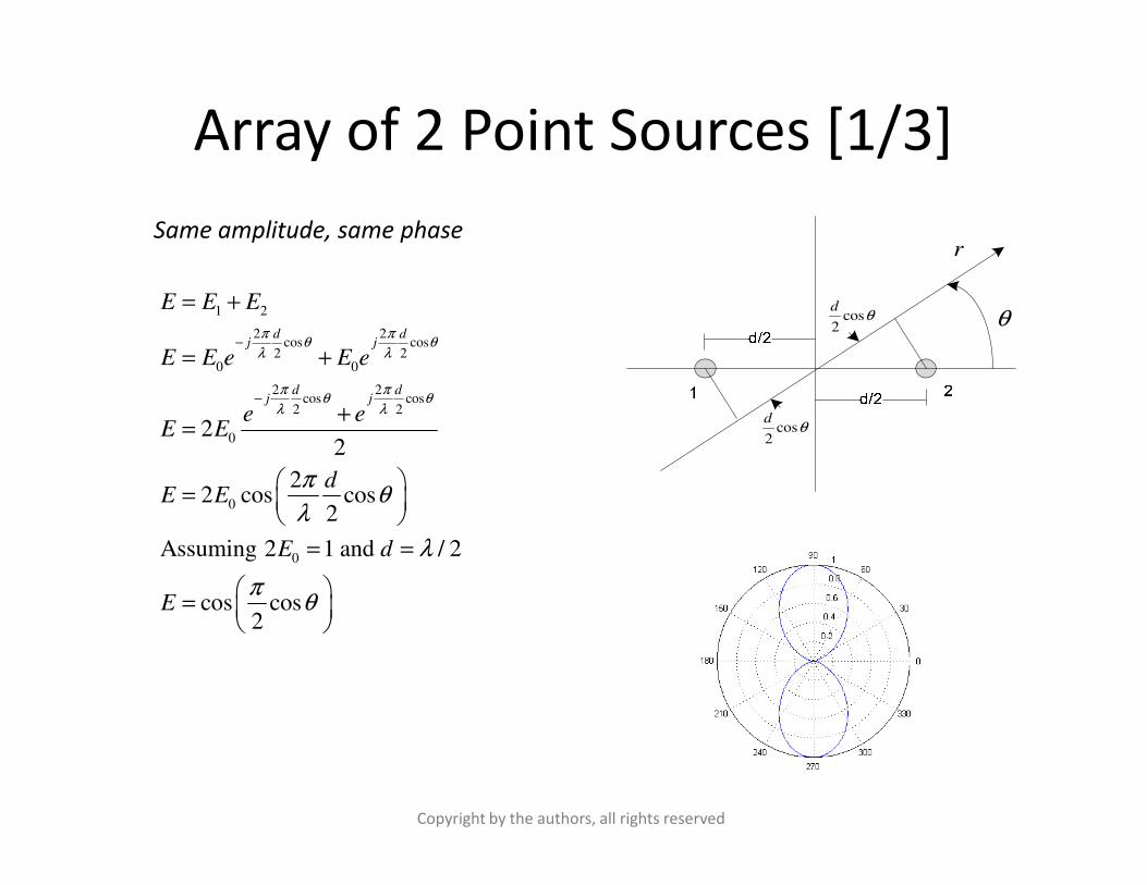
Array of 2 Point Sources [1/3]
θ
r
cos2
dθ
cos2
dθ
1 2
2 2cos cos
2 20 0
2 2cos cos
2 2
022
d dj j
d dj j
E E E
E E e E e
e eE E
π πθ θ
λ λ
π πθ θ
λ λ
−
−
= +
= +
+=
Same amplitude, same phase
20
0
0
2
22 cos cos
2
Assuming 2 1 and / 2
cos cos2
dE E
E d
E
πθ
λ
λ
πθ
=
= =
=
Copyright by the authors, all rights reserved
Array of 2 Point Sources [2/3]
θ
r
cos2
dθ
cos2
dθ
1 2
2 2cos cos
2 20 0
2 2cos cos
2 2
022
d dj j
d dj j
E E E
E E e E e
e eE E
π πθ θ
λ λ
π πθ θ
λ λ
−
−
= −
= −
−=
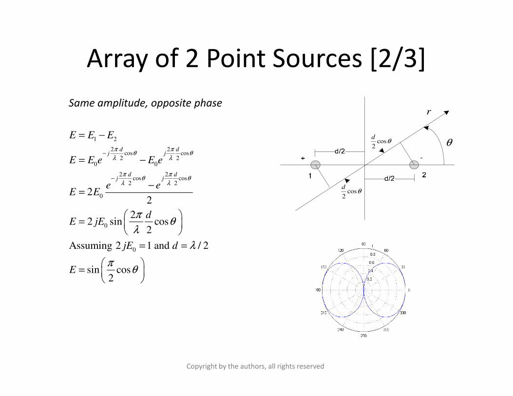
Same amplitude, opposite phase
20
0
0
2
22 sin cos
2
Assuming 2 1 and / 2
sin cos2
dE jE
jE d
E
πθ
λ
λ
πθ
=
= =
=
Copyright by the authors, all rights reserved
Array of 2 Point Sources [2/3]
1 2
2 2cos cos
2 2 2 2
0 0
2 2cos cos
2 2 2 2
022
d dj j
d dj j
E E E
E E e E e
e eE E
π δ π δθ θ
λ λ
π δ π δθ θ
λ λ
− + +
− + +
= +
= +
+=
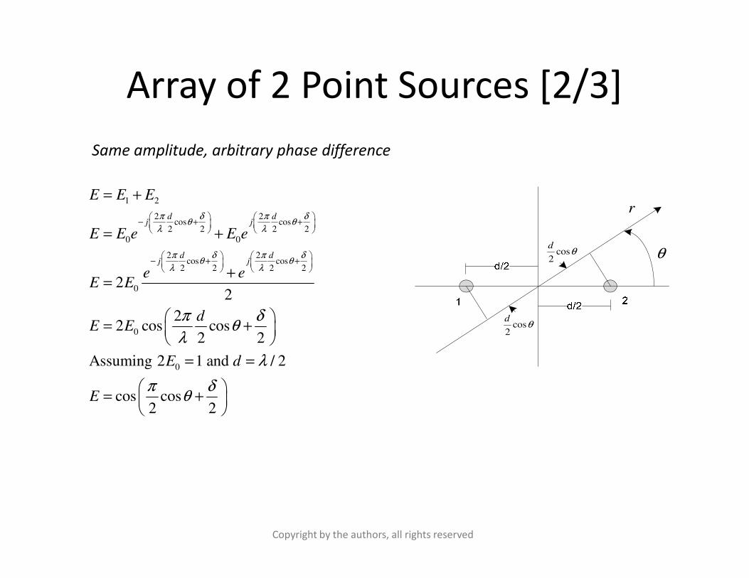
Same amplitude, arbitrary phase difference
θ
r
cos2
dθ
0
0
0
22
22 cos cos
2 2
Assuming 2 1 and / 2
cos cos2 2
E E
dE E
E d
E
π δθ
λ
λ
π δθ
=
= +
= =
= +
Copyright by the authors, all rights reserved
cos2
dθ
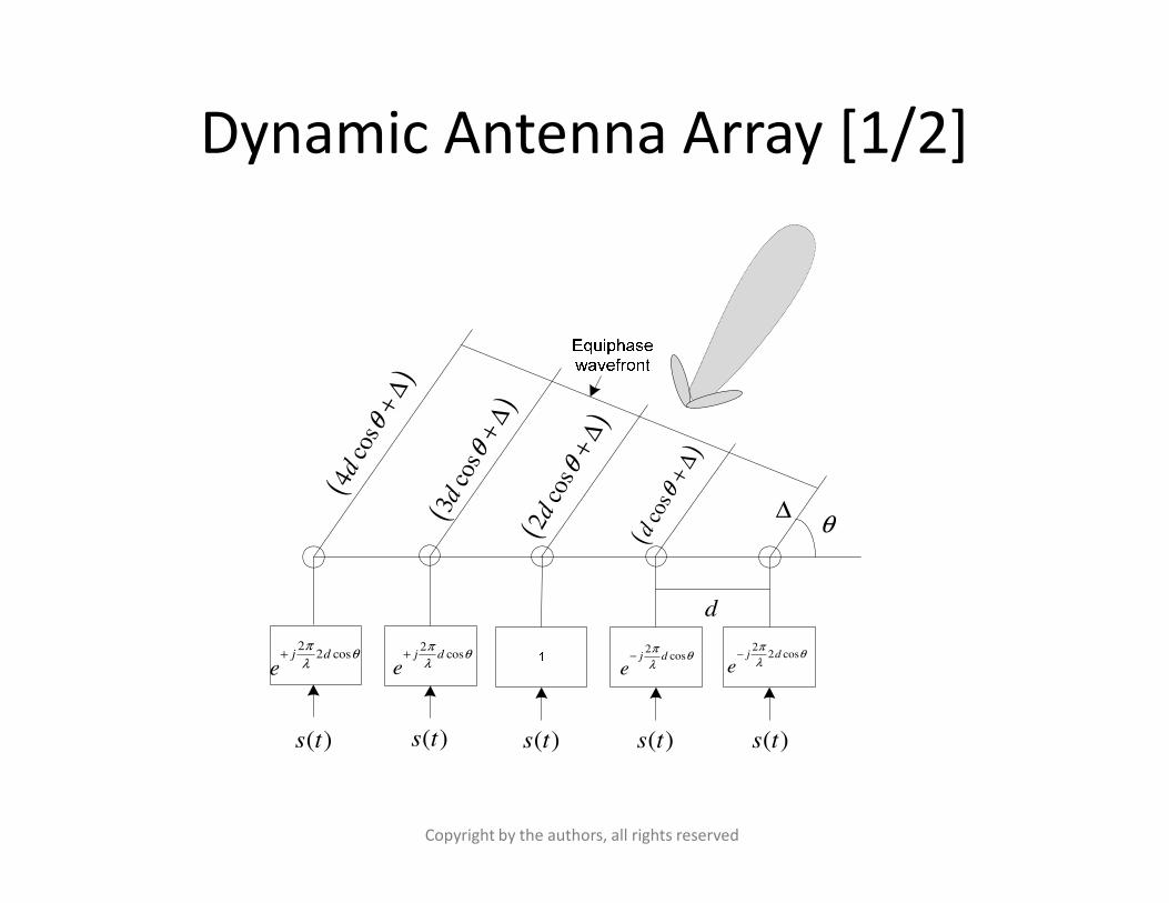
Dynamic Antenna Array [1/2]
)
)+
∆
)
3co
sθ
+∆
)
4co
sθ
+∆
θ(
)
cos
d
θ
+∆
d
22 cosj d
e
πθ
λ−2
cosj d
e
πθ
λ−
( )s t( )s t( )s t( )s t
22 cosj d
e
πθ
λ+
2cosj d
e
πθ
λ+
( )s t
∆(2
cos
d
θ+
∆
(3co
sd
θ
(4co
sd
Copyright by the authors, all rights reserved
Dynamic Antenna Array [2/2]
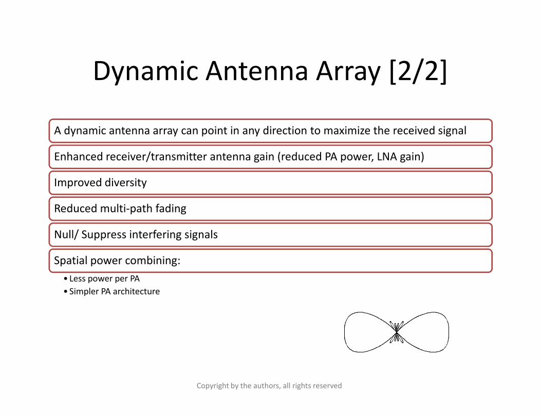
A dynamic antenna array can point in any direction to maximize the received signal
Enhanced receiver/transmitter antenna gain (reduced PA power, LNA gain)
Improved diversity
Reduced multi-path fadingReduced multi-path fading
Null/ Suppress interfering signals
Spatial power combining:
• Less power per PA
• Simpler PA architecture
Copyright by the authors, all rights reserved
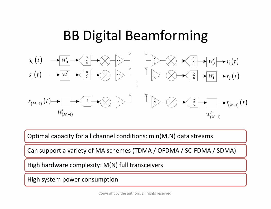
BB Digital Beamforming
( ) ( )1Ms t
− ( ) ( )1Nr t
−
( )1s t 1
tw
1
rw ( )2r t
( )0s t 0
tw0
rw ( )1r t
M
Optimal capacity for all channel conditions: min(M,N) data streams
Can support a variety of MA schemes (TDMA / OFDMA / SC-FDMA / SDMA)
High hardware complexity: M(N) full transceivers
High system power consumption
( ) ( )1M − ( ) ( )1Nr t
−
( )1
t
Mw
−( )1
r
Nw
−
Copyright by the authors, all rights reserved
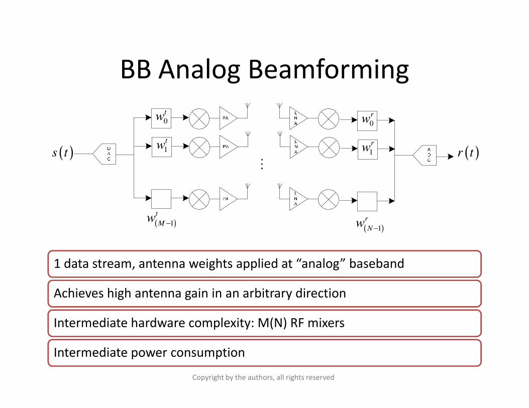
BB Analog Beamforming
1
tw
1
rw( )s t
0
tw0
rw
( )r tM
1 data stream, antenna weights applied at “analog” baseband
Achieves high antenna gain in an arbitrary direction
Intermediate hardware complexity: M(N) RF mixers
Intermediate power consumption
( )1
t
Mw
−( )1
r
Nw
−
Copyright by the authors, all rights reserved
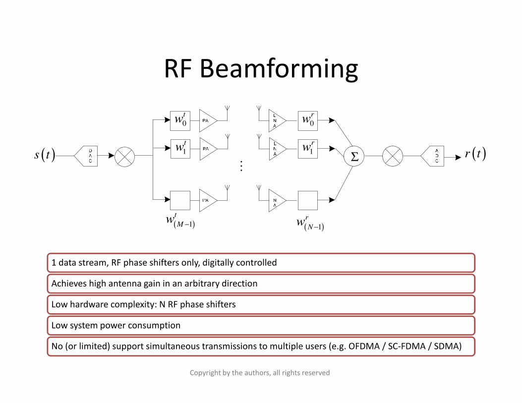
RF Beamforming
1
rw( )s t
0
rw
( )r tM
1
tw
0
tw
Σ
1 data stream, RF phase shifters only, digitally controlled
Achieves high antenna gain in an arbitrary direction
Low hardware complexity: N RF phase shifters
Low system power consumption
No (or limited) support simultaneous transmissions to multiple users (e.g. OFDMA / SC-FDMA / SDMA)
( )1
r
Nw
−( )1
t
Mw
−
Copyright by the authors, all rights reserved
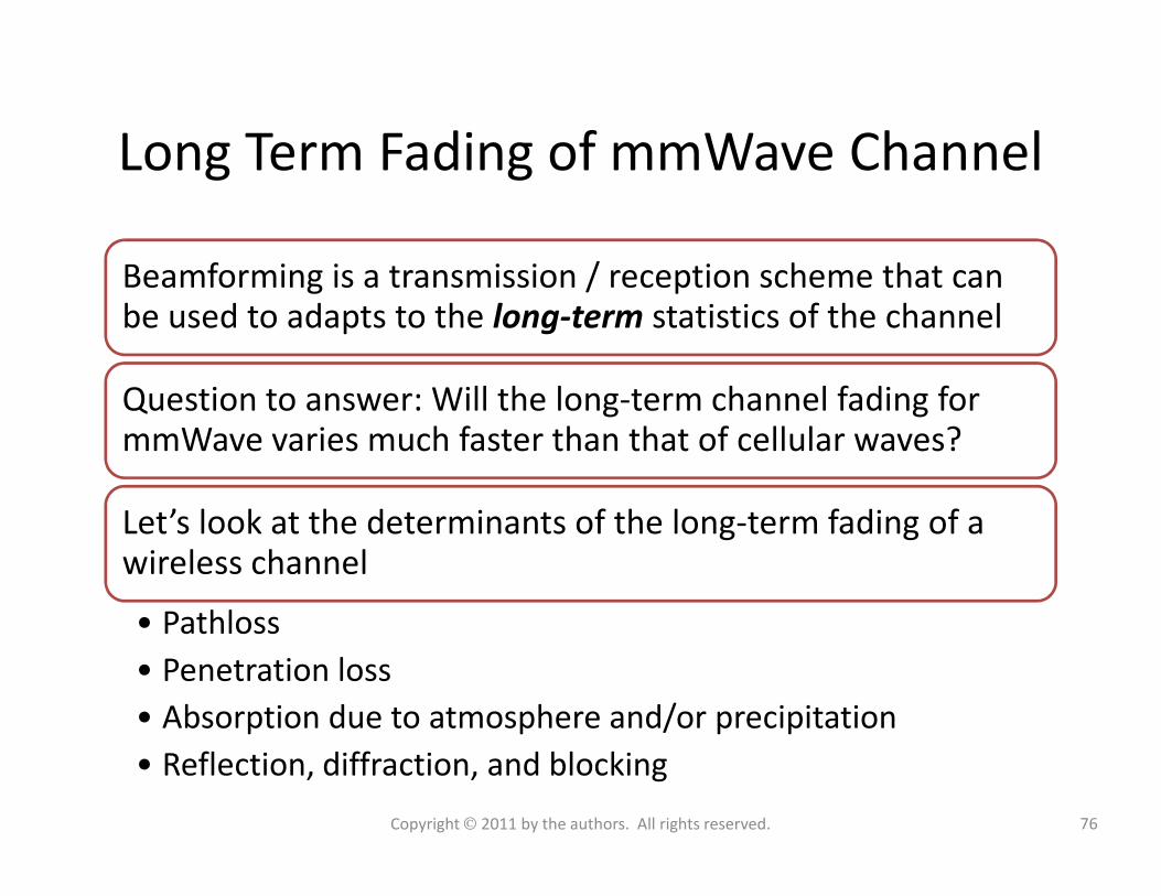
Long Term Fading of mmWave Channel
Beamforming is a transmission / reception scheme that can be used to adapts to the long-term statistics of the channel
Question to answer: Will the long-term channel fading for mmWave varies much faster than that of cellular waves?mmWave varies much faster than that of cellular waves?
Let’s look at the determinants of the long-term fading of a wireless channel
• Pathloss
• Penetration loss
• Absorption due to atmosphere and/or precipitation
• Reflection, diffraction, and blocking
76Copyright 2011 by the authors. All rights reserved.
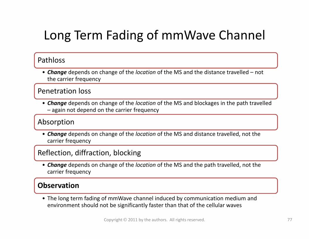
Long Term Fading of mmWave Channel
Pathloss
• Change depends on change of the location of the MS and the distance travelled – not the carrier frequency
Penetration loss
• Change depends on change of the location of the MS and blockages in the path travelled – again not depend on the carrier frequency
AbsorptionAbsorption
• Change depends on change of the location of the MS and distance travelled, not the carrier frequency
Reflection, diffraction, blocking
• Change depends on change of the location of the MS and the path travelled, not the carrier frequency
Observation
• The long term fading of mmWave channel induced by communication medium and environment should not be significantly faster than that of the cellular waves
77Copyright 2011 by the authors. All rights reserved.
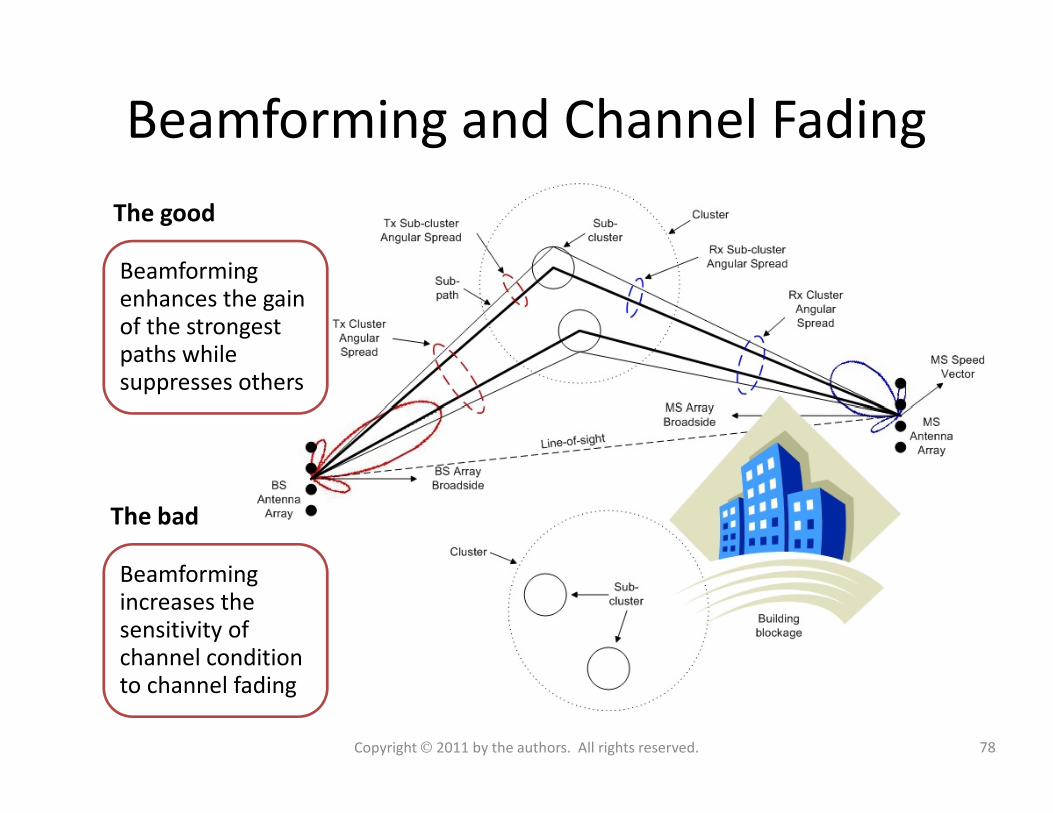
Beamforming and Channel Fading
Beamformingenhances the gain of the strongest paths while suppresses others
The good
Beamformingincreases the sensitivity of channel condition to channel fading
The bad
78Copyright 2011 by the authors. All rights reserved.
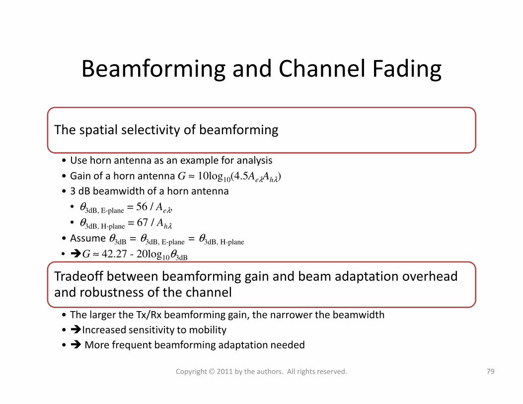
Beamforming and Channel Fading
The spatial selectivity of beamforming
• Use horn antenna as an example for analysis
• Gain of a horn antenna G ≈ 10log10(4.5AeλAhλ)
• 3 dB beamwidth of a horn antenna
• θ = 56 / A , • θ3dB, E-plane = 56 / Aeλ,
• θ3dB, H-plane = 67 / Ahλ
• Assume θ3dB = θ3dB, E-plane = θ3dB, H-plane
• G ≈ 42.27 - 20log10θ3dB
Tradeoff between beamforming gain and beam adaptation overhead and robustness of the channel
• The larger the Tx/Rx beamforming gain, the narrower the beamwidth
• Increased sensitivity to mobility
• More frequent beamforming adaptation needed
79Copyright 2011 by the authors. All rights reserved.
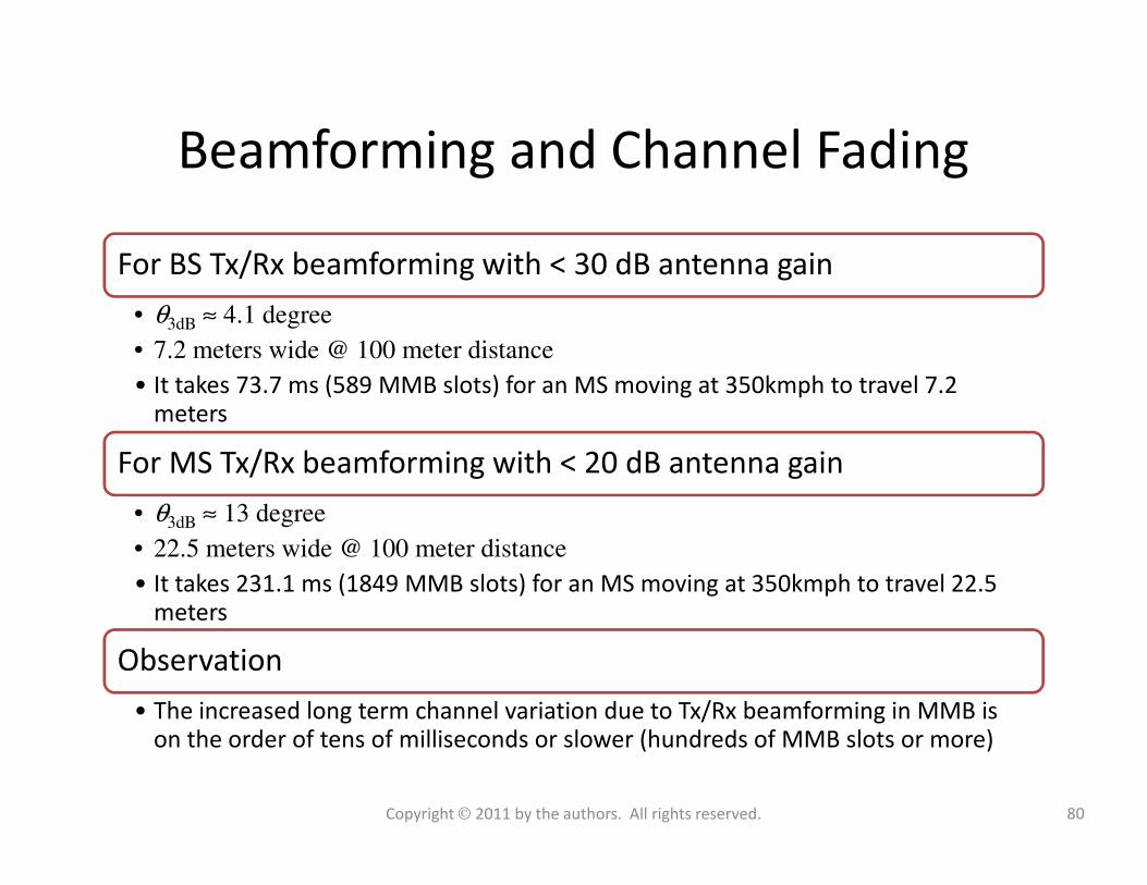
Beamforming and Channel Fading
For BS Tx/Rx beamforming with < 30 dB antenna gain
• θ3dB ≈ 4.1 degree
• 7.2 meters wide @ 100 meter distance
• It takes 73.7 ms (589 MMB slots) for an MS moving at 350kmph to travel 7.2 meters
For MS Tx/Rx beamforming with < 20 dB antenna gainFor MS Tx/Rx beamforming with < 20 dB antenna gain
• θ3dB ≈ 13 degree
• 22.5 meters wide @ 100 meter distance
• It takes 231.1 ms (1849 MMB slots) for an MS moving at 350kmph to travel 22.5 meters
Observation
• The increased long term channel variation due to Tx/Rx beamforming in MMB is on the order of tens of milliseconds or slower (hundreds of MMB slots or more)
80Copyright 2011 by the authors. All rights reserved.
Outline• Introduction
– Mobile broadband growth
– The myth of traffic and revenue gap
– The national broadband plan
• mmW spectrum
– History of millimeter wave communications
– Unleashing 3-300GHz spectrum
– LMDS and 70/80/90 GHz bands
• mmW Propagation characteristics
– Free Space Propagation
• MMB air-interface design
– Duplex and multiple access schemes
– Frame Structure
– Channel coding and modulation
• Dynamic beamforming with miniature antennas
– Beamforming fundamentals
– Baseband beamforming
– Analog beamforming
– RF beamforming
– Beamforming in fading channels– Free Space Propagation
– Material penetration loss
– Oxygen and water absorption
– Foliage absorption
– Rain absorption
– Diffraction
– Ground reflection
• mmW Mobile Broadband (MMB) network
architecture
– Stand-alone MMB system
– MMB base station grid
– Hybrid MMB + 4G systems
– Deployment and antenna configuration
– Beamforming in fading channels
• Radio frequency components design and
challenges
– RF transceiver architecture
– MMB RF transceiver requirement
– mmWave Power amplifier
– mmWave LNA
• MMB system performance
– Link budget analysis
– Link Level performance
– Geometry distribution
– System throughput analysis
• Summary
81Copyright 2011 by the authors. All rights reserved.
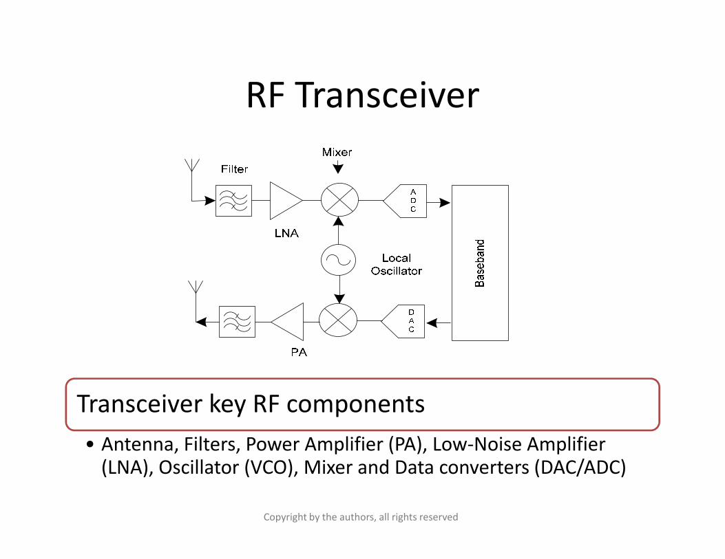
RF Transceiver
Transceiver key RF components
• Antenna, Filters, Power Amplifier (PA), Low-Noise Amplifier (LNA), Oscillator (VCO), Mixer and Data converters (DAC/ADC)
Copyright by the authors, all rights reserved
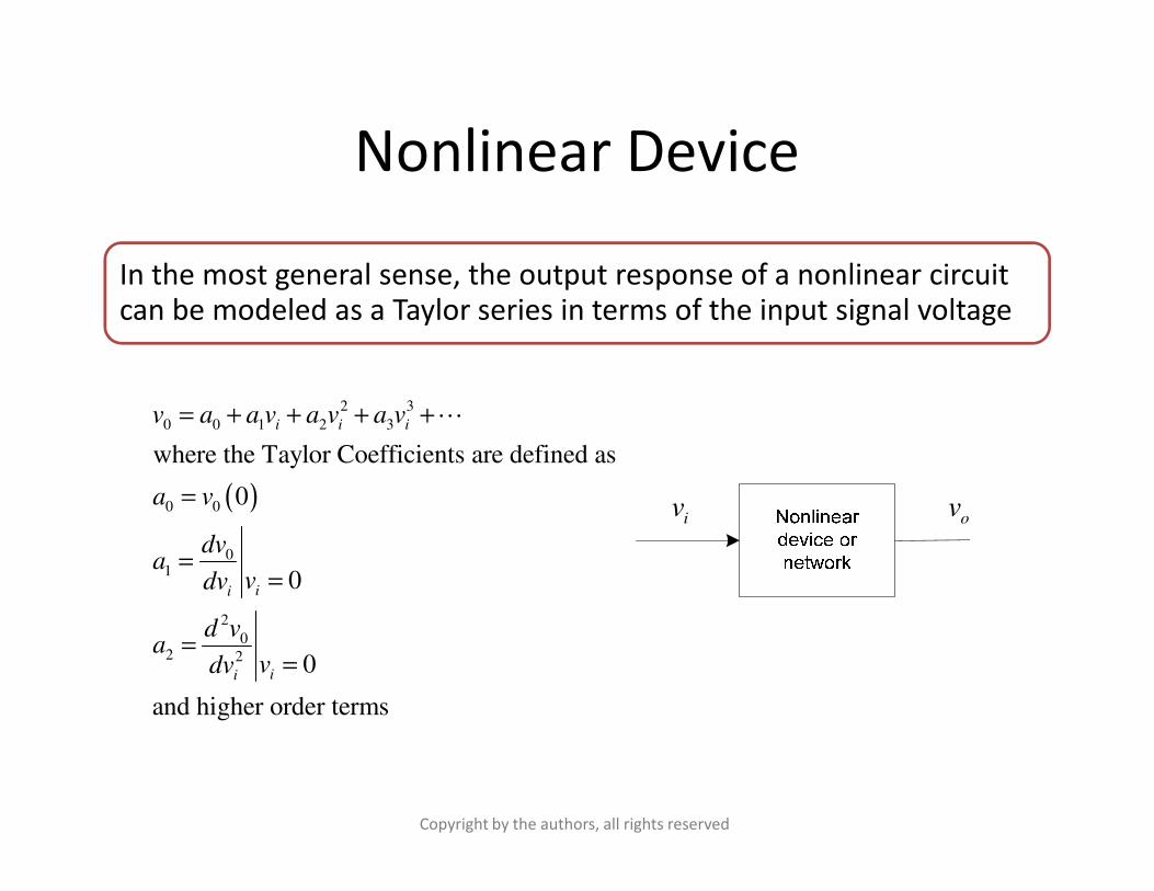
Nonlinear Device
In the most general sense, the output response of a nonlinear circuit can be modeled as a Taylor series in terms of the input signal voltage
2 3
0 0 1 2 3
where the Taylor Coefficients are defined as
i i iv a a v a v a v= + + + +L
( )0 0
01
2
02 2
where the Taylor Coefficients are defined as
0
0
0
and higher order terms
ii
ii
a v
dva
vdv
d va
vdv
=
==
==
iv ov
Copyright by the authors, all rights reserved
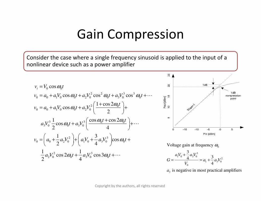
Gain Compression
Consider the case where a single frequency sinusoid is applied to the input of a nonlinear device such as a power amplifier
0 0
2 2 3 3
0 0 1 0 0 2 0 0 3 0 0
cos
cos cos cos
iv V t
v a a V t a V t a V t
ω
ω ω ω
ω
=
= + + + +
+
L
2 00 0 1 0 0 2 0
3 3 0 03 0 0 3 0
2 3
0 0 2 0 1 0 3 0 0
2
2 0 0 3
1 cos 2cos
2
cos cos 21cos
2 4
1 3cos
2 4
1 1cos 2
2 4
tv a a V t a V
t ta V t a V
v a a V a V a V t
a V t a
ωω
ω ωω
ω
ω
+ = + + +
+ + +
= + + + +
+
L
3
0 0cos3V tω +L
0
3
1 0 3 02
1 3 0
0
3
Voltage gain at frequency
334
4
is negative in most practical amplifiers
a V a V
G a a VV
a
ω
+= = +
Copyright by the authors, all rights reserved
Intermodulation Distortion
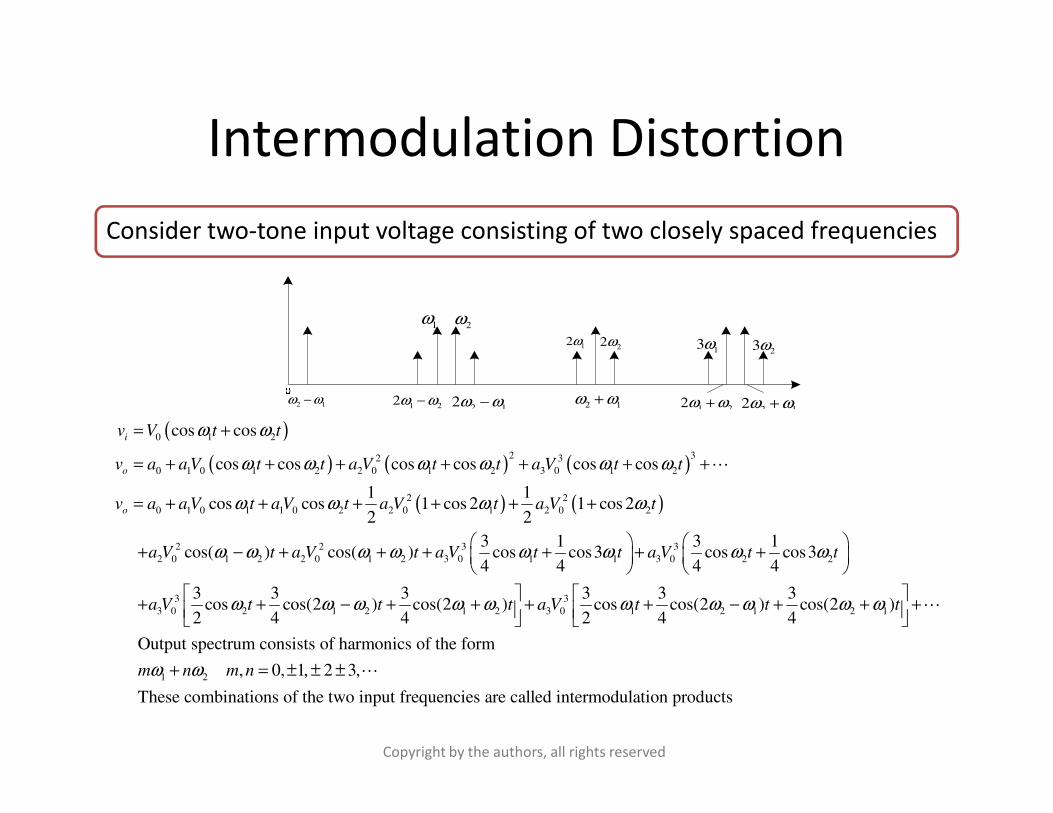
Consider two-tone input voltage consisting of two closely spaced frequencies
2 1ω ω−1 22ω ω−
2 12ω ω−
1ω2ω
12ω22ω
2 1ω ω+
13ω23ω
2 12ω ω+1 22ω ω+
( )
( ) ( ) ( )
( ) ( )
0 1 2
2 32 3
0 1 0 1 2 2 0 1 2 3 0 1 2
2 2
0 1 0 1 1 0 2 2 0 1 2 0 2
2 2 3
2 0 1 2 2 0 1 2 3 0 1
cos cos
cos cos cos cos cos cos
1 1cos cos 1 cos 2 1 cos 2
2 2
3 1cos( ) cos( ) cos cos3
4 4
i
o
o
v V t t
v a a V t t a V t t a V t t
v a a V t a V t a V t a V t
a V t a V t a V t
ω ω
ω ω ω ω ω ω
ω ω ω ω
ω ω ω ω ω ω
= +
= + + + + + + +
= + + + + + +
+ − + + + +
L
3
1 3 0 2 2
3 3
3 0 2 1 2 1 2 3 0 1 2 1 2 1
1 2
3 1cos cos3
4 4
3 3 3 3 3 3cos cos(2 ) cos(2 ) cos cos(2 ) cos(2 )
2 4 4 2 4 4
Output spectrum consists of harmonics of the form
,
t a V t t
a V t t t a V t t t
m n m n
ω ω
ω ω ω ω ω ω ω ω ω ω
ω ω
+ +
+ + − + + + + − + + +
+ =
L
0, 1, 2 3,
These combinations of the two input frequencies are called intermodulation products
± ± ± L
2 1 1 22ω ω−2 12ω ω− 2 1
2 12ω ω+1 22ω ω+
Copyright by the authors, all rights reserved
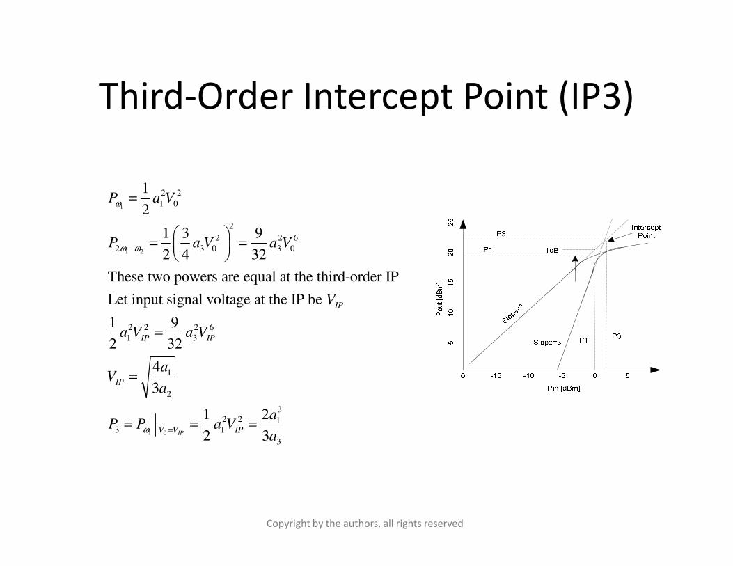
Third-Order Intercept Point (IP3)
1
1 2
2 2
1 0
2
2 2 6
2 3 0 3 0
1
2
1 3 9
2 4 32
These two powers are equal at the third-order IP
P a V
P a V a V
ω
ω ω−
=
= =
1 0
2 2 2 6
1 3
1
2
32 2 1
3 1
3
These two powers are equal at the third-order IP
Let input signal voltage at the IP be
1 9
2 32
4
3
21
2 3IP
IP
IP IP
IP
V V IP
V
a V a V
aV
a
aP P a V
aω =
=
=
= = =
Copyright by the authors, all rights reserved
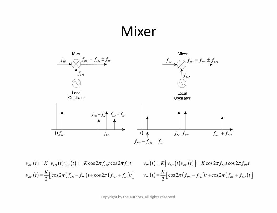
Mixer
IFf
LOf
RF LO IFf f f= ±RFf
LOf
IF RF LOf f f= ±
IFfLOf
LO IFf f+
LO IFf f−
0
RF LO IFf f f− =
RF LOf f+LO
f0 RFf
( ) ( ) ( )
( ) ( ) ( )
cos 2 cos 2
cos 2 cos 22
RF LO IF LO IF
RF LO IF LO IF
v t K v t v t K f t f t
Kv t f f t f f t
π π
π π
= =
= − + +
( ) ( ) ( )
( ) ( ) ( )
cos 2 cos 2
cos 2 cos 22
IF LO RF LO RF
IF RF LO RF LO
v t K v t v t K f t f t
Kv t f f t f f t
π π
π π
= =
= − + +
Copyright by the authors, all rights reserved
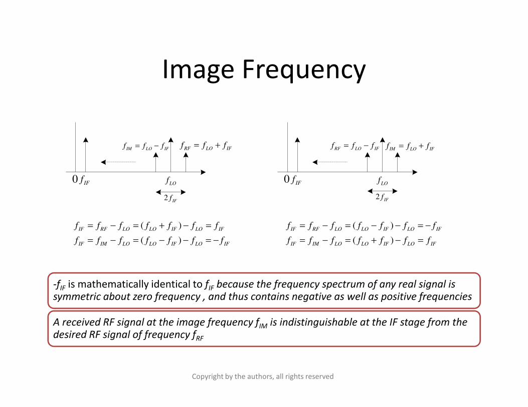
Image Frequency
IFfLOf
RF LO IFf f f= +
0
IM LO IFf f f= −
IFfLOf
IM LO IFf f f= +
0
RF LO IFf f f= −
2IF
f 2IF
f
-fIF is mathematically identical to fIF because the frequency spectrum of any real signal is symmetric about zero frequency , and thus contains negative as well as positive frequencies
A received RF signal at the image frequency fIM is indistinguishable at the IF stage from the desired RF signal of frequency fRF
( )
( )
IF RF LO LO IF LO IF
IF IM LO LO IF LO IF
f f f f f f f
f f f f f f f
= − = + − =
= − = − − = −
( )
( )
IF RF LO LO IF LO IF
IF IM LO LO IF LO IF
f f f f f f f
f f f f f f f
= − = − − = −
= − = + − =
Copyright by the authors, all rights reserved
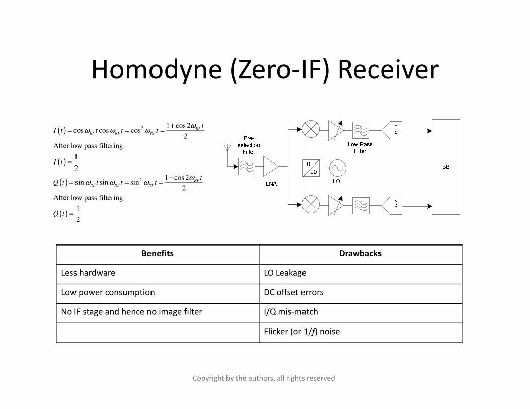
Homodyne (Zero-IF) Receiver
( )
( )
( )
2
2
1 cos 2cos cos cos
2
After low pass filtering
1
2
1 cos 2sin sin sin
2
After low pass filtering
1
RFRF RF RF
RFRF RF RF
tI t t t t
I t
tQ t t t t
ωω ω ω
ωω ω ω
+= = =
=
−= = =
( )1
2Q t =
Copyright by the authors, all rights reserved
Benefits Drawbacks
Less hardware LO Leakage
Low power consumption DC offset errors
No IF stage and hence no image filter I/Q mis-match
Flicker (or 1/f) noise
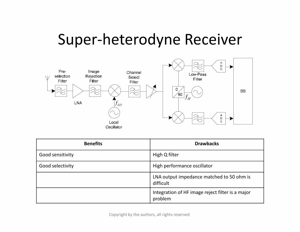
Super-heterodyne Receiver
LOf
IFf
Copyright by the authors, all rights reserved
Benefits Drawbacks
Good sensitivity High Q filter
Good selectivity High performance oscillator
LNA output impedance matched to 50 ohm is
difficult
Integration of HF image reject filter is a major
problem
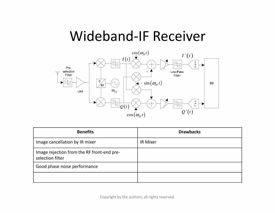
Wideband-IF Receiver
( )sinIF
tω
( )cos IF tω
LOω
( )I t
( )Q t
( )'I t
( )cos IF tω
( )Q t
( )'Q t
Copyright by the authors, all rights reserved
Benefits Drawbacks
Image cancellation by IR mixer IR Mixer
Image rejection from the RF front-end pre-
selection filter
Good phase noise performance
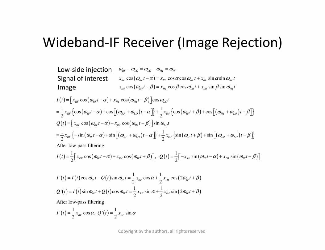
Wideband-IF Receiver (Image Rejection)
( ) ( ) ( )
( ) ( ) ( ) ( )
( ) ( ) ( )
cos cos cos
1 1cos cos cos cos
2 2
cos cos sin
RF RF IM IM LO
RF IF RF LO IM IF IM LO
RF RF IM IM LO
I t x t x t t
x t t x t t
Q t x t x t t
ω α ω β ω
ω α ω ω α ω β ω ω β
ω α ω β ω
= − + −
= − + + − + + + + −
= − + −
Low-side injection
Signal of interest
Image
RF LO LO IM IFω ω ω ω ω− = − =
( )cos cos cos sin sinRF RF RF RF RF RF
x t x t x tω α α ω α ω− = +
( )cos cos cos sin sinIM IM IM IM IM IMx t x t x tω β β ω β ω− = +
( ) ( ) ( )
( ) ( ) ( )
cos cos sin
1 1sin sin sin sin
2 2
RF RF IM IM LO
RF IF RF LO IM IF IM
Q t x t x t t
x t t x t
ω α ω β ω
ω α ω ω α ω β ω
= − + −
= − − + + − + + + ( )
( ) ( ) ( ) ( ) ( ) ( )
( ) ( ) ( ) ( )
( ) ( ) ( )
After low-pass filtering
1 1cos cos , sin sin
2 2
1 1' cos sin cos cos 2
2 2
1 1' sin cos sin sin 2
2 2
LO
RF IF IM IF RF IF IM IF
IF IF RF IM IF
IF IF RF IM
t
I t x t x t Q t x t x t
I t I t t Q t t x x t
Q t I t t Q t t x x
ω β
ω α ω β ω α ω β
ω ω α ω β
ω ω α ω
+ −
= − + + = − − + +
= − = + +
= + = + ( )
( ) ( )
After low-pass filtering
1 1' cos , ' sin
2 2
IF
RF RF
t
I t x Q t x
β
α α
+
= =
Copyright by the authors, all rights reserved
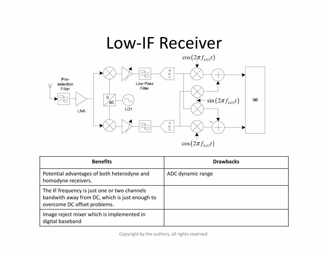
Low-IF Receiver
( )2sin 2 LOf tπ
( )2cos 2 LOf tπ
( )2cos 2 LOf tπ
Copyright by the authors, all rights reserved
Benefits Drawbacks
Potential advantages of both heterodyne and
homodyne receivers.
ADC dynamic range
The IF frequency is just one or two channels
bandwith away from DC, which is just enough to
overcome DC offset problems.
Image reject mixer which is implemented in
digital baseband
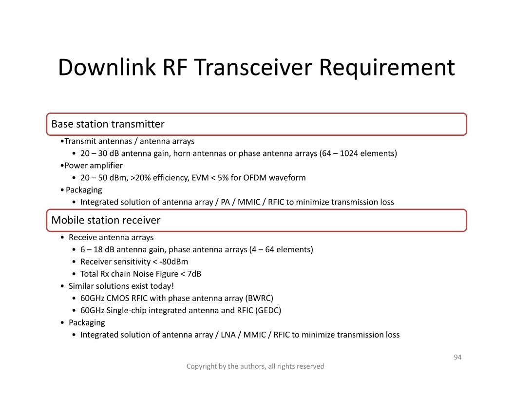
Downlink RF Transceiver Requirement
Base station transmitter
•Transmit antennas / antenna arrays
• 20 – 30 dB antenna gain, horn antennas or phase antenna arrays (64 – 1024 elements)
•Power amplifier
• 20 – 50 dBm, >20% efficiency, EVM < 5% for OFDM waveform
• Packaging
• Integrated solution of antenna array / PA / MMIC / RFIC to minimize transmission loss• Integrated solution of antenna array / PA / MMIC / RFIC to minimize transmission loss
Mobile station receiver
• Receive antenna arrays
• 6 – 18 dB antenna gain, phase antenna arrays (4 – 64 elements)
• Receiver sensitivity < -80dBm
• Total Rx chain Noise Figure < 7dB
• Similar solutions exist today!
• 60GHz CMOS RFIC with phase antenna array (BWRC)
• 60GHz Single-chip integrated antenna and RFIC (GEDC)
• Packaging
• Integrated solution of antenna array / LNA / MMIC / RFIC to minimize transmission loss
94
Copyright by the authors, all rights reserved
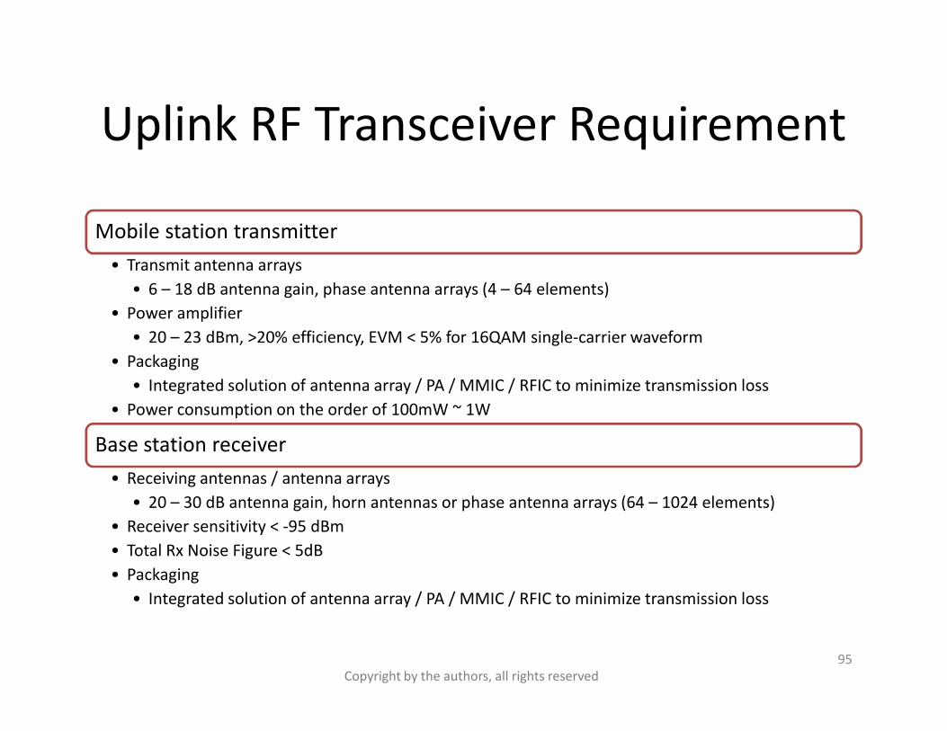
Uplink RF Transceiver Requirement
Mobile station transmitter
• Transmit antenna arrays
• 6 – 18 dB antenna gain, phase antenna arrays (4 – 64 elements)
• Power amplifier
• 20 – 23 dBm, >20% efficiency, EVM < 5% for 16QAM single-carrier waveform
• Packaging• Packaging
• Integrated solution of antenna array / PA / MMIC / RFIC to minimize transmission loss
• Power consumption on the order of 100mW ~ 1W
Base station receiver
• Receiving antennas / antenna arrays
• 20 – 30 dB antenna gain, horn antennas or phase antenna arrays (64 – 1024 elements)
• Receiver sensitivity < -95 dBm
• Total Rx Noise Figure < 5dB
• Packaging
• Integrated solution of antenna array / PA / MMIC / RFIC to minimize transmission loss
95
Copyright by the authors, all rights reserved
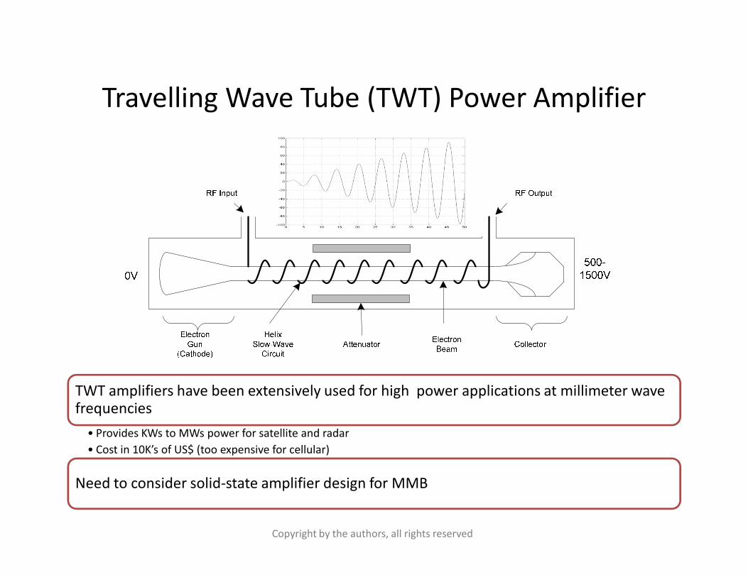
Travelling Wave Tube (TWT) Power Amplifier
TWT amplifiers have been extensively used for high power applications at millimeter wave frequencies
• Provides KWs to MWs power for satellite and radar
• Cost in 10K’s of US$ (too expensive for cellular)
Need to consider solid-state amplifier design for MMB
Copyright by the authors, all rights reserved
Solid-state Power Amplifier
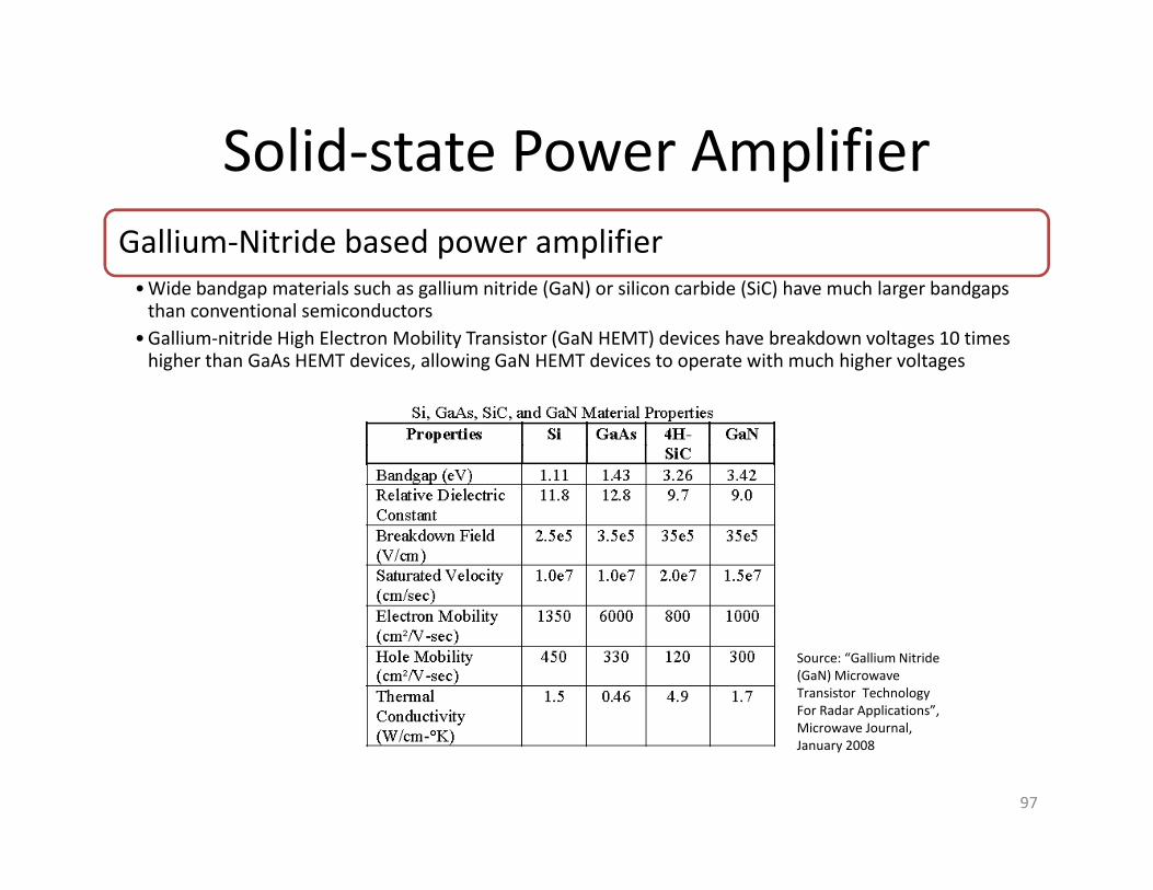
Gallium-Nitride based power amplifier
• Wide bandgap materials such as gallium nitride (GaN) or silicon carbide (SiC) have much larger bandgapsthan conventional semiconductors
• Gallium-nitride High Electron Mobility Transistor (GaN HEMT) devices have breakdown voltages 10 times higher than GaAs HEMT devices, allowing GaN HEMT devices to operate with much higher voltages
97
Source: “Gallium Nitride
(GaN) Microwave
Transistor Technology
For Radar Applications”,
Microwave Journal,
January 2008
Solid-state Power Amplifier
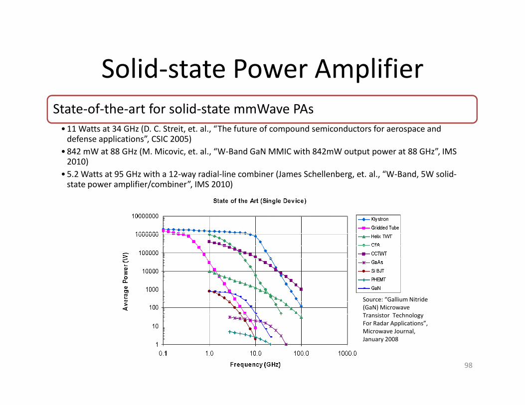
State-of-the-art for solid-state mmWave PAs
• 11 Watts at 34 GHz (D. C. Streit, et. al., “The future of compound semiconductors for aerospace and defense applications”, CSIC 2005)
• 842 mW at 88 GHz (M. Micovic, et. al., “W-Band GaN MMIC with 842mW output power at 88 GHz”, IMS 2010)
• 5.2 Watts at 95 GHz with a 12-way radial-line combiner (James Schellenberg, et. al., “W-Band, 5W solid-state power amplifier/combiner”, IMS 2010)
98
Source: “Gallium Nitride
(GaN) Microwave
Transistor Technology
For Radar Applications”,
Microwave Journal,
January 2008
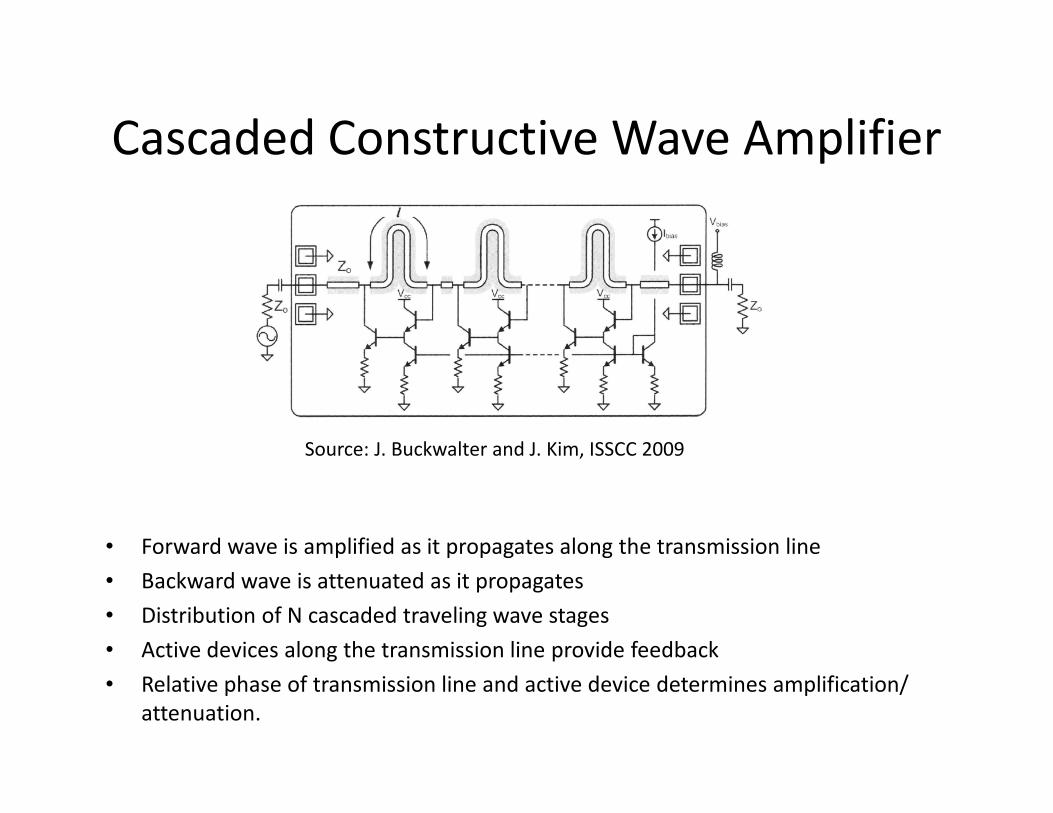
Cascaded Constructive Wave Amplifier
• Forward wave is amplified as it propagates along the transmission line
• Backward wave is attenuated as it propagates
• Distribution of N cascaded traveling wave stages
• Active devices along the transmission line provide feedback
• Relative phase of transmission line and active device determines amplification/
attenuation.
Source: J. Buckwalter and J. Kim, ISSCC 2009
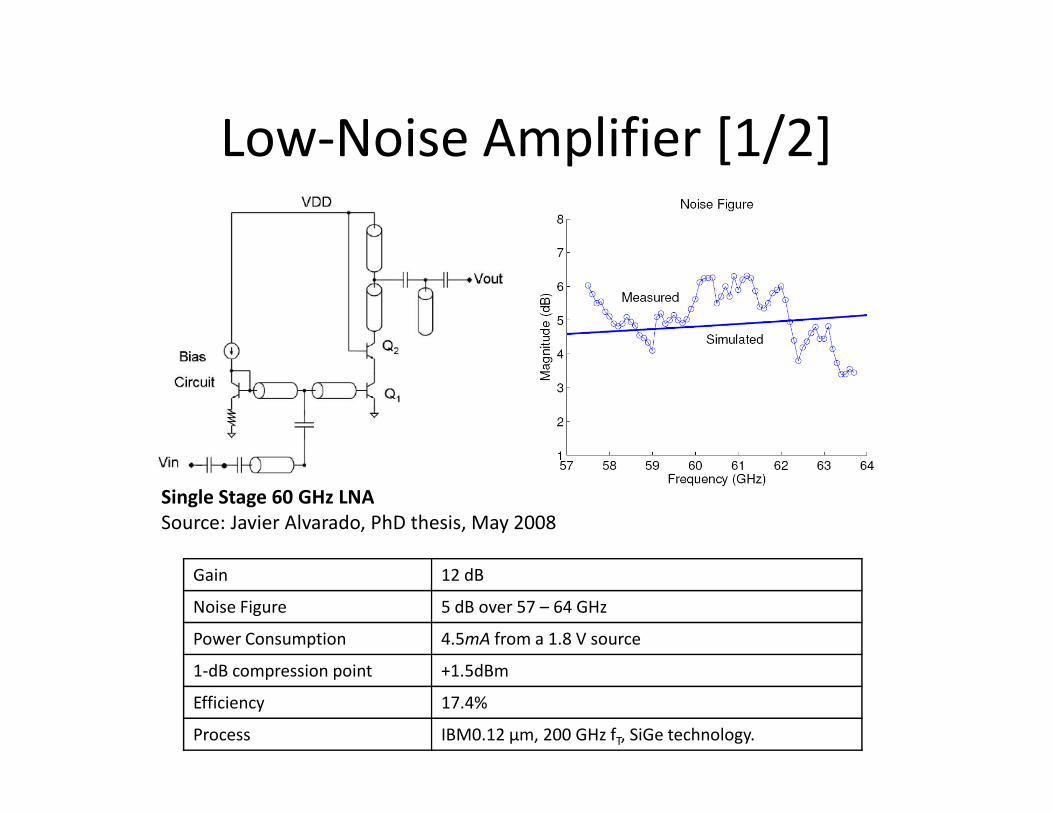
Low-Noise Amplifier [1/2]
Single Stage 60 GHz LNA
Source: Javier Alvarado, PhD thesis, May 2008
Gain 12 dB
Noise Figure 5 dB over 57 – 64 GHz
Power Consumption 4.5mA from a 1.8 V source
1-dB compression point +1.5dBm
Efficiency 17.4%
Process IBM0.12 μm, 200 GHz fT, SiGe technology.
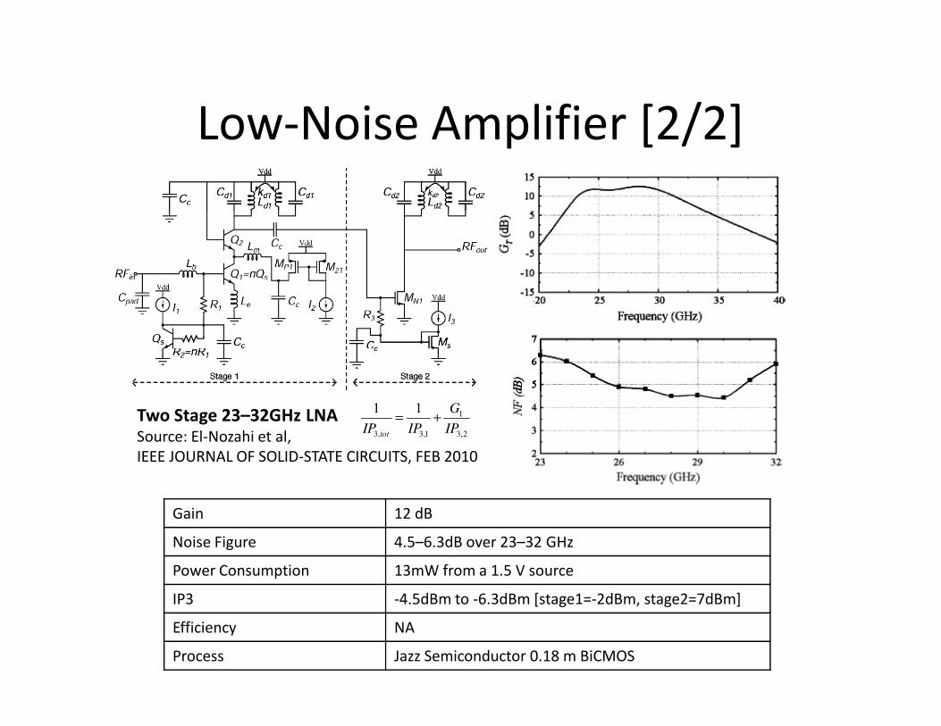
Low-Noise Amplifier [2/2]
Two Stage 23–32GHz LNASource: El-Nozahi et al,
IEEE JOURNAL OF SOLID-STATE CIRCUITS, FEB 2010
Gain 12 dB
Noise Figure 4.5–6.3dB over 23–32 GHz
Power Consumption 13mW from a 1.5 V source
IP3 -4.5dBm to -6.3dBm [stage1=-2dBm, stage2=7dBm]
Efficiency NA
Process Jazz Semiconductor 0.18 m BiCMOS
1
3, 3,1 3,2
1 1
tot
G
IP IP IP= +
Outline• Introduction
– Mobile broadband growth
– The myth of traffic and revenue gap
– The national broadband plan
• mmW spectrum
– History of millimeter wave communications
– Unleashing 3-300GHz spectrum
– LMDS and 70/80/90 GHz bands
• mmW Propagation characteristics
– Free Space Propagation
• MMB air-interface design
– Duplex and multiple access schemes
– Frame Structure
– Channel coding and modulation
• Dynamic beamforming with miniature antennas
– Beamforming fundamentals
– Baseband beamforming
– Analog beamforming
– RF beamforming
– Beamforming in fading channels– Free Space Propagation
– Material penetration loss
– Oxygen and water absorption
– Foliage absorption
– Rain absorption
– Diffraction
– Ground reflection
• mmW Mobile Broadband (MMB) network
architecture
– Stand-alone MMB system
– MMB base station grid
– Hybrid MMB + 4G systems
– Deployment and antenna configuration
– Beamforming in fading channels
• Radio frequency components design and
challenges
– RF transceiver architecture
– MMB RF transceiver requirement
– mmWave Power amplifier
– mmWave LNA
• MMB system performance
– Link budget analysis
– Link Level performance
– Geometry distribution
– System throughput analysis
• Summary
102Copyright 2011 by the authors. All rights reserved.

MMB downlink budget
MMB link downlink budget analysis Case 1 Case 2 Case 3 Case 4 Case 5 Case 6 Case 7 Case 8
Transmit Power (dBm) 35.00 40.00 35.00 40.00 35.00 40.00 35.00 40.00
Transmit Antenna Gain (dBi) 17.00 17.00 23.00 23.00 17.00 17.00 23.00 23.00
Carrier Frequency (GHz) 28.00 28.00 28.00 28.00 28.00 28.00 28.00 28.00
Distance (km) 0.50 0.50 0.50 0.50 0.50 0.50 0.50 0.50
Key system configuration parameters
•Base station Tx power: 35dBm – 40dBm
•Base station Tx antenna gain: 17 dB – 23 dB
•Mobile station Rx antenna gain: 3 dB – 10 dB
Distance (km) 0.50 0.50 0.50 0.50 0.50 0.50 0.50 0.50
Propagation Loss (dB) 115.32 115.32 115.32 115.32 115.32 115.32 115.32 115.32
Other losses 20.00 20.00 20.00 20.00 20.00 20.00 20.00 20.00
Receive Antenna Gain (dB) 3.00 3.00 3.00 3.00 10.00 10.00 10.00 10.00
Received Power (dBm) -80.32 -75.32 -74.32 -69.32 -73.32 -68.32 -67.32 -62.32
Bandwidth (MHz) 500 500 500 500 500 500 500 500
Thermal Noise PSD (dBm/Hz) -174.00 -174.00 -174.00 -174.00 -174.00 -174.00 -174.00 -174.00
Noise Figure 7.00 7.00 7.00 7.00 7.00 7.00 7.00 7.00
Thermal Noise (dBm) -80.01 -80.01 -80.01 -80.01 -80.01 -80.01 -80.01 -80.01
SNR (dB) -0.31 4.69 5.69 10.69 6.69 11.69 12.69 17.69
Implementation loss (dB) 5.00 5.00 5.00 5.00 5.00 5.00 5.00 5.00
Spectram Efficiency 0.37 0.95 1.12 2.23 1.31 2.50 2.78 4.29
Data rate (Mbps) 186.08 474.53 559.37 1117.08 653.70 1250.93 1390.35 2145.23
103Copyright 2011 by the authors. All rights reserved.
Path loss formula: PL = 141.3 + 20log10d with d in km (free-space loss + 20dB)
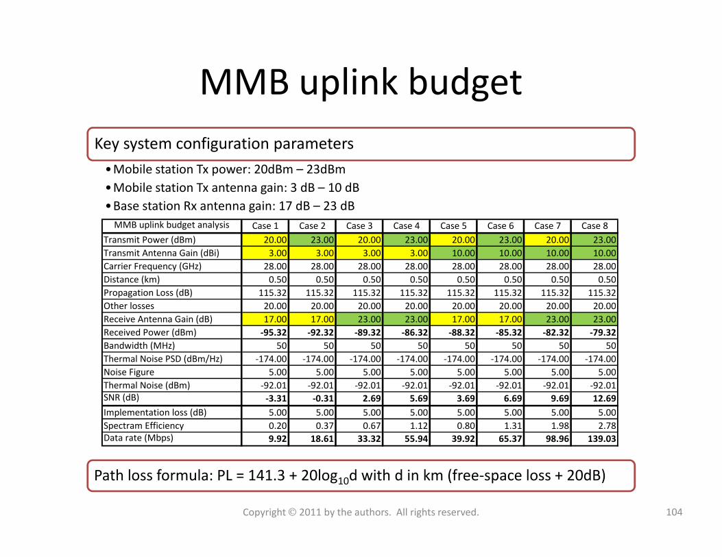
MMB uplink budget
MMB uplink budget analysis Case 1 Case 2 Case 3 Case 4 Case 5 Case 6 Case 7 Case 8
Transmit Power (dBm) 20.00 23.00 20.00 23.00 20.00 23.00 20.00 23.00
Transmit Antenna Gain (dBi) 3.00 3.00 3.00 3.00 10.00 10.00 10.00 10.00
Carrier Frequency (GHz) 28.00 28.00 28.00 28.00 28.00 28.00 28.00 28.00
Distance (km) 0.50 0.50 0.50 0.50 0.50 0.50 0.50 0.50
Key system configuration parameters
•Mobile station Tx power: 20dBm – 23dBm
•Mobile station Tx antenna gain: 3 dB – 10 dB
•Base station Rx antenna gain: 17 dB – 23 dB
Distance (km) 0.50 0.50 0.50 0.50 0.50 0.50 0.50 0.50
Propagation Loss (dB) 115.32 115.32 115.32 115.32 115.32 115.32 115.32 115.32
Other losses 20.00 20.00 20.00 20.00 20.00 20.00 20.00 20.00
Receive Antenna Gain (dB) 17.00 17.00 23.00 23.00 17.00 17.00 23.00 23.00
Received Power (dBm) -95.32 -92.32 -89.32 -86.32 -88.32 -85.32 -82.32 -79.32
Bandwidth (MHz) 50 50 50 50 50 50 50 50
Thermal Noise PSD (dBm/Hz) -174.00 -174.00 -174.00 -174.00 -174.00 -174.00 -174.00 -174.00
Noise Figure 5.00 5.00 5.00 5.00 5.00 5.00 5.00 5.00
Thermal Noise (dBm) -92.01 -92.01 -92.01 -92.01 -92.01 -92.01 -92.01 -92.01
SNR (dB) -3.31 -0.31 2.69 5.69 3.69 6.69 9.69 12.69
Implementation loss (dB) 5.00 5.00 5.00 5.00 5.00 5.00 5.00 5.00
Spectram Efficiency 0.20 0.37 0.67 1.12 0.80 1.31 1.98 2.78
Data rate (Mbps) 9.92 18.61 33.32 55.94 39.92 65.37 98.96 139.03
104Copyright 2011 by the authors. All rights reserved.
Path loss formula: PL = 141.3 + 20log10d with d in km (free-space loss + 20dB)
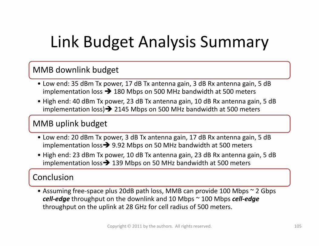
Link Budget Analysis Summary
MMB downlink budget
• Low end: 35 dBm Tx power, 17 dB Tx antenna gain, 3 dB Rx antenna gain, 5 dB implementation loss 180 Mbps on 500 MHz bandwidth at 500 meters
• High end: 40 dBm Tx power, 23 dB Tx antenna gain, 10 dB Rx antenna gain, 5 dB implementation loss) 2145 Mbps on 500 MHz bandwidth at 500 meters
MMB uplink budgetMMB uplink budget
• Low end: 20 dBm Tx power, 3 dB Tx antenna gain, 17 dB Rx antenna gain, 5 dB implementation loss 9.92 Mbps on 50 MHz bandwidth at 500 meters
• High end: 23 dBm Tx power, 10 dB Tx antenna gain, 23 dB Rx antenna gain, 5 dB implementation loss 139 Mbps on 50 MHz bandwidth at 500 meters
Conclusion
• Assuming free-space plus 20dB path loss, MMB can provide 100 Mbps ~ 2 Gbpscell-edge throughput on the downlink and 10 Mbps ~ 100 Mbps cell-edge
throughput on the uplink at 28 GHz for cell radius of 500 meters.
105Copyright 2011 by the authors. All rights reserved.
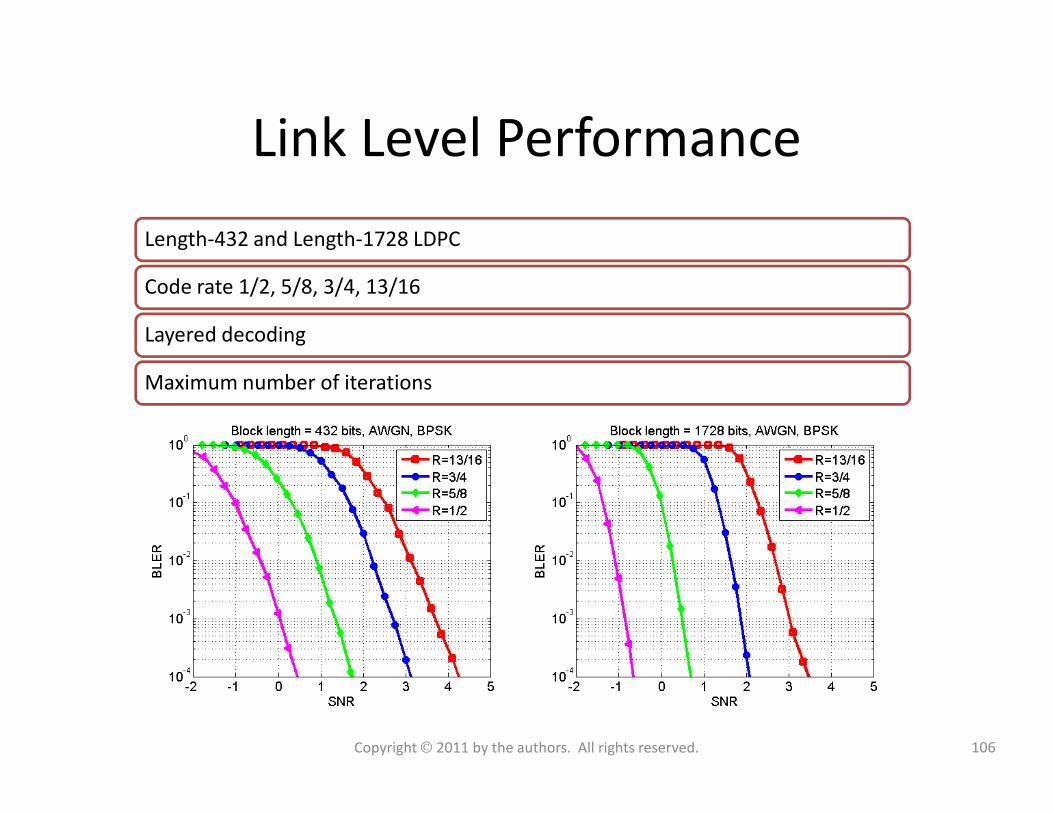
Link Level Performance
Length-432 and Length-1728 LDPC
Code rate 1/2, 5/8, 3/4, 13/16
Layered decoding
Maximum number of iterations
106Copyright 2011 by the authors. All rights reserved.
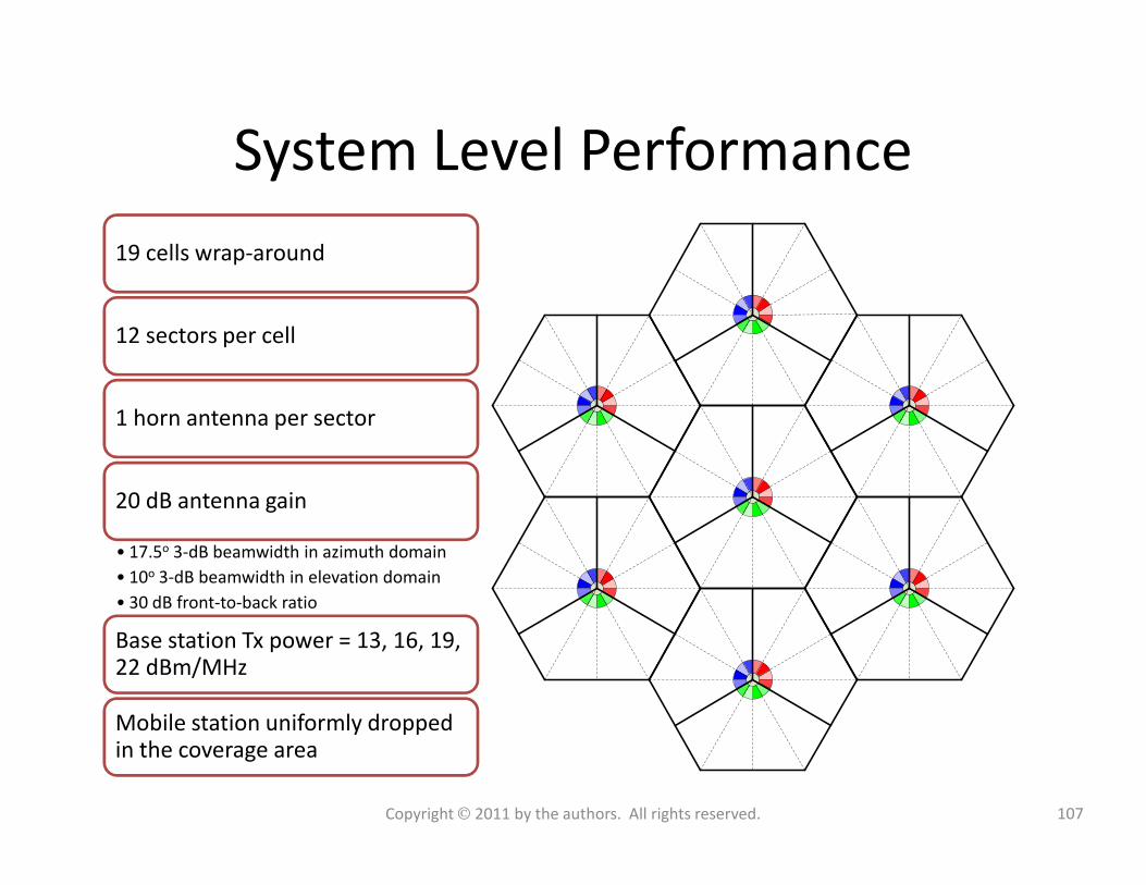
System Level Performance
19 cells wrap-around
12 sectors per cell
1 horn antenna per sector
20 dB antenna gain
• 17.5o 3-dB beamwidth in azimuth domain
• 10o 3-dB beamwidth in elevation domain
• 30 dB front-to-back ratio
Base station Tx power = 13, 16, 19, 22 dBm/MHz
Mobile station uniformly dropped in the coverage area
107Copyright 2011 by the authors. All rights reserved.
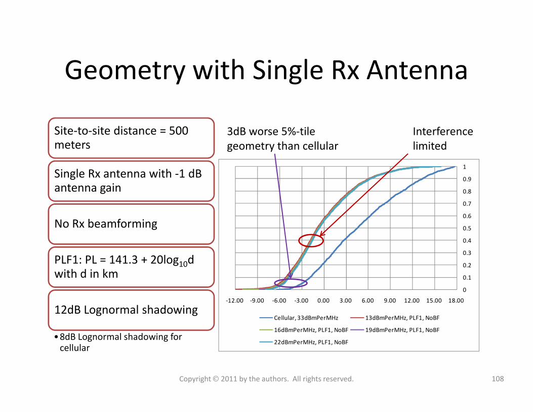
Geometry with Single Rx Antenna
Site-to-site distance = 500 meters
Single Rx antenna with -1 dB antenna gain
0.7
0.8
0.9
1
Interference
limited
3dB worse 5%-tile
geometry than cellular
No Rx beamforming
PLF1: PL = 141.3 + 20log10d with d in km
12dB Lognormal shadowing
•8dB Lognormal shadowing for cellular
0
0.1
0.2
0.3
0.4
0.5
0.6
0.7
-12.00 -9.00 -6.00 -3.00 0.00 3.00 6.00 9.00 12.00 15.00 18.00
Cellular, 33dBmPerMHz 13dBmPerMHz, PLF1, NoBF
16dBmPerMHz, PLF1, NoBF 19dBmPerMHz, PLF1, NoBF
22dBmPerMHz, PLF1, NoBF
108Copyright 2011 by the authors. All rights reserved.
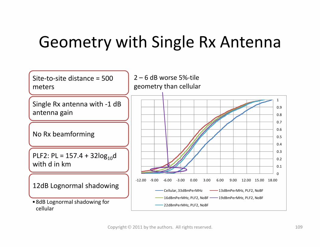
Geometry with Single Rx Antenna
0.7
0.8
0.9
1
Site-to-site distance = 500 meters
Single Rx antenna with -1 dB antenna gain
2 – 6 dB worse 5%-tile
geometry than cellular
0
0.1
0.2
0.3
0.4
0.5
0.6
0.7
-12.00 -9.00 -6.00 -3.00 0.00 3.00 6.00 9.00 12.00 15.00 18.00
Cellular, 33dBmPerMHz 13dBmPerMHz, PLF2, NoBF
16dBmPerMHz, PLF2, NoBF 19dBmPerMHz, PLF2, NoBF
22dBmPerMHz, PLF2, NoBF
109Copyright 2011 by the authors. All rights reserved.
No Rx beamforming
PLF2: PL = 157.4 + 32log10d with d in km
12dB Lognormal shadowing
•8dB Lognormal shadowing for cellular
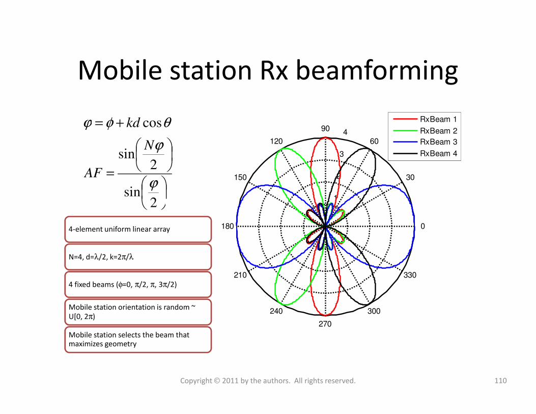
1
2
3
4
30
60
90
120
150
RxBeam 1
RxBeam 2
RxBeam 3
RxBeam 4
Mobile station Rx beamforming
=
+=
2sin
2sin
cos
ϕ
ϕ
θφϕ
N
AF
kd
210
240
270
300
330
180 0
4-element uniform linear array
N=4, d=λ/2, k=2π/λ
4 fixed beams (φ=0, π/2, π, 3π/2)
Mobile station orientation is random ~ U[0, 2π)
Mobile station selects the beam that maximizes geometry
2
110Copyright 2011 by the authors. All rights reserved.
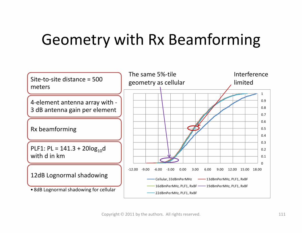
Geometry with Rx Beamforming
0.7
0.8
0.9
1
Site-to-site distance = 500 meters
4-element antenna array with -3 dB antenna gain per element
Interference
limited
The same 5%-tile
geometry as cellular
0
0.1
0.2
0.3
0.4
0.5
0.6
-12.00 -9.00 -6.00 -3.00 0.00 3.00 6.00 9.00 12.00 15.00 18.00
Cellular, 33dBmPerMHz 13dBmPerMHz, PLF1, RxBF
16dBmPerMHz, PLF1, RxBF 19dBmPerMHz, PLF1, RxBF
22dBmPerMHz, PLF1, RxBF
111Copyright 2011 by the authors. All rights reserved.
Rx beamforming
PLF1: PL = 141.3 + 20log10d with d in km
12dB Lognormal shadowing
• 8dB Lognormal shadowing for cellular
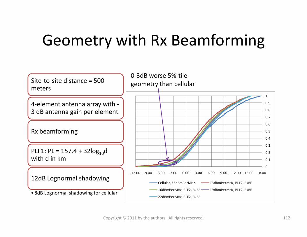
Geometry with Rx Beamforming
0.7
0.8
0.9
1
Site-to-site distance = 500 meters
4-element antenna array with -3 dB antenna gain per element
0-3dB worse 5%-tile
geometry than cellular
0
0.1
0.2
0.3
0.4
0.5
0.6
0.7
-12.00 -9.00 -6.00 -3.00 0.00 3.00 6.00 9.00 12.00 15.00 18.00
Cellular, 33dBmPerMHz 13dBmPerMHz, PLF2, RxBF
16dBmPerMHz, PLF2, RxBF 19dBmPerMHz, PLF2, RxBF
22dBmPerMHz, PLF2, RxBF
112Copyright 2011 by the authors. All rights reserved.
Rx beamforming
PLF1: PL = 157.4 + 32log10d with d in km
12dB Lognormal shadowing
• 8dB Lognormal shadowing for cellular
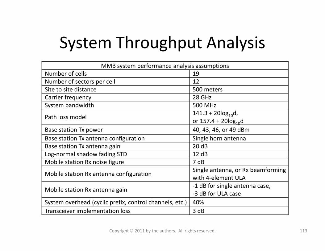
System Throughput AnalysisMMB system performance analysis assumptions
Number of cells 19
Number of sectors per cell 12
Site to site distance 500 meters
Carrier frequency 28 GHz
System bandwidth 500 MHz
Path loss model141.3 + 20log10d,
or 157.4 + 20log10d
Base station Tx power 40, 43, 46, or 49 dBmBase station Tx power 40, 43, 46, or 49 dBm
Base station Tx antenna configuration Single horn antenna
Base station Tx antenna gain 20 dB
Log-normal shadow fading STD 12 dB
Mobile station Rx noise figure 7 dB
Mobile station Rx antenna configurationSingle antenna, or Rx beamforming
with 4-element ULA
Mobile station Rx antenna gain-1 dB for single antenna case,
-3 dB for ULA case
System overhead (cyclic prefix, control channels, etc.) 40%
Transceiver implementation loss 3 dB
113Copyright 2011 by the authors. All rights reserved.
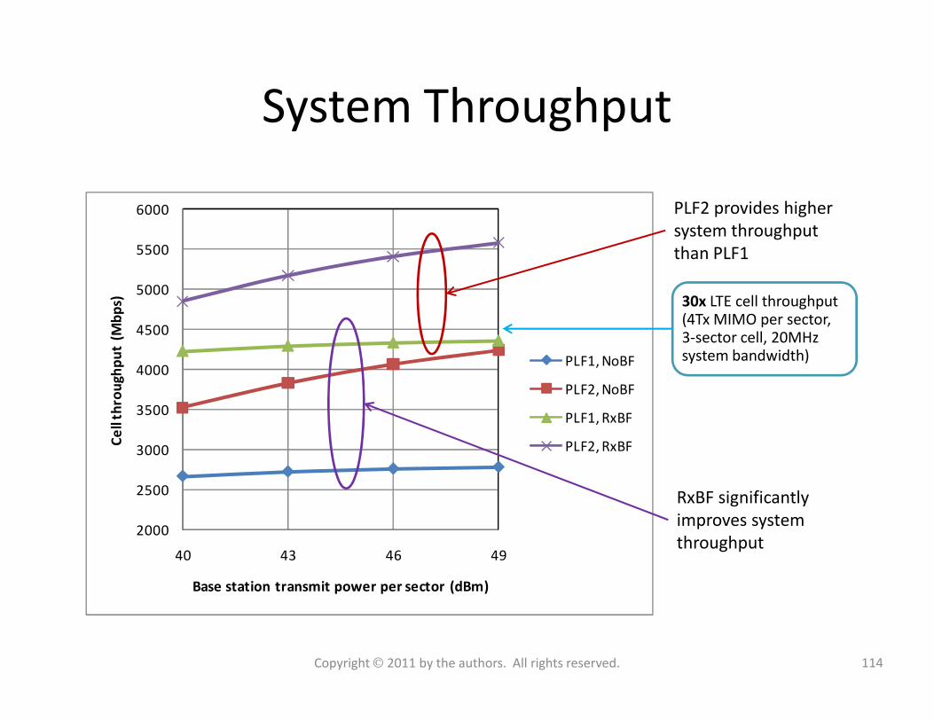
System Throughput
4000
4500
5000
5500
6000
Ce
ll t
hro
ug
hp
ut
(Mb
ps)
PLF1, NoBF
PLF2 provides higher
system throughput
than PLF1
30x LTE cell throughput (4Tx MIMO per sector, 3-sector cell, 20MHz system bandwidth)
2000
2500
3000
3500
4000
40 43 46 49
Ce
ll t
hro
ug
hp
ut
(Mb
ps)
Base station transmit power per sector (dBm)
PLF1, NoBF
PLF2, NoBF
PLF1, RxBF
PLF2, RxBF
114Copyright 2011 by the authors. All rights reserved.
RxBF significantly
improves system
throughput
system bandwidth)
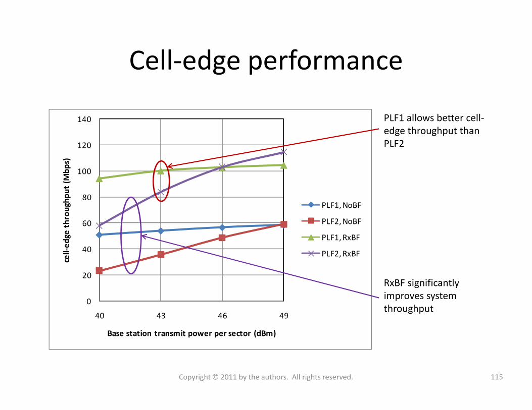
Cell-edge performance
80
100
120
140
ed
ge
th
rou
gh
pu
t (M
bp
s)
PLF1, NoBF
PLF1 allows better cell-
edge throughput than
PLF2
0
20
40
60
40 43 46 49
cell
-ed
ge
th
rou
gh
pu
t (M
bp
s)
Base station transmit power per sector (dBm)
PLF1, NoBF
PLF2, NoBF
PLF1, RxBF
PLF2, RxBF
115Copyright 2011 by the authors. All rights reserved.
RxBF significantly
improves system
throughput
Outline• Introduction
– Mobile broadband growth
– The myth of traffic and revenue gap
– The national broadband plan
• mmW spectrum
– History of millimeter wave communications
– Unleashing 3-300GHz spectrum
– LMDS and 70/80/90 GHz bands
• mmW Propagation characteristics
– Free Space Propagation
• MMB air-interface design
– Duplex and multiple access schemes
– Frame Structure
– Channel coding and modulation
• Dynamic beamforming with miniature antennas
– Beamforming fundamentals
– Baseband beamforming
– Analog beamforming
– RF beamforming
– Beamforming in fading channels– Free Space Propagation
– Material penetration loss
– Oxygen and water absorption
– Foliage absorption
– Rain absorption
– Diffraction
– Ground reflection
• mmW Mobile Broadband (MMB) network
architecture
– Stand-alone MMB system
– MMB base station grid
– Hybrid MMB + 4G systems
– Deployment and antenna configuration
– Beamforming in fading channels
• Radio frequency components design and
challenges
– RF transceiver architecture
– MMB RF transceiver requirement
– mmWave Power amplifier
– mmWave LNA
• MMB system performance
– Link budget analysis
– Link Level performance
– Geometry distribution
– System throughput analysis
• Summary
116Copyright 2011 by the authors. All rights reserved.
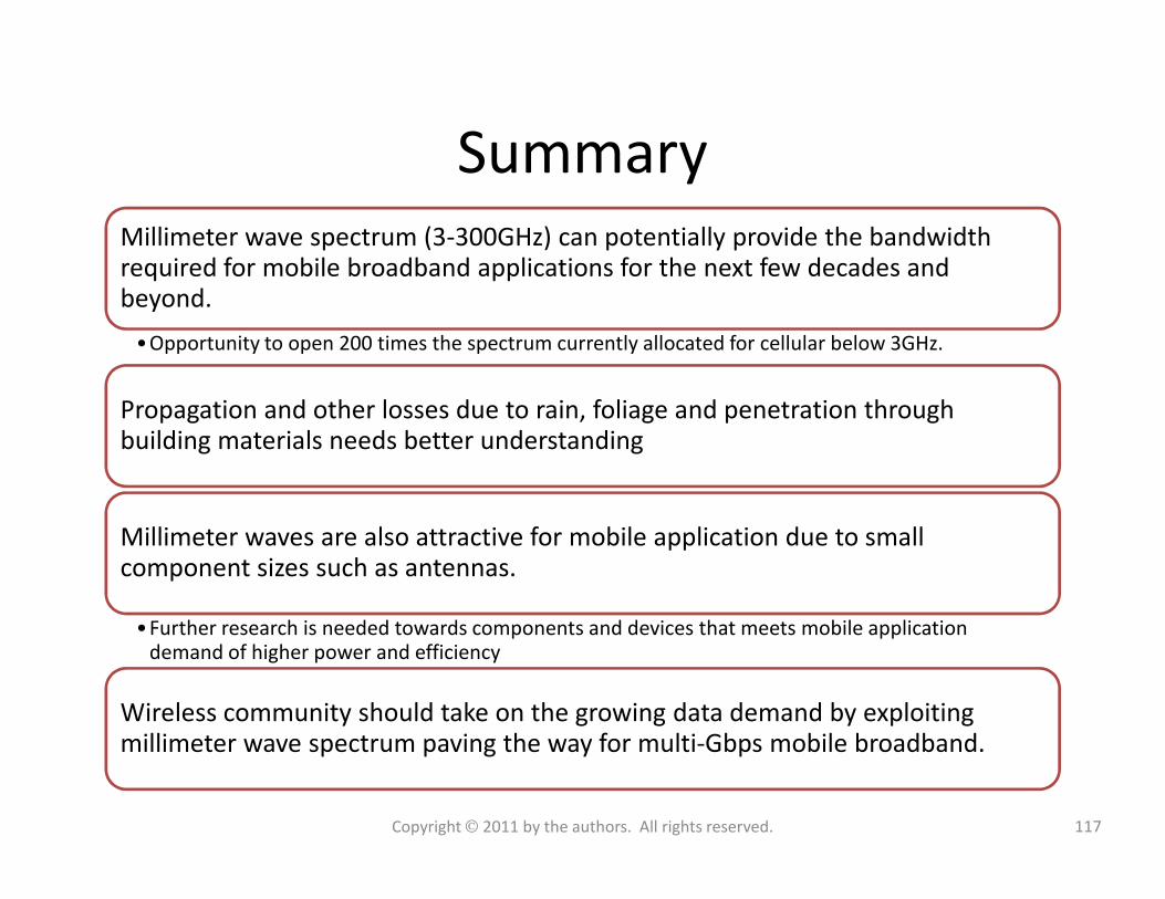
SummaryMillimeter wave spectrum (3-300GHz) can potentially provide the bandwidth required for mobile broadband applications for the next few decades and beyond.
•Opportunity to open 200 times the spectrum currently allocated for cellular below 3GHz.
Propagation and other losses due to rain, foliage and penetration through building materials needs better understandingbuilding materials needs better understanding
Millimeter waves are also attractive for mobile application due to small component sizes such as antennas.
•Further research is needed towards components and devices that meets mobile application demand of higher power and efficiency
Wireless community should take on the growing data demand by exploiting millimeter wave spectrum paving the way for multi-Gbps mobile broadband.
117Copyright 2011 by the authors. All rights reserved.