1

Abstract—Industrial data are often high-dimensional, nonlinear and multiple-modal. This paper develops a soft sensor model based on Gaussian mixture Variational Autoencoder (GMVAE) under the just-in-time learning (JITL) framework. To extract latent representations with multimode characteristics, GMVAE as a deep neural network model is utilized by considering Gaussian mixture models (GMM) in the latent space. After training the GMVAE model, each latent (or feature) variable can be described through a Gaussian mixture distribution. Subsequently, when a new sample arrives, a mixture symmetric Kullback-Leibler (MSKL) divergence is utilized to measure its similarity with historical data samples. MSKL divergence can measure similarity between two Gaussian mixture probability density functions. Based on the MSKL divergence, weighted input and output historical data are obtained, and then a local model is established. The effectiveness of the proposed soft sensor modeling method is validated through a numerical example along with simulation on the Tennessee Eastman benchmark process.

Keywords—Gaussian mixture variational autoencoder; Mixture symmetric Kullback-Leibler divergence; Mixture probabilistic principal component regression; Just-in-time learning.

1. INTRODUCTION

Soft sensor modeling includes the first principle modelingand data-driven modeling (Kadlec et al., 2009; Khatibisepehr et al., 2013). This work focuses on the latter, considering availability of a large amount of data and flexibility of data-driven approaches to describing complex industrial process. Data-driven approaches have been studied extensively in the literature, such as partial least squares, principal component regression, artificial neural networks, support vector regression, and Gaussian process regression (Kaneko and Funatsu, 2014; Daemia et al., 2019; Jiang et al., 2020).

* Corresponding author.E-mail address: biao.huang@ualberta.ca (B. Huang).

Generally, data selection plays a crucial role in constructing effective data-based soft sensors. Especially in industrial process, process characteristics may change with the changes of operating environment, raw material, and catalyst, etc. Correspondingly, the stored historical data record many kinds of possible changes, including both incipient and abrupt changes. Although a global modeling approach can construct a single complex model by utilizing entire historical data, it is usually difficult and even impossible to employ one model to obtain satisfactory prediction performance under all possible different operating conditions. Consequently, adaptive soft sensor modeling methods, such as recursive method, moving window method, and Just-in-time learning (JITL)-based method, are developed to solve the aforementioned issues (Qin , 1998; Kaneko and Funatsu, 2015; Kadlec and Gabrys, 2011; Ge and Song, 2010). However, the recursive or moving-window strategy is not suitable for abrupt or quick changes of the process. As a local modeling method, on the other hand, JITL has attracted a lot of attention in soft sensor modeling (Kadlec and Gabrys, 2011; Ge and Song, 2010). The core of the JITL is to build a local model using the most relevant data consistent with current operating conditions. In JITL, determination of data relevancy is the most important factor for building a high-quality soft sensor model. Various deterministic point-to-point methods have been proposed in literatures (Cheng and Chiu, 2004; Fujiwara et al., 2009; Chan et al., 2018) to evaluate data similarity. A probabilistic similarity measurement is also presented to compute data similarity with consideration of data uncertainties through comparison between two Gaussian distributions (Yuan et al., 2017a; Guo et al., 2020b). Subsequently, to build a predictive model, the relevant historical data samples are selected based on the results of similarity measurement. Those selected modeling samples are most relevant to the given query sample, which usually can improve the performance of soft senor models.

Extracting features from collected historical dataset is a key step, due to high-dimensionality and redundancy of the data. To capture the latent representations, traditional unsupervised learning methods, like principal component analysis (PCA),

A Just-in-time Modeling Approach for Multimode Soft Sensor Based on Gaussian Mixture Variational

Autoencoder Fan Guo a, Bing Wei b, Biao Huang a, *

a Department of Chemical and Materials Engineering, University of Alberta, Edmonton, AB T6G2G6, Canada

b College of Information Sciences and Technology, Donghua University, Shanghai 201620, China

Preprint for F. Guo, B. Huang*, A Just-in-time Modeling Approach for Multimode Soft Sensor Based on Gaussian Mixture Variational Autoencoder, Computers and Chemical Engineering, Volume 146, March 2021, 107230.

2

probabilistic PCA (PPCA), and kernel PCA etc. (Yuan et al., 2017b; Schölkopf et al., 1977) map the observed high-dimensional data into lower-dimensional space based on a latent space model. Being a neural network, autoencoder belongs to an unsupervised learning method, which has been employed to extract features from the given dataset especially for image preprocessing and pattern recognition (Bengio et al., 2013). As a deep generative model, Variational Autoencoder (VAE) is proposed based on variational Bayesian inference and deep learning methodologies by Kingma and Welling (2013). It has attracted increasing attention, and has also been successfully applied to natural language processing, static images forecast, automatic speech recognition, and process monitoring etc. (de-la-Calle-Silos and Stern, 2017; Collobert et al., 2011; Walker et al., 2016; Wu and Zhao, 2020). Compared to autoencoder, VAE models the probability distribution of data in the latent space through variational inference. In the VAE model, the latent variables have a predefined probability distribution, also known as the prior. Commonly, this prior is considered to follow a multivariate Gaussian distribution. This choice of prior induces learned latent representations that are structured. Additionally, under the Gaussian prior assumption, those learnt representations are only suitable to describing unimodal data properties. However, if the observed data is of multiple mode, the Gaussian prior assumption will not be valid.

Recently, for extracting features from multiple-mode dataset, several extensions have been developed based on the traditional VAE (Abbasnejad et al., 2016; Dilokthanakul et al., 2017; Jiang et al., 2017; Liu et al., 2019; Shi et al., 2019; Varolgunes et al., 2019; Zhao et al., 2019). Considering that a single VAE model cannot describe the multimode data, an infinite mixture VAE was proposed by Abbasnejad et al. (2016). Dilokthanakul et al. (2017) introduced a variant of the regular VAE by considering a GMM as a prior distribution instead of an isotropic Gaussian distribution. Jiang et al. (2017) proposed a variational deep embedding method, which embeds GMM in the data generative process through a deep neural network under the regular VAE framework. Liu et al. (2019) considered a GMM as the posterior distribution to approximate the real multimodal posterior in the original VAE. For enhancing the interpretability of text generation, Shi et al. (2019) introduced a dispersed-GMVAE (Gaussian mixture VAE) to alleviate mode-collapse problem by utilizing Gaussian mixture distribution as the prior in the vanilla VAE. Those extensions consider GMM as a prior distribution or a posterior distribution in the VAE latent space. Varolgunes et al. (2019) developed a GMVAE, which considers the prior and posterior distribution to follow Gaussian mixture distribution in the latent space simultaneously. Zhao et al. (2019) considered the truncated GMM in the traditional VAE to deal with the problems of outlier detection and clustering simultaneously.

Furthermore, considering that industrial process has nonlinearities by nature, nonlinear modeling methods have been presented (Kaneko and Funatsu, 2014; Daemia et al., 2019; Jiang et al., 2020; Shao et al., 2019). Note that most JITL-based soft sensors consider single-modal data only. They cannot effectively express the multimode data characteristics.

Thus, this work proposes a JITL-based multimodal soft sensor modeling method based on GMVAE. For building a local model, a mixture probabilistic principal component regression (MPPCR) model is utilized, which has been successfully employed to deal with multimode modeling problems (Ge et al., 2011; Sedghi et al., 2017).

The main contributions of the present work are summarized as below. (i) Under the JITL framework, the observed input dataset is first preprocessed by utilizing the GMVAE. The features of the observed input data are then extracted. Correspondingly, each feature follows a Gaussian mixture distribution. (ii) Mixture symmetric Kullback-Leibler (MSKL) divergence is used for calculating relevance between historical data samples and the query sample, which is calculated based on two Gaussian mixture probability distributions. (iii) The input-output data samples for local modeling are determined by first calculating the MSKL divergence, and then weights are assigned to each input-output sample based on the computed MSKL values. Finally, based on these weighted input-output data, a MPPCR model is applied to establish a local model.

The rest of this paper is organized as follows. The proposed JITL-based soft sensor model is presented in section 2, GMVAE model is introduced in subsection 2.1, assignment of weights to input-output samples based on the MSKL divergence is presented in subsection 2.2, and then MPPCR as a local multi-mode modeling method is applied in subsection 2.3. The simulation results through a numerical example and a Tennessee Eastman (TE) process are shown in Section 3. Conclusions are provided in Section 4.

2. PROPOSED JITL-BASED SOFT SENSOR MODEL Generally, JITL has the following procedure: 1) similarity

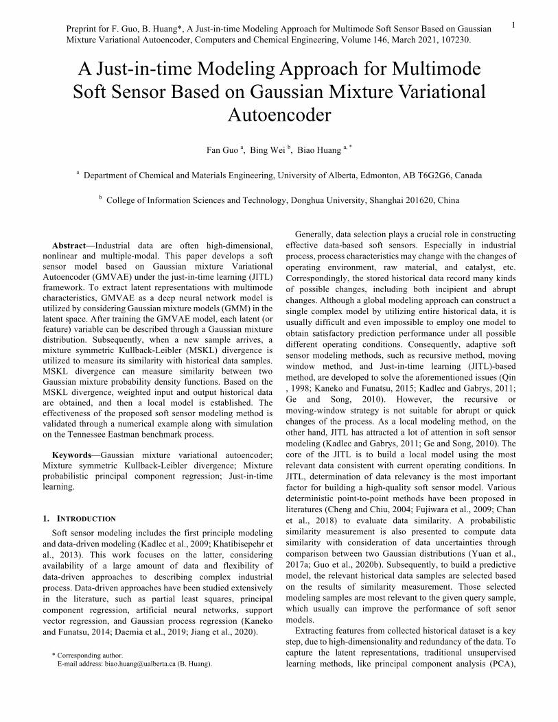
measurement; 2) building a local model; 3) making a prediction. Most of JITL-based soft sensors focus on a unimodal data and conduct similarity measurement in the original data space. This paper considers multimode data and conducts the similarity measurement in the latent space. The flowchart of the proposed JITL-based multimode soft sensor modeling approach is provided in Fig. 1.

Historical dataset

(1) Feature extraction through GMVAE;(2) Similarity measurement through

MSKL divergence;(3) Weight calculation through

equation (9).

Build a local model

Make a prediction

Query dataset

Fig. 1. Proposed JITL-based soft sensor framework.

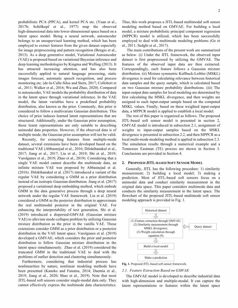
2.1. Feature Extraction Based on GMVAE The GMVAE model is developed to describe industrial data

with high-dimension and multiple-modal. It can capture the latent representations or features within the latent space

3

(Varolgunes et al., 2019). Moreover, these extracted multimode features can be utilized to construct or generate multiple-modal data. The advantage of GMVAE is that it can perform dimensionality reduction and unsupervised clustering simultaneously. In the GMVAE model, the prior distribution of latent variable ( )p Z and the approximate posterior distribution ( ,C | )q Z Xf with parameters f are both assumed to be GMM. Note that categorical variable C is introduced, which is utilized to represent the probability of each data sample belonging to each individual Gaussian model. GMVAE consists of an encoder and a decoder. The encoder model can be written as ( ,C | ) (C | ) ( | ,C)q q qZ X X Z Xf f f= (1) where (C | )qf X represents probabilities of M Gaussian components. Assume that the GMM model in the latent space includes M individual Gaussian components, which then indicates ( | , )mq cf Z X to be a single Gaussian distribution for

a given C mc= ， where 1,2,...,m M= . Therefore, the posterior ( ,C | )q Z Xf follows a Gaussian mixture. The Evidence Lower Bound (ELBO) is expressed by

( ,C| )( , ,C)

ELBO=E log .( ,C | )qpqZ XX ZZ Xf

q

f

é ùê úê úë û

(2)

where the joint probability distribution ( , ,C)p X Zq with parameters q can be decomposed as follows, ( , ,C) ( | ,C) ( | C) (C).p p p pX Z X Z Zq q q q= (3) where

( )2( | ,C) ( ,C), ( ,C) .p X ZX Z Z Zq µ s= N

( )2( | C) (C), (C) .p Z ZZq µ s= N

( )(C) Uniform 1 .p Mq = The approximate posterior probability distribution ( ,C | )q Z Xf with parameters f is written as

( ,C | ) ( | ,C) (C | )q q qZ X Z X Xf f f= (4) where

( )2( | ,C) ( ,C), ( ,C)q Z ZZ X X Xf µ s= N

(C | ) Multinomial( ( )).q rf =X X Further, equation (2) can be decomposed as

( ,C| )

(C) ( | C)log log

(C | ) ( | ,C)ELBO=E .log ( | )

q

p pq qp

Z X

ZX Z XX Z

f

q q

f f

q

é ù+ê úê úê ú+ë û

(5)

In (5), the first term is entropy between the prior (C)pq and the posterior (C | )q Xf . The second term represents the

regularization between the actual posterior ( | C)p Zq and approximate posterior ( | ,C)q Z Xf . The last term is the reconstruction term. For more details regarding the calculation, the readers can refer to (Varolgunes et al., 2019). Fig. 2 shows the model structure of the GMVAE model.

2.2. Calculating Weights of Data Samples for Local Modeling Based on MSKL Divergence

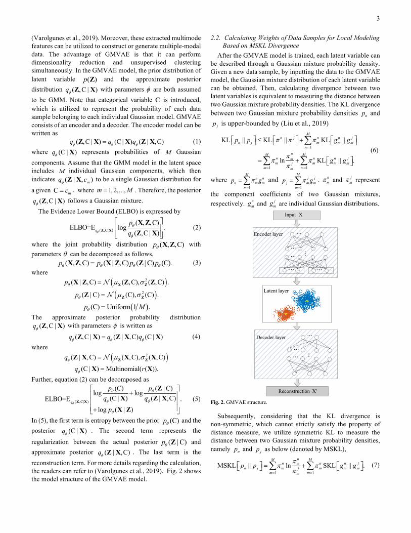
After the GMVAE model is trained, each latent variable can be described through a Gaussian mixture probability density. Given a new data sample, by inputting the data to the GMVAE model, the Gaussian mixture distribution of each latent variable can be obtained. Then, calculating divergence between two latent variables is equivalent to measuring the distance between two Gaussian mixture probability densities. The KL divergence between two Gaussian mixture probability densities np and

jp is upper-bounded by (Liu et al., 2019)

1

1 1

KL || KL || KL ||

ln KL || .

Mn j n n j

n j m m mm

nM Mn n n jmm m m mj

m mm

p p g g

g g

p p p

pp p

p

=

= =

é ù é ùé ù £ +ë û ë û ë û

é ù= + ë û

å

å å(6)

where 1

Mn n

n m mm

p gp=

=å and1

Mj j

j m mm

p gp=

=å . nmp and j

mp represent

the component coefficients of two Gaussian mixtures, respectively. n

mg and jmg are individual Gaussian distributions.

...

......

Encoder layer

...

...

...

...

Decoder layer

...

...

XInput

Reconstruction X'

...

...

Latent layer

Fig. 2. GMVAE structure.

Subsequently, considering that the KL divergence is non-symmetric, which cannot strictly satisfy the property of distance measure, we utilize symmetric KL to measure the distance between two Gaussian mixture probability densities, namely np and jp as below (denoted by MSKL),

1 1

MSKL || ln SKL || .nM M

n n n jmn j m m m mj

m mm

p p g gp

p pp= =

é ùé ù = +ë û ë ûå å (7)

4

jx

... ...

MSKL divergence

...

1qz1 1 1( , )m m mq q qNp µ så

2jx 2jz

jHx jDz

1jx 1jz

qDz

2qz

1 1 1( , )m m mj j jNp µ så

...

... ...

2 2 2( , )m m mq q qNp µ så

( , )m m mqD qD qDNp µ så

2 2 2( , )m m mj j jNp µ så

( , )m m mjD jD jDNp µ så

1qx

2qx

qHx qx

GMVAE GMVAE Fig. 3. Similarity measurement between two samples

The second term SKL ||n j

m mg gé ùë û in (7) can be calculated by

( )

( ), , , ,

1

, , , 1 , 1

1

SKL ||

SKL ( ( ), ( )), ( ( ), ( ))

SKL ( ( ), ( )), ( ( ), ( ))

0.5 ( ( ) ( ))( ( ) ( ) )

n jm m

n n j jm m m m

Hn h n h j h j hm m m m

hH

j h n h n h j hm m m m

h

g g

g g g g

g g g g

trace g g g g

µ s µ s

µ s µ s

s s s s

=

- -

=

é ùë û

=

=

é ù= - -ë û

å

å

N N

N N (8)

( ), , T , 1 , 1 , ,

1

0.5 ( ) ( )) ( ( ) ( ) )( ( ) ( ) .H

j h n h n h j h j h n hm m m m m m

hg g g g g gµ µ s s µ µ- -

=

+ - + -å

In (8), ( )( ), ( )n nm mg gµ sN and ( )( ), ( )j j

m mg gµ sN represent

the Gaussian distributions of nmg with mean ( )nmgµ and

variance ( )nmgs , and jmg with mean ( )jmgµ and variance

( )jmgs , respectively. Fig. 3 provides the similarity calculation between two Gaussian mixture probability densities based on the MSKL divergence.

Furthermore, the MSKL divergence as the similarity measure is computed between a query sample and all of the historical samples. Afterwards, a weight jw is calculated as below, and then assigned to each historical input-output sample ( )2 2(exp .) /jj MSKLw s-= (9)

where 2s is a parameter used for adjusting the changes of the weight with changes of similarity. Subsequently, the weighted historical input-output samples are utilized to establish a local model to predict the output corresponding to the query input.

2.3. Local Modeling and Prediction through MPPCR According to the calculated similarities, the historical

input-output samples have been assigned with the corresponding weights as shown in subsection 2.2. This subsection will briefly introduce the local modeling method based on MPPCR model. The mathematical expression of MPPCR model is provided as follows (Ge et al., 2011; Sedghi et al., 2017), , , , , .j m m j m m j mP xx t µ n= + + (10)

, , , , .j m m j m y m j my C t µ e= + + (11)

where ,xH

j mx !Î represents the j -th sample of input variable

corresponding to the m -th sub-model, 1,...,j J= . xH

represents the input variable dimension. 1,...,m M= denotes

the sub-model identity. In the m -th sub-model, x tH HmP !

´Î

denotes the loading matrix, y tH HmC !

´Î denotes the regression matrix, tH represents the principal component dimension, and

yH is the output variable dimension. Principal component or

latent variable of the m -th local model ,tH

j mt !Î follows

Gaussian distribution, i.e. , ~ (0, )j mt IN . ,mxµ is the mean of

the input, and ,y mµ denotes the mean of the output of the m -th

sub-model. ,yH

j my !Î denotes the output of the m -th

sub-model. ,xH

j m !n Î and ,yH

j m !e Î denote input noise and output noise of the m -th sub-model, respectively, which follow Gaussian distribution, i.e. 2

, ~ (0, )j m Inn sN , and 2

, ~ (0, )j m Iee sN . In the MPPCR model, the predicted j -th input and output

data can be expressed as ,1

( )M

j j mmp mx x

=

=å and

,1

( )M

j j mm

y p m y=

=å , respectively, where ( )p m is the

probability of m -th local model taking effect. Parameters

{ }2 2, y,, , , , ,m m m mP C x n eµ µ s sW = can be estimated by employing

the Expectation Maximization (EM) algorithm. The EM algorithm is performed by iteratively updating parameters between the E step and M step until convergence (Guo et al., 2020a). The Appendix provides the updated equations of the MPPCR model parameters through the EM algorithm. The complete details can be found in references (Ge et al., 2011; Sedghi et al., 2017).

After determining the parameter set W , given the query input queryx , the posterior probability of each mode

( | , )queryp m x W can be computed by

( | , ) ( | )( | , ) .

( | )query

queryquery

p m p mp m

px

xx

W WW =

W (12)

Correspondingly, the principal component of the m -th local model can be calculated by

5

( ) ( )12, , ,

T Tm query m m m m query mt P P P xI xns µ

-= + - (13)

The predicted output of the m -th local model is then , , , .m query m m query y my C t µ= + (14)

Finally, the overall predicted output can be calculated as below,

,1

( | , ) .M

query query m querym

y p m yx=

= Wå (15)

3. SIMULATIONS A numerical example and a TE benchmark process are

employed to validate the proposed JITL-based soft sensor modeling method. The following three error criteria are considered to evaluate the prediction performance, i.e. root-mean-squared error (RMSE), mean-relative error (MRE) and mean-absolute error (MAE),

( )21

ˆRMSE .J

j jjy y J

=

= -å (16)

1

ˆMRE .J

j j jjy y y

=

= -å (17)

1

ˆMAE .J

j jjy y J

=

= -å (18)

where ˆ jy represents the j -th predicted output.

3.1. Numerical Example A multimode model as shown below is utilized to validate

the proposed soft sensor. This multimode model includes five-dimensional input variables X and one-dimensional output variable y . The following input noise g is added to the input data. The output measurement is corrupted by Gaussian noise h as below,

, ~ (0,0.1).TX B Z g g= + N (19) 1 2 3[ , , ] . ~ (0,0.02)y y y y h h= + N (20)

where Z is the latent variable, 2 1RZ ´Î , which consists of three different components 1z , 2z , and 3z . In this simulation, mixture coefficients are 1 0.4441w = , 2 0.3333w = , and

3 0.2226w = , respectively. Fig. 4 shows the multimodal latent data. In Fig. 4, each mode corresponds to a single Gaussian distribution, that is, 1 1 1~ ( , )z µ SN , 2 2 2~ ( , )z µ SN , and

3 3 3~ ( , )z µ SN ,

where [ ]1 1

6.3 1.517 15 , .

1.5 2.5µ

-é ù= S = ê ú-ë û

[ ]2 2

3.3 1.22 10 , .

1.2 5.7µ

é ù= S = ê ú

ë û

[ ]3 3

6.1 1.314 23 , .

1.3 4.2µ

-é ù= S = ê ú-ë û

and 0.2 0.1 0.2 0.2 0.3

.0.1 0.3 0.5 0.3 0.3

B é ù= ê úë û

Furthermore, 1z , 2z , and 3z can also be written as

1 11 12[z ,z ]z = , 2 21 22[z ,z ]z = , 3 31 32[z ,z ]z = . Noise-free output data is generated by the following three different nonlinear functions,

1/21 11 12 12

1/32 22 21 12

1/23 32 31 32

0.01sin( )cos( ) 0.3( ) .

0.03 sin( ) ( ) .

0.05 cos(3 ) 0.15( ) .

y z z zy z z zy z z z

= +

= +

= +

(21)

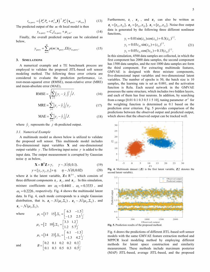
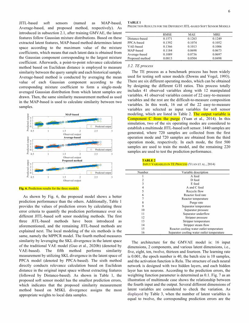
In this simulation, 4500 data samples are collected, in which the first component has 2000 data samples, the second component has 1500 data samples, and the rest 1000 data samples are form the third component. For extracting multimode features, GMVAE is designed with three mixture components, five-dimensional input variables and two-dimensional latent variables. The number of epochs is 50, the batch size is 10 samples, the learning rate is set as 0.001, and the activation function is Relu. Each neural network in the GMVAE possesses the same structure, which includes two hidden layers, and each of them has four neurons. In addition, by searching from a range [0.01 0.1 0.3 0.5 1 5 10], tuning parameter 2s for the weighting function is determined as 0.1 based on the prediction error criterion. Fig. 5 provides comparison of the predictions between the observed output and predicted output, which shows that the observed output can be tracked well.

Fig. 4. Multimode dataset ( 1Z is the first latent variable, 2Z denotes the second latent variable).

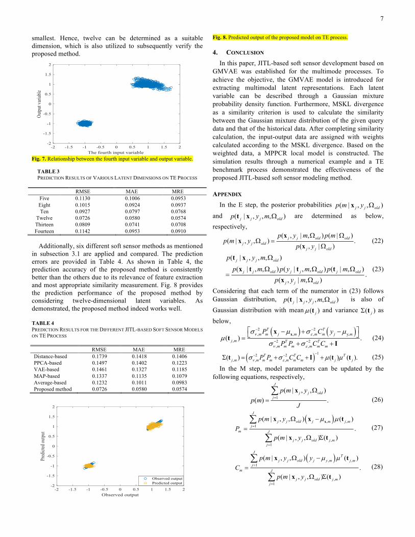
Fig. 5. Prediction results of the proposed method. Fig. 6 draws the predictions of different JITL-based soft sensor models with the same GMVAE feature extraction method and MPPCR local modeling method by employing different methods for latent space construction and similarity measurement. These methods include maximum posterior (MAP) JITL-based, average JITL-based, and the proposed

6

JITL-based soft sensors (named as MAP-based, Average-based, and proposed method, respectively). As introduced in subsection 2.1, after training GMVAE, the latent features follow Gaussian mixture distributions. Based on these extracted latent features, MAP-based method determines latent space according to the maximum value of the mixture coefficients, which means that each latent data is obtained from the Gaussian component corresponding to the largest mixture coefficient. Afterwards, a point-to-point relevance calculation method based on Euclidean distance is employed to measure similarity between the query sample and each historical sample. Average-based method is conducted by averaging the mean value of each Gaussian component according to the corresponding mixture coefficient to form a single-mode averaged Gaussian distribution from which latent samples are drawn. Then, the same similarity measurement method as used in the MAP-based is used to calculate similarity between two samples.

Fig. 6. Prediction results for the three models.

As shown by Fig. 6, the proposed model shows a better prediction performance than the others. Additionally, Table 1 provides the values of prediction errors by calculating three error criteria to quantify the prediction performance over six different JITL-based soft senor modeling methods. The first three JITL-based methods have been introduced as aforementioned, and the remaining JITL-based methods are explained next. The local modeling of the six methods is the same, namely the MPPCR model. The fourth method measures similarity by leveraging the SKL divergence in the latent space of the traditional VAE model (Guo et al., 2020b) (denoted by VAE-based). The fifth method performs similarity measurement by utilizing SKL divergence in the latent space of PPCA model (denoted by PPCA-based). The sixth method directly conducts relevance calculation based on Euclidean distance in the original input space without extracting features (followed by Distance-based). As shown in Table 1, the proposed soft sensor model has the smallest prediction errors, which indicates that the proposed similarity measurement method based on MSKL divergence assigns the most appropriate weights to local data samples.

TABLE 1 PREDICTION RESULTS FOR THE DIFFERENT JITL-BASED SOFT SENSOR MODELS

RMSE MAE MRE Distance-based 0.1571 0.1263 0.1249 PPCA-based 0.1392 0.1074 0.1052 VAE-based 0.1366 0.1013 0.1006 MAP-based 0.1184 0.0698 0.0673 Average-based 0.1089 0.0736 0.0697 Proposed method 0.0813 0.0504 0.0498

3.2. TE process The TE process as a benchmark process has been widely

used for testing soft senor models (Downs and Vogel, 1993). There are six different operating modes, which can be obtained by designing the different G/H ratios. This process totally includes 41 observed variables along with 12 manipulated variables. 41 observed variables consist of 22 easy-to-measure variables and the rest are the difficult-to-measure composition variables. In this work, 16 out of the 22 easy-to-measure variables are selected as input variables for soft sensor modeling, which are listed in Table 2. The output variable is Component C from the purge (Yuan et al., 2014). In this simulation, two of the six operating modes are considered to establish a multimode JITL-based soft sensor. 1440 samples are generated, where 720 samples are collected from the first operation mode and 720 samples are obtained from the third operation mode, respectively. In each mode, the first 500 samples are used to train the model, and the remaining 220 samples are used to test the prediction performance. TABLE 2

INPUT VARIABLES IN TE PROCESS (YUAN ET AL., 2014)

Number Variable description 1 A feed 2 D feed 3 E feed 4 A and C feed 5 Recycle flow 6 Reactor feed rate 7 Reactor temperature 8 Purge rate 9 Separator temperature

10 Separator pressure 11 Separator underflow 12 Stripper pressure 13 Stripper temperature 14 Stripper steam flow 15 Reactor cooling water outlet temperature 16 Separator cooling water outlet temperature

The architecture for the GMVAE model is: 16 input

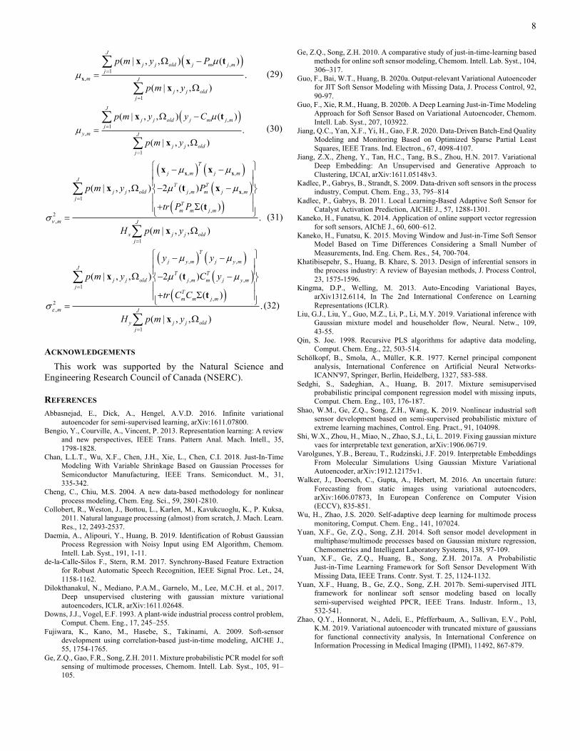
dimensions, 2 components, and various latent dimensions, i.e., five, eight, ten, twelve, thirteen and fourteen. The learning rate is 0.001, the epoch number is 40, the batch size is 10 samples, and the activation function is Relu. The structure of each neural network is designed with two hidden layers, and each hidden layer has ten neurons. According to the prediction errors, the weighting function parameter is determined as 0.1. Fig. 7 as an illustration of multimode case shows the relationship between the fourth input and the output. Several different dimensions of latent variables are considered to check the variation. As displayed by Table 3, when the number of latent variables is equal to twelve, the corresponding prediction errors are the

7

smallest. Hence, twelve can be determined as a suitable dimension, which is also utilized to subsequently verify the proposed method.

Fig. 7. Relationship between the fourth input variable and output variable.

TABLE 3

PREDICTION RESULTS OF VARIOUS LATENT DIMENSIONS ON TE PROCESS RMSE MAE MRE

Five 0.1130 0.1006 0.0953 Eight 0.1015 0.0924 0.0937 Ten 0.0927 0.0797 0.0768

Twelve 0.0726 0.0580 0.0574 Thirteen 0.0809 0.0741 0.0708 Fourteen 0.1142 0.0953 0.0910

Additionally, six different soft sensor methods as mentioned

in subsection 3.1 are applied and compared. The prediction errors are provided in Table 4. As shown in Table 4, the prediction accuracy of the proposed method is consistently better than the others due to its relevance of feature extraction and most appropriate similarity measurement. Fig. 8 provides the prediction performance of the proposed method by considering twelve-dimensional latent variables. As demonstrated, the proposed method indeed works well.

TABLE 4 PREDICTION RESULTS FOR THE DIFFERENT JITL-BASED SOFT SENSOR MODELS ON TE PROCESS RMSE MAE MRE Distance-based 0.1739 0.1418 0.1406 PPCA-based 0.1497 0.1402 0.1223 VAE-based 0.1461 0.1327 0.1185 MAP-based 0.1337 0.1135 0.1079 Average-based 0.1232 0.1011 0.0983 Proposed method 0.0726 0.0580 0.0574

Fig. 8. Predicted output of the proposed model on TE process.

4. CONCLUSION In this paper, JITL-based soft sensor development based on

GMVAE was established for the multimode processes. To achieve the objective, the GMVAE model is introduced for extracting multimodal latent representations. Each latent variable can be described through a Gaussian mixture probability density function. Furthermore, MSKL divergence as a similarity criterion is used to calculate the similarity between the Gaussian mixture distribution of the given query data and that of the historical data. After completing similarity calculation, the input-output data are assigned with weights calculated according to the MSKL divergence. Based on the weighted data, a MPPCR local model is constructed. The simulation results through a numerical example and a TE benchmark process demonstrated the effectiveness of the proposed JITL-based soft sensor modeling method.

APPENDIX In the E step, the posterior probabilities ( | , , )j j oldp m yx W

and ( | , , , )j j j oldp y mt x W are determined as below, respectively,

( , | , ) ( | )

( | , , ) .( , | )

j j old oldj j old

j j old

p y m p mp m y

p yx

xx

W WW =

W (22)

( | , , , )

( | , , ) ( | , , ) ( | , ).

( , | , )

j j j old

j j old j j old j old

j j old

p y mp m p y m p m

p y m

t xx t t t

x

W

W W W=

W

(23)

Considering that each term of the numerator in (23) follows Gaussian distribution, ( | , , , )j j j oldp y mt x W is also of Gaussian distribution with mean ( )jtµ and variance ( )jtS as below,

( ) ( )2 2

, , , y,, 2 2

, ,

( ) .T T

m m j m m m j mj m T T

m m m m m m

P C y

P P C Cxx

tI

n e

n e

s µ s µµ

s s

- -

- -

é ù- + -ë û=+ +

(24)

( ) 12 2, , ,( ) ( ) ( ).T T Tj m m m m m m m j jP P C Ct I t tn es s µ µ

-- -S = + + + (25)

In the M step, model parameters can be updated by the following equations, respectively,

1( | , , )

( ) .

J

j j oldjp m y

p mJ

x=

W=å

(26)

( ), ,

1

,1

( | , , ) ( ).

( | , , ) ( )

J

j j old j m j mj

m J

j j old j mj

p m yP

p m y

xx x t

x t

µ µ=

=

W -=

W S

å

å (27)

( ), ,

1

,1

( | , , ) ( ).

( | , , ) ( )

JT

j j old j y m j mj

m J

j j old j mj

p m y yC

p m y

x t

x t

µ µ=

=

W -=

W S

å

å (28)

8

( ),

1,

1

( | , , ) ( ).

( | , , )

J

j j old j m j mj

m J

j j oldj

p m y P

p m yx

x x t

x

µµ =

=

W -=

W

å

å (29)

( ),

1,

1

( | , , ) ( ).

( | , , )

J

j j old j m j mj

y m J

j j oldj

p m y y C

p m y

x t

x

µµ =

=

W -=

W

å

å (30)

( ) ( )( )

( )

, ,

, ,1

,2,

1

( | , , ) 2 ( )

( ).

( | , , )

T

j m j mJ

T Tj j old j m m j m

jTm m j m

m J

x j j oldj

p m y P

tr P P

H p m y

x x

x

x x

x t x

t

xn

µ µ

µ µ

s

=

=

ì ü- -ï ïï ïW - -í ýï ï+ Sï ïî þ=

W

å

å (31)

( ) ( )( )

( )

, ,

, ,1

,2,

1

( | , , ) 2 ( )

( ).

( | , , )

T

j y m j y mJ

T Tj j old j m m j y m

jTm m j m

m J

y j j oldj

y y

p m y C y

tr C C

H p m y

x t

t

xe

µ µ

µ µ

s

=

=

ì ü- -ï ïï ïW - -í ýï ï+ Sï ïî þ=

W

å

å(32)

ACKNOWLEDGEMENTS This work was supported by the Natural Science and

Engineering Research Council of Canada (NSERC).

REFERENCES Abbasnejad, E., Dick, A., Hengel, A.V.D. 2016. Infinite variational

autoencoder for semi-supervised learning, arXiv:1611.07800. Bengio, Y., Courville, A., Vincent, P. 2013. Representation learning: A review

and new perspectives, IEEE Trans. Pattern Anal. Mach. Intell., 35, 1798-1828.

Chan, L.L.T., Wu, X.F., Chen, J.H., Xie, L., Chen, C.I. 2018. Just-In-Time Modeling With Variable Shrinkage Based on Gaussian Processes for Semiconductor Manufacturing, IEEE Trans. Semiconduct. M., 31, 335-342.

Cheng, C., Chiu, M.S. 2004. A new data-based methodology for nonlinear process modeling, Chem. Eng. Sci., 59, 2801-2810.

Collobert, R., Weston, J., Bottou, L., Karlen, M., Kavukcuoglu, K., P. Kuksa, 2011. Natural language processing (almost) from scratch, J. Mach. Learn. Res., 12, 2493-2537.

Daemia, A., Alipouri, Y., Huang, B. 2019. Identification of Robust Gaussian Process Regression with Noisy Input using EM Algorithm, Chemom. Intell. Lab. Syst., 191, 1-11.

de-la-Calle-Silos F., Stern, R.M. 2017. Synchrony-Based Feature Extraction for Robust Automatic Speech Recognition, IEEE Signal Proc. Let., 24, 1158-1162.

Dilokthanakul, N., Mediano, P.A.M., Garnelo, M., Lee, M.C.H. et al., 2017. Deep unsupervised clustering with gaussian mixture variational autoencoders, ICLR, arXiv:1611.02648.

Downs, J.J., Vogel, E.F. 1993. A plant-wide industrial process control problem, Comput. Chem. Eng., 17, 245–255.

Fujiwara, K., Kano, M., Hasebe, S., Takinami, A. 2009. Soft-sensor development using correlation-based just-in-time modeling, AICHE J., 55, 1754-1765.

Ge, Z.Q., Gao, F.R., Song, Z.H. 2011. Mixture probabilistic PCR model for soft sensing of multimode processes, Chemom. Intell. Lab. Syst., 105, 91–105.

Ge, Z.Q., Song, Z.H. 2010. A comparative study of just-in-time-learning based methods for online soft sensor modeling, Chemom. Intell. Lab. Syst., 104, 306–317.

Guo, F., Bai, W.T., Huang, B. 2020a. Output-relevant Variational Autoencoder for JIT Soft Sensor Modeling with Missing Data, J. Process Control, 92, 90-97.

Guo, F., Xie, R.M., Huang, B. 2020b. A Deep Learning Just-in-Time Modeling Approach for Soft Sensor Based on Variational Autoencoder, Chemom. Intell. Lab. Syst., 207, 103922.

Jiang, Q.C., Yan, X.F., Yi, H., Gao, F.R. 2020. Data-Driven Batch-End Quality Modeling and Monitoring Based on Optimized Sparse Partial Least Squares, IEEE Trans. Ind. Electron., 67, 4098-4107.

Jiang, Z.X., Zheng, Y., Tan, H.C., Tang, B.S., Zhou, H.N. 2017. Variational Deep Embedding: An Unsupervised and Generative Approach to Clustering, IJCAI, arXiv:1611.05148v3.

Kadlec, P., Gabrys, B., Strandt, S. 2009. Data-driven soft sensors in the process industry, Comput. Chem. Eng., 33, 795–814

Kadlec, P., Gabrys, B. 2011. Local Learning-Based Adaptive Soft Sensor for Catalyst Activation Prediction, AICHE J., 57, 1288-1301.

Kaneko, H., Funatsu, K. 2014. Application of online support vector regression for soft sensors, AIChE J., 60, 600–612.

Kaneko, H., Funatsu, K. 2015. Moving Window and Just-in-Time Soft Sensor Model Based on Time Differences Considering a Small Number of Measurements, Ind. Eng. Chem. Res., 54, 700-704.

Khatibisepehr, S., Huang, B. Khare, S. 2013. Design of inferential sensors in the process industry: A review of Bayesian methods, J. Process Control, 23, 1575-1596.

Kingma, D.P., Welling, M. 2013. Auto-Encoding Variational Bayes, arXiv1312.6114, In The 2nd International Conference on Learning Representations (ICLR).

Liu, G.J., Liu, Y., Guo, M.Z., Li, P., Li, M.Y. 2019. Variational inference with Gaussian mixture model and householder flow, Neural. Netw., 109, 43-55.

Qin, S. Joe. 1998. Recursive PLS algorithms for adaptive data modeling, Comput. Chem. Eng., 22, 503-514.

Schölkopf, B., Smola, A., Müller, K.R. 1977. Kernel principal component analysis, International Conference on Artificial Neural Networks- ICANN'97, Springer, Berlin, Heidelberg, 1327, 583-588.

Sedghi, S., Sadeghian, A., Huang, B. 2017. Mixture semisupervised probabilistic principal component regression model with missing inputs, Comput. Chem. Eng., 103, 176-187.

Shao, W.M., Ge, Z.Q., Song, Z.H., Wang, K. 2019. Nonlinear industrial soft sensor development based on semi-supervised probabilistic mixture of extreme learning machines, Control. Eng. Pract., 91, 104098.

Shi, W.X., Zhou, H., Miao, N., Zhao, S.J., Li, L. 2019. Fixing gaussian mixture vaes for interpretable text generation, arXiv:1906.06719.

Varolgunes, Y.B., Bereau, T., Rudzinski, J.F. 2019. Interpretable Embeddings From Molecular Simulations Using Gaussian Mixture Variational Autoencoder, arXiv:1912.12175v1.

Walker, J., Doersch, C., Gupta, A., Hebert, M. 2016. An uncertain future: Forecasting from static images using variational autoencoders, arXiv:1606.07873, In European Conference on Computer Vision (ECCV), 835-851.

Wu, H., Zhao, J.S. 2020. Self-adaptive deep learning for multimode process monitoring, Comput. Chem. Eng., 141, 107024.

Yuan, X.F., Ge, Z.Q., Song, Z.H. 2014. Soft sensor model development in multiphase/multimode processes based on Gaussian mixture regression, Chemometrics and Intelligent Laboratory Systems, 138, 97-109.

Yuan, X.F., Ge, Z.Q., Huang, B., Song, Z.H. 2017a. A Probabilistic Just-in-Time Learning Framework for Soft Sensor Development With Missing Data, IEEE Trans. Contr. Syst. T. 25, 1124-1132.

Yuan, X.F., Huang, B., Ge, Z.Q., Song, Z.H. 2017b. Semi-supervised JITL framework for nonlinear soft sensor modeling based on locally semi-supervised weighted PPCR, IEEE Trans. Industr. Inform., 13, 532-541.

Zhao, Q.Y., Honnorat, N., Adeli, E., Pfefferbaum, A., Sullivan, E.V., Pohl, K.M. 2019. Variational autoencoder with truncated mixture of gaussians for functional connectivity analysis, In International Conference on Information Processing in Medical Imaging (IPMI), 11492, 867-879.